arX

iv:0

911.

2841

v2 [

gr-q

c] 5

Jan

201

0

Further Extended Theories of Gravitation: Part I∗

by M.Di Mauro, L.Fatibene, M.Ferraris, M.Francaviglia

Abstract:We shall here propose a class of relativistic theories of gravitation, based on a foundational paper

of Ehlers Pirani and Schild (EPS). All “extended theories of gravitation” (also known as f(R) theories) in

Palatini formalism are shown to belong to this class. In a forthcoming paper we shall show that this class

of theories contains other more general examples.

EPS framework helps in the interpretation and solution of these models that however have exotic behaviours

even compared to f(R) theories.

1. Introduction

Once one starts to generalize GR in order to include new observational data it is not clear

whether there is a natural border that physically reasonable models of gravitation should not

cross. Ehlers, Pirani and Schild (EPS) proposed in 1972 some axioms to deduce GR from

observational structures; see [1]. Their subtle analysis was based on physical and mathematical

axioms and turned into the understanding that gravity and causality require on spacetime both

an affine and a metric structure a priori independent but related by suitable compatibility

requirements. The program was never completed in a fully satisfactory way, in the sense that

they could not finally prove that one needs to use as a connection the Levi-Civita connection

of the metric structure on spacetime.

However, EPS framework turns out to be a natural framework for the interpretation of Palatini

extended theories of gravitation in general, and in particular for f(R) models. These models

have been recently used with the hope that they could account for effects attributed to dark

matter and energy; [2], [3], [4], [5], [6], [7] and references quoted therein. A number of

criticisms have been variously raised on Palatini framework; see e.g. [3] , [8] and references

quoted therein. However, in view of EPS framework it appears as the most natural setting for

gravitational theories, at least from a foundational viewpoint; see also [9], [10].

This paper is divided into two parts. In this first part we shall review the EPS, define the class

of further extended theories of gravitation (FETG) and show that f(R) theories are particular

cases of FETG.

In the second part we shall consider some examples of FETG other than standard f(R)

theories. We shall show that FETG allow projective structures (i.e., connections) that are

not necessarily metric. Moreover, a specific example will be considered that reproduces the

behaviour of purely metric f(R) theories starting from a Palatini framework. This is particularly

interesting since it overcomes some of the recent criticisms against Palatini framework based

on problems in modelling polytropic stars; see [8].

Hereafter, spacetime M is assumed to be a 4-dimensional, connected, paracompact manifold

which allows global Lorentzian metrics.

∗This paper is published despite the effects of the Italian law 133/08 (http://groups.google.it/group/scienceaction). This law

drastically reduces public funds to public Italian universities, which is particularly dangerous for free scientific research, and it will

prevent young researchers from getting a position, either temporary or tenured, in Italy. The authors are protesting against this law to

obtain its cancellation.

1

2. EPS Axioms and Compatibility

Ehlers, Pirani and Schild (EPS) proposed in the seventies an axiomatic construction of General

Theory of Relativity (see [1]). They showed that spacetime geometry can be obtained from

few assumptions about two observational quantities: the worldlines of light rays and free falling

mass particles. Light rays and particles are to be understood in a classical sense: light rays are

“small wave packets” and particles are material balls with negligible extension.

In order to introduce a differential structure on M , EPS defined the radar coordinates: given

an event e ∈ M and two particles (closed enough to e) one can consider echoes from the particles

on the event e. Radar coordinates are in particular defined by the following map:

Φpp′ : e 7→ (u, v, u′, v′) (2.1)

where (u, v, u′, v′) are the leaving and arriving parameters of echoes on the two particles.

Then EPS introduced a function g (see Axiom L1 in [1]) considering a particle P passing

through an event e and light cone ve emitted from an event p external to P . The function g is

defined by g = t(e1)t(e2), where t(e1) and t(e2) are parameters on P relative to the encounter

of ve with the particle P .

The Hessian matrix (at e) of this map g defines a tensor gµν with the following properties:

gµνTµT ν = 0 gµνL

µLν = 2 (2.2)

for any vector T tangent to light rays passing through e and any vector L tangent to particles

passing through e. Unfortunately, the tensor gµν depends on the parametrization fixed along

the particles which are unphysical; they in fact correspond to fix a conventional clock (see [11]).

One can show that physically one can single out a class of tensors which are defined modulo a

conformal factor (which in fact does not affect light cones defined by g).

One can easily check that EPS axioms are coherent. For example one can start with M = R4

and two families of straight lines and show that in Cartesian coordinates the tensor gµν turns

out to be

gµν = 2‖u‖2 ηµν (2.3)

where (∂0, u) are the 4-velocities of the particles involved in the definition of radar coordinates

and for ηµν is the standard Minkowski metric. So we have found that the tensor gµν verifies

(2.2). Moreover det(gµν) 6= 0 so it defines in fact a spacetime metric which exhibits M as

equivalent to Minkowski spacetime.

In order to introduce an object that is invariant with respect to particles reparametrizations

(i.e. conformal transformations on g) EPS considered the conformal metric

gµν =gµν

4√

|detg|(2.4)

which is a tensor density of weight 12 .

The quantity gµν is invariant for conformal transformations g′µν = ϕ · gµν ; in fact

g′µν =

g′µν4√

g′=

ϕ · gµν4√

ϕ4 · g=

gµν4√g

= gµν (2.5)

2

For simplicity let us set 4√g := 4√

|detg|. The conformal metric gµν defines a conformal

structure on M . The equation gµνTµT ν = 0 represents light cones emitted from (or received at)

an event e so it allows to distinguish among timelike, spacelike and lightlike vectors through e.

The conformal structure is equivalent to assigning the light cones at each point. Hereafter in

this Section, spactime indices will be lowered and raised by the conformal metric g.

Then EPS axiom P2 relates to an infinitesimal version of the law of inertia in projective

coordinates xα, namelyd2xα

du2= 0

Changing parameters and coordinates the previous equation becomes:

xα +Παµν x

µxν = λxα (2.6)

The coefficients Παµν can be choosen without loss of generality to obey the properties Πα

[µν] = 0

and Παµα = 0; they are called projective coefficients. On the other hand one can fix parametriza-

tion so to have λ = 0.

They do not directly refer to a connection because in view of the traceless condition they

transform differently according to the following transformation rules:

Π′αβµ = Jα

λ

(

ΠλρσJ

ρβ J

σµ + Jλ

βµ

)

+ 25δ

α(βδ

ǫµ)J

ρǫ ∂ρ ln J (2.7)

The projective coefficients define thence a geometric object which is called a projective connec-

tion and a projective structure on M . Any curve that satisfies equation (2.6) is said geodesic

(trajectory). In particular, particles follow geodesics.

Once the conformal and the projective structure of spacetime have been introduced, EPS

proposed a compatibility axiom (see [1] Axiom C):

a solution of equations (2.6) is a particle iff its initial 4-velocity at e is contained in

the interior of the light cone νe.

This axiom allows to express an analytical relation between the conformal and the projective

structure. They introduced {g}αµν , the “Christoffel symbols” of gµν :

{g}αµν := {g}αµν + 18

(

gγαgµν − 2δα(µδγν)

)

∂γ ln g (2.8)

where g is any representative of the conformal class identified by g. The coefficients {g}αµνtransform as:

{g′}αβµ = Jαλ ({g}λρσJρ

β Jσµ + Jλ

βµ)− 14J

αλ

(

gλǫgρσ − 2δλ(ρδ

ǫσ)

)

Jρβ J

σµ∂ǫ ln J (2.9)

The difference ∆αβµ = Πα

βµ − {g}αβµ has the following two properties ∆α[βµ] = 0 and ∆α

βα = 0.

Then EPS obtained the relation for ∆αβµ := gαλ∆λβµ:

∆αβγ = ∆(αβγ) +12 (pαgβγ − gα(βpγ)) + Lα(βγ) (2.10)

where we set Lαβγ = 43∆[αβ]γ − p[αgβ]γ and pα = 8

9∆[αλ]λ. (In [1] the definition of pα was given

with a different sign probably due to a typo. With our definition the quantity Lαβγ has the

3

following properties Lαβα = 0, L[αβγ] = 0 e L(αβ)γ = 0 while with the original EPS definition

the first one does not hold true; see Appendix A).

Equation (2.10) can be recasted into the following form

∆αβµ = Lα

(βµ) + 5qαgβµ − 2δα(β qµ) (2.11)

by setting qα = 118∆

αβµg

βµ.

Now consider a sequence {Pn : n ∈ N} of particles passing through an event e. For Axiom C

all Pn are internal to the light cone ve. Pn are particles (hence projective geodesics). Let us

consider a sequence determined by initial velocities that tend to a light velocity cµ. Let P be

the light ray with initial velocity cµ. Since Pn → P , the 4-velocity of particles can be as near

as one wishes to cµ; accordingly, P is a projective geodesic and a conformal geodesics. Hence

Axiom C can be equivalently expressed in this way:

null projective-geodesic are identical to null conformal-geodesics.

Conformal geodesics are obtained as solution of the following equation:

xα + {g}αµν xµxν = ν xα (2.12)

EPS were at this point able to give a formal expression to the compatibility condition as

∆αµν = 5qαgµν − 2δα(µqν) (2.13)

Another equivalent form of Axiom C is:

the set of particles is identical with the set of conformal-timelike projective-geodesics.

Finally, EPS introduced a connection Γαβµ given in terms of the projective and conformal

structures

Γαβµ := {g}αβµ +

(

gαǫgβµ − 2δα(βδ

ǫµ)

)

qǫ (2.14)

where we set qǫ := 5qǫ.

This can be introduced as a generic linear combination

Γαβµ = a {g}αβµ + bqαgβµ − 2c δα(β qµ) (2.15)

and then fixing the coefficients so that Γ transforms as a connection. In view of (2.7) and (2.9)

one can check that Γ transfoms in fact as a connection

Γ′αβµ = a {g}′αβµ + bq′αg′βµ − 2c δα(β q′µ) =

= Jαλ

(

Γ′λρσ Jρβ J

σµ + aJλβµ

)

+ Jαλ

((

b20 − a

4

)

gλǫgρσ +

( a2 − c

10

)

δλ(ρδǫσ)

)

Jρβ J

σµ ∂ǫ ln J

(2.16)

This transforms as a connection iff we set a = 1 and b = c = 5. Accordingly we have (2.14).

4

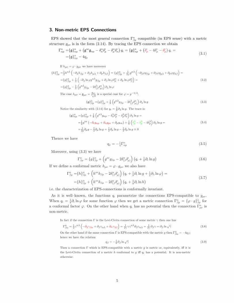
3. Non-metric EPS Connections

EPS showed that the most general connection Γαβµ compatible (in EPS sense) with a metric

structure gµν is in the form (2.14). By tracing the EPS connection we obtain

Γααµ ={g}ααµ +

(

gαǫgαµ − δααδ

ǫµ − δαµδ

ǫα

)

qǫ = {g}ααµ +(

δǫµ − 4δǫµ − δǫµ)

qǫ =

={g}ααµ − 4qµ(3.1)

If hµν = ϕ · gµν we have moreover

{h}αβµ = 12h

αλ(

−∂λhβµ + ∂βhµλ + ∂µhλβ

)

= {g}αβµ + 12ϕ g

αλ(

−∂λϕgβµ + ∂βϕgµλ + ∂µϕgλβ

)

=

={g}αβµ + 12

(

−∂λ lnϕgαλgβµ + ∂β lnϕδαµ + ∂µ lnϕδαβ

)

=

={g}αβµ − 12

(

gαλgβµ − 2δλ(βδαµ)

)

∂λ lnϕ

(3.2)

The case hµν = gµν =gµν4√g

is a special case for ϕ = g−1/4;

{g}αβµ ={g}αβµ + 18

(

gαλgβµ − 2δλ(βδαµ)

)

∂λ ln g (3.3)

Notice the similarity with (2.14) for qǫ =18∂λ ln g. The trace is:

{g}ααµ ={g}ααµ + 18

(

gαλgαµ − δλαδαµ − δλµδ

αα

)

∂λ ln g =

= 12 g

αǫ (−∂ǫgαµ + ∂αgµǫ + ∂µgǫα)

+ 18

(

δλµ − δλµ − 4δλµ

)

∂λ ln g =

= 12g ∂µg −

12∂µ ln g = 1

2∂µ ln g − 12∂µ ln g ≡ 0

(3.4)

Thence we have

qµ = − 14Γ

ααµ (3.5)

Moreover, using (3.3) we have

Γαβµ = {g}αβµ +

(

gαǫgβµ − 2δα(βδǫµ)

)

(

qǫ +18∂ǫ ln g

)

(3.6)

If we define a conformal metric hµν = ϕ · gµν we also have

Γαβµ ={h}αβµ +

(

hαǫhβµ − 2δα(βδǫµ)

)

(

qǫ +18∂ǫ ln g +

12∂λ lnϕ

)

=

={h}αβµ +(

hαǫhβµ − 2δα(βδǫµ)

)

(

qǫ +18∂ǫ lnh

)

(3.7)

i.e. the characterization of EPS-connections is conformally invariant.

As it is well–known, the functions qǫ parametrize the connections EPS-compatible to gµν .

When qǫ =18∂ǫ lnϕ for some function ϕ then we get a metric connection Γα

βµ = {ϕ · g}αβµ for

a conformal factor ϕ. On the other hand when qǫ has no potential then the connection Γαµν is

non-metric.

In fact if the connection Γ is the Levi-Civita connection of some metric γ then one has

Γαβα = 12γ

αλ(

−∂λγβα + ∂βγαλ + ∂αγλβ

)

= 12γ γγ

αλ∂βγαλ = 12γ ∂βγ = ∂β ln

√γ (3.8)

On the other hand if the same connection Γ is EPS-compatible with the metric g then Γαβα = −4qβ ;

hence we have the relation

qβ = − 18∂β ln

√γ (3.9)

Then a connection Γ which is EPS-compatible with a metric g is metric or, equivalently, iff it is

the Levi-Civita connection of a metric h conformal to g iff qǫ has a potential. It is non-metric

otherwise.

5

4. EPS-Compatibility Condition

We need a condition to express EPS-compatibility in differential form. We shall then look for

relativitic theories in which field equations imply EPS-compatibility.

Let us start by considering the quantityΓ

∇µ

(√hhαβ

)

when Γ is EPS-compatible with h (or

any metric g conformal to h); we have

Γ

∇µ

(√hhαβ

)

=h

∇µ

(√hhαβ

)

+Kαǫµ

√hhǫβ +Kβ

ǫµ

√hhαǫ −Kǫ

ǫµ

√hhαβ =

=−√h(

hρλhαβ − 2δ

(αλ δβ)ρ

)

hǫρKλǫµ

(4.1)

where we set Kαǫµ := Γα

ǫµ − {h}αǫµ; if Γ is EPS-compatible with h then we have

Kλǫµ =

(

hλσhǫµ − 2δλ(ǫδσµ)

)

(

qσ +18∂σ lnh

)

(4.2)

and substituting back into (4.1) we obtain

Γ

∇µ

(√hhαβ

)

=−√h(

hρλhαβ − 2δ

(αλ δβ)ρ

)

hǫρ(

hλσhǫµ − 2δλ(ǫδσµ)

)

(

qσ +18∂σ lnh

)

=

=−√h(

hρλhαβ − δαλδ

βρ − δβλδ

αρ

)

(

hλσδρµ − hλρδσµ − hσρδλµ) (

qσ +18∂σ lnh

)

=

=−√h(

hαβδσµ − 4hαβδσµ − hαβδσµ − δβµhασ + hαβδσµ + hσβδαµ − hβσδαµ+

+ hβαδσµ + hσαδβµ

)

(

qσ +18∂σ lnh

)

= 2√hhαβ

(

qµ +18∂µ lnh

)

(4.3)

Hence the necessary condition for a connection Γ to be EPS-compatible with the metric h (or

any other metric g conformal to h) is that

Γ

∇µ

(√hhαβ

)

= αµ

√hhαβ (4.4)

Viceversa, if (4.4) holds true then we can define

qµ := 12αµ − 1

8∂µ lnh Γαβµ := {h}αβµ +

(

hαǫhβµ − 2δα(βδǫµ)

)

(

qǫ +18∂ǫ lnh

)

(4.5)

Then one has of course that also for this connection the following holds true

Γ

∇µ

(√hhαβ

)

= αµ

√hhαβ (4.6)

Let us now define the tensor Hαβµ := Γα

βµ − Γαβµ; by subtracting (4.4) and (4.6) we obtain

Hαǫµh

ǫβ + Hβǫµh

αǫ − Hǫǫµh

αβ = 0 (4.7)

By tracing this last equation with hαβ we obtain

Hααµ +Hβ

βµ − 4Hǫǫµ = 0 ⇒ Hα

αµ = 0 (4.8)

and substituting back into (4.7)

H(αǫµh

β)ǫ = 0 (4.9)

6

One can now choose coordinates so that at a point x ∈ M one has hµν(x) = ηµν ; one can prove

algebraically that (4.9) implies Hαǫµ(x) = 0. This can be done at any point x ∈ M and since

equation (4.9) is tensorial then Hαǫµ = 0 holds everywhere and in any coordinate system. Hence

one has necessarily Γαβµ = Γα

βµ; in other words the connection Γαβµ that obeys (4.4) is necessarily

in the form:

Γαβµ := {h}αβµ + 1

2

(

hαǫhβµ − 2δα(βδǫµ)

)

αǫ (4.10)

We are hence able to define:

Definition: a Further Extended Gravitational Theory (FEGT) as a metric-affine relativistic

theory (i.e. a Lagrangian theory on a triple (M, g,Γ) with g a Lorentzian metric and Γ a linear

connection a priori independent of g) defined by an action

L = L(g,R(Γ)) + Lm(g,Γ, φ) (4.11)

such that field equations imply EPS-compatibility, i.e. that

Γ

∇µ

(√hhαβ

)

= αµ

√hhαβ (4.12)

for some metric h = ϕ(φ) · g conformal to g and some 1-form α = αµ(g, φ)dxµ functions of g

and the matter field φ (possibly together with their derivatives up to some finite order).

Notice that this encompasses usual f(R) theories (in Palatini formulation) in which the matter

Lagrangian is usually assumed to be independent of the connection Γ. We shall hereafter show

that there are in fact non-trivial FEGT, i.e. FEGT other that the usual f(R) theories.

In such a kind of FEGT the connection Γ is defined as in (4.10). If the differential form

α := αµdxµ is not closed then the theory is non-trivial and its connection is non-metrical

though it turns out to be EPS-compatible with the original metric structure g (or equivalently

to any conformal metric structure h).

In such theories the lightlike geodesics coincide with the metric geodesics, but the timelike

geodesics (i.e. worldlines of matter points) are exotic. This situation has been considered in lit-

erature (see [12]) though not in connection with EPS criteria. Of course, further investigations

should be devoted to the possibility that such exotic dynamics can model anomalous rotation

curves in galaxies and/or cosmological acceleration (as is already proven with f(R) theories) or

be detected by solar system experiments.

5. A “Trivial” Example: f(R) Theories

We shall hereafter inestigate the class of FETG. One class of examples is well-known: in any

f(R) theory, in Palatini formulation one has a connection Γαβµ = {h}αβµ which is the Levi-Civita

connection of a conformal metric hµν = f ′(R(Γ, g)) · gµν = f ′(T ) · gµν , where T = Tµνgµν ; see

[13]. Thus Γαβµ, in view of (3.2), has the following expression:

Γαµν = {f ′ · g}αµν = {g}αµν − 1

2

(

gαǫgµν − 2δα(µδǫν)

)

∂ǫ ln f′ (5.1)

7

Now we calculate the trace Γαµα:

Γαµα = 1

2gǫλ∂µgǫλ − 1

2 (1− 5) ∂µ ln f′ = 1

2∂µ ln g + 2∂µ ln f′ = ∂µ ln(f

′2√g) = ∂µ ln√h (5.2)

and thence qǫ = − 18∂ǫ lnh.

The connection Γαµν is in fact compatible in the sense of EPS with the conformal structure

identified by g.

To check this one can simply check that the identity (3.6)

Γαβµ = {g}αβµ +(

gαǫgβµ − 2δα(βδǫµ)

)(

qǫ +18∂ǫ ln g

)

(5.3)

holds true.

Hence, by comparing (5.1) and (5.3), one has to check that

− 12∂ǫ ln f

′ = qǫ +18∂ǫ ln g = − 1

8∂ǫ lnh+ 18∂ǫ ln g = − 1

2∂ǫ ln f′ − 1

8∂ǫ ln g +18∂ǫ ln g (5.4)

We can also check that compatibility condition (4.4) holds true directly; we have that

Hαβµ =Γα

βµ − {g}αβµ = − 12

(

gαǫgβµ − 2δα(βδǫµ)

)

∂ǫ ln f′ (5.5)

Thus we have

Γ

∇α(√ggµν) =

g

∇α(√ggµν) +Hµ

λα

√ggλν +Hν

λα

√ggµλ −Hλ

λα

√ggµν =

=√g

2

(

(−gµǫδνα + δǫαgµν + δµαg

ǫν) + (−gνǫδµα + δǫαgµν + δναg

µǫ)+

+ (δǫαgµν − 4δǫαg

µν − δǫαgµν)

)

∂ǫ ln f′ = −√

ggµν∂α ln f′ = αα

√ggµν

(5.6)

which is in fact in the expected form with α = −∂α ln f′dxα = d(− ln f ′). The form α is exact,

in view of the fact that the connection Γ is metric by construction.

6. Conclusions and Perspectives

We here reviewed EPS framework. In particular we corrected a misprint in the original paper

and we proved identity (2.10) proving also that it is essentially unique (modulo two inessential

parameters). We also find an equivalent, covariant characterization of EPS compatibility which

will be expected to be consequence of field equations in FETG. In this models the connection is

intially independent of the spacetime metric, but it is guaranteed to be on-shell EPS compatible

with the metric.

EPS compatibility is used in two ways: first it enhances a physical interpretation in terms of

observational quantities such as light rays and free falling mass particles. On the other hand,

EPS compatibility allows to determine the connection in terms of metric and matter fields.

We finally showed that f(R) are examples of FETG. We called this example as “trivial” FETG.

In the second part (see [14]) we shall present and discuss non-trivial examples of FETG.

8

Appendix A. EPS Compatibility

EPS introduced in [1] relation (2.10) for ∆αµν using Lαβγ = 4

3∆[αβ]γ−p[αgβ]γ and pα = − 89∆[αλ]

λ.

Moreover they assert that:

Lλβλ = 0 L[αβγ] = 0 L(αβ)γ = 0 (A.1)

which are used later on to deduce equation (2.13) which is important for deducing the compat-

ibility condition (2.14). However, considering that:

Lαβγ = 23 (∆αβγ −∆βαγ) +

29 (∆

λαλgβγ −∆λ

βλgαγ) (A.2)

we find that the first relation of (A.1) is not verified:

Lλβλ = 2

3 (∆λβλ −∆βλ

λ) + 29 (∆

λǫǫgβλ −∆βǫ

ǫδλλ) = − 43∆βǫ

ǫ 6≡ 0 (A.3)

Thus in order to obtain the correct definitions of the objects involved we started from general

linear combinations

Lαβγ = 2b∆[αβ]γ + 2cp[αgβ]γ (A.4)

and we set pα = 2a∆[αλ]λ = a∆α and ∆α = ∆αµνg

µν . Then we determined the unknown

coefficients (a, b, c) so that the required properties (A.1) hold true.

The second and third property in (A.1) are trivially satisfied; for the first one we have:

Lλβλ = b(∆λ

βλ −∆β) + ac(∆λgβλ −∆βδ

λλ) =

= −(3ac+ b)∆β ≡ 0 ⇒ b = −3ac(A.5)

So the general expression of Lαβγ and pα that satisfies (A.1) is:

Lαβγ = −2ac(

3∆[λβ]γ −∆[αgβ]γ

)

pα = a∆α (A.6)

These objects are defined in order to be able to prove the identity (2.10). Let us consider a

linear combination

∆αβγ = 3A∆(αβγ) +Bpαgβγ + 2Cggα(β pγ) + 2DLα(βγ) (A.7)

and we search for the most general set of coefficients (A,B,C,D) for which this is an identity.

By using (A.6) one finds:

∆αβγ =(A− 6acD)∆αβγ + (A+ 3acD)∆βγα + (A+ 3acD)∆γαβ+

+ a(B + 2cD)∆αgβγ + a(C − cD)∆γgαβ + a(C − cD)∆βgγα

(A.8)

Choosing (α, ν) as free parameters, the general solution is{

A = 13

c = − 19aD

{

C = − 19a

B = 29a

(A.9)

and the identity is found in the form

∆αβγ = ∆(αβγ) +29a (pαgβγ − gα(β pγ)) + 2DLα(βγ) (A.10)

where (a,D) are free parameters. Above in the paper we chose the particular solution a = 49 ,

D = 12 and thence

{

A = 13

c = − 12

{

C = − 14

B = 12

(A.11)

9

Acknowledgments

We wish to thank G.Magnano for useful discussions. This work is partially supported by

MIUR: PRIN 2005 on Leggi di conservazione e termodinamica in meccanica dei continui e

teorie di campo. We also acknowledge the contribution of INFN (Iniziativa Specifica NA12)

and the local research funds of Dipartimento di Matematica of Torino University.

References

[1] J.Ehlers, F.A.E.Pirani, A.Schild, The Geometry of Free Fall and Light Propagation, in General Relativity, ed.L.ORaifeartaigh (Clarendon, Oxford, 1972).

[2] S. Capozziello, M. De Laurentis, V. Faraoni A bird’s eye view of f(R)-gravity (2009); arXiv:0909.4672

[3] T.P. Sotiriou, V. Faraoni, f(R) theories of gravity, (2008); arXiv: 0805.1726v2

[4] T.P. Sotiriou, S. Liberati, Metric-affine f(R) theories of gravity, Annals Phys. 322 (2007) 935-966; gr-qc/0604006

[5] T.P. Sotiriou, Modified Actions for Gravity: Theory and Phenomenology, Ph.D. Thesis; gr-qc/0710.4438

[6] S. Capozziello, M. De Laurentis, M. Francaviglia, S. Mercadante, First Order Extended Gravity and the Dark Sideof the Universe: the General Theory Proceedings of the Conference “Univers Invisibile”, Paris June 29 July 3, 2009 -

to appear in 2010

[7] S. Capozziello, M. De Laurentis, M. Francaviglia, S. Mercadante, First Order Extended Gravity and the Dark Sideof the Universe II: Matching Observational Data, Proceedings of the Conference “Univers Invisibile”, Paris June 29July 3, 2009 to appear in 2010

[8] E. Barausse, T.P. Sotiriou, J.C. Miller, A no-go theorem for polytropic spheres in Palatini f(R) gravity, Class.Quant. Grav. 25 (2008) 062001; gr-qc/0703132

[9] S. Capozziello, M. Francaviglia, Extended Theories of Gravity and their Cosmological and Astrophysical Applications,Journal of General Relativity and Gravitation 40 (2-3), (2008) 357-420.

[10] S. Capozziello, M.F. De Laurentis, M. Francaviglia, S. Mercadante, From Dark Energy and Dark Matter to Dark

Metric, Foundations of Physics 39 (2009) 1161-1176 gr-qc/0805.3642v4

[11] V. Perlick, Characterization of standard clocks by means of light rays and freely falling particles General Relativityand Gravitation, 19(11) (1987) 1059-1073

[12] T.P. Sotiriou, f(R) gravity, torsion and non-metricity, Class. Quant. Grav. 26 (2009) 152001; gr-qc/0904.2774

[13] G. Magnano, L.M. Sokolowski, On Physical Equivalence between Nonlinear Gravity Theories Phys.Rev. D50 (1994)5039-5059; gr-qc/9312008

[14] L. Fatibene, M. Ferraris, M. Francaviglia, S. Mercadante, Further Extended Theories of Gravitation: Part II;arXiv:0911.2842

10