FUP PROGRAMA DE PÓS-GRADUAÇÃO EM CIÊNCIAS ...
143
UNIVERSIDADE DE BRASÍLIA - UnB FACULDADE UNB DE PLANALTINA - FUP PROGRAMA DE PÓS-GRADUAÇÃO EM CIÊNCIAS AMBIENTAIS - PPGCA INFLUÊNCIAS AMBIENTAIS E ESPACIAIS SOBRE A COMUNIDADE ZOOPLANCTÔNICA EM UM LAGO AMAZÔNICO LEONARDO FERNANDES GOMES TESE DE DOUTORADO EM CIÊNCIAS AMBIENTAIS Planaltina - DF Março/2020
-
Upload
khangminh22 -
Category
Documents
-
view
0 -
download
0
Transcript of FUP PROGRAMA DE PÓS-GRADUAÇÃO EM CIÊNCIAS ...

UNIVERSIDADE DE BRASÍLIA - UnB
FACULDADE UNB DE PLANALTINA - FUP
PROGRAMA DE PÓS-GRADUAÇÃO EM CIÊNCIAS AMBIENTAIS - PPGCA
INFLUÊNCIAS AMBIENTAIS E ESPACIAIS SOBRE A COMUNIDADE
ZOOPLANCTÔNICA EM UM LAGO AMAZÔNICO
LEONARDO FERNANDES GOMES
TESE DE DOUTORADO EM CIÊNCIAS AMBIENTAIS
Planaltina - DF
Março/2020
1
UNIVERSIDADE DE BRASÍLIA - UnB
FACULDADE UNB DE PLANALTINA - FUP
PROGRAMA DE PÓS-GRADUAÇÃO EM CIÊNCIAS AMBIENTAIS - PPGCA
INFLUÊNCIAS AMBIENTAIS E ESPACIAIS SOBRE A COMUNIDADE
ZOOPLANCTÔNICA EM UM LAGO AMAZÔNICO
LEONARDO FERNANDES GOMES
Orientador: Prof. Dr. Ludgero Cardoso Galli Vieira
Tese de Doutorado apresentada ao Programa de
Pós-Graduação em Ciências Ambientais da
Universidade de Brasília como requisito para
obtenção do título de Doutor em Ciências
Ambientais.
Área de concentração: Estrutura, dinâmica e
conservação ambiental
Linha de pesquisa: Manejo e conservação de
recursos naturais
Planaltina - DF
Março/2020
Ficha Catalográfica
1. Metacomunidades. 2. Diversidade beta. 3. Atributos funcionais. 4. Zooplâncton. 5. Amazônia. I. Cardoso Galli Vieira, Ludgero, orient.
Gomes, Leonardo Fernandes Influências ambientais e espaciais sobre a comunidade
zooplanctônica em um lago amazônico / Leonardo Fernandes Gomes; orientador Ludgero Cardoso Galli Vieira. -- Brasília, 2020.
143 p.
Tese (Doutorado - Doutorado em Ciências Ambientais) -- Universidade de Brasília, 2020.
Fi

“I planned each charted course
Each careful step along the byway
And more, much more than this
I did it my way
Yes, there were times, I'm sure you knew
When I bit off more than I could chew
But through it all, when there was doubt
I ate it up and spit it out
I faced it all and I stood tall
And did it my way”
(Frank Sinatra)
AGRADECIMENTOS
O doutorado compreendeu um período extenso e intenso da minha vida. No atual cenário
político-econômico, não se ingressa em uma pós-graduação por dinheiro ou status. Se, por um
lado, sou grato por ter o privilégio de ter sido amparado ao longo dos últimos 48 meses por uma
bolsa de doutorado, por outro, ressalto que a instabilidade financeira promovida pelas políticas
econômicas, sociais e educacionais do país repercutiram diretamente na minha vida pessoal e
na minha estabilidade emocional. Talvez seja peculiar começar os agradecimentos com um
desabafo, mas todo ele será voltado às pessoas que estiveram comigo nesses momentos de altos
e baixos pelos quais passei enquanto pós-graduando. Por isso, agradeço a Deus por ter colocado
pessoas tão importantes em meu caminho (e não foram poucas).
Meus pais (José Airton e Zuleika Gomes), juntamente com a minha irmã (Dagmar
Gomes) foram figuras importantíssimas nesse processo. A todo o momento me apoiaram nas
minhas decisões, me aconselharam e foram os meus “ouvidos de aluguel” quando precisei
trilhar caminhos e tomar decisões importantíssimas que envolveram a minha vida pessoal e
acadêmica. Infelizmente, boa parte dos bons pesquisadores que ainda não conseguiram uma
estabilidade financeira (somos muitos) são sustentados pelos pais ou familiares. Comigo, não
foi diferente. Muitas vezes, tive que recorrer aos meus para conseguir apoio financeiro para
realizar as minhas coletas e me sustentar enquanto desenvolvia as pesquisas de doutorado.
Por falar em compreensão, agradeço também à minha esposa (Ana Caroline Gomes)
que aceitou o desafio de casar-se (após dez anos de namoro) durante o doutorado com um noivo
ansioso e sem um futuro profissional certo. Carol, muito obrigado por me compreender, apoiar
as minhas decisões, ler cada linha da minha tese, suportar as minhas noites insones e me dar os
melhores conselhos como esposa e amiga. Sem você eu não teria suportado toda a intensidade
desse processo.
Agradeço também à família da minha esposa, minha segunda família (Aurenildo,
Anarlene, Aliny, Any e Ana Júlia). Vocês sempre estiveram dispostos e deram o suporte quando
necessitei. Agradeço, principalmente à minha cunhada e fisioterapeuta, Aliny Missias.
Muitíssimo obrigado por todo o apoio que compreendeu discussões acadêmicas e tratamentos
fisioterápicos devido às minhas más posturas em laboratório e outras lesões durante esse
período.
Nos meus agradecimentos, não poderia faltar a pessoa que mais me inspirou e norteou
o meu desenvolvimento acadêmico. Pena que não posso imitá-lo por texto: “Úh, rapaz” (posso
sim). Professor Ludgero, muitíssimo obrigado pela sua paciência ao longo dos últimos onze
anos. Te agradeço pela paciência com a qual me aconselhou profissionalmente, pessoalmente
(inclusive, foi meu padrinho de casamento) e pela motivação constante para manter o ritmo das
pesquisas. Contigo, aprendi a importância de ser colaborativo e amigável. “Se enxerguei mais
longe, foi porque me apoiei sobre os ombros de gigantes” (Isaac Newton).
Agradeço também aos meus amigos do Núcleo de Estudos e Pesquisas Ambientais e
Limnológicas (NEPAL). A vocês, terei que agradecer individualmente. Vocês fizeram com que
tudo se tornasse mais leve. Carla Albuquerque, você me ensinou a importância de ser
cientificamente rigoroso e me deu bons conselhos em muitos momentos. Cleber Kraus,
obrigado por ter me integrado ao projeto que desenvolvi ao longo do meu mestrado e doutorado.
Obrigado também pelas conversas descontraídas que me fizeram sorrir muitas vezes. Gustavo
Leite, obrigado pelas discussões científicas e pelo apoio profissional. Gleicon, apesar de você
quase não aparecer no laboratório (brincadeira, ‘risos’), muito obrigado por ser essa pessoa
humilde e sempre disposta a ajudar nas discussões e infinitas coletas que participamos.
Hasley, Hugo e Maísa, vocês foram os irmãos acadêmicos que encontrei durante o
doutorado. Agradeço a vocês por aceitarem e me ajudarem nas minhas empolgações e
ansiedades de querer abraçar o mundo. Agradeço também aos amigos que sempre estiveram
dispostos a ler e discutir as minhas dúvidas e questões acadêmicas, bem como prestarem
assistência em diversos momentos e serem meus parceiros nas publicações desenvolvidas:
Pedro Martins, obrigado pelo apoio com o seu grande conhecimento sobre mapas e
geoprocessamento. Johnny Rodrigues, muito obrigado por todo o seu apoio e gentiliza.
Principalmente nessa etapa de conclusão do manuscrito, o seu apoio foi essencial nas
discussões, que sempre contribuíram muito, e revisões da lingua inglesa. Leonardo Beserra, as
nossas discussões, principalmente nessa etapa final da tese, me ajudaram muito a refletir sobre
a aplicabilidade de algumas análises. Gustavo Granjeiro, muito obrigado pelo apoio e pela
contribuição nas discussões conceituais. Sérgio Mendonça Filho, agradeço pelas conversas e
discussões ao longo de todo esse período. Iara Fernandes, Thallia Santana, Lilian Moraes,
Galgane Patrícia, Jéssica Sampaio, Adriana Carneiro, Rodrigo Xavier, Sandy Flora e Taís
Barbosa, agradeço a vocês pelas oportunidades de discussão e parcerias na produção de algumas
publicações em conjunto.
Também agradeço aos meus amigos que, apesar de fora do convívio acadêmico,
demonstraram preocupação, carinho e compreensão com a minha ausência durante esse extenso
período de doutorado. Laedson Júnior, muito obrigado por todo o apoio, conversas e conselhos.
Agradeço também aos meus amigos: Silder Andrade, Gildenor Nunes, Marcos Façanha,
Benedito Neto, Nayltton Jouber e Weslei Araújo.
Também não posso deixar de agradecer aos Professores do Programa de Pós-Graduação
em Ciências Ambientais (PPGCA) e da FUP. Em especial, obrigado Antonio Felipe, Dulce
Rocha, Erina Rodrigues, Ludgero Vieira, Luiz Salemi e Vicente Bernardi. Além de seres
humanos incríveis, vocês abriram infinitas portas para que eu pudesse avançar nas minhas
pesquisas acadêmicas.
Agradeço ao projeto Clim-FABIAM, coordenado pelos pesquisadores Marie-Paule
Bonnet e Jérémie Garnier, que me deu a oportunidade de realizar as coletas dos dados utilizados
na tese. Ao longo das coletas de campo tive a oportunidade de conhecer e trabalhar com pessoas
incríveis. Agradeço também à Coordenação de Aperfeiçoamento de Pessoal de Nível Superior
(CAPES) por me conceder a bolsa de doutorado ao longo dos últimos quatro anos (Código de
Financiamento 001); à Fondation pour la Recherche sur la Biodiversité (FRB) e ao Conselho
Nacional de Desenvolvimento Científico e Tecnológico (CNPq) que em parceria com o Institut
de Recherche pour le Développement (IRD), financiaram o projeto de número: 490634/2013-
3.
INFLUÊNCIAS AMBIENTAIS E ESPACIAIS SOBRE A COMUNIDADE
ZOOPLANCTÔNICA EM UM LAGO AMAZÔNICO
RESUMO
Planícies de inundação são ambientes que envolvem uma complexidade de fatores ecológicos,
visto que, além dos preditores ambientais e espaciais, o volume de água nessas regiões é
amplamente controlado pelo pulso de inundação. Portanto, compreender a dinâmica ecológica
que controla a composição dos organismos e os padrões de distribuição, pode ser um acréscimo
valoroso para estudos ecológicos na região. Por isso, o objetivo geral desse estudo é
compreender os a composição e os padrões de distribuição da comunidade zooplanctônica em
um lago de uma planície de inundação amazônica. No primeiro capítulo, apresentamos uma
revisão sistemática sobre os atributos funcionais da comunidade zooplanctônica em ambientes
aquáticos continentais; no segundo capítulo, avaliamos a influência dos preditores ambientais
e espaciais sobre as diferentes facetas taxonômica e funcional da comunidade zooplanctônica;
no terceiro capítulo, avaliamos os padrões de distribuição e partições da diversidade beta
zooplanctônico, sob a perspectiva de Podani, em quatro diferentes períodos hidrológicos, bem
como os preditores ambientais e espaciais e a concordância temporal entre as diferentes
partições; no quarto capítulo, realizamos um estudo cienciométrico sobre o biomonitoramento
em ambientes aquáticos continentais e avaliamos os organismos, ambientes e tendências nos
estudos publicados entre 1991 e 2016. Com isso, verificamos que os atributos funcionais
relacionados ao tamanho corpóreo dos organismos são os mais utilizados nas publicações. Além
disso, há lacunas sobre o tema para diversas partes do mundo. Apesar disso, para a região
avaliada, os dados taxonômicos responderam mais efetivamente às variações ambientais e
espaciais do que os dados funcionais. As regiões litorâneas, principalmente associadas à
igarapés, foram as que mais contribuíram para a diversidade beta. Além disso, os dados de
presença-ausência, foram mais efetivos que os de abundância em resposta às variações
ambientais. A revisão cienciométrica sobre estudos de biomonitoramento em ambientes
aquáticos continentais, revelou que há uma maior proporção de estudos em abientes lóticos e
com maiores organismos (e.g., peixes e macroinvertebrados), entretanto, há lacunas com
organismos menores (e.g., fitoplâncton e zooplâncton) em ambientes lênticos.
Palavras-chave: Metacomunidades, diversidade beta, atributos funcionais, diversidade, planície
de inundação
ENVIRONMENTAL AND SPACE INFLUENCES ON THE ZOOPLANCTONIC
COMMUNITY IN AN AMAZON LAKE
ABSTRACT
Floodplains are environments that involve a complexity of ecological factors, since, in addition
to environmental and spatial predictors, the volume of water in these regions is largely
controlled by the flood pulse. Therefore, understanding the ecological dynamics that control
the composition of organisms and distribution patterns can be a valuable addition to ecological
studies in the region. Therefore, the general objective of this study is to understand the
composition and distribution patterns of the zooplankton community in a lake in an Amazonian
floodplain. In the first chapter, we present a systematic review on the functional attributes of
the zooplankton community in continental aquatic environments; in the second chapter, we
evaluate the influence of environmental and spatial predictors on the different taxonomic and
functional facets of the zooplankton community; in the third chapter, we evaluated the
distribution patterns and partitions of beta zooplanktonic diversity, under Podani's perspective,
in four different hydrological periods, as well as the environmental and spatial predictors and
the temporal agreement between the different partitions; in the fourth chapter, we carried out a
scientometric study on biomonitoring in continental aquatic environments and evaluated the
organisms, environments and trends in the studies published between 1991 and 2016. With this,
we verified that the functional attributes related to the body size of the organisms are the most
used in publications. In addition, there are gaps on the topic for different parts of the world.
Nevertheless, for the evaluated region, taxonomic data responded more effectively to
environmental and spatial variations than functional data. Coastal regions, mainly associated
with streams, were the ones that most contributed to beta diversity. In addition, the presence-
absence data was more effective than the abundance data in response to environmental
variations. The scientometric review of biomonitoring studies in continental aquatic
environments revealed that there is a greater proportion of studies in lotic environments and
with larger organisms (e.g., fish and macroinvertebrates), however, there are gaps with smaller
organisms (e.g., phytoplankton and zooplankton) in lentic environments.
Keywords: Metacommunity, Beta Diversity, Functional Traits, Diversity, Floodplain
SUMÁRIO
APRESENTAÇÃO GERAL .................................................................................................. 11
Referências ............................................................................................................................... 14
CAPÍTULO 1 .......................................................................................................................... 16
Abstract ..................................................................................................................................... 17
Introduction .............................................................................................................................. 18
Methods .................................................................................................................................... 19
Eligibility criteria ..................................................................................................................... 20
Selection of studies ................................................................................................................... 20
Description of studies ............................................................................................................... 21
Data collection process ............................................................................................................ 21
Results ...................................................................................................................................... 21
Discussion ................................................................................................................................. 31
Conclusion ................................................................................................................................ 35
References ................................................................................................................................ 36
CAPÍTULO 2 .......................................................................................................................... 46
Abstract ..................................................................................................................................... 47
Acknowledgments .................................................................................................................... 47
Introduction .............................................................................................................................. 48
Material and methods ............................................................................................................... 50
Study area ................................................................................................................................. 50
Environmental variables ........................................................................................................... 51
Collection and identification of zooplankton............................................................................ 52
Data analyses ........................................................................................................................... 52
Results ...................................................................................................................................... 55
Predictors about the taxonomic structure................................................................................. 55
Predictors of functional structure ............................................................................................. 59
Discussion ................................................................................................................................. 59
Conclusion ................................................................................................................................ 62
References ................................................................................................................................ 63
CAPÍTULO 3 .......................................................................................................................... 69
Abstract ..................................................................................................................................... 70
Acknowledgments .................................................................................................................... 70
Introduction .............................................................................................................................. 71
Material and methods ............................................................................................................... 73
Study area ................................................................................................................................. 73
Environmental variables ........................................................................................................... 74
Zooplankton .............................................................................................................................. 74
Data analysis ............................................................................................................................ 75

Results ...................................................................................................................................... 76
Discussion ................................................................................................................................. 84
Conclusions .............................................................................................................................. 89
References ................................................................................................................................ 89
CAPÍTULO 4 .......................................................................................................................... 94
Abstract ..................................................................................................................................... 95
Resumo ..................................................................................................................................... 96
Introduction .............................................................................................................................. 97
Methods .................................................................................................................................... 98
Data sampling........................................................................................................................... 98
Data analysis ............................................................................................................................ 99
Discussion ............................................................................................................................... 103
Conclusion .............................................................................................................................. 104
References .............................................................................................................................. 105
CONSIDERAÇÕES FINAIS ............................................................................................... 108
SUPPLEMENTARY MATERIAL (CHAPTER 2) ............................................................ 109
SUPPLEMENTARY MATERIAL (CHAPTER 3) ............................................................ 132
11
APRESENTAÇÃO GERAL
Os impactos antrópicos têm um profundo efeito sobre as distribuições espaciais
(taxonômica e funcional) das espécies, com ênfase para os menores organismos aquáticos, que
detêm capacidade de dispersão ativa mais limitada e, por isso, podem ser mais suscetíveis às
variações ambientais (FERNANDES et al., 2013; LAURETO; CIANCIARUSO; SAMIA,
2015). A expansão das fronteiras agropastoris em diversos biomas, para fins de abastecimento
da crescente população mundial (JOHNSON et al., 2017), tem como consequência a perda de
diversidade local, regional e, em maior escala, a extinção global de espécies e prejuízos ao
suprimento de serviços ecossistêmicos essenciais (ISBELL et al., 2017).
A distribuição dos organismos pode obedecer a diversos padrões, que podem ser avaliados
sob as perspectivas taxonômica, onde é possível verificar a distribuição de espécies ao longo
de um gradiente ambiental e funcional, onde são consideradas as características das espécies
que são relevantes para a sua interação com o ecossistema (PETCHEY; GASTON, 2002). Desta
forma, a distribuição de espécies e o padrão de extinção ao longo de um gradiente ambiental
pode não ocorrer de forma aleatória, mas de acordo com os atributos funcionais das espécies
para estabelecerem-se em determinado hábitat (DIRZO et al., 2014; PETCHEY; GASTON,
2002).
A avaliação desses atributos e suas relações com o ecossistema, tem se destacado nas
pesquisas mundiais para diversos grupos biológicos, por levarem em consideração a função
ecossistêmica dos organismos encontrados (HÉBERT; BEISNER; MARANGER, 2017). Além
disso, um ambiente pode apresentar elevada riqueza taxonômica e uma baixa riqueza funcional,
indicando a ausência de organismos essenciais para o devido funcionamento do ecossistema.
Por isso, avaliar a distribuição por atributos, permite uma atribuição mais clara dos fatores
determinantes para a composição biológica de uma região (CIANCIARUSO; SILVA;
BATALHA, 2009).
Dentre os grupos de organismos aquáticos estudados, o zooplâncton possui elevada
importância na transferência dos fluxos de energia, entre produtores primários e os demais
consumidores (HÉBERT; BEISNER; MARANGER, 2015; PEREIRA et al., 2011; PINHEIRO
et al., 2010), além da capacidade de responder rapidamente às variações ambientais como a
eutrofização (VIEIRA et al., 2011) e a presença de inseticidas (MANO; TANAKA, 2016).
Apesar da abordagem funcional ter se desenvolvido nos últimos anos, ainda há necessidade de
avanço nos estudos com o zooplâncton límnico, principalmente acerca dos atributos de efeito
sobre o funcionamento ecossistêmico (COLINA et al., 2016; HÉBERT; BEISNER;
12
MARANGER, 2015; MOROZOV; POGGIALE; CORDOLEANI, 2012; OBERTEGGER;
FLAIM, 2015). Avaliar os padrões de distribuição da diversidade zooplanctônica ao longo de
gradientes espaciais e temporais, é relevante para compreender os efeitos da conectividade e
isolamentos promovidos pelo pulso de inundação, tendo em vista que esse grupo é fortemente
controlado por essas variações (BOZELLI et al., 2015).
Por isso, nosso objetivo geral neste trabalho foi compreender a composição e os padrões de
distribuição da comunidade zooplanctônica em um lago de uma planície de inundação
amazônica.
No primeiro capítulo, intitulado “Zooplankton functional-approach studies in
continental aquatic environments: a systematic review”, realizamos uma revisão sistemática
para avaliar as tendências e lacunas sobre a abordagem de atributos funcionais para os principais
grupos da comunidade zooplanctônica (amebas testáceas, cladóceros, copépodes e rotíferos)
em ambientes aquáticos continentais. Nosso foco foi determinar quais características funcionais
foram avaliadas para esses grupos e se foram baseadas em medidas diretas ou na literatura. Esse
capítulo está publicado na revista Aquatic Ecology: GOMES, Leonardo Fernandes et al.
Zooplankton functional-approach studies in continental aquatic environments: a systematic
review. Aquatic Ecology, v. 53, n. 2, p. 191-203, 2019.
No segundo capítulo, intitulado “Taxonomic and functional distribution of zooplankton
in an Amazonian floodplain: a metacommunity approach”, avaliamos a influência dos
preditores ambientais e espaciais sobre a distribuição taxonômica e funcional da comunidade
zooplanctônica. Verificamos que a comunidade apresenta um padrão mais associado a species
sorting, onde há uma maior predominância da influência dos preditores ambientais sobre a
distribuição dos organismos. Além disso, a variação hidrológica foi mais determinante para a
distribuição da comunidade zooplanctônica do que as variáveis ambientais limnológicas locais.
Entretanto, ao contrário das nossas expectativas, os dados taxonômicos das espécies
responderam mais efetivamente às variáveis do que os atributos funcionais ponderados pela
densidade de organismos. As variáveis espaciais não apresentaram influência sobre a
distribuição dos organismos.
No terceiro capítulo, intitulado: “Zooplankton community beta diversity in an
Amazonian floodplain lake”, avaliamos os padrões de distribuição e partições da diversidade
beta zooplanctônico, sob a perspectiva de Podani, em quatro diferentes períodos hidrológicos
(enchente, vazante, águas altas e águas baixas), bem como os preditores ambientais e espaciais
e a concordância temporal entre as diferentes partições. Percebemos que houve um padrão
predominante de substituição de espécies, para os dados de presença e ausência, e de
13
substituição de abundância em todos os períodos hidrológicos. As variáveis ambientais
apresentaram predições para apenas algumas partições da diversidade beta e, além disso, não
houve concordância entre as partições quando comparamos os períodos hidrológicos. Esse fator
evidencia a necessidade de estudar todos os períodos hidrológicos para a compreensão das
dinâmicas da diversidade beta para a comunidade zooplanctônica.
No quarto capítulo, intitulado: “Biomonitoring in limnic environments: a scientometric
approach” realizamos um estudo cienciométrico sobre o biomonitoramento em ambientes
aquáticos continentais e avaliamos os organismos, ambientes e tendências nos estudos
publicados entre 1991 e 2016. Houve uma tendência no aumento dos estudos ao longo dos
últimos anos, o que evidencia um maior interesse científico no assunto. Também verificamos
que os países que apresentaram maiores quantidades de estudos, também possuem um Índice
de Desenvolvimento Humano (IDH) mais elevado, o que tem efeitos sobre a preocupação social
e a legislação sobre as causas ambientais. A maior parte dos estudos foi relacionada a peixes e
macroinvertebrados, bem como há uma maior quantidade de estudos em ambientes lóticos.

14
Referências
BOZELLI, R. L.; THOMAZ, S. M.; PADIAL, A. A.; LOPES, P. M.; BINI, L. M. Floods
decrease zooplankton beta diversity and environmental heterogeneity in an Amazonian
floodplain system. Hydrobiologia, v. 753, n. 1, p. 233–241, 17 jul. 2015.
CIANCIARUSO, M. V.; SILVA, I. A.; BATALHA, M. A. Diversidades filogenética e
funcional: novas abordagens para a Ecologia de comunidades. Biota Neotropica, v. 9, n. 3, p.
93–103, set. 2009.
COLINA, M.; CALLIARI, D.; CARBALLO, C.; KRUK, C. A trait-based approach to
summarize zooplankton–phytoplankton interactions in freshwaters. Hydrobiologia, v. 767, n.
1, p. 221–233, 30 mar. 2016.
DIRZO, R.; YOUNG, H. S.; GALETTI, M.; CEBALLOS, G.; ISAAC, N. J. B.; COLLEN, B.
Defaunation in the Anthropocene. Science, v. 345, n. 6195, p. 401–406, 25 jul. 2014.
FERNANDES, I. M.; HENRIQUES-SILVA, R.; PENHA, J.; ZUANON, J.; PERES-NETO, P.
R. Spatiotemporal dynamics in a seasonal metacommunity structure is predictable: the case of
floodplain-fish communities. Ecography, v. 37, n. 5, p. no-no, dez. 2013.
HÉBERT, M.-P.; BEISNER, B. E.; MARANGER, R. A meta-analysis of zooplankton
functional traits influencing ecosystem function. Ecology, v. 97, n. 4, p. 15- 1084.1, 3 nov.
2015.
HÉBERT, M.-P.; BEISNER, B. E.; MARANGER, R. Linking zooplankton communities to
ecosystem functioning: toward an effect-trait framework. Journal of Plankton Research, v.
39, n. 1, p. 3–12, jan. 2017.
ISBELL, F.; GONZALEZ, A.; LOREAU, M.; COWLES, J.; DÍAZ, S.; HECTOR, A. et al.
Linking the influence and dependence of people on biodiversity across scales. Nature, v. 546,
n. 7656, p. 65–72, 31 maio 2017.
JOHNSON, C. N.; BALMFORD, A.; BROOK, B. W.; BUETTEL, J. C.; GALETTI, M.;
GUANGCHUN, L. et al. Biodiversity losses and conservation responses in the Anthropocene.
Science, v. 356, n. 6335, p. 270–275, 21 abr. 2017.
LAURETO, L. M. O.; CIANCIARUSO, M. V.; SAMIA, D. S. M. Functional diversity: an
overview of its history and applicability. Natureza & Conservação, v. 13, n. 2, p. 112–116,
jul. 2015.

15
MANO, H.; TANAKA, Y. Mechanisms of compensatory dynamics in zooplankton and
maintenance of food chain efficiency under toxicant stress. Ecotoxicology, v. 25, n. 2, p. 399–
411, 18 mar. 2016.
MOROZOV, A.; POGGIALE, J.-C.; CORDOLEANI, F. Implementation of the zooplankton
functional response in plankton models: State of the art, recent challenges and future
directions. Progress in Oceanography, v. 103, p. 80–91, set. 2012.
OBERTEGGER, U.; FLAIM, G. Community assembly of rotifers based on morphological
traits. Hydrobiologia, v. 753, n. 1, p. 31–45, 31 jul. 2015.
PEREIRA, A. P. S.; DO VASCO, A. N.; BRITTO, F. B.; JÚNIOR, A. V. M.; DE SOUZA
NOGUEIRA, E. M. Biodiversidade e estrutura da comunidade zooplanctônica na Sub-bacia
Hidrográfica do Rio Poxim, Sergipe, Brasil. Revista Ambiente & Água-An
Interdisciplinary Journal of Applied Science: v, v. 6, n. 2, 2011.
PETCHEY, O. L.; GASTON, K. J. Functional diversity (FD), species richness and community
composition. Ecology Letters, v. 5, n. 3, p. 402–411, maio 2002.
PINHEIRO, S. C. C.; PEREIRA, L. C. C.; DA ROCHA LEITE, N.; CARMONA, P. A.; DA
COSTA, R. M. Dinâmica e estrutura populacional do Zooplâncton no canal de Chavascal-PA
(litoral amazônico), Brasil. Revista da Gestão Costeira Integrada, v. 2, p. 1–8, 2010.
VIEIRA, A. C. B.; MEDEIROS, A. M. A.; RIBEIRO, L. L.; CRISPIM, M. C. Population
dynamics of Moina minuta Hansen (1899), Ceriodaphnia cornuta Sars (1886), and
Diaphanosoma spinulosum Herbst (1967) (Crustacea: Branchiopoda) in different nutrients (N
and P) concentration ranges. Acta Limnologica Brasiliensia, v. 23, n. 1, p. 48–56, 2011.
16
Capítulo 1
Zooplankton functional-approach studies in continental aquatic environments: a
systematic review
Capítulo publicado e parcialmente formatado (para adequações à tese) conforme a revista
Aquatic Ecology (Qualis A2 em Ciências Ambientais e fator de impacto (JCR) 2.505)
GOMES, Leonardo Fernandes et al. Zooplankton functional-approach studies in continental
aquatic environments: a systematic review. Aquatic Ecology, v. 53, n. 2, p. 191-203, 2019.
17
Abstract
Functional approach studies are currently increasing in Ecology. However, for zooplankton
communities, studies are mostly concentrated in marine environments. This study provides a
systematic review to reveal the trends and gaps in scientific literature regarding zooplankton
functional-approach in continental aquatic environments, including its main groups (testate
amoebas, cladocerans, copepods, and rotifers). We focused on determining which functional
traits were evaluated for these groups and whether they were based on direct measurements or
on literature. We found that, despite the recent increase in publications, most studies were
limited to Canada, Unites States, Brazil, and Italy. Publications have been increasing over the
last three years, representing an advance towards the understanding of the dynamics of these
organisms in relation to environmental variations. Most studies used size-related functional
traits. Nonetheless, other studies that deal with dietary and feeding strategies have improved
the understanding of the dynamics of these organisms. Therefore, we highlight that the use of
functional approach is an important tool to understand ecosystem processes, and thus to
contribute to the knowledge of biodiversity conservation and ecosystem dynamics.
Keywords: functional facet, functional attributes, cladocerans, copepods, rotifers, testate
amoebae
18
INTRODUCTION
Functional traits are characteristic of organisms related to how they interact with their
ecosystem (Tilman 2001; Petchey and Gaston 2002). Including both taxonomic and functional-
approach analyses can improve the assessment of organisms’ responses to environmental
changes (Petchey and Gaston 2006; Cianciaruso et al. 2009). For this reason, functional-
approach studies are increasing in many research areas in Ecology, such as metacommunity
(Gianuca et al. 2018), beta diversity (Pool et al. 2014), and ecological succession (Raevel et al.
2012). However, designating and measuring functional traits is a difficult task, especially for
small organisms (Martiny et al. 2013).
In zooplankton communities, functional traits can be grouped into morphological,
physiological, behavioral and life-history traits. These groups may comprise different
ecological functions such as feeding, growth/reproduction and survival. For example, the body
size of an organism (functional morphological trait) covers the three ecological functions above
(Litchman et al. 2013). Some authors have evaluated functional traits related to feeding guilds
of zooplankton organisms (e.g., raptorial or microphage organisms) (Obertegger et al. 2011;
Rizo et al. 2017).
Zooplankton communities perform important ecological functions in aquatic
environments, such as the connection in energy and matter flow between small primary
producers (e.g., phytoplankton) and larger secondary consumers (e.g., fish). In addition, these
organisms play an important role in biogeochemical cycles by the participation, such as
consumers, in alternative food webs (e.g., microbial and detritus) (Leoni 2016; Lira et al. 2018).
Zooplankton are also important in biomonitoring programs because they can respond rapidly to
natural and/or anthropogenic environmental variations (Vieira et al. 2011; Mano and Tanaka
2016). Therefore, the functional approach may improve the understanding of the importance of
the zooplankton communities in these processes.
19
The present study provides a systematic review to reveal the trends and gaps in scientific
literature regarding the functional facet of zooplankton biodiversity in continental aquatic
environments, including its main groups (testate amoebae, cladocerans, copepods, and rotifers).
We focused on determining which functional traits were evaluated for these groups, and
whether they were based on direct measurements or on literature. We expected organism-size
and locomotion-capacity traits to be the most common ones, due to their importance in terms
of energy allocation and transfer to higher trophic levels, regardless of the zooplankton group.
In addition, the size of organisms can be measured during identification processes. We also
expected that most studies included literature-based traits because it is faster than obtaining
them by evaluative processes for each publication.
METHODS
The systematic review followed the guidelines provided in the PRISMA platform, which
recommends a series of procedures for systematic reviews and meta-analyses to make them
repeatable and prevent low-quality or methodologically biased studies (Moher et al. 2015).
We used the advanced research engine in Scopus and Web of Science databases (search
for titles, abstracts or keywords). The strategy described below (Table 1) resulted in selection
the following combinations of terms: {(zooplank* OR cladocer* OR copepod* OR rotifer* OR
(testat* AND amoebae)} AND {"functional group*" OR "functional approach" OR "functional
trait*" OR "functional attribut*" OR "functional diversit*" OR "functional richness" OR
"functional divergenc*" OR "functional uniformit*"} AND {river* OR stream* OR lagoon*
OR pond* OR lake* OR floodplain* OR estuar* OR limnolog* OR freshwater OR dam* OR
hydroelectric* OR reservoir* OR weir* OR swamp* OR marsh*}. We searched for articles in
the English language and without time restriction for the years of publications between June
16, 2018 and June 18, 2018.
20
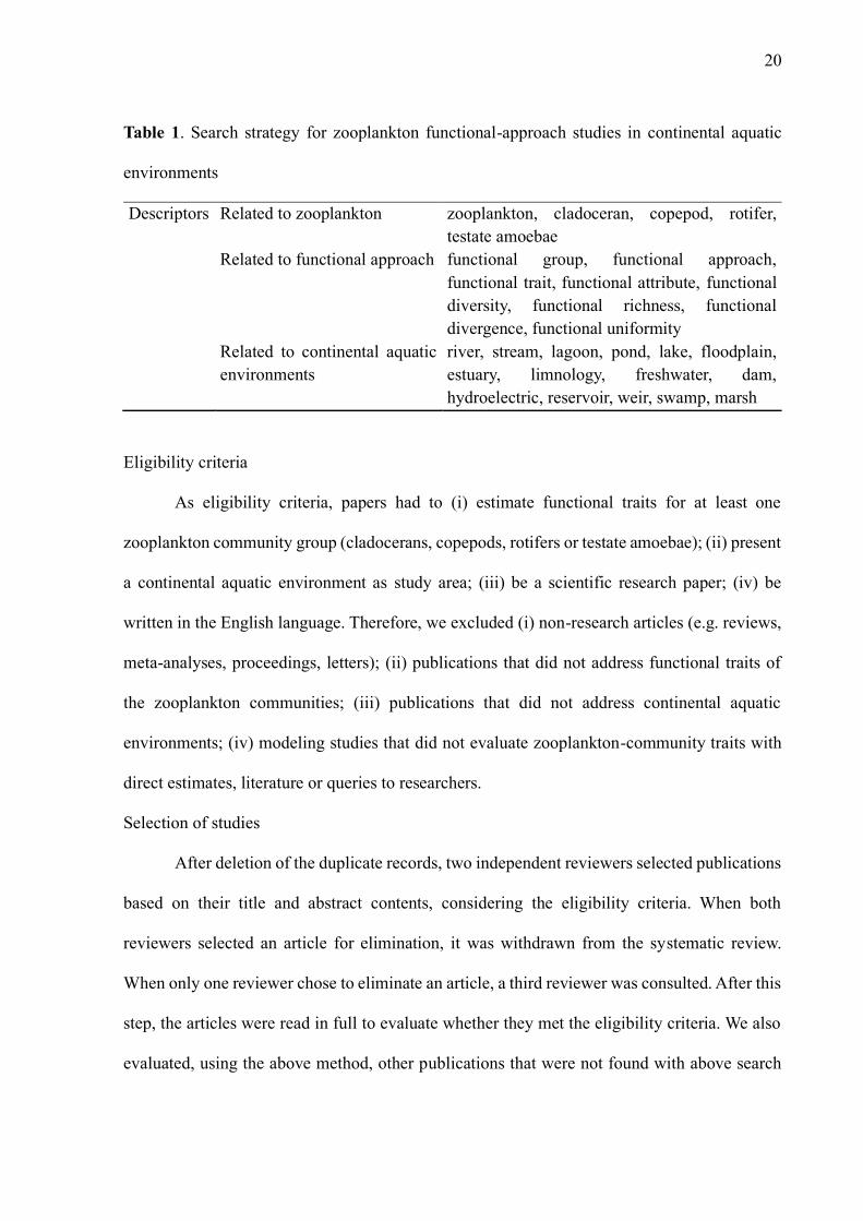
Table 1. Search strategy for zooplankton functional-approach studies in continental aquatic
environments
Descriptors Related to zooplankton zooplankton, cladoceran, copepod, rotifer,
testate amoebae Related to functional approach functional group, functional approach,
functional trait, functional attribute, functional
diversity, functional richness, functional
divergence, functional uniformity Related to continental aquatic
environments
river, stream, lagoon, pond, lake, floodplain,
estuary, limnology, freshwater, dam,
hydroelectric, reservoir, weir, swamp, marsh
Eligibility criteria
As eligibility criteria, papers had to (i) estimate functional traits for at least one
zooplankton community group (cladocerans, copepods, rotifers or testate amoebae); (ii) present
a continental aquatic environment as study area; (iii) be a scientific research paper; (iv) be
written in the English language. Therefore, we excluded (i) non-research articles (e.g. reviews,
meta-analyses, proceedings, letters); (ii) publications that did not address functional traits of
the zooplankton communities; (iii) publications that did not address continental aquatic
environments; (iv) modeling studies that did not evaluate zooplankton-community traits with
direct estimates, literature or queries to researchers.
Selection of studies
After deletion of the duplicate records, two independent reviewers selected publications
based on their title and abstract contents, considering the eligibility criteria. When both
reviewers selected an article for elimination, it was withdrawn from the systematic review.
When only one reviewer chose to eliminate an article, a third reviewer was consulted. After this
step, the articles were read in full to evaluate whether they met the eligibility criteria. We also
evaluated, using the above method, other publications that were not found with above search

21
terms but included functional traits of the zooplankton communities in continental aquatic
environments included (e.g., papers cited in selected publications).
Description of studies
We used the Web of Science and Scopus platforms to obtain the annual number of
publications, countries’ participation in publications. We extracted the data into a data sheet and
checked the countries. After this step, we imported the data into the R program (R Core Team
2017), with the ggplot and geom_point functions from ggplot2 package (Wickham 2016).
We classified the location of sampling units of each publication into state or province,
and produced a global map of regions with highest sampling densities.
Data collection process
We extracted the following information from the selected publications: (i) authors and
year of publication, (ii) zooplankton group, (iii) evaluated functional traits, (iv) Traits
determination method, and (iv) study-area location/country.
RESULTS
The search retrieved 252 publications in the Web of Science and 210 in Scopus database.
After removal of duplicate publications and article selection with the eligibility criteria, only
41 articles remained for further analyses (Fig. 1).
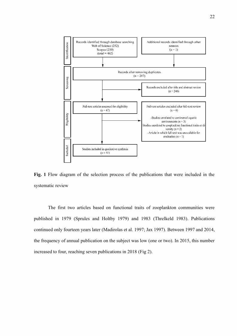
22
Fig. 1 Flow diagram of the selection process of the publications that were included in the
systematic review
The first two articles based on functional traits of zooplankton communities were
published in 1979 (Sprules and Holtby 1979) and 1983 (Threlkeld 1983). Publications
continued only fourteen years later (Madirolas et al. 1997; Jax 1997). Between 1997 and 2014,
the frequency of annual publication on the subject was low (one or two). In 2015, this number
increased to four, reaching seven publications in 2018 (Fig 2).

23
Fig. 2 Number of publications per year of studies using the functional-trait approach for
zooplankton communities in continental aquatic environments
Canada had the largest number of publication authorships, followed by the United States
of America (USA), Brazil, and Italy (Fig. 3). The country and regions that had the largest
number of samplings were Eastern Canada, followed by the Eastern USA, Southern Brazil and
Northern Italy (Fig. 4).

24
Fig. 3 Number of publications using the functional-trait approach for zooplankton communities
in continental aquatic environments considering the main authorship nationality
Fig. 4 Number of studies per country and sampling areas in studies using the functional-trait
approach for zooplankton communities in continental aquatic environments. The color of the
25
countries indicates the number of studies per country. Colored circles indicate the number of
sampling areas in States or Provinces.
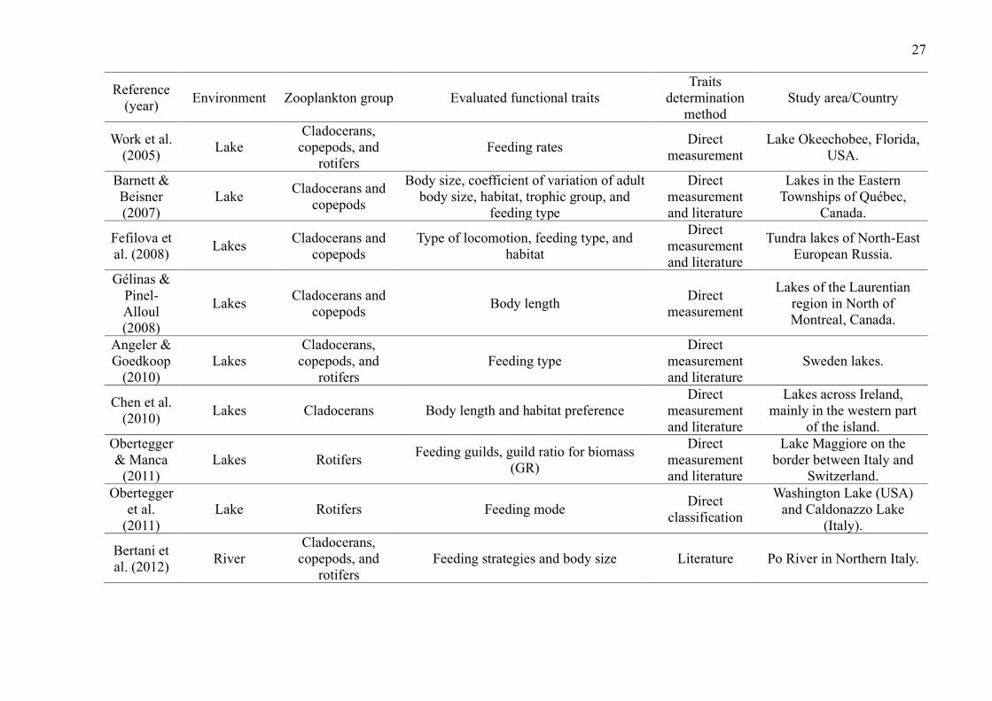
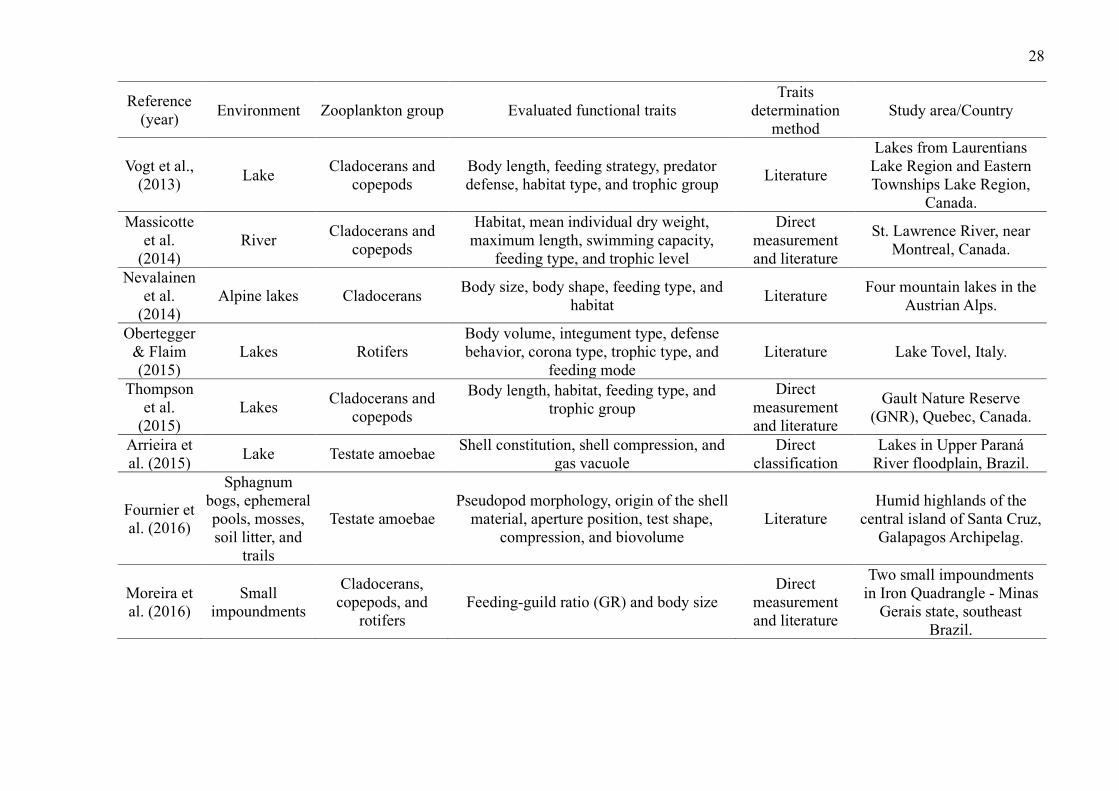
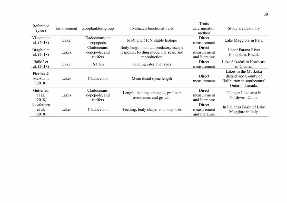
Lakes were the environments with the largest number of studies (29 publications,
72.5%). The most studied zooplankton groups were cladocerans (27 publications, 67.5%),
followed by copepods (22 publications, 55%), rotifers (15 publications, 37.5%) and testate
amoebae (5 publications, 12.5%) (Table 2). While some groups were evaluated in the same
studies, studies that included testate amoebae evaluated exclusively this group.
Overall, studies evaluated a wide of variety of traits (such as anatomical dimensions,
trophic group, feeding habits and rates, predator defense strategies, habitat, and swimming
capacity) and environments (such as lakes, ponds, reservoirs, streams, estuaries, and bogs)
(Table 2). The most common ones were related to volume and body measurements (26
publications, 65%). Although many publications used their direct measurements, especially
those related to body measurements, many authors have used the literature to obtain the traits.
Only 5 studies used dispersion as a trait (Table 2).

26
Table 2. Description of studies using the functional-trait approach for zooplankton communities in continental aquatic environments
Reference
(year) Environment Zooplankton group Evaluated functional traits
Traits
determination
method
Study area/Country
Sprules
and Holtby
(1979)
Lakes
Cladocerans,
copepods, and
rotifers
Body length and trophic group
Direct
measurement
and literature
Lakes on the Bruce
Peninsula, Ontario, Canada.
Threlkeld
(1983) Reservoir
Cladocerans,
copepods, and
rotifers
Feeding type and trophic group, body size,
scape ability, and behavioral (solitary or
colonial)
Literature Reservoir in southcentral
Tennessee, U.S.A.
Jax (1997) Stream Testate amoebae
Dispersal ability, preference for particular
phases of succession, and ability to
dominate the assemblages during late
phases of succession.
Direct
measurement
Ilm River in Thuringia,
Germany.
Madirolas
et al.
(1997)
Estuary Copepods Body length and body composition Literature
Río de la Plata Estuary
located between Argentina
and Uruguay.
Fischer et
al. (2001) Lake
Cladocerans and
copepods Body size and feeding type
Direct
measurement
and literature
Little Rock Lake, located in
the Northern Highlands
Lake District of Wisconsin,
USA.
Havlicek &
Carpenter
(2001)
Lakes
Cladocerans,
copepods, and
rotifers
Average body size Direct
measurement
Lakes from Wisconsin
(USA).
Rusak et
al. (2002) Lake
Cladocerans and
copepods Body size and food web position
Direct
classification
Lakes in three regions of
central North America.
Stemberger
& Miller
(2003)
Lakes Cladocerans Body size and grazing potential
Direct
measurement
and literature
Lakes in New York,
Vermont, and New
Hampshire, U.S.A.
27
Reference
(year) Environment Zooplankton group Evaluated functional traits
Traits
determination
method
Study area/Country
Work et al.
(2005) Lake
Cladocerans,
copepods, and
rotifers
Feeding rates Direct
measurement
Lake Okeechobee, Florida,
USA.
Barnett &
Beisner
(2007)
Lake Cladocerans and
copepods
Body size, coefficient of variation of adult
body size, habitat, trophic group, and
feeding type
Direct
measurement
and literature
Lakes in the Eastern
Townships of Québec,
Canada.
Fefilova et
al. (2008) Lakes
Cladocerans and
copepods
Type of locomotion, feeding type, and
habitat
Direct
measurement
and literature
Tundra lakes of North-East
European Russia.
Gélinas &
Pinel-
Alloul
(2008)
Lakes Cladocerans and
copepods Body length
Direct
measurement
Lakes of the Laurentian
region in North of
Montreal, Canada.
Angeler &
Goedkoop
(2010)
Lakes
Cladocerans,
copepods, and
rotifers
Feeding type
Direct
measurement
and literature
Sweden lakes.
Chen et al.
(2010) Lakes Cladocerans Body length and habitat preference
Direct
measurement
and literature
Lakes across Ireland,
mainly in the western part
of the island.
Obertegger
& Manca
(2011)
Lakes Rotifers Feeding guilds, guild ratio for biomass
(GR)
Direct
measurement
and literature
Lake Maggiore on the
border between Italy and
Switzerland.
Obertegger
et al.
(2011)
Lake Rotifers Feeding mode Direct
classification
Washington Lake (USA)
and Caldonazzo Lake
(Italy).
Bertani et
al. (2012) River
Cladocerans,
copepods, and
rotifers
Feeding strategies and body size Literature Po River in Northern Italy.
28
Reference
(year) Environment Zooplankton group Evaluated functional traits
Traits
determination
method
Study area/Country
Vogt et al.,
(2013) Lake
Cladocerans and
copepods
Body length, feeding strategy, predator
defense, habitat type, and trophic group Literature
Lakes from Laurentians
Lake Region and Eastern
Townships Lake Region,
Canada.
Massicotte
et al.
(2014)
River Cladocerans and
copepods
Habitat, mean individual dry weight,
maximum length, swimming capacity,
feeding type, and trophic level
Direct
measurement
and literature
St. Lawrence River, near
Montreal, Canada.
Nevalainen
et al.
(2014)
Alpine lakes Cladocerans Body size, body shape, feeding type, and
habitat Literature
Four mountain lakes in the
Austrian Alps.
Obertegger
& Flaim
(2015)
Lakes Rotifers
Body volume, integument type, defense
behavior, corona type, trophic type, and
feeding mode
Literature Lake Tovel, Italy.
Thompson
et al.
(2015)
Lakes Cladocerans and
copepods
Body length, habitat, feeding type, and
trophic group
Direct
measurement
and literature
Gault Nature Reserve
(GNR), Quebec, Canada.
Arrieira et
al. (2015) Lake Testate amoebae
Shell constitution, shell compression, and
gas vacuole
Direct
classification
Lakes in Upper Paraná
River floodplain, Brazil.
Fournier et
al. (2016)
Sphagnum
bogs, ephemeral
pools, mosses,
soil litter, and
trails
Testate amoebae
Pseudopod morphology, origin of the shell
material, aperture position, test shape,
compression, and biovolume
Literature
Humid highlands of the
central island of Santa Cruz,
Galapagos Archipelag.
Moreira et
al. (2016)
Small
impoundments
Cladocerans,
copepods, and
rotifers
Feeding-guild ratio (GR) and body size
Direct
measurement
and literature
Two small impoundments
in Iron Quadrangle - Minas
Gerais state, southeast
Brazil.

29
Reference
(year) Environment Zooplankton group Evaluated functional traits
Traits
determination
method
Study area/Country
Schwind et
al. (2016a)
Lakes and
Rivers Testate amoebae Shell composition
Direct
measurement
and literature
Upper Paraná River
floodplain, Brazil.
Bolduc et
al. (2016) Lake
Cladocerans and
copepods
Mean dry weight and maximum length,
habitat, swimming capacity, feeding type,
and trophic level
Direct
measurement
and literature
Lake Saint-Pierre of the St-
Lawrence River (Quebec,
Canada).
Schwind et
al. (2016b) Lake Testate amoebae
Shell constitution, gas vacuole, and
pseudopod morphology
Direct
classification
Osmar Lake, upper Paraná
River floodplain, Brazil.
Wen et al.
(2017) Lakes Rotifers
Functional traits relying on the guild ratio
(GR) and the modified guild ratio (GR′)
Direct
measurements
Lake Jinghu and Lake
Xiyanghu in Wuhu, China.
Oh et al.
(2017) Reservoirs Rotifers Trophic structure Literature
Agricultural reservoirs of
different locations and
various water environments
across South Korea.
Sodré et al.
(2017) Lake
Cladocerans,
copepods, and
rotifers
Body length, habitat, trophic group,
feeding type, and reproduction mode
Direct
measurement
and literature
Batata Lake in Pará, Brazil.
Verissimo
et al.
(2017)
Estuary Copepods Feeding, body size, feeding type, and
reproduction
Direct
measurement
and literature
Paraiba and Mamanguape
Estuaries in Brazil
Gianuca et
al. (2017) Farmland ponds Cladocerans Body size and habitat Literature
Farmland ponds across
Belgium.
Nevalainen
& Luoto
(2017)
Lakes Cladocerans Body size, body shape, feeding type, and
habitat Literature
Eutrophicated lakes from
southern Finland.
Redmond
et al.
(2018)
Lakes and
ponds spanning
Cladocerans and
copepods
Body size, photoprotection potential,
reproduction mode, habitat type Literature
Alberta/British Columbia
border in Western Canada.
30
Reference
(year) Environment Zooplankton group Evaluated functional traits
Traits
determination
method
Study area/Country
Visconti et
al. (2018) Lake
Cladocerans and
copepods δ13C and δ15N Stable Isotope
Direct
measurement Lake Maggiore in Italy.
Braghin et
al. (2018) Lakes
Cladocerans,
copepods, and
rotifers
Body length, habitat, predatory escape
response, feeding mode, life span, and
reproduction
Direct
measurement
and literature
Upper Parana River
floodplain, Brazil.
Balkić et
al. (2018) Lake Rotifers Feeding rates and types
Direct
measurement
Lake Sakadaš in Northeast
of Croatia.
Fiorino &
McAdam
(2018)
Lakes Cladocerans Mean distal spine length Direct
measurement
Lakes in the Muskoka
district and County of
Haliburton in southcentral
Ontario, Canada.
Gutierrez
et al.
(2018)
Lakes
Cladocerans,
copepods, and
rotifers
Length, feeding strategies, predator
avoidance, and growth
Direct
measurement
and literature
Ulungur Lake area in
Northwest China.
Nevalainen
et al.
(2018)
Lakes Cladocerans Feeding, body shape, and body size
Direct
measurement
and literature
In Pallanza Basin of Lake
Maggiore in Italy.
31
DISCUSSION
We restricted our search to studies that evaluated one or more characteristics of
zooplanktonic organisms and explicitly mentioned them as functional traits or synonyms (e.g.
functional group, functional approach, functional trait). Therefore, we may have missed
publications that described some zooplankton traits but have not used the terms functional
attributes/traits in the title, abstract, or keywords.
The first studies evaluating functional traits of the zooplankton communities in
continental aquatic environments were published more than three decades ago (Sprules and
Holtby 1979; Threlkeld 1983). Only more recently, the interest on the subject has increased,
particularly after studies showing greater effectiveness of the functional-approach evaluation
when compared to the taxonomic approach (Tilman 1997, 2001; Petchey and Gaston 2002;
Laureto et al. 2015), and indicating the predictive potential of the functional approach regarding
ecosystems’ responses to global environmental changes (Petchey and Gaston 2002; McGill et
al. 2006; Toussaint et al. 2016).
There has been a gradual increase in the number of studies on functional traits of
zooplankton communities. This approach has been consolidated with different aquatic
organisms such as phytoplankton (Kruk et al. 2012; Reynolds et al. 2014), macrophyte (Weiher
et al. 1999), and fish (Pont et al. 2006; Winemiller et al. 2015). Nonetheless, this growth may
be due to fact that including the functional approach is more elucidative than just using the
taxonomic approach, considering that an environment can have a large number of species with
similar functional traits (functional redundancy). Therefore, the diversity of functional traits
may correspond to environmental variations in cases that can be undetected using the only
taxonomic approach (Petchey and Gaston 2002, 2006). Most zooplankton functional-approach
studies in continental aquatic environments are concentrated in North America (Canada and the
USA) and Brazil. Overall, the number of research studies in developed countries (e.g. USA and
Canada) is higher when compared to developing or emerging countries, and often related to

32
social and political factors (e.g. Gross Domestic Product and national research investments)
(Nabout et al. 2010; de Souza Vanz and Stumpf 2012).
Brazil has recently increased the number of publication authorships on zooplankton
functional-approach studies, following the tendency of other emerging countries (de Souza
Vanz and Stumpf 2012; Leta 2012). Besides the fact that the functional approach is
complementary to the taxonomic one, the increase is mostly due to the rising number of
researchers in these countries and to recent national and international scientific-collaboration
policies (de Souza Vanz and Stumpf 2012; Mena-Chalco et al. 2014; Grossetti et al. 2014;
Zhang et al. 2016).
Environments, functional traits, and ecological function
Most studies evaluating functional traits of zooplankton communities comprised lentic
environments, especially lakes. In fact, zooplankton are more abundant in low-current
environments because of their low water-resistance capacity and their feeding and reproduction
difficulties in lotic environments (Schwind et al. 2013; Maznah et al. 2018), this may justify the
high number of studies in these environments. In addition, lakes are natural environments,
which may explain the greater amount of publications in these areas. Meanwhile, reservoirs,
for example, are designed ecosystems (Morse et al. 2014). Therefore, the studies of these
environments and their relation with the effects on the functional diversity are often restricted
to the companies in charge of these areas.
The few numbers of studies on testate amoebae may be because some authors do not
consider them as zooplankton organisms since they belong to the kingdom Protista.
Furthermore, some claim that planktonic environments are unfriendly habitats for the group
and their presence in these environments is hardly accidental, especially in low salinity
environments. However, testate amoebae are frequent and abundant in planktonic environments
(Lansac-Tôha et al. 2007). On the other hand, the largest number of publications on

33
microcrustaceans and rotifers may be a result of the greater availability of functional-trait
descriptions in the literature for these groups (Barnett et al. 2007; Obertegger et al. 2011;
Braghin et al. 2018).
These factors may explain the fact that while a large number of studies included
cladocerans, copepods and rotifers altogether, testate amoebae were evaluated exclusively in
other studies. Although there are fewer publications on testate amoebae, this group is a good
ecological indicator because of its high environmental sensitivity and rapid response time to
environmental variations (Yang et al. 2011; Payne 2013). The separation of testate amoebae in
studies may also be related to its most distinct phenotype. For example, measures such as body
size are often used for cladocerans, copepods, and rotifers (Nevalainen and Luoto 2017;
Verissimo et al. 2017; Sodré et al. 2017). However, other measures are used for testate amoebae
(e.g. carapace constitution, pseudopodia morphology and presence of vacuoles) (Arrieira et al.
2015; Schwind et al. 2016a). In view of these distinctions, more studies should include this
group with other zooplankton groups in places where this group is more abundant, in order to
better understand the relation of the functional traits of these organisms with their ecosystem.
This could improve the understanding of environmental dynamics due to a greater range of
functional traits in response to environmental characteristics.
We found few studies on small water bodies with low water flow, such as sphagnum
bogs, ephemeral pools, small impoundments and ponds. These smaller reservoirs, which often
have accessibility limitations, are also less investigated for other groups of species (Rosenberg
et al. 2000; Alexandre and Almeida 2009). Therefore, the difficult accessibility may be a factor
that makes zooplankton community studies in these environments unviable. Despite their small
size, these environments host many endemic species and strongly contribute to regional
biodiversity. Some ponds, for instance, may harbor greater taxonomic diversity than large rivers
34
(Oertli et al. 2005). Thus, more studies should investigate these environments to the interaction
of functional diversity in these environments.
For all zooplankton groups, the most common functional traits were the ones related to
body measurements. Body size is a morphological trait that encompasses several ecological
functions ranging from feeding, growth and reproduction, and survival. Larger organisms have
a wider diversity spectrum of smaller organisms that they can capture and higher reproductive
and survival capacity because of their increased locomotion abilities for reproduction and
escaping predators (Litchman et al. 2013). Besides being readily determined during the
identification process, body size is a fundamental trait for ecosystem dynamics. Thus, it is
widely used as a functional trait. Therefore, although the scatterability is poorly evaluated, its
ecological functions can be understood by the use of body size, considering that these traits are
strongly related (Litchman et al. 2013).
Many studies also evaluated feeding-related traits. However, unlike body dimensions,
most were obtained in literature. This can be justified by the greater difficulty in measuring
such traits during the identification process. Many researchers have used the feeding guilds and
guild ratio for biomass (GR) approach for rotifers proposed by Obertegger et al. (2011). This
approach compares the relative contribution of biomass from organisms that share feeding
strategies with the total biomass. This method effectively improved the understanding of
biological dynamics in relation to the environment and, therefore, was used in other
publications (Moreira et al. 2016; Wen et al. 2017). The GR also reflects the importance of the
guild’s feeding strategy for the ecosystem dynamics (Litchman et al. 2013).
Studies that integrate different types of functional traits have a greater chance of
evaluating effective responses in relation to the ecosystem (Litchman et al. 2013). Functional
traits can be classified into traits such as those that occur as a result of ecosystem variations
(response) or those that are capable of influencing their dynamics (effect). Despite this fact,
35
most authors have emphasized the response traits. Therefore, there is a gap on the effects of
zooplankton community traits on ecosystems (Hébert et al. 2017). In Barnett & Beisner (2007),
taxonomic richness provided a unimodal response to the variation of total-phosphorus input.
Nonetheless, there was a loss in functional diversity with increasing total-phosphorus inputs.
Furthermore, the increase in the heterogeneity of cyanobacteria also caused an increase in
zooplankton functional diversity.
CONCLUSION
Functional-approach research studies for zooplankton communities in continental
aquatic environments are scarce, and authors and samplings areas are mostly concentrated in
Canada, USA, Brazil, and Italy. Nonetheless, the recent increase in publications in the last three
years is a step forward in improving the understanding of the structure and functioning of these
communities.
Most functional-approach studies examined body-size related functional traits. Body
size integrates several ecological functions, and researchers can easily measure it during the
identification process. Other studies considered the traits related to feeding strategies and diet
and these traits deserve attention because they interfere with the transfer of energy between
lower and higher trophic levels. These studies also provided important insights into the different
ways in which groups explore their respective niches. Thus, the functional approach is an
important tool to understand the ecosystem processes, and thus to contribute to the knowledge
of biodiversity conservation and ecosystem dynamics. Therefore, the scientific community
must continue to investigate the traits related to the different ecological functions of these
organisms, considering their environmental and spatial dynamics. In addition, the dispersion
capacity may have a strong relationship with the organisms’ responses to environmental
variations and, therefore, deserves further attention in future studies.
36
Our study also demonstrated that there is a gap in functional-approach studies
worldwide. Even in countries with scientific production on the subject, sampling areas were
concentrated in few regions. Therefore, we highlight the need for environmental policies to
include the functional approach in a complementary way to taxonomic surveys in biomonitoring
programs and scientific studies. This should improve the knowledge of the dynamics of
zooplankton organisms and their ecosystems.
REFERENCES
Alexandre CM, Almeida PR (2009) The impact of small physical obstacles on the structure of
freshwater fish assemblages. River Res Appl 26:977–994. doi: 10.1002/rra.1308
Angeler DG, Goedkoop W (2010) Biological responses to liming in boreal lakes: An
assessment using plankton, macroinvertebrate and fish communities. J Appl Ecol
47:478–486. doi: 10.1111/j.1365-2664.2010.01794.x
Arrieira RL, Schwind LTF, Bonecker CC, Lansac-Tôha FA (2015) Use of functional diversity
to assess determinant assembly processes of testate amoebae community. Aquat Ecol
49:561–571. doi: 10.1007/s10452-015-9546-z
Balkić AG, Ternjej I, Špoljar M (2018) Hydrology driven changes in the rotifer trophic
structure and implications for food web interactions. Ecohydrology 11:e1917. doi:
10.1002/eco.1917
Barnett A, Beisner BE (2007) Zooplankton biodiversity and lake trophic state: Explanations
invoking resource abundance and distribution. Ecology 88:1675–1686. doi: 10.1890/06-
1056.1
Barnett AJ, Finlay K, Beisner BE (2007) Functional diversity of crustacean zooplankton
communities: towards a trait-based classification. Freshw Biol 52:796–813. doi:
10.1111/j.1365-2427.2007.01733.x

37
Bertani I, Ferrari I, Rossetti G (2012) Role of intra-community biotic interactions in
structuring riverine zooplankton under low-flow, summer conditions. J Plankton Res
34:308–320. doi: 10.1093/plankt/fbr111
Bolduc P, Bertolo A, Pinel-Alloul B (2016) Does submerged aquatic vegetation shape
zooplankton community structure and functional diversity? A test with a shallow fluvial
lake system. Hydrobiologia 778:151–165. doi: 10.1007/s10750-016-2663-4
Braghin L de SM, Almeida B de A, Amaral DC, et al (2018) Effects of dams decrease
zooplankton functional -diversity in river-associated lakes. Freshw Biol 63:721–730. doi:
10.1111/fwb.13117
Chen G, Dalton C, Taylor D (2010) Cladocera as indicators of trophic state in Irish lakes. J
Paleolimnol 44:465–481. doi: 10.1007/s10933-010-9428-2
Cianciaruso MV, Silva IA, Batalha MA (2009) Diversidades filogenética e funcional: novas
abordagens para a Ecologia de comunidades. Biota Neotrop 9:93–103. doi:
10.1590/S1676-06032009000300008
de Souza Vanz SA, Stumpf IRC (2012) Scientific Output Indicators and Scientific
Collaboration Network Mapping in Brazil. Collnet J Sci Inf Manag 6:315–334. doi:
10.1080/09737766.2012.10700942
Fefilova EB, Loskutova OA, Pestov S V (2008) Micro-benthic crustacean communities in
tundra lakes of North-East European Russia. Aquat Ecol 42:449–461. doi:
10.1007/s10452-007-9109-z
Fiorino GE, McAdam AG (2018) Local differentiation in the defensive morphology of an
invasive zooplankton species is not genetically based. Biol Invasions 20:235–250. doi:
10.1007/s10530-017-1530-1
Fischer JM, Frost TM, Ives AR (2001) Compensatory dynamics in zooplankton community
responses to acidification: Measurement and mechanisms. Ecol Appl 11:1060–1072. doi:
38
10.1890/1051-0761(2001)011[1060:CDIZCR]2.0.CO;2
Fournier B, Coffey EED, van der Knaap WO, et al (2016) A legacy of human-induced
ecosystem changes: spatial processes drive the taxonomic and functional diversities of
testate amoebae in Sphagnum peatlands of the Galápagos. J Biogeogr 43:533–543. doi:
10.1111/jbi.12655
Gélinas M, Pinel-Alloul B (2008) Relating crustacean zooplankton community structure to
residential development and landcover disturbance near Canadian Shield lakes. Can J
Fish Aquat Sci 65:2689–2702. doi: 10.1139/F08-163
Gianuca AT, Declerck SAJ, Cadotte MW, et al (2017) Integrating trait and phylogenetic
distances to assess scale-dependent community assembly processes. Ecography (Cop)
40:742–752. doi: 10.1111/ecog.02263
Gianuca AT, Engelen J, Brans KI, et al (2018) Taxonomic, functional and phylogenetic
metacommunity ecology of cladoceran zooplankton along urbanization gradients.
Ecography (Cop) 41:183–194. doi: 10.1111/ecog.02926
Grossetti M, Eckert D, Gingras Y, et al (2014) Cities and the geographical deconcentration of
scientific activity: A multilevel analysis of publications (1987–2007). Urban Stud
51:2219–2234. doi: 10.1177/0042098013506047
Gutierrez MF, Tavsanoglu UN, Vidal N, et al (2018) Salinity shapes zooplankton communities
and functional diversity and has complex effects on size structure in lakes.
Hydrobiologia 813:237–255. doi: 10.1007/s10750-018-3529-8
Havlicek TD, Carpenter SR (2001) Pelagic species size distributions in lakes: Are they
discontinuous? Limnol Oceanogr 46:1021–1033. doi: 10.4319/lo.2001.46.5.1021
Hébert M-P, Beisner BE, Maranger R (2017) Linking zooplankton communities to ecosystem
functioning: toward an effect-trait framework. J Plankton Res 39:3–12. doi:
10.1093/plankt/fbw068
39
Jax K (1997) On functional attributes of testate amoebae in the succession of freshwater
aufwuchs. Eur J Protistol 33:219–226. doi: 10.1016/S0932-4739(97)80040-5
Kruk C, Segura AM, Peeters ETHM, et al (2012) Phytoplankton species predictability
increases towards warmer regions. Limnol Oceanogr 57:1126–1135. doi:
10.4319/lo.2012.57.4.1126
Lansac-Tôha FA, Zimmermann-callegari MC, Mucio G, et al (2007) Species richness and
geographic distribution of testate amoebae (Rhizopoda) in Brazilian freshwater
environments. Acta Sci Biol Sci 29:185–195
Laureto LMO, Cianciaruso MV, Samia DSM (2015) Functional diversity: an overview of its
history and applicability. Nat Conserv 13:112–116. doi: 10.1016/j.ncon.2015.11.001
Leoni B (2016) Zooplankton predators and prey: body size and stable isotope to investigate
the pelagic food web in a deep lake (Lake Iseo, Northern Italy). J Limnol. doi:
10.4081/jlimnol.2016.1490
Leta J (2012) Brazilian growth in the mainstream science: The role of human resources and
national journals. J Scientometr Res 1:44–52. doi: 10.5530/jscires.2012.1.9
Lira A, Angelini R, Le Loc’h F, et al (2018) Trophic flow structure of a neotropical estuary in
northeastern Brazil and the comparison of ecosystem model indicators of estuaries. J Mar
Syst 182:31–45. doi: 10.1016/j.jmarsys.2018.02.007
Litchman E, Ohman MD, Kiørboe T (2013) Trait-based approaches to zooplankton
communities. J Plankton Res 35:473–484. doi: 10.1093/plankt/fbt019
Madirolas A, Acha EM, Guerrero RA, Lasta C (1997) Sources of acoustic scattering near a
halocline in an estuarine frontal system. Sci Mar 61:431–438
Mano H, Tanaka Y (2016) Mechanisms of compensatory dynamics in zooplankton and
maintenance of food chain efficiency under toxicant stress. Ecotoxicology 25:399–411.
doi: 10.1007/s10646-015-1598-2
40
Martiny AC, Treseder K, Pusch G (2013) Phylogenetic conservatism of functional traits in
microorganisms. ISME J 7:830–838. doi: 10.1038/ismej.2012.160
Massicotte P, Frenette J-J, Proulx R, et al (2014) Riverscape heterogeneity explains spatial
variation in zooplankton functional evenness and biomass in a large river ecosystem.
Landsc Ecol 29:67–79. doi: 10.1007/s10980-013-9946-1
Maznah WOW, Intan S, Sharifah R, Lim CC (2018) Lentic and lotic assemblages of
zooplankton in a tropical reservoir, and their association with water quality conditions.
Int J Environ Sci Technol 15:533–542
McGill B, Enquist B, Weiher E, Westoby M (2006) Rebuilding community ecology from
functional traits. Trends Ecol Evol 21:178–185. doi: 10.1016/j.tree.2006.02.002
Mena-Chalco JP, Digiampietri LA, Lopes FM, Cesar RM (2014) Brazilian bibliometric
coauthorship networks. J Assoc Inf Sci Technol 65:1424–1445. doi: 10.1002/asi.23010
Moher D, Shamseer L, Clarke M, et al (2015) Preferred reporting items for systematic review
and meta-analysis protocols (PRISMA-P) 2015 statement. Syst Rev 4:1. doi:
10.1186/2046-4053-4-1
Moreira FWA, Leite MGP, Fujaco MAG, et al (2016) Assessing the impacts of mining
activities on zooplankton functional diversity [Avaliando os impactos das atividades de
mineração sobre a diversidade funcional do zooplâncton]. Acta Limnol Bras 28:. doi:
10.1590/S2179-975X0816
Morse NB, Pellissier PA, Cianciola EN, et al (2014) Novel ecosystems in the Anthropocene: a
revision of the novel ecosystem concept for pragmatic applications. Ecol Soc 19:art12.
doi: 10.5751/ES-06192-190212
Nabout JC, Bini LM, Diniz-Filho JAF (2010) Global literature of fiddler crabs, genus Uca
(Decapoda, Ocypodidae): trends and future directions. Iheringia Série Zool 100:463–
468. doi: 10.1590/S0073-47212010000400019
41
Nevalainen L, Brown M, Manca M (2018) Sedimentary record of cladoceran functionality
under Eutrophication and re-oligotrophication in Lake Maggiore, Northern Italy. Water
(Switzerland) 10:. doi: 10.3390/w10010086
Nevalainen L, Luoto TP (2017) Relationship between cladoceran (Crustacea) functional
diversity and lake trophic gradients. Funct Ecol 31:488–498. doi: 10.1111/1365-
2435.12737
Nevalainen L, Luoto TP, Manca M, Weisse T (2014) A paleolimnological perspective on
aquatic biodiversity in Austrian mountain lakes. Aquat Sci 77:59–69. doi:
10.1007/s00027-014-0363-6
Obertegger U, Flaim G (2015) Community assembly of rotifers based on morphological traits.
Hydrobiologia 753:31–45. doi: 10.1007/s10750-015-2191-7
Obertegger U, Manca M (2011) Response of rotifer functional groups to changing trophic
state and crustacean community. J Limnol 70:231–238. doi: 10.3274/JL11-70-2-07
Obertegger U, Smith HA, Flaim G, Wallace RL (2011) Using the guild ratio to characterize
pelagic rotifer communities. Hydrobiologia 662:157–162. doi: 10.1007/s10750-010-
0491-5
Oertli B, Biggs J, Céréghino R, et al (2005) Conservation and monitoring of pond
biodiversity: introduction. Aquat Conserv Mar Freshw Ecosyst 15:535–540. doi:
10.1002/aqc.752
Oh H-J, Jeong H-G, Nam G-S, et al (2017) Comparison of taxon-based and trophi-based
response patterns of rotifer community to water quality: applicability of the rotifer
functional group as an indicator of water quality. Animal Cells Syst (Seoul) 21:133–140.
doi: 10.1080/19768354.2017.1292952
Payne RJ (2013) Seven reasons why protists make useful bioindicators. Acta Protozool
52:105–113. doi: 10.4467/16890027AP.13.0011.1108

42
Petchey OL, Gaston KJ (2006) Functional diversity: back to basics and looking forward. Ecol
Lett 9:741–758. doi: 10.1111/j.1461-0248.2006.00924.x
Petchey OL, Gaston KJ (2002) Functional diversity (FD), species richness and community
composition. Ecol Lett 5:402–411. doi: 10.1046/j.1461-0248.2002.00339.x
Pont D, Hugheny B, Beuer U, et al (2006) Assessing river biotic condition at a continental
scale: a European approach using functional metrics and fish assemblages. J Appl Ecol
43:70–80. doi: 10.1111/j.1365-2664.2005.01126.x
Pool TK, Grenouillet G, Villéger S (2014) Species contribute differently to the taxonomic,
functional, and phylogenetic alpha and beta diversity of freshwater fish communities.
Divers Distrib 20:1235–1244. doi: 10.1111/ddi.12231
R Core Team (2017) R: A Language and Environment for Statistical Computing
Raevel V, Violle C, Munoz F (2012) Mechanisms of ecological succession: insights from
plant functional strategies. Oikos 121:1761–1770. doi: 10.1111/j.1600-
0706.2012.20261.x
Redmond LE, Loewen CJG, Vinebrooke RD (2018) A Functional Approach to Zooplankton
Communities in Mountain Lakes Stocked With Non-Native Sportfish Under a Changing
Climate. Water Resour Res 54:2362–2375. doi: 10.1002/2017WR021956
Reynolds CS, Alex Elliott J, Frassl MA (2014) Predictive utility of trait-separated
phytoplankton groups: A robust approach to modeling population dynamics. J Great
Lakes Res 40:143–150. doi: 10.1016/j.jglr.2014.02.005
Rizo EZC, Gu Y, Papa RDS, et al (2017) Identifying functional groups and ecological roles of
tropical and subtropical freshwater Cladocera in Asia. Hydrobiologia 799:83–99. doi:
10.1007/s10750-017-3199-y
Rosenberg DM, McCully P, Pringle CM (2000) Global-scale environmental effects of
hydrological alterations: Introduction. Bioscience 50:746–751. doi: 10.1641/0006-

43
3568(2000)050{[}0746:GSEEOH]2.0.CO;2
Rusak JA, Yan ND, Somers KM, et al (2002) Temporal, spatial, and taxonomic patterns of
crustacean zooplankton variability in unmanipulated north-temperate lakes. Limnol
Oceanogr 47:613–625. doi: 10.4319/lo.2002.47.3.0613
Schwind LTF, Arrieira RL, Bonecker CC, Lansac-Toha FA (2016a) Chlorophyll-a and
Suspended Inorganic Material Affecting the Shell Traits of Testate Amoebae Community.
ACTA Protozool 55:145–154. doi: 10.4467/16890027AP.16.014.5746
Schwind LTF, Arrieira RL, Mantovano T, et al (2016b) Temporal influence on the functional
traits of testate amoebae in a floodplain lake. LIMNETICA 35:355–364
Schwind LTF, Dias JD, Joko CY, et al (2013) Advances in studies on testate amoebae
(Arcellinida and Euglyphida): a scientometric approach. Acta Sci Biol Sci 35:549–555.
doi: http://dx.doi.org/10.4025/actascibiolsci.v35i4.18184
Sodré E de O, Figueiredo-Barros MP, Roland F, et al (2017) Complimentary biodiversity
measures applied to zooplankton in a recovering floodplain lake. Fundam Appl Limnol /
Arch für Hydrobiol 190:279–298. doi: 10.1127/fal/2017/1064
Sprules WG, Holtby LB (1979) Body Size and Feeding Ecology as Alternatives to Taxonomy
for the Study of Limnetic Zooplankton Community Structure. J Fish Res Board Canada
36:1354–1363. doi: 10.1139/f79-194
Stemberger RS, Miller EK (2003) Cladoceran body length and Secchi disk transparency in
northeastern U.S. lakes. Can J Fish Aquat Sci 60:1477–1486. doi: 10.1139/f03-124
Thompson PL, Davies TJ, Gonzalez A (2015) Ecosystem functions across trophic levels are
linked to functional and phylogenetic diversity. PLoS One 10:. doi:
10.1371/journal.pone.0117595
Threlkeld ST (1983) Spatial and temporal variation in the summer zooplankton community of
a riverine reservoir. Hydrobiologia 107:249–254. doi: 10.1007/BF00036694
44
Tilman D (1997) The Influence of Functional Diversity and Composition on Ecosystem
Processes. Science (80- ) 277:1300–1302. doi: 10.1126/science.277.5330.1300
Tilman D (2001) Functional Diversity. In: Encyclopedia of Biodiversity. Elsevier, pp 587–596
Toussaint A, Charpin N, Brosse S, Villéger S (2016) Global functional diversity of freshwater
fish is concentrated in the Neotropics while functional vulnerability is widespread. Sci
Rep 6:22125. doi: 10.1038/srep22125
Verissimo H, Patricio J, Goncalves E, et al (2017) Functional diversity of zooplankton
communities in two tropical estuaries (NE Brazil) with different degrees of human-
induced disturbance. Mar Environ Res 129:46–56. doi: 10.1016/j.marenvres.2017.04.011
Vieira ACB, Medeiros AMA, Ribeiro LL, Crispim MC (2011) Population dynamics of Moina
minuta Hansen (1899), Ceriodaphnia cornuta Sars (1886), and Diaphanosoma
spinulosum Herbst (1967) (Crustacea: Branchiopoda) in different nutrients (N and P)
concentration ranges. Acta Limnol Bras 23:48–56. doi: 10.4322/actalb.2011.018
Visconti A, Caroni R, Rawcliffe R, et al (2018) Defining Seasonal Functional Traits of a
Freshwater Zooplankton Community Using delta C-13 and delta N-15 Stable Isotope
Analysis. Water 10:108. doi: 10.3390/w10020108
Vogt RJ, Peres-Neto PR, Beisner BE (2013) Using functional traits to investigate the
determinants of crustacean zooplankton community structure. Oikos 122:1700–1709.
doi: 10.1111/j.1600-0706.2013.00039.x
Weiher E, van der Werf A, Thompson K, et al (1999) Challenging Theophrastus: A common
core list of plant traits for functional ecology. J Veg Sci 10:609–620. doi:
10.2307/3237076
Wen X, Zhai P, Feng R, et al (2017) Comparative analysis of the spatiotemporal dynamics of
rotifer community structure based on taxonomic indices and functional groups in two
subtropical lakes. Sci Rep 7:. doi: 10.1038/s41598-017-00666-Y
45
Wickham H (2016) ggplot2: Elegant Graphics for Data Analysis. Springer-Verlag New York
Winemiller KO, Fitzgerald DB, Bower LM, Pianka ER (2015) Functional traits, convergent
evolution, and periodic tables of niches. Ecol Lett 18:737–751. doi: 10.1111/ele.12462
Work K, Havens K, Sharfstein B, East T (2005) How important is bacterial carbon to
planktonic grazers in a turbid, subtropical lake? J Plankton Res 27:357–372. doi:
10.1093/plankt/fbi013
Yang Z-C, Wang Z-H, Zhang Z-H (2011) Biomonitoring of testate amoebae (protozoa) as
toxic metals absorbed in aquatic bryophytes from the Hg-Tl mineralized area (China).
Environ Monit Assess 176:321–329. doi: 10.1007/s10661-010-1585-2
Zhang Y, Chen K, Zhu G, et al (2016) Inter-organizational scientific collaborations and policy
effects: an ego-network evolutionary perspective of the Chinese Academy of Sciences.
Scientometrics 108:1383–1415. doi: 10.1007/s11192-016-2022-2

46
Capítulo 2
Taxonomic and functional distribution of zooplankton in an Amazonian floodplain: a
metacommunity approach
Capítulo parcialmente formatado (para adequações à tese) conforme regras de submissão da
revista Hydrobiologia (Qualis A2 em Ciências Ambientais e fator de impacto (JCR) 2.325)

47
Abstract
The biological distribution is mainly due to the complexity of environmental and spatial
predictors interacting ecologically with factors such as predation and intraspecific and
interspecific competition. Due to the flood pulse dynamics in floodplains, these relationships
are more complex and distinct according to each hydrological period. Therefore, we evaluated
the relevance of environmental and spatial predictors in the taxonomic and functional structure
of the zooplankton community in an Amazonian floodplain, taking into account the
hydrological periods (flooding, flushing, high water and, low water). The flood pulse influenced
the most the structuring of the zooplankton community between hydrological periods. Some
taxa showed response patterns to the local environmental variables during flooding, flushing,
and low water periods. The functional structure of zooplankton was significantly related to the
local environmental variables only in the low water period. Spatial variation had no influence
on the community for either period. Thus, zooplankton is more associated with the species
sorting pattern, where environmental variations rather than spatial predictors predominantly
determine species. This factor shows the importance of the zooplankton community in
environmental monitoring programs due to its susceptibility to environmental variations.
However, there is still a gap regarding the functional traits of the zooplankton community.
Therefore, we suggest advancement in experimental studies that contemplate zooplanktonic
responses to ecosystem variations.
Keywords: species sorting, flood pulse, functional traits, functional approach
Acknowledgments
The authors thank to Coordenação de Aperfeiçoamento de Pessoal de Nível Superior (CAPES)
for providing financial assistance to L.F.G., to Fondation pour la Recherche sur la Biodiversité
(FRB) and to Conselho Nacional de Desenvolvimento Científico e Tecnológico (CNPq) that, in
partnership with Institut de Recherche pour le Développement (IRD), financed the project
number process: 490634/2013-3.

48
Introduction
The metacommunity approach evaluates the determining factors for the distribution of
communities possibly interconnected by the active or passive dispersion of organisms. From
this perspective, the two main factors that can control the structure of organisms are the
environmental characteristics and the dispersal capacity of species in the face of spatial barriers
or connections (Leibold et al., 2004). Although zooplanktonic organisms are mostly passively
dispersed, species with higher active dispersal capacity can migrate over short distances in
search of food or disperse under local environmental conditions that are not conducive to their
survival, so they are more controlled by spatial factors. On the other hand, smaller species are
more susceptible and filtered by environmental variations (De Bie et al., 2012). However, the
level of interconnection between habitats may vary, influencing species distribution by creating
barriers or connections that block or allow dispersal (Leibold et al., 2004; Penha et al., 2017).
Under the mechanistic approach, metacommunity assessment seeks to understand the
influence of environmental and spatial variables on community distribution through four main
paradigms (Leibold et al., 2004; Cottenie, 2005; Holyoak et al., 2005; Logue et al., 2011; Prado
& Rossa-Feres, 2014): species-sorting, mass-effects, patch-dynamics and neutral. However,
due to the complexity of classifying the ecological dynamics of organisms into paradigms, some
authors propose simplifying this approach to only two approaches, one fully environmental
(species-sorting) and one spatial (neutral) (Logue et al., 2011; Winegardner et al., 2012). From
a species-sorting perspective, communities can be present everywhere because they do not have
limited dispersion, for example, by spatial barriers. However, they are filtered by local
environmental variables. This paradigm differs from the mass-effects paradigm because the
species have a more limited active dispersal and are therefore more susceptible to
environmental variations. The patch-dynamics perspective differs from the others mainly due
to the homogeneity of the studied environment and, therefore, the composition of the
communities occurs by the interspecific competition. In this sense, species with lower
dominance or less competitive species have higher dispersal capacity, while dominant species
are weaker colonizers. On the other hand, from a neutral perspective, communities are
predominantly controlled by spatial variables, so all species are present in all environments,
and those locally extinct gradually are replaced by colonization.
In addition to the complexity and stochasticity of metacommunity assessment in natural
environments (Logue et al., 2011), aquatic environments are even more complex due to the
different levels of interconnectivity between areas of the same water body, which is influenced
49
by terrestrial ecosystem and water flow (Pellowe-Wagstaff & Simonis, 2014). Especially on
floodplains, where aquatic organisms are susceptible to seasonal hydrological variations. In low
waters, habitats are spatially isolated and thus promote greater environmental and biological
heterogeneities. On the other hand, in the high water period, there tends to be greater
homogenization due to interconnectedness (Junk et al., 1989; Thomaz et al., 2007). Moreover,
the flood pulse allows the constant exchange of organisms from the river to the lakes during the
flooding period and the opposite process during the flushing period (Lopes et al., 2014; Bozelli
et al., 2015).
In this context of complexity promoted by hydrological variations in flood plains, it is
relevant to understand the dynamics of zooplanktonic organisms in floodplains under different
facets (e.g., taxonomic and functional), due to its susceptibility to hydrological and
environmental variations (Goździejewska et al., 2016). Because it is composed of functionally
distinct groups (e.g., cladocerans, copepods, rotifers, and testates amoebae), the zooplankton
community can respond in different ways to environmental and spatial variations (Frisch et al.,
2012). Functional characteristics allow certain species to be more susceptible to environmental
variations than others, or to more easily disperse for food or due to the presence of potential
predators (Petchey & Gaston, 2002; Laureto et al., 2015).
Therefore, incorporating the functional facet in metacommunity studies makes the
understanding of structuring processes more complete, this has been done for many
communities of aquatic and terrestrial groups, such as fishes (Medina Torres & Higgins, 2016),
periphyton (Algarte et al., 2014), plants (Swan et al., 2017), microalgae (Vilmi et al., 2017) and
the zooplankton community (Gianuca et al., 2018). The determining factors for the variation of
species' functional traits are relevant not only for ecological studies but for management
programs that aim to assess biological resilience in areas prone to disturbance.
Therefore, we evaluated the relevance of environmental and spatial predictors in the
taxonomic and functional structure of the zooplankton community in an Amazonian floodplain,
considering the hydrological periods. For the present study area, we expect that, regardless of
the evaluated facet (taxonomic or functional), zooplankton will tend to fit the species-sorting
paradigm, where the species distribution is strongly determined by the environmental
component, due to its general characteristics of low active dispersal capacity. We also expect
that, despite the importance of local environmental variables for the structuring of the
zooplankton community, hydrological variation will be the most determining factor in that
structuring.

50
Material and methods
Study area
Our study area comprises Lago Grande do Curuai (Figure 1), located in the state of Pará,
Brazil. The floodplain lake is situated in the Amazon basin and connects directly to the Amazon
River. Its average area ranges from 575 to 2430 km², between periods of low and high waters,
respectively (Bonnet et al., 2008). The lake has an extensive floodplain region and high seasonal
variation in water level and may exceed 11.5 meters when it reaches the maximum volume
(Bonnet et al., 2008).
The hydrological cycle in the lake has well-defined periods. The first phase (high water
peak) occurs between May and July, and the second one (low water peak) occurs between
October and December (Bonnet et al., 2008). The sampling in our study comprised four
hydrological periods (Figure 1), and due to logistical and accessibility issues, there was a
different number of sample units per hydrological period. Therefore, we collect in 27 sampling
units in March/2013 (flooding period), 25 in September/2013 (flushing period), 23 in May/2014
(high water period), and 20 in november/2014 (low water period).

51
Fig.1 Map of the region and location of Lago Grande do Curuai for the four hydrological
periods. Black dots represent the sampling units selected for each sampling period. The filled
black circle on the map of Brazil refers to the location of the sampling region
Environmental variables
To obtain dissolved oxygen (mg/L), blue-green algae (µg/L), dissolved fluorescent
organic matter (raw), pH, temperature (ºC), conductivity (µS/cm), total dissolved solids (mg/L)
52
and turbidity (NTU), we used a YSY multiparametric probe, model EXO2. For alkalinity
(mg/L), total chlorophyll (µg/L), total dissolved nitrogen (mg/L), ammonia (mg/L), nitrate
(mg/L), silica (mg/L), we collected and froze water samples, and subsequently, we determined
their values in a laboratory (APHA, 2005).
Collection and identification of zooplankton
In each sampling unit, we collected a sample of the zooplankton community at
approximately 0.5 m depth from the water surface. We filtrated 300 liters of water through a 68
µm opening mesh plankton net per sample. We preserved the samples with 4% formaldehyde,
buffered with sodium tetraborate, and stored in polyethylene bottles (Steedman, 1976).
For the identification of organisms and density calculations using a microscope, we
concentrated all the samples. Then we subsampled 10 % of each concentrated sample using a
Hensen-Stempel pipette. We put each subsample in a Sedgewick-Rafter chamber to count and
identify the organisms. If we did not find at least 200 organisms in those 10 % subsampled, we
would identify the complete sample. Complementarily, we performed a qualitative analysis
using new subsamples until there was no record of new taxa (Bottrell et al., 1976).
Selection of functional traits
In order to evaluate the relationship between functional traits and environmental
variables, we selected the traits that are considered representative of multiple ecological
functions (Table S2). Body size, represented by length or diameter, for organisms with circular
areas (e.g., Arcella, Centropyxis) may represent functions related to feeding, growth and
reproduction, and survival (Litchman et al., 2013). Longevity is a physiological functional trait
that is related to survival. We considered the longevity high when species had a life span greater
than ninety days. The feeding type guild in which the organism is inserted is also a physiological
trait, but it is associated with food. Dispersion capacity, on the other hand, is a behavioral trait
also related to survival. The form of reproduction (sexual/asexual) is a trait related to life history
and also related to the function of growth and reproduction (Litchman et al., 2013). Habitat
reflects those environments in which organisms have greater adaptability. Therefore, our set of
functional traits maximized the number of possible ecological functions.
Data analyses
Predictors of the taxonomic structure of the zooplankton community
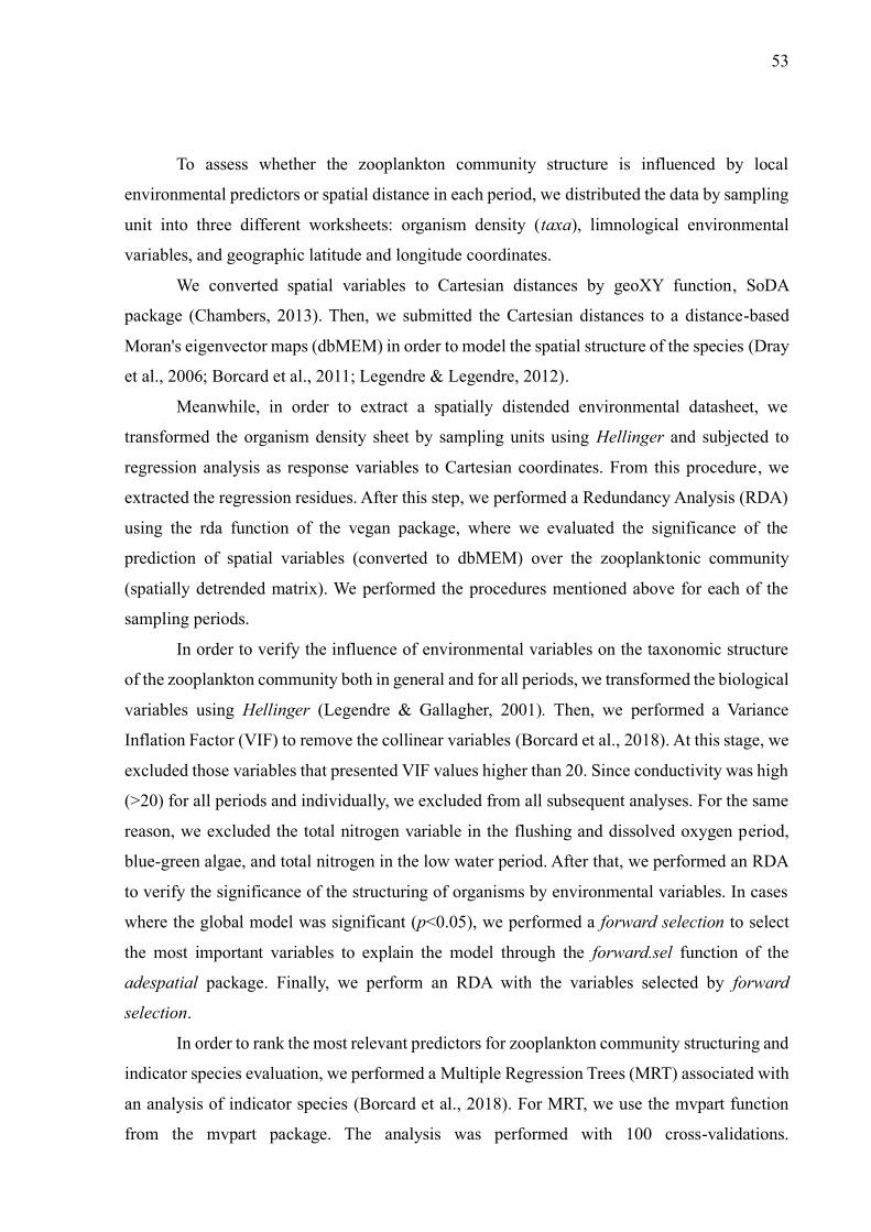
53
To assess whether the zooplankton community structure is influenced by local
environmental predictors or spatial distance in each period, we distributed the data by sampling
unit into three different worksheets: organism density (taxa), limnological environmental
variables, and geographic latitude and longitude coordinates.
We converted spatial variables to Cartesian distances by geoXY function, SoDA
package (Chambers, 2013). Then, we submitted the Cartesian distances to a distance-based
Moran's eigenvector maps (dbMEM) in order to model the spatial structure of the species (Dray
et al., 2006; Borcard et al., 2011; Legendre & Legendre, 2012).
Meanwhile, in order to extract a spatially distended environmental datasheet, we
transformed the organism density sheet by sampling units using Hellinger and subjected to
regression analysis as response variables to Cartesian coordinates. From this procedure, we
extracted the regression residues. After this step, we performed a Redundancy Analysis (RDA)
using the rda function of the vegan package, where we evaluated the significance of the
prediction of spatial variables (converted to dbMEM) over the zooplanktonic community
(spatially detrended matrix). We performed the procedures mentioned above for each of the
sampling periods.
In order to verify the influence of environmental variables on the taxonomic structure
of the zooplankton community both in general and for all periods, we transformed the biological
variables using Hellinger (Legendre & Gallagher, 2001). Then, we performed a Variance
Inflation Factor (VIF) to remove the collinear variables (Borcard et al., 2018). At this stage, we
excluded those variables that presented VIF values higher than 20. Since conductivity was high
(>20) for all periods and individually, we excluded from all subsequent analyses. For the same
reason, we excluded the total nitrogen variable in the flushing and dissolved oxygen period,
blue-green algae, and total nitrogen in the low water period. After that, we performed an RDA
to verify the significance of the structuring of organisms by environmental variables. In cases
where the global model was significant (p<0.05), we performed a forward selection to select
the most important variables to explain the model through the forward.sel function of the
adespatial package. Finally, we perform an RDA with the variables selected by forward
selection.
In order to rank the most relevant predictors for zooplankton community structuring and
indicator species evaluation, we performed a Multiple Regression Trees (MRT) associated with
an analysis of indicator species (Borcard et al., 2018). For MRT, we use the mvpart function
from the mvpart package. The analysis was performed with 100 cross-validations.

54
Subsequently, we performed the analysis of indicator species, through the indval function of
the labdsv package, associated with the MRT categorizations. For the recommendation of
indicator species, we used an adjusted alpha value of 0.05.
Environmental and spatial predictors of the functional structure of the zooplankton community
We arranged the environmental and biological data in three different spreadsheets: (L)
density of organisms per sampling unit, (R) values of environmental variables per sampling
unit, and (Q) functional traits by species. In order to categorize the different length of the
organisms and insert them into the functional traits worksheet, we performed a non-hierarchical
grouping through a kmeans, via the cascadeKM function, from the vegan package (Oksanen et
al., 2016). We based the separation into three groups on the highest value of simple structure
index (ssi). Therefore, we classified organisms smaller than 380 µm as small, organisms
between 380 and 911 µm as medium, and organisms larger than 911 µm as large.
We performed RLQ analysis (Dray et al., 2014), through the function rlq of the ade4
package (Dray & Dufour, 2007). For this, we subjected the density of organisms (L) to a
correspondence analysis by the dudi.coa function. As they presented numerical and categorical
data (sampling periods), we submitted the environmental variables (R) to a Hill & Smith PCA
(Hill, M.O. and Smith, 1976), through the dudi.hillsmith function. Since they presented only
categorical data, we submitted functional traits (Q) to a multiple correspondence analysis
(MCA), using the dudi.acm function. All the analyzes above are available in the ade4 package.
After this step, we entered the ordinances in the RLQ analysis, and we tested their significance
using the randtest function. For this, we used the type 6 model, where models 2 and 4 are tested
(ter Braak et al., 2012).
To evaluate the influence of spatial predictors on the zooplankton community structure,
we associated the functional traits of each zooplankton species with species density per
sampling unit through a CWM, functcomp function, analysis of the FD package. Thus, we
created a matrix with the proportion of functional traits per sampling unit.
After this step, we converted the geographic coordinates to Cartesian coordinates and
subjected them to a dbMEM. Then, we tested the geographic coordinates in a global model to
evaluate the prediction of spatial variables on the variation of functional traits by sampling
units. The overall result was not significant, and therefore we did not continue testing (Bauman
et al., 2018).

55
We performed all previously mentioned analyses using the R statistical software (R Core
Team, 2017). We show a schematic representation of our statistical analyses in Figure 2.
Fig. 2 Schematic representation of the statistical analyses performed in this study. dbMEM =
distance-based Moran's eigenvector maps; RDA = redundancy analysis; VIF = variance
inflation factor; MRT = multivariate regression trees; CWM = community-weighted mean; PCA
= principal component analysis; CA = correspondence analysis; MCA = multiple
correspondence analysis
Results
The mean density of zooplanktonic taxa and environmental variables per sampling
period can be found in Table S1 and Table S3, respectively.
Predictors about the taxonomic structure

56
According to the forward selection for the RDA's that presented significant explanatory
values in the global test, we selected the following variables as predictors of zooplankton
community variation for the respective hydrological periods: alkalinity, blue-green algae, total
chlorophyll, conductivity, phosphorus, total dissolved nitrogen and temperature (all periods);
alkalinity and dissolved fluorescent organic matter (flooding); blue-green algae, total
chlorophyll, and temperature (low water).
According to the results of the RDA (Figure 3), the environmental variables showed
significant prediction of the structure of the zooplankton when considered all periods (R²adj =
0.22, F = 4.94, p = 0.001), flooding periods (R²adj = 0.17, F = 2.32, p = 0.001), flushing (R²adj
= 0.16, F = 3.35, p = 0.001) and low water periods ( R²adj = 0.27, F = 3.43, p = 0.001). For the
high water period (R²adj = 0.00, F = 1,004, p = 0.503), the environmental variables were not
able to explain the zooplankton taxonomic variation.
When considering all periods, Lecane proiecta was strongly associated with higher
concentrations of ammonia, BGA, and total chlorophyll. However, Bosminopsis deitersi
presented an opposite pattern. The larval stages of copepods showed different responses
concerning total dissolved solids. While Diaptomidae nauplius and copepodites were more
associated with higher values, Cyclopidae nauplii was associated with lower values. During the
flooding period, it should be noted that Cyclopidae nauplii was more associated with higher
chlorophyll values, while Conochilus unicornis was more associated with low chlorophyll and
nitrate values. However, during the flushing period, Cyclopidae nauplius was associated with
lower chlorophyll and alkalinity values. In the low water period, Brachionus caudatus was more
associated with low TDS values.
57
Fig. 3 Significant analysis of redundancies (RDA) for zooplankton as a function of
environmental variables for: all periods, flooding, flushing and low water. Alc = alkalinity,
Ammo = Ammonia, BGA = blue-green algae, Chlor = Total Chlorophyll, fDOM = Fluorescent
Dissolved Organic Matter, N = Total Nitrogen, Nit = Nitrate, TDN = Total Dissolved Solids,
Temp = temperature and Turb = turbidity. (*) represents the RDA axes with significant
explanation. Acronyms can be verified in Table S1
The spatial variables did not explain the structuring of zooplanktonic communities in
any of the sampling periods (Flooding: R²adj = 0.01, F = 1.053, p = 0.376; Flushing: R²adj = -
0.01, F = 0.97, p = 0.559; High water: R²adj = -0.04, F = 0.853, p = 0.893; Low water: R²adj =
-0.06, F = 0.625, p = 0.936).

58
When considering the limnological environmental variables along with the hydrological
periods, the multiple regression trees (MRT, Figure 4) showed that the hydrological variations
were more determinant for the zooplanktonic organisms’ structure than the environmental
variables. In this case, the flushing and low water periods presented a more similar prediction
pattern, while flooding and high water were more similar to each other.
Besides, it should be noted that seven species of rotifers were indicative of the flushing
period. However, Keratella americana was the most indicated species for the period. The low
water period presented species of rotifers and microcrustaceans, but Lecane proiecta and
Cephalodella catelina were the major indicators of the period. For the flooding and flushing
periods, total dissolved solids were the most important predictors for species structuring.
Therefore, for environments with TDS values greater than or equal to 31.5, they had seven
representative species, with emphasis on Holopedium amazonicum. For values below 31.5,
there were 11 indicator species, however, Lecane leontina was the one with the highest
indication value.
Fig. 4 Multiple Regression Trees (MRT) and Analysis of Indicator Species, including
environmental variables and hydrological periods. n = number of sampling units belonging to
the MRT sheet. * = indicator species (p <0.05), RE = relative error, TDS = total dissolved solids

59
Predictors of functional structure
When we evaluated all periods together, the results of the RLQ (Figure 5) indicated no
explanation of the environmental variables on the variation of organism density-weighted
functional traits (model 2: p <0.05, model 4: p = 0.112). On the other hand, when we evaluated
by period, the environmental variables explained the functional structure of the zooplankton
community only in the low water period (model 2: p <0.05, model 4: p = 0.024). The spatial
variables had no significant explanation for the variation of zooplankton community functional
traits by sampling unit for any of the periods (p> 0.05).
Fig. 5 RLQ between environmental variables (a), functional traits (b), and species (c) for low
water periods. Alc = alkalinity, Ammo = Ammonia, BGA = blue-green algae, Chlor = total
chlorophyll, fDOM = Fluorescent Dissolved Organic Matter, N = total nitrogen, Nit = Nitrate,
ODO = Dissolved Oxygen P = Total Phosphorus, TDN = Total Dissolved Nitrogen, TDS = Total
Dissolved Solids, Temp = Temperature and Turb = Turbidity. Species acronyms can be found
in Table S1
Discussion
By evaluating the influence of environmental and spatial predictors on taxonomic
composition and functional traits by sampling unit, we found that environmental variables
significantly explained taxonomic structuring for all periods when evaluated together and
separately for flooding, flushing, and low water periods. On the other hand, the same variables
explained the functional structuring only in the low water period. The spatial variables had no
significant explanation about the taxonomic and functional structure.
60
Taxonomic Approach
Following our expectations, environmental variables were relevant to the structuring of
the zooplankton community, except for the high water period. As in other studies, the
zooplankton community is controlled by the environmental and limnological variations
resulting from the flood pulse (Schöll et al., 2012; Goździejewska et al., 2016). This happens
because, in addition to the material and organisms that enter the plains during the flooding
period, lake filling promotes interactions with the aquatic/terrestrial transition zones, which
alters the dynamics of organisms and inserts organic compounds that contribute to feeding of
these organisms and promotes higher associations between the amount of resources made
available (Junk et al., 1989). This increase in interaction is most considerable during the
flooding and flushing periods. On the other hand, the low water period promotes isolation of
habitats, which consolidates a heterogeneity of organisms that are associated with isolated
habitats. This same factor also justifies the absence of responses in the high water period, due
to the homogenization promoted by interconnectedness (Thomaz et al., 2007).
In more detail, during flushing and low water periods, total dissolved solids were the
most relevant predictors for the zooplankton community. This period is characterized by a large
volume of water leaving the lake towards the main river channel, which may be determinant
for the extinction of those organisms less resistant to the flow (Junk et al., 2012).
As for the lack of explanation of environmental variables on the zooplankton
community structure during the high water period, the flood pulse promotes environmental and
biological homogenization in the periods of major flooding due to increased water
interconnectivity (Thomaz et al., 2007). This factor may have determined the lack of response
to environmental predictors.
When we observed the responses of the taxa, Cyclopidae nauplius responded differently
to the total chlorophyll variations for each hydrological period. This factor shows that taxa can
respond differently to environmental variables according to the hydrological period. These
different responses may be related to the adaptations of the organisms to the floodplain
dynamics (Junk et al., 1989). Also, copepods have a high reproductive capacity (Hairston &
Bohonak, 1998). Therefore, a high amount of nauplius present does not necessarily indicate
that the environment is conducive for them to reach adulthood. Nevertheless, when generally
evaluated, Cyclopidae nauplius is more associated with low total chlorophyll concentrations.
The cladoceran Bosminopsis deitersi was more associated with lower ammonia values,
total nitrogen, turbidity, blue-green algae, and total chlorophyll, while the Lecane proiecta
presented de opposite pattern. Although fish also produce ammonia in the digestion process of
61
organisms that increase excretion at higher temperatures due to the acceleration in metabolism
(Chew et al., 2005) and also by decomposing organic matter in a process called ammonification
(US Agency, 2013), agriculture also uses this substance to extend the production process and,
despite its importance for agricultural production, the substance is often used indiscriminately
and ends up being leached to water bodies (Rao & Puttanna, 2000). Thus, ammonia is a major
pollutant of aquatic environments, has toxicity to many aquatic organisms, and can be a
predictor of the population of Bosminopsis deitersi. Although the species is constantly present
in Amazonian lakes (Ghidini & Santos-Silva, 2018), there are associations of this species to
environments with higher water quality and transparency (De-Carli et al., 2018).
There was no explanation of spatial variables on community structure. The
zooplanktonic community is widely represented by organisms with micrometric dimensions,
reaching a few millimeters (Chiba et al., 2015). Thus, its dispersal capacity is passive and
limited to environmental hydrological variations, especially for testate amoebae and rotifers,
which correspond, on average, to the smallest organisms in this community (Dias et al., 2016).
This factor limits organisms from dispersing under unfavorable environmental conditions and
is more vulnerable to local hydrological and environmental variations (Henriques-Silva et al.,
2016).
As expected, the zooplankton community has a pattern strongly associated with the
species-sorting paradigm, which associates demographic variations of species with
environmental gradients (Leibold et al., 2004; Holyoak et al., 2005; Henriques-Silva et al.,
2016). With a short life cycle typically less than 30 days for cladocerans, rotifers and testate
amoebae and less than one year for copepods (Gilbert & Williamson, 1983), the favorable
environmental conditions promote the local reproduction of organisms (Dias et al., 2017). On
the other hand, unfavorable conditions mean that organisms do not survive or continue to
reproduce in certain localities (Agadjihouede et al., 2011). This zooplankton responsiveness to
environmental variables makes them possible indicators for environmental monitoring, as long
as flood pulse variations are observed.
Functional Approach
Contrary to our expectations, the variation in functional traits, weighted by the density
of organisms, did not respond to environmental and spatial variables when evaluating all
periods together. On the other hand, when evaluating the periods individually, the traits were
related to the low water period. The dynamics of floodplains are distinct due to their
characteristic of being temporally dynamic and, therefore, different mechanisms may influence
the biological composition and environmental characteristics throughout hydrological cycles

62
(Junk et al., 1989). That, in the case of the Amazon River and the lakes connected to it, there is
the influence of melting in the Andes and the rainfall that occurs in the region of its tributaries
(Junk et al., 2012). As explained for taxonomic structuring in the same period, low water allows
greater interactions of organisms with local environmental variables that are naturally more
heterogeneous, and low water volume prevents species from being passively dispersed.
Therefore, those that are not adapted are locally extinct (Thomaz et al., 2007). In the present
study, this pattern reflected in the functional structuring in response to environmental variables.
Many species have the same functional traits, and thus, there was a high functional
redundancy. This may have been one of the determining factors for the low response of
functional traits to environmental and spatial variables. Nevertheless, functional redundancy
allows the zooplankton community to become more resilient to anthropic actions (Petchey &
Gaston, 2002) because, in the same environment, there are many species capable of fulfilling
the same ecological function. Therefore, the eventual local extinction of a moderate number of
species may not compromise the ecosystem balance (Petchey & Gaston, 2002).
Despite constant deforestation, agricultural expansions, and dam construction for
advancing hydroelectric dams in the Amazon region have effects on zooplanktonic functional
diversity (Braghin et al., 2018), In this environment, the dynamics promoted by the flood pulse
are still the most significant control factor of the community. Nevertheless, the advance of
deforestation may be a major factor for future changes in the region's aquatic environments,
with effects on hydrological and biogeochemical cycles (Davidson et al., 2012).
Conclusion
The taxonomic and functional approaches were different in the structuring of the
zooplankton community. The taxonomic variation responded more strongly to the hydrological
variations promoted by the flood pulse, and the functional structure responded to local
environmental variables in the low water period. However, none of the approaches was related
to the spatial variation for any of the periods.
Thus, zooplankton is more associated with the species sorting pattern, where
environmental variations rather than spatial predictors predominantly determine species. This
factor denotes the importance of the zooplankton community in environmental monitoring
programs, due to its susceptibility to environmental variations. However, there is still a large
gap regarding the exploration of the functional traits of the zooplankton community. We
63
suggest, therefore, the advance in experimental studies that contemplate zooplanktonic
responses to ecosystem variations.
References
Agadjihouede, H., C. A. Bonou, E. Montchowui, A. Chikou, & P. Laleye, 2011. Capacité de
développement de trois espèces zooplanctoniques d’intérêts aquacoles (Brachionus
calyciflorus , Moina micrura et Thermocyclops sp .) élevées en condition monospécifique en
aquariums avec la fiente de volaille. Tropicultura 29: 231–237.
Algarte, V. M., L. Rodrigues, V. L. Landeiro, T. Siqueira, & L. M. Bini, 2014. Variance
partitioning of deconstructed periphyton communities: does the use of biological traits
matter?. Hydrobiologia 722: 279–290.
APHA, 2005. Standard Methods for the Examination of Water and Wastewater. American
Public Health Association/American Water Works Association/Water Environment
Federation, Washington DC.
Bauman, D., T. Drouet, S. Dray, & J. Vleminckx, 2018. Disentangling good from bad
practices in the selection of spatial or phylogenetic eigenvectors. Ecography 41: 1638–1649.
Bonnet, M. P., G. Barroux, J. M. Martinez, F. Seyler, P. Moreira-Turcq, G. Cochonneau, J. M.
Melack, G. Boaventura, L. Maurice-Bourgoin, J. G. León, E. Roux, S. Calmant, P. Kosuth, J.
L. Guyot, & P. Seyler, 2008. Floodplain hydrology in an Amazon floodplain lake (Lago
Grande de Curuaí). Journal of Hydrology 349: 18–30.
Borcard, D., F. Gillet, & P. Legendre, 2011. Numerical ecology with R. Springer.
Borcard, D., F. Gillet, & P. Legendre, 2018. Numerical Ecology with R. Springer International
Publishing, Cham.
Bottrell, H. H., A. Duncan, Z. M. Gliwicz, E. Grygierek, A. Herzig, A. Hillbrichtilkowska, H.
Kurasawa, P. Larsson, & T. Weglenska, 1976. Review of some problems in zooplankton
production studies. Norwegian Journal of Zoology 24: 419–456.
Bozelli, R. L., S. M. Thomaz, A. A. Padial, P. M. Lopes, & L. M. Bini, 2015. Floods decrease
zooplankton beta diversity and environmental heterogeneity in an Amazonian floodplain
system. Hydrobiologia 753: 233–241.
Braghin, L. de S. M., B. de A. Almeida, D. C. Amaral, T. F. Canella, B. C. Garcia Gimenez, &
C. C. Bonecker, 2018. Effects of dams decrease zooplankton functional -diversity in river-
associated lakes. Freshwater biology 63: 721–730.
Chambers, J. M., 2013. SoDA: Functions and Examples for “Software for Data Analysis.” ,
64
https://cran.r-project.org/package=SoDA.
Chew, S. F., J. M. Wilson, Y. K. Ip, & D. J. Randall, 2005. Nitrogen Excretion And Defense
Against Ammonia Toxicity 21: 307–395,
https://linkinghub.elsevier.com/retrieve/pii/S1546509805210087.
Chiba, S., S. D. Batten, T. Yoshiki, Y. Sasaki, K. Sasaoka, H. Sugisaki, & T. Ichikawa, 2015.
Temperature and zooplankton size structure: climate control and basin-scale comparison in
the North Pacific. Ecology and Evolution 5: 968–978,
http://doi.wiley.com/10.1002/ece3.1408.
Cottenie, K., 2005. Integrating environmental and spatial processes in ecological community
dynamics. Ecology Letters 8: 1175–1182, http://doi.wiley.com/10.1111/j.1461-
0248.2005.00820.x.
Davidson, E. A., A. C. de Araújo, P. Artaxo, J. K. Balch, I. F. Brown, M. M. C. Bustamante,
M. T. Coe, R. S. DeFries, M. Keller, M. Longo, J. W. Munger, W. Schroeder, B. S. Soares-
Filho, C. M. Souza, & S. C. Wofsy, 2012. The Amazon basin in transition. Nature Nature
Publishing Group 481: 321–328, http://www.nature.com/articles/nature10717.
De-Carli, B. P., F. P. de Albuquerque, V. Moschini-Carlos, & M. Pompêo, 2018. Comunidade
zooplanctônica e sua relação com a qualidade da água em reservatórios do Estado de São
Paulo. Iheringia. Série Zoologia 108:,
http://www.scielo.br/scielo.php?script=sci_arttext&pid=S0073-
47212018000100213&lng=pt&tlng=pt.
De Bie, T., L. De Meester, L. Brendonck, K. Martens, B. Goddeeris, D. Ercken, H. Hampel,
L. Denys, L. Vanhecke, & K. Van Der Gucht, 2012. Body size and dispersal mode as key
traits determining metacommunity structure of aquatic organisms. Ecology letters Wiley
Online Library 15: 740–747.
Dias, J. D., M. R. Miracle, & C. C. Bonecker, 2017. Do water levels control zooplankton
secondary production in Neotropical floodplain lakes?. Fundamental and Applied Limnology
/ Archiv für Hydrobiologie 190: 49–62,
http://www.ingentaconnect.com/content/10.1127/fal/2017/0869.
Dias, J. D., N. R. Simões, M. Meerhoff, F. A. Lansac-Tôha, L. F. M. Velho, & C. C. Bonecker,
2016. Hydrological dynamics drives zooplankton metacommunity structure in a Neotropical
floodplain. Hydrobiologia 781: 109–125, http://link.springer.com/10.1007/s10750-016-2827-
2.
Dray, S., P. Choler, S. Dolédec, P. R. Peres-Neto, W. Thuiller, S. Pavoine, & C. J. F. ter Braak,
2014. Combining the fourth-corner and the RLQ methods for assessing trait responses to
65
environmental variation. Ecology 95: 14–21, http://doi.wiley.com/10.1890/13-0196.1.
Dray, S., & A. B. Dufour, 2007. The ade4 package: implementing the duality diagram for
ecologists. Journal of Statistical Software 22: 1–20.
Dray, S., P. Legendre, & P. R. Peres-Neto, 2006. Spatial modelling: a comprehensive
framework for principal coordinate analysis of neighbour matrices (PCNM). Ecological
Modelling 196: 483–493, http://linkinghub.elsevier.com/retrieve/pii/S0304380006000925.
Frisch, D., K. Cottenie, A. Badosa, & A. J. Green, 2012. Strong Spatial Influence on
Colonization Rates in a Pioneer Zooplankton Metacommunity. PLoS ONE 7:,
http://journals.plos.org/plosone/article/file?id=10.1371/journal.pone.0040205&type=printable
.
Ghidini, A. R., & E. N. dos Santos-Silva, 2018. Composition, abundance, and diversity of
limnetic cladocerans (Crustacea: Anomopoda and Ctenopoda) in a black-water lake in the
Negro River basin, Amazonas State, Brazil. Nauplius 26:,
http://www.scielo.br/scielo.php?script=sci_arttext&pid=S0104-
64972018000100214&lng=en&tlng=en.
Gianuca, A. T., J. Engelen, K. I. Brans, F. T. T. Hanashiro, M. Vanhamel, E. M. van den Berg,
C. Souffreau, & L. De Meester, 2018. Taxonomic, functional and phylogenetic
metacommunity ecology of cladoceran zooplankton along urbanization gradients. Ecography
Blackwell Publishing Ltd 41: 183–194, http://doi.wiley.com/10.1111/ecog.02926.
Gilbert, J. J., & C. E. Williamson, 1983. Sexual Dimorphism in Zooplankton (Copepoda,
Cladocera, and Rotifera). Annual Review of Ecology and Systematics 14: 1–33.
Goździejewska, A., K. Glińska-Lewczuk, K. Obolewski, M. Grzybowski, R. Kujawa, S. Lew,
& M. Grabowska, 2016. Effects of lateral connectivity on zooplankton community structure
in floodplain lakes. Hydrobiologia 774: 7–21, http://link.springer.com/10.1007/s10750-016-
2724-8.
Hairston, N. G., & A. J. Bohonak, 1998. Copepod reproductive strategies: life-history theory,
phylogenetic pattern and invasion of inland waters. Journal of Marine Systems 15: 23–34,
https://linkinghub.elsevier.com/retrieve/pii/S0924796397000468.
Henriques-Silva, R., B. Pinel-Alloul, & P. R. Peres-Neto, 2016. Climate, history and life-
history strategies interact in explaining differential macroecological patterns in freshwater
zooplankton. Global Ecology and Biogeography 25: 1454–1465,
http://doi.wiley.com/10.1111/geb.12505.
Hill, M.O. and Smith, A. J. E., 1976. Principal Component Analysis of Taxonomic Data with
Multi-State Discrete Characters. Taxon 249–255.
66
Holyoak, M., M. A. Leibold, R. D. Holt, & W. . Ecological Society of America. Meeting
(2001 : Madison, 2005. Metacommunities : spatial dynamics and ecological communities.
University of Chicago Press.
Junk, W. J., P. B. Bayley, & R. E. Sparks, 1989. The flood pulse concept in river-floodplain
systems. Canadian special publication of fisheries and aquatic sciences 106: 110–127.
Junk, W. J., M. T. F. Piedade, J. Schöngart, & F. Wittmann, 2012. A classification of major
natural habitats of Amazonian white-water river floodplains (várzeas). Wetlands Ecology and
Management 20: 461–475, http://link.springer.com/10.1007/s11273-012-9268-0.
Laureto, L. M. O., M. V. Cianciaruso, & D. S. M. Samia, 2015. Functional diversity: an
overview of its history and applicability. Natureza & Conservação ASSOC BRASILEIRA
CIENCIA ECOLOGICA E CONSERVACAO, CAIXA POSTAL 68038, CIDADE UNIV,
ILHA DO FUNDAO, RIO DE JANEIRO, RJ 00000, BRAZIL 13: 112–116,
http://linkinghub.elsevier.com/retrieve/pii/S1679007315000390.
Legendre, P., & E. Gallagher, 2001. Ecologically meaningful transformations for ordination of
species data. Oecologia Springer-Verlag 129: 271–280,
http://link.springer.com/10.1007/s004420100716.
Legendre, P., & L. Legendre, 2012. Numerical ecology. Elsevier, Amsterdam.
Leibold, M. A., M. Holyoak, N. Mouquet, P. Amarasekare, J. M. Chase, M. F. Hoopes, R. D.
Holt, J. B. Shurin, R. Law, & D. Tilman, 2004. The metacommunity concept: a framework for
multi‐scale community ecology. Ecology letters Wiley Online Library 7: 601–613.
Litchman, E., M. D. Ohman, & T. Kiørboe, 2013. Trait-based approaches to zooplankton
communities. Journal of Plankton Research 35: 473–484,
https://academic.oup.com/plankt/article-lookup/doi/10.1093/plankt/fbt019.
Logue, J. B., N. Mouquet, H. Peter, & H. Hillebrand, 2011. Empirical approaches to
metacommunities: a review and comparison with theory. Trends in Ecology & Evolution 26:
482–491, http://www.sciencedirect.com/science/article/pii/S0169534711001315.
Lopes, P. M., L. M. Bini, S. A. J. Declerck, V. F. Farjalla, L. C. G. Vieira, C. C. Bonecker, F.
A. Lansac-Toha, F. A. Esteves, & R. L. Bozelli, 2014. Correlates of zooplankton beta
diversity in tropical lake systems. PLoS ONE 9:.
Medina Torres, K. M., & C. L. Higgins, 2016. Taxonomic and functional organization in
metacommunity structure of stream-fish assemblages among and within river basins in Texas.
Aquatic Ecology 50: 247–259, http://link.springer.com/10.1007/s10452-016-9572-5.
Oksanen, J., F. Blanchet, Guillaume, M. Friendly, R. Kindt, P. Legendre, D. Mcglinn, P. R.
Minchin, R. B. O ’hara, G. L. Simpson, P. Solymos, H. Stevens, E. Szoecs, & H. Wagner,
67
2016. Vegan: Community Ecology Package. R package version 2.4-0 .
Pellowe-Wagstaff, K. E., & J. L. Simonis, 2014. The ecology and mechanisms of overflow-
mediated dispersal in a rock-pool metacommunity. Freshwater Biology 59: 1161–1172,
http://doi.wiley.com/10.1111/fwb.12337.
Penha, J., V. L. Landeiro, J. C. G. Ortega, & L. Mateus, 2017. Interchange between flooding
and drying, and spatial connectivity control the fish metacommunity structure in lakes of the
Pantanal wetland. Hydrobiologia , http://link.springer.com/10.1007/s10750-017-3164-9.
Petchey, O. L., & K. J. Gaston, 2002. Functional diversity (FD), species richness and
community composition. Ecology Letters 5: 402–411, http://doi.wiley.com/10.1046/j.1461-
0248.2002.00339.x.
Prado, V. H. M., & D. de C. Rossa-Feres, 2014. The influence of niche and neutral processes
on a neotropical anuran metacommunity. Austral Ecology 39: 540–547,
http://doi.wiley.com/10.1111/aec.12114.
R Core Team, 2017. R: A Language and Environment for Statistical Computing. R
Foundation for Statistical Computing, Vienna, Austria, https://www.r-project.org/.
Rao, E., & K. Puttanna, 2000. Nitrates, agriculture and environment. CURRENT SCIENCE
CURRENT SCIENCE ASSN, C V RAMAN AVENUE, PO BOX 8005, BANGALORE 560
080, INDIA 79: 1163–1168.
Schöll, K., A. Kiss, M. Dinka, & Á. Berczik, 2012. Flood-Pulse Effects on Zooplankton
Assemblages in a River-Floodplain System (Gemenc Floodplain of the Danube, Hungary).
International Review of Hydrobiology 97: 41–54,
http://doi.wiley.com/10.1002/iroh.201111427.
Steedman, H. F., 1976. Zooplankton fixation and preservation. The Unesco Press, Paris.
Swan, C. M., A. Johnson, & D. J. Nowak, 2017. Differential organization of taxonomic and
functional diversity in an urban woody plant metacommunity. Applied Vegetation Science 20:
7–17, http://doi.wiley.com/10.1111/avsc.12266.
ter Braak, C. J. F., A. Cormont, & S. Dray, 2012. Improved testing of species traits–
environment relationships in the fourth-corner problem. Ecology 93: 1525–1526,
http://doi.wiley.com/10.1890/12-0126.1.
Thomaz, S. M., L. M. Bini, & R. L. Bozelli, 2007. Floods increase similarity among aquatic
habitats in river-floodplain systems. Hydrobiologia 579: 1–13,
http://link.springer.com/10.1007/s10750-006-0285-y.
US Agency, U. E. P., 2013. Aquatic life ambient water quality criteria for ammonia—
freshwater. USEPA, 822-R-13-001, Washington, DC.

68
Vilmi, A., K. T. Tolonen, S. M. Karjalainen, & J. Heino, 2017. Metacommunity structuring in
a highly-connected aquatic system: effects of dispersal, abiotic environment and grazing
pressure on microalgal guilds. Hydrobiologia 790: 125–140,
http://link.springer.com/10.1007/s10750-016-3024-z.
Winegardner, A. K., B. K. Jones, I. S. Y. Ng, T. Siqueira, & K. Cottenie, 2012. The
terminology of metacommunity ecology. Trends in Ecology & Evolution 27: 253–254.
69
Capítulo 3
Zooplankton community beta diversity in an Amazonian floodplain lake
Capítulo parcialmente formatado (para adequações à tese) conforme regras de submissão
da revista Hydrobiologia (Qualis A2 em Ciências Ambientais e fator de impacto (JCR)
2.325)

70
Abstract
Understanding the mechanisms that generate organism distribution patterns from the beta
diversity perspective can assist in environmental monitoring strategies. In this study, we
emphasized the limnic zooplankton due to the ability of these organisms to respond
quickly to environmental variations. Therefore, we evaluated the following questions: (i)
Do different regions of the same lake have the same importance in contributing to beta
diversity? (ii) Do beta diversity and its components vary over the hydrological cycle? (iii)
What is the importance of local and spatial predictors in beta diversity and its
components? (iv) Do beta diversity and its components show a consistent pattern
throughout the hydrological cycle? We found that the contribution of different sites to
diversity was more associated with regions with low abundance and richness of organisms
values, such as the littoral and igarapés, which shows the relevance of these areas for
biological monitoring and for the delimitation of priority areas for the zooplankton
diversity conservation. Despite the peculiarities of each hydrological period and
regarding beta diversity components, we verified a species substitution and differences in
abundance patterns in the lake. We also found low concordance patterns between the
periods and low environmental and spatial variables prediction on beta diversity patterns.
Keywords: Lago Grande do Curuai, hydrological cycle, Podani, flood pulse, beta
diversity partitioning
Acknowledgments
The authors thank to Coordenação de Aperfeiçoamento de Pessoal de Nível Superior
(CAPES) for providing financial assistance to L.F.G., to Fondation pour la Recherche sur
la Biodiversité (FRB) and to Conselho Nacional de Desenvolvimento Científico e
Tecnológico (CNPq) that, in partnership with Institut de Recherche pour le
Développement (IRD), financed the project number process: 490634/2013-3.
71
Introduction
Species can present different distribution patterns in response to natural factors
such as competition, predation, dispersive processes limitations, and/or local and regional
environmental variables influences (Guisan & Thuiller, 2005). These factors may be
intensified by human activities, which makes even more relevant to understand the
mechanisms that generate such structuring patterns in biological communities. Thus, the
understanding of these mechanisms can assist in the formulation of efficient
environmental monitoring strategies and, even, in the delimitation of priority areas for
conservation in several ecosystems (Socolar et al., 2016). The comparative diversity
across multiple sites, known as beta diversity (Whittaker, 1960), has undergone advances
over the years both for understanding patterns of presence-absence of organisms and for
density values per site (Baselga, 2010; Podani & Schmera, 2011; Podani et al., 2013).
Both for organism occurrence and abundance, Podani family of beta diversity
(Podani & Schmera, 2011; Podani et al., 2013) can be partitioned into the following main
components: (i) species similarities: commonly measured by the Jaccard index for
presence-absence data and Ruzicka, for abundance data. High values of this partition
mean that the pairs of sites put in comparison share many species or species with similar
abundances; (ii) difference in relative richness/abundance: is the difference in species
richness, or species abundance, between pairs of sites. Therefore, high values of that
partition show that the number of species or specimens between compared sites is
discrepant; (iii) species replacement/abundance: it can be maximized when there is a high
replacement of species, or species with equivalent abundances, along an environmental
gradient or between pairs of sites. Therefore, high replacement values for the abundance
data mean that, although the sites in comparison have similar abundances, the species
composition is different. Also, although the approach with abundance data may represent
more subtle differences concerning environmental variations, the values between the
assessments for abundance and presence-absence data can be quite different, even if
evaluated with the same data set (Podani et al., 2013).
The evaluation of the factors that influence beta diversity and its components can
be even more complex in floodplain lakes since they are predominantly dominated by the
flood pulse that controls the dynamics of entry and output of sediments, water, and
organisms that naturally contribute for changes in biological diversity in the ecosystem
(Junk et al., 2012). These plains are continuously or periodically flooded by direct
72
precipitation or by the overflow of the main river, and, depending on the level of
connectivity with the river, there may be a loss of connection between habitats during
periods of low water (Thomaz et al., 2007). However, as the cycle of extensive floodplains
is usually slow and monomodal, the biological dynamics of organisms can adapt in order
to maximize their performance according to hydrological cycles (Junk et al., 2011).
In Amazonian rivers, the flow tends to be more intense and requires a high
resilience capacity of the organisms. Therefore, smaller aquatic organisms tend to be
present with greater richness and density in the lakes of these plains, where they can find
shelter against predation and food (Junk et al., 1989). Furthermore, according to the
hydrological period, these organisms may present beta diversity patterns that change over
time (Bozelli et al., 2015).
Assessing beta diversity and its components over space, but also highlighting
whether the pattern generated is consistent throughout the hydrological cycle is important
in different aspects. For example, due to the scarcity of financial resources and time
allocated in environmental monitoring programs and scientific research, if different
hydrological periods show a concordant pattern of diversity, there is a real possibility of
adjustment in the sampling effort, reducing the number of sampling campaigns, which
would save financial resources and time. In the same way, it is possible to use other
alternatives as is the case of using lower taxonomic resolutions and or presence-absence
data instead of abundance data (Carneiro et al., 2013; Vieira et al., 2017; de Morais et al.,
2018).
In this study, we emphasized the limnic zooplankton due to the ability of these
organisms to respond quickly to environmental variations. Therefore, we evaluated the
following questions: (i) Do different regions of the same lake have the same importance
in contributing to beta diversity? (ii) Do beta diversity and its components vary over the
hydrological cycle? (iii) What is the importance of local (environmental characterization)
and spatial (dispersive processes) predictors in beta diversity and its components? (iv) Do
beta diversity and its components show a consistent pattern throughout the hydrological
cycle? Taking into account that the ecological dynamics of floodplains is temporally
complex, we expected that the sites contribution to beta diversity would be different
between hydrological periods. Besides, due to the large spatial extent of the study area,
we expected that species replacement patterns would be predominant, considering values
of presence-absence of organisms, and patterns of differences in abundance, considering
values of species abundance per site. Also, due to the complex interactions that dominate
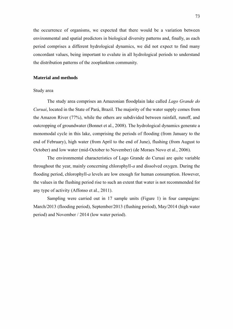
73
the occurrence of organisms, we expected that there would be a variation between
environmental and spatial predictors in biological diversity patterns and, finally, as each
period comprises a different hydrological dynamics, we did not expect to find many
concordant values, being important to evalute in all hydrological periods to understand
the distribution patterns of the zooplankton community.
Material and methods
Study area
The study area comprises an Amazonian floodplain lake called Lago Grande do
Curuai, located in the State of Pará, Brazil. The majority of the water supply comes from
the Amazon River (77%), while the others are subdivided between rainfall, runoff, and
outcropping of groundwater (Bonnet et al., 2008). The hydrological dynamics generate a
monomodal cycle in this lake, comprising the periods of flooding (from January to the
end of February), high water (from April to the end of June), flushing (from August to
October) and low water (mid-October to November) (de Moraes Novo et al., 2006).
The environmental characteristics of Lago Grande do Curuai are quite variable
throughout the year, mainly concerning chlorophyll-a and dissolved oxygen. During the
flooding period, chlorophyll-a levels are low enough for human consumption. However,
the values in the flushing period rise to such an extent that water is not recommended for
any type of activity (Affonso et al., 2011).
Sampling were carried out in 17 sample units (Figure 1) in four campaigns:
March/2013 (flooding period), September/2013 (flushing period), May/2014 (high water
period) and November / 2014 (low water period).
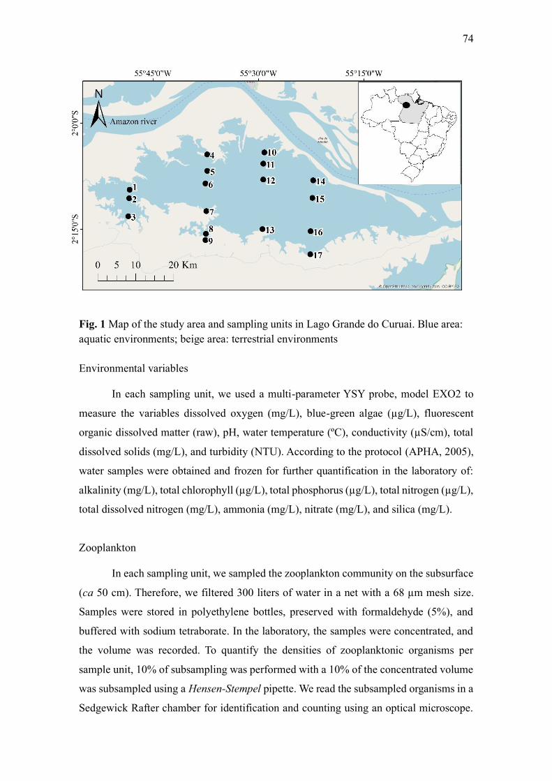
74
Fig. 1 Map of the study area and sampling units in Lago Grande do Curuai. Blue area:
aquatic environments; beige area: terrestrial environments
Environmental variables
In each sampling unit, we used a multi-parameter YSY probe, model EXO2 to
measure the variables dissolved oxygen (mg/L), blue-green algae (µg/L), fluorescent
organic dissolved matter (raw), pH, water temperature (ºC), conductivity (µS/cm), total
dissolved solids (mg/L), and turbidity (NTU). According to the protocol (APHA, 2005),
water samples were obtained and frozen for further quantification in the laboratory of:
alkalinity (mg/L), total chlorophyll (µg/L), total phosphorus (µg/L), total nitrogen (µg/L),
total dissolved nitrogen (mg/L), ammonia (mg/L), nitrate (mg/L), and silica (mg/L).
Zooplankton
In each sampling unit, we sampled the zooplankton community on the subsurface
(ca 50 cm). Therefore, we filtered 300 liters of water in a net with a 68 µm mesh size.
Samples were stored in polyethylene bottles, preserved with formaldehyde (5%), and
buffered with sodium tetraborate. In the laboratory, the samples were concentrated, and
the volume was recorded. To quantify the densities of zooplanktonic organisms per
sample unit, 10% of subsampling was performed with a 10% of the concentrated volume
was subsampled using a Hensen-Stempel pipette. We read the subsampled organisms in a
Sedgewick Rafter chamber for identification and counting using an optical microscope.

75
Additionally, we carried out qualitative sampling to verify and record the existence of
new taxa that were not identified during quantitative sampling (Bottrell et al., 1976).
Data analysis
We performed a Local Contribution to Beta Diversity (LCBD) (Legendre & De
Cáceres, 2013; Borcard et al., 2018) to obtain the degree of exclusivity of the sites in the
species composition in each hydrological period using the function beta.div, package
adespatial (Dray et al., 2018). To evaluate and partition Podani family beta diversity by
sample period, we used the function beta.div.comp of adespatial package (Dray et al.,
2018). In both cases, we used the Jaccard index for presence and absence values and
Ruzicka for organism density data.
To verify if there were significant differences in the values resulting from the beta
diversity partitioning by period, we performed a Permutational Multivariate Analysis of
Variance Using Distance Matrices (PERMANOVA). We obtained these matrices using
the beta.div.comp function for both create a matrix encompassing all periods and generate
matrices by pairs of periods. For PERMANOVA, we use the adonis2 function of the
vegan package (Oksanen et al., 2016) and the matrices resulted from the partition were
inserted in response to hydrological periods. Additionally, we constructed triangular plots
(simplex) to check the distributions of the pairs of sites concerning the partitive
components of beta diversity for both Ruzicka distance matrices and Jaccard in each
hydrological period.
To assess the influence of environmental and spatial variables in the beta diversity
partitions of zooplankton community by hydrological period, we performed Distance-
Based Redundancy Analysis (dbRDA’s) (Legendre & Andersson, 1999) with different
matrices resulted from the beta diversity partitioning (as response variables) and different
environmental and spatial variables (as predictor variables). To determine which variables
would be inserted in the dbRDA, we performed the analysis of variation inflation factor
(VIF) (Borcard et al., 2018), removing the environmental variables that showed high
collinearity in each sample period (VIF values greater than 20). To determine the spatial
predictors (geographic coordinates), we first converted the coordinates to Cartesian
distances using the geoXY function of the SoDA package (Chambers, 2013). Then, we
ordered the variables in a Distance-Based Moran’s Eigenvector Maps (dbMEM) (Dray et
al., 2006; Legendre & Legendre, 2012) using the dbmem function of the adespatial
package (Dray et al., 2018).
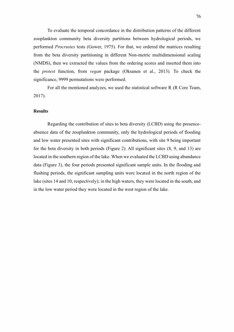
76
To evaluate the temporal concordance in the distribution patterns of the different
zooplankton community beta diversity partitions between hydrological periods, we
performed Procrustes tests (Gower, 1975). For that, we ordered the matrices resulting
from the beta diversity partitioning in different Non-metric multidimensional scaling
(NMDS), then we extracted the values from the ordering scores and inserted them into
the protest function, from vegan package (Oksanen et al., 2013). To check the
significance, 9999 permutations were performed.
For all the mentioned analyzes, we used the statistical software R (R Core Team,
2017).
Results
Regarding the contribution of sites to beta diversity (LCBD) using the presence-
absence data of the zooplankton community, only the hydrological periods of flooding
and low water presented sites with significant contributions, with site 9 being important
for the beta diversity in both periods (Figure 2). All significant sites (8, 9, and 13) are
located in the southern region of the lake. When we evaluated the LCBD using abundance
data (Figure 3), the four periods presented significant sample units. In the flooding and
flushing periods, the significant sampling units were located in the north region of the
lake (sites 14 and 10, respectively); in the high waters, they were located in the south, and
in the low water period they were located in the west region of the lake.
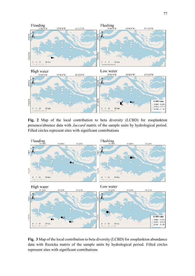
77
Fig. 2 Map of the local contribution to beta diversity (LCBD) for zooplankton
presence/absence data with Jaccard matrix of the sample units by hydrological period.
Filled circles represent sites with significant contributions
Fig. 3 Map of the local contribution to beta diversity (LCBD) for zooplankton abundance
data with Ruzicka matrix of the sample units by hydrological period. Filled circles
represent sites with significant contributions
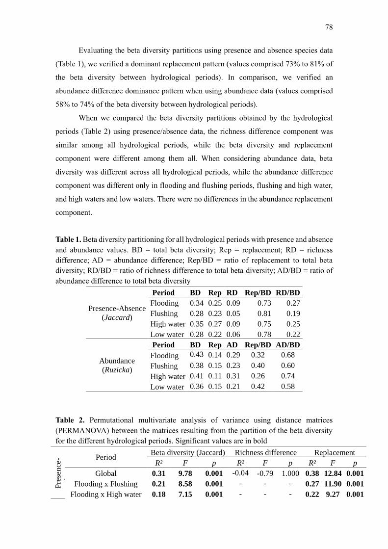
78
Evaluating the beta diversity partitions using presence and absence species data
(Table 1), we verified a dominant replacement pattern (values comprised 73% to 81% of
the beta diversity between hydrological periods). In comparison, we verified an
abundance difference dominance pattern when using abundance data (values comprised
58% to 74% of the beta diversity between hydrological periods).
When we compared the beta diversity partitions obtained by the hydrological
periods (Table 2) using presence/absence data, the richness difference component was
similar among all hydrological periods, while the beta diversity and replacement
component were different among them all. When considering abundance data, beta
diversity was different across all hydrological periods, while the abundance difference
component was different only in flooding and flushing periods, flushing and high water,
and high waters and low waters. There were no differences in the abundance replacement
component.
Table 1. Beta diversity partitioning for all hydrological periods with presence and absence
and abundance values. BD = total beta diversity; Rep = replacement; RD = richness
difference; AD = abundance difference; Rep/BD = ratio of replacement to total beta
diversity; RD/BD = ratio of richness difference to total beta diversity; AD/BD = ratio of
abundance difference to total beta diversity
Presence-Absence
(Jaccard)
Period BD Rep RD Rep/BD RD/BD
Flooding 0.34 0.25 0.09 0.73 0.27
Flushing 0.28 0.23 0.05 0.81 0.19
High water 0.35 0.27 0.09 0.75 0.25
Low water 0.28 0.22 0.06 0.78 0.22
Abundance
(Ruzicka)
Period BD Rep AD Rep/BD AD/BD
Flooding 0.43 0.14 0.29 0.32 0.68
Flushing 0.38 0.15 0.23 0.40 0.60
High water 0.41 0.11 0.31 0.26 0.74
Low water 0.36 0.15 0.21 0.42 0.58
Table 2. Permutational multivariate analysis of variance using distance matrices
(PERMANOVA) between the matrices resulting from the partition of the beta diversity
for the different hydrological periods. Significant values are in bold
Pre
sence
-
abse
nce
Period Beta diversity (Jaccard) Richness difference Replacement
R² F p R² F p R² F p
Global 0.31 9.78 0.001 -0.04 -0.79 1.000 0.38 12.84 0.001
Flooding x Flushing 0.21 8.58 0.001 - - - 0.27 11.90 0.001
Flooding x High water 0.18 7.15 0.001 - - - 0.22 9.27 0.001

79
Flooding x Low water 0.25 10.66 0.001 - - - 0.32 15.26 0.001
Flushing x High water 0.24 9.87 0.001 - - - 0.27 12.01 0.001
Flushing x Low water 0.25 10.43 0.001 - - - 0.30 13.66 0.001
High water x Low water 0.28 12.49 0.001 - - - 0.33 15.50 0.001
Abundan
ce
Period Beta diversity (Ruzicka) Abundance difference Replacement
R² F p R² F p R² F p
Global 0.20 5.32 0.001 0.27 7.92 0.001 0.10 2.48 0.077
Flooding x Flushing 0.12 4.52 0.001 0.12 4.27 0.012 - - -
Flooding x High water 0.10 3.63 0.001 0.14 5.35 0.004 - - -
Flooding x Low water 0.13 4.66 0.001 0.09 3.19 0.035 - - -
Flushing x High water 0.17 6.70 0.001 0.33 16.04 0.001 - - -
Flushing x Low water 0.13 4.81 0.001 -0.01 -0.27 0.997 - - -
High water x Low water 0.20 7.88 0.001 0.34 16.66 0.001 - - -
In proportion, when we partitioned the beta diversity using presence-absence data,
the pairs of sample units were more associated with greater similarities and replacement
values considering all periods (Figure 4). On the other hand, when we evaluated the
partition using abundance data, the pairs of sample units were more associated with
abundance difference component and, secondly, with higher replacement levels (Figure
5).
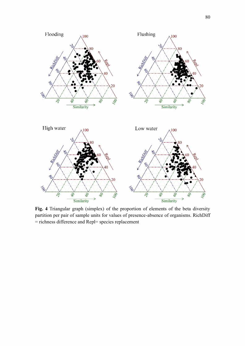
80
Fig. 4 Triangular graph (simplex) of the proportion of elements of the beta diversity
partition per pair of sample units for values of presence-absence of organisms. RichDiff
= richness difference and Repl= species replacement

81
Fig. 5 Triangular graph (simplex) of the proportion of elements in the beta diversity
partition per pair of sample units for organism abundance values. AbDiff = abundance
difference and Repl = species abundance replacement
Because presented high collinearity or multicollinearity values, we removed the
following environmental variables of each hydrological period: total chlorophyll, pH,
conductivity and total dissolved solids (flooding); dissolved oxygen, pH, conductivity
and total dissolved nitrogen (flushing); temperature, conductivity and total dissolved
solids (high water) and dissolved oxygen, blue-green algae, pH, conductivity and total
dissolved nitrogen (low water).
The environmental and spatial variables showed little influence on the distribution
patterns of beta diversity and its components, regardless of the hydrological period (Table
3). Considering the presence-absence species data, the environmental variables explained

82
the beta diversity patterns in flushing and low waters periods and the richness difference
component in the low water period. Regarding the abundance data, the environmental
variables explained the beta diversity and the abundance difference component in the high
water period (Table 3).
Concerning the presence-absence values, spatial variables explained the beta
diversity patterns in flooding, flushing, and low water periods, and replacement
component in flushing and low water periods. However, concerning the abundance data,
spatial variables did not explain beta diversity nor its components in any of the
hydrological periods analyzed (Table 3).

83
Table 3. Distance-based redundancy analysis (dbRDA) of the influence of environmental and spatial predictors on the matrices resulting from the
beta diversity partition. Rep = replacement; RD = richness difference; AD = abundance difference. Significant values are in bold
Data Season Environmental variables Spatial variables
Presence-Absence
Beta diversity
(Jaccard) Rep RD
Beta diversity
(Jaccard) Rep RD
R²adj F p R²adj F p R²adj F p R²adj F p R²adj F p R²adj F p
Flooding 0.07 1.09 0.290 0.01 1.01 0.453 0.09 1.13 0.425 0.05 1.27 0.034 0.01 1.06 0.251 0.03 1.19 0.300
Flushing 0.31 1.61 0.008 0.09 1.13 0.125 0.37 1.79 0.124 0.14 1.85 0.001 0.06 1.33 0.003 0.02 1.12 0.356
High water 0.08 1.11 0.238 0.00 0.97 0.665 0.32 1.57 0.200 0.02 1.11 0.216 0.00 0.93 0.841 0.14 1.87 0.084
Low water 0.31 1.66 0.005 0.07 1.11 0.181 0.45 2.19 0.019 0.15 1.93 0.002 0.05 1.26 0.020 0.13 1.83 0.072
Abundance
Beta diversity
(Ruzicka) Rep AD
Beta diversity
(Ruzicka) Rep AD
R²adj F p R²adj F p R²adj F p R²adj F p R²adj F p R²adj F p
Flooding 0.02 1.02 0.494 0.02 1.02 0.375 -0.04 0.95 0.574 0.03 1.156 0.257 0.01 1.04 0.316 -0.01 0.95 0.462
Flushing 0.06 1.09 0.407 -0.01 0.98 0.615 0.07 1.10 0.430 0.08 1.474 0.080 0.01 1.06 0.252 0.02 1.12 0.325
High water 0.54 2.42 0.007 -0.10 0.89 0.974 0.63 3.06 0.008 0.07 1.372 0.159 -0.01 0.93 0.831 0.09 1.51 0.138
Low water 0.25 1.49 0.089 -0.03 0.96 0.746 0.23 1.44 0.163 0.03 1.168 0.256 0.02 1.09 0.090 -0.02 0.88 0.577

84
Regarding the concordance analyzes, zooplankton beta diversity and its
components showed low values between hydrological periods (Table 4). Taking into
account the presence-absence species data, there was concordance of beta diversity only
in the comparisons between low water and flushing periods, and low water and high water
periods (Table 4). Concerning the beta diversity components, there was concordance only
in the comparisons between high water and low water (richness difference component)
and between flooding and flushing (richness replacement component) and flooding and
low water (richness replacement component). On the other hand, the abundance data did
not show concordant patterns between the hydrological periods.
Table 4. Procrustes test evaluating the concordance of beta diversity and its components
values between hydrological periods. Significant values are in bold
Presence-absence
Season
Beta diversity
(Jaccard)
Richness
difference
Replacemen
t
r p r p r p
Flooding x Flushing 0.39 0.153 0.38 0.173 0.62 0.003
Flooding x High water 0.42 0.096 0.17 0.832 0.41 0.124
Flooding x Low water 0.45 0.088 0.26 0.468 0.49 0.031
Flushing x High water 0.42 0.110 0.13 0.917 0.46 0.058
Flushing x Low water 0.47 0.045 0.27 0.404 0.36 0.242
High water x Low water 0.69 0.001 0.66 0.001 0.41 0.125
Abundance
Season
Beta diversity
(Ruzicka)
Abundance
difference
Replacemen
t
r p r p r p
Flooding x Flushing 0.26 0.522 0.06 0.909 0.27 0.574
Flooding x High water 0.35 0.205 0.25 0.277 0.27 0.543
Flooding x Low water 0.35 0.241 0.22 0.398 0.19 0.823
Flushing x High water 0.35 0.208 0.34 0.196 0.19 0.847
Flushing x Low water 0.44 0.075 0.18 0.602 0.36 0.253
High water x Low water 0.23 0.555 0.09 0.974 0.17 0.890
Discussion
Local contributions to beta diversity
When evaluating the beta diversity local contributions patterns using the presence-
absence data, we found that the main contribution sites were located in the south during
85
flooding and low water periods. This lake region has a higher proportion of areas with
pastoral use (Peres et al., 2018) and also the highest proportion of igarapés area. On the
other hand, the northern region connects more predominantly with the Amazon River
(Bonnet et al., 2008). Given that the variation in species composition and abundance
influence the LCBD contributions, the land use may have influenced the difference in
species composition between sites, which, consequently, influenced the increase in the
beta diversity contribution.
The significant LCBD site located in the southern region presented the lowest
richness of individuals per sampling unit during the flooding period, while in the flushing
period, it showed a different occurrence of species compared to the other sites. High
LCBD values may not be directly associated with high richness or abundance values,
since areas with low richness and occurrences of differentiated species may also present
higher contribution values, which may denote these areas as priorities for species
conservation (Legendre & De Cáceres, 2013).
In the flooding and flushing periods, some sites in the northern region were
differentiated concerning organism abundance. There was a low abundance of
zooplanktonic organisms at the significant site during the flooding period. Moreover, in
flushing, the sampling unit ten, which most contributed to the beta diversity, stood out for
the occurrence of different species compared to other sampling units in the same period
(e.g., Lecane elsa, Lecane luna and Nebela collaris). In the low water period, the
sampling unit also showed distinct species (e.g., Difflugia elegans). This distinction in
the diversity patterns of the sampling units by hydrological period showed that the flood
pulse promoted different dynamics in the floodplain lake. In the low water period, the
sampling units were isolated from the main river, which means that the considerable
environmental heterogeneity may have been influenced differences in species with
different characteristics in each sampling period (Thomaz et al., 2007). In this case, as the
sampling unit two, which has a higher LCBD value, is on the opposite side of the most
important contribution area of the river's water flow, located to the east, the isolation of
the site may have justified such differentiation.
Whereas zooplanktonic organisms respond effectively to environmental
variations (Vieira et al., 2011; Wang et al., 2016) and even greater impacts such as
hydrological changes in cases of dams (Souza et al., 2019), we consider that the sampling
units highlighted accordingly to the criteria of uniqueness by the LCBD analysis, being
always associated with the marginal regions of the lake. These regions have higher

86
interactions with igarapés and are in contact with the aquatic-terrestrial transition zones.
Therefore, despite the hydrological importance of the flood pulse over the lake and the
control over ecological dynamics, it is also important to take into account the importance
that these igarapés and vegetation areas have for the existence of unique sites concerning
biodiversity for the Lago Grande do Curuai.
Beta diversity partition
Related to the presence-absence data, there was a predominance of replacement
concerning total beta diversity. It means that, despite a greater constancy in species
richness per sampling unit, the species composition between pairs of units was different.
Species are expected to show a substitution pattern over large environmental gradients,
depending on other factors such as ecological tolerance of species (Legendre, 2014).
Some studies report the sensitivity of organisms in the zooplankton community to
environmental variations (Vieira et al., 2011), in some cases responding through changes
in the trophic structure of the community (Ejsmont-Karabin et al., 2018) and changes in
reproductive rates and species composition in the presence of other organisms (e.g., fish)
(Feniova et al., 2019).
The high water period showed the highest beta diversity values and species
replacement rate. It differed from our expectations, since we expected a greater
environmental homogeneity and consequent biological homogeneity, reflecting a higher
biological similarity between the sites due to the flood pulse in the high water period and
due to the greater interconnectivity between habitats (Thomaz et al., 2007; Bozelli et al.,
2015). Despite this, the increase in beta diversity values may have been attributable to a
greater interaction area with the floodplain that began during the flooding period (Junk et
al., 1989) and continued to settle during the high water period. This same pattern may
have justified the lower beta diversity and replacement values in low water and flushing
periods where, despite the isolation of habitats promoted by the reduction in the water
volume, it consequently minimized the interaction with the floodplain region and the
main river.
On the other hand, although the beta diversity patterns using abundance data were
the same for the presence-absence data with the highest values in the high water and
flooding periods, the abundance difference component predominated over the
replacement component. These values denote that, despite a greater tendency to replace
87
species along the environmental gradient, these species had wide variations in abundance
values. It highlighted the importance of understanding the zooplankton community
abundance variations that, despite the ability to respond to environmental variations (e.g.,
variation in trophic status and phosphorus concentration in water), is often overlooked in
some ecological studies (García-Chicote et al., 2018).
Environmental and spatial predictors
Despite the distinctions observed in the patterns of similarity and substitution of
species between hydrological periods, we observed that the environmental variables
showed little prediction about the diversity patterns of the zooplankton community for
presence and absence data. These variables explained only the patterns of similarity in
the flushing and low water periods and the richness difference in the low water period.
On the other hand, there was a higher pattern of prediction of spatial variables
over patterns of similarity in the composition of species, not explaining only in the high
water period. These values denote that spatial variation may have greater control over the
organisms composition dynamics than environmental variation. Despite this, the control
was only related to presence-absence values. The patterns of organism abundance and
presence-absence refer to different factors. For example, for presence and absence data,
beta diversity corresponding to the inverse of similarity in the composition is prioritized
(Podani & Schmera, 2011), while for abundance data, besides the composition, variations
in the number of individuals of each species are also considered. Therefore, when
abundance is taken into account, sites with high species dissimilarity values are those that
present a high distinction in species composition and the abundance of the corresponding
organisms (Podani et al., 2013).
Therefore, the explanation obtained in the low water period using the presence-
absence data may be related to the heterogeneity of ecological niches (Legendre, 2014).
The low water period may have promoted the existence of different niches, some with
more species and others with fewer species, due to the isolation. The substitution of
species explained spatially may also be based on the isolation that makes the species of
an environment unable to reach other places (Thomaz et al., 2007). For this reason, spatial
isolation can drive the pattern of differentiation of species within the habitat and this same
pattern may explain the spatial prediction in the period of flushing.

88
For the beta diversity components using abundance data, there was a low standard
of explanation for both environmental and spatial variables, which showed that there was
a greater complexity of factors (e.g., competition and predation) that may have been the
most responsible for these variations and that were not evaluated in this study. This low
pattern of response shows that the zooplankton community is not responding only to
environmental variations at that time, but to changes that occurred in other periods before
the sampling carried out. Besides, as the abundance and presence-absence data responded
differently to different factors, we emphasize that both approaches can be complementary
when used for biological monitoring purposes.
Temporal concordance between beta diversity components
Despite the occurrence of significant values when evaluating the temporal
concordance between the beta diversity patterns using presence-absence values, no pair
of periods showed concordance between all the diversity patterns over the hydrological
cycle. There was also no concordance between the periods using the abundance values.
These results are in agreement with our expectations since even in other environments,
there is a low standard of predictability and synchrony of zooplankton with other variables
that allow us to predict a constant and predictable pattern for this community (Vieira et
al., 2019).
These results also show that the environmental and biological dynamics of the
floodplains are complex to be predictable and, depending on the hydrological period,
which changes the entrance of river sediments and the inflow or outflow of water in the
floodplain, and the evaluated group, the structuring of the communities can be different
(Amoros & Bornette, 2002). There are proposals that the dynamics are so distinct and
susceptible to hydrological variations that the high water period acts as a resumption of
the successional regime of the structure and composition of the zooplankton community
(Baranyi et al., 2002; Bozelli et al., 2015). Therefore, despite the economic advantages of
sampling in less hydrological periods, we found that, in order to understand the beta
diversity patterns of the zooplankton community, sampling are necessary to occur in all
the hydrological periods of high and low waters, as well as in the flooding and flushing
intermediate periods.

89
Conclusions
Hydrological variations govern the zooplankton community dynamics. Thus the
contribution of different locations depending on the hydrological period evaluated. With
some exceptions, the sites that most contributed to the beta diversity presented less
organism richness or abundance and also showed proximity to the coastal regions of the
lake, especially those associated with Igarapés when using the organisms' presence-
absence data. This result denotes the relevance of these areas for biological monitoring
and for the delimitation of priority areas for the conservation of zooplankton diversity.
Beta diversity was greatest in flooding and high water periods. Despite the
differences in the partition values by hydrological period, the species replacement was
dominant in all hydrological periods using the organisms' presence-absence data, while
the abundance difference was dominant using the quantitative values of organisms per
sample unit. Therefore, the studies must evaluate both abundance and presence-absence
data as a complementary way, considering that they can portray different processes in the
face of environmental and spatial variations. Due to the complexity of factors that govern
the distribution of zooplankton organisms in floodplains, there was a little prediction of
environmental and spatial variables on the beta diversity distribution patterns for the
community. Also, there was a low concordance between the patterns for the different
hydrological periods, which highlights the need to study the hydrological periods of high
and low waters, as well as the transient periods of flooding and flushing to obtain an
adequate assessment of the dynamics distribution patterns of the zooplankton community
from the perspective of beta diversity.
References
Affonso, A., C. Barbosa, & E. Novo, 2011. Water quality changes in floodplain lakes
due to the Amazon River flood pulse: Lago Grande de Curuaí (Pará). Brazilian Journal
of Biology 71: 601–610.
Amoros, C., & G. Bornette, 2002. Connectivity and biocomplexity in waterbodies of
riverine floodplains. Freshwater Biology 47: 761–776.
APHA, 2005. Standard Methods for the Examination of Water and Wastewater.
American Public Health Association/American Water Works Association/Water
Environment Federation, Washington DC.
Baranyi, C., T. Hein, C. Holarek, S. Keckeis, & F. Schiemer, 2002. Zooplankton
90
biomass and community structure in a Danube River floodplain system: effects of
hydrology. Freshwater Biology 47: 473–482.
Baselga, A., 2010. Partitioning the turnover and nestedness components of beta
diversity. Global Ecology and Biogeography Blackwell Publishing Ltd 19: 134–143.
Bonnet, M. P., G. Barroux, J. M. Martinez, F. Seyler, P. Moreira-Turcq, G. Cochonneau,
J. M. Melack, G. Boaventura, L. Maurice-Bourgoin, J. G. León, E. Roux, S. Calmant, P.
Kosuth, J. L. Guyot, & P. Seyler, 2008. Floodplain hydrology in an Amazon floodplain
lake (Lago Grande de Curuaí). Journal of Hydrology 349: 18–30.
Borcard, D., F. Gillet, & P. Legendre, 2018. Numerical Ecology with R. Springer
International Publishing, Cham.
Bottrell, H. H., A. Duncan, Z. M. Gliwicz, E. Grygierek, A. Herzig, A.
Hillbrichtilkowska, H. Kurasawa, P. Larsson, & T. Weglenska, 1976. Review of some
problems in zooplankton production studies. Norwegian Journal of Zoology 24: 419–
456.
Bozelli, R. L., S. M. Thomaz, A. A. Padial, P. M. Lopes, & L. M. Bini, 2015. Floods
decrease zooplankton beta diversity and environmental heterogeneity in an Amazonian
floodplain system. Hydrobiologia 753: 233–241.
Carneiro, F. M., J. C. Nabout, L. C. G. Vieira, S. Lodi, & L. M. Bini, 2013. Higher Taxa
Predict Plankton Beta-diversity Patterns Across an Eutrophication Gradient. Natureza &
Conservação 11: 43–47.
Chambers, J. M., 2013. SoDA: Functions and Examples for “Software for Data
Analysis.” , https://cran.r-project.org/package=SoDA.
de Moraes Novo, E. M. L., C. C. de Farias Barbosa, R. M. de Freitas, Y. E.
Shimabukuro, J. M. Melack, & W. P. Filho, 2006. Seasonal changes in chlorophyll
distributions in Amazon floodplain lakes derived from MODIS images. Limnology 7:
153–161.
de Morais, G. F., L. G. dos Santos Ribas, J. C. G. Ortega, J. Heino, & L. M. Bini, 2018.
Biological surrogates: A word of caution. Ecological Indicators 88: 214–218.
Dray, S., G. Blanchet, D. Borcard, S. Clappe, G. Guenard, T. Jombart, G. Larocque, P.
Legendre, N. Madi, & H. H. Wagner, 2018. adespatial: Multivariate Multiscale Spatial
Analysis. R package version 0.1-1 .
Dray, S., P. Legendre, & P. R. Peres-Neto, 2006. Spatial modelling: a comprehensive
framework for principal coordinate analysis of neighbour matrices (PCNM). Ecological
Modelling 196: 483–493.
91
Ejsmont-Karabin, J., I. Feniova, I. Kostrzewska-Szlakowska, M. Rzepecki, V. G.
Petrosyan, & A. R. Dzialowski, 2018. Factors influencing phosphorus regeneration by
lake zooplankton—An experimental approach. Limnologica 70: 58–64.
Feniova, I., E. Sakharova, M. Karpowicz, M. I. Gladyshev, N. N. Sushchik, P.
Dawidowicz, Z. Gorelysheva, A. Górniak, Y. Stroinov, & A. Dzialowski, 2019. Direct
and Indirect Impacts of Fish on Crustacean Zooplankton in Experimental Mesocosms.
Water 11: 2090.
García-Chicote, J., X. Armengol, & C. Rojo, 2018. Zooplankton abundance: A
neglected key element in the evaluation of reservoir water quality. Limnologica 69: 46–
54.
Gower, J. C., 1975. Generalized procrustes analysis. Psychometrika 40: 33–51.
Guisan, A., & W. Thuiller, 2005. Predicting species distribution: offering more than
simple habitat models. Ecology Letters 8: 993–1009.
Junk, W. J., P. B. Bayley, & R. E. Sparks, 1989. The flood pulse concept in river-
floodplain systems. Canadian special publication of fisheries and aquatic sciences 106:
110–127.
Junk, W. J., M. T. F. Piedade, J. Schöngart, M. Cohn-Haft, J. M. Adeney, & F.
Wittmann, 2011. A Classification of Major Naturally-Occurring Amazonian Lowland
Wetlands. Wetlands 31: 623–640.
Junk, W. J., M. T. F. Piedade, J. Schöngart, & F. Wittmann, 2012. A classification of
major natural habitats of Amazonian white-water river floodplains (várzeas). Wetlands
Ecology and Management 20: 461–475.
Legendre, P., 2014. Interpreting the replacement and richness difference components of
beta diversity. Global Ecology and Biogeography 23: 1324–1334.
Legendre, P., & M. J. Andersson, 1999. Distance-based redundancy analysis: Testing
multispecies responses in multifactorial ecological experiments. Ecological
Monographs 69: 1–24.
Legendre, P., & M. De Cáceres, 2013. Beta diversity as the variance of community data:
dissimilarity coefficients and partitioning. Ecology Letters Wiley/Blackwell (10.1111)
16: 951–963.
Legendre, P., & L. Legendre, 2012. Numerical ecology. Elsevier, Amsterdam.
Oksanen, J., F. Blanchet, Guillaume, M. Friendly, R. Kindt, P. Legendre, D. Mcglinn, P.
R. Minchin, R. B. O ’hara, G. L. Simpson, P. Solymos, H. Stevens, E. Szoecs, & H.
Wagner, 2016. Vegan: Community Ecology Package. R package version 2.4-0 .
92
Oksanen, J., F. G. Blanchet, R. Kindt, P. Legendre, P. R. Minchin, R. B. O’hara, G. L.
Simpson, P. Solymos, M. H. H. Stevens, & H. Wagner, 2013. Package ‘vegan.’
Community ecology package, version 2:.
Peres, L. G. M., H. Gurgel, & A.-E. Laques, 2018. Dinâmica da paisagem em planícies
de inundação amazônicas: o caso do Lago Grande do Curuai, Pará, Brasil. Confins.
Revue franco-brésilienne de géographie/Revista franco-brasilera de geografia Théry,
Hervé.
Podani, J., C. Ricotta, & D. Schmera, 2013. A general framework for analyzing beta
diversity, nestedness and related community-level phenomena based on abundance data.
Ecological Complexity 15: 52–61.
Podani, J., & D. Schmera, 2011. A new conceptual and methodological framework for
exploring and explaining pattern in presence - absence data. Oikos 120: 1625–1638.
R Core Team, 2017. R: A Language and Environment for Statistical Computing. R
Foundation for Statistical Computing, Vienna, Austria, https://www.r-project.org/.
Socolar, J. B., J. J. Gilroy, W. E. Kunin, & D. P. Edwards, 2016. How Should Beta-
Diversity Inform Biodiversity Conservation? Trends in Ecology & Evolution 31: 67–80,
https://linkinghub.elsevier.com/retrieve/pii/S016953471500289X.
Souza, C. A. de, L. C. G. Vieira, P. Legendre, P. de Carvalho, L. F. M. Velho, & B. E.
Beisner, 2019. Damming interacts with the flood pulse to alter zooplankton
communities in an Amazonian river. Freshwater Biology fwb.13284.
Thomaz, S. M., L. M. Bini, & R. L. Bozelli, 2007. Floods increase similarity among
aquatic habitats in river-floodplain systems. Hydrobiologia 579: 1–13.
Vieira, A. C. B., A. M. A. Medeiros, L. L. Ribeiro, & M. C. Crispim, 2011. Population
dynamics of Moina minuta Hansen (1899), Ceriodaphnia cornuta Sars (1886), and
Diaphanosoma spinulosum Herbst (1967) (Crustacea: Branchiopoda) in different
nutrients (N and P) concentration ranges. Acta Limnologica Brasiliensia 23: 48–56.
Vieira, M. C., L. M. Bini, L. F. M. Velho, L. F. Gomes, J. C. Nabout, & L. C. G. Vieira,
2017. Biodiversity shortcuts in biomonitoring of novel ecosystems. Ecological
Indicators 82: 505–512.
Vieira, M. C., I. Roitman, H. de Oliveira Barbosa, L. F. M. Velho, & L. Cardoso Galli
Vieira, 2019. Spatial synchrony of zooplankton during the impoundment of amazonic
reservoir. Ecological Indicators 98: 649–656.
Wang, C., L. Wang, D. Deng, & Z. Zhou, 2016. Temporal and spatial variations in
rotifer correlations with environmental factors in Shengjin Lake, China. Environmental

93
Science and Pollution Research 23: 8076–8084.
Whittaker, R. H., 1960. Vegetation of the Siskiyou Mountains, Oregon and California.
Ecological Monographs 30: 279–338.
94
Capítulo 4
Biomonitoring in limnic environments: a scientometric approach
Capítulo submetido e parcialmente formatado (para adequações à tese) conforme as
regras de submissão à revista Fronteiras: Journal of Social, Technological and
Environmental Science (Qualis B1 em Ciências Ambientais)

95
Abstract
In the face of increasing human impacts, biomonitoring emerges as an approach to
evaluate the status of these ecosystems. Our purpose was to evaluate the publications on
biomonitoring in limnic environments and to answer the following questions: (i) What
are the approaches in biomonitoring studies around the world? (ii) Are the countries'
human development index (HDI) and the available water volume capable to influence
publications on biomonitoring? (iii) How are distributed biomonitoring publications by
biological groups (e.g., fish, plants, phytoplankton, zooplankton, periphyton, insects) and
by environments (lotic and lentic)? To access the publications about biomonitoring in
limnic environments, we performed a search in the Web of Science database, restricted
between 1991 and 2016. The scientific interest in biomonitoring in limnic environments
showed an increasing trend over the years. Furthermore, the countries that presented the
highest number of biomonitoring publications had also high HDI values, which reflected
high investments in research and development or specific legislation for water quality
monitoring. Despite the significant relationship, the water volume was not a major factor
influencing the research development. Our study revealed that fish, macroinvertebrates,
and lotic environments were the most used for biological monitoring purposes.
Keywords: biological monitoring, HDI, water resources, bioindicators.
96
Resumo
Diante dos crescentes impactos humanos, o biomonitoramento surge como uma
abordagem para avaliar o status desses ecossistemas. Nosso objetivo foi avaliar as
publicações sobre biomonitoramento em ambientes límnicos e responder às seguintes
questões: (i) Quais são as abordagens em estudos de biomonitoramento ao redor do
mundo? (ii) O índice de desenvolvimento humano (IDH) e o volume de água disponível
dos países são capazes de influenciar publicações sobre biomonitoramento? (iii) Como
são distribuídas publicações de biomonitoramento por grupos biológicos (e.g., peixes,
plantas, fitoplâncton, zooplâncton, perifíton, insetos) e por ambientes (lótico e lêntico)?
Para acessar as publicações sobre biomonitoramento em ambientes límbicos, foi realizada
uma busca na base de dados Web of Science, restrita entre 1991 e 2016. O interesse
científico em biomonitoramento em ambientes limnicos mostrou uma tendência crescente
ao longo dos anos. Além disso, os países que apresentaram o maior número de
publicações em biomonitoramento também apresentaram altos valores de IDH, o que
refletiu altos investimentos em pesquisa e desenvolvimento ou legislação específica para
o monitoramento da qualidade da água. Apesar da relação significativa, o volume de água
não foi um fator importante que influenciou o desenvolvimento da pesquisa. Nosso estudo
revelou que peixes, macroinvertebrados e ambientes lóticos foram os mais utilizados para
fins de monitoramento biológico.
Palavras-chave: monitoramento biológico, IDH, recursos hídricos, bioindicadores.
97
Introduction
Due to severe habitat loss, fragmentation, pollutant emissions, and world
population growth, the extinction tendency is higher than what has already been estimated
in various geological epochs (Ceballos et al., 2015; Isbell et al., 2017). The increase in
the incidence of anthropogenic stressors to natural processes with excessive nitrogen and
phosphorus inputs, improper use of the freshwater available and the industry growth put
in doubt the real land boundaries and create the possibility of a new geologic epoch,
named "Anthropocene" (Corlett, 2015).
Human activities such as irrigation, riverine transpositions, navigation, industrial
waste discharges, and agricultural inputs, among others, may negatively affect the quality
and availability of freshwater in continental environments, also called limnic
environments (Peters & Meybeck, 2000). Such activities, when carried out without
planning, may generate significant impacts in the structuring and functioning of global
freshwater ecosystems (Steffen et al., 2015; Isbell et al., 2017). This is of concern because,
even though it represents only 0.8% of the planet's surface, the limnic environment is the
habitat of around 6% of all number of species described (Peters & Meybeck, 2000).
The human population growth on earth increased the demand for natural resources
and, consequently, expanded the anthropic impacts on natural environments (Crist et al.,
2017). Therefore, actions from public entities to measure and control these impacts have
become necessary, like the use of organisms as monitoring instruments of anthropic
impacts in natural environments (biomonitoring) (Isbell et al., 2017). Biomonitoring is an
approach to evaluate the conservation status of these ecosystems in which species
richness, diversity, biomass, population size, presence of chemical compounds or metal
bioaccumulation in organisms, among others, may be used as biological variables (Oertel
& Salánki, 2003; Zhou et al., 2008). The use of such variables is considered relevant to
complement physical and chemical assessments because organisms respond to changes
in environments throughout their lives (Oertel & Salánki, 2003); some respond faster
(e.g., zooplankton and phytoplankton) (Reynolds, 1980; Vieira et al., 2011) and others
need more time (e.g., fish) (Karr, 1981; Flotemersch et al., 2006), usually according to
their life cycle. So, the biomonitoring covers a temporal assessment beyond the sampling
moment (Dziock et al., 2006). On the other hand, environmental variables (e.g., chemical
and physical variables) represent the environmental conditions of the sampling moment.
Several countries, generally those that are environmental resources abundant,
have been negligent in their policies for biodiversity conservation in a way that the
legislation became incompatible with the maintenance of a rich biological diversity
(Pelicice et al., 2017). On the other hand, other regions with less abundance in water
resources, such as the European Union, faced with a social demand, implemented the
"Water Framework Directive" in 2000 to promote the improvement of water quality
through environmental and biological monitoring (WFD, 2000). Such legislation
highlighted the importance of social pressure as one of the main factors for the
implementation of public policies.
98
It is essential to understand the directions of studies involving biomonitoring. The
scientometric method is a viable approach to understand the interest of the scientific
community in a particular topic, as well as the factors that may determine this interest in
order to point out gaps and questions for future studies (Vaz et al., 2015). In this way, our
purpose was to evaluate the publications on biomonitoring in limnic environments, and
to answer the following questions: (i) What are the approaches in biomonitoring studies
around the world? (ii) Are the countries' human development index and the available
water volume capable to influence publications on biomonitoring? (iii) How are
distributed biomonitoring publications by biological groups (e.g., fish, plants,
phytoplankton, zooplankton, periphyton, insects) and by environments (e.g., lotic and
lentic, estuary, general and laboratory)?
Methods
Data sampling
To access the publications related to biomonitoring in limnic environments, we
conducted an advanced search in the main database of Web of ScienceTM, named Web of
Science Core Collection. We restricted the search for the period of 1991 to 2016, and we
used the following keywords (and sometimes variations of these, shown below) to limit
the search to limnic environments: river, stream, lagoon, lake, floodplain, dam and
freshwater, and also estuary when it was not used to evaluate seawater.
We used the Boolean vectors “AND” to select publications with all the words
specified; “OR” to select publications with one or other word; or “NOT” to exclude
articles with certain words. We also used the codes TI and TS to restrict the search to
words found only in title or topics (topics = title, abstract, and keywords), respectively.
Following this description, we inserted exactly the following expression in the advanced
search of Web of ScienceTM: TI= (biomonitor* OR (biologic* AND monitor*) OR
(biologic* AND indicat*) OR bioindicator* OR (ecologic* AND indicat*) OR (index
AND biologic* AND integrit*) OR (index AND biotic* AND integrit*)) AND TS=(water
OR river* OR stream OR lagoon OR lake OR floodplain OR estuar* OR limnolog* OR
freshwater OR dam OR hydroelectric) NOT TS=(sea OR ocean OR marine).
Additionally, we performed another search in order to add only the articles related
to marine environments and estuary together, because in the previous search, we realized
that removing marine environments we automatically removed most articles related to
estuary that did biomonitoring in limnic environments but mentioned marine
environments in their abstracts. So, for this new search, we inserted exactly the following
expression: TI= (biomonitor* OR (biologic* AND monitor*) OR (biologic* AND
indicat*) OR bioindicator* OR (ecologic* AND indicat*) OR (index AND biologic*
AND integrit*) OR (index AND biotic* AND integrit*)) AND TS=(water OR river* OR
stream OR lagoon OR lake OR floodplain OR estuar* OR limnolog* OR freshwater OR
dam OR hydroelectric) AND TS=(sea OR ocean OR marine) AND TS=estuar*.
Then, both results were combined into Web of ScienceTM to unify and to avoid
duplication. We performed all searches until November 10, 2017. Then, we imported the
data set from Web of Science TM to 26 spreadsheets, each one corresponding to one year
99
evaluated. All article titles and abstracts were analyzed by one reviewer to ensure that all
the articles were related to the purpose of this study.
We identified 1828 publications through search terms in the Web of Science Core
Collection. After checking that there were no duplicate publications, we investigated
whether the publications dealt with biomonitoring in limnic environments and, in this
stage, we excluded 487 publications that were not related to the aim of this study. We
used 1341 publications for the descriptive analyses. Then, we randomized 20% of these
publications (n = 269) and selected for the evaluation of environments, organisms, and
organisms by the environment.
After the selection of the articles, we analyzed each spreadsheet in the HistCite™
software to be possible to access the following results: number of articles per year,
principal authors, number of publications by journal, and number of publications by
country.
Data analysis
First, we performed a linear regression between years and the number of
publications by year. Then we estimated the annual diversity index of journals using the
Shannon-Wiener diversity index (H') (Magurran, 1988), and we provided the number of
publications as abundance and the number of journals as richness, by year.
To evaluate the different main subjects and tendencies of the articles, we created
a map of words using the software VOSviewer (van Eck & Waltman, 2010). This software
creates maps based on similarity association strength matrices, so the words that are closer
in the map tend to be more associated with each other, as well as more distant words are
less associated. The program also creates a clustering of similarity, in which words that
belong to the same group have the same color, and the size of the words are related to the
number of citations in publications (van Eck & Waltman, 2010). To perform this analysis,
we imported the file from Web of Science™, inserted it into the program VOSviewer, and
created the map based on text files (titles and abstracts). Then we selected the binary
counting method in order to count only one occurrence of the given term for each
publication. To create the word map, we required that words must occur in at least fifty
publications, thus avoiding words with small occurrences.
We obtained the water volume availability and the HDI in each country in the page
of the Food and Agriculture Organization of the United Nations (FAO,
http://www.fao.org/nr/water/aquastat/data/query/) related to the year 2014 and the values
were given in km³. We performed a correlation of Spearman to evaluate the relation
between factors – water availability volume and HDI – and the number of publications
and also between years and number of articles published in each country in order to
evaluate the interest and tendency on biological monitoring by countries over the years.
Then, we performed a descriptive analysis to evaluate the number of publications by
biological groups and environments studied.
Finally, we divided the environments into four categories to classify the sampled
studies: lotic, lentic, lotic/lentic (when it was related to both), estuary, general (when it
was related to continental aquatic environments in a general form) and laboratory (studies
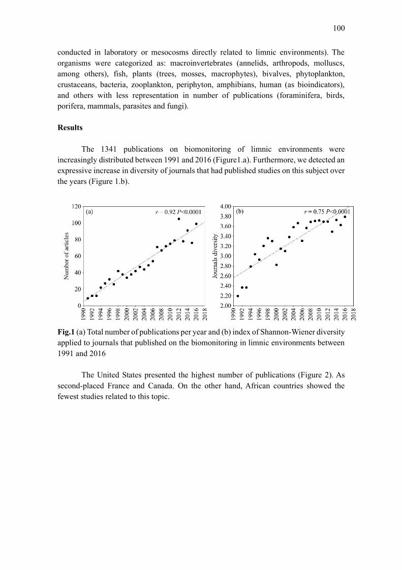
100
conducted in laboratory or mesocosms directly related to limnic environments). The
organisms were categorized as: macroinvertebrates (annelids, arthropods, molluscs,
among others), fish, plants (trees, mosses, macrophytes), bivalves, phytoplankton,
crustaceans, bacteria, zooplankton, periphyton, amphibians, human (as bioindicators),
and others with less representation in number of publications (foraminifera, birds,
porifera, mammals, parasites and fungi).
Results
The 1341 publications on biomonitoring of limnic environments were
increasingly distributed between 1991 and 2016 (Figure1.a). Furthermore, we detected an
expressive increase in diversity of journals that had published studies on this subject over
the years (Figure 1.b).
Fig.1 (a) Total number of publications per year and (b) index of Shannon-Wiener diversity
applied to journals that published on the biomonitoring in limnic environments between
1991 and 2016
The United States presented the highest number of publications (Figure 2). As
second-placed France and Canada. On the other hand, African countries showed the
fewest studies related to this topic.
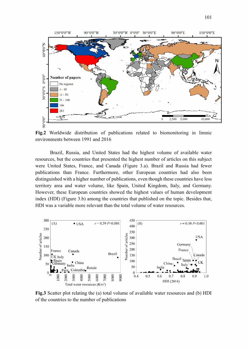
101
Fig.2 Worldwide distribution of publications related to biomonitoring in limnic
environments between 1991 and 2016
Brazil, Russia, and United States had the highest volume of available water
resources, but the countries that presented the highest number of articles on this subject
were United States, France, and Canada (Figure 3.a). Brazil and Russia had fewer
publications than France. Furthermore, other European countries had also been
distinguished with a higher number of publications, even though these countries have less
territory area and water volume, like Spain, United Kingdom, Italy, and Germany.
However, these European countries showed the highest values of human development
index (HDI) (Figure 3.b) among the countries that published on the topic. Besides that,
HDI was a variable more relevant than the total volume of water resources.
Fig.3 Scatter plot relating the (a) total volume of available water resources and (b) HDI
of the countries to the number of publications

102
We identified two groups with different tendencies related to the words in
publications title and abstract (Figure 4): (i) "metal concentration in organisms and
exposure to pollution and contamination", with the following words more related to this
group: concentration, metal, activity, exposure; and (ii) "ecological responses of
biological organisms", with the words/expressions index, metric, taxa, biotic integrity,
abundance and diversity more related to this group.
Fig.4 Map based on title and abstract words. Words closer and with the same colors
indicate similarity and the size is related to the number of publications
Fishes, macroinvertebrates, and plants received considerable attention from the
scientific community over the years, in the same way that lotic environments were highly
representative in biomonitoring publications, representing more than twice as many
publications as lentic environments (Table 1). Fish were the most representative
organisms in laboratory studies, followed by bivalve organisms (Table 1).
Table 1. Number of publications from the screened articles per group and environment.
The total value exceeds the number of publications evaluated because a study can evaluate
more than one group or more than one environment simultaneously
Groups
Environments
Total Lotic Lentic
Lotic/
Lentic Estuary General Laboratorial
Amphibians 2 0 1 0 0 0 3
Birds 0 1 0 0 1 0 2
Bacteria 1 0 2 1 3 1 8
Bivalves 3 6 4 3 2 8 26
Crustaceans 7 3 2 4 1 3 20
Fishes 46 15 2 6 3 9 81
Foraminiferans 0 0 0 2 0 0 2
Fungi 0 0 1 0 0 0 1
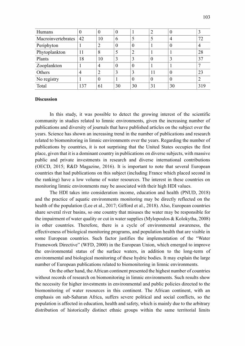
103
Humans 0 0 0 1 2 0 3
Macroinvertebrates 42 10 6 5 5 4 72
Periphyton 1 2 0 0 1 0 4
Phytoplankton 11 8 5 2 1 1 28
Plants 18 10 3 3 0 3 37
Zooplankton 1 4 0 0 1 1 7
Others 4 2 3 3 11 0 23
No registry 1 0 1 0 0 0 2
Total 137 61 30 30 31 30 319
Discussion
In this study, it was possible to detect the growing interest of the scientific
community in studies related to limnic environments, given the increasing number of
publications and diversity of journals that have published articles on the subject over the
years. Science has shown an increasing trend in the number of publications and research
related to biomonitoring in limnic environments over the years. Regarding the number of
publications by countries, it is not surprising that the United States occupies the first
place, given that it is a dominant country in publications on diverse subjects, with massive
public and private investments in research and diverse international contributions
(OECD, 2015; R&D Magazine, 2016). It is important to note that several European
countries that had publications on this subject (including France which placed second in
the ranking) have a low volume of water resources. The interest in these countries on
monitoring limnic environments may be associated with their high HDI values.
The HDI takes into consideration income, education and health (PNUD, 2018)
and the practice of aquatic environments monitoring may be directly reflected on the
health of the population (Lee et al., 2017; Gifford et al., 2018). Also, European countries
share several river basins, so one country that misuses the water may be responsible for
the impairment of water quality or cut in water supplies (Mylopoulos & Kolokytha, 2008)
in other countries. Therefore, there is a cycle of environmental awareness, the
effectiveness of biological monitoring programs, and population health that are visible in
some European countries. Such factor justifies the implementation of the “Water
Framework Directive” (WFD, 2000) in the European Union, which emerged to improve
the environmental status of the surface waters, in addition to the long-term of
environmental and biological monitoring of these hydric bodies. It may explain the large
number of European publications related to biomonitoring in limnic environments.
On the other hand, the African continent presented the highest number of countries
without records of research on biomonitoring in limnic environments. Such results show
the necessity for higher investments in environmental and public policies directed to the
biomonitoring of water resources in this continent. The African continent, with an
emphasis on sub-Saharan Africa, suffers severe political and social conflicts, so the
population is affected in education, health and safety, which is mainly due to the arbitrary
distribution of historically distinct ethnic groups within the same territorial limits
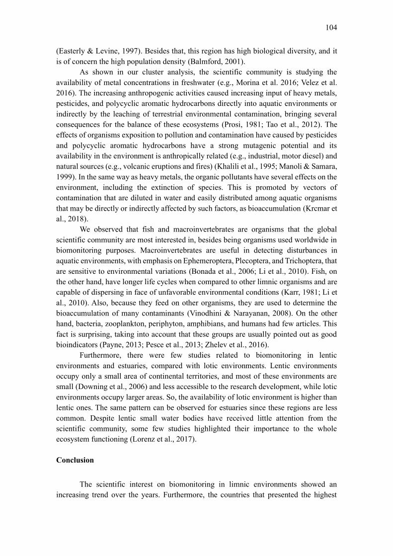
104
(Easterly & Levine, 1997). Besides that, this region has high biological diversity, and it
is of concern the high population density (Balmford, 2001).
As shown in our cluster analysis, the scientific community is studying the
availability of metal concentrations in freshwater (e.g., Morina et al. 2016; Velez et al.
2016). The increasing anthropogenic activities caused increasing input of heavy metals,
pesticides, and polycyclic aromatic hydrocarbons directly into aquatic environments or
indirectly by the leaching of terrestrial environmental contamination, bringing several
consequences for the balance of these ecosystems (Prosi, 1981; Tao et al., 2012). The
effects of organisms exposition to pollution and contamination have caused by pesticides
and polycyclic aromatic hydrocarbons have a strong mutagenic potential and its
availability in the environment is anthropically related (e.g., industrial, motor diesel) and
natural sources (e.g., volcanic eruptions and fires) (Khalili et al., 1995; Manoli & Samara,
1999). In the same way as heavy metals, the organic pollutants have several effects on the
environment, including the extinction of species. This is promoted by vectors of
contamination that are diluted in water and easily distributed among aquatic organisms
that may be directly or indirectly affected by such factors, as bioaccumulation (Krcmar et
al., 2018).
We observed that fish and macroinvertebrates are organisms that the global
scientific community are most interested in, besides being organisms used worldwide in
biomonitoring purposes. Macroinvertebrates are useful in detecting disturbances in
aquatic environments, with emphasis on Ephemeroptera, Plecoptera, and Trichoptera, that
are sensitive to environmental variations (Bonada et al., 2006; Li et al., 2010). Fish, on
the other hand, have longer life cycles when compared to other limnic organisms and are
capable of dispersing in face of unfavorable environmental conditions (Karr, 1981; Li et
al., 2010). Also, because they feed on other organisms, they are used to determine the
bioaccumulation of many contaminants (Vinodhini & Narayanan, 2008). On the other
hand, bacteria, zooplankton, periphyton, amphibians, and humans had few articles. This
fact is surprising, taking into account that these groups are usually pointed out as good
bioindicators (Payne, 2013; Pesce et al., 2013; Zhelev et al., 2016).
Furthermore, there were few studies related to biomonitoring in lentic
environments and estuaries, compared with lotic environments. Lentic environments
occupy only a small area of continental territories, and most of these environments are
small (Downing et al., 2006) and less accessible to the research development, while lotic
environments occupy larger areas. So, the availability of lotic environment is higher than
lentic ones. The same pattern can be observed for estuaries since these regions are less
common. Despite lentic small water bodies have received little attention from the
scientific community, some few studies highlighted their importance to the whole
ecosystem functioning (Lorenz et al., 2017).
Conclusion
The scientific interest on biomonitoring in limnic environments showed an
increasing trend over the years. Furthermore, the countries that presented the highest
105
number of publications related to this subject had also high HDI indicators, high
investments in research and development or specific legislation for water quality
monitoring. Despite the significant relationship, national water volume was not a major
factor influencing the research development.
Our study also revealed that fish and macroinvertebrates are the most studied
groups of organisms with biological monitoring purposes, as well as lotic environments.
On the other hand, there were few studies on lentic continental environments and estuary
regions. There were also few studies evaluating the utility of bacteria, zooplankton,
periphyton, amphibians, humans, foraminifera, birds, porifera, mammals, fungi and
parasites on biomonitoring purposes.
References
Balmford A 2001. Conservation Conflicts Across Africa. Science, 291(5513): 2616–
2619.
Bonada N, Prat N, Resh VH & Statzner B 2006. Developments in aquatic insect
biomonitoring: A Comparative Analysis of Recent Approaches. Annual Review of
Entomology, 51(1): 495–523.
Ceballos G, Ehrlich PR, Barnosky AD, Garcia A, Pringle RM & Palmer TM 2015.
Accelerated modern human-induced species losses: Entering the sixth mass
extinction. Science Advances, 1(5): e1400253–e1400253.
Corlett RT 2015. The Anthropocene concept in ecology and conservation. Trends in
Ecology & Evolution, 30(1): 36–41.
Crist E, Mora C & Engelman R 2017. The interaction of human population, food
production, and biodiversity protection. Science, 356(6335).
Downing JA, Prairie YT, Cole JJ, Duarte CM, Tranvik LJ, Striegl RG, McDowell WH,
Kortelainen P, Caraco NF, Melack JM & Middelburg JJ 2006. The global
abundance and size distribution of lakes, ponds, and impoundments. Limnology
and Oceanography, 51(5): 2388–2397.
Dziock F, Henle K, Foeckler F, Follner K & Scholz M 2006. Biological Indicator
Systems in Floodplains – a Review. International Review of Hydrobiology, 91(4):
271–291.
Easterly W & Levine R 1997. Africa’s Growth Tragedy: Policies and Ethnic Divisions.
The Quarterly Journal of Economics, 112(4): 1203–1250.
Flotemersch JE, Stribling J & Paul M 2006. Concepts and Approaches for the
Bioassessment of Streams and Rivers. US Environmental Protection Agency,
Cincinnati ,Ohio, 245 pp.
Gifford M, Chester M, Hristovski K & Westerhoff P 2018. Human health tradeoffs in
wellhead drinking water treatment: Comparing exposure reduction to embedded
life cycle risks. Water Research, 128: 246–254.
Isbell F, Gonzalez A, Loreau M, Cowles J, Díaz S, Hector A, Mace GM, Wardle DA,
O’Connor MI, Duffy JE, Turnbull LA, Thompson PL & Larigauderie A 2017.
Linking the influence and dependence of people on biodiversity across scales.
Nature, 546(7656): 65–72.
Karr JR 1981. Assessment of Biotic Integrity Using Fish Communities. Fisheries, 6(6):
21–27.
Khalili NR, Scheff PA & Holsen TM 1995. PAH source fingerprints for coke ovens,
diesel and, gasoline engines, highway tunnels, and wood combustion emissions.

106
Atmospheric Environment, 29(4): 533–542.
Krcmar D, Tenodi S, Grba N, Kerkez D, Watson M, Rončević S & Dalmacija B 2018.
Preremedial assessment of the municipal landfill pollution impact on soil and
shallow groundwater in Subotica, Serbia. Science of The Total Environment, 615:
1341–1354.
Lee S, Jiang X, Manubolu M, Riedl K, Ludsin SA, Martin JF & Lee J 2017. Fresh
produce and their soils accumulate cyanotoxins from irrigation water: Implications
for public health and food security. Food Research International, 102: 234–245.
Li L, Zheng B & Liu L 2010. Biomonitoring and Bioindicators Used for River
Ecosystems: Definitions, Approaches and Trends. Procedia Environmental
Sciences, 2: 1510–1524.
Lorenz S, Rasmussen JJ, Süß A, Kalettka T, Golla B, Horney P, Stähler M, Hommel B
& Schäfer RB 2017. Specifics and challenges of assessing exposure and effects of
pesticides in small water bodies. Hydrobiologia, 793(1): 213–224.
Magurran AE 1988. Diversity indices and species abundance models. In: Ecological
Diversity and Its Measurement. Springer Netherlands, Dordrecht, pp. 7–45.
Manoli E & Samara C 1999. Polycyclic aromatic hydrocarbons in natural waters:
sources, occurrence and analysis. TrAC Trends in Analytical Chemistry, 18(6):
417–428.
Morina A, Morina F, Djikanović V, Spasić S, Krpo-Ćetković J, Kostić B & Lenhardt M
2016. Common barbel (Barbus barbus) as a bioindicator of surface river sediment
pollution with Cu and Zn in three rivers of the Danube River Basin in Serbia.
Environmental Science and Pollution Research, 23(7): 6723–6734.
Mylopoulos YA & Kolokytha EG 2008. Integrated water management in shared water
resources: The EU Water Framework Directive implementation in Greece. Physics
and Chemistry of the Earth, Parts A/B/C, 33(5): 347–353.
OECD 2015. Gross domestic spending on R&D (indicator).
Oertel N & Salánki J 2003. Biomonitoring and Bioindicators in Aquatic Ecosystems. In:
Modern Trends in Applied Aquatic Ecology. Springer US, Boston, MA, pp. 219–
246.
Payne RJ 2013. Seven reasons why protists make useful bioindicators. Acta
Protozoologica, 52(3): 105–113.
Pelicice FM, Azevedo-Santos VM, Vitule JRS, Orsi ML, Lima Junior DP, Magalhães
ALB, Pompeu PS, Petrere M & Agostinho AA 2017. Neotropical freshwater fishes
imperilled by unsustainable policies. Fish and Fisheries.
Pesce S, Margoum C, Rouard N, Foulquier A & Martin-Laurent F 2013. Freshwater
sediment pesticide biodegradation potential as an ecological indicator of microbial
recovery following a decrease in chronic pesticide exposure: A case study with the
herbicide diuron. Ecological Indicators, 29: 18–25.
Peters NE & Meybeck M 2000. Water Quality Degradation Effects on Freshwater
Availability: Impacts of Human Activities. Water International, 25(2): 185–193.
PNUD 2018. http://www.br.undp.org/content/brazil/pt/home/idh0.html. (Accessed 24
January 2018).
Prosi F 1981. Heavy Metals in Aquatic Organisms. In: Metal Pollution in the Aquatic
Environment. Springer Berlin Heidelberg, Berlin, Heidelberg, pp. 271–323.
R&D Magazine 2016. R&D Magazine. 2016 GLOBAL R&D FUNDING FORECAST.
https://www.iriweb.org/sites/default/files/2016GlobalR&DFundingForecast_2.pdf.
(Accessed 23 January 2018).
Reynolds CS 1980. Phytoplankton assemblages and their periodicity in stratifying lake
systems. Ecography, 3(3): 141–159.

107
Steffen W, Richardson K, Rockstrom J, Cornell SE, Fetzer I, Bennett EM, Biggs R,
Carpenter SR, de Vries W, de Wit CA, Folke C, Gerten D, Heinke J, Mace GM,
Persson LM, Ramanathan V, Reyers B & Sorlin S 2015. Planetary boundaries:
Guiding human development on a changing planet. Science, 347(6223): 1259855–
1259855.
Tao Y, Yuan Z, Xiaona H & Wei M 2012. Distribution and bioaccumulation of heavy
metals in aquatic organisms of different trophic levels and potential health risk
assessment from Taihu lake, China. Ecotoxicology and Environmental Safety, 81:
55–64.
van Eck NJ & Waltman L 2010. Software survey: VOSviewer, a computer program for
bibliometric mapping. Scientometrics, 84(2): 523–538.
Vaz UL, Cunha HF & Nabout JC 2015. Trends and biases in global scientific literature
about ecological niche models. Brazilian Journal of Biology, 75(4 suppl 1): 17–24.
Velez C, Pires A, Sampaio L, Cardoso P, Moreira A, Leandro S, Figueira E, Soares
AMVM & Freitas R 2016. The use of Cerastoderma glaucum as a sentinel and
bioindicator species: Take-home message. Ecological Indicators, 62: 228–241.
Vieira ACB, Medeiros AMA, Ribeiro LL & Crispim MC 2011. Population dynamics of
Moina minuta Hansen (1899), Ceriodaphnia cornuta Sars (1886), and
Diaphanosoma spinulosum Herbst (1967) (Crustacea: Branchiopoda) in different
nutrients (N and P) concentration ranges. Acta Limnologica Brasiliensia, 23(1):
48–56.
Vinodhini R & Narayanan M 2008. Bioaccumulation of heavy metals in organs of fresh
water fish Cyprinus carpio (Common carp). International Journal of Environmental
Science & Technology, 5(2): 179–182.
WFD Directive of the European Parliament and of the Council 2000/60/EC., European
Union, Luxembourg PE-CONS 3639/1/00 REV 1. § (2000).
Zhelev ZM, Mehterov NH & Popgeorgiev GS 2016. Seasonal changes of basic
erythrocyte-metric parameters in Pelophylax ridibundus (Amphibia: Ranidae) from
anthropogenically polluted biotopes in Southern Bulgaria and their role as
bioindicators. Ecotoxicology and Environmental Safety, 124: 406–417.
Zhou Q, Zhang J, Fu J, Shi J & Jiang G 2008. Biomonitoring: An appealing tool for
assessment of metal pollution in the aquatic ecosystem. Analytica Chimica Acta,
606(2): 135–150.
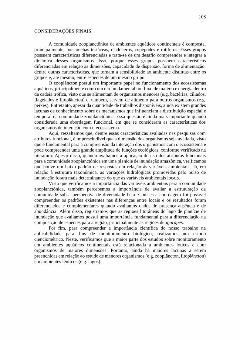
108
CONSIDERAÇÕES FINAIS
A comunidade zooplanctônica de ambientes aquáticos continentais é composta,
principalmente, por amebas testáceas, cladóceros, copépodes e rotíferos. Esses grupos
possuem características diferenciadas e trata-se de um desafio compreender e integrar a
dinâmica desses organismos. Isso, porque esses grupos possuem características
diferenciadas em relação às dimensões, capacidade de dispersão, forma de alimentação,
dentre outras características, que tornam a sensibilidade ao ambiente distintas entre os
grupos e, até mesmo, entre espécies de um mesmo grupo.
O zooplâncton possui um importante papel no funcionamento dos ecossistemas
aquáticos, principalmente como um elo fundamental no fluxo de matéria e energia dentro
da cadeia trófica, visto que se alimentam de organismos menores (e.g. bactérias, ciliados,
flagelados e fitoplâncton) e, também, servem de alimento para outros organismos (e.g.
peixes). Entretanto, apesar da quantidade de trabalhos disponíveis, ainda existem grandes
lacunas de conhecimento sobre os mecanismos que influenciam a distribuição espacial e
temporal da comunidade zooplanctônica. Essa questão é ainda mais importante quando
considerada uma abordagem funcional, em que se consideram as características dos
organismos de interação com o ecossistema.
Aqui, ressaltamos que, dentre essas características avaliadas nas pesquisas com
atributos funcional, é imprescindível que a dimensão dos organismos seja avaliada, visto
que é fundamental para a compreensão da interação dos organismos com o ecossistema e
pode compreender uma grande amplitude de funções ecológicas, conforme verificado na
literatura. Apesar disso, quando avaliamos a aplicação do uso dos atributos funcionais
para a comunidade zooplanctônica em uma planície de inundação amazônica, verificamos
que houve um baixo padrão de respostas em relação às variáveis ambientais. Já, em
relação à estrutura taxonômica, as variações hidrológicas promovidas pelo pulso de
inundação foram mais determinantes do que as variáveis ambientais locais.
Visto que verificamos a importância das variáveis ambientais para a comunidade
zooplanctônica, também percebemos a importância de avaliar a estruturação da
comunidade sob a perspectiva de diversidade beta. Com essa abordagem foi possível
compreender os padrões existentes nas diferenças entre locais e os resultados foram
diferenciados e complementares quando avaliamos dados de presença-ausência e de
abundância. Além disso, registramos que as regiões litorâneas do lago de planície de
inundação que avaliamos possui uma importância fundamental para a diferenciação na
composição de espécies para a região, principalmente as regiões de igarapés.
Por fim, para compreender a importância científica do nosso trabalho na
aplicabilidade para fins de monitoramento biológico, realizamos um estudo
cienciométrico. Neste, verificamos que a maior parte dos estudos sobre monitoramento
em ambientes aquáticos continentais está relacionada a ambientes lóticos e com
organismos de maiores dimensões. Portanto, ainda há maiores lacunas a serem
preenchidas em relação ao estudo de menores organismos (e.g. zooplâncton, fitoplâncton)
em ambientes lênticos (e.g. lagos).
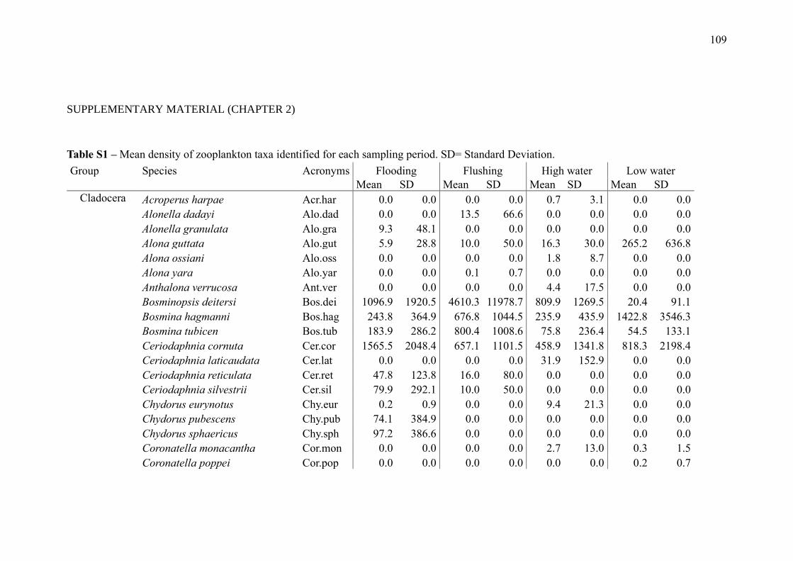
109
SUPPLEMENTARY MATERIAL (CHAPTER 2)
Table S1 – Mean density of zooplankton taxa identified for each sampling period. SD= Standard Deviation.
Group Species Acronyms Flooding Flushing High water Low water
Mean SD Mean SD Mean SD Mean SD
Cladocera Acroperus harpae Acr.har 0.0 0.0 0.0 0.0 0.7 3.1 0.0 0.0
Alonella dadayi Alo.dad 0.0 0.0 13.5 66.6 0.0 0.0 0.0 0.0
Alonella granulata Alo.gra 9.3 48.1 0.0 0.0 0.0 0.0 0.0 0.0
Alona guttata Alo.gut 5.9 28.8 10.0 50.0 16.3 30.0 265.2 636.8
Alona ossiani Alo.oss 0.0 0.0 0.0 0.0 1.8 8.7 0.0 0.0
Alona yara Alo.yar 0.0 0.0 0.1 0.7 0.0 0.0 0.0 0.0
Anthalona verrucosa Ant.ver 0.0 0.0 0.0 0.0 4.4 17.5 0.0 0.0
Bosminopsis deitersi Bos.dei 1096.9 1920.5 4610.3 11978.7 809.9 1269.5 20.4 91.1
Bosmina hagmanni Bos.hag 243.8 364.9 676.8 1044.5 235.9 435.9 1422.8 3546.3
Bosmina tubicen Bos.tub 183.9 286.2 800.4 1008.6 75.8 236.4 54.5 133.1
Ceriodaphnia cornuta Cer.cor 1565.5 2048.4 657.1 1101.5 458.9 1341.8 818.3 2198.4
Ceriodaphnia laticaudata Cer.lat 0.0 0.0 0.0 0.0 31.9 152.9 0.0 0.0
Ceriodaphnia reticulata Cer.ret 47.8 123.8 16.0 80.0 0.0 0.0 0.0 0.0
Ceriodaphnia silvestrii Cer.sil 79.9 292.1 10.0 50.0 0.0 0.0 0.0 0.0
Chydorus eurynotus Chy.eur 0.2 0.9 0.0 0.0 9.4 21.3 0.0 0.0
Chydorus pubescens Chy.pub 74.1 384.9 0.0 0.0 0.0 0.0 0.0 0.0
Chydorus sphaericus Chy.sph 97.2 386.6 0.0 0.0 0.0 0.0 0.0 0.0
Coronatella monacantha Cor.mon 0.0 0.0 0.0 0.0 2.7 13.0 0.3 1.5
Coronatella poppei Cor.pop 0.0 0.0 0.0 0.0 0.0 0.0 0.2 0.7

110
Dadaya macrops Dad.mac 4.8 24.0 0.0 0.0 0.0 0.0 0.0 0.0
Daphnia cf. gessneri Dap.ges 1349.9 2342.2 378.7 656.1 235.3 913.2 1818.9 3324.1
Diaphanosoma birgei Dia.bir 4.0 21.0 0.0 0.0 0.3 1.4 0.0 0.0
Diaphanosoma polyspina Dia.pol 0.0 0.0 0.0 0.0 0.0 0.0 33.3 149.1
Diaphanosoma sp. Dia.sp. 892.4 1237.8 37.7 140.2 207.4 523.6 250.0 1118.0
Diaphanosoma spinulosum Dia.spi 0.0 0.0 0.0 0.0 9.8 29.1 0.0 0.0
Disparalona leptorhyncha Dis.lep 0.0 0.0 0.0 0.0 2.9 13.9 0.0 0.0
Grimaldina brazzai Gri.bra 0.0 0.0 0.0 0.0 0.9 4.3 0.0 0.0
Holopedium amazonicum Hol.ama 1262.9 2602.0 58.3 266.8 0.0 0.0 0.0 0.0
Ilyocryptus spinifer Ily.spi 0.0 0.0 0.0 0.0 0.7 3.5 0.0 0.0
Karualona muelleri Kar.mue 0.0 0.0 17.3 86.7 0.0 0.0 17.5 74.4
Leydigiopsis megalops Ley.meg 0.0 0.0 0.0 0.0 0.1 0.7 0.0 0.0
Macrothrix laticornis Mac.lat 9.4 48.1 17.3 86.7 5.8 27.8 34.3 148.9
Macrothrix mira Mac.mir 9.3 48.1 0.0 0.0 0.0 0.0 0.3 1.5
Magnospina dentifera Mag.den 0.0 0.0 0.0 0.0 11.6 52.1 0.0 0.0
Moina micrura Moi.mic 654.5 1957.9 1308.0 2204.3 121.1 487.6 292.5 661.6
Moina minuta Moi.min 1192.7 3766.7 1403.6 2945.2 136.2 294.8 3737.5 4036.2
Moina reticulata Moi.ret 0.0 0.0 16.0 80.0 0.0 0.0 0.0 0.0
Moina sp. Moi.sp. 0.0 0.0 0.0 0.0 15.9 76.5 0.0 0.0
Nicsmirnovius incredibilis Nic.inc 0.0 0.0 0.0 0.0 2.6 12.5 0.0 0.0
Picripleuroxus similis Pic.sim 2.4 12.0 0.0 0.0 3.6 17.4 0.0 0.0
Pleuroxus sp. Ple.sp. 2.3 12.0 0.0 0.0 0.0 0.0 0.0 0.0
Simocephalus sp. Sim.sp. 0.0 0.0 0.0 0.0 0.0 0.0 20.8 93.2
Copepod Argyrodiaptomus azevedoi Arg.aze 57.5 162.4 0.0 0.0 0.0 0.0 0.0 0.0
Argyrodiaptomus robertsonae Arg.rob 526.5 2570.9 0.0 0.0 55.1 264.1 0.0 0.0
Cyclopidae copepodite Cop.cyc 5321.9 5868.1 10051.0 12221.8 5183.2 11498.0 5453.1 4471.0
Diaptomidae copepodite Cop.diap 5121.6 9860.9 2056.3 2823.0 1187.6 2561.7 3370.4 2959.1

111
Cyclopidae nauplii Nau.cyc 13716.1 16434.7 60918.2 41487.7 7802.1 12483.4 21722.4 15918.9
Diaptomidae nauplii Nau.diap 11518.2 24618.4 2362.1 2447.6 815.2 2287.6 3334.9 3355.3
Diaptomus deitersi Dia.dei 0.0 0.0 10.0 50.0 0.0 0.0 0.0 0.0
Mesocyclops meridianus Mes.mer 37.7 163.1 0.0 0.0 0.0 0.0 0.0 0.0
Metacyclops mendocinus Met.men 9.3 48.1 0.0 0.0 29.3 139.0 16.7 74.5
Microcyclops alius Mic.ali 83.5 311.8 168.7 549.1 687.9 2845.8 433.5 809.9
Microcyclops anceps Mic.anc 0.9 4.8 130.6 487.6 24.9 71.4 220.8 415.6
Microcyclops ceibaensis Mic.cei 0.0 0.0 115.6 388.8 95.7 333.6 0.0 0.0
Microcyclops finitimus Mic.fin 168.5 431.2 40.0 156.1 0.0 0.0 0.0 0.0
Microcyclops sp. Mic.sp. 0.0 0.0 17.5 86.6 13.0 55.7 40.0 178.9
Notodiaptomus amazonicus Not.ama 90.6 201.4 54.3 160.9 15.9 76.5 804.9 1021.0
Notodiaptomus kieferi Not.kie 20.3 96.3 0.0 0.0 0.0 0.0 0.0 0.0
Notodiaptomus paraensis Not.par 18.0 56.3 0.0 0.0 17.0 67.2 0.0 0.0
Thermocyclops inversus The.inv 168.4 421.7 100.8 503.4 278.3 1249.6 366.7 517.5
Thermocyclops minutus The.min 47.6 216.2 0.0 0.0 6.5 27.9 33.3 149.1
Thermocyclops sp. The.sp. 0.0 0.0 0.0 0.0 35.9 141.4 0.0 0.0
Rotifer Ascomorpha agilis Asc.agi 0.0 0.0 16.0 80.0 36.2 173.8 20.8 93.2
Ascomorpha eucadis Asc.euc 142.0 510.5 68.0 256.1 0.0 0.0 637.4 1163.3
Ascomorpha saltans Asc.sal 24.7 128.3 0.0 0.0 250.5 577.0 554.2 1071.4
Ascomorpha sp. Asc.sp. 0.0 0.0 0.0 0.0 0.0 0.0 200.0 451.1
Asplanchna herricki Asp.her 0.0 0.0 0.0 0.0 111.6 535.2 166.7 607.0
Asplanchna priodonta Asp.pri 0.0 0.0 0.0 0.0 0.0 0.0 83.3 372.7
Asplanchna sieboldii Asp.sie 30.1 144.4 772.0 2385.9 4.2 12.9 984.7 3738.9
Asplanchna sp. Asp.sp. 0.0 0.0 0.0 0.0 0.0 0.0 16.8 74.5
Bdelloidea Bdell 0.0 0.0 401.0 1727.4 0.0 0.0 20.8 93.2
Beauchampiella eudactylota Bea.eud 0.0 0.0 0.0 0.0 10.1 21.0 0.0 0.0
Brachionus ahlstromi Bra.ahl 18.5 66.7 240.0 1149.0 0.0 0.0 0.0 0.0
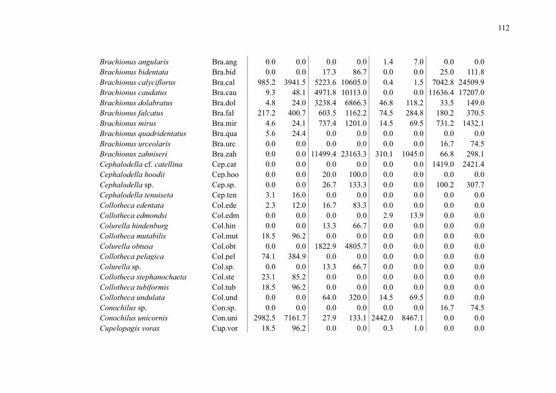
112
Brachionus angularis Bra.ang 0.0 0.0 0.0 0.0 1.4 7.0 0.0 0.0
Brachionus bidentata Bra.bid 0.0 0.0 17.3 86.7 0.0 0.0 25.0 111.8
Brachionus calyciflorus Bra.cal 985.2 3941.5 5223.6 10605.0 0.4 1.5 7042.8 24509.9
Brachionus caudatus Bra.cau 9.3 48.1 4971.8 10113.0 0.0 0.0 11636.4 17207.0
Brachionus dolabratus Bra.dol 4.8 24.0 3238.4 6866.3 46.8 118.2 33.5 149.0
Brachionus falcatus Bra.fal 217.2 400.7 603.5 1162.2 74.5 284.8 180.2 370.5
Brachionus mirus Bra.mir 4.6 24.1 737.4 1201.0 14.5 69.5 731.2 1432.1
Brachionus quadridentatus Bra.qua 5.6 24.4 0.0 0.0 0.0 0.0 0.0 0.0
Brachionus urceolaris Bra.urc 0.0 0.0 0.0 0.0 0.0 0.0 16.7 74.5
Brachionus zahniseri Bra.zah 0.0 0.0 11499.4 23163.3 310.1 1045.0 66.8 298.1
Cephalodella cf. catellina Cep.cat 0.0 0.0 0.0 0.0 0.0 0.0 1419.0 2421.4
Cephalodella hoodii Cep.hoo 0.0 0.0 20.0 100.0 0.0 0.0 0.0 0.0
Cephalodella sp. Cep.sp. 0.0 0.0 26.7 133.3 0.0 0.0 100.2 307.7
Cephalodella tenuiseta Cep.ten 3.1 16.0 0.0 0.0 0.0 0.0 0.0 0.0
Collotheca edentata Col.ede 2.3 12.0 16.7 83.3 0.0 0.0 0.0 0.0
Collotheca edmondsi Col.edm 0.0 0.0 0.0 0.0 2.9 13.9 0.0 0.0
Colurella hindenburg Col.hin 0.0 0.0 13.3 66.7 0.0 0.0 0.0 0.0
Collotheca mutabilis Col.mut 18.5 96.2 0.0 0.0 0.0 0.0 0.0 0.0
Colurella obtusa Col.obt 0.0 0.0 1822.9 4805.7 0.0 0.0 0.0 0.0
Collotheca pelagica Col.pel 74.1 384.9 0.0 0.0 0.0 0.0 0.0 0.0
Colurella sp. Col.sp. 0.0 0.0 13.3 66.7 0.0 0.0 0.0 0.0
Collotheca stephanochaeta Col.ste 23.1 85.2 0.0 0.0 0.0 0.0 0.0 0.0
Collotheca tubiformis Col.tub 18.5 96.2 0.0 0.0 0.0 0.0 0.0 0.0
Collotheca undulata Col.und 0.0 0.0 64.0 320.0 14.5 69.5 0.0 0.0
Conochilus sp. Con.sp. 0.0 0.0 0.0 0.0 0.0 0.0 16.7 74.5
Conochilus unicornis Con.uni 2982.5 7161.7 27.9 133.1 2442.0 8467.1 0.0 0.0
Cupelopagis vorax Cup.vor 18.5 96.2 0.0 0.0 0.3 1.0 0.0 0.0

113
Dicranophorus forcipatus Dic.for 0.0 0.0 10.0 50.0 0.0 0.0 0.0 0.0
Dicranophorus sp. Dic.sp. 4.6 24.1 0.0 0.0 0.0 0.0 0.0 0.0
Drilophaga delagei Dri.del 196.8 636.1 0.0 0.0 0.0 0.0 0.0 0.0
Elosa worrali Elo.wor 0.0 0.0 0.0 0.0 143.7 412.7 0.0 0.0
Epiphanes clavatula Epi.cla 259.3 1347.2 669.3 2316.9 0.0 0.0 0.0 0.0
Epiphanes macrorus Epi.mac 252.2 831.4 0.0 0.0 0.0 0.0 3312.8 10314.9
Epiphanes pelagica Epi.pel 1.5 8.0 0.0 0.0 0.0 0.0 0.0 0.0
Euchlanis callysta Euc.cal 0.0 0.0 0.0 0.0 1.4 7.0 0.0 0.0
Euchlanis incisa Euc.inc 0.0 0.0 0.0 0.0 0.0 0.0 5.6 24.8
Euchlanis meneta Euc.men 0.0 0.0 0.0 0.0 1.8 8.7 0.0 0.0
Euchlanis sp. Euc.sp. 0.0 0.0 0.0 0.0 0.0 0.0 66.7 298.1
Euchlanis triquetra Euc.tri 0.0 0.0 0.0 0.0 123.7 269.0 133.3 463.9
Filinia camasecla Fil.cam 0.0 0.0 245.6 412.7 4.3 14.1 0.0 0.0
Filinia longiseta Fil.lon 115.2 249.0 4749.7 5621.8 56.3 165.3 6730.7 10070.5
Filinia opoliensis Fil.opo 9.3 48.1 100.0 294.4 29.7 138.9 33.7 149.0
Filinia terminalis Fil.ter 179.9 414.4 762.7 2411.6 32.2 98.2 50.2 223.6
Filinia unicornis Fil.uni 9.3 48.1 0.0 0.0 0.0 0.0 0.0 0.0
Gastropus hyptopus Gas.hyp 0.0 0.0 330.0 1598.7 89.9 364.9 0.0 0.0
Gastropus stylifer Gas.sty 0.0 0.0 0.0 0.0 11.3 48.7 0.0 0.0
Harringia eupoda Har.eup 675.9 2969.2 0.0 0.0 3.6 17.4 33.3 149.1
Heterolepadella cf. heterodactyla Het.het 0.0 0.0 40.0 200.0 0.0 0.0 0.0 0.0
Hexarthra cf. fenica Hex.fen 0.0 0.0 16.0 80.0 0.0 0.0 0.0 0.0
Hexarthra intermedia Hex.int 0.0 0.0 218.0 875.7 0.0 0.0 0.0 0.0
Hexarthra cf. mira Hex.mir 0.0 0.0 96.0 318.2 0.0 0.0 0.0 0.0
Hexarthra sp. Hex.sp. 0.0 0.0 160.0 800.0 0.0 0.0 0.0 0.0
Horaela brehmi Hor.bre 0.0 0.0 0.0 0.0 5.8 27.8 0.0 0.0
Kellicottia longispina Kel.lon 0.0 0.0 0.0 0.0 0.3 1.4 0.0 0.0
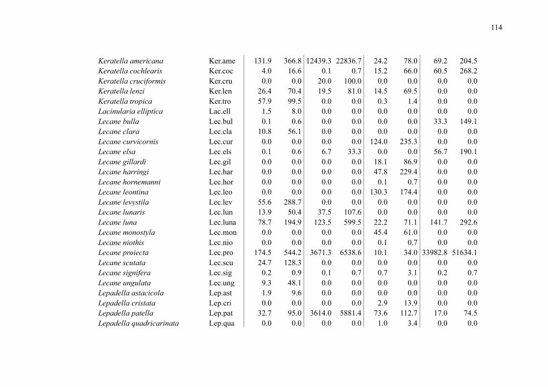
114
Keratella americana Ker.ame 131.9 366.8 12439.3 22836.7 24.2 78.0 69.2 204.5
Keratella cochlearis Ker.coc 4.0 16.6 0.1 0.7 15.2 66.0 60.5 268.2
Keratella cruciformis Ker.cru 0.0 0.0 20.0 100.0 0.0 0.0 0.0 0.0
Keratella lenzi Ker.len 26.4 70.4 19.5 81.0 14.5 69.5 0.0 0.0
Keratella tropica Ker.tro 57.9 99.5 0.0 0.0 0.3 1.4 0.0 0.0
Lacinularia elliptica Lac.ell 1.5 8.0 0.0 0.0 0.0 0.0 0.0 0.0
Lecane bulla Lec.bul 0.1 0.6 0.0 0.0 0.0 0.0 33.3 149.1
Lecane clara Lec.cla 10.8 56.1 0.0 0.0 0.0 0.0 0.0 0.0
Lecane curvicornis Lec.cur 0.0 0.0 0.0 0.0 124.0 235.3 0.0 0.0
Lecane elsa Lec.els 0.1 0.6 6.7 33.3 0.0 0.0 56.7 190.1
Lecane gillardi Lec.gil 0.0 0.0 0.0 0.0 18.1 86.9 0.0 0.0
Lecane harringi Lec.har 0.0 0.0 0.0 0.0 47.8 229.4 0.0 0.0
Lecane hornemanni Lec.hor 0.0 0.0 0.0 0.0 0.1 0.7 0.0 0.0
Lecane leontina Lec.leo 0.0 0.0 0.0 0.0 130.3 174.4 0.0 0.0
Lecane levystila Lec.lev 55.6 288.7 0.0 0.0 0.0 0.0 0.0 0.0
Lecane lunaris Lec.lun 13.9 50.4 37.5 107.6 0.0 0.0 0.0 0.0
Lecane luna Lec.luna 78.7 194.9 123.5 599.5 22.2 71.1 141.7 292.6
Lecane monostyla Lec.mon 0.0 0.0 0.0 0.0 45.4 61.0 0.0 0.0
Lecane niothis Lec.nio 0.0 0.0 0.0 0.0 0.1 0.7 0.0 0.0
Lecane proiecta Lec.pro 174.5 544.2 3671.3 6538.6 10.1 34.0 33982.8 51634.1
Lecane scutata Lec.scu 24.7 128.3 0.0 0.0 0.0 0.0 0.0 0.0
Lecane signifera Lec.sig 0.2 0.9 0.1 0.7 0.7 3.1 0.2 0.7
Lecane ungulata Lec.ung 9.3 48.1 0.0 0.0 0.0 0.0 0.0 0.0
Lepadella astacicola Lep.ast 1.9 9.6 0.0 0.0 0.0 0.0 0.0 0.0
Lepadella cristata Lep.cri 0.0 0.0 0.0 0.0 2.9 13.9 0.0 0.0
Lepadella patella Lep.pat 32.7 95.0 3614.0 5881.4 73.6 112.7 17.0 74.5
Lepadella quadricarinata Lep.qua 0.0 0.0 0.0 0.0 1.0 3.4 0.0 0.0
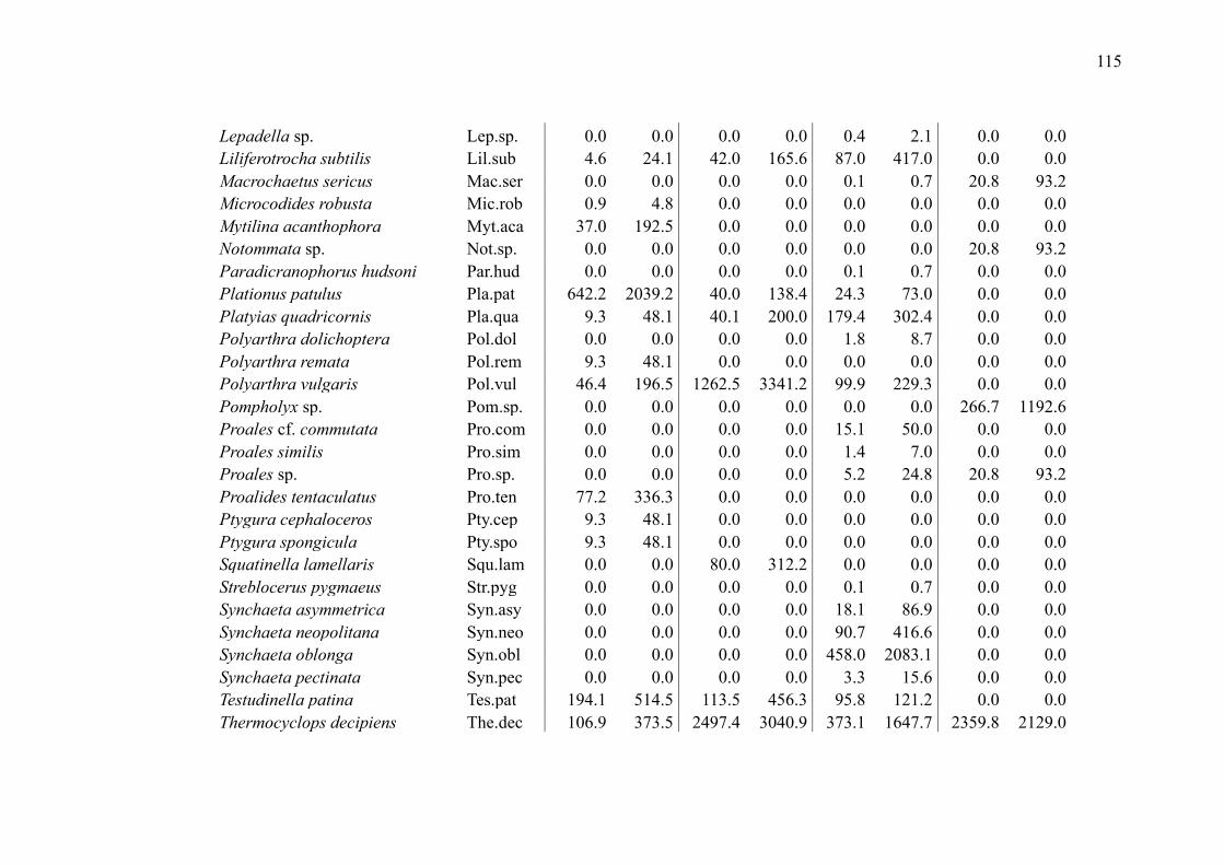
115
Lepadella sp. Lep.sp. 0.0 0.0 0.0 0.0 0.4 2.1 0.0 0.0
Liliferotrocha subtilis Lil.sub 4.6 24.1 42.0 165.6 87.0 417.0 0.0 0.0
Macrochaetus sericus Mac.ser 0.0 0.0 0.0 0.0 0.1 0.7 20.8 93.2
Microcodides robusta Mic.rob 0.9 4.8 0.0 0.0 0.0 0.0 0.0 0.0
Mytilina acanthophora Myt.aca 37.0 192.5 0.0 0.0 0.0 0.0 0.0 0.0
Notommata sp. Not.sp. 0.0 0.0 0.0 0.0 0.0 0.0 20.8 93.2
Paradicranophorus hudsoni Par.hud 0.0 0.0 0.0 0.0 0.1 0.7 0.0 0.0
Plationus patulus Pla.pat 642.2 2039.2 40.0 138.4 24.3 73.0 0.0 0.0
Platyias quadricornis Pla.qua 9.3 48.1 40.1 200.0 179.4 302.4 0.0 0.0
Polyarthra dolichoptera Pol.dol 0.0 0.0 0.0 0.0 1.8 8.7 0.0 0.0
Polyarthra remata Pol.rem 9.3 48.1 0.0 0.0 0.0 0.0 0.0 0.0
Polyarthra vulgaris Pol.vul 46.4 196.5 1262.5 3341.2 99.9 229.3 0.0 0.0
Pompholyx sp. Pom.sp. 0.0 0.0 0.0 0.0 0.0 0.0 266.7 1192.6
Proales cf. commutata Pro.com 0.0 0.0 0.0 0.0 15.1 50.0 0.0 0.0
Proales similis Pro.sim 0.0 0.0 0.0 0.0 1.4 7.0 0.0 0.0
Proales sp. Pro.sp. 0.0 0.0 0.0 0.0 5.2 24.8 20.8 93.2
Proalides tentaculatus Pro.ten 77.2 336.3 0.0 0.0 0.0 0.0 0.0 0.0
Ptygura cephaloceros Pty.cep 9.3 48.1 0.0 0.0 0.0 0.0 0.0 0.0
Ptygura spongicula Pty.spo 9.3 48.1 0.0 0.0 0.0 0.0 0.0 0.0
Squatinella lamellaris Squ.lam 0.0 0.0 80.0 312.2 0.0 0.0 0.0 0.0
Streblocerus pygmaeus Str.pyg 0.0 0.0 0.0 0.0 0.1 0.7 0.0 0.0
Synchaeta asymmetrica Syn.asy 0.0 0.0 0.0 0.0 18.1 86.9 0.0 0.0
Synchaeta neopolitana Syn.neo 0.0 0.0 0.0 0.0 90.7 416.6 0.0 0.0
Synchaeta oblonga Syn.obl 0.0 0.0 0.0 0.0 458.0 2083.1 0.0 0.0
Synchaeta pectinata Syn.pec 0.0 0.0 0.0 0.0 3.3 15.6 0.0 0.0
Testudinella patina Tes.pat 194.1 514.5 113.5 456.3 95.8 121.2 0.0 0.0
Thermocyclops decipiens The.dec 106.9 373.5 2497.4 3040.9 373.1 1647.7 2359.8 2129.0

116
Trichocerca bicristata Tri.bic 12.5 50.1 0.0 0.0 79.2 153.9 0.0 0.0
Trichocerca bidens Tri.bid 0.0 0.0 10.0 50.0 33.0 98.7 406.4 878.1
Trichotria cornuta Tri.cor 170.4 865.5 0.0 0.0 4.9 23.5 0.0 0.0
Trichocerca cylindrica Tri.cyl 0.0 0.0 167.3 267.0 65.4 201.6 0.0 0.0
Trinema enchelys Tri.enc 3.1 16.0 0.0 0.0 0.0 0.0 0.0 0.0
Trichocerca iernis Tri.ier 341.5 727.4 2457.0 2416.2 24.0 51.5 158.8 469.6
Trichocerca longiseta Tri.lon 0.0 0.0 0.0 0.0 1.2 5.6 0.0 0.0
Trichocerca marina Tri.mar 0.0 0.0 0.0 0.0 0.6 2.8 0.0 0.0
Trichocerca sp. Tri.sp. 0.0 0.0 0.0 0.0 0.0 0.0 33.3 149.1
Trichotria tetractis Tri.tet 0.0 0.0 0.0 0.0 1.2 4.1 0.0 0.0
Wierzejskiella elongata Wie.elo 0.0 0.0 0.0 0.0 32.6 139.3 0.0 0.0
Xenolepadella monodactyla Xen.mon 101.9 481.7 0.0 0.0 0.0 0.0 0.0 0.0
Testate
amobae Arcella conica Arc.con 0.0 0.0 0.0 0.0 0.1 0.7 0.0 0.0
Arcella costata Arc.cos 0.0 0.0 30.0 150.0 14.4 38.5 0.0 0.0
Arcella discoides Arc.dis 0.0 0.0 0.0 0.0 0.0 0.0 0.2 0.7
Arcella gibbosa Arc.gib 9.3 48.1 30.0 109.9 16.1 69.6 0.0 0.0
Arcella hemisphaerica Arc.hem 32.4 145.4 0.0 0.0 8.8 28.5 0.0 0.0
Arcella megastoma Arc.meg 11.2 48.7 0.0 0.0 14.2 66.0 0.0 0.0
Arcella mitrata Arc.mit 0.0 0.0 0.0 0.0 1.6 7.8 0.0 0.0
Arcella rotundata Arc.rot 0.0 0.0 0.0 0.0 1.6 7.8 0.0 0.0
Arcella vulgaris Arc.vul 84.0 170.0 0.1 0.7 85.1 206.1 0.2 0.7
Centropyxis aculeata Cen.acu 9.3 48.1 0.0 0.0 35.8 80.9 77.7 180.2
Centropyxis arcelloides Cen.arc 0.0 0.0 0.0 0.0 0.0 0.0 33.3 149.1
Centropyxis cassis Cen.cas 0.0 0.0 0.0 0.0 89.6 382.2 0.0 0.0
Centropyxis discoides Cen.dis 12.3 50.1 0.0 0.0 14.5 69.5 20.0 89.4
Centropyxis ecornis Cen.eco 0.0 0.0 0.0 0.0 0.0 0.0 0.6 2.7
Centropyxis gibba Cen.gib 134.8 471.0 28.0 98.1 0.0 0.0 66.7 298.1

117
Centropyxis spinosa Cen.spi 0.0 0.0 0.0 0.0 0.0 0.0 20.0 89.4
Cucurbitella dentata Cuc.den 0.0 0.0 0.0 0.0 84.2 345.9 0.0 0.0
Cucurbitella mespiliformis Cuc.mes 0.1 0.6 585.3 984.2 5.9 19.6 0.0 0.0
Cucurbitella sp. Cuc.sp. 9.3 48.1 0.0 0.0 0.0 0.0 0.0 0.0
Cucurbitella vlasinensis Cuc.vla 9.3 48.1 0.0 0.0 0.0 0.0 0.0 0.0
Difflugia capreolata Dif.cap 0.0 0.0 0.0 0.0 0.0 0.0 0.5 1.6
Difflugia corona Dif.cor 0.0 0.0 0.0 0.0 1.6 7.8 0.0 0.0
Difflugia cylindrus Dif.cyl 830.4 1585.9 56.0 212.3 6.7 24.6 16.7 74.5
Difflugia difficilis Dif.dif 10.8 48.5 0.0 0.0 38.8 141.5 0.2 0.7
Difflugia elegans Dif.ele 0.0 0.0 0.0 0.0 0.0 0.0 17.2 74.5
Difflugia gramen Dif.gra 0.0 0.0 0.0 0.0 5.6 23.4 0.0 0.0
Difflugia kempnyi Dif.kem 0.0 0.0 0.0 0.0 35.1 153.0 0.5 1.2
Difflugia limnetica Dif.lim 447.8 896.0 898.1 2895.5 13.6 62.5 21.7 93.0
Difflugia lobostoma Dif.lob 0.0 0.0 0.0 0.0 1.8 7.8 0.0 0.0
Difflugia muriformis Dif.mur 0.0 0.0 0.0 0.0 17.0 51.7 0.0 0.0
Difflugia oblonga Dif.obl 0.0 0.0 0.0 0.0 0.0 0.0 53.3 169.8
Difflugia pleustonica Dif.ple 0.0 0.0 0.0 0.0 4.5 21.7 0.0 0.0
Difflugia sp. Dif.sp. 66.4 214.4 0.0 0.0 0.0 0.0 33.3 149.1
Difflugia tuberculata Dif.tub 37.2 135.4 490.0 1371.1 0.9 3.5 4.2 18.6
Difflugia urceolata Dif.urc 55.6 211.8 0.0 0.0 29.7 51.8 0.0 0.0
Difflugiela sp. Difa.sp. 2.3 12.0 0.0 0.0 0.0 0.0 0.0 0.0
Euglypha acanthophora Eug.aca 0.0 0.0 0.0 0.0 2.6 12.5 0.0 0.0
Euglypha filifera Eug.fil 0.0 0.0 0.0 0.0 1.6 7.8 0.0 0.0
Hyalosphenia elegans Hya.ele 9.3 48.1 0.0 0.0 0.0 0.0 0.0 0.0
Lesquereusia globulosa Les.glo 1661.1 2759.0 20.0 100.0 1.3 6.3 0.0 0.0
Lesquereusia sp. Les.sp. 9.3 48.1 0.0 0.0 0.0 0.0 0.2 0.7
Lesquereusia spiralis Les.spi 436.9 796.3 601.1 1043.0 161.8 350.8 0.0 0.0
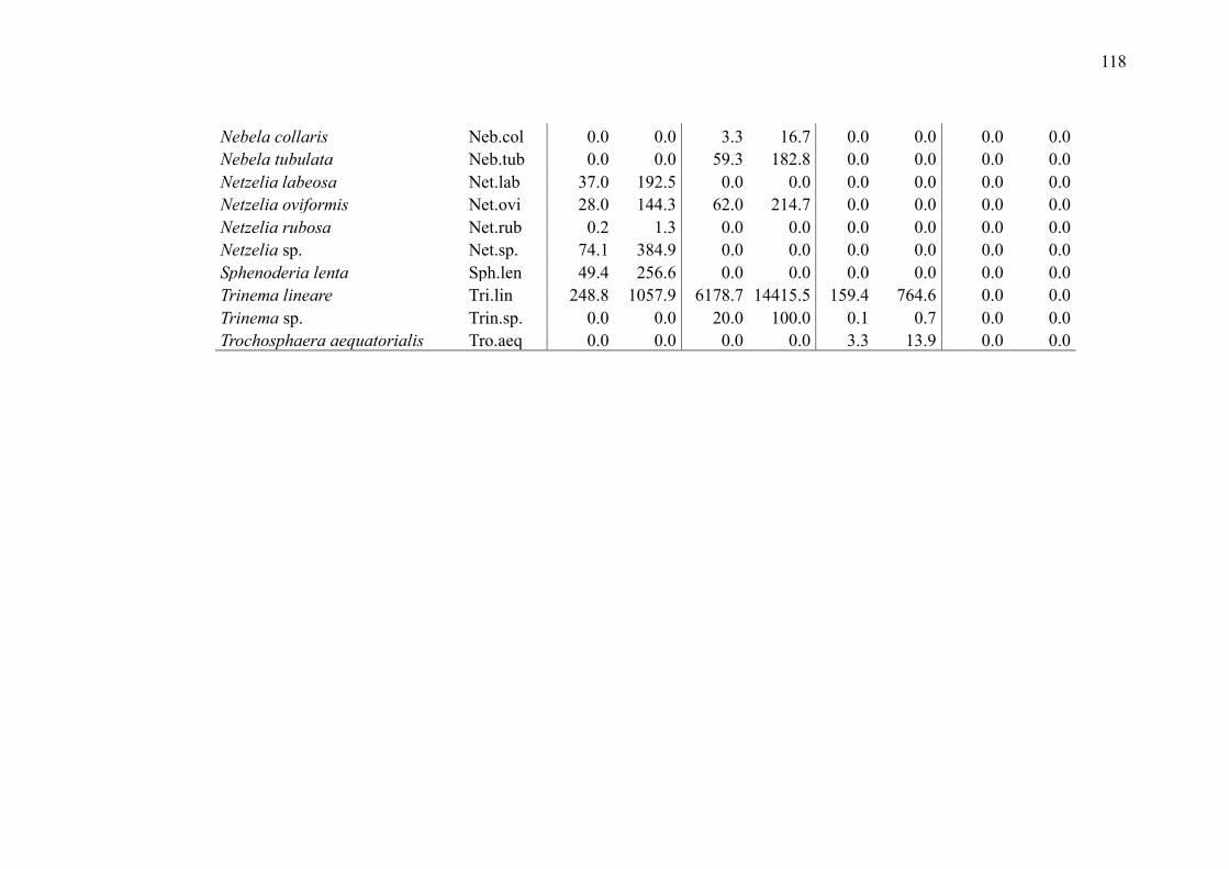
118
Nebela collaris Neb.col 0.0 0.0 3.3 16.7 0.0 0.0 0.0 0.0
Nebela tubulata Neb.tub 0.0 0.0 59.3 182.8 0.0 0.0 0.0 0.0
Netzelia labeosa Net.lab 37.0 192.5 0.0 0.0 0.0 0.0 0.0 0.0
Netzelia oviformis Net.ovi 28.0 144.3 62.0 214.7 0.0 0.0 0.0 0.0
Netzelia rubosa Net.rub 0.2 1.3 0.0 0.0 0.0 0.0 0.0 0.0
Netzelia sp. Net.sp. 74.1 384.9 0.0 0.0 0.0 0.0 0.0 0.0
Sphenoderia lenta Sph.len 49.4 256.6 0.0 0.0 0.0 0.0 0.0 0.0
Trinema lineare Tri.lin 248.8 1057.9 6178.7 14415.5 159.4 764.6 0.0 0.0
Trinema sp. Trin.sp. 0.0 0.0 20.0 100.0 0.1 0.7 0.0 0.0
Trochosphaera aequatorialis Tro.aeq 0.0 0.0 0.0 0.0 3.3 13.9 0.0 0.0
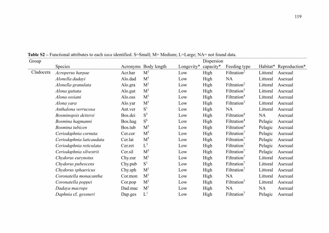
119
Table S2 – Functional attributes to each taxa identified. S=Small; M= Medium; L=Large; NA= not found data.
Group
Species Acronyms Body length Longevity*
Dispersion
capacity* Feeding type Habitat* Reproduction*
Cladocera Acroperus harpae Acr.har M1 Low High Filtration2 Littoral Asexual
Alonella dadayi Alo.dad M1 Low High NA Littoral Asexual
Alonella granulata Alo.gra M1 Low High Filtration2 Littoral Asexual
Alona guttata Alo.gut M1 Low High Filtration3 Littoral Asexual
Alona ossiani Alo.oss M1 Low High Filtration4 Littoral Asexual
Alona yara Alo.yar M1 Low High Filtration3 Littoral Asexual
Anthalona verrucosa Ant.ver S1 Low High NA Littoral Asexual
Bosminopsis deitersi Bos.dei S5 Low High Filtration4 NA Asexual
Bosmina hagmanni Bos.hag S6 Low High Filtration4 Pelagic Asexual
Bosmina tubicen Bos.tub M5 Low High Filtration4 Pelagic Asexual
Ceriodaphnia cornuta Cer.cor M5 Low High Filtration7 Pelagic Asexual
Ceriodaphnia laticaudata Cer.lat M5 Low High Filtration7 Pelagic Asexual
Ceriodaphnia reticulata Cer.ret L5 Low High Filtration7 Pelagic Asexual
Ceriodaphnia silvestrii Cer.sil M5 Low High Filtration7 Pelagic Asexual
Chydorus eurynotus Chy.eur M1 Low High Filtration7 Littoral Asexual
Chydorus pubescens Chy.pub S1 Low High Filtration7 Littoral Asexual
Chydorus sphaericus Chy.sph M1 Low High Filtration7 Littoral Asexual
Coronatella monacantha Cor.mon M1 Low High NA Littoral Asexual
Coronatella poppei Cor.pop M1 Low High Filtration3 Littoral Asexual
Dadaya macrops Dad.mac M1 Low High NA NA Asexual
Daphnia cf. gessneri Dap.ges L1 Low High Filtration7 Pelagic Asexual
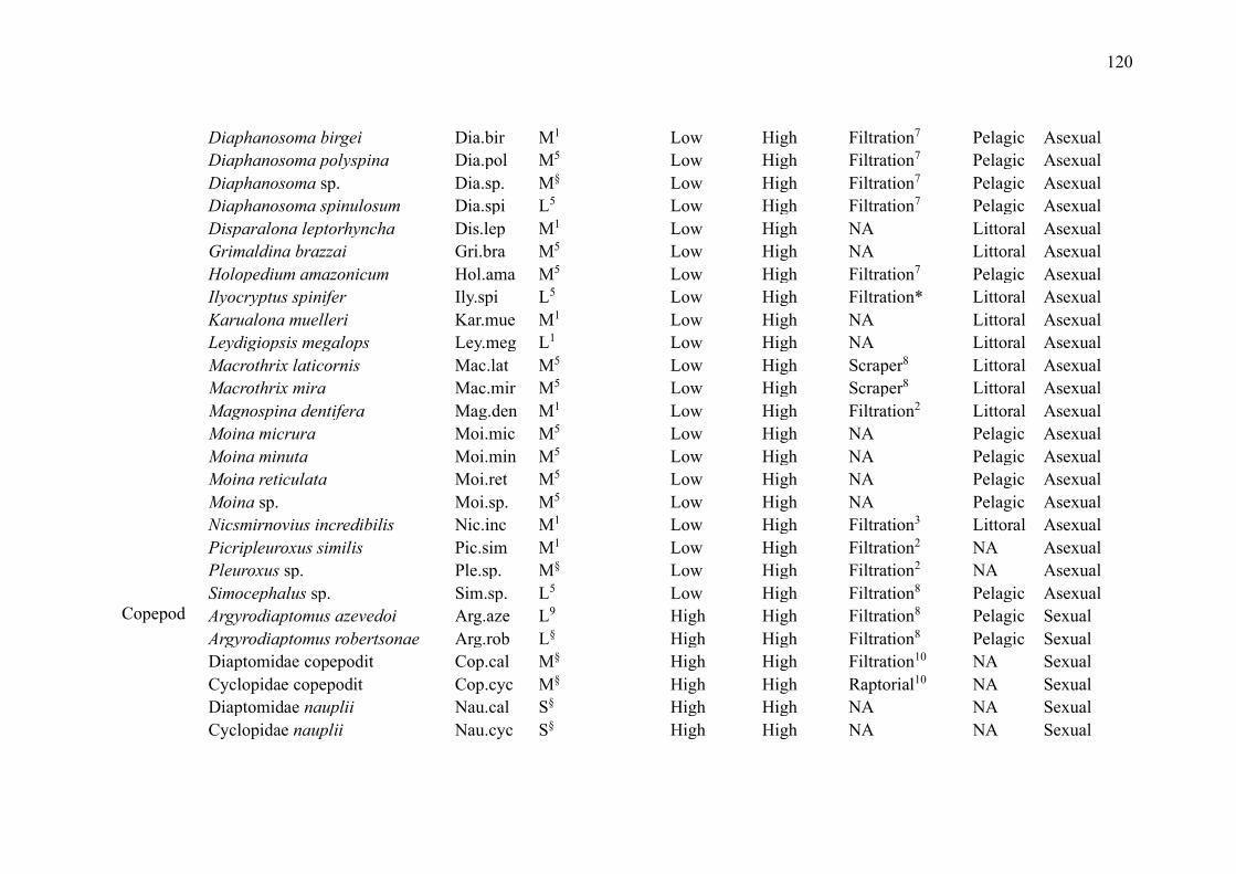
120
Diaphanosoma birgei Dia.bir M1 Low High Filtration7 Pelagic Asexual
Diaphanosoma polyspina Dia.pol M5 Low High Filtration7 Pelagic Asexual
Diaphanosoma sp. Dia.sp. M§ Low High Filtration7 Pelagic Asexual
Diaphanosoma spinulosum Dia.spi L5 Low High Filtration7 Pelagic Asexual
Disparalona leptorhyncha Dis.lep M1 Low High NA Littoral Asexual
Grimaldina brazzai Gri.bra M5 Low High NA Littoral Asexual
Holopedium amazonicum Hol.ama M5 Low High Filtration7 Pelagic Asexual
Ilyocryptus spinifer Ily.spi L5 Low High Filtration* Littoral Asexual
Karualona muelleri Kar.mue M1 Low High NA Littoral Asexual
Leydigiopsis megalops Ley.meg L1 Low High NA Littoral Asexual
Macrothrix laticornis Mac.lat M5 Low High Scraper8 Littoral Asexual
Macrothrix mira Mac.mir M5 Low High Scraper8 Littoral Asexual
Magnospina dentifera Mag.den M1 Low High Filtration2 Littoral Asexual
Moina micrura Moi.mic M5 Low High NA Pelagic Asexual
Moina minuta Moi.min M5 Low High NA Pelagic Asexual
Moina reticulata Moi.ret M5 Low High NA Pelagic Asexual
Moina sp. Moi.sp. M5 Low High NA Pelagic Asexual
Nicsmirnovius incredibilis Nic.inc M1 Low High Filtration3 Littoral Asexual
Picripleuroxus similis Pic.sim M1 Low High Filtration2 NA Asexual
Pleuroxus sp. Ple.sp. M§ Low High Filtration2 NA Asexual
Simocephalus sp. Sim.sp. L5 Low High Filtration8 Pelagic Asexual
Copepod Argyrodiaptomus azevedoi Arg.aze L9 High High Filtration8 Pelagic Sexual
Argyrodiaptomus robertsonae Arg.rob L§ High High Filtration8 Pelagic Sexual
Diaptomidae copepodit Cop.cal M§ High High Filtration10 NA Sexual
Cyclopidae copepodit Cop.cyc M§ High High Raptorial10 NA Sexual
Diaptomidae nauplii Nau.cal S§ High High NA NA Sexual
Cyclopidae nauplii Nau.cyc S§ High High NA NA Sexual

121
Diaptomus deitersi Dia.dei L11 High High NA NA Sexual
Mesocyclops meridianus Mes.mer L12 High High Raptorial7 Pelagic Sexual
Metacyclops mendocinus Met.men L12 High High NA Pelagic Sexual
Microcyclops alius Mic.ali L12 High High Raptorial2 Littoral Sexual
Microcyclops anceps Mic.anc M12 High High Raptorial2 Littoral Sexual
Microcyclops ceibaensis Mic.cei L12 High High Raptorial2 Littoral Sexual
Microcyclops finitimus Mic.fin M12 High High Raptorial2 Littoral Sexual
Microcyclops sp. Mic.sp. M12 High High Raptorial2 Littoral Sexual
Notodiaptomus amazonicus Not.ama L13 High High Filtration8 Pelagic Sexual
Notodiaptomus kieferi Not.kie L13 High High Filtration8 Pelagic Sexual
Notodiaptomus paraensis Not.par L13 High High Filtration8 Pelagic Sexual
Thermocyclops inversus The.inv M12 High High Raptorial3 Pelagic Sexual
Thermocyclops minutus The.min M12 High High Raptorial3 Pelagic Sexual
Thermocyclops sp. The.sp. M12 High High Raptorial3 Pelagic Sexual
Rotifer Ascomorpha agilis Asc.agi S14 Low Low Raptorial15 Pelagic Asexual
Ascomorpha eucadis Asc.euc S14 Low Low Raptorial15 Pelagic Asexual
Ascomorpha saltans Asc.sal S14 Low Low Raptorial15 Pelagic Asexual
Ascomorpha sp. Asc.sp. L§ Low Low Raptorial15 Pelagic Asexual
Asplanchna herricki Asp.her L14 Low Low Raptorial15 Pelagic Asexual
Asplanchna priodonta Asp.pri M14 Low Low Raptorial15 Pelagic Asexual
Asplanchna sieboldii Asp.sie L14 Low Low Raptorial15 Pelagic Asexual
Asplanchna sp. Asp.sp. L§ Low Low Raptorial15 Pelagic Asexual
Bdelloidea Bdell M§ Low Low NA Littoral Asexual
Beauchampiella eudactylota Bea.eud M16 Low Low NA NA Asexual
Brachionus ahlstromi Bra.ahl S17 Low Low Microphagous15 Pelagic Asexual
Brachionus angularis Bra.ang S18 Low Low Microphagous15 Pelagic Asexual
Brachionus bidentata Bra.bid S§ Low Low Microphagous15 Pelagic Asexual
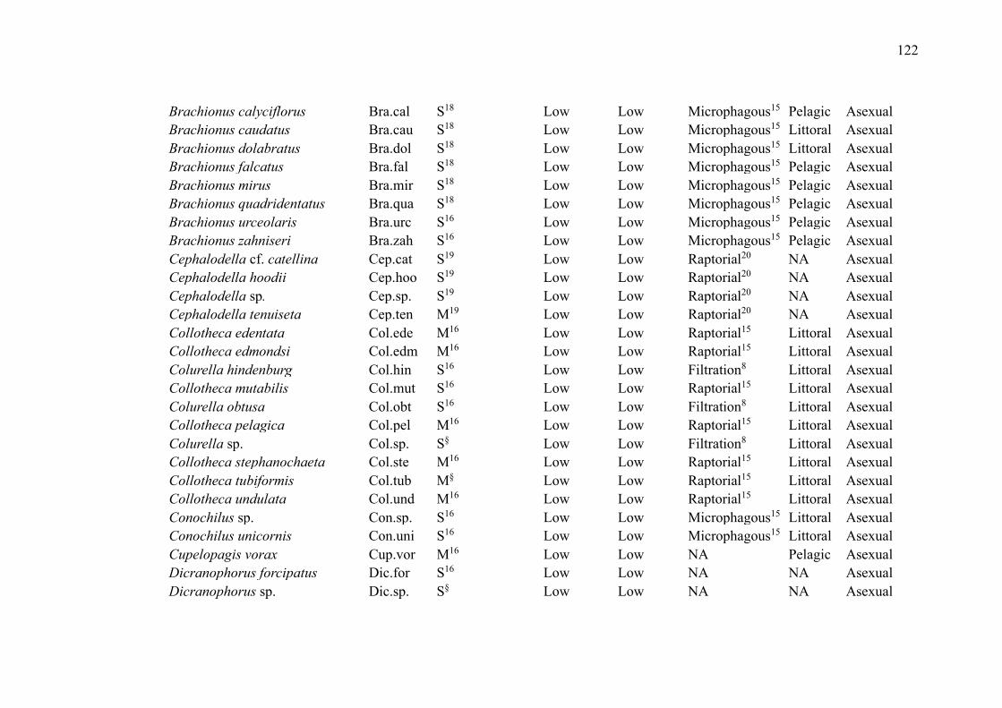
122
Brachionus calyciflorus Bra.cal S18 Low Low Microphagous15 Pelagic Asexual
Brachionus caudatus Bra.cau S18 Low Low Microphagous15 Littoral Asexual
Brachionus dolabratus Bra.dol S18 Low Low Microphagous15 Littoral Asexual
Brachionus falcatus Bra.fal S18 Low Low Microphagous15 Pelagic Asexual
Brachionus mirus Bra.mir S18 Low Low Microphagous15 Pelagic Asexual
Brachionus quadridentatus Bra.qua S18 Low Low Microphagous15 Pelagic Asexual
Brachionus urceolaris Bra.urc S16 Low Low Microphagous15 Pelagic Asexual
Brachionus zahniseri Bra.zah S16 Low Low Microphagous15 Pelagic Asexual
Cephalodella cf. catellina Cep.cat S19 Low Low Raptorial20 NA Asexual
Cephalodella hoodii Cep.hoo S19 Low Low Raptorial20 NA Asexual
Cephalodella sp. Cep.sp. S19 Low Low Raptorial20 NA Asexual
Cephalodella tenuiseta Cep.ten M19 Low Low Raptorial20 NA Asexual
Collotheca edentata Col.ede M16 Low Low Raptorial15 Littoral Asexual
Collotheca edmondsi Col.edm M16 Low Low Raptorial15 Littoral Asexual
Colurella hindenburg Col.hin S16 Low Low Filtration8 Littoral Asexual
Collotheca mutabilis Col.mut S16 Low Low Raptorial15 Littoral Asexual
Colurella obtusa Col.obt S16 Low Low Filtration8 Littoral Asexual
Collotheca pelagica Col.pel M16 Low Low Raptorial15 Littoral Asexual
Colurella sp. Col.sp. S§ Low Low Filtration8 Littoral Asexual
Collotheca stephanochaeta Col.ste M16 Low Low Raptorial15 Littoral Asexual
Collotheca tubiformis Col.tub M§ Low Low Raptorial15 Littoral Asexual
Collotheca undulata Col.und M16 Low Low Raptorial15 Littoral Asexual
Conochilus sp. Con.sp. S16 Low Low Microphagous15 Littoral Asexual
Conochilus unicornis Con.uni S16 Low Low Microphagous15 Littoral Asexual
Cupelopagis vorax Cup.vor M16 Low Low NA Pelagic Asexual
Dicranophorus forcipatus Dic.for S16 Low Low NA NA Asexual
Dicranophorus sp. Dic.sp. S§ Low Low NA NA Asexual

123
Drilophaga delagei Dri.del S16 Low Low NA NA Asexual
Elosa worrali Elo.wor S§ Low Low NA Littoral Asexual
Epiphanes clavatula Epi.cla S18 Low Low NA Littoral Asexual
Epiphanes macrorus Epi.mac S16 Low Low NA Littoral Asexual
Epiphanes pelagica Epi.pel S16 Low Low NA Littoral Asexual
Euchlanis callysta Euc.cal S16 Low Low Microphagous15
Lit
toral Asexual
Euchlanis incisa Euc.inc S18 Low Low Microphagous15 Littoral Asexual
Euchlanis meneta Euc.men S18 Low Low Microphagous15 Littoral Asexual
Euchlanis sp. Euc.sp. S§ Low Low Microphagous15 Littoral Asexual
Euchlanis triquetra Euc.tri M16 Low Low Microphagous15 Littoral Asexual
Filinia camasecla Fil.cam S16 Low Low Microphagous15 Pelagic Asexual
Filinia longiseta Fil.lon S16 Low Low Microphagous15 Pelagic Asexual
Filinia opoliensis Fil.opo S16 Low Low Microphagous15 Pelagic Asexual
Filinia terminalis Fil.ter S16 Low Low Microphagous15 Pelagic Asexual
Filinia unicornis Fil.uni S§ Low Low Microphagous15 Pelagic Asexual
Gastropus hyptopus Gas.hyp S16 Low Low Raptorial15 Pelagic Asexual
Gastropus stylifer Gas.sty S§ Low Low Raptorial15 Pelagic Asexual
Harringia eupoda Har.eup M16 Low Low NA NA Asexual
Heterolepadella cf.
Heterodactyla Het.het S21 Low Low NA NA Asexual
Hexarthra cf. fenica Hex.fen S16 Low Low Filtration8 Pelagic Asexual
Hexarthra intermedia Hex.int S16 Low Low Filtration8 Pelagic Asexual
Hexarthra cf. mira Hex.mir S16 Low Low Filtration8 Pelagic Asexual
Hexarthra sp. Hex.sp. S§ Low Low Filtration8 Pelagic Asexual
Horaela brehmi Hor.bre S22 Low Low NA NA Asexual
Kellicottia longispina Kel.lon M§ Low Low Filtration8 NA Asexual
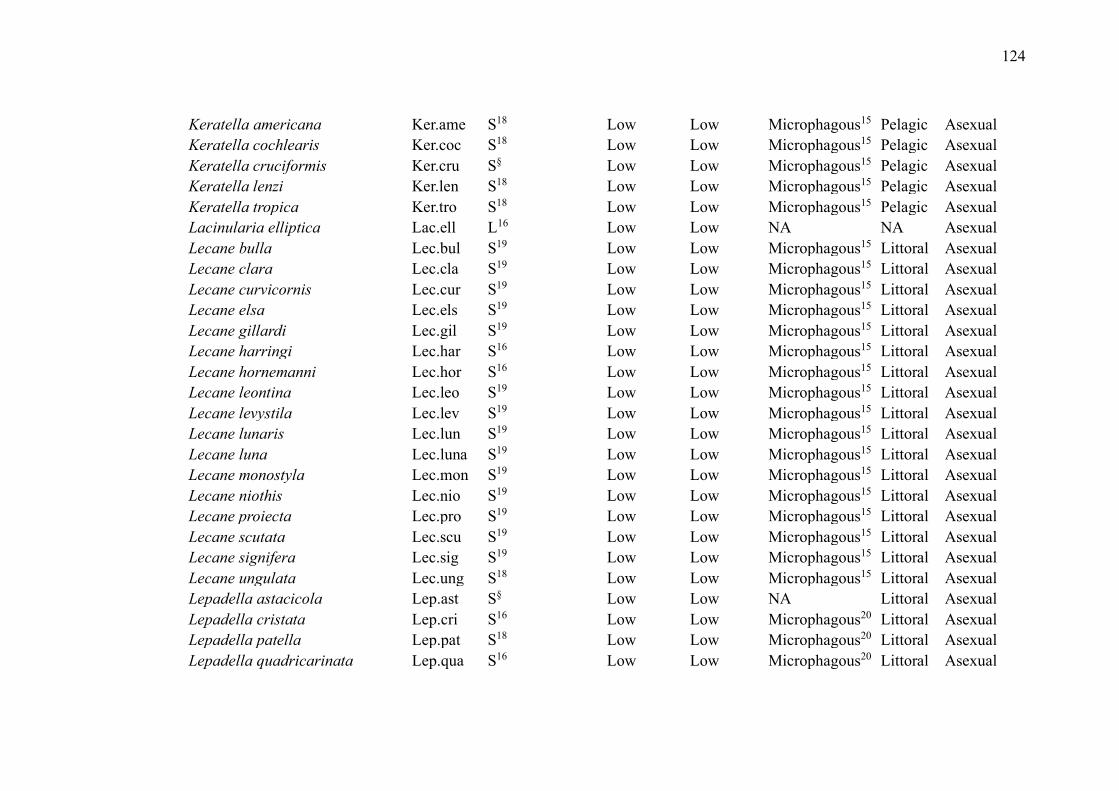
124
Keratella americana Ker.ame S18 Low Low Microphagous15 Pelagic Asexual
Keratella cochlearis Ker.coc S18 Low Low Microphagous15 Pelagic Asexual
Keratella cruciformis Ker.cru S§ Low Low Microphagous15 Pelagic Asexual
Keratella lenzi Ker.len S18 Low Low Microphagous15 Pelagic Asexual
Keratella tropica Ker.tro S18 Low Low Microphagous15 Pelagic Asexual
Lacinularia elliptica Lac.ell L16 Low Low NA NA Asexual
Lecane bulla Lec.bul S19 Low Low Microphagous15 Littoral Asexual
Lecane clara Lec.cla S19 Low Low Microphagous15 Littoral Asexual
Lecane curvicornis Lec.cur S19 Low Low Microphagous15 Littoral Asexual
Lecane elsa Lec.els S19 Low Low Microphagous15 Littoral Asexual
Lecane gillardi Lec.gil S19 Low Low Microphagous15 Littoral Asexual
Lecane harringi Lec.har S16 Low Low Microphagous15 Littoral Asexual
Lecane hornemanni Lec.hor S16 Low Low Microphagous15 Littoral Asexual
Lecane leontina Lec.leo S19 Low Low Microphagous15 Littoral Asexual
Lecane levystila Lec.lev S19 Low Low Microphagous15 Littoral Asexual
Lecane lunaris Lec.lun S19 Low Low Microphagous15 Littoral Asexual
Lecane luna Lec.luna S19 Low Low Microphagous15 Littoral Asexual
Lecane monostyla Lec.mon S19 Low Low Microphagous15 Littoral Asexual
Lecane niothis Lec.nio S19 Low Low Microphagous15 Littoral Asexual
Lecane proiecta Lec.pro S19 Low Low Microphagous15 Littoral Asexual
Lecane scutata Lec.scu S19 Low Low Microphagous15 Littoral Asexual
Lecane signifera Lec.sig S19 Low Low Microphagous15 Littoral Asexual
Lecane ungulata Lec.ung S18 Low Low Microphagous15 Littoral Asexual
Lepadella astacicola Lep.ast S§ Low Low NA Littoral Asexual
Lepadella cristata Lep.cri S16 Low Low Microphagous20 Littoral Asexual
Lepadella patella Lep.pat S18 Low Low Microphagous20 Littoral Asexual
Lepadella quadricarinata Lep.qua S16 Low Low Microphagous20 Littoral Asexual
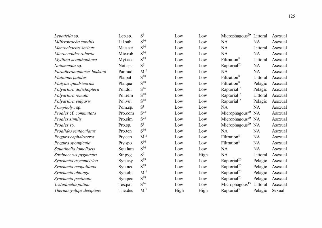
125
Lepadella sp. Lep.sp. S§ Low Low Microphagous20 Littoral Asexual
Liliferotrocha subtilis Lil.sub S16 Low Low NA NA Asexual
Macrochaetus sericus Mac.ser S16 Low Low NA Littoral Asexual
Microcodides robusta Mic.rob S16 Low Low NA NA Asexual
Mytilina acanthophora Myt.aca S18 Low Low Filtration8 Littoral Asexual
Notommata sp. Not.sp. S§ Low Low Raptorial20 NA Asexual
Paradicranophorus hudsoni Par.hud M16 Low Low NA NA Asexual
Plationus patulus Pla.pat S18 Low Low Filtration8 Littoral Asexual
Platyias quadricornis Pla.qua S18 Low Low Filtration8 Pelagic Asexual
Polyarthra dolichoptera Pol.dol S16 Low Low Raptorial15 Pelagic Asexual
Polyarthra remata Pol.rem S18 Low Low Raptorial15 Littoral Asexual
Polyarthra vulgaris Pol.vul S18 Low Low Raptorial15 Pelagic Asexual
Pompholyx sp. Pom.sp. S§ Low Low NA NA Asexual
Proales cf. commutata Pro.com S23 Low Low Microphagous20 NA Asexual
Proales similis Pro.sim S23 Low Low Microphagous20 NA Asexual
Proales sp. Pro.sp. S§ Low Low Microphagous20 NA Asexual
Proalides tentaculatus Pro.ten S16 Low Low NA NA Asexual
Ptygura cephaloceros Pty.cep M16 Low Low Filtration8 NA Asexual
Ptygura spongicula Pty.spo S16 Low Low Filtration8 NA Asexual
Squatinella lamellaris Squ.lam S16 Low Low NA NA Asexual
Streblocerus pygmaeus Str.pyg S§ Low High NA Littoral Asexual
Synchaeta asymmetrica Syn.asy S19 Low Low Raptorial20 Pelagic Asexual
Synchaeta neopolitana Syn.neo S19 Low Low Raptorial20 Pelagic Asexual
Synchaeta oblonga Syn.obl M18 Low Low Raptorial20 Pelagic Asexual
Synchaeta pectinata Syn.pec S18 Low Low Raptorial20 Pelagic Asexual
Testudinella patina Tes.pat S16 Low Low Microphagous15 Littoral Asexual
Thermocyclops decipiens The.dec M12 High High Raptorial3 Pelagic Sexual
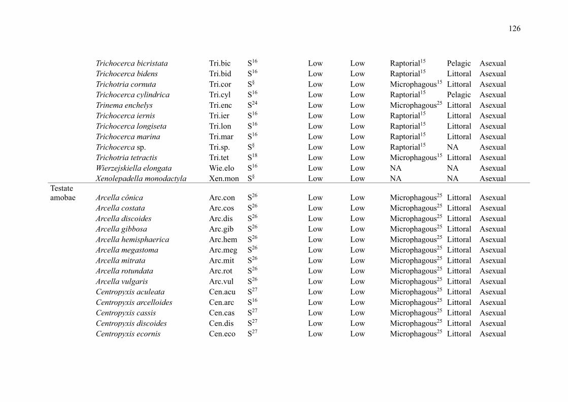
126
Trichocerca bicristata Tri.bic S16 Low Low Raptorial15 Pelagic Asexual
Trichocerca bidens Tri.bid S16 Low Low Raptorial15 Littoral Asexual
Trichotria cornuta Tri.cor S§ Low Low Microphagous15 Littoral Asexual
Trichocerca cylindrica Tri.cyl S16 Low Low Raptorial15 Pelagic Asexual
Trinema enchelys Tri.enc S24 Low Low Microphagous25 Littoral Asexual
Trichocerca iernis Tri.ier S16 Low Low Raptorial15 Littoral Asexual
Trichocerca longiseta Tri.lon S16 Low Low Raptorial15 Littoral Asexual
Trichocerca marina Tri.mar S16 Low Low Raptorial15 Littoral Asexual
Trichocerca sp. Tri.sp. S§ Low Low Raptorial15 NA Asexual
Trichotria tetractis Tri.tet S18 Low Low Microphagous15 Littoral Asexual
Wierzejskiella elongata Wie.elo S16 Low Low NA NA Asexual
Xenolepadella monodactyla Xen.mon S§ Low Low NA NA Asexual
Testate
amobae Arcella cônica Arc.con S26 Low Low Microphagous25 Littoral Asexual
Arcella costata Arc.cos S26 Low Low Microphagous25 Littoral Asexual
Arcella discoides Arc.dis S26 Low Low Microphagous25 Littoral Asexual
Arcella gibbosa Arc.gib S26 Low Low Microphagous25 Littoral Asexual
Arcella hemisphaerica Arc.hem S26 Low Low Microphagous25 Littoral Asexual
Arcella megastoma Arc.meg S26 Low Low Microphagous25 Littoral Asexual
Arcella mitrata Arc.mit S26 Low Low Microphagous25 Littoral Asexual
Arcella rotundata Arc.rot S26 Low Low Microphagous25 Littoral Asexual
Arcella vulgaris Arc.vul S26 Low Low Microphagous25 Littoral Asexual
Centropyxis aculeata Cen.acu S27 Low Low Microphagous25 Littoral Asexual
Centropyxis arcelloides Cen.arc S16 Low Low Microphagous25 Littoral Asexual
Centropyxis cassis Cen.cas S27 Low Low Microphagous25 Littoral Asexual
Centropyxis discoides Cen.dis S27 Low Low Microphagous25 Littoral Asexual
Centropyxis ecornis Cen.eco S27 Low Low Microphagous25 Littoral Asexual

127
Centropyxis gibba Cen.gib S27 Low Low Microphagous25 Littoral Asexual
Centropyxis spinosa Cen.spi S27 Low Low Microphagous25 Littoral Asexual
Cucurbitella dentata Cuc.den S28 Low Low Microphagous25 Littoral Asexual
Cucurbitella mespiliformis Cuc.mes S24 Low Low Microphagous25 Littoral Asexual
Cucurbitella sp. Cuc.sp. S§ Low Low Microphagous25 Littoral Asexual
Cucurbitella vlasinensis Cuc.vla S24 Low Low Microphagous25 Littoral Asexual
Difflugia capreolata Dif.cap S24 Low Low Microphagous25 Littoral Asexual
Difflugia corona Dif.cor S16 Low Low Microphagous25 Littoral Asexual
Difflugia cylindrus Dif.cyl S§ Low Low Microphagous25 Littoral Asexual
Difflugia difficilis Dif.dif S24 Low Low Microphagous25 Littoral Asexual
Difflugia elegans Dif.ele S24 Low Low Microphagous25 Littoral Asexual
Difflugia gramen Dif.gra S16 Low Low Microphagous25 Littoral Asexual
Difflugia kempnyi Dif.kem L29 Low Low Microphagous25 Littoral Asexual
Difflugia limnetica Dif.lim S24 Low Low Microphagous25 Littoral Asexual
Difflugia lobostoma Dif.lob S29 Low Low Microphagous25 Littoral Asexual
Difflugia muriformis Dif.mur S§ Low Low Microphagous25 Littoral Asexual
Difflugia oblonga Dif.obl S24 Low Low Microphagous25 Littoral Asexual
Difflugia pleustonica Dif.ple S§ Low Low Microphagous25 Littoral Asexual
Difflugia sp. Dif.sp. S§ Low Low Microphagous25 Littoral Asexual
Difflugia tuberculata Dif.tub S24 Low Low Microphagous25 Littoral Asexual
Difflugia urceolata Dif.urc S24 Low Low Microphagous25 Littoral Asexual
Difflugiela sp. Difa.sp. S§ Low Low Microphagous25 Littoral Asexual
Euglypha acanthophora Eug.aca S24 Low Low Microphagous25 Littoral Asexual
Euglypha filifera Eug.fil S§ Low Low Microphagous25 Littoral Asexual
Hyalosphenia elegans Hya.ele S16 Low Low Microphagous25 Littoral Asexual
Lesquereusia globulosa Les.glo S22 Low Low Microphagous25 Littoral Asexual
Lesquereusia sp. Les.sp. S22 Low Low Microphagous25 Littoral Asexual
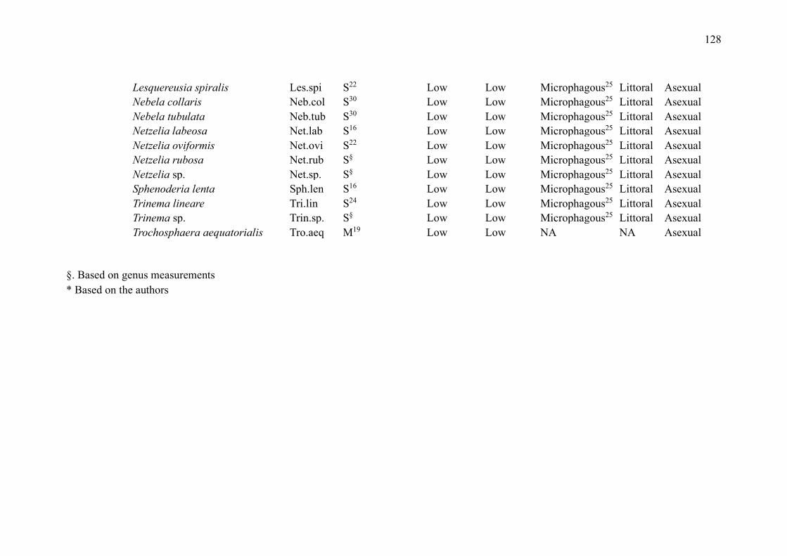
128
Lesquereusia spiralis Les.spi S22 Low Low Microphagous25 Littoral Asexual
Nebela collaris Neb.col S30 Low Low Microphagous25 Littoral Asexual
Nebela tubulata Neb.tub S30 Low Low Microphagous25 Littoral Asexual
Netzelia labeosa Net.lab S16 Low Low Microphagous25 Littoral Asexual
Netzelia oviformis Net.ovi S22 Low Low Microphagous25 Littoral Asexual
Netzelia rubosa Net.rub S§ Low Low Microphagous25 Littoral Asexual
Netzelia sp. Net.sp. S§ Low Low Microphagous25 Littoral Asexual
Sphenoderia lenta Sph.len S16 Low Low Microphagous25 Littoral Asexual
Trinema lineare Tri.lin S24 Low Low Microphagous25 Littoral Asexual
Trinema sp. Trin.sp. S§ Low Low Microphagous25 Littoral Asexual
Trochosphaera aequatorialis Tro.aeq M19 Low Low NA NA Asexual
§. Based on genus measurements
* Based on the authors
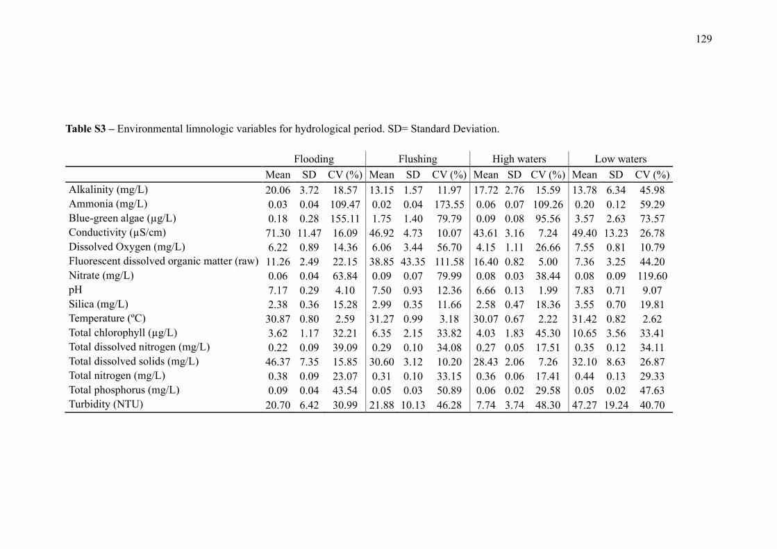
129
Table S3 – Environmental limnologic variables for hydrological period. SD= Standard Deviation.
Flooding Flushing High waters Low waters Mean SD CV (%) Mean SD CV (%) Mean SD CV (%) Mean SD CV (%)
Alkalinity (mg/L) 20.06 3.72 18.57 13.15 1.57 11.97 17.72 2.76 15.59 13.78 6.34 45.98
Ammonia (mg/L) 0.03 0.04 109.47 0.02 0.04 173.55 0.06 0.07 109.26 0.20 0.12 59.29
Blue-green algae (µg/L) 0.18 0.28 155.11 1.75 1.40 79.79 0.09 0.08 95.56 3.57 2.63 73.57
Conductivity (µS/cm) 71.30 11.47 16.09 46.92 4.73 10.07 43.61 3.16 7.24 49.40 13.23 26.78
Dissolved Oxygen (mg/L) 6.22 0.89 14.36 6.06 3.44 56.70 4.15 1.11 26.66 7.55 0.81 10.79
Fluorescent dissolved organic matter (raw) 11.26 2.49 22.15 38.85 43.35 111.58 16.40 0.82 5.00 7.36 3.25 44.20
Nitrate (mg/L) 0.06 0.04 63.84 0.09 0.07 79.99 0.08 0.03 38.44 0.08 0.09 119.60
pH 7.17 0.29 4.10 7.50 0.93 12.36 6.66 0.13 1.99 7.83 0.71 9.07
Silica (mg/L) 2.38 0.36 15.28 2.99 0.35 11.66 2.58 0.47 18.36 3.55 0.70 19.81
Temperature (ºC) 30.87 0.80 2.59 31.27 0.99 3.18 30.07 0.67 2.22 31.42 0.82 2.62
Total chlorophyll (µg/L) 3.62 1.17 32.21 6.35 2.15 33.82 4.03 1.83 45.30 10.65 3.56 33.41
Total dissolved nitrogen (mg/L) 0.22 0.09 39.09 0.29 0.10 34.08 0.27 0.05 17.51 0.35 0.12 34.11
Total dissolved solids (mg/L) 46.37 7.35 15.85 30.60 3.12 10.20 28.43 2.06 7.26 32.10 8.63 26.87
Total nitrogen (mg/L) 0.38 0.09 23.07 0.31 0.10 33.15 0.36 0.06 17.41 0.44 0.13 29.33
Total phosphorus (mg/L) 0.09 0.04 43.54 0.05 0.03 50.89 0.06 0.02 29.58 0.05 0.02 47.63
Turbidity (NTU) 20.70 6.42 30.99 21.88 10.13 46.28 7.74 3.74 48.30 47.27 19.24 40.70

130
References
1. Elmoor-loureiro LMA. Cladóceros do Brasil. https://cladocera.wordpress.com/. Published 2019. Accessed June 3, 2019.
2. Massicotte P, Frenette J-J, Proulx R, Pinel-Alloul B, Bertolo A. Riverscape heterogeneity explains spatial variation in zooplankton
functional evenness and biomass in a large river ecosystem. Landsc Ecol. 2014;29(1):67-79. doi:10.1007/s10980-013-9946-1
3. Barnett AJ, Finlay K, Beisner BE. Functional diversity of crustacean zooplankton communities: towards a trait-based classification.
Freshw Biol. 2007;52(5):796-813. doi:10.1111/j.1365-2427.2007.01733.x
4. Barnett AJ, Finlay K, Beisner BE. Functional diversity of crustacean zooplankton communities: Towards a trait-based classification.
Freshwater Biology, 52, 796-813. DOI: 10.1111/j.1365-2427.2007.01733.x. Freshw Biol. 2013;58(8):1755-1765. doi:10.1111/fwb.12177
5. Elmoor-Loureiro LMA. Manual de Identificação de Cladóceros Límnicos Do Brasil. Universa; 1997.
6. Elmoor-Loureiro L. Ciclomorfose em Bosmina (Crustacea, Cladocera) no Lago Paranoá, Brasília. Rev Bras Zool. 1989;6(1):37-44.
7. Barnett AJ, Finlay K, Beisner BE. Functional diversity of crustacean zooplankton communities: towards a trait-based classification.
Freshw Biol. 2007;52(5):796-813. doi:10.1111/j.1365-2427.2007.01733.x
8. Braghin L de SM, Almeida B de A, Amaral DC, Canella TF, Garcia Gimenez BC, Bonecker CC. Effects of dams decrease zooplankton
functional -diversity in river-associated lakes. Freshw Biol. 2018;63(7):721-730. doi:10.1111/fwb.13117
9. Azevedo F de, Dias JD, Braghin L de SM, Bonecker CC. Length-weight regressions of the microcrustacean species from a tropical
floodplain. Acta Limnol Bras. 2012;24(1):01-11. doi:10.1590/S2179-975X2012005000021
10. Gutierrez MF, Tavsanoglu UN, Vidal N, et al. Salinity shapes zooplankton communities and functional diversity and has complex effects
on size structure in lakes. Hydrobiologia. 2018;813(1):237-255. doi:10.1007/s10750-018-3529-8
11. Wright S. A Revision of the South American Species of Diaptomus. Trans Am Microsc Soc. 1927;46(2):73. doi:10.2307/3221654
12. Silva WM da. Diversidade dos Cyclopoida (Copepoda, Crustácea) de água doce do estado de São Paulo: taxonomia, ecologia e genética.
2003.
13. Silva EN dos S, Robertson BA, Reid JLW, Hardy ER. Atlas de copépodos planctônicos, Calanoida e Cyclopoida (Crustacea), da Amazônia
Brasileira: I. Represa de Curuá-Una, Pará. Rev Bras Zool. 1989;6(4):725-758. doi:10.1590/S0101-81751989000400019
14. Nogrady T, Segers H. Guides to the Identification of the Microinvertebrates of the Continental Waters of the World. Rotifera. (Dumont HJ,
ed.). Leiden: Backhuys Publishers; 2002.
15. Obertegger U, Smith HA, Flaim G, Wallace RL. Using the guild ratio to characterize pelagic rotifer communities. Hydrobiologia.
2011;662(1):157-162. doi:10.1007/s10750-010-0491-5
16. NIES. National Institute for Environmental Studies, Japan. https://www.nies.go.jp/. Published 2019. Accessed June 3, 2019.
17. Haney JF, Aliberti M, Allan E, et al. An image-based key to the zooplankton of North America. University of New Hampshire Center for

131
Freshwater Biology. http://cfb.unh.edu/cfbkey/html/index.html. Published 2013. Accessed June 3, 2019.
18. Joko CY. Taxonomia de rotíferos monogonontas da planície de inundação do alto rio Paraná (MS/PR). 2011.
http://repositorio.uem.br:8080/jspui/bitstream/1/5108/1/000191813.pdf.
19. Nogrady T, Pourriot R, Segers H. Rotifera 3. Notommatidae and Scaridiidae. Guid to Identif Microinvertebrates Cont Waters World 8(H
Dumont, T Nogrady, eds) SPB Acad Publ BV, 248 p. 1995.
20. Obertegger U, Flaim G. Community assembly of rotifers based on morphological traits. Hydrobiologia. 2015;753(1):31-45.
doi:10.1007/s10750-015-2191-7
21. May L, Wallace R, Herzig A. Rotifer Symposium IV: Proceedings of the Fourth Rotifer Symposium, Held in Edinburgh, Scotland, August
18–25, 1985. Vol 42. Springer Science & Business Media; 2012.
22. Gomes e Souza MB. Guia de Invertebrados Das Águas Doces. Vol 3. Portugal: Almargem; 2018.
23. De Smet WH. Rotifera vol. 4: The Proalidae (Monogononta). Guides to the Identification of the Microinvertebrates of the Continental
Waters of the World (ed. HJ Dumont).–SPB Academic Publishing bv, 102 pp. 1996.
24. Siemensma FJ. Microworld, world of amoeboid organisms. https://www.arcella.nl/. Published 2019. Accessed June 3, 2019.
25. Gilbert D, Amblard C, Bourdier G, André-Jean F, Mitchell EAD. Le régime alimentaire des Thécamoebiens (Protista, Sarcodina). L’Année
Biol. 2000;39(2):57-68. doi:10.1016/S0003-5017(00)80001-X
26. Deflandre G. Le genre Arcella Ehrenberg. Arch für Protistenkd. 1928;64(1):152-287.
27. Deflandre G. Le Genre Centropyxis Stein. G. Fischer; 1929.
28. JST. Digital specimen archives. http://protist.i.hosei.ac.jp/. Accessed June 3, 2019.
29. Мазей Ю, Цыганов А. Пресноводные Раковинные Амебы. Litres; 2018.
30. Ogden GG, Hedley RH. An Atlas of Freshwater Testate Amoebae. Oxford University Press; 1980.
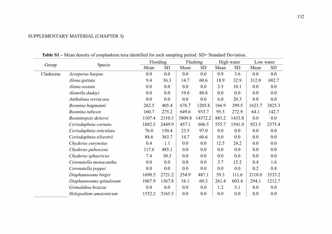
132
SUPPLEMENTARY MATERIAL (CHAPTER 3)
Table S1 – Mean density of zooplankton taxa identified for each sampling period. SD= Standard Deviation.
Group Specie Flooding Flushing High water Low water
Mean SD Mean SD Mean SD Mean SD
Cladocera Acroperus harpae 0.0 0.0 0.0 0.0 0.9 3.6 0.0 0.0
Alona guttata 9.4 36.3 14.7 60.6 18.9 32.9 312.0 682.7
Alona ossiani 0.0 0.0 0.0 0.0 2.5 10.1 0.0 0.0
Alonella dadayi 0.0 0.0 19.6 80.8 0.0 0.0 0.0 0.0
Anthalona verrucosa 0.0 0.0 0.0 0.0 6.0 20.3 0.0 0.0
Bosmina hagmanni 262.5 405.4 676.7 1205.8 166.9 299.5 1623.7 3825.3
Bosmina tubicen 160.7 275.2 649.6 933.7 95.5 272.9 64.1 142.7
Bosminopsis deitersi 1107.4 2110.3 5809.8 14372.2 883.2 1433.8 0.0 0.0
Ceriodaphnia cornuta 1882.5 2449.9 457.1 606.5 555.7 1541.0 923.5 2375.4
Ceriodaphnia reticulata 76.0 150.4 23.5 97.0 0.0 0.0 0.0 0.0
Ceriodaphnia silvestrii 88.6 363.7 14.7 60.6 0.0 0.0 0.0 0.0
Chydorus eurynotus 0.4 1.1 0.0 0.0 12.5 24.2 0.0 0.0
Chydorus pubescens 117.6 485.1 0.0 0.0 0.0 0.0 0.0 0.0
Chydorus sphaericus 7.4 30.3 0.0 0.0 0.0 0.0 0.0 0.0
Coronatella monacantha 0.0 0.0 0.0 0.0 3.7 15.2 0.4 1.6
Coronatella poppei 0.0 0.0 0.0 0.0 0.0 0.0 0.2 0.8
Diaphanosoma birgei 1690.5 2721.2 254.9 487.1 59.3 111.6 2118.0 3533.2
Diaphanosoma spinulosum 1067.9 1367.8 16.1 60.3 261.4 603.4 294.1 1212.7
Grimaldina brazzai 0.0 0.0 0.0 0.0 1.2 5.1 0.0 0.0
Holopedium amazonicum 1552.2 3165.5 0.0 0.0 0.0 0.0 0.0 0.0

133
Karualona muelleri 0.0 0.0 25.5 105.1 0.0 0.0 20.6 80.6
Leydigiopsis megalops 0.0 0.0 0.0 0.0 0.2 0.8 0.0 0.0
Macrothrix laticornis 0.2 0.8 25.5 105.1 7.8 32.3 40.4 161.4
Macrothrix mira 14.7 60.6 0.0 0.0 0.0 0.0 0.4 1.6
Moina micrura 274.9 519.7 1250.0 2318.0 163.5 565.3 344.1 707.8
Moina minuta 1580.6 4727.4 701.4 1128.3 92.1 238.6 3911.2 4176.3
Moina reticulata 0.0 0.0 23.5 97.0 0.0 0.0 0.0 0.0
Nicsmirnovius incredibilis 0.0 0.0 0.0 0.0 3.5 14.6 0.0 0.0
Picripleuroxus similis 3.9 15.1 0.0 0.0 0.0 0.0 0.0 0.0
Simocephalus sp. 0.0 0.0 0.0 0.0 0.0 0.0 24.5 101.1
Streblocerus pygmaeus 0.0 0.0 0.0 0.0 0.2 0.8 0.0 0.0
Copepoda Argyrodiaptomus azevedoi 44.1 132.1 0.0 0.0 0.0 0.0 0.0 0.0
Argyrodiaptomus robertsonae 832.2 3236.0 0.0 0.0 74.5 307.2 0.0 0.0
Cyclopidae copepodit 6352.8 6972.1 8217.6 6887.5 6274.4 13228.9 6064.7 4475.1
Cyclopidae nauplii 10291.8 9572.5 53820.6 40730.0 8928.7 14298.1 24213.7 15382.4
Diaptomidae copepodit 6575.5 11675.1 1245.1 1457.9 1194.3 2790.3 3725.5 2975.0
Diaptomidae nauplii 14521.1 29058.7 1904.0 1777.7 934.6 2617.8 3444.1 3265.9
Diaptomus deitersi 6.4 26.5 0.0 0.0 0.4 1.6 0.0 0.0
Mesocyclops meridianus 10.3 31.9 0.0 0.0 0.0 0.0 0.0 0.0
Metacyclops mendocinus 14.7 60.6 0.0 0.0 39.6 161.6 19.6 80.8
Microcyclops alius 116.2 388.0 26.9 110.9 826.2 3309.5 470.8 866.4
Microcyclops anceps 0.0 0.0 0.0 0.0 14.1 27.1 259.8 440.8
Microcyclops ceibaensis 0.0 0.0 138.2 457.2 93.1 384.0 0.0 0.0
Microcyclops finitimus 232.4 522.6 14.7 60.6 0.0 0.0 0.0 0.0
Microcyclops sp. 0.0 0.0 25.7 105.1 17.6 64.7 47.1 194.0
Notodiaptomus amazonicus 115.6 246.1 40.2 118.0 0.0 0.0 731.3 882.2
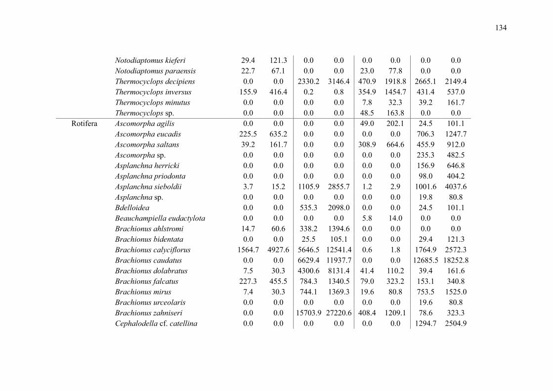
134
Notodiaptomus kieferi 29.4 121.3 0.0 0.0 0.0 0.0 0.0 0.0
Notodiaptomus paraensis 22.7 67.1 0.0 0.0 23.0 77.8 0.0 0.0
Thermocyclops decipiens 0.0 0.0 2330.2 3146.4 470.9 1918.8 2665.1 2149.4
Thermocyclops inversus 155.9 416.4 0.2 0.8 354.9 1454.7 431.4 537.0
Thermocyclops minutus 0.0 0.0 0.0 0.0 7.8 32.3 39.2 161.7
Thermocyclops sp. 0.0 0.0 0.0 0.0 48.5 163.8 0.0 0.0
Rotifera Ascomorpha agilis 0.0 0.0 0.0 0.0 49.0 202.1 24.5 101.1
Ascomorpha eucadis 225.5 635.2 0.0 0.0 0.0 0.0 706.3 1247.7
Ascomorpha saltans 39.2 161.7 0.0 0.0 308.9 664.6 455.9 912.0
Ascomorpha sp. 0.0 0.0 0.0 0.0 0.0 0.0 235.3 482.5
Asplanchna herricki 0.0 0.0 0.0 0.0 0.0 0.0 156.9 646.8
Asplanchna priodonta 0.0 0.0 0.0 0.0 0.0 0.0 98.0 404.2
Asplanchna sieboldii 3.7 15.2 1105.9 2855.7 1.2 2.9 1001.6 4037.6
Asplanchna sp. 0.0 0.0 0.0 0.0 0.0 0.0 19.8 80.8
Bdelloidea 0.0 0.0 535.3 2098.0 0.0 0.0 24.5 101.1
Beauchampiella eudactylota 0.0 0.0 0.0 0.0 5.8 14.0 0.0 0.0
Brachionus ahlstromi 14.7 60.6 338.2 1394.6 0.0 0.0 0.0 0.0
Brachionus bidentata 0.0 0.0 25.5 105.1 0.0 0.0 29.4 121.3
Brachionus calyciflorus 1564.7 4927.6 5646.5 12541.4 0.6 1.8 1764.9 2572.3
Brachionus caudatus 0.0 0.0 6629.4 11937.7 0.0 0.0 12685.5 18252.8
Brachionus dolabratus 7.5 30.3 4300.6 8131.4 41.4 110.2 39.4 161.6
Brachionus falcatus 227.3 455.5 784.3 1340.5 79.0 323.2 153.1 340.8
Brachionus mirus 7.4 30.3 744.1 1369.3 19.6 80.8 753.5 1525.0
Brachionus urceolaris 0.0 0.0 0.0 0.0 0.0 0.0 19.6 80.8
Brachionus zahniseri 0.0 0.0 15703.9 27220.6 408.4 1209.1 78.6 323.3
Cephalodella cf. catellina 0.0 0.0 0.0 0.0 0.0 0.0 1294.7 2504.9

135
Cephalodella hoodii 0.0 0.0 29.4 121.3 0.0 0.0 0.0 0.0
Cephalodella sp. 0.0 0.0 0.0 0.0 0.0 0.0 117.6 332.1
Cephalodella tenuiseta 4.9 20.2 0.0 0.0 0.0 0.0 0.0 0.0
Collotheca edentata 3.7 15.2 24.5 101.1 0.0 0.0 0.0 0.0
Collotheca edmondsi 0.0 0.0 0.0 0.0 3.9 16.2 0.0 0.0
Collotheca mutabilis 29.4 121.3 0.0 0.0 0.0 0.0 0.0 0.0
Collotheca stephanochaeta 22.1 91.0 0.0 0.0 0.0 0.0 0.0 0.0
Collotheca tubiformis 29.4 121.3 0.0 0.0 0.0 0.0 0.0 0.0
Collotheca undulata 0.0 0.0 0.0 0.0 19.6 80.8 0.0 0.0
Colurella hindenburg 0.0 0.0 19.6 80.8 0.0 0.0 0.0 0.0
Colurella obtusa 0.0 0.0 994.5 3014.7 0.0 0.0 0.0 0.0
Colurella sp. 0.0 0.0 19.6 80.8 0.0 0.0 0.0 0.0
Conochilus sp. 0.0 0.0 0.0 0.0 0.0 0.0 19.6 80.8
Conochilus unicornis 3251.6 7934.5 1.9 5.5 1039.2 3655.1 0.0 0.0
Dicranophorus forcipatus 0.0 0.0 0.0 0.0 13.2 33.4 0.0 0.0
Dicranophorus sp. 0.0 0.0 14.7 60.6 0.0 0.0 0.0 0.0
Drilophaga delagei 253.7 769.4 0.0 0.0 0.0 0.0 0.0 0.0
Elosa worrali 0.0 0.0 0.0 0.0 152.3 466.2 0.0 0.0
Epiphanes clavatula 411.8 1697.7 984.3 2779.0 0.0 0.0 0.0 0.0
Epiphanes macrourus 400.5 1029.6 0.0 0.0 0.0 0.0 3681.8 11172.4
Epiphanes pelagica 2.5 10.1 0.0 0.0 0.0 0.0 0.0 0.0
Euchlanis meneta 0.0 0.0 0.0 0.0 2.5 10.1 0.0 0.0
Euchlanis sp. 0.0 0.0 0.0 0.0 0.0 0.0 78.4 323.4
Euchlanis triquetra 0.0 0.0 0.0 0.0 123.5 267.7 156.9 501.6
Filinia camasecla 0.0 0.0 278.8 441.1 2.0 4.4 0.0 0.0
Filinia longiseta 101.9 261.2 4502.0 4730.1 33.0 85.7 7698.4 10641.8
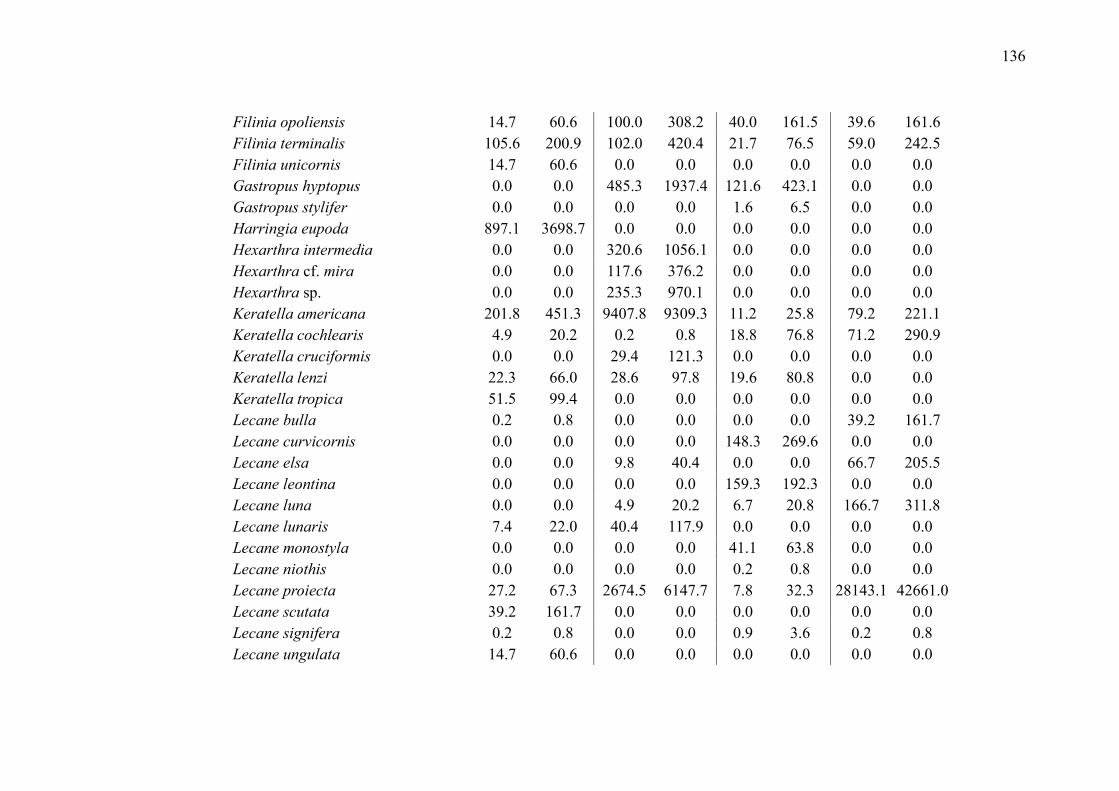
136
Filinia opoliensis 14.7 60.6 100.0 308.2 40.0 161.5 39.6 161.6
Filinia terminalis 105.6 200.9 102.0 420.4 21.7 76.5 59.0 242.5
Filinia unicornis 14.7 60.6 0.0 0.0 0.0 0.0 0.0 0.0
Gastropus hyptopus 0.0 0.0 485.3 1937.4 121.6 423.1 0.0 0.0
Gastropus stylifer 0.0 0.0 0.0 0.0 1.6 6.5 0.0 0.0
Harringia eupoda 897.1 3698.7 0.0 0.0 0.0 0.0 0.0 0.0
Hexarthra intermedia 0.0 0.0 320.6 1056.1 0.0 0.0 0.0 0.0
Hexarthra cf. mira 0.0 0.0 117.6 376.2 0.0 0.0 0.0 0.0
Hexarthra sp. 0.0 0.0 235.3 970.1 0.0 0.0 0.0 0.0
Keratella americana 201.8 451.3 9407.8 9309.3 11.2 25.8 79.2 221.1
Keratella cochlearis 4.9 20.2 0.2 0.8 18.8 76.8 71.2 290.9
Keratella cruciformis 0.0 0.0 29.4 121.3 0.0 0.0 0.0 0.0
Keratella lenzi 22.3 66.0 28.6 97.8 19.6 80.8 0.0 0.0
Keratella tropica 51.5 99.4 0.0 0.0 0.0 0.0 0.0 0.0
Lecane bulla 0.2 0.8 0.0 0.0 0.0 0.0 39.2 161.7
Lecane curvicornis 0.0 0.0 0.0 0.0 148.3 269.6 0.0 0.0
Lecane elsa 0.0 0.0 9.8 40.4 0.0 0.0 66.7 205.5
Lecane leontina 0.0 0.0 0.0 0.0 159.3 192.3 0.0 0.0
Lecane luna 0.0 0.0 4.9 20.2 6.7 20.8 166.7 311.8
Lecane lunaris 7.4 22.0 40.4 117.9 0.0 0.0 0.0 0.0
Lecane monostyla 0.0 0.0 0.0 0.0 41.1 63.8 0.0 0.0
Lecane niothis 0.0 0.0 0.0 0.0 0.2 0.8 0.0 0.0
Lecane proiecta 27.2 67.3 2674.5 6147.7 7.8 32.3 28143.1 42661.0
Lecane scutata 39.2 161.7 0.0 0.0 0.0 0.0 0.0 0.0
Lecane signifera 0.2 0.8 0.0 0.0 0.9 3.6 0.2 0.8
Lecane ungulata 14.7 60.6 0.0 0.0 0.0 0.0 0.0 0.0

137
Lepadella astacicola 14.7 60.6 0.0 0.0 0.0 0.0 0.0 0.0
Lepadella patella 37.3 105.3 4173.5 6930.0 72.5 104.6 20.0 80.8
Lepadella quadricarinata 0.0 0.0 0.0 0.0 1.3 3.9 0.0 0.0
Lepadella sp. 0.0 0.0 0.0 0.0 0.6 2.4 0.0 0.0
Liliferotrocha subtilis 7.4 30.3 47.1 194.0 117.6 485.1 0.0 0.0
Macrochaetus sericus 0.0 0.0 0.0 0.0 0.2 0.8 24.5 101.1
Notommata sp. 0.0 0.0 0.0 0.0 0.0 0.0 24.5 101.1
Paradicranophorus hudsoni 0.0 0.0 0.0 0.0 0.2 0.8 0.0 0.0
Plationus patulus var. macracanthus 127.8 226.8 29.4 121.3 32.3 84.0 0.0 0.0
Platyias quadricornis 0.0 0.0 0.2 0.8 205.4 345.3 0.0 0.0
Polyarthra dolichoptera 0.0 0.0 0.0 0.0 2.5 10.1 0.0 0.0
Polyarthra vulgaris 14.9 60.6 1616.5 3984.4 131.2 261.0 0.0 0.0
Pompholyx sp. 0.0 0.0 0.0 0.0 0.0 0.0 313.7 1293.5
Proales cf. commutata 0.0 0.0 0.0 0.0 9.8 40.4 0.0 0.0
Proales sp. 0.0 0.0 0.0 0.0 7.0 28.8 24.5 101.1
Proalides tentaculatus 117.6 422.7 0.0 0.0 0.0 0.0 0.0 0.0
Ptygura spongicula 14.7 60.6 0.0 0.0 0.0 0.0 0.0 0.0
Squatinella lamellaris 0.0 0.0 29.4 121.3 0.0 0.0 0.0 0.0
Synchaeta asymmetrica 0.0 0.0 0.0 0.0 24.5 101.1 0.0 0.0
Synchaeta neopolitana 0.0 0.0 0.0 0.0 122.7 484.2 0.0 0.0
Synchaeta oblonga 0.0 0.0 0.0 0.0 619.6 2420.7 0.0 0.0
Synchaeta pectinata 0.0 0.0 0.0 0.0 4.4 18.2 0.0 0.0
Testudinella patina 85.8 169.6 34.5 121.6 100.8 131.0 0.0 0.0
Trichocerca bicristata 5.1 20.2 0.0 0.0 88.7 176.3 0.0 0.0
Trichocerca bidens 0.0 0.0 14.7 60.6 18.6 76.8 436.7 944.2
Trichocerca cylindrica 0.0 0.0 159.8 275.3 39.4 161.6 0.0 0.0
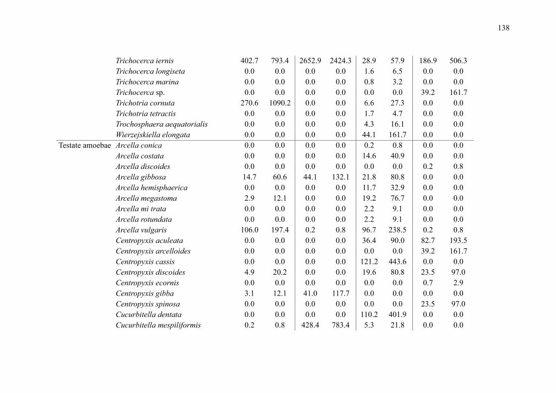
138
Trichocerca iernis 402.7 793.4 2652.9 2424.3 28.9 57.9 186.9 506.3
Trichocerca longiseta 0.0 0.0 0.0 0.0 1.6 6.5 0.0 0.0
Trichocerca marina 0.0 0.0 0.0 0.0 0.8 3.2 0.0 0.0
Trichocerca sp. 0.0 0.0 0.0 0.0 0.0 0.0 39.2 161.7
Trichotria cornuta 270.6 1090.2 0.0 0.0 6.6 27.3 0.0 0.0
Trichotria tetractis 0.0 0.0 0.0 0.0 1.7 4.7 0.0 0.0
Trochosphaera aequatorialis 0.0 0.0 0.0 0.0 4.3 16.1 0.0 0.0
Wierzejskiella elongata 0.0 0.0 0.0 0.0 44.1 161.7 0.0 0.0
Testate amoebae Arcella conica 0.0 0.0 0.0 0.0 0.2 0.8 0.0 0.0
Arcella costata 0.0 0.0 0.0 0.0 14.6 40.9 0.0 0.0
Arcella discoides 0.0 0.0 0.0 0.0 0.0 0.0 0.2 0.8
Arcella gibbosa 14.7 60.6 44.1 132.1 21.8 80.8 0.0 0.0
Arcella hemisphaerica 0.0 0.0 0.0 0.0 11.7 32.9 0.0 0.0
Arcella megastoma 2.9 12.1 0.0 0.0 19.2 76.7 0.0 0.0
Arcella mi trata 0.0 0.0 0.0 0.0 2.2 9.1 0.0 0.0
Arcella rotundata 0.0 0.0 0.0 0.0 2.2 9.1 0.0 0.0
Arcella vulgaris 106.0 197.4 0.2 0.8 96.7 238.5 0.2 0.8
Centropyxis aculeata 0.0 0.0 0.0 0.0 36.4 90.0 82.7 193.5
Centropyxis arcelloides 0.0 0.0 0.0 0.0 0.0 0.0 39.2 161.7
Centropyxis cassis 0.0 0.0 0.0 0.0 121.2 443.6 0.0 0.0
Centropyxis discoides 4.9 20.2 0.0 0.0 19.6 80.8 23.5 97.0
Centropyxis ecornis 0.0 0.0 0.0 0.0 0.0 0.0 0.7 2.9
Centropyxis gibba 3.1 12.1 41.0 117.7 0.0 0.0 0.0 0.0
Centropyxis spinosa 0.0 0.0 0.0 0.0 0.0 0.0 23.5 97.0
Cucurbitella dentata 0.0 0.0 0.0 0.0 110.2 401.9 0.0 0.0
Cucurbitella mespiliformis 0.2 0.8 428.4 783.4 5.3 21.8 0.0 0.0
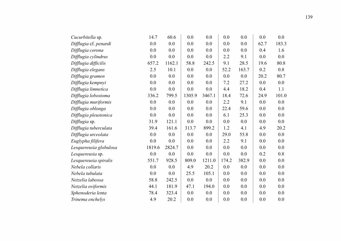
139
Cucurbitella sp. 14.7 60.6 0.0 0.0 0.0 0.0 0.0 0.0
Difflugia cf. penardi 0.0 0.0 0.0 0.0 0.0 0.0 62.7 183.3
Difflugia corona 0.0 0.0 0.0 0.0 0.0 0.0 0.4 1.6
Difflugia cylindrus 0.0 0.0 0.0 0.0 2.2 9.1 0.0 0.0
Difflugia difficilis 657.2 1162.1 58.8 242.5 9.1 28.5 19.6 80.8
Difflugia elegans 2.5 10.1 0.0 0.0 52.2 163.7 0.2 0.8
Difflugia gramen 0.0 0.0 0.0 0.0 0.0 0.0 20.2 80.7
Difflugia kempnyi 0.0 0.0 0.0 0.0 7.2 27.2 0.0 0.0
Difflugia limnetica 0.0 0.0 0.0 0.0 4.4 18.2 0.4 1.1
Difflugia lobostoma 336.2 799.5 1305.9 3467.1 18.4 72.6 24.9 101.0
Difflugia muriformis 0.0 0.0 0.0 0.0 2.2 9.1 0.0 0.0
Difflugia oblonga 0.0 0.0 0.0 0.0 22.4 59.6 0.0 0.0
Difflugia pleustonica 0.0 0.0 0.0 0.0 6.1 25.3 0.0 0.0
Difflugia sp. 31.9 121.1 0.0 0.0 0.0 0.0 0.0 0.0
Difflugia tuberculata 39.4 161.6 313.7 899.2 1.2 4.1 4.9 20.2
Difflugia urceolata 0.0 0.0 0.0 0.0 29.0 55.8 0.0 0.0
Euglypha filifera 0.0 0.0 0.0 0.0 2.2 9.1 0.0 0.0
Lesquereusia globulosa 1819.6 2824.7 0.0 0.0 0.0 0.0 0.0 0.0
Lesquereusia sp. 0.0 0.0 0.0 0.0 0.0 0.0 0.2 0.8
Lesquereusia spiralis 551.7 928.5 809.0 1211.0 174.2 382.9 0.0 0.0
Nebela collaris 0.0 0.0 4.9 20.2 0.0 0.0 0.0 0.0
Nebela tubulata 0.0 0.0 25.5 105.1 0.0 0.0 0.0 0.0
Netzelia labeosa 58.8 242.5 0.0 0.0 0.0 0.0 0.0 0.0
Netzelia oviformis 44.1 181.9 47.1 194.0 0.0 0.0 0.0 0.0
Sphenoderia lenta 78.4 323.4 0.0 0.0 0.0 0.0 0.0 0.0
Trinema enchelys 4.9 20.2 0.0 0.0 0.0 0.0 0.0 0.0
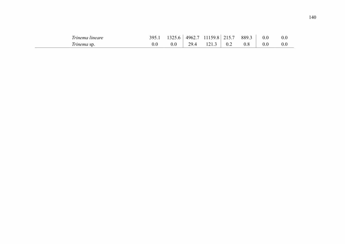
140
Trinema lineare 395.1 1325.6 4962.7 11159.8 215.7 889.3 0.0 0.0
Trinema sp. 0.0 0.0 29.4 121.3 0.2 0.8 0.0 0.0
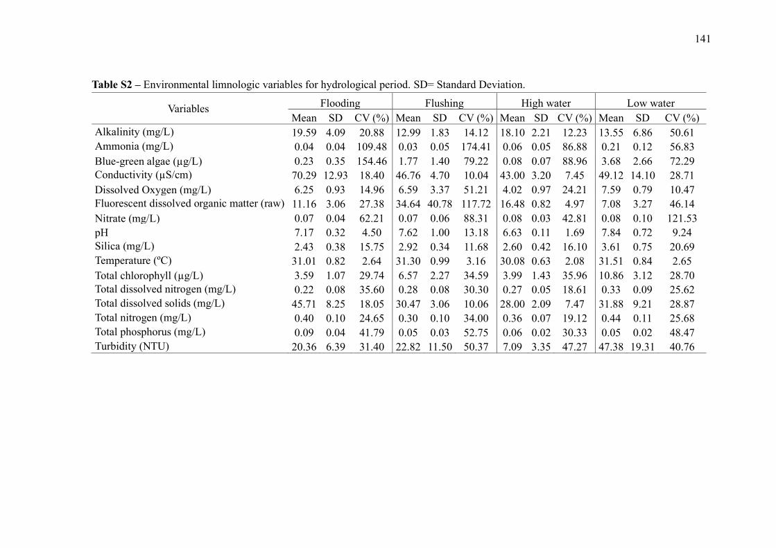
141
Table S2 – Environmental limnologic variables for hydrological period. SD= Standard Deviation.
Variables Flooding Flushing High water Low water
Mean SD CV (%) Mean SD CV (%) Mean SD CV (%) Mean SD CV (%)
Alkalinity (mg/L) 19.59 4.09 20.88 12.99 1.83 14.12 18.10 2.21 12.23 13.55 6.86 50.61
Ammonia (mg/L) 0.04 0.04 109.48 0.03 0.05 174.41 0.06 0.05 86.88 0.21 0.12 56.83
Blue-green algae (µg/L) 0.23 0.35 154.46 1.77 1.40 79.22 0.08 0.07 88.96 3.68 2.66 72.29
Conductivity (µS/cm) 70.29 12.93 18.40 46.76 4.70 10.04 43.00 3.20 7.45 49.12 14.10 28.71
Dissolved Oxygen (mg/L) 6.25 0.93 14.96 6.59 3.37 51.21 4.02 0.97 24.21 7.59 0.79 10.47
Fluorescent dissolved organic matter (raw) 11.16 3.06 27.38 34.64 40.78 117.72 16.48 0.82 4.97 7.08 3.27 46.14
Nitrate (mg/L) 0.07 0.04 62.21 0.07 0.06 88.31 0.08 0.03 42.81 0.08 0.10 121.53
pH 7.17 0.32 4.50 7.62 1.00 13.18 6.63 0.11 1.69 7.84 0.72 9.24
Silica (mg/L) 2.43 0.38 15.75 2.92 0.34 11.68 2.60 0.42 16.10 3.61 0.75 20.69
Temperature (ºC) 31.01 0.82 2.64 31.30 0.99 3.16 30.08 0.63 2.08 31.51 0.84 2.65
Total chlorophyll (µg/L) 3.59 1.07 29.74 6.57 2.27 34.59 3.99 1.43 35.96 10.86 3.12 28.70
Total dissolved nitrogen (mg/L) 0.22 0.08 35.60 0.28 0.08 30.30 0.27 0.05 18.61 0.33 0.09 25.62
Total dissolved solids (mg/L) 45.71 8.25 18.05 30.47 3.06 10.06 28.00 2.09 7.47 31.88 9.21 28.87
Total nitrogen (mg/L) 0.40 0.10 24.65 0.30 0.10 34.00 0.36 0.07 19.12 0.44 0.11 25.68
Total phosphorus (mg/L) 0.09 0.04 41.79 0.05 0.03 52.75 0.06 0.02 30.33 0.05 0.02 48.47
Turbidity (NTU) 20.36 6.39 31.40 22.82 11.50 50.37 7.09 3.35 47.27 47.38 19.31 40.76
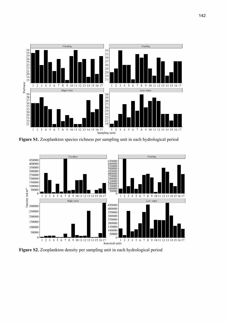
142
Figure S1. Zooplankton species richness per sampling unit in each hydrological period
Figure S2. Zooplankton density per sampling unit in each hydrological period