Fundamental and derived modes of climate variability

Tellus (2004), 56A, 229–249 Copyright C© Blackwell Munksgaard, 2004

Printed in UK. All rights reserved T E L L U S

Fundamental and derived modes of climate variability:concept and application to interannual time-scales

By MIHAI DIMA 1,2∗ and GERRIT LOHMANN 1, 1Bremen University, Department of Geosciences andResearch Center Ocean Margins, PO Box 330 440, D-28334 Bremen, Germany; 2University of Bucharest, Faculty of

Physics, Department of Atmospheric Physics, PO Box MG-11, Bucharest, Romania

(Manuscript received 3 April 2003; in final form 19 December 2003)

ABSTRACTThe notion of mode interaction is proposed as a deterministic concept for understanding climatic modes at various time-scales. This concept is based on the distinction between fundamental modes relying on their own physical mechanismsand derived modes that emerge from the interaction of two other modes. The notion is introduced and applied tointerannual climate variability. Observational evidence is presented for the tropospheric biennial variability to be theresult of the interaction between the annual cycle and a quasi-decadal mode originating in the Atlantic basin. Withinthe same framework, Pacific interannual variability at time-scales of about 4 and 6 yr is interpreted as the result ofinteractions between the biennial and quasi-decadal modes of climate variability. We show that the negative feedbackof the interannual modes is linked to the annual cycle and the quasi-decadal mode, both originating outside the Pacificbasin, whereas the strong amplitudes of interannual modes result from resonance and local positive feedback. It isargued that such a distinction between fundamental and derived modes of variability is important for understanding theunderlying physics of climatic modes, with strong implications for climate predictability.

1. Introduction

Spectra of climatic time series are characterized by three impor-tant features: continuity, redness (slope towards longer time-scales in the power spectra) and presence of multiple peaks(Mitchell, 1976). The redness can be attributed to stochasticmechanisms in which random high-frequency fluctuations, e.g.weather systems, are being integrated by the much slower re-sponding components of the climate system, e.g. the ocean(Hasselmann, 1976). Therefore, the low-frequency fluctuationsdevelop and grow in amplitude with increasing time-scale. Inthis stochastic climate model concept (Hasselmann, 1976), thevariance is limited by the negative feedback mechanisms withinthe climate system.

The clear distinction of peaks in the climate spectra suggeststhat deterministic processes may be responsible for their gener-ation. For example, there is climate variability at preferred time-scales due to internal oscillations such as the El Nino SouthernOscillation (ENSO) phenomenon (Philander, 1990) or the At-lantic quasi-decadal (QD) mode (Deser and Blackmon, 1993;Dima et al. 2001), or due to external forcing such as the annualcycle or the astronomical Milankovitch cycles.

∗Corresponding author.e-mail: [email protected]

The stochastic climate model is based on its analogy with theBrownian motion, being characterized by slow and fast evolvingsystems within the same model (Einstein, 1905). However, cli-matic oscillations may be the result of deterministic processesassociated with two active climate components, e.g. atmosphere–ocean interactions (Bjerknes, 1964; Latif and Barnett, 1994;Latif, 1998; Timmermann et al. 1998). Because of their decorre-lation time-scale, such oscillatory modes can yield much longerpredictability than is expected to emerge from the stochastic cli-mate model.

Modes of climate variability have been identified through sta-tistical analysis of observations and model data. For example,recent observational studies have shown that a large part of thePacific climate variance can be attributed to ENSO or ENSO-likemodes (Mantua et al. 1997) while a distinct part of the surfaceclimate variability in the North Atlantic can be attributed to a QDmode characterized by a ‘tripole pattern’ of sea surface temper-ature (SST; Deser and Blackmon, 1993; Mann and Park, 1994;Zhang et al. 1997).

Two general characteristics of the climate variability emergefrom the analysis of historical data. First, modes of interan-nual and interdecadal variability are identified and describedin both the Pacific and Atlantic basins. Secondly, we can notethat the patterns associated with different modes of variabilityshare common features; for example, the Pacific modes with their

Tellus 56A (2004), 3 229

230 M. DIMA AND G. LOHMANN

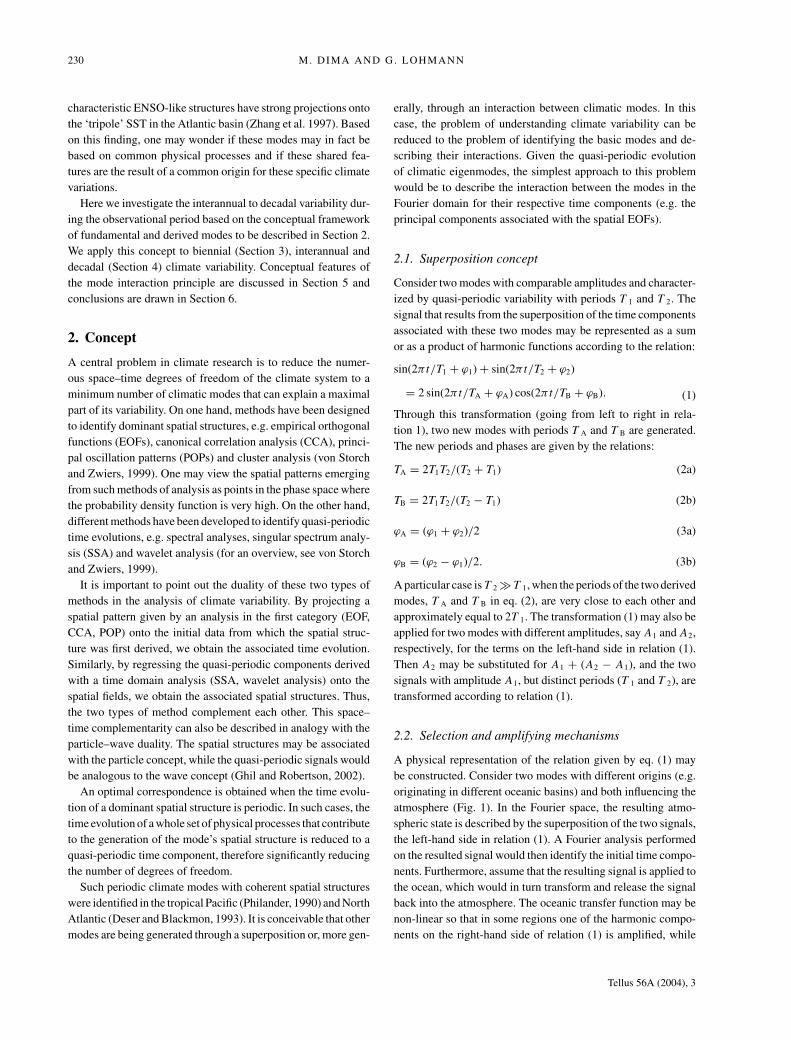
characteristic ENSO-like structures have strong projections ontothe ‘tripole’ SST in the Atlantic basin (Zhang et al. 1997). Basedon this finding, one may wonder if these modes may in fact bebased on common physical processes and if these shared fea-tures are the result of a common origin for these specific climatevariations.

Here we investigate the interannual to decadal variability dur-ing the observational period based on the conceptual frameworkof fundamental and derived modes to be described in Section 2.We apply this concept to biennial (Section 3), interannual anddecadal (Section 4) climate variability. Conceptual features ofthe mode interaction principle are discussed in Section 5 andconclusions are drawn in Section 6.

2. Concept

A central problem in climate research is to reduce the numer-ous space–time degrees of freedom of the climate system to aminimum number of climatic modes that can explain a maximalpart of its variability. On one hand, methods have been designedto identify dominant spatial structures, e.g. empirical orthogonalfunctions (EOFs), canonical correlation analysis (CCA), princi-pal oscillation patterns (POPs) and cluster analysis (von Storchand Zwiers, 1999). One may view the spatial patterns emergingfrom such methods of analysis as points in the phase space wherethe probability density function is very high. On the other hand,different methods have been developed to identify quasi-periodictime evolutions, e.g. spectral analyses, singular spectrum analy-sis (SSA) and wavelet analysis (for an overview, see von Storchand Zwiers, 1999).

It is important to point out the duality of these two types ofmethods in the analysis of climate variability. By projecting aspatial pattern given by an analysis in the first category (EOF,CCA, POP) onto the initial data from which the spatial struc-ture was first derived, we obtain the associated time evolution.Similarly, by regressing the quasi-periodic components derivedwith a time domain analysis (SSA, wavelet analysis) onto thespatial fields, we obtain the associated spatial structures. Thus,the two types of method complement each other. This space–time complementarity can also be described in analogy with theparticle–wave duality. The spatial structures may be associatedwith the particle concept, while the quasi-periodic signals wouldbe analogous to the wave concept (Ghil and Robertson, 2002).

An optimal correspondence is obtained when the time evolu-tion of a dominant spatial structure is periodic. In such cases, thetime evolution of a whole set of physical processes that contributeto the generation of the mode’s spatial structure is reduced to aquasi-periodic time component, therefore significantly reducingthe number of degrees of freedom.

Such periodic climate modes with coherent spatial structureswere identified in the tropical Pacific (Philander, 1990) and NorthAtlantic (Deser and Blackmon, 1993). It is conceivable that othermodes are being generated through a superposition or, more gen-

erally, through an interaction between climatic modes. In thiscase, the problem of understanding climate variability can bereduced to the problem of identifying the basic modes and de-scribing their interactions. Given the quasi-periodic evolutionof climatic eigenmodes, the simplest approach to this problemwould be to describe the interaction between the modes in theFourier domain for their respective time components (e.g. theprincipal components associated with the spatial EOFs).

2.1. Superposition concept

Consider two modes with comparable amplitudes and character-ized by quasi-periodic variability with periods T 1 and T 2. Thesignal that results from the superposition of the time componentsassociated with these two modes may be represented as a sumor as a product of harmonic functions according to the relation:

sin(2π t/T1 + ϕ1) + sin(2π t/T2 + ϕ2)

= 2 sin(2π t/TA + ϕA) cos(2π t/TB + ϕB). (1)

Through this transformation (going from left to right in rela-tion 1), two new modes with periods T A and T B are generated.The new periods and phases are given by the relations:

TA = 2T1T2/(T2 + T1) (2a)

TB = 2T1T2/(T2 − T1) (2b)

ϕA = (ϕ1 + ϕ2)/2 (3a)

ϕB = (ϕ2 − ϕ1)/2. (3b)

A particular case is T 2 � T 1, when the periods of the two derivedmodes, T A and T B in eq. (2), are very close to each other andapproximately equal to 2T 1. The transformation (1) may also beapplied for two modes with different amplitudes, say A1 and A2,respectively, for the terms on the left-hand side in relation (1).Then A2 may be substituted for A1 + (A2 − A1), and the twosignals with amplitude A1, but distinct periods (T 1 and T 2), aretransformed according to relation (1).

2.2. Selection and amplifying mechanisms

A physical representation of the relation given by eq. (1) maybe constructed. Consider two modes with different origins (e.g.originating in different oceanic basins) and both influencing theatmosphere (Fig. 1). In the Fourier space, the resulting atmo-spheric state is described by the superposition of the two signals,the left-hand side in relation (1). A Fourier analysis performedon the resulted signal would then identify the initial time compo-nents. Furthermore, assume that the resulting signal is applied tothe ocean, which would in turn transform and release the signalback into the atmosphere. The oceanic transfer function may benon-linear so that in some regions one of the harmonic compo-nents on the right-hand side of relation (1) is amplified, while

Tellus 56A (2004), 3

FUNDAMENTAL MODES OF CLIMATE VARIABILITY 231

Fig 1. Schematic representation of the superposition of two climatemodes.

Fig 2. Schematic representation of the mode interaction concept.

in other regions the other harmonic component in the productbecomes amplified. Such non-linearity may be given by the dif-ferent spatial propagation of oceanic waves with various periodsor by the waveguides. Therefore, we can define a selection mech-anism through the physical processes with different character-istic time-scales which generate distinct spatial and/or temporaleffects. Furthermore, some of the already differentiated frequen-cies may be significantly amplified, generally through positivefeedbacks. In other words, a frequency on the right-hand sidein relation (1), separated through selection mechanisms, maysubsequently fall into resonant structures, and therefore the cor-responding mode becomes amplified. In this way the amplitudeof this mode may grow significantly larger than the amplitudeof the other component on the right-hand side of eq. (1). As aresult, the resonant modes appear as quasi-independent modesthat can be detected in the Fourier spectrum.

A schematic representation of our concept is presented inFig. 2. Here it is suggested that the signal resulting from twofundamental modes is non-linearly transformed (selected) bythe ocean so that two new modes (derived modes) are generated.The resulting selected modes (derived modes) may be amplifiedby positive feedbacks associated with inherent growing climatemodes.

To exemplify, we consider climate variations in the tropicalPacific ocean where spatial structures linked to the Rossby andKelvin waveguides provide a pool of resonant structures withspecific time periods (Gill, 1982). Waves with characteristic pe-riods can propagate optimally in some regions, while waves withother periods are damped in the same areas. This property of theocean may be regarded as a differential spatial resonance be-tween atmospheric and oceanic modes and we refer to it as ‘se-lection’. If the ocean is forced by an atmospheric signal whichmay be represented as a product of two periodic components,due to its ‘selective’ property and to possible positive feedbackinvolved, it may amplify one of the two components in someregions, while the other component is amplified in different re-gions. Therefore, through the selection process, the two com-ponents which initially were part of the product (the right-handside of relation 1), appear as quasi-independent signals.

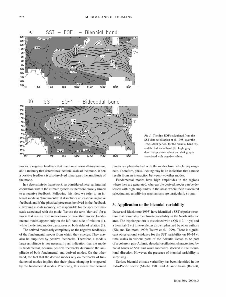
Figure 3 presents an example for such ‘selection’. The fig-ure shows the first modes obtained from two EOF analyses onthe SST fields (Kaplan et al. 1998), for the 1856–2000 peri-ods. In both cases, the anomalous fields were first detrended.In the first EOF analysis, only time-scales in the biennial bandwere retained, while in the second analysis only time-scales inthe bidecadal band were retained. The main difference betweenthe two EOFs is the latitudinal extensions of SST anomalieswhich is most likely due to the differential propagation of plane-tary waves (Moore et al. 1978; Gill, 1982; Killworth et al. 1997;Tourre et al. 2001). Such wave differential propagation can bethen considered a spatial selection mechanism.

Distinct from this, a spatio-temporal selection mechanism isrepresented by the concept of rectification (Milankovitch, 1941;Clement et al. 1999; Huybers and Wunsch, 2003). Rectifica-tion may be viewed as the transformation through which a low-frequency signal only modulates one phase (for example, thepositive phase) of a high-frequency component. A physical anal-ogy to the tropical Pacific variability may be constructed if oneconsiders the meridional movement of the Walker Cell, whichis modulated by a product term like the one on the right-handside of eq. (1), a product of 8- and 20-yr signals. We assumethat the relatively high-frequency signal (e.g. the 8-yr mode)influences the meridional movement of the Walker circulation.Then, at a given point not far from equator, the direct WalkerCell influence would be felt only during given phases of the8-yr components. Therefore, the bidecadal component, as themodulating frequency, is detected by Fourier analysis due to therectification of the 8-yr mode. To summarize, it is argued thatthe derived modes of variability are being generated by specificselecting and amplifying mechanisms.

2.3. Fundamental versus derived modes

One may wonder about what causes an internal mode of variabil-ity to be considered a fundamental mode? We argue that there aretwo elements necessary for the generation of oscillatory internal

Tellus 56A (2004), 3


Fig 3. The first EOFs calculated from theSST data set (Kaplan et al. 1998) over the1856–2000 period, for the biennial band (a),and the bidecadal band (b). Light graydescribes positive values and dark gray isassociated with negative values.

modes: a negative feedback that maintains the oscillatory nature,and a memory that determines the time-scale of the mode. Whena positive feedback is also involved it increases the amplitude ofthe mode.

In a deterministic framework, as considered here, an internaloscillation within the climate system is therefore closely linkedto a negative feedback. Following this idea, we refer to an in-ternal mode as ‘fundamental’ if it includes at least one negativefeedback and if the physical processes involved in the feedback(involving also its memory) are responsible for the specific time-scale associated with the mode. We use the term ‘derived’ for amode that results from interactions of two other modes. Funda-mental modes appear only on the left-hand side of relation (1),while the derived modes can appear on both sides of relation (1).

The derived modes rely completely on the negative feedbacksof the fundamental modes from which they emerge. They mayalso be amplified by positive feedbacks. Therefore, a mode’slarge amplitude is not necessarily an indication that the modeis fundamental, because positive feedbacks determine the am-plitude of both fundamental and derived modes. On the otherhand, the fact that the derived modes rely on feedbacks of fun-damental modes implies that their phase changing is triggeredby the fundamental modes. Practically, this means that derived

modes are phase-locked with the modes from which they origi-nate. Therefore, phase-locking may be an indication that a moderesults from an interaction between two other modes.

Fundamental modes have high amplitudes in the regionswhere they are generated, whereas the derived modes can be de-tected with high amplitudes in the areas where their associatedselecting and amplifying mechanisms are particularly strong.

3. Application to the biennial variability

Deser and Blackmon (1993) have identified a SST tripolar struc-ture that dominates the climate variability in the North Atlanticarea. The tripolar pattern is associated with a QD (12–14 yr) anda biennial (2 yr) time-scale, as also emphasized by other authors(Xie and Tanimoto, 1998; Tourre et al. 1999). There is signifi-cant observational evidence for the SST variability on 10–14 yrtime-scales in various parts of the Atlantic Ocean to be partof a coherent pan-Atlantic decadal oscillation, characterized byzonal bands of SST and wind anomalies stacked in the merid-ional direction. However, the presence of biennial variability issurprising.

Surface biennial climate variability has been identified in theIndo-Pacific sector (Meehl, 1987 and Atlantic basin (Barnett,

Tellus 56A (2004), 3


1991; Deser and Blackmon, 1993; Mann and Park, 1994) andseveral mechanisms have been proposed to explain the 2-yrperiod variability (Meehl, 1987; Li et al. 2001). One of themain features of the tropospheric biennial signal is its tendencyfor phase-locking with the annual cycle (Lau and Shen, 1988).Barnett (1991) emphasizes the global character of the biennialsignal and suggests that global interactions have to be consideredin order to explain the variability for this mode.

We will show that the 2-yr period variability can be understoodin terms of two fundamental modes: the annual cycle and a verystable QD mode originating in the Atlantic basin (Dima et al.2001). Our methodology is based on the statistical analysis ofinstrumental data sets.

Fig 4. Real (a) and imaginary (b) parts of the dominant POP derived from the North Atlantic COADS SST data and their associated timecomponents (c). The imaginary component is represented by a solid line and the imaginary component by a dashed line. The POP has a period of13.1 yr and an e-folding time of 44.0 yr; it explains 21.6% of the variance. Prior to the analysis the data were detrended, normalized and a 5-yrrunning mean filter was applied.

3.1. Fundamental modes

A POP analysis (Hasselmann, 1988; von Storch et al. 1988)was performed on the Comprehensive Ocean–Atmosphere DataSet (COADS) SST (da Silva et al. 1994) for the Atlantic sector(80◦ W–0◦, 0◦–65◦ N) in order to identify dominant oscillatorymodes. POP is a multivariate method used to empirically infer thecharacteristics of the space–time variations of a complex systemin a high-dimensional space. The method is used to identify andfit a linear low-order system to a few parameters.

The data, extending over the period 1945–1989, were de-trended and normalized prior to the analysis, and only time-scaleslonger than 5 yr were considered. The analysis reveals a very

Tellus 56A (2004), 3


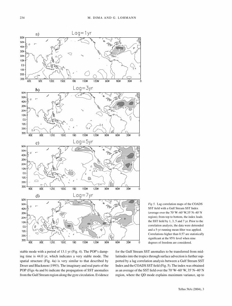
Fig 5. Lag correlation maps of the COADSSST field with a Gulf Stream SST Index(average over the 70◦W–60◦W,35◦N–40◦Nregion); from top to bottom, the index leadsthe SST field by 1, 3, 5 and 7 yr. Prior to thecorrelation analysis, the data were detrendedand a 5-yr running mean filter was applied.Correlations higher than 0.57 are statisticallysignificant at the 95% level when ninedegrees of freedom are considered.

stable mode with a period of 13.1 yr (Fig. 4). The POP’s damp-ing time is 44.0 yr, which indicates a very stable mode. Thespatial structure (Fig. 4a) is very similar to that described byDeser and Blackmon (1993). The imaginary and real parts of thePOP (Figs 4a and b) indicate the propagation of SST anomaliesfrom the Gulf Stream region along the gyre circulation. Evidence

for the Gulf Stream SST anomalies to be transferred from mid-latitudes into the tropics through surface advection is further sup-ported by a lag correlation analysis between a Gulf Stream SSTIndex and the COADS SST field (Fig. 5). The index was obtainedas an average of the SST field over the 70◦W–60◦W, 35◦N–40◦Nregion, where the QD mode explains maximum variance, up to

Tellus 56A (2004), 3


90% (Dima et al. 2001). For the analysis, a 5-yr running meanfilter was applied to the time series. Correlations higher than0.57 are significant at the 95% level when nine degrees of free-dom are considered. The correlation maps obtained (Fig. 5) showthe propagation of the surface thermal anomalies in the Atlanticsubtropical gyre; after propagating eastward, the signal evolvesnorthward and southward where it meets the tropical region ofthe Atlantic. These tropical anomalies affect the tropical convec-tion in the Atlantic sector (Czaja and Frankignoul, 2002; Terrayand Cassou, 2002) and the atmospheric circulation at midlati-tudes. This anomalous circulation provides for SST anomaliesof reverse sign in the Gulf Stream region turning the cycle intoits opposite phase (Fig. 4a, with reversed sign). Together withthe POP analysis (Fig. 4), the lag correlation maps support themechanism proposed to explain the Atlantic 13-yr mode as acoupled air–sea mode (Dima et al. 2001).

Figure 5 also shows that the SST anomalies become trans-ferred into the Pacific and Indian basins when the signal reachesthe tropical Atlantic realm. This is consistent with the ideathat the Intertropical Convergence Zone (ITCZ) acts as a zonalwaveguide through which the phase of the decadal signal is prop-agating westward (White and Cayan, 2000). Within a 7-yr timelag, the signal is dominant in the northern tropical Atlantic andtropical Pacific (Fig. 5). The signature of the Atlantic mode inthe Pacific basin closely resembles the decadal Pacific mode de-scribed in several studies (Zhang et al. 1997). A regression ofthe time component associated with the QD mode derived froman EOF analysis on the Atlantic SST fields, onto the global SST,exhibits the same decadal pattern as in Fig. 5d (not shown).

Based on the observational evidence given by the POP analysisand the correlation maps, we consider the Atlantic QD cyclea fundamental mode, as is also the case for the annual cycle.Considering the 1-yr and 13.1-yr modes as fundamental, andusing eqs (2a) and (2b), the periods obtained for the derivedmodes are 1.9 and 2.2 yr. The obtained derived periods are veryclose and both have biennial time-scales.

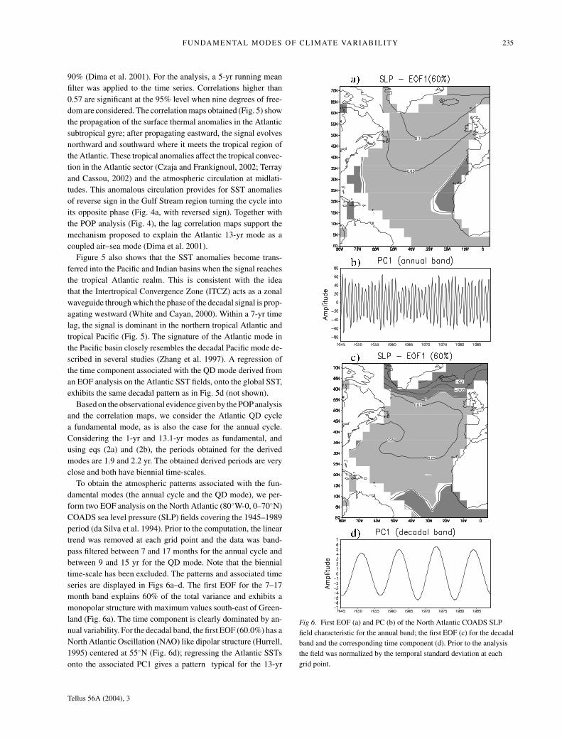
To obtain the atmospheric patterns associated with the fun-damental modes (the annual cycle and the QD mode), we per-form two EOF analysis on the North Atlantic (80◦W-0, 0–70◦N)COADS sea level pressure (SLP) fields covering the 1945–1989period (da Silva et al. 1994). Prior to the computation, the lineartrend was removed at each grid point and the data was band-pass filtered between 7 and 17 months for the annual cycle andbetween 9 and 15 yr for the QD mode. Note that the biennialtime-scale has been excluded. The patterns and associated timeseries are displayed in Figs 6a–d. The first EOF for the 7–17month band explains 60% of the total variance and exhibits amonopolar structure with maximum values south-east of Green-land (Fig. 6a). The time component is clearly dominated by an-nual variability. For the decadal band, the first EOF (60.0%) has aNorth Atlantic Oscillation (NAO) like dipolar structure (Hurrell,1995) centered at 55◦N (Fig. 6d); regressing the Atlantic SSTsonto the associated PC1 gives a pattern typical for the 13-yr

Fig 6. First EOF (a) and PC (b) of the North Atlantic COADS SLPfield characteristic for the annual band; the first EOF (c) for the decadalband and the corresponding time component (d). Prior to the analysisthe field was normalized by the temporal standard deviation at eachgrid point.

Tellus 56A (2004), 3


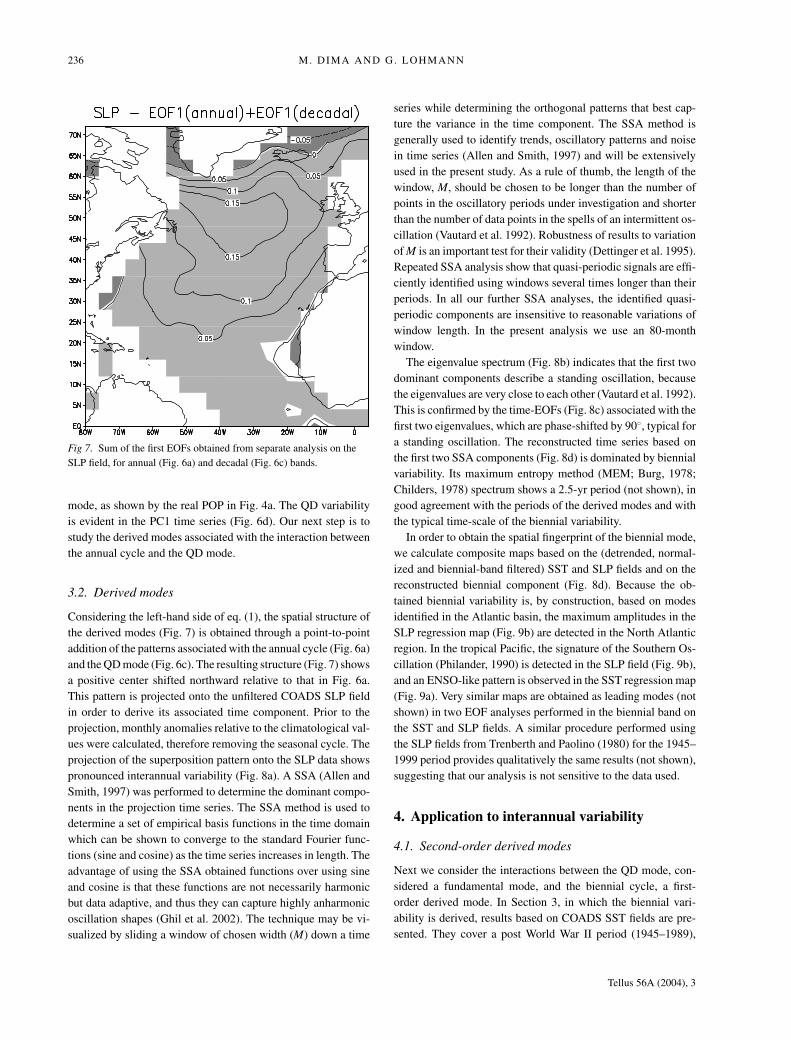
Fig 7. Sum of the first EOFs obtained from separate analysis on theSLP field, for annual (Fig. 6a) and decadal (Fig. 6c) bands.

mode, as shown by the real POP in Fig. 4a. The QD variabilityis evident in the PC1 time series (Fig. 6d). Our next step is tostudy the derived modes associated with the interaction betweenthe annual cycle and the QD mode.

3.2. Derived modes

Considering the left-hand side of eq. (1), the spatial structure ofthe derived modes (Fig. 7) is obtained through a point-to-pointaddition of the patterns associated with the annual cycle (Fig. 6a)and the QD mode (Fig. 6c). The resulting structure (Fig. 7) showsa positive center shifted northward relative to that in Fig. 6a.This pattern is projected onto the unfiltered COADS SLP fieldin order to derive its associated time component. Prior to theprojection, monthly anomalies relative to the climatological val-ues were calculated, therefore removing the seasonal cycle. Theprojection of the superposition pattern onto the SLP data showspronounced interannual variability (Fig. 8a). A SSA (Allen andSmith, 1997) was performed to determine the dominant compo-nents in the projection time series. The SSA method is used todetermine a set of empirical basis functions in the time domainwhich can be shown to converge to the standard Fourier func-tions (sine and cosine) as the time series increases in length. Theadvantage of using the SSA obtained functions over using sineand cosine is that these functions are not necessarily harmonicbut data adaptive, and thus they can capture highly anharmonicoscillation shapes (Ghil et al. 2002). The technique may be vi-sualized by sliding a window of chosen width (M) down a time

series while determining the orthogonal patterns that best cap-ture the variance in the time component. The SSA method isgenerally used to identify trends, oscillatory patterns and noisein time series (Allen and Smith, 1997) and will be extensivelyused in the present study. As a rule of thumb, the length of thewindow, M, should be chosen to be longer than the number ofpoints in the oscillatory periods under investigation and shorterthan the number of data points in the spells of an intermittent os-cillation (Vautard et al. 1992). Robustness of results to variationof M is an important test for their validity (Dettinger et al. 1995).Repeated SSA analysis show that quasi-periodic signals are effi-ciently identified using windows several times longer than theirperiods. In all our further SSA analyses, the identified quasi-periodic components are insensitive to reasonable variations ofwindow length. In the present analysis we use an 80-monthwindow.

The eigenvalue spectrum (Fig. 8b) indicates that the first twodominant components describe a standing oscillation, becausethe eigenvalues are very close to each other (Vautard et al. 1992).This is confirmed by the time-EOFs (Fig. 8c) associated with thefirst two eigenvalues, which are phase-shifted by 90◦, typical fora standing oscillation. The reconstructed time series based onthe first two SSA components (Fig. 8d) is dominated by biennialvariability. Its maximum entropy method (MEM; Burg, 1978;Childers, 1978) spectrum shows a 2.5-yr period (not shown), ingood agreement with the periods of the derived modes and withthe typical time-scale of the biennial variability.

In order to obtain the spatial fingerprint of the biennial mode,we calculate composite maps based on the (detrended, normal-ized and biennial-band filtered) SST and SLP fields and on thereconstructed biennial component (Fig. 8d). Because the ob-tained biennial variability is, by construction, based on modesidentified in the Atlantic basin, the maximum amplitudes in theSLP regression map (Fig. 9b) are detected in the North Atlanticregion. In the tropical Pacific, the signature of the Southern Os-cillation (Philander, 1990) is detected in the SLP field (Fig. 9b),and an ENSO-like pattern is observed in the SST regression map(Fig. 9a). Very similar maps are obtained as leading modes (notshown) in two EOF analyses performed in the biennial band onthe SST and SLP fields. A similar procedure performed usingthe SLP fields from Trenberth and Paolino (1980) for the 1945–1999 period provides qualitatively the same results (not shown),suggesting that our analysis is not sensitive to the data used.

4. Application to interannual variability

4.1. Second-order derived modes

Next we consider the interactions between the QD mode, con-sidered a fundamental mode, and the biennial cycle, a first-order derived mode. In Section 3, in which the biennial vari-ability is derived, results based on COADS SST fields are pre-sented. They cover a post World War II period (1945–1989),

Tellus 56A (2004), 3


Fig 8. Analysis of the time componentassociated with the pattern in Fig. 7. (a)Projection of the map in Fig. 7 onto theunfiltered COADS SLP field. (b) Eigenvaluespectrum obtained from a SSA, using an80-month window. (c) First pair oftime-EOFs; the unit on the time axis is 1 yr.(d) Reconstructed component associatedwith the first pair of time-EOFs.

Tellus 56A (2004), 3


Fig 9. Composite maps constructed basedon the reconstructed component in Fig. 8dand the COADS SST (a) and SLP (b) fields;both fields were detrended, normalized andfiltered in the biennial band.

assuring a maximum possible data quality. However, when an-alyzing derived modes with longer characteristic time-scales,longer data sets are necessary. Therefore, in order to test thegeneration of second-order derived modes, monthly SST andSLP fields of Kaplan et al. (1998) for the 1856–1991 period areused. Prior to the analysis, the linear trend is removed, fields arenormalized by their temporal standard deviations at each gridpoint and data are filtered so that only time-scales between 7–31months and 9–14 yr are retained, respectively.

In order to identify the dominant global coupled SST–SLPpatterns associated with the biennial (7–31 months) and the QDmodes, coupled simultaneous ocean–atmosphere patterns overboth basins are identified in the two fields using two CCAs(von Storch and Zwiers, 1999) performed in the 7–31 monthand 9–14 yr bands, respectively. Note that the 4- and 6-yr time-scales are excluded from the analysis. The CCA method is usedhere to identify dominant coupled ocean–atmosphere patternsbecause for the modes under consideration, having interannualtime-scales, the air–sea interactions are essential.

The dominant SST (23.8%) and SLP (34.8%) coupled pat-terns corresponding to the 7–31 month bands are presented inFig. 10. The SST field (Fig. 10a) has an ENSO-like structure withnegative anomalies extending westward from the South Ameri-

can coast to the 160◦E longitude and with positive values overthe central North Pacific. In the Atlantic sector, a band of nega-tive anomalies extends between the equator and 30◦N. The SLPfield (Fig. 10b) resembles the Southern Oscillation structure inthe Pacific while negative anomalies are observed in the tropi-cal Atlantic. The associated SST and SLP time series (Fig. 10c)are highly correlated (0.89) and show pronounced interannualvariability.

For the 9–14 yr band, the dominant SST pattern (Fig. 11a)explaining 33.7% of the variance in the Atlantic sector (30◦Sto 60◦N) is characterized by zonal bands with alternating sign(Fig. 11a). Such a pattern is typical for the Atlantic 12–14 yr cycle(Deser and Blackmon, 1993; Dima et al. 2001). The SLP pattern(37.0%) is also consistent with this cycle, with a western AtlanticOscillation like structure. The SST field has maximum values inthe center of the Pacific sector (between 170◦E–130◦W, 10◦S–10◦N) while pronounced negative anomalies occur in the centralNorth Pacific. The SST and SLP time series (Fig. 11c) are highlycorrelated (0.94) and they show enhanced QD variability. Thefeatures of this coupled pattern, like its 12–14 yr characteristictime-scale and SST and SLP patterns in the Atlantic sector, ar-gue for associating these coupled patterns with the Atlantic QDmode.

Tellus 56A (2004), 3


Fig 10. Dominant coupled modes obtainedthrough CCA of the SST and SLP fieldsfrom Kaplan et al. (1998). The analysis isperformed in the biennial band. Prior to theanalysis the fields were normalized by thetemporal standard deviation at each gridpoint. (a) SST map; (b) SLP map; (c)associated time components, SST (solid) andSLP (dots).

In order to derive the specific structure associated with the su-perposition between the main modes of variability in the Pacificand Atlantic basins, we linearly combine (addition) the two dom-inant SST patterns corresponding to the 7–31 month and 9–14 yrbands. The resulting SST field (Fig. 12a) presents features fromboth dominant SST patterns derived through the CCAs. In orderto obtain the temporal variability corresponding to this pattern,and therefore the temporal variability associated with the combi-

nation between the two modes, we project the initial (unfiltered)SST field onto this map. Prior to the projection, the SST fieldwas detrended and normalized by the standard deviation at eachgrid point. The projection of the ‘interaction’ pattern onto theSST field is shown in Fig. 12b. The signal is characterized byhigh interannual variability.

Furthermore, an SSA is performed on this time series usinga 30-yr window, in order to identify the dominant oscillatory

Tellus 56A (2004), 3


Fig 11. As in Fig. 10, but the analysis isperformed for the decadal band.

signals embedded within. The eigenvalue spectrum (Fig. 13a)emphasizes two pairs of dominant values. The time-EOFs as-sociated with the first and second eigenvalues (Figs 13b and c)describe a standing oscillation with a 6.2-yr period, identifiedusing the MEM analysis. The second dominant oscillatory com-ponent (the second pair of eigenvalues; Figs 13d and e) alsodescribes a standing oscillation with a 3.6-yr period. These pe-riods are very close to the 4.2- and 6.2-yr modes obtained usingeq. (2) with T 1 = 2.5 and T 2 = 13.1 yr.

Our results are also supported by observational evidence(Rogers, 1984; Huang et al. 1998) that the tropical Pacific in-dices (SOI and Nino3) and the NAO index show significantcoherence in the 2–4 and 5–6 yr frequency bands. The SSTand SLP patterns associated with these second-order derivedmodes are obtained by constructing composite maps based on theKaplan et al. (1998) SST and SLP fields and the SSA recon-structed time components. The fields are detrended and filteredin the ∼3–5 band (for the 4-yr mode) and in the ∼5–7 yr band

Tellus 56A (2004), 3


Fig 12. (a) Sum of the first SST patternsobtained from the two CCAs, correspondingto biennial and to decadal bands, displayedin Figs 10a and 11a, respectively. (b)Projection of the map in Fig. 12a onto theunfiltered SST field.

(for the 6-yr mode). The SST pattern corresponding to the 4-yr mode (Fig. 14a) has an ENSO-like structure in the Pacificbasin while a tripole-like structure is detected in the Atlanticsector. Note that this 4-yr time-scale is also discernible in thespectrum presented by Deser and Blackmon (1993) in associa-tion with the tripole structure. The corresponding SLP structure(Fig. 14b) has a Southern Oscillation like pattern in the PacificOcean and a Western Atlantic structure in the Atlantic basin. Thepatterns associated with the ∼6-yr mode are similar to the 4-yrmaps in the Pacific region. We have applied different techniques(EOF and CCA) to derive the biennial, 4- and 6-yr modes andfind that our results are not sensitive to the statistical methodsused in analyses.

4.2. Third-order derived modes

The large amplitudes of the 4- and 6-yr modes (as second-orderderived modes) in the tropical Pacific suggest that third-ordermodes may also be generated in a similar manner. To test thishypothesis we combine (addition) the SST fields associated withthe 13-yr fundamental mode (obtained through CCA) and the6-yr mode. This latter mode was obtained from a CCA analysison the SST and the SLP fields, filtered to retain time-scales inthe 5–7 yr band (not shown). Similar results are obtained if a

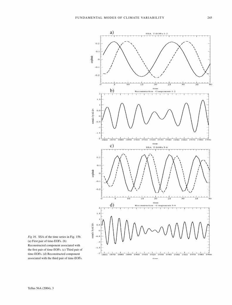
composite SST map, based on the 6-yr component derived fromSSA (Fig. 13c), is used. The resulting map (Fig. 15a) is then pro-jected onto the detrended and normalized annual mean SST fieldto obtain the associated time component (Fig. 15b). This timeseries was smoothed using a 3-yr running mean filter and then aSSA analysis was performed on it, using a 40-yr window. Thetime-EOFs and the reconstruction of the first and the third domi-nant components are presented in Fig. 16. The second component(not shown) is associated with the 13-yr mode. The first and thirdcomponents appear as standing oscillations (Figs 16a, b, c and d,respectively) and are characterized by periods of approximately20 and 9 yr, respectively. When combining the 6.2- and 13.1-yrmodes, the fundamental and derived mode concept gives third-order modes of 23.5- and 8.4-yr periods, very close to the valuesobtained above (20 and 9 yr). The SST and SLP composite mapsassociated with these components are shown in Fig. 17. Theywere obtained based on the reconstructed time components andannual SST and SLP fields from Kaplan et al. (1998). The fieldswere detrended and a 3-yr running mean filter was applied toremove the relatively high-frequency variability. The SST mapassociated with the 8-yr mode (Fig. 17a) has a tripole structurein the North Atlantic and a center of negative anomalies in theNorth Pacific close to the western part of the North Americancoast. The SLP field (Fig. 17b) has a NAO-like (Hurrell, 1995)

Tellus 56A (2004), 3


Fig 13. SSA of the time series in Fig. 12b.(a) Eigenvalue spectrum obtained from aSSA analysis using an 80-month window. (b)First pair of time-EOFs; the unit on the timeaxis is 1 yr. (c) Reconstructed componentassociated with the first pair of time-EOFs.(d) Second pair of time-EOFs; the unit onthe time axis is 1 yr. (e) Reconstructedcomponent associated with the second pairof time-EOFs.

Tellus 56A (2004), 3


Fig 14. Composite maps of thereconstructed component in Fig. 13e basedon the Kaplan SST (a) and SLP (b);composite maps of the reconstructedcomponent in Fig. 13c based on the Kaplanet al. (1998) SST (c) and SLP (d). The SSTanomalies are expressed in degrees and theSLP anomalies in hPa.

Tellus 56A (2004), 3


Fig 15. (a) Sum of the first SST patternsobtained from two CCAs, corresponding tothe 5–7 and 9–14 yr bands. (b) Projection ofthe map in Fig. 15a on the detrended andnormalized annual mean SST field.

structure, consistent with studies showing this particular time-scale to be observed within the NAO variability (Rogers, 1984).The SST ENSO-like pattern (Zhang et al. 1997) is observed inthe map associated with the bidecadal mode (Fig. 17c). Note thatbidecadal variability was reported in the Atlantic sector by Cooket al. (1998).

Therefore, the concept of fundamental and derived modes is ingood agreement with the observational results when consideringhigher-order (second and third) derived modes. It is worth notingthat, as the time-scale of the modes increases from a 2-yr toa 23-yr period (Figs 3, 14 and 17), the meridional extensionof the SST anomalies centered in the eastern tropical Pacificextends further and further. The waveguides of Rossby wavesmay be responsible for this meridional extension and supportthe ‘selection’ mechanism as part of our concept.

Also consistent with the waveguide notion, as the time-scaleincreases, the maximum amplitude of the SST anomalies movesfrom the tropical Pacific (in the case of the 2- and 4-yr modes) tothe North Pacific (in the case of the 6-, 8-, and 23-yr modes). Thelarge SST anomalies in these two regions may also be favoredby local positive feedbacks that optimally amplify these specifictime-scales. Such feedbacks were identified by Philander (1990)

in the tropical Pacific and by Seager et al. (2001) in the NorthPacific Ocean.

Interestingly, as the period of a derived mode is closer to thatof the fundamental mode from which it originates, its associatedpatterns are more similar to that of the fundamental mode. Forexample, the SST map associated with the 8-yr mode (Fig. 17)shares, in the Atlantic basin, more common features with thepattern of the 13-yr mode (Fig. 11) than the 4- and 6-yr modes(Fig. 14) share with the QD mode. This brings additional supportto our concept.

5. Conceptual features of the mode interactions

In the framework of our concept, it is worth evaluating the fac-tors that may contribute to the amplitude of a mode at a givenlocation. For this purpose we propose an analogy involving twowave sources placed in distinct points (Fig. 1). These sources arevirtually associated with two fundamental climate modes. Onemay assume that each of the sources generates a wave field, in asimilar way as the fundamental modes generate quasi-periodicclimate signals. These signals may be damped or amplified asthey propagate. A typical climate problem would be to identify

Tellus 56A (2004), 3


Fig 16. SSA of the time series in Fig. 15b.(a) First pair of time-EOFs. (b)Reconstructed component associated withthe first pair of time-EOFs. (c) Third pair oftime-EOFs. (d) Reconstructed componentassociated with the third pair of time-EOFs.

Tellus 56A (2004), 3


Fig 17. Composite maps of thereconstructed component in Fig. 16d basedon the Kaplan et al. (1998) SST (a) and SLP(b); composite maps of the reconstructedcomponent in Fig. 16b based on the Kaplanet al. (1998) SST (c) and SLP (d). The fieldswere normalized by the standard deviation ateach grid point.

Tellus 56A (2004), 3


the signal produced by each source by analyzing the field that re-sults from the combination between the fields generated by eachmode. The best location for detecting the first source is point 1.Similarly, the best location for detecting the second source ispoint 2. At locations far enough from both sources, the domi-nant signal would be associated with the superposition betweenthe two sources (e.g. points A and B). By analogy, the signals as-sociated with fundamental modes are easily identified in regionswhere the modes originate, while in other regions the resultingderived modes dominate. As a possible application, a multivari-ate EOF analysis would emphasize the fundamental modes ifthe analysis is performed over regions where these modes orig-inate. However, if the same analysis is performed over regionswhere no fundamental modes originate, or over regions that in-clude the ‘sources’ of two or more fundamental modes, then itwould most likely emphasize the derived modes. Therefore, thefirst two factors that influence the detection of the modes are the‘position’ and the ‘extent’ of the analyzed region with respect tothe location of the sources for the fundamental modes.

In our study, all the modes considered are in connection to theannual and QD cycles, as fundamental modes. The connectionswere put into evidence through multiple iterations of our con-cept: three combinations of modes result in periods in the 4- and6-yr bands, while two combinations are associated with the 8-and 23-yr modes, respectively. This is consistent with observa-tional evidence which shows that the tropical Pacific variability(as, for example, described by the Nino3 index) is dominatedby time-scales of 4 and 6 yr. Also, the 8- and 23-yr time-scalesare identified in both the Pacific and the Atlantic basin (Rogers,1984; Cook et al. 1998). Therefore, a third factor that may influ-ence the mode detection is the ‘frequency overlapping’ betweentwo or more modes.

Another element to be considered is the possible positive feed-backs involved. For example, the coupled ocean–atmospheretropical Pacific system may amplify even weak signals throughocean–atmosphere interactions (Bjerknes, 1969). A character-istic time-scale for such a positive feedback may be providedby particular physical processes such as oceanic adjustment tovariable wind conditions, through Rossby and Kelvin wave prop-agation in the equatorial waveguide (Gill, 1982). If we considerthat these derived modes are efficiently amplified by the pos-itive feedback generated by ocean–atmosphere interactions inthis sector, then the dominance of the 4- and 6-yr time-scalesin the tropical Pacific is a natural consequence. Therefore, thefourth element that may influence mode detection is related to‘local feedbacks’ that may amplify the signals. These local feed-backs may also be viewed as resonances between global modesand location-specific growing modes.

A standard inference from statistical analyses of climatic datais that a mode originates in a particular region if it explains a largepercentage of the variance in that area. However, in our view, ifthe mode considered is a derived one, then large percentagesof explained variance are not necessarily an indication for the

origins of the mode in that specific region. Most likely, the correctinference would be that the derived mode is efficiently amplifiedby local positive feedbacks in that region. Moreover, it is naturalto expect that in the region where a fundamental mode has itsorigins, the potential derived modes do not explain an importantpart of the variance.

The above considerations may be part of a picture in whichthe ENSO phenomenon appears as an amplification and over-lapping of derived modes in the tropical Pacific coupled ocean–atmosphere system. Such a picture is in agreement with theconcept that ENSO results from interactions between multipletime-scales in the tropical Pacific (Barnett, 1991). However, animportant consequence resulting from applying the fundamen-tal and derived mode concept to the tropical Pacific is that thenegative feedback (necessary in changing the phase of the mode)does not necessarily originate in the tropical Pacific sector. Over-all, the picture constructed based on our concept is in agreementwith previous observational studies that have successfully de-scribed the positive feedback in the tropical Pacific (Bjerknes,1969), while no conclusive observational evidence was yet pre-sented for a potential negative feedback in this region (Fedorovand Philander, 2001).

6. Conclusions

In the present study we propose a concept of mode interactions.The concept is based on the distinction between fundamental andderived modes of climate variability and assumes that the ‘fun-damental’ modes can be combined in the Fourier space in orderto obtain ‘derived’ modes of variability. As a first application,we considered the annual cycle and the QD mode to be funda-mental. Using SLP fields we showed that the biennial variabilityresults from an interaction between the two fundamental modes,which is in agreement with the periods provided by our theory.Similar results are obtained when analyzing different data sets.

Specific spatial features associated with the biennial climatevariability are well explained by our concept. For example, thesurface biennial variability has a clear signature in the tropicalbelt, but does not have a global signature in the midlatitude SLPfield. The only midlatitudinal region where the biennial variabil-ity has a significant fingerprint is the North Atlantic region (Bar-nett, 1991); here the mode shows a very coherent structure, whichis easy to understand considering that the mode originates fromthe interaction between the annual cycle and the North AtlanticQD mode. In accordance with our concept, the strong biennialsignal reported in the Indian Ocean goes together with the largeamplitudes of the annual cycle in that region. The phase-lockingbetween the annual cycle and the biennial variability (Lau andShen, 1988) is also consistent with our interaction model. Thedecadal modulation of the global biennial mode appears as anatural consequence in our concept (White and Allan, 2001).

We further applied the fundamental and derived mode conceptto the interannual variability. Based on the biennial and on the

Tellus 56A (2004), 3


QD modes, it is shown that second-order derived modes (withperiods of about 4 and 6 yr) and third-order derived modes (withperiods of about 8 and 23 yr) are thus being generated.

To summarize, we can construct a scheme for the applicationof our fundamental and derived mode concept:

(1 yr, ∼13 yr) => (∼2 yr, ∼2 yr)(∼2 yr, ∼13 yr) => (∼4 yr, ∼6 yr)(∼6 yr, ∼13 yr) => (∼8 yr, ∼23 yr).

We suggest that the large amplitude and/or the large percent-age of the variance explained by a mode in a region is not nec-essarily an indication for the mode originating in that region.This inference may be valid for a fundamental mode, if theanalysis is performed in the region where it originates, but itis not necessarily valid for a derived mode. The fundamentaland derived mode concept emphasizes two elements that mayexplain the prominence of the 4- and 6-yr modes (as second-order derived modes) in the Pacific basin: the overlapping of thefrequencies of several derived modes and a local positive feed-back which optimally amplifies the modes characterized by thesetime-scales.

In our view, the derived modes depend essentially on thephysics of the fundamental modes. Therefore, the negative feed-backs changing the phase of a derived mode are locked to thefundamental modes. Then, an important consequence of the ap-plication of the fundamental and derived mode concept to inter-annual variability is that the negative feedback responsible forthe generation of interannual variability in the tropical Pacificdoes not necessarily originate in the Pacific basin. Note that thephase-locking of the ENSO mode to the annual cycle appears asa natural consequence of our concept. Moreover, phase-lockingprovides support for a deterministic origin of the consideredmodes. In this view, the Pacific basin appears as a ‘resonator’that optimally amplifies modes with specific time-scales (e.g.interannual variability).

Our concept emphasizes that the variability of the derivedmodes stems from that of the fundamental modes and from theinherent climate resonances at certain time-scales. These reso-nances are connected to internal dynamics, as for exapmle thewave dynamics in the tropical Pacific. As in the framework of thestochastic climate model (Hasselmann, 1976), our deterministicperspective on climate variability is based on the interaction ofthe climate components with different typical time-scales. Whilein the stochastic paradigm an important problem is identifyingthe stabilizing feedback limiting the amplitude of the climatesignals, in the framework of our concept the main points are re-lated to the identification of the fundamental modes and of theselection mechanisms. Therefore, we believe that our determin-istic concept complements the stochastic paradigm. As a naturalfurther step, future studies will concentrate on the application ofour concept to longer time-scales and on the implications of theresults on climate predictability.

7. Acknowledgments

We wish to thank to Dr Norel Rimbu for useful discussions,and two anonymous reviewers for their constructive suggestions.This research was funded by the Bundesbildungsministerium furBildung und Forschung through DEKLIM and by the DeutscheForschungsgemeinschaft as part of the Research Center ‘Oceanmargins’ of the University of Bremen (No. RCOM0097).

References

Allen, M. and Smith, L. A. 1997. Optimal filtering in Singular SpectrumAnalysis. Phys. Lett. 234, 419–428.

Barnett, T. P. 1991. The interaction of multiple time scales in the tropicalclimate system. J. Climate 4, 269–285.

Bjerknes, J. 1964. Atlantic air–sea interaction. Adv. Geophys. 10, 1–82.Bjerknes, J. 1969. Atmospheric teleconections from the equatorial

Pacific. Mon. Wea. Rev. 97, 163–172.Burg, J. P. 1978. Maximum entropy spectral analysis. Modern Spectrum

Analysis. IEEE Press, Piscataway, NJ, 42–48.Childers, D. G. 1978. Modern Spectrum Analysis. IEEE Press, Piscat-

away, NJ, 331 pp.Clement, A. C., Seager, R. and Cane, M. A. 1999. Orbital controls on

ENSO and the tropical climate. Paleoceanography 14, 441–456.Cook, E. R., D’Arrigo, R. D. and Briffa, K. R. 1998. A reconstruction

of the North Atlantic Oscillation using tree-ring chronologies fromNorth America and Europe. The Holocene 8, 9–17.

Czaja, A. and Frankignoul, C. 2002. Observed impact of Atlantic SSTAnomalies on the North Atlantic Oscillation. J. Climate 15, 606–623.

da Silva, A., Young, A. C. and Levitus, S. 1994. Atlas of Surface MarineData 1994. Algorithms and Procedures,Vol. 1. NOAA Atlas NESDIS6, Washington, DC.

Deser, C. and Blackmon, M. L. 1993. Surface climate variations overNorth Atlantic Ocean during winter: 1900–1989. J. Climate 6, 1743–1753.

Dettinger, M. D., Ghil, M., Strong, C. M., Weibel, W. and Yiou, P. 1995.Software expedities singular-spectrum analysis of noisy time series.Eos. Trans. Am. Geophys. Union 76, 14–21.

Dima, M., Rimbu, N., Stefan, S. and Dima, I. 2001. Quasi-decadal vari-ability in the Atlantic Basin involving tropics-midlatitudes and ocean–atmosphere interactions. J. Climate 14, 823–832.

Einstein, A. 1905. Uber die von der molekularkinetischen Theorie derWarme geforderte Bewegung von in ruhenden Flussigkeiten sus-pendierten Teilchen. Ann. Phys. 17, 549–560.

Fedorov, A. V. and Philander, S. G. 2001. A stability analysis of tropicalocean–atmosphere interactions: bridging measurements and theoryfor El Nino. J. Climate 14, 3086–3101.

Ghil, M. and Robertson, A. W. 2002. ‘Waves’ vs. ‘particles’ in the at-mosphere’s phase space: A pathway to long-range forecasting? Proc.Natl. Acad. Sci. 99 (Suppl. 1), 2493–2500.

Ghil, M., Allen, M. R., Dettinger, M. D., Ide, K., Kondrashov, D., et al.2002. Advanced spectral methods for climatic time series. Rev. Geo-phys. 10, 1029/2000GR000092.

Gill, A. E. 1982. Atmosphere–Ocean Dynamics. Academic Press, NewYork, 662 pp.

Hasselmann, K. 1976. Stochastic climate models. Tellus 28, 473–484.

Tellus 56A (2004), 3


Hasselmann, K. 1988. PIPs and POPs: The reduction of complexdynamical systems using principal interaction and oscillation patterns.J. Geophys. Res. 93, 11 015–11 021.

Huang, J., Higuchi, K. and Shabbar, A. 1998. The relationship betweenthe North Atlantic Oscillation and El Nino-Southern Oscillation. Geo-phys. Res. Lett. 25, 2707–2710.

Hurrell, J. W. 1995. Decadal trends in the North Atlantic Oscillation:Regional temperatures and precipitation. Science 269, 676–679.

Huybers, P. and Wunsch, C. 2003. Rectification and precession signalsin the climate system. Geophys. Res. Lett. 30, 2011.

Kaplan, A., Cane, M. A., Kushnir, Y., Clement, A. C., Blumenthal, M.B. et al. 1998. Analyses of global sea surface temperature 1856–1991.J. Geophys. Res. 103, 27 835–27 860.

Killworth, P. D., Chelton, D. B. and DeZoeke, R. A. 1997. The speed ofobserved and theoretical long extra-tropical planetary waves. J. Phys.Oceanogr. 27, 1946–1966.

Latif, M. 1998. Dynamics of interdecadal variability in coupled ocean-atmosphere models. J. Climate 11, 602–624.

Latif, M. and Barnett, T. P. 1994. Causes of decadal climate variabilityover the North Pacific and North America. Science 266, 634–637.

Lau, K.-H. and Shen, P. J. 1988. Annual cycle, quasi-biennial oscillation,and Southern Oscillation in global precipitation. J. Geophys. Res. 93,10 975–10 988.

Li, T., Tham, C.-W. and Chang, C.-P. 2001. A coupled air–sea-monsoonoscillator for the tropospheric biennial oscillation. J. Climate 14, 752–764.

Mann, M. E. and Park, J. 1994. Global-scale modes of surface tempera-ture variability on interannual to century time scales. J. Geophys. Res.99, 25 819–25 833.

Mantua, N., Hare, S., Zhang, Y., Wallace, J. M. and Francis, R. 1997.A Pacific interdecadal climate oscillation with impacts on salmonproduction. Bull. Amr. Meteorol. Soc. 78, 1069–1079.

Meehl, G. A. 1987. The annual cycle and interannual variability in thetropical Pacific and Indian Ocean region. Mon. Wea. Rev. 115, 27–50.

Milankovitch, M. 1941. Kanon der Erdbestrahlung und seine Anwen-dung auf das Eiszeitproblem. Spec. Publ. 132,Vol. 33, Sect. Math. Nat.Sci., R. Serb. Acad., Belgrad.

Mitchell, J. M. 1976. An overview of climatic variability and its causalmechanisms. Quat. Res. 6, 481–494.

Moore, D. W., Hisard, P., McCreary, J. P., Merle, J., O’Brien, J. J., et al.1978. Equatorial adjustment in the eastern Atlantic. Geophys. Res.Lett. 5, 637–640.

Philander, S. G. 1990. El Nio, La Nina, and the Southern Oscillation.Academic Press, New York, 293 pp.

Rogers, J. C. 1984. The association between the North Atlantic Oscilla-tion and the Southern Oscillation in the Northern Hemisphere. Mon.Wea. Rev. 112, 1999–2015.

Seager, R., Kushnir, Y., Naik, N. H., Cane, N. A. and Miller, J. 2001.Wind-driven shifts in the latitude of the Kuroshio-Oyashio extensionand generation of SST anomalies on decadal time scales. J. Climate14, 4249–4265.

Terray, L. and Cassou, C. 2002. Tropical Atlantic sea surface temperatureforcing of quasi-decadal climate variability over the North Atlantic-European Region. J. Climate 15, 3170–3187.

Timmermann, A., Latif, M., Voss, R. and Grotzner, A. 1998. North-ern Hemispheric interdecadal variability: a coupled air–sea mode.J. Climate 11, 1906–1931.

Tourre, Y. M., Rajagopalan, B. and Kushnir, Y. 1999. Dominant patternsof climate variability in the Atlantic Ocean region during the last136 years. J. Climate 12, 2285–2299.

Tourre, Y. M., Rajagopalan, B., Kushnir, Y., Barlow, M. and White,W. B. 2001. Patterns of coherent decadal and interdecadal climatesignals in the Pacific Basin during the 20th century. Geophys. Res.Lett. 28, 2069–2072.

Trenberth, K. A. and Paolino, D. A. 1980. The Northern Hemispheresea-level pressure data set: trends, errors and discontinuities. Mon.Wea. Rev. 108, 855–872.

Vautard, R., Yiou, P. and Ghil, M. 1992. Singular-spectrum analysis: Atoolkit for short, noisy chaotic signals. Physica D 58, 95–126.

von Storch, H. V. and Zwiers, F. W. 1999. Statistical Analysis in ClimateResearch. Cambridge University Press, Cambridge, 484 pp.

von Storch, H., Bruns, T., Fisher-Bruns, I. and Hasselmann, K. 1988.Principal oscillation pattern analysis of the 30-to 60-day oscillation ina general circulation model equatorial troposphere. J. Geophys. Res.93, 11 012–11 036.

White, W. B. and Allan, R. J. 2001. A global quasi-biennial wave insurface temperature and pressure and its decadal modulation from1900 to 1994. J. Geophys. Res. 105, 26 789–26 803.

White, W. B. and Cayan, D. R. 2000. A global El Nino-Southern Oscil-lation wave in surface temperature and pressure and its interdecadalmodulation from 1900 to 1997. J. Geophys. Res. 105, 11 223–11 242.

Xie, S. P. and Tanimoto, Y. 1998. A pan-Atlantic decadal climate oscil-lation. Geophys. Res. Lett. 25, 2185–2188.

Zhang, Y., Wallace, J. M. and Battisti, D. S. 1997. ENSO-like inter-decadal variability: 1900–93. J. Climate 10, 1004–1020.

Tellus 56A (2004), 3

Fundamental and derived modes of climate variability

Documents

Transcript of Fundamental and derived modes of climate variability