University of Zagreb

Faculty of mechanical engineering

and naval architecture

Aeronautical engineering

FSB TX TEAM

FSB TX Team

i

FSB TX Team

Contents

1 Airplane configuration and mission analysis 1

1.1 Mission analysis . . . . . . . . . . . . . . . . . . . . . . . . . . . . . . . . . . . . . 1

1.2 Aircraft configuration . . . . . . . . . . . . . . . . . . . . . . . . . . . . . . . . . 3

1.2.1 Introduction . . . . . . . . . . . . . . . . . . . . . . . . . . . . . . . . . . 3

1.2.2 Discusing the factors which do have significant meaning to design . . . . . 3

1.2.3 Multicriteria decision making . . . . . . . . . . . . . . . . . . . . . . . . . 4

1.2.4 General Aircraft Configuration . . . . . . . . . . . . . . . . . . . . . . . . 5

1.2.5 Wing position . . . . . . . . . . . . . . . . . . . . . . . . . . . . . . . . . . 6

2 Weight estimation 11

2.1 Class I . . . . . . . . . . . . . . . . . . . . . . . . . . . . . . . . . . . . . . . . . . 11

2.2 Class II . . . . . . . . . . . . . . . . . . . . . . . . . . . . . . . . . . . . . . . . . 13

3 Performance estimation 15

3.1 Estimating wing area, take-off thrust and maximum lift coefficient . . . . . . . . 15

3.1.1 Take-off requirements . . . . . . . . . . . . . . . . . . . . . . . . . . . . . 15

3.1.2 Landing requirements . . . . . . . . . . . . . . . . . . . . . . . . . . . . . 16

3.1.3 Cruise requirements . . . . . . . . . . . . . . . . . . . . . . . . . . . . . . 16

3.1.4 Maneuvering requirements . . . . . . . . . . . . . . . . . . . . . . . . . . . 16

3.1.5 Ceiling requirements . . . . . . . . . . . . . . . . . . . . . . . . . . . . . . 17

3.1.6 Engine . . . . . . . . . . . . . . . . . . . . . . . . . . . . . . . . . . . . . . 17

3.2 Trade study . . . . . . . . . . . . . . . . . . . . . . . . . . . . . . . . . . . . . . . 18

3.2.1 Lift coefficient influence on Take-Off . . . . . . . . . . . . . . . . . . . . . 18

3.2.2 Lift coefficient influence on landing conditions . . . . . . . . . . . . . . . . 19

3.2.3 Lift coefficient influence on maneuvering . . . . . . . . . . . . . . . . . . . 20

3.3 Matching diagram with all limitations . . . . . . . . . . . . . . . . . . . . . . . . 21

4 Wing and tail geometry 24

4.1 Airfoil . . . . . . . . . . . . . . . . . . . . . . . . . . . . . . . . . . . . . . . . . . 26

4.2 Additional lift surfaces . . . . . . . . . . . . . . . . . . . . . . . . . . . . . . . . . 28

4.3 Fuel reservoirs . . . . . . . . . . . . . . . . . . . . . . . . . . . . . . . . . . . . . 29

ii

FSB TX Team

5 Undercarriage design 34

5.1 Undercarriage placement . . . . . . . . . . . . . . . . . . . . . . . . . . . . . . . . 35

5.2 Tire size estimation . . . . . . . . . . . . . . . . . . . . . . . . . . . . . . . . . . . 35

5.3 Oleo strut sizing . . . . . . . . . . . . . . . . . . . . . . . . . . . . . . . . . . . . 36

5.4 Undercarriage retraction and stow . . . . . . . . . . . . . . . . . . . . . . . . . . 37

5.5 Undercarriage criteria . . . . . . . . . . . . . . . . . . . . . . . . . . . . . . . . . 38

6 Weight and balance 39

6.1 Component weight estimation . . . . . . . . . . . . . . . . . . . . . . . . . . . . . 39

6.2 CG travel . . . . . . . . . . . . . . . . . . . . . . . . . . . . . . . . . . . . . . . . 39

7 Stability and control analysis 41

7.1 Class 1 method - static stability and control . . . . . . . . . . . . . . . . . . . . 41

7.1.1 Longitudinal static stability and control . . . . . . . . . . . . . . . . . . . 41

7.1.2 Lateral static stability and control . . . . . . . . . . . . . . . . . . . . . . 44

7.2 Class 2 method - dynamic stability and control . . . . . . . . . . . . . . . . . . . 45

8 Aircraft Performance 51

8.1 Take-off and Landing distance requirements . . . . . . . . . . . . . . . . . . . . . 51

8.2 Climb . . . . . . . . . . . . . . . . . . . . . . . . . . . . . . . . . . . . . . . . . . 52

8.3 Range and endurance . . . . . . . . . . . . . . . . . . . . . . . . . . . . . . . . . 54

8.4 Maximum Mach Number at 10058 m (36000 ft) and wave drag . . . . . . . . . . 55

8.5 1-g Maximum Thrust Specific Excess Power Envelope . . . . . . . . . . . . . . . 57

8.6 5-g Maximum Thrust Specific Excess Power Envelope . . . . . . . . . . . . . . . 58

8.7 Energy Maneuverability Diagram at 4572 m MSL . . . . . . . . . . . . . . . . . . 59

8.8 L/D vs Mach at 10058 m (36000 ft) . . . . . . . . . . . . . . . . . . . . . . . . . 60

9 Cost estimation 62

9.1 Research, Development, Test and Evaluation cost . . . . . . . . . . . . . . . . . . 62

9.2 Manufacturing and Acquisition Cost . . . . . . . . . . . . . . . . . . . . . . . . . 63

9.2.1 Flyaway cost . . . . . . . . . . . . . . . . . . . . . . . . . . . . . . . . . . 64

9.2.2 Per Unit Cost . . . . . . . . . . . . . . . . . . . . . . . . . . . . . . . . . . 65

9.3 Operational cost . . . . . . . . . . . . . . . . . . . . . . . . . . . . . . . . . . . . 65

iii

FSB TX Team

9.4 Life cycle cost . . . . . . . . . . . . . . . . . . . . . . . . . . . . . . . . . . . . . . 66

10 Structure and manufacturing 68

10.1 Systems . . . . . . . . . . . . . . . . . . . . . . . . . . . . . . . . . . . . . . . . . 68

10.1.1 Fuel tanks and fuel pumps . . . . . . . . . . . . . . . . . . . . . . . . . . . 68

10.1.2 Hydraulic system . . . . . . . . . . . . . . . . . . . . . . . . . . . . . . . . 68

10.1.3 Electrical system . . . . . . . . . . . . . . . . . . . . . . . . . . . . . . . . 69

10.1.4 Environmental control system . . . . . . . . . . . . . . . . . . . . . . . . . 69

10.1.5 System layout design . . . . . . . . . . . . . . . . . . . . . . . . . . . . . . 69

10.2 V-n diagram . . . . . . . . . . . . . . . . . . . . . . . . . . . . . . . . . . . . . . . 70

10.3 Structural arrangement . . . . . . . . . . . . . . . . . . . . . . . . . . . . . . . . 71

10.4 Material selection and technology . . . . . . . . . . . . . . . . . . . . . . . . . . 75

10.5 Managment and Manufacturing . . . . . . . . . . . . . . . . . . . . . . . . . . . 78

10.6 Maintenance . . . . . . . . . . . . . . . . . . . . . . . . . . . . . . . . . . . . . . 79

11 Conclusion 80

iv

FSB TX Team

List of Figures

1 Mission . . . . . . . . . . . . . . . . . . . . . . . . . . . . . . . . . . . . . . . . . 1

2 Multicriteria decision making . . . . . . . . . . . . . . . . . . . . . . . . . . . . . 4

3 Objectives . . . . . . . . . . . . . . . . . . . . . . . . . . . . . . . . . . . . . . . . 5

4 Configuration 1 . . . . . . . . . . . . . . . . . . . . . . . . . . . . . . . . . . . . . 8

5 Configuration 2 . . . . . . . . . . . . . . . . . . . . . . . . . . . . . . . . . . . . . 8

6 Configuration 3 . . . . . . . . . . . . . . . . . . . . . . . . . . . . . . . . . . . . . 9

7 Priority vector diagram . . . . . . . . . . . . . . . . . . . . . . . . . . . . . . . . 9

8 Regression . . . . . . . . . . . . . . . . . . . . . . . . . . . . . . . . . . . . . . . . 12

9 Lift coefficient with take-off requirements, A=5 . . . . . . . . . . . . . . . . . . . 19

10 Lift coefficient with landing requirements, A=5 . . . . . . . . . . . . . . . . . . . 20

11 Lift coefficient with maneuvering requirements, A=5 . . . . . . . . . . . . . . . . 21

12 Matching diagram . . . . . . . . . . . . . . . . . . . . . . . . . . . . . . . . . . . 22

13 NACA 63209 with 200 panels . . . . . . . . . . . . . . . . . . . . . . . . . . . . . 27

14 Comparison of section lift for different NACA 6-series airfoils . . . . . . . . . . . 27

15 NACA 0009 airfoil . . . . . . . . . . . . . . . . . . . . . . . . . . . . . . . . . . . 28

16 NACA 63209 with different flaps settings . . . . . . . . . . . . . . . . . . . . . . 28

17 Section lift increase for different flaps settings . . . . . . . . . . . . . . . . . . . . 29

18 Wing model in SolidWorks . . . . . . . . . . . . . . . . . . . . . . . . . . . . . . 30

19 Tricycle configuration . . . . . . . . . . . . . . . . . . . . . . . . . . . . . . . . . 34

20 F = 4.121m; L = 3.481m; M = 0.44m; N = 3.681m; J = 1.37m . . . . . . . . . . 35

21 Undercarriage retraction . . . . . . . . . . . . . . . . . . . . . . . . . . . . . . . . 37

22 Longitudinal criteria . . . . . . . . . . . . . . . . . . . . . . . . . . . . . . . . . . 38

23 Lateral criteria . . . . . . . . . . . . . . . . . . . . . . . . . . . . . . . . . . . . . 38

24 Weight and balance travel . . . . . . . . . . . . . . . . . . . . . . . . . . . . . . . 40

25 Side view of CG positions . . . . . . . . . . . . . . . . . . . . . . . . . . . . . . . 40

26 Aerodinamic symbols . . . . . . . . . . . . . . . . . . . . . . . . . . . . . . . . . . 41

27 Static margin . . . . . . . . . . . . . . . . . . . . . . . . . . . . . . . . . . . . . . 42

28 Feedback gain . . . . . . . . . . . . . . . . . . . . . . . . . . . . . . . . . . . . . . 43

29 Rudder feedback gain . . . . . . . . . . . . . . . . . . . . . . . . . . . . . . . . . 44

30 Airplane geometric model . . . . . . . . . . . . . . . . . . . . . . . . . . . . . . . 45

v

FSB TX Team

31 Ceasiom derivative . . . . . . . . . . . . . . . . . . . . . . . . . . . . . . . . . . . 46

32 Closed loop feedback system . . . . . . . . . . . . . . . . . . . . . . . . . . . . . . 48

33 Phugoid mode damping ratio with respect to TAS (MIL standard) . . . . . . . . 49

34 Dutch roll . . . . . . . . . . . . . . . . . . . . . . . . . . . . . . . . . . . . . . . . 49

35 Cooper-Harper pilot assessment rating . . . . . . . . . . . . . . . . . . . . . . . . 50

36 Rate of Climb with Altitude . . . . . . . . . . . . . . . . . . . . . . . . . . . . . . 53

37 Time to Climb with Altitude . . . . . . . . . . . . . . . . . . . . . . . . . . . . . 53

38 Range . . . . . . . . . . . . . . . . . . . . . . . . . . . . . . . . . . . . . . . . . . 54

39 Endurance . . . . . . . . . . . . . . . . . . . . . . . . . . . . . . . . . . . . . . . . 55

40 Wave Drag shown in OpenVSP . . . . . . . . . . . . . . . . . . . . . . . . . . . . 56

41 Drag coefficient with Mach number . . . . . . . . . . . . . . . . . . . . . . . . . . 57

42 1-g Maximum Excess Power Envelope . . . . . . . . . . . . . . . . . . . . . . . . 58

43 5-g Maximum Excess Power Envelope . . . . . . . . . . . . . . . . . . . . . . . . 59

44 Energy Maneuverability Diagram . . . . . . . . . . . . . . . . . . . . . . . . . . . 60

45 L/D with Mach number . . . . . . . . . . . . . . . . . . . . . . . . . . . . . . . . 61

46 Contribution of certain parts to the total RDTE price . . . . . . . . . . . . . . . 63

47 Contribution of certain parts to the total Manufacturing and Acquisition price . 63

48 Price of Manufacturing and Acquisition depending on the number of produced

aircraft; price in billion of USD . . . . . . . . . . . . . . . . . . . . . . . . . . . . 64

49 Flyaway cost per unit depending on the number of produced aircraft; price in

million of USD . . . . . . . . . . . . . . . . . . . . . . . . . . . . . . . . . . . . . 64

50 Per unit cost depending on the number of produced aircraft; price in million of

USD . . . . . . . . . . . . . . . . . . . . . . . . . . . . . . . . . . . . . . . . . . . 65

51 Contribution of items to the Operating cost . . . . . . . . . . . . . . . . . . . . . 66

52 Operating cost depending on the number of produced aircraft; price in billion of

USD . . . . . . . . . . . . . . . . . . . . . . . . . . . . . . . . . . . . . . . . . . . 66

53 Life cycle cost depending on the number of produced aircraft; price in billion of

USD . . . . . . . . . . . . . . . . . . . . . . . . . . . . . . . . . . . . . . . . . . . 67

54 Contribution of items to the Life cycle cost . . . . . . . . . . . . . . . . . . . . . 67

55 Fuel tank storage in the aircraft . . . . . . . . . . . . . . . . . . . . . . . . . . . . 68

56 Layout of basic aircraft systems . . . . . . . . . . . . . . . . . . . . . . . . . . . . 69

57 Top view and side view of basic aircraft systems . . . . . . . . . . . . . . . . . . 70

vi

FSB TX Team

58 V-n diagram . . . . . . . . . . . . . . . . . . . . . . . . . . . . . . . . . . . . . . . 71

59 Top view of aircraft and structure elements . . . . . . . . . . . . . . . . . . . . . 73

60 Side view of aircraft and structure elements . . . . . . . . . . . . . . . . . . . . . 73

61 Aircraft parts and materials in the ground plan . . . . . . . . . . . . . . . . . . . 77

62 Parts and materials of the aircraft in the side view . . . . . . . . . . . . . . . . . 78

vii

FSB TX Team

List of Tables

1 RFP requirements . . . . . . . . . . . . . . . . . . . . . . . . . . . . . . . . . . . 2

2 Wing position . . . . . . . . . . . . . . . . . . . . . . . . . . . . . . . . . . . . . . 6

3 Stability surfaces . . . . . . . . . . . . . . . . . . . . . . . . . . . . . . . . . . . . 6

4 Similar aircraft . . . . . . . . . . . . . . . . . . . . . . . . . . . . . . . . . . . . . 11

5 Trade study analisys . . . . . . . . . . . . . . . . . . . . . . . . . . . . . . . . . . 13

6 Component weights . . . . . . . . . . . . . . . . . . . . . . . . . . . . . . . . . . . 14

7 F125IN Technical Data . . . . . . . . . . . . . . . . . . . . . . . . . . . . . . . . . 18

8 Wing parameters and dimensions . . . . . . . . . . . . . . . . . . . . . . . . . . . 25

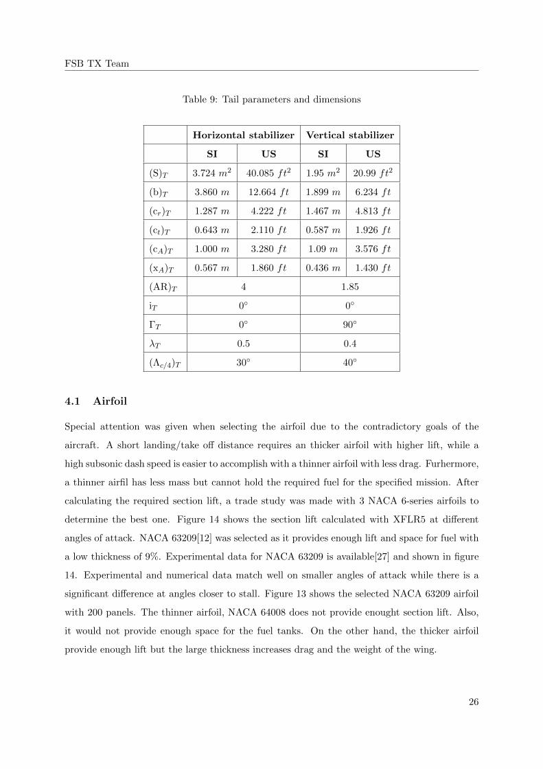
9 Tail parameters and dimensions . . . . . . . . . . . . . . . . . . . . . . . . . . . . 26

10 Tire loading . . . . . . . . . . . . . . . . . . . . . . . . . . . . . . . . . . . . . . . 36

11 Tire types . . . . . . . . . . . . . . . . . . . . . . . . . . . . . . . . . . . . . . . . 36

12 Strut dimensions . . . . . . . . . . . . . . . . . . . . . . . . . . . . . . . . . . . . 37

13 Component weight data . . . . . . . . . . . . . . . . . . . . . . . . . . . . . . . . 39

14 Stability derivative . . . . . . . . . . . . . . . . . . . . . . . . . . . . . . . . . . . 47

15 Take-off and landing requirements . . . . . . . . . . . . . . . . . . . . . . . . . . 52

16 Aircraft Specifications . . . . . . . . . . . . . . . . . . . . . . . . . . . . . . . . . 61

17 Required data for V-n diagram . . . . . . . . . . . . . . . . . . . . . . . . . . . . 70

18 Wing components . . . . . . . . . . . . . . . . . . . . . . . . . . . . . . . . . . . 72

19 Fuselage components . . . . . . . . . . . . . . . . . . . . . . . . . . . . . . . . . . 72

20 Vertical tail components . . . . . . . . . . . . . . . . . . . . . . . . . . . . . . . . 72

21 Materials and technologies for structural elements . . . . . . . . . . . . . . . . . 75

viii

FSB TX Team

Nomenclature

A A regression constant based on similar aircraft, [-]

ARoskam A regression constant [?], [-]

B B regression constant based on similar aircraft, [-]

BRoskam B regression [?], [-]

kf weight reduction coefficient for fuselage, [-]

klg weight reduction coefficient for landing gear, [-]

kt weight reduction coefficient for tail, [-]

kw weight reduction coefficient for wing, [-]

Mff total fuel fraction, [-]

WE empty weight of the aircraft, [lbs]

Wcrew weight of two pilots and their personal equipment, [lb]

Weq eqiupment weight, [lb]

Wfeq CLASS II fixed equipment weight, [lbs]

WPL payload weight, [lb]

Wpwr CLASS II powerplant weight, [lbs]

Wstruct CLASS II structure weight, [lbs]

WTOest estimated weight based on similar aricraft, [lbs]

A Aspect Ratio, [-]

br Wing span, [m]

CD Aircraft drag, [-]

CD0 Aircarft drag with CL = 0, [-]

ix

FSB TX Team

cLmax Max lift coefficient , [-]

CGR Climb gradient, [-]

CGR climb gradient, [rad]

e Oswald coefficient, [-]

h Aircraft altitude, [m]

h altitude, [m]

k1 constant, [-]

k2 constant, [-]

L/D Lift to drag ratio, [-]

L/D lift/drag ratio, [-]

nmax Load Factor, [-]

nmax Loading coefficient, [-]

Pdl parameter, [-]

RC Climb speed, [m/s]

S Wing surface, [m2]

(Λc/4)T tail sweep angle, [◦]

(Λc/4)w wing sweep angle, [◦]

(ΛLE)w wing leading edge, [◦]

(ΛTE)w wing trailing edge, [◦]

(AR)w wing aspect ratio, []

(AR)T tail aspect ratio, []

(cA)T tail MAC, [m]

x

FSB TX Team

(cA)w wing mean aerodinamic chord [MAC], [m]

(ct)T tail tip chord, [m]

(xA)T distance tail MAC, [m]

(xA)w distance wing MAC, [m]

ΓT tail dihedral, [◦]

Γw wing dihedral, [◦]

λT tail taper, []

λw wing taper, []

3s shock absorber efficiency, []

3t tire absorber efficiency, []

Xac Aerodynamic center

Xcg Center of gravity

CG center of gravity, []

ds diameter of shock absorber, [mm]

iT tail angle of incidence, [◦]

iw wing angle of incidence, [◦]

ls length of shock absorber, [mm]

MTOW maximum takeoff weight, [kg]

Ng load factor, []

PM static load on main gear, [kg]

PN static load on nosegear, [kg]

PNdin dynamic load on nosegear, [kg]

xi

FSB TX Team

ss stroke of the shock absorber, [mm]

Swet Aircraft surface, [m2]

VFfus fuselage fuel reservoir volume, [m3]

VFreq required fuel reservoir volume, [m3]

VFwing wing fuel reservoir volume, [m3]

WF required fuel weight, [kg]

wt touchdown rate, [fps]

WL landing weight, [kg]

WTO takeoff weight, [kg]

MAC mean aerodynamic chord, [mm]

MAC mean aerodynamic chord, [mm]

sFL Landing runway length, [m]

sTOG Take off runway length, [m]

T Take off thrust, [kN]

T/W Engine loading, [-]

T/W thrust to weight ratio, [-]

VA Approach speed, [m/s]

VA approach speed, [m/s]

Vcruise Cruise speed, [km/h]

Vn Maneuvering speed, [m/s]

VS Stall speed, [m/s]

VSL stall speed, [m/s]

xii

FSB TX Team

VTO Take off speed, [m/s]

W/S Wing loading, [N/m2]

q Dinamic pressure, [N/m2]

q dynamic pressure, [N/m2]

γ Angle of climb, [◦]

γ flight path angle, [◦]

Λ Bypass-ratio, [-]

Λ bypass-ratio, [-]

µg Ground friction coefficinet

µg friction coefficient, [-]

ρ Air density, [kg/m3]

ρ air density, [kg/m3]

xiii

FSB TX Team

1 Airplane configuration and mission analysis

1.1 Mission analysis

This airplane was made with respect to the mission given by the RFP, which can be divided

into 16 phases shown on the diagram below (figure 1). Every number on the diagram represents

one phase of the mission which will be discussed in detail later in the text.

Figure 1: Mission

Mission phases given by the RFP (Request for Proposal):

1) Warm up and taxi

2) Take off

3) Climb from the sea level to the cruise altitude

4) Cruise (150nm – BCA and BCM)

5) Tanker rendezvous at the altitude of 20000 ft at the speed of 300 KIAS

6) Air refueling simulation (20 minutes at the altitude of 20000ft, 250KIAS)

7) Climb from the altitude of 20000 ft to BCA (lowest fuel consumption regime)

8) Cruise at BCA with the BCM

9) Descent to the altitude of 15000ft

10) 20 minutes long air combat and maneuvering training (max 8-9 g)

11) Climb to the BCA (lowest fuel consumption)

1

FSB TX Team

12) Cruise (150NM BCM)

13) Descent on 10000ft

14) Loiter at the altitude of 10000 ft with optimum endurance speed (30 minutes or 10% of

total mission duration)

15) Descent to the sea level

16) Landing

For the purpose of weight estimation, it is necessary to mention that the aircraft will have no

external fuel tanks (”clean configuration“). The mission described above was used to determine

the airplanes which are meant to complete a similar mission, which gave us the information

about possible configuration solutions. Threshold and desirable values of some performances

were demanded by the RFP which will be shown in the table below, but since it isn’t possible to

maximize all of the performances, the final value of some airplane performance will depend on

previously determined objectives with respect to their importance. AHP method was used to

determine the level of importance of the objectives that were set earlier. Airplane performances

demanded by the RFP.

Table 1: RFP requirements

Performance Threshold value Objective value

Maximum loading at 15000ft 8 9

Ceiling 40000 50000

Runway length 8000 6000

Payload [lbs] 500 1000

Maximum range [NM] without refueling 1000 1500

Cruise speed [Ma] 0.7 0.8

Dash speed [Ma] 0.95 1.2

2

FSB TX Team

1.2 Aircraft configuration

1.2.1 Introduction

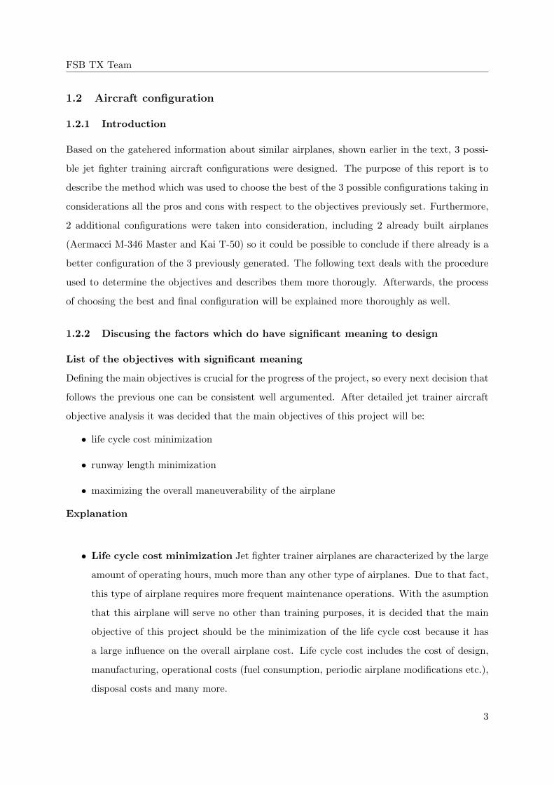
Based on the gatehered information about similar airplanes, shown earlier in the text, 3 possi-

ble jet fighter training aircraft configurations were designed. The purpose of this report is to

describe the method which was used to choose the best of the 3 possible configurations taking in

considerations all the pros and cons with respect to the objectives previously set. Furthermore,

2 additional configurations were taken into consideration, including 2 already built airplanes

(Aermacci M-346 Master and Kai T-50) so it could be possible to conclude if there already is a

better configuration of the 3 previously generated. The following text deals with the procedure

used to determine the objectives and describes them more thorougly. Afterwards, the process

of choosing the best and final configuration will be explained more thoroughly as well.

1.2.2 Discusing the factors which do have significant meaning to design

List of the objectives with significant meaning

Defining the main objectives is crucial for the progress of the project, so every next decision that

follows the previous one can be consistent well argumented. After detailed jet trainer aircraft

objective analysis it was decided that the main objectives of this project will be:

• life cycle cost minimization

• runway length minimization

• maximizing the overall maneuverability of the airplane

Explanation

• Life cycle cost minimization Jet fighter trainer airplanes are characterized by the large

amount of operating hours, much more than any other type of airplanes. Due to that fact,

this type of airplane requires more frequent maintenance operations. With the asumption

that this airplane will serve no other than training purposes, it is decided that the main

objective of this project should be the minimization of the life cycle cost because it has

a large influence on the overall airplane cost. Life cycle cost includes the cost of design,

manufacturing, operational costs (fuel consumption, periodic airplane modifications etc.),

disposal costs and many more.

3

FSB TX Team

• Runway length minimization Take-off and landing phases are critical in every mission

(civil or non-civil), due to the fact that they require a high level of engagement of the

pilot compared to all other phases of the mission. By minimizing the runway length, the

duration of those critical phases is reduced, which reliefs the pilot and reduces the need of

infrastructural investments

• Maximizing the overall maneuverability level Aircraft’s maneuverability level is

defined with the ability to change it’s attitude as fast as possible. Since the purpose of

this project is design of the new 5th generation jet fighter training aircraft, it was decided

that this airplane should have the highest possible maneuverability so it could reduce

pilot’s adjusting time, once he is done with the training process. The fact that the degree

of maneuverability grows with the increase of forces and moments acting upon the control

surfaces will be used later in the design process.

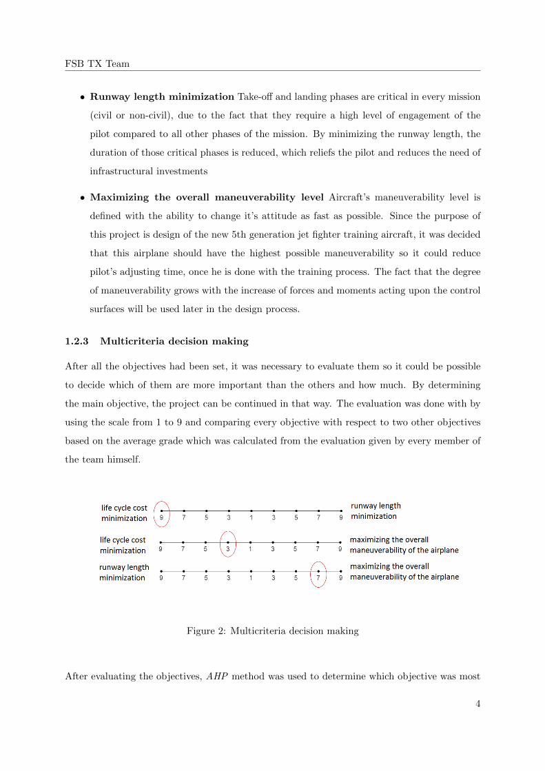
1.2.3 Multicriteria decision making

After all the objectives had been set, it was necessary to evaluate them so it could be possible

to decide which of them are more important than the others and how much. By determining

the main objective, the project can be continued in that way. The evaluation was done with by

using the scale from 1 to 9 and comparing every objective with respect to two other objectives

based on the average grade which was calculated from the evaluation given by every member of

the team himself.

Figure 2: Multicriteria decision making

After evaluating the objectives, AHP method was used to determine which objective was most

4

FSB TX Team

important. All the calculations of the given method were made using the MATLAB software,

which resulted with the following pie chart:

Figure 3: Objectives

1.2.4 General Aircraft Configuration

Based on similar aircraft and the given mission, it has been decided that only conventional

configurations will be considered since they are cheapest and easiest to manufacture. Additional

surfaces (eng. cannards) were rejected due to the additional drag that they produce. We will

now examine the advantages and disadvantages from certain elements to determine the final

configuration of the aircraft.

The following elements of the configuration will be examined:

• Wing type

• Wing position

• Stabilizing sufraces type

• Undercarrage type

5

FSB TX Team

1.2.5 Wing position

Table 2: Wing position

Table 3: Stability surfaces

Landing gear configuration While considering the posible landing gear configurations, it

has been decided that a conventional tricycle configuration will be used. Main landing gear

struts can be placed in the hull ori n the wings. Placing the main landing gear in the wing

means a higher lateral stability during take off and landing, but also longer struts. This in

term decreases the stiffness of the construction meaning that the construction would need to be

6

FSB TX Team

heavier. Furthermore, this would reduce the available space in the wings for the fuel reservoirs.

Finally, it has been decided that all the struts will be placed in the hull.

Engine location The RFP states that comertially available engines will be user since developing

a new engine for a smaller aircraft series would not be economical. In order to decrease the Life

Cycle Cost, one engines will be used. The best position to place the engines is the hull, with

intakes positioned at the root of the wing.

Intake position

Nose

+ good intake flow without aircraft interferance

− Long intake, higher mass, high friction losses

Underhull

+ no flow interference at higher angles of attack, possibility of placing an engine in the nose

− Front leg placement, danger in foreign object damage, intake flow interference, intake needs

to be 50 to 80% of the intake diameter above ground

Side of the hull

+ smaller hull dimensions from the above, no inlet interferance

− stability problem when inlets merge before the first stage of the compressor

Armpit

+ no foreign object damage during take off and landing, shorter inlet pipe, simplest construction

enableing the wing to be directly joined to the hull, best position to minimize maintenance time

(no need for ground equipment)

− Boundary layer interferance from hull and wings, sensitive to higher angles of attack and

sideslip

7

FSB TX Team

Figure 4: Configuration 1

Figure 5: Configuration 2

8

FSB TX Team

Figure 6: Configuration 3

Considered configurations Based on the above, three different configurations were made

(shown on images 4, 5 and 6). Also, two additional aircraft were considered, Kai T-50 and

M-346. Using the AHP method, the following priority vector diagram was calculated (figure 7)

Figure 7: Priority vector diagram

9

FSB TX Team

As seen on figure 7, configuration 2 was selected as the best configuration for the previously

determined objectives and will be further developed.

10

FSB TX Team

2 Weight estimation

This chapter shows weight estimation of military trainer described in previous chapters. RFP

stated objectives and thresholds which have to be fulfilled. Regarding those reqiurements, weight

estimation was conducted as a trade study. Biggest issue at the begining of conceptual design

of this aircraft was engine selection. After thorough research, five engines were selected (GE

F404, GE F414, GE F110, Snecma M88 and Honeywell F125). Data for these five engines was

aquired using Jane’s Aero Engines [20] and for them was weight estimation conducted.

2.1 Class I

Class I weight sizing was completed following iterative process as described in [1]. Fuel weight

was determined using fuel fractions in every phase of mission. After calculating fuel fractions

and fuel weight, empty weight was determined. Maximum takeoff weight was calculated as a

sum of all component weights. In summary, that was class I weight estimation and more detailed

estimation process follows.

According to [1], regression constants had to be determined using similar aircraft. These con-

stants are iportant for empty weight calculation. In [1], regression constants for military trainer

were

ARoskam = 0.6632

BRoskam = 0.8640(1)

Using data of similar aircraft, which are shown in table 4.

Table 4: Similar aircraft

Aircraft WTO [lbs] WE [lbs]

T-38 Talon 12092 7209

T-45 Goshawk 13393 9394

Hongdu L-15 Falcon 14330 9921

Alpha jet 15432 7661

Hawk T2 20062 10935

Because of time that has passed since Roskam Part 1 [1] was released, for similar aircraft were

11

FSB TX Team

chosen aircraft that don’t have large amount of composite and other newer and lighter materials.

That has been done so that process described in [1] can be applied to this project.

As it was previously stated, weight estimation is iterative process and West = 15432 lbs was

weight chosen for a beginning of iterative process. In figure 8 are shown regression curves based

on [1] and on similar aircraft, takeoff and empty weights of similar aircraft and beginning weight

estimation of iterative process.

WTO

[lbs] ×104

1.2 1.3 1.4 1.5 1.6 1.7 1.8 1.9 2 2.1

WE [l

bs]

103

104

105

Similar aircraftBeginning estimate, W

est

Regression lineRegression line - Roskam

Figure 8: Regression

Regression constants are last of all information that had to be aquired based on similar aircraft.

Having all neccessary data, fuel fractions can be calculated using equation

Mff =W1

WTO

16∏i=1

Wi+1

Wi(2)

Fuel fraction for air combat mission phase was calculated as described in Aircraft Design: A

Conceptual Approach [19] because [1] haven’t provided ways to calculate this particular mission

phase. After fuel weight, empty weight can be estimated. Using regression constants, linear

12

FSB TX Team

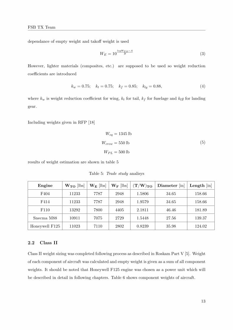
dependance of empty weight and takoff weight is used

WE = 10logWTO−A

B (3)

However, lighter materials (composites, etc.) are supposed to be used so weight reduction

coefficients are introduced

kw = 0.75; kt = 0.75; kf = 0.85; klg = 0.88, (4)

where kw is weight reduction coefficient for wing, kt for tail, kf for fuselage and klg for landing

gear.

Including weights given in RFP [18]

Weq = 1345 lb

Wcrew = 550 lb

WPL = 500 lb

(5)

results of weight estimation are shown in table 5

Table 5: Trade study analisys

Engine WTO [lbs] WE [lbs] WF [lbs] (T/W)TO Diameter [in] Length [in]

F404 11233 7787 2948 1.5806 34.65 158.66

F414 11233 7787 2948 1.9579 34.65 158.66

F110 13292 7800 4405 2.1811 46.46 181.89

Snecma M88 10911 7075 2729 1.5448 27.56 139.37

Honeywell F125 11023 7110 2802 0.8239 35.98 124.02

2.2 Class II

Class II weight sizing was completed following process as described in Roskam Part V [5]. Weight

of each component of aircraft was calculated and empty weight is given as a sum of all component

weights. It should be noted that Honeywell F125 engine was chosen as a power unit which will

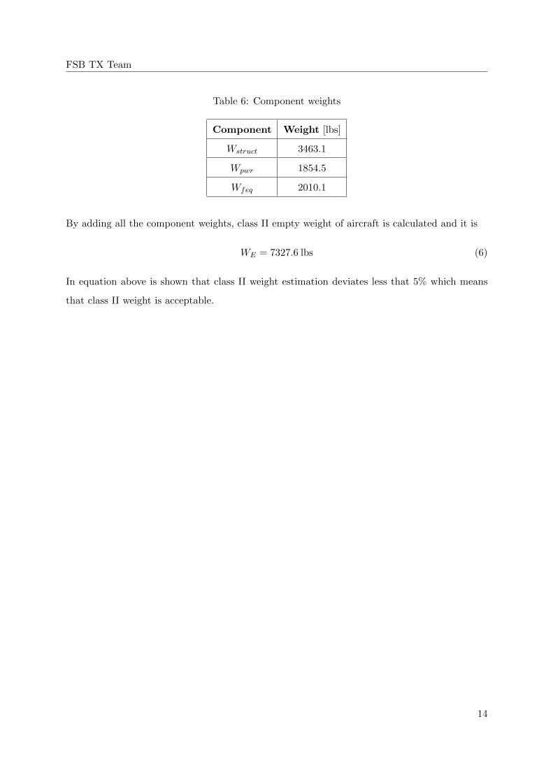
be described in detail in following chapters. Table 6 shows component weights of aircraft.

13

FSB TX Team

Table 6: Component weights

Component Weight [lbs]

Wstruct 3463.1

Wpwr 1854.5

Wfeq 2010.1

By adding all the component weights, class II empty weight of aircraft is calculated and it is

WE = 7327.6 lbs (6)

In equation above is shown that class II weight estimation deviates less that 5% which means

that class II weight is acceptable.

14

FSB TX Team

3 Performance estimation

3.1 Estimating wing area, take-off thrust and maximum lift coefficient

In order to meet the performance requirements defined in RFP, an estimation of wing area S,

take-off thrust T , maximum lift coefficient for clean, take-off and landing configuration cLmax as

much as aspect ratio A, is given in this chapter. The method has resulted in the determination

of a range of values of Wing Loading W/S, Thrust loading T/W , and maximum lift coefficient

CLmax, within which certain requirements are met. All set requirements and final solution were

shown in matching diagram.

3.1.1 Take-off requirements

Take-off and landing requirements are defined in RFP, and it includes adding take-off and

landing distance together for single engine aircraft. Besides that, these procedures are taken on

icy runway with maximum gross weight.

The take-off groundrun may be estimated from:

sTOG =k1 · (W/S)TO

ρ · [CLmax(k2 · (X/W )TO − µg)− 0.72CD0], (7)

with no wind and leveled runway. According to the requirements of the RFP, the aim is to

minimize the runway length so we decided that the runway length sTOG should be 457.2 m (1500

ft). Estimating is done for the standard day, with the runway friction coefficient µG=0.015 and

lift coefficient cLmax=1.4 in take-off configuration. The parameter k1 is 0.047 for jet engine,

with the estimated bypass ratio of 0.35, so the parameter k2 is

k2 = 0.75(5 + Λ

4 + Λ) = 0.9224. (8)

To determine the take-off conditions, the relationship between Thrust-to-Weight ratio and the

Wing Loading determines the formula

(T/W ) =

k1(W/S)

sTOG · ρ+ 0.72CD0 + µgCLmax

CLmaxk2. (9)

15

FSB TX Team

3.1.2 Landing requirements

Landing requirements for military aircraft are treated according to FAR 25 standard as well as

for civil aircraft above 5700 kg. To met these requirements, we have decided to minimize the

runway length, which is 6000 ft according to the RFP, and represents the runway length for

take-off and landing procedure. Estimated lift coefficient in landing configuration is cLmax=1.6.

Approach speed for FAR 25 standard is

VA =

√sFL0.3

= 67.617 m/s. (10)

Aircraft stall speed is

VSL =VA1.2

= 56.3475 m/s. (11)

And at the end, values that determine the landing parameters depend on the Wing Loading

according to the formula

(W/S) =V 2SL

2ρCLmaxL. (12)

3.1.3 Cruise requirements

The cruising speed is defined in the RFP specification. Since we have decided to minimize

costs, as we have already said, which is the opposite of maximizing cruising speed, we will take

a lower speed limit that meets the specification, and that is Macruise=0.7. At cruising speed

and altitude of 10058 m (33000 ft), with clear aircraft configuration and (W5/WTO)=0.9432,

Thrust-to-Weight ratio depends on the Wing Loading according to the formula

(T/W )n =qcombatCD0

WS+

WSn2max

qcombatπ Aeclean0.875. (13)

3.1.4 Maneuvering requirements

According to the requirements in the specification, it was decided to minimize the load factor

due to low cycle cost, so the load factor will be nmax=8. Maneuvering is carried out at altitude

of 4572 m (15000 ft) with a 50% of internal fuel capacity. With that amount of fuel, weight

16

FSB TX Team

ratio is (W11/WTO)=0.875. This requirements are determined for the standard day and clean

configuration. Thrust-to-Weight ratio is

(T/W )n =nmaxCD0

CLmax+nmaxCLmaxπAeclean

. (14)

3.1.5 Ceiling requirements

Operational ceiling for military trainer aircraft, is defined as an altitude at which it is still

possible to achieve positive Rate of Climb of 0.5 m/s (100 ft/min). Limit of the 12192 m (40000

ft) was chosen to reduce the structure load and cost of structure lifespan. Lift to Drag ratio is

(L/D)maxceiling =1

2

√π ·A · ecleanCD0clean

= 11.147. (15)

Thrust to weight ratio with the weight ratio (W4/WTO)=0.9509, is

(T/W )ceiling =RC√√√√√ 2

ρ

√CD0

πAeclean

0.9509(W/S)

+1

(L/D)maxceiling. (16)

3.1.6 Engine

After reviewing all commercially available engines, the Honeywell F125IN engine was selected.

Since the minimum required Thrust-to-Weight ratio is 0.8236, for the intended mass of 5000 kg,

engine provides enough force to meet all these requirements. Other engines that were reviewed,

provide more thrust than this one, but they were not chosen due to higher lifecycle cost of an

aircraft with higher thrust to weight ratio. The technical data of chosen engine is given in the

Table 7.

17

FSB TX Team

Table 7: F125IN Technical Data

Take-off thrust (Dry), N 25617

Take-off thrust (maximum afterburner), N 40383

Diameter, mm 914

Length, mm 3150

Weight, kg 618.5

Specific fuel consumption, mg/Ns 22

Cost, m$ 2,5

3.2 Trade study

In this Trade Study influence of lift coefficient on performance is analyzed. All of the following

diagrams were considered while deciding about appropriate performance point.

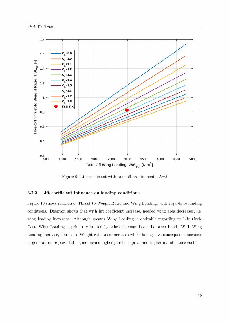
3.2.1 Lift coefficient influence on Take-Off

Diagram shows Thrust-to-Weight ratio vs. Wing Loading, for fixed take off distance and for

various lift coefficients. For example, for take-off lift coefficient of CL=0.9, acceptable are all

combinations above the blue line. It is concluded that with lift coefficient increase, required

thrust decreases while wing loading increases. Wing loading increase means decrease in wing

area. Wide span of this lines with CL=constant means more acceptable points. Regarding to

project goals, chosen lift coefficient value will be as low as possible with limits on thrust and

runway length.

18

FSB TX Team

Take-Off Wing Loading, W/STO

, [N/m2]

500 1000 1500 2000 2500 3000 3500 4000 4500 5000

Tak

e-O

ff T

hru

st-t

o-W

eig

ht

Rat

io, T

/WT

O, [

-]

0.2

0.4

0.6

0.8

1

1.2

1.4

1.6

1.8

CL=0.9

CL=1.0

CL=1.1

CL=1.2

CL=1.3

CL=1.4

CL=1.5

CL=1.6

CL=1.7

CL=1.8

FSB T-X

Figure 9: Lift coefficient with take-off requirements, A=5

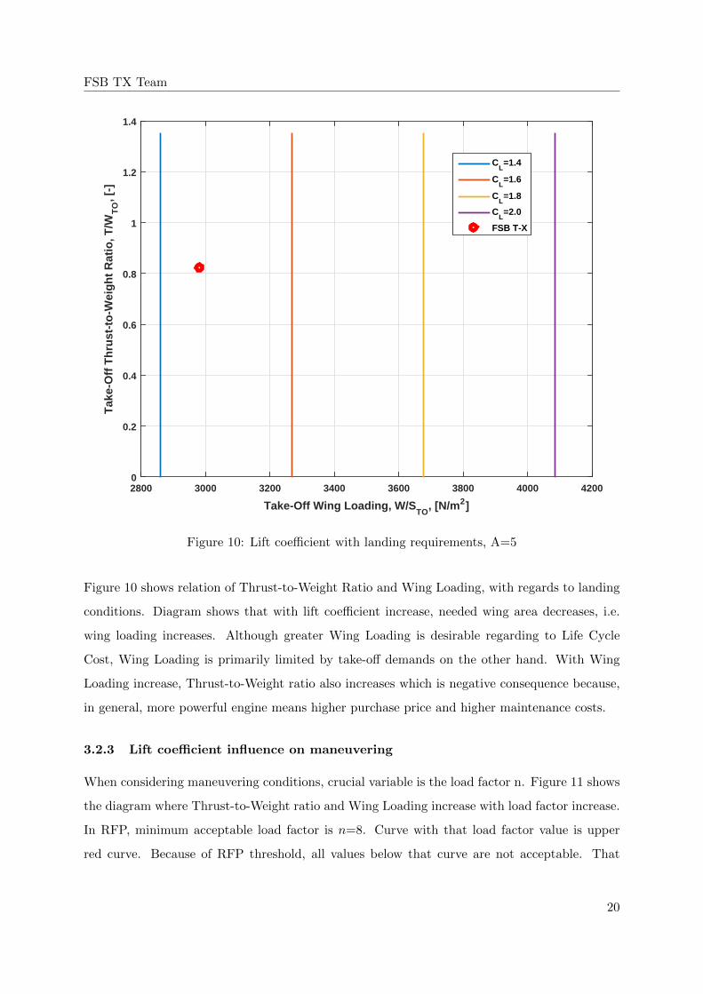
3.2.2 Lift coefficient influence on landing conditions

Figure 10 shows relation of Thrust-to-Weight Ratio and Wing Loading, with regards to landing

conditions. Diagram shows that with lift coefficient increase, needed wing area decreases, i.e.

wing loading increases. Although greater Wing Loading is desirable regarding to Life Cycle

Cost, Wing Loading is primarily limited by take-off demands on the other hand. With Wing

Loading increase, Thrust-to-Weight ratio also increases which is negative consequence because,

in general, more powerful engine means higher purchase price and higher maintenance costs.

19

FSB TX Team

Take-Off Wing Loading, W/STO

, [N/m2]

2800 3000 3200 3400 3600 3800 4000 4200

Tak

e-O

ff T

hru

st-t

o-W

eig

ht

Rat

io, T

/WT

O, [

-]

0

0.2

0.4

0.6

0.8

1

1.2

1.4

CL=1.4

CL=1.6

CL=1.8

CL=2.0

FSB T-X

Figure 10: Lift coefficient with landing requirements, A=5

Figure 10 shows relation of Thrust-to-Weight Ratio and Wing Loading, with regards to landing

conditions. Diagram shows that with lift coefficient increase, needed wing area decreases, i.e.

wing loading increases. Although greater Wing Loading is desirable regarding to Life Cycle

Cost, Wing Loading is primarily limited by take-off demands on the other hand. With Wing

Loading increase, Thrust-to-Weight ratio also increases which is negative consequence because,

in general, more powerful engine means higher purchase price and higher maintenance costs.

3.2.3 Lift coefficient influence on maneuvering

When considering maneuvering conditions, crucial variable is the load factor n. Figure 11 shows

the diagram where Thrust-to-Weight ratio and Wing Loading increase with load factor increase.

In RFP, minimum acceptable load factor is n=8. Curve with that load factor value is upper

red curve. Because of RFP threshold, all values below that curve are not acceptable. That

20

FSB TX Team

means that maneuvering requirements are excluding conditions and need to be fulfilled. Range

between of Wing Loading between 1000 and 1500 N/m2 is interesting because of minimum values

of Thrust-to-Weight ratio. Although is minimizing the Thrust-to-Weight ratio positive, that low

Wing Loading means relatively large, i.e. expensive wing.

Take-Off Wing Loading, W/STO

, [N/m2]

500 1000 1500 2000 2500 3000 3500 4000 4500 5000

Tak

e-O

ff T

hru

st-t

o-W

eig

ht

Rat

io, T

/WT

O, [

-]

0.2

0.4

0.6

0.8

1

1.2

1.4

1.6

n=4n=4.5n=5n=5.5n=6n=6.5n=7n=7.5n=8n=8.5n=9FSB T-X

Figure 11: Lift coefficient with maneuvering requirements, A=5

3.3 Matching diagram with all limitations

After calculation of initial values, range of Wing Loading and Thrust-to-Weight ratio is assumed.

Assumed range of Wing Loading is between 957 to 4788 N/m2 (20 to 100 psf). That range was

used to compute how Thrust-to-Weight ration depends on Wing Loading in maneuver. That

dependence is displayed on matching diagram with purple color (figure 12).

21

FSB TX Team

Take-Off Wing Loading, W/STO

, [N/m2]

500 1000 1500 2000 2500 3000 3500 4000 4500 5000

Tak

e-O

ff T

hru

st-t

o-W

eig

ht

Rat

io, T

/WT

O, [

-]

0

0.2

0.4

0.6

0.8

1

1.2

1.4

1.6Matching diagram

CLmaxTO

=1.4

CLmaxcr

=1.0

CLmaxceil

=1.0

CLmaxLDG

=1.6

CLn

=1.0

Engine F125INFinalAermacchi M346KAI T-50Northrop T-38

Figure 12: Matching diagram

Behavior of cruise parameters is shown with red curve, while ceiling parameters are shown with

green line. For take-off requirements, range of Thrust-to-Weight ratio is assumed and Wing

Loading is calculated. That dependence is illustrated with blue color in the matching diagram.

Matching diagram also shows the maximum values of Wing Loading during landing, which

decreases with shorter runway. That characteristic is illustrated black. Dashed pink line is

Thrust-to-Weight with maximum engine thrust. Orange, blue and green points are Thrust-to-

Weight ratios and Wing Loadings of similar aircraft. Characteristic point, i.e. Thrust-to-Weight

ratio and Wing Loading for this aircraft is selected iteratively. On first iteration of matching

diagram, few available of-the-shelf engines with enough performance are selected and drawn

to matching diagram. Because of great load factor in maneuvering and according to trade

study, demand on minimum load factor n=8 is also drawn to diagram. After that, full thrust

characteristic of Honeywell F125IN was added to diagram. Experimenting with combinations of

22

FSB TX Team

lift coefficients during take off and landing, as seen in trade study, CL for take off is reduced to

CL=1.4 for which the curve occurs nearly parallel to curve with constant n=8. With that data,

lift coefficient for landing is minimized (vertical line). In the end, other non-critical curves are

added to check all of the given flight requirements.

23

FSB TX Team

4 Wing and tail geometry

A trapezoid wing with a sweep of 30◦ (at 1/4 of the chord) was selected. A high sweep angle

is suitable for high subsonic speeds because it increases the value of the critical Mach number.

Unfortunately, a high sweep angle reduces the lift at lower speeds increasing the landing speed

and landing/take off distance. A variable sweep wing was considered, but ultimately rejected

because it would result in an increase in mass, maintenance complexity and Life cycle cost.

A mid wing configuration was selected as it provides the lowest interference drag and good

longitudinal stability. Cabin visibility is also excellent which is important for trainer aircraft.

Aspect ratio (AR)w = 5 was selected as it is a compromise between a low aspect ratio wing, with

a high roll rate and simple construction and a high aspect ratio wing, with a lower interference

drag.

The selected taper λw = 0.33 reduces the mass of the wing and gives a better wing load, mak-

ing the construction of the wing simpler. Furthermore, it provides better performance when

approaching stalling conditions.

A dihedral angle positively affects longitudinal stability, but since a feedback loop will be im-

plemented the dihedral angle Γ = 0◦ is selected to simplify the construction and manufacturing,

reducing the mass and Life cycle cost. Table 8 shows the specifications and dimensions of the

selected wing.

A standard configuration tail with an ”All-Moving” horizontal tail was selected because of

high subsonic speeds. This configuration reduces the mass and maintenance complexity of the

horizontal stabilizer. The dihedral angles of the ”All-Moving” horizontal tail is ΓHT = 0◦ to

simplify the construction. The vertical stabilizer is a standard configuration with a rudder.

Table 9 shows the specifications and dimensions of the selected tail.

24

FSB TX Team

Table 8: Wing parameters and dimensions

Parameter SI US

(S)w 16.5 m2 177 ft2

(b)w 9.08 m 29.80 ft

(cr)w 2.73 m 8.96 ft

(ct)w 0.90 m 2.96 ft

(cA)w 1.97 m 6.46 ft

(xA)w 1.28 m 4.20 ft

(AR)w 5

iw 0 ◦

Γw 0 ◦

λw 0.33

(Λc/4)w 30 ◦

(ΛLE)w 34.14 ◦

(ΛTE)w 15.38 ◦

25

FSB TX Team

Table 9: Tail parameters and dimensions

Horizontal stabilizer Vertical stabilizer

SI US SI US

(S)T 3.724 m2 40.085 ft2 1.95 m2 20.99 ft2

(b)T 3.860 m 12.664 ft 1.899 m 6.234 ft

(cr)T 1.287 m 4.222 ft 1.467 m 4.813 ft

(ct)T 0.643 m 2.110 ft 0.587 m 1.926 ft

(cA)T 1.000 m 3.280 ft 1.09 m 3.576 ft

(xA)T 0.567 m 1.860 ft 0.436 m 1.430 ft

(AR)T 4 1.85

iT 0◦ 0◦

ΓT 0◦ 90◦

λT 0.5 0.4

(Λc/4)T 30◦ 40◦

4.1 Airfoil

Special attention was given when selecting the airfoil due to the contradictory goals of the

aircraft. A short landing/take off distance requires an thicker airfoil with higher lift, while a

high subsonic dash speed is easier to accomplish with a thinner airfoil with less drag. Furhermore,

a thinner airfil has less mass but cannot hold the required fuel for the specified mission. After

calculating the required section lift, a trade study was made with 3 NACA 6-series airfoils to

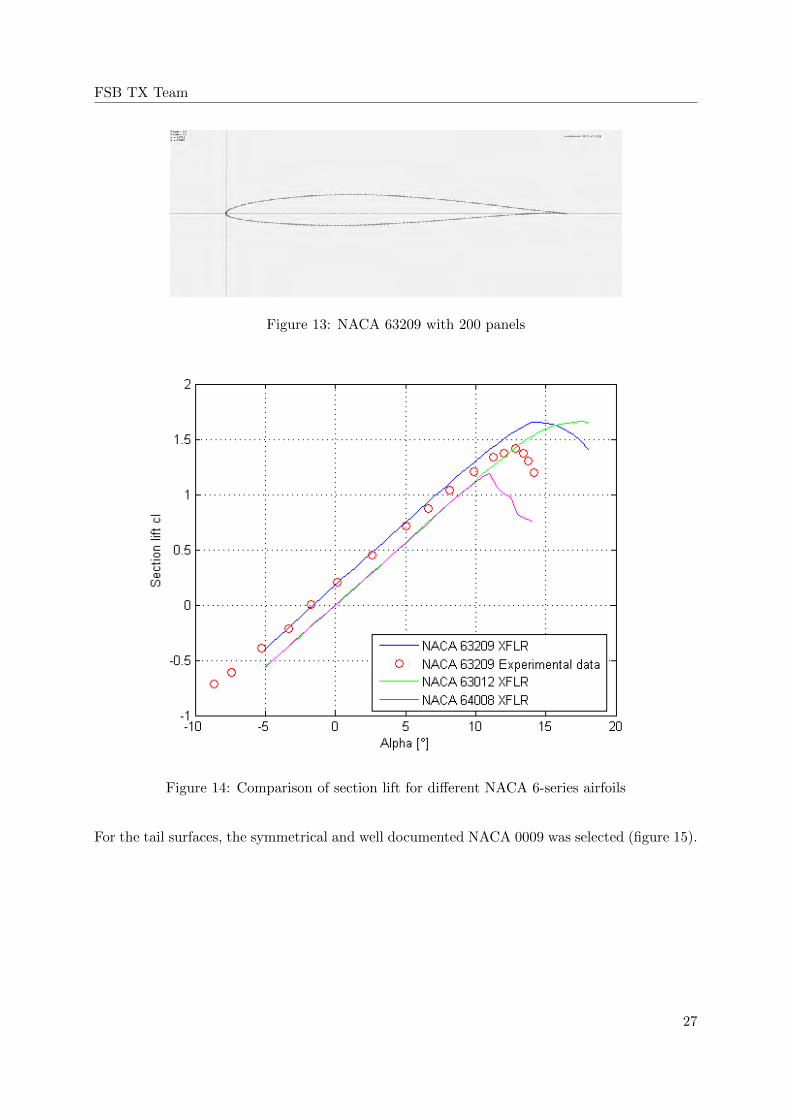
determine the best one. Figure 14 shows the section lift calculated with XFLR5 at different

angles of attack. NACA 63209[12] was selected as it provides enough lift and space for fuel with

a low thickness of 9%. Experimental data for NACA 63209 is available[27] and shown in figure

14. Experimental and numerical data match well on smaller angles of attack while there is a

significant difference at angles closer to stall. Figure 13 shows the selected NACA 63209 airfoil

with 200 panels. The thinner airfoil, NACA 64008 does not provide enought section lift. Also,

it would not provide enough space for the fuel tanks. On the other hand, the thicker airfoil

provide enough lift but the large thickness increases drag and the weight of the wing.

26

FSB TX Team

Figure 13: NACA 63209 with 200 panels

Figure 14: Comparison of section lift for different NACA 6-series airfoils

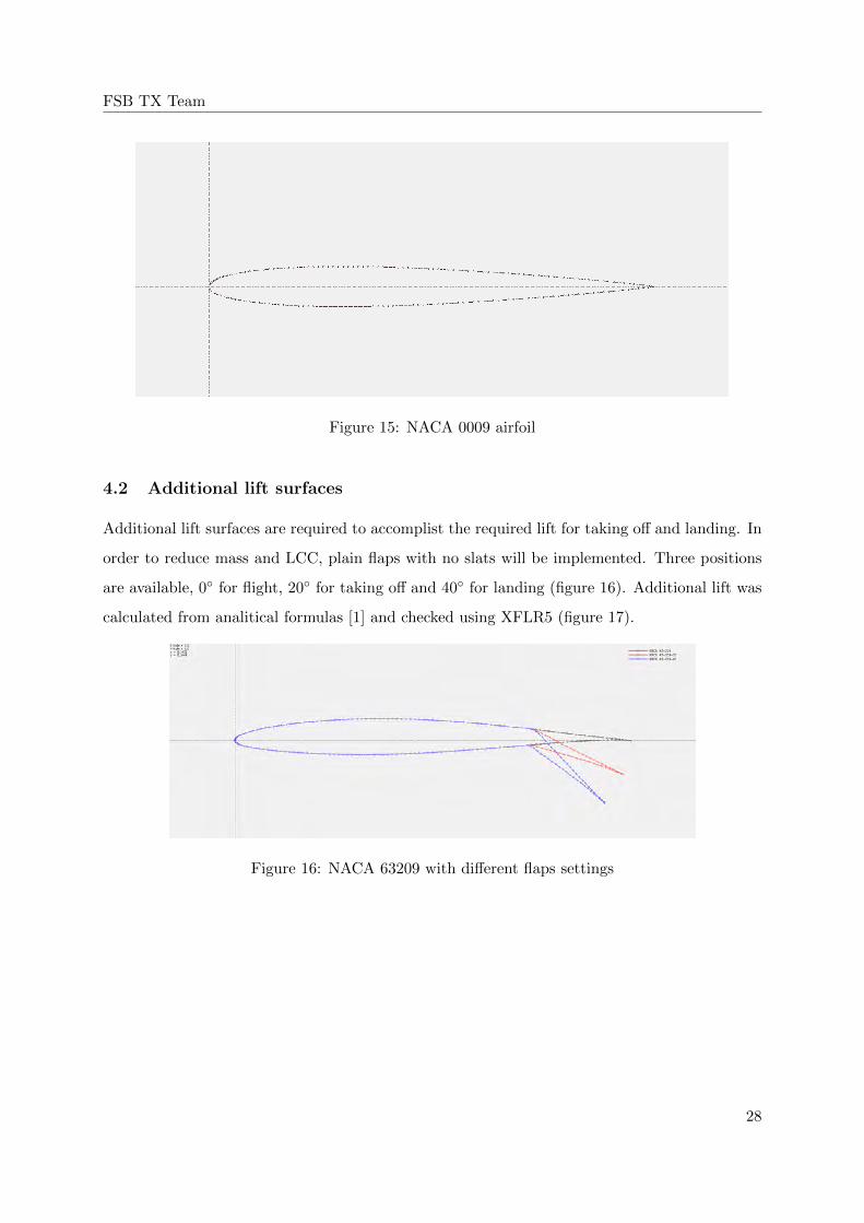
For the tail surfaces, the symmetrical and well documented NACA 0009 was selected (figure 15).

27

FSB TX Team

Figure 15: NACA 0009 airfoil

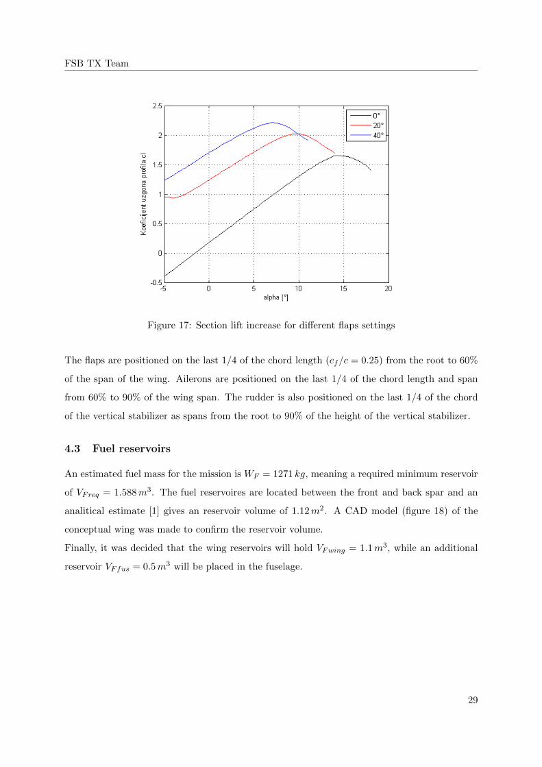
4.2 Additional lift surfaces

Additional lift surfaces are required to accomplist the required lift for taking off and landing. In

order to reduce mass and LCC, plain flaps with no slats will be implemented. Three positions

are available, 0◦ for flight, 20◦ for taking off and 40◦ for landing (figure 16). Additional lift was

calculated from analitical formulas [1] and checked using XFLR5 (figure 17).

Figure 16: NACA 63209 with different flaps settings

28

FSB TX Team

Figure 17: Section lift increase for different flaps settings

The flaps are positioned on the last 1/4 of the chord length (cf/c = 0.25) from the root to 60%

of the span of the wing. Ailerons are positioned on the last 1/4 of the chord length and span

from 60% to 90% of the wing span. The rudder is also positioned on the last 1/4 of the chord

of the vertical stabilizer as spans from the root to 90% of the height of the vertical stabilizer.

4.3 Fuel reservoirs

An estimated fuel mass for the mission is WF = 1271 kg, meaning a required minimum reservoir

of VFreq = 1.588m3. The fuel reservoires are located between the front and back spar and an

analitical estimate [1] gives an reservoir volume of 1.12m2. A CAD model (figure 18) of the

conceptual wing was made to confirm the reservoir volume.

Finally, it was decided that the wing reservoirs will hold VFwing = 1.1m3, while an additional

reservoir VFfus = 0.5m3 will be placed in the fuselage.

29

FSB TX Team

Figure 18: Wing model in SolidWorks

30

2731,76

901,52

677,26

431

4,43

272

2,90

45,

42

245,32

AA

BB

CC

4541,50

SECTION A-A

SECTION B-B

SECTION C-C

FSB TX Team

A

8 7

F

23456 1

B

E

D

C C

E

B

D

F

A

468 1357 2

DRAWN

CHK'D

APPV'D

MFG

Q.A

UNLESS OTHERWISE SPECIFIED:DIMENSIONS ARE IN MILLIMETERSSURFACE FINISH:TOLERANCES: LINEAR: ANGULAR:

FINISH: DEBURR AND BREAK SHARP EDGES

NAME SIGNATURE DATE

MATERIAL:

DO NOT SCALE DRAWING REVISION

TITLE:

DWG NO.

SCALE:1:50 SHEET 1 OF 1

A3

WEIGHT:

WING

1286,50

643,20

33,47°

AA

BB

1794,70

SECTION A-A

SECTION B-B

6 5 234 1

A

B

C

D

6 5 2 134

D

B

A

C

DRAWN

CHK'D

APPV'D

MFG

Q.A

UNLESS OTHERWISE SPECIFIED:DIMENSIONS ARE IN MILLIMETERSSURFACE FINISH:TOLERANCES: LINEAR: ANGULAR:

FINISH: DEBURR AND BREAK SHARP EDGES

NAME SIGNATURE DATE

MATERIAL:

DO NOT SCALE DRAWING REVISION

TITLE:

DWG NO.

SCALE:1:50 SHEET 1 OF 1

A4

WEIGHT:

FSB TX Team

Horizontal stabilizer

587

158,89

1467 362,99

43,68°

AA

BB

189

9

170

9,10

SECTION A-A

SECTION B-B

6 5 234 1

A

B

C

D

6 5 2 134

D

B

A

C

DRAWN

CHK'D

APPV'D

MFG

Q.A

UNLESS OTHERWISE SPECIFIED:DIMENSIONS ARE IN MILLIMETERSSURFACE FINISH:TOLERANCES: LINEAR: ANGULAR:

FINISH: DEBURR AND BREAK SHARP EDGES

NAME SIGNATURE DATE

MATERIAL:

DO NOT SCALE DRAWING REVISION

TITLE:

DWG NO.

SCALE:1:20 SHEET 1 OF 1

A4

WEIGHT:

FSB TX Team

Vertical stabilizer

FSB TX Team

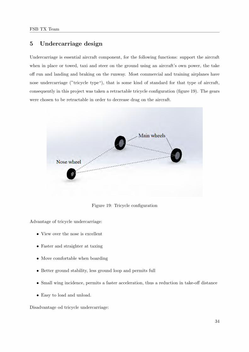
5 Undercarriage design

Undercarriage is essential aircraft component, for the following functions: support the aircraft

when in place or towed, taxi and steer on the ground using an aircraft’s own power, the take

off run and landing and braking on the runway. Most commercial and training airplanes have

nose undercarriage (”tricycle type“), that is some kind of standard for that type of aircraft,

consequently in this project was taken a retractable tricycle configuration (figure 19). The gears

were chosen to be retractable in order to decrease drag on the aircraft.

Figure 19: Tricycle configuration

Advantage of tricycle undercarriage:

• View over the nose is excellent

• Faster and straighter at taxing

• Move comfortable when boarding

• Better ground stability, less ground loop and permits full

• Small wing incidence, permits a faster acceleration, thus a reduction in take-off distance

• Easy to load and unload.

Disadvantage od tricycle undercarriage:

34

FSB TX Team

• Havier, because it takes greater load than tail wheel type

• Higher drag so must be retractable

• Static nose wheel reaction is about 6 − 16% MTOW due to c.g. position and the nose

unit must take 20 to 30% of the aircraft’s weight in a steady braked condition and it is

therefore relatively heavy

• High load on nose wheel makes it hard to rotate nose up on takeoff through an insufficient

elevator power

• There is tendency for the aircraft to sit on its tail.

5.1 Undercarriage placement

The main gear is palced 7.2m from aircraft nose, to carry majority of the load on landing. The

nose gear is paced 3.079m from the aircraft nose. To reduce weight and avoid additional frame

and bulkhead in fuselage, the nose gear will be attached on front pressure bulkhead of fuselage,

and main landing gear will be attached on fuselage frame.

5.2 Tire size estimation

Figure 20: F = 4.121m; L = 3.481m; M = 0.44m; N = 3.681m; J = 1.37m

35

FSB TX Team

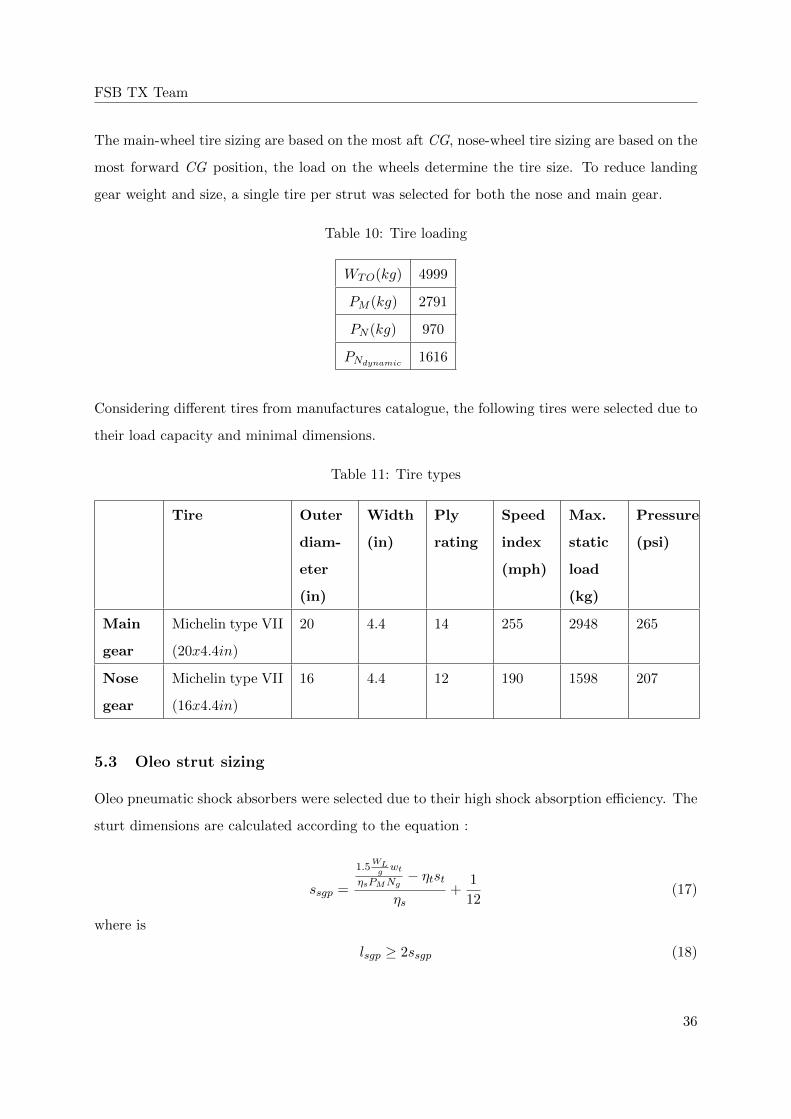
The main-wheel tire sizing are based on the most aft CG, nose-wheel tire sizing are based on the

most forward CG position, the load on the wheels determine the tire size. To reduce landing

gear weight and size, a single tire per strut was selected for both the nose and main gear.

Table 10: Tire loading

WTO(kg) 4999

PM (kg) 2791

PN (kg) 970

PNdynamic 1616

Considering different tires from manufactures catalogue, the following tires were selected due to

their load capacity and minimal dimensions.

Table 11: Tire types

Tire Outer

diam-

eter

(in)

Width

(in)

Ply

rating

Speed

index

(mph)

Max.

static

load

(kg)

Pressure

(psi)

Main

gear

Michelin type VII

(20x4.4in)

20 4.4 14 255 2948 265

Nose

gear

Michelin type VII

(16x4.4in)

16 4.4 12 190 1598 207

5.3 Oleo strut sizing

Oleo pneumatic shock absorbers were selected due to their high shock absorption efficiency. The

sturt dimensions are calculated according to the equation :

ssgp =

1.5WLgwt

ηsPMNg− ηtst

ηs+

1

12(17)

where is

lsgp ≥ 2ssgp (18)

36

FSB TX Team

Table 12: Strut dimensions

Nose strut Main strut

Ng 5 5

wt 13ft/s 13ft/s

ηt 0.47 0.47

ηs 0.8 0.8

Ss 267mm 398mm

ls 534mm 796mm

ds 48mm 73mm

and

ds = 0.041 + 0.0025√PM . (19)

5.4 Undercarriage retraction and stow

After evaluation size of tires and shock absorbers we are able to find appropriates way of retrac-

tion of undercarriage and place in fuselage to stow wheels and struts (figure 21).

Figure 21: Undercarriage retraction

The nose strut will be retracted in fuselage bay between the radar and cabin bulkhead. The

main struts will be retracted in side of fuselage, extended construction of intake.

37

FSB TX Team

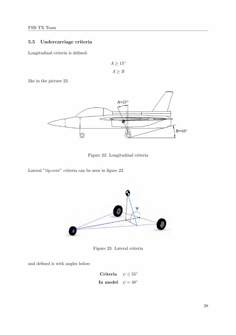
5.5 Undercarriage criteria

Longitudinal criteria is defined:

A ≥ 15◦

A ≥ B

like in the picture 22.

Figure 22: Longitudinal criteria

Lateral ”tip-over” criteria can be seen in figure 23.

Figure 23: Lateral criteria

and defined is with angles below:

Criteria ψ ≤ 55◦

In model ψ = 48◦

38

FSB TX Team

6 Weight and balance

The purpose of this chapter is to perform the weight and balance analysis of aircraft. A com-

ponent weight buildup was performed to improve the accuracy of the total aircraft weight and

determination of CG travel.

6.1 Component weight estimation

The weight of the components is determined by aircraft of a similar purpose, from statistically

known component weight data.

Table 13: Component weight data

Component Weight (kg)

Engine 620

Wing 487

Empennage 142

Fuselage 886

Undercarriage 266

Fixed equipment 827

Empty weight 3228

Crew 250

Trapped fuel and oil 25

Operating empty weight 3503

Payload 225

Fuel 1271

Take off weight 4999

6.2 CG travel

The following chart (figure 24) show weight and balance travel of the aircraft. Chart showes

different loading conditions of aircraft, and for each condition, associated weight and center of

gravity. For all loading conditions CG travel is less than 7% of M.A.C. The aircraft has the

ability to fly from one military base to another with only one crew member.

39

FSB TX Team

Figure 24: Weight and balance travel

Figure 25: Side view of CG positions

40

FSB TX Team

7 Stability and control analysis

The process of aircraft stability analysis is divided into two parts: Class 1 and Class 2 (Class

2 including dynamic stability analysis). Both of the methods used for the stability analysis will

be shown in the further text.

7.1 Class 1 method - static stability and control

7.1.1 Longitudinal static stability and control

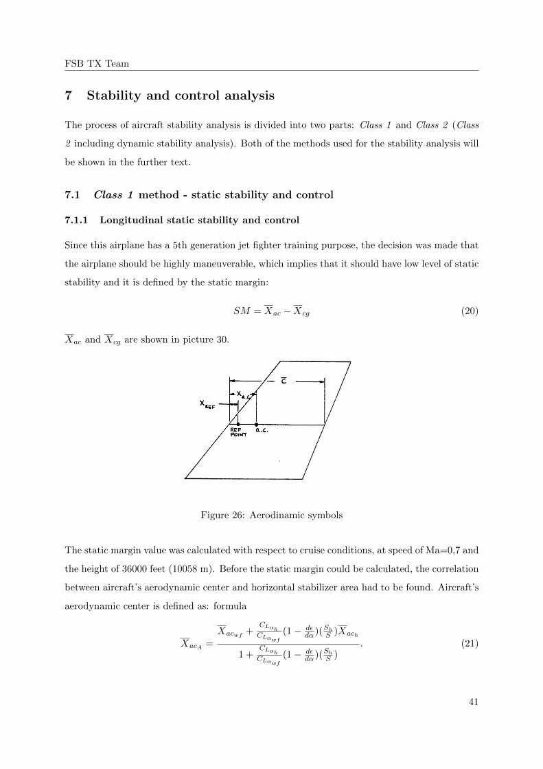
Since this airplane has a 5th generation jet fighter training purpose, the decision was made that

the airplane should be highly maneuverable, which implies that it should have low level of static

stability and it is defined by the static margin:

SM = Xac −Xcg (20)

Xac and Xcg are shown in picture 30.

Figure 26: Aerodinamic symbols

The static margin value was calculated with respect to cruise conditions, at speed of Ma=0,7 and

the height of 36000 feet (10058 m). Before the static margin could be calculated, the correlation

between aircraft’s aerodynamic center and horizontal stabilizer area had to be found. Aircraft’s

aerodynamic center is defined as: formula

XacA =Xacwf +

CLαhCLαwf

(1− dεdα)(ShS )Xach

1 +CLαhCLαwf

(1− dεdα)(ShS )

. (21)

41

FSB TX Team

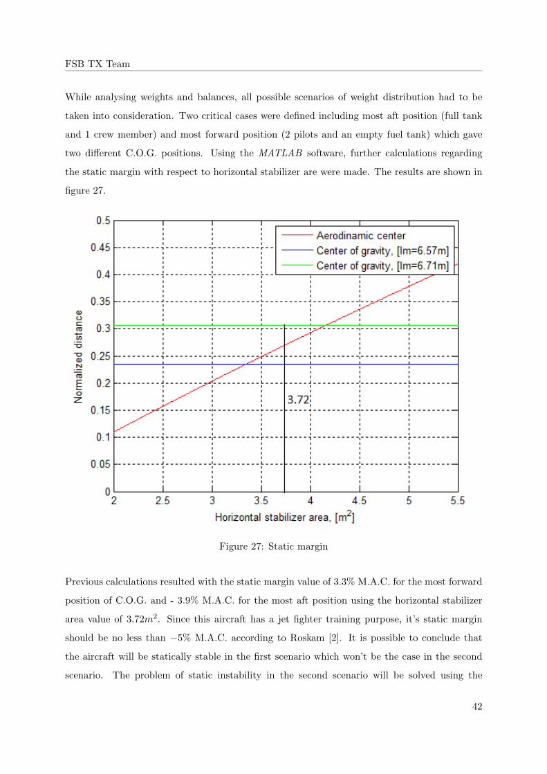
While analysing weights and balances, all possible scenarios of weight distribution had to be

taken into consideration. Two critical cases were defined including most aft position (full tank

and 1 crew member) and most forward position (2 pilots and an empty fuel tank) which gave

two different C.O.G. positions. Using the MATLAB software, further calculations regarding

the static margin with respect to horizontal stabilizer are were made. The results are shown in

figure 27.

Figure 27: Static margin

Previous calculations resulted with the static margin value of 3.3% M.A.C. for the most forward

position of C.O.G. and - 3.9% M.A.C. for the most aft position using the horizontal stabilizer

area value of 3.72m2. Since this aircraft has a jet fighter training purpose, it’s static margin

should be no less than −5% M.A.C. according to Roskam [2]. It is possible to conclude that

the aircraft will be statically stable in the first scenario which won’t be the case in the second

scenario. The problem of static instability in the second scenario will be solved using the

42

FSB TX Team

closed loop flight control system. The feedback gain value of 1.77◦/◦ needed to compensate the

longitudinal instability problem for the most aft position of the C.O.G. was found satisfactory

since it doesn’t exceed maximum feedback gain value of 5◦/◦ [2]

kα =(∆SM)CLα

Cmδe. (22)

Interconnection between the horizontal stabilizer area and longitudinal feedback gain value can

be found in figures 28.

Figure 28: Feedback gain

Using the horizontal stabilizer area value Sh = 3.72m2, following longitudinal feedback gains

for the most forward and most aft positions were found:

(kα)forward = −0.33◦, (23)

(kα)aft = −1.77◦. (24)

43

FSB TX Team

7.1.2 Lateral static stability and control

After defining the yaw moment derivative due to sideslip angle:

Cnβ = Cnβw + Cnβf + Cnβv , (25)

it is possible to calculate the rudder feedback gain value, defined as:

kβ =(∆Cnβ )

Cnδr(26)

Interconnection between the vertical stabilizer area and longitudinal feedback area is shown in

the figure 29.

Figure 29: Rudder feedback gain

It was found that the vertical stabilizer didn’t give enough contribution to directional stability

(the rudder feedback gain value exceeded 5◦/degree), it’s surface had to be increased enough

to result with the satisfactory value of rudder feedback gain. Due to the difference more than

44

FSB TX Team

10% from the original value of the vertical stabilizer, center of gravity had to be recalculated

and it was found out that it moved backwards for a very small value, so the calculations could

be continued. Furthermore, the rudder feedback gain value was found to be satisfactory, but

still pretty high, which wasn’t considered to be a problem since it should result in high lateral

maneuverability. Both, longitudinal and directional static stability calculations were made using

the MATLAB 2015 software.

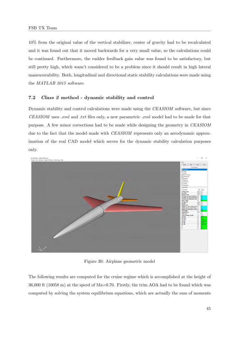
7.2 Class 2 method - dynamic stability and control

Dynamic stability and control calculations were made using the CEASIOM software, but since

CEASIOM uses .xml and .txt files only, a new parametric .xml model had to be made for that

purpose. A few minor corrections had to be made while designing the geometry in CEASIOM

due to the fact that the model made with CEASIOM represents only an aerodynamic approx-

imation of the real CAD model which serves for the dynamic stability calculation purposes

only.

Figure 30: Airplane geometric model

The following results are computed for the cruise regime which is accomplished at the height of

36,000 ft (10058 m) at the speed of Ma=0.70. Firstly, the trim AOA had to be found which was

computed by solving the system equilibrium equations, which are actually the sum of moments

45

FSB TX Team

and forces acting upon the aircraft during the cruise regime. The trimmed angle of attack value

was found to be [αtrim] = 0.86◦, with the corresponding value of elevator deflection which was

found to be [δe] = 9◦.

Now, when the trimmed AoA and elevator deflection are found, it is posible to extract the

stability derivatives using the CEASIOM software. Stability derivatives can be easely read in

figure below:

Figure 31: Ceasiom derivative

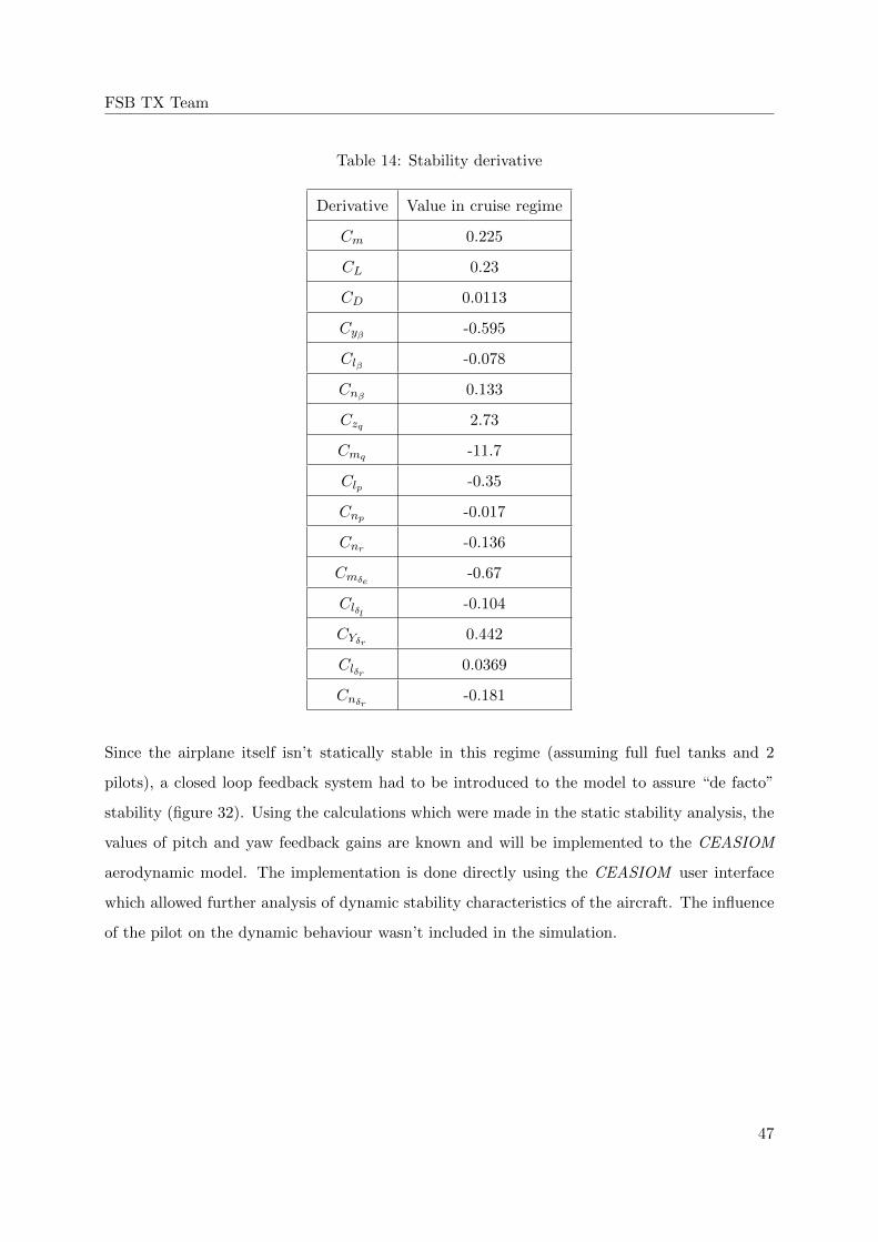
The following table contains dynamic stability gradients for the cruise regime mentioned earlier.

46

FSB TX Team

Table 14: Stability derivative

Derivative Value in cruise regime

Cm 0.225

CL 0.23

CD 0.0113

Cyβ -0.595

Clβ -0.078

Cnβ 0.133

Czq 2.73

Cmq -11.7

Clp -0.35

Cnp -0.017

Cnr -0.136

Cmδe -0.67

Clδl -0.104

CYδr 0.442

Clδr 0.0369

Cnδr -0.181

Since the airplane itself isn’t statically stable in this regime (assuming full fuel tanks and 2

pilots), a closed loop feedback system had to be introduced to the model to assure “de facto”

stability (figure 32). Using the calculations which were made in the static stability analysis, the

values of pitch and yaw feedback gains are known and will be implemented to the CEASIOM

aerodynamic model. The implementation is done directly using the CEASIOM user interface

which allowed further analysis of dynamic stability characteristics of the aircraft. The influence

of the pilot on the dynamic behaviour wasn’t included in the simulation.

47

FSB TX Team

Figure 32: Closed loop feedback system

Once the feedback gain values for pitch and yaw were introduced to the model, the stability

criteria calculations according to MIL-F-8785-C, Class IV (high maneuverability airplanes) stan-

dard could be completed. Furthermore, the results for the phugoid mode, roll, spiral, and dutch

roll mode will be shown, comparing the values with and without the closed loop flight control

system (figure 32). Various feedback gain values for the yaw and pitch to determine which value

would give the best response results. After the analysis had been done, three feedback gain

values were chosen. The yaw feedback gain value was found to give the best results at 4.9, pitch

feedback gain value is 1.45 and roll feedback gain value was only 1.

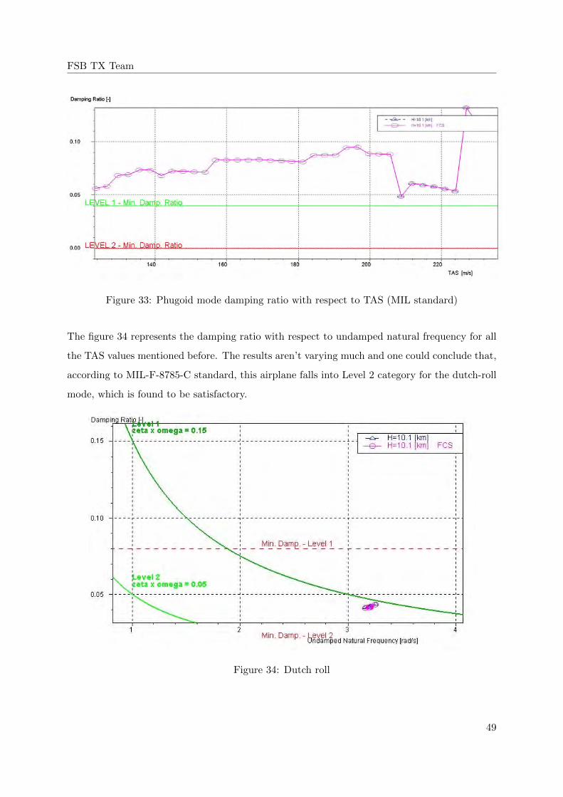
The picture 33 represents the graph of damping ratio with respect to TAS, with minimum damp-

ing ratio limit according to MIL standard MIL-F-8785-C for high maneuverability airplanes. The

aircraft shows satisfactory results for all TAS values taken into consideration.

48

FSB TX Team

Figure 33: Phugoid mode damping ratio with respect to TAS (MIL standard)

The figure 34 represents the damping ratio with respect to undamped natural frequency for all

the TAS values mentioned before. The results aren’t varying much and one could conclude that,

according to MIL-F-8785-C standard, this airplane falls into Level 2 category for the dutch-roll

mode, which is found to be satisfactory.

Figure 34: Dutch roll

49

FSB TX Team

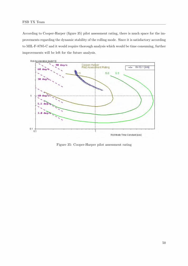
According to Cooper-Harper (figure 35) pilot assessment rating, there is much space for the im-

provements regarding the dynamic stability of the rolling mode. Since it is satisfactory according

to MIL-F-8785-C and it would require thorough analysis which would be time consuming, further

improvements will be left for the future analysis.

Figure 35: Cooper-Harper pilot assessment rating

50

FSB TX Team

8 Aircraft Performance

Performance analysis consists of a number of cases required for the current proposal. First

case includes take-off and landing distance at max gross weight including standard day and icy

runway balanced field length at sea level. Since this is a single-engine aircraft, runway length

requirements would be approximated by adding take-off and landing distance together. Second

case will show climb and ceiling performance. Third case demonstrates aircraft maneuvering

at 4572 m (15000 ft) within several examples of load factor. Fourth case demonstrates cruise,

range and endurance requirements. Besides all of this cases, this chapter includes maximum

Mach Number at 10972.8 m (36000 ft), 1-g and 5-g Maximum Thrust Specific Excess Power

Envelope, Energy Maneuverability Diagram at 15,000 ft MSL, L/D vs Mach at 10972.8 m (36000

ft) and V-n diagram showing response to 9.144 m/s (30 ft/s) equivalent sharp-edged vertical

gust.

8.1 Take-off and Landing distance requirements

Take-off and landing requirements are one of the most critical variables that determined the air-

craft layout. This requirements depends on aircraft aerodynamics, powerful engine and weight.

All this requirements are considered on icy runway with maximum gross weight of the aircraft.

To perform take-off and landing analysis, key aircraft speeds must be determined. Minimum

speed is 1.1/1.2 higher than aircraft stall speed in Take-off/Landing configuration. All values

according take-off and landing requirements are given in Table 15.

51

FSB TX Team

Table 15: Take-off and landing requirements

TAKE-OFF LANDING

Vstall, m/s 58.953 55.149

VLOF1, m/s 64.849 -

VLOF2 to pass 50ft obstacle, m/s 76.639 -

VTD, m/s - 62.782

VA, m/s - 66.178

sTOG, m 292.609 -

sTO with 50ft obstacle, m 408.686 -

sAIR from 50ft obstacle, m - 375.515

sLG, m - 502.010

sL=sAIR+sLG, m - 877.526

As can be seen from the Table 15, adding take-off and landing distance together is equal to

sTO+sL=1286.212 m or 4219.804 ft, which meets RFP conditions.

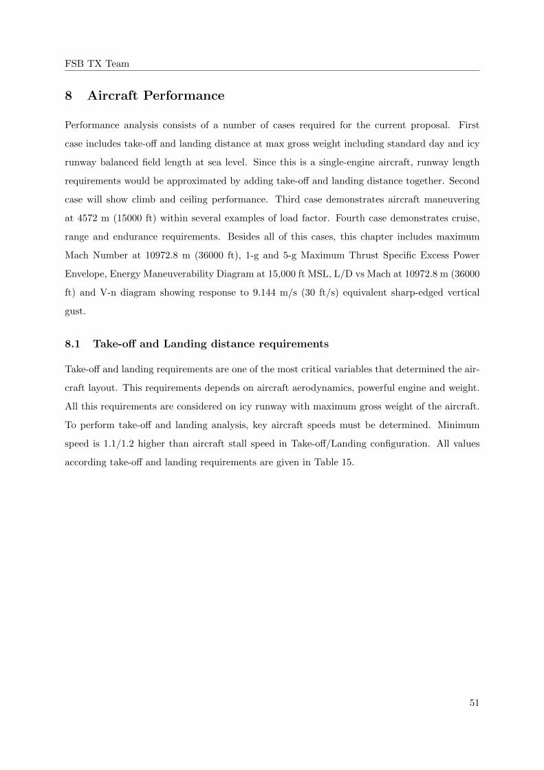
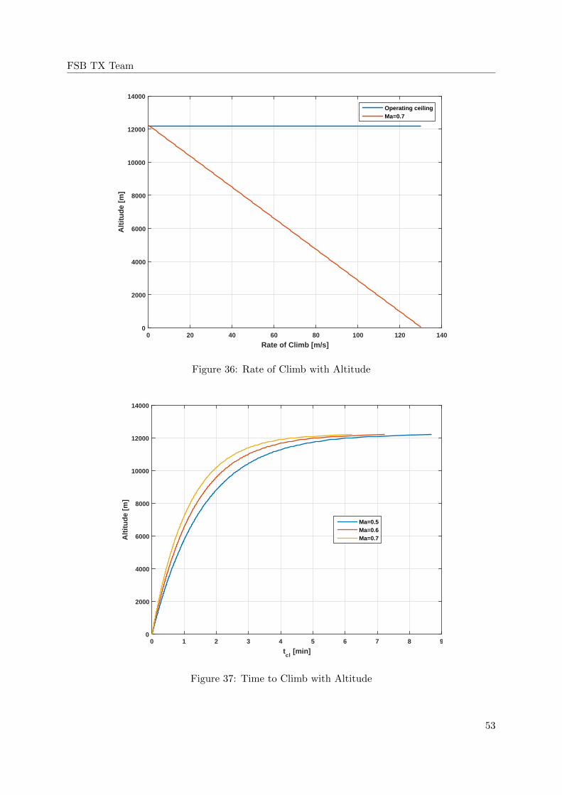
8.2 Climb

Climb performance is shown on Figure 36 and 37. It demonstrates climb performance with

maximum gross weight. Rate of Climb is shown after take-off, in clear configuration with Mach

number 0.5 and 0.7 as well as time to climb. Maximum rate of climb is reachable at altitude of

0 m with higher possible Mach number. Time to 10973 m is 4.5 min at an initial climb rate of

180 m/s.

52

FSB TX Team

Rate of Climb [m/s]0 20 40 60 80 100 120 140

Alt

itu

de

[m]

0

2000

4000

6000

8000

10000

12000

14000

Operating ceilingMa=0.7

Figure 36: Rate of Climb with Altitude

tcl

[min]0 1 2 3 4 5 6 7 8 9

Alt

itu

de

[m]

0

2000

4000

6000

8000

10000

12000

14000

Ma=0.5Ma=0.6Ma=0.7

Figure 37: Time to Climb with Altitude

53

FSB TX Team

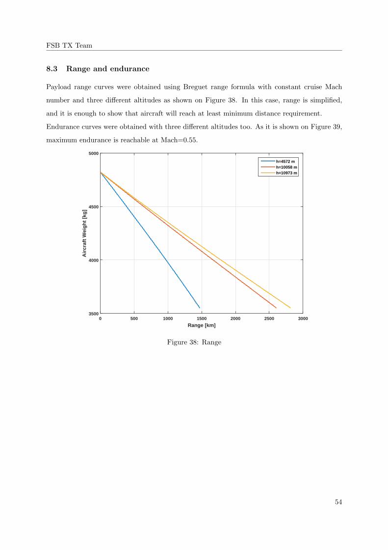
8.3 Range and endurance

Payload range curves were obtained using Breguet range formula with constant cruise Mach

number and three different altitudes as shown on Figure 38. In this case, range is simplified,

and it is enough to show that aircraft will reach at least minimum distance requirement.

Endurance curves were obtained with three different altitudes too. As it is shown on Figure 39,

maximum endurance is reachable at Mach=0.55.

Range [km]0 500 1000 1500 2000 2500 3000

Air

craf

t W

eig

ht

[kg

]

3500

4000

4500

5000

h=4572 mh=10058 mh=10973 m

Figure 38: Range

54

FSB TX Team

Ma0.4 0.45 0.5 0.55 0.6 0.65 0.7 0.75 0.8 0.85 0.9

En

du

ran

ce [

h]

1

1.5

2

2.5

3

3.5

4

4.5

h=4572 mh=10058 mh=10973 m

Figure 39: Endurance

8.4 Maximum Mach Number at 10058 m (36000 ft) and wave drag

Wave drag was analysed with OpenVSP software (Figure 40). Drag below critical Mach number

can be computed from aerodynamic equations. Wave drag can be analysed with OpenVSP

software for Mach greater than 1.0. Numbers around Mach 1 are difficult to compute and wave

drag is more accurate for higher Mach values.

55

FSB TX Team

Figure 40: Wave Drag shown in OpenVSP

Because of that, in transonic flight, total drag needs to be approximated by following procedure:

1. first point is where the wave drag starts to grow from 0, on diagram that is at Mach 0.85

2. most accurate supersonic point is the drag value at Mach 1.2.

3. with rest of the points as orientation values, continuous curve is drawn.

That analysis provides enough accurate results for this stage of design. 41 shows the result of

described procedure. Except total drag, on 41 is the maximum thrust expressed as corresponding

drag coefficient value which can be achieved with this aircraft and chosen engine. Intersection

of orange and black curve is around Mach 0.95 which represents the maximum Mach number at

36,000 feet. That is also the Dash speed of the aircraft in level flight.

56

FSB TX Team

Figure 41: Drag coefficient with Mach number

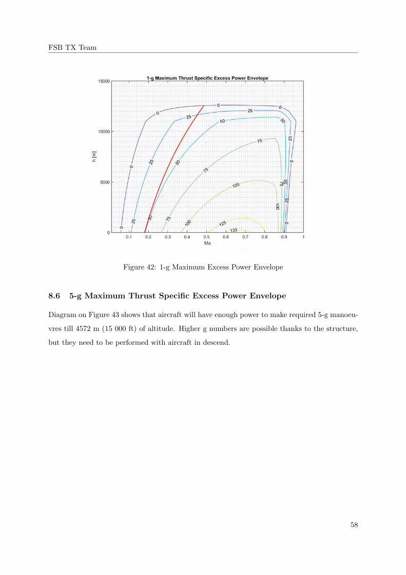
8.5 1-g Maximum Thrust Specific Excess Power Envelope

Given diagram on Figure 42 shows that aircraft has enough power to fly at the large span of

speeds and heights. Maximum (dash) speed is at Ma=0.95, and maximum altitude is around

10058 m (40 000 ft). Red line represents stall speed. Values on the circular lines represent

constant available Rate of Climb. Diagram represents operative envelope with operative ceiling

of 12192 m (40000 ft).

57

FSB TX Team

Figure 42: 1-g Maximum Excess Power Envelope

8.6 5-g Maximum Thrust Specific Excess Power Envelope

Diagram on Figure 43 shows that aircraft will have enough power to make required 5-g manoeu-

vres till 4572 m (15 000 ft) of altitude. Higher g numbers are possible thanks to the structure,

but they need to be performed with aircraft in descend.

58

FSB TX Team

Figure 43: 5-g Maximum Excess Power Envelope

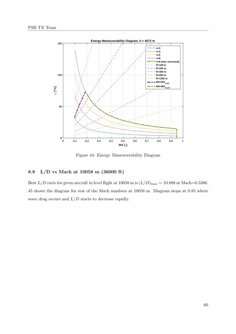
8.7 Energy Maneuverability Diagram at 4572 m MSL

To demonstrate aircraft maneuverability, it is important to show characteristics such as turn

radius and turn rate. Since this is trainer aircraft, which will show the characteristics of some

combat aircraft, it is necessary to show that it will be able to achieve small turning radius as well

as high turning speeds. This diagram shows relation between turn rate in degrees per second

and Mach Number. Full lines are for constant g-load, while dashed lines are for constant turn

radii in meters. Bold dashed lines represent the limits – from left side limit is stall speed, from

right side maximum speed (Mach Number) and from above is maximum sustained load on a

structure.

59

FSB TX Team

MA [-]0 0.1 0.2 0.3 0.4 0.5 0.6 0.7 0.8 0.9 1

ψ [°

/s]

0

50

100

150Energy Maneuverability Diagram, h = 4572 m

n=2n=4n=6n=8n=8 (max structural)R=100 mR=200 mR=300 mR=600 mR=1200 mMA=MA

s ta ll

MA=MAdash

Figure 44: Energy Maneuverability Diagram

8.8 L/D vs Mach at 10058 m (36000 ft)

Best L/D ratio for given aircraft in level flight at 10058 m is (L/D)max = 10.888 at Mach=0.5386.

45 shows the diagram for rest of the Mach numbers at 10058 m. Diagram stops at 0.85 where

wave drag occurs and L/D starts to decrease rapidly.

60

FSB TX Team

Figure 45: L/D with Mach number

Table 16: Aircraft Specifications

Dash speed at 10973 m, - 0.95M

Cruise speed at 10973 m, - 0.7M

Maximum Range at 10058 m, km 2800

Maximum Endurance at 10973 m, h 4.4

Maximum Rate of Climb (Initial), m/s 130

Service ceiling, m 12192

Take-off runway length, m 408.69

Landing runway length, m 877.53

Sustained g at 4572 m MSL, - 8

Payload, kg 226.8

61

FSB TX Team

9 Cost estimation

In this chapter, we will estimate the total life cycle cost of the aircraft, further dividing it into

non-recurring cost such as research, development and testing as well as recurring cost such as

acquisition, operation and disposal costs[1]. Per unit production cost, as well as per unit flyaway

cost will be estimated. All presented estimates are expressed in 2018 USD.

9.1 Research, Development, Test and Evaluation cost

The research, development, test and evaluation (RDTE) cost is a non-recurring cost that ac-

counts for most of the cost of an aircraft program The following assumptions are made:

• 8 aircraft produced for RTDE of which one is an iron bird,

• Knowledge of CAD tools,

• The aircraft will be fitted with existing technologies and systems,

• No aircraft stealth requirements,

• Available manufacturing and research facilities,

• RTDE profit of 10 percent,

• Interest rate of 10 percent.

The total non-recurring cost of research, development, test and evaluation is approximately

464,000,000.00 USD. Figure 46 shows the contribution of certain items to the total RTDE

price.

62

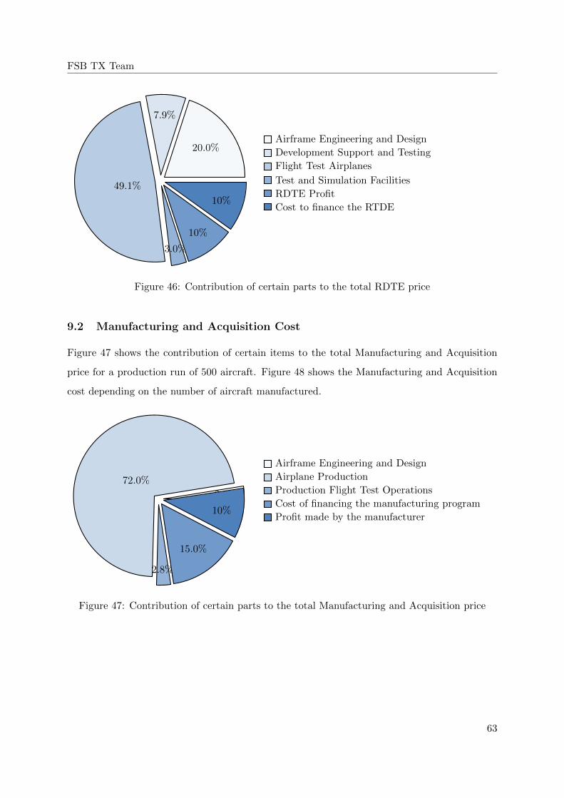
FSB TX Team

20.0%

7.9%

49.1%

3.0%

10%

10%

Airframe Engineering and Design

Development Support and Testing

Flight Test Airplanes

Test and Simulation Facilities

RDTE Profit

Cost to finance the RTDE

Figure 46: Contribution of certain parts to the total RDTE price

9.2 Manufacturing and Acquisition Cost

Figure 47 shows the contribution of certain items to the total Manufacturing and Acquisition

price for a production run of 500 aircraft. Figure 48 shows the Manufacturing and Acquisition

cost depending on the number of aircraft manufactured.

2.55%

72.0%

2.8%

15.0%

10%

Airframe Engineering and Design

Airplane Production

Production Flight Test Operations

Cost of financing the manufacturing program

Profit made by the manufacturer

Figure 47: Contribution of certain parts to the total Manufacturing and Acquisition price

63

FSB TX Team

100 200 300 400 500 600 7000

1

2

3

4

5

1.06

1.83

2.54

3.2

3.84

4.46

5.06

Figure 48: Price of Manufacturing and Acquisition depending on the number of produced air-

craft; price in billion of USD

9.2.1 Flyaway cost

Flyaway cost is the cost per aircraft including manufacturing and tooling but excluding RTDE.

Figure 49 shows the flyaway cost per unit depending on the number of aircraft produced.

100 200 300 400 500 600 7000

2

4

6

8

10

12 11.18

9.698.94

8.47 8.13 7.87 7.66

Figure 49: Flyaway cost per unit depending on the number of produced aircraft; price in million

of USD

64

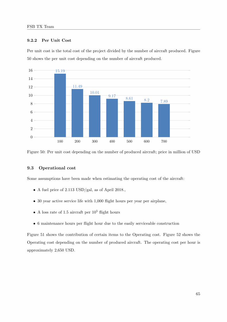
FSB TX Team

9.2.2 Per Unit Cost

Per unit cost is the total cost of the project divided by the number of aircraft produced. Figure

50 shows the per unit cost depending on the number of aircraft produced.

100 200 300 400 500 600 7000

2

4

6

8

10

12

14

16 15.19

11.49

10.019.17

8.61 8.2 7.89

Figure 50: Per unit cost depending on the number of produced aircraft; price in million of USD

9.3 Operational cost

Some assumptions have been made when estimating the operating cost of the aircraft:

• A fuel price of 2.113 USD/gal, as of April 2018.,

• 30 year active service life with 1,000 flight hours per year per airplane,

• A loss rate of 1.5 aircraft per 105 flight hours

• 6 maintenance hours per flight hour due to the easily serviceable construction

Figure 51 shows the contribution of certain items to the Operating cost. Figure 52 shows the

Operating cost depending on the number of produced aircraft. The operating cost per hour is

approximately 2,650 USD.

65

FSB TX Team

38.6%

16.5%

2.9%

10%

12%

13%

7%

Aircrew and maintenance crew cost

Fuel oil and lubricants cost

Consumable materials costIndirect personel cost

Cost of spares

Cost associated with depots

Miscellaneous cost

Figure 51: Contribution of items to the Operating cost

100 200 300 400 500 600 7000

10

20

30

40

6.53

12.58

18.63

24.68

30.73

36.77

42.82

Figure 52: Operating cost depending on the number of produced aircraft; price in billion of USD

9.4 Life cycle cost

Life cycle cost of an airplane program (LCC) is the total cost of developing, purchasing, operating

and disposing of a fleet of aircraft. Figure 53 shows the Life cycle cost depending on the number

of produced aircraft. Figure 54 shows the items contributing to the Life cycle cost on an example

of a production of 500 aircraft. The disposal cost is assumed to be 1% of the life cycle cost.

66

FSB TX Team

100 200 300 400 500 600 7000

10

20

30

40

50

8.13

15.03

21.85

28.63

35.38

42.11

48.83

Figure 53: Life cycle cost depending on the number of produced aircraft; price in billion of USD

1.3%

10.9%

86.8%1.0%

RDTE costAcquisition cost

Operating cost

Disposal cost

Figure 54: Contribution of items to the Life cycle cost

67

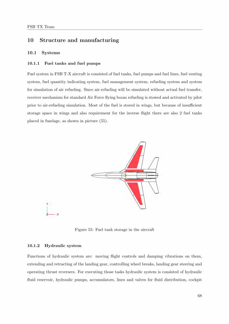
FSB TX Team

10 Structure and manufacturing

10.1 Systems

10.1.1 Fuel tanks and fuel pumps

Fuel system in FSB T-X aircraft is consisted of fuel tanks, fuel pumps and fuel lines, fuel venting

system, fuel quantity indicating system, fuel management system, refueling system and system

for simulation of air refueling. Since air-refueling will be simulated without actual fuel transfer,

receiver mechanism for standard Air Force flying boom refueling is stowed and activated by pilot

prior to air-refueling simulation. Most of the fuel is stored in wings, but because of insufficient

storage space in wings and also requirement for the inverse flight there are also 2 fuel tanks

placed in fuselage, as shown in picture (55).

Figure 55: Fuel tank storage in the aircraft

10.1.2 Hydraulic system

Functions of hydraulic system are: moving flight controls and damping vibrations on them,

extending and retracting of the landing gear, controlling wheel breaks, landing gear steering and

operating thrust reversers. For executing those tasks hydraulic system is consisted of hydraulic

fluid reservoir, hydraulic pumps, accumulators, lines and valves for fluid distribution, cockpit

68

FSB TX Team

controls to operate the functions served by the hydraulic system.

10.1.3 Electrical system

Electrical system provides electrical power for flight instrument and avionics system, internal

and external lightning, engine starting systems and flight control systems. Electrical power is

provided primary by engine driven generators and secondary by APU, RAT and batteries.

10.1.4 Environmental control system

Environmental control system is consisted of: pressurization system, pneumatic system, air-

conditioning system and oxygen system. The purpose of these subsystems is to provide normal

atmosphere conditions in cockpit while pneumatic system is also used as ice protection system.

10.1.5 System layout design

Pictures (56) and (57) show layout of main aircraft systems.

Figure 56: Layout of basic aircraft systems

69

FSB TX Team

Figure 57: Top view and side view of basic aircraft systems

More detailed overview of the aircraft systems is given in figure (57). The list is based on aircraft

systems used in 5 similar military and training aircrafts and default systems given by the RFP.

Those aircrafts are F-22, F-16, KAI T-50 Golden Eagle, Aermacchi M-346 and Hawk T2. Due

to aircraft safety, redundancy of system is used.

10.2 V-n diagram

In Table 17 are shown required data for V-n diagram.

Table 17: Required data for V-n diagram

Symbol Name Value

m maximum gross weight 11023.1 lb

Clmax maximum positive lift coefficient 1.121 [-]

S wing area 177.6ft2

b span 29.79 ft

nlim,pos positive design limit load factor 9

nlim,neg negative design limit load factor -3

nult,pos positive ulitimate load factor 13.5

nult,neg negative ulitimate load factor -4.5

In Figure 58 are shown the V-n diagram, of the FSB-TX, which represents the aircraft load

factor as a function of airspeed. Stall boundaries are shown in the diagram as well as positive

70

FSB TX Team

and negative design limit load factor and ultimate load factors. By observing the V-n diagram

it is seen that the gust diagram shown in dashed lines does not influence the maneuver diagram.

It is also relevant to note that the dive speed of 1.2 Ma (calculated from the maximum dynamic

pressure of 2133 psf as given in the RFP) is higher than would be expected for the final design.

According to [[3] [4] [5]] and a maximum cruise speed of 0.7 Ma would give this aircraft a dive

speed of 0.875 Ma.

Figure 58: V-n diagram

10.3 Structural arrangement

The design of the training aircraft FSB T-X was made in accordance with the design of the

Aermacchi M-346 training aircraft. The structural arrangement of fuselage, wing, and empen-

nage are shown in figure 59 and 60. The fuselage of aircraft is made as the semi-monocoque

structure composed of skin, frames, and longerons. The frames are replaced with pressure bulk-

heads on the entrance and exit of the cockpit. The mainframes are placed where fuselage and

wings are attached and on the place where empennages and fuselage are attached. According

71

FSB TX Team

to the recommendation from Roskam [3] [4] [5], the mass reduction of the structure is made by

using mainframes, who are already used for empennage, to mount engine. The mainframes who

are used for attachment fuselage and wings are also used for attachment of the main landing

gear, while the front landing gear is attached on pressure bulkhead. The wings and vertical

tail surfaces are composed of ribs, spars, and skin. The horizontal tail surfaces (rudder) and

other control surfaces are made of honeycomb composite material. The engine is attached in

three points. Two points of attachment are placed on the mainframe behind wings, and the

third point is placed on the mainframe where is attached front spar of the vertical tail surface.

Attachment points are made of steel alloy.

Table 18: Wing components

Wing SelectedSpacing / Location

Rib 10 inches

FrontSpar Location 15 %

MiddleSpar Spacing 15 - 19 inches

AftSpar Location 15 %

Table 19: Fuselage components

Fuselage SelectedSpacing / Location

FrameSpacing 11 –20 inches

FrameDepth 2inches [3] [4] [5]

LongeronSpace 8 – 12inches [3] [4] [5]

Table 20: Vertical tail components

VerticalTail SelectedSpacing / Location

RibSpacing 8 – 12inches

FrontSpar Locating 15 %

AftSpar Locating 75 %

72

FSB TX Team

Figure 59: Top view of aircraft and structure elements

Figure 60: Side view of aircraft and structure elements

73

36.

9980

36.9220

14.

1680

SCALE 1:100Wing Horizontal Tail Vertical Tail

Area - S 177 ft2 40.085 ft2 20.989 ft2Span - b 29.80 ft 12.664 ft 6.061 ft

Root chord - cr 8.96 ft 4.222 ft 4.707 ftTip chord - ct 2.96 ft 2.110 ft 1.926 ft

Aerodynamic midchord - cA 6.46 ft 3.280 ft 3.576 ft

Aerodynamic apces - xA 4.20 ft 1.860 ft 1.430 ftIncidence angle - i 0° 0° 0°Dihedral angle - Γ 0° 0° 0°

Taper ratio - λ 0.33 0.5 0.4Sweep angle - Λ 1/4 30° 30° 40°

Aspect ratio - AR 5 4 1.85

Inboard sweep- ΛLE 34.14° - -

Outbord sweep - ΛTE 15.38° - -

Fuselage OverallLength 36.209 ft 36.998 ft

Maximal height 6.107 ft 14.168 ftMaximal width 6.824 ft 36.922 ft

FSB TX Team

10.4 Material selection and technology

As a structural elements arrangement, materials for structural elements are selected accord-

ing to training aircraft Aermacchi M-346. In Table 21 are given materials and manufacturing

technology of structural parts.

Table 21: Materials and technologies for structural elements

Part Material Manufacturing Technology

Radomes GFRP autoclave

Windshield acrylic/ polycarbonate automated thermoforming

Pilot cabin cover acrylic/ polycarbonate automated thermoforming

[6]

Canopy frame Aluminium alloy - 7050 machining

Intake Aluminium alloy - 7050 machining

Intake channel CFRP autoclave

Front fuselage skin CFRP autoclave

Middle fuselage skin CFRP / Aluminium alloy -

5052

autoclave

Tail skin CFRP / Aluminium alloy -

5052

autoclave [7]

Frames Aluminium alloy 7075 machining

Fuselage and wing attach-

ments

Aluminium alloy - 7175 machining

Wing skin CFRP autoclave

Leading edge and peaks Aluminium alloy machining + chemical

treatment

Spars and ribs of wings Aluminium alloy - 7050 machining

75

FSB TX Team

Ailerons and flaps CFRP (skin) + aluminium

honeycomb - 5052

autoclave , The thermal

expansion, bonding

Horizontal tail CFRP (skin) + aluminium

honeycomb - 5052

autoclave , The thermal

expansion, bonding

Fuselage and horizontal

tail attachments

Aluminium alloy - 7050 machining

Skin of vertical tail CFRP autoclave

Spars and ribs of vertical

tail

Aluminium alloy - 7050 machining

Fuselage and vertical tail

attachments

Aluminium alloy - 7175 machining

Rudder CFRP (skin) + aluminium

honeycomb - 5052

autoclave , The thermal

expansion, bonding

Landing gear Steel alloy – AerMet 340

Alloy

minting

Pressure bulkhead aluminium alloy 2124 machining

Engine mounts steel chrome-molybdenum

(4130)

machining

Table 21 shows that all basic structural elements are made of aluminum alloys and / or carbon

fiber composite materials. More detailed information about the materials used in the individual

structural elements are given as guidelines below.

• Radomes are made by E-glass fibers because of good radar permeability and significantly

lower material price compared to other types of fibers. [[13]]

• The aluminum alloy is used for frames because of demands placed on them, such as

strength, fatigue and damage resistance, and compression strength [14].

• The aluminum alloy 2124 will be used for pressure bulkheads [14].

• Airelons, flaps, rudder, and elevator are made of sandwich-structured composite made

by honeycomb core and carbon fiber cover. Honeycomb core is made of aluminum alloy

5502 with a galvanic coating to protect aluminum from corrosion. The advantage of these

76

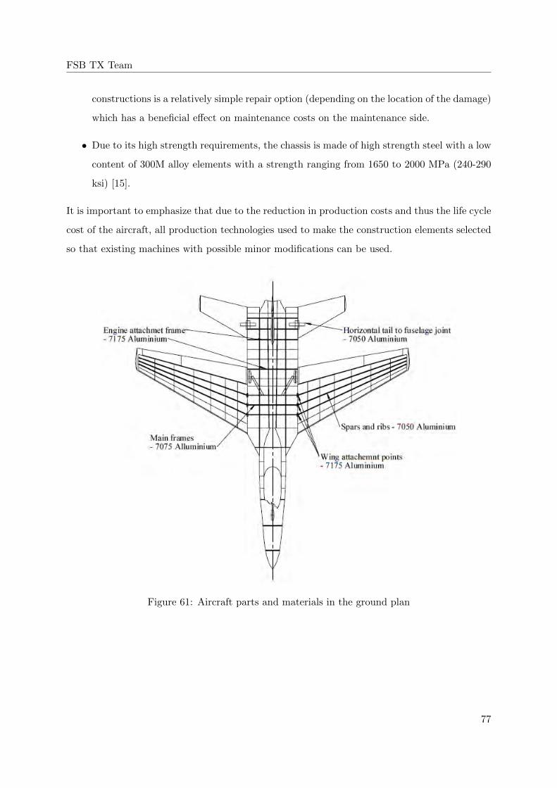
FSB TX Team

constructions is a relatively simple repair option (depending on the location of the damage)

which has a beneficial effect on maintenance costs on the maintenance side.

• Due to its high strength requirements, the chassis is made of high strength steel with a low

content of 300M alloy elements with a strength ranging from 1650 to 2000 MPa (240-290

ksi) [15].

It is important to emphasize that due to the reduction in production costs and thus the life cycle

cost of the aircraft, all production technologies used to make the construction elements selected

so that existing machines with possible minor modifications can be used.

Figure 61: Aircraft parts and materials in the ground plan

77

FSB TX Team

Figure 62: Parts and materials of the aircraft in the side view

10.5 Managment and Manufacturing

Aircraft production is divided into a stand-alone production of parts in the home facility and

parts and equipment purchased as a finished product. As a finished product, all systems are built

into the aircraft, the engine and the chassis. Aircraft production is divided into 4 production

units:

1) Front of the fuselage (till the cockpit)

2) The middle part of the fuselage (from the rear pressure bar to the first stage of the

compressor)

3) The rear of the fuselage with horizontal and vertical stabilizers

4) Wings

Each of the production units is subject to the following actions:

• production of appropriate structural elements

• assembly of structural elements

• installation of purchased parts

• final control

78

FSB TX Team

After completing all necessary operations on the production units, the final assembly is followed,

where they are assembled into a finished product.

Each of the production units is subject to the following actions:

10.6 Maintenance

Since maintenance is one of the biggest contributions to the aircraft life cycle, it is important

to optimize it as much as possible. Maintenance optimization for this aircraft was carried out

through the following steps:

• Reducing the need and use of existing field equipment

• Opening the cockpit cover to the right for easier replacement of the pilot seats

• Setting all aircraft and electronics maintenance opening on the left at a level that does

not require additional ground equipment (open down)

• One port through which all the fuel tanks in the level with the maintenance openings are

also to the left

• Replacement of parts such as steering wheel, rudder height, actuators - lightweight parts

procurement [16].

79

FSB TX Team

11 Conclusion

FSB-TX aircraft was designed in response to the 2017./2018. AIAA RFP for a new jet fighter

training aircraft which was supposed to replace previously used T-38C Talon. Before the start

of the design phase, it was necessary to determine a few main objectives which would later serve

the team as guidelines and furthermore help in every decision that was made. After analysing

a few jet fighter training aircraft, it was identified that the main difference between jet fighter

training aircraft and all the other airplanes lays in the fact that the training airplanes have

much more operating hours. The main drawback of having a large amount of operating hours is

the frequency of maintenance operations which make the majority of overall airplane life cycle

expenses. Because of that fact, it was commonly decided that the focus of this project should be

on minimizing the life cycle cost. Since the airplane was meant to be designed for new pilots, the

FSB-TX team found importance in enabling the pilot and the instructor to land safely almost

everywhere in case of emergency, by minimizing the overall runway length. Afterwards, the team

analysed the career path for the new pilots and decided that it would be the best to make the

adaption process from the trainer aircraft to 5th generation fighters as easy as possible in terms

of maneuverability. Having the main objectives in mind, the project could start with the weight

estimation based on the information about the airplanes of similar purpose. When it came to

the decision about the engine that will be used, a trade study was made. Five commercialy

available jet engines were taken into consideration including F-404, F-414, F-110, Snecma M88

and Honeywell F125. Since all the combinations gave a similar value of take-off and empty

weight, it was decided that the cheapest engine (Honeywell F125) should be the first candidate

among all the engines previously taken into consideration. Before the final decision was made,

performance estimation had to be made, so the team could be sure that the engine will satisfy

all the requirements given by the RFP. Performance estimation showed that the engine that was

chosen was found satisfactory although it had the lowest T/W ratio. Some more trade studies

regarding the influence of the lift coeffiecient on take off, landing conditions and maneuvering

were made to make a decision that would result with optimal wing construction regarding the

price and performance. The wing was designed without slats to minimize the wing maintenance

cost. As a consequence of the team striving to minimize the mass of every constructive element,

vertical stabilizer was found to be too small for the lateral stability purpose which was detected

on time and corrected by enlarging the vertical stabilizer construction. During the process of of

80

FSB TX Team

stability analysis, it was decided that the wing and tail configuration will be joined to the body

in a way which will result with static instability in some regimes of the flight, so the airplane

could be more maneuverable with the use of closed loop feedback system. All possible weight

loading scenarios were taken into consideration in stability analysis to ensure that the static

margin isn’t larger than 13% of mean aerodynamic chord. The airplane was also tested against

the MIL-F-8785-C by simulation which was done with Ceasiom and proved to be satisfactory,

showing some good flying qualities. After the stability analysis, it was mandatory to check

the performances one more time which resulted with final performance values that were found

satisfactory in all cases. It was found that the design resulted with a very short runway length,

even less than the value required by the RFP. Finally, the cost estimation was made, which

resulted with pretty low prices compared to the competition. It can be concluded that the

aircraft accomplished all the objectives that were set in the beginning of the project.

81

FSB TX Team

References

[1] Roskam J., Airplane Design – Part I – Preliminary sizing of airplanes. Roskam Aviation

and Engineering Corporation. Kansas, 1985.

[2] Roskam J., Airplane Design – Part II – Preliminary configuration desgin and integration

of the propulsion system.Roskam Aviation and Engineering Corporation. Ottawa, Kansas,

1985.

[3] Roskam J., Airplane Design – Part III – Layout design of cockpit, fuselage, wing and

empennage: cutaways and inboard profiles. Roskam Aviation and Engineering Corporation.

Ottawa, Kansas, 1986.

[4] Roskam J., Airplane Design – Part IV – Layout design of landing gear and systems. Roskam

Aviation and Engineering Corporation. Ottawa, Kansas, 1986.

[5] Roskam J., Airplane Design – Part V – Component weight estimation. Roskam Aviation

and Engineering Corporation. Ottawa, Kansas, 1985.

[6] Roskam J., Airplane Design – Part VI – Preliminary calculation of aerodynamic, thrust

and power characteristics. Roskam Aviation and Engineering Corporation. Ottawa, Kansas,

1987.

[7] Roskam J., Airplane Design – Part VII – Determination of stability, control and perfor-

mance characteristics: FAR and Military requirements. Roskam Aviation and Engineering

Corporation. Ottawa, Kansas, 1988.

[8] Jankovic S. Mehanika leta zrakoplova. Poglavlje Kinematika leta. FSB. Zagreb, 2001.

[9] Jackson P. Jane’s All the World’s Aircraft. 2004-2005.

[10] Jackson P. Jane’s Aero Engines. 2002

[11] http://www.viscopedia.com/viscosity-tables/substances/aviation-fuels/ ,

09.02.2018.

[12] http://airfoiltools.com/airfoil/details?airfoil=naca63209-il , 09.02.2018.

[13] Baker, A. , Dutton, S. , Kelly, D.: Composite Materials for Aircraft Structures , Second

edition, AIAA 2004.

82

FSB TX Team

[14] N. Eswara Prasad, R. J. H. Wanhill.: Aerospace Materials and Material Technologies,

Volume 1: Aerospace Materials, 2017.

[15] Niu, M.C.Y. ; Airframe Structural Design , 1988

[16] Maintenance Matters, https://www.boeing.com/features/2017/11/t-x-maintenance-

matters.page , 16.04.2018.

[17] GKN Aerospace team win 2014 Defense Manufacturing Technology Award,

http://www.adsadvance.co.uk/gkn-aerospace-team-win-2014-defense-manufacturing-

technology-award.html , 25.04.2018.

[18] AIAA Request for proposal – Advanced Pilot Training Aircraft.

[19] Raymer D. Aircraft Design: A Conceptual Approach.

[20] Jane’s Aero Engines.

https://www.janes.com

[21] Jackson P. Jane’s All the World’s aircraft 2004-2005.

[22] Jackson P. Jane’s All the World’s Aircraft. 2004-2005.

[23] http://www.viscopedia.com/viscosity-tables/substances/aviation-fuels/ ,

09.02.2018.

[24] https://airfoiltools.com/airfoil/details?airfoil=n0009sm-il , 27.03.2018.

[25] Jackson P. Jane’s All the World’s Aircraft. 2004-2005.

[26] Jackson P. Jane’s Aero Engines. 2002

[27] Abbott, Ira Herbert, and Albert Edward Von Doenhoff. Theory of wing sections, including

a summary of airfoil data. Courier Corporation, 1959.

83