
From the Desk of Managing Editor… - The Science and ...
260
-
Upload
khangminh22 -
Category
Documents
-
view
1 -
download
0
Transcript of From the Desk of Managing Editor… - The Science and ...


(IJACSA) International Journal of Advanced Computer Science and Applications,
Vol. 6, No. 7, 2015
(i)
www.ijacsa.thesai.org
Editorial Preface
From the Desk of Managing Editor…
It may be difficult to imagine that almost half a century ago we used computers far less sophisticated than current
home desktop computers to put a man on the moon. In that 50 year span, the field of computer science has
exploded.
Computer science has opened new avenues for thought and experimentation. What began as a way to simplify the
calculation process has given birth to technology once only imagined by the human mind. The ability to communicate
and share ideas even though collaborators are half a world away and exploration of not just the stars above but the
internal workings of the human genome are some of the ways that this field has moved at an exponential pace.
At the International Journal of Advanced Computer Science and Applications it is our mission to provide an outlet for
quality research. We want to promote universal access and opportunities for the international scientific community to
share and disseminate scientific and technical information.
We believe in spreading knowledge of computer science and its applications to all classes of audiences. That is why we
deliver up-to-date, authoritative coverage and offer open access of all our articles. Our archives have served as a
place to provoke philosophical, theoretical, and empirical ideas from some of the finest minds in the field.
We utilize the talents and experience of editor and reviewers working at Universities and Institutions from around the
world. We would like to express our gratitude to all authors, whose research results have been published in our journal,
as well as our referees for their in-depth evaluations. Our high standards are maintained through a double blind review
process.
We hope that this edition of IJACSA inspires and entices you to submit your own contributions in upcoming issues. Thank
you for sharing wisdom.
Thank you for Sharing Wisdom!
Managing Editor
IJACSA
Volume 6 Issue 7 July 2015
ISSN 2156-5570 (Online)
ISSN 2158-107X (Print)
©2013 The Science and Information (SAI) Organization

(IJACSA) International Journal of Advanced Computer Science and Applications,
Vol. 6, No. 7, 2015
(ii)
www.ijacsa.thesai.org
Editorial Board
Editor-in-Chief
Dr. Kohei Arai - Saga University
Domains of Research: Technology Trends, Computer Vision, Decision Making, Information Retrieval,
Networking, Simulation
Associate Editors
Chao-Tung Yang
Department of Computer Science, Tunghai University, Taiwan
Domain of Research: Software Engineering and Quality, High Performance Computing, Parallel and Distributed
Computing, Parallel Computing
Elena SCUTELNICU
“Dunarea de Jos" University of Galati, Romania
Domain of Research: e-Learning, e-Learning Tools, Simulation
Krassen Stefanov
Professor at Sofia University St. Kliment Ohridski, Bulgaria
Domains of Research: e-Learning, Agents and Multi-agent Systems, Artificial Intelligence, Big Data, Cloud
Computing, Data Retrieval and Data Mining, Distributed Systems, e-Learning Organisational Issues, e-Learning
Tools, Educational Systems Design, Human Computer Interaction, Internet Security, Knowledge Engineering and
Mining, Knowledge Representation, Ontology Engineering, Social Computing, Web-based Learning Communities,
Wireless/ Mobile Applications
Maria-Angeles Grado-Caffaro
Scientific Consultant, Italy
Domain of Research: Electronics, Sensing and Sensor Networks
Mohd Helmy Abd Wahab
Universiti Tun Hussein Onn Malaysia
Domain of Research: Intelligent Systems, Data Mining, Databases
T. V. Prasad
Lingaya's University, India
Domain of Research: Intelligent Systems, Bioinformatics, Image Processing, Knowledge Representation, Natural
Language Processing, Robotics

(IJACSA) International Journal of Advanced Computer Science and Applications,
Vol. 6, No. 7, 2015
(iii)
www.ijacsa.thesai.org
Reviewer Board Members
Abassi Ryma
Higher Institute of Communications Studies of Tunis , Iset’com
Abbas Karimi
Islamic Azad University Arak Branch
Abdelghni Lakehal Université Abdelmalek Essaadi Faculté Polydisciplinaire de Larache Route de Rabat, Km 2 - Larache BP. 745 - Larache 92004. Maroc.
Abdel-Hameed A. Badawy Arkansas Tech University
Abdur Rashid Khan Gomal Unversity
Abeer Mohamed ELkorany Faculty of computers and information, Cairo Univesity
ADEMOLA ADESINA University of the Western Cape
Aderemi A. Atayero Covenant University
Ahmed S.A AL-Jumaily Ahlia University
Ahmed Boutejdar Ahmed Nabih Zaki Rashed
Menoufia University Akbar Hossain Akram Belghith
University Of California, San Diego Albert Alexander S
Kongu Engineering College Alcinia Zita Sampaio
Technical University of Lisbon
Alexandre Bouënard Sensopia
Ali Ismail Awad Luleå University of Technology
Amitava Biswas Cisco Systems
Anand Nayyar KCL Institute of Management and Technology, Jalandhar
Andi Wahju Rahardjo Emanuel Maranatha Christian University
Andrews Samraj
Mahendra Engineering College Anirban Sarkar
National Institute of Technology, Durgapur Antonio Formisano Anuranjan misra
Bhagwant Institute of Technology, Ghaziabad, India Appasami Govindasamy Arash Habibi Lashkari
University Technology Malaysia(UTM) Aree Ali Mohammed
Directorate of IT/ University of Sulaimani Aris Skander Skander
Constantine 1 University Ashok Matani
Government College of Engg, Amravati Ashraf Mohammed Iqbal
Dalhousie University and Capital Health Ashraf Hamdy Owis
Cairo University Asoke Nath
St. Xaviers College(Autonomous), 30 Park Street, Kolkata-700 016
Ayad Ghany Ismaeel Department of Information Systems Engineering- Technical Engineering College-Erbil Polytechnic University, Erbil-Kurdistan Region- IRAQ
Ayman EL-SAYED Computer Science and Eng. Dept., Faculty of Electronic Engineering, Menofia University
Babatunde Opeoluwa Akinkunmi University of Ibadan
Badre Bossoufi University of Liege
BASANT KUMAR VERMA JNTU
Basil Hamed Islamic University of Gaza
Basil M Hamed Islamic University of Gaza
Bhanu Prasad Pinnamaneni Rajalakshmi Engineering College; Matrix Vision GmbH
Bharti Waman Gawali Department of Computer Science & information T

(IJACSA) International Journal of Advanced Computer Science and Applications,
Vol. 6, No. 7, 2015
(iv)
www.ijacsa.thesai.org
Bilian Song LinkedIn
Brahim Raouyane FSAC
Bright Keswani Associate Professor and Head, Department of Computer Applications, Suresh Gyan Vihar University, Jaipur (Rajasthan) INDIA
Brij Gupta University of New Brunswick
C Venkateswarlu Venkateswarlu Sonagiri JNTU
Chandrashekhar Meshram Chhattisgarh Swami Vivekananda Technical University
Chao Wang Chao-Tung Yang
Department of Computer Science, Tunghai University
Charlie Obimbo University of Guelph
Chien-Peng Ho Information and Communications Research Laboratories, Industrial Technology Research Institute of Taiwan
Chun-Kit (Ben) Ngan The Pennsylvania State University
Ciprian Dobre University Politehnica of Bucharest
Constantin Filote Stefan cel Mare University of Suceava
Constantin POPESCU Department of Mathematics and Computer Science, University of Oradea
CORNELIA AURORA Gyorödi University of Oradea
Dana - PETCU West University of Timisoara
Deepak Garg Thapar University
Dheyaa Kadhim University of Baghdad
Dong-Han Ham Chonnam National University
Dr K Ramani K.S.Rangasamy College of Technology, Tiruchengode
Dr. Harish Garg
Thapar University Patiala Dr. Sanskruti V Patel
Charotar Univeristy of Science & Technology, Changa, Gujarat, India
Dr. Santosh Kumar Graphic Era University, Dehradun (UK)
Dr.JOHN S MANOHAR VTU, Belgaum
Dragana Becejski-Vujaklija University of Belgrade, Faculty of organizational sciences
Driss EL OUADGHIRI Duck Hee Lee
Medical Engineering R&D Center/Asan Institute for Life Sciences/Asan Medical Center
Elena Camossi Joint Research Centre
Elena SCUTELNICU Dunarea de Jos University of Galati
Eui Chul Lee Sangmyung University
Evgeny Nikulchev Moscow Technological Institute
Ezekiel Uzor OKIKE UNIVERSITY OF BOTSWANA, GABORONE
FANGYONG HOU School of IT, Deakin University
Faris Al-Salem GCET
Firkhan Ali Hamid Ali UTHM
Fokrul Alom Mazarbhuiya King Khalid University
Frank AYO Ibikunle Botswana Int’l University of Science & Technology (BIUST), Botswana.
Fu-Chien Kao Da-Y eh University
Gamil Abdel Azim Suez Canal University
Ganesh Chandra Sahoo RMRIMS
Gaurav Kumar Manav Bharti University, Solan Himachal Pradesh,
George Mastorakis Technological Educational Institute of Crete
George D. Pecherle

(IJACSA) International Journal of Advanced Computer Science and Applications,
Vol. 6, No. 7, 2015
(v)
www.ijacsa.thesai.org
University of Oradea Georgios Galatas
The University of Texas at Arlington Gerard Dumancas
Oklahoma Baptist University Ghalem Belalem Belalem
University of Oran 1, Ahmed Ben Bella Giacomo Veneri
University of Siena Giri Babu
Indian Space Research Organisation Govindarajulu Salendra Grebenisan Gavril
University of Oradea Gufran Ahmad Ansari
Qassim University Gunaseelan Devaraj
Jazan University, Kingdom of Saudi Arabia GYÖRÖDI ROBERT STEFAN
University of Oradea Hadj Hamma Tadjine
IAV GmbH Hamid Mukhtar
National University of Sciences and Technology Hamid Alinejad-Rokny
The University of New South Wales Hamid Ali Abed AL-Asadi
Department of Computer Science, Faculty of Education for Pure Science, Basra University
Hany Kamal Hassan EPF
Harco Leslie Hendric SPITS WARNARS Surya university
Hazem I. El Shekh Ahmed Pure mathematics
Hesham G. Ibrahim Faculty of Marine Resources, Al-Mergheb University
Himanshu Aggarwal Department of Computer Engineering
Hossam Faris Huda K. AL-Jobori
Ahlia University Iwan Setyawan
Satya Wacana Christian University JAMAIAH HAJI YAHAYA
NORTHERN UNIVERSITY OF MALAYSIA (UUM)
James Patrick Henry Coleman Edge Hill University
Jatinderkumar Ramdass Saini Narmada College of Computer Application, Bharuch
Jayaram A M Ji Zhu
University of Illinois at Urbana Champaign Jia Uddin Jia
Assistant Professor Jim Jing-Yan Wang
The State University of New York at Buffalo, Buffalo, NY
John P Sahlin George Washington University
JOSE LUIS PASTRANA University of Malaga
Jyoti Chaudhary high performance computing research lab
K V.L.N.Acharyulu Bapatla Engineering college
Ka-Chun Wong Kashif Nisar
Universiti Utara Malaysia Kayhan Zrar Ghafoor
University Technology Malaysia Khin Wee Lai
Biomedical Engineering Department, University Malaya
KITIMAPORN CHOOCHOTE Prince of Songkla University, Phuket Campus
Kohei Arai Saga University
Krasimir Yankov Yordzhev South-West University, Faculty of Mathematics and Natural Sciences, Blagoevgrad, Bulgaria
Krassen Stefanov Stefanov Professor at Sofia University St. Kliment Ohridski
Labib Francis Gergis Misr Academy for Engineering and Technology
Lazar Stošic Collegefor professional studies educators Aleksinac, Serbia
Leandros A Maglaras University of Surrey
Leon Andretti Abdillah Bina Darma University
Lijian Sun

(IJACSA) International Journal of Advanced Computer Science and Applications,
Vol. 6, No. 7, 2015
(vi)
www.ijacsa.thesai.org
Chinese Academy of Surveying and Ljubomir Jerinic
University of Novi Sad, Faculty of Sciences, Department of Mathematics and Computer Science
Lokesh Kumar Sharma Indian Council of Medical Research
Long Chen Qualcomm Incorporated
M. Reza Mashinchi Research Fellow
M. Tariq Banday University of Kashmir
Manas deep Masters in Cyber Law & Information Security
Manju Kaushik Manoharan P.S.
Associate Professor Manoj Wadhwa
Echelon Institute of Technology Faridabad Manpreet Singh Manna
Associate Professor, SLIET University, Govt. of India Manuj Darbari
BBD University Marcellin Julius Antonio Nkenlifack
University of Dschang Maria-Angeles Grado-Caffaro
Scientific Consultant Marwan Alseid
Applied Science Private University Mazin S. Al-Hakeem
LFU (Lebanese French University) - Erbil, IRAQ MD RANA
University of Sydney Md. Zia Ur Rahman
Narasaraopeta Engg. College, Narasaraopeta Mehdi Bahrami
University of California, Merced Messaouda AZZOUZI
Ziane AChour University of Djelfa Milena Bogdanovic
University of Nis, Teacher Training Faculty in Vranje Miriampally Venkata Raghavendra
Adama Science & Technology University, Ethiopia Mirjana Popovic
School of Electrical Engineering, Belgrade University Miroslav Baca
University of Zagreb, Faculty of organization and informatics / Center for biometrics
Mohamed Ali Mahjoub Preparatory Institute of Engineer of Monastir
Mohamed A. El-Sayed Faculty of Science, Fayoum University, Egypt.
Mohamed Najeh LAKHOUA ESTI, University of Carthage
Mohammad Ali Badamchizadeh University of Tabriz
Mohammad Hani Alomari Applied Science University
Mohammad Azzeh Applied Science university
Mohammad Jannati Mohammad Haghighat
University of Miami Mohammed Shamim Kaiser
Institute of Information Technology Mohammed Sadgal
Cadi Ayyad University Mohammed Abdulhameed Al-shabi
Associate Professor Mohammed Ali Hussain
Sri Sai Madhavi Institute of Science & Technology Mohd Helmy Abd Wahab
Universiti Tun Hussein Onn Malaysia Mona Elshinawy
Howard University
Mostafa Mostafa Ezziyyani FSTT
Mourad Amad Laboratory LAMOS, Bejaia University
Mueen Uddin University Malaysia Pahang
Murthy Sree Rama Chandra Dasika Geethanjali College of Engineering & Technology
Mustapha OUJAOURA Faculty of Science and Technology Béni-Mellal
MUTHUKUMAR S SUBRAMANYAM DGCT, ANNA UNIVERSITY
N.Ch. Sriman Narayana Iyengar VIT University,
Nagy Ramadan Darwish Department of Computer and Information Sciences, Institute of Statistical Studies and Researches, Cairo University.

(IJACSA) International Journal of Advanced Computer Science and Applications,
Vol. 6, No. 7, 2015
(vii)
www.ijacsa.thesai.org
Najib A. Kofahi Yarmouk University
Natarajan Subramanyam PES Institute of Technology
Nazeeruddin - Mohammad Prince Mohammad Bin Fahd University
NEERAJ SHUKLA ITM UNiversity, Gurgaon, (Haryana) Inida
Nestor Velasco-Bermeo UPFIM, Mexican Society of Artificial Intelligence
Nidhi Arora M.C.A. Institute, Ganpat University
Ning Cai Northwest University for Nationalities
Noura Aknin University Abdelamlek Essaadi
Oliviu Matei Technical University of Cluj-Napoca
Om Prakash Sangwan Omaima Nazar Al-Allaf
Asesstant Professor Osama Omer
Aswan University Ousmane THIARE
Associate Professor University Gaston Berger of Saint-Louis SENEGAL
Paresh V Virparia Sardar Patel University
Poonam Garg Institute of Management Technology, Ghaziabad
Prabhat K Mahanti
UNIVERSITY OF NEW BRUNSWICK PROF DURGA PRASAD SHARMA ( PHD)
AMUIT, MOEFDRE & External Consultant (IT) & Technology Tansfer Research under ILO & UNDP, Academic Ambassador for Cloud Offering IBM-USA
Professor Ajantha Herath Qifeng Qiao
University of Virginia Rachid Saadane
EE departement EHTP Raed Kanaan
Amman Arab University Raghuraj Singh
Harcourt Butler Technological Institute Rahul Malik Raja Sarath Kumar Boddu
LENORA COLLEGE OF ENGINEERNG Rajesh Kumar
National University of Singapore Rakesh Chandra Balabantaray
IIIT Bhubaneswar Rakesh Kumar Dr.
Madan Mohan Malviya University of Technology Rashad Abdullah Al-Jawfi
Ibb university Rashid Sheikh
Shri Aurobindo Institute of Technology, Indore Ravi Prakash
University of Mumbai Ravisankar Hari
CENTRAL TOBACCO RESEARCH INSTITUE Rawya Y. Rizk
Port Said University Reshmy Krishnan
Muscat College affiliated to stirling University.U Ricardo Ângelo Rosa Vardasca
Faculty of Engineering of University of Porto Ritaban Dutta
ISSL, CSIRO, Tasmaniia, Australia Ruchika Malhotra
Delhi Technoogical University SAADI Slami
University of Djelfa Sachin Kumar Agrawal
University of Limerick Sagarmay Deb
Central Queensland Universiry, Australia
Said Ghoniemy Taif University
Sandeep Reddivari University of North Florida
Sasan Adibi Research In Motion (RIM)
Satyendra Prasad Singh Professor
Sebastian Marius Rosu Special Telecommunications Service
Seema Shah Vidyalankar Institute of Technology Mumbai,
Selem Charfi University of Pays and Pays de l'Adour
SENGOTTUVELAN P Anna University, Chennai

(IJACSA) International Journal of Advanced Computer Science and Applications,
Vol. 6, No. 7, 2015
(viii)
www.ijacsa.thesai.org
Senol Piskin Istanbul Technical University, Informatics Institute
Sérgio André Ferreira School of Education and Psychology, Portuguese Catholic University
Seyed Hamidreza Mohades Kasaei University of Isfahan,
Shafiqul Abidin Northern India Engineering College (Affiliated to G GS I P University), New Delhi
Shahanawaj Ahamad The University of Al-Kharj
Shaiful Bakri Ismail Shawki A. Al-Dubaee
Assistant Professor Sherif E. Hussein
Mansoura University Shriram K Vasudevan
Amrita University Siddhartha Jonnalagadda
Mayo Clinic Sim-Hui Tee
Multimedia University Simon Uzezi Ewedafe
Baze University Siniša Opic
University of Zagreb, Faculty of Teacher Education Sivakumar Poruran
SKP ENGINEERING COLLEGE Slim BEN SAOUD
National Institute of Applied Sciences and Technology
Sohail Jabbar Bahria University
Sri Devi Ravana University of Malaya
Sudarson Jena GITAM University, Hyderabad
Suhas J Manangi Microsoft
SUKUMAR SENTHILKUMAR Universiti Sains Malaysia
Sumazly Sulaiman Institute of Space Science (ANGKASA), Universiti Kebangsaan Malaysia
Sumit Goyal National Dairy Research Institute
Suresh Sankaranarayanan Institut Teknologi Brunei
Susarla Venkata Ananta Rama Sastry JNTUK, Kakinada
Suxing Liu Arkansas State University
Syed Asif Ali SMI University Karachi Pakistan
T C.Manjunath HKBK College of Engg
T V Narayana rao Rao SNIST
T. V. Prasad Lingaya's University
Taiwo Ayodele Infonetmedia/University of Portsmouth
Tarek Fouad Gharib Ain Shams University
Thabet Mohamed Slimani College of Computer Science and Information Technology
Totok R. Biyanto Engineering Physics, ITS Surabaya
Touati Youcef Computer sce Lab LIASD - University of Paris 8
Uchechukwu Awada Dalian University of Technology
Urmila N Shrawankar GHRCE, Nagpur, India
Vaka MOHAN TRR COLLEGE OF ENGINEERING
Vinayak K Bairagi AISSMS Institute of Information Technology, Pune
Vishnu Narayan Mishra SVNIT, Surat
Vitus S.W. Lam The University of Hong Kong
VUDA SREENIVASARAO PROFESSOR AND DEAN, St.Mary's Integrated Campus,Hyderabad.
Wei Wei Xi’an Univ. of Tech.
Xiaojing Xiang AT&T Labs
Yi Fei Wang The University of British Columbia
Yihong Yuan

(IJACSA) International Journal of Advanced Computer Science and Applications,
Vol. 6, No. 7, 2015
(ix)
www.ijacsa.thesai.org
University of California Santa Barbara Yilun Shang
Tongji University Yu Qi
Mesh Capital LLC Zacchaeus Oni Omogbadegun
Covenant University Zairi Ismael Rizman
Universiti Teknologi MARA Zenzo Polite Ncube
North West University
Zhao Zhang Deptment of EE, City University of Hong Kong
Zhixin Chen ILX Lightwave Corporation
Ziyue Xu National Institutes of Health, Bethesda, MD
Zlatko Stapic University of Zagreb, Faculty of Organization and Informatics Varazdin
Zuraini Ismail Universiti Teknologi Malaysia

(IJACSA) International Journal of Advanced Computer Science and Applications,
Vol. 6, No. 7, 2015
(x)
www.ijacsa.thesai.org
CONTENTS
Paper 1: Enhancing CRM Business Intelligence Applications by Web User Experience Model
Authors: Natheer K. Gharaibeh
PAGE 1 – 6
Paper 2: Mind-Reading System - A Cutting-Edge Technology
Authors: Farhad Shir
PAGE 7 – 12
Paper 3: Enrichment of Object Oriented Petri Net and Object Z Aiming at Business Process Optimization
Authors: Aliasghar Ahmadikatouli, Homayoon Motameni
PAGE 13 – 19
Paper 4: FSL-based Hardware Implementation for Parallel Computation of cDNA Microarray Image Segmentation
Authors: Bogdan Bot, Simina Emerich, Sorin Martoiu, Bogdan Belean
PAGE 20 – 27
Paper 5: Indexing of Ears using Radial basis Function Neural Network for Personal Identification
Authors: M.A. Jayaram, Prashanth G.K, M.Anusha
PAGE 28 – 33
Paper 6: Classification of Premature Ventricular Contraction in ECG
Authors: Yasin Kaya, Hüseyin Pehlivan
PAGE 34 – 40
Paper 7: Signal Reconstruction with Adaptive Multi-Rate Signal Processing Algorithms
Authors: Korhan Cengiz
PAGE 41 – 46
Paper 8: Image Edge Detection based on ACO-PSO Algorithm
Authors: Chen Tao, Sun Xiankun, Han Hua,You Xiaoming
PAGE 47 – 54
Paper 9: Improvement on Classification Models of Multiple Classes through Effectual Processes
Authors: Tarik A. Rashid
PAGE 55 – 62
Paper 10: A Modified Clustering Algorithm in WSN
Authors: Ezmerina Kotobelli, Elma Zanaj, Mirjeta Alinci, Edra Bumçi, Mario Banushi
PAGE 63 – 67
Paper 11: A Frame Work for Preserving Privacy in Social Media using Generalized Gaussian Mixture Model
Authors: P Anuradha, Y.Srinivas, MHM Krishna Prasad
PAGE 68 – 71
Paper 12: Survey on Chatbot Design Techniques in Speech Conversation Systems
Authors: Sameera A. Abdul-Kader, Dr. John Woods
PAGE 72 – 80

(IJACSA) International Journal of Advanced Computer Science and Applications,
Vol. 6, No. 7, 2015
(xi)
www.ijacsa.thesai.org
Paper 13: Research on Islanding Detection of Grid-Connected System
Authors: Liu Zhifeng, Zhang Liping, Chen Yuchen, Jia Chunying
PAGE 81 – 86
Paper 14: Using Induced Fuzzy Bi-Model to Analyze Employee Employer Relationship in an Industry
Authors: Dhrubajyoti Ghosh, Anita Pal
PAGE 87 – 99
Paper 15: Analyzing the Changes in Online Community based on Topic Model and Self-Organizing Map
Authors: Thanh Ho, Phuc Do
PAGE 100 – 108
Paper 16: Design of Orthonormal Filter Banks based on Meyer Wavelet
Authors: Teng Xudong, Dai Yiqing, Lu Xinyuan, Liang Jianru
PAGE 109 – 112
Paper 17: An Integrated Architectural Clock Implemented Memory Design Analysis
Authors: Ravi Khatwal, Manoj Kumar Jain
PAGE 113 – 124
Paper 18: Using GIS for Retail Location Assessment at Jeddah City
Authors: Abdulkader A Murad
PAGE 125 – 134
Paper 19: Information Management System based on Principles of Adaptability and Personalization
Authors: Dragan Đokić, Dragana Šarac, Dragana Bečejski Vujaklija
PAGE 135 – 143
Paper 20: Assessment of High and Low Rate Protocol-based Attacks on Ethernet Networks
Authors: Mina Malekzadeh, M.A. Beiruti, M.H. Shahrokh Abadi
PAGE 144 – 157
Paper 21: A Survey of Emergency Preparedness
Authors: Aaron Malveaux, A. Nicki Washington
PAGE 158 – 162
Paper 22: Integrating Service Design and Eye Tracking Insight for Designing Smart TV User Interfaces
Authors: Sheng-Ming Wang
PAGE 163 – 171
Paper 23: Investigating on Mobile Ad-Hoc Network to Transfer FTP Application
Authors: Ako Muhammad Abdullah
PAGE 172 – 183
Paper 24: Load Balancing for Improved Quality of Service in the Cloud
Authors: AMAL ZAOUCH, FAOUZIA BENABBOU
PAGE 184 – 189
Paper 25: An Improved Brain Mr Image Segmentation using Truncated Skew Gaussian Mixture
Authors: Nagesh Vadaparthi, Srinivas Yerramalle, Suresh Varma Penumatsa
PAGE 190 – 197

(IJACSA) International Journal of Advanced Computer Science and Applications,
Vol. 6, No. 7, 2015
(xii)
www.ijacsa.thesai.org
Paper 26: Research on the UHF RFID Channel Coding Technology based on Simulink
Authors: Changzhi Wang, Zhicai Shi, Dai Jian, Li Meng
PAGE 198 – 202
Paper 27: Artificial Intelligence in Performance Analysis of Load Frequency Control in Thermal-Wind-Hydro Power
Systems
Authors: K. Jagatheesan, B. Anand, Nilanjan Dey, Amira S. Ashour
PAGE 203 – 212
Paper 28: New 2-D Adaptive K-Best Sphere Detection for Relay Nodes
Authors: Ahmad El-Banna
PAGE 213 – 216
Paper 29: Geographic Routing Using Logical Levels in Wireless Sensor Networks for Sensor Mobility
Authors: Yassine SABRI, Najib EL KAMOUN
PAGE 217 – 223
Paper 30: Cost-Effective, Cognitive Undersea Network for Timely and Reliable Near-Field Tsunami Warning
Authors: X. Xerandy, Taieb Znati, Louise K Comfort
PAGE 224 – 233
Paper 31: Exploiting SCADA vulnerabilities using a Human Interface Device
Authors: Grigoris Tzokatziou, Helge Janicke, Leandros A. Maglaras, Ying He
PAGE 234 – 241
Paper 32: Image Mining: Review and New Challenges
Authors: Barbora Zahradnikova, Sona Duchovicova, Peter Schreiber
PAGE 242 – 246

(IJACSA) International Journal of Advanced Computer Science and Applications,
Vol. 6, No. 7, 2015
1 | P a g e
www.ijacsa.thesai.org
Enhancing CRM Business Intelligence Applications
by Web User Experience Model
Natheer K. Gharaibeh
College Computer Science and Engineering at Yanbu, Taibah University
Yanbu, KSA
Abstract—several trends are emerging in the field of CRM
technology which promises a brighter future of more profitable
customers and decreasing costs. One of the most critical trends is
enhancing Business Intelligence applications using Web
Technologies, Web technologies can improve the CRM BI
implementation, but it still need evaluation, The Web has focused
the attention of organizations towards the User Experience and
the need to learn about their customer, The UX paradigm calls
for enhancing CRMBI by Web technologies. This paper deals
with this issue and provide a framework for building Web based
CRMBI depending on the Process mapping between CRMBI and
UX. It provides a conceptual overview of CRM and its
relationship to the main disciplines BI, UX and Web.
Keywords—CRM; Data warehouse; User Experience; Business
intelligence; Web
I. INTRODUCTION
Business Intelligence and Web Technologies [1] [10] has gained greater attention since the last two decades. for both practitioners and researchers BI includes business-centric practices and methodologies that can be applied to various high-impact applications such as e-commerce , market intelligence , customer intelligence and specifically customer relationship management (CRM). The high failure rates reported [2] in CRM Applications raised questions about how CRM applications are developed and especially what Design preconditions are required for implementing and building CRM successfully.
Analysts such as Gartner, AMR and Forrester Research studied the problem seriously From 2001 till 2009, a variety of analyst firms reported failure rates ranging up to 70 percent, with over 50 percent of organizations in 2009 indicating that CRM projects did not fully meet expectations, and it was noted 1
that the percentage of firms implementing CRM has increased, from 53 percent in 2003 to 75 percent in 2010.
As with the problem of CRM, it is founded that 50% to 66% of all initial Business Intelligence and DW efforts fail [3]. Gartner [4] estimates that more than 50% of DW projects have limited acceptance or fail. Therefore, it is crucial to have a thorough understanding of the critical success factors and variables that determine the efficient implementation of a DW solution. What is interesting to note that two of the top three CSFs were focused on understanding the business context and process in which the data warehouse would operate. From this
1 http://www.destinationcrm.com/Articles/Editorial/Magazine-Features/CRM-
Then-and-Now-68083.aspx
perspective we want take CRM as the business context and the process that need to be improved.
To illustrate a good starting point between CRM and BI, on the one hand, there is a general acceptance among researchers [5] of the categorization of CRM components into Technology, people, and Process. On the other hand, Gartner [4] provides these three pillars as working framework for the success of BI , the intermediate pillar is process which represents the connection between people and technology [6] , therefore ,There is essential shift toward process orientation of BI [7] , By applying Process oriented BI We Replace function-oriented separation of work by processes that span both functional and organizational boundaries, Therefore CRM as a process has been added to BI To coin the concept of CRMBI applications.
Thus, we define CRMBI as all BI capabilities that are dedicated to the analysis as well as to the systematic purposeful transformation of CRM relevant data from communication , transactional level into relational level, this implies the transformation from reach to richness [1], Reach means make communication with large numbers of customers, while Richness means more meaningful communication with those customers through real transactions, and then establish useful relations with those loyal customers. This relational model must be done through Web based applications in order to access larger number of people. This is what we mean by Web Based CRMBI Application. CRMBI can be exist in many forms and examples, in this study the problem at hand is Frequent Flyer Program (FFP) from the Airline application domain, which will be explained in section 5.
There are a lot of research about how to combine between CRM and BI, but there is a little research about extending the capabilities of CRM Business Intelligence applications by web , the importance of web come from meeting the requirements of large numbers of connected customers and the huge amount of available c lick stream data available through the web. Furthermore, the processes of connecting with customers through the Web are a key resource that will enable the organization strengthen its relationships with their customers and gain a sustainable competitive advantage. , The Web has focused the attention of organizations towards the User Experience [8] and the need to learn about their customer, The UX paradigm calls for enhancing CRMBI by web technologies. In this paper the Process mapping between CRMBI and UX will be discussed.
In order to get insight into the development process of CRMBI, a design science approach was applied in this paper,

(IJACSA) International Journal of Advanced Computer Science and Applications,
Vol. 6, No. 7, 2015
2 | P a g e
www.ijacsa.thesai.org
the following structure was organized. In the second section some background information on the main concepts of the paper will be provided. A more detailed overview of the main concepts (CRM, BI, UX and Web) are presented in section 3. Subsequently, a vision for the CRMBI process is outlined in Section 4. whereas section 5 offer a detailed analysis of the main components of the developed model. In section 6 conclusions are drawn.
II. BACKGROUND
In this section, every concept and its relationship with the problem at hand are explained.
A. CRM and relational function
There are many determinants for the CRM , but in this paper the determinants of e-relationship quality in most recent CRM literature [22] [23] will be followed: the communicational function, followed by transactional function and then relational function, these three dimensions were the most important dimensions that would affect customer loyalty as indicator for CRM Success.
Communication function represents the use of Internet as customer service tool to display information and answer all enquiries from customers. Transactional function represents the use of Internet technology as a platform to transact with companies such as place orders, accomplishing payments, and view profile of previous activities. Relational function consists of value adding elements such as customized services and personalized Web Pages. In this paper the focus will be transferred from Communication to transactional, then from transactional to the relational level. The containment of these three levels will five a broader vision of building CRMBI, which is the main goal of this paper.
B. DW as a specific Research Area (The need to expand
capabilities of DW)
Since 30 years data warehouses [25] have been deployed as an integral part of a modern decision support environment. Therefore, a DW/BI is not only a software package or product, it also a process. The adoption of DW technology requires massive capital expenditure and a certain deal of implementation time. DW projects are hence very expensive, time-consuming and risky undertakings compared with other information technology initiatives, as cited by prior researchers [7]. Further Project Management practices do not work easily on DW [14], because they needs more integration with other systems, developing DW is a process more than product. Moreover, the DW/BI projects can’t be initiated unless their benefits have been associated to the organization‘s specific business problems and strategic business goals [14]. Justification for a DW initiative must always be business-driven and not technology-driven. So it is very important for such projects to get support from top level management.
Although a data warehouse empowers knowledge workers with information that allows them to make decisions based on a solid basis of fact. However, only a fraction of the required knowledge exists on computers; the vast majority of a firm’s intellectual assets exist as knowledge in the minds of its employees, in the form of tacit knowledge [24]. Hence, a data
warehouse does not necessarily provide adequate support for knowledge intensive queries in an organization. This situation can be interpreted as a sign that the field of BI development must enter into new stage of multi-perspectives research, which depends more on Web technologies. This viewpoint copes with the DW research agenda proposed by Nemati et al. [25]. They said, bone research area of decision support technologies such as BI and DW needs to the development of a set of theoretical foundations upon which to build future applications.
Since the early 2000s, the Internet and the Web began to offer unique data collection and analytical research and development opportunities which extend and enhance the CRM and BI applications. Especially IP-specific user search and interaction logs [10], Before that there where many difficulties in collecting this huge amount of customer data [28], but now with the advance in Web2.0, Web intelligence, web analytics, and the user-generated content have led to a new and exciting era of BI&A 2.0 research [10] which is centered on text and web analytics for unstructured web contents. In which the customer data can be collected seamlessly through cookies and server logs have become a new gold mine for understanding customer’s needs and identifying new business opportunities.
Fig. 1. Intersection between three Areas
What is needed is a new generation of DW that provides the infrastructure required to capture not only data and information but also knowledge. The existing data warehouses model can be extended and enhanced by Web Technologies to create a knowledge as we will show in the next section. The key idea of Web 2.0 [26] is putting the user at the center. It enables people to participate, collaborate and interact with each other. Web 2.0 has become a mass phenomenon.
C. CRMBI
As we defined CRMBI in the introduction, in this section we will show more details about this concept. At a general level, development of Web based CRMBI applications depend on the combination of the three main areas, CRM, BI, and UX as depicted in Figure 1. CRMBI can be found at the intersection of these three circles. The research problems originate from both CRM and BI fields in a way that Web technologies provide solution for both problems. By doing this we increase the opportunity of developing CRMBI successfully. By taking the impacts of these important fields on the required Software Artifact. In the next sections a new framework for CRMBI development will be presented. This
(IJACSA) International Journal of Advanced Computer Science and Applications,
Vol. 6, No. 7, 2015
3 | P a g e
www.ijacsa.thesai.org
review of theory and practice of CRM , BI and Web will help the Information System developers and Business analysts to have a clear mind of the development of CRMBI applications. This kind of studies is exploratory in nature, and it may be the seed for ongoing research on more than one emergent direction. To provide concrete evidence of applicability a technical vision for the possible CRMBI implementation is introduced in section 5.
III. CRMBI AND UX
A. The three CRM Processes
Through transferring from just Communication with customers into Transactional function. a Data base or ARS (Airline Reservations System) is created and updated, The value-adding features such as personalized recommendations personalized webpages, and customized service could be established in the relational function
These three functions of CRM could be mapped into the five elements of user experience, which will be shown in the next section.
B. User experience elements
Most people, at one time or another, have reserved a ticket (or any other service) over the Web. The experience is pretty much the same every time, the customer go to the site, he find the flight he want, maybe by using a search engine, by browsing a catalog or maybe by a Third-party online intermediaries (TPIs),, then after this Communication, the customer give the site his credit card number and his address, and the site confirms that the book will be shipped to him.
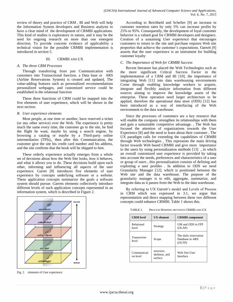
These orderly experience actually emerges from a whole set of decisions about how the Web Site looks, how it behaves, and what it allows you to do. These decisions build upon each other, informing and influencing all aspects of the user experience. Garret [8] introduces five elements of user experience by concepts underlying software or a website. These application concepts summarize the goals a software system should pursue. Garrets elements collectively introduce different levels of such application concepts represented in an information system, which is described in Figure 2.
Fig. 2. elements of User experience
According to Reichheld and Schefter [9] an increase in customer retention rates by only 5% can increase profits by 25% to 95%. Consequently, the development of loyal customer behavior is a valued goal for CRMBI developers and designers. Creation of a sustaining User experience that encourages customers to return to the site and purchase requires Web site properties that achieve the customer’s expectations. Garrett [8] asserts that the user experience is an instrument for building customer loyalty
C. The Importance of Web for CRMBI Success
Recent literature has placed the Web Technologies such as the more significant Critical Success Factor in the implementation of a CRM and BI [10], the importance of integrating Web [11] into data warehousing environments Come through enabling knowledge workers to acquire, integrate and flexibly analyze information from different sources aiming to improve the knowledge assets of the enterprise. These operation need larger architecture to be applied, therefore the operational data store (ODS) [12] has been introduced as a way of interfacing of the Web environment to the data warehouse.
Since the processes of customers are a key resource that will enable the company strengthen its relationships with them and gain a sustainable competitive advantage. , The Web has focused the attention of organizations towards the User Experience [8] and the need to learn about their customer , The UX paradigm calls for extending the capabilities of CRMBI through Web technologies , This represents the main driving factor towards Web based CRMBI and give more importance to the users by using personalization methods [13] , in which an overall customized user experience is provided by taking into account the needs, preferences and characteristics of a user or group of users , this personalization consists of defining and exploiting a user profiles . In addition to ODS we need Granularity Manager [12], which is positioned between the Web site and the data warehouse. The purpose of the granularity manager is to edit, aggregate, summarize, and integrate data as it passes from the Web to the data warehouse.
By referring to UX Garrett’s model and Levels of Process in CRM which was expressed in 3.1, we argue that representation and direct mapping between these two different concepts could enhance CRMBI. Table 1 shows this.
TABLE I. PROCESS MAPPING BETWEEN CRMBI AND UX
CRM level UX element CRMBI component
Relational level
Strategy GM and ODS in FFP (OLAP)
Transaction level
Scope
The daily reservation
Database in ARS
(OLTP)
Communicati
on level
structure,
skeleton, and surface
Web Site User
Interface

(IJACSA) International Journal of Advanced Computer Science and Applications,
Vol. 6, No. 7, 2015
4 | P a g e
www.ijacsa.thesai.org
IV. CRMBI STRATEGY PLAN
As it has been shown in the introduction, building CRMBI is not operational nor tactical, instead of that it must begin at the strategic level, because DW is not only system that is built or product you can buy [14], but also it is process of building a OLAP (Online Analytical Processing) system that must be integrated into other OLTP (Online Transaction Processing) systems. In this section the process will be improved at the strategic level, and a vision for the possible CRMBI technical implementation is introduced by exploiting the Web Technologies.
This first require Understanding CRM Process at the relational level, with its mapping element In UX, the Strategy, this phase include [8] Success metrics, user needs and Customer Segmentation
A. Loyalty as indicator for CRMBI Success
Because we are dealing with a Problem of empirical basis, we can follow the Critical thinking [15] approach by taking the position that certain elements within a problem context are more critical to the solution, It is therefore [16] crucial for a company to direct its marketing efforts towards retaining the top 20% of existing customers rather than spending it on communicating with customers who are likely to be unprofitable.
The key for successful development of CRM application [27] is to focus on measuring and managing customers with the intention to create loyal and profitable customers is to build lasting relationships with customers through identifying, understanding and meeting their needs. Identifying the most profitable customers has been a difficult task, but mixing of Data Warehousing and web technology has enabled companies to start pursuing this goal with a whole new level of intensity.
While relationships are a central part of loyalty, they alone are not enough to build CRMBI application; this what this research is trying to answer. The process of building customer loyalty is often described using a loyalty ladder [18] with five ascending steps: suspect, prospect, customer, client and advocate. This issue will be discussed in the next subsection.
B. User Segmentation
Historical data could be provided by Data warehouses [12], in which a time variant approach is used, where transactional data is summarized and kept to future uses, this need approaches of how data evolve from transactional focus to a relational customer focus. There is little theoretical empirical research that meaningfully addresses issues of how companies evolve from a transactional focus to a relational customer focus. Furthermore, while customer segmentation (or customer classification) [19] can be a powerful analysis, there are some limitations on using single classification techniques when the customer may belong to multiple segments (or classifications). Cunningham [19] discussed data mining algorithms can be classified into three categories:
1) math-based methods such as neural networks and
linear discriminant analysis,
2) distance-based methods and
3) logic-based methods such as decision trees and rule
induction. Although these methods are powerful and accurate but they
can be time consuming, especially for business analysts and Software developers. So, another potential research area would be to develop better software development methodologies that can be used efficiently and effectively to analyze customers that belong to multiple segments. This goal can be achieved by expanding the CRMBI Application by Web Technologies.
C. Voice Of the Customer
In the following scenario The researcher played the role of A passenger: he reserved through One of the travel agents who use Sabre distribution system, it seems that the agent didn’t match the FFP correctly, or there is a problem in integration between Sabre and Amadeus (which mostly used by RJ)
When the passenger returns to his FFP account he didn’t find his recent flights, after the passenger tried to submit the claim to RJ, he was asked to enter the Ticket Number and rest of Flight information.
But This FFP assigning process needs from the passenger long time to collect all the data, further he couldn’t do that, because he has no access to the Data Base, especially if his family members were registered with the family account, further to the fact that he traveled several number of times , therefore the FFP assigning process must be automatic , in order to avoid this problem [20] , the CRM Process must be reengineered, this could be done through 6 Sigma Improve step , the following case study will show that.
This mean that personalizing a system consists of defining and exploiting a user profile which is in our case the FFP for the passenger or customer, the FFP refine and aggregate data taken from the ARS Data Base, which is considered transactional systems, this must be done automatically but unfortunately this is done manually in many Airlines companies, Royal Jordanian one of these companies,
V. THE SOLUTION ARCHITECTURE
In Traditional Operational systems (OLTP) ,Transactions and reservations [21] are fine grained and are agent to change; by contrast, data warehouse (OLAP) information is much more coarse grained and is refreshed according to a careful choice of refresh policy,
To guarantee efficiency for the fine-grained Transaction system and effectiveness for the coarse grained data warehouse, we need an important component in CRMBI, Which is the ODS mentioned in figure 3. The ODS is a hybrid structure that has some aspects of a data warehouse and other aspects of an operational system,

(IJACSA) International Journal of Advanced Computer Science and Applications,
Vol. 6, No. 7, 2015
5 | P a g e
www.ijacsa.thesai.org
Fig. 3. CRMBI Process Steps
We have to increase the ability to collect fine-grained, location-specific, context-aware, highly personalized content [10] through many sources, for example: Third-party online intermediaries (TPIs) such as Kayak, destina , Expedia Travelocity, or Orbitz , this Click stream data is almost always at too high level of fine-grained granularity. It is the job of the granularity manager to condense the click stream data into the proper level of granularity (more coarse grained) before it passes into the data warehouse and FFP.
A. The three CRMBI levels of process
The following steps shows the gradual refinement of the customer from prospected users into advocate passengers and finally members in FFP.
1) Communication level UI This level begin communicating with customers (which
may be passengers or users) at the first moments , by knowing their IP addresses or even by catching their data through forms , As Web users interact with websites via these User Interfaces they are providing a enormous foundation of Clickstream data about their behavior. This raw data can possibly reveal extraordinary details about the customers’ usage and wishes, through which ARSs and TPIs will refine their reports and summaries; there are many examples show scenarios of booking flights through the internet which will be considered ARS, besides the Company own log files, it can also get clickstream data from different parties. it may get clickstream data from referring partners, you can reserve a ticket from any TPI, e.g.: Kayak, destina , Expedia or others
2) Transaction level The customers enters their data through reservation form
(flight’s number, segment, Source and destination etc.), this data is stored into reservation table, as this transaction happens many times for many passengers per specific period of time, this information is recorded in ODS , which in turns is responsible for analyzing the flight activities of each member to be sent to FFP, which in turns interested in seeing what flights the company’s frequent flyers take.
3) Relational level In updating FFP the number of passengers who fly
frequently is determined, If the same passenger travels more than o nce, then he is candidate to be a member in FFP, FFP system should depends on the type of customer, or the membership tier, which is divided into many segmentation levels: Blue Plus, Silver Plus, Gold Plus and Platinum Plus.
This Tiers structure makes it easier for the passengers or members to qualify to the higher tiers based on either the miles they accumulate or the number of segments they travel. It also makes it easier for them to maintain their tier for another year.
VI. CONCLUSION
The study aims to exploits CRM determinants (Communication, Transaction and Relational functions) to gain loyal customers through CRMBI process. Which leads to the development of Web based CRMBI applications depending on the combination of the three main areas, CRM, BI, and UX
The scope of this work fall in the topic of integration of operational CRM (OLTP) and the analytical CRM (OLAP) , this idea expressed in the solution architecture , which shows the life cycle of shifting customers from users at the communication level , passengers who reserve a ticket at the transaction level , and finally Frequent Flyer Passenger at the relational level.
REFERENCES
[1] Ramesh Sharda, Dursun Delen, Efraim Turban and David King, Business Intelligence: A Managerial Perspective on Analytics (3rd Edition) , 2013.
[2] Joseph Przybyla and Ann Parker ,”Customer Relationship Management Systems: Why They Fail, How to Succeed” , 2013, http://www.elite.com/exchange/2013/spring/pdf/BD_CRM_WhyTheyFail_wp_L-384265US_4-13.pdf , accessed in 15/6/2015
[3] Kimpel, J.F and Morris, R. . “Critical success factors for data warehousing: a classic answer to a modern question”, Issues in Information Systems, 2013 , Volume 14, Issue 1, pp.376-384.
[4] IBM: A practical framework for business intelligence and planning in midsize companies – featuring research from Gartner. http://www-304.ibm.com/businesscenter/cpe/download0/211180/practicalframework.pdf (accessed May 1. 2015)
[5] Chen, I. J. and Popovich, K., “Understanding Customer Relationship Management – People, Process and Technology”; Business Process Management Journal, 9, 5, (2003), 672-688.
[6] Edwards, J. S. (2009). Business processes and knowledge management. In M. Khosrow-Pour (Ed.), Encyclopedia of Information Science and Technology (Second ed., Vol. I, pp. 471-476). Hershey, PA: IGI Global.
[7] Tobias Bucher and Anke Gericke, 2009, “Process-centric business Intelligence”, Business Process Management Journal, Vol. 15 No. 3, 2009, pp. 408-429, DOI 10.1108/14637150910960648
[8] Garrett, J. J. (2006). Customer loyalty and the elements of user experience. Design Management Review, 17(1), 35-39.
[9] Cyr, D. Bonanni, C, and Ilsever, J. "Design and E-loyalty Across Cultures in Electronic Commerce". Sixth International Conference on Electronic Commerce (ICEC04), Delft, Netherlands, 2004.
[10] Hsinchun Chen, Roger H. L. Chiang, Veda C. Storey,“Business Intelligence and Analytics: From Big Data to Big Impact”. MIS Quarterly 36(4): 1165-1188 , 2012.
[11] Matteo Golfarelli, Stefano Rizzi, “Data warehouse design from XML sources” , DOLAP 2001: 40-47
[12] Inmon , Building the Data Warehouse, 4th Edition , John Wiley and Sons, ISBN 978-8-1265-0645-3 , 2005 .
[13] Eya Ben Ahmed, Ahlem Nabli, Faïez Gargouri , “A Survey of User-Centric Data Warehouses: From Personalization to Recommendation”. International Journal of Database Management Systems ,2011.
[14] Larissa T. Moss, Extreme Scoping: An Agile Approach to Enterprise Data Warehousing and Business Intelligence, Perfect Paperback – August 15, 2013
[15] Marakas, G. M. (2003).Decision support systems in the 21st century. Upper Saddle River, NJ,Prentice Hall.

(IJACSA) International Journal of Advanced Computer Science and Applications,
Vol. 6, No. 7, 2015
6 | P a g e
www.ijacsa.thesai.org
[16] Sathyapriya.P, Naghabushana R, and Silky,(2012).“Customer Satisfaction of Retail Services Offered in. Palamudhir Nizhayam” International Journal of Research in in Finance & Marketing .
[17] Abu-Kasim, N.A. and Minai, B. (2009). Linking CRM strategy, Customer performance measures, and performance in Hotel Industry. International Journal of Economics and Management, 3(2), 297-316.
[18] Roberts, Mary Lou & Berger, Paul D. (1999). Direct Marketing Management. Second Edition. Upper Saddle River: Prentice-Hall, Inc.
[19] C. Cunningham, I. Song, and P.P. Chen, "Data Warehouse Design to Support Customer Relationship Management ", ;presented at Database Technologies: Concepts, Methodologies, Tools, and Applications, 2009, pp.702-724.
[20] Tullis, Tom; Albert, Bill (2008). Measuring the User Experience: Collecting, Analyzing, and Presenting Usability Metrics. Morgan Kaufmann.
[21] Ramez Elmasri, Shamkant B. Navathe, Fundamentals of Database Systems (6th Edition) , April 9, 2010
[22] Asgari (2012) The Association between Three Dimensions of eRelationship Quality in Lodging. Advanced in Modern Management Journal , VOL.1, NO.1.
[23] Ab Hamid, N. R . E-CRM: Are we there yet? Journal of American Academy of Business, Cambridge, 6(1), 2005,pp 51-57.
[24] Nonaka, “A Dynamic Theory of Organizational Knowledge Creation”, Organization Science, Vol. 5, No. 1, 1994, pp.14-37.
[25] Nemati, H., Steiger, D. , Iyer ,L., Herschel, R, "Knowledge warehouse: an architectural integration of knowledge management decision support, artificial intelligence and data warehousing", Journal of Decision Support Systems 33, , 2002,43– 161.
[26] Bebensee,T., Helms,R., & Spruit,M. (2012). Exploring the Impact of Web 2.0 on Knowledge Management. In Boughzala,I., & Dudezert,A. (Eds.),Knowledge Management 2.0: Organizational Models and Enterprise Strategies (pp. 17–43). IGI Global.
[27] Abu-Kasim, N.A. and Minai, B. , Linking CRM strategy, Customer performance measures, and performance in Hotel Industry. International Journal of Economics and Management, 3(2), 2009, pp 297-316.
[28] Kimball, Ralph & Ross, Margy (2002). The Data Warehouse Toolkit: The Complete Guide to Dimensional Modeling, Second Edition: John Wiley & Sons

(IJACSA) International Journal of Advanced Computer Science and Applications,
Vol. 6, No. 7, 2015
7 | P a g e
www.ijacsa.thesai.org
Mind-Reading System - A Cutting-Edge Technology
Farhad Shir, Ph.D.
McGinn IP Law, PLLC
Vienna, Virginia, U.S.A.
Abstract—In this paper, we describe a human-computer
interface (HCI) system that includes an enabler for controlling
gadgets based on signal analysis of brain activities transmitted
from the enabler to the gadgets. The enabler is insertable in a
user’s ear and includes a recorder that records brain signals. A
processing unit of the system, which is inserted in a gadget,
commands the gadget based on decoding the recorded brain
signals. The proposed device and system could facilitate a brain-
machine interface to control the gadget from
electroencephalography signals in the user’s brain.
Keywords—Brain-machine interface; Bio-signal computer
command; mind-reading device; human-computer interface
I. INTRODUCTION
HCI has been primarily implemented by monitoring direct manipulation of devices such as mice, keyboards, pens, touch surfaces, etc. However, as digital information becomes more integrated into everyday life, situations arise where it may be inconvenient to use hands to directly manipulate a gadget. For example, a driver might find it useful to interact with a vehicle navigation system without removing hands from the steering wheel. Further, a person in a meeting may wish to invisibly interact with a communication device. Accordingly, in the past few years there have been significant activities in the field of hands-free human-machine interface [1]. It is predicted that the future of HCI is moving toward compact and convenient hands-free devices.
Notably, in a recent report [2], IBM has predicted that at least in the next five years, mind-reading technologies for controlling gadgets would be available in the communication market. In the IBM report it is predicted that "if you just need to think about calling someone, it happens…or you can control the cursor on a computer screen just by thinking about where you want to move it." Accordingly, there is a need to make such enablers that could capture, analyze, process, and transfer the brain signals, and command a gadget based on the instructions that a user has in mind. This paper discusses an enabler that is insertable in a user’s ear to record an electroencephalography in the brain as brain signals while the user imagines various commands for controlling a gadget. The ear could provide a relatively inconspicuous location. Indeed, ear is known as a site where brain wave activity is detectable. Certain areas of the ear, such as the area of the ear canal have proven to be better locations for detecting brain wave activity. Particularly, the area of the upper part of the ear, called the triangular fossa has high brain wave activity, especially near the skull. It is considered that the thinness of the skull at this area could facilitate higher reading of the brain wave activities. The proposed enabler of this paper could transmit, for example wirelessly, the brain signals to a
processing unit inserted in the gadget. The processing unit decodes the received brain signals by a pattern recognition technique. Based on the decoded brain signals, the processing unit could control applications that are installed in the gadget. The details of the device and system that could facilitate such brain-machine interface are discussed in this paper. This paper addresses the current technologies in mind-reading systems, the deficiencies and limits of the existing technologies, along with possible solutions to have a practical device for brain-computer interaction, and the future plans to achieve such cutting-edge technology.
II. CURRENT STATUS OF TECHNOLOGY
Traditional human-computer interfaces are limited since they require a human to physically interact with a device, such as pressing a button by a finger. In one of the most recent attempts to address this problem, speech processing devices have been considered for voice activation. However, voice activation technology suffers from many use-related limitations, including poor operation in noisy environments, inappropriateness in public places, difficulty of use by those with speech and hearing problems, and issues to capture and recognize different and not previously stored patterns of accents and languages. Further, attempts have been made to use head and eye movement schemes to move a cursor around on a computer screen. Such methods are limited in functionality and require additional measures to provide a reliable control interface [3]. It is noted that the direction of HCI is moving toward hands-free brain-computer interface with a fast pace [4]. Among promising technologies in this field, Nokia Corporation (hereinafter “Nokia”) recently has proposed a system for providing a hierarchical approach to command-control tasks using a brain-computer interface [5]. This system includes a hierarchical multi-level decision tree structure that applies internal nodes and leaf nodes, in which the decision tree structure represents a task. The system performs navigating, using information derived from detected mental states of a user, through levels of the decision tree structure to reach a leaf node for achieving the task. The navigating includes selecting, using the information derived from the detected mental states of the user, between attribute values associated with the internal nodes of the decision tree structure to communicate with a device, including a name dialing or a command/control task. However, Nokia’s device suffers from the complexity of the system, which requires a noticeable space that could not be accommodated in a compact unit to be carried by the user or inserted in the gadget. Further, in Nokia’s system there is a possibility of a limited understanding of the user’s brain and its electrical activities, since the accuracy of a mind signal detection could be degraded as the number of mind states increases. For

(IJACSA) International Journal of Advanced Computer Science and Applications,
Vol. 6, No. 7, 2015
8 | P a g e
www.ijacsa.thesai.org
example, it is unclear if this system can recognize a series of words that the user may think to implement a task. Another system recently proposed by Koninklijke Philips Electronics N.V. (hereinafter “Philips”) [6] includes creating a user profile for use in a brain-computer interface that includes conducting a training exercise, measuring the user's brain signals during the training exercise, mapping specific signals of the user's brain signals to predefine mental task descriptions, and creating a user profile including the user's brain signals mapped to the mental task descriptions. The created user profile can be used in a method of creating the brain-computer interface for the user to conduct an application.
Further, Philips’ system includes accessing the profile of the user that includes the user's brain signals mapped to mental task descriptions, accessing an application profile that includes properties of the application, matching mental task descriptions from the user profile to a respective property from the application profile, and creating a brain-computer interface. However, one of the problems that could arise from the Philips’ system is that before applying the brain-computer interface by the user, a significant training is required. The users need to learn how to modulate their brain activities to generate proper electrophysiological signals. Further, the Philips’ system needs to log many signals of the user, and then design a model or extract features. The electroencephalogram signals, however, are non-stationary, differ from subject to subject, and are very noisy. Indeed, the signal variability and the noises could distort the performance of Philips’ device, and for such systems, a tedious and time-consuming training process is needed for learning the specific characteristic of the brain signals [7].
Yet in another system proposed by Microsoft Corporation [8] (hereinafter “Microsoft”), an HCI includes a wearable device having a plurality of sensor nodes, in which each sensor node includes electromyography sensors, a module for measuring muscle generated electrical signals using the sensors, a module for determining the electrical signals correspond to which ones of a user gestures, and a module for causing computing devices to automatically execute commands corresponding to the specific user gestures. The problem that could arise from Microsoft’s system is the requirement of utilizing the plurality of sensors collectively in various areas of the user’s body including chest, head, forehead, etc. This could be cumbersome, time consuming, and inconvenient for the user. Further, systems have been proposed for wireless electroencephalogram transmission, such as a system considered by Pedifutures, Inc. (hereinafter “Pedifutures”) [9]. Although this system includes a device to transmit and receive electromyography data by radio frequency telemetry, it requires Manchester encoding which includes combining data with its associated clock in a single transmitted data stream. Manchester encoding is essential to obviate inherent frequency instability of the transmitter, which instability may result in impairment of the performance of the overall system. However, Manchester encoding does not provide error correction of transmitted signals and could reduce the effective data transmission rate, which would reduce data transmission efficiency and transmitted data integrity. Indeed, it is essential to a brain-computer interface
system to produce and compare the brain response of a subject to audible stimuli. This would require accurate timing of the brain wave response to the stimuli and a high degree of transmitted data integrity. Pedifutures’s system, however, does not provide an accurate timing and transmitted data integrity essential for an effective brain-computer interface system. Based on the systems and devices discussed above, considering that the HCI field is growing fast in the direction of compact and user-friendly interface devices, there is a need to provide a comfortable and compact device and system to collect mind signals, to transmit the recorded signals to a processing unit, and to process the transmitted signals into commands that could control a gadget.
III. FUTURE PLANS, LIMITATIONS
In view of the above deficiencies in the conventional devices, considering aforementioned predictions in the area of mind-reading technologies, it appears that the trend for the HCI is toward providing affordable and convenient enablers that could efficiently facilitate conveying the brain signals of a user to command various gadgets. This paper discusses an enabler for controlling a gadget based on signal analysis of brain activities transmitted from the enabler to the gadget in a system, which could overcome the issues set forth above in the conventional devices. Therefore, it is an advantage of the system disclosed in this paper to provide an improved human-computer interface system, having many of the same capabilities as conventional input devices, but which is hands-free and does not require hand operated electromechanical controls, or microphone-based speech processing methods, and is easy to insert to provide comfort for a user of the enabler to enable easily controlling gadgets such as mobile phones, personal digital assistant devices, media players, etc.
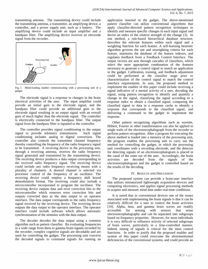
With the proposed enabler and system of this paper, these gadgets can be controlled without a need for an additional hardware, particularly without additional electrodes outside the enabler. The enabler includes a recorder that is insertable in an outer ear area of the user. The recorder records electroencephalography signals generated in the brain. The recorded signals are transferred to a processing unit inserted in the gadget for converting the signals to command applications in the gadget. The proposed system is illustrated in Fig. 1, in which signals derived from the user’s ear are used for decoding the brain activities to enable mental controlling of a gadget. As shown in the figure, in the proposed system, an HCI enabler is inserted in the ear of the user.
The enabler uses electroencephalography recordings from the canal of the external ear to obtain brain activities in a way that is used as a brain-computer interface using signals of complex cognitive. A recorder that is inserted in the enabler records the brain signals. The recorder has an electrode that is located at the entrance of the ear, and could be mounted with an earplug. Signals can be amplified and digitized for transmitting from the enabler. The enabler wirelessly transmits the recorded brain signals to the processing unit that includes a decoder. A transmitting device installed in the enabler produces a radio frequency signal corresponding to voltages sensed by the recorder and transmits the radio frequency signal by radio frequency telemetry through a
(IJACSA) International Journal of Advanced Computer Science and Applications,
Vol. 6, No. 7, 2015
9 | P a g e
www.ijacsa.thesai.org
transmitting antenna. The transmitting device could include the transmitting antenna, a transmitter, an amplifying device, a controller, and a power supply unit, such as a battery. The amplifying device could include an input amplifier and a bandpass filter. The amplifying device receives an electrode signal from the recorder.
Fig. 1. Mind-reading enabler communicating with a processing unit of a
gadget
The electrode signal is a response to changes in the brain electrical activities of the user. The input amplifier could provide an initial gain to the electrode signal, and the bandpass filter could provide an additional gain to the electrode signal resulting in an output signal with an overall gain of much higher than the electrode signal. The controller is electrically connected to the bandpass filter. The output signal from the bandpass filter is inputted to the controller.
The controller provides signal conditioning to the output signal to provide telemetry transmission. Such signal conditioning includes analog to digital conversion. The controller also controls the transmitter channel frequency thereby controlling the frequency of the radio frequency signal to be transmitted. A receiving device in the processing unit, through a receiving antenna, receives the radio frequency signal generated and transmitted by the transmitting device. The receiving device produces a data output corresponding to the received radio frequency signal. The receiving device could include any radio frequency receiving means with a plurality of channels. A desired channel is selected via processor control of the frequency of an oscillator. The receiving device could employ a frequency shift keyed demodulation format. The receiving could also include a microcontroller incorporated to program the oscillator. The receiving device outputs data and error correction bits to the microcontroller which removes error correction bits and outputs corrected data as the data output to an operator interface. The data output corresponds to the radio frequency signal received by the receiving device. The receiving device outputs the data output to the operator interface. The operator interface could include software which allows automatic synchronization of the stimulus with the data output.
The decoder decodes the data output using a common algorithm such as pattern classifier. By evaluating frequencies in a wide range from theta to gamma brain signals recorded by the recorder, complex cognitive signals are decodable and are used for controlling the gadget. The processing unit converts the decoded signals to command signals for running an
application inserted in the gadget. The above-mentioned pattern classifier can utilize conventional algorithms that apply classifier-directed pattern recognition techniques to identify and measure specific changes in each input signal and derive an index of the relative strength of the change [3]. In one method, a rule-based hierarchical database structure, describes the relevant features within each signal and a weighting function for each feature. A self-learning heuristic algorithm governs the use and reweighting criteria for each feature, maintains the database of the feature indexes, and regulates feedback from a Feedback Control Interface. The output vectors are sent through cascades of classifiers, which select the most appropriate combination of the features necessary to generate a control signal to match an application in the gadget. Calibration, training, and feedback adjustment could be performed at the classifier stage prior to characterization of the control signal to match the control interface requirements. In sum, the proposed method to implement the enabler of this paper could include receiving a signal indicative of a mental activity of a user, decoding the signal, using pattern recognition to identify and quantify a change in the signal, classifying the signal according to a response index to obtain a classified signal, comparing the classified signal to data in a response cache to identify a response that corresponds to the classified signal, and delivering a command to the gadget to implement the response.
Other pattern recognizing algorithms such as wavelet, Hilbert, Fourier or other transformation can also be applied to single trails of the electroencephalograph from the recorder to perform pattern recognition. After a program for executing the above method is loaded into a memory of the processing unit, the program enables the processing unit to carry out the method for controlling the gadget, in which the processing unit coordinates with a recording electrode, and the detector for detecting signals of an electroencephalogram is placed in the canal of the outer ear of the user. Accordingly, the brain activities are decoded from the signals of the electroencephalogram and the gadget is controlled based on the results of the decoding.
IV. RESULTS AND DISCUSSION
The proposed system can provide a brain-user interface that utilizes miniaturized lightweight acquisition devices and computing electronics, and applies signal processing methods to acquire and measure mind data under real-time conditions.
It is noted that in conventional devices one of the issues associated with implementing the brain signals is that it can be relatively difficult for a user to control the brain activities [10]. Alpha, beta, and gamma brain waves are readily accessible for sensing with sensors that sense electroencephalography and can be separated into subgroups based on frequency properties. However, for most individuals it is very difficult to influence activity of selected subgroups of brain waves, particularly in a time-controlled manner. Indeed, timing of signals is critical for the most control functions. In order to justify that the proposed enabler and system of this paper could overcome the aforementioned deficiencies of the conventional systems, and could provide an
(IJACSA) International Journal of Advanced Computer Science and Applications,
Vol. 6, No. 7, 2015
10 | P a g e
www.ijacsa.thesai.org
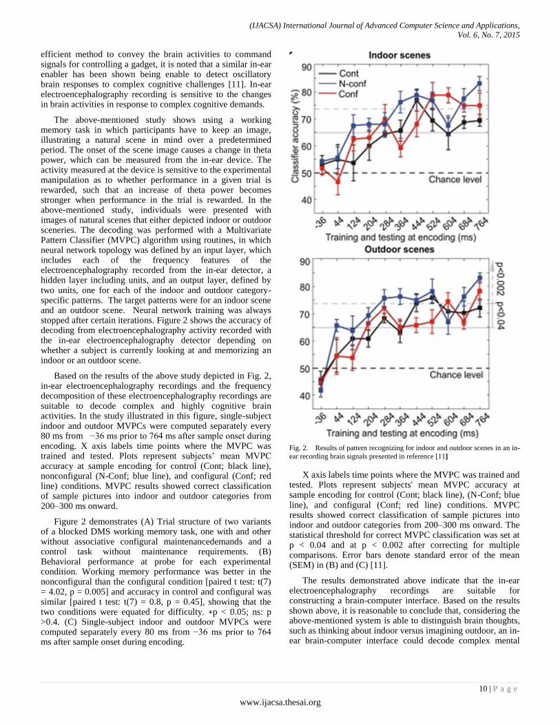
efficient method to convey the brain activities to command signals for controlling a gadget, it is noted that a similar in-ear enabler has been shown being enable to detect oscillatory brain responses to complex cognitive challenges [11]. In-ear electroencephalography recording is sensitive to the changes in brain activities in response to complex cognitive demands.
The above-mentioned study shows using a working memory task in which participants have to keep an image, illustrating a natural scene in mind over a predetermined period. The onset of the scene image causes a change in theta power, which can be measured from the in-ear device. The activity measured at the device is sensitive to the experimental manipulation as to whether performance in a given trial is rewarded, such that an increase of theta power becomes stronger when performance in the trial is rewarded. In the above-mentioned study, individuals were presented with images of natural scenes that either depicted indoor or outdoor sceneries. The decoding was performed with a Multivariate Pattern Classifier (MVPC) algorithm using routines, in which neural network topology was defined by an input layer, which includes each of the frequency features of the electroencephalography recorded from the in-ear detector, a hidden layer including units, and an output layer, defined by two units, one for each of the indoor and outdoor category-specific patterns. The target patterns were for an indoor scene and an outdoor scene. Neural network training was always stopped after certain iterations. Figure 2 shows the accuracy of decoding from electroencephalography activity recorded with the in-ear electroencephalography detector depending on whether a subject is currently looking at and memorizing an indoor or an outdoor scene.
Based on the results of the above study depicted in Fig. 2, in-ear electroencephalography recordings and the frequency decomposition of these electroencephalography recordings are suitable to decode complex and highly cognitive brain activities. In the study illustrated in this figure, single-subject indoor and outdoor MVPCs were computed separately every 80 ms from −36 ms prior to 764 ms after sample onset during encoding. X axis labels time points where the MVPC was trained and tested. Plots represent subjects’ mean MVPC accuracy at sample encoding for control (Cont; black line), nonconfigural (N-Conf; blue line), and configural (Conf; red line) conditions. MVPC results showed correct classification of sample pictures into indoor and outdoor categories from 200–300 ms onward.
Figure 2 demonstrates (A) Trial structure of two variants of a blocked DMS working memory task, one with and other without associative configural maintenancedemands and a control task without maintenance requirements. (B) Behavioral performance at probe for each experimental condition. Working memory performance was better in the nonconfigural than the configural condition [paired t test: t(7) = 4.02, p = 0.005] and accuracy in control and configural was similar [paired t test: t(7) = 0.8, p = 0.45], showing that the two conditions were equated for difficulty. ∗p < 0.05; ns: p >0.4. (C) Single-subject indoor and outdoor MVPCs were computed separately every 80 ms from −36 ms prior to 764 ms after sample onset during encoding.
Fig. 2. Results of pattern recognizing for indoor and outdoor scenes in an in-
ear recording brain signals presented in reference [11]
X axis labels time points where the MVPC was trained and tested. Plots represent subjects' mean MVPC accuracy at sample encoding for control (Cont; black line), (N-Conf; blue line), and configural (Conf; red line) conditions. MVPC results showed correct classification of sample pictures into indoor and outdoor categories from 200–300 ms onward. The statistical threshold for correct MVPC classification was set at p < 0.04 and at p < 0.002 after correcting for multiple comparisons. Error bars denote standard error of the mean (SEM) in (B) and (C) [11].
The results demonstrated above indicate that the in-ear electroencephalography recordings are suitable for constructing a brain-computer interface. Based on the results shown above, it is reasonable to conclude that, considering the above-mentioned system is able to distinguish brain thoughts, such as thinking about indoor versus imagining outdoor, an in-ear brain-computer interface could decode complex mental
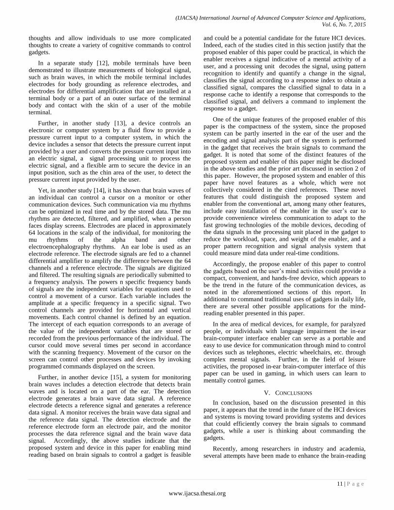
(IJACSA) International Journal of Advanced Computer Science and Applications,
Vol. 6, No. 7, 2015
11 | P a g e
www.ijacsa.thesai.org
thoughts and allow individuals to use more complicated thoughts to create a variety of cognitive commands to control gadgets.
In a separate study [12], mobile terminals have been demonstrated to illustrate measurements of biological signal, such as brain waves, in which the mobile terminal includes electrodes for body grounding as reference electrodes, and electrodes for differential amplification that are installed at a terminal body or a part of an outer surface of the terminal body and contact with the skin of a user of the mobile terminal.
Further, in another study [13], a device controls an electronic or computer system by a fluid flow to provide a pressure current input to a computer system, in which the device includes a sensor that detects the pressure current input provided by a user and converts the pressure current input into an electric signal, a signal processing unit to process the electric signal, and a flexible arm to secure the device in an input position, such as the chin area of the user, to detect the pressure current input provided by the user.
Yet, in another study [14], it has shown that brain waves of an individual can control a cursor on a monitor or other communication devices. Such communication via mu rhythms can be optimized in real time and by the stored data. The mu rhythms are detected, filtered, and amplified, when a person faces display screens. Electrodes are placed in approximately 64 locations in the scalp of the individual, for monitoring the mu rhythms of the alpha band and other electroencephalography rhythms. An ear lobe is used as an electrode reference. The electrode signals are fed to a channel differential amplifier to amplify the difference between the 64 channels and a reference electrode. The signals are digitized and filtered. The resulting signals are periodically submitted to a frequency analysis. The powers n specific frequency bands of signals are the independent variables for equations used to control a movement of a cursor. Each variable includes the amplitude at a specific frequency in a specific signal. Two control channels are provided for horizontal and vertical movements. Each control channel is defined by an equation. The intercept of each equation corresponds to an average of the value of the independent variables that are stored or recorded from the previous performance of the individual. The cursor could move several times per second in accordance with the scanning frequency. Movement of the cursor on the screen can control other processes and devices by invoking programmed commands displayed on the screen.
Further, in another device [15], a system for monitoring brain waves includes a detection electrode that detects brain waves and is located on a part of the ear. The detection electrode generates a brain wave data signal. A reference electrode detects a reference signal and generates a reference data signal. A monitor receives the brain wave data signal and the reference data signal. The detection electrode and the reference electrode form an electrode pair, and the monitor processes the data reference signal and the brain wave data signal. Accordingly, the above studies indicate that the proposed system and device in this paper for enabling mind reading based on brain signals to control a gadget is feasible
and could be a potential candidate for the future HCI devices. Indeed, each of the studies cited in this section justify that the proposed enabler of this paper could be practical, in which the enabler receives a signal indicative of a mental activity of a user, and a processing unit decodes the signal, using pattern recognition to identify and quantify a change in the signal, classifies the signal according to a response index to obtain a classified signal, compares the classified signal to data in a response cache to identify a response that corresponds to the classified signal, and delivers a command to implement the response to a gadget.
One of the unique features of the proposed enabler of this paper is the compactness of the system, since the proposed system can be partly inserted in the ear of the user and the encoding and signal analysis part of the system is performed in the gadget that receives the brain signals to command the gadget. It is noted that some of the distinct features of the proposed system and enabler of this paper might be disclosed in the above studies and the prior art discussed in section 2 of this paper. However, the proposed system and enabler of this paper have novel features as a whole, which were not collectively considered in the cited references. These novel features that could distinguish the proposed system and enabler from the conventional art, among many other features, include easy installation of the enabler in the user’s ear to provide convenience wireless communication to adapt to the fast growing technologies of the mobile devices, decoding of the data signals in the processing unit placed in the gadget to reduce the workload, space, and weight of the enabler, and a proper pattern recognition and signal analysis system that could measure mind data under real-time conditions.
Accordingly, the propose enabler of this paper to control the gadgets based on the user’s mind activities could provide a compact, convenient, and hands-free device, which appears to be the trend in the future of the communication devices, as noted in the aforementioned sections of this report. In additional to command traditional uses of gadgets in daily life, there are several other possible applications for the mind-reading enabler presented in this paper.
In the area of medical devices, for example, for paralyzed people, or individuals with language impairment the in-ear brain-computer interface enabler can serve as a portable and easy to use device for communication through mind to control devices such as telephones, electric wheelchairs, etc. through complex mental signals. Further, in the field of leisure activities, the proposed in-ear brain-computer interface of this paper can be used in gaming, in which users can learn to mentally control games.
V. CONCLUSIONS
In conclusion, based on the discussion presented in this paper, it appears that the trend in the future of the HCI devices and systems is moving toward providing systems and devices that could efficiently convey the brain signals to command gadgets, while a user is thinking about commanding the gadgets.
Recently, among researchers in industry and academia, several attempts have been made to enhance the brain-reading

(IJACSA) International Journal of Advanced Computer Science and Applications,
Vol. 6, No. 7, 2015
12 | P a g e
www.ijacsa.thesai.org
interface technologies. However, as set forth in this paper, each of these devices and systems suffers from deficiencies that refrains the field from achieving maturity. Indeed, it appears that much more research is needed to achieve to a point of commercializing these systems and devices that could be affordable and comfortable for the users. One of the major obstacles in this journey appears to be in the area of pattern recognition of the mind signals, considering the limited understanding of a user’s brain and its electrical activities, since the accuracy of a mind signal detection could be degraded as the number of mind states increases, such as when the user thinks about a series of words to implement a task. In this paper a system was proposed that includes an enabler for controlling gadgets based on signal analysis of brain activities transmitted from the enabler to the gadget. The enabler could be inserted in the user’s ear and includes a recorder that records brain signals. A processing unit of the system commands the device based on decoding the recorded brain signals. The proposed enabler could provide a compact, convenient, and hands-free device to facilitate a brain-machine interface to control the gadget from electroencephalography signals in the user’s brain.
ACKNOWLEDGEMENT
The author would like to thank Mr. Sam Sahota of McGinn IP Law, PLLC, and Dr. JoAnn Paul of Electrical and Computer Engineering Department at Virginia Tech for their helpful suggestions in preparing this paper.
REFERENCES
[1] Vaughan, T. M., Heetderks, W. J., Trejo, L. J., Rymer , W. Z., Weinrich, M., Moore, M. M., Kübler, A., Dobkin, B. H., Birbaumer, N., Donchin, E., Wolpaw, E. W., Wolpaw, J. R. 2003. Brain-Computer Interface Technology: A Review of the Second International Meeting. IEEE Transactions on Neural Systems and Rehabilitation Engineering, 11 (Jun. 2003), 94-109.
[2] Giles, N. O. 2011. IBM '5 in 5' predicts no more passwords, mind-reading smartphones. Los Angeles Times (Dec. 2011). http://latimesblogs.latimes.com/technology/2011/12/ibm-predicts-a-future-with-no-passwords-mind-reading-smartphones.html.
[3] DuRousseau, D. R., Method and system for initiating activity based on sensed electrophysiological data, U.S. Patent Application Publication No. 2002/0077534, June 20, 2002.
[4] Wolpaw, J. R., Birbaumer N., McFarland, D. J., Pfurtscheller, G., Vaughan, T. M., 2002. Brain-computer interfaces for communication and control. Clinical Neurophysiology, 113 (Jun. 2002), 767-791.
[5] Tian, J., Ahmaniemi, T., Boda, P., Vetek, K., Apparatus, method and computer program product providing a hierarchical approach to command-control tasks using a brain-computer interface, U.S. Patent No. 8,005,766, August 23, 2011.
[6] Molina, G., Nelson G., Bruekers, A., Damstra, M., Weda, J., Relating to computer brain interfaces, U.S. Patent Application Publication No. 2011/0238685, September 29, 2011.
[7] Liao, X., Yao, D., Li, C. 2007. Transductive SVM for reducing the training effort in BCI. Journal of Neural Engineering. 4 (Dec. 2007), 246-254.
[8] Tan, D., Saponas, T., Morris, D., Turner, J., Wearable electromyography-based for human-computer interface, U.S. Patent Application Publication No. 2009/0326406, December 31, 2009.
[9] Zimmerman, A. W., Pepper, B. T., Blankenship, D. V., Electroencephalograph incorporating at least one wireless link, U.S. Patent No. 5,279,305, January 18, 1994.
[10] Schuette, F. M., Junker, A., Method and apparatus for using biopotentials for simultaneous multiple control functions in computer systems, U.S. Patent Application Publication No. 2011/0301488, December 8, 2011
[11] Fuentemilla, L., Cashdollar, N., Bunzeck, N., Penny, W., Dyzel, E. 2010. Theta coupled periodic replay in working memory. Curr Biol. 20 (Apr. 2010), 606-612.
[12] Manabe, H., Nakano, H., Sugimura, T., Hiraiwa, A., Mobile terminal capable of measuring biological signal, and measuring method, Japanese Patent Application Publication No. JP 2004-016658 A, January 22, 2004.
[13] Bonnat, P., Apparatus to support a device to control an electronic or computer system by means of a fluid flow and a method of manufacturing the same, U.S. Patent Application Publication No. 2004/0252103, December 16, 2004.
[14] Wolpaw, J. R., McFarland, D. J., Neat, G. W., Forneris, C. A., 1991. An EEG-based brain-computer interface for cursor control. Electroencephalography and Clinical Neurophysiology. 78 (Mar. 1991), 252-259.
[15] Cain, R., Systems and methods for detecting brain waves, U.S. Patent Application Publication No. 2006/0094974, May 4, 2006.

(IJACSA) International Journal of Advanced Computer Science and Applications,
Vol. 6, No. 7, 2015
13 | P a g e
www.ijacsa.thesai.org
Enrichment of Object Oriented Petri Net and Object Z
Aiming at Business Process Optimization
Aliasghar Ahmadikatouli
Islamic Azad University, Sari Branch
Sari, Iran
Homayoon Motameni
Islamic Azad University, Sari Branch
Sari, Iran
Abstract—Software development process is on the basis of two
important steps each of which has to be taken seriously, system
requirement analysis and system modeling. There have been
many different approaches in the literature that has their own
strengths and weaknesses to tackle these two important steps,
however, there is none comprehensive approach. Among them,
formal methods by using their mathematical supporting
background could achieve a precise, clear and in detail
requirement analysis. However they were not able to illustrate
graphically a system for stakeholders. On the other hand, semi-
formal methods owning graphically representation of a system’s
behavior make it easy for the stakeholders to perceive
thoroughly. In this paper we represent an integration of object Z
formal language and a graphically modeling tool hierarchical
object oriented petri net. The application of business process was
used to be modeled by this intergraded language.
Keywords—Object Z; Hierarchical object oriented Petri net;
Formal methods integration; Business process; process
improvement; process optimization
I. INTRODUCTION
Many efforts have been devoted to develop software systems that could meet all customer expectations and without any faults and ambiguities. Therefore, software development methods succeed to attract more interests among software mania in last decade. In the last 25 years we observe the emerge of different software development approaches such as structural methods, mathematical, object oriented and some approach to develop parallel and distributed systems. However, none of them could be applied as a comprehensive approach to describe all types of systems and different aspects of systems. Hence, researchers pursuits an integrated method that cover each other’s weaknesses and bring new aspects. Method integration was studied in a number of contexts: combining formal and informal methods, combining multiple formal methods. Method integration can involve the definition of relationships between the processes of the methods being combined. It may happen to be involving constructing formal definition of the meaning of compositions written in different notation. Method integration can also be carried out via the linking of individual tools that support separate methods.
In this paper we intend to develop an integrated approach, OPOZ, which is an enrichment of two different languages, object Z and hierarchical object oriented petri net to model business processes. This new approach can complete business process optimization and their verification with less time and cost comparing to using only one of them. The importance of formal method for developing reliable and fault tolerant
systems has been widely recognized in last decade. Therefore, many formal methods have been developed. Formal methods based on a formal foundation only used to specify some aspects (control, data, structure, behavior, etc.) and only some types (sequential, concurrent, distributed, real time and etc.) of software systems.
It is indispensible to say that there isn’t a single formal language to satisfy the analysis of all functional and non-functional requirements. There exists several technical and philosophical reasons like, most formal methods are not able to describe non-functional requirements of systems or each formal language possess a separate set of properties to specify aspects of systems [1]. Integration of methods presents some advantages that mapping one of them to the other cannot achieve the same goal. Another way is that the system analyst modeled a system and describes its specification by different methods. Formal methods use different formalism and never an analyst could apply all these notations and formalisms on a single same system and if this happens it needed to model a system over and over which all these leads to consume time and cost. However, using integration language can help to diminish this gap in analyzing and modeling a system.
The rest of paper organized as follows: in section 2 we describe main aspects of Object Z and hierarchical object oriented petri nets. Section 3 describes the integrated model of these two languages. In section 4 we develop some reduction rules which will be uses in business process optimization and finally in last section we model a simple system by this integrated model.
RELATED WORK
Formal methods up to now have been applied on safe and critical application. Formal method integration attracts many researches in recent years. Richard F. Paige [1] proposed a Meta model to integrate formal method and semi-formal method and analyze and evaluate the Meta model with some case studies. It is necessary to add that the way two methods must be chosen is based on the research [2] that defines when a method is incomplete and should be integrated. In [3] an integrated Object-Z and Use case diagram method has been proposed to insure the completeness and consistent of model. Soon-Kyeong Kim et. al. [4] develops an approach to express classes in class diagram via Object Z and they could reason a class diagram. Also the communications among class are fully defined as communications among OZ schemas. . A method to map use case diagram to Z schema has been proposed in [5] and a type checking by using ZTC tool was performed to

(IJACSA) International Journal of Advanced Computer Science and Applications,
Vol. 6, No. 7, 2015
14 | P a g e
www.ijacsa.thesai.org
extract ER diagram. Furthermore, though UML models graphically represent the structure of models and interaction among them, the lack of formal definition was immensely required, therefore, UML models were formalized by object Z schema in [7].
Researches carried out extensive research for business process modeling and analysis and many modeling and analysis techniques have been developed. However, the lack of a systematic approach that software designer could take its steps and produce an optimum model was the reason to propose methods to optimize business process models [8]. Zho and Chen [9] claimed that business process optimization can lead to less running cost and turnaround time and intensify quality of product and customer satisfaction. Vetschera and Hofacker [10] by using a genetic algorithm proposed a mathematical modeling to optimize a business process. Tiwari et al [11] and Vergdis et al [18,19] developed this mathematical model and proposed a multi-objective optimization algorithm to optimize a business process. Using formal methods to detect bottlenecks and redundant processes in a model can help designers to improve their models and optimize their predefined objective functions.
II. PRINCIPLE CONCEPTS
A. Hierarchical Object Oriented Petri Net:
HOOPN is a graphical representation of system using petri net and classes in object oriented paradigm [14]. A HOONet is a three tuple including (OIP, ION, DD) that OIP is a unique property and identification of a class. Inter Object Net (ION) is inter structural of system that represent the behavior of class and data dictionary (DD) declare the attribute of a class. The formal definition of a HOONet is [14]:
A HOONet is a three tuple (OIP,ION,DD) that must satisfy the following conditions
1) OIP is a specific place that is defined as a tuple (oip,
pid, M0,status)
Oip is a variable for the unique name of a HOONet
Pid a unique process identifier to distinguish multiple instances of a class
M0 is a function that gives specific value to the tokens
Status is a flag variable to specify the state of OIP
2) Is a type of CPN that shows the variant of attributes
and behavior of methods
3) DD is a dictionary of variables, token types and
functions
B. Object Z Formal Method:
Applying formal methods in software development process is indispensible. We need to consider modularity and reusability concepts to deal with the complexity of today’s software and using methods. Therefore, using object oriented formal method that models a system based on objects and their interactions can help us.
Fig. 1. The general structure of a HOONet [14]
Here, we summarize some important concepts of object Z which is an extension of Z and the key important feature added to it is the concept of class schema [16]. Class schema capsulate a schema with its all operations that may effect on its attributes. Figure 2 shows a class schema defined in object Z. Specifying a system in object Z, we must identify and specify the underlying objects and specify the system in terms of the communication between the underlying objects. However, an object may itself be a system of communication objects. A class can incorporates all the features of its inherited classes and their local types have based on Z syntax. Variables also called attributes in form of Z. All details of Object z specification and notation can be found on [19].
Fig. 2. Class schema defined in object Z
C. Business Process:
Today organizations consist of a set of business process that each one possess a unique functionality. Business process can be specified and model based on goals and missions in an organization. In other word, each business process defines a specific workflow in organization and workflow in basis of organization operation [13]. There have been many definitions of business process in literature. Harvey [6] defines a business process as a set of specific rules to analyze a business problem. In last decade, many researchers devoted their efforts on process modeling and many notations, methods and tools were developed [17,18]. From organization view, different goals can be considered in modeling a process. Modeling aiming at documentation or execution and etc. some of the most important business process modeling are UML, EPDL, EPC, WSDL, BPEL4WS, BPMN.

(IJACSA) International Journal of Advanced Computer Science and Applications,
Vol. 6, No. 7, 2015
15 | P a g e
www.ijacsa.thesai.org
III. OBJECT Z – OBJECT ORIENTED PETRI NETS (OPOZ)
In this section we present the integrated approach of object Z and object oriented petri nets. Main advantages emerge by object oriented petri net are:
1) Object oriented petri net is a good graphically tool to
model concurrent and distributed system.
2) Object oriented petri net is able to comprehensively
describe control structure and dynamic behavior of systems. Also, main merits bring by object Z include suitable
notations to describe and specify sequential system’s function and appropriate to define types and logical and formal reasoning. In addition, advantages carries out by integrated methods are included into these:
1) A unified model for specifying different aspects of a
system ( structure, control flow, data types, and functionality)
2) A unified formal model for specifying different types of
systems ( sequential, concurrent, and distributed systems)
3) A rich set of complementary specification development
and analysis techniques
4) New theoretical and methodological research problems
resulted from the integration. Similar to the [ 7,15] the general strategy is to use object
oriented petri net to define structure and control and behavior of system and to use object Z schemas to define data abstraction , structure, system constraints and functional process. Therefore the structure of OPOZ net is as follow:
A OPOZ net is a tuple (Net, OZ, des) that
1) Net = (P,T,F) is a net structure, in which
a) P and T are non-empty finite sets satisfying P∩T= Ø
(P and T are the sets of places and transitions of Net,
respectively),
b) F (P × T) (T × P) is a flow relation (the arcs of
Net);
2) OZ = (Zp, ZT,ZI) is a tuple of collection of OZ schemas Also we uses three functions, Pro(Z), Signature(Z),
Title(Z) to specify the name and signature and property of schema. Here a schema has to satisfy following conditions:
o ( ( )
( ) )
o ( ( )
( ) ) and
o | | | |
The first two conditions show that the signature of OZ schema are pair-wise disjoingt, and the last condition depicts that the number of OZ schema in Zp is the same as that in ZI, i.e. one to one correspondence.
des= (PM,TM,L,M0) is a net inscription that
associates a net element in N with its notation in Z
o PM: P→ZP For each place p P, S maps p
to a unique OZ schema oz Zp such that
p=Title(oz). The type of p is defined by the
signature of oz
o TM: T→ZT is one to one mapping
providing the functionality definition of Net.
For each transition t T, TM maps t to a
OZ schema oz ZT such that t=Title(oz).
o L: F→ Var is the control flow definition of
Net, where Var is the set of all hidden
variables (through quantification) in OZT .
o M0: P→ZI is an PM-respecting (i.e.
signature(PM(p)) = signature (M0(p)) initial
marking of Net, where ZI is a set of OZ
schemas defining the initial state of the
system.
The process of development of OPOZ model should be based on following steps:
1) Considering the requirement of systems that includes a
list of events. Each event can be model by a separate petri net
and then integrate by common places.
2) Using OZ schema to express data and function of
system that defines the behavioral model of system.
3) Define a state schema with a specific type of each
place
4) Define an initial state schema of each state schema
5) Define a functional schema for each transition and the
predicate section of schema must be written based on the
constraint on each transition That is obvious that organizations need to adapt
themselves with the changes in customer requirements and therefore they have to change their business processes. Besides, pervious processes and pervious models are not usable any longer and a modification in modeling is necessary. Therefore, modeling business processes using this integrated model avoid most of remodeling. We can change schema predicate if there exist any changes in business functionalities. Hence, we develop some rules to reduce or join processes. In addition, if function of only a process changed, therefore only correspond predicate in its schema needs to be modified.
Rule 1 – addition of a new predicate: Let P be a new place, Z1 be its type and state defining OZ schema, and Z2 be its initial state defining Z schema, addition place p to P results in:
a) Adding z1 to Zp and Z2 to ZI
b) Addition relationship (p,Z1) to S, and relationship
(p,Z2) to M0
Rule 2 – addition of a new transition: let t be a new transition needs to be added to the model and z be its OZ schema, adding t to T results in:

(IJACSA) International Journal of Advanced Computer Science and Applications,
Vol. 6, No. 7, 2015
16 | P a g e
www.ijacsa.thesai.org
a) Adding z to ZT and
b) Adding relationship (t,z) to TM
Rule 3- Merging two places with same preset and post set
Assuming p1 and p2 two places with exact equal preset and post sets and following condition ( figure 3) :
{
where Ii and Oi are input condition and output condition of transition Ti respectively. Therefore merging those results in:
a) Adding p to the P
b) Adding arc (p,t) to F. if ( ) then adds
(( ) ( ) ( )) to L
c) Adding new arc (t,p) the same opposite to the b
d) Adding Z1 to the Zp that we use schema conjunction
on PM(p1) and PM(p2)
e) Adding Z2 to the ZI that we use schema conjunction
on M0(p1) and M0(p2) and adding (p,Z0) to the M0
Fig. 3. Merging two places with the same presets and post sets conditions
Rule 4: Merging two serial transitions:
Assuming that t1 and t2 two transitions with the exact same preset and post set (figure 4).
Consider the following condition Ti . Oi = Tj .Ij =Pk
Fig. 4. Merging two Transition with the same presets and post sets
conditions
Merging two Ti and Tj result in T and following constraints
a) Adding t to the T
b) Adding z schema to the ZT that define based on figure
5.
c) Adding new arc (p,t) to the F
d) Removing p from P and state schema p from Zp
e) Removing t1,t2 from T and correspond schemas from
ZT and related arcs from F.
(a) (b)
(c)
Fig. 5. Merging two ZTi , ZTj, ZT schemas(c)
Rule 5: Merging to parallel transitions:
Assuming T1 and T2 two parallel transitions with exact equal preset and post sets and with the schema t1 and t2 and following condition:
a) Ti . I1,2,…, n = Tj . I1,2,…,n = Tn . I1,2,..,n b) Ti . O1,2,…,n = Tj . O1,2,…,n = Tn . I1,2,…,n
The purpose of this rule is that the all function with the same input and output that apply simultaneously can be merged into one function that improves the overall performance of business process. The figure 6 shows this merging procedure.
Fig. 6. Merging two parallel Transitions
P
1
P
2
T
i
P
Ti Tj Pk T
q2 Tj
q1 Ti
P1
P2
pn
q
2 T
j
q1 P
1
P2
pn

(IJACSA) International Journal of Advanced Computer Science and Applications,
Vol. 6, No. 7, 2015
17 | P a g e
www.ijacsa.thesai.org
Also, the functional states will be modified according to the figure 7 and it shows that predicates will be merged together and logical conjunction will be applied on predicate P and Q.
Fig. 7. The Modification of Two parallel OZ schemas
IV. CASE STUDY
Here we consider a car renting system and following interaction should be supported
1) Checking for renting availability of a car
2) Restoring a car to the garage Also all cars should be available for renting or be rented
already. According to the pervious section with the requirement analysis our system component includes customers, cars, car state, and contracts. The overall system model is depicted in figure 8.
Fig. 8. Model of Car renting system
Based on the requirements of car renting system two events correspond to the renting a car and restoring to the garage have been noticed. Therefore, the HOONet structure of these two events are depicted in figure 9,10. The renting HOONet structure includes 1) customer validating 2) car availability 3) car status updating , and the HOONet structure of restoring a car contain 1) customer validating and 2) car status updating and then these two nets are integrated by common places and figure 11 are resulted.
Fig. 9. Petri net model of Renting event
Fig. 10. Petri net model of Restoring event
Fig. 11. Combining two petri net model (fig 9,10) based on common places
Cars
Customers Car status
Transactions
Cars
Customers
Car status
Renting
Customers
Car status
Restoring
Restoring
Cars
Customers
Car status
Renting

(IJACSA) International Journal of Advanced Computer Science and Applications,
Vol. 6, No. 7, 2015
18 | P a g e
www.ijacsa.thesai.org
Based on the HOONet structure we propose three schemas in OZ for customers, cars and car status which are illustrated in figure 12,13,14 respectively.
Fig. 12. Customer OZ
Fig. 13. Car OZ schema
Fig. 14. Car_Status OZ schema
The last predicate in Car status shows that a car must be available for renting or have been rented already not both. Renting transaction requires both validate a customer and update a car status. The input of this transaction includes customer identification and car information and car status flag. The renting schema shows in figure 15.
Fig. 15. Renting OZ schema
In the renting schema we do not need the information of cars and therefore the restoring schema shows in figure 16
Fig. 16. Restoring OZ schema
Assuming that we need to add a new transaction that shows if a car is not available or the customer is not valid the system should reported an error message.
Therefore adding this new transaction resulted in updating only one HOONet structure and designing a new schema which is depicted in figure 17 and figure 18 respectively.
Fig. 17. Renting Error OZ schema
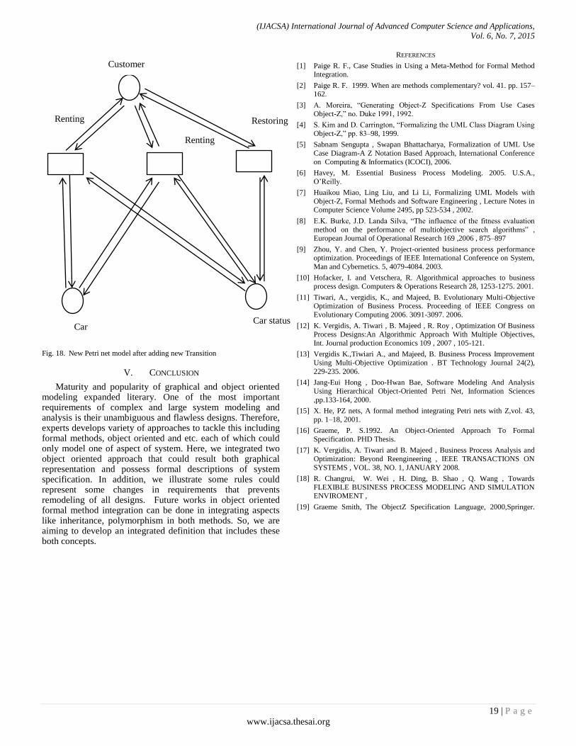
(IJACSA) International Journal of Advanced Computer Science and Applications,
Vol. 6, No. 7, 2015
19 | P a g e
www.ijacsa.thesai.org
Fig. 18. New Petri net model after adding new Transition
V. CONCLUSION
Maturity and popularity of graphical and object oriented modeling expanded literary. One of the most important requirements of complex and large system modeling and analysis is their unambiguous and flawless designs. Therefore, experts develops variety of approaches to tackle this including formal methods, object oriented and etc. each of which could only model one of aspect of system. Here, we integrated two object oriented approach that could result both graphical representation and possess formal descriptions of system specification. In addition, we illustrate some rules could represent some changes in requirements that prevents remodeling of all designs. Future works in object oriented formal method integration can be done in integrating aspects like inheritance, polymorphism in both methods. So, we are aiming to develop an integrated definition that includes these both concepts.
REFERENCES
[1] Paige R. F., Case Studies in Using a Meta-Method for Formal Method
Integration.
[2] Paige R. F. 1999. When are methods complementary? vol. 41. pp. 157–162.
[3] A. Moreira, ―Generating Object-Z Specifications From Use Cases
Object-Z,‖ no. Duke 1991, 1992.
[4] S. Kim and D. Carrington, ―Formalizing the UML Class Diagram Using
Object-Z,‖ pp. 83–98, 1999.
[5] Sabnam Sengupta , Swapan Bhattacharya, Formalization of UML Use
Case Diagram-A Z Notation Based Approach, International Conference
on Computing & Informatics (ICOCI), 2006.
[6] Havey, M. Essential Business Process Modeling. 2005. U.S.A.,
O’Reilly.
[7] Huaikou Miao, Ling Liu, and Li Li, Formalizing UML Models with
Object-Z, Formal Methods and Software Engineering , Lecture Notes in Computer Science Volume 2495, pp 523-534 , 2002.
[8] E.K. Burke, J.D. Landa Silva, ―The influence of the fitness evaluation
method on the performance of multiobjective search algorithms‖ , European Journal of Operational Research 169 ,2006 , 875–897
[9] Zhou, Y. and Chen, Y. Project-oriented business process performance optimization. Proceedings of IEEE International Conference on System,
Man and Cybernetics. 5, 4079-4084. 2003.
[10] Hofacker, I. and Vetschera, R. Algorithmical approaches to business process design. Computers & Operations Research 28, 1253-1275. 2001.
[11] Tiwari, A., vergidis, K., and Majeed, B. Evolutionary Multi-Objective Optimization of Business Process. Proceeding of IEEE Congress on
Evolutionary Computing 2006. 3091-3097. 2006.
[12] K. Vergidis, A. Tiwari , B. Majeed , R. Roy , Optimization Of Business Process Designs:An Algorithmic Approach With Multiple Objectives,
Int. Journal production Economics 109 , 2007 , 105-121.
[13] Vergidis K.,Tiwiari A., and Majeed, B. Business Process Improvement
Using Multi-Objective Optimization . BT Technology Journal 24(2),
229-235. 2006.
[14] Jang-Eui Hong , Doo-Hwan Bae, Software Modeling And Analysis
Using Hierarchical Object-Oriented Petri Net, Information Sciences
,pp.133-164, 2000.
[15] X. He, PZ nets, A formal method integrating Petri nets with Z,vol. 43,
pp. 1–18, 2001.
[16] Graeme, P. S.1992. An Object-Oriented Approach To Formal
Specification. PHD Thesis.
[17] K. Vergidis, A. Tiwari and B. Majeed , Business Process Analysis and
Optimization: Beyond Reengineering , IEEE TRANSACTIONS ON
SYSTEMS , VOL. 38, NO. 1, JANUARY 2008.
[18] R. Changrui, W. Wei , H. Ding, B. Shao , Q. Wang , Towards
FLEXIBLE BUSINESS PROCESS MODELING AND SIMULATION ENVIROMENT ,
[19] Graeme Smith, The ObjectZ Specification Language, 2000,Springer.
Renting
True
Car
Customer
Car status
Restoring
Renting
Error
(IJACSA) International Journal of Advanced Computer Science and Applications,
Vol. 6, No. 7, 2015
20 | P a g e
www.ijacsa.thesai.org
FSL-based Hardware Implementation for Parallel
Computation of cDNA Microarray Image
Segmentation
Bogdan Bot
Student within Technical University of Cluj-Napoca,
Faculty of Automation and Computer Science
Cluj-Napoca, Romania
Simina Emerich
Department of Communication, Technical University of
Cluj-Napoca, Cluj-Napoca, Romania
Sorin Martoiu
National Institute of Nuclear Physics and Engineering
“Horia Hulubei” – IFIN-HH, Bucuresti, Romania
Bogdan Belean
Department of Mass Spectrometry, Chromatography and
Applied Physics, INCDTIM
Department of Communication, Technical University of
Cluj-Napoca, Romania
Abstract—The present paper proposes a FPGA based
hardware implementations for microarray image processing
algorithms in order eliminate the shortcomings of the existing
software platforms: user intervention, increased computation
time and cost. The proposed image processing algorithms exclude
user intervention from processing. An application-specific
architecture is designed aiming microarray image processing
algorithms parallelization in order to speed up computation.
Hardware architectures for logarithm based image enhancement,
profile computation and image segmentation are described. The
methodology to integrate the hardware architecture within a
microprocessor system is detailed. The Fast Simplex Link (FSL)
bus is used to connect the hardware architecture as speed up co-
processor of the microarray image processing system. Timing
considerations were presented considering the levels of
parallelism that can be achieved by using our proposed hardware
architectures. The FPGA technology was chosen for
implementation, due to its parallel computation capabilities and
ease of reconfiguration.
Keywords—microarray; FPGA; image processing; hardware
algorithms
I. CDNA MICROARRAY TECHNOLOGY
Measurement of gene expression can provide clues about regulatory mechanism, biochemical pathways and broader cellular function. By gene expression we understand the transformation of gene‟s information into proteins. The informational pathway in gene expression is as follows: DNA → mRNA → protein. The protein coding information is transmitted by an intermediate molecule called messenger ribonucleic acid mRNA. This molecule passes from nucleus to cytoplasm carrying the information to build up proteins [1]. This mRNA acid is a single stranded molecule from the original DNA and is subject to degradation, so it is transformed into stable complementary DNA for further examination. Microarray technology is based on creating DNA microarrays which represents gene specific probes arrayed on a matrix such as a glass slide or microchip. The most common use for DNA
microarrays is to measure, simultaneously, the level of gene expression for every gene in a genome [2]. In this way the microarray compares genes from normal cells with abnormal or treated cells, determining and understanding the genes involved in different diseases.
DNA microarrays represent gene specific probes arrayed on a matrix such as a glass slide or microchip. Usually samples from two sources are labeled with two different fluorescent markers and hybridized on the same array (glass slide). The hybridization process represents the tendency of 2 single stranded DNA molecules to bind together. After hybridization, the array is scanned using two light sources with different lengths (red and green) to determine the amount of labeled sample bound to each spot through hybridization process. The light sources induce fluorescence in the spots which is captured by a scanner and a composite image is produced [3].
Classical genomic microarray experiment involves complex steps including slide production and scanning. A brief description of a microarray experiment can be summarized as follows: a) generation of array ready cDNA, b) cDNA selection and microarray slide printing, c) selection of specific cell material and fluorescent labeling, d) hybridization of the target material on the microarray slide, e) microarray image scanning, f) microarray image processing for gene expression evaluation, g) high order processing (clustering and interpretation, gene regulatory network estimation).
The present paper provides a detailed description of microarray image processing algorithms. The classical flow of processing a microarray image is generally separated in the following tasks: addressing, segmentation, intensity extraction and pre-processing to improve image quality and enhance weakly expressed spots. The first step associates an address to each spot of the image. In the second one, pixels are classified either as fore-ground, representing the DNA spots, or as background. The last step calculates the intensities of each spot and also estimates background intensity values.
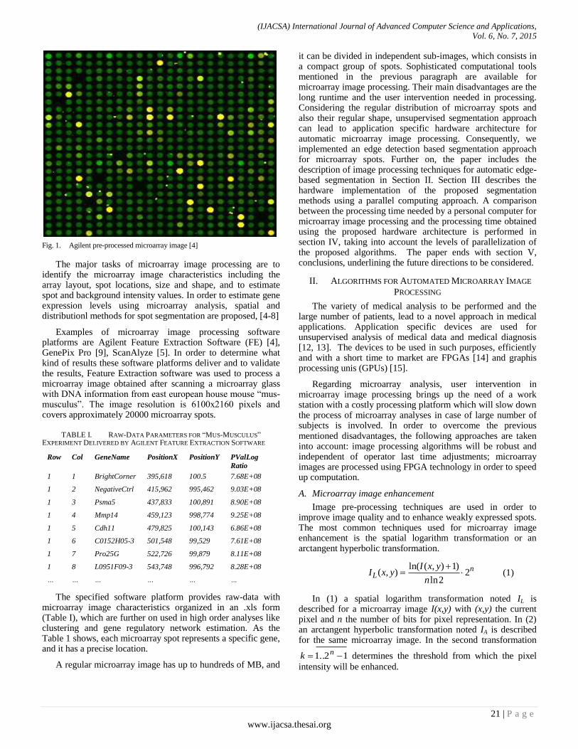
(IJACSA) International Journal of Advanced Computer Science and Applications,
Vol. 6, No. 7, 2015
21 | P a g e
www.ijacsa.thesai.org
Fig. 1. Agilent pre-processed microarray image [4]
The major tasks of microarray image processing are to identify the microarray image characteristics including the array layout, spot locations, size and shape, and to estimate spot and background intensity values. In order to estimate gene expression levels using microarray analysis, spatial and distributionl methods for spot segmentation are proposed, [4-8]
Examples of microarray image processing software platforms are Agilent Feature Extraction Software (FE) [4], GenePix Pro [9], ScanAlyze [5]. In order to determine what kind of results these software platforms deliver and to validate the results, Feature Extraction software was used to process a microarray image obtained after scanning a microarray glass with DNA information from east european house mouse “mus-musculus”. The image resolution is 6100x2160 pixels and covers approximately 20000 microarray spots.
TABLE I. RAW-DATA PARAMETERS FOR “MUS-MUSCULUS”
EXPERIMENT DELIVERED BY AGILENT FEATURE EXTRACTION SOFTWARE
Row
Col
GeneName
PositionX
PositionY
PValLog
Ratio
1 1 BrightCorner 395,618 100.5 7.68E+08
1 2 NegativeCtrl 415,962 995,462 9.03E+08
1 3 Psma5 437,833 100,891 8.90E+08
1 4 Mmp14 459,123 998,774 9.25E+08
1 5 Cdh11 479,825 100,143 6.86E+08
1 6 C0152H05-3 501,548 99,529 7.61E+08
1 7 Pro25G 522,726 99,879 8.11E+08
1 8 L0951F09-3 543,748 996,792 8.28E+08
… … … … … …
The specified software platform provides raw-data with microarray image characteristics organized in an .xls form (Table I), which are further on used in high order analyses like clustering and gene regulatory network estimation. As the Table 1 shows, each microarray spot represents a specific gene, and it has a precise location.
A regular microarray image has up to hundreds of MB, and
it can be divided in independent sub-images, which consists in a compact group of spots. Sophisticated computational tools mentioned in the previous paragraph are available for microarray image processing. Their main disadvantages are the long runtime and the user intervention needed in processing. Considering the regular distribution of microarray spots and also their regular shape, unsupervised segmentation approach can lead to application specific hardware architecture for automatic microarray image processing. Consequently, we implemented an edge detection based segmentation approach for microarray spots. Further on, the paper includes the description of image processing techniques for automatic edge-based segmentation in Section II. Section III describes the hardware implementation of the proposed segmentation methods using a parallel computing approach. A comparison between the processing time needed by a personal computer for microarray image processing and the processing time obtained using the proposed hardware architecture is performed in section IV, taking into account the levels of parallelization of the proposed algorithms. The paper ends with section V, conclusions, underlining the future directions to be considered.
II. ALGORITHMS FOR AUTOMATED MICROARRAY IMAGE
PROCESSING
The variety of medical analysis to be performed and the large number of patients, lead to a novel approach in medical applications. Application specific devices are used for unsupervised analysis of medical data and medical diagnosis [12, 13]. The devices to be used in such purposes, efficiently and with a short time to market are FPGAs [14] and graphis processing unis (GPUs) [15].
Regarding microarray analysis, user intervention in microarray image processing brings up the need of a work station with a costly processing platform which will slow down the process of microarray analyses in case of large number of subjects is involved. In order to overcome the previous mentioned disadvantages, the following approaches are taken into account: image processing algorithms will be robust and independent of operator last time adjustments; microarray images are processed using FPGA technology in order to speed up computation.
A. Microarray image enhancement
Image pre-processing techniques are used in order to improve image quality and to enhance weakly expressed spots. The most common techniques used for microarray image enhancement is the spatial logarithm transformation or an arctangent hyperbolic transformation.
nL
n
yxIyxI 2
2ln
)1),(ln(),(
(1)
In (1) a spatial logarithm transformation noted IL is described for a microarray image I(x,y) with (x,y) the current pixel and n the number of bits for pixel representation. In (2) an arctangent hyperbolic transformation noted IA is described for the same microarray image. In the second transformation
12..1 nk determines the threshold from which the pixel
intensity will be enhanced.
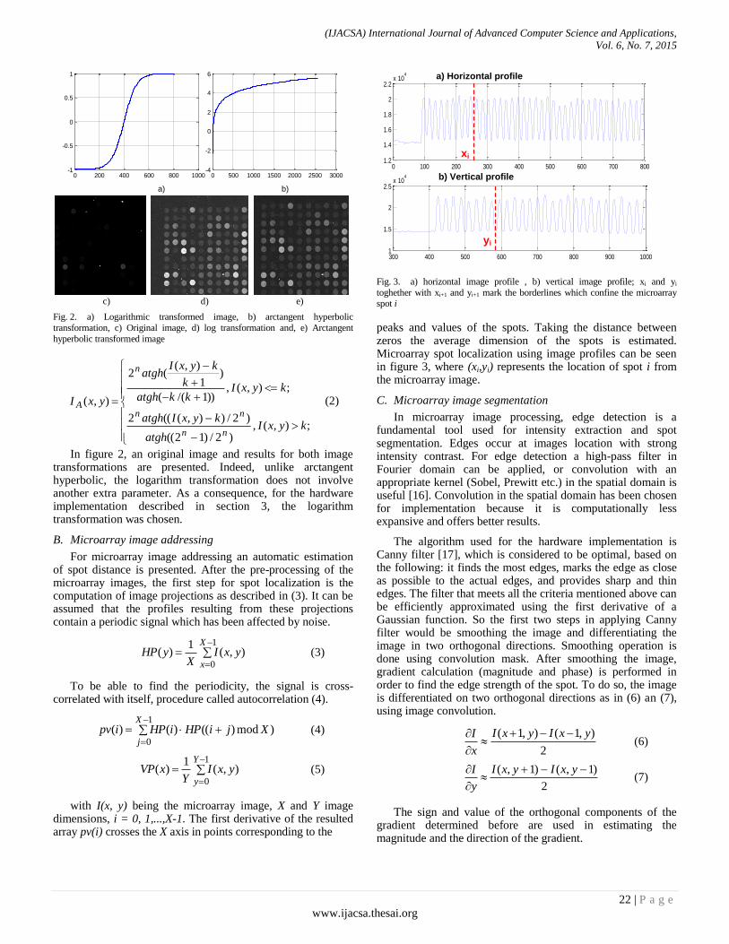
(IJACSA) International Journal of Advanced Computer Science and Applications,
Vol. 6, No. 7, 2015
22 | P a g e
www.ijacsa.thesai.org
c) d) e)
Fig. 2. a) Logarithmic transformed image, b) arctangent hyperbolic
transformation, c) Original image, d) log transformation and, e) Arctangent
hyperbolic transformed image
;),(,)2/)12((
)2/)),(((2
;),(,))1/((
)1
),((2
),(
kyxIatgh
kyxIatgh
kyxIkkatgh
k
kyxIatgh
yxI
nn
nn
n
A (2)
In figure 2, an original image and results for both image transformations are presented. Indeed, unlike arctangent hyperbolic, the logarithm transformation does not involve another extra parameter. As a consequence, for the hardware implementation described in section 3, the logarithm transformation was chosen.
B. Microarray image addressing
For microarray image addressing an automatic estimation of spot distance is presented. After the pre-processing of the microarray images, the first step for spot localization is the computation of image projections as described in (3). It can be assumed that the profiles resulting from these projections contain a periodic signal which has been affected by noise.
1
0
),(1
)(X
x
yxIX
yHP (3)
To be able to find the periodicity, the signal is cross-correlated with itself, procedure called autocorrelation (4).
)mod)(()()(1
0
XjiHPiHPipvX
j
(4)
1
0
),(1
)(Y
y
yxIY
xVP (5)
with I(x, y) being the microarray image, X and Y image dimensions, i = 0, 1,...,X-1. The first derivative of the resulted array pv(i) crosses the X axis in points corresponding to the
0 100 200 300 400 500 600 700 8001.2
1.4
1.6
1.8
2
2.2x 10
4
300 400 500 600 700 800 900 10001
1.5
2
2.5x 10
4
a) Horizontal profile
b) Vertical profile
xi
yi
Fig. 3. a) horizontal image profile , b) vertical image profile; xi and yi
toghether with xi+1 and yi+1 mark the borderlines which confine the microarray spot i
peaks and values of the spots. Taking the distance between zeros the average dimension of the spots is estimated. Microarray spot localization using image profiles can be seen in figure 3, where (xi,yi) represents the location of spot i from the microarray image.
C. Microarray image segmentation
In microarray image processing, edge detection is a fundamental tool used for intensity extraction and spot segmentation. Edges occur at images location with strong intensity contrast. For edge detection a high-pass filter in Fourier domain can be applied, or convolution with an appropriate kernel (Sobel, Prewitt etc.) in the spatial domain is useful [16]. Convolution in the spatial domain has been chosen for implementation because it is computationally less expansive and offers better results.
The algorithm used for the hardware implementation is Canny filter [17], which is considered to be optimal, based on the following: it finds the most edges, marks the edge as close as possible to the actual edges, and provides sharp and thin edges. The filter that meets all the criteria mentioned above can be efficiently approximated using the first derivative of a Gaussian function. So the first two steps in applying Canny filter would be smoothing the image and differentiating the image in two orthogonal directions. Smoothing operation is done using convolution mask. After smoothing the image, gradient calculation (magnitude and phase) is performed in order to find the edge strength of the spot. To do so, the image is differentiated on two orthogonal directions as in (6) an (7), using image convolution.
2
),1(),1( yxIyxI
x
I
(6)
2
)1,()1,(
yxIyxI
y
I (7)
The sign and value of the orthogonal components of the gradient determined before are used in estimating the magnitude and the direction of the gradient.
a) b)
0 500 1000 1500 2000 2500 3000-4
-2
0
2
4
6
0 200 400 600 800 1000-1
-0.5
0
0.5
1

(IJACSA) International Journal of Advanced Computer Science and Applications,
Vol. 6, No. 7, 2015
23 | P a g e
www.ijacsa.thesai.org
Once the direction of the gradient is known, pixels values around the pixel being analysed are interpolated. The pixel that does not represent a local maximum is eliminated, by comparing it with its neighbours along the direction of the gradient (non-maximum suppression).
Up to this point, image processing algorithms were presented in order to realize a robust detection of microarray image features. A solution for implementing the previous processing chain is presented next.
III. HARDWARE IMPLEMENTATIONS FOR MICROARRAY
IMAGE PROCESSING ALGORITHMS
FPGA technology uses pre-built logic blocks and programmable routing resources for configuration and for implementing custom hardware functionality. Their main benefits are the low cost, the short time to market and the ease of reconfiguration. Microarray images are analysed and processed using FPGA technology in order to speed up computation. The hardware implementations of microarray image processing techniques make use of the FPGA features, which allow accessing at the same time hundreds of memory addresses. Indeed, FPGA technology offers the possibility to exploit spatial and temporal parallelism for microarray image processing in order to create a fast automated process which delivers raw-data information about microarray image characteristics. As a consequence, FPGA are well-adapted for processing microarray images as show in [18].
Further on an FPGA based application specific architecture for microarray image processing is described. Xilinx board Virtex5 ML505 was used for the application development. The architecture includes 3 processing units PUi: PU1 realizes the microarray image enhancement, PU2 computes image vertical and horizontal profiles and the last processing unit PU3 uses spatial parallelism for image segmentation. The processing units together with a DMA controller for RAM memory access are connected to the processor trough the plb_v46 data bus. Autocorrelation and shock filters for microarray image addressing are implemented using C code. Future work aims creating processing units in order to speed up their computation. A detailed description of our application-specific architecture is presented in the figure 4. The same approach which uses hardware coprocessors for high-throughput processing was proposed in [19].
The image processing PUi units are connected as co-processor to the Microblaze system through FSL bus in order to speed up computation. The FSL interfaces are used to transfer data to and from the register file on the processor to the hardware running on the FPGA.
The FSL represents a uni-directional point to point FIFO based communication. The methodology to interconnect the image processing hardware units to the FSL bus is detailed in section III.D.
A. Microarray image enhancement implementation
Spatial logarithm transformation is used for microarray
μp
PU1: Log
Enhance
PU3:
Segmentation
PU2: Profile
Computation
Memory
Controller
FSL bus
FPGA
Virtex 5
RAM
256MB
Fig. 4. Application specific architecture for microarray image processing
image enhancement. The logic bloc LOG from figure 5 calculates the logarithm of image intensity for each pixel. The logarithm transformation is implemented on the luminance information Y of the image, obtained using R, G, B channels like in (8).
BGRY 114.0587.0299.0 (8)
The hardware implementation of the logarithm trans-formation is based on linear approximation of the logarithm function. The logarithm function is calculated in a number of An(x,y) points stored in a memory named ROM_LOG.
Also the slope m for each line described by two adjacent points is calculated and stored in a memory called ROM_SLOPE. In order to calculate the logarithm of the luminance, we are using (9) which represent the equation of a line which has the slope m and passes through the point Ai(xi, yi) from the initial An points.
ii yxymy )(log (9)
For the implementation described in Fig. 6 there is a number of 3 clock cycles necessary for processing. In order to evaluate the log function estimation, mean square error was calculated for y values between 1 and YMAX = 256 and the result is shown in (10). A pipelined architecture will reduce the computational time for the logarithm unit to 1 pixel/clock cycle.
52 10807.1)](ln_)[ln(1
yMAX
yestyY
MSE (10)
The same type of implementation was successfully used in [20] for high-throughput decoding of LDPC codes.
B. Microarray image profile computation
Computing the horizontal and vertical image profiles for spot localization involves logarithm computation of pixel intensity. Figure 5 describes the hardware architecture for evaluating image profiles. The luminous component (Y component) of the microarray image I(x,y), is extracted from the RGB colour space. The spatial logarithm transformation is
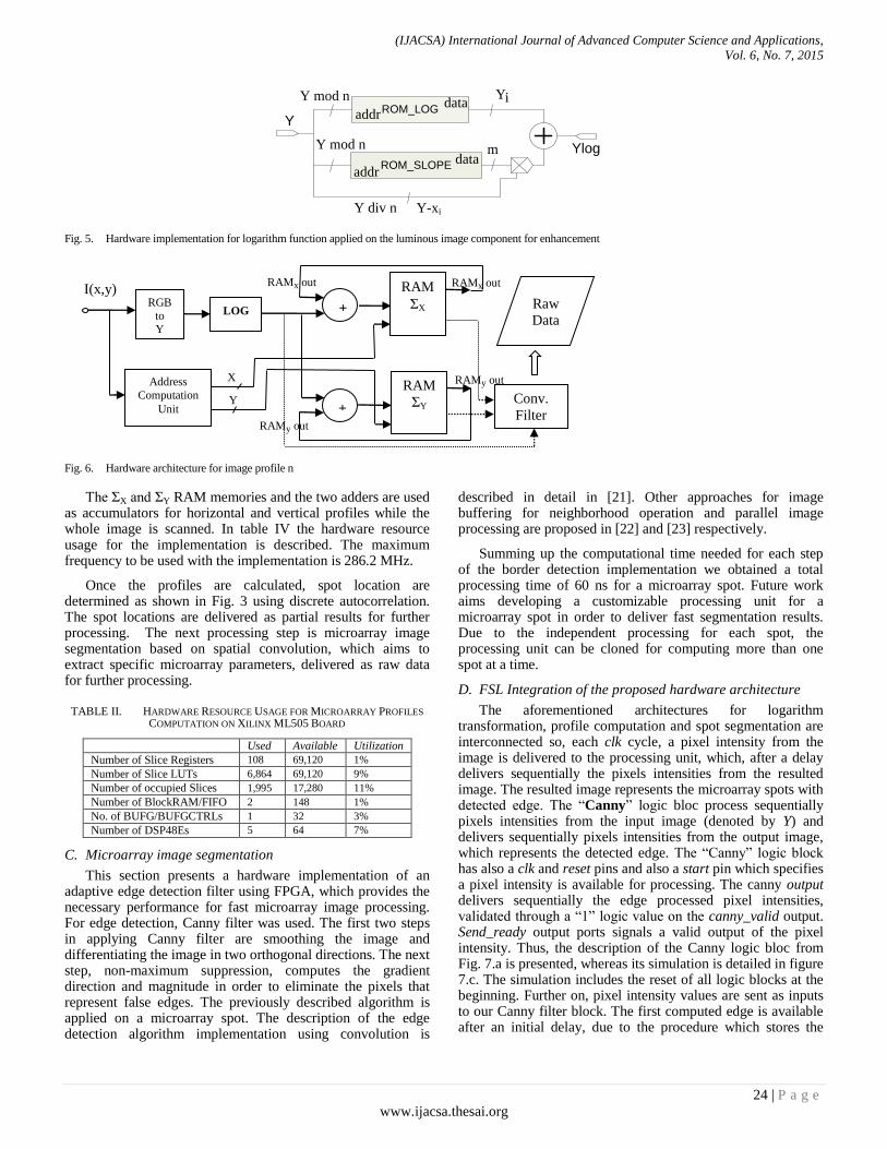
(IJACSA) International Journal of Advanced Computer Science and Applications,
Vol. 6, No. 7, 2015
24 | P a g e
www.ijacsa.thesai.org
ROM_LOGaddrdata
ROM_SLOPEaddr
data
Y
Ylog
Y mod n
Y mod n
Y div n
Y
m
Y-xi
i
Fig. 5. Hardware implementation for logarithm function applied on the luminous image component for enhancement
Fig. 6. Hardware architecture for image profile n
The ΣX and ΣY RAM memories and the two adders are used as accumulators for horizontal and vertical profiles while the whole image is scanned. In table IV the hardware resource usage for the implementation is described. The maximum frequency to be used with the implementation is 286.2 MHz.
Once the profiles are calculated, spot location are determined as shown in Fig. 3 using discrete autocorrelation. The spot locations are delivered as partial results for further processing. The next processing step is microarray image segmentation based on spatial convolution, which aims to extract specific microarray parameters, delivered as raw data for further processing.
TABLE II. HARDWARE RESOURCE USAGE FOR MICROARRAY PROFILES
COMPUTATION ON XILINX ML505 BOARD
Used Available Utilization
Number of Slice Registers 108 69,120 1%
Number of Slice LUTs 6,864 69,120 9%
Number of occupied Slices 1,995 17,280 11%
Number of BlockRAM/FIFO 2 148 1%
No. of BUFG/BUFGCTRLs 1 32 3%
Number of DSP48Es 5 64 7%
C. Microarray image segmentation
This section presents a hardware implementation of an adaptive edge detection filter using FPGA, which provides the necessary performance for fast microarray image processing. For edge detection, Canny filter was used. The first two steps in applying Canny filter are smoothing the image and differentiating the image in two orthogonal directions. The next step, non-maximum suppression, computes the gradient direction and magnitude in order to eliminate the pixels that represent false edges. The previously described algorithm is applied on a microarray spot. The description of the edge detection algorithm implementation using convolution is
described in detail in [21]. Other approaches for image buffering for neighborhood operation and parallel image processing are proposed in [22] and [23] respectively.
Summing up the computational time needed for each step of the border detection implementation we obtained a total processing time of 60 ns for a microarray spot. Future work aims developing a customizable processing unit for a microarray spot in order to deliver fast segmentation results. Due to the independent processing for each spot, the processing unit can be cloned for computing more than one spot at a time.
D. FSL Integration of the proposed hardware architecture
The aforementioned architectures for logarithm transformation, profile computation and spot segmentation are interconnected so, each clk cycle, a pixel intensity from the image is delivered to the processing unit, which, after a delay delivers sequentially the pixels intensities from the resulted image. The resulted image represents the microarray spots with detected edge. The “Canny” logic bloc process sequentially pixels intensities from the input image (denoted by Y) and delivers sequentially pixels intensities from the output image, which represents the detected edge. The “Canny” logic block has also a clk and reset pins and also a start pin which specifies a pixel intensity is available for processing. The canny output delivers sequentially the edge processed pixel intensities, validated through a “1” logic value on the canny_valid output. Send_ready output ports signals a valid output of the pixel intensity. Thus, the description of the Canny logic bloc from Fig. 7.a is presented, whereas its simulation is detailed in figure 7.c. The simulation includes the reset of all logic blocks at the beginning. Further on, pixel intensity values are sent as inputs to our Canny filter block. The first computed edge is available after an initial delay, due to the procedure which stores the
RAMx out
Y x
X
x
I(x,y)
RAMy out
RAMy out
RAMx out
RGB
to Y
LOG
Address
Computation
Unit
RAM
ΣX
RAM
ΣY
Raw
Data
Conv.
Filter
+
+
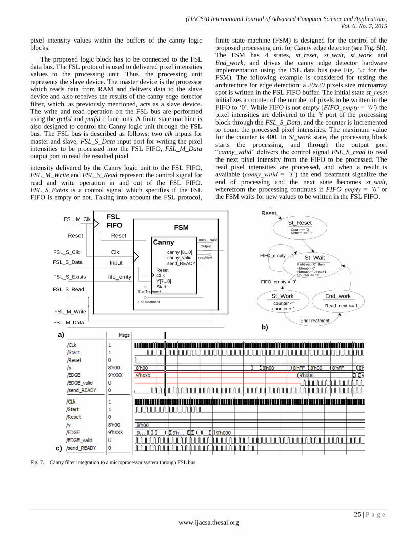
(IJACSA) International Journal of Advanced Computer Science and Applications,
Vol. 6, No. 7, 2015
25 | P a g e
www.ijacsa.thesai.org
pixel intensity values within the buffers of the canny logic blocks.
The proposed logic block has to be connected to the FSL data bus. The FSL protocol is used to delivered pixel intensities values to the processing unit. Thus, the processing unit represents the slave device. The master device is the processor which reads data from RAM and delivers data to the slave device and also receives the results of the canny edge detector filter, which, as previously mentioned, acts as a slave device. The write and read operation on the FSL bus are performed using the getfsl and putfsl c functions. A finite state machine is also designed to control the Canny logic unit through the FSL bus. The FSL bus is described as follows: two clk inputs for master and slave, FSL_S_Data input port for writing the pixel intensities to be processed into the FSL FIFO, FSL_M_Data output port to read the resulted pixel
intensity delivered by the Canny logic unit to the FSL FIFO, FSL_M_Write and FSL_S_Read represent the control signal for read and write operation in and out of the FSL FIFO. FSL_S_Exists is a control signal which specifies if the FSL FIFO is empty or not. Taking into account the FSL protocol,
finite state machine (FSM) is designed for the control of the proposed processing unit for Canny edge detector (see Fig. 5b). The FSM has 4 states, st_reset, st_wait, st_work and End_work, and drives the canny edge detector hardware implementation using the FSL data bus (see Fig. 5.c for the FSM). The following example is considered for testing the architecture for edge detection: a 20x20 pixels size microarray spot is written in the FSL FIFO buffer. The initial state st_reset initializes a counter of the number of pixels to be written in the FIFO to „0‟. While FIFO is not empty (FIFO_empty = ‘0’) the pixel intensities are delivered to the Y port of the processing block through the FSL_S_Data, and the counter is incremented to count the processed pixel intensities. The maximum value for the counter is 400. In St_work state, the processing block starts the processing, and through the output port “canny_valid” delivers the control signal FSL_S_read to read the next pixel intensity from the FIFO to be processed. The read pixel intensities are processed, and when a result is available (canny_valid = ‘1’) the end_treatment signalize the end of processing and the next state becomes st_wait, wherefrom the processing continues if FIFO_empty = ‘0’ or the FSM waits for new values to be written in the FSL FIFO.
FSL_M_Write
FSM
Output
fifo_emty
FSL_M_Clk
FSL_S_Clk
Reset Reset
Clk
FSL_S_Data Input
FSL_S_Exists
FSL_S_Read
FSL_M_Data
Canny
Reset
CLk
Y[7...0]
Start
canny [8...0]
canny_valid
send_READY
StartTreatment
EndTreatment
output_valid
End_workSt_Work
St_Reset
Reset
Nbtreat <= ‘’0'Count <= ‘0’
St_Wait
nbtreat<=nbtreat+1Counter <= ‘0’
If nbtreat=’0' then
nbtreat<=’0'
FIFO_empty = ‘1’
FIFO_empty = ‘0’
EndTreatment
counter <=
counter + 1;Read_next <= 1
readNext
FSL
FIFO
a)b)
c)
Fig. 7. Canny filter integration to a microprocessor system through FSL bus
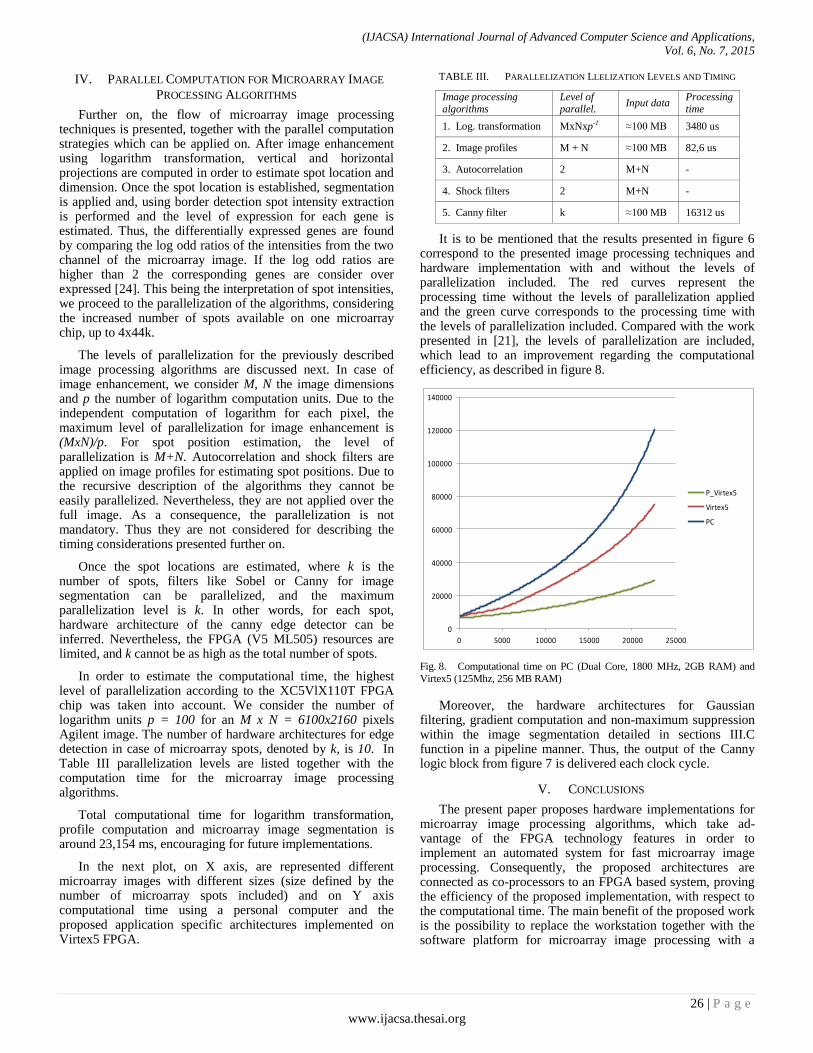
(IJACSA) International Journal of Advanced Computer Science and Applications,
Vol. 6, No. 7, 2015
26 | P a g e
www.ijacsa.thesai.org
IV. PARALLEL COMPUTATION FOR MICROARRAY IMAGE
PROCESSING ALGORITHMS
Further on, the flow of microarray image processing techniques is presented, together with the parallel computation strategies which can be applied on. After image enhancement using logarithm transformation, vertical and horizontal projections are computed in order to estimate spot location and dimension. Once the spot location is established, segmentation is applied and, using border detection spot intensity extraction is performed and the level of expression for each gene is estimated. Thus, the differentially expressed genes are found by comparing the log odd ratios of the intensities from the two channel of the microarray image. If the log odd ratios are higher than 2 the corresponding genes are consider over expressed [24]. This being the interpretation of spot intensities, we proceed to the parallelization of the algorithms, considering the increased number of spots available on one microarray chip, up to 4x44k.
The levels of parallelization for the previously described image processing algorithms are discussed next. In case of image enhancement, we consider M, N the image dimensions and p the number of logarithm computation units. Due to the independent computation of logarithm for each pixel, the maximum level of parallelization for image enhancement is (MxN)/p. For spot position estimation, the level of parallelization is M+N. Autocorrelation and shock filters are applied on image profiles for estimating spot positions. Due to the recursive description of the algorithms they cannot be easily parallelized. Nevertheless, they are not applied over the full image. As a consequence, the parallelization is not mandatory. Thus they are not considered for describing the timing considerations presented further on.
Once the spot locations are estimated, where k is the number of spots, filters like Sobel or Canny for image segmentation can be parallelized, and the maximum parallelization level is k. In other words, for each spot, hardware architecture of the canny edge detector can be inferred. Nevertheless, the FPGA (V5 ML505) resources are limited, and k cannot be as high as the total number of spots.
In order to estimate the computational time, the highest level of parallelization according to the XC5VlX110T FPGA chip was taken into account. We consider the number of logarithm units p = 100 for an M x N = 6100x2160 pixels Agilent image. The number of hardware architectures for edge detection in case of microarray spots, denoted by k, is 10. In Table III parallelization levels are listed together with the computation time for the microarray image processing algorithms.
Total computational time for logarithm transformation, profile computation and microarray image segmentation is around 23,154 ms, encouraging for future implementations.
In the next plot, on X axis, are represented different microarray images with different sizes (size defined by the number of microarray spots included) and on Y axis computational time using a personal computer and the proposed application specific architectures implemented on Virtex5 FPGA.
TABLE III. PARALLELIZATION LLELIZATION LEVELS AND TIMING
Image processing algorithms
Level of parallel.
Input data Processing time
1. Log. transformation MxNxp-1 ≈100 MB 3480 us
2. Image profiles M + N ≈100 MB 82,6 us
3. Autocorrelation 2 M+N -
4. Shock filters 2 M+N -
5. Canny filter k ≈100 MB 16312 us
It is to be mentioned that the results presented in figure 6 correspond to the presented image processing techniques and hardware implementation with and without the levels of parallelization included. The red curves represent the processing time without the levels of parallelization applied and the green curve corresponds to the processing time with the levels of parallelization included. Compared with the work presented in [21], the levels of parallelization are included, which lead to an improvement regarding the computational efficiency, as described in figure 8.
0
20000
40000
60000
80000
100000
120000
140000
0 5000 10000 15000 20000 25000
P_Virtex5
Virtex5
PC
Fig. 8. Computational time on PC (Dual Core, 1800 MHz, 2GB RAM) and
Virtex5 (125Mhz, 256 MB RAM)
Moreover, the hardware architectures for Gaussian filtering, gradient computation and non-maximum suppression within the image segmentation detailed in sections III.C function in a pipeline manner. Thus, the output of the Canny logic block from figure 7 is delivered each clock cycle.
V. CONCLUSIONS
The present paper proposes hardware implementations for microarray image processing algorithms, which take ad-vantage of the FPGA technology features in order to implement an automated system for fast microarray image processing. Consequently, the proposed architectures are connected as co-processors to an FPGA based system, proving the efficiency of the proposed implementation, with respect to the computational time. The main benefit of the proposed work is the possibility to replace the workstation together with the software platform for microarray image processing with a

(IJACSA) International Journal of Advanced Computer Science and Applications,
Vol. 6, No. 7, 2015
27 | P a g e
www.ijacsa.thesai.org
system on a chip. The proposed FPGA-based system can be easily integrated within the microarray canner level. Due to the reduced computational time and cost, a large number of microarray analyses can be performed, compared with the existing computational tools.
The levels of parallelism for microarray image processing algorithms are described. Considering the computation efficiency of the proposed microarray image processing task, the experimental results based on algorithm parallelization show significant improvements compared both with a general purpose processor (PC) and with a FPGA based system without levels of parallelization included. Thus, FPGA technology is proved to be an efficient solution for an application-specific architecture for microarray image processing.
Future work aims to develop application-specific hardware architecture for more complex methods for automatic microarray image processing such us, partial differential equations (PDE)-based gridding or clustering-based spot segmentation.
ACKNOWLEDGEMENTS
This paper is supported by the Human Resources Development Programme POSDRU/159/1.5/S/137516 financed by the European Social Fund and by the Romanian Government.
REFERENCES
[1] Mark Schena, Micropuce Biochip Technology: Oxford University Press, 1999.
[2] A. M. Campbell, W. T. Hatfield, L. Heyer, "Make microarray data with known ratios," CBE – Life Sciences Education, vol. 6, 196-197, 2007.
[3] Peter Bajcsy, "An Overview of DNA Microarray Image Requirements for Automated Processing," IEEE Transac-tions on Image Processing, VOL 13, NO 1, pp. 15-25, Janu-ary 2004.
[4] Yang Y, Staord P and Kim YJ. Segmentation and intensity estimation for microarray images with saturated pixels. BMC Bioinformatics; 2011. 12:462.
[5] Wanga Z et al. Hybrid clustering for microarray image analysis combining intensity and shape features. Neurocomputing; 2014. 142:408{418.
[6] Using fuzzy logic and particle swarm optimization to design a decision-based filter for cDNA microarray image restoration, Chang, Bae-Muu; Tsai, Hung-Hsu; Shih, Ji-Shiang, Engineering Applications Of Artificial Intelligence, 36 Pages: 12-26, 2014.
[7] Giannakeas Net al. Spot addressing for microarray images structured in hexagonal grids. Computer Methods and Programs in Biomedicine; 2012. 106:1.
[8] Giannakeas N et al. Segmentation of microarray images using pixel classication - Comparison with clustering-based methods. Computers in Biology and Medicine; 2013. 43:705{716.
[9] Agilent Feature Extraction Software v10.5, User guide, 2008.
[10] Handran S, Zhai YZ (2003) Biological relevance of GenePix results. Molecular Devices - Application Notes, pp 1–9
[11] M.B. Eisen, "ScanAlyze User Manual," Stanford University, 1999.
[12] Florea L, Florea C, Vertan C, Sultana A (2011) Automatic tools for diagnosis support of total hip replacement follow-up. Adv Electr Comput Eng 11(4):55–62.
[13] Tonti, Simone et al.n An automated approach to the segmentation of HEp-2 cells for the indirect immunofluorescence ANA test Computerized Medical Imaging and Graphics , Volume 40 , 62 – 69, 2015
[14] ]Kamal A. ElDahshan et al., Hardware Segmentation on Digital Microscope Images for Acute Lymphoblastic Leukemia Diagnosis Using Xilinx System Generator , International Journal of Advanced Computer Science and Applications, 5(9), pp. 33-37, 2014
[15] Moulay Ali Nassiri, Jean-François Carrier, Philippe Després, Fast GPU-based computation of spatial multigrid multiframe LMEM for PET, Medical & Biological Engineering & Computing, April 2015.
[16] Tanvir Abassi, Usaid Abassim, "A Proposed FPGA Based Architecture for Sobel Edge Detection Operator," Journal of Active and Passive Electronic Devices, pp. 271–277, 2007.
[17] J. Canny, "A computational approach to edge detection," IEEE Trans Pattern Analysis and Machine Intelligence, vol. 8, no. 6, pp. 679-698, Nov. 1986.
[18] B. Belean, M. Borda, A. Fazakas, "Adaptive Microarray Image Acquisition System and Microarray Image Processing Using FPGA Technology," Lecture Notes in Computer Science 5179, pp. 327-334, 2008.
[19] Călin BÎRĂ, Lucian PETRICĂ, Radu HOBINCU, OPINCAA: A Light-Weight and Flexible Programming Environment For Parallel SIMD Accelerators, Romanian Journal of Information Science and Technology, 16(4), pp. 336–350, 2013.
[20] Belean B et al., Low Complexity Approach for High Throughput Belief-Propagation based Decoding of LDPC Codes, Advances in Electrical and Computer Engineering, 13(4):2013, pp 69-72.
[21] Belean B, Borda M, Le Gal B, Terebes R (2012) FPGA based system for automatic cDNA microarray image processing. Comput Med Imaging Graph 36(5):419–429.
[22] Kazmi M. et al., FPGA Based Compact and Efficient Full Image Buffering for Neighborhood Operations, Advances in Electrical and Computer Engineering, 15(1):2015, pp. 95-104.
[23] Maciej Wielgosz, Mauritz Panggabean and Leif Arne Rønningen, FPGA Architecture for Kriging Image Interpolation, (IJACSA) International Journal of Advanced Computer Science and Applications, Vol. 4, No. 12, 2013
[24] Marczyk M. et al., Adaptive filtering of microarray gene expression data based on Gaussian mixture decomposition, BMC Bioinformatics 2013, 14:101

(IJACSA) International Journal of Advanced Computer Science and Applications,
Vol. 6, No. 7, 2015
28 | P a g e
www.ijacsa.thesai.org
Indexing of Ears using Radial basis Function Neural
Network for Personal Identification
M.A. Jayaram1
1Director,
Department of Master of Computer
Applications
Siddaganga Institute of Technology,
Tumkur
karnataka, India
Prashanth G.K2.
2Assistant Professor,
Department of Master of Computer
Applications
Siddaganga Institute of Technology,
Tumkur
karnataka, India
M.Anusha3,
3Project Student
Department of Master of Computer
Applications
Siddaganga Institute of Technology,
Tumkur
karnataka, India
Abstract—This paper elaborates a novel method to recognize
persons using ear biometrics. We propose a method to index the
ears using Radial Basis Function Neural Networks (RBFNN). In
order to obtain the invariant features, an ear has been considered
as a planar surface of irregular shape. The shape based features
like planar area, moment of inertia with respect to minor and
major axes, and radii of gyration with respect to minor and
major axes are considered. The indexing equation is generated
using the weights, centroids and kernel function of the stabilized
RBFN network. The so developed indexing equation was tested
and validated. The analysis of the equation revealed 95.4%
recognition accuracy. The retrieval rate of personal details
became faster by an average of 13.8% when the database was
organized as per the indices. Further, the three groups elicited by
RBFNN were evaluated for parameters like entropy, precision,
recall, specificity and F-measure. And all the parameters are
found to be excellent in terms of their values and thus showcase
the adequacy of the indexing model.
Keywords—RBFNN; kernel function; Indexing equation;
Moment of inertia; radii of gyration
I. INTRODUCTION
Alfred Iannarelli developed a new class of biometrics, based upon ear features and introduced it for use in the development of passive identification systems [1]. Identification by ear biometrics is promising because it is passive like face recognition. The ear is considered to be a unique feature for human beings. Even the ears of “identical twins” differ in some respects [2]. Unlike face, the configuration of ear will never be subjected to changes associated with changes in the facial expression, and the make-up effects. The configuration and the complexion of the ear do not vary with age. It has the biometric traits like uniqueness, universality, permanence and collectability.
A profound work of ear identification involving over 10000 ears has been documented [1]. In an experiment involving larger datasets more rigorously controlled for relative quality of face and ear, the recognition performance was almost same when ear and face were individually considered. However, the performance shot up to 90.9% when both ear and face were considered [3].
Ear biometrics is an unexplored biometric field, but has received a growing amount of attention over the past few
years. There are three modes of ear biometrics: ear photographs, ear prints obtained by pressing the ear against a flat plane, and thermograph pictures of the ear. The most common implementation of ear biometrics is via photographs for identification systems [4].
This paper presents a novel method to index years by using radial basis function neural networks. By indexing, we mean provide an integer number to an Ear indicating to what group it belongs. This integer number will have evolved through RBFNN centroids, the kernel function and the weights of the stabilized network. The rest of the paper is organized as follows. Use of RBFNN in allied areas of biometrics is discussed in section II. The shape based biometrics developed by authors is presented in section III. Section IV presents about the data used in the model. A brief presentation of RBFNN is done in section V. The indexing equation is illustrated in section VI. Analysis of the results is elaborated in section VII. Section VIII concludes the paper.
II. RELATED WORKS
Considerable amount of research has gone into identifying methods suitable for indexing and classification of entities. The application of RBFNN in the domain of biometrics has been scarce. Mai V et al [5] proposed a new method to identify people using Electrocardiogram (ECG). QRS complex (Q waves, R waves, S waves) which is a stable parameter against heart rate variability is used as a biometric feature. This work has reported for having achieved a classification accuracy of 97% using RBF.
Sulong et al [6] have used a combination of maximum pressure exerted on the keyboard and the time latency between the keystrokes to recognize the authenticate users and to reject imposters. In this work, RBFNN is used as a pattern matching method. The system so developed has been evaluated using False Reject Rate (FRR) and False Accept Rate (FAR). The researchers have affirmed the effectiveness of the security system designed by them.
Chatterjee et al [7] have proposed a new biometric system which is based on four types of temporal postural signals. The system employs S-transform to determine the characteristic features for each human posture. An RBFNN with these characteristic features as input is developed for specific

(IJACSA) International Journal of Advanced Computer Science and Applications,
Vol. 6, No. 7, 2015
29 | P a g e
www.ijacsa.thesai.org
authentication. The training of the network has augmented extended Kalman filtering (EKF). The overall authentication accuracy of the system is reported to be of the order of 95%.
In a study, multi-modal biometric consisting of fingerprint images and finger vein patterns were used to identify the authorized users after determining the class of users by RBFNN as a classifier. The parameters of the RBFNN were optimized using BAT algorithm. The performance of RBFNN was found to be superior when compared with KNN, Naïve Bayesian and non-optimized RBFNN classifier [8].
Ankit Chadha et al have used signature of persons for verification and authentication purpose. RBFNN was trained with sample images in the database. The network successfully identified the original images with the recognition accuracy of 80% for image sample size of 200 [9].
Handwriting recognition with features such as aspect ratio, end points, junction, loop, and stroke direction were used for recognition of writers [10]. The system used over 500 text lines from 20 writers. RBFNN showed a recognition accuracy of 95.5% when compared to backpropagation network.
An Optical Character Recognition (OCR) is developed for the recognition of the basic characters such as vowels and consonants for Kannada text. The system can handle different font size and font types. Features such as Hu’s invariant moments and Zernike moments are extracted and RBFNN is used as a classifier to identify and classify the characters [11].
III. SHAPE BASED BIOMETRICS
In this work, the five shape based features of ears that were considered for classification are listed in the Table I. The details of feature extraction, authentication, their evaluation and the elaboration of a personal identification system developed are available in seminal work of authors [12]. However, for the sake of completeness, the features are explained in the following paragraphs.
The surface area of the ear is the projected area of the curved surface on a vertical plane. Moment of Inertia (MI) is the property of a planar surface which originates whenever one has to compute the moment of distributed load that varies linearly from the moment axis. Moment of Inertia is also viewed as a physical measure that signifies the shape of a planar surface and it is proved that by configuring the shape of planar surface and hence by altering the moment of inertia, the resistance of the planar surface against rotation with respect to a particular axis could be modulated or altered [13]. Therefore in this work, moment of inertia of ear surface with respect to two axes i.e. the major axis and the minor axis are considered to be the best biometric attributes that could capture the shape of irregular surface of the ear in a scientific way.
As far as features are concerned, major axis is the one which has the longest distance between the two points on the edge of the ear, the distance here is the maximum among point to point Euclidean distance. The minor axis is drawn in such way that it passes through tragus and is orthogonal to the major axis. Therefore, with different orientation of ears the orientation of major axis also changes. Being perpendicular to major axis, the orientation of minor axis is fixed.
The projected area is assumed to be formed out of segments. The area of an ear to the right side of the major axis is considered to be made out of six segments. Each of the segments thus subtends 30
0 with respect to the point of the
intersection of the major axis and minor axis. The extreme edge of a sector is assumed to be a circular arc. Thus converting each segment into a sector of circle of varying area. Typical ear edge with measurements is shown in Figure 1.
The measurements are
Inclination of the central radial axis of the
segment with respect to minor axis (in degrees).
r The length of the radial axis (in mm).
The conversion of number of pixel into linear dimension (in mm) was based on the resolution of the camera expressed in PPI (Pixel Per Inch). In this work 16Mega pixel camera, at 300 PPI was used. The computation of linear distance is straight farward mm=(number of pixel*25.4)/PPI [1 inch=25.4 mm]. With these measurements, the following parameters are computed.
Moment of inertia with respect to minor axis Imin
∑
(1) Where ai is the area of a the i
th segment and yi is the
perpendicular distance of the centroid of the ith
segment with respect to minor axis.
(2)
(3)
Here, C is the centroidal distance of the segment with respect to the intersection point of the axes, which is given by[14];
(4)
Simlarly, moment of inertia with respect to major axis Imax ,xi is the perpendicular distance of the centroid of the ith segment with respect to major axis.
∑
(5)
(6)
From the computed values of moment of inertia and area of the ear surface, the radii of gyration with respect to minor axis(RGx)and major axis(RGy) were computed. The formulae for radii of gyration are given by[15].
√
(7)
√
(8)
Where , A is the sum of areas of six segments.
∑ (9)
Radius of gyration is the distance from an axis at which the mass of a body may be assumed to be concentrated and at
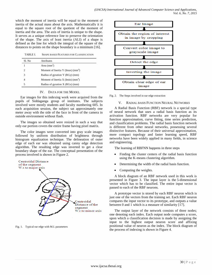
(IJACSA) International Journal of Advanced Computer Science and Applications,
Vol. 6, No. 7, 2015
30 | P a g e
www.ijacsa.thesai.org
which the moment of inertia will be equal to the moment of inertia of the actual mass about the axis. Mathematically it is equal to the square root of the quotient of the moment of inertia and the area. The axis of inertia is unique to the shape. It serves as a unique reference line to preserve the orientation of the shape. The axis of least inertia (ALI) of a shape is defined as the line for which the integral of the square of the distances to points on the shape boundary is a minimum [16].
TABLE I. SHAPE BASED FEATURES FOR CLASSIFICATION
Sl. No Attributes
1 Area (mm2)
2 Moment of Inertia Y (Imax) (mm4)
3 Radius of gyration Y (RGy) (mm)
4 Moment of Inertia X (Imin) (mm4)
5 Radius of gyration X (RGx) (mm)
IV. DATA FOR THE MODEL
Ear images for this indexing work were acquired from the pupils of Siddaganga group of institutes. The subjects involved were mostly students and faculty numbering 605. In each acquisition session, the subject sat approximately one meter away with the side of the face in front of the camera in outside environment without flash.
The images so obtained were resized in such a way that only ear portion covers the entire frame having pixel matrix.
The color images were converted into gray scale images followed by uniform distribution of brightness through histogram equalization technique. The delineation of outer edge of each ear was obtained using canny edge detection algorithm. The resulting edge was inverted to get a clear boundary shape of the ear. The conceptual presentation of the process involved is shown in Figure 2.
Fig. 1. Typical ear edge with M.I. parameters
Fig. 2. The Steps involved in ear edge extraction
V. RADIAL BASIS FUNCTION NEURAL NETWORKS
A Radial Basis Function (RBF) network is a special type of neural network that uses a radial basis function as its activation function. RBF networks are very popular for function approximation, curve fitting, time series prediction, and classification problems. The radial basis function network is different from other neural networks, possessing several distinctive features. Because of their universal approximation, more compact topology and faster learning speed, RBF networks have been widely applied in many fields, in science and engineering.
The learning of RBFNN happens in three steps
Finding the cluster centers of the radial basis function using the K-means clustering algorithm.
Determining the width of the radial basis function.
Computing the weights.
A block diagram of an RBF network used in this work is presented in Figure 3. The input layer is the 5-dimensional vector which has to be classified. The entire input vector is passed to each of the RBF neurons.
A prototype vector is stored by each RBF neuron which is just one of the vectors from the training set. Each RBF neuron compares the input vector to its prototype, and outputs a value between 0 and 1 which is a measure of similarity [17].
The output layer of the network consists of three nodes; one denoting each index. Each output node computes a score, upon which a classification decision is made by assigning the input to the highest output neuron score and affixing positional value of neuron as the index. The block diagram of the process of indexing is shown in Figure 4.
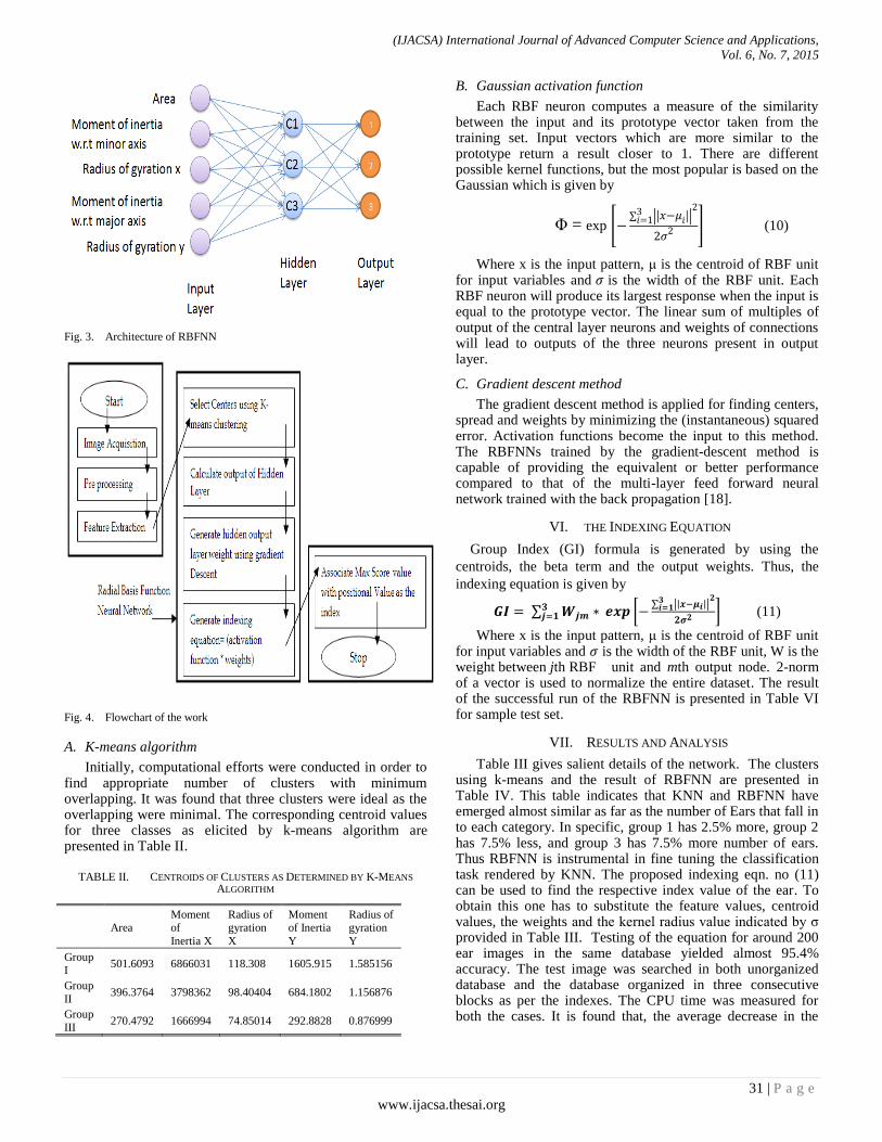
(IJACSA) International Journal of Advanced Computer Science and Applications,
Vol. 6, No. 7, 2015
31 | P a g e
www.ijacsa.thesai.org
Fig. 3. Architecture of RBFNN
Fig. 4. Flowchart of the work
A. K-means algorithm
Initially, computational efforts were conducted in order to find appropriate number of clusters with minimum overlapping. It was found that three clusters were ideal as the overlapping were minimal. The corresponding centroid values for three classes as elicited by k-means algorithm are presented in Table II.
TABLE II. CENTROIDS OF CLUSTERS AS DETERMINED BY K-MEANS
ALGORITHM
Area Moment of
Inertia X
Radius of gyration
X
Moment of Inertia
Y
Radius of gyration
Y
Group I
501.6093 6866031 118.308 1605.915 1.585156
Group II
396.3764 3798362 98.40404 684.1802 1.156876
Group
III 270.4792 1666994 74.85014 292.8828 0.876999
B. Gaussian activation function
Each RBF neuron computes a measure of the similarity between the input and its prototype vector taken from the training set. Input vectors which are more similar to the prototype return a result closer to 1. There are different possible kernel functions, but the most popular is based on the Gaussian which is given by
Φ = exp [ ∑ || ||
] (10)
Where x is the input pattern, μ is the centroid of RBF unit for input variables and is the width of the RBF unit. Each RBF neuron will produce its largest response when the input is equal to the prototype vector. The linear sum of multiples of output of the central layer neurons and weights of connections will lead to outputs of the three neurons present in output layer.
C. Gradient descent method
The gradient descent method is applied for finding centers, spread and weights by minimizing the (instantaneous) squared error. Activation functions become the input to this method. The RBFNNs trained by the gradient-descent method is capable of providing the equivalent or better performance compared to that of the multi-layer feed forward neural network trained with the back propagation [18].
VI. THE INDEXING EQUATION
Group Index (GI) formula is generated by using the
centroids, the beta term and the output weights. Thus, the
indexing equation is given by
∑ [
∑ || ||
] (11)
Where x is the input pattern, μ is the centroid of RBF unit for input variables and is the width of the RBF unit, W is the weight between jth RBF unit and mth output node. 2-norm of a vector is used to normalize the entire dataset. The result of the successful run of the RBFNN is presented in Table VI for sample test set.
VII. RESULTS AND ANALYSIS
Table III gives salient details of the network. The clusters using k-means and the result of RBFNN are presented in Table IV. This table indicates that KNN and RBFNN have emerged almost similar as far as the number of Ears that fall in to each category. In specific, group 1 has 2.5% more, group 2 has 7.5% less, and group 3 has 7.5% more number of ears. Thus RBFNN is instrumental in fine tuning the classification task rendered by KNN. The proposed indexing eqn. no (11) can be used to find the respective index value of the ear. To obtain this one has to substitute the feature values, centroid values, the weights and the kernel radius value indicated by σ provided in Table III. Testing of the equation for around 200 ear images in the same database yielded almost 95.4% accuracy. The test image was searched in both unorganized database and the database organized in three consecutive blocks as per the indexes. The CPU time was measured for both the cases. It is found that, the average decrease in the

(IJACSA) International Journal of Advanced Computer Science and Applications,
Vol. 6, No. 7, 2015
32 | P a g e
www.ijacsa.thesai.org
CPU time was around 13.77% with organized database. This aspect of the model is shown in Table V, here again, 200 ear images were selected at random (1/3
rd of the database) and
CPU time was noted. Justifiably, maximum time was consumed while matching and retrieving for the ears that fell in third category. Group characteristics are presented in Table VII A This table illustrates that though there are clear distinguishing features between groups as far are the appearance of the ear the attribute values overlap.
The contribution of this work lies in according an integer index to an ear based on certain moment of inertia related properties. By just looking at the index value of the ear, it is possible to get the notion of the articulation of the ear. To unearth this capability of indexing, the entire data base was studied with the ear image along with the attribute values and the corresponding index. Based on this empirical study it is possible to judge the group characteristic as shown in Table VII B. Classification performance evaluation measures are given in Table VIII and Table IX. An entropy value of 0.99395 indicates that the classes are more dispersed. An accuracy rate as high as 96% showcases an excellent classification. Precision values in the range 0.8-1 of clusters determine high positive predictive value. Recall value in the range 0.9-1 indicates that the clusters have high true positive rate. The value of specificity shows the high true-negative rate which is in the range 0.94-1. F-measure concludes that there is a good balance between precision and recall in the second and third cluster.
TABLE III. SALIENT DETAILS OF RBFNN IMPLEMENTED
No of input layer neurons 5
No of neurons in hidden layer 3
The basis function Gaussian
No of output neurons 3
Width of cluster as given by 1.1028e+06
6.7926e+05
5.9865e+05
C1 C2 C3
C1 72 8 0
C2 0 247 0
C3 9 11 258
Fig. 5. Confusion matrix
TABLE IV. TEST SET AND GROUP INDEXING BY RBFNN
Sl.
No Area Imax RGy Imin RGx GI
1 131.3487 195355.9 38.56563 50.89822 0.622499 2
2 135.0409 371368.5 52.44088 140.7316 1.020853 2
3 404.5635 3158077 88.35233 766.4084 1.376375 3
4 241.7773 744226.9 55.48108 116.0455 0.692798 2
5 370.4741 2691695 85.23815 310.3129 0.91521 2
6 272.2138 3054815 105.9345 0.344449 0.035572 3
7 358.0337 3395618 97.38621 254.3965 0.842934 3
8 369.2937 2464924 81.69882 264.376 0.846107 2
9 217.2377 2858884 114.7178 11.01563 0.225184 3
10 360.2648 2844322 88.8543 641.5627 1.334469 3
11 338.5039 1991710 76.70634 368.703 1.043654 2
12 379.9424 5368573 118.8695 240.5883 0.795753 1
13 412.1489 4025855 98.833 316.661 0.876537 3
14 639.5815 9003344 118.6462 3243.304 2.251883 2
15 376.3808 2785671 86.03025 647.0868 1.311196 2
16 435.8933 4651435 103.3007 822.7214 1.37384 3
17 369.8076 2818062 87.2946 258.6729 0.836349 3
18 266.0732 1406845 72.71474 437.977 1.282995 2
19 441.7652 7186791 127.5474 537.809 1.103363 1
20 450.2947 4146650 95.96222 1295.909 1.696441 3
21 405.7415 3655038 94.91202 237.0266 0.764318 3
22 414.6593 4291438 101.7316 1138.657 1.657108 3
23 439.04 5612504 113.0645 1007.022 1.514494 1
24 569.4626 7267216 112.967 1253.937 1.483902 1
25 388.5733 4062368 102.2476 810.9251 1.444621 3
TABLE V. AVERAGE CPU TIME
TABLE VI. K-MEANS AND RBFNN CLUSTERS
No. of test
images
With unorganized
database (sec)
With organized database as
per indexes(sec)
200 0.0721 0.0622
Group I Group II Group III
K-means 80 277 247
RBFNN 82 256 266

(IJACSA) International Journal of Advanced Computer Science and Applications,
Vol. 6, No. 7, 2015
33 | P a g e
www.ijacsa.thesai.org
TABLE VII. A: GROUP CHARACTERISTICS
Group Index
Area (mm2)
Imax (mm4)
RGy (mm)
1 200.022 624.117
5157372.515 8525384.26
101.726672- 177.111404
2
79.676
834.711
16329.42748
14331267.47
8.960133-
156.117258
3
167.320
514.583
2818062.292
5126772.995
83.6197-
151.046937
TABLE VII. B: GROUP CHARACTERISTICS
Group
Index
Imin
(mm4)
RGx
(mm)
Approximate
shape
1 2.143216- 7720.379626
0.077902- 3.920185
Almost Round, oblong or
rectangular
2
0.000004-
3992.773763
0.000121-
2.436946
Oval shaped,
small sized
3
0.096981-
2381.771594
0.018607-
2.444452
Triangular
shaped and
other shapes
TABLE VIII. PERFORMANCE EVALUATION MEASURES
Training Accuracy 95.4%
Classification Error 0.56033
Entropy 0.99395
TABLE IX. CLASSIFICATION EFFICIENCY EVALUATION METRICS
C1 C2 C3
Accuracy 0.9719 0.9686 0.9669
Precision 0.88889 0.92857 1
Recall 0.9 1 0.92806
Specificity 0.98286 0.94693 1
F-measure 0.89441 0.96296 0.96269
VIII. CONCLUSIONS
This paper presented a novel method to identify persons using shape related features of ear. In a nutshell, the significant contributions of this work are:
Indexes to ears based on their five shape related biometric features.
Creating and organising template database of ear biometric features with their index values elicited from RBFNN.
Quick retrieval of the details of the person when test ear image is presented to the system.
However, the limitation of the work is that, though the system is able attach an index to an ear, there seems to be overlapping of attribute values across the groups. This may
lead to a kind of uncertainty due to partaking of an ear in multiple groups. To address this issue, the future enhancement could be to develop a fuzzy indexing scheme.
REFERENCES
[1] Iannarelli, A., “Ear Identification”, Forensic Identification Series, Paramount Publishing Company, Fremont, California, 1989.
[2] Mahbubur Rahman et al, “Person Identification Using Ear Biometrics”, International Journal of The Computer, the Internet and Management Vol. 15#2 , pp 1 – 8, 2007.
[3] Chang, K., Bowyer, K.W., Sarker, S., Victor, B., “Comparison and Combination of Ear and Face Machine Image in appearance –Based Biometrics’, IEEE Transaction on pattern Analysis and machine Intelligence, vol. 25, no, 9 ,2003.
[4] Sukhdeep Singh, Dr. Sunil Kumar Singla, “A Review on Biometrics and Ear Recognition Techniques”, Singh et al., International Journal of Advanced Research in Computer Science and Software Engineering 3(6), pp. 1624-1630, June - 2013.
[5] Mai V, Khalil I, Meli C, “ECG biometric using multilayer perceptron and radial basis function neural networks”, 33rd Annual International Conference of the IEEE EMBS Boston, Massachusetts USA, August 30 - September 3, 2011.
[6] A. Sulong , Wahyudi and M.D. Siddiqi, “Intelligent Keystroke Pressure-Based Typing Biometrics Authentication System Using Radial Basis Function Network”, 5th International Colloquium on Signal Processing & Its Applications (CSPA), 2009.
[7] Chatterjee, A., Fournier, R., Nait-Ali, A., Siarry, P., “A Postural Information-Based Biometric Authentication System Employing S-Transform, Radial Basis Function Network, and Extended Kalman Filtering”, Instrumentation and Measurement, IEEE Transactions on (Volume:59 , Issue: 12 ).
[8] Anand Viswanathan, S. Chitra, “Optimized Radial Basis Function Classifier for Multi Modal Biometrics”, Research Journal of Applied Sciences, Engineering and Technology 8(4): 521-529, 2014 ISSN: 2040-7459; e-ISSN: 2040-7467.
[9] Ankit Chadha, Neha Satam, Vibha Wali, “Biometric Signature Processing & Recognition Using Radial Basis Function Network”, CiiT International Journal of Digital Image Processing, ISSN 0974 – 9675 (Print) & ISSN 0974 – 956X (Online) September 2013.
[10] Ashok.J, Rajan.E.G,”Writer Identification and Recognition Using Radial Basis Function”, Int. Jour. of Computer Science and Information Technologies, 1(2), 51-57, 2010.
[11] Kunte.R.S and Samuel.R.D.S, “A simple and efficient optical character recognition system for basic symbols in printed Kannada text”, SADHANA ,32(5),521–533, 2007.
[12] M.A.Jayaram, Prashanth.G.K., Sachin.C.Patil, “Inertia based ear biometrics: A novel approach”, Journal of Intelligent systems, De_Gruiter publishing, Germany, 2015.
[13] Egor P Popov, “Engineering mechanics of solids, Easter economy edition, 2nd edition 1998.
[14] B Arbab Zavar, Mark S Nixon, “Model based analysis for ear biometric”, Computer Vision and Image understanding, vol 115, issue 4, P 487-502, 2011.
[15] Braja M. Das, Paul C. Hassler, “Statics and Mechanics of materials”, Prentice Hall, 1988.
[16] Yang Mingqiang, Kpalma Kidiyo1 , Ronsin Joseph, A Survey of shape feature extraction techniques, Pattern Recognition Techniques, Technology and Applications, availabl at: www.intechopen.com , pp1-49.
[17] Riyadh A.K. Mehdi, ”The Effect of Dimensionality Reduction on the Performance of Software Cost Estimation Models International Journal of Engineering and Innovative Technology (IJEIT) Volume 4, Issue 9, March 2015.
[18] Shivpuje Nitin Parappa, DR. Manu Pratap Singh, “Conjugate descent of gradient descent radial basis function for generalization of feed forward neural network”, International Journal of Advancements in Research & Technology, Volume 2, Issue 12,ISSN 2278-7763, Dec. 2013.

(IJACSA) International Journal of Advanced Computer Science and Applications,
Vol. 6, No. 7, 2015
34 | P a g e
www.ijacsa.thesai.org
Classification of Premature Ventricular Contraction in
ECG
Yasin Kaya and Hüseyin Pehlivan
Department of Computer Engineering
Karadeniz Technical University
Trabzon, TURKEY
Abstract—Cardiac arrhythmia is one of the most important
indicators of heart disease. Premature ventricular contractions
(PVCs) are a common form of cardiac arrhythmia caused by
ectopic heartbeats. The detection of PVCs by means of ECG
(electrocardiogram) signals is important for the prediction of
possible heart failure. This study focuses on the classification of
PVC heartbeats from ECG signals and, in particular, on the
performance evaluation of time series approaches to the
classification of PVC abnormality. Moreover, the performance
effects of several dimension reduction approaches were also
tested. Experiments were carried out using well-known machine
learning methods, including neural networks, k-nearest
neighbour, decision trees, and support vector machines. Findings
were expressed in terms of accuracy, sensitivity, specificity, and
running time for the MIT-BIH Arrhythmia Database. Among the
different classification algorithms, the k-NN algorithm achieved
the best classification rate. The results demonstrated that the
proposed model exhibited higher accuracy rates than those of
other works on this topic. According to the experimental results,
the proposed approach achieved classification accuracy,
sensitivity, and specificity rates of 99.63%, 99.29% and 99.89%,
respectively.
Keywords—ECG; arrhythmia; classification; k-NN; PVC
I. INTRODUCTION
According to recent reports, cardiovascular disease (CVD) is listed as a major underlying cause of death, accounting for 54.5% and 47.73% of all deaths in the United States[1] and in Turkey[2], respectively. In order to reduce the mortality rate caused by CVD, monitoring heart cycles for the recognition of early complications is a vital concern for cardiologists and related medical personnel.
An arrhythmia is an abnormal cardiac rhythm. Heart arrhythmias are caused by any disruption in the regularity, rate, or transmission of the cardiac electrical impulse [3]. Among the various abnormalities, premature ventricular contraction (PVC) is one of the most significant arrhythmias [4]. PVC results from the early depolarisation of the myocardium originating in the ventricular area and is a widespread form of arrhythmia in adults. PVC is common, with an estimated occurrence of 1 to 4% in the general population. It is often seen along with structural heart disease and increases the risk of sudden death. Moreover, its assessment and treatment are complex [4], [5]. This paper focuses on the classification of PVC arrhythmias.
In recent years, numerous studies have been conducted on automatic recognition of cardiovascular system problems. Researchers attempting to classify PVC arrhythmias have mostly used time-frequency analysis techniques, statistical measurements, and hybrid methods. The most recently published works are those presented in [6–15]. In [6], the authors applied a dynamic Bayesian network for PVC classification. In [7], Ittatirut et al. attempted to detect PVCs for real-time applications. Their work employed a real-time algorithm for PVC detection based on a low computational method. Simple decision rules were used in the classifier process, which was suitable for embedded applications. Another study [8] compared the learning capability and classification skill for normal heartbeats with PVC clustering using four classification techniques: neural networks (NN), the k-nearest neighbour method (k-NN), discriminant analysis (DA) and fuzzy logic (FL). In [9], the authors used the k-NN method to classify PVC beats and normal beats, while the authors in [10] tried to detect PVC using a neural network-based classification scheme and extracted 10 ECG (electrocardiogram) structural features and one timing interval feature. In [11], a low-complexity data-adaptive method for PVC recognition was designed which achieved an accuracy of 98.2% in the tests. In [12], the authors focused on manifold learning for PVC detection and proposed a method for PVC recognition using manifold learning and support vector machines (SVM). A neural network-based ECG pattern recognition method was presented in [13]. In that study, NN correctly distinguished normal heartbeats and PVCs in 92% of the proposed cases. In [14], the authors tried to classify PVC via an NN classifier and used a wavelet transform to extract morphological features from ECG data. In [15], Independent Component Analysis (ICA) was used for feature extraction and k-means and Fuzzy C-Means(FCM) classifiers were employed to recognize the PVC beat. All of these studies [6-15] used ECG records from the MIT-BIH Arrhythmia Database.
In this paper, an effective and comparative approach was developed for the classification of PVC arrhythmias. The main objective was to improve the accuracy of cardiac arrhythmia classification and examine the performance of time series and their equivalent reduced-size features of ECG signals. The time series of the signal was used to evaluate performance metrics for classification. In addition, principal component analysis (PCA), independent component analysis (ICA), and self-organising maps (SOM) were used to reduce the size of input
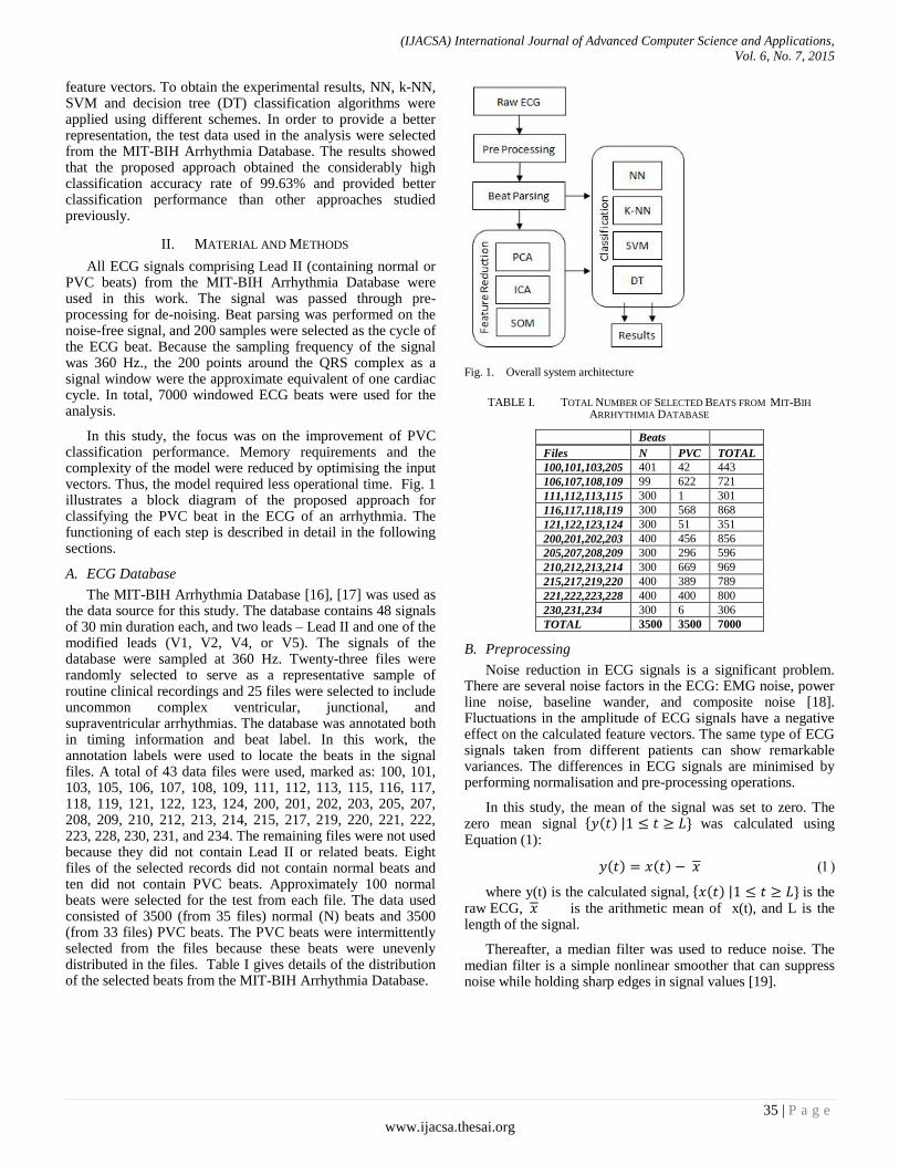
(IJACSA) International Journal of Advanced Computer Science and Applications,
Vol. 6, No. 7, 2015
35 | P a g e
www.ijacsa.thesai.org
feature vectors. To obtain the experimental results, NN, k-NN, SVM and decision tree (DT) classification algorithms were applied using different schemes. In order to provide a better representation, the test data used in the analysis were selected from the MIT-BIH Arrhythmia Database. The results showed that the proposed approach obtained the considerably high classification accuracy rate of 99.63% and provided better classification performance than other approaches studied previously.
II. MATERIAL AND METHODS
All ECG signals comprising Lead II (containing normal or PVC beats) from the MIT-BIH Arrhythmia Database were used in this work. The signal was passed through pre-processing for de-noising. Beat parsing was performed on the noise-free signal, and 200 samples were selected as the cycle of the ECG beat. Because the sampling frequency of the signal was 360 Hz., the 200 points around the QRS complex as a signal window were the approximate equivalent of one cardiac cycle. In total, 7000 windowed ECG beats were used for the analysis.
In this study, the focus was on the improvement of PVC classification performance. Memory requirements and the complexity of the model were reduced by optimising the input vectors. Thus, the model required less operational time. Fig. 1 illustrates a block diagram of the proposed approach for classifying the PVC beat in the ECG of an arrhythmia. The functioning of each step is described in detail in the following sections.
A. ECG Database
The MIT-BIH Arrhythmia Database [16], [17] was used as the data source for this study. The database contains 48 signals of 30 min duration each, and two leads – Lead II and one of the modified leads (V1, V2, V4, or V5). The signals of the database were sampled at 360 Hz. Twenty-three files were randomly selected to serve as a representative sample of routine clinical recordings and 25 files were selected to include uncommon complex ventricular, junctional, and supraventricular arrhythmias. The database was annotated both in timing information and beat label. In this work, the annotation labels were used to locate the beats in the signal files. A total of 43 data files were used, marked as: 100, 101, 103, 105, 106, 107, 108, 109, 111, 112, 113, 115, 116, 117, 118, 119, 121, 122, 123, 124, 200, 201, 202, 203, 205, 207, 208, 209, 210, 212, 213, 214, 215, 217, 219, 220, 221, 222, 223, 228, 230, 231, and 234. The remaining files were not used because they did not contain Lead II or related beats. Eight files of the selected records did not contain normal beats and ten did not contain PVC beats. Approximately 100 normal beats were selected for the test from each file. The data used consisted of 3500 (from 35 files) normal (N) beats and 3500 (from 33 files) PVC beats. The PVC beats were intermittently selected from the files because these beats were unevenly distributed in the files. Table I gives details of the distribution of the selected beats from the MIT-BIH Arrhythmia Database.
Fig. 1. Overall system architecture
TABLE I. TOTAL NUMBER OF SELECTED BEATS FROM MIT-BIH
ARRHYTHMIA DATABASE
Beats
Files N PVC TOTAL
100,101,103,205 401 42 443
106,107,108,109 99 622 721
111,112,113,115 300 1 301
116,117,118,119 300 568 868
121,122,123,124 300 51 351
200,201,202,203 400 456 856
205,207,208,209 300 296 596
210,212,213,214 300 669 969
215,217,219,220 400 389 789
221,222,223,228 400 400 800
230,231,234 300 6 306
TOTAL 3500 3500 7000
B. Preprocessing
Noise reduction in ECG signals is a significant problem. There are several noise factors in the ECG: EMG noise, power line noise, baseline wander, and composite noise [18]. Fluctuations in the amplitude of ECG signals have a negative effect on the calculated feature vectors. The same type of ECG signals taken from different patients can show remarkable variances. The differences in ECG signals are minimised by performing normalisation and pre-processing operations.
In this study, the mean of the signal was set to zero. The zero mean signal * ( ) | + was calculated using Equation (1):
( ) ( )
where y(t) is the calculated signal, * ( ) | + is the raw ECG, is the arithmetic mean of x(t), and L is the length of the signal.
Thereafter, a median filter was used to reduce noise. The median filter is a simple nonlinear smoother that can suppress noise while holding sharp edges in signal values [19].

(IJACSA) International Journal of Advanced Computer Science and Applications,
Vol. 6, No. 7, 2015
36 | P a g e
www.ijacsa.thesai.org
The filtered signal * ( ) | + was calculated using Equation (2):
( ) * ( ) ( ) ( )+
where Y(t) is the filtered signal and y(t) is the input signal.
Fig. 2. Input signal, cascade low-pass filter result, and final result of the filter
from data file 203
A cascade low-pass filter to remove frequency components below 2 and 0.5 Hz from the signal was applied in the final signal ( ) to remove the baseline wander and powerline noise. Frequency components of the baseline wander are generally below 0.5 Hz; however, in the event of a stress test, this value can be higher. Consequently, the frequency limit was adjusted to 2 Hz [20]. The required change of filter type from low- to high-pass filters can be achieved by subtracting the output of the low-pass filter from the suitably delayed input signal. Fig. 2 demonstrates the input signal, cascade-filtered signal, and filter results of the first 5000 samples of data file 203 on the MIT-BIH Database.
C. Beat Parsing
Each beat’s window length of 200 points was established from the filtered ECG signal according to the location of the R point in the QRS complex (99 points on the left side of the R point, 100 points on the right side of the R point, and the R point itself). The associated location of the R points composed the annotation files of the MIT-BIH Database. No QRS detection algorithm was used. The selected beats constituted a 7000 × 200 data matrix.
D. Feature Reduction
In this study, the time series of the one beat was used for classification. In addition, feature reduction methods were used for dimension reduction. Consequently, the performance of the classification algorithms using the time series and their reduced features were compared. PCA, ICA, and SOM were used to reduce the size of the input vectors, and the computation time of classification was diminished. Both single-beat time series and reduced dimension data were used as input vectors of the classifiers for comparison and a notable acceleration was obtained.
PCA is a numerical technique that uses perpendicular conversion to transform a set of observations of possibly correlated features into a set of values of uncorrelated features, called principal components [21]. ICA is a very versatile statistical method in which observed random data are linearly transformed into elements that are maximally independent from each other [22]. SOM is an unsupervised neural network method, improved by Kohonen, which proposes an effective and easily interpretable mapping from a higher dimensional input space into a lower dimensional (especially, two-dimensional) space [23], [24]. The feature reduction parameters are described in the result section.
E. Classification
In this work, NN, k-NN, SVM, and DT classification algorithms were used for classification, and are briefly discussed below.
A three-layered feed-forward neural network was applied for pattern classification in this study [25]. The input layer was composed of 200 nodes corresponding to the 200 points of one beat. Moreover, results of the PCA, ICA and SOM feature reduction approaches were also tested using this method. In that case, the sizes of the input layer were 2, 17, and 10 for the PCA, ICA and SOM, respectively. The output layer consisted of two nodes.
The k-NN algorithm is one of the most conventional methods in pattern recognition because of its effective non-parametric nature. The nearest neighbour decision rule assigns the classification of the closest training samples in the feature space to an uncategorised sample point [26]. This algorithm does not depend on the statistical distribution of training samples. The classification process of the samples is realised according to the nearest neighbourhood of training examples. The algorithm uses numerous distance measures. An instance is classified by a majority vote of its k-nearest neighbours. In this work, k was established as 1 after the parameter optimisation step. Euclidean distance was used as the measure function.
SVM is popular in machine learning for pattern recognition, especially for binary classification [27], [28]. The input data are transformed into a high-dimensional feature space. In this space, the data points are linearly separated by a hyper-plane. Because the patterns are not linearly separable in most cases, the patterns are mapped into a high-dimensional space using an appropriate kernel, and then, the optimisation step is fulfilled. Various kernel transformations are used for mapping the data into high-dimensional space, some of which include linear, sigmoid, polynomial, and radial basis function (RBF). In this study, parameter optimisation was used to find the optimum SVM parameters. After this stage, the C parameter was set as 100, the Gamma parameter was set as 4, and the polynomial was selected as the kernel-type parameter.
DT is a predictive model which can be used to characterise both classifiers and regression models. DT refers to a hierarchical model of decisions and their results and is used to classify a sample into a predefined set of classes based on their feature values. DT consists of nodes that form a rooted tree meaning. It is a directed tree with a node called a root that has
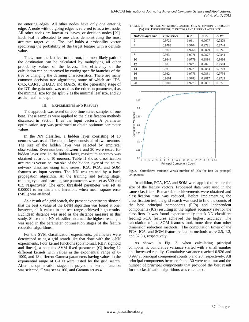
(IJACSA) International Journal of Advanced Computer Science and Applications,
Vol. 6, No. 7, 2015
37 | P a g e
www.ijacsa.thesai.org
no entering edges. All other nodes have only one entering edge. A node with outgoing edges is referred to as a test node. All other nodes are known as leaves, or decision nodes [29]. Each leaf is allocated to one class demonstrating the most accurate target value. The leaf holds a probability vector specifying the probability of the target feature with a definite value.
Thus, from the last leaf to the root, the most likely path to the destination can be calculated by multiplying all other probability values of the leaves. The efficiency of the calculation can be improved by cutting specific branches of the tree or changing the defining characteristics. There are many common decision tree algorithms, some of which are ID3, C4.5, CART, CHAID, and MARS. At the generating stage of the DT, the gain ratio was used as the criterion parameter, 4 as the minimal size for the split, 2 as the minimal leaf size, and 20 as the maximal depth.
III. EXPERIMENTS AND RESULTS
The approach was tested on 200 time series samples of one beat. These samples were applied to the classification methods discussed in Section II as the input vectors. A parameter optimisation step was performed to obtain optimum parameter values.
In the NN classifier, a hidden layer consisting of 10 neurons was used. The output layer consisted of two neurons. The size of the hidden layer was selected by empirical observation. Even numbers between 2 and 20 were tested for hidden layer size. In the hidden layer, maximum accuracy was obtained at around 10 neurons. Table II shows classification accuracies versus neuron size of the hidden layer of the neural network classifier using time series, ICA, PCA, and SOM features as input vectors. The NN was trained by a back propagation algorithm. At the training and testing stage, training cycle and learning rate parameters were set as 500 and 0.3, respectively. The error threshold parameter was set as 0.00001 to terminate the iterations when mean square error (MSE) was attained.
As a result of a grid search, the present experiments showed that the best k value of the k-NN algorithm was found at one; however, all k values in the test range achieved high results. Euclidean distance was used as the distance measure in this study. Since the k-NN classifier obtained the highest results, it was used in the parameter optimisation stages of the feature reduction algorithms.
For the SVM classification experiments, parameters were determined using a grid search like that done with the k-NN experiments. Four kernel functions (polynomial, RBF, sigmoid and linear), a complex SVM fixed parameter (C) having 12 different kernels with values in the exponential range of 0-1000, and 18 different Gamma parameters having values in the exponential range of 0-100 were tested by the grid search. After the optimisation stage, the polynomial kernel function was selected, C was set as 100, and Gamma set as 4.
TABLE II. NEURAL NETWORK CLASSIFIER CLASSIFICATION ACCURACIES
(%) FOR DIFFERENT INPUT VECTORS AND HIDDEN LAYER SIZE
Hidden layer size Time series ICA PCA SOM
2 0.9729 0.961 0.9677 0.7879
4 0.9783 0.9704 0.9791 0.8744
6 0.9873 0.9766 0.9829 0.924
8 0.983 0.9771 0.9827 0.9343
10 0.9846 0.9779 0.9814 0.9466
12 0.98 0.9773 0.982 0.9574
14 0.981 0.977 0.9864 0.9703
16 0.982 0.9776 0.9831 0.9756
18 0.9801 0.9783 0.9817 0.9723
20 0.9809 0.9779 0.9851 0.977
Fig. 3. Cumulative variance versus number of PCs for first 20 principal
components
In addition, PCA, ICA and SOM were applied to reduce the size of the feature vectors. Processed data were used in the same classifiers. Remarkable achievements were obtained and classification time was reduced. Before implementing the classification test, the grid search was used to find the counts of the best principal components (PCs) and independent components (ICs) resulting in the highest accuracy rate for the classifiers. It was found experimentally that k-NN classifiers feeding PCA features achieved the highest accuracy. The calculation of the SOM features took more time than other dimension reduction methods. The computation times of the PCA, ICA, and SOM feature reduction methods were 2.5, 1.2, and 67.3 s, respectively.
As shown in Fig. 3, when calculating principal components, cumulative variance started with a small number and increased rapidly. Cumulative variance reached 0.926 and 0.997 at principal component counts 5 and 20, respectively. All principal components between 0 and 30 were tried out and the number of principal components that provided the best result for the classification algorithms was calculated.
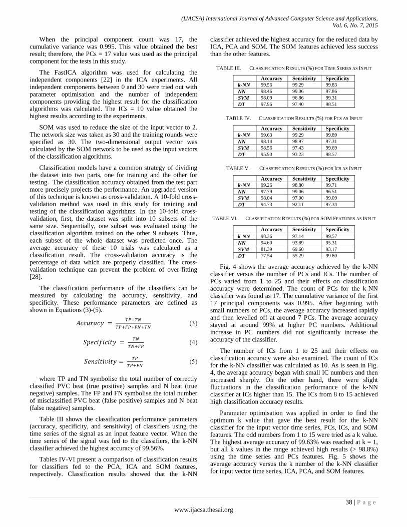
(IJACSA) International Journal of Advanced Computer Science and Applications,
Vol. 6, No. 7, 2015
38 | P a g e
www.ijacsa.thesai.org
When the principal component count was 17, the cumulative variance was 0.995. This value obtained the best result; therefore, the PCs = 17 value was used as the principal component for the tests in this study.
The FastICA algorithm was used for calculating the independent components [22] in the ICA experiments. All independent components between 0 and 30 were tried out with parameter optimisation and the number of independent components providing the highest result for the classification algorithms was calculated. The ICs = 10 value obtained the highest results according to the experiments.
SOM was used to reduce the size of the input vector to 2. The network size was taken as 30 and the training rounds were specified as 30. The two-dimensional output vector was calculated by the SOM network to be used as the input vectors of the classification algorithms.
Classification models have a common strategy of dividing the dataset into two parts, one for training and the other for testing. The classification accuracy obtained from the test part more precisely projects the performance. An upgraded version of this technique is known as cross-validation. A 10-fold cross-validation method was used in this study for training and testing of the classification algorithms. In the 10-fold cross-validation, first, the dataset was split into 10 subsets of the same size. Sequentially, one subset was evaluated using the classification algorithm trained on the other 9 subsets. Thus, each subset of the whole dataset was predicted once. The average accuracy of these 10 trials was calculated as a classification result. The cross-validation accuracy is the percentage of data which are properly classified. The cross-validation technique can prevent the problem of over-fitting [28].
The classification performance of the classifiers can be measured by calculating the accuracy, sensitivity, and specificity. These performance parameters are defined as shown in Equations (3)-(5).
where TP and TN symbolise the total number of correctly classified PVC beat (true positive) samples and N beat (true negative) samples. The FP and FN symbolise the total number of misclassified PVC beat (false positive) samples and N beat (false negative) samples.
Table III shows the classification performance parameters (accuracy, specificity, and sensitivity) of classifiers using the time series of the signal as an input feature vector. When the time series of the signal was fed to the classifiers, the k-NN classifier achieved the highest accuracy of 99.56%.
Tables IV-VI present a comparison of classification results for classifiers fed to the PCA, ICA and SOM features, respectively. Classification results showed that the k-NN
classifier achieved the highest accuracy for the reduced data by ICA, PCA and SOM. The SOM features achieved less success than the other features.
TABLE III. CLASSIFICATION RESULTS (%) FOR TIME SERIES AS INPUT
Accuracy Sensitivity Specificity
k-NN 99.56 99.29 99.83
NN 98.46 99.06 97.86
SVM 98.09 96.86 99.31
DT 97.96 97.40 98.51
TABLE IV. CLASSIFICATION RESULTS (%) FOR PCS AS INPUT
Accuracy Sensitivity Specificity
k-NN 99.63 99.29 99.89
NN 98.14 98.97 97.31
SVM 98.56 97.43 99.69
DT 95.90 93.23 98.57
TABLE V. CLASSIFICATION RESULTS (%) FOR ICS AS INPUT
Accuracy Sensitivity Specificity
k-NN 99.26 98.80 99.71
NN 97.79 99.06 96.51
SVM 98.04 97.00 99.09
DT 94.73 92.11 97.34
TABLE VI. CLASSIFICATION RESULTS (%) FOR SOM FEATURES AS INPUT
Accuracy Sensitivity Specificity
k-NN 98.36 97.14 99.57
NN 94.60 93.89 95.31
SVM 81.39 69.60 93.17
DT 77.54 55.29 99.80
Fig. 4 shows the average accuracy achieved by the k-NN classifier versus the number of PCs and ICs. The number of PCs varied from 1 to 25 and their effects on classification accuracy were determined. The count of PCs for the k-NN classifier was found as 17. The cumulative variance of the first 17 principal components was 0.995. After beginning with small numbers of PCs, the average accuracy increased rapidly and then levelled off at around 7 PCs. The average accuracy stayed at around 99% at higher PC numbers. Additional increase in PC numbers did not significantly increase the accuracy of the classifier.
The number of ICs from 1 to 25 and their effects on classification accuracy were also examined. The count of ICs for the k-NN classifier was calculated as 10. As is seen in Fig. 4, the average accuracy began with small IC numbers and then increased sharply. On the other hand, there were slight fluctuations in the classification performance of the k-NN classifier at ICs higher than 15. The ICs from 8 to 15 achieved high classification accuracy results.
Parameter optimisation was applied in order to find the optimum k value that gave the best result for the k-NN classifier for the input vector time series, PCs, ICs, and SOM features. The odd numbers from 1 to 15 were tried as a k value. The highest average accuracy of 99.63% was reached at k = 1, but all k values in the range achieved high results (> 98.8%) using the time series and PCs features. Fig. 5 shows the average accuracy versus the k number of the k-NN classifier for input vector time series, ICA, PCA, and SOM features.
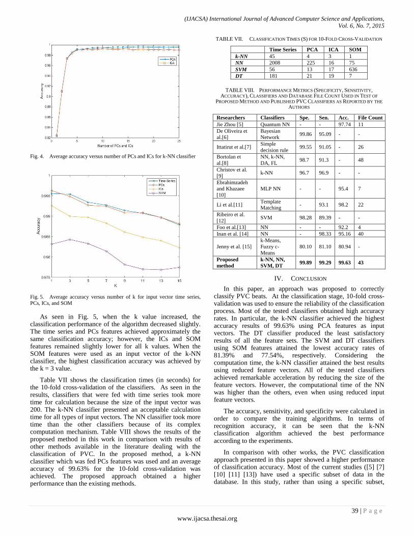
(IJACSA) International Journal of Advanced Computer Science and Applications,
Vol. 6, No. 7, 2015
39 | P a g e
www.ijacsa.thesai.org
Fig. 4. Average accuracy versus number of PCs and ICs for k-NN classifier
Fig. 5. Average accuracy versus number of k for input vector time series,
PCs, ICs, and SOM
As seen in Fig. 5, when the k value increased, the classification performance of the algorithm decreased slightly. The time series and PCs features achieved approximately the same classification accuracy; however, the ICs and SOM features remained slightly lower for all k values. When the SOM features were used as an input vector of the k-NN classifier, the highest classification accuracy was achieved by the k = 3 value.
Table VII shows the classification times (in seconds) for the 10-fold cross-validation of the classifiers. As seen in the results, classifiers that were fed with time series took more time for calculation because the size of the input vector was 200. The k-NN classifier presented an acceptable calculation time for all types of input vectors. The NN classifier took more time than the other classifiers because of its complex computation mechanism. Table VIII shows the results of the proposed method in this work in comparison with results of other methods available in the literature dealing with the classification of PVC. In the proposed method, a k-NN classifier which was fed PCs features was used and an average accuracy of 99.63% for the 10-fold cross-validation was achieved. The proposed approach obtained a higher performance than the existing methods.
TABLE VII. CLASSIFICATION TIMES (S) FOR 10-FOLD CROSS-VALIDATION
Time Series PCA ICA SOM
k-NN 45 4 3 1
NN 2008 225 16 75
SVM 56 13 17 636
DT 181 21 19 7
TABLE VIII. PERFORMANCE METRICS (SPECIFICITY, SENSITIVITY, ACCURACY), CLASSIFIERS AND DATABASE FILE COUNT USED IN TEST OF
PROPOSED METHOD AND PUBLISHED PVC CLASSIFIERS AS REPORTED BY THE
AUTHORS
Researchers Classifiers Spe. Sen. Acc. File Count
Jie Zhou [5] Quantum NN - - 97.74 11
De Oliveira et
al.[6]
Bayesian
Network 99.86 95.09 - -
Ittatirut et al.[7] Simple
decision rule 99.55 91.05 - 26
Bortolan et
al.[8]
NN, k-NN,
DA, FL 98.7 91.3 - 48
Christov et al.
[9] k-NN 96.7 96.9 - -
Ebrahimzadeh
and Khazaee
[10]
MLP NN - - 95.4 7
Li et al.[11] Template Matching
- 93.1 98.2 22
Ribeiro et al.
[12] SVM 98.28 89.39 - -
Foo et al.[13] NN - - 92.2 4
Inan et al. [14] NN - 98.33 95.16 40
Jenny et al. [15]
k-Means,
Fuzzy c-
Means
80.10 81.10 80.94 -
Proposed
method
k-NN, NN,
SVM, DT 99.89 99.29 99.63 43
IV. CONCLUSION
In this paper, an approach was proposed to correctly classify PVC beats. At the classification stage, 10-fold cross-validation was used to ensure the reliability of the classification process. Most of the tested classifiers obtained high accuracy rates. In particular, the k-NN classifier achieved the highest accuracy results of 99.63% using PCA features as input vectors. The DT classifier produced the least satisfactory results of all the feature sets. The SVM and DT classifiers using SOM features attained the lowest accuracy rates of 81.39% and 77.54%, respectively. Considering the computation time, the k-NN classifier attained the best results using reduced feature vectors. All of the tested classifiers achieved remarkable acceleration by reducing the size of the feature vectors. However, the computational time of the NN was higher than the others, even when using reduced input feature vectors.
The accuracy, sensitivity, and specificity were calculated in order to compare the training algorithms. In terms of recognition accuracy, it can be seen that the k-NN classification algorithm achieved the best performance according to the experiments.
In comparison with other works, the PVC classification approach presented in this paper showed a higher performance of classification accuracy. Most of the current studies ([5] [7] [10] [11] [13]) have used a specific subset of data in the database. In this study, rather than using a specific subset,

(IJACSA) International Journal of Advanced Computer Science and Applications,
Vol. 6, No. 7, 2015
40 | P a g e
www.ijacsa.thesai.org
almost all PVC beats existing in the database were used. De Oliveira et al. used 947 PVC beats for classification, with 80% of the data used for training and 20% for testing. However, they did not give sufficient details of their experimental implementation, such as the number of cross validations. Furthermore, the number of records used in the study was not specified [6].
In another work, Ittatirut et al. tested their method with 26 records. They excluded some records such as those using pacemakers and those containing heart blockage and atrial fibrillation from their experiments [7].
On the other hand, Bortolan et al. used all the ECG recordings from the MIT-BIH Database. However, the size of the learning set was very small (260 beats for the global set, 76 beats for the local set). The best accuracy achieved was 88.5% from the global set with a DA classifier and 98.7% from the local set with a k-NN classifier [8]. Similarly, Christov et al. used a k-NN algorithm to classify PVC beats in all files in the Database and achieved sensitivity and specificity rates of 96.9% and 96.7%, respectively [9]. Inan et al. used most of the signal files, tested the data with an NN classification algorithm and achieved an accuracy of 95.16% [14]. Jenny et al. used an unsupervised learning algorithm and, therefore, achieved lower accuracy rates than those of the other works [15].
This study showed that high classification accuracy can be obtained without implementing any feature extraction method and by using time series of the signal for input. PCA can be used to reduce the size of the input vectors representing the data. Because of its high computational speed, the proposed method in this work may advance the capability of any system performing real-time PVC analysis. The classification approach presented in this paper can be implemented as part of a computer-aided diagnosis system and can speed up the diagnosis process. The proposed method can be further developed for future use in detecting more ECG arrhythmias.
REFERENCES
[1] A. S. Go, D. Mozaffarian, V. L. Roger, E. J. Benjamin, J. D. Berry, M. J. Blaha, S. Dai, E. S. Ford, C. S. Fox, S. Franco, H. J. Fullerton, C. Gillespie, S. M. Hailpern, J. A. Heit, V. J. Howard, M. D. Huffman, S. E. Judd, B. M. Kissela, S. J. Kittner, D. T. Lackland, J. H. Lichtman, L. D. Lisabeth, R. H. Mackey, D. J. Magid, G. M. Marcus, A. Marelli, D. B. Matchar, D. K. McGuire, E. R. Mohler, C. S. Moy, M. E. Mussolino, R. W. Neumar, G. Nichol, D. K. Pandey, N. P. Paynter, M. J. Reeves, P. D. Sorlie, J. Stein, A. Towfighi, T. N. Turan, S. S. Virani, N. D. Wong, D. Woo, and M. B. Turner, “Heart disease and stroke statistics-2014 update: a report from the American Heart Association.,” Circulation, vol. 129, no. 3, pp. e28–e292, Jan. 2014.
[2] N. Tosun, Y. Erkoç, T. Buzgan, B. Keskinkılıç, D. Aras, N. Yardım, S. Gögen, G. Sarıoğlu, and M. Soylu, Türkiye Kalp ve Damar Hastalıklarının Önleme ve Kontrol Programı (2010-2014), Ankara: Anıl Matbaası, 2014.
[3] G.D. Clifford, F. Azuaje, and P.E. McSharry (Eds.), Advanced Methods and Tools for ECG Data Analysis, Boston: Artech House, 2006.
[4] G. K. Lee, K. W. Klarich, M. Grogan, and Y.-M. Cha, “Premature ventricular contraction-induced cardiomyopathy: a treatable condition,” Circ. Arrhythm. Electrophysiol., vol. 5, no. 1, pp. 229–36, Feb. 2012.
[5] Jie Zhou, “Automatic detection of premature ventricular contraction using quantum neural networks,” in Third IEEE Symposium on Bioinformatics and Bioengineering, 2003. Proceedings, pp. 169–173, 2003.
[6] L. S. C. De Oliveira, R. V Andreão, and M. Sarcinelli-Filho, “Premature Ventricular beat classification using a dynamic Bayesian Network.,” Conf. Proc. IEEE Eng. Med. Biol. Soc., vol. 2011, pp. 4984–7, 2011.
[7] S. Ittatirut, A. Lek-Uthai, and A. Teeramongkonrasmee, “Detection of Premature Ventricular Contraction for real-time applications,” in 2013 10th International Conference on Electrical Engineering/Electronics, Computer, Telecommunications and Information Technology, ECTI-CON 2013, 2013.
[8] G. Bortolan, I. Jekova, and I. Christov, “Comparison of four methods for premature ventricular contraction and normal beat clustering,” Computers in Cardiology, vol. 32, pp. 921–924, 2005.
[9] I. Christov, I. Jekova, and G. Bortolan, “Premature ventricular contraction classification by the K th nearest-neighbours rule,” Physiol. Meas., vol. 26, no. 1, pp. 123–130, Feb. 2005.
[10] A. Ebrahimzadeh and A. Khazaee, “Detection of premature ventricular contractions using MLP neural networks: A comparative study,” Meas. J. Int. Meas. Confed., vol. 43, pp. 103–112, 2010.
[11] P. Li, C. Liu, X. Wang, D. Zheng, Y. Li, and C. Liu, “A low-complexity data-adaptive approach for premature ventricular contraction recognition,” Signal, Image Video Process, vol. 8, no. 1, pp. 111–120, Apr. 2013.
[12] B. R. Ribeiro, J. H. Henirques, A. M. Marques, and M. A. Antunes, “Manifold learning for premature ventricular contraction detection,” Computers in Cardiology, vol. 35, pp. 917–920, 2008.
[13] S. Y. Foo, G. Stuart, B. Harvey, and A. Meyer-Baese, “Neural network-based EKG pattern recognition,” Eng. Appl. Artif. Intell., vol. 15, no. 3–4, pp. 253–260, June 2002.
[14] O. T. Inan, L. Giovangrandi, and G. T. A. Kovacs, “Robust neural-network-based classification of premature ventricular contractions using wavelet transform and timing interval features,” IEEE Trans. Biomed. Eng., vol. 53, no. 12, pt. 1, pp. 2507–15, Dec. 2006.
[15] N. Z. N. Jenny, O. Faust, and W. Yu, “Automated Classification of Normal and Premature Ventricular Contractions in Electrocardiogram Signals,” J. Med. Imaging Heal. Informatics, vol. 4, no. 6, pp. 886–892, Dec. 2014.
[16] G. B. Moody and R. G. Mark, “The impact of the MIT-BIH arrhythmia database.,” IEEE Eng. Med. Biol. Mag., vol. 20, no. 3, pp. 45–50, 2001.
[17] G. Moody and R. Mark, “The MIT-BIH Arrhythmia Database on CD-ROM and software for use with it,” in [1990] Proceedings Computers in Cardiology, pp. 185–188, 1990.
[18] M. Kania, M. Fereniec, and R. Maniewski, “Wavelet denoising for multi-lead high resolution ECG signals,” Meas. Sci. Rev., vol. 7, section 2, no. 3, pp. 30–33, 2007.
[19] T. Nodes and N. Gallagher, “Median filters: Some modifications and their properties,” IEEE Trans. Acoust., vol. 30, no. 5, pp. 739–746, Oct. 1982.
[20] D. Kicmerova, “Methods for detection and classification in ECG analysis,” Brno University of Technology, 2009.
[21] S. Theodoridis and K. Koutroumbas, Pattern Recognition, 4th Ed. Burlington: Academic Press, 2009.
[22] A. Hyvärinen and E. Oja, “Independent component analysis: algorithms and applications,” Neural Netw., vol. 13, pp. 411–30, 2000.
[23] T. Kohonen, “Self-organized formation of topologically correct feature maps,” Biol. Cybern., vol. 43, no. 1, pp. 59–69, 1982.
[24] T. Kohonen, “The self-organizing map,” Proc. IEEE, vol. 78, no. 9, pp. 1464–1480, 1990.
[25] S. Haykin, Neural Networks: a comprehensive foundation, 2nd Ed. Ontario: Pearson, 1999.
[26] T. Cover and P. Hart, “Nearest neighbor pattern classification,” IEEE Trans. Inf. Theory, vol. 13, no. 1, pp. 21–27, Jan. 1967.
[27] C. Cortes and V. Vapnik, “Support-vector networks,” Mach. Learn., vol. 20, no. 3, pp. 273–297, Sept. 1995.
[28] R. O. Duda, P. E. Hart, and D. G. Stork, Pattern Classification, 2nd Ed. New York: John Wiley & Sons, Inc., 2000.
[29] L. Rokach and O. Maimon, Data Mining with Decision Trees: Theory and Applications. Singapore: World Scientific Publishing Co., 2008.
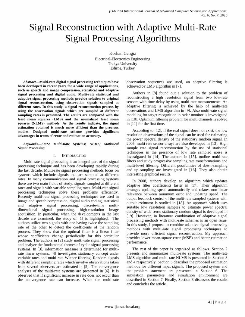
(IJACSA) International Journal of Advanced Computer Science and Applications,
Vol. 6, No. 7, 2015
41 | P a g e
www.ijacsa.thesai.org
Signal Reconstruction with Adaptive Multi-Rate
Signal Processing Algorithms
Korhan Cengiz
Electrical-Electronics Engineering
Trakya University
Edirne, Turkey
Abstract—Multi-rate digital signal processing techniques have
been developed in recent years for a wide range of applications,
such as speech and image compression, statistical and adaptive
signal processing and digital audio. Multi-rate statistical and
adaptive signal processing methods provide solution to original
signal reconstruction, using observation signals sampled at
different rates. In this study, a signal reconstruction process by
using the observation signals which are sampled at different
sampling rates is presented. The results are compared with the
least mean squares (LMS) and the normalized least mean
squares (NLMS) methods. As the results indicate, the signal
estimation obtained is much more efficient than the previous
studies. Designed multi-rate scheme provides significant
advantages in terms of error and estimation accuracy.
Keywords—LMS; Multi-Rate Systems; NLMS; Statistical
Signal Processing
I. INTRODUCTION
Multi-rate signal processing is an integral part of the signal processing technique and has been developing rapidly during the last decade. Multi-rate signal processing methods focus on systems which include signals that are sampled at different rates. In many communication and signal processing systems there are two main fields of study: signals sampled at different rates and signals with variable sampling rates. Multi-rate signal processing techniques solve these problems efficiently. Recently multi-rate signal processing techniques are used in image and speech compression, digital audio coding, statistical and adaptive signal processing, discrete-time multi-dimensional signal processing, high-resolution image acquisition. In particular, when the developments in the last decade are examined, the study of [1] is highlighted. The authors utilize two signals with one having twice the sampling rate of the other to detect the coefficients of the random process. They show that the optimal filter is a linear filter whose coefficients change periodically for this particular problem. The authors in [2] study multi-rate signal processing and analyze the fundamental themes of cyclic signal processing systems. In [3], information measure is determined for multi-rate linear systems. [4] investigates stationary concept under variable rates and multi-rate Wiener filtering. Random signals with different sampling rates which involve observations taken from several observers are estimated in [5]. The convergence analyses of the multi-rate systems are presented in [6]. It is observed that if significant increase in rate does not occur than the convergence rate can increase. When the multi-rate
observation sequences are used, an adaptive filtering is achieved by LMS algorithm in [7].
Authors in [8] found out a solution to the problem of reconstructing a high resolution signal from two low-rate sensors with time delay by using multi-rate measurements. An adaptive filtering is achieved by the help of multi-rate observations and LMS algorithm in [9]. Also multi-rate signal modeling for target recognition in radar monitor is investigated in [10]. Optimum filtering problem for multi channels is solved in [11] for the first time.
According to [12], if the real signal does not exist, the low resolution observations of the signal can be used for estimating the power spectral density of the stationary random signal. In 2005, multi rate sensor arrays are also developed in [13]. High sample rate signal reconstruction by the use of statistical techniques in the presence of low rate sampled noise is investigated in [14]. The authors in [15], outline multi-rate filters and study progressive sampling rate transformations and multi-level filtering. Different possibilities of down-sampling and up-sampling are investigated in [16]. They also obtain interesting graphical results.
In 2008, authors develop an algorithm which updates adaptive filter coefficients faster in [17]. Their algorithm arranges updating speed automatically and relates non-linear relevance between minimum error and updating speed. The output feedback control of the multi-rate sampled systems with output estimator is studied in [18]. An approach which uses suitable low resolution samples to estimate power spectral density of wide sense stationary random signal is developed in [19]. However, in literature combination of adaptive signal processing methods with multi-rate schemes is an open issue. In this study, I propose to combine adaptive signal processing methods with multi-rate signal processing techniques to provide more efficient signal reconstruction. My approach provides lower mean-square error (MSE) and better estimation performance.
The rest of the paper is organized as follows. Section 2 presents and summarizes multi-rate systems. The multi-rate LMS algorithm and multi-rate NLMS is presented in Section 3 and 4 respectively. Section 5 describes the proposed estimation methods for different input signals. The proposed system and the problem statement are presented in Section 6. The simulation parameters and simulation environment are described in Section 7. Finally, Section 8 discusses the results and concludes the article.

(IJACSA) International Journal of Advanced Computer Science and Applications,
Vol. 6, No. 7, 2015
42 | P a g e
www.ijacsa.thesai.org
II. MULTI-RATE SYSTEMS
The observation signals are sampled at different rates in some signal processing applications. These signals should be processed together for detection, prediction and classification. To solve the problems of multi-rate systems, the single rate signal theory should be extended to multi-rate signal theory. This theory should be implemented to single-channel, single-rate or multi-channel, multi-rate problems. In this section, the theory which is developed for multi-rate systems is explained and the basic processes in multi-rate systems are presented.
The changing of the sampling frequency caused problems in many digital signal processing systems. For example, CD players, digital audio tapes and digital broadcasting have different sampling frequencies. Especially, sampling rates of many voice signals should be convertible to each other. Also in some systems, the discrete-time signals with different sampling rates should be made compatible with each other. Separation of wide-band digital signal for transmitting in narrow-band channels is an example for multi-rate systems.
The method of multi-rate signal processing includes decimation and inter leaver. Decimation which includes filtering and down-sampling decreases sampling rate of the signal. Inter leaver which includes up-sampling and filtering increases sampling rate of the signal. There is also transformation of sampling rate process which includes cascade connection of decimation and inter leaver.
For optimal filtering, the estimated signal and observed signal are considered wide-sense-stationary. The sampling rates are equal for both signals and the filter is linear time-invariant filter (LTI). LTI filter preserves stationarity. However for multi-rate systems, the situation is different. The periodicity is discussed in multi-rate systems because down and up sampling processes vary with time and they do not preserve stationarity. So wide-sense-stationarity becomes crucial.
III. MULTI-RATE LEAST MEAN SQUARES (LMS)
ALGORITHM
The least mean square optimum filtering is related to observed data. Desired data sequence and observed data sequence are measured, saved and used for designing the filter in this method. The criterion in least mean square (LMS) algorithm is to minimize the sum of the squares of error function. Multi-rate least mean square filter is designed in [7]. By this filter, using two observation sequences provide lower mean square error than using one high-rated or low-rated observation sequences.
Multi-rate LMS algorithm is designed for several input signals with different sampling rates. The equations are more complex than traditional LMS algorithm. (1) and (2) show the high-rated observation vector and low-rated observation vector respectively.
x[n] x[n] x[n-1] … x[n-(P-1)]T
y[m] y[m] y[m-1] … y[m-(Q-1)]T
The filter coefficients are periodic and coefficient vectors are updated in each iteration in multi-rate LMS algorithm. The filter coefficient updates is expressed in (3) and (4).
hk[m+1]hk[m] +μxe[n]x[n]
gk[m+1]gk[m] +μye[n]y[m]
IV. MULTI-RATE NORMALIZED LEAST MEAN SQUARES
(NLMS) ALGORITHM
Multi-rate NLMS algorithm is designed for several input signals with different sampling rates. The equations are more complex than traditional NLMS algorithm. (5) and (6) show the high-rated observation vector and low-rated observation vector respectively.
x[n] x[n] x[n-1] … x[n-(P-1)]T
y[m] y[m] y[m-1] … y[m-(Q-1)]T
The filter coefficients are periodic and coefficient vectors are updated in each iteration in multi-rate NLMS algorithm. The filter coefficient updates is expressed in (7) and (8). Note that in here α>0 coefficient is used for preventing divide by zero error.
][][
][][][]1[
nxnx
nenxmhmh
T
xkk
(7)
][][
][][][]1[
mymy
nemymgmg
T
y
kk
(8)
V. PROPOSED ESTIMATION METHODS FOR INPUT SIGNALS
In this study, the input signals are derived from first-order auto regressive process. It can be defined as in (9).
x[n]c+αx[n-1] +u[n]
In the above equation, x[n] shows the value at n th moment, x[n-1] corresponds to the value at a previous moment, c is a constant, α is used for model parameter and u[n]
corresponds to White Gaussian Noise. The u[n] is assumed as zero mean and having σ
2u[n] variance. For |α|<1 the process
becomes wide-sense stationary (WSS). If α=1, x[n] has infinite variance and becomes not WSS. For c=0 the process becomes zero mean process. The signal-to-noise ratio can be defined as in (10).
noise
signal
P
PSNR (10)
SNR defines the ratio between signal and noise. In here, Psignal is the average power of the signal. Both signal and noise power should be measured at the same points in the system. Traditionally in many applications, SNR is used in logarithmic decibel scale. It can be defined as in (11).
dBnoisedBsignal
noise
signal
dB PPP
PSNR ,,10log10
(11)
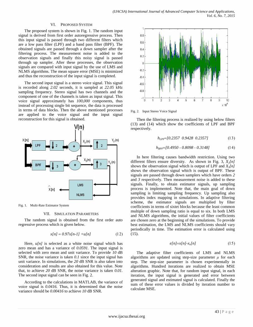
(IJACSA) International Journal of Advanced Computer Science and Applications,
Vol. 6, No. 7, 2015
43 | P a g e
www.ijacsa.thesai.org
VI. PROPOSED SYSTEM
The proposed system is shown in Fig. 1. The random input signal is derived from first order autoregressive process. Then this input signal is passed through two different filters which are a low pass filter (LPF) and a band pass filter (BPF). The obtained signals are passed through a down sampler after the filtering process. The measurement noise is added to the observation signals and finally this noisy signal is passed through up sampler. After these processes, the observation signals are compared with input signal by the use of LMS and NLMS algorithms. The mean square error (MSE) is minimized and thus the reconstruction of the input signal is completed.
The second input signal is a stereo voice signal. This signal is recorded along 2.02 seconds, it is sampled at 22.05 kHz sampling frequency. Stereo signal has two channels and the component of one of the channels is taken as input signal. This voice signal approximately has 100,000 components, thus instead of processing single bit sequence, the data is processed in terms of data blocks. Then the above mentioned processes are applied to the voice signal and the input signal reconstruction for this signal is obtained.
Fig. 1. Multi-Rate Estimator System
VII. SIMULATION PARAMETERS
The random signal is obtained from the first order auto regressive process which is given below.
x[n]0.97x[n-1] +u[n]
Here, u[n] is selected as a white noise signal which has zero mean and has a variance of 0.0591. The input signal is selected with zero mean and unit variance. To provide 10 dB SNR, the noise variance is taken 0.1 since the input signal has unit variance. In simulations, the 20 dB SNR is also taken into consideration and results are also obtained for this value. Note that, to achieve 20 dB SNR, the noise variance is taken 0.01. The second input signal can be seen in Fig. 2.
According to the calculations in MATLAB, the variance of voice signal is 0.0416. Thus, it is determined that the noise variance should be 0.00416 to achieve 10 dB SNR.
Fig. 2. Input Stereo Voice Signal
Then the filtering process is realized by using below filters (13) and (14) which show the coefficients of LPF and BPF respectively.
hLPF[0.2357 0.9428 0.2357]
hBPF[0.4950 - 0.8098 - 0.3148]
In here filtering causes bandwidth restriction. Using two different filters ensure diversity. As shown in Fig. 3, X2[n] shows the observation signal which is output of LPF and X3[n] shows the observation signal which is output of BPF. These signals are passed through down samplers which have orders 2 and 3 respectively. Then measurement noise is added to these signals. Finally, to obtain estimator signals, up sampling process is implemented. Note that, the main goal of down sampling is limiting sampling frequency. Up sampling also provides index mapping in simulations. In adaptive filtering scheme, the estimator signals are multiplied by filter coefficients in terms of sixtet blocks because the least common multiple of down sampling ratio is equal to six. In both LMS and NLMS algorithms, the initial values of filter coefficients are chosen zero at the beginning of the simulations. To provide best estimation, the LMS and NLMS coefficients should vary periodically in time. The estimation error is calculated using (15).
e[n]x[n]-xe[n]
The adaptive filter coefficients of LMS and NLMS algorithms are updated using step-size parameter μ for each step. The step-size parameter is chosen experimentally in algorithms. Hundred iterations are realized to obtain MSE alteration graphic. Note that, for random input signal, in each iteration, the input signal is generated and error between generated signal and estimated signal is calculated. Finally the sum of these error values is divided by iteration number to calculate MSE.
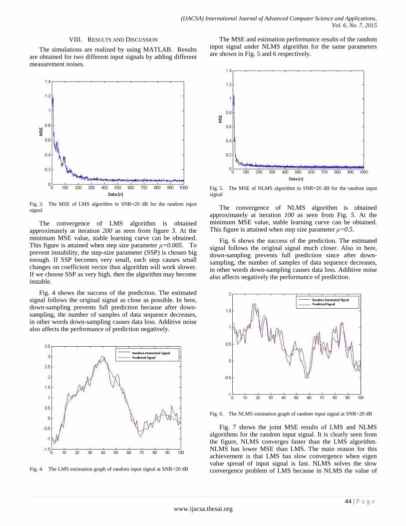
(IJACSA) International Journal of Advanced Computer Science and Applications,
Vol. 6, No. 7, 2015
44 | P a g e
www.ijacsa.thesai.org
VIII. RESULTS AND DISCUSSION
The simulations are realized by using MATLAB. Results are obtained for two different input signals by adding different measurement noises.
Fig. 3. The MSE of LMS algorithm in SNR=20 dB for the random input
signal
The convergence of LMS algorithm is obtained approximately at iteration 200 as seen from figure 3. At the minimum MSE value, stable learning curve can be obtained. This figure is attained when step size parameter μ=0.005. To prevent instability, the step-size parameter (SSP) is chosen big enough. If SSP becomes very small, each step causes small changes on coefficient vector thus algorithm will work slower. If we choose SSP as very high, then the algorithm may become instable.
Fig. 4 shows the success of the prediction. The estimated signal follows the original signal as close as possible. In here, down-sampling prevents full prediction because after down-sampling, the number of samples of data sequence decreases, in other words down-sampling causes data loss. Additive noise also affects the performance of prediction negatively.
Fig. 4. The LMS estimation graph of random input signal at SNR=20 dB
The MSE and estimation performance results of the random input signal under NLMS algorithm for the same parameters are shown in Fig. 5 and 6 respectively.
Fig. 5. The MSE of NLMS algorithm in SNR=20 dB for the random input
signal
The convergence of NLMS algorithm is obtained approximately at iteration 100 as seen from Fig. 5. At the minimum MSE value, stable learning curve can be obtained. This figure is attained when step size parameter μ=0.5.
Fig. 6 shows the success of the prediction. The estimated signal follows the original signal much closer. Also in here, down-sampling prevents full prediction since after down-sampling, the number of samples of data sequence decreases, in other words down-sampling causes data loss. Additive noise also affects negatively the performance of prediction.
Fig. 6. The NLMS estimation graph of random input signal at SNR=20 dB
Fig. 7 shows the joint MSE results of LMS and NLMS algorithms for the random input signal. It is clearly seen from the figure, NLMS converges faster than the LMS algorithm. NLMS has lower MSE than LMS. The main reason for this achievement is that LMS has slow convergence when eigen value spread of input signal is fast. NLMS solves the slow convergence problem of LMS because in NLMS the value of
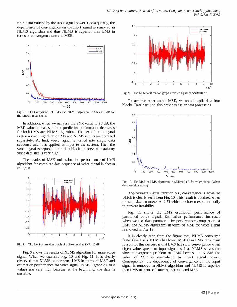
(IJACSA) International Journal of Advanced Computer Science and Applications,
Vol. 6, No. 7, 2015
45 | P a g e
www.ijacsa.thesai.org
SSP is normalized by the input signal power. Consequently, the dependence of convergence on the input signal is removed in NLMS algorithm and thus NLMS is superior than LMS in terms of convergence rate and MSE.
Fig. 7. The Comparison of LMS and NLMS algorithm in SNR=20 dB for
the random input signal
In addition, when we increase the SNR value to 10 dB, the MSE value increases and the prediction performance decreases for both LMS and NLMS algorithms. The second input signal is stereo voice signal. The LMS and NLMS results are obtained separately. At first, voice signal is turned into single data sequence and it is applied as input to the system. Then the voice signal is separated into data blocks to prevent instability since data size is very high.
The results of MSE and estimation performance of LMS algorithm for complete data sequence of voice signal is shown in Fig. 8.
Fig. 8. The LMS estimation graph of voice signal at SNR=10 dB
Fig. 9 shows the results of NLMS algorithm for same voice signal. When we examine Fig. 10 and Fig. 11, it is clearly observed that NLMS outperforms LMS in terms of MSE and estimation performance for voice signal. In MSE graphics, first values are very high because at the beginning, the data is unstable.
Fig. 9. The NLMS estimation graph of voice signal at SNR=10 dB
To achieve more stable MSE, we should split data into blocks. Data partition also provides easier data processing.
Fig. 10. The MSE of LMS algorithm in SNR=10 dB for voice signal (When
data partition exists)
Approximately after iteration 100, convergence is achieved which is clearly seen from Fig. 10. This result is obtained when the step size parameter μ=0.13 which is chosen experimentally to prevent instability.
Fig. 11 shows the LMS estimation performance of partitoned voice signal. Estimation performance increases when we use data partition. The performance comparison of LMS and NLMS algorithms in terms of MSE for voice signal is showed in Fig. 12.
It is clearly seen from the figure that, NLMS converges faster than LMS. NLMS has lower MSE than LMS. The main reason for this success is that LMS has slow convergence when eigen value spread of input signal is fast. NLMS solves the slow convergence problem of LMS because in NLMS the value of SSP is normalized by input signal power. Consequently, the dependence of convergence on the input signal is removed in NLMS algorithm and NLMS is superior than LMS in terms of convergence rate and MSE.
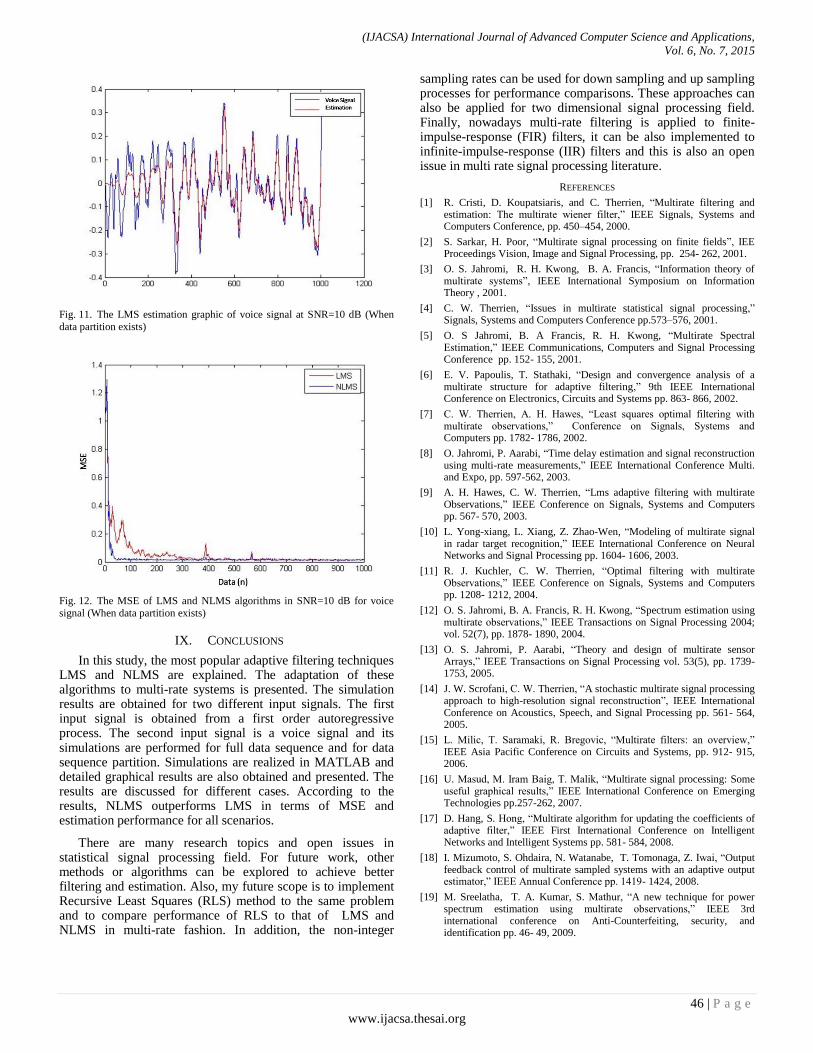
(IJACSA) International Journal of Advanced Computer Science and Applications,
Vol. 6, No. 7, 2015
46 | P a g e
www.ijacsa.thesai.org
Fig. 11. The LMS estimation graphic of voice signal at SNR=10 dB (When
data partition exists)
Fig. 12. The MSE of LMS and NLMS algorithms in SNR=10 dB for voice
signal (When data partition exists)
IX. CONCLUSIONS
In this study, the most popular adaptive filtering techniques LMS and NLMS are explained. The adaptation of these algorithms to multi-rate systems is presented. The simulation results are obtained for two different input signals. The first input signal is obtained from a first order autoregressive process. The second input signal is a voice signal and its simulations are performed for full data sequence and for data sequence partition. Simulations are realized in MATLAB and detailed graphical results are also obtained and presented. The results are discussed for different cases. According to the results, NLMS outperforms LMS in terms of MSE and estimation performance for all scenarios.
There are many research topics and open issues in statistical signal processing field. For future work, other methods or algorithms can be explored to achieve better filtering and estimation. Also, my future scope is to implement Recursive Least Squares (RLS) method to the same problem and to compare performance of RLS to that of LMS and NLMS in multi-rate fashion. In addition, the non-integer
sampling rates can be used for down sampling and up sampling processes for performance comparisons. These approaches can also be applied for two dimensional signal processing field. Finally, nowadays multi-rate filtering is applied to finite-impulse-response (FIR) filters, it can be also implemented to infinite-impulse-response (IIR) filters and this is also an open issue in multi rate signal processing literature.
REFERENCES
[1] R. Cristi, D. Koupatsiaris, and C. Therrien, “Multirate filtering and estimation: The multirate wiener filter,” IEEE Signals, Systems and Computers Conference, pp. 450–454, 2000.
[2] S. Sarkar, H. Poor, “Multirate signal processing on finite fields”, IEE Proceedings Vision, Image and Signal Processing, pp. 254- 262, 2001.
[3] O. S. Jahromi, R. H. Kwong, B. A. Francis, “Information theory of multirate systems”, IEEE International Symposium on Information Theory , 2001.
[4] C. W. Therrien, “Issues in multirate statistical signal processing,” Signals, Systems and Computers Conference pp.573–576, 2001.
[5] O. S Jahromi, B. A Francis, R. H. Kwong, “Multirate Spectral Estimation,” IEEE Communications, Computers and Signal Processing Conference pp. 152- 155, 2001.
[6] E. V. Papoulis, T. Stathaki, “Design and convergence analysis of a multirate structure for adaptive filtering,” 9th IEEE International Conference on Electronics, Circuits and Systems pp. 863- 866, 2002.
[7] C. W. Therrien, A. H. Hawes, “Least squares optimal filtering with multirate observations,” Conference on Signals, Systems and Computers pp. 1782- 1786, 2002.
[8] O. Jahromi, P. Aarabi, “Time delay estimation and signal reconstruction using multi-rate measurements,” IEEE International Conference Multi. and Expo, pp. 597-562, 2003.
[9] A. H. Hawes, C. W. Therrien, “Lms adaptive filtering with multirate Observations,” IEEE Conference on Signals, Systems and Computers pp. 567- 570, 2003.
[10] L. Yong-xiang, L. Xiang, Z. Zhao-Wen, “Modeling of multirate signal in radar target recognition,” IEEE International Conference on Neural Networks and Signal Processing pp. 1604- 1606, 2003.
[11] R. J. Kuchler, C. W. Therrien, “Optimal filtering with multirate Observations,” IEEE Conference on Signals, Systems and Computers pp. 1208- 1212, 2004.
[12] O. S. Jahromi, B. A. Francis, R. H. Kwong, “Spectrum estimation using multirate observations,” IEEE Transactions on Signal Processing 2004; vol. 52(7), pp. 1878- 1890, 2004.
[13] O. S. Jahromi, P. Aarabi, “Theory and design of multirate sensor Arrays,” IEEE Transactions on Signal Processing vol. 53(5), pp. 1739-1753, 2005.
[14] J. W. Scrofani, C. W. Therrien, “A stochastic multirate signal processing approach to high-resolution signal reconstruction”, IEEE International Conference on Acoustics, Speech, and Signal Processing pp. 561- 564, 2005.
[15] L. Milic, T. Saramaki, R. Bregovic, “Multirate filters: an overview,” IEEE Asia Pacific Conference on Circuits and Systems, pp. 912- 915, 2006.
[16] U. Masud, M. Iram Baig, T. Malik, “Multirate signal processing: Some useful graphical results,” IEEE International Conference on Emerging Technologies pp.257-262, 2007.
[17] D. Hang, S. Hong, “Multirate algorithm for updating the coefficients of adaptive filter,” IEEE First International Conference on Intelligent Networks and Intelligent Systems pp. 581- 584, 2008.
[18] I. Mizumoto, S. Ohdaira, N. Watanabe, T. Tomonaga, Z. Iwai, “Output feedback control of multirate sampled systems with an adaptive output estimator,” IEEE Annual Conference pp. 1419- 1424, 2008.
[19] M. Sreelatha, T. A. Kumar, S. Mathur, “A new technique for power spectrum estimation using multirate observations,” IEEE 3rd international conference on Anti-Counterfeiting, security, and identification pp. 46- 49, 2009.
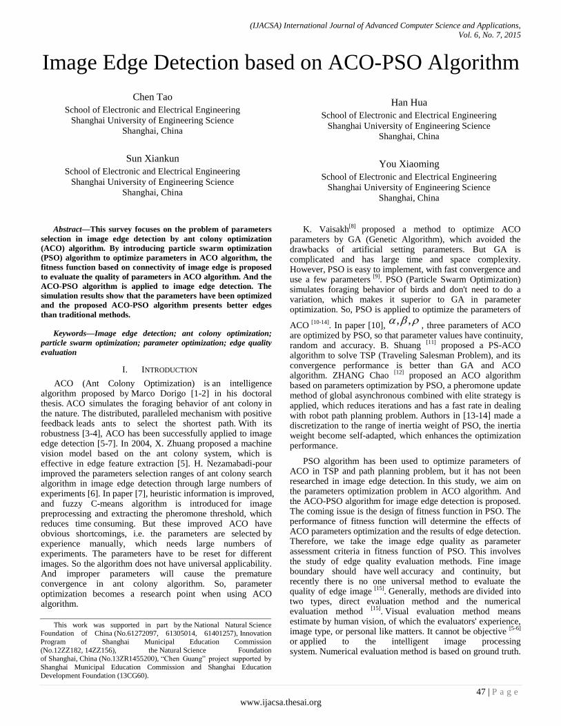
(IJACSA) International Journal of Advanced Computer Science and Applications,
Vol. 6, No. 7, 2015
47 | P a g e
www.ijacsa.thesai.org
Image Edge Detection based on ACO-PSO Algorithm
Chen Tao
School of Electronic and Electrical Engineering
Shanghai University of Engineering Science
Shanghai, China
Sun Xiankun
School of Electronic and Electrical Engineering
Shanghai University of Engineering Science
Shanghai, China
Han Hua
School of Electronic and Electrical Engineering
Shanghai University of Engineering Science
Shanghai, China
You Xiaoming
School of Electronic and Electrical Engineering
Shanghai University of Engineering Science
Shanghai, China
Abstract—This survey focuses on the problem of parameters
selection in image edge detection by ant colony optimization
(ACO) algorithm. By introducing particle swarm optimization
(PSO) algorithm to optimize parameters in ACO algorithm, the
fitness function based on connectivity of image edge is proposed
to evaluate the quality of parameters in ACO algorithm. And the
ACO-PSO algorithm is applied to image edge detection. The
simulation results show that the parameters have been optimized
and the proposed ACO-PSO algorithm presents better edges
than traditional methods.
Keywords—Image edge detection; ant colony optimization;
particle swarm optimization; parameter optimization; edge quality
evaluation
I. INTRODUCTION
ACO (Ant Colony Optimization) is an intelligence algorithm proposed by Marco Dorigo [1-2] in his doctoral thesis. ACO simulates the foraging behavior of ant colony in the nature. The distributed, paralleled mechanism with positive feedback leads ants to select the shortest path. With its robustness [3-4], ACO has been successfully applied to image edge detection [5-7]. In 2004, X. Zhuang proposed a machine vision model based on the ant colony system, which is effective in edge feature extraction [5]. H. Nezamabadi-pour improved the parameters selection ranges of ant colony search algorithm in image edge detection through large numbers of experiments [6]. In paper [7], heuristic information is improved, and fuzzy C-means algorithm is introduced for image preprocessing and extracting the pheromone threshold, which reduces time consuming. But these improved ACO have obvious shortcomings, i.e. the parameters are selected by experience manually, which needs large numbers of experiments. The parameters have to be reset for different images. So the algorithm does not have universal applicability. And improper parameters will cause the premature convergence in ant colony algorithm. So, parameter optimization becomes a research point when using ACO algorithm.
K. Vaisakh[8]
proposed a method to optimize ACO parameters by GA (Genetic Algorithm), which avoided the drawbacks of artificial setting parameters. But GA is complicated and has large time and space complexity. However, PSO is easy to implement, with fast convergence and use a few parameters
[9]. PSO (Particle Swarm Optimization)
simulates foraging behavior of birds and don't need to do a variation, which makes it superior to GA in parameter optimization. So, PSO is applied to optimize the parameters of
ACO [10-14]
. In paper [10], , ,
, three parameters of ACO are optimized by PSO, so that parameter values have continuity, random and accuracy. B. Shuang
[11] proposed a PS-ACO
algorithm to solve TSP (Traveling Salesman Problem), and its convergence performance is better than GA and ACO algorithm. ZHANG Chao
[12] proposed an ACO algorithm
based on parameters optimization by PSO, a pheromone update method of global asynchronous combined with elite strategy is applied, which reduces iterations and has a fast rate in dealing with robot path planning problem. Authors in [13-14] made a discretization to the range of inertia weight of PSO, the inertia weight become self-adapted, which enhances the optimization performance.
PSO algorithm has been used to optimize parameters of ACO in TSP and path planning problem, but it has not been researched in image edge detection. In this study, we aim on the parameters optimization problem in ACO algorithm. And the ACO-PSO algorithm for image edge detection is proposed. The coming issue is the design of fitness function in PSO. The performance of fitness function will determine the effects of ACO parameters optimization and the results of edge detection. Therefore, we take the image edge quality as parameter assessment criteria in fitness function of PSO. This involves the study of edge quality evaluation methods. Fine image boundary should have well accuracy and continuity, but recently there is no one universal method to evaluate the quality of edge image
[15]. Generally, methods are divided into
two types, direct evaluation method and the numerical evaluation method
[15]. Visual evaluation method means
estimate by human vision, of which the evaluators' experience, image type, or personal like matters. It cannot be objective
[5-6]
or applied to the intelligent image processing system. Numerical evaluation method is based on ground truth.
This work was supported in part by the National Natural Science Foundation of China (No.61272097, 61305014, 61401257), Innovation
Program of Shanghai Municipal Education Commission
(No.12ZZ182, 14ZZ156), the Natural Science Foundation of Shanghai, China (No.13ZR1455200), “Chen Guang” project supported by
Shanghai Municipal Education Commission and Shanghai Education
Development Foundation (13CG60).

(IJACSA) International Journal of Advanced Computer Science and Applications,
Vol. 6, No. 7, 2015
48 | P a g e
www.ijacsa.thesai.org
The standard boundary is drawn by hand or a certain edge detection algorithm. The differences between the detected images are taken as the evaluation index. But this method is complicated and inefficient. Boundary extracted by canny operator is used as the ground truth in paper [16]. Or benchmarks were generated by traditional detectors
[17].
In response to these shortcomings, this paper proposes a method without ground truth, evaluate the quality of image edge, and represent the quality by image edge quality evaluation function. By analyzing the connected component of pixels, the fitness function of PSO is designed to evaluate the quality of edge image and the parameters of ACO are self-adapted to find the balance between parameter selection and the effect of edge detection. Experiment shows that, the proposed method has the characteristics of real-time and high efficiency and is suitable for image edge detection of ACO-PSO algorithm.
The organization of the paper is as follows. Sect. II demonstrates the basic theory of ACO algorithm. Section III provides details about the proposed methodology of edge detection based on ACO-PSO. Experimental results are discussed in Sect. IV and V gives the conclusions of this paper.
II. EDGE DETECTION BASED ON ACO ALGORITHM
For an image of size M N , M N ants are distributed in the image randomly and search edge location according to the variance of grayscale and the pheromone distribution.
This study selects the maximum gray level gradient in eight neighbors of four directions as the pixel gradient:
( , 1) ( , 1)
( 1, ) ( 1, )
,
max ( 1, 1) ( 1, 1)
( 1, 1) ( 1, 1)
1= max
i j i j
i j i j
i j
i j i j
i j i j
I I
I II
I I I
I I
(1)
where ,i jI is the gray value of pixel
( , )i j; maxI
is the biggest gray value of image.
Ant colony select the location of the next randomly with
probability, the transition probability of ants in pixel( , )i j
is as follow:
, ,
, ,
( ) ( )
( ) ( )
( , )
, ;
0, .
i j i j
i s i s
s allowedk
k
i j
j allowedP
otherwise
(2)
where ,i j is the pheromone at pixel
( , )i j, ,i j
is
heuristic information. , ,= /i j i jI c , 1c . kallowed
is the allowed pixel for the next step.
After all the ants move from the k th step to the 1k th step, update the pheromone given by:
1
, , ,(1 ) ,k k k
i j i j i j (3)
, , ( ).k k
i j i j
ant
ant (4)
,
k
i j is the pheromone released by all the passing ants
thought ( , )i j
in k th step. Where
, ,
,
= / ,if ant pass through (i,j)( )
0, .
i j i jk
i j
I cant
otherwise
;
(5)
When ants go through all the steps, which meet the termination condition, finish one time of searching for image edge. Although there are many parameters of ACO, but three main parameters have larger impact on the algorithm
performance: the pheromone impact factor , the heuristic
function factor
, the pheromone volatilization coefficient
. The selection and optimization of parameters are crucial to the performance of ACO algorithm
[18-20]. In addition,
extracting the edge is the primary purpose of the algorithm, while keep the randomicity of search and convergence of algorithm.
To get the edge image, threshold segmentation is made to the pheromone matrix, removing the background information and guaranteeing the integrity of the edge information. The method of setting threshold manually is inefficient and not suitable for massive calculation through repeated experiments and observing results
[5]. Our method is by iteration, calculates
the threshold by statistics histogram of grayscale, which produces satisfactory image edges.
III. EDGE DETECTION BASED ON ACO-PSO ALGORITHM
A. Parameters update by PSO
To optimize these three parameters simultaneously, an
array, ,
is set for optimization. Randomly generate an
array as the position 1 2 3( , , )id i i ix x x xof a particle, and the
speed of the particle in the solution space is
1 2 3( , , )id i i iv v v v. Particles updated speed and location as
follows:
1
1 1 2 2( ) ( ),k k k k k k
id id id id gd idv v c p x c p x (6)
1 .k k k
id id idx x v (7)
Where is inertia weight, control the influence of
its inertia to the evolution of particle. 1c, 2c
are constants, show the weight of its own best position and the global optimal
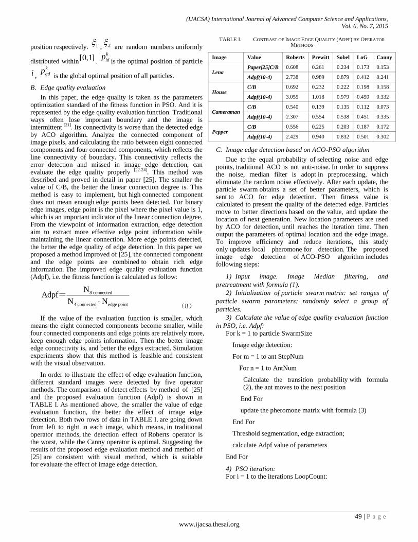
(IJACSA) International Journal of Advanced Computer Science and Applications,
Vol. 6, No. 7, 2015
49 | P a g e
www.ijacsa.thesai.org
position respectively. 1 , 2 are random numbers uniformly
distributed within[0,1]
.
k
idpis the optimal position of particle
i ,
k
gdp is the global optimal position of all particles.
B. Edge quality evaluation
In this paper, the edge quality is taken as the parameters optimization standard of the fitness function in PSO. And it is represented by the edge quality evaluation function. Traditional ways often lose important boundary and the image is intermittent
[21]. Its connectivity is worse than the detected edge
by ACO algorithm. Analyze the connected component of image pixels, and calculating the ratio between eight connected components and four connected components, which reflects the line connectivity of boundary. This connectivity reflects the error detection and missed in image edge detection, can evaluate the edge quality properly
[22-24]. This method was
described and proved in detail in paper [25]. The smaller the value of C/B, the better the linear connection degree is. This method is easy to implement, but high connected component does not mean enough edge points been detected. For binary edge images, edge point is the pixel where the pixel value is 1, which is an important indicator of the linear connection degree. From the viewpoint of information extraction, edge detection aim to extract more effective edge point information while maintaining the linear connection. More edge points detected, the better the edge quality of edge detection. In this paper we proposed a method improved of [25], the connected component and the edge points are combined to obtain rich edge information. The improved edge quality evaluation function (Adpf), i.e. the fitness function is calculated as follow:
8 connected
4 connected edge point
NAdpf
N N=
(8)
If the value of the evaluation function is smaller, which means the eight connected components become smaller, while four connected components and edge points are relatively more, keep enough edge points information. Then the better image edge connectivity is, and better the edges extracted. Simulation experiments show that this method is feasible and consistent with the visual observation.
In order to illustrate the effect of edge evaluation function, different standard images were detected by five operator methods. The comparison of detect effects by method of [25] and the proposed evaluation function (Adpf) is shown in TABLE I. As mentioned above, the smaller the value of edge evaluation function, the better the effect of image edge detection. Both two rows of data in TABLE I. are going down from left to right in each image, which means, in traditional operator methods, the detection effect of Roberts operator is the worst, while the Canny operator is optimal. Suggesting the results of the proposed edge evaluation method and method of [25] are consistent with visual method, which is suitable for evaluate the effect of image edge detection.
TABLE I. CONTRAST OF IMAGE EDGE QUALITY (ADPF) BY OPERATOR
METHODS
Image Value Roberts Prewitt Sobel LoG Canny
Lena Paper[25]C/B 0.608 0.261 0.234 0.173 0.153
Adpf(10-4) 2.738 0.989 0.879 0.412 0.241
House C/B 0.692 0.232 0.222 0.198 0.158
Adpf(10-4) 3.055 1.018 0.979 0.459 0.332
Cameraman C/B 0.540 0.139 0.135 0.112 0.073
Adpf(10-4) 2.307 0.554 0.538 0.451 0.335
Pepper C/B 0.556 0.225 0.203 0.187 0.172
Adpf(10-4) 2.429 0.940 0.832 0.501 0.302
C. Image edge detection based on ACO-PSO algorithm
Due to the equal probability of selecting noise and edge points, traditional ACO is not anti-noise. In order to suppress the noise, median filter is adopt in preprocessing, which eliminate the random noise effectively. After each update, the particle swarm obtains a set of better parameters, which is sent to ACO for edge detection. Then fitness value is calculated to present the quality of the detected edge. Particles move to better directions based on the value, and update the location of next generation. New location parameters are used by ACO for detection, until reaches the iteration time. Then output the parameters of optimal location and the edge image. To improve efficiency and reduce iterations, this study only updates local pheromone for detection. The proposed image edge detection of ACO-PSO algorithm includes following steps:
1) Input image. Image Median filtering, and
pretreatment with formula (1).
2) Initialization of particle swarm matrix: set ranges of
particle swarm parameters; randomly select a group of
particles.
3) Calculate the value of edge quality evaluation function
in PSO, i.e. Adpf: For k = 1 to particle SwarmSize
Image edge detection:
For m = 1 to ant StepNum
For n = 1 to AntNum
Calculate the transition probability with formula (2), the ant moves to the next position
End For
update the pheromone matrix with formula (3)
End For
Threshold segmentation, edge extraction;
calculate Adpf value of parameters
End For
4) PSO iteration: For i = 1 to the iterations LoopCount:

(IJACSA) International Journal of Advanced Computer Science and Applications,
Vol. 6, No. 7, 2015
50 | P a g e
www.ijacsa.thesai.org
update the particle velocity and position with formula (6) (7) ;
calculate edge quality of new particle group (refer to step 3).
End For
5) Output the optimal parameters and edge image. Massive experiment results show that, the number of ants is
proportional to the square root of the number of image pixels, without considering the complex degree of image. The complexity of ACO-PSO algorithm for edge detection rely on the particle swarm iterations, swarm size, step number of ants, ants quantity, the image size and its complexity of edge. The larger the image and more complex the edges, the more number of ants used searching for edge points, and higher complexity of algorithm. But there is still no unified standard for edge complexity or image complexity. As for different images, the number of each grayscale, the spatial distribution of pixels and target are extreme variation and hard to describe [26]
.
IV. SIMULATION AND ANALYSIS
In this study, runtime environment: Windows 7 32-bit OS, MATLAB 8.1, Intel Core i5 2.30 GHz CPU, 2.00 GB RAM. Lena standard drawing was chosen as research object, the image size is 256*256. The ACO-PSO algorithm parameter
settings are as follows: ranges of , ,
are
[0.12.5],[4.58.5],[01]; others: ant colony step is 300,
memory length is 40; particle swarm size is 3, the coefficients
1 2 1.2c c , coefficient of inertia weights is reduced from 0.5 to 0.3 by linear gradient.
A. Edge quality evaluation function
Lena、House、Cameraman、Peppers were detected by
ACO-PSO algorithm with method of [25] and the proposed evaluation method (Adpf). The simulation results are shown in Fig.1. It can be seen that the improved evaluation method detected more edge points, and obtain rich edge information. For example, the showcase behind Lena, the shadow under the eaves of House, Cameraman's leg and ground, the outline of three peppers in the middle of Peppers in Fig.1 (c). While all these details are get lost in Fig.1 (b). So, the improved edge quality evaluation function is superior to the method of [25], which obtains high quality of image edge.
(a) (b)
(c)

(IJACSA) International Journal of Advanced Computer Science and Applications,
Vol. 6, No. 7, 2015
51 | P a g e
www.ijacsa.thesai.org
Fig. 1. Effects comparison of evaluation functions. (a) the original image;
(b) image detection before improved; (c) image detection after improved
B. Algorithm performance
Preset the PSO iterations to 20, run the ACO-PSO algorithm 4 times, the evaluation function values of different images are shown in Fig.2. The vertical axis represents the minimum Adpf value of the edge image during iteration. 15 iterations later, the global optimal solution was obtained, the algorithm was convergent, and the quality of edge image came to a steady level. For example, the Adpf values of Lena edges are below 0.130, which is lower than 0.241, the Adpf value of Canny operator (in TABLE I). Likewise, the Adpf values of
House、Cameraman and Peppers edges have reached a stable
detection results, and they are lower than the Adpf values of Canny operator. It indicates that the edge quality detected based on ACO-PSO algorithm is superior to the operator detectors. In order to save time, the iteration was set at 15.
(a)
(b)
(c)
(d)
Fig. 2. Statistics value of the best evaluation function in 20 iterations. (a)
Lena; (b) House; (c) Cameraman; (d) Peppers
In order to verify the noise sensitivity of the algorithm, the salt and pepper noise, whose density is 0.1, was add into image the detection, results are shown in Fig.3. This algorithm can effectively eliminate noise and extract true edges. Traditional methods have their problems. For example, Sobel operator detection causes discontinuity while Canny operator detection causes severe false detection. And both of them cannot restrain noises in image or obtain complete true edges. So this algorithm has strong robustness.
0 5 10 15 200.11
0.12
0.13
0.14
0.15
0.16
Iterations
min
(Adpf)
0 5 10 15 200.1
0.15
0.2
0.25
Iterations
min
(Adpf)
0 5 10 15 200.22
0.24
0.26
0.28
0.3
0.32
0.34
0.36
Iterations
min
(Adp
f)
0 5 10 15 200.18
0.2
0.22
0.24
0.26
0.28
0.3
Iterations
min
(Adp
f)
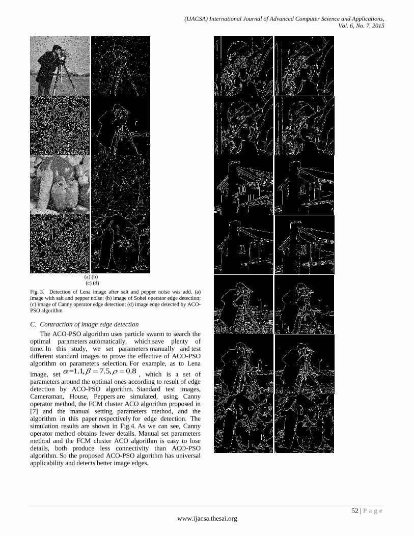
(IJACSA) International Journal of Advanced Computer Science and Applications,
Vol. 6, No. 7, 2015
52 | P a g e
www.ijacsa.thesai.org
(a) (b) (c) (d)
Fig. 3. Detection of Lena image after salt and pepper noise was add. (a)
image with salt and pepper noise; (b) image of Sobel operator edge detection;
(c) image of Canny operator edge detection; (d) image edge detected by ACO-PSO algorithm
C. Contraction of image edge detection
The ACO-PSO algorithm uses particle swarm to search the optimal parameters automatically, which save plenty of time. In this study, we set parameters manually and test different standard images to prove the effective of ACO-PSO algorithm on parameters selection. For example, as to Lena
image, set =1.1, 7.5, 0.8 , which is a set of parameters around the optimal ones according to result of edge detection by ACO-PSO algorithm. Standard test images, Cameraman, House, Peppers are simulated, using Canny operator method, the FCM cluster ACO algorithm proposed in [7] and the manual setting parameters method, and the algorithm in this paper respectively for edge detection. The simulation results are shown in Fig.4. As we can see, Canny operator method obtains fewer details. Manual set parameters method and the FCM cluster ACO algorithm is easy to lose details, both produce less connectivity than ACO-PSO algorithm. So the proposed ACO-PSO algorithm has universal applicability and detects better image edges.
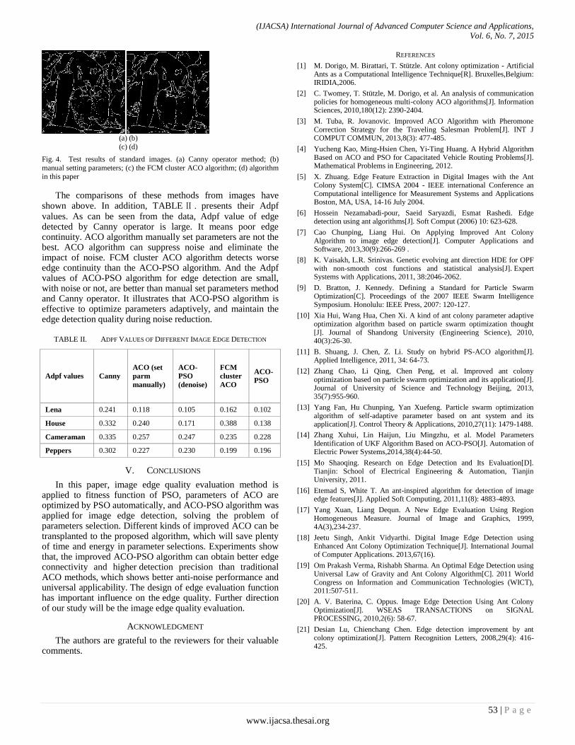
(IJACSA) International Journal of Advanced Computer Science and Applications,
Vol. 6, No. 7, 2015
53 | P a g e
www.ijacsa.thesai.org
(a) (b)
(c) (d)
Fig. 4. Test results of standard images. (a) Canny operator method; (b)
manual setting parameters; (c) the FCM cluster ACO algorithm; (d) algorithm in this paper
The comparisons of these methods from images have shown above. In addition, TABLEⅡ . presents their Adpf values. As can be seen from the data, Adpf value of edge detected by Canny operator is large. It means poor edge continuity. ACO algorithm manually set parameters are not the best. ACO algorithm can suppress noise and eliminate the impact of noise. FCM cluster ACO algorithm detects worse edge continuity than the ACO-PSO algorithm. And the Adpf values of ACO-PSO algorithm for edge detection are small, with noise or not, are better than manual set parameters method and Canny operator. It illustrates that ACO-PSO algorithm is effective to optimize parameters adaptively, and maintain the edge detection quality during noise reduction.
TABLE II. ADPF VALUES OF DIFFERENT IMAGE EDGE DETECTION
Adpf values Canny
ACO (set
parm
manually)
ACO-
PSO
(denoise)
FCM
cluster
ACO
ACO-
PSO
Lena 0.241 0.118 0.105 0.162 0.102
House 0.332 0.240 0.171 0.388 0.138
Cameraman 0.335 0.257 0.247 0.235 0.228
Peppers 0.302 0.227 0.230 0.199 0.196
V. CONCLUSIONS
In this paper, image edge quality evaluation method is applied to fitness function of PSO, parameters of ACO are optimized by PSO automatically, and ACO-PSO algorithm was applied for image edge detection, solving the problem of parameters selection. Different kinds of improved ACO can be transplanted to the proposed algorithm, which will save plenty of time and energy in parameter selections. Experiments show that, the improved ACO-PSO algorithm can obtain better edge connectivity and higher detection precision than traditional ACO methods, which shows better anti-noise performance and universal applicability. The design of edge evaluation function has important influence on the edge quality. Further direction of our study will be the image edge quality evaluation.
ACKNOWLEDGMENT
The authors are grateful to the reviewers for their valuable comments.
REFERENCES
[1] M. Dorigo, M. Birattari, T. Stützle. Ant colony optimization - Artificial Ants as a Computational Intelligence Technique[R]. Bruxelles,Belgium: IRIDIA,2006.
[2] C. Twomey, T. Stützle, M. Dorigo, et al. An analysis of communication policies for homogeneous multi-colony ACO algorithms[J]. Information Sciences, 2010,180(12): 2390-2404.
[3] M. Tuba, R. Jovanovic. Improved ACO Algorithm with Pheromone Correction Strategy for the Traveling Salesman Problem[J]. INT J COMPUT COMMUN, 2013,8(3): 477-485.
[4] Yucheng Kao, Ming-Hsien Chen, Yi-Ting Huang. A Hybrid Algorithm Based on ACO and PSO for Capacitated Vehicle Routing Problems[J]. Mathematical Problems in Engineering, 2012.
[5] X. Zhuang. Edge Feature Extraction in Digital Images with the Ant Colony System[C]. CIMSA 2004 - IEEE international Conference an Computational intelligence for Measurement Systems and Applications Boston, MA, USA, 14-16 July 2004.
[6] Hossein Nezamabadi-pour, Saeid Saryazdi, Esmat Rashedi. Edge detection using ant algorithms[J]. Soft Comput (2006) 10: 623-628.
[7] Cao Chunping, Liang Hui. On Applying Improved Ant Colony Algorithm to image edge detection[J]. Computer Applications and Software, 2013,30(9):266-269 .
[8] K. Vaisakh, L.R. Srinivas. Genetic evolving ant direction HDE for OPF with non-smooth cost functions and statistical analysis[J]. Expert Systems with Applications, 2011, 38:2046-2062.
[9] D. Bratton, J. Kennedy. Defining a Standard for Particle Swarm Optimization[C]. Proceedings of the 2007 IEEE Swarm Intelligence Symposium. Honolulu: IEEE Press, 2007: 120-127.
[10] Xia Hui, Wang Hua, Chen Xi. A kind of ant colony parameter adaptive optimization algorithm based on particle swarm optimization thought [J]. Journal of Shandong University (Engineering Science), 2010, 40(3):26-30.
[11] B. Shuang, J. Chen, Z. Li. Study on hybrid PS-ACO algorithm[J]. Applied Intelligence, 2011, 34: 64-73.
[12] Zhang Chao, Li Qing, Chen Peng, et al. Improved ant colony optimization based on particle swarm optimization and its application[J]. Journal of University of Science and Technology Beijing, 2013, 35(7):955-960.
[13] Yang Fan, Hu Chunping, Yan Xuefeng. Particle swarm optimization algorithm of self-adaptive parameter based on ant system and its application[J]. Control Theory & Applications, 2010,27(11): 1479-1488.
[14] Zhang Xuhui, Lin Haijun, Liu Mingzhu, et al. Model Parameters Identification of UKF Algorithm Based on ACO-PSO[J]. Automation of Electric Power Systems,2014,38(4):44-50.
[15] Mo Shaoqing. Research on Edge Detection and Its Evaluation[D]. Tianjin: School of Electrical Engineering & Automation, Tianjin University, 2011.
[16] Etemad S, White T. An ant-inspired algorithm for detection of image edge features[J]. Applied Soft Computing, 2011,11(8): 4883-4893.
[17] Yang Xuan, Liang Dequn. A New Edge Evaluation Using Region Homogeneous Measure. Journal of Image and Graphics, 1999, 4A(3),234-237.
[18] Jeetu Singh, Ankit Vidyarthi. Digital Image Edge Detection using Enhanced Ant Colony Optimization Technique[J]. International Journal of Computer Applications. 2013,67(16).
[19] Om Prakash Verma, Rishabh Sharma. An Optimal Edge Detection using Universal Law of Gravity and Ant Colony Algorithm[C]. 2011 World Congress on Information and Communication Technologies (WICT), 2011:507-511.
[20] A. V. Baterina, C. Oppus. Image Edge Detection Using Ant Colony Optimization[J]. WSEAS TRANSACTIONS on SIGNAL PROCESSING, 2010,2(6): 58-67.
[21] Desian Lu, Chienchang Chen. Edge detection improvement by ant colony optimization[J]. Pattern Recognition Letters, 2008,29(4): 416-425.

(IJACSA) International Journal of Advanced Computer Science and Applications,
Vol. 6, No. 7, 2015
54 | P a g e
www.ijacsa.thesai.org
[22] Kevin W B, Chang K, Flynn P. A Survey of Approaches and Challengings in 3D and Multi-modal 3D+2D Face Recognition[J]. Computer Vision and Image Understanding, 2006, 101(6): 1-15.
[23] Zeng Shuyan, Zhang Guangjun, Li Xiuzhi. Image target distinguish based on Gabor filters[J]. Journal of Beijing University of Aeronautics and Astronautics, 2006,32(8): 954-957.
[24] Chen Yanyan, Wang Yuanqing. Quantitative Comparison of Common Edge Detection Algorithms[J]. Computer Engineering, 2008,34(17):202-204.
[25] Lin Hui, Shu Ning, Zhao Chang-sheng. A new edge evaluation method based on connection components[J]. Remote sensing for land & resources, 2003, (3):37-40.
[26] Gao Zhenyu, Yang Xiaomei, Gong Jianming, et al. Research on Image Complexity Description Methods[J]. Journal of Image and Graphics, 2010,15(1): 129-135.
(IJACSA) International Journal of Advanced Computer Science and Applications,
Vol. 6, No. 7, 2015
55 | P a g e
www.ijacsa.thesai.org
Improvement on Classification Models of Multiple
Classes through Effectual Processes
Tarik A. Rashid
Software Engineering, College of Engineering,
Salahadin University, Halwer, Kurdistan
Abstract—Classify cases in one of two classes referred to as a
binary classification. However, some classification algorithms
will allow, of course the use of more than two classes. This
research work focuses on improving the results of classification
models of multiple classes via some effective techniques. A case
study of students’ achievement at Salahadin University is used in
this research work. The collected data are pre-processed,
cleaned, filtered, normalised, the final data was balanced and
randomised, then a combining technique of Naïve Base Classifier
and Best First Search algorithms are used to ultimately reduce
the number of features in data sets. Finally, a multi-classification
task is conducted through some effective classifiers such as K-
Nearest Neighbor, Radial Basis Function, and Artificial Neural
Network to forecast the students’ performance.
Keywords—Non-Balanced Data; Feature Selection; Multiple
Classification; Machine Learning Techniques; Student
Performance Forecasting
I. INTRODUCTION
Classification is a data mining technique that maps data into groups. It is a supervised learning method which requires labeled training data to generate rules for classifying test data into predetermined classes [1]. It is a two-phase process. The first phase is the learning phase, where the training data is analysed and classification rules are generated. The next phase is the classification, where test data is classified into classes according to the generated rules. Since classification algorithms require that classes be defined based on data attribute values. Generally speaking, the classification task can be divided into several types; these are namely: Binary classification, Multi-class classification, Multi-label classification and Multi-output-multiclass classification and multi-task classification. The binary classification algorithms can be converted into multinomial classifiers by several strategies. The four diffident types of classification are described as follows [2-5]:-
1) Binary classification type: it means a classification
task that can have no more than two classes.
2) Multiple classes’ classification type: it is a
classification task with more than two classes; in the field of
classification, multi-class or multi-nominal classification is
the problem of classifying instances into one of more than two
classes. For instance, classifying a group of items of tools
which may be electrical or computer or construction. Multiple
classes’ classification makes the assumption that each sample
is allocated to one and only one label. Multi-class
classification should not be mixed up with multi-label
classification, where multiple labels are to be predicted for
each instance.
3) Multi-label classification: this type is about allocating
to each sample a set of target labels. This is seen as the
forecasting attributes of a data item that are not happening at
the same time, as themes that are relevant to a document. For
example, an ordinary manuscript can fall into a belief,
legislation, economics and learning all at once or fall into
none of them at all.
4) Multi-Output-multi-class classification and multi-task
certification: it means that a single appraiser has to work out
some common classification tasks. This is a generalisation of
the multi-label classification task, in which, the set of the
classification problem is limited to binary classification and of
the multi-class classification task. This means that each
classifier handles multi-output multi-class or multi-task
classification task supports the multi-label classification task
as a distinctive example. Multi-task classification sounds like
the multi-output classification task with different model
formulations. This work focuses on multiple classes’ classification type
and it takes students achievement model for classification as a case study, this is because, in recent time, a new phenomenon of increasing demand by students for pursuing further studies is emerged in universities in Kurdistan. This is due to the rapid economic growth and increasing technologies that have a greater impact on our lives in general and in the educational system, in particular. Thus, examining the past performance of the admitted students would provide a stronger perspective of the likely educational achievements of scholars in the future. This may very well be achieved through the concepts of data mining and machine learning [6]. Naturally, any quality of education at the university is found in its analysis work and educational activities, so it is, therefore, appropriate to mention that the amount of accepted students affect the level of the classes may have [6, 7].
It is very useful for any learning system to have the right student performance of the system itself. The right student performance of the system makes the body staff ready to recognise between the accepted and not accepted candidate students for an educational course or subject. It is hence, important to make a correct prediction or to conduct the right assortments of student achievement, in order to help improve the level of involvement of academic staff for students learning. Also facilitating more help to support students and

(IJACSA) International Journal of Advanced Computer Science and Applications,
Vol. 6, No. 7, 2015
56 | P a g e
www.ijacsa.thesai.org
provide guidance resources or may be the teachers are able to determine what the most satisfactory teaching jobs will be for each bunch of students, plus teachers deliver their assistance through made-to-order substantive materials to students. The power of predicting the learning performance of students is very significant for academic institutions. It is worth noticing that the goal can also be achieved by the use of machine learning and data mining techniques. These techniques have a great ability to process enormous data to discover and extract hidden patterns and important relationships that are very useful for decision making [6, 7].
This paper focuses on the use of a combination technique of Naïve Base and Best First Search algorithms as a proposed technique for feature reduction to enhance the performance of the classification techniques, which are used for predicting students’ achievement.
The paper is structured as follows: in Section 2, related works are explained. Then, the description of the overall forecasting system is demonstrated. Next, in Section 4, the process of data collection is described. Then after, data pre-processing, and data preparation are defined. In Section 6, the feature selection techniques are explained. In Section 7, the multi-class classification techniques are designated and described. Section 8, describes different experimental results, and finally, the main points in this paper work are outlined.
II. RELATED WORKS
Data mining is the process of discerning interesting knowledge via predicting, classifying, associating, or changing important structures and abnormalities of large amounts of data stored in databases, data warehouses and other information repositories [1, 8]. Data mining has been widely used in recent years with the availability of large amounts of data in electronic form, and there is a need to turn the stored data into useful information and knowledge for large applications. It is worth mentioning that data mining techniques that are supported by machine learning and soft computing techniques are the creation of a new research area called educational data mining to university levels, authors in [9-11] stated that new and useful knowledge about students can be detected by the application of data mining in education. These applications are found in areas such as artificial intelligence, machine learning, market analysis, statistics, database systems, business, management and decision support [1, 9].
Authors in [12] suggested that techniques for exploring the types of data from educational institutions can be developed through educational data mining. There are several practices of
data mining, examples of these statistics, visualization, clustering, and revealing outliers, included in this, classification, which is one of the most studied techniques. Classification can possibly acquire a method of control where information is separated into completely different categories. Classification maps information into pre-arranged groups of types. The main objective of a classification model is to consider the target class for each sample in the dataset. There are numerous techniques for classification of any data, which are namely; support vector machine (SVM), artificial neural network (ANN) and Bayesian classifier [12]. Based on these techniques, the classification task can be performed by describing and distinguishing data categories. Basically, these classification techniques are often used in educational settings in several research works as indicated in [13-17]. In addition, authors in [18] have dealt with another aspect which is an unbalanced knowledge or so-called having a different sampling number for each class. This can be a difficult undertaking. The non-balanced data will cause limitations when training classification algorithms, eventually, it will have a negative influence on the performance of the system.
This research work suggests two effectual processes so that to overcome the problem of non-balanced data, these two processes are resampling and randomised, in addition to these, the research work proposes a mutual technique for feature reduction so that to improve the performance of the classification models of multiple classes such as ANNs, K-Nearest Neighbor, and Radial Basis Function.
III. THE OVERALL FORECASTING SYSTEM
The suggested overall forecasting system for the students’ performance consists of three mains parts (See Figure 1), and these are as follows:
1) Data Collection
2) Data Preprocessing & Preparation
a) Cleaning, normalising, scaling
b) Non-Balanced Data
c) Re-Sampling
d) Randomised Data
3) Feature Selection
a) Classification
b) Selecting the best group
4) Multi-Classification
a) Classification model
b) Selecting the best model
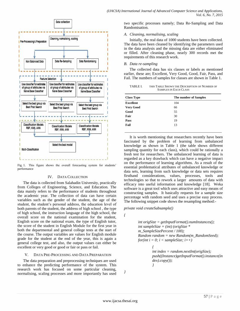
(IJACSA) International Journal of Advanced Computer Science and Applications,
Vol. 6, No. 7, 2015
57 | P a g e
www.ijacsa.thesai.org
Fig. 1. This figure shows the overall forecasting system for students’ performance
IV. DATA COLLECTION
The data is collected from Salahadin University, practically from Colleges of Engineering, Science, and Education. The data mainly refers to the performance of students throughout the academic year. The collection of data can have certain variables such as the gender of the student, the age of the student, the student’s personal address, the education level of both parents of the student, the address of high school , the type of high school, the instruction language of the high school, the overall score on the national examination for the student, English score on the national exam, the type of English tutor, the score of the student in English Module for the first year in both the departmental and general college tests at the start of the course. The output variables are values for English module grade for the student at the end of the year, this is again a general college test, and also, the output values can either be excellent or very good or good or fair or pass or fail.
V. DATA PRE-PROCESSING AND DATA PREPARATION
The data preparation and preprocessing techniques are used to enhance the predicting performance of the system. This research work has focused on some particular cleaning, normalising, scaling processes and more importantly has used
two specific processes namely; Data Re-Sampling and Data Randomisation.
A. Cleaning, normalising, scaling
Initially, the real data of 1000 students have been collected. The data have been cleaned by identifying the parameters used in the data analysis and the missing data are either eliminated or filled. After cleaning phase, nearly 300 records met the requirements of this research work.
B. Data re-sampling
The collected data has six classes or labels as mentioned earlier, these are; Excellent, Very Good, Good, Fair, Pass, and Fail. The numbers of samples for classes are shown in Table 1.
TABLE I. THIS TABLE SHOWS THE DESCRIPTION OF NUMBER OF
SAMPLES IN EACH CLASS
Class Type The number of Samples
Excellent 104
Very Good 66
Good 55
Fair 30
Pass 19
Fail 13
It is worth mentioning that researchers recently have been fascinated by the problem of learning from unbalanced knowledge as shown in Table 1 (the table shows different sampling quantity for each class), which could be rationally a fresh test for researchers. The unbalanced learning of data is regarded as a key drawback which can have a negative impact on the performance of learning algorithms. As a result of the essential problematical attributes of unbalanced knowledge or data sets, learning from such knowledge or data sets requires firsthand considerations, values, processes, tools and technologies so that to rework a larger amounts of data with efficacy into useful information and knowledge [18]. Weka software is a great tool which uses attractive and easy means of constructing samples. It basically requests for a sample size percentage with random seed and uses a precise easy process. The following snippet code shows the resampling method:-
private void createSubsample()
{
int origSize = getInputFormat().numInstances();
int sampleSize = (int) (origSize *
m_SampleSizePercent / 100);
Random random = new Random(m_RandomSeed);
for(int i = 0; i < sampleSize; i++)
{
int index = random.nextInt(origSize);
push((Instance)getInputFormat().instance(in
dex).copy());
}
}
(IJACSA) International Journal of Advanced Computer Science and Applications,
Vol. 6, No. 7, 2015
58 | P a g e
www.ijacsa.thesai.org
In short, this process is a kind of choosing an integer number randomly from the original size and pushing them in a new instance. Obviously, the instance is a new set of samples. Table 2, shows data set after the resampling process is performed. It can be seen from the table that the instances in the data are reweighted in a way that all classes have the exact and same total value of weight, in our case, each class is become 47. This means that the sum of weights through all instances will be preserved.
TABLE II. THIS TABLE SHOWS THE RESAMPLING PROCESS
Class Type The number of Samples Weights
Excellent 47 47
Very Good 47 47
Good 47 47
Fair 47 47
Pass 47 47
Fail 47 47
C. Data Randomising
Another important process is called Randomising, which is also a very simple method that can generate a random number within the size of the samples used. This method is basically switching the instances of the position of random number with its next random position as described in following snippet:-
public void randomize(Random random)
{
for (int j = numInstances() - 1; j > 0; j--)
swap(j, random.nextInt(j+1));
}
To conclude, the whole sample set is provided and fed into a format of instances so that to create a fresh sample, this can be expressed in the following snippet code:-
getInputFormat().randomize(m_Random);
for (int i = 0; i < getInputFormat().numInstances(); i++)
{
push(getInputFormat().instance(i));
}
The details of these and other methods in Weka software can be found as free sources and available at the following link: http://www.cs.waikato.ac.nz/ml/weka/downloading.html.
VI. FEATURE SELECTION
In any raw data set, there can be several redundant or not significant features or even bad features that could have a negative impact on a model in terms of performance. This is because; these bad features cannot supply useful evidence to a constructed model. Thus, the feature selection stage comes in here to segregate important variables, in other words, it is a process of picking subgroups of significant attributes.
Here, in this paper, an arrangement of two techniques is used to select the most important features. These two techniques are explained as follows:-
A. Naïve Bayes Classifier (NBC)
Naive Bayes Classifier (NBC), is regarded as one of the key classifiers in machine learning field. Naïve Bayes are considered as mathematical models developed by Thomas Naïve. These are independence Bayes and are a family of simple probabilistic classifiers centered on applying Bayes’ theorem to properties discretely. Naïve Bayes is the simplest form of Bayesian network, where all features are temporary and directly connected to classes. This can be called conditional freedom. Naive Bayes is taken into account as a good classifier supported via a Posteriori rule.
If it is assumed that there is a problem with K classes such as {C1,C2,C3……, CK} with prior probabilities ( , then the label c is allocated to unknown instance described as x=(x1,x2,x3,….xN). See Equation (1):
( ( This suggests that selecting the category with the most
posterior chance given the ascertained information. This posterior probability is expressed via Bayes theorem in Equation (2):-
( ( Then c can be expressed in Equation (3):-
( ( ( ( ( (
Since the denominator is identical for each class, this can be eliminated from the evaluation. Next, the class conditional probabilities of the properties given the available classes are calculated. The process is very difficult considering the dependencies between properties. The technique of naïve Bayes is supposing class conditional independence i.e. is independent assuming the class. Thus, the numerator can be simplified as expressed in Equation (4):-
( ( ( ( Then after, picking the category c, this will make the most
of this value over all the categories c=1, 2, 3….K, evidently this method is surely modifiable to the condition of getting more than 2 categories and was demonstrated to work well despite the essential simplifying presumptuous of restricted independence [19]. In this work, the NBC is used to allocate and divide features of the data sets into subgroups. This is done based on the similarities of features within each group. So, the idea is very simple, instead of having one set of data with all features, NBC will create several subgroups of similar features from the entire date set.
B. Best First Search
Best First Search (BFS) is an approach that searches the attribute subsets space via a method of Greedy Hill Climbing improved with a backtracking aptitude. The controls of the amount of backtracking can be achieved via setting the quantity of consecutive non-improving nodes.

(IJACSA) International Journal of Advanced Computer Science and Applications,
Vol. 6, No. 7, 2015
59 | P a g e
www.ijacsa.thesai.org
This approach might start to search in both directions; forwardly or backwardly. It can start with the empty set of attributes and search forwardly, or it can start with the full set of attributes and search backwardly. Equally it can start at any point and search in each direction by considering all doable specific attribute additions and deletions at a given point. The Best First Search algorithm can overcome the drawbacks of Hill Climbing via victimisation priority queue. The approach of the Best First Search algorithm can be considered as an amalgamation of both Depth search (DFS) and Breath First Search (BFS) algorithms. The depth First Search takes a single path, whereas, the Breadth First Search does not end up with loops nor does get onto a dead end path. Details of the algorithm are as follows [20]:-
Open=[Start]; Closed=[];
While Open not equal []do
{ Remove the left most state from open, call it X;
If X=goal then return path from start to X;
Else{
Generate children of X;
For each child of X do
Case
the Child is not on Open or Closed;
{
assign the child a heuristic value;
add the child to Open
}
{
the child already on Open
if the child was reached by shortest path
then give the state on Open the shortest path
}
the child already on Closed.
{
remove the state from Closed
add the child to Open;
}; }; put X on Closed;
re-order states on open by heuristic (best leftmost)
}; return FAIL
BFS algorithm is used to act as an optimiser to search and find the best sub group of similar feature among all subgroups which are mentioned earlier as they were created by Naïve Base Classifier. Finally the classification can only be done on the best selected sub group of feature.
VII. CLASSIFICATION OF MULTIPLE CLASSES ALGORITHMS
Several classification techniques such as Radial Basic Functions, K-Nearest Neighbors and Artificial Neural
Networks are considered, details of each classifier is provided in sub sections below:-
A. Radial Basis Function
Radial basis functions (RBF) are considered to be a different type of neural network; the architecture of Radial Basis Function is constant with only three layers namely; input, hidden and output layers. First, the input layer is clearly providing the network with data samples. Second, the hidden layer processes these data samples with a nonlinear activation function so that to make them linearly separable. Finally, the output neurons with a liner activation function will do a linear separation. It was agreed that the architecture of Radial Basis Function networks is similar to the feed forward neural network; this is because both networks can have three layers. A Radial Basis Function can be implemented via engaging an Artificial Neural Network (ANN) approach. The objectivity between RBF and ANN is in the restricted structure type of networks. In fact, both networks perform their duties in their own method quite completely different. Radial Basis Function can have solely 3 layers, whereas, the feed-forward networks might have more than 3 layers. The input samples can be
formulated as a vector of real numbers such as . The output of the network is then a scalar function of the input vector . In this case, the output of the network can be computed via Equation (5).
( ∑
(| |) (
Where ( , is the network output, in such a case, it is a scalar function of the input vector, N, is the number of the neurons in the hidden layer, is the center vector of neuron i, , is the weight of neuron i in the linear output neuron [21].
B. K-Nearest Neighbor
K-Nearest Neighbors algorithm (KNN) is widely used in machine learning and soft computing fields for the purpose of classification and regression tasks and it is defined as a technique of non-parametric. The input consists of the K nearest training sample in the feature space. In KNN technique, the type of task whether it is classification or regression can only determine the output. In the regression task, KNN considers the output is the feature of an unknown point or object, in other words, the value is computed via averaging the values of its K nearest neighbors, whereas, KNN in classification, treats the output as a class membership. This means that the unknown point is classified via the rule of a majority vote of its neighbors, so the unknown point can be allocated to the class that is best common among its K nearest neighbors. If in case the value of K is set to one, then the unknown point is merely allocated to the class of that distinct nearest neighbor [22, 23].
C. Artificial Neural Network
Artificial Neural Network (ANN) has been determined to act as a third classifier for this research work; which is a feed- forward neural network that is trained with back propagation. The network has the flexibility for constructing a map between the inputs and outputs. The network is extremely versatile and

(IJACSA) International Journal of Advanced Computer Science and Applications,
Vol. 6, No. 7, 2015
60 | P a g e
www.ijacsa.thesai.org
it is also a non-linear simulation that includes a range of neurons established into many layers. The amount of hidden neurons is extremely syndicate since the hidden neurons are thought to be the processing neurons within the network, and having a low range of hidden neurons will increase the speed of the training session whereas an oversized range of hidden layers will prolong the training session. This parameter can be selected via two techniques, these are namely; Growing approaches via that the range of hidden neurons is chosen as a low number then the amount gets augmented bit by bit. The opposite technique is named pruning via that the range of hidden neurons is chosen as an oversized number so it gets faded via eliminating some insignificant parts [24, 25]. It is also suggested to pick the initial range of hidden in accordance with adding the inputs to outputs and dividing the total by 2, then after, either the Growing or Pruning approach is employed to hit the simplest choice of hidden neurons so that to realise promising results for the network.
VIII. EXPERIMENTAL RESULTS
Numerous practical investigational tests and several data sets are used in this research work so that to optimise the forecasting results. Based on the Figure 1, the data set is divided into sub sets to reflect the performance of each process. Six different sets of data are prepared to conduct different experiments; these data sets are as follows:-
1) Non-balanced data without feature selection (NBD)
2) Non-balanced data with feature selection (NDFS)
3) Balanced data without feature selection (BD)
4) Balanced data with feature selection (BDFS)
5) Balanced data and randomised without feature
selection (BRD)
6) Balanced data and randomised with feature selection
(BRDFS) Note that the result of feature selection in Section 4 was
only 9 features, which are selected out of 20 features, these features are:-
1) The age of the student
2) Education of mother for the student
3) The address of the high school
4) The instruction language of the high school
5) Overall score for the national exam
6) Department
7) English Tutor-Internal
8) English Tutor-Native
9) English Module Score for year one (General University
Test)- at the start of course The above data sets are used to train Radial Basis Function,
K-Nearest Neighbors, and Artificial Neural Networks. Table 3, shows the forecasting results of RBF. Models with feature selection produced better results than others in terms of correctly classified instances (CCI), incorrectly classified intendances (ICI) and Relative Square Error (RSE).
TABLE III. SHOWS THE PERFORMANCE RESULTS OF RBF CLASSIFIER
Table 4; show the forecasting results of KNN models. The models demonstrate better accuracy compared to RBF models. Besides, KNN models with feature selection produced better results than others.
TABLE IV. SHOWS THE PERFORMANCE RESULTS OF KNN CLASSIFIER
Model-
Data Set/
Performance
KNN-
ND
KNN-
NDFS
KNN-
BD
KNN-
BDFS
KNN-
BRD
KNN-
BRDFS
CCI % 38.5965 49.1228 70.9219 78.531 81.2202 85.3306
ICI % 61.4035 50.8772 29.0781 21.469 18.7798 14.6694
RSE % 125.1661 67.6013 82.0456 70.7932 65.3407 58.0631
Table 5; show the forecasting results of ANN models which are the most accurate among other models.
TABLE V. SHOWS THE PERFORMANCE RESULTS OF ANN CLASSIFIER
Model-
Data Set/
Performance
ANN-
ND
ANN-
NDFS
ANN-
BD
ANN-
BDFS
ANN-
BRD
ANN-
BRDFS
CCI % 43.8596 66.8588 70.0123 73.2714 80.3798 91.0714
ICI % 56.1404 33.1412 29.9877 26.7286 19.6202 8.9286
RSE % 114.707 80.9631 84.8795 75.4903 57.1275 43.3149
The above results of Tables 3, 4 and 5, show that the three classifiers RBF, KNN, ANN used with a mutual technique (NBC and BFS) for feature selection produce more accurate results than others. This is clearly seen in columns 3, 5, 7 in the above tables. Table 6, shows the difference that each process makes, the columns show the differences in correctly instances between every two models with different data sets, for example, the first column, in the first row, is the difference in correctly instances between RBF with non-balanced data and RBF with non-balanced data with selected features, and the difference is 15.7895. This means that using RBF with non-balanced with selected feature via our mutual features selection technique (NBC and BFS) will help increase the accuracy rate of correctly instances by 15.7895 percent. The same thing is applied to the rest of the table.
Model-
Data Set/
Performance
RBF-
NBD
RBF-
NDFS
RBF-
BD
RBF-
BDFS
RBF-
BRD
RBF-
BRDFS
CCI % 40.3509 56.1404 57.1005 66.4122 70.5582 78.3903
ICI % 59.6491 43.8596 42.8995 33.5878 29.4418 21.6097
RSE % 106.81 92.4126 90.8422 87.5996 83.1042 72.1832

(IJACSA) International Journal of Advanced Computer Science and Applications,
Vol. 6, No. 7, 2015
61 | P a g e
www.ijacsa.thesai.org
TABLE VI. SHOWS THE IMPROVEMENT OF RESULTS OF PERCENTAGE
RATE OF CORRECTLY INSTANCES ON EACH MODEL
Models Improvement % Sum of Improvement %
RBF-(ND-NDFS) 15.7895
32.9333
RBF-(BD-BDFS) 9.3117
RBF-(BRD-BRDFS) 7.8321
KNN-(ND-NDFS) 10.5263
22.2458
K-NN-(BD-BDFS) 7.6091
K-NN-(BRD-BRDFS) 4.1104
ANN-(ND-NDFS) 22.9992
36.9499
ANN-(BD-BDFS) 3.2591
ANN-(BRD-BRDFS) 10.6916
Since all the three models produced the best results with the data sets with features. Thus, Table 7, 8 and 9 are demonstrated to show the confusion matrices of models RBF-BRDFS, KNN-BRDFS and ANN-BRDFS respectively, all with selected features only. Table 7, show misclassifications in classes Failed, Pass, Medium and Good, however, no misclassifications are found in V. Good and Excellent classes.
TABLE VII. SHOWS THE CONFUSION MATRIX OF RBF-BRDFS
Class Failed Pass Medium Good V.Good Excellent
Failed 7.82 1.84 0 0 0 0
Pass 2.9 9.42 0 0 0 0
Medium 0 0.87 5.22 0 0 1.74
Good 0 1.59 1.59 9.57 0 0
V.Good 0 0 0 0 2.52 0
Excellent 0 0 0 0 0 3.68
Likewise Table 8, show misclassifications in the same classes as above for the model KNN- BRDFS; nonetheless, the misclassification rates are lesser than RBF- BRDFS.
TABLE VIII. SHOWS THE CONFUSION MATRIX OF K-NN-BRDFS
Class Failed Pass Medium Good V.Good Excellent
Failed 8.74 0.92 0 0 0 0
Pass 1.45 9.42 1.45 0 0 0
Medium 0.87 0 6.09 0 0 0.87
Good 0 0 1.59 11.16 0 0
V.Good 0 0 0 0 2.52 0
Excellent 0 0 0 0 0 3.68
Table 9, show misclassifications in three classes; Failed, Good, and Excellent only for the model ANN- BRDFS; and no misclassifications are found in classes Pass, Medium and Good, besides, the overall misclassification rates are reduced favorably.
TABLE IX. SHOWS THE CONFUSION MATRIX OF ANN-BRDFS
Class Failed Pass Medium Good V.Good Excellent
Failed 6 1 0 02 03 04
Pass 0 10 0 0 0 0
Medium 0 0 10 0 0 0
Good 0 0 0 9 0 0
V.Good 0 0 0 1 9 2
Excellent 0 0 1 0 0 7
Finally, based on the results obtained in this research work, it is noticed that among all models, the ANN models produced the best results, but the ANN networks take longer time than others to get settled, it is also worth mentioning that KNN models are found the fastest among all others on all data sets, and they needed even less than a second in the worst case to produce results. Figure 2: the y- axis shows the time in seconds for each model, whereas, x-axis show different models with different data sets. It can clearly be seen that Model RBF-RBD takes the longest time among all models to produce the results.
Fig. 2. Shows the time in seconds for each model
IX. CONCLUSION
The student’ academic achievement is used as a case study in this research work. Three different techniques such as ANN, KNN, and Radial Basis Function are used for classification models of multiple classes to forecast the student’s achievement. This paper is largely focused on enhancing the performance of the classification models of multiple classes. This research work proposed two effectual processes namely; resampling and randomised to tackle the non-balanced data problem, besides, a combination technique of Naïve Base and Best First Search algorithms is used to reduce the dimension of the data set. The paper produced promising results in terms of improvement on the accuracy rate.

(IJACSA) International Journal of Advanced Computer Science and Applications,
Vol. 6, No. 7, 2015
62 | P a g e
www.ijacsa.thesai.org
X. FUTRURE WORKS
This research work recommended two effectual processes to tackle the problem of non-balanced data, these two processes are resampling and randomised, besides, the research work presented a combination technique of Naïve Base and Best First Search algorithms as a proposed technique for feature reduction so that to improve the performance of the classification models. However, this is only the foundation of this research work, there still more works have to be conducted in this area and these can be described as follows:-
1) Increase the size and type of the dataset and conduct
further research studies to explore and examine different
attributes that are related to students and their environments
which might have better impacts on the overall performance
of the students.
2) Examine different ways and techniques to work out the
problem with unbalanced data since it has greater impact on
the performance of the system.
3) Examine and work closely with other feature selection
techniques that increase the performance of classification
techniques.
ACKNOWLEDGMENT
The author would like to thank Software Engineering Department at Salahadin University, and Mr. Mohammad Arif Ul Alam from University of Maryland, United States for his thoughtful ides.
REFERENCES
[1] M.H. Dunham, “Data Mining: Introductory and Advanced Topics,” Pearson Education Inc, 2003.
[2] C. M. Bishop, “Pattern Recognition and Machine Learning,” Springer, 2006.
[3] T. Dietterich and G. Bakiri, “Solving multiclass learning problems via error-correcting output codes,” Journal of Artificial Intelligence Research, 2, 1995.
[4] G. James. and T. Hastie, “The error coding method and PICTs,” Journal of Computational and Graphical statistics 7, 1998.
[5] T. Hastie, R. Tibshirani, and J. Friedman. “The Elements of Statistical Learning, Data Mining, Inference, and Prediction,” Second-edition, Springer, pp. 606, 2008.
[6] K. Adhatrao, A. Gaykar, A. Dhawan, R. Jha, and V. Honrao, “Predicting Students’ Performance Using Id3 and C4.5 Classification Algorithms,” International Journal of Data Mining & Knowledge Management Process (IJDKP). Vol.3, No.5, 2013.
[7] C.C. Chang and C.J. Lin., “LIBSVM A Library for Support Vector Machines,”. Department of Computer Science, National Taiwan University, Taipei, Taiwan,.URL: http://www.csie.ntu.edu.tw/~cjlin/libsvm/. This LIBSVM implementation document was created in 2001 and has been maintained at http: //www.csie.ntu.edu.tw/~cjlin/papers/libsvm.pdf. 2013.
[8] J. Han, J. and M. Kamber, “Data Mining: Concepts and Techniques,” Elsevier, 2006.C. Romero, S. Ventura, and E. Garcia, “Data mining in course management systems: Moodle case study and tutorial, ” Computers & Education, Vol. 51, No. 1, 2008, pp. 368–384.
[9] M. Iraji, M. Aboutalebi, N Seyedaghaee,A. Tosinia, “Students Classification With Adaptive Neuro Fuzzy,” International Journal of Modern Education and Computer Science (IJMECS) , Publisher: MECS IJMECS, vol.4, no.7, 2012.
[10] A. Merceron, and K. Ycef, “Educational data mining: a case study,” In Proceedings of the 12th International Conference on Artificial Intelligence in Education (AIED '05), (IOS Press, Amsterdam, the Netherlands, 2005.
[11] A. Sharma, R. Kumat, P.k. Varadwaj, A. Ahmad, and G.M. Ashraf, “A comparative study of support vector machine, artificial neural network and bayesian classifier for mutagenicity prediction,” Interdisciplinary Sciences, Computational Life Sciences, vol. 3, no. 3, 2001, pp. 232–239.
[12] K. Barker, T. Trafalis, and T.R. Rhoads, “Learning from student data,” in Proceedings of IEEE Systems and Information Engineering Design Symposium, 2004, pp. 79–86.
[13] N.T. Nghe, P. Janecek, and P. Haddawy, “A comparative analysis of techniques for predicting academic performance,” in Proceedings of the 37th ASEE/IEEE Frontiers in Education Conference (FIE '07), Milwaukee, Wis, USA, 2007, pp. T2–G7.
[14] B.K. Bhardwaj and S Pal, “Data mining: a prediction for performance improvement using classification,”. International Journal of Computer Science and Information Security, vol. 9, no. 4, 2011, pp. 1–5.
[15] S. Huang and N. Fang, “Predicting student academic performance in an engineering dynamics course: a comparison of four types of predictive mathematical models,” Computers & Education, vol. 61, 2013, pp. 133–145.
[16] K. Kongsakun, “Neural Network Modeling for an Intelligent Recommendation System Supporting SRM for Universities in Thailand,” WSEAS Transaction on Computers, Vol. 11, No.1, 2012.
[17] H. Haibo and A Edwardo, “Learning from Imbalanced Data,” IEEE Transactions On Knowledge And Data Engineering, vol. 21, no. 9, 2009.
[18] I. Rish, “An empirical study of the naive bayes classifier,” In IJCAI Workshop on Empirical Methods in Artificial Intelligence, 2001.
[19] F. G. Luger, “Artificial Intelligence: Structures and Strategies for Complex Problem Solving,” Addison-Wesley, 5th edition, 2005.
[20] D. M. Buhmann, “Radial Basis Functions: Theory and Implementations, ”, Cambridge University Press, 2003.
[21] L. K Kozma, “Nearest Neighbours Algorithm,” Helsinki University of Technology, Available: http://www.lkozma.net/knn2.pdf, /01/02/2015. 2008.
[22] T. Sergios, and K. Konstantinos, “Pattern Recognition,” Second Edition Published by Academic Press, 2003.
[23] R. Singh, A. Kainthola, and T.N. Singh, “Estimation of elastic constant of rocks using an ANFIS approach,” Applied Soft Computing Journal, vol. 12, no. 1, 2012, pp. 40–45.
[24] B.Q. Huang , T.-M. Kechadi, B. Buckley, G. Kiernan, E. Keogh, T. Rashid “A new feature set with new window techniques for customer churn prediction in land-line telecommunications,” Expert Systems with Applications 37, 2010, 3657–3665.
(IJACSA) International Journal of Advanced Computer Science and Applications,
Vol. 6, No. 7, 2015
63 | P a g e
www.ijacsa.thesai.org
A Modified Clustering Algorithm in WSN
Ezmerina Kotobelli, Elma Zanaj, Mirjeta Alinci
Department of Electronics and Telecommunications
Faculty of Information Technology
Polytechnic University of Tirana
Tirana, ALBANIA
Edra Bumçi, Mario Banushi
Department of Computer Engineering
Faculty of Information Technology
Polytechnic University of Tirana
Tirana, ALBANIA
Abstract—Nowadays many applications use Wireless Sensor
Networks (WSN) as their fulfill the purpose of collection of data
from a particular phenomenon. Their data centric behavior as
well as harsh restrictions on energy makes WSN different from
many other networks known. During this work the energy
management problem of WSN is studied, by using our proposed
modified algorithm. It is a clustering algorithm, where nodes are
organized in clusters and send their data to a shift selected
cluster head. It will provide improvement on energy consumption
in terms of member nodes, by making cluster heads static.
LEACH already has a good energy saving strategy but our
modification will provide an easier approach towards efficiency.
Keywords—energy efficient; algorithm; WSN; clustering;
Cluster Head; LEACH
I. INTRODUCTION
New technologies and semiconductor elements usage have brought to an evolution in to the electronics world. By integrating systems development in chips has brought a significant change on the way we perceive the world around us. The development of microchips has led to the production of small sized devices used in many applications, there are called sensors. These nodes are still in development phase but many applications nowadays use them for their purposes. Sensor elements are not only capable of measuring a physical factor to which they are designed, but also to process and store the collected data [1].
Sensor nodes cooperate with each other to build an ad-hoc system, using wireless communication form to create a wireless sensor networks. A wireless sensor network consists of two main elements, nodes and sinks. A node represents an active point of the network where all data collection is done. A sink represents a fixed element that acts as a repository for the data gathered in the nodes. One common problem of wireless sensor networks is the communication nodes range of that is formatted based on energy consumption and obstacles in the network. A solution to this is by using multi-hop communication networks where nodes can transmit to other nodes rather than to the sink. This approach is only used if the network is big enough and in the case where nodes that are far away from the sink [2].
Usually sensor nodes are placed at random places within the study area. They perform signal processing, computation as well as self-configuration to achieve a strong, scalable and durable network. Therefore WSN provide cost-effective opportunities, practical and able to support many real-life applications. WSN consist of a large number of small sensor
nodes. These sensor nodes have a great advantage in communicating their data. Unlike other wireless systems, they do not need necessarily to forward the collected information to the base station if there is a neighboring node that can further forward it. Sensors differ from one another based on type and magnitude of monitored phenomenon. WSN used for monitoring require sensor deployment in environments where it maybe is impossible to recover them again. These applications include toxic levels of a pond, temperature in a mountain and more. Therefore energy levels are very important for the sensors in these kinds of networks. Many protocols propose different ways to conserve efficiently energy in wireless nodes [3].
In this paper, we focus on LEACH, which is the foundation of a new algorithm proposed. LEACH is a clustering algorithm, which means the nodes of the network are organized within clusters and they communicate between themselves via sensor elements called Cluster Heads (CH). Energy saving is reached throughout rotation of the cluster head role among cluster nodes because CH spend much more energy than the normal nodes. Our proposal aims in modifying LEACH algorithm in order to reach more effectiveness in energy terms. In the following section we present the related work that is a general knowledge of WSN protocols, focusing on different implementations. Then section III briefly explained clustering as it is the main technique used in LEACH algorithm. Proceeding in this section with a detailed explanation of LEACH and the proposed algorithm. Section IV describes the simulation experiments and the results. Finally, section V concludes the paper.
II. RELATED WORKS
Having a limited power, sensor nodes are very much affected by the routing protocol used in transmission. To cooperate with this constrain direct transmission was firstly discussed [11]. In this kind of transmission a node senses data from the environment and sends it directly to the base station. This is a method which certainly ensures data security. However it is needed to do a compromise on power consumption due to the energy needed to transmit information in such long distances.
To solve this problem, multi-hop concept was introduced via Minimum Transmission Energy algorithm (MTE) [4]. Using this algorithm, the nodes distant from the base station save their energy by forwarding information to nodes near to them, rather than to the base station. Its drawback, unfortunately, is connected to the nodes near the base station.
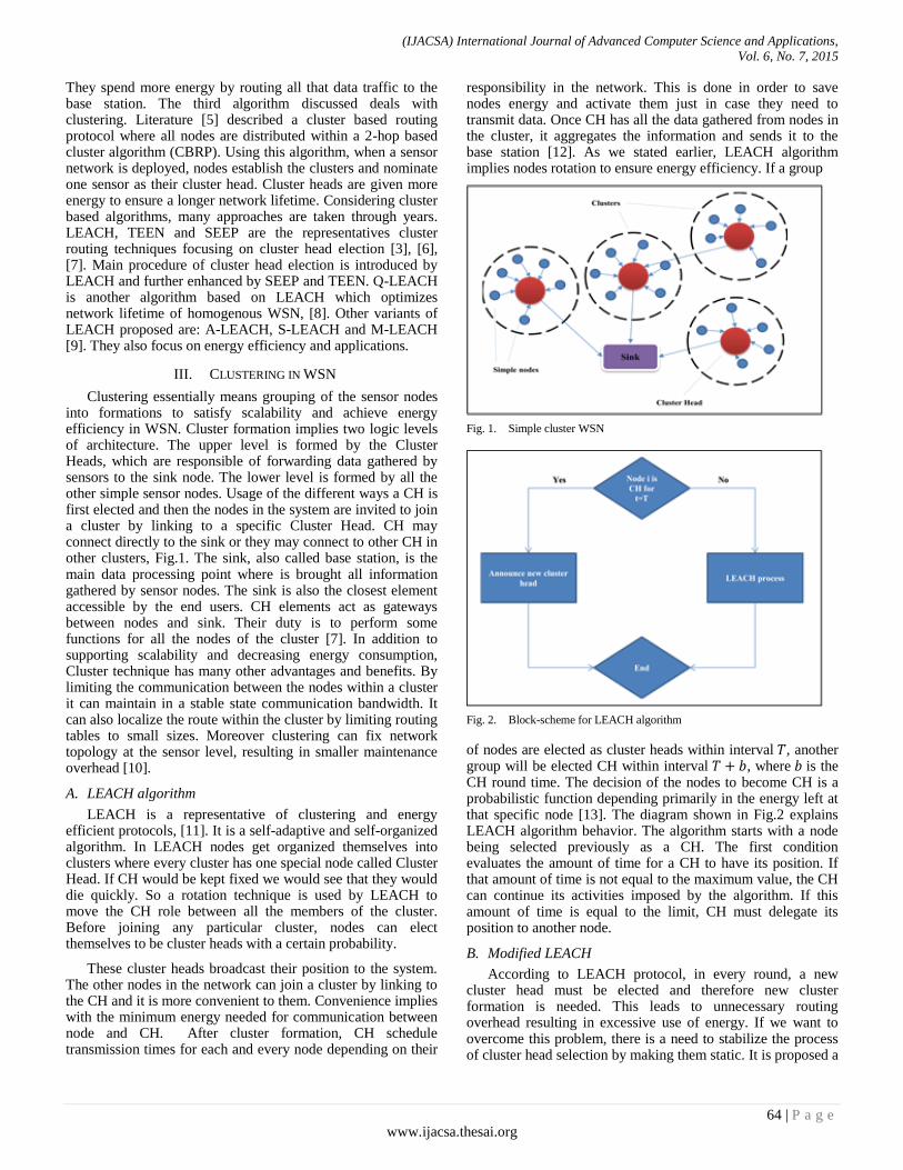
(IJACSA) International Journal of Advanced Computer Science and Applications,
Vol. 6, No. 7, 2015
64 | P a g e
www.ijacsa.thesai.org
They spend more energy by routing all that data traffic to the base station. The third algorithm discussed deals with clustering. Literature [5] described a cluster based routing protocol where all nodes are distributed within a 2-hop based cluster algorithm (CBRP). Using this algorithm, when a sensor network is deployed, nodes establish the clusters and nominate one sensor as their cluster head. Cluster heads are given more energy to ensure a longer network lifetime. Considering cluster based algorithms, many approaches are taken through years. LEACH, TEEN and SEEP are the representatives cluster routing techniques focusing on cluster head election [3], [6], [7]. Main procedure of cluster head election is introduced by LEACH and further enhanced by SEEP and TEEN. Q-LEACH is another algorithm based on LEACH which optimizes network lifetime of homogenous WSN, [8]. Other variants of LEACH proposed are: A-LEACH, S-LEACH and M-LEACH [9]. They also focus on energy efficiency and applications.
III. CLUSTERING IN WSN
Clustering essentially means grouping of the sensor nodes into formations to satisfy scalability and achieve energy efficiency in WSN. Cluster formation implies two logic levels of architecture. The upper level is formed by the Cluster Heads, which are responsible of forwarding data gathered by sensors to the sink node. The lower level is formed by all the other simple sensor nodes. Usage of the different ways a CH is first elected and then the nodes in the system are invited to join a cluster by linking to a specific Cluster Head. CH may connect directly to the sink or they may connect to other CH in other clusters, Fig.1. The sink, also called base station, is the main data processing point where is brought all information gathered by sensor nodes. The sink is also the closest element accessible by the end users. CH elements act as gateways between nodes and sink. Their duty is to perform some functions for all the nodes of the cluster [7]. In addition to supporting scalability and decreasing energy consumption, Cluster technique has many other advantages and benefits. By limiting the communication between the nodes within a cluster it can maintain in a stable state communication bandwidth. It can also localize the route within the cluster by limiting routing tables to small sizes. Moreover clustering can fix network topology at the sensor level, resulting in smaller maintenance overhead [10].
A. LEACH algorithm
LEACH is a representative of clustering and energy efficient protocols, [11]. It is a self-adaptive and self-organized algorithm. In LEACH nodes get organized themselves into clusters where every cluster has one special node called Cluster Head. If CH would be kept fixed we would see that they would die quickly. So a rotation technique is used by LEACH to move the CH role between all the members of the cluster. Before joining any particular cluster, nodes can elect themselves to be cluster heads with a certain probability.
These cluster heads broadcast their position to the system. The other nodes in the network can join a cluster by linking to the CH and it is more convenient to them. Convenience implies with the minimum energy needed for communication between node and CH. After cluster formation, CH schedule transmission times for each and every node depending on their
responsibility in the network. This is done in order to save nodes energy and activate them just in case they need to transmit data. Once CH has all the data gathered from nodes in the cluster, it aggregates the information and sends it to the base station [12]. As we stated earlier, LEACH algorithm implies nodes rotation to ensure energy efficiency. If a group
Fig. 1. Simple cluster WSN
Fig. 2. Block-scheme for LEACH algorithm
of nodes are elected as cluster heads within interval , another group will be elected CH within interval , where is the CH round time. The decision of the nodes to become CH is a probabilistic function depending primarily in the energy left at that specific node [13]. The diagram shown in Fig.2 explains LEACH algorithm behavior. The algorithm starts with a node being selected previously as a CH. The first condition evaluates the amount of time for a CH to have its position. If that amount of time is not equal to the maximum value, the CH can continue its activities imposed by the algorithm. If this amount of time is equal to the limit, CH must delegate its position to another node.
B. Modified LEACH
According to LEACH protocol, in every round, a new cluster head must be elected and therefore new cluster formation is needed. This leads to unnecessary routing overhead resulting in excessive use of energy. If we want to overcome this problem, there is a need to stabilize the process of cluster head selection by making them static. It is proposed a
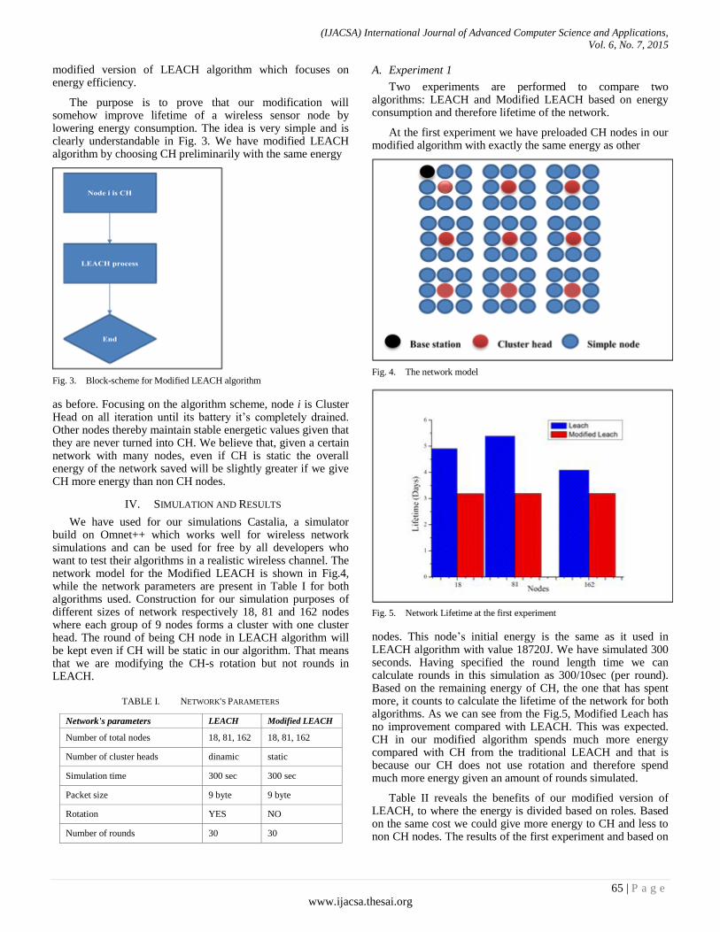
(IJACSA) International Journal of Advanced Computer Science and Applications,
Vol. 6, No. 7, 2015
65 | P a g e
www.ijacsa.thesai.org
modified version of LEACH algorithm which focuses on energy efficiency.
The purpose is to prove that our modification will somehow improve lifetime of a wireless sensor node by lowering energy consumption. The idea is very simple and is clearly understandable in Fig. 3. We have modified LEACH algorithm by choosing CH preliminarily with the same energy
Fig. 3. Block-scheme for Modified LEACH algorithm
as before. Focusing on the algorithm scheme, node i is Cluster Head on all iteration until its battery it’s completely drained. Other nodes thereby maintain stable energetic values given that they are never turned into CH. We believe that, given a certain network with many nodes, even if CH is static the overall energy of the network saved will be slightly greater if we give CH more energy than non CH nodes.
IV. SIMULATION AND RESULTS
We have used for our simulations Castalia, a simulator build on Omnet++ which works well for wireless network simulations and can be used for free by all developers who want to test their algorithms in a realistic wireless channel. The network model for the Modified LEACH is shown in Fig.4, while the network parameters are present in Table I for both algorithms used. Construction for our simulation purposes of different sizes of network respectively 18, 81 and 162 nodes where each group of 9 nodes forms a cluster with one cluster head. The round of being CH node in LEACH algorithm will be kept even if CH will be static in our algorithm. That means that we are modifying the CH-s rotation but not rounds in LEACH.
TABLE I. NETWORK'S PARAMETERS
Network's parameters LEACH Modified LEACH
Number of total nodes 18, 81, 162 18, 81, 162
Number of cluster heads dinamic static
Simulation time 300 sec 300 sec
Packet size 9 byte 9 byte
Rotation YES NO
Number of rounds 30 30
A. Experiment 1
Two experiments are performed to compare two algorithms: LEACH and Modified LEACH based on energy consumption and therefore lifetime of the network.
At the first experiment we have preloaded CH nodes in our modified algorithm with exactly the same energy as other
Fig. 4. The network model
Fig. 5. Network Lifetime at the first experiment
nodes. This node’s initial energy is the same as it used in LEACH algorithm with value 18720J. We have simulated 300 seconds. Having specified the round length time we can calculate rounds in this simulation as 300/10sec (per round). Based on the remaining energy of CH, the one that has spent more, it counts to calculate the lifetime of the network for both algorithms. As we can see from the Fig.5, Modified Leach has no improvement compared with LEACH. This was expected. CH in our modified algorithm spends much more energy compared with CH from the traditional LEACH and that is because our CH does not use rotation and therefore spend much more energy given an amount of rounds simulated.
Table II reveals the benefits of our modified version of LEACH, to where the energy is divided based on roles. Based on the same cost we could give more energy to CH and less to non CH nodes. The results of the first experiment and based on
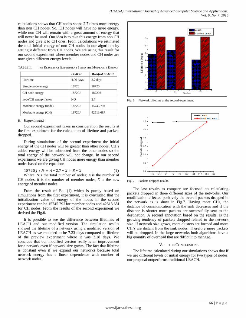
(IJACSA) International Journal of Advanced Computer Science and Applications,
Vol. 6, No. 7, 2015
66 | P a g e
www.ijacsa.thesai.org
calculations shows that CH nodes spend 2.7 times more energy than non CH nodes. So, CH nodes will have no more energy, while non CH will remain with a great amount of energy that will never be used. Our idea is to take this energy from non CH nodes and give it to CH ones. From calculations we estimated the total initial energy of non CH nodes in our algorithm by setting it different from CH nodes. We are using this result for our second experiment where member nodes and CH nodes are now given different energy levels.
TABLE II. THE RESULTS OF EXPERIMENT 1 AND THE MODERATE ENERGY
LEACH Modified LEACH
Lifetime 4.06 days 3.2 days
Simple node energy 18720 18720
CH node energy 18720J 18720J
node/CH energy factor NO 2.7
Moderate energy (node) 18720J 15745.79J
Moderate energy (CH) 18720J 42513.68J
B. Experiment2
Our second experiment takes in consideration the results at the first experiment for the calculation of lifetime and packets dropped.
During simulations of the second experiment the initial energy of the CH nodes will be greater than other nodes. CH’s added energy will be subtracted from the other nodes so the total energy of the network will not change. In our second experiment we are giving CH nodes more energy than member nodes based on the equation:
Where: is the total number of nodes; is the number of
CH nodes; is the number of member nodes; is the new energy of member nodes.
From the result of Eq. (1) which is purely based on simulations from the first experiment, it is concluded that the initialization value of energy of the nodes in the second experiment can be 15745.79J for member nodes and 42513.68J for CH nodes. From the results of the second experiment we derived the Fig.6.
It is possible to see the difference between lifetimes of LEACH and our modified version. The simulation results showed the lifetime of a network using a modified version of LEACH as we modeled to be 7.23 days compared to lifetime of the preview experiment where it was 3.18 days. We conclude that our modified version really is an improvement for a network even if network size grows. The fact that lifetime is constant even if we expand our networks because total network energy has a linear dependence with number of network nodes.
Fig. 6. Network Lifetime at the second experiment
Fig. 7. Packets dropped results
The last results to compare are focused on calculating packets dropped in three different sizes of the networks. Our modification affected positively the overall packets dropped in the network as is show in Fig.7. Having more CHs, the distance of communication with the sink decreases and if the distance is shorter more packets are successfully sent to the destination. A second annotation based on the results, is the growing tendency of packets dropped related to the network size. If network size grows, more clusters are formed and more CH’s are distant from the sink nodes. Therefore more packets will be dropped. In the large networks both algorithms have a big quantity of overhead that are difficult to manage.
V. THE CONCLUSIONS
The lifetime calculated during our simulations shows that if we use different levels of initial energy for two types of nodes, our proposal outperforms traditional LEACH.

(IJACSA) International Journal of Advanced Computer Science and Applications,
Vol. 6, No. 7, 2015
67 | P a g e
www.ijacsa.thesai.org
The modified LEACH also improved packets dropped. That because nodes can transmit in smaller distances having more CHs and so has less packets dropped as in our modified version.
Our work concluded to be really a pleasant improvement. Being a cost effective algorithm and having static nodes as CH we believe that our next challenge will be the proposal of new hybrid algorithms that use modified LEACH as part of their logic. Further, as a future work connecting with the routing method of CH with another known routing algorithm would be worth studying.
REFERENCES
[1] B.Krishnamachari, “An introduction to wireless sensor networks”, Second International Conference on Intelligent Sensing and Information Processing (ICISIP), Chennai, India, January 2005.
[2] J.Lester Hill, “System architecture for wireless sensor networks”, PhD dissertation, University of California at Berkeley, 2003.
[3] X.Liu, “A survey on clustering routing protocols in wireless sensor networks” Sensors 2012, pp.11113-11153.
[4] Singh, Woo & Raghavendra, “Power-aware routing in mobile ad hoc networks”, 4th Annual IEEE/ACM Int. Conf. Mobile Computing and Networking, pp. 181–190, Dallas, Texas, USA, 1998.
[5] T.Daniel Hollerung, “The cluster-based routing protocol”,University of Paderborn, winter semester 2003/2004.
[6] O.Boyinbode,L.Hanh,A Mbogho,M.Takizawa, R. Poliah,“A survey on clustering algorithms for wireless sensor networks”, Network-Based Information Systems (NBiS), 13th International Conference, 2010.
[7] O.Younis, M.Krunz and S.Ramasubramanian, “Node clustering in wireless sensor networks: Recent Developments and Deployment Challenges”, IEEE Network – 0890-8044 / 2006.
[8] B.Manzoor, N.Javaid, O.Rehman, M.Akbar, Q.Nadeem, A.Iqbal, M.Ishfaq, “Q-LEACH: A new routing protocol for WSN”, Procedia Computer Science 2013.
[9] D.Mahmod, S.Mahmod, S.Qureshi, A.Memon, T.Zaman, “MODLEACH: A variant of LEACH for WSN” July 2013.
[10] Y.Zhang, L.T. Yang, J.Chen, “RFID and sensor networks: architectures, protocols, security, and integrations”. New York: CRC Press, 2010.
[11] W.Rabiner Heinzelman, A.Chandrakasan and H.Balakrishnan 2000, “Energy-Efficient communication protocol for wireless microsensor networks”, Washington DC: IEEE Computer Society, 2000.
[12] L.Cao, Ch.Xu, W.Shao, G.Zhang, H.Zhou, Q.Sun, “Distributed power allocation for Sink-Centric clusters in multiple Sink wireless sensor networks”, www.mdpi.com/journal/sensors, 2010.
[13] D.Kumar, T.C. Aseri, R.B. Patel, “EEHC: Energy efficient heterogeneous clustered scheme for wireless sensor networks”, Computer Communications 32 (2009) 662–667.
(IJACSA) International Journal of Advanced Computer Science and Applications,
Vol. 6, No. 7, 2015
68 | P a g e www.ijacsa.thesai.org
A Frame Work for Preserving Privacy in Social
Media using Generalized Gaussian Mixture Model
P Anuradha
Department of CSE
GITAM University
Visakhapatnam, India
Y.Srinivas
Department of IT
GITAM University
Visakhapatnam, India
MHM Krishna Prasad
Department of CSE
J NT University,
Kakinada
Abstract—Social networking sites helps in developing virtual
communities for people to share their thoughts, interest activities
or to increase their horizon of camaraderie. Social networking
sites come under few of the most frequently browsed categories
websites in the world. Nevertheless Social Networking sites are
also vulnerable to various problems, threats and attacks such as
disclosure of information, identity thefts etc. Privacy practice in
social networking sites often come into sight, as information
sharing stands in conflict with the disclosure-related misuse. Face
book is one such most popular and widely used Social
Networking sites which have its own robust set of Privacy
mechanisms. Yet they are also prone to various privacy issues
and attacks. The impulse in this paper lies in proposing a novel
approach for improving the privacy among the social networking
sites .The article presents the issues by a novel approach based on
tagging and a model based technique based on generalized
Gaussian Mixture Model.
Index Terms—Privacy; Social Network; Social Relevant
Groups; Generalized GMM, Tagging
I. INTRODUCTION
The recent advancements in technologies, in particular, the internet technology, benefitted the users to share and view useful information from across the globe. Thousands of clients share their thoughts online through the social network sites[1],[2],[3]. With the mammoth options available on Social Networking sites, it creates a Virtual world for the users. Social Networking sites go upwards because of all these reasons. These technologies help to share the information by the individuals and experts [4]. Methodologies were also framed wherein interested groups can formulate a group and each of the members within these groups can share and communicate to each other and these groups are called specific groups. The main advantage of these formation of groups is that the most relevant information needed by a group members can be retrieved from the members within the group or from the specific designated groups[5][6]. This popularity resulted in the formulation of social networking groups such as Twitter, Orkut , Face book [7][8].
Today, fan page is one amongst the different groups available in the social media, through this page important conversation and interesting communications are broadcasted among these groups. This fan page can be very much useful to advertise a particular brand, the brand advertisements in Face book dominate the Twitter and YouTube [1].This indirectly resulted in privacy and secrecy concerns about misusing the crucial information by internet users, one primary concern is
that, virus authors use this social networking medium as a base and transmitting the virus among the groups [8]. Of late, Face book scams shoot the news with the tremendous increase in the number of fraud cases. This forced people rethink about the privacy of their Face book profiles, and also confirmed that several apps used in the Face book are being shared among the unauthorized people.
A. Privacy Issues in Social Media
There are several issues with regard to privacy, such as user Anonymity, where the identity of a user is exposed by the attacker and tries to at victim‘s profile. In De- Anonymization attack, the group member ship information is hacked by the attackers and tries to send anonymous mails by the attackers from the victims group. In the neighborhood attack, the neighbors around the network try to attack the victims. [5]
Apart from the privacy issues, there are several other issues, like user Profile leakage, leakage of information to third parties and Profile cloning.
Several other issues, that are target towards the privacy, include Spam mail attacks on Emails, Broad cast spam attacks, context spam attacks, where the attackers attack the victims sites, by sending several bulk mails.[5] . These are the factors that cause problems with regard to the privacy among the social networking sites.
It is therefore necessary to upgrade the present security methods of the face book and explore the privacy methodologies related to Social Networking Sites. In this paper, we have analyzed the offered privacy methodologies for the social networking sites, and in particular focused on the De-Anonymization attack and propose some new privacy model to strengthen the existing ones. To overcome these disadvantages privacy preserving approach together with network security approaches have been listed the literature [9][10]. In most of these approaches the authors have considered only about presenting the sensitive information and very little work is reported about the sharing of the information together with protection of the sensitive information.
In this article, we proceed to describe the methodology wherein each of the group members within a group are associated with a tag and for the efficient retrievals , the related tag of the images are given as input to the Generalized Gaussian Mixture Model for the experimentation purpose we have considered dataset of Flicker.

(IJACSA) International Journal of Advanced Computer Science and Applications,
Vol. 6, No. 7, 2015
69 | P a g e www.ijacsa.thesai.org
Each of the images in the dataset are subjected to normalization varying the invariable rotation are overcome. For this purpose the concept of Local Binary Pattern is used. Each of the user registered within the group are given an id and a code book is generated by summing up ids of all the individuals within the group. This sum is considered as the group code and with this as a tag, the images are retrieved. The main advantage is that if an unauthorized person wants to access the data from the group, the group id is to be understood. Therefore by this methodology we can overcome the fore said disadvantages. The rest of the paper is organized as follows. Section 2 of the paper deals with probability density function of the considered generalized GMM. In section 3 of the paper the details of the dataset are considered and presented. Section 4 of the paper deals with procedure of normalization based on a Local Binary Pattern. In section 5 of the paper the feature extraction is presented by using the concepts of relevance score and tagging. The results derived together with experimentation are presented in section 6. The conclusion is highlighted in section 7 of the paper. The future scope is presented in section 8 of the paper.
B. Related Work
Many authors have discussed about the issues of privacy in social networks. Most of the works are based on using Anonymization techniques (Zhou et.al(2008))[22],Encryption based(Guha et.al(2008))[23], Optimization model base, collaborative technique based(Blosser et.al(2008))[24], K-anonymity and sensitivity based approach(Ford et.al(2009))[25], Anonymized graphs(Narayanan et.al(2009))[26] access control model (Fong et.al(2009))[27]. Tang et.al(2010)[28] proposed a model using K-nearest neighborhood along with EBB algorithm for utilizing the privacy and the concepts of sub-graphs are considered by(Lan et.al(2010))[29] and the concepts of friendship means have been focused to ensure privacy and sending the sensitive information to these links was proposed by Heathely et.al(2013)[30].
In most of these models, the authors have proposed models towards the usage of models based on K-anonymity, L-diversity and the main disadvantages with these models is that they are prone to be a loss of information also Anonymization techniques failed to preserve the data based on dynamic releases. Further to add the models based on distributed approaches failed to uphold the privacy since preserving the privacy in a network environment in these cases are most sensible. To add most of the works proposed by the earlier researches are subjected to model the privacy issues which failed to overcome the attacks like homogeneity attack, background knowledge attack, distance based attacks and sensitive attacks. To overcome these advantages, the proposed article presents a model varying the disadvantages cited about
can be overcome. Since it is a model based approach it holds the issues of homogeneity since every group which is subjected to the model presented in section 2 generates a unique PDF and also the model is more robust since it has a shape parameter and scale parameter which helps to model different sizes of groups and generating unique PDF‘s to each of these proposed groups. By varying the shape parameter and scale parameter, the model can be further extended for partitioning the groups into subsets where each subset can be a related or non-related.
II. GENERALIZED GAUSSIAN MIXTURE MODEL
In this article Generalized Gaussian Mixture Model is used to classify the images more appropriate basing on the symmetry of distribution. The probability density function of the Generalized Gaussian Mixture Model is presented in the following equation
P
ii
PA
Z
e
PAP
Pzf),(
)(
),()1
1(2
1),,|(
- ---(1)
)2()3(
)1(),(,0
2
1
2
P
PPA
Where µ and σ are the mean and standard deviation and Γ defines the General Gamma Variate.
III. DATASET CONSIDERED
To perform the experiment we have considered the Flick database consisting of 25,000 images and each image is labeled with a tag description with labels like nature, cigar, flora and watch etc. Each image is coupled with a tag depiction; among these images 450 have unique tags. The experimentation is performed by taking into account 100 images, Query image is considered with the size 100 x 100.
IV. LOCAL BINARY PATTERN
Local Binary Pattern is used to encode the relationship between the reference pixels with its surrounding neighbors by computing gray-level values. The Local Binary Pattern value is computed by comparing gray-scale value with its neighborhood.
LBP= ))()(()1)1
1 cp
P
p
gIglfXP
1f (x) = 1 x ≥ 0
= 0 otherwise --(3)

(IJACSA) International Journal of Advanced Computer Science and Applications,
Vol. 6, No. 7, 2015
70 | P a g e www.ijacsa.thesai.org
Fig. 1. Dataset considered from Flicker
V. FEATURE EXTRACTION
For mining the images effectively from the database, Feature plays a crucial part. The features may perhaps be low level features or high level features which can be correlation, size, moments, histogram etc. Nevertheless, to retrieve the images more successfully, these features are to be linked with semantic understanding. The semantic interpretations aid to mine the data by means of the semantic characteristics and also lessen the semantic gap. These semantic traits are easily understood by the users when compared to the low level features which embrace contrast, symmetry, homogeneity and uniformity.
A. Score Level Fusion
For efficient image retrievals, score level fusion is used, the procedure operates on a Logical AND/ OR operation, where the relevancy is indicated as ‗Y‘, and non-relevancy by ‗N‘.
B. KL-divergence
KL-divergence is used for the purpose to measure the distance between two probability density functions. It is a non-symmetric measure of the differences between two probability distributions .It is also known as relative entropy and information divergence.
)4()(
)(log)(),(
2
1121
dx
xp
xpxpppKL
Where ‗p1‘, ‗p2‘ are the two Probability Density Functions
VI. EXPERIMENTATION
In this model each of the users are identified basing on the grouping interest. These related users are formatted into a group by registering themselves with the data consisting of their e-mail ids and the group interest is considered and is tagged. These tags along with the e-mail ids are fused using score level fusion, discussed in above section-5.1 and these fused values are given as inputs to the model depicted in section 2 of the paper. In order to transmit or communicate the information among the groups, the authentication is to be established. And for the identification of the relatedness, the PDF‘s are compared using KL-divergence, proposed in section-5.2 and the authentication users are allowed to communicate and share the information.
VII. CONCLUSION
In this article a new framework is proposed to uphold the privacy issues by proposing the new methodology based on Generalized Gaussian Mixture model. The methodology developed helps in safeguarding the privacy of the information shared among the groups, such that the users can share the data with great deal of confidence. This method will be useful in Social Networking Sites and in particular on the Face book.
VIII. FUTURE SCOPE
In this paper, a methodology is presented to safe guard the group user‘s information in the social networking media. This paper address the methodology for overcoming the De-Annomyzation attack, however , effective mechanism are to be developed to overcome the other attacks , such as spam attack, hijacker attack . Also, most of the data can be transmitted by using the watermarking techniques. Therefore methods are to be developed to overcome this issue.
Fig. 2. The proposed architecture

(IJACSA) International Journal of Advanced Computer Science and Applications,
Vol. 6, No. 7, 2015
71 | P a g e www.ijacsa.thesai.org
REFERENCES
[1] MARK Hachman (Aoril 23,2012). ―Facebook Now Totals 1.20 billion Users, Profits Slip‖. PCMag.com. Retrieved September 24, 2013.
[2] D. M. Boyd and N. B. Ellison, ―Social Network Sites: Definition, History, and Scholarship,‖J. Comp.-Mediated Communication., vol. 13, no. 1, Oct. 2007, pp.210–30.
[3] S. B. Barnes, ―A Privacy Paradox: Social Networking in the United States,‖First Monday , vol. 11, no. 9, Sept. 2006.
[4] Aimeur, E.; gambus,S.; Ai Ho; , ―UPP: User Privacy Policy for Social Networking Sites,‖Internet and Web Applications and Services,2009. ICIW ‘09.Fourth International Conference on vol., no., pp.267-272,24-28 May 2009.
[5] A Survey of Privacy and Security Issues Social Networks http://www.cse.wustl.edu/~jain/cse571-11/ftp/social/index.htm
[6] Stutzman, F.and Kramer-Duffield, J. Friends only: Examining a Privacy Enhancing behaviour in Facebook. In Proc. CHI‘10.ACM Press, 2010.1553—1562.
[7] A. Ho, A4. Maiga, and E. Aimeur, ―Privacy protection issues in social networking sites,‖IEEE/Acs International Conference on Computer Systems and Applications 2009 (AICCSA 2009),PP.271-278,Country,2009
[8] Thomas,K., Grier, C., and Nicol,D.M.unFriendly: Multi party privacy risks in social networks.In proceedings of the 10th international conference on Privacy enhancing technologies(2010),Soringer-Verlag,pp.236
[9] http://www.facebook.com\privacy [10] Ai Ho; Maiga, A.; Aimeur, E.; , ―Privacy protection issues in social
networking sites,‖ Computer Systems and Applications, 2009. AICCSA 2009.IEEE/ACS International Conference on vol.,no., pp.271-278, 10-13 May 2009
[11] Xi Chen; Shuo Shi; ,‖A Literature review of Privacy Research on Social Network Sites,‖ Multimedia Information Networking and Security,2009.MINES‘09.International Conference on, vol.1,no.,pp.93-97,18-20 Nov.2009
[12] SeyedHossein Mohtasebi and Ali Dehghantanha,‖ A Mitigation Approach to the Malwares Threats of Social Network Services,‖ Muktimedia Information Networking and Security,2009. MINES‘09. International Conference on, vol.1,no.,pp.448-459,2011
[13] Mohammad Mannan, Paul C. Van Oorschot,‖ privacy-Enhanced Sharing of Personal Content on the Web,‖ Security And Privacy- Misc‖ , pp.487-496,April 21-25,2008 Beijing, China
[14] Privacy Policy Facebook (2011), www.facebook.com/policy.php [15] Chi Zhang; Jinyuan Sun;, ‖Privacy and Security for Online Social
networks:Challenges and Opportunities,‖ IEEE Network,Aug.2010
[16] Vorakulpipat, Marks, Rezgui, ― Security and Privacy Issues in Social Networking Sites from User‘s Viewpoint,‖IEEE Network,Jun.2011
[17] P.Kodeswaran, and E.Viegas, ―Towards A privacy preserving Policy Based Infrastructure for Social Data Access To enable Scientific Research,‖2010 Eighth Annual International Conference on Privacy,Security and Trust,Jun 2010
[18] I. Polakis and G. Kontaxis,‖ Using Social Networks to harvest Email Addresses,‖ In Proc.CHI‖10. ACM Press,2010
[19] C.Squicciarini and M.Shehab,‖ Privacy policies for shared content in social network sites,‖ In Proc.Chi‘10.Acm Press,30 June 2010
[20] Yabing Liu and P. Gummadi, ―Analyzing Facebook Privacy Settings:User Expectations vs. Reality,‖ In Proceedings of the 10th international conference on Privacy enhancing technologies(2011)
[21] P. Joshi and C Kuo ,‖ Security and Privacy in Online Social Networks: A Survey‖,IEEE Network,2011
[22] B. Zhou, Jian Pei,Wo-Shun Luk, ― A brief survey on anonymization techniques for privacy preserving publishing of social network data,‖ ACM SIGKDD Explorations Newsletter, Vol. 10,pp. 12-22,2008.
[23] Saikat Guha , Kevin Tang, Paul Francis, ―NOYB: Privacy in Online Social Networks‖, In Proc. of first workshop on Online social networks WOSN‘08, ACM New YORK, NY, USA, pp 49-54,2008.
[24] Gary Blosser, Justin Zhan, ―Privacy Preserving Collaborative Social Network‖, In Proc. Of International Conference on Information Security and Assurance ISA 2008,Busan,pp.543-548,2008.
[25] Roy Ford, Traian Marius Truta, and Alina Campan, ―P-Sensitive K-Anonymity for Social Networks‖.
[26] A. Narayanan, V. Shmatikov, ―De-anonymyzing social networks‖, In Proc of 30th IEEE Symposium on Security and Privacy, Berkely, CA, pp 173-187,2009.
[27] Philip W. L. Fong, Mohd Anwar, and Zhen Zhao,‖ A Privacy Preservation Model for Facebook-style Social Network Systems‖, In: Computer Security- ESORICS 2009, Lecture Notes in Computer Science, Vol.5789,2009,pp 303-320,2009.
[28] X. Tang and C. C. Yang, ― Generalizing Terrorist Social Networks with K-Nearest Neighbor and Edge Betweenness for Social Network Integration and Privacy Preservation,‖ In Proc. of IEEE International Conference on Intelligence and Security Informatics, 2010.
[29] Lihui Lan, Shiguang Ju Hua Jin,‖Anonymizing Social Network using Bipartite Graph‖,In Proc. of International Conference on Computational and Informatics Sciences(ICCIS), Chengdu, pp 993-996,2010.
[30] Raymond Heatherly, Murat Kantarcioglu, and Bhavani Thuraisingham, ―Preventing Private Information Inference Attacks on Social Networks‖, In: IEEE Transactions On Knowledge And Data Engineering, Vol.25, No.8,pp 1849-1862,2013.

(IJACSA) International Journal of Advanced Computer Science and Applications,
Vol. 6, No. 7, 2015
72 | P a g e
www.ijacsa.thesai.org
Survey on Chatbot Design Techniques in Speech
Conversation Systems
Sameera A. Abdul-Kader
School of Computer Science and Electronic
Engineering/University of Essex Colchester/ UK
Diyala University/ Diyala/ Iraq
Dr. John Woods
School of Computer Science and Electronic
Engineering/University of Essex Colchester/ UK
Abstract—Human-Computer Speech is gaining momentum as
a technique of computer interaction. There has been a recent
upsurge in speech based search engines and assistants such as
Siri, Google Chrome and Cortana. Natural Language Processing
(NLP) techniques such as NLTK for Python can be applied to
analyse speech, and intelligent responses can be found by
designing an engine to provide appropriate human like
responses. This type of programme is called a Chatbot, which is
the focus of this study. This paper presents a survey on the
techniques used to design Chatbots and a comparison is made
between different design techniques from nine carefully selected
papers according to the main methods adopted. These papers are
representative of the significant improvements in Chatbots in the
last decade. The paper discusses the similarities and differences
in the techniques and examines in particular the Loebner prize-
winning Chatbots.
Keywords—AIML; Chatbot; Loebner Prize; NLP; NLTK; SQL;
Turing Test
I. INTRODUCTION
Speech is one of the most powerful forms of communication between humans; hence, it is the researchers‟ ambition in the human computer interaction research field to improve speech interaction between the human and the computer in order to simulate human-human speech interaction. Speech interaction with modern networked computing devices has received increasing interest in the past few years with contributions from Google, Android and IOS. Because they are more natural than graphic-based interfaces, spoken dialogue systems are beginning to form the primary interaction method with a machine [1]. Therefore, speech interaction will play a significant role in humanising machines in the near future [2].
Much research work has focussed on improving recognition rates of the human voice and the technology is now approaching viability for speech based human computer interaction. Speech Interaction splits into more than one area including: speech recognition, speech parsing, NLP (Natural Language Processing), keyword identification, Chabot design/personality, artificial intelligence etc. Chatbot is a computer program that have the ability to hold a conversation with human using Natural Language Speech.
In this paper, a survey of Chatbot design techniques in speech conversation between the human and the computer is presented. Nine studies that made identifiable contributions in Chatbot design in the last ten years are selected and then, reviewed. The different techniques used for Chatbots in the
selected works are compared with those used in Loebner-Prize Chatbots. The findings are discussed and conclusions are drawn at the end.
II. BACKGROUND
A. Human-Computer Speech interaction
Speech recognition is one of the most natural and sought after techniques in computer and networked device interaction has only recently become possible (last two decades) with the advent of fast computing.
Speech is a sophisticated signal and happens at different levels: “semantic, linguistic, articulatory, and acoustic” [3]. Speech is considered as the most natural among the aspects of human communication, owing to copious information implicitly existing beyond the meaning of the spoken words. One of the speech information extraction stages is converting speech to text via Automatic Speech Recognition (ASR) and mining speech information [4]; then, the resulting text can be treated to extract the meaning of the words.
Speech recognition is widely accepted as the future of interaction with computers and mobile applications; there is no need to use traditional input devices such as the mouse, keyboard or touch sensitive screen and is especially useful for users who do not have the ability to use these traditional devices [5]. It can help disabled people with paralysis, for example, to interact with modern devices easily by voice only without moving their hands.
B. Natural Language Toolkit (NLTK)
In order to deal with and manipulate the text resulting from speech recognition and speech to text conversion, specific toolkits are needed to organise the text into sentences then split them into words, to facilitate semantic and meaning extraction. One of these toolkits is the widely used NLTK which is a free plugin for Python.
The Natural Language ToolKit (NLTK) is a set of modules, tutorials and exercises which are open source and cover Natural Language Processing symbolically and statistically. NLTK was developed at the University of Pennsylvania in 2001allowing computational linguistics with three educational applications in mind: projects, assignments and demonstrations [6] [7]. It can be found within the Python Libraries for Graph manipulation GPL open license. NLTK is used to split words in a string of text and separate the text into parts of speech by tagging word labels according to their positions and functions in the sentence. The resulting tagged
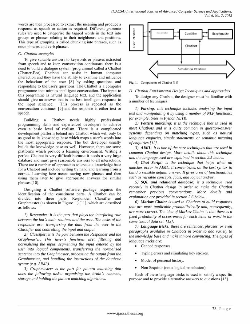
(IJACSA) International Journal of Advanced Computer Science and Applications,
Vol. 6, No. 7, 2015
73 | P a g e
www.ijacsa.thesai.org
words are then processed to extract the meaning and produce a response as speech or action as required. Different grammar rules are used to categorise the tagged words in the text into groups or phrases relating to their neighbours and positions. This type of grouping is called chunking into phrases, such as noun phrases and verb phrases.
C. Chatbot strategies
To give suitable answers to keywords or phrases extracted from speech and to keep conversation continuous, there is a need to build a dialogue system (programme) called a Chatbot (Chatter-Bot). Chatbots can assist in human computer interaction and they have the ability to examine and influence the behaviour of the user [8] by asking questions and responding to the user's questions. The Chatbot is a computer programme that mimics intelligent conversation. The input to this programme is natural language text, and the application should give an answer that is the best intelligent response to the input sentence. This process is repeated as the conversation continues [9] and the response is either text or speech.
Building a Chatbot needs highly professional programming skills and experienced developers to achieve even a basic level of realism. There is a complicated development platform behind any Chatbot which will only be as good as its knowledge base which maps a user‟s words into the most appropriate response. The bot developer usually builds the knowledge base as well. However, there are some platforms which provide a learning environment. Writing a perfect Chatbot is very difficult because it needs a very large database and must give reasonable answers to all interactions. There are a number of approaches to create a knowledge base for a Chatbot and include writing by hand and learning from a corpus. Learning here means saving new phrases and then using them later to give appropriate answers for similar phrases [10].
Designing a Chatbot software package requires the identification of the constituent parts. A Chatbot can be divided into three parts: Responder, Classifier and Graphmaster (as shown in Figure. 1) [11], which are described as follows:
1) Responder: it is the part that plays the interfacing role
between the bot’s main routines and the user. The tasks of the
responder are: transferring the data from the user to the
Classifier and controlling the input and output.
2) Classifier: it is the part between the Responder and the
Graphmaster. This layer’s functions are: filtering and
normalising the input, segmenting the input entered by the
user into logical components, transferring the normalised
sentence into the Graphmaster, processing the output from the
Graphmaster, and handling the instructions of the database
syntax (e.g. AIML).
3) Graphmaster: is the part for pattern matching that
does the following tasks: organising the brain’s contents,
storage and holding the pattern matching algorithms.
Fig. 1. Components of Chatbot [11]
D. Chatbot Fundamental Design Techniques and approaches
To design any Chatbot, the designer must be familiar with a number of techniques:
1) Parsing: this technique includes analysing the input
text and manipulating it by using a number of NLP functions;
for example, trees in Python NLTK.
2) Pattern matching: it is the technique that is used in
most Chatbots and it is quite common in question-answer
systems depending on matching types, such as natural
language enquiries, simple statements, or semantic meaning
of enquiries [12].
3) AIML: it is one of the core techniques that are used in
common Chatbot design. More details about this technique
and the language used are explained in section 2.5 below.
4) Chat Script: is the technique that helps when no
matches occur in AIML. It concentrates on the best syntax to
build a sensible default answer. It gives a set of functionalities
such as variable concepts, facts, and logical and/or.
5) SQL and relational database: is a technique used
recently in Chatbot design in order to make the Chatbot
remember previous conversations. More details and
explanation are provided in section 2.6 below.
6) Markov Chain: is used in Chatbots to build responses
that are more applicable probabilistically and, consequently,
are more correct. The idea of Markov Chains is that there is a
fixed probability of occurrences for each letter or word in the
same textual data set [13].
7) Language tricks: these are sentences, phrases, or even
paragraphs available in Chatbots in order to add variety to
the knowledge base and make it more convincing. The types of
language tricks are:
Canned responses.
Typing errors and simulating key strokes.
Model of personal history.
Non Sequitur (not a logical conclusion)
Each of these language tricks is used to satisfy a specific purpose and to provide alternative answers to questions [13].

(IJACSA) International Journal of Advanced Computer Science and Applications,
Vol. 6, No. 7, 2015
74 | P a g e
www.ijacsa.thesai.org
8) Ontologies: they are also named semantic networks
and are a set of concepts that are interconnected relationally
and hierarchically. The aim of using ontologies in a Chatbot
is to compute the relation between these concepts, such as
synonyms, hyponyms and other relations which are natural
language concept names. The interconnection between these
concepts can be represented in a graph enabling the computer
to search by using particular rules for reasoning [13].
E. Loebner Prize and Turing Test
a) Turing Test
In the field of Artificial Intelligence, Turing was the first to pose the question, “Can a machine think?” [14], where thinking is defined as the ability held by humans. According to this question and this definition, Turing suggests the “imitation game” as a method to directly avoid the question and to specify a measurement of achievement for researchers in Artificial Intelligence [15] if the machine appears to be human. The imitation game can be played between three people: (A) which is a man, (B) which is a woman, and (C) which is the interrogator and can be either a man or a woman. The aim of the interrogator here is to determine who the woman is and who the man is (A and B). The interrogator knows the two as labels X and Y and has to decide at the end of the game either “X is B and Y is A” or “X is A and Y is B”. The interrogator also has the right to direct questions to A and B. Turing then questions what will happen if A is replaced with a machine; can the interrogator differentiate between the two? The original question “Can machines think?” can then be replaced by this question [14]. In this imitation game, the Chatbot represents the machine and it tries to mislead the interrogator to think that it is the human or the designers try to programme it to do so [16].
b) Loebner Prize
In 1990 an agreement was held between Hugh Loebner and The Cambridge Centre for Behavioural Studies to establish a competition based on implementing the Turing Test. A Gold Medal and $100,000 have been offered by Hugh Loebner as a Grand Prize for the first computer that makes responses which cannot be distinguished from humans‟. A bronze medal and an annual prize of $2000 are still pledged in every annual contest for the computer which seems to be more human in relation to the other competitors, regardless of how good it is absolutely [15]. It is the first known competition that represents a Turing test formal instantiation [13]. The competition has been run from 1991 annually with slight changes made to the original conditions over the years. The important thing in this competition is to design a Chatbot that has the ability to drive a conversation. During the chat session, the interrogator tries to guess whether they are talking to a programme or a human. After a ten-minute conversation between the judge and a Chatbot on one side and the judge and a confederate independently on the other side, the judge has to nominate which one was the human. The scale of non-human to human is from 1 to 4 and the judge must evaluate
the Chatbot in this range [16]. According to this judgement, the more human Chatbot is the winner.
No Chatbot has ever achieved the golden medal and passed the test to win the Loebner Prize. However, some Chatbots have scored as highly as 3 out of the 12 judges believing they were human. There is a winning bot every year and there is a list of Chatbots called Loebner Prized Chatbots. This list commences from 1991 to the current date.
c) Prized Chatbots and Their Design Techniques
Although no Chatbot has won the Loebner Prize yet, there is a winning Chatbot each year and the standard of entry continues to improve with time. Table 1 shows the prized Chatbots as the name of the programmer, the programme name, the year they won, and the techniques used to design and programme them.
F. AIML
To build a Chatbot, a flexible, easy to understand and universal language is needed. AIML, a derivative of XML is one of the widely used approaches that satisfies the requirements. AIML represents the knowledge put into Chatbots and is based on the software technology developed for A.L.I.C.E. (the Artificial Linguistic Internet Computer Entity). It has the ability to characterise the type of data object (AIML objects) and describe partial conductance of the programmes that it processes. These objects consist of two units: topics and categories; the data contained in these categories is either parsed or unparsed [19].
The purpose of the AIML language is to simplify the job of conversational modelling, in relation to a “stimulus-response” process. It is also a mark-up language based on XML and depends on tags which are the identifiers that make snippets of codes to send commands into the Chatbot. The data object class is defined in AIML as an AIML object, and the responsibility of these objects is modelling conversational patterns. This means that each AIML object is the language tag that associates with a language command. The general structure of AIML objects is put forward by [20]:
<command> List of parameters </command> The most important object among the AIML objects is
category, pattern, and template. The task of the category tag is defining the knowledge unit of the conversation. The pattern tag identifies the input from the user and the task of template tag is to respond to the specific user input [20]; these are the most frequent tags and the bases to design AIML Chatbots with an intelligent response to natural language speech conversations. The structure of category, pattern, and template object is shown below:
<category>
<pattern> User Input</pattern>
<template>
Corresponding Response to input
</template>
</category>

(IJACSA) International Journal of Advanced Computer Science and Applications,
Vol. 6, No. 7, 2015
75 | P a g e
www.ijacsa.thesai.org
TABLE I. LOEBNER PRIZED CHATBOTS‟ DESIGN TECHNIQUES AND APPROACHES [13]
Year Programme
Name
Winner Designer
Name Design Technique
1991 PC Therapist Joseph Weintraub
Canned and non-sequitur responses in addition to pattern matching after
parsing, and word vocabulary that make it remember sentences. 1992 PC Therapist Joseph Weintraub
1993 PC Therapist Joseph Weintraub
1994 TIPS Thomas Whalen A personal history model database like the system with pattern matching.
1995 PC Therapist Joseph Weintraub The same as in 1991.
1996 HeX Jason Hutchens Has got a trick sentences database, Markov Chain models, pattern matching, and a model of personal history.
1997 Converse David Levy
A database for facts, pattern matching, proactivity, WordNet synonyms, a
statistical parser, ontology, a list of proper names, and a modular of weighted modules.
1998 Albert One Robby Garner Hierarchical structure of previous Chatbots, such as Fred, Eliza, pattern
matching and proactivity. 1999 Albert One Robby Garner
2000 A.L.I.C.E Richard Wallace Advance pattern matching, AIML.
2001 A.L.I.C.E Richard Wallace
2002 Ella Kevin Copple Language tricks, phrase normalisation, pattern matching, WordNet, and expanding abbreviation.
2003 Jabberwock Juergen Pirner Markov Chains, simple pattern matching, context free grammar (CFG), and
parser.
2004 A.L.I.C.E Richard Wallace The same as in 2000.
2005 George
(Jabberwacky) Rollo Carpenter
No scripts or pattern matching, a huge database of responses of people, and
they are based on the Chatbot Jabberwacky. 2006
Joan (Jabberwacky)
Rollo Carpenter
2007 UltraHAL Robert Medeksza Scripts of pattern matching and VB code combination.
2008 Elbot Fred Roberts Commercial Natural Language Interaction system.
2009 Do-Much-More David Levy Intelligent Toys Commercial Property.
2010 Suzette Bruce Wilcox AIML based chat script with database of variables, triples and concepts.
2011 Rosette Bruce Wilcox
2012 Chip Vivant Mohan Embar Responses using unformatted chat script and AI, and ontology.
2013 Mitsuku Steve Worswick Based on rules written in AIML [17].
2014 Rose Bruce Wilcox
It contains a comprehensive natural language engine to recognise the
meaning of the input sentence accurately. A chat script is also included in the design [18].
Matching of words or phrase patterns for Chatbots with keywords needs to be as accurate as possible. The pattern matching for language „query‟ for AIML is simpler than for example SQL. However, this does not mean that AIML is a simple question and answer database. It depends on more than one matching category because it uses a recursive tag like <srai> [19]. It is important to give a variety of responses from the knowledge base to achieve the highest number of possible matches.
G. SQL
A Relational Data Base (RDB) is one of the techniques recently used to build Chatbot knowledge bases. The technique has been used to build a database for a Chatbot, i.e. to enable the Chatbot to remember previous conversations and to make the conversation more continuous and meaningful.
The most familiar RDB language is SQL (Structured Query Language), which can be used for this purpose.
SQL or MYSQL has gained a high recognition in RDB because it is the high-level language for nonprocedural data. Query blocks nesting to arbitrary depths is one of the most interesting features of it, and the SQL query can be divided into five basic kinds of nesting. Algorithms are developed to change queries that include these basic nesting types into "semantically equivalent queries". Semantically equivalent series are adjustable to achieve effective processing via existing query processing subsystems. SQL as a data language is implemented in ZETA; also as a calculus-based and block-structured language, it is implemented in System R, ORACLE, as well as SEQUEL[21]. Some researchers, as seen in the next sections, have recently used SQL to generate a
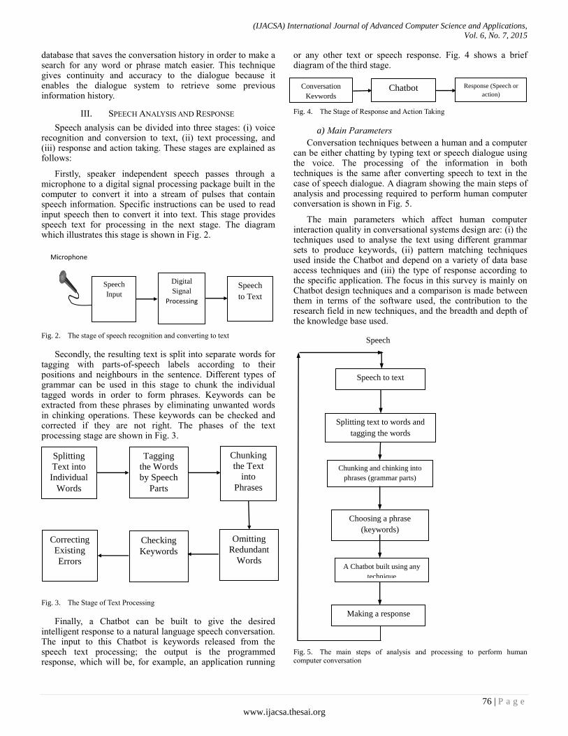
(IJACSA) International Journal of Advanced Computer Science and Applications,
Vol. 6, No. 7, 2015
76 | P a g e
www.ijacsa.thesai.org
database that saves the conversation history in order to make a search for any word or phrase match easier. This technique gives continuity and accuracy to the dialogue because it enables the dialogue system to retrieve some previous information history.
III. SPEECH ANALYSIS AND RESPONSE
Speech analysis can be divided into three stages: (i) voice recognition and conversion to text, (ii) text processing, and (iii) response and action taking. These stages are explained as follows:
Firstly, speaker independent speech passes through a microphone to a digital signal processing package built in the computer to convert it into a stream of pulses that contain speech information. Specific instructions can be used to read input speech then to convert it into text. This stage provides speech text for processing in the next stage. The diagram which illustrates this stage is shown in Fig. 2.
Fig. 2. The stage of speech recognition and converting to text
Secondly, the resulting text is split into separate words for tagging with parts-of-speech labels according to their positions and neighbours in the sentence. Different types of grammar can be used in this stage to chunk the individual tagged words in order to form phrases. Keywords can be extracted from these phrases by eliminating unwanted words in chinking operations. These keywords can be checked and corrected if they are not right. The phases of the text processing stage are shown in Fig. 3.
Fig. 3. The Stage of Text Processing
Finally, a Chatbot can be built to give the desired intelligent response to a natural language speech conversation. The input to this Chatbot is keywords released from the speech text processing; the output is the programmed response, which will be, for example, an application running
or any other text or speech response. Fig. 4 shows a brief diagram of the third stage.
Fig. 4. The Stage of Response and Action Taking
a) Main Parameters
Conversation techniques between a human and a computer can be either chatting by typing text or speech dialogue using the voice. The processing of the information in both techniques is the same after converting speech to text in the case of speech dialogue. A diagram showing the main steps of analysis and processing required to perform human computer conversation is shown in Fig. 5.
The main parameters which affect human computer interaction quality in conversational systems design are: (i) the techniques used to analyse the text using different grammar sets to produce keywords, (ii) pattern matching techniques used inside the Chatbot and depend on a variety of data base access techniques and (iii) the type of response according to the specific application. The focus in this survey is mainly on Chatbot design techniques and a comparison is made between them in terms of the software used, the contribution to the research field in new techniques, and the breadth and depth of the knowledge base used.
Fig. 5. The main steps of analysis and processing to perform human
computer conversation
Speech
to Text
Speech
Input
Digital
Signal
Processing
Microphone
Tagging
the Words
by Speech
Parts
Splitting
Text into
Individual
Words
Chunking
the Text
into
Phrases
Omitting
Redundant
Words
Checking
Keywords
Correcting
Existing
Errors
Choosing a phrase
(keywords)
A Chatbot built using any
technique
Speech to text
Splitting text to words and
tagging the words
Chunking and chinking into
phrases (grammar parts)
Making a response
Speech
Conversation
Keywords
Response (Speech or
action) Chatbot

(IJACSA) International Journal of Advanced Computer Science and Applications,
Vol. 6, No. 7, 2015
77 | P a g e
www.ijacsa.thesai.org
IV. A REVIEW ON RECENT CHATBOT DESIGN WORK
A considerable body of work is associated with Chatbots and they have recently become a promising technique for human-computer interaction. Dialogue systems have been built to meet a variety of applications and can be applied in a number of fields. A number of selected studies between 2003 and 2013 are reviewed and explained below.
Although creating a new type of Chatbot is a contribution to the field there are a limited number of options available to the software designer. The authors in [10] created knowledge bases for Chatbots by combining the attributes of two other Chatbots. The authors processed the knowledge bases using three filters to eliminate overlapping, identify personal questions, and reject unwanted words or topics. The corpus is built from a combination of an ALICE foundation type Chatbot, which is a QA form, and another, such as CLEVERBOT or JABBERWACKY, which are good for handling conversational chatter. The authors processed the Chatbot to either dialog or QA pair format according to gathered interaction ordering. Then, according to the processed interaction, they produced a Chat corpus with around 7800 pairs of interactions in total. The purpose of their study was to improve Chatbot design techniques.
Chatbots tend to evolve from one contribution to the next with extensions added by subsequent researchers, adding new features to the software. The author in [22] looked at how to extend serious types of games by adding dialogue using simple Chatbots. In fact, it is a serious and positive step in conversation insertion into the games world. The existing serious game EMERGO has been used as a case study of the work. The author describes the Chatbot-EMERGO, which is designed to train students or trainees in a medical treatment environment [22]. The purpose of the study is to enhance speech interaction between the training programme and the trainees or students.
A new Chatbot can be designed to solve health problems or any other application in a wide variety of fields. In [23] the authors presented the Chatbot ViDi (Virtual Dietician) that interacts with diabetic patients as a virtual adviser. The authors proposed a special design for the Chatbot ViDi to make it remember the conversational paths taken during the question and answer session. The path splits into three levels of 9 questions each and it can be obtained by analysing the parameter Vpath which determines the path taken by the patient. The natural language that is used to interface with the user is the Malaysian local language.
An extension has been made to the chat bot ViDi when the authors in [24] proposed the entire redesign of the ViDi Chatbot by employing the advantages of a relational database. They also added an extension and prerequisite algorithm to update ViDi into a web-based Chatbot. The authors used web programming languages such as PHP, HTML and XHR to implement the coding of the Chatbot in addition to Asynchronous
Javascript + XML (AJAX). Again Malaysian is used. The extension of ViDi designed in [23] makes it available to users on the internet through a web browser.
Pattern matching techniques can also be applied in the Chatbot design world, and can lead to increased accuracy of retrieval. The authors in [25] proposed a new technique for keyword matching using ViDi, ([23] and updated in [24]) as a test environment. The proposed technique is called One Match or All Match Categories (OMAMC). OMAMC is used to test the generation of possible keywords associated with one sample sentence. Then, the results are compared to other keywords generated by another previous Chatbot around the same sample sentence. It is found that OMAMC improves on keyword matching compared to previous techniques. This new approach is likely to be found in future instantiations of Chatbots.
Educational systems are another application of Chatbots. The objective is to answer students‟ questions or to test for an examination by asking questions and assessing the answers. In [26] the authors concentrates on an improvement to the Chatbot CHARLIE (CHAtteR Learning Interface Entity). The platform is an INtelligent Educational System (INES) with an AIML Chatbot incorporated inside. The performance and contribution of CHARLIE are documented in his paper and CHARLIE is able to establish a general conversation with students; it can show the material of the courses they study and it is prepared to ask questions associated with the material learned. Educational applications of dialogue systems are particularly useful and are highly interactive. They can be improved and updated easily since they are used in an academic environment.
The application of Chatbots to Disability care requires the design of packages and systems in order to empower disabled people with new technologies. The authors in [5] suggested a question-answer educational system for disabled people, considering natural language speech and isolated word conversation. The system has been designed using an AIML knowledge base with limited vocabulary including voice recognition or “groups of phonemes and words”. The AIML question-answer system is implemented to give answers to queries, and then training data of 2000 words is used to test it. 200 words of the data were used in the test and 156 of them were recognised; therefore, the system accuracy was 78%. The aim of the study was to insert it in English language tutorial software easy access by disabled people. People with blindness and hand paralysis can benefit from adding this kind of feature into E-learning systems.
Introducing new matching models represents true innovation within Chatbots. In [27] the author proposed a new model that produces a new sentence from two existing sentences. The study proposes employing a Genetic Algorithm (GA) to build a new

(IJACSA) International Journal of Advanced Computer Science and Applications,
Vol. 6, No. 7, 2015
78 | P a g e
www.ijacsa.thesai.org
sentence depending on the sentences that are retrieved from an available database. The proposal is presented in order to adapt the GA to a natural language structure.
The proposal in [27] was implemented when the authors in [9] presented their new approach to Chatbot design. The approach combines indexing and query matching methods with pattern matching and applies Information Retrieval (IR) techniques to produce a new sentence from existing ones. In their study, the existing sentences became the initial population of the GA, then the swap and crossover operators were applied to produce the new sentence as a new generation of the GA. Experimental evaluation for the Chatbot before and after applying the sentence combination approach were presented. The purpose of the approach was to
improve the diversity of the Chatbot response. The two main contributions of the study are i) converting two sentences into one and ii) Applying information retrieval techniques to Chatbots.
As seen in the above review, conversational techniques can be applied to a variety of different applications involving the interaction between people and computers. Efforts to insert conversation into these different systems is shown to be useful with all studies concluding that adding a Chatbot to a system or software improves the interaction with the system.
V. SELECTED FACTORS INFLUENCING CHATBOT DESIGN
Commonalities and differences in Chatbot designs have been highlighted with the Influential factors included in the survey. A summary of these factors can be seen in table 2.
TABLE II. A SUMMARY OF THE SELECTED FACTORS INFLUENCING CHABOT DESIGN
Study
Factors Influencing Chatbot Design
Voice Text Creating new
Chatbot
Using
available
Chatbo
ts
AIML
usage
SQL usage (Relational
Database)
Matching technique Corpus (knowledge
base)
Application
Pereira et al [10]
Yes
Yes
NO
Yes
Yes
NO
Edger Chatbot matching
technique (combination of
TfIdf algorithms with
natural language
normalization)
Edgar
Chatbot Chatbot design.
Rosmalen [22] NO Yes NO Yes Yes Yes QA matching form AIML Medical education
Lokman et al
[23] NO Yes Yes NO Yes Yes QA matching form VP bot Health assistance
Lokman et al [24]
NO Yes NO Yes NO Yes Prerequisite
Matching
ViDi
Chatbot Health assistance
Lokman et al [25]
NO Yes NO Yes NO Yes One-Match All-Match
Category (OMAMC)
ViDi
Chatbot Health assistance
Mikic et al [26] NO Yes NO Yes Yes NO AIML category pattern
matching AIML
Educational
systems
Bhargava et al [5]
Yes NO Yes NO Yes NO AIML category pattern matching
AIML E-learning
Vrajitoru [27]
NO Yes Yes NO NO NO Genetic
Algorithms (GA)
Manual
pattern and
data chosen
Any
Ratkiewicz
[9] NO Yes Yes NO NO NO
Genetic
Algorithms (GA)
Manual
pattern and
data chosen
Any
VI. SUMMARY OF SIGNIFICANT IMPROVEMENTS IN THE
ANALYSED STUDIES
Each of the selected studies made improvements in Chatbot design. A summary of contributions made is shown in table 3.
VII. DISCUSSION
The examination of factors which influence Chatbot design shows that there are commonalities and differences between the highlighted studies.

(IJACSA) International Journal of Advanced Computer Science and Applications,
Vol. 6, No. 7, 2015
79 | P a g e
www.ijacsa.thesai.org
Although the processing steps are the same for voice and text after the voice to text conversion, there are distinct differences in the use in conversational systems, particularly in terms of their applications. Text is used in most of the studies, except [5], due to simplicity, whereas voice is used in [5] and [10] for special needs applications e.g. for disabled people. The response in the case of disability applications should be a voice response. The commercial mobile applications (Chatbots) which have emerged recently, e.g. Cortana and Siri, accept speech as an input and give a voice response in addition to text.
New Chatbots have been created in [5], [9], [23], and [27], which add new techniques or use improved previous designs. Also new techniques, algorithms or extensions have been added to existing Chatbots in [10], [22], [24], [25], and [26] in order to improve their function or extend available software by adding chat interaction. For example, the Loebner Prized Chatbot ALICE (which won three times) was improved several times in later iterations, and Joan (Jabberwacky) was the updated form of George (Jabberwacky).
Knowledge bases are built using different techniques. For example, AIML, which is the technique first used with the ALICE Chatbot, is used to build the Chatbots in [5], [10], and [26], while SQL (or RDB) is used in [24] and [25]. Both AIML and SQL are used in [22] and [23]. Neither AIML or SQL are used in [9] and [27]. The use of SQL (no clear
evidence of using it in Loebner Prized Chatbots) added a new technique to knowledge-bases, namely the Relational Data Base, which enables the Chatbot to remember previous conversations by accessing the history stored in the database designed using SQL. However, an AIML knowledgebase is still effective for Chatbot designs; for example, Mitsuku Chatbot won Loebner Prize in 2013 and it was based on AIML.
In order to design new Chatbots or extend previous ones, each study has used a corpus that is different from the other as illustrated in table 2. The corpus that is relied on to build a Chatbot affects the design because it affects the knowledge base of the Chatbot and then the accuracy of the response since the response is a knowledgebase reflection.
The application column in table 2 shows that each Chatbot has been designed to meet certain needs for conversation by holding a chat with a specific group of people in a specific organisation. The work in the future needs more focus on general purpose conversational systems by designing Chatbots with more comprehensive knowledge bases in order to cover general topics by using the latest techniques.
Table 3, which covers the contribution presented by each of the selected studies, displays how each has made an improvement to Chatbot design in spite of using different techniques, algorithms, or programmes.
TABLE III. A SUMMARY OF CONTRIBUTIONS FOR CHATBOT DESIGN IN ANALYSED STUDIES
Study
Significant Improvements
Pereira et al [10]
Producing a new corpus (knowledge base) that avoids overlapping, identifies personal questions, and rejects
unwanted words or topics by combining available QA and dialogue formats.
Rosmalen [22] Extending an existing serious game by adding a simple Chatbot to give the opportunity for trainees to be aware of work and activities on the first day of their employment.
Lokman et al [23]
Designing a new Chatbot (ViDi) that has the ability to remember previous conversation in order to work as a
virtual adviser for diabetic patients.
Lokman et al
[24]
Redesigning and extending the Chatbot ViDi by adding the prerequisite matching techniques in order to attain a conversational manner rather than a QA form and make it available to users on the internet via a web browser.
Lokman et al [25]
Proposing a new matching technique OMAMC in order to produce improved results by reducing matching time
and increasing context flexibility.
Mikic et al [26]
Updating the Chatbot CHARLIE to incorporate it into the platform INtelligent Educational System (INES) in order
to improve the conversation between students and educational systems.
Bhargava et al [5]
Designing a new AIML based Chatbot of natural language speech and limited word input and output so as to use it
in an E-learning systems to enable disabled people to learn via speech.
Vrajitoru
[27]
Proposing a new innovative pattern matching approach in a Chatbot. The authors adjusted Genetic Algorithms with natural language to generate a new sentence from existing ones in order to improve the diversity of response.
Ratkiewicz [9]
i) Implementing the model proposed in [27], i.e. employing GA in pattern matching to produce a new sentence
from sentences retrieved from an existing database in order to increase the diversity of responses. ii). Applying information retrieval techniques to the Chatbot.

(IJACSA) International Journal of Advanced Computer Science and Applications,
Vol. 6, No. 7, 2015
80 | P a g e
www.ijacsa.thesai.org
VIII. CONCLUSIONS
In this paper, the literature review has covered a number of selected papers that have focused specifically on Chatbot design techniques in the last decade. A survey of nine selected studies that affect Chatbot design has been presented, and the contribution of each study has been identified. In addition, a comparison has been made between Chatbot design techniques in the selected studies and then with the Loebner Prize winning Chatbot techniques. From the survey above, it can be said that the development and improvement of Chatbot design is not grow at a predictable rate due to the variety of methods and approaches used to design a Chatbot. The techniques of Chatbot design are still a matter for debate and no common approach has yet been identified. Researchers have so far worked in isolated environments with reluctance to divulge any improved techniques they have found, consequently, slowing down the improvements to Chatbots. Moreover, the Chatbots designed for dialogue systems in the selected studies are, in general, limited to particular applications. General-purpose Chatbots need improvements by designing more comprehensive knowledge bases.
Although some commercial products have emerged recently in the market (e.g. Microsoft Cortana) as dialogue Chatbots, improvements need continuous research and lack a
common solution.
Each researcher needs to robustly document any successful improvements to allow the human computer speech interaction to agree a common approach. This will always be at odds with commercial considerations.
REFERENCES
[1] C. I. Nass, and S. Brave, Wired for speech: How voice activates and advances the human-computer relationship: MIT Press Cambridge, 2005.
[2] Y.-P. Yang, “An Innovative Distributed Speech Recognition Platform for Portable, Personalized and Humanized Wireless Devices,” Computational Linguistics and Chinese Language Processing, vol. 9, no. 2, pp. 77-94, 2004.
[3] J. P. Campbell Jr, “Speaker recognition: a tutorial,” Proceedings of the IEEE, vol. 85, no. 9, pp. 1437-1462, 1997.
[4] C.-H. Lee, "From knowledge-ignorant to knowledge-rich modeling: a new speech research paradigm for next generation automatic speech recognition", 2004.
[5] V. Bhargava, and N. Maheshwari, “An Intelligent Speech Recognition System for Education System,” 2009.
[6] E. Loper, and S. Bird, "NLTK: The natural language toolkit." pp. 63-70, 2002.
[7] S. Bird, "NLTK: the natural language toolkit." pp. 69-72, 2006.
[8] A. M. Galvao, F. A. Barros, A. M. Neves, and G. L. Ramalho, "Persona-aiml: An architecture developing chatterbots with personality." pp. 1266-1267, 2004.
[9] J. Ratkiewicz, “Evolutionary Sentence Combination for Chatterbots Dana Vrajitoru Computer and Information Sciences Indiana University South Bend, 1700 Mishawaka Ave,” 2004.
[10] M. J. Pereira, and L. Coheur, “Just. Chat-a platform for processing information to be used in chatbots,” 2013.
[11] D. J. Stoner, L. Ford, and M. Ricci, “Simulating Military Radio Communications Using Speech Recognition and Chat-Bot Technology,” 2003.
[12] K. Meffert, "Supporting design patterns with annotations." pp. 8 pp.-445, 2006.
[13] D. Mladenić, and L. Bradeško, “A survey of chabot system through a Loebner prize competition,” 2012.
[14] A. M. Turing, “Computing machinery and intelligence,” Mind, pp. 433-460, 1950.
[15] B. Kirkpatrick, and B. Klingner, “Turing‟s Imitation Game: a discussion with the benefit of hind-sight,” Berkeley Computer Science course. See http://www. cs. berkeley. edu/~ christos/classics/ttest. pdf Accessed, vol. 1, pp. 13, 2009.
[16] P. Hingston, “A turing test for computer game bots,” Computational Intelligence and AI in Games, IEEE Transactions on, vol. 1, no. 3, pp. 169-186, 2009.
[17] R. Higashinaka, K. Imamura, T. Meguro, C. Miyazaki, N. Kobayashi, H. Sugiyama, T. Hirano, T. Makino, and Y. Matsuo, "Towards an open domain conversational system fully based on natural language processing", 2014.
[18] B. Wilcox, "Winning the Loebner's," http://www.gamasutra.com/blogs/BruceWilcox/20141020/228091/Winning_the_Loebners.php, 2014.
[19] R. Wallace, “The elements of AIML style,” Alice AI Foundation, 2003.
[20] M. d. G. B. Marietto, R. V. de Aguiar, G. d. O. Barbosa, W. T. Botelho, E. Pimentel, R. d. S. França, and V. L. da Silva, “Artificial Intelligence MArkup Language: A Brief Tutorial,” arXiv preprint arXiv:1307.3091, 2013.
[21] W. Kim, “On optimizing an SQL-like nested query,” ACM Transactions on Database Systems (TODS), vol. 7, no. 3, pp. 443-469, 1982.
[22] P. Van Rosmalen, J. Eikelboom, E. Bloemers, K. Van Winzum, and P. Spronck, “Towards a Game-Chatbot: Extending the Interaction in Serious Games,” 2012.
[23] A. S. Lokman, and J. M. Zain, "An architectural design of Virtual Dietitian (ViDi) for diabetic patients." pp. 408-411, 2009.
[24] A. S. Lokman, and J. M. Zain, “Extension and prerequisite: An algorithm to enable relations between responses in chatbot technology,” Journal of Computer Science, vol. 6, no. 10, pp. 1212, 2010.
[25] A. S. Lokman, and J. M. Zain, “One-Match and All-Match Categories for Keywords Matching in Chatbot,” American Journal of Applied Sciences, vol. 7, no. 10, pp. 1406, 2010.
[26] F. A. Mikic, J. C. Burguillo, M. Llamas, D. A. Rodríguez, and E. Rodríguez, "CHARLIE: An AIML-based Chatterbot which Works as an Interface among INES and Humans." pp. 1-6, 2009.
[27] D. Vrajitoru, "Evolutionary sentence building for chatterbots." pp. 315-321, 2003.

(IJACSA) International Journal of Advanced Computer Science and Applications,
Vol. 6, No. 7, 2015
81 | P a g e
www.ijacsa.thesai.org
Research on Islanding Detection of Grid-Connected
System
Liu Zhifeng
School of Electronic and Electrical Engineering
Shanghai University of Engineering Science, SUES
Shanghai, China
Zhang Liping*
School of Electronic and Electrical Engineering
Shanghai University of Engineering Science, SUES
Shanghai, China
Chen Yuchen
School of Electronic and Electrical Engineering
Shanghai University of Engineering Science, SUES
Shanghai, China
Jia Chunying
School of Electronic and Electrical Engineering
Shanghai University of Engineering Science, SUES
Shanghai, China
Abstract—This paper proposed a modified detection based on
the point of common coupling (PCC) voltage in the three−phrase
inverter, combined over/under frequency protection, to achieve
the detection of islanding states rapidly. Islanding detection is an
common issue existing in distributed generation system.
Compared with active islanding detection ,this method could
detect the islanding quickly and effectively .The simulation and
experimental results shows that this new method can detect the
islanding phenomenon quickly and accurately, which can meet
the requirement of islanding detection standard, which ensure
the stability of the system and the power quality recycling to the
grid.
Index Terms—islanding detection; self−adaptive; active
frequency shift; d−q transform
I. INTRODUCTION
Islanding effect is also called Islanding phenomenon, the phenomenon is common in the photovoltaic grid−connected generation system. The power grid stop supplying the local load because of the fault or misoperation , however, the power system cannot detect it, still supplying the peripheral load, forming the power island out of the control of power grid.
Islanding effect will lead to serious results, such as disturbing the operation of the electricity system, destroying user devices, even severely endangered the life safety of the staff who is working for lines maintenance. Consequently, whether the condition of islanding can be detected effectively and timely or not is of great significant for the entire grid-connected system.
II. MECHANISM AND DETECTION METHOD OF THE
ISLANDING EFFECT
In a real world application, the lord of the photovoltaic employs RLC parallel resonance circuit. According to the IEEE Std.929-2000 [1] , the recommended generic system for islanding detection [2] study is shown in Fig.1.
S1 S2
R L C
Ua,ωa
a
Ppv,Qpv
PL,
QL
ΔP,ΔQ
The pv grid-connected inverter
Electric network source
Fig. 1. System for islanding detection study
If the distributed grid-connected generation system works properly, namely
2
aL
UP
R
21
L a a
a
Q c UL
After the electric network cuts off the power, the photovoltaic grid-connected generation system generate islanding effect [3] , namely
2
apv L
UP P
R
pv LP P P
pv LQ Q Q
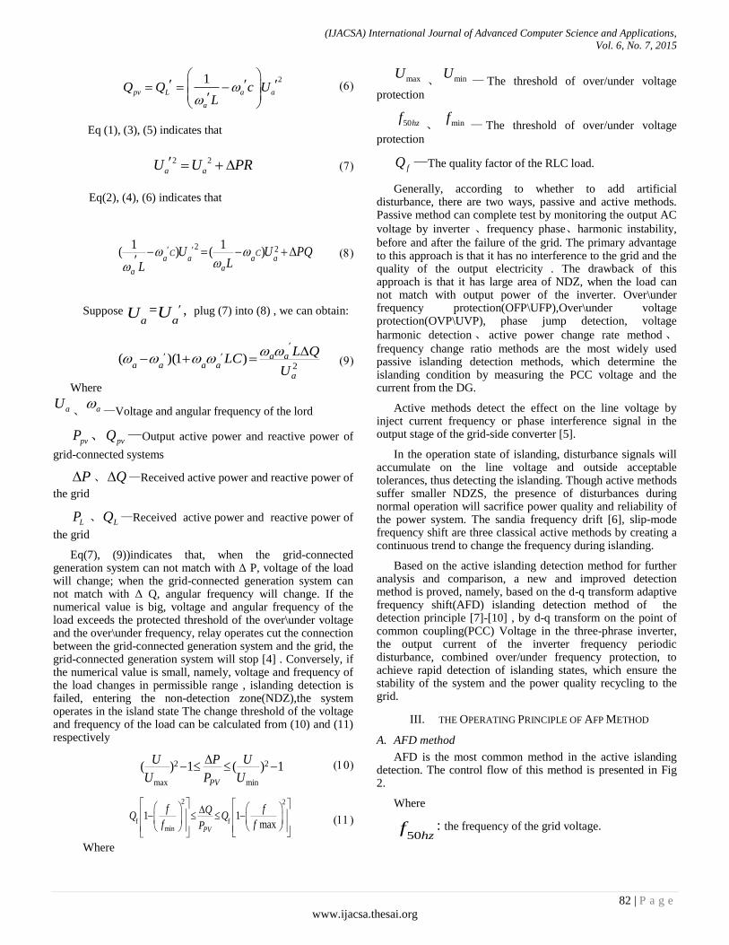
(IJACSA) International Journal of Advanced Computer Science and Applications,
Vol. 6, No. 7, 2015
82 | P a g e
www.ijacsa.thesai.org
21
pv L a a
a
Q Q c UL
Eq (1), (3), (5) indicates that
2 2
a aU U PR
Eq(2), (4), (6) indicates that
Suppose a
U =a
U , plug (7) into (8) , we can obtain:
Where
aU、 a —Voltage and angular frequency of the lord
pvP 、 pvQ —Output active power and reactive power of
grid-connected systems
P 、 Q —Received active power and reactive power of
the grid
LP
、 LQ —Received active power and reactive power of
the grid
Eq(7), (9))indicates that, when the grid-connected generation system can not match with Δ P, voltage of the load will change; when the grid-connected generation system can not match with Δ Q, angular frequency will change. If the numerical value is big, voltage and angular frequency of the load exceeds the protected threshold of the over\under voltage and the over\under frequency, relay operates cut the connection between the grid-connected generation system and the grid, the grid-connected generation system will stop [4] . Conversely, if the numerical value is small, namely, voltage and frequency of the load changes in permissible range , islanding detection is failed, entering the non-detection zone(NDZ),the system operates in the island state The change threshold of the voltage and frequency of the load can be calculated from (10) and (11) respectively
Where
maxU、 minU
— The threshold of over/under voltage
protection
50hzf、 minf
— The threshold of over/under voltage
protection
fQ —The quality factor of the RLC load.
Generally, according to whether to add artificial disturbance, there are two ways, passive and active methods. Passive method can complete test by monitoring the output AC
voltage by inverter 、frequency phase、harmonic instability,
before and after the failure of the grid. The primary advantage to this approach is that it has no interference to the grid and the quality of the output electricity . The drawback of this approach is that it has large area of NDZ, when the load can not match with output power of the inverter. Over\under frequency protection(OFP\UFP),Over\under voltage protection(OVP\UVP), phase jump detection, voltage
harmonic detection 、 active power change rate method 、frequency change ratio methods are the most widely used passive islanding detection methods, which determine the islanding condition by measuring the PCC voltage and the current from the DG.
Active methods detect the effect on the line voltage by inject current frequency or phase interference signal in the output stage of the grid-side converter [5].
In the operation state of islanding, disturbance signals will accumulate on the line voltage and outside acceptable tolerances, thus detecting the islanding. Though active methods suffer smaller NDZS, the presence of disturbances during normal operation will sacrifice power quality and reliability of the power system. The sandia frequency drift [6], slip-mode frequency shift are three classical active methods by creating a continuous trend to change the frequency during islanding.
Based on the active islanding detection method for further analysis and comparison, a new and improved detection method is proved, namely, based on the d-q transform adaptive frequency shift(AFD) islanding detection method of the detection principle [7]-[10] , by d-q transform on the point of common coupling(PCC) Voltage in the three-phrase inverter, the output current of the inverter frequency periodic disturbance, combined over/under frequency protection, to achieve rapid detection of islanding states, which ensure the stability of the system and the power quality recycling to the grid.
III. THE OPERATING PRINCIPLE OF AFP METHOD
A. AFD method
AFD is the most common method in the active islanding detection. The control flow of this method is presented in Fig 2.
Where
50hzf : the frequency of the grid voltage.
PQUL
UL
aC
aa
aC
a
a
22)
1()
1(
2)1)((
a
aaaaaa
U
QLLC
2 2
max min
( ) 1 ( ) 1PV
U P U
U P U
2 2
f fmin
1 1max
PV
f fQQ Q
f fP

(IJACSA) International Journal of Advanced Computer Science and Applications,
Vol. 6, No. 7, 2015
83 | P a g e
www.ijacsa.thesai.org
invf :the output voltage frequency of the inverter
f : the set value of frequency perturbation in the
control system
START
50inv hzf f f
Inverter
The grid is normal or not
50inv hzf f f ( 1) ( )
inv invf k f k f
50.5inv
f hz
Power network fault
Y N
N
Y
Fig. 2. Flowchart of the AFD method
Active frequency drift method works as follows:
Firstly, there are certain errors-Δf, between the frequency of the output voltage and the grid voltage through the control of the inverter. Secondly, Δf is always within a narrow range because of the corrective action in the phase-locked loops circuit, when the grid operates properly [11] . Thirdly, the
output voltage frequency of the inverter finv will change, when
the grid failure. At the following power frequency periodic of
the inverter, based on the finv,, adding the set value of
frequency perturbation to control the output voltage frequency of the inverter. It leads to the increasement of errors between output voltage frequency and the grid voltage frequency. The cycle continues after this, until output voltage frequency of triggering protection circuit [12], cutting the connection between inverter and the grid.
Fig 3 illustrate the waveform of the perturbation frequencies using AFD method. The curve describe the wave of current and interference signal in one power frequency periodic, plotted by time on the horizontal axis and per unit value of current on the vertical. The relations are as follows:
/z gridcf t T
Where
zt : The period of the voltage value is zero.
gridT : A half cycle of the fundamental voltage
B. The shortage of AFD method
As presented in [13],if the islanding occurs in the grid-connected generation system. There will be a much smaller
NDZS using AFD method than using passive detection methods. Once the value of cf is too small, compared with the traditional voltage frequency detection method, AFD method can not highlight its superiority; however, when the cf exceed the permitted value, the distortion ratio of current harmonic on AC grid side will increase, harmonics will affect the power quality recycling to the grid seriously. Therefore, NDZS in the AFD [14] would still need to be reduced in order to satisfy the increasing harsh conditions of the grid.
When the system load does not conform to (1), the system frequency will always beyond the normal range of work in theory. But, there is a time limit on detecting the islanding, especially the use of the automatic reclosing at present. If the detecting speed is too slow, the grid-connected generation system is not completely cut off before the automatic reclosing recloses again, it is very likely to make considerable oscillation, leading to accidents. Such a scenario may be typically in the AFD method, for example when the load is inductive, there is a trend that the phase of voltage is prior to current, the frequency of value will keep rising based on the assumption that without using AFD method, when the islanding happens [15]. However, if the value of cf is fixed in the AFD method, mitigating voltage frequency change, but tend to delay the trip time, and vice versa.
Fig. 3. Waveform of the perturbation frequencies using AFD method
C. Adaptive Acive Frequency Shift Islanding Detection Based
on the d-q Transform
For overcoming the shortcomings of AFD method for islanding detection ,the detection algorithm of AFD method needs to be improved, convert the output current frequency disturbance of the inverter within single-phase into three-phase
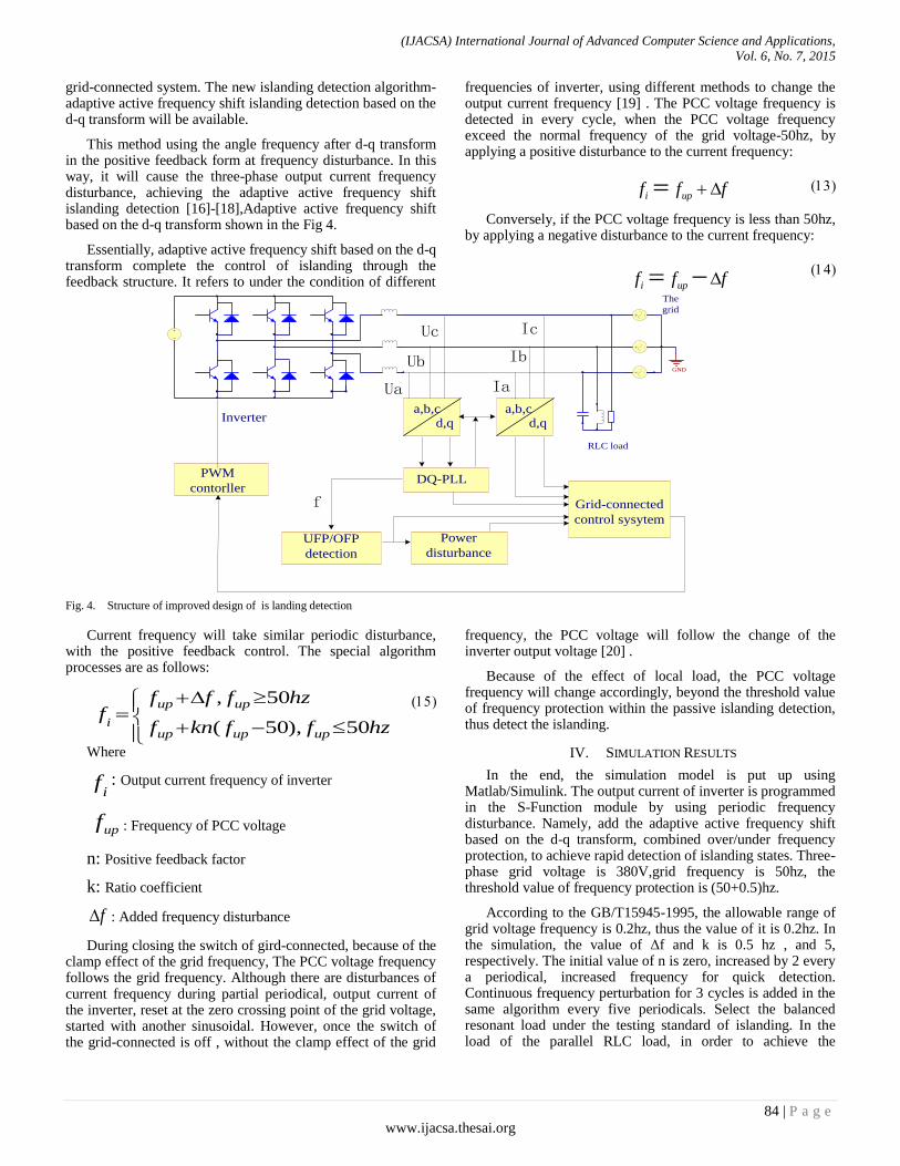
(IJACSA) International Journal of Advanced Computer Science and Applications,
Vol. 6, No. 7, 2015
84 | P a g e
www.ijacsa.thesai.org
grid-connected system. The new islanding detection algorithm-adaptive active frequency shift islanding detection based on the d-q transform will be available.
This method using the angle frequency after d-q transform in the positive feedback form at frequency disturbance. In this way, it will cause the three-phase output current frequency disturbance, achieving the adaptive active frequency shift islanding detection [16]-[18],Adaptive active frequency shift based on the d-q transform shown in the Fig 4.
Essentially, adaptive active frequency shift based on the d-q transform complete the control of islanding through the feedback structure. It refers to under the condition of different
frequencies of inverter, using different methods to change the output current frequency [19] . The PCC voltage frequency is detected in every cycle, when the PCC voltage frequency exceed the normal frequency of the grid voltage-50hz, by applying a positive disturbance to the current frequency:
Conversely, if the PCC voltage frequency is less than 50hz, by applying a negative disturbance to the current frequency:
Fig. 4. Structure of improved design of is landing detection
Current frequency will take similar periodic disturbance, with the positive feedback control. The special algorithm processes are as follows:
Where
if : Output current frequency of inverter
upf : Frequency of PCC voltage
n: Positive feedback factor
k: Ratio coefficient
f : Added frequency disturbance
During closing the switch of gird-connected, because of the clamp effect of the grid frequency, The PCC voltage frequency follows the grid frequency. Although there are disturbances of current frequency during partial periodical, output current of the inverter, reset at the zero crossing point of the grid voltage, started with another sinusoidal. However, once the switch of the grid-connected is off , without the clamp effect of the grid
frequency, the PCC voltage will follow the change of the inverter output voltage [20] .
Because of the effect of local load, the PCC voltage frequency will change accordingly, beyond the threshold value of frequency protection within the passive islanding detection, thus detect the islanding.
IV. SIMULATION RESULTS
In the end, the simulation model is put up using Matlab/Simulink. The output current of inverter is programmed in the S-Function module by using periodic frequency disturbance. Namely, add the adaptive active frequency shift based on the d-q transform, combined over/under frequency protection, to achieve rapid detection of islanding states. Three-phase grid voltage is 380V,grid frequency is 50hz, the threshold value of frequency protection is (50+0.5)hz.
According to the GB/T15945-1995, the allowable range of grid voltage frequency is 0.2hz, thus the value of it is 0.2hz. In the simulation, the value of Δf and k is 0.5 hz , and 5, respectively. The initial value of n is zero, increased by 2 every a periodical, increased frequency for quick detection. Continuous frequency perturbation for 3 cycles is added in the same algorithm every five periodicals. Select the balanced resonant load under the testing standard of islanding. In the load of the parallel RLC load, in order to achieve the
i upf f f
, 50
( 50), 50
up up
iup up up
f f f hzf
f kn f f hz
i upf f f
GND
Inverter
PWM
contorller
UFP/OFP
detection
Power
disturbance
DQ-PLL
a,b,cd,q
Grid-connected
control sysytem
a,b,cd,q
RLC load
The
grid
f
Ua
Ub
Uc
Ia
Ib
Ic
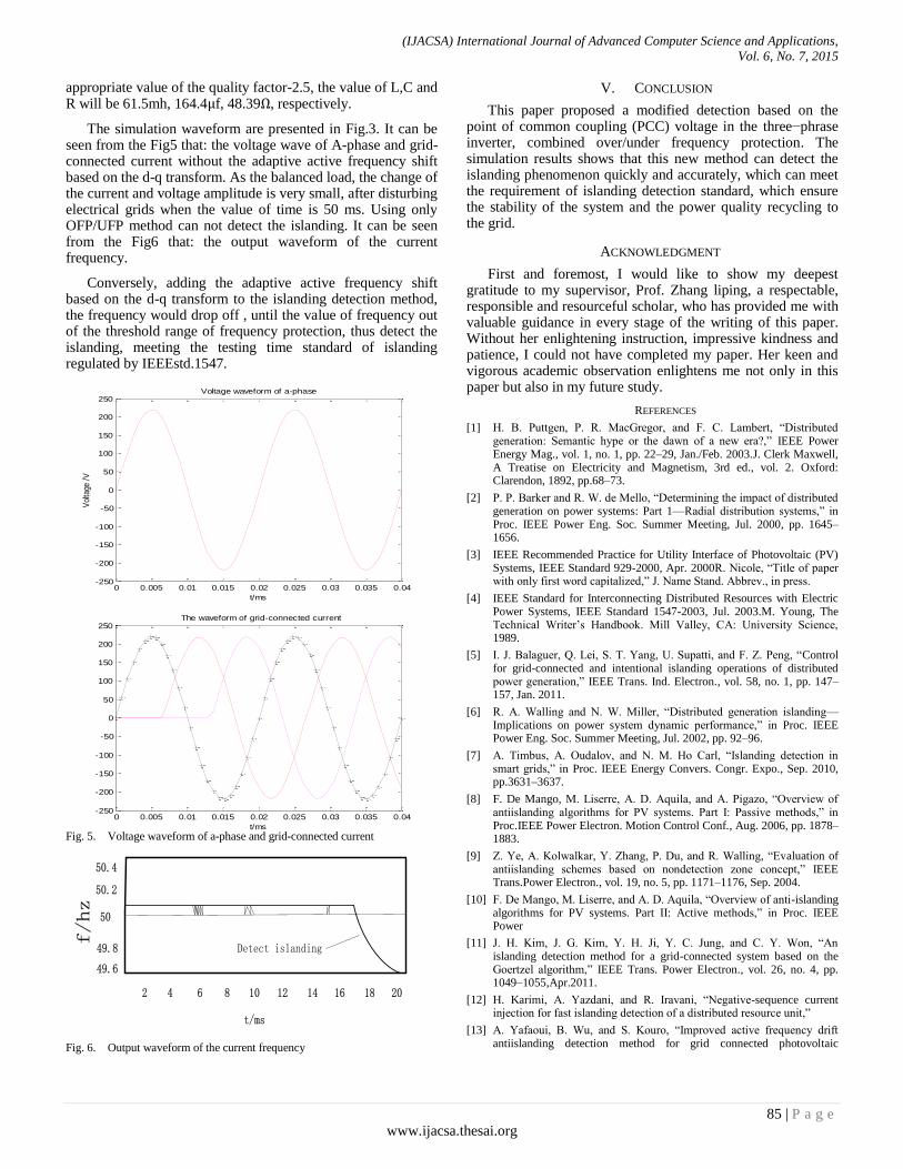
(IJACSA) International Journal of Advanced Computer Science and Applications,
Vol. 6, No. 7, 2015
85 | P a g e
www.ijacsa.thesai.org
appropriate value of the quality factor-2.5, the value of L,C and R will be 61.5mh, 164.4μf, 48.39Ω, respectively.
The simulation waveform are presented in Fig.3. It can be seen from the Fig5 that: the voltage wave of A-phase and grid-connected current without the adaptive active frequency shift based on the d-q transform. As the balanced load, the change of the current and voltage amplitude is very small, after disturbing electrical grids when the value of time is 50 ms. Using only OFP/UFP method can not detect the islanding. It can be seen from the Fig6 that: the output waveform of the current frequency.
Conversely, adding the adaptive active frequency shift based on the d-q transform to the islanding detection method, the frequency would drop off , until the value of frequency out of the threshold range of frequency protection, thus detect the islanding, meeting the testing time standard of islanding regulated by IEEEstd.1547.
Fig. 5. Voltage waveform of a-phase and grid-connected current
Fig. 6. Output waveform of the current frequency
V. CONCLUSION
This paper proposed a modified detection based on the point of common coupling (PCC) voltage in the three−phrase inverter, combined over/under frequency protection. The simulation results shows that this new method can detect the islanding phenomenon quickly and accurately, which can meet the requirement of islanding detection standard, which ensure the stability of the system and the power quality recycling to the grid.
ACKNOWLEDGMENT
First and foremost, I would like to show my deepest gratitude to my supervisor, Prof. Zhang liping, a respectable, responsible and resourceful scholar, who has provided me with valuable guidance in every stage of the writing of this paper. Without her enlightening instruction, impressive kindness and patience, I could not have completed my paper. Her keen and vigorous academic observation enlightens me not only in this paper but also in my future study.
REFERENCES
[1] H. B. Puttgen, P. R. MacGregor, and F. C. Lambert, ―Distributed generation: Semantic hype or the dawn of a new era?,‖ IEEE Power Energy Mag., vol. 1, no. 1, pp. 22–29, Jan./Feb. 2003.J. Clerk Maxwell, A Treatise on Electricity and Magnetism, 3rd ed., vol. 2. Oxford: Clarendon, 1892, pp.68–73.
[2] P. P. Barker and R. W. de Mello, ―Determining the impact of distributed generation on power systems: Part 1—Radial distribution systems,‖ in Proc. IEEE Power Eng. Soc. Summer Meeting, Jul. 2000, pp. 1645–1656.
[3] IEEE Recommended Practice for Utility Interface of Photovoltaic (PV) Systems, IEEE Standard 929-2000, Apr. 2000R. Nicole, ―Title of paper with only first word capitalized,‖ J. Name Stand. Abbrev., in press.
[4] IEEE Standard for Interconnecting Distributed Resources with Electric Power Systems, IEEE Standard 1547-2003, Jul. 2003.M. Young, The Technical Writer’s Handbook. Mill Valley, CA: University Science, 1989.
[5] I. J. Balaguer, Q. Lei, S. T. Yang, U. Supatti, and F. Z. Peng, ―Control for grid-connected and intentional islanding operations of distributed power generation,‖ IEEE Trans. Ind. Electron., vol. 58, no. 1, pp. 147–157, Jan. 2011.
[6] R. A. Walling and N. W. Miller, ―Distributed generation islanding—Implications on power system dynamic performance,‖ in Proc. IEEE Power Eng. Soc. Summer Meeting, Jul. 2002, pp. 92–96.
[7] A. Timbus, A. Oudalov, and N. M. Ho Carl, ―Islanding detection in smart grids,‖ in Proc. IEEE Energy Convers. Congr. Expo., Sep. 2010, pp.3631–3637.
[8] F. De Mango, M. Liserre, A. D. Aquila, and A. Pigazo, ―Overview of antiislanding algorithms for PV systems. Part I: Passive methods,‖ in Proc.IEEE Power Electron. Motion Control Conf., Aug. 2006, pp. 1878–1883.
[9] Z. Ye, A. Kolwalkar, Y. Zhang, P. Du, and R. Walling, ―Evaluation of antiislanding schemes based on nondetection zone concept,‖ IEEE Trans.Power Electron., vol. 19, no. 5, pp. 1171–1176, Sep. 2004.
[10] F. De Mango, M. Liserre, and A. D. Aquila, ―Overview of anti-islanding algorithms for PV systems. Part II: Active methods,‖ in Proc. IEEE Power
[11] J. H. Kim, J. G. Kim, Y. H. Ji, Y. C. Jung, and C. Y. Won, ―An islanding detection method for a grid-connected system based on the Goertzel algorithm,‖ IEEE Trans. Power Electron., vol. 26, no. 4, pp. 1049–1055,Apr.2011.
[12] H. Karimi, A. Yazdani, and R. Iravani, ―Negative-sequence current injection for fast islanding detection of a distributed resource unit,‖
[13] A. Yafaoui, B. Wu, and S. Kouro, ―Improved active frequency drift antiislanding detection method for grid connected photovoltaic
49.6
50
49.8
50.2
50.4
2 4 6 8 12 14 16 18 2010
t/ms
f/hz
Detect islanding
0 0.005 0.01 0.015 0.02 0.025 0.03 0.035 0.04-250
-200
-150
-100
-50
0
50
100
150
200
250The waveform of grid-connected current
t/ms
0 0.005 0.01 0.015 0.02 0.025 0.03 0.035 0.04-250
-200
-150
-100
-50
0
50
100
150
200
250Voltage waveform of a-phase
t/ms
Vol
tage
/V

(IJACSA) International Journal of Advanced Computer Science and Applications,
Vol. 6, No. 7, 2015
86 | P a g e
www.ijacsa.thesai.org
systems,‖IEEE Trans. Power Electron., vol. 27, no. 5, pp. 2367–2375, May,2012.
[14] L. A. C. Lopes and H. L. Sun, ―Performance assessment of active frequency drifting islanding detection methods,‖ IEEE Trans. Energy Convers.,vol.21,no.1,pp.171–180,Mar.2006
[15] H. Vahedi and M. Karrari, ―Adaptive fuzzy Sandia frequency-shift method for islanding protection of inverter-based distributed generation,‖ IEEE Trans. Power Del., vol. 28, no. 1, pp. 84–92, Jan. 2013.
[16] G. A. Kern, ―SunSine300, utility interactive AC module anti-islanding test results,‖ in Proc. 26th IEEE Power Photovoltaic Spec. Conf., Sep. 1997,pp.1265–1268
[17] E. J. Estebanez, V. M. Moreno, A. Pigazo, M. Liserre, and A.
DellAquila,―Performance evaluation of active islanding - detection algorithms in distributed-generation photovoltaic systems: Two inverters case,‖ IEEE Trans. Ind. Electron., vol. 58, no. 4, pp. 1185–1193, Apr. 2011
[18] L. A. C. Lopes and Y. Z. Zhang, ―Islanding detection assessment of multiinverter systems with active frequency drifting methods,‖ IEEE Trans.PowerDel.,vol.23,no.1,pp.480–486,Jan.2008.
[19] M. A. Kashem and G. Ledwish, ―Distributed generation as voltage support for single wire earth return systems,‖ IEEE Trans. Power Del., vol.19,no.3,pp.1002–1011,Jul.2004.
[20] H. H. Zeineldin, ―A Q–f droop curve for facilitating islanding detection of inverter-based distributed generation,‖ IEEE Trans. Power Electron.,vol. 24, no. 3, pp. 665–673, Mar. 2009.
(IJACSA) International Journal of Advanced Computer Science and Applications,
Vol. 6, No. 7, 2015
87 | P a g e
www.ijacsa.thesai.org
Using Induced Fuzzy Bi-Model to Analyze Employee
Employer Relationship in an Industry
Dhrubajyoti Ghosh
Department of Mathematics
National Institute of Technology, Durgapur
Durgapur, India
Anita Pal
Department of Mathematics
National Institute of Technology, Durgapur
Durgapur, India
Abstract—The employee-employer relationship is an intricate
one. In an industry, the employers expect to achieve
performances in quality and production in order to earn profit,
on the other side employees need good pay and all possible
allowances and best advantages than any other industry. Our
main objective of this paper is to analyze the relationship
between employee and employer in workplace and discussed how
to maintain a strong employee and employer relationship which
can produce the ultimate success of an organization using
Induced Fuzzy bi-model called Induced Fuzzy Cognitive
Relational Maps (IFCRMs). IFCRMs are a directed special
fuzzy digraph modelling approach based on expert's opinion.
This is a non statistical approach to study the problems with
imprecise information.
Keywords—Fuzzy Cognitive Map; Fuzzy Relational Maps;
Fuzzy Cognitive Relational Maps; Induced Fuzzy Cognitive
Relational Maps; Fuzzy bi-model; employee employer relationship
I. INTRODUCTION
The fuzzy model is a finite set of fuzzy relations that form an algorithm for determining the outputs of a process from some finite number of past inputs and outputs. Fuzzy model can be used in applied mathematics, to study social and psychological problem and also used by doctors, engineers, scientists, industrialists and statisticians. Fuzzy models are mathematical tools introduced by L.A. Zadeh (1965). Later Politician scientist Axelord (1976) used this fuzzy model Coginitive Maps (CMs) to study decision making in social and political systems. CMs are signed digraphs designed to represent causal assertion and belief system of a person (or group of experts) with respect to a specific domain, and use that statement in order to analyze the effect of a certain choice on a particular objective.
Using the concepts of neural networks and fuzzy logical approach Bart Kosko (1986) proposed some models which extend the idea of Cognitive Maps by allowing the concepts to be represented linguistically with an associated fuzzy set. These models are well suited to get a clear representation of the knowledge to support decision making process and assist in the area of computational intelligence, which involves the application of soft computing methodologies even though the given inputs are vague, uncertain and even contradictory in nature. There are various types of fuzzy models like Fuzzy Cognitive Maps (FCMs), Fuzzy Relational Maps (FRMs), Fuzzy Relational Equations (FREs), Induced Fuzzy Cognitive Maps (IFCMs). Those models plays a vital role in several real
world data problems like various infectious diseases problems (cancer, tuberculosis, migration etc.), student life in rural area, problems of private employees in their day to day life, effects of social networks on children's daily life etc. In this paper we use fuzzy bi-model called Induced Fuzzy Cognitive Relational Maps (IFCRMs) which is a directed bi-graph with concepts like policies, events, etc. as nodes and causalities as edges. It represents causal relationship between concepts. This fuzzy bi-model studied various social problems. Among these problems we are going to discuss about a particular one. Recent years deals with one of the key human resources (HR) issues in current working life, namely employee relations. Employee relations is a term used to describe a company's efforts to prevent and resolve problems arising from situations at work. In this paper we have focused on employee relation programs and its essential elements which increase employee satisfaction and good morale among workers. Happy workers are more productive, and more productive means a better bottom line for an industry. This paper have organized in nine section. Section one contains introduction. Section two represents basic definition of FCMs and FRMs models. Section three describes about fuzzy bi-model method. Section four gives the idea of FCRMs. Section five gives the mathematical approach of FCRMs of discussed problems. Section six gives the idea of IFCRMs. Section gives the mathematical approach of IFCRMs of discussed problems. Section eight describes the difference between FCRMs and its induced form IFCRMs. Section nine conclusions based on our study.
II. FUZZY MAPPING
Before the discussion of FCMs we describe about the CMs. CMs were introduced by Axelord (1976), in order to develop and study social scientific knowledge in the field of decision making in activities related to international politics. CMs are signed digraphs designed to represent causal assertion and belief system of a person (or group of experts) with respect to a specific domain, and use that statement in order to analyze the effect of a certain choice on particular objectives.
A. Fuzzy Cognitive Maps
Fuzzy Cognitive Maps (FCMs) introduced by Kosko (1986) extend the idea of Cognitive Maps by allowing the concepts to be represented linguistically with an associated fuzzy set. FCMs are fuzzy signed digraph with feedback (Kosko, 1986, 1988). It represents causal relationship between concepts. FCMs list the fuzzy rule or causal flow paths that relate events.

(IJACSA) International Journal of Advanced Computer Science and Applications,
Vol. 6, No. 7, 2015
88 | P a g e
www.ijacsa.thesai.org
B. Formation of FCMs
If increase in one concept or node leads to increase in another concepts, we assign the value 1 and for decreasing we assign the value -1. If there exists no relation between concepts the value 0 is given. Consider the be the nodes of the FCM. Suppose the directed graphs drawn using edge weight . The Matrix E be defined
by where is the weight of the directed edge
. E is called adjacency matrix of the FCM. All matrices
associated with an FCM are always square matrices with diagonal entries as zero. Now
The instantaneous state vector where , and it denotes the ON-OFF position of the node at an instant; if is off and if is on for .
Let be the nodes of the edge of the
FCM form a directed cycle and FCM is said to be cyclic if it possesses a directed cycle. Otherwise it is acyclic.
FCM with cycles is said to have a feedback. when there is a feedback in an FCM, i.e., when the causal relations flow through a cycle in a revolutionary way, the FCM is called dynamical system.
When node i switched on and if the causality flows through the edges of a cycle and if it again caused i, we say that dynamical system goes round and round where .
The equilibrium state for this dynamical system is called hidden pattern.
If the equilibrium state of a dynamical system is a unique state vector, then is called fixed point.
If the FCM settles down with a state vector repeating in the form then this equilibrium is called a limit cycle.
Finite number of FCMs can be combined together to produce the joint effect of all the FCMs with nodes i.e. Combined FCMs denotes the relational matrix by .
Suppose is a vector which is passed into a dynamical system E. Then
after thresholding and updating the vector suppose we get .We denote that by
. Thus the symbol ' ' means the resultant vector has been threshold and updated.
C. Definition of Fuzzy Relational Maps
Fuzzy Relational Maps (FRMs) are a directed graph or a map from domain space to range space with concepts and causalities as edges.
Let,
Domain space
Range space be the nodes of range space.
if i.e. is on state
else i.e. is off state
Similarly,
be the nodes of domain space.
if i.e. is on state
else i.e. is off state.
D. Formation of FRMs
Let and denotes the two nodes of FRMs. be the
weight of the edge (or ), then The
relational matrix be defined as .
Let , where . A is called the instantaneous state vector of the domain space and it denotes the on-off position of the nodes at any instant i.e. if is off and if is on for for domain space. Similarly, , where . is the instantaneous state vector of the range space. if is off and if is on
for for range space.
Let (or ) be the edges of an FRM where
form a directed cycle, FRM is said to be cycle if it possesses a directed cycle. Otherwise, it is acyclic.
An FRM with cycle is said to be an FRM with feedback. When there is feedback in the FRM, the FRM is called a dynamical system.
Let (or )where and .
When (or ) is switched on and if causality flows
and if again causes (or ) an equilibrium is attained.
This equilibrium state is called hidden pattern.
If the equilibrium state of this system is a unique state vector then it is called fixed point. Example: Let us assume dynamical system by switching on . FRM settles down with and ( and ) on i.e. state vector remains as as in . This state vector is called the fixed point.
If the FRM reach a state vector in the forms: ; This form is called limit cycle.
Let be the relational matrices of the
FRMs. Combined FRMs denotes the relational matrix by
Let and be the nodes of FRM. Let us assume is switched on i.e. when an input is given as vector in and the relational matrix is . Now , after thresholding and updating the resultant vector . Now let , passing into and obtain . After threshold and update the vector

(IJACSA) International Journal of Advanced Computer Science and Applications,
Vol. 6, No. 7, 2015
89 | P a g e
www.ijacsa.thesai.org
. The procedure repeated till we get a fixed point or limit cycle.
III. FUZZY MODEL
In this section we describe the basic notions of Fuzzy Bi-model.
A. Bi-Set
Let , where and are non-empty sets with and , then we call as biset.
B. Bi-Vector
Let and
be the two vectors of length n and m respectively. Then is a bi-vector. Let , where is a bi-vector. Now, , where is a zero vector. If , then is an unit vector.
C. Bi-matrix
A matrix T is said to be a fuzzy bi-matrix if where and are two different matrices. Example: let , then is called a bi-matrix or row bi- matrix. Let
*
+ *
+ then is
called square bi-matrix.
D. Bi-graph
Let where and are two distinct graphs then we call as a bi-graph.
E. Product rule of bi-matrix
Let be a bi-matrix where is a matrix and is a matrix. If is a bi-vector such that has components and has components then the product of with is defined as . is a matrix or more mathematically; a bi-vector or a row bi-vector.
F. Bi-transpose of bi-matrix
Let be a bi-matrix. Then the bi- transpose of the bi-matrix is defined as
.
IV. FUZZY COGNITIVE RELATIONAL MAPS
Fuzzy Cognitive Relational Maps (FCRMs) is a directed bi-graph where the pair of associated nodes are bi-nodes. If the order of the bi-matrix associated with FCRMs is square matrix and matrix then the bi-nodes are bi- vectors of length or length .
A. Adjacency Bi-matrix
Consider the bi-nodes concepts
of
FCMs and { } and of FRMs to define a
new FCRMs model. Suppose the directed graph is drawn using the edge bi-weight
, . The bi-matrix
is defined by
, where is
the weight of the directed edge and is the directed
edge of . is called adjacency bi-matrix of FCRMs model, also known as the connecting relational bi-matrix of FCRMs model.
B. Instantaneous rate
Let {( ) } be the bi-
nodes of FCRMs. Now ( ) ( ) where . A is called instantaneous state bi-vector and it denotes the position of the node at an instant.
1) if is and if is for .
2) if is and if is for .
3) if is and if is for .
C. Bi-cyclic FCRMs
Let {( ) } be the bi-
nodes of FCRMs. Now be the bi-edges of FCRMs
where , then the bi-edges form a directed bi-cycle. An FCRMs are said to be bi-cyclic if it possesses a directed bi-cycle. FCRMs are said to be abi-cyclic if it does not possess any directed bi-cycle.
D. Dynamicalbi-system
An FCRMs with bi-cycles is said to have a feedback, when there is a feedback in an FCRMs, i.e. when the causal relations flow through a cycle in a revolutionary way, the FCRMs are called a dynamical bi-systems.
E. Hidden bi-pattern
Let {( ) ( )
} be a bi-cycle. If ( ) is switched ON
and if the causality flows through the edges of the bi-cycle and
if it again causes ( ) we say that the dynamical bi-
system in a loop. This is true for the bi-nodes ( ) The
equilibrium bi-state for the dynamical bi-system is called hidden pattern. If the equilibrium bi-state of the dynamical bi-system is a unique bi-state bi-vector then it is called fixed bi-point.
F. Limit-bicycle
If the FCRMs settles down with a bi-state bi-vector repeating in the form then this equilibrium is called a limit bi-cycle.
G. Threshold and update
Suppose is bi-vector which is passes into a dynamical bi-system .Then
(
) (
)
after thresholding and updating the bi-vector; suppose we get

(IJACSA) International Journal of Advanced Computer Science and Applications,
Vol. 6, No. 7, 2015
90 | P a g e
www.ijacsa.thesai.org
( ) ( ) we denote that
by
(
)
( )( ). Thus the symbol means the
resultant bi-vector has been threshold and updated.
H. Properties of bi-edges
The bi-edges ( )
take the values in fuzzy
causal bi-interval . We have 9 possibilities in FCRMs which making the solution of the problem more sensitive or accurate.
1) denotes no causality between the bi-nodes.
2) indicates that both and
; this
implies increase in bi-nodes .
3) indicates that both and
; this
implies decrease in bi-nodes .
4) Considering the case when ( ) and
then no relation in one bi-node and an increase in other node.
5) If ( ) and
then no causality in the
FCMs node and decreasing relation in FRMs mode.
6) ( ) and
then increasing relation in
FCMs mode and no relation in FRMs.
7) ( ) and
then no relation in FRMs
and an increasing relation in FCMs mode.
8) ( ) and
then decreasing relation in
FCMs mode and increasing relations in FRMs.
9) ( ) and
then increasing relation in
FCMs mode and decreasing relations in FRMs.
I. Modification of given problem
Connection bi-matrix of FCRMs bi-model which has both FCMs and FRMs bi-model. We have assumed be the initial input bi-vector. In , a particular vector components, and , which is in FCMs and FRMs be kept ON state and all other components are OFF state. Now we pass the state vector through the FCRMs bi-model. To convert the resultant vector, the values in FCMs and FRMs component which are greater than or equal to one are made as on state and all others denote as OFF state by assigning the values 1 and 0. The component of FCMs of the resulting vector is kept as it is and the components of FRMs of the resulting vector is multiplied with the inverse of the FCMRs bi-matrix and thresholding yield in a new vector . Using this new input bi-vector, we repeat the same procedure until a fixed point or a limit cycle is obtained. The process has been repeated for all the vectors separately. From this operation we have found the hidden pattern of some vectors in all or many cases from which we have analyzed the causes.
V. ANALYZE THE PROBLEMS OF EMPLOYEE EMPLOYER
RELATIONSHIP USING FCRMS MODEL
The most important part of any business is its people. No business can run effectively without them. But people don't work in a vacuum; they need to communicate and work with others to get their jobs done. To be successful, employers need to manage relationships in the workplace to keep the business
functioning smoothly, avoid problems and make sure individual employees are performing at their best. An organisation with good employee-employer relations provide fair and consistent treatment to all means employers must provide. Employee relations programs are typically part of a human resource strategy designed to ensure the most effective use of people to accomplish the organization's mission. Human resource strategies are deliberate plans companies use to help them gain and maintain a competitive edge in the marketplace. One way to stay ahead is to make sure employees are happy so they don't leave their job and go work for the competition. An effective employee-employer relations program starts with clearly written policies which describe the company's rules, philosophy, procedure for addressing employee-related matters and resolving problems in the workplace. Strategies for good employee-employee relations can take many forms and vary by a number of factors including company size, job security, salaries, promotion, responsibility and many more. Now we proceed onto study and analyze the relationship between employee-employer which is the key to the ultimate success of an organization using FCRMs model. According to experts view and adaptation of the necessary requirement of employee and employer in an industry associated to FCMs of FCRMs model have done by taking as the attribute , This is very important, that we have several nodes and several opinions to draw various model of this relationship. Attributes relating with FCMs of FCRMS model are as follows:
X1 → Pay with allowances and bonus to the employee
X2 → Only pay to the employee
X3 → Pay with allowances (or bonus) to the employee
X4 → Best performance
X5→ Average performance
X6→ Poor performance
X7 → Employee works more number of hours
X8→ Employee works less number of hours
X9 → Maximum profit to the industry
X10 → Only profit to the industry
X11 → Neither profit nor loss to the industry
X12 → Loss to the industry
X13 → Heavy loss to the industry
X14→ Stop work or strike by the employee
X15→ Good relation between employee and employer
X16 → Demand of the employee which are not fulfilled
Similarly we have drawn aFRMs of the bi-matrix FCRMs model. We have taken 16 nodes , in domain
space which denote the employee's requirement.
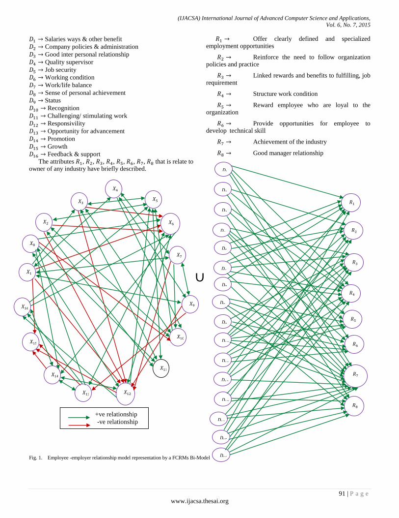
(IJACSA) International Journal of Advanced Computer Science and Applications,
Vol. 6, No. 7, 2015
91 | P a g e
www.ijacsa.thesai.org
Salaries ways & other benefit
Company policies & administration
Good inter personal relationship
Quality supervisor
Job security
Working condition
Work/life balance
Sense of personal achievement
Status
Recognition
Challenging/ stimulating work
Responsivility
Opportunity for advancement
Promotion
Growth
Feedback & support The attributes , , , , , , , that is relate to
owner of any industry have briefly described.
Offer clearly defined and specialized employment opportunities
Reinforce the need to follow organization policies and practice
Linked rewards and benefits to fulfilling, job requirement
Structure work condition
Reward employee who are loyal to the organization
Provide opportunities for employee to develop technical skill
Achievement of the industry
Good manager relationship
Fig. 1. Employee -employer relationship model representation by a FCRMs Bi-Model
+ve relationship
-ve relationship
𝑋
𝑋
𝑋
𝑋
𝑋
𝑋
𝑋
𝑋
𝑋
𝑋
𝑋
𝑋 𝑋
𝑋
𝑋
𝑋
𝐷
𝐷
𝐷
𝐷
𝐷
𝐷
𝐷
𝐷
𝐷
𝐷
𝐷
𝐷
𝐷
𝐷
𝐷
𝐷
𝑅
𝑅
𝑅
𝑅
𝑅
𝑅
𝑅
𝑅

(IJACSA) International Journal of Advanced Computer Science and Applications,
Vol. 6, No. 7, 2015
92 | P a g e
www.ijacsa.thesai.org
With the help of relational model we have drawn a adjacency matrix called E.
TABLE I. ADJACENCY MATRIX OF FCRMS
Here E denotes the connection matrix of the directed graph of FCRMs model. Considering all cases on this relationship model with taking some nodes are on or off and try to find out some hidden pattern
Case 1:
Now we have considered the node (Pay with allowances and bonus to the employee) in FCMs and (Salaries and
other benefits) in FRMs as the on state and all the remaining nodes are in the state.
According the FCRMs method when the same threshold value occurs twice, the value is considered as the fixed point and the iteration and also the calculation gets terminated. Similarly we consider all the different input vectors on and find the hidden patterns for this FCRMs model which are shown in table 2.
0 0 1 1 0 -1 1 0 1 0 0 -1 0 0 1 0
0 0 0 0 1 -1 0 0 0 1 1 -1 0 0 0 0
0 0 0 0 1 -1 0 0 0 1 1 -1 0 0 0 0
1 0 0 0 0 0 1 0 1 1 0 0 0 0 0 0
0 1 1 0 0 0 0 0 0 0 1 0 0 0 0 0
0 0 0 0 0 0 0 0 0 0 0 1 1 1 0 0
1 0 0 1 0 0 0 0 1 1 0 -1 0 0 0 0
0 0 0 0 0 1 0 0 0 -1 1 1 0 1 0 0
1 0 0 1 0 0 1 0 0 0 0 -1 -1 0 0 0
0 1 1 0 1 0 0 0 0 0 0 0 0 0 0 0
0 1 1 0 1 0 0 0 0 0 0 0 0 0 0 0
0 0 0 0 1 1 0 1 0 0 0 0 0 1 -1 1
0 0 0 0 0 1 0 1 0 0 0 0 0 1 -1 1
0 0 0 0 0 0 0 0 0 0 0 1 1 0 -1 1
0 0 0 0 0 0 0 0 0 0 0 0 0 0 0 0
0 0 0 0 1 1 0 0 0 0 0 0 0 1 0 0
1 0 0 1 0 1 1 0
0 1 0 1 0 0 1 0
0 0 0 1 1 0 0 1
0 0 1 0 1 1 1 0
1 1 0 0 0 0 1 0
1 1 1 1 0 0 1 0
1 0 0 1 0 0 0 1
0 0 0 0 1 1 1 1
0 0 1 0 0 1 1 0
1 1 1 0 1 1 1 0
0 0 1 1 1 1 0 0
1 1 0 1 0 0 1 0
0 1 1 0 0 0 1 1
0 0 1 0 0 0 1 1
1 1 0 1 0 0 1 1
0 0 1 1 0 0 1 1
E =
E =

(IJACSA) International Journal of Advanced Computer Science and Applications,
Vol. 6, No. 7, 2015
93 | P a g e
www.ijacsa.thesai.org
TABLE II. THE SET OF FIXED POINTS CORRESPONDS TO DIFFERENT INPUT VECTORS OF FCRMS
Hence from the above table 2 we define the set of limit points as well as fixed point for each different input vectors of FCRMs bi-model and observe the hidden pattern of each cases. Hidden pattern of some vectors found in all or many cases. Inference from this hidden pattern summarizes or highlights the causes.
VI. INDUCED FUZZY COGNITIVE RELATIONAL MAPS
Induced Fuzzy Cognitive Relational Maps (IFCRMs) is a modified version of FCRMs. IFCRMs focussed on algorithmic approaches of FCRMs which works on unsupervised data to derive an optimistic solution.
Step 1: Collect the nodes for the given problem, which is unsupervised data that is in determinant factors.
Step 2: Draw the directed bi-graph for FCRMs model, according to the expert opinion.
Step 3: From FCRMs, obtain the connection matrix E which is combination of both FCMs and FRMs.
Step 4: Consider the initial input bi-vector by setting the first component of this vector in ON position which is denoted by 1 and the rest of the components as 0 which are OFF state.
Step 5: Find . At each stage the state vector is updated and threshold. The symbol ' ' represents the threshold value for the product of the result. The threshold value is calculated from M of FCMs components by assigning 1 for the values and assigning 0 when and two highest values in FRMs components are assigned as state and all others as state by the giving values 1 or 0.
Step 6: The new bi-vector is related with the bi-matrix and that bi-vector which triggers the highest number
Node Input Vector Limit Points
1
2
3
4
5
6
7
8
9
10
11
12
13
14
15
16

(IJACSA) International Journal of Advanced Computer Science and Applications,
Vol. 6, No. 7, 2015
94 | P a g e
www.ijacsa.thesai.org
of attributes to state i.e. for each positive entry we get a set of resultant vectors from which a vector which contain maximum number of 1s is chosen as . If there are two or more bi-vector with equal number of 1s as state, choose the first occurring one.
Step 7: Considered as fixed point when the same threshold value occurs twice and the iteration gets terminated. This process is done to give due importance to each vector separately as one vector induces another or many more vectors into state.
Step 8: Set the state vector in state which is assigning the second component of the vector to be 1 and the rest of the components as 0. Precede the calculations discussed in steps 4 to 7.
Step 9: Continue the above process for all the remaining state vector and find out the hidden pattern.
VII. ANALYZE THE RELATIONS BETWEEN EMPLOYEE-
EMPLOYER USING FCRMS MODEL
We illustrate a general study to access the impact of daily requirement, satisfactory and dissatisfactory problems of both workers and owner of an Industry. We consider the dynamical system of this problem. At the first stage, we have taken the connection matrix of the directed graph of FCRMs model.
Let
Let
Let is the state are and in
the states are .
Now considering each vector as .
Now passing through the bi-matrix to get the new bi-vector .
Row sum: (0,5)
Row sum: (3,0)
Row sum: (4,0)
Row sum: (0,4)
Row sum: (4,0)
Row sum: (3,0)
Row sum: (0,3)
Row sum: (0,7)
Row sum: (4,0)
Now new input vector

(IJACSA) International Journal of Advanced Computer Science and Applications,
Vol. 6, No. 7, 2015
95 | P a g e
www.ijacsa.thesai.org
Now passing through the bi-matrix to get the new bi-vector .
Row sum: (5,5)
Row sum: (3,5)
Row sum: (3,0)
Row sum: (4,0)
Row sum: (3,5)
Row sum: (0,4)
Row sum: (4,0)
Row sum: (3,0)
Row sum: (3,3)
Row sum: (0,7)
Row sum: (0,9)
Now new input vector

(IJACSA) International Journal of Advanced Computer Science and Applications,
Vol. 6, No. 7, 2015
96 | P a g e
www.ijacsa.thesai.org
Now passing through the bi-matrix to get the new bi-vector .
Row sum: (0,9)
Row sum: (3,9)
Row sum: (4,9)
Row sum: (3,9)
Row sum: (4,9)
Row sum: (3,9)
Row sum: (4,9)
Row sum: (3,9)
Row sum: (0,9)
Repeating the above process we get
According the IFCRMs method when the same threshold value occurs twice, the value is considered as the fixed point and the iteration and also the calculation gets terminated. Similarly we consider all the different input vectors on and find the hidden patterns for this IFCRMs model which are shown in table 3.
TABLE III. INDUCED PATTERN FOR E BY IFCRMS
Node Input Vector Limit Points Induced Path
1
2
3
4
5
6
7
8
9
10

(IJACSA) International Journal of Advanced Computer Science and Applications,
Vol. 6, No. 7, 2015
97 | P a g e
www.ijacsa.thesai.org
11
12
13
14
15
16
The above table helps us to study the triggering patterns of a particular node which are in state when the remaining nodes are in state.
Fig. 2. Induced graph on directed bi-graph
Terminal node
Intermediary Path
Intermediary Node
𝑋
𝑋
𝑋
𝑋
𝑋 𝑋
𝑋
𝑋
𝑋
𝑋
𝑋
𝑋
𝑋 𝑋
𝑋
𝑋
𝐷
𝐷
𝐷
𝐷 𝐷
𝐷
𝐷
𝐷
𝐷
𝐷
𝐷
𝐷
𝐷
𝐷
𝐷
𝐷

(IJACSA) International Journal of Advanced Computer Science and Applications,
Vol. 6, No. 7, 2015
98 | P a g e
www.ijacsa.thesai.org
The interrelationship between the nodes of the above diagram states that (pay with allowances and bonus to the employee), (average performance) and (loss to the industry) is terminal node and (neither profit nor loss to the industry), (employee works less number of hours) is the intermediary node of this discussed problem. Similarly (opportunity for advancement), (status of the employee), (good inter personal relationship) and (growth) are the intermediary nodes.
VIII. COMPARISONS BETWEEN FCRMS MODEL AND IFCRMS
MODEL
FCMs have several advantage on various fuzzy model. The main advantage of this method is easy to handle and based on expert's opinion. It also helps to work when the data is unsupervised. This fuzzy model help us to find out the hidden pattern of any type of given problem in any situation. Although this FCMs method are so simple and unique, it has some limitation also. First, this model consists of lengthy procedure for calculation when the matrices has higher number of rows and columns. Second, the manual calculation is fully based on Expert's opinion which may lead the personal bias. According to FCRMs bi-model, the experts choose certain vectors on state and others are state. If we have chosen many vectors as state at the input level, the resultant vector will have two many s as on state. There is no specific criteria or framework laid down to guide the experts while choosing the input vectors. To avoid this problem, IFCMs model predicates the appropriate results when comparing with FCRMs model. There are many advantages of IFCRMs model over FCRMs model.
1) Each vector is given its due importance by keeping it
ON state.
2) The impact of all attributes are gathered into one
induced bi-graph for the final analysis. In the process it is possible to detect the interrelationship
between the attributes and how one influences the other while reaching the equilibrium state.
The fixed point obtained will include the impact of all the mentioned attributes and the interpretation of the results will be complete solution rather than partial solution.
IX. CONCLUSION
In this section we have discussed employee--employer relationship which are evolved through IFCRMs method. The above discussed algorithm of the given problem focussed on the node that and which play role of fixed point and (only pay to the employee), (pay with allowance (or bonus) to the employee), (best performance), (average performance), (employee works more number of hours), (maximum profit to the industry), (good relation between employee and employer), (demand of the employee which is not fulfilled) are the major factor of this relationship. Similarly for the FRMs model , , play role of fixed point and (structure work condition), (reward to the employee who are loyal to the organization), (good relationship of manager with other employees), (linked rewards and benefits to fulfilling job requirement), (Provide
opportunities for employee to develop technical skill), (achievement of the industry), (reinforce the need to follow organization policies and practice) are the major factors of this relationship. To increase strong employer employee relations in an any industry they should follow some remedial measures which are discussed in below:
1) Strong employment relations create a pleasant
atmosphere within the work environment; its increase the
employee motivation. Companies that have invested into
employee relations programs have experienced increase in the
productivity and therefore the increased productivity leads to
increase in profits for the industry.
2) Creating the productive and pleasant work
environment has a drastic effect on an employee's loyalty to
the business; it encourages a loyal workforce. Having such
workforce improves employee retention.
3) When a work environment is efficient and friendly, the
extent of conflict within the workplace is reduced. Less
conflict results in the employees being able to concentrate on
the tasks at hand and they are therefore more productive.
4) Employer always motivate their employee through
encouragement and incentives. It is known throughout all
levels of management that happy employee make productive
employees.
5) When creating a work environment with a an effective
communication network there is one key factor i.e. employer's
always keep their door open. Maintaining an open channel of
communication will solve the problems quickly, which is
beneficial for quick resolution.
6) Most employers aren't into equality as they would like
to believe they are. But by embracing equality for all
employees will create a fair and equal workplace environment
for all. If every employee feels equal and important they are
more likely to work harder and be more productive.
ACKNOWLEDGMENT
The author would like to express their gratitude to all the referees for their valuable comments.
REFERENCES
[1] A. V. Devadoss and M. C. J. Anand, "Dimensions of Persnality of Women in Chennai using CETD Matrix", International Journal of Computer and Applications (ISSN 0975-8887), vol. 50, no. 5, pp. 10-17, July, 2012.
[2] M. C. J. Anand and A. V. Devadoss,"Application of Topsis method to analyze causes of suicide thought in domestic violence", International Journal of Computing Algorithm, vol. 2, pp. 354-362, October 2013.
[3] A. V. Devadoss and M. C. J. Anand, "A New Fuzzy Tool: Induced Cluster Method (ICM) to Study about Suicide Thought in Domestic Violence", International Journal of Computing Algorithm, vol. 02, pp. 463-473, December 2013.
[4] A. Prakash Praveen "Analysis of the problems faced by the rural disadvantaged persons with dis-abilities using new fuzzy bi-models, Ph.D. thesis, University of Madras, (2010).J. Clerk Maxwell, A Treatise on Electricity and Magnetism, 3rd ed., vol. 2. Oxford: Clarendon, 1892, pp.68–73.
[5] B. Kosko, Neural Networks and fuzzy systems,Prentice Hall, India,1988.
[6] D. Ghosh,, A. Pal," Using Fuzzy Cognitive Maps and Fuzzy Relational Maps to Analyze Employee-Employer Relationship in an Industry",

(IJACSA) International Journal of Advanced Computer Science and Applications,
Vol. 6, No. 7, 2015
99 | P a g e
www.ijacsa.thesai.org
International Journal of Marketing and Technology (ISSN 2249-1058),vol. 1, Issue 6, pp. 105-130, November 2011
[7] D. Ghosh,, A. Pal," Using Fuzzy Cognitive Maps and Fuzzy Relation Equation to Estimate the Peak Hours of the Day for Transport Systems", CIIT International Journal of Fuzzy Systems (ISSN 0974-9608) February 2012.
[8] D. Ghosh,, A. Pal,"Use of Fuzzy Relational Maps and Intuitionistic Fuzzy Sets to Analyze Health Problem of Agricultural Labourers", Annals of Pure and Applied Mathematics (APAM), ISSN 2279-087X(P), 2279-0888 (Online), Vol 1, No. 1, pp. 1-10, November 2013.
[9] G. Klir and T. Folger, Fuzzy sets, uncertainty and information, Prentice Hall, New Jersey, 1998.
[10] K. Balasangu, K. Thirusangu and V. Dare Rajkumar, "A fuzzy approach on the analysis of health hazards faced by the agriculture labourers due to chemical pollutions, Proc, of the Indian Conf. on Intelligent Systems Allied Publ. 123-128,2007.
[11] K. Balasangu , K. Thirusangu and V. Dare Rajkumar, On the health hazards of the rice cultivators using IFRM model . Int. J. Analyzing Methods of Components & Combinatorial Biol. in Mathematics (IJAMCCBM), 1(1),1-10,2009.
[12] K. Balasangu, K. Thirusangu and V. Dare Rajkumar, IFAM model approach on the impact of pesticide on agricultural labourers, Indian J. Sci. Technol., vol. 4, pp. 151-154,2011.
[13] k . Ponnivalavan, T. Pathinathan, " The Study of Symptoms of Tuberculosis Using Induced Fuzzy Cognitive Maps (IFCMS)" Indo-Bhutan International Conference On Gross National Happiness, vol. 02, pp. 237-241, October 2013,.
[14] R. Axelord, Structure of decision: The cognitive maps of political elites, Princeton, NJ: Princeton University Press, (1976).
[15] R.Kamala, Personality Medicine Model using Fuzzy Associative Memories, Masters Dissertation, Guide: Dr. W. B. Vasantha Kandasamy, Department of mathematics, Indian Institute of Technology, (2000).
[16] S. Narayanamoorthy, S. Kalaiselvan "Adaptation of Induced Fuzzy Cognitive Maps to the Problems Faced by the Power Loom Workers", I.J. Intelligent Systems and Application, vol. 9, pp. 75-80.2012.
[17] W.B. Vasantha Kandasamy and Florentin Smarandache, "Analysis of Social aspects of Migrant labourers living with HIV/AIDS using Fuzzy Theory and Neutrosophic Cognitive Maps", Xiquan, Phoenix, 2004.
[18] W.B. Vasantha, and T. Pathinathan, “Linked Fuzzy Relational maps to study the relation between migration and school dropouts in TamilNadu”. Ultra. Sci.17, 3(M), pp. 441- 465, 2004.
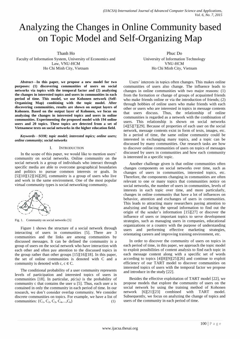
(IJACSA) International Journal of Advanced Computer Science and Applications,
Vol. 6, No. 7, 2015
100 | P a g e www.ijacsa.thesai.org
Analyzing the Changes in Online Community based
on Topic Model and Self-Organizing Map
Thanh Ho
Faculty of Information System, University of Economics and
Law, VNU-HCM
Ho Chi Minh City, Vietnam
Phuc Do
University of Information Technology
VNU-HCM
Ho Chi Minh City, Vietnam
Abstract—In this paper, we propose a new model for two
purposes: (1) discovering communities of users on social
networks via topics with the temporal factor and (2) analyzing
the changes in interested topics and users in communities in each
period of time. This model, we use Kohonen network (Self-
Organizing Map) combining with the topic model. After
discovering communities, results are shown on output layers of
Kohonen. Based on the output layer of Kohonen, we focus on
analyzing the changes in interested topics and users in online
communities. Experimenting the proposed model with 194 online
users and 20 topics. These topics are detected from a set of
Vietnamese texts on social networks in the higher education field.
Keywords—SOM; topic model; interested topics; online users;
online community; social networks
I. INTRODUCTION
In the scope of this paper, we would like to mention users’ community on social networks. Online community on the social network is a group of individuals who interact through specific media are able to overcome geographical boundaries and politics to pursue common interests or goals. In [5][10][12][16][20], community is a group of users who live and work in the same environment. One of the most popular virtual community types is social networking community.
Fig. 1. Community on social networks [5]
Figure 1 shows the structure of a social network through interacting of users in communities [5]. There are 3 communities and the links are among communities by discussed messages. It can be defined the community is a group of users on the social network who have interaction with each other and often pay attention to the discussed topics in the group rather than other groups [15][16][18]. In this paper, the set of online communities is denoted with C and a community is denoted with c, c ∈ C.
The conditional probability of a user community represents levels of participation and interested topics of users in communities [18]. In particular, p(c|u) is the probability of community c that contains the user u [5]. Thus, each user u is contained in only the community in each period of time. In our research, we don’t consider overlap community. We consider discrete communities on topics. For example, we have a list of communities: {C1, C2, C3, C4,...,Ck} (1)
Users’ interests in topics often changes. This makes online communities of users also change. The influence leads to changes in online communities with two major reasons: (1) from the formation or change of groups of acquainted friends who make friends online or via the introduction of friends; (2) through hobbies of online users who make friends with each other or users who are interested in topics in message contents that users discuss. Thus, the relationship of online communities is regarded as a network with the combination of users. This relationship is shown on social networks [4][5][7][29]. Because of properties of each user on the social network, message contents exist in form of texts, images, etc. In a period of time, the same online community could be interested in exchanging many topics, and a topic can be discussed by many communities. Our research tasks are how to discover online communities of users on topics of messages discussed by users in communities and how each community is interested in a specific topic.
Another challenge given is that online communities often changes components on social networks over time, such as changes of users in communities, interested topics, etc. Therefore, the components changing in communities are often relevant to one or many topics that communities notice on social networks, the number of users in communities, levels of interests in each topic over time, and more particularly, changes in online community that have a lot of influences on behavior, attention and exchanges of users in communities. This leads to attracting many researchers paying attention to analyzing and facing the spread information to find out the origin of the sender’s information [15][27] or discover the influence of users or important topics to serve development strategies, such as managing users in companies, educational organizations or a country with the purpose of understanding users and performing effective marketing strategies, orientating careers and improving training environment, etc.
In order to discover the community of users on topics in each period of time, in this paper, we approach the topic model to exploit possibilities of content analysis to find each topic in each message content along with a specific set of words according to topics [4][8][9][25][26] and continue to exploit efficiency of our TART model to discover communities on interested topics of users with the temporal factor we propose and introduce in the study [22].
Besides the effective exploitation of TART model [22], we propose models that explore the community of users on the social network by using the training method of Kohonen network [6][21][23] combined with TART model. Subsequently, we focus on analyzing the change of topics and users of the community in each period of time.

(IJACSA) International Journal of Advanced Computer Science and Applications,
Vol. 6, No. 7, 2015
101 | P a g e www.ijacsa.thesai.org
The next sections of the paper: section 2 presents the related researches; section 3 presents the proposed model that discovers the community of users on the social network and analyzes the change of interested topics of users of communities in each period of time; section 4 presents experimental results and evaluation; section 5 presents conclusion, development directions and references.
II. RELATED WORKS
A. Group-Topic Model (GT)
In [7], authors aim to use as much of the commonly shared information that is available for the purposes of entity resolution. This information is organized via the latent concept of a group of authors (which characterizes which authors might be co-authors) along with topic information associated with each group (which helps disambiguate authors which could be authors of a number of groups). This leads to a model which authors call the grouped author-topic model.
To describe the model we need to introduce two concepts, that of group and that of topic. The idea of topic is common to other papers on topic model, where a topic is a mixture component defining a distribution of words. An individual abstract will only contain a small number of topics out of the total possible number. This is a result of the model taking a Bayesian non-parametric approach to the problem and allowing broad uninformative priors to be set on the number of entities.
B. Community-User-Topic model (CUT)
In [29], the authors propose two generative Bayesian models for semantic community discovery in social networks, combining probabilistic modeling with community detection in social networks. To simulate the generative models, an Gibbs sampling algorithm is proposed to address the efficiency and performance problems of traditional methods. In which, [29] approach successfully detects the communities of individuals and in addition provides semantic topic descriptions of these communities with two models: CUT1 and CUT2. CUT2 differs from CUT1 in strengthening the relation between community and topic. In CUT2, semantics play a more important role in the discovery of communities. Similar to CUT1, the side-effect of advancing topic z in the generative process might lead to loose ties between com-munity and users
C. Community-Author-Recipient-Topic model (CART)
In [5], the authors introduce CART model (Community - Author - Recipient - Topic), the model is tested on the Enron email data system
1. The model shows that the discussion and
exchange between users within a community are related to the other users in community. This model is binding on all relevant users and the topics discussed in the emails belonging to a community, while the same users and the various topics can link to other communities. Compared with the above models including CUT, CART model is closer to further emphasize the ways that the topics and their relationships affect the structure of the online community in exploring community on topics.
1 https://www.cs.cmu.edu/~./enron/
CART model [5] is one of the first attempts to discover the community by combining research-based content message that users of community to exchange on social network. The model consists of 4 main components in CART are C, A, R and T. In particular, C is a community of users, R is the recipients, A is authors, T is topics [5].
The CART model has the following:
1) To generate email ed , a community cd is chosen
uniformly at random.
2) Based the community cd, the author ad and set of
recipients are chosen.
3) To generate every word in that email, a recipient
is chosen uniformly at random from the set of recipients
.
4) Based on the community cd, author ad, and recipient
, a topic is chosen.
5) The word itself is chosen from the topic . Gibb sampling for CART model as:
( ) ( ) ( | )
∏ ( | ) ∏ ( | ) ∈
( | )
(2)
where, set of recipients R, is the sequence of latent recipients (selected from ), ad is author and is the sequence of latent topic corresponding to word sequence in document d, and Nd is the total number of words in the
email.
III. MOTIVATION RESEARCH
The above-mentioned studies [3][5][7][29] and other studies such as [3][10][23][24][30] studied the models of discovering communities based on content analysis. However, these studies have not attached special importance to the temporal factor and analyzed the changes in users’ interests in topics in community in each period of time. Because the changes in users’ interests in topics can affect changes in interested topics of communities and may also change the components of the online community, such as the geographical area forming community, the number of users, time and topics in community. We focus on analyzing the distribution of interested topics in the online community and analyzing the changes in interested topics and users in communities.
IV. DISCOVERING COMMUNITY MODEL
A. Kohonen network
Kohonen network was invented by a man named Teuvo Kohonen, a professor of the Academy of Finland. The Self-Organizing Map (SOM), commonly also known as Kohonen network is a computational method for the visualization and analysis of high-dimensional data, especially experimentally acquired information [2][17][19][28].
Determine the suitability through the survey of relevant researches and use of methods and algorithms for clustering to explore communities of users on topics, we choose the method Kohonen network. Kohonen network can cluster data without prior designated clusters (cluster correlation data in this study are interested topics of online community, corpus message
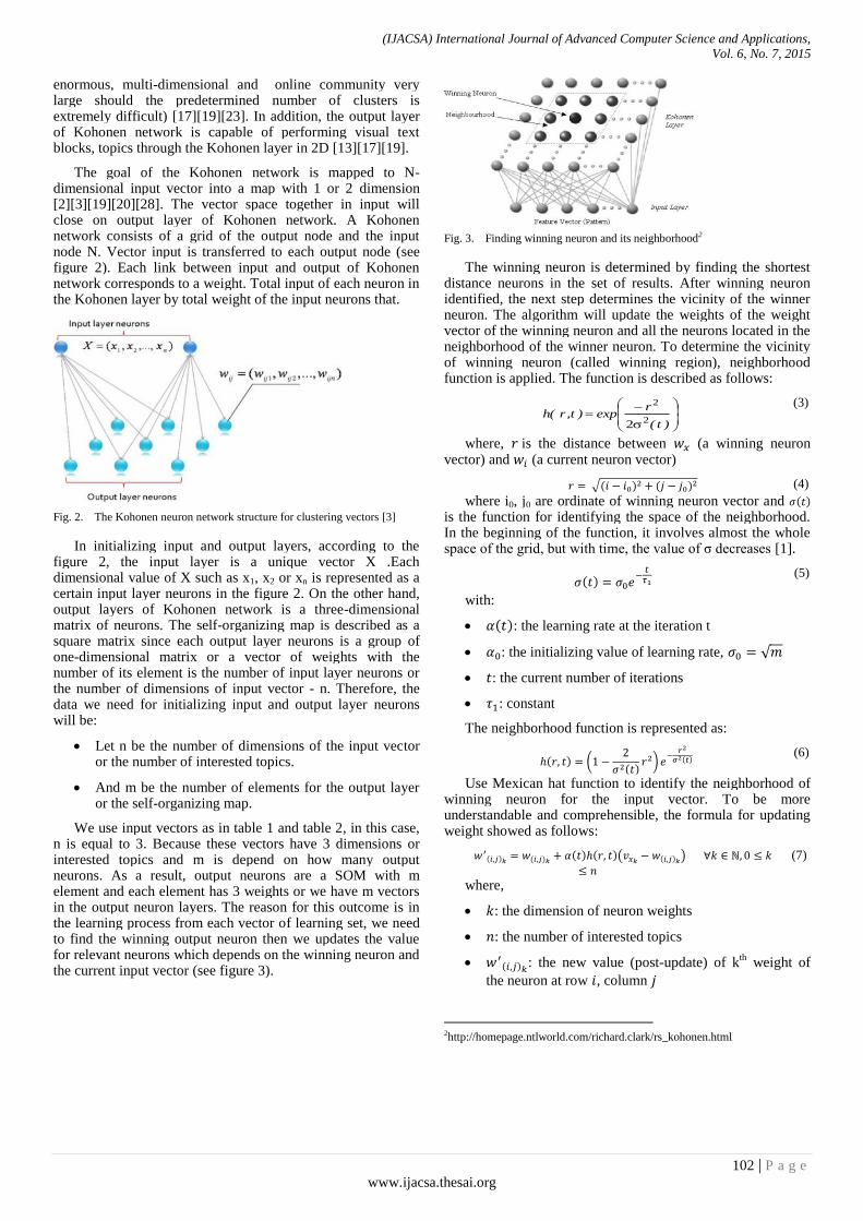
(IJACSA) International Journal of Advanced Computer Science and Applications,
Vol. 6, No. 7, 2015
102 | P a g e www.ijacsa.thesai.org
enormous, multi-dimensional and online community very large should the predetermined number of clusters is extremely difficult) [17][19][23]. In addition, the output layer of Kohonen network is capable of performing visual text blocks, topics through the Kohonen layer in 2D [13][17][19].
The goal of the Kohonen network is mapped to N-dimensional input vector into a map with 1 or 2 dimension [2][3][19][20][28]. The vector space together in input will close on output layer of Kohonen network. A Kohonen network consists of a grid of the output node and the input node N. Vector input is transferred to each output node (see figure 2). Each link between input and output of Kohonen network corresponds to a weight. Total input of each neuron in the Kohonen layer by total weight of the input neurons that.
Fig. 2. The Kohonen neuron network structure for clustering vectors [3]
In initializing input and output layers, according to the figure 2, the input layer is a unique vector X .Each dimensional value of X such as x1, x2 or xn is represented as a certain input layer neurons in the figure 2. On the other hand, output layers of Kohonen network is a three-dimensional matrix of neurons. The self-organizing map is described as a square matrix since each output layer neurons is a group of one-dimensional matrix or a vector of weights with the number of its element is the number of input layer neurons or the number of dimensions of input vector - n. Therefore, the data we need for initializing input and output layer neurons will be:
Let n be the number of dimensions of the input vector or the number of interested topics.
And m be the number of elements for the output layer or the self-organizing map.
We use input vectors as in table 1 and table 2, in this case, n is equal to 3. Because these vectors have 3 dimensions or interested topics and m is depend on how many output neurons. As a result, output neurons are a SOM with m element and each element has 3 weights or we have m vectors in the output neuron layers. The reason for this outcome is in the learning process from each vector of learning set, we need to find the winning output neuron then we updates the value for relevant neurons which depends on the winning neuron and the current input vector (see figure 3).
Fig. 3. Finding winning neuron and its neighborhood2
The winning neuron is determined by finding the shortest distance neurons in the set of results. After winning neuron identified, the next step determines the vicinity of the winner neuron. The algorithm will update the weights of the weight vector of the winning neuron and all the neurons located in the neighborhood of the winner neuron. To determine the vicinity of winning neuron (called winning region), neighborhood function is applied. The function is described as follows:
)t(
r exp)t,r (h
2
2
2
(3)
where, is the distance between (a winning neuron vector) and (a current neuron vector)
√( ) ( )
(4) where i0, j0 are ordinate of winning neuron vector and ( )
is the function for identifying the space of the neighborhood. In the beginning of the function, it involves almost the whole space of the grid, but with time, the value of σ decreases [1].
( )
(5)
with:
( ): the learning rate at the iteration t
: the initializing value of learning rate, √
: the current number of iterations
: constant
The neighborhood function is represented as:
( ) (
( ) )
( ) (6)
Use Mexican hat function to identify the neighborhood of winning neuron for the input vector. To be more understandable and comprehensible, the formula for updating weight showed as follows:
( ) ( ) ( ) ( )(
( ) ) ∈
(7)
where,
: the dimension of neuron weights
: the number of interested topics
( )
: the new value (post-update) of kth
weight of
the neuron at row , column
2http://homepage.ntlworld.com/richard.clark/rs_kohonen.html

(IJACSA) International Journal of Advanced Computer Science and Applications,
Vol. 6, No. 7, 2015
103 | P a g e www.ijacsa.thesai.org
( ) : the current (pre-update) value of k
th weight of
the neuron at row , column
( ): the learning rate at the current number of iterations
( ): the result of topological neighborhood function with is the current number of iterations, is the distance between the current neuron and the winning neuron
: the value of k
th weight of the current learning
vector
Function α(t) is the learning rate, this value will decrease as the number of iterations t. If a neuron is a winning neuron or neighborhood of the winner neuron, then the weight of vector is updated, reverse that neuron will not be updated. At each iteration, SOM have chosen the same weight vector to update its vector and weight vector to make them closer to the input vector.
B. Temporal – Author – Recipient – Topic model (TART)
We proposed a Temporal-Author-Recipient-Topic model [23] in the field of social network analysis and information extraction based on the topic model. The key ideas of the model focus on extracting words, discovering and labeling topics, and analyzing topics with authors, recipients and temporal factor.
Fig. 4. TART model [23]
During parameter estimation for TART model, the system will keep track 4 matrices to analyze users’ interests topics, including: T (topic) x W (word), A (author) x T (topic), R (recipient) x T (topic) and T (topic) x T (temporal). Based on these matrices, topics and temporal distribution Φzw, topic and temporal distribution Ψzt, author and topic distribution ϴaz, recipient and topic distribution ϴrz, the matrices are given by (8), (9), (10) and (11):
z azm
azm
az)(
w zwn
zwn
zw)(
(8)(9)
t ztn
ztn
zt)(
z )rzm(
rzmrz
(10)(11)
C. General model
We propose the model for discovering online community and analyzing the changes in topics interests and users in communities on social networks in each period of time approaching the topic model with temporal factor. In this model, through results of the analysis and evaluation of the
relevant models in discovering communities, we choose Kohonen network. Kohonen network combines with TART model [23]. The output of TART model is the set of interested topic vectors of users in each period of time. The general model consists of 3 main modules (figure 5):
1) Normalization the set of vectors from the output of
TART model in order to suit the input vectors of Kohonen
network.
2) Discovering community by using Kohonen network
(SOM) to cluster users based on interested topic vectors. In
this discovery, each cluster is a community of users on topics,
corresponding to a neuron on the output layer of SOM.
3) Analyzing the changes of users and interested topics in
communities on social networks based on the output layer of
SOM and the relationship among output layers.
Fig. 5. General model of discovering community
The algorithm 1 describes the way to discover community users based-on topic model combined Kohonen network by clustering interested topics vectors of users and analyze the changes in communities of users.
Algorithm 1. Discovering communities and analyzing the
changes in communities of users.
Input: the set of interested topic vectors of users (called the set of input vectors) from TART model [22]. The components of vectors include the topics probability and temporal factor which users are interested in.
Output: the set of communities of users on specific topics in each period of time and the changes in interested topics and users in online communities.
Process: Using method of Kohonen network. In this method, we introduce the main process steps, include:
1. Putting the set of input vectors.
2. For each i ϵ [1,...,n] //n is row and column on output layer
of Kohonen.
For each j ϵ [1,...,n]
Finding neurons which have weight vectors wij
nearest with input vector v. Called (i0, j0) is of
winning neuron. Hence, euclician distance between
d(v,wi0j0) = min (d(v,wij) with i,j ϵ [1,...,n] and wi0j0
are weight of winning neuron.
3. Finding winning neuron and its neighborhood (figure 3)
4. Discovering online community based on the winning
neuron and its neighborhood.
5. Analyzing the changes in interested topics and users in
online communities based on online community on the
output layer of SOM.

(IJACSA) International Journal of Advanced Computer Science and Applications,
Vol. 6, No. 7, 2015
104 | P a g e www.ijacsa.thesai.org
V. IMPLEMENTATION AND DISCUSSION
A. Experimental Data
Experimenting the proposed model (figure 5) for discovery communities with 194 interested topic vectors of 194 users who discuss 9 topics (random survey 9 topics are "facilities and services", "learning and examination", "international cooperation", "quality control", "scientific research", "living and life", "sport", "employment recruitment", "admission", "finance and fees", "friendship and love", "social activities" and "training" from 20 topics in the system of topics built in [11]). We analyze the above topics belonging to the period from December, 2008 to January, 2010 on 48.264 messages from social networks. In each period of time, we have interested topic vectors of different users. For example, the user u1 during the period from t1 to t2, has an interested topic vector of user ( ) ∈ , during the period from t2 to
t3, we have the vector ( ). In general, each user has
an interested topic vector at the time t is ( )
or X = (x1, x2, ..., xn). Thus, we have
interested topic vectors of users as follows:
TABLE I. THE SET OF INTERESTED TOPIC VECTORS
User Temporal ti Temporal tj ( )
u1 Dec 01, 2008 Dec 31, 2008 ( )
u2 Feb 01, 2009 Feb 28, 2009 ( )
u3 Apr 01, 2009 Apr 30, 2009 ( )
u1 Feb 01, 2009 Feb 28, 2009 ( )
TABLE II. THE SET OF INTERESTED TOPIC VECTORS OF USERS IN OTHER
FORM
Users
Topic
―international
cooperation‖
Topic
―admission‖
Topic
―learning
and
examination‖
Temporal
ti – tj
Interested Probability
u1 0.85246 0.0 0.772527 Dec 01, 2008 - Dec 31, 2008
u2 0.85000 0.86956 0.676793 Feb 01, 2009 - Feb 28, 2009
u3 0.62417 0.34132 0.893421 Apr 01, 2009 – Apr 30,
2009
u1 0.52345 0.52341 0.834212 Feb 01, 2009 - Feb 28, 2009
Table 1 and table 2 are the forms of interested topics of users on social networks. This is the set of input vectors for Kohonen network. The input vectors include 3 users interested in 3 topics in 3 periods of time t1-t2, t2-t3 and t3-t4. The goal of training process is to cluster the set of interested topic vectors.
Thus, with ( ) we have the output layer of Kohonen
( ) which is a 2-dimensional array (see figure 9).
B. Discovering online community
This section presents the results of test to discover communities of users on the social network in each period of time. This section focuses on modules (1) and (2) of the model in figure 6.
Figure 6 shows the results of the training process to discover communities of users on the output layer, experimenting with 194 topic vectors with 194 users in discussing on 9 topics.
Each neuron (cell) on the output layer (see figure 6) corresponds to a community of users to exchange topics in each period of time. Each neuron has a dark or light color corresponding to the number of users more or less in communities. The darker the color on each neuron is, the more the number of users in the community is. If the neuron is white, users in communities do not exist.
Fig. 6. Results of discovery communities is shown on the output layer of
SOM
C. Analyzing the changes in interested topics and users in
online communities
This section focuses on testing the proposed model of the module (3) in figure 5. Based on the output layer of SOM in each period of time in figure 6, we can examine the relationship between the clusters (neurons) in the output layer based on the components such as users, interested topics, probability and number of clusters in each period of time.
Based on the output layer of SOM in each period of time in figure 6, we can examine the relationship between the clusters (neurons) in the output layer based on the components such as users, interested topics, probability and number of clusters in each period of time.
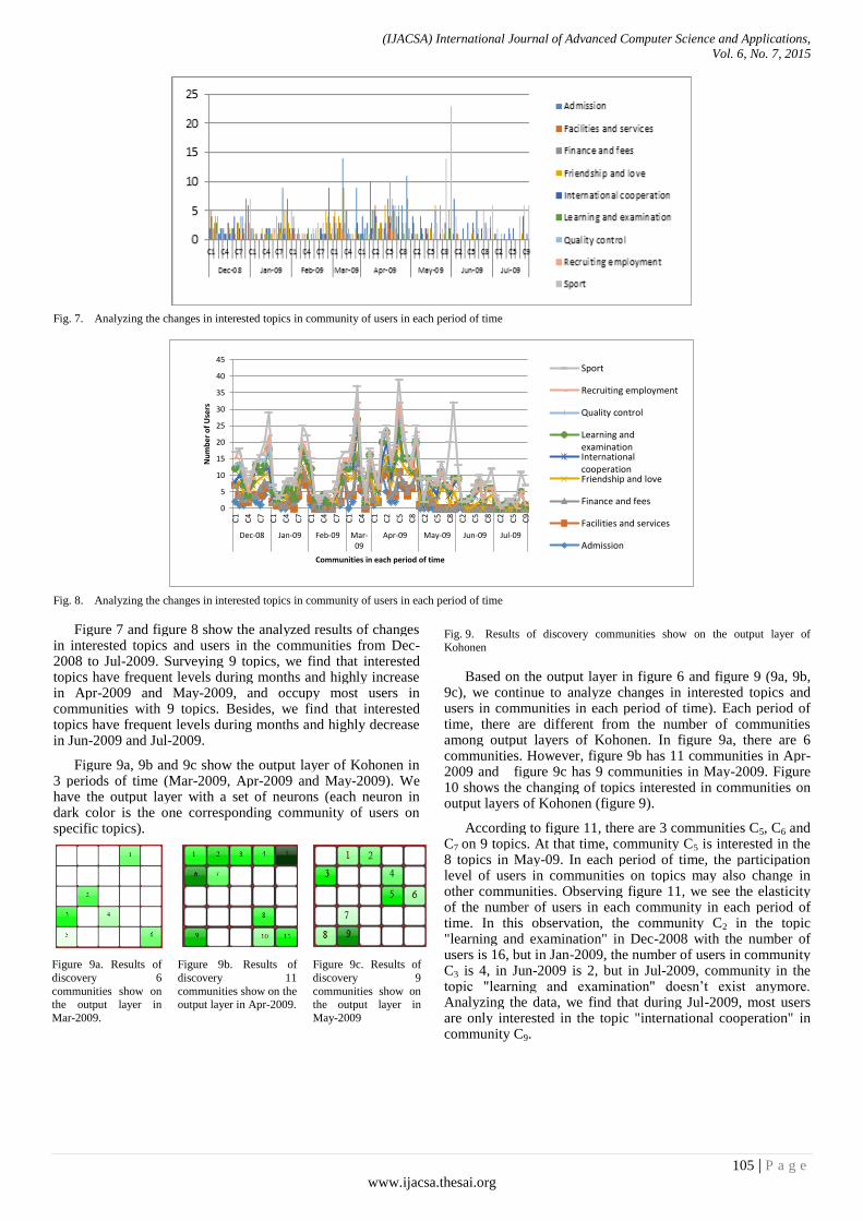
(IJACSA) International Journal of Advanced Computer Science and Applications,
Vol. 6, No. 7, 2015
105 | P a g e www.ijacsa.thesai.org
Fig. 7. Analyzing the changes in interested topics in community of users in each period of time
Fig. 8. Analyzing the changes in interested topics in community of users in each period of time
Figure 7 and figure 8 show the analyzed results of changes in interested topics and users in the communities from Dec-2008 to Jul-2009. Surveying 9 topics, we find that interested topics have frequent levels during months and highly increase in Apr-2009 and May-2009, and occupy most users in communities with 9 topics. Besides, we find that interested topics have frequent levels during months and highly decrease in Jun-2009 and Jul-2009.
Figure 9a, 9b and 9c show the output layer of Kohonen in 3 periods of time (Mar-2009, Apr-2009 and May-2009). We have the output layer with a set of neurons (each neuron in dark color is the one corresponding community of users on specific topics).
�
Figure 9a. Results of
discovery 6
communities show on the output layer in
Mar-2009.
Figure 9b. Results of
discovery 11
communities show on the output layer in Apr-2009.
Figure 9c. Results of
discovery 9
communities show on the output layer in
May-2009
Fig. 9. Results of discovery communities show on the output layer of
Kohonen
Based on the output layer in figure 6 and figure 9 (9a, 9b, 9c), we continue to analyze changes in interested topics and users in communities in each period of time). Each period of time, there are different from the number of communities among output layers of Kohonen. In figure 9a, there are 6 communities. However, figure 9b has 11 communities in Apr-2009 and figure 9c has 9 communities in May-2009. Figure 10 shows the changing of topics interested in communities on output layers of Kohonen (figure 9).
According to figure 11, there are 3 communities C5, C6 and C7 on 9 topics. At that time, community C5 is interested in the 8 topics in May-09. In each period of time, the participation level of users in communities on topics may also change in other communities. Observing figure 11, we see the elasticity of the number of users in each community in each period of time. In this observation, the community C2 in the topic "learning and examination" in Dec-2008 with the number of users is 16, but in Jan-2009, the number of users in community C3 is 4, in Jun-2009 is 2, but in Jul-2009, community in the topic "learning and examination" doesn’t exist anymore. Analyzing the data, we find that during Jul-2009, most users are only interested in the topic "international cooperation" in community C9.
0
5
10
15
20
25
30
35
40
45
C1
C4
C7
C1
C4
C7
C1
C4
C7
C1
C4
C1
C2
C5
C8
C2
C5
C8
C2
C5
C8
C2
C5
C9
Dec-08 Jan-09 Feb-09 Mar-09
Apr-09 May-09 Jun-09 Jul-09
Nu
mb
er o
f U
sers
Communities in each period of time
Sport
Recruiting employment
Quality control
Learning andexaminationInternationalcooperationFriendship and love
Finance and fees
Facilities and services
Admission
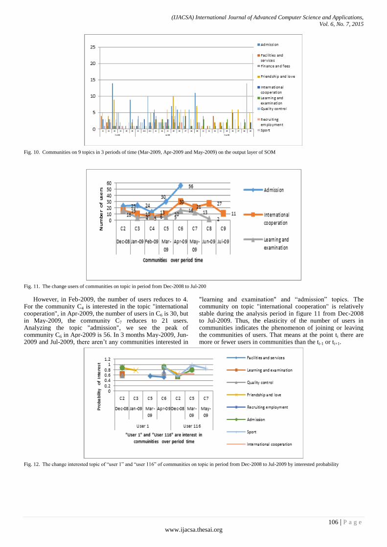
(IJACSA) International Journal of Advanced Computer Science and Applications,
Vol. 6, No. 7, 2015
106 | P a g e www.ijacsa.thesai.org
Fig. 10. Communities on 9 topics in 3 periods of time (Mar-2009, Apr-2009 and May-2009) on the output layer of SOM
Fig. 11. The change users of communities on topic in period from Dec-2008 to Jul-200
However, in Feb-2009, the number of users reduces to 4. For the community C4 is interested in the topic "international cooperation", in Apr-2009, the number of users in C6 is 30, but in May-2009, the community C7 reduces to 21 users. Analyzing the topic "admission", we see the peak of community C6 in Apr-2009 is 56. In 3 months May-2009, Jun-2009 and Jul-2009, there aren’t any communities interested in
"learning and examination" and ―admission‖ topics. The community on topic "international cooperation" is relatively stable during the analysis period in figure 11 from Dec-2008 to Jul-2009. Thus, the elasticity of the number of users in communities indicates the phenomenon of joining or leaving the communities of users. That means at the point ti there are more or fewer users in communities than the ti-1 or ti+1.
Fig. 12. The change interested topic of ―user 1‖ and ―user 116‖ of communities on topic in period from Dec-2008 to Jul-2009 by interested probability

(IJACSA) International Journal of Advanced Computer Science and Applications,
Vol. 6, No. 7, 2015
107 | P a g e www.ijacsa.thesai.org
Figure 12 shows the communities which ―user 1‖ and ―user 116‖ join in. We survey random with two users ―user 1‖ and ―user 116‖ on 9 topics. With user ―user 1‖ joins in communities are C2, C3, C5 and C6 with each different interested probability on each different topic. And user ―user
116‖ joins in communities are C2, C5 and C7. These users have
the changes about interested topic, probability and community in each period of time.
D. Results Evaluate
Application of the Precision (P), Recall (R) and F-measure (F) in [14] to evaluate the clustering results by Kohonen network. We compare the results of clustering vector of topics according to the proposed model and the clustering results by manual [19][23]. Assume that in set of actors we divide these actors into clusters of actors by manual (by clustering based on the topics of the forum). On the other hand, by using SOM, the set is split to clusters. Precision measure represents the ratio of the accuracy of a SOM cluster. If the ratio is 1, it means that all the actors in SOM cluster belong to cluster , or . Precision measure represents the ratio of the accuracy of a SOM cluster. If the ratio is 1, it means that all the actors in SOM cluster belong to cluster , or . According to Brew & Schulte im Walde (2002), F-Measure, which is the combination of Precision and Recall, is used to compute the accuracy of the system. For the clustering system, this is the equation:
(12)
The greater value F-Measure has, the more accurate the SOM is. Theo Brew C. [4] proposed evaluation method follows: corresponding to a cluster in the clustering result of the system we calculate the value of the F-measure for all clusters to be created manually. Choosing cluster which has the value of the highest F-measure and remove that cluster and repeating the above step for the remaining term. The total values of F-measure higher clustering system more accurately.
Here are the results of the corresponding F-measure (see table 3) with m = 5 clusters and k = 6 clusters (by Kohonen). We we compute the table of Precision, Recall, then manipulate the total F-measure.
TABLE III. THE RESULTS OF F-MEASURE VALUE BETWEEN MANUAL
(CLUSTER BASED ON THE TOPICS OF THE FORUM) AND KOHONEN
Kohonen/Manual C
0 C
1 C
2 C
3 C
4
C0 0.43 0.15 0.84 0.52 0.68
C1 0.67 0.61 0.00 0.16 0.00
C2 0.00 0.36 0.51 0.62 0.16
C3 0.72 0.00 0.55 0.55 0.34
C4 0.81 0.73 0.25 0.00 0.72
C5 0.19 0.00 0.15 0.29 0.36
MAX 0.81 0.73 0.84 0.62 0.72
Total MAX for clustering by Kohonen network is:
0.81 + 0.73 + 0.84 + 0.62 + 0.72 = 3.72. Total max value of F-measuare in table 4 is 3.72
(respectively 74%). This value according to our assessment is
high, this proves the proposed method using the clustering method of Kohonen network combined TART model with high accuracy.
VI. CONCLUSIONS AND FUTURE WORKS
A. Conclusions
The contributions to this paper are summarized into two major issues:
1) Proposing a new model to discover online communities
based on the topic model: We focus on exploiting and combining Kohonen network
and TART model. The model consists of two main components: (1) standardizing and selecting the result from the output of TART model. This is a set of interested topic vectors of users on social networks and is also a set of input vectors for Kohonen network, (2) proposing the model of using Kohonen network to discover communities of users interested in specific topics which are called communities of users on topics. The model can discover users’ interested topics in each period of time and probability of topics interests, calculating topics apportion according to each online community. The challenge given in this content is to discover online communities through discussed contents because communities frequently change interested topics as well as members who participate in social network communities.
2) Analyzing changes in interested topics and users in
communities on social networks in each period of time is
based on the output layer of SOM and the relationship among
that output layer.
B. Future work
The results of this paper will be the basis for researches in the future such as looking for important people in communities, analyzing the influence spread of topics and searching for the origin of information on social networks.
ACKNOWLEDGEMENT
This research is funded by Viet Nam National University HCM City (VNU-HCMC) under Grant number B2013-26-02.
REFERENCE
[1] Alexandru Berlea1, et al., Content and communication based sub-community detection using probabilistic topic models, IADIS International Conference Intelligent Systems and Agents, 2009.
[2] Andrew McCallum, Andr´es Corrada, Xuerui Wang, The Author-Recipient-Topic Model for Topic and Role Discovery in Social Networks: Experiments with Enron and Academic Email, Department of Computer Science, University of MA, 2004.
[3] B. Magomedov, "Self-Organizing Feature Maps (Kohonen maps)," 7 November. [Online]. Available: http://www.codeproject.com/ Articles/16273/Self-Organizing-Feature-Maps-Kohonen-maps, 2006.
[4] Brew C, Schulte im Walde. Spectral Clustering for German Verbs, In Proc of the Conf in Natural Language Proocessing, Philadenphia, PA, 2002, pp. 117-124.
[5] Chunshan Li, William K. Cheung, Yunming Ye, Xiaofeng Zhang, Dianhui Chu, Xin Li, The Author-Topic-Community model for author interest profiling and community discovery, Springer-Verlag London, 2014, pp. 74-85.
[6] D. Zhou et al., Probabilistic models for discovering e-communities. In WWW ’06: Proceedings of the 15th international conference on World Wide Web, page 182. ACM, 2006, pp. 173-182.

(IJACSA) International Journal of Advanced Computer Science and Applications,
Vol. 6, No. 7, 2015
108 | P a g e www.ijacsa.thesai.org
[7] Ding Zhou, Isaac Councill, Hongyuan Zha, C. Lee Giles, Discovering Temporal Communities from Social Network Documents, IEEE ICDM, 2007, pp. 745-750.
[8] Do Phuc, Mai Xuan Hung, Using SOM based Graph Clustering for Extracting Main Ideas from Documents, RVIF, 2008, pp. 209-214.
[9] Ho Trung Thanh, Do Phuc, Ontology Vietnamese in Higher Education, Journal of Science and Technology, Vietnam Academy of Science and Technology, Volume 52, No. 1B, 2014, pp. 89-100.
[10] István Bíró, Jácint Szabó, Latent Dirichlet Allocation for Automatic Document Categorization, Research Institute of the Hungarian Academy of Sciences Budapest, 2008, pp. 430-441.
[11] Kaski, S., Honkela, T., Lagus, K., and Kohonen. T.WEBSOM--self-organizing maps of document collections. Neurocomputing, volume 21, 1998, pp. 101-117.
[12] Kohonen T.. Self-Organization and Associative Memory, Springer, Berlin, 1984.
[13] Kohonen T. and Honkela T., Kohonen network, http://www.scholarpedia.org/article/Kohonen_network, 2007.
[14] Kohonen, T., Self-organized formation of topologically correct feature maps.Biological Cybernetics, 1982, 43:59-69.
[15] Kohonen, T. , Self-Organizing Maps. Extended edition. Springer.
[16] Kohonen, T. and Somervuo, P. (2002). How to make large self-organizing maps for nonvectorial data. Neural Networks 15(8-9), 2001, pp. 945-952.
[17] Kohonen, T., Kaski, S. and Lappalainen, H., Self-organized formation of various invariant-feature filters in the adaptive-subspace SOM. Neural Computation, 1997, 9: 1321-1344.
[18] Michal Rosen-Zvi, Thomas Griffths et. al, Probabilistic AuthorTopic Models for Information Discovery, 10th ACM SigKDD, Seattle, 2004, pp. 306-315.
[19] Mr inmaya Sachan, et al, Using Content and Interactions for Discovering Communities in Social Networks, International World Wide Web Conference Com-mittee (IW3C2), Lyon, France, 2012, pp. 331-340. 28
[20] N. Pathak, C. DeLong, A. Banerjee, and K. Erickson, Social topic models for community extraction. In The 2nd SNA-KDD Workshop, volume 8, 2008.
[21] Nguyen Le Hoang, Do Phuc, et al, Predicting Preferred Topics of Authors based on Co-Authorship Network, The 10th IEEE RIVF International Conference on Computing and Communication Technologies, IEEE, 2013, pp. 70-75.
[22] Teuvo Kohonen , Self-Organized Formation of Topologically Correct Feature Maps, Biol. Cybern. 43, Springer-Verlag,npp. 59-69. 17
[23] Thanh Ho, Phuc Do (2015), Analyzing Users’ Interests with the Temporal Factor Based on Topic Modeling, 23-25 March 2015, Indonesia, Springer, 1982, pp. 106-115.
[24] The Anh Dang, Emmanuel Viennet, Community Detection based on Structural and Attribute Similarities, ICDS 2012 : The Sixth International Conference on Digital Society, 2012, pp. 7-14.
[25] Tianbao Yang, Yun Chi, Shenghuo Zhu, Yihong Gong, Rong Jin, Detecting communities and their evolutions in dynamic social networks—a Bayesian approach, Mach Learn 82, Springer, 2011, pp. 157–189.
[26] Tom Fawcett, Introduction to ROC Analysis, Elsevier B.V., Available online www.sciencedirct.com, 2005.
[27] Tran Quang Hoa, Vo Ho Tien Hung, Nguyen Le Hoang, Ho Trung Thanh, Do Phuc, Finding the Cluster of Actors in Social Network based on the Topic of Messages, ACIIDS 04/2014, ThaiLan. Springer, 2014, pp. 183-190.
[28] Wenjun Zhou, Hongxia Jin, Yan Liu, Community Discovery and Profiling with Social Messages, KDD’12, August 12–16, 2012, Beijing, China, 2012, pp. 388-396.
[29] X. Wang, N. Mohanty, and A. McCallum. Group and topic discovery from relations and their attributes. Advances in Neural Information Processing Systems 18, 2006, pp. 1449-1456.
[30] Zhijun Yin et. al, Latent community Topic Analysis: Integration of Community Discovery with Topic Modeling, ACM Transactions on Intelligent Systems and Technology, 2012, pp. 1-21.

(IJACSA) International Journal of Advanced Computer Science and Applications,
Vol. 6, No. 7, 2015
109 | P a g e
www.ijacsa.thesai.org
Design of Orthonormal Filter Banks based on Meyer
Wavelet
Teng Xudong
School of Electronic and Electric Engineering, Shanghai
University of Engineering Science,
Shanghai, China
Dai Yiqing
Communication and Signal Branch
Shanghai Rail Transit Maintenance Support Co. Ltd;
Shanghai, China
Lu Xinyuan
Communication and Signal Branch
Shanghai Rail Transit Maintenance Support Co. Ltd;
Shanghai, China
Liang Jianru
School of Electronic and Electric Engineering, Shanghai
University of Engineering Science,
Shanghai, China
Abstract—A new design method for orthonormal FIR filter
banks, which can be constructed using the generalized Meyer
wavelet by taking into account the effect of time-shift factor, is
proposed in this paper. These generalized Meyer wavelets are
proved to be of the same basic properties and the time-frequency
localization characteristics as the classical Meyer wavelet,
furthermore some performances of the Meyer wavelets are
improved by change of time-shift factor, which can better satisfy
requirements of constructing orthonormal filter banks. The
simulation shows that design of orthonormal filter banks based
on the generalized Meyer wavelets with maximal symmetrical
index is rational and effective.
Keywords—Meyer wavelet; Time-shift factor; orthonormal FIR
filter banks; Symmetrical Index
I. INTRODUCTION
The Wavelets transform serves as an effective tool for Multi-resolution signal analysis that have found applications in data compression, image processing and information extraction. The time-frequency character of wavelet transform can be widely utilized to perform fine temporal analysis and fine spectrum analysis in high-frequency and low-frequency respectively. As is well known, the discrete wavelet transform is obtained by repeated sampling and filtering with low and high-pass finite impulse response (FIR) so that if the wavelet is orthonormal, the inverse problem, e.g. signal de-noising and perfect reconstruction , can be realized easily. In fact, from a traditional signal processing point of view, a wavelet is a band-pass filter, and therefore the wavelet transform can be interpreted as a constant-Q filtering with a set of filter banks. In terms of the investigation by Daubechies ,as in [1][2], when the
wavelet bases are orthonormal, the scaling function ( )t
and wavelet ( )t obey two-scale difference equations as:
( x l ) , ( x l )
( x l ) , ( x l )
kl
kl
, (1)
which means the wavelet ( )t bases are a group of
perfect reconstruction FIR filter banks. Thus, these orthogonal
FIR filter banks with orthogonal impulse responses can be designed by means of compactly supported wavelet bases. The Meyer wavelet is one of the earlier classical orthonormal wavelets bases, as in [3][4], which has good properties, such as fast convergence on frequency domain, regularity, localization in time domain as well as infinitely differentiable, so the Meyer wavelet can be introduced to design such orthonormal perfect reconstruction FIR filter banks, as in [5][6][7]. In this paper,
Start with scaling functions ( )t of the (classical) Meyer
wavelet, the (classical) Meyer wavelets base is extended to the generalized Meyer wavelet bases to design the orthonormal filter banks, then analyze characteristics of the generalized Meyer wavelet including periodicity, symmetry and compact support conditions, finally, the simulation results show that these new wavelet bases are not only provide new approach for design of orthonormal filter banks and the construction of complex wavelets , but also develop and enrich the (classical) Meyer wavelet and others applications.
II. THEORETICAL BACKGROUND
A. The Meyer wavelt
The Meyer wavelet function M( )t and scaling function
M( )t have better localization characteristics, which are
defined in the frequency domain, as in [2]. Usually, the wavelet function can be obtained by scaling function as follows:
others,0
3
4||
3
2,1||
2
3
2cos
3/2||,1
)(ˆM
v (2)
where function satisfy 1)1()( xvxv .
In light of theory of multi-resolution, since the )(ˆM
defined by (2) is compact support, its support interval is
)2,2(]3/4,3/4[ and
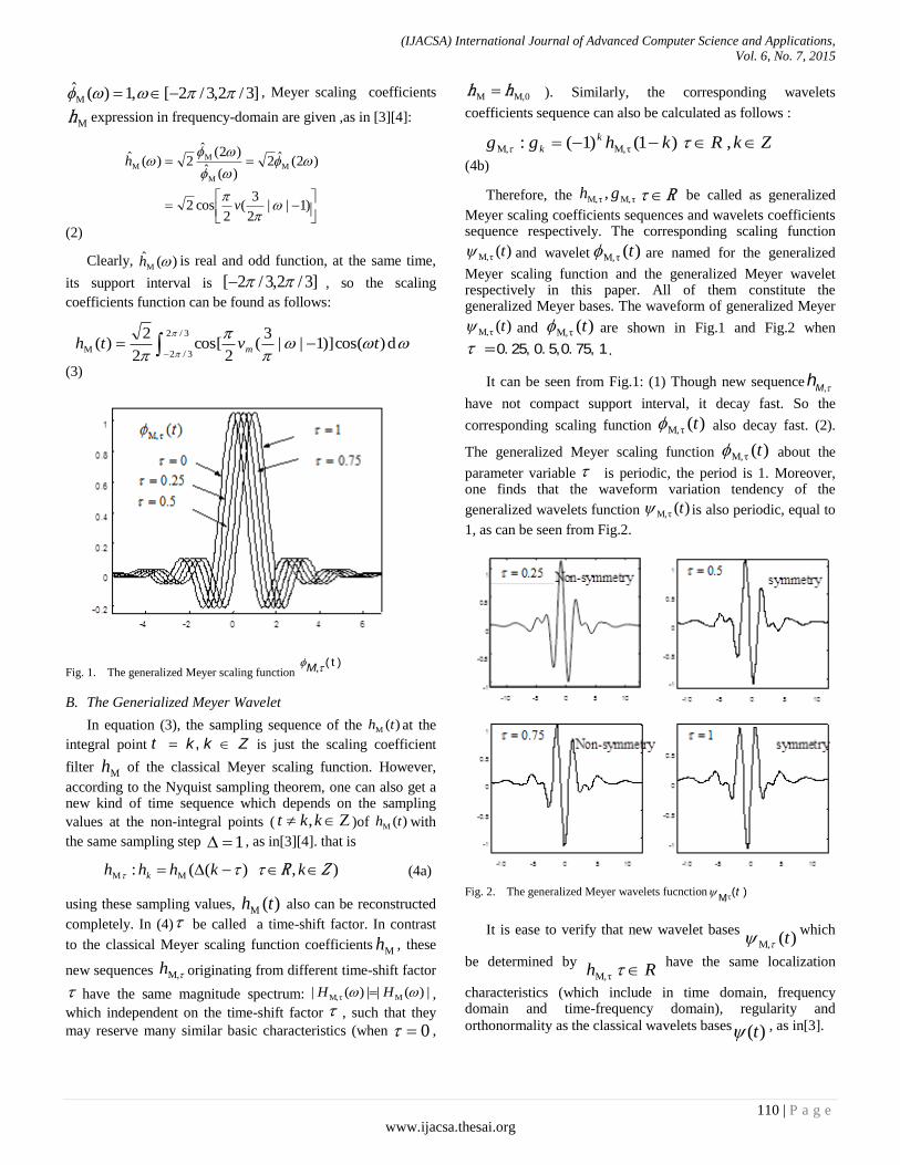
(IJACSA) International Journal of Advanced Computer Science and Applications,
Vol. 6, No. 7, 2015
110 | P a g e
www.ijacsa.thesai.org
]3/2,3/2[,1)(ˆM , Meyer scaling coefficients
Mh expression in frequency-domain are given ,as in [3][4]:
)1||2
3(
2cos2
)2(ˆ2)(ˆ
)2(ˆ2)(ˆ
M
M
MM
v
h
(2)
Clearly, )(ˆM h is real and odd function, at the same time,
its support interval is ]3/2,3/2[ , so the scaling
coefficients function can be found as follows:
d)cos()]1||
3(
2cos[
2
2)(
3/2
3/2M tvth m
(3)
Fig. 1. The generalized Meyer scaling function ( t )
,M
B. The Generialized Meyer Wavelet
In equation (3), the sampling sequence of the )(M th at the
integral point ,t k k Z is just the scaling coefficient
filter Mh of the classical Meyer scaling function. However,
according to the Nyquist sampling theorem, one can also get a new kind of time sequence which depends on the sampling
values at the non-integral points ( Ζ, kkt )of )(M th with
the same sampling step 1 , as in[3][4]. that is
),)((: MM Z kkhhh k R (4a)
using these sampling values, )(M th also can be reconstructed
completely. In (4) be called a time-shift factor. In contrast
to the classical Meyer scaling function coefficientsMh , these
new sequences M,h originating from different time-shift factor
have the same magnitude spectrum: |)(||)(| MτM, HH ,
which independent on the time-shift factor , such that they
may reserve many similar basic characteristics (when 0 ,
M,0M hh ). Similarly, the corresponding wavelets
coefficients sequence can also be calculated as follows :
ZkRkhgg k
k ,)1()1(: τM,M,
(4b)
Therefore, the τM,τM, , gh R be called as generalized
Meyer scaling coefficients sequences and wavelets coefficients sequence respectively. The corresponding scaling function
)(τM, t and wavelet )(τM, t are named for the generalized
Meyer scaling function and the generalized Meyer wavelet respectively in this paper. All of them constitute the generalized Meyer bases. The waveform of generalized Meyer
)(τM, t and )(τM, t are shown in Fig.1 and Fig.2 when
0. 25, 0. 5,0. 75, 1 .
It can be seen from Fig.1: (1) Though new sequence,M
h
have not compact support interval, it decay fast. So the
corresponding scaling function )(τM, t also decay fast. (2).
The generalized Meyer scaling function )(τM, t about the
parameter variable is periodic, the period is 1. Moreover, one finds that the waveform variation tendency of the
generalized wavelets function )(τM, t is also periodic, equal to
1, as can be seen from Fig.2.
Fig. 2. The generalized Meyer wavelets fucnctionM,τ
( )t
It is ease to verify that new wavelet bases )(M, t
which
be determined by Rh τM,
have the same localization
characteristics (which include in time domain, frequency domain and time-frequency domain), regularity and
orthonormality as the classical wavelets bases )(t , as in[3].

(IJACSA) International Journal of Advanced Computer Science and Applications,
Vol. 6, No. 7, 2015
111 | P a g e
www.ijacsa.thesai.org
III. SIMULATION AND DISCUSSION
The generalized Meyer bases symmetry, including function
scaling )(τM, t and wavelets function )(τM, t , depends on
the generalized Meyer scaling function )(M th and time-
shifting factor , in other words, be decided completely by
symmetry of sequence τM,h . In order to study the symmetrical
degree of the generalized Meyer bases, the symmetrical index can be considered into sequence },{: Zkhh k , as
following:
.max2
2hhh
Z
kik
( 5)
The symmetrical index ( 10 ) can effectively
evaluate symmetrical degree of sequence h and have nothing
to do with position of central point. Here, In terms of maximal
symmetrical index, the coefficients ,Mh at 0. 5 and
1 will be selected prior to other sequence τM,h for
designing the orthonormal FIR filter banks, as in [4], which have linear phase or approximate linear phase . According to
relation of hgt )( , one can easily obtain a fast
algorithm for decomposing real signal (R)Lts 2)( and
complex signal by a group of filters constructed by the generalized Meyer bases, as in [7][8]. Naturally, the initialized sequence can be given by
n
k
n
k
knnxxc
knnxxc
)()(:
)()(:
00
00
. (6)
Fig. 3. The original signal ( )s t polluted by gauss white noise
Assuming the polluted signal is modeled as s(t) = sin(20t) + n(t), where n(t) denotes gauss white noise. It can been seen from Fig.3 that the distortions happened at peak value of the primitive signal sin(20t), and thereby the signal s(t) is composed of multiple frequency components. According to
the above Generalizing method, the wavelet decomposition
coefficients ,0. 5M
h can be easily obtained as:
,0. 5{ 0. 1403 0. 1686 0. 6668 0. 6668
0. 1686 0. 1403 0. 0404 0. 0664}
Mh
Fig. 4. The Reconstruction signal by orthonormal filter banks
Here, these generalized Meyer wavelet coefficients can be used to construct the orthonormal filter banks, as in [5][6], and such filter banks can be used for de-noising signals, which be called signal reconstruction. As shown in Fig.4, the primitive sine function are perfectly reconstructed and the noise is also reduced completely. These results show the generalized Meyer wavelets controlled by time shift really produce different
properties of filter banks to satisfy such requirements as orthonormality, symmetry and regularity, as in [9][10].
IV. CONCLUSION
In this paper, the time shift can be considered into the
scale function of the Meyer wavelet so as to produce a group of new wavelet bases, called the generalized Meyer wavelets. Because all generalized Meyer bases inherit many good properties of the original Meyer bases, a set of perfect reconstruction FIR filter banks designed by the generalized Meyer wavelet are regular and orthonormal accordingly. In addition, FIR filter banks with linear phase also might be constructed on the basis of symmetrical index, and has better smoothness for extracting signal envelope and construction of signal. As the time shift only affects the phase of filter function, it is also convenient to construct the complex analytical signal with desired phase for digital signal processing. In the subsequent work, the fast algorithm of these generalized Meyer wavelet coefficients will be discussed more in-depth and the analytical relation between the time shift and the phase change of will be derived for applications.
ACKNOWLEDGMENT
This work is funded by the project named “The study of the safe control monitor device for centralized screen door” (Grant No. JS-KY13R036-2).

(IJACSA) International Journal of Advanced Computer Science and Applications,
Vol. 6, No. 7, 2015
112 | P a g e
www.ijacsa.thesai.org
REFERENCES
[1] I. Daubechies, Ten Lectures on wavelets, SIAM, Philadelphia, PA, 1992
[2] Y. Meyer, Wavelets and Operators, Cambridge University Press, 1992.
[3] Y. Xiao, C. X. Dong , W. Jun, “A simple method for generalizing classical orthonormal wavelets and its application”, Journal of Electronics and Information Technology, vol. 24(12), pp. 1870~1877 , 2002.
[4] T. Xudong, Y. Xiao, “The generalized wavelets based on Meyer Wavelet”, Computational Science and Its Applications- ICCSA. Seoul, 2009, pp. 708-716
[5] A. Rezaee, A. N. Khaleqhi, “Application of coevolutionary algorithm for wavelet filter design”, International Journal of Information and Electronics Engineering, vol. 2, No.4, pp. 581-585, July 2012
[6] O. Rioul, “Regular wavelets: a discrete time approach”, IEEE Trans SP, vol. 41(12), pp. 3572 - 3579, 1993
[7] M. Vetterli, C. Herley, “Wavelet and filter banks: theory and design” , IEEE Trans Signal Process, vol. 40, pp. :2208-32, 1992
[8] T. Nili, S. Wan-Chi, T. Kok-Lay and D. Qingyun,” Maximally decimated paraunitary linear phase FIR filter bank design via Iterative SVD approach,” IEEE Trans SP, vol. 63, pp 466 – 481, Jan.15, 2015.
[9] N. Fukuda and T. Kinoshita, ”On the interpolation of orthonormal wavelets with compact support,” Current Trends in Analysis and Its Applications Trends in Mathematics, Springer International Publishing pp 459-465 , 2015
[10] L. Debnath and F. A. Shah, Wavelet Transforms and Their Applications,. 2nd, Birkhäuser Boston , pp 29-127, 2015.

(IJACSA) International Journal of Advanced Computer Science and Applications,
Vol. 6, No. 7, 2015
113 | P a g e
www.ijacsa.thesai.org
An Integrated Architectural Clock Implemented
Memory Design Analysis
Ravi Khatwal
Research scholar
Department of computer science
MLS University
Udaipur, India
Manoj Kumar Jain
Professor Department of computer science
MLS University
Udaipur, India
Abstract—Recently Low power consumption and Custom
Memory design is major issue for embedded designer. Micro
wind and Xilinx simulator implements SRAM design
architecture and performs efficient simulation. These simulators
implements high performances and low power consumption of
SRAM design. SRAM efficiency analyzed with 6-T architecture
design and row/column based architectural design. We have
analyzed clock implemented memory design and simulated with
specific application. We have implemented clock based SRAM
architecture that improves the internal clock efficiency of SRAM.
Architectural Clock implemented memory design reduces the
propagation delay and access time. Internal semiconductor
material design implemented technique also improves the SRAM
data transitions scheme. Semiconductor material and clock
implemented design improve simulation performance of SRAM
and these design implements for recently developed Application
Specific Memory Design Architecture and mobile devices.
Keywords—SRAM Architecture; Simulation; Micro wind;
Xilinx; Clock Implemented Memory Design; RTL Design
I. INTRODUCTION
Custom architecture design analyzes the behavior of memory implements for high performance and low power consumption. Various simulators implements High performance and they simulate cache design in various structures. We have used some simulators such as micro wind, Xilinx. By the help of these simulators we implements memory structure in various formats. Micro wind simulator used to design architectural memory cell and simulates an integrated circuit. It’s contains a library of common logic and analog ICs to view and simulate logic circuits.
Electric extraction of this circuit is automatically performs analog simulation curve immediately. A sense amplifier is used to read the contents of SRAM cells and performs the amplification, delay reduction and power reduction. Sense amplifier plays dominant role in SRAM cell architecture and used to sense the stored data. Xilinx simulator used to verify the functionality and timing of integrated circuit designs. Xilinx simulation process is allowed as to creating and verifying complex circuit’s functions. Recently transistor technology increases the SRAM capability usually 6-12 transistors used for high performance but the cell size is
gradually increases is the major issue. The no. of transistors can be reduces and implements clock and materials design techniques that reduces data losses of SRAM.
A cell design architecture implementation method improves the SRAM performance and consumes low power. Cache implementation technique also implements high speed data transfer scheme. Kuldar at el. [1] proposed a technique to synthesize the local memory architecture of a clustered accelerator using a phase-ordered approach. Merolla at el. [2] designed fabricated key building block of neurosynaptic core, with 256 digital integrated neurons and 1024x256 bit SRAM crossbar memory design architecture. Panda at el. [3] proposed scratch-pad memory architecture design for application specific processor and used optimization technique to customize embedded system. Park and Diniz [4] designed Static RAM and synchronous Dynamic RAM with efficient latency and access modes. The synthesis methods implement the advanced memory structure, such as “smart buffer”, that require recovery of additional high-level information about loops and array [5]. Sense amplifier designs improve sensing delay and it’s performs excellent tolerance to process variations [7]. Three novel cache models [9] using Multiple-Valued Logic (MVL) to reduces the cache data storage area and cache energy consumption for embedded systems. Spin-transfer torque RAM (STT-RAM) [10] is an emerging nonvolatile Memory technology that used low-power and high-density advantages over the SRAM.
Calhaun and Chandrkasan [11] proposed low-voltage operation technique for traditional transistor (6 t) SRAM. Dhanumjaya at el. [12] presented the dynamic column based power supply of 8T SRAM cell design and these architecture design is implements with conventional SRAM 6T in various aspects. Chen at el. [13] compared of 6T and 8T bit cell design in various domains with specific condition. Shukla at el. [14] presented a novel structure of the SRAM Bit-Cell, called as P4-SRAM Bit-Cell structure. These proposed bit-cells utilizes the Gated-VDD technique for transistor stacking in the PP-SRAM along with the full-supply body biasing to reduce the active, standby, and dynamic power in the memory. Dadoria at el. [15] analyzed the comparison of different type of SRAM topology, at 180nm CMOS technology that improves stability, power dissipation and performance.
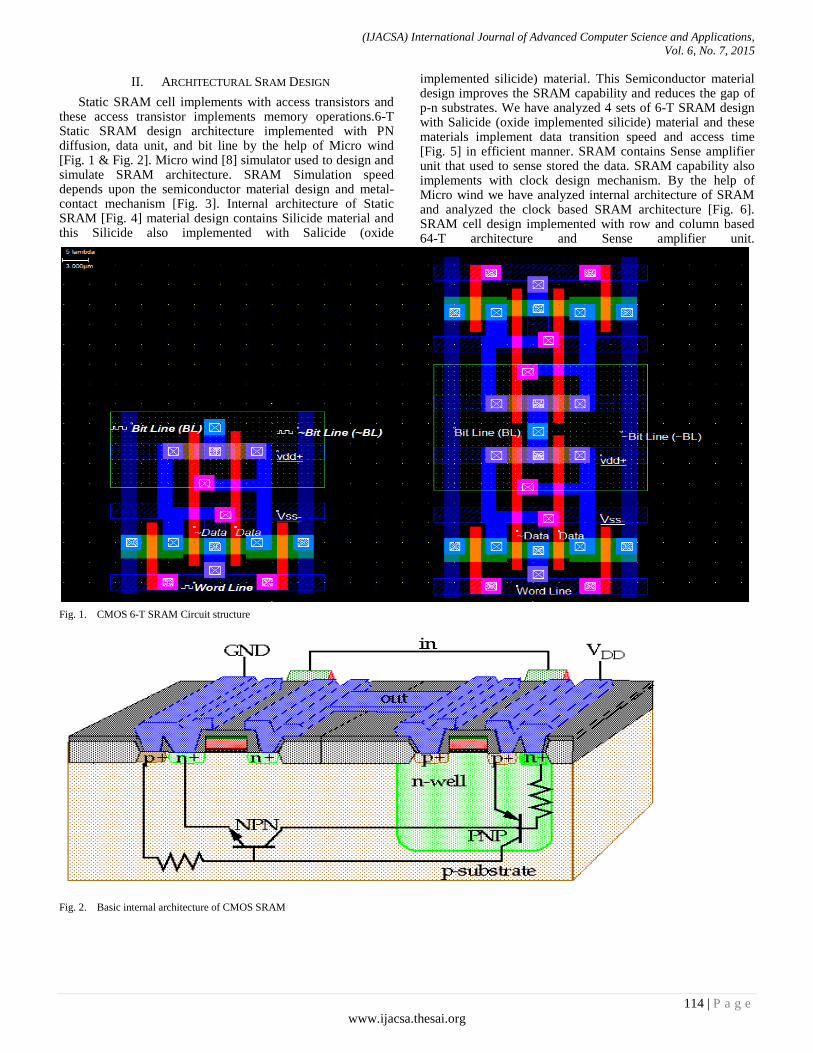
(IJACSA) International Journal of Advanced Computer Science and Applications,
Vol. 6, No. 7, 2015
114 | P a g e
www.ijacsa.thesai.org
II. ARCHITECTURAL SRAM DESIGN
Static SRAM cell implements with access transistors and these access transistor implements memory operations.6-T Static SRAM design architecture implemented with PN diffusion, data unit, and bit line by the help of Micro wind [Fig. 1 & Fig. 2]. Micro wind [8] simulator used to design and simulate SRAM architecture. SRAM Simulation speed depends upon the semiconductor material design and metal-contact mechanism [Fig. 3]. Internal architecture of Static SRAM [Fig. 4] material design contains Silicide material and this Silicide also implemented with Salicide (oxide
implemented silicide) material. This Semiconductor material design improves the SRAM capability and reduces the gap of p-n substrates. We have analyzed 4 sets of 6-T SRAM design with Salicide (oxide implemented silicide) material and these materials implement data transition speed and access time [Fig. 5] in efficient manner. SRAM contains Sense amplifier unit that used to sense stored the data. SRAM capability also implements with clock design mechanism. By the help of Micro wind we have analyzed internal architecture of SRAM and analyzed the clock based SRAM architecture [Fig. 6]. SRAM cell design implemented with row and column based 64-T architecture and Sense amplifier unit.
Fig. 1. CMOS 6-T SRAM Circuit structure
Fig. 2. Basic internal architecture of CMOS SRAM
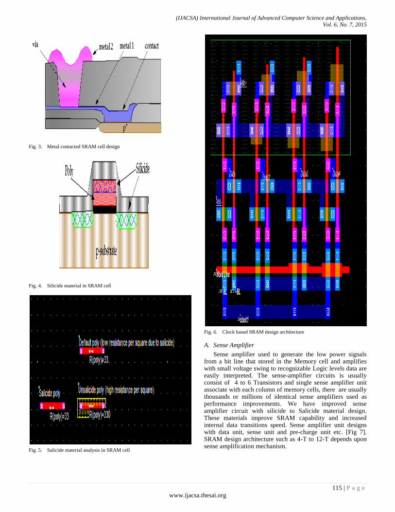
(IJACSA) International Journal of Advanced Computer Science and Applications,
Vol. 6, No. 7, 2015
115 | P a g e
www.ijacsa.thesai.org
Fig. 3. Metal contacted SRAM cell design
Fig. 4. Silicide material in SRAM cell
Fig. 5. Salicide material analysis in SRAM cell
Fig. 6. Clock based SRAM design architecture
A. Sense Amplifier
Sense amplifier used to generate the low power signals from a bit line that stored in the Memory cell and amplifies with small voltage swing to recognizable Logic levels data are easily interpreted. The sense-amplifier circuits is usually consist of 4 to 6 Transistors and single sense amplifier unit associate with each column of memory cells, there are usually thousands or millions of identical sense amplifiers used as performance improvements. We have improved sense amplifier circuit with silicide to Salicide material design. These materials improve SRAM capability and increased internal data transitions speed. Sense amplifier unit designs with data unit, sense unit and pre-charge unit etc. [Fig 7]. SRAM design architecture such as 4-T to 12-T depends upon sense amplification mechanism.
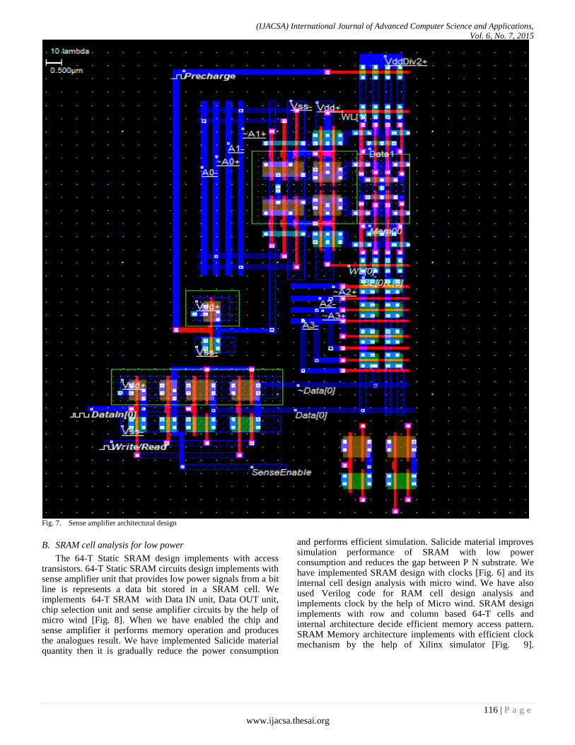
(IJACSA) International Journal of Advanced Computer Science and Applications,
Vol. 6, No. 7, 2015
116 | P a g e
www.ijacsa.thesai.org
Fig. 7. Sense amplifier architectural design
B. SRAM cell analysis for low power
The 64-T Static SRAM design implements with access transistors. 64-T Static SRAM circuits design implements with sense amplifier unit that provides low power signals from a bit line is represents a data bit stored in a SRAM cell. We implements 64-T SRAM with Data IN unit, Data OUT unit, chip selection unit and sense amplifier circuits by the help of micro wind [Fig. 8]. When we have enabled the chip and sense amplifier it performs memory operation and produces the analogues result. We have implemented Salicide material quantity then it is gradually reduce the power consumption
and performs efficient simulation. Salicide material improves simulation performance of SRAM with low power consumption and reduces the gap between P N substrate. We have implemented SRAM design with clocks [Fig. 6] and its internal cell design analysis with micro wind. We have also used Verilog code for RAM cell design analysis and implements clock by the help of Micro wind. SRAM design implements with row and column based 64-T cells and internal architecture decide efficient memory access pattern. SRAM Memory architecture implements with efficient clock mechanism by the help of Xilinx simulator [Fig. 9].
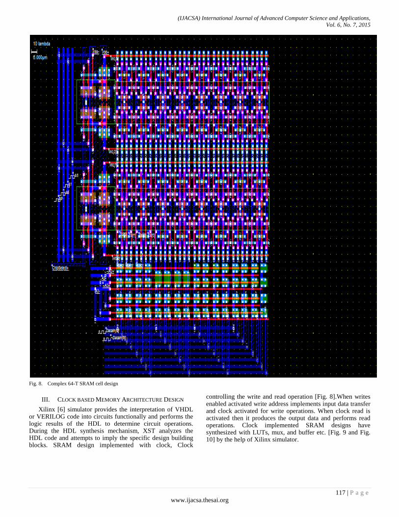
(IJACSA) International Journal of Advanced Computer Science and Applications,
Vol. 6, No. 7, 2015
117 | P a g e
www.ijacsa.thesai.org
Fig. 8. Complex 64-T SRAM cell design
III. CLOCK BASED MEMORY ARCHITECTURE DESIGN
Xilinx [6] simulator provides the interpretation of VHDL or VERILOG code into circuits functionally and performs the logic results of the HDL to determine circuit operations. During the HDL synthesis mechanism, XST analyzes the HDL code and attempts to imply the specific design building blocks. SRAM design implemented with clock, Clock
controlling the write and read operation [Fig. 8].When writes enabled activated write address implements input data transfer and clock activated for write operations. When clock read is activated then it produces the output data and performs read operations. Clock implemented SRAM designs have synthesized with LUTs, mux, and buffer etc. [Fig. 9 and Fig. 10] by the help of Xilinx simulator.

(IJACSA) International Journal of Advanced Computer Science and Applications,
Vol. 6, No. 7, 2015
118 | P a g e
www.ijacsa.thesai.org
Fig. 9. SRAM cell design
A. Dual Clock SRAM design
Dual clock implemented cache design that implemented with separate read clocks and separate write clock when signal activated and performs memory operations. When write enabled then activated the write address for input data transfer and these separate write clock performs write operations.
Another read clock signal is activated then it activates for read address and produces the output data and performs read operations. The Dual clock architectural of SRAM design implemented with ffd, buffer designs etc. [Fig.11 and Fig.12] and these dual clock design implements the data transitions scheme. These dual clocks SRAM design implements access time and reduces the propagation delay.
Fig. 10. RTL Design section of SRAM
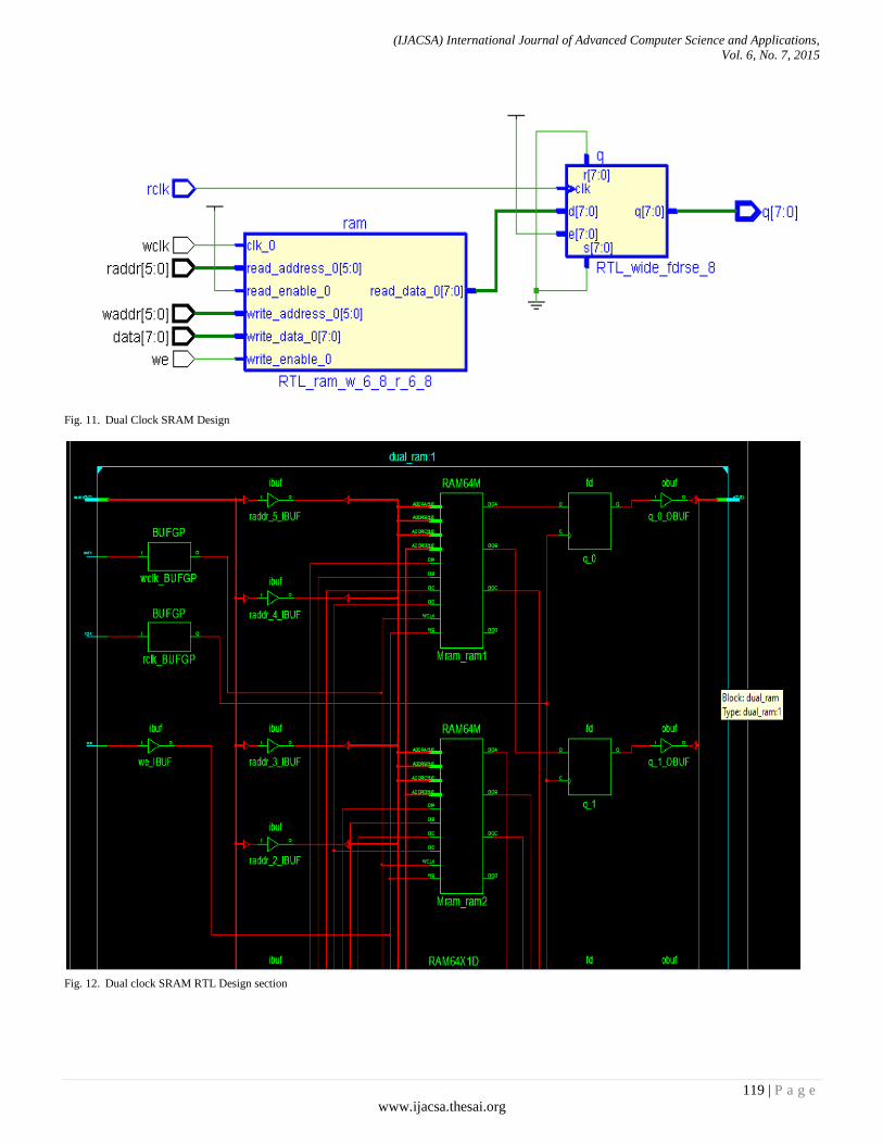
(IJACSA) International Journal of Advanced Computer Science and Applications,
Vol. 6, No. 7, 2015
119 | P a g e
www.ijacsa.thesai.org
Fig. 11. Dual Clock SRAM Design
Fig. 12. Dual clock SRAM RTL Design section

(IJACSA) International Journal of Advanced Computer Science and Applications,
Vol. 6, No. 7, 2015
120 | P a g e
www.ijacsa.thesai.org
B. Clock implemented SRAM Design
Clocks have implemented with subdivision mechanism and used counters are associated with a stream of ticks that represent time periods. Clock manage read and write operations with help of clock subdivision mechanism. Architectural clock based SRAM design implemented with counters, buffer etc. [Fig. 13 & Fig. 14]. Clock based counter used to manage all memory operation with schedule process and these architecture implements multiple data transitions scheme [Fig. 15].
Scheduled write/read operation reduces the data losses and implements memory access time and propagation delay time. We have analyzed that Single clock SRAM memory performs access time as 1ns and dual clock SRAM design implements simulation access time as 0.8ns because both operation implements data transitions with proper active state. Clock behavior implemented with clock subdivision mechanism and implements memory design that reduces the propagation delay time as 0.2ns or ten times reduces its depends upon clock edges pattern [Fig. 16 and Fig 17].
Fig. 13. Clock Implementation RTL design section of SRAM
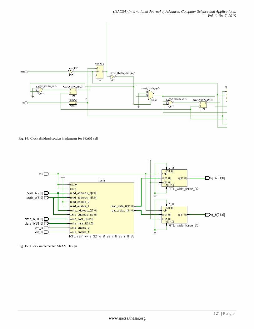
(IJACSA) International Journal of Advanced Computer Science and Applications,
Vol. 6, No. 7, 2015
121 | P a g e
www.ijacsa.thesai.org
Fig. 14. Clock dividend section implements for SRAM cell
Fig. 15. Clock implemented SRAM Design
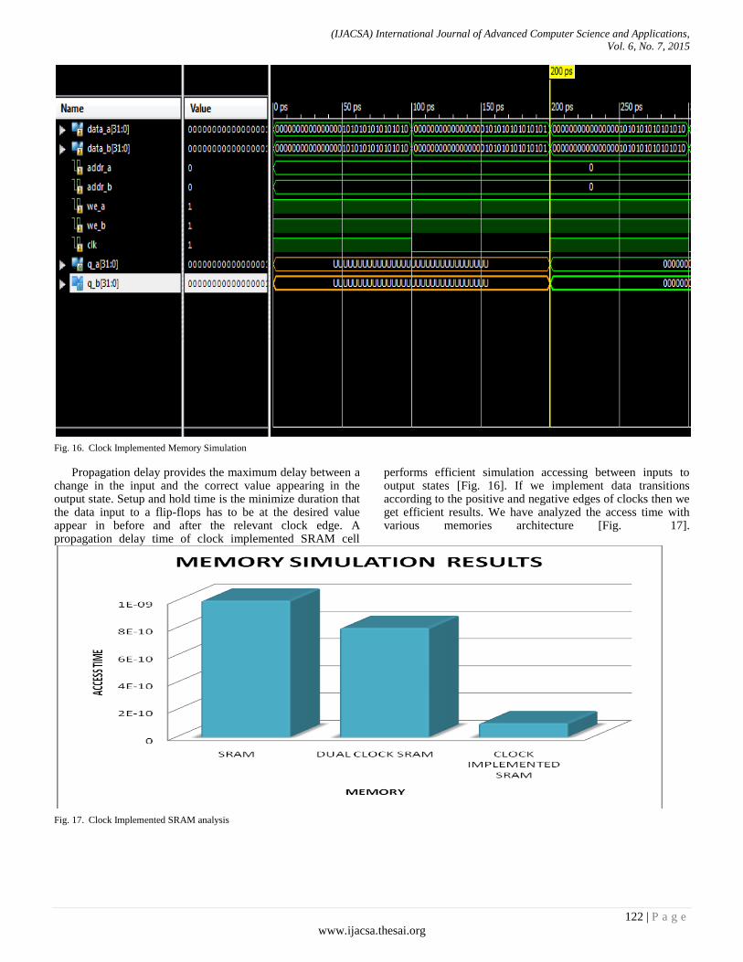
(IJACSA) International Journal of Advanced Computer Science and Applications,
Vol. 6, No. 7, 2015
122 | P a g e
www.ijacsa.thesai.org
Fig. 16. Clock Implemented Memory Simulation
Propagation delay provides the maximum delay between a change in the input and the correct value appearing in the output state. Setup and hold time is the minimize duration that the data input to a flip-flops has to be at the desired value appear in before and after the relevant clock edge. A propagation delay time of clock implemented SRAM cell
performs efficient simulation accessing between inputs to output states [Fig. 16]. If we implement data transitions according to the positive and negative edges of clocks then we get efficient results. We have analyzed the access time with various memories architecture [Fig. 17].
Fig. 17. Clock Implemented SRAM analysis
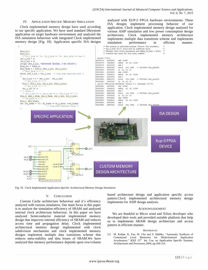
(IJACSA) International Journal of Advanced Computer Science and Applications,
Vol. 6, No. 7, 2015
123 | P a g e
www.ijacsa.thesai.org
IV. APPLICATION SPECIFIC MEMORY SIMULATION
Clock implemented memory design have used according to our specific application. We have used standard Dhrystone application on target hardware environment and analyzed the ISA simulation behaviour with integrated Clock implemented memory design [Fig. 18]. Application specific ISA designs
analyzed with XUP-5 FPGA hardware environments. These ISA designs implement processing behavior of our application. Clock implemented memory design analyzed for various ASIP simulation and low power consumption design architecture. Clock implemented memory architecture implements multiple data transitions scheme and implements simulation performance in efficient manner.
Fig. 18. Clock Implemented Application Specific Architectural Memory Design Simulation
V. CONCLUSION
Custom Cache architecture behaviour and it’s efficiency analyzed with various simulators. Our main focus in this paper is to analyze the simulation efficiency of SRAM and analyzed internal clock architecture behaviour. In this paper we have analyzed Semiconductor material implemented memory design that improves internal efficiency of SRAM and reduces access time and propagation delay. Clock implemented architectural memory design implemented with clock subdivision mechanism and clock implemented memory designs implement multiple data transitions scheme that reduces meta-stability and data losses of SRAM.We have analyzed that memory performance depends upon row/column
based architecture design and application specific access pattern.Clock implemented architectural memory design implements for ASIP design analysis.
ACKNOWLEDGMENT
We are thankful to Micro wind and Xilinx developer who developed their tools and provided suitable platform that help us to implements SRAM design architecture and access pattern in efficient manner.
REFERENCES
[1] M. Kuldar, K. Fan, M. Chu and S. Mahlke, “Automatic Synthesis of Customized Local Memories for Multiclustered Application Accelerators,” IEEE 15th Int. Con. on Application Specific Systems, Architectures and Processors,2004, pp.304-314.

(IJACSA) International Journal of Advanced Computer Science and Applications,
Vol. 6, No. 7, 2015
124 | P a g e
www.ijacsa.thesai.org
[2] P. Merolla, J. Arthur, F. Akopyan, N. Imam, R. Manohar and D.S. Modha, “A Digital Nero synaptic Core Using Embedded Memory with 45PJ per spike in 45nm,” In Proc. of CICC, 2011,pp.25-32.
[3] P. R Panda, N. D. Dutt and A. Nicoulau, “Data Memory Organization and Optimization in Application Specific Systems,” IEEE design & Tests of Computers,2001,pp.56-68.
[4] J. Park and P. C. Diniz, “Synthesis and Estimation of memory interfaces for FPGA-based Reconfigurable Computing Engines,” In Pr. of FCCM’03, 2003,pp.297-299.
[5] F. Vahid, G. Stitt, Z. Guo and W. Najjar, “Technique for Synthesizing Binaries to an advanced Register/Memory Structure,” In Pr. of ACM FPGA ’05, 2005, USA.
[6] Xilinx tool Available on: http://www.xilinx.com/homepage/.
[7] B.S. Reniwal and S. K.Vishvakarma, “A Reliable, Process-Sensitive-Tolerant Hybrid Sense Amplifier for Ultralow Power SRAM,”Int. J. of Electronics and Electrical Engineering, vol. 1, no.1,2013,pp.34-38.
[8] Micro wind tool available on: http://www.microwind.net/.
[9] E. Ozer, R. Sendag and D. Gregg, “Multiple-Valued Caches for Power-Efficient Embedded Systems,” In Pr. of.ISMVL’05, 2005.
[10] P. Wang, G. Sun, T. Wang, Y. Xie and J. Cong, “Designing Scratchpad Memory Architecture with Emerging STT-RAM Memory Technologies,” In Pr. of ISCAS,2013, pp.1244-1247.
[11] B. H. Calhaun and A.P. Chandrkasan, “A 256-kb 65-nm Sub-threshold SRAM designs for ultra-low-voltage operation,” Journal of solid-state circuits, vol.42, no. 3, 2007,pp. 680-688.
[12] K. Dhanumjaya, M. Sudha, M.N. Giri Prasad and K.Padmaraju, “Cell stability analysis of conventional 6t dynamic 8t SRAM cell in 45 nm technology,” Int. J. of VLSI design & Communication Systems (VLSICS), vol.3, no.2, 2012, pp.41-51.
[13] G. Chen, D. Sylvester, D. Blauw and T. Mudge, “Yield-Driven Near-Threshold SRAM Design,” IEEE Transactions on Very Large Scale Integration (VLSI) Systems,vol.18,no.11,2010,pp.1590-1598.
[14] N. K. Shukla, R.K. Singh and M. Pattanaik, “Design and Analysis of a Novel Low-Power SRAM Bit-Cell Structure at Deep-Sub-Micron CMOS Technology for Mobile Multimedia Applications,” Int. J. of Advanced Computer Science and Applications,vol.2,no.5,2011,pp.43-49.
[15] A. K. Dadoria, A. S. Yadav and C.M. Roy, “Comparative Analysis of Variable N-T SRAM Cells,” Int.J. of Advanced Research in Computer Science and Software Engineering,vol.3,no.4, 2013,pp.612-619.

(IJACSA) International Journal of Advanced Computer Science and Applications,
Vol. 6, No. 7, 2015
125 | P a g e
www.ijacsa.thesai.org
Using GIS for Retail Location Assessment at Jeddah
City
Abdulkader A Murad
Faculty of Environmental Design, King Abdulaziz University, P O Box 80210, Jeddah- 21589, Saudi Arabia
Abstract—GIS software has different useful tools that can be
used for sites, demographic and competitive analysis. These tools
enable retail and market researchers to find solutions related to
many retail planning issues. The aim of this paper is to use
Geographical Information Systems (GIS) for retail location
assessment of two retail centers called Al-Dawly and Al-Mahmal
centers located at Jeddah city, Saudi Arabia. The first part of the
paper presents a review about retail centers classification and
about GIS applications in retail planning field. The second part
of the paper discuss the outputs of the created application which
include a- defining retail catchment area, b- building retail
demand profile, and c- analyzing retail catchment area. The
results of this application can be used by retail planners for
evaluating retail centers location and for identifying the extent of
retail market
Keywords—Retail Planning; Retail Catchment Area; GIS;
Market Penetration; Drive Time
I. INTRODUCTION
One of the main noticeable features of Jeddah city is related to the rapid growth and expansion in retail facilities. Every city district has different types of retail centers. Some of these centers are small and specialized in certain goods or products e.g. mobile phone centers, and others are large retail centers e.g. Hera or Altahlia centers which have various types of retail facilities. All of these centers are faced today with many important issues related to their existing or potential demand. These issues include location of customers, income level of people or clients living within retail center catchment area, location of competitors and their related demand and the level of retail center attractiveness. In addition to these issues, retail developers face different strategic and operating decisions, ranging from initial site selection to mall configuration and tenant mix to managing lease receivables. These decisions can be facilitated by relevant timely accessible information. This indicates that there is a great need to use information technologies for handling this information. One of the most useful technologies that can handle and manipulate retail data is known as Geographical Information Systems (GIS) that are defined as computerized based systems that provides different tools for handling and manipulating spatial data. The use of GIS and spatial modeling in applied retail location analysis is a relatively new phenomenon [1]. While GIS technology dates to the 1960s, most early applications were associated with natural resources, municipal/ public service and military applications [2]. Birkin et al, 1996 [1], have identified five main retail analytical techniques that can be covered with GIS. These are called: trial and error, analogue techniques, regression techniques,
catchment area analysis and mathematical models that include spatial interaction models, location allocation and optimization models. Some of these techniques are explored by GIS based studies [1,2,3,4,and 5], . This paper is concentrated on applying GIS at one of these retail analytical techniques which is called the catchment area analysis. This technique is defined as abroad set of procedures aimed to measure more objectively the size of existing centers (and hence their potential) and to understand the break down of their catchment areas in terms of population structure [5]. At first, the paper will review the size and the extent of existing retail centers catchment area and then will focus on applying GIS for defining and analysis catchment area of two retail centers called Al-Dawly and Al-Mahmal center at Jeddah city, Saudi Arabia. Two main types of retail catchment areas are produced which are called the primary catchment area, and the drive time catchment area. The former is created based on customers’ location, and the latter is produced based on the expected drive time to the selected center. Each one of these catchement areas is created to support retail developers and planners in understanding the spatial extent of their center’s catchment area, and also to help them in deciding upon the performance of their retail center too.
II. BACKGROUND
A. Types of Retail Centres
There are two basic methods of classifying retail centres, and they are based on either the types of goods and shops included or based on the trade area [6] . In the forms method, retail centres are divided into two groups, those selling convenience goods such as food items and toiletries, and those selling durables, such as clothing, furniture and household appliances. The latter method of retail centers classification produces the following types of centres:
1) Neighbourhood Centre: The function of neighborhood
centre is to provide a range of convenience goods and
personal services, for the day to day needs. The assumed
catchment population is 2500 to 40,000 people within a six
minute drive times and it is generally assumed that consumers
visit their nearest centre [7]. The location of neighbourhood
centre should be embedded in residential areas. However,
commercial developers prepare sites at intersections on major
roads, which are on the edge of residential blocks. The
average area for this type of centres is 40,000 to 50,000
square feet [8].
2) Community Centre: This type of retail centres offers
shoppers greater depth and range of merchandize-assortments

(IJACSA) International Journal of Advanced Computer Science and Applications,
Vol. 6, No. 7, 2015
126 | P a g e
www.ijacsa.thesai.org
in clothing sizes, styles, colors, and prices than does a
neighbourhood centre. The community center serves from
40,000 to 150,000 people, and has a site area of 4-12 ha [7].
Community centres have convenience goods more than
neighborhood centres, but at the same time they have durable
goods less than regional centres.
3) Regional Centre: The third type of retail centres
provides all forms of general merchandise, apparel and
furniture, and almost all those retail facilities available in the
town centre. The size of regional centres varies dramatically
from 10 acres for a multilevel centre to over 100 acres for a
large single level centre (ibid). These centres comprised a
great number and variety of shops selling convenience goods
and competing with one another by low prices and range of
assortment [9]. The above retail centre hierarchy represents a general
frame for classifying retail centres. However, there are other retail centre types which can be added to those three classes e.g. Ancillary centres, and specialty centres.
B. Existing Retail Catchment
The aim of this part of the paper is to present several existing retail centers and identifies their catchment areas. This is considered as a literature background that at the end will conclude with a realistic definition of retail centers catchment area. This review covers some retail centers that are located at different European countries. In general, retail centers can be classified into three groups based on their physical sizes. These are called large, medium and small retail centers.
1) Large retail centers The first type of retail center classification is known as
large retail centers. These are characterized with larger catchment population (800,000 person) and with the availability of large mixed-use schemes. Tres Aguas center at Madrid, Spain, is an example of retail centers that falls within this group. It provides a total of 46,000 sqm GLA (Gross Leasable Area) for its 800,000 person total catchment area and provides 3200 car parking spaces for its visitors [10]. Carre senart at France is another example of large retail centers. It is one of the largest shopping centers of its kind in France located 35 km south west of Paris. It enjoys a total catchment population of 800,000 and has 130 shops with 65,000 sqm GLA and provides 4700 car parking spaces for its customers that are summed by 4.3 million shoppers on its first 4 trading months [11] . Bonaire retail center at Valencia - Spain is a third example of this group. It serves a total catchment area of 1.1 million inhabitants within 20-minute drive and it is considered as the biggest (135,000 sqm GLA) retail development of Southern Europe [12] . Looking at those three large centers, it can be said that every large retail center should serve a minimum catchment population of 800,000 people and should provide at least 4000-car parking spaces.
2) Medium-sized retail center The second type of retail centers is called medium-sized
centers. These centers are very important in any city because they can be distributed at different areas of the city and create remarkable impacts on land uses and transportation network
too. For example, Spandan Arcaden is a medium sized retail center at Berlin, Germany, located to revitalize the center of Spandau by bringing modern retail space and recreational facilities within easy reach of the historic town center and residents of West Berlin. This center has a catchment population of 230,000 within 15 minutes drive time and provides 125 shops for its customers [13] . The second similar example is Altmarkt Galerie, which is located in the heart of Dresden, the historical capital city of Saxony in the south east of Germany. It has a primary catchment population of some 180,000 person, 26,000 sqm GLA, 107 shops and 500 car parking spaces [14] . This center is another example showing how medium sized retail centers can be integrated into historical city center life without loosing customer comfort or retailing efficiency. Fiumara center in Italy is a third example of this type of retail centers situated in the historical docklands area just west of Genoa city with a catchment area of approximately, 180,000 inhabitants living within 30 minutes drive. It consists of approximately 25,000-sqm retail GLA with over 100 shop units and has 2,200 car parking spaces [15] . This center is another good example of a development that has successfully integrates both the old and the new future of Genoa city.
In comparing between the above examples of medium sized retail centers, it can be said that these centers can be located at old or declined areas to increase the growth of such areas, and they serve an average catchment of 200,000 person living within 20 minutes drive and has at least 100 shops.
3) Small retail centers Small retail centers are another interested retail types that
are located at or close to residential districts. For example, Les passages center is located southwest of Paris and provides retail services for a total catchment area of 150,000 inhabitants. It has 21,700 sqm GLA (56 shop units) and allows access to car parking with about 600 spaces [16] . One of the other features of this type of retail centers is that they can be integrated easily with ribbon retail streets that are mainly fond at city center or along main road. The second example of this type of retail centers is found at Espace Jaures center at Brest town in France. This center has 30 shops with a total 14,000 sqm GLA, located on a shopping street with a 400 car parking spaces [17].
Accordingly, it can be concluded from this review that small retail centers are characterized with about 50 shops and catchment population of 150,000 people and provide about 15,000 sqm GLA for retail activities.
C. GIS and its development in retail planning
The objective of retail planning can be summarized as the provision of the right amount of land for retailing in the right place. To achieve this objective, retail planners use catchment area and market penetration techniques as analytical methods for retail assessment purposes. The catchment area can be used as a descriptive method to observe the degree of centre coverage, to identify areas of under-representation as obvious gaps in the map, and thus to spit potential new sites [18]. A market penetration approach, on the other hand, is more relevant to a single operating retail outlet that which to increase its sales, either by extending its trade area in space or
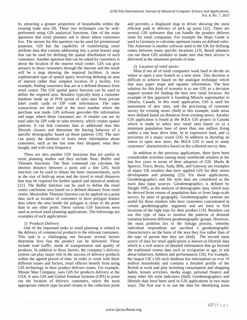
(IJACSA) International Journal of Advanced Computer Science and Applications,
Vol. 6, No. 7, 2015
127 | P a g e
www.ijacsa.thesai.org
by attracting a greater proportion of households within the existing trade area [8]. These two techniques can be well-performed using GIS analytical functions. One of the main questions that retail planners ask is about where customers live. The answer for this question can be used for promotional purposes. GIS has the capability of transforming retail attribute data that contain addressing into a point feature map that can be used for defining the spatial distribution of such customers. Another question that can be asked by customers is about the location of the nearest retail centre. GIS can give answers to those customers through the Internet and the result will be a map showing the required facilities. A more sophisticated type of spatial query involving defining an area of interest rather than simplest location of a facility. For example, finding customers that are at a defined distance from retail centre. The GIS spatial query function can be used to define the required area. Retailers typically keep a customer database made up of POS (point of sale) data from private label credit cards or ZIP code information. The sales transactions are then tied to the store number where the purchase was made. GIS software geocodes this information and maps where those customers are. A retailer can see its total sales by ZIP code or sales territory, which creates spatial patterns. It can link customer data to additional data like lifestyle clusters and determine the buying behavior of a specific demographic based on those patterns [19]. The user can query the database to learn more information about customers, such as the last time they shopped, what they bought, and with what frequency.
There are also another GIS functions that are useful in retial planning studies and they include Near, Buffer and Thiessen functions. The Near command can calculate the shortest distance between a point and a line [20]. Such function can be used to obtain the basic measurements, such as the size of built-up areas and the travel to retail distances that may be required for further spatial and statistical analysis [21]. The Buffer function can be used to define the retail centre catchment area based on a defined distance from retail centre. Meanwhile Thiessen function can be applied on a point data such as location of customers to have polygon feature data where the area inside the polygon is closer to the point than to any other point. These various GIS functions were used at several retail planning applications. The followings are examples of such applications:
1) Products Delivery One of the important tasks in retail planning is related to
the delivery of commercial products to the relevant customers. This task is a challanging one because several factors determine how fast the product can be delivered. These include road traffic, mode of transportation and quality of products. In addition to these factors, the company’s delivery system can play major role in the success of delivery products within the agreed period of time. In order to work with these different issues and factors, retail officers benefit from using GIS technology in their product delivers routes. For example, Minute Man Company, uses GIS for products delivery at the USA. It uses GIS and Global Position Systems (GPS) to point out the location of delivery customers, select the most appropriate vehicle type located closest to the collection point
and provides a displayed map to driver showing the most efficient path to delivery of pick up point [22]. There are several GIS softwares that can handle the product delivers issue for retail companies. For example the Maps Guide is used in Germany to calculate optimum routes on defined rules. The Autoroute is another software used in the UK for defining routes between many specific locations [23]. Retail planners can use these GIS modules to make sure that their service is delivered at the minimum periods of time.
2) Location of retail stores: Most if not all of retail companies work hard to decide on
where to open a new branch or a new store. This decision is difficult to achieve based on the analogue technique which that uses paper maps and squatter information. The best solution for this kind of scenario is to use GIS as a decision support system for finding the best new retail location. An example of this approach is founding Miracle supermarket in Ontario, Canada. In this retail application, GIS is used for assessment of new sites, and the processing of customer survey for existing stores (ibid) in this example, trade areas were defined based on distances from existing stores. Another GIS application is found at the IKEA GIS project in Canada which is made to select new retail sites based on a) a minimum population base of more than one million living within a one hour drive time, b) in expressive land, and c) proximity of a major round [24]. In addition to deciding on where to open new store, the IKEA GIS is used to study customers’ characteristics based on the collected survey data.
In addition to the previous applications, there have been considerable activities among many worldwide retailers in the last few years in terms of their adoption of GIS. Marks & Spencer, Tesco, Boots, Asda, BHs, and Gateway are examples of major UK retailers that have applied GIS for their stores development and planning [25]. For those applications, Geodemographics and life style data are considered as the main data input sources. Geodemographics is defined by Sleight 1995, as the analysis of demographic data, which may be derived from census of population data or from large-scale survey, by units of geography. Geodemographic systems are useful for those retailers who have customers concentrated in certain geodemographic segments and are keen to find locations of the right type for their product [19]. Retailers can use this type of data to monitor the patterns of demand variation between different geodemographic groups. However, the main problem lies in the linkage process, whereby individual respondents are ascribed a geodemographic characteristics on the basis of the area they live rather than of the type of person that they are (ibid). The second main source of data for retail applications is known as lifestyle data which is a rich source of detailed information that go beyond the traditional census data such as occupation or age, to ask about behaviors, hobbies and performances [26]. For example, the largest UK’s life style database has information on over 10 million households and contains a detailed profile of the British at work and play including consumption and shopping habits, leisure activities, media usage, personal finance and many other life style indicators (ibid). Geodemographics and lifestyle data have been used in GIS applications in two main ways. The first one is to use the data for identifying areas

(IJACSA) International Journal of Advanced Computer Science and Applications,
Vol. 6, No. 7, 2015
128 | P a g e
www.ijacsa.thesai.org
having a high proportion of inhabitants who are seen as desirable from the points of view of a retail product or service. While the second method of using these data with GIS is found where users identify demand profile and then derive a measure of potential within specific areas.
D. GIS tools for retail studies
GIS softwares have different useful tools that can be used for sites, demographic and competitive analysis. These tools enable retail and market researchers to find solutions related to retail issues such as:
Performing customer or store prospecting
Defining customer-based or store trade areas
Finding best retail location
Conducting market penetration analysis
Creating gravity models and
Performing drive-time analysis
All of the above retail analysis issues can be handled in GIS using various types of tools and functions. Some of these tools and functions are going to be discussed at this section.
1) Data query and display The simplest GIS tool that can be used at every retail GIS
application is related to displaying and queering spatial and attribute data. For example, ArcGIS software has several functions that can be used for data query and display. This software can display attributes in relation to points, lines or polygons which is known as thematic mapping [22]. Retailers can use thematic mapping technique to present any collection of tabular data such as the numbers people within a 30-minute drive time from a selected retail center. Data query tools in GIS can be applied on a single attribute field such as number of retail customers, or on a multiple attribute data field such as retail demand, and retail supply. Retailers can perform their needed spatial query and see the results of that query on the study area map. For example, they could use the mouse or other pointing device at the place of interest on a map and then GIS will search the database and show the data about the selected location. If a multiple query searching is required at any retail data set, spatial features can be selected through logical operations that deal directly with the database and allow the user to identify and select features by a specific set of Criteria. For example, finding all parcels that are having greater than 10,000 customers of certain retail center. Retail database can be displayed in GIS in different ways depending on the attribute types of that data. For example, the unique value technique can be used to display string attribute data, meanwhile the data classification procedure can be applied on numerical data. The unique value function lets the user to assign a unique symbol to each unique value of the attribute. With this type of GIS functions, retailers can identify how different types of features are located with respect to each other and their relative frequency and distribution [27].
The second useful GIS function related to data display is related to drawing quantities of features by graduated color or graduated symbols. This function is considered, as another
effective was to visualize numerical attributes of continuous data such population size, temperature or elevation. Most of GIS softwares (e.g. ArcGIS software) have separate modules for displaying and visualization geographical data (such as retail demand distribution) in 3D views. These modules are useful for viewing retail data from multiple viewpoint using different viewers [28].
2) Data analysis and manipulation One of the most important features of any GIS software is
related to its ability to analyze spatial data in different ways and with various functions. These functions are mad for different users. The most common function is called the proximity analysis function that could be used for finding answers for questions such as “what geographical features are near other features?” Such questions can be answered using a buffer to define the area of proximity, for example 0.5 kilometer, and then overlaying a second map layer containing the map features required [22]. To create a buffer, retailers should specify the source feature e.g. retail center and the buffer distance (e.g. 2 km) and then GIS will draw a circle of a radius equal to the distance specified.
Proximity analysis can be applied at GIS based on straight-line distance, distance cost over a network, or cost over surface. Each one of these types of GIS analysis can be applied in retail studies and can find answers to several questions including finding out how many customers are within a 20-minute drive of existing or new store site [29]. One way of defining and measuring how close a store to customers is by measuring the distance to that store. However, this distance can be measured using cost such as time rather than length. Mapping travel costs in GIS gives retail planners a more precise measure of what’s nearby than mapping distance, but it required more data preparation and processing (ibid). This technique is going to be discussed in more detail at the GIS application section.
III. METHODS
Based on the above discussion, it can be said that GIS has different tools which can be used by retail developers and planners for the purpose of identifying and analyzing retail catchment area. This part of the study will concentrate on explaining how to use these tools for two exciting retail centers called Al-Dawly and Al-Mahmal center located in Jeddah city, Saudi Arabia. Based on the retail classifications that are presented at this study, these centers fall with the medium sized retail centers group. In order to define the catchment area of this selected centers, a GIS application is created which covers three main retail issues which are : a- defining retail catchment area, b- building retail demand profile, and c- analysisng retail catchment area.
In order to build this GIS application, several data sets were collected and then entered into the ArcGIS software. These data fall into the three major vector data model types which are as following:
A. Line data
This type of data is stored in GIS as a series of ordered X, Y coordinates and the segments of a line can be straight, circular, elliptical or splined [27]. Road network of Jeddah

(IJACSA) International Journal of Advanced Computer Science and Applications,
Vol. 6, No. 7, 2015
129 | P a g e
www.ijacsa.thesai.org
city is an example of line data model that is created for the present study. This coverage has several attributes including road length, type and speed.
B. Point Data
GIS softwares store point data as single X, Y coordinate with several attributes. This type of data model is used in this study to represent location of retail center and retail customers. Several attributes are made with these data including center size, parking size, no. of shops and amount of GLA. For retail customer coverage the attributes are including district name and purpose of visits.
C. Polygon data
This type of features is modeled at GIS as a series of segments that enclose an area and form a set of closed area [27]. City districts coverage is an example of this type of GIS data that is created for the present study. This coverage includes attributes such as district name and area, and size of population and households for each district.
All of the above data were originally in a non-digital format. Therefore, manual digitizing and keyboard entry methods are used to convert all of these data into GIS digital formats (shape files and coverages). The next section will discuss the results of this GIS application that can be used by retail developers and planners of the selected centers.
IV. RESULTS
A. Defining retail catchment area
There are several GIS methods that can be used for defining the primary catchment area of retail centers. The most common one is related to customers spotting. Several studies have used this type of GIS function for defining retail catchment and for demographic analysis [30, 31, 32, and 4] . For example, Jones et al, 1995 [4], have defined primary catchment areas for retail centers based on the nearest 60% of retail center consumers. In order to define the primary catchment area of Al-Dawly center, a survey is made on a sample of customers visiting this center. According to the records of this center the average amount of customers visiting the center is about 4500 customers per month. Unfortunately, there are no spatial records for each one of those customers. Therefore, a survey on 5% of the total customers is made to show the spatial distribution of the center demand. This data is used for the main objective of this part of the study that is defining the primary retail catchment area. The survey is made using a questioner that shows the address of customer, reason for visiting this center and the social economical background of each customer. All of the collected survey questionnaire are captured into the GIS using the address geo-coding function. This function use address information in the attribute table of a reference data (e.g. street network) to figure out where to locate address points [33]. The more detailed the reference data, the more accurately addresses can be located. The output of this function is either a shape file or a geodatabase having feature class of points with all the attributes of the address table, some of the attribute of the reference data and optionally some new attributes, such as the X, Y coordinates of each point (ibid).
Once the location of retail customers is defined (Fig. 1), the following task was to select the nearest 60% of Al-Dawly customers. This was achieved using the following steps.
1) Query builder is applied on customer location shape
file to select the nearest 60% of Al-Dawly customers.
2) The ‘select by them’ function of ArcGIS is used to
define areas and districts that fall within the results found at
step 1. In this case, ArcGIS selects city districts that intersect
with the selected features of Al-Dawly customer shape file.
Fig. 1. Customer Distribution of Al-Dawly Center
Fig. 2. Primary Trade area of Al-Dawly Center
#
#
#
#
#
#
#
##
#
#
#
#
#
#
#
#
# #
#
#
#
#
#
#
#
#
#
#
#
#
#
#
#
#
##
#
#
#
#
#
#
#
#
#
#
#
#
#
##
#
#
#
#
#
#
# #
##
#
#
#
#
#
##
#
#
#
#
#
#
##
#
#
#
#
#
#
#
##
#
##
#
#
#
#
#
#
##
#
#
#
#
#
#
#
#
#
#
#
#
#
r
10000 0 10000 20000 Meters
Road
# Customers Locationr Al-Dawly Center
N
EW
S
r
10000 0 10000 20000 Meters
Primary Trade Area
Roadr Al-Dawly Center
N
EW
S
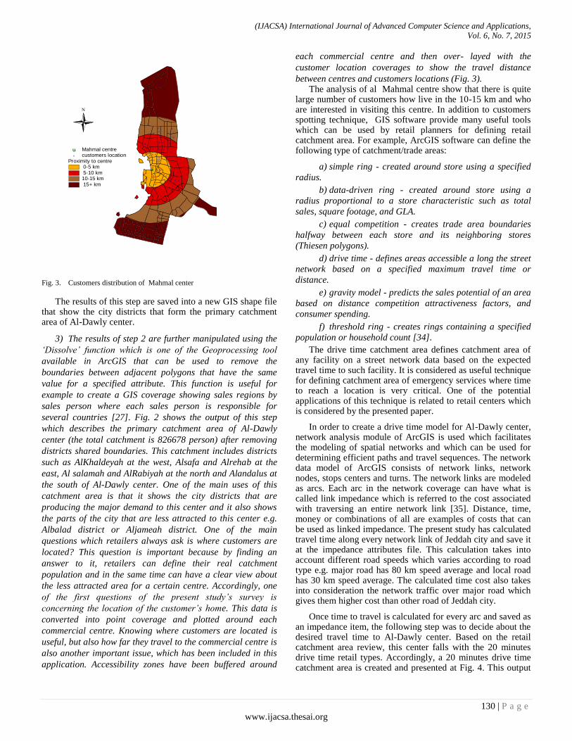
(IJACSA) International Journal of Advanced Computer Science and Applications,
Vol. 6, No. 7, 2015
130 | P a g e
www.ijacsa.thesai.org
Fig. 3. Customers distribution of Mahmal center
The results of this step are saved into a new GIS shape file that show the city districts that form the primary catchment area of Al-Dawly center.
3) The results of step 2 are further manipulated using the
‘Dissolve’ function which is one of the Geoprocessing tool
available in ArcGIS that can be used to remove the
boundaries between adjacent polygons that have the same
value for a specified attribute. This function is useful for
example to create a GIS coverage showing sales regions by
sales person where each sales person is responsible for
several countries [27]. Fig. 2 shows the output of this step
which describes the primary catchment area of Al-Dawly
center (the total catchment is 826678 person) after removing
districts shared boundaries. This catchment includes districts
such as AlKhaldeyah at the west, Alsafa and Alrehab at the
east, Al salamah and AlRabiyah at the north and Alandalus at
the south of Al-Dawly center. One of the main uses of this
catchment area is that it shows the city districts that are
producing the major demand to this center and it also shows
the parts of the city that are less attracted to this center e.g.
Albalad district or Aljameah district. One of the main
questions which retailers always ask is where customers are
located? This question is important because by finding an
answer to it, retailers can define their real catchment
population and in the same time can have a clear view about
the less attracted area for a certain centre. Accordingly, one
of the first questions of the present study’s survey is
concerning the location of the customer’s home. This data is
converted into point coverage and plotted around each
commercial centre. Knowing where customers are located is
useful, but also how far they travel to the commercial centre is
also another important issue, which has been included in this
application. Accessibility zones have been buffered around
each commercial centre and then over- layed with the
customer location coverages to show the travel distance
between centres and customers locations (Fig. 3). The analysis of al Mahmal centre show that there is quite
large number of customers how live in the 10-15 km and who are interested in visiting this centre. In addition to customers spotting technique, GIS software provide many useful tools which can be used by retail planners for defining retail catchment area. For example, ArcGIS software can define the following type of catchment/trade areas:
a) simple ring - created around store using a specified
radius.
b) data-driven ring - created around store using a
radius proportional to a store characteristic such as total
sales, square footage, and GLA.
c) equal competition - creates trade area boundaries
halfway between each store and its neighboring stores
(Thiesen polygons).
d) drive time - defines areas accessible a long the street
network based on a specified maximum travel time or
distance.
e) gravity model - predicts the sales potential of an area
based on distance competition attractiveness factors, and
consumer spending.
f) threshold ring - creates rings containing a specified
population or household count [34].
The drive time catchment area defines catchment area of any facility on a street network data based on the expected travel time to such facility. It is considered as useful technique for defining catchment area of emergency services where time to reach a location is very critical. One of the potential applications of this technique is related to retail centers which is considered by the presented paper.
In order to create a drive time model for Al-Dawly center, network analysis module of ArcGIS is used which facilitates the modeling of spatial networks and which can be used for determining efficient paths and travel sequences. The network data model of ArcGIS consists of network links, network nodes, stops centers and turns. The network links are modeled as arcs. Each arc in the network coverage can have what is called link impedance which is referred to the cost associated with traversing an entire network link [35]. Distance, time, money or combinations of all are examples of costs that can be used as linked impedance. The present study has calculated travel time along every network link of Jeddah city and save it at the impedance attributes file. This calculation takes into account different road speeds which varies according to road type e.g. major road has 80 km speed average and local road has 30 km speed average. The calculated time cost also takes into consideration the network traffic over major road which gives them higher cost than other road of Jeddah city.
Once time to travel is calculated for every arc and saved as an impedance item, the following step was to decide about the desired travel time to Al-Dawly center. Based on the retail catchment area review, this center falls with the 20 minutes drive time retail types. Accordingly, a 20 minutes drive time catchment area is created and presented at Fig. 4. This output
ÑÑÑÑ
Ñ
Ñ
ÑÑ
Ñ
Ñ Ñ
ÑÑ
Ñ
Ñ
Ñ
Ñ
Ñ
Ñ
Ñ
ÑÑÑ
Ñ
Ñ
Ñ Ñ
ÑÑ
ÑÑ
Ñ Ñ
Ñ
Ñ
Ñ
ÑÑ
Ñ
Ñ
Ñ
Ñ
Ñ
Ñ
Ñ
Ñ
Ñ
%U
Proximity to centre 0-5 km 5-10 km10-15 km 15+ km
Ñ customers location%U Mahmal centre
N

(IJACSA) International Journal of Advanced Computer Science and Applications,
Vol. 6, No. 7, 2015
131 | P a g e
www.ijacsa.thesai.org
defines the total catchment area of Al-Dawly center and the same technique can be applied for all other retail centers located at Jeddah city including Al-Mahmal center.
Fig. 4. A 20-minutes Drive time Trade area
Fig. 5. Household size of Mahaml customers
Fig. 6. Home ownership for Mahaml customers
B. Building retail demand profile
Retail customers profile is useful for retailers because it gives them the opportunity of knowing who are their customers? By doing so, retailers can approach certain customers for a specific retailing purposes. Jonsek and Simmons, 1991 [36], have mentioned that once the centre catchment area is drawn then analyst tries to identify the customers profile for such areas. The present study has created customers profile for al Mahmal shopping centre, which includes data regarding income, age – sex status, age, home-ownership, car ownership, purposes for visit as well frequencies of visiting such shopping centre. This large profile is very useful for retailers because it shows the actual demand characteristics. The collected survey data can be divided into two categories, which are the demographic profile and the demand profile. The former includes information about income, age-sex, household size, education level, and housing ownership. The later has information about the purpose of visit (i.e. to pay certain goods or for general shopping) reasons for selecting the shopping centre (i.e. close to home, low prices, free parking etc), and frequent of visits. The present study has selected two demographic data (household size and home ownership) and one demand-status data (visits to centres). The spatial distribution of household size and home ownership for al Mahmal centre is shown in Figures 5 and 6. The results of these figures show the existing demand status of the shopping centre. They are very useful in identify a clear image about the types of customers in each shopping centre. In addition, such profile is of great value to retail developers
One of the possible GIS applications in retail studies is related to identifying the location of potential target markets. For example, GIS can be used to define the spatial distribution of one customer sequent such as middle-income customers, large size families or families with large children numbers. This type of GIS-based retail analysis can be used for:
a) evaluating the potential of new tenants serving a
particular market niche,
r
5000 0 5000 10000 15000 20000 Meters
Drive time area
20 Minutes
Road
Drive time arcs
20 Minutes
r Al-Dawly Center
N
EW
S
%U
Househols size1 - 22 - 44 - 66 - 88 - 9
%U Mahmal centre
N
%U
Home ownership
1- 2
2 -3
3 - 4
5 - 8
9 - 10
%U Mahmal centre
N

(IJACSA) International Journal of Advanced Computer Science and Applications,
Vol. 6, No. 7, 2015
132 | P a g e
www.ijacsa.thesai.org
b) providing marketing advice to existing retail tenants
that do not have the skills or technology to undertake detailed
geo-demographic analysis, and
c) identifying market/lifestyle segments that the
shopping center is under-serving [2].
The collected data about Al-Dawly center customers cover several social and economical information about those customers that can use for the purpose of target market identification. One example of this type of analysis is to identify location of households that own houses. This type of customers can be seen as middle-to-high income customers that can be reached for promoting certain goods or services available at Al-Dawly center (e.g. electronic products). Fig. 7 presents the spatial distribution of house owners’ customers as well as tenants customers. One of the main findings of this output is that house owner customers of this retail center are concentrated at the western city districts; meanwhile tenant customers are located mainly at the eastern city districts.
The present study has used Intersect function (which is on of GIS overlay analysis functions) with the drive time model to identify the potential demand of Al-Dawly center. It was found that there is 208,163 households live within the retail center drive time catchment area. Fig. 8 defines classification of total households that are living within the resulted drive time trade area. It also identifies the spatial distribution of all households that are considered as potential customers for Al-Dawly center.
Fig. 7. Location of House owners Customers
Fig. 8. Spatial distribution of households living inside retail trade area
Fig. 9. Market Penetration for Al-Dawly retail center
r
10000 0 10000 20000 Meters
House Oweners
Owners
Tenants
Roadr Al-Dawly Center
N
EW
S
r
6000 0 6000 12000 18000 24000 Meters
Households0 - 1983
1984 - 4440
4441 - 7284
7285 - 1308713088 - 21932
Roadr Al-Dawly Center
N
EW
S
r
5000 0 5000 10000 Meters
Road
Market Penetration (%)
6 - 16
16 - 30
30 - 58
58 - 111
111 - 182
r Al-Dawly Center
N
EW
S
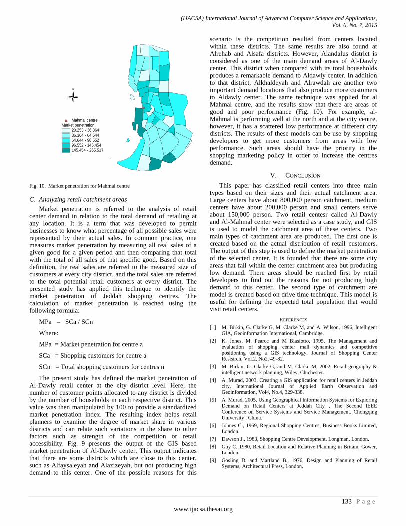
(IJACSA) International Journal of Advanced Computer Science and Applications,
Vol. 6, No. 7, 2015
133 | P a g e
www.ijacsa.thesai.org
Fig. 10. Market penetration for Mahmal centre
C. Analyzing retail catchment areas
Market penetration is referred to the analysis of retail center demand in relation to the total demand of retailing at any location. It is a term that was developed to permit businesses to know what percentage of all possible sales were represented by their actual sales. In common practice, one measures market penetration by measuring all real sales of a given good for a given period and then comparing that total with the total of all sales of that specific good. Based on this definition, the real sales are referred to the measured size of customers at every city district, and the total sales are referred to the total potential retail customers at every district. The presented study has applied this technique to identify the market penetration of Jeddah shopping centres. The calculation of market penetration is reached using the following formula:
MPa = SCa / SCn
Where:
MPa = Market penetration for centre a
SCa = Shopping customers for centre a
SCn = Total shopping customers for centres n
The present study has defined the market penetration of Al-Dawly retail center at the city district level. Here, the number of customer points allocated to any district is divided by the number of households in each respective district. This value was then manipulated by 100 to provide a standardized market penetration index. The resulting index helps retail planners to examine the degree of market share in various districts and can relate such variations in the share to other factors such as strength of the competition or retail accessibility. Fig. 9 presents the output of the GIS based market penetration of Al-Dawly center. This output indicates that there are some districts which are close to this center, such as Alfaysaleyah and Alazizeyah, but not producing high demand to this center. One of the possible reasons for this
scenario is the competition resulted from centers located within these districts. The same results are also found at Alrehab and Alsafa districts. However, Alandalus district is considered as one of the main demand areas of Al-Dawly center. This district when compared with its total households produces a remarkable demand to Aldawly center. In addition to that district, Alkhaldeyah and Alrawdah are another two important demand locations that also produce more customers to Aldawly center. The same technique was applied for al Mahmal centre, and the results show that there are areas of good and poor performance (Fig. 10). For example, al- Mahmal is performing well at the north and at the city centre, however, it has a scattered low performance at different city districts. The results of these models can be use by shopping developers to get more customers from areas with low performance. Such areas should have the priority in the shopping marketing policy in order to increase the centres demand.
V. CONCLUSION
This paper has classified retail centers into three main types based on their sizes and their actual catchment area. Large centers have about 800,000 person catchment, medium centers have about 200,000 person and small centers serve about 150,000 person. Two retail centesr called Al-Dawly and Al-Mahmal center were selected as a case study, and GIS is used to model the catchment area of these centers. Two main types of catchment area are produced. The first one is created based on the actual distribution of retail customers. The output of this step is used to define the market penetration of the selected center. It is founded that there are some city areas that fall within the center catchment area but producing low demand. There areas should be reached first by retail developers to find out the reasons for not producing high demand to this center. The second type of catchment are model is created based on drive time technique. This model is useful for defining the expected total population that would visit retail centers.
REFERENCES
[1] M. Birkin, G. Clarke G, M. Clarke M, and A. Wilson, 1996, Intelligent GIA, Geoinformation International, Cambridge.
[2] K. Jones, M. Pearcc and M Biasiotto, 1995, The Management and evaluation of shopping center mall dynamics and competitive positioning using a GIS technology, Journal of Shopping Center Research, Vol.2, No2, 49-82.
[3] M. Birkin, G. Clarke G, and M. Clarke M, 2002, Retail geography & intelligent network planning, Wiley, Chichester.
[4] A. Murad, 2003, Creating a GIS application for retail centers in Jeddah city, International Journal of Applied Earth Observation and Geoinformation, Vol4, No.4, 329-338.
[5] A. Murad, 2005, Using Geographical Information Systems for Exploring Demand on Retail Centers at Jeddah City , The Second IEEE Conference on Service Systems and Service Management, Chongqing University , China.
[6] Johnes C., 1969, Regional Shopping Centres, Business Books Limited, London.
[7] Dawson J., 1983, Shopping Centre Development, Longman, London.
[8] Guy C, 1980, Retail Location and Relative Planning in Britain, Gower, London.
[9] Gosling D. and Martland B., 1976, Design and Planning of Retail Systems, Architectural Press, London.
%U
Market penetration20.253 - 36.36436.364 - 64.64464.644 - 96.55296.552 - 145.454145.454 - 265.517
%U Mahmal centre
N

(IJACSA) International Journal of Advanced Computer Science and Applications,
Vol. 6, No. 7, 2015
134 | P a g e
www.ijacsa.thesai.org
[10] ICSC, 2003a, New Large Centers: Tres Aguas, International Council of Shop ping Centers, New York.
[11] ICSC, 2003b, New Large Centers: Carre Senart, International Council of Shopping Centers, New York.
[12] ICSC, 2003c, New Large Centers: Bonaire, International Council of Shopping Centers, New York.
[13] ICSC, 2003d, New Medium-sized Centers: Spandau Arcaden, International Council of Shopping Centers, New York.
[14] ICSC, 2003e, New Medium-sized Centers: Atmarkt Galerie, International Council of Shopping Centers, New York.
[15] ICSC, 2003f, New Medium-sized Centers: Fiumara Centro Cmmerciale, International Council of Shopping Centers, New York.
[16] ICSC, 2003g, New Small Centers: Centre Commercial Les Passages, International Council of Shopping Centers, New York.
[17] ICSC, 2003h, New Small Centers: Espace Jaures, International Council of Shopping Centers, New York.
[18] k. Jones & J. Simmons, 1991, The Retail Environment, Rortledge, London.
[19] P. Brown , 1991, Geodemogrsphics: a review of recent developments and emerging issues, in Masser I and Blakemore M (Eds), Handling Geographic information, [36] Longman, London, 221-58.
[20] Y. Chou, 1997, Exploring spatial analysis in geographic information systems, Onward press, Santa Fe.
[21] M. Charlton, L. Raol , and S. Laiuer , 1995, GIS and the census, in Openshaw S (Ed), Cnsus user’s handbook, Geoinformation international, Cambridge, p.p. 134-160.
[22] D. Grimshaw, 2000, Bringing geographical information systems into Business, John wiley and sons, New York.
[23] S. Dibb, and J. Simkin, 1991, Targeting, segments and positioning, Intenational Journal of retail distribution and management, 19(3),4-10.
[24] IKEA, 1992, The IKEA world 92/93, Humlebaek, Denmark.
[25] P. Sleight, 1995, Neighbourhoodwatch Geodemographic and Lifestyle Data in the UK GIS Market Place, Mapping Awareness, Vol. 9, No. 6, pp. 18-21.
[26] P. Longley, and G. Clarke, 1995, GIS for Business and service Planning, Geoinformation international, Cambridge.
[27] ZEILER M, 1999, Modeling our World: The ESRI Guide to Geodatabase Design, ESRI, Redlands.
[28] B. Booth, 2000, Using ArcGIS 3D Analyst, ESRI, Redlands.
[29] A. Mitchell, 1999, The ESRI Guide to GIS Analysis Volume 1: Geographic Patterns & Relationships, ESRI, Redlands.
[30] C. Reid, 1993, Vertical Industry Applications: Retail Trade, In Castle G.H. (ed), Profiting from a Geographic Information System, GIS World Books, Colorado, 131-151.
[31] C. King, 1993, Vertical industry applications: Financial institutions, In Castle G.H. (ed), Profiting from a Geographic Information System, GIS World Books, Colorado, 57-74.
[32] T. Moloney, T. Lea and C. Kowalchuk, 1993, Vertical Industry Applications: Manufacturing and Packaging Goods, In Castle G.H. (ed), Profiting from a Geographic Information System, GIS World Books, Colorado, 105-129.
[33] T. Ormsby, E. Napoleon, R. Burke , L. Feaster, and C. Groessle, 2004, Getting to Know ArcGIS Desktop, ESRI, Redlands.
[34] ESRI, 2004, ArcGIS Business Analyst, ESRI, Redlands.
[35] ESRI, 1992, Network Analysis, ESRI, Redlands.
[36] Jones K. & Simmons J., 1991, The Retail Environment, Rortledge, London.

(IJACSA) International Journal of Advanced Computer Science and Applications,
Vol. 6, No. 7, 2015
135 | P a g e
www.ijacsa.thesai.org
Information Management System based on Principles
of Adaptability and Personalization
Ph.D. Dragan Đokić
IT & Electronic Communications
Division
PE Post of Serbia
Belgrade, Serbia
Ph.D. Dragana Šarac
Faculty of Technical Sciences
University of Novi Sad
Belgrade, Serbia
Prof. Ph.D. Dragana Bečejski
Vujaklija
Faculty of Organizational Sciences
University of Belgrade
Belgrade, Serbia
Abstract—Among the most significant values of a business
system that contribute to its competitiveness in comparison with
others, the leading point and the highest value, second to the
human factor, is the information at the company’s disposal,
unified in the company’s know how. Unfortunately, the sole
awareness of the importance and significance of information is
mostly not enough. It is for this reason that this resource is
unfairly neglected and is insufficiently used. What results from
this situation is that information is mostly unavailable and
insufficiently protected. This paper will show one of the possible
models of systems for managing information based on principles
of adaptability and personalization which aims towards
adequate, fast, efficient and secure access to protected
information in the company.
The subject of this manuscript is to explore the possibilities of
modern information and communication technology application
in developing information management system based on
principles of adaptability and personalization. The main part of
this system is the portal for intelligent document management.
The solution proposed in the dissertation is based on integration
and implementation of services for adaptation in modern
document management systems.
Keywords—adaptability; personalization; management
information system; business process optimization; collaboration;
portals; web services; digital identities; electronic document
management
I. INTRODUCTION
The transformation of technologies has led to a transformation of the role and the focus of the people in charge in IT firms. The traditional interest in information infrastructure and the functionality of hardware and software components have been directed primarily towards big data, cloud, social networks by current IT experts, … Nowadays the function of the CIO (chief information officer) takes a higher and a more significant position at the very top of large business systems placing the function holders in the same rank with the strategy decision makers.
This high authority goes with high responsibility. The main items to take care of in big business systems refer to the collaboration of employees, to managing information, to digital transformation and to raising the employees’ awareness in relation with significance of information, while being aware of safety and protection of information.
The latest trends in the areas of administration and administrative jobs in large business systems that are engaged in different kinds of business and belong to different industry segments lead to the following general conclusions:
Most of the companies do not have standards for information exchange. Information is exchanged in different ways: e-mail, LinkedIn, Viber, File servers...;
Data are stored in different formats, in different mediums and on different locations: as attachments in e-mail clients, as files in folders or in a private cloud...;
Most employees believe that the current way of information management is not efficient. This is a clear sign that a problem exists (when the employees are aware of it);
The security and protection of information are not on the satisfactorily high level;
The steps in the direction of digital transformation have not been started yet;
Information management training and raising awareness about the importance of information as intellectual capital of company can improve the company’s productivity in many ways.
II. SYSTEMS FOR MANAGEMENT OF INFORMATION
No matter what activity a large business system is engaged in, is cannot by any means function efficiently without high quality management of information which is itself a result of good and developed information system.
The system for management of information is a comprehensive system, compatible with a variety of software platforms that can be applicable in any business environment. The system for information management does not provide an “in house” solution, but rather starts with an analysis of an organization’s needs. In this way, the organization is more flexible regarding technology choice, ways of systematization and standardization of the elements of the system and ways of a solution application [1].
Information management means a daily processing of large amount of electronic and paper documents connecting them with business processes. Information management has its use value in different segments. Besides information processing,

(IJACSA) International Journal of Advanced Computer Science and Applications,
Vol. 6, No. 7, 2015
136 | P a g e
www.ijacsa.thesai.org
indexing, metadata adding and storage, it is very important to know what to do with it and to what purpose we can use them. Maximum benefit should be provided for business processes owners in their everyday work.
Also, it is very important how and in which way information is placed depending on the intended outcome. With information filtering, there is a possibility for information selection for employees (according to hierarchy level), business partners or end users. Besides information filtering, it is very important to use new technologies and trends we have at our disposal. In this respect, social networks and different models of cloud computing are increasingly being used. In relation with this topic SaaS emerges, because it offers document management as web, i.e., cloud service.
Current users demand that information should be available from any location (office, vehicle, restaurant...) and from any device (desktop, laptop, PDA, tablet, smart phone...). Modern systems must fulfill these user demands. Such functionality enables comfort and user mobility, but, on the other hand, is potentially a security risk. The danger lies in the fact that unregistered devices from the Internet access intranet information [2].
The implementation of information management system provides optimization at different levels. Figure1.
Fig. 1. Information management and optimization levels
III. TECHNOLOGIES FOR THE DEVELOPMENT OF THE
SYSTEM FOR INFORMATION MANAGEMENT
Basic technologies used for the development of an information management system model in an adaptive and personalized environment are:
Web portals;
Digital identity management;
Adaptive system for information management;
Business intelligence;
Key Performance Indicators;
A. WEB Portals
A large body of research has shown that in modern e-business systems, web portals are the best solutions for information management; particularly when there is a need for managing big quantities of heterogenic information.
A portal can be described as a tool that provides unique interface toward information located in various parts of an information system. It includes a big number of services that
enable access and information retrieval, development of communities, collaboration, commerce and other advantages [3].
Portals connect users not only with things that are needed, but with other users too. Further, they provide tools that are used for collaborative work. It means that services, such as e-mail, workflow and desktop applications, even critical business applications, should be provided via portal [4].
Key advantages of a portal are reflected in: simpler retrieval, analysis and organization of business information, according to business needs and aims. Integrated user interface is used both for information presentation and for interaction with the user.
B. Digital identity management
Requirements and limitations of a distributed information system lead to a solution that is based on digital identity management through integrated, efficient and centralized infrastructure. This concept of network services and technologies enables [5, 6, 7]:
secure access to all resources;
more efficient control of access to resources;
prompt change of the relations between identities and resources;
protection of confidential information from unauthorized access.
The goal of the system for digital identity management is to implement a relationship between identifiers of various services, so as to integrate information about the user with the identifier. Accordingly, digital identity management system integrates business processes, security policies and technologies that help digital identities management, as well as the control of access to resources [8].
C. Adaptive system for information management
According to Oxford Advanced Learner’s dictionary, the term adaptive is defined as a “possibility for changing when it is needed in order to adapt to different situations” [9].
Work environment is adaptive if it is able to:
Track users’ activities;
Interpret them in the basic sectors of specific models;
Conclude on the user's needs and preferences apart from the interpreted activities, appropriately representing the above-mentioned model;
Act on the available knowledge on its users and dynamically manage the business process.
In the context of e-document management, adaptive systems are more specialized and focused on content adaptation and presentation. They take the following issues into account: users’ activities, users’ adaptation of the system, cognitive structures and context of documents and available materials [9, 10, 11]. Figure 2 shows the structure of an adaptive system.
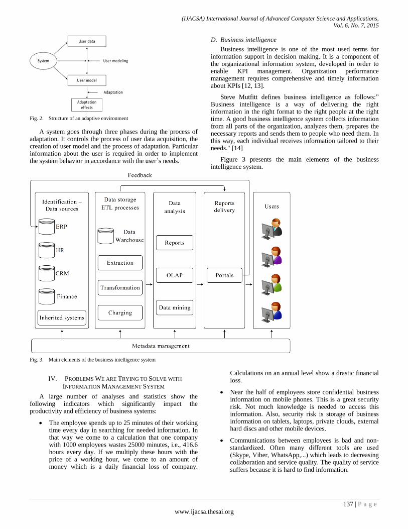
(IJACSA) International Journal of Advanced Computer Science and Applications,
Vol. 6, No. 7, 2015
137 | P a g e
www.ijacsa.thesai.org
Fig. 2. Structure of an adaptive environment
A system goes through three phases during the process of adaptation. It controls the process of user data acquisition, the creation of user model and the process of adaptation. Particular information about the user is required in order to implement the system behavior in accordance with the user’s needs.
D. Business intelligence
Business intelligence is one of the most used terms for information support in decision making. It is a component of the organizational information system, developed in order to enable KPI management. Organization performance management requires comprehensive and timely information about KPIs [12, 13].
Steve Mutfitt defines business intelligence as follows:” Business intelligence is a way of delivering the right information in the right format to the right people at the right time. A good business intelligence system collects information from all parts of the organization, analyzes them, prepares the necessary reports and sends them to people who need them. In this way, each individual receives information tailored to their needs." [14]
Figure 3 presents the main elements of the business intelligence system.
Fig. 3. Main elements of the business intelligence system
IV. PROBLEMS WE ARE TRYING TO SOLVE WITH
INFORMATION MANAGEMENT SYSTEM
A large number of analyses and statistics show the following indicators which significantly impact the productivity and efficiency of business systems:
The employee spends up to 25 minutes of their working time every day in searching for needed information. In that way we come to a calculation that one company with 1000 employees wastes 25000 minutes, i.e., 416.6 hours every day. If we multiply these hours with the price of a working hour, we come to an amount of money which is a daily financial loss of company.
Calculations on an annual level show a drastic financial loss.
Near the half of employees store confidential business information on mobile phones. This is a great security risk. Not much knowledge is needed to access this information. Also, security risk is storage of business information on tablets, laptops, private clouds, external hard discs and other mobile devices.
Communications between employees is bad and non-standardized. Often many different tools are used (Skype, Viber, WhatsApp,...) which leads to decreasing collaboration and service quality. The quality of service suffers because it is hard to find information.
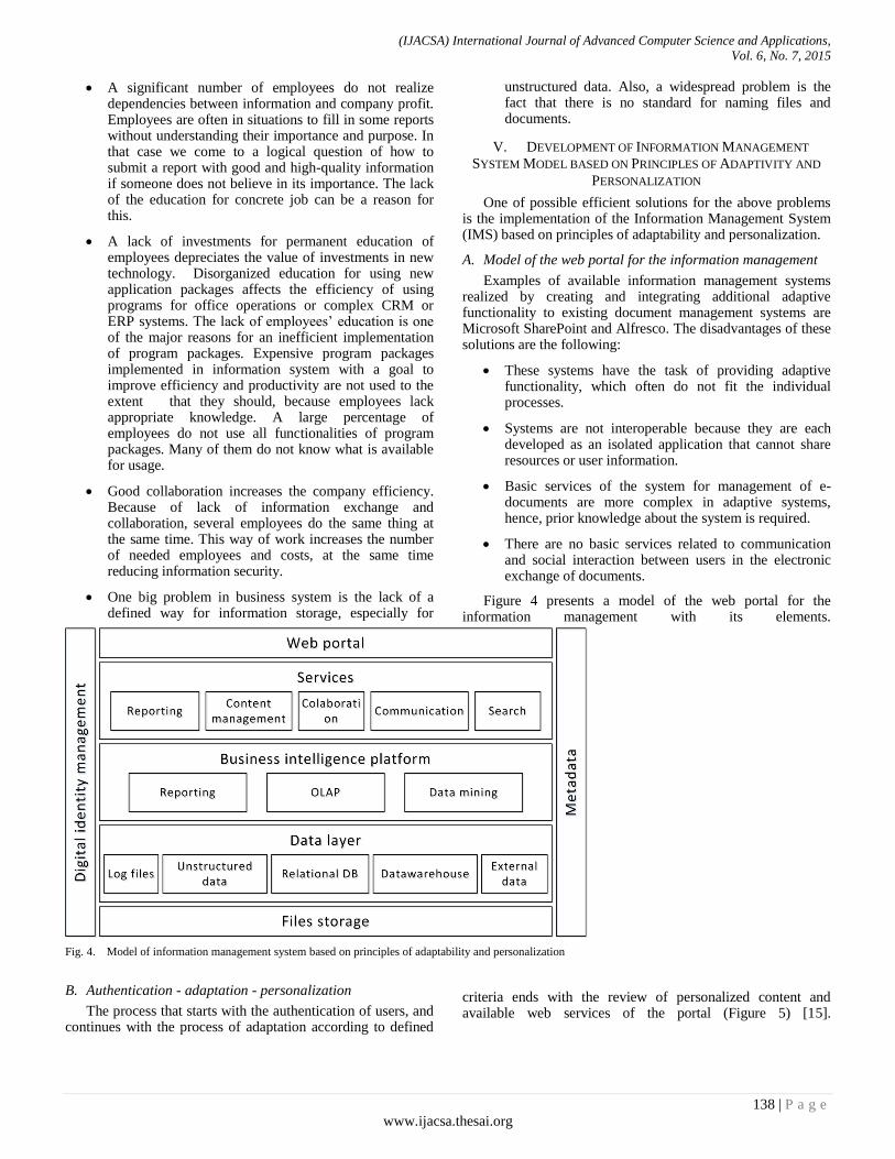
(IJACSA) International Journal of Advanced Computer Science and Applications,
Vol. 6, No. 7, 2015
138 | P a g e
www.ijacsa.thesai.org
A significant number of employees do not realize dependencies between information and company profit. Employees are often in situations to fill in some reports without understanding their importance and purpose. In that case we come to a logical question of how to submit a report with good and high-quality information if someone does not believe in its importance. The lack of the education for concrete job can be a reason for this.
A lack of investments for permanent education of employees depreciates the value of investments in new technology. Disorganized education for using new application packages affects the efficiency of using programs for office operations or complex CRM or ERP systems. The lack of employees’ education is one of the major reasons for an inefficient implementation of program packages. Expensive program packages implemented in information system with a goal to improve efficiency and productivity are not used to the extent that they should, because employees lack appropriate knowledge. A large percentage of employees do not use all functionalities of program packages. Many of them do not know what is available for usage.
Good collaboration increases the company efficiency. Because of lack of information exchange and collaboration, several employees do the same thing at the same time. This way of work increases the number of needed employees and costs, at the same time reducing information security.
One big problem in business system is the lack of a defined way for information storage, especially for
unstructured data. Also, a widespread problem is the fact that there is no standard for naming files and documents.
V. DEVELOPMENT OF INFORMATION MANAGEMENT
SYSTEM MODEL BASED ON PRINCIPLES OF ADAPTIVITY AND
PERSONALIZATION
One of possible efficient solutions for the above problems is the implementation of the Information Management System (IMS) based on principles of adaptability and personalization.
A. Model of the web portal for the information management
Examples of available information management systems realized by creating and integrating additional adaptive functionality to existing document management systems are Microsoft SharePoint and Alfresco. The disadvantages of these solutions are the following:
These systems have the task of providing adaptive functionality, which often do not fit the individual processes.
Systems are not interoperable because they are each developed as an isolated application that cannot share resources or user information.
Basic services of the system for management of e-documents are more complex in adaptive systems, hence, prior knowledge about the system is required.
There are no basic services related to communication and social interaction between users in the electronic exchange of documents.
Figure 4 presents a model of the web portal for the information management with its elements.
Fig. 4. Model of information management system based on principles of adaptability and personalization
B. Authentication - adaptation - personalization
The process that starts with the authentication of users, and continues with the process of adaptation according to defined
criteria ends with the review of personalized content and available web services of the portal (Figure 5) [15].
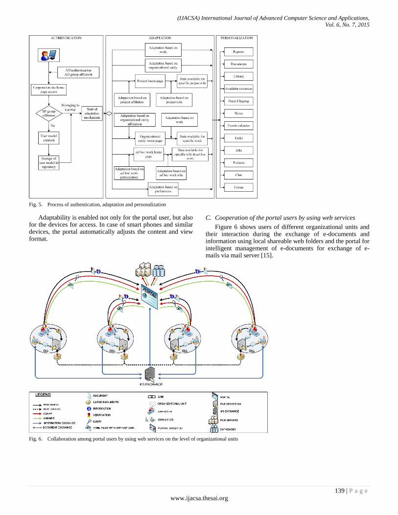
(IJACSA) International Journal of Advanced Computer Science and Applications,
Vol. 6, No. 7, 2015
139 | P a g e
www.ijacsa.thesai.org
Fig. 5. Process of authentication, adaptation and personalization
Adaptability is enabled not only for the portal user, but also for the devices for access. In case of smart phones and similar devices, the portal automatically adjusts the content and view format.
C. Cooperation of the portal users by using web services
Figure 6 shows users of different organizational units and their interaction during the exchange of e-documents and information using local shareable web folders and the portal for intelligent management of e-documents for exchange of e-mails via mail server [15].
Fig. 6. Collaboration among portal users by using web services on the level of organizational units

(IJACSA) International Journal of Advanced Computer Science and Applications,
Vol. 6, No. 7, 2015
140 | P a g e
www.ijacsa.thesai.org
VI. IMPLEMENTATION AND APPLICATION OF DEVELOPED
MODEL OF INTELLIGENT MANAGEMENT OF E-DOCUMENTS
By applying a model which consists of: collecting data, data exploration, classifying users, content and service
adaptation, portal usage and defining goals, the model of portal for intelligent management of e-documents is implemented (Figure 7) [16].
Fig. 7. Realization flow graphics view of portal for intelligent management of e-documents model
Collecting and researching users’ data in the portal for intelligent management of e-documents can be managed from:
questionnaires;
different databases;
different log files;
interview.
Information about the documents, user groups, business processes, projects and applications are stored in:
Document database: types of documents, document metadata.
Groups on AD and SP: structure and group names; authorization at the group level.
Database of business processes: specification of business processes.
Project database: specification of projects in the phase of realization.
Application database: specification of internally developed applications; specification of external application.
Log files of the operating system: the number of access locations, the number of documents per location; commonly accessed sites; most users accessing the portal and other.
One of the main functionalities of the portal for intelligent management of e-documents is a possibility of an adaptable and personalized view of information and reports intended for different levels of the hierarchical management.
Figure 8 shows a pyramid with a chronological view of processes of assigning, realization and reporting related to assignments. Hierarchical levels of management are shown with different shades of grey colour. According to hierarchy, the general director and a deputy general manager are coloured in the darkest grey, while the executive officers, directors of directorates, directors of sectors, heads of departments and the perpetrators are coloured in the lighter colours of grey.
Information is marked with ellipses. Grey ellipses present a view of personalized information intended for employers of certain hierarchical levels and by job type, while white ellipses present information related to some reports, news, assignments and are used to inform other employees [15].
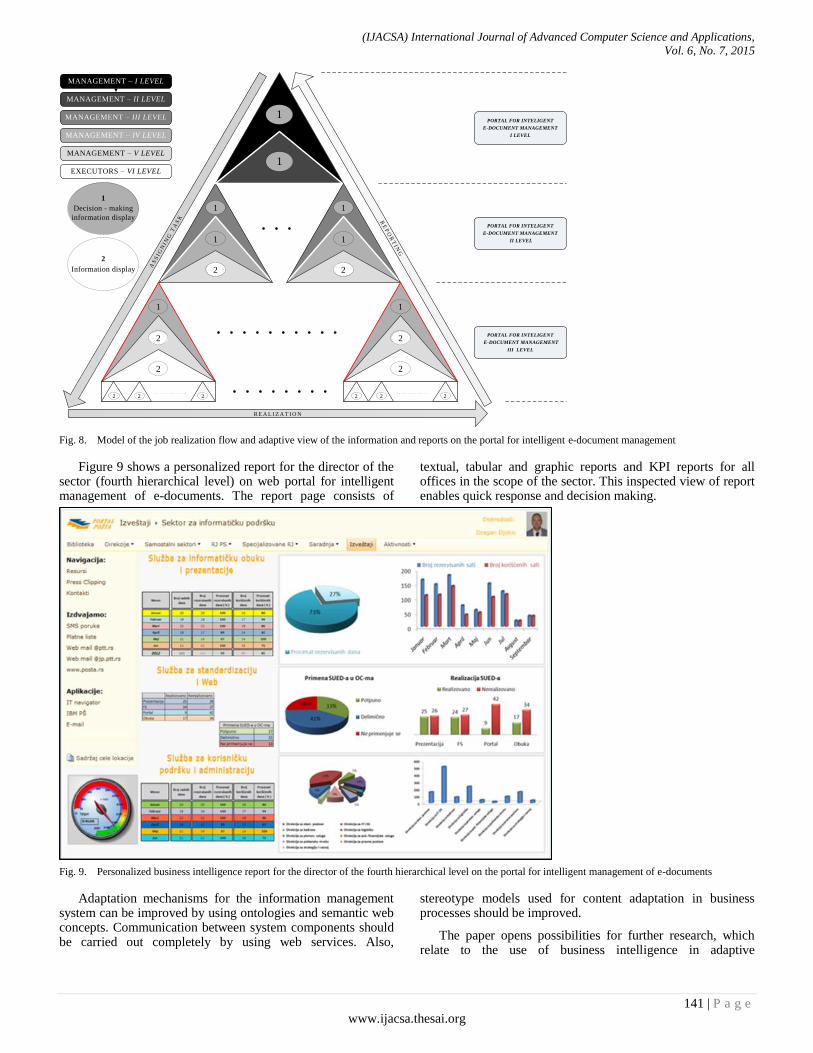
(IJACSA) International Journal of Advanced Computer Science and Applications,
Vol. 6, No. 7, 2015
141 | P a g e
www.ijacsa.thesai.org
Fig. 8. Model of the job realization flow and adaptive view of the information and reports on the portal for intelligent e-document management
Figure 9 shows a personalized report for the director of the sector (fourth hierarchical level) on web portal for intelligent management of e-documents. The report page consists of
textual, tabular and graphic reports and KPI reports for all offices in the scope of the sector. This inspected view of report enables quick response and decision making.
Fig. 9. Personalized business intelligence report for the director of the fourth hierarchical level on the portal for intelligent management of e-documents
Adaptation mechanisms for the information management system can be improved by using ontologies and semantic web concepts. Communication between system components should be carried out completely by using web services. Also,
stereotype models used for content adaptation in business processes should be improved.
The paper opens possibilities for further research, which relate to the use of business intelligence in adaptive
2
1
1
PORTAL FOR INTELIGENT
E-DOCUMENT MANAGEMENT
III LEVEL
AS
SIG
NIN
G T
AS
K RE
PO
RT
INGR E A L I Z A T I O N
PORTAL FOR INTELIGENT
E-DOCUMENT MANAGEMENT
II LEVEL
PORTAL FOR INTELIGENT
E-DOCUMENT MANAGEMENT
I LEVEL
MANAGEMENT – II LEVEL
MANAGEMENT – III LEVEL
MANAGEMENT – IV LEVEL
MANAGEMENT – V LEVEL
EXECUTORS – VI LEVEL
1
2 2 2 2 2 2
2 2
22
1 1
2
1
1
1
Decision - making
information display
2
Information display
MANAGEMENT – I LEVEL
1
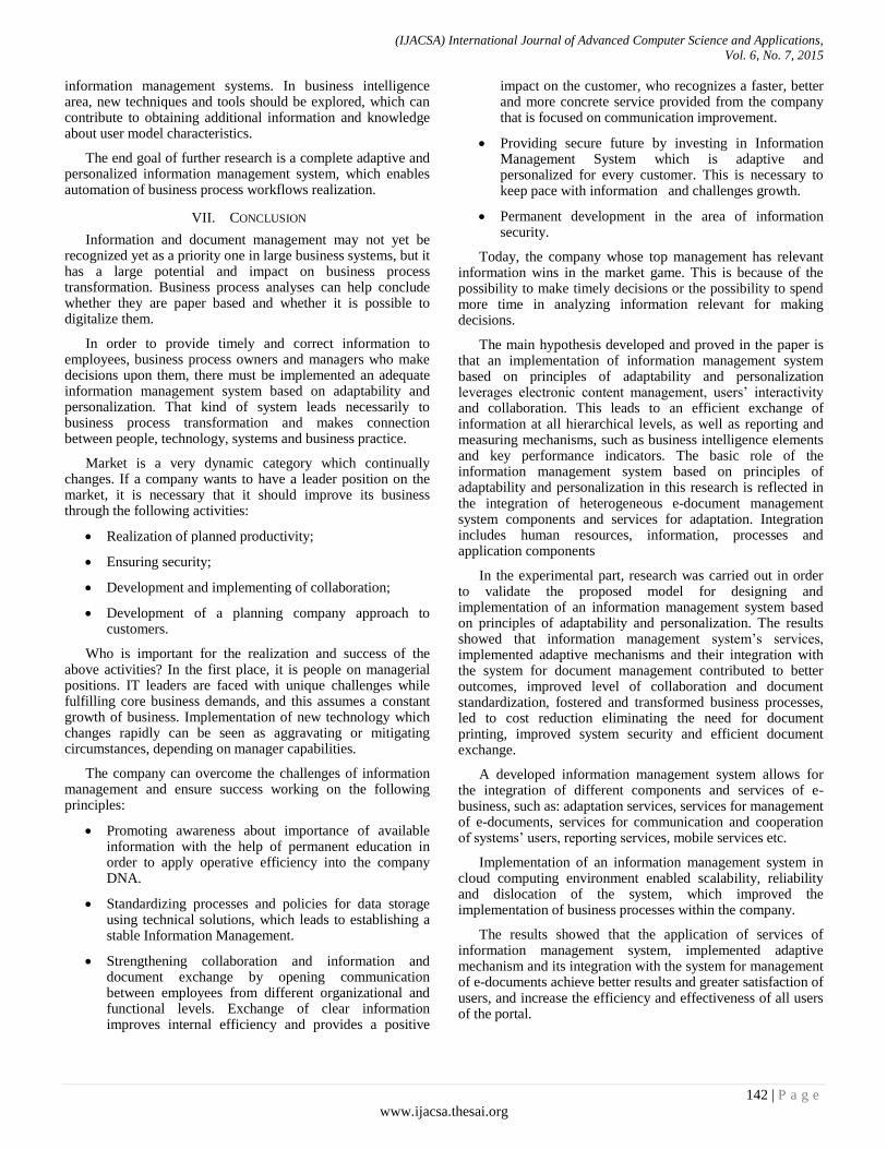
(IJACSA) International Journal of Advanced Computer Science and Applications,
Vol. 6, No. 7, 2015
142 | P a g e
www.ijacsa.thesai.org
information management systems. In business intelligence area, new techniques and tools should be explored, which can contribute to obtaining additional information and knowledge about user model characteristics.
The end goal of further research is a complete adaptive and personalized information management system, which enables automation of business process workflows realization.
VII. CONCLUSION
Information and document management may not yet be recognized yet as a priority one in large business systems, but it has a large potential and impact on business process transformation. Business process analyses can help conclude whether they are paper based and whether it is possible to digitalize them.
In order to provide timely and correct information to employees, business process owners and managers who make decisions upon them, there must be implemented an adequate information management system based on adaptability and personalization. That kind of system leads necessarily to business process transformation and makes connection between people, technology, systems and business practice.
Market is a very dynamic category which continually changes. If a company wants to have a leader position on the market, it is necessary that it should improve its business through the following activities:
Realization of planned productivity;
Ensuring security;
Development and implementing of collaboration;
Development of a planning company approach to customers.
Who is important for the realization and success of the above activities? In the first place, it is people on managerial positions. IT leaders are faced with unique challenges while fulfilling core business demands, and this assumes a constant growth of business. Implementation of new technology which changes rapidly can be seen as aggravating or mitigating circumstances, depending on manager capabilities.
The company can overcome the challenges of information management and ensure success working on the following principles:
Promoting awareness about importance of available information with the help of permanent education in order to apply operative efficiency into the company DNA.
Standardizing processes and policies for data storage using technical solutions, which leads to establishing a stable Information Management.
Strengthening collaboration and information and document exchange by opening communication between employees from different organizational and functional levels. Exchange of clear information improves internal efficiency and provides a positive
impact on the customer, who recognizes a faster, better and more concrete service provided from the company that is focused on communication improvement.
Providing secure future by investing in Information Management System which is adaptive and personalized for every customer. This is necessary to keep pace with information and challenges growth.
Permanent development in the area of information security.
Today, the company whose top management has relevant information wins in the market game. This is because of the possibility to make timely decisions or the possibility to spend more time in analyzing information relevant for making decisions.
The main hypothesis developed and proved in the paper is that an implementation of information management system based on principles of adaptability and personalization leverages electronic content management, users’ interactivity and collaboration. This leads to an efficient exchange of information at all hierarchical levels, as well as reporting and measuring mechanisms, such as business intelligence elements and key performance indicators. The basic role of the information management system based on principles of adaptability and personalization in this research is reflected in the integration of heterogeneous e-document management system components and services for adaptation. Integration includes human resources, information, processes and application components
In the experimental part, research was carried out in order to validate the proposed model for designing and implementation of an information management system based on principles of adaptability and personalization. The results showed that information management system’s services, implemented adaptive mechanisms and their integration with the system for document management contributed to better outcomes, improved level of collaboration and document standardization, fostered and transformed business processes, led to cost reduction eliminating the need for document printing, improved system security and efficient document exchange.
A developed information management system allows for the integration of different components and services of e-business, such as: adaptation services, services for management of e-documents, services for communication and cooperation of systems’ users, reporting services, mobile services etc.
Implementation of an information management system in cloud computing environment enabled scalability, reliability and dislocation of the system, which improved the implementation of business processes within the company.
The results showed that the application of services of information management system, implemented adaptive mechanism and its integration with the system for management of e-documents achieve better results and greater satisfaction of users, and increase the efficiency and effectiveness of all users of the portal.

(IJACSA) International Journal of Advanced Computer Science and Applications,
Vol. 6, No. 7, 2015
143 | P a g e
www.ijacsa.thesai.org
The results of this paper open the door for further research in the area of information management system development, through an integration of a larger number of services that ensure different functionalities and additionally provide adaptability. Improvements of the described model can be considered as contributing to the development of sophisticated adaptation mechanisms and advanced services for key business processes support.
Adaptation mechanisms for information management system can be improved by using ontologies and semantic web concepts. Communication between system components should be carried out completely by using web services. Also, stereotype models used for content adaptation in business processes should be improved.
The paper opens possibilities for further research in relation to the use of business intelligence in adaptive information management systems. In the business intelligence area, new techniques and tools should be explored, which can contribute to obtaining additional information and knowledge about user model characteristics.
The end goal of further research is an integrated adaptive and personalized information management system, which enables automation of business process workflows realization.
REFERENCES
[1] D. Đokić, A. Labus, S. Jevremović, A. Stokić and A. Milić, “Portal for the management of digitally signed electronic documents”, Metalurgia international, Vol.: 17, No.: 9, pp.: 120-129, 2012.
[2] D. Đokić and D. Bečejski Vujaklija, “Adaptive access to the information in large business systems”, University Metropolitan, Seventh Annual Conference BISEC, 2015, Belgrade, Serbia, pp. 30-37, 17 June, 2015, available at: http://bisec.rs/en/conference-programme/ (accessed 26 June, 2015).
[3] J. M. Raol, K.S. Koong, L.C. Liu and C.S. Yu, “An identification and classification of enterprise portal functions and features”, Industrial Management & Data Systems, Vol.: 102, No.: 7, pp.: 390-399, 2002.
[4] B. Ives, “Gartner`s Magic Quadrant for Intranet Portals”, 2012, available at: http://billives.typepad.com/portals_and_km/2008/11/toby-ward-recently-shared-the-highlights-of-the-gartners-magic-quadrant-for-intranet-portals-first-this-is-a-consolidati.html, (accessed 26 June, 2015).
[5] J. Yong, “Digital Identity Design and Privacy Preservation for e-Learning”, In: Swinburne University of Technology. 11th International Conference Computer Supported Cooperative Work in Design. Melbourne, Australia, pp.: 858 – 863, 26-28 April, 2007.
[6] Y. Zhang and J.L. Chen, “A Delegation Solution for Universal Identity Management in SOA”, IEEE Transactions on Services Computing, Vol.: 4, No.: 1, pp.: 70-81, 2011.
[7] S. Popović, A. Njeguš, M. Vulić, D. Đokić and Đ. Mazinjanin, “ Service oriented framework for system interoperability modeling”, Metalurgia international, Vo.: 17, No.: 11, pp.: 171-17, 2012.
[8] D. Recordon and D. Reed, “Open ID 2.0: a platform for user-centric identity management”, In: Association for Computing Machinery. 13th ACM Conference on Computer and Communications Security 2006. Alexandria, VA, USA, 30. October-3. November, ACM: New York, pp.: 11-16, 2006.
[9] P. Brusilovsky and M. T. Maybury, “From adaptive hypermedia to the adaptive web”, Communications of the ACM, Vol.: 45, No.: 5, pp.: 30–33, 2002.
[10] C. Gutl and F. Modritscher, “Towards a Generic Adaptive System applicable for Web-based Learning Management Environments”, In: ABIS. 13th Annual Workshop of the SIG Adaptivity and User Modeling in Interactive Systems ABIS 2005. Saarbrücken, pp.: 1-6, 10-12 October, 2005.
[11] D. Đokić, M. Despotović-Zrakić, D. Barać and K. Simić, “Document management system for e-government”, In Uroš Pinterič, Lea Prijon (Ed.), Selected issues of modern democracy, Ljubljana: Založba Vega, pp.: 277-292, 2012.
[12] T. Anderson and F. Elloumi, “Theory and Practice of Online Learning”, Edmonton: Athabasca University, 2004.
[13] A. R. Anaya and J. G. Boticari, “Content-free collaborative learning modeling using data mining, User Modeling and User-Adapted Interaction”, Vol.: 21, No.: 1-2, pp. 181-216, 2011.
[14] Y. Atif, R. Benlamri and J, Berri, “Dynamic Learning Modeler”, Journal of Educational Technology & Society, Vol.: 6, No.: 4, pp. 60-72, 2003.
[15] D. Đokić, “Model of portal for intelligent management of electronic documents”, Ph.D Dissertation, Faculty of Organizational Sciences, University of Belgrade, 2012.
[16] M. Despotović-Zrakić, A. Marković, Z. Bogdanović, D. Barać and S. Krčo, “Providing Adaptivity in Moodle LMS Courses”, Journal of Educational Technology & Society, Vol.: 15, No.: 1, pp.: 326-338, 2012, available at: http://www.ifets.info/journals/15_1/28.pdf , (accessed 26 June, 2015).

(IJACSA) International Journal of Advanced Computer Science and Applications,
Vol. 6, No. 7, 2015
144 | P a g e
www.ijacsa.thesai.org
Assessment of High and Low Rate Protocol-based
Attacks on Ethernet Networks
Mina Malekzadeh
Faculty of Electrical and Computer
Engineering, Hakim Sabzevari
University
Sabzevar, Iran
M.A. Beiruti
Engineering Faculty of Golestan
University
Gorgan, Iran
M.H. Shahrokh Abadi (M’06 IEEE)
Faculty of Electrical and Computer
Engineering, Hakim Sabzevari
University
Sabzevar, Iran
Abstract—The Internet and Web have significantly
transformed the world’s communication system. The capability
of the Internet to instantly access information at anytime from
anywhere has brought benefit for a wide variety of areas
including business, government, education, institutions, medical,
and entertainment services. However, the Internet has also
opened up the possibilities for hackers to exploit flaws and
limitations in the target networks to attack and break in without
gaining physical access to the target systems. The OSI layer
protocol-based attacks are among them. In this work we
investigate feasibility as well as severity of the attacks against
three common layering protocols including TCP, UDP, and
ICMP on Ethernet-based networks in the real world through a
testbed. Then a simulation environment is designed to implement
the exact same attacks under similar conditions using NS2
network simulator. The testbed results and simulation results are
compared with each other to explore the accuracy of the findings
and measure the damages the attacks caused to the network.
Keywords—protocol attacks; OSI layer attacks; UDP attacks;
TCP attacks; ICMP attacks
I. INTRODUCTION
Online services have given users the opportunity to access data in a fast and convenient way. While the Internet has greatly amplified benefits for individuals and organizations, its critical importance has also attracted the attention of the hackers and attackers to conduct their malicious intentions.
Today, attacks against the networks are increasing in frequency, severity and sophistication. The flaws or bugs in operating systems or vulnerabilities and limitations in the TCP/IP protocols implementation are exploited to conduct the attacks which cause serious problems for normal networks operations. The OSI protocol-based attacks are among the common threats in today's cyber security landscape. The attacks are characterized by explicit attempts of the attackers to block the intended users from accessing the network services and rendering them unreachable, causing massive political or financial damages for the target networks. Losing money and time, physical harm, and invasion of privacy for individuals and organizations can be other objectives of the attacks [1].
Despite development of many mechanisms to defend against today's cybercrimes, protocol-based attacks are still regarded as an elevated threat which turns them into high concern of the organizations. Due to increasing the rate of
these attacks on government and corporate sites, their protection has become an ever-growing challenge that demands knowing the attacks methods in depth which in turn leads to finding solutions to effectively stay out of harm.
A. Contributions
This work investigates the feasibility and damage severity of different protocol-based attacks against the 802.3 Ethernet networks. The contributions of this paper are summarized in three-folds. First, a simulation environment is designed using NS2 to implement the attacks. Under different attack scenarios, we quantify the damage severity of the attacks. Second, a testbed is designed to measure the amount of damage imposed by the attacks against real target Ethernet networks. The testbed is designed with the same characteristics as the simulation environment to provide fair conditions for the comparison process. Third, the simulation results and the testbed results are compared to investigate the feasibility and severity of the attacks and also the accuracy of the findings.
The rest of this paper is organized as follows. Section II describes the protocol-based attacks which we aim to investigate in this paper and the related works regarding to these attacks. In Section III we propose an attack model to implement the attacks against Ethernet networks by designing different experiments in both the testbed and the simulation environment. We present and analyze the simulation results and the testbed results in Section IV. We conclude this paper in Section V.
II. RELATED WORKS
With various motives in mind, protocol-based attacks are carried out in a variety of forms and methods [1]. Some of the common attacks include TCP attacks (SYN attacks), smurf attack, port scan attack, UDP attacks, DNS-based attack, ICMP attack, Ping flood attack, IP fragmentation, and CGI attacks [4,8,9,11]. This paper studies the attacks against 802.3 Ethernet networks based on design flaws in three protocols as TCP, UDP, and ICMP. Below we summarize the attacks considered in this paper.
UDP-based attack: User Datagram Protocol (UDP) is a connectionless protocol used for a variety of applications such as VOIP, DNS, SNMP, video streaming, and DHCP. Since the UDP does not have a congestion control mechanism, the attackers are able to send a very large number of packets [1].
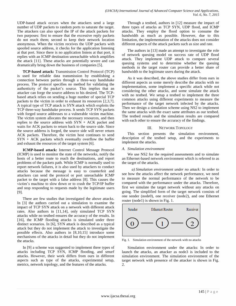
(IJACSA) International Journal of Advanced Computer Science and Applications,
Vol. 6, No. 7, 2015
145 | P a g e
www.ijacsa.thesai.org
UDP-based attack occurs when the attackers send a large number of UDP packets to random ports to saturate the target. The attackers can also spoof the IP of the attack packets for two purposes: first to ensure that the excessive reply packets do not reach them; second to keep their network location anonymous. When the victim receives the UDP packets with spoofed source address, it checks for the application listening at that port. Since there is no application listens at that port, it replies with an ICMP destination unreachable which amplifies the attack [11]. These attacks are potentially severe and can dramatically bring down the business of companies [5].
TCP-based attack: Transmission Control Protocol (TCP) is used for reliable data transmission by establishing a connection between parties through a three-way handshake process. The protocol specifies no method for validating the authenticity of the packet’s source. This implies that an attacker can forge the source address to his desired. The TCP-based attack relies on sending a huge number of special TCP packets to the victim in order to exhaust its resources [2,3,7]. A typical type of TCP attack is SYN attack which exploits the TCP three-way handshake process. It sends TCP SYN packets with forged source addresses to a vulnerable victim machine. The victim system allocates the necessary resources, and then replies to the source address with SYN + ACK packet and waits for ACK packets to return back to the source side. Since the source address is forged, the source side will never return ACK packets. Therefore, the victim host continues to send SYN + ACK packets which eventually overflow the buffer and exhaust the resources of the target system [6].
ICMP-based attack: Internet Control Message Protocol (ICMP) is used to monitor the state of the networks, notify the hosts of a better route to reach the destinations, and report problems of the packets path. While ICMP is normally used to report network failures, it is also used by attackers to conduct attacks because the message is easy to counterfeit and attackers can send the protocol or port unreachable ICMP packet to the target with a false address [8]. This causes the victim’s machine to slow down or to crash the TCP/IP buffer and stop responding to requests made by the legitimate users [9].
There are few studies that investigated the above attacks. In [3] the authors carried out a simulation to examine the impact of TCP SYN attack on a network with different attack rates. Also authors in [11,14], only simulated TCP SYN attacks while no testbed ensures the accuracy of the results. In [16], the ICMP flooding attacks is simulated under three distinct scenarios. In [6], SYN attack is described as a typical attack but they do not implement the attack to investigate the possible effects. Also authors in [8,10,15] introduce some mechanisms of the attacks in detail but they do not implement the attacks.
In [9] a scheme was suggested to implement three types of attacks including TCP SYN, ICMP flooding, and smurf attacks. However, their work differs from ours in different aspects such as type of the attacks, experimental setup, metrics, network topology, and the features of the attacks.
Through a testbed, authors in [12] measure the impact of three types of attacks as TCP SYN, UDP flood, and ICMP attacks. They employ the flood option to consume the bandwidth as much as possible. However, due to this limitation, the implementation of the attacks does not consider different aspects of the attack packets such as size and rate.
The authors in [13] made an attempt to investigate the role of network queuing model on success rate of UDP flood attack. They implement UDP attack to compare several queuing systems and to determine whether the queuing methods in the target router can provide a better share of bandwidth to the legitimate users during the attack.
As it was described, the above studies differ from ours in different aspects as some merely describe the attacks with no implementation, some implement a specific attack while not considering the other attacks, and some simulate the attack with no testbed. We setup a testbed to implement the three common attacks using different experiments to measure the performance of the target network infected by the attacks. Then we design a simulation scheme using NS2 to implement the same attacks with the exact same attributes as our testbed. The testbed results and the simulation results are compared with each other to ensure the accuracy of the findings.
III. NETWORK TOPOLOGY
This section presents the simulation environment, description of the testbed setup, and the experiments to implement the attacks.
A. Simulation environment
We use NS2 for the required assessments and to simulate an Ethernet-based network environment which is referred to as the target of the attacks.
a) Simulation environment under no attack: In order to
see how the attacks affect the network performance, we need
to measure the normal performance of the network to be
compared with the performance under the attacks. Therefore,
first we simulate the target network without any attacks on
going. The simplified form of the target network consists of
one sender (node0), one receiver (node2), and one Ethernet
router (node1) is shown in Fig. 1.
Fig. 1. Simulation environment of the network with no attacks
Simulation environment under the attacks: In order to launch the attacks, an attacker as node3 is included to the simulation environment. The simulation environment of the target network with presence of the attacker is shown in Fig. 2.

(IJACSA) International Journal of Advanced Computer Science and Applications,
Vol. 6, No. 7, 2015
146 | P a g e
www.ijacsa.thesai.org
Fig. 2. Simulation environment of the network under attacks
b) Network parameters: The simulation time is
considered 20s divided into two 10 seconds. In the first 10
seconds (0-9s) the network operates under normal conditions.
The next 10 seconds (10-20s) is when the attacker initiates the
attacks to disrupt the normal operation of the target network.
During the entire simulation time, including before and during
the attacks, a constant UDP traffic with the characteristics
shown in Table I are transmitted in the network.
TABLE I. CONSTANT NETWORK PARAMETER
Parameter Value
Traffic type UDP/CBR
Packet size 1500B
Transmission rate 1Mbps
Simulation time 20s
c) Attack parameters and experiments: Based on the
three types of attacks described in the previous section, we
design ten distinct experiments. The comparison between the
attacks in the experiments is done in terms of the attack rates,
type of the attack traffics, size of the attack packets, type of
the attack target, and impact of the attacks:
Attack rates (intensity): we take two attack rates into account, categorized as: low rate attacks and high rate attacks.
Attack traffics: the types of traffics used to launch the attacks examined in this study are: UDP, ICMP, and TCP packets.
Attack packet size: different sizes are selected for the attack packets to examine the impact of the small, medium, and large packets on severity of the attacks.
Attack target: the attacks will target both the client machines (either Windows or Linux) and routers separately to compare vulnerability of the targets.
Attack impact: severity of the attacks is quantified in terms of our metrics as transmission delay, throughput, and packet lost rate.
Based on the above variable attack parameters, the ten distinct experiments are designed to implement three types of attacks. These attacks are summarized in Table II, Table III, and Table IV.
TABLE II. EXPERIMENTS TO IMPLEMENT UDP-BASED ATTACKS
Protocol to attack: UDP
Experiment
number Description
Attack
packets size
Attack packets
rate/interval
1 Initial rate
and size 200B 4 Mbps/0.0004s
2 Changing packets size
10000B 4 Mbps/0.0001s
3 Changing
packets rate 10000B 2 Mbps/0.0001s
4
Same parameters as
the target
network
1500B 1Mbps/0.0001s
TABLE III. EXPERIMENTS TO IMPLEMENT TCP-BASED ATTACKS
Protocol to attack: TCP
Experiment
number Description
Attack
packets size
Attack packets
interval
5 Initial rate
and size 1500B 0.0001s
6 Changing
packet size 200B 0.0001s
7 Changing
packet size 100B 0.0001s
TABLE IV. EXPERIMENTS TO IMPLEMENT ICMP-BASED ATTACKS
Protocol to attack: ICMP
Experiment
number Description
Attack
packets size
Attack packets
interval
8 Initial rate and
size 5000B 0.00001s
9 Changing
packet size 500B 0.00001s
10
Changing
packets interval & size
200B 0.001s
B. Testbed environment
We setup a testbed to measure the results of the attacks which are compared against the simulation results to verify the accuracy of the findings. Therefore, to fulfill our purpose, the hardware components and software configurations applied in our testbed are described as follows.
a) Hardware details
Router: wire router (brand remains unmentioned) with IDS enabled is used through all the experiments in the testbed to protect the target network as it is done in the real world. The router by default is configured to discard ping to WAN interface and the firewall features are enabled with default settings.
Clients Processor: Intel® core i7 2.70GHz
Clients RAM: 4.00 GB
b) Software details
Penetration tool: we use Kali security distribution Linux with pre-installed metasploit in it to conduct the attacks.
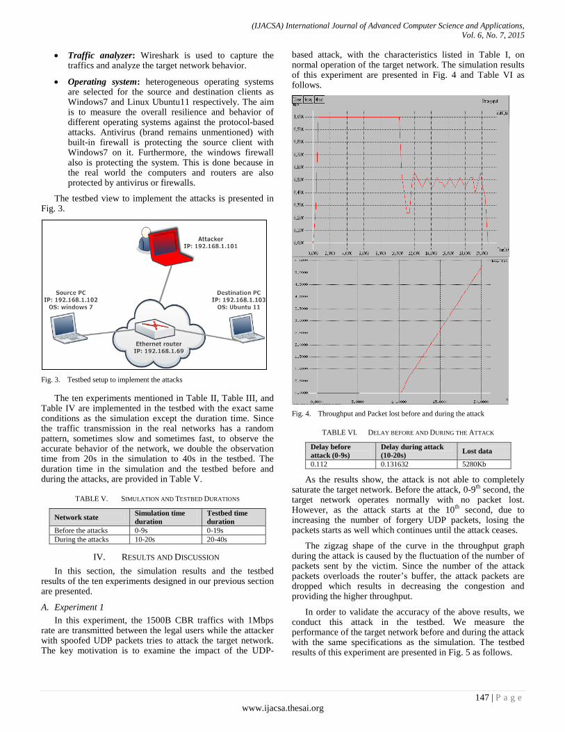
(IJACSA) International Journal of Advanced Computer Science and Applications,
Vol. 6, No. 7, 2015
147 | P a g e
www.ijacsa.thesai.org
Traffic analyzer: Wireshark is used to capture the traffics and analyze the target network behavior.
Operating system: heterogeneous operating systems are selected for the source and destination clients as Windows7 and Linux Ubuntu11 respectively. The aim is to measure the overall resilience and behavior of different operating systems against the protocol-based attacks. Antivirus (brand remains unmentioned) with built-in firewall is protecting the source client with Windows7 on it. Furthermore, the windows firewall also is protecting the system. This is done because in the real world the computers and routers are also protected by antivirus or firewalls.
The testbed view to implement the attacks is presented in Fig. 3.
Fig. 3. Testbed setup to implement the attacks
The ten experiments mentioned in Table II, Table III, and Table IV are implemented in the testbed with the exact same conditions as the simulation except the duration time. Since the traffic transmission in the real networks has a random pattern, sometimes slow and sometimes fast, to observe the accurate behavior of the network, we double the observation time from 20s in the simulation to 40s in the testbed. The duration time in the simulation and the testbed before and during the attacks, are provided in Table V.
TABLE V. SIMULATION AND TESTBED DURATIONS
Network state Simulation time
duration
Testbed time
duration
Before the attacks 0-9s 0-19s
During the attacks 10-20s 20-40s
IV. RESULTS AND DISCUSSION
In this section, the simulation results and the testbed results of the ten experiments designed in our previous section are presented.
A. Experiment 1
In this experiment, the 1500B CBR traffics with 1Mbps rate are transmitted between the legal users while the attacker with spoofed UDP packets tries to attack the target network. The key motivation is to examine the impact of the UDP-
based attack, with the characteristics listed in Table I, on normal operation of the target network. The simulation results of this experiment are presented in Fig. 4 and Table VI as follows.
Fig. 4. Throughput and Packet lost before and during the attack
TABLE VI. DELAY BEFORE AND DURING THE ATTACK
Delay before
attack (0-9s)
Delay during attack
(10-20s) Lost data
0.112 0.131632 5280Kb
As the results show, the attack is not able to completely saturate the target network. Before the attack, 0-9
th second, the
target network operates normally with no packet lost. However, as the attack starts at the 10
th second, due to
increasing the number of forgery UDP packets, losing the packets starts as well which continues until the attack ceases.
The zigzag shape of the curve in the throughput graph during the attack is caused by the fluctuation of the number of packets sent by the victim. Since the number of the attack packets overloads the router’s buffer, the attack packets are dropped which results in decreasing the congestion and providing the higher throughput.
In order to validate the accuracy of the above results, we conduct this attack in the testbed. We measure the performance of the target network before and during the attack with the same specifications as the simulation. The testbed results of this experiment are presented in Fig. 5 as follows.
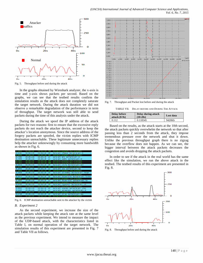
(IJACSA) International Journal of Advanced Computer Science and Applications,
Vol. 6, No. 7, 2015
148 | P a g e
www.ijacsa.thesai.org
Fig. 5. Throughput before and during the attack
In the graphs obtained by Wireshark analyzer, the x-axis is time and y-axis shows packets per second. Based on the graphs, we can see that the testbed results confirm the simulation results as the attack does not completely saturate the target network. During the attack duration we did not observe a remarkable degradation of the performance in term of throughput. The target network was still able to send packets during the time of this analysis under the attack.
During the attack we spoof the IP address of the attack packets for two reasons: first to ensure that the excessive reply packets do not reach the attacker device, second to keep the attacker’s location anonymous. Since the source address of the forgery packets are spoofed, the victim replies with ICMP destination unreachable. These legitimate unnecessary replies help the attacker unknowingly by consuming more bandwidth as shown in Fig. 6.
Fig. 6. ICMP destination unreachable sent to the attacker by the victim
B. Experiment 2
As the second experiment, we increase the size of the attack packets while keeping the attack rate at the same level as the previous experiment. We intend to measure the impact of the UDP-based attack, with the characteristics listed in Table I, on normal operation of the target network. The simulation results of this experiment are presented in Fig. 7 and Table VII as follows.
Fig. 7. Throughput and Packet lost before and during the attack
TABLE VII. DELAY BEFORE AND DURING THE ATTACK
Delay before
attack (0-9s)
Delay during attack
(10-20s) Lost data
0.112 0.118345 9420Kb
Based on the results, as the attack starts at the 10th second, the attack packets quickly overwhelm the network so that after passing less than 2 seconds from the attack, they impose tremendous pressure over the network and shut it down. Unlike the previous throughput graph there is no zigzag because the overflow does not happen. As we can see, the bigger interval between the attack packets decreases the congestion and avoids dropping the attack packets.
In order to see if the attack in the real world has the same effect like the simulation, we run the above attack in the testbed. The testbed results of this experiment are presented in Fig. 8.
Fig. 8. Throughput before and during the attack
Attacker traffics
Normal traffics
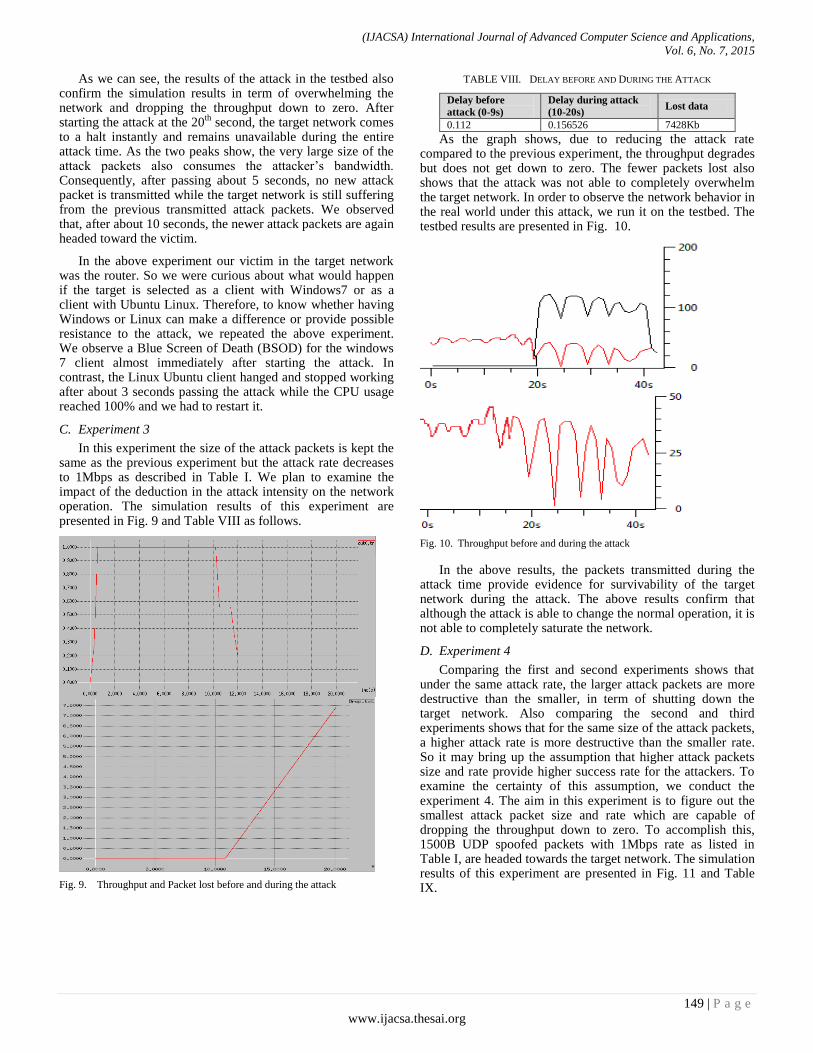
(IJACSA) International Journal of Advanced Computer Science and Applications,
Vol. 6, No. 7, 2015
149 | P a g e
www.ijacsa.thesai.org
As we can see, the results of the attack in the testbed also confirm the simulation results in term of overwhelming the network and dropping the throughput down to zero. After starting the attack at the 20
th second, the target network comes
to a halt instantly and remains unavailable during the entire attack time. As the two peaks show, the very large size of the attack packets also consumes the attacker’s bandwidth. Consequently, after passing about 5 seconds, no new attack packet is transmitted while the target network is still suffering from the previous transmitted attack packets. We observed that, after about 10 seconds, the newer attack packets are again headed toward the victim.
In the above experiment our victim in the target network was the router. So we were curious about what would happen if the target is selected as a client with Windows7 or as a client with Ubuntu Linux. Therefore, to know whether having Windows or Linux can make a difference or provide possible resistance to the attack, we repeated the above experiment. We observe a Blue Screen of Death (BSOD) for the windows 7 client almost immediately after starting the attack. In contrast, the Linux Ubuntu client hanged and stopped working after about 3 seconds passing the attack while the CPU usage reached 100% and we had to restart it.
C. Experiment 3
In this experiment the size of the attack packets is kept the same as the previous experiment but the attack rate decreases to 1Mbps as described in Table I. We plan to examine the impact of the deduction in the attack intensity on the network operation. The simulation results of this experiment are presented in Fig. 9 and Table VIII as follows.
Fig. 9. Throughput and Packet lost before and during the attack
TABLE VIII. DELAY BEFORE AND DURING THE ATTACK
Delay before
attack (0-9s)
Delay during attack
(10-20s) Lost data
0.112 0.156526 7428Kb
As the graph shows, due to reducing the attack rate compared to the previous experiment, the throughput degrades but does not get down to zero. The fewer packets lost also shows that the attack was not able to completely overwhelm the target network. In order to observe the network behavior in the real world under this attack, we run it on the testbed. The testbed results are presented in Fig. 10.
Fig. 10. Throughput before and during the attack
In the above results, the packets transmitted during the attack time provide evidence for survivability of the target network during the attack. The above results confirm that although the attack is able to change the normal operation, it is not able to completely saturate the network.
D. Experiment 4
Comparing the first and second experiments shows that under the same attack rate, the larger attack packets are more destructive than the smaller, in term of shutting down the target network. Also comparing the second and third experiments shows that for the same size of the attack packets, a higher attack rate is more destructive than the smaller rate. So it may bring up the assumption that higher attack packets size and rate provide higher success rate for the attackers. To examine the certainty of this assumption, we conduct the experiment 4. The aim in this experiment is to figure out the smallest attack packet size and rate which are capable of dropping the throughput down to zero. To accomplish this, 1500B UDP spoofed packets with 1Mbps rate as listed in Table I, are headed towards the target network. The simulation results of this experiment are presented in Fig. 11 and Table IX.
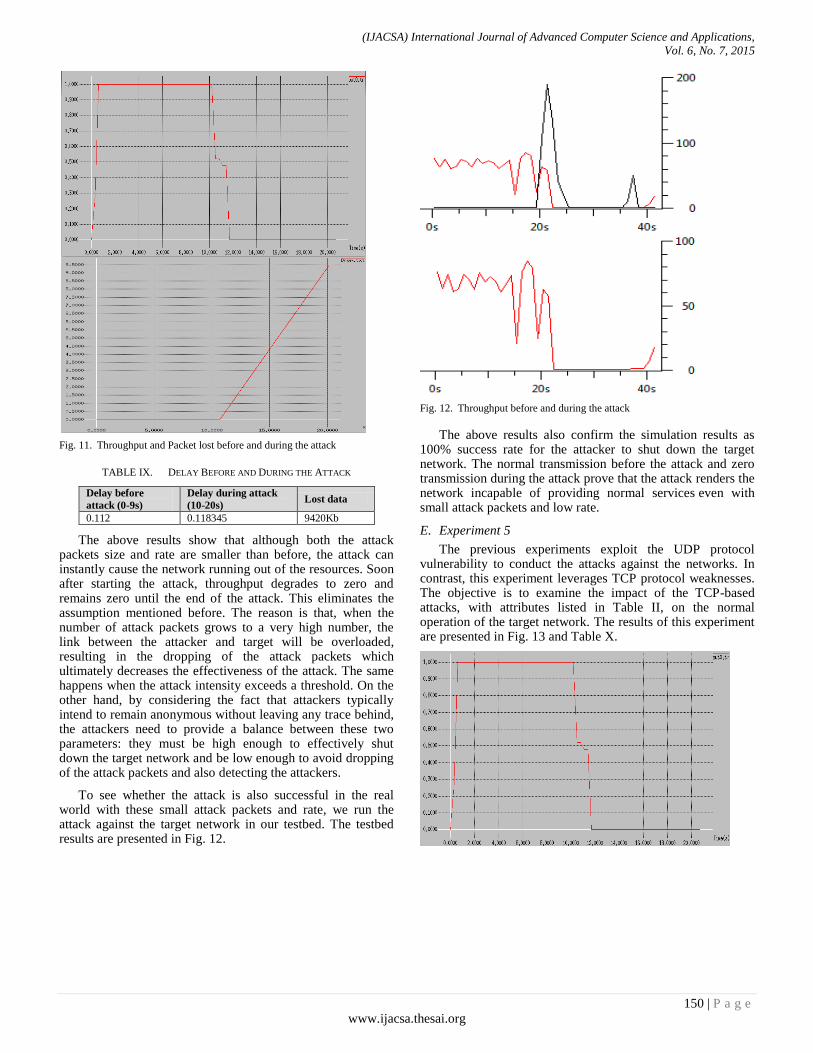
(IJACSA) International Journal of Advanced Computer Science and Applications,
Vol. 6, No. 7, 2015
150 | P a g e
www.ijacsa.thesai.org
Fig. 11. Throughput and Packet lost before and during the attack
TABLE IX. DELAY BEFORE AND DURING THE ATTACK
Delay before
attack (0-9s)
Delay during attack
(10-20s) Lost data
0.112 0.118345 9420Kb
The above results show that although both the attack packets size and rate are smaller than before, the attack can instantly cause the network running out of the resources. Soon after starting the attack, throughput degrades to zero and remains zero until the end of the attack. This eliminates the assumption mentioned before. The reason is that, when the number of attack packets grows to a very high number, the link between the attacker and target will be overloaded, resulting in the dropping of the attack packets which ultimately decreases the effectiveness of the attack. The same happens when the attack intensity exceeds a threshold. On the other hand, by considering the fact that attackers typically intend to remain anonymous without leaving any trace behind, the attackers need to provide a balance between these two parameters: they must be high enough to effectively shut down the target network and be low enough to avoid dropping of the attack packets and also detecting the attackers.
To see whether the attack is also successful in the real world with these small attack packets and rate, we run the attack against the target network in our testbed. The testbed results are presented in Fig. 12.
Fig. 12. Throughput before and during the attack
The above results also confirm the simulation results as 100% success rate for the attacker to shut down the target network. The normal transmission before the attack and zero transmission during the attack prove that the attack renders the network incapable of providing normal services even with small attack packets and low rate.
E. Experiment 5
The previous experiments exploit the UDP protocol vulnerability to conduct the attacks against the networks. In contrast, this experiment leverages TCP protocol weaknesses. The objective is to examine the impact of the TCP-based attacks, with attributes listed in Table II, on the normal operation of the target network. The results of this experiment are presented in Fig. 13 and Table X.
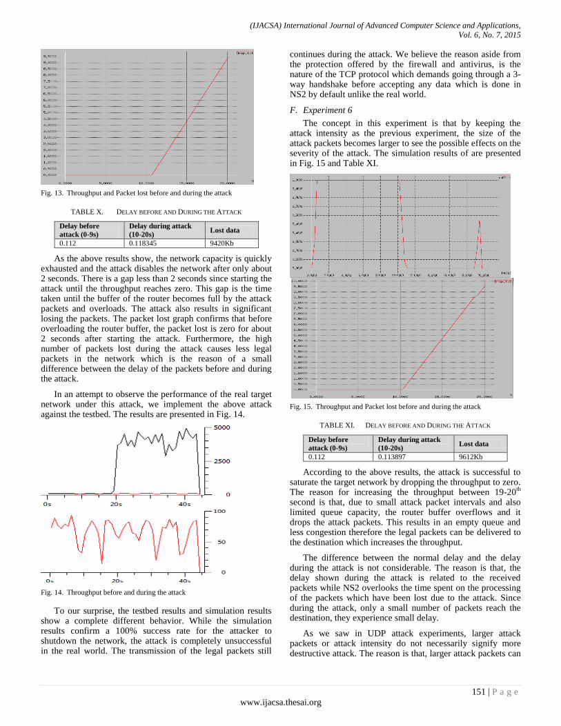
(IJACSA) International Journal of Advanced Computer Science and Applications,
Vol. 6, No. 7, 2015
151 | P a g e
www.ijacsa.thesai.org
Fig. 13. Throughput and Packet lost before and during the attack
TABLE X. DELAY BEFORE AND DURING THE ATTACK
Delay before
attack (0-9s)
Delay during attack
(10-20s) Lost data
0.112 0.118345 9420Kb
As the above results show, the network capacity is quickly exhausted and the attack disables the network after only about 2 seconds. There is a gap less than 2 seconds since starting the attack until the throughput reaches zero. This gap is the time taken until the buffer of the router becomes full by the attack packets and overloads. The attack also results in significant losing the packets. The packet lost graph confirms that before overloading the router buffer, the packet lost is zero for about 2 seconds after starting the attack. Furthermore, the high number of packets lost during the attack causes less legal packets in the network which is the reason of a small difference between the delay of the packets before and during the attack.
In an attempt to observe the performance of the real target network under this attack, we implement the above attack against the testbed. The results are presented in Fig. 14.
Fig. 14. Throughput before and during the attack
To our surprise, the testbed results and simulation results show a complete different behavior. While the simulation results confirm a 100% success rate for the attacker to shutdown the network, the attack is completely unsuccessful in the real world. The transmission of the legal packets still
continues during the attack. We believe the reason aside from the protection offered by the firewall and antivirus, is the nature of the TCP protocol which demands going through a 3-way handshake before accepting any data which is done in NS2 by default unlike the real world.
F. Experiment 6
The concept in this experiment is that by keeping the attack intensity as the previous experiment, the size of the attack packets becomes larger to see the possible effects on the severity of the attack. The simulation results of are presented in Fig. 15 and Table XI.
Fig. 15. Throughput and Packet lost before and during the attack
TABLE XI. DELAY BEFORE AND DURING THE ATTACK
Delay before
attack (0-9s)
Delay during attack
(10-20s) Lost data
0.112 0.113897 9612Kb
According to the above results, the attack is successful to saturate the target network by dropping the throughput to zero. The reason for increasing the throughput between 19-20
th
second is that, due to small attack packet intervals and also limited queue capacity, the router buffer overflows and it drops the attack packets. This results in an empty queue and less congestion therefore the legal packets can be delivered to the destination which increases the throughput.
The difference between the normal delay and the delay during the attack is not considerable. The reason is that, the delay shown during the attack is related to the received packets while NS2 overlooks the time spent on the processing of the packets which have been lost due to the attack. Since during the attack, only a small number of packets reach the destination, they experience small delay.
As we saw in UDP attack experiments, larger attack packets or attack intensity do not necessarily signify more destructive attack. The reason is that, larger attack packets can
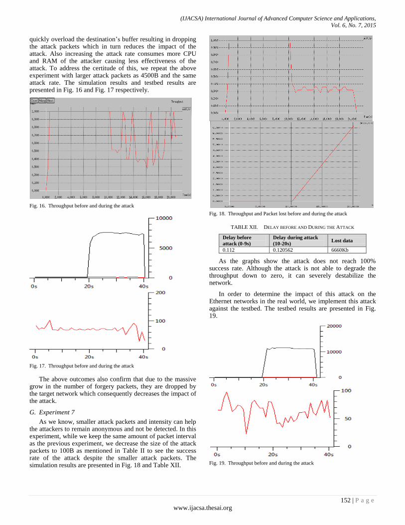
(IJACSA) International Journal of Advanced Computer Science and Applications,
Vol. 6, No. 7, 2015
152 | P a g e
www.ijacsa.thesai.org
quickly overload the destination’s buffer resulting in dropping the attack packets which in turn reduces the impact of the attack. Also increasing the attack rate consumes more CPU and RAM of the attacker causing less effectiveness of the attack. To address the certitude of this, we repeat the above experiment with larger attack packets as 4500B and the same attack rate. The simulation results and testbed results are presented in Fig. 16 and Fig. 17 respectively.
Fig. 16. Throughput before and during the attack
Fig. 17. Throughput before and during the attack
The above outcomes also confirm that due to the massive grow in the number of forgery packets, they are dropped by the target network which consequently decreases the impact of the attack.
G. Experiment 7
As we know, smaller attack packets and intensity can help the attackers to remain anonymous and not be detected. In this experiment, while we keep the same amount of packet interval as the previous experiment, we decrease the size of the attack packets to 100B as mentioned in Table II to see the success rate of the attack despite the smaller attack packets. The simulation results are presented in Fig. 18 and Table XII.
Fig. 18. Throughput and Packet lost before and during the attack
TABLE XII. DELAY BEFORE AND DURING THE ATTACK
Delay before
attack (0-9s)
Delay during attack
(10-20s) Lost data
0.112 0.120562 6660Kb
As the graphs show the attack does not reach 100% success rate. Although the attack is not able to degrade the throughput down to zero, it can severely destabilize the network.
In order to determine the impact of this attack on the Ethernet networks in the real world, we implement this attack against the testbed. The testbed results are presented in Fig. 19.
Fig. 19. Throughput before and during the attack
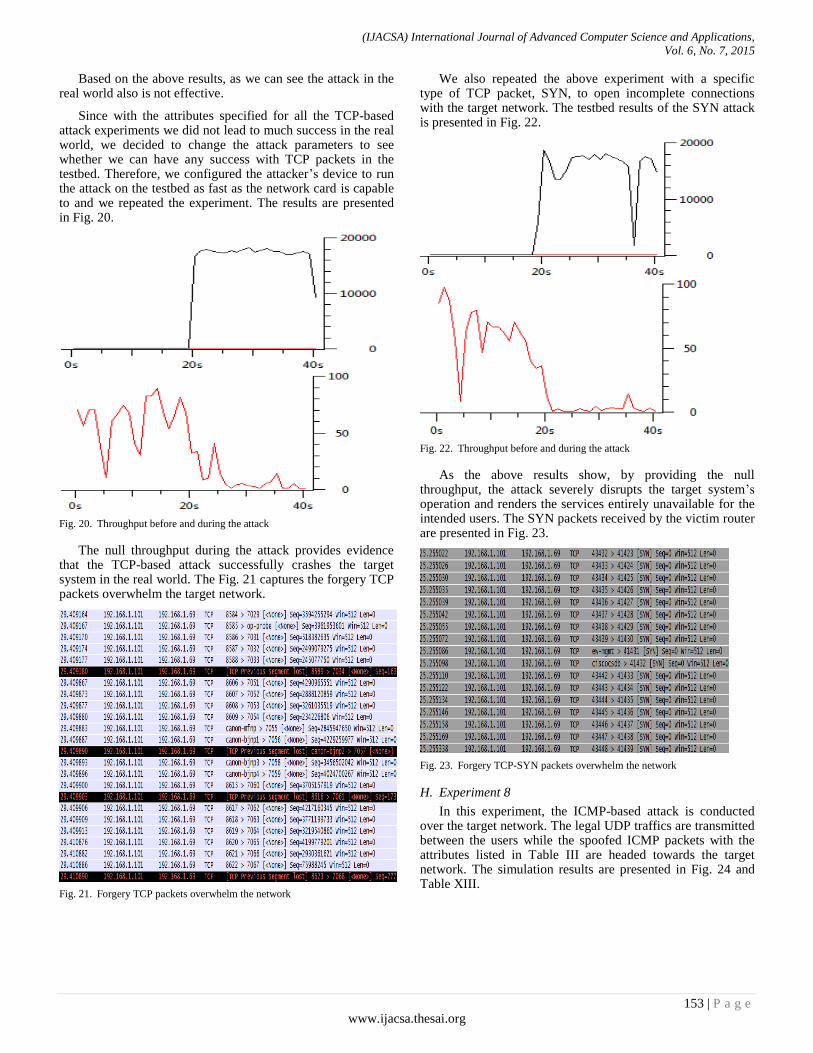
(IJACSA) International Journal of Advanced Computer Science and Applications,
Vol. 6, No. 7, 2015
153 | P a g e
www.ijacsa.thesai.org
Based on the above results, as we can see the attack in the real world also is not effective.
Since with the attributes specified for all the TCP-based attack experiments we did not lead to much success in the real world, we decided to change the attack parameters to see whether we can have any success with TCP packets in the testbed. Therefore, we configured the attacker’s device to run the attack on the testbed as fast as the network card is capable to and we repeated the experiment. The results are presented in Fig. 20.
Fig. 20. Throughput before and during the attack
The null throughput during the attack provides evidence that the TCP-based attack successfully crashes the target system in the real world. The Fig. 21 captures the forgery TCP packets overwhelm the target network.
Fig. 21. Forgery TCP packets overwhelm the network
We also repeated the above experiment with a specific type of TCP packet, SYN, to open incomplete connections with the target network. The testbed results of the SYN attack is presented in Fig. 22.
Fig. 22. Throughput before and during the attack
As the above results show, by providing the null throughput, the attack severely disrupts the target system’s operation and renders the services entirely unavailable for the intended users. The SYN packets received by the victim router are presented in Fig. 23.
Fig. 23. Forgery TCP-SYN packets overwhelm the network
H. Experiment 8
In this experiment, the ICMP-based attack is conducted over the target network. The legal UDP traffics are transmitted between the users while the spoofed ICMP packets with the attributes listed in Table III are headed towards the target network. The simulation results are presented in Fig. 24 and Table XIII.
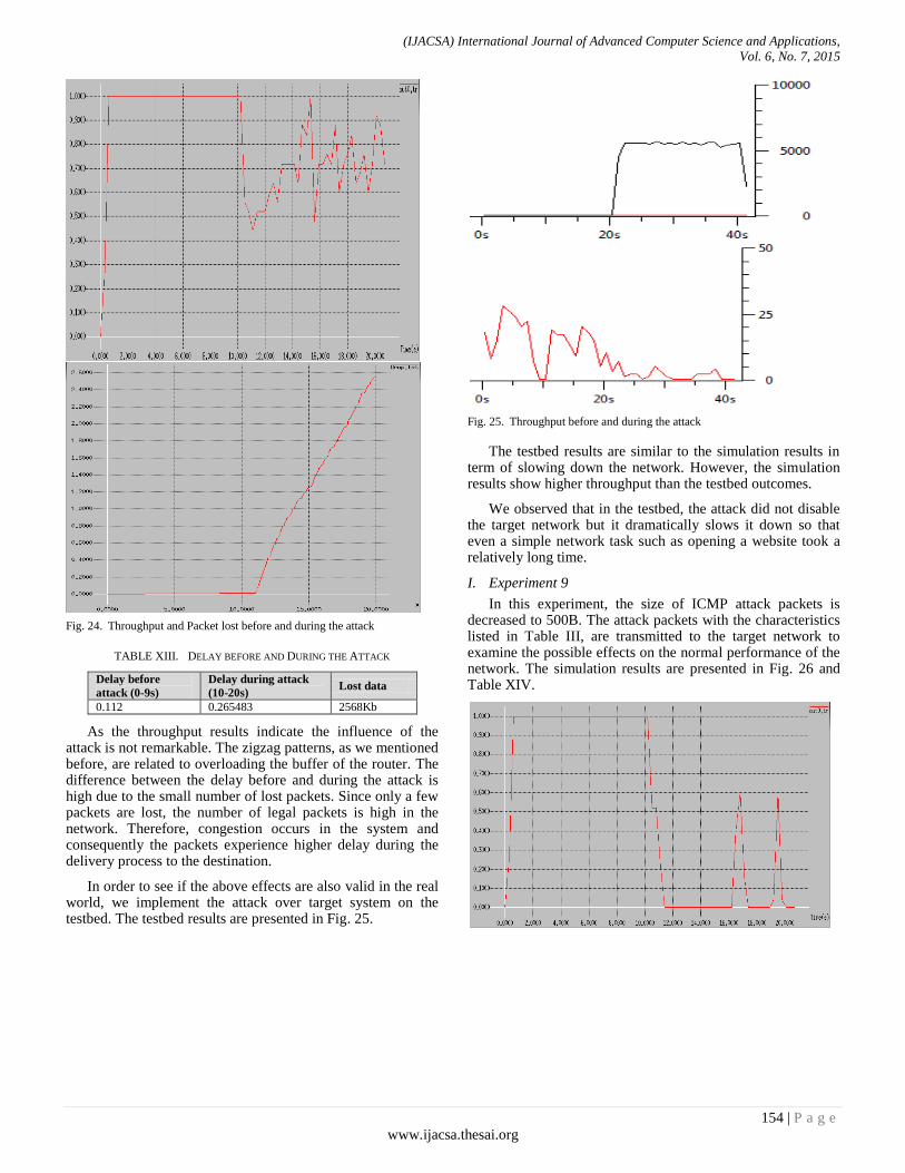
(IJACSA) International Journal of Advanced Computer Science and Applications,
Vol. 6, No. 7, 2015
154 | P a g e
www.ijacsa.thesai.org
Fig. 24. Throughput and Packet lost before and during the attack
TABLE XIII. DELAY BEFORE AND DURING THE ATTACK
Delay before
attack (0-9s)
Delay during attack
(10-20s) Lost data
0.112 0.265483 2568Kb
As the throughput results indicate the influence of the attack is not remarkable. The zigzag patterns, as we mentioned before, are related to overloading the buffer of the router. The difference between the delay before and during the attack is high due to the small number of lost packets. Since only a few packets are lost, the number of legal packets is high in the network. Therefore, congestion occurs in the system and consequently the packets experience higher delay during the delivery process to the destination.
In order to see if the above effects are also valid in the real world, we implement the attack over target system on the testbed. The testbed results are presented in Fig. 25.
Fig. 25. Throughput before and during the attack
The testbed results are similar to the simulation results in term of slowing down the network. However, the simulation results show higher throughput than the testbed outcomes.
We observed that in the testbed, the attack did not disable the target network but it dramatically slows it down so that even a simple network task such as opening a website took a relatively long time.
I. Experiment 9
In this experiment, the size of ICMP attack packets is decreased to 500B. The attack packets with the characteristics listed in Table III, are transmitted to the target network to examine the possible effects on the normal performance of the network. The simulation results are presented in Fig. 26 and Table XIV.
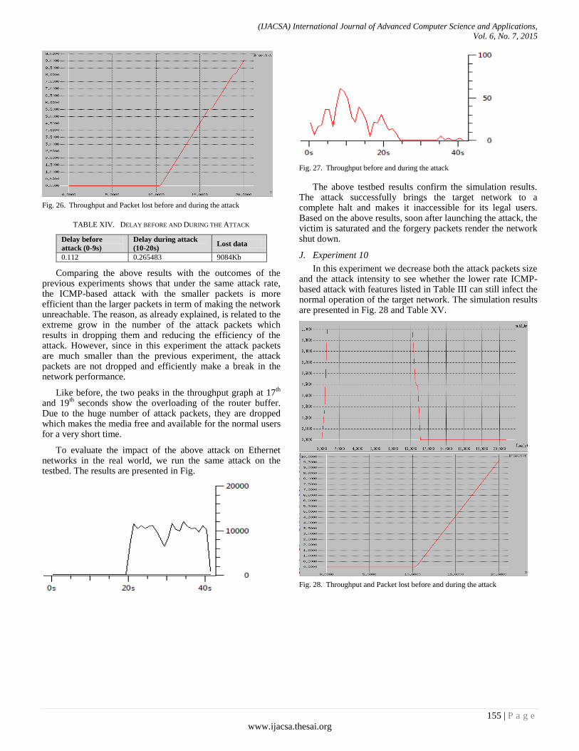
(IJACSA) International Journal of Advanced Computer Science and Applications,
Vol. 6, No. 7, 2015
155 | P a g e
www.ijacsa.thesai.org
Fig. 26. Throughput and Packet lost before and during the attack
TABLE XIV. DELAY BEFORE AND DURING THE ATTACK
Delay before
attack (0-9s)
Delay during attack
(10-20s) Lost data
0.112 0.265483 9084Kb
Comparing the above results with the outcomes of the previous experiments shows that under the same attack rate, the ICMP-based attack with the smaller packets is more efficient than the larger packets in term of making the network unreachable. The reason, as already explained, is related to the extreme grow in the number of the attack packets which results in dropping them and reducing the efficiency of the attack. However, since in this experiment the attack packets are much smaller than the previous experiment, the attack packets are not dropped and efficiently make a break in the network performance.
Like before, the two peaks in the throughput graph at 17th
and 19
th seconds show the overloading of the router buffer.
Due to the huge number of attack packets, they are dropped which makes the media free and available for the normal users for a very short time.
To evaluate the impact of the above attack on Ethernet networks in the real world, we run the same attack on the testbed. The results are presented in Fig.
Fig. 27. Throughput before and during the attack
The above testbed results confirm the simulation results. The attack successfully brings the target network to a complete halt and makes it inaccessible for its legal users. Based on the above results, soon after launching the attack, the victim is saturated and the forgery packets render the network shut down.
J. Experiment 10
In this experiment we decrease both the attack packets size and the attack intensity to see whether the lower rate ICMP-based attack with features listed in Table III can still infect the normal operation of the target network. The simulation results are presented in Fig. 28 and Table XV.
Fig. 28. Throughput and Packet lost before and during the attack
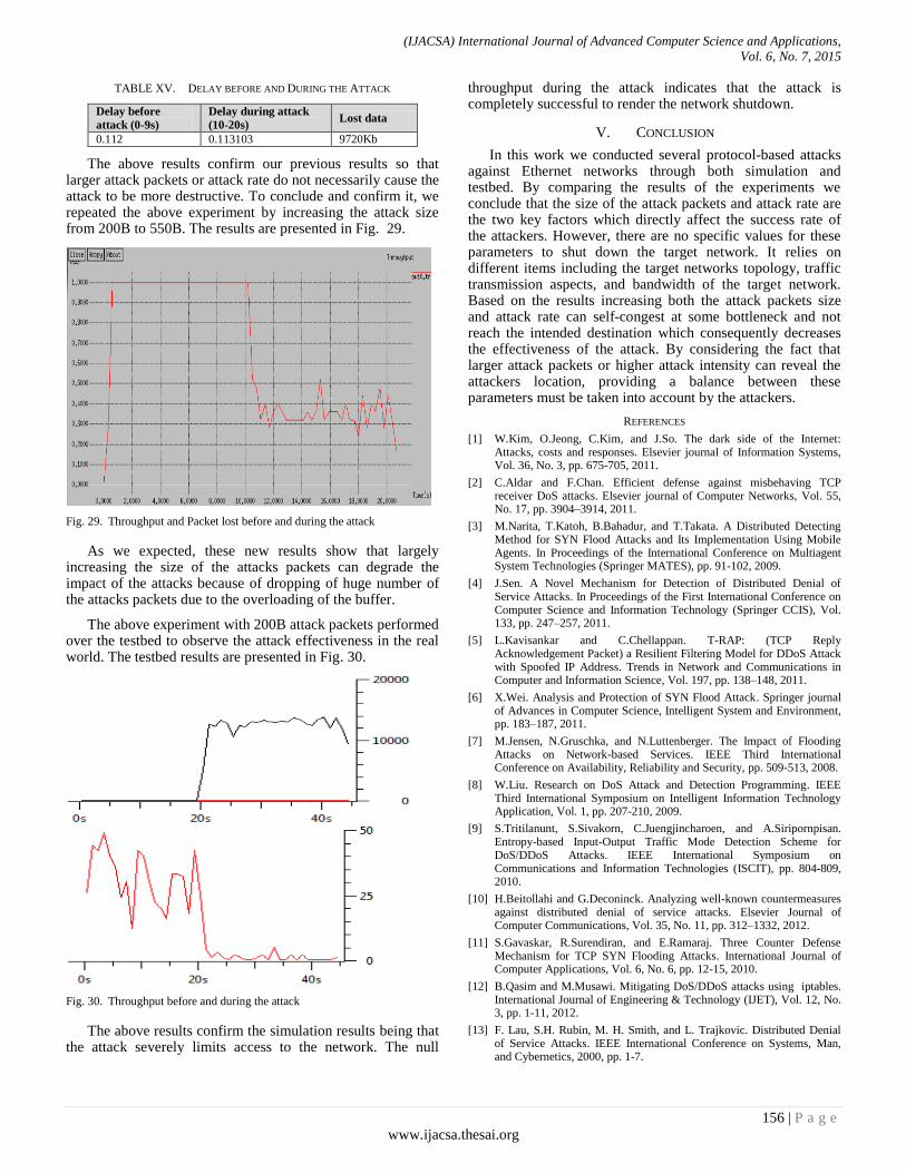
(IJACSA) International Journal of Advanced Computer Science and Applications,
Vol. 6, No. 7, 2015
156 | P a g e
www.ijacsa.thesai.org
TABLE XV. DELAY BEFORE AND DURING THE ATTACK
Delay before
attack (0-9s)
Delay during attack
(10-20s) Lost data
0.112 0.113103 9720Kb
The above results confirm our previous results so that larger attack packets or attack rate do not necessarily cause the attack to be more destructive. To conclude and confirm it, we repeated the above experiment by increasing the attack size from 200B to 550B. The results are presented in Fig. 29.
Fig. 29. Throughput and Packet lost before and during the attack
As we expected, these new results show that largely increasing the size of the attacks packets can degrade the impact of the attacks because of dropping of huge number of the attacks packets due to the overloading of the buffer.
The above experiment with 200B attack packets performed over the testbed to observe the attack effectiveness in the real world. The testbed results are presented in Fig. 30.
Fig. 30. Throughput before and during the attack
The above results confirm the simulation results being that the attack severely limits access to the network. The null
throughput during the attack indicates that the attack is completely successful to render the network shutdown.
V. CONCLUSION
In this work we conducted several protocol-based attacks against Ethernet networks through both simulation and testbed. By comparing the results of the experiments we conclude that the size of the attack packets and attack rate are the two key factors which directly affect the success rate of the attackers. However, there are no specific values for these parameters to shut down the target network. It relies on different items including the target networks topology, traffic transmission aspects, and bandwidth of the target network. Based on the results increasing both the attack packets size and attack rate can self-congest at some bottleneck and not reach the intended destination which consequently decreases the effectiveness of the attack. By considering the fact that larger attack packets or higher attack intensity can reveal the attackers location, providing a balance between these parameters must be taken into account by the attackers.
REFERENCES
[1] W.Kim, O.Jeong, C.Kim, and J.So. The dark side of the Internet: Attacks, costs and responses. Elsevier journal of Information Systems, Vol. 36, No. 3, pp. 675-705, 2011.
[2] C.Aldar and F.Chan. Efficient defense against misbehaving TCP receiver DoS attacks. Elsevier journal of Computer Networks, Vol. 55, No. 17, pp. 3904–3914, 2011.
[3] M.Narita, T.Katoh, B.Bahadur, and T.Takata. A Distributed Detecting Method for SYN Flood Attacks and Its Implementation Using Mobile Agents. In Proceedings of the International Conference on Multiagent System Technologies (Springer MATES), pp. 91-102, 2009.
[4] J.Sen. A Novel Mechanism for Detection of Distributed Denial of Service Attacks. In Proceedings of the First International Conference on Computer Science and Information Technology (Springer CCIS), Vol. 133, pp. 247–257, 2011.
[5] L.Kavisankar and C.Chellappan. T-RAP: (TCP Reply Acknowledgement Packet) a Resilient Filtering Model for DDoS Attack with Spoofed IP Address. Trends in Network and Communications in Computer and Information Science, Vol. 197, pp. 138–148, 2011.
[6] X.Wei. Analysis and Protection of SYN Flood Attack. Springer journal of Advances in Computer Science, Intelligent System and Environment, pp. 183–187, 2011.
[7] M.Jensen, N.Gruschka, and N.Luttenberger. The Impact of Flooding Attacks on Network-based Services. IEEE Third International Conference on Availability, Reliability and Security, pp. 509-513, 2008.
[8] W.Liu. Research on DoS Attack and Detection Programming. IEEE Third International Symposium on Intelligent Information Technology Application, Vol. 1, pp. 207-210, 2009.
[9] S.Tritilanunt, S.Sivakorn, C.Juengjincharoen, and A.Siripornpisan. Entropy-based Input-Output Traffic Mode Detection Scheme for DoS/DDoS Attacks. IEEE International Symposium on Communications and Information Technologies (ISCIT), pp. 804-809, 2010.
[10] H.Beitollahi and G.Deconinck. Analyzing well-known countermeasures against distributed denial of service attacks. Elsevier Journal of Computer Communications, Vol. 35, No. 11, pp. 312–1332, 2012.
[11] S.Gavaskar, R.Surendiran, and E.Ramaraj. Three Counter Defense Mechanism for TCP SYN Flooding Attacks. International Journal of Computer Applications, Vol. 6, No. 6, pp. 12-15, 2010.
[12] B.Qasim and M.Musawi. Mitigating DoS/DDoS attacks using iptables. International Journal of Engineering & Technology (IJET), Vol. 12, No. 3, pp. 1-11, 2012.
[13] F. Lau, S.H. Rubin, M. H. Smith, and L. Trajkovic. Distributed Denial of Service Attacks. IEEE International Conference on Systems, Man, and Cybernetics, 2000, pp. 1-7.

(IJACSA) International Journal of Advanced Computer Science and Applications,
Vol. 6, No. 7, 2015
157 | P a g e
www.ijacsa.thesai.org
[14] S. Oshima and T. Nakashima. Performance Evaluation for Linux under SYN Flooding Attacks. International Journal of Innovative Computing, Information and Control (IJICIC), Special Issue on New Trends in Information Processing and Applications, Vol. 5, No. 3, pp. 1-4, 2009.
[15] K.W.M. Ghazali and R.Hassan. Flooding Distributed Denial of Service
Attacks-A Review. Journal of Computer Science, Vol. 7, No. 8, pp. 1218-1223, 2011.
[16] A.Kumar, A.Sharma, and A.Singh. Performance Evaluation of Centralized Multicasting Network over ICMP Ping Flood for DDoS. International Journal of Computer Applications, Vol. 37, No. 10, pp. 1-6, 2012.

(IJACSA) International Journal of Advanced Computer Science and Applications,
Vol. 6, No. 7, 2015
158 | P a g e
www.ijacsa.thesai.org
A Survey of Emergency Preparedness
Aaron Malveaux
Department of Computer Science
Howard University
Washington, DC USA
A. Nicki Washington, Ph.D.
Department of Computer Science
Howard University
Washington, DC USA
Abstract—Emergency preparedness is a discipline that
harnesses technology, citizens, and government agencies to
handle and potentially avoid natural disasters and emergencies.
In this paper, a survey of the use of information technology,
including social media, in emergency preparedness is presented.
In addition, the current direction of research is identified, and
future trends are forecasted that will lead to more effective and
efficient methods of preparing for and responding to disasters.
Keywords—emergency preparedness; natural disasters;
emergencies
I. INTRODUCTION
Emergency preparedness is a discipline that harnesses technology, citizens, and government agencies to handle and potentially avoid natural disasters and emergencies. Research in this field seeks ways to avert, guard against, and efficiently recover from emergency situations, especially those that pose a threat to the stability of society. In this paper a survey of the use of information technology in emergency preparedness is presented. The work also examines how social media can be leveraged to warn the public of emergencies and analyze how people respond to emergency situations. In addition, it analyzes systems used to increase awareness to the public and government agencies on the importance of supporting the technology to reduce the impact of disasters. Finally, the current direction of research is identified, and future trends that will lead to more effective and efficient methods of preparing for and responding to disasters are forecasted.
The remainder of this paper is organized as follows. Section II discusses current research in emergency preparedness. Section III presents taxonomy of the current research and identifies future trends. Finally, Section IV concludes.
II. CURRENT TRENDS IN EMERGENCY PREPAREDNESS
RESEARCH
A review of the current literature on emergency preparedness identified several major trends in the research.
A. Social Networking and the Citizen’s Role in Emergency
Management
The use of the Internet as a resource during emergency situations has continued to augment over the years. The web has served as a vessel filled with vital information, and therefore, has introduced a novel and unique aspect to emergency preparedness research. Information from social networks can be used to monitor events in real time, as well as gather information after emergencies.
The level of social interaction via the web has increased exponentially. Social convergence has changed due to Web 2.0, allowing people to converge faster and from any location. Because of this, there has been an increase in public participation during disaster relief. The general archetypes of social convergence include helping, being anxious, returning, supporting, mourning, exploiting, and being curious [18]. Traces of each of the characteristics can be found when examining online behavior during disasters.
During disasters, people use online tools such as Twitter, Facebook, and Flickr. Online searches also help the anxious quickly determine who has been affected by the disaster and if they are safe. For example, online security cameras assisted families in California after wildfires, by informing them of the status of their property. After disasters, many people express support for relief efforts on social media sites and provide encouragement for those affected [12].
Apart from distributing information, researchers at the University of Colorado at Boulder examined social networking to understand the relationship between technology and social behavior during high profile events. Events such as the Republican National Convention, Democratic National Convention, Hurricane Gustav, and Hurricane Ike were reference points for data found on Twitter [11]. The study found that user-to-user communication decreases during large events. Instead of directing tweets at other users, people tend to direct their messages to the entire Twitter community. Also, the amount of tweets containing website addresses as references increases in order to provide more information than the 140 character tweet limit permits. The study concluded that the use of Twitter during mass incidents increased overall. In addition, Twitter can be exploited as a channel for the distribution of information. This was easy to identify when examining past events, but also shed light on limitations when examining real time information. An experiment conducted by the same group revealed that real-time, useful information can be extracted from Twitter in the event of a crisis, but the information is difficult to fully validate. The group suggested that in its current iteration, the information be accepted as a starting point for further investigation [9].
While Twitter serves as an effective outlet for text-based material, Flickr opens up a pathway for photographs that provide even more detail. The aforementioned study examined Flickr activity during major disasters to determine the volume of disaster-related posts and their relevance. They also interviewed top contributors, Flickr group administrators, and other interesting users, to determine what motivated users to share photographs. The research yielded that not only is their
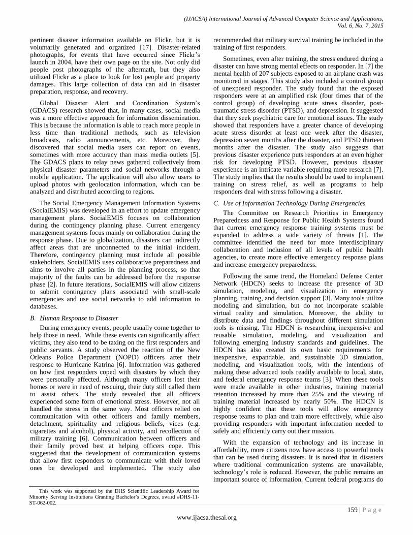
(IJACSA) International Journal of Advanced Computer Science and Applications,
Vol. 6, No. 7, 2015
159 | P a g e
www.ijacsa.thesai.org
pertinent disaster information available on Flickr, but it is voluntarily generated and organized [17]. Disaster-related photographs, for events that have occurred since Flickr’s launch in 2004, have their own page on the site. Not only did people post photographs of the aftermath, but they also utilized Flickr as a place to look for lost people and property damages. This large collection of data can aid in disaster preparation, response, and recovery.
Global Disaster Alert and Coordination System’s (GDACS) research showed that, in many cases, social media was a more effective approach for information dissemination. This is because the information is able to reach more people in less time than traditional methods, such as television broadcasts, radio announcements, etc. Moreover, they discovered that social media users can report on events, sometimes with more accuracy than mass media outlets [5]. The GDACS plans to relay news gathered collectively from physical disaster parameters and social networks through a mobile application. The application will also allow users to upload photos with geolocation information, which can be analyzed and distributed according to regions.
The Social Emergency Management Information Systems (SocialEMIS) was developed in an effort to update emergency management plans. SocialEMIS focuses on collaboration during the contingency planning phase. Current emergency management systems focus mainly on collaboration during the response phase. Due to globalization, disasters can indirectly affect areas that are unconnected to the initial incident. Therefore, contingency planning must include all possible stakeholders. SocialEMIS uses collaborative preparedness and aims to involve all parties in the planning process, so that majority of the faults can be addressed before the response phase [2]. In future iterations, SocialEMIS will allow citizens to submit contingency plans associated with small-scale emergencies and use social networks to add information to databases.
B. Human Response to Disaster
During emergency events, people usually come together to help those in need. While these events can significantly affect victims, they also tend to be taxing on the first responders and public servants. A study observed the reaction of the New Orleans Police Department (NOPD) officers after their response to Hurricane Katrina [6]. Information was gathered on how first responders coped with disasters by which they were personally affected. Although many officers lost their homes or were in need of rescuing, their duty still called them to assist others. The study revealed that all officers experienced some form of emotional stress. However, not all handled the stress in the same way. Most officers relied on communication with other officers and family members, detachment, spirituality and religious beliefs, vices (e.g. cigarettes and alcohol), physical activity, and recollection of military training [6]. Communication between officers and their family proved best at helping officers cope. This suggested that the development of communication systems that allow first responders to communicate with their loved ones be developed and implemented. The study also
recommended that military survival training be included in the training of first responders.
Sometimes, even after training, the stress endured during a disaster can have strong mental effects on responder. In [7] the mental health of 207 subjects exposed to an airplane crash was monitored in stages. This study also included a control group of unexposed responder. The study found that the exposed responders were at an amplified risk (four times that of the control group) of developing acute stress disorder, post-traumatic stress disorder (PTSD), and depression. It suggested that they seek psychiatric care for emotional issues. The study showed that responders have a greater chance of developing acute stress disorder at least one week after the disaster, depression seven months after the disaster, and PTSD thirteen months after the disaster. The study also suggests that previous disaster experience puts responders at an even higher risk for developing PTSD. However, previous disaster experience is an intricate variable requiring more research [7]. The study implies that the results should be used to implement training on stress relief, as well as programs to help responders deal with stress following a disaster.
C. Use of Information Technology During Emergencies
The Committee on Research Priorities in Emergency Preparedness and Response for Public Health Systems found that current emergency response training systems must be expanded to address a wide variety of threats [1]. The committee identified the need for more interdisciplinary collaboration and inclusion of all levels of public health agencies, to create more effective emergency response plans and increase emergency preparedness.
Following the same trend, the Homeland Defense Center Network (HDCN) seeks to increase the presence of 3D simulation, modeling, and visualization in emergency planning, training, and decision support [3]. Many tools utilize modeling and simulation, but do not incorporate scalable virtual reality and simulation. Moreover, the ability to distribute data and findings throughout different simulation tools is missing. The HDCN is researching inexpensive and reusable simulation, modeling, and visualization and following emerging industry standards and guidelines. The HDCN has also created its own basic requirements for inexpensive, expandable, and sustainable 3D simulation, modeling, and visualization tools, with the intentions of making these advanced tools readily available to local, state, and federal emergency response teams [3]. When these tools were made available in other industries, training material retention increased by more than 25% and the viewing of training material increased by nearly 50%. The HDCN is highly confident that these tools will allow emergency response teams to plan and train more effectively, while also providing responders with important information needed to safely and efficiently carry out their mission.
With the expansion of technology and its increase in affordability, more citizens now have access to powerful tools that can be used during disasters. It is noted that in disasters where traditional communication systems are unavailable, technology’s role is reduced. However, the public remains an important source of information. Current federal programs do
This work was supported by the DHS Scientific Leadership Award for Minority Serving Institutions Granting Bachelor’s Degrees, award #DHS-11-ST-062-002.
(IJACSA) International Journal of Advanced Computer Science and Applications,
Vol. 6, No. 7, 2015
160 | P a g e
www.ijacsa.thesai.org
not utilize volunteered information and only allow volunteer participation in disaster response, leaving a huge void that the public usually fills [13].
Information technology can also be used in the disaster management phase. A National Research Council workshop sought to increase and optimize its use in disaster management [16]. The research focused on human characteristics that obstruct the application of information technology systems. The study found that improved wireless networking connectivity, the ability to fuse data from different sources, detection of change and balancing the role of humans and computers are all necessary to successfully use information technology during emergency events.
D. Emergency Alert Systems
Emergency alert systems, like amber alerts and weather alerts, serve an important role in emergency management. Unfortunately, these systems do not take advantage of the new media for information dissemination. Many alert systems still operate on television and radio networks and have not expanded to the Internet.
The Emergency Alert System (EAS) used in the United States does not have a strong presence on the Internet. Prompt notification of emergencies and guidance are essential elements to keeping the public safe. However, the current system leaves a significant population without information. A recent study asserted the characteristics of effective systems [4]. The characteristics found to be most operative are location-awareness, automated operation, non-intrusiveness, spontaneity, ubiquity, and support for second languages [4]. In order to be feasible, an Internet-based EAS requires the cooperation of the government, Internet service providers, and website operators to achieve the qualities that a viable EAS demands.
The GDACS also provided recommendations on an Internet based alert system [5]. It determined that, in many cases, social media, especially Twitter, was a more effective approach for circulating information and news. This was because the Internet reaches a broad audience in small time periods.
E. Mobile Devices
While the Internet previously only allowed widespread consumption of information distributed by a few groups, Web 2.0 allows information to flow freely to and from all users of the Internet [10]. Many web programs allow information to be collected by users, such as Wikipedia, Open Street Map, and Google Earth. However, there is a lack of methods that ensure quality and detect and remove errors. Mobile devices equipped with GPS hardware (included in a large portion of devices sold) can collect this information. With the rise of Web 2.0 and Global Positioning System (GPS) receivers, citizens can obtain information that is relevant to their location and surroundings. Without the conveniences that these
systems offer, important information on events such as natural disasters or terrorist attacks would be lost to many people.
A study performed in part by the Institute for Environment and Sustainability examined how Volunteered Geographic Information (VGI) helps detect crisis events quickly and efficiently [8]. The study also explored how VGI can provide crisis management groups more accurate understanding of situations through photographs and social media updates. The group tested the validity of this claim by conducting two trials based on prior events. The first trial was conducted using a flood example and utilized only one social networking source. The second trial was conducted using a forest fire example and utilized two social networking sources. Once the information was stored and validated, the alerts were created and sent out to the organizations relevant to the emergency situation. The results of the trials showed that the system could provide high-level, useful information to emergency management organizations at affordable prices [8]. VGI can also be used to fill the shortage of geographical information worldwide [10].
Although cellular networks perform successfully most times, during emergencies, they are usually crippled and fail to function at full capacity. In an effort to remedy this weakness, a team of developers created the mobile ad hoc network MyMANET. MyMANET does not use typical communication technologies, but rather a lighter-weight infrastructure that is suitable for developing nations. MyMANET is a great contender for developing mobile ad hoc networks, because it is easy to use, efficient, and flexible. However, it is extremely vulnerable to security breaches. [14] As mentioned above, mobile devices enable citizens to easily share their locations and experiences. During disasters, this collective information can prove indispensable as a method to aid primary responders and concerned people.
III. FUTURE TRENDS
A review of the literature revealed a number of key and future research trends in emergency preparedness. Table 1 presents taxonomy of the current research in the area, including literature reviewed. This taxonomy was used to identify open areas of research and future trends.
Social media is still an open area of research in emergency preparedness. The majority of research is expected to move in the direction of incorporating social media into disaster response. The large increase of information on social media makes it a great resource for emergency management. People are sharing large parts of their lives on social media, and this typically increases during emergencies. Moreover, the information could be used during all phases of emergency management. Social media is also more accessible, as they provide platforms (APIs) that researchers or developers can use to extract and exploit the information. Researchers use social media data to track the roles of citizens during emergency events and map it to what is going on around them.

(IJACSA) International Journal of Advanced Computer Science and Applications,
Vol. 6, No. 7, 2015
161 | P a g e
www.ijacsa.thesai.org
TABLE I. TAXONOMY
Paper Social
Networking Human Response
Information
Technology Alert Systems
Mobile
Devices
1
X
2 X
3
X
4
X
5 X
X
6
X
7
X
8 X
X
9 X
X
10 X
X
11 X
12 X
13
X
X
14
X
15 X
16
X
17 X
X
18 X
The observations are then used to determine whether social media can be used to detect emergency events.
Review of the literature also determined that online emergency alert systems have not been researched in depth. Traditional systems use radio and television to alert citizens of emergencies, but the users of those mediums are declining. More people are using Internet services that rival traditional radio and television broadcasts. The Internet is a popular platform and needs a sustainable and reliable alert system that can reach people and notify them of emergency situations. Twitter introduced an emergency alert system for organizations to leverage. However, it is strictly opt-in, so the scope of the system is limited. This is a step forward. However, it still falls short of replicating the success of television and radio alert systems.
IV. CONCLUSION
In this study, the current literature in emergency response was reviewed to identify current and future trends. Research currently emphasizes the incorporation of social media into disaster response and the collaboration of governments and citizens. These two topics are very similar, because social media is the outlet that citizens use to aid in emergency management. However, it is an unofficial role. Dedicated mediums should be created for citizens to volunteer their time and information. Many of the studies examined in the survey show that there are users of social media who want to aid in the emergency management process. It is essential to offer support for information technology advances and utilize citizens during emergency management.
ACKNOWLEDGMENT
This work was supported by the DHS Scientific Leadership Award for Minority Serving Institutions Granting Bachelor’s Degrees, under award #DHS-11-ST-062-002.
REFERENCES
[1] Liu, S., Palen, L., Sutton, J., Hughes, A. and Vieweg, S. In Search of the Bigger Picture: The Emergent Role of On-Line Photo Sharing in Times of Disaster. In Proceedings of the 2008 ISCRAM Conference, 2008.
Retrieved from http://www.educause.edu/ero/article/online-social-media-crisis-events
[2] Hughes, Amanda L., Palen, Leysia, Sutton, Jeannette, Liu, Sophia B., Vieweg, Sarah. “Site-Seeing” in Disaster: An Examination of On-Line Social Convergence. Retrieved from https://www.cs.colorado.edu/~palen/Papers/iscram08/OnlineConvergenceISCRAM08.pdf
[3] Hughes, Amanda L., Palen, Leysia. Twitter Adoption and Use in Mass Convergence and Emergency Events. In Proceedings of the 6th International ISCRAM Conference – Gothenburg, Sweden, 2009. Retrieved from http://inderscience.metapress.com/content/h71150k3v8511021/
[4] De Longueville, B., Smith, R. S., & Luraschi, G. OMG, from here, I can see the flames!: a use case of mining location based social networks to acquire spatio-temporal data on forest fires. In Proceedings of the 2009 International Workshop on Location Based Social Networks, 2009. Retrieved from http://dl.acm.org/citation.cfm?id=1629907
[5] Stollberg, B., de Groeve, T. The Use of Social Media within the Global Disaster Alert and Coordination System, 2012. Retrieved from http://www2012.org/proceedings/companion/p703.pdf
[6] Mejri, O. and Plebani, P. SocialEMIS: Improving Emergency Preparedness through Collaboration, 2012. Retrieved from http://delivery.acm.org/10.1145/2190000/2188182/p691-mejri.pdf?ip=138.238.233.9&acc=ACTIVE%20SERVICE&CFID=142395012&CFTOKEN=72476836&__acm__=1353069000_0f4ea6f0b3dce6c7bf48a22080e370cc
[7] Adams, T., Anderson, L., Turner, M., Armstrong, J. Coping through a Disaster: Lessons from Hurricane Katrina, 2011. Retrieved from http://pacercenter.org/media/18822/coping%20through%20adams%20et%20al.pdf
[8] Fullerton, S., Ursano, R., Wang, L. Acute Stress Disorder, Posttraumatic Stress Disorder, and depression in Disaster and or Rescue Workers, 2004. Retrieved from http://ajp.psychiatryonline.org/article.aspx?articleID=176964
[9] Altevogt, B. M., Pope, A. M., Hill, M. N., and Shine, K. I. Research priorities in emergency preparedness and response for public health systems: A letter report, 2008. Retrieved from http://www.nap.edu/catalog/12136.html
[10] Emergency Preparedness, Response and Mitigation, 2003. Retrieved from http://delivery.acm.org/10.1145/1040000/1030959/p1061-corley.pdf?ip=138.238.233.9&acc=ACTIVE%20SERVICE&CFID=153951563&CFTOKEN=98287454&__acm__=1354893839_ffe66c22a670529b7e5fc1dd09d19660
[11] Palen, Leysia, Liu, Sophia B. Citizen communications in crisis: anticipating a future of ICT-supported public participation. In Proceedings of the SIGCHI Conference on Human Factors in

(IJACSA) International Journal of Advanced Computer Science and Applications,
Vol. 6, No. 7, 2015
162 | P a g e
www.ijacsa.thesai.org
Computing Systems, 2007. Retrieved from http://dl.acm.org/citation.cfm?id=1240736
[12] National Research Council, Committee on Using Information Technology to Enhance Disaster Management. Improving disaster management: The role of it in mitigation, preparedness, response, and recovery, 2007. Retrieved from National Academies Press website: http://www.nap.edu/catalog.php?record_id=11824
[13] Verma, P., Verma, D. Internet Emergency Alert System, 2005. Retrieved from http://domino.watson.ibm.com/library/cyberdig.nsf/papers/2DF643D577E6C48985256FF0005191CA/$File/rc23594.pdf
[14] Goodchild, Michael F. Citizens as Voluntary Sensors: Spatial Data Infrastructure in the World of Web 2.0. In International Journal of Spatial Data Infrastructures Research, 2007, Vol. 2, 24-32, 2007. Retrieved from http://ijsdir.jrc.ec.europa.eu/index.php/ijsdir/article/view/28
[15] Schade, S., Díaz L., Ostermann, F., Spinsanti L., Luraschi, G., Cox, S., Nuñez, M., DeLongueville, B. Citizen-based sensing of crisis events: sensor web enablement for volunteered geographic
[16] Paranjpe, A., and Vempala, S. Mymanet: A customizable mobile ad hoc network, 2009. Retrieved from http://www.dritte.org/nsdr09/files/nsdr09_camera/s4p2_paranjpe09nsdr.pdf
(IJACSA) International Journal of Advanced Computer Science and Applications,
Vol. 6, No. 7, 2015
163 | P a g e
www.ijacsa.thesai.org
Integrating Service Design and Eye Tracking Insight
for Designing Smart TV User Interfaces
Sheng-Ming Wang
Department of Interaction Design,
National Taipei University of Technology,
Taipei, TAIWAN
Abstract—This research proposes a process that integrate
service design method and eye tracking insight for designing a
Smart TV user interface. The Service Design method, which is
utilized for leading the combination of the quality function
deployment (QFD) and the analytic hierarchy process (AHP), is
used to analyze the features of three Smart TV user interface
design mockups. Scientific evidences, which include the
effectiveness and efficiency testing data obtained from eye
tracking experiments with six participants, are provided the
information for analysing the affordance of these design mockups.
The results of this research demonstrate a comprehensive
methodology that can be used iteratively for redesigning,
redefining and evaluating of Smart TV user interfaces. It can
also help to make the design of Smart TV user interfaces relate to
users' behaviors and needs. So that to improve the affordance of
design. Future studies may analyse the data that are derived
from eye tracking experiments to improve our understanding of
the spatial relationship between designed elements in a Smart TV
user interface.
Keywords—Smart TV; User Interface Design; Eye Tracking;
Design Affordance; Service Design
I. INTRODUCTION
Smart TV devices provide both broadcast and broadband content on a TV[1, 2]. They facilitate the curation of content by combining Internet-based information with content from TV providers[3]. These devices have the potential to combine the strengths of TV broadcasting and broadband network services. Accordingly, Smart TV depends innovative human-computer interaction(HCIs) to provide suitable services and to meet user requirements[4, 5]. Unlike those of a conventional TV with a remote control, new Smart TV features, such as web search, social networking, multi-user operation, personalized services and application development, require innovative “natural” HCIs[6]. Not only are the interactions and functions of a Smart TV user interface(UI) important, but also is its adaptability to individual users. To develop a Smart TV UI with service, researchers with technical and design backgrounds must work together in an interdisciplinary fashion with a comprehensive roadmap that specifies relevant requirements [3, 4, 7]. Although a Smart TV serves audiences by the delivery of innovative services, a number of questions about the mechanism of that delivery to various users via a single platform remain. Smart TV HCIs and UIs are important to all users, content providers and Smart TV manufacturers because innovative HCIs and UIs are required to provide enhanced services and meet user requirements[4, 8]. Numerous works
have established the importance of different criteria in designing HCIs and UIs[9-13]. Some researchers have proposed various processes for designing Smart TV HCIs and UIs [3, 5, 13, 14]. However, evaluation of the effectiveness, efficiency, and usability or, more generally, the affordance, of Smart TV HCI and UI designs results requires further investigation. Therefore, this work develops a comprehensive methodology for evaluating the design affordance of Smart TV UIs. Affordance evaluation is a technique that is widely used to identify the quality of various aspects of web site design[15, 16], product design[17], interaction design[18], and engineering design[19]. The purpose of an affordance evaluation is to ensure that users of the Smart TV UIs can use design mockups efficiently and effectively. The two classes of affordance evaluation are empirical methods and inspections. Empirical methods are based on observing, capturing, and analyzing data about usage by real end-users, while inspections are conducted by expert evaluators or designers, and involve reviewing the usability-related aspects of the design(such as mock-ups, conceptual models, user interfaces), commonly associated with UIs, with regard to their conformance with a set of guidelines. This research mostly concerns inspections. Firstly, in an interdisciplinary service design workshop, Quality Function Deployment (QFD) and the Analytic Hierarchy Process (AHP) were integrated to derive qualitative and quantitative information about user-related scenarios and user requirements for developing three Smart TV UI mockup designs. Then, eye tracking evaluations are performed with six participants to gather gazing data, eye paths, and heat maps for further analysis. The results of the eye tracking analysis are then compared with the results obtained from a service design workshop to evaluate the design affordance of the Smart TV UIs.
The remainder of this paper is organized as follows. Section II reviews related work. Section III discusses the relevant design mechanism and proposed methodology for Smart TV UIs design. Section IV discusses results of the implementation of QFD and AHP for a Smart TV UI design mockup. Section V presents the eye tracking results and analyzes the Smart TV UI design affordance. Section V draws conclusions and offers idea for future works.
II. RELATED WORKS
A. Services design method for develpoing smart tv uis
Service interfaces are designed for intangible products that are, from the customer’s point of view, useful, profitable and

(IJACSA) International Journal of Advanced Computer Science and Applications,
Vol. 6, No. 7, 2015
164 | P a g e
www.ijacsa.thesai.org
desirable, while they are effective, efficient and different for the provider. The method for making this process integral and holistic is to incorporate the particular visions of all stakeholders, including users, designers, investors, researchers, technicians, policy makers, consultants and competitors. Bill Moggridge offered the following definition; “service design is the design of intangible experiences that reach people through many different touch-points”[11]. That is, service design is a process of continual updates based on the responses of users who are observed and monitored. Service design is a means of transferring traditional product design and interface design to commercial services. Also, service design can help to elucidate user requirements and find solutions to the design of services, products, and other related elements to users. The principles of service design have been implemented in scenario planning[11, 22].
By integrating the internet into television sets, Smart TVs allow consumers to use on-demand streaming media services, listen to radio, access interactive media, use social networks, and download applications[20]. Nowadays, Smart TVs not only offer access to the internet and legacy web services, but also provide content services that are immediately coupled to broadcast content that is rendered on the terminal device[2]. To provide more and better services, a Smart TV must have a menu system and UI that can be navigated to complete a task. As several researched have noted, an intuitive and easily navigated HCI and UI are critical to a good user experience of a Smart TV[1, 9, 13, 18, 21]. Hence, a comprehensive process that includes design and evaluation of Smart TV UIs is very important for making Smart TV services more desirable and useful .Unlike the features of a conventional TV with a remote control, new Smart TV features, such as web search, social networking, multi-user support, personalized services and application development, depend on innovative “natural” HCIs[4]. To improve the HCIs with a Smart TV, our earlier work brought together technicians and designers in an inter-disciplinary context to generate a comprehensive roadmap for the development of Smart TVs and identify future requirements thereof[3, 5]. Any application of service design to the multimodal interaction development of Smart TV must consider aspects of both product design and interface design. Moreover, this work follows some features and characteristics of service design that were summarized as follows.
1) Assessing services from a holistic and detailed point of
view.
2) Considering both artifacts and experiences.
3) Making services tangible and visible via visualizations.
B. QFD-AHP Integration for Smart TV UIs Design
In addition to the service design approach, the quality function deployment(QFD) matrix and analytical hierarchy process(AHP) method are also utilized simultaneously to systematically identify the criteria derived from service design scenario planning, and to weight and prioritize criteria.
The (QFD) method is a qualitative approach that is used to systematically assess the correlation between user requirements and technical features. The QFD matrix is a systematic design approach based on an in-depth awareness of customer desires, coupled with integrated corporate functional groups. The QFD
matrix translates customer desires into design characteristics for each stage of product development. The ultimate goal of is to translate often subjective criteria into objective criteria that can be quantified and measured and which can then be used to design and manufacture the product. However, it has two weaknesses: firstly, it does not prioritize customer requirements; secondly, the weights are subjectively evaluated and depend on consensus among a panel of experts.
The AHP method is a structured technique that converge the opinions from domain experts for dealing with complex decisions[23, 24]. The AHP enables groups of people to interact and focus on a certain problem, modify their judgments and, as a result, combine group judgments in accordance with the main criteria. Applying the AHP to weight CRs in a QFD matrix provides a rational framework for structuring a decision problem. The combined AHP-QFD approach can quantify CRs and elements, relate those elements to overall CR goals and evaluate alternative solutions. The combined AHP-QFD approach has been used successfully to assess customer needs based on a multiple-choice decision analysis. Gupta et al. reviewed uses of the QFD-AHP to evaluate and select methodology for an innovative product design concept. The methodology combining QFD-AHP was mainly used as a multi-criteria decision method for evaluating user requirements. By considering the requirements of designing Smart TVs and characteristics of service design, this work uses this methodology to evaluate the design and development of Smart TV UIs.
C. Evaluation of Design Affordance and Eye-Tracking
The perceptual psychologist J. J. Gibson coined the word “affordance” to refer to the actionable properties between the world and an actor[26]. Don Norman argues that, to Gibson, affordances are relationships. They exist naturally: they do not have to be visible, known, or desirable[27] ; he would make a global change, replacing all instances of the word “affordance” with the expression “perceived affordance.” Don Norman also points out that affordances, both real and perceived, play very different roles in physical products, from their roles in screen-based products, such as UIs design. In product design, which deals with real, physical objects, both real and perceived affordances are involved, and the two sets may differ. With respect to graphical, screen-based interfaces, a designer primarily can control only perceived affordances[27]. Obrenovic and Starcevic claimed that HCIs are moving the balance of interactions closer to the human and support expressive, transparent, efficient, and robust interaction[10]. Therefore, the design of Smart TV UIs should focus on usability, which refers to “the extent to which a product can be used by specified users to achieve specified goals with effectiveness, efficiency and satisfaction in a specified context of use."[9] However, usability issues commonly arise concerning HCI and UI navigation that has been poorly designed, typically because of the organization, placement, visual design, or terminology involved. Current methods for measuring the effectiveness of navigation are limited to observable behaviors and verbal feedback from participants.
Eye tracking is becoming an increasingly common tool in UX testing, enabling new ways to optimize navigational elements in UI design to be discovered [9]. Research into

(IJACSA) International Journal of Advanced Computer Science and Applications,
Vol. 6, No. 7, 2015
165 | P a g e
www.ijacsa.thesai.org
results for evaluating eye tracking indicates that the relationship between interface and human reading habits can be recorded and analyzed systematically and scientifically to provide references for UI design[28, 29]. A book entitled “Measuring the User Experience: Collecting, Analyzing, and Presenting”, states that Eye Tracking (Gaze Tracker) is a good example of evaluating user experience and does not measuring not only where an eye is looking but also its motion, which makes measurement more easier and accurate[30]. A group of researchers used Gaze Tracker to determine whether object placement based on user expectation results in faster and better recall of the object’s location[31]. Aesthetic usability effect is influenced by the user’s affective response to the interaction, so Smart TV UI design should be evaluated to determine whether users recognize something that they appreciate and find to be aesthetically pleasing . Another issue proposed by Soussan Djamasbi found that Gaze Tracker can be utilized to measure the preferences of members of Generation Y (age 18-31) among various interfaces[29]. This research addresses how eye tracking can be used to understand the effectiveness of the design of mockups of Smart TV UIs, based on information derived from the QFD-AHP model. Three interface mockups were displays on a screen and Gaze Tracker was used to collect the gaze data of participants for 20 minutes. The evaluation of the eye tracking function was then used in the roadmap for designing Smart TV UIs to review the results.
III. METHODOLOGY
A. Define the Features of Smart TV UIs
The concept of design thinking is integrated here with technology development to develop a Smart TV UI. The four major phases of the interdisciplinary integration of the design thinking concept with technology development are as follows. The first phase is to outline the vision for the Smart TV HCI design, based on a review of trends of the development of, and visions for, Smart TVs. The second phase is to propose a plan for the interdisciplinary integration of technology and experts in the domain of interaction design by holding service design workshops to foster interdisciplinary brainstorming. The third phase, which provides the kernel of the integration, is to define user scenarios and technology benchmarks based on insights into user-centered design. In the last phase, the combined QFD-AHP approach is implemented to analyze the features and classes of Smart TV UIs mockup designs. Finally, an eye-tracking evaluation is conducted to the pupil is tracked and its movement is recorded for further analysis. The results are used to evaluate the design affordance of the developed Smart TV UIs.
B. QFD-AHP Model
The QFD matrix specifies the importance of each feature based on a correlation analysis of user requirements and technical features. It also shows user recognition by describing their experiences to competitors by giving a value to their importance. The importance range is 1–5 and their thinking is limited to strong, moderate, or poor. This method reveals how strongly the features (product characteristics) are related to user requirements and reflects the strengths of existing products. This work uses the QFD matrix to systematically list the features of the multimodal HCI design. This work uses the
QFD matrix to list systematically the features of Smart TV UI design. An inter-disciplinary team of faculty members, researchers and graduate students with interaction design, computer science, and electronic engineering backgrounds participated in a service design workshop. This workshop helped the team gain a clear understanding of the features of Smart TV UIs design. The many ideas of the Smart TV UIs design that were generated in the workshop were narrowed down from global thoughts to specific and applicable features that meet user requirements and could be developed technically . All of the features that were obtained from service design workshop are represented in a QFD matrix. The importance of each feature is obtained by performing a correlation analysis of user requirements and the technical features that users demand.
After the QFD analysis, the AHP method is used to evaluate the results. The three basic steps in the AHP research areas follows.
1) Describe a complex decision-making problem as a
hierarchy.
2) Perform pair wise comparison to estimate the priorities
of various elements on each level of the hierarchy.
3) Integrate these priorities to obtain an overall
evaluation of decision alternatives. The AHP calculation template that was provided by
Goepel[32] is used here for the primitive analysis of AHP results. The result workbook consists of20 input worksheets for pair wise comparisons, a sheet consolidating all assessments, a summary sheet of systematic results, a sheet of reference tables ( a random index, limits for the geometric consistency index (GCI), and judgment scales) and a sheet for solving the eigenvalue problem using the eigenvector method (EVM).
C. Eye Tracking Evaluation
A gaze tracking device, EyeLink 1000 Plus, which was made available by the National Taipei University of Technology, was used to trace participants’ eye movements. The device was set 2.75 m away from optical receiver. Since the device comes an infrared lamp, the room was made dark to eliminate any inaccuracy during the experiment. The evaluation involved six participants, who were asked to sync their eye’s gaze to the sensor before beginning the task. Participants were required to describe the contents of a selected Smart TV UI design, while the Gaze Tracker recorded their eye position. The obtained were presented as eye movement points and timed trajectories. GazeTrail, LookZone, and HeatMap methods are used to verify the design affordance of the designed mockups of the Smart TV UIs. The GazeTrail shows the subject's ocular scan path by drawing a connected path of the recorded gaze position data on the Smart TV UI mockup design. LookZone calculates the area of interest in certain a Smart TV UI . HeatMap shows the intensity calculated from the GazePoint results. Data that collected on fixations and saccades from an eye-tracker will be visualized in an eye tracking software as gaze plot and heat map. The information that was collected from eye tracking evaluation is then provided for the design affordance analysis.
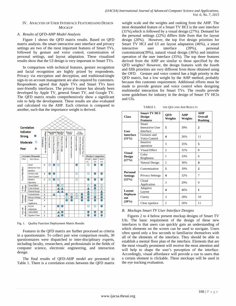
(IJACSA) International Journal of Advanced Computer Science and Applications,
Vol. 6, No. 7, 2015
166 | P a g e
www.ijacsa.thesai.org
IV. ANALYSIS OF USER INTERFACE FEATURESAND DESIGN
MOCKUP
A. Results of QFD-AHP Model Analysis
Figure 1 shows the QFD matrix results. Based on QFD matrix analysis. the smart interactive user interface and privacy settings are two of the most important features of Smart TVs, followed by gesture and voice control, customization of personal settings, and layout adaptation. These visualized results show that the UI design is very important to Smart TVs.
In comparison with technical features, gesture recognition and facial recognition are highly prized by respondents. Privacy via encryption and decryption, and traditional/single sign-in on account management are also required by customers. Respondents agreed that Apple TVs and Smart TVs have user-friendly interfaces. The privacy feature has already been developed by Apple TV, general Smart TV, and Google TV. The QFD matrix results comprehensively show a significant role to help the development. These results are also evaluated and calculated via the AHP. Each criterion is compared to another, such that the importance weight is derived.
Fig. 1. Quality Function Deployment Matrix Results
Features in the QFD matrix are further processed as criteria in a questionnaire. To collect pair wise comparison results, 30 questionnaires were dispatched to inter-disciplinary experts, including faculty, researchers, and professionals in the fields of computer science, electronic engineering, and interaction design.
The final results of QFD-AHP model are presented in Table 1. There is a correlation exists between the QFD matrix
weight scale and the weights and ranking from the AHP. The most demanded feature of a Smart TV HCI is the user interface (31%),which is followed by a visual design (27%). Demand for the personal settings (22%) differs little from that for layout design (20%). However, the top five design priorities for Smart TV HCI and UI are layout adaptation (46%), a smart interactive user interface (39%), personal customization(39%), natural visual design (36%) and intuitive operation of the user interface (35%). The top three features derived from the AHP are similar to those specified by the QFD weights? However, the design features with the fourth and fifth priorities are very different from those obtained using the OFD. Gesture and voice control has a high priority in the QFD matrix, but a low weight by the AHP method, probably because this customer requirement. Additional efforts must be made to provide gesture and voice control when designing multimodal interaction for Smart TVs. The results provide some guidelines for industry in the design of Smart TV HCIs and UIs.
TABLE I. THE QFD AND AHP RESULTS
Class Smart TV HCI
Design
Features
QFD
Weights AHP
Weights
AHP
Overall
Ranking
User Interface
(31%)
Smart Interactive User
Interface 5 39% 2
Gestures and
Voice Control 4 26% 11
Intuitive
operation 3 35% 5
Visual Design
(27%)
Visual Effect 2 31% 8
Color
Brightness 1 33% 6
Natural Design 2 36% 4
Personal
Settings (22%)
Customization 5 39% 2
Privacy Settings 4 32% 7
Cloud
Application 3 29% 9
Layout
Deploym
ent (20%)
Adaptive Layout
4 46% 1
Clarity 3 28% 10
Clear typeface 2 26% 11
B. Mockups Smart TV User Interface Designs
Figures 2 to 4 below present mockup designs of Smart TV UIs. The basic requirement of the design of these new interfaces is that users can quickly gain an understanding of which elements on the screen can be used to navigate. Users often spend only a few seconds to familiarize themselves with all of the elements of the interface. They should be able to establish a mental floor plan of the interface. Elements that are the most visually prominent will receive the most attention and will help to shape the user’s perception of the interface. Accordingly, visual affordance will provide a cue to users that a certain element is clickable. These mockups will be used in the eye tracking evaluation.

(IJACSA) International Journal of Advanced Computer Science and Applications,
Vol. 6, No. 7, 2015
167 | P a g e
www.ijacsa.thesai.org
Fig. 2. Smart TV UI Design Mockup 1
Fig. 3. Smart TV UI Mockup 2
Fig. 4. Smart TV UI Mockup 3
C. Design of Eye-Tracking Evaluation
Before the experiment was begun, five look zones (LZ) were established on the interface in different colors to help to track each participant’s eye movement. These five LZs correspond to Search, Notification, Launcher, User Account, and Movie (Categories). The pictures below show the locations of the LZs on the screen. The time and position of viewing are recorded to determine gaze time and the sequence of eye path.
Fig. 5. Look Zones on Screen
V. EVALUATION AND DISCUSSION
A. Analysis of Efficiency of Mockup of Design of Smart TV UI
Eye tracking experiment was carried out using the Gaze Tracker EyeLink 1000 Plus. Six participants took the test. Participant were asked to sync their eye’s gaze to the sensor before beginning the task. Participants were required to identify the contents of a selected Smart TV UI design, while the Gaze Tracker recorded their eye position and searching time. The obtained were presented as eye movement points and timed trajectories.
The following tables presents the time taken by each participant while searching and identifying the contents of each Smart TV UIs mockup design.
TABLE II. GAZE TIME RECORD OF PARTICIPANT 01
Contents UI #1 UI #2 UI #3
Categories 3.63 3.7 1.8
Search (sec) 2.05 3.85 1.5
User Account(sec) 3.31 1.15 3.53
Movie Selection (sec) 3.76 4.98 1.66
App Launcher (sec) 3.06 3.03 3.45
Notification (sec) 2.18 5.43 3.43
Average Time (sec) 3 3.7 2.6
TABLE III. TIME RECORD OF PARTICIPANT 02
Contents UI #1 UI #2 UI #3
Categories (sec) 5.03 3.3 1.48
Search (sec) 1.71 1.06 5.48
Users (sec) 3.18 2.21 1.88
Movie Selection (sec) 4.28 2.13 1.3
App Launcher (sec) 3.15 2.48 4.08
Notification (sec) 1.53 1.54 2
Average Time (sec) 3.1 2.1 2.7

(IJACSA) International Journal of Advanced Computer Science and Applications,
Vol. 6, No. 7, 2015
168 | P a g e
www.ijacsa.thesai.org
TABLE IV. TIME RECORD OF PARTICIPANT 03
Contents UI #1 UI #2 UI #3
Categories (sec) 2.11 4.66 1.33
Search (sec) 1.93 2.33 8.5
Users Account(sec) 2.6 4.88 4.2
Movie Selection (sec) 3.18 4.46 2.55
App Launcher (sec) 5.65 2.75 1.78
Notification (sec) 4.05 3.63 5.23
Average Time (sec) 3.3 3.8 3.9
TABLE V. TIME RECORD OF PARTICIPANT 04
Contents UI #1 UI #2 UI #3
Categories (sec) 2.56 3.11 2.66
Search (sec) 1.76 2.96 2.35
Users Account(sec) 2.33 2.16 1.55
Movie Selection (sec) 11.58 3.33 1.55
App Launcher (sec) 6.41 1.95 16.7
Notification (sec) 1.23 2.53 2.1
Average Time (sec) 4.3 2.7 4.5
TABLE VI. TIME RECORD OF PARTICIPANT 05
Contents UI #1 UI #2 UI #3
Categories (sec) 8.68 2.36 6.11
Search (sec) 2.91 1.26 1.81
Users Account(sec) 1.13 1.38 1.98
Movie (sec) Selection 13.33 2.76 3.2
App Launcher (sec) 2.58 1.28 6.6
Notification (sec) 4.43 3.16 7.85
Average Time (sec) 5.5 2 4.6
TABLE VII. TIME RECORD OF PARTICIPANT 06
Contents UI #1 UI #2 UI #3
Categories (sec) 3.08 5 14.06
Search (sec) 2.03 2.76 2.56
Users Account (sec) 2.21 2.4 2
Movie (sec) Selection 4.51 3.96 3.93
App Launcher (sec) 1.68 2.98 6.3
Notification (sec) 5.46 3.3 2.58
Average Time (sec) 3.1 3.4 5.2
Table 8 presents the average of the times taken to complete identify the contents of each Smart TV UIs design mockup.
TABLE VIII. GRAND AVERAGE TIME FOR PARTICIPANT TO COMPLETE
IDENTIFY THE CONTENTS OF EACH SMART TV UI DESIGN
UI #1 UI #2 UI #3
Participate 01 3 3.7 2.6
Participate 02 3.1 2.1 2.7
Participate 03 3.2 3.8 3.9
Participate 04 4.3 2.7 4.5
Participate 05 5.5 2 4.6
Participate 06 3.1 3.4 5.2
Average Time 3.7 3.0 3.9
This table demonstrates that the users can perceive the proposed Smart TV UI mockup design less than 5s, revealing the efficiency of the design. Efficiency can be described as the speed and accuracy with which users can complete tasks for which they use the UIs. The results also reveal that the design can create a favorable user experience of the Smart TV UIs as it guides the participants effortlessly through the UIs to reach their goal.
All of the participants in this research had little trouble in identifying the contents in the test, indicating that the mockups of the Smart TV UI designs that are presented in this research are sufficiently effective. Effectiveness is the completeness and accuracy with which users achieve specified goals; it is determined by determined whether the user’s goals are met successfully and whether all work is correct. Effectiveness is the driving force behind successful task completion and helps users to complete their goals. The effectiveness of these Smart TV UIs is determined by whether users can locate and use the navigation option to take them to the expected location. UI#2 performs best, followed by UI#1. Therefore, in the next part, UI #2 and UI#1 are used as the wireframes for the evaluation of eye tracking.
B. Eye Tracking: Evaluation and Discussion
Five look zones (LZ) were established to determine the eye movement of each participant. These five LZ are set for Search, Notification, Launcher, and Movie (Categories). The following figures show the locations of the set-up LZs on the screen. In Fig. 6, the pink rectangle represents the User LZ; the yellow rectangle represents the Search LZ; the blue rectangle represents the Notification LZ; the green rectangle represents the Launcher LZ, and the purple rectangle represents the Movie LZ. Each table following a figure presents detailed information about eye movement on a slide of the mockup design of the Smart TV UIs and the five look zones. UI#2 and UI#1 are installed on the eye-tracking device and six participants are involved in the evaluation. The system recorded tracking data from only three participants owing to some problems with the system. Therefore, only three datasets are analyzed.
The eye tracking results demonstrate that LookZone-Movie Selection receives more gazing time than others(total time in zone: 84.37 s for three participants), and LookZone-User is also perceived as important (gaze point count: 3157 times for three participants). The grid system design helps these three participants to distinguish parts of interface, and all participants described the process of movie selection systematically. LookZone-User Account and LookZone-Launcher are located in the same column, so the three participants all found moving between these two sections convenient.
Fig. 6. LookZones for Smart TV UI#2
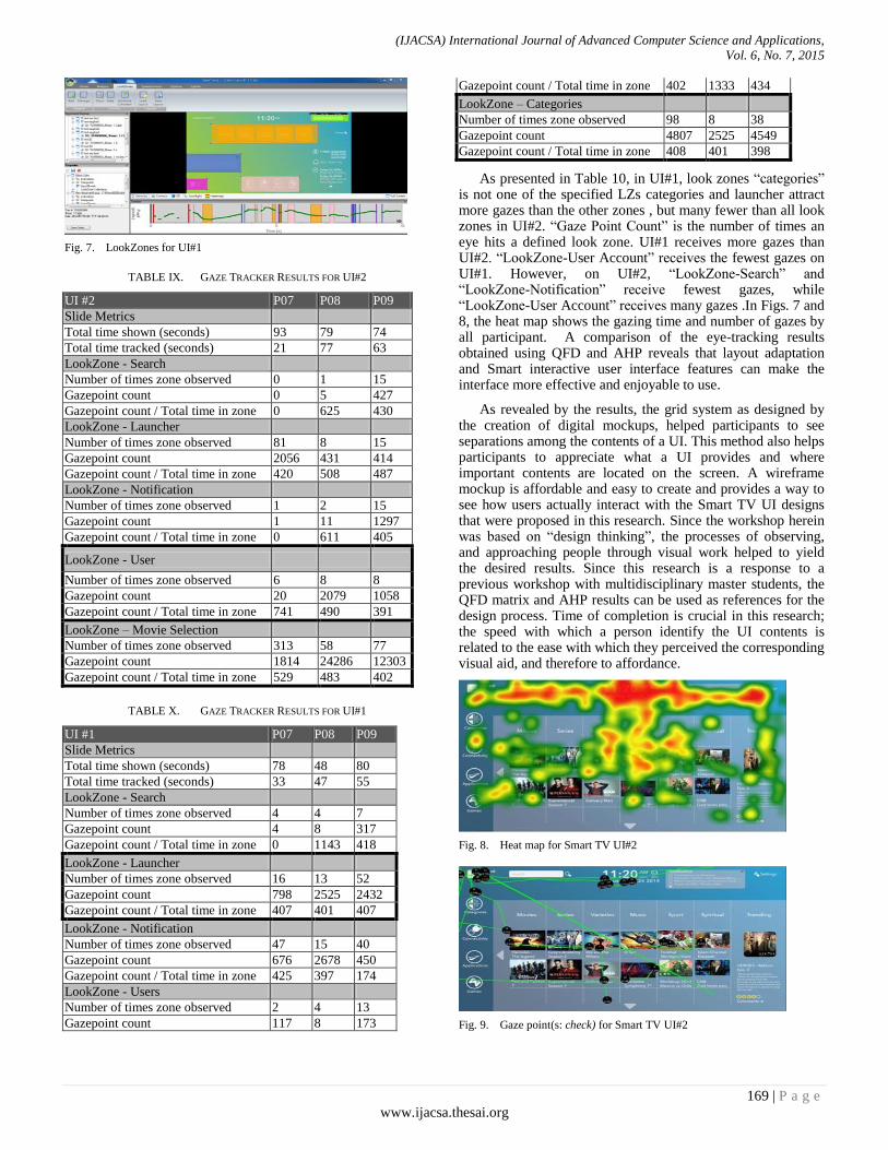
(IJACSA) International Journal of Advanced Computer Science and Applications,
Vol. 6, No. 7, 2015
169 | P a g e
www.ijacsa.thesai.org
Fig. 7. LookZones for UI#1
TABLE IX. GAZE TRACKER RESULTS FOR UI#2
UI #2 P07 P08 P09
Slide Metrics
Total time shown (seconds) 93 79 74
Total time tracked (seconds) 21 77 63
LookZone - Search
Number of times zone observed 0 1 15
Gazepoint count 0 5 427
Gazepoint count / Total time in zone 0 625 430
LookZone - Launcher
Number of times zone observed 81 8 15
Gazepoint count 2056 431 414
Gazepoint count / Total time in zone 420 508 487
LookZone - Notification
Number of times zone observed 1 2 15
Gazepoint count 1 11 1297
Gazepoint count / Total time in zone 0 611 405
LookZone - User
Number of times zone observed 6 8 8
Gazepoint count 20 2079 1058
Gazepoint count / Total time in zone 741 490 391
LookZone – Movie Selection
Number of times zone observed 313 58 77
Gazepoint count 1814 24286 12303
Gazepoint count / Total time in zone 529 483 402
TABLE X. GAZE TRACKER RESULTS FOR UI#1
UI #1 P07 P08 P09
Slide Metrics
Total time shown (seconds) 78 48 80
Total time tracked (seconds) 33 47 55
LookZone - Search
Number of times zone observed 4 4 7
Gazepoint count 4 8 317
Gazepoint count / Total time in zone 0 1143 418
LookZone - Launcher
Number of times zone observed 16 13 52
Gazepoint count 798 2525 2432
Gazepoint count / Total time in zone 407 401 407
LookZone - Notification
Number of times zone observed 47 15 40
Gazepoint count 676 2678 450
Gazepoint count / Total time in zone 425 397 174
LookZone - Users
Number of times zone observed 2 4 13
Gazepoint count 117 8 173
Gazepoint count / Total time in zone 402 1333 434
LookZone – Categories
Number of times zone observed 98 8 38
Gazepoint count 4807 2525 4549
Gazepoint count / Total time in zone 408 401 398
As presented in Table 10, in UI#1, look zones “categories” is not one of the specified LZs categories and launcher attract more gazes than the other zones , but many fewer than all look zones in UI#2. “Gaze Point Count” is the number of times an eye hits a defined look zone. UI#1 receives more gazes than UI#2. “LookZone-User Account” receives the fewest gazes on UI#1. However, on UI#2, “LookZone-Search” and “LookZone-Notification” receive fewest gazes, while “LookZone-User Account” receives many gazes .In Figs. 7 and 8, the heat map shows the gazing time and number of gazes by all participant. A comparison of the eye-tracking results obtained using QFD and AHP reveals that layout adaptation and Smart interactive user interface features can make the interface more effective and enjoyable to use.
As revealed by the results, the grid system as designed by the creation of digital mockups, helped participants to see separations among the contents of a UI. This method also helps participants to appreciate what a UI provides and where important contents are located on the screen. A wireframe mockup is affordable and easy to create and provides a way to see how users actually interact with the Smart TV UI designs that were proposed in this research. Since the workshop herein was based on “design thinking”, the processes of observing, and approaching people through visual work helped to yield the desired results. Since this research is a response to a previous workshop with multidisciplinary master students, the QFD matrix and AHP results can be used as references for the design process. Time of completion is crucial in this research; the speed with which a person identify the UI contents is related to the ease with which they perceived the corresponding visual aid, and therefore to affordance.
Fig. 8. Heat map for Smart TV UI#2
Fig. 9. Gaze point(s: check) for Smart TV UI#2

(IJACSA) International Journal of Advanced Computer Science and Applications,
Vol. 6, No. 7, 2015
170 | P a g e
www.ijacsa.thesai.org
Research has established that users of any new interface need to quickly gain an understanding of which elements on the screen can be used. Users frequently take only a few seconds to familiarize themselves with all of the elements on the page and then establish a mental plan of the interface in a very short time. Therefore, design blocks or elements that are the most visually prominent attract the most attention and will help to shape a user’s perception of the interface. The information in Tables 9 and 10 indicates the visual affordance of the Smart TV UI mockup designs that are proposed in this research. The overall results provide clues to users that certain elements are operable Further analysis based on the method with Gestalt principles, which are time-tested methods that shape the visual hierarchy that a user will see, will be conducted in the future to revise the original mockup Smart TV UIs.
VI. CONCLUSIONS AND FUTURE WORKS
Creating a usable user interface for a Smart TV is critical to a positive user experience. Designing interactive content would have been difficult without a pertinent method. Indeed, in the field of design, people are encouraged to create their own solutions to problems, but appropriate methods are highly recommended to be considered before any design is conducted, to facilitate the effective solution to particular problems.
This research aims to proposed a comprehensive process for designing and evaluation Smart TV UIs with high affordance. A design process is implemented, based on the output of design thinking, and the results are evaluated and analyzed Also, interdisciplinary collaboration among people from various fields and backgrounds were engaged to ensure that the proper design approaches were taken. QFD and AHP supported the initial process of creating a new prototype specification that accounted users’ desired features and correlating to the possibilities of engineering technologies. This scheme comprehends incorporates users’ experiences and allows problems with this system to be identified and the system to be assessed. Eye tracking verifies the effectiveness and efficiency of the Smart TV UIs mockup design by recording of the gaze of users. This technology provides clear traces and calculates the numbers, percentages, and time of a user’s eye movements.
In conclusion, the iterative process of redesigning Smart TV UIs that is proposed in this research may help to improve its effectiveness and efficiency, and enable changes in users’ behaviors and needs to be responded to. Visual affordance provides clues to users that some elements are operable. Further analysis based on the methods with Gestalt principles, which are time-tested methods that shape the visual hierarchy that a user will see, will be performed in future research to revise the original Smart TV UI mockup designs. Moreover, in future work, many possible interactive designs will be developed. Voice and gesture-based interactions or other affordable inputs may elevate the user’s experience of communicating through the interface, possibly opening up another basis for a universal design that would enable a disabled person to interact with the user interface. Even though many possible types of input connectivity may exist, a user’s behavior should be given a high priority in the design process.
ACKNOWLEDGMENTS
This work was supported the Ministry of Science and Technology, Taiwan, under the projects NSC 101-2219-E-027-007 and MOST 103-2221-E-027-062. The assistance of my students Cheih-Ju Huang and Cipto Hartanto is greatly appreciated. Ted Knoy is appreciated for his editorial assistance.
REFERENCES
[1] K. Merkel, "Hybrid broadcast broadband TV, the new way to a comprehensive TV experience," in Electronic Media Technology (CEMT), 2011 14th ITG Conference on, 2011, pp. 1-4.
[2] L. B. Yuste and S. Al-Majeed, "Effective synchronisation of hybrid broadcast and broadband TV," in 2012 IEEE International Conference on Consumer Electronics (ICCE), Las Vegas, NV, USA, 2012, pp. 160-161.
[3] S.-M. Wang, "Service Design for Developing Multimodal Human Computer Interaction for Smart TVs," International Journal of Advanced Computer Science and Applications, vol. 6, pp. 227-234, 2015.
[4] P. Hamisu, G. Heinrich, C. Jung, V. Hahn, C. Duarte, P. Langdon, and P. Biswas, "Accessible UI design and multimodal interaction through hybrid TV platforms: towards a virtual-user centered design framework," in Universal Access in Human-Computer Interaction. Users Diversity, ed: Springer, 2011, pp. 32-41.
[5] S.-M. Wang, V. Bailey, and C. Hartanto, "Developing Hybrid Internet Broadcast Television user interface base on user experience design principle," in Consumer Electronics-Taiwan (ICCE-TW), 2014 IEEE International Conference on, Taipei, Taiwan, 2014, pp. 61-62.
[6] O. Martinez-Bonastre, M.-J. Montpetit, and P. Cesar, "IP-based tv technologies, services, and multidisciplinary applications," Communications Magazine, IEEE, vol. 51, 2013.
[7] S.-M. Wang and C. J. Huang, "QFD and AHP integration for Smart TV human-computer interaction design," in Consumer Electronics-Taiwan (ICCE-TW), 2014 IEEE International Conference on, Taipei, Taiwan, 2014, pp. 59-60.
[8] T.-H. You, Y.-J. Wu, C.-L. Lin, and Y. Chuang, "Enhancing People’s Television Experience by Capturing, Memoing, Sharing, and Mixing," in Cross-Cultural Design. Methods, Practice, and Case Studies, ed: Springer, 2013, pp. 510-518.
[9] A. Schall, "Eye tracking insights into effective navigation design," in Design, User Experience, and Usability. Theories, Methods, and Tools for Designing the User Experience, ed: Springer, 2014, pp. 363-370.
[10] Z. Obrenovic and D. Starcevic, "Modeling multimodal human-computer interaction," Computer, vol. 37, pp. 65-72, 2004.
[11] B. Moggridge and B. Atkinson, Designing interactions vol. 14: MIT press Cambridge, 2007.
[12] M. Tambe, "TV Human Interface: Different Paradigm from that of PC and Mobile," IEEE Code of Ethics, 2012.
[13] S.-F. M. Liang, Y.-C. Kuo, and S.-C. Chen, "Identifying Usability Problems in a Smart TV Music Service," in Cross-Cultural Design. Methods, Practice, and Case Studies, ed: Springer, 2013, pp. 306-312.
[14] V. Vinayagamoorthy, P. Allen, M. Hammond, and M. Evans, "Researching the user experience for connected tv: a case study," in CHI'12 Extended Abstracts on Human Factors in Computing Systems, 2012, pp. 589-604.
[15] Y. Lu, Y. Kim, X. Y. Dou, and S. Kumar, "Promote physical activity among college students: Using media richness and interactivity in web design," Computers in Human Behavior, vol. 41, pp. 40-50, 2014.
[16] S. Abrahão, E. Insfran, and A. Fernandez, "Designing Highly Usable Web Applications," 2014.
[17] T. Ha and S. Lee, "User behavior model based on affordances and emotions: A new approach for an optimal use method in product-user interactions," International Journal of Human-Computer Interaction, 2014.
[18] A. L. Blackler, V. Popovic, and D. P. Mahar, "Applying and testing design for intuitive interaction," International Journal of Design Sciences and Technology, vol. 20, pp. 7-26, 2014.

(IJACSA) International Journal of Advanced Computer Science and Applications,
Vol. 6, No. 7, 2015
171 | P a g e
www.ijacsa.thesai.org
[19] P. Cormier, A. Olewnik, and K. Lewis, "Toward a formalization of affordance modeling for engineering design," Research in Engineering Design, vol. 25, pp. 259-277, 2014.
[20] E. J. Park, "Creating a sustainable business model for the TV industry: strategic analysis on the Smart TV ecosystem," Master, Sloan School of Management, Massachusetts Institute of Technology, 2014.
[21] P. Ramakrisnan, A. Jaafar, F. H. A. Razak, and D. A. Ramba, "Evaluation of user interface design for leaning management system (LMS): investigating student's eye tracking pattern and experiences," Procedia-Social and Behavioral Sciences, vol. 67, pp. 527-537, 2012.
[22] S. Moritz, "Service design: practical access to an evolving field," Cologne, Germany: Köln International School of Design, 2005.
[23] T. L. Saaty, "An exposition of the AHP in reply to the paper “remarks on the analytic hierarchy process”," Management science, vol. 36, pp. 259-268, 1990.
[24] T. L. Saaty, "Decision making with the analytic hierarchy process," International journal of services sciences, vol. 1, pp. 83-98, 2008.
[25] F. De Felice and A. Petrillo, "A multiple choice decision analysis: an integrated QFD–AHP model for the assessment of customer needs," International Journal of Engineering, Science and Technology, vol. 2, 2011.
[26] J. J. Gibson, "The theory of affordances," in Perceiving, Acting, and Knowing: toward an ecological psychology, R. E. Shaw and J. Bransford, Eds., ed Hillsdale, NJ: Lawrence Erlbaum Associates, 1977, pp. 67-82.
[27] D. A. Norman, "Affordance, conventions, and design," interactions, vol. 6, pp. 38-43, 1999.
[28] D. Bruneau, M. A. Sasse, and J. McCarthy, "The eyes never lie: The use of eye tracking data in HCI research," in Proceedings of the CHI, 2002, p. 25.
[29] S. Djamasbi, M. Siegel, and T. Tullis, "Generation Y, web design, and eye tracking," International journal of human-computer studies, vol. 68, pp. 307-323, 2010.
[30] L. E. Nacke, M. N. Grimshaw, and C. A. Lindley, "More than a feeling: Measurement of sonic user experience and psychophysiology in a first-person shooter game," Interacting with Computers, vol. 22, pp. 336-343, 2010.
[31] S. P. Roth, A. N. Tuch, E. D. Mekler, J. A. Bargas-Avila, and K. Opwis, "Location matters, especially for non-salient features–An eye-tracking study on the effects of web object placement on different types of websites," International journal of human-computer studies, vol. 71, pp. 228-235, 2013.
[32] K. D. Goepel, "Implementing the analytic hierarchy process as a standard method for multi-criteria decision making in corporate enterprises–a new AHP excel template with multiple inputs," in Proceedings of the international symposium on the analytic hierarchy process, Kuala Lumpur, Malaysia, 2013.
(IJACSA) International Journal of Advanced Computer Science and Applications,
Vol. 6, No. 7, 2015
172 | P a g e
www.ijacsa.thesai.org
Investigating on Mobile Ad-Hoc Network to
Transfer FTP Application
Ako Muhammad Abdullah
Computer Science Department
Faculty of Physical & Basic Education
University of Sulaimani
Kurdistan Region-Iraq
Abstract—Mobile Ad-hoc Network (MANET) is the collection
of mobile nodes without requiring of any infrastructure. Mobile
nodes in MANET are operating as a router and MANET
network topology can change quickly. Due to nodes in the
network are mobile and thus can move randomly and organize
arbitrarily regardless of the directions that generate great
complexity in routing traffic from source to destination. To
communicate with other nodes MANET nodes contain multiple
applications and it needs the different level of data traffic. While
data communicate different routing protocols require whereas
every node must act as a router. Nowadays, different routing
protocols have available for MANET. MANET protocols
designed and implemented at the network layer have vital roles
that affect the application running at the application layer. In
this paper, the performance of On Demand Distance Vector
(AODV), Dynamic Source Routing (DSR) and Geographic
Routing Protocol (GRP) will be evaluated. The main purpose of
this research is to analyze the performance of MANET routing
protocols to identify “Which routing protocol has ability to
provide the best performance to transfer FTP Application in
high mobility case under low, medium and high density
scenario?”. The performance analyze with respect to Average
End-to-End Delay, Media Access Delay, Network Load,
Retransmission Attempt and Throughput. All simulations have
been done using OPNET. On the basis of results show that the
GRP gives better performance in End-to-End Delay, Media
Access Delay, and Retransmission Attempt when varying
network size and provide the best Throughput in small and
medium network size. Simulation results verify that AODV gives
better Throughput in a large network and lower Network Load
in small and medium network size compared to GRP. DSR
produces low Average Network load as compared to other
protocols. The overall study of the FTP application shows that
the performance of theses routing protocols differences by
varying number of nodes and node speed. This paper results will
produce enough information to identify the best routing protocol
for MANET to transfer FTP application.
Keywords—MANET; AODV; DSR; GRP; FTP Application
I. INTRODUCTION
In recent years, a network structure is changing rapidly. In the area of the wireless network, Mobile Ad-hoc Network (MANET) is the most demanding field. MANET is a dynamic distributed system and which has no fixed infrastructure and it has mobile devices or users that generally known as nodes each one of which equip with radio transmitter and receiver. In this network each mobile nodes can establish a
communication with each other directly within transmission range. Otherwise the nodes between them forward the packets for them from source to destination. Every node acts as a router to forward the packets to other nodes whenever required [1].
Routing protocols has an important role to find route packets from source to destination among randomly distributed nodes. There are many protocols have proposed for MANET.
The routes change very fast and frequent with the dynamic nature of network topology, and so the routing protocols play significant roles in handling it [2]. They need be capable to ensure the delivery of packets safely to their destinations. MANETs has ability to handle topology changes malfunctions in nodes through network reconfigurations due to wireless mobile ad-hoc network for several types of applications are very flexible and suitable as allowing the establishment of temporary communication without any preinstalled infrastructure. To find a route between the end-points is a main problem in multi-hop ad-hoc dynamic. The problem is further aggravated because of the nodes mobility. [5].
Nowadays, to handle this problem many different approaches are proposed. However, it is very difficult to decide which one is best routing protocol. Other aspects of MANET are also dynamic changing network topology of nodes.
The purpose of this paper is to evaluate the performance of proactive and reactive routing protocols in MANET. Nowadays, different routing protocols have available to transfer data over MANET. However, these protocols have different behaviors with respect to wireless routing perspective. The main problem is to choose the correct routing protocol is reliable and efficient for MANET.
The main questions arise for the evaluation of these problems such as which routing protocols has the ability to provide a better performance in MANET? And what factors can be affected the performance of these routing protocols. To answer all these questions, we will deploy the different scenarios with varying network size and speed under different metrics.
In this study, the performance evaluation of these routing protocols such as AODV, DSR, and GRP will be carried out to determine which routing protocols has the ability to provide
(IJACSA) International Journal of Advanced Computer Science and Applications,
Vol. 6, No. 7, 2015
173 | P a g e
www.ijacsa.thesai.org
the best performance to transfer FTP application over MANET. Our evaluation metrics is End–to-End Delay, Media Access Delay, Network Load, Retransmission Attempts and Throughput. Different scenarios will be simulated based on the above mentioned metrics and from the results we can decide which routing protocols has ability to provide the best suitable for transferring FTP application over MANET.
This paper is organized as follows: related works discuss in Section 2. In Section 3 we describe routing protocols design issues in MANET. Next section presents a brief overview of MANET routing protocols that we evaluate. The Simulation environment discuss in Section 5. Section 6 describes matrices used in this paper. Results and analysis presents in Section 7. Finally, we provide a conclusion and future work in Section 8.
II. RELATED WORK
In [8], Shah et al. compared the performance of AODV, DSR and DSDV routing protocols under different routing metrics such as network size, network load and mobility. They used NS-2. According to the results that they have obtained that both DSR and AODV perform better than DSDV under mobility. In [6], Kaushik et al. do a performance comparison of AODV, DSDV and DSR. The concluded that AODV performs predictably with low mobility virtually to deliver data at nodes and it has problem when node mobility increases. However, in this situation DSR has ability to provide the good performance when that node has mobility and DSDV performs almost as well as DSR but it requires many routing overhead packets. Furthermore, dropped packets and packet delay ratio are concerned and with the large of nodes the AODV and DSR better than DSDV. In addition, DSDV performance is better for less mobility and less number of nodes.
In [3], Abdullah et al. evaluate the performance of AODV and DSR protocols to transfer multimedia data over MANET. Performance of these routing protocols is evaluated under different metrics such as network load, throughput and end-to-end delay. During the simulation they have changed network size. They concluded that AODV perform better than DSR under high mobility and varying network size.
In [4] Al-Maashr et al. evaluate the performance of AODV, DSR and OLSR in the presence of the burst self-similar traffic under four different metrics such as routing overhead, delivery ratio, end-to-end delay and throughput. They concluded that DSR protocol performs well with burst traffic models compared to AODV and OLSR in terms of delivery ratio, end-to-end delay and throughput. On the other hand, OLSR performed poorly in the presence of self-similar traffic at high mobility especially in terms of data packet delivery ratio, routing overhead and end-to-end delay. As for AODV routing protocol, the results show an average performance yet remarkably low and stable end-to-end delay.
Gupta et al. [7] the performance of AODV, DSR and TORA analyzed. The simulator used was Network Simulator Version 2 (NS-2). The simulation was carried out in a field of 500m x 500m and the number of nodes in the network was 50 nodes. CBR traffic was used as the traffic source and the
simulation time was 200 seconds. The performance metrics used were average end-to-end delay and Packet Delivery Fraction. The results showed that the AODV protocol has the best overall performance and the DSR protocol is suitable for networks with moderate mobility rate and since it has a low overhead that makes it suitable for low power network and low bandwidth. The results also demonstrated that TORA protocol is suitable for operation in large mobile networks having a dense population of nodes.
Naumov and Gross [8] analyzed the impact of the network size up to 550 nodes, nodes density, nodes mobility and suggested data traffic on DSR and AODV performance.
The authors performed the experimented in the areas of 2121m x 425m, 3000m x 600m, 3675m x 735m, 4250m x 850m and 5000m x 1000m. The traffic used was CBR. The performance metrics used were average end-to-end delay, Packet Delivery Fraction and routing overhead. The results illustrated that the AODV and DSR protocols demonstrated good scalability with respected to the number of nodes and density of nodes in stationary scenarios with a low number of traffic source. However, as the mobility rate increases, the routing overhead of DSR prevent this protocol from delivering data packets effectively.
III. ROUTING PROTOCOL DESIGN ISSUES
When designing MANET routing protocols a number of issues are considered. Designing routing protocol is very challenging because the distributed state of unreliable environment they are found in such as limited network capacity, dynamic topology and different kind of wireless communication constraints. Several of these constrains are interference and hidden collisions, variable link quality and energy constrained nodes. In addition, hidden and exposed terminal and limited resource in terms of power are a vital problem that will be considered when routing protocol is designed [10].
A. Distributed State in Unreliable Environment
To performance routing protocols the status and condition of the environmental challenges is an important role. In addition, in any unreliable environment for the distribution of resource becomes a challenge to enable communication, due to routing protocols have to consider best utilization of resources such as processing power, battery life and bandwidth [11].
B. Dynamic Topology
Due to the network topology in mobile ad-hoc network is dynamically changing, therefore causing sessions of transferring packet to suffer from interferences leading to frequent path breaks. From the network range when a destination or intermediate node in a route dis appears the interference occurs. Moreover, when a route broken it is important for routing protocol to find a new route and build a new topology efficiently. The network load causing overhead if lowered, the overall performance will be increased and in any MANET routing protocol the mobility management is extremely important due to it justifies the need for efficiency [20].

(IJACSA) International Journal of Advanced Computer Science and Applications,
Vol. 6, No. 7, 2015
174 | P a g e
www.ijacsa.thesai.org
C. Limited Bandwidth
MANET is limited in radio bandwidth compared to wire network with an abundant bandwidth therefore, data transfer rates are less than those of wired networks. This increased the need for a routing protocol to optimally use the bandwidth. Furthermore, limited bandwidth results in less stored topology information. For an efficient routing protocol complete topology information is required. However, in MANET routing protocol cannot be case as this will cause an increase in node control messages and overheads which loses more bandwidth. The purpose of control message is a message that nodes are used to establish connections before packet messages are transfer over the network. In addition, a balanced usage of the limited bandwidth is required an efficient routing protocol [17].
D. Resource Constraints
In MANET two resource constraints are essential to nodes which are battery life and processing power. Increasing power consumes more battery life is limited for nodes in a MANET. When overheads occur more processing and battery life is utilized to resolve the situation due to it is important to design a routing protocol that efficiently to reduce the limited life of battery life and using less processing power [18].
E. Interference and Collisions
Collisions occur during simultaneously transmission of two nodes when each node does not know about each other transmission. The exposed terminal problem contributes to the inability of a node that has been blocked due to transmission of a nearby node to another node, thus the radio reusability spectrum is affected, when spectrum is affected transmission cannot occur so it is important to correct the transmission and promote handshakes [19].
IV. MANET ROUTING PROTOCOLS
Routing is a process of finding paths from a known source to the destination nodes [15]. In recent years, different routing protocols have designed and developed for Mobile Ad-hoc Network to establish communication and transfer data between nodes. These protocols can be classified into three groups such as Flat, Hierarchical and Geographical routing [16]. This paper focuses on three routing protocols that are Ad-hoc On Demand Distance Vector (AODV), Dynamic Source Routing (DSR) and Geographic Routing Protocol (GRP).
A. Ad-hoc On-Demand Distance Vector Routing (AODV)
AODV routing protocol is a reactive routing protocol in MANET. The operation of AODV is done by using two mechanisms. First one is a Route Discovery and second one is a Route Maintenance. Route Discovery process starts to find the routes from source to destination when the source node does not have routing information in its table to send data to the destination. Route Discovery begins with broadcasting a Route Request (RREQ) packet by the source node to its neighbors [12]. RREQ packet contains broadcast ID, two sequence numbers, hop count and the address of source and destination [13]. The receiving RREQ packet by intermediary nodes can do two steps: intermediary nodes will be
rebroadcast the RREQ packet to its neighbors if it is not the destination node. Otherwise, it will be the destination node and then it will send a unicast replay message, Route Replay (RREP), directly to the source from which it was received the RREQ packet. A copied RREQ will be ignored due to in MANET each node has a sequence number. When a mobile node needs to start route discovery process, it includes its sequence number and the most fresh sequence number it has for destination. Furthermore, when the intermediate node receives the route request packet directly reply to the route request packet only when the sequence number of its path is equal to or larger than the sequence number contained in the route request packet from the intermediate node a reverse path to the source forms with storing the address for nodes which initial copy of Route Request [14].
In addition, some routes are expired and should be dropped from the table due to that routes are not applied within their life time period but the life time period is updated for route and are not expired when routes are used by nodes. If a source node wants to send data to some destination, at the first time it must be reached to the routing table and when it can find the route, it will use it. Otherwise, source node must be started a route discovery to find a route [15]. Moreover, AODV uses Route Error (RERR) message to notify the other nodes regarding some failures in other nodes or links [9].
B. Dynamic Source Routing (DSR)
DSR is another reactive routing protocol that discovers and maintains routes between nodes. DSR also uses the concept of source routing. In source routing the sender knows all hop- by- hop routes to the destination [21]. In addition, it uses the route cache to store all the routes. When mobile node is attempted to send a data packet to the destination it does not know the route. Each node has ability to maintain a route cache with route entries which are updated continuously and DSR protocol is not required periodic routing packets. It is used to updates its route caches by finding new routes [22]. Furthermore, DSR can handle unidirectional links. The sender of the packets controls and selects the route used for its own packets, which has also the capability to support features such as load balancing [8].
C. Geographic Routing Protocol (GRP)
In wireless mobile ad-hoc network Geographic Routing Protocol (GRP) has become one of the most suitable routing strategy due to its scalability and there is no need to maintain explicit routes [24]. The principle approach in geographic routing is depended on geographic position information instead of using the network address.
In other word, the source sends a message to the geographic location of the destination instead of using the network address. Each node has ability to determine its own location and that the source node takes responsibility to aware of the location of the destination. In addition, information that contains in a message can be routed to the destination without knowledge of a prior route discovery such as GEoCast, GPSR, DREAM and LAR or network topology [31]. Node can find the best route that relying on the gather position information and transmit the data continuously even if the current route is
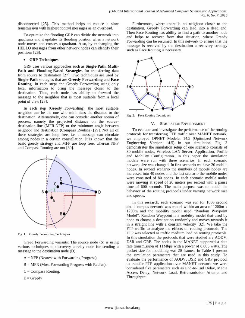
(IJACSA) International Journal of Advanced Computer Science and Applications,
Vol. 6, No. 7, 2015
175 | P a g e
www.ijacsa.thesai.org
disconnected [25]. This method helps to reduce a slow transmission with highest control messages as an overhead.
To optimize the flooding GRP can divide the network into quadrants and it updates its flooding position when a network node moves and crosses a quadrant. Also, by exchanging the HELLO messages from other network nodes can identify their positions [26].
GRP Techniques
GRP uses various approaches such as Single-Path, Multi-Path and Flooding-Based Strategies for transferring data from source to destination [27]. Two techniques are used by Single-Path strategies that are Greedy Forwarding and Face Routing. In each steps the Greedy Forwarding using only local information to bring the message closer to the destination. Thus, each node has ability to forward the message to the neighbor that is most suitable from a local point of view [28].
In each step (Greedy Forwarding), the most suitable neighbor can be the one who minimizes the distance to the destination. Alternatively, one can consider another notion of process, namely the projected distance on the source-destination-line (MFR-NFP) or the minimum angle between neighbor and destination (Compass Routing) [29]. Not all of these strategies are loop free, i.e. a message can circulate among nodes in a certain constellation. It is known that the basic greedy strategy and MFP are loop free, whereas NFP and Compass Routing are not [30].
Fig. 1. Greedy Forwarding Techniques
Greed Forwarding variants: The source node (S) is using various techniques to discovery a relay node for sending a message to the destination node (D).
A = NFP (Nearest with Forwarding Progress).
B = MFR (Most Forwarding Progress with Radius).
C = Compass Routing.
E = Greedy
Furthermore, where there is no neighbor closer to the destination, Greedy Forwarding can lead into a dead end. Then Face Routing has ability to find a path to another node and helps to recover from that situation, where Greedy Forwarding can be resumed. In this network to ensure that the message is received by the destination a recovery strategy such as Face Routing is necessary.
Fig. 2. Face Routing Techniques
V. SIMULATION ENVIRONMENT
To evaluate and investigate the performance of the routing protocols for transferring FTP traffic over MANET network, we employed OPNET Modeler 14.5 (Optimized Network Engineering Version 14.5) in our simulation. Fig. 3 demonstrates the simulation setup of one scenario consists of 80 mobile nodes, Wireless LAN Server, Application, Profile and Mobility Configuration. In this paper the simulation models were run with three scenarios. In each scenario network size was changed. In first scenario we have 20 mobile nodes. In second scenario the numbers of mobile nodes are increased into 40 nodes and the last scenario the mobile nodes were consisted of 80 nodes. In each scenario mobile nodes were moving at speed of 20 meters per second with a pause time of 600 seconds. The main purpose was to model the behavior of the routing protocols under varying network size and speeds.
In this research, each scenario was run for 1800 second and a campus network was model within an area of 1200m x 1200m and the mobility model used “Random Waypoint Model”. Random Waypoint is a mobility model that used by node to choose a destination randomly and moves towards it in a straight line with a constant velocity [32]. We take the FTP traffic to analyze the effects on routing protocols. The FTP was selected as traffic medium load on routing protocols. In this simulation the protocols that were studied are AODV, DSR and GRP. The nodes in the MANET supported a data rate transmission of 11Mbps with a power of 0.005 watts. The packet size for modelling was 20 frames. In Table 1 present the simulation parameters that are used in this study. To evaluate the performance of AODV, DSR and GRP protocol to transfer FTP application over MANET network we were considered five parameters such as End-to-End Delay, Media Access Delay, Network Load, Retransmission Attempt and Throughput.

(IJACSA) International Journal of Advanced Computer Science and Applications,
Vol. 6, No. 7, 2015
176 | P a g e
www.ijacsa.thesai.org
Fig. 3. Simulation Setup
TABLE I. PARAMETERS OF SIMULATION
Simulation Time 1800 second
Simulation Area 1200m x 1200m
Number of Nodes 20, 40, 80
Application Traffic FTP Traffic (Medium Load)
File Size 20 Frames
Data Rate 11Mbps
Mobility Algorithm Random Way Point
Routing Protocol AODV, DSR, GRP
Performance Metrics
End-to-End Delay, Media Access Delay, Network Load,
Retransmission Attempt, Throughput.
VI. PERFORMANCE METRICS
To evaluate the best routing protocols for transferring FTP application over MANT network we use five different metrics such as End-to- End Delay, Media Access Delay, Network Load, Retransmission Packet Attempt and Throughput.
A. End-to- End Delay
It is defined as the average time between the sources generates and the data packet to the destination receives it across a MANET. It is expressed in second. Hence in the network all the delays are called packet End-to-End Delay. In the network the delay consists of Propagation Delay (PropD), Processing Delay (PD), Transmission Delay (TD), Queuing Delay (QD) [33].
B. Media Access Delay
It is providing the results for a received packet with a routing Address Resolution Protocol (ARP) and control packet reply transmitted by MAC layer. For each frame, this delay is calculated as the duration from the time when it is inserted into the transmission queue, which is arrival time for higher layer data packets and creation time for all other frames types, until the time when the frame is sent to the physical layer for the first time. Media Access Delay is very useful metrics to identify congestion hot spots and measure link interference in MANET [36]. In addition, it can be used to improve network throughput in multi-rate networks [37].
C. Retransmission Packet Attempt
Retransmission Attempt can be defined as the total number of retransmission attempt by WLAN MAC in the network until either packet is successfully transmitted or it is discarded as a results of reaching short or long retry limit [38].
D. Network Load
Network Load is defined as the total amount of data traffic being carried by the network. When there is excess traffic in the network which is unable to be controlled is known as Network Load. The efficient network can easily cope with large traffic coming in and to make a best network. High Network Load affects the MANET routing packets that reduce the delivery of packets for reaching to the channel [34].
E. Throughput
Throughput represents as the ratio of the amount of data reaches from the source to the destination. The time it takes by the destination to receive the last packet is called Throughput. It is expressed as bytes or bits per second [35]. It can be expressed as:
VII. RESULTS AND ANALYSIS
In this section, the experiments results are presented and discussed. Our protocols evaluations are done according to the performance metrics, varying network size and speed mobile nodes. In each scenario, we were considered with a constant speed of 20 meters/second and pause time is considered in this network environment in analyzing the protocols performance and is set to 600 second and then each protocol performance is observed on FTP traffic medium load.
A. Average End-to- End Delay
In Fig. 4 the simulation results for the 20 mobile nodes on AODV, DSR and GRP protocols over FTP traffic shows that the End-to-End Delay for GRP routing protocol is lower than that of AODV and DSR. However, we can see a very small difference between AODV and GRP when GRP End-to-End Delay is equal to 0.0003903 sec and AODV is equal to 0.0003948 sec. in this scenario DSR protocol quite high delay compared to AODV and GRP. It is because the DSR protocol is using the cache route causing the higher delay that it is equal to 0.0020406 sec and DSR protocol needs to find the paths for transmitting the data and when it receives the data
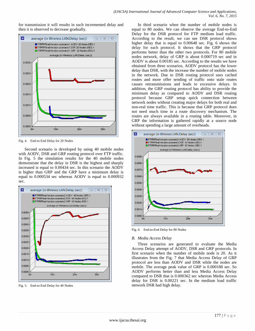
(IJACSA) International Journal of Advanced Computer Science and Applications,
Vol. 6, No. 7, 2015
177 | P a g e
www.ijacsa.thesai.org
for transmission it will results in such incremented delay and then it is observed to decrease gradually.
Fig. 4. End-to-End Delay for 20 Nodes
Second scenario is developed by using 40 mobile nodes with AODV, DSR and GRP routing protocol over FTP traffic. In Fig. 5 the simulation results for the 40 mobile nodes demonstrate that the delay in DSR is the highest and sharply increased is equal to 0.00434 sec. In this scenario the AODV is higher than GRP and the GRP have a minimum delay is equal to 0.000534 sec whereas AODV is equal to 0.000932 sec.
Fig. 5. End-to-End Delay for 40 Nodes
In third scenario when the number of mobile nodes is equal to 80 nodes. We can observe the average End-to-End Delay for the DSR protocol for FTP medium load traffic. According to the result, we can see DSR protocol shows higher delay that is equal to 0.00648 sec. Fig. 6 shows the delay for each protocol. It shows that the GRP protocol performs better than the other two protocols. For 80 mobile nodes network, delay of GRP is about 0.000719 sec and in AODV is about 0.00185 sec. According to the results we have obtained from three scenarios, AODV protocol has the lower delay than DSR, with the increase the number of mobile nodes in the network. Due to DSR routing protocol uses cached routes and more offer sending of traffic onto stale routes causes retransmissions and leads to excessive delays. In addition, the GRP routing protocol has ability to provide the minimum delay as compared to AODV and DSR routing protocol because GRP setup quick connection between network nodes without creating major delays for both real and non-real time traffic. This is because that GRP protocol does not need much time in a route discovery mechanism. The routes are always available in a routing table. Moreover, in GRP the information is gathered rapidly at a source node without spending a large amount of overheads.
Fig. 6. End-to-End Delay for 80 Nodes
B. Media Access Delay
Three scenarios are generated to evaluate the Media Access Delay attempt of AODV, DSR and GRP protocols. In first scenario when the number of mobile node is 20. As it illustrates from the Fig. 7 that Media Access Delay of GRP protocol are less than AODV and DSR while the nodes are mobile. The average peak value of GRP is 0.000188 sec. So AODV performs better than and less Media Access Delay compared to DSR that is 0.000362 sec whereas Media Access delay for DSR is 0.00221 sec. In the medium load traffic network DSR had high delay.
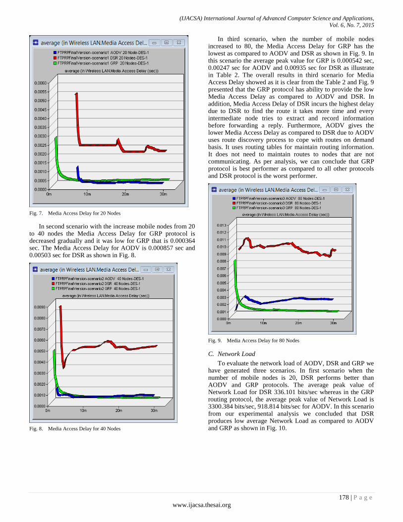
(IJACSA) International Journal of Advanced Computer Science and Applications,
Vol. 6, No. 7, 2015
178 | P a g e
www.ijacsa.thesai.org
Fig. 7. Media Access Delay for 20 Nodes
In second scenario with the increase mobile nodes from 20 to 40 nodes the Media Access Delay for GRP protocol is decreased gradually and it was low for GRP that is 0.000364 sec. The Media Access Delay for AODV is 0.000857 sec and 0.00503 sec for DSR as shown in Fig. 8.
Fig. 8. Media Access Delay for 40 Nodes
In third scenario, when the number of mobile nodes increased to 80, the Media Access Delay for GRP has the lowest as compared to AODV and DSR as shown in Fig. 9. In this scenario the average peak value for GRP is 0.000542 sec, 0.00247 sec for AODV and 0.00935 sec for DSR as illustrate in Table 2. The overall results in third scenario for Media Access Delay showed as it is clear from the Table 2 and Fig. 9 presented that the GRP protocol has ability to provide the low Media Access Delay as compared to AODV and DSR. In addition, Media Access Delay of DSR incurs the highest delay due to DSR to find the route it takes more time and every intermediate node tries to extract and record information before forwarding a reply. Furthermore, AODV gives the lower Media Access Delay as compared to DSR due to AODV uses route discovery process to cope with routes on demand basis. It uses routing tables for maintain routing information. It does not need to maintain routes to nodes that are not communicating. As per analysis, we can conclude that GRP protocol is best performer as compared to all other protocols and DSR protocol is the worst performer.
Fig. 9. Media Access Delay for 80 Nodes
C. Network Load
To evaluate the network load of AODV, DSR and GRP we have generated three scenarios. In first scenario when the number of mobile nodes is 20, DSR performs better than AODV and GRP protocols. The average peak value of Network Load for DSR 336.101 bits/sec whereas in the GRP routing protocol, the average peak value of Network Load is 3300.384 bits/sec, 918.814 bits/sec for AODV. In this scenario from our experimental analysis we concluded that DSR produces low average Network Load as compared to AODV and GRP as shown in Fig. 10.
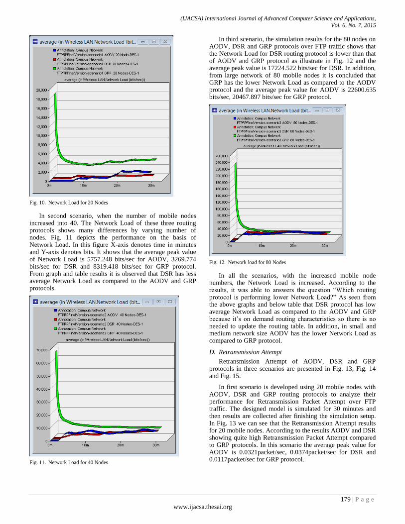
(IJACSA) International Journal of Advanced Computer Science and Applications,
Vol. 6, No. 7, 2015
179 | P a g e
www.ijacsa.thesai.org
Fig. 10. Network Load for 20 Nodes
In second scenario, when the number of mobile nodes increased into 40. The Network Load of these three routing protocols shows many differences by varying number of nodes. Fig. 11 depicts the performance on the basis of Network Load. In this figure X-axis denotes time in minutes and Y-axis denotes bits. It shows that the average peak value of Network Load is 5757.248 bits/sec for AODV, 3269.774 bits/sec for DSR and 8319.418 bits/sec for GRP protocol. From graph and table results it is observed that DSR has less average Network Load as compared to the AODV and GRP protocols.
Fig. 11. Network Load for 40 Nodes
In third scenario, the simulation results for the 80 nodes on AODV, DSR and GRP protocols over FTP traffic shows that the Network Load for DSR routing protocol is lower than that of AODV and GRP protocol as illustrate in Fig. 12 and the average peak value is 17224.522 bits/sec for DSR. In addition, from large network of 80 mobile nodes it is concluded that GRP has the lower Network Load as compared to the AODV protocol and the average peak value for AODV is 22600.635 bits/sec, 20467.897 bits/sec for GRP protocol.
Fig. 12. Network load for 80 Nodes
In all the scenarios, with the increased mobile node numbers, the Network Load is increased. According to the results, it was able to answers the question “Which routing protocol is performing lower Network Load?” As seen from the above graphs and below table that DSR protocol has low average Network Load as compared to the AODV and GRP because it’s on demand routing characteristics so there is no needed to update the routing table. In addition, in small and medium network size AODV has the lower Network Load as compared to GRP protocol.
D. Retransmission Attempt
Retransmission Attempt of AODV, DSR and GRP protocols in three scenarios are presented in Fig. 13, Fig. 14 and Fig. 15.
In first scenario is developed using 20 mobile nodes with AODV, DSR and GRP routing protocols to analyze their performance for Retransmission Packet Attempt over FTP traffic. The designed model is simulated for 30 minutes and then results are collected after finishing the simulation setup. In Fig. 13 we can see that the Retransmission Attempt results for 20 mobile nodes. According to the results AODV and DSR showing quite high Retransmission Packet Attempt compared to GRP protocols. In this scenario the average peak value for AODV is 0.0321packet/sec, 0.0374packet/sec for DSR and 0.0117packet/sec for GRP protocol.
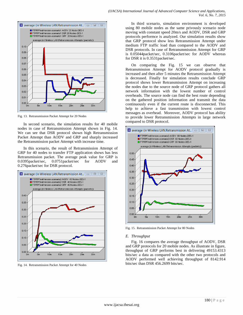
(IJACSA) International Journal of Advanced Computer Science and Applications,
Vol. 6, No. 7, 2015
180 | P a g e
www.ijacsa.thesai.org
Fig. 13. Retransmission Packet Attempt for 20 Nodes
In second scenario, the simulation results for 40 mobile nodes in case of Retransmission Attempt shown in Fig. 14. We can see that DSR protocol shown high Retransmission Packet Attempt than AODV and GRP and sharply increased the Retransmission packet Attempt with increase time.
In this scenario, the result of Retransmission Attempt of GRP for 40 nodes to transfer FTP application shows has less Retransmission packet. The average peak value for GRP is 0.0395packet/sec, 0.0751packet/sec for AODV and 0.276packet/sec for DSR protocol.
Fig. 14. Retransmission Packet Attempt for 40 Nodes
In third scenario, simulation environment is developed using 80 mobile nodes as the same privously scenario node moving with constant speed 20m/s and AODV, DSR and GRP protocols performce is analyzed. Our simulation results show that GRP protocol show less Retransmission Attempt under medium FTP traffic load than compared to the AODV and DSR protocols. In case of Retransmmission Attempt for GRP is 0.05044packet/sec, 0.3106packet/sec for AODV whereas for DSR it is 0.3531packet/sec.
On comparing the Fig. 15 we can observe that Retransmission Attempt for AODV protocol gradually is increased and then after 5 minutes the Retransmission Attempt is decreased. Finally for simulation results conclude GRP protocol shows lower Retransmission Attempt on increasing the nodes due to the source node of GRP protocol gathers all network information with the lowest number of control overheads. The source node can find the best route depending on the gathered position information and transmit the data continuously even if the current route is disconnected. This help to achieve a fast transmission with lowest control messages as overhead. Moreover, AODV protocol has ability to provide lower Retransmission Attempts in large network compared to DSR protocol.
Fig. 15. Retransmission Packet Attempt for 80 Nodes
E. Throughput
Fig. 16 compares the average throughput of AODV, DSR and GRP protocols for 20 mobile nodes. As illustrate in figure, throughput of GRP performs best in delivering 49153.4313 bits/sec a data as compared with the other two protocols and AODV performed well achieving throughput of 8142.914 bits/sec than DSR 456.2699 bits/sec.
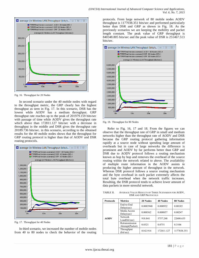
(IJACSA) International Journal of Advanced Computer Science and Applications,
Vol. 6, No. 7, 2015
181 | P a g e
www.ijacsa.thesai.org
Fig. 16. Throughput for 20 Nodes
In second scenario under the 40 mobile nodes with regard to the throughput metric, the GRP clearly has the highest throughput as seen in Fig. 17. In this scenario, DSR has the lowest while AODV has a medium throughput. GRP throughput rate reaches up to the peak of 201979.159 bits/sec with passage of time while AODV gives the throughput rate which above than 172811.127 bits/sec with a decrease in throughput in the middle and DSR gives the throughput rate 20189.736 bits/sec. in this scenario, according to the obtained results for the 40 mobile nodes shows that the throughput for GRP routing protocol is higher than that of AODV and DSR routing protocols.
Fig. 17. Throughput for 40 Nodes
In third scenario, we increased the number of mobile nodes from 40 to 80 nodes to check the behavior of the routing
protocols. From large network of 80 mobile nodes AODV throughput is 1177038.351 bits/sec and performed particularly better than DSR and GRP as shown in Fig. 18. As the previously scenarios we are keeping the mobility and packet length constant. The peak value of GRP throughput is 840348.805 bits/sec and the peak value of DSR is 251467.513 bits/sec.
Fig. 18. Throughput for 80 Nodes
Refer to Fig. 16, 17 and 18. From the figures we can observe that the throughput rate of GRP in small and medium networks higher than the throughput rate of AODV and DSR because the GRP routing protocol gathering information rapidly at a source node without spending large amount of overheads but in case of large networks the difference is prominent and AODV by far performs better than GRP and DSR due to AODV protocol follows a routing mechanism known as hop by hop and removes the overhead of the source routing within the network related to above. The availability of multiple route information in the AODV assists in producing the higher amount of throughput in the network. Whereas DSR protocol follows a source routing mechanism and the byte overhead in each packet extremely affects the total byte overhead when the network traffic increases. Resulting, the DSR protocol tends to achieve lower amount of data packets in more stressful network.
TABLE II. AVERAGE VALUE RESULTS OF THREE SCENARIOS FOR AODV, DSR AND GRP PROTOCOLS
Protocols Metrics 20 Nodes 40 Nodes 80 Nodes
AODV
End-to-End
Delay(sec) 0.0003948 0.000932 0.00185
Media Access Delay(sec)
0.000362 0.000857 0.00247
Network
Load(bit/sec) 918.841 5757.248 22600.635
Retransmission Attempt(Packet)
0.0321 0.0751 0.3106
Throughput
(bit/sec) 8142.914 172811.127 1177038.351

(IJACSA) International Journal of Advanced Computer Science and Applications,
Vol. 6, No. 7, 2015
182 | P a g e
www.ijacsa.thesai.org
DSR
End-to-End
Delay(sec) 0.0020406 0.00434 0.00648
Media Access
Delay(sec) 0.00221 0.00503 0.00935
Network
Load(bit/sec) 336.101 3269.774 17224.522
Retransmission
Attempt(Packet) 0.0374 0.276 0.3531
Throughput(bit/s
ec) 456.2699 20189.736 251467.513
GRP
End-to-End
Delay(sec) 0.0003903 0.000534 0.000719
Media Access Delay(sec)
0.000188 0.000364 0.000542
Network
Load(bit/sec) 33.00384 8319.418 20467.897
Retransmission Attempt(Packet)
0.0117 0.0395 0.05044
Throughput(bit/s
ec) 49153.4313 201979.159 840348.805
VIII. CONCLUSION & FUTURE WORK
In this study analyzed the performance of AODV, DSR and GRP routing protocols by varying number of mobile nodes from 20 (low density), 40 (medium density) to 80 (high density) to transfer FTP application over MANET network in terms of End-to-End Delay, Media Access Delay, Network Load, Retransmission Attempt and Throughput. In this paper to generate node mobility, we used Random Way Point Mobility Model with the speed 0f 20 meters/second in an area of 1200 x 1200m. In this experiment we found that the performance varies widely across different network size and results from one scenario cannot be applied to those from the other scenario. From the simulation results we can conclude that average End-to-End Delay, Media Access Delay and Retransmission Attempt of GRP routing protocol in all scenarios is much better than AODV and DSR protocols However, GRP protocol provides the best Throughput in small and medium network size and GRP protocol in terms of Network Load shows high average Network Load as compared to DSR routing protocol. As far as Network Load of GRP perform better than the AODV from large network. In addition, the study demonstrate that AODV has less End-to-End Delay, Media Access Delay, Retransmission Attempt and high Throughput for FTP application compared to DSR protocol and we found that average Network Load of DSR in all scenarios is much lower than GRP and AODV.
In the future work, we will conduct with a new technique to improve security issues in AODV and DSR routing protocols.
ACKNOWLEDGMENT
I would like to thank University of Sulaimani- Kurdistan Region- Iraq for their helps and supports in the implementation in my research.
REFERENCES
[1] C. Imrich, et al., “Mobile Ad-hoc Networking: Imperatives and Challenges”. Ad-hoc Networks, vol. 1, no. 1, pp. 13-64, 2003.
[2] N. Parma, et al., “Mobility Based Performance Analysis DYMO, STAR And DSR Adhoc Routing Protocols,” International Journal of Comp. Tech. Appl., vol. 2, mo. (6), pp. 1755-1760, 2011.
[3] A. Ako, et al., "The Impact of Reactive Routing Protocols for Transferring Multimedia Data over MANET," Journal of Zankoy Sulaimani-Part A, vol. 4, no. 16, 2014.
[4] A. Al Maashri, et al., “Performance Analysis of MANET Routing Protocols In The Presence Of Self-Similar Traffic,”. Local Computer Networks, Proceedings 2006 31st IEEE Conference on (2006): pp. 801 - 807.
[5] R. kumar, “A Fault Tolerant Congestion Aware Routing Protocol For Mobile Ad-hoc Networks,” Journal of Computer Science vol. 8, no. 5, pp. 673-680, 2012.
[6] K. Sapna, et al., "Comparison of effectiveness of AODV, DSDV and DSR Routing Protocols in Mobile Ad-hoc Networks," International Journal of Information Technology and Knowledge Management, vol. 2, no .2, pp. 499-502, 2009.
[7] G. IJatin, et al., “A Review of Performance Evaluation of the Routing Protocols in Manets,” International Journal of Advanced Research in Computer Science & Technology (IJARCST), vol. 2. No. 2, pp. 46-48, 2014.
[8] N. Valery, et al., “Scalability of Routing Methods in Ad-hoc Networks,” Elsevier, vol. 6, no. 2, pp. 193-209, 2005.
[9] C. Manish, “Simulation and Study of AODV Routing Protocol under CBR and TCP Traffic Source,” IJET vol. 4, no. 2, pp. 84-88, 2014
[10] M. Debra, et al., “Performance Evaluation on Extended Routing Protocol of AODV in MANET,” IJASUC, vol. 4, no. 4, pp. 27-37, . 2013.
[11] M. Mohammad, et al., “Multipath Routing Protocols in Wireless Sensor Networks: A Survey and Analysis,” International Journal of Future Generation Communication and Networking, vol. 6, no. 6, pp. 181-192, 2013.
[12] Z. Yan,et al., “Performance Evaluation of Routing Protocols on the Reference Region Group Mobility Model for MANET,” International Journal of Wireless Sensor Network, vol. 3, no. 3, pp. 92-105, 2011.
[13] H. Xi et al., “Stability-Based RREQ Forwarding Game For Stability-Oriented Route Discovery in Manets,” Wireless Personal Communication, vol. 68, no. 4, pp. 1689-1705, 2012.
[14] K. Venetis et al., “A New RREQ Message Forwarding Technique Based On Bayesian Probability Theory,” EURASIP J Wirel Commun Netw, vol. 20, no. 12, pp. 318-325, 2012.
[15] N. Humaira, et al., “Energy Efficient Routing Protocols For Mobile Ad-hoc Networks,” International Journal of Computer Applications, vol. 1, no. 4, pp. 121-132, 2011.
[16] S. Samadi, et al., “An Adaptive Multipath Ant Routing Algorithm for Mobile Ad-hoc Networks,” IJCEE, vol. 7, no. 3, pp. 175-180, 2012.
[17] M. Reza, et al., “Fundamental Lifetime Mechanisms in Routing Protocols for Wireless Sensor Networks: A Survey and Open Issues'. Sensors, pp. 13508-13544, 2012.
[18] A. Rabia, et al., “Bandwidth Estimation in Mobile Ad-Hoc Network (MANET),” International Journal of Computer Science (IJCSI), vol. 8, no. 5, pp. 331-337, 2011.
[19] S. Alka, “Power Efficient Scheme for Performance Optimization in Ad-hoc Networks,” International Journal of Computer Applications, vol. 14, no .6, pp. 38-42, 2011.
[20] B. Stefano et al., “Mobile Ad-hoc Networking,” Piscataway, NJ: IEEE Press, 2004.
[21] G. Parul, et al., “Energy-Efficiency Based Analysis of Routing Protocols in Mobile Ad-Hoc Networks (Manets),” International Journal of Computer Applications, vol. 96, no. 15, pp 15-23, 2014.
[22] M. Mahesh, et al., "Ad-hoc on‐demand multipath distance vector routing." Wireless Communications and Mobile Computing, vol. 6, no. 7, pp. 969-988, 2006.
[23] N. Singla, et al., “A Review of Performance Evaluation of the Routing Protocols in MANETs,” International Journal of Innovative Research in Computer and Communication Engineering, vol. 2, Issue. 11, pp.6360-6364, 2014.
[24] X. Ya, et al., "Geography-informed energy conservation for ad-hoc routing" Proceedings of the 7th annual international conference on Mobile computing and networking. ACM, 2001.

(IJACSA) International Journal of Advanced Computer Science and Applications,
Vol. 6, No. 7, 2015
183 | P a g e
www.ijacsa.thesai.org
[25] F. Bai, et al., "IMPORTANT: A framework to systematically analyze the Impact of Mobility on Performance of Routing protocols for Ad-hoc Networks," INFOCOM 2003. Twenty-Second Annual Joint Conferences of the IEEE Computer and Communications. IEEE Societies. vol. 2. IEEE, 2003.
[26] I. Stojmenovic, “Position-based routing in ad-hoc networks,” IEEE Communications Magazine, vol. 40, Issue 7, pp.128-134, 2012.
[27] R. Bassel et al., “Multipath Grid-Based Enabled Geographic Routing For Wireless Sensor Networks,” Wireless Sensor Network, vol. 6, no. 12, pp. 265-280, 2014.
[28] K. Shwaita, et al., "Energy Efficient Geographical Routing Protocol with Location Aware Routing in MANET," International Journal of Advanced Research in Computer Engineering & Technology (IJARCET), vol. 1, no. 5 pp. 172- 182, 2014.
[29] Y. Yan, et al., “Geographical and energy aware routing: A recursive data dissemination protocol for wireless sensor networks,” Technical report ucla/csd-tr-01-0023, UCLA Computer Science Department, 2001.
[30] A. Boussad, et al., “A Hybrid Multi agent Routing Approach for Wireless Ad-hoc Networks,” Wireless Networks vol. 18, no. 7, pp. 837-845, 2012.
[31] F. Maan, et al., “MANET Routing Protocols vs. Mobility Models: A Performance Evaluation,” Proc. of IEEE-ICUFN, 2011.
[32] M. Narendra et al., “Performance Evaluation of AODV and DSR Routing Protocols for Vehicular Ad-hoc Network (VANETs),” International Journal of Emerging Technology and Advanced Engineering, vol. 4, Issue 6, pp. 522-530, 2014.
[33] G. Vikas, et al., “Performance Investigation of Routing Protocols for Database and Voice Data in MANETS,” International Journal of Emerging Trends & Technology in Computer Science, ISSN 2278-6856, vol. 2, Issue 4, pp. 326-332, 2013.
[34] A. Akshai,, et al., “Performance Analysis of AODV, DSDV and DSR in MANET,” International Journal of Distributed and Parallel System, vol. 2, no. 6, pp. 167-177, 2011.
[35] A. Ainiwan et al., “A Novel Multicarrier CDMA Scheme With Interference Free Performance In Very Large Delay Spread,” ITE Transactions on Media Technology and Applications, vol. 2, no. 4, pp. 362-369, 2014.
[36] D. Holmer, et al., “The Medium Time Metric: High Throughput Route Selection In Multi-Rate Ad-hoc Wireless Networks,” Mobile Networks and Applications, vol. 11, no. 2, pp. 253-266, 2006.
[37] B. Devendra, et al., “Performance Evaluation Of MAC Protocol For IEEE 802. 11, 802. 11Ext. WLAN And IEEE 802. 15. 4 WPAN Using NS-2,” International Journal of Computer Applications, vol. 119, no. 16, pp. 25- 30, 2015.
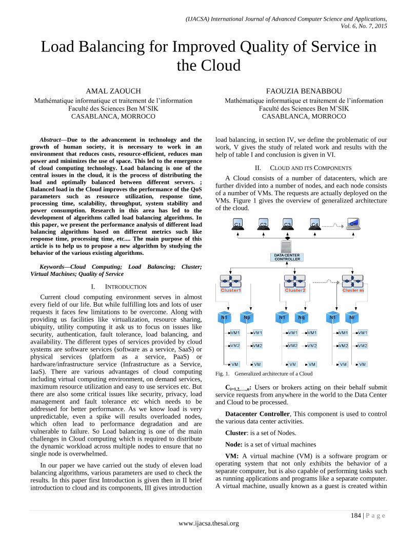
(IJACSA) International Journal of Advanced Computer Science and Applications,
Vol. 6, No. 7, 2015
184 | P a g e
www.ijacsa.thesai.org
Load Balancing for Improved Quality of Service in
the Cloud
AMAL ZAOUCH
Mathématique informatique et traitement de l’information
Faculté des Sciences Ben M’SIK
CASABLANCA, MORROCO
FAOUZIA BENABBOU
Mathématique informatique et traitement de l’information
Faculté des Sciences Ben M’SIK
CASABLANCA, MORROCO
Abstract—Due to the advancement in technology and the
growth of human society, it is necessary to work in an
environment that reduces costs, resource-efficient, reduces man
power and minimizes the use of space. This led to the emergence
of cloud computing technology. Load balancing is one of the
central issues in the cloud, it is the process of distributing the
load and optimally balanced between different servers. ;
Balanced load in the Cloud improves the performance of the QoS
parameters such as resource utilization, response time,
processing time, scalability, throughput, system stability and
power consumption. Research in this area has led to the
development of algorithms called load balancing algorithms. In
this paper, we present the performance analysis of different load
balancing algorithms based on different metrics such like
response time, processing time, etc.... The main purpose of this
article is to help us to propose a new algorithm by studying the
behavior of the various existing algorithms.
Keywords—Cloud Computing; Load Balancing; Cluster;
Virtual Machines; Quality of Service
I. INTRODUCTION
Current cloud computing environment serves in almost every field of our life. But while fulfilling lots and lots of user requests it faces few limitations to be overcome. Along with providing us facilities like virtualization, resource sharing, ubiquity, utility computing it ask us to focus on issues like security, authentication, fault tolerance, load balancing, and availability. The different types of services provided by cloud systems are software services (software as a service, SaaS) or physical services (platform as a service, PaaS) or hardware/infrastructure service (Infrastructure as a Service, IaaS). There are various advantages of cloud computing including virtual computing environment, on demand services, maximum resource utilization and easy to use services etc. But there are also some critical issues like security, privacy, load management and fault tolerance etc which needs to be addressed for better performance. As we know load is very unpredictable, even a spike will results overloaded nodes, which often lead to performance degradation and are vulnerable to failure. So Load balancing is one of the main challenges in Cloud computing which is required to distribute the dynamic workload across multiple nodes to ensure that no single node is overwhelmed.
In our paper we have carried out the study of eleven load balancing algorithms, various parameters are used to check the results. In this paper first Introduction is given then in II brief introduction to cloud and its components, III gives introduction
load balancing, in section IV, we define the problematic of our work, V gives the study of related work and results with the help of table I and conclusion is given in VI.
II. CLOUD AND ITS COMPONENTS
A Cloud consists of a number of datacenters, which are further divided into a number of nodes, and each node consists of a number of VMs. The requests are actually deployed on the VMs. Figure 1 gives the overview of generalized architecture of the cloud.
Fig. 1. Generalized architecture of a Cloud
Ci=1,2,….,n: Users or brokers acting on their behalf submit service requests from anywhere in the world to the Data Center and Cloud to be processed.
Datacenter Controller, This component is used to control the various data center activities.
Cluster: is a set of Nodes.
Node: is a set of virtual machines
VM: A virtual machine (VM) is a software program or operating system that not only exhibits the behavior of a separate computer, but is also capable of performing tasks such as running applications and programs like a separate computer. A virtual machine, usually known as a guest is created within

(IJACSA) International Journal of Advanced Computer Science and Applications,
Vol. 6, No. 7, 2015
185 | P a g e
www.ijacsa.thesai.org
another computing environment referred as a "host." Multiple virtual machines can exist within a single host at one time.
III. PROBLEM STATEMENT
As it s shown in the previous section, when a request arrive to the Datacenter Controller, it has to be allocated to one of the nodes composed the cluster, but the requests have to be distributed evenly and equally among the system to avoid workloads and degradation of system’s performance; if we refer to the architecture of cloud shown in figure 1 we deduce that we need another components to balance the load overall the system called Load Balancer. The Load Balancer plays a very important role in the overall response time of the cloud. In Cloud Computing Scenario Load Balancing is composed of selecting Data Center for upcoming request and Virtual machine management at individual Data Center So, how can we guarantee a good quality of service though balancing the load in the cloud?
Our aim is to design a new Load Balancer to improve quality of service by optimizing load balancing in cloud computing.
IV. LOAD BALANCING
Load Balancing is a computer networking method to distribute workload across multiple computers or a computer cluster, network links, central processing units, disk drives, or other resources, to achieve optimal resource utilization, maximize throughput, minimize response time, and avoid overload [1]. It is a mechanism that distributes the dynamic local workload evenly across all the nodes in the whole cloud to achieve a high user satisfaction and resource utilization, hence improving the overall performance and resource utility of the system. It also ensures that every computing resource is distributed efficiently and fair, prevents bottlenecks and fail-over.
A. Classification of Load Balancing Algorithms
Based on the current state of the system the algorithms can be classified as [2]:
Static Load Balancing: Static load balancing algorithms decide how to distribute the workload according to a prior knowledge of the problem and the system characteristics. Static load balancing algorithms are not pre-emptive and therefore each machine has at least one task assigned for itself. Its aims in minimizing the execution time of the task and limit communication overhead and delays. This algorithm has a drawback that the task is assigned to the processors or machines only after it is created and that task cannot be shifted during its execution to any other machine for balancing the load.
Dynamic Load Balancing: Dynamic algorithms use state information to make decisions during program execution. An important advantage of this approach is that its decision for balancing the load is based on the current state of the system which helps in improving the overall performance of the
system by shifting the load dynamically.
B. Metrics For Load Balancing In Clouds
Various metrics considered in existing load balancing techniques in cloud computing are discussed below [15]:
Throughput is used to calculate the no. of tasks whose execution has been completed. It should be high to improve the performance of the system.
Overhead Associated determines the amount of overhead involved while implementing a load-balancing algorithm. It is composed of overhead due to movement of tasks, interprocessor and inter-process communication. This should be minimized so that a load balancing technique can work efficiently.
Fault Tolerance is the ability of an algorithm to perform uniform load balancing in spite of arbitrary node or link failure. The load balancing should be a good fault-tolerant technique.
Migration time is the time to migrate the jobs or resources from one node to other. It should be minimized in order to enhance the performance of the system.
Response Time is the amount of time taken to respond by a particular load balancing algorithm in a distributed system. This parameter should be minimized.
Resource Utilization is used to check the utilization of resources. It should be optimized for an efficient load balancing.
Scalability is the ability of an algorithm to perform load balancing for a system with any finite number of nodes. This metric should be improved.
Performance is used to check the efficiency of the system. This has to be improved at a reasonable cost, e.g., reduce task response time while keeping acceptable delays
V. RELATED WORK
In cloud computing, load balancing is required to distribute the dynamic local workload evenly across all the nodes. It helps to achieve a high user satisfaction and resource utilization ratio by ensuring an efficient and fair allocation of every computing resource. Proper load balancing aids in minimizing resource consumption, implementing fail-over, enabling scalability, avoiding bottlenecks and over-provisioning etc. In this section, a systematic review of existing load balancing techniques is presented. This study concludes that all the existing techniques mainly focus on reducing associated overhead, service response time and improving performance etc. Various parameters are also identified, and these are used to compare the existing techniques.
Throttled load balancer [4] this algorithm ensures only a pre-defined number of Internet Cloudlets are allocated to a single VM at any given time. If more request groups are present than the number of available VM’s at a data center, some of the requests will have to be queued until the next VM
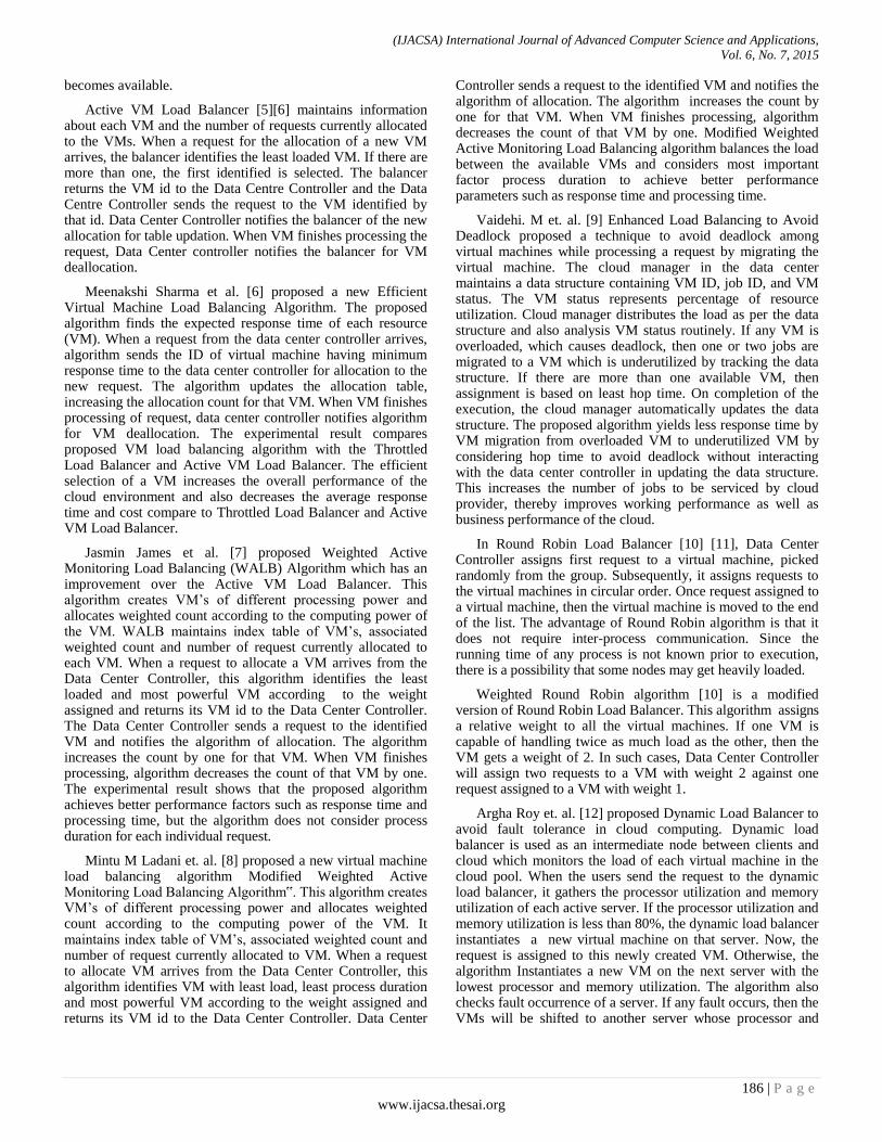
(IJACSA) International Journal of Advanced Computer Science and Applications,
Vol. 6, No. 7, 2015
186 | P a g e
www.ijacsa.thesai.org
becomes available.
Active VM Load Balancer [5][6] maintains information about each VM and the number of requests currently allocated to the VMs. When a request for the allocation of a new VM arrives, the balancer identifies the least loaded VM. If there are more than one, the first identified is selected. The balancer returns the VM id to the Data Centre Controller and the Data Centre Controller sends the request to the VM identified by that id. Data Center Controller notifies the balancer of the new allocation for table updation. When VM finishes processing the request, Data Center controller notifies the balancer for VM deallocation.
Meenakshi Sharma et al. [6] proposed a new Efficient Virtual Machine Load Balancing Algorithm. The proposed algorithm finds the expected response time of each resource (VM). When a request from the data center controller arrives, algorithm sends the ID of virtual machine having minimum response time to the data center controller for allocation to the new request. The algorithm updates the allocation table, increasing the allocation count for that VM. When VM finishes processing of request, data center controller notifies algorithm for VM deallocation. The experimental result compares proposed VM load balancing algorithm with the Throttled Load Balancer and Active VM Load Balancer. The efficient selection of a VM increases the overall performance of the cloud environment and also decreases the average response time and cost compare to Throttled Load Balancer and Active VM Load Balancer.
Jasmin James et al. [7] proposed Weighted Active Monitoring Load Balancing (WALB) Algorithm which has an improvement over the Active VM Load Balancer. This algorithm creates VM’s of different processing power and allocates weighted count according to the computing power of the VM. WALB maintains index table of VM’s, associated weighted count and number of request currently allocated to each VM. When a request to allocate a VM arrives from the Data Center Controller, this algorithm identifies the least loaded and most powerful VM according to the weight assigned and returns its VM id to the Data Center Controller. The Data Center Controller sends a request to the identified VM and notifies the algorithm of allocation. The algorithm increases the count by one for that VM. When VM finishes processing, algorithm decreases the count of that VM by one. The experimental result shows that the proposed algorithm achieves better performance factors such as response time and processing time, but the algorithm does not consider process duration for each individual request.
Mintu M Ladani et. al. [8] proposed a new virtual machine load balancing algorithm Modified Weighted Active Monitoring Load Balancing Algorithm‟. This algorithm creates VM’s of different processing power and allocates weighted count according to the computing power of the VM. It maintains index table of VM’s, associated weighted count and number of request currently allocated to VM. When a request to allocate VM arrives from the Data Center Controller, this algorithm identifies VM with least load, least process duration and most powerful VM according to the weight assigned and returns its VM id to the Data Center Controller. Data Center
Controller sends a request to the identified VM and notifies the algorithm of allocation. The algorithm increases the count by one for that VM. When VM finishes processing, algorithm decreases the count of that VM by one. Modified Weighted Active Monitoring Load Balancing algorithm balances the load between the available VMs and considers most important factor process duration to achieve better performance parameters such as response time and processing time.
Vaidehi. M et. al. [9] Enhanced Load Balancing to Avoid Deadlock proposed a technique to avoid deadlock among virtual machines while processing a request by migrating the virtual machine. The cloud manager in the data center maintains a data structure containing VM ID, job ID, and VM status. The VM status represents percentage of resource utilization. Cloud manager distributes the load as per the data structure and also analysis VM status routinely. If any VM is overloaded, which causes deadlock, then one or two jobs are migrated to a VM which is underutilized by tracking the data structure. If there are more than one available VM, then assignment is based on least hop time. On completion of the execution, the cloud manager automatically updates the data structure. The proposed algorithm yields less response time by VM migration from overloaded VM to underutilized VM by considering hop time to avoid deadlock without interacting with the data center controller in updating the data structure. This increases the number of jobs to be serviced by cloud provider, thereby improves working performance as well as business performance of the cloud.
In Round Robin Load Balancer [10] [11], Data Center Controller assigns first request to a virtual machine, picked randomly from the group. Subsequently, it assigns requests to the virtual machines in circular order. Once request assigned to a virtual machine, then the virtual machine is moved to the end of the list. The advantage of Round Robin algorithm is that it does not require inter-process communication. Since the running time of any process is not known prior to execution, there is a possibility that some nodes may get heavily loaded.
Weighted Round Robin algorithm [10] is a modified version of Round Robin Load Balancer. This algorithm assigns a relative weight to all the virtual machines. If one VM is capable of handling twice as much load as the other, then the VM gets a weight of 2. In such cases, Data Center Controller will assign two requests to a VM with weight 2 against one request assigned to a VM with weight 1.
Argha Roy et. al. [12] proposed Dynamic Load Balancer to avoid fault tolerance in cloud computing. Dynamic load balancer is used as an intermediate node between clients and cloud which monitors the load of each virtual machine in the cloud pool. When the users send the request to the dynamic load balancer, it gathers the processor utilization and memory utilization of each active server. If the processor utilization and memory utilization is less than 80%, the dynamic load balancer instantiates a new virtual machine on that server. Now, the request is assigned to this newly created VM. Otherwise, the algorithm Instantiates a new VM on the next server with the lowest processor and memory utilization. The algorithm also checks fault occurrence of a server. If any fault occurs, then the VMs will be shifted to another server whose processor and
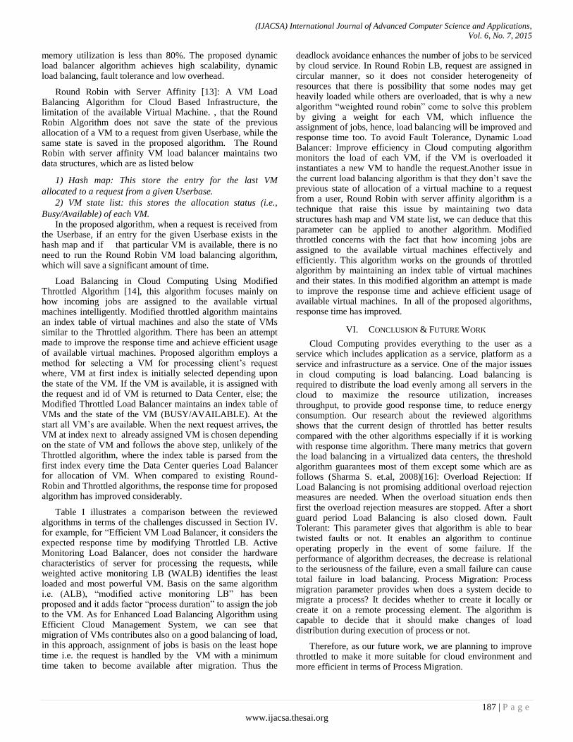
(IJACSA) International Journal of Advanced Computer Science and Applications,
Vol. 6, No. 7, 2015
187 | P a g e
www.ijacsa.thesai.org
memory utilization is less than 80%. The proposed dynamic load balancer algorithm achieves high scalability, dynamic load balancing, fault tolerance and low overhead.
Round Robin with Server Affinity [13]: A VM Load Balancing Algorithm for Cloud Based Infrastructure, the limitation of the available Virtual Machine. , that the Round Robin Algorithm does not save the state of the previous allocation of a VM to a request from given Userbase, while the same state is saved in the proposed algorithm. The Round Robin with server affinity VM load balancer maintains two data structures, which are as listed below
1) Hash map: This store the entry for the last VM
allocated to a request from a given Userbase.
2) VM state list: this stores the allocation status (i.e.,
Busy/Available) of each VM. In the proposed algorithm, when a request is received from
the Userbase, if an entry for the given Userbase exists in the hash map and if that particular VM is available, there is no need to run the Round Robin VM load balancing algorithm, which will save a significant amount of time.
Load Balancing in Cloud Computing Using Modified Throttled Algorithm [14], this algorithm focuses mainly on how incoming jobs are assigned to the available virtual machines intelligently. Modified throttled algorithm maintains an index table of virtual machines and also the state of VMs similar to the Throttled algorithm. There has been an attempt made to improve the response time and achieve efficient usage of available virtual machines. Proposed algorithm employs a method for selecting a VM for processing client’s request where, VM at first index is initially selected depending upon the state of the VM. If the VM is available, it is assigned with the request and id of VM is returned to Data Center, else; the Modified Throttled Load Balancer maintains an index table of VMs and the state of the VM (BUSY/AVAILABLE). At the start all VM’s are available. When the next request arrives, the VM at index next to already assigned VM is chosen depending on the state of VM and follows the above step, unlikely of the Throttled algorithm, where the index table is parsed from the first index every time the Data Center queries Load Balancer for allocation of VM. When compared to existing Round-Robin and Throttled algorithms, the response time for proposed algorithm has improved considerably.
Table I illustrates a comparison between the reviewed algorithms in terms of the challenges discussed in Section IV. for example, for “Efficient VM Load Balancer, it considers the expected response time by modifying Throttled LB. Active Monitoring Load Balancer, does not consider the hardware characteristics of server for processing the requests, while weighted active monitoring LB (WALB) identifies the least loaded and most powerful VM. Basis on the same algorithm i.e. (ALB), “modified active monitoring LB” has been proposed and it adds factor “process duration” to assign the job to the VM. As for Enhanced Load Balancing Algorithm using Efficient Cloud Management System, we can see that migration of VMs contributes also on a good balancing of load, in this approach, assignment of jobs is basis on the least hope time i.e. the request is handled by the VM with a minimum time taken to become available after migration. Thus the
deadlock avoidance enhances the number of jobs to be serviced by cloud service. In Round Robin LB, request are assigned in circular manner, so it does not consider heterogeneity of resources that there is possibility that some nodes may get heavily loaded while others are overloaded, that is why a new algorithm “weighted round robin” come to solve this problem by giving a weight for each VM, which influence the assignment of jobs, hence, load balancing will be improved and response time too. To avoid Fault Tolerance, Dynamic Load Balancer: Improve efficiency in Cloud computing algorithm monitors the load of each VM, if the VM is overloaded it instantiates a new VM to handle the request.Another issue in the current load balancing algorithm is that they don’t save the previous state of allocation of a virtual machine to a request from a user, Round Robin with server affinity algorithm is a technique that raise this issue by maintaining two data structures hash map and VM state list, we can deduce that this parameter can be applied to another algorithm. Modified throttled concerns with the fact that how incoming jobs are assigned to the available virtual machines effectively and efficiently. This algorithm works on the grounds of throttled algorithm by maintaining an index table of virtual machines and their states. In this modified algorithm an attempt is made to improve the response time and achieve efficient usage of available virtual machines. In all of the proposed algorithms, response time has improved.
VI. CONCLUSION & FUTURE WORK
Cloud Computing provides everything to the user as a service which includes application as a service, platform as a service and infrastructure as a service. One of the major issues in cloud computing is load balancing. Load balancing is required to distribute the load evenly among all servers in the cloud to maximize the resource utilization, increases throughput, to provide good response time, to reduce energy consumption. Our research about the reviewed algorithms shows that the current design of throttled has better results compared with the other algorithms especially if it is working with response time algorithm. There many metrics that govern the load balancing in a virtualized data centers, the threshold algorithm guarantees most of them except some which are as follows (Sharma S. et.al, 2008)[16]: Overload Rejection: If Load Balancing is not promising additional overload rejection measures are needed. When the overload situation ends then first the overload rejection measures are stopped. After a short guard period Load Balancing is also closed down. Fault Tolerant: This parameter gives that algorithm is able to bear twisted faults or not. It enables an algorithm to continue operating properly in the event of some failure. If the performance of algorithm decreases, the decrease is relational to the seriousness of the failure, even a small failure can cause total failure in load balancing. Process Migration: Process migration parameter provides when does a system decide to migrate a process? It decides whether to create it locally or create it on a remote processing element. The algorithm is capable to decide that it should make changes of load distribution during execution of process or not.
Therefore, as our future work, we are planning to improve throttled to make it more suitable for cloud environment and more efficient in terms of Process Migration.

(IJACSA) International Journal of Advanced Computer Science and Applications,
Vol. 6, No. 7, 2015
188 | P a g e
www.ijacsa.thesai.org
TABLE I. SYNTHESIS TABLE OF EXISTING LOAD BALANCING ALGORITHMS
Techniques Metaphors Conclusion
Throttled load balancer
This algorithm ensures only a pre-defined
number of Internet Cloudlets are allocated to a single VM at any given time.
Response time improved But other parameters are not taken
into account such as: weight of VM,
processing time, etc …
MODIFIED THROTTLED ALGORITHM Focuses mainly on how incoming jobs are assigned to the available virtual machines.
load nearly distributed uniformly among VMs.
Resource Utilization
Response time has improved
Efficient Virtual Machine Load Balancing Algorithm. The proposed algorithm finds the expected
response time of each resource (VM).
Increases performance of the cloud environment
Decreases response time and cost
Active VM Load Balancer maintains information about each VM and the number of requests currently allocated to the
VMs
Does not consider the hardware
capacity of VMs.
Weighted Active Monitoring Load Balancing (WALB)
Algorithm
Allocates weighted count according to the computing power of the VM. But the
algorithm does not consider process duration
for each individual request
Increase response time and
processing time.
Modified Weighted Active Monitoring Load Balancing Algorithm
This algorithm identifies VM with least load,
least process duration and most powerful VM according to the weight assigned But it
considers process duration.
Increase response time and
processing time.
Hence they tried best to consider the most affecting factor (process
duration) in performance increase
Enhanced Load Balancing to Avoid Deadlock
Propose a technique to avoid deadlock among
virtual machines while processing a request by
migrating the virtual machine.
Improves :
Migration time
Performance
Response time
Round Robin Load Balancer
Data Center Controller assigns first request to
a virtual machine, picked randomly from the
group. it assigns requests to the rest of VMs in circular order.
There is a possibility that some nodes
may get heavily loaded while others are overloaded.
Decrease Resource Utilization
Weighted Round Robin algorithm This algorithm assigns a relative weight to all the virtual machines.
Improvement of resource utilization
Dynamic Load Balancing: Improve efficiency in Cloud
Computing
When the users send the request to the dynamic load balancer, it gathers the
processor utilization and memory utilization
of each active server
Fault tolerance
high scalability
low overhead
Round Robin with Server Affinity: A VM Load Balancing
Algorithm for Cloud Based Infrastructure
The limitation of Round Robin Algorithm is
that it does not save the state of the previous
allocation of a VM to a request while the same state is saved in the proposed algorithm.
Improved Response time
Data center processing time
REFERENCES
[1] P.Mathur, “Cloud Computing: new challenge to the entire computer industry”, 1stInternational conference on parallel, distributed and grid computing, 2010, pp978-1- 4244-767
[2] Ms. Ms. Parin. V. Patel, Mr. Hitesh. D. Patel, Asst. Prof. Pinal. J. Patel, "A Survey On Load Balancing In Cloud Computing", International Journal of Engineering Research & Technology (IJERT) Vol. 1 Issue 9, November- 2012 ISSN: 2278-0181.
[3] Kansal, N. J., & Chana, I. (2012). Existing load balancing techniques in cloud computing: a systematic review. Journal of Information Systems and Communication, 3(1), 87-91.
[4] Makroo, A., & Dahiya, D. An efficient VM load balancer for Cloud. Applied Mathematics, Computational Science and Engineering 2014
[5] Meenakshi Sharma, Pankaj Sharma, “Performance Evaluation of Adaptive Virtual Machine Load Balancing Algorithm”,International Journal of Advanced Computer Science and Applications, pp 86-88, Volume 3, Issue2, ISSN: 2156-5570, 2012.
[6] Meenakshi Sharma, Pankaj Sharma, Sandeep Sharma, “Efficient Load Balancing Algorithm in VM Cloud Environment”, International Journal of Computer Science and Technology, pp 439-441, Vol 3, Issue 1, ISSN: 0976-8491[online], ISSN: 2229-433[print], Jan-March 2012
[7] Jasmin James, Bhupendra Verma, "Efficient VM Load Balancing Algorithm for a Cloud Computing Environment", International Journal on Computer Science & Engineering, pp 1658-1663, Volume. 4, ISSN: 0975-3397, September 2012.
[8] Mintu M. Ladani, Vinit Kumar Gupta, "A Framework for Performance Analysis of Computing Clouds", International Journal of Innovative Technology and Exploring Engineering (IJITEE), pp 245-247, Volume 2, Issue 6, ISSN: 2278-3075, May 2013.
[9] Vaidehi. M, Rashmi. K. S, Suma. V, ”Enhanced Load Balancing to Avoid Deadlock in Cloud”, International Journal of Computer Applications on Advanced Computing and Communication Technologies for HPC Applications, pp 31-35, June 2012.
[10] Shanti Swaroop Moharana, Rajadeepan D. Ramesh, Digamber Powar, “Analysis of Load Balancers in Cloud Computing “, International Journal of Computer Science and Engineering (IJCSE), Volume 2, Issue 2, ISSN 2278-9960, pp 101-108, May 2013.
[11] Namrata Swarnkar, Atesh Kumar Singh, Shankar “A Survey of Load Balancing Technique in Cloud Computing”, International Journal of Engineering Research & Technology, pp 800-804, Vol 2, Issue 8, August 2013.
[12] Argha Roy, Diptam Dutta, “Dynamic Load Balancing: Improve efficiency in Cloud Computing”, International Journal of Emerging

(IJACSA) International Journal of Advanced Computer Science and Applications,
Vol. 6, No. 7, 2015
189 | P a g e
www.ijacsa.thesai.org
Research in Management Technology, pp 78-82, Vol 2, Issue 4, ISSN:2278-9359, April 2013.
[13] Komal Mahajan, Ansuyia Makroo and Deepak Dahiya Round Robin with Server Affinity: A VM Load Balancing Algorithm for Cloud Based Infrastructure http://dx.doi.org/10.3745/JIPS.2013.9.3.379 J Inf Process Syst, Vol.9, No.3, September 2013
[14] Domanal, S. G., & Reddy, G. R. M. (2013, October). Load Balancing in Cloud Computingusing Modified Throttled Algorithm. In Cloud
Computing in Emerging Markets (CCEM), 2013 IEEE International Conference on (pp. 1-5). IEEE.
[15] Shahapure, N. H., & Jayarekha, P. LOAD BALANCING IN CLOUD COMPUTING: ASurvey. International Journal of Advances in Engineering & Technology, Jan. 2014.
[16] Sharma, S., Singh, S., & Sharma, M. (2008). Performance analysis of load balancing algorithms. World Academy of Science, Engineering and Technology, 38, 269-272.

(IJACSA) International Journal of Advanced Computer Science and Applications,
Vol. 6, No. 7, 2015
190 | P a g e
www.ijacsa.thesai.org
An Improved Brain Mr Image Segmentation using
Truncated Skew Gaussian Mixture
Nagesh Vadaparthi
Department of Information
Technology
MVGR College of Engineering
Vizianagaram, India
Srinivas Yerramalle
Department of Information
Technology
GIT, GITAM University
Visakhapatnam, India
Suresh Varma Penumatsa
Department of Computer Science &
Engineering
Adikavi Nannayya University
Rajahmundry, India
Abstract—A novel approach for segmenting the MRI brain
image based on Finite Truncated Skew Gaussian Mixture Model
using Fuzzy C-Means algorithm is proposed. The methodology is
presented evaluated on bench mark images. The obtained results
are compared with various other techniques and the
performance evaluation is performed using Image quality
metrics and Segmentation metrics.
Keywords—Truncated Skew Gaussian Mixture model;
Segmentation; Image quality metrics; Segmentation metrics; Fuzzy
C-Means clustering
I. INTRODUCTION
MRI segmentation plays a vital role in medical research and applications. MRI has wide range of advantages over other conventional imaging techniques since magnetization and radio waves are used instead of X-rays in making the detailed and cross-sectional images of the brain [1]. Various operations based on image processing were defined earlier on MR images. Among these, segmentation of brain images into sub-regions has enormous research and medical applications. These sub-regions are utilized in visualizing and analyzing the anatomical structures in the brain which help in neuro-surgical planning [2].
There are various conventional methods for MRI segmentation which require human interaction in terms of mentioning number of classes for obtaining accurate and reliable segmentation. Thus, it is necessary to derive new techniques for effective segmentation. Much of the emphasis has been given to the segmentation algorithm based on finite normal mixture models where each image is assumed to be a mixture of Gaussian distributions. But actually it is observed that the pixels are quantized through the brightness or contrast in the gray scale level (Z) at that point. It is also observed that the image regions have finite range of pixel intensities (-∞, +∞) and may not be symmetric and Meso kurtic [3]. In this paper, to have an accurate modeling of the feature vector, finite truncated skew Gaussian is considered by assuming that the pixel intensities in the entire image follow a Finite Truncated Skew Gaussian distribution [4][5][6][7][8].
Hence, in order to segment more accurately Fuzzy C-Means algorithm is preferred because of the additional flexibility that allows the pixel to belong to multiple classes with varying degree of membership [9].
Thus, in this paper Fuzzy C-Means (FCM) clustering algorithm is considered for segmenting the image into number of regions and derive the model parameters. The obtained parameters are thus refined further using the EM algorithm.
The rest of the paper is organized as follows: section-2 explains about the FCM algorithm, section-3 deals with the concept of Finite Truncated Skew Gaussian distribution and section-4 handles the initialization of parameters. Section-5 shows the updating of parameters and section-6 demonstrates the proposed segmentation algorithm. In section-7 the experimental results are discussed, section-8 concludes the paper, the scope for further enhancement is proposed in section 9 of the paper.
II. FUZZY C-MEANS CLUSTERING ALGORITHM
The first step in any segmentation algorithm is to divide image into different image regions. Many segmentation algorithms are presented in literature [10],[11],[12],[13],[14]. Among these techniques, medical image segmentation based on K-Means is mostly utilized [4]. But, the main disadvantage with K-Means is that, K-Means are slow in convergence and pseudo unsupervised learning that requires the initial value of K. Apart from K-Means, hierarchical clustering algorithm[5] is also used but even this algorithm shares similar arguments as the case of K-Means algorithm. Fuzzy C-Means clustering algorithm in considered, in order to identify the initial clusters. The algorithm for Fuzzy C-means clustering is presented below.
The FCM employs fuzzy partitioning such that a data point can belong to all groups with different membership grades between 0 and 1 and it is an iterative algorithm. The aim of FCM is to find cluster centers (centroids) that minimize a dissimilarity function. To accommodate the introduction of fuzzy partitioning, the membership matrix (U) is randomly initialized according to Equation (1).
c
i
ij nju1
,...,1,1 (1)
The dissimilarity function which is used in FCM is given Equation (2)
c
i
n
j
ij
m
ij
c
i
ic duJcccUJ1 1
2
1
21 ),...,,,( (2)

(IJACSA) International Journal of Advanced Computer Science and Applications,
Vol. 6, No. 7, 2015
191 | P a g e
www.ijacsa.thesai.org
Where, uij is between 0 and 1;
ci is the centroid of cluster i;
dij is the Euclidian distance between ith
centroid(ci) and jth
data point;
m є [1,∞] is a weighting exponent.
To reach a minimum of dissimilarity function there are two conditions. These are given in Equation (3) and Equation (4).
n
j
m
ij
n
j j
m
ij
i
u
xuc
1
1 (3)
c
k
m
kj
ij
ij
d
du
1
)1/(2
1 (4)
This algorithm determines the following steps.
Step-1:Randomly initialize the membership matrix (U) that has constraints in Equation (1).
Step-2: Calculate centroids (ci) by using Equation (3).
Step-3:Compute dissimilarity between centroids and data points using equation (2). Stop if itsimprovement over previous iteration is below a threshold.
Step-4: Compute a new U using Equation (4). Go to Step 2.
By iteratively updating the cluster centers and the membership grades for each data point, FCM iteratively moves the cluster centers to the "right" location within a data set. FCM does not ensure that it converges to an optimal solution. Because of cluster centers (centroids) are initialized using U that randomly initialized (Equation (3)).
Performance depends on initial centroids. For a robust approach there are two ways which is described below.
1) Using an algorithm to determine all of the centroids
(for example: arithmetic means of all data points).
2) Run FCM several times each starting with different
initial centroids.
III. FINITE TRUNCATED SKEW GAUSSIAN DISTRIBUTION
In any medical image, pixel is used as a measure of quantification and the entire medical image is assumed as a heterogeneous collection of pixels and each pixel is influenced by various factors such as brightness, contrast, saturation etc. For effectual analysis and classification of the brain tissues, it is obligatory to uphold good contrast between white matter and grey matter, but in general the grey matter structure consists of tissues with varying intensities compared to that of white matter, thereby making it a challenging task for effective classification of tissues in these regions.
A further issue associated is the problem of partial volume, many models assume that the pixels inside a particular tissue have homogenous properties, and follow a symmetric pattern
and with this very assumption, the classification process is carried out. But in reality, white matter regions contain certain portion of grey matter at the boundaries and the tissues within these regions are assumed to contain the pixels having the probabilities which may be both symmetric and non-symmetric [5]. The problem gets multifold in case of abnormal brains, since registering these images with prior probabilities is difficult, as each pixel inside a region may belongs to a different class.
The effect of partial volume is due to the assumption of considering the distribution of the pixels inside the image regions as normal. Hence it is necessary to consider asymmetric distributions as the brain can diverge from the symmetric population, in order for it to be segmented satisfactorily.
The crucial information regarding the deformities in the brain can be available from the segmented regions, which may be skewed. In most of the brain related data, the information about the damaged tissues may be located at the boundaries (outliers) and the pixels inside these regions may exhibit non homogenous features, which include asymmetry, multimodality exhibiting long tails.
Hence to have an effective analysis about the damaged tissues, one need to consider mixture models which can accommodate data having non-normal features. Notable distribution among such models include the skew normal mixture model [15][16], the skew t -mixture model [17][18][19], the skew t –normal mixture model [20], and some other non-elliptical approaches [21][22][23]. The log-Normal, the Burr, the Weibull the Gamma and the Generalized Pareto distribution are also considered in the literature for analyzing asymmetric data. Among these models, to model the data having long tails efficiently Skew Gaussian Mixture models are more appropriate [24][25][26].
Skew symmetric distributions are mainly used for the set of images where the shape of image regions are not symmetric or bell shaped distribution and these distributions can be well utilized for the medical images where the bone structure of the humans are asymmetric in nature. To have a more accurate analysis of the medical images, it is customary to consider that in any image, the range of the pixels is finite in nature. Among the pixels generated from the brain images, to extract the features effectively only finite ranges of pixels are very much useful. Hence, to have a more closure and deeper approximation of the medical data, truncated skew normal distribution are well suited
The probability density function of the truncated skew normal distribution is given by
( )
(
) (
) (5)
where, µ ϵ R, σ > 0 and λ ϵ R represents the location, scale and shape parameters respectively. Where and 𝜱 denote the probability density function and the cumulative density function of the standard normal distribution.
The limits and of the truncated normal distribution are Zl =a and Zm = b. Where Zl and Zm denotes the truncation limits.

(IJACSA) International Journal of Advanced Computer Science and Applications,
Vol. 6, No. 7, 2015
192 | P a g e
www.ijacsa.thesai.org
Truncating equation (1) between these limits, the following equations are obtained
( ) ∫
( ) ( ) (6)
where,
( ) ∫ ( )
(7)
and
( ) ∫ ( )
(8)
where,
fµ, σ, λ (x) is as given in equation (1)
∫
(
) (
( )
) ∫
(
) (
( )
) (9)
IV. INITIALIZATION OF PARAMETERS
In order to initialize the parameters, it is needed to obtain the initial values of the model distribution. The estimates of the Mixture model µi, σi and αi where i=1, 2.., k are estimated using Fuzzy C-Means Clustering algorithm as proposed in section-II. It is assumed that the pixel intensities of the entire image is segmented into a K component model πi, i=1, 2...K with the assumption that πi = 1/K where K is the value obtained from Fuzzy C-Means Clustering algorithm discussed in section-2.
V. UPDATING INITIAL ESTIMATES THROUGH EM
ALGORITHM
The initial estimates of µi, σi and αi that are obtained from section – 4 are to be refined to obtain the final estimates. For this purpose EM algorithm is utilized. The EM algorithm consists of 2 steps E-step and M-Step. In the E-Step, the initial estimates obtained in section – 4 are taken as input and the final updated equations are obtained in the M-Step. The updated equations for the model parameters µ, σ and α are given below.
∫ (
) (
( )
) ∫
(
) (
( )
)
∫ (
) (
( )
) ∫
(
) (
( )
)
(10)
∫ (
) (
( )
) ∫
(
) (
( )
)
∫ (
) (
( )
) ∫
(
) (
( )
)
(11)
{
*∫
(
) (
( )
)
∫
(
) (
( )
)
+
*∫
(
) (
( )
)
∫
(
) (
( )
)
+
}
[ (∫
(
) (
( )
)
∫
(
) (
( )
)
)
(∫
(
) (
( )
)
∫
(
) (
( )
)
)
]
[ (∫
(
) (
( )
)
∫
(
) (
( )
)
)
(∫
(
) (
( )
)
∫
(
) (
( )
)
)
]
⁄ (12)
VI. SEGMENTATION ALGORITHM
After refining the estimates, the important step is to convert the heterogeneous data into homogenous data or group the related pixels. This process is carried out by performing the segmentation. The image segmentation is done in 3 steps:
Step-1: Obtain the initial estimates of the finite truncated skew Gaussian mixture model using Fuzzy C-Means Clustering algorithm.
Step-2: Using the initial estimates obtained from step-1, the EM algorithm is iteratively carried out.
Step-3: The image segmentation is carried out by assigning each pixel into a proper region (Segment) according to maximum likelihood estimates of the jth element Lj according to the following equation
{∫
(
) (
( )
) ∫
(
) (
( )
) }
VII. EXPERIMENTAL RESULTS & PERFORMANCE
EVALUATION
In order to evaluate the performance of the developed algorithm, T1 weighted images were used. The input medical images are obtained from brain web images. It is assumed that the intensities of the pixels in medical images are asymmetric in nature. Hence, follow a skew Gaussian distribution and as the limits are finite and within the specified range of values are only necessary in medical image segmentation process Truncated skew Gaussian distribution. Is used The initialization of parameters for each segment is achieved by using Fuzzy C-Means Clustering algorithm and the estimates are updated using the EM algorithm. The experimentation is carried out by using the segmentation algorithm depicted in section-6 and the obtained results are evaluated using segmentation quality metrics[27] such as Jacquard Coefficient (JC), Volumetric Similarity (VS), Variation of Information (VOI), Probabilistic Rand Index (PRI) and Global Consistency Error (GCE) and the formulas for calculating these metrics are given as follows:
( ) | |
| |
(13)
( ) || | | ||
| | | |
| |
(14)
Where, a=|X ∩Y |, b= |X/Y|, c=|Y/X|, d | |
( )
*∑ ( ) ∑ ( )+ (15)
Where, LRE = | ( ) ( )|
| ( )| S and S’ are segment classes
and xi is the pixel.
VOI (X,Y)= H(X) = H (Y) – 2I(X;Y) (16) Where, X and Y are two clusters
PRI(St,{S})=
( )∑ [ (
) (
)( ) ] (17)
Where, ( )
∑ (
)
and the
values range from 0 to 1. The value 1 denotes the segments are identical.

(IJACSA) International Journal of Advanced Computer Science and Applications,
Vol. 6, No. 7, 2015
193 | P a g e
www.ijacsa.thesai.org
TABLE I. SEGMENTATION QUALITY METRICS
Image Quality
Metric GMM
Skew
GMM with K-
Means-
EM
Truncated
SGMM
with K-Means
Skew
GMM
with HC-EM
Truncated SGMM with
HC
Skew
GMM
with FCM -EM
Truncated SGMM
with FCM
Standard
Limits
Standard
Criteria
B0S1
JC VS
VOI
GCE PRI
0.089 0.432
2.3665
0.2802 0.504
0.689 0.733
5.3173
0.5964 0.6396
0.711 0.781
5.2323
0.6088 0.6697
0.703 0.8799
5.142
0.561 0.619
0.736 0.887
5.381
0.626 0.663
0.795 0.891
5.232
0.4223 0.7958
0.832 0.923
4.7099
0.5025 0.6009
0 to 1 0 to 1
-∞ to ∞
0 to 1 0 to 1
Close to 1
Close to 1
Possible Big
Close to 1
Close to 1
B0S2
JC VS
VOI
GCE PRI
0.0677 0.3212
1.9724
0.2443 0.416
0.7656 0.8767
3.924
0.4741 0.5016
0.7921 0.8801
0
0 1
0.7921 0.8814
4.35
0.419 0.514
0.812 0.892
4.63
0.5013 0.542
0.819 0.8914
6.2894
0.4664 0.6847
0.851 0.923
4.9823
0.5125 0.6506
0 to 1 0 to 1
-∞ to ∞
0 to 1 0 to 1
Close to 1 Close to 1
Possible Big
Close to 1
Close to 1
B0S3
JC
VS VOI
GCE
PRI
0.0434
0.123 0.7684
0.089
0.576
0.6567
0.812 0.2916
0.031
0.5853
0.689
0.849 0
0
1
0.7143
0.916 1.659
0.107
0.632
0.722
0.932 2.956
0.02
0.661
0.784
0.926 5.5318
0.4001
0.706
0.818
0.947 4.3623
0.3943
0.7111
0 to 1
0 to 1 -∞ to ∞
0 to 1
0 to 1
Close to 1 Close to 1
Possible
Big Close to 1
Close to 1
B0S4
JC
VS VOI
GCE
PRI
0.0456
0.2233 1.268
0.056
0.189
0.7878
0.3232 1.569
0.091
0.191
0.7891
0.465 0
0
1
0.874
0.54 3.354
0.157
0.496
0.896
0.621 3.693
0.199
0.519
0.911
0.643 4.1619
0.2949
0.5628
0.933
0.722 2.9053
0.2554
0.6987
0 to 1
0 to 1 -∞ to ∞
0 to 1
0 to 1
Close to 1 Close to 1
Possible
Big Close to 1
Close to 1
B1S1
JC
VS
VOI GCE
PRI
0.141
0.313
1.6499 0.1874
0.9256
0.776
0.397
4.0874 0.4487
0.6678
0.779
0.452
3.9136 0.4651
0.7578
0.791
0.784
3.951 0.418
0.6258
0.8123
0.797
4.13 0.4468
0.6692
0.826
0.7910
4.4115 0.2752
0.686
0.861
0.811
3.5797 0.4103
0.8044
0 to 1
0 to 1
-∞ to ∞ 0 to 1
0 to 1
Close to 1
Close to 1 Possible
Big
Close to 1
Close to 1
B1S2
JC
VS
VOI GCE
PRI
0.098
0.0433
2.3215 0.2838
0.3807
0.7892
0.878
2.8047 0.3407
0.369
0.7902
0.898
2.921 0.348
0.429
0.877
0.881
3.91 0.339
0.485
0.908
0.896
5.122 0.3695
0.561
0.896
0.918
6.6411 0.4661
0.6322
0.912
0.931
2.8047 0.3407
0.8690
0 to 1
0 to 1
-∞ to ∞ 0 to 1
0 to 1
Close to 1
Close to 1 Possible
Big
Close to 1 Close to 1
B1S3
JC
VS
VOI GCE
PRI
0.0222
0.3223
1.2411 0.1466
0.9576
0.8926
0.3429
0.9988 0.1157
0.9662
0.899
0.425
1.252 0.227
0.856
0.9124
0.3543
2.665 0.398
0.652
0.9236
0.359
3.6351 0.424
0.698
0.946
0.3869
6.7129 0.4559
0.7202
0.969
0.441
0.9988 0.1157
0.9675
0 to 1
0 to 1
-∞ to ∞ 0 to 1
0 to 1
Close to 1
Close to 1 Possible
Big
Close to 1 Close to 1
B1S4
JC VS
VOI
GCE PRI
0.455
0.329
-8.8e-
16
0.119
0.065
0.762 0.7001
0.201
0.112 0.1001
0.797 0.779
1.332
0.176 0.129
0.815 0.7158
0.19
0.212 0.27
0.826 0.754
2.35
0.265 0.353
0.854 0.786
5.0898
0.3062 0.5573
0.889 0.895
5.561
0.5214 0.691
0 to 1 0 to 1
-∞ to ∞
0 to 1 0 to 1
Close to 1
Close to 1
Possible
Big
Close to 1
Close to 1
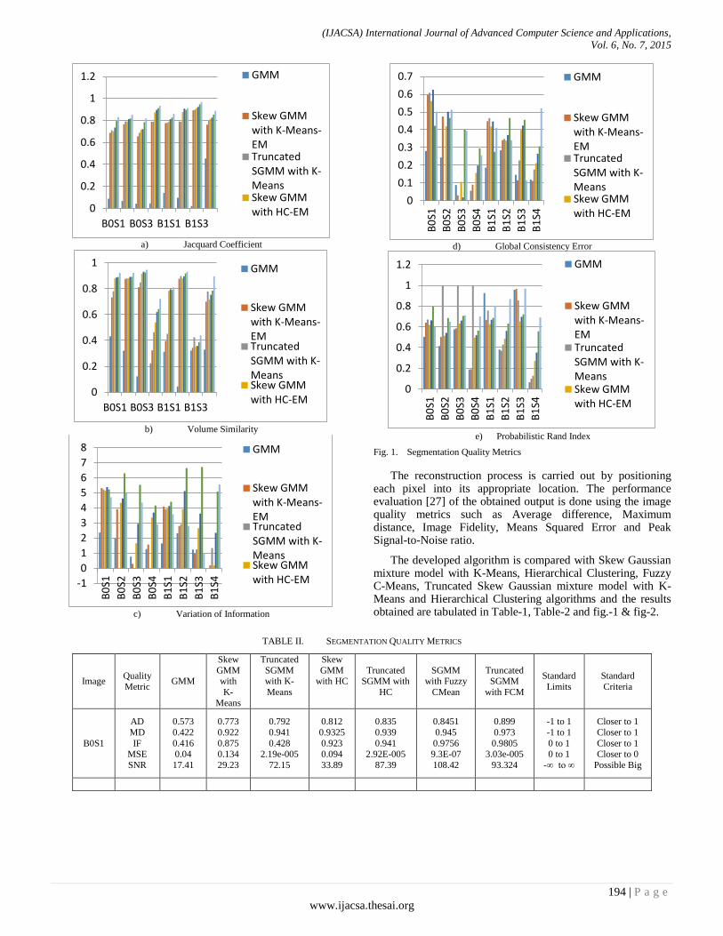
(IJACSA) International Journal of Advanced Computer Science and Applications,
Vol. 6, No. 7, 2015
194 | P a g e
www.ijacsa.thesai.org
a) Jacquard Coefficient
b) Volume Similarity
c) Variation of Information
d) Global Consistency Error
e) Probabilistic Rand Index
Fig. 1. Segmentation Quality Metrics
The reconstruction process is carried out by positioning each pixel into its appropriate location. The performance evaluation [27] of the obtained output is done using the image quality metrics such as Average difference, Maximum distance, Image Fidelity, Means Squared Error and Peak Signal-to-Noise ratio.
The developed algorithm is compared with Skew Gaussian mixture model with K-Means, Hierarchical Clustering, Fuzzy C-Means, Truncated Skew Gaussian mixture model with K-Means and Hierarchical Clustering algorithms and the results obtained are tabulated in Table-1, Table-2 and fig.-1 & fig-2.
TABLE II. SEGMENTATION QUALITY METRICS
Image Quality
Metric GMM
Skew
GMM with
K-
Means
Truncated
SGMM with K-
Means
Skew
GMM with HC
Truncated SGMM with
HC
SGMM with Fuzzy
CMean
Truncated SGMM
with FCM
Standard
Limits
Standard
Criteria
B0S1
AD
MD
IF MSE
SNR
0.573
0.422
0.416 0.04
17.41
0.773
0.922
0.875 0.134
29.23
0.792
0.941
0.428 2.19e-005
72.15
0.812
0.9325
0.923 0.094
33.89
0.835
0.939
0.941 2.92E-005
87.39
0.8451
0.945
0.9756 9.3E-07
108.42
0.899
0.973
0.9805 3.03e-005
93.324
-1 to 1
-1 to 1
0 to 1 0 to 1
-∞ to ∞
Closer to 1
Closer to 1
Closer to 1 Closer to 0
Possible Big
0
0.2
0.4
0.6
0.8
1
1.2
B0S1 B0S3 B1S1 B1S3
GMM
Skew GMMwith K-Means-EMTruncatedSGMM with K-MeansSkew GMMwith HC-EM
0
0.2
0.4
0.6
0.8
1
B0S1 B0S3 B1S1 B1S3
GMM
Skew GMMwith K-Means-EMTruncatedSGMM with K-MeansSkew GMMwith HC-EM
-1
0
1
2
3
4
5
6
7
8
B0
S1
B0
S2
B0
S3
B0
S4
B1
S1
B1
S2
B1
S3
B1
S4
GMM
Skew GMMwith K-Means-EMTruncatedSGMM with K-MeansSkew GMMwith HC-EM
0
0.1
0.2
0.3
0.4
0.5
0.6
0.7
B0
S1
B0
S2
B0
S3
B0
S4
B1
S1
B1
S2
B1
S3
B1
S4
GMM
Skew GMMwith K-Means-EMTruncatedSGMM with K-MeansSkew GMMwith HC-EM
0
0.2
0.4
0.6
0.8
1
1.2
B0
S1
B0
S2
B0
S3
B0
S4
B1
S1
B1
S2
B1
S3
B1
S4
GMM
Skew GMMwith K-Means-EMTruncatedSGMM with K-MeansSkew GMMwith HC-EM
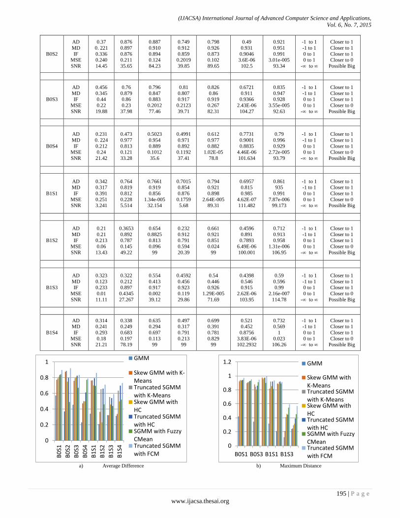
(IJACSA) International Journal of Advanced Computer Science and Applications,
Vol. 6, No. 7, 2015
195 | P a g e
www.ijacsa.thesai.org
B0S2
AD
MD
IF MSE
SNR
0.37
0. 221
0.336 0.240
14.45
0.876
0.897
0.876 0.211
35.65
0.887
0.910
0.894 0.124
84.23
0.749
0.912
0.859 0.2019
39.85
0.798
0.926
0.873 0.102
89.65
0.49
0.931
0.9046 3.6E-06
102.5
0.921
0.951
0.991 3.01e-005
93.34
-1 to 1
-1 to 1
0 to 1 0 to 1
-∞ to ∞
Closer to 1
Closer to 1
Closer to 1 Closer to 0
Possible Big
B0S3
AD
MD IF
MSE
SNR
0.456
0.345 0.44
0.22
19.88
0.76
0.879 0.86
0.23
37.98
0.796
0.847 0.883
0.2012
77.46
0.81
0.807 0.917
0.2123
39.71
0.826
0.86 0.919
0.267
82.31
0.6721
0.911 0.9366
2.43E-06
104.27
0.835
0.947 0.928
3.55e-005
92.63
-1 to 1
-1 to 1 0 to 1
0 to 1
-∞ to ∞
Closer to 1
Closer to 1 Closer to 1
Closer to 0
Possible Big
B0S4
AD
MD
IF MSE
SNR
0.231
0. 224
0.212 0.24
21.42
0.473
0.977
0.813 0.121
33.28
0.5023
0.954
0.889 0.1012
35.6
0.4991
0.971
0.892 0.1192
37.41
0.612
0.977
0.882 1.02E-05
78.8
0.7731
0.9001
0.8835 4.46E-06
101.634
0.79
0.996
0.929 2.72e-005
93.79
-1 to 1
-1 to 1
0 to 1 0 to 1
-∞ to ∞
Closer to 1
Closer to 1
Closer to 1 Closer to 0
Possible Big
B1S1
AD MD
IF
MSE SNR
0.342 0.317
0.391
0.251 3.241
0.764 0.819
0.812
0.228 5.514
0.7661 0.919
0.856
1.34e-005 32.154
0.7015 0.854
0.876
0.1759 5.68
0.794 0.921
0.898
2.64E-005 89.31
0.6957 0.815
0.985
4.62E-07 111.482
0.861 935
0.991
7.87e-006 99.173
-1 to 1 -1 to 1
0 to 1
0 to 1 -∞ to ∞
Closer to 1 Closer to 1
Closer to 1
Closer to 0 Possible Big
B1S2
AD
MD IF
MSE
SNR
0.21
0.21 0.213
0.06
13.43
0.3653
0.892 0.787
0.145
49.22
0.654
0.8825 0.813
0.096
99
0.232
0.912 0.791
0.594
20.39
0.661
0.921 0.851
0.024
99
0.4596
0.891 0.7893
6.49E-06
100.001
0.712
0.913 0.958
1.31e-006
106.95
-1 to 1
-1 to 1 0 to 1
0 to 1
-∞ to ∞
Closer to 1
Closer to 1 Closer to 1
Closer to 0
Possible Big
B1S3
AD
MD IF
MSE
SNR
0.323
0.123 0.233
0.01
11.11
0.322
0.212 0.897
0.4345
27.267
0.554
0.413 0.917
0.002
39.12
0.4592
0.456 0.923
0.119
29.86
0.54
0.446 0.926
1.29E-005
71.69
0.4398
0.546 0.915
2.62E-06
103.95
0.59
0.596 0.99
2.16e-007
114.78
-1 to 1
-1 to 1 0 to 1
0 to 1
-∞ to ∞
Closer to 1
Closer to 1 Closer to 1
Closer to 0
Possible Big
B1S4
AD MD
IF
MSE SNR
0.314 0.241
0.293
0.18 21.21
0.338 0.249
0.683
0.197 78.19
0.635 0.294
0.697
0.113 99
0.497 0.317
0.791
0.213 99
0.699 0.391
0.781
0.829 99
0.521 0.452
0.8756
3.83E-06 102.2932
0.732 0.569
1
0.023 106.26
-1 to 1 -1 to 1
0 to 1
0 to 1 -∞ to ∞
Closer to 1 Closer to 1
Closer to 1
Closer to 0 Possible Big
a) Average Difference
b) Maximum Distance
0
0.2
0.4
0.6
0.8
1
B0
S1
B0
S2
B0
S3
B0
S4
B1
S1
B1
S2
B1
S3
B1
S4
GMM
Skew GMM with K-MeansTruncated SGMMwith K-MeansSkew GMM withHCTruncated SGMMwith HCSGMM with FuzzyCMeanTruncated SGMMwith FCM
0
0.2
0.4
0.6
0.8
1
1.2
B0S1 B0S3 B1S1 B1S3
GMM
Skew GMM withK-MeansTruncated SGMMwith K-MeansSkew GMM withHCTruncated SGMMwith HCSGMM with FuzzyCMeanTruncated SGMMwith FCM
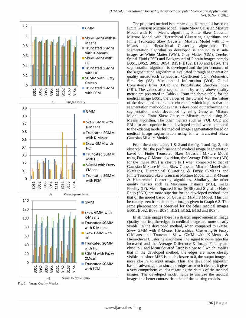
(IJACSA) International Journal of Advanced Computer Science and Applications,
Vol. 6, No. 7, 2015
196 | P a g e
www.ijacsa.thesai.org
c) Image Fidelity
d) Mean Square Error
e) Signal to Noise Ratio
Fig. 2. Image Quality Metrics
The proposed method is compared to the methods based on Finite Gaussian Mixture Model, Finite Skew Gaussian Mixture Model with K – Means algorithms, Finite Skew Gaussian Mixture Model with Hierarchical Clustering algorithms and Finite Truncated Skew Gaussian Mixture Model with K – Means and Hierarchical Clustering algorithms. The segmentation algorithm so developed is applied to 8 sub-images as White Matter (WM), Gray Matter (GM), Cerebro Spinal Fluid (CSF) and Background of 2 brain images namely B0S1, B0S2, B0S3, B0S4, B1S1, B1S2, B1S3 and B1S4. The segmentation algorithm is developed and the performance of the segmentation algorithm is evaluated through segmentation quality metric such as jacquard Coefficient (JC), Volumetric Similarity (VS), Variation of Information (VOI), Global Consistency Error (GCE) and Probabilistic Random Index (PRI). The values after segmentation by using above quality metric are presented in Table-1. From the above table, for the medical image B0S1, the values of the JC and VS, the values of the developed method are close to 1 which implies that the segmentation methodology that is developed outperforming the segmentation model developed by using Gaussian Mixture Model and Finite Skew Gaussian Mixture model using K-Means algorithm. The other metrics such as VOI, GCE and PRI also are superior in the developed model when compared to the existing model for medical image segmentation based on medical image segmentation using Finite Truncated Skew Gaussian Mixture Models.
From the above tables-1 & 2 and the fig.-1 and fig.-2, it is observed that the performance of medical image segmentation based on Finite Truncated Skew Gaussian Mixture Model using Fuzzy C-Means algorithm, the Average Difference (AD) for the image B0S1 is closure to 1 when compared to that of Gaussian Mixture Model, Skew Gaussian Mixture Model with K-Means, Hierarchical Clustering & Fuzzy C-Means and Finite Truncated Skew Gaussian Mixture Model with K-Means & Hierarchical Clustering algorithms. Similarly, the other quality metrics such as Maximum Distance (MD), Image Fidelity (IF), Mean Squared Error (MSE) and Signal to Noise Ratio (SNR) are more superior for the developed method than that of the model based on Gaussian Mixture Model. This can be clearly seen from the output images given in Graph-6.3. The same phenomenon is observed for the other medical images B0S1, B0S2, B0S3, B0S4, B1S1, B1S2, B1S3 and B0S4.
In all these images there is a drastic improvement in Image Quality metrics, the edges in medical image are more clearly visible. In the developed method, when compared to GMM, Skew GMM with K-Means, Hierarchical Clustering & Fuzzy C-Means and Truncated Skew GMM with K-Means & Hierarchical Clustering algorithms, the signal to noise ratio has increased and the Average Difference & Image Fidelity are close to 1 and Mean Squared Error is close to 0 which implies that in the developed method, the edges are more closely visible and since MSE is much closure to 0, the output image is more closure to input image. Thus, the developed algorithm has the advantage that since the edges are much clearer, it gives a very comprehensive idea regarding the details of the medical images. The developed model helps to analyze the medical images in a better contrast than that of the existing models.
0
0.2
0.4
0.6
0.8
1
1.2
B0
S1
B0
S2
B0
S3
B0
S4
B1
S1
B1
S2
B1
S3
B1
S4
GMM
Skew GMM with K-Means
Truncated SGMMwith K-Means
Skew GMM withHC
Truncated SGMMwith HC
SGMM with FuzzyCMean
Truncated SGMMwith FCM
0
0.1
0.2
0.3
0.4
0.5
0.6
0.7
0.8
0.9
B0
S1
B0
S2
B0
S3
B0
S4
B1
S1
B1
S2
B1
S3
B1
S4
GMM
Skew GMM withK-Means
Truncated SGMMwith K-Means
Skew GMM withHC
Truncated SGMMwith HC
SGMM with FuzzyCMean
Truncated SGMMwith FCM
0
20
40
60
80
100
120
140
B0
S1
B0
S2
B0
S3
B0
S4
B1
S1
B1
S2
B1
S3
B1
S4
GMM
Skew GMM withK-Means
Truncated SGMMwith K-Means
Skew GMM withHC
Truncated SGMMwith HC
SGMM with FuzzyCMean
Truncated SGMMwith FCM

(IJACSA) International Journal of Advanced Computer Science and Applications,
Vol. 6, No. 7, 2015
197 | P a g e
www.ijacsa.thesai.org
VIII. CONCLUSION
This proposed article is focused towards MRI Brain Image Segmentation. A new approach based on Finite Truncated Skew Gaussian Mixture Model is introduced. The performance evaluation of the developed model is investigated by using Image quality metrics which depict that the developed algorithm outperforms the other existing algorithms based on Skew Gaussian mixture model using K-Means, Skew Gaussian mixture model Hierarchical Clustering, Skew Gaussian mixture model Fuzzy C-Means, Truncated Skew Gaussian mixture model with K-Means and Hierarchical Clustering algorithms and the results obtained showcase that the developed model has better segmentation accuracy. Effective segmentation helps in efficient identification of the damaged tissues much more effectively Therefore, the proposed method will be very much useful in diagnosing the diseases like acoustic neuroma, Alzheimer’s, Parkinson’s etc. more accurately.
IX. FUTURE SCOPE
A methodology is presented for analyzing the brain images based on Truncated Gaussian Mixture models. However, to have a more precise segmentation, it is needed to consider the other features of the images also, which may include the shape, size, orientation and texture. Therefore, multivariate features should be considered to have a more detailed and effective analysis, further work is to be projected in this direction.
REFERENCES
[1] Vasant Manohar and Yuhua Gu: MRI Segmentation Using Fuzzy C-Means and Finite Gaussian Mixture Model, Digital Image Processing – CAP5400, 2008.
[2] Z Y Shan, G H Yue and J Z Liu: Automated Histogram-Based Brain Segmentation in T1-Weighted Three-Dimensional Magnetic Resonance Head Images, NeuroImage v.17, pp. 1587-1598, 2002.
[3] G V S Raj Kumar, K Srinivasa Rao, and P Srinivasa Rao: Image Segmentation Method Based on Finite Doubly Truncated Bivariate Gaussian Mixture Model with Hierarchical Clustering, International Journal of Computer Science Issues, 8(4-2):151-159, July, 2011.
[4] Nagesh Vadaparthi, Srinivas Yerramalle, and Suresh Varma.P: Unsupervised Medical Image Segmentation on Brain MRI images using Skew Gaussian Distribution, IEEE – ICRTIT 2011, pp.1293 – 1297.
[5] Nagesh Vadaparthi, Srinivas Yerramalle, and Suresh Varma.P: Unsupervised Medical Image Classification based on Skew Gaussian Mixture Model and Hierarchical Clustering Algorithm” in CCIS of Springer-Links, Volume – 203, pp. 65-74, 2011.
[6] Nagesh Vadaparthi, Srinivas Yerramalle, and Suresh Varma.P: Segmentation of Brain MR Images based on Finite Skew Gaussian Mixture Model with Fuzzy C-Means Clustering and EM Algorithm”, International Journal of Computer Applications, 28(10):18-26, August 2011.
[7] Nagesh Vadaparthi, Srinivas Yerramalle, and Suresh Varma.P: An Efficient Approach for Medical Image Segmentation Based on Truncated Skew Gaussian Mixture Model Using K-Means Algorithm”, International Journal of Computer Science and Telecommunications, (ISSN 2047-3338), 2(6):79-86, August 2011.
[8] Nagesh Vadaparthi, Srinivas Yerramalle, and Suresh Varma.P: On Improved Medical Brain MR Image Segmentation Based on Truncated Skew Gaussian Mixture Model using Hierarchical Clustering and EM algorithms”, International Journal of Advanced Research in Computer Science (ISSN: 0976-5697) , 2(6) November-December 2011.
[9] M. Sashidhar et al: MRI Brain Image Segmentation using Modified Fuzzy C-Means Clustering Algorithm, IEEE-Int. Conf. on Communication systems and Network Technologies, 2011, Pp.473-478.
[10] D. L. Pham, C. Y. Xu, and J. L. Prince: A survey of current methodsin medical image segmentation, Annu. Rev. Biomed. Eng., vol. 2, pp.315–337, 2000.
[11] K. Van Leemput, F. Maes, D. Vandeurmeulen, and P. Suetens: Automatedmodel-based tissue classification of MR images of the brain, IEEE Trans. Med. Imag., 18(10): 897–908, Oct. 1999.
[12] Dugas-Phocion, M. Á. González Ballester, G. Malandain, C. Lebrun and N. Ayache: Improved EM-based tissue segmentation andpartial volume effect quantification in multi-sequence brain MRI, Int. Conf. Med. Image Comput. Comput. Assist. Int. (MICCAI), 2004, pp. 26–33.
[13] K. Van Leemput, F. Maes, D. Vandermeulen, and P. Suetens: A unifying framework for partial volume segmentation of brainMR Images, IEEE Trans. Med. Imag., 22(1):105–119, Jan. 2003.
[14] M. Prastawa, E. Bullitt, S. Ho, and G. Gerig: Robust estimation forbrain tumor segmentation, Int. Conf. Med. Image Comput. Comput.Assist. Inter (MICCAI), 2003, pp. 530–537.
[15] Lee TI, Maximum likelihood estimation for multivariate skew normal mixture models, Journal of Multivariate Analysis 100 (2009) 257–265, 2009.
[16] Cabral CS, Lachos VH, Prates MO, Multivariate mixture modeling using skew-normal independent distributions. Computational Statistics and Data Analysis 56:126–142, 2012.
[17] Lee TI, Robust mixture modeling using multivariate skew distributions, stat comp (2010) 20:343-356, DOI 10.1007/s I 1222-009-9128-9, 2010.
[18] Lee S, McLachlan GJ, On the fitting of mixtures of multivariate skew t-distributions via the EM algorithm. arXiv:11094706 [statME], 2011.
[19] Vrbik I, McNicholas PD, Analytic calculations for the EM algorithm for multivariate skew t-mixture models. Statistics and Probability Letters, 32 Sharon X. Lee, Geoffrey J. McLachlan 82:1169–1174, 2012.
[20] Lin TI, Ho HJ, Kee CR, Flexible mixture modelling using the multivariate skew-t-normal distribution. Statistics and Computing DOI 10.1007/s11222-013-9386-4, 2013.
[21] Karlis D, Xekalaki E, Choosing initial values for the EM algorithm for finite mixtures. Computational Statistics & Data Analysis 41:577–590, 2003
[22] Franczak BC, Browne RP, McNicholas PD, Mixtures of shifted asymmetric laplace distributions. arXiv:12071727 [statME], 2012.
[23] McNeil AJ, Frey R, Embrechts P, Quantitative risk management : concepts, techniques and tools. Princeton University Press, USA, 1997.
[24] Embrechts, P., Kl¨uppelberg, C., and Mikosch, T., Modelling Extremal Events for Insurance and Finance. Springer-Verlag, New York, 1997.
[25] Burnecki, K., Misiorek, A., and Weron, R., Loss distributions. In Statistical Tools for Finance and Insurance. Cizek, P., H¨ardle, W. K., and Weron, R. Eds. Springer-Verlag.2010.
[26] Sylvain Bouix et al.: Evaluating Brain Tissue Classifiers without a ground truth, Journal of NeuroImage (ELSEVIER) - 36, pp. 1207 – 1224, 2007.
[27] Ahmet M. Eskicioglu and Paul S. Fisher: Image Quality Measures and Their Performance, IEEE Transactions on Communications, 43(12):2959 – 2965, Dec.1995.

(IJACSA) International Journal of Advanced Computer Science and Applications,
Vol. 6, No. 7, 2015
198 | P a g e
www.ijacsa.thesai.org
Research on the UHF RFID Channel Coding
Technology based on Simulink
Changzhi Wang
School of Electronic and Electrical
Engineering
Shanghai University of Engineering
Science, SUES
Shanghai 201620, China
Zhicai Shi*
School of Electronic and Electrical
Engineering
Shanghai University of Engineering
Science, SUES
Shanghai 201620, China
Dai Jian
School of Electronic and Electrical
Engineering
Shanghai University of Engineering
Science, SUES
Shanghai 201620, China
Li Meng
School of Electronic and Electrical
Engineering
Shanghai University of Engineering
Science, SUES
Shanghai 201620, China
Abstract—In this letter, we propose a new UHF RFID channel
coding method, which improves the reliability of the system by
using the excellent error correcting performance of the
convolutional code. We introduce the coding principle of
convolutional code, and compare with the cyclic codes used in the
past. Finally, we analyze the error correcting performance of
convolutional codes. The analysis results show that the results
show that the transmission rate of the system is guaranteed, and
the bit error rate can be reduced by 2.561%.
Keywords—UHF RFID; channel coding; convolution code; bit
error rate
I. INTRODUCTION
UHF RFID tags are working in the range of 860~960MHz frequency band. Compared with the daily use of the high frequency radio frequency tags (its typical operating frequency is 13.56MHz), its communication distance is longer, its transmission data rate is quicker and so on. However, the overall technology of RFID UHF system is still not perfect. There is still a high bit error rate [1].
To solve these problems and to further reduce the bit error rate of RFID UHF system, we need to use the error control mode for channel encoding. According to the constraint mode between the monitor element and information element, the error control encoding can be divided into block codes and convolutional codes. The cyclic code (CRC) is based on the strict mathematical method, which is easy to implement and can be used in the channel coding. Although the cyclic code error detection capability is high, but its error correction performance is weak. In communication, when the CRC detects the fault code, which will ask the sender to resend the data until the receiving end of the data is right. This inevitably increases the time to repeat the communication, which affects the efficiency of the RFID UHF system. Compared to the cyclic codes, although convolutional code has not yet found a
rigorous mathematical method, and closely related to the error correcting performance and structure of the code. But its error correction performance is relatively strong, the device is also simple. Therefore, when the convolutional code is sent, the decoding end of convolutional code can detect error and correct when a general error code is generated in the communication process. It will reduce the bit error rate of the receiver and the communication time.
II. CONVOLUTIONAL CODE DESCRIPTION
Convolutional code is a kind of non block code, commonly used (n, k, K) said. It was proposed by Elias in 1955. Where k is the number of input symbol information, n is the number of output symbols and K is the constraint length of the encoder. Its encoding efficiency is k/n x100%. The typical n and K (k<n) of the convolutional codes are small. However, in order to obtain a simple and high performance of the channel encoding and improve the reliability of data transmission, the constrained length K is preferred (K<10). In convolutional codes, N symbols of each (n, K) code word is not only related to K information element within the code word, but also it related to the information symbols that belongs to the m=K-1 code word in front. But in the (n, K) linear block codes, N symbols in the each code word is only related to its K information symbols [2].Therefore, in the process of encoding, the convolutional code can take full advantage of the correlation between the information code. It is a kind of memory encoding, which is superior to the block code (including cyclic code).
A. Convolutional code
Convolutional code encoder is composed of input shift register, module 2 and output shift register. In this paper, we take the (2, 1, 2) convolutional code encoding circuit as an example. It is composed of two shift register, two adder of mode 2 and switch circuit, as shown in Fig 1.
The relative work about this paper is supported by the Innovation Program of Shanghai University of Engineering Science under Grant No.E1-
0903-15-01027.
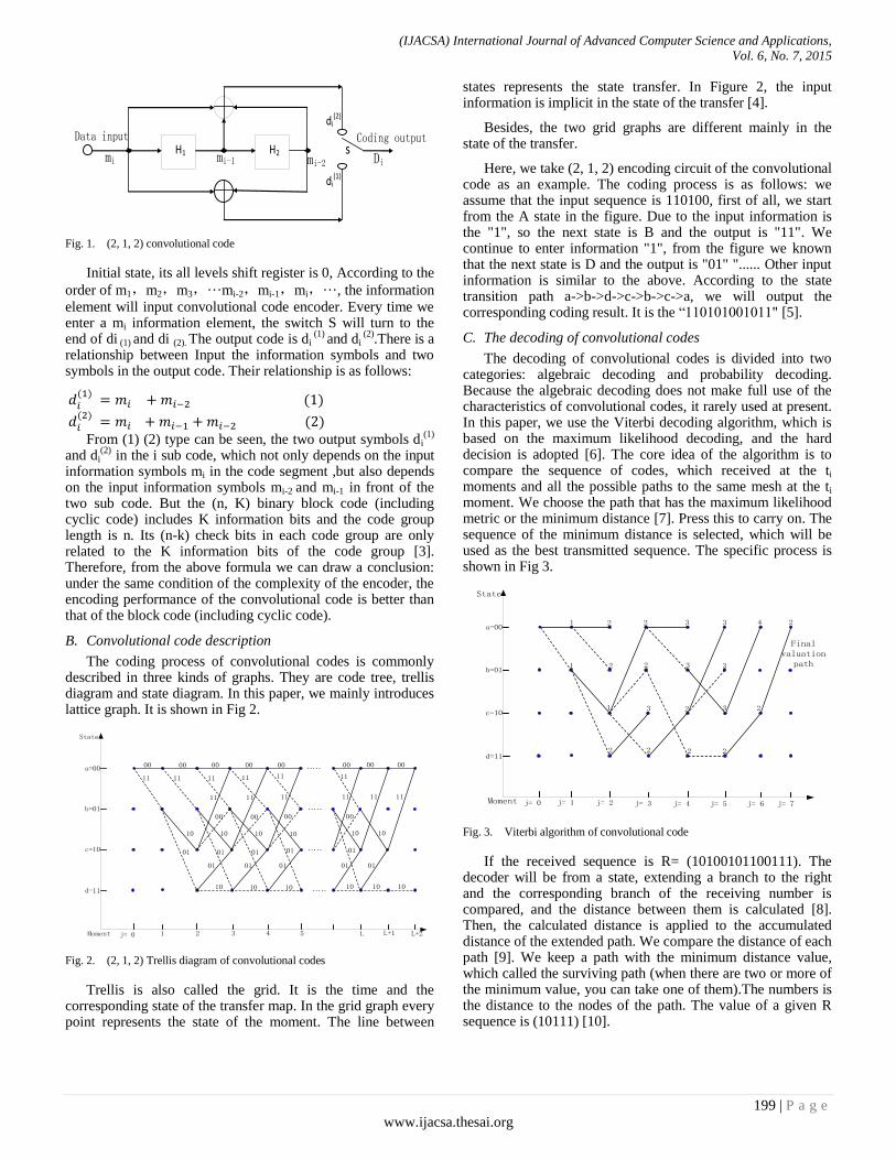
(IJACSA) International Journal of Advanced Computer Science and Applications,
Vol. 6, No. 7, 2015
199 | P a g e
www.ijacsa.thesai.org
Data input Coding output
mi-1mi mi-2 Di
di(1)
di(2)
s
H1 H2
Fig. 1. (2, 1, 2) convolutional code
Initial state, its all levels shift register is 0, According to the
order of m1,m2,m3,···mi-2,mi-1,mi,···, the information
element will input convolutional code encoder. Every time we enter a mi information element, the switch S will turn to the end of di (1) and di (2). The output code is di
(1) and di
(2).There is a
relationship between Input the information symbols and two symbols in the output code. Their relationship is as follows:
From (1) (2) type can be seen, the two output symbols di(1)
and di(2)
in the i sub code, which not only depends on the input information symbols mi in the code segment ,but also depends on the input information symbols mi-2 and mi-1 in front of the two sub code. But the (n, K) binary block code (including cyclic code) includes K information bits and the code group length is n. Its (n-k) check bits in each code group are only related to the K information bits of the code group [3]. Therefore, from the above formula we can draw a conclusion: under the same condition of the complexity of the encoder, the encoding performance of the convolutional code is better than that of the block code (including cyclic code).
B. Convolutional code description
The coding process of convolutional codes is commonly described in three kinds of graphs. They are code tree, trellis diagram and state diagram. In this paper, we mainly introduces lattice graph. It is shown in Fig 2.
j= 0 2 3 4
State
a=00
b=01
c=10
d=11
00 00 00 00 00
11 11
11 11 11
11 11 11
10 10 10
01 01 01
00 00 00
10 10 10 10
01 01 01 01
1 5
00 00 00
11
11 11 11
01
01 01
1010
00
10 10 10
L L+1 L+2Moment
Fig. 2. (2, 1, 2) Trellis diagram of convolutional codes
Trellis is also called the grid. It is the time and the corresponding state of the transfer map. In the grid graph every point represents the state of the moment. The line between
states represents the state transfer. In Figure 2, the input information is implicit in the state of the transfer [4].
Besides, the two grid graphs are different mainly in the state of the transfer.
Here, we take (2, 1, 2) encoding circuit of the convolutional code as an example. The coding process is as follows: we assume that the input sequence is 110100, first of all, we start from the A state in the figure. Due to the input information is the "1", so the next state is B and the output is "11". We continue to enter information "1", from the figure we known that the next state is D and the output is "01" "...... Other input information is similar to the above. According to the state transition path a->b->d->c->b->c->a, we will output the corresponding coding result. It is the “110101001011" [5].
C. The decoding of convolutional codes
The decoding of convolutional codes is divided into two categories: algebraic decoding and probability decoding. Because the algebraic decoding does not make full use of the characteristics of convolutional codes, it rarely used at present. In this paper, we use the Viterbi decoding algorithm, which is based on the maximum likelihood decoding, and the hard decision is adopted [6]. The core idea of the algorithm is to compare the sequence of codes, which received at the ti moments and all the possible paths to the same mesh at the ti moment. We choose the path that has the maximum likelihood metric or the minimum distance [7]. Press this to carry on. The sequence of the minimum distance is selected, which will be used as the best transmitted sequence. The specific process is shown in Fig 3.
j= 0Moment
State
a=00
b=01
c=10
d=11
j= 1 j= 2 j= 3 j= 4 j= 5 j= 6 j= 7
1 2
21
2 3
32
1
2
3
2 22
2
3
3
3
4 2
2
Final valuation
path
Fig. 3. Viterbi algorithm of convolutional code
If the received sequence is R= (10100101100111). The decoder will be from a state, extending a branch to the right and the corresponding branch of the receiving number is compared, and the distance between them is calculated [8]. Then, the calculated distance is applied to the accumulated distance of the extended path. We compare the distance of each path [9]. We keep a path with the minimum distance value, which called the surviving path (when there are two or more of the minimum value, you can take one of them).The numbers is the distance to the nodes of the path. The value of a given R sequence is (10111) [10].
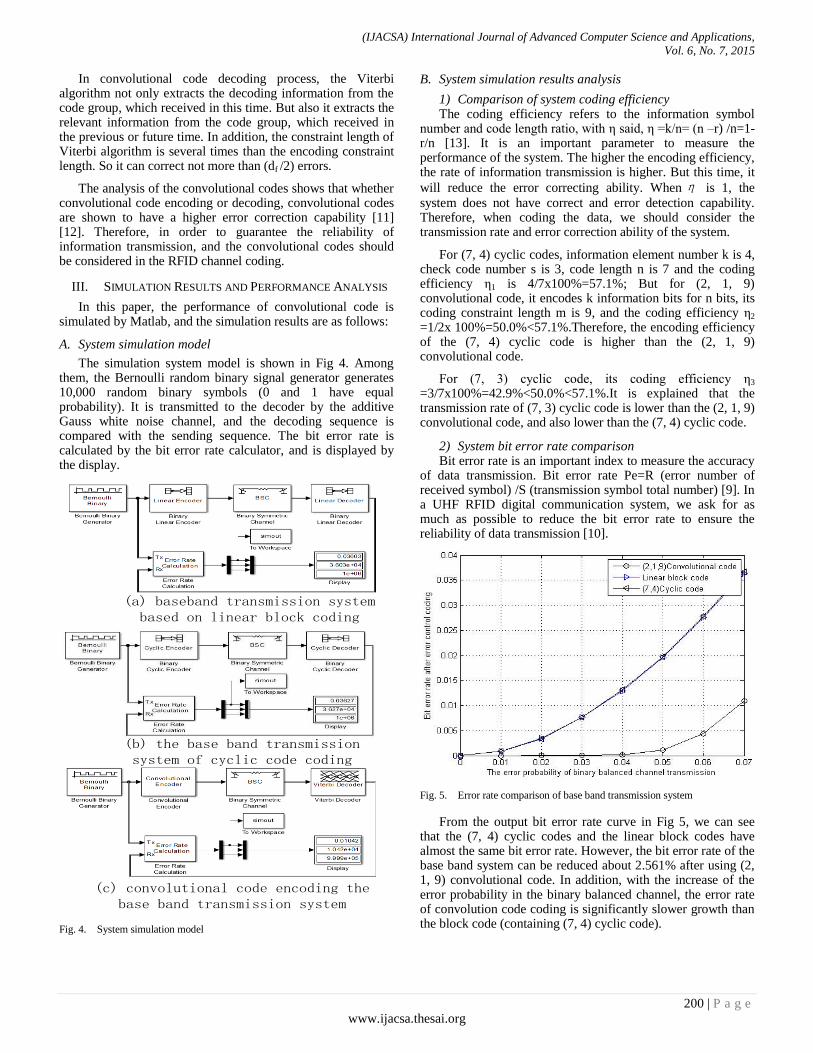
(IJACSA) International Journal of Advanced Computer Science and Applications,
Vol. 6, No. 7, 2015
200 | P a g e
www.ijacsa.thesai.org
In convolutional code decoding process, the Viterbi algorithm not only extracts the decoding information from the code group, which received in this time. But also it extracts the relevant information from the code group, which received in the previous or future time. In addition, the constraint length of Viterbi algorithm is several times than the encoding constraint length. So it can correct not more than (df /2) errors.
The analysis of the convolutional codes shows that whether convolutional code encoding or decoding, convolutional codes are shown to have a higher error correction capability [11] [12]. Therefore, in order to guarantee the reliability of information transmission, and the convolutional codes should be considered in the RFID channel coding.
III. SIMULATION RESULTS AND PERFORMANCE ANALYSIS
In this paper, the performance of convolutional code is simulated by Matlab, and the simulation results are as follows:
A. System simulation model
The simulation system model is shown in Fig 4. Among them, the Bernoulli random binary signal generator generates 10,000 random binary symbols (0 and 1 have equal probability). It is transmitted to the decoder by the additive Gauss white noise channel, and the decoding sequence is compared with the sending sequence. The bit error rate is calculated by the bit error rate calculator, and is displayed by the display.
(a) baseband transmission system based on linear block coding
(c) convolutional code encoding the base band transmission system
(b) the base band transmission system of cyclic code coding
Fig. 4. System simulation model
B. System simulation results analysis
1) Comparison of system coding efficiency The coding efficiency refers to the information symbol
number and code length ratio, with η said, η =k/n= (n –r) /n=1-r/n [13]. It is an important parameter to measure the performance of the system. The higher the encoding efficiency, the rate of information transmission is higher. But this time, it
will reduce the error correcting ability. Whenη is 1, the
system does not have correct and error detection capability. Therefore, when coding the data, we should consider the transmission rate and error correction ability of the system.
For (7, 4) cyclic codes, information element number k is 4, check code number s is 3, code length n is 7 and the coding efficiency η1 is 4/7x100%=57.1%; But for (2, 1, 9) convolutional code, it encodes k information bits for n bits, its coding constraint length m is 9, and the coding efficiency η2 =1/2x 100%=50.0%<57.1%.Therefore, the encoding efficiency of the (7, 4) cyclic code is higher than the (2, 1, 9) convolutional code.
For (7, 3) cyclic code, its coding efficiency η3 =3/7x100%=42.9%<50.0%<57.1%.It is explained that the transmission rate of (7, 3) cyclic code is lower than the (2, 1, 9) convolutional code, and also lower than the (7, 4) cyclic code.
2) System bit error rate comparison Bit error rate is an important index to measure the accuracy
of data transmission. Bit error rate Pe=R (error number of received symbol) /S (transmission symbol total number) [9]. In a UHF RFID digital communication system, we ask for as much as possible to reduce the bit error rate to ensure the reliability of data transmission [10].
Fig. 5. Error rate comparison of base band transmission system
From the output bit error rate curve in Fig 5, we can see that the (7, 4) cyclic codes and the linear block codes have almost the same bit error rate. However, the bit error rate of the base band system can be reduced about 2.561% after using (2, 1, 9) convolutional code. In addition, with the increase of the error probability in the binary balanced channel, the error rate of convolution code coding is significantly slower growth than the block code (containing (7, 4) cyclic code).
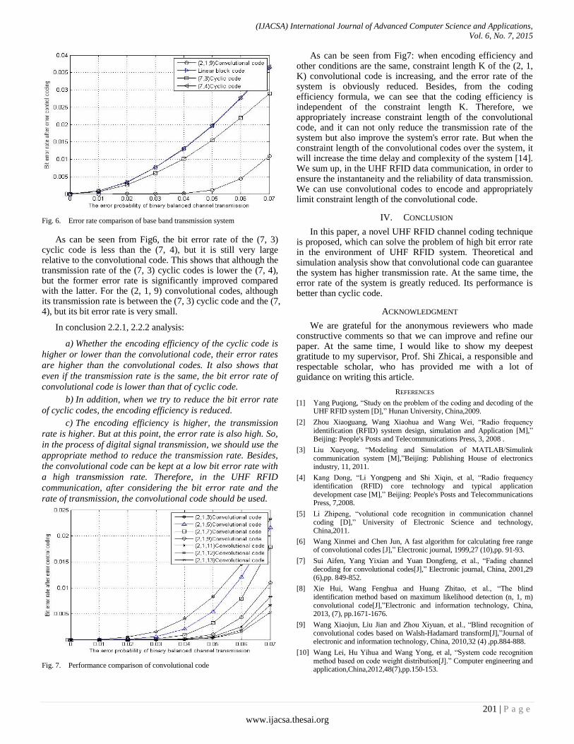
(IJACSA) International Journal of Advanced Computer Science and Applications,
Vol. 6, No. 7, 2015
201 | P a g e
www.ijacsa.thesai.org
Fig. 6. Error rate comparison of base band transmission system
As can be seen from Fig6, the bit error rate of the (7, 3) cyclic code is less than the (7, 4), but it is still very large relative to the convolutional code. This shows that although the transmission rate of the (7, 3) cyclic codes is lower the (7, 4), but the former error rate is significantly improved compared with the latter. For the (2, 1, 9) convolutional codes, although its transmission rate is between the (7, 3) cyclic code and the (7, 4), but its bit error rate is very small.
In conclusion 2.2.1, 2.2.2 analysis:
a) Whether the encoding efficiency of the cyclic code is
higher or lower than the convolutional code, their error rates
are higher than the convolutional codes. It also shows that
even if the transmission rate is the same, the bit error rate of
convolutional code is lower than that of cyclic code.
b) In addition, when we try to reduce the bit error rate
of cyclic codes, the encoding efficiency is reduced.
c) The encoding efficiency is higher, the transmission
rate is higher. But at this point, the error rate is also high. So,
in the process of digital signal transmission, we should use the
appropriate method to reduce the transmission rate. Besides,
the convolutional code can be kept at a low bit error rate with
a high transmission rate. Therefore, in the UHF RFID
communication, after considering the bit error rate and the
rate of transmission, the convolutional code should be used.
Fig. 7. Performance comparison of convolutional code
As can be seen from Fig7: when encoding efficiency and other conditions are the same, constraint length K of the (2, 1, K) convolutional code is increasing, and the error rate of the system is obviously reduced. Besides, from the coding efficiency formula, we can see that the coding efficiency is independent of the constraint length K. Therefore, we appropriately increase constraint length of the convolutional code, and it can not only reduce the transmission rate of the system but also improve the system's error rate. But when the constraint length of the convolutional codes over the system, it will increase the time delay and complexity of the system [14]. We sum up, in the UHF RFID data communication, in order to ensure the instantaneity and the reliability of data transmission. We can use convolutional codes to encode and appropriately limit constraint length of the convolutional code.
IV. CONCLUSION
In this paper, a novel UHF RFID channel coding technique is proposed, which can solve the problem of high bit error rate in the environment of UHF RFID system. Theoretical and simulation analysis show that convolutional code can guarantee the system has higher transmission rate. At the same time, the error rate of the system is greatly reduced. Its performance is better than cyclic code.
ACKNOWLEDGMENT
We are grateful for the anonymous reviewers who made constructive comments so that we can improve and refine our paper. At the same time, I would like to show my deepest gratitude to my supervisor, Prof. Shi Zhicai, a responsible and respectable scholar, who has provided me with a lot of guidance on writing this article.
REFERENCES
[1] Yang Puqiong, “Study on the problem of the coding and decoding of the UHF RFID system [D],” Hunan University, China,2009.
[2] Zhou Xiaoguang, Wang Xiaohua and Wang Wei, “Radio frequency identification (RFID) system design, simulation and Application [M],” Beijing: People's Posts and Telecommunications Press, 3, 2008 .
[3] Liu Xueyong, “Modeling and Simulation of MATLAB/Simulink communication system [M],”Beijing: Publishing House of electronics industry, 11, 2011.
[4] Kang Dong, “Li Yongpeng and Shi Xiqin, et al, “Radio frequency identification (RFID) core technology and typical application development case [M],” Beijing: People's Posts and Telecommunications Press, 7,2008.
[5] Li Zhipeng, “volutional code recognition in communication channel coding [D],” University of Electronic Science and technology, China,2011.
[6] Wang Xinmei and Chen Jun, A fast algorithm for calculating free range of convolutional codes [J],” Electronic journal, 1999,27 (10),pp. 91-93.
[7] Sui Aifen, Yang Yixian and Yuan Dongfeng, et al., “Fading channel decoding for convolutional codes[J],” Electronic journal, China, 2001,29 (6),pp. 849-852.
[8] Xie Hui, Wang Fenghua and Huang Zhitao, et al., “The blind identification method based on maximum likelihood detection (n, 1, m) convolutional code[J],”Electronic and information technology, China, 2013, (7), pp.1671-1676.
[9] Wang Xiaojun, Liu Jian and Zhou Xiyuan, et al., “Blind recognition of convolutional codes based on Walsh-Hadamard transform[J],”Journal of electronic and information technology, China, 2010,32 (4) ,pp.884-888.
[10] Wang Lei, Hu Yihua and Wang Yong, et al, “System code recognition method based on code weight distribution[J].” Computer engineering and application,China,2012,48(7),pp.150-153.

(IJACSA) International Journal of Advanced Computer Science and Applications,
Vol. 6, No. 7, 2015
202 | P a g e
www.ijacsa.thesai.org
[11] Liu Kaihua and Zhang Rui, “Application of shortening cyclic code in burst channel [J].” Electronic measurement technology, China, 2005,(1), pp.73-74.
[12] Zhu Lianxiang and Li Li, “Improved binary cyclic code blind identification method[J].” Computer applications, China, 2013,33(10),pp.62-64,68.
[13] Liu Jing, “Research on convolutional code and cyclic code recognition technology [D].” Xi'an Electronic and Science University, China,2010.
[14] Wang Juan and Shang Lin, “Simulation Research on the cascaded code of optical communication system [J].”Communication technology, China, 2010,43(3),pp.40-41,44.

(IJACSA) International Journal of Advanced Computer Science and Applications,
Vol. 6, No. 7, 2015
203 | P a g e
www.ijacsa.thesai.org
Artificial Intelligence in Performance Analysis of
Load Frequency Control in Thermal-Wind-Hydro
Power Systems
K. Jagatheesan
Graduate Student Member IEEE, Assistant Professor,
Dept. of Electrical and Electronics Engineering
Mahendra Institute of Engineering and Technology
Namakkal, Tamilnadu, INDIA
B. Anand
Member IEEE, Associate Professor
Dept. of Electrical and Electronics Engineering
Hindusthan college of Engineering and Technology
Coimbatore, Tamilnadu, INDIA
Nilanjan Dey
Dept. of CSE, Bengal College of Engineering &
Technology, West Bengal, India
Amira S. Ashour
Department of Electronics & Electrical Communications
Engineering, Faculty of Engg., Tanta Univ., EGYPT.
College of CIT, Taif University, KSA
Abstract—In this article, Load Frequency Control (LFC) of
three area unequal interconnected thermal, wind and Hydro
power generating units has been developed with Proportional-
Integral (PI) controller under MATLAB/SIMULINK
environment. Further, the PI controller gains values that
optimized using trial and error method with two different
objective functions, namely the Integral Time Square Error
(ITSE) and the Integral Time Absolute Error (ITAE). The
performance of ITAE objective function based PI controller is
compared with the ITSE objective function optimized PI
controller. Analysis reveals that the ITSE optimized controller
gives more superior performance than ITAE based controller
during one percent Step Load Perturbation (1% SLP) in area 1
(thermal area). In addition, Proportional–Integral –Derivative
(PID) controller is employed to improve the same power system
performance. The controller gain values are optimized using
Artificial Intelligence technique based Ant Colony Optimization
(ACO) algorithm. The simulation performance compares the
ACO-PID controller to the conventional PI. The results proved
that the proposed optimization technique based the ACO-PID
controller provides a superior control performance compared to
the PI controller. As the system using the ACO-PID controller
yield minimum overshoot, undershoot and settling time
compared to the conventional PI controlled equipped system
performance.
Keywords—Cost curve; Interconnected Power system; Load
Frequency Control (LFC); Objective Function; Performance
Index; Proportional-Integral controller
I. INTRODUCTION
Generally, in power generating units another form of energy is converted into electric energy or mechanical energy. Mechanical energy is converted into electrical energy by the use of electrical generator. The thermal power system converts heat energy into electrical energy. While, the gravitational/ falling force of water is converted into electric power via the
use of hydro power plant. In addition, the wind power is extracted from the air flow using wind turbines.
The quality of generating power supply from the generating unit depends on the consistency in voltage and frequency during sudden or continuous load demand. But practically maintaining the mentioned quantity/ parameters within the specified or nominal value is very complex as the load is continuously varied due to enormous growth in industries. In order to overcome this drawback power generating units are interconnected through tie-line [1-6]. During normal loading conditions each area carries its own load and keep the system parameters within the specified limit. When sudden load demand occurs in any one of the interconnected power system, suddenly the system parameters oscillate. At the same time remaining power system share the power (through tie-line) between them to maintain system stability [11-13].
Several control techniques have been proposed for the LFC of power systems to keep the system parameters at their specified value during sudden and normal loading conditions [1-10]. Literatures show that the system performance depends on both the employed controller and the selected objective function for tuning the controller parameters. In addition, it is clearly shown that many control strategies have been developed for load frequency control/Automatic Generation control application through the past few years. Such control strategies are as: Parameter-plane technique [15], Lyapunov Technique [16], Continuous and Discrete mode Optimization [18], Optimal Control theory [19], Adaptive Controller [20], Variable Structure Control(VSC) [22], Decentralized controller [21], Conventional controller [23], Fuzzy Logic controller [5], Classical Controller [1], Integral Controller [1], Bat inspired algorithm (BID) [26], Beta Wavelet Neural Network (BWNN) [27], Teaching Learning Based Optimization (TLBO) [28], Firefly Algorithm [29], Cuckoo Search [30], on Multi Input
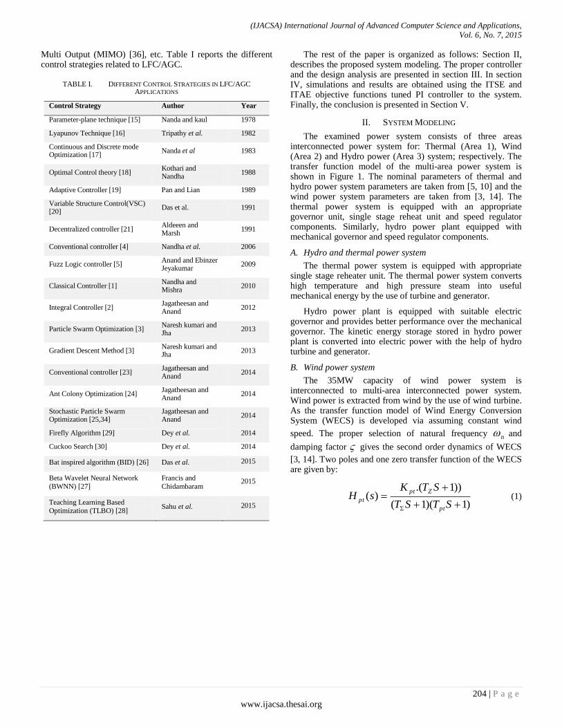
(IJACSA) International Journal of Advanced Computer Science and Applications,
Vol. 6, No. 7, 2015
204 | P a g e
www.ijacsa.thesai.org
Multi Output (MIMO) [36], etc. Table I reports the different control strategies related to LFC/AGC.
TABLE I. DIFFERENT CONTROL STRATEGIES IN LFC/AGC
APPLICATIONS
Control Strategy Author Year
Parameter-plane technique [15] Nanda and kaul 1978
Lyapunov Technique [16] Tripathy et al. 1982
Continuous and Discrete mode Optimization [17]
Nanda et al 1983
Optimal Control theory [18] Kothari and Nandha
1988
Adaptive Controller [19] Pan and Lian 1989
Variable Structure Control(VSC) [20]
Das et al. 1991
Decentralized controller [21] Aldeeen and Marsh
1991
Conventional controller [4] Nandha et al. 2006
Fuzz Logic controller [5] Anand and Ebinzer Jeyakumar
2009
Classical Controller [1] Nandha and Mishra
2010
Integral Controller [2] Jagatheesan and Anand
2012
Particle Swarm Optimization [3] Naresh kumari and Jha
2013
Gradient Descent Method [3] Naresh kumari and Jha
2013
Conventional controller [23] Jagatheesan and Anand
2014
Ant Colony Optimization [24] Jagatheesan and Anand
2014
Stochastic Particle Swarm Optimization [25,34]
Jagatheesan and Anand
2014
Firefly Algorithm [29] Dey et al. 2014
Cuckoo Search [30] Dey et al. 2014
Bat inspired algorithm (BID) [26] Das et al. 2015
Beta Wavelet Neural Network (BWNN) [27]
Francis and Chidambaram
2015
Teaching Learning Based
Optimization (TLBO) [28] Sahu et al. 2015
The rest of the paper is organized as follows: Section II, describes the proposed system modeling. The proper controller and the design analysis are presented in section III. In section IV, simulations and results are obtained using the ITSE and ITAE objective functions tuned PI controller to the system. Finally, the conclusion is presented in Section V.
II. SYSTEM MODELING
The examined power system consists of three areas interconnected power system for: Thermal (Area 1), Wind (Area 2) and Hydro power (Area 3) system; respectively. The transfer function model of the multi-area power system is shown in Figure 1. The nominal parameters of thermal and hydro power system parameters are taken from [5, 10] and the wind power system parameters are taken from [3, 14]. The thermal power system is equipped with an appropriate governor unit, single stage reheat unit and speed regulator components. Similarly, hydro power plant equipped with mechanical governor and speed regulator components.
A. Hydro and thermal power system
The thermal power system is equipped with appropriate single stage reheater unit. The thermal power system converts high temperature and high pressure steam into useful mechanical energy by the use of turbine and generator.
Hydro power plant is equipped with suitable electric governor and provides better performance over the mechanical governor. The kinetic energy storage stored in hydro power plant is converted into electric power with the help of hydro turbine and generator.
B. Wind power system
The 35MW capacity of wind power system is interconnected to multi-area interconnected power system. Wind power is extracted from wind by the use of wind turbine. As the transfer function model of Wind Energy Conversion System (WECS) is developed via assuming constant wind
speed. The proper selection of natural frequency n and
damping factor gives the second order dynamics of WECS
[3, 14]. Two poles and one zero transfer function of the WECS are given by:
)1)(1(
))1.()(
STST
STKsH
pt
Zpt
pt (1)
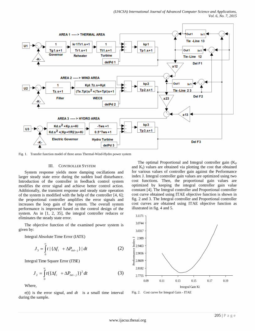
(IJACSA) International Journal of Advanced Computer Science and Applications,
Vol. 6, No. 7, 2015
205 | P a g e
www.ijacsa.thesai.org
Fig. 1. Transfer function model of three areas Thermal-Wind-Hydro power system
III. CONTROLLER SYSTEM
System response yields more damping oscillations and larger steady state error during the sudden load disturbance. Introduction of the controller in feedback control system modifies the error signal and achieve better control action. Additionally, the transient response and steady state operation of the system is modified with the help of the controller [4, 6]; the proportional controller amplifies the error signals and increases the loop gain of the system. The overall system performance is improved based on the control design of the system. As in [1, 2, 35], the integral controller reduces or eliminates the steady state error.
The objective function of the examined power system is given by:
Integral Absolute Time Error (IATE)
0
3 |}{| dtPftJ jtieii (2)
Integral Time Square Error (ITSE)
0
2
2 })({ dtPftJ jtieii (3)
Where,
e(t) is the error signal, and dt is a small time interval during the sample.
The optimal Proportional and Integral controller gain (KP and KI) values are obtained via plotting the cost that obtained for various values of controller gain against the Performance index J. Integral controller gain values are optimized using two cost functions. Then, the proportional gain values are optimized by keeping the integral controller gain value constant [4]. The Integral controller and Proportional controller cost curve obtained using ITAE objective function is shown in fig. 2 and 3. The Integral controller and Proportional controller cost curves are obtained using ITAE objective function as illustrated in fig. 4 and 5.
Fig. 2. Cost curve for Integral Gain - ITAE
2.7755
2.8182
2.8609
2.9036
2.9463
2.989
3.0317
3.0744
3.1171
0.09 0.11 0.13 0.15 0.17 0.19
Integral Gain Ki
Perf
orm
an
ce I
nd
ex
J
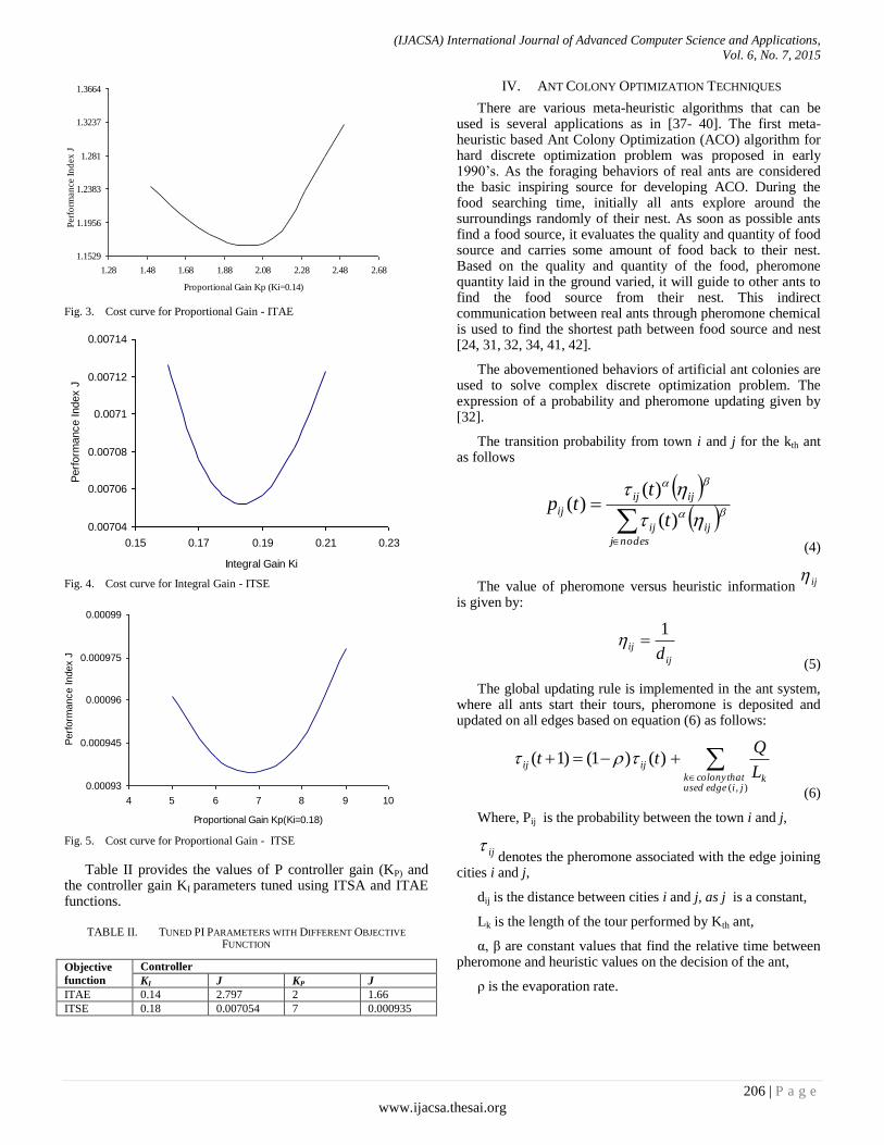
(IJACSA) International Journal of Advanced Computer Science and Applications,
Vol. 6, No. 7, 2015
206 | P a g e
www.ijacsa.thesai.org
Fig. 3. Cost curve for Proportional Gain - ITAE
Fig. 4. Cost curve for Integral Gain - ITSE
Fig. 5. Cost curve for Proportional Gain - ITSE
Table II provides the values of P controller gain (KP) and the controller gain KI parameters tuned using ITSA and ITAE functions.
TABLE II. TUNED PI PARAMETERS WITH DIFFERENT OBJECTIVE
FUNCTION
Objective
function
Controller
KI J KP J
ITAE 0.14 2.797 2 1.66
ITSE 0.18 0.007054 7 0.000935
IV. ANT COLONY OPTIMIZATION TECHNIQUES
There are various meta-heuristic algorithms that can be used is several applications as in [37- 40]. The first meta-heuristic based Ant Colony Optimization (ACO) algorithm for hard discrete optimization problem was proposed in early 1990’s. As the foraging behaviors of real ants are considered the basic inspiring source for developing ACO. During the food searching time, initially all ants explore around the surroundings randomly of their nest. As soon as possible ants find a food source, it evaluates the quality and quantity of food source and carries some amount of food back to their nest. Based on the quality and quantity of the food, pheromone quantity laid in the ground varied, it will guide to other ants to find the food source from their nest. This indirect communication between real ants through pheromone chemical is used to find the shortest path between food source and nest [24, 31, 32, 34, 41, 42].
The abovementioned behaviors of artificial ant colonies are used to solve complex discrete optimization problem. The expression of a probability and pheromone updating given by [32].
The transition probability from town i and j for the kth ant as follows
nodesj
ijij
ijij
ijt
ttp
)(
)()(
(4)
The value of pheromone versus heuristic information ij
is given by:
ij
ijd
1
(5)
The global updating rule is implemented in the ant system, where all ants start their tours, pheromone is deposited and updated on all edges based on equation (6) as follows:
),(
)()1()1(
jiedgeusedthatcolonyk k
ijijL
Qtt
(6)
Where, Pij is the probability between the town i and j,
ijdenotes the pheromone associated with the edge joining
cities i and j,
dij is the distance between cities i and j, as j is a constant,
Lk is the length of the tour performed by Kth ant,
α, β are constant values that find the relative time between pheromone and heuristic values on the decision of the ant,
ρ is the evaporation rate.
1.1529
1.1956
1.2383
1.281
1.3237
1.3664
1.28 1.48 1.68 1.88 2.08 2.28 2.48 2.68
Proportional Gain Kp (Ki=0.14)
Perf
orm
an
ce I
nd
ex
J
0.00704
0.00706
0.00708
0.0071
0.00712
0.00714
0.15 0.17 0.19 0.21 0.23
Integral Gain Ki
Perf
orm
ance Index J
0.00093
0.000945
0.00096
0.000975
0.00099
4 5 6 7 8 9 10
Proportional Gain Kp(Ki=0.18)
Perf
orm
ance Index J

(IJACSA) International Journal of Advanced Computer Science and Applications,
Vol. 6, No. 7, 2015
207 | P a g e
www.ijacsa.thesai.org
In this study these parameters are selected as follows: Number of ants=50, pheromone (τ) =0.6, evaporation rate (ρ) =0.95 and number of iterations=100.
V. DYNAMIC RESPONSE ANALYSIS
The transfer function model of investigating the power system is developed using the MATLAB/SIMULINK environment. Initially, the system is equipped with integral controller in all areas with one percent SLP in area 1. The trial and error method is used to optimize the Integral gain values. Different performance index values are tabulated with various integral gain values and cost curve is plotted (Performance Index versus Integral Gain) as illustrated in figures 2 and 4 for two different objective functions. After that system is equipped with the PI controller, the proportional gain values are optimized via keeping the integral gain constant in all areas. Various proportional gain values are noted with different values of performance index and cost curves (Performance Index versus Proportional Gain) are plotted for two different objective functions.
A. Performance Comparison PI controller with two different
objective functions
The dynamic performance of the proposed power system is compared with two different objective function optimized PI controller. The performance of power systems is obtained by considering one percent Step Load Perturbation in a thermal area (Area 1). Frequency deviations (delF1, delF2 and delF3), tie-line power flow between interconnected area (delPtie12, delPtie13 and delPtie23) and area control error(ACE1, ACE2 and ACE3) are shown in figures 6-14.
0 20 40 60 80 100 120-0.008
-0.006
-0.004
-0.002
0.000
0.002
0.004
delF
1 (
Hz)
Time(s)
PI controller - ITSE
PI controller - ITAE
Fig. 6. Frequency deviations (delF1) for 1% SLP in area 1
Fig. 7. Tie-line power deviations (delPtie12) for 1% SLP in area 1
0 20 40 60 80 100 120-0.020
-0.016
-0.012
-0.008
-0.004
0.000
0.004
del
F2 (
Hz)
Time(s)
PI controller - ITSE
PI controller - ITAE
Fig. 8. Frequency deviations (delF2) for 1% SLP in area 1
0 20 40 60 80 100 120-0.002
0.000
0.002
0.004
delP
tie13 (
p.u
. M
W)
Time(s)
PI controller - ITSE
PI controller - ITAE
Fig. 9. Tie-line power deviations (delPtie13) for 1% SLP in area 1
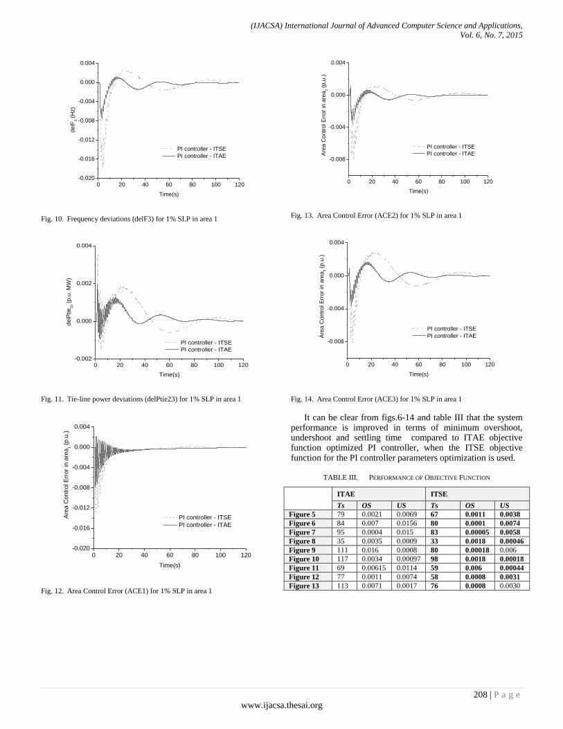
(IJACSA) International Journal of Advanced Computer Science and Applications,
Vol. 6, No. 7, 2015
208 | P a g e
www.ijacsa.thesai.org
0 20 40 60 80 100 120-0.020
-0.016
-0.012
-0.008
-0.004
0.000
0.004
delF
3 (
Hz)
Time(s)
PI controller - ITSE
PI controller - ITAE
Fig. 10. Frequency deviations (delF3) for 1% SLP in area 1
0 20 40 60 80 100 120-0.002
0.000
0.002
0.004
delP
tie
23 (
p.u
. M
W)
Time(s)
PI controller - ITSE
PI controller - ITAE
Fig. 11. Tie-line power deviations (delPtie23) for 1% SLP in area 1
0 20 40 60 80 100 120-0.020
-0.016
-0.012
-0.008
-0.004
0.000
0.004
Are
a C
ontr
ol E
rro
r in
are
a1 (
p.u
.)
Time(s)
PI controller - ITSE
PI controller - ITAE
Fig. 12. Area Control Error (ACE1) for 1% SLP in area 1
0 20 40 60 80 100 120
-0.008
-0.004
0.000
0.004
Are
a C
ontr
ol E
rror
in a
rea
2 (
p.u
.)
Time(s)
PI controller - ITSE
PI controller - ITAE
Fig. 13. Area Control Error (ACE2) for 1% SLP in area 1
0 20 40 60 80 100 120
-0.008
-0.004
0.000
0.004
Are
a C
ontr
ol E
rro
r in
are
a3 (
p.u
.)
Time(s)
PI controller - ITSE
PI controller - ITAE
Fig. 14. Area Control Error (ACE3) for 1% SLP in area 1
It can be clear from figs.6-14 and table III that the system performance is improved in terms of minimum overshoot, undershoot and settling time compared to ITAE objective function optimized PI controller, when the ITSE objective function for the PI controller parameters optimization is used.
TABLE III. PERFORMANCE OF OBJECTIVE FUNCTION
ITAE ITSE
Ts OS US Ts OS US
Figure 5 79 0.0021 0.0069 67 0.0011 0.0038
Figure 6 84 0.007 0.0156 80 0.0001 0.0074
Figure 7 95 0.0004 0.015 83 0.00005 0.0058
Figure 8 35 0.0035 0.0009 33 0.0018 0.00046
Figure 9 111 0.016 0.0008 80 0.00018 0.006
Figure 10 117 0.0034 0.00097 98 0.0018 0.00018
Figure 11 69 0.00615 0.0114 59 0.006 0.00044
Figure 12 77 0.0011 0.0074 58 0.0008 0.0031
Figure 13 113 0.0071 0.0017 76 0.0008 0.0030
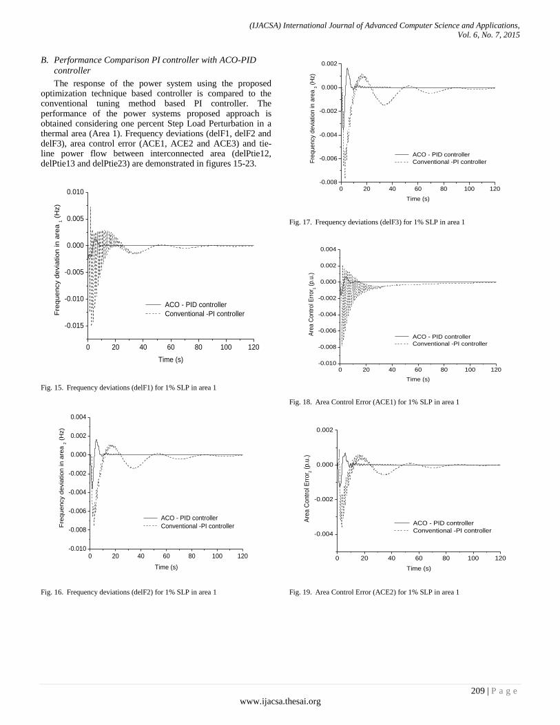
(IJACSA) International Journal of Advanced Computer Science and Applications,
Vol. 6, No. 7, 2015
209 | P a g e
www.ijacsa.thesai.org
B. Performance Comparison PI controller with ACO-PID
controller
The response of the power system using the proposed optimization technique based controller is compared to the conventional tuning method based PI controller. The performance of the power systems proposed approach is obtained considering one percent Step Load Perturbation in a thermal area (Area 1). Frequency deviations (delF1, delF2 and delF3), area control error (ACE1, ACE2 and ACE3) and tie-line power flow between interconnected area (delPtie12, delPtie13 and delPtie23) are demonstrated in figures 15-23.
0 20 40 60 80 100 120
-0.015
-0.010
-0.005
0.000
0.005
0.010
Fre
qu
en
cy d
evia
tion
in a
rea
1 (
Hz)
Time (s)
ACO - PID controller
Conventional -PI controller
Fig. 15. Frequency deviations (delF1) for 1% SLP in area 1
0 20 40 60 80 100 120-0.010
-0.008
-0.006
-0.004
-0.002
0.000
0.002
0.004
Fre
qu
en
cy d
evia
tion
in a
rea
2 (
Hz)
Time (s)
ACO - PID controller
Conventional -PI controller
Fig. 16. Frequency deviations (delF2) for 1% SLP in area 1
0 20 40 60 80 100 120-0.008
-0.006
-0.004
-0.002
0.000
0.002
Fre
quency
devi
ation in a
rea 3 (
Hz)
Time (s)
ACO - PID controller
Conventional -PI controller
Fig. 17. Frequency deviations (delF3) for 1% SLP in area 1
0 20 40 60 80 100 120-0.010
-0.008
-0.006
-0.004
-0.002
0.000
0.002
0.004
Are
a C
ontr
ol E
rror 1 (
p.u
.)
Time (s)
ACO - PID controller
Conventional -PI controller
Fig. 18. Area Control Error (ACE1) for 1% SLP in area 1
0 20 40 60 80 100 120
-0.004
-0.002
0.000
0.002
Are
a C
ontr
ol E
rro
r 2 (p
.u.)
Time (s)
ACO - PID controller
Conventional -PI controller
Fig. 19. Area Control Error (ACE2) for 1% SLP in area 1
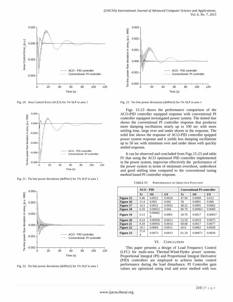
(IJACSA) International Journal of Advanced Computer Science and Applications,
Vol. 6, No. 7, 2015
210 | P a g e
www.ijacsa.thesai.org
0 20 40 60 80 100 120
-0.004
-0.002
0.000
0.002A
rea C
ontr
ol E
rro
r 3 (
p.u
.)
Time (s)
ACO - PID controller
Conventional -PI controller
Fig. 20. Area Control Error (ACE3) for 1% SLP in area 1
0 20 40 60 80 100 120-0.008
-0.006
-0.004
-0.002
0.000
0.002
Tie
-lin
e p
ow
er
flo
w d
evi
ation
in a
rea
1 (
p.u
. M
W)
Time (s)
ACO - PID controller
Conventional -PI controller
Fig. 21. Tie-line power deviations (delPtie1) for 1% SLP in area 1
0 20 40 60 80 100 120-0.002
-0.001
0.000
0.001
0.002
0.003
Tie
-lin
e p
ow
er
flo
w d
evia
tion
in a
rea
2 (
p.u
. M
W)
Time (s)
ACO - PID controller
Conventional -PI controller
Fig. 22. Tie-line power deviations (delPtie2) for 1% SLP in area 1
0 20 40 60 80 100 120-0.002
-0.001
0.000
0.001
0.002
0.003
Tie
-lin
e p
ow
er
flo
w d
evia
tion
in a
rea
3 (
p.u
. M
W)
Time (s)
ACO - PID controller
Conventional -PI controller
Fig. 23. Tie-line power deviations (delPtie3) for 1% SLP in area 1
Figs. 15-23 shows the performance comparison of the ACO-PID controller equipped response with conventional PI controller equipped investigated power system. The dotted line shows the conventional PI controller response that produces more damping oscillations nearly up to 100 sec with more settling time, large over and under shoots in the response. The solid line shows the response of ACO-PID controller quipped power system response and it yields less damping oscillations up to 50 sec with minimum over and under shoot with quickly settled response.
It can be observed and concluded from Figs.15-23 and table IV that using the ACO optimized PID controller implemented in the power system, improvise effectively the performance of the power system in terms of minimum overshoot, undershoot and good settling time compared to the conventional tuning method based PI controller response.
TABLE IV. PERFORMANCE OF OBJECTIVE FUNCTION
ACO - PID Conventional PI controller
Ts OS US Ts OS US
Figure 15 9.46 0.0012 0.0018 47.94 0.0069 0.012
Figure 16 11.4 0.003 0.001 58 0.0001 0.006
Figure 17 14.3 0.0012 0.0032 48.52 0.0005 0.0062
Figure 18 6.59 0.00032 0.004 80.79 0.00063 0.0069
Figure 19 9.13 0.000026
0.0001 30.76 0.0017 0.00057
Figure 20 8.24 0.00058 0.0013 53.59 0.0019 0.0075
Figure 21 8.18 0.00056 0.0014 68.68 0.0017 0.0077
Figure 22 10.1 0.0004 0.0011 43.9 0.0062 0.0028
Figure 23 21.04
0.0073 0.0013 61.29 0.00071 0.0029
VI. CONCLUSION
This paper presents a design of Load Frequency Control (LFC) for multi-area Thermal-Wind-Hydro power systems. Proportional Integral (PI) and Proportional Integral Derivative (PID) controllers are employed to achieve better control performance during the load disturbance. PI Controller gain values are optimized using trial and error method with two

(IJACSA) International Journal of Advanced Computer Science and Applications,
Vol. 6, No. 7, 2015
211 | P a g e
www.ijacsa.thesai.org
different objective functions, namely ITAE and ITSE. The PI controller effectiveness is examined and compared by considering one percent Step Load perturbation in the thermal area (Area 1). Simulation results reveal that, ITSE objective function based controller provides much better result (Less Settling Time, Peak over and undershoot, Damping oscillations) compared to ITAE objective function based controller. Further PID controller gain values are optimized using the ACO algorithm and comparisons between PI controller and ACO tuned controller reveal that the ACO-PID controller effectively reduces the electromechanical oscillations, settling time, peak over and undershoots in the system response compared to conventional PI controller equipped power system response. The proposed approach is can also extended to multi-area (more then three areas) with the addition of more renewable energy resource into the same issue of interconnected power system with different bio-inspired algorithms.
REFERENCES
[1] J. Nandha, and S. Mishra, “A novel classical controller for Automatic generation control in thermal and hydro thermal systems,” PEDES, pp.1-6, 2010.
[2] K. Jagatheesan, and B. Anand, “Dynamic Performance of Multi-Area Hydro Thermal Power Systems with Integral Controller considering various performance Indices methods,” Proceedings of the IEEE International conference of Emerging trends in Science, Engineering and Technology (INCOSET), pp.474-478, 2012.
[3] N. Kumari, and A.N. Jha, “ Particle Swarm Optimization and Gradiend descent mmethods for Optimization pf PI controller for AGC of multi-area Thermal-Wind-Hydro power plants,” 2013 UKSim 15th International conference on computer modeling and simulation, pp. 536-541, 2013.
[4] J. Nanda, A. Mangla, and S. sanjay,” Some New findings on Automatic control of an interconnected hydrothermal system with conventional controllers,” IEEE Trans Energy Convers, vol. 21, pp.187-194, 2006.
[5] B. Anand, and A. Jeyakumar, “Fuzzy Logic load frequency Control of hydro-Thermal system with non-Linearities,” Int.J.Elec.Power Eng, vol. 3, pp. 112-118,2009.
[6] K. Chatterjee, “PI controller for Automatic Generation Control Based on Performance Indices,” World Academy of Science, Engineering and Technology, vol.75, pp.321-356, 2011.
[7] M.L. Kothari, J. Nanda, and P.S.Satsangi, “Automatic generation control of hydrothermal system considering generation rate constraints,” J.Inst.Eng.India, vol.63, pp.289-297, June 1983.
[8] S. kumar, and G. Sharma, “AGC & AVR of interconnected thermal power system while considering the effect of GRCs.” Int.Journal of soft computing and engineering, vol.2, pp.69-74, March 2012.
[9] R. Thottungal, P Anbalagan, “Frequency stabilization in multi area system using HVDC link.” Proceedings of the IEEE, pp.590-595, 2006.
[10] B. Anand, and A. Jeyakumar, “Load Frequency control with Fuzzy logic Controller considering Non-Linearities and Boiler Dynamics,” ACSE, vol8, pp .15-20, January2009.
[11] O.I. Elgerd, “Electric Energy System Theory: An Introduction,” Tata Mc-Graw Hill Publishing company limited,, New York,1970.
[12] I.J. Nagrath, and D.P. Kothari, “Power system engineering,” Tata Mc-Graw Hill Publishing Company limited, 1994, New Delhi, India.
[13] M. Iuian, and N.A.Cutululis, “Opticl control of wind energy systems,” Ist ed., springer-Verlad, londan, pp.93-145, 2008.
[14] P. Kundur, “Power system stability and control,” Tata Mc-Graw Hill Publishing company limited, 1994, New Delhi, India.
[15] J. Nanda, and B.L. Kaul, “Automatic generation control of an interconnected power system,” Proc. IEE, vol.125, pp. 385-390, 1978.
[16] S.C.Tripathy, G.S. Hope, and O.P.Malik, “Optimization of load-frequency control parameters for power systems with reheat steam
turbines and governor dead band nonlinearity,” IEE Proc., vol.129- Pt.C, pp. 10-16, 1982.
[17] S.C.Tripathy, T.S. Bhatti, C.S.Jha, O.P. Malik, and G.S.Hope, “Sampled data automatic generation control analysis with reheat steam turbines and governor dead-band effects,” IEE transactions on power apparatus and systems, Vol.PAS-103, pp.1045-1051, 1984.
[18] J. Nanda, M.L. Kothari, and P.S.Satsangi, “Automatic generation control of an interconnected hydrothermal system in continuous and discrete modes considering generation rate constraints,” IEE proc., vol.130, Pt. D, pp. 17-27, 1983.
[19] M. L. Kothari, and J. Nanda, “Application of optimal control strategy to automatic generation control of a hydrothermal system,” IEE proceedings, Vol.135, Pt.D, pp.268-274, 1988.
[20] C.T. Pan, and C..M. Liaw, “An adaptive controller for power system load-frequency control,’ IEEE transaction on power systems, Vol.4, No.1, pp: 122-128, 1989.
[21] M. Aldeeen, and J.F. Marsh, “Decentralized proportional-plus-integral design method for interconnected power systems,” IEE Proceedings-C, vol.138, pp. 263-274, 1991.
[22] S. Das, M. L. Kothari, D. P. Kothari, and J. Nanda, “ Variable structure control strategy to automatic generation control of interconnected reheat thermal system, IEE proceedings-D , vol. 138, pp.579-585,1991.
[23] K. Jagatheesan, and B. Anand, “ Load frequency control of an interconnected three area reheat thermal power systems considering non linearity and boiler dynamics with conventional controller”, Advances in Natural and Applied Science, ISSN: 1998-1090, vol.8, pp.16-24, 2014.
[24] K. Jagatheesan, and B. Anand, “Automatic Generation Control of Three Area Hydro-Thermal Power Systems considering Electric and Mechanical Governor with conventional and Ant Colony Optimization technique”, Advances in Natural and Applied Science, ISSN: 1998-1090, vol.8, pp.25-33, 2014.
[25] K. Jagatheesan, B. Anand, and M.A. Ebrahim, “Stochastic Particle Swarm Optimization for tuning of PID Controller in Load Frequency Control of Single Area Reheat Thermal Power System”, International Journal of Electrical and Power Engineering, ISSN: 1990-7958, vol.8, pp.33-40, 2014.
[26] P. Dash, L. C. Saikia, and N. Sinha, “Automatic generation control of multi area thermal system using Bat algorithm optimized PD-PID cascade controller,” Electric power and Energy systems, vol.68, pp. 364-372, 2015.
[27] R. Francis, and I.A. Chidambaram, “ Optimized PI+ load-frequency controller using BWNN approach for an interconnected reheat power system with RFB and hydrogen electrolyser units,” Electric power and Energy systems, vol.67, pp. 381-392, 2015.
[28] B. K. Sahu, S. Pati, P. K. Mohanty, and S. Panda, “ Teaching-learning based optimization algorithm based fuzzy-PID controller for automatic generation control of multi-area power system,” Applied Soft Computing, vol.27, pp. 240-249, 2015.
[29] N. Day, S. Samanta, S. Chakraborty, A. Das, S. S. Chaudhuri, and J.S. Suri, “Firefly Algorithm for Optimization of Scaling Factors during Embedding of Manifold Medical Information: An Application in Ophthalmology Imaging,” Journal of Medical Imaging and Health Informatics, vol. 4, pp. 384-394, 2015.
[30] N. Dey, S. Samanta, X. S. Yang, S. S. Chaudhri, and A. Das, “Optimization of Scaling Factors in Electrocardiogram Signal Watermarking using Cuckoo Search,” International Journal of Bio-Inspired Computation (IJBIC), vol. 5, pp. 315-326, 2014.
[31] K. Jagatheesan, B. Anand, and N. Dey, “Automatic generation control of Thermal-Thermal-Hydro power systems with PID controller using ant colony optimization,” International Journal of Service Science, Management, Engineering, and Technology, vol.6, pp. 18-34, 2015.
[32] M. Omar, M. Solimn, A.M. Abdel ghany, and F. Bendary, “Optimal tuning of PID controllers for hydrothermal load frequency control using ant colony optimization,” International journal on electrical engineering and informatics, vol.5, pp. 348-356, 2013.
[33] N. Dey, S. Samanta, X-S. Yang, S. S. Chaudhri, and A. Das, "Optimisation of Scaling Factors in Electrocardiogram Signal Watermarking using Cuckoo Search", International Journal of Bio-Inspired Computation (IJBIC), vol 5, pp-315-326, 2013.

(IJACSA) International Journal of Advanced Computer Science and Applications,
Vol. 6, No. 7, 2015
212 | P a g e
www.ijacsa.thesai.org
[34] S. Samanta, S. Acharjee, A. Mukherjee, D. Das, and N. Dey, “Ant Weight Lifting Algorithm for Image Segmentation,” 2013 IEEE International Conference on Computational Intelligence and Computing Research(ICCIC), pp.1-5, 2013.
[35] S. Acharjee, S. Chakraborty, W. Karaa, A. Azar, and N. Dey, “Performance Evaluation of Different Cost Functions in Motion Vector Estimation” , International Journal of Service Science, Management, Engineering, and Technology (IJSSMET), IGI Global, vol. 5, pp. 1- 21, 2014 .
[36] S. Chowdhuri, S. Chakraborty, N. Dey, M. M. Salem, A. T. Azar, Sheli S. Chaudhury, and P. Banerjee,“ Recent Research on Multi Input Multi Output (MIMO) based Mobile ad hoc Network: A Review”, International Journal of Service Science, Management, Engineering, and Technology (IJSSMET), IGI Global, vol. 5, pp. 54-65, 2014.
[37] W. Karaa, A.S. Ashour, D. Ben Sassi, P. Roy, N. Kausar, and N. Dey, “MEDLINE Text Mining: An Enhancement Genetic Algorithm based Approach for Document Clustering, Applications of Intelligent Optimization in Biology and Medicine: Current Trends and Open Problems," In book: Applications of Intelligent Optimization in Biology and Medicine:Current Trends and Open Problems, Springer, Chapter 10, 2015.
[38] S. Samanta, N. Dey, P. Das, S. Acharjee, and S. S. Chaudhuri, “Multilevel Threshold Based Gray Scale Image Segmentation using Cuckoo Search”, International Conference on Emerging Trends in Electrical, Communication And Information Technologies -ICECIT, Dec 12-23, 2012,
[39] S. Chakraborty, A. K. Pal, N. Dey, D. Das, and S. Acharjee, “Foliage Area Computation using Monarch Butterfly Algorithm,” 2014 International Conference on Non Conventional Energy (ICONCE 2014), JIS college of Engineering, Kalyani, January 16-17, 2014.
[40] S. Chakraborty, S. Samanta, A. Mukherjee, N. Dey, and S. S. Chaudhuri “Particle Swarm Optimization Based Parameter Optimization Technique in Medical Information Hiding”, 2013 IEEE International Conference on Computational Intelligence and Computing Research(ICCIC), Madurai, Dec . 2013.
[41] S. Samanta, S. Acharjee, A. Mukherjee, D. Das, and N. Dey, “Ant Weight Lifting Algorithm for Image Segmentation”, 2013 IEEE International Conference on Computational Intelligence and Computing Research(ICCIC), Madurai, Dec. 2013.
[42] S. Samanta, S. Chakraborty, S. Acharjee, A. Mukherjee, and N. Dey, “Solving 0/1 Knapsack Problem using Ant Weight Lifting Algorithm”, 2013 IEEE International Conference on Computational Intelligence and Computing Research(ICCIC), Madurai, Dec. 2013.

(IJACSA) International Journal of Advanced Computer Science and Applications,
Vol. 6, No. 7, 2015
213 | P a g e
www.ijacsa.thesai.org
New 2-D Adaptive K-Best Sphere Detection for
Relay Nodes
Ahmad El-Banna*1,2
1Electrical Eng. department, Faculty of Engineering at Shoubra, Benha Univ., Egypt.
2ECE department, Egypt-Japan University of Science and Technology (E-JUST), Alexandria, Egypt
Abstract—Relay nodes are the main players of cooperative
networks that used to improve the system performance and to
offer virtual multiple antennas for limited antenna devices in a
multi-user environment. However, employing relaying strategies
requires considerable resources at the relay side and places a
large burden on the relay helping node especially when
considering the power consumption. Partial detection at the relay
is one strategy that reduces the computational load and power
consumption. In this paper, we propose a new 2-D Adaptive K-
Best Sphere Decoder (2-D AKBSD) for partial detection to be
used MISO relays in cooperative networks. Simulation results
show that 2-D AKBSD is capable of improving the system
performance and also reduces its complexity.
Keywords—Sphere Detection; K-Best; Relay; MIMO; MISO;
Cooperative Communication
I. INTRODUCTION
Cooperative networks enhance the performance of the communication system by increasing the transmission data rate making use of the cooperative diversity property. It removes the need for installing multiple antennas at the network nodes which may be in many cases impractical due to size, hardware complexity and/or power limitations [1]-[6]. Cooperative networks can also be used to extend the network coverage area and to reduce the transmit power [7].
To utilize the cooperative networks merits, cooperation protocols need to be employed, two main protocols have been widely adopted for relaying. The first one is “Amplify and Forward” (AF) in which the received signal is amplified at the relay and then forwarded to the destination. The second one is “Detect” or “Decode and Forward” (DF) in which the received signal is detected and then decoded and forwarded to the destination. DF gives better performance than the simpler AF scheme, a property that made DF the favorable relaying protocol for multihop system suffering from incremental loss of performance per hop [7]. However, DF requires more processing and consumes considerable resources at the relay. Hence, the relay consumed power is increased causing a problem in many cases, e.g. an idle mobile MIMO user may not choose to operate as a relay in DF mode due to its limited battery power.
Partial Detection (PD) at the relay can reduce the complexity of the decoding by detecting only part of the received signal, depending on its available resources, then forwarding it. The destination combines both the source signal and the partial relay signal to recover the transmitted signal [8]. However, PD performance is poor when the number of the
detected symbols at the relay is small [7], [8]. The PD in [8] modifies the tree search of the tree-based sphere detector depending on the relay available resources to include only some levels of the tree instead of all tree levels in the case of Full Detect and Forward (FDF); we name this a change in the number of vertical levels in a tree search.
The partial sphere detection scheme proposed in [8] was employed for the spatial multiplexing transmission technique in a MIMO wireless communication. In this work, we utilize it for transmit antenna diversity techniques by employing the Alamouti and the Golden codewords in a time varying environment.
In this paper, we propose a new idea that allows a change in the two dimensions of the tree during the tree traversal to give more complexity reduction at the relay node. The first dimension is the horizontal dimension, in which we change the number of the visited nodes per level depending on some criteria [9] e.g. the channel quality. The second dimension to change is the vertical dimension in which the number of the explored tree levels is chosen depending on the source-relay link capacity, besides this change is adaptive depending on the current state of the network environment specifically the channel and link qualities in the network. The proposed detector, namely 2-D AKBSD, gives a considerable complexity reduction in the relay and destination nodes.
The rest of the paper is organized as follows; Section II describes the network and system model of the 2×1 MISO scenarios that was used to verify the 2-D AKBSD. Section III illustrates how the 2-D AKBSD can be used as the decoding strategy in the 2×1 relay. Section IV shows the simulation results and finally, section V concludes the paper.
II. NETWORK AND SYSTEM MODELS
Following the same system model notations in [8], we consider a 3 nodes wireless network with one Source node (S) that cooperate with one Relay node (R) assisting in data transmission to one Destination node (D). The distance between the S and D nodes is denoted as dsd while dsr and drd define the distances between the S-R and R-D nodes respectively. Each node is equipped with Nt and Nr
transmitting and receiving antennas respectively. We studied the MISO case with Nt =2 and Nr =1. The transmission is
assumed to be executed over two phasesТ1 and Т2. We
assume a half-duplex communication i.e. nodes can only transmit or receive at the same instance, and consider a Rayleigh time-varying fading channel, a case where linear
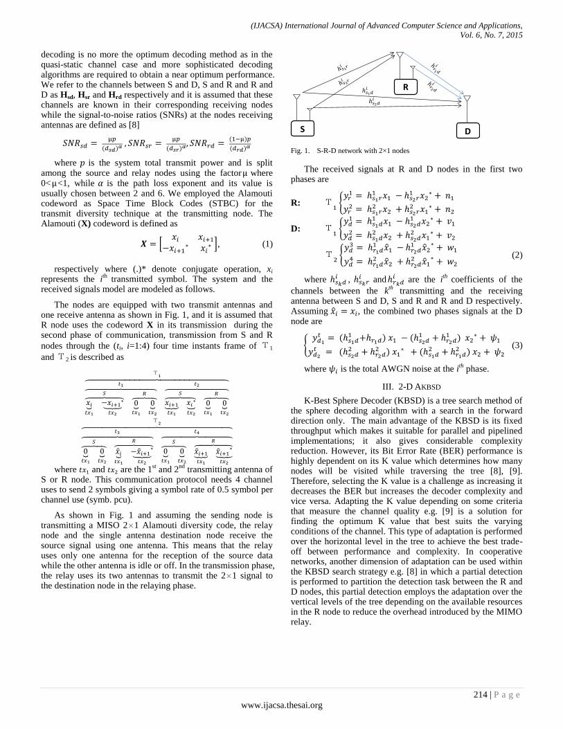
(IJACSA) International Journal of Advanced Computer Science and Applications,
Vol. 6, No. 7, 2015
214 | P a g e
www.ijacsa.thesai.org
decoding is no more the optimum decoding method as in the quasi-static channel case and more sophisticated decoding algorithms are required to obtain a near optimum performance. We refer to the channels between S and D, S and R and R and D as Hsd, Hsr and Hrd respectively and it is assumed that these channels are known in their corresponding receiving nodes while the signal-to-noise ratios (SNRs) at the nodes receiving antennas are defined as [8]
where is the system total transmit power and is split among the source and relay nodes using the factor where 0< <1, while is the path loss exponent and its value is usually chosen between 2 and 6. We employed the Alamouti codeword as Space Time Block Codes (STBC) for the transmit diversity technique at the transmitting node. The Alamouti (X) codeword is defined as
[
], (1)
respectively where (.)* denote conjugate operation, xi
represents the ith
transmitted symbol. The system and the received signals model are modeled as follows.
The nodes are equipped with two transmit antennas and one receive antenna as shown in Fig. 1, and it is assumed that R node uses the codeword X in its transmission during the second phase of communication, transmission from S and R
nodes through the (ti, i=1:4) four time instants frame of Т1
and Т2 is described as
⏟
⏟
⏞
⏟
⏟
⏞ ⏞
⏟
⏟
⏞
⏟
⏟
⏞ ⏞
⏞
Т
⏟
⏟
⏞
⏟
⏟
⏞ ⏞
⏟
⏟
⏞
⏟
⏟
⏞ ⏞
⏞
Т
where and are the 1st and 2
nd transmitting antenna of
S or R node. This communication protocol needs 4 channel uses to send 2 symbols giving a symbol rate of 0.5 symbol per channel use (symb. pcu).
As shown in Fig. 1 and assuming the sending node is transmitting a MISO 2×1 Alamouti diversity code, the relay node and the single antenna destination node receive the source signal using one antenna. This means that the relay uses only one antenna for the reception of the source data while the other antenna is idle or off. In the transmission phase, the relay uses its two antennas to transmit the 2×1 signal to the destination node in the relaying phase.
Fig. 1. S-R-D network with 2×1 nodes
The received signals at R and D nodes in the first two phases are
R: Т {
D: Т {
Т {
(2)
where ,
and are the i
th coefficients of the
channels between the kth
transmitting and the receiving antenna between S and D, S and R and R and D respectively. Assuming , the combined two phases signals at the D node are
{
(3)
where is the total AWGN noise at the ith
phase.
III. 2-D AKBSD
K-Best Sphere Decoder (KBSD) is a tree search method of the sphere decoding algorithm with a search in the forward direction only. The main advantage of the KBSD is its fixed throughput which makes it suitable for parallel and pipelined implementations; it also gives considerable complexity reduction. However, its Bit Error Rate (BER) performance is highly dependent on its K value which determines how many nodes will be visited while traversing the tree [8], [9]. Therefore, selecting the K value is a challenge as increasing it decreases the BER but increases the decoder complexity and vice versa. Adapting the K value depending on some criteria that measure the channel quality e.g. [9] is a solution for finding the optimum K value that best suits the varying conditions of the channel. This type of adaptation is performed over the horizontal level in the tree to achieve the best trade-off between performance and complexity. In cooperative networks, another dimension of adaptation can be used within the KBSD search strategy e.g. [8] in which a partial detection is performed to partition the detection task between the R and D nodes, this partial detection employs the adaptation over the vertical levels of the tree depending on the available resources in the R node to reduce the overhead introduced by the MIMO relay.
S
R
D

(IJACSA) International Journal of Advanced Computer Science and Applications,
Vol. 6, No. 7, 2015
215 | P a g e
www.ijacsa.thesai.org
vertical level adaptation determines how many tree levels
will be explored
horizontal level adaptation determines how many nodes per level will be
explored Fig. 2. Tree structure for 2-D AKBSD shows the horizontal and vertical
adaptation
The 2-D AKBSD makes use of the two vertical and horizontal dimensions of the adaptation process in the R node to suit the dynamic conditions of the network. As shown in Fig.2, some criteria specify how many tree levels will be explored and how many nodes per level will be visited while traversing the tree. Adaptation criterion in horizontal dimension can be selectivity of the channel or channel matrix analysis as measures of channel quality i.e. selecting low or high K value depending on the quality of the channel or an estimation of SNR value as in [9] while vertical dimension adaptation can be done based on available resources in the relay as in [8], received signal strength or the instantaneous capacity measurement as a measure of the S-R link outage. In this paper, we select the channel selectivity as a channel quality estimation and the instantaneous capacity measurement as the adaptation criteria for the horizontal and vertical dimensions respectively. To measure the channel selectivity, we calculate a parameter as [9]
(4)
where and are two adjacent coefficients of the
time-varying channel i between any two nodes in the network. And if Ci is greater than a defined threshold Γ then the channel is very frequency selective and hence the channel quality is good and vice versa. The instantaneous capacity can be used as one metric that indicate the channel state information as a measure for the S-R link quality and can be calculated as [10]
(5)
where Ex is the transmitted signal energy and N0 is the noise power spectral density.
The 2-D AKBSD adds a pre-process part over the regular KBSD and hence it has the advantages of the KBSD, besides the advantage of being adapted based on the system dynamic conditions. The algorithm of the 2-D AKBSD is as follows:
for each pair of symbols of the frame NS, do:
Preprocess:
Calculate ρi∀i=1:4 ; j=1:NS-1;
if all ρi > Γ then ka=k1;
else if three of ρi > Γ then ka=k2;
else if two of ρi > Γ then ka=k3;
else ka=k4;
end if
calculate C ;
using δk <δk+1 , k=1:v levels ;
if C <δ1 then lt =1;
else if C <δ2 then lt =2;
…
else lt =v;
end if
Search the tree:
start from root level
initialize a zero metric path between the root and the first tree level
nodes
loop:
extend the survivor paths and update their PEDs
sort and select the ka Best PEDs and discard the others
if lt level reached then exit
else go back to loop
end if
end
A. The detection strategy
For conventional FDF, both R and D nodes performs full detection of all the symbols using regular KBSD while for PD, the R node applies the 2-D AKBSD to detect part of the transmitted symbols, this part is determined based on the S-R
link capacity, and inТ2, R transmits the detected signals to the
D node which uses 2-D AKBSD with horizontal adaptation only to retrieve the original signals.
B. Single antenna relay in MISO environment
A major advantage of the partial sphere detection is using a single antenna relay in a MISO transmission, using the codeword sent from the S node, R node can make horizontal adaptation and fix the vertical levels traversing to the half of the tree levels to send only half the symbols by its single antenna. In this manner, we can make use of an idle single antenna device to assist in data transmission in a 2×1 MISO protocol as shown in Fig. 3. This lifts the constraints of only involving multiple antennas relays in the transmission. Moreover, this will increase the data rate as we need only 3 channel uses instead of 4 giving symbol rate of 2/3 symb. pcu.
Fig. 3. Single antenna relay in 2×1 MISO protocol
IV. SIMULATION RESULTS
We suppose half-duplex communication in a 3 node wireless relay network topology as shown in Fig. 1. We assume that the R node is in-between the S and D nodes with dsd =dsr + drd =1, fixing dsr = 0.35, and also we used fixed
values of =3, =0.6 and =1. We work on 16-QAM
modulation scheme and assumed that Hsd, Hsr and Hrd are Rayleigh time-varying fading channels i.e. their coefficients are not constant during the transmission of the codeword elements as in the case of quasi-static channels. Monte Carlo simulations were used to calculate the BER values in the R
Phase
Time
Slot
Transmit
NodeS S R
__ S
R
D
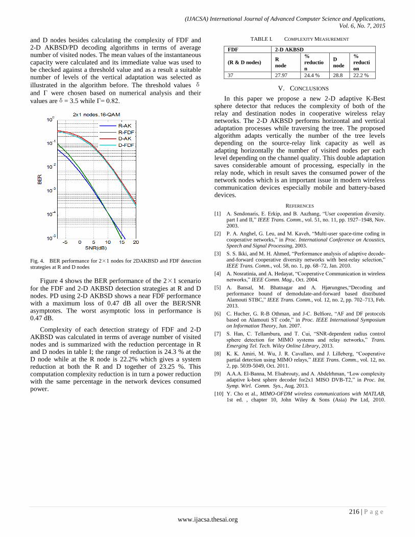
(IJACSA) International Journal of Advanced Computer Science and Applications,
Vol. 6, No. 7, 2015
216 | P a g e
www.ijacsa.thesai.org
and D nodes besides calculating the complexity of FDF and 2-D AKBSD/PD decoding algorithms in terms of average number of visited nodes. The mean values of the instantaneous capacity were calculated and its immediate value was used to be checked against a threshold value and as a result a suitable number of levels of the vertical adaptation was selected as
illustrated in the algorithm before. The threshold values δ
and Γ were chosen based on numerical analysis and their
values areδ= 3.5 while Γ= 0.82.
Fig. 4. BER performance for 2×1 nodes for 2DAKBSD and FDF detection
strategies at R and D nodes
Figure 4 shows the BER performance of the 2×1 scenario for the FDF and 2-D AKBSD detection strategies at R and D nodes. PD using 2-D AKBSD shows a near FDF performance with a maximum loss of 0.47 dB all over the BER/SNR asymptotes. The worst asymptotic loss in performance is 0.47 dB.
Complexity of each detection strategy of FDF and 2-D AKBSD was calculated in terms of average number of visited nodes and is summarized with the reduction percentage in R and D nodes in table I; the range of reduction is 24.3 % at the D node while at the R node is 22.2% which gives a system reduction at both the R and D together of 23.25 %. This computation complexity reduction is in turn a power reduction with the same percentage in the network devices consumed power.
TABLE I. COMPLEXITY MEASUREMENT
FDF 2-D AKBSD
(R & D nodes) R
node
%
reductio
n
D
node
%
reducti
on
37 27.97 24.4 % 28.8 22.2 %
V. CONCLUSIONS
In this paper we propose a new 2-D adaptive K-Best sphere detector that reduces the complexity of both of the relay and destination nodes in cooperative wireless relay networks. The 2-D AKBSD performs horizontal and vertical adaptation processes while traversing the tree. The proposed algorithm adapts vertically the number of the tree levels depending on the source-relay link capacity as well as adapting horizontally the number of visited nodes per each level depending on the channel quality. This double adaptation saves considerable amount of processing, especially in the relay node, which in result saves the consumed power of the network nodes which is an important issue in modern wireless communication devices especially mobile and battery-based devices.
REFERENCES
[1] A. Sendonaris, E. Erkip, and B. Aazhang, “User cooperation diversity. part I and II,” IEEE Trans. Comm., vol. 51, no. 11, pp. 1927–1948, Nov. 2003.
[2] P. A. Anghel, G. Leu, and M. Kaveh, “Multi-user space-time coding in cooperative networks,” in Proc. International Conference on Acoustics, Speech and Signal Processing, 2003.
[3] S. S. Ikki, and M. H. Ahmed, “Performance analysis of adaptive decode-and-forward cooperative diversity networks with best-relay selection,” IEEE Trans. Comm., vol. 58, no. 1, pp. 68–72, Jan. 2010.
[4] A. Nosratinia, and A. Hedayat, “Cooperative Communication in wireless networks,” IEEE Comm. Mag., Oct. 2004.
[5] A. Bansal, M. Bhatnagar and A. Hjørungnes,“Decoding and performance bound of demodulate-and-forward based distributed Alamouti STBC,” IEEE Trans. Comm., vol. 12, no. 2, pp. 702–713, Feb. 2013.
[6] C. Hucher, G. R-B Othman, and J-C. Belfiore, “AF and DF protocols based on Alamouti ST code,” in Proc. IEEE International Symposium on Information Theory, Jun. 2007.
[7] S. Han, C. Tellambura, and T. Cui, “SNR-dependent radius control sphere detection for MIMO systems and relay networks,” Trans. Emerging Tel. Tech. Wiley Online Library, 2013.
[8] K. K. Amiri, M. Wu, J. R. Cavallaro, and J. Lilleberg, “Cooperative partial detection using MIMO relays,” IEEE Trans. Comm., vol. 12, no. 2, pp. 5039-5049, Oct. 2011.
[9] A.A.A. El-Banna, M. Elsabrouty, and A. Abdelrhman, “Low complexity adaptive k-best sphere decoder for2x1 MISO DVB-T2,” in Proc. Int. Symp. Wirl. Comm. Sys., Aug. 2013.
[10] Y. Cho et al., MIMO-OFDM wireless communications with MATLAB, 1st ed. , chapter 10, John Wiley & Sons (Asia) Pte Ltd, 2010.

Geographic Routing Using Logical Levels inWireless Sensor Networks for Sensor Mobility
Yassine SABRI
NTIC Laboratory,Higher Institute of Applied Engineering (IGA),
El Jadida MOROCCO
Najib EL KAMOUN
STIC Laboratory,Chouaib Doukkali University,
El Jadida MOROCCO
Abstract—In this paper we propose an improvement to theGRPW algorithm for wireless sensor networks called GRPW-M , which collects data in a wireless sensor network (WSN)using a mobile nodes. Performance of GRPW algorithm algorithmdepends heavily on the immobile sensor nodes . This predictioncan be hard to do. For that reason, we propose a modifiedalgorithm that is able to adapt to the current situation in thenetwork in which the sensor node considered mobile. The goalof the proposed algorithm is to decrease the reconstructioncost and increase the data delivery ratio. In comparing theGRPW-M protocol with GRPW protocol in simulation, this paperdemonstrates that adjustment process executed by GRPW-M doesin fact decrease the reconstruction cost and increase the datadelivery ratio . Simulations were performed on GRPW as wellas on the proposed Routing algorithm. The efficiency factorsthat were evaluated was total number of transmissions in thenetwork and total delivery rate. And in general the proposedRouting algorithm may perform reasonable well for a largenumber network setups.
Keywords—WSN ; Routing ; Ad hoc ; Localization ; Scalability
I. INTRODUCTION
Remarkable advances have been made in micro-electronicsmechanical system (MEMS) and wirelesscommunication technologies. This development has enabledsensors to collect contexts from the real world. Many sensornodes compose a wireless sensor network (WSN) that detectsdata regarding a physiological change or the presence ofvarious chemical or biological materials. An external device,called a base station or a sink, such as a mobile device or amobile robot, is used to detect events and collect data fromthe sensing environment. One or multiple mobile sinks movethroughout the WSN to gather data coming from all nodes.There is a lot of research on the moving strategy of mobilesinks [1], [2], [3], [4] . Almost all of them use the routingbased on the physical locations of nodes for data transmission. It is important to choose a routing protocol for WSN witha mobile sink, because the efficient routing paths betweenthe sensor node and the sink change with time. The greedyforwarding is a candidate because it is simple and efficientabout data transmission in WSN. In greedy forwarding, eachnode just needs to know three pieces of information: itslocation, the location of neighbors, and the location of thesink. In the WSN with mobile sink, the first two pieces
are fixed and the location of the sink could be broadcastedto the nodes with a virtual backbone [9]. However, greedyforwarding may lead into a dead end when there is noneighbor closer to the destination, and recovery strategy suchas GPSR [10] is necessary to guaranty data packets can bedelivered to the destination.
Research in WSN has developed fast during the last coupleof years and has made the implementation of WSN feasible.However the cost and the size of the nodes in the networkshave to be lowered to make the WSN attractive to be used inmainstream applications.Wireless Sensor Networks (WSN) are constituted of a largenumber of tiny sensor nodes randomly distributed over ageographical region whose power consumption is low. How-ever, as shown in current research [5] , the classical rout-ing protocols are not applicable to sensor networks in areal environment,mainly because of specific radio conditions.Noise, interference, collisions and the volatility of the nodeneighborhood leading to a significant drop in performance.Many applications for sensor networks such as monitoring offorest fires, the remote meter reading,...For these cases,The Ge-ographic routing of data in this type of network is an importantchallenge, Geographic routing uses nodes locations as theiraddresses, and forwards packets (when possible) in a greedymanner towards the destination. Since location information isoften available to all nodes in a sensor network (if not directly,then through a network localization algorithm) in order to pro-vide location-stamped data or satisfy location-based queries,geographic routing techniques are often a natural choice.
II. RELATED WORK AND BACKGROUND
Various routing protocols have been proposed for theWSNs with mobile sinks. In [12], Nazir proposes the MobileSink based Routing Protocol (MSRP) in which the sinkmovement strategy depend on the residual energy informationfrom the cluster-heads and takes the movement based onthe residual energy of the cluster-heads [12]. In the LocalUpdate-based Routing Protocol (LURP) [13], a broadcastprotocol is proposed to resolve the problem that frequentlocation updates from the sink can lead to both rapid energyconsumption of the sensor nodes and increased collisions inwireless transmissions . The most widely known proposal is[6][7], but several other geographic routing schemes have beenproposed [8] One of the key challenges in geographic routing
(IJACSA) International Journal of Advanced Computer Science and Applications,
Vol. 6, No. 7, 2015
217 | P a g ewww.ijacsa.thesai.org
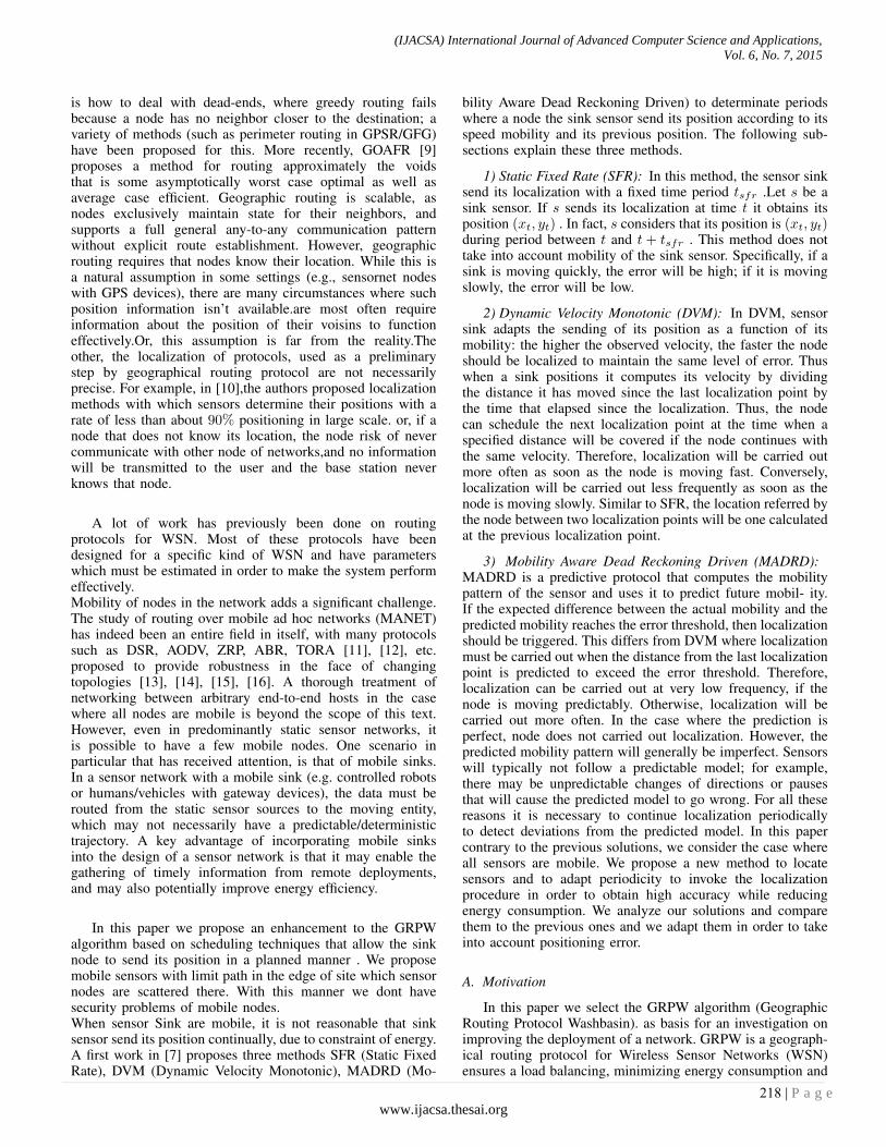
is how to deal with dead-ends, where greedy routing failsbecause a node has no neighbor closer to the destination; avariety of methods (such as perimeter routing in GPSR/GFG)have been proposed for this. More recently, GOAFR [9]proposes a method for routing approximately the voidsthat is some asymptotically worst case optimal as well asaverage case efficient. Geographic routing is scalable, asnodes exclusively maintain state for their neighbors, andsupports a full general any-to-any communication patternwithout explicit route establishment. However, geographicrouting requires that nodes know their location. While this isa natural assumption in some settings (e.g., sensornet nodeswith GPS devices), there are many circumstances where suchposition information isn’t available.are most often requireinformation about the position of their voisins to functioneffectively.Or, this assumption is far from the reality.Theother, the localization of protocols, used as a preliminarystep by geographical routing protocol are not necessarilyprecise. For example, in [10],the authors proposed localizationmethods with which sensors determine their positions with arate of less than about 90% positioning in large scale. or, if anode that does not know its location, the node risk of nevercommunicate with other node of networks,and no informationwill be transmitted to the user and the base station neverknows that node.
A lot of work has previously been done on routingprotocols for WSN. Most of these protocols have beendesigned for a specific kind of WSN and have parameterswhich must be estimated in order to make the system performeffectively.Mobility of nodes in the network adds a significant challenge.The study of routing over mobile ad hoc networks (MANET)has indeed been an entire field in itself, with many protocolssuch as DSR, AODV, ZRP, ABR, TORA [11], [12], etc.proposed to provide robustness in the face of changingtopologies [13], [14], [15], [16]. A thorough treatment ofnetworking between arbitrary end-to-end hosts in the casewhere all nodes are mobile is beyond the scope of this text.However, even in predominantly static sensor networks, itis possible to have a few mobile nodes. One scenario inparticular that has received attention, is that of mobile sinks.In a sensor network with a mobile sink (e.g. controlled robotsor humans/vehicles with gateway devices), the data must berouted from the static sensor sources to the moving entity,which may not necessarily have a predictable/deterministictrajectory. A key advantage of incorporating mobile sinksinto the design of a sensor network is that it may enable thegathering of timely information from remote deployments,and may also potentially improve energy efficiency.
In this paper we propose an enhancement to the GRPWalgorithm based on scheduling techniques that allow the sinknode to send its position in a planned manner . We proposemobile sensors with limit path in the edge of site which sensornodes are scattered there. With this manner we dont havesecurity problems of mobile nodes.When sensor Sink are mobile, it is not reasonable that sinksensor send its position continually, due to constraint of energy.A first work in [7] proposes three methods SFR (Static FixedRate), DVM (Dynamic Velocity Monotonic), MADRD (Mo-
bility Aware Dead Reckoning Driven) to determinate periodswhere a node the sink sensor send its position according to itsspeed mobility and its previous position. The following sub-sections explain these three methods.
1) Static Fixed Rate (SFR): In this method, the sensor sinksend its localization with a fixed time period tsfr .Let s be asink sensor. If s sends its localization at time t it obtains itsposition (xt, yt) . In fact, s considers that its position is (xt, yt)during period between t and t+ tsfr . This method does nottake into account mobility of the sink sensor. Specifically, if asink is moving quickly, the error will be high; if it is movingslowly, the error will be low.
2) Dynamic Velocity Monotonic (DVM): In DVM, sensorsink adapts the sending of its position as a function of itsmobility: the higher the observed velocity, the faster the nodeshould be localized to maintain the same level of error. Thuswhen a sink positions it computes its velocity by dividingthe distance it has moved since the last localization point bythe time that elapsed since the localization. Thus, the nodecan schedule the next localization point at the time when aspecified distance will be covered if the node continues withthe same velocity. Therefore, localization will be carried outmore often as soon as the node is moving fast. Conversely,localization will be carried out less frequently as soon as thenode is moving slowly. Similar to SFR, the location referred bythe node between two localization points will be one calculatedat the previous localization point.
3) Mobility Aware Dead Reckoning Driven (MADRD):MADRD is a predictive protocol that computes the mobilitypattern of the sensor and uses it to predict future mobil- ity.If the expected difference between the actual mobility and thepredicted mobility reaches the error threshold, then localizationshould be triggered. This differs from DVM where localizationmust be carried out when the distance from the last localizationpoint is predicted to exceed the error threshold. Therefore,localization can be carried out at very low frequency, if thenode is moving predictably. Otherwise, localization will becarried out more often. In the case where the prediction isperfect, node does not carried out localization. However, thepredicted mobility pattern will generally be imperfect. Sensorswill typically not follow a predictable model; for example,there may be unpredictable changes of directions or pausesthat will cause the predicted model to go wrong. For all thesereasons it is necessary to continue localization periodicallyto detect deviations from the predicted model. In this papercontrary to the previous solutions, we consider the case whereall sensors are mobile. We propose a new method to locatesensors and to adapt periodicity to invoke the localizationprocedure in order to obtain high accuracy while reducingenergy consumption. We analyze our solutions and comparethem to the previous ones and we adapt them in order to takeinto account positioning error.
A. Motivation
In this paper we select the GRPW algorithm (GeographicRouting Protocol Washbasin). as basis for an investigation onimproving the deployment of a network. GRPW is a geograph-ical routing protocol for Wireless Sensor Networks (WSN)ensures a load balancing, minimizing energy consumption and
(IJACSA) International Journal of Advanced Computer Science and Applications,
Vol. 6, No. 7, 2015
218 | P a g ewww.ijacsa.thesai.org
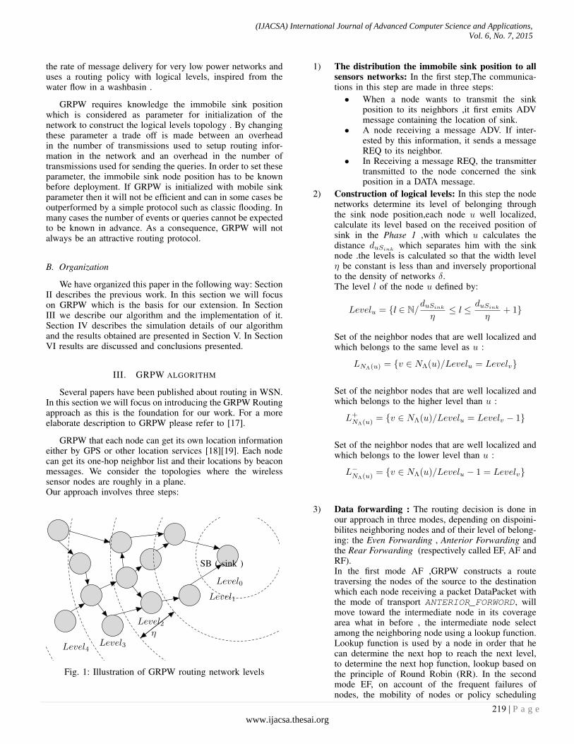
the rate of message delivery for very low power networks anduses a routing policy with logical levels, inspired from thewater flow in a washbasin .
GRPW requires knowledge the immobile sink positionwhich is considered as parameter for initialization of thenetwork to construct the logical levels topology . By changingthese parameter a trade off is made between an overheadin the number of transmissions used to setup routing infor-mation in the network and an overhead in the number oftransmissions used for sending the queries. In order to set theseparameter, the immobile sink node position has to be knownbefore deployment. If GRPW is initialized with mobile sinkparameter then it will not be efficient and can in some cases beoutperformed by a simple protocol such as classic flooding. Inmany cases the number of events or queries cannot be expectedto be known in advance. As a consequence, GRPW will notalways be an attractive routing protocol.
B. Organization
We have organized this paper in the following way: SectionII describes the previous work. In this section we will focuson GRPW which is the basis for our extension. In SectionIII we describe our algorithm and the implementation of it.Section IV describes the simulation details of our algorithmand the results obtained are presented in Section V. In SectionVI results are discussed and conclusions presented.
III. GRPW ALGORITHM
Several papers have been published about routing in WSN.In this section we will focus on introducing the GRPW Routingapproach as this is the foundation for our work. For a moreelaborate description to GRPW please refer to [17].
GRPW that each node can get its own location informationeither by GPS or other location services [18][19]. Each nodecan get its one-hop neighbor list and their locations by beaconmessages. We consider the topologies where the wirelesssensor nodes are roughly in a plane.Our approach involves three steps:
Level0
Level1
Level2
Level3Level4
SB ( sink )
η
Fig. 1: Illustration of GRPW routing network levels
1) The distribution the immobile sink position to allsensors networks: In the first step,The communica-tions in this step are made in three steps:• When a node wants to transmit the sink
position to its neighbors ,it first emits ADVmessage containing the location of sink.
• A node receiving a message ADV. If inter-ested by this information, it sends a messageREQ to its neighbor.
• In Receiving a message REQ, the transmittertransmitted to the node concerned the sinkposition in a DATA message.
2) Construction of logical levels: In this step the nodenetworks determine its level of belonging throughthe sink node position,each node u well localized,calculate its level based on the received position ofsink in the Phase 1 ,with which u calculates thedistance duSink
which separates him with the sinknode .the levels is calculated so that the width levelη be constant is less than and inversely proportionalto the density of networks δ.The level l of the node u defined by:
Levelu = {l ∈ N/duSink
η≤ l ≤ duSink
η+ 1}
Set of the neighbor nodes that are well localized andwhich belongs to the same level as u :
LNΛ(u) = {v ∈ NΛ(u)/Levelu = Levelv}
Set of the neighbor nodes that are well localized andwhich belongs to the higher level than u :
L+NΛ(u) = {v ∈ NΛ(u)/Levelu = Levelv − 1}
Set of the neighbor nodes that are well localized andwhich belongs to the lower level than u :
L−NΛ(u) = {v ∈ NΛ(u)/Levelu − 1 = Levelv}
3) Data forwarding : The routing decision is done inour approach in three modes, depending on dispoini-bilites neighboring nodes and of their level of belong-ing: the Even Forwarding , Anterior Forwarding andthe Rear Forwarding (respectively called EF, AF andRF).In the first mode AF ,GRPW constructs a routetraversing the nodes of the source to the destinationwhich each node receiving a packet DataPacket withthe mode of transport ANTERIOR_FORWORD, willmove toward the intermediate node in its coveragearea what in before , the intermediate node selectamong the neighboring node using a lookup function.Lookup function is used by a node in order that hecan determine the next hop to reach the next level,to determine the next hop function, lookup based onthe principle of Round Robin (RR). In the secondmode EF, on account of the frequent failures ofnodes, the mobility of nodes or policy scheduling
(IJACSA) International Journal of Advanced Computer Science and Applications,
Vol. 6, No. 7, 2015
219 | P a g ewww.ijacsa.thesai.org

of activities used, disconnections can occur in thenetwork generates, so, what are called holes in thissituation, GRPW will change the routing mode toEVEN_FORWORD to reroute the packet in EF modeand to overcome the void case. In the third mode RF,GRPW reroute the packet DataPacket, who was failedin AF and EF, RF fact sends a packet to the low levelL−NΛ() by seeking the next hop among neighboring
based on the lookup function. RF is leaning on sametechnique used in EF, for avoids the routing loop wesafeguard the sets of node traversed by the packetDataPacket in a vector-type structure
IV. GRPW-M: ADAPTIVE ROUTING FOR SENSORMOBILITY IN WSNS
Let us now consider the use of GRPW in a sensornetwork with static nodes and a single mobile sink. If thesink moves, its virtual level will change, and the messagesrouted to the old coordinates will not reach the sink. A simplesolution would be to notify all the nodes about the sinks newcoordinates. This solution, however is expensive in termsof the number of messages, and the corresponding energyconsumption.The GRPW-M algorithm takes an idea which had beensuccessfully applied to geographical routing to reduce thenumber of update messages necessary to maintain routability.The general idea is that as long as the sink moves inside alimited local level area, the nodes outside that level area willnot be notified about the sinks movement. The routing willrely on the nodes at the periphery of the level area to forwardthe messages to the sink. Thus, the local area will be definedas all the nodes which are belong to the same level to theinitial location of the sink :
Note, however, that the current location of the mobile sinkmight be different . Defining the local level area, we say thatthe sink can make two different types of moves:
• a local move keeps the sink inside the local levelarea. In this case, the sink will update only the nodesinside the local level about its new location usingone of the scheduling methods previously presentedSFR,MADRD or DVM, and the local level area willnot change.
• in an external move the sink leaves the current locallevel area . As a result, the sink must create a newlocal level area (see Figure 1) and (b) notify the wholenetwork about its new virtual coordinates and newlocal level area .
GRPW-M uses three type of messages: (a) LOCAL messagescarry updates about the local moves of the sink and they arebroadcasted only within the confines of the local level area ,(b) EXTERNAL messages carry updates about the externalmove of the sink and they are broadcasted to the whole areaand (c) SENSING messages which carry data collected by thenetwork, and are transmitted by hop-by-hop transmission fromthe nodes to the sink (whichever its current location it may be)
Fig. 2: Illustration of GRPW-M routing network
V. SIMULATION
In this section, details about how the simulations werecarried out are presented. Using a simulator J-Sim based on theJava programming language, which is able to simulate GRPW-M routing as well as the original routing GRPW .
A. Simulation Specifics
In this section, the simulation results using J-Sim. Thesensor nodes were randomly deployed in a monitoring areaof 300m × 300m, where one node is the mobile sink andthe others are static sensor nodes. The number of nodesvaried from 150 to 400 nodes. All sensor nodes had the samecommunication range and energy, where the communicationrange was 15m.
• The nodes are arranged within a rectangular grid,with every node residing in a particular sector ofthe grid. As a result, the neighbours of a particularnode are determined by the square formed around thatnode instead of the radial distance computed in theoriginal paper. This, however, should not effect theperformance of the algorithm.
• The nodes are placed randomly on the grid, rather thanfixing them. As a result, the events are also assignedrandomly to the generated nodes.
• The node from which the queries originates is alsorandomly selected. It is checked that the querying nodeis not a node which has been assigned the same eventas in the query.
• In the simulation , the network lifetime is defined asthe time when the first sensor node dies .
In order to ensure reproducibility, all random values areinitialized with a seed from the configuration file. This way,any simulation which is run from a particular configurationwill generate the same result.
B. Simulation Results
1) Varying the communication radius of nodes: Figs. 3show the average hops decrease when the communicationradius increases. This is caused by the increase of R resultsthe increase of average distance of one hop and fewer nodes
(IJACSA) International Journal of Advanced Computer Science and Applications,
Vol. 6, No. 7, 2015
220 | P a g ewww.ijacsa.thesai.org
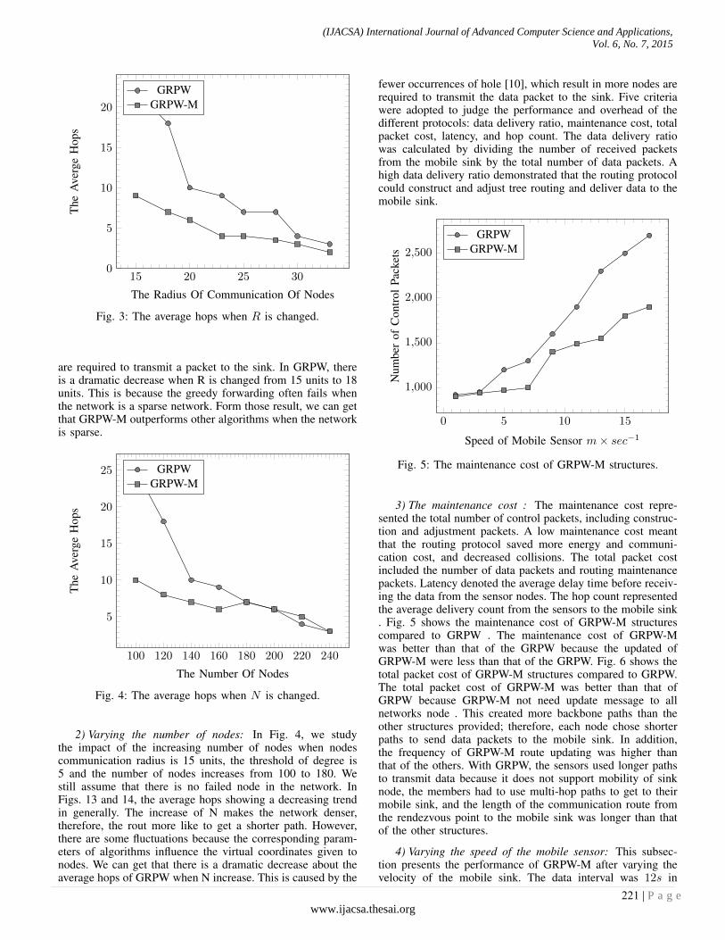
15 20 25 300
5
10
15
20
The Radius Of Communication Of Nodes
The
Ave
rge
Hop
sGRPW
GRPW-M
Fig. 3: The average hops when R is changed.
are required to transmit a packet to the sink. In GRPW, thereis a dramatic decrease when R is changed from 15 units to 18units. This is because the greedy forwarding often fails whenthe network is a sparse network. Form those result, we can getthat GRPW-M outperforms other algorithms when the networkis sparse.
100 120 140 160 180 200 220 240
5
10
15
20
25
The Number Of Nodes
The
Ave
rge
Hop
s
GRPWGRPW-M
Fig. 4: The average hops when N is changed.
2) Varying the number of nodes: In Fig. 4, we studythe impact of the increasing number of nodes when nodescommunication radius is 15 units, the threshold of degree is5 and the number of nodes increases from 100 to 180. Westill assume that there is no failed node in the network. InFigs. 13 and 14, the average hops showing a decreasing trendin generally. The increase of N makes the network denser,therefore, the rout more like to get a shorter path. However,there are some fluctuations because the corresponding param-eters of algorithms influence the virtual coordinates given tonodes. We can get that there is a dramatic decrease about theaverage hops of GRPW when N increase. This is caused by the
fewer occurrences of hole [10], which result in more nodes arerequired to transmit the data packet to the sink. Five criteriawere adopted to judge the performance and overhead of thedifferent protocols: data delivery ratio, maintenance cost, totalpacket cost, latency, and hop count. The data delivery ratiowas calculated by dividing the number of received packetsfrom the mobile sink by the total number of data packets. Ahigh data delivery ratio demonstrated that the routing protocolcould construct and adjust tree routing and deliver data to themobile sink.
0 5 10 15
1,000
1,500
2,000
2,500
Speed of Mobile Sensor m× sec−1
Num
ber
ofC
ontr
olPa
cket
s
GRPWGRPW-M
Fig. 5: The maintenance cost of GRPW-M structures.
3) The maintenance cost : The maintenance cost repre-sented the total number of control packets, including construc-tion and adjustment packets. A low maintenance cost meantthat the routing protocol saved more energy and communi-cation cost, and decreased collisions. The total packet costincluded the number of data packets and routing maintenancepackets. Latency denoted the average delay time before receiv-ing the data from the sensor nodes. The hop count representedthe average delivery count from the sensors to the mobile sink. Fig. 5 shows the maintenance cost of GRPW-M structurescompared to GRPW . The maintenance cost of GRPW-Mwas better than that of the GRPW because the updated ofGRPW-M were less than that of the GRPW. Fig. 6 shows thetotal packet cost of GRPW-M structures compared to GRPW.The total packet cost of GRPW-M was better than that ofGRPW because GRPW-M not need update message to allnetworks node . This created more backbone paths than theother structures provided; therefore, each node chose shorterpaths to send data packets to the mobile sink. In addition,the frequency of GRPW-M route updating was higher thanthat of the others. With GRPW, the sensors used longer pathsto transmit data because it does not support mobility of sinknode, the members had to use multi-hop paths to get to theirmobile sink, and the length of the communication route fromthe rendezvous point to the mobile sink was longer than thatof the other structures.
4) Varying the speed of the mobile sensor: This subsec-tion presents the performance of GRPW-M after varying thevelocity of the mobile sink. The data interval was 12s in
(IJACSA) International Journal of Advanced Computer Science and Applications,
Vol. 6, No. 7, 2015
221 | P a g ewww.ijacsa.thesai.org
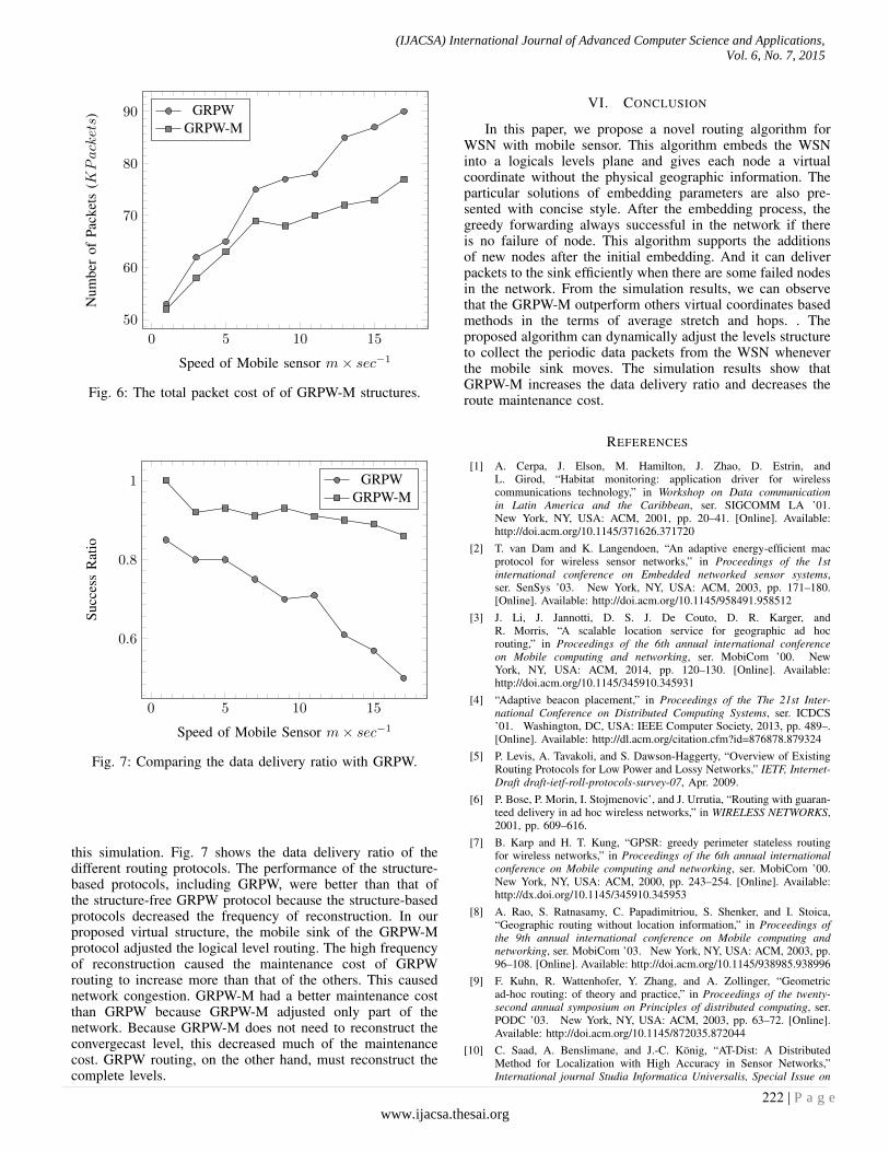
0 5 10 15
50
60
70
80
90
Speed of Mobile sensor m× sec−1
Num
ber
ofPa
cket
s(KPackets)
GRPWGRPW-M
Fig. 6: The total packet cost of of GRPW-M structures.
0 5 10 15
0.6
0.8
1
Speed of Mobile Sensor m× sec−1
Succ
ess
Rat
io
GRPWGRPW-M
Fig. 7: Comparing the data delivery ratio with GRPW.
this simulation. Fig. 7 shows the data delivery ratio of thedifferent routing protocols. The performance of the structure-based protocols, including GRPW, were better than that ofthe structure-free GRPW protocol because the structure-basedprotocols decreased the frequency of reconstruction. In ourproposed virtual structure, the mobile sink of the GRPW-Mprotocol adjusted the logical level routing. The high frequencyof reconstruction caused the maintenance cost of GRPWrouting to increase more than that of the others. This causednetwork congestion. GRPW-M had a better maintenance costthan GRPW because GRPW-M adjusted only part of thenetwork. Because GRPW-M does not need to reconstruct theconvergecast level, this decreased much of the maintenancecost. GRPW routing, on the other hand, must reconstruct thecomplete levels.
VI. CONCLUSION
In this paper, we propose a novel routing algorithm forWSN with mobile sensor. This algorithm embeds the WSNinto a logicals levels plane and gives each node a virtualcoordinate without the physical geographic information. Theparticular solutions of embedding parameters are also pre-sented with concise style. After the embedding process, thegreedy forwarding always successful in the network if thereis no failure of node. This algorithm supports the additionsof new nodes after the initial embedding. And it can deliverpackets to the sink efficiently when there are some failed nodesin the network. From the simulation results, we can observethat the GRPW-M outperform others virtual coordinates basedmethods in the terms of average stretch and hops. . Theproposed algorithm can dynamically adjust the levels structureto collect the periodic data packets from the WSN wheneverthe mobile sink moves. The simulation results show thatGRPW-M increases the data delivery ratio and decreases theroute maintenance cost.
REFERENCES
[1] A. Cerpa, J. Elson, M. Hamilton, J. Zhao, D. Estrin, andL. Girod, “Habitat monitoring: application driver for wirelesscommunications technology,” in Workshop on Data communicationin Latin America and the Caribbean, ser. SIGCOMM LA ’01.New York, NY, USA: ACM, 2001, pp. 20–41. [Online]. Available:http://doi.acm.org/10.1145/371626.371720
[2] T. van Dam and K. Langendoen, “An adaptive energy-efficient macprotocol for wireless sensor networks,” in Proceedings of the 1stinternational conference on Embedded networked sensor systems,ser. SenSys ’03. New York, NY, USA: ACM, 2003, pp. 171–180.[Online]. Available: http://doi.acm.org/10.1145/958491.958512
[3] J. Li, J. Jannotti, D. S. J. De Couto, D. R. Karger, andR. Morris, “A scalable location service for geographic ad hocrouting,” in Proceedings of the 6th annual international conferenceon Mobile computing and networking, ser. MobiCom ’00. NewYork, NY, USA: ACM, 2014, pp. 120–130. [Online]. Available:http://doi.acm.org/10.1145/345910.345931
[4] “Adaptive beacon placement,” in Proceedings of the The 21st Inter-national Conference on Distributed Computing Systems, ser. ICDCS’01. Washington, DC, USA: IEEE Computer Society, 2013, pp. 489–.[Online]. Available: http://dl.acm.org/citation.cfm?id=876878.879324
[5] P. Levis, A. Tavakoli, and S. Dawson-Haggerty, “Overview of ExistingRouting Protocols for Low Power and Lossy Networks,” IETF, Internet-Draft draft-ietf-roll-protocols-survey-07, Apr. 2009.
[6] P. Bose, P. Morin, I. Stojmenovic’, and J. Urrutia, “Routing with guaran-teed delivery in ad hoc wireless networks,” in WIRELESS NETWORKS,2001, pp. 609–616.
[7] B. Karp and H. T. Kung, “GPSR: greedy perimeter stateless routingfor wireless networks,” in Proceedings of the 6th annual internationalconference on Mobile computing and networking, ser. MobiCom ’00.New York, NY, USA: ACM, 2000, pp. 243–254. [Online]. Available:http://dx.doi.org/10.1145/345910.345953
[8] A. Rao, S. Ratnasamy, C. Papadimitriou, S. Shenker, and I. Stoica,“Geographic routing without location information,” in Proceedings ofthe 9th annual international conference on Mobile computing andnetworking, ser. MobiCom ’03. New York, NY, USA: ACM, 2003, pp.96–108. [Online]. Available: http://doi.acm.org/10.1145/938985.938996
[9] F. Kuhn, R. Wattenhofer, Y. Zhang, and A. Zollinger, “Geometricad-hoc routing: of theory and practice,” in Proceedings of the twenty-second annual symposium on Principles of distributed computing, ser.PODC ’03. New York, NY, USA: ACM, 2003, pp. 63–72. [Online].Available: http://doi.acm.org/10.1145/872035.872044
[10] C. Saad, A. Benslimane, and J.-C. Konig, “AT-Dist: A DistributedMethod for Localization with High Accuracy in Sensor Networks,”International journal Studia Informatica Universalis, Special Issue on
(IJACSA) International Journal of Advanced Computer Science and Applications,
Vol. 6, No. 7, 2015
222 | P a g ewww.ijacsa.thesai.org

”Wireless Ad Hoc and Sensor Networks”, vol. 6, no. 1, p. N/A, 2008.[Online]. Available: http://hal-lirmm.ccsd.cnrs.fr/lirmm-00270283
[11] G. S. Sara and D. Sridharan, “Routing in mobile wireless sensornetwork: A survey,” Telecommun. Syst., vol. 57, no. 1, pp. 51–79, Sep.2014. [Online]. Available: http://dx.doi.org/10.1007/s11235-013-9766-2
[12] Z. H. Mir, S. Imran, and Y.-B. Ko, “Neighbor-assisted datadelivery to mobile sink in wireless sensor networks,” in Proceedingsof the 9th International Conference on Ubiquitous InformationManagement and Communication, ser. IMCOM ’15. New York,NY, USA: ACM, 2015, pp. 107:1–107:8. [Online]. Available:http://doi.acm.org/10.1145/2701126.2701230
[13] M. Salamanca, N. Pena, and N. da Fonseca, “Impact of the routingprotocol choice on the envelope-based admission control scheme forad hoc networks,” Ad Hoc Netw., vol. 31, no. C, pp. 20–33, Aug. 2015.[Online]. Available: http://dx.doi.org/10.1016/j.adhoc.2015.03.008
[14] S. Tan, X. Li, and Q. Dong, “Trust based routingmechanism for securing oslr-based manet,” Ad Hoc Netw.,vol. 30, no. C, pp. 84–98, Jul. 2015. [Online]. Available:http://dx.doi.org/10.1016/j.adhoc.2015.03.004
[15] F. Carrabs, R. Cerulli, C. D’Ambrosio, M. Gentili, and A. Raiconi,“Maximizing lifetime in wireless sensor networks with multiple sensorfamilies,” Comput. Oper. Res., vol. 60, no. C, pp. 121–137, Aug. 2015.[Online]. Available: http://dx.doi.org/10.1016/j.cor.2015.02.013
[16] T.-S. Chen, H.-W. Tsai, Y.-H. Chang, and T.-C. Chen, “Geographicconvergecast using mobile sink in wireless sensor networks,” Comput.Commun., vol. 36, no. 4, pp. 445–458, Feb. 2013. [Online]. Available:http://dx.doi.org/10.1016/j.comcom.2012.11.008
[17] Y. Sabri and N. E. Kamoun, “Article: Geographic routing with logicallevels forwarding for wireless sensor network,” International Journalof Computer Applications, vol. 51, no. 11, pp. 1–8, August 2012, fulltext available.
[18] Y.SABRI and N.ElKAMOUN, “ A Distributed Method for Localizationin Large-Scale Sensor Networks based on Graham’s scan ,” Journalof Selected Areas in Telecommunications (JSAT). [Online]. Available:http://www.cyberjournals.com/Papers/Jan2012/04.pdf
[19] Y. Sabri and N. E. Kamoun, “Article: A distributed method to localiza-tion for mobile sensor networks based on the convex hull,” InternationalJournal of Advanced Computer Science and Applications(IJACSA),vol. 3, no. 10, August 2012.
(IJACSA) International Journal of Advanced Computer Science and Applications,
Vol. 6, No. 7, 2015
223 | P a g ewww.ijacsa.thesai.org

Cost-Effective, Cognitive Undersea Network forTimely and Reliable Near-Field Tsunami Warning
X. Xerandy†, Taieb Znati‡, Louise K Comfort±†School of Information Sciences‡Computer Science Department
±Graduate School of Public and International Affairs University of Pittsburgh, Pittsburgh
Abstract—The focus of this paper is on developing an earlydetection and warning system for near-field tsunami to mitigateits impact on communities at risk. This a challenging task,given the stringent reliability and timeliness requirements, thedevelopment of such an infrastructure entails. To address thischallenge, we propose a hybrid infrastructure, which combinescheap but unreliable undersea sensors with expensive but highlyreliable fiber optic, to meet the stringent constraints of thiswarning system. The derivation of a low-cost tsunami detectionand warning infrastructure is cast as an optimization problem,and a heuristic approach is used to determine the minimum costnetwork configuration that meets the targeted reliability andtimeliness requirements. To capture the intrinsic properties ofthe environment and model accurately the main characteristics ofthe sound wave propagation undersea, the proposed optimizationframework incorporates the Bellhop propagation model andaccounts for significant environment factors, including noise,varying undersea sound speed and sea floor profile. We applyour approach to a region which is prone to near-field tsunamithreats to derive a cost-effective under sea infrastructure fordetection and warning. For this case study, the results derivedfrom the proposed framework show that a feasible infrastructure,which operates with a carrier frequency of 12-KHz, can bedeployed in calm, moderate and severe environments and meet thestringent reliability and timeliness constraints, namely 20 minuteswarning time and 99 % data communication reliability, requiredto mitigate the impact of a near-field tsunami. The proposedframework provides useful insights and guidelines toward thedevelopment of a realistic detection and warning system for near-field tsunami.
Keywords—near field tsunami, undersea, sensor, fiber optic,detection, optimization, cost, reliable, timeliness
I. INTRODUCTION
Tsunami is a series of seismic sea waves, usually generatedby disturbances associated with earthquakes occurring belowor near the ocean floor, volcanic eruptions, submarine landslideand coastal rock falls [1]. Tsunami waves are of extremely longlength and period. Based on the distance of the tsunami sourceto the coast, or alternatively the coast travel time, a tsunami canbe classified as local, regional or distant. A local tsunami, alsoreferred to as near-field tsunami (NFT), originates at a nearbysource, typically 100 km (or less than 1 hour travel time).Its destructive effects are confined to the coast within this
distance. A regional tsunami originates from within about 1000km from the coast. It is capable of massive destruction withina geographic region where it occurs, although it may occasion-ally inflict a limited and localized destructive effect outside theregion. A distant tsunami, also referred to as far-field tsunami,originates from a far away source, generally more than 1000km away from the coast. Although less frequent than local andregional tsunami, distant tsunami causes extensive destructionsnear the source and has sufficient energy to cause additionaldestruction on shores more than 1000 km away from thesource. A study of tsunami in the Pacific region, shows that87% tsunamigenous sources are located closer than 100 kmfrom the coast [2]. Reliable detection of a near-field tsunamibecomes critical to ensure timely evacuation and prevent lossof lives and severe damage.
Several systems were developed for early tsunami detection.NOAA developed and deployed Deep-ocean Assessment andReporting of Tsunami (DART) [3]. DART consists of a seafloor bottom pressure recorder and a moored surface buoy.An acoustic link connects the recorder to the buoy for realtime communication of temperature and pressure data. Thebuoy sends the data to the land station through satellitecommunication. However, DART buoy is primarily suitableto detect far-field tsunami, as they are deployed and anchoredat least 250 miles away from the shore [4]. In addition todamage caused by weather condition, floating buoys may alsobe subject to vandalism, particularly in marine water that isfavorable to fishing [5]. This makes servicing damaged buoyschallenging and costly. The ocean-bottom seismographic andtsunami observation system, based on fiber-optics submarinecable, was also developed for tsunami detection [6]. It monitorssea floor earthquake to detect tsunami over higher accuracyand finer dynamic range. However, this system comes withprohibitively high deployment cost and may not be affordablefor third world countries.
This paper focuses on near-field tsunami and seeks todevelop a cost effective tsunami detection system for reliabledelivery of warnings to ensure timely evacuation. To this end,a hybrid, buoy-less underwater communication infrastructureis proposed. The infrastructure is composed of a fiber opticand an undersea network of sensors. Fiber optic provides highreliability and fast data transmission. Its acquisition, deploy-
(IJACSA) International Journal of Advanced Computer Science and Applications,
Vol. 6, No. 7, 2015
224 | P a g ewww.ijacsa.thesai.org
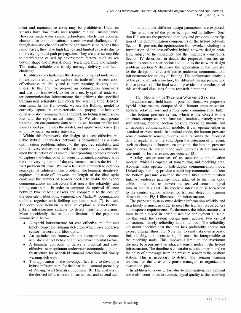
ment and maintenance costs may be prohibitive. Underseasensors have low costs and require minimal maintenance.However, underwater sensor technology, which uses acousticchannels for communication, presents several challenges. Al-though acoustic channels offer longer transmission ranges thanradio waves, they have high latency and limited capacity due totime-varying multi-path propagation. They are also susceptibleto interference caused by environment factors, such as seabottom shape and material, noise, sea temperature and salinity.This makes reliable and timely message delivery a difficultchallenge.
To address the challenges the design of a hybrid underwaterinfrastructure entails, we explore the trade-offs between cost-effectiveness, reliability and tsunami warning delivery time-liness. To this end, we propose an optimization frameworkand use this framework to derive a nearly-optimal underwa-ter communication infrastructure that achieves the specifiedtransmission reliability and meets the warning time deliveryconstraint. In this framework, we use the Bellhop model tocorrectly capture the characteristics and propagation behaviorof an acoustic communications channel, including transmissionloss and the ray’s arrival times [7]. We also incorporaterequired sea environment data such as sea bottom profile andsound speed profile into the model, and apply Wenz curve [8]to approximate sea noise intensity.
Within this framework, the design of a cost-effective, re-liable hybrid underwater network is formulated as a cost-optimization problem, subject to the specified reliability andtime delivery constraints needed to ensure timely evacuation,upon the detection of a tsunami. Incorporating complex modelsto capture the behavior of an acoustic channel, combined withthe time-varying nature of the environment, makes the formal-ized problem NP hard. We use a heuristic approach to developnear-optimal solution to this problem. The heuristic iterativelyexplores the trade-off between the length of the fiber opticcable and the number of sensors needed to enable the hybridcommunications infrastructure that meets the reliability andtiming constraints. In order to compute the optimal distancebetween two adjacent sensors and compare it to the cost ofthe equivalent fiber optic segment, the Matlab™ optimizationtoolbox, together with Bellhop application suit [7], is used.The developed heuristic is used to explore a cost-effective.hybrid infrastructure suitable to detect near-field tsunamis.More specifically, the main contributions of the paper aresummarized below:• A hybrid infrastructure for cost effective, reliable and
timely near-field tsunami detection which uses underseasensor network and fiber optic.
• An optimization framework that incorporates accurateacoustic channel behavior and sea environmental factors.
• A heuristic approach to derive a practical and cost-effective, near-optimum underwater communications in-frastructure for near-field tsunami detection and timelywarning delivery.
• The application of the developed heuristic to develop ahybrid infrastructure for the near-field tsunami prone cityof Padang, West Sumatra, Indonesia [9]. The analysis ofthe derived infrastructure is carried out and several sce-
narios, under different design parameters, are explored.The remainder of the paper is organized as follows: Sec-
tion II discusses the proposed topology and provides a descrip-tion of the communication components of the hybrid network.Section III presents the optimization framework, including theformulation of the cost-effective hybrid network design prob-lem, subject to the reliability and the timeliness constraints.Section IV describes, in detail, the proposed heuristic ap-proach to obtain a near-optimal solution to the network designproblem. Section V discusses the application of the heuristicto the design of a cost-effective undersea communicationsinfrastructure for the city of Padang. The performance analysisof the proposed infrastructure, for different design parameters,is also presented. The final section provides the conclusion ofthis work and discusses future research directions.
II. NEAR-FIELD TSUNAMI WARNING SYSTEMTo address near-field tsunami potential threat, we propose a
hybrid infrastructure, composed of a bottom pressure sensor,acoustic relay sensors and a fiber optic communication link.
The bottom pressure sensor, which is the closest to theepicenter, comprises three functional modules, namely a pres-sure sensing module, bottom pressure recording module andan acoustic communication module. It can operate either instandard or event mode. In standard mode, the bottom pressuresensor routinely senses, records, and transmits the recordeddata at regular time intervals. Upon the detection of an event,such as changes in bottom sea pressure, the bottom pressuresensor enters the event mode and increases its transmissionrate until no further events are detected [3].
A relay sensor consists of an acoustic communicationmodule, which is capable of transmitting and receiving data.Acoustic links operate in half-duplex communication mode.Linked together, they provide a multi-hop communication fromthe bottom pressure sensor to the optic fiber communicationlink. An undersea gateway node, attached to the fiber opticcable, is required to convert the received acoustic signalinto an optical signal. The received information is forwardedto the control station ashore, for tsunami detection warningdissemination. Fig 1 illustrates the infrastructure.
The proposed system must deliver information reliably andin a timely manner, in order to meet the tsunami preparednessand response requirements. Furthermore, the infrastructure costmust be minimized in order to achieve deployment at scale.To this end, the system design must address two criticalconstraints, namely reliability and timeliness. The reliabilityconstraint specifies that the data loss probability should notexceed a target threshold. Note that to send data over acousticlink reliably, the acoustic signal must be interpretable atthe receiving node. This imposes a limit on the maximumdistance between any two adjacent sensor nodes in the hybridinfrastructure. The timeliness constraint sets an upper bound onthe delay of a message from the pressure sensor to the onshorestation. This is necessary to deliver the tsunami warningon time for the disaster response managers to organize theevacuation plan.
In addition to acoustic loss due to propagation, sea ambientnoise also contributes to acoustic signal quality at the receiving
(IJACSA) International Journal of Advanced Computer Science and Applications,
Vol. 6, No. 7, 2015
225 | P a g ewww.ijacsa.thesai.org
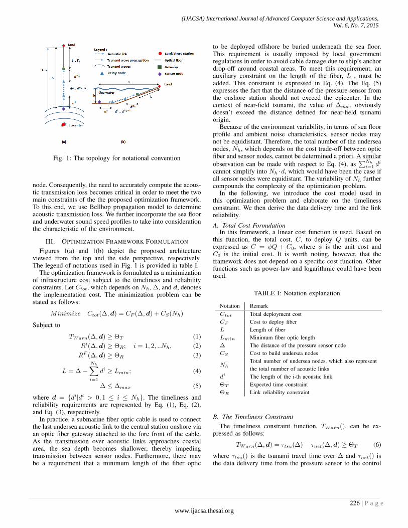
Fig. 1: The topology for notational convention
node. Consequently, the need to accurately compute the acous-tic transmission loss becomes critical in order to meet the twomain constraints of the the proposed optimization framework.To this end, we use Bellhop propagation model to determineacoustic transmission loss. We further incorporate the sea floorand underwater sound speed profiles to take into considerationthe characteristic of the environment.
III. OPTIMIZATION FRAMEWORK FORMULATION
Figures 1(a) and 1(b) depict the proposed architectureviewed from the top and the side perspective, respectively.The legend of notations used in Fig. 1 is provided in table I.
The optimization framework is formulated as a minimizationof infrastructure cost subject to the timeliness and reliabilityconstraints. Let Ctot, which depends on Nh, ∆, and d, denotesthe implementation cost. The minimization problem can bestated as follows:
Minimize Ctot(∆,d) = CF (∆,d) + CS(Nh)
Subject to
TWarn(∆,d) ≥ ΘT (1)Ri(∆,d) ≥ ΘR; i = 1, 2, ..Nh, (2)RF (∆,d) ≥ ΘR (3)
L = ∆−Nh∑i=1
di ≥ Lmin; (4)
∆ ≤ ∆max (5)
where d = {di|di > 0, 1 ≤ i ≤ Nh}. The timeliness andreliability requirements are represented by Eq. (1), Eq. (2),and Eq. (3), respectively.
In practice, a submarine fiber optic cable is used to connectthe last undersea acoustic link to the central station onshore viaan optic fiber gateway attached to the fore front of the cable.As the transmission over acoustic links approaches coastalarea, the sea depth becomes shallower, thereby impedingtransmission between sensor nodes. Furthermore, there maybe a requirement that a minimum length of the fiber optic
to be deployed offshore be buried underneath the sea floor.This requirement is usually imposed by local governmentregulations in order to avoid cable damage due to ship’s anchordrop-off around coastal areas. To meet this requirement, anauxiliary constraint on the length of the fiber, L , must beadded. This constraint is expressed in Eq. (4). The Eq. (5)expresses the fact that the distance of the pressure sensor fromthe onshore station should not exceed the epicenter. In thecontext of near-field tsunami, the value of ∆max obviouslydoesn’t exceed the distance defined for near-field tsunamiorigin.
Because of the environment variability, in terms of sea floorprofile and ambient noise characteristics, sensor nodes maynot be equidistant. Therefore, the total number of the underseanodes, Nh, which depends on the cost trade-off between opticfiber and sensor nodes, cannot be determined a priori. A similarobservation can be made with respect to Eq. (4), as
∑Nh
i=1 di
cannot simplify into Nh ·d, which would have been the case ifall sensor nodes were equidistant. The variability of Nh furthercompounds the complexity of the optimization problem.
In the following, we introduce the cost model used inthis optimization problem and elaborate on the timelinessconstraint. We then derive the data delivery time and the linkreliability.
A. Total Cost FormulationIn this framework, a linear cost function is used. Based on
this function, the total cost, C, to deploy Q units, can beexpressed as C = φQ + C0, where φ is the unit cost andC0 is the initial cost. It is worth noting, however, that theframework does not depend on a specific cost function. Otherfunctions such as power-law and logarithmic could have beenused.
TABLE I: Notation explanation
Notation RemarkCtot Total deployment costCF Cost to deploy fiberL Length of fiberLmin Minimum fiber optic length∆ The distance of the pressure sensor nodeCS Cost to build undersea nodes
NhTotal number of undersea nodes, which also representthe total number of acoustic links
di The length of the i-th acoustic linkΘT Expected time constraintΘR Link reliability constraint
B. The Timeliness ConstraintThe timeliness constraint function, TWarn(), can be ex-
pressed as follows:
TWarn(∆,d) = τtsu(∆)− τnet(∆,d) ≥ ΘT (6)
where τtsu() is the tsunami travel time over ∆ and τnet() isthe data delivery time from the pressure sensor to the control
(IJACSA) International Journal of Advanced Computer Science and Applications,
Vol. 6, No. 7, 2015
226 | P a g ewww.ijacsa.thesai.org

station ashore. Since fiber optic link is reliable and fast, theacoustic links bear the highest portion of the data deliverytime.
Eq. (6) imposes a minimum distance of the pressure sensornode for a given ΘT . This minimum distance, denoted as∆min, can be derived if the data delivery time of the proposedinfrastructure is made practically negligible. This would bepossible if all-fiber deployment is chosen to cover ∆min.This solution is considered as the most expensive solution.If either the epicenter or the pressure sensor distance is lessthan ∆min, then Eq 1 will never be satisfied. In our heuristicapproach algorithm, ∆min holds important role for initialfeasible solution.
1) The Data Delivery Time : This quantity is dictated bytransmission delay, propagation delay, processing delay andretransmissions due to packet error. A less reliable link requiresmore time to complete a successful data delivery. Hence, weneed to take the link reliability constraint function into account.Since the reliability constraint function implies a probabilistictype of quantity, the data delivery time, τnet(), is calculatedas an average.
If T F () represents the average of data delivery time in thefiber optic link and T S() represent the average of data deliverytime in the acoustic links, then the total data delivery timeτnet() is expressed as follow:
τnet(∆,d) = T F (∆,d) + T S(∆,d) (7)
2) Tsunami Travel Time: To obtain tsunami travel timeover ∆, tsunami propagation speed needs to be determined.However, tsunami propagation speed is dictated by the seadepth. Given a sea depth of h, the tsunami speed, vtsu, canbe derived from vtsu =
√g · h, where g is the gravitational
acceleration. To approximate tsunami travel time by taking thevariation of sea depth into account, the pressure sensor distance∆ is divided into K small intervals. The tsunami propagationspeed in each interval is assumed to remain constant. Eq.(8) expresses the overall tsunami travel time as the sum ofthe travel time over K intervals, where xj and vjtsu denotethe length and the tsunami propagation speed at j-th interval.Indeed, larger K results in more accurate result.
τtsu =K∑j=1
xj
vjtsu(8)
C. The Reliability ConstraintThe reliability constraint measures the probability of a
successful data transmission. Given the data length of m, theprobability of error-free received data at receiving node, R(),can be expressed as follows:
R(∆,d) =(1−BERr(∆,d)
)m(9)
where BERr is the probability of bit error. Since the fiberoptic link offers very high reliability, the discussion focuseson the acoustic link reliability constraints expressed in Eq.(2). To obtain the bit error probability over an acoustic linki, a probability distribution function F(p) is specified. This
probability distribution function represents the bit error char-acteristic in undersea environment. The probability functionF(p) also depends on the modulation scheme. In section V,we will specify F(p) in more detail.
To apply this function, we use p =Ei
b
Ni0
for the parameter.The Eib and N i
0 denote the energy per bit and equivalent whitenoise on acoustic link i. The following equation:
Eib =1
rs· P it ·Ai(∆,d, f) (10)
provides the formulation to obtain the energy per bit on linki, where P it , Ai(), f and rs represent the node’s transmissionpower, the acoustic channel loss, the acoustic wave frequencyand the sensor transmission rate at link i, respectively.
To approximate the equivalent white noise energy, N i0, Eq.
(11) is used. The equation divides the total noise power in thereceiving node, W (f,B), with the receiver’s bandwidth B.
N i0 =
1
B·W (f,B) (11)
1) Acoustic Channel Loss: Acoustic channel loss is cal-culated as the total transmission loss inflicted by two mainfactors, namely spreading and absorption loss. A spreadingloss is a signal attenuation as the acoustic signal travels furtherfrom the source, whereas the absorption loss is caused by theacoustic energy absorption as it traverses within sea water [10].The acoustic energy absorption loss factor, denoted as a(f), isfrequency dependent. This paper incorporates this absorptionloss into Bellhop model in order to increase the accuracy ofthe channel loss computation.
To quantify the absorption loss, a(f), an empirical model,called as Thorp [11], is expressed as follows (in dB) :
a(f) =0.11f2
1 + f2+
44f2
4100 + f2+ 2.75 · 10−4f2 + 0.003
where f is in KHz. The equation above is still sufficientlyvalid for frequency above few hundreds of Hz.
2) Sea Background Noise: Sea background noise, sometimeis referred to as sea ambient noise, is inherent acoustic fieldsthat may interfere the acoustic channel. Their characteristicsand intensities are location-specific. Based on their sources, theambient noise main contributors can be grouped as follows:water motion, including also the effects of surf, rain, hail andtides, man-made sources, including ship activity and marinelife [8]. Each contributor causes a frequency-dependent impactto the acoustic channel. The ambient noise also increases inshallower depth.
A number of ambient noise studies and measurements havebeen made since 1945 in deep-water and open ocean areas [8].The ambient noise spectra then are summarized and presentedin a group of curves [8], [12] as shown in figure 2. Fig. 2 isalso known as Wenz curve.
To obtain the total noise power W (f,B) at the receiver withthe receiving bandwidth of B Hz, the following equation,
W (f,B) =
∫B
w(f)df (12)
(IJACSA) International Journal of Advanced Computer Science and Applications,
Vol. 6, No. 7, 2015
227 | P a g ewww.ijacsa.thesai.org
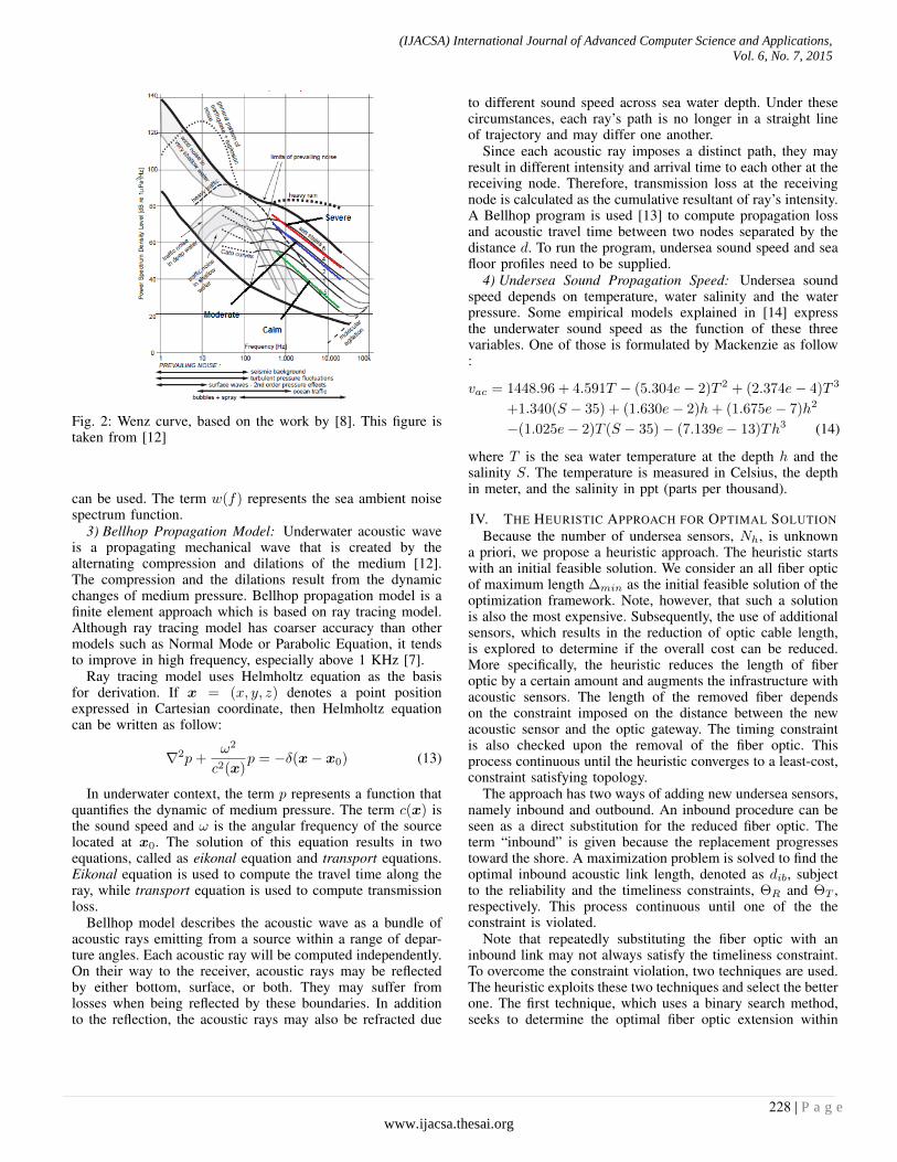
Fig. 2: Wenz curve, based on the work by [8]. This figure istaken from [12]
can be used. The term w(f) represents the sea ambient noisespectrum function.
3) Bellhop Propagation Model: Underwater acoustic waveis a propagating mechanical wave that is created by thealternating compression and dilations of the medium [12].The compression and the dilations result from the dynamicchanges of medium pressure. Bellhop propagation model is afinite element approach which is based on ray tracing model.Although ray tracing model has coarser accuracy than othermodels such as Normal Mode or Parabolic Equation, it tendsto improve in high frequency, especially above 1 KHz [7].
Ray tracing model uses Helmholtz equation as the basisfor derivation. If x = (x, y, z) denotes a point positionexpressed in Cartesian coordinate, then Helmholtz equationcan be written as follow:
∇2p+ω2
c2(x)p = −δ(x− x0) (13)
In underwater context, the term p represents a function thatquantifies the dynamic of medium pressure. The term c(x) isthe sound speed and ω is the angular frequency of the sourcelocated at x0. The solution of this equation results in twoequations, called as eikonal equation and transport equations.Eikonal equation is used to compute the travel time along theray, while transport equation is used to compute transmissionloss.
Bellhop model describes the acoustic wave as a bundle ofacoustic rays emitting from a source within a range of depar-ture angles. Each acoustic ray will be computed independently.On their way to the receiver, acoustic rays may be reflectedby either bottom, surface, or both. They may suffer fromlosses when being reflected by these boundaries. In additionto the reflection, the acoustic rays may also be refracted due
to different sound speed across sea water depth. Under thesecircumstances, each ray’s path is no longer in a straight lineof trajectory and may differ one another.
Since each acoustic ray imposes a distinct path, they mayresult in different intensity and arrival time to each other at thereceiving node. Therefore, transmission loss at the receivingnode is calculated as the cumulative resultant of ray’s intensity.A Bellhop program is used [13] to compute propagation lossand acoustic travel time between two nodes separated by thedistance d. To run the program, undersea sound speed and seafloor profiles need to be supplied.
4) Undersea Sound Propagation Speed: Undersea soundspeed depends on temperature, water salinity and the waterpressure. Some empirical models explained in [14] expressthe underwater sound speed as the function of these threevariables. One of those is formulated by Mackenzie as follow:
vac = 1448.96 + 4.591T − (5.304e− 2)T 2 + (2.374e− 4)T 3
+1.340(S − 35) + (1.630e− 2)h+ (1.675e− 7)h2
−(1.025e− 2)T (S − 35)− (7.139e− 13)Th3 (14)
where T is the sea water temperature at the depth h and thesalinity S. The temperature is measured in Celsius, the depthin meter, and the salinity in ppt (parts per thousand).
IV. THE HEURISTIC APPROACH FOR OPTIMAL SOLUTIONBecause the number of undersea sensors, Nh, is unknown
a priori, we propose a heuristic approach. The heuristic startswith an initial feasible solution. We consider an all fiber opticof maximum length ∆min as the initial feasible solution of theoptimization framework. Note, however, that such a solutionis also the most expensive. Subsequently, the use of additionalsensors, which results in the reduction of optic cable length,is explored to determine if the overall cost can be reduced.More specifically, the heuristic reduces the length of fiberoptic by a certain amount and augments the infrastructure withacoustic sensors. The length of the removed fiber dependson the constraint imposed on the distance between the newacoustic sensor and the optic gateway. The timing constraintis also checked upon the removal of the fiber optic. Thisprocess continuous until the heuristic converges to a least-cost,constraint satisfying topology.
The approach has two ways of adding new undersea sensors,namely inbound and outbound. An inbound procedure can beseen as a direct substitution for the reduced fiber optic. Theterm “inbound” is given because the replacement progressestoward the shore. A maximization problem is solved to find theoptimal inbound acoustic link length, denoted as dib, subjectto the reliability and the timeliness constraints, ΘR and ΘT ,respectively. This process continuous until one of the theconstraint is violated.
Note that repeatedly substituting the fiber optic with aninbound link may not always satisfy the timeliness constraint.To overcome the constraint violation, two techniques are used.The heuristic exploits these two techniques and select the betterone. The first technique, which uses a binary search method,seeks to determine the optimal fiber optic extension within
(IJACSA) International Journal of Advanced Computer Science and Applications,
Vol. 6, No. 7, 2015
228 | P a g ewww.ijacsa.thesai.org
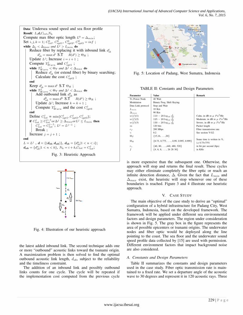
Data: Undersea sound speed and sea floor profileResult: L,d,Ctot,Nh
Compute max fiber optic length L0 = ∆min;Set i, j, k = 1; C0
tot, C0opt1, C0
opt2, C0opt3 = inf ;
while ∆j < ∆max and Lj > Lmin doReduce fiber by replacing it with inbound link diib
diib = max di S.T R(di) ≥ ΘR ;Update Lj ; Increase i = i + 1 ;Compute T j
Warn and Cjopt1 ;
while T jWarn < ΘT and ∆j < ∆max do
Reduce diib (or extend fiber) by binary searching;Calculate the cost Cj
opt2 ;endKeep diib = max di S.T ΘR ;while T j
Warn < ΘT and ∆j < ∆max doAdd outbound link dkob as
dkob = max dk S.T R(do) ≥ ΘR ;Update ∆j ; Increase k = k + 1 ;Compute T j
Warn and the cost Cjopt3
endDefine Cj
tot = min{Cjopt1, C
jopt2, C
jopt3};
if Cjtot ≥ Cj−1
tot or∆j ≥ ∆maxorLj ≤ Lmin thenCj
tot = Cj−1tot ; Lj = Lj−1 ;
Break ;Increase j = j + 1 ;
endL = Lj , d = {(dib,dob)}, dib = {dnib|1 < n < i};dob = {dnob|1 < n < k}, Nh = i + k,Ctot = Cj
tot;
Fig. 3: Heuristic Approach
Fig. 4: Illustration of our heuristic approach
the latest added inbound link. The second technique adds oneor more “outbound” acoustic links toward the tsunami origin.A maximization problem is then solved to find the optimaloutbound acoustic link length, dob, subject to the reliabilityand the timeliness constraint.
The addition of an inbound link and possibly outboundlinks counts for one cycle. The cycle will be repeated ifthe implementation cost computed from the previous cycle
Fig. 5: Location of Padang, West Sumatra, Indonesia
TABLE II: Constants and Design Parameters
Parameter Value RemarkTx Power Node 40 WattModulation Binary Freq. Shift KeyingData Link protocol Stop and WaitLmin 10 Km∆max 90 Kmw(f)(1) 110− 20 log10
f10 Calm, in dB re µ Pa2/Hz
w(f)(2) 125− 20 log10f10 Moderate, in dB re µ Pa2/Hz
w(f)(3) 130− 20 log10f10 Severe, in dB re µ Pa2/Hz
m 120 bits Packet lengthrf 200 Mbps Fiber transmission rateγ 0.2 See section V-G2ΘT {15,16, . . .,20}
ΘR {0.75, 0.775, . . ., 0.99, 0.995, 0.999} Some time is written in %,i.e 0.75=75%
rs {40, 80, . . .,440, 480, 520} in bit per second (bps)f {4, 6, 8, . . ., 26 28 30} in KHz
is more expensive than the subsequent one. Otherwise, theapproach will stop and returns the final result. These cyclesmay either eliminate completely the fiber optic or reach aninfinite detection distance, ∆. Given the fact that Lmin and∆max exist, the heuristic will stop whenever one of theseboundaries is reached. Figure 3 and 4 illustrate our heuristicapproach.
V. CASE STUDY
The main objective of the case study to derive an “optimal”configuration of a hybrid infrastructure for Padang City, WestSumatra, Indonesia, based on the developed framework. Theframework will be applied under different sea environmentalfactors and design parameters. The region under considerationis shown in Fig. 5. The gray box in the figure represents thearea of possible epicenters or tsunami origins. The underwaternodes and fiber optic would be deployed along the linepointing to the coast. The sea floor and the underwater soundspeed profile data collected by [15] are used with permission.Different environment factors that impact background noiseare also considered.
A. Constants and Design ParametersTable II summarizes the constants and design parameters
used in the case study. Fiber optic transmission rate is main-tained to a fixed rate. We set a departure angle of the acousticwave to 30 degrees and represent it in 120 acoustic rays. Three
(IJACSA) International Journal of Advanced Computer Science and Applications,
Vol. 6, No. 7, 2015
229 | P a g ewww.ijacsa.thesai.org

levels of ambient noise spectrum are assumed, namely calm,moderate, and severe. These assumptions reflect the wind-generated noise and associate them to the sea states scaleas depicted in Wenz curve [12]. A ”calm” assumption isassociated to the sea state of 0.5. In this state, the noise iscreated by a calm sea with waves reaching up to 0.1 meter inaverage. A ”moderate” level is referred to as the noise inducedby the sea with sea state of 4. At this level, the waves mayreach a height of 3 meter in average. The highest noise levelis attained when the sea is in ”severe” state, which is causedby the wind that brings the sea waves up to 7 meters height.This state represents a sea scale of 6 in Wenz curve. In ourcase study, the underwater sensor transmits pressure data withsome attributes, including the date, time, and battery status. Weconsider a 120 bit frame length to be sufficient to accommodatethese data, including the frame overhead. We also assume thatno forward error correction scheme is applied.
To deal with different ambient noise levels, this paperdefines three design parameters, namely the link reliabilityconstraint, acoustic carrier frequency and underwater transmis-sion rate. This paper derives the optimal configuration and theimplementation cost with these design parameters varied andanalyze the results under different ambient noise conditions.
B. Cost Function AssumptionTo limit the scope of analysis, the case study only focuses on
linear cost function. Our discussion associates the variable Q totwo independent quantities. They mainly represent the physicalattributes with respect to the infrastructure’s component. Morespecifically, the fiber optic implementation cost is governed bythe length of fiber optic L and the fiber optic transmission raterf , whereas the underwater sensor network cost is dictated bythe number of nodes Nh and the node’s transmission rate rs.The following two equations express the cost function for thefiber optic and the undersea sensor network, respectively.
CF = φf · rf · LCS = φs · rs ·Nh (15)
To carry the cost analysis, the unit cost of sensor φs isnormalized to the fiber optic unit cost φf such that φs = γφf .The total cost,Ctot, is expressed as the ratio of the cost of themost expensive solution. Without loss of generality, we assumethat the initial deployment cost of the fiber optic and underseasensors are the same.
C. Formulation for Data Delivery TimeBoth the fiber optic and multi-hop acoustic links use auto-
matic repeat request (ARQ) as the retransmission scheme. Astop and wait ARQ will be implemented in a per-hop basis.Consequently, the round trip transmission time of a packet andits associated acknowledgment can be expressed as follows:
trt(d) = tm + 2tp(d) + ta
The parameter tm represents the data transmission time,tp(d) the acoustic propagation time traversing through a linkof length d and ta the acknowledgment packet transmissiontime. Given the reliability function, R(∆,d), the average delay
Fig. 6: Courtesy of BPPT [15]: Underwater Sound Speedaround of our case study area
to transmit a packet and receive its acknowledgment can beexpressed as follows:
T =1
R(∆,d)· trt(d) (16)
Eq. (16) is applicable for both fiber optic and acoustic links.Based on Eq. (7), we can deduce a formulation for total datadelivery time, τnet(), as follows :
τnet(∆,d) =tFrt(L)
RF (∆,d)+
Nh∑i=1
tSrt(di)
Ri(∆,d)(17)
In the above equation, tFrt denotes the round trip timetransmission in the fiber optic link and tSrt(d
i) is the round triptime transmission in acoustic link i. In the proposed heuristic,Eq. (17) is invoked each time the timeliness constraint isverified with a new value of Nh being assigned for eachinvocation. In this paper, the fiber optic reliability is consideredhight, i.e. RF ≈ 1. Thus, the data delivery time in fiber opticlink, T F is approximately equal to tFrt.
D. Assumption on Bit Error Probability Distribution FunctionThe case study uses binary frequency shift keying (BFSK)
for the modulation scheme. To calculate bit error probability,this paper adopts the probability distribution function formu-lated in [16]. Let Ei
b
Ni0
be the ratio of bit energy to equivalentwhite noise at link i. The bit error probability at link i can beexpressed as follows:
BERir(∆,d) =v
Γ(v)
∫ ∞0
uv−1
(2v + u
EibN i
0
)du (18)
In the above equation, Γ() represents the Gamma function,with u = y2, where y is the real part of complex value ofsignal amplitude random variable.
E. Underwater Sound Speed and Sea Floor profileFigure 6 shows the characteristic of the underwater sound
speed associated with the area under study. The figure showsthat the speed of the acoustic wave drops rapidly in shallowwaters of around 100 to 200 meters. The decrease in speedin deeper waters continue but at lower rate and re-bounce at adepth of about 800 meters. This profile is obtained by applyingthe measurement data collected by [15] into Eq. (14). Fig. 7depicts the sea bottom profile along the line in Fig. 5.
(IJACSA) International Journal of Advanced Computer Science and Applications,
Vol. 6, No. 7, 2015
230 | P a g ewww.ijacsa.thesai.org
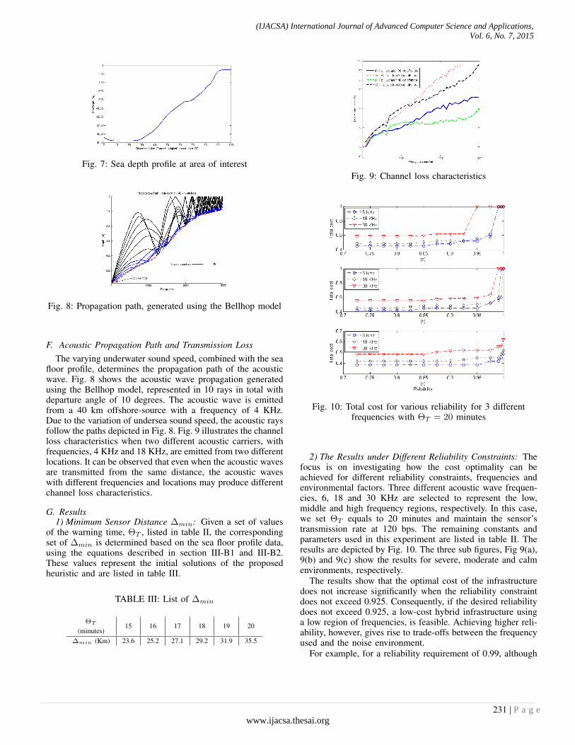
Fig. 7: Sea depth profile at area of interest
Fig. 8: Propagation path, generated using the Bellhop model
F. Acoustic Propagation Path and Transmission LossThe varying underwater sound speed, combined with the sea
floor profile, determines the propagation path of the acousticwave. Fig. 8 shows the acoustic wave propagation generatedusing the Bellhop model, represented in 10 rays in total withdeparture angle of 10 degrees. The acoustic wave is emittedfrom a 40 km offshore-source with a frequency of 4 KHz.Due to the variation of undersea sound speed, the acoustic raysfollow the paths depicted in Fig. 8. Fig. 9 illustrates the channelloss characteristics when two different acoustic carriers, withfrequencies, 4 KHz and 18 KHz, are emitted from two differentlocations. It can be observed that even when the acoustic wavesare transmitted from the same distance, the acoustic waveswith different frequencies and locations may produce differentchannel loss characteristics.
G. Results1) Minimum Sensor Distance ∆min: Given a set of values
of the warning time, ΘT , listed in table II, the correspondingset of ∆min is determined based on the sea floor profile data,using the equations described in section III-B1 and III-B2.These values represent the initial solutions of the proposedheuristic and are listed in table III.
TABLE III: List of ∆min
ΘT
(minutes)15 16 17 18 19 20
∆min (Km) 23.6 25.2 27.1 29.2 31.9 35.5
Fig. 9: Channel loss characteristics
Fig. 10: Total cost for various reliability for 3 differentfrequencies with ΘT = 20 minutes
2) The Results under Different Reliability Constraints: Thefocus is on investigating how the cost optimality can beachieved for different reliability constraints, frequencies andenvironmental factors. Three different acoustic wave frequen-cies, 6, 18 and 30 KHz are selected to represent the low,middle and high frequency regions, respectively. In this case,we set ΘT equals to 20 minutes and maintain the sensor’stransmission rate at 120 bps. The remaining constants andparameters used in this experiment are listed in table II. Theresults are depicted by Fig. 10. The three sub figures, Fig 9(a),9(b) and 9(c) show the results for severe, moderate and calmenvironments, respectively.
The results show that the optimal cost of the infrastructuredoes not increase significantly when the reliability constraintdoes not exceed 0.925. Consequently, if the desired reliabilitydoes not exceed 0.925, a low-cost hybrid infrastructure usinga low region of frequencies, is feasible. Achieving higher reli-ability, however, gives rise to trade-offs between the frequencyused and the noise environment.
For example, for a reliability requirement of 0.99, although
(IJACSA) International Journal of Advanced Computer Science and Applications,
Vol. 6, No. 7, 2015
231 | P a g ewww.ijacsa.thesai.org
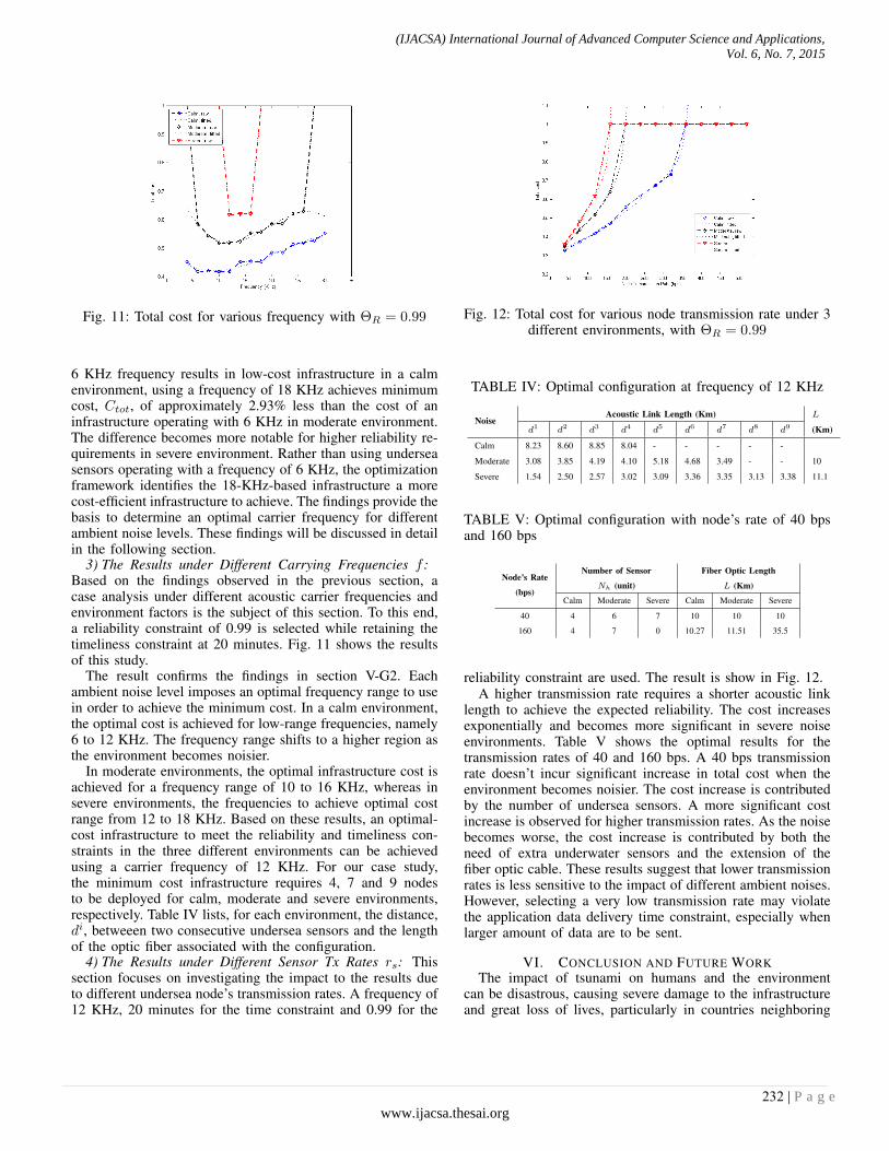
Fig. 11: Total cost for various frequency with ΘR = 0.99
6 KHz frequency results in low-cost infrastructure in a calmenvironment, using a frequency of 18 KHz achieves minimumcost, Ctot, of approximately 2.93% less than the cost of aninfrastructure operating with 6 KHz in moderate environment.The difference becomes more notable for higher reliability re-quirements in severe environment. Rather than using underseasensors operating with a frequency of 6 KHz, the optimizationframework identifies the 18-KHz-based infrastructure a morecost-efficient infrastructure to achieve. The findings provide thebasis to determine an optimal carrier frequency for differentambient noise levels. These findings will be discussed in detailin the following section.
3) The Results under Different Carrying Frequencies f :Based on the findings observed in the previous section, acase analysis under different acoustic carrier frequencies andenvironment factors is the subject of this section. To this end,a reliability constraint of 0.99 is selected while retaining thetimeliness constraint at 20 minutes. Fig. 11 shows the resultsof this study.
The result confirms the findings in section V-G2. Eachambient noise level imposes an optimal frequency range to usein order to achieve the minimum cost. In a calm environment,the optimal cost is achieved for low-range frequencies, namely6 to 12 KHz. The frequency range shifts to a higher region asthe environment becomes noisier.
In moderate environments, the optimal infrastructure cost isachieved for a frequency range of 10 to 16 KHz, whereas insevere environments, the frequencies to achieve optimal costrange from 12 to 18 KHz. Based on these results, an optimal-cost infrastructure to meet the reliability and timeliness con-straints in the three different environments can be achievedusing a carrier frequency of 12 KHz. For our case study,the minimum cost infrastructure requires 4, 7 and 9 nodesto be deployed for calm, moderate and severe environments,respectively. Table IV lists, for each environment, the distance,di, betweeen two consecutive undersea sensors and the lengthof the optic fiber associated with the configuration.
4) The Results under Different Sensor Tx Rates rs: Thissection focuses on investigating the impact to the results dueto different undersea node’s transmission rates. A frequency of12 KHz, 20 minutes for the time constraint and 0.99 for the
Fig. 12: Total cost for various node transmission rate under 3different environments, with ΘR = 0.99
TABLE IV: Optimal configuration at frequency of 12 KHz
NoiseAcoustic Link Length (Km) L
(Km)d1 d2 d3 d4 d5 d6 d7 d8 d9
Calm 8.23 8.60 8.85 8.04 - - - - -
Moderate 3.08 3.85 4.19 4.10 5.18 4.68 3.49 - - 10
Severe 1.54 2.50 2.57 3.02 3.09 3.36 3.35 3.13 3.38 11.1
TABLE V: Optimal configuration with node’s rate of 40 bpsand 160 bps
Node’s Rate
(bps)
Number of Sensor
Nh (unit)
Fiber Optic Length
L (Km)
Calm Moderate Severe Calm Moderate Severe
40 4 6 7 10 10 10
160 4 7 0 10.27 11.51 35.5
reliability constraint are used. The result is show in Fig. 12.A higher transmission rate requires a shorter acoustic link
length to achieve the expected reliability. The cost increasesexponentially and becomes more significant in severe noiseenvironments. Table V shows the optimal results for thetransmission rates of 40 and 160 bps. A 40 bps transmissionrate doesn’t incur significant increase in total cost when theenvironment becomes noisier. The cost increase is contributedby the number of undersea sensors. A more significant costincrease is observed for higher transmission rates. As the noisebecomes worse, the cost increase is contributed by both theneed of extra underwater sensors and the extension of thefiber optic cable. These results suggest that lower transmissionrates is less sensitive to the impact of different ambient noises.However, selecting a very low transmission rate may violatethe application data delivery time constraint, especially whenlarger amount of data are to be sent.
VI. CONCLUSION AND FUTURE WORKThe impact of tsunami on humans and the environment
can be disastrous, causing severe damage to the infrastructureand great loss of lives, particularly in countries neighboring
(IJACSA) International Journal of Advanced Computer Science and Applications,
Vol. 6, No. 7, 2015
232 | P a g ewww.ijacsa.thesai.org
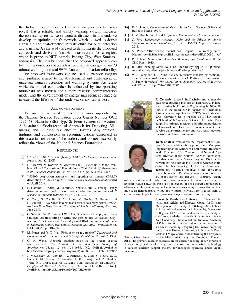
the Indian Ocean. Lessons learned from previous tsunamisreveal that a reliable and timely warning system increasesthe community resilience to tsunami disaster. To this end, wedevelop an optimization framework, which is used to derivea feasible and cost-effective infrastructure for NFT detectionand warning. A case study is used to demonstrate the proposedapproach and derive a feasible infrastructure for a region,which is prone to NFT, namely Padang City, West Sumatra,Indonesia. The results show that the proposed approach canlead to the derivation of an infrastructure that can guarantee 20minute warning time and 99 % data communication reliability.
The proposed framework can be used to provide insightsand guidance related to the development and deployment ofundersea tsunami detection and warning systems. As futurework, the model can further be enhanced by incorporatingmulti-path loss models for a more realistic communicationmodel and the development of energy management strategiesto extend the lifetime of the undersea sensor subnetwork.
ACKNOWLEDGMENT
This material is based in part upon work supported bythe National Science Foundation under Grants Number OCE1331463: Hazards SEES Type 2: From Sensors to Tweeters:A Sustainable Socio-technical Approach for Detecting, Mit-igating, and Building Resilience to Hazards. Any opinions,findings, and conclusions or recommendations expressed inthis material are those of the authors and do not necessarilyreflect the views of the National Science Foundation
REFERENCES
[1] UNESCO-IOC, “Tsunami glossary, 2008,” IOC Technical Series, Paris,France, vol. 85, 2008.
[2] E. Sasorova, M. Korovin, V. Morozov, and P. Savochkin, “On the Prob-lem of Local Tsunamis and Possibilities of Their Warning,” Oceanology2008, Pleiades Publishing Inc, vol. 48, no. 8, pp. 634–645, 2008.
[3] “NDBC- deep-ocean assessment and reporting of tsunamis (DART)description,” [online] http://www.ndbc.noaa.gov/dart/dart.shtml, visitedon April 2014.
[4] L. Comfort, T. Znati, M. Voortman, Xerandy, and L. Freitag, “Earlydetection of near-field tsunamis using underwater sensor networks.”Science of Tsunami Hazards, vol. 31, no. 4, 2012.
[5] C. Teng, S. Cucullu, S. M. Arthur, C. Kohler, B. Burnett, andL. Bernard, “Buoy vandalism by noaa national data buoy center,” NOAANational Data Buoy Center1 University of Southern Mississippi2 report,June 2010.
[6] G. Schmitz, W. Rutzen, and W. Jokat, “Cable-based geophysical mea-surement and monitoring systems, new possibilities for tsunami early-warnings,” in Underwater Technology and Workshop on Scientific Useof Submarine Cables and Related Technologies, 2007. Symposium on.IEEE, 2007, pp. 301–304.
[7] M. Porter and Y.-C. Liu, “Finite-element ray tracing,” Theoretical andComputational Acoustics, World Scientific Publishing Co, vol. 2, 1994.
[8] G. M. Wenz, “Acoustic ambient noise in the ocean: Spectraand sources,” The Journal of the Acoustical Society ofAmerica, vol. 34, no. 12, pp. 1936–1956, 1962. [Online]. Available:http://scitation.aip.org/content/asa/journal/jasa/34/12/10.1121/1.1909155
[9] J. McCloskey, A. Antonioli, A. Piatanesi, K. Sieh, S. Steacy, S. S.Nalbant, M. Cocco, C. Giunchi, J. D. Huang, and P. Dunlop,“Near-field propagation of tsunamis from megathrust earthquakes,”Geophysical Research Letters, vol. 34, no. 14, 2007. [Online].Available: http://dx.doi.org/10.1029/2007GL030494
[10] F. B. Jensen, Computational Ocean Acoustics. Springer Science &Business Media, 1994.
[11] L. M. Brekhovskikh and I. Lysanov, Fundamentals of ocean acoustics.[12] C. Erbe, Underwater Acoustics: Noise and the Effects on Marine
Mammals, a Pocket Handbook, 3rd ed. JASCO Applied Sciences,2011.
[13] M. Porter, “The bellhop manual and userguide: Preliminary draft.”[Online]. Available: http://oalib.hlsresearch.com/Rays/HLS-2010-1.pdf
[14] P. C. Etter, Underwater Acoustics Modeling and Simulation, 4th ed.CRC Press, 2013.
[15] B. Balai Teknologi Survei Kelautan, “Baruna jaya bppt 2014.” [Online].Available: http://barunajaya.bppt.go.id/index.php/en.html
[16] W.-B. Yang and T. C. Yang, “M-ary frequency shift keying communi-cations over an underwater acoustic channel: Performance comparisonof data with models,” The Journal of the Acoustical Society of America,vol. 120, no. 5, pp. 2694–2701, 2006.
X. Xerandy received the Bachelor and Master de-gree from Bandung Institute of Technology, Indone-sia, majoring in Electrical Engineering in 2006. Hejoined as the researcher in Agency of TechnologyAssessment and Application (BPPT), Indonesia since2008. Currently, he is enrolled as a PhD studentin School of Information Science, University Pitts-burgh. His primary research is in telecommunicationand networking. His current research project is todevelop environment-aware undersea sensor networkfor tsunami disaster mitigation.
Taieb Znati is Professor in the Department of Com-puter Science, with a joint appointment in ComputerEngineering at the School of Engineering. He servedas the Director of the Computer and Network Sys-tems Division at the National Science Foundation.He also served as a Senior Program Director fornetworking research at the National Science Foun-dation. In this capacity, He led the InformationTechnology Research Initiative, a cross-directorateresearch program. Dr. Znatis main research interestsare in the design and analysis of evolvable, secure
and resilient network architectures and protocols for wired and wirelesscommunication networks. He is also interested in bio-inspired approaches toaddress complex computing and communications design issues that arise inlarge-scale heterogeneous wired and wireless networks. He is a recipient ofseveral research grants from government agencies and from industry.
Louise K Comfort is Professor of Public and In-ternational Affairs and Director, Center for DisasterManagement, University of Pittsburgh. She holds aB.A. in political science and philosophy, MacalesterCollege, a M.A. in political science, University ofCalifornia, Berkeley, and a Ph.D. in political science,Yale University. She is a Fellow, National Academyof Public Administration, and author or co-author ofsix books, including Designing Resilience: Preparingfor Extreme Events, University of Pittsburgh Press,2010 and Mega-Crises: Understanding the Prospects,
Nature, Characteristics and the Effects of Cataclysmic Events, C. Thomas,2012. Her primary research interests are in decision making under conditionsof uncertainty and rapid change, and the uses of information technologyto develop decision support systems for managers operating under urgentconditions.
(IJACSA) International Journal of Advanced Computer Science and Applications,
Vol. 6, No. 7, 2015
233 | P a g ewww.ijacsa.thesai.org
Exploiting SCADA vulnerabilities using a HumanInterface Device
Grigoris TzokatziouSchool of Computer Science and Informatics
De Montfort University, Leicester, UK
Leandros A. MaglarasSchool of Computer Science and Informatics
De Montfort University, Leicester, UK
Helge JanickeSchool of Computer Science and Informatics
De Montfort University, Leicester, UK
Ying HeSchool of Computer Science and Informatics
De Montfort University, Leicester, UK
Abstract—SCADA (Supervisory Control and Data Acquisition)systems are used to control and monitor critical national infras-tructure functions like electricity, gas, water and railways. Fielddevices such as PLC’s (Programmable Logic Controllers) are oneof the most critical components of a control system. Cyber-attacksusually target valuable infrastructures assets, taking advantage ofarchitectural/technical vulnerabilities or even weaknesses in thedefense systems. Even though novel intrusion detection systemsare being implemented and used for defending cyber-attacks,certain vulnerabilities of SCADA systems can still be exploited.In this article we present an attack scenario based on a HumanInterface Device (HID) device which is used as a means ofcommunication/exploitation tool to compromise SCADA systems.The attack, which is a normal series of commands that are sentfrom the HID to the PLC cannot be detected through currentintrusion detection mechanisms. Finaly we provide possiblecounter measures and defense mechanisms against this kind ofcyber attacks.
Index Terms—SCADA; Cyber Security; HID; PLC
I. INTRODUCTION
One of the biggest issues that SCADA systems face isthat they were designed to work solely in their environmentsegregated from inter-connected IT networks or ad-hoc sys-tems. The primary reason for this is that there was no needfor remote access at the time of their introduction. However,nowadays organizations want to establish local convenienceor remote access, which will enable them to take decisions onproduction changes and apply them quickly from a centralizedlocation rather than have to travel to different locations in orderto make changes to their ICS systems. This interconnection ofIndustrial Control System (ICS) networks with organizationalICT network infrastructures, and even with the exterior hasbrought a new wave of security problems and attacks. In fact,the number of externally initiated attacks on ICS systems hasincreased much more rapidly than internal ones [1].
Moreover, SCADA communication protocols, which areresponsible for the interaction between field devices, suchas PLC (Programmable Logic Controller) or RTU (RemoteTerminal Unit) components and the stations that control andmonitor them, pose security concerns [2]. One such example
is the Modbus protocol, originally developed by Modicon.Modbus messages are exchanged between entities by usingTCP, which imposes more complexity with regard to managingthe reliable delivery of packets in a control environment withstrong real time constraints. In addition, it provides attackerswith new avenues to target industrial systems [3]. Modbus isone of the most popular protocols for SCADA applications, butit suffers from security problems such as the lack of encryptionor any other protection measures which thus exposes it todifferent vulnerabilities.
Serial communication has not been considered as an impor-tant or viable attack vector, but the researchers say breachinga power system through serial communication devices can beeasier than attacking through the IP network since it does notrequire bypassing layers of firewalls [4]. Potential attackersuse common vulnerabilities in order to put controlling serversinto infinite loops. This case is not the same as not havingaccess to the field network, but it could mean that the operatorsare not aware of the conditions on the ground. The worst ofthe vulnerabilities exposed so far enables a potential buffer-overflow attack, whereby code stored for one purpose over-flows its container, and can end up being executed in differenttime instances than programmed to or in a different way. Thisallows for malicious code to be injected into control servers,giving access to attackers to the control system.
Modern intrusion detection systems (IDSs) focus mainly onanalyzing the traffic that flows in the network. By capturingbehaviour or traffic patterns in the network, misbehavior is de-tected and dedicated security events are reported. IDSs can beclassified into centralized intrusion detection systems (CIDSs)and distributed intrusion detection systems (DIDSs), accordingto the way in which their components are distributed. Due tothe rapid increase of sophisticated cyber threats with exponen-tially destructive effects, IDSs are systematically evolving [5],[6]. Among other approaches, neural networks, support vectormachines, K-nearest neighbor (KNN) and the Hidden Markovmodel can be used for intrusion detection, while existingsignature-based network IDS, such as Snort or Suricata can
(IJACSA) International Journal of Advanced Computer Science and Applications,
Vol. 6, No. 7, 2015
234 | P a g ewww.ijacsa.thesai.org
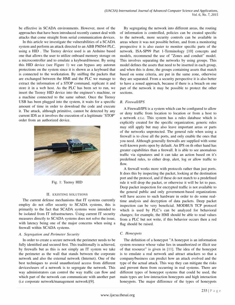
be effective in SCADA environments. However, most of theapproaches that have been introduced recently cannot deal withattacks that come straight from serial communication devices.
In this article we investigate the vulnerabilities of a SCADAsystem and perform an attack directed to an ABB PM564 PLC,using a HID . The Teensy device used is an Arduino basedone that allows the user to utilize onboard memory storage ona microcontroller and to emulate a keyboard/mouse. By usingthis HID device (see Figure 1) we can bypass any autorunprotections on the system since it is shown as a keyboard thatis connected to the workstation. By sniffing the packets thatare exchanged between the HMI and the PLC we manage toextract the information of a STOP command, replicate it andstore it in a web host. As the PLC has been set to run, weinsert the Teensy HID device into the engineer’s machine, ora machine connected to the same subnet. Once the TeensyUSB has been plugged into the system, it waits for a specificamount of time in order to download the code and executeit. The attack, although primitive, cannot be detected by anycurrent IDS as it involves the execution of a legitimate ’STOP’order from an authorized device.
Fig. 1: Teensy HID
II. EXISTING SOLUTIONS
The current defense mechanisms that IT systems currentlyemploy do not offer security to SCADA systems, this isprimarily to the fact that SCADA systems were intended tobe isolated from IT infrastructures. Using current IT securitymeasures directly to SCADA systems does not solve the issue,with latency being one of the major concerns when using afirewall within SCADA systems.
A. Segregation and Perimeter SecurityIn order to create a secure network the perimeter needs to be
fully identified and secured first. This traditionally is achieved,by firewalls but as this is not simply an IT system we takethe perimeter as the wall that stands between the corporatenetwork and also the external network (Internet). One of thebest techniques to avoid unauthorized access from differentdevices/users of a network is to segregate the network. Thisway administrators can control the way traffic can flow andwhich part of the network can communicate with another part(i.e corporate network/management network)[9].
By segregating the network into different areas, the routingof information is controlled, policies can be created specificto the network, more security controls can be available inareas where it was not possible before, and from a monitoringprospective it is also easier to monitor specific parts of thenetwork. ISA-SP99 Part 1-Terminology [10] concepts andmodels, recommend the use of ”Zones and conduit” model.This involves separating the networks by using groups. Thismodel defines the assets that need to be inserted in each group,and when this is done, the groups containing assets that matchbased on some criteria, are put in the same zone, otherwisethey are separated. From a security perspective it is also betterto have a zoned approach, because if there is a breach on onepart of the network it may be possible to protect the othersections.
B. Firewall/IPS
A Firewall/IPS is a system which can be configured to allowor deny traffic from location to location or from a host toa network e.t.c. This system has a rules database which isexplicitly created for the specific organization; generic rulesmay still apply but may also leave important areas or partsof the networks unprotected. The general rule when using afirewall is to close all the ports, and only enable the ones thatyou need. Although generally firewalls are supplied with somewell-known ports open by default. An IPS on th other hand hasgreater capabilities than a firewall. It is able to see anomaloustraffic via signatures and it can take an action based on it’spredefined rules, to either drop, alert, log or allow traffic toflow.
A firewall works more with protocols rather than just ports.It does this by inspecting the packet, looking at the destinationport and the protocol, and if these do not match to a predefinedrule it will drop the packet, or otherwise it will be let to pass.Deep packet inspection for encrypted traffic is not available tothe general public and only government-based organizationswill have access to such hardware in order to do some real-time analysis and decryption of data packets. Deep packetinspection can be very beneficial. MODBUS TCP protocolwhich is used by PLC’s can be analyzed for behavioralchanges; for example, the HMI should be able to read valuesfrom a PLC but not write, if this behavior occurs then a redflag should be raised.
C. Honeypots
The definition of a honeypot ”A honeypot is an informationsystem resource whose value lies in unauthorized or illicit useof that resource” is given in [11]. The idea of the honeypotis to emulate a real network and attract attackers so that acompany/business can predict how an attack evolved and thetype of the actual attack. This way they can mitigate the risksand prevent them from occurring in real systems. There aredifferent types of honeypot systems that could be used, themain types are low-interaction honeypots and high interactionhoneypots. The major difference of the types of honeypots
(IJACSA) International Journal of Advanced Computer Science and Applications,
Vol. 6, No. 7, 2015
235 | P a g ewww.ijacsa.thesai.org
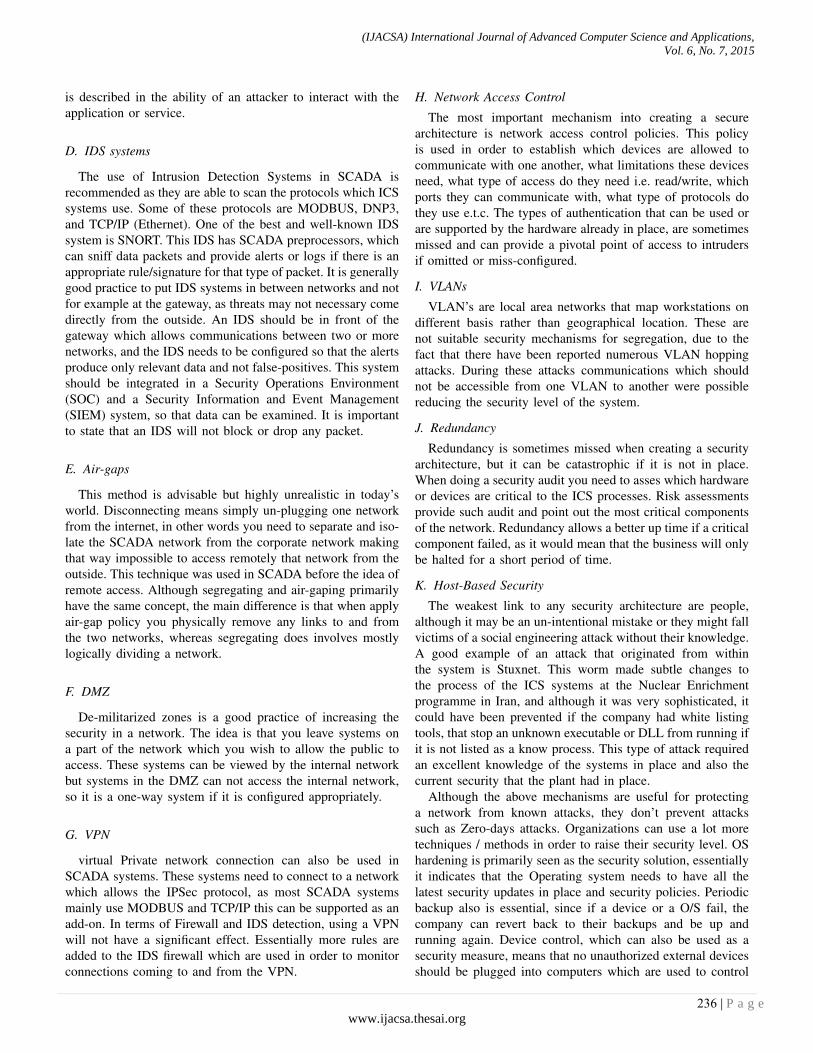
is described in the ability of an attacker to interact with theapplication or service.
D. IDS systems
The use of Intrusion Detection Systems in SCADA isrecommended as they are able to scan the protocols which ICSsystems use. Some of these protocols are MODBUS, DNP3,and TCP/IP (Ethernet). One of the best and well-known IDSsystem is SNORT. This IDS has SCADA preprocessors, whichcan sniff data packets and provide alerts or logs if there is anappropriate rule/signature for that type of packet. It is generallygood practice to put IDS systems in between networks and notfor example at the gateway, as threats may not necessary comedirectly from the outside. An IDS should be in front of thegateway which allows communications between two or morenetworks, and the IDS needs to be configured so that the alertsproduce only relevant data and not false-positives. This systemshould be integrated in a Security Operations Environment(SOC) and a Security Information and Event Management(SIEM) system, so that data can be examined. It is importantto state that an IDS will not block or drop any packet.
E. Air-gaps
This method is advisable but highly unrealistic in today’sworld. Disconnecting means simply un-plugging one networkfrom the internet, in other words you need to separate and iso-late the SCADA network from the corporate network makingthat way impossible to access remotely that network from theoutside. This technique was used in SCADA before the idea ofremote access. Although segregating and air-gaping primarilyhave the same concept, the main difference is that when applyair-gap policy you physically remove any links to and fromthe two networks, whereas segregating does involves mostlylogically dividing a network.
F. DMZ
De-militarized zones is a good practice of increasing thesecurity in a network. The idea is that you leave systems ona part of the network which you wish to allow the public toaccess. These systems can be viewed by the internal networkbut systems in the DMZ can not access the internal network,so it is a one-way system if it is configured appropriately.
G. VPN
virtual Private network connection can also be used inSCADA systems. These systems need to connect to a networkwhich allows the IPSec protocol, as most SCADA systemsmainly use MODBUS and TCP/IP this can be supported as anadd-on. In terms of Firewall and IDS detection, using a VPNwill not have a significant effect. Essentially more rules areadded to the IDS firewall which are used in order to monitorconnections coming to and from the VPN.
H. Network Access Control
The most important mechanism into creating a securearchitecture is network access control policies. This policyis used in order to establish which devices are allowed tocommunicate with one another, what limitations these devicesneed, what type of access do they need i.e. read/write, whichports they can communicate with, what type of protocols dothey use e.t.c. The types of authentication that can be used orare supported by the hardware already in place, are sometimesmissed and can provide a pivotal point of access to intrudersif omitted or miss-configured.
I. VLANs
VLAN’s are local area networks that map workstations ondifferent basis rather than geographical location. These arenot suitable security mechanisms for segregation, due to thefact that there have been reported numerous VLAN hoppingattacks. During these attacks communications which shouldnot be accessible from one VLAN to another were possiblereducing the security level of the system.
J. Redundancy
Redundancy is sometimes missed when creating a securityarchitecture, but it can be catastrophic if it is not in place.When doing a security audit you need to asses which hardwareor devices are critical to the ICS processes. Risk assessmentsprovide such audit and point out the most critical componentsof the network. Redundancy allows a better up time if a criticalcomponent failed, as it would mean that the business will onlybe halted for a short period of time.
K. Host-Based Security
The weakest link to any security architecture are people,although it may be an un-intentional mistake or they might fallvictims of a social engineering attack without their knowledge.A good example of an attack that originated from withinthe system is Stuxnet. This worm made subtle changes tothe process of the ICS systems at the Nuclear Enrichmentprogramme in Iran, and although it was very sophisticated, itcould have been prevented if the company had white listingtools, that stop an unknown executable or DLL from running ifit is not listed as a know process. This type of attack requiredan excellent knowledge of the systems in place and also thecurrent security that the plant had in place.
Although the above mechanisms are useful for protectinga network from known attacks, they don’t prevent attackssuch as Zero-days attacks. Organizations can use a lot moretechniques / methods in order to raise their security level. OShardening is primarily seen as the security solution, essentiallyit indicates that the Operating system needs to have all thelatest security updates in place and security policies. Periodicbackup also is essential, since if a device or a O/S fail, thecompany can revert back to their backups and be up andrunning again. Device control, which can also be used as asecurity measure, means that no unauthorized external devicesshould be plugged into computers which are used to control
(IJACSA) International Journal of Advanced Computer Science and Applications,
Vol. 6, No. 7, 2015
236 | P a g ewww.ijacsa.thesai.org
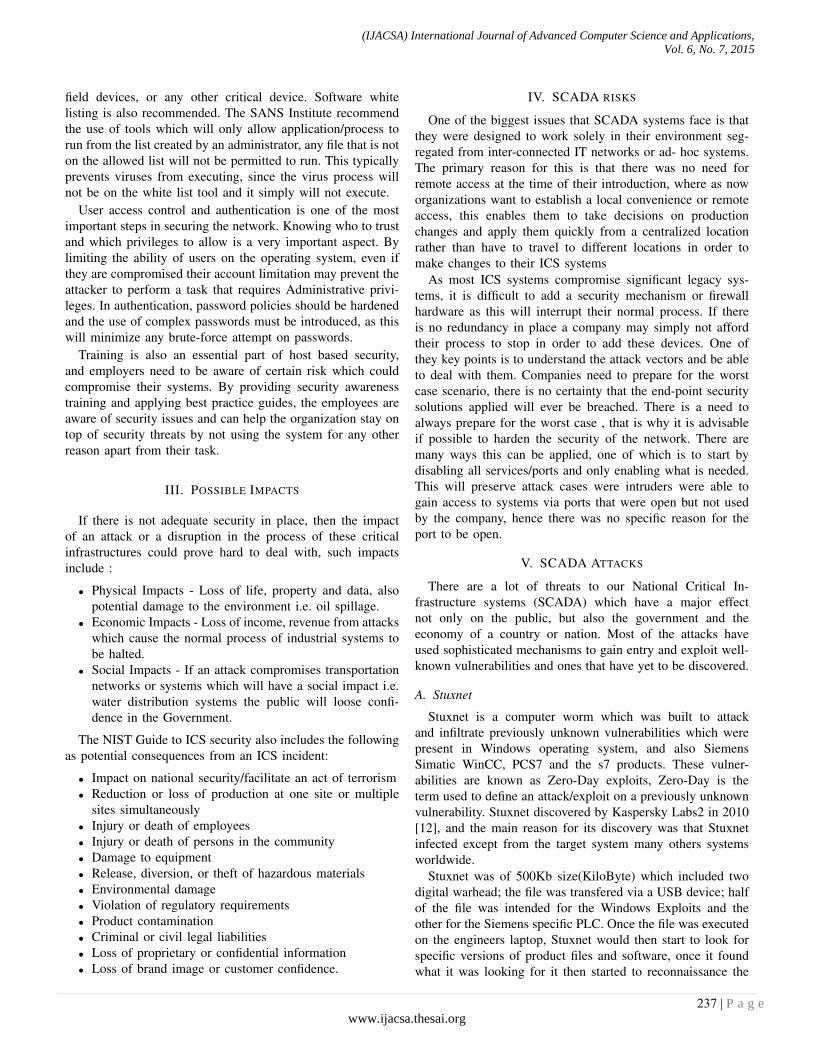
field devices, or any other critical device. Software whitelisting is also recommended. The SANS Institute recommendthe use of tools which will only allow application/process torun from the list created by an administrator, any file that is noton the allowed list will not be permitted to run. This typicallyprevents viruses from executing, since the virus process willnot be on the white list tool and it simply will not execute.
User access control and authentication is one of the mostimportant steps in securing the network. Knowing who to trustand which privileges to allow is a very important aspect. Bylimiting the ability of users on the operating system, even ifthey are compromised their account limitation may prevent theattacker to perform a task that requires Administrative privi-leges. In authentication, password policies should be hardenedand the use of complex passwords must be introduced, as thiswill minimize any brute-force attempt on passwords.
Training is also an essential part of host based security,and employers need to be aware of certain risk which couldcompromise their systems. By providing security awarenesstraining and applying best practice guides, the employees areaware of security issues and can help the organization stay ontop of security threats by not using the system for any otherreason apart from their task.
III. POSSIBLE IMPACTS
If there is not adequate security in place, then the impactof an attack or a disruption in the process of these criticalinfrastructures could prove hard to deal with, such impactsinclude :
• Physical Impacts - Loss of life, property and data, alsopotential damage to the environment i.e. oil spillage.
• Economic Impacts - Loss of income, revenue from attackswhich cause the normal process of industrial systems tobe halted.
• Social Impacts - If an attack compromises transportationnetworks or systems which will have a social impact i.e.water distribution systems the public will loose confi-dence in the Government.
The NIST Guide to ICS security also includes the followingas potential consequences from an ICS incident:
• Impact on national security/facilitate an act of terrorism• Reduction or loss of production at one site or multiple
sites simultaneously• Injury or death of employees• Injury or death of persons in the community• Damage to equipment• Release, diversion, or theft of hazardous materials• Environmental damage• Violation of regulatory requirements• Product contamination• Criminal or civil legal liabilities• Loss of proprietary or confidential information• Loss of brand image or customer confidence.
IV. SCADA RISKS
One of the biggest issues that SCADA systems face is thatthey were designed to work solely in their environment seg-regated from inter-connected IT networks or ad- hoc systems.The primary reason for this is that there was no need forremote access at the time of their introduction, where as noworganizations want to establish a local convenience or remoteaccess, this enables them to take decisions on productionchanges and apply them quickly from a centralized locationrather than have to travel to different locations in order tomake changes to their ICS systems
As most ICS systems compromise significant legacy sys-tems, it is difficult to add a security mechanism or firewallhardware as this will interrupt their normal process. If thereis no redundancy in place a company may simply not affordtheir process to stop in order to add these devices. One ofthey key points is to understand the attack vectors and be ableto deal with them. Companies need to prepare for the worstcase scenario, there is no certainty that the end-point securitysolutions applied will ever be breached. There is a need toalways prepare for the worst case , that is why it is advisableif possible to harden the security of the network. There aremany ways this can be applied, one of which is to start bydisabling all services/ports and only enabling what is needed.This will preserve attack cases were intruders were able togain access to systems via ports that were open but not usedby the company, hence there was no specific reason for theport to be open.
V. SCADA ATTACKS
There are a lot of threats to our National Critical In-frastructure systems (SCADA) which have a major effectnot only on the public, but also the government and theeconomy of a country or nation. Most of the attacks haveused sophisticated mechanisms to gain entry and exploit well-known vulnerabilities and ones that have yet to be discovered.
A. Stuxnet
Stuxnet is a computer worm which was built to attackand infiltrate previously unknown vulnerabilities which werepresent in Windows operating system, and also SiemensSimatic WinCC, PCS7 and the s7 products. These vulner-abilities are known as Zero-Day exploits, Zero-Day is theterm used to define an attack/exploit on a previously unknownvulnerability. Stuxnet discovered by Kaspersky Labs2 in 2010[12], and the main reason for its discovery was that Stuxnetinfected except from the target system many others systemsworldwide.
Stuxnet was of 500Kb size(KiloByte) which included twodigital warhead; the file was transfered via a USB device; halfof the file was intended for the Windows Exploits and theother for the Siemens specific PLC. Once the file was executedon the engineers laptop, Stuxnet would then start to look forspecific versions of product files and software, once it foundwhat it was looking for it then started to reconnaissance the
(IJACSA) International Journal of Advanced Computer Science and Applications,
Vol. 6, No. 7, 2015
237 | P a g ewww.ijacsa.thesai.org
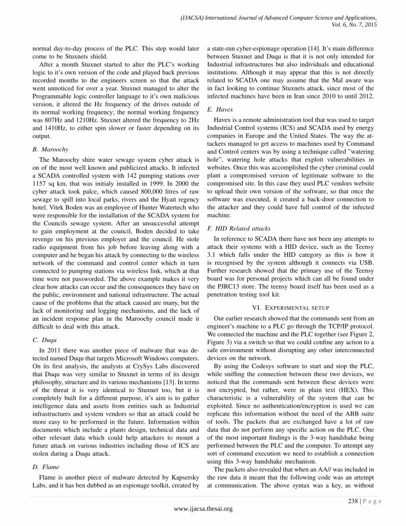
normal day-to-day process of the PLC. This step would latercome to be Stuxnets shield.
After a month Stuxnet started to alter the PLC’s workinglogic to it’s own version of the code and played back previousrecorded months to the engineers screen so that the attackwent unnoticed for over a year. Stuxnet managed to alter theProgrammable logic controller language to it’s own maliciousversion, it altered the Hz frequency of the drives outside ofits normal working frequency; the normal working frequencywas 807Hz and 1210Hz. Stuxnet altered the frequency to 2Hzand 1410Hz, to either spin slower or faster depending on itsoutput.
B. Maroochy
The Maroochy shire water sewage system cyber attack ison of the most well known and publicized attacks. It infecteda SCADA controlled system with 142 pumping stations over1157 sq km, that was initialy installed in 1999. In 2000 thecyber attack took palce, which caused 800,000 litres of rawsewage to spill into local parks, rivers and the Hyatt regencyhotel. Vitek Boden was an employee of Hunter Watertech whowere responsible for the installation of the SCADA system forthe Councils sewage system. After an unsuccessful attemptto gain employment at the council, Boden decided to takerevenge on his previous employer and the council. He stoleradio equipment from his job before leaving along with acomputer and he began his attack by connecting to the wirelessnetwork of the command and control center which in turnconnected to pumping stations via wireless link, which at thattime were not passworded. The above example makes it veryclear how attacks can occur and the consequences they have onthe public, environment and national infrastructure. The actualcause of the problems that the attack caused are many, but thelack of monitoring and logging mechanisms, and the lack ofan incident response plan in the Maroochy council made itdifficult to deal with this attack.
C. Duqu
In 2011 there was another piece of malware that was de-tected named Duqu that targets Microsoft Windows computers.On its first analysis, the analysts at CrySys Labs discoveredthat Duqu was very similar to Stuxnet in terms of its designphilosophy, structure and its various mechanisms [13]. In termsof the threat it is very identical to Stuxnet too, but it iscompletely built for a different purpose, it’s aim is to gatherintelligence data and assets from entities such as Industrialinfrastructures and system vendors so that an attack could bemore easy to be performed in the future. Information withindocuments which include a plants design, technical data andother relevant data which could help attackers to mount afuture attack on various industries including those of ICS arestolen during a Duqu attack.
D. Flame
Flame is another piece of malware detected by KapserskyLabs, and it has ben dubbed as an espionage toolkit, created by
a state-run cyber-espionage operation [14]. It’s main differencebetween Stuxnet and Duqu is that it is not only intended forIndustrial infrastructures but also individuals and educationalinstitutions. Although it may appear that this is not directlyrelated to SCADA one may assume that the Mal aware wasin fact looking to continue Stuxnets attack, since most of theinfected machines have been in Iran since 2010 to until 2012.
E. Havex
Havex is a remote administration tool that was used to targetIndustrial Control systems (ICS) and SCADA used by energycompanies in Europe and the United States. The way the at-tackers managed to get access to machines used by Commandand Control centers was by using a technique called ”wateringhole”, watering hole attacks that exploit vulnerabilities inwebsites. Once this was accomplished the cyber criminal couldplant a compromised version of legitimate software to thecompromised site. In this case they used PLC vendors websiteto upload their own version of the software, so that once thesoftware was executed, it created a back-door connection tothe attacker and they could have full control of the infectedmachine.
F. HID Related attacks
In reference to SCADA there have not been any attempts toattack their systems with a HID device, such as the Teensy3.1 which falls under the HID category as this is how itis recognised by the system although it connects via USB.Further research showed that the primary use of the Teensyboard was for personal projects which can all be found underthe PJRC13 store. The teensy board itself has been used as apenetration testing tool kit.
VI. EXPERIMENTAL SETUP
Our earlier research showed that the commands sent from anengineer’s machine to a PLC go through the TCP/IP protocol.We connected the machine and the PLC together (see Figure 2,Figure 3) via a switch so that we could confine any action to asafe environment without disrupting any other interconnecteddevices on the network.
By using the Codesys software to start and stop the PLC,while sniffing the connection between these two devices, wenoticed that the commands sent between these devices werenot encrypted, but rather, were in plain text (HEX). Thischaracteristic is a vulnerability of the system that can beexploited. Since no authentication/encryption is used we canreplicate this information without the need of the ABB suiteof tools. The packets that are exchanged have a lot of rawdata that do not perform any specific action on the PLC. Oneof the most important findings is the 3-way handshake beingperformed between the PLC and the computer. To attempt anysort of command execution we need to establish a connectionusing this 3-way handshake mechanism.
The packets also revealed that when an AA// was included inthe raw data it meant that the following code was an attemptat communication. The above syntax was a key, as without
(IJACSA) International Journal of Advanced Computer Science and Applications,
Vol. 6, No. 7, 2015
238 | P a g ewww.ijacsa.thesai.org
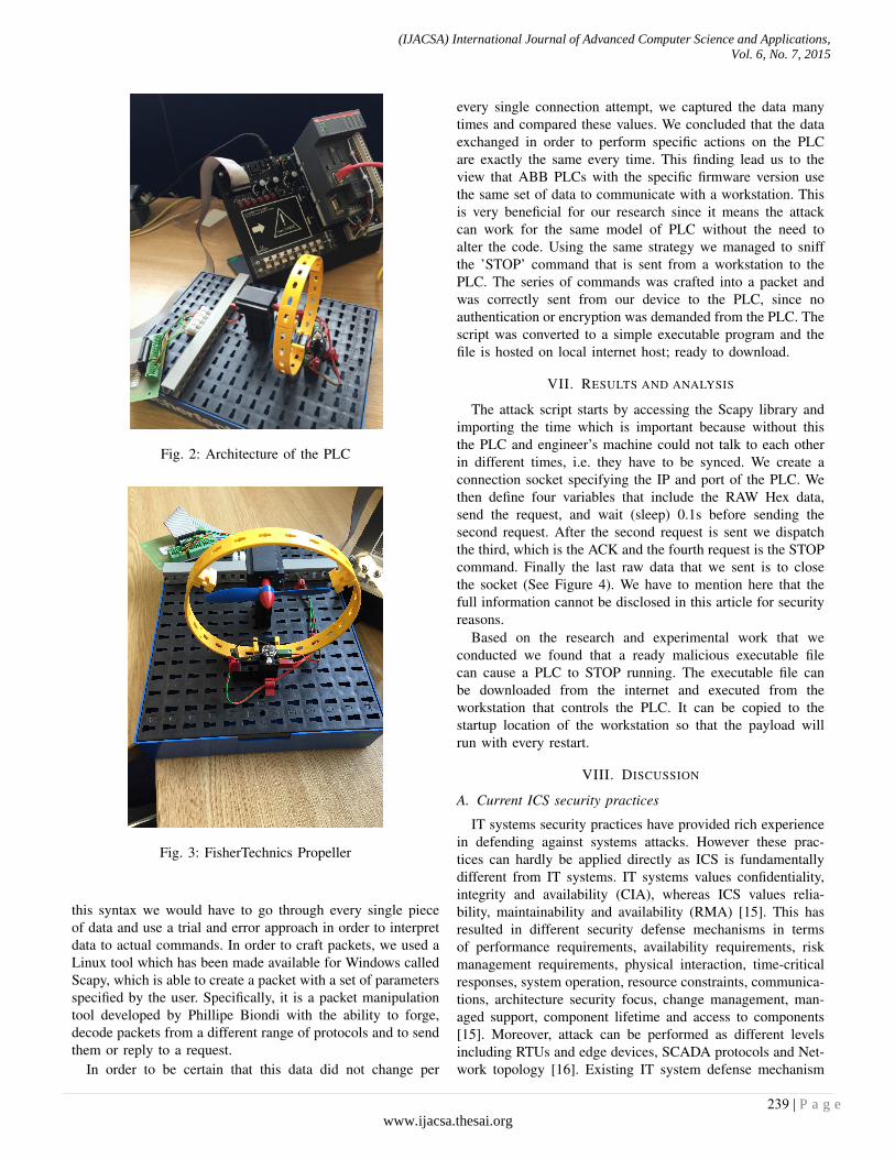
Fig. 2: Architecture of the PLC
Fig. 3: FisherTechnics Propeller
this syntax we would have to go through every single pieceof data and use a trial and error approach in order to interpretdata to actual commands. In order to craft packets, we used aLinux tool which has been made available for Windows calledScapy, which is able to create a packet with a set of parametersspecified by the user. Specifically, it is a packet manipulationtool developed by Phillipe Biondi with the ability to forge,decode packets from a different range of protocols and to sendthem or reply to a request.
In order to be certain that this data did not change per
every single connection attempt, we captured the data manytimes and compared these values. We concluded that the dataexchanged in order to perform specific actions on the PLCare exactly the same every time. This finding lead us to theview that ABB PLCs with the specific firmware version usethe same set of data to communicate with a workstation. Thisis very beneficial for our research since it means the attackcan work for the same model of PLC without the need toalter the code. Using the same strategy we managed to sniffthe ’STOP’ command that is sent from a workstation to thePLC. The series of commands was crafted into a packet andwas correctly sent from our device to the PLC, since noauthentication or encryption was demanded from the PLC. Thescript was converted to a simple executable program and thefile is hosted on local internet host; ready to download.
VII. RESULTS AND ANALYSIS
The attack script starts by accessing the Scapy library andimporting the time which is important because without thisthe PLC and engineer’s machine could not talk to each otherin different times, i.e. they have to be synced. We create aconnection socket specifying the IP and port of the PLC. Wethen define four variables that include the RAW Hex data,send the request, and wait (sleep) 0.1s before sending thesecond request. After the second request is sent we dispatchthe third, which is the ACK and the fourth request is the STOPcommand. Finally the last raw data that we sent is to closethe socket (See Figure 4). We have to mention here that thefull information cannot be disclosed in this article for securityreasons.
Based on the research and experimental work that weconducted we found that a ready malicious executable filecan cause a PLC to STOP running. The executable file canbe downloaded from the internet and executed from theworkstation that controls the PLC. It can be copied to thestartup location of the workstation so that the payload willrun with every restart.
VIII. DISCUSSION
A. Current ICS security practices
IT systems security practices have provided rich experiencein defending against systems attacks. However these prac-tices can hardly be applied directly as ICS is fundamentallydifferent from IT systems. IT systems values confidentiality,integrity and availability (CIA), whereas ICS values relia-bility, maintainability and availability (RMA) [15]. This hasresulted in different security defense mechanisms in termsof performance requirements, availability requirements, riskmanagement requirements, physical interaction, time-criticalresponses, system operation, resource constraints, communica-tions, architecture security focus, change management, man-aged support, component lifetime and access to components[15]. Moreover, attack can be performed as different levelsincluding RTUs and edge devices, SCADA protocols and Net-work topology [16]. Existing IT system defense mechanism
(IJACSA) International Journal of Advanced Computer Science and Applications,
Vol. 6, No. 7, 2015
239 | P a g ewww.ijacsa.thesai.org

d e f p k t s e n d ( ) :mysocket = s o c k e t . s o c k e t ( )mysocket . c o n n e c t
( ( ’ 1 9 2 . 1 6 8 . 0 . 1 0 ’ , 1 2 0 1 ) )myStream = S t r e a m S o c k e t ( mysocket )r e q = Raw( l o a d =”\xbb\xbb\x00\x00
. . . . . . ” )r eq 1 = Raw ( l o a d =”\xbb\xbb\x00\x00
. . . . . ” )r eq 2 = Raw ( l o a d =”\xbb\xbb\x00\x00
. . . . . ” )r eq 3 = Raw ( l o a d =”\xbb\xbb\x00\x00
. . . . . ” )myStream . send ( r e q )t ime . s l e e p ( 0 . 1 )myStream . send ( r eq1 )t ime . s l e e p ( 0 . 1 )myStream . send ( r eq2 )t ime . s l e e p ( 1 )myStream . send ( r eq3 )t ime . s l e e p ( 0 . 1 )mysocket . c l o s e ( )
p k t s e n d ( )
Fig. 4: Attack code
has to be tailored to address the above-mentioned aspects inICS security defense.
There have been some existing researches on adaptingexisting IT system security to satisfy the needs of ICS security.Snort, a signature-based intrusion detection open source solu-tion have been widely used. Yang et al. [17] proposed a rule-based Intrusion Detection System (IDS), which is a signature-based and model-based approach specifically designed forSCADA networks. The proposed rules were implementedand validated using Snort rules. Cheung et al. also usedSnort implementation for a model-based intrusion detectionapproach for SCADA Networks [18]. Artificial intelligencehas also been applied into ICS security defending. Tsang andKwong [19] proposed multi-agent intrusion detection systemsand distributed the operational process into multiple agents.Jiang and Yasakethu [20] applied support vector machines(SVMs) for automated anomaly detection in SCADA. Theresults showed that the proposed algorithm achieves highdetection rates. Maglaras [5] extended this work and appliedOCSVM (One-Class Support Vector Machine) for detectingintrusions.
Existing work also provide control system security stan-dards, guidelines and best practices. IEC/ISA-62443 [21] isan internationally recognised industrial control system securitystandard. The content is organized into four categories, whichare General, Policy & Procedures, Systems and Component.NIST SP 800-82 [15] provides cross-industry guidance forestablishing secure industrial control systems (ICS). The U.K.
CPNI has produced a good practice guide for ICS security.It includes seven parts encompassing both technical aspect(implementation [22] of security techniques) and manage-rial aspects (governance [25] and security awareness [24]).The U.S. Department of Homeland Security [26] producedguidance on the enhancement of ICS security. It provides ageneral structure of ICS security management and rich links toother industrial guidelines. The Swedish Civil ContingenciesAgency (SEMA) has also produced guidelines to increasesecurity and people’s awareness of industrial control systemsecurity [27]. It provides 15 recommendations and these rec-ommendations were integrated into Deming Cycle, also knownas the PDCA (plan, do, check and act) [28].
B. Future directions for ICS security
Although security standards, guidelines, best practices andsecurity mechanisms are available for ICS, limited researchescan be found in the change management and interdependenciesbetween IT and ICS systems.
1) Change management: unlike IT systems, ICS systemavailability is a primary concern and ICS processes are alwayscontinuous in nature. Frequent software patching and updatesare not suitable for ICS. Future research should focus ondeveloping new security mechanisms to allow patching andupdating equipment without affecting the main operation ofICS systems. The impact of patches and system updates needsto be thoroughly measured and tested.
2) Complex interdependencies: ICS has complex integra-tion with IT systems and physical system. Future researchshould investigate interdependencies on communication net-works and ICT components, develop new tools and processesfor security defense.
Future research should focus on these directions and retrofitIT security into existing ICS components. This is consistentwith H2020 call in the protection of critical infrastructure [22].Future research should consider developing security solutionsfor the next generation ICS and integrating security measurein the ICS product lifecycle.
C. Proposed defense mechanisms
The Teensy HID device appears on the system under theUniversal Serial Bus. Traditionally, Windows does not requireany privileges for the installation of this device as these driversare already part of the O/S and by default are automaticallyinstalled. A way to stop any input from a certain HID deviceis to blacklist it by vendor and product ID, but this is notvery reliable as the vendor can change the identifiers whichthen” can by-pass the blacklist enabled within Windows [7].Another option would be to create a policy within Windows toallow only one keyboard and mouse to be present at any onetime. Another available option is to allow the administratorto specify a list of device set-up GUIDs (global unique iden-tifiers) for device drivers that windows is allowed to install.Cryptographic solutions are incomplete without effective keymanagement which remains an open problem in SCADAnetworks.
(IJACSA) International Journal of Advanced Computer Science and Applications,
Vol. 6, No. 7, 2015
240 | P a g ewww.ijacsa.thesai.org

The security properties of ICS can be improved by usingmany of the current cryptographic methods. Although SCADAprotocols typically do not support any sort of cryptography,this capability would be useful in securing these networks. Theunique characteristics of SCADA networks, on the other hand,make it difficult to adapt existing cryptographic techniques forthese systems. Except from strict policies and maintenanceissues, security technologies and procedures that are appliedon a SCADA network must be audited and updated in a regularbasis. Regarding which, more research is needed to developproper metrics to assess the security of SCADA networks. Theintegration of new technologies introduce new threats to thesecurity of the ICS. In the ICS network there are three crucialaspects of security that must be protected: Confidentiality,Integrity, and Availability [8].
IX. CONCLUSION
This article has investigated the vulnerabilities of a SCADAsystem and performed an attack directed at an ABB PM564PLC, using a HID (Human Interface Device). This PLC usesthe Codesys programming software as its SCADA program-ming interface. The HID device is inserted into the workstationand is recognized as a keyboard. Once the Teensy USBhas been plugged into the system it will wait for a specificamount of time (set in the code) in order to download thecode and execute it. The attack, although primitive, cannot bedetected by any current IDS, since it involves the executionof a legitimate ’STOP’ order from an authorized device. Themalicious packet which alters the behaviour of the PLC can beexecuted in random time periods and in different PLCs, thusmaking the situation harder to be controlled.
The article then reviewed current security counter measuresand ICS defense mechanisms from both technical and manage-rial perspectives. It also provided possible counter measuresand defense mechanisms against this kind of cyber attack.As future work, more sophisticated attacks are going to beperformed with real time defense systems tested against themin order to assess their detection capabilities.
REFERENCES
[1] Igure, Vinay M., Sean A. Laughter, and Ronald D. Williams. ”Securityissues in SCADA networks.” Computers & Security 25.7 (2006): 498-506.
[2] Robinson, Michael, Kevin Jones, and Helge Janicke, ”Cyber warfare:Issues and challenges”, Computers & Security 49 (2015): 70-94
[3] A. Carcano, I. Nai Fovino, M. Masera and A. Trombetta, ”SCADAmalware: A proof of concept”, in Third International Workshop on CriticalInformation Infrastructure Security, 2008.
[4] Ashford, W, ”US Researchers Find 25 Security Vulnerabilitiesin SCADA Systems”, ComputerWeekly.com, 2013, October 18,http://www.computerweekly.com/news/2240207488/USresearchers-find-25-security-vulnerabilities-in-SCADA-systems
[5] L. Maglaras, J. Jiang, T. Cruz, ”Integrated OCSVM Mechanismfor intrusion detection in SCADA systems”,in Electronics Letters50.25(2014):1935-1936
[6] M. Gil Perez, F. Gomez Marmol, G. Martinez Perez, A. Skarmeta Gomez,”Repcidn: A reputation-based collaborative intrusion detection network tolessen the impact of malicious alarms”, in Journal of Network and Systems730 Management 21 (1) (2013) 128-167
[7] Crenshaw, Adrian. ”Plug and prey: Malicious USB devices.” URL:http://www.irongeek.com/downloads/Malicious%20USB%20Devices.pdf(2011).
[8] Khurana, Himanshu, et al. ”Smart-grid security issues.” IEEE Security &Privacy 1 (2010): 81-85.
[9] CPNI. PROCESS CONTROL AND SCADA SECURITY GUIDE 2.IMPLEMENT SECURE ARCHITECTURE. In Good Practice Guide,2008.
[10] Digital Bond. ISA99 Part 1, 2011. URL http://www.digitalbond.com/scadapedia/standards/isa99-part-1/.
[11] Spitzner, Lance. ”The honeynet project: Trapping the hackers.” IEEESecurity & Privacy 1.2 (2003): 15-23.
[12] Kushner, David. ”The real story of stuxnet.” IEEE Spectrum 50.3 (2013):48-53.
[13] Bencsth, Boldizsr, et al. ”Duqu: Analysis, detection, and lessonslearned.” ACM European Workshop on System Security (EuroSec). Vol.2012. 2012.
[14] Zetter, Kim. ”Meet FlameThe Massive Spy Mal-ware Infiltrating Iranian Computers.” Wired, 28thMay,Online resource Available at: https://www. securelist.com/en/blog/208193522/The Flame Questions and Answers,[Accessed20/11/2012] (2012).
[15] Stouffer, K., Falco, J., Scarfone, K.Guide to industrial control systems(ICS) security. NIST special publication, 800-82, 2011.
[16] Alcaraz, C., Fernandez, G., Carvajal, F. Security aspects of SCADAand DCS environments. In Critical Infrastructure Protection (pp. 120-149).Springer Berlin Heidelberg. 2012.
[17] Yang, Yi, et al. ”Intrusion Detection System for IEC 60870-5-104 basedSCADA networks.” Power and Energy Society General Meeting (PES),2013 IEEE. IEEE, 2013.
[18] Cheung, Steven, et al. ”Using model-based intrusion detection forSCADA networks.” Proceedings of the SCADA security scientific sym-posium. Vol. 46. 2007.
[19] Tsang, Chi-Ho, and Sam Kwong. ”Multi-agent intrusion detectionsystem in industrial network using ant colony clustering approach andunsupervised feature extraction.” Industrial Technology, 2005. ICIT 2005.IEEE International Conference on. IEEE, 2005.
[20] Jiang, Jianmin, and Lasith Yasakethu. ”Anomaly detection via one classsvm for protection of scada systems.” Cyber-Enabled Distributed Comput-ing and Knowledge Discovery (CyberC), 2013 International Conferenceon. IEEE, 2013.
[21] International Electrotechnical Commission, Industrial CommunicationNetworks Network and System Security Part 1-1: Terminology, Conceptsand Models, IEC/TS 62443- 1-1 ed1.0, Geneva, Switzerland, 2009.
[22] European Commission. Digital Security: Cybersecurity,Privacy and Trust - The role of ICT in Critical InfrastructureProtection. 2015. URL http://ec.europa.eu/research/participants/portal/desktop/en/opportunities/h2020/topics/1052-ds-03-2015.html.
[23] Centre for the Protection of National Infrastructure, Good PracticeGuide, Process Control and SCADA Security, Guide 2: Implement SecureArchitecture, London, United Kingdom, 2008.
[24] Centre for the Protection of National Infrastructure, Good PracticeGuide, Process Control and SCADA Security, Guide 4: Improve Awarenessand Skills, London, United Kingdom, 2008.
[25] Centre for the Protection of National Infrastructure, Good PracticeGuide, Process Control and SCADA Security, Guide 7: Establish OngoingGovernance, London, United Kingdom, 2008.
[26] Technical Support Working Group, Securing Your SCADA and Indus-trial Control Systems, Department of Defense, Washington, DC, 2005.
[27] Swedish Emergency Management Agency, Guide to Increased Securityin Process Control Systems for Critical Societal Functions, Stockholm,Sweden, 2008.
[28] Deming, William Edwards. The new economics: for industry, govern-ment, education. MIT press, 2000.
(IJACSA) International Journal of Advanced Computer Science and Applications,
Vol. 6, No. 7, 2015
241 | P a g ewww.ijacsa.thesai.org

Image Mining: Review and New Challenges
Barbora Zahradnikova, Sona Duchovicova and Peter Schreiber Institute of Applied Informatics, Automation and Mechatronics,
Faculty of Materials Science and Technology,Slovak University of Technology,Hajdoczyho 1, Trnava, Slovakia
Abstract—Besides new technology, a huge volume of data invarious form has been available for people. Image data representsa keystone of many research areas including medicine, forensiccriminology, robotics and industrial automation, meteorology andgeography as well as education. Therefore, obtaining specific in-formation from image databases has become of great importance.Images as a special category of data differ from text data as interms of their nature so in terms of storing and retrieving. ImageMining as a research field is an interdisciplinary area combiningmethodologies and knowledge of many branches including datamining, computer vision, image processing, image retrieval, statis-tics, recognition, machine learning, artificial intelligence etc. Thisreview focuses researching the current image mining approachesand techniques aiming at widening the possibilities of facial imageanalysis. This paper aims at reviewing the current state of theIM as well as at describing challenges and identifying directionsof the future research in the field.
Keywords—image mining; image classification; indexing; imageretrieval;
I. INTRODUCTION
Due to the enormous research and development of therecent years, the lack of information has not been an issuein the most fields of human activity. On the contrary, besidesnew technology, there is a huge volume of data availablefor people. Therefore, sorting the data and obtaining specificinformation from databases has become of great significance.In the last decade, data mining as a research field has expandedand progress in data processing is getting both more accurateand convenient. Besides text data mining; novel data miningalgorithm; web mining and social network analysis, imagemining belongs to the spheres of interest.
Analysing image data forms a keystone of many researchareas including medicine (evaluating MRI, interpreting X-Rays/CT scans), forensic criminology (fingerprint identifica-tion, face recognition), robotics and industrial automation(robotic vision), meteorology and geography (satellite im-agery) as well as education (computer-aided visualization) andmany other fields.
Searching information within images represents a specialentity of data processing. Images as a unique category ofdata differ from text data in several aspects as in terms oftheir nature so in terms of storing and retrieving. Imageshave visual character, they can be represented in numericalform, however large amount of numbers is to be evaluatedin order to search image databases. Finding, extracting andclassifying objects from images are the basic requirements of
processing an image successfully. Tools of data mining havebeen utilised for these tasks to be performed with increasedefficiency. Nevertheless, applying data mining solely would notbring satisfactory results for image processing.
Image mining deals with extraction of implicit knowledge,image data relationship or other patterns not explicitly storedin image [1]. Unlike other image processing techniques, IMdoes not aim at detecting a specific pattern in images. It focusesrather on identifying and finding image patterns and derivingthe knowledge from images within an image set based onthe low-level (pixel) information. As a research field, it hasdeveloped to an interdisciplinary area combining knowledgeand tools of data mining, databases, computer vision, imageprocessing, image retrieval, statistics, recognition, machinelearning, artificial intelligence, etc. Image mining processconsists of several components including
• image analysis covering image preprocessing, objectrecognition and feature extraction,
• image classification,
• image indexing,
• image retrieval,
• data management.
A number of approaches for each of the above mentionedprocedures have been proposed. Yet, image processing stays adomain where humans still can outperform computer.
This paper aims at reviewing the steps of image mining,the most often utilised techniques for the individual sub-processes of IM and at identifying the major current issuesand challenges in image mining.
II. IMAGE ANALYSIS
Image analysis is an inevitable step of image Mining. Theanalysis is often said to be a pre-processing stage of the imageminig [2]. The objective of analysing an image is to find andextract all relevant features required to represent an image.
A. Image Preprocessing
Image preprocessing is an initial step of processing images.It is utilised for improving the quality of an image beforeobject detection algorithms are applied. Normalising imagesis usually performed in order to reduce noise and/or enhanceresolution of an image. Different pre-processing procedures
(IJACSA) International Journal of Advanced Computer Science and Applications,
Vol. 6, No. 7, 2015
242 | P a g ewww.ijacsa.thesai.org
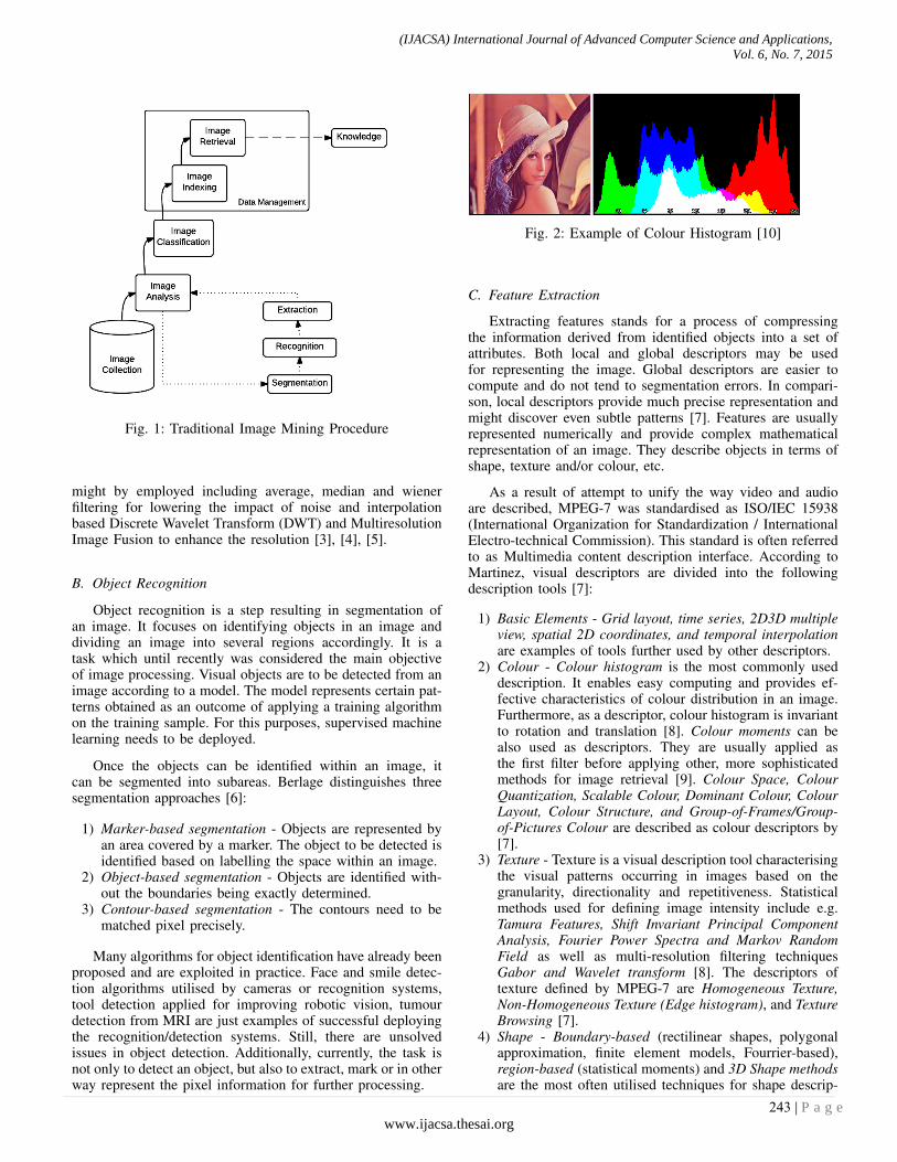
Fig. 1: Traditional Image Mining Procedure
might by employed including average, median and wienerfiltering for lowering the impact of noise and interpolationbased Discrete Wavelet Transform (DWT) and MultiresolutionImage Fusion to enhance the resolution [3], [4], [5].
B. Object Recognition
Object recognition is a step resulting in segmentation ofan image. It focuses on identifying objects in an image anddividing an image into several regions accordingly. It is atask which until recently was considered the main objectiveof image processing. Visual objects are to be detected from animage according to a model. The model represents certain pat-terns obtained as an outcome of applying a training algorithmon the training sample. For this purposes, supervised machinelearning needs to be deployed.
Once the objects can be identified within an image, itcan be segmented into subareas. Berlage distinguishes threesegmentation approaches [6]:
1) Marker-based segmentation - Objects are represented byan area covered by a marker. The object to be detected isidentified based on labelling the space within an image.
2) Object-based segmentation - Objects are identified with-out the boundaries being exactly determined.
3) Contour-based segmentation - The contours need to bematched pixel precisely.
Many algorithms for object identification have already beenproposed and are exploited in practice. Face and smile detec-tion algorithms utilised by cameras or recognition systems,tool detection applied for improving robotic vision, tumourdetection from MRI are just examples of successful deployingthe recognition/detection systems. Still, there are unsolvedissues in object detection. Additionally, currently, the task isnot only to detect an object, but also to extract, mark or in otherway represent the pixel information for further processing.
Fig. 2: Example of Colour Histogram [10]
C. Feature Extraction
Extracting features stands for a process of compressingthe information derived from identified objects into a set ofattributes. Both local and global descriptors may be usedfor representing the image. Global descriptors are easier tocompute and do not tend to segmentation errors. In compari-son, local descriptors provide much precise representation andmight discover even subtle patterns [7]. Features are usuallyrepresented numerically and provide complex mathematicalrepresentation of an image. They describe objects in terms ofshape, texture and/or colour, etc.
As a result of attempt to unify the way video and audioare described, MPEG-7 was standardised as ISO/IEC 15938(International Organization for Standardization / InternationalElectro-technical Commission). This standard is often referredto as Multimedia content description interface. According toMartinez, visual descriptors are divided into the followingdescription tools [7]:
1) Basic Elements - Grid layout, time series, 2D3D multipleview, spatial 2D coordinates, and temporal interpolationare examples of tools further used by other descriptors.
2) Colour - Colour histogram is the most commonly useddescription. It enables easy computing and provides ef-fective characteristics of colour distribution in an image.Furthermore, as a descriptor, colour histogram is invariantto rotation and translation [8]. Colour moments can bealso used as descriptors. They are usually applied asthe first filter before applying other, more sophisticatedmethods for image retrieval [9]. Colour Space, ColourQuantization, Scalable Colour, Dominant Colour, ColourLayout, Colour Structure, and Group-of-Frames/Group-of-Pictures Colour are described as colour descriptors by[7].
3) Texture - Texture is a visual description tool characterisingthe visual patterns occurring in images based on thegranularity, directionality and repetitiveness. Statisticalmethods used for defining image intensity include e.g.Tamura Features, Shift Invariant Principal ComponentAnalysis, Fourier Power Spectra and Markov RandomField as well as multi-resolution filtering techniquesGabor and Wavelet transform [8]. The descriptors oftexture defined by MPEG-7 are Homogeneous Texture,Non-Homogeneous Texture (Edge histogram), and TextureBrowsing [7].
4) Shape - Boundary-based (rectilinear shapes, polygonalapproximation, finite element models, Fourrier-based),region-based (statistical moments) and 3D Shape methodsare the most often utilised techniques for shape descrip-
(IJACSA) International Journal of Advanced Computer Science and Applications,
Vol. 6, No. 7, 2015
243 | P a g ewww.ijacsa.thesai.org
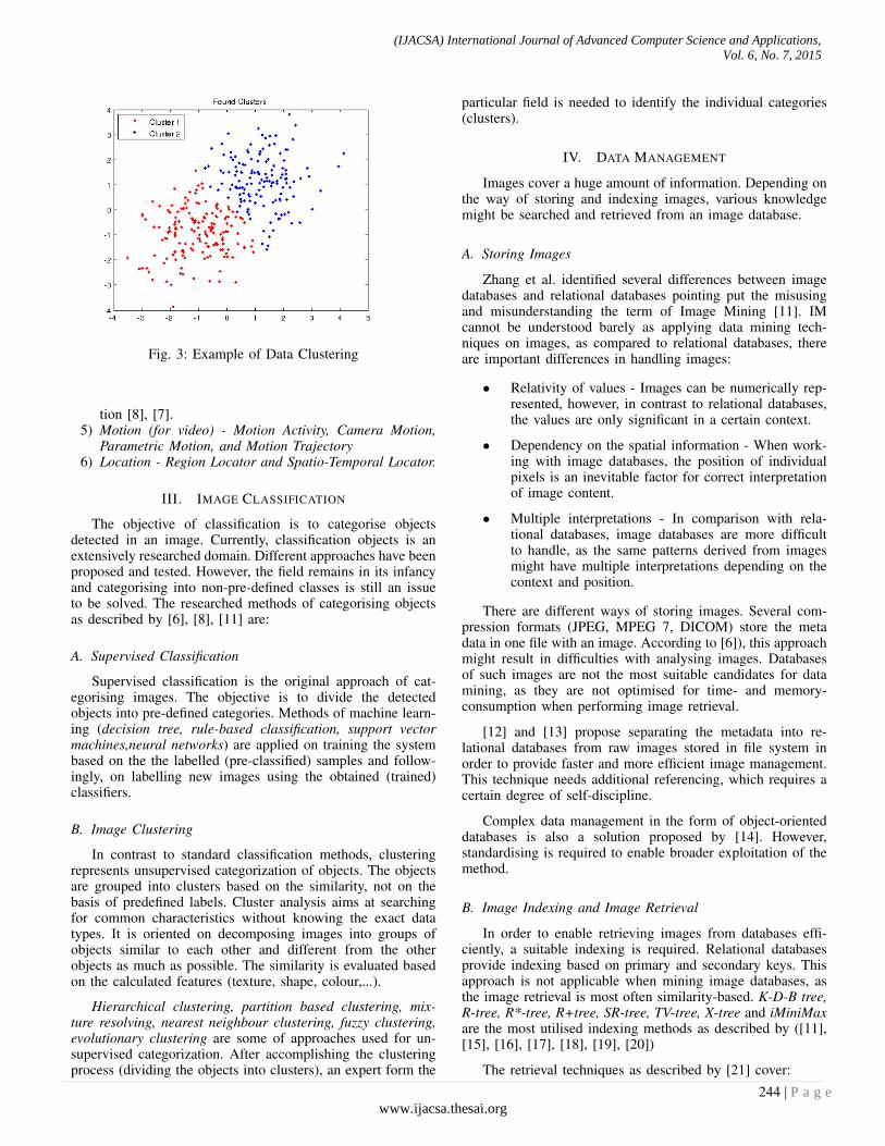
Fig. 3: Example of Data Clustering
tion [8], [7].5) Motion (for video) - Motion Activity, Camera Motion,
Parametric Motion, and Motion Trajectory6) Location - Region Locator and Spatio-Temporal Locator.
III. IMAGE CLASSIFICATION
The objective of classification is to categorise objectsdetected in an image. Currently, classification objects is anextensively researched domain. Different approaches have beenproposed and tested. However, the field remains in its infancyand categorising into non-pre-defined classes is still an issueto be solved. The researched methods of categorising objectsas described by [6], [8], [11] are:
A. Supervised Classification
Supervised classification is the original approach of cat-egorising images. The objective is to divide the detectedobjects into pre-defined categories. Methods of machine learn-ing (decision tree, rule-based classification, support vectormachines,neural networks) are applied on training the systembased on the the labelled (pre-classified) samples and follow-ingly, on labelling new images using the obtained (trained)classifiers.
B. Image Clustering
In contrast to standard classification methods, clusteringrepresents unsupervised categorization of objects. The objectsare grouped into clusters based on the similarity, not on thebasis of predefined labels. Cluster analysis aims at searchingfor common characteristics without knowing the exact datatypes. It is oriented on decomposing images into groups ofobjects similar to each other and different from the otherobjects as much as possible. The similarity is evaluated basedon the calculated features (texture, shape, colour,...).
Hierarchical clustering, partition based clustering, mix-ture resolving, nearest neighbour clustering, fuzzy clustering,evolutionary clustering are some of approaches used for un-supervised categorization. After accomplishing the clusteringprocess (dividing the objects into clusters), an expert form the
particular field is needed to identify the individual categories(clusters).
IV. DATA MANAGEMENT
Images cover a huge amount of information. Depending onthe way of storing and indexing images, various knowledgemight be searched and retrieved from an image database.
A. Storing Images
Zhang et al. identified several differences between imagedatabases and relational databases pointing put the misusingand misunderstanding the term of Image Mining [11]. IMcannot be understood barely as applying data mining tech-niques on images, as compared to relational databases, thereare important differences in handling images:
• Relativity of values - Images can be numerically rep-resented, however, in contrast to relational databases,the values are only significant in a certain context.
• Dependency on the spatial information - When work-ing with image databases, the position of individualpixels is an inevitable factor for correct interpretationof image content.
• Multiple interpretations - In comparison with rela-tional databases, image databases are more difficultto handle, as the same patterns derived from imagesmight have multiple interpretations depending on thecontext and position.
There are different ways of storing images. Several com-pression formats (JPEG, MPEG 7, DICOM) store the metadata in one file with an image. According to [6]), this approachmight result in difficulties with analysing images. Databasesof such images are not the most suitable candidates for datamining, as they are not optimised for time- and memory-consumption when performing image retrieval.
[12] and [13] propose separating the metadata into re-lational databases from raw images stored in file system inorder to provide faster and more efficient image management.This technique needs additional referencing, which requires acertain degree of self-discipline.
Complex data management in the form of object-orienteddatabases is also a solution proposed by [14]. However,standardising is required to enable broader exploitation of themethod.
B. Image Indexing and Image Retrieval
In order to enable retrieving images from databases effi-ciently, a suitable indexing is required. Relational databasesprovide indexing based on primary and secondary keys. Thisapproach is not applicable when mining image databases, asthe image retrieval is most often similarity-based. K-D-B tree,R-tree, R*-tree, R+tree, SR-tree, TV-tree, X-tree and iMiniMaxare the most utilised indexing methods as described by ([11],[15], [16], [17], [18], [19], [20])
The retrieval techniques as described by [21] cover:
(IJACSA) International Journal of Advanced Computer Science and Applications,
Vol. 6, No. 7, 2015
244 | P a g ewww.ijacsa.thesai.org
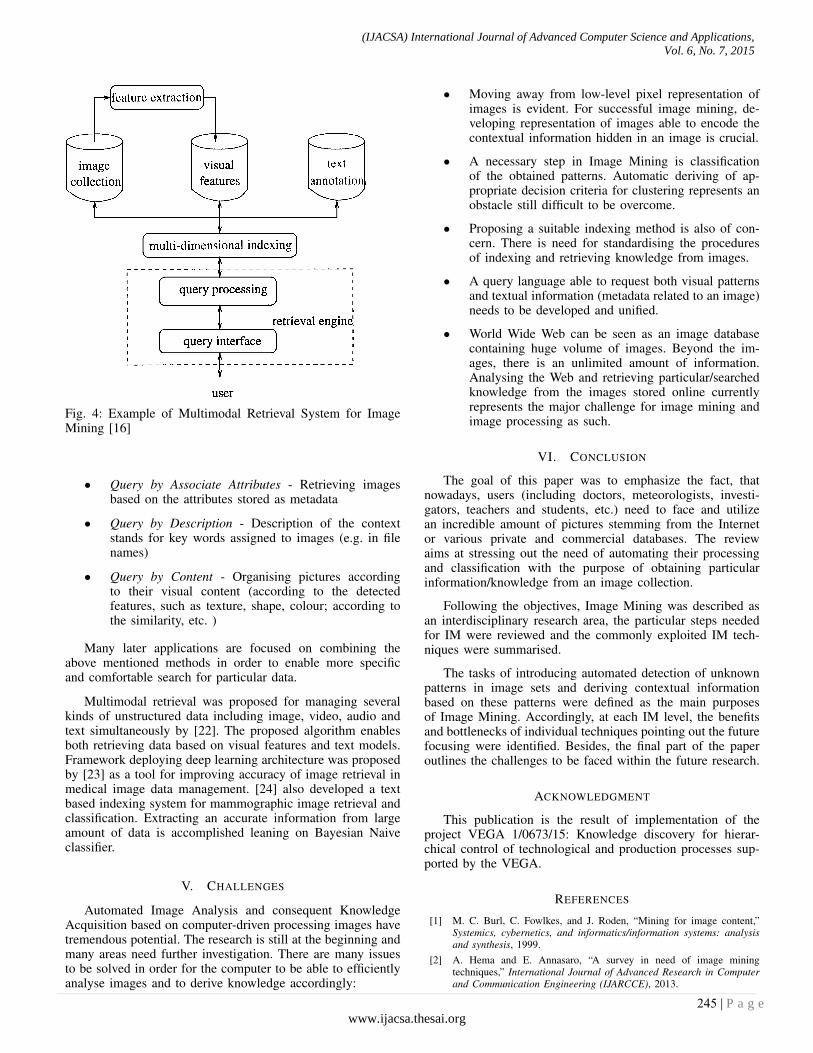
Fig. 4: Example of Multimodal Retrieval System for ImageMining [16]
• Query by Associate Attributes - Retrieving imagesbased on the attributes stored as metadata
• Query by Description - Description of the contextstands for key words assigned to images (e.g. in filenames)
• Query by Content - Organising pictures accordingto their visual content (according to the detectedfeatures, such as texture, shape, colour; according tothe similarity, etc. )
Many later applications are focused on combining theabove mentioned methods in order to enable more specificand comfortable search for particular data.
Multimodal retrieval was proposed for managing severalkinds of unstructured data including image, video, audio andtext simultaneously by [22]. The proposed algorithm enablesboth retrieving data based on visual features and text models.Framework deploying deep learning architecture was proposedby [23] as a tool for improving accuracy of image retrieval inmedical image data management. [24] also developed a textbased indexing system for mammographic image retrieval andclassification. Extracting an accurate information from largeamount of data is accomplished leaning on Bayesian Naiveclassifier.
V. CHALLENGES
Automated Image Analysis and consequent KnowledgeAcquisition based on computer-driven processing images havetremendous potential. The research is still at the beginning andmany areas need further investigation. There are many issuesto be solved in order for the computer to be able to efficientlyanalyse images and to derive knowledge accordingly:
• Moving away from low-level pixel representation ofimages is evident. For successful image mining, de-veloping representation of images able to encode thecontextual information hidden in an image is crucial.
• A necessary step in Image Mining is classificationof the obtained patterns. Automatic deriving of ap-propriate decision criteria for clustering represents anobstacle still difficult to be overcome.
• Proposing a suitable indexing method is also of con-cern. There is need for standardising the proceduresof indexing and retrieving knowledge from images.
• A query language able to request both visual patternsand textual information (metadata related to an image)needs to be developed and unified.
• World Wide Web can be seen as an image databasecontaining huge volume of images. Beyond the im-ages, there is an unlimited amount of information.Analysing the Web and retrieving particular/searchedknowledge from the images stored online currentlyrepresents the major challenge for image mining andimage processing as such.
VI. CONCLUSION
The goal of this paper was to emphasize the fact, thatnowadays, users (including doctors, meteorologists, investi-gators, teachers and students, etc.) need to face and utilizean incredible amount of pictures stemming from the Internetor various private and commercial databases. The reviewaims at stressing out the need of automating their processingand classification with the purpose of obtaining particularinformation/knowledge from an image collection.
Following the objectives, Image Mining was described asan interdisciplinary research area, the particular steps neededfor IM were reviewed and the commonly exploited IM tech-niques were summarised.
The tasks of introducing automated detection of unknownpatterns in image sets and deriving contextual informationbased on these patterns were defined as the main purposesof Image Mining. Accordingly, at each IM level, the benefitsand bottlenecks of individual techniques pointing out the futurefocusing were identified. Besides, the final part of the paperoutlines the challenges to be faced within the future research.
ACKNOWLEDGMENT
This publication is the result of implementation of theproject VEGA 1/0673/15: Knowledge discovery for hierar-chical control of technological and production processes sup-ported by the VEGA.
REFERENCES
[1] M. C. Burl, C. Fowlkes, and J. Roden, “Mining for image content,”Systemics, cybernetics, and informatics/information systems: analysisand synthesis, 1999.
[2] A. Hema and E. Annasaro, “A survey in need of image miningtechniques,” International Journal of Advanced Research in Computerand Communication Engineering (IJARCCE), 2013.
(IJACSA) International Journal of Advanced Computer Science and Applications,
Vol. 6, No. 7, 2015
245 | P a g ewww.ijacsa.thesai.org

[3] S. Rajeshwari and T. S. Sharmila, “Efficient quality analysis of mriimage using preprocessing techniques,” in Information & Communica-tion Technologies (ICT), 2013 IEEE Conference on. IEEE, 2013, pp.391–396.
[4] V. Starovoitov, D. Samal, and D. Briliuk, “Image enhancement for facerecognition,” in International Conference on Iconics, 2003.
[5] M. Stankovic, B. J. Falkowski, D. Jankovic, and R. S. Stankovic,“Calculation of the paired haar transform through shared binary decisiondiagrams,” Computers & Electrical Engineering, vol. 29, no. 1, pp. 13–24, 2003.
[6] T. Berlage, “Analyzing and mining image databases,” Drug discoverytoday, vol. 10, no. 11, pp. 795–802, 2005.
[7] J. M. Martınez, R. Koenen, and F. Pereira, “Mpeg-7: the genericmultimedia content description standard, part 1,” MultiMedia, IEEE,vol. 9, no. 2, pp. 78–87, 2002.
[8] N. Mishra and D. S. Silakari, “Image mining in the context of contentbased image retrieval: a perspective,” IJCSI International Journal ofComputer Science Issues, vol. 9, no. 4, pp. 98–107, 2012.
[9] R. da Silva Torres and A. X. Falcao, “Content-based image retrieval:Theory and applications.” RITA, vol. 13, no. 2, pp. 161–185, 2006.
[10] “Understanding how the image colors are distributed,”http://opensource.graphics/, accessed: 2010-05-20.
[11] J. Zhang, W. Hsu, and M. L. Lee, “Image mining: Issues, frameworksand techniques,” in Proceedings of the 2nd ACM SIGKDD InternationalWorkshop on Multimedia Data Mining (MDM/KDD’01). Universityof Alberta, 2001.
[12] M. E. Martone, S. Zhang, A. Gupta, X. Qian, H. He, D. L. Price,M. Wong, S. Santini, and M. H. Ellisman, “The cell-centered database,”Neuroinformatics, vol. 1, no. 4, pp. 379–395, 2003.
[13] S. Manley, N. R. Mucci, A. M. De Marzo, and M. A. Rubin, “Relationaldatabase structure to manage high-density tissue microarray data andimages for pathology studies focusing on clinical outcome: the prostatespecialized program of research excellence model,” The Americanjournal of pathology, vol. 159, no. 3, pp. 837–843, 2001.
[14] B. Diallo, F. Dolidon, J.-M. Travere, and B. Mazoyer, “B-spid: Anobject-relational database architecture to store, retrieve, and manipulateneuroimaging data,” Human brain mapping, vol. 7, no. 2, pp. 136–150,1999.
[15] D. Robinson and L. R. Foulds, “Comparison of phylogenetic trees,”Mathematical Biosciences, vol. 53, no. 1, pp. 131–147, 1981.
[16] Y. Rui, T. S. Huang, and S.-F. Chang, “Image retrieval: Currenttechniques, promising directions, and open issues,” Journal of visualcommunication and image representation, vol. 10, no. 1, pp. 39–62,1999.
[17] N. Katayama and S. Satoh, “The sr-tree: An index structure forhigh-dimensional nearest neighbor queries,” in ACM SIGMOD Record,vol. 26, no. 2. ACM, 1997, pp. 369–380.
[18] N. Beckmann, H.-P. Kriegel, R. Schneider, and B. Seeger, The R*-tree:an efficient and robust access method for points and rectangles. ACM,1990, vol. 19, no. 2.
[19] S. Berchtold, D. A. Keim, and H.-P. Kriegel, “The x-tree: An indexstructure for high-dimensional data,” Readings in multimedia computingand networking, vol. 451, 2001.
[20] B. C. Ooi and K.-L. Tan, “B-trees: bearing fruits of all kinds,” in Aus-tralian Computer Science Communications, vol. 24, no. 2. AustralianComputer Society, Inc., 2002, pp. 13–20.
[21] R. Kazman and J. Kominek, “Information organization in multimediaresources,” in Proceedings of the 11th annual international conferenceon Systems documentation. ACM, 1993, pp. 149–162.
[22] J. Luo, B. Lang, C. Tian, and D. Zhang, “Image retrieval in theunstructured data management system audr,” in E-Science (e-Science),2012 IEEE 8th International Conference on. IEEE, 2012, pp. 1–7.
[23] S. Liu, S. Liu, W. Cai, H. Che, S. Pujol, R. Kikinis, M. Fulham, andD. Feng, “High-level feature based pet image retrieval with deep learn-ing architecture,” Journal of Nuclear Medicine, vol. 55, no. supplement1, pp. 2028–2028, 2014.
[24] A. Farruggia, R. Magro, and S. Vitabile, “A text based indexingsystem for mammographic image retrieval and classification,” FutureGeneration Computer Systems, vol. 37, pp. 243–251, 2014.
(IJACSA) International Journal of Advanced Computer Science and Applications,
Vol. 6, No. 7, 2015
246 | P a g ewww.ijacsa.thesai.org