From static to temporal network theory - MIT Press Direct

METHODS

From static to temporal network theory:Applications to functional brain connectivity

William Hedley Thompson1, Per Brantefors1, and Peter Fransson1

1Department of Clinical Neuroscience, Karolinska Institutet, Stockholm, Sweden

Keywords: Resting-state, Temporal network theory, Temporal networks, Functional connectome,Dynamic functional connectivity

ABSTRACT

Network neuroscience has become an established paradigm to tackle questions related to thefunctional and structural connectome of the brain. Recently, interest has been growing inexamining the temporal dynamics of the brain’s network activity. Although differentapproaches to capturing fluctuations in brain connectivity have been proposed, there havebeen few attempts to quantify these fluctuations using temporal network theory. This theory isan extension of network theory that has been successfully applied to the modeling of dynamicprocesses in economics, social sciences, and engineering article but it has not been adoptedto a great extent within network neuroscience. The objective of this article is twofold:(i) to present a detailed description of the central tenets of temporal network theory anddescribe its measures, and; (ii) to apply these measures to a resting-state fMRI dataset toillustrate their utility. Furthermore, we discuss the interpretation of temporal network theoryin the context of the dynamic functional brain connectome. All the temporal networkmeasures and plotting functions described in this article are freely available as the Pythonpackage Teneto.

AUTHOR SUMMARY

Temporal network theory is a subfield of network theory that has had limited application todate within network neuroscience. The aims of this work are to introduce temporal networktheory, define the metrics relevant to the context of network neuroscience, and illustrate theirpotential by analyzing a resting-state fMRI dataset. We found both between-subjects andbetween-task differences that illustrate the potential for these tools to be applied in a widercontext. Our tools for analyzing temporal networks have been released in a Python packagecalled Teneto.

It is well known that the brain’s large-scale activity is organized into networks. The under-lying organization of the brain’s infrastructure into networks, at different spatial levels, hasbeen dubbed the brain’s functional and structural connectome (Sporns, 2009; Sporns, Tononi,& Kotter, 2005). Functional connectivity, derived by correlating the brain’s activity over a pe-riod of time, has been successfully applied in both functional magnetic resonance imaging(fMRI; Greicius, Krasnow, Reiss, & Menon, 2003; Fransson, 2005; Fox et al., 2005; Smith et al.,2009) and magnetoencephalography (MEG; de Pasquale et al., 2010; Brookes et al., 2011;Hipp, Hawellek, Corbetta, Siegel, & Engel, 2012), yielding knowledge about functional net-work properties (Buckner et al., 2009; Power et al., 2011; Power, Schlaggar, Lessov-Schlaggar,

a n o p e n a c c e s s j o u r n a l

Citation: Thompson, W. H., Brantefors,P., & Fransson, P. (2017). From static totemporal network theory: Applicationsto functional brain connectivity.Network Neuroscience, 1(2), 69–99.https://doi.org/10.1162/netn_a_00011

DOI:https://doi.org/10.1162/netn_a_00011

Supporting Information:

Received: 23 December 2016Accepted: 29 March 2017

Competing Interests: The authors havedeclared that no competing interestsexist.

Corresponding Author:William Hedley [email protected]

Handling Editor:Marcus Kaiser

Copyright: © 2017Massachusetts Institute of TechnologyPublished under a Creative CommonsAttribution 4.0 International(CC BY 4.0) license

The MIT Press

Dow

nloaded from http://direct.m

it.edu/netn/article-pdf/1/2/69/1091947/netn_a_00011.pdf by guest on 02 June 2022

https://dx.doi.org/10.1162/netn_a_00011

mailto:[email protected]

Temporal network theory applied to brain connectivity

& Petersen, 2013; Nijhuis, van Cappellen van Walsum, & Norris, 2013) that has been appliedto clinical populations (Fox & Greicius, 2010; Zhang & Raichle, 2010).

In parallel to research on the brain’s connectome, there has been a focus on studying thedynamics of brain activity. When the brain is modeled as a dynamic system, a diverse rangeof properties can be explored. Prominent examples of this are metastability (Bressler & Kelso,2001; Deco, Jirsa, & McIntosh, 2011; Kelso, 1995; Tognoli & Kelso, 2009, 2014) and oscilla-tions (Buzsáki, 2006; Buzsáki & Draguhn, 2004; Siegel, Donner, & Engel, 2012). Brain oscil-lations, inherently dynamic, have become a vital ingredient in proposed mechanisms rangingfrom psychological processes such as memory (Buzsáki, 2005; Friese et al., 2013; Montgomery& Buzsaki, 2007), and attention (Fries, 2005; Bosman et al., 2012), to basic neural communi-cation in top-down or bottom-up information transfer (Bressler, Richter, Chen, & Ding, 2007;Buschman & Miller, 2007; Bastos et al., 2012; Bastos et al., 2015; Richter, Thompson,Bosman, & Fries, 2016; Richter, Coppola, & Bressler, 2016; Michalareas et al., 2016;van Kerkoerle et al., 2014).

Recently, approaches to study brain connectomics and the dynamics of neuronal commu-nication have started to merge. A significant amount of work has recently been carried out thataims to quantify dynamic fluctuations of network activity in the brain using fMRI (Allen et al.,2014; Hutchison et al., 2013; Zalesky, Fornito, Cocchi, Gollo, & Breakspear, 2014; Shineet al., 2015; Thompson & Fransson, 2015a, 2016a; Shine, Koyejo, & Poldrack, 2016) as wellas MEG (de Pasquale et al., 2010; de Pasquale et al., 2012; Hipp, Hawellek, Corbetta, Siegel& Engel, 2012; Baker et al., 2014; Michalareas et al., 2016). This research area which aims tounify brain connectommics with the dynamic properties of neuronal communication, has beencalled the “dynome” (Kopell, Gritton, Whittington, & Kramer, 2014) and the “chronnectome”(Calhoun, Miller, Pearlson, & Adalı, 2014). Since the brain can quickly fluctuate between dif-ferent tasks, the overarching aim of this area of research is to understand the dynamic interplayof the brain’s networks. The intent of this research is that it will yield insight into the complexand dynamic nature of cognitive human abilities.

Although temporal network theory has been successfully applied in others fields (e.g., theTemporal network:A multigraph whose edges containtemporal information

social sciences), its implementation in network neuroscience has been limited. In the Theoryand Methods section, we provide an introduction to temporal network theory, by extendingthe definitions and logic of static network theory, and define a selection of temporal networkmeasures. In the Results section, we apply these measures to a resting-state fMRI dataset ac-quired during eyes-open and eyes-closed conditions, revealing differences in dynamic brainconnectivity between subjects and conditions. Together this material illustrates the potentialand varying information available from applying temporal network theory to network neuro-science.

THEORY AND METHODS

From Static Networks to Temporal Networks

We begin by defining temporal networks, by expanding upon the basic definitions of networktheory. In network theory, a graph (G) is defined as a set of nodes and edges:

G = (V , E), (1)

where V is a set containing N nodes. E is a set of tuples that represent the edges or connectionsbetween pairs of nodes (i, j) : i, j ∈ V . The graph may have binary edges (i.e., an edge is either

Network Neuroscience 70

Dow




present or absent), or E may be weighted, often normalized between 0 and 1, to represent themagnitude of connectivity. When each edge has a weight, the definition of E is extended to a3-tuple (i, j, w), where w denotes the weight of the edge between i and j. E is often representedas a matrix of the tuples, which is called a connectivity matrix, A (sometimes the term adjacencymatrix is used). An element of the connectivity matrix Ai,j represents the degree of connectivityfor a given edge. When G is binary, Ai,j = {0, 1}, and in the weighted version, Ai,j = w. In thecase of Ai,j = Aj,i, for all i and j, the matrix is considered undirected; when this is not the case,the matrix is directed. With static networks, many different properties regarding the patternsof connectivity between nodes can be quantified, for example through centrality measures,hub detection, small-world properties, clustering, and efficiency (see Newman, 2010; Sporns,2009; Bullmore & Sporns, 2009, for detailed discussion).

A graph is only a representation of some state of the world being modeled. The correspon-dence between the graph model and the state of the world may decrease due to aggregations,simplifications, and generalizations. Adding more information to the way that nodes are con-nected can entail that G provides a better representation, thus increasing the likelihood thatsubsequently derived properties of the graph will correspond with the state of the world be-ing modeled. One simplification in Eq. 1 is that two nodes can be connected by one edgeonly.

To capture such additional information in the graph, edges need to be expressed alongadditional, nonnodal dimensions. We can modify Eq. 1 to

G = (V , E ,D), (2)

where D is a set of the additional, nonnodal dimensions. In the case of multiple additional di-mensions, D is a class of disjoint sets where each dimension is a set. Equation 2 is sometimesreferred to in mathematics as a multigraph network, and in network theory as a multilayerMultigraph:

A network whose nodes can beconnected by multiple edges

network (Kivelä et al., 2014). For example, D could be a set containing three experimentalparadigms {“n back,” “go/no go,” “Stroop task”} and/or temporal indices in seconds{0,1,2, … T}. A graph is said to be a temporal network when D contains an ordered set oftemporal indices that represents time. This type of multilayer network is sometimes called amultiplex (Kivelä et al., 2014).

In a static graph, the edges E are elements that contain indices (2-tuples) for the nodes thatare connected. In a multilayer network, E consists of (|D|+ 2)-tuples for binary graphs, where|D| expresses the number of sets in D. If time is the only dimension in D, then an element inE is a triplet (i, j, t) : i, j ∈ V , t ∈ D. When G is weighted, E contains ((2 × |D|) + 2)-tuplesas w becomes the size of D, representing one weight per edge.

While shorter definitions of temporal graphs are often used without using general definitionsof multigraph/multilayer networks instead starting directly with the multiplex (see e.g., Holme& Saramäki, 2012; Masuda & Lambiotte, 2016), these formulations are mathematically equiv-alent when D only contains temporal information in Eq. 2. We have chosen to define a tem-poral network in terms of a multilayer network because this is appropriate when consideringwhat a detailed network description of the human connectome will require. A multilayer net-work representation of the connectome could include many dimensions of information aboutan edge—for example, (i) activity 100 ms after stimulus onset (time), (ii) activity in the gammafrequency band, and (iii) activity associated with an n-back trial (task context). Thus we haveintroduced temporal networks by extending static network definitions to the broader concept


Dow




of multilayer networks. However, in more complex multilayer networks with additional,nontemporal dimensions, the temporal-network measures presented in this article can be usedto examine relationships across time, but either fixation or aggregation over the other dimen-sions will be required. However, more complex measures that consider all dimensions in Dhave been proposed elsewhere (e.g., Berlingerio, Coscia, Giannotti, Monreale, & Pedreschi,2011).

For the remainder of this article we will consider only the case in which D contains onlyan ordered set of temporal indexes. In this case, each edge is indexed by i,j and t. To fa-cilitate readability, connectivity matrix elements are written as At

i,j—that is, with the tem-poral index of D in the superscript. Instead of referring to “At” as the “connectivity matrixat time point t”, some refer to this as a graphlet (Basu, Bar-noy, Johnson, & Ramanathan, 2010;Graphlet:

A discrete connectivity matrix thatexpresses part of a larger network

Thompson & Fransson, 2015a, 2016a); others prefer to call this a snapshot representation(Masuda & Lambiotte, 2016), and still others call it a supra-adjacency matrix (Kivelä et al.,2014). It should be noted that some dislike the term graphlet due to possible confusionwith the static network theory conception of a graphlet. Here a graphlet is a complete, in-dependent two-dimensional connectivity matrix, but each graphlet is only a part of the en-tire network. Because graphlets do not need to be snapshots of temporal information underthis definition, it is useful to describe what type of graphlet is being used. For example,a graphlet that expresses temporal information can be called a time-graphlet or t-graphlet(Thompson & Fransson, 2016a), and a graphlet carrying frequency information, an f-graphlet(Thompson & Fransson, 2015a).

Instead of representing the data with multiple graphlets, E can be used to derive the contactsequence or event-based representation containing the nodes and temporal index (Holme &Saramaäki, 2012; Masuda & Lambiotte, 2016). Unlike the graphlet representations, whichmust be discrete, contact sequences can also be used on continuous data and, when connec-tions are sparse, can be a more memory-efficient way to store the data.

MEASURES FOR TEMPORAL NETWORKS

Once the t-graphlets have been derived, various measures can be implemented in order toquantify the degree and characteristics of the temporal flow of information through the net-work. We begin by introducing two concepts that are used in several of the temporal networkmeasures that will be defined later. The focus is on measures that derive temporal properties ata local level (i.e., per node or edge) or a global level (see Discussion for other approaches). Wehave limited our scope to describe only the case of binary, undirected, and discrete t-graphlets,although many measures can be extended to continuous time, directed edges, and nonbinarydata.

Shortest temporal path:The shortest path by which a nodecommunicates with another nodeacross multiple intermediate nodes

Concept: Shortest Temporal Path

In static networks, the shortest path is the minimum number of edges (or sum of edge weights)that it takes for a node to communicate with another node. In temporal networks, a similarmeasure can be derived. Within temporal networks, we can quantify the time taken for onenode to communicate with another node. This is sometimes called the “shortest temporaldistance” or “waiting time.” Temporal paths can be measured differently by calculating eitherhow many edges are traveled or how many time steps are taken (see Masuda & Lambiotte,2016); here we quantify the time steps taken.


Dow




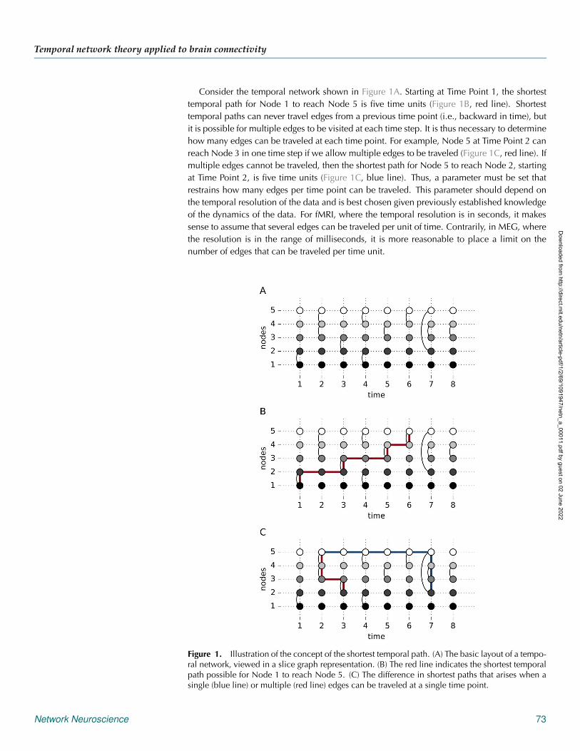
Consider the temporal network shown in Figure 1A. Starting at Time Point 1, the shortesttemporal path for Node 1 to reach Node 5 is five time units (Figure 1B, red line). Shortesttemporal paths can never travel edges from a previous time point (i.e., backward in time), butit is possible for multiple edges to be visited at each time step. It is thus necessary to determinehow many edges can be traveled at each time point. For example, Node 5 at Time Point 2 canreach Node 3 in one time step if we allow multiple edges to be traveled (Figure 1C, red line). Ifmultiple edges cannot be traveled, then the shortest path for Node 5 to reach Node 2, startingat Time Point 2, is five time units (Figure 1C, blue line). Thus, a parameter must be set thatrestrains how many edges per time point can be traveled. This parameter should depend onthe temporal resolution of the data and is best chosen given previously established knowledgeof the dynamics of the data. For fMRI, where the temporal resolution is in seconds, it makessense to assume that several edges can be traveled per unit of time. Contrarily, in MEG, wherethe resolution is in the range of milliseconds, it is more reasonable to place a limit on thenumber of edges that can be traveled per time unit.

Figure 1. Illustration of the concept of the shortest temporal path. (A) The basic layout of a tempo-ral network, viewed in a slice graph representation. (B) The red line indicates the shortest temporalpath possible for Node 1 to reach Node 5. (C) The difference in shortest paths that arises when asingle (blue line) or multiple (red line) edges can be traveled at a single time point.


Dow




Regarding the shortest temporal path, it is useful to keep in mind that the path is rarelysymmetric, not even when the t-graphlets themselves are symmetric. This is illustrated byconsidering the network shown in Figure 1A, in which it takes five units of time for Node 1to reach Node 5 when starting at t = 1. However, for the reversed path, it takes only threeunits of time for Node 5 to reach Node 1 (allowing for multiple edges to be traveled per timepoint).

Some consideration is needed of whether thinking about shortest temporal paths makessense in all neuroimaging contexts. Shortest temporal paths represent information being trans-ferred in a network. Thus, the concept of the shortest temporal path is appropriate in the situ-ation in which one can assume that the transfer of information is continued across subsequenttime points. When the time scale is in the range of milliseconds (e.g., EEG and MEG), the short-est temporal path should be unproblematic to interpret. In contrast, for a longitudinal study inwhich the temporal resolution is in years, the concept of the shortest temporal path makes nosense. Less clear-cut situations are neuroimaging techniques with sluggish temporal resolution(e.g., fMRI). However, the shortest temporal path seems to be a reasonable measure for ongo-ing BOLD signals that allow for considering previously observed temporal dynamics, includ-ing avalanche behavior (Tagliazucchi, Balenzuela, Fraiman, & Chialvo, 2012), bursty behavior(Thompson & Fransson, 2016a), and metastability (Deco & Kringelbach, 2016).

Intercontact time:The time taken between two nodeswith a direct connection

Concept: Intercontact Time

The intercontact time between two nodes is defined as the temporal difference distinguishingtwo consecutive nonzero edges between those nodes. This definition differs from the shortesttemporal path in so far as it only considers direct connections between two nodes. ConsideringFigure 1A, the intercontact times between Nodes 4 and 5 become a list [2,2], since there areedges present at Time Points 2, 4, and 6. Each edge will have a list of intercontact times. Thenumber of intercontact times in each list will be the number of nonzero edges between thenodes minus one. Unlike with shortest temporal paths, graphs that contain intercontact timeswill always be symmetric.

Nodal Measure: Temporal Centrality

A node’s influence in a temporal network can be calculated in a way akin to degree centralityin the static case, where the sum of the edges for a node is calculated. The difference from itsstatic counterpart is that we also sum the number of edges across time. Formally, the temporaldegree centrality, DT, for a node i is computed as

DTi =

N

∑j=1

T

∑t=1

Ati,j, (3)

where T is the number of time points, N is the number of nodes, and Ati,j is a graphlet.

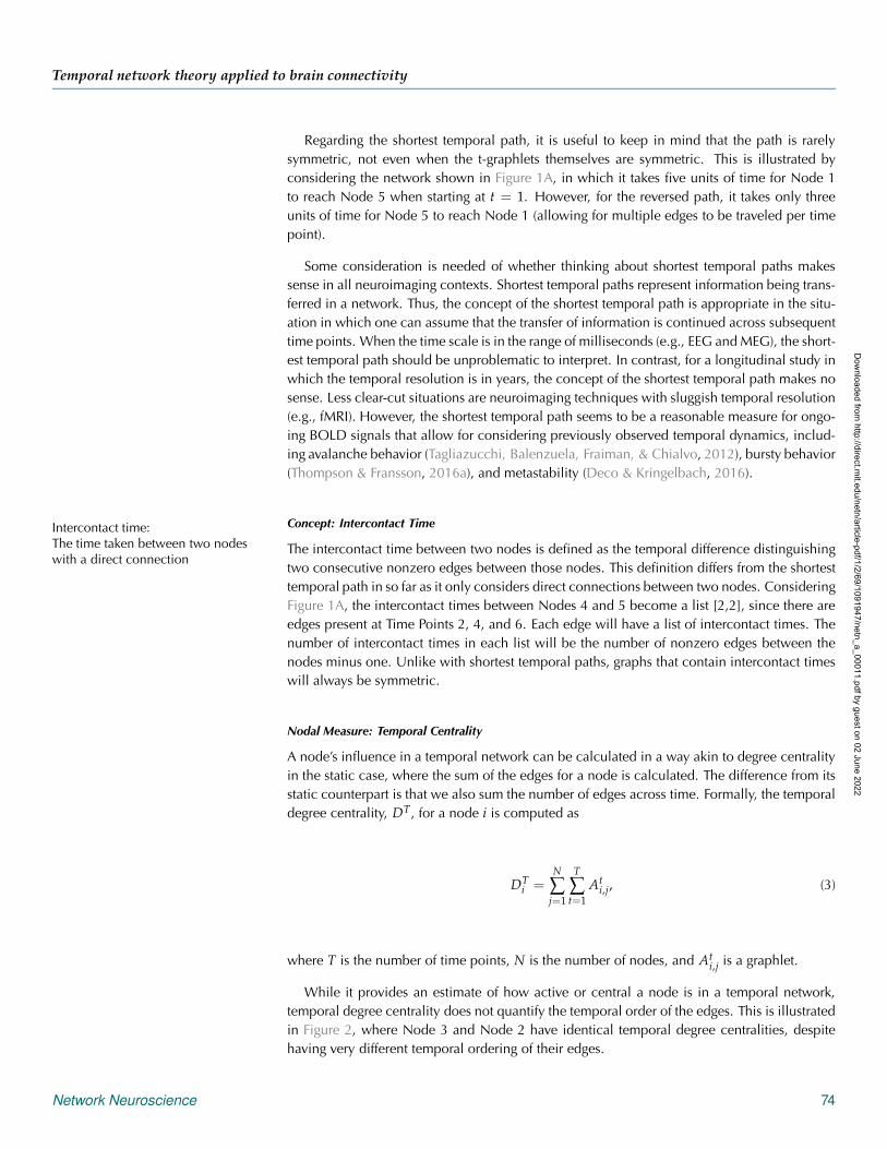
While it provides an estimate of how active or central a node is in a temporal network,temporal degree centrality does not quantify the temporal order of the edges. This is illustratedin Figure 2, where Node 3 and Node 2 have identical temporal degree centralities, despitehaving very different temporal ordering of their edges.


Dow




Figure 2. A slice graph representation of a simple example of a temporal network that illustratesthe conceptual difference between temporal degree centrality and temporal closeness centrality.

Nodal Measure: Temporal Closeness Centrality

A centrality measure that does consider the temporal order is temporal closeness centrality(Pan & Saramäki, 2011). This is an extension of the static closeness centrality, which is theinverse sum of the shortest paths. Temporal closeness centrality is calculated as

CTi,t =

1N − 1

N

∑j=1

1dτ

i,j, (4)

where dτi,j is the average shortest path between nodes i and j across all time points for which

a shortest path exists. As in the static counterpart, if a node has shorter temporal paths thanother nodes, it will have a larger temporal closeness centrality.

Consider the example given in Figure 2, which shows a temporal sequence of connectivityamong three nodes over 20 time points. Note that the temporal degree centralities are identicalfor both Node 2 and Node 3, while the degree centrality for Node 1 is twice as large. Node 2has the largest temporal closeness centrality, since the time between edges is longer for Node2 than for Node 3, which has the lowest value of temporal closeness centrality.

Edge Measure: Bursts

By using temporal network theory, bursts have been identified as an important property ofmany processes in nature (Barabási, 2005, 2010; Vázquez et al., 2006; Vazquez, Rácz,Lukács, & Barabási, 2007; Min, Goh, & Vazquez, 2011). A hallmark of a bursty edge is thepresence of multiple edges with short intercontact times, followed by longer and varying inter-contact times. In statistical terms, such a process is characterized by a heavy-tailed distributionof intercontact time probabilities. Numerous patterns of social communication and behaviorhave been successfully modeled as bursty in temporal network theory, including email com-munication (Barabási, 2005; Eckmann, Moses, & Sergi, 2004), mobile phone communication(Jo, Karsai, Kertész, & Kaski, 2012), spreading of sexually transmitted diseases (Vazquez, 2013),soliciting online prostitution (Rocha, Liljeros, & Holme, 2010), and epidemics Takaguchi,Masuda, & Holme, 2013. With regard to network neuroscience, we have recently shown thatbursts of brain connectivity can be detected in resting-state fMRI data (Thompson & Fransson,2016a). Furthermore, bursty temporal patterns have also been identified in the amplitudes


Dow




of the EEG alpha signal (Freyer, Aquino, Robinson, Ritter, & Breakspear, 2009; Freyer, Roberts,Ritter, & Breakspear, 2012; Roberts, Boonstra, & Breakspear, 2015).

There are several strategies to quantify bursts. A first way to check whether a time series ofbrain connectivity between two nodes is bursty is simply to plot the distribution of intercontacttimes. Thus, the complete distribution of τ for a given edge contains information about the tem-poral evolution of brain connectivity. However, other methods are available to quantify bursts.One example is the burstiness coefficient (B), first presented in Goh and Barabási (2008) andformulated for discrete graphs, Holme and Saramäki (2012):

Bij =σ(τij)− μ(τi,j)

σ(τij) + μ(τij), (5)

where τij is a vector of the intercontact times between nodes i and j through time. WhenB > 0, it is an indication that the temporal connectivity is bursty. This occurs when thestandard deviation σ(τ) is greater than the mean μ(τ). In Eq. 5, bursts are calculated peredge, which can be problematic when only a limited number of data are available. Functionalimaging sessions must be long enough to accurately establish whether or not a given temporaldistribution is bursty (too few intercontact times will entail too poor an estimation of σ toaccurately estimate B). Typically, for resting-state fMRI datasets acquired over rather shorttime spans (5–6 minutes) with low temporal resolution (typically 2–3 seconds), it might bedifficult to quantify B in a single subject. A potential remedy in some situations is to computeB after concatenating intercontact times across subjects.

Equation 5 calculates the number of bursts per edge. This can easily be extended to anodal measure by summing over the bursty coefficients across all edges for a given node.Alternatively, a nodal form of B can be calculated by using the intercontact times for all j insteadof averaging over j in Bij. Finally, if a process is known to be bursty, instead of quantifying B,it is possible simply to count the number of bursts present in a time series.

Global Measure: Fluctuability

Although centrality measures provide information about the degree of temporal connectivity,and bursts describe the distribution of the temporal patterns of connectivity at a nodal level,one might also want to retrieve information about the global state of a temporal network. Tothis end, fluctuability aims to quantify the temporal variability of connectivity. We define thefluctuability F as the ratio of the number of edges present in A over the grand sum of At:

F =∑i ∑j U(Ai,j)

∑i ∑j ∑t Ati,j

, (6)

where U is a function that delivers a binary output. U(Ai,j)is set to 1 if at least one of an edgeoccurs between nodes i and j across times t = 1, 2, ..., T. If not, U(Ai,j)is set to 0. This can beexpressed as

U(Aij) =

⎧⎨⎩

1 if ∑Tt At

ij > 0,

0 if ∑Tt At

ij = 0,(7)


Dow




where T is the total number of time points and A has at least one nonzero edge. From thedefinition given in Eq. 6, it follows that the maximum value of F is 1 and that this value onlyoccurs when every edge is unique and occurs only once in time.

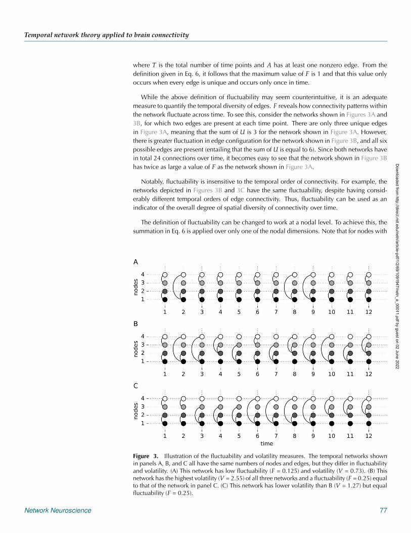
While the above definition of fluctuability may seem counterintuitive, it is an adequatemeasure to quantify the temporal diversity of edges. F reveals how connectivity patterns withinthe network fluctuate across time. To see this, consider the networks shown in Figures 3A and3B, for which two edges are present at each time point. There are only three unique edgesin Figure 3A, meaning that the sum of U is 3 for the network shown in Figure 3A. However,there is greater fluctuation in edge configuration for the network shown in Figure 3B, and all sixpossible edges are present (entailing that the sum of U is equal to 6). Since both networks havein total 24 connections over time, it becomes easy to see that the network shown in Figure 3Bhas twice as large a value of F as the network shown in Figure 3A.

Notably, fluctuability is insensitive to the temporal order of connectivity. For example, thenetworks depicted in Figures 3B and 3C have the same fluctuability, despite having consid-erably different temporal orders of edge connectivity. Thus, fluctuability can be used as anindicator of the overall degree of spatial diversity of connectivity over time.

The definition of fluctuability can be changed to work at a nodal level. To achieve this, thesummation in Eq. 6 is applied over only one of the nodal dimensions. Note that for nodes with

Figure 3. Illustration of the fluctuability and volatility measures. The temporal networks shownin panels A, B, and C all have the same numbers of nodes and edges, but they differ in fluctuabilityand volatility. (A) This network has low fluctuability (F = 0.125) and volatility (V = 0.73). (B) Thisnetwork has the highest volatility (V = 2.55) of all three networks and a fluctuability (F = 0.25) equalto that of the network in panel C. (C) This network has lower volatility than B (V = 1.27) but equalfluctuability (F = 0.25).


Dow




no connections at all, the denominator will be 0, and to circumvent this hindrance, the nodalfluctuability FN

i is defined as

FNi =

⎧⎨⎩

∑j U(Ai,j)

∑j ∑t Ati,j

if U(Ai,j) > 0,

0 if U(Ai,j) = 0.(8)

Global Measure: Volatility

One possible global measure of temporal order is how much, on average, the connectivitybetween consecutive t-graphlets changes. This indicates how volatile the temporal network isover time. Thus, volatility (V) can be defined as

V =1

T − 1

T−1

∑t=1

D(At, At+1), (9)

where D is a distance function and T is the total number of time points. The distance functionquantifies the difference between a graphlet at t and the graphlet at t + 1. In all the followingexamples in this article, for volatility we use the Hamming distance, because it is appropriatefor binary data.

Whereas there was no difference in fluctuability between the networks shown in Figures 3Band 3C, there is a difference in volatility, since the network in Figure 3B has more abruptchanges in connectivity than the network shown in Figure 3C.

Extensions of the volatility measure are possible. Like fluctuability, volatility can be definedat a local level. A per-edge version of volatility can be formulated as

VLi,j =

1T − 1

T−1

∑t=1

D(Ati,j, At+1

i,j ). (10)

Additionally, taking the mean VLi,j over j would give an estimate of volatility centrality.

Global Measure: Reachability Latency

Measures of reachability focus on estimating the time taken to “reach” the nodes in a temporalnetwork. In Holme (2005), both the reachability ratio and reachability time are used. Thereachability ratio is the percentage of edges that have a temporal path connecting them. Thereachability time is the average length of all temporal paths. However, when applying reach-ability to the brain, the two aforementioned measures are not ideal, given the noncontroversialassumption that any region in the brain, given sufficient time, can reach all other regions.

With this assumption in mind, we define a measure of reachability, reachability latency,that quantifies the average time it takes for a temporal network to reach an a-priori-definedreachability ratio. This is defined as

Rr =1

TN ∑t

∑i

dti,k, (11)

where dti is an ordered vector of length N of the shortest temporal paths for node i at time point

t. The value k represents the �rN�th element in the vector, which is the rounded product of thefraction of nodes that can be reached, r, with N being the total number of nodes in the network.


Dow




In the case of r = 1, (i.e., 100% of nodes are reachable), Eq. 11 can be rewritten as

R1 =1

TN ∑t

∑i

maxj dti,j. (12)

Equation 12 has been referred to as the temporal diameter of the network (Nicosia et al., 2013).If Eq. 12 were modified and calculated per node instead of averaging over nodes, it would bea temporal extension of node eccentricity.

Unless all nodes are reached at the last time point in the sequence of recorded data, therewill be a percentage of time points from which all nodes can not be reached. This effectivelyreduces their value of R, because dt

i,j cannot always be calculated, but R is still normalizedby T. If this penalization is considered too unfair, it is possible to normalize R by replacing Twith T∗, which is the number of time points where dT

i,j has a real value.

Global Measure: Temporal Efficiency

A similar concept is the idea of temporal efficiency. In the static case, efficiency is computed asthe inverse of the average shortest path for all nodes. Temporal efficiency is first calculated ateach time point as the inverse of the average shortest path length for all nodes. Subsequently,the inverse average shortest path lengths are averaged across time points to obtain an estimateof global temporal efficiency, which is defined as

E =1

T(N2 − N) ∑i,j,t

1dt

i,j, i �= j. (13)

Although reachability and efficiency estimate similar temporal properties, since both arebased on the shortest temporal paths, the global temporal efficiency may result in differentresults than the reachability latency. This is because efficiency is proportional to the averageshortest temporal path, whereas reachability is proportional to the longest shortest temporalpath to reach r percent of the network. Similar to the case of static graphs, temporal efficiencycould be calculated at a nodal level as well, and this would equal the closeness centrality.

Summary of Temporal Network Measures

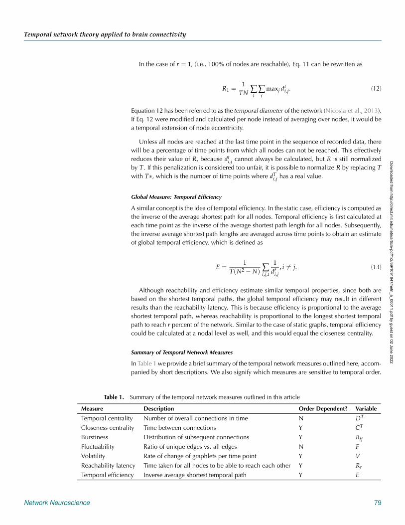
In Table 1 we provide a brief summary of the temporal network measures outlined here, accom-panied by short descriptions. We also signify which measures are sensitive to temporal order.

Table 1. Summary of the temporal network measures outlined in this article

Measure Description Order Dependent? Variable

Temporal centrality Number of overall connections in time N DT

Closeness centrality Time between connections Y CT

Burstiness Distribution of subsequent connections Y Bij

Fluctuability Ratio of unique edges vs. all edges N F

Volatility Rate of change of graphlets per time point Y V

Reachability latency Time taken for all nodes to be able to reach each other Y Rr

Temporal efficiency Inverse average shortest temporal path Y E


Dow




Statistical Considerations of Temporal Network Measures

When implementing temporal graph measures, it is important to perform adequate statisticaltests to infer differences between the subject groups, task conditions, or chance levels. Forgroup comparisons, nonparametric permutation methods are advantageous where the groupassignment of the calculated measure can be shuffled between the groups and a null distri-bution can be created. Alternatively, to justify that a measure is significantly present abovechance levels, the construction of null graphs is required. There are multiple ways to createtemporal null graphs, and they each have their own benefits and drawbacks. One methodis to permute the temporal order of entire time series, but this will destroy any autocorrela-tion present in the data. Another alternative is to permute the phase of the time series prior tothresholding the t-graphlets. A third option would be to permute blocks of time series data, butthis may not be appropriate for all network measures (e.g., volatility). A fourth option wouldbe to use vector autoregressive null models (Chang & Glover, 2010; Zalesky et al., 2014). Werefer the reader to Holme & Saramäki (2012) for a full account of approaches to performingstatistical tests on measures derived from temporal network theory.

METHODS

fMRI data

Two resting-state fMRI sessions (3-tesla, TR = 2,000 ms, TE = 30 ms) from 48 healthy subjectswere used in the analysis (19–31 years, 24 female). The fMRI data were downloaded froman online repository: the Beijing Eyes-Open/Eyes-Closed dataset, available at www.nitrc.org(Liu & Duyn, 2013). Each functional volume comprised 33 axial slices (thickness/gap = 3.5/0.7 mm, in-plane resolution = 64 × 64, field of view = 200 × 200 mm). The dataset containedthree resting-state sessions per subject, and each session lasted 480 s (200 image volumes,two eyes-closed sessions and one eyes-open session). We used data only from the 2nd or 3rdsession, which were the eyes-open (EO) and second eyes-closed (EC) sessions, where the orderwas counterbalanced across subjects. Two subjects were excluded due to incomplete data.Further details regarding the scanning procedure are given in Liu & Duyn (2013).

All resting-state fMRI data was preprocessed using Matlab (Version 2014b, Mathworks,Inc.) with the CONN (Whitfield-Gabrieli & Nieto-Castanon, 2012) and SPM8 (Friston et al.,1995) toolboxes. The functional imaging data were realigned and normalized to the EPI MNItemplate as implemented in SPM. Spatial smoothing was applied using a Gaussian filterkernel (FWHM = 8 mm). Additional image artifact regressors attributed to head movement(Dijk, Sabuncu, & Buckner, 2012; Power, Barnes, Snyder, Schlaggar, & Petersen, 2012) werederived by using the ART toolbox for scrubbing (www.nitrc.org). Signal contributions fromwhite brain matter, cerebrospinal fluid (CSF), and head movement (six parameters), as wellas the ART micromovement regressors for scrubbing, were regressed from the data usingthe CompCor algorithm (Behzadi, Restom, Liau, & Liu, 2007; the first five principal compo-nents were removed for both white matter and CSF). After regression, the data were band-passed between 0.008 and 0.1 Hz, as well as linearly detrended and despiked. Time seriesof fMRI brain activity were extracted from 264 regions of interest (ROIs; spherical with a5-mm radius) using the parcellation scheme for cortex and subcortical structures describedin Power et al. (2011). Each ROI was normalized by demeaning and scaling the standard de-viation to 1. These 264 ROIs were further divided into ten brain networks, as described inCole et al. (2013) (technically subgraphs, in network theory terminology). Automatic anatom-ical labeling (AAL) regions associated with specific ROIs, shown in the Supplementary Tables(Thompson, Brantefors, & Fransson, 2017), were determined by taking the AAL region at (or


Dow




closest to) the center of the ROI. Note that this offers only an approximate anatomical labelingof the positions of ROIs.

Creating Time-Graphlets (t-Graphlets)

While there are many proposed methods for dynamic functional connectivity (Smith et al.,2012; Allen et al., 2014; Liu & Duyn, 2013; Lindquist, Xu, Nebel, & Caffo, 2014; Shine et al.,2015; Thompson & Fransson, 2016a), we chose a weighted correlation strategy (described be-low) because it does not require optimizing any parameters or clustering. The method is basedon our previous work (Thompson & Fransson, 2016a), using the same fundamental assump-tions, which results in high temporal sensitivity to fluctuating connectivity. However, we hereextended the method presented in Thompson & Fransson (2016a) so that it would computeunique connectivity estimates for each time point, and thereby avoid the necessity to clusterthe data using a clustering technique such as k-means.

Our logic was to calculate dynamic functional brain connectivity estimates based on aweighted Pearson correlation. To calculate the conventional Pearson correlation coefficient,Weighted Pearson correlation:

A correlation coefficient for whichthe significance of each observationis determined by a weight

all points are weighted equally. In the weighted version, data points contribute differently to thecorrelation coefficient, depending on what weight they have been assigned. These weights arethen used to calculate the weighted mean and weighted covariance to estimate the weightedcorrelation coefficient. By using a unique weighting vector per time point, we were able toget unique connectivity estimates for each time point.

The weighted Pearson correlation between the signals x and y is defined as

r(x, y; w) =Σx,y;w

Σx,x;wΣy,y;w, (14)

where Σ is the weighted covariance matrix and w is a vector of weights that is equal in lengthto x and y. The weighted covariance matrix is defined as

Σx,y;w =∑n

i wi(x − μx;w)(y − μy;w)

∑ni wi

, (15)

where n is the length of the time series. Note that Σ is the covariance matrix and ∑ni is a sum

over time points. The variables μx;w and μy;w are the weighted means, defined as

μx;w =∑n

i wixi

∑ni wi

, μy;w =∑n

i wiyi

∑ni wi

. (16)

Equations 14–16 define the weighted Pearson coefficient with the exception of the weightvector w. If every element in w is identical, we can easily observe that the unweighted (conven-tional) Pearson coefficient will be calculated. Here, we instead wished to calculate a uniquew for each time point, providing a connectivity estimate based on the weighted mean andweighted covariance.

Different weighting schemes could be applied. In fact, many of the different dynamic con-nectivity methods proposed in the literature are merely different weighting schemes (e.g., anontapered sliding window approach is just a binary weight vector).

We decided upon a global weighting of the spatial dimensions by calculating the distancebetween the nodes at a specific time point with all other nodes for every other time point.


Dow




This entails that the weights for the covariance estimates at t are larger for other time pointsthat display a global spatial pattern across all nodes similar to that of the nodes at t. A newweight vector is calculated for each time point. The unique weight vector per time point pro-duces a unique weighted Pearson correlation at each time point. This reflects the weightedcovariance, where time points with similar global spatial brain activation are weighted higher.This produces, for each edge, a connectivity time series with fluctuating covariance.

More formally, the weights for estimating the connectivity at time t are derived by takingthe distance between the activation of the ROIs at t and at each other time point (indexedby v):

wtv =

1D(yt, yv)

, (17)

where D is a distance function and y is the multivariate time series of the ROIs. For the distance

function, we used Euclidean distance (i.e., D(a, b) =√[∑n

i (ai − bi)2]).

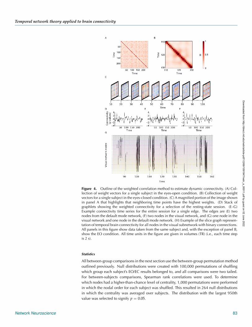
The weight vector of t is created by applying Eq. 17 for all v ∈ T, v �= t. This implies that atthe time point of interest, t, we calculate a vector of weights (indexed by v) that reflects howmuch the global spatial pattern of brain activity (i.e., all ROIs) differs from the brain activityat t. Each collection of weight vectors wt can form a t by t matrix w for each subject andeach condition. The values of each matrix are scaled to range between 0 and 1. Finally, thediagonal of w is set to 1. The collection of weight vectors for a single subject is shown for bothEO and EC sessions in Figures 4A–4C. Although this is not explicitly assumed in our method,neighboring time points have the highest weights (Figure 4C).

After the derivation of the connectivity time series, a Fisher transform and a Box–Cox trans-form were applied. For the Box–Cox transform, the λ parameter was fit by taking the maximumlikelihood after a grid-search procedure from -5 to 5 in increments of 0.1 for each edge. Priorto the Box–Cox transformation, the smallest value was scaled to 1 to make sure the Box–Coxtransform performed similarly throughout the time series (Thompson & Fransson, 2016b). Eachconnectivity time series was then standardized by subtracting the mean and dividing by thestandard deviation. Snapshots of the weighted graphlets can be seen in Figure 4D. The entireconnectivity time series for three different ROI pairings are shown in Figures 4E–4G. Binaryt-graphlets were created by setting edges exceeding two standard deviations to 1, or otherwise0, for each time series.

Our thresholding approach to create binary connectivity matrices is suboptimal and couldbe improved upon in future work (see Discussion). The need to formulate more robust thresh-olding practices has been an ongoing area of research in static network theory in the neuro-sciences (Drakesmith et al., 2015). Similar work needs to be carried out for temporal networks,because a limitation of the current approach is a heightened risk of false positive connections.

Tools for Temporal Network Theory

We have implemented all temporal network measures described in the present work in aPython package of temporal network tools called Teneto (www.github.com/wiheto/teneto)for Python 3.x, although the package itself is still under development. The package currentlycontains code for all the measures mentioned above and plotting functions for slice plots (e.g.,Figure 4F) and for stacking graphlets (e.g., Figure 4D). Data formats for both the graphlet/snapshot and event/contact sequence data representations are available.


Dow




Figure 4. Outline of the weighted correlation method to estimate dynamic connectivity. (A) Col-lection of weight vectors for a single subject in the eyes-open condition. (B) Collection of weightvectors for a single subject in the eyes-closed condition. (C) A magnified portion of the image shownin panel A that highlights that neighboring time points have the highest weights. (D) Stack ofgraphlets showing the weighted connectivity for a selection of the resting-state session. (E–G)Example connectivity time series for the entire session for a single edge. The edges are (E) twonodes from the default mode network, (F) two nodes in the visual network, and (G) one node in thevisual network and one node in the default mode network. (H) Example of the slice graph represen-tation of temporal brain connectivity for all nodes in the visual subnetwork with binary connections.All panels in this figure show data taken from the same subject and, with the exception of panel B,show the EO condition. All time units in the figure are given in volumes (TR) (i.e., each time stepis 2 s).

Statistics

All between-group comparisons in the next section use the between-group permutation methodoutlined previously. Null distributions were created with 100,000 permutations of shufflingwhich group each subject’s EO/EC results belonged to, and all comparisons were two tailed.For between-subjects comparisons, Spearman rank correlations were used. To determinewhich nodes had a higher-than-chance level of centrality, 1,000 permutations were performedin which the nodal order for each subject was shuffled. This resulted in 264 null distributionsin which the centrality was averaged over subjects. The distribution with the largest 950thvalue was selected to signify p = 0.05.


Dow




RESULTS

Applying Temporal Degree Centrality and Temporal Closeness Centrality

With temporal centrality measures we can formulate research questions along the followinglines: (i) which nodes have the most connections through time (temporal degree centrality), or(ii) which nodes have short temporal paths to all other nodes (temporal closeness centrality).For the shortest-paths calculations, we allowed all possible steps at a single time point to beused in this example.

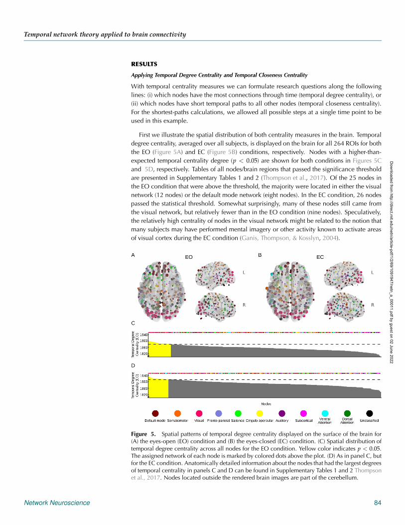
First we illustrate the spatial distribution of both centrality measures in the brain. Temporaldegree centrality, averaged over all subjects, is displayed on the brain for all 264 ROIs for boththe EO (Figure 5A) and EC (Figure 5B) conditions, respectively. Nodes with a higher-than-expected temporal centrality degree (p < 0.05) are shown for both conditions in Figures 5Cand 5D, respectively. Tables of all nodes/brain regions that passed the significance thresholdare presented in Supplementary Tables 1 and 2 (Thompson et al., 2017). Of the 25 nodes inthe EO condition that were above the threshold, the majority were located in either the visualnetwork (12 nodes) or the default mode network (eight nodes). In the EC condition, 26 nodespassed the statistical threshold. Somewhat surprisingly, many of these nodes still came fromthe visual network, but relatively fewer than in the EO condition (nine nodes). Speculatively,the relatively high centrality of nodes in the visual network might be related to the notion thatmany subjects may have performed mental imagery or other activity known to activate areasof visual cortex during the EC condition (Ganis, Thompson, & Kosslyn, 2004).

Figure 5. Spatial patterns of temporal degree centrality displayed on the surface of the brain for(A) the eyes-open (EO) condition and (B) the eyes-closed (EC) condition. (C) Spatial distribution oftemporal degree centrality across all nodes for the EO condition. Yellow color indicates p < 0.05.The assigned network of each node is marked by colored dots above the plot. (D) As in panel C, butfor the EC condition. Anatomically detailed information about the nodes that had the largest degreesof temporal centrality in panels C and D can be found in Supplementary Tables 1 and 2 Thompsonet al., 2017. Nodes located outside the rendered brain images are part of the cerebellum.


Dow




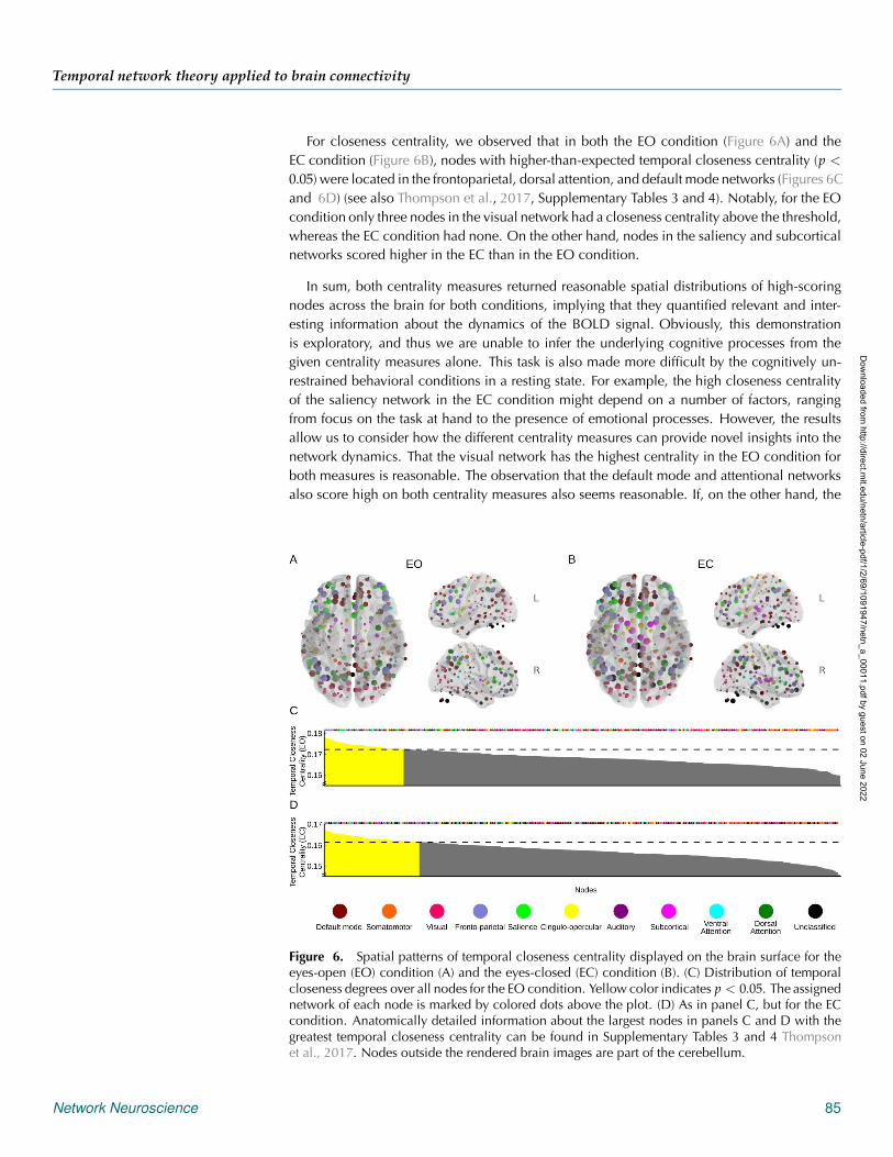
For closeness centrality, we observed that in both the EO condition (Figure 6A) and theEC condition (Figure 6B), nodes with higher-than-expected temporal closeness centrality (p <

0.05) were located in the frontoparietal, dorsal attention, and default mode networks (Figures 6Cand 6D) (see also Thompson et al., 2017, Supplementary Tables 3 and 4). Notably, for the EOcondition only three nodes in the visual network had a closeness centrality above the threshold,whereas the EC condition had none. On the other hand, nodes in the saliency and subcorticalnetworks scored higher in the EC than in the EO condition.

In sum, both centrality measures returned reasonable spatial distributions of high-scoringnodes across the brain for both conditions, implying that they quantified relevant and inter-esting information about the dynamics of the BOLD signal. Obviously, this demonstrationis exploratory, and thus we are unable to infer the underlying cognitive processes from thegiven centrality measures alone. This task is also made more difficult by the cognitively un-restrained behavioral conditions in a resting state. For example, the high closeness centralityof the saliency network in the EC condition might depend on a number of factors, rangingfrom focus on the task at hand to the presence of emotional processes. However, the resultsallow us to consider how the different centrality measures can provide novel insights into thenetwork dynamics. That the visual network has the highest centrality in the EO condition forboth measures is reasonable. The observation that the default mode and attentional networksalso score high on both centrality measures also seems reasonable. If, on the other hand, the

Figure 6. Spatial patterns of temporal closeness centrality displayed on the brain surface for theeyes-open (EO) condition (A) and the eyes-closed (EC) condition (B). (C) Distribution of temporalcloseness degrees over all nodes for the EO condition. Yellow color indicates p < 0.05. The assignednetwork of each node is marked by colored dots above the plot. (D) As in panel C, but for the ECcondition. Anatomically detailed information about the largest nodes in panels C and D with thegreatest temporal closeness centrality can be found in Supplementary Tables 3 and 4 Thompsonet al., 2017. Nodes outside the rendered brain images are part of the cerebellum.


Dow




somato-motor network had scored high in both EC and EO, or if the centrality of nodes inthe visual network had been higher during EC than EO, such results would call into questionwhether our temporal centrality measures were actually quantifying anything meaningful.

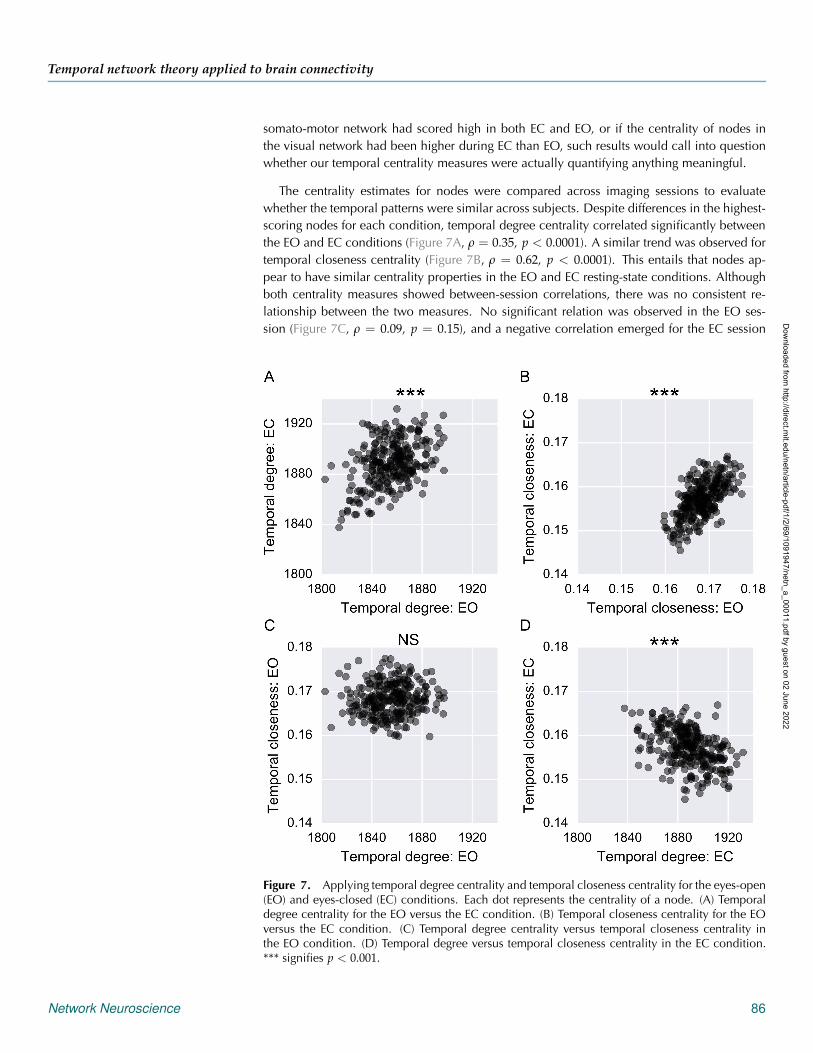
The centrality estimates for nodes were compared across imaging sessions to evaluatewhether the temporal patterns were similar across subjects. Despite differences in the highest-scoring nodes for each condition, temporal degree centrality correlated significantly betweenthe EO and EC conditions (Figure 7A, ρ = 0.35, p < 0.0001). A similar trend was observed fortemporal closeness centrality (Figure 7B, ρ = 0.62, p < 0.0001). This entails that nodes ap-pear to have similar centrality properties in the EO and EC resting-state conditions. Althoughboth centrality measures showed between-session correlations, there was no consistent re-lationship between the two measures. No significant relation was observed in the EO ses-sion (Figure 7C, ρ = 0.09, p = 0.15), and a negative correlation emerged for the EC session

Figure 7. Applying temporal degree centrality and temporal closeness centrality for the eyes-open(EO) and eyes-closed (EC) conditions. Each dot represents the centrality of a node. (A) Temporaldegree centrality for the EO versus the EC condition. (B) Temporal closeness centrality for the EOversus the EC condition. (C) Temporal degree centrality versus temporal closeness centrality inthe EO condition. (D) Temporal degree versus temporal closeness centrality in the EC condition.*** signifies p < 0.001.


Dow




(Figure 7D; ρ = 0.45, p < 0.0001). This result is not surprising, since the measures are quitedifferent by definition, but it is still useful to demonstrate that these different centrality measuresquantify different aspects of the temporal dynamics of the brain.

Applying Burstiness

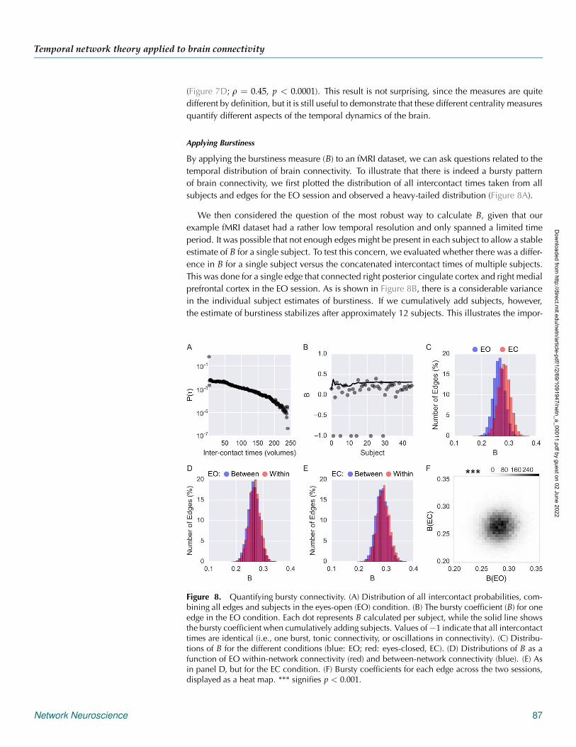
By applying the burstiness measure (B) to an fMRI dataset, we can ask questions related to thetemporal distribution of brain connectivity. To illustrate that there is indeed a bursty patternof brain connectivity, we first plotted the distribution of all intercontact times taken from allsubjects and edges for the EO session and observed a heavy-tailed distribution (Figure 8A).

We then considered the question of the most robust way to calculate B, given that ourexample fMRI dataset had a rather low temporal resolution and only spanned a limited timeperiod. It was possible that not enough edges might be present in each subject to allow a stableestimate of B for a single subject. To test this concern, we evaluated whether there was a differ-ence in B for a single subject versus the concatenated intercontact times of multiple subjects.This was done for a single edge that connected right posterior cingulate cortex and right medialprefrontal cortex in the EO session. As is shown in Figure 8B, there is a considerable variancein the individual subject estimates of burstiness. If we cumulatively add subjects, however,the estimate of burstiness stabilizes after approximately 12 subjects. This illustrates the impor-

Figure 8. Quantifying bursty connectivity. (A) Distribution of all intercontact probabilities, com-bining all edges and subjects in the eyes-open (EO) condition. (B) The bursty coefficient (B) for oneedge in the EO condition. Each dot represents B calculated per subject, while the solid line showsthe bursty coefficient when cumulatively adding subjects. Values of −1 indicate that all intercontacttimes are identical (i.e., one burst, tonic connectivity, or oscillations in connectivity). (C) Distribu-tions of B for the different conditions (blue: EO; red: eyes-closed, EC). (D) Distributions of B as afunction of EO within-network connectivity (red) and between-network connectivity (blue). (E) Asin panel D, but for the EC condition. (F) Bursty coefficients for each edge across the two sessions,displayed as a heat map. *** signifies p < 0.001.


Dow




tance of having enough data to calculate reliable B estimates. Henceforth, all B estimates arecalculated by pooling intercontact times over subjects.

We then wished to contrast EO versus EC in terms of burstiness. Both conditions showedbursty distributions across all edges (see Figure 8C), and slightly more so for the EC than for theEO condition. Both within- and between-network connectivity showed bursty distributions ofconnectivity patterns in both conditions (Figures 8D and 8E).

Given that both EO and EC showed bursty correlations, we tested whether the values ofB correlated between conditions (Figure 8F). We found a weak, but significant, correlationbetween conditions (ρ = 0.066, p < 0.0001). This weak between-condition correlation (ac-counting for less than one percent of the variance, and probably driven by the number of datapoints) suggests that much of the variance of burstiness may have been task-specific. However,more research on this topic will be needed.

Applying Fluctuability

Using the fluctuability measure, researchers may ask questions regarding how many uniqueedges exist in a temporal network model of the dynamic functional brain connectome, indicat-ing whether more resources (i.e., diversity of connections) are required during a given task.

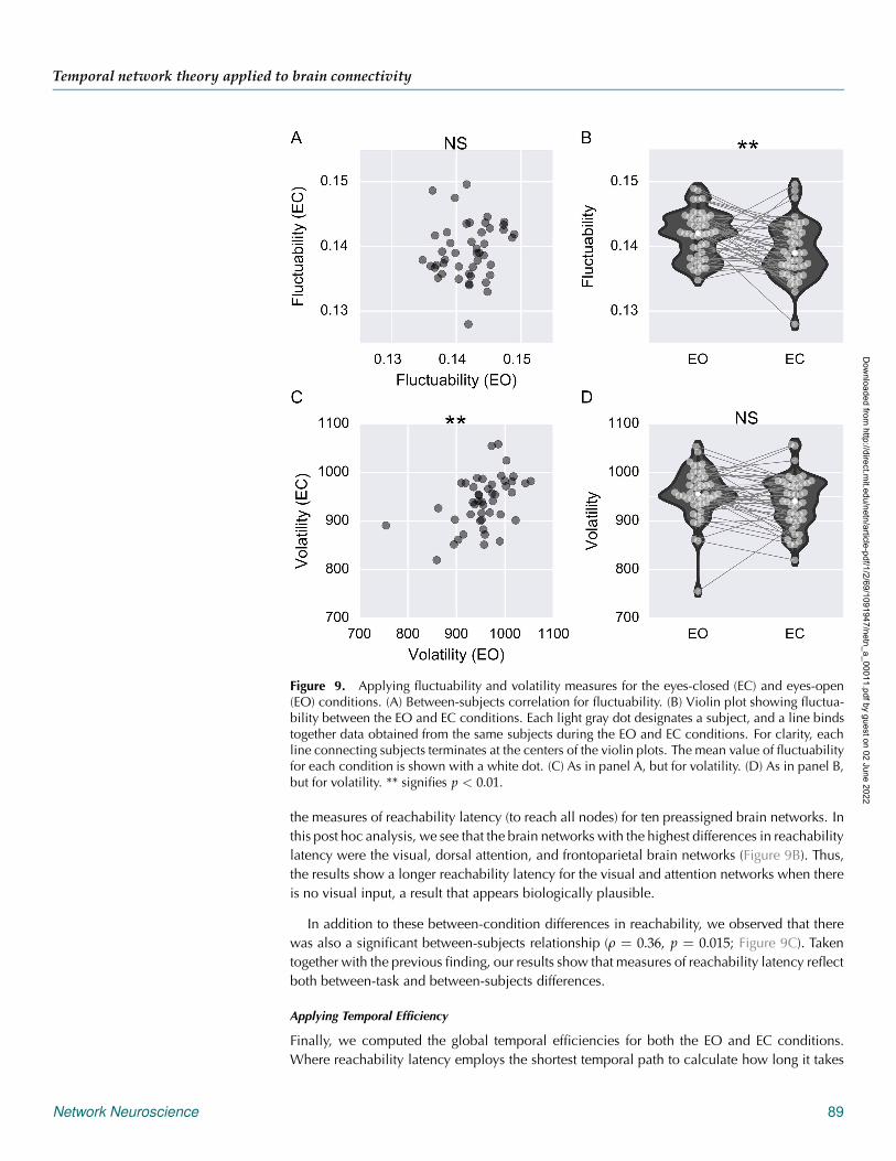
The fluctuability measure was applied to contrast the EO and EC conditions both between(Figure 9A) and within (Figure 9B) subjects. We observed no significant between-subjects cor-relation in F (ρ = 0.18 , p = 0.23) but did find a difference between the average values ofF between conditions (p = 0.0020), with the EO condition having a higher degree of fluctua-bility. Thus, the EO condition had a more varying configuration of connections through timethan did the EC condition.

Applying Volatility

With volatility, we can ask whether the connectivity changes faster or slower through time.Some tasks might require the subject to switch between different cognitive faculties or brainstates, while other tasks may require the brain to be more stable and to switch states less.

As with fluctuability, we computed volatility both between subjects (Figure 9C) and betweenconditions (Figure 9D). We observed a significant correlation for between-subject volatilityover the two conditions (ρ = 0.46, p = 0.0012; Figure 9C). Additionally, no significant differ-ence in volatility was observed between EO and EC (p = 0.051; Figure 9D).

Applying Reachability Latency

The measure of reachability latency addresses the following question regarding the overallconnectivity pattern along the temporal axis: how long does it take to travel to every single nodein the temporal network? For example, the reachability latency may be useful for evaluating thedynamics when either functional or structural connectomes differ substantially. We computedthe reachability latency by setting r = 1 (i.e., all nodes must be reached).

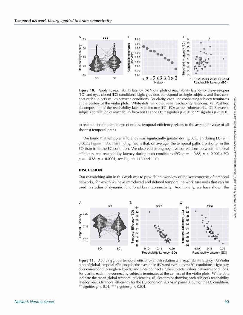
The results are shown in Figure 10, where a significant difference in the average reachabilitylatencies between conditions is visible (Figure 10A; EO: 21.07, EC: 22.96, p = 0.0005). Giventhat there was an overall increase in reachability latencies during EC as compared to EO, wedecided to unpack this finding post hoc and check whether the discovered global differencein reachability could be localized to brain networks that should differ between the EC and EOconditions. So, rather than calculating the reachability latency for the entire brain, we averaged


Dow




Figure 9. Applying fluctuability and volatility measures for the eyes-closed (EC) and eyes-open(EO) conditions. (A) Between-subjects correlation for fluctuability. (B) Violin plot showing fluctua-bility between the EO and EC conditions. Each light gray dot designates a subject, and a line bindstogether data obtained from the same subjects during the EO and EC conditions. For clarity, eachline connecting subjects terminates at the centers of the violin plots. The mean value of fluctuabilityfor each condition is shown with a white dot. (C) As in panel A, but for volatility. (D) As in panel B,but for volatility. ** signifies p < 0.01.

the measures of reachability latency (to reach all nodes) for ten preassigned brain networks. Inthis post hoc analysis, we see that the brain networks with the highest differences in reachabilitylatency were the visual, dorsal attention, and frontoparietal brain networks (Figure 9B). Thus,the results show a longer reachability latency for the visual and attention networks when thereis no visual input, a result that appears biologically plausible.

In addition to these between-condition differences in reachability, we observed that therewas also a significant between-subjects relationship (ρ = 0.36, p = 0.015; Figure 9C). Takentogether with the previous finding, our results show that measures of reachability latency reflectboth between-task and between-subjects differences.

Applying Temporal Efficiency

Finally, we computed the global temporal efficiencies for both the EO and EC conditions.Where reachability latency employs the shortest temporal path to calculate how long it takes


Dow




Figure 10. Applying reachability latency. (A) Violin plots of reachability latency for the eyes-open(EO) and eyes-closed (EC) conditions. Light gray dots correspond to single subjects, and lines con-nect each subject’s values between conditions. For clarity, each line connecting subjects terminatesat the centers of the violin plots. White dots mark the mean reachability latencies. (B) Post hocdecomposition of the reachability latency difference (EC−EO) across subnetworks. (C) Between-subjects correlation of reachability between EO and EC. * signifies p < 0.05; *** signifies p < 0.001

to reach a certain percentage of nodes, temporal efficiency relates to the average inverse of allshortest temporal paths.

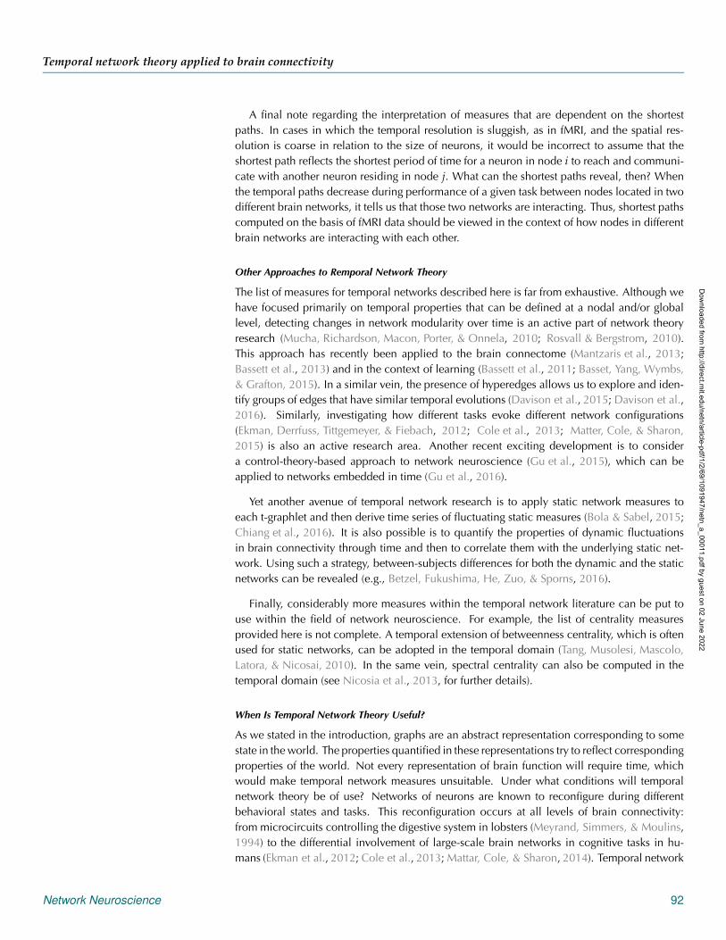
We found that temporal efficiency was significantly greater during EO than during EC (p =

0.0011; Figure 11A). This finding means that, on average, the temporal paths are shorter in theEO than in to the EC condition. We observed strong negative correlations between temporalefficiency and reachability latency during both conditions (EO: ρ = −0.88, p < 0.0001; EC:ρ = −0.88, p < 0.0001; see Figures 11B and 11C).

DISCUSSION

Our overarching aim in this work was to provide an overview of the key concepts of temporalnetworks, for which we have introduced and defined temporal network measures that can beused in studies of dynamic functional brain connectivity. Additionally, we have shown the

Figure 11. Applying global temporal efficiency and its relation with reachability latency. (A) Violinplots of global temporal efficiency for the eyes-open (EO) and eyes-closed (EC) conditions. Light graydots correspond to single subjects, and lines connect single subjects, values between conditions.For clarity, each line connecting subjects terminates at the centers of the violin plots. White dotsindicate the mean global temporal efficiencies. (B) Scatterplot showing each subject’s reachabilitylatency versus temporal efficiency for the EO condition. (C) As in panel B, but for the EC condition.** signifies p < 0.01; *** signifies p < 0.001.


Dow




applicability of temporal metrics in network neuroscience by applying them fMRI resting-statedatasets, and then shown that resting-state networks differ in their dynamical properties.

Summary of Applying Temporal Network Measures to fMRI Data

Both temporal degree centrality and closeness centrality were correlated across conditions,whereas no correlation between the two centrality measures was observed. This entails thatthe two centrality measures quantify different dynamic properties of the brain.

At a global network level, we examined the temporal uniqueness of edges (fluctuability) aswell as the rate of change of connectivity (volatility). We could identify a significant condition-dependent difference in fluctuability, but no difference was observed in volatility between con-ditions. Conversely, a significant between-subjects correlation was found for temporal networkvolatility, but the between-subjects correlation in fluctuability was not significant. The ob-served differences in volatility—that is, the differences in brain connectivity at different pointsin time—were driven to a relatively larger extent by intersubject differences in connectivitydynamics than by differences related to the tasks (EO/EC) per se.

Our results regarding reachability latencies during the EO and EC conditions indicate task-driven changes in latencies, especially since the connectivity of the visual and attention brainnetworks is known to reconfigure between EO and EC conditions (Zhang et al., 2015). Thus,the observed difference in reachability latencies might be a reflection of a putative networkreconfiguration. Furthermore, reachability also showed a between-subjects correlation acrossconditions.

The distribution of intercontact time points of connectivity between brain nodes was bursty,in agreement with our previous findings (Thompson & Fransson, 2016a). Notably, our previ-ous findings were obtained at a high temporal resolution (TR = 0.72 s), and it is thereforereassuring that we were able to detect similar properties of burstiness in brain connectivity ata lower temporal resolution (TR = 2 s). Of note, the between-network versus within-networkconnectivity difference here varied from that obtained in a previous study that had shownbetween-network connectivity to be significantly more bursty than within-network connectiv-ity (Thompson & Fransson, 2016a). This difference is probably due to the different kinds ofthresholding being applied. Here a variance-based thresholding was applied, instead of themagnitude-based form used in the previous study. We have discussed previously that thesedifferent strategies will prioritize different edges (Thompson & Fransson, 2015b, 2016b).

In sum, we have shown that measures founded in temporal network theory can be appliedto fMRI data and are sensitive to the dynamical properties of fMRI BOLD connectivity. Whileattempting to interpret temporal network measures in a psychological and biological contexthas an intuitive appeal, such interpretations remain speculative at this point. Our intention herewas to explore the dynamic connectivity across subjects and across a simple task differenceto demonstrate that temporal network measures are appropriate measures given the signal.We showned that certain properties may be subject-specific, while others are task-specific.Furthermore, temporal network measures lead to rankings of network properties that are inagreement in a resting state during eyes-open and eyes-closed conditions. However, to inferpsychological properties from a specific measure, hypothesis-driven work will be necessaryin which the a priori hypothesis can be explicitly tested. We believe that the present workdemonstrates that such future studies are possible using temporal network theory.


Dow




A final note regarding the interpretation of measures that are dependent on the shortestpaths. In cases in which the temporal resolution is sluggish, as in fMRI, and the spatial res-olution is coarse in relation to the size of neurons, it would be incorrect to assume that theshortest path reflects the shortest period of time for a neuron in node i to reach and communi-cate with another neuron residing in node j. What can the shortest paths reveal, then? Whenthe temporal paths decrease during performance of a given task between nodes located in twodifferent brain networks, it tells us that those two networks are interacting. Thus, shortest pathscomputed on the basis of fMRI data should be viewed in the context of how nodes in differentbrain networks are interacting with each other.

Other Approaches to Remporal Network Theory

The list of measures for temporal networks described here is far from exhaustive. Although wehave focused primarily on temporal properties that can be defined at a nodal and/or globallevel, detecting changes in network modularity over time is an active part of network theoryresearch (Mucha, Richardson, Macon, Porter, & Onnela, 2010; Rosvall & Bergstrom, 2010).This approach has recently been applied to the brain connectome (Mantzaris et al., 2013;Bassett et al., 2013) and in the context of learning (Bassett et al., 2011; Basset, Yang, Wymbs,& Grafton, 2015). In a similar vein, the presence of hyperedges allows us to explore and iden-tify groups of edges that have similar temporal evolutions (Davison et al., 2015; Davison et al.,2016). Similarly, investigating how different tasks evoke different network configurations(Ekman, Derrfuss, Tittgemeyer, & Fiebach, 2012; Cole et al., 2013; Matter, Cole, & Sharon,2015) is also an active research area. Another recent exciting development is to considera control-theory-based approach to network neuroscience (Gu et al., 2015), which can beapplied to networks embedded in time (Gu et al., 2016).

Yet another avenue of temporal network research is to apply static network measures toeach t-graphlet and then derive time series of fluctuating static measures (Bola & Sabel, 2015;Chiang et al., 2016). It is also possible is to quantify the properties of dynamic fluctuationsin brain connectivity through time and then to correlate them with the underlying static net-work. Using such a strategy, between-subjects differences for both the dynamic and the staticnetworks can be revealed (e.g., Betzel, Fukushima, He, Zuo, & Sporns, 2016).

Finally, considerably more measures within the temporal network literature can be put touse within the field of network neuroscience. For example, the list of centrality measuresprovided here is not complete. A temporal extension of betweenness centrality, which is oftenused for static networks, can be adopted in the temporal domain (Tang, Musolesi, Mascolo,Latora, & Nicosai, 2010). In the same vein, spectral centrality can also be computed in thetemporal domain (see Nicosia et al., 2013, for further details).

When Is Temporal Network Theory Useful?

As we stated in the introduction, graphs are an abstract representation corresponding to somestate in the world. The properties quantified in these representations try to reflect correspondingproperties of the world. Not every representation of brain function will require time, whichwould make temporal network measures unsuitable. Under what conditions will temporalnetwork theory be of use? Networks of neurons are known to reconfigure during differentbehavioral states and tasks. This reconfiguration occurs at all levels of brain connectivity:from microcircuits controlling the digestive system in lobsters (Meyrand, Simmers, & Moulins,1994) to the differential involvement of large-scale brain networks in cognitive tasks in hu-mans (Ekman et al., 2012; Cole et al., 2013; Mattar, Cole, & Sharon, 2014). Temporal network


Dow




theory allows us to track and study these reconfigurations, which has the potential to offer moredetailed information about fluctuations in brain network configuration than can be achievedby aggregating over tasks or behavioral states.

The potential fields of application for the methods described in this work are vast. Obvi-ous examples range from real-time neuroimaging to tracking ongoing cognitive processes. Tobe able to isolate and identify the dynamics of networks may indeed be necessary when thesame networks are involved in multiple cognitive processes. Furthermore, the increased tem-poral sensitivity provided by temporal networks offers greater systematic discriminative powerbetween healthy and patient cohorts. To give an example, alterations in static default mode net-work connectivity have been implicated in depression (Sheline et al., 2009; Hamilton et al.,2012), schizophrenia (Garrity et al., 2007; Pomarol-Clotet et al., 2008), traumatic brain in-jury (Bonnelle et al., 2011; Sharp et al., 2011; Thompson, Thelin, Lilja, Bellander, & Fransson,2016), obsessive–compulsive disorder (Stern, Fitzgerald, Welsh, Abelson, & Taylor, 2012),autism (Cherkassky, Kana, Keller, & Just, 2006; Weng et al., 2010), fibromyalgia (Nadapowet al, 2010; Flodin et al., 2014), posttraumatic stress (Sripada et al., 2012), and Alzheimer’sdisease (Greicius, Srivastava, Reiss, & Menon, 2004). This is not an exhaustive list, but it listsuggests that it is very difficult to make inferences regarding static differences in connectivity inthe default network that are specific to a particular patient cohort. We hope that, by adding atemporal dimension and thus reducing the aggregations and simplifications of a static networkanalysis, unique connectivity markers may become viable for different patient cohorts.

A couple of additional Factors should be considered when applying temporal network the-ory. Interpreting what a measure means can only be done in relation to the temporal resolutionof the data. For example, volatility will obviously entail a different interpretation when it is ap-plied to a dataset obtained with a temporal resolution of years versus a dataset acquired with atemporal resolution of milliseconds. Furthermore, measures using shortest temporal paths canbe altogether inappropriate in certain situations (e.g., longtitudinal studies).

Finally, consideration is also needed about which temporal network measure(s) should beapplied to a research question. Although temporal network theory puts a wide array of mea-sures at the user’s disposal, we advise against applying the entire battery of measures to a givendataset. Given a hypothesis about some state of the world (S), this should first be translatedinto a hypothesis about which network measure will quantify the network representation of S.A more exploratory analysis showing significant (and multiple-comparison-corrected) correla-tions in five out of ten measures, when these measures were not first formulated in relation toS, may become hard, if not impossible, to translate into something meaningful.

Limitations and Extensions for Temporal Network Measures

Our scope was limited to temporal measures that operate on binary time series of brain con-nectivity (i.e., binary t-graphlets). Most of the measures discussed here can be extended anddefined for series of weighted connectivity matrices. However, certain temporal measures arenot straightforward to convert to the weighted case. Pertinent examples are burstiness andreachability for which no simple strategy has been identified to apply them in a weighted-connectivity context.

Regardless of the method used to derive the brain connectivity time series, it is impor-tant that adequate preprocessing steps be performed on the data to avoid potential bias inthe analysis. Our method of deriving t-graphlets with weighted Pearson correlation coeffi-cients to compute time series of brain connectivity is not exempted from this concern. In a


Dow




connectivity analysis based on sequences of binary t-graphlets, the absence or presence ofan edge might potentially be influenced by the user’s selection of thresholding. Hence, thestrategy regarding how to optimally threshold the t-graphles into binary graphlets is of vitalimportance. We believe that it is important to keep in mind that comparisons of the vari-ances as well as the means of connectivity time series might be biased by the underlyingmean–variance relationship (Thompson & Fransson, 2015b, 2016b). This further emphasizesthe need for adequate thresholding strategies for connectivity time series. Moreover, subjecthead motion, known to be a large problem for fMRI connectivity studies (Dijk et al., 2012;Power et al., 2012, Power, Schlaggar, & Petersen, 2015), can also lead to spurious dynamicproperties (Laumann et al., 2016).

By providing a survey of the theory of temporal networks and showing their applicabilityand usefulness in network neuroscience, we hope that we have stirred the reader’s interestin using models based on temporal networks when studying the dynamics of functional brainconnectivity. To this end, we have implemented all temporal network measures described inthe present article in a software package that is freely available (Teneto, which is written inPython and can be downloaded at http://github.com/wiheto/teneto). We plan to extend theTeneto package to include additional temporal network measures, plotting routines, wrappersfor other programming languages, and dynamic connectivity estimation.

ACKNOWLEDGMENTS

We thank Pontus Plavén-Sigray, Bjärn Schiffler, Granville Matheson, Simon Skau, and Lieke deBoer for helpful comments and discussions about the manuscript. This work was supportedby the Swedish Research Council (Grant Nos. 621-2012-4911 and 013-61X-08276-26-4) andthe Swedish e-Science Research Center.

AUTHOR CONTRIBUTIONS

William Hedley Thompson: Conceptualization; Formal analysis; Investigation; Methodology;Software; Visualization; Writing – original draft; Writing – review & editing Per Brantefors:Conceptualization; Methodology; Writing – review & editing Peter Fransson: Conceptualiza-tion; Funding acquisition; Investigation; Methodology; Supervision; Writing – original draft;Writing – review & editing.

REFERENCES

Allen, E. A., Damaraju, E., Plis, S. M., Erhardt, E. B., Eichele, T.,& Calhoun, V. D. (2014). Tracking whole-brain connectivitydynamics in the resting state. Cerebral Cortex, 24, 663–676.https://doi.org/10.1093/cercor/bhs352

Baker, A. P., Brookes, M. J., Rezek, I. A., Smith, S. M., Behrens, T.,Smith, P. J. P., & Woolrich, M. (2014). Fast transient networks inspontaneous human brain activity. ELife, 2014(3), 1–18. https://doi.org/10.7554/eLife.01867

Barabási, A.-L. (2005). The origin of bursts and heavy tails in hu-man dynamics. Nature, 435, 207–211. Retrieved from http://arxiv.org/abs/cond-mat/0505371

Barabási, A.-L. (2010). Bursts: The hidden pattern behind every-thing we do. New York, NY: Dutton.

Bassett, D. S., Porter, M. A., Wymbs, N. F., Grafton, S. T., Carlson,J. M., & Mucha, P. J. (2013). Robust detection of dynamic com-

munity structure in networks. Chaos, 23(1). https://doi.org/10.1063/1.4790830

Bassett, D. S., Wymbs, N. F., Porter, M. A., Mucha, P. J., Carlson,J. M., & Grafton, S. T. (2011). Dynamic reconfiguration of hu-man brain networks during learning. Proceedings of the NationalAcademy of Sciences, 108(18), 7641–7646. https://doi.org/10.1073/pnas.1018985108

Bassett, D. S., Yang, M., Wymbs, N. F., & Grafton, S. T. (2015).Learning-induced autonomy of sensorimotor systems. NatureNeuroscience, 18(5), 744–751. https://doi.org/10.1038/nn.3993

Bastos, A. M., Usrey, W. M., Adams, R. A., Mangun, G. R., Fries,P., & Friston, K. J. (2012). Canonical microcircuits for pre-dictive coding. Neuron, 76(4), 695–711. https://doi.org/10.1016/j.neuron.2012.10.038


Dow



https://dx.doi.org/10.1093/cercor/bhs352

https://dx.doi.org/10.7554/eLife.01867

https://dx.doi.org/10.7554/eLife.01867

http://arxiv.org/abs/cond-mat/0505371

http://arxiv.org/abs/cond-mat/0505371

https://dx.doi.org/10.1063/1.4790830

https://dx.doi.org/10.1063/1.4790830

https://dx.doi.org/10.1073/pnas.1018985108


https://dx.doi.org/10.1038/nn.3993

https://dx.doi.org/10.1016/j.neuron.2012.10.038



Bastos, A. M., Vezoli, J., Bosman, C. A., Schoffelen, J. M.,Oostenveld, R., Dowdall, J. R., . . . Fries, P. (2015). Visualareas exert feedforward and feedback influences through distinctfrequency channels. Neuron, 85(2), 390–401. https://doi.org/10.1016/j.neuron.2014.12.018

Basu, P., Bar-noy, A., Johnson, M. P., & Ramanathan, R. (2010).Modeling and analysis of time-varying graphs. ArXiv:1012.0260

Behzadi, Y., Restom, K., Liau, J., & Liu, T. T. (2007). A componentbased noise correction method (CompCor) for BOLD and perfu-sion based fMRI. NeuroImage, 37(1), 90–101. https://doi.org/10.1016/j.neuroimage.2007.04.042

Berlingerio, M., Coscia, M., Giannotti, F., Monreale, A., &Pedreschi, D. (2011). Foundations of multidimensional networkanalysis. In Proceedings of the 2011 International Conferenceon Advances in Social Networks Analysis and Mining, ASONAM2011 (pp. 485–487). Piscataway, NJ: IEEE Press. https://doi.org/10.1109/ASONAM.2011.103

Betzel, R. F., Fukushima, M., He, Y., Zuo, X. N., & Sporns, O.(2016). Dynamic fluctuations coincide with periods of high andlow modularity in resting-state functional brain networks. Neu-roImage, 127, 287–297. https://doi.org/10.1016/j.neuroimage.2015.12.001

Bola, M., & Sabel, B. A. (2015). Dynamic reorganization of brainfunctional networks during cognition. NeuroImage, 114, 398–413. https://doi.org/10.1016/j.neuroimage.2015.03.057

Bonnelle, V., Leech, R., Kinnunen, K. M., Ham, T. E., Beckmann,C. F., De Boissezon, X., . . . Sharp, D. J. (2011). Default modenetwork connectivity predicts sustained attention deficits aftertraumatic brain injury. Journal of Neuroscience, 31(38), 13442–13451. https://doi.org/10.1523/JNEUROSCI.1163-11.2011

Bosman, C. A., Schoffelen, J.-M., Brunet, N., Oostenveld, R.,Bastos, A. M., Womelsdorf, T., . . . Fries, P. (2012). Atten-tional stimulus selection through selective synchronization be-tween monkey visual areas. Neuron, 75(5), 875–888. https://doi.org/10.1016/j.neuron.2012.06.037

Bressler, S. L., & Kelso, J. A. S. (2001). Cortical coordination dy-namics and cognition. Trends in Cognitive Sciences, 5(1), 26–36.Retrieved from http://doi.org/10.1016/51364-6613(00)01564-3

Bressler, S. L., Richter, C. G., Chen, Y., & Ding, M. (2007). Corticalfunctional network organization from autoregressive modeling oflocal field potential oscillations. Statistics in Medicine, 26(21),3875–3885. https://doi.org/10.1002/sim.2935

Brookes, M. J., Woolrich, M., Luckhoo, H., Price, D., Hale, J. R.,Stephenson, M. C., . . . Morris, P. G. (2011). Investigating theelectrophysiological basis of resting state networks using mag-netoencephalography. Proceedings of the National Academy ofSciences, 108(40), 16783–16788. https://doi.org/10.1073/pnas.1112685108

Buckner, R. L., Sepulcre, J., Talukdar, T., Krienen, F. M., Liu, H.,Hedden, T., . . . Johnson, K. A. (2009). Cortical hubs revealed byintrinsic functional connectivity: Mapping, assessment of stabil-ity, and relation to Alzheimer’s disease. Journal of Neuroscience,29(6), 1860–1873. https://doi.org/10.1523/JNEUROSCI.5062-08.2009

Bullmore, E., & Sporns, O. (2009). Complex brain networks: Graphtheoretical analysis of structural and functional systems. Nature

Reviews Neuroscience, 10(3), 186–198. https://doi.org/10.1038/nrn2575

Buschman, T. J., & Miller, E. K. (2007). Top-down versus bottom-upcontrol of attention in the prefrontal and posterior parietal cor-tices. Science, 315(5820), 1860–1862. https://doi.org/10.1126/science.1138071

Buzsáki, G. (2005). Theta rhythm of navigation: Link betweenpath integration and landmark navigation, episodic and seman-tic memory. Hippocampus, 15(7), 827–840. https://doi.org/10.1002/hipo.20113

Buzsáki, G. (2006). Rhythms of the brain. Oxford, UK: OxfordUniversity Press. https://doi.org/10.1093/acprof:oso/9780195301069.001.0001

Buzsáki, G., & Draguhn, A. (2004). Neuronal oscillations in cor-tical networks. Science, 304(5679), 1926–1929. https://doi.org/10.1126/science.1099745

Calhoun, V. D., Miller, R., Pearlson, G., & Adalı, T. (2014). Thechronnectome: Time-varying connectivity networks as the nextfrontier in fMRI data discovery. Neuron, 84(2), 262–274. https://doi.org/10.1016/j.neuron.2014.10.015

Chang, C., & Glover, G. H. (2010). Time-frequency dynamicsof resting-state brain connectivity measured with fMRI. Neuro-Image, 50(1), 81–98. https://doi.org/10.1016/j.neuroimage.2009.12.011

Cherkassky, V. L., Kana, R. K., Keller, T. A., & Just, M. A. (2006).Functional connectivity in a baseline resting-state network inautism. NeuroReport, 17(16), 1687–1690. https://doi.org/10.1097/01.wnr.0000239956.45448.4c

Chiang, S., Cassese, A., Guindani, M., Vannucci, M., Yeh, H. J.,Haneef, Z., & Stern, J. M. (2016). Time-dependence of graphtheory metrics in functional connectivity analysis. NeuroImage,125, 601–615. https://doi.org/10.1016/j.neuroimage.2015.10.070

Cole, M. W., Reynolds, J. R., Power, J. D., Repovs, G., Anticevic,A., & Braver, T. S. (2013). Multi-task connectivity reveals flexi-ble hubs for adaptive task control. Nature Neuroscience, 16(9),1348–1355. https://doi.org/10.1038/nn.3470

Davison, E. N., Schlesinger, K. J., Bassett, D. S., Lynall, M.-E.,Miller, M. B., Grafton, S. T., & Carlson, J. M. (2015). Brain net-work adaptability across task states. PLoS Computational Biology,11(1). https://doi.org/10.1371/journal.pcbi.1004029

Davison, E. N., Turner, B. O., Schlesinger, K. J., Miller, M. B.,Grafton, T., Bassett, D. S. (2016). Individual differences indynamic functional brain connectivity across the human life-span. ArXiv Preprint, 1–26. https://doi.org/10.1371/journal.pcbi.1005178

Deco, G., Jirsa, V. K., & McIntosh, A. R. (2011). Emerging con-cepts for the dynamical organization of resting-state activity inthe brain. Nature Reviews Neuroscience, 12(1), 43–56. https://doi.org/10.1038/nrn2961

Deco, G., & Kringelbach, M. L. (2016). Metastability and coher-ence: Extending the communication through coherence hypoth-esis using a Whole-Brain computational perspective. Trends inNeurosciences, 39(3), 125–135. https://doi.org/10.1016/j.tins.2016.01.001

de Pasquale, F., Della Penna, S., Snyder, A. Z., Lewis, C.,Mantini, D., Marzetti, L., . . . Corbetta, M. (2010). Temporal


Dow





https://dx.doi.org/10.1016/j.neuroimage.2007.04.042


https://dx.doi.org/10.1109/ASONAM.2011.103

https://dx.doi.org/10.1109/ASONAM.2011.103




https://dx.doi.org/10.1523/JNEUROSCI.1163-11.2011



http://dx.doi.org/10.1016/51364-6613(00)01564-3

https://dx.doi.org/10.1002/sim.2935





https://dx.doi.org/10.1038/nrn2575


https://dx.doi.org/10.1126/science.1138071


https://dx.doi.org/10.1002/hipo.20113

https://dx.doi.org/10.1002/hipo.20113

https://dx.doi.org/10.1093/acprof:oso/9780195301069.001.0001

https://dx.doi.org/10.1093/acprof:oso/9780195301069.001.0001







https://dx.doi.org/10.1097/01.wnr.0000239956.45448.4c

https://dx.doi.org/10.1097/01.wnr.0000239956.45448.4c




https://dx.doi.org/10.1371/journal.pcbi.1004029





https://dx.doi.org/10.1016/j.tins.2016.01.001

https://dx.doi.org/10.1016/j.tins.2016.01.001


dynamics of spontaneous MEG activity in brain networks.Proceedings of the National Academy of Sciences, 107(13),6040–6045. https://doi.org/10.1073/pnas.0913863107

de Pasquale, F., Della Penna, S., Snyder, A. Z., Marzetti, L., Pizzella,V., Romani, G. L., & Corbetta, M. (2012). A cortical core fordynamic integration of functional networks in the resting hu-man brain. Neuron, 74(4), 753–764. https://doi.org/10.1016/j.neuron.2012.03.031

Dijk, K. R. A., Sabuncu, M. R., & Buckner, R. L. (2012). Theinfluence of head motion on intrinsic functional connectivityMRI. NeuroImage, 59(1), 431–438. https://doi.org/10.1016/j.neuroimage.2011.07.044

Drakesmith, M., Caeyenberghs, K., Dutt, a., Lewis, G., David, &Jones, D. (2015). Overcoming the effects of false positivesand threshold bias in graph theoretical analyses of neuroimag-ing data. NeuroImage, 118, 313–333. https://doi.org/10.1016/j.neuroimage.2015.05.011

Eckmann, J. P., Moses, E., & Sergi, D. (2004). Entropy of di-alogues creates coherent structures in e-mail traffic. Proceed-ings of the National Academy of Sciences of the United States ofAmerica, 101(7), 14333–14337. https://doi.org/10.1073/pnas.0405728101

Ekman, M., Derrfuss, J., Tittgemeyer, M., & Fiebach, C. J.(2012). Predicting errors from reconfiguration patterns in hu-man brain networks. Proceedings of the National Academy ofSciences, 109(41), 16714–16719. https://doi.org/10.1073/pnas.1207523109

Flodin, P. D., Martinsen, S., Löfgren, M., Bileviciute-Ljungar, I.,Kosek, E., & Fransson, P. (2014). Fibromyalgia is associated withdecreased connectivity between pain- and sensorimotor brainareas. Brain Connectivity, 62(2010), 2545. https://doi.org/10.1089/brain.2014.0274

Fox, M. D., & Greicius, M. D. (2010). Clinical applications of restingstate functional connectivity. Frontiers in Systems Neuroscience,4, 19. https://doi.org/10.3389/fnsys.2010.00019

Fox, M. D., Snyder, A. Z., Vincent, J. L., Corbetta, M., Van Essen,D. C., & Raichle, M. E. (2005). The human brain is intrinsicallyorganized into dynamic, anticorrelated functional networks.Proceedings of the National Academy of Sciences, 102(27),9673–9678. https://doi.org/10.1073/pnas.0504136102

Fransson, P. (2005). Spontaneous low-frequency BOLD signalfluctuations: An fMRI investigation of the resting-state defaultmode of brain function hypothesis. Human Brain Mapping,26(1), 15–29. https://doi.org/10.1002/hbm.20113

Freyer, F., Aquino, K., Robinson, P. A., Ritter, P., & Breakspear, M.(2009). Bistability and non-Gaussian fluctuations in spontaneouscortical activity. Journal of Neuroscience, 29(26), 8512–8524.https://doi.org/10.1523/JNEUROSCI.0754-09.2009

Freyer, F., Roberts, J. A., Ritter, P., & Breakspear, M. (2012). Acanonical model of multistability and scale-invariance in biolog-ical systems. PLoS Computational Biology, 8(8). https://doi.org/10.1371/journal.pcbi.1002634

Fries, P. (2005). A mechanism for cognitive dynamics: Neuronalcommunication through neuronal coherence. Trends in Cog-nitive Sciences, 9(10), 474–480. https://doi.org/10.1016/j.tics.2005.08.011

Friese, U., Köster, M., Hassler, U., Martens, U., Trujillo-Barreto, N.,& Gruber, T. (2013). Successful memory encoding is associatedwith increased cross-frequency coupling between frontal thetaand posterior gamma oscillations in human scalp-recordedEEG. NeuroImage, 66, 642–647. https://doi.org/10.1016/j.neuroimage.2012.11.002

Friston, K. J., Holmes, A. P., Worsley, K. J., Poline, J.-P., Frith, C. D.,& Frackowiak, R. S. J. (1995). Statistical parametric maps in func-tional imaging: A general linear approach. Human Brain Map-ping, 2(4), 189–210. https://doi.org/10.1002/hbm.460020402

Ganis, G., Thompson, W. L., & Kosslyn, S. M. (2004). Brain ar-eas underlying visual mental imagery and visual perception: AnfMRI study. Cognitive Brain Research, 20(2), 226–241. https://doi.org/10.1016/j.cogbrainres.2004.02.012

Garrity, A. G., Pearlson, G. D., McKiernan, K., Lloyd, D., Kiehl,K. A., & Calhoun, V. D. (2007). Aberrant “default mode”functional connectivity in schizophrenia. American Journal ofPsychiatry, 164(3), 450–457. https://doi.org/10.1176/ajp.2007.164.3.450

Goh, K.-I., & Barabási, A.-L. (2008). Burstiness and memory in com-plex systems. EPL (Europhysics Letters), 81(4), 48002. https://doi.org/10.1209/0295-5075/81/48002

Greicius, M. D., Krasnow, B., Reiss, A. L., & Menon, V. (2003).Functional connectivity in the resting brain: A network analy-sis of the default mode hypothesis. Proceedings of the NationalAcademy of Sciences, 100, 253–258. https://doi.org/10.1073/pnas.0135058100

Greicius, M. D., Srivastava, G., Reiss, A. L., & Menon, V. (2004).Default-mode network activity distinguishes Alzheimer’s diseasefrom healthy aging: Evidence from functional MRI. Proceed-ings of the National Academy of Sciences, 101(13), 4637–4642.https://doi.org/10.1073/pnas.0308627101

Gu, S., Betzel, R. F., Cieslak, M., Delio, P. R., Grafton, S. T.,Pasqualetti, F., & Bassett, D. S. (2016). Optimal trajectories ofbrain state transitions, 1–10. http://arxiv.org/abs/1607.01706

Gu, S., Pasqualetti, F., Cieslak, M., Telesford, Q. K., Yu, A. B., Kahn,A. E., . . . Bassett, D. S. (2015). Controllability of structural brainnetworks. Nature Communications, 6, 8414. https://doi.org/10.1038/ncomms9414

Hamilton, J., Furman, D., Chang, C., Thomason, M., Dennis, E., &Gotlib, I. (2012). Default-mode and task-positive network activ-ity in Major Depressive Disorder: Implications for adaptive andmaladaptive rumination. Biological Psychiatry, 70(4), 327–333.https://doi.org/10.1016/j.biopsych.2011.02.003.Default-mode

Hipp, J. F., Hawellek, D. J., Corbetta, M., Siegel, M., & Engel,A. K. (2012). Large-scale cortical correlation structure of sponta-neous oscillatory activity. Nature Neuroscience, 15(6), 884–890.https://doi.org/10.1038/nn.3101

Holme, P. (2005). Network reachability of real-world contact se-quences. Physical Review E, 71(4), 1–8. https://doi.org/10.1103/PhysRevE.71.046119

Holme, P., & Saramäki, J. (2012). Temporal networks. Physics Re-ports, 519(3), 97–125. https://doi.org/10.1016/j.physrep.2012.03.001

Hutchison, R. M., Womelsdorf, T., Allen, E. A., Bandettini,P. A., Calhoun, V. D., Corbetta, M., . . . Chang, C. (2013).


Dow














https://dx.doi.org/10.1089/brain.2014.0274


https://dx.doi.org/10.3389/fnsys.2010.00019


https://dx.doi.org/10.1002/hbm.20113




https://dx.doi.org/10.1016/j.tics.2005.08.011

https://dx.doi.org/10.1016/j.tics.2005.08.011



https://dx.doi.org/10.1002/hbm.460020402

https://dx.doi.org/10.1016/j.cogbrainres.2004.02.012

https://dx.doi.org/10.1016/j.cogbrainres.2004.02.012

https://dx.doi.org/10.1176/ajp.2007.164.3.450

https://dx.doi.org/10.1176/ajp.2007.164.3.450

https://dx.doi.org/10.1209/0295-5075/81/48002

https://dx.doi.org/10.1209/0295-5075/81/48002




http://arxiv.org/abs/1607.01706

https://dx.doi.org/10.1038/ncomms9414

https://dx.doi.org/10.1038/ncomms9414

https://dx.doi.org/10.1016/j.biopsych.2011.02.003.Default-mode


https://dx.doi.org/10.1103/PhysRevE.71.046119


https://dx.doi.org/10.1016/j.physrep.2012.03.001

https://dx.doi.org/10.1016/j.physrep.2012.03.001


Dynamic functional connectivity: Promise, issues, and inter-pretations. NeuroImage, 80, 360–378. https://doi.org/10.1016/j.neuroimage.2013.05.079

Jo, H. H., Karsai, M., Kertész, J., & Kaski, K. (2012). Circadianpattern and burstiness in human communication activity. NewJournal of Physics, 14, 013055. https://doi.org/10.1088/1367-2630/14/1/013055

Kelso, J. A. S. (1995). Dynamic patterns: The self-organization ofbrain and behavior. Cambridge, MA: MIT Press. https://doi.org/10.1016/S0925-2312(00)00221-6

Kivelä, M., Arenas, A., Barthelemy, M., Gleeson, J. P., Moreno,Y., & Porter, M. A. (2014). Multilayer networks. Journal of Com-plex Networks, 2(3), 203–271. https://doi.org/10.1093/comnet/cnu016

Kopell, N. J., Gritton, H. J., Whittington, M. A., & Kramer, M. A.(2014). Beyond the connectome: The dynome. Neuron, 83(6),1319–1328. https://doi.org/10.1016/j.neuron.2014.08.016

Laumann, T. O., Snyder, A. Z., Mitra, A., Gordon, E. M., Gratton,C., Adeyemo, B., . . . Petersen, S. E. (2016). On the stability ofBOLD fMRI correlations. Cerebral Cortex, Advance online pub-lication. https://doi.org/10.1093/cercor/bhw265

Lindquist, M. A., Xu, Y., Nebel, M. B., & Caffo, B. S. (2014). Evalu-ating dynamic bivariate correlations in resting-state fMRI: A com-parison study and a new approach. NeuroImage, 101, 531–546.https://doi.org/10.1016/j.neuroimage.2014.06.052

Liu, X., & Duyn, J. H. (2013). Time-varying functional networkinformation extracted from brief instances of spontaneousbrain activity. Proceedings of the National Academy of Sciences,110(11), 4392–4397. https://doi.org/10.1073/pnas.1216856110

Mantzaris, A. V., Bassett, D. S., Wymbs, N. F., Estrada, E., Porter,M. A., Mucha, P. J., . . . Higham, D. J. (2013). Dynamic net-work centrality summarizes learning in the human brain. Jour-nal of Complex Networks, 1(1), 83–92. https://doi.org/10.1093/comnet/cnt001

Masuda, N., & Lambiotte, R. (2016). A guide to temporal networks(1st ed.). London, UK: World Scientific.

Mattar, M. G., Cole, M. W., & Sharon, L. (2014). A functionalcartography of cognitive systems. PLoS Computational Biol-ogy, 11, e10045331:1–36, https://doi.org/10.1371/journal.pcbi.1004533

Meyrand, P., Simmers, J., & Moulins, M. (1994). Dynamic construc-tion of a neural network from multiple pattern generators in thelobster stomatogastric nervous system. Journal of Neuroscience,14(2), 630–644.

Michalareas, G., Vezoli, J., van Pelt, S., Schoffelen, J. M., Kennedy,H., & Fries, P. (2016). Alpha-beta and gamma rhythms subservefeedback and feedforward influences among human visual cor-tical areas. Neuron, 89(2), 384–397. https://doi.org/10.1016/j.neuron.2015.12.018

Min, B., Goh, K.-I., & Vazquez, A. (2011). Spreading dynamics fol-lowing bursty human activity patterns. Physical Review E, 83(3),036102. https://doi.org/10.1103/PhysRevE.83.036102

Montgomery, S. M., & Buzsáki, G. (2007). Gamma oscillationsdynamically couple hippocampal CA3 and CA1 regions duringmemory task performance. Proceedings of the National Academyof Sciences, 104(36), 14495–14500. https://doi.org/10.1073/pnas.0701826104

Mucha, P. J., Richardson, T., Macon, K., Porter, M. A., & Onnela,J.-P. (2010). Community structure in time-dependent, multiscale,and multiplex networks. Science, 328(5980), 876–878. https://doi.org/10.1126/science.1184819

Napadow, V., LaCount, L., Park, K., As-Sanie, S., Clauw, D. J., &Harris, R. E. (2010). Intrinsic brain connectivity in fibromyalgiais associated with chronic pain intensity. Arthritis and Rheuma-tism, 62(8), 2545–2555. https://doi.org/10.1002/art.27497

Newman, M. (2010). Networks: An introduction. Oxford, UK:Oxford University Press.

Nicosia, V., Tang, J., Mascolo, C., Musolesi, M., Russo, G., &Latora, V. (2013). Graph metrics for temporal networks. In Tem-poral networks (pp. 15–40). Berlin, Germany: Springer. Re-trieved from http://arxiv.org/abs/1306.0493v1

Nijhuis, E. H. J., van Cappellen van Walsum, A.-M., & Norris, D. G.(2013). Topographic hub maps of the human structural neocor-tical network. PLoS ONE, 8(6), e65511. https://doi.org/10.1371/journal.pone.0065511

Pan, R. K., & Saramäki, J. (2011). Path lengths, correlations, andcentrality in temporal networks. Physical Review E, 84(1). https://doi.org/10.1103/PhysRevE.84.016105

Pomarol-Clotet, E., Salvador, R., Sarró, S., Gomar, J., Vila, F.,Martínez, A., . . . McKenna, P. J. (2008). Failure to deactivatein the prefrontal cortex in schizophrenia: Dysfunction of the de-fault mode network? Psychological Medicine, 38(8), 1185–1193.https://doi.org/10.1017/S0033291708003565

Power, J. D., Barnes, K. A., Snyder, A. Z., Schlaggar, B. L., &Petersen, S. E. (2012). Spurious but systematic correlationsin functional connectivity MRI networks arise from subject mo-tion. NeuroImage, 59(3), 2142–2154. https://doi.org/10.1016/j.neuroimage.2011.10.018

Power, J. D., Cohen, A. L., Nelson, S. M., Wig, G. S., Barnes, K. A.,Church, J. A., . . . Petersen, S. E. (2011). Functional network or-ganization of the human brain. Neuron, 72(4), 665–678. https://doi.org/10.1016/j.neuron.2011.09.006

Power, J. D., Schlaggar, B. L., Lessov-Schlaggar, C. N., & Petersen,S. E. (2013). Evidence for hubs in human functional brainnetworks. Neuron, 79(4), 798–813. https://doi.org/10.1016/j.neuron.2013.07.035

Power, J. D., Schlaggar, B. L., & Petersen, S. E. (2015). Recentprogress and outstanding issues in motion correction in restingstate fMRI. NeuroImage, 105, 536–551. https://doi.org/10.1016/j.neuroimage.2014.10.044

Richter, C. G., Coppola, R., & Bressler, S. L. (2016). Top-downbeta oscillatory signaling conveys behavioral context to primaryvisual cortex. BioRxiv, 074609. https://doi.org/10.1101/074609

Richter, C. G., Thompson, W. H., Bosman, C. A., & Fries, P. (2016).Top-down beta enhances bottom-up gamma [Preprint article],1–40. https://doi.org/10.1101/054288

Roberts, J. A., Boonstra, T. W., & Breakspear, M. (2015). The heavytail of the human brain. Current Opinion in Neurobiology, 31,164–172. https://doi.org/10.1016/j.conb.2014.10.014

Rocha, L. E. C., Liljeros, F., & Holme, P. (2010). Information dy-namics shape the sexual networks of Internet-mediated prostitu-tion. Proceedings of the National Academy of Sciences, 107(13),5706–5711. https://doi.org/10.1073/pnas.0914080107


Dow





https://dx.doi.org/10.1088/1367-2630/14/1/013055

https://dx.doi.org/10.1088/1367-2630/14/1/013055

https://dx.doi.org/10.1016/S0925-2312(00)00221-6

https://dx.doi.org/10.1016/S0925-2312(00)00221-6

https://dx.doi.org/10.1093/comnet/cnu016

https://dx.doi.org/10.1093/comnet/cnu016


https://dx.doi.org/10.1093/cercor/bhw265



https://dx.doi.org/10.1093/comnet/cnt001

https://dx.doi.org/10.1093/comnet/cnt001










https://dx.doi.org/10.1002/art.27497

http://arxiv.org/abs/1306.0493v1

https://dx.doi.org/10.1371/journal.pone.0065511




https://dx.doi.org/10.1017/S0033291708003565









https://dx.doi.org/10.1101/074609

https://dx.doi.org/10.1101/054288

https://dx.doi.org/10.1016/j.conb.2014.10.014



Rosvall, M., & Bergstrom, C. T. (2010). Mapping change in largenetworks. PLoS ONE, 5(1), e8694. https://doi.org/10.1371/journal.pone.0008694

Sharp, D. J., Beckmann, C. F., Greenwood, R., Kinnunen, K. M.,Bonnelle, V., De Boissezon, X., . . . Leech, R. (2011). Defaultmode network functional and structural connectivity after trau-matic brain injury. Brain, 134(Pt 8), 2233–2247. https://doi.org/10.1093/brain/awr175

Sheline, Y. I., Barch, D. M., Price, J. L., Rundle, M. M., Vaishnavi,S. N., Snyder, A. Z., . . . Raichle, M. E. (2009). The default modenetwork and self-referential processes in depression. Proceed-ings of the National Academy of Sciences, 106(6), 1942–1947.https://doi.org/10.1073/pnas.0812686106

Shine, J. M., Koyejo, O., Bell, P. T., Gorgolewski, K. J., Gilat, M.,& Poldrack, R. A. (2015). Estimation of dynamic functional con-nectivity using multiplication of temporal derivatives. Neuro-Image, 122, 399–407. https://doi.org/10.1016/j.neuroimage.2015.07.064

Shine, J. M., Koyejo, O., & Poldrack, R. A. (2016). Temporal meta-states are associated with differential patterns of dynamic con-nectivity, network topology and attention. Proceedings of theNational Academy of Sciences, 113, 9888–9891. https://doi.org/10.1073/pnas.1604898113

Siegel, M., Donner, T. H., & Engel, A. K. (2012). Spectral finger-prints of large-scale neuronal interactions. Nature Reviews Neu-roscience, 13(2), 121–134. https://doi.org/10.1038/nrn3137

Smith, S. M., Fox, P. T., Miller, K. L., Glahn, D. C., Fox, P. M.,Mackay, C. E., . . . Beckmann, C. F. (2009). Correspondenceof the brain’s functional architecture during activation and rest.Proceedings of the National Academy of Sciences, 106(31),13040–13045. https://doi.org/10.1073/pnas.0905267106

Smith, S. M., Miller, K. L., Moeller, S., Xu, J., Auerbach, E. J.,Woolrich, M. W., . . . Ugurbil, K. (2012). Temporally-independent functional modes of spontaneous brain activity.Proceedings of the National Academy of Sciences, 109(8), 3131–3136. https://doi.org/10.1073/pnas.1121329109

Sporns, O. (2009). Networks of the brain. Cambridge, MA: MITPress.

Sporns, O., Tononi, G., & Kötter, R. (2005). The human connec-tome: A structural description of the human brain. PLoS Com-putational Biology, 1(4), 0245–0251. https://doi.org/10.1371/journal.pcbi.0010042

Sripada, R. K., King, A. P., Welsh, R. C., Garfinkel, S. N., Wang,X., Sripada, C. S., & Liberzon, I. (2012). Neural dysregulation inposttraumatic stress disorder: Evidence for disrupted equilibriumbetween salience and default mode brain networks. Psychoso-matic Medicine, 911(35), 904–911. https://doi.org/10.1097/PSY.0b013e318273bf33

Stern, E. R., Fitzgerald, K. D., Welsh, R. C., Abelson, J. L., & Taylor,S. F. (2012). Resting-state functional connectivity between fronto-parietal and default mode networks in obsessive–compulsive dis-order. PLoS ONE, 7(5), e36356. https://doi.org/10.1371/journal.pone.0036356

Tagliazucchi, E., Balenzuela, P., Fraiman, D., & Chialvo, D. R.(2012). Criticality in large-scale brain fMRI dynamics unveiledby a novel point process analysis. Frontiers in Physiology, 3, 15.https://doi.org/10.3389/fphys.2012.00015

Takaguchi, T., Masuda, N., & Holme, P. (2013). Bursty communica-tion patterns facilitate spreading in a threshold-based epidemicdynamics. PLoS ONE, 8(7), e68629. https://doi.org/doi:10.1371/journal.pone.0068629

Tang, J., Musolesi, M., Mascolo, C., Latora, V., & Nicosia, V. (2010).Analysing information flows and key mediators through temporalcentrality metrics categories and subject descriptors. In Proceed-ings of the 3rd Workshop on Social Network Systems (Article 3).New York,NY: ACM. https://doi.org/10.1145/1852658.1852661

Thompson, W. H., Brantefors, P., & Fransson, P. (2017). Supplemen-tal material to “From static to temporal network theory: Applica-tions to functional brain connectivity.” Network Neuroscience,1(2). https://doi.org/10.1162/netn_a_00011

Thompson, W. H., & Fransson, P. (2015a). The frequency dimensionof fMRI dynamic connectivity: Network connectivity, functionalhubs and integration in the resting brain. NeuroImage, 121,227–242. https://doi.org/10.1016/j.neuroimage.2015.07.022

Thompson, W. H., & Fransson, P. (2015b). The mean–variance re-lationship reveals two possible strategies for dynamic brain con-nectivity analysis in fMRI. Frontiers in Human Neuroscience, 9,398:1–7. https://doi.org/10.3389/fnhum.2015.00398

Thompson, W. H., & Fransson, P. (2016a). Bursty properties re-vealed in large-scale brain networks with a point-based methodfor dynamic functional connectivity. Scientific Reports, 6, 39156.https://doi.org/10.1038/srep39156

Thompson, W. H., & Fransson, P. (2016b). On stabilizing thevariance of dynamic functional brain connectivity time series.Brain Connectivity, 6(10), 735–746. https://doi.org/10.1089/brain.2016.0454

Thompson, W. H., Thelin, E. P., Lilja, A., Bellander, B.-M., &Fransson, P. (2016). Functional resting-state fMRI connectivitycorrelates with serum levels of the S100B protein in the acutephase of traumatic brain injury. NeuroImage: Clinical, 12, 1004–1012. https://doi.org/10.1016/j.nicl.2016.05.005

Tognoli, E., & Kelso, J. A. S. (2009). Brain coordination dynam-ics: True and false faces of phase synchrony and metastability.Progress in Neurobiology, 87(1), 31–40. https://doi.org/10.1016/j.pneurobio.2008.09.014

Tognoli, E., & Kelso, J. A. S. (2014). The metastable brain. Neuron,81(1), 35–48. https://doi.org/10.1016/j.neuron.2013.12.022

van Kerkoerle, T., Self, M. W., Dagnino, B., Gariel-Mathis, M.-A.,Poort, J., van der Togt, C., & Roelfsma, P. R. (2014). Alpha andgamma oscillations characterize feedback and feedforward pro-cessing in monkey visual cortex. Proceedings of the NationalAcademy of Sciences, 111(40), 14332–14341. https://doi.org/10.1073/pnas.1402773111

Vazquez, A. (2013). Spreading dynamics following bursty activitypatterns. In Temporal networks (pp. 161–174). Berlin, Germany:Springer. https://doi.org/10.1007/978-3-642-36461-7_8

Vázquez, A., Oliveira, J. G., Dezsö, Z., Goh, K. I., Kondor, I., &Barabási, A. L. (2006). Modeling bursts and heavy tails in hu-man dynamics. Physical Review E, 73(3), 1–19. https://doi.org/10.1103/PhysRevE.73.036127

Vazquez, A., Rácz, B., Lukács, A., & Barabási, A. L. (2007). Im-pact of non-poissonian activity patterns on spreading processes.Physical Review Letters, 98(15), 1–4. https://doi.org/10.1103/PhysRevLett.98.158702


Dow





https://dx.doi.org/10.1093/brain/awr175

https://dx.doi.org/10.1093/brain/awr175











https://dx.doi.org/10.1097/PSY.0b013e318273bf33

https://dx.doi.org/10.1097/PSY.0b013e318273bf33



https://dx.doi.org/10.3389/fphys.2012.00015

https://dx.doi.org/doi:10.1371/journal.pone.0068629

https://dx.doi.org/doi:10.1371/journal.pone.0068629

https://dx.doi.org/10.1145/1852658.1852661

https://dx.doi.org/10.1162/netn_a_00011


https://dx.doi.org/10.3389/fnhum.2015.00398

https://dx.doi.org/10.1038/srep39156



https://dx.doi.org/10.1016/j.nicl.2016.05.005

https://dx.doi.org/10.1016/j.pneurobio.2008.09.014

https://dx.doi.org/10.1016/j.pneurobio.2008.09.014




https://dx.doi.org/10.1007/978-3-642-36461-7_8



https://dx.doi.org/10.1103/PhysRevLett.98.158702

https://dx.doi.org/10.1103/PhysRevLett.98.158702


Weng, S.-J., Wiggins, J. L., Peltier, S. J., Carrasco, M., Risi, S., Lord,C., & Monk, C. S. (2010). Alterations of resting state functionalconnectivity in the default network in adolescents with autismspectrum disorders. Brain, 1313, 202–214. https://doi.org/10.1016/j.brainres.2009.11.057

Whitfield-Gabrieli, S., & Nieto-Castanon, A. (2012). Conn: Afunctional connectivity toolbox for correlated and anticorrelatedbrain networks. Brain Connectivity, 2(3), 125–141. https://doi.org/10.1089/brain.2012.0073

Zalesky, A., Fornito, A., Cocchi, L., Gollo, L. L., & Breakspear, M.(2014). Time-resolved resting-state brain networks. Proceedings

of the National Academy of Sciences, 111, 10341–10346.https://doi.org/10.1073/pnas.1400181111

Zhang, D., Liang, B., Wu, X., Wang, Z., Xu, P., Chang, S., . . .Huang, R. (2015). Directionality of large-scale resting-state brainnetworks during eyes open and eyes closed conditions. Frontiersin Human Neuroscience, 9, 81. https://doi.org/10.3389/fnhum.2015.00081

Zhang, D., & Raichle, M. E. (2010). Disease and the brain’s darkenergy. Nature Reviews Neurology, 6(1), 15–28. https://doi.org/10.1038/nrneurol.2009.198


Dow



https://dx.doi.org/10.1016/j.brainres.2009.11.057

https://dx.doi.org/10.1016/j.brainres.2009.11.057






https://dx.doi.org/10.1038/nrneurol.2009.198

https://dx.doi.org/10.1038/nrneurol.2009.198

From static to temporal network theory - MIT Press Direct

Documents

Transcript of From static to temporal network theory - MIT Press Direct