From precedence constraint posting to partial order schedules: A CSP approach to Robust Scheduling

1

From Precedence Constraint Postingto Partial Order SchedulesA CSP approach to Robust Scheduling

Nicola Policellaa, Amedeo Cestaa, Angelo Oddia, and Stephen F. Smithba ISTC-CNRInstitute for Cognitive Science and Technology, National Research Council of ItalyE-mail: [email protected] The Robotics Institute, Carnegie Mellon UniversityE-mail: [email protected]

Constraint-based approaches to scheduling have typicallyformulated the problem as one of finding a consistent as-signment of start times for each goal activity. In contrast,we are pursuing an approach that operates with a prob-lem formulation more akin to least-commitment frameworks,where the objective is to post sufficient additional prece-dence constraints between pairs of activities contending forthe same resources to ensure feasibility with respect to timeand resource constraints. One noteworthy characteristic ofthis Precedence Constraint Posting (PCP) approach, is thatsolutions generated in this way generally encapsulate a set offeasible schedules (i.e., a solution contains the sets of activ-ity start times that remain consistent with posted sequencingconstraints). Such solutions can offer advantages when thereis temporal uncertainty associated with executing activities.

In this paper, we consider the problem of generating tem-porally flexible schedules that possess good robustness prop-erties. We first introduce the concept of a Partial OrderSchedule (POS), a type of temporally flexible schedule inwhich each embedded temporal solution is also guaranteedto be resource feasible, as a target class of solutions that ex-ploit flexibility in a robust way. We then present and an-alyze two PCP-based methods for generatingPOSs. Thefirst method uses a pure least commitment approach, wherethe set of all possible time-feasible schedules is successivelywinnowed into a smaller resource-feasible set. The secondmethod alternatively utilizes a focused analysis of one pos-sible solution, and first generates a single, resource-feasible,fixed-times schedule. This point solution is then transformedinto aPOS in a second post processing phase. Somewhatsurprisingly, this second method is found to be a quite effec-tive means of generating robust schedules.

Keywords: Scheduling, Robustness, Constraint Program-ming.

1. Introduction

In most practical scheduling environments, off-linesolutions can have a very limited lifetime and schedul-ing has to consider the on-line process of responding tounexpected and evolving circumstances. In such envi-ronments, insurance of robust response is generally thefirst concern. Unfortunately, the lack of guidance thatmight be provided by a schedule often leads to myopic,sub-optimal decision-making.

One way to address this problem isreactively,through schedule repair. To keep pace with execution,the repair process must be fast, so that the execution ofthe schedule can be re-started as soon as possible. Tobe maximally effective, a repair should also be com-plete in the sense of accounting for all changes thathave occurred, while attempting to avoid the introduc-tion of new changes. As these two goals can be con-flicting, a compromise solution is often required. Dif-ferent approaches exist and they tend to favor eithertimeliness [33] or completeness [16] of the reactive re-sponse.

An alternative,proactiveapproach to managing exe-cution in dynamic environments is to focus on buildingschedules that retain flexibility and are able to absorbsome amount of unexpected events without reschedul-ing. One technique consists of factoring time and/orresource redundancy into the schedule, taking into ac-count the types and nature of uncertainty present in thetarget domain [11]. Alternatively, it is sometimes pos-sible to construct an explicit set of contingencies (i.e., aset of complementary solutions) and use the most suit-able with respect to the actual evolution of the envi-

AI CommunicationsISSN 0921-7126, IOS Press. All rights reserved

2 Policella, Cesta, Oddi, and Smith / From PCP toPOSs

ronment [15]. Both of these proactive techniques pre-sume an awareness of the possible events that can oc-cur in the operating environment, and in some cases,these knowledge requirements can present a barrier totheir use.

In this paper, we consider a less knowledge inten-sive approach to generating robust schedules: to sim-ply build schedules that retain flexibility where prob-lem constraints allow. We take two solution properties– the flexibility to absorb unexpected events and a so-lution structure that promotes localized change – asour primary solution robustness objectives, to promoteboth high reactivity and solution stability as executionproceeds.

We develop and analyze two methods for producingtemporally flexible schedules. Both methods follow ageneral Precedence Constraint Posting (PCP) schedul-ing strategy, which aims at the construction of a par-tially ordered solution, and proceeds by iteratively in-troducing sequencing constraints between pairs of ac-tivities that are competing for the same resources. Thetwo methods considered differ in the way that theydetect and analyze potential resource conflicts. Thefirst method uses a pure least commitment approach.It computes upper and lower bounds on resource us-age across all possible executions according to the ex-act computations proposed in [25] (referred to as theresource envelope), and successively winnows the totalset of time feasible solutions into a smaller resource-feasible set. The second method, alternatively, takesthe opposite extreme approach. It utilizes a focusedanalysis of one possible execution (the early start timeprofile) as in [6,8], and establishes resource feasibil-ity for a specific single-point solution (the early starttime solution). This second approach is coupled with apost-processing phase which then transforms this ini-tially generated point solution into a temporally flexi-ble schedule.

The paper is organized as it follows. We first reviewbasic concepts of constraint-based scheduling and theparticular approach that underlies our work: Prece-dence Constraint Posting. We then introduce the notionof Partial Order Schedules as a target class of solutionsthat exploit temporal flexibility in a robust way. Nextwe describe the two PCP-based scheduling methodsmentioned above. These are evaluated on a challeng-ing benchmark from the Operations Research (OR) lit-erature, and the solution sets produced in each case arecompared with respect to solution robustness proper-ties. Finally, we draw some conclusions about the pro-posed solving methods.

A preliminary version of this work appeared in [29].The current paper extends this work in several ways.First, it emphasizes the key role of constraint pro-gramming in formulating precedence constraint post-ing methods and in generatingPOSs. Second, the pa-per includes a more comprehensive experimental anal-ysis using a larger size benchmark problem set. Finally,the paper extrapolates from the results of the compari-son, and summarizes the broader characteristics of thetwo-stepSolve & Robustifymodel for generating ro-bust schedules.

2. Constraint-based Scheduling

Our approach is characterized by the use of the Con-straint Satisfaction Problem paradigm (CSP): a CSPconsists of a network of constraints defined over a setof variables where a solution is an assignment to thevariables that satisfies all constraints.

Constraints do not simply represent the problembut also play an important role in the solving pro-cess by effectively narrowing the space of possible so-lutions. Constraint satisfaction and propagation ruleshave been successfully used to model, solve and rea-son about many classes of problems in such diverse ar-eas as scheduling, temporal reasoning, resource allo-cation, network optimization and graphical interfaces.In particular, CSP approaches have proven to be an ef-fective way to model and solve complex schedulingproblems (see for instance [17,32,33,5,3,8]). The useof variables and constraints provides representationalflexibility and reasoning power. For example, variablescan represent the start and the end times of an activ-ity, and these variables can be constrained in arbitraryways.

In the remainder of this section we first provide aformal definition of Constraint Satisfaction Problemand then an overview of the different ways in whichthis paradigm has been used to solve scheduling prob-lems.

2.1. Constraint Satisfaction Problem

A constraint satisfaction problem, CSP, consists ofa finite set of variables, each associated with a domainof values, and a set of constraints that define the rela-tion between the values that the variables can assume.Therefore a CSP is defined by the tuple〈V,D, C〉where:

- V = {v1, v2, . . . , vn} is a set ofn variables;

Policella, Cesta, Oddi, and Smith / From PCP toPOSs 3

- D = {D1, D2, . . . , Dn} is the set of correspond-ing domains for any variable, that is,v1 ∈ D1,v2 ∈ D2 andvn ∈ Dn;

- C = {c1, c2, . . . , cm}, is a set ofm constraints,ck(v1, v2, . . . , vn), that are predicates defined onthe Cartesian product of the variable domains,D1 ×D2 × . . .×Dn.

A solutionis a value assignment to each variable, fromits domain,

(λ1, λ2, . . . , λn) ∈ D1 ×D2 × . . .×Dn

such that the set of constraints is satisfied. A funda-mental aspect of constraint satisfaction problems isthat a CSP instance〈V,D, C〉 can be conceptualizedas a constraint graph,G = {V,E}. For every variablevi ∈ V, there is a corresponding node inV . For everyset of variables connected by a constraintcj ∈ C, thereis a corresponding hyper-edge in E. In the particularcase in which only binary constraints (each constraintinvolves at most two variables) are defined the hyper-edges become simple edges. In the following sectionswe consider a particular type of binary CSP: the Sim-ple Temporal Problem, or STP, [12].

Constraint Programming is an approach to solvingcombinatorial optimization problems based on the CSPrepresentation [24,21,35]. This framework is basedon the combination of sophisticated search technolo-gies and constraint propagation. Constraint propaga-tion consists of using constraints actively to prune thesearch space. These propagation techniques are gener-ally polynomial w.r.t. the size of the problem and aimat reducing the domains of variables involved in theconstraints by removing the values that cannot be partof any feasible solution. Different techniques with dif-ferent pruning power have been defined for differenttypes of constraint.

As described in [13], “in general, constraint satisfac-tion tasks, like finding one or all solutions or the bestsolution, are computationally intractable, NP-hard”.For this reason a polynomial constraint propagationprocess cannot be complete, that is, some infeasiblevalues may still sit in the domains of the variables andthus decisions are necessary to find a complete feasiblevaluation of the variables.

2.2. CSP approaches to Scheduling Problems

Scheduling problems are very hard problems: forinstance simple scheduling problems like job-shopscheduling are NP-hard [18]. Therefore, schedulingrepresents an important application for constraint di-

rected search, requiring the definition of heuristic com-mitments and propagation techniques. A first attemptto model scheduling problems like CSP instances isgiven in [31] where the authors describe a graph basedformalism to represent a job-shop scheduling problem.

Different constraint programming approaches havebeen developed in this direction, for instance, thereader can refer to [3] for a thorough analysis of dif-ferent constraint based techniques for scheduling prob-lems. The work of Constraint directed Scheduling ofthe 80’s (see for example [17,32,33]) has developedinto Constraint-based Scheduling approaches in thelate 90’s (see [2,27,5]). These approaches are basedon the representation of a scheduling problem and thesearch for a solution to it by focusing upon the con-straints in the problem. The search for a solution to aCSP can be viewed as modifying the constraint graphG = {V, E} by addition and removal of constraints,where the constraint graph is an evolving representa-tion of the search state, and a solution is a state with asingle value remaining in the domain of each variable,and all constraints are satisfied.

Research in constraint-based scheduling (e.g., [32,26]) has typically formulated the problem as that offinding a consistent assignment of start times for eachgoal activity. Under this model, decision variables aretime points that designate the start times of variousactivities and CSP search focuses on determinating aconsistent assignment of start time values. In contrast,we are investigating approaches to scheduling that op-erate with a problem formulation more akin to least-commitment frameworks. In this formulation, referredto asPrecedence Constraint Posting[34], the goal isto post sufficient additional precedence constraints be-tween pairs of activities for the purpose of pruning allinconsistent allocations of resources to activities. Thefollowing section is dedicated to discussion of theseapproaches.

3. Precedence Constraint Posting

In this paper we follow a different research trendwith respect to solving scheduling problems, that isbased on the general concept of “temporal flexibil-ity”. This approach, introduced in [34,10] for prob-lems with binary resources and then extended to moregeneral problems in an amount of later work, is basedon the fact that the relevant events on a schedulingproblem can be represented in a temporal CSP, usu-ally called Simple Temporal Problem (STP) [12]. The


temporalflexiblesolution

precedenceconstraint

resource

time

resource profile analysis

temporal constraint propagation

Fig. 1. Precedence Constraint Posting Schema

search schema used in this approach focuses on deci-sion variables which represent conflicts in the use ofthe available resources; the solving process proceedsby ordering pair of activities until all the current re-source violations are removed. This approach is usu-ally referred to as the Precedence Constraint Posting,PCP, because it revolves around imposing precedenceconstraints to solve the resource conflicts, rather thanfixing rigid values to the start times.

The general schema of these approaches is providedin Fig. 1. The approach consists of representing, an-alyzing, and solving different aspects of the problemin two separate layers. In the former the temporal as-pects of the scheduling problem like activity durations,constraints between pairs of activities, due dates, re-lease time, etc., are considered. The second layer, in-stead, represents and analyzes the resource aspects ofthe problem.1 Let us now explain the details of the twolayers.

Time layer. The temporal aspects of the schedulingproblems are represented through an STP (simple tem-poral problem) network [12]. This is a temporal graphin which the set of nodes represents a set of temporalvariables named time points,tpi, while temporal con-straints, of the formtpi − tpj ≤ dij , define the dis-tances among them. Each time point has initially a do-main of possible values equal to[0,H] whereH is thehorizon of the problem (generallyH can be infinite).

The problem is represented by associating with eachactivity a pair of time points which represent, respec-tively, the start and the end time of the activity. Atemporal constraint between two time-points may de-fine either ordering constraints between two activi-ties (when the two time-points do not belong to thesame activity) or activity durations (when the two time-points belong to the same activity).

1A similar distinction between temporal and resource aspects ofthe scheduling problem is introduced in [16].

By propagating the temporal constraints it is possi-ble to bound the domains of each time point,tpi ∈[lbi, ubi]. In the case of empty domains for one or moretime points the temporal graph does not admit any so-lution. In [12] it has been proved that it is possible tocompletely propagate the whole set of temporal con-straints in polynomial time,O(n3), and, moreover, asolution can be obtained selecting for each time pointits lower bound value,tpi = lbi (this solution is namedtheearliest start-time solution).

The temporal layer then, considering the temporalaspects of a scheduling problem, provides, in polyno-mial time (using constraint propagation) a set of solu-tions defined by a temporal graph. This result is takenas input in the second layer. In fact, at this stage wehave a set of temporal solutions (time feasible) thatneed to also be proven to be resource feasible.

Resource layer. This layer takes into account theother aspect of the scheduling problem, namely re-sources. The problem is that there are constraints onresource utilization (i.e., capacity). Resources can besingle or multi capacitive, and reusable or consumable.

The input of this layer is a temporally flexible so-lution – a set of temporal solutions (see also Fig. 1).Like in the previous layer it is possible to use constraintpropagation (i.e. resource propagation) to reduce thesearch space. Even though there are different method-ologies described in the literature, see [27,22], theseare not sufficient in general. In fact these are not com-plete, that is, they are not able to prune all inconsistenttemporal solutions. Therefore, it is necessary to intro-duce a method for deciding among the possible alter-natives.

For this reason a PCP procedure uses aResourceProfile to analyze resource usage over time and de-tect periods of resource violations and the set of ac-tivities, or contention peaks, which create this situa-tion. The procedure then proceeds to post additional


constraints on the time layer to level (or solve) one ormore detected contention peaks. These new constraintsare propagated in the time layer to check the temporalconsistency. Then the time layer provides a new tem-porally flexible solution that is analyzed again usingthe resource profiles. The search stops when either thetemporal graph becomes inconsistent or the resourceprofiles are consistent with the resource capacities.

Remarks. The outcome of a PCP solver is a STP thatnot only contains the temporal constraints belonging tothe initial problem, but also the additional precedenceswhich have been added during the resolution process.The goal of PCP approaches is to retain the temporalflexibility of the underlying temporal network as muchas possible (somehow maximizing the domain size ofthe time points).

This kind of flexible solutions can offer advantageswhen there is uncertainty associated with executing ac-tivities. Unfortunately, exploiting this flexibility mightoften lead to other kinds of inconsistencies. This is dueto the fact that not all allocations in time allowed bythe temporal network are also resource consistent, andthere might be many value assignments to time pointswhich, though temporally consistent, could trigger re-source conflict in the solution. For this reason, in thenext section we introduce a solution paradigm to gobeyond flexible schedules.

4. Flexible Solutions, Robustness, and PartialOrder Schedules

In any given scheduling domain, there can be differ-ent sources of executional uncertainty: durations maynot be exactly known, there may be less resource ca-pacity than expected (e.g., in a factory context, due toa breakdown of a sub-set of the available machines),or new tasks may need to be taken into account pur-suant to new requests and/or goals. Current researchapproaches are based on different meanings of robustsolutions, e.g., the ability of preserving solution qual-ities and/or solution stability. The concept of robust-ness pursued in this work can be viewed as execution-oriented; a solution to a scheduling problem will beconsideredrobust if it provides two general features:(1) the ability to absorb exogenous and/or unforeseenevents without loss of consistency, and (2) the abil-ity to keep the pace with the execution guaranteeing aprompt answer to the various events.

We base our approach on the generation of flexibleschedules, i.e., schedules that retain temporal flexibil-

schedule

repairschanges

execution monitoring

scheduler

(a) General rescheduling phase

schedule

scheduler

"hard & slow"

"light & fast"

repairschanges

execution monitoring

scheduler

(b) Rescheduling phase using aflexible solution

Fig. 2. Rescheduling actions during the execution

ity. We expect a flexible schedule to be easy to change,and the intuition is that the degree of flexibility in thisschedule is indicative of its robustness. Figure 2 un-derlines the importance of having a flexible solution.In Fig. 2(a) a schedule is given to an executor (it canbe either a machine or a human) that manages the dif-ferent activities. If something happens (i.e., an unfore-seen event occurs) the executor will give feedback toa scheduler module asking for a new solution. Then,once a new solution is computed, it is given back to theexecutor. In Fig. 2(b), instead, the execution of a flexi-ble schedule is highlighted. The substantial differencein this case is that the use of flexible solutions allowsthe introduction of two separate phases of reschedul-ing: the first consists of facing the change by immedi-ate means like its propagation over the set of activities.In practice, in this phase the flexibility characteristicsof the solution are exploited (for this reason we namedthis modulelight & fast scheduler). Of course it is notalways possible to face an unforeseen event by usingonly “light” adjustments. In this case, it will be nec-essary to ask for a more complete scheduling phase.This will involve a greater number of operations thanin the light phase. This module has been namedhard& slow scheduling. It is worth noting that the use offlexible schedules makes it possible to bypass the last,more complicated, phase in favor of a prompt answer.2

Depending on the scheduling problem considered wecan have very different behaviors of the two schedulermodules: for instance, in the next sections, we discussthe RCPSP/max problem. This problem implies an ex-ponential complexity for the hard & slow module while

2However the reader should note that these solutions are in generalsub-optimal.


for the light & fast module a polynomial approach issufficient.

Our approach adopts a graph formulation of thescheduling problem and focuses on generation ofPar-tial Order Schedules(POSs).

Definition 1 (Partial Order Schedule) A Partial Or-der SchedulePOS for a problemP is an activity net-work, such that any possible temporal solution is alsoa resource-consistent assignment.

Within a POS, each activity retains a set of feasiblestart times, and these options provide a basis for re-sponding to unexpected disruptions.

An attractive property of aPOS is that reactive re-sponse to many external changes can be accomplishedvia simple propagation in an underlying temporal net-work (a polynomial time calculation); only when anexternal change exhausts all options for an activity isnecessary to recompute a new schedule from scratch.In fact the augmented duration of an activity, as well asa greater release time, can be modeled as a new tem-poral constraint to post on the graph. To propagate allthe effects of the new edge over the entire graph it isnecessary to achieve thearc-consistencyof the graph(that is, ensure that any activity has a legal allocationwith respect the temporal constraints of the problem).

It is worth noting that, even though the propagationprocess does not consider consistency with respect re-source changes, it is guaranteed to obtain a feasible so-lution by definition. Therefore a partial order scheduleprovides a means to find a new solution and ensuresthat it can be computed in a fast way.

Example 1 Figure 3 summarizes the aspects intro-duced so far. We have a problem, Fig. 3(a), withfour activities {a,b,c,d} which require respectively{1,1,2,1} resource units during their execution (notethe double height of activity c, representing the higherresource demand). The activity network describes prece-dence constraints{a ≺ b, a ≺ c, a ≺ d}. Moreover,supposing that the only available resource has maxi-mum capacity equal to 2, we have a resource conflictamong the activities{b,c,d}. For this problem we con-sider two alternative solutions: a fixed-time solutionand a partial order schedule, Fig. 3(c). While the fixed-time solution consists of a complete activity allocationthe other one consists of a further ordering of the sub-set of activities{b,c,d}: {b ≺ c, d ≺ c}. For the fixed-time schedule it is the case that any perturbation cre-ates a conflict and requires a rescheduling phase. Onthe other hand, thePOS is able to preserve the con-

a d

c

b

(a) Problem

a d cb

(b) Fixed-time schedule

a d

c

b

(c) POS

Fig. 3. Types of scheduling solutions

sistency of the solution thanks to the additional con-straints: delay of any of the activities does not requirerescheduling to reinforce solution consistency.

Before concluding we make a further remark aboutpartial order schedules. In [31] the authors introducethe disjunctive graph representation of the classical jobshop scheduling problem and describe how a solutioncan be achieved by solving all the disjunctive con-straints and transforming each into a conjunctive one.Also in our case, solving all disjunctive constraints isrequired to achieve aPOS. Now, the disjunctive graphrepresentation can be extended to the more generalcase where multi-capacity resources are defined. Inthis case “disjunctive” hyper-constraints among activ-ities that use the same resource are introduced. Basedon this representation we can note that a partial or-der schedule is obtained once any disjunctive hyper-constraint is solved. In this case, a set of precedenceconstraints is posted to solve each hyper-constraint.

5. Partial Order Schedules: a constraint-basedapproach

The ability to manage precedence constraints dur-ing the solving process represents the main reasonfor which we have pursued a PCP approach. In fact,solutions generated in this way generally representa set of feasible schedules (i.e., the sets of activitystart times that remain consistent with posted sequenc-ing constraints), as opposed to a single assignment ofstart times. In the following sections we will describeseveral algorithms, in whichPOSs are produced byadding new precedence constraints.

The remainder of this section is dedicated to de-scribe the basic framework and the heuristics that are


used for the analysis of the resource profile and thesynthesis of new constraints. However, one importantissue that needs to be explored is how to compute theseprofiles. In fact, the input temporal graph representsa set of solutions, possibly infinite, and to considerall the possible combinations is impossible in practice.A possible affordable alternative consists of comput-ing bounds for the resource utilization. Examples ofbounds can be found in [14,9,22,25]. It is worth notingthat considering resource bounds assures generation ofa partial order schedule at the end of the search process.In fact, the search can stop when the resource profile isconsistent with respect to the capacity constraints; thisimplies that all temporal solutions represented by thetemporal graph are also resource feasible.

A different approach to dealing with resources con-sists of focusing attention on a specific temporal solu-tion and its resource utilization. Even though the prece-dence constraint posting method produces a temporalgraph when the resource utilization is consistent withresource capacity, this graph, in general, is not aPOS.Indeed, this process only assures that the final graphcontains at least one resource feasible solution (the onefor which the resource utilization is considered); someof the temporal solutions may not be resource feasible.Thus it is necessary to add a method which is capa-ble of transforming the resulting temporal graph into apartial order schedule.

(a) Bounds of the resource uti-lization for the set of solutionsdefined by a temporal graph

(b) Resource utilization of asingle temporal solution

Fig. 4. Two different ways to consider the resource utilization

Figure 4 summarizes the two alternative resourceprofiles. In the first case resource bounds are used toconsider all the temporal solutions and their associatedresource utilization (Fig. 4(a)). Alternatively, only onetemporal solution of the set is considered in the sec-ond case (Fig. 4(b)). This allows reasoning about oneprecise resource profile but, in fact, produces temporalgraphs that are not in generalPOSs.

We proceed now by introducing the reference schedul-ing problem (RCPSP/max) and then the core compo-nents that need to be explained to complete the descrip-tion of the approach. In Section 6 we will discuss howdifferent ways of computing and using resource pro-files lead to different PCP-style algorithms.

5.1. The Reference Scheduling Problem:RCPSP/max

We adopt the Resource-Constrained Project Schedul-ing Problem with minimum and maximum time lags,RCPSP/max, as a reference problem [4]. The basic en-tities of interest in this problem areactivities. The setof activities is denoted byA = {a1, a2, . . . an} whereeach activity has a fixedprocessing time, or duration,pi and must be scheduled without preemption.

A scheduleis an assignment of start times to activ-ities a1, a2, . . . an, i.e. a vectorS = (s1, s2, . . . , sn)wheresi denotes the start time of activityai. The timeat which activityai has been completely processed iscalled itscompletion timeand is denoted byei. Sincewe assume that processing times are deterministic andpreemption is not permitted, completion times are de-termined by:

ei = si + pi (1)

Schedules are subject to two types of constraints,temporal constraintsandresource constraints. In theirmost general form temporal constraints designate ar-bitrary minimum and maximum time lags between thestart times of any two activities,

lminij ≤ sj − si ≤ lmax

ij (2)

where lminij and lmax

ij are the minimum and maxi-mum time lag of activityaj relative toai. A scheduleS = (s1, s2, . . . , sn) is time feasible, if all inequali-ties given by the activity precedences/time lags 2 anddurations 1 hold for start timessi.

During their processing, activities require specificresource units from a setR = {r1 . . . rm} of resources.Resources arereusable, i.e. they are released when nolonger required by an activity and are then available foruse by another activity. Each activityai requires of theuse ofreqik units of the resourcerk during its process-ing timepi. Each resourcerk has a limited capacity ofcapk units.

A scheduleS is resource feasibleif at each timetthe demand for each resourcerk ∈ R does not exceedits capacitycapk, i.e.

QSk (t) =

∑

si≤t<ei

reqik ≤ capk. (3)


A scheduleS is calledfeasibleif it is both time andresource feasible.

TheRCPSP/max problem is a very complex schedul-ing problem: in fact not only the optimization versionbut also the feasibility problem is NP-hard [4]. The rea-son for this NP-hardness result lies in the presence ofmaximum time-lags. In fact these constraints imply thepresence of deadline constraints, transforming feasibil-ity problems for precedence-constrained scheduling toscheduling problems with time windows.

It is worth remarking that the start times and theend times of each activity correspond to the timepoints of the time-layer described above. Moreovereach time point will have an associated resource pro-duction/consumptionru: given an activityai and theresourcerk, the start time has a resource productionru = reqik whereas the end time has a consumptionru = −reqik.

It is also worth noticing that when in the followingwe say that a precedence constraint is added betweentwo activities,ai ≺ aj , it means that a precedence con-straint is added between the end time ofai and the starttime ofaj , i.e.,sj ≥ ei.

5.2. The Core Constraint-based Framework

The core of the implemented framework is basedon the greedy procedure described in Algorithm 1.Within this framework, a solution is generated by pro-gressively detecting time periods where resource de-mand is higher than resource capacity and posting se-quencing constraints between competing activities toreduce demand and eliminate capacity conflicts. As ex-plained above, after the current situation is initializedwith the input problem,S0 ← P, the procedure buildsan estimate of the required resource profile accordingto the current temporal precedences in the network.This analysis can highlight contention peaks, where re-source needs are greater than resource availability. Ifthere are resource violations new constraints are syn-thesized and posted on the current situation. The searchproceeds until either the temporal graph becomes in-consistent or a solution is found.

5.2.1. How to identify conflictsThe starting point in identifying the possible con-

flicts in a situation is to compute the possible con-tention peaks. A couple of definitions are necessary be-fore proceeding:

Algorithm 1 GREEDYPCP(P)Input: a problemPOutput: a solutionS (or the empty set otherwise)

S0 ← Pif Exists an unresolvable conflict inS0 then

S ← ∅else

Cs ← CONFLICTSET(S0)if Cs = ∅ then

S ← S0

else{ai ≺ aj} ← LEVELINGCONSTRAINT(Cs)S0 ← S0 ∪ {ai ≺ aj}S ← GREEDYPCP(S0)

return S

1. a contention peakis a set of activities whose si-multaneous execution exceeds the resource ca-pacity. A contention peak designates a conflict ofa certain size (corresponding to the number of ac-tivities in the peak);

2. aconflict is a pair of activities〈ai, aj〉 belongingto the same contention peak.

In Algorithm 1 the functionCONFLICTSET(S0) col-lects all peaks in the current schedule, ranks them,picks the most critical one and then selects a conflictfrom this last peak. The conflict is solved by orderingthe conflicting activities with a new precedence con-straint,ai ≺ aj . In the remainder of this section wedescribe first how conflicts can be extracted from con-tention peaks and, second, how to select and solve themore critical conflict. The discussion of how to to iden-tify contention peaks is deferred until Section 6.

A first way to extract a conflict from a peak isby pairwise selection[34]. This consists of collectingany competing pair of activities associated with eachpeak. The myopic consideration on any pair of activ-ities in a peak can, however, lead to an over commit-ment. For example, consider a resourcerk with capac-ity capk = 4 and three activitiesa1, a2 anda3 com-peting for this resource. Assume that each activity re-quires respectively1, 2 and 3 units of the resource.Taking into account all possible pairs of activities willlead to consideration of the pair〈a1, a2〉. But the se-quencing of this pair will not resolve the conflict be-cause the combined capacity requirement does not ex-ceed the capacity.

An enhanced conflict selection procedure which canavoid this problem is based on the identification ofMinimal Critical Sets[23] inside each contention peak.A Minimal Critical Set, MCS, isa contention peak with


the property that no proper subset of activities con-tained in theMCS is itself a conflict. The important ad-vantage of isolatingMCSs is that a single precedencerelation between any pair of activities (or conflict) inthe MCS eliminates the resource conflict. Let us con-sider again the previous example: in this case the onlyMCS is {a2, a3} and both the precedence constraintsa2 ≺ a3 anda3 ≺ a2 level the peak. Application ofthis method can be seen generally as a filtering step. In-deed, it extracts from each contention peak those sub-sets that are necessary to solve.

MCS analysis has been used in [23], whereMCSs areseen as particular cliques that are collected via system-atic search of an activity “intersection graph” (whichis constructed starting from the temporal information).The unfortunate drawback of this approach is the expo-nential nature of the intersection graph search, whichprohibits the use of this basic approach on schedulingproblems of any interesting size. In [7], it is shown thatmuch of the advantage of this type of global conflictanalysis can be retained by using an approximate pro-cedure for computingMCSs. In particular the authorsdefine two polynomial strategies for samplingMCSsfrom a peak of sizep. Both strategies first sort the ac-tivities in each peak according to their resource us-age (largest first), then they collect theMCSs by vis-iting such a list. The two methods are namedlinearandquadraticaccording to their complexity (they re-spectively collectO(p) andO(p2) elements). In whatfollows we utilize three different operators for gath-ering conflicts: the simplepairwise selection, and theincreasingly accuratelinear andquadratic MCS sam-pling strategy.

5.2.2. Select and solve conflictsThe basic idea is to resolve the conflict that is the

most “dangerous” and solve it with a commitmentas small as possible. More specifically, the followingheuristics are assumed:

Ranking conflicts: for evaluatingMCSs we have usedthe heuristic estimatorK() described in [23]. Theheuristic estimatorK() chooses theMCS withhighest value. A conflict is unsolvable if no pairof activities in the conflict can be ordered. Basi-cally,K() will measure how close a given conflictis to being unsolvable.

Slack-based conflict resolution:to choose an orderbetween the selected pair of activities we ap-ply dominance conditionsthat analyze the recip-rocal flexibility between activities [34]. In thecase where both orderings are feasible, the choicewhich retains the most temporal slack is taken.

These two heuristics have been selected because theyadopt a minimal commitment strategy with respect topreserving temporal slack, and this again favors tem-poral flexibility.

6. Two Profile-Based Solution Methods

As suggested previously, different solution methodscan be specified by varying the approach taken to gen-eration and use of resource profiles. Here, we considertwo extreme approaches: (1) a pure least commitmentapproach, which uses the resource envelope compu-tation introduced in [25] to anticipate all possible re-source conflicts and establish ordering constraints onthis basis, and (2) an “inside-out” approach which usesthe focused analysis of early start time profiles intro-duced in [6] to first establish a resource-feasible earlystart time solution and then applies a chaining pro-cedure to expand this early start time solution into aPOS.

Figure 5 gives a sketched view of both approaches tobuildingPOSs investigated in this paper with respectto the underlying search space. The different sets rep-resent temporal solutions associated to a graph obtain-able by posting new constraints on the initial schedul-ing problem. The use of the resource envelope (on the

least commitment

Fig. 5. Two Profile-Based Solution Approaches

left hand picture) implies an iterative reduction of thespace of all the possible temporal solutions until thisset contains only feasible solutions. On the contrary,the inside-out procedure first computes a single solu-tion (a point in the search space) then generalizes theresult to obtain a set of solutions (see the right handpicture in Fig. 5). Thus on one hand the envelope-basedapproach considers all temporal solutions at each stageand tries to select decisions which reduce as minimallyas possible this set (i.e. least commitment). Conversely,in the two step procedure the final objective, i.e. to ob-tain a partial order schedule, is neglected in the first


step where the actual goal is to find a feasible fixed-time solution. Only in the successive phase the aimof building flexible solutions is taken under considera-tion.

6.1. Least-Commitment Generation Using Envelopes

The perspective of a “pure” least commitment ap-proach to scheduling consists of carrying out a refine-ment search that incrementally restricts a partial solu-tion (the possible temporal solutionsτ ∈ ST ) with re-source conflicts until a set of solutions (aPOS in ourcase) is identified that is resource consistent. A usefultechnical result has been introduced in [25]. This po-tentially can contribute to the effectiveness of this typeof approach with an exact computation of the so-calledResource Envelope. According to the terminology in-troduced previously we can define the Resource Enve-lope as follows:

Definition 2 (Resource Envelope)Let ST be the setof temporal solutions and letτ be inST . For each re-sourcerk we define the Resource Envelope in terms oftwo functions:

Lmaxk (t) = max

τ∈ST

{Qτk(t)}

Lmink (t) = min

τ∈ST

{Qτk(t)}

By definition the Resource Envelope represents thetightest possible resource-level bound for a flexibleplan.

A brief introduction of the resource envelope as de-scribed in [25] requires, given a time instantt, the fol-lowing partition of the set of time points (or events):

- Bt: the set of eventstpi which must have occurredby the instantt (i.e., lst(tpi) ≤ t);

- Et: the set of eventstpi which can occur at timet(i.e.,est(tpi) ≤ t < lst(tpi));

- At: the set of eventstpi which have to occur aftertime t (i.e.,est(tpi) > t).

where an eventtpi is either the start time or the endtime of an activityal and, given a resourcerk, it has as-sociated a resource usage valueruik respectively equalto−reqlk andreqlk.

Based on this partition, the contribution of any timepoint tpi to the maximum (minimum) resource valuecan be computed according to which of the three setsthe eventtpi belongs to. In fact, since the time pointsin Bt are those which happen before or at timet, theyall contribute - with the associated resource usageruik

- to the value of the resource profile ofrk in the in-stantt. By the same argument we can exclude fromthis computation the events inAt, as they happen af-ter t. Thus it is evident that the maximum (minimum)resource value depends on the maximum (minimum)contribution that the events inEt may give: the maxi-mum resource usage at timet is:

Lmaxk (t) =

∑

tpi∈Bt

ruik +∑

tpi∈Pmax(Et)

ruik (4)

wherePmax(Et) is a subset ofEt which gives themaximum contribution that any combination of ele-ments in Et can give. Thus a fundamental step isto calculate the subsetPmax(Et): a trivial and, un-fortunately, expensive approach consists of enumer-ating all possible combinations. Indeed this approachmight require exponential CPU-time to compute theresource bounds which makes this approach unrealis-tic. A method to overcome this problem has been intro-duced in [25] where the author describes a polynomialalgorithm to compute the setPmax (Pmin).

Integration of the envelope computation into a PCPalgorithm is quite natural. It can be used to restrict re-source profile bounds, in accordance with the currenttemporal constraints in the underlying STP. The advan-tage of using the resource envelope is that all possibletemporal allocations are taken into account at each stepof the solving process. In the remainder of this sectionwe describe how peak detection has been performedstarting from an envelope.

6.1.1. Detecting peaks on resource envelopesEnvelope characteristics can be used as a means to

analyze the current situation for possible flaws. Indeed,if the value of the resource envelope does not respectthe capacity constraints then the current situation is notadmissible, or more precisely, there exists at least atemporal solution which is not feasible. At this pointit is necessary to extract from the current situation theset of activities orcontention peakwhich leads to a re-source conflict.

In [29] we introduced a collection method based onthe analysis of setsBt, Et, At, andPmax(Et). It alsoassumes that each activity simply uses resources; with-out production and/or consumption. It is worth notingthat the sets above are collected during the resource en-velope computation thus their use does not imply anyadditional computational overhead.

In this method the two first steps to collect con-tention peaks consist of computing the resource enve-lope and matching it with the resource capacity to find


possible intervals of over-allocation. Then in the fol-lowing step, the contention peaks are collected accord-ing to the following rules:

1. pick any activityai such that the time point as-sociated with its start time is inPmax(Et) whilethe time point associated with its end time is notin Pmax(Et), that is:

{ai|sti ∈ Pmax(Et) ∧ eti /∈ Pmax(Et)}.2. to avoid collecting redundant contention peaks,

the collection of a new contention peak is per-formed only if:

(a) there exists at least an activityai such thatthe time point associated to its end time,eti,moves fromAt−1 to Bt∪Et (i.e.eti ∈ At−1∩(Bt ∪ Et));

(b) there exists at least an activityaj such thatthe time point associated to its start time,stj ,moved in toPmax since the last time a conflictpeak has been collected.

The first rule is necessary to identify if an activityai iscontributing to the value ofLmax

k (t). In fact when itsend time will belong toPmax the start time will belongto Pmax∪Bt. Thus the effects of the two events will bebalanced out, giving a void contribution to the resourceenvelope value.

1

a4

a1

a3 a5

a2

Fig. 6. Resource Envelope: detection of maximal peaks

The second rule is necessary to avoid the collec-tion of redundant peaks. Let us consider the examplein Fig. 6: here there are five activities each one requir-ing the same binary resource. The arrows represent thepossible interval of allocation of each activity. If peakswere collected considering only the interval of over al-location, we would have the following result:{a1, a2},{a1, a2, a3}, {a1, a4} and{a1, a4, a5}. It is possible tonote that the first and the third set are subsets of, re-spectively, the second and the fourth. Considering in-stead the changes into bothAt andBt, we are able tocompute non-redundant sets; in the case of the example{a1, a2, a3} and{a1, a4, a5}.

6.2. Inside-Out Generation Using Early Start Profiles

A quite different analysis of resource profiles hasbeen proposed in [6]. In that paper an algorithm calledESTA (for Earliest Start Time Algorithm) was first pro-posed which reasons with the earliest start time profile:

Definition 3 (Earliest Start Time Profile) Let beest(tpi)the earliest time value for the time pointtpi. For eachresourcerk we define the Earliest Start Time Profile asthe function:

Qestk (t) =

∑

∀tpi:est(tpi)6t

ruik

This method computes the resource profile accord-ing to one precise temporal solution: the Earliest StartTime Solution, that is, the solution obtained by allocat-ing each activity to its temporal lower bound. This canbe easily computed when an activity network is givenby just computing the shortest path distance betweenthe temporal source and each activity of the problem(for further details see [12]). This method exploits thefact that unlike the Resource Envelope, it analyzes awell-defined scenario instead of the range of all possi-ble temporal behaviors.

It is worth noting that the key difference between theearliest start time approach with respect to the resourceenvelope approach is that while the latter gives a mea-sure of the worst-case hypothesis, the former identifies“actual” conflicts in a particular situation (earliest starttime solution). In other words, the envelope-based ap-proach considers whatmayhappen in such a situationrelative to the entire set of possible solutions; the ear-liest start-time approach, instead, considers whatwillhappen in such a particular case.

As in the case of the resource envelope analysis inthe particular case of activities that only use resources,we can use a peak detection approach that avoids sam-pling peaks which are subsets of other peaks. Specifi-cally, we follow a strategy of collecting sets of maxi-mal peaks, i.e., sets of activities such that none of thesets is a subset of the others (see [8] for a detailed de-scription).

The limitation of this approach with respect to ourbroader purpose of producing aPOS is that it ensuresresource-consistency of only one solution of the prob-lem, the earliest start time solution. Using a PCP com-putation for solving, we always have a set of tempo-rally consistent solutionsST . However,ESTA will notsynthesize a set of solutions for the problem (i.e.,ST *S), but the single solution in the earliest start time of


Algorithm 2 Chaining procedureInput: a problemP and one of its fixed-time schedulesSOutput: A partial order solutionPOSPOS← PSort all the activities according to their start times inSInitialize the all chains with the dummy activitya0

for all resourcerk dofor all activity ai do

for 1 to reqik dochain ← SELECTCHAIN(ai, rk)ak ← last(chain)POS←POS∪{ak ≺ ai}last(chain) ← ai

return POS

the resulting STP. Below, we describe a method forovercoming this limitation and generalizing an earlystart time solution into a partial ordered schedule. Thiswill enable direct comparison with thePOS producedby the envelope-based approach.

6.2.1. Producing a POS with ChainingA first method for producing flexible solutions from

an early start time solution has been introduced in [6].It consists of a flexible solution where achainof activ-ities is associated with each unit of each resource.

In this section we generalize that method for themore generalRCPSP/max scheduling problem consid-ered in this paper (see Algorithm 2). Given a earlieststart solution, a transformation method, namedchain-ing, is defined that proceeds to create sets of chains ofactivities. This operation is accomplished by deletingall previously posted leveling constraints and using theresource profiles of the earliest start solution to post anew set of constraints. The basic idea is to “stretch”earliest start time solution into a set of solutions con-sistent with the initial problem constraints.

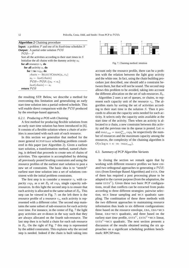
The first step is to consider a resourcerk with ca-pacity capk as a setRk of capk single capacity sub-resources. In this light the second step is to ensure thateach activity is allocated to the same subset ofRk. Thisstep can be viewed in Fig. 7: on the left there is theresource profile of a resourcerk, each activity is rep-resented with a different color. The second step main-tains the same subset of sub-resources for each activityover time. For instance, in the center of Fig. 7 the lightgray activities are re-drawn in the way such that theyare always allocated on the fourth sub-resource. Thelast step then is to build a chain for each sub resourcein Rk. On the right of Fig. 7 this step is representedby the added constraints. This explains why the secondstep is needed. Indeed if the chain is built taking into

Fig. 7. Chaining method: intuition

account only the resource profile, there can be a prob-lem with the relation between the light gray activityand the white one. In fact, using the chain building pro-cedure just described, one should add a constraint be-tween them, but that will not be sound. The second stepallows this problem to be avoided, taking into accountthe different allocation on the set of sub-resourcesRk.

Algorithm 2 uses a set of queues, or chains, to rep-resent each capacity unit of the resourcerk. The al-gorithm starts by sorting the set of activities accord-ing to their start time in the solutionS. Then it pro-ceeds to allocate the capacity units needed for each ac-tivity. It selects only the capacity units available at thestart time of the activity. Then when an activity is al-located to a chain, a new constraint between this activ-ity and the previous one in the queue is posted. Letmandmaxcap = maxm

k=1 capk be respectively the num-ber of resources and the maximum capacity among theresources, the complexity of the chaining algorithm isO(n log n + n ·m ·maxcap).

6.3. Summary of PCP Algorithm Variants

In closing the section we remark again that byworking with different resource profiles we have cre-ated two orthogonal approaches to generating aPOS:EBA (from Envelope Based Algorithm) andESTA. Oneof them has required a post processing phase to beadapted to the current purpose (from the adaptation, thenameESTAC). Given these two basic PCP configura-tions, recall that conflicts can be extracted from peaksaccording to three different strategies: pairwise selec-tion, MCS linear sampling andMCS quadratic sam-pling. The combination of these three methods withthe two different approaches to maintaining resourceinformation thus leads to six different configurations:three based on the resource envelope,EBA, EBA+MCS

linear, EBA+MCS quadratic, and three based on theearliest start time profile,ESTAC , ESTAC+MCS linear,ESTAC+MCS quadratic. The next section presents adiscussion of the results obtained testing the six ap-proaches on a significant scheduling problem bench-mark: RPCSP/max.


7. Experimental Analysis

In this section we provide an empirical evaluation ofthe methods introduced above. First of all we introduceand analyze metrics to capture desirable properties ofrobust partial order schedules. Once a pair of metricsis introduced we analyze the results obtained applyingthe methods on differentRCPSP/max benchmarks.

7.1. Metrics to Compare Partial Order Schedules

It is intuitive that the quality of a partial order sched-ule is tightly related to the set of solutions that it rep-resents. In fact the greater the number of solutions, thegreater the expected ability of facing scheduling uncer-tainty. Furthermore, another aspect to consider in theanalysis of the solutions clustered into a partial orderschedule is the distribution of these alternatives. Thisdistribution will be the result of the configuration givenby the constraints present in the solution.

A first measure to consider the aspects above istaken from [1]. In this work the authors describe a met-ric, namedflex, that can be defined as it follows:

flex =|{(ai, aj)|ai ⊀ aj ∧ aj ⊀ ai}|

n(n− 1)(5)

where n is the number of activities and the set{(ai, aj)|ai ⊀ aj ∧ aj ⊀ ai} contains all the pairs ofactivities for which no precedence relation is defined.This measure counts thenumber of pairs of activitiesin the solution which are not reciprocally related bysimple precedence constraints. It provides a first anal-ysis of the configuration of the solution. The rationaleis that when two activities are not related it is possi-ble to move one without moving the other one. Hence,the higher the value offlex the lower the degree ofinteraction among the activities.

Unfortunatelyflex is able to give only a qualita-tive evaluation of the solution. In fact it considers onlywhether a “path” exists between two activities, not howlong it is. Even though this may be sufficient for ascheduling problem with no time lag constraints likethe one used in [1], in a problem like theRCPSP/maxit is necessary to integrate the flexibility measure de-scribed above with an other one that also takes into ac-count this quantitative aspect of the problem (or solu-tion).

Before introducing a different measure, it is worthnoting that in order to compare two or morePOSs itis also necessary to have a finite number of solutions.This is possible assuming that all the activities in a

given problem must be completed within a specified,finite, horizon.Hence, it follows that within the samehorizonH, the greater the number of solutions repre-sented in aPOS, the greater its robustness. The goalthen is to compute a fair bound (or horizon) that doesnot introduce any bias in the evaluation of a solution(therefore a time interval that allows all the activities tobe executed). A possible alternative is the following:

H =n∑

i=1

pi +∑

∀(i,j)lminij (6)

that is, the sum of all activity processing timespi plusthe sum of all the minimal time lagslmin

ij . The minimaltime lags are taken into account to guarantee the min-imal distance between pairs of activities. In fact con-sidering the activities in a complete sequence (i.e., thesum of all durations) may not be sufficient.

The presence of a fixed horizon allows introductionof a further metric taken from [6]: this is defined as theaverage width, relative to the temporal horizon, of thetemporal slack associated with each pair of activities(ai, aj):

fldt =n∑

i=1

n∑

j=1∧j 6=i

slack(ai, aj)H × n× (n− 1)

× 100 (7)

whereH is the horizon of the problem defined above,n is the number of activities,slack(ai, aj) is the widthof the allowed distance interval between the end timeof activityai and the start time of activityaj , and100 isa scaling factor.3 This metric characterizes thefluidityof a solution, i.e., the ability to use flexibility to absorbtemporal variation in the execution of activities. Fur-thermore it considers that a temporal variation involv-ing an activity is absorbed by the temporal flexibility ofthe solution instead of generating deleterious dominoeffects (the higher the value offldt, the lower the risk,i.e., the higher the probability of localized changes).

In order to produce an evaluation of the two crite-ria fldt andflex that is independent from the problemdimension, we present the normalization of the resultsaccording to an upper bound. The latter is obtained foreach metricµ() considering the valueµ(P) that is thequality of the initial network that represents the tempo-ral aspect of the problem. In fact, for each metric theaddition of precedence constraints between activitiesthat are necessary to establish a resource-consistent so-lution can only reduce the initial valueµ(P). Then the

3In the original work this was defined as robustness, using thesymbolRB, of a solution.


normalized value for the solutionS of the problemPwill have the following form:

|µ(S)| = µ(S)µ(P)

(8)

where the higher|flex| or |fldt| value the better.

7.2. Results Analysis

In this section we present a comparison of each algo-rithm on the benchmark problems defined in [20]. Thisbenchmark consists of four sets j10, j20, j30, and j100.The first three are composed of 270 problem instancesof different size10 × 5, 20 × 5 and30 × 5 (numberof activities× number of resources). The benchmarkj100 is instead composed of 540 instances each of 100activities and 5 resources.

The results obtained are subdivided according to thebenchmark set in Table 1. First, we observe that noneof the six tested strategies are able to solve all the prob-lems in the benchmark sets (% column). This is pos-sible because all the strategies are based on an incom-plete search schema. To take into account these differ-ent solving capabilities the rest of the experimental re-sults are computed with respect to the subset of prob-lem instances solved by all the six approaches.

In the following results analysis we distinguish twocomplementary aspects of the different techniques:(1) the capabilities of the solving process and (2) thequality of the solutions obtained.

Solving capabilities. As shown before we have dif-ferent capabilities in terms of number of solved prob-lem with respect to theEBA andESTAC variants. In par-ticular it is worth noting the lack of scalability of theEBAs. The reader can see that we have 97.78% (bestEBA result) vs. 98.15% (bestESTAC result) in the caseof j10, 89.63% vs 96.67% in the case of j20, 43.33%vs. 97.04% in the case of j30, and 27.04% vs. 99.26%in the case of j100.

Another aspect to consider in evaluating solvingprocess capabilities is the required CPU-time (shownin seconds). The results obtained for theEBA variantsare worse than the CPU values obtained forESTACs.In fact the larger the benchmark size the larger the dif-ference in required CPU times. The results range froma ratio of 5.5 (in the case of j10) to one of about 400(in the case of j100).

These facts induce further observations about the ba-sic strategies behind the two algorithms.EBA removesall possible resource conflicts from a problemP byposting precedence constraints and relying on an en-

velope computation that produces thetightestpossibleresource-level bounds for a flexible schedule. Whenthese bounds are less than or equal to the resourcecapacities, we have a resource-feasible partial orderready tofaceexecutional uncertainty. However, in or-der to remove all possible conflictsEBA has to im-pose more precedence constraints than doesESTAC

(see columns labeled withpc, posted constraints), withthe risk of overcommitment in the final solution.

Solution qualities. For the evaluation of the solutionqualities we have taken into account three differentmeasures:flex, fldt, andmk.

The first two are directly correlated to solution ro-bustness. Considering these measures in the case ofthe smaller benchmarks j10, j20, and j30, we have avery small difference in general between the results ob-tained withEBAs andESTACs, even though theESTAC

variants present a better behavior. A completely differ-ent result comes considering the benchmark j100: inthis case theEBA variants seem more suitable than theESTACs, for obtaining robust solutions. Notwithstand-ing in evaluating this result, we have to keep in consid-eration also the different solving capabilities (27.04%vs 99.26%) and the fact that this evalution is done onthe subset of common solved instances. Therefore itseems to us that the number of instances taken into ac-count are too few to make strong claims in the case ofthe benchmark j100.

On the other hand, as previously explained,ESTAC

is a two step procedure: theESTA step creates a par-ticular partial order that guarantees only the existenceof the early start time solution; the chaining step con-verts this partial order into aPOS. It is worth remind-ing that the number of precedence constraints is alwaysO(n) and for each resource, theform of the partial or-der graph is a set ofparallel chains. These last obser-vations probably identify the main factors which en-able a more robust solution behavior, i.e.,ESTAC solu-tions can be seen as a set oflayers, one for each unitof resource capacity, which canslide independently tohedge against unexpected temporal shifts.

The last aspect we present in this evaluation is themakespan of the solutions. First of all it is necessaryto clarify what we mean for makespan of a partial or-der schedule. In fact aPOS represents several fixed-time schedules each with a different makespan. Inthis case we consider the minimum makespan amongthe makespans of the solutions in thePOS, i.e. themakespan of the earliest start time solution of thePOS. The results in Table 1 show as theESTAC vari-ants outperform theEBA ones. In particular we can


Table 1

Results on the four benchmarks

j10 j20% mk cpu pc |flex| |fldt| % mk cpu pc |flex| |fldt|

EBA 77.04 58.31 0.11 11.54 0.14 0.63 50.74 96.48 1.37 33.40 0.16 0.64

EBA+MCS linear 85.19 55.29 0.18 11.12 0.17 0.65 71.11 92.65 1.83 32.87 0.15 0.60

EBA+MCS quadratic 97.78 55.47 0.19 12.38 0.16 0.65 89.63 94.03 1.99 34.98 0.13 0.58

ESTAC 96.30 47.35 0.02 6.40 0.19 0.67 95.56 72.90 0.12 18.69 0.20 0.65

ESTAC+MCS linear 98.15 46.63 0.03 6.23 0.20 0.66 96.67 72.45 0.18 17.49 0.20 0.65

ESTAC+MCS quadratic 98.15 46.70 0.03 6.26 0.20 0.68 96.67 72.75 0.19 17.40 0.19 0.64

j30 j100% mk cpu pc |flex| |fldt| % mk cpu pc |flex| |fldt|

EBA 43.33 118.17 7.53 63.29 0.23 0.69 21.11 501.61 33.00 53.67 0.13 0.72

EBA+MCS linear 68.89 112.14 8.82 56.84 0.18 0.59 26.11 606.31 78.64 73.41 0.13 0.58

EBA+MCS quadratic 82.22 116.10 10.94 59.64 0.16 0.56 27.04 632.27 183.79 76.88 0.11 0.56

ESTAC 96.30 79.21 0.41 35.10 0.25 0.60 99.26 374.24 0.48 68.47 0.07 0.50

ESTAC+MCS linear 96.67 78.45 0.74 34.07 0.26 0.62 99.44 374.22 0.48 67.94 0.07 0.50

ESTAC+MCS quadratic 97.04 78.55 0.83 34.00 0.25 0.64 99.26 374.35 0.48 68.18 0.07 0.50

note that the larger the problem size the larger the gapbetween the two methodologies, e.g., in the case ofbenchmark j100 we have an average value of 501.61for the bestEBA variant against 374.22 obtained withESTAC + MCS linear.

8. Discussion: the Solve & Robustify model

In this paper, different needs – and, dually, differ-ent trade-offs between quality and computational times– are addressed by different algorithms or combina-tions of solving techniques in a meta-heuristic schema.The results in Table 1 have shown theESTAC vari-ants be better suited to generating robust solutions.Even thoughEBA methods directly produce partial or-der schedules considering this aim at each step of thesolving process, theESTAC methods yield solutionsthat are no less robust (in terms of the measuresflexandfldt). Moreover these methods show better perfor-mance when problem size is increased. They are able,in fact, to limit the increase in CPU times and maintaina high percentage of solved instances.

This two-step approach, which we refer to asSolve& Robustify, is based on the assumption of indepen-dence between the classical scheduling objectives –like minimizing the makespan – and the need to ob-tain a robust (or flexible) solution. Even though this as-sumption is in general not true, the two step approachcan allow exploitation ofstate-of-the-artschedulers toobtain optimal solutions with respect to the classical

objectives. Then, in a next step, a flexible solution canbe generated trying to preserve the optimality of thestarting schedule. Preserving optimality can be veryimportant when a low degree of uncertainty is present.In this case the actual execution of the problem remains“close” to theexpected value problem(i.e., the prob-lem as described in input). Therefore, the characteris-tics of aPOS tend to maintain, due to necessary re-pairs, a new allocation of the activities that is close tothe original schedule. It is intuitive that the closer thetwo allocations are the less loss that is incurred in ob-jective function values.

solve

fail

solutionproblem robustify

Fig. 8. Solve & Robustify model

Figure 8 shows a possible sketch of the two step ap-proach. This model is based on the use of two separatemodules: a greedy solver that has the aim of findingan initial fixed-time solution, and a “robustify” mod-ule where a partial order schedule is synthesized fromthis solution. Different variants of the two step ap-proach can be obtained by different combinations ofthe two modules. As the figure highlights, only in thefirst phase, in which the search for a solution occurs, isit possible to fail (i.e., when it is not possible to find a


first fixed-time schedule). In the Robustify step in con-trast, whenever a starting schedule exists, it is alwayspossible to generate aPOS.

A further remark concerns the generation of flexi-ble schedules. In the case of multi-capacitive resourceproblems, we have in general more than one possiblePOS corresponding to a fixed-time schedule. On thecontrary in the case of binary resources, i.e. job shopproblem, a fixed-time solution also gives a unique “lin-earization” of all the activities. This aspect of multi-capacitive resource problems has supported and sug-gested the idea of exploring the space of possiblePOSs obtainable from the same fixed-time schedulewith the aim of increasing robustness characteristics[28,30]. A different chaining algorithm is described in[19] where the authors usePOSs and their flexibilitycharacteristics to apply a local search approach withthe aim of optimizing schedule makespan.

9. Conclusion

Research in constraint-based scheduling has typi-cally formulated the problem as one of finding a con-sistent assignment of start times for each goal activity.In contrast, we are investigating approaches to schedul-ing that operate with a problem formulation more akinto least-commitment frameworks: the Precedence Con-straint Posting procedure. In this approach the goal isto post sufficient additional precedence constraints be-tween pairs of activities contending for the same re-sources to ensure feasibility with respect to time andcapacity constraints. Solutions generated in this waygenerally represent a set of feasible schedules by usinga temporally flexible graph.

Exploiting this flexibility, in this work we have in-vestigated two orthogonal PCP approaches (EBA andESTAC) to building scheduling solutions that hedgeagainst unexpected events. The two approaches arebased on two different methods for maintaining pro-file information: one that considers all temporal solu-tions (the resource envelope) and one that analyzes theprofile for a precise temporal solution (the earliest starttime solution).

To evaluate the quality of respective solutions we in-troduced two measures that capture desirable proper-ties of robust solutions,fldt andflex, correlated to thedegree of schedule robustness that is retained in gener-ated solutions. Considering comparative performanceon a set of benchmark project scheduling problems, wehave shown that the two stepESTAC procedure, which

first computes a single-point solution and then trans-lates it into a temporally flexible partial order sched-ule, is a more effective approach than the pure, least-commitmentEBA approach. In fact, the first step pre-serves the effectiveness of theESTA approach, whilethe second step has been shown to be capable of re-instating temporal flexibility in a way that produces afinal schedule with better robustness properties.

Acknowledgements

Stephen F. Smiths work is supported in part by theNational Science Foundation under contract #9900298,by the Department of Defense Advanced ResearchProjects Agency under contract #FA8750-05-C-0033and by the CMU Robotics Institute. Amedeo Cesta,Angelo Oddi and Nicola Policella’s work is partiallysupported by MIUR (Italian Ministry for Education,University and Research) under projectROBOCARE

(L. 449/97) and contract #2005-015491 (PRIN).

References

[1] M. A. Aloulou and M. C. Portmann. An Efficient Proactive-Reactive Scheduling Approach to Hedge Against Shop FloorDisturbances. In G. Kendall, E. Burke, S. Petrovic, andM. Gendreau, editors,Multidisciplinary Scheduling: Theoryand Applications, pages 223–246. Springer, 2005.

[2] P. Baptiste and C. Le Pape. A Theoretical and ExperimentalComparison of Constraint Propagation Techniques for Disjunc-tive Scheduling. InProceedings of the14th International JointConference on Artificial Intelligence, IJCAI-95, pages 600–606. Morgan Kaufmann, 1995.

[3] P. Baptiste, C. Le Pape, and W. Nuijten.Constraint-BasedScheduling, volume 39 ofInternational Series in OperationsResearch and Management Science. Kluwer Academic Pub-lishers, 2001.

[4] M. Bartusch, R. H. Mohring, and F. J. Radermacher. Schedul-ing project networks with resource constraints and time win-dows.Annals of Operations Research, 16:201–240, 1988.

[5] J. C. Beck, E. D. Davenport, A. J. Davis, and M. S. Fox. TheODO Project: Towards a Unified Basis for Constraint-DirectedScheduling.Journal of Scheduling, 1:89–125, 1998.

[6] A. Cesta, A. Oddi, and S. F. Smith. Profile Based Algorithmsto Solve Multiple Capacitated Metric Scheduling Problems.In Proceedings of the4th International Conference on Artifi-cial Intelligence Planning Systems, AIPS-98, pages 214–223.AAAI Press, 1998.

[7] A. Cesta, A. Oddi, and S. F. Smith. An Iterative SamplingProcedure for Resource Constrained Project Scheduling withTime Windows. InProceedings of the 16th International JointConference on Artificial Intelligence, IJCAI-99, pages 1022–1029. Morgan Kaufmann, 1999.


[8] A. Cesta, A. Oddi, and S. F. Smith. A Constraint-based methodfor Project Scheduling with Time Windows.Journal of Heuris-tics, 8(1):109–136, January 2002.

[9] A. Cesta and C. Stella. A Time and Resource Problem forPlanning Architectures. In S. Steel and R. Alami, editors,Pro-ceedings of the4th European Conference on Planning, ECP-97, volume 1348 ofLecture Notes in Computer Science, pages117–129. Springer, 1997.

[10] C. Cheng and S. F. Smith. Generating Feasible Schedules un-der Complex Metric Constraints. InProceedings of the12th

National Conference on Artificial Intelligence, AAAI-94, pages1086–1091. AAAI Press, 1994.

[11] A. J. Davenport, C. Gefflot, and J. C. Beck. Slack-based Tech-niques for Robust Schedules. InProceedings of6th EuropeanConference on Planning, ECP-01, 2001.

[12] R. Dechter, I. Meiri, and J. Pearl. Temporal constraint net-works. Artificial Intelligence, 49:61–95, 1991.

[13] R. Dechter and F. Rossi. Constraint Satisfaction. In L. Nadel,editor, Encyclopedia of Cognitive Science. Nature PublishingGroup, 2002.

[14] B. Drabble and A. Tate. The Use of Optimistic and PessimisticResource Profiles to Inform Search in an Activity Based Plan-ner. In Proceedings of the 2nd International Conference onArtificial Intelligence Planning Systems, AIPS-94, pages 243–248. AAAI Press, 1994.

[15] M. Drummond, J. Bresina, and K. Swanson. Just-in-CaseScheduling. InProceedings of the12th National Conferenceon Artificial Intelligence, AAAI-94, pages 1098–1104. AAAIPress, 1994.

[16] H. H. El Sakkout and M. G. Wallace. Probe Backtrack Searchfor Minimal Perturbation in Dynamic Scheduling.Constraints,5(4):359–388, 2000.

[17] M. S. Fox. Constraint Guided Scheduling: A Short History ofScheduling Research at CMU.Computers and Industry, 14(1–3):79–88, 1990.

[18] M. R. Garey and D. S. Johnson.Computers and Intractability:A Guide to the Theory of NP-Completeness. W. H. Freemanand Company, New York, 1979.

[19] D. Godard, P. Laborie, and W. Nuitjen. Randomized LargeNeighborhood Search for Cumulative Scheduling. InPro-ceedings of the15th International Conference on AutomatedPlanning & Scheduling, ICAPS’05, pages 81–89. AAAI Press,2005.

[20] R. Kolisch, C. Schwindt, and A. Sprecher. Benchmark In-stances for Project Scheduling Problems. In J. Weglarz, edi-tor,Project Scheduling - Recent Models, Algorithms and Appli-cations, pages 197–212. Kluwer Academic Publishers, Boston,1998.

[21] V. Kumar. Algorithms for Constraint-Satisfaction Problems:ASurvey.Artificial Intelligence Magazine, 13(1):32–44, 1992.

[22] P. Laborie. Algorithms for Propagating Resource Constraints inA.I. Planning and Scheduling: Existing Approaches and NewResults.Artificial Intelligence, 143(2):151–188, 2003.

[23] P. Laborie and M. Ghallab. Planning with Sharable ResourceConstraints. InProceedings of the 14th International JointConference on Artificial Intelligence, IJCAI-95, pages 1643–1651. Morgan Kaufmann, 1995.

[24] U. Montanari. Networks of constraints: Fundamental proper-ties and applications to picture processing.Information Sci-ences, 7:95–132, 1974.

[25] N. Muscettola. Computing the Envelope for Stepwise-ConstantResource Allocations. InPrinciples and Practice of ConstraintProgramming,8th International Conference, CP 2002, volume2470 ofLecture Notes in Computer Science, pages 139–154.Springer, 2002.

[26] W. Nuijten and C. Le Pape. Constraint-Based Job ShopScheduling with Ilog-Scheduler. Journal of Heuristics,3(4):271–286, March 1998.

[27] W. P. M. Nuijten and E. H. L. Aarts. A ComputationalStudy of Constraint Satisfaction for Multiple Capacitated JobShop Scheduling.European Journal of Operational Research,90(2):269–284, 1996.

[28] N. Policella, A. Oddi, S. F. Smith, and A. Cesta. GeneratingRobust Partial Order Schedules. In M. Wallace, editor,Prin-ciples and Practice of Constraint Programming,10th Interna-tional Conference, CP 2004, volume 3258 ofLecture Notes inComputer Science, pages 496–511. Springer, 2004.

[29] N. Policella, S. F. Smith, A. Cesta, and A. Oddi. GeneratingRobust Schedules through Temporal Flexibility. InProceed-ings of the14th International Conference on Automated Plan-ning & Scheduling, ICAPS’04, pages 209–218. AAAI Press,2004.

[30] Nicola Policella.Scheduling with Uncertainty: A Proactive Ap-proach using Partial Order Schedules. PhD thesis, Departmentof Computer and Systems Science, University of Rome “LaSapienza”, March 2005.

[31] B. Roy and B. Sussman. Les problemes d’ordonnancementavec contraintes disjonctives. Note DS n. 9 bis, SEMA, Paris,1964.

[32] N. M. Sadeh.Look-ahead Techniques for Micro-opportunisticJob Shop Scheduling. PhD thesis, School of Computer Science,Carnegie Mellon University, Pittsburgh PA, March 1991.

[33] S. F. Smith. OPIS: A Methodology and Architecture for Reac-tive Scheduling. In M. Fox and M. Zweben, editors,IntelligentScheduling, pages 29–66. Morgan Kaufmann, 1994.

[34] S. F. Smith and C. Cheng. Slack-based Heuristics for Con-straint Satisfactions Scheduling. InProceedings of the11th

National Conference on Artificial Intelligence, AAAI-93, pages139–144. AAAI Press, 1993.

[35] E. P. K. Tsang.Foundations of Constraint Satisfaction. Aca-demic Press, London and San Diego, 1993.

From precedence constraint posting to partial order schedules: A CSP approach to Robust Scheduling

Documents

Transcript of From precedence constraint posting to partial order schedules: A CSP approach to Robust Scheduling