From exploitation to conservation: habitat models using whaling data predict distribution patterns...

BIODIVERSITYRESEARCH

From exploitation to conservation:habitat models using whaling datapredict distribution patterns and threatexposure of an endangered whaleLeigh G. Torres1*, Tim D. Smith2, Phil Sutton1, Alison MacDiarmid1,

John Bannister3 and Tomio Miyashita4

1National Institute of Water and

Atmospheric Research Ltd., Hataitai,

Wellington, 6021, New Zealand, 2World

Whaling History, Redding, CA, USA, 3The

Western Australian Museum, Perth, WA,

6000, Australia, 4National Research Institute

of Far Seas Fisheries, Shimizu, Shizuoka,

424, Japan

*Correspondence: Leigh G. Torres, National

Institute of Water and Atmospheric Research,

Ltd (NIWA), 301 Evans Bay Parade, Greta

Point, Hataitai, Wellington 6021, New

Zealand.

E-mail: [email protected]

ABSTRACT

Aim Sufficient data to describe spatial distributions of rare and threatened

populations are typically difficult to obtain. For example, there are minimal

modern offshore sightings of the endangered southern right whale, limiting our

knowledge of foraging grounds and habitat use patterns. Using historical

exploitation data of southern right whales (SRW), we aim to better understand

their seasonal offshore distribution patterns in relation to broad-scale oceano-

graphy, and to predict their exposure to shipping traffic and response to global

climate change.

Location Australasian region between 130° W and 100° E, and 30° S and

55° S.

Methods We model 19th century whaling data with boosted regression trees

to determine functional responses of whale distribution relative to environmen-

tal factors. Habitat suitability maps are generated and we validate these predic-

tions with independent historical and recent sightings. We identify areas of

increased risk of ship-strike by integrating predicted whale distribution maps

with shipping traffic patterns. We implement predicted ocean temperatures for

the 2090–2100 decade in our models to predict changes in whale distribution

due to climate change.

Results Temperature in the upper 200 m, distance from the subtropical front,

mixed layer depth, chlorophyll concentration and distance from ridges are the

most consistent and influential predictors of whale distribution. Validation tests

of predicted distributions determined generally high predictive capacity. We

identify two areas of increased risk of vessel strikes and predict substantial

shifts in habitat suitability and availability due to climate change.

Main conclusions Our results represent the first quantitative description of

the offshore foraging habitat of SRW. Conservation applications include identi-

fying areas and causes of threats to SRW, generating effective mitigation strate-

gies, and directing population monitoring and research efforts. Our study

demonstrates the benefits of incorporating unconventional datasets such as

historical exploitation data into species distribution models to inform manage-

ment and help combat biodiversity loss.

Keywords

Boosted regression trees, distribution patterns, global climate change, habitat

use, historical data, rare species, southern right whale, species distribution

models.

DOI: 10.1111/ddi.120691138 http://wileyonlinelibrary.com/journal/ddi ª 2013 John Wiley & Sons Ltd

Diversity and Distributions, (Diversity Distrib.) (2013) 19, 1138–1152A

Jou

rnal

of

Cons

erva

tion

Bio

geog

raph

yD

iver

sity

and

Dis

trib

utio

ns

INTRODUCTION

Biodiversity loss from marine ecosystems is an extreme prob-

lem with widespread impacts (Worm et al., 2006; Estes et al.,

2011). Knowledge of species distribution patterns is essential

for assessing threats to biodiversity that range from fine-scale

risks such as fisheries (Thrush & Dayton, 2002) to broad-

scale habitat alterations like climate change (Trathan et al.,

2007). Ecological-niche modelling has become an integral

part of species conservation, including identification of

important habitats, reserve planning, species reintroduction

programs and ecosystem restoration (Hirzel et al., 2006).

Based on the assumption that the distribution of encounters

reflects a species’ environmental preferences (Guisan &

Zimmermann, 2000; Hirzel et al., 2006), a variety of statisti-

cal techniques are used to associate distribution patterns with

habitat variability to identify a species’ realized environmen-

tal niche (Elith et al., 2006).

For remnant populations with historically broad distribu-

tion patterns prior to exploitation, it is often difficult or

impossible to collect comprehensive distribution data across

their current and historical ranges. However, data derived

from historical sources, such as harvest or museum records,

can be used to describe historical distribution patterns (Elith

& Leathwick, 2007; Gregr, 2011). The accuracy of distribu-

tion models produced from historical datasets for modern

times depends upon the conservation of a species’ ecological

niche over time (Peterson et al., 1999).

Whaling in the South Pacific decimated southern right

whale (Eubalaena australis) populations (Jackson et al.,

2008). An estimated 40,000 southern right whales (SRW)

were killed in waters around New Zealand and east Australia

(Carroll et al., 2011a) and an unknown, but likely compara-

ble, number off southern Australia. The current population

estimate of SRW off New Zealand is just 908 (Carroll et al.,

2011b) and off southern Australia is c. 3500 (Bannister,

2011). To ensure protection of these remnant populations

from present and future threats, a reliable understanding of

SRW distribution and habitat use patterns is essential.

Southern right whales have a strong migration cycle

between coastal wintering grounds used for calving and off-

shore foraging areas. These whales are capital breeders that

use previously accumulated energy stores to nurse calves in

winter, and thus need to encounter dense aggregations of

their preferred prey items (copepods and euphausiids) within

their dive limits while foraging offshore (c. 300 m; Gregr &

Coyle, 2009). Although the wintering grounds of SRW in

Australia and New Zealand are reasonably well defined (Ban-

nister, 2001; Patenaude & Baker, 2001), little is known about

their offshore and migratory habitat preferences (Ohsumi &

Kasamatsu, 1986; Bannister et al., 1999; Richards, 2002).

Despite the end of commercial whaling, SRW are not free

from anthropogenic threats. SRW in the Australasian region

are prone to ship strikes, with a single mortality negatively

affecting population vitality in such a small population

(Kemper et al., 2008). In addition, SRW may be subject to

oceanic changes due to climate change. The distribution

patterns of North Atlantic right whales (Eubalaena glacialis)

and their copepod prey are affected by climate change

(Greene & Pershing, 2004) and the breeding success of SRW

in the South Atlantic shows sensitivity to climate variation

(Leaper et al., 2006).

Historical whaling data have been used to examine diet

from stomach contents (Tormosov et al., 1998), describe

general distribution patterns (Townsend, 1935; Richards,

2002), generate habitat characterizations or models based on

presence-only data (Jaquet et al., 1996; Gregr & Trites, 2001;

Gregr, 2011) and estimate historical population sizes (Smith,

2001). Here, we use historical whaling data, including pres-

ence and absence data from the Australasian region to exam-

ine ecological responses of SRW to environmental variability.

The dataset derives from 19th century offshore whaling

vessels, allowing our study to focus on offshore habitat use

patterns where SRW spend a majority of their time and

where their distribution patterns are least understood. We

use boosted regression trees (BRT), a machine-learning tech-

nique recently applied to species distribution modelling

(Elith et al., 2006; Leathwick et al., 2006), to define func-

tional habitat use patterns of SRW. We use these models to

predict the distribution patterns of whales both today, which

are compared with shipping traffic density, and in the year

2100, as a result of climate change. Based on the resolution

of our datasets, we expect our models to be applicable at

meso and large scales for predicting how whales respond to

habitat variation such as temperature and density gradients

that may aggregate prey (Gregr & Coyle, 2009).

METHODS

Historical whaling data

We obtained daily observations from American whaling

vessels within our study region (130° W to 100° E, and

30° S to 55° S) extracted from voyage logbooks by Maury

(1852) and recently by the Census of Marine Life (www.

coml.org/) using methods described in Smith et al. (2012).

Whalers recorded their location daily and indicated when

whales were encountered. These data amounted to 24,733

daily records of vessel location over the period 1825–88

(Fig. 1). Mean vessel location error was estimated to be

0.22° latitude (c. 24 km) and 0.54° longitude (c. 34 km;

Smith et al., 2012). Therefore, we applied a spatial resolution

of 25 km 9 25 km grid cells to all analyses.

We grouped data by season to generate predictive models

that reflect seasonal changes in whale behaviour and environ-

ment. Spring (September, October, November): whales leave

calving grounds for foraging habitat, ocean temperatures

begin to warm, spring productivity blooms occur. Summer

(December, January, February): most whales occupy foraging

habitat, ocean temperatures are at a maximum. Autumn

(March, April, May): whales may begin to migrate towards

calving habitats, ocean temperatures begin to cool. No winter

Diversity and Distributions, 19, 1138–1152, ª 2013 John Wiley & Sons Ltd 1139

Habitat models based on historical data

habitat models were generated because our historical dataset

did not include sufficient observations in those months. We

also divided our study area into two regions that grouped

prominent habitat features based on geomorphology and

currents. We split the study area into eastern and western

regions along a natural gap in encounters at 155° E (Fig. 1).

A total of 1792 encounters with SRW (presence) were mod-

elled in the two regions, across three seasons (Table 1). No

model was generated in the western region during autumn

because of limited presence data (n = 11). The southern

boundary in both regions was limited to the extent of data

points, confining predictive models to only areas with data

(eastern: 55° S; western: 53° S).

Our historical whaling data reflect the inconsistent spatial

and temporal distribution of whaling effort through time

(Smith et al., 2012). To determine the need to group data

temporally for habitat models, we examined our data for

changes in the spatial distribution of SRW encounters over

time (see Appendix S1 in Supporting Information).

Habitat modelling

We generated predictive models of SRW probability of

occurrence using BRT. Our response variable was binomial

presence/absence data composed of daily encounters with

SRW and days with no encounters. The numerical

(a)

(b)

(c)

Figure 1 Seasonal spatial distribution of historical whaling data illustrating absence (grey dots) and southern right whale presence

(black dots) locations. Spring (a), summer (b), autumn (c). Black boxes demarcate boundaries of western and eastern regions in each

plot. North arrow and scale bar in (a) applies to all plots. The Chatham Rise, Macquarie Ridge (labelled in a), and Louisville Ridge

(labelled in c) are illustrated on plots; numerous presence and absence points fall under these features. Inadequate presence data in

western region during autumn restricted analyses. Maps in Mercator projection, datum wgs1984.

1140 Diversity and Distributions, 19, 1138–1152, ª 2013 John Wiley & Sons Ltd

L. G. Torres et al.

dominance of absence data relative to presence data in all

region–season combinations (Table 1) may be due to rela-

tively low prevalence (even prior to declines in SRW abun-

dance), and to false-absences (caused by dive behaviour, sea

state and weather conditions that decrease surface visibility).

Absence data are also biased by inconsistent observer effort

across the region. Therefore, we down-weighted absence data

in each region–season model so that presence and absence

data carried equal weight, a method that has been shown to

increase model accuracy (Table 1; Barbet-Massin et al.,

2012). The following equation was applied:

# presence =# absence ¼ weight applied to each absence point

Boosted regression trees is an ensemble method that inter-

prets complex relationships between species and their envi-

ronment (Elith et al., 2006; Leathwick et al., 2006). The first

of two algorithms implemented in BRT partitions the

response variable into groups with similar characteristics

using regression or classification trees. Boosting is the second

algorithm where trees are fitted iteratively; emphasizing

observations that poorly fit the existing collection of trees.

Boosting combines these trees to minimize misclassification

errors and improve predictive performance over a single tree

model (Leathwick et al., 2006). Boosting is optimized by the

learning rate (lr) that considers residual variation during tree

building, and tree complexity (tc) that estimates interactions

between predictor variables. Model fit and predictive perfor-

mance are balanced to reduce overfitting by jointly optimiz-

ing the number of trees (nt), lr, and tc (Elith et al., 2008).

We used the ‘GBM’ package (version 1.6-3.1, Ridgeway, 2007)

implemented in R (R Development Core Team) plus custom

code available online (Elith et al., 2008) to generate BRT

models of SRW distribution.

We generated multiple BRT models for each region–

season using different sets of predictor variables, and varying

the lr (range: 0.05–0.0005) and tc (range: 1–4) to fit models

with at least 1000 trees as recommended by Elith et al. (2008).

The relative importance of a predictor variable is determined

by its contribution to the model as measured by the number of

times it is selected for tree splitting (Elith et al., 2008). Our

first step to determine an ‘optimal’ model removed all vari-

ables that contributed < 3%. Then, we assessed response–pre-

dictor relationships and removed predictor variables that

produced ecologically unrealistic relationships. Fitted-func-

tions produced by BRT show the effect of each predictor vari-

able on the response while controlling for the average effect of

all other variables in the model (Buston & Elith, 2011). Finally,

we compared two performance metrics: area under the receiver

operating curve (AUC) and cross-validation per cent deviance

explained (CVdev). AUC is widely used to evaluate binomial

models (Fawcett, 2006) by measuring the ability to discrimi-

nate between areas with species presence or absence. AUC

ranges from 0 to 1: 1 = perfect discrimination, < 0.5 = worse

than random, > 0.7 is considered ‘useful’ (Swets, 1988).

Although AUC has limitations for measuring model perfor-

mance (Austin, 2007; Lobo et al., 2008), we use it as a relative

metric of model performance because it provides a single value

that is easy to interpret. CVdev is estimated by a cross-valida-

tion procedure run during the modelling process that with-

holds a subset of data at each tree. CVdev indicates how well

the model predicted the subsets of withheld data (Buston &

Elith, 2011).

Environmental layers

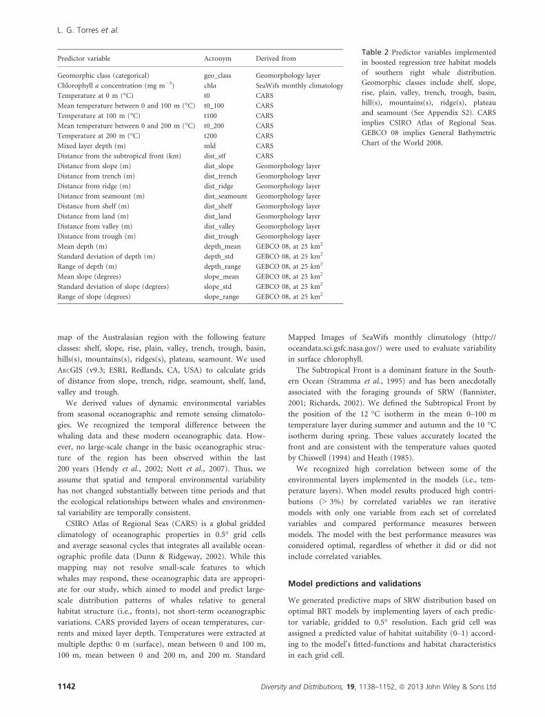
We assigned each presence and absence location values

from 23 environmental layers based on location and season

when relevant (Table 2). We derived mean, range and stan-

dard deviation values of depth and slope from the General

Bathymetric Chart of the World (http://www.gebco.net/).

We generated layers of these bathymetry statistics using a

12.5-km radius neighbourhood to correspond with the

assumed spatial accuracy of the whaling data

(25 km 9 25 km grid cells), and applied a buffer zone

around the boundary of the study region to minimize edge

effects. We generated a regional geomorphology map that

grouped areas of the seafloor into defined features based on

bathymetric parameters (See Appendix S2). We merged this

geomorphic map with a global layer of seamount locations

(Yesson et al., 2011) to produce a final geomorphology

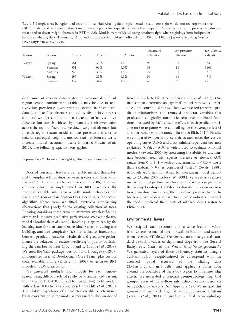
Table 1 Sample sizes by region and season of historical whaling data implemented in southern right whale boosted regression tree

(BRT) models and validation datasets used to assess predictive capacity of prediction maps. P : A ratio indicates the presence to absence

ratio used to down-weight absences in BRT models. Models were validated using southern right whale sightings from independent

historical whaling data (Townsend, 1935) and a more modern dataset collected from 1965 to 1985 by Japanese Scouting Vessels

(JSV; Miyashita et al., 1995).

Region Season Presence Absence P: A ratio

Townsend

validation

JSV presence

validation

JSV absence

validation

Eastern Spring 561 3506 0.16 96 1 346

Summer 351 9608 0.037 88 11 1409

Autumn 246 3992 0.062 22 1 318

Western Spring 297 2358 0.126 56 61 719

Summer 337 3477 0.097 48 165 1710



map of the Australasian region with the following feature

classes: shelf, slope, rise, plain, valley, trench, trough, basin,

hills(s), mountains(s), ridges(s), plateau, seamount. We used

ARCGIS (v9.3; ESRI, Redlands, CA, USA) to calculate grids

of distance from slope, trench, ridge, seamount, shelf, land,

valley and trough.

We derived values of dynamic environmental variables

from seasonal oceanographic and remote sensing climatolo-

gies. We recognized the temporal difference between the

whaling data and these modern oceanographic data. How-

ever, no large-scale change in the basic oceanographic struc-

ture of the region has been observed within the last

200 years (Hendy et al., 2002; Nott et al., 2007). Thus, we

assume that spatial and temporal environmental variability

has not changed substantially between time periods and that

the ecological relationships between whales and environmen-

tal variability are temporally consistent.

CSIRO Atlas of Regional Seas (CARS) is a global gridded

climatology of oceanographic properties in 0.5° grid cells

and average seasonal cycles that integrates all available ocean-

ographic profile data (Dunn & Ridgeway, 2002). While this

mapping may not resolve small-scale features to which

whales may respond, these oceanographic data are appropri-

ate for our study, which aimed to model and predict large-

scale distribution patterns of whales relative to general

habitat structure (i.e., fronts), not short-term oceanographic

variations. CARS provided layers of ocean temperatures, cur-

rents and mixed layer depth. Temperatures were extracted at

multiple depths: 0 m (surface), mean between 0 and 100 m,

100 m, mean between 0 and 200 m, and 200 m. Standard

Mapped Images of SeaWifs monthly climatology (http://

oceandata.sci.gsfc.nasa.gov/) were used to evaluate variability

in surface chlorophyll.

The Subtropical Front is a dominant feature in the South-

ern Ocean (Stramma et al., 1995) and has been anecdotally

associated with the foraging grounds of SRW (Bannister,

2001; Richards, 2002). We defined the Subtropical Front by

the position of the 12 °C isotherm in the mean 0–100 m

temperature layer during summer and autumn and the 10 °Cisotherm during spring. These values accurately located the

front and are consistent with the temperature values quoted

by Chiswell (1994) and Heath (1985).

We recognized high correlation between some of the

environmental layers implemented in the models (i.e., tem-

perature layers). When model results produced high contri-

butions (> 3%) by correlated variables we ran iterative

models with only one variable from each set of correlated

variables and compared performance measures between

models. The model with the best performance measures was

considered optimal, regardless of whether it did or did not

include correlated variables.

Model predictions and validations

We generated predictive maps of SRW distribution based on

optimal BRT models by implementing layers of each predic-

tor variable, gridded to 0.5° resolution. Each grid cell was

assigned a predicted value of habitat suitability (0–1) accord-

ing to the model’s fitted-functions and habitat characteristics

in each grid cell.

Predictor variable Acronym Derived from

Geomorphic class (categorical) geo_class Geomorphology layer

Chlorophyll a concentration (mg m�3) chla SeaWifs monthly climatology

Temperature at 0 m (°C) t0 CARS

Mean temperature between 0 and 100 m (°C) t0_100 CARS


Mean temperature between 0 and 200 m (°C) t0_200 CARS


Mixed layer depth (m) mld CARS

Distance from the subtropical front (km) dist_stf CARS

Distance from slope (m) dist_slope Geomorphology layer

Distance from trench (m) dist_trench Geomorphology layer

Distance from ridge (m) dist_ridge Geomorphology layer

Distance from seamount (m) dist_seamount Geomorphology layer

Distance from shelf (m) dist_shelf Geomorphology layer

Distance from land (m) dist_land Geomorphology layer

Distance from valley (m) dist_valley Geomorphology layer

Distance from trough (m) dist_trough Geomorphology layer

Mean depth (m) depth_mean GEBCO 08, at 25 km2

Standard deviation of depth (m) depth_std GEBCO 08, at 25 km2

Range of depth (m) depth_range GEBCO 08, at 25 km2

Mean slope (degrees) slope_mean GEBCO 08, at 25 km2

Standard deviation of slope (degrees) slope_std GEBCO 08, at 25 km2

Range of slope (degrees) slope_range GEBCO 08, at 25 km2

Table 2 Predictor variables implemented

in boosted regression tree habitat models

of southern right whale distribution.

Geomorphic classes include shelf, slope,

rise, plain, valley, trench, trough, basin,

hill(s), mountains(s), ridge(s), plateau

and seamount (See Appendix S2). CARS

implies CSIRO Atlas of Regional Seas.

GEBCO 08 implies General Bathymetric

Chart of the World 2008.


L. G. Torres et al.

Few recent offshore sightings of SRW have been reported

in our study region (See Appendix S3). Therefore, we vali-

dated each prediction map using two datasets where each

presence and absence (or pseudo-absence, see below) point

sampled the appropriate prediction layer to obtain values of

habitat suitability. We used these values to determine each

map’s predictive capacity by calculating the AUC, sensitivity

(true positive rate), and 1�specificity (false positive rate).

First, we used data collected by Townsend (1935) from

other whaling logbooks to evaluate the representativeness of

our modelled dataset. We did not include these data in the

modelling process because absence data were not collected.

The Townsend data included 310 encounters with SRW

over the same spatial extent and similar time period (1831–

1907) as the modelled whaling data (Table 1). For each

region-season prediction map, we randomized 10,000

validation tests using all the presence locations in that

region-season against subsampled, randomly placed pseudo-

absences in equal number to the presence data. Second, we

used survey data collected by Japanese Scouting Vessels

(JSV) from 1965 to 1985 (Miyashita et al., 1995) to deter-

mine if models derived from historical data are consistent

over time. These data consisted of vessel noon positions

when SRW were (presence) and were not (absence) encoun-

tered. Few SRW were encountered in the eastern region.

Absence days greatly exceeded presence in all regions

(Table 1, Fig. 3). To minimize the effect of this disparity,

for each season, we randomized 10,000 validation tests

using all presence locations against a subsample of JSV

absence points of equal size.

A global map of commercial shipping traffic (Halpern

et al., 2008) was used to identify areas of collision risk with

SRW. This map represents ship density per 1 km2 grid cells

and ranges from 0 to 1158, which is the maximum number

of ship tracks per grid cell globally. We spatially calculated a

risk index of vessel collision with an SRW using Raster

Calculator (ARCGIS, v9.3; ESRI) and the formula:

SRW habitat suitability prediction � ship densityð Þ=1158ð Þ� 100

These values reflect the predicted probability of whale

presence and the relative level of ship traffic density globally

to provide a comparative risk index of collision between the

regions and seasons modelled. Similar to a spatial assessment

between north Atlantic right whale habitat and shipping traf-

fic (Ward-Geiger et al., 2005), we assume no seasonality to

shipping traffic. To assess the impact of global climate

change on SRW distribution patterns, we generated predic-

tive maps by replacing modern layers of ocean temperature

with predicted temperature layers for the period January

2090–December 2100. We derived predicted ocean tempera-

ture data from the ‘business as usual’ emissions scenario of

the CM2.1 climate model (Delworth et al., 2006; Gnanadesi-

kan et al., 2006; See Appendix S4).

RESULTS

Although the distribution of whaling effort changed over

time (Smith et al., 2012), we detected no distributional shift

of SRW (see Appendix S1) and generated habitat models for

each region-season without partitioning whaling data by

temporal period.

Predictor variables were removed from the model if they

had minimal contributions (< 3%) or the associated fitted-

functions were not ecologically meaningful. For instance,

distance from slope contributed to some initial models but

the fitted-function described increasing whale presence with

increasing distance (beyond 1000 km). While this relation-

ship may be true spatially, whales are unlikely to respond

ecologically at such a distance. Other variables removed from

models for lack of ecological realism were distance from

seamount, distance from shelf, distance from trench and

distance from land.

Optimal models in each region-season were also deter-

mined based on performance measures calculated during the

BRT routine (mean AUC = 0.846; mean CVdev = 0.357;

Table 3). In optimal models, complexity(tc) was two or

three, number of trees (nt) ranged from 1250 to 1750, and

the learning rate (lr) ranged from 0.00125 to 0.005. These

models included similar combinations of predictor variables

(Table 3). The mean temperature between 0 and 200 m

(t0_200) had high contributions to all five models (mean

contribution: 42.5%). Mixed layer depth (mld) was also

included in every model, but with minor contributions

(mean 7.6%). All models but eastern-spring included dis-

tance from the Subtropical Front (dist_stf; mean contribu-

tion: 28.1%). Chlorophyll concentration (chla) contributed

to three models (mean contribution: 14.5%). Mean depth

(depth_mean) was included in three models (mean contribu-

tion: 12.5%). Distance from ridge (dist_ridge) contributed to

all seasonal models in the eastern region (mean contribution:

13.6%). Temperature at the surface (t0) only contributed to

the western-spring model (15.2%), in addition to a large

contribution by t0_200.

Although fitted functions are not perfect representations

of species–environment relationships, they provide a useful

basis for interpretation (Elith et al., 2008) from which we

can surmise SRW habitat preferences (Fig. 2). Habitat use by

SRW appears to be strongly influenced by t0_200; a prefer-

ence for habitats where t0_200 is between 9 and 11 °C is

indicated. The maximum temperature at which SRW pres-

ence was predicted to occur was 14 °C in the eastern-spring

when whales were at their northern limit. The minimum

preferred temperature could not be determined due to a lack

of sufficient data from habitats with temperatures < 9 °C.Fitted-functions for all models imply that the presence of

SRW was most associated with habitat where the mld was

< 30 m, except in the western-summer model where habitats

with mld between 30 and 50 m were preferred. Relationships

with dist_stf derived from all models indicate a preference

for areas close to the Subtropical Front. For instance, SRW



presence was predicted to decline beyond 200 km (eastern-

summer) or 100 km (eastern-autumn) north of the front

and suggested distinct peaks at the front (dist_stf = 0). Rela-

tionships with dist_ridge indicated increased SRW presence

with proximity to the ridge. A maximum contribution

(27.8%) was made to the eastern-spring model where high-

suitability habitat surrounded the Louisville Ridge (Fig. 3a).

In autumn, whale presence declined dramatically beyond

250 km from the ridge; here the ridge of consequence is the

Chatham Rise that limits the northern extent of the Subtrop-

ical Front (Chiswell, 1994). During summer, as whales

transition between spring and autumn distributions, high-

suitability habitat encompassed the southern portion of

the Louisville Ridge, south of Chatham Rise, and

southwest of mainland New Zealand near the Macquarie

Ridge (Fig. 3a–c).

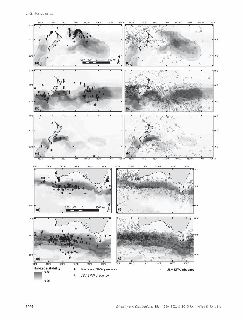
Except for the western-spring model, validation tests using

the Townsend historical data indicated high predictive capac-

ity for all models (mean AUC = 0.820, mean sensitiv-

ity = 0.56, mean 1�specificity = 0.05; Table 3). In all

models, a majority of SRW encounters coincided with areas

predicted to have high habitat suitability (stars in Fig. 3).

The validation test of the western-spring model indicated a

relatively low true positive rate (sensitivity = 0.41) but main-

tained a low false-positive rate (1�specificity = 0.03); com-

bining this led to relatively low overall discrimination

(AUC = 0.66).

Validation of the western-spring model with the modern

JSV data determined high predictive capacity (Table 3).

Despite the vast majority of SRW encounters occurring

within the east–west band of predicted high suitability

(Fig. 3j), validation of the western-summer model performed

poorly (AUC = 0.52). Limited JSV presence data in the east-

ern region restricted adequate tests, yet the validation of the

eastern-summer model based on 11 SRW encounters pro-

duced an AUC of 0.70.

The spatial calculation of collision risk between ships and

SRW implies that the majority of habitat predicted as high

suitability is without risk (Fig. 4a–e). Results suggest that

SRW only face relatively substantial risk (> 12%) in a few

areas. During summer and autumn, high SRW habitat suit-

ability south of the Chatham Rise overlaps with relatively

dense ship traffic (Appendix S4). In summer, this area has

the highest risk index of vessel collision (> 16%) and high

Table 3 Model parameters and validation results of southern right whale boosted regression tree habitat models.

Region/Season

Variables

(% contribution)

Tree

complexity

Learning

rate

Number

of trees AUC CVdev

Validation AUC

Townsend (sensitivity;

1�specificity)

Validation AUC

JSV (sensitivity;

1�specificity)

Eastern/Spring dist_ridge (27.8) 3 0.005 1300 0.835 0.306 0.84 (0.56; 0.01) NA

t0_200 (24.1)

depth_mean (21.7)

chla (15.5)

mld (10.8)

Eastern/Summer t0_200 (56.3) 3 0.0025 1250 0.876 0.407 0.85 (0.65; 0.07) 0.70* (0.27; 0.13)

dist_stf (27.6)

dist_ridge (7.6)

depth_mean (5.5)

mld (3.0)

Eastern/Autumn dist_stf (37.3) 2 0.00125 1750 0.928 0.587 0.89 (0.55; 0.01) NA

t0_200 (32.5)

chla (20.7)

dist_ridge (5.5)

mld (4.0)

Western/Spring t0_200 (45.8) 3 0.0025 1500 0.796 0.226 0.66 (0.41; 0.03) 0.77 (0.44; 0.16)

t0 (15.2)

dist_stf (14.8)

depth_mean (10.4)

chla (7.2)

mld (6.7)

Western/Summer t0_200 (53.8) 2 0.005 1700 0.797 0.232 0.86 (0.65; 0.15) 0.52 (0.56; 0.55)

dist_stf (32.6)

mld (13.6)

AUC, Area under the receiver operator curve; CVdev, Cross-validation per cent deviance explained; Townsend, Townsend (1935) historical whal-

ing data; JSV, Japanese Scouting Vessel data (Miyashita et al., 1995); dist_ridge, distance from ridge; t0_200, mean temperature between surface

(0 m) and 200 m; depth_mean, mean depth; chla, chlorophyll a concentration; mld, mixed layer depth; dist_stf, distance from the Subtropical

Front; t0, temperature at surface (0 m).

*AUC value calculated with only 11 presence locations.


L. G. Torres et al.

collision risk is maintained during autumn. In the western

region during spring, an area of moderate to high habitat

suitability around 38° S and 135° E overlaps a very dense

shipping lane causing relatively high-risk indices of collision.

Minimal shipping traffic crosses high suitability habitat pre-

dicted by the eastern-spring and western-summer models,

leading to scattered grid cells with low to moderate values of

risk.

With predicted temperature layers for the 2090–2100 dec-

ade incorporated into predictions of SRW distribution, habi-

tat shifted southward in all region-season combinations and

the amount of high suitability habitat (yellow and red grid

cells in Fig. 4f–j) decreased, with the exception of the wes-

tern-spring prediction. Suitable habitat along the Louisville

Ridge in spring virtually disappeared and was compressed to

a thin band around 46° S (Fig. 4f). During summer in the

eastern region, the predicted distribution of SRW shifted

southward and contracted to between 47° and 50° S

(Fig. 4g). The suitability of habitat south of Chatham Rise in

autumn declined substantially with only a few grid cells

maintaining high (red) suitability (Fig. 4h). During spring in

the western region, SRW habitat shifted south and expanded

Figure 2 Fitted-functions produced by boosted regression trees of southern right whale distribution indicating the marginal effect on

whale presence/absence (y-axes) by each habitat predictor variable. Contribution of each variable given in parentheses. Y-axes are on a

logit scale and are standardized between fitted-function plots for each region-season. Rug plots show distribution of data across that

variable, in deciles, and are used as a measure of confidence in the shape of the fitted-function. Dist_ridge = distance from ridge (m);

t0_200 = mean temperature between 0 and 200 m (°C); Depth_mean = mean depth (m); Chla = chlorophyll a concentration

(mg m�3); mld = mixed layer depth (m); Dist_stf = distance from the subtropical front (km) with sign denoting south (�) or north

(+) of the front; t0 = temperature at the surface (°C).

Figure 3 Predicted habitat suitability of southern right whales produced by boosted regression tree models. (a–e) Townsend (1935)

data (stars) and Japanese Scouting Vessel (crosses) presence locations used in validation tests overlaid. (f–j) Japanese Scouting Vessel

absence locations (circles) overlaid. Eastern region, spring (a,f); eastern region, summer (b,g); eastern region, autumn (c,h); western

region, spring (d,i); western region, summer (e,j). Grey scale of habitat suitability is standardized across all maps. North arrow and scale

bar in first map for each region apply to other regional plots. Note that symbols may overlap at this scale causing apparent, but false,

discrepancies with sample sizes presented in Table 1. The Louisville Ridge, Chatham Rise and Macquarie Ridge are shown in eastern

maps (a–c; f–h). Maps in Mercator projection, datum wgs1984.



(a)

N

(b)

(c)

(d)

(e)

(f)

(g)

(h)

(i)

(j)

N


L. G. Torres et al.

150°E140°E130°E120°E110°E100°E

30°S

40°S

50°S

130°W140°W150°W160°W170°W180°170°E160°E30°S

40°S

50°S

30°S

40°S

50°S

130°W140°W150°W160°W170°W180°170°E160°E

30°S

40°S

50°S

150°E140°E130°E120°E110°E100°E

40°S

50°S

1000 0 1000 km500

1000 0 1000 km500

Risk index of vessel collision0.15% – 4%5% – 8%9% – 11%12% – 15%16% – 19%

130°W140°W150°W160°W170°W180°170°E160°E

40°S

50°S

30°S

40°S

50°S

130°W140°W150°W160°W170°W180°170°E160°E

30°S

40°S

50°S

150°E140°E130°E120°E110°E100°E30°S

40°S

50°S

150°E140°E130°E120°E110°E100°E

30°S

40°S

50°S

SRW habitat suitability

Value0.85

0.01

(a)

(b)

(c)

(f)

(g)

(h)

(d)

(e)

(i)

(j)



to an area between 40 and 45° S (Fig. 4i). Suitable habitat in

the western-summer prediction reduced considerably, losing

its cohesive structure, and decreasing in suitability (Fig. 4j).

DISCUSSION

Our southern right whale habitat models incorporate histori-

cal whaling data and modern environmental datasets to

describe habitat use characteristics, predict current and

future distribution patterns, and assess threats to this vulner-

able population. Validation results using independent histori-

cal whaling observations suggest that models are able to

proficiently predict historical SRW foraging distribution pat-

terns. Furthermore, the majority of recent SRW sightings

overlap predicted high suitability habitat indicating an

adequate ability to predict present-day SRW foraging habitat

at these broad spatial and temporal scales. These results

support our assumptions of (1) environmental stability

between the time periods of our datasets and (2) temporally

consistent ecological relationships between whales and their

environment.

Apparent exceptions in these affirmative validation tests

are worth further consideration. Poor model fit may explain

the low scores in the western-spring Townsend and western-

summer JSV validation tests. Many SRW encounters in the

Townsend western-spring dataset occurred outside predicted

foraging grounds and likely represent migratory whales leav-

ing calving grounds in southeast and southwest Australia

(Bannister, 2001). Our models did not describe migration

corridors causing low validation scores here. Strong valida-

tion of the western-spring prediction using JSV data suggests

that this model can adequately predict modern SRW distri-

butions with relatively high discrimination. Although JSV

presence data in the western-summer area overlaps well with

predicted high-suitability habitat, dominance of absence data

also within this high-suitability habitat may attribute to the

very low AUC (0.52). Low SRW prevalence led to high JSV

search effort with few encounters. Absence does not necessar-

ily indicate unsuitable habitat, just non-occupancy during

times of observational effort.

Mean water temperature between the surface and 200 m

(t0_200) was a consistently influential predictor of SRW dis-

tribution across all models and, as a result, dramatic changes

in SRW distribution were predicted for the 2090–2100

decade due to climate change effects on ocean temperatures.

Overall, the preferred offshore foraging habitat of SRW in

the Australasian region was characterized by t0_200 between

10 and 13 °C, mixed layer depth (mld) < 40 m, chlorophyll

concentration above 0.2 mg m�3, and being near the

Subtropical Front or close to the Louisville Ridge in spring.

These results represent the first quantitative description of

the offshore habitat of SRW.

At a regional to basin-wide scale, these broad oceano-

graphic features and patterns function to increase prey avail-

ability and density for whales by concentrating zooplankton

along vertical (i.e., thermoclines) and horizontal (i.e.,

currents) boundaries (Bakun, 1996; Gregr & Coyle, 2009).

Stomach samples of harvested SRW suggest a diet dominated

by copepods north of 50° S (Tormosov et al., 1998). We

extend this basic information by hypothesizing that SRW in

our study region prey on Neocalanus tonsus, a large-bodied

copepod common between 20 and 50° S and abundant in

the top 200 m during spring and summer (Voronina et al.,

1988). This hypothesis is based on similar habitat use pat-

terns of SRW as predicted by our models and N. tonsus as

documented in the literature.

Kawamura (1974) documented large swarms of N. tonsus

southwest of Australia in December, with maximum concen-

trations just north of the Subtropical Front and in surface

water of temperature ranging 13–14 °C. These patterns are

coincident with those derived by our western models for

SRW. In the eastern region, a longitudinal transect at

158° W during summer documented N. tonsus as the great-

est zooplankton species by mass and, at certain depths, by

quantity (up to 98%; Voronina et al., 1988). Neocalanus

tonsus was distributed from the Subtropical Front into

subtropical waters, aggregated in vast patches within the

upper mixed layer, and was depth-limited by the thermo-

cline. The top of the seasonal thermocline and the bottom

of the mixed layer are at approximately the same depth; this

link may explain the inclusion of mld in all our models.

Foraging dive depths of northern right whales are positively

correlated with depth of the bottom mixed layer, above

which prey is concentrated allowing more efficient foraging

dives (Baumgartner & Mate, 2003). Similarly, SRW may

select habitats with relatively shallow mld to promote effi-

cient foraging by spending less time transiting and more

time feeding. While temperature, mixed layer depth and

distance from the Subtropical Front do not determine the

fine-scale dynamics of zooplankton distribution (Bakun,

1996), the seasonal foraging distributions of SRW at scales

of 10s to 100s of km are likely to respond to these broad-

scale oceanic features that concentrate prey (Gregr & Coyle,

2009). Our hypothesis of SRW feeding on N. tonsus could

Figure 4 Predicted impacts from anthropogenic threats on southern right whale (SRW) habitat, by region and season. (a–e) Predictedrisk index of collision between ships and southern right whales based on spatial calculation (see ‘Methods’) between predicted whale

habitat suitability and ship traffic density layer (Appendix S4; Halpern et al., 2008). (f–j) Predicted SRW habitat suitability in the 2090–2100 decade based on changes in ocean temperatures due to global climate change. Colour scales of habitat suitability and collision risk

are standardized across all prediction maps. North arrow and scale bar in first map for each region apply to other regional plots.

Eastern region, spring (a,f); eastern region, summer (b,g); eastern region, autumn (c,h); western region, spring (d,i); western region,

summer (e,j). Maps in Mercator projection, datum wgs1984.


L. G. Torres et al.

be tested by sampling near feeding SRW or by stable isotope

comparisons.

The calculation of relative collision risk between shipping

traffic and SRW based on present-day predicted distribution

patterns revealed generally lower risk across the majority of

high- suitability habitat and two relatively discrete areas of

higher risk. These areas are the southern slope of the Chatham

Rise in summer and autumn, and near 38° S and 135° E in

the western region during spring. Although the methods we

have used in our study are not directly comparable with those

used in the North Atlantic to identify areas of higher risk of

ship strikes for northern right whales (Ward-Geiger et al.,

2005), it appears that the threat of ship-strike to SRW in the

Australasian region is less than that for North Atlantic right

whales (Knowlton & Brown, 2007). However, SRW leaving

coastal wintering grounds along the south Australian coast are

likely to encounter heavy vessel traffic when they cross dense

shipping lanes to access foraging grounds. Results from our

analysis of vessel collision risk can guide research into SRW

ship-strikes and, if needed, inform mitigation measures.

Predicted effects of global climate change include increased

ocean temperatures (Smith et al., 1999; Levitus et al., 2000)

and changes to current structures (Mitchell & Hulme, 1999).

Zooplankton distributions have been shown to be sensitive

to ocean temperatures (Rutherford et al., 1999; Beaugrand

et al., 2002) and changes in location and strength of ocean

boundaries that concentrate zooplankton (Bakun, 1996).

Therefore, climate change could affect the distribution or

foraging efficiency of zooplankton-feeding organisms such as

right whales. Our integration of predicted ocean tempera-

tures for the 2090–2100 decade and the functional relation-

ships modelled between SRW and ocean temperature,

predicts substantial changes in the availability and location

of suitable SRW habitat. Areas of high habitat suitability

shifted south in all region–season combinations, including a

shift of more than 1000 km in the eastern region during

spring. Although our results suggest decreased availability of

suitable habitat for SRW, actual changes are likely to be

more complex because (1) we have not accounted for

changes in the distribution or strength of the mixed layer

depth, primary productivity or the Subtropical Front, and

(2) the unknown ecological responses of copepod prey and

their predators. Yet, if oceans continue to warm due to

global climate change as predicted, our work indicates that

SRW will face dramatic temperature changes in areas with

previously high habitat suitability. Although it is unknown if

the narrow temperature range in the upper 200 m preferred

by SRW is due to physiological limits of whales or their prey,

or both, this temperature sensitivity makes SRW particularly

vulnerable to the impacts of climate change, which may be

exacerbated due to matrilineal fidelity to feeding grounds

(Valenzuela et al., 2009).

Despite minimal recent offshore sightings of SRW, our

study described the locations and environmental characteris-

tics of SRW foraging grounds for the first time. In addition,

based on coincident distribution and habitat use patterns of

N. tonsus and SRW, we are the first to hypothesize the

main copepod prey species of SRW in the region. Without

the novel use of a historical dataset, the offshore habitat

use patterns of this endangered species in this area would

remain unknown. Furthermore, our assessment of threats to

this SRW population identified discrete locations of

increased risk of vessel collision and predicted large-scale

areas of habitat loss due to climate change. Our results can

aid conservation management of SRW by directing popula-

tion monitoring efforts, generating effective regulation strat-

egies, identifying critical habitats threatened by other

activities and guiding future research efforts. These pop-

ulations of SRW are currently increasing (Bannister, 2011;

Carroll et al., 2011b) and may recolonize former calving

and foraging grounds. Therefore, best management policies

will not only protect SRW from current threats but also

look ahead to protect these vulnerable populations from

future threats by minimizing degradation and exploitation

of critical habitats.

ACKNOWLEDGEMENTS

This project was jointly funded by the Australian Marine

Mammal Centre and the National Institute of Water and

Atmospheric Research, Ltd. (NIWA). We thank the

following people from NIWA for their advice, time

and insight: S. Bardsley, T. Compton, S. Moremede, S.

Mikaloff-Fletcher, J. Grieve, H. Neil. We also thank R.

Reeves, J. Lund and E. Josephson for help with historical

data collection, and three anonymous reviewers for help-

ful comments on this manuscript.

REFERENCES

Austin, M. (2007) Species distribution models and ecological

theory: a critical assessment and some possible new

approaches. Ecological Modelling, 200, 1–19.

Bakun, A. (1996) Patterns in the ocean: ocean processes and

marine population dynamics. California Sea Grant College

System, La Jolla, CA.

Bannister, J. (2001) Status of southern right whales (Eubalaena

australis) off Australia. Journal of Cetacean Research and

Management, 2, 103–110.

Bannister, J. (2011) Population trend in right whales off

southern Australia 1993–2010. Southern right whale

assessment workshop. International Whaling Commission,

Buenos Aires, Argentina.

Bannister, J.L., Pastene, L.A. & Burnell, S.R. (1999) First

record of movement of a southern right whale (Eubalaena

australis) between warm water breeding grounds and the

Antarctic Ocean, south of 60S. Marine Mammal Science,

15, 1337–1342.

Barbet-Massin, M., Jiguet, F., Albert, C.H. & Thuiller, W.

(2012) Selecting pseudo-absences for species distribution

models: how, where and how many? Methods in Ecology

and Evolution, 3, 327–338.



Baumgartner, M.F. & Mate, B.R. (2003) Summertime forag-

ing ecology of North Atlantic right whales. Marine Ecology-

Progress Series, 264, 123–135.

Beaugrand, G., Reid, P.C., Iba~nez, F., Lindley, J.A. &

Edwards, M. (2002) Reorganization of North Atlantic

marine copepod biodiversity and climate. Science, 296,

1692–1694.

Buston, P.M. & Elith, J. (2011) Determinants of reproductive

success in dominant pairs of clownfish: a boosted regres-

sion tree analysis. Journal of Animal Ecology, 80, 528–538.

Carroll, E., Jackson, J.A., Paton, D. & Smith, T.D. (2011a)

Estimating nineteenth and twentieth century right whale

catches and removals around east Australia and New Zea-

land. Report to the Ministry of Fisheries, p. 13. Wellington.

Carroll, E.L., Patenaude, N.J., Childerhouse, S.J., Kraus, S.D.,

Fewster, R.M. & Baker, C.S. (2011b) Abundance of the

New Zealand subantarctic southern right whale population

estimated from photo-identification and genotype mark-

recapture. Marine Biology, 158, 2565–2575.

Chiswell, S.M. (1994) Variability in sea surface temperature

around New Zealand from AVHRR images. New Zealand

Journal of Marine and Freshwater Research, 28, 179–192.

Delworth, T.L., Broccoli, A.J., Rosati, A. et al. (2006) GFDL’s

CM2 global coupled climate models. Part I: formulation

and simulation characteristics. Journal of Climate, 19, 643–

674.

Dunn, J.R. & Ridgeway, K.R. (2002) Mapping ocean proper-

ties in regions of complex topography. Deep Sea Research I:

Oceanographic Research, 49, 591–604.

Elith, J. & Leathwick, J. (2007) Predicting species distribu-

tions from museum and herbarium records using multire-

sponse models fitted with multivariate adaptive regression

splines. Diversity and Distributions, 13, 265–275.

Elith, J., Graham, C.H., Anderson, R.P. et al. (2006) Novel

methods improve prediction of species’ distributions from

occurrence data. Ecography, 29, 129–151.

Elith, J., Leathwick, J.R. & Hastie, T. (2008) A working guide

to boosted regression trees. Journal of Animal Ecology, 77,

802–813.

Estes, J.A., Terborgh, J., Brashares, J.S. et al. (2011) Trophic

downgrading of planet earth. Science, 333, 301–306.

Fawcett, T. (2006) An introduction to ROC analysis. Pattern

Recognition Letters, 27, 861–874.

Gnanadesikan, A., Dixon, K.W., Griffies, S.M. et al. (2006)

GFDL’s CM2 global coupled climate models. Part II: the

baseline ocean simulation. Journal of Climate, 19, 675–697.

Greene, C.H. & Pershing, A.J. (2004) Climate and the con-

servation biology of North Atlantic right whales: the right

whale at the wrong time? Frontiers in Ecology and the Envi-

ronment, 2, 29–34.

Gregr, E.J. (2011) Insights into North Pacific right whale

Eubalaena japonica habitat from historic whaling records.

Endangered Species Research, 15, 223–239.

Gregr, E.J. & Coyle, K.O. (2009) The biogeography of the

North Pacific right whale (Eubalaena japonica). Progress in

Oceanography, 80, 188–198.

Gregr, E.J. & Trites, A.W. (2001) Predictions of critical habi-

tat for five whale species in the waters of coastal British

Columbia. Canadian Journal of Fish and Aquatic Science,

58, 1265–1285.

Guisan, A. & Zimmermann, N.E. (2000) Predictive habitat

distribution models in ecology. Ecological Modelling, 135,

147–186.

Halpern, B.S., Walbridge, S., Selkoe, K.A., Kappel, C.V., Mic-

heli, F., D’Agrosa, C., Bruno, J.F., Casey, K.S., Ebert, C.,

Fox, H.E., Fujita, R., Heinemann, D., Lenihan, H.S., Ma-

din, E.M.P., Perry, M.T., Selig, E.R., Spalding, M., Steneck,

R. & Watson, R. (2008) A global map of human impact

on marine ecosystems. Science, 319, 948–952.

Heath, R.A. (1985) A review of the physical oceanography of

the seas around New Zealand – 1982. New Zealand Journal

of Marine and Freshwater Research, 19, 79–124.

Hendy, E.J., Gagan, M.K., Alibert, C.A., McCulloch, M.T.,

Lough, J.M. & Isdale, P.J. (2002) Abrupt decrease in tropi-

cal Pacific sea surface salinity at end of little ice age.

Science, 295, 1511–1514.

Hirzel, A.H., Le Lay, G., Helfer, V., Randin, C. & Guisan, A.

(2006) Evaluating the ability of habitat suitability models

to predict species presences. Ecological Modelling, 199, 142–

152.

Jackson, J.A., Patenaude, N.J., Carroll, E.L. & Baker, C.S.

(2008) How few whales were there after whaling? Inference

from contemporary mtDNA diversity. Molecular Ecology,

17, 236–251.

Jaquet, N., Whitehead, H. & Lewis, M. (1996) Coherence

between 19th century sperm whale distributions and satel-

lite-derived pigments in the tropical Pacific. Marine Ecology

Progress Series, 145, 1–10.

Kawamura, A. (1974) Food and feeding ecology in the south-

ern sei whale. Scientific report of whales research institute.

pp. 25–144. Tokyo.

Kemper, C., Coughran, D., Warneke, R., Pirzl, R., Watson,

M., Gales, R. & Gibbs, S. (2008) Southern right whale

(Eubalaena australis) mortalities and human interactions in

Australia, 1950–2006. Journal of Cetacean Research and

Management, 10, 1–8.

Knowlton, A.R. & Brown, M.W. (2007) Running the gauntlet:

right whales and vessel strikes. Harvard University Press,

Boston, MA.

Leaper, R., Cooke, J., Trathan, P.N., Reid, K., Rowntree, V.J.

& Payne, R.S. (2006) Global climate change drives south-

ern right whale (Eubalaena australis) population dynamics.

Biology Letters, 2, 289–292.

Leathwick, J.R., Elith, J., Francis, M.P., Hastie, T. & Taylor,

P. (2006) Variation in demersal fish species richness in the

oceans surrounding New Zealand: an analysis using

boosted regression trees. Marine Ecology-Progress Series,

321, 267–281.

Levitus, S., Antonov, J.I., Boyer, T.P. & Stephens, C. (2000)

Warming of the world ocean. Science, 287, 2225–2229.

Lobo, J.M., Jim�enez-Valverde, A. & Real, R. (2008) AUC:

a misleading measure of the performance of predictive


L. G. Torres et al.

distribution models. Global Ecology and Biogeography, 17,

145–151.

Maury, M.F. (1852) Whales chart of the world. Series F

(wind and current charts) sheet 1. (1852), U.S. Naval Obser-

vatory, Washington, DC.

Mitchell, T.D. & Hulme, M. (1999) Predicting regional cli-

mate change: living with uncertainty. Progress in Physical

Geography, 23, 57–78.

Miyashita, T., Kato, H. & Kasuya, T. (1995) Worldwide map

of cetacean distribution based on Japanese sighting data.

National Research Institute of Far Seas Fisheries, Shizuoka,

Japan.

Nott, J., Haig, J., Neil, H. & Gillieson, D. (2007) Greater

frequency variability of landfalling tropical cyclones at

centennial compared to seasonal and decadal scales. Earth

and Planetary Science Letters, 255, 367–372.

Ohsumi, S. & Kasamatsu, F. (1986) Recent off-shore distri-

bution of the southern right whale in summer. Report to

the International Whaling Commission (Special Issue 10).

pp. 177–184.

Patenaude, N. & Baker, C.S. (2001) Population status and

habitat use of southern right whales in the sub-Antarctic

Auckland Islands of New Zealand. Journal of Cetacean

Research and Management, 2, 111–116.

Peterson, A.T., Sober�on, J. & S�anchez-Cordero, V. (1999)

Conservatism of ecological niches in evolutionary time.

Science, 285, 1265–1267.

Richards, R. (2002) Southern right whales: a reassessment of

their former distribution and migration routes in New

Zealand waters, including on the Kermadec grounds. Jour-

nal of the Royal Society of New Zealand, 32, 355–377.

Ridgeway, G. (2007) Generalized boosted regression models.

V1.6-3.1. March 2011.

Rutherford, S., D’Hondt, S. & Prell, W. (1999) Environmen-

tal controls on the geographic distribution of zooplankton

diversity. Nature, 400, 749–753.

Smith, T.D. (2001) Examining cetacean ecology using histor-

ical fishery data. The exploited seas: new direction for marine

environmental history (ed. by P. Holm, T.D. Smith and D.J.

Starkey), pp. 207–214. Memorial University of Newfound-

land, Newfoundland.

Smith, R.C., Ainley, D., Baker, K., Domack, E., Emslie, S.,

Fraser, B., Kennett, J., Leventer, A., Mosley-Thompson, E.,

Stammerjohn, S. & Vernet, M. (1999) Marine ecosystem

sensitivity to climate change. BioScience, 49, 393–404.

Smith, T.D., Reeves, R.R., Josephson, E.A. & Lund, J.N.

(2012) Spatial and seasonal distribution of American whal-

ing and whales in the age of sail. PLoS ONE, 7, e34905.

Stramma, L., Peterson, R.G. & Tomczak, M. (1995) The

South Pacific current. Journal of Physical Oceanography, 25,

77–91.

Swets, J.A. (1988) Measuring the accuracy of diagnostic

systems. Science, 240, 1285–1293.

Thrush, S.F. & Dayton, P.K. (2002) Disturbance to marine

benthic habitats by trawling and dredging: implications for

marine biodiversity. Annual Review of Ecology and

Systematics, 33, 449–473.

Tormosov, D.D., Mikhaliev, Y.A., Best, P.B., Zemsky, V.A.,

Sekiguchi, K. & Brownell, R.L. (1998) Soviet catches of

southern right whales Eubalaena australis, 1951–1971.

Biological data and conservation implications. Biological

Conservation, 86, 185–197.

Townsend, C.H. (1935) The distribution of certain whales as

shown by logbook records of American whaleships. Zoolog-

ica (NY), 19, 1–50.

Trathan, P.A., Forcada, J. & Murphy, E.J. (2007) Environ-

mental forcing and southern ocean marine predator popu-

lations: effects of climate change and variability.

Philosophical Transactions of the Royal Society B: Biological

Sciences, 362, 2351–2365.

Valenzuela, L.O., Sironi, M., Rowntree, V.J. & Seger, J.

(2009) Isotopic and genetic evidence for culturally inher-

ited site fidelity to feeding grounds in southern right

whales (Eubalaena australis). Molecular Ecology, 18, 782–

791.

Voronina, N.M., Kolosova, Y.G. & Flint, M.V. (1988) Distri-

bution and biomass of abundant mesoplankton species.

Pacific subantarctic ecosystems (ed. by M.E. Vinogradov and

M.V. Flint), pp. 197–210. Nauka Press, Moscow.

Ward-Geiger, L.I., Silber, G.K., Baumstark, R.D. & Pulfer,

T.L. (2005) Characterization of ship traffic in right whale

critical habitat. Coastal Management, 33, 263–278.

Worm, B., Barbier, E.B., Beaumont, N., Duffy, J.E., Folke,

C., Halpern, B.S., Jackson, J.B.C., Lotze, H.K., Micheli, F.,

Palumbi, S.R., Sala, E., Selkoe, K.A., Stachowicz, J.J. &

Watson, R. (2006) Impacts of biodiversity loss on ocean

ecosystem services. Science, 314, 787–790.

Yesson, C., Clark, M.R., Taylor, M.L. & Rogers, A.D. (2011)

The global distribution of seamounts based on 30 arc

seconds bathymetry data. Deep Sea Research Part I: Oceano-

graphic Research Papers, 58, 442–453.

SUPPORTING INFORMATION

Additional Supporting Information may be found in the

online version of this article:

Appendix S1 Temporal distribution of whaling effort.

Appendix S2 Methods, definitions and illustration of the

geomorphic map.

Appendix S3 Description of recent southern right whale

sightings in the region.

Appendix S4 Details on the shipping layer and implementa-

tion of the CM2.1 model.



BIOSKETCH

Leigh G. Torres is a marine spatial ecologist with research

focused on the distribution and habitat use patterns of

marine mammals and seabirds in relation to environmental

variability and anthropogenic impacts. Leigh is particularly

interested in how behaviour patterns vary with habitat, how

spatial scale impacts predator-prey interactions, what envi-

ronmental cues species use to find prey, how species spatially

and behaviourally reduce inter- and intra-specific competi-

tion, and how foraging strategies change relative to prey

availability and spatio-temporal variability.

Author contributions: L.G.T. and A.M. conceived the idea;

T.D.S. contributed historical whaling data and assisted with

manuscript preparation; P.S. provided dynamic environmen-

tal data; T.M. contributed Japanese Scouting Vessel (JSV)

data; L.G.T. performed analyses and led the writing; all

authors discussed the results and commented on earlier

versions of the manuscript.

Editor: Janet Franklin


L. G. Torres et al.

From exploitation to conservation: habitat models using whaling data predict distribution patterns...

Documents

Transcript of From exploitation to conservation: habitat models using whaling data predict distribution patterns...