fractal and fractional

Article

Fractional Dynamics of Typhoid Fever Transmission Modelswith Mass Vaccination Perspectives

Hamadjam Abboubakar 1,* , Raissa Kom Regonne 2,† and Kottakkaran Sooppy Nisar 3,*,†

�����������������

Citation: Abboubakar, H.; Kom

Regonne, R.; Sooppy Nisar, K.

Fractional Dynamics of Typhoid

Fever Transmission Models with

Mass Vaccination Perspectives.

Fractal Fract. 2021, 5, 149. https://

doi.org/10.3390/fractalfract5040149

Academic Editor: Vasily E. Tarasov

Received: 7 August 2021

Accepted: 20 September 2021

Published: 30 September 2021

Publisher’s Note: MDPI stays neutral

with regard to jurisdictional claims in

published maps and institutional affil-

iations.

Copyright: © 2021 by the authors.

Licensee MDPI, Basel, Switzerland.

This article is an open access article

distributed under the terms and

conditions of the Creative Commons

Attribution (CC BY) license (https://

creativecommons.org/licenses/by/

4.0/).

1 Department of Computer Engineering, University Institute of Technology of Ngaoundéré,University of Ngaoundéré, Ngaoundéré P.O. Box 455, Cameroon

2 National School of Agro-Industrial Sciences, University of Ngaoundéré, Ngaoundéré P.O. Box 455, Cameroon;rkregonne@yahoo.fr

3 Department of Mathematics, College of Arts and Science, Prince Sattam bin Abdulaziz University,Wadi Aldawaser 11991, Saudi Arabia

* Correspondence: h.abboubakar@gmail.com or hamadjam.abboubakar@univ-ndere.cm (H.A.);n.sooppy@psau.edu.sa (K.S.N.); Tel.: +237-694-52-3111 (H.A.)

† These authors contributed equally to this work.

Abstract: In this work, we formulate and mathematically study integer and fractional models oftyphoid fever transmission dynamics. The models include vaccination as a control measure. Afterrecalling some preliminary results for the integer model (determination of the epidemiologicalthreshold denoted by Rc, asymptotic stability of the equilibrium point without disease wheneverRc < 1, the existence of an equilibrium point with disease wheneverRc > 1), we replace the integerderivative with the Caputo derivative. We perform a stability analysis of the disease-free equilibriumand prove the existence and uniqueness of the solution of the fractional model using fixed pointtheory. We construct the numerical scheme and prove its stability. Simulation results show that whenthe fractional-order η decreases, the peak of infected humans is delayed. To reduce the proliferationof the disease, mass vaccination combined with environmental sanitation is recommended. Wethen extend the previous model by replacing the mass action incidences with standard incidences.We compute the corresponding epidemiological threshold denoted byRc? and ensure the uniformstability of the disease-free equilibrium, for both new models, when Rc? < 1. A new calibrationof the new model is conducted with real data of Mbandjock, Cameroon, to estimate Rc? = 1.4348.We finally perform several numerical simulations that permit us to conclude that such diseases canpossibly be tackled through vaccination combined with environmental sanitation.

Keywords: typhoid fever disease; vaccination; model calibration; Caputo derivative; asymptoticstability; fixed point theory

MSC: 26A33; 93D20; 47H10; 93E24; 92D30

1. Introduction

Typhoid fever, caused by a salmonella bacterium (Salmonella typhi), is a tropicaldisease transmitted by the ingestion of food or/and water contaminated with feces. Itis most prevalent in countries located below the equator, in Southeast Asia, and in theIndian subcontinent, where hygiene conditions are poor [1,2]. The principal symptoms oftyphoid fever are insomnia, fever, generalized fatigue, headaches, stomach ache, anorexia,constipation or diarrhea, and vomiting. These symptoms can last several weeks. Withouteffective treatment, typhoid fever can lead to death. According to the World HealthOrganization (WHO), the number of cases of typhoid fever is estimated to be between11 and 21 million, with 128,000 to 161,000 deaths annually due to the severity of thedisease [1,2]. Vaccination, sanitary measures, and hygiene measures are the best ways toprevent the spread of the disease [2].

Fractal Fract. 2021, 5, 149. https://doi.org/10.3390/fractalfract5040149 https://www.mdpi.com/journal/fractalfract

Fractal Fract. 2021, 5, 149 2 of 31

Since the work of Sir Ronald Ross on malaria [3], mathematical tools such as dif-ferential equations have usually been used to understand and describe the dynamics ofinfectious diseases [4–12]. In [7], the authors proposed a SVIIcR that takes into accountsome control mechanisms (treatment, education campaigns, and vaccination). Quarantin-ing the infected individuals and their treatment are the main control measures studiedin [8]. The author used optimal control methods to conclude that the outbreak can beeliminated or controlled if the control strategies are combined to their highest levels. Thesame conclusions are given in [10,11]. Recently, Olumuyiwa James et al. [9] formulated andstudied an optimal control model for typhoid fever that takes into account both indirectand direct transmission. They compared various proposed strategies using numericalsimulations and concluded that the disease burden can be controlled if all the availablecontrol measures are combined.

Very recently, many authors have proposed fractional-order models in mathematicalepidemiology (ref. [13]), ecology (ref. [14]), plant epidemiology (refs. [15,16]), and psychol-ogy (ref. [17]). Indeed, the necessity of the use of fractional derivatives in epidemiology,for example, comes from the fact that these operators have many properties, such as theirdifferent types of kernels and the crossover behavior in the model, which can only be de-scribed using these operators. Moreover, any real data that have zigzag dynamics (mostlymany) that cannot be projected by an integer-order derivative can be solved by a fractionalmodel more clearly.

The principal disadvantage of models with integer derivatives is that they do notpermit the definition of memory effects. Replacing integer derivatives with fractionalderivatives makes it possible to remedy this problem. Indeed, they offer different waysto forecast data by varying the fractional-order parameter [12,18,19]. Several fractionaloperators have been defined so far. The most popular are the fractional operators of Caputo,the fractional Caputo–Fabrizio operator, and the fractional operator of Atangana–Baleanu.Each operator explores the dynamics of the studied phenomenon differently, thus helpingus to predict more variations in the evolution of the phenomenon. The advantages anddisadvantages of each fractional operator and their application domains can be foundin [20–22].

To the best of our knowledge, there are few mathematical works on typhoid fever usingfractional operators [6,12]. In [12], the authors used the Caputo–Fabrizio operator to extendthe model proposed in [23]. They provided existence, uniqueness, and stability criteriafor the proposed fractional-order typhoid model. More recently, Abboubakar et al. [6]formulated a SIR-B-type compartmental model with both integer and Caputo derivatives.The only control measure was vaccination. They computed the control reproductionnumber, Rc, and performed stability analysis of the disease-free equilibrium point for bothmodels. The present contributions are listed as follows:

1. Using a fractional derivative in place of an integer derivative, as used in our previousmodel [5], we formulate a new model. To prove the existence and uniqueness ofthe solutions, we use fixed point theory. The corresponding numerical scheme isobtained through the Adams–Bashforth–Moulton method [24,25]. The stability of thisnumerical scheme is also proven. Finally, several numerical simulations are carriedout from the real values of parameters estimated with real data of Mbandjock, inCameroon (see [5]).

2. Secondly, we extend the previous models by replacing the mass action incidencelaw with the standard incidence law. For these new models, we compute the corre-sponding control reproduction number,Rc?, and ensure the uniform stability of theequilibrium point without disease. As in [6], model parameters are estimated. Withthese new parameter values, we finally perform several numerical simulations thatpermit us to compare the quantitative dynamics of the two types of models.

The rest of the work is organized as follows. We devote Section 2 to preliminary defini-tions of the fractional derivative in the sense of Caputo and useful results. Formulation ofthe models with mass incidence law and standard incidence, as well as their mathematical

Fractal Fract. 2021, 5, 149 3 of 31

analysis (computation of control reproduction numbers, asymptotic stability analysis ofthe disease-free equilibrium, existence as well as the uniqueness of solutions, constructionof the numerical scheme with its stability), is also described in this section. The calibrationof the model with standard incidences and several numerical results is given in Section 3.We end the paper with a discussion and conclusions.

2. Materials and Methods2.1. Useful Definitions and Results

For over ten years, fractional derivatives have captured the attention of researchers,who use these fractional operators to model physical, chemical, and biological processes.One can cite the dynamics of transmissible diseases [26–28]. Before the formulation of thefractional models, it is important to recall their definition, as well as two results that will beused later in the fractional model analysis.

Definition 1. Let f ∈ Cl−1, and we have the following relation:

Dντ f (τ) =

{dr f (τ)

dτr , ν = r ∈ N1

Γ(r−ν)

∫ τ0 (τ − ι)r−ν−1 f (r)(ι)dι, −1 + r < ν < r , r ∈ N,

(1)

which represents the Caputo derivative of f .

Lemma 1. Assume that χ, Q, h, Y > 0, kh ≤ Y with k ∈ N, and

yq,m =

{(m− q)χ−1 q = 1, 2, . . . , m− 1,0 q ≥ m.

Let ∑q=iq=k yq,m|eq| = 0 for k > m ≥ 1.If

|em| ≤ Qhχm−1

∑q=1

yq,m|eq|+ |η0|, m = 1, 2, . . . , k,

then|ek| ≤ M|η0|, k ∈ {1, 2, . . .}

whereM ∈ R+ does not depend on h and k.

Lemma 2. If 0 < χ < 1 and d ∈ N, then there exist positive constants Wχ,1 and Wχ,2 onlydependent on χ, such that

(1 + v)χ − vχ ≤ Wχ,1(1 + v)χ−1 and (2 + v)χ+1 − 2(1 + v)χ+1 + vχ+1 ≤ Wχ,2(1 + v)χ−1.

2.2. Model Dynamics with Mass Action Incidence Law2.2.1. Model Formulation in ODE Sense and Its Analysis

In a previous work [5], we formulated and analyzed a new mathematical model for thetransmission dynamics of typhoid fever with application to the town of Mbandjock, in thecentral region of Cameroon. The model is divided into seven compartments: susceptibleindividuals S(t), vaccinated individuals V(t), infected individuals in latent stage E(t),infected individuals without any sign of the disease C(t), symptomatic infected individualsI(t), recovered individuals R(t), and the density of bacteria in the environment B(t).Each individual in each compartment naturally dies at a rate µh. Susceptible humansare recruited at a constant rate Λh. The population in compartment Sh decreases eitherby vaccination at a rate ξ, or by infection at an incidence rate νB(t)S(t), where ν is thecontact rate. We denote by θ the rate at which vaccinated individuals lose their immunity.The vaccine efficacy is denoted by ε. The compartment E of latent individuals, whichinclude infected susceptible individuals and vaccinated individuals, progresses either to

Fractal Fract. 2021, 5, 149 4 of 31

the carriers compartment C at a rate qγ1 or to the compartment I at the rate (1− q)γ1.Asymptomatic individuals become symptomatic at the rate (1− p)γ2 or recover at therate pγ2. δ denotes the disease-induced death rate of symptomatic individuals. Recoveredindividuals become susceptible at a rate α. With this brief description, the mathematicalformulation of the model studied in [5] is presented as follows:

S(t) = Λh − (k1 + νB(t))S(t) + θV(t) + αR(t), (2a)

V(t) = −[k2 + (1− ε)νB(t)]V(t) + ξS(t), (2b)

E(t) = −k3E(t) + ν[πV(t) + S(t)]B(t), (2c)

C(t) = qγ1E(t)− k4C(t), (2d)

I(t) = q1γ1E(t) + p1γ2C(t)− [k5 + σ]I(t), (2e)

R(t) = pγ2C(t) + σI(t)− k6R(t), (2f)

B(t) = pcC(t) + pi I(t)− µbB(t), (2g)

where k1 = ξ + µh, k2 = θ + µh, k3 = γ1 + µh, k4 = µh + γ2, k5 = δ + µh, k6 = α + µh,π = −1 + ε, q1 = 1− q, p1 = −p + 1, k7 = k1k2 − θξ = µh(k2 + ξ) > 0, k8 = k5 + σ.

Model (2) is defined in the following set:

W =

{(S, V, E, C, I, R, B)′ ∈ R7

+ : N = V + S + C + E + I + R ≤ Λhµh

; B ≤ (pi + pc)Λhµhµb

},

in which a dynamical system is defined, and where N denotes the human population.Without disease, model (2) has the following equilibrium: Q0 = (S0, V0, 0, 0, 0, 0, 0)′,

where S0 = Λhk2/(µh(k2 + ξ)) and V0 = Λhξ/(µh(k2 + ξ)). Using the same approachdeveloped in [29], we obtain the control reproduction number given by

Rc =

√νΛh(k2 + πξ)γ1[pcq(σ + k5) + pi(k4(1− q) + γ2q(1− p))]

µbµhk3k4(k2 + ξ)(σ + k5). (3)

Considering the model without vaccination, Rc is equal to the basic reproduction number:

R0 =

√νΛhγ1[pcq(σ + k5) + pi(k4(1− q) + γ2q(1− p))]

µbµhk3k4(σ + k5). (4)

Thus, it follows that

Rc = R0

√(k2 + πξ)

(k2 + ξ).

Since πξ = (1− ε)ξ ≤ ξ, we have(k2 + πξ)

(k2 + ξ)≤ 1, which means thatRc ≤ R0. This proves

that mass vaccination is a useful tool that can be used to effectively tackle this kind oftropical disease.

For typhoid model (2) in the ODE sense, the following results were proven in [5].

Proposition 1 ([5]). For model (2),Q0 is locally and globally asymptotically stable inW ifRc < 1and unstable ifRc > 1.

Fractal Fract. 2021, 5, 149 5 of 31

Proposition 2 ([5]). Let us define the following coefficients:

a2 = R4c k2

3k24k2

8µ2h(ξ + k2)

2π×× (µhγ1α(k5 + σq) + γ2µhk8(α + γ1) + γ1γ2α(1− pq)k5 + [µ2

h + (α + γ2 + γ1)µh]µhk8),

a1 = −R2c k2

3k24k2

8µ2h(ξ + k2)

2γ1Λhk6π(k4q1 + γ2 p1q)(R2c −R2

b),

a0 = −γ21µhΛ2

hk3k4k6k8(k4q1 + γ2 p1q)2(πξ + k2)2(ξ + k2)(R2

c − 1).

Model (2) with the integer derivative either has (1) only one endemic equilibrium whenever (a0 <0⇐⇒ Rc > 1) or (a1 < 0 and a0 = 0 or a2

1 − 4a2a0 = 0), (2) two endemic equilibrium points if(a0 > 0 (Rc < 1), a1 < 0 (Rc > Rb) and a2

1 − 4a2a0 > 0), or (3) no equilibrium otherwise.

Theorem 1 ([5]). Model (2) exhibits a supercritical bifurcation at Rc = 1, which implies thatwheneverRc > 1, the endemic equilibrium is locally asymptotically stable.

Remark 1. Proposition 1 combined with Theorem 1 implies that Proposition 2 (iii) will never holdtrue for model (2). Thus, the conditionRc < 1 is sufficient to eradicate the disease.

2.2.2. Fractional-Order Typhoid Model

The following model is obtained when we replace the integer derivative operatorin (2) with the non-integer operator in the Caputo sense.

Ct0

Dηt S(t) = Λh − (k1 + νB(t))S(t) + θV(t) + αR(t), (5a)

Ct0

Dηt V(t) = −[k2 + (1− ε)νB(t)]V(t) + ξS(t), (5b)

Ct0

Dηt E(t) = −k3E(t) + ν[πV(t) + S(t)]B(t), (5c)

Ct0

Dηt C(t) = qγ1E(t)− k4C(t), (5d)

Ct0

Dηt I(t) = q1γ1E(t) + p1γ2C(t)− [k5 + σ]I(t), (5e)

Ct0

Dηt R(t) = pγ2C(t) + σI(t)− k6R(t), (5f)

Ct0

Dηt B(t) = pcC(t) + pi I(t)− µbB(t). (5g)

with S(0) ≥ 0, V(0) ≥ 0, B(0) ≥ 0, E(0) ≥ 0, I(0) ≥ 0, C(0) ≥ 0, and R(0) ≥ 0.

Asymptotic Stability of the Disease-Free Equilibrium

Before investigating the stability of the disease-free equilibrium point, we considerthe fractional-order system (5) as follows:

Ct0

Dηt x(t) = F (x(t)), (6)

where x(ζ) ∈ R7, F ∈ R7 ×R7, 0 < η < 1. The characteristic equation of the matrix Fevaluated at any equilibrium (see [30]) is given by

det(s(I− (1− η)F )− ηF ) = 0. (7)

For the fractional model (5), the asymptotic stability ofQ0 is claimed in the following result.

Theorem 2. The disease-free equilibrium Q0 is uniformly asymptotically stable if Rc < 1, andunstable otherwise.

Fractal Fract. 2021, 5, 149 6 of 31

Proof. The Jacobian matrix of system (5) evaluated at the disease–free equilibrium Q0 isgiven by

J(Q0) =

−k1 θ 0 0 0 α −νS0ξ −k2 0 0 0 0 −νπV00 0 −k3 0 0 0 ν(S0 + πV0)0 0 qγ1 −k4 0 0 00 0 q1γ1 p1γ2 −(k5 + σ) 0 00 0 0 pγ2 σ −k6 00 0 0 pc pi 0 −µb

=

(J1 J2J3 J4

),

where J1 =

(−k1 θ

ξ −k2

), J2 =

(0 0 0 α −νS00 0 0 0 −νπV0

), J3 = OR5×2 , and

J4 =

−k3 0 0 0 ν(S0 + πV0)qγ1 −k4 0 0 0q1γ1 p1γ2 −(k5 + σ) 0 0

0 pγ2 σ −k6 00 pc pi 0 −µb

.

The characteristic Equation (7) of the typhoid fractional model (5) becomes{det(s(I2 − (1− η)J1)− η J1) = 0det(s(I5 − (1− η)J4)− η J4) = 0,

(8)

which is equivalent to{a2s2 + a1s + a0 = 0,

{s[(1− η)k6 + 1] + k6η}(

s4 + A1A5

s3 + A2A5

s2 + A3A5

s + A4A5

)= 0,

(9)

where a2 = (1− η)2k7 + (1− η)(k1 + k2) + 1, a1 = 2η(1− η)k7 + η(k1 + k2), a0 = η2k7,

A5 = η31k3k4k8µb(η1k9 + q1 pi + pcq)(1−R2

c )

+ η31µb[k3k8(k8 pcq + p1γ2 piq) + k3k4(q1k4 pi + p1γ2 piq) + k4k8k9]

+ η21µb(k8k9 + k4k9 + k3k9) + η1k9µb

+(((

η31k3 + η2

1

)k4 + η2

1k3 + η1

)k8 +

(η2

1k3 + η1

)k4 + η1k3 + 1

)k9,

A1 ={

4k3k4k8k9µbη31η + 3η2

1k3k8µbηq1k4 pi + 3η21ηk3k4µbk8 pcq

}(1− R2

c )

+ 3η21ηk3k4µb(q1k4 pi + p1γ2 piq) + 3η2

1k3k8µbη[k8 pcq + p1γ2 piq]

+ 2η1k4k9µbη + (2η1k3 + 1)k9µbη + 3η21k4k8k9µbη + 2η1k8k9µbη

+(((

3η21k3 + 2η1

)k4 + 2η1k3 + 1

)k8 + (2η1k3 + 1)k4 + k3

)k9η,

A2 =[6η2

1k3k4k8k9µbη2 + 3η1k3k4k8µbη2(pcq + q1 pi)](1−R2

c )

+ 3η1η2[k3k8µb(k8 pcq + p1γ2 piq) + k4k8k9(µb + k3) + k3k4µb(q1k4 pi + p1γ2 piq)]

+ (k4k8 + k3k8 + k3k4 + k8µb + k4µb + k3µb)k9η2,

A3 = µbη3k3k4k8[4k9η1 + q1 pi + pcq](1−R2c )

+ (µb + k3)k4k8k9η3 + k3µbη3{k8q(k8 pc + p1γ2 pi) + k4 pi(q1k4 + p1γ2q)},

A4 =(

1−R2c

)η4k3k4k8µb

k9︷ ︸︸ ︷[q1k4 pi + k8 pcq + p1γ2 piq],

and η1 = 1− η.Since both coefficients of the first equation of (9) are positive, it follows that the real

parts of the solution of (9) are negative. From the second equation of (9), we have that

Fractal Fract. 2021, 5, 149 7 of 31

s1 = − k6η[(1−η)k6+1] is one solution, and the other solutions are the root of

T (s) := A5s4 + A1s3 + A2s2 + A3s + A4. Note that A4 > 0⇐⇒ Rc < 1, andRc < 1 =⇒(A1 > 0, A2 > 0, A3 > 0, and A5 > 0). Then, it follows that, if Rc < 1, then the disease-free equilibrium Q0 is asymptotically stable whenever the following Routh–Hurwitz

criteria A1 A2A2

5− A3

A5> 0 and A1 A2 A3

A35− A2

1 A4A3

5− A2

3A2

5> 0 are satisfied for polynomial T (s) .

For uniform stability, we use the Lyapunov function:

M(E, C, I, B) = b1E(t) + b2C(t) + b3 I(t) + b4B(t), (10)

where b1 = 1, b2 = k3(k8 pc + pi p1γ2)/[k4 piq1γ1 + qγ1(k8 pc + pi p1γ2)], and b3 = k3k4 pi/[k4 piq1γ1 + qγ1(k8 pc + pi p1γ2)] and b4 = k3k4k8/[k4 piq1γ1 + qγ1(k8 pc + pi p1γ2)].

The fractional derivative ofM is given by

Ct0

DηtM(E, C, I, B) ≤ C

t0Dη

t Eb1 +Ct0

Dηt Cb2 +

Ct0

Dηt Ib3 +

Ct0

Dηt Bb4

= b1(νB[S + πV]− k3E) + b2(qγ1E− k4C) + b3(q1γ1E + p1γ2C− k8 I)

+ b4(pcC + pi I − µbB)

≤ b1

(νB[S0 + πV0

]− k3E

)+ b2(qγ1E− k4C) + b3(q1γ1E + p1γ2C− k8 I)

+ b4(pcC + pi I − µbB)

= b1νB(

S0 + πV0)− b1k3E + b2qγ1E− b2k4C + b3q1γ1E + b3 p1γ2C

− b3k8 I + b4 pcC + b4 pi I − b4µbB

= b1νB(

S0 + πV0)− b4µbB + (b3q1γ1 + b2qγ1 − b1k3)E

+ (b4 pc + b3 p1γ2 − b2k4)C + (b4 pi − b3k8)I

=µbk3k4(k5 + σ)

piq1γ1k4 + qγ1(p1 piγ2 + pc(k5 + σ))

(R2

c − 1)

B.

Thus, Ct0

DηtM(E, C, I, B) < 0 whenever Rc < 1, and C

t0Dη

tM(E, C, I, B) = 0 if and only ifRc = 1 or B(ζ) = 0. Setting B = 0 in (5), we obtain S = S0, V = V0, and E = C = I = R = 0.Thus, lim

t→∞(S(t), V(t), E(t), C(t), I(t), R(t))′ → (S0, V0, 0, 0, 0, 0, 0)′ := Q0. Consequently,

by [31] (Theorem 2.5), it follows that ifRc < 1, then Q0 is uniformly asymptotically stableinW .

Existence and Uniqueness Analysis

Before describing the existence and uniqueness of solutions for the fractional modelusing the fixed point theorem, we define T as a Banach space of continuous functionsdefined on an interval P with the norm

‖ X ‖=i=7

∑i=1‖ Xi ‖,

where X = (S, V, E, C, I, R, B), ‖ Xi ‖= sup{|Xi(t)| : t ∈ P}, and T =M(P)×M(P)×M(P)×M(P)×M(P)×M(P)×M(P).

Fractal Fract. 2021, 5, 149 8 of 31

Let us write system (5) as follows:

CDηt S(t) = H1(t, S),

CDηt V(t) = H2(t, V),

CDηt E(t) = H3(t, E),

CDηt C(t) = H4(t, C)

CDηt I(t) = H5(t, I)

CDηt R(t) = H6(t, R)

CDηt B(t) = H7(t, B)

(11)

Application of the Caputo fractional integral operator permits us to reduce (11) to thefollowing system:

− S(0) + S(t) =[∫ t

0(t− ς)η−1H1(ς, S)dς

]1

Γ(η),

−V(0) + V(t) =[∫ t

0(t− ς)η−1H2(ς, V)dς

]1

Γ(η),

− E(0) + E(t) =[∫ t

0(t− ς)η−1H3(ς, E)dς

]1

Γ(η),

− C(0) + C(t) =[∫ t

0(t− ς)η−1H4(ς, C)dς

]1

Γ(η),

− I(0) + I(t) =[∫ t

0(t− ς)η−1H5(ς, I)dς

]1

Γ(η),

− R(0) + R(t) =[∫ t

0(t− ς)η−1H6(ς, R)dς

]1

Γ(η),

− B(0) + B(t) =[∫ t

0(t− ς)η−1H7(ς, R)dς

]1

Γ(η),

(12)

with 0 < η < 1.Now, we will provide the Lipschitz conditions fulfilled by Hi, for i = 1, 2, . . . , 7, as

well as the contraction conditions. In the following theorem, we only provide the conditionfor H1, the rest being similar.

Theorem 3. The kernel H1 satisfies the Lipschitz and contraction conditions provided that0 ≤ νκ7 + k1 < 1.

Proof. For S, we proceed as below:

‖ H1(t, S)−H1(t, S1) ‖ =‖ −νB(S− S1)− k1(S− S1) ‖=‖ νB + k1 ‖‖ (S(t)− S1(t)) ‖≤‖ νκ7 + k1 ‖‖ S(t)− S1(t) ‖

where κ7 is the upper bound of the function B(t). Now, setting W1 = νκ7 + k1, wefinally obtain

‖ H1(t, S)−H1(t, S1) ‖≤W1 ‖ S(t)− S(t1) ‖, (13)

which provide the Lipschitz condition. If, additionally, we can have 0 < W1 = νκ7 + k1 < 1,then the contraction is also obtained.

Fractal Fract. 2021, 5, 149 9 of 31

As in the case of H1, it is easy to obtain the Lipschitz condition for the other kernels.Thus, we have

‖ H2(t, C)−H2(t, C1) ‖ ≤W2 ‖ V(t)−V(t1) ‖,‖ H3(t, E)−H3(t, E1) ‖ ≤W3 ‖ E(t)− E(t1) ‖,‖ H4(t, C)−H4(t, C1) ‖ ≤W4 ‖ C(t)− C(t1) ‖,‖ H5(t, I)−H5(t, I1) ‖ ≤W5 ‖ I(t)− I(t1) ‖,‖ H6(t, R)−H6(t, R1) ‖ ≤W6 ‖ R(t)− R(t1) ‖,‖ H7(t, B)−H7(t, B1) ‖ ≤W7 ‖ B(t)− B(t1) ‖ .

(14)

Recursively, Equation (12) can be rewritten as follows:

Sn(t)− S(0) =1

Γ(η)

∫ t

0(t− ς)η−1H1(ς, Sn−1)dς,

Vn(t)−V(0) =1

Γ(η)

∫ t

0(t− ς)η−1H2(ς, Vn−1)dς,

En(t)− E(0) =1

Γ(η)

∫ t

0(t− ς)η−1H3(ς, En−1)dς,

Cn(t)− C(0) =1

Γ(η)

∫ t

0(t− ς)η−1H4(ς, Cn−1)dς,

In(t)− I(0) =1

Γ(η)

∫ t

0(t− ς)η−1H5(ς, In−1)dς,

Rn(t)− R(0) =1

Γ(η)

∫ t

0(t− ς)η−1H6(ς, Rn−1)dς,

Bn(t)− B(0) =1

Γ(η)

∫ t

0(t− ς)η−1H7(ς, Bn−1)dς.

(15)

By determing, in a recursive manner, the difference between the successive terms of (11),we obtain

ψ1n(t) = Sn(t)− Sn−1(t) =1

Γ(η)

∫ t

0(t− ς)η−1(H1(ς, Sn−1)−H1(ς, Sn−2))dς,

ψ2n(t) = Vn(t)−Vn−1(t) =1

Γ(η)

∫ t

0(t− ς)η−1(H2(ς, Vn−1)−H2(ς, Vn−2))dς,

ψ3n(t) = En(t)− En−1(t) =1

Γ(η)

∫ t

0(t− ς)η−1(H3(ς, En−1)−H3(ς, En−2))dς,

ψ4n(t) = Cn(t)− Cn−1(t) =1

Γ(η)

∫ t

0(t− ς)η−1(H4(ς, Cn−1)−H4(ς, Cn−2))dς,

ψ5n(t) = In(t)− In−1(t) =1

Γ(η)

∫ t

0(t− ς)η−1(H5(ς, In−1)−H5(ς, In−2))dς,

ψ6n(t) = Rn(t)− Rn−1(t) =1

Γ(η)

∫ t

0(t− ς)η−1(H6(ς, Rn−1)−H6(ς, Rn−2))dς,

ψ7n(t) = Bn(t)− Bn−1(t) =1

Γ(η)

∫ t

0(t− ς)η−1(H7(ς, Bn−1)−H7(ς, Bn−2))dς,

(16)

with S0(t) = S(0), V0(t) = V(0), E0(t) = E(0), C0(t) = C(0), I0(t) = I(0), R0(t) = R(0),and B0(t) = B(0).

Fractal Fract. 2021, 5, 149 10 of 31

The norm of φ1n(t) gives

‖ ψ1n(t) ‖=‖ Sn(t)− Sn−1(t) ‖ =‖1

Γ(η)

∫ t

0(t− ς)η−1(H1(ς, Sn−1)−H1(ς, Sn−2))dς ‖

≤ 1Γ(η)

‖∫ t

0(t− ς)η−1(H1(ς, Sn−1)−H1(ς, Sn−2))dς ‖ .

(17)

With the Lipschitz condition (13), we obtain

‖ ψ1n(t) ‖=‖ Sn(t)− Sn−1(t) ‖≤1

Γ(η)W1

∫ t

0(t− ς)η−1 ‖ Sn−1 − Sn−2 ‖ dς. (18)

Thus, we have

‖ ψ1n(t) ‖≤1

Γ(η)W1

∫ t

0(t− ς)η−1 ‖ ψ1(n−1)(ς) ‖ dς. (19)

By proceeding in a similar way, we obtain, for the other φin(t), i = 2, . . . , 7,

‖ ψ2n(t) ‖≤1

Γ(η)W2

∫ t

0(t− ς)η−1 ‖ ψ2(n−1)(ς) ‖ dς,

‖ ψ3n(t) ‖≤1

Γ(η)W3

∫ t

0(t− ς)η−1 ‖ ψ3(n−1)(ς) ‖ dς,

‖ ψ4n(t) ‖≤1

Γ(η)W4

∫ t

0(t− ς)η−1 ‖ ψ4(n−1)(ς) ‖ dς,

‖ ψ5n(t) ‖≤1

Γ(η)W5

∫ t

0(t− ς)η−1 ‖ ψ5(n−1)(ς) ‖ dς,

‖ ψ6n(t) ‖≤1

Γ(η)W6

∫ t

0(t− ς)η−1 ‖ ψ6(n−1)(ς) ‖ dς,

‖ ψ7n(t) ‖≤1

Γ(η)W7

∫ t

0(t− ς)η−1 ‖ ψ7(n−1)(ς) ‖ dς.

(20)

Each nth term of the state variables of (5) is given by

Sn(t) =n∑

i=1ψ1i(t), Vn(t) =

n∑

i=1ψ2i(t), En(t) =

n∑

i=1ψ3i(t),

Cn(t) =n∑

i=1ψ4i(t), In(t) =

n∑

i=1ψ5i(t), Rn(t) =

n∑

i=1ψ6i(t),

Bn(t) =n∑

i=1ψ7i(t).

(21)

The following result guarantees that the solution of the fractional model (5) is unique.

Theorem 4. If the following inequality holds,

1Γ(η)

xηWi < 1, for i = 1, 2, . . . , 7, (22)

then the solution of the fractional model (5), for t ∈ [0, T], is unique.

Fractal Fract. 2021, 5, 149 11 of 31

Proof. With Equation (13), inequalities (19) and (20), combined with a recursive technique,we obtain:

‖ ψ1n(t) ‖≤‖ S0(t) ‖[

W1

Γ(η)xη

]n

, ‖ ψ2n(t) ‖≤‖ W0(t) ‖[

W2

Γ(η)xη

]n

,

‖ ψ3n(t) ‖≤‖ E0(t) ‖[

W3

Γ(η)xη

]n

, ‖ ψ4n(t) ‖≤‖ C0(t) ‖[

W4

Γ(η)xη

]n

,

‖ ψ5n(t) ‖≤‖ I0(t) ‖[

W5

Γ(η)xη

]n

, ‖ ψ6n(t) ‖≤‖ R0(t) ‖[

W6

Γ(η)xη

]n

,

‖ ψ7n(t) ‖≤‖ B0(t) ‖[

W7

Γ(η)xη

]n

.

(23)

Therefore, the above sequences satisfy limn→∞

‖ ψin(t) ‖→ 0, j = 1, 2, . . . , 7. The triangle

inequality applied to (23) permits us to obtain

‖ Sk+n(t)− Sn(t) ‖≤k+n

∑j=n+1

Zj1 =

Zn+11 − Zk+n+1

11− Z1

,

‖ Vk+n(t)−Vn(t) ‖≤k+n

∑j=n+1

Zj2 =

Zn+12 − Zk+n+1

21− Z2

,

‖ Ek+n(t)− En(t) ‖≤k+n

∑j=n+1

Zj3 =

Zn+13 − Zk+n+1

31− Z3

,

‖ Ck+n(t)− Cn(t) ‖≤k+n

∑j=n+1

Zj4 =

Zn+14 − Zk+n+1

41− Z4

,

‖ Ik+n(t)− In(t) ‖≤k+n

∑j=n+1

Zj5 =

Zn+15 − Zk+n+1

51− Z5

,

‖ Rk+n(t)− Rn(t) ‖≤k+n

∑j=n+1

Zj6 =

Zn+16 − Zk+n+1

61− Z6

,

‖ Bk+n(t)− Bn(t) ‖≤k+n

∑j=n+1

Zj7 =

Zn+17 − Zn+k+1

71− Z7

,

(24)

with1

Γ(η)bηWl < 1 and Zl =

(1

Γ(η)Wlxη

)n, l = 1, 2, . . . , 7.

Therefore, Sn, Vn, En, Cn, In, Rn, and Bn are uniformly convergent Cauchy sequences(see [32]). With n→ ∞, it follows that the limit of these sequences represents the uniquesolution to model (5).

Numerical Scheme of the Fractional Model and Its Stability Analysis

Several methods have been developed to construct numerical schemes for fractionalmodels. One can cite, among others, the Implicit Quadrature method [24], the ApproximateMittag–Leffler method [33], the Predictor Corrector method [34], and the Adams–Bashforth–Moulton method [25]. The choice of the method depends on several factors, such as theamount of information treated [35] and the accuracy order [36]. The numerical schemeproposed in this work is constructed using the Adams–Bashforth–Moulton method.

Let us consider the following general form of a fractional differential equation [37]:{Dη

t ϕ(t) = h(t, ϕ(t)), 0 ≤ t ≤ T,ϕ(l)(0) = ϕl

0, l = 0, 1, 2, . . . , n− 1, where n = [η],(25)

Fractal Fract. 2021, 5, 149 12 of 31

which is equivalent to

ϕ(t) =n−1

∑l=0

hl0

tl

l!+

1Γ(η)

∫ t

0(t− ζ)η−1h(ζ, ϕ(ζ))dζ. (26)

For η ∈ [0, 1], 0 ≤ t ≤ T and setting κ = T/N and tm = mκ, for m = 0, 1, 2, . . . , N ∈Z+, the solution of the fractional model is

S1+m = S0 +κη

Γ(η + 2)

(Λh + ηRp

1+m + θVp1+m − (νBp

1+m + k1)Sp1+m

)+

κη

Γ(η + 2)

m

∑j=0

aj,1+m

(Λh + ηRj + θVj − (νBj + k1)Sj

),

V1+m = V0 +κη

Γ(η + 2)

(ξSp

1+m −[(1− ε)νBp

1+m + k2

]Vp

1+m

)+

κη

Γ(η + 2)

m

∑j=0

aj,1+m

(ξSj −

[(1− ε)νBj + k2

]Vj

),

E1+m = E0 +κη

Γ(η + 2)

(νBp

1+m

[Sp

1+m + πVp1+m

]− k3Ep

1+m

)+

κη

Γ(η + 2)

m

∑j=0

aj,1+m

(νBj[Sj + πVj

]− k3Ej

),

C1+m = C0 +κη

Γ(η + 2)

(qγ1Ep

1+m − k4Cp1+m

)+

κη

Γ(η + 2)

m

∑j=0

aj,1+m

(qγ1Ej − k4Cj

),

I1+m = I0 +κη

Γ(η + 2)

(q1γ1Ep

1+m + p1γ2Cp1+m − [k5 + σ]Ip

1+m

)+

κη

Γ(η + 2)

m

∑j=0

aj,1+m

(q1γ1Ej + p1γ2Cj − [k5 + σ]Ij

),

R1+m = R0 +κη

Γ(η + 2)

(pγ2Cp

1+m + σIp1+m − k6Rp

1+m

)+

κη

Γ(η + 2)

m

∑j=0

aj,1+m

(pγ2Cj + σIj − k6Rj

),

B1+m = B0 +κη

Γ(η + 2)

(pcCp

1+m + pi Ip1+m − µbBp

1+m

)+

κη

Γ(η + 2)

m

∑j=0

aj,1+m

(pcCj + pi Ij − µbBj

),

(27)

Fractal Fract. 2021, 5, 149 13 of 31

where

Sp1+m = S0 +

1Γ(η)

m

∑j=0

bj,1+m

(Λh + ηRj + θVj − (νBj + k1)Sj

),

Vp1+m = V0 +

1Γ(η)

m

∑j=0

bj,1+m

(ξSj −

[(1− ε)νBj + k2

]Vj

),

Ep1+m = E0 +

1Γ(η)

m

∑j=0

bj,1+m

(νBj[Sj + πVj

]− k3Ej

),

Cp1+m = C0 +

1Γ(η)

m

∑j=0

bj,1+m

(qγ1Ej − k4Cj

),

Ip1+m = I0 +

1Γ(η)

m

∑j=0

bj,1+m

(= q1γ1Ej + p1γ2Cj − [k5 + σ]Ij

),

Rp1+m = R0 +

1Γ(η)

m

∑j=0

bj,1+m

(pγ2Cj + σIj − k6Rj

),

Bp1+m = B0 +

1Γ(η)

m

∑j=0

bj,1+m

(pcCj + pi Ij − µbBj

),

(28)

and

aj,1+m =

mη+1 − (m + 1)(−η + m), j = 0,(2− j + m)η+1 − 2(m− j + 1)1+η + (−j + m)1+η 1 ≤ j ≤ m,1, j = 1 + m,

bj,1+m =κη

η

((m + 1− j)η − (m− j)η

), 0 ≤ j ≤ m.

We then claim the following result.

Theorem 5. Under some conditions, the above numerical scheme (see Equations (27) and (28))is stable.

Proof. Let S?0 , S?

j (j = 0, . . . , 1 + m) and S?p1+m(m = 0, . . . , N − 1) be perturbations of S0,

Sj, and Sp1+m, respectively. By using Equations (19) and (28), the following perturbation

equations are obtained:

S?p1+m = S?

0 +1

Γ(η)

m

∑j=0

bj,1+m(G1(tj, Sj + S?j )− G1(tj, Sj)), (29)

S?1+m = S?

0 +κη

Γ(η + 2)(G1(t1+m, Sp

1+m + SP1+m)− G1(t1+m, Sp

1+m))

+κη

Γ(η + 2)

m

∑j=0

aj,1+m(G1(tj, Sj + S?j )− G1(tj, Sj)).

(30)

The Lipschitz condition permits us to obtain

|S?1+m| ≤ φ0 +

κη MΓ(η + 2)

(|S?p

1+m|+m

∑j=1

aj,1+m|S?j |)

, (31)

Fractal Fract. 2021, 5, 149 14 of 31

where φ0 = max0≤m≤N

{|S?

0 |+κη Mam,0

Γ(η + 2)|S?

0 |}

. From [32] (Equation (3.18)), it follows that

|S?p1+m| ≤ Θ0 +

MΓ(η)

m

∑j=1

bj,1+m|S?j |, (32)

where Θ0 = max0≤m≤N

{|S?

0 |+Mbm,0

Γ(η)|S?

0 |}

. Substituting |S?p1+m| from Equation (32) into

Equation (31) gives

|S?1+m| ≤ $0 +

κη MΓ(η + 2)

(M

Γ(η)

m

∑j=1

bj,1+m|S?j |+

m

∑j=1

aj,1+m|S?j |)

≤ $0 +κη M

Γ(η + 2)

m

∑j=1

(M

Γ(η)bj,1+m + aj,1+m

)|S?

j |

≤ $0 +κη MCη,2

Γ(η + 2)

m

∑j=1

(m + 1− j)η−1|S?j |,

(33)

where $0 = max{φ0 +κη Ma1+m,1+m

Γ(η + 2)Θ0}.

Thanks to Lemma 2, we have that Cη,2 > 0 and depends only on η, and κ is assumedto be small enough. A direct application of Lemma 1 implies |S?

1+m| ≤ C$0. The proof forthe other variables is obtained in the same way. This ends the proof.

2.3. Model Dynamics with the Standard Incidence Law

In this section, we extend model (2) by replacing the mass action incidence law withthe standard incidence law, and considering direct transmission (human to human). Thenew typhoid fever transmission dynamics model is thus presented as follows:

S(t) = Λh + θV(t) + αR(t)− k1S(t)− β(I + C)

N(t)S(t)− ν

B(t)B(t) + K

S(t), (34a)

V(t) = −[

k2 + πβ(C + I)

N(t)+ πν

B(t)K + B(t)

]V(t) + ξS(t), (34b)

E(t) =[

β(C + I)

N(t)+ ν

B(t)B(t) + K

](πV(t) + S(t))− k3E(t), (34c)

C(t) = qγ1E(t)− k4C(t), (34d)

I(t) = q1γ1E(t) + p1γ2C(t)− k8 I(t), (34e)

R(t) = pγ2C(t) + σI(t)− k6R(t), (34f)

B(t) = pcC(t) + pi I(t)− µbB(t), (34g)

where β is the direct transmission rate, and K represents the half-saturation constant.

Fractal Fract. 2021, 5, 149 15 of 31

The corresponding fractional model is given by

Ct0

Dηt S(t) = Λh + θV(t) + αR(t)− k1S(t)− β

(I + C)N(t)

S(t)− νB(t)

K + B(t)S(t), (35a)

Ct0

Dηt V(t) = −

[k2 + πβ

(I + C)N(t)

+ πνB(t)

K + B(t)

]V(t) + ξS(t), (35b)

Ct0

Dηt E(t) =

[β(I + C)

N(t)+ ν

B(t)K + B(t)

](πV(t) + S(t))− k3E(t), (35c)

Ct0

Dηt C(t) = qγ1E(t)− k4C(t), (35d)

Ct0

Dηt I(t) = q1γ1E(t) + p1γ2C(t)− k8 I(t), (35e)

Ct0

Dηt R(t) = pγ2C(t) + σI(t)− k6R(t), (35f)

Ct0

Dηt B(t) = pcC(t) + pi I(t)− µbB(t). (35g)

Without loss of generality, it is evident that the new model (34) (resp. (35)) is alsodefined inW .

Model (34) has the same disease-free equilibrium as model system (2). Using the sameapproach developed in [29], we define the next-generation matrix of model system (34) as

NGM =

R1

H0 p1γ2βN0k4k8

+ H0βN0k4

H0βN0k8

R4

0 0 0 00 0 0 0

R5p1γ2 pi

k4k8+ pc

k4

pik8

0

where R1 =

H0βγ1

N0k3k4

[(p1γ2q + q1k4)

k8+ q]

, R4 =H0ν

Kµb, R5 =

γ1

k3k4

[pi(p1γ2q + q1k4)

k8+ pcq

],

and H0 = S0 + πV0.Thus, the control reproduction number of model (34), which is the spectral radius of

NGM, is given by

Rc? =R1 +

√R2

1 + 4R4R5

2. (36)

The following result is a direct consequence of Theorem 2 in [29] (see Appendix A forthe proof).

Proposition 3. For model (34) (resp. (35)), Q0 is locally asymptotically stable inW ifRc? < 1and unstable ifRc? > 1.

Theorem 6. For the new typhoid model (34) (resp. (35)), the disease-free equilibriumQ0 is globallyasymptotically stable ifRc? < 1 and unstable otherwise.

Proof. See Appendix B.

3. Results3.1. Numerical Results of the Fractional Model with Mass Action Incidence Law

We perform several simulations with the parameter values listed in Table 1.

Table 1. Parameter values of (2) taken from [5].

Parameter Value Parameter Value Parameter Value

Λh 1 µb 0.149990 ν 3.2618× 10−6

γ1 0.2145 ε 0.9495 δ 0.1499γ2 0.1498 ξ 0.3221 σ 0.49992α 0.0834 θ 0.0833 Rc 2.4750

Fractal Fract. 2021, 5, 149 16 of 31

The step size is κ = 10−8, the initial time is T = 0, and the final time is T > 0. Webegin by showing the impact of fractional order on the dynamics of the disease. To thisaim, the fractional-order parameter varies between η = 1 and η = 0.5.

Figure 1 displays the impact of the Caputo fractional operator on the model dynamics.For different values of the fractional-order parameter η, the infected state profiles are drawn.From Figure 1, it follows that when the fractional order η decreases, the solutions of ourfractional model (5) have different behaviors. Indeed, when the fractional order decreases,the number of infected humans in latent, carrier, and symptomatic states increases. Thisis the same for the compartment B. This phenomenon was also observed in a malariafractional model studied by [38]. It is important to note that for η = 1, the solutions of thefractional model converge to the solutions of the integer model.

0 20 40 60 80 100

Time (Months)

0

50

100

150

200

E=1

=0.9

=0.8

=0.7

=0.6

=0.5

0 20 40 60 80 100

Time (Months)

0

50

100

150

C

=1

=0.9

=0.8

=0.7

=0.6

=0.5

0 20 40 60 80 100

Time (Months)

0

20

40

60

80

I=1

=0.9

=0.8

=0.7

=0.6

=0.5

0 20 40 60 80 100

Time (Months)

0

500

1000

1500

2000

B=1

=0.9

=0.8

=0.7

=0.6

=0.5

Figure 1. Simulation results showing the fractional dynamics on the infected state variable profilesfor different values of the fractional-order parameter η.

To evaluate the impact of vaccination on typhoid fever transmission dynamics, wefix the vaccine efficacy at ε = 70% while the vaccine coverage parameter varies betweenξ = 0% and ξ = 90% (ξ ∈ {0.90, 0.50, 0.20, 0}), with different values of the fractional-orderη (η ∈ {1, 0.90, 0.80, 0.70, 0.60, 0.50}). The results are displayed in Figures 2–5.

0 20 40 60 80 100

Time (Months)

0

500

1000

1500

2000

2500

3000

E

=1

=0.9

=0.8

=0.7

=0.6

=0.5

0 20 40 60 80 100

Time (Months)

0

100

200

300

400

C

=1

=0.9

=0.8

=0.7

=0.6

=0.5

0 20 40 60 80 100

Time (Months)

0

200

400

600

800

1000

I

=1

=0.9

=0.8

=0.7

=0.6

=0.5

0 20 40 60 80 100

Time (Months)

0

0.5

1

1.5

2

2.5

3

B

104

=1

=0.9

=0.8

=0.7

=0.6

=0.5

Figure 2. Simulation results showing the infected state variable profiles without vaccination (ξ = 0).

Fractal Fract. 2021, 5, 149 17 of 31

0 20 40 60 80 100

Time (Months)

0

200

400

600

800

E

=1

=0.9

=0.8

=0.7

=0.6

=0.5

0 20 40 60 80 100

Time (Months)

50

100

150

C

=1

=0.9

=0.8

=0.7

=0.6

=0.5

0 20 40 60 80 100

Time (Months)

50

100

150

200

250

300

I

=1

=0.9

=0.8

=0.7

=0.6

=0.5

0 20 40 60 80 100

Time (Months)

0

2000

4000

6000

8000

B

=1

=0.9

=0.8

=0.7

=0.6

=0.5

Figure 3. Simulation results showing the infected state variable profiles when the vaccinationcoverage ξ = 20% with different values of the fractional order.

0 20 40 60 80 100

Time (Months)

200

220

240

260

280

300

E=1

=0.9

=0.8

=0.7

=0.6

=0.5

0 20 40 60 80 100

Time (Months)

40

60

80

100

120

140

C

=1

=0.9

=0.8

=0.7

=0.6

=0.5

0 20 40 60 80 100

Time (Months)

50

60

70

80

90

100

I=1

=0.9

=0.8

=0.7

=0.6

=0.5

0 20 40 60 80 100

Time (Months)

500

1000

1500

2000

2500

3000

B=1

=0.9

=0.8

=0.7

=0.6

=0.5

Figure 4. Simulation results showing the infected state variable profiles when the vaccinationcoverage ξ = 50% with different values of the fractional order.

0 20 40 60 80 100

Time (Months)

160

170

180

190

200

E=1

=0.9

=0.8

=0.7

=0.6

=0.5

0 20 40 60 80 100

Time (Months)

0

50

100

150

C

=1

=0.9

=0.8

=0.7

=0.6

=0.5

0 20 40 60 80 100

Time (Months)

50

55

60

65

70

I =1

=0.9

=0.8

=0.7

=0.6

=0.5

0 20 40 60 80 100

Time (Months)

500

1000

1500

2000

B=1

=0.9

=0.8

=0.7

=0.6

=0.5

Figure 5. Cont.

Fractal Fract. 2021, 5, 149 18 of 31

0 20 40 60 80 100

Time (Months)

160

170

180

190

200

E=1

=0.9

=0.8

=0.7

=0.6

=0.5

0 20 40 60 80 100

Time (Months)

0

50

100

150

C

=1

=0.9

=0.8

=0.7

=0.6

=0.5

0 20 40 60 80 100

Time (Months)

50

55

60

65

70

I =1

=0.9

=0.8

=0.7

=0.6

=0.5

0 20 40 60 80 100

Time (Months)

500

1000

1500

2000

B=1

=0.9

=0.8

=0.7

=0.6

=0.5

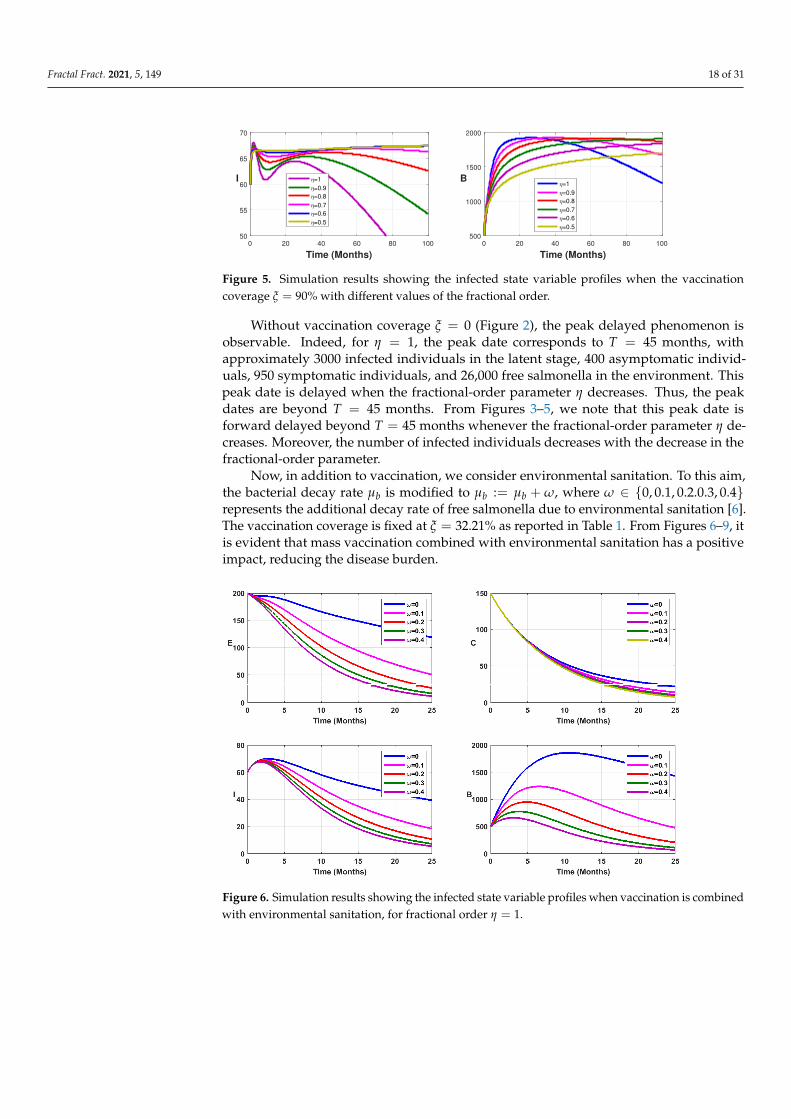
Figure 5. Simulation results showing the infected state variable profiles when the vaccinationcoverage ξ = 90% with different values of the fractional order.

Without vaccination coverage ξ = 0 (Figure 2), the peak delayed phenomenon isobservable. Indeed, for η = 1, the peak date corresponds to T = 45 months, withapproximately 3000 infected individuals in the latent stage, 400 asymptomatic individ-uals, 950 symptomatic individuals, and 26,000 free salmonella in the environment. Thispeak date is delayed when the fractional-order parameter η decreases. Thus, the peakdates are beyond T = 45 months. From Figures 3–5, we note that this peak date isforward delayed beyond T = 45 months whenever the fractional-order parameter η de-creases. Moreover, the number of infected individuals decreases with the decrease in thefractional-order parameter.

Now, in addition to vaccination, we consider environmental sanitation. To this aim,the bacterial decay rate µb is modified to µb := µb + ω, where ω ∈ {0, 0.1, 0.2.0.3, 0.4}represents the additional decay rate of free salmonella due to environmental sanitation [6].The vaccination coverage is fixed at ξ = 32.21% as reported in Table 1. From Figures 6–9, itis evident that mass vaccination combined with environmental sanitation has a positiveimpact, reducing the disease burden.

Figure 6. Simulation results showing the infected state variable profiles when vaccination is combinedwith environmental sanitation, for fractional order η = 1.

Fractal Fract. 2021, 5, 149 19 of 31

Figure 7. Simulation results showing the infected state variable profiles when vaccination is combinedwith environmental sanitation, for fractional order η = 0.90.

Figure 8. Simulation results showing the infected state variable profiles when vaccination is combinedwith environmental sanitation, for fractional order η = 0.80.

Figure 9. Cont.

Fractal Fract. 2021, 5, 149 20 of 31

Figure 9. Simulation results showing the infected state variable profiles when vaccination is combinedwith environmental sanitation, for fractional order η = 0.70.

3.2. Numerical Results of the Fractional Model with Standard Incidence Law

To simulate the new fractional model (35), we use the parameter values listed in Table 2.Note that the new typhoid model has been calibrated using real data from Mbandjock,Cameroon (see [5,6]). In Figure 10, panel (a) shows the cumulative typhoid cases versus fittedconfirmed cases (infectious individuals tested positive), which is equal to (1− q)γ1E(t) +(1− p)γ2C(t), while panel (b) presents the cumulative estimated cases for the next year.The following fractions are used as initial conditions S(0) = 20,950/32,000, V(0) = 20/32,000,E(0) = 200/32,000, C(0) = 150/32,000, I(0) = 60/32,000, R(0) = 1/32,000, andB(0) = 500/106. The relative change is r = 1.83 × 10−7 and the function tolerance is equalto 10−6.

Table 2. Estimated parameter values of the new typhoid model (35).

Parameter Values Source Parameter Values Source

Λh 3 Fitted µb 0.0015 Fittedγ1 0.1512 Fitted ε 0.9497 Fittedγ2 0.3039 Fitted ξ 0.1538 Fittedδ 0.1382 Fitted β 0.60 Fittedν 0.00050 Fitted K 995.7957 Fittedσ 0.4992 Fitted Rc? 1.4348 Estimated

0 2 4 6 8 10 12

Time (months)

0

100

200

300

400

500

600

Co

nfi

rme

d c

as

e p

er

mo

nth

(a)

Figure 10. Cont.

Fractal Fract. 2021, 5, 149 21 of 31

0 5 10 15 20 25

Time (months)

0

100

200

300

400

500

600

700

Esti

mate

d n

ew

cases p

er

mo

nth

(b)

Figure 10. Parameter estimation and forecasting of cumulative new cases of typhoid fever inMbandjock, Cameroon, from 1 July 2019 to 31 August 2020, for the new model (35). Red bulletsdenote real data (see [5,6]). The fitted model is represented with the blue line, and new forecastedcases are represented by the dotted line.

First, we observe the general dynamics of the new fractional model. The results aredisplayed in Figure 11. As for the case of the fractional model with mass incidence law (5),Figure 11 reveals that when the fractional order η decreases, the solutions of our fractionalmodel (35) have different behaviors. The number of typhoid cases decreases and the peakis delayed when the fractional order decreases.

Figure 11. Simulation results showing the fractional dynamics on the infected state variable profilesfor different values of the fractional-order parameter η.

Vaccination coverage impact is studied numerically. From Figures 12–15, it follows thatthe more ξ increases, the fewer individuals are infected. This shows that mass vaccinationplays a important role in reducing the spread of the disease.

Fractal Fract. 2021, 5, 149 22 of 31

Figure 12. Simulation results showing the infected state variable profiles when the vaccinationcoverage ξ = 0% with different values of the fractional order.

Figure 13. Simulation results showing the infected state variable profiles when the vaccinationcoverage ξ = 20% with different values of the fractional order.

Figure 14. Cont.

Fractal Fract. 2021, 5, 149 23 of 31

Figure 14. Simulation results showing the infected state variable profiles when the vaccinationcoverage ξ = 50% with different values of the fractional order.

Figure 15. Simulation results showing the infected state variable profiles when the vaccinationcoverage ξ = 90% with different values of the fractional order.

4. Discussion and Conclusions

In this work, we extended our previous SVEIR-B compartmental model [5] by replac-ing the integer derivative with fractional derivatives, to evaluate the memory effect on thetransmission dynamics of typhoid fever. We began by recalling some previous results onthe integer model (the control reproduction numberRc, existence and stability of equilib-rium points). In order to describe the non-local character as well as long-term memoryeffects in the typhoid fever transmission dynamics, we replaced the integer derivativewith the fractional derivative in the Caputo sense and studied the asymptotic stability ofthe disease-free equilibrium. Using fixed point theory, we proved the existence as well asthe uniqueness of the solutions of the fractional model. We used the Adams–Bashforthmethod to construct the numerical scheme of the proposed fractional model. We thenestablished the stability of this proposed numerical scheme. We simulated our fractionalmodel using the Adams–Bashforth–Moulton scheme implemented by [39]. Using parame-ter values for Mbandjock, a city in the central region of Cameroon, we simulates the modelby varying the fractional-order parameter, the vaccination coverage, and the bacterialdecay rate. Apart from the fact that the solutions of the fractional model converged tothe solutions of the integer model when the fractional-order approached one (η = 1), thesimulation results showed that the expected date of the disease peak was forward delayedwhen the fractional-order parameter decreased. In addition, combining vaccination withenvironmental sanitation can permit a considerable reduction in the disease’s spread.

Fractal Fract. 2021, 5, 149 24 of 31

We then extended the previous models by replacing the mass action incidence lawwith the standard incidence. The analysis of the models showed that the disease-freeequilibrium is also globally asymptotically stable whenever the corresponding reproduc-tion number Rc? is less than one. Due to the complexity of the newly proposed models,we could not prove the existence and uniqueness of the endemic equilibrium. However,numerical simulations showed that it is possible that the new typhoid fever models permita unique endemic equilibrium that is globally stable whenever Rc? > 1, and no equi-librium otherwise. We also found that, from a quantitative point of view, the diseaseburden was overestimated with the models the with mass incidence law compared to theone with the standard incidence law. Indeed, for the models with mass incidence, thecontrol reproduction number was estimated at 2.4750, while the one with the standardincidence was estimated at 1.4348. This was in accordance with our previous work inwhich we considered the standard incidence law. In [6], the control reproduction numberwas estimated at 1.3722. As for the models with mass action incidences, we observed adelay in the disease peaks whenever the fractional-order derivative decreased.

It was observed that mass vaccination can overcome this disease. In fact, if the meansare put in place to finance and implement vaccination campaigns in rural areas, it is possibleto eradicate typhoid fever. Moreover, these vaccination campaigns must be accompaniedby awareness campaigns among the population in order to combat this type of disease, aswell as instructing citizens on ways to protect their environment against the proliferationof salmonella.

Our main contribution in this paper consisted in the formulation, using both integerand fractional derivatives, of new transmission dynamics typhoid fever models that in-corporate the standard incidence rates and mass vaccination. The values of the controlreproductive number differ from the model with mass action incidence and those withthe standard incidences. Indeed, for the model with mass action incidences,Rc = 2.4750,while, for those with standard incidences, Rc∗ = 1.4348. This proves that mass actionincidence overestimates the disease burden.

Author Contributions: Conceptualization, H.A. and R.K.R.; methodology, H.A. and R.K.R.; software,H.A. and R.K.R.; validation, H.A., R.K.R. and K.S.N.; formal analysis, H.A.; investigation, H.A.and R.K.R.; resources, H.A., R.K.R. and K.S.N.; data curation, H.A. and R.K.R.; writing—originaldraft preparation, H.A.; writing—review and editing, H.A., R.K.R. and K.S.N.; visualization, H.A.;supervision, H.A.; project administration, H.A.; funding acquisition, K.S.N. All authors have readand agreed to the published version of the manuscript.

Funding: The APC was funded by Kottakkaran Sooppy Nisar. No other funds have been receivedfor this work.

Institutional Review Board Statement: Not applicable.

Informed Consent Statement: Not applicable.

Data Availability Statement: The data used to calibrate our model were taken from Mbandjockdistrict hospital.

Acknowledgments: The authors thank the LESIA laboratory manager of the National School ofAgro-industrial Sciences of the University of Ngaoundéré for their hospitality during the performanceof the numerical simulations. The authors thank the Handling Editor and the anonymous reviewersfor their comments and suggestions, which enabled us to improve the manuscript.

Conflicts of Interest: The authors declare no conflict of interest.

Fractal Fract. 2021, 5, 149 25 of 31

Appendix A. Proof of Proposition 3

Proof. The Jacobian matrix of (34) (resp. (35)) evaluated at the disease-free equilibrium Q0is given by

J (Q0) =

−k1 θ 0 − S0βN0

− S0βN0

α − S0νK

ξ −k2 0 −πV0βN0

−πV0βN0

0 −πV0νK

0 0 −k3H0βN0

H0βN0

0 H0νK

0 0 γ1q −k4 0 0 00 0 q1γ1 p1γ2 −k8 0 00 0 0 pγ2 σ −k6 00 0 0 pc pi 0 −µb

=

(J1 J2J3 J4

),

where J1 =

(−k1 θ

ξ −k2

), J4 =

−k3

H0βN0

H0βN0

0 H0νK

γ1q −k4 0 0 0q1γ1 p1γ2 −k8 0 0

0 pγ2 σ −k6 00 pc pi 0 −µb

,

J2 =

(0 − S0β

N0− S0β

N0α − S0ν

K

0 −πV0βN0

−πV0βN0

0 −πV0νK

), and J3 = 0R5×2 . The eigenvalues of J (Q0)

are those of J1 and J4. It is evident that the eigenvalues of J1 have negative realparts. Indeed, the characteristic polynomial of J1 is T (x) = det(J1 − xI2) = x2 + (k1 +k2)x + k7. Since all its coefficients are positive, it follows that all its roots have negativereal parts. A trivial eigenvalue of J4 is x = −k6. The others are the roots of the fol-lowing polynomial: I(x) = x4 + a1x3 + a2x2 + a3x + a4, with a1 = µb + k8 + k4 + k3,a4 = k3k4k8µb(1−R?

c )(R?c − R1 + 1),

a2 =1

k8q + p1γ2q + q1k4

[k2

8µbq + k4k8µbq + k3k8µbq + p1γ2k8µbq + p1γ2k4µbq + p1γ2k3µbq

+k4k28q + k3k2

8q + k3k4k8q(1− R1) + p1γ2k4k8q + p1γ2k3k8q + p1γ2k3k4q + q1k4k8µb

+q1k24µb + q1k3k4µb + q1k2

4k8 + q1k3k4k8(1− R1) + q1k3k24

],

and

a3 =1

((p1γ2k8 + p21γ2

2)pi + (k28 + p1γ2k8)pc)q2 + ((q1k4k8 + 2p1q1γ2k4)pi + q1k4k8 pc)q + q2

1k24 pi×

×[((((p1γ2k4 + p1γ2k3)k2

8 + (((1− R1)p1γ2k3 + p21γ2

2)k4 + p21γ2

2k3)k8 + p21γ2

2k3k4)µb

+(1− R1)p1γ2k3k4k28 + (1− R1)p2

1γ22k3k4k8)pi + K1 pc)q2

+(K2 pi + (q1k3k24k8µb

(1−R2

c? + R1Rc?

)+ q1k2

4k28µb + (1− R1)q1k3k4k2

8µb + (1− R1)q1k3k24k2

8)pc)q

+(q21k3k2

4k8µb(1−Rc?)(1− R1 +Rc?) + q21k3

4k8µb + q21k3k3

4µb + (1− R1)q21k3k3

4k8)pi

].

K1 ={

k8(1−Rc?)(1− R1 +Rc?) + p1γ2

(1−R2

c? + R1Rc?

)}k3k4k8µb

+ (k4 + k3)(k8 + p1γ2)k28µb + (1− R1)(k8 + p1γ2)k3k4k2

8

K2 = (k8 + p1γ2)q1k3k4k8µb

(1−R2

c? + R1Rc?

)+ (1− R1)p1γ2q1k3k4k8µb + ((1− R1)q1k3 + 2p1γ2q1)k2

4k8µ2b + 2p1γ2q1k3k2

4µb

+ q1k24k2

8µb + q1k3k24k8(1− R1)(k8 + 2p1γ2)

Fractal Fract. 2021, 5, 149 26 of 31

It is clear that a1 is always positive, and ai, i ∈ {2, 3, 4} are positive ifRc? < 1. Indeed, it isimportant to note that

Rc? < 1 =⇒ R1 < 1, (A1)

which implies that K1 > 0 and K2 > 0.Thus, all coefficients of the polynomial I(x) are always positive wheneverRc? < 1. It

follows that, ifRc? < 1, then the disease-free equilibrium is locally asymptotically stableif and only if the following conditions hold (because of the length of the expressions, weomit them here):

a1a2 − a3 > 0 and a1a2a3 − a21a4 − a2

3 > 0. (A2)

This ends the proof.

It remains now to prove the corresponding result for the new fractional model (35).To this aim, let us define the following equation:

det[r(I − (1− η)J (Q0))− ηJ (Q0)] = 0, (A3)

which is the characteristic equation of

J (Q0) =

−k1 ϑ 0 − S0βN0

− S0βN0

0 − S0νK

ξ −k2 0 −V0βπN0

−V0βπN0

0 −V0νπN0

0 0 −k3H0βN0

H0βN0

0 H0νK

0 0 γ1q −k4 0 0 00 0 q1γ1 p1γ2 −k8 0 00 0 0 γ2 p σ −k6 00 0 0 pc pi 0 −µb

.

From [4,30], it follows thatQ0 is asymptotically stable, for the new fractional model, ifall solutions of (A3) have negative real parts.

Setting D := [r(I − (1− η)J (Q0))− ηQ0] =

(D1 •

0R5×2 D4

), with

D1 :=((η1k1 + 1)r + k1η −η1rϑ− ηϑ−η1rξ − ηξ (η1k2 + 1)r + k2η

)and

D4 :=

(η1k3 + 1)r + k3η − H0η1 βr

N0− H0 βη

N0− H0η1 βr

N0− H0 βη

N00 − H0η1νr

K − H0ηνK

−η1γ1qr− γ1ηq (η1k4 + 1)r + k4η 0 0 0−η1q1γ1r− q1γ1η −η1 p1γ2r− p1γ2η (η1k8 + 1)r + k8η 0 0

0 −η1γ2 pr− γ2ηp −η1rσ− ησ (η1k6 + 1)r + k6η 00 −η1 pcr− pcη −η1 pir− ηpi 0 (η1µb + 1)r + µbη

,

it follows that the solutions of (A3) are the solutions of det(D1) = 0 and det(D4) = 0. Fromthe Proof of Theorem 2, it follows that the solutions of det(D1) = 0 have negative real parts.

It thus remains to show that the same is true for det(D4) = 0. Note that r = − k8η

η1k8 + 1< 0

is a solution of det(D4) = 0. The others are the solutions of det(D?4 ) = 0, where

D?4 :=

(η1k3 + 1)r + k3η −H0η1βr

N0− H0βη

N0−H0η1βr

N0− H0βη

N0−H0η1νr

K − H0ηνK

−η1γ1qr− γ1ηq (η1k4 + 1)r + k4η 0 0−η1q1γ1r− q1γ1η −η1 p1γ2r− p1γ2η (η1k8 + 1)r + k8η 0

0 −η1 pcr− pcη −η1 pir− ηpi (η1µb + 1)r + µbη

.

After some straightforward algebraic computations, we obtain that

det(D?4 ) = 0⇐⇒ r4 +

A2

A1r3 +

A3

A1r2 +

A4

A1r +

A5

A1= 0, (A4)

where

Fractal Fract. 2021, 5, 149 27 of 31

A1 = ((((−p1γ2k3k4k28 − p2

1γ22k3k4k8)µbR2

c? + (R1 p1γ2k3k4k28 + R1 p2

1γ22k3k4k8)µbRc?

+ ((1− R1)p1γ2k3k4k28 + (1− R1)p2

1γ22k3k4k8)µb)η

4

+ (((p1γ2k4 + p1γ2k3)k28 + (((1− R1)p1γ2k3 + p2

1γ22)k4 + p2

1γ22k3)k8 + p2

1γ22k3k4)µb

+ (1− R1)p1γ2k3k4k28 + (1− R1)p2

1γ22k3k4k8)η

3 + ((p1γ2k28 + (p1γ2k4 + p1γ2k3 + p2

1γ22)k8 + p2

1γ22k4 + p2

1γ22k3)µb

+ (p1γ2k4 + p1γ2k3)k28 + (((1− R1)p1γ2k3 + p2

1γ22)k4 + p2

1γ22k3)k8 + p2

1γ22k3k4)η

2

+ ((p1γ2k8 + p21γ2

2)µb + p1γ2k28 + (p1γ2k4 + p1γ2k3 + p2

1γ22)k8 + p2

1γ22k4 + p2

1γ22k3)η + p1γ2k8 + p2

1γ22)pi

+ ((−k3k4k38 − p1γ2k3k4k2

8)µbR2c + (R1k3k4k3

8 + R1 p1γ2k3k4k28)µbRc? + ((1− R1)k3k4k3

8 + (1− R1)p1γ2k3k4k28)µb)pcη4

+ ((−k3k4k28 − p1γ2k3k4k8)µbR2

c? + (R1k3k4k28 + R1 p1γ2k3k4k8)µbRc? + ((k4 + k3)k3

8 + (((1− R1)k3 + p1γ2)k4 + p1γ2k3)k28

+ p1γ2k3k4k8)µb + (1− R1)k3k4k38 + (1− R1)p1γ2k3k4k2

8)pcη3 + ((k38 + (k4 + k3 + p1γ2)k2

8 + (p1γ2k4 + p1γ2k3)k8)µb

+ (k4 + k3)k38 + (((1− R1)k3 + p1γ2)k4 + p1γ2k3)k2

8 + p1γ2k3k4k8)pcη2 + ((k28 + p1γ2k8)µb + k3

8 + (k4 + k3 + p1γ2)k28

+ (p1γ2k4 + p1γ2k3)k8)pcη + (k28 + p1γ2k8)pc)q2

+ ((((−q1k3k24k2

8 − 2p1q1γ2k3k24k8)µbR2

c? + (R1q1k3k24k2

8 + 2R1 p1q1γ2k3k24k8)µbRc?

+ ((1− R1)q1k3k24k2

8 + (2− 2R1)p1q1γ2k3k24k8)µb)η

4

+ ((−q1k3k4k28 − p1q1γ2k3k4k8)µbR2

c? + (R1q1k3k4k28 + R1 p1q1γ2k3k4k8)µbRc?

+ ((q1k24 + q1k3k4)k2

8 + (((1− R1)q1k3 + 2p1q1γ2)k24 + (2− R1)p1q1γ2k3k4)k8 + 2p1q1γ2k3k2

4)µb

+ (1− R1)q1k3k24k2

8 + (2− 2R1)p1q1γ2k3k24k8)η

3 + ((q1k4k28 + (q1k2

4 + (q1k3 + 2p1q1γ2)k4)k8 + 2p1q1γ2k24 + 2p1q1γ2k3k4)µb

+ (q1k24 + q1k3k4)k2

8 + (((1− R1)q1k3 + 2p1q1γ2)k24 + (2− R1)p1q1γ2k3k4)k8 + 2p1q1γ2k3k2

4)η2 + ((q1k4k8 + 2p1q1γ2k4)µb

+ q1k4k28 + (q1k2

4 + (q1k3 + 2p1q1γ2)k4)k8 + 2p1q1γ2k24 + 2p1q1γ2k3k4)η + q1k4k8 + 2p1q1γ2k4)pi

+ (−q1k3k24k2

8µbR2c? + R1q1k3k2

4k28µbRc? + (1− R1)q1k3k2

4k28µb)pcη4

+ (−q1k3k24k8µbR2

c? + R1q1k3k24k8µbRc? + ((q1k2

4 + (1− R1)q1k3k4)k28 + q1k3k2

4k8)µb + (1− R1)q1k3k24k2

8)pcη3

+ ((q1k4k28 + (q1k2

4 + q1k3k4)k8)µb + (q1k24 + (1− R1)q1k3k4)k2

8 + q1k3k24k8)pcη2

+ (q1k4k8µb + q1k4k28 + (q1k2

4 + q1k3k4)k8)pcη + q1k4k8 pc)q

+ ((−q21k3k3

4k8µbR2c? + R1q2

1k3k34k8µbRc? + (1− R1)q2

1k3k34k8µb)η

4

+ (−q21k3k2

4k8µbR2c? + R1q2

1k3k24k8µbRc? + ((q2

1k34 + (1− R1)q2

1k3k24)k8 + q2

1k3k34)µb + (1− R1)q2

1k3k34k8)η

3

+ ((q21k2

4k8 + q21k3

4 + q21k3k2

4)µb + (q21k3

4 + (1− R1)q21k3k2

4)k8 + q21k3k3

4)η2 + (q2

1k24µb + q2

1k24k8 + q2

1k34 + q2

1k3k24)η + q2

1k24)pi,

A4 = ((4(k8 + p1γ2)p1γ2k3k4k8µb(1−Rc?)(1 +Rc? − R1)η4

+ (((p1γ2k4 + p1γ2k3)k28 + (((1− R1)p1γ2k3 + p2

1γ22)k4 + p2

1γ22k3)k8 + p2

1γ22k3k4)µb

+ (1− R1)p1γ2k3k4k28 + (1− R1)p2

1γ22k3k4k8)η

3)pi + 4(k8 + p1γ2)(1−Rc?)(1 +Rc? − R1)k3k4k28µb pcη4

+ ((k8 + p1γ2)k3k4k8µbRc?(R1 −Rc?) + ((k4 + k3)k38

+ (((1− R1)k3 + p1γ2)k4 + p1γ2k3)k28 + p1γ2k3k4k8)µb + (1− R1)k3k4k3

8 + (1− R1)p1γ2k3k4k28)pcη3)q2

+ ((((−4q1k3k24k2

8 − 8p1q1γ2k3k24k8)µbR2

c? + (4R1q1k3k24k2

8 + 8R1 p1q1γ2k3k24k8)µbRc?

+ ((4− 4R1)q1k3k24k2

8 + (8− 8R1)p1q1γ2k3k24k8)µb)η

4

+ ((−q1k3k4k28 − p1q1γ2k3k4k8)µbR2

c? + (R1q1k3k4k28 + R1 p1q1γ2k3k4k8)µbRc? + ((q1k2

4 + q1k3k4)k28

+ (((1− R1)q1k3 + 2p1q1γ2)k24 + (2− R1)p1q1γ2k3k4)k8 + 2p1q1γ2k3k2

4)µb + (1− R1)q1k3k24k2

8

+ (2− 2R1)p1q1γ2k3k24k8)η

3)pi + (−4q1k3k24k2

8µbR2c? + 4R1q1k3k2

4k28µbRc? + (4− 4R1)q1k3k2

4k28µb)pcη4

+ (−q1k3k24k8µbR2

c? + R1q1k3k24k8µbRc? + ((q1k2

4 + (1− R1)q1k3k4)k28 + q1k3k2

4k8)µb

+ (1− R1)q1k3k24k2

8)pcη3)q + ((−4q21k3k3

4k8µbR2c? + 4R1q2

1k3k34k8µbRc? + (4− 4R1)q2

1k3k34k8µb)η

4

+ (−q21k3k2

4k8µbR2c? + R1q2

1k3k24k8µbRc? + ((q2

1k34 + (1− R1)q2

1k3k24)k8 + q2

1k3k34)µb + (1− R1)q2

1k3k34k8)η

3)pi,

Fractal Fract. 2021, 5, 149 28 of 31

A5 = k3k4k8µb(Rc? − R1 + 1)η4(k8q + p1γ2q + q1k4)(p1γ2 piq + k8 pcq + q1k4 pi)(1−Rc?),

A2 = ((((−4p1γ2k3k4k28 − 4p2

1γ22k3k4k8)µbR2

c? + (4R1 p1γ2k3k4k28 + 4R1 p2

1γ22k3k4k8)µbRc?

+ ((4− 4R1)p1γ2k3k4k28 + (4− 4R1)p2

1γ22k3k4k8)µb)η

4

+ (((3p1γ2k4 + 3p1γ2k3)k28 + (((3− 3R1)p1γ2k3 + 3p2

1γ22)k4 + 3p2

1γ22k3)k8 + 3p2

1γ22k3k4)µb

+ (3− 3R1)p1γ2k3k4k28 + (3− 3R1)p2

1γ22k3k4k8)η

3 + ((2p1γ2k28 + (2p1γ2k4 + 2p1γ2k3 + 2p2

1γ22)k8 + 2p2

1γ22k4 + 2p2

1γ22k3)µb

+ (2p1γ2k4 + 2p1γ2k3)k28 + (((2− 2R1)p1γ2k3 + 2p2

1γ22)k4 + 2p2

1γ22k3)k8 + 2p2

1γ22k3k4)η

2

+ ((p1γ2k8 + p21γ2

2)µb + p1γ2k28 + (p1γ2k4 + p1γ2k3 + p2

1γ22)k8 + p2

1γ22k4 + p2

1γ22k3)η)pi

+ ((−4k3k4k38 − 4p1γ2k3k4k2

8)µbR2c? + (4R1k3k4k3

8 + 4R1 p1γ2k3k4k28)µbRc? + 4(1− R1)(k8 + p1γ2)k3k4k2

8µb)pcη4

+ ((−3k3k4k28 − 3p1γ2k3k4k8)µbR2

c? + (3R1k3k4k28 + 3R1 p1γ2k3k4k8)µbRc?

+ (3(k4 + k3)k38 + ((3(1− R1)k3 + 3p1γ2)k4 + 3p1γ2k3)k2

8 + 3p1γ2k3k4k8)µb + 3(1− R1)k3k4k38 + 3(1− R1)p1γ2k3k4k2

8)pcη3

+ ((2k38 + (2k4 + 2k3 + 2p1γ2)k2

8 + (2p1γ2k4 + 2p1γ2k3)k8)µb + (2k4 + 2k3)k38 + (((2− 2R1)k3 + 2p1γ2)k4 + 2p1γ2k3)k2

8

+ 2p1γ2k3k4k8)pcη2 + ((k28 + p1γ2k8)µb + k3

8 + (k4 + k3 + p1γ2)k28 + (p1γ2k4 + p1γ2k3)k8)pcη)q2

+ ((((−4q1k3k24k2

8 − 8p1q1γ2k3k24k8)µbR2

c? + (4R1q1k3k24k2

8 + 8R1 p1q1γ2k3k24k8)µbRc?

+ ((4− 4R1)q1k3k24k2

8 + (8− 8R1)p1q1γ2k3k24k8)µb)η

4

+ ((−3q1k3k4k28 − 3p1q1γ2k3k4k8)µbR2

c? + (3R1q1k3k4k28 + 3R1 p1q1γ2k3k4k8)µbRc?

+ ((3q1k24 + 3q1k3k4)k2

8 + (((3− 3R1)q1k3 + 6p1q1γ2)k24 + (6− 3R1)p1q1γ2k3k4)k8 + 6p1q1γ2k3k2

4)µb + (3− 3R1)q1k3k24k2

8

+ (6− 6R1)p1q1γ2k3k24k8)η

3 + ((2q1k4k28 + (2q1k2

4 + (2q1k3 + 4p1q1γ2)k4)k8 + 4p1q1γ2k24 + 4p1q1γ2k3k4)µb

+ (2q1k24 + 2q1k3k4)k2

8 + (((2− 2R1)q1k3 + 4p1q1γ2)k24 + (4− 2R1)p1q1γ2k3k4)k8 + 4p1q1γ2k3k2

4)η2

+ ((q1k4k8 + 2p1q1γ2k4)µb + q1k4k28 + (q1k2

4 + (q1k3 + 2p1q1γ2)k4)k8 + 2p1q1γ2k24 + 2p1q1γ2k3k4)η)pi

+ 4(1− R1 + R1Rc? −R2c?)q1k3k2

4k28µb pcη4

+ (−3q1k3k24k8µbR2

c? + 3R1q1k3k24k8µbRc? + ((3q1k2

4 + (3− 3R1)q1k3k4)k28 + 3q1k3k2

4k8)µb + (3− 3R1)q1k3k24k2

8)pcη3

+ ((2q1k4k28 + (2q1k2

4 + 2q1k3k4)k8)µb + (2q1k24 + (2− 2R1)q1k3k4)k2

8 + 2q1k3k24k8)pcη2

+ (q1k4k8µb + q1k4k28 + (q1k2

4 + q1k3k4)k8)pcη)q

+ ((−4q21k3k3

4k8µbR2c? + 4R1q2

1k3k34k8µbRc? + (4− 4R1)q2

1k3k34k8µb)η

4

+ (−3q21k3k2

4k8µbR2c + 3R1q2

1k3k24k8µbRc? + ((3q2

1k34 + (3− 3R1)q2

1k3k24)k8 + 3q2

1k3k34)µb + (3− 3R1)q2

1k3k34k8)η

3

+ ((2q21k2

4k8 + 2q21k3

4 + 2q21k3k2

4)µb + (2q21k3

4 + (2− 2R1)q21k3k2

4)k8 + 2q21k3k3

4)η2 + (q2

1k24µb + q2

1k24k8 + q2

1k34 + q2

1k3k24)η)pi,

Fractal Fract. 2021, 5, 149 29 of 31

A3 = ((((−6p1γ2k3k4k28 − 6p2

1γ22k3k4k8)µbR2

c + (6R1 p1γ2k3k4k28 + 6R1 p2

1γ22k3k4k8)µbRc

+ ((6− 6R1)p1γ2k3k4k28 + (6− 6R1)p2

1γ22k3k4k8)µb)η

4 + (((3p1γ2k4 + 3p1γ2k3)k28

+ (((3− 3R1)p1γ2k3 + 3p21γ2

2)k4 + 3p21γ2

2k3)k8 + 3p21γ2

2k3k4)µb + (3− 3R1)p1γ2k3k4k28 + (3− 3R1)p2

1γ22k3k4k8)η

3

+ ((p1γ2k28 + (p1γ2k4 + p1γ2k3 + p2

1γ22)k8 + p2

1γ22k4 + p2

1γ22k3)µb + (p1γ2k4 + p1γ2k3)k2

8

+ (((1− R1)p1γ2k3 + p21γ2

2)k4 + p21γ2

2k3)k8 + p21γ2

2k3k4)η2)pi

+ ((−6k3k4k38 − 6p1γ2k3k4k2

8)µbR2c? + (6R1k3k4k3

8 + 6R1 p1γ2k3k4k28)µbRc? + (6− 6R1)(k3k4k3

8 + p1γ2k3k4k28)µb)pcη4

+ ((−3k3k4k28 − 3p1γ2k3k4k8)µbR2

c? + (3R1k3k4k28 + 3R1 p1γ2k3k4k8)µbRc

+ ((3k4 + 3k3)k38 + (((3− 3R1)k3 + 3p1γ2)k4 + 3p1γ2k3)k2

8 + 3p1γ2k3k4k8)µb + 3(1− R1)k3k4k28(k8 + p1γ2))pcη3

+ ((k38 + (k4 + k3 + p1γ2)k2

8 + p1γ2(k4 + k3)k8)µb + (k4 + k3)k38 + (((1− R1)k3 + p1γ2)k4 + p1γ2k3)k2

8 + p1γ2k3k4k8)pcη2)q2

+ ((((−6q1k3k24k2

8 − 12p1q1γ2k3k24k8)µbR2

c + (6R1q1k3k24k2

8 + 12R1 p1q1γ2k3k24k8)µbRc?

+ ((6− 6R1)q1k3k24k2

8 + (12− 12R1)p1q1γ2k3k24k8)µb)η

4

+ ((−3q1k3k4k28 − 3p1q1γ2k3k4k8)µbR2

c? + (3R1q1k3k4k28 + 3R1 p1q1γ2k3k4k8)µbRc

+ ((3q1k24 + 3q1k3k4)k2

8 + (((3− 3R1)q1k3 + 6p1q1γ2)k24 + (6− 3R1)p1q1γ2k3k4)k8 + 6p1q1γ2k3k2

4)µb

+ (3− 3R1)q1k3k24k2

8 + (6− 6R1)p1q1γ2k3k24k8)η

3

+ ((q1k4k28 + (q1k2

4 + (q1k3 + 2p1q1γ2)k4)k8 + 2p1q1γ2k24 + 2p1q1γ2k3k4)µb + (q1k2

4 + q1k3k4)k28

+ (((1− R1)q1k3 + 2p1q1γ2)k24 + (2− R1)p1q1γ2k3k4)k8 + 2p1q1γ2k3k2

4)η2)pi

+ (−6q1k3k24k2

8µbR2c? + 6R1q1k3k2

4k28µbRc? + (6− 6R1)q1k3k2

4k28µb)pcη4

+ (−3q1k3k24k8µbR2

c? + 3R1q1k3k24k8µbRc? + ((3q1k2

4 + (3− 3R1)q1k3k4)k28 + 3q1k3k2

4k8)µb + (3− 3R1)q1k3k24k2

8)pcη3

+ ((q1k4k28 + (q1k2

4 + q1k3k4)k8)µb + (q1k24 + (1− R1)q1k3k4)k2

8 + q1k3k24k8)pcη2)q

+ ((−6q21k3k3

4k8µbR2c? + 6R1q2

1k3k34k8µbRc? + (6− 6R1)q2

1k3k34k8µb)η

4

+ (−3q21k3k2

4k8µbR2c? + 3R1q2

1k3k24k8µbRc? + ((3q2

1k34 + (3− 3R1)q2

1k3k24)k8 + 3q2

1k3k34)µb + (3− 3R1)q2

1k3k34k8)η

3

+ ((q21k2

4k8 + q21k3

4 + q21k3k2

4)µb + (q21k3

4 + (1− R1)q21k3k2

4)k8 + q21k3k3

4)η2)pi.

It is possible to show that all the above coefficients are positive whenever Rc? < 1.Then, it follows that, ifRc < 1, then the disease-free equilibriumQ0 is asymptotically stable

whenever the following Routh–Hurwitz criteria, A1 A2A2

5− A3

A5> 0 and A1 A2 A3

A35− A2

1 A4A3

5− A2

3A2

5> 0,

are satisfied for polynomial det(D?4). (Given the heaviness of these coefficients, we do not

present the Routh–Hurwitz conditions here.)

Appendix B. Proof of Theorem 6

Let us rewrite system (34) as

dEdtdCdtdIdtdBdt

=

−k3

H0βN0

H0βN0

H0νK

γ1q −k4 0 0q1γ1 p1γ2 −k8 0

0 pc pi −µb

ECIB

−N (S, V, E, C, I, R, B), (A5)

where N (S, V, E, C, I, R, B) =

β(C + I)

(H0

N0− H

N

)+ νB

(H0

K− H

K + B

)000

.

Fractal Fract. 2021, 5, 149 30 of 31

In W , H = S + πV < H0 = S0 + πV0 for t > 0; thus, N (S, V, E, C, I, R, B) ≥ OR4 .Note that Proposition 3 ensures that the following matrix

J (Q0) =

−k3

H0βN0

H0βN0

H0νK

γ1q −k4 0 0q1γ1 p1γ2 −k8 0

0 pc pi −µb

has all its eigenvalues with negative real parts. It follows that from the comparisontheorem [40], (E, C, I, B) −→ (0, 0, 0, 0) and (S, V, R) −→ (S0, V0, 0) as t −→ +∞. Thus,(S, V, E, C, I, R, B) −→ Q0 = (S0, V0, 0, 0, 0, 0, 0) as t −→ +∞. We finally conclude that thedisease–free equilibrium is globally asymptotically stable inW ifRc? < 1.

References1. World Health Organization. Typhoid vaccines: WHO position paper. Wkly. Epidemiol. Rec. 2008, 83, 49–59.2. World Health Organization. Typhoid vaccines: WHO position paper–March 2018–Vaccins antityphoïdiques: Note de synthèse de

l’OMS–mars 2018. Wkly. Epidemiol. Rec. 2018, 93, 153–172.3. Ross, R. Some quantitative studies in epidemiology. Nature 1911, 87, 466–467. [CrossRef]4. Abboubakar, H.; Kumar, P.; Erturk, V.S.; Kumar, A. A mathematical study of a tuberculosis model with fractional derivatives. Int.

J. Model. Simul. Sci. Comput. 2021, 12, 2150037. [CrossRef]5. Abboubakar, H.; Racke, R. Mathematical modeling, forecasting, and optimal control of typhoid fever transmission dynamics.

Chaos Solitons Fractals 2021, 149, 111074. [CrossRef]6. Abboubakar, H.; Kombou, L.K.; Koko, A.D.; Fouda, H.P.E.; Kumar, A. Projections and fractional dynamics of the typhoid fever: A

case study of Mbandjock in the Centre Region of Cameroon. Chaos Solitons Fractals 2021, 150, 111129. [CrossRef]7. Edward, S.; Nyerere, N. Modelling typhoid fever with education, vaccination and treatment. Eng. Math. 2016, 1, 44–52.8. Mushayabasa, S. Modeling the impact of optimal screening on typhoid dynamics. Int. J. Dyn. Control 2016, 4, 330–338. [CrossRef]9. Peter, O.J.; Ibrahim, M.O.; Edogbanya, H.O.; Oguntolu, F.A.; Oshinubi, K.; Ibrahim, A.A.; Ayoola, T.A.; Lawal, J.O. Direct and

Indirect Transmission of Typhoid Fever Model with Optimal Control. Results Phys. 2021, 27, 104463. [CrossRef]10. Tilahun, G.T.; Makinde, O.D.; Malonza, D. Modelling and optimal control of typhoid fever disease with cost-effective strategies.

Comput. Math. Methods Med. 2017, 2017, 2324518. [CrossRef]11. Tilahun, G.T.; Makinde, O.D.; Malonza, D. Co-dynamics of pneumonia and typhoid fever diseases with cost effective optimal

control analysis. Appl. Math. Comput. 2018, 316, 438–459. [CrossRef]12. Shaikh, A.S.; Nisar, K.S. Transmission dynamics of fractional order Typhoid fever model using Caputo–Fabrizio operator. Chaos

Solitons Fractals 2019, 128, 355–365. [CrossRef]13. Erturk, V.S.; Kumar, P. Solution of a COVID-19 model via new generalized Caputo-type fractional derivatives. Chaos Solitons

Fractals 2020, 139, 110280. [CrossRef]14. Kumar, P.; Erturk, V.S. Environmental persistence influences infection dynamics for a butterfly pathogen via new generalised

Caputo type fractional derivative. Chaos Solitons Fractals 2021, 144, 110672. [CrossRef]15. Kumar, P.; Erturk, V.S.; Almusawa, H. Mathematical structure of mosaic disease using microbial biostimulants via Caputo and

Atangana–Baleanu derivatives. Results Phys. 2021, 24, 104186. [CrossRef]16. Kumar, P.; Suat Ertürk, V.; Nisar, K.S. Fractional dynamics of huanglongbing transmission within a citrus tree. Math. Methods

Appl. Sci. 2021, 44, 11404–11424. [CrossRef]17. Kumar, P.; Erturk, V.S.; Murillo-Arcila, M. A complex fractional mathematical modeling for the love story of Layla and Majnun.

Chaos Solitons Fractals 2021, 150, 111091. [CrossRef]18. Loverro, A. Fractional Calculus: History, Definitions and Applications for the Engineer; Rapport Technique; Department of Aerospace

and Mechanical Engineering, Univeristy of Notre Dame: Notre Dame, IN, USA, 2004; pp. 1–28.19. Nabi, K.N.; Abboubakar, H.; Kumar, P. Forecasting of COVID-19 pandemic: From integer derivatives to fractional derivatives.

Chaos Solitons Fractals 2020, 141, 110283. [CrossRef] [PubMed]20. Angstmann, C.N.; Jacobs, B.A.; Henry, B.I.; Xu, Z. Intrinsic Discontinuities in Solutions of Evolution Equations Involving

Fractional Caputo–Fabrizio and Atangana–Baleanu Operators. Mathematics 2020, 8, 2023. [CrossRef]21. Tarasov, V.E. On chain rule for fractional derivatives. Commun. Nonlinear Sci. Numer. Simul. 2016, 30, 1–4. [CrossRef]22. Tarasov, V.E. No violation of the Leibniz rule. No fractional derivative. Commun. Nonlinear Sci. Numer. Simul. 2013, 18, 2945–2948.

[CrossRef]23. Peter, O.; Ibrahim, M.; Oguntolu, F.; Akinduko, O.; Akinyemi, S. Direct and indirect transmission dynamics of typhoid fever

model by differential transform method. ATBU J. Sci. Technol. Educ. (JOSTE) 2018, 6, 167–177.24. Diethelm, K. An algorithm for the numerical solution of differential equations of fractional order. Electron. Trans. Numer. Anal

1997, 5, 1–6.25. Diethelm, K.; Ford, N.J. Analysis of fractional differential equations. J. Math. Anal. Appl. 2002, 265, 229–248. [CrossRef]

Fractal Fract. 2021, 5, 149 31 of 31

26. Boccaletti, S.; Ditto, W.; Mindlin, G.; Atangana, A. Modeling and forecasting of epidemic spreading: The case of Covid-19 andbeyond. Chaos Solitons Fractals 2020, 135, 109794. [CrossRef]

27. Khan, M.A.; Atangana, A.; Alzahrani, E. The dynamics of COVID-19 with quarantined and isolation. Adv. Differ. Equ. 2020,2020, 425. [CrossRef]

28. Schmidt, A.; Gaul, L. On the numerical evaluation of fractional derivatives in multi-degree-of-freedom systems. Signal Process.2006, 86, 2592–2601. [CrossRef]

29. van den Driessche, P.; Watmough, J. Reproduction numbers and the sub-threshold endemic equilibria for compartmental modelsof disease transmission. Math. Biosci. 2002, 180, 29–48. [CrossRef]

30. Li, H.; Cheng, J.; Li, H.B.; Zhong, S.M. Stability analysis of a fractional-order linear system described by the Caputo–Fabrizioderivative. Mathematics 2019, 7, 200. [CrossRef]

31. Wojtak, W.; Silva, C.J.; Torres, D.F. Uniform asymptotic stability of a fractional tuberculosis model. Math. Model. Nat. Phenom.2018, 13, 9. [CrossRef]

32. Li, C.; Zeng, F. The finite difference methods for fractional ordinary differential equations. Numer. Funct. Anal. Optim. 2013,34, 149–179. [CrossRef]

33. Diethelm, K.; Luchko, Y. Numerical solution of linear multi-term initial value problems of fractional order. J. Comput. Anal. Appl.2004, 6, 243–263.

34. Diethelm, K.; Ford, N.J.; Freed, A.D. A predictor-corrector approach for the numerical solution of fractional differential equations.Nonlinear Dyn. 2002, 29, 3–22. [CrossRef]

35. Pieskä, J.; Laitinen, E.; Lapin, A. Predictor-corrector methods for solving continuous casting problem. In Domain DecompositionMethods in Science and Engineering; Springer: Berlin/Heidelberg, Germany, 2005; pp. 677–684.

36. Butcher, J.C. Numerical methods for ordinary differential equations in the 20th century. J. Comput. Appl. Math. 2000, 125, 1–29.[CrossRef]

37. Li, C.; Tao, C. On the fractional Adams method. Comput. Math. Appl. 2009, 58, 1573–1588. [CrossRef]38. Abboubakar, H.; Kumar, P.; Rangaig, N.A.; Kumar, S. A Malaria Model with Caputo-Fabrizio and Atangana-Baleanu Derivatives.

Int. J. Model. Simul. Sci. Comput. 2021, 12, 2150013. [CrossRef]39. Garrappa, R. Predictor-Corrector PECE Method for Fractional Differential Equations. MATLAB, Central File Exchange [File ID:

32918]. Available online: https://www.mathworks.com/matlabcentral/fileexchange/32918-predictor-corrector-pece-method-for-fractional-differential-equations (accessed on 23 September 2021).

40. Lakshmikantham, V.; Leela, S.; Martynyuk, A.A. Stability Analysis of Non Linear Systems; Springer: Berlin/Heidelberg, Germany, 1989.