arX

iv:1

110.

5468

v1 [

mat

h.R

A]

25

Oct

201

1

Fraction-free algorithm for the computation of

diagonal forms matrices over Ore domains

using Grobner bases

Viktor Levandovskyy 1

Lehrstuhl D fur Mathematik, RWTH Aachen, Templergraben 64, 52062 Aachen, Germany

Kristina Schindelar

Siemens AG, Corporate Technology, Corporate Research and Technologies, Otto-Hahn-Ring 6,

81739 Munchen, Germany

Abstract

This paper is a sequel to “Computing diagonal form and Jacobson normal form of a matrix usingGrobner bases” (Levandovskyy and Schindelar, 2011). We present a new fraction-free algorithmfor the computation of a diagonal form of a matrix over a certain non-commutative Euclideandomain over a computable field with the help of Grobner bases. This algorithm is formulated ina general constructive framework of non-commutative Ore localizations of G-algebras (OLGAs).We use the splitting of the computation of a normal form for matrices over Ore localizations intothe diagonalization and the normalization processes. Both of them can be made fraction-free.For a given matrix M over an OLGA R we provide a diagonalization algorithm to compute U, Vand D with fraction-free entries such that UMV = D holds and D is diagonal. The fraction-free approach allows to obtain more information on the associated system of linear functionalequations and its solutions, than the classical setup of an operator algebra with coefficientsin rational functions. In particular, one can handle distributional solutions together with, say,meromorphic ones. We investigate Ore localizations of common operator algebras over K[x] anduse them in the unimodularity analysis of transformation matrices U, V . In turn, this allowsto lift the isomorphism of modules over an OLGA Euclidean domain to a smaller polynomialsubring of it. We discuss the relation of this lifting with the solutions of the original systemof equations. Moreover, we prove some new results concerning normal forms of matrices overnon-simple domains. Our implementation in the computer algebra system Singular:Plural

follows the fraction-free strategy and shows impressive performance, compared with methodswhich directly use fractions. In particular, we experience moderate swell of coefficients andobtain simple transformation matrices. Thus the method we propose is well suited for solvingnontrivial practical problems.

1 Corresponding author. Tel. +49 241 80 94546, Fax +49 241 80 92108

Preprint submitted to Elsevier 26 October 2011

Contents

1 Introduction 22 OLGAs and their Properties 32.1 Notations 43 Fraction-free or Polynomial Strategy 54 Solving Systems of Operator Equations 114.1 Ore Multiplicative Closure 124.2 Ore Closure in Classical Algebras 124.3 F is an R-module 144.4 F is an R∗-module 145 Cyclic Vector Method 156 Normal Form over a General Domain 177 Implementation and Examples 197.1 Comparison 197.2 Examples 198 Conclusion, Further Research and Open Problems 218.1 Further Research 218.2 Open Problems 229 Appendix. The Code for an Example 24

We know what we are, but know notwhat we may be.

William Shakespeare, “Hamlet”.

1. Introduction

This paper is a natural extension of our paper (Levandovskyy and Schindelar, 2011).

We focus on the algorithmic computation of a diagonal form of a given matrix with

entries in a Euclidean Ore algebra A. In contrast to commutative principal ideal domains

(Z or K[x] for a field K), there is no such strong normal form as the Smith normal

form. However, in the case when A is a simple algebra, there is a celebrated Jacobson

normal form (Jacobson, 1943; Cohn, 1971) of remarkable structure. The existing proofs

of diagonal and Jacobson normal forms offer an algorithm directly. However, such direct

algorithms are rarely efficient in general.

We proposed the splitting of the computation of a normal form (like Jacobson form

over simple domain) for matrices over Ore localizations into the diagonalization and

the normalization processes. The diagonalization process can be formulated and applied

in a fairly general setting, while the normalization depends on the algebra and on the

properties of concretely given diagonal elements. Both diagonalization and normalization

can be performed in a fraction-free fashion, and of course, the same ideas apply to the

computation of the Smith normal form over a commutative Euclidean domain. As we

demonstrate in Section 6, the question of normal forms over non-simple domains is widely

open and distinctly differs from the case where Jacobson form exists.

Email addresses: Viktor.Levandovskyy@math.rwth-aachen.de (Viktor Levandovskyy),kristina.schindelar@siemens.com (Kristina Schindelar).

2

In this paper we concentrate on the diagonalization and present the fraction-freeAlgorithm 3.12, which is based on Grobner bases, and its implementation in Singu-

lar:Plural Greuel et al. (2010). As a byproduct, we obtain a fraction-free algorithmfor the computation of the Smith normal form over a commutative Euclidean domain.

Many operator algebras are non-commutative skew polynomial rings (Kredel, 1993;Chyzak and Salvy, 1998; Bueso et al., 2003; Levandovskyy, 2005; Chyzak et al., 2007).We propose a new class of univariate skew polynomial rings, which are obtained as Orelocalizations of G-algebras (OLGAs, see Def. 2.2). This framework is powerful, conve-nient and constructive at the same time. Notably, it is possible to perform algorithmiccomputations like Grobner bases for modules in such algebras. Moreover, many compu-tations can be done in a fraction-free manner and hence they can be implemented inany computer algebra system, which can handle G-algebras or general polynomial Orealgebras.

Such algebras allow to describe time varying systems in systems and control theory(Zerz, 2007), (Ilchmann and Mehrmann, 2006), (Ilchmann et al., 1984) and constitute ageneral framework for dealing with linear operator equations with variable coefficients.In (Culianez and Quadrat, 2005), applications of a Jacobson form to systems of partialdifferential equations are shown and several concrete examples are introduced.

In Section 4 we discuss solutions to a given system of operator equations with variablecoefficients. Starting with a polynomial ring R∗ and its ’big’ localization R, we denoteby M the presentation matrix R∗-module, corresponding to the system of equations.We compute matrices U, V and a diagonal matrix D, such that UMV = D . Then, wedetermine a smaller localization R′ ⊂ R of R∗, over which both U, V become invertible.We provide a module isomorphism for R′-modules, which allows to treat more generalsolutions, than those one can obtain with the R-module structure.

In Prop. 5.1 we propose an algorithm for a probabilistic computation of a Jacobsonform via a cyclic vector. Moreover, we provide both experimental data from computationsand analysis of this data.

At the end, we pose five open problems. In the Appendix, we put the detailed expla-nation on the usage of our implementation.

2. OLGAs and their Properties

ByK we denote a computable field. Describing associativeK-algebras via finite sets ofgenerators G and relations R, one usually writes A = K〈G | R〉 = K〈G〉/〈R〉. It meansthat A is a factor algebra of the free associative algebra K〈G〉 modulo the two-sidedideal, generated by R. Recall the following definition.

Definition 2.1. Let A be a quotient of the free associative algebra K〈x1, . . . , xn〉 by thetwo-sided ideal I, generated by the finite set xjxi − cijxixj − dij for all 1 ≤ i < j ≤ n,where cij ∈ K∗ and dij are polynomials 2 in x1, . . . , xn. Then A is called a G–algebra

(Levandovskyy and Schonemann, 2003; Levandovskyy, 2005), if• for all 1 ≤ i < j < k ≤ n the expression cikcjk ·dijxk−xkdij + cjk ·xjdik− cij ·dikxj +djkxi − cijcik · xidjk reduces to zero modulo I and

2 Without loss of generality (cf. (Levandovskyy, 2005)) we can assume that dij are given in terms ofstandard monomials x

a1

1. . . x

ann

3

• there exists a monomial ordering ≺ on K[x1, . . . , xn], such that for each i < j withdij 6= 0, lm(dij) ≺ xixj . Here, lm stands for the classical notion of leading monomial of

a polynomial from K[x1, . . . , xn].

A monomial ordering on K[x1, . . . , xn] carries over to a G-algebra (and is called ad-

missible) as in the definition as soon as it satisfies the second condition of the definition.As in Levandovskyy and Schindelar (2011), we continue working with Ore localizations

of G-algebras, which are principal ideal domains. A G-algebra R is a Noetherian integraldomain, hence there exists its total two-sided ring of fractions Quot(R) = (R \ 0)−1R,

which is a division ring (skew field). It is convenient to define a class of subalgebrasbetween R and Quot(R) as follows.

Definition 2.2. Let R be a G-algebra, generated by the set X = x1, . . . , xn+1.Suppose, that there is a m with 1 ≤ m ≤ n and a subset Y = xi1 , . . . , xim, suchthat dij ,ik does not involve other variables than those from Y . Then B := K〈Y |

xjxi − cijxixj − dij | i < j, xi, xj ∈ Y 〉 is a G-algebra. For a proper completelyprime ideal I ⊂ B, B/I is a domain. If, in addition, S := (B/I) \ 0 3 is an Ore set inA, then we call S−1R an OLGA (Ore-localized G-algebra). It is encoded via the triple(R,B, I).

From now on (for simplicity) we consider only OLGAs of the form (R,B, 0).

Prop. 28 of (Garcıa Garcıa et al., 2009) implies the following characterization of OL-GAs. Let Z = X \ Y in the notations as in the above definition. If there exists anadmissible (Y, Z)-block ordering on R, then B \ 0 is an Ore set in R.

If we put m = n in Definition 2.2, a corresponding OLGA is a Euclidean domain,

which we then shorten as OLGAED. Let X \ Y = d. In Levandovskyy and Schindelar(2011), we proved in Theorem 2.6, that for the case of OLGAED it is enough to requirethe existence of an admissible ordering on A, which satisfies d > xij for all 1 ≤ j ≤ n.Moreover, the OLGAED (B \ 0)−1R can be presented as an Ore extension of Quot(B)

by the variable d.

2.1. Notations

In what follows we will work with OLGAED, given as Ore extension R = A[ d;σ, δ],

where A = Quot(A∗) and A∗ is a G-algebra in variables x1, . . . , xn. The computationswill be performed in a G-algebra R∗ = A∗[ d;σ, δ]

4 with respect to the monomial mod-ule ordering POT (position-over-term), defined as follows. For r, s ∈ Mon(R∗) and thecanonical basis ek of a free module of finite rank,

rei < sej ⇔ i < j OR (i = j and r < s),

and r < s with respect to an admissible well-ordering on R∗, in which d is bigger thanany monomial not involving d. In R, a Grobner basis is computed with respect to theinduced POT ordering.

3 Note, that I is an ideal in B and may not be an ideal in R. Moreover, elements of S are identifiedwith residue classes modulo I.4 Note, that A∗ ⊂ A ⊂ R and A∗ ⊂ R∗ ⊂ R.

4

3. Fraction-free or Polynomial Strategy

Suppose a matrix M over a non-commutative Euclidean domain R is given. Without

loss of generality, we suppose that M does not contain a zero row. In this section, we

show our main approach of this paper. We introduce a method that allows to execute

Algorithm 3.5 from Levandovskyy and Schindelar (2011) in a completely fraction-free

framework. The idea comes from commutative algebra (see e. g. (Gianni et al., 1988)).

Grobner bases were used for the computation of commutative Smith forms in e. g. (Insua,

2005).

We define the degree of an element in R∗ to be the weighted degree function with

weight 0 to any generator of A∗ and weight 1 to ∂. Thus this weighted degree of f ∈ R∗

coincides with the degree of f in R and it is invariant under the multiplication by nonzero

elements in A∗.

Lemma 3.1. Let M ∈ Rp×q. Then there exists a diagonal R-unimodular matrix T ∈

Ap×p∗ such that TM ∈ R∗

p×q. Moreover, the computation of such T is algorithmic.

Proof. If M ∈ R∗p×q, there is nothing to do. Suppose that M contains elements with

fractions. At first, we show how to bring two fractional elements a−1b, c−1d for a, c ∈ A∗,

b, d ∈ R∗ to a common left denominator, cf. (Apel, 1988). For any h1, h2 ∈ A∗, such that

h1a = h2c, it is easy to see that

(h1a)−1(h1b) = a−1h−1

1 h1b = a−1b and (h1a)−1(h2d) = (h2c)

−1(h2d) = c−1d,

hence (h1a)−1 = a−1h−1

1 = (h2c)−1 is a common left denominator. Analogously we can

compute a common left denominator for any finite set of fractions. Let Tii be a common

left denominator of all non-zero elements in the i-th row of M , then TM contains no

fractions. Moreover, T is a diagonal matrix with non-zero entries from A∗, hence it is

R-unimodular.

Remark 3.2. Note that the computation of compatible factors hi for a1, a2 ∈ A∗ can

be achieved by computing syzygies, since (h1, h2) ∈ A2∗ | h1a1 = h2a2 is precisely the

module Syz(a1,−a2) ⊂ A2∗. The factors hi for more ai’s can be obtained as well.

Notation. By G(R∗M∗) we denote the reduced left Grobner basis of the submodule R∗

M∗

with respect to the module ordering <∗ on R∗, defined in (2.1). Note, that monomials

of R1×q∗ are of the form xα1

1 · · ·xαnn ∂βek for αi, β ∈ N, 1 ≤ k ≤ q and ek is the k-th

canonical basis vector. Let m be a nonzero vector with entries in R∗. Then by lm(m) we

denote the leading monomial of m with respect to <∗ and by lpos(m) = k the leading

position of lm(m). By deg(m) we denote deg(lm(m)) = deg(xα1

1 · · ·xαnn ∂βek) = β.

For M ∈ Rp×q, we denote by RM = R1×pM the left R-module, generated by the rows

of M .Define M∗ := TM ∈ Rp×q

∗ using the notation of Lemma 3.1. Then the relationsR∗

M∗ ⊆ RM and RM∗ = RM hold obviously. Thus whenever we speak about a finitelygenerated submodule RM ⊂ R1×q, we denote by RM∗ a presentation of RM with gener-ators contained in R∗. In what follows, we will show how to find R-unimodular matrices

5

U ∈ Rp×p∗ and V ∈ Rq×q

∗ such that

U(TM)V =

r1

. . .

rq

0

∈ Rp×q∗ .

Since U(TM)V = (UT )MV and UT is a R-unimodular matrix, our initial aim follows.

Remark 3.3. Using the fraction-free strategy, two improvements can be observed. On

the one hand, once we have mapped the matrix we work with from Rp×q to Rp×q∗ , the

complicated arithmetics in the skew field of fractions is not used anymore. The other

improvement lies in the nature of the construction of normal forms for matrices and

the corresponding transformation matrices. The naive approach would be to apply el-

ementary operations inclusive division by invertibles on the rows and columns, that is,

operations from the left and from the right. Indeed, there are methods using differ-

ent techniques like, for instance, p-adic arguments to calculate the invariant factors of

the Smith form over Z (Lubeck, 2002), but this method does not help in constructing

transformation matrices. Surely the swap from left to right has no influence in the com-

mutative framework. But already in the rational Weyl algebra B1,1xis an unit in B1

and ∂ 1x= 1

x∂ − 1

x2 . Comparing the multiplication by the inverse element, that is, with

x, we see that ∂x = x∂ + 1 holds. Thus a multiplication of any polynomial containing d

with the element 1xin the field of fractions causes an immediate coefficient swell. Since a

normal form of a matrix is given modulo unimodular operations, the previous example

illustrates the variations of possible representations. In examples, which we gather in the

Subsection 7.2, the fraction-free strategy leads to a moderate increase of coefficients.

On the other hand, switching to the polynomial framework changes the setup. The

algebra R∗ is not a principal ideal domain anymore, which was the essential property for

the existence of a diagonal form over R. In the sequel, we show how that this problem can

be resolved by introducing a suitable sorting condition for the chosen module ordering.

Referring to the argumentation of Lemma 3.5 yields the block-diagonal form 1 with the

0 block above.

6

G(R∗M∗) =

0 . . . . . . 0

*

.

.. 0

∗

*

... 0

∗

. . .

*

∗...

∗

. (1)

Moreover, the rows with the boxed element have the smallest leading monomial with

respect to the chosen ordering in the corresponding block. A block denotes all elements

of the same leading position in G(R∗M∗). In Theorem 3.9 we show that these elements

indeed generate RM , while in Lemma 3.7 we show that these elements provide us with

additional information. However, this result requires some preparations.

Lemma 3.4. Let P be R or R∗. For M ∈ P p×q of full rank and for every 1 ≤ i ≤ q,

define αi := mindeg(a) | a ∈ PM \ 0 and lpos(a) = i. Then for all 1 ≤ i ≤ q, there

exists hi ∈ G(PM) of degree αi with lpos(hi) = i.

Proof. Recall that with respect to <∗, d is bigger than any monomial not involving

d. Let f ∈ PM with lpos(f) = i and deg(f) = αi. Suppose that for all g ∈ G(PM)

with leading position i, deg(g) > αi holds. Since G(PM) is a Grobner basis, there exists

g ∈ G(PM) such that lm(g) divides lm(f). This happens if and only if deg(g) ≤ deg(f)

(because R∗ is a G-algebra and R is an OLGAED), which yields a contradiction.

The full rank assumption in the lemma guarantees the existence of αi for each com-

ponent 1 ≤ i ≤ q. Note, that over P = R∗ the cardinality of deg(a) | a ∈ PM\0

and lpos(a) = i is greater than one in general, hence there might be different selection

strategies. We propose to select an element according to min<∗, see Lemma 3.7. Recall

the Lemma 3.3. from (Levandovskyy and Schindelar, 2011):

Lemma 3.5. If one orders a reduced Grobner basis in such a way, that lm(G(RM)1) <

· · · < lm(G(RM)m), then [G(RM)1, . . . ,G(RM)m]Tis a lower triangular matrix.

Corollary 3.6. Lemma 3.4 and Lemma 3.5 yield

deg(G(RM)i) = mindeg(a) | a ∈ RM \ 0 and lpos(a) = i.

7

Lemma 3.7. Let αi be the degree of the boxed entry with leading position in the i-thcolumn, that is

αi := deg(min<∗

lm(b) | b ∈ G(R∗M∗) and lpos(b) = i ).

Then for all h ∈ RM with lpos(h) = i we have deg(lm(h)) ≥ αi.

Proof. Suppose that the claim does not hold and there is h ∈ RM with lpos(h) = i ofdegree smaller than αi. By Lemma 3.1, there exists a ∈ A∗ such that ah ∈ R∗

M∗. Thendeg(ah) = deg(h) and lpos(ah) = i. Due to Lemma 3.4, deg(f) ≥ αi for all f ∈ R∗

M∗

with leading position i, hence we obtain a contradiction.

Corollary 3.8. Lemma 3.7 and Corollary 3.6 imply, that for all 1 ≤ i ≤ q

mindeg(a) | a ∈ RM \ 0 ∧ lpos(a) = i = mindeg(a) | a ∈ R∗M∗ \ 0 ∧ lpos(a) = i.

Theorem 3.9. Let M ∈ Rp×p be of full rank. For each 1 ≤ i ≤ p, let αi be as in Lemma3.7. Let us define bi to be the element from b ∈ G(R∗

M∗) : lpos(b) = i, deg(b) = αi withthe smallest leading monomial. Then R〈b1, . . . , bp〉 = RM . Moreover, the set b1, . . . , bpcorresponds to the subset of all rows with a boxed entry in the block triangular form 1.

Proof. Since M is of full rank, the minimum in the definition of bi exists for each 1 ≤i ≤ p. Let f ∈ RM\0. Due to Corollary 3.8, there exists 1 ≤ k ≤ p such thatlpos(bk) = lpos(f) and deg(bk) ≤ deg(f). Thus there exists an element sk ∈ R suchthat deg(f − skbk) < deg(bk). Since f − skbk ∈ RM , Corollary 3.8 implies that we havelpos(f − skbk) < lpos(f). Iterating this reduction leads to the remainder zero and thus

f =∑k

i=1 sibi.

Notation. Using the notation of the previous theorem, let G∗(RM) := [b1, . . . , bg]T,

which is by construction a lower triangular matrix. In the sequel, let M ∈ Rp×p be offull rank. Then G∗(RM) is a square matrix.

Recall that an involutive anti-automorphism (or an involution) θ of a ring A is aK-linear map, satisfying θ(ab) = θ(b)θ(a) for all a, b ∈ A and θ2 = idA. Moreover, we

define by θ(M) the application of an involution θ to the entries of the transpose of M .

Proposition 3.10. Suppose M ∈ Rp×p is a full rank matrix and there is U∗ ∈ Rℓ×p∗

such that U∗M∗ = G(R∗M∗). Let us select the indices

t1, . . . , tp ⊆ 1, . . . , ℓ such that (U∗M∗)t1 , . . . , (U∗M∗)tp = G∗(RM) (2)

Then U := [(U∗)t1 , . . . , (U∗)tp ]T is R-unimodular in Rp×p and UM∗ = G∗(RM).

Proof. The equality UM∗ = G∗(RM) follows by the definition of U . Now we show that Uis R-unimodular. Note that UM∗ ⊂ Rp×p ⊃M∗ and R(UM∗) = RG

∗(RM) = RM = RM∗

holds. Thus there exists V ∈ Rp×p such that M∗ = V (UM∗). Then V U = idp×p andanalogously UV = idp×p since M has full row rank.

Lemma 3.11. The equality of the following left ideals holds:

R〈θ(G∗(RM)p1), . . . , θ(G

∗(RM)pp)〉 = R〈G∗(θ(G∗(RM)))pp〉.

8

Proof. Using the argumentation given in the proof of Lemma 3.4. of (Levandovskyy andSchindelar, 2011), we obtain

R〈θ(G∗(RM)p1), . . . , θ(G

∗(RM)pp)〉 = R〈G(θ(G∗(RM)))pp〉.

Because of RG∗(RM) = RG(RM) we have θ(G∗(RM))R = θ(G(RM))R and thus

RG∗(θ(G∗(RM))) = RG(θ(G(RM))). Since both G(θ(G(RM)) and G∗(θ(G∗(RM))) are

lower triangular matrices, with the latter identity above we obtain R〈G(θ(G(RM)))pp〉 =

R〈G∗(θ(G∗(RM)))pp〉.

Now we are ready to formulate the fraction-free version of the Algorithm 3.5 Diago-

nalization with Grobner bases from (Levandovskyy and Schindelar, 2011).

Algorithm 3.12 (Fraction-free diagonalization with Grobner Bases).

Input: M ∈ Rp×p of full rank, θ an involution on R∗ and θ as above.Output: R-unimodular matrices U, V,D ∈ Rp×p

∗ such that U ·M ·V = D = Diag(r1, . . . , rp).Find T ∈ Rp×p unimodular such that TM ∈ Rp×p

∗

M (0) ← TM , U ← T , V ← idp×p

i← 0while M (i) is not a diagonal matrix or i ≡2 1 doi← i+ 1Compute U (i) so that U (i) ·M (i−1) = G(R∗

M (i−1)) ∈ Rℓ×p∗

Select t1, . . . , tp ⊆ 1, . . . , ℓ as in (2) of Prop. 3.10U (i) ← [(U (i))t1 , . . . , (U

(i))tp ]T

M (i) ← θ(G∗(RM))if i ≡2 0 thenV ← V · θ(U (i))

elseU ← U (i) · U

end ifend whilereturn (U, V,M (i))

Remark 3.13. It is important to mention, that the matrices U, V,D (hence the elementsri as well) have entries from R∗, that is, they are polynomials. However, U and V areonly unimodular over R and, in general, they need not be unimodular over R∗ for obviousreasons. In Subsection 7.2 we will investigate, over which subalgebras of R the matricesU or V become unimodular.

Theorem 3.14. Algorithm 3.12 terminates with the correct result.

Proof. The proof is a natural generalization of the proof of the Theorem 3.6. from (Levan-dovskyy and Schindelar, 2011). At first, we use Proposition 3.10. Moreover, Lemma 3.11provides a replacement for the arguments we used in the Lemma 3.4. of (Levandovskyyand Schindelar, 2011).

Algorithm 3.12, as well as the original algorithm of (Levandovskyy and Schindelar,2011), can be extended to M ∈ Rp×q along the lines already discussed in Remark 3.7

9

of (Levandovskyy and Schindelar, 2011). Our implementation (cf. Section 7) works forarbitrary matrices.

As for examples, a 2× 2 matrix over the Weyl algebra has been considered in detail inExample 3.8 of (Levandovskyy and Schindelar, 2011). Note that a fraction-free methodwas used indeed.

Example 3.15. Consider the first shift algebra R∗ = S1 = K〈x, s | sx = xs + s〉 andits localization (often called the first rational shift algebra) R = K(x)〈s | sx = xs + s〉.There are precisely two involutions, which can be presented by diagonal matrices on R∗,namely x 7→ −x, s 7→ −s and x 7→ −x, s 7→ s. Let us take the latter and call it θ. Considerthe matrix in R2×3

∗

M =

(x − 1)s+ x2 − x xs+ x2 (x+ 2)s+ x2 + 2x

s+ x 0 s

.

As we can see, T = id2×2 and thus M (0) := M, U = id2×2, V = id3×3 and i = 0.Since M is not a square matrix, under the while condition “while M (i) is not a diagonalmatrix” in the Algorithm we mean the following. The computation will run until thematrix we obtain contains a diagonal square submatrix and the entries outside of thissubmatrix are zero.

1: Since M (0) is not diagonal, we enter the while loop. i := 1.

M ′ := G(R∗M (0)) =

[−3s2 − (x2 + 7x+ 6)s− x3 − 4x2 − 3x (x+ 1)s2 + (x2 + 2x+ 1)s 0

−3s− 3x xs+ x2 x2 + 2x

]

We set U := U1, where U1M(0) = M ′ and

U1 =

[s −(x+ 3)s− x2− 4x− 3

1 −x− 2

].

Moreover, M (1) := θ(M ′) ∈ R3×2∗ .

2: Since M (1) is not diagonal, we enter the while loop. i := 2.

M (1) =

−3s2 − x2s+ 5xs+ x3 − 4x2 + 3x −3s+ 3x

−xs2 − s2 + x2s −xs− s+ x2

0 x2 − 2x

M ′ := G(R∗M (1)) =

0 0

4x4 + 12x3 − 4x2 − 12x 0

−4xs− 4s −4x

The transformation matrix U2 ∈ R3×3∗ is dense, so we show its highest terms with

respect to s:

U2 =

−(x2 + 5x− 6)s2 + . . . −7(x− 1)s2 + . . . (−x+ 1)s2 + . . .

−3(x+ 6)s2 + . . . −21s2 + . . . −3s2 + . . .

(x2 + 5x− 6)s2 + . . . 7(x− 1)s2 + . . . (x− 1)s2 + . . .

10

Moreover, we put M (2) := θ(M ′) ∈ R2×3∗ and V := θ(U2).

3: Since M (2) is not diagonal, we enter the while loop. i := 3.

M (2) =

0 4x4 + 12x3 − 4x2 − 12x −4xs− 4s

0 0 −4x

M ′ := G(R∗M (2)) =

[0 4(x4 + 3x3 − x2 − 3x) 0

0 0 4x

]= U3M

(2), where U3 =

[1 −s

0 −1

].

Thus we define M (3) := θ(M ′) ∈ R2×3∗ and U := U3 · U .

4:. Since M (3) is diagonal (that is, consists of a diagonal submatrix and the rest ofentries are zeros) but i = 1 mod 2, we do one more run, which finishes and returns thefinal data:

D =

0 (x− 1)x(x+ 1)(x+ 3) 0

0 0 x

, U =1

4

0 −(x+ 1)(x+ 3)

1 −(x+ 2)

, V =

−(x2 + 5x− 6)s2 − (x3 + 4x2 − x− 4)s −7(x− 1)s2 − (3x2 + 5x− 8)s − 4x+ 4 v13

−3(x+ 6)s2 − (x3 + 7x2 + 5x− 13)s− x4 − 2x3 + 7x2 + 8x− 12 −21s2 − (7x2 + 2x− 11)s− 3x3 − 2x2 + 13x− 8 v23

(x2 + 5x− 6)s2 + (2x3 + 6x2 − 14x+ 6)s+ x4 − 7x2 + 6x 7(x− 1)s2 + (10x2 − 16x+ 6)s+ 3x3 − 4x2 − 5x+ 6 v33

,

where v13 = (x − 1)s2 + (x2 − x)s, v23 = 3s2 + (x2 + 2x − 5)s + x3 − 2x2 − 3x + 8 and v33 =

(−x + 1)s2 − 2(x− 1)2s− x3 + 4x2 − 5x+ 2 . Indeed, since both nonzero diagonal entries areunits in K(x), the output matrix can be further reduced to

D′ =

0 1 0

0 0 1

.

However, then one has to divide explicitly by polynomials in x in transformation matrices.We are not going to do this. Moreover, in what follows we will show, how to get importantinformation from such matrices containing units from the non-constant ground field. Asfor the concrete example, we conclude, that R3/R2M ∼= R, thus a system module of Mis free of rank 1 over R.

4. Solving Systems of Operator Equations

Remark 4.1. Let us settle the terminology. Let A be the K-algebra of K-linear op-

erators. Consider a system of equations in unknown functions ω1, . . . , ωm. A system islinear, if it can be written in the matrix notation, that is S · [ω1, . . . , ωm]T = 0, where Sis a rectangular matrix with entries from A. Then one associates to S a left A-moduleM, which is finitely presented by the matrix S. Given a left A-module F , we usuallyspeak of solutions of M in F . The celebrated Lemma of B. Malgrange tells us, thatthe solutions to a linear system of equations S in a left A-module F are in one-to-onecorrespondence with the elements of the abelian group HomA(M,F). This allows us to

11

avoid the reference to a specific solution space by adressing an abstract one. However, in

the context of this paper we address the space of distributions (though yet more general

hyperfunctions fit into our framework as well) as the space of more general solutions in

addition to meromorphic functions.

Assume there is a bigger function space G, which is an A-module. Thus we have an

exact sequence 0 → F → G. Due to the left exactness of the Hom functor, we obtain

that 0 → HomA(M,F) → HomA(M,G) is an exact sequence as well. This justifies the

fact, that working with a more general solution space G we obtain not less solutions to

a moduleM as with F .

An R-module is naturally an R∗-module, but an R∗-module is not necessarily an R-

module. There can be R∗-modules M with S-torsion, that is those for which S−1M =

0 holds. Hence, though working over R brings significant comfort, we are interested

in gaining more information from the algebraic structure by looking at R∗ and, more

generally, subalgebras between R∗ and R. Since there are R∗-modules, which are not

R-modules, in view of Malgrange’s Lemma there might be more solutions in R∗-modules

as in R-modules. See Examples 4.9 and 4.10 for illustrative details.

We need to recall and develop mechanisms, which allow us to tackle localizations

of operator algebras. We will show, how different small enough localizations look for

common operator algebras.

4.1. Ore Multiplicative Closure

Let W ∈ Rr×r be a square matrix with entries in R. Assume that there exists left

inverse matrix T , that is TW = idr×r. Then by Lemma 3.1 there exists a diagonal

matrix Q = Diag(. . . , qii, . . .) such that Q (resp. QT ) has entries from A∗ (resp. R∗). Let

Ω = qii | 1 ≤ i ≤ r, qii 6∈ K ∪ 1. Denote by RW the Ore localization of R∗ with

respect to a multiplicatively closed Ore set SW , which is defined as follows. LetM(Ω) be

the two-sided multiplicative closure of Ω, equivalently the (possibly non-commutative)

monoid, generated by a finite set Ω ⊂ R∗ \ 0. Let SW be an Ore closure ofM(Ω) in

R∗, that is a set, containing M(Ω), which is an Ore set in R∗. Such a closure always

exists since R is a localization of R∗ with respect to S = A∗ \ 0, but we are interested

in computing a closure, which is minimal in the sense that there exists no closure S′

satisfyingM(Ω) ( S′ ( SW .

4.2. Ore Closure in Classical Algebras

In order to localize a domain R with respect to a multiplicatively closed set S, the

latter needs to be a (left and right) Ore set in R. Thus, we are going to show, how

to compute an Ore closure of S in R. Moreover, we ask for small generating sets of a

monoidal localization.

Let us recall the well-known Lemma (see e. g. Zariski and Samuel (1975)) first.

Lemma 4.2. Let f ∈ K[x] := K[x1, . . . , xn] be a non-constant monic polynomial and

S = f i | i ∈ N0. Moreover, let f = fd1

1 · · · fdrr be an irreducible factorization in K[x]

and T := fα1

1 , . . . , fαrr | α ∈ Nr

0. Then S−1K[x] = T−1K[x].

12

Thus, if f = (x+ 1)2y3, then S = (x+ 1)2iy3i | i ∈ N0 and T = (x+ 1)i, yi | i ∈ N0.

Let S be a multiplicatively closed subset of a domain R and 0 6∈ S. In order to prove,that S is an Ore set in R, one has to show, that ∀ (s, r) ∈ S×R, there exist (t, q) ∈ S×R,such that r · t = s · q in R and ∀(t, q) ∈ S × R there exist (s, r) ∈ S × R, satisfying thesame condition. In other words, one can rewrite any left (resp. right) fraction as a right(resp. left) fraction.

We will analyze the smallest nontrivial Ore sets in the firstWeyl, shift and q-commutativealgebras (these results seem to be folklore) and give simple constructive proofs of the Oreproperty for them.

Lemma 4.3. Let A1 be the first Weyl algebra and f ∈ K[x]\K. Then S = f i | i ∈ N0is an Ore set in A1.

Proof. We have for f i+1 and i ∈ N, that d · f i+1 = f i · (f d + (i+ 1) dfdx ). By induction,

one can prove, that for j ∈ N and i + 1 ≥ j one has dj · f i+1 = f i−j+1 · (f j dj + vij),where the terms of vij ∈ A1 have degree at most j− 1 and contain derivatives up to f (j).

Suppose we are given g =∑d

j=0 bj(x) dj ∈ A1 with bd 6= 0 and fk for a fixed k ∈ N.

Thendj · fd+k = dj · f j+k · fd−j = fk(f j dj + vj+k,j)f

d−j

Thus

g · fd+k =

d∑

j=0

bj(x) dj · fd+k = fk ·

d∑

j=0

bj(x)(fj dj + vj+k,j)f

d−j.

Consider now the first shift algebra S1 (cf. Example 3.15). Since sx = (x+1)s, we seethat for all z ∈ Z

(x + z + 1)−1s = s(x+ z)−1

thus it seems natural to have polynomials with integer shifts of their argument in the setS as above in addition to S itself.

Remark 4.4. For f ∈ K[x] \ K, the set S = f i | i ∈ N is not an Ore set in thefirst shift algebra. Take s and fk(x) ∈ S, we’re looking for f ℓ(x) and t ∈ S1, suchthat sf ℓ(x) = fk(x)t. The left hand side is f(x + 1)ℓs thus fk(x)t = f(x + 1)ℓs. Butf(x) ∤ f(x + 1) for non-constant f , thus there exists no t ∈ S1 satisfying the latteridentity. It means, that we have to enlarge S in order to obtain an Ore set in S1.

Lemma 4.5. Let S1 be the first shift algebra (cf. Example 3.15) and f ∈ K[x]\K. ThenS = fn(x± z) | n, z ∈ N0 is an Ore set in S1.

Proof. Given g =∑d

j=0 bj(x)sj ∈ S1 with bd 6= 0 and h(x) = fk(x + z0) ∈ S with

k ∈ N, z0 ∈ Z, let us define gf (x) :=∏d

i=0 h(x− i) ∈ S. Then

g · gf (x) =

d∑

j=0

bj(x)sj ·

d∏

i=0

h(x− i) = h(x)d ·

d∑

j=0

bj(x)( d∏

i=0,i6=j

h(x+ j − i)sj).

13

A similar phenomenon can be observed in quantum algebras as well.

Lemma 4.6. Let Q1 be the first q-commutative algebra K(q)〈x, s | yx = qxy〉 andf ∈ K[x] \K. Then S = fn(q±zx) | n, z ∈ N0 is an Ore set in Q1.

Proof. Note, that for any g(x) ∈ K[x] one has ymg(x) = g(qmx)y. Suppose we are given

g =∑d

j=0 bj(x)yj ∈ Q1 and h(x) = fk(qℓx) ∈ S1. Let us define gf (x) :=

∏d

i=0 h(q−ix) ∈

S. Then

g · gf (x) =

d∑

j=0

bj(x)yj ·

d∏

i=0

h(q−ix) = h(x) ·

d∑

j=0

bj(x)

d∏

i=0,i6=j

h(qj−ix)yj .

Let R′ be a K-algebra with R∗ ⊆ R′ ⊆ R, where R∗, R are as above and M ∈ Rm×m.Consider a system of equations Mω = 0 in unknown functions ω = (ω1, . . . , ωm) from aspace of functions F , which will possess some module structure, see below. Assume, thatwe have computed U, V (unimodular over R) and D = Diag(d11, . . . , dmm) satisfyingUMV = D.

4.3. F is an R-module

Inverting V , we obtain UM = DV −1, hence Mω = 0 is equivalent to 0 = UMω =DV −1ω. Thus, introducing an R-automorphism of F , defined by := V −1ω, we obtaina decoupled system diii = 0. Note that if dii = 0, then i is called a free variable ofthe system, e. g. in (Zerz, 2006). The solutions of the decoupled system in F are preciselythe solutions of Mω = 0 in F .

4.4. F is an R∗-module

Indeed, the R-automorphism of F above can be defined as soon as V is invertible. Wecan regard this as a kind of “analytic” transformation of F .

Proposition 4.7. Let UMV = D as before. Let SU and SV be Ore multiplicativeclosures of U and V respectively, according to Sect. 4.1. Moreover, let S be an Oremultiplicative closure of the monoid SV ∪ SU . Then, over S−1R∗ ⊂ R we have Mω =0⇔ D(V −1ω) = 0. Thus it is possible to decouple the system M . Moreover, there mightbe solutions in an S−1R∗-module G.

Proof. LetRV = (SV )−1R∗. Then on anRV -module G we can define an RV -automorphism

ω 7→ V −1ω. Thus over RV we have UMω = 0⇔ D = 0. Moreover, U is invertible over(SU )

−1R∗. Hence, over S−1R∗ we have Mω = 0⇔ UMω = 0⇔ D = 0.

Corollary 4.8. With notations of the Proposition, there is an explicit isomorphism ofS−1R-modules

(S−1R)m/(S−1R)nM ∼= (S−1R)m/(S−1R)nUMV = (S−1R)m/(S−1R)nD.

Note that the left transformation matrix U also can contain essential informationabout the so-called singularities of a system, which often are connected to meromorphic(and non-holomorphic) solutions.

14

Example 4.9. Over the first Weyl algebra A1 = R∗, consider the single equation

(xd)ω = 0. Here U = x and thus SU = xi | i ∈ N0. So RU = (SU )−1R∗

∼=K[x, x−1]〈d〉 ( K(x)〈d〉 and over RU , the equation is equivalent to dω = 0, whose

solutions in any nonzero R-module F contain K.

On the other hand, the division by x over R∗ is not allowed. Consider an R∗-module

D′(R) of distributions. Then, we see that a K-multiple of the Heaviside step function is

a solution. Thus, K ·H(x)⊕K is a subspace of solutions of the system (xd)ω = 0.

Example 4.10. Consider the univariate sequence space S, that is the K-vector space

of all functions f : Z → K, which is an S1(K)-module. Recall, that a discrete analogue

H(n) of the Heaviside step function is defined to be 0, if n < 0 and 1 otherwise.

Consider the analogon of the equation above (n(s − 1))ω = 0 over the shift algebra

S1(K) = R∗, cf. Example 3.15, where s acts as (sω)(n) = ω(n+ 1). The invertibility of

n is reflected in the localization with respect to (n± k)m | k,m ∈ N0 (cf. Lemma 4.5)

and implies that there is 1-dimensional subspace of constant solutions.

Over R∗, n is not invertible. Moreover, the ideal 〈n〉 ⊂ R∗ annihilates any constant

multiple of the Kronecker delta δn,0 ∈ S. Since δn,0 = H(n)−H(n−1) = (s−1)(H(n−1)),

another set of solutions to the considered equation are K-multiples of H(n− 1). Hence,

as one can easily check, K ·H(n− 1)⊕K ⊂ S is indeed the whole set of solutions to the

equation (n(s− 1))ω = 0.

5. Cyclic Vector Method

The existence of the Jacobson form of a matrix over a simple Euclidean domain (Cohn,

1971; Jacobson, 1943) is a very strong result. In particular, for a square matrix M of full

rank over R, a Jacobson form is Diag(1, . . . , 1, r) for some r ∈ R \ 0. Then a module,

presented by M is isomorphic to a cyclic module and its presentation is a principal ideal.

The method of finding a cyclic vector in a finitely presented module and obtaining a left

annihilating ideal for it is also used in D-module theory.

Proposition 5.1. LetR be a simple OLGAED, representable asA[ d;σ, δ] with a division

ring A over the field K. Let M = Diag(m1, . . . ,mr) be a full rank r × r matrix, that is

mi 6= 0. Then d := d(M) =∑

deg(mi) is an invariant of the module Rr/RrM , since it

is the dimension of the module over the division ring A. Let p = [p1, . . . , pr]T ∈ Rr×1

and c ∈ R be a generator of the left annihilator ideal of p in the module Rr/RrM . If

deg(c) =∑

deg(mi), then Diag(1, . . . , 1, c) is a Jacobson form of M .

Proof. There is an R-module homomorphism ϕp and the corresponding induced exact

sequence

0 −→ R/〈c〉 = R/ kerϕp·p−→ Rr/RrM −→ cokerϕp −→ 0.

Since all R-modules above are finite dimensional over A, the dimension of cokerϕp is

precisely d− deg(c). Hence if deg(c) = d, then

Rr/Rr Diag(1, . . . , 1, c) ∼= R/〈c〉 ∼= Rr/RrM = Rr/Rr Diag(m1, . . . ,mr).

15

Remark 5.2. By using the previous Proposition, we propose the following probabilisticapproach for the computation of a cyclic presentation of a module. We use the dimensiond of M as the certificate. For every 1 ≤ i ≤ r, consider a polynomial pi of degree at mostdeg(mi)−1 in d with random coefficients from A. Compute the generator c ∈ R of kerϕp.If deg c = d, we are done. Otherwise (it means that the image of ϕp is a proper submodule)one takes another set of random polynomials pi and repeats the procedure. In order toturn this approach into an algorithm, one needs to obtain probabilistic estimations onthe length of random coefficients like in (Kaltofen et al., 1989) and (Storjohann andLabahn, 1997). However, it is more complicated in the case when A is non-commutativedivision ring and needs to be investigated in more detail. Our experiments, illustratedby the examples below, detect a considerable coefficient swell both in the intermediatecomputations and in the output. Thus we conclude, that the deterministic method byLeykin (Leykin, 2003) is better for the case, when random vectors contain polynomialsfrom K[x] as coefficients.

Yet another application of this approach is the search for a proper submodule of amodule. Namely, if deg c < d, the image of ϕp is such a submodule.

In the following examples we work in the first rational Weyl algebra A. Considertwo 3 × 3 diagonal matrices with polynomials of degrees 1, 2, 3 in d at the diagonal.We call these matrices M1 and M2. By the remark above, in order to find a cyclicvector of the corresponging module, it is enough to consider a vector p of the form[c(x), a(x) d + b(x), u(x) d2 + v(x) d + w(x)]T for a, b, c, u, v, w ∈ K[x]. We generate thelatter polynomials in a random way, taking their coefficients from Q from the range[0, . . . , 100). The vector p1 has coefficients of x-degree at most 3 and the vector p2 ofx-degree at most 4:p1 = [98x3 + 4, (2x2 + 17) d + 87x3, (98x2 + 11x) d2 + (8x3 + 62x2 + 31) d + 89x]T ,p2 = [50x4 +13x3 + 97x2, (25x4 +91x+ 72) d + 53x4 +96x3 +90x, (41x3 + 57x2)d2 + (36x4 + 53x2 +

54x+ 83) d + 2x3 + 87]T .

By computing kernels as in Prop. 5.1 we obtain generators ci1, ci2 for i = 1, 2 respec-

tively. Since deg cij = 6 =∑3

k=1 degMkk, it follows that pj are cyclic vectors for both

matrices M1,M2 and the Jacobson form of Mi with respect to pj is Diag(1, 1, cij).

Example 5.3. Consider the matrix M1 = Diag( d, xd2 + 2d, x2 d3 + 4xd2 + 2d). Forthe vector p1 we obtain the cyclic generator c11 = (1011752x8 − 348435x7 − 846320x5 −

2965480x4) d6 + (9105768x7 − 3484350x6 − 10155840x4 − 38551240x3) d5 + (15176280x6 − 6271830x5 −

25389600x3 − 115653720x2) d4 − 35585760x d3 + 35585760 d2.

For the vector p2we obtain the cyclic generator c12 = (395647200x16 − 264348000x15 + 72499244880x14 −

432343555560x13 + 267049574380x12 + 8987298499008x11 − 45076322620512x10 + 91959270441432x9 −

24315286945590x8 + 20084358713472x7 − 19034034270714x6 − 3963517931016x5 + 240924562515x4 +

239689051938x3) d6 + . . . .

Example 5.4. Consider the matrix M2 = Diag( d, xd2 +2d, x2 d3 +3xd2+ d). For thevector p1 we obtain the cyclic generator c21 = (8352x12 +149292x11+3213954x10 −8623701x9+

46759968x8 + 18251056x7 + 12525848x6 + 1085484x5 + 968320x4) d6 + . . . .For the vector p2 we obtain the cyclic generator c22 = (544946x21−8586000x20+4018843296x19−

2355826816422x18+7580096636636x17−91394273346228x16+394488979119486x15−1039358677414560x14+

2049350822715951x13−6702303668155704x12+15453420608607570x11−9398963461913820x10−1453404219438726x9−

16

83615730159492x8+313903596685743x7+646008054793470x6+64626268386222x5−13528366907400x4−

3553905268080x3) d6 + . . . .

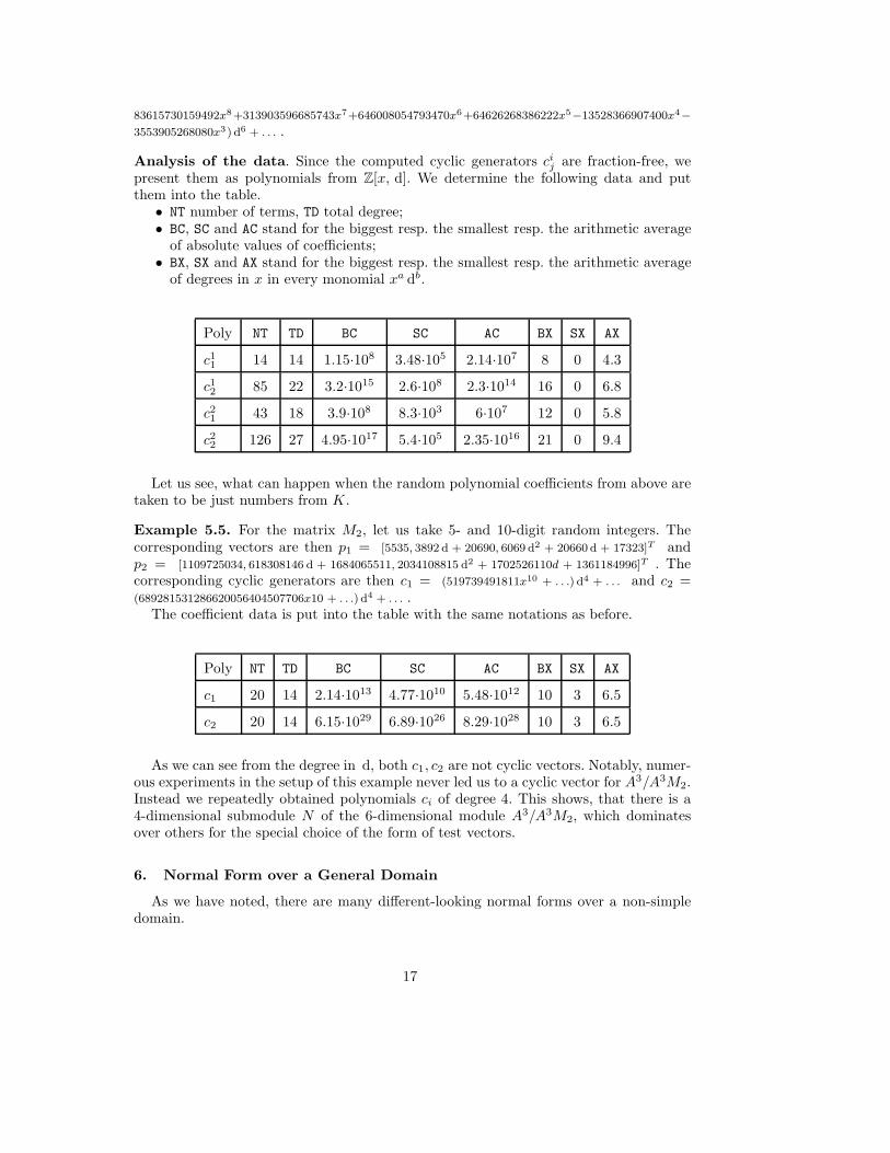
Analysis of the data. Since the computed cyclic generators cij are fraction-free, wepresent them as polynomials from Z[x, d]. We determine the following data and putthem into the table.• NT number of terms, TD total degree;• BC, SC and AC stand for the biggest resp. the smallest resp. the arithmetic averageof absolute values of coefficients;• BX, SX and AX stand for the biggest resp. the smallest resp. the arithmetic averageof degrees in x in every monomial xa db.

Poly NT TD BC SC AC BX SX AX

c11 14 14 1.15·108 3.48·105 2.14·107 8 0 4.3

c12 85 22 3.2·1015 2.6·108 2.3·1014 16 0 6.8

c21 43 18 3.9·108 8.3·103 6·107 12 0 5.8

c22 126 27 4.95·1017 5.4·105 2.35·1016 21 0 9.4

Let us see, what can happen when the random polynomial coefficients from above aretaken to be just numbers from K.

Example 5.5. For the matrix M2, let us take 5- and 10-digit random integers. Thecorresponding vectors are then p1 = [5535, 3892 d + 20690, 6069 d2 + 20660 d + 17323]T andp2 = [1109725034, 618308146 d + 1684065511, 2034108815 d2 + 1702526110d + 1361184996]T . Thecorresponding cyclic generators are then c1 = (519739491811x10 + . . .) d4 + . . . and c2 =(689281531286620056404507706x10 + . . .) d4 + . . . .

The coefficient data is put into the table with the same notations as before.

Poly NT TD BC SC AC BX SX AX

c1 20 14 2.14·1013 4.77·1010 5.48·1012 10 3 6.5

c2 20 14 6.15·1029 6.89·1026 8.29·1028 10 3 6.5

As we can see from the degree in d, both c1, c2 are not cyclic vectors. Notably, numer-ous experiments in the setup of this example never led us to a cyclic vector for A3/A3M2.Instead we repeatedly obtained polynomials ci of degree 4. This shows, that there is a4-dimensional submodule N of the 6-dimensional module A3/A3M2, which dominatesover others for the special choice of the form of test vectors.

6. Normal Form over a General Domain

As we have noted, there are many different-looking normal forms over a non-simpledomain.

17

Definition 6.1. Let R be a ring. An element r ∈ R is called two-sided, if r is not adivisor of zero and R〈r〉 = 〈r〉R. It is called proper, if R〈r〉 ( R.

Though in Cohn (1971) a two-sided element has been called invariant, we proposeto use two-sided instead, due to the ubiquity of the word invariant.

Let R be a domain and a K-algebra. Then r ∈ R is proper two-sided if and only if∀s, s′ ∈ R ∃t, t′ ∈ R such that rs = tr and s′r = rt′ . If R admits a Grobner basis theory,this is the same as to say “r is a two-sided Grobner basis of the two-sided ideal 〈r〉”.It is straightforward, that for a simple domain 0 is the only proper two-sided element.

Generalizing the statement in the Example 4.4 of (Levandovskyy and Schindelar, 2011)leads to the following result.

Lemma 6.2. Let R be a non-simple Euclidean domain and a K-algebra. Moreover, letm ≤ n be natural numbers and r ∈ R be a proper two-sided element. Then for the2 × 2 matrices D1 = Diag(rm, rn) and D2 = Diag(1, rm+n) the corresponding modulesM1 = R2/R2D1 and M2 = R2/R2D2 are not isomorphic.

Proof. At first, we note that the set of proper two-sided elements is multiplicativelyclosed, thus rn, rm, rn+m are proper two-sided. As we can see, AnnR M2 = 〈rm+n〉 andAnnR M1 = AnnR(R/〈rm〉⊕R/〈rn〉) = 〈rm〉∩〈rn〉 = 〈rn〉. We have to show that the two-sided ideals AnnR M1,AnnR M2 are not equal, then the claim follows. Let S = R⊗KRopp

be the enveloping algebra of R and ι : R → S a natural embedding of K-algebras,then any two-sided ideal of R is a left ideal over S. Suppose that for two-sided ideals〈rn〉 ⊆ 〈rm+n〉. Over S we have the inequality of left ideals 〈ι(rn)〉 ⊆ 〈ι(rm+n)〉, hencethere exists s ∈ S, such that ι(rn) = sι(rm+n) = sι(rm)ι(rn). Then (sι(rm)−1)·ι(rn) = 0and hence sι(rm) = 1, since S is a domain. Thus, 〈ι(rm)〉 = S as a left ideal andhence 〈rm〉 = R, what is a contradiction to the assumption that r is a proper two-sidedelement.

Recall that for a, b ∈ R, one says that a totally divides b (and denotes a || b) if andonly if there exists a two-sided c ∈ R, such that a | c | b 5 (Cohn, 1971). Moreover, a || aif and only if a is two-sided element.

Example 6.3. In the first shift algebra R∗ = S1, cf. Example 3.15, consider the diagonalmatrices

D1 =

s+ x 0

0 s(s+ x)

and D2 =

s 0

0 s(s+ x)

.

At first, let us analyze the appearing elements for the proper two-sidedness. By computingtwo-sided Grobner bases over S1, we obtain that s is already such a basis, whereas

S1〈s+ x〉S1

= S1〈x, s〉S1

and S1〈s(s+ x)〉S1

= S1〈(x + 1)s, s2〉S1

. Thus neither s+ x nors(s + x) are proper two-sided in R∗. In the localization R = (K[x] \ 0)−1R∗, we evensee that R〈s+ x〉R = R and R〈s(s+ x)〉R = R〈s〉R.

In the matrix D2 there is a total divisibility on the diagonal. Indeed, s is propertwo-sided and s | s(s + x). Hence, for any f ∈ R the result of reduction of s withfs(s+x) = f(s+x+1)s will be (1− f(s+x+1))s ∈ 〈s〉. Hence, no reduction procedurewill lead to a unit instead of s.

5 Recall, that a | c if ∃d ∈ R such that either c = ad or c = da holds.

18

On the other hand, we see that s(s+ x) ∈ 〈s〉. Then s(s+ x)− fs = (s+ x+ 1− f)s

has degree 1 in s only for f = s− g(x), where g(x) 6= −(x+ 1). This reduction produces

[0, s(s + x)]T − (s − g(x)) · [s, s]T = [−(s − g(x))s, (g(x) + x + 1)s]T , which does not

lower the degree in the column but only interchanges terms of degrees 1 and 2. Hence

no further essential simplification is possible, since replacing s(s+ x) by a similar factor

can neither lower the degree nor lead to a two-sided element.

In the matrix D1, there is no total divisibility on the diagonal, hence we will be able

to achieve the lower degree. And indeed, for

U =

1 1

s2 + xs+ 2s s2 + xs+ 2s+ x+ 2

, V =

s+ 1 −s2 − xs− s

−1 s+ x− 1

which are R-unimodular, we obtain that

UD1V =

x 0

0 x+ 2

·

1 0

0 s(s+ x)(s + x− 1)

.

Thus D1 possesses even the Jacobson normal form Diag(1, s(s+x)(s+x− 1)) over R.

7. Implementation and Examples

Our implementation of the computation of a diagonal form together with transforma-

tion matrices is called jacobson.lib. It is distributed together with Singular (Decker

et al., 2011) since its version 3-1-0. In the Appendix we put an example of a Singular

session with input, output and explanations.

7.1. Comparison

There are other packages to compute diagonal and Jacobson forms. The package

Janet for Maple (Blinkov et al., 2003; Chyzak et al., 2007) directly follows the classical

algorithm with no special optimizations. In Maple packages by H. Cheng et al. (Becker-

mann et al., 2006; Cheng and Labahn, 2007; Davies et al., 2008) modular (Modreduce)

and fraction-free (FFreduce) versions of an order basis of a polynomial matrix M from

an Ore algebra A are implemented. The computation of the left nullspace of M and

indirectly the Popov form of M uses order bases. There are also experimental implemen-

tations, mentioned in (Culianez and Quadrat, 2005) and (Middeke, 2008).

In (Levandovskyy and Schindelar, 2011), we compared our implementation with the

one by D. Robertz. In turned out that with our implementation, one experiences moderate

swell of coefficients and obtains uncomplicated transformation matrices.

Unlike in theoretical considerations, our implementation usually returns diagonal ma-

trices with elements of descending degrees on the main diagonal.

7.2. Examples

Example 7.1. Consider two versions of the Example 3.8 in (Levandovskyy and Schin-

delar, 2011).

19

(A). In the first Weyl algebra R∗ = K[x][∂; id, ddx], consider the matrix

M =

∂2 − 1 ∂ + 1

∂2 + 1 ∂ − x

∈ R2×2.

Then the algorithm computes

UMV =

[(x+ 1)2∂2 + 2(x + 1)∂ − (x2 + 1) 0

0 1

]= D,

U =

[−(x+ 1)∂ + x2 + x+ 1 (x+ 1)∂ + x

∂ − x −∂ − 1

], V =

[1 0

(x+ 1)∂2 + 2∂ − x+ 1 1

].

Let us analyze the transformation matrices for R∗-unimodularity. Indeed, V is uni-modular over R∗ since it admits an inverse V ′. However, U is unimodular over S−1R∗

for S = (x + 1)i | i ∈ N0 (cf. Lemma 4.3) since U · Z = W and W is invertible in thering containing the inverse of (x+ 1)2, that is over a ring, containing S−1R∗.

V ′ =

[1 0

−(x+ 1) d2 − 2 d + x− 1 1

], Z =

[2( d + 1) (x+ 1) d + x− 2

2( d− x) (x+ 1) d− x2 − x− 3

],W =

[0 −4(x+ 1)2

2 5(x+ 1)

].

(B). In the first shift algebra S1, cf. Example 3.15, one has

Diag( (x+ 1)(x+ 2)s2 + 2(x+ 1)s− (x − 1)(x+ 2), 1) =[−(x+ 1)s+ x(x+ 2) (x+ 1)s+ x+ 2

−s+ x+ 1 s+ 1

]·

[s2 − 1 s+ 1

s2 + 1 s− x

]·

[1 0

−(x+ 2)s2 − 2s+ x 1

].

Denote the equality above as D = UMV , it turns out, that V is even R∗-unimodular. Ubecomes invertible in a localization, containing (x+2)−1, thus, by Lemma 4.5, containinga ring S−1R∗ for S = (x± n)m | n,m ∈ N0.

Example 7.2. Consider now the same matrix as in Example 3.15 over the first Weylalgebra R∗ = K〈x, d | dx = xd + 1〉, respectively R = K(x)〈d | dx = xd + 1〉:

M =

[(x− 1) d + x2 − x x d + x2 (x+ 2) d + x2 + 2x

d + x 0 d

].

We obtain

D =

[0 3x2(x+ 2)2 0

0 0 1

], U =

1

2

[x(x+ 2) d− 2(x+ 1) −x(x+ 2)2 d− (x4 + 4x3 + 3x2 − 4x− 4)

(x+ 1) d− 2 −(x+ 1)(x+ 2) d− (x3 + 3x2 + x− 3)

],

V =

−(x4 − 9x2) d2 − (x5 − x3 − 18x) d− (6x4 − 24x2 + 18) v12 0

−(3x3 − 27x) d2 − (x5 + 5x4 − 9x3 − 18x2 − 81) d− (x6 + 2x5 − 6x4 + 8x3 + 9x2 − 54x) v22 0

(x4 − 9x2) d2 + (2x5 − 10x3 − 18x) d + (x6 − 15x2 + 18) v23 1

,

where v12 = (x3 + 3x2 − 2x) d2 + (x4 + 3x3 + 4x2 + 6x + 2) d + (5x3 + 12x2 − 6), v22 = (3x2 +

9x − 6) · d2 + (x4 + 8x3 + 13x2 + 11x + 27) · d + (x5 + 5x4 + 6x3 + 14x2 + 42x + 23) and v23 =

−(x3 + 3x2 − 2x) d2 − (2x4 + 6x3 + 2x2 + 6x+ 2) d− (x5 + 3x4 + 8x3 + 18x2 + 12x− 6) .U is unimodular in the localization with respect to SU , which is generated as monoid byx, x+1, x+2. V is unimodular in the localization with respect to SV , which is generated

20

by x, x+2, x+3, x− 3. Thus, the isomorphism of modules lifts from R to S−1R∗, whereS = xi1(x + 1)i2(x + 2)i3(x+ 3)i4(x− 3)i5 | ij ∈ N0.

The same system over the shift algebra was computed in detail in Example 3.15. Thereit turns out, that U is unimodular over a ring containing (x+2)−1 and V is unimodularover a ring containing the inverses of x− 2, x − 1, x, x + 3, x + 4. Due to Lemma 4.5,the needed Ore set for the localization is not smaller than S = SU = SV = (x ± n)m |n,m ∈ N0.

8. Conclusion, Further Research and Open Problems

8.1. Further Research

We do not perform an analysis of the theoretical complexity of our algorithm, since ithas been designed by using Grobner bases, thus the formal complexity is too high. Indeed,one can see, that we use Grobner bases rather for convenience, that is in order to presentan algorithm, working over arbitrary OLGAED. The original (non-fraction-free) algo-rithm can be reformulated in terms of extended left and right greatest common divisorsover a concrete algebra. To the best of our knowledge, the theoretical complexity of suchGCD algorithms depends on the given algebra. For rational Weyl algebras over generalfields of characteristic zero there is a paper (Grigor’ev, 1990). It is interesting to find es-timations for classical operator algebras like the shift algebra, q-Weyl and q-commutativealgebras with rational coefficients. Having this information, one could perform complex-ity analysis for the kind of algorithms we propose. It was reported in (Middeke, 2008),that the Jacobson form can be computed in polynomial time. In our opinion this shouldbe formulated more precisely in the framework, proposed in (Grigor’ev, 1990). We donot claim that our algorithm is superior in terms of theoretical complexity to the othersbut stress, that its fraction-free version is widely applicable in practical computations. Inparticular, our algorithm returns transformation matrices with reasonable sizes of theirentries and their coefficients.

Concerning the further development of our implementation in Singular (Deckeret al., 2011) called jacobson.lib, we plan the following enhancements. In order to pro-vide diagonal form computations over q-algebras like q-commutative, q-shift, q-differenceand q-Weyl algebras, we need to find involutive antiautomorphisms. It turns out, thatthere are no K(q)-linear but K-linear involutions, which act on q as a non-identical in-volutive automorphism of K(q). We will work on finding such involutions and adapt theimplementation to the more general situation. Moreover, it is possible to employ modularGrobner bases in the implementation.

We have demonstrated, how working with a ring R∗ and its localization S−1R∗ withrespect to some Ore set S ⊂ R∗ is used in various situations. In this paper we concen-trated on rings of polynomials respectively rational functions. The same ideas in theoryimmediately apply to operator algebras R∗ = K[[x]]〈d〉 and R = K((x))〈d〉. However,in practical computations with the computer we are restricted to finite power series,presented by a Laurent polynomial.

For the Weyl and q-Weyl algebras over a field K with charK = 0, algorithmic compu-tations are possible over the local ring K[x]mp

for p ∈ Kn and mp = 〈x1−p1, . . . , xn−pn〉.Notably, the Ore completion of the set K[x] \ mp over shift and q-shift algebras willcontain zero. Thus, there is no analogon to the situation with (q)-Weyl algebras.

21

8.2. Open Problems

1. From the description and the proof of the Algorithm 3.12, we need in principle onlythe existence of a terminating Grobner basis algorithm over R resp. R∗. The latter relieson the constructivity of basic operations with fractions in R via R∗. Thus the Algorithm3.12 immediately extends to the case of a general OLGA (R,B, I) (cf. Def. 2.2) for anontrivial completely prime ideal I ⊂ B by Bueso et al. (2003). In which bigger classof algebras one can perform concrete computations? One can work with local rings likeK[x]mp

, p ∈ Kn and K[[x]] for charK = 0 or with Kx for K = R,C as coefficientdomains.

2. The algorithm computes U, V,D such that UMV = D. It is clear, that U, V arenot unique. By fixing M and D, how can one describe the set (U, V ) | UMV = D?Does there exist U ′ resp. V ′ from this set, such that special properties like unimodularityhold? This is connected, in particular, to the recent results of A. Quadrat and T. Cluseau(Cluzeau and Quadrat, 2010). Namely, they prove the existence of matrices U and V ,which are unimodular over R∗ for certain situations and present an algorithm for thecomputation of these matrices.

3. One of the most important problems in non-commutative computer algebra is toshow algorithmically, that two given finitely presented modules are not isomorphic. It isstill open even for cyclic modules over general simple Euclidean Ore domain. Namely,let R be the latter domain and a, b ∈ R with deg a = deg b > 0. Up to now there is noalgorithm, which determines that R/〈a〉 6∼= R/〈b〉. However, there are several situations,where this question has been solved.

In Cluzeau and Quadrat (2008), the authors presented a semi-algorithm for finitelypresented modules. Given degree bounds for the variables, the algorithm first looks formatrices, determining a homomorphism. If such a pair has been found, the kernel andcokernel of the corresponding homomorphism are computed and returned.

4. As we have seen, over non-simple domains we have many different normal forms.Starting with classical operator algebras like the (q-)shift algebra and q-Weyl algebra, itis important to describe possible normal forms.

5. As in the previous item, what is the most probable normal form for a random squarematrix (which is then of full rank) over a non-simple domain? Though it seems that thismight depend on the algebra, we conjecture the Diag(1, .., 1, p), that is a Jacobson form,is the most probable one. Such approach might lead to the classification as in 4.

Acknowledgments

We express our gratitude to Eva Zerz and Hans Schonemann for discussions and theiradvice on numerous aspects of the problems, treated in this article. We thank DanielRobertz, Johannes Middeke and Howard Cheng for explanations about respective imple-mentations. We are grateful to Mark Giesbrecht, George Labahn and Dima Grigoriev fordiscussions concerning normal forms for matrices and complexity of algorithms. Manythanks to Moulay Barkatou and Sergey Abramov for explanations of their algorithms forlinear functional systems. The first author is grateful to the SCIEnce project (Transna-tional access) at RISC for supporting his visits to RISC and the usage of computationalinfrastructure at RISC. We would like to thank the anonymous referees, who helped usa lot with their insightful remarks and suggestions. Kristina Schindelar carried out herwork on this paper during her Ph.D. studies at Lehrstuhl D fur Mathematik of RWTHAachen University.

22

References

Apel, J., 1988. Grobnerbasen in nichtkommutativen Algebren und ihre Anwendung. Dis-sertation, Universitat Leipzig.

Beckermann, B., Cheng, H., Labahn, G., 2006. Fraction-free row reduction of matricesof Ore polynomials. J. Symbolic Computation 41 (5), 513–543.

Blinkov, Y. A., Cid, C. F., Gerdt, V. P., Plesken, W., Robertz, D., 2003. The MAPLEpackage ”janet”: II. Linear Partial Differential Equations. In: Proceedings of the 6thInternational Workshop on Computer Algebra in Scientific Computing. pp. 41–54.URL http://wwwb.math.rwth-aachen.de/Janet

Bueso, J., Gomez-Torrecillas, J., Verschoren, A., 2003. Algorithmic methods in non-commutative algebra. Applications to quantum groups. Kluwer Academic Publishers.

Cheng, H., Labahn, G., 2007. Modular computation for matrices of Ore polynomials. In:Computer Algebra 2006: Latest Advances in Symbolic Algorithms. pp. 43–66.

Chyzak, F., Quadrat, A., Robertz, D., 2007. OreModules: A symbolic package forthe study of multidimensional linear systems. In: Chiasson, J., Loiseau, J.-J. (Eds.),Applications of Time-Delay Systems. Springer LNCIS 352, pp. 233–264.URL http://wwwb.math.rwth-aachen.de/OreModules

Chyzak, F., Salvy, B., 1998. Non–commutative elimination in Ore algebras proves mul-tivariate identities. J. Symbolic Computation 26 (2), 187–227.

Cluzeau, T., Quadrat, A., 2008. Factoring and decomposing a class of linear functionalsystems. Linear Algebra and its Applications 428 (1), 324 – 381.

Cluzeau, T., Quadrat, A., 2010. Serre’s reduction of linear partial differential systemswith holonomic adjoints. Tech. Rep. 7486, INRIA.

Cohn, C., 1971. Free Rings and their Relations. Academic Press.Culianez, G., Quadrat, A., 2005. Formes de Hermite et de Jacobson: implementations etapplications. Tech. rep., INRIA Sophia Antipolis.

Davies, P., Cheng, H., Labahn, G., 2008. Computing Popov form of general Ore polyno-mial matrices. In: Proceedings of the Milestones in Computer Algebra (MICA) Con-ference. pp. 149–156.

Decker, W., Greuel, G.-M., Pfister, G., Schonemann, H., 2011. Singular 3-1-3 — Acomputer algebra system for polynomial computations.URL http://www.singular.uni-kl.de

Garcıa Garcıa, J. I., Garcıa Miranda, J., Lobillo, F. J., 2009. Elimination orderings andlocalization in PBW algebras. Linear Algebra Appl. 430 (8-9), 2133–2148.

Gianni, P., Trager, B., Zacharias, G., 1988. Grobner bases and primary decompositionof polynomial ideals. J. Symbolic Computation 6 (2-3), 149–167.

Greuel, G.-M., Levandovskyy, V., Motsak, O., Schonemann, H., 2010. Plural. A Sin-

gular 3-1 Subsystem for Computations with Non-commutative Polynomial Algebras.URL http://www.singular.uni-kl.de

Grigor’ev, D., 1990. Complexity of factoring and calculating the GCD of linear ordinarydifferential operators. J. Symbolic Computation 10 (1), 7 – 37.

Ilchmann, A., Mehrmann, V., 2006. A behavioral approach to time-varying linear sys-tems. I: General theory. SIAM J. Control Optim. 44 (5), 1725–1747.

Ilchmann, A., Nurnberger, I., Schmale, W., 1984. Time-varying polynomial matrix sys-tems. Int. J. Control 40, 329–362.

23

Insua, M. A., 2005. Varias perspectives sobre las bases de Grobner: Forma normal deSmith, Algoritme de Berlekamp y algebras de Leibniz. Ph.D. thesis, Universidade deSantiago de Compostela, Spain.

Jacobson, N., 1943. The Theory of Rings. American Mathematical Society.Kaltofen, E., Krishnamoorthy, M. S., Saunders, B. D., 1989. Mr. Smith goes to Las Vegas:Randomized parallel computation of the Smith normal form of polynomial matrices.In: Davenport, J. H. (Ed.), Proc. EUROCAL ’87. Vol. 378 of LNCS. Springer, pp.317–322.

Kredel, H., 1993. Solvable polynomial rings. Shaker.URL http://krum.rz.uni-mannheim.de/publicatons.html

Levandovskyy, V., 2005. Non-commutative computer algebra for polynomial algebras:Grobner bases, applications and implementation. Ph.D. thesis, Universitat Kaiser-slautern.URL http://kluedo.ub.uni-kl.de/volltexte/2005/1883/

Levandovskyy, V., Schindelar, K., 2011. Computing diagonal form and Jacobson normalform of a matrix using Grobner bases. J. Symbolic Computation, 46 (5), 595–608.

Levandovskyy, V., Schonemann, H., 2003. Plural — a computer algebra system for non-commutative polynomial algebras. In: Proc. of the International Symposium on Sym-bolic and Algebraic Computation (ISSAC’03). ACM Press, pp. 176 – 183.URL http://doi.acm.org/10.1145/860854.860895

Leykin, A., 2003. Algorithms in computational algebraic analysis. Ph.D. dissertation,University of Minnesota.URL http://scholar.lib.vt.edu/theses/available/etd-03262004-082608/

Lubeck, F., 2002. On the computation of elementary divisors of integer matrices. J.Symbolic Computation 33 (1), 57–65.

Middeke, J., 2008. A polynomial-time algorithm for the Jacobson form for matrices ofdifferential operators. Tech. Rep. 2008-13, RISC, J. Kepler University Linz.

Storjohann, A., Labahn, G., 1997. A fast Las Vegas algorithm for computing the Smithnormal form of a polynomial matrix. Linear Algebra Appl. 253, 155–173.

Zariski, O., Samuel, P., 1975. Commutative Algebra. Vol. 1. With the cooperation of I.S. Cohen. 2nd ed. Graduate Texts in Mathematics. 28. Springer-Verlag.

Zerz, E., 2006. An algebraic analysis approach to linear time-varying systems. IMA J.Math. Control Inf. 23 (1), 113–126.

Zerz, E., 2007. State representations of time-varying linear systems. In: Park, H., Re-gensburger, G. (Eds.), Grobner Bases in Control Theory and Signal Processing. Vol. 3of Radon Series Comp. Appl. Math. Walter de Gruyter & Co., pp. 235–251.

9. Appendix. The Code for an Example

Consider the code for Example 3.15. After starting a Singular session, we need toset up the algebra first.> LIB "jacobson.lib"; // load the library

> ring w = 0,(x,s),(a(0,1),Dp);

The ring w is a commutative one in variables x,s over the field Q (0 stands for thecharacteristic). The substring (a(0,1),Dp) defines a monomial ordering on w, which inthis case is an extra weight ordering, assigning weights 0 to x and 1 to s. If two mono-mials are of the same weight, they are further compared with Dp (degree lexicographic

24

ordering). The described ordering mimicks the ordering on the rational shift algebra. Forcomputations one can also use other orderings, like Dp or dp, cf. the Singular manual.> def W=nc_algebra(1,s); // set up shift algebra

> setring W;

This code creates and sets active a new ring W as a non-commutative ring from w withthe relation s · x = 1 · xs + s. By executing W; a user will obtain the description of theactive ring.> matrix m[2][3]=

> x*s-s+x^2-x, x*s+x^2, x*s+2*s+x^2+2*x,

> s+x,0,s;

> list J=jacobson(m,0);

Here the matrix was entered and the algorithm called. Note, that putting a stringprintlevel=2; before the jacobson call will output the progress of the algorithm. Highervalues of printlevel will lead to more details printed during the execution. The list Jhas three entries, namely U,D, V .> print(J[1]*m*J[3]-J[2]); // check UmV=D

==> 0,0,0,

0,0,0

> print(J[2]); // that is D

==> 0,x4+3x3-x2-3x,0,

0,0, x

> print(J[1]); // that is U

==> 0, -1/4x2-x-3/4,

1/4,-1/4x-1/2

> print(J[3]); // that is V

==> _[1,1],_[1,2],xs2-s2+x2s-xs,

_[2,1],_[2,2],_[2,3],

_[3,1],_[3,2],_[3,3]

The symbols _[2,2] before are printed, when the entries are long. One can access themas single polynomials> print(J[3][2,2]);

==> -21s2-7x2s-2xs+11s-3x3-2x2+13x-8

25