Northeast Area Monitoring and Assessment Program (NEAMAP)

Data collection and analysis in support of single and multispecies stock assessments in the Mid-Atlantic: Northeast Area Monitoring and

Assessment Program Near Shore Trawl Survey

Final Report

Award Number:

NA11NMF4540005

Award Period:

January 1, 2011 to December 31, 2011

Submitted to:

National Oceanographic and Atmospheric Administration, National Marine Fisheries Service - Northeast Fisheries Science Center

& Mid-Atlantic Fishery Management Council

By:

Christopher F. Bonzek James Gartland

Debra J. Gauthier Robert J. Latour, Ph.D.

Department of Fisheries Science Virginia Institute of Marine Science

College of William and Mary Gloucester Point, Virginia

March 2012

Table of Contents

Introduction ........................................................................................................................ 1

Methods .............................................................................................................................. 2

Results ............................................................................................................................... 13

Literature Cited................................................................................................................. 55

Figures

Survey Area ........................................................................................................... 57 Sampling Sites ....................................................................................................... 58 Bottom Temperatures .......................................................................................... 64 Gear Performance ................................................................................................. 73 Trawl Door Tilt Sensor Results .............................................................................. 74 Atlantic Sturgeon Catch History ............................................................................ 75 Sea Turtle Catch History ........................................................................................ 76 Coastal Shark Catch History .................................................................................. 77

Species Data Summaries (Figures and Tables)

Alewife .................................................................................................................. 78 American Lobster .................................................................................................. 85 American Shad ...................................................................................................... 91 Atlantic Croaker .................................................................................................... 98 Atlantic Menhaden ............................................................................................. 110 Bay Anchovy ........................................................................................................ 116 Black Sea Bass ..................................................................................................... 120 Blueback Herring ................................................................................................. 127 Bluefish................................................................................................................ 133 Brown Shrimp ..................................................................................................... 143 Butterfish ............................................................................................................ 147 Clearnose Skate ................................................................................................... 153 Horseshoe Crab ................................................................................................... 160 Kingfish ................................................................................................................ 166 Little Skate........................................................................................................... 170 Longfin Inshore Squid ......................................................................................... 177 Scup ..................................................................................................................... 181 Silver Hake........................................................................................................... 192

Smooth Dogfish ................................................................................................... 199 Spanish Mackerel ................................................................................................ 206 Spiny Dogfish ....................................................................................................... 212 Spot ..................................................................................................................... 220 Striped Anchovy .................................................................................................. 226 Striped Bass ......................................................................................................... 230 Summer Flounder ............................................................................................... 237 Weakfish ............................................................................................................. 250 White Shrimp ...................................................................................................... 263 Windowpane Flounder ....................................................................................... 267 Winter Flounder .................................................................................................. 271 Winter Skate ....................................................................................................... 284

1

Introduction Concerns regarding the status of fishery-independent data collection from continental shelf waters between Cape Hatteras, North Carolina and the U.S. / Canadian border led the Atlantic States Marine Fisheries Commission’s (ASMFC) Management and Science Committee (MSC) to draft a resolution in 1997 calling for the formation of the Northeast Area Monitoring and Assessment Program (NEAMAP) (ASMFC 2002). NEAMAP is a cooperative state-federal program modeled after the Southeast Area Monitoring and Assessment Program (SEAMAP), which has been coordinating fishery-independent data collection south of Cape Hatteras since the mid-1980s (Rester 2001). The four main goals of this new program directly address the deficiencies noted by the MSC for this region and include 1) developing fishery-independent surveys for areas where current sampling is either inadequate or absent 2) coordinating data collection among existing surveys as well as any new surveys 3) providing for efficient management and dissemination of data and 4) establishing outreach programs (ASMFC 2002). The NEAMAP Memorandum of Understanding was signed by all partner agencies by July 2004. One of the first major efforts of the NEAMAP was to design a trawl survey that would operate in the coastal zone (i.e., between the 6.1 m and 27.4 m depth contours) of the Mid-Atlantic Bight (MAB - i.e., Montauk, New York to Cape Hatteras, North Carolina). The National Marine Fisheries Service (NMFS), Northeast Fisheries Science Center’s (NEFSC) Bottom Trawl Survey had been sampling from Cape Hatteras to the U.S./Canadian border in waters less than 366 m since 1963 (NEFSC 1998, R. Brown, NMFS, pers. comm.), with areas inshore of the 27.4 m contour sampled at lower densities than desired to assess coastal species managed by the Atlantic States Marine Fisheries Commission. In addition, of the six coastal states in the MAB, only New Jersey conducts a fishery-independent trawl survey in its coastal zone (Byrne 2004). The NEAMAP Near Shore Trawl Survey was therefore developed to address this gap in fishery-independent survey coverage, which is consistent with the program goals. The main objectives of this new survey were defined to include the estimation of abundance, biomass, length frequency distribution, age-structure, diet composition, and various other assessment-related parameters for fishes and select invertebrates inhabiting the survey area. In early 2005, the ASMFC received $250,000 through the Atlantic Coastal Fisheries Cooperative Management Act (ACFCMA) and made these funds available for pilot work designed to assess the viability of the NEAMAP Near Shore Trawl Survey. The Virginia Institute of Marine Science (VIMS) provided the sole response to the Commission’s request for proposals and was awarded the contract for this work in August 2005. VIMS conducted two brief pre-pilot cruises and a full pilot survey in 2006 (Bonzek et al. 2007). Following a favorable review of the pilot sampling, the ASMFC bundled funds from a combination of sources in an effort to provide the resources necessary to support the initiation of full-scale sampling operations for NEAMAP. The ASMFC awarded VIMS this new contract in the late spring of 2007, and the first full NEAMAP cruise was scheduled for fall 2007.

2

Two significant changes to the NEAMAP survey area were implemented prior to this first full-scale cruise:

• In 2007, the NEFSC took delivery of the FSV Henry B. Bigelow, began preliminary sampling operations with this new vessel, and determined that this boat could safely operate in waters as shallow as 18.3 m. NEFSC personnel then determined that future surveys would likely extend inshore to that depth contour (R. Brown, NMFS, pers. comm.). The NEAMAP Operations Committee subsequently decided that the offshore boundary of the NEAMAP survey between Montauk and Cape Hatteras should be realigned to coincide with the inshore boundary of the NEFSC survey, and that NEAMAP should discontinue sampling between the 18.3 m and 27.4 m contours in these waters.

• The NEFSC contributed an appreciable amount of funding toward NEAMAP full implementation with the provision that Block Island Sound (BIS) and Rhode Island Sound (RIS), regions that were under-sampled at the time, be added to the NEAMAP sampling area. These waters are deeper than those sampled along the coast by NEAMAP; however, the offshore extent of sampling in these sounds (with respect to distance from shore) is consistent with that along the coast. The NEAMAP Survey has sampled BIS and RIS since the fall of 2007 and intends to continue to do so.

VIMS acquired funding for full sampling (i.e., two cruises, one in the spring and one in the fall, each covering the entire survey range) in 2008 from two sources, ASMFC “Plus-up” funds and Research Set-Aside (RSA) quota provided by the Mid-Atlantic Fishery Management Council and the National Oceanographic and Atmospheric Administration (NOAA). ASMFC “Plus-up” was used for the spring survey, while the proceeds derived from the auction of RSA quota supported the fall cruise. All sampling in 2009 and 2010 was funded through the Mid-Atlantic RSA Program; for 2011 (and 2012), partial support (approximately 20%) was gained though the Commercial Fisheries Research Foundation (CFRF) for operations in BIS and RIS. This report summarizes the results of the both the spring and fall 2011 survey cruises and for some analyses includes data for all prior cruises. Methods The following protocols and procedures were developed by the ASMFC NEAMAP Operations Committee, Trawl Technical Committee, and survey personnel at VIMS and approved through an external peer review of the NEAMAP Trawl Survey. This review was conducted in December 2008 in Virginia Beach, Virginia, and all associated documents are currently available (Bonzek et al. 2008, ASMFC 2009). While the review found no major deficiencies with the survey, some recommendations were offered to improve data collection both in the field and in the laboratory. Efforts to implement these suggestions are ongoing and are discussed in the following sections where they occur. Stratification of the Survey Area / Station Selection Sampling sites are selected for each cruise of the NEAMAP Near Shore Trawl Survey using a stratified random design. During the planning stages of the survey, the Operations Committee and personnel at VIMS developed a stratification scheme for the survey area. Because the

3

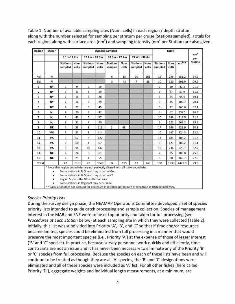
NEFSC sampled these same waters for decades prior to the arrival of the Bigelow, and since the NEAMAP Survey is effectively viewed as an inshore compliment to the NEFSC Bottom Trawl Surveys, consistency with the historical strata boundaries used by the NEFSC for the inshore waters of the MAB and Southern New England (SNE) was the primary consideration. Alternate stratification options for the near shore coastal zone (i.e., NEAMAP sampling area) were also open for consideration, however, given NEFSC plans to reevaluate the stratification of their survey area in the near future. An examination of NEFSC inshore strata revealed that the major divisions among survey regions (latitudinal divisions from New Jersey to the south, longitudinal divisions off of Long Island and in BIS and RIS) generally correspond well with major estuarine outflows (Figure 1). These boundary definitions were therefore adopted for use by the NEAMAP Survey; minor modifications were made to align regional boundaries more closely with state borders. Evaluation of the NEFSC depth strata definitions, however, indicated that in some areas (primarily in the more southern regions) near shore stratum boundaries did not correspond well to actual depth contours. NEAMAP depth strata were therefore redrawn using depth sounding data from the National Ocean Service and strata ranges of 6.1 m - 12.2 m and 12.2 m - 18.3 m from Montauk to Cape Hatteras, and 18.3 m - 27.4 m and 27.4 m - 36.6 m in BIS and RIS. Following the delineation of strata, each region / depth stratum combination was subdivided into a grid pattern, with each cell of the grid measuring 1.5 x 1.5 minutes (1.8 nm2 , corrected for the difference in nm per degree of longitude at the latitudes sampled by the survey) and representing a potential sampling site. One of the main goals of the NEAMAP trawl survey is to increase fishery-independent sampling intensity in the nearshore zone of the MAB and SNE. When designing the survey, it was decided that the target sampling intensity would be approximately 1 station per 30 nm2, a moderately high intensity when compared with other fishery-independent trawl surveys operating along the US East Coast. This intensity, when applied to the NEAMAP survey area, results in the sampling of 150 sites per cruise. The number of cells (sites) to be sampled in each stratum during each survey cruise was then determined by proportional allocation, based on the surface area of each stratum (Table 1). A minimum of 2 sites was assigned to smallest of the strata (i.e., those receiving less than 2 based on proportional allocation). Prior to each survey, a SAS program is used to randomly select the cells to be sampled from each region / depth stratum during that cruise (SAS, 2002). Again, the number of cells selected in a particular stratum is proportional to the surface area of that stratum. Once these 150 ‘primary’ sampling sites (i.e., those to be sampled during the upcoming cruise) are generated, the program is run a second time to produce a set of ‘alternate’ sites. In instances where sampling a primary site is not possible due to fixed gear, bad bottom, vessel traffic, etc., an alternate site is selected in its stead. If an alternate is sampled in the place of an untowable primary, the alternate is required to occupy the same region / depth stratum as the aberrant primary. Usually, the alternate chosen is the closest towable alternate to that primary. The actual locations sampled during both 2011 cruises are provided (Figure 2.).

4

Table 1. Number of available sampling sites (Num. cells) in each region / depth stratum along with the number selected for sampling per stratum per cruise (Stations sampled). Totals for each region, along with surface area (nm2) and sampling intensity (nm2 per Station) are also given.

Species Priority Lists During the survey design phase, the NEAMAP Operations Committee developed a set of species priority lists intended to guide catch processing and sample collection. Species of management interest in the MAB and SNE were to be of top priority and taken for full processing (see Procedures at Each Station below) at each sampling site in which they were collected (Table 2). Initially, this list was subdivided into Priority ‘A’, ‘B’, and ‘C’ so that if time and/or resources became limited, species could be eliminated from full processing in a manner that would preserve the most important species (i.e., Priority ‘A’) at the expense of those of lesser interest (‘B’ and ‘C’ species). In practice, because survey personnel work quickly and efficiently, time constraints are not an issue and it has never been necessary to eliminate any of the Priority ‘B’ or ‘C’ species from full processing. Because the species on each of these lists have been and will continue to be treated as though they are all ‘A’ species, the ‘B’ and ‘C’ designations were eliminated and all of these species were included as ‘A’ list. For all other fishes (here called Priority ‘D’), aggregate weights and individual length measurements, at a minimum, are

Region State* Stations Sampled Totals nm2 per

Station 6.1m-12.2m 12.2m – 18.3m 18.3m – 27.4m 27.4m –36.6m

Stations sampled

Num. cells

Stations sampled

Num. cells

Stations sampled

Num. cells

Stations sampled

Num. cells

Stations sampled

Num. cells

nm2**

RIS RI 6 85 10 161 16 246 553.2 34.6

BIS RI 3 42 7 88 10 130 291.9 29.2

1 NY 0 0 2 19 2 19 42.3 21.2

2 NY 2 8 3 19 5 27 57.9 11.6

3 NY 2 16 3 28 5 44 95.4 19.1

4 NY 2 16 3 29 5 45 100.7 20.1

5 NY 2 27 3 45 5 72 160.6 32.1

6 NJ 2 20 3 42 5 62 132.1 26.4

7 NJ 4 49 6 97 10 146 318.9 31.9

8 NJ 2 32 7 90 9 122 269.2 29.9

9 DE 4 53 8 113 5 68 17 166 523.9 30.8

10 MD 2 33 8 114 10 147 324.3 32.4

11 VA 5 62 8 122 13 184 408.2 31.4

12 VA 5 60 4 67 9 127 280.2 31.1

13 VA 6 94 10 142 16 236 523.7 32.7

14 NC 2 24 5 61 7 85 180.8 25.8

15 NC 2 25 4 55 6 80 165.7 27.6

Total 42 519 77 1043 14 195 17 249 150 1938 4429.0 29.5 * Note that region boundaries are not perfectly aligned with all state boundaries:

• Some stations in RI Sound may occur in MA • Some stations in BI Sound may occur in NY • Region 5 spans the NY-NJ Harbor area • Some stations in Region 9 may occur in NJ

** Calculation does not account for decreases in distance per minute of longitude as latitude increases.

5

recorded. A third category (‘E’) includes species which require special handling, such as sharks (other than dogfish) and sturgeon, which are measured, weighed, tagged, and released. Select invertebrates of management interest are also Priority ‘E’ species; individual length, weight, and sex are recorded, at a minimum, from these. Table 2. Species priority lists (A list only – includes all species from the A-C categories presented in previous reports).

A LIST Alewife Alosa pseudoharengus Pollock Pollachius virens All skate species Leucoraja sp. & Raja sp. Red drum Sciaenops ocellatus American shad Alosa sapidissima Scup Stenotomus chrysops Atlantic cod Gadus morhua Silver hake Merluccius bilinearis Atlantic croaker Micropogonias undulatus Smooth dogfish Mustelus canis Atlantic herring Clupea harengus Spanish mackerel Scomberomorus maculatus Atlantic mackerel Scomber scombrus Speckled trout Cynoscion nebulosus Atlantic menhaden Brevoortia tyrannus Spiny dogfish Squalus acanthias Black drum Pogonias cromis Spot Leiostomus xanthurus Black sea bass Centropristis striata Striped bass Morone saxatilis Blueback herring Alosa aestivalis Summer flounder Paralichthys dentatus Bluefish Pomatomus saltatrix Tautog Tautoga onitis Butterfish Peprilus triacanthus Weakfish Cynoscion regalis Haddock Melanogrammus aeglefinus Winter founder Pseudopleuronectes americanus

Monkfish Lophius americanus Yellowtail flounder Limanda ferruginea Gear Performance The NEAMAP Survey uses the 400 x 12cm, three-bridle four-seam bottom trawl designed by the Mid-Atlantic / New England Fishery Management Council Trawl Survey Advisory Panel for all sampling operations. This net is paired with a set of Thyboron, Type IV 66” doors. Wingspread, doorspread, and headrope height were monitored during each tow of the spring and fall 2011 cruises using a digital Netmind® Trawl Monitoring System. Bottom contact of the footgear was also evaluated using the Netmind system. Wingspread sensors were positioned on the middle ‘jib’ of the net, which is consistent with NEFSC procedures for this gear, and doorspread sensors were mounted in the trawl doors according to manufacturer specifications. The headrope sensor was affixed to the center of the headline. The bottom contact sensor, which is effectively an inclinometer, was attached to the center of the footrope and used to evaluate the timing of the initial bottom contact of the footgear at the beginning of a tow, liftoff of the footgear during haulback, and the behavior of the gear throughout each tow. The inclusion of this bottom contact sensor was based on the recommendations of the NEAMAP peer review panel. The bottom contact sensor was attached for all tows during the fall of 2009 and the resulting data confirmed that the net was on the bottom at the proper phases of each tow. Due to the relative complexity in attaching and detaching this sensor before and after each tow, in 2011 the sensor was used for only one tow per stratum per cruise. A catch sensor was mounted

6

in the cod-end, and set to signal when the catch reached approximately 2,200 kg. GPS coordinates and vessel speed were recorded every 2 seconds during each tow. These data were used to plot tow tracks for each station. It is important to note that, while the performance of the survey gear had been recorded on all previous cruises, NEAMAP began to use these data to assess tow validity in 2009. The peer review panel recommended that acceptable ranges be defined for headrope height and wingspread such that if the average value of either or both of these parameters for a given tow fell outside of these ranges, the tow be considered invalid, the catch discarded, and a re-tow of the sampling site be initiated. Doorspread was not included since doorspread and wingspread are typically highly correlated (Gómez and Jiménez 1994). Such a procedure is intended to promote consistency in the performance of the survey gear and resulting catch data. The review panel and VIMS personnel agreed that 4.7 m to 5.8 m would be an appropriate range for headrope height while 12.3 m to 14.7 m would be acceptable for wingspread. These values were generated by adding to the optimal ranges of each parameter (defined by the Trawl Survey Advisory Panel), 5% of the midpoint of each range. This use of trawl performance to assess tow validity was used successfully during both the spring and fall 2011 survey cruises, and it was not necessary to discard any tows due to poor gear performance. Procedures at Each Sampling Site The F/V Darana R served as the sampling platform for all field operations in 2011 as well as for all previous surveys (both pilot and full-scale cruises). This vessel is a 27.4 m (waterline length) commercial stern-dragger, owned and operated by Captain James A. Ruhle, Sr. of Wanchese, North Carolina. All fishing operations were conducted during daylight hours. Standard tows were 20 minutes in duration with a target tow speed of 3.0 kts. During the spring 2011 cruise, three tows were truncated at less than the full 20 minutes, one due to triggering of the catch sensor (17 minutes), and two due to logistical constraints (15 and 19 minutes). Five tows were shortened during the fall 2011 cruise, two due to the catch sensor activating (17 and 19 minutes) and three others due factors such as fixed gear and grass or mud buildup in the net, as evidenced by the net measurements contracting to reach the predefined limits (18, 18, and 19 minutes). At each station, several standard variables were recorded. These included:

• Station identification parameters - date, station number, stratum, station sampling cell number.

• Tow parameters - beginning & ending tow location, vessel speed & direction, engine RPMs, duration of tow, water depth, current direction.

• Gear identification and operational parameters - net type code & net number, door type code & door numbers, tow warp length, trawl door spread, wing spread, headline height & bottom contact of the footgear.

• Atmospheric and weather data - air temperature, wind speed & direction, barometric pressure, relative humidity, general weather state, sea state.

• Hydrographic data - water temperature, salinity, and dissolved oxygen.

7

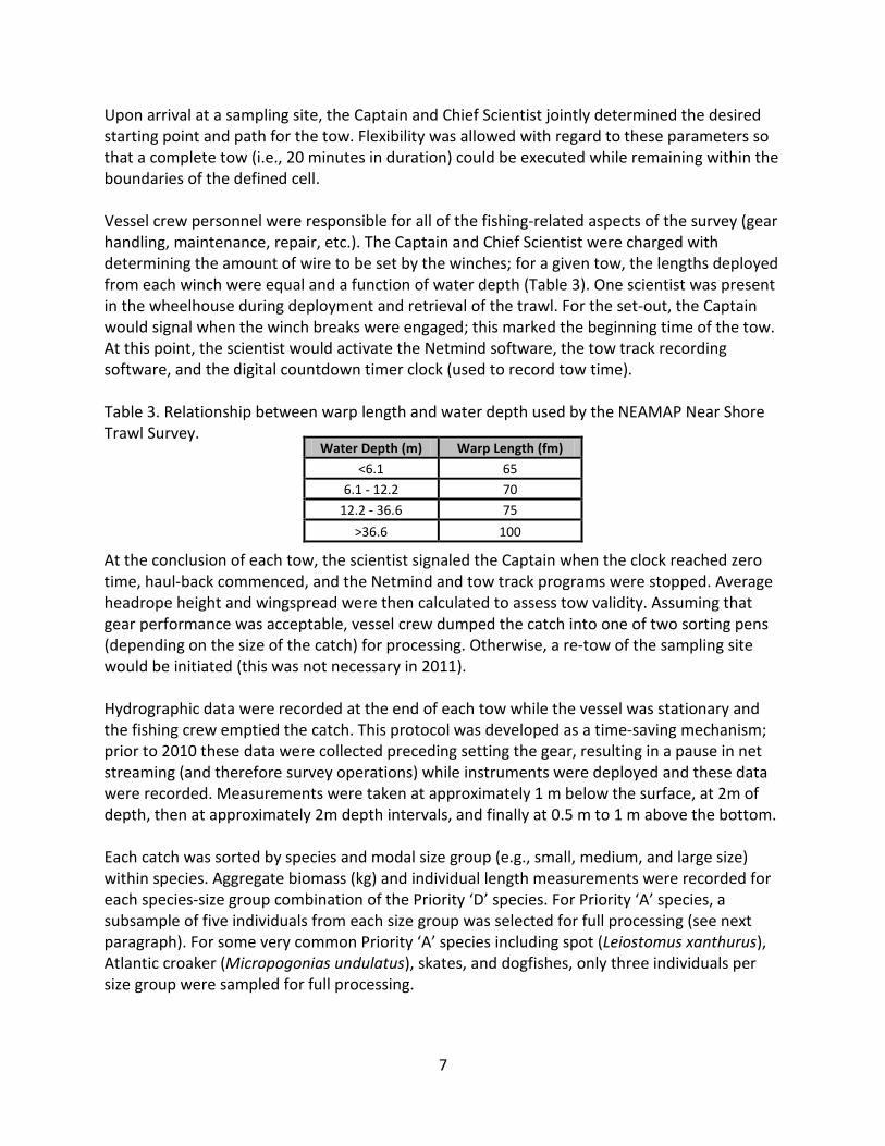
Upon arrival at a sampling site, the Captain and Chief Scientist jointly determined the desired starting point and path for the tow. Flexibility was allowed with regard to these parameters so that a complete tow (i.e., 20 minutes in duration) could be executed while remaining within the boundaries of the defined cell. Vessel crew personnel were responsible for all of the fishing-related aspects of the survey (gear handling, maintenance, repair, etc.). The Captain and Chief Scientist were charged with determining the amount of wire to be set by the winches; for a given tow, the lengths deployed from each winch were equal and a function of water depth (Table 3). One scientist was present in the wheelhouse during deployment and retrieval of the trawl. For the set-out, the Captain would signal when the winch breaks were engaged; this marked the beginning time of the tow. At this point, the scientist would activate the Netmind software, the tow track recording software, and the digital countdown timer clock (used to record tow time). Table 3. Relationship between warp length and water depth used by the NEAMAP Near Shore Trawl Survey.

At the conclusion of each tow, the scientist signaled the Captain when the clock reached zero time, haul-back commenced, and the Netmind and tow track programs were stopped. Average headrope height and wingspread were then calculated to assess tow validity. Assuming that gear performance was acceptable, vessel crew dumped the catch into one of two sorting pens (depending on the size of the catch) for processing. Otherwise, a re-tow of the sampling site would be initiated (this was not necessary in 2011). Hydrographic data were recorded at the end of each tow while the vessel was stationary and the fishing crew emptied the catch. This protocol was developed as a time-saving mechanism; prior to 2010 these data were collected preceding setting the gear, resulting in a pause in net streaming (and therefore survey operations) while instruments were deployed and these data were recorded. Measurements were taken at approximately 1 m below the surface, at 2m of depth, then at approximately 2m depth intervals, and finally at 0.5 m to 1 m above the bottom. Each catch was sorted by species and modal size group (e.g., small, medium, and large size) within species. Aggregate biomass (kg) and individual length measurements were recorded for each species-size group combination of the Priority ‘D’ species. For Priority ‘A’ species, a subsample of five individuals from each size group was selected for full processing (see next paragraph). For some very common Priority ‘A’ species including spot (Leiostomus xanthurus), Atlantic croaker (Micropogonias undulatus), skates, and dogfishes, only three individuals per size group were sampled for full processing.

Water Depth (m) Warp Length (fm) <6.1 65

6.1 - 12.2 70 12.2 - 36.6 75

>36.6 100

8

Data collected from each of these subsampled specimens included individual length (mm fork length where appropriate, mm total length for species lacking a forked caudal fin, mm pre-caudal length for sharks and dogfishes, mm disk width for skates), individual whole and eviscerated weights (measured in grams, accuracy depended upon the balance on which individuals were measured), and macroscopic sex and maturity stage (immature, mature-resting, mature-ripe, mature-spent) determination. Stomachs were removed (except for spot and butterfish; previous sampling indicated that little useful data could be obtained from the stomach contents of these species) and those containing prey items were preserved for subsequent examination. Otoliths or other appropriate ageing structures were removed from each subsampled specimen for later age determination. For the Priority ‘A’ species, all specimens not selected for the full processing were weighed (aggregate weight), and individual length measurements were recorded as described for Priority ‘D’ species above. Following the recommendation of the peer review panel, the NEAMAP Survey began recording individual length, weight, and sex from an additional 15 specimens per size-class per species per tow from the following fishes: black sea bass (Centropristis striata), summer flounder (Paralichthys dentatus), striped bass (Morone saxatilis), winter flounder (Pseudopleuronectes americanus), skates, and dogfishes. These species were chosen because either they are known to exhibit sex-specific growth patterns or sex determination through the examination of external characters is possible. In the event of a large catch, appropriate subsampling methods were implemented (Bonzek et al. 2008). In accordance with recommendations of the NEAMAP peer review panel, improved subsampling methods to more closely approximate random sampling procedures were implemented in 2009 and continued throughout 2011. Laboratory Methods Otoliths and other appropriate ageing structures were (and are in the process of being) prepared according to methodology established by the NEFSC, Old Dominion University, and VIMS. Typically, one otolith was selected and mounted on a piece of 100 weight paper with a thin layer of Crystal Bond. A thin transverse section was cut through the nucleus of the otolith, perpendicular to the sulcal groove, using two Buehler diamond wafering blades and a low speed Isomet saw. The resulting section was mounted on a glass slide and covered with Crystal Bond. If necessary, the sample was wet-sanded to an appropriate thickness before being covered. Some smaller, fragile otoliths were read whole. Both sectioned and whole otoliths were most commonly viewed using transmitted light under a dissecting microscope. Other structures such as vertebrae, opercles, and spines were processed and read using the standardized and accepted methodologies for each. For all hard parts, ages were assigned as the mode of three independent readings, one by each of three readers, and were adjusted as necessary to account for the timing of sample collection and mark formation. Stomach samples were (and are being) analyzed according to standard procedures (Hyslop 1980). Prey items were identified to the lowest possible taxonomic level. Experienced

9

laboratory personnel are able to process, on average, approximately 60 to 70 stomachs per person per day. Analytical Methods Abundance Indices: The methodology employed to calculate relative abundance indices for the NEAMAP survey has evolved with nearly every annual report and is still being developed.

• Initially, as it was considered impractical to report point estimates with only one or two data points, abundance was reported as ‘minimum trawlable abundance’ by state. These were area-expanded area-swept calculations and helped show the general pattern of distribution of species of interest (Bonzek et al., 2007).

• Catch data from fishery-independent trawl surveys tend not to be normally distributed. Preliminary analyses of NEAMAP data showed that, at least for some species, these data followed a log-normal distribution. As a result, following reports utilized the stratified geometric mean of catch per standard area swept, including catch data from all stations for every species so analyzed, as an appropriate form for the abundance indices generated by this survey (Bonzek et al. 2009).

• The next iteration involved making two simultaneous changes to the methodology used for calculating abundance indices. First, due to the small number of years sampled through 2009, as stated above, prior abundances had been calculated using data from all survey strata, for all species. Given the broad geographic range of the survey, for many species this resulted in a larger than necessary number of zero values entering the calculation, as some species were rarely captured in many survey strata. These zero values both unnecessarily biased point estimates and inflated variance estimates. In 2010-2011 it was considered that enough data had been gathered over relatively warm and relatively cold years so that reasonable restrictions could be defined as to which strata were to be used for each species. Therefore strata were selected for inclusion and exclusion on a species by species basis (these defined strata can still be refined as more data are gathered in future years).

• The other change made in 2011 involved the ‘transformation’ and ‘back-transformation’ involved in calculating the geometric mean. As stated above, this and many other fishery surveys have used the geometric mean for reporting indices of abundance because survey data catch rates often approximate a log-normal distribution. However, the process of calculating the geometric mean introduces statistical anomalies in and of itself. For example, back-transformed confidence limits are non-symmetrical, and because the variance estimate itself cannot be back-transformed, coefficients of variation have to be calculated on transformed data and then reported on the back-transformed means. To address these issues, in the immediately preceding NEAMAP annual report (Bonzek 2011) we reported indices without retransforming data from the log scale. This was done on an exploratory basis and subsequently NEAMAP survey investigators recognized that the disadvantage of compression of the ranges of abundance indices due to the logarithmic scale outweighed any perceived advantages.

• For the current report, abundance estimates are presented as the (back-transformed) geometric mean, using only the strata of importance for each species.

10

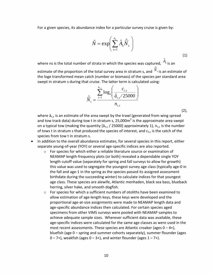
For a given species, its abundance index for a particular survey cruise is given by:

= ∑

=

sn

sss NAN

1

ˆˆexpˆ

(1)

where ns is the total number of strata in which the species was captured, sA is an

estimate of the proportion of the total survey area in stratum s, and sN is an estimate of the loge transformed mean catch (number or biomass) of the species per standard area swept in stratum s during that cruise. The latter term is calculated using:

st

n

t st

ste

s n/ac

N

st

,

1 ,

,,

25000ˆlog

ˆ∑=

=

(2), where ât,s is an estimate of the area swept by the trawl (generated from wing spread and tow track data) during tow t in stratum s, 25,000m2 is the approximate area swept on a typical tow (making the quantity [ât,s / 25000] approximately 1), nt,s is the number of tows t in stratum s that produced the species of interest, and ct,s is the catch of the species from tow t in stratum s.

• In addition to the overall abundance estimates, for several species in this report, either separate young-of-year (YOY) or several age-specific indices are also reported.

o For species for which either a reliable literature source or examination of NEAMAP length-frequency plots (or both) revealed a dependable single YOY length cutoff value (separately for spring and fall surveys to allow for growth) this value was used to segregate the youngest survey age class (typically age-0 in the fall and age-1 in the spring as the species passed its assigned assessment birthdate during the succeeding winter) to calculate indices for that youngest age class. These species are alewife, Atlantic menhaden, black sea bass, blueback herring, silver hake, and smooth dogfish.

o For species for which a sufficient numbers of otoliths have been examined to allow estimation of age-length keys, these keys were developed and the proportional age-at-size assignments were made to NEAMAP length data and age-specific abundance indices then calculated. For certain species aged specimens from other VIMS surveys were pooled with NEAMAP samples to achieve adequate sample sizes. Wherever sufficient data was available, these age-specific indices were calculated for the same age classes as were used in the most recent assessments. These species are Atlantic croaker (ages 0 – 4+), bluefish (age 0 – spring and summer cohorts separately), summer flounder (ages 0 – 7+), weakfish (ages 0 – 3+), and winter flounder (ages 1 – 7+).

11

• NEAMAP investigators are still evaluating alternatives for abundance index calculation. Preliminary examination of NEAMAP catches indicates that for at least some species a delta lognormal based index may best fit the underlying statistical distribution of catches. While these investigators realize that these several changes can result in a certain amount of confusion by users of these data, it is still (hopefully!) early in the NEAMAP time series and it is considered preferable to eventually make these calculations as statistically robust as they can be rather than to too-early settle on an inferior methodology simply for the sake of consistency. It was hoped that these investigations could have been completed in time for the present annual report but this was not possible.

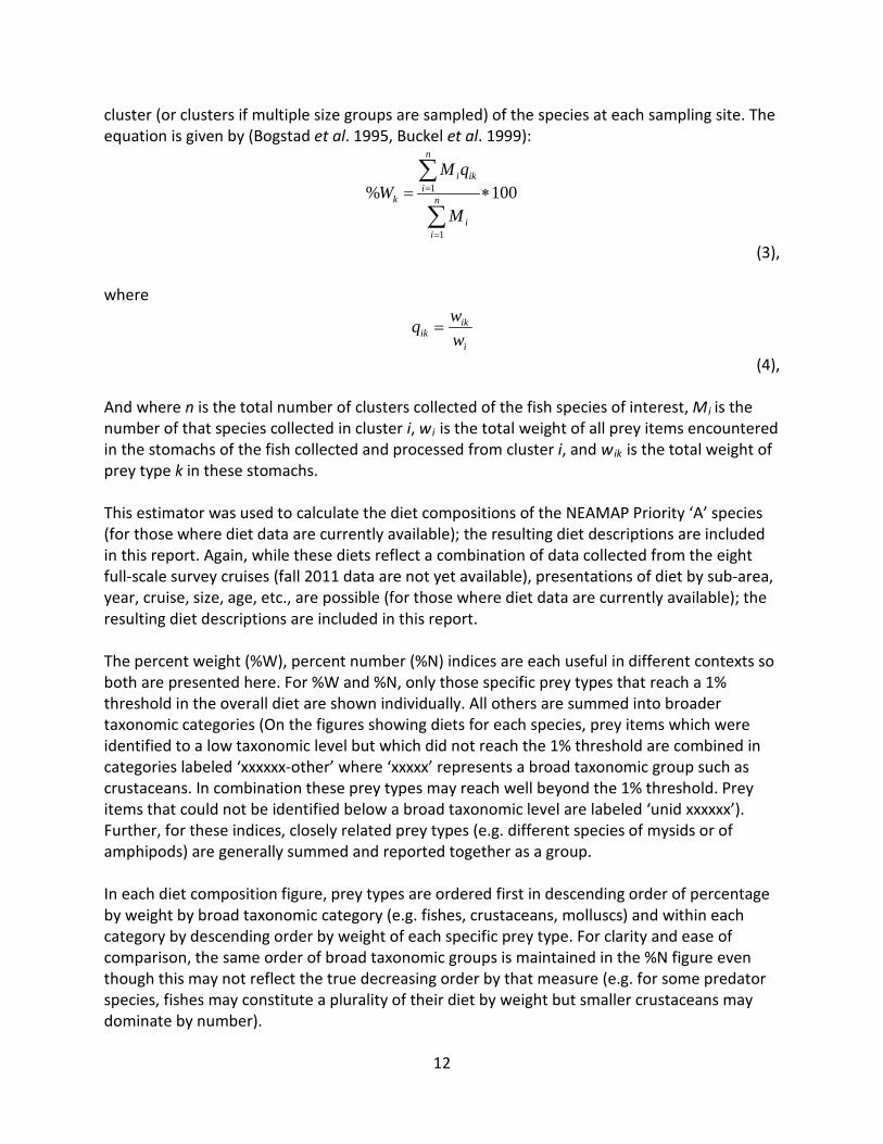
Length-Frequency: Length-frequency histograms were constructed for each species by survey cruise using 1cm or 0.5cm length bins (depending on the size range of the species). These were identified using bin midpoints (e.g., a 25cm bin represented individuals ranging from 24.5cm to 25.4cm in length). Although these histograms are presented by survey cruise, the generation of length-frequency distributions by year, sex, sub-area, overall, and a number of other variables, is possible. For this and several other stock parameters, data from specimens taken as a subsample (either for full processing or in the event of a large catch) were expanded to the entire sample (i.e., catch-level) for parameter estimation. Because of the potential for differential rates of subsampling among size groups of a given species, failure to account for such factors would bias resulting parameter estimates. In the NEAMAP database, each specimen was assigned a calculated expansion factor, which indicated the number of fish that the individual represented in the total sample for the station in which the animal was collected. Age-Structure: Age-frequency histograms were generated by cruise for each of the Priority ‘A’ species for which age data are currently available (i.e., processing, reading, and age assignment has been completed). These distributions were constructed by scaling the age data from specimens taken for full processing to the catch-level, using the expansion factors described above. Again, while the age data are presented by survey cruise, the generation of these age-structures by year, sex, sub-area, overall, and a number of other variables (or a combination of these variables), is possible. Diet Composition: It is well known that fishes distribute in temporally and spatially varying aggregations. The biological and ecological characteristics of a particular fish species collected by fishery-independent or -dependent activities inevitably reflect this underlying spatio-temporal structure. Intuitively, it follows then that the diets (and other biological parameters) of individuals captured by a single gear deployment (e.g., NEAMAP tow) will be more similar to one another than to the diets of individuals captured at a different time or location (Bogstad et al. 1995). Under this assumption, the diet index percent by weight for a given species can be represented as a cluster sampling estimator since, as implied above, trawl collections essentially yield a

12

cluster (or clusters if multiple size groups are sampled) of the species at each sampling site. The equation is given by (Bogstad et al. 1995, Buckel et al. 1999):

100%

1

1 ∗=

∑

∑

=

=n

ii

ik

n

ii

k

M

qMW

(3),

where

i

ikik w

wq =

(4), And where n is the total number of clusters collected of the fish species of interest, Mi is the number of that species collected in cluster i, wi is the total weight of all prey items encountered in the stomachs of the fish collected and processed from cluster i, and wik is the total weight of prey type k in these stomachs. This estimator was used to calculate the diet compositions of the NEAMAP Priority ‘A’ species (for those where diet data are currently available); the resulting diet descriptions are included in this report. Again, while these diets reflect a combination of data collected from the eight full-scale survey cruises (fall 2011 data are not yet available), presentations of diet by sub-area, year, cruise, size, age, etc., are possible (for those where diet data are currently available); the resulting diet descriptions are included in this report. The percent weight (%W), percent number (%N) indices are each useful in different contexts so both are presented here. For %W and %N, only those specific prey types that reach a 1% threshold in the overall diet are shown individually. All others are summed into broader taxonomic categories (On the figures showing diets for each species, prey items which were identified to a low taxonomic level but which did not reach the 1% threshold are combined in categories labeled ‘xxxxxx-other’ where ‘xxxxx’ represents a broad taxonomic group such as crustaceans. In combination these prey types may reach well beyond the 1% threshold. Prey items that could not be identified below a broad taxonomic level are labeled ‘unid xxxxxx’). Further, for these indices, closely related prey types (e.g. different species of mysids or of amphipods) are generally summed and reported together as a group. In each diet composition figure, prey types are ordered first in descending order of percentage by weight by broad taxonomic category (e.g. fishes, crustaceans, molluscs) and within each category by descending order by weight of each specific prey type. For clarity and ease of comparison, the same order of broad taxonomic groups is maintained in the %N figure even though this may not reflect the true decreasing order by that measure (e.g. for some predator species, fishes may constitute a plurality of their diet by weight but smaller crustaceans may dominate by number).

13

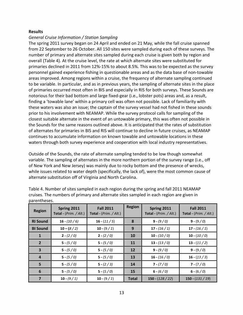
Results General Cruise Information / Station Sampling The spring 2011 survey began on 24 April and ended on 21 May, while the fall cruise spanned from 22 September to 26 October. All 150 sites were sampled during each of these surveys. The number of primary and alternate sites sampled during each cruise is given both by region and overall (Table 4). At the cruise level, the rate at which alternate sites were substituted for primaries declined in 2011 from 12%-15% to about 8.5%. This was to be expected as the survey personnel gained experience fishing in questionable areas and as the data base of non-towable areas improved. Among regions within a cruise, the frequency of alternate sampling continued to be variable. In particular, and as in previous years, the sampling of alternate sites in the place of primaries occurred most often in BIS and especially in RIS for both surveys. These Sounds are notorious for their bad bottom and large fixed-gear (i.e., lobster pots) areas and, as a result, finding a ‘towable lane’ within a primary cell was often not possible. Lack of familiarity with these waters was also an issue; the captain of the survey vessel had not fished in these sounds prior to his involvement with NEAMAP. While the survey protocol calls for sampling of the closest suitable alternate in the event of an untowable primary, this was often not possible in the Sounds for the same reasons outlined above. It is anticipated that the rates of substitution of alternates for primaries in BIS and RIS will continue to decline in future cruises, as NEAMAP continues to accumulate information on known towable and untowable locations in these waters through both survey experience and cooperation with local industry representatives. Outside of the Sounds, the rate of alternate sampling tended to be low though somewhat variable. The sampling of alternates in the more northern portion of the survey range (i.e., off of New York and New Jersey) was mainly due to rocky bottom and the presence of wrecks, while issues related to water depth (specifically, the lack of), were the most common cause of alternate substitution off of Virginia and North Carolina. Table 4. Number of sites sampled in each region during the spring and fall 2011 NEAMAP cruises. The numbers of primary and alternate sites sampled in each region are given in parentheses.

Region Spring 2011 Total - (Prim. / Alt.)

Fall 2011 Total - (Prim. / Alt.)

Region Spring 2011 Total - (Prim. / Alt.)

Fall 2011 Total - (Prim. / Alt.)

RI Sound 16 - (10 / 6) 16 - (11 / 5) 8 9 - (9 / 0) 9 - (9 / 0)

BI Sound 10 – (8 / 2) 10 - (9 / 1) 9 17 - (16 / 1) 17 - (16 / 1)

1 2 - (2 / 0) 2 - (2 / 0) 10 10 - (10 / 0) 10 - (10 / 0)

2 5 - (5 / 0) 5 - (5 / 0) 11 13 - (13 / 0) 13 - (11 / 2)

3 5 - (5 / 0) 5 - (5 / 0) 12 9 - (9 / 0) 9 - (9 / 0)

4 5 - (5 / 0) 5 - (5 / 0) 13 16 - (16 / 0) 16 - (13 / 3)

5 5 - (5 / 0) 5 - (2 / 3) 14 7 - (7 / 0) 7 - (7 / 0)

6 5 - (5 / 0) 5 - (5 / 0) 15 6 - (6 / 0) 6 - (6 / 0)

7 10 - (9 / 1) 10 - (9 / 1) Total 150 - (128 / 22) 150 - (131 / 19)

14

Water Temperature Because of the relatively narrow near shore band of water sampled by NEAMAP, catches can be influenced by environmental factors that affect the movement of fish into and out of the sampling area. Most likely, bottom temperature is a driving force in the distribution and availability of many species. For each cruise, geographic information system (GIS) figures are provided which summarize the bottom temperature data recorded at each station with interpolation among stations (Figures 3A-3I). Each figure has three representations of temperature data: a) a figure at the top of each page gives the bottom temperatures averaged over all spring or fall cruises (as appropriate), b) interpolated actual measurements from the cruise, and c) a figure with the difference between a and b. From these figures it is seen that in the spring of 2008 it was warmer than average through the sampling range; the spring of 2009 most areas were cooler than average except in southern NY and northern NJ; spring 2010 had below average bottom temperatures except in the middle portion of the sampling range between mid-NJ and VA; and in spring 2011 a mixture of above and below average temperatures was seen up and down the coast. During the fall of 2007, below average temperatures were found in RIS, BIS, to a point about halfway down Long Island and considerably above average temperatures below that point; in fall 2008 temperatures were measured as about average throughout the survey range; for the fall 2009 cruise, the 2007 pattern was exactly reversed with above average temperatures found in RIS and BIS and cool to very cool from there southward; fall 2010 again saw generally average-to-slightly-below-average temperatures through the sampling area; and temperatures in fall 2011 again were near average in most locations except for a patch of very cold water at deeper stations in RIS. It is expected/hoped that future analyses of such environmental variability can help explain variability in survey catches and could even be incorporated into abundance index calculations. Gear Performance The NEAMAP Trawl Survey currently owns three nets (identical in design and construction) and a single set of trawl doors. Generally, NEAMAP has used one of these nets during the spring cruises and a second net during fall sampling (to date, the third net has yet to be fished) and this held true during 2011. The ‘fall net’ (designated net # G01) had its bottom bellies replaced, due to normal wear and tear, prior to 2010 sampling. Likewise the ‘spring net’ (#G02) underwent extensive repairs (bottom bellies, footrope, sweep, and traveler wires, up and down lines all replaced) due to its being torn in half off of the coast of New Jersey during the 107th tow of the spring 2009 survey. This net was returned to the manufacturer to be rebuilt according to the original specifications. Both of these nets were subjected to the NEAMAP gear certification process before being returned to service (Bonzek et al. 2008). VIMS currently owns only a single pair of Thyboron type IV 66” trawl doors that have been used for all sampling thus far. No excessive wear and tear has been experienced, though the rear ‘knife edges’ upon which the doors ride along the bottom are replaced prior to each survey. As was observed during the pilot cruises and all previous full-scale surveys, the NEAMAP survey gear performed consistently and within expected ranges during the spring and fall 2011 cruises (Figure 4). The cruise averages for door spread (32.1m spring, 32.3 m fall), wing spread (13.6m

15

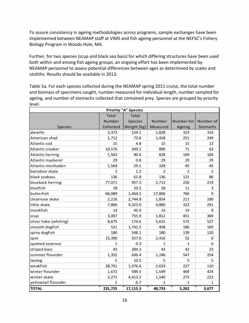
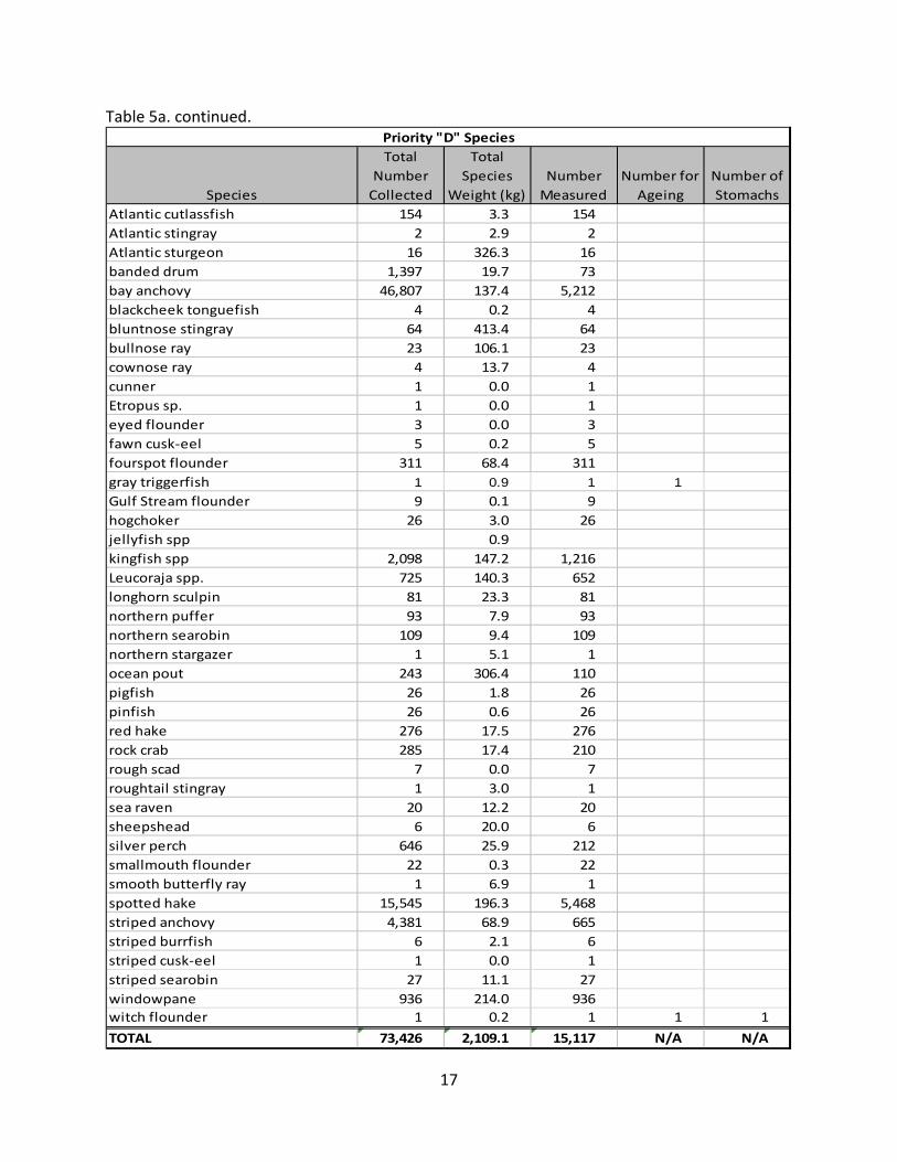
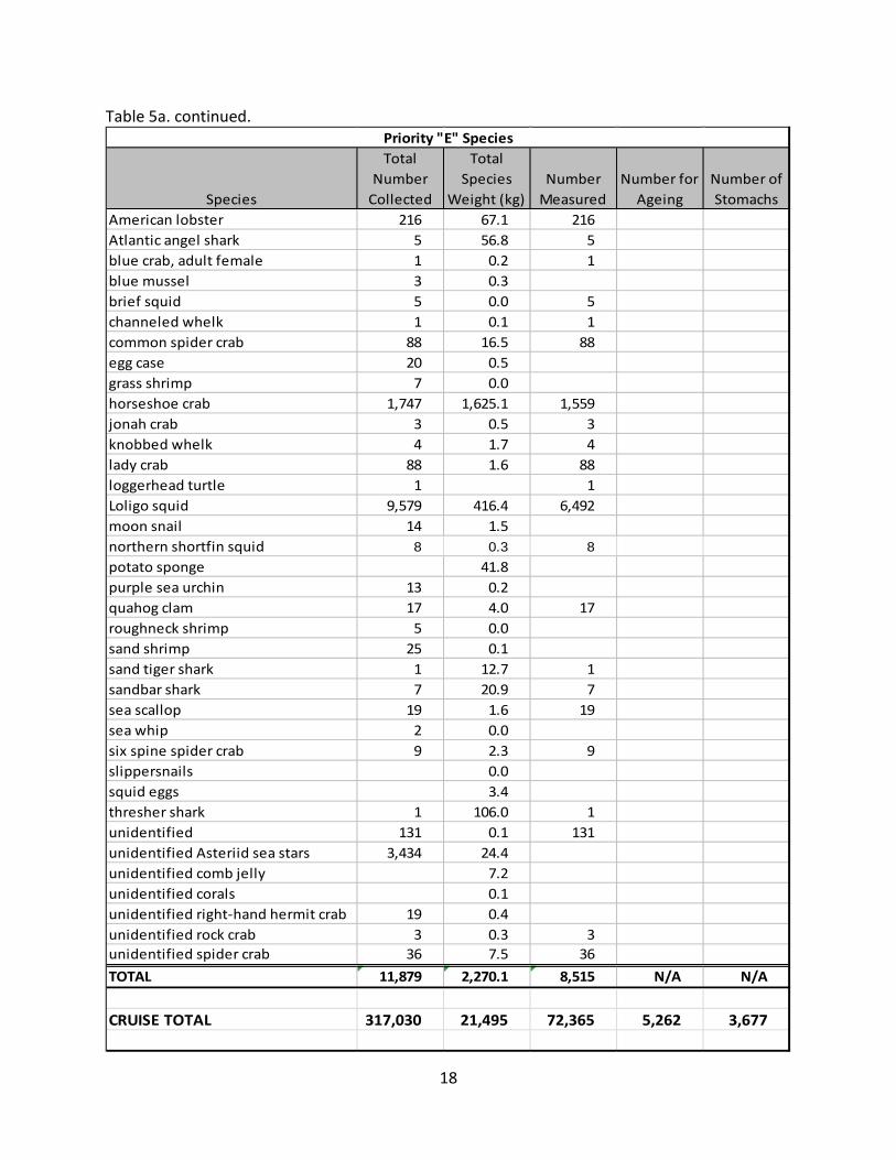
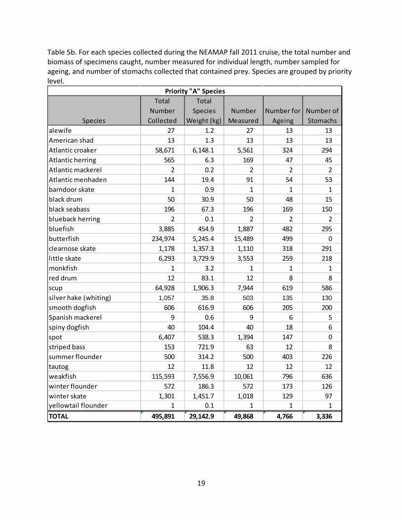
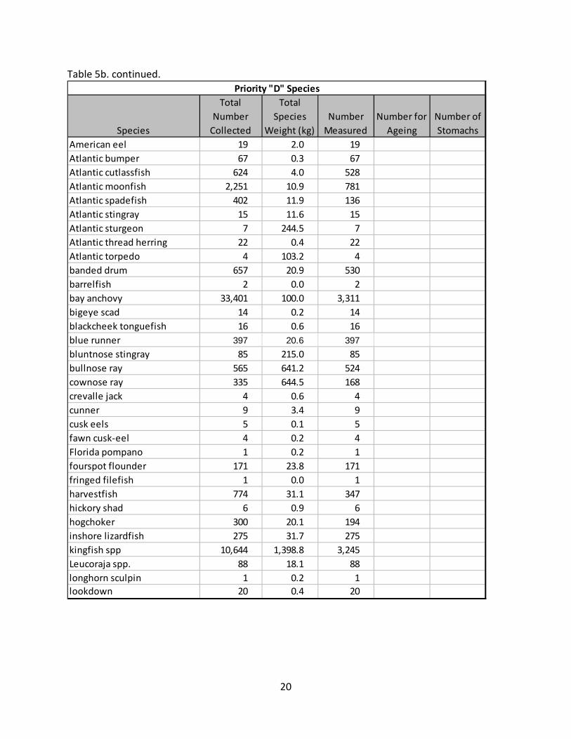
spring, 13.4 m fall), and headline height (5.4m spring, 5.6 m fall) were within optimal ranges for the spring 2011 cruise. Average towing speed was 3.1 kts and 3.0 kts for the spring and fall cruises respectively. For both cruises, the overwhelming majority of the station averages for each of these parameters fell within the optimal ranges. It was not necessary to disregard any tows due to poor net performance. On four consecutive tows during the fall 2011 cruise, a small tilt sensor (Star-Oddi® DST-COMP-TILT) was attached to one door which collected data on depth and door angle, both pitch (whether the door angles up or down in the direction of travel) and heel (the angle the door assumes perpendicular to the direction of travel). All four tows yielded very similar measurements. At the beginning of each tow as wire is deployed and the doors settle on the bottom, the doors are heeled in nearly flat to the bottom, indicating that they are not pulling the net open at that point. Within about 15-20 seconds of increased RPMs, the doors assume their normal condition. While at fishing speed, the doors pitch up (i.e. travel on their back third) at an average of about 12° and heel in (i.e. tops toward each other) at about 7°. At the end of a tow, within about 30 seconds of the official stop time and while the boat is slowing down, they again fall flat and are no longer performing their normal function (Figure 5). Catch Summary Almost 1,023,000 individual specimens (fishes and invertebrates) weighing approximately 62,000 kg and representing 149 species, including boreal, temperate, and tropical fishes, were collected during the two surveys conducted in 2011 (Table 5a & b). As expected, catches were larger and more diverse on the fall surveys relative to the spring cruises. In all, individual length measurements were recorded for 158,890 animals. Lab processing is proceeding on the 7,013 stomach samples and 10,028 ageing structures (otoliths, vertebrae, spines, opercles) collected in the field. As of the date of this report, stomachs from all cruises except for fall 2011 have been examined and prey contents identified and quantified. Likewise, preparation of ageing structures is proceeding for all species and all cruises, though ages have yet to be assigned for many species as methodology must be verified (for some species) and each specimen must be examined by three independent readers and then the final age assigned by one of two senior age readers. A change has been implemented in ageing protocols to improve the accuracy of age determination. As noted in previous reports the NEAMAP protocol was to process all age structures collected from a given species in a given year at one time (i.e., spring and fall samples processed together after the fall survey). The aforementioned protocol was in place to facilitate ‘blind reading’ of these samples to avoid bias. Previously only the senior readers had information about the catch time and location because they must interpret otolith edge patterns in the context of the season in which the specimen was captured. As experience has been gained however, it became apparent that each reader must be aware of the season and general latitude of capture in order to correctly interpret edge patterns in relation to the time of annulus formation. No readers are aware of the specimen’s size or sex.

16

To assure consistency in ageing methodologies across programs, sample exchanges have been implemented between NEAMAP staff at VIMS and fish ageing personnel at the NEFSC’s Fishery Biology Program in Woods Hole, MA. Further, for two species (scup and black sea bass) for which differing structures have been used both within and among fish ageing groups, an ongoing effort has been implemented by NEAMAP personnel to assess potential differences between ages as determined by scales and otoliths. Results should be available in 2013. Table 5a. For each species collected during the NEAMAP spring 2011 cruise, the total number and biomass of specimens caught, number measured for individual length, number sampled for ageing, and number of stomachs collected that contained prey. Species are grouped by priority level.

Species

Total Number

Collected

Total Species

Weight (kg)Number

MeasuredNumber for

AgeingNumber of Stomachs

alewife 3,373 154.1 1,828 323 314American shad 1,712 73.6 1,418 251 249Atlantic cod 15 4.8 15 15 13Atlantic croaker 10,576 349.2 890 71 62Atlantic herring 1,563 90.6 828 169 164Atlantic mackerel 29 0.8 29 29 29Atlantic menhaden 1,564 59.1 328 45 45barndoor skate 2 1.2 2 2 2black seabass 136 61.8 136 121 86blueback herring 77,071 957.3 2,713 226 219bluefish 18 10.5 18 11 3butterfish 66,089 1,464.5 17,806 766 0clearnose skate 2,216 2,744.8 1,854 211 190little skate 7,800 4,323.0 4,880 322 291monkfish 14 45.4 14 14 9scup 3,007 755.9 1,812 451 369silver hake (whiting) 8,675 174.6 5,631 572 527smooth dogfish 521 1,741.5 458 186 169spiny dogfish 180 548.1 180 139 120spot 15,390 557.0 2,416 52 0spotted seatrout 1 0.3 1 1 0striped bass 43 284.3 43 42 23summer flounder 1,352 636.4 1,246 547 254tautog 5 10.5 5 5 5weakfish 28,701 1,476.6 2,633 227 110winter flounder 1,672 589.5 1,549 464 424winter skate 2,271 4,413.2 1,540 275 222yellowtail flounder 2 0.7 2 1 1TOTAL 231,725 17,115.3 48,733 5,262 3,677

Priority "A" Species

17

Table 5a. continued.

Species

Total Number

Collected

Total Species

Weight (kg)Number

MeasuredNumber for

AgeingNumber of Stomachs

Atlantic cutlassfish 154 3.3 154Atlantic stingray 2 2.9 2Atlantic sturgeon 16 326.3 16banded drum 1,397 19.7 73bay anchovy 46,807 137.4 5,212blackcheek tonguefish 4 0.2 4bluntnose stingray 64 413.4 64bullnose ray 23 106.1 23cownose ray 4 13.7 4cunner 1 0.0 1Etropus sp. 1 0.0 1eyed flounder 3 0.0 3fawn cusk-eel 5 0.2 5fourspot flounder 311 68.4 311gray triggerfish 1 0.9 1 1Gulf Stream flounder 9 0.1 9hogchoker 26 3.0 26jellyfish spp 0.9kingfish spp 2,098 147.2 1,216Leucoraja spp. 725 140.3 652longhorn sculpin 81 23.3 81northern puffer 93 7.9 93northern searobin 109 9.4 109northern stargazer 1 5.1 1ocean pout 243 306.4 110pigfish 26 1.8 26pinfish 26 0.6 26red hake 276 17.5 276rock crab 285 17.4 210rough scad 7 0.0 7roughtail stingray 1 3.0 1sea raven 20 12.2 20sheepshead 6 20.0 6silver perch 646 25.9 212smallmouth flounder 22 0.3 22smooth butterfly ray 1 6.9 1spotted hake 15,545 196.3 5,468striped anchovy 4,381 68.9 665striped burrfish 6 2.1 6striped cusk-eel 1 0.0 1striped searobin 27 11.1 27windowpane 936 214.0 936witch flounder 1 0.2 1 1 1TOTAL 73,426 2,109.1 15,117 N/A N/A

Priority "D" Species

18

Table 5a. continued.

Species

Total Number

Collected

Total Species

Weight (kg)Number

MeasuredNumber for

AgeingNumber of Stomachs

American lobster 216 67.1 216Atlantic angel shark 5 56.8 5blue crab, adult female 1 0.2 1blue mussel 3 0.3brief squid 5 0.0 5channeled whelk 1 0.1 1common spider crab 88 16.5 88egg case 20 0.5grass shrimp 7 0.0horseshoe crab 1,747 1,625.1 1,559jonah crab 3 0.5 3knobbed whelk 4 1.7 4lady crab 88 1.6 88loggerhead turtle 1 1Loligo squid 9,579 416.4 6,492moon snail 14 1.5northern shortfin squid 8 0.3 8potato sponge 41.8purple sea urchin 13 0.2quahog clam 17 4.0 17roughneck shrimp 5 0.0sand shrimp 25 0.1sand tiger shark 1 12.7 1sandbar shark 7 20.9 7sea scallop 19 1.6 19sea whip 2 0.0six spine spider crab 9 2.3 9slippersnails 0.0squid eggs 3.4thresher shark 1 106.0 1unidentified 131 0.1 131unidentified Asteriid sea stars 3,434 24.4unidentified comb jelly 7.2unidentified corals 0.1unidentified right-hand hermit crab 19 0.4unidentified rock crab 3 0.3 3unidentified spider crab 36 7.5 36TOTAL 11,879 2,270.1 8,515 N/A N/A

CRUISE TOTAL 317,030 21,495 72,365 5,262 3,677

Priority "E" Species

19

Table 5b. For each species collected during the NEAMAP fall 2011 cruise, the total number and biomass of specimens caught, number measured for individual length, number sampled for ageing, and number of stomachs collected that contained prey. Species are grouped by priority level.

Species

Total Number

Collected

Total Species

Weight (kg)Number

MeasuredNumber for

AgeingNumber of Stomachs

alewife 27 1.2 27 13 13American shad 13 1.3 13 13 13Atlantic croaker 58,671 6,148.1 5,561 324 294Atlantic herring 565 6.3 169 47 45Atlantic mackerel 2 0.2 2 2 2Atlantic menhaden 144 19.4 91 54 53barndoor skate 1 0.9 1 1 1black drum 50 30.9 50 48 15black seabass 196 67.3 196 169 150blueback herring 2 0.1 2 2 2bluefish 3,885 454.9 1,887 482 295butterfish 234,974 5,245.4 15,489 499 0clearnose skate 1,178 1,357.3 1,110 318 291little skate 6,293 3,729.9 3,553 259 218monkfish 1 3.2 1 1 1red drum 12 83.1 12 8 8scup 64,928 1,906.3 7,944 619 586silver hake (whiting) 1,057 35.8 503 135 130smooth dogfish 606 616.9 606 205 200Spanish mackerel 9 0.6 9 6 5spiny dogfish 40 104.4 40 18 6spot 6,407 538.3 1,394 147 0striped bass 153 721.9 63 12 8summer flounder 500 314.2 500 403 226tautog 12 11.8 12 12 12weakfish 115,593 7,556.9 10,061 796 636winter flounder 572 186.3 572 173 126winter skate 1,301 1,451.7 1,018 129 97yellowtail flounder 1 0.1 1 1 1TOTAL 495,891 29,142.9 49,868 4,766 3,336

Priority "A" Species

20

Table 5b. continued.

Species

Total Number

Collected

Total Species

Weight (kg)Number

MeasuredNumber for

AgeingNumber of Stomachs

American eel 19 2.0 19Atlantic bumper 67 0.3 67Atlantic cutlassfish 624 4.0 528Atlantic moonfish 2,251 10.9 781Atlantic spadefish 402 11.9 136Atlantic stingray 15 11.6 15Atlantic sturgeon 7 244.5 7Atlantic thread herring 22 0.4 22Atlantic torpedo 4 103.2 4banded drum 657 20.9 530barrelfish 2 0.0 2bay anchovy 33,401 100.0 3,311bigeye scad 14 0.2 14blackcheek tonguefish 16 0.6 16blue runner 397 20.6 397bluntnose stingray 85 215.0 85bullnose ray 565 641.2 524cownose ray 335 644.5 168crevalle jack 4 0.6 4cunner 9 3.4 9cusk eels 5 0.1 5fawn cusk-eel 4 0.2 4Florida pompano 1 0.2 1fourspot flounder 171 23.8 171fringed filefish 1 0.0 1harvestfish 774 31.1 347hickory shad 6 0.9 6hogchoker 300 20.1 194inshore lizardfish 275 31.7 275kingfish spp 10,644 1,398.8 3,245Leucoraja spp. 88 18.1 88longhorn sculpin 1 0.2 1lookdown 20 0.4 20

Priority "D" Species

21

Table 5b. continued.

Species

Total Number

Collected

Total Species

Weight (kg)Number

MeasuredNumber for

AgeingNumber of Stomachs

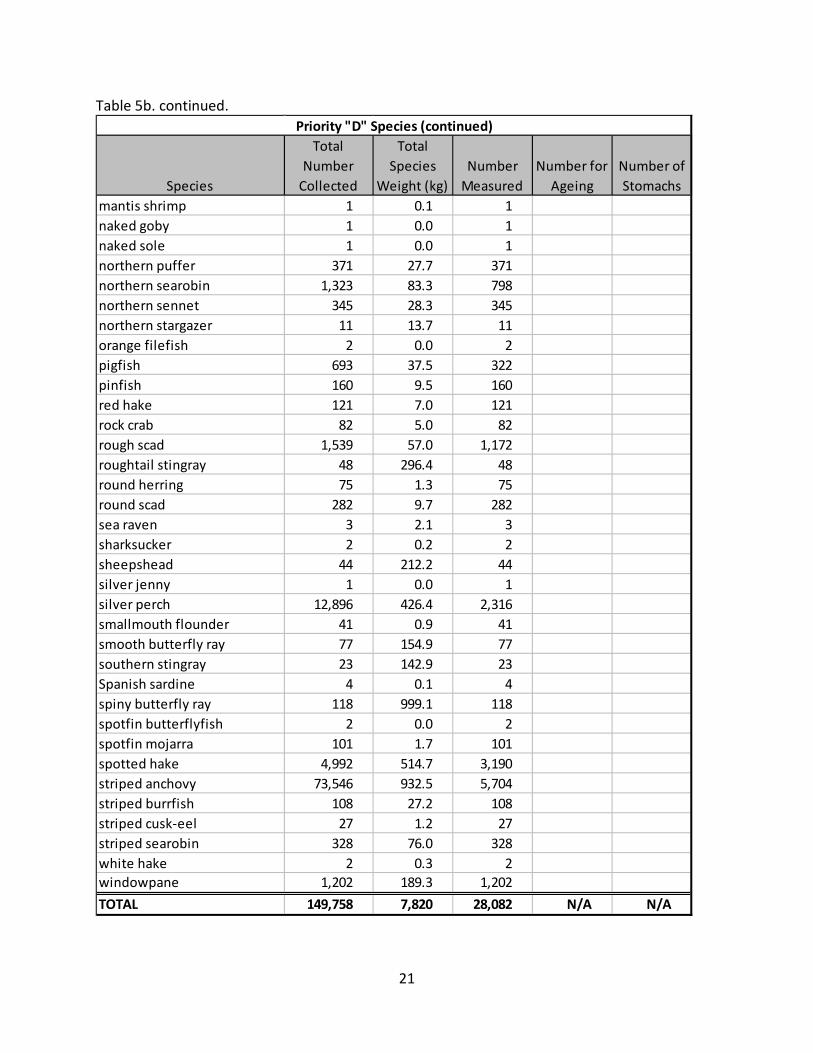
mantis shrimp 1 0.1 1naked goby 1 0.0 1naked sole 1 0.0 1northern puffer 371 27.7 371northern searobin 1,323 83.3 798northern sennet 345 28.3 345northern stargazer 11 13.7 11orange filefish 2 0.0 2pigfish 693 37.5 322pinfish 160 9.5 160red hake 121 7.0 121rock crab 82 5.0 82rough scad 1,539 57.0 1,172roughtail stingray 48 296.4 48round herring 75 1.3 75round scad 282 9.7 282sea raven 3 2.1 3sharksucker 2 0.2 2sheepshead 44 212.2 44silver jenny 1 0.0 1silver perch 12,896 426.4 2,316smallmouth flounder 41 0.9 41smooth butterfly ray 77 154.9 77southern stingray 23 142.9 23Spanish sardine 4 0.1 4spiny butterfly ray 118 999.1 118spotfin butterflyfish 2 0.0 2spotfin mojarra 101 1.7 101spotted hake 4,992 514.7 3,190striped anchovy 73,546 932.5 5,704striped burrfish 108 27.2 108striped cusk-eel 27 1.2 27striped searobin 328 76.0 328white hake 2 0.3 2windowpane 1,202 189.3 1,202TOTAL 149,758 7,820 28,082 N/A N/A

Priority "D" Species (continued)

22

Table 5b. continued.

Species

Total Number

Collected

Total Species

Weight (kg)Number

MeasuredNumber for

AgeingNumber of Stomachs

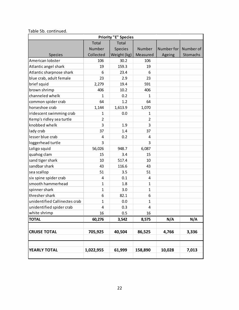
American lobster 106 30.2 106Atlantic angel shark 19 159.3 19Atlantic sharpnose shark 6 23.4 6blue crab, adult female 23 2.9 23brief squid 2,279 19.4 591brown shrimp 406 10.2 406channeled whelk 1 0.2 1common spider crab 64 1.2 64horseshoe crab 1,144 1,613.9 1,070iridescent swimming crab 1 0.0 1Kemp's ridley sea turtle 2 2knobbed whelk 3 1.9 3lady crab 37 1.4 37lesser blue crab 4 0.2 4loggerhead turtle 3 3Loligo squid 56,026 948.7 6,087quahog clam 15 3.4 15sand tiger shark 10 517.4 10sandbar shark 43 116.6 43sea scallop 51 3.5 51six spine spider crab 4 0.1 4smooth hammerhead 1 1.8 1spinner shark 1 3.0 1thresher shark 6 82.1 6unidentified Callinectes crab 1 0.0 1unidentified spider crab 4 0.3 4white shrimp 16 0.5 16TOTAL 60,276 3,542 8,575 N/A N/A

CRUISE TOTAL 705,925 40,504 86,525 4,766 3,336

YEARLY TOTAL 1,022,955 61,999 158,890 10,028 7,013

Priority "E" Species

23

Species Data Summaries

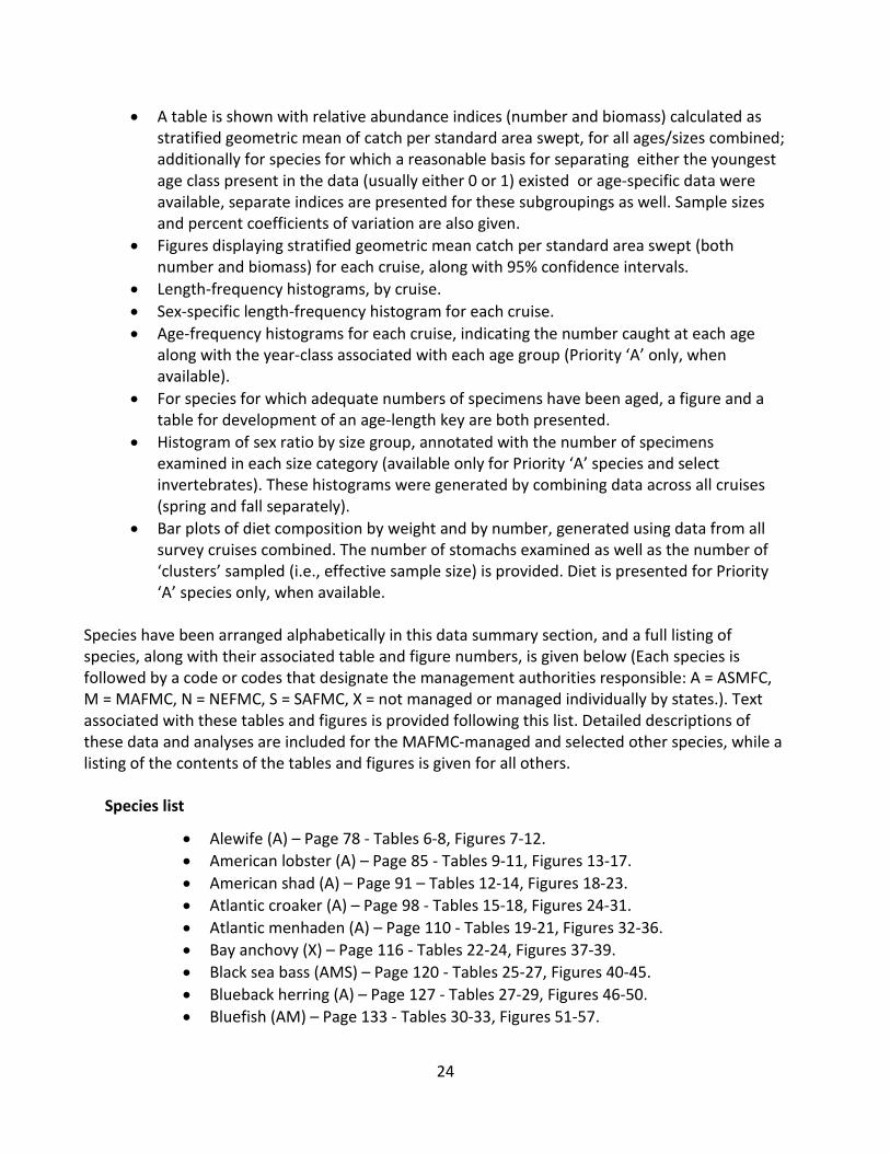
The data summaries presented in this report include the information collected on each of the NEAMAP Trawl Survey full-scale cruises conducted to date and focus on species that are of management interest to the Mid-Atlantic Fishery Management Council. Some that are of interest to the New England Fishery Management Council and the ASMFC, or that are not managed but considered valuable from an ecological standpoint, are also included. It is important to note that these summaries represent only a subset of the biological and ecological analyses that are feasible using the data collected by the NEAMAP Survey. Several additional analyses are possible for each of the species included in this report, as well as for others that have been collected by this survey but are not presented. Some analyses (e.g., length-weight relationships, growth curves, maturity ogives) found in previous reports are excluded here in an effort to make the scope of this document somewhat manageable. Certainly, any NEAMAP information (data or analyses) requested by assessment scientists and managers would be made available in a timely manner. For a small subset of species that are not captured in large numbers but are of particular interest or concern (Atlantic sturgeon – Figure 6A, sea turtles – Figure 6B, and coastal sharks – Figure 6C) single-page summaries of NEAMAP catches over all survey years are presented, showing geographic locations and numbers in a GIS format. Although this report focuses on the data collected during 2011, some information from previous years is included in these species summaries to both place the 2011 data in context as well as to increase sample sizes. Relative indices of abundance are given for each species included in this report and are presented by survey as stratified logarithmic mean of catch per standard area swept. The total number and biomass collected, number sampled for individual length measurements, and numbers taken and processed for age determination and diet composition (Priority ‘A’ species only) are also given for each cruise. Catch distribution plots and length-frequencies are provided for these species on a per-cruise basis. Sex-specific length frequency histograms and sex ratios by size are presented for all Priority ‘A’ species as well as for some of the invertebrates, and were generated by combining data across all cruises (spring and fall separately). Age-frequency distributions (by cruise) and diet compositions (all cruises combined) are also included for these priority species where field collections and subsequent laboratory progress have resulted in sufficient sample sizes. For most species, the following tables and figures are presented:

• GIS figures showing the biomass of that species collected at each sampling site for each of the 2011 cruises.

• A table presenting, for each cruise, the total number of specimens of that species collected, total biomass of these individuals, number sampled for individual length measurements, number taken for full processing (including age and stomach analysis), and the number of age and stomach samples processed to date.

• A table highlighting which strata were included for calculation of abundance indices.

24

• A table is shown with relative abundance indices (number and biomass) calculated as stratified geometric mean of catch per standard area swept, for all ages/sizes combined; additionally for species for which a reasonable basis for separating either the youngest age class present in the data (usually either 0 or 1) existed or age-specific data were available, separate indices are presented for these subgroupings as well. Sample sizes and percent coefficients of variation are also given.

• Figures displaying stratified geometric mean catch per standard area swept (both number and biomass) for each cruise, along with 95% confidence intervals.

• Length-frequency histograms, by cruise. • Sex-specific length-frequency histogram for each cruise. • Age-frequency histograms for each cruise, indicating the number caught at each age

along with the year-class associated with each age group (Priority ‘A’ only, when available).

• For species for which adequate numbers of specimens have been aged, a figure and a table for development of an age-length key are both presented.

• Histogram of sex ratio by size group, annotated with the number of specimens examined in each size category (available only for Priority ‘A’ species and select invertebrates). These histograms were generated by combining data across all cruises (spring and fall separately).

• Bar plots of diet composition by weight and by number, generated using data from all survey cruises combined. The number of stomachs examined as well as the number of ‘clusters’ sampled (i.e., effective sample size) is provided. Diet is presented for Priority ‘A’ species only, when available.

Species have been arranged alphabetically in this data summary section, and a full listing of species, along with their associated table and figure numbers, is given below (Each species is followed by a code or codes that designate the management authorities responsible: A = ASMFC, M = MAFMC, N = NEFMC, S = SAFMC, X = not managed or managed individually by states.). Text associated with these tables and figures is provided following this list. Detailed descriptions of these data and analyses are included for the MAFMC-managed and selected other species, while a listing of the contents of the tables and figures is given for all others.

Species list

• Alewife (A) – Page 78 - Tables 6-8, Figures 7-12. • American lobster (A) – Page 85 - Tables 9-11, Figures 13-17. • American shad (A) – Page 91 – Tables 12-14, Figures 18-23. • Atlantic croaker (A) – Page 98 - Tables 15-18, Figures 24-31. • Atlantic menhaden (A) – Page 110 - Tables 19-21, Figures 32-36. • Bay anchovy (X) – Page 116 - Tables 22-24, Figures 37-39. • Black sea bass (AMS) – Page 120 - Tables 25-27, Figures 40-45. • Blueback herring (A) – Page 127 - Tables 27-29, Figures 46-50. • Bluefish (AM) – Page 133 - Tables 30-33, Figures 51-57.

25

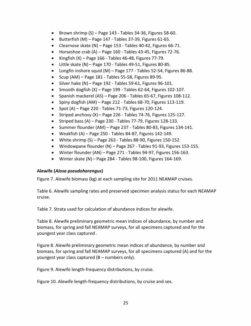
• Brown shrimp (S) – Page 143 - Tables 34-36, Figures 58-60. • Butterfish (M) – Page 147 - Tables 37-39, Figures 61-65. • Clearnose skate (N) – Page 153 - Tables 40-42, Figures 66-71. • Horseshoe crab (A) – Page 160 - Tables 43-45, Figures 72-76. • Kingfish (X) – Page 166 - Tables 46-48, Figures 77-79. • Little skate (N) – Page 170 - Tables 49-51, Figures 80-85. • Longfin inshore squid (M) – Page 177 - Tables 52-54, Figures 86-88. • Scup (AM) – Page 181 - Tables 55-58, Figures 89-95. • Silver hake (N) – Page 192 - Tables 59-61, Figures 96-101. • Smooth dogfish (X) – Page 199 - Tables 62-64, Figures 102-107. • Spanish mackerel (AS) – Page 206 - Tables 65-67, Figures 108-112. • Spiny dogfish (AM) – Page 212 - Tables 68-70, Figures 113-119. • Spot (A) – Page 220 - Tables 71-73, Figures 120-124. • Striped anchovy (X) – Page 226 - Tables 74-76, Figures 125-127. • Striped bass (A) – Page 230 - Tables 77-79, Figures 128-133. • Summer flounder (AM) – Page 237 - Tables 80-83, Figures 134-141. • Weakfish (A) – Page 250 - Tables 84-87, Figures 142-149. • White shrimp (S) – Page 263 - Tables 88-90, Figures 150-152. • Windowpane flounder (N) – Page 267 - Tables 91-93, Figures 153-155. • Winter flounder (AN) – Page 271 - Tables 94-97, Figures 156-163. • Winter skate (N) – Page 284 - Tables 98-100, Figures 164-169.

Alewife (Alosa pseudoharengus)

Figure 7. Alewife biomass (kg) at each sampling site for 2011 NEAMAP cruises. Table 6. Alewife sampling rates and preserved specimen analysis status for each NEAMAP cruise. Table 7. Strata used for calculation of abundance indices for alewife. Table 8. Alewife preliminary geometric mean indices of abundance, by number and biomass, for spring and fall NEAMAP surveys, for all specimens captured and for the youngest year class captured . Figure 8. Alewife preliminary geometric mean indices of abundance, by number and biomass, for spring and fall NEAMAP surveys, for all specimens captured (A) and for the youngest year class captured (B – numbers only). Figure 9. Alewife length-frequency distributions, by cruise. Figure 10. Alewife length-frequency distributions, by cruise and sex.

26

Figure 11. Alewife sex ratio, by length group, for NEAMAP Spring and Fall cruises 2007-2011. Figure 12. Alewife preliminary diet composition, expressed as percent by weight and number collected during NEAMAP cruises in 2007 through Spring 2011. American Lobster (Homarus americanus)

Figure 13. American lobster biomass (kg) at each sampling site for 2011 NEAMAP cruises. Table 9. American lobster sampling rates for each NEAMAP cruise. Table 10. Strata used for calculation of abundance indices for American lobster. Table 11. American lobster preliminary geometric mean indices of abundance, by number and biomass, for spring and fall NEAMAP surveys, for all specimens captured. Figure 14. American lobster preliminary geometric mean indices of abundance, by number and biomass, for spring and fall NEAMAP surveys, for all specimens captured. Figure 15. American lobster length-frequency distributions, by cruise. Figure 16. American lobster length-frequency distributions, by cruise and sex. Figure 17. American lobster sex ratio, by length group, for NEAMAP Spring and Fall cruises 2007-2011. American Shad (Alosa sapidissima)

Figure 18. American shad biomass (kg) at each sampling site for 2011 NEAMAP cruises. Table 12. American shad sampling rates and preserved specimen analysis status for each NEAMAP cruise. Table 13. Strata used for calculation of abundance indices for American shad. Table 14. American shad preliminary geometric mean indices of abundance, by number and biomass, for spring NEAMAP surveys, for all specimens captured. Figure 19. American shad preliminary geometric mean indices of abundance, by number and biomass, for spring NEAMAP surveys, for all specimens captured. Figure 20. American shad length-frequency distributions, by cruise. Figure 21. American shad length-frequency distributions, by cruise and sex.

27

Figure 22. American shad sex ratio, by length group, for NEAMAP Spring and Fall cruises 2007-2011. Figure 23. American shad preliminary diet composition, expressed as percent by weight and number collected during NEAMAP cruises in 2007 through Spring 2011. Atlantic Croaker (Micropogonias undulatus)

Figure 24. Atlantic croaker biomass (kg) at each sampling site for 2011 NEAMAP cruises. Table 15. Atlantic croaker sampling rates and preserved specimen analysis status for each NEAMAP cruise. Table 16. Strata used for calculation of abundance indices for Atlantic croaker. Table 17. Atlantic croaker preliminary geometric mean indices of abundance, for all specimens captured and by age-class for spring and fall NEAMAP surveys (age-specific indices for age-2 and older calculated for fall surveys only). Figure 25. Atlantic croaker preliminary geometric mean indices of abundance, for all specimens captured (A - by number and biomass) and by age-class (B – numbers only) for spring and fall NEAMAP surveys (age-specific indices for age-2 and older calculated for fall surveys only). Figure 26. Atlantic croaker length-frequency distributions, by cruise. Figure 27. Atlantic croaker length-frequency distributions, by cruise and sex. Figure 28. Atlantic croaker age-frequency distribution, by cruise. The estimated total number collected at a given age is provided above each corresponding bar. Figure 29. Atlantic croaker age-at-length proportions for all spring vs. all fall cruises combined, showing actual and loess smoothed proportions at each 1cm length bin. Table 18. Atlantic croaker loess smoothed age-at-length proportions for all fall cruises combined. Figure 30. Atlantic croaker sex ratio, by length group, for NEAMAP Spring and Fall cruises 2007-2011. Figure 31. Atlantic croaker diet composition, expressed as percent by weight and number collected during NEAMAP cruises in 2007 through Spring 2011. Atlantic Menhaden (Brevoortia tyrannus)

28

Figure 32. Atlantic menhaden biomass (kg) at each sampling site for 2011 NEAMAP cruises. Table 19. Atlantic menhaden sampling rates and preserved specimen analysis status for each NEAMAP cruise. Table 20. Strata used for calculation of abundance indices for American menhaden.. Table 21. Atlantic menhaden preliminary geometric mean indices of abundance, by number and biomass, for spring and fall NEAMAP surveys, for all specimens captured and for the youngest year class captured. Figure 33. Atlantic menhaden preliminary geometric mean indices of abundance, by number and biomass, for spring and fall NEAMAP surveys, for all specimens captured (A) and for the youngest year class captured (B – numbers only). Figure 34. Atlantic menhaden length-frequency distributions, by cruise. (Blue reference lines are placed at the size cutoff values used to separate recruits from older specimens. Cutoff values – Spring 17cm, Fall 15cm - taken from http://www.asmfc.org/speciesDocuments/menhaden/reports/ stockAssessments/04MenhadenPeerReviewReport.pdf.). Figure 35. Atlantic menhaden length-frequency distributions, by cruise and sex. Figure 36. Atlantic menhaden sex ratio, by length group, for NEAMAP Spring and Fall cruises 2007-2011. Bay Anchovy (Anchoa mitchilli)

Figure 37. Bay anchovy biomass (kg) at each sampling site for 2011 NEAMAP cruises. Table 22. Bay anchovy sampling rates for each NEAMAP cruise. Table 23. Strata used for calculation of abundance indices for bay anchovy. Table 24. Bay anchovy preliminary geometric mean indices of abundance, by number and biomass, for spring and fall NEAMAP surveys, for all specimens captured. Figure 38. Bay anchovy preliminary geometric mean indices of abundance, by number and biomass, for spring and fall NEAMAP surveys, for all specimens captured. Figure 39. Bay anchovy length-frequency distributions, by cruise. Black Sea Bass (Centropristis striata)

Figure 40. Black sea bass biomass (kg) at each sampling site for 2011 NEAMAP cruises.

29

Table 25. Black sea bass sampling rates and preserved specimen analysis status for each NEAMAP cruise. Table 26. Strata used for calculation of abundance indices for black sea bass. Table 27. Black sea bass preliminary geometric mean indices of abundance, by number and biomass, for spring and fall NEAMAP surveys, for all specimens captured and for the youngest year class captured. Figure 41. Black sea bass preliminary geometric mean indices of abundance, by number and biomass, for spring and fall NEAMAP surveys, for all specimens captured (A) and for the youngest year class captured (B – numbers only). Figure 42. Black sea bass length-frequency distributions, by cruise (Blue reference lines are placed at the size cutoff values used to separate recruits from older specimens. Cutoff values – Spring 16cm, Fall 12cm - taken from http://mrl.cofc.edu/pdf/tr40s/Techreport43.pdf). Figure 43. Black sea bass length-frequency distributions, by cruise and sex. Figure 44. Black sea bass sex ratio, by length group, for NEAMAP Spring and Fall cruises 2007-2011. Figure 45. Black sea bass diet composition, expressed as percent by weight and number collected during NEAMAP cruises in 2007 through Spring 2011. With respect to the distribution of the catches of black sea bass, collections during the spring 2011 survey, were low and were concentrated in the northern portion of the survey area, especially in Block Island and Rhode Island Sounds though specimens were captured as far south as Region 11 in Virginia. During the fall survey catches again were also generally low, were more dispersed (ranging between RIS and Region 14 in North Carolina), and often occurred in clusters of nearby stations. Overall, the largest samples of black sea bass occurred near Block Island (Figure 40). No consistent inter or intra-annual patterns were observed between the spring and fall survey cruises in terms of the number or biomass of black sea bass caught, although it appeared that catches may be greater in the fall (Table 25). The largest number of sea bass was collected during the Fall 2009 cruise, while the fewest were sampled during the Spring 2010 survey. In biomass units, the largest and small total amounts caught were in the Fall 2009 and Fall 2010 cruises respectively. Trawl surveys are not considered to be the ideal platforms for sampling this species, given the structure-orientated nature of sea bass and the tendency for trawl surveys to avoid towing their gear over structure. It seems, however, as though enough fish were collected by NEAMAP to extract a variety of useful information. Except for the most recent cruise, virtually all stomach samples have been analyzed; otoliths

30

however have not yet been assigned ages pending development and verification of analytical methods. Overall abundance indices for black sea bass appeared to show declines, both in terms of number and biomass, over the short time series, for both spring and fall surveys (Table 27, Figure 41). Variability, as measured by the coefficient of variation (CV) was generally higher for the fall surveys than for the spring, likely the result of more widespread but spotty catch rates during fall cruises, and was generally higher for biomass indices than for those based on counts. CVs ranged from 9.7% (Spring 2009, numerical index) to 49.6% (Spring 2010, biomass index). Considering the youngest age-classes captured (Age-0 in the fall, Age-1 in the spring), both surveys showed increasing trends through 2009, significant declines in 2010 followed by higher values in 20111 (Figure 41). A broad size range (~4cm – 60cm TL among all cruises) of sea bass was collected during each of the surveys, and included both juvenile and adult specimens (Figure 42). The majority of the sea bass collected ranged between 15cm and 40cm TL, and it appeared that multiple modal size groups (likely corresponding to age-classes) were present. A 60cm sea bass, which is believed to be the maximum size for this species, was collected during the spring 2008 cruise and a second one of the same size was collected during the fall of 2010. Black sea bass are protogynous hermaphrodites, meaning that they begin life as female and, around a certain size, switch to male. This life history characteristic is evident in the trends both in length distribution by sex (Figure 43) and in sex ratio by size (Figure 44) documented by the NEAMAP Survey. It is important to note however that this species is incompletely metagonous, meaning that some fish are actually born as males are remain so throughout their lifetime, while some females never switch to male and as is evidenced in both of the aforementioned figures. Crustaceans comprised the largest portion (51.3% by weight, 59.4% by number) of the diet of black sea bass sampled by the NEAMAP Survey (Figure 45). This is consistent with the findings of several past studies. Rock crabs (Cancer irroratus), hermit crabs (superfamily Paguroidea), and sand shrimp (Crangon septemspinosa) were the main crustaceans consumed. Fishes accounted for 21.8% of the sea bass diet by weight and 16.1% by number and were represented mainly by butterfish and bay anchovy among identifiable species. Longfin inshore squid accounted for approximately 10% of the diet by both weight and number. Blueback Herring (Alosa aestivalis)

Figure 46. Blueback herring biomass (kg) at each sampling site for 2011 NEAMAP cruises. Table 27. Blueback herring sampling rates and preserved specimen analysis status for each NEAMAP cruise.

31

Table 28. Strata used for calculation of abundance indices for blueback herring. Table 29. Blueback herring preliminary geometric mean indices of abundance, by number and biomass, for spring NEAMAP surveys, for all specimens captured and for the youngest year class captured. Figure 47. Blueback herring preliminary geometric mean indices of abundance, by number and biomass, for spring NEAMAP surveys, for all specimens captured (A) and for the youngest year class captured (B – numbers only). Figure 48. Blueback herring length-frequency distributions, by cruise (Blue reference lines are placed at the size cutoff values used to separate recruits from older specimens. Cutoff values - Spring 14cm - estimated by examination of these length frequency figures.). Figure 49. Blueback herring length-frequency distributions, by cruise and sex. Figure 50. Blueback herring sex ratio, by length group, for NEAMAP Spring and Fall cruises 2007-2011. Bluefish (Pomatomus saltatrix)

Figure 51. Bluefish biomass (kg) at each sampling site for 2011 NEAMAP cruises. Table 30. Bluefish sampling rates and preserved specimen analysis status for each NEAMAP cruise. Table 31. Strata used for calculation of abundance indices for bluefish. Table 32. Bluefish preliminary geometric mean indices of abundance, by number and biomass, for spring and fall NEAMAP surveys, for all specimens captured and for the youngest year class captured (numbers only – spring and summer cohorts shown separately). Figure 52. Bluefish preliminary geometric mean indices of abundance, by number and biomass, for spring and fall NEAMAP surveys, for all specimens captured (A), for the youngest year class captured (B – numbers only) and (using fall data only) for the spring and summer age-0 cohorts separately (C – numbers only). Figure 53. Bluefish length-frequency distributions, by cruise (Blue reference line is placed at the size cutoff value – 17cm - used to separate the spring YOY cohort – to the right of the line – from the summer YOY cohort – to the left. Age-length key values presented in Table 33 were applied to the spring cohort specimens). Figure 54. Bluefish length-frequency distributions, by cruise and sex.

32

Figure 55. Bluefish age-at-length proportions for all spring vs. all fall cruises combined, showing actual and loess smoothed proportions at each 1cm length bin (Data from a single aged NEAMAP survey year pooled with samples from the VIMS ChesMMAP survey). Table 33. Bluefish loess-smoothed age-at-length proportions for all fall cruises combined. Figure 56. Bluefish sex ratio, by length group, for NEAMAP Spring and Fall cruises 2007-2011. Figure 57. Bluefish diet composition, expressed as percent by weight and number collected during NEAMAP cruises in 2007 through Spring 2011. This species was sampled throughout the NEAMAP survey range during the fall 2011 cruise. Catches tended to be largest and most consistent along the western coast of Long Island and in northern New Jersey waters. Collections of bluefish during the Spring 2011 were rare, occurring at only seven widely dispersed stations, with no catches greater than 5 specimens (Figure 51). Bluefish are a fast-swimming, coastal pelagic species, and as such survey trawls are not deemed the most effective tool for sampling this species, especially at larger sizes. Nevertheless, appreciable amounts (number and biomass) of bluefish were caught during fall surveys and one of the four spring surveys through 2011 (few fish were sampled during the spring 2008, 2011 and 2011 surveys – Table 30). Fall bluefish indices of overall abundance (both number and biomass) were relatively stable over the time, with low survey variability (Table 32 – Figure 52). As the species does not usually reinvade the survey area until later in the spring after survey operations are completed Indices as measured during spring cruises are likely not representative of true abundance. This is evidenced by the small number of survey strata in which the species appears in the spring and by the large percent CVs for spring cruises. It is likely that spring catches are determined more by water temperatures than by abundance. Bluefish are believed to exhibit an extended and geographically widespread spawning season, with two distinct concentrations, one in the spring in the South Atlantic Bight and one during summer in the Middle Atlantic Bight (Kendall and Walford, 1979). This pattern results in two distinct YOY cohorts. Examination of NEAMAP length frequency plots (Figure 53) shows that these two cohorts reveal themselves in NEAMAP data and cohort strength can likely be estimated separately. Therefore, using fall survey data only, YOY indices are calculated both for all YOY fish pooled and for each cohort separately (Figure 52). Interestingly, the indices for each cohort appear to have followed substantially different trends over the time series. The spring cohort followed a mild but consistent decline between 2007 and 2010 before reaching a time series high value in 2011. Summer cohort YOY increased consistently between 2007 and 2009 before following an equally consistent decline in 2010 and 2011.

33

Bluefish collected during the fall surveys generally ranged from 7cm to 75cm FL (Figure 53). The sizes of the majority of the specimens sampled during each of these surveys indicate that YOY and age-1 fish were the dominant age-classes sampled. This is probably due both to the structure of the population (i.e., more younger fish available) and the ability for larger, faster bluefish to avoid the trawl. Bluefish collected during spring cruises were almost exclusively those from the previous summer cohort, though a small number of larger specimens are normally captured. Un-aged specimens were assigned to age-classes by use of an age-length key developed from a single NEAMAP survey-year’s aged samples pooled with similar specimens (343) aged by the VIMS ChesMMAP survey. Data were loess-smoothed and the smoothed values were used as the age-length key (Figure 55 – Table 33). In neither the sex-specific length analyses (Figure 54) nor a plot of sex ratio by size (Figure 56) did bluefish exhibit any apparent sexually dimorphic trends, and ratios were approximately 1:1 (male to female) for most length groups. As expected, the diet of bluefish collected by NEAMAP was overwhelmingly dominated by fishes, 96.9% by %W, and 92.5% by %N (Figure 57). Bay anchovy accounted for nearly half of the bluefish diet by both weight and by number. Butterfish, striped anchovy and sand lances also constituted significant amounts of the identifiable teleost prey types. The morphology and behavior of this species are well suited for a piscivorous lifestyle. Besides fishes, squid were the only other prey type accounting for any appreciable portion of bluefish diets. Brown Shrimp (Farfantepenaeus aztecus)

Figure 58. Brown shrimp biomass (kg) at each sampling site for 2011 NEAMAP cruises. Table 34. Brown shrimp sampling rates for each NEAMAP cruise. Table 35. Strata used for calculation of abundance indices for brown shrimp. Table 36. Brown shrimp preliminary geometric mean indices of abundance, by number and biomass, for spring and fall NEAMAP surveys, for all specimens captured. Figure 59. Bay anchovy preliminary geometric mean indices of abundance, by number and biomass, for spring and fall NEAMAP surveys, for all specimens captured. Figure 60. Brown shrimp length-frequency distributions, by cruise. Butterfish (Peprilis triacantus) Figure 61. Butterfish biomass (kg) at each sampling site for 2011 NEAMAP cruises.

34

Table 37. Butterfish sampling rates and preserved specimen analysis status for each NEAMAP cruise. Table 38. Strata used for calculation of abundance indices for butterfish. Table 39. Butterfish preliminary geometric mean indices of abundance, by number and biomass, for spring and fall NEAMAP surveys, for all specimens captured. Figure 62. Butterfish preliminary geometric mean indices of abundance, by number and biomass, for spring and fall NEAMAP surveys, for all specimens captured. Figure 63. Butterfish length-frequency distributions, by cruise. Figure 64. Butterfish length-frequency distributions, by cruise and sex. Figure 65. Butterfish sex ratio, by length group, for NEAMAP Spring and Fall cruises 2007-2011. Butterfish have consistently been one of the most abundant species in collections made by the NEAMAP Trawl Survey and are ubiquitous throughout the survey’s range (Figure 61). In the spring of 2011 catches were greatest in the Sounds but large collections were also made along western Long Island. Fall abundances were also high in the Sounds and low but consistent at most other sites but high in isolated locations throughout the survey area. Catches of this species in the fall have been several times greater than those in the spring, both in terms of number and biomass (Table 37). The largest collections to date, by both number and biomass occurred during the fall 2009 survey cruise, where over a half of a million specimens, weighing more than 8,600 kg in all, were encountered. The second largest levels of catch occurred in the fall 2011 and total catch by number for all other fall cruises has been surprisingly stable, though the total biomass of this species captured in fall 2010 was over twice that in 2007 and 2008. Given the relatively consistent and abundant catches of this species by the NEAMAP gear, it is likely that butterfish were well sampled by this survey. Butterfish fall indices of abundance exhibited a steady upward trend over the first four survey years before falling substantially in 2011, both in numbers and biomass (Table 39 - Figure 62). Spring index trends however were generally flat between 2008 and 2010 before increasing to a time series high in 2011. Estimates of index variability are quite small. Examination of cruise-by-cruise length frequencies (Figure 63) reveals that in most years distinct year-classes may be evident. However, separate YOY indices have not been calculated here pending confirmation of age-class age-length keys or reliable distinct cutoff values. Penttila et. al (1989) estimated mean length-at-age for YOY butterfish in the fall at

35

about 10cm, thus an age-0/age-1 cutoff value for the fall survey would be somewhat larger. Length frequencies show that the large majority of butterfish in the fall survey are smaller than about 14cm so the ‘All Specimens’ index may be a reasonable proxy for a YOY index until a reliable age-length key or specific age analyses can be completed for NEAMAP butterfish. Butterfish sampled during spring surveys ranged from 2cm and 22cm FL (Figure 63). Two distinct modal groups, likely representing age-classes, were observed during the spring 2008 cruise; the smaller group appeared to be less abundant in 2009 and again in 2010 though in that year a larger size group appeared with a mode at about 14cm; the smaller cohort appeared again in spring 2011 survey catches. For both surveys, the majority of the specimens collected were between 8cm and 12cm FL. The overall size range encountered during the fall cruises was identical to that documented for the spring surveys, although the average size on the former tended to be smaller. Examination of inter-annual patterns indicates that the relative abundances of the two cohorts may alternate on a yearly basis. No apparent trends were evident in the butterfish sex-specific size frequencies (Figure 64) or sex ratio by size (Figure 65); however it was not possible to accurately classify most of the fish smaller than 10cm FL due to the small size of the gonads. Clearnose Skate (Raja eglanteria)

Figure 66. Clearnose skate biomass (kg) at each sampling site for 2011 NEAMAP cruises. Table 40. Clearnose skate sampling rates and preserved specimen analysis status for each NEAMAP cruise. Table 41. Strata used for calculation of abundance indices for clearnose skate. Table 42. Clearnose skate preliminary geometric mean indices of abundance, by number and biomass, for spring and fall NEAMAP surveys, for all specimens captured. Figure 67. Clearnose skate preliminary geometric mean indices of abundance, by number and biomass, for spring and fall NEAMAP surveys, for all specimens captured. Figure 68. Clearnose skate width-frequency distributions, by cruise. Figure 69. Clearnose skate width-frequency distributions, by cruise and sex. Figure 70. Clearnose skate sex ratio, by length group, for NEAMAP Spring and Fall cruises 2007-2011. Figure 71. Clearnose skate diet composition, expressed as percent by weight and number collected during NEAMAP cruises in 2007 through Spring 2011.

36

Horseshoe Crab (Limulus polyphemus)

Figure 72. Horseshoe crab biomass (kg) at each sampling site for 2011 NEAMAP cruises. Table 43. Horseshoe crab sampling rates for each NEAMAP cruise. Table 44. Strata used for calculation of abundance indices for horseshoe crab. Table 45. Horseshoe crab preliminary geometric mean indices of abundance, by number and biomass, for spring and fall NEAMAP surveys, for all specimens captured. Figure 73. Horseshoe crab preliminary geometric mean indices of abundance, by number and biomass, for spring and fall NEAMAP surveys, for all specimens captured. Figure 74. Horseshoe crab width-frequency distributions, by cruise. Figure 75. Horseshoe crab width-frequency distributions, by cruise and sex. Figure 76. Horseshoe crab sex ratio, by length group, for NEAMAP Spring and Fall cruises 2007-2011. Kingfish (Menticirrhus spp.)

Figure 77. Kingfish biomass (kg) at each sampling site for 2011 NEAMAP cruises. Table 46. Kingfish sampling rates for each NEAMAP cruise. Table 47. Strata used for calculation of abundance indices for kingfish. Table 48. Kingfish preliminary geometric mean indices of abundance, by number and biomass, for spring and fall NEAMAP surveys, for all specimens captured. Figure 78. Kingfish preliminary geometric mean indices of abundance, by number and biomass, for spring and fall NEAMAP surveys, for all specimens captured. Figure 79. Kingfish length-frequency distributions, by cruise. Little Skate (Leucoraja erinacea)

Figure 80. Little skate biomass (kg) at each sampling site for 2011 NEAMAP cruises. Table 49. Little skate sampling rates and preserved specimen analysis status for each NEAMAP cruise. Table 50. Strata used for calculation of abundance indices for little skate.

37

Table 51. Little skate preliminary geometric mean indices of abundance, by number and biomass, for spring and fall NEAMAP surveys, for all specimens captured. Figure 81. Little skate preliminary geometric mean indices of abundance, by number and biomass, for spring and fall NEAMAP surveys, for all specimens captured. Figure 82. Little skate width-frequency distributions, by cruise. Figure 83. Little skate width-frequency distributions, by cruise and sex. Figure 84. Little skate sex ratio, by length group, for NEAMAP Spring and Fall cruises 2007-2011. Figure 85. Little skate diet composition, expressed as percent by weight and number collected during NEAMAP cruises in 2007 through Spring 2011. Longfin Inshore Squid (Doryteuthis pealeii)

Figure 86. Longfin inshore squid biomass (kg) at each sampling site for 2011 NEAMAP cruises. Table 52. Longfin inshore squid sampling rates for each NEAMAP cruise. Table 53. Strata used for calculation of abundance indices for longfin inshore squid. Table 54. Longfin inshore squid preliminary geometric mean indices of abundance, by number and biomass, for spring and fall NEAMAP surveys, for all specimens captured. Figure 87. Longfin inshore squid preliminary geometric mean indices of abundance, by number and biomass, for spring and fall NEAMAP surveys, for all specimens captured. Figure 88. Longfin inshore squid length-frequency distributions, by cruise. In 2011, longfin inshore squid (commonly called Loligo though the scientific name was recently changed) were collected nearly throughout the NEAMAP survey area in both the spring and the fall (Figure 86). In both surveys catch levels were very consistent from station to station with the exception of high catch rates at several sites in the Sounds during the fall cruise. The abundances of Loligo squid encountered during the fall cruises have consistently been greater than those observed during spring (Table 52). When comparing within seasons, during the spring there appears to be a generally decreasing level of total catch; during fall

38

cruises 2010 and 2011 had substantially lower levels of catch than the first three survey years. Abundance indices for Loligo squid followed similar patterns as overall catches both in terms of number and biomass (Table 54 - Figure 87). Indices for both spring and fall vary year by year with a decreasing trend. With respect to the sizes of specimens collected, squid caught on the spring cruises ranged from 1cm mantle length (ML) to 29cm ML (Figure 88). Most of the Loligo collected in fall surveys are less than 15cm while many larger specimens tend to be captured in the spring. Examination of the length frequencies reveals apparent cohorts within our catches but no attempt has yet been made to develop a distinct YOY index for NEAMAP. This may be possible with additional research. Scup (Stenotomus chrysops)

Figure 89. Scup biomass (kg) at each sampling site for 2011 NEAMAP cruises. Table 55. Scup sampling rates and preserved specimen analysis status for each NEAMAP cruise. Table 56. Strata used for calculation of abundance indices for scup. Table 57. Scup preliminary geometric mean indices of abundance, for all specimens captured (by number and biomass) and by age-class (numbers only) for spring and fall NEAMAP surveys. Age-specific indices for ages 1 and older calculated using fall survey data only. Figure 90. Scup preliminary geometric mean indices of abundance, for all specimens captured (A - by number and biomass) and by age-class (B – numbers only) for spring and fall NEAMAP surveys. Age-specific indices for ages 1 and older calculated using fall survey data only. Figure 91. Scup length-frequency distributions, by cruise (Blue reference line is placed at the size cutoff value used to separate recruits from older specimens, 14cm for Spring - estimated by examination of these length frequency figures. Age-class separation for Fall is by age-length key). Figure 92. Scup length-frequency distributions, by cruise and sex. Figure 93. Scup age-at-length proportions for all spring vs. all fall cruises combined, showing actual and loess smoothed proportions at each 1cm length bin. Table 58. Scup loess-smoothed age-at-length proportions for all spring vs. all fall cruises combined.

39

Figure 94. Scup sex ratio, by length group, for NEAMAP Spring and Fall cruises 2007-2011. Figure 95. Scup diet composition, expressed as percent by weight and number collected during NEAMAP cruises in 2007 through Spring 2011. Scup were collected from throughout the survey area during the spring 2011 cruise, with the highest biomass tows being in the northern (BIS and RIS) and consistent but small catches south to nearly the mouth of Chesapeake Bay (Figure 89). During the fall 2011 survey the highest catch rates were again in RIS and BIS and catch rates were small but steady all the way to the southernmost stations. Scup have typically been one of the most abundant species collected by the NEAMAP Trawl Survey (Table 55). Over a quarter of a million specimens were sampled during the fall 2007 cruise, weighing nearly 4,000 kg. Catches on the subsequent surveys were much smaller with respect to number but the total biomass captured in fall 2010 was even higher than that in fall 2007, evidence that those individuals captured were of a larger size. Both 2011 cruises saw the lowest levels of total catch as measured either in numbers or biomass. Even during the relative ‘down’ cruises, scup was still one of the dominant species collected. It is likely, then, that the scup population within the NEAMAP sampling area was well sampled by the survey trawl. The abundance indices for scup showed large declines between the fall of 2007 and 2008, followed by a leveling off or small decline through 2011 (Table 57 - Figure 90). Small decreases in abundance were also seen among the spring indices over the time series. This decline between spring surveys may have been the result of the availability of this species in the sampling area. Scup move inshore to spawn during the spring, and their migration is likely triggered by temperature. In varying portions of the survey area in each year, water temperatures remained cold, throughout the time of the survey and may have affected catch rates for this species. As the overwhelming majority of the scup collected during the fall surveys were YOY specimens (see below), the youngest-age indices tend to follow those for overall abundance. However, age-specific indices for age-1 and for ages 2+ (fall only) follow similar trends as the overall abundance estimates. Scup sampled during the fall cruises ranged from 3cm to 41cm FL (Figure 91– difficult to see range due to scale of y-axis). As noted above, an overwhelming number of fish collected during the fall surveys were likely YOY individuals. The provisional age-length key for fall scup (Figure 93 – Table 58) assigns all specimens less than 6cm FL and a decreasing proportion up to 18cm FL to age-0. Currently the spring YOY indices are based on using a single size cutoff value of 14cm FL to assign specimens to the age-0 cohort. Generally, a broader size range and somewhat more even distribution of specimens is seen in spring surveys and a significant number of larger individuals ranging up to 43cm FL were captured.

40

No particular trends were evident in either sex specific length frequencies (Figure 92) or in the sex ratio of scup presented by size (Figure 94). The largest specimens collected were mainly female, but sample sizes of the bigger fish are relatively small, so it would be necessary to collect additional information prior to drawing any conclusions. Crustaceans accounted for about 54% of the scup diet composition by weight and 61% by number (Figure 95). Amphipods and small, shrimp-like animals were the dominant prey types within this category. Of the remaining prey categories, worms accounted for roughly 15% (by %W and %N) of the diet, with fishes and molluscs at about 6% or less. Silver Hake (Merluccius bilinearis)

Figure 96. Silver hake biomass (kg) at each sampling site for 2011 NEAMAP cruises. Table 59. Silver hake sampling rates and preserved specimen analysis status for each NEAMAP cruise. Table 60. Strata used for calculation of abundance indices for silver hake. Table 61. Silver hake preliminary geometric mean indices of abundance, by number and biomass, for spring and fall NEAMAP surveys, for all specimens captured and for the youngest year class captured (numbers only). Figure 97. Silver hake preliminary geometric mean indices of abundance, by number and biomass, for spring and fall NEAMAP surveys, for all specimens captured (A) and for the youngest year class captured (B – numbers only). Figure 98. Silver hake length-frequency distributions, by cruise (Blue reference lines are placed at the size cutoff values used to separate recruits from older specimens. Cutoff values - Spring 14cm, Fall 17cm - estimated by examination of these length frequency figures.). Figure 99. Silver hake length-frequency distributions, by cruise and sex. Figure 100. Silver hake sex ratio, by length group, for NEAMAP Spring and Fall cruises 2007-2011. Figure 101. Silver hake diet composition, expressed as percent by weight and number collected during NEAMAP cruises in 2007 through Spring 2011. Smooth Dogfish (Mustelus canis)

Figure 102. Smooth dogfish biomass (kg)at each sampling site for 2011 NEAMAP cruises. Table 62. Smooth dogfish sampling rates and preserved specimen analysis status for each NEAMAP cruise.

41

Table 63. Strata used for calculation of abundance indices for smooth dogfish. Table 64. Smooth dogfish preliminary geometric mean indices of abundance, by number and biomass, for spring and fall NEAMAP surveys, for all specimens captured and for the youngest year class captured (numbers only). Figure 103. Smooth dogfish preliminary geometric mean indices of abundance, by number and biomass, for spring and fall NEAMAP surveys, for all specimens captured (A) and for the youngest year class captured (B – numbers only). Figure 104. Smooth dogfish length-frequency distributions, by cruise (Blue reference line is placed at the size cutoff value used to separate recruits from older specimens. Cutoff value - Fall 47cm - estimated by examination of these length frequency figures and from Conrath et al., (2002)). Figure 105. Smooth dogfish length-frequency distributions, by cruise and sex. Figure 106. Smooth dogfish sex ratio, by length group, for NEAMAP Spring and Fall cruises 2007-2011. Figure 107. Smooth dogfish diet composition, expressed as percent by weight and number collected during NEAMAP cruises in 2007 through Spring 2011. Spanish Mackerel (Scomberomorus maculatus)

Figure 108. Spanish mackerel biomass (kg) at each sampling site for 2011 NEAMAP cruises. Table 65. Spanish mackerel sampling rates and preserved specimen analysis status for each NEAMAP cruise. Table 66. Strata used for calculation of abundance indices for Spanish mackerel. Table 67. Spanish mackerel preliminary geometric mean indices of abundance, by number and biomass, for fall NEAMAP surveys, for all specimens captured. Figure 109. Spanish mackerel preliminary geometric mean indices of abundance, by number and biomass, for fall NEAMAP surveys, for all specimens captured. Figure 110. Spanish mackerel length-frequency distributions, by cruise. Figure 111. Spanish mackerel length-frequency distributions, by cruise and sex. Figure 112. Spanish mackerel diet composition, expressed as percent by weight and number collected during NEAMAP cruises in 2007 through Spring 2011.

42

Spiny Dogfish (Squalus acanthias)

Figure 113. Spiny dogfish biomass (kg) at each sampling site for 2011 NEAMAP cruises. Table 68. Spiny dogfish sampling rates and preserved specimen workup status for each NEAMAP cruise. Table 69. Strata used for calculation of abundance indices for spiny dogfish. Table 70. Spiny dogfish preliminary geometric mean indices of abundance, by number and biomass, for spring and fall NEAMAP surveys, for all specimens captured. Figure 114. Spiny dogfish preliminary geometric mean indices of abundance, by number and biomass, for spring and fall NEAMAP surveys, for all specimens captured. Figure 115. Spiny dogfish length-frequency distributions, by cruise. Figure 116. Spiny dogfish length-frequency distributions, by cruise and sex. Figure 117. Spiny dogfish sex ratio, by length group, for NEAMAP Spring and Fall cruises 2007-2011. Figure 118. Spiny dogfish diet composition, expressed as percent by weight and number collected during NEAMAP cruises in 2007 through Spring 2011. Figure 119. Spiny dogfish reproductive data; A – frequency histogram of number of embryos found in females, B – frequency histogram of embryo stages, C – length-frequency histogram of embryos. The seasonality of the NEAMAP collections of spiny dogfish is consistent with the accepted migratory patterns of this species. These fish congregate in Mid-Atlantic waters in winter and early spring, and then migrate north in the late spring and summer. By fall, the southern extent of this species’ range only overlaps with the most northeastern reaches of the NEAMAP sampling area (i.e., RIS and BIS). The catch distribution of spiny dogfish from the 2010 NEAMAP survey cruises reflected this migratory pattern (Figure 114). In 2011 this species was largely absent from collections during the fall survey except for a small number of individuals in the northern extent of the survey range. Spiny dogfish were consistently collected through a large portion of the NEAMAP survey area (mid NJ and south) during the spring 2011 cruise, along with isolated catches near Block Island. Sites near the mouths of Delaware and Chesapeake Bays, tend to produce the largest catches of this species during fall NEAMAP surveys.

43

Catches of spiny dogfish by the NEAMAP Trawl Survey varied seasonally, and within seasons annual variability is high; spring collections consistently exceeded fall catches (Table 68). Approximately 1,300 specimens, weighing between 3,300 kg and 3,600 kg, were sampled during the spring cruises in 2008 and 2009 but only 249 and 180 individuals (804 kg, 548 kg) were captured in spring 2010 and 2011 respectively. Catches on the second and third fall surveys exceeded those on the first by an order of magnitude in terms of number and by two orders of magnitude with respect to weight but were almost nonexistent (4 and 40 specimens respectively) in fall 2010 and 2011. Likewise, the abundance indices for spiny dogfish, both in terms of number and biomass, showed a slight increase between the 2008 and 2009 spring surveys before falling considerably in 2010 and 2011 (Table 70 - Figure 114). For the fall surveys, abundance with respect to biomass generally increased between 2007 and 2009 and, similarly to the spring survey, fell dramatically in 2010 and was flat in 2011. These fluctuations are as likely to be due to variability in annual migration patterns and availability to the survey as to real changes in stock size and must be used in consideration with data from other surveys. Based on the length-frequency distributions, it appeared that both juvenile and adult dogfish were collected on most NEAMAP surveys (Figure 115). Fish sampled on the first fall survey ranged from 63cm to 88cm pre-caudal length (PCL). Those collected during the fall 2008 cruise were from 21cm to 78cm PCL, but two very distinct modal size groups were present (21cm to 36cm PCL and 52cm to 78cm PCL). These modal size groups represented the juvenile and adult fish. The length distribution documented during the fall 2009 cruise was similar, however the size range of the smaller modal group was slightly larger (i.e., 29cm PCL to 40cm PCL) that that observed in 2008. Length data for fall 2010 and 2011 was generally uninformative due to very small sample sizes. Dogfish collected on the spring 2008 survey ranged from 18cm to 87cm PCL, and two distinct modal groups were again observed. Juvenile fish, while present, were much less abundant on the spring 2009 cruise. For both spring surveys, the size range of most of the adults collected was between 55cm and 80cm PCL. Specimens collected in spring 2010 and spring 2011 had a similar length distribution but generally compacted due to a considerably smaller sample size Spiny dogfish are known to school by sex, with males most often found in offshore waters and females typically inhabiting shallower waters. NEAMAP sex ratio by size data were consistent with this pattern; nearly all of the spiny dogfish collected across all sizes were female (Figures 116 & 117). Approximately half of the spiny dogfish diet by both weight and number was fishes (Figure 118). The largest ‘prey type’ within this category was unidentifiable fish followed by a combination of 36 species of fishes, each of which individually contributed a small amount to the dogfish diet. Atlantic menhaden, striped bass, and butterfish comprised between 2% and 7% of the diet by weight. Of the remaining prey categories, molluscs (primarily Loligo squid) accounted for the greatest percentage of the diet of spiny dogfish.

44

Beginning with the spring 2010 survey cruise data on the reproductive status of spiny (and smooth) dogfish have been recorded on specimens sampled for ‘full workup.’ These data include number of embryos/pups present, the development stage (‘candle’, embryo, pups with yolk sac, pups without yolk sac) and gross weights and individual lengths of any pups present. For 2010 and 2011 combined, the number of pups present in female spiny dogfish ranged from 0 to 11 with the non-zero peak being between 4 and 6. Of those that were gravid, most were either at the ‘candle’ or ‘pups with yolk sac’ stage of development, though specimens with all four stages were noted. Length frequencies of pups seem to exhibit two distinct modal groups, one with a center at about 60cm and one at 150cm (Figure 119). Spot (Leiostomus xanthurus)

Figure 120. Spot biomass (kg) at each sampling site for 2011 NEAMAP cruises. Table 71. Spot sampling rates and preserved specimen analysis status for each NEAMAP cruise. Table 72. Strata used for calculation of abundance indices for spot. Table 73. Spot preliminary geometric mean indices of abundance, by number and biomass, for spring and fall NEAMAP surveys, for all specimens captured. Figure 121. Spot preliminary geometric mean indices of abundance, by number and biomass, for spring and fall NEAMAP surveys, for all specimens captured. Figure 122. Spot length-frequency distributions, by cruise. Figure 123. Spot length-frequency distributions, by cruise and sex. Figure 124. Spot sex ratio, by length group, for NEAMAP Spring and Fall cruises 2007-2011. Striped Anchovy (Anchoa hepsetus)

Figure 125. Striped anchovy biomass (kg) at each sampling site for 2011 NEAMAP cruises. Table 74. Striped anchovy sampling rates for each NEAMAP cruise. Table 75. Strata used for calculation of abundance indices for striped anchovy. Table 76. Spot preliminary geometric mean indices of abundance, by number and biomass, for spring and fall NEAMAP surveys, for all specimens captured. Figure 126. Striped anchovy preliminary geometric mean indices of abundance, by number and biomass, for spring and fall NEAMAP surveys, for all specimens captured.

45

Figure 127. Striped anchovy length-frequency distributions, by cruise. Striped Bass (Morone saxatilis)

Figure 128. Striped bass biomass (kg) at each sampling site for 2011 NEAMAP cruises. Table 77. Striped bass sampling rates and preserved specimen analysis status for each NEAMAP cruise. Table 78. Strata used for calculation of abundance indices for striped bass. Table 79. Striped bass preliminary geometric mean indices of abundance, by number and biomass, for spring and fall NEAMAP surveys, for all specimens captured. Figure 129. Striped bass preliminary geometric mean indices of abundance, by number and biomass, for spring and fall NEAMAP surveys, for all specimens captured. Figure 130. Striped bass length-frequency distributions, by cruise. Figure 131. Striped bass length-frequency distributions, by cruise and sex. Figure 132. Striped bass sex ratio, by length group, for NEAMAP Spring and Fall cruises 2007-2011. Figure 133. Striped bass diet composition, expressed as percent by weight and number collected during NEAMAP cruises in 2007 through Spring 2011. Summer Flounder (Paralichthys dentatus)

Figure 134. Summer flounder biomass (kg) at each sampling site for 2011 NEAMAP cruises. Table 80. Summer flounder sampling rates and preserved specimen analysis status for each NEAMAP cruise. Table 81. Strata used for calculation of abundance indices for summer flounder. Table 82. Summer flounder preliminary geometric mean indices of abundance, for all specimens captured (by number and biomass) and by age-class for spring and fall NEAMAP surveys. Figure 135. Summer flounder preliminary geometric mean indices of abundance, for all specimens captured (A - by number and biomass) and by age-class (B – numbers only) for spring and fall NEAMAP surveys.

46

Figure 136. Summer flounder length-frequency distributions, by cruise. Figure 137. Summer flounder length-frequency distributions, by cruise and sex. Figure 138. Summer flounder age-frequency distribution, by cruise. The estimated total number collected at a given age is provided above each corresponding bar. Figure 139. Summer flounder age-at-length proportions for all spring vs. all fall cruises combined, showing actual and loess smoothed proportions at each 1cm length bin. Table 83. Summer flounder loess-smoothed age-at-length proportions for all spring vs. all fall cruises combined Figure 140. Summer flounder sex ratio, by length group, for NEAMAP Spring and Fall cruises 2007-2011. Figure 141. Summer flounder diet composition, expressed as percent by weight and number collected during NEAMAP cruises in 2007 through Spring 2011. Summer flounder were collected from throughout the NEAMAP survey range on each of the 2011 cruises (Figure 134). A restriction of summer flounder to the southern portion of the survey area during spring, as was observed with other fishes such as sciaenids, was not seen for summer flounder as this species undertakes inshore-offshore, rather than north-south, migrations each spring and fall. For both of the survey cruises, summer flounder catches were greatest in the northern portion of the sampling area (i.e., off of the coast of Long Island and in BIS and RIS) though this pattern was more pronounced in the spring than in the fall. Small but consistent catches of summer flounder were encountered throughout the rest of survey area during both 2011 surveys. In general, however, catches became patchier and declined with decreasing latitude. Catches of summer flounder by the NEAMAP Near Shore Trawl Survey were relatively consistent among survey cruises (500 – 1,352 specimens weighing 314 kg to 636 kg; Table 80). The number of specimens sampled during the fall 2011 survey was the smallest out of nine surveys conducted to date. It is apparent that the NEAMAP survey gear samples this species well. After a two year decline in the numerical and biomass overall number-based indices for summer flounder exhibited an increase to a (brief) time series high in spring 2011, though the biomass index for 2011 did not quite reach the previous high value seen in spring 2008 (Table 82 – Figure 135). Fall survey numerical indices reached a high in 2009 and have declined in the following two survey years, whereas the overall biomass fall index has declined at a fairly constant, though small, rate over the time series.

47

Abundance indices for young-of-year (fall only) mirrored the overall abundance estimates with an increase from 2007 to 2009 and a decline in the succeeding two years. Indices for the older age groups (both spring and fall) generally followed a similar pattern, indicating that at least to some degree, NEAMAP abundance estimates for this species may be related to availability to the survey as well as to stock size. A broad range of sizes of summer flounder were collected during the all cruises ranging from 12cm to 78cm TL, with several distinct modal size groups normally evident in each survey (Figure 136). The size ranges collected during the spring surveys were similar to those seen during the fall cruises (18cm to 78cm TL, Spring; 12cm to 76cm TL, Fall). Because the gear used by NEAMAP collects appreciable numbers of summer flounder over a broad size range, it is likely that this survey will prove to be a valuable source of information for this species into the future. As noted in previous project reports, a distinct trend was evident in the sex ratio of summer flounder collected by NEAMAP when examined by flounder size (Figures 137, 140). Specifically, the proportion of females in the sample increased with increasing length. Females began to outnumber males at about 35cm TL, and nearly all fish greater than 60cm TL were female. Specimens between ages 0 and 13 have been collected during the nine NEAMAP surveys to date with the large majority usually aged 3 and younger (Figure 138). Strong vs. weak year classes do not generally propagate themselves in the successive years as is often seen with other species. For example, the large number of age-0 specimens found in fall 2009 is not evident as age-1s in fall 2010, though the number of age-2s in spring 2011 is exceptionally high. Likely due to the large sample sizes, broad age range, and careful ageing protocols, age-length keys for this species appear to be quite reliable, as the observed and regressed values for each age class follow nearly identical patterns (Figure 139 – Table 83) except at ages and sizes with very small sample sizes (e.g. large age-5 specimens in the fall survey). NEAMAP personnel have worked closely with staff at NEFSC to assure consistent ageing protocols. Summer flounder are known piscivores, and the diet of flounder collected by NEAMAP confirmed this classification (Figure 141). Specifically, fishes accounted for 57% of the summer flounder diet by weight and 46% by number; a wide array of species comprised this category. Crustaceans (mostly small, shrimp-like animals) and molluscs (mainly Loligo squid) composed the remainder of the diet. A similar feeding ecology was recently documented for summer flounder in Chesapeake Bay. Loligo squid were absent from flounder stomachs collected in the bay, however, likely due to the relative absence of this prey from this estuary. Weakfish (Cynoscion regalis)

48

Figure 142. Weakfish biomass (kg) at each sampling site for 2011 NEAMAP cruises. Table 84. Weakfish sampling rates and preserved specimen analysis status for each NEAMAP cruise. Table 85. Strata used for calculation of abundance indices for weakfish. Table 86. Weakfish preliminary geometric mean indices of abundance, for all specimens captured and by age-class for spring and fall NEAMAP surveys. Figure 143. Weakfish preliminary geometric mean indices of abundance, by number and biomass, for spring and fall NEAMAP surveys, for all specimens captured (A) and for the youngest year class captured (B – numbers only). Figure 144. Weakfish length-frequency distributions, by cruise. Figure 145. Weakfish length-frequency distributions, by cruise and sex. Figure 146. Weakfish age-frequency distribution, by cruise. The estimated total number collected at a given age is provided above each corresponding bar. Figure 147. Weakfish age-at-length proportions for all spring vs. all fall cruises combined. Table 86. Weakfish loess-smoothed age-at-length proportions for all spring vs. all fall cruises combined. Figure 148. Weakfish sex ratio, by length group, for NEAMAP Spring and Fall cruises 2007-2011. Figure 149. Weakfish diet composition, expressed as percent by weight and number collected during NEAMAP cruises in 2007 through Spring 2011. In spring 2011 weakfish were captured at nearly all stations south of Chesapeake Bay and at about half of the stations between Chesapeake Bay and Delaware Bay. In the fall of 2011 this species was captured throughout the survey range but highest concentrations were found between Delaware Bay and Chesapeake Bay (Figure 142). Catches during fall cruises are consistently higher than during the spring. The largest spring total catch was in 2008, followed by the smallest in 2009, with increasing numbers and biomass in 2010 and 2011. Numbers captured during fall surveys have followed an up and down pattern with the largest number taken in fall 2011. Fall biomass has followed a generally increasing pattern (Table 84).

49

Overall abundance indices for spring surveys declined sharply between 2008 and 2009 and have risen modestly in following years (2008 indices were heavily influenced by a small number of very large catches). Fall indices have alternately risen and fallen each year but perhaps with an upward overall trend. As the survey catches are dominated by age-0 and age-1 fish, the age-specific indices closely follow the patterns seen for the total catch. Spring and fall trend lines seem to follow opposite patterns of up and down years but upon further examination this may actually reveal a consistency. The young weakfish captured during fall surveys would be the same year classes captured during the following spring, so if the pattern were offset by one calendar year there would actually be good agreement in the patterns between the two time series (Figure 143). Weakfish have been captured at sizes ranging between 5cm and 56cm. Examination of length frequencies reveals apparent length (likely age) groups but with significant overlap among modal groups. This is not surprising given the protracted spawning season of this species. Considering the known historical size range for this species the observed length frequencies are considerably compressed with the vast majority of specimens captured at less than 30cm (Figure 144). Inspection of sex-specific length frequencies (Figure 145) and sex ratios by size group (Figure 148) reveals an approximate 50-50 sex ratio at all size groups and no pattern of sexually dimorphic growth. As with the length frequency examination, cruise-by-cruise age-frequencies exposes a stock that appears to be both size and age compressed. In all cruises the large preponderance of captured specimens are between ages 0 and 2. A small and decreasing number of age-3 specimens have been captured and only a single age-4 weakfish has been captured (Figure 146). Attempted development of an age-length key for NEAMAP captured weakfish also reveals an odd growth pattern. Typically the youngest and oldest age classes exhibit smooth sigmoidal patterns (in opposite directions) of proportion of age-x at size and all ages in between have a normal-shaped pattern (see Figure 139 for summer flounder). For weakfish, the youngest age classes (age-0 in the fall, age-1 in the spring) do display the smooth sigmoidal shape but for succeeding age classes the right-hand side of the normal curve never fully descends. This implies that a significant proportion of specimens are achieving a large size at younger ages. The oddly shaped curves are undoubtedly affected by small sample sizes of larger older individuals but it is apparent that some weakfish are exhibiting a very fast growth rate, perhaps due to a lack of older individuals in the stock. In order to force the age-length calculations to ‘behave’ in a more traditional way, all specimens greater than 38cm were pooled and indeed the curves did show somewhat more traditional shapes (Figure 147 – Table 87). Weakfish are known to be significantly pisciverous. While this is confirmed (Figure 149) from examination of stomachs sampled by NEAMAP (46% by weight, 30% by number,

50

dominated by species of anchovies), at the sizes of fish generally sampled by NEAMAP thus far crustaceans also contribute large portions to the diet of this species (44% by weight, 64% by number, primarily mysids). White Shrimp (Litopenaeus setiferus)

Figure 150. White shrimp biomass (kg) at each sampling site for 2011 NEAMAP cruises. Table 88. White shrimp sampling rates for each NEAMAP cruise. Table 89. Strata used for calculation of abundance indices for white shrimp. Table 90. White shrimp preliminary geometric mean indices of abundance, by number and biomass, for spring and fall NEAMAP surveys, for all specimens captured. Figure 151. White shrimp preliminary geometric mean indices of abundance, by number and biomass, for spring and fall NEAMAP surveys, for all specimens captured. Figure 152. White shrimp length-frequency distributions, by cruise. Windowpane Flounder (Scopthalmus aquosus)

Figure 153. Windowpane flounder biomass (kg) collected at each sampling site for 2011 NEAMAP cruises. Table 91. Windowpane flounder sampling rates for each NEAMAP cruise. Table 92. Strata used for calculation of abundance indices for windowpane flounder. Table 93. Windowpane flounder preliminary geometric mean indices of abundance, by number and biomass, for spring and fall NEAMAP surveys, for all specimens captured. Figure 154. Windowpane flounder preliminary geometric mean indices of abundance, by number and biomass, for spring and fall NEAMAP surveys, for all specimens captured. Figure 155. Windowpane flounder length-frequency distributions, by cruise. Winter Flounder (Pseudopleuronectes americanus)

Figure 156. Winter flounder biomass (kg) collected at each sampling site for 2011 NEAMAP cruises. Table 94. Winter flounder sampling rates and preserved specimen analysis status for each NEAMAP cruise. Table 95. Strata used for calculation of abundance indices for winter flounder.

51

Table 96. Winter flounder preliminary geometric mean indices of abundance, for all specimens captured and by age-class for spring and fall NEAMAP surveys. Figure 157. Winter flounder preliminary geometric mean indices of abundance, for all specimens captured (A - by number and biomass) and by age-class (B – numbers only) for spring and fall NEAMAP surveys. Figure 158. Winter flounder length-frequency distributions, by cruise. Figure 159. Winter flounder length-frequency distributions, by cruise and sex Figure 160. Winter flounder age-frequency distribution, by cruise. The estimated total number collected at a given age is provided above each corresponding bar. Figure 161. Winter flounder age-at-length proportions for all spring vs. all fall cruises combined. Table 97. Winter flounder age-at-length proportions for all spring vs. all fall cruises combined. Figure 162. Winter flounder sex ratio, by length group, for NEAMAP Spring and Fall cruises 2007-2011. Figure 163. Winter flounder diet composition, expressed as percent by weight and number collected during NEAMAP cruises in 2007 through Spring 2011. Winter flounder are nearly always captured in the largest numbers in the Sounds and this pattern held in 2011 (Figure 156). In spring however, this species was consistently captured down to the mid-New Jersey coast specimens were even captured at a single station in Maryland. While significant numbers of winter flounder are seen in both spring and fall surveys, total numbers captured in spring are typically three to four times higher than in the fall. While natural variations are observed, over the survey time series thus far, catch rates for this species have been relatively constant within the seasonal surveys (Table 94). Not surprisingly then, both the overall and age-specific indices of abundance have generally varied without trend (Table 96 – Figure 157). A wide range of sizes of winter flounder (7cm – 50cm) have been captured. Length frequency figures typically exhibit a pattern with obvious modal groups, presumably age classes, and the pattern is typically more pronounced in the fall than in the spring (Figure 158).

52

As is typical of many Pleuronectiform fishes, sexually dimorphic growth, with females typically growing faster and to larger maximum sizes, is seen in examination of sex-specific length frequencies (Figure 159) and sex ratios by size group (Figure 162). Winter flounder between ages 0 (a single specimen) and 19 (2 specimens) have been captured during NEAMAP cruises. Most specimens captured are younger than age-6 to age-7. These significant numbers of aged specimens has allowed development of age-length keys for calculation of age-specific abundance indices (Figure 161 – Table 97). Together, various worms and small crustaceans constitute 69% of winter flounder diets by weight and 85% by number. Amphipods constitute the largest identifiable prey type at 28% by weight and 58% by number. Winter Skate (Leucoraja ocellata)

Figure 164. Winter skate biomass (kg) at each sampling site for 2011 NEAMAP cruises. Table 98. Winter skate sampling rates and preserved specimen analysis status for each NEAMAP cruise. Table 99. Strata used for calculation of abundance indices for winter skate. Table 100. Winter skate preliminary geometric mean indices of abundance, by number and biomass, for spring and fall NEAMAP surveys, for all specimens captured. Figure 165. Winter skate preliminary geometric mean indices of abundance, by number and biomass, for spring and fall NEAMAP surveys, for all specimens captured. Figure 166. Winter skate length-frequency distributions, by cruise. Figure 167. Winter skate length-frequency distributions, by cruise and sex. Figure 168. Winter skate sex ratio, by length group, for NEAMAP Spring and Fall cruises 2007-2011. Figure 169. Winter skate diet composition, expressed as percent by weight and number collected during NEAMAP cruises in 2007 through Spring 2011.

Public Outreach

In an effort to share survey information with interested parties, such as fishery managers, fishermen and those involved in support industries, other scientists, political figures, students, and the general public, NEAMAP staff use a multi-faceted approach. The centerpiece of these efforts is the survey ‘demonstration tows’, where guests are invited to observe sampling operations first hand for a few hours at sea. During these events, past project reports, current

53

data summaries, and informational brochures are available. Approximately 100 individuals from the aforementioned groups observed survey operations both in port and in the field during layovers in New Bedford, Massachusetts, Point Judith, Rhode Island, Montauk, New York, Cape May, New Jersey and Hampton, Virginia during the 2011 survey cruises. The demonstration in New Bedford was conducted as part of that city’s annual Working Waterfront Festival. With respect to political figures, 2011 guests included U.S. Senator Jack Reed from Rhode Island Kyle Strober(a staff member of U.S. Senator Charles Schumer from New York), Bob King (a staff member of Senator Mark Begich of Alaska), and Josh Bowlen (a staff member of U.S. Representative Walter Jones from North Carolina). In all, we estimate that approximately 400 guests have participated in these demonstrations since the inception of the survey in 2007. Outside of the demonstrations, dockside interactions have proven to be an excellent way to share NEAMAP survey data with the fishing communities, and these will continue. More formally, the ASMFC maintains the official NEAMAP website (www.neamap.net – referenced in the brochures), which contains an array of background information on the survey and past reports and is expected to offer much more data in the near future. VIMS also maintains a site, www.vims.edu/fisheries/neamap, which contains several links that enable users to interact with the survey data (i.e., www.vims.edu/fisheries/fishfood). Also, staff have made thorough presentations of NEAMAP results at several Mid-Atlantic Fishery Management Council, New England Fishery Management Council, and ASMFC meetings to date. During 2011, formal presentations of survey activities and results were made for the ASMFC NEAMAP Board. Data Utilization

While the time series of relative abundance data generated by the NEAMAP Trawl Survey is still deemed insufficient for the most part to support stock assessment efforts for the MAB and SNE, the biological and life history information that this program yields has been (or is currently being) incorporated into the assessments for various species. These include:

• Atlantic croaker • Atlantic sea scallop • Black sea bass • Bluefish • Butterfish • Black drum • Longfin inshore squid • River herring

• Scup • Sea scallop • Skates (Clearnose, Little, and Winter) • Summer flounder • Spiny dogfish • Spot • Weakfish • Winter flounder

It is expected that, as the time series of data collected by this survey continues to become established, the abundance data for each of these species will also begin to be incorporated into the assessment process. In fact, several assessment scientists have indicated that NEAMAP abundance data will be incorporated during the next ‘round’ of assessments for some of these species. Also, it is anticipated that the number of species for which assessment data is provided will expand as additional data become available and the assessments for some of the species not listed above are undertaken.

54

The data and samples collected by NEAMAP also support a number of collaborative efforts beyond the stock assessment process. These include:

• Inclusion of catch data from BIS and RIS into the Rhode Island Ocean Special Area Management Plan (SAMP) process

• Collection of scale samples to support striped bass scale/otolith ageing comparisons • Collection of scale samples to support black sea bass scale/otolith ageing comparisons • Sampling of monkfish tissue to facilitate a genetics-based population analysis • Acquisition of whole specimens to support a library of fishes in Virginia • Recording of acoustic data to track the movement of bats off of the MAB and SNE

coasts • Collection of spleen samples of striped bass to delineate the prevalence and severity of

Mycobacterium infection of striped bass along the coast • Collection of sciaenid samples in conjunction with SEAMAP to support investigations of

coast-wide stock structure • Collection of gadid samples to support investigations of stock structure.

A number of these collaborative efforts are expected to continue into the foreseeable future, and it is very likely that additional initiatives will be undertaken as the opportunities arise.

55

Literature Cited Atlantic States Marine Fisheries Commission (ASMFC). 2002. Development of a Cooperative State/Federal Fisheries Independent Sampling Program. ASMFC. Washington, DC.

Atlantic States Marine Fisheries Commission (ASMFC). 2009. Terms of Reference & Advisory Report of the NEAMAP Near Shore Trawl Survey Peer Review. ASMFC Report 09-01, Washington, DC.

Bogstad, B., M. Pennington, and J.H. Volstad. 1995. Cost-efficient survey designs for estimating food consumption by fish. Fisheries Research 23:37-46.

Bonzek, C.F., J. Gartland, and R.J. Latour. 2007. Northeast Area Monitoring and Assessment

Program (NEAMAP) Mid-Atlantic Nearshore Trawl Program Pilot Survey Completion Report. ASMFC. 97pp.

Bonzek, C.F., J. Gartland, R.A. Johnson, and J.D. Lange, Jr. 2008. NEAMAP Near Shore Trawl Survey: Peer Review Documentation. A report to the Atlantic States Marine Fisheries Commission by the Virginia Institute of Marine Science, Gloucester Point, Virginia.

Bonzek, C.F., J. Gartland, J.D. Lange, and R.J. Latour. 2009. Northeast Area Monitoring and Assessment Program (NEAMAP) Mid-Atlantic Nearshore Trawl Program Final Report 2005-2009. ASMFC. 341pp. Bonzek, C.F., J. Gartland, J.D. Lange, and R.J. Latour. 2011. Northeast Area Monitoring and Assessment Program (NEAMAP) Mid-Atlantic Nearshore Trawl Program Final Report Award Number: NA10NMF4540018. NOAA, MAFMC. 242pp. Buckel, J.A., D.O. Conover, N.D. Steinberg, and K.A. McKown. 1999. Impact of age-0 bluefish

(Pomatomus saltatrix) predation on age-0 fishes in the Hudson River estuary: evidence for density-dependent loss of juvenile striped bass (Morone saxatilis). Canadian Journal of Fisheries and Aquatic Sciences 56:275-287.

Byrne, Don. 2004. Counting the fish in the ocean. Online. Internet. <http://www.state.nj.us/dep/fgw/artoceancount.htm>

Conrath, C.L.; Gelsleichter, J.; Musick, J.A. (2002). Age and growth of the smooth dogfish (Mustelus canis) in the northwest Atlantic Ocean Fish. Bull. 100(4): 674-682. Gómez, J.D. and J.R.V. Jiménez. 1994. Methods for the theoretical calculation of wing spread

and door spread of bottom trawls. Journal of Northwest Atlantic Fishery Science 16:41-48.

Kendall, A.W., and L.A. Walford. 1979. Sources and distribution of bluefish, Pomatomus saltatrix, larvae and juveniles off the east coast of the United States. Fishery Bulletin. Vol, 77, No 1.

56

Hyslop, E.J. 1980. Stomach contents analysis – a review of methods and their application. Journal of Fish Biology 17:411-429.

Northeast Fisheries Science Center (NEFSC). 1988. An evaluation of the bottom trawl survey program of the Northeast Fisheries Center. NOAA Tech. Memo. NMFS-F/NEC-52, p. 83. Penttila, J.A., G.A. Nelson, J.M. Burnett, III. 1989. Guidelines for estimating lengths at age for 18 Northwest Atlantic finfish and shellfish species. NOAA Tech. Memo. NMFS-F/NEC- 66, pp. 14-15.

Rester, J.K. 2001. Annual report to the Technical Coordinating Committee Gulf States Marine Fisheries Commission. Report of the Southeast Area Monitoring and Assessment

Program (SEAMAP) to the Gulf States Marine Fisheries Commission, Ocean Springs, Mississippi.

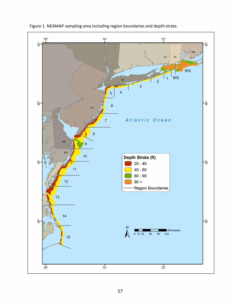
Figure 1. NEAMAP sampling area including region boundaries and depth strata.

57

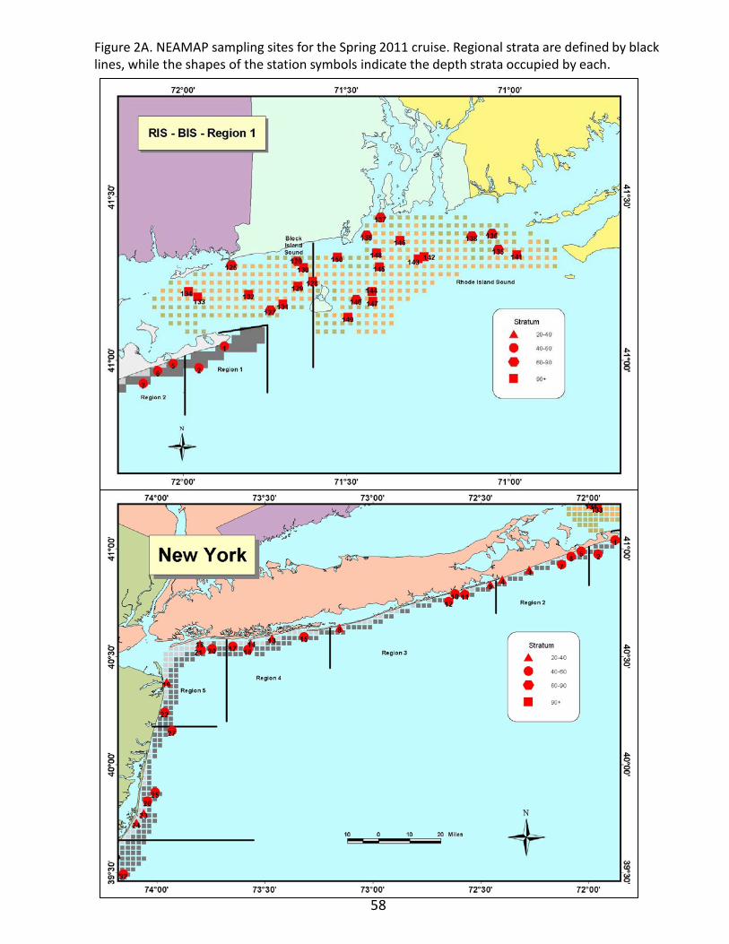
Figure 2A. NEAMAP sampling sites for the Spring 2011 cruise. Regional strata are defined by black lines, while the shapes of the station symbols indicate the depth strata occupied by each.

58

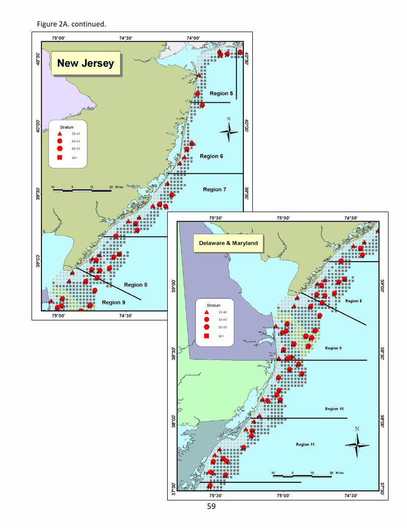
Figure 2A. continued.

59

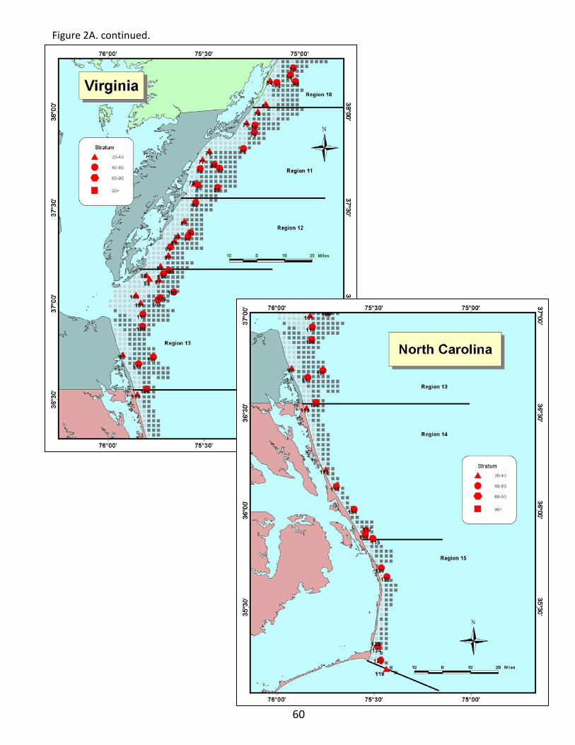
Figure 2A. continued.

60

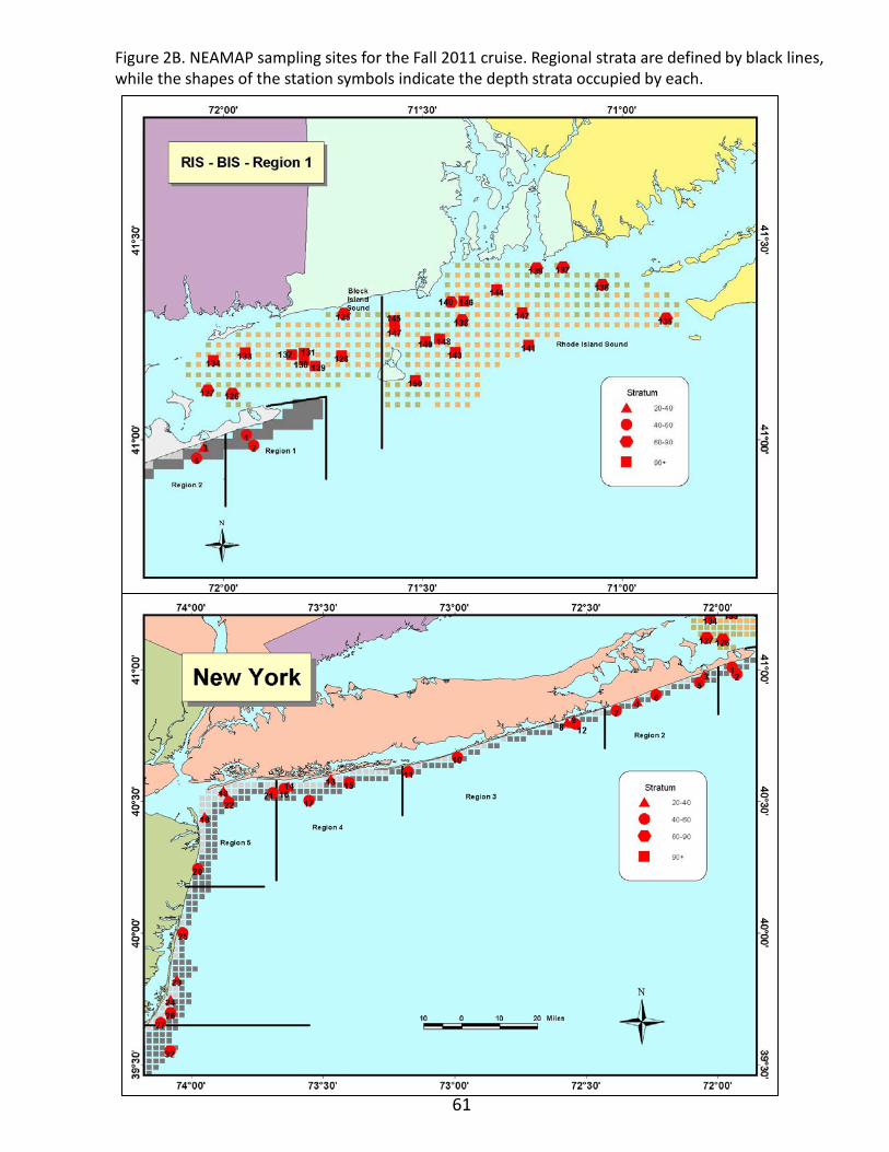
61

Figure 2B. NEAMAP sampling sites for the Fall 2011 cruise. Regional strata are defined by black lines, while the shapes of the station symbols indicate the depth strata occupied by each.

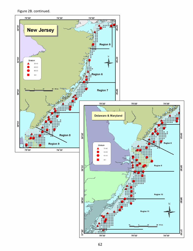
Figure 2B. continued.

62

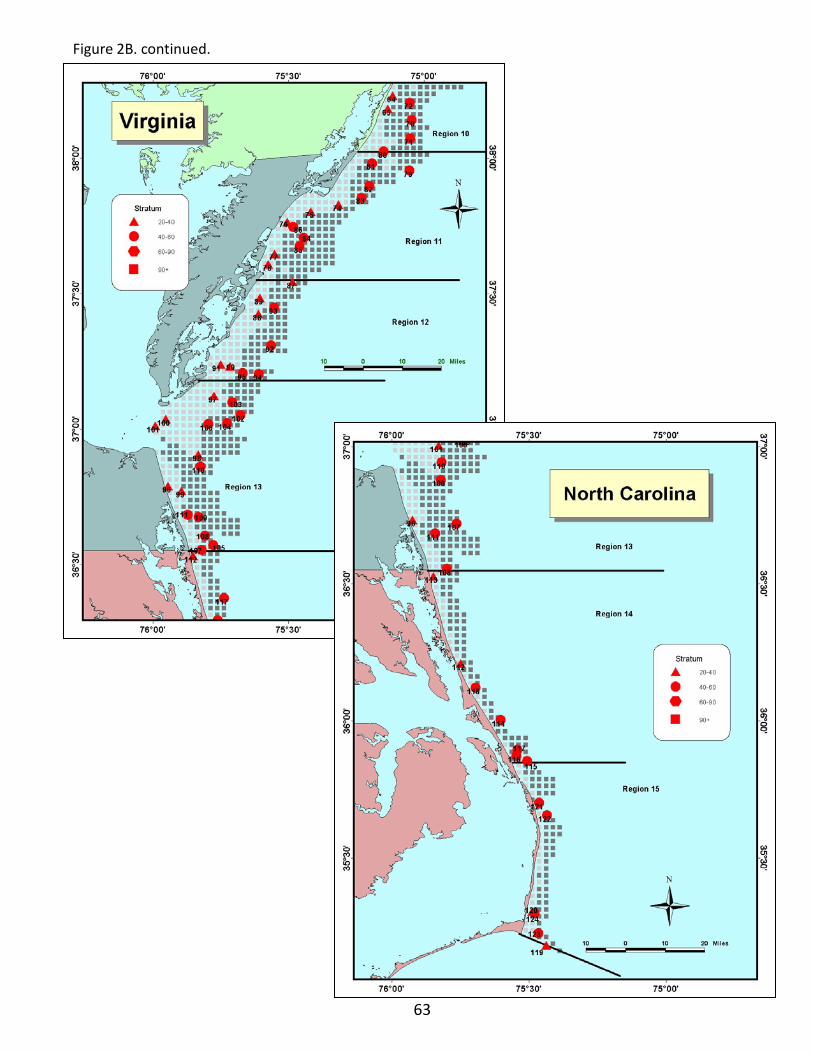
Figure 2B. continued.

63

Figure 3A. Bottom temperatures as measured by NEAMAP for Spring 2008. (Map ‘a’ represents measured values averaged over all spring cruises , ‘b’ gives actual values for spring 2008, and ‘c’ represents the difference. Note that the color scheme and value ranges are the same for ‘a’ and ‘b’ which both differ from ‘c.’)

a

b c

64

a

Figure 3B. Bottom temperatures as measured by NEAMAP for Spring 2009. (Map ‘a’ represents measured values averaged over all spring cruises , ‘b’ gives actual values for spring 2009, and ‘c’ represents the difference. Note that the color scheme and value ranges are the same for ‘a’ and ‘b’ which both differ from ‘c.’)

b c

65

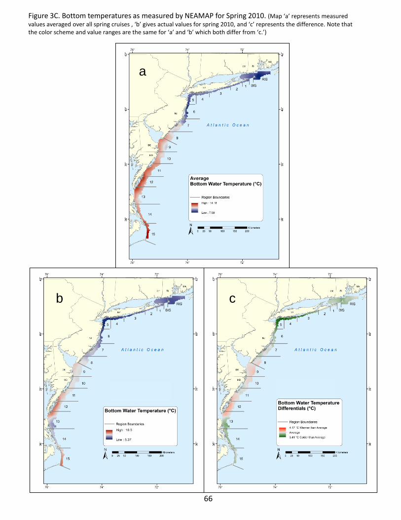
Figure 3C. Bottom temperatures as measured by NEAMAP for Spring 2010. (Map ‘a’ represents measured values averaged over all spring cruises , ‘b’ gives actual values for spring 2010, and ‘c’ represents the difference. Note that the color scheme and value ranges are the same for ‘a’ and ‘b’ which both differ from ‘c.’)

a

b c

66

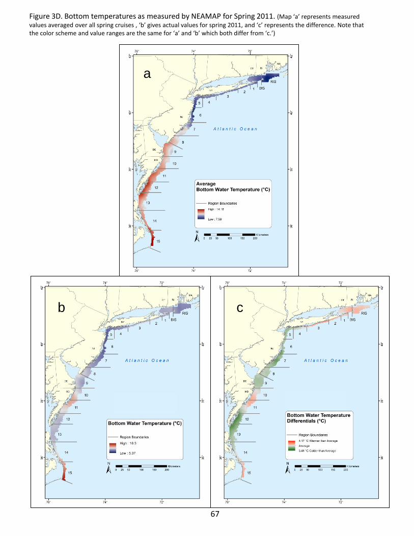
b c

Figure 3D. Bottom temperatures as measured by NEAMAP for Spring 2011. (Map ‘a’ represents measured values averaged over all spring cruises , ‘b’ gives actual values for spring 2011, and ‘c’ represents the difference. Note that the color scheme and value ranges are the same for ‘a’ and ‘b’ which both differ from ‘c.’)

a

67

68

Figure 3E. Bottom temperatures as measured by NEAMAP for Fall 2007. (Map ‘a’ represents measured values averaged over all fall cruises , ‘b’ gives actual values for fall 2007, and ‘c’ represents the difference. Note that the color scheme and value ranges are the same for ‘a’ and ‘b’ which both differ from ‘c.’)

a

b c

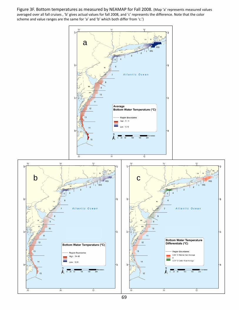
69

Figure 3F. Bottom temperatures as measured by NEAMAP for Fall 2008. (Map ‘a’ represents measured values averaged over all fall cruises , ‘b’ gives actual values for fall 2008, and ‘c’ represents the difference. Note that the color scheme and value ranges are the same for ‘a’ and ‘b’ which both differ from ‘c.’)

a

b c

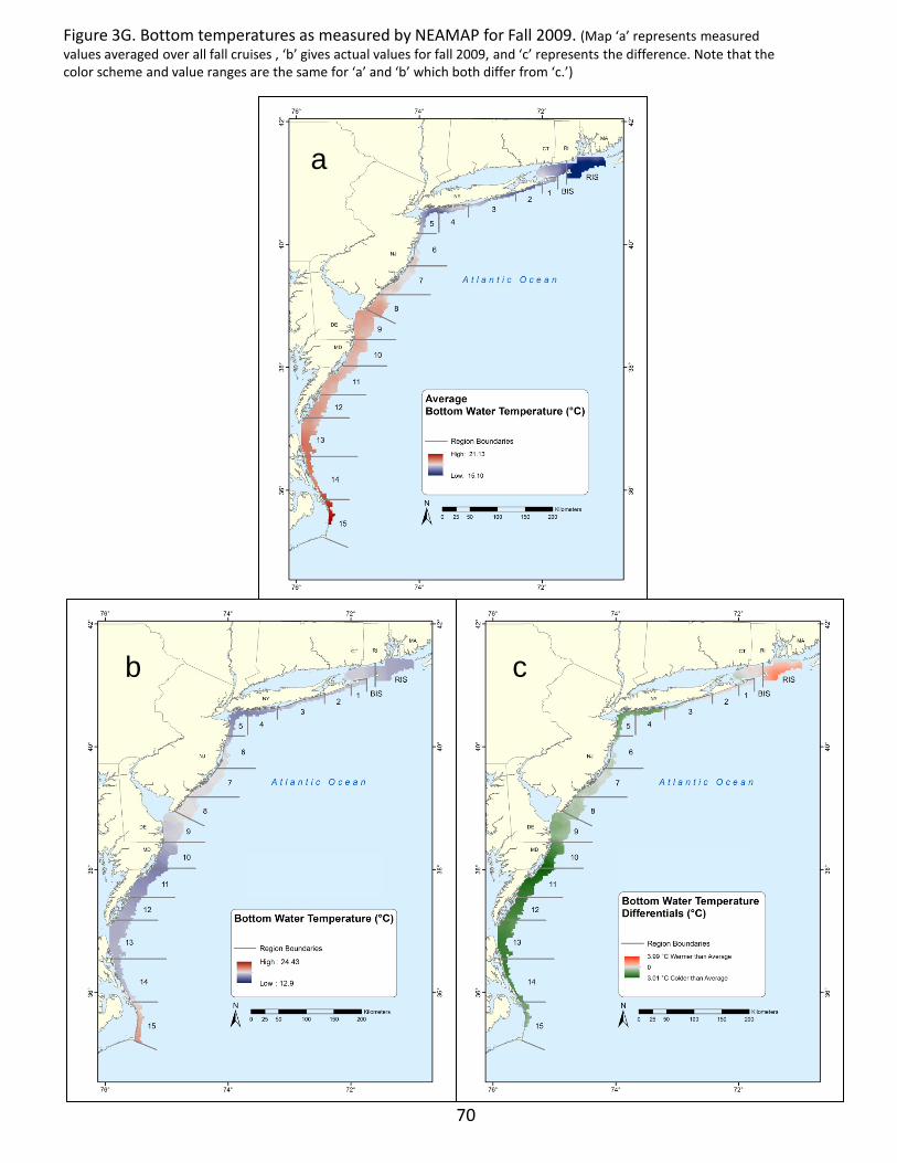
70

Figure 3G. Bottom temperatures as measured by NEAMAP for Fall 2009. (Map ‘a’ represents measured values averaged over all fall cruises , ‘b’ gives actual values for fall 2009, and ‘c’ represents the difference. Note that the color scheme and value ranges are the same for ‘a’ and ‘b’ which both differ from ‘c.’)

a

b c

71

Figure 3H. Bottom temperatures as measured by NEAMAP for Fall 2010. (Map ‘a’ represents measured values averaged over all fall cruises , ‘b’ gives actual values for fall 2010, and ‘c’ represents the difference. Note that the color scheme and value ranges are the same for ‘a’ and ‘b’ which both differ from ‘c.’)

a

b c

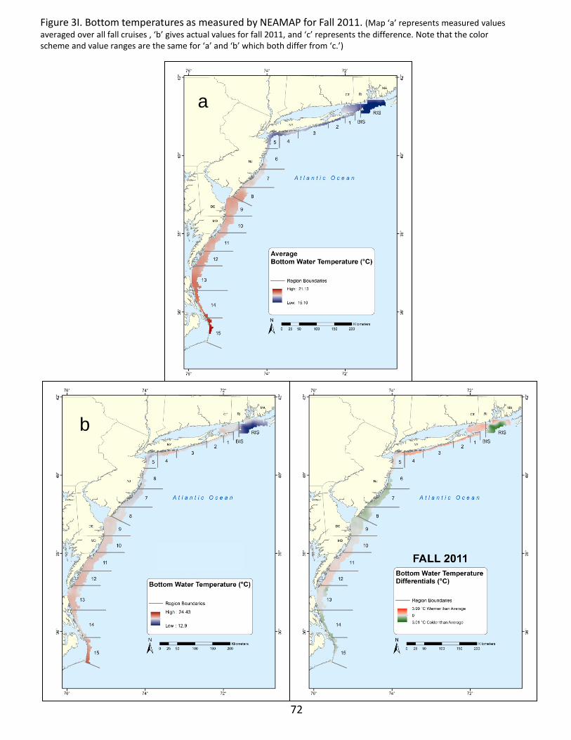
72

Figure 3I. Bottom temperatures as measured by NEAMAP for Fall 2011. (Map ‘a’ represents measured values averaged over all fall cruises , ‘b’ gives actual values for fall 2011, and ‘c’ represents the difference. Note that the color scheme and value ranges are the same for ‘a’ and ‘b’ which both differ from ‘c.’)

a

b c

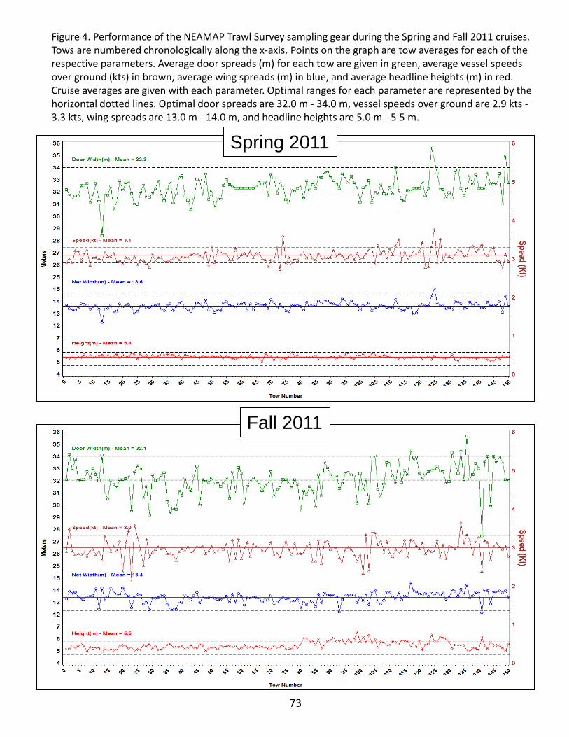
Figure 4. Performance of the NEAMAP Trawl Survey sampling gear during the Spring and Fall 2011 cruises. Tows are numbered chronologically along the x-axis. Points on the graph are tow averages for each of the respective parameters. Average door spreads (m) for each tow are given in green, average vessel speeds over ground (kts) in brown, average wing spreads (m) in blue, and average headline heights (m) in red. Cruise averages are given with each parameter. Optimal ranges for each parameter are represented by the horizontal dotted lines. Optimal door spreads are 32.0 m - 34.0 m, vessel speeds over ground are 2.9 kts - 3.3 kts, wing spreads are 13.0 m - 14.0 m, and headline heights are 5.0 m - 5.5 m.

Fall 2011

Spring 2011

73

Figure 5. Performance of the NEAMAP Trawl Survey Thyboron Type IV 66” trawl doors on one tow during which the doors were equipped with ‘tilt sensors.’ These sensors measured Depth in meters (blue line), Pitch in degrees (red line - the extent that the doors either lean forward or back) and Heel in degrees (green line - the amount that the doors tilt in or out perpendicular to the direction of travel). Expected positive values for Pitch indicate that the doors were angled up in front. Expected negative values for Heel show that the doors tilted in during normal operation. Readings are presented from the entrance and exit times of the doors in the water. Dashed lines indicate the brakes-on to brakes-off official start and end times of the tow. These sensors were used on four consecutive tows with nearly identical results on all tows.

Pitch Heel

74

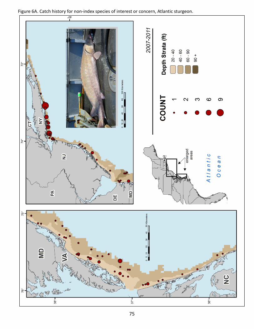
Figure 6A. Catch history for non-index species of interest or concern, Atlantic sturgeon.

75

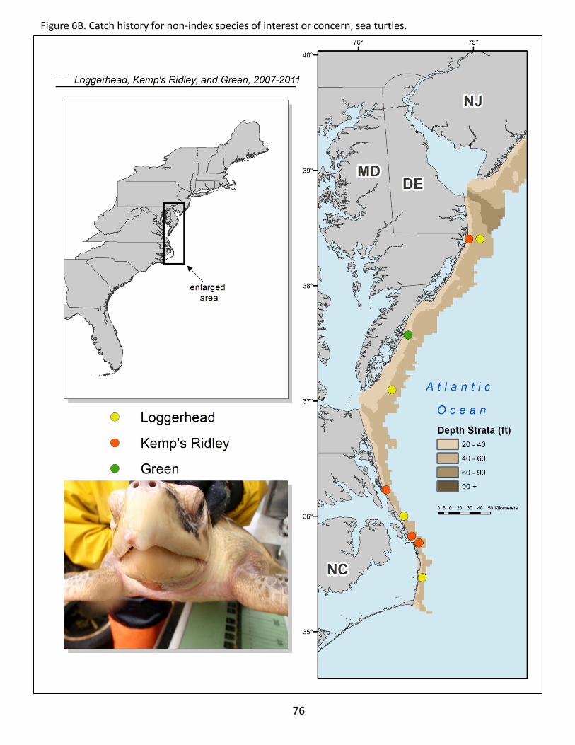
76

Figure 6B. Catch history for non-index species of interest or concern, sea turtles.

77

Figure 6C. Catch history for non-index species of interest or concern, coastal sharks.

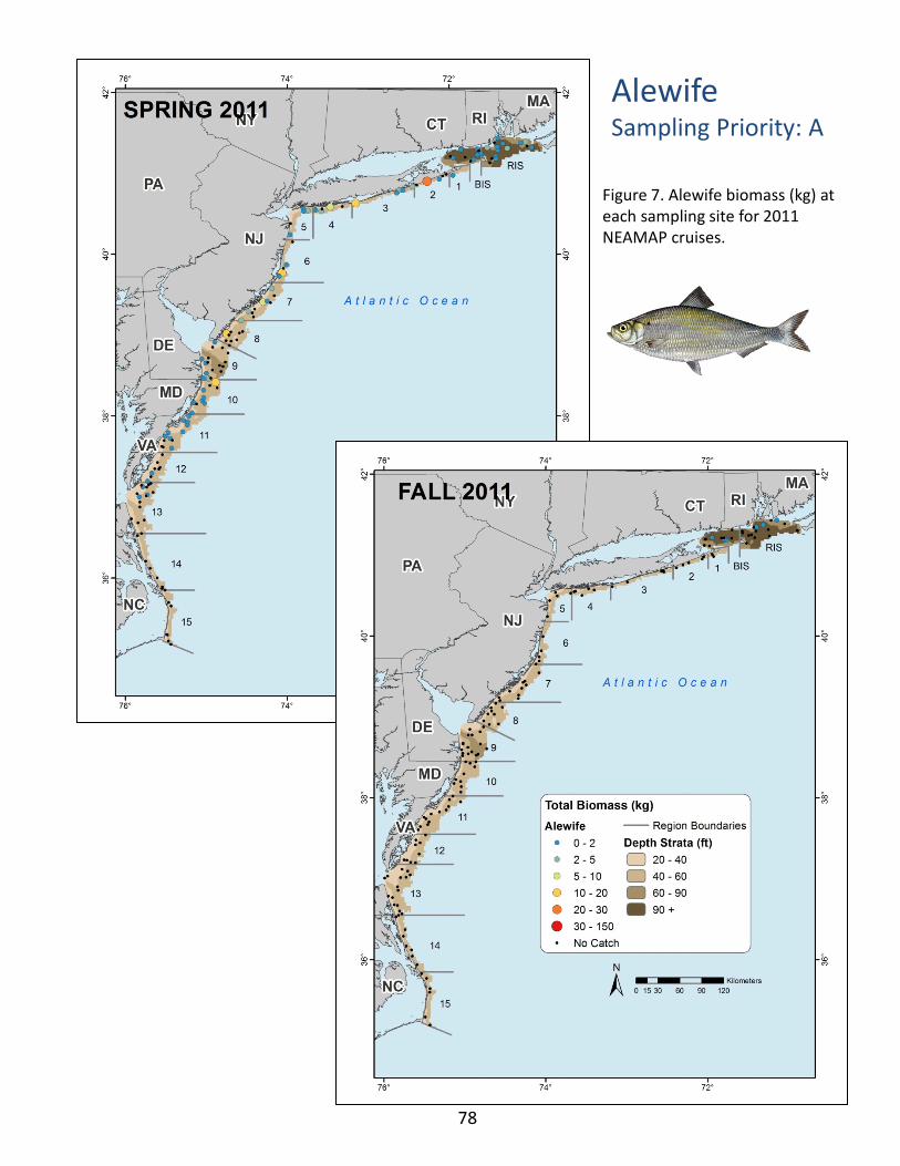
Alewife Sampling Priority: A

Figure 7. Alewife biomass (kg) at each sampling site for 2011 NEAMAP cruises.

78

Table 6. Alewife sampling rates and preserved specimen analysis status for each NEAMAP cruise.

Table 7. Strata used for calculation of abundance indices for alewife (Depth strata definitions are in feet).

Table 8. Alewife preliminary geometric mean indices of abundance, by number and biomass, for spring and fall NEAMAP surveys, for all specimens captured and for the youngest year class captured . .

79

Season YearNumber Caught

Biomass Caught (kg)

Number Measured

Age Specimens

Ages Read

Stomach Specimens

Stomachs Analyzed

Spring 2008 2,419 141.8 1,572 350 0 344 52009 2,955 233.0 1,225 235 0 235 42010 3,735 209.7 1,547 273 0 270 212011 3,373 154.1 1,828 323 0 314 309

Fall 2007 56 3.1 56 24 0 24 02008 5 0.3 5 5 0 5 02009 87 3.9 87 17 0 16 162010 565 13.7 360 39 0 38 382011 27 1.2 27 13 0 13 0

Season Year Agen LCI Index UCI CV (%) n LCI Index UCI CV (%)

Spring 2008 All 150 1.67 2.27 3.00 8.5 150 0.26 0.38 0.51 14.12009 160 0.86 1.23 1.67 11.4 160 0.16 0.27 0.39 19.62010 150 0.95 1.43 2.02 12.3 150 0.15 0.27 0.40 20.52011 150 1.39 1.97 2.68 9.9 150 0.23 0.33 0.45 14.6

Fall 2007 All 17 0.06 0.63 1.51 44.1 17 0.00 0.10 0.25 62.72008 16 0.00 0.06 0.18 100.0 16 0.00 0.01 0.02 100.02009 16 0.00 0.36 1.34 87.8 16 0.00 0.11 0.35 98.32010 16 1.36 5.69 18.02 27.5 16 0.11 0.50 1.02 36.92011 16 0.00 0.40 1.16 65.0 16 0.00 0.06 0.16 80.1

Fall 2007 0 17 0.00 0.00 0.00 17 0.00 0.00 0.002008 16 0.00 0.00 0.00 16 0.00 0.00 0.002009 16 0.00 0.09 0.23 70.8 16 0.00 0.01 0.01 75.32010 16 0.97 4.69 15.50 30.6 16 0.09 0.45 0.94 38.72011 16 0.00 0.23 0.72 79.2 16 0.00 0.03 0.09 92.1

Spring 2008 1 150 0.93 1.31 1.76 10.6 150 0.11 0.18 0.25 18.92009 160 0.51 0.75 1.02 13.0 160 0.07 0.13 0.19 20.72010 150 0.72 1.08 1.53 13.2 150 0.09 0.17 0.26 23.22011 150 0.89 1.32 1.85 12.2 150 0.11 0.19 0.27 19.1

Numerical Index Biomass Index

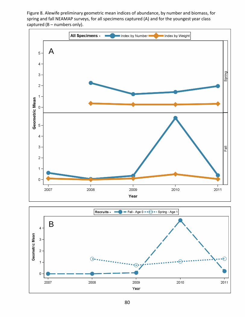
80

Figure 8. Alewife preliminary geometric mean indices of abundance, by number and biomass, for spring and fall NEAMAP surveys, for all specimens captured (A) and for the youngest year class captured (B – numbers only).

B

A

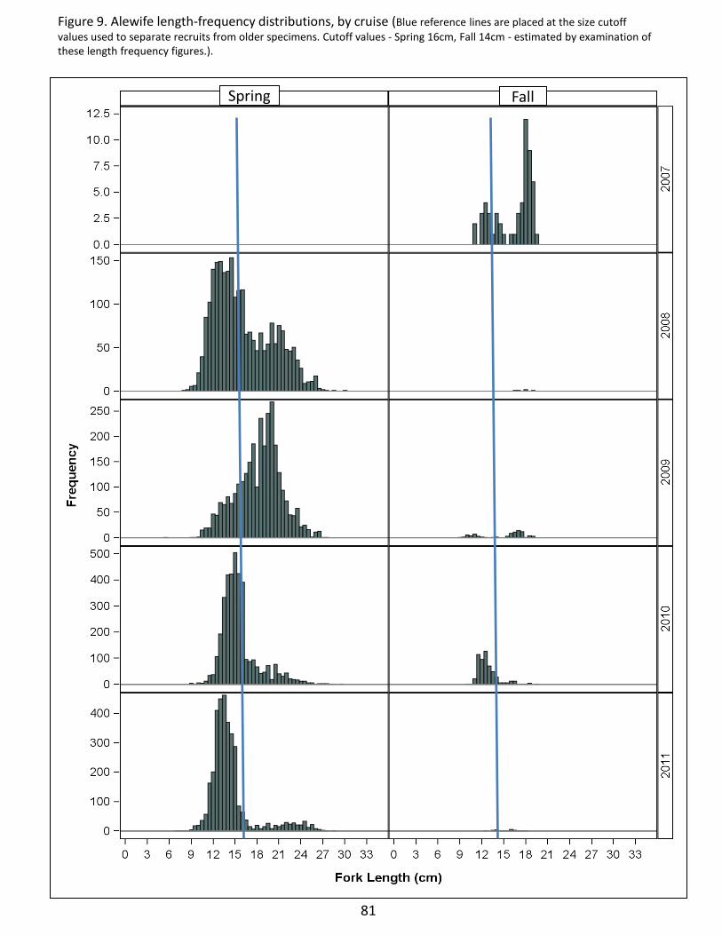
Figure 9. Alewife length-frequency distributions, by cruise (Blue reference lines are placed at the size cutoff values used to separate recruits from older specimens. Cutoff values - Spring 16cm, Fall 14cm - estimated by examination of these length frequency figures.).

81

Spring Fall

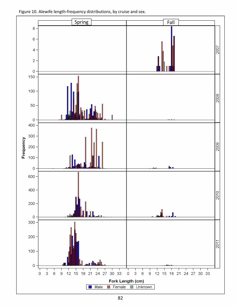
Figure 10. Alewife length-frequency distributions, by cruise and sex.

Spring Fall

82

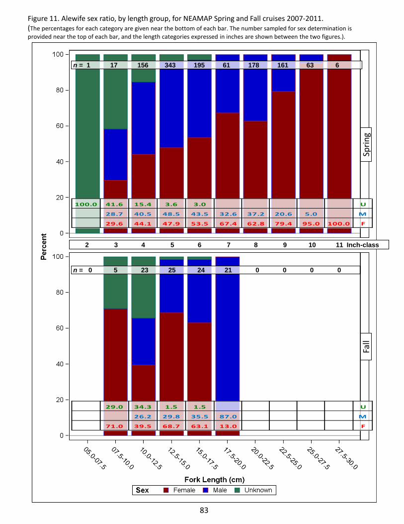
Figure 11. Alewife sex ratio, by length group, for NEAMAP Spring and Fall cruises 2007-2011. (The percentages for each category are given near the bottom of each bar. The number sampled for sex determination is provided near the top of each bar, and the length categories expressed in inches are shown between the two figures.).

83

2 3 4 5 6 7 8 9 10 11 Inch-class

n = 1 17 156 343 195 61 178 161 63 6

100.0 41.6 15.4 3.6 3.0 U

28.7 40.5 48.5 43.5 32.6 37.2 20.6 5.0 M

29.6 44.1 47.9 53.5 67.4 62.8 79.4 95.0 100.0 F

29.0 34.3 1.5 1.5 U

26.2 29.8 35.5 87.0 M

71.0 39.5 68.7 63.1 13.0 F

n = 0 5 23 25 24 21 0 0 0 0

Sprin

g F

all

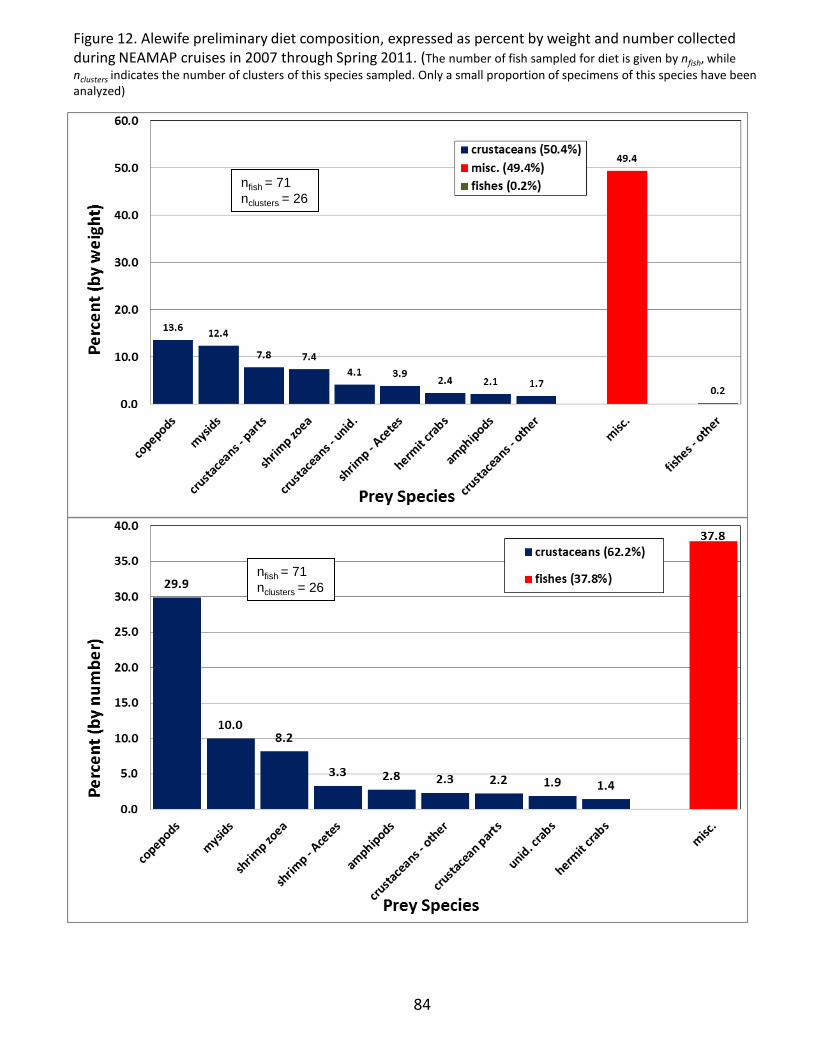
Figure 12. Alewife preliminary diet composition, expressed as percent by weight and number collected during NEAMAP cruises in 2007 through Spring 2011. (The number of fish sampled for diet is given by nfish, while nclusters indicates the number of clusters of this species sampled. Only a small proportion of specimens of this species have been analyzed)

nfish = 71 nclusters = 26

nfish = 71 nclusters = 26

84

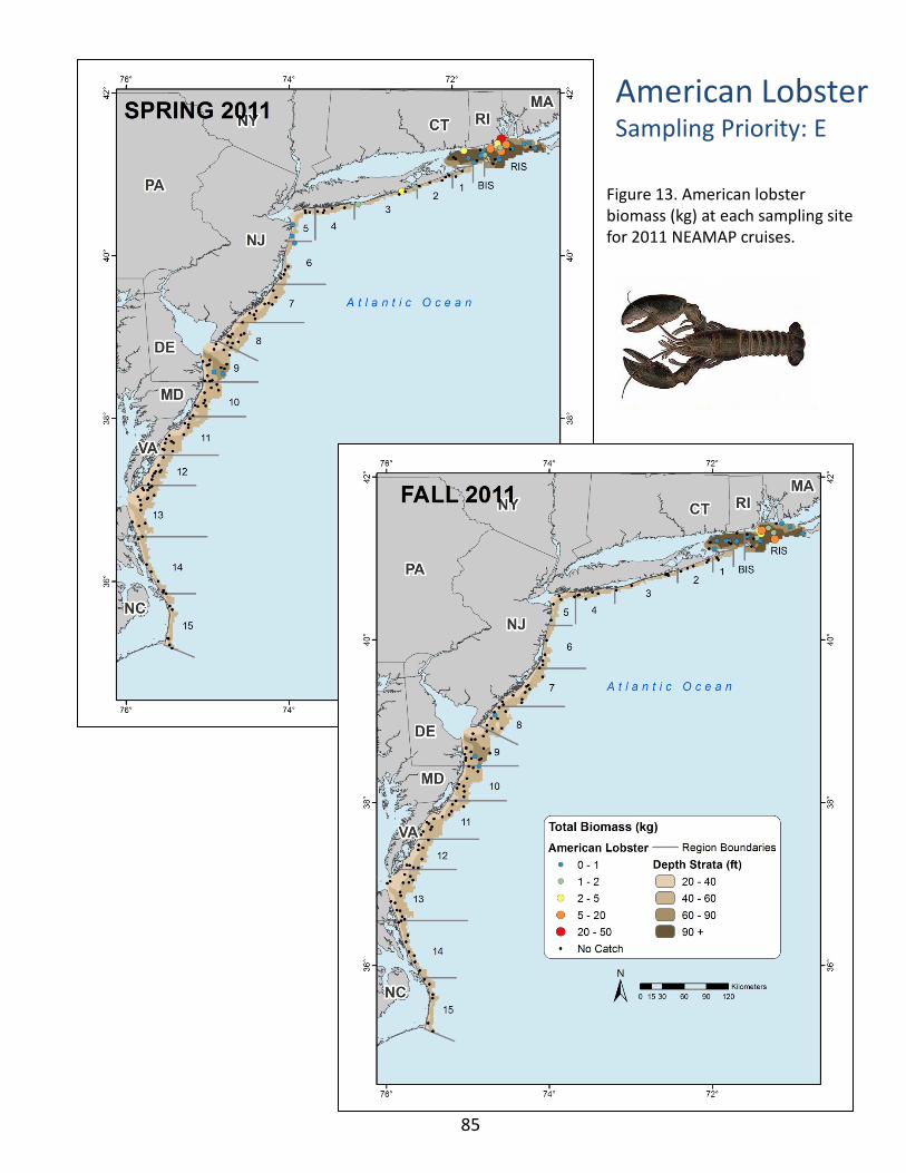
Figure 13. American lobster biomass (kg) at each sampling site for 2011 NEAMAP cruises.

American Lobster Sampling Priority: E

85

Table 9. American lobster sampling rates for each NEAMAP cruise.

Table 11. American lobster preliminary geometric mean indices of abundance, by number and biomass, for spring and fall NEAMAP surveys, for all specimens captured.

Table 10. Strata used for calculation of abundance indices for American lobster.

86

Season YearNumber Caught

Biomass Caught (kg)

Number Measured

Age Specimens

Ages Read

Stomach Specimens

Stomachs Analyzed

Spring 2008 519 89.8 286 N/A N/A N/A N/A2009 290 89.9 248 N/A N/A N/A N/A2010 86 24.0 86 N/A N/A N/A N/A2011 216 67.1 216 N/A N/A N/A N/A

Fall 2007 262 59.0 262 N/A N/A N/A N/A2008 352 80.6 178 N/A N/A N/A N/A2009 89 29.1 89 N/A N/A N/A N/A2010 63 19.4 63 N/A N/A N/A N/A2011 106 30.2 106 N/A N/A N/A N/A

Season Year Agen LCI Index UCI CV (%) n LCI Index UCI CV (%)

Spring 2008 All 27 2.16 4.43 8.32 16.0 27 0.61 1.27 2.20 21.02009 26 2.05 3.79 6.52 14.4 26 0.86 1.60 2.63 17.52010 26 0.54 1.29 2.41 23.8 26 0.23 0.54 0.93 26.42011 26 0.97 2.32 4.58 21.7 26 0.32 0.91 1.76 28.7

Fall 2007 All 26 0.98 2.41 4.86 22.1 26 0.34 0.88 1.65 27.02008 26 1.75 3.23 5.50 14.9 26 0.50 1.05 1.81 21.82009 26 0.79 1.58 2.73 19.4 26 0.26 0.57 0.95 24.22010 26 0.47 1.00 1.73 22.4 26 0.14 0.36 0.63 28.72011 26 0.97 1.94 3.39 18.7 26 0.33 0.71 1.20 23.3

Numerical Index Biomass Index

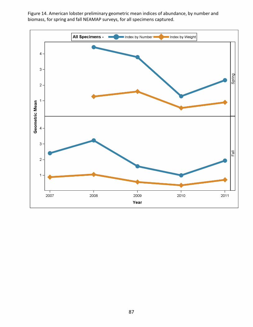
87

Figure 14. American lobster preliminary geometric mean indices of abundance, by number and biomass, for spring and fall NEAMAP surveys, for all specimens captured.

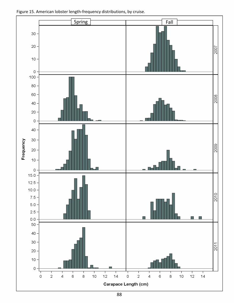
Figure 15. American lobster length-frequency distributions, by cruise.

88

Spring Fall

89

Spring Fall

Figure 16. American lobster length-frequency distributions, by cruise and sex.

89

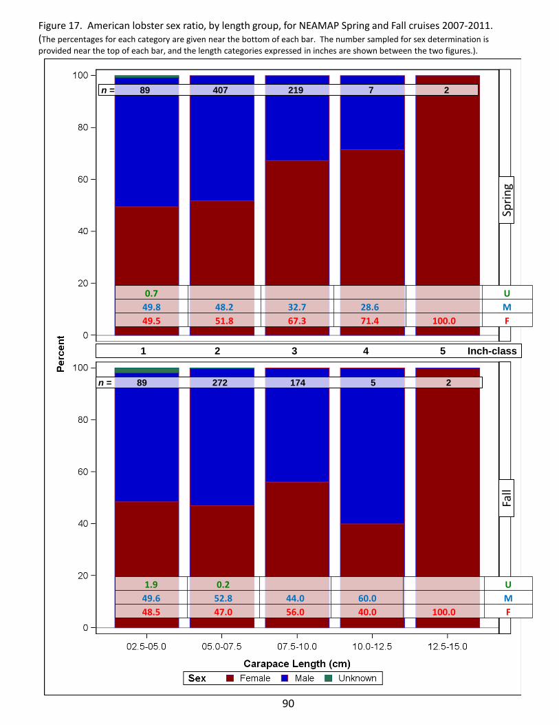
1 2 3 4 5 Inch-class

90

Figure 17. American lobster sex ratio, by length group, for NEAMAP Spring and Fall cruises 2007-2011. (The percentages for each category are given near the bottom of each bar. The number sampled for sex determination is provided near the top of each bar, and the length categories expressed in inches are shown between the two figures.).

n = 89 407 219 7 2

n = 89 272 174 5 2

0.7 U 49.8 48.2 32.7 28.6 M 49.5 51.8 67.3 71.4 100.0 F

1.9 0.2 U 49.6 52.8 44.0 60.0 M 48.5 47.0 56.0 40.0 100.0 F

Sprin

g F

all

American Shad Sampling Priority: A

Figure 18. American shad biomass (kg) at each sampling site for 2011 NEAMAP cruises.

91

Table 12. American shad sampling rates and preserved specimen analysis status for each NEAMAP cruise.

Table 13. Strata used for calculation of abundance indices for American shad.

Table 14. American shad preliminary geometric mean indices of abundance, by number and biomass, for spring NEAMAP surveys, for all specimens captured.

92

Season YearNumber Caught

Biomass Caught (kg)

Number Measured

Age Specimens

Ages Read

Stomach Specimens

Stomachs Analyzed

Spring 2008 1,205 40.8 1,205 327 0 321 02009 1,141 33.2 859 260 0 260 92010 1,236 43.8 942 274 0 273 222011 1,712 73.6 1,418 251 0 249 248

Fall 2007 9 0.8 9 9 0 9 02008 9 0.5 9 5 0 5 02009 28 3.1 28 10 0 10 92010 32 1.1 6 3 0 3 32011 13 1.3 13 13 0 13 0

Season Year Agen LCI Index UCI CV (%) n LCI Index UCI CV (%)

Spring 2008 All 150 1.81 2.36 3.02 7.4 150 0.16 0.20 0.25 10.32009 160 1.09 1.47 1.93 9.4 160 0.09 0.14 0.19 16.52010 150 1.26 1.70 2.21 8.9 150 0.11 0.17 0.23 16.32011 150 1.07 1.52 2.07 10.7 150 0.14 0.21 0.29 15.2

Numerical Index Biomass Index

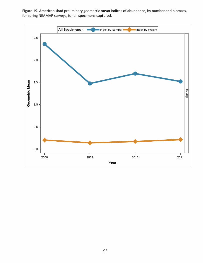
93

Figure 19. American shad preliminary geometric mean indices of abundance, by number and biomass, for spring NEAMAP surveys, for all specimens captured.

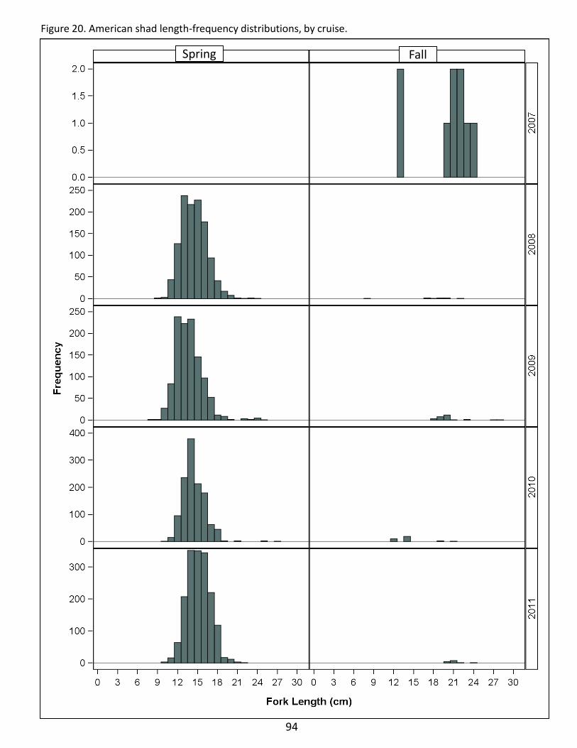
Figure 20. American shad length-frequency distributions, by cruise.

94

Spring Fall

94

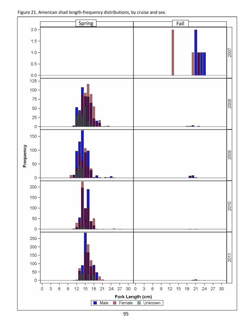
95

Figure 21. American shad length-frequency distributions, by cruise and sex.

Spring Fall

95

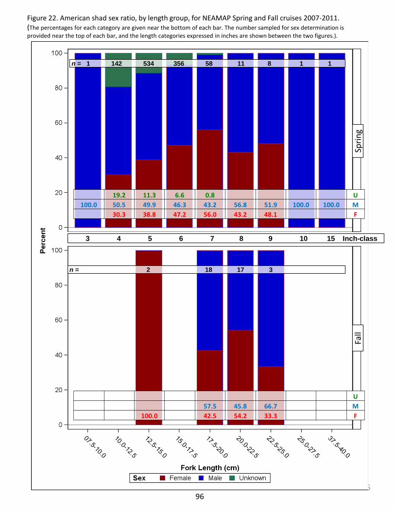
96

Figure 22. American shad sex ratio, by length group, for NEAMAP Spring and Fall cruises 2007-2011. (The percentages for each category are given near the bottom of each bar. The number sampled for sex determination is provided near the top of each bar, and the length categories expressed in inches are shown between the two figures.).

3 4 5 6 7 8 9 10 15 Inch-class

n = 1 142 534 356 58 11 8 1 1

n = 2 18 17 3

19.2 11.3 6.6 0.8 U 100.0 50.5 49.9 46.3 43.2 56.8 51.9 100.0 100.0 M

30.3 38.8 47.2 56.0 43.2 48.1 F

U 57.5 45.8 66.7 M 100.0 42.5 54.2 33.3 F

96

Sprin

g F

all

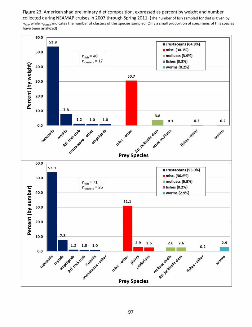
Figure 23. American shad preliminary diet composition, expressed as percent by weight and number collected during NEAMAP cruises in 2007 through Spring 2011. (The number of fish sampled for diet is given by nfish, while nclusters indicates the number of clusters of this species sampled. Only a small proportion of specimens of this species have been analyzed)

97

nfish = 40 nclusters = 17

nfish = 71 nclusters = 26

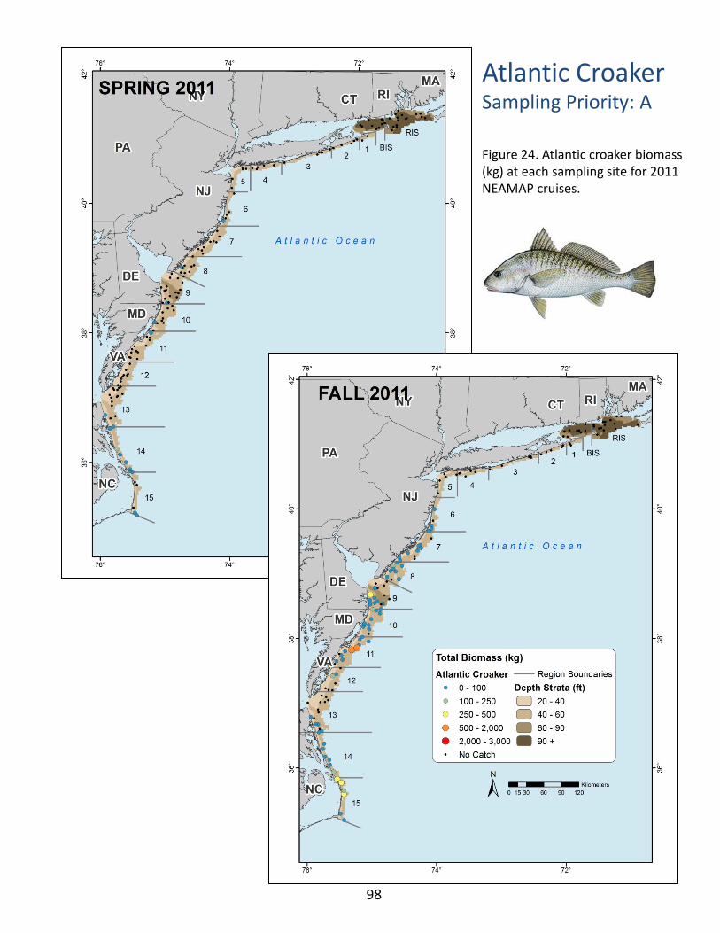
Atlantic Croaker Sampling Priority: A

Figure 24. Atlantic croaker biomass (kg) at each sampling site for 2011 NEAMAP cruises.

98

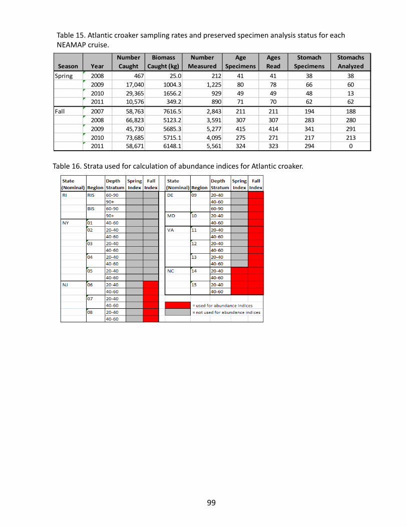
Table 15. Atlantic croaker sampling rates and preserved specimen analysis status for each NEAMAP cruise.

Table 16. Strata used for calculation of abundance indices for Atlantic croaker.

99

Season YearNumber Caught

Biomass Caught (kg)

Number Measured

Age Specimens

Ages Read

Stomach Specimens

Stomachs Analyzed

Spring 2008 467 25.0 212 41 41 38 382009 17,040 1004.3 1,225 80 78 66 602010 29,365 1656.2 929 49 49 48 132011 10,576 349.2 890 71 70 62 62

Fall 2007 58,763 7616.5 2,843 211 211 194 1882008 66,823 5123.2 3,591 307 307 283 2802009 45,730 5685.3 5,277 415 414 341 2912010 73,685 5715.1 4,095 275 271 217 2132011 58,671 6148.1 5,561 324 323 294 0

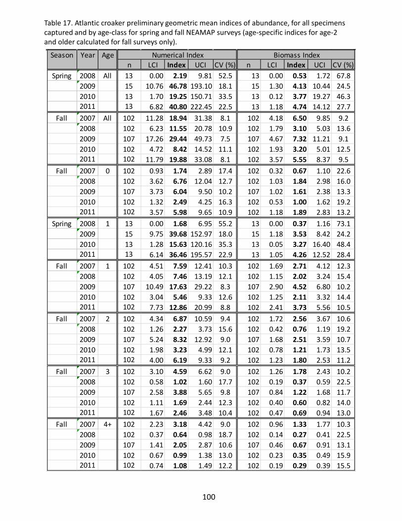
Table 17. Atlantic croaker preliminary geometric mean indices of abundance, for all specimens captured and by age-class for spring and fall NEAMAP surveys (age-specific indices for age-2 and older calculated for fall surveys only).

100

Season Year Agen LCI Index UCI CV (%) n LCI Index UCI CV (%)

Spring 2008 All 13 0.00 2.19 9.81 52.5 13 0.00 0.53 1.72 67.82009 15 10.76 46.78 193.10 18.1 15 1.30 4.13 10.44 24.52010 13 1.70 19.25 150.71 33.5 13 0.12 3.77 19.27 46.32011 13 6.82 40.80 222.45 22.5 13 1.18 4.74 14.12 27.7

Fall 2007 All 102 11.28 18.94 31.38 8.1 102 4.18 6.50 9.85 9.22008 102 6.23 11.55 20.78 10.9 102 1.79 3.10 5.03 13.62009 107 17.26 29.44 49.73 7.5 107 4.67 7.32 11.21 9.12010 102 4.72 8.42 14.52 11.1 102 1.93 3.20 5.01 12.52011 102 11.79 19.88 33.08 8.1 102 3.57 5.55 8.37 9.5

Fall 2007 0 102 0.93 1.74 2.89 17.4 102 0.32 0.67 1.10 22.62008 102 3.62 6.76 12.04 12.7 102 1.03 1.84 2.98 16.02009 107 3.73 6.04 9.50 10.2 107 1.02 1.61 2.38 13.32010 102 1.32 2.49 4.25 16.3 102 0.53 1.00 1.62 19.22011 102 3.57 5.98 9.65 10.9 102 1.18 1.89 2.83 13.2

Spring 2008 1 13 0.00 1.68 6.95 55.2 13 0.00 0.37 1.16 73.12009 15 9.75 39.68 152.97 18.0 15 1.18 3.53 8.42 24.22010 13 1.28 15.63 120.16 35.3 13 0.05 3.27 16.40 48.42011 13 6.14 36.46 195.57 22.9 13 1.05 4.26 12.52 28.4

Fall 2007 1 102 4.51 7.59 12.41 10.3 102 1.69 2.71 4.12 12.32008 102 4.05 7.46 13.19 12.1 102 1.15 2.02 3.24 15.42009 107 10.49 17.63 29.22 8.3 107 2.90 4.52 6.80 10.22010 102 3.04 5.46 9.33 12.6 102 1.25 2.11 3.32 14.42011 102 7.73 12.86 20.99 8.8 102 2.41 3.73 5.56 10.5

Fall 2007 2 102 4.34 6.87 10.59 9.4 102 1.72 2.56 3.67 10.62008 102 1.26 2.27 3.73 15.6 102 0.42 0.76 1.19 19.22009 107 5.24 8.32 12.92 9.0 107 1.68 2.51 3.59 10.72010 102 1.98 3.23 4.99 12.1 102 0.78 1.21 1.73 13.52011 102 4.00 6.19 9.33 9.2 102 1.23 1.80 2.53 11.2

Fall 2007 3 102 3.10 4.59 6.62 9.0 102 1.26 1.78 2.43 10.22008 102 0.58 1.02 1.60 17.7 102 0.19 0.37 0.59 22.52009 107 2.58 3.88 5.65 9.8 107 0.84 1.22 1.68 11.72010 102 1.11 1.69 2.44 12.3 102 0.40 0.60 0.82 14.02011 102 1.67 2.46 3.48 10.4 102 0.47 0.69 0.94 13.0

Fall 2007 4+ 102 2.23 3.18 4.42 9.0 102 0.96 1.33 1.77 10.32008 102 0.37 0.64 0.98 18.7 102 0.14 0.27 0.41 22.52009 107 1.41 2.05 2.87 10.6 107 0.46 0.67 0.91 13.12010 102 0.67 0.99 1.38 13.0 102 0.23 0.35 0.49 15.92011 102 0.74 1.08 1.49 12.2 102 0.19 0.29 0.39 15.5

Numerical Index Biomass Index

101

A

Figure 25. Atlantic croaker preliminary geometric mean indices of abundance, for all specimens captured (A - by number and biomass) and by age-class (B – numbers only) for spring and fall NEAMAP surveys (age-specific indices for age-2 and older calculated for fall surveys only).

B

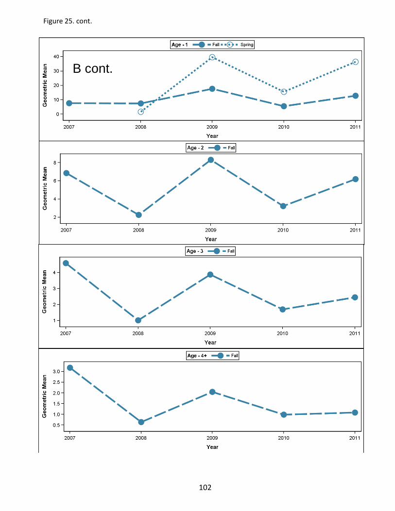
102

B cont.

Figure 25. cont.

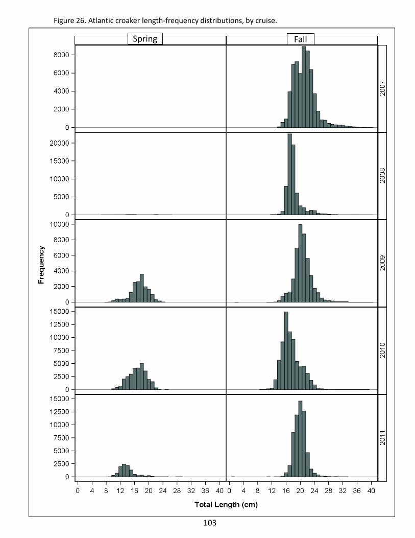
Figure 26. Atlantic croaker length-frequency distributions, by cruise.

103

Spring Fall

103

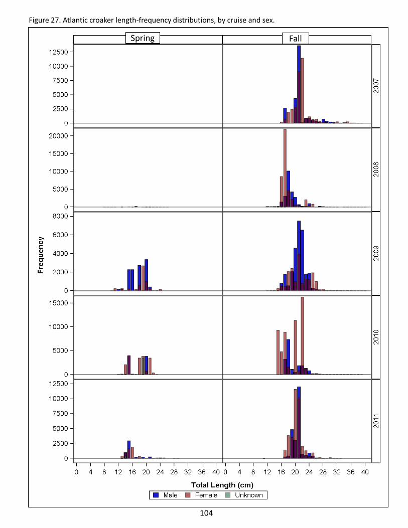
104

Figure 27. Atlantic croaker length-frequency distributions, by cruise and sex.

Spring Fall

104

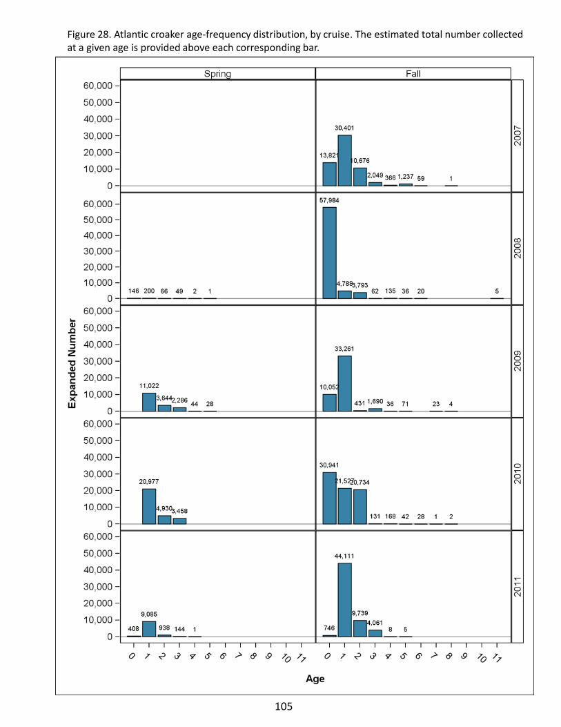
Figure 28. Atlantic croaker age-frequency distribution, by cruise. The estimated total number collected at a given age is provided above each corresponding bar.

105

Figure 29. Atlantic croaker age-at-length proportions for all spring vs. all fall cruises combined, showing actual and loess smoothed proportions at each 1cm length bin.

106

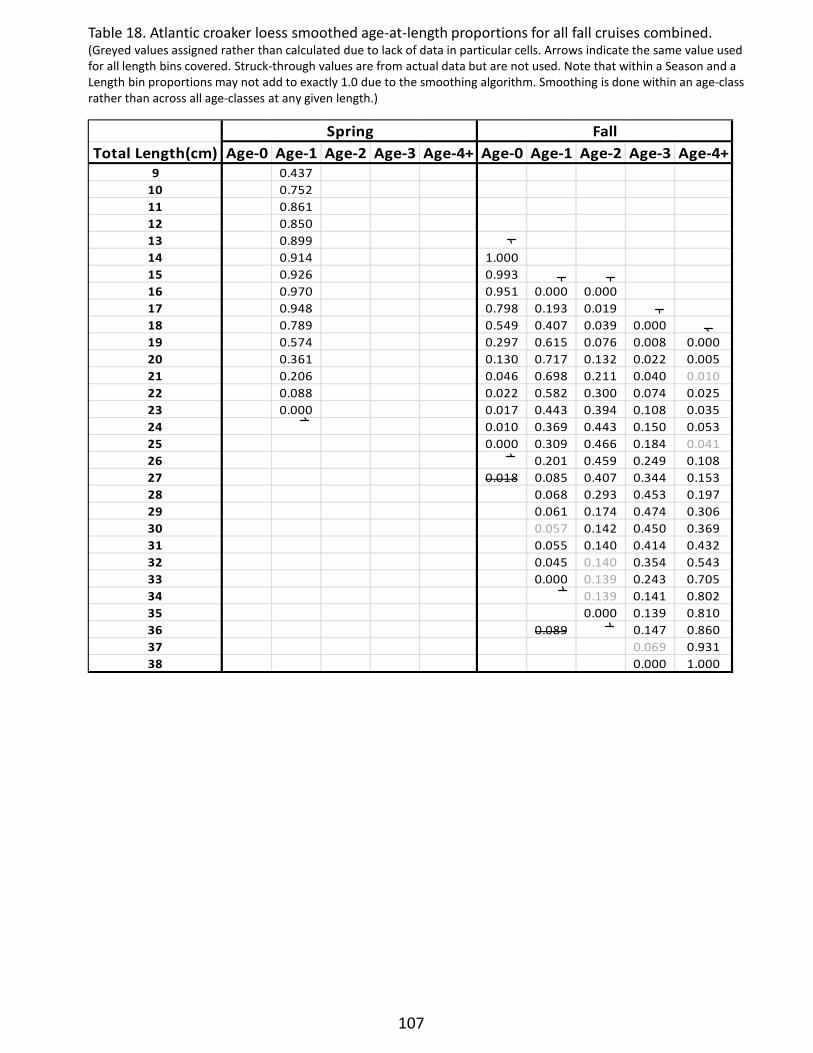
Table 18. Atlantic croaker loess smoothed age-at-length proportions for all fall cruises combined. (Greyed values assigned rather than calculated due to lack of data in particular cells. Arrows indicate the same value used for all length bins covered. Struck-through values are from actual data but are not used. Note that within a Season and a Length bin proportions may not add to exactly 1.0 due to the smoothing algorithm. Smoothing is done within an age-class rather than across all age-classes at any given length.)

Total Length(cm) Age-0 Age-1 Age-2 Age-3 Age-4+ Age-0 Age-1 Age-2 Age-3 Age-4+9 0.437

10 0.75211 0.86112 0.85013 0.89914 0.914 1.00015 0.926 0.99316 0.970 0.951 0.000 0.00017 0.948 0.798 0.193 0.01918 0.789 0.549 0.407 0.039 0.00019 0.574 0.297 0.615 0.076 0.008 0.00020 0.361 0.130 0.717 0.132 0.022 0.00521 0.206 0.046 0.698 0.211 0.040 0.01022 0.088 0.022 0.582 0.300 0.074 0.02523 0.000 0.017 0.443 0.394 0.108 0.03524 0.010 0.369 0.443 0.150 0.05325 0.000 0.309 0.466 0.184 0.04126 0.201 0.459 0.249 0.10827 0.018 0.085 0.407 0.344 0.15328 0.068 0.293 0.453 0.19729 0.061 0.174 0.474 0.30630 0.057 0.142 0.450 0.36931 0.055 0.140 0.414 0.43232 0.045 0.140 0.354 0.54333 0.000 0.139 0.243 0.70534 0.139 0.141 0.80235 0.000 0.139 0.81036 0.089 0.147 0.86037 0.069 0.93138 0.000 1.000

Spring Fall

107

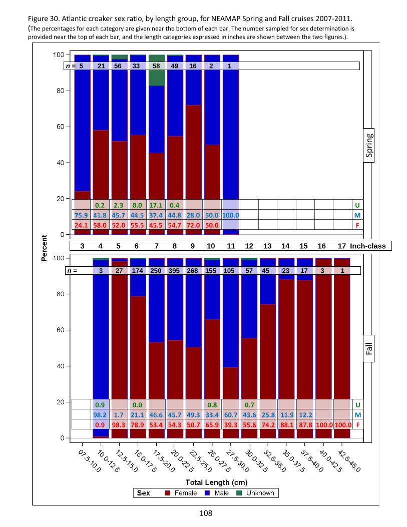
108

Figure 30. Atlantic croaker sex ratio, by length group, for NEAMAP Spring and Fall cruises 2007-2011. (The percentages for each category are given near the bottom of each bar. The number sampled for sex determination is provided near the top of each bar, and the length categories expressed in inches are shown between the two figures.).

n = 5 21 56 33 58 49 16 2 1

n = 3 27 174 250 395 268 155 105 57 45 23 17 3 1

3 4 5 6 7 8 9 10 11 12 13 14 15 16 17 Inch-class

0.2 2.3 0.0 17.1 0.4 U 75.9 41.8 45.7 44.5 37.4 44.8 28.0 50.0 100.0 M 24.1 58.0 52.0 55.5 45.5 54.7 72.0 50.0 F

0.9 0.0 0.8 0.7 U 98.2 1.7 21.1 46.6 45.7 49.3 33.4 60.7 43.6 25.8 11.9 12.2 M 0.9 98.3 78.9 53.4 54.3 50.7 65.9 39.3 55.6 74.2 88.1 87.8 100.0 100.0 F

Sprin

g F

all

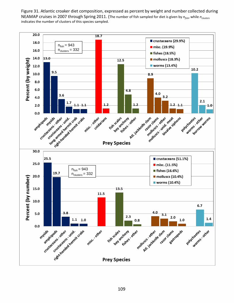
nfish = 943 nclusters = 332

109

Figure 31. Atlantic croaker diet composition, expressed as percent by weight and number collected during NEAMAP cruises in 2007 through Spring 2011. (The number of fish sampled for diet is given by nfish, while nclusters indicates the number of clusters of this species sampled.

nfish = 943 nclusters = 332

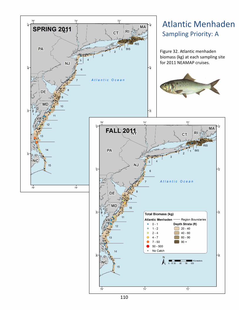
Atlantic Menhaden Sampling Priority: A

Figure 32. Atlantic menhaden biomass (kg) at each sampling site for 2011 NEAMAP cruises.

110

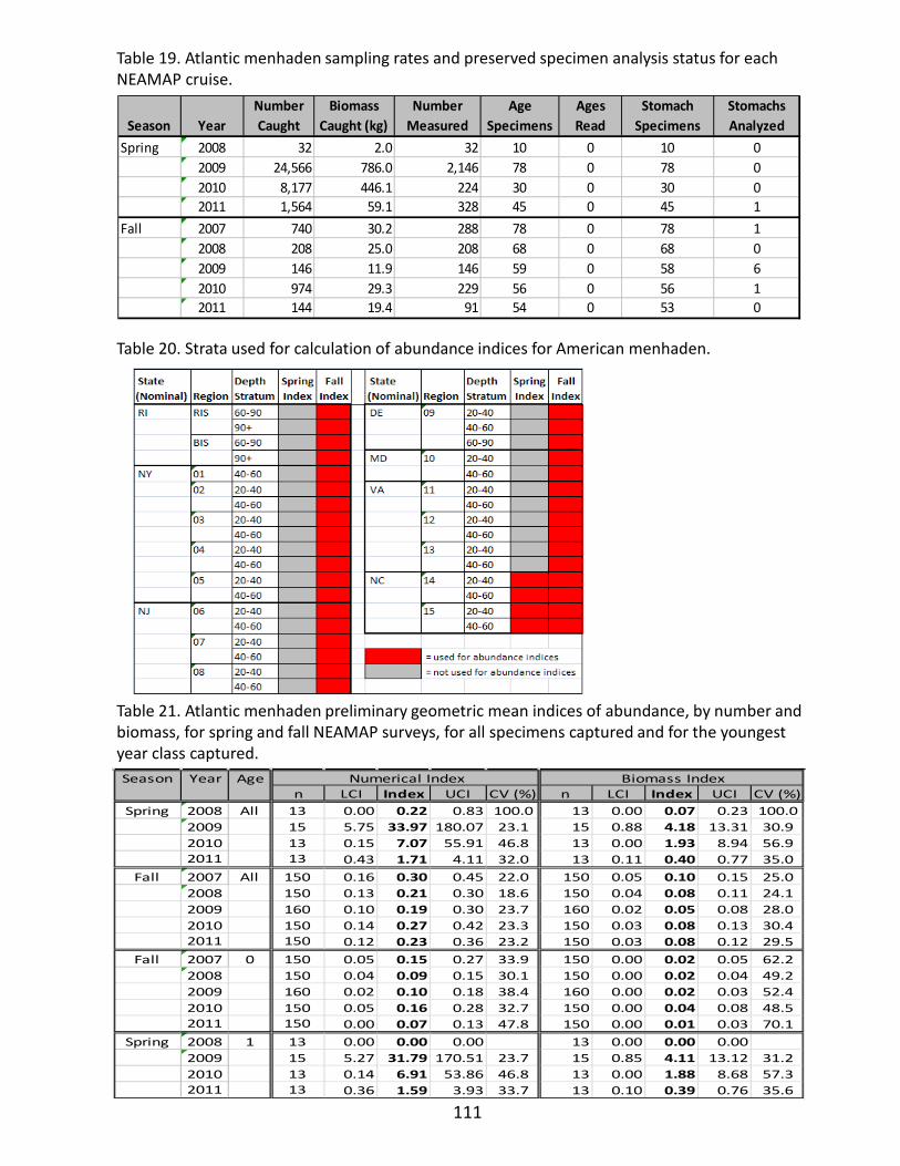
Table 19. Atlantic menhaden sampling rates and preserved specimen analysis status for each NEAMAP cruise.

Table 20. Strata used for calculation of abundance indices for American menhaden.

Table 21. Atlantic menhaden preliminary geometric mean indices of abundance, by number and biomass, for spring and fall NEAMAP surveys, for all specimens captured and for the youngest year class captured.

111

Season YearNumber Caught

Biomass Caught (kg)

Number Measured

Age Specimens

Ages Read

Stomach Specimens

Stomachs Analyzed

Spring 2008 32 2.0 32 10 0 10 02009 24,566 786.0 2,146 78 0 78 02010 8,177 446.1 224 30 0 30 02011 1,564 59.1 328 45 0 45 1

Fall 2007 740 30.2 288 78 0 78 12008 208 25.0 208 68 0 68 02009 146 11.9 146 59 0 58 62010 974 29.3 229 56 0 56 12011 144 19.4 91 54 0 53 0

Season Year Agen LCI Index UCI CV (%) n LCI Index UCI CV (%)

Spring 2008 All 13 0.00 0.22 0.83 100.0 13 0.00 0.07 0.23 100.02009 15 5.75 33.97 180.07 23.1 15 0.88 4.18 13.31 30.92010 13 0.15 7.07 55.91 46.8 13 0.00 1.93 8.94 56.92011 13 0.43 1.71 4.11 32.0 13 0.11 0.40 0.77 35.0

Fall 2007 All 150 0.16 0.30 0.45 22.0 150 0.05 0.10 0.15 25.02008 150 0.13 0.21 0.30 18.6 150 0.04 0.08 0.11 24.12009 160 0.10 0.19 0.30 23.7 160 0.02 0.05 0.08 28.02010 150 0.14 0.27 0.42 23.3 150 0.03 0.08 0.13 30.42011 150 0.12 0.23 0.36 23.2 150 0.03 0.08 0.12 29.5

Fall 2007 0 150 0.05 0.15 0.27 33.9 150 0.00 0.02 0.05 62.22008 150 0.04 0.09 0.15 30.1 150 0.00 0.02 0.04 49.22009 160 0.02 0.10 0.18 38.4 160 0.00 0.02 0.03 52.42010 150 0.05 0.16 0.28 32.7 150 0.00 0.04 0.08 48.52011 150 0.00 0.07 0.13 47.8 150 0.00 0.01 0.03 70.1

Spring 2008 1 13 0.00 0.00 0.00 13 0.00 0.00 0.002009 15 5.27 31.79 170.51 23.7 15 0.85 4.11 13.12 31.22010 13 0.14 6.91 53.86 46.8 13 0.00 1.88 8.68 57.32011 13 0.36 1.59 3.93 33.7 13 0.10 0.39 0.76 35.6

Numerical Index Biomass Index

112

Figure 33. Atlantic menhaden preliminary geometric mean indices of abundance, by number and biomass, for spring and fall NEAMAP surveys, for all specimens captured (A) and for the youngest year class captured (B – numbers only).

B

A

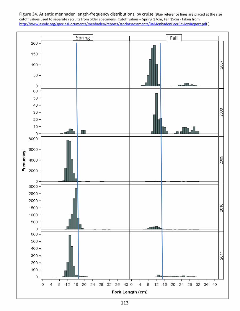
Figure 34. Atlantic menhaden length-frequency distributions, by cruise (Blue reference lines are placed at the size cutoff values used to separate recruits from older specimens. Cutoff values – Spring 17cm, Fall 15cm - taken from http://www.asmfc.org/speciesDocuments/menhaden/reports/stockAssessments/04MenhadenPeerReviewReport.pdf.).

113

Spring Fall

113

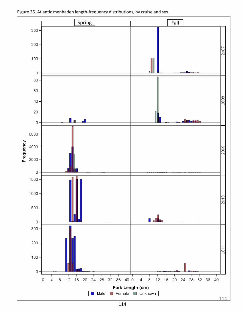
114

Figure 35. Atlantic menhaden length-frequency distributions, by cruise and sex.

Spring Fall

114

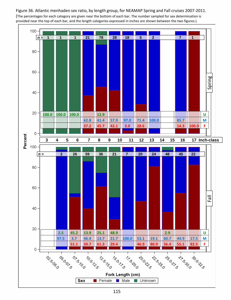
115

Figure 36. Atlantic menhaden sex ratio, by length group, for NEAMAP Spring and Fall cruises 2007-2011. (The percentages for each category are given near the bottom of each bar. The number sampled for sex determination is provided near the top of each bar, and the length categories expressed in inches are shown between the two figures.).

n = 1 1 1 21 78 28 18 5 2 7 1

n = 2 26 59 36 21 7 20 24 48 45 22

3 4 5 6 7 8 9 10 11 12 13 14 15 16 17 Inch-class

100.0 100.0 100.0 12.9 U 62.8 41.4 57.9 97.0 71.4 100.0 85.7 M 37.2 45.7 42.1 3.0 28.6 14.3 100.0 F

2.5 45.2 13.9 25.1 48.9 2.9 U 97.5 3.7 46.4 13.7 21.7 100.0 53.1 19.1 60.7 44.9 17.5 M 51.1 39.7 61.3 29.4 46.9 80.9 36.4 55.1 82.5 F

Sprin

g F

all

Bay Anchovy Sampling Priority: D

Figure 37. Bay anchovy biomass (kg) at each sampling site for 2011 NEAMAP cruises.

116

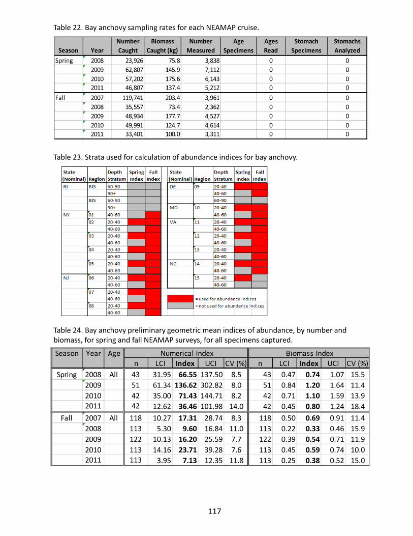
Table 22. Bay anchovy sampling rates for each NEAMAP cruise.

Table 23. Strata used for calculation of abundance indices for bay anchovy.

Table 24. Bay anchovy preliminary geometric mean indices of abundance, by number and biomass, for spring and fall NEAMAP surveys, for all specimens captured.

117

Season YearNumber Caught

Biomass Caught (kg)

Number Measured

Age Specimens

Ages Read

Stomach Specimens

Stomachs Analyzed

Spring 2008 23,926 75.8 3,838 0 02009 62,807 145.9 7,112 0 02010 57,202 175.6 6,143 0 02011 46,807 137.4 5,212 0 0

Fall 2007 119,741 203.4 3,961 0 02008 35,557 73.4 2,362 0 02009 48,934 177.7 4,527 0 02010 49,991 124.7 4,614 0 02011 33,401 100.0 3,311 0 0

Season Year Agen LCI Index UCI CV (%) n LCI Index UCI CV (%)

Spring 2008 All 43 31.95 66.55 137.50 8.5 43 0.47 0.74 1.07 15.52009 51 61.34 136.62 302.82 8.0 51 0.84 1.20 1.64 11.42010 42 35.00 71.43 144.71 8.2 42 0.71 1.10 1.59 13.92011 42 12.62 36.46 101.98 14.0 42 0.45 0.80 1.24 18.4

Fall 2007 All 118 10.27 17.31 28.74 8.3 118 0.50 0.69 0.91 11.42008 113 5.30 9.60 16.84 11.0 113 0.22 0.33 0.46 15.92009 122 10.13 16.20 25.59 7.7 122 0.39 0.54 0.71 11.92010 113 14.16 23.71 39.28 7.6 113 0.45 0.59 0.74 10.02011 113 3.95 7.13 12.35 11.8 113 0.25 0.38 0.52 15.0

Numerical Index Biomass Index

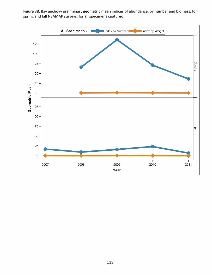
118

Figure 38. Bay anchovy preliminary geometric mean indices of abundance, by number and biomass, for spring and fall NEAMAP surveys, for all specimens captured.

Figure 39. Bay anchovy length-frequency distributions, by cruise.

119

Spring Fall

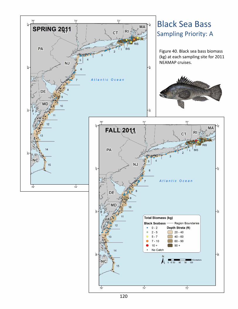
Black Sea Bass Sampling Priority: A

Figure 40. Black sea bass biomass (kg) at each sampling site for 2011 NEAMAP cruises.

120

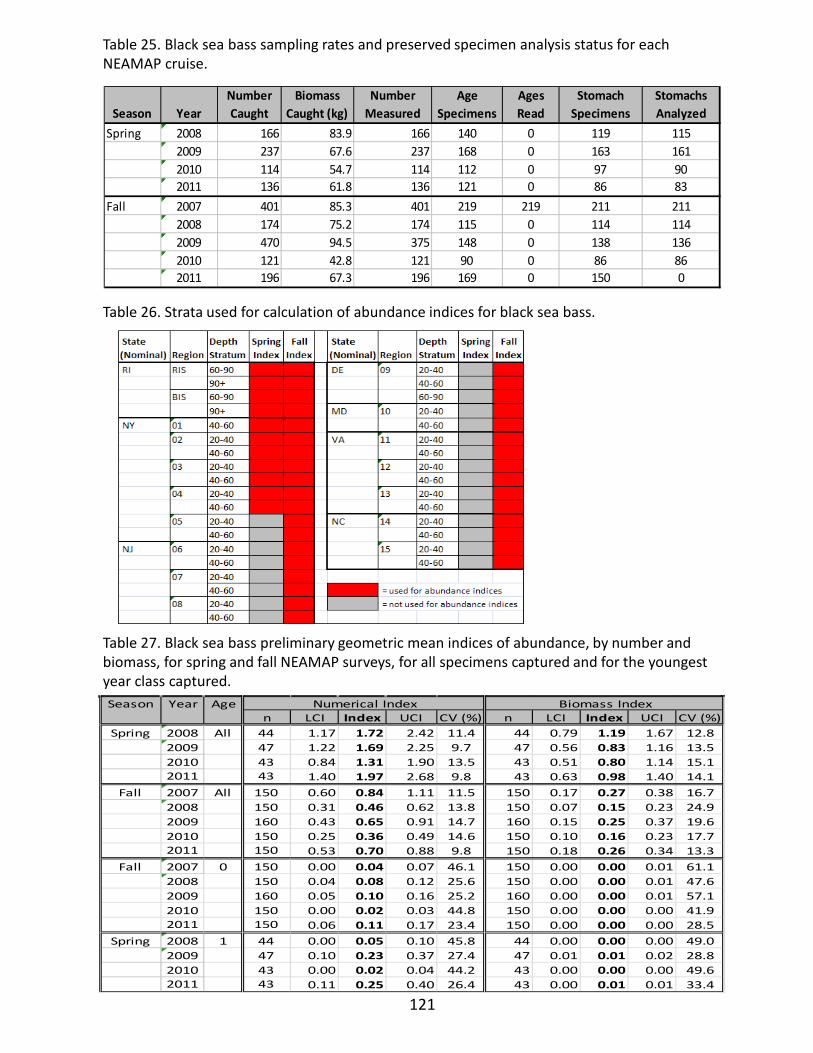
Table 25. Black sea bass sampling rates and preserved specimen analysis status for each NEAMAP cruise.

Table 26. Strata used for calculation of abundance indices for black sea bass.

Table 27. Black sea bass preliminary geometric mean indices of abundance, by number and biomass, for spring and fall NEAMAP surveys, for all specimens captured and for the youngest year class captured.

121

Season YearNumber Caught

Biomass Caught (kg)

Number Measured

Age Specimens

Ages Read

Stomach Specimens

Stomachs Analyzed

Spring 2008 166 83.9 166 140 0 119 1152009 237 67.6 237 168 0 163 1612010 114 54.7 114 112 0 97 902011 136 61.8 136 121 0 86 83

Fall 2007 401 85.3 401 219 219 211 2112008 174 75.2 174 115 0 114 1142009 470 94.5 375 148 0 138 1362010 121 42.8 121 90 0 86 862011 196 67.3 196 169 0 150 0

Season Year Agen LCI Index UCI CV (%) n LCI Index UCI CV (%)

Spring 2008 All 44 1.17 1.72 2.42 11.4 44 0.79 1.19 1.67 12.82009 47 1.22 1.69 2.25 9.7 47 0.56 0.83 1.16 13.52010 43 0.84 1.31 1.90 13.5 43 0.51 0.80 1.14 15.12011 43 1.40 1.97 2.68 9.8 43 0.63 0.98 1.40 14.1

Fall 2007 All 150 0.60 0.84 1.11 11.5 150 0.17 0.27 0.38 16.72008 150 0.31 0.46 0.62 13.8 150 0.07 0.15 0.23 24.92009 160 0.43 0.65 0.91 14.7 160 0.15 0.25 0.37 19.62010 150 0.25 0.36 0.49 14.6 150 0.10 0.16 0.23 17.72011 150 0.53 0.70 0.88 9.8 150 0.18 0.26 0.34 13.3

Fall 2007 0 150 0.00 0.04 0.07 46.1 150 0.00 0.00 0.01 61.12008 150 0.04 0.08 0.12 25.6 150 0.00 0.00 0.01 47.62009 160 0.05 0.10 0.16 25.2 160 0.00 0.00 0.01 57.12010 150 0.00 0.02 0.03 44.8 150 0.00 0.00 0.00 41.92011 150 0.06 0.11 0.17 23.4 150 0.00 0.00 0.00 28.5

Spring 2008 1 44 0.00 0.05 0.10 45.8 44 0.00 0.00 0.00 49.02009 47 0.10 0.23 0.37 27.4 47 0.01 0.01 0.02 28.82010 43 0.00 0.02 0.04 44.2 43 0.00 0.00 0.00 49.62011 43 0.11 0.25 0.40 26.4 43 0.00 0.01 0.01 33.4

Numerical Index Biomass Index

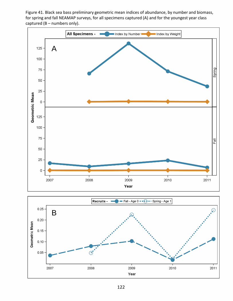
122

Figure 41. Black sea bass preliminary geometric mean indices of abundance, by number and biomass, for spring and fall NEAMAP surveys, for all specimens captured (A) and for the youngest year class captured (B – numbers only).

B

A

Figure 42. Black sea bass length-frequency distributions, by cruise (Blue reference lines are placed at the size cutoff values used to separate recruits from older specimens. Cutoff values – Spring 16cm, Fall 12cm - taken from http://mrl.cofc.edu/pdf/tr40s/Techreport43.pdf).

123

Spring Fall

Figure 43. Black sea bass length-frequency distributions, by cruise and sex.

Spring Fall

124

125

Figure 44. Black sea bass sex ratio, by length group, for NEAMAP Spring and Fall cruises 2007-2011. (The percentages for each category are given near the bottom of each bar. The number sampled for sex determination is provided near the top of each bar, and the length categories expressed in inches are shown between the two figures.).

n = 1 4 52 52 8 9 20 46 48 37 62 62 38 30 23 18 19 16 6 5 2 2 3

1 2 3 4 5 6 7 8 9 10 11 12 13 14 15 16 17 18 19 20 21 22 23 Inch-class

n = 4 36 42 10 49 118 160 120 57 40 46 37 18 18 23 17 16 13 8 10 3 4 2

100 75.0 50.0 15.0 6.3 7.0 5.8 U

1.8 10.9 15.0 39.7 35.2 43.3 28.2 27.6 35.9 36.6 39.1 60.9 62.0 65.2 32.3 100 100 100 100 M

25.0 48.2 85.0 93.8 89.1 85.0 60.3 64.8 56.7 64.7 72.4 64.1 63.4 60.9 39.1 38.0 29.0 67.7 F

100 76.0 61.6 58.7 1.8 19.8 0.4 2.4 3.6 2.9 13.2 U

1.8 6.5 11.8 12.8 17.6 15.8 17.7 44.5 26.3 22.8 26.8 12.1 75.0 23.6 87.5 80.8 68.8 50.0 100 M

24.0 38.4 41.3 96.5 73.7 88.2 86.8 80.0 80.6 82.3 52.6 60.5 77.2 73.2 87.9 25.0 76.4 12.5 19.2 31.3 50.0 F

Sprin

g F

all

nfish = 748 nclusters = 356

126

Figure 45. Black sea bass diet composition, expressed as percent by weight and number collected during NEAMAP cruises in 2007 through Spring 2011. (The number of fish sampled for diet is given by nfish, while nclusters indicates the number of clusters of this species sampled.

nfish = 748 nclusters = 356

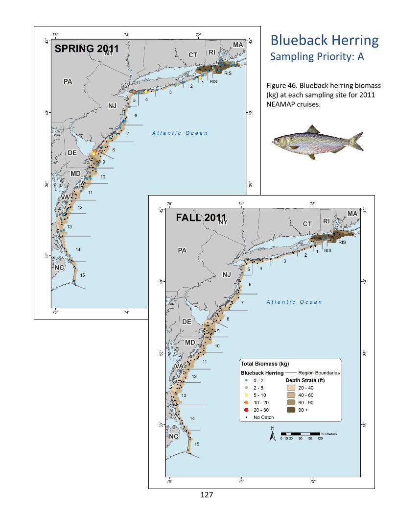
Blueback Herring Sampling Priority: A

Figure 46. Blueback herring biomass (kg) at each sampling site for 2011 NEAMAP cruises.

127

Table 27. Blueback herring sampling rates and preserved specimen analysis status for each NEAMAP cruise.

Table 28. Strata used for calculation of abundance indices for blueback herring.

Table 29. Blueback herring preliminary geometric mean indices of abundance, by number and biomass, for spring NEAMAP surveys, for all specimens captured and for the youngest year class captured.

128

Season YearNumber Caught

Biomass Caught (kg)

Number Measured

Age Specimens

Ages Read

Stomach Specimens

Stomachs Analyzed

Spring 2008 3,693 62.2 1,774 237 0 235 02009 5,603 160.3 2,808 315 0 315 22010 4,992 86.6 2,436 280 0 276 212011 77,071 957.3 2,713 226 0 219 216

Fall 2007 50 1.6 50 18 0 18 02008 20 0.7 20 9 0 9 02009 15 0.6 15 6 0 6 62010 22 0.6 22 15 0 14 122011 2 0.1 2 2 0 2 0

Season Year Agen LCI Index UCI CV (%) n LCI Index UCI CV (%)

Spring 2008 All 150 1.17 1.76 2.52 11.9 150 0.12 0.20 0.28 18.52009 160 1.55 2.30 3.26 10.7 160 0.23 0.34 0.47 15.42010 150 1.30 1.99 2.90 12.0 150 0.12 0.20 0.30 20.22011 150 0.81 1.27 1.84 13.7 150 0.11 0.19 0.27 19.7

Spring 2008 1 150 0.91 1.40 2.02 13.1 150 0.08 0.14 0.20 21.12009 160 0.77 1.20 1.73 13.8 160 0.08 0.15 0.21 21.32010 150 1.06 1.66 2.44 13.1 150 0.09 0.17 0.25 22.32011 150 0.59 0.98 1.48 16.3 150 0.07 0.14 0.22 24.0

Numerical Index Biomass Index

129

Figure 47. Blueback herring preliminary geometric mean indices of abundance, by number and biomass, for spring NEAMAP surveys, for all specimens captured (A) and for the youngest year class captured (B – numbers only).

B

A

Figure 48. Blueback herring length-frequency distributions, by cruise (Blue reference lines are placed at the size cutoff values used to separate recruits from older specimens. Cutoff values - Spring 14cm - estimated by examination of these length frequency figures.).

130

Spring Fall

131

Figure 49. Blueback herring length-frequency distributions, by cruise and sex.

Spring Fall

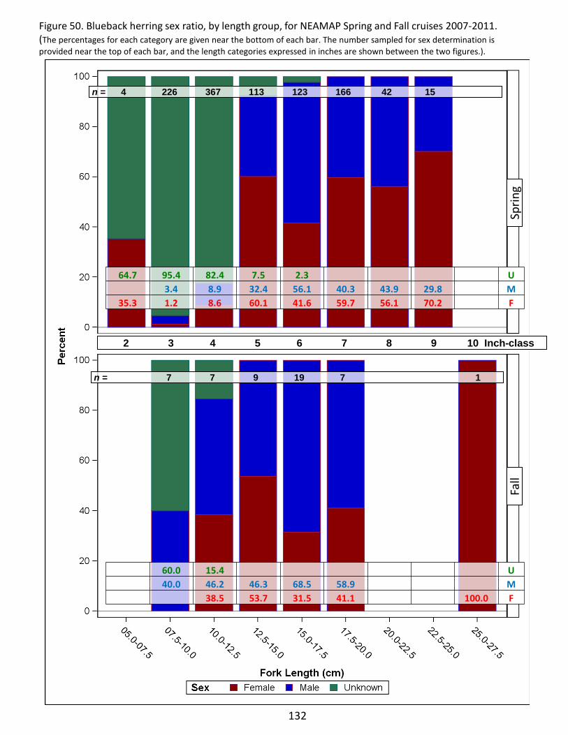
132

Figure 50. Blueback herring sex ratio, by length group, for NEAMAP Spring and Fall cruises 2007-2011. (The percentages for each category are given near the bottom of each bar. The number sampled for sex determination is provided near the top of each bar, and the length categories expressed in inches are shown between the two figures.).

n = 4 226 367 113 123 166 42 15

n = 7 7 9 19 7 1

2 3 4 5 6 7 8 9 10 Inch-class

64.7 95.4 82.4 7.5 2.3 U 3.4 8.9 32.4 56.1 40.3 43.9 29.8 M

35.3 1.2 8.6 60.1 41.6 59.7 56.1 70.2 F

60.0 15.4 U 40.0 46.2 46.3 68.5 58.9 M 38.5 53.7 31.5 41.1 100.0 F

Sprin

g F

all

Bluefish Sampling Priority: A

Figure 51. Bluefish biomass (kg) at each sampling site for 2011 NEAMAP cruises.

133

Table 30. Bluefish sampling rates and preserved specimen analysis status for each NEAMAP cruise.

Table 31. Strata used for calculation of abundance indices for bluefish.

Table 32. Bluefish preliminary geometric mean indices of abundance, by number and biomass, for spring and fall NEAMAP surveys, for all specimens captured and for the youngest year class captured (numbers only – spring and summer cohorts shown separately).

134

Season YearNumber Caught

Biomass Caught (kg)

Number Measured

Age Specimens

Ages Read

Stomach Specimens

Stomachs Analyzed

Spring 2008 37 10.9 37 27 0 24 242009 1,580 91.2 274 35 0 14 132010 312 21.4 68 18 0 15 152011 18 10.5 18 11 0 3 3

Fall 2007 4,635 394.5 2,613 588 588 485 4782008 7,120 908.7 2,214 529 0 409 4022009 18,075 910.7 4,016 632 0 432 4212010 4,432 271.6 1,967 498 0 379 3692011 3,885 454.9 1,887 482 0 295 0

n LCI Index UCI CV (%) n LCI Index UCI CV (%) n LCI Index UCI CV (%) n LCI Index UCI CV (%)Spring 2008 All 5 0.00 0.40 1.72 100.0 5 0.00 0.04 0.13 100.0 Fall 2007 0 150 1.58 2.12 2.78 8.4 150 0.43 0.57 0.72 10.2

2009 6 5.66 8.19 11.69 7.3 6 1.57 4.05 8.92 20.8 2008 150 1.48 2.06 2.77 9.3 150 0.28 0.44 0.62 16.42010 5 0.00 0.44 2.00 100.0 5 0.00 0.05 0.16 100.0 2009 160 1.16 1.63 2.19 10.1 160 0.23 0.34 0.46 15.02011 5 0.00 0.00 0.00 5 0.00 0.00 0.00 2010 150 0.79 1.08 1.42 10.2 150 0.18 0.26 0.34 13.6

Fall 2007 All 150 3.20 4.36 5.83 7.3 150 1.01 1.29 1.61 7.9 2011 150 2.29 3.03 3.94 7.3 150 0.56 0.75 0.96 10.32008 150 4.03 5.51 7.43 6.9 150 0.98 1.33 1.75 9.8 Fall 2007 0 150 0.87 1.29 1.80 12.1 150 0.17 0.27 0.37 16.72009 160 4.15 5.52 7.26 6.3 160 0.73 0.95 1.20 9.1 2008 150 1.98 2.75 3.72 8.7 150 0.33 0.46 0.61 12.82010 150 2.56 3.44 4.55 7.5 150 0.65 0.85 1.06 9.0 2009 160 2.29 3.03 3.93 7.2 160 0.29 0.39 0.49 11.12011 150 3.01 3.99 5.19 6.7 150 0.86 1.14 1.46 9.2 2010 150 1.26 1.78 2.41 10.0 150 0.17 0.25 0.34 15.6

Spring 2008 1 5 0.00 0.40 1.72 100.0 5 0.00 0.04 0.13 100.0 2011 150 0.52 0.77 1.05 13.0 150 0.10 0.18 0.27 21.62009 6 5.35 5.68 6.04 1.4 6 1.44 1.59 1.74 3.12010 5 0.00 0.44 2.00 100.0 5 0.00 0.05 0.15 100.02011 5 0.00 0.00 0.00 5 0.00 0.00 0.00

Fall 2007 0 150 2.51 3.49 4.74 8.2 150 0.60 0.79 1.01 9.92008 150 3.40 4.68 6.33 7.3 150 0.59 0.83 1.09 11.42009 160 3.77 5.05 6.68 6.6 160 0.53 0.70 0.90 10.32010 150 2.16 2.96 3.96 8.1 150 0.37 0.50 0.64 11.42011 150 2.65 3.51 4.57 7.0 150 0.63 0.84 1.08 10.1

Sp

ring

C

oh

ort

Su

mm

er

Co

ho

rt

135

Figure 52. Bluefish preliminary geometric mean indices of abundance, by number and biomass, for spring and fall NEAMAP surveys, for all specimens captured (A), for the youngest year class captured (B – numbers only) and (using fall data only) for the spring and summer age-0 cohorts separately (C – numbers only).

A

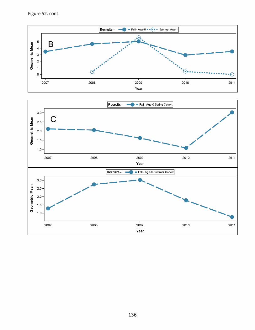
136

C

Figure 52. cont.

B

Figure 53. Bluefish length-frequency distributions, by cruise.(Blue reference line is placed at the size cutoff value – 17cm - used to separate the spring YOY cohort – to the right of the line – from the summer YOY cohort – to the left. Age-length key values presented in Table 33 were applied to the spring cohort specimens).

137

Spring Fall

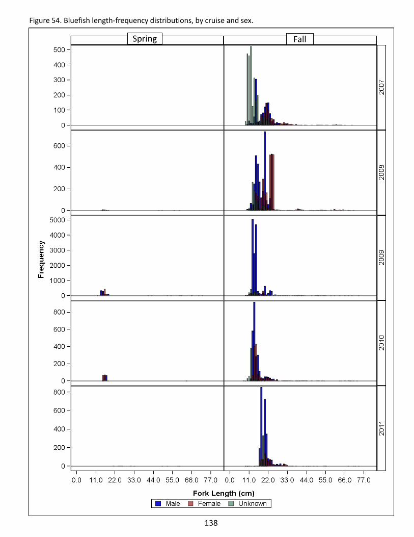
138

Figure 54. Bluefish length-frequency distributions, by cruise and sex.

Spring Fall

Figure 55. Bluefish age-at-length proportions for all spring vs. all fall cruises combined, showing actual and loess smoothed proportions at each 1cm length bin (Data from a single aged NEAMAP survey year pooled with samples from the VIMS ChesMMAP survey).

139

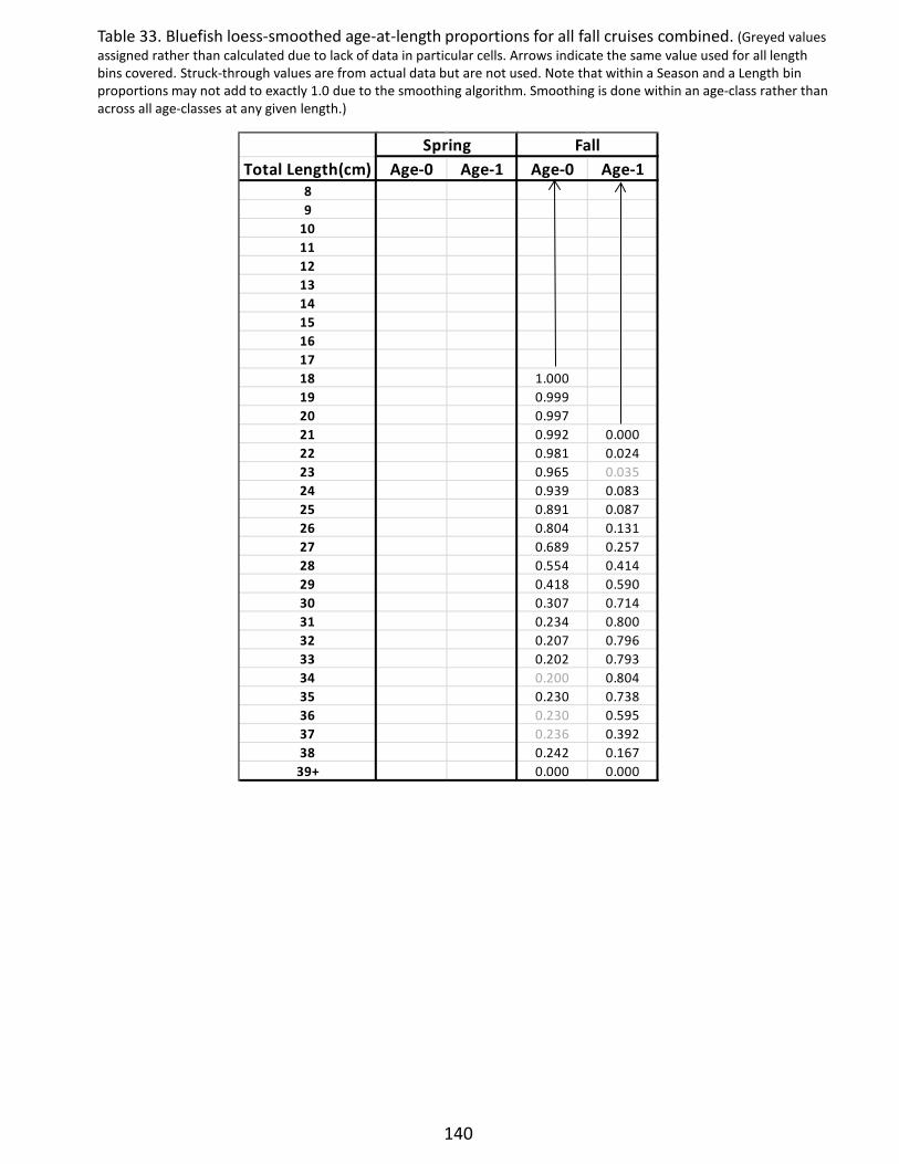
Table 33. Bluefish loess-smoothed age-at-length proportions for all fall cruises combined. (Greyed values assigned rather than calculated due to lack of data in particular cells. Arrows indicate the same value used for all length bins covered. Struck-through values are from actual data but are not used. Note that within a Season and a Length bin proportions may not add to exactly 1.0 due to the smoothing algorithm. Smoothing is done within an age-class rather than across all age-classes at any given length.)

Total Length(cm) Age-0 Age-1 Age-0 Age-189

101112131415161718 1.00019 0.99920 0.99721 0.992 0.00022 0.981 0.02423 0.965 0.03524 0.939 0.08325 0.891 0.08726 0.804 0.13127 0.689 0.25728 0.554 0.41429 0.418 0.59030 0.307 0.71431 0.234 0.80032 0.207 0.79633 0.202 0.79334 0.200 0.80435 0.230 0.73836 0.230 0.59537 0.236 0.39238 0.242 0.167

39+ 0.000 0.000

Spring Fall

140

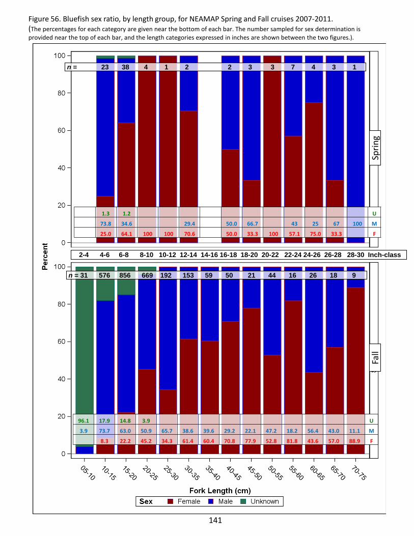
141

Figure 56. Bluefish sex ratio, by length group, for NEAMAP Spring and Fall cruises 2007-2011. (The percentages for each category are given near the bottom of each bar. The number sampled for sex determination is provided near the top of each bar, and the length categories expressed in inches are shown between the two figures.).

n = 23 38 4 1 2 2 3 3 7 4 3 1

n = 31 576 856 669 192 153 59 50 21 44 16 26 18 9

2-4 4-6 6-8 8-10 10-12 12-14 14-16 16-18 18-20 20-22 22-24 24-26 26-28 28-30 Inch-class

Sprin

g

1.3 1.2 U

73.8 34.6 29.4 50.0 66.7 43 25 67 100 M

25.0 64.1 100 100 70.6 50.0 33.3 100 57.1 75.0 33.3 F

96.1 17.9 14.8 3.9 U

3.9 73.7 63.0 50.9 65.7 38.6 39.6 29.2 22.1 47.2 18.2 56.4 43.0 11.1 M

8.3 22.2 45.2 34.3 61.4 60.4 70.8 77.9 52.8 81.8 43.6 57.0 88.9 F

Fal

l

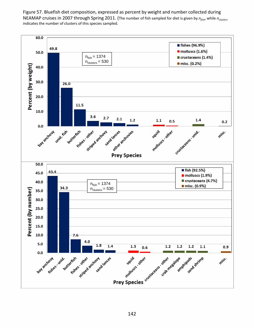
nfish = 1374 nclusters = 530

nfish = 1374 nclusters = 530

142

Figure 57. Bluefish diet composition, expressed as percent by weight and number collected during NEAMAP cruises in 2007 through Spring 2011. (The number of fish sampled for diet is given by nfish, while nclusters indicates the number of clusters of this species sampled.

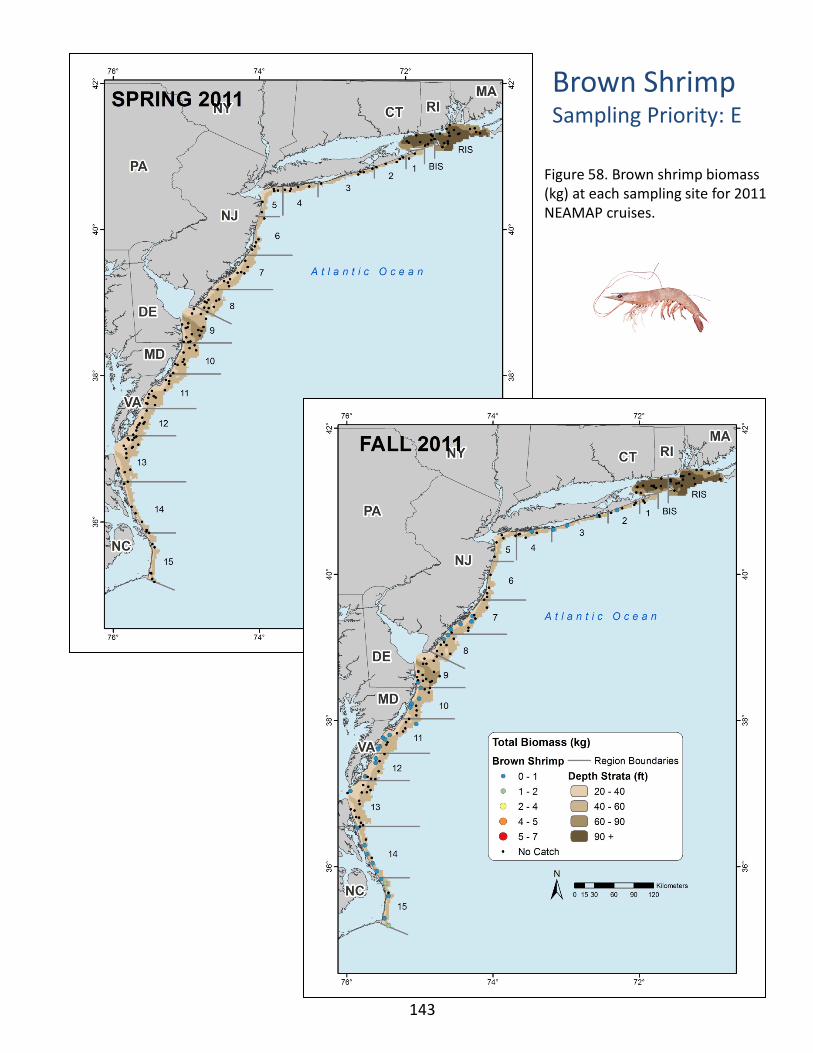
Brown Shrimp Sampling Priority: E

Figure 58. Brown shrimp biomass (kg) at each sampling site for 2011 NEAMAP cruises.

143

Table 34. Brown shrimp sampling rates for each NEAMAP cruise.

Table 35. Strata used for calculation of abundance indices for brown shrimp.

Table 36. Brown shrimp preliminary geometric mean indices of abundance, by number and biomass, for spring and fall NEAMAP surveys, for all specimens captured.

144

Season YearNumber Caught

Biomass Caught (kg)

Number Measured

Age Specimens

Ages Read

Stomach Specimens

Stomachs Analyzed

Spring 2008 5 0.2 5 N/A N/A N/A N/A2009 7 0.1 7 N/A N/A N/A N/A2010 0 0.0 0 N/A N/A N/A N/A2011 0 0.0 0 N/A N/A N/A N/A

Fall 2007 898 21.6 459 N/A N/A N/A N/A2008 509 15.3 372 N/A N/A N/A N/A2009 45 0.9 45 N/A N/A N/A N/A2010 565 8.6 21 N/A N/A N/A N/A2011 406 10.2 406 N/A N/A N/A N/A

Season Year Agen LCI Index UCI CV (%) n LCI Index UCI CV (%)

Spring 2008 All 5 0.00 0.18 0.65 100.0 5 0.00 0.01 0.03 100.02009 6 0.00 0.25 0.61 57.6 6 0.00 0.01 0.02 69.32010 5 0.00 0.00 0.00 5 0.00 0.00 0.002011 5 0.00 0.00 0.00 5 0.00 0.00 0.00

Fall 2007 All 23 0.89 2.62 5.93 25.2 23 0.05 0.22 0.42 37.32008 22 0.81 2.51 5.82 26.4 22 0.04 0.22 0.44 40.12009 25 0.05 0.47 1.05 43.7 25 0.00 0.02 0.03 47.52010 22 0.00 0.08 0.24 100.0 22 0.00 0.00 0.01 100.02011 22 1.44 2.81 4.94 16.6 22 0.10 0.17 0.24 18.6

Numerical Index Biomass Index

145

Figure 59. Brown shrimp preliminary geometric mean indices of abundance, by number and biomass, for spring and fall NEAMAP surveys, for all specimens captured.

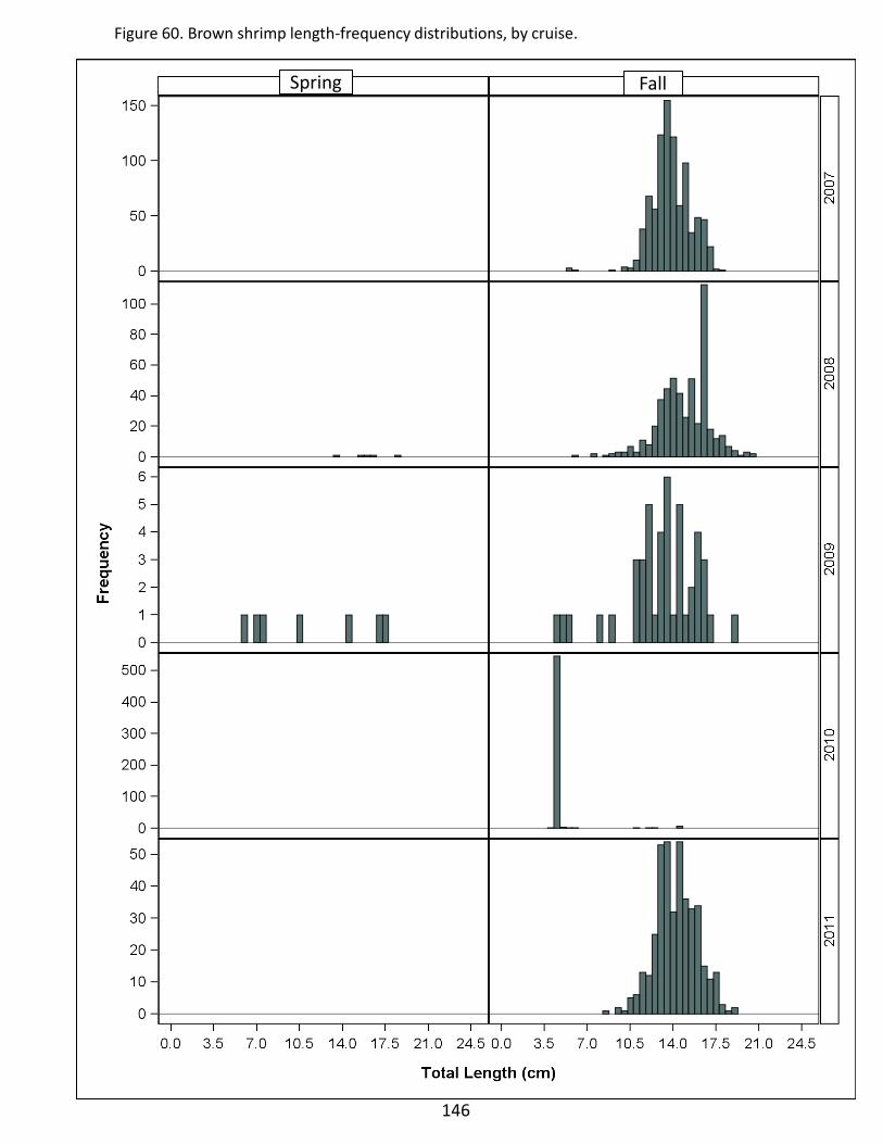
Figure 60. Brown shrimp length-frequency distributions, by cruise.

146

Spring Fall

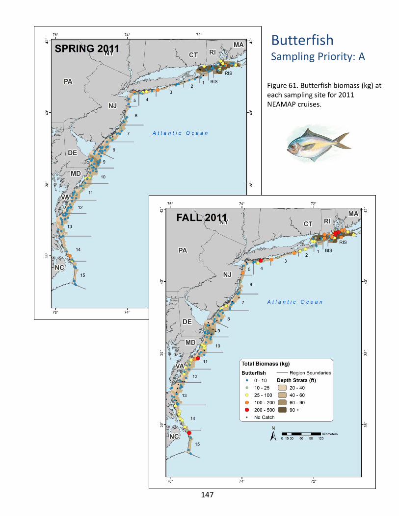
Butterfish Sampling Priority: A

Figure 61. Butterfish biomass (kg) at each sampling site for 2011 NEAMAP cruises.

147

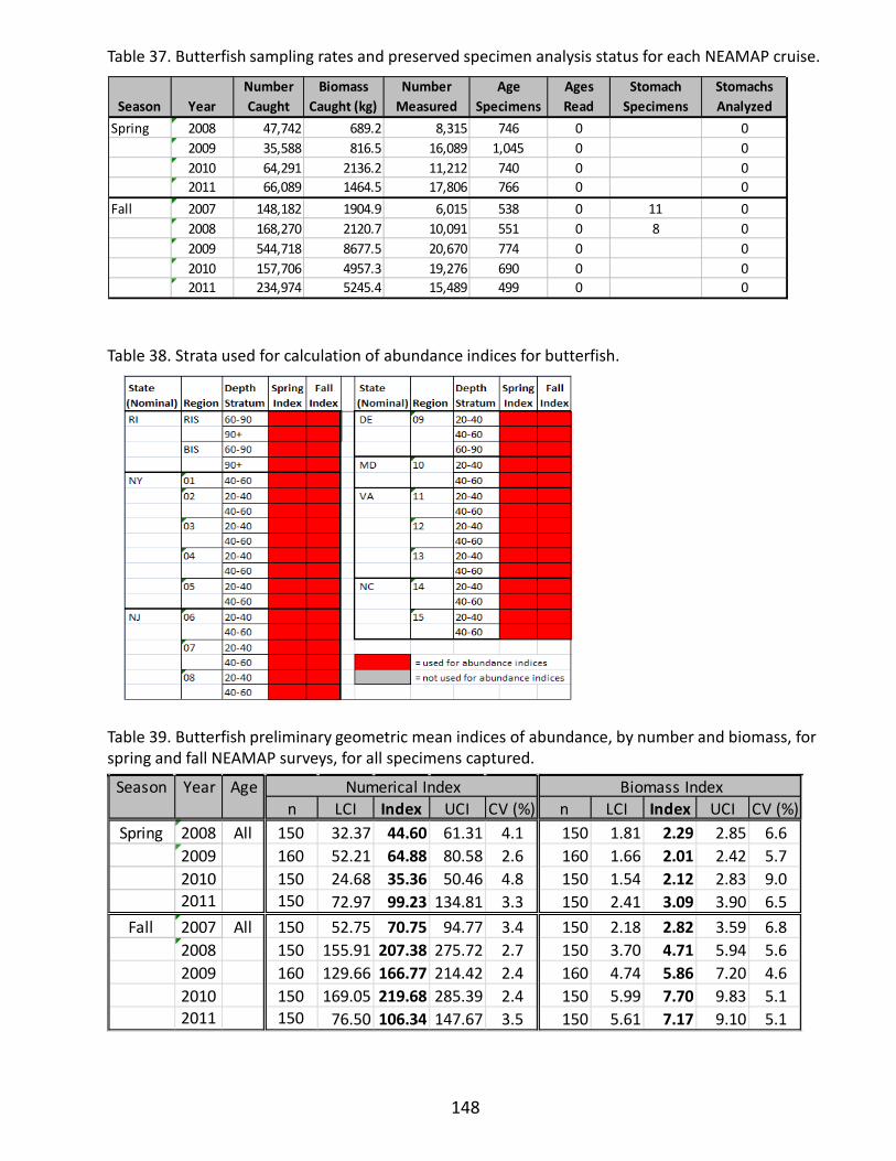
Table 37. Butterfish sampling rates and preserved specimen analysis status for each NEAMAP cruise.

Table 38. Strata used for calculation of abundance indices for butterfish.

Table 39. Butterfish preliminary geometric mean indices of abundance, by number and biomass, for spring and fall NEAMAP surveys, for all specimens captured.

148

Season YearNumber Caught

Biomass Caught (kg)

Number Measured

Age Specimens

Ages Read

Stomach Specimens

Stomachs Analyzed

Spring 2008 47,742 689.2 8,315 746 0 02009 35,588 816.5 16,089 1,045 0 02010 64,291 2136.2 11,212 740 0 02011 66,089 1464.5 17,806 766 0 0

Fall 2007 148,182 1904.9 6,015 538 0 11 02008 168,270 2120.7 10,091 551 0 8 02009 544,718 8677.5 20,670 774 0 02010 157,706 4957.3 19,276 690 0 02011 234,974 5245.4 15,489 499 0 0

Season Year Agen LCI Index UCI CV (%) n LCI Index UCI CV (%)

Spring 2008 All 150 32.37 44.60 61.31 4.1 150 1.81 2.29 2.85 6.62009 160 52.21 64.88 80.58 2.6 160 1.66 2.01 2.42 5.72010 150 24.68 35.36 50.46 4.8 150 1.54 2.12 2.83 9.02011 150 72.97 99.23 134.81 3.3 150 2.41 3.09 3.90 6.5

Fall 2007 All 150 52.75 70.75 94.77 3.4 150 2.18 2.82 3.59 6.82008 150 155.91 207.38 275.72 2.7 150 3.70 4.71 5.94 5.62009 160 129.66 166.77 214.42 2.4 160 4.74 5.86 7.20 4.62010 150 169.05 219.68 285.39 2.4 150 5.99 7.70 9.83 5.12011 150 76.50 106.34 147.67 3.5 150 5.61 7.17 9.10 5.1

Numerical Index Biomass Index

149

Figure 62. Butterfish preliminary geometric mean indices of abundance, by number and biomass, for spring and fall NEAMAP surveys, for all specimens captured.

Figure 63. Butterfish length-frequency distributions, by cruise.

150

Spring Fall

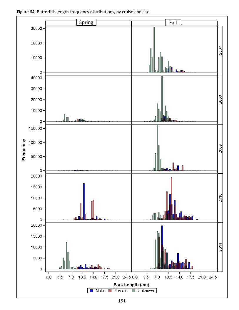
151

Figure 64. Butterfish length-frequency distributions, by cruise and sex.

Spring Fall

152

Figure 65. Butterfish sex ratio, by length group, for NEAMAP Spring and Fall cruises 2007-2011. (The percentages for each category are given near the bottom of each bar. The number sampled for sex determination is provided near the top of each bar, and the length categories expressed in inches are shown between the two figures.).

n = 1 326 512 601 620 757 354 115 10

n = 118 675 646 550 595 343 102 6

Sprin

g F

all

0 1 2 3 4 5 6 7 8 Inch-class

100.0 100.0 98.9 24.2 10.9 0.3 0.2 0.1 U 1.0 33.9 61.8 28.9 32.5 34.6 25.0 M 0.1 41.9 27.3 70.8 67.3 65.3 75.0 F

100.0 95.5 64.3 16.6 1.2 2.6 U 0.6 16.5 34.8 56.7 28.1 56.1 95.7 M 3.9 19.3 48.6 42.1 69.3 43.9 4.3 F

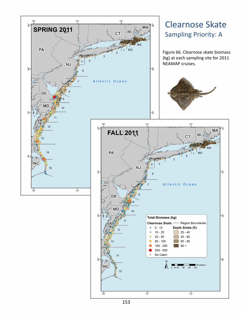
Clearnose Skate Sampling Priority: A

Figure 66. Clearnose skate biomass (kg) at each sampling site for 2011 NEAMAP cruises.

153

Table 40. Clearnose skate sampling rates and preserved specimen analysis status for each NEAMAP cruise.

Table 41. Strata used for calculation of abundance indices for clearnose skate.

Table 42. Clearnose skate preliminary geometric mean indices of abundance, by number and biomass, for spring and fall NEAMAP surveys, for all specimens captured.

154

Season YearNumber Caught

Biomass Caught (kg)

Number Measured

Age Specimens

Ages Read

Stomach Specimens

Stomachs Analyzed

Spring 2008 3,219 4237.3 1,050 212 0 207 2052009 2,429 3382.1 1,431 205 0 188 1832010 1,702 2516.4 1,353 197 0 183 1762011 2,216 2744.8 1,854 211 0 190 190

Fall 2007 1,505 1854.6 1,361 346 0 330 2942008 885 1196.2 806 289 0 287 2872009 1,107 1352.1 1,007 335 0 306 3022010 875 1056.7 875 307 0 278 2742011 1,178 1357.3 1,110 318 0 291 0

Season Year Agen LCI Index UCI CV (%) n LCI Index UCI CV (%)

Spring 2008 All 86 9.76 12.03 14.78 3.7 86 11.57 14.31 17.65 3.62009 91 5.53 7.21 9.31 5.4 91 6.80 9.01 11.85 5.42010 87 6.27 7.61 9.20 3.9 87 7.68 9.43 11.53 3.92011 87 7.86 9.75 12.04 4.1 87 8.92 11.26 14.17 4.2

Fall 2007 All 124 6.62 7.73 9.00 3.1 124 7.78 9.20 10.84 3.22008 124 3.86 4.51 5.25 3.7 124 4.67 5.57 6.63 3.92009 134 4.77 5.56 6.47 3.4 134 5.54 6.50 7.61 3.42010 124 3.95 4.62 5.38 3.7 124 4.64 5.43 6.32 3.52011 124 5.57 6.40 7.33 3.0 124 6.36 7.31 8.39 2.9

Numerical Index Biomass Index

155

Figure 67. Clearnose skate preliminary geometric mean indices of abundance, by number and biomass, for spring and fall NEAMAP surveys, for all specimens captured.

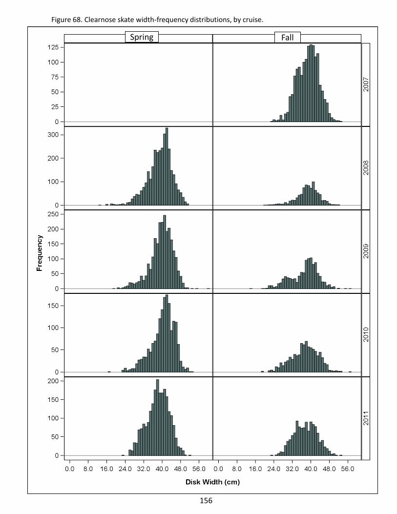
Figure 68. Clearnose skate width-frequency distributions, by cruise.

156

Spring Fall

157

Figure 69. Clearnose skate width-frequency distributions, by cruise and sex.

Spring Fall

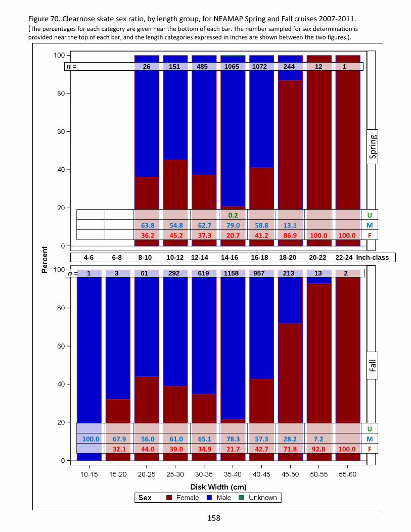
158

Figure 70. Clearnose skate sex ratio, by length group, for NEAMAP Spring and Fall cruises 2007-2011. (The percentages for each category are given near the bottom of each bar. The number sampled for sex determination is provided near the top of each bar, and the length categories expressed in inches are shown between the two figures.).

n = 26 151 485 1065 1072 244 12 1

n = 1 3 61 292 619 1158 957 213 13 2

Sprin

g F

all

4-6 6-8 8-10 10-12 12-14 14-16 16-18 18-20 20-22 22-24 Inch-class

0.2 U 63.8 54.8 62.7 79.0 58.8 13.1 M 36.2 45.2 37.3 20.7 41.2 86.9 100.0 100.0 F

U 100.0 67.9 56.0 61.0 65.1 78.3 57.3 28.2 7.2 M

32.1 44.0 39.0 34.9 21.7 42.7 71.8 92.8 100.0 F

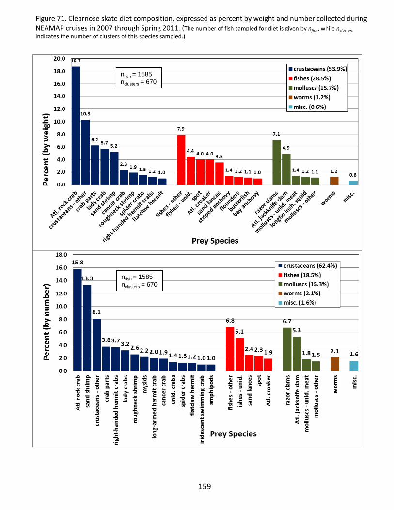
nfish = 1585 nclusters = 670

nfish = 1585 nclusters = 670

159

Figure 71. Clearnose skate diet composition, expressed as percent by weight and number collected during NEAMAP cruises in 2007 through Spring 2011. (The number of fish sampled for diet is given by nfish, while nclusters indicates the number of clusters of this species sampled.)

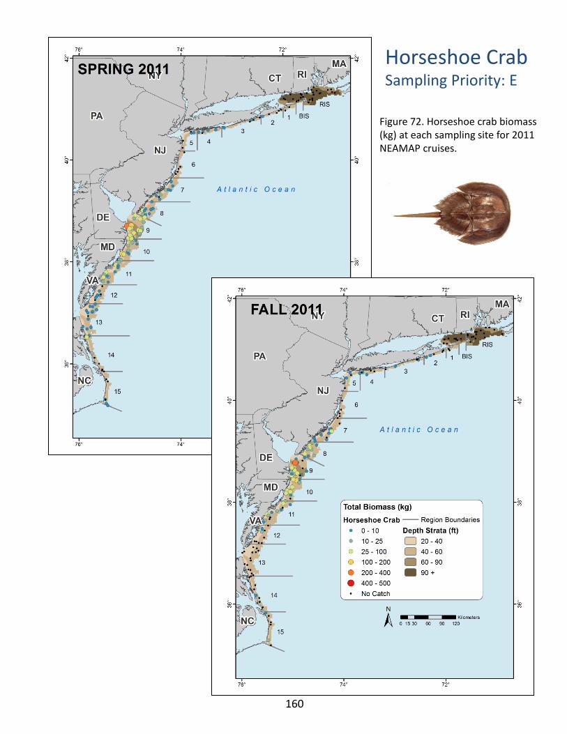
Horseshoe Crab Sampling Priority: E

Figure 72. Horseshoe crab biomass (kg) at each sampling site for 2011 NEAMAP cruises.

160

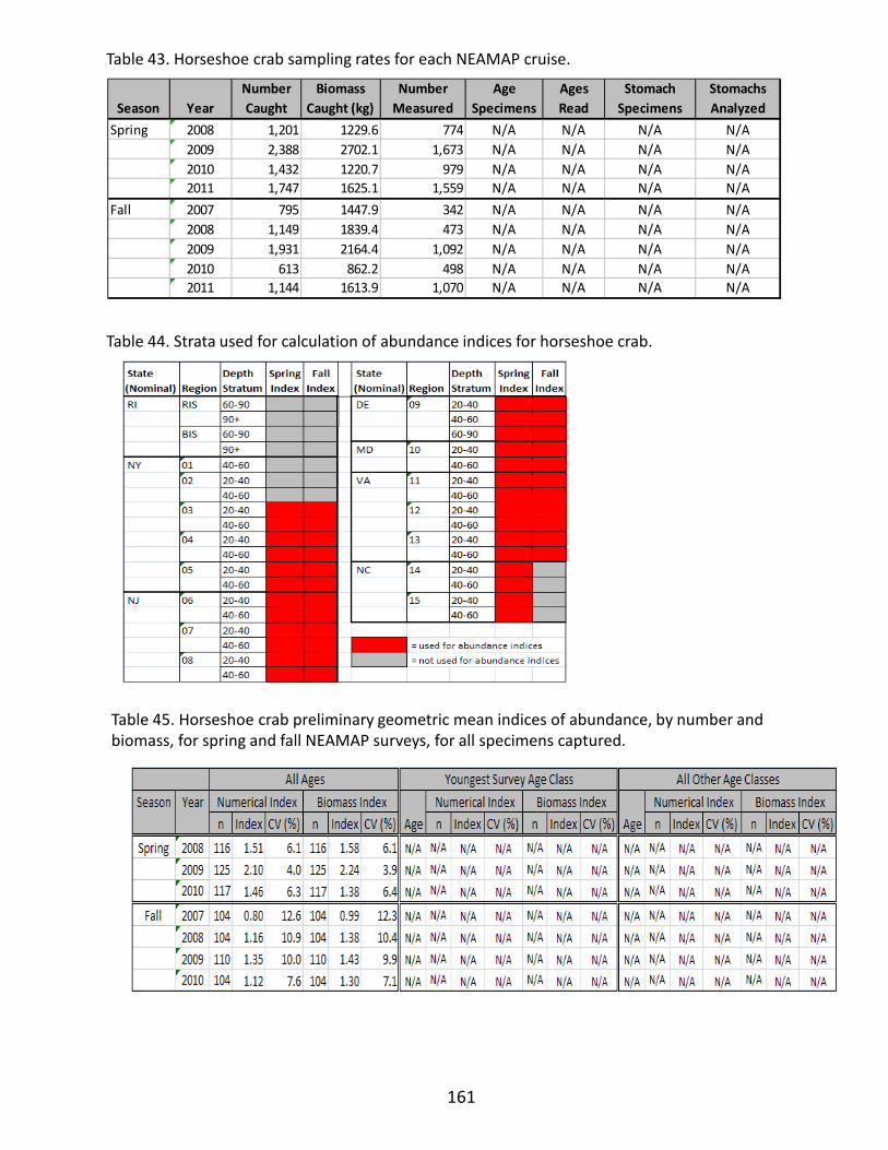
Table 43. Horseshoe crab sampling rates for each NEAMAP cruise.

Table 44. Strata used for calculation of abundance indices for horseshoe crab.

Table 45. Horseshoe crab preliminary geometric mean indices of abundance, by number and biomass, for spring and fall NEAMAP surveys, for all specimens captured.

161

Season YearNumber Caught

Biomass Caught (kg)

Number Measured

Age Specimens

Ages Read

Stomach Specimens

Stomachs Analyzed

Spring 2008 1,201 1229.6 774 N/A N/A N/A N/A2009 2,388 2702.1 1,673 N/A N/A N/A N/A2010 1,432 1220.7 979 N/A N/A N/A N/A2011 1,747 1625.1 1,559 N/A N/A N/A N/A

Fall 2007 795 1447.9 342 N/A N/A N/A N/A2008 1,149 1839.4 473 N/A N/A N/A N/A2009 1,931 2164.4 1,092 N/A N/A N/A N/A2010 613 862.2 498 N/A N/A N/A N/A2011 1,144 1613.9 1,070 N/A N/A N/A N/A

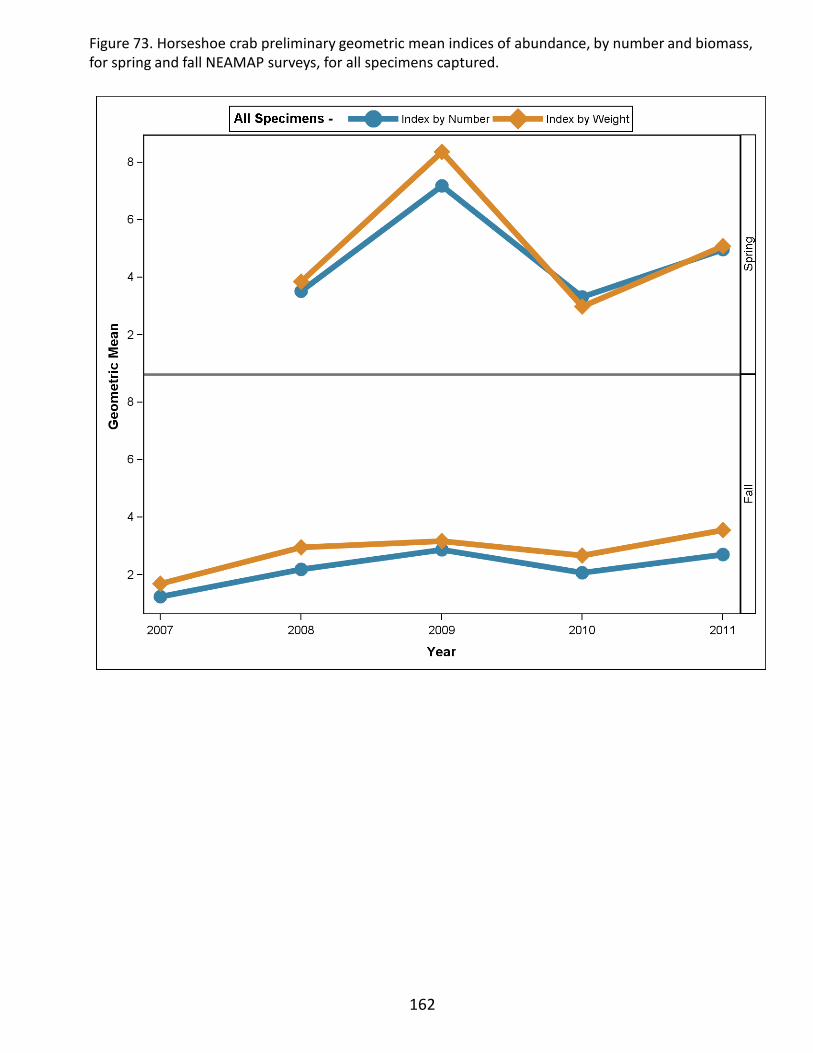
162

Figure 73. Horseshoe crab preliminary geometric mean indices of abundance, by number and biomass, for spring and fall NEAMAP surveys, for all specimens captured.

Figure 74. Horseshoe crab width-frequency distributions, by cruise.

163

Spring Fall

164

Figure 75. Horseshoe crab width-frequency distributions, by cruise and sex.

Spring Fall

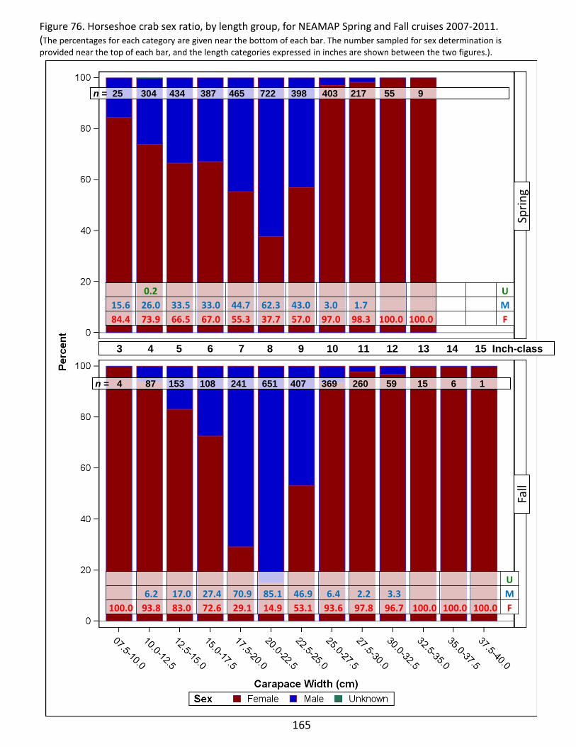
165

Figure 76. Horseshoe crab sex ratio, by length group, for NEAMAP Spring and Fall cruises 2007-2011. (The percentages for each category are given near the bottom of each bar. The number sampled for sex determination is provided near the top of each bar, and the length categories expressed in inches are shown between the two figures.).

n = 25 304 434 387 465 722 398 403 217 55 9

n = 4 87 153 108 241 651 407 369 260 59 15 6 1

Sprin

g F

all

3 4 5 6 7 8 9 10 11 12 13 14 15 Inch-class

0.2 U 15.6 26.0 33.5 33.0 44.7 62.3 43.0 3.0 1.7 M 84.4 73.9 66.5 67.0 55.3 37.7 57.0 97.0 98.3 100.0 100.0 F

U 6.2 17.0 27.4 70.9 85.1 46.9 6.4 2.2 3.3 M

100.0 93.8 83.0 72.6 29.1 14.9 53.1 93.6 97.8 96.7 100.0 100.0 100.0 F

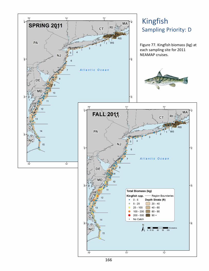
Kingfish Sampling Priority: D

Figure 77. Kingfish biomass (kg) at each sampling site for 2011 NEAMAP cruises.

166

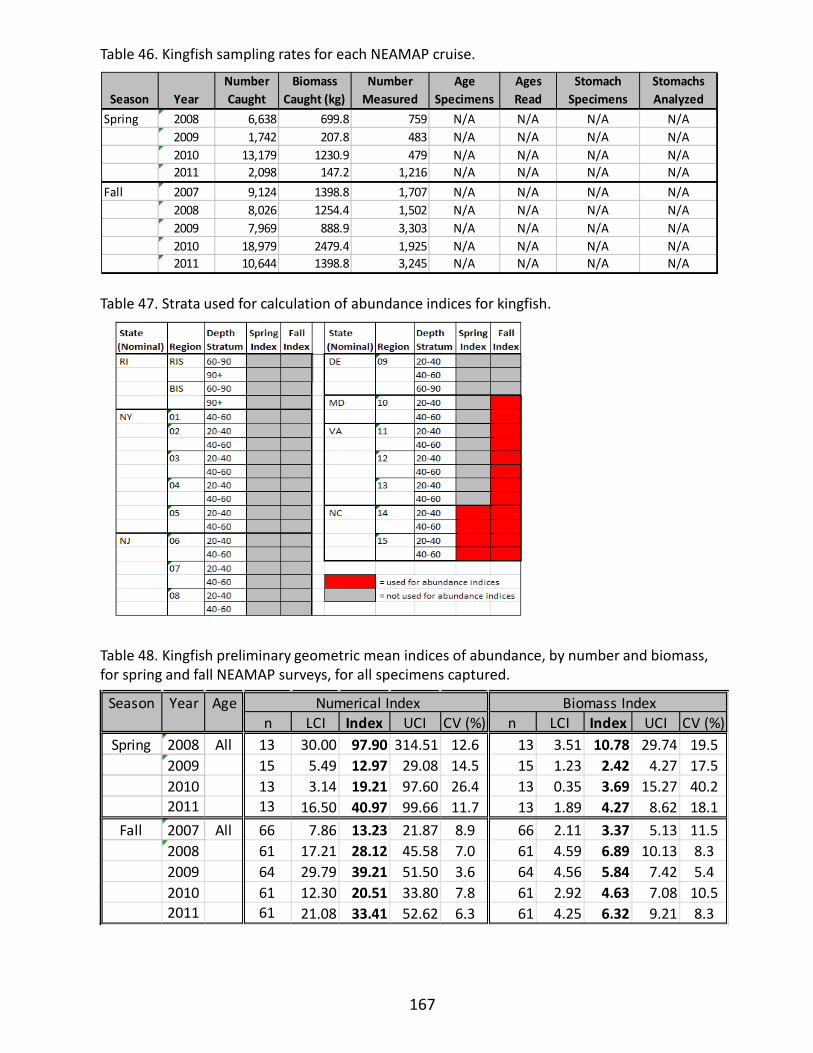
Table 46. Kingfish sampling rates for each NEAMAP cruise.

Table 47. Strata used for calculation of abundance indices for kingfish.

Table 48. Kingfish preliminary geometric mean indices of abundance, by number and biomass, for spring and fall NEAMAP surveys, for all specimens captured.

167

Season YearNumber Caught

Biomass Caught (kg)

Number Measured

Age Specimens

Ages Read

Stomach Specimens

Stomachs Analyzed

Spring 2008 6,638 699.8 759 N/A N/A N/A N/A2009 1,742 207.8 483 N/A N/A N/A N/A2010 13,179 1230.9 479 N/A N/A N/A N/A2011 2,098 147.2 1,216 N/A N/A N/A N/A

Fall 2007 9,124 1398.8 1,707 N/A N/A N/A N/A2008 8,026 1254.4 1,502 N/A N/A N/A N/A2009 7,969 888.9 3,303 N/A N/A N/A N/A2010 18,979 2479.4 1,925 N/A N/A N/A N/A2011 10,644 1398.8 3,245 N/A N/A N/A N/A

Season Year Agen LCI Index UCI CV (%) n LCI Index UCI CV (%)

Spring 2008 All 13 30.00 97.90 314.51 12.6 13 3.51 10.78 29.74 19.52009 15 5.49 12.97 29.08 14.5 15 1.23 2.42 4.27 17.52010 13 3.14 19.21 97.60 26.4 13 0.35 3.69 15.27 40.22011 13 16.50 40.97 99.66 11.7 13 1.89 4.27 8.62 18.1

Fall 2007 All 66 7.86 13.23 21.87 8.9 66 2.11 3.37 5.13 11.52008 61 17.21 28.12 45.58 7.0 61 4.59 6.89 10.13 8.32009 64 29.79 39.21 51.50 3.6 64 4.56 5.84 7.42 5.42010 61 12.30 20.51 33.80 7.8 61 2.92 4.63 7.08 10.52011 61 21.08 33.41 52.62 6.3 61 4.25 6.32 9.21 8.3

Numerical Index Biomass Index

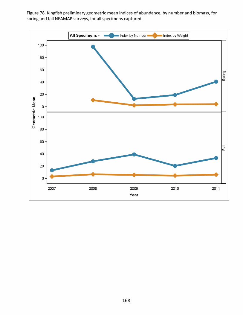
168

Figure 78. Kingfish preliminary geometric mean indices of abundance, by number and biomass, for spring and fall NEAMAP surveys, for all specimens captured.

Figure 79. Kingfish length-frequency distributions, by cruise.

169

Spring Fall

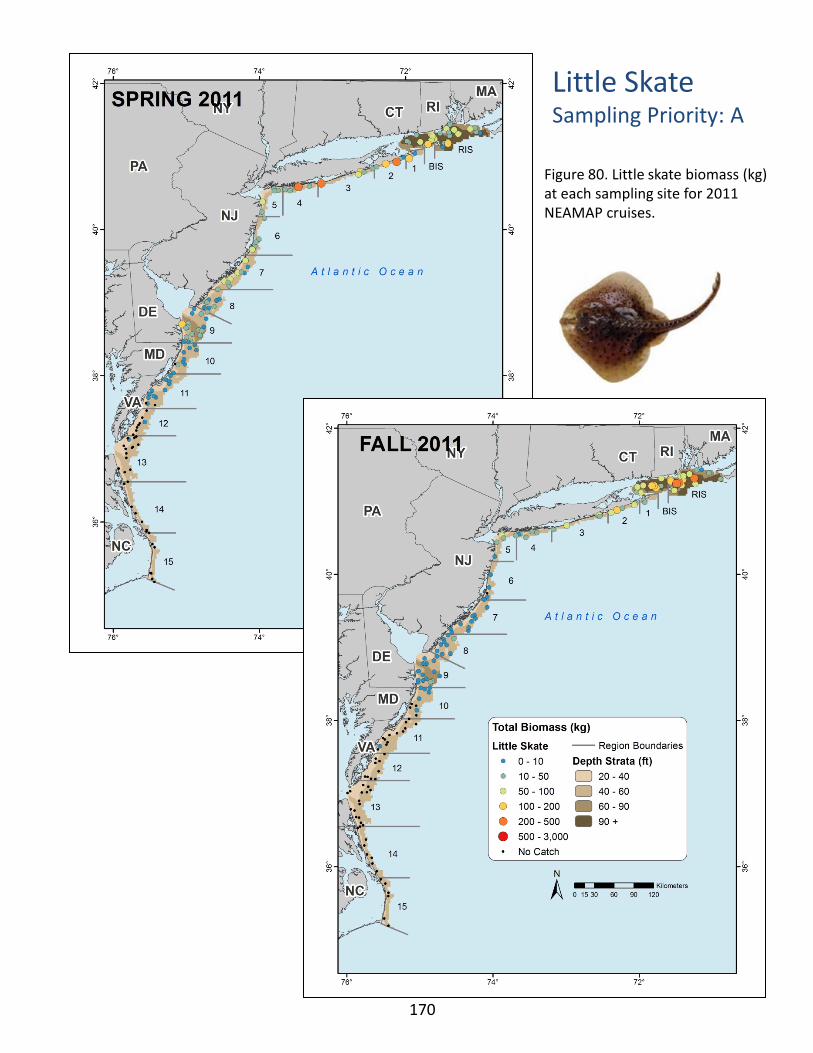
Little Skate Sampling Priority: A

Figure 80. Little skate biomass (kg) at each sampling site for 2011 NEAMAP cruises.

170

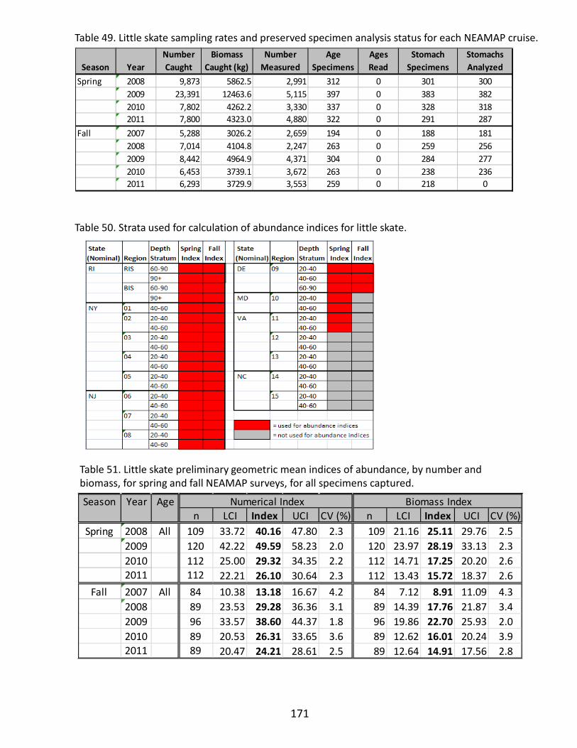
Table 49. Little skate sampling rates and preserved specimen analysis status for each NEAMAP cruise.

Table 50. Strata used for calculation of abundance indices for little skate.

Table 51. Little skate preliminary geometric mean indices of abundance, by number and biomass, for spring and fall NEAMAP surveys, for all specimens captured.

171

Season YearNumber Caught

Biomass Caught (kg)

Number Measured

Age Specimens

Ages Read

Stomach Specimens

Stomachs Analyzed

Spring 2008 9,873 5862.5 2,991 312 0 301 3002009 23,391 12463.6 5,115 397 0 383 3822010 7,802 4262.2 3,330 337 0 328 3182011 7,800 4323.0 4,880 322 0 291 287

Fall 2007 5,288 3026.2 2,659 194 0 188 1812008 7,014 4104.8 2,247 263 0 259 2562009 8,442 4964.9 4,371 304 0 284 2772010 6,453 3739.1 3,672 263 0 238 2362011 6,293 3729.9 3,553 259 0 218 0

Season Year Agen LCI Index UCI CV (%) n LCI Index UCI CV (%)

Spring 2008 All 109 33.72 40.16 47.80 2.3 109 21.16 25.11 29.76 2.52009 120 42.22 49.59 58.23 2.0 120 23.97 28.19 33.13 2.32010 112 25.00 29.32 34.35 2.2 112 14.71 17.25 20.20 2.62011 112 22.21 26.10 30.64 2.3 112 13.43 15.72 18.37 2.6

Fall 2007 All 84 10.38 13.18 16.67 4.2 84 7.12 8.91 11.09 4.32008 89 23.53 29.28 36.36 3.1 89 14.39 17.76 21.87 3.42009 96 33.57 38.60 44.37 1.8 96 19.86 22.70 25.93 2.02010 89 20.53 26.31 33.65 3.6 89 12.62 16.01 20.24 3.92011 89 20.47 24.21 28.61 2.5 89 12.64 14.91 17.56 2.8

Numerical Index Biomass Index

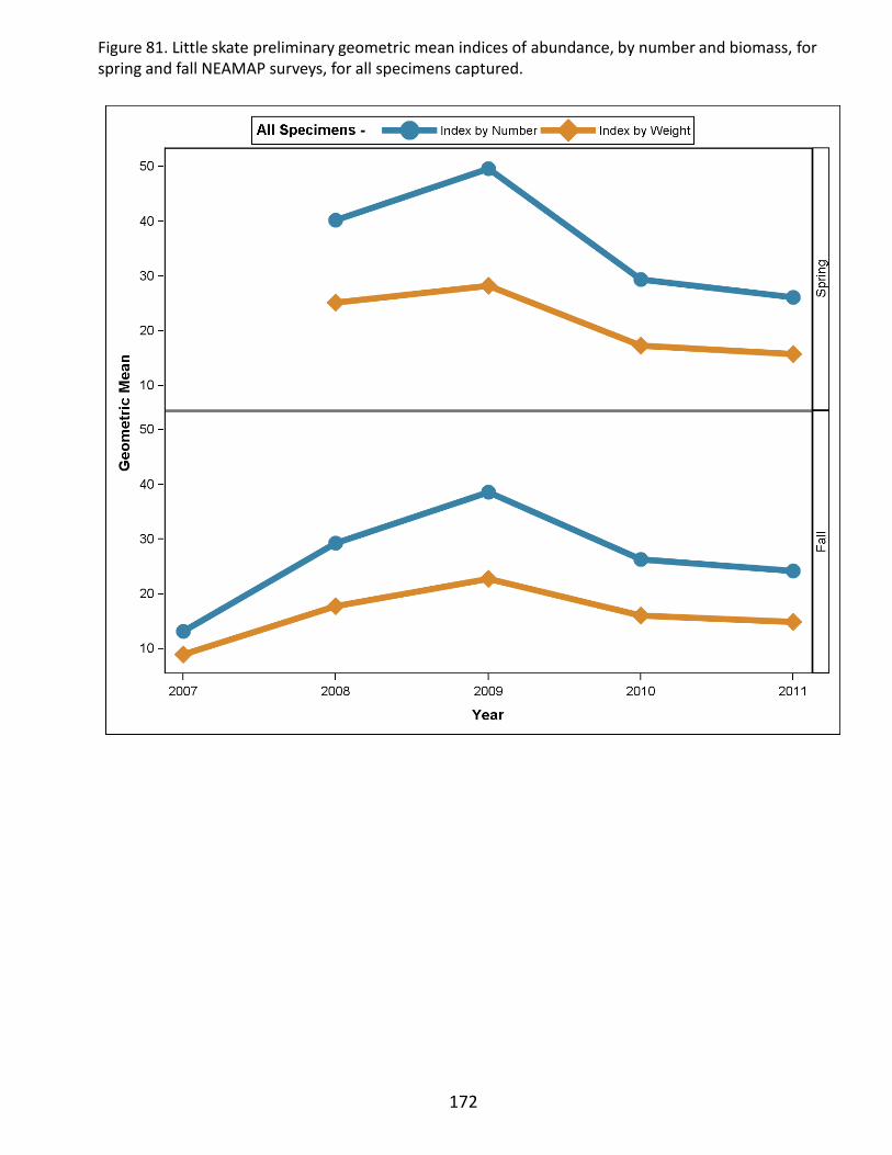
172

Figure 81. Little skate preliminary geometric mean indices of abundance, by number and biomass, for spring and fall NEAMAP surveys, for all specimens captured.

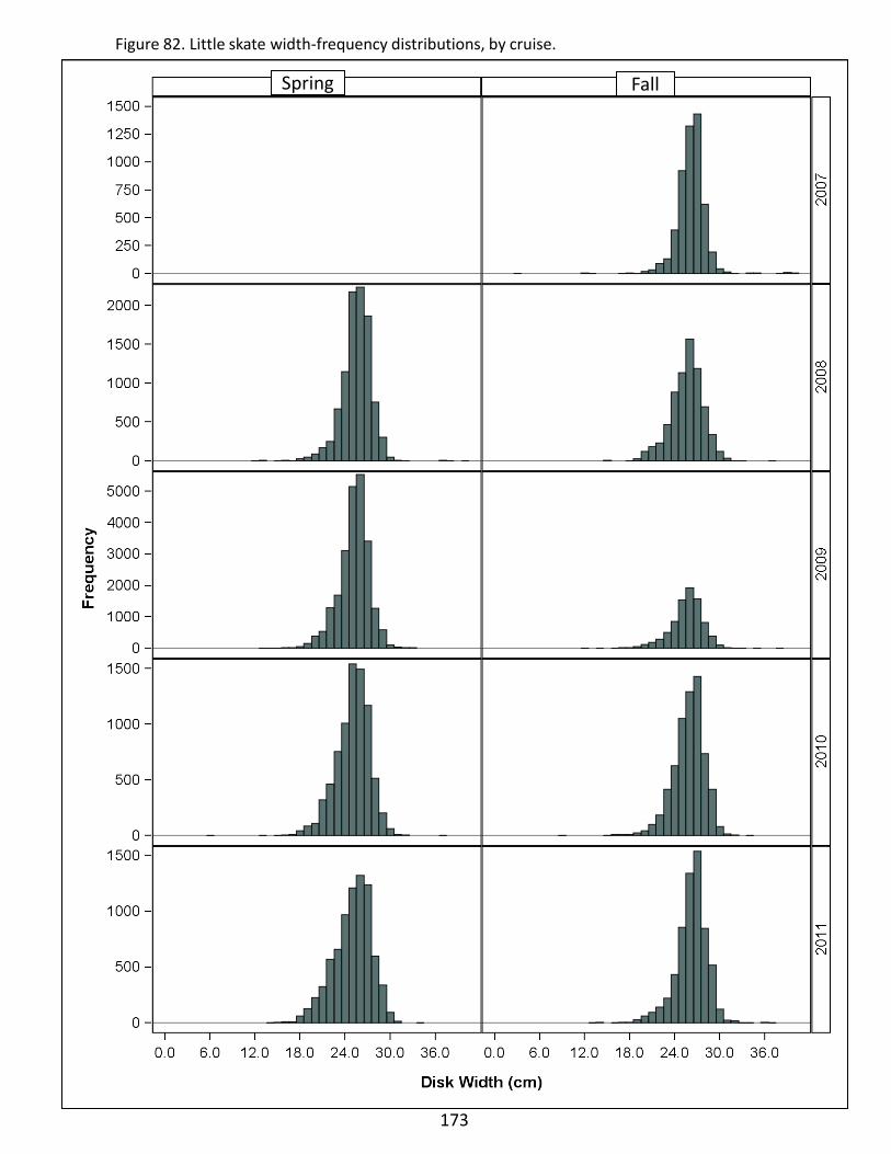
Figure 82. Little skate width-frequency distributions, by cruise.

173

Spring Fall

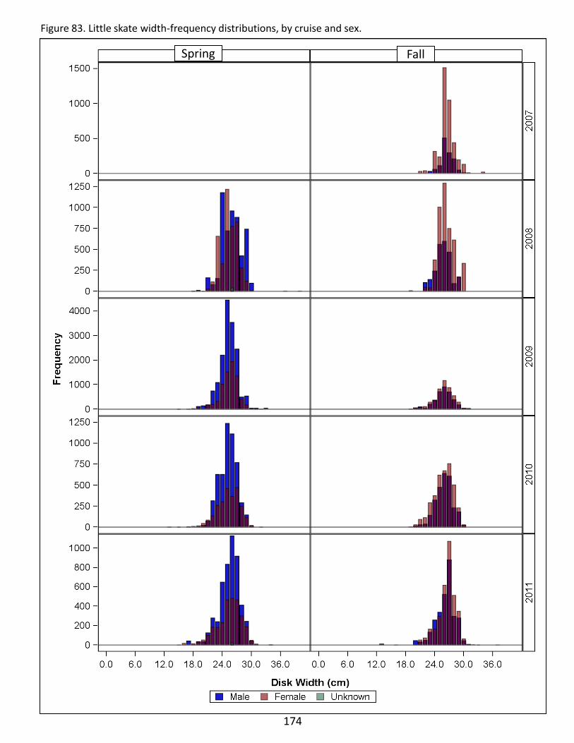
174

Figure 83. Little skate width-frequency distributions, by cruise and sex.

Spring Fall

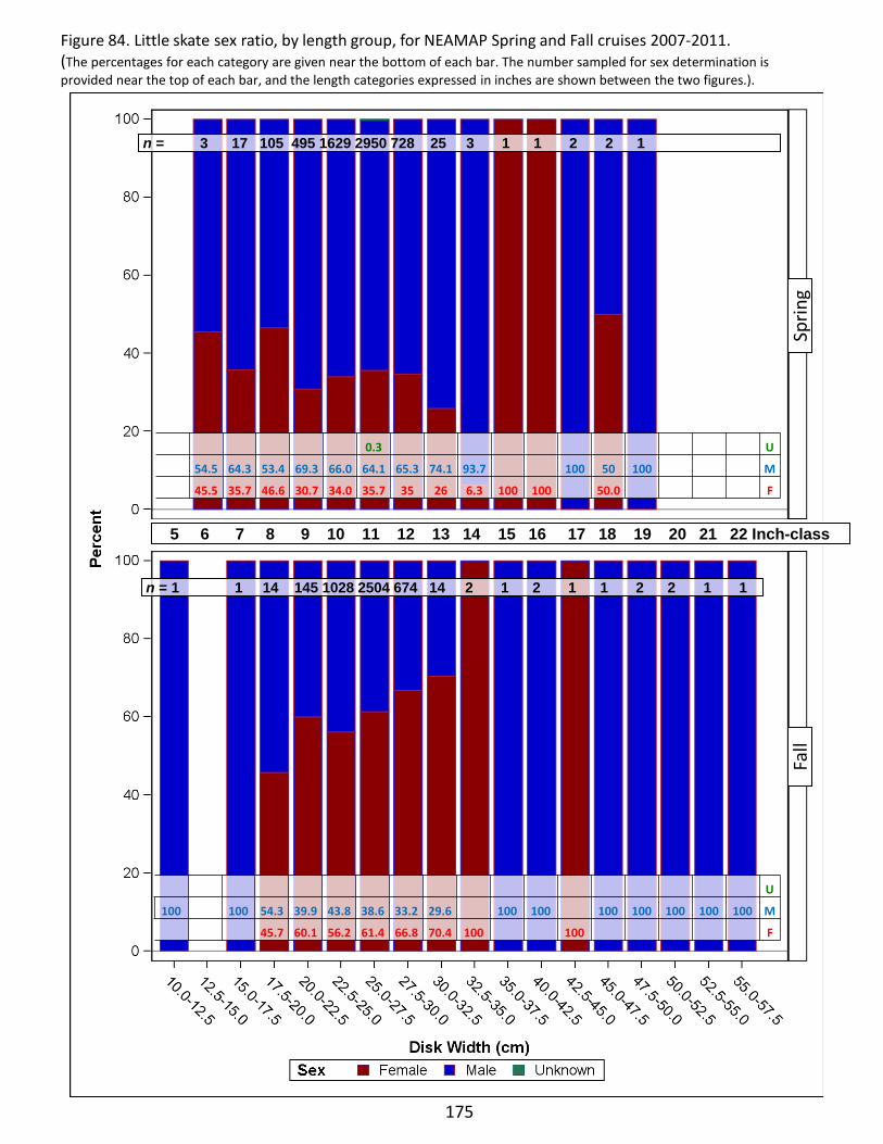
175

Figure 84. Little skate sex ratio, by length group, for NEAMAP Spring and Fall cruises 2007-2011. (The percentages for each category are given near the bottom of each bar. The number sampled for sex determination is provided near the top of each bar, and the length categories expressed in inches are shown between the two figures.).

n = 3 17 105 495 1629 2950 728 25 3 1 1 2 2 1

n = 1 1 14 145 1028 2504 674 14 2 1 2 1 1 2 2 1 1

Sprin

g F

all

5 6 7 8 9 10 11 12 13 14 15 16 17 18 19 20 21 22 Inch-class

0.3 U

54.5 64.3 53.4 69.3 66.0 64.1 65.3 74.1 93.7 100 50 100 M

45.5 35.7 46.6 30.7 34.0 35.7 35 26 6.3 100 100 50.0 F

U

100 100 54.3 39.9 43.8 38.6 33.2 29.6 100 100 100 100 100 100 100 M

45.7 60.1 56.2 61.4 66.8 70.4 100 100 F

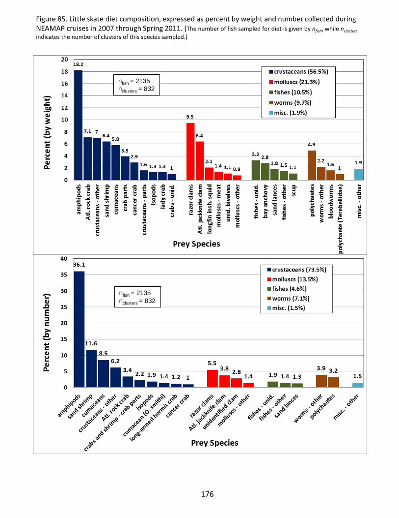
nfish = 2135 nclusters = 832

176

Figure 85. Little skate diet composition, expressed as percent by weight and number collected during NEAMAP cruises in 2007 through Spring 2011. (The number of fish sampled for diet is given by nfish, while nclusters indicates the number of clusters of this species sampled.)

nfish = 2135 nclusters = 832

Longfin Inshore Squid Sampling Priority: E

Figure 86. Longfin inshore squid biomass (kg) at each sampling site for 2011 NEAMAP cruises.

177

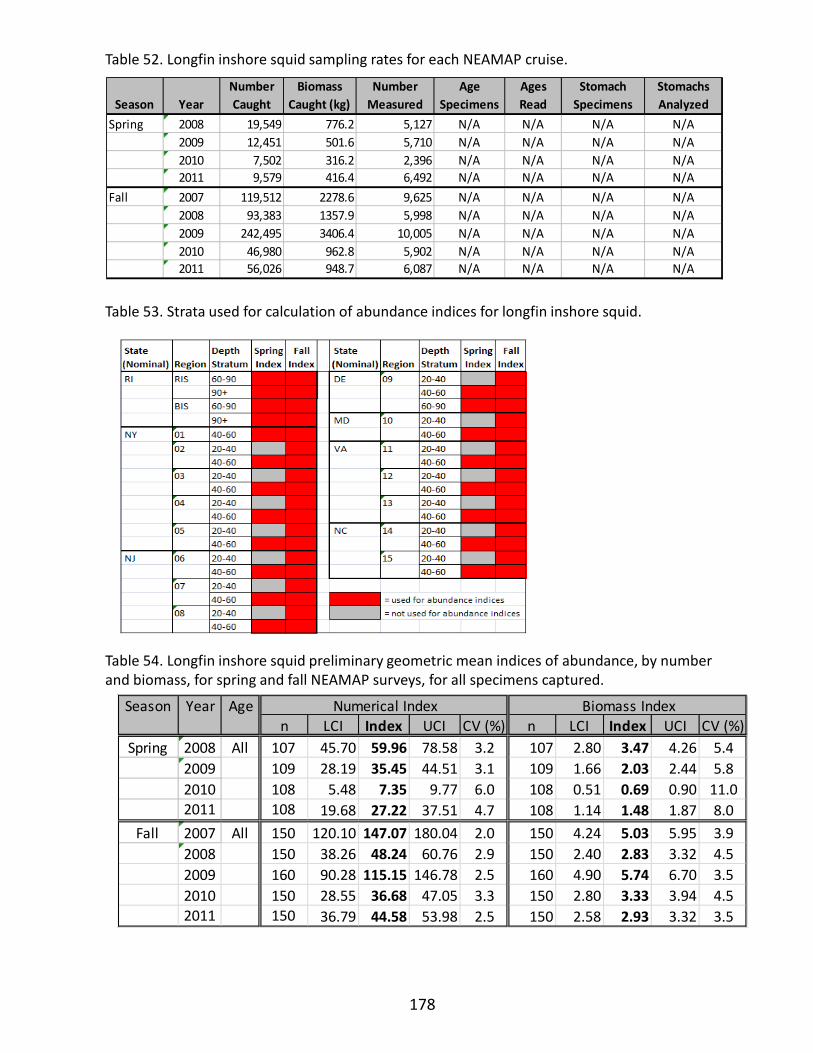
Table 52. Longfin inshore squid sampling rates for each NEAMAP cruise.

Table 53. Strata used for calculation of abundance indices for longfin inshore squid.

Table 54. Longfin inshore squid preliminary geometric mean indices of abundance, by number and biomass, for spring and fall NEAMAP surveys, for all specimens captured.

178

Season YearNumber Caught

Biomass Caught (kg)

Number Measured

Age Specimens

Ages Read

Stomach Specimens

Stomachs Analyzed

Spring 2008 19,549 776.2 5,127 N/A N/A N/A N/A2009 12,451 501.6 5,710 N/A N/A N/A N/A2010 7,502 316.2 2,396 N/A N/A N/A N/A2011 9,579 416.4 6,492 N/A N/A N/A N/A

Fall 2007 119,512 2278.6 9,625 N/A N/A N/A N/A2008 93,383 1357.9 5,998 N/A N/A N/A N/A2009 242,495 3406.4 10,005 N/A N/A N/A N/A2010 46,980 962.8 5,902 N/A N/A N/A N/A2011 56,026 948.7 6,087 N/A N/A N/A N/A

Season Year Agen LCI Index UCI CV (%) n LCI Index UCI CV (%)

Spring 2008 All 107 45.70 59.96 78.58 3.2 107 2.80 3.47 4.26 5.42009 109 28.19 35.45 44.51 3.1 109 1.66 2.03 2.44 5.82010 108 5.48 7.35 9.77 6.0 108 0.51 0.69 0.90 11.02011 108 19.68 27.22 37.51 4.7 108 1.14 1.48 1.87 8.0

Fall 2007 All 150 120.10 147.07 180.04 2.0 150 4.24 5.03 5.95 3.92008 150 38.26 48.24 60.76 2.9 150 2.40 2.83 3.32 4.52009 160 90.28 115.15 146.78 2.5 160 4.90 5.74 6.70 3.52010 150 28.55 36.68 47.05 3.3 150 2.80 3.33 3.94 4.52011 150 36.79 44.58 53.98 2.5 150 2.58 2.93 3.32 3.5

Numerical Index Biomass Index

179

Figure 87. Longfin inshore squid preliminary geometric mean indices of abundance, by number and biomass, for spring and fall NEAMAP surveys, for all specimens captured.

Figure 88. Longfin inshore squid length-frequency distributions, by cruise.

180

Spring Fall

Scup Sampling Priority: A

Figure 89. Scup biomass (kg) at each sampling site for 2011 NEAMAP cruises.

181

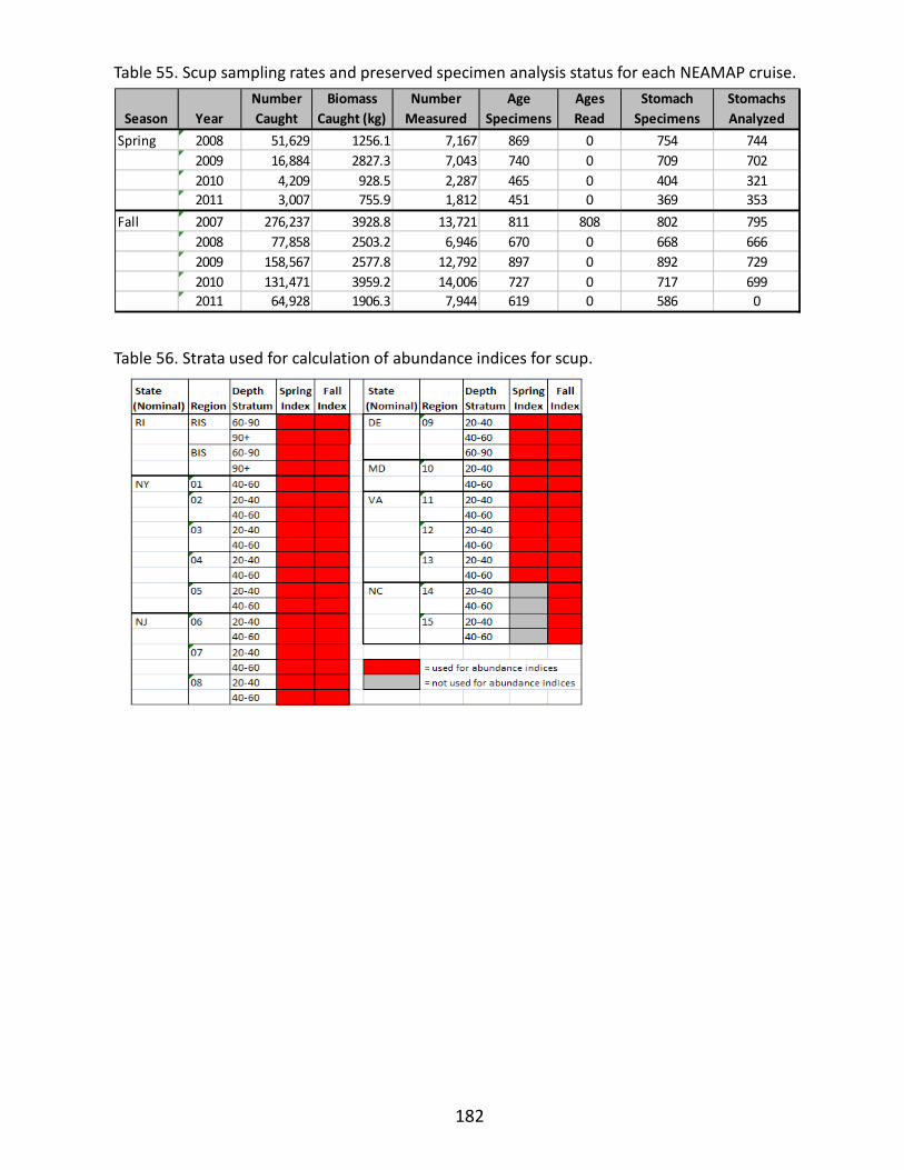
Table 55. Scup sampling rates and preserved specimen analysis status for each NEAMAP cruise.

Table 56. Strata used for calculation of abundance indices for scup.

182

Season YearNumber Caught

Biomass Caught (kg)

Number Measured

Age Specimens

Ages Read

Stomach Specimens

Stomachs Analyzed

Spring 2008 51,629 1256.1 7,167 869 0 754 7442009 16,884 2827.3 7,043 740 0 709 7022010 4,209 928.5 2,287 465 0 404 3212011 3,007 755.9 1,812 451 0 369 353

Fall 2007 276,237 3928.8 13,721 811 808 802 7952008 77,858 2503.2 6,946 670 0 668 6662009 158,567 2577.8 12,792 897 0 892 7292010 131,471 3959.2 14,006 727 0 717 6992011 64,928 1906.3 7,944 619 0 586 0

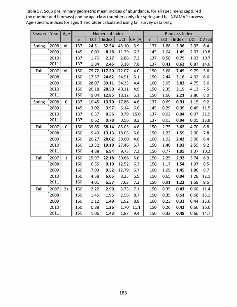
Table 57. Scup preliminary geometric mean indices of abundance, for all specimens captured (by number and biomass) and by age-class (numbers only) for spring and fall NEAMAP surveys. Age-specific indices for ages 1 and older calculated using fall survey data only.

183

Season Year Agen LCI Index UCI CV (%) n LCI Index UCI CV (%)

Spring 2008 All 137 24.51 32.54 43.10 3.9 137 1.88 2.36 2.93 6.42009 145 6.00 8.28 11.29 6.3 145 1.04 1.49 2.03 10.82010 137 1.76 2.27 2.88 7.2 137 0.58 0.79 1.03 10.72011 137 1.84 2.45 3.18 7.8 137 0.41 0.62 0.87 14.6

Fall 2007 All 150 79.72 117.20 172.07 4.0 150 5.68 7.49 9.79 5.62008 150 17.57 24.82 34.91 5.1 150 2.44 3.16 4.02 6.62009 160 28.07 39.11 54.33 4.4 160 3.05 3.82 4.75 5.62010 150 20.18 28.50 40.11 4.9 150 2.35 3.15 4.13 7.52011 150 9.04 12.85 18.12 6.1 150 1.66 2.21 2.86 8.0

Spring 2008 0 137 10.45 13.70 17.86 4.6 137 0.69 0.91 1.15 9.22009 145 3.02 3.97 5.14 6.6 145 0.29 0.39 0.49 11.52010 137 0.37 0.56 0.79 15.0 137 0.02 0.04 0.07 31.92011 137 0.62 0.78 0.96 8.2 137 0.03 0.04 0.05 13.8

Fall 2007 0 150 39.65 58.14 85.03 4.6 150 2.75 3.62 4.70 6.82008 150 9.49 13.13 18.05 5.6 150 1.23 1.59 2.00 7.82009 160 20.27 28.02 38.60 4.6 160 1.92 2.42 3.00 6.42010 150 13.32 19.19 27.46 5.7 150 1.40 1.92 2.55 9.22011 150 4.88 6.94 9.73 7.3 150 0.77 1.05 1.37 10.2

Fall 2007 1 150 15.97 22.18 30.66 5.0 150 2.25 2.92 3.74 6.92008 150 6.55 9.10 12.52 6.3 150 1.17 1.54 1.97 8.52009 160 7.03 9.52 12.79 5.7 160 1.09 1.45 1.86 8.72010 150 4.38 6.05 8.23 6.9 150 0.65 0.94 1.28 12.12011 150 4.01 5.57 7.63 7.2 150 0.91 1.22 1.58 9.5

Fall 2007 2+ 150 2.22 2.90 3.73 7.1 150 0.35 0.47 0.60 11.42008 150 1.45 1.95 2.56 8.7 150 0.35 0.51 0.68 13.12009 160 1.12 1.49 1.92 8.8 160 0.23 0.33 0.44 13.62010 150 0.88 1.26 1.70 11.1 150 0.26 0.42 0.60 16.62011 150 1.06 1.43 1.87 9.4 150 0.32 0.48 0.66 14.7

Numerical Index Biomass Index

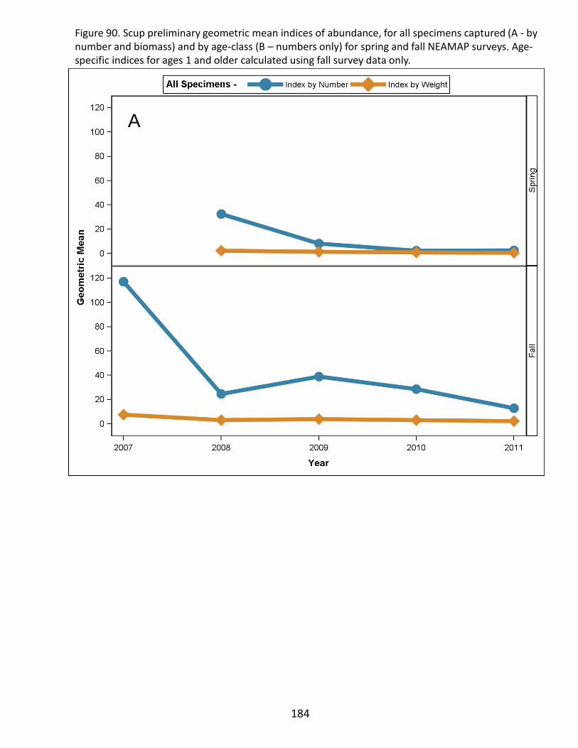
184

A

Figure 90. Scup preliminary geometric mean indices of abundance, for all specimens captured (A - by number and biomass) and by age-class (B – numbers only) for spring and fall NEAMAP surveys. Age-specific indices for ages 1 and older calculated using fall survey data only.

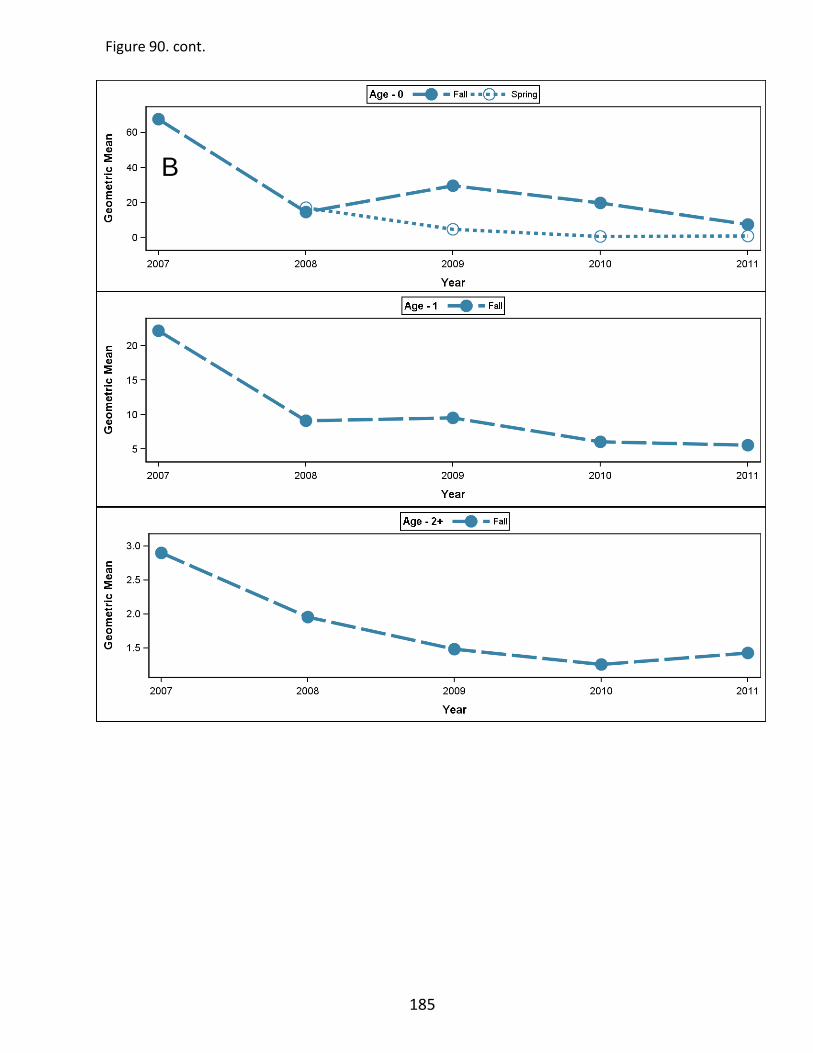
185

Figure 90. cont.

B

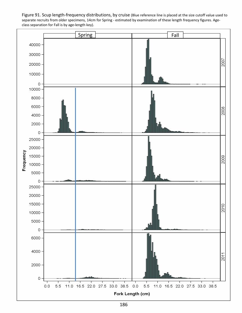
Figure 91. Scup length-frequency distributions, by cruise (Blue reference line is placed at the size cutoff value used to separate recruits from older specimens, 14cm for Spring - estimated by examination of these length frequency figures. Age-class separation for Fall is by age-length key).

186

Spring Fall

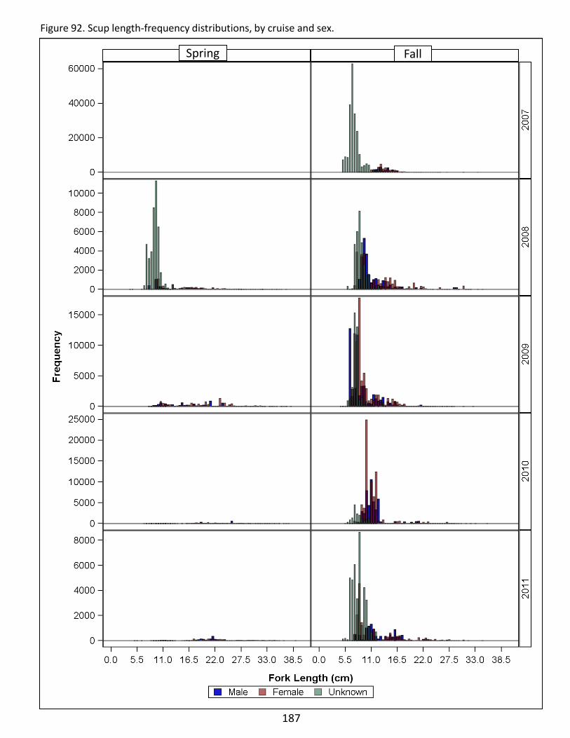
187

Figure 92. Scup length-frequency distributions, by cruise and sex.

Spring Fall

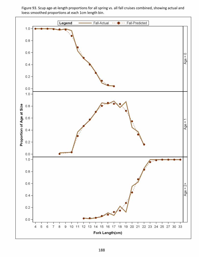
188

Figure 93. Scup age-at-length proportions for all spring vs. all fall cruises combined, showing actual and loess smoothed proportions at each 1cm length bin.

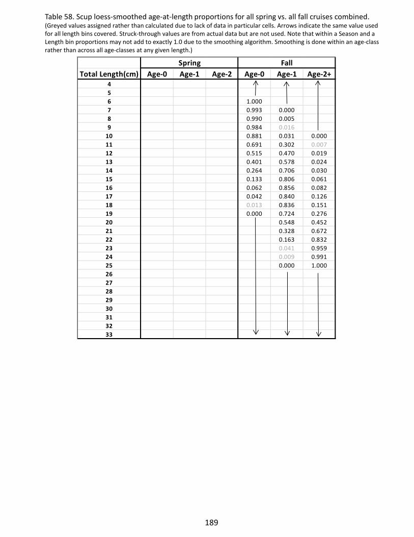
Total Length(cm) Age-0 Age-1 Age-2 Age-0 Age-1 Age-2+456 1.0007 0.993 0.0008 0.990 0.0059 0.984 0.016

10 0.881 0.031 0.00011 0.691 0.302 0.00712 0.515 0.470 0.01913 0.401 0.578 0.02414 0.264 0.706 0.03015 0.133 0.806 0.06116 0.062 0.856 0.08217 0.042 0.840 0.12618 0.013 0.836 0.15119 0.000 0.724 0.27620 0.548 0.45221 0.328 0.67222 0.163 0.83223 0.041 0.95924 0.009 0.99125 0.000 1.0002627282930313233

Spring Fall

Table 58. Scup loess-smoothed age-at-length proportions for all spring vs. all fall cruises combined. (Greyed values assigned rather than calculated due to lack of data in particular cells. Arrows indicate the same value used for all length bins covered. Struck-through values are from actual data but are not used. Note that within a Season and a Length bin proportions may not add to exactly 1.0 due to the smoothing algorithm. Smoothing is done within an age-class rather than across all age-classes at any given length.)

189

190

Figure 94. Scup sex ratio, by length group, for NEAMAP Spring and Fall cruises 2007-2011. (The percentages for each category are given near the bottom of each bar. The number sampled for sex determination is provided near the top of each bar, and the length categories expressed in inches are shown between the two figures.).

n = 4 29 464 527 165 308 244 203 181 149 99 68 54 21 2

n = 4 321 837 633 697 662 159 148 96 77 34 21 6 1

Sprin

g F

all

1 2 3 4 5 6 7 8 9 10 11 12 13 14 15 Inch-class

100 99.8 88.4 52.4 18.1 0.2 0.3 1.1 U

6.1 16.9 31.2 48.4 37.7 57.4 32.3 49.0 27.6 57.4 58.6 22.5 M

0.2 5.5 30.7 50.7 51.3 62.3 42.6 67.7 50.7 72.4 41.5 41.4 77.5 100 F

100 88.6 46.6 13.4 8.6 1.6 U

7.9 16.6 44.0 39.6 40.4 42.3 37.8 26.3 15.2 80.9 2.5 6.4 100 M

3.5 36.8 42.5 51.8 58.1 57.7 62.2 73.7 84.8 19.1 97.5 93.6 F

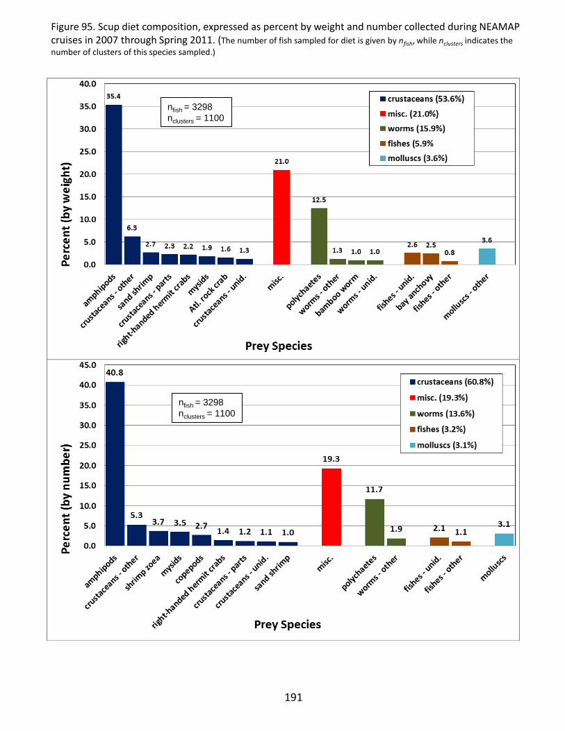
nfish = 3298 nclusters = 1100

nfish = 3298 nclusters = 1100

191

Figure 95. Scup diet composition, expressed as percent by weight and number collected during NEAMAP cruises in 2007 through Spring 2011. (The number of fish sampled for diet is given by nfish, while nclusters indicates the number of clusters of this species sampled.)

Silver Hake (Whiting) Sampling Priority: A

Figure 96. Silver hake biomass (kg) at each sampling site for 2011 NEAMAP cruises.

192

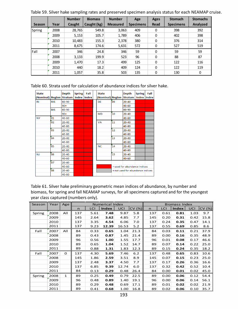
Table 59. Silver hake sampling rates and preserved specimen analysis status for each NEAMAP cruise.

Table 60. Strata used for calculation of abundance indices for silver hake.

Table 61. Silver hake preliminary geometric mean indices of abundance, by number and biomass, for spring and fall NEAMAP surveys, for all specimens captured and for the youngest year class captured (numbers only).

193

Season YearNumber Caught

Biomass Caught (kg)

Number Measured

Age Specimens

Ages Read

Stomach Specimens

Stomachs Analyzed

Spring 2008 28,765 549.8 3,063 409 0 398 3922009 5,153 105.7 1,789 406 0 402 3982010 10,483 155.3 2,378 380 0 376 3142011 8,675 174.6 5,631 572 0 527 519

Fall 2007 346 24.8 346 59 0 59 592008 3,133 199.9 523 96 0 88 872009 1,470 17.3 499 125 0 122 1162010 440 18.2 409 124 0 122 1192011 1,057 35.8 503 135 0 130 0

Season Year Agen LCI Index UCI CV (%) n LCI Index UCI CV (%)

Spring 2008 All 137 5.61 7.48 9.87 5.8 137 0.61 0.81 1.03 9.72009 145 2.64 3.62 4.85 7.7 145 0.20 0.31 0.42 15.82010 137 3.35 4.54 6.06 7.0 137 0.24 0.35 0.47 14.12011 137 9.23 12.39 16.53 5.2 137 0.55 0.69 0.85 8.6

Fall 2007 All 84 0.33 0.65 1.04 21.3 84 0.03 0.11 0.21 37.92008 89 0.43 0.87 1.45 21.4 89 0.00 0.16 0.35 48.92009 96 0.56 1.00 1.55 17.7 96 0.01 0.08 0.17 46.62010 89 0.65 1.04 1.52 14.7 89 0.07 0.14 0.22 25.02011 89 0.88 1.31 1.83 12.3 89 0.15 0.24 0.35 18.2

Fall 2007 0 137 4.30 5.69 7.46 6.2 137 0.48 0.65 0.83 10.62008 145 1.86 2.59 3.51 8.9 145 0.07 0.15 0.23 25.02009 137 2.48 3.37 4.50 7.7 137 0.17 0.26 0.36 16.62010 137 6.85 9.39 12.74 6.0 137 0.32 0.42 0.52 10.42011 84 0.13 0.29 0.48 26.4 84 0.00 0.01 0.02 45.0

Spring 2008 1 89 0.25 0.49 0.79 22.5 89 0.00 0.06 0.12 54.42009 96 0.48 0.89 1.40 19.1 96 0.00 0.06 0.14 56.12010 89 0.29 0.48 0.69 17.1 89 0.01 0.02 0.02 21.92011 89 0.41 0.68 1.00 16.8 89 0.02 0.06 0.10 35.7

Numerical Index Biomass Index

194

Figure 97. Silver hake preliminary geometric mean indices of abundance, by number and biomass, for spring and fall NEAMAP surveys, for all specimens captured (A) and for the youngest year class captured (B – numbers only).

B

A

Figure 98. Silver hake length-frequency distributions, by cruise (Blue reference lines are placed at the size cutoff values used to separate recruits from older specimens. Cutoff values - Spring 14cm, Fall 17cm - estimated by examination of these length frequency figures.).

195

Spring Fall

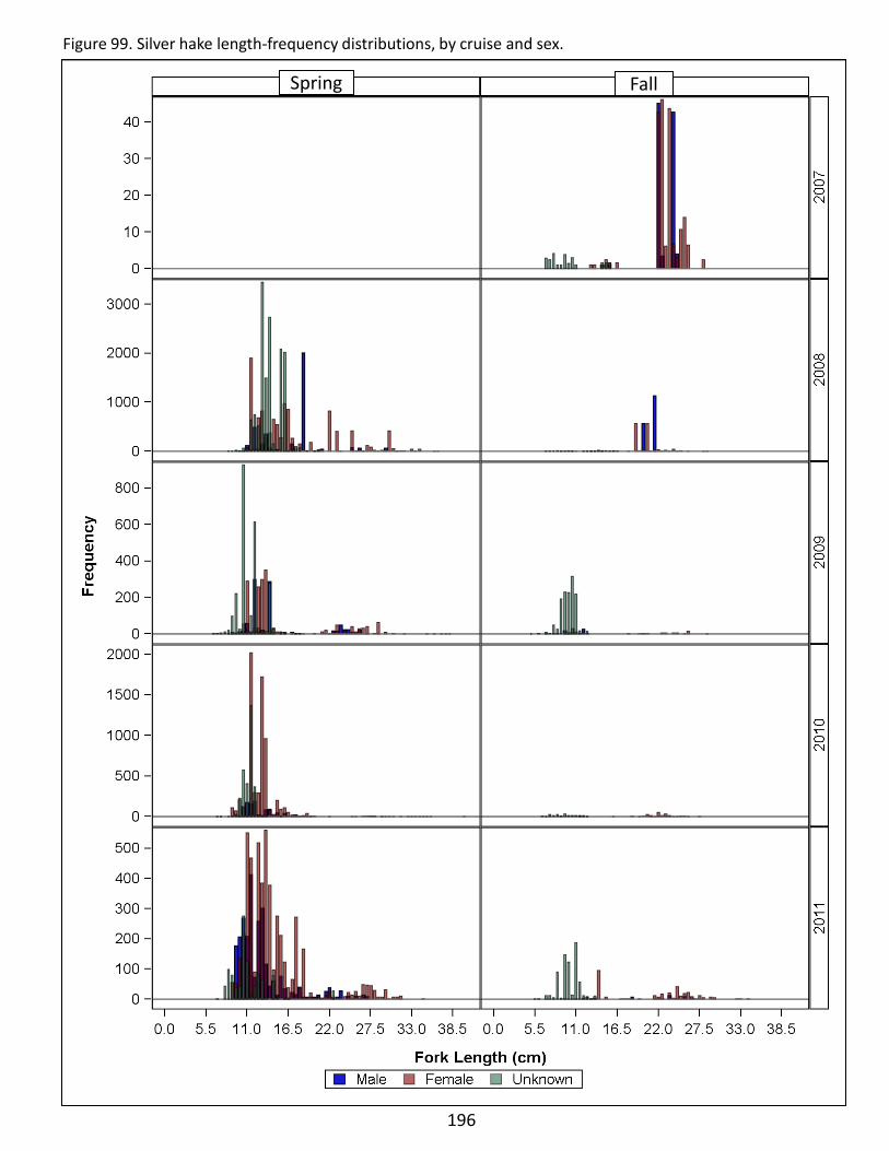
Figure 99. Silver hake length-frequency distributions, by cruise and sex.

Spring Fall

196

197

Figure 100. Silver hake sex ratio, by length group, for NEAMAP Spring and Fall cruises 2007-2011. (The percentages for each category are given near the bottom of each bar. The number sampled for sex determination is provided near the top of each bar, and the length categories expressed in inches are shown between the two figures.).

n = 11 151 535 454 237 90 52 64 85 43 21 12 6 2 1

n = 36 149 107 38 14 13 67 72 36 9 1 2

Sprin

g F

all

2 3 4 5 6 7 8 9 10 11 12 13 14 15 16 Inch-class

100 47.9 39.4 46.0 52.2 3.2 3.2 U

19.8 16.5 9.3 5.2 73.4 11.7 16.1 27.6 11.0 3.4 M

32.3 44.1 44.7 42.6 23.4 85.1 83.9 72.4 89.0 96.6 100 100 100 100 F

98.8 97.4 89.9 27.8 43.8 U

1.2 1.8 3.8 7.9 3.3 5.0 67.8 19.4 12.0 M

0.8 6.3 64.3 52.9 95.0 32.2 80.6 88.0 100 100 100 F

nfish = 1523 nclusters = 509

198

Figure 101. Silver hake diet composition, expressed as percent by weight and number collected during NEAMAP cruises in 2007 through Spring 2011. (The number of fish sampled for diet is given by nfish, while nclusters indicates the number of clusters of this species sampled.)

nfish = 1523 nclusters = 509

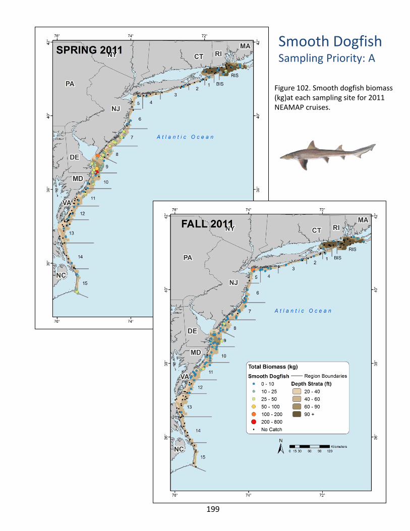
Smooth Dogfish Sampling Priority: A

Figure 102. Smooth dogfish biomass (kg)at each sampling site for 2011 NEAMAP cruises.

199

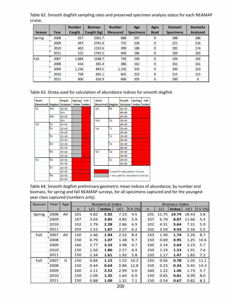
Table 62. Smooth dogfish sampling rates and preserved specimen analysis status for each NEAMAP cruise.

Table 63. Strata used for calculation of abundance indices for smooth dogfish.

Table 64. Smooth dogfish preliminary geometric mean indices of abundance, by number and biomass, for spring and fall NEAMAP surveys, for all specimens captured and for the youngest year class captured (numbers only).

200

Season YearNumber Caught

Biomass Caught (kg)

Number Measured

Age Specimens

Ages Read

Stomach Specimens

Stomachs Analyzed

Spring 2008 927 2501.7 688 297 0 288 2862009 947 2741.4 725 236 0 221 2162010 402 1232.6 399 188 0 181 1742011 521 1741.5 458 186 0 169 165

Fall 2007 1,684 1548.7 759 196 0 194 1922008 414 365.4 386 162 0 161 1612009 1,156 843.5 1,156 333 0 330 3232010 758 691.1 602 223 0 215 2152011 606 616.9 606 205 0 200 0

Season Year Agen LCI Index UCI CV (%) n LCI Index UCI CV (%)

Spring 2008 All 101 4.82 5.92 7.23 4.5 101 11.75 14.74 18.43 3.82009 107 3.03 3.85 4.85 5.9 107 6.70 8.87 11.66 5.42010 102 1.79 2.28 2.86 6.9 102 4.31 5.64 7.31 5.92011 102 1.52 1.87 2.27 6.2 102 3.50 4.43 5.56 5.5

Fall 2007 All 150 1.46 1.94 2.52 8.4 150 1.30 1.74 2.26 8.72008 150 0.79 1.07 1.38 9.7 150 0.69 0.95 1.25 10.62009 160 2.77 3.33 3.98 4.7 160 2.14 2.64 3.23 5.72010 150 1.50 1.86 2.27 6.4 150 1.19 1.53 1.91 7.62011 150 1.34 1.61 1.92 5.8 150 1.17 1.47 1.82 7.2

Fall 2007 0 150 0.84 1.15 1.52 10.2 150 0.56 0.78 1.02 11.12008 150 0.44 0.64 0.86 12.8 150 0.23 0.34 0.45 14.32009 160 2.11 2.52 2.99 5.0 160 1.22 1.46 1.73 5.72010 150 1.09 1.35 1.64 6.9 150 0.65 0.81 0.99 8.02011 150 0.88 1.09 1.31 7.1 150 0.54 0.67 0.82 8.2

Numerical Index Biomass Index

Figure 103. Smooth dogfish preliminary geometric mean indices of abundance, by number and biomass, for spring and fall NEAMAP surveys, for all specimens captured (A) and for the youngest year class captured (B – numbers only).

B

A

201

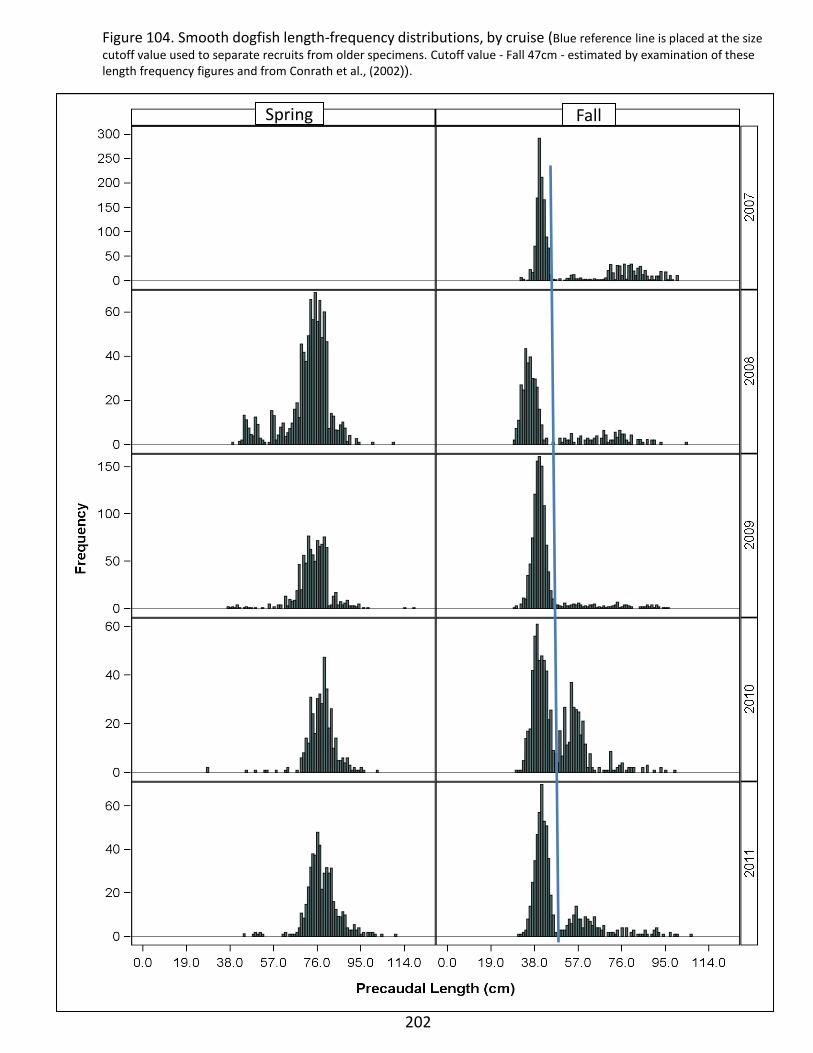
Figure 104. Smooth dogfish length-frequency distributions, by cruise (Blue reference line is placed at the size cutoff value used to separate recruits from older specimens. Cutoff value - Fall 47cm - estimated by examination of these length frequency figures and from Conrath et al., (2002)).

202

Spring Fall

Figure 105. Smooth dogfish length-frequency distributions, by cruise and sex.

Spring Fall

203

204

Figure 106. Smooth dogfish sex ratio, by length group, for NEAMAP Spring and Fall cruises 2007-2011. (The percentages for each category are given near the bottom of each bar. The number sampled for sex determination is provided near the top of each bar, and the length categories expressed in inches are shown between the two figures.).

n = 2 5 18 33 15 27 53 206 584 730 221 105 32 16

n = 3 119 806 786 82 84 95 55 44 64 60 29 36 21 11

Sprin

g F

all

10-12 12-14 14-16 16-18 18-20 20-22 22-24 24-26 26-28 28-30 30-32 32-34 34-36 36-38 38+ Inch-class

14.0 0.1 U

50.0 64.4 48.0 59.9 72.5 53.9 66.0 86.4 92.0 81.3 63.7 32.1 16.4 16.9 M

50.0 35.6 52.0 40.1 27.5 32.1 34.0 13.6 8.0 18.6 36.3 67.9 83.6 83.1 F

U

33.3 54.7 57.4 53.9 50.8 56.6 48.4 48.8 63.1 38.4 54.5 16.6 10.5 20.8 9.1 M

66.7 45.3 42.6 46.1 49.2 43.4 51.6 51.2 36.9 61.6 45.5 83.4 89.5 79.2 90.9 F

nfish = 1538 nclusters = 664

nfish = 1538 nclusters = 664

205

Figure 107. Smooth dogfish diet composition, expressed as percent by weight and number collected during NEAMAP cruises in 2007 through Spring 2011. (The number of fish sampled for diet is given by nfish, while nclusters indicates the number of clusters of this species sampled.)

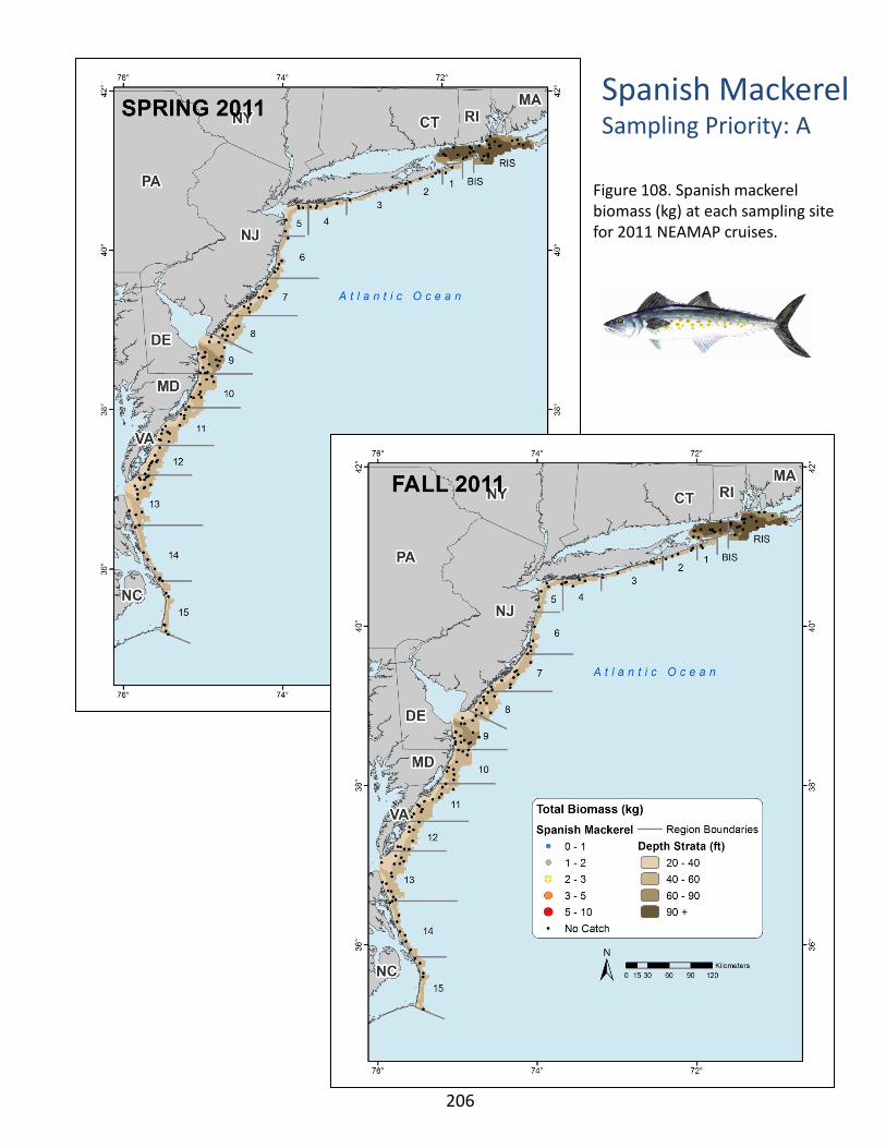
Spanish Mackerel Sampling Priority: A

Figure 108. Spanish mackerel biomass (kg) at each sampling site for 2011 NEAMAP cruises.

206

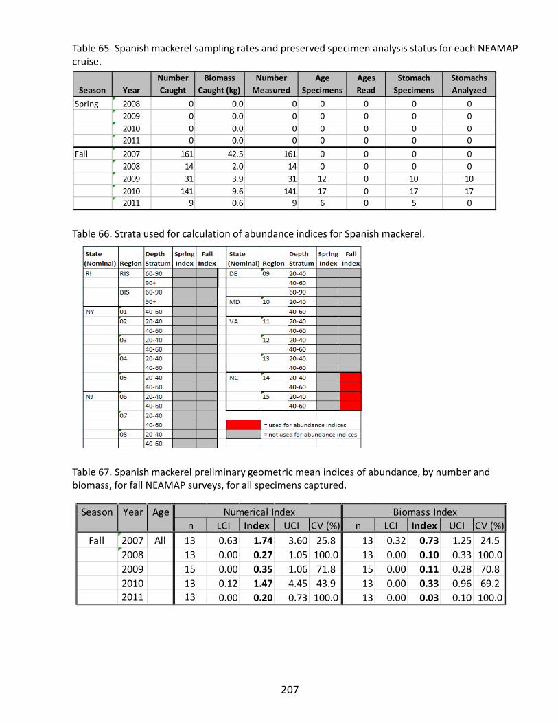
Table 65. Spanish mackerel sampling rates and preserved specimen analysis status for each NEAMAP cruise.

Table 66. Strata used for calculation of abundance indices for Spanish mackerel.

Table 67. Spanish mackerel preliminary geometric mean indices of abundance, by number and biomass, for fall NEAMAP surveys, for all specimens captured.

207

Season YearNumber Caught

Biomass Caught (kg)

Number Measured

Age Specimens

Ages Read

Stomach Specimens

Stomachs Analyzed

Spring 2008 0 0.0 0 0 0 0 02009 0 0.0 0 0 0 0 02010 0 0.0 0 0 0 0 02011 0 0.0 0 0 0 0 0

Fall 2007 161 42.5 161 0 0 0 02008 14 2.0 14 0 0 0 02009 31 3.9 31 12 0 10 102010 141 9.6 141 17 0 17 172011 9 0.6 9 6 0 5 0

Season Year Agen LCI Index UCI CV (%) n LCI Index UCI CV (%)

Fall 2007 All 13 0.63 1.74 3.60 25.8 13 0.32 0.73 1.25 24.52008 13 0.00 0.27 1.05 100.0 13 0.00 0.10 0.33 100.02009 15 0.00 0.35 1.06 71.8 15 0.00 0.11 0.28 70.82010 13 0.12 1.47 4.45 43.9 13 0.00 0.33 0.96 69.22011 13 0.00 0.20 0.73 100.0 13 0.00 0.03 0.10 100.0

Numerical Index Biomass Index

208

Figure 109. Spanish mackerel preliminary geometric mean indices of abundance, by number and biomass, for fall NEAMAP surveys, for all specimens captured.

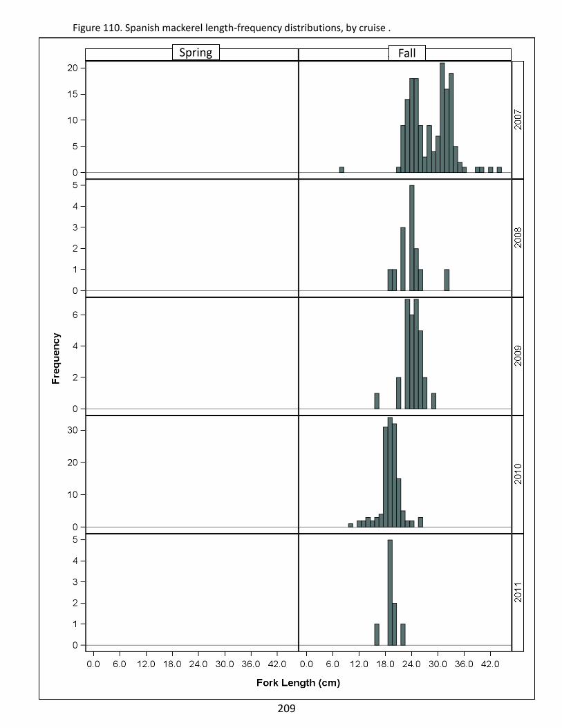
Figure 110. Spanish mackerel length-frequency distributions, by cruise .

209

Spring Fall

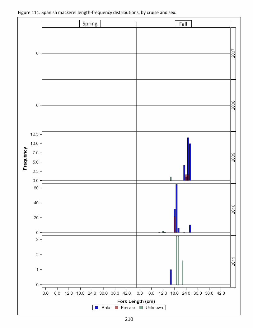
210

Figure 111. Spanish mackerel length-frequency distributions, by cruise and sex.

Spring Fall

Figure 112. Spanish mackerel diet composition, expressed as percent by weight and number collected during NEAMAP cruises in 2007 through Spring 2011. (The number of fish sampled for diet is given by nfish, while nclusters indicates the number of clusters of this species sampled. Note the very small sample size.)

nfish = 24 nclusters = 8

nfish = 24 nclusters = 8

211

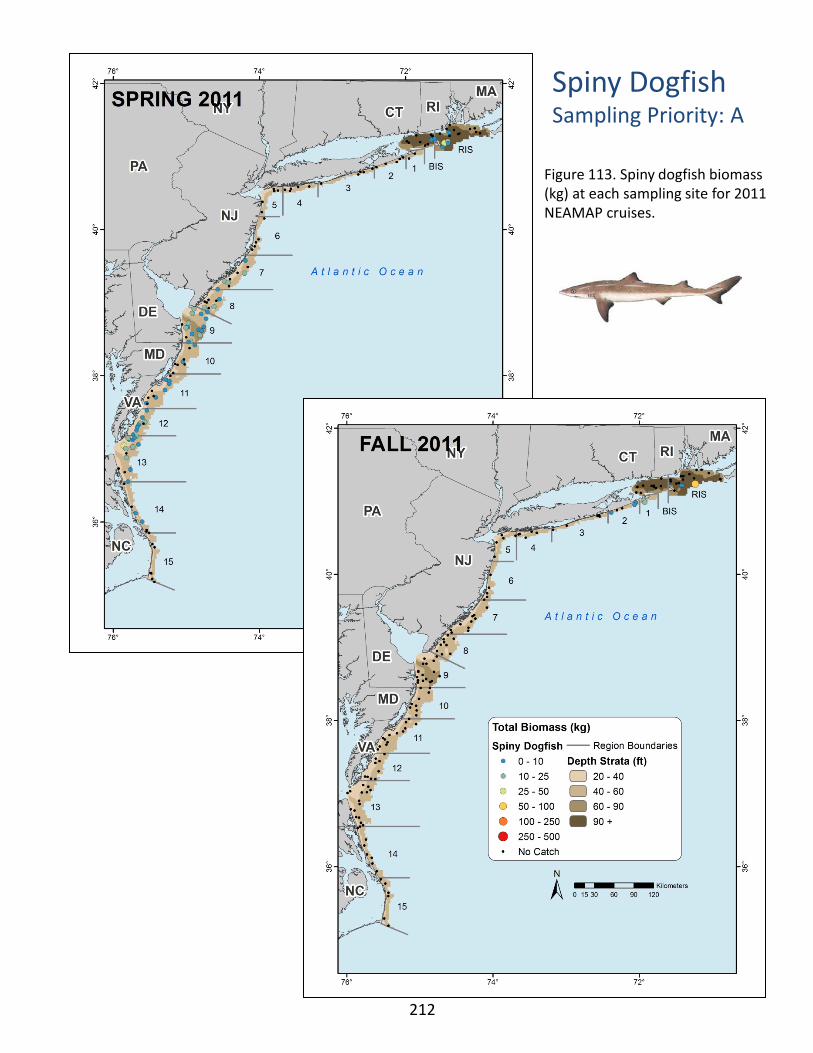
Spiny Dogfish Sampling Priority: A

Figure 113. Spiny dogfish biomass (kg) at each sampling site for 2011 NEAMAP cruises.

212

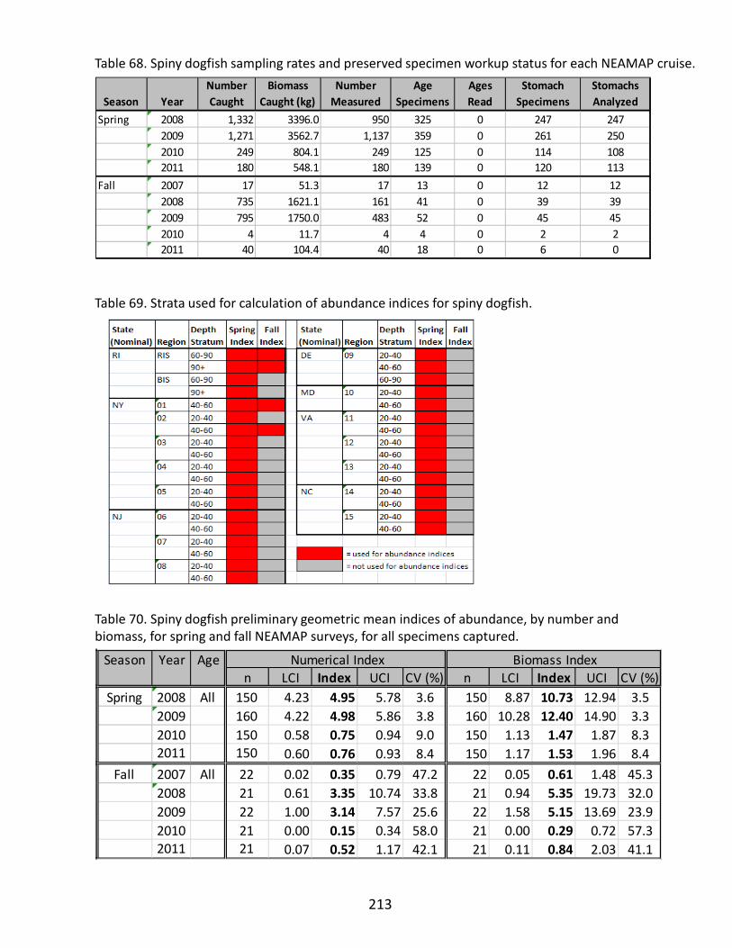
Table 68. Spiny dogfish sampling rates and preserved specimen workup status for each NEAMAP cruise.

Table 69. Strata used for calculation of abundance indices for spiny dogfish.

Table 70. Spiny dogfish preliminary geometric mean indices of abundance, by number and biomass, for spring and fall NEAMAP surveys, for all specimens captured.

213

Season YearNumber Caught

Biomass Caught (kg)

Number Measured

Age Specimens

Ages Read

Stomach Specimens

Stomachs Analyzed

Spring 2008 1,332 3396.0 950 325 0 247 2472009 1,271 3562.7 1,137 359 0 261 2502010 249 804.1 249 125 0 114 1082011 180 548.1 180 139 0 120 113

Fall 2007 17 51.3 17 13 0 12 122008 735 1621.1 161 41 0 39 392009 795 1750.0 483 52 0 45 452010 4 11.7 4 4 0 2 22011 40 104.4 40 18 0 6 0

Season Year Agen LCI Index UCI CV (%) n LCI Index UCI CV (%)

Spring 2008 All 150 4.23 4.95 5.78 3.6 150 8.87 10.73 12.94 3.52009 160 4.22 4.98 5.86 3.8 160 10.28 12.40 14.90 3.32010 150 0.58 0.75 0.94 9.0 150 1.13 1.47 1.87 8.32011 150 0.60 0.76 0.93 8.4 150 1.17 1.53 1.96 8.4

Fall 2007 All 22 0.02 0.35 0.79 47.2 22 0.05 0.61 1.48 45.32008 21 0.61 3.35 10.74 33.8 21 0.94 5.35 19.73 32.02009 22 1.00 3.14 7.57 25.6 22 1.58 5.15 13.69 23.92010 21 0.00 0.15 0.34 58.0 21 0.00 0.29 0.72 57.32011 21 0.07 0.52 1.17 42.1 21 0.11 0.84 2.03 41.1

Numerical Index Biomass Index

214

Figure 114. Spiny dogfish preliminary geometric mean indices of abundance, by number and biomass, for spring and fall NEAMAP surveys, for all specimens captured.

Figure 115. Spiny dogfish length-frequency distributions, by cruise.

215

Spring Fall

Figure 116. Spiny dogfish length-frequency distributions, by cruise and sex.

Spring Fall

216

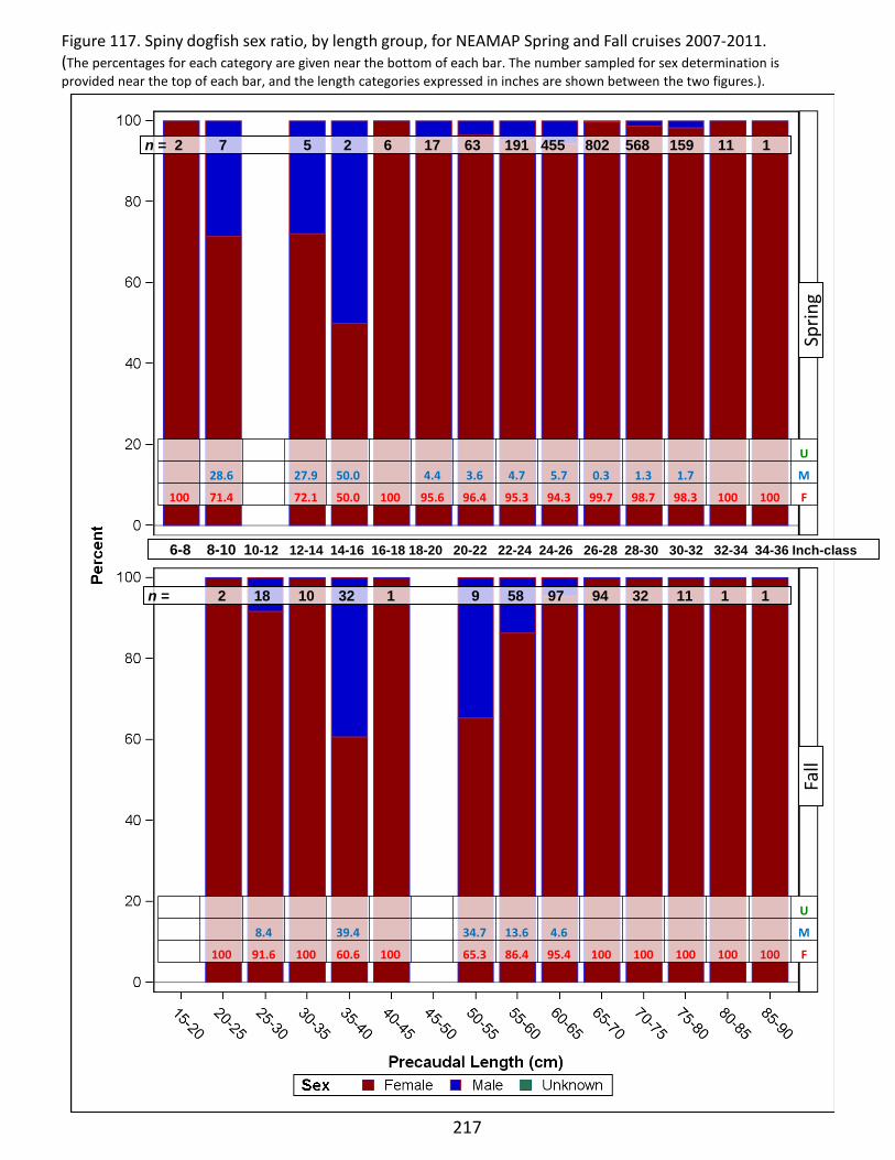
217

Figure 117. Spiny dogfish sex ratio, by length group, for NEAMAP Spring and Fall cruises 2007-2011. (The percentages for each category are given near the bottom of each bar. The number sampled for sex determination is provided near the top of each bar, and the length categories expressed in inches are shown between the two figures.).

n = 2 7 5 2 6 17 63 191 455 802 568 159 11 1

n = 2 18 10 32 1 9 58 97 94 32 11 1 1

Sprin

g F

all

6-8 8-10 10-12 12-14 14-16 16-18 18-20 20-22 22-24 24-26 26-28 28-30 30-32 32-34 34-36 Inch-class

U

28.6 27.9 50.0 4.4 3.6 4.7 5.7 0.3 1.3 1.7 M

100 71.4 72.1 50.0 100 95.6 96.4 95.3 94.3 99.7 98.7 98.3 100 100 F

U

8.4 39.4 34.7 13.6 4.6 M

100 91.6 100 60.6 100 65.3 86.4 95.4 100 100 100 100 100 F

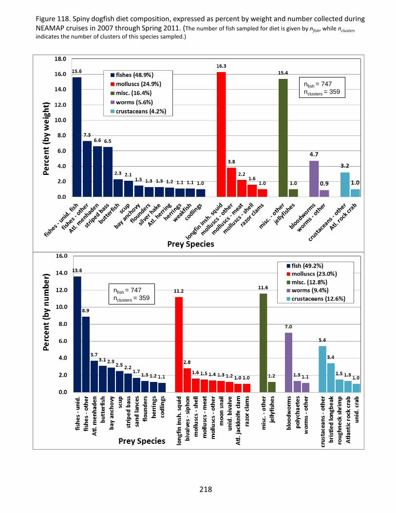
nfish = 747 nclusters = 359

nfish = 747 nclusters = 359

218

Figure 118. Spiny dogfish diet composition, expressed as percent by weight and number collected during NEAMAP cruises in 2007 through Spring 2011. (The number of fish sampled for diet is given by nfish, while nclusters indicates the number of clusters of this species sampled.)

Figure 119. Spiny dogfish reproductive data; A – frequency histogram of number of embryos found in females, B – frequency histogram of embryo stages, C – length-frequency histogram of embryos.

B

A

C

219

(cm)

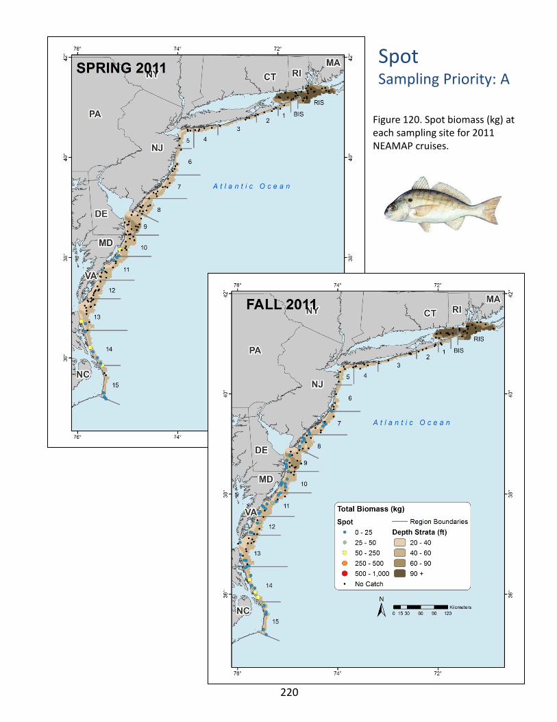
Spot Sampling Priority: A

Figure 120. Spot biomass (kg) at each sampling site for 2011 NEAMAP cruises.

220

Table 71. Spot sampling rates and preserved specimen analysis status for each NEAMAP cruise.

Table 72. Strata used for calculation of abundance indices for spot.

Table 73. Spot preliminary geometric mean indices of abundance, by number and biomass, for spring and fall NEAMAP surveys, for all specimens captured.

221

Season YearNumber Caught

Biomass Caught (kg)

Number Measured

Age Specimens

Ages Read

Stomach Specimens

Stomachs Analyzed

Spring 2008 28,561 1059.2 1,220 61 0 N/A N/A2009 29,643 824.9 3,454 59 0 N/A N/A2010 19,664 822.1 894 44 0 N/A N/A2011 15,390 557.0 2,416 52 0 N/A N/A

Fall 2007 44,437 3942.0 2,507 160 0 N/A N/A2008 56,878 3872.0 3,435 213 0 N/A N/A2009 8,428 593.0 2,699 169 0 N/A N/A2010 95,990 5060.0 6,861 181 0 N/A N/A2011 6,407 538.3 1,394 147 0 N/A N/A

Season Year Agen LCI Index UCI CV (%) n LCI Index UCI CV (%)

Spring 2008 All 31 8.25 19.62 44.98 13.2 31 1.59 3.06 5.35 16.02009 31 7.43 25.09 79.79 17.3 31 1.27 3.39 7.51 22.42010 29 1.14 3.98 10.56 26.2 29 0.13 0.99 2.50 41.12011 29 2.67 7.56 18.97 19.7 29 0.59 1.57 3.14 25.3

Fall 2007 All 87 8.19 14.66 25.68 9.7 87 2.42 3.92 6.09 11.42008 87 26.14 49.17 91.74 7.8 87 5.09 8.09 12.56 9.12009 91 4.06 5.93 8.49 8.1 91 0.77 1.13 1.57 12.42010 87 9.05 17.07 31.49 10.1 87 2.08 3.44 5.38 12.22011 87 3.09 4.70 6.95 9.5 87 0.80 1.17 1.61 12.1

Numerical Index Biomass Index

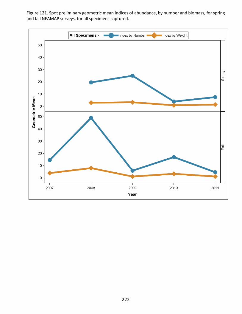
222

Figure 121. Spot preliminary geometric mean indices of abundance, by number and biomass, for spring and fall NEAMAP surveys, for all specimens captured.

Figure 122. Spot length-frequency distributions, by cruise.

223

Spring Fall

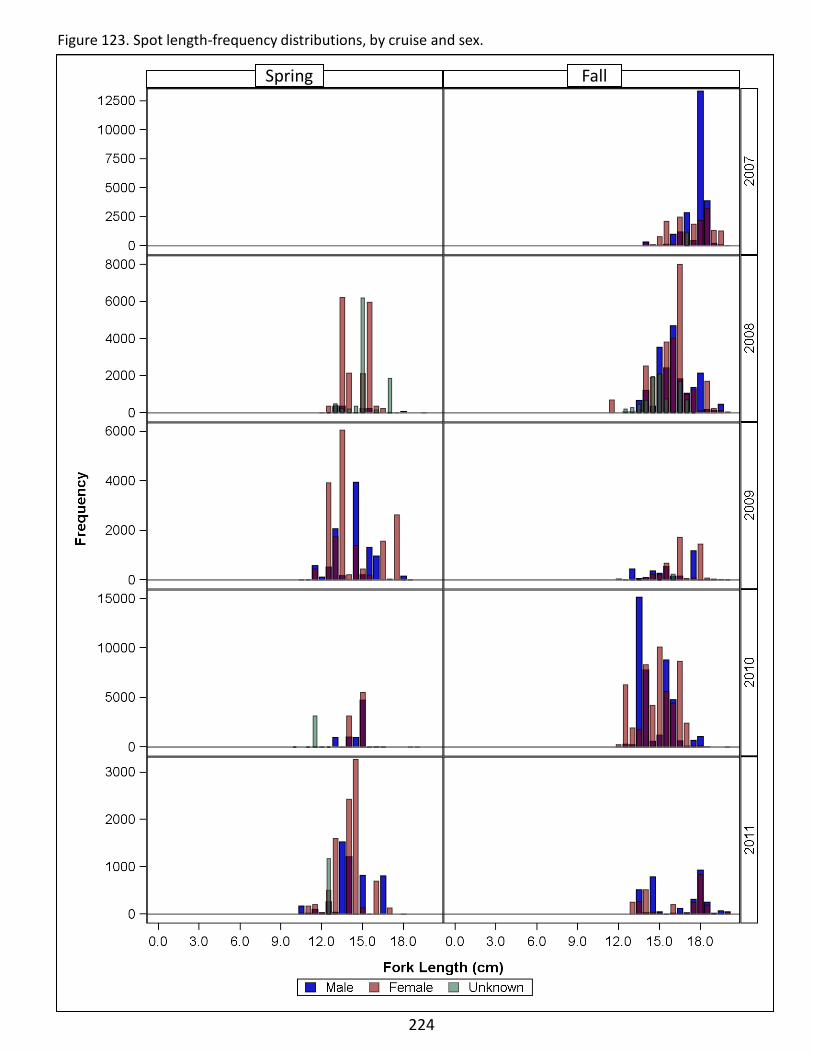
224

Figure 123. Spot length-frequency distributions, by cruise and sex.

Spring Fall

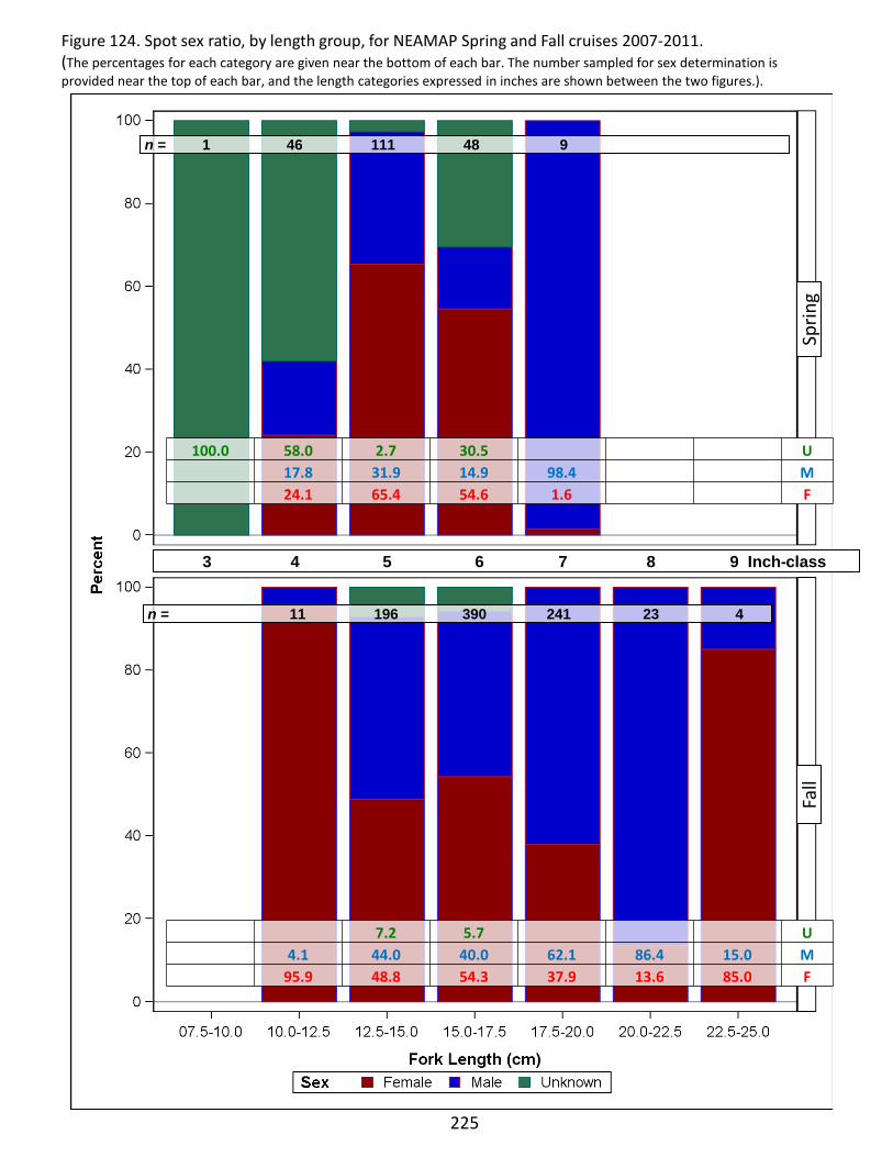
225

Figure 124. Spot sex ratio, by length group, for NEAMAP Spring and Fall cruises 2007-2011. (The percentages for each category are given near the bottom of each bar. The number sampled for sex determination is provided near the top of each bar, and the length categories expressed in inches are shown between the two figures.).

n = 1 46 111 48 9

n = 11 196 390 241 23 4

Sprin

g F

all

3 4 5 6 7 8 9 Inch-class

100.0 58.0 2.7 30.5 U 17.8 31.9 14.9 98.4 M 24.1 65.4 54.6 1.6 F

7.2 5.7 U 4.1 44.0 40.0 62.1 86.4 15.0 M 95.9 48.8 54.3 37.9 13.6 85.0 F

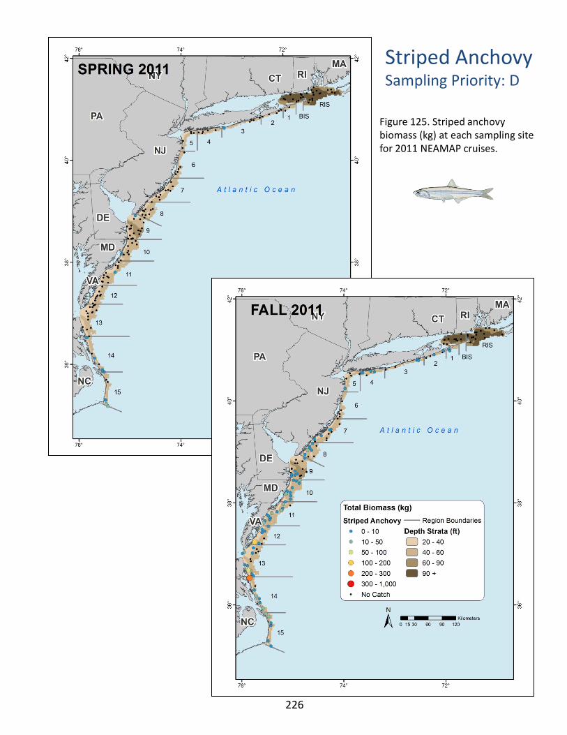
Striped Anchovy Sampling Priority: D

Figure 125. Striped anchovy biomass (kg) at each sampling site for 2011 NEAMAP cruises.

226

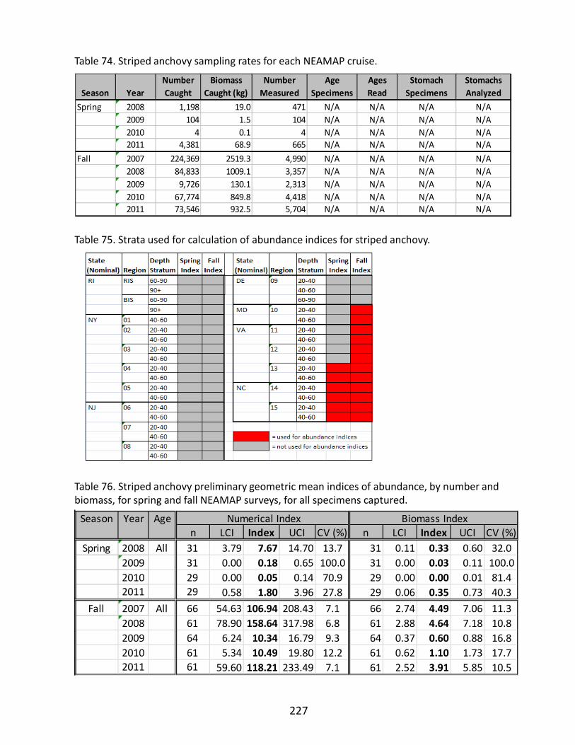
Table 75. Strata used for calculation of abundance indices for striped anchovy.

Table 76. Striped anchovy preliminary geometric mean indices of abundance, by number and biomass, for spring and fall NEAMAP surveys, for all specimens captured.

Table 74. Striped anchovy sampling rates for each NEAMAP cruise.

227

Season YearNumber Caught

Biomass Caught (kg)

Number Measured

Age Specimens

Ages Read

Stomach Specimens

Stomachs Analyzed

Spring 2008 1,198 19.0 471 N/A N/A N/A N/A2009 104 1.5 104 N/A N/A N/A N/A2010 4 0.1 4 N/A N/A N/A N/A2011 4,381 68.9 665 N/A N/A N/A N/A

Fall 2007 224,369 2519.3 4,990 N/A N/A N/A N/A2008 84,833 1009.1 3,357 N/A N/A N/A N/A2009 9,726 130.1 2,313 N/A N/A N/A N/A2010 67,774 849.8 4,418 N/A N/A N/A N/A2011 73,546 932.5 5,704 N/A N/A N/A N/A

Season Year Agen LCI Index UCI CV (%) n LCI Index UCI CV (%)

Spring 2008 All 31 3.79 7.67 14.70 13.7 31 0.11 0.33 0.60 32.02009 31 0.00 0.18 0.65 100.0 31 0.00 0.03 0.11 100.02010 29 0.00 0.05 0.14 70.9 29 0.00 0.00 0.01 81.42011 29 0.58 1.80 3.96 27.8 29 0.06 0.35 0.73 40.3

Fall 2007 All 66 54.63 106.94 208.43 7.1 66 2.74 4.49 7.06 11.32008 61 78.90 158.64 317.98 6.8 61 2.88 4.64 7.18 10.82009 64 6.24 10.34 16.79 9.3 64 0.37 0.60 0.88 16.82010 61 5.34 10.49 19.80 12.2 61 0.62 1.10 1.73 17.72011 61 59.60 118.21 233.49 7.1 61 2.52 3.91 5.85 10.5

Numerical Index Biomass Index

228

Figure 126. Striped anchovy preliminary geometric mean indices of abundance, by number and biomass, for spring and fall NEAMAP surveys, for all specimens captured.

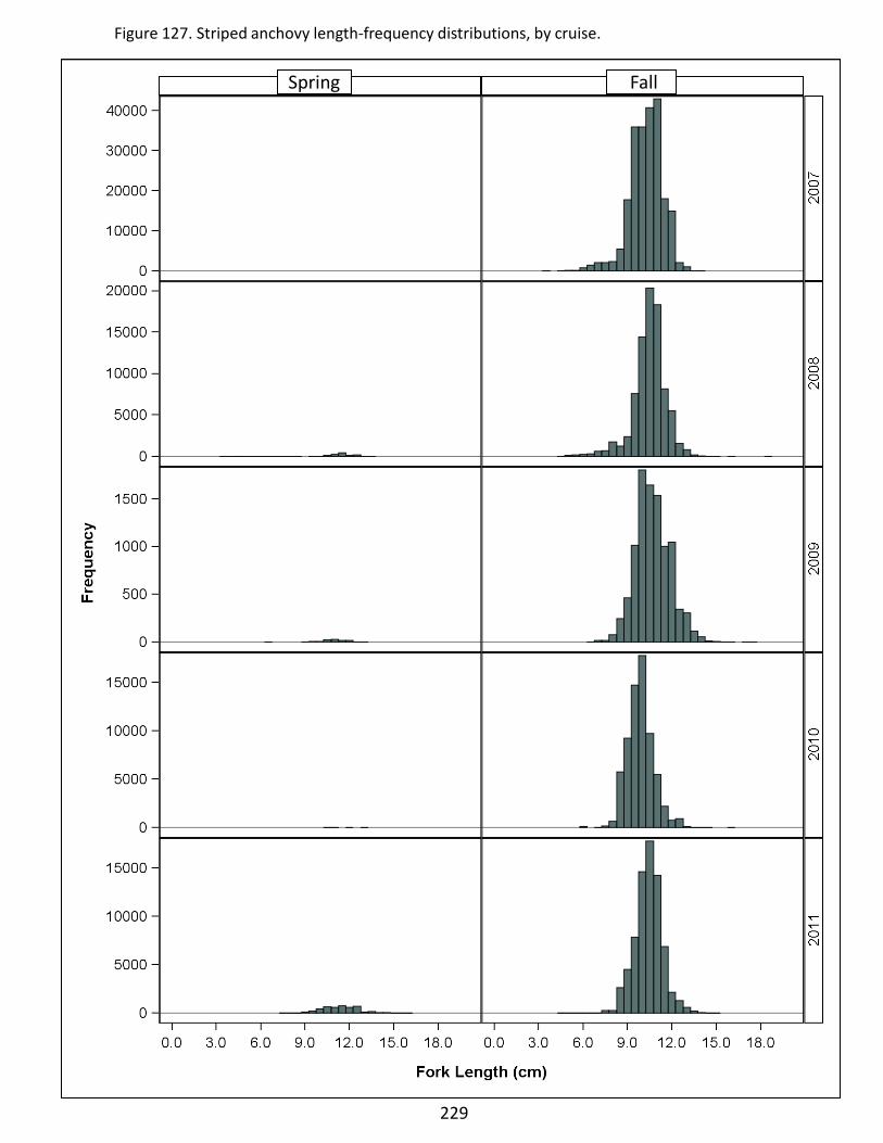
Figure 127. Striped anchovy length-frequency distributions, by cruise.

229

Spring Fall

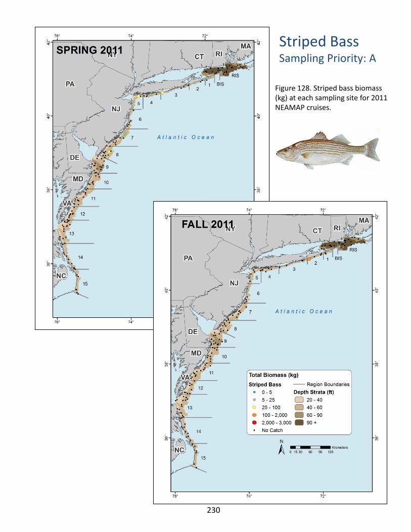
Striped Bass Sampling Priority: A

Figure 128. Striped bass biomass (kg) at each sampling site for 2011 NEAMAP cruises.

230

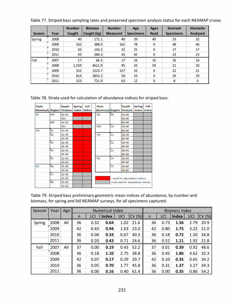
Table 78. Strata used for calculation of abundance indices for striped bass.

Table 79. Striped bass preliminary geometric mean indices of abundance, by number and biomass, for spring and fall NEAMAP surveys, for all specimens captured.

Table 77. Striped bass sampling rates and preserved specimen analysis status for each NEAMAP cruise.

231

Season YearNumber Caught

Biomass Caught (kg)

Number Measured

Age Specimens

Ages Read

Stomach Specimens

Stomachs Analyzed

Spring 2008 40 171.1 40 39 40 33 322009 162 388.9 162 78 0 48 462010 32 143.2 32 25 0 17 172011 43 284.3 43 42 0 23 23

Fall 2007 17 66.3 17 16 16 16 162008 1,559 4611.9 95 43 59 21 202009 352 1523.7 127 32 0 22 212010 814 2853.2 59 33 0 29 292011 153 721.9 63 12 0 8 0

Season Year Agen LCI Index UCI CV (%) n LCI Index UCI CV (%)

Spring 2008 All 36 0.32 0.64 1.02 21.6 36 0.73 1.56 2.79 20.92009 42 0.43 0.94 1.63 23.0 42 0.80 1.75 3.22 21.02010 36 0.06 0.33 0.67 40.3 36 0.18 0.72 1.50 34.82011 36 0.20 0.43 0.71 24.6 36 0.52 1.11 1.92 21.8

Fall 2007 All 37 0.00 0.19 0.43 52.2 37 0.01 0.39 0.92 48.62008 36 0.18 1.10 2.75 38.8 36 0.45 1.86 4.62 32.32009 42 0.07 0.17 0.29 29.7 42 0.10 0.35 0.65 34.22010 36 0.05 0.70 1.77 45.8 36 0.31 1.37 3.27 34.32011 36 0.00 0.16 0.40 61.4 36 0.00 0.35 0.86 54.2

Numerical Index Biomass Index

232

Figure 129. Striped bass preliminary geometric mean indices of abundance, by number and biomass, for spring and fall NEAMAP surveys, for all specimens captured.

Figure 130. Striped bass length-frequency distributions, by cruise.

233

Spring Fall

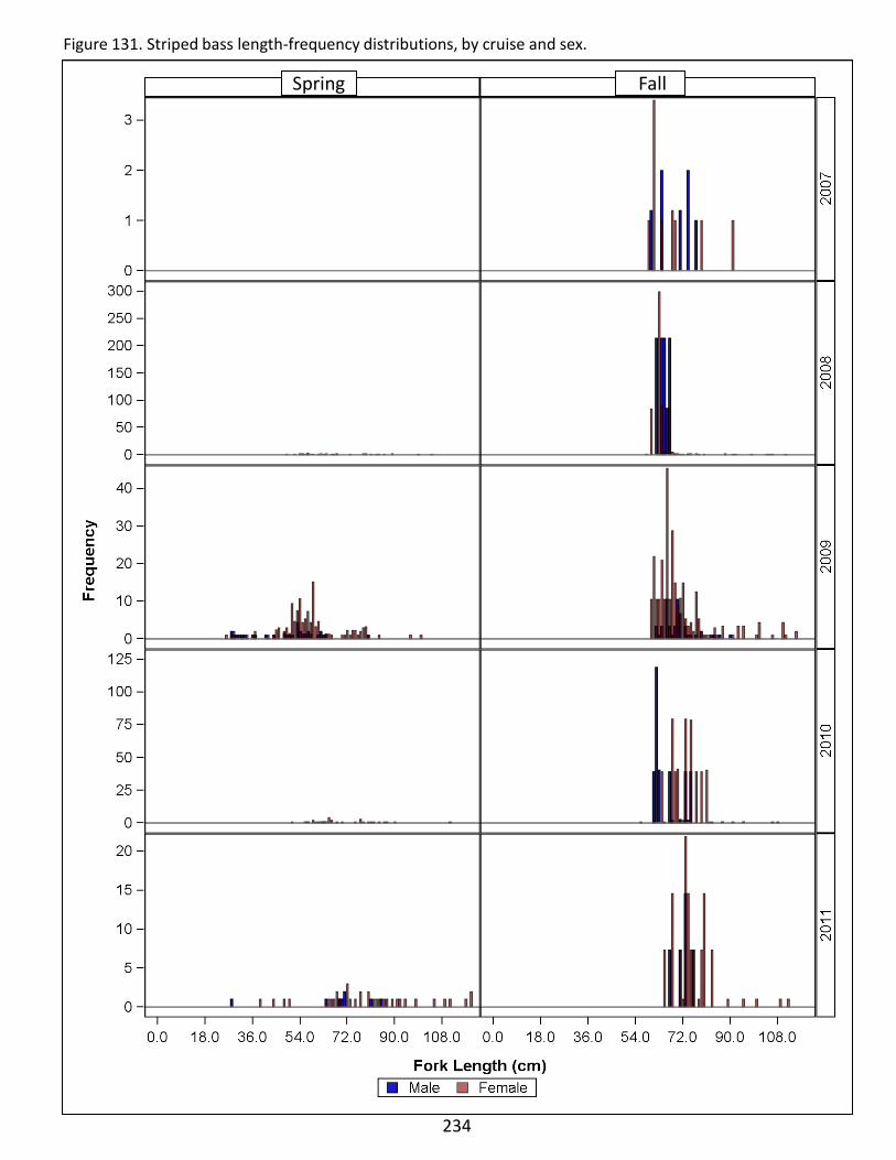
Figure 131. Striped bass length-frequency distributions, by cruise and sex.

Spring Fall

234

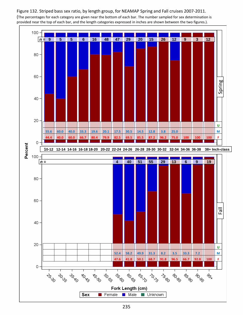
235

Figure 132. Striped bass sex ratio, by length group, for NEAMAP Spring and Fall cruises 2007-2011. (The percentages for each category are given near the bottom of each bar. The number sampled for sex determination is provided near the top of each bar, and the length categories expressed in inches are shown between the two figures.).

n = 9 5 5 6 16 48 47 29 20 15 26 12 9 3 12

n = 4 40 51 55 29 13 6 9 19

Sprin

g F

all

10-12 12-14 14-16 16-18 18-20 20-22 22-24 24-26 26-28 28-30 30-32 32-34 34-36 36-38 38+ Inch-class

U

55.6 60.0 40.0 33.3 19.6 20.1 17.5 30.5 14.5 12.8 3.8 25.0 M

44.4 40.0 60.0 66.7 80.4 79.9 82.5 69.5 85.5 87.2 96.2 75.0 100 100 100 F

U

52.4 58.2 49.9 31.3 8.2 3.5 33.3 7.2 M

47.6 41.8 50.1 68.7 91.8 96.5 66.7 92.8 100 F

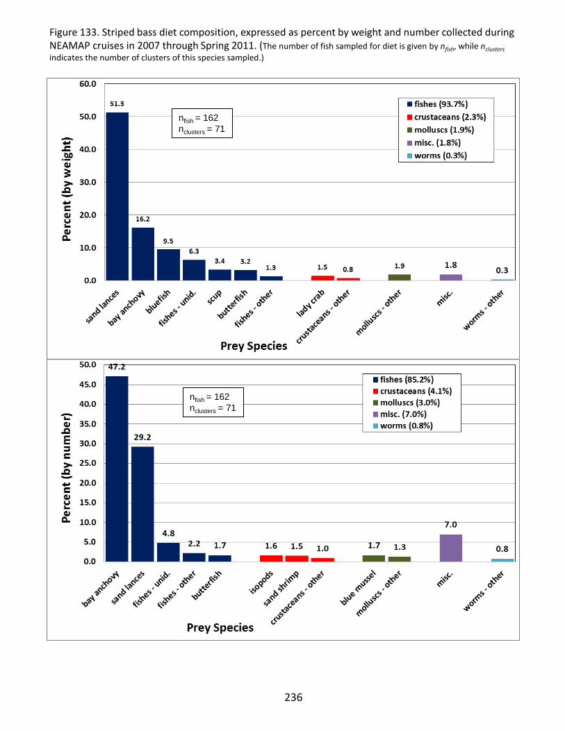
nfish = 162 nclusters = 71

nfish = 162 nclusters = 71

236

Figure 133. Striped bass diet composition, expressed as percent by weight and number collected during NEAMAP cruises in 2007 through Spring 2011. (The number of fish sampled for diet is given by nfish, while nclusters indicates the number of clusters of this species sampled.)

Summer Flounder Sampling Priority: A

Figure 134. Summer flounder biomass (kg) at each sampling site for 2011 NEAMAP cruises.

237

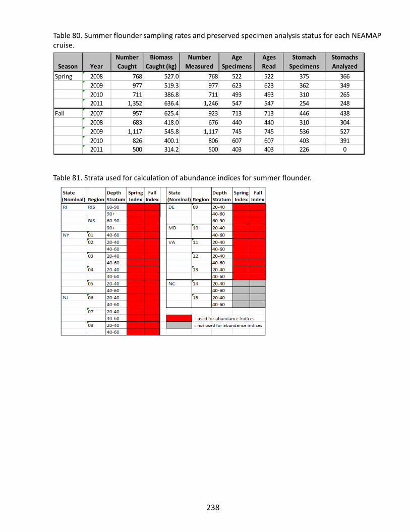
Table 81. Strata used for calculation of abundance indices for summer flounder.

Table 80. Summer flounder sampling rates and preserved specimen analysis status for each NEAMAP cruise.

238

Season YearNumber Caught

Biomass Caught (kg)

Number Measured

Age Specimens

Ages Read

Stomach Specimens

Stomachs Analyzed

Spring 2008 768 527.0 768 522 522 375 3662009 977 519.3 977 623 623 362 3492010 711 386.8 711 493 493 310 2652011 1,352 636.4 1,246 547 547 254 248

Fall 2007 957 625.4 923 713 713 446 4382008 683 418.0 676 440 440 310 3042009 1,117 545.8 1,117 745 745 536 5272010 826 400.1 806 607 607 403 3912011 500 314.2 500 403 403 226 0

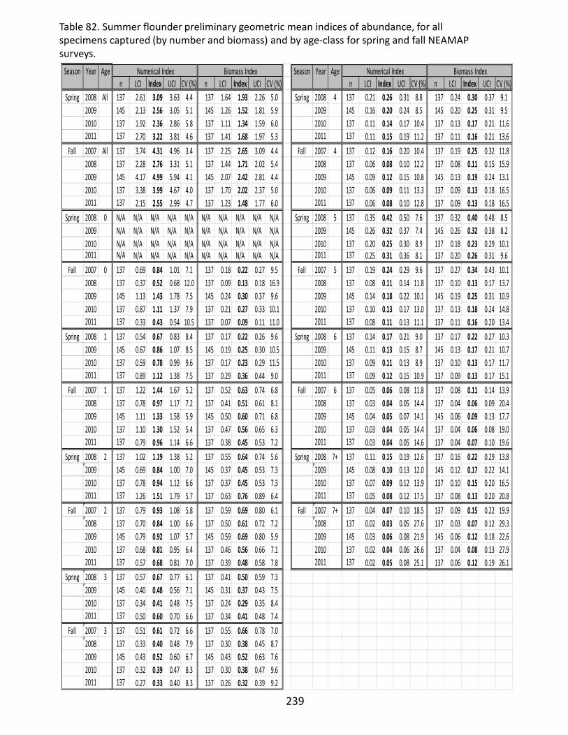
Table 82. Summer flounder preliminary geometric mean indices of abundance, for all specimens captured (by number and biomass) and by age-class for spring and fall NEAMAP surveys.

239

Season Year Age Season Year Agen LCI Index UCI CV (%) n LCI Index UCI CV (%) n LCI Index UCI CV (%) n LCI Index UCI CV (%)

Spring 2008 All 137 2.61 3.09 3.63 4.4 137 1.64 1.93 2.26 5.0 Spring 2008 4 137 0.21 0.26 0.31 8.8 137 0.24 0.30 0.37 9.12009 145 2.13 2.56 3.05 5.1 145 1.26 1.52 1.81 5.9 2009 145 0.16 0.20 0.24 8.5 145 0.20 0.25 0.31 9.52010 137 1.92 2.36 2.86 5.8 137 1.11 1.34 1.59 6.0 2010 137 0.11 0.14 0.17 10.4 137 0.13 0.17 0.21 11.62011 137 2.70 3.22 3.81 4.6 137 1.41 1.68 1.97 5.3 2011 137 0.11 0.15 0.19 11.2 137 0.11 0.16 0.21 13.6

Fall 2007 All 137 3.74 4.31 4.96 3.4 137 2.25 2.65 3.09 4.4 Fall 2007 4 137 0.12 0.16 0.20 10.4 137 0.19 0.25 0.32 11.82008 137 2.28 2.76 3.31 5.1 137 1.44 1.71 2.02 5.4 2008 137 0.06 0.08 0.10 12.2 137 0.08 0.11 0.15 15.92009 145 4.17 4.99 5.94 4.1 145 2.07 2.42 2.81 4.4 2009 145 0.09 0.12 0.15 10.8 145 0.13 0.19 0.24 13.12010 137 3.38 3.99 4.67 4.0 137 1.70 2.02 2.37 5.0 2010 137 0.06 0.09 0.11 13.3 137 0.09 0.13 0.18 16.52011 137 2.15 2.55 2.99 4.7 137 1.23 1.48 1.77 6.0 2011 137 0.06 0.08 0.10 12.8 137 0.09 0.13 0.18 16.5

Spring 2008 0 N/A N/A N/A N/A N/A N/A N/A N/A N/A N/A Spring 2008 5 137 0.35 0.42 0.50 7.6 137 0.32 0.40 0.48 8.52009 N/A N/A N/A N/A N/A N/A N/A N/A N/A N/A 2009 145 0.26 0.32 0.37 7.4 145 0.26 0.32 0.38 8.22010 N/A N/A N/A N/A N/A N/A N/A N/A N/A N/A 2010 137 0.20 0.25 0.30 8.9 137 0.18 0.23 0.29 10.12011 N/A N/A N/A N/A N/A N/A N/A N/A N/A N/A 2011 137 0.25 0.31 0.36 8.1 137 0.20 0.26 0.31 9.6

Fall 2007 0 137 0.69 0.84 1.01 7.1 137 0.18 0.22 0.27 9.5 Fall 2007 5 137 0.19 0.24 0.29 9.6 137 0.27 0.34 0.43 10.12008 137 0.37 0.52 0.68 12.0 137 0.09 0.13 0.18 16.9 2008 137 0.08 0.11 0.14 11.8 137 0.10 0.13 0.17 13.72009 145 1.13 1.43 1.78 7.5 145 0.24 0.30 0.37 9.6 2009 145 0.14 0.18 0.22 10.1 145 0.19 0.25 0.31 10.92010 137 0.87 1.11 1.37 7.9 137 0.21 0.27 0.33 10.1 2010 137 0.10 0.13 0.17 13.0 137 0.13 0.18 0.24 14.82011 137 0.33 0.43 0.54 10.5 137 0.07 0.09 0.11 11.0 2011 137 0.08 0.11 0.13 11.1 137 0.11 0.16 0.20 13.4

Spring 2008 1 137 0.54 0.67 0.83 8.4 137 0.17 0.22 0.26 9.6 Spring 2008 6 137 0.14 0.17 0.21 9.0 137 0.17 0.22 0.27 10.32009 145 0.67 0.86 1.07 8.5 145 0.19 0.25 0.30 10.5 2009 145 0.11 0.13 0.15 8.7 145 0.13 0.17 0.21 10.72010 137 0.59 0.78 0.99 9.6 137 0.17 0.23 0.29 11.5 2010 137 0.09 0.11 0.13 8.9 137 0.10 0.13 0.17 11.72011 137 0.89 1.12 1.38 7.5 137 0.29 0.36 0.44 9.0 2011 137 0.09 0.12 0.15 10.9 137 0.09 0.13 0.17 15.1

Fall 2007 1 137 1.22 1.44 1.67 5.2 137 0.52 0.63 0.74 6.8 Fall 2007 6 137 0.05 0.06 0.08 11.8 137 0.08 0.11 0.14 13.92008 137 0.78 0.97 1.17 7.2 137 0.41 0.51 0.61 8.1 2008 137 0.03 0.04 0.05 14.4 137 0.04 0.06 0.09 20.42009 145 1.11 1.33 1.58 5.9 145 0.50 0.60 0.71 6.8 2009 145 0.04 0.05 0.07 14.1 145 0.06 0.09 0.13 17.72010 137 1.10 1.30 1.52 5.4 137 0.47 0.56 0.65 6.3 2010 137 0.03 0.04 0.05 14.4 137 0.04 0.06 0.08 19.02011 137 0.79 0.96 1.14 6.6 137 0.38 0.45 0.53 7.2 2011 137 0.03 0.04 0.05 14.6 137 0.04 0.07 0.10 19.6

Spring 2008 2 137 1.02 1.19 1.38 5.2 137 0.55 0.64 0.74 5.6 Spring 2008 7+ 137 0.11 0.15 0.19 12.6 137 0.16 0.22 0.29 13.82009 145 0.69 0.84 1.00 7.0 145 0.37 0.45 0.53 7.3 2009 145 0.08 0.10 0.13 12.0 145 0.12 0.17 0.22 14.12010 137 0.78 0.94 1.12 6.6 137 0.37 0.45 0.53 7.3 2010 137 0.07 0.09 0.12 13.9 137 0.10 0.15 0.20 16.52011 137 1.26 1.51 1.79 5.7 137 0.63 0.76 0.89 6.4 2011 137 0.05 0.08 0.12 17.5 137 0.08 0.13 0.20 20.8

Fall 2007 2 137 0.79 0.93 1.08 5.8 137 0.59 0.69 0.80 6.1 Fall 2007 7+ 137 0.04 0.07 0.10 18.5 137 0.09 0.15 0.22 19.92008 137 0.70 0.84 1.00 6.6 137 0.50 0.61 0.72 7.2 2008 137 0.02 0.03 0.05 27.6 137 0.03 0.07 0.12 29.32009 145 0.79 0.92 1.07 5.7 145 0.59 0.69 0.80 5.9 2009 145 0.03 0.06 0.08 21.9 145 0.06 0.12 0.18 22.62010 137 0.68 0.81 0.95 6.4 137 0.46 0.56 0.66 7.1 2010 137 0.02 0.04 0.06 26.6 137 0.04 0.08 0.13 27.92011 137 0.57 0.68 0.81 7.0 137 0.39 0.48 0.58 7.8 2011 137 0.02 0.05 0.08 25.1 137 0.06 0.12 0.19 26.1

Spring 2008 3 137 0.57 0.67 0.77 6.1 137 0.41 0.50 0.59 7.32009 145 0.40 0.48 0.56 7.1 145 0.31 0.37 0.43 7.52010 137 0.34 0.41 0.48 7.5 137 0.24 0.29 0.35 8.42011 137 0.50 0.60 0.70 6.6 137 0.34 0.41 0.48 7.4

Fall 2007 3 137 0.51 0.61 0.72 6.6 137 0.55 0.66 0.78 7.02008 137 0.33 0.40 0.48 7.9 137 0.30 0.38 0.45 8.72009 145 0.43 0.52 0.60 6.7 145 0.43 0.52 0.63 7.62010 137 0.32 0.39 0.47 8.3 137 0.30 0.38 0.47 9.62011 137 0.27 0.33 0.40 8.3 137 0.26 0.32 0.39 9.2

Numerical Index Biomass Index Numerical Index Biomass Index

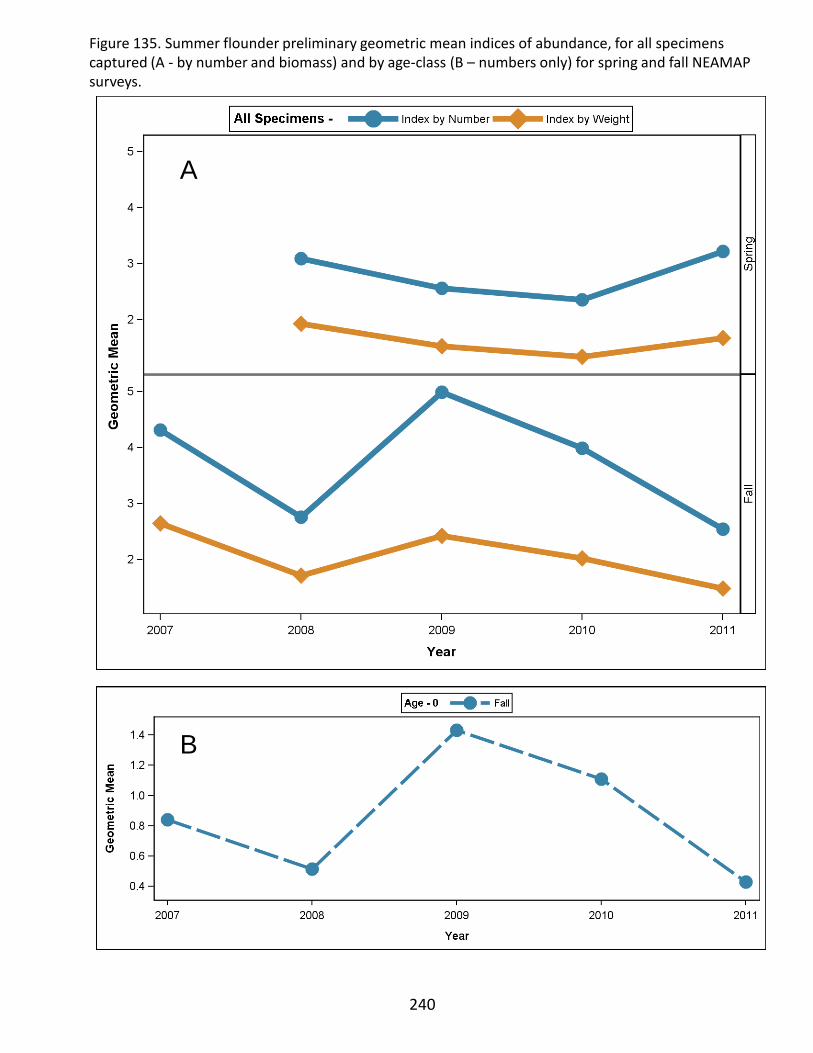
240

Figure 135. Summer flounder preliminary geometric mean indices of abundance, for all specimens captured (A - by number and biomass) and by age-class (B – numbers only) for spring and fall NEAMAP surveys.

B

A

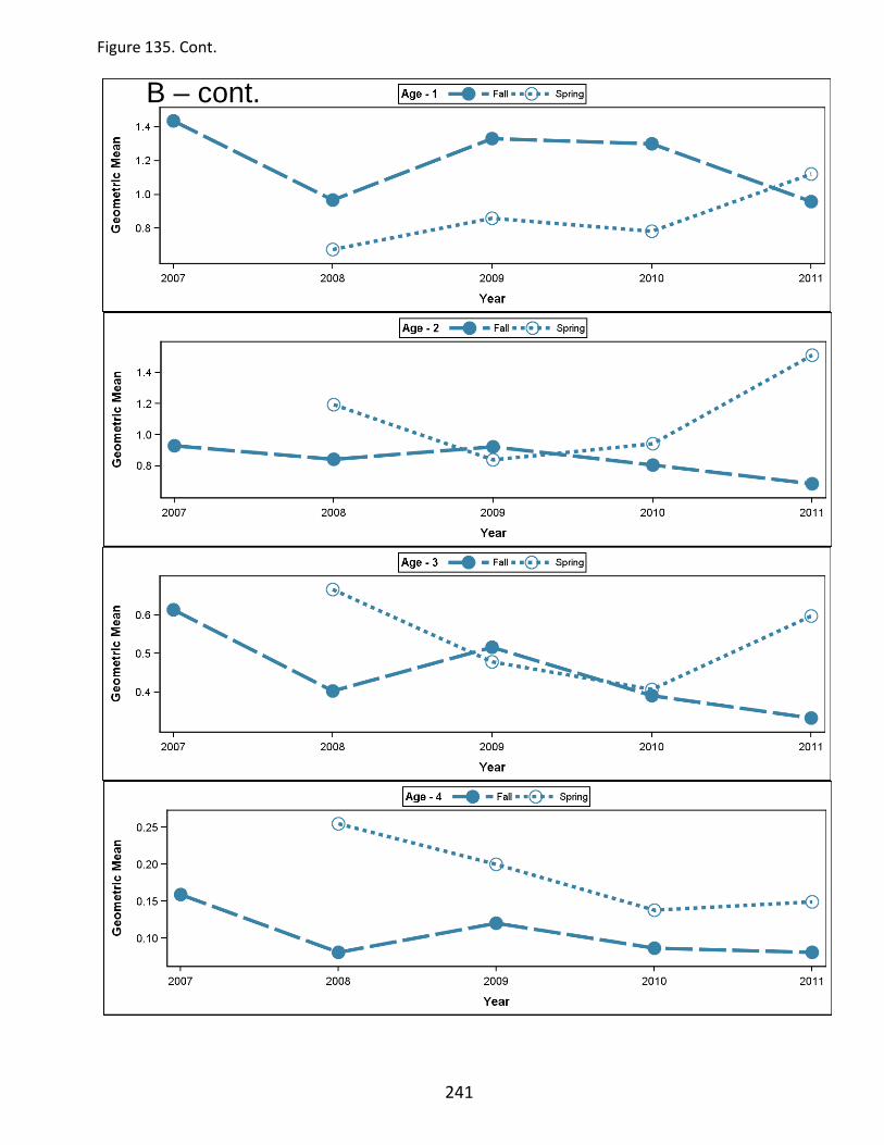
241

B – cont.

Figure 135. Cont.

B – cont.

Figure 135. Cont.

242

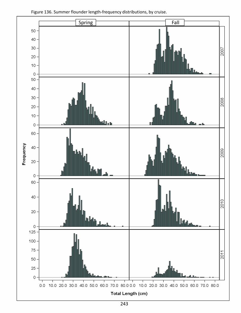
Figure 136. Summer flounder length-frequency distributions, by cruise.

243

Spring Fall

244

Figure 137. Summer flounder length-frequency distributions, by cruise and sex.

Spring Fall

Figure 138. Summer flounder age-frequency distribution, by cruise. The estimated total number collected at a given age is provided above each corresponding bar.

245

Figure 139. Summer flounder age-at-length proportions for all spring vs. all fall cruises combined, showing actual and loess smoothed proportions at each 1cm length bin.

246

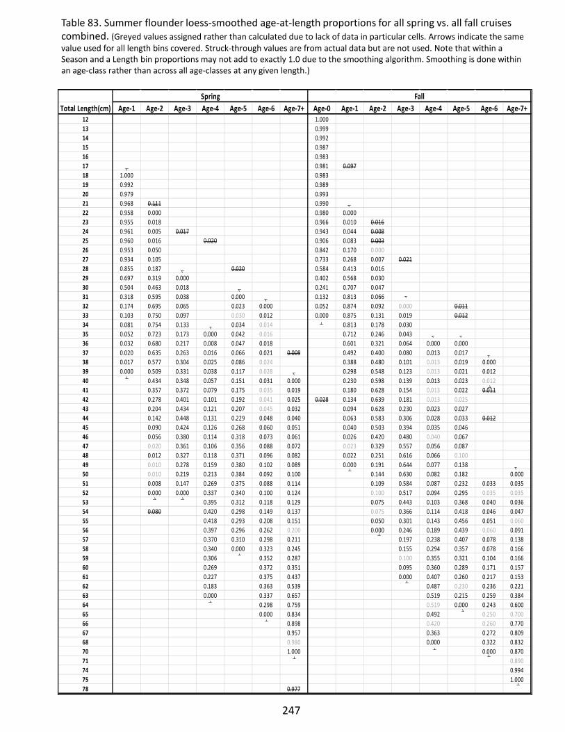
Table 83. Summer flounder loess-smoothed age-at-length proportions for all spring vs. all fall cruises combined. (Greyed values assigned rather than calculated due to lack of data in particular cells. Arrows indicate the same value used for all length bins covered. Struck-through values are from actual data but are not used. Note that within a Season and a Length bin proportions may not add to exactly 1.0 due to the smoothing algorithm. Smoothing is done within an age-class rather than across all age-classes at any given length.)

247

Total Length(cm) Age-1 Age-2 Age-3 Age-4 Age-5 Age-6 Age-7+ Age-0 Age-1 Age-2 Age-3 Age-4 Age-5 Age-6 Age-7+12 1.00013 0.99914 0.99215 0.98716 0.98317 0.981 0.09718 1.000 0.98319 0.992 0.98920 0.979 0.99321 0.968 0.111 0.99022 0.958 0.000 0.980 0.00023 0.955 0.018 0.966 0.010 0.01624 0.961 0.005 0.017 0.943 0.044 0.00825 0.960 0.016 0.020 0.906 0.083 0.00326 0.953 0.050 0.842 0.170 0.00027 0.934 0.105 0.733 0.268 0.007 0.02128 0.855 0.187 0.020 0.584 0.413 0.01629 0.697 0.319 0.000 0.402 0.568 0.03030 0.504 0.463 0.018 0.241 0.707 0.04731 0.318 0.595 0.038 0.000 0.132 0.813 0.06632 0.174 0.695 0.065 0.023 0.000 0.052 0.874 0.092 0.000 0.01133 0.103 0.750 0.097 0.030 0.012 0.000 0.875 0.131 0.019 0.01234 0.081 0.754 0.133 0.034 0.014 0.813 0.178 0.03035 0.052 0.723 0.173 0.000 0.042 0.016 0.712 0.246 0.04336 0.032 0.680 0.217 0.008 0.047 0.018 0.601 0.321 0.064 0.000 0.00037 0.020 0.635 0.263 0.016 0.066 0.021 0.009 0.492 0.400 0.080 0.013 0.01738 0.017 0.577 0.304 0.025 0.086 0.024 0.388 0.480 0.101 0.013 0.019 0.00039 0.000 0.509 0.331 0.038 0.117 0.028 0.298 0.548 0.123 0.013 0.021 0.01240 0.434 0.348 0.057 0.151 0.031 0.000 0.230 0.598 0.139 0.013 0.023 0.01241 0.357 0.372 0.079 0.175 0.035 0.019 0.180 0.628 0.154 0.013 0.022 0.01142 0.278 0.401 0.101 0.192 0.041 0.025 0.028 0.134 0.639 0.181 0.013 0.02543 0.204 0.434 0.121 0.207 0.045 0.032 0.094 0.628 0.230 0.023 0.02744 0.142 0.448 0.131 0.229 0.048 0.040 0.063 0.583 0.306 0.028 0.033 0.01245 0.090 0.424 0.126 0.268 0.060 0.051 0.040 0.503 0.394 0.035 0.04646 0.056 0.380 0.114 0.318 0.073 0.061 0.026 0.420 0.480 0.040 0.06747 0.020 0.361 0.106 0.356 0.088 0.072 0.023 0.329 0.557 0.056 0.08748 0.012 0.327 0.118 0.371 0.096 0.082 0.022 0.251 0.616 0.066 0.10049 0.010 0.278 0.159 0.380 0.102 0.089 0.000 0.191 0.644 0.077 0.13850 0.010 0.219 0.213 0.384 0.092 0.100 0.144 0.630 0.082 0.182 0.00051 0.008 0.147 0.269 0.375 0.088 0.114 0.109 0.584 0.087 0.232 0.033 0.03552 0.000 0.000 0.337 0.340 0.100 0.124 0.100 0.517 0.094 0.295 0.035 0.03553 0.395 0.312 0.118 0.129 0.075 0.443 0.103 0.368 0.040 0.03654 0.080 0.420 0.298 0.149 0.137 0.075 0.366 0.114 0.418 0.046 0.04755 0.418 0.293 0.208 0.151 0.050 0.301 0.143 0.456 0.051 0.06056 0.397 0.296 0.262 0.200 0.000 0.246 0.189 0.439 0.060 0.09157 0.370 0.310 0.298 0.211 0.197 0.238 0.407 0.078 0.13858 0.340 0.000 0.323 0.245 0.155 0.294 0.357 0.078 0.16659 0.306 0.352 0.287 0.100 0.355 0.321 0.104 0.16660 0.269 0.372 0.351 0.095 0.360 0.289 0.171 0.15761 0.227 0.375 0.437 0.000 0.407 0.260 0.217 0.15362 0.183 0.363 0.539 0.487 0.230 0.236 0.22163 0.000 0.337 0.657 0.519 0.215 0.259 0.38464 0.298 0.759 0.519 0.000 0.243 0.60065 0.000 0.834 0.492 0.250 0.70066 0.898 0.420 0.260 0.77067 0.957 0.363 0.272 0.80968 0.980 0.000 0.322 0.83270 1.000 0.000 0.87071 0.89074 0.99475 1.00078 0.977

Spring Fall

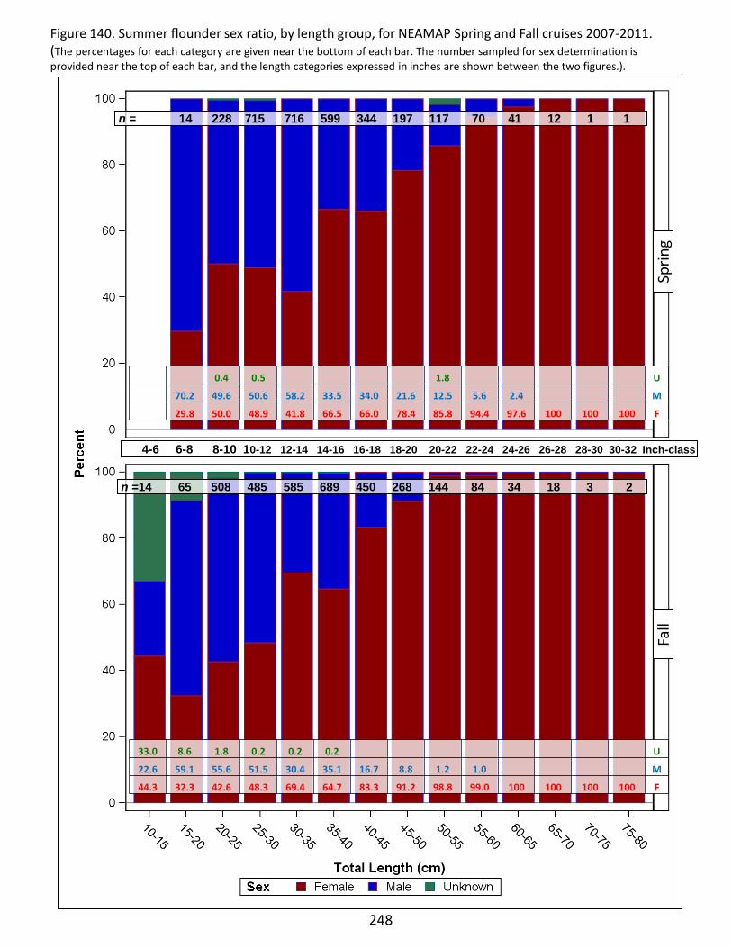
248

Figure 140. Summer flounder sex ratio, by length group, for NEAMAP Spring and Fall cruises 2007-2011. (The percentages for each category are given near the bottom of each bar. The number sampled for sex determination is provided near the top of each bar, and the length categories expressed in inches are shown between the two figures.).

n = 14 228 715 716 599 344 197 117 70 41 12 1 1

n =14 65 508 485 585 689 450 268 144 84 34 18 3 2

Sprin

g F

all

4-6 6-8 8-10 10-12 12-14 14-16 16-18 18-20 20-22 22-24 24-26 26-28 28-30 30-32 Inch-class

0.4 0.5 1.8 U

70.2 49.6 50.6 58.2 33.5 34.0 21.6 12.5 5.6 2.4 M

29.8 50.0 48.9 41.8 66.5 66.0 78.4 85.8 94.4 97.6 100 100 100 F

33.0 8.6 1.8 0.2 0.2 0.2 U

22.6 59.1 55.6 51.5 30.4 35.1 16.7 8.8 1.2 1.0 M

44.3 32.3 42.6 48.3 69.4 64.7 83.3 91.2 98.8 99.0 100 100 100 100 F

nfish = 2172 nclusters = 983

nfish = 2172 nclusters = 983

249

Figure 141. Summer flounder diet composition, expressed as percent by weight and number collected during NEAMAP cruises in 2007 through Spring 2011. (The number of fish sampled for diet is given by nfish, while nclusters indicates the number of clusters of this species sampled.)

Weakfish Sampling Priority: A

Figure 142. Weakfish biomass (kg) at each sampling site for 2011 NEAMAP cruises.

250

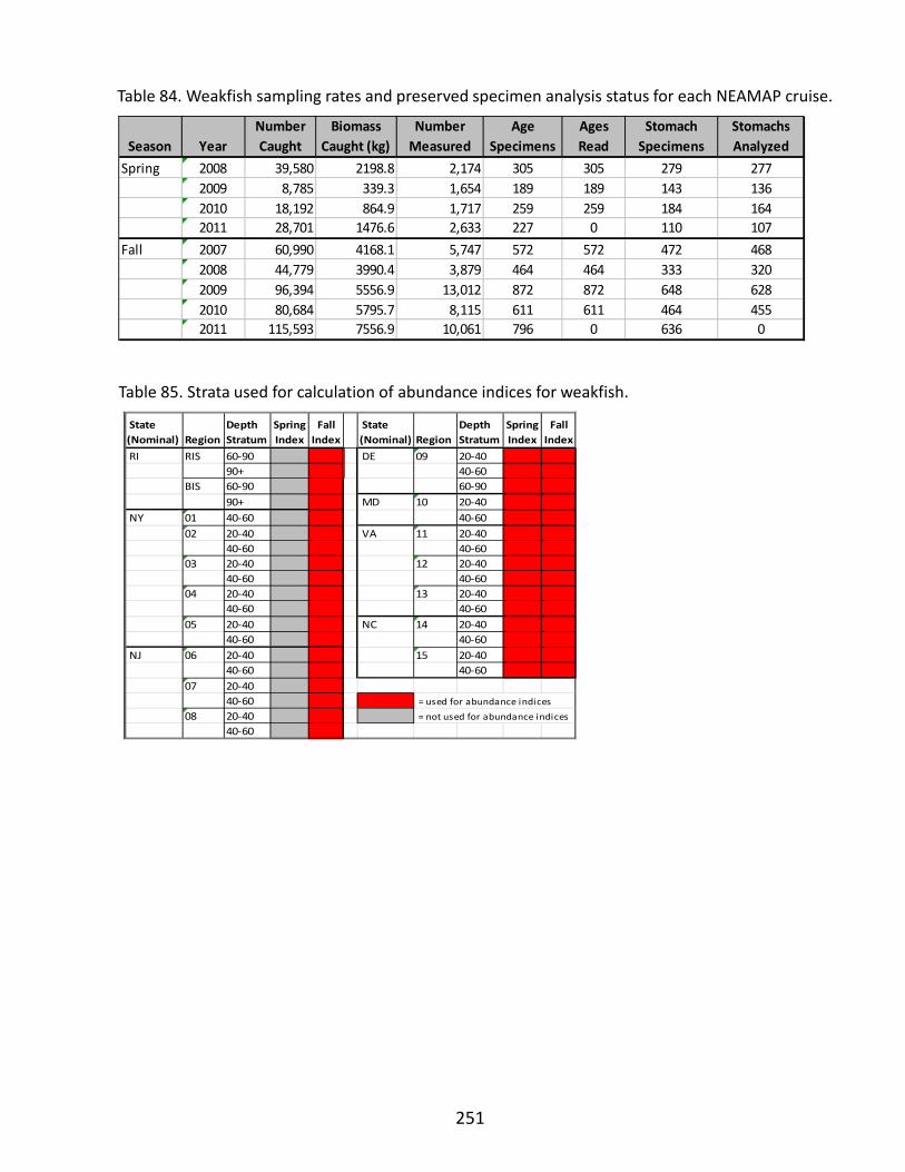
Table 85. Strata used for calculation of abundance indices for weakfish.

Table 84. Weakfish sampling rates and preserved specimen analysis status for each NEAMAP cruise.

251

Season YearNumber Caught

Biomass Caught (kg)

Number Measured

Age Specimens

Ages Read

Stomach Specimens

Stomachs Analyzed

Spring 2008 39,580 2198.8 2,174 305 305 279 2772009 8,785 339.3 1,654 189 189 143 1362010 18,192 864.9 1,717 259 259 184 1642011 28,701 1476.6 2,633 227 0 110 107

Fall 2007 60,990 4168.1 5,747 572 572 472 4682008 44,779 3990.4 3,879 464 464 333 3202009 96,394 5556.9 13,012 872 872 648 6282010 80,684 5795.7 8,115 611 611 464 4552011 115,593 7556.9 10,061 796 0 636 0

State (Nominal) Region

Depth Stratum

Spring Index

Fall Index

State (Nominal) Region

Depth Stratum

Spring Index

Fall Index

RI RIS 60-90 DE 09 20-4090+ 40-60

BIS 60-90 60-9090+ MD 10 20-40

NY 01 40-60 40-6002 20-40 VA 11 20-40

40-60 40-6003 20-40 12 20-40

40-60 40-6004 20-40 13 20-40

40-60 40-6005 20-40 NC 14 20-40

40-60 40-60 NJ 06 20-40 15 20-40

40-60 40-6007 20-40

40-60 = used for abundance indices08 20-40 = not used for abundance indices

40-60

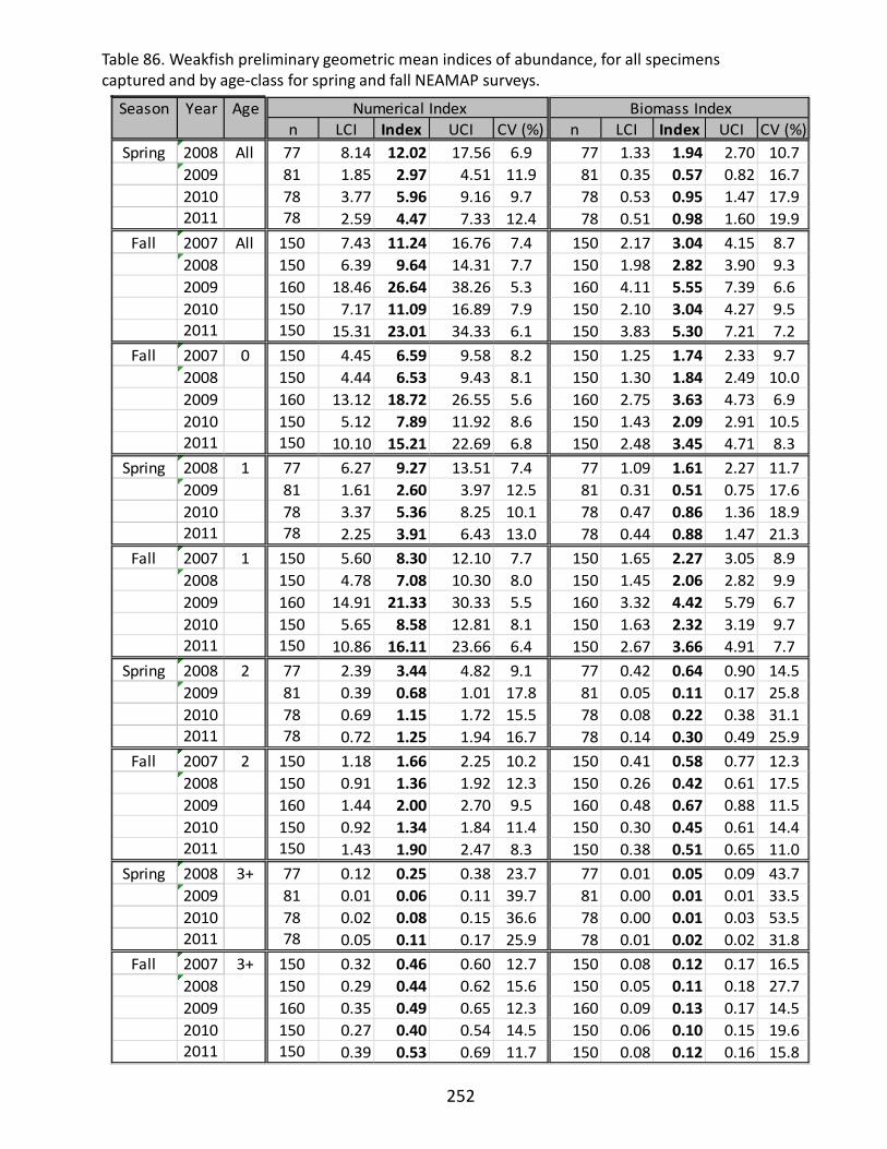
Table 86. Weakfish preliminary geometric mean indices of abundance, for all specimens captured and by age-class for spring and fall NEAMAP surveys.

252

Season Year Agen LCI Index UCI CV (%) n LCI Index UCI CV (%)

Spring 2008 All 77 8.14 12.02 17.56 6.9 77 1.33 1.94 2.70 10.72009 81 1.85 2.97 4.51 11.9 81 0.35 0.57 0.82 16.72010 78 3.77 5.96 9.16 9.7 78 0.53 0.95 1.47 17.92011 78 2.59 4.47 7.33 12.4 78 0.51 0.98 1.60 19.9

Fall 2007 All 150 7.43 11.24 16.76 7.4 150 2.17 3.04 4.15 8.72008 150 6.39 9.64 14.31 7.7 150 1.98 2.82 3.90 9.32009 160 18.46 26.64 38.26 5.3 160 4.11 5.55 7.39 6.62010 150 7.17 11.09 16.89 7.9 150 2.10 3.04 4.27 9.52011 150 15.31 23.01 34.33 6.1 150 3.83 5.30 7.21 7.2

Fall 2007 0 150 4.45 6.59 9.58 8.2 150 1.25 1.74 2.33 9.72008 150 4.44 6.53 9.43 8.1 150 1.30 1.84 2.49 10.02009 160 13.12 18.72 26.55 5.6 160 2.75 3.63 4.73 6.92010 150 5.12 7.89 11.92 8.6 150 1.43 2.09 2.91 10.52011 150 10.10 15.21 22.69 6.8 150 2.48 3.45 4.71 8.3

Spring 2008 1 77 6.27 9.27 13.51 7.4 77 1.09 1.61 2.27 11.72009 81 1.61 2.60 3.97 12.5 81 0.31 0.51 0.75 17.62010 78 3.37 5.36 8.25 10.1 78 0.47 0.86 1.36 18.92011 78 2.25 3.91 6.43 13.0 78 0.44 0.88 1.47 21.3

Fall 2007 1 150 5.60 8.30 12.10 7.7 150 1.65 2.27 3.05 8.92008 150 4.78 7.08 10.30 8.0 150 1.45 2.06 2.82 9.92009 160 14.91 21.33 30.33 5.5 160 3.32 4.42 5.79 6.72010 150 5.65 8.58 12.81 8.1 150 1.63 2.32 3.19 9.72011 150 10.86 16.11 23.66 6.4 150 2.67 3.66 4.91 7.7

Spring 2008 2 77 2.39 3.44 4.82 9.1 77 0.42 0.64 0.90 14.52009 81 0.39 0.68 1.01 17.8 81 0.05 0.11 0.17 25.82010 78 0.69 1.15 1.72 15.5 78 0.08 0.22 0.38 31.12011 78 0.72 1.25 1.94 16.7 78 0.14 0.30 0.49 25.9

Fall 2007 2 150 1.18 1.66 2.25 10.2 150 0.41 0.58 0.77 12.32008 150 0.91 1.36 1.92 12.3 150 0.26 0.42 0.61 17.52009 160 1.44 2.00 2.70 9.5 160 0.48 0.67 0.88 11.52010 150 0.92 1.34 1.84 11.4 150 0.30 0.45 0.61 14.42011 150 1.43 1.90 2.47 8.3 150 0.38 0.51 0.65 11.0

Spring 2008 3+ 77 0.12 0.25 0.38 23.7 77 0.01 0.05 0.09 43.72009 81 0.01 0.06 0.11 39.7 81 0.00 0.01 0.01 33.52010 78 0.02 0.08 0.15 36.6 78 0.00 0.01 0.03 53.52011 78 0.05 0.11 0.17 25.9 78 0.01 0.02 0.02 31.8

Fall 2007 3+ 150 0.32 0.46 0.60 12.7 150 0.08 0.12 0.17 16.52008 150 0.29 0.44 0.62 15.6 150 0.05 0.11 0.18 27.72009 160 0.35 0.49 0.65 12.3 160 0.09 0.13 0.17 14.52010 150 0.27 0.40 0.54 14.5 150 0.06 0.10 0.15 19.62011 150 0.39 0.53 0.69 11.7 150 0.08 0.12 0.16 15.8

Numerical Index Biomass Index

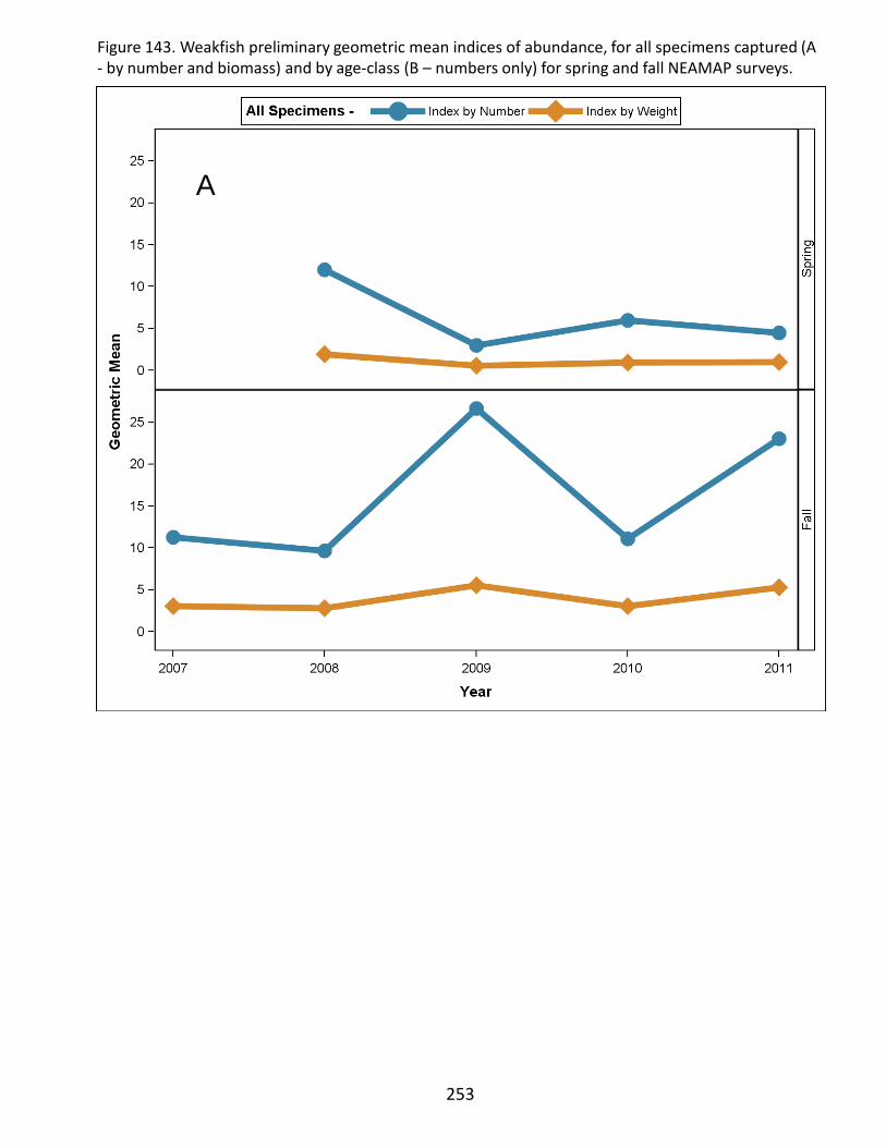
253

A

Figure 143. Weakfish preliminary geometric mean indices of abundance, for all specimens captured (A - by number and biomass) and by age-class (B – numbers only) for spring and fall NEAMAP surveys.

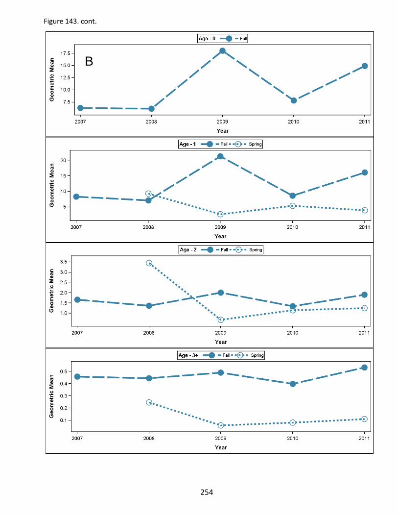
Figure 143. cont.

B

254

Figure 144. Weakfish length-frequency distributions, by cruise.

255

Spring Fall

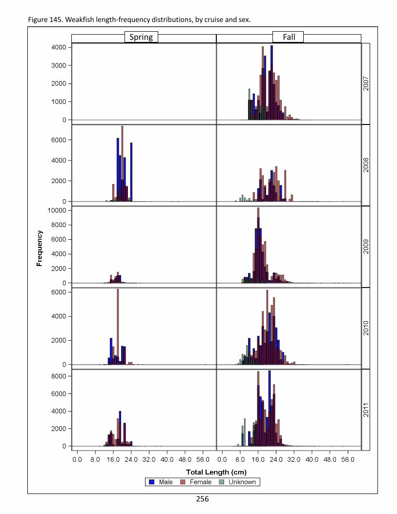
Figure 145. Weakfish length-frequency distributions, by cruise and sex.

Spring Fall

256

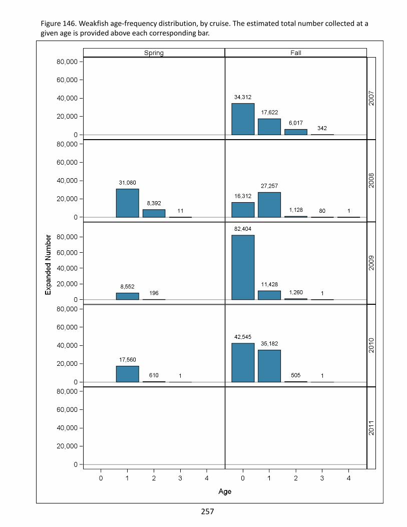
Figure 146. Weakfish age-frequency distribution, by cruise. The estimated total number collected at a given age is provided above each corresponding bar.

257

Figure 147. Weakfish age-at-length proportions for all spring vs. all fall cruises combined (A: for data including all 1cm length groups and B: for data with all specimens greater than 37cm pooled).

258

A

259

+

Figure 147. cont.

B

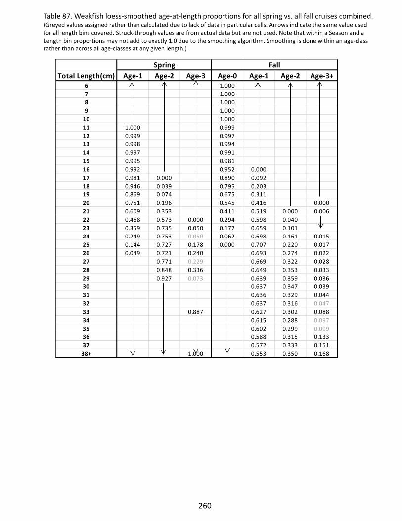
260

Table 87. Weakfish loess-smoothed age-at-length proportions for all spring vs. all fall cruises combined. (Greyed values assigned rather than calculated due to lack of data in particular cells. Arrows indicate the same value used for all length bins covered. Struck-through values are from actual data but are not used. Note that within a Season and a Length bin proportions may not add to exactly 1.0 due to the smoothing algorithm. Smoothing is done within an age-class rather than across all age-classes at any given length.)

Total Length(cm) Age-1 Age-2 Age-3 Age-0 Age-1 Age-2 Age-3+6 1.0007 1.0008 1.0009 1.000

10 1.00011 1.000 0.99912 0.999 0.99713 0.998 0.99414 0.997 0.99115 0.995 0.98116 0.992 0.952 0.00017 0.981 0.000 0.890 0.09218 0.946 0.039 0.795 0.20319 0.869 0.074 0.675 0.31120 0.751 0.196 0.545 0.416 0.00021 0.609 0.353 0.411 0.519 0.000 0.00622 0.468 0.573 0.000 0.294 0.598 0.04023 0.359 0.735 0.050 0.177 0.659 0.10124 0.249 0.753 0.050 0.062 0.698 0.161 0.01525 0.144 0.727 0.178 0.000 0.707 0.220 0.01726 0.049 0.721 0.240 0.693 0.274 0.02227 0.771 0.229 0.669 0.322 0.02828 0.848 0.336 0.649 0.353 0.03329 0.927 0.073 0.639 0.359 0.03630 0.637 0.347 0.03931 0.636 0.329 0.04432 0.637 0.316 0.04733 0.887 0.627 0.302 0.08834 0.615 0.288 0.09735 0.602 0.299 0.09936 0.588 0.315 0.13337 0.572 0.333 0.151

38+ 1.000 0.553 0.350 0.168

Spring Fall

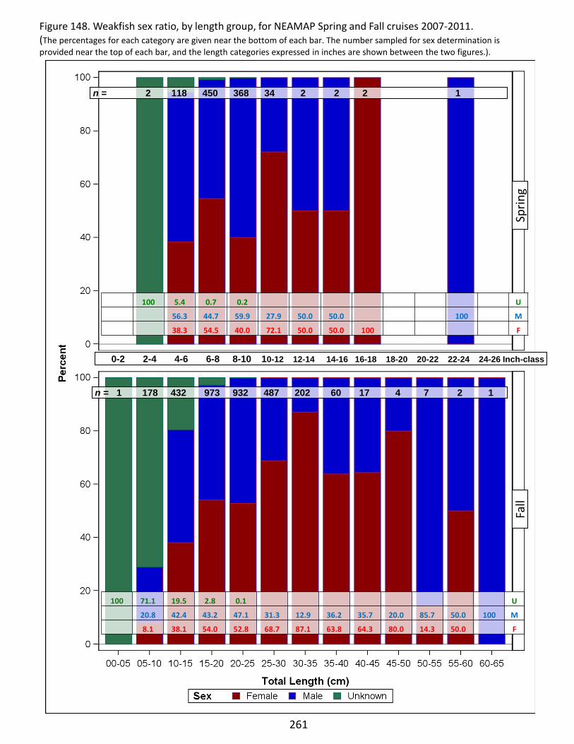
261

Figure 148. Weakfish sex ratio, by length group, for NEAMAP Spring and Fall cruises 2007-2011. (The percentages for each category are given near the bottom of each bar. The number sampled for sex determination is provided near the top of each bar, and the length categories expressed in inches are shown between the two figures.).

n = 2 118 450 368 34 2 2 2 1

n = 1 178 432 973 932 487 202 60 17 4 7 2 1

Sprin

g F

all

0-2 2-4 4-6 6-8 8-10 10-12 12-14 14-16 16-18 18-20 20-22 22-24 24-26 Inch-class

100 5.4 0.7 0.2 U

56.3 44.7 59.9 27.9 50.0 50.0 100 M

38.3 54.5 40.0 72.1 50.0 50.0 100 F

100 71.1 19.5 2.8 0.1 U

20.8 42.4 43.2 47.1 31.3 12.9 36.2 35.7 20.0 85.7 50.0 100 M

8.1 38.1 54.0 52.8 68.7 87.1 63.8 64.3 80.0 14.3 50.0 F

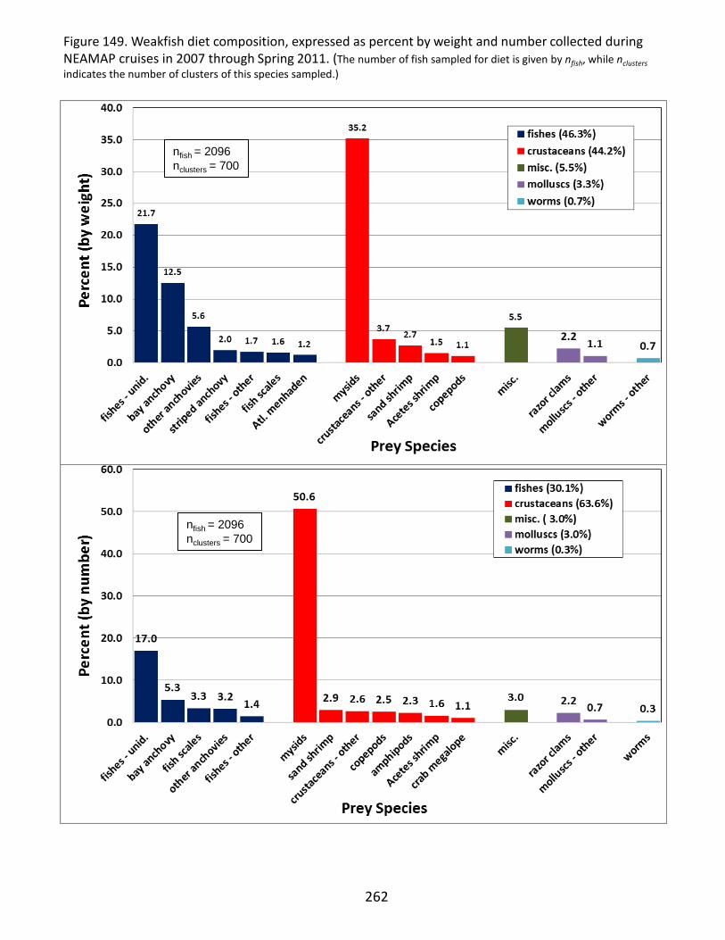
nfish = 2096 nclusters = 700

nfish = 2096 nclusters = 700

262

Figure 149. Weakfish diet composition, expressed as percent by weight and number collected during NEAMAP cruises in 2007 through Spring 2011. (The number of fish sampled for diet is given by nfish, while nclusters indicates the number of clusters of this species sampled.)

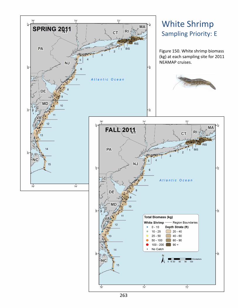
White Shrimp Sampling Priority: E

Figure 150. White shrimp biomass (kg) at each sampling site for 2011 NEAMAP cruises.

263

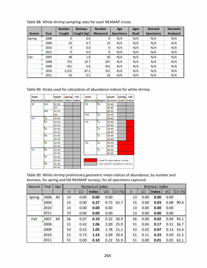
Table 89. Strata used for calculation of abundance indices for white shrimp.

Table 90. White shrimp preliminary geometric mean indices of abundance, by number and biomass, for spring and fall NEAMAP surveys, for all specimens captured.

Table 88. White shrimp sampling rates for each NEAMAP cruise.

264

Season YearNumber Caught

Biomass Caught (kg)

Number Measured

Age Specimens

Ages Read

Stomach Specimens

Stomachs Analyzed

Spring 2008 0 0.0 0 N/A N/A N/A N/A2009 23 0.7 23 N/A N/A N/A N/A2010 0 0.0 0 N/A N/A N/A N/A2011 0 0.0 0 N/A N/A N/A N/A

Fall 2007 48 1.8 20 N/A N/A N/A N/A2008 753 19.7 267 N/A N/A N/A N/A2009 451 6.6 451 N/A N/A N/A N/A2010 3,312 87.2 521 N/A N/A N/A N/A2011 16 0.5 16 N/A N/A N/A N/A

Season Year Agen LCI Index UCI CV (%) n LCI Index UCI CV (%)

Spring 2008 All 13 0.00 0.00 0.00 13 0.00 0.00 0.002009 15 0.00 0.27 0.73 62.7 15 0.00 0.03 0.08 90.42010 13 0.00 0.00 0.00 13 0.00 0.00 0.002011 13 0.00 0.00 0.00 13 0.00 0.00 0.00

Fall 2007 All 56 0.07 0.19 0.32 30.9 56 0.00 0.02 0.04 45.12008 51 0.42 1.06 2.00 25.9 51 0.04 0.17 0.31 36.72009 53 0.52 1.05 1.78 21.1 53 0.02 0.07 0.13 33.42010 51 0.73 1.53 2.69 20.4 51 0.11 0.33 0.59 31.52011 51 0.00 0.10 0.22 55.9 51 0.00 0.01 0.02 63.1

Numerical Index Biomass Index

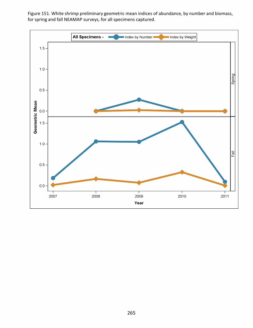
265

Figure 151. White shrimp preliminary geometric mean indices of abundance, by number and biomass, for spring and fall NEAMAP surveys, for all specimens captured.

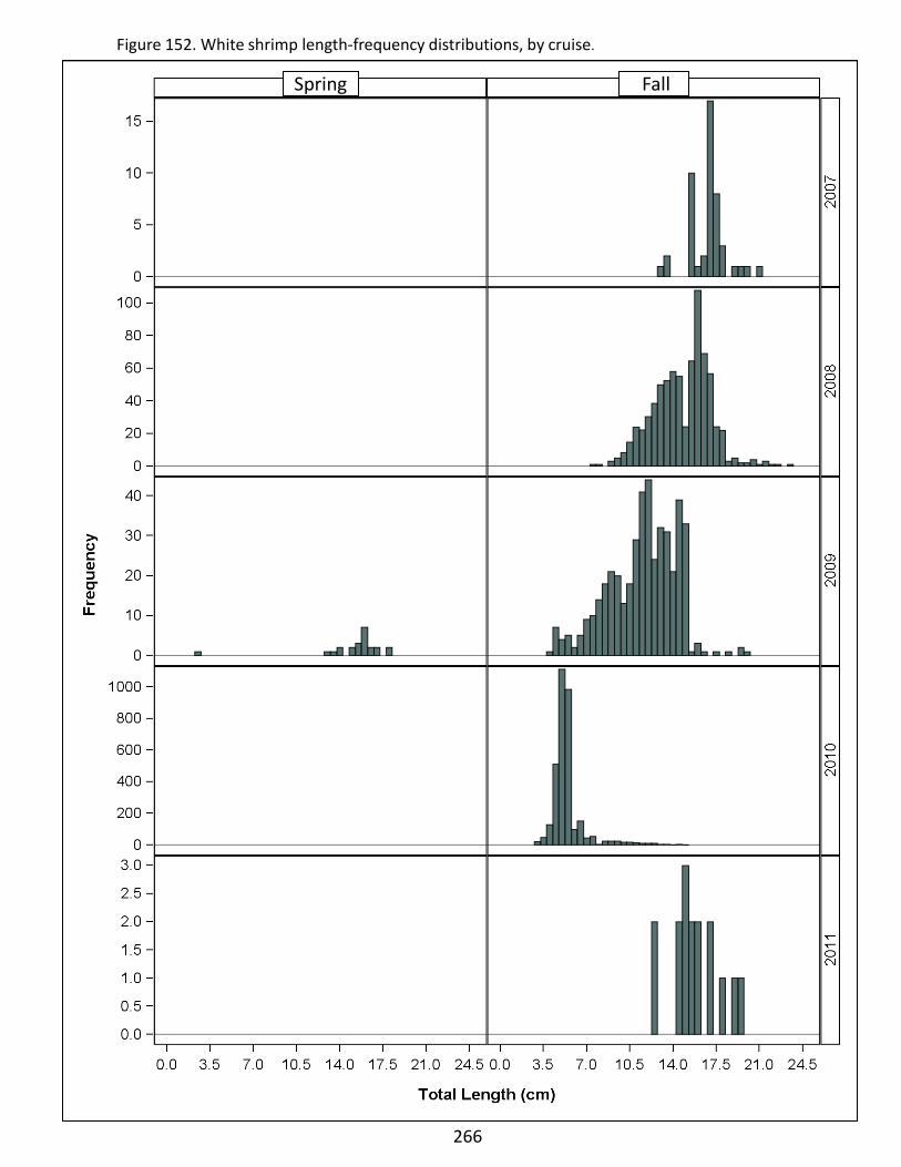
Figure 152. White shrimp length-frequency distributions, by cruise.

266

Spring Fall

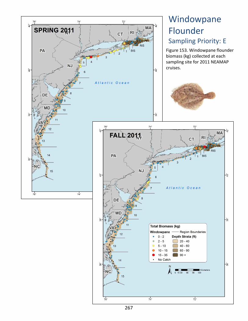
Windowpane Flounder Sampling Priority: E

Figure 153. Windowpane flounder biomass (kg) collected at each sampling site for 2011 NEAMAP cruises.

267

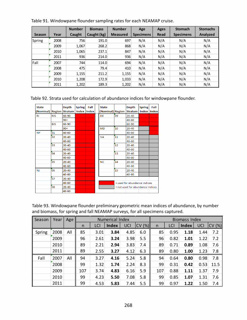
Table 92. Strata used for calculation of abundance indices for windowpane flounder.

Table 93. Windowpane flounder preliminary geometric mean indices of abundance, by number and biomass, for spring and fall NEAMAP surveys, for all specimens captured.

Table 91. Windowpane flounder sampling rates for each NEAMAP cruise.

268

Season YearNumber Caught

Biomass Caught (kg)

Number Measured

Age Specimens

Ages Read

Stomach Specimens

Stomachs Analyzed

Spring 2008 756 191.0 697 N/A N/A N/A N/A2009 1,067 268.2 868 N/A N/A N/A N/A2010 1,065 237.1 847 N/A N/A N/A N/A2011 936 214.0 936 N/A N/A N/A N/A

Fall 2007 744 114.0 694 N/A N/A N/A N/A2008 475 79.4 410 N/A N/A N/A N/A2009 1,155 211.2 1,155 N/A N/A N/A N/A2010 1,208 172.9 1,033 N/A N/A N/A N/A2011 1,202 189.3 1,202 N/A N/A N/A N/A

Season Year Agen LCI Index UCI CV (%) n LCI Index UCI CV (%)

Spring 2008 All 85 3.01 3.84 4.85 6.0 85 0.95 1.18 1.44 7.22009 96 2.61 3.24 3.98 5.5 96 0.82 1.01 1.22 7.22010 89 2.21 2.94 3.83 7.4 89 0.71 0.89 1.08 7.62011 89 2.55 3.27 4.12 6.3 89 0.80 1.00 1.23 7.8

Fall 2007 All 94 3.27 4.16 5.24 5.8 94 0.64 0.80 0.98 7.82008 99 1.32 1.74 2.24 8.3 99 0.31 0.42 0.53 11.52009 107 3.74 4.83 6.16 5.9 107 0.88 1.11 1.37 7.92010 99 4.23 5.50 7.08 5.8 99 0.85 1.07 1.31 7.62011 99 4.53 5.83 7.44 5.5 99 0.97 1.22 1.50 7.4

Numerical Index Biomass Index

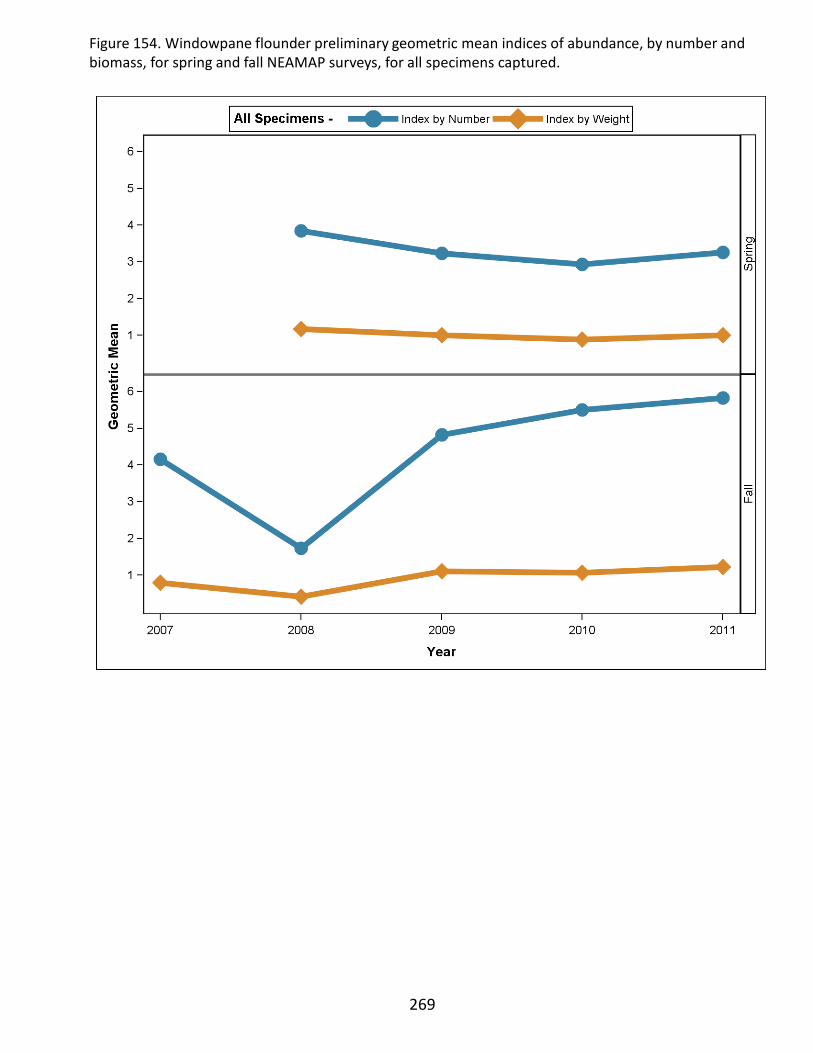
269

Figure 154. Windowpane flounder preliminary geometric mean indices of abundance, by number and biomass, for spring and fall NEAMAP surveys, for all specimens captured.

Figure 155. Windowpane flounder length-frequency distributions, by cruise.

270

Spring Fall

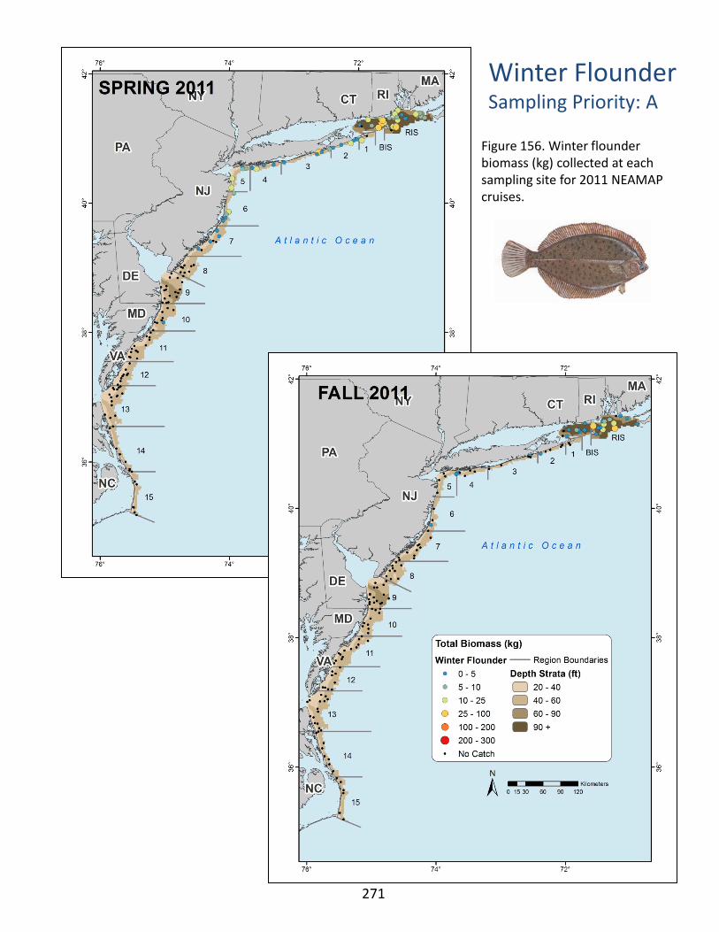
Winter Flounder Sampling Priority: A

Figure 156. Winter flounder biomass (kg) collected at each sampling site for 2011 NEAMAP cruises.

271

Table 95. Strata used for calculation of abundance indices for winter flounder.

Table 94. Winter flounder sampling rates and preserved specimen analysis status for each NEAMAP cruise.

272

Season YearNumber Caught

Biomass Caught (kg)

Number Measured

Age Specimens

Ages Read

Stomach Specimens

Stomachs Analyzed

Spring 2008 1,863 554.1 1,525 466 466 450 4442009 1,954 628.2 1,746 543 531 526 5132010 1,498 574.7 1,498 548 536 495 4442011 1,672 589.5 1,549 464 464 424 409

Fall 2007 392 99.1 392 119 117 116 1162008 670 142.0 522 137 137 133 1312009 558 127.4 558 214 211 178 1782010 264 72.3 264 150 145 108 1062011 572 186.3 572 173 173 126 0

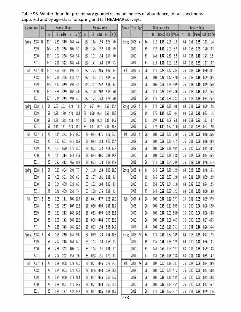
273

Table 96. Winter flounder preliminary geometric mean indices of abundance, for all specimens captured and by age-class for spring and fall NEAMAP surveys.

Season Year Age Season Year Agen LCI Index UCI CV (%) n LCI Index UCI CV (%) n LCI Index UCI CV (%) n LCI Index UCI CV (%)

Spring 2008 All 137 2.61 3.09 3.63 4.4 137 1.64 1.93 2.26 5.0 Spring 2008 4 64 1.12 1.55 2.06 9.8 64 0.61 0.85 1.13 11.42009 145 2.13 2.56 3.05 5.1 145 1.26 1.52 1.81 5.9 2009 69 1.22 1.62 2.09 8.7 69 0.68 0.93 1.20 10.32010 137 1.92 2.36 2.86 5.8 137 1.11 1.34 1.59 6.0 2010 63 1.46 1.94 2.51 8.2 63 0.83 1.11 1.43 9.62011 137 2.70 3.22 3.81 4.6 137 1.41 1.68 1.97 5.3 2011 63 1.13 1.52 1.99 9.2 63 0.65 0.89 1.17 10.7

Fall 2007 All 137 3.74 4.31 4.96 3.4 137 2.25 2.65 3.09 4.4 Fall 2007 4 26 0.11 0.28 0.47 28.4 26 0.07 0.18 0.30 30.12008 137 2.28 2.76 3.31 5.1 137 1.44 1.71 2.02 5.4 2008 26 0.09 0.27 0.47 32.0 26 0.05 0.16 0.29 34.52009 145 4.17 4.99 5.94 4.1 145 2.07 2.42 2.81 4.4 2009 26 0.06 0.17 0.29 30.9 26 0.03 0.11 0.19 35.02010 137 3.38 3.99 4.67 4.0 137 1.70 2.02 2.37 5.0 2010 26 0.13 0.25 0.39 23.6 26 0.08 0.16 0.25 25.42011 137 2.15 2.55 2.99 4.7 137 1.23 1.48 1.77 6.0 2011 26 0.26 0.54 0.88 23.2 26 0.17 0.38 0.63 25.2

Spring 2008 1 64 2.37 3.22 4.29 7.8 64 0.27 0.41 0.56 15.4 Spring 2008 5 64 0.70 0.97 1.28 10.8 64 0.41 0.59 0.79 12.62009 69 1.28 1.90 2.70 11.4 69 0.20 0.34 0.50 19.2 2009 69 0.76 1.04 1.37 10.4 69 0.51 0.71 0.93 11.52010 63 1.36 1.88 2.53 9.5 63 0.16 0.23 0.30 14.7 2010 63 0.97 1.30 1.69 9.4 63 0.63 0.87 1.13 10.72011 63 1.11 1.61 2.23 11.0 63 0.17 0.27 0.39 18.3 2011 63 0.72 1.00 1.32 11.0 63 0.49 0.69 0.92 12.0

Fall 2007 1 26 1.15 2.42 4.46 19.0 26 0.34 0.71 1.19 23.0 Fall 2007 5 26 0.04 0.13 0.22 34.0 26 0.03 0.09 0.16 35.62008 26 3.77 6.71 11.46 11.8 26 0.93 1.58 2.46 15.4 2008 26 0.02 0.13 0.26 41.5 26 0.01 0.08 0.16 43.92009 26 3.53 6.30 10.76 12.0 26 0.72 1.32 2.13 17.8 2009 26 0.00 0.08 0.18 50.5 26 0.00 0.07 0.15 53.12010 26 1.41 2.64 4.48 15.9 26 0.34 0.61 0.93 19.3 2010 26 0.03 0.10 0.18 33.8 26 0.02 0.08 0.14 36.42011 26 2.92 4.82 7.65 11.2 26 0.73 1.23 1.88 15.8 2011 26 0.11 0.31 0.54 29.9 26 0.09 0.26 0.46 31.4

Spring 2008 2 64 3.13 4.34 5.92 7.7 64 1.10 1.53 2.05 10.0 Spring 2008 6 64 0.40 0.57 0.76 12.9 64 0.23 0.35 0.48 15.12009 69 4.00 5.31 6.96 6.3 69 1.37 1.81 2.33 8.3 2009 69 0.45 0.63 0.83 12.0 69 0.31 0.44 0.59 12.92010 63 3.64 4.79 6.23 6.3 63 1.22 1.60 2.05 8.3 2010 63 0.58 0.79 1.04 11.0 63 0.39 0.55 0.74 12.52011 63 3.46 4.79 6.52 7.4 63 1.28 1.75 2.32 9.3 2011 63 0.44 0.62 0.82 12.3 63 0.32 0.45 0.60 13.0

Fall 2007 2 26 0.95 1.81 3.05 17.7 26 0.41 0.77 1.22 20.0 Fall 2007 6 26 0.02 0.07 0.12 37.7 26 0.01 0.05 0.09 37.92008 26 1.52 2.57 4.07 13.8 26 0.50 0.90 1.42 18.7 2008 26 0.00 0.06 0.13 50.5 26 0.00 0.04 0.08 52.02009 26 1.61 2.82 4.60 14.2 26 0.53 0.99 1.58 19.1 2009 26 0.00 0.04 0.09 58.0 26 0.00 0.04 0.08 58.82010 26 0.90 1.62 2.60 16.6 26 0.36 0.64 0.99 19.3 2010 26 0.00 0.04 0.08 46.3 26 0.00 0.03 0.07 46.52011 26 2.15 3.65 5.85 12.6 26 0.93 1.54 2.33 14.7 2011 26 0.04 0.16 0.28 35.1 26 0.04 0.14 0.26 35.4

Spring 2008 3 64 1.79 2.50 3.40 9.0 64 0.89 1.23 1.64 10.5 Spring 2008 7+ 64 0.28 0.42 0.57 14.9 64 0.18 0.29 0.42 17.52009 69 2.22 2.86 3.63 6.7 69 1.03 1.33 1.68 8.3 2009 69 0.36 0.51 0.68 12.5 69 0.30 0.42 0.56 13.12010 63 2.36 3.12 4.06 7.2 63 1.14 1.51 1.94 8.7 2010 63 0.48 0.69 0.93 12.7 63 0.39 0.58 0.79 13.82011 63 2.04 2.72 3.55 7.6 63 0.98 1.31 1.70 9.2 2011 63 0.38 0.56 0.76 13.8 63 0.31 0.47 0.65 14.7

Fall 2007 3 26 0.38 0.78 1.29 22.0 26 0.21 0.46 0.75 24.5 Fall 2007 7+ 26 0.02 0.10 0.18 38.7 26 0.02 0.08 0.14 39.92008 26 0.35 0.73 1.21 22.6 26 0.16 0.40 0.68 28.1 2008 26 0.00 0.10 0.20 51.2 26 0.00 0.06 0.13 53.02009 26 0.35 0.70 1.13 21.4 26 0.17 0.35 0.56 23.7 2009 26 0.00 0.07 0.16 58.5 26 0.00 0.07 0.15 58.82010 26 0.39 0.71 1.11 19.5 26 0.21 0.39 0.60 21.2 2010 26 0.01 0.07 0.13 45.5 26 0.00 0.06 0.12 46.72011 26 0.84 1.47 2.32 16.2 26 0.47 0.85 1.33 18.7 2011 26 0.11 0.32 0.57 31.1 26 0.11 0.33 0.59 31.6

Numerical Index Biomass Index Numerical Index Biomass Index

274

A

Figure 157. Winter flounder preliminary geometric mean indices of abundance, for all specimens captured (A - by number and biomass) and by age-class (B – numbers only) for spring and fall NEAMAP surveys.

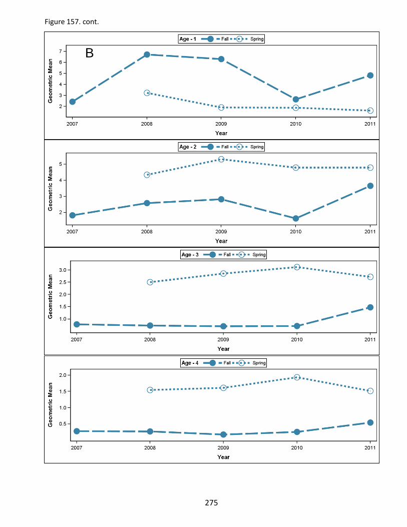
Figure 157. cont.

275

B

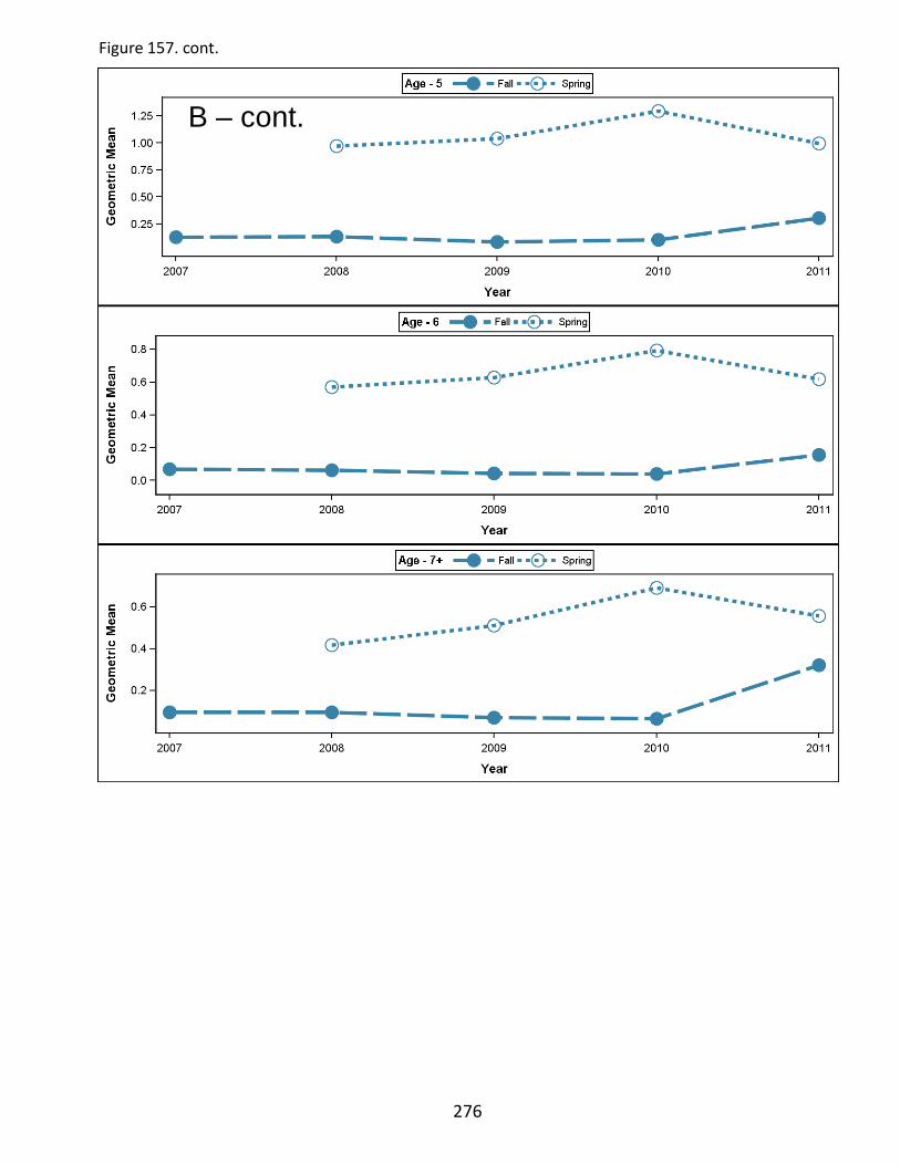
Figure 157. cont.

B – cont.

276

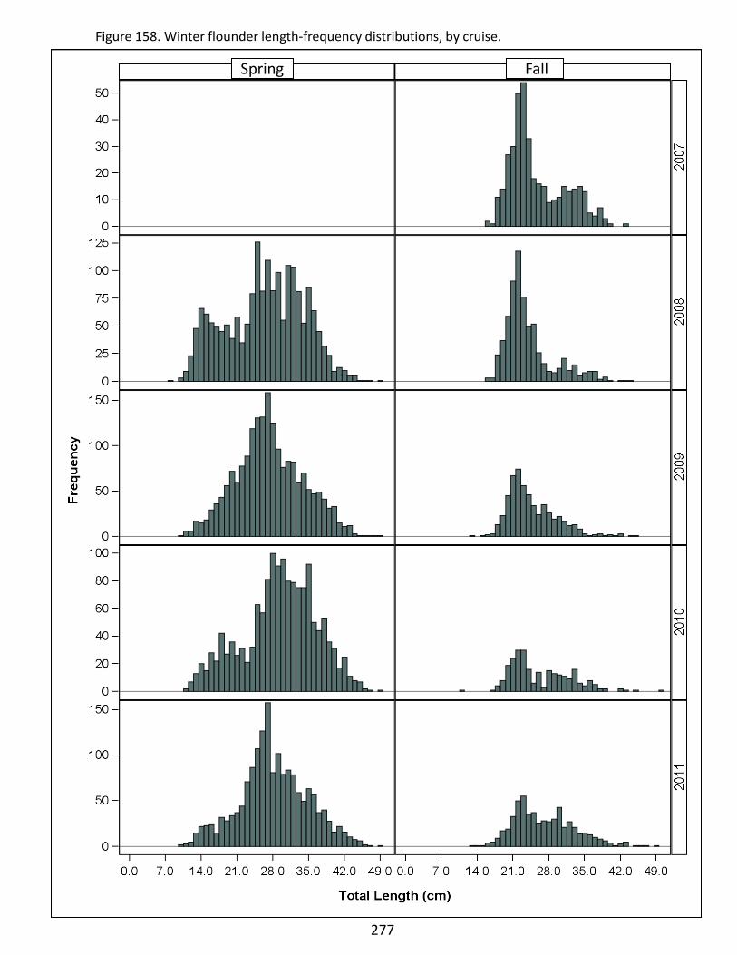
Figure 158. Winter flounder length-frequency distributions, by cruise.

277

Spring Fall

Figure 159. Winter flounder length-frequency distributions, by cruise and sex.

Spring Fall

278

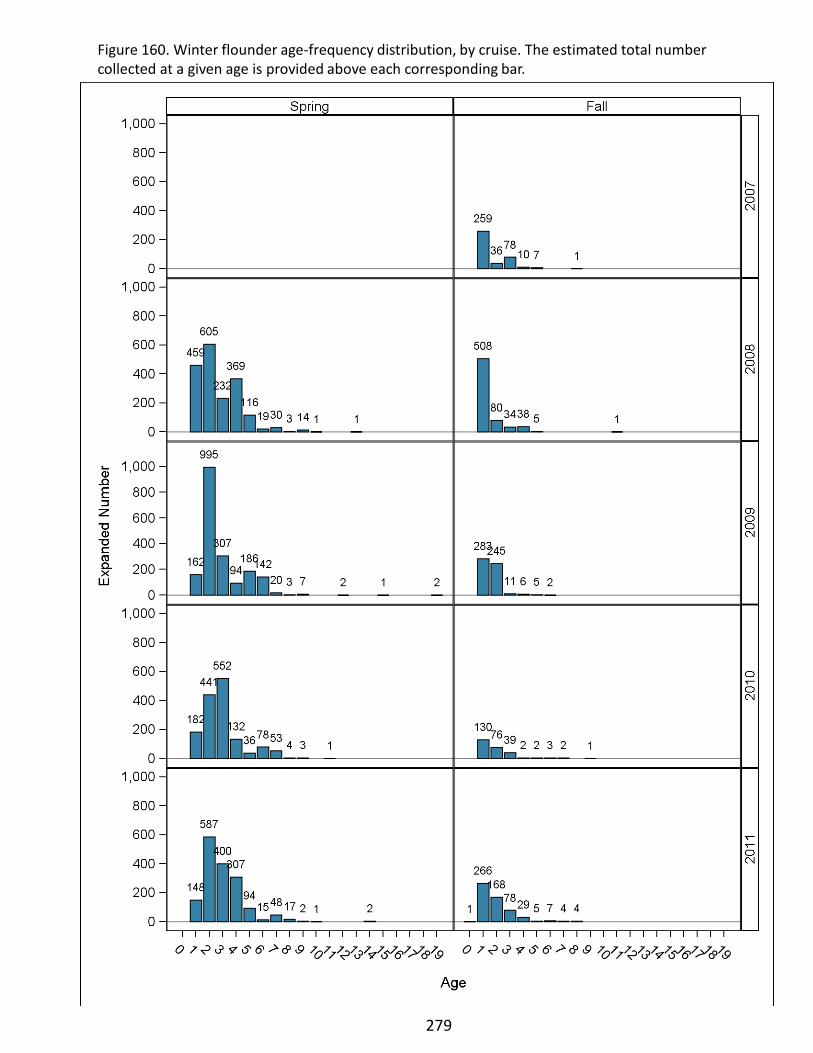
Figure 160. Winter flounder age-frequency distribution, by cruise. The estimated total number collected at a given age is provided above each corresponding bar.

279

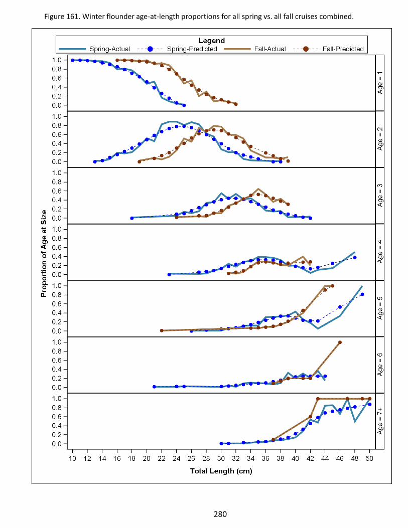
280

Figure 161. Winter flounder age-at-length proportions for all spring vs. all fall cruises combined.

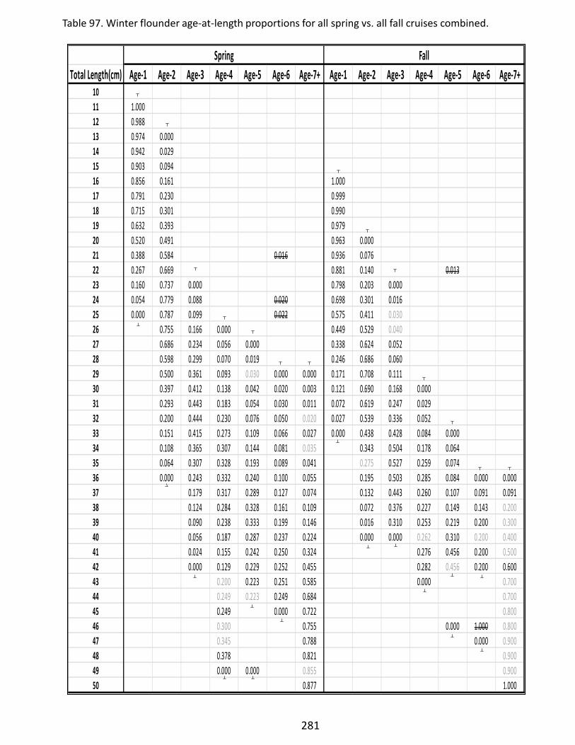
Table 97. Winter flounder age-at-length proportions for all spring vs. all fall cruises combined.

Total Length(cm) Age-1 Age-2 Age-3 Age-4 Age-5 Age-6 Age-7+ Age-1 Age-2 Age-3 Age-4 Age-5 Age-6 Age-7+1011 1.00012 0.98813 0.974 0.00014 0.942 0.02915 0.903 0.09416 0.856 0.161 1.00017 0.791 0.230 0.99918 0.715 0.301 0.99019 0.632 0.393 0.97920 0.520 0.491 0.963 0.00021 0.388 0.584 0.016 0.936 0.07622 0.267 0.669 0.881 0.140 0.01323 0.160 0.737 0.000 0.798 0.203 0.00024 0.054 0.779 0.088 0.020 0.698 0.301 0.01625 0.000 0.787 0.099 0.022 0.575 0.411 0.03026 0.755 0.166 0.000 0.449 0.529 0.04027 0.686 0.234 0.056 0.000 0.338 0.624 0.05228 0.598 0.299 0.070 0.019 0.246 0.686 0.06029 0.500 0.361 0.093 0.030 0.000 0.000 0.171 0.708 0.11130 0.397 0.412 0.138 0.042 0.020 0.003 0.121 0.690 0.168 0.00031 0.293 0.443 0.183 0.054 0.030 0.011 0.072 0.619 0.247 0.02932 0.200 0.444 0.230 0.076 0.050 0.020 0.027 0.539 0.336 0.05233 0.151 0.415 0.273 0.109 0.066 0.027 0.000 0.438 0.428 0.084 0.00034 0.108 0.365 0.307 0.144 0.081 0.035 0.343 0.504 0.178 0.06435 0.064 0.307 0.328 0.193 0.089 0.041 0.275 0.527 0.259 0.07436 0.000 0.243 0.332 0.240 0.100 0.055 0.195 0.503 0.285 0.084 0.000 0.00037 0.179 0.317 0.289 0.127 0.074 0.132 0.443 0.260 0.107 0.091 0.09138 0.124 0.284 0.328 0.161 0.109 0.072 0.376 0.227 0.149 0.143 0.20039 0.090 0.238 0.333 0.199 0.146 0.016 0.310 0.253 0.219 0.200 0.30040 0.056 0.187 0.287 0.237 0.224 0.000 0.000 0.262 0.310 0.200 0.40041 0.024 0.155 0.242 0.250 0.324 0.276 0.456 0.200 0.50042 0.000 0.129 0.229 0.252 0.455 0.282 0.456 0.200 0.60043 0.200 0.223 0.251 0.585 0.000 0.70044 0.249 0.223 0.249 0.684 0.70045 0.249 0.000 0.722 0.80046 0.300 0.755 0.000 1.000 0.80047 0.345 0.788 0.000 0.90048 0.378 0.821 0.90049 0.000 0.000 0.855 0.90050 0.877 1.000

Spring Fall

281

282

Figure 162. Winter flounder sex ratio, by length group, for NEAMAP Spring and Fall cruises 2007-2011. (The percentages for each category are given near the bottom of each bar. The number sampled for sex determination is provided near the top of each bar, and the length categories expressed in inches are shown between the two figures.).

n = 1 37 154 202 265 201 288 495 439 427 399 294 227 128 55 9 5 1

n = 1 17 123 292 215 145 151 143 102 57 32 14 8 2 2

Sprin

g F

all

3 4 5 6 7 8 9 10 11 12 13 14 15 16 17 18 19 20 Inch-class

61.4 56.8 35.5 15.7 7.6 1.2 0.9 U

18.8 24.2 30.8 45.1 48.7 45.1 46.5 37.2 45.9 29.7 19.5 6.0 5.4 9.2 13.8 M

100 19.7 19.1 33.7 39.2 43.7 53.6 53.5 62.8 54.1 70.3 80.5 93.1 94.6 90.8 86.2 100 100 F

3.9 1.3 1.7 0.2 0.4 1.4 U

100 53.9 60.3 44.5 46.1 47.9 21.8 15.4 13.9 2.0 7.1 12.5 M

42.2 38.4 53.8 53.7 51.7 78.2 84.6 84.7 98.0 100 92.9 87.5 100 100 F

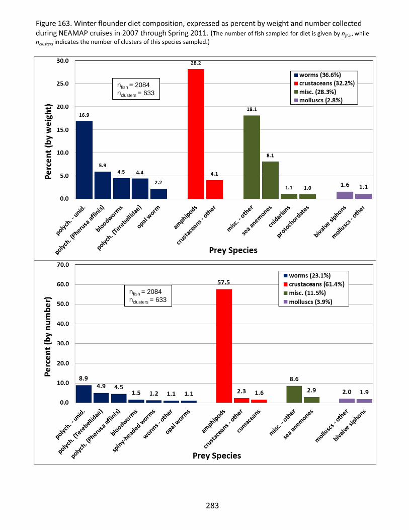
nfish = 2084 nclusters = 633

nfish = 2084 nclusters = 633

283

Figure 163. Winter flounder diet composition, expressed as percent by weight and number collected during NEAMAP cruises in 2007 through Spring 2011. (The number of fish sampled for diet is given by nfish, while nclusters indicates the number of clusters of this species sampled.)

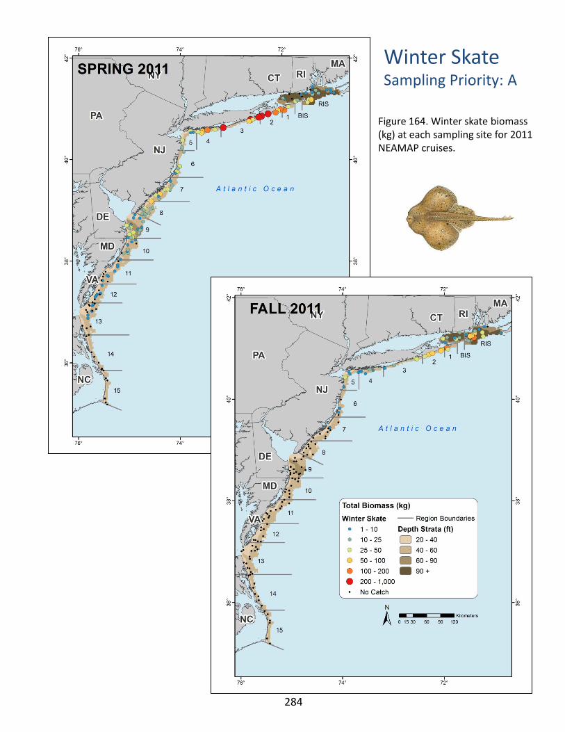
Winter Skate Sampling Priority: A

Figure 164. Winter skate biomass (kg) at each sampling site for 2011 NEAMAP cruises.

284

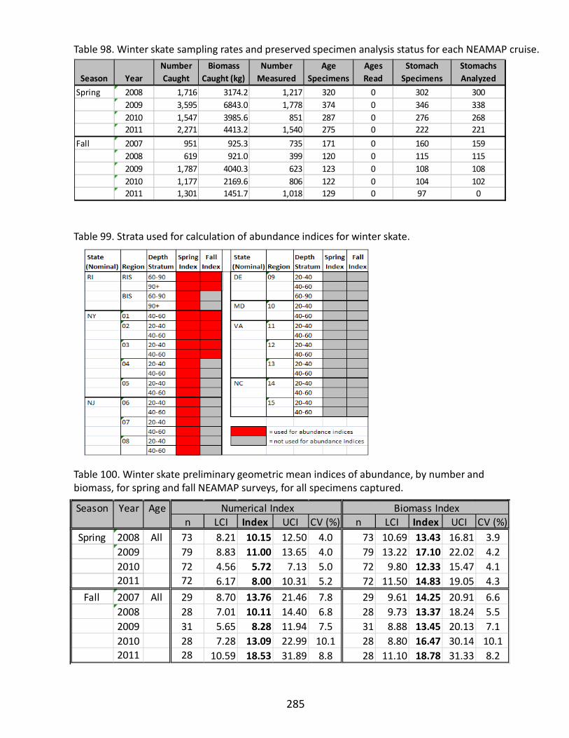
Table 99. Strata used for calculation of abundance indices for winter skate.

Table 100. Winter skate preliminary geometric mean indices of abundance, by number and biomass, for spring and fall NEAMAP surveys, for all specimens captured.

Table 98. Winter skate sampling rates and preserved specimen analysis status for each NEAMAP cruise.

285

Season YearNumber Caught

Biomass Caught (kg)

Number Measured

Age Specimens

Ages Read

Stomach Specimens

Stomachs Analyzed

Spring 2008 1,716 3174.2 1,217 320 0 302 3002009 3,595 6843.0 1,778 374 0 346 3382010 1,547 3985.6 851 287 0 276 2682011 2,271 4413.2 1,540 275 0 222 221

Fall 2007 951 925.3 735 171 0 160 1592008 619 921.0 399 120 0 115 1152009 1,787 4040.3 623 123 0 108 1082010 1,177 2169.6 806 122 0 104 1022011 1,301 1451.7 1,018 129 0 97 0

Season Year Agen LCI Index UCI CV (%) n LCI Index UCI CV (%)

Spring 2008 All 73 8.21 10.15 12.50 4.0 73 10.69 13.43 16.81 3.92009 79 8.83 11.00 13.65 4.0 79 13.22 17.10 22.02 4.22010 72 4.56 5.72 7.13 5.0 72 9.80 12.33 15.47 4.12011 72 6.17 8.00 10.31 5.2 72 11.50 14.83 19.05 4.3

Fall 2007 All 29 8.70 13.76 21.46 7.8 29 9.61 14.25 20.91 6.62008 28 7.01 10.11 14.40 6.8 28 9.73 13.37 18.24 5.52009 31 5.65 8.28 11.94 7.5 31 8.88 13.45 20.13 7.12010 28 7.28 13.09 22.99 10.1 28 8.80 16.47 30.14 10.12011 28 10.59 18.53 31.89 8.8 28 11.10 18.78 31.33 8.2

Numerical Index Biomass Index

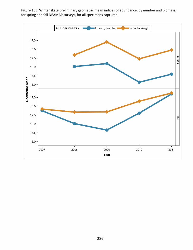
286

Figure 165. Winter skate preliminary geometric mean indices of abundance, by number and biomass, for spring and fall NEAMAP surveys, for all specimens captured.

Figure 166. Winter skate length-frequency distributions, by cruise.

287

Spring Fall

288

Figure 167. Winter skate length-frequency distributions, by cruise and sex.

Spring Fall

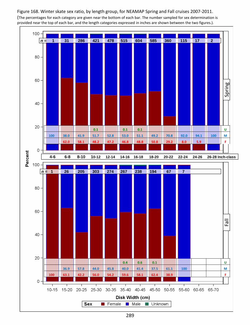
289

Figure 168. Winter skate sex ratio, by length group, for NEAMAP Spring and Fall cruises 2007-2011. (The percentages for each category are given near the bottom of each bar. The number sampled for sex determination is provided near the top of each bar, and the length categories expressed in inches are shown between the two figures.).

n = 1 31 286 421 478 515 604 585 360 115 17 2

n = 1 26 205 303 274 267 238 194 67 7

Sprin

g F

all

4-6 6-8 8-10 10-12 12-14 14-16 16-18 18-20 20-22 22-24 24-26 26-28 Inch-class

0.1 0.1 0.1 U

100 38.0 41.9 51.7 52.8 53.0 51.1 49.2 70.8 92.0 94.1 100 M

62.0 58.1 48.2 47.2 46.8 48.8 50.8 29.2 8.0 5.9 F

0.4 0.6 0.1 U

36.9 57.8 44.0 45.8 40.0 41.4 37.5 61.1 100 M

100 63.1 42.2 56.0 54.2 59.6 58.1 62.4 38.9 F

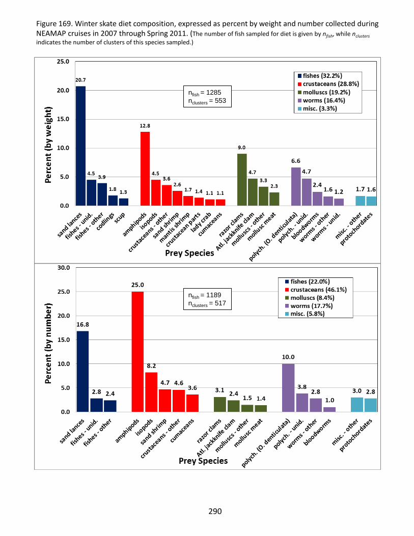
nfish = 1285 nclusters = 553

nfish = 1189 nclusters = 517

290

Figure 169. Winter skate diet composition, expressed as percent by weight and number collected during NEAMAP cruises in 2007 through Spring 2011. (The number of fish sampled for diet is given by nfish, while nclusters indicates the number of clusters of this species sampled.)