Four-dimensional effective supergravity and soft terms in M theory
23
arXiv:hep-th/9711158v2 26 Nov 1997 KAIST–TH 97/20 FTUAM 97/16 Four-Dimensional Effective Supergravity and Soft Terms in M –Theory Kiwoon Choi 1 , Hang Bae Kim 1 and Carlos Mu˜ noz 1,2 1 Department of Physics, Korea Advanced Institute of Science and Technology Taejon 305-701, Korea 2 Departamento de F´ ısica Te´ orica C-XI, Universidad Aut´ onoma de Madrid Cantoblanco, 28049 Madrid, Spain Abstract We provide a simple macroscopic analysis of the four-dimensional effective supergravity of the Hoˇ rava-Witten M -theory which is expanded in powers of κ 2/3 /ρV 1/3 and κ 2/3 ρ/V 2/3 where κ 2 , V and ρ denote the eleven-dimensional gravitational coupling, the Calabi-Yau volume and the eleventh length re- spectively. Possible higher order terms in the K¨ ahler potential are identified and matched with the heterotic string corrections. In the context of this M - theory expansion, we analyze the soft supersymmetry–breaking terms under the assumption that supersymmetry is spontaneously broken by the auxiliary components of the bulk moduli superfields. It is examined how the pattern of soft terms changes when one moves from the weakly coupled heterotic string limit to the M -theory limit. Typeset using REVT E X 1
-
Upload
independent -
Category
Documents
-
view
0 -
download
0
Transcript of Four-dimensional effective supergravity and soft terms in M theory
arX
iv:h
ep-t
h/97
1115
8v2
26
Nov
199
7
KAIST–TH 97/20
FTUAM 97/16
Four-Dimensional Effective Supergravity and Soft Terms in
M–Theory
Kiwoon Choi1, Hang Bae Kim1 and Carlos Munoz1,2
1Department of Physics, Korea Advanced Institute of Science and Technology
Taejon 305-701, Korea
2Departamento de Fısica Teorica C-XI, Universidad Autonoma de Madrid
Cantoblanco, 28049 Madrid, Spain
Abstract
We provide a simple macroscopic analysis of the four-dimensional effective
supergravity of the Horava-Witten M -theory which is expanded in powers of
κ2/3/ρV 1/3 and κ2/3ρ/V 2/3 where κ2, V and ρ denote the eleven-dimensional
gravitational coupling, the Calabi-Yau volume and the eleventh length re-
spectively. Possible higher order terms in the Kahler potential are identified
and matched with the heterotic string corrections. In the context of this M -
theory expansion, we analyze the soft supersymmetry–breaking terms under
the assumption that supersymmetry is spontaneously broken by the auxiliary
components of the bulk moduli superfields. It is examined how the pattern of
soft terms changes when one moves from the weakly coupled heterotic string
limit to the M -theory limit.
Typeset using REVTEX
1
Recently Horava and Witten proposed that the strong coupling limit of E8×E8 heterotic
string theory can be described by 11-dimensional supergravity (SUGRA) on a manifold with
boundary where the two E8 gauge multiplets are restricted to the two 10-dimensional bound-
aries respectively (M-theory) [1]. The effective action of this limit has been systematically
analyzed in an expansion in powers of κ2/3 where κ2 denotes the 11-dimensional gravita-
tional coupling. At zeroth order, the effective action is simply that of the 11-dimensional
supergravity which includes only the bulk fields whose kinetic terms are of order κ−2. How-
ever at first order in the expansion, there appear a variety of additional terms including the
10-dimensional boundary action of the E8 ×E8 gauge multiplets which is of order κ−4/3. It
was also noted that a four-gaugino term appears at higher order which would lead to an
interesting phenomenological consequence when supersymmetry (SUSY) is broken by the
gaugino condensation on the hidden boundary [2].
Some phenomenological implications of the strong-coupling limit of E8 × E8 heterotic
string theory has been studied by compactifying the 11-dimensional M-theory on a Calabi-
Yau manifold times the eleventh segment [3]. The resulting 4-dimensional effective theory
can reconcile the observed Planck scale MP = 1/√
8πGN ≈ 2.4 × 10¹⁸ GeV with the phe-
nomenologically favored GUT scale MGUT ≈ 3 × 10¹⁶ GeV in a natural manner, providing
an attractive framework for the unification of couplings [3,4]. In this framework, MGUT
corresponds to 1/V 1/6 where V is the Calabi-Yau volume, while M2P = 2πρV/κ2 for πρ
denoting the length of the eleventh segment. Then by choosing πρ ≈ 4V 1/6 together with
MGUT = 1/V 1/6 ≈ 3 × 10¹⁶ GeV, one could get the correct values of αGUT and MP , which
was not allowed in the weakly coupled heterotic string theory. An additional phenomeno-
logical virtue of the M-theory limit is that there can be a QCD axion whose high energy
axion potential is suppressed enough so that the strong CP problem can be solved by the
axion mechanism [4,5]. These phenomenological virtues have motivated many of the recent
studies of the 4-dimensional effective theory of M-theory [6–15].
As is well known, the 4-dimensional effective action of the weakly coupled heterotic string
theory can be expanded in powers of the two dimensionless variables: the string coupling
2
ǫs = e2φ/(2π)5 and the worldsheet sigma model coupling ǫσ = 4πα′/V 1/3 [16]. The effective
action of M-theory can be similarly analyzed by expanding it in powers of the two dimen-
sionless variables: ǫ1 = κ2/3πρ/V 2/3 and ǫ2 = κ2/3/πρV 1/3. To compute the 4-dimensional
effective action, one first expands the 11-dimensional action in powers of κ2/3 to find the
compactification solution which is expanded in powers of ǫ1 and ǫ2. The subsequent Kaluza-
Klein reduction of the 11-dimensional action for this compactification solution will lead to
the desired 4-dimensional effective action. At the leading order in this expansion, the Kahler
potential, superpotential and gauge kinetic functions have been computed in [4,8,9,11]. It is
rather easy to determine the order ǫ1 correction to the leading order gauge kinetic functions
[4,5,11,17], while it is much more nontrivial to compute the order ǫ1 correction to the leading
order Kahler potential, which was recently done by Lukas, Ovrut and Waldram [15]. As we
will argue later, the holomorphy and Peccei–Quinn symmetries guarantee that there is no
further correction to the gauge kinetic functions and the superpotential at any finite order
in the M-theory expansion [18]. However generically the Kahler potential is expected to re-
ceive corrections which are higher order in ǫ1 or ǫ2. An explicit computation of these higher
order corrections will be highly nontrivial since first of all the 11-dimensional action is known
only up to the terms of order κ2/3 relative to the zeroth order action (except for the order
κ4/3 four-gaugino term) and secondly the higher order computation of the compactification
solution and its Kaluza-Klein reduction are much more complicated.
In this paper, we wish to provide a simple macroscopic analysis of the 4-dimensional
effective SUGRA action by expanding it in powers of ǫ1 and ǫ2, and apply the results for
the computation of soft SUSY–breaking terms. As we will see, this analysis allows us to
extract the form of possible higher order corrections to the Kahler potential and also to
estimate their size for the physically interesting values of moduli. An interesting feature
of the 4-dimensional effective SUGRA is that the forms of the gauge kinetic function and
superpotential are not changed (up to nonperturbative corrections) when one moves from
the weakly coupled heterotic string domain to the M-theory domain in the moduli space.
3

The same is true for the leading order Kahler potential, i.e. the Kahler potential of the
weakly coupled heterotic string computed at the leading order in the string loop and sigma
model perturbation theory is the same as the M-theory Kahler potential computed at the
leading order in the M-theory expansion. In fact, one can smoothly move from the M-theory
domain with ǫs ≫ 1 to the heterotic string domain with ǫs ≪ 1 while keeping ǫ1 and ǫ2 to
be small enough. This means that the M-theory Kahler potential expanded in ǫ1 and ǫ2 is
valid even on the heterotic string domain up to (nonperturbative) corrections which can not
be taken into account by the M-theory expansion. Then as in the case of the gauge kinetic
functions, one can determine the expansion coefficients in the M-theory Kahler potential
by matching the heterotic string Kahler potential which can be computed in the string loop
and sigma model perturbation theory.
About the issue of SUSY breaking, the possibility of SUSY breaking by the gaugino
condensation on the hidden boundary has been studied [2,11,12] and also some interesting
features of the resulting soft SUSY–breaking terms were discussed in [11]. Here we analyze
the soft SUSY–breaking terms under the more general assumption that SUSY is sponta-
neously broken by the auxiliary components of the bulk moduli superfields in the model.
We examine in particular how the soft terms vary when one moves from the weakly coupled
heterotic string limit to the M-theory limit in order to see whether these two limits can be
distinguished by the soft term physics. Our analysis implies that there can be a sizable dif-
ference between the heterotic string limit and the M-theory limit even in the overall pattern
of soft terms.
Let us first discuss possible perturbative expansions of the 4-dimensional effective
SUGRA action of M-theory. As in the case of weakly coupled heterotic string theory,
the effective SUGRA of compactified M-theory contains two model–independent moduli
superfields S and T whose scalar components can be identified as
Re(S) =1
2π(4πκ2)−2/3V ,
Re(T ) =61/3
8π(4πκ2)−1/3πρV 1/3 , (1)
4
where these normalizations of S and T have been chosen to keep the conventional form of the
gauge kinetic functions in the effective SUGRA. (See (7) for our form of the gauge kinetic
functions. Our S and T correspond to 14π
S and 18π
T of [5] respectively.) The pseudoscalar
components Im(S) and Im(T ) are the well known model–independent axion and the Kahler
axion whose couplings are constrained by the non–linear Peccei–Quinn symmetries:
U(1)S : S → S + iβS , U(1)T : T → T + iβT , (2)
where βS and βT are continuous real numbers. These Peccei-Quinn symmetries appear as
exact symmetries at any finite order in the M-theory expansion, but they are explicitly
broken by nonperturbative effects that will not be taken into account in this paper.
The moduli S and T can be used to define various kind of expansions which may be
applied for the low–energy effective action. For instance, in the weakly coupled heterotic
string limit, we have
Re(S) = e−2φ V
(2α′)3,
Re(T ) =61/3
32π3
V 1/3
2α′, (3)
where φ and√
2α′ denote the heterotic string dilaton and length scale respectively. One
may then expand the effective action of the heterotic string theory in powers of the string
loop expansion parameter ǫs and the world–sheet sigma model expansion parameter ǫσ:
ǫs =e2φ
(2π)5≈ 0.3
[4π2Re(T )]3
Re(S),
ǫσ =4πα′
V 1/3≈ 0.5
1
4π2Re(T ). (4)
Here we are interested in the possible expansion in the M-theory limit of the strong
heterotic string coupling ǫs ≫ 1 for which πρ >∼ κ2/9 and V >∼ κ4/3 and so the physics can
be described by 11-dimensional supergravity. Since we have two independent length scales,
ρ and V 1/6, there can be two dimensionless expansion parameters in the M-theory limit
also. The analysis of the 11-dimensional theory suggests that the expansion parameters
5
should scale as κ2/3 which may be identified as the inverse of the membrane tension. One
obvious candidate for the expansion parameter in the M-theory limit is the straightforward
generalization of the string world–sheet coupling ∼ α′/V 1/3 to the membrane world–volume
coupling ∼ κ2/3/ρV 1/3. Note that in the M-theory limit, heterotic string corresponds to a
membrane stretched along the eleventh dimension. Information for the other expansion pa-
rameter comes from the Witten’s strong coupling expansion of the compactification solution
[3], implying that one needs an expansion parameter which is linear in ρ. The analysis of
[3] shows that a ρ-independent modification of the bulk physics at higher order in κ2/3 can
lead to a modification of the boundary physics which is proportional to ρ. As was noticed
in [4,15], this leads to an expansion parameter which scales as κ2/3ρ/V 2/3. The above obser-
vations lead us to expand the 4-dimensional effective SUGRA action of the Horava-Witten
M-theory in powers of
ǫ1 = κ2/3πρ/V 2/3 ≈ Re(T )
Re(S),
ǫ2 = κ2/3/πρV 1/3 ≈ 1
4π2Re(T ), (5)
where (1) has been used to arrive at this expression of ǫ1 and ǫ2. Note that ǫ1ǫ2 ≈
1/[4π2Re(S)] ≈ αGUT /π which is essentially the 4-dimensional field theory expansion pa-
rameter. Thus if one goes to the limit in which one expansion works better while keeping
the realistic value of αGUT , the other expansion becomes worse. Here we will simply assume
that both ǫ1 and ǫ2 are small enough so that the double expansion in ǫ1 and ǫ2 provides a
good perturbative scheme for the effective action of M-theory. As we will argue later, this
expansion works well even when ǫ1 becomes of order one, which is in fact the case when
MGUT ≈ 3 × 10¹⁶ GeV.
Possible guidelines for the M-theory expansion of the 4–dimensional effective action
would be (i) microscopically, the expansion parameter scales as κ2/3(πρ)−nV (n−3)/6 and it
has a sensible limiting behavior when the Calabi-Yau volume or the 11-th segment becomes
large, (ii) macroscopically, the expansion parameter scales as integral powers of Re(S) and
Re(T ). In M-theory, V can be arbitrarily large independently of the value of πρ. However
6
as was noted in [3], for a given value of the averaged Calabi-Yau volume V , in order to
avoid that one of the boundary Calabi-Yau volume shrinks to zero, πρ is restricted as
πρ ≤ κ−2/3V 2/3. Then one can demand that the expansion parameter κ2/3(πρ)−nV (n−3)/6
should not blow up in the limit that V → ∞ for a fixed value of πρ and also in another limit
that πρ → ∞ and V → ∞ while keeping V 1/6 ≪ πρ ≤ κ−2/3V 2/3. Obviously this condition
is satisfied only for −1 ≤ n ≤ 3. There are then only three possible expansion parameters
which meet the guidelines (i) and (ii), ǫ1 and ǫ2 in (5) and finally ǫ3 = κ2/3/(πρ)3 ≈
10−3Re(S)/[Re(T )]3 which scales as the inverse of the string loop expansion parameter ǫs.
As will be discussed later, the 4–dimensional effective action computed in the heterotic
string limit can be smoothly extrapolated to the M-theory limit, suggesting that there can
be a complete matching between the heterotic string effective action (expanded in ǫs and ǫσ)
and the M-theory effective action (expanded in ǫ1 and ǫ2). In view of this matching, it is
not likely that there is an additional correction which would require to introduce the third
expansion parameter ǫ3, although we can not rule out this possibility at this moment. Even
when there is such correction, ǫ3 is smaller than ǫ2 and ǫ1 by one or two orders of magnitude
for the phenomenologically interesting case that both Re(S) and Re(T ) are essentially of
order one, which is necessary to have MGUT ≈ 3× 10¹⁶ GeV together with the correct value
of αGUT (see the discussion below (17).). This would justify our scheme of including only
the expansions in ǫ1 and ǫ2.
To be explicit, let us consider a simple compactification on a Calabi-Yau manifold with
the Hodge-Betti number h1,1 = 1 and h1,2 = 0. In this model, the low–energy degrees of
freedom include first the gravity multiplet and S and T which are the massless modes of the
11-dimensional bulk fields. If the spin connection is embedded into the gauge connection
in the observable sector boundary, we also have the E6 gauge multiplet and the charged
matter multiplet C together with the hidden E8 gauge multiplet as the massless modes of
the 10-dimensional boundary fields. It is then easy to compute the Kahler potential K, the
observable and hidden sector gauge kinetic functions fE6and fE8
, and the superpotential
W at the leading order in the M-theory expansion. Obviously the leading contribution to
7
the moduli Kahler metric is from the 11-dimensional bulk field action which is of order κ−2,
while the charged matter Kahler metric, the gauge kinetic functions, and the charged matter
superpotential receive the leading contributions from the 10-dimensional boundary action
which is of order κ−4/3. Including only the non-vanishing leading contributions, one finds
[4,8,9,11]
K = − ln(S + S) − 3 ln(T + T ) +3|C|2
(T + T ),
fE6= fE8
= S ,
W = dpqrCpCqCr , (6)
where dpqr is a constant E6-tensor coefficient.
The holomorphy and the Peccei-Quinn symmetries of (2) imply that there is no correction
to the superpotential at any finite order in the S and T -dependent expansion parameters ǫ1
and ǫ2. However the gauge kinetic functions can receive a correction at order ǫ1 in a way
consistent with the holomorphy and the Peccei-Quinn symmetries. An explicit computation
leads to [4,5,17]
fE6= S + αT , fE8
= S − αT , (7)
where the integer coefficient α = 18π2
∫
ω ∧ [tr(F ∧ F ) − 12tr(R ∧ R)] for the Kahler form ω
normalized as the generator of the integer (1,1) cohomology1. As was discussed in [4,5], the
coefficient α in the M-theory gauge kinetic function can be determined either by a direct
M-theory computation [3] or by matching the string loop threshold correction to the gauge
kinetic function [19,20]. At any rate, the holomorphy and the Peccei-Quinn symmetries
imply that there is no further correction to the gauge kinetic functions at any finite order
in the M-theory expansion.
1 Usually α is considered to be an arbitrary real number. For T normalized as (1), it is required
to be an integer [5].
8
Let us now consider the possible higher order corrections to the Kahler potential. With
the Peccei-Quinn symmetries, the Kahler potential can be written as
K = K(S + S, T + T ) + Z(S + S, T + T )|C|2 , (8)
with
K = K0 + δK , Z = Z0 + δZ , (9)
where K0 = − ln(S + S)− 3 ln(T + T ) and Z0 = 3/(T + T ) denote the leading order results
in (6), while δK and δZ are the higher order corrections. Before going to the M-theory
expansion of δK and δZ, it is useful to note that the bulk physics become blind to the
existence of boundaries in the limit ρ → ∞. (This is true up to the trivial scaling of the
4–dimensional Planck scale M2P ∼ ρ.) However some of the boundary physics, e.g. the
boundary Calabi-Yau volume, can be affected by the integral of the bulk variables over the
11-th dimension and then they can include a piece linear in ρ [3]. This implies that δK/K0,
being the correction to the pure bulk dynamics, contains only a non-negative power of 1/ρ
in the M-theory expansion, while δZ/Z0 which concerns the couplings between the bulk and
boundary fields can include a piece linear in ρ. Since ǫn1ǫ
m2 ∼ ρn−m, one needs m ≥ n for the
expansion of δK/K0 and m ≥ n − 1 for the expansion of δZ/Z0. Taking account of these,
the M-theory expansion of the Kahler potential is given by
δK =∑
(n+m≥1,m≥n)
Anmǫn1 ǫm
2
=∑
m≥1
A0m
[4π2Re(T )]m+
A11
4π2Re(S)
[
1 + O(1
4π2Re(S),
1
4π2Re(T ))
]
,
δZ =3
(T + T )
∑
(n+m≥1,m≥n−1)
Bnmǫn1 ǫm
2
=3
(T + T )
∑
m≥1
B0m
[4π2Re(T )]m+
3B10
2Re(S)
[
1 + O(1
4π2Re(S),
1
4π2Re(T ))
]
, (10)
where the n = 0 terms are separated from the other terms with n ≥ 1. Here the coefficients
Anm and Bnm are presumed to be of order one, and then they can have a logarithmic
9
dependence on Re(S) or Re(T ), while all the power-law dependence on Re(S) and Re(T )
appear through the expansion parameters ǫ1 and ǫ2 which are presumed to be small enough.
The above expansion would work well in the M-theory limit:
[4π2Re(T )]3 ≫ Re(S) ≫ Re(T ) ≫ 1
4π2, (11)
while the heterotic string loop and sigma model expansions work well in the heterotic string
limit:
Re(S) ≫ [4π2Re(T )]3, Re(T ) ≫ 1
4π2. (12)
By varying Re(S) while keeping Re(T ) fixed, one can smoothly move from the M-theory
limit to the heterotic string limit (or vice versa) while keeping ǫ1 ≈ Re(T )/Re(S) and
ǫ2 ≈ 1/[4π2Re(T )] small enough. Obviously then the M-theory Kahler potential expanded
in ǫ1 and ǫ2 remains to be valid over this procedure, and thus is a valid expression of the
Kahler potential even in the heterotic string limit. This means that, like the case of the
gauge kinetic functions, one can determine the expansion coefficients in (10) by matching the
heterotic string Kahler potential which can be computed in the string loop and sigma model
perturbation theory. Since ǫn1ǫ
m2 ∼ ǫn
s ǫm+2nσ , (n, m)-th order in the M-theory expansion
corresponds to (n, m+2n)-th order in the string loop and sigma-model perturbation theory.
Thus all the terms in the M-theory expansion have their counterparts in the heterotic string
expansion. It appears that the converse is not true in general, for instance the term ǫpsǫ
qσ
with q < 2p in the heterotic string expansion does not have its counterpart in the M-theory
expansion. However all string one-loop corrections which have been computed so far [21–23]
lead to corrections which scale (relative to the leading terms) as ǫsǫ2σ or ǫsǫ
3σ, and thus have
M-theory counterparts. This leads us to suspect that all the terms that actually appear in
the heterotic string expansion have q ≥ 2p and thus have their counterparts in the M-theory
expansion. Then there will be a complete matching (up to nonperturbative corrections) of
the Kahler potential between the M-theory limit and the heterotic string limit, like the case
of the gauge kinetic function and superpotential.
10
Let us now collect available informations on the coefficients in (10), either from the
heterotic string analysis or from the direct M-theory analysis. Clearly in the heterotic
string limit, n corresponds to the number of involved string loops. It has been argued that
for (2,2) Calabi-Yau compactifications, a non-vanishing correction to the Kahler potential
starts to occur at 3-rd order in sigma-model perturbation theory2 and thus
A01 = A02 = B01 = B02 = 0 , (13)
while A03 and B03 are generically nonvanishing [24]. The coefficients A03 and B03 were ex-
plicitly computed for some (2,2) Calabi-Yau compactifications, yielding for instance [25–27]
A03 =3
11B03 = −15ζ(3)/8 , −51ζ(3)/16 , −111ζ(3)/16 , −27ζ(3)/2 , (14)
where ζ(3) ≈ 1.2. Also the orbifold computation of the string one-loop correction to K [21]
suggests that A11 is generically nonvanishing with a possible dependence on ln(T + T ), more
explicitly A11 ≈ 14δGS ln(T +T ) for the orbifold case where the Green–Schwarz coefficient δGS
is generically of order one. The coefficient B10 has been recently computed in the context
of the M-theory expansion [15], yielding
B10 =2
3α . (15)
Putting these informations altogether, we finally obtain the following higher order corrections
to the leading order Kahler potential in (6):
δK =A03
[4π2Re(T )]3
[
1 + O(1
4π2Re(T ))
]
+A11
4π2Re(S)
[
1 + O(1
4π2Re(S),
1
4π2Re(T ))
]
,
δZ =3
(T + T )
B03
[4π2Re(T )]3
[
1 + O(1
4π2Re(T ))
]
+α
Re(S)
[
1 + O(1
4π2Re(S),
1
4π2Re(T ))
]
. (16)
2 For (2,0) compactifications, there may be a correction at lower order, and then our subsequent
discussion should be accordingly modified.
11
As a phenomenological application of the M-theory expansion discussed so far, in the
following we are going to analyze the soft SUSY–breaking terms under the assumption
that SUSY is spontaneously broken by the auxiliary components F S and F T of the moduli
superfields S and T . To simplify the analysis, we will concentrate on the moduli values
leading to MGUT ≈ 3×10¹⁶ GeV. Using (1) and the M-theory expression of the 4-dimensional
Planck scale, M2P = 2πρV/κ2, one easily finds
MGUT = 1/V 1/6 ≈ 3.6 × 10¹⁶
(
2
Re(S)
)1/2 (1
Re(T )
)1/2
GeV . (17)
Since from (7) one obtains Re(S) + αRe(T ) = RefE6= 1/g2
GUT ≈ 2, the above relation
implies that Re(T ) is essentially of order one when MGUT ≈ 3× 10¹⁶ GeV. Clearly, if Re(T )
is of order one, we are in the M-theory domain with ǫs ≫ 1. (See (4)). One may worry that
the M-theory expansion (10) would not work in this case since ǫ1 = Re(T )/Re(S) is of order
one also. However as we have noticed, any correction which is n-th order in ǫ1 accompanies
at least (n − 1)-powers of ǫ2 and thus is suppressed by (ǫ1ǫ2)n−1 ≈ (αGUT /π)n−1 compared
to the order ǫ1 correction. This allows the M-theory expansion (10) to be valid even when
ǫ1 becomes of order one. Obviously if Re(T ) is of order one, only the order ǫ1 correction
to Z, i.e. δZ = α/Re(S), can be sizable. The other corrections are suppressed by either
ǫ1ǫ2 ≈ 1/4π2Re(S) or ǫ32 ≈ 1/[4π2Re(T )]3 and thus smaller than the leading order results
at least by O(αGUT
π). Thus we will include only δZ = α/Re(S) in the later analysis of soft
terms, while ignoring the other corrections to the Kahler potential3.
Summarizing the above discussion, our starting point of the soft term analysis is the
effective SUGRA model given by
K = − ln(S + S) − 3 ln(T + T ) +(
3
T + T+
α
S + S
)
|C|2 ,
3 In fact, in the weakly coupled heterotic string limit, it is quite possible that 1/4π2Re(T ) is not
so small, and then the sigma model corrections of order 1/[4π2Re(T )]3 can significantly affect the
soft terms [24,27]. However in the M -theory limit, 1/4π2Re(T ) is quite small and thus the effects
of these sigma model corrections are negligible compared to those of δZ = α/Re(S).
12
fE6= S + αT , fE8
= S − αT ,
W = dpqrCpCqCr . (18)
Here the superpotential and gauge kinetic functions are exact up to nonperturbative correc-
tions, while there can be small additional perturbative corrections to the Kahler potential
which are of order 1/4π2Re(S) or 1/[4π2Re(T )]3. Since the above SUGRA model includes
only a single T -modulus, the resulting soft terms would describe the case that only one com-
bination of the T -moduli, if there are more than one, participates in the SUSY breaking.
Later, we will also discuss the multimoduli case.
Applying the standard (tree–level) soft term formulae [28,29] for the above SUGRA
model (18), we can compute the soft terms straightforwardly. Since the bilinear parameter,
B, depends on the specific mechanism which could generate the associated µ term, let us
concentrate on gaugino masses, M , scalar masses, m, and trilinear parameters, A. After
normalizing the observable fields, these are given by
M =
√3Cm3/2
(S + S) + α(T + T )
(
(S + S) sin θe−iγS +α(T + T )√
3cos θe−iγT
)
,
m2 = V0 + m23/2 −
3m23/2C
2
3(S + S) + α(T + T )
×{
α(T + T )
(
2 − α(T + T )
3(S + S) + α(T + T )
)
sin2 θ
+(S + S)
(
2 − 3(S + S)
3(S + S) + α(T + T )
)
cos2 θ
− 2√
3α(T + T )(S + S)
3(S + S) + α(T + T )sin θ cos θ cos(γS − γT )
}
,
A =√
3Cm3/2
{(
−1 +3α(T + T )
3(S + S) + α(T + T )
)
sin θe−iγS
+√
3
(
−1 +3(S + S)
3(S + S) + α(T + T )
)
cos θe−iγT
}
, (19)
where we are using the parametrization introduced in [30] in order to know what fields,
either S or T , play the predominant role in the process of SUSY breaking
F S =√
3m3/2C(S + S) sin θe−iγS ,
F T = m3/2C(T + T ) cos θe−iγT , (20)
13
with m3/2 for the gravitino mass, C2 = 1+V0/3m23/2 and V0 for the tree-level vacuum energy
density. In what follows, given the current experimental limits, we will assume V0 = 0 and
γS = γT = 0 (mod π). More specifically, we will set γS and γT to zero and allow θ to vary
in a range [0, 2π).
Notice that the structure of these soft terms is qualitatively different from those of the
weakly coupled heterotic string case [30] which can be recovered from (19) by taking the
limit4 α(T + T ) ≪ (S + S):
M = −A =√
3m3/2 sin θ , m2 = m23/2
(
1 − cos2 θ)
. (21)
Whereas there are only two free parameters in (21), viz m3/2 and θ, the M–theory result (19)
is more involved due to the additional dependence on (S+ S) and α(T + T ) even when we set
C = 1 and γS = γT = 0. As a consequence, even in the dilaton–dominated SUSY–breaking
scenario with | sin θ| = 1, it is no longer true that simple results M = −A = ±√
3m and
m = m3/2 hold. (We will discuss in more detail this scenario below.) Nevertheless we can
simplify the analysis by taking into account, as already mentioned above, that the real part
of the gauge kinetic functions in (18) are the inverse squared gauge coupling constants and
thus
(S + S) + α(T + T ) ≈ 4 (22)
to produce the known values of αGUT . We then have only one more parameter, say α(T +
T ), than the result (21) in the heterotic string limit. In fact, this parameter is severely
constrained by Re(fE8) > 0, leading to α(T + T ) < (S + S). Using (22), we then obtain the
following bound
0 < α(T + T ) <∼ 2 . (23)
4 Of course, in this limit the corrections of order 1/[4π2Re(T )]3 in (16) which are ignored in (18)
can be important, however we will ignore this point for simplicity.
14
Given these results, and recalling the analysis of the GUT scale (17) where we obtained
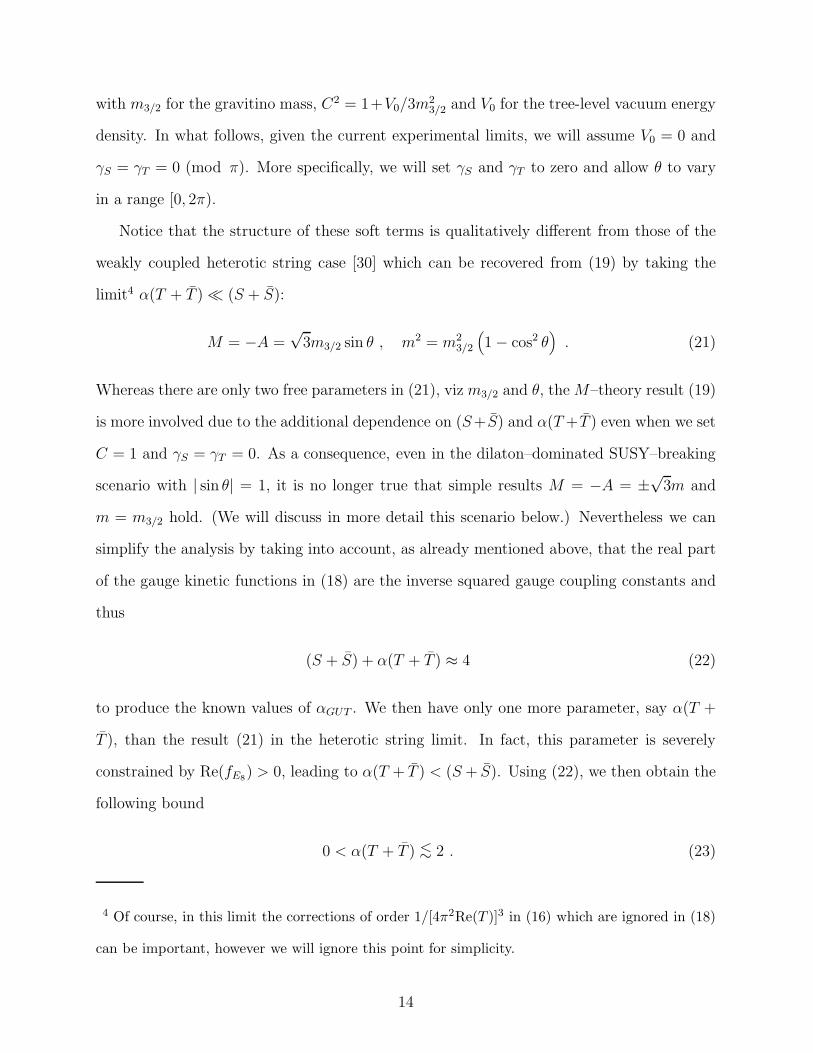
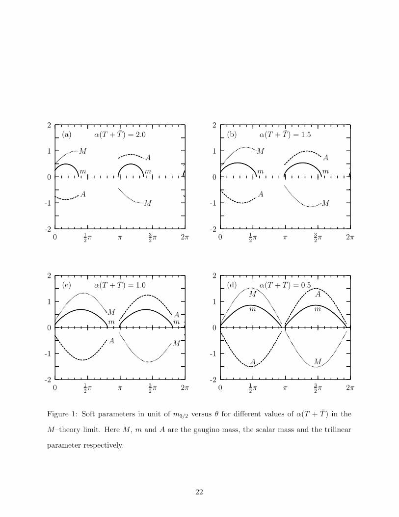
that Re(T ) should be of order one, we show in Fig. 1 the dependence on θ of the soft
terms M , m, and A in units of the gravitino mass for different values of α(T + T ). Several
comments are in order. First of all, some ranges of θ are forbidden by having a negative
scalar mass-squared. The figures clearly show that the smaller the value of α(T + T ), the
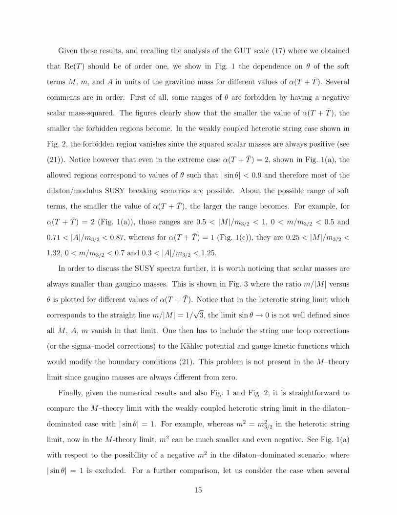
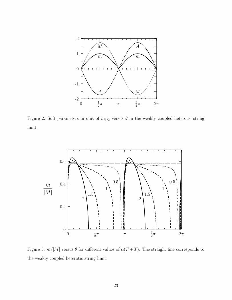
smaller the forbidden regions become. In the weakly coupled heterotic string case shown in
Fig. 2, the forbidden region vanishes since the squared scalar masses are always positive (see
(21)). Notice however that even in the extreme case α(T + T ) = 2, shown in Fig. 1(a), the
allowed regions correspond to values of θ such that | sin θ| < 0.9 and therefore most of the
dilaton/modulus SUSY–breaking scenarios are possible. About the possible range of soft
terms, the smaller the value of α(T + T ), the larger the range becomes. For example, for
α(T + T ) = 2 (Fig. 1(a)), those ranges are 0.5 < |M |/m3/2 < 1, 0 < m/m3/2 < 0.5 and
0.71 < |A|/m3/2 < 0.87, whereas for α(T + T ) = 1 (Fig. 1(c)), they are 0.25 < |M |/m3/2 <
1.32, 0 < m/m3/2 < 0.7 and 0.3 < |A|/m3/2 < 1.25.
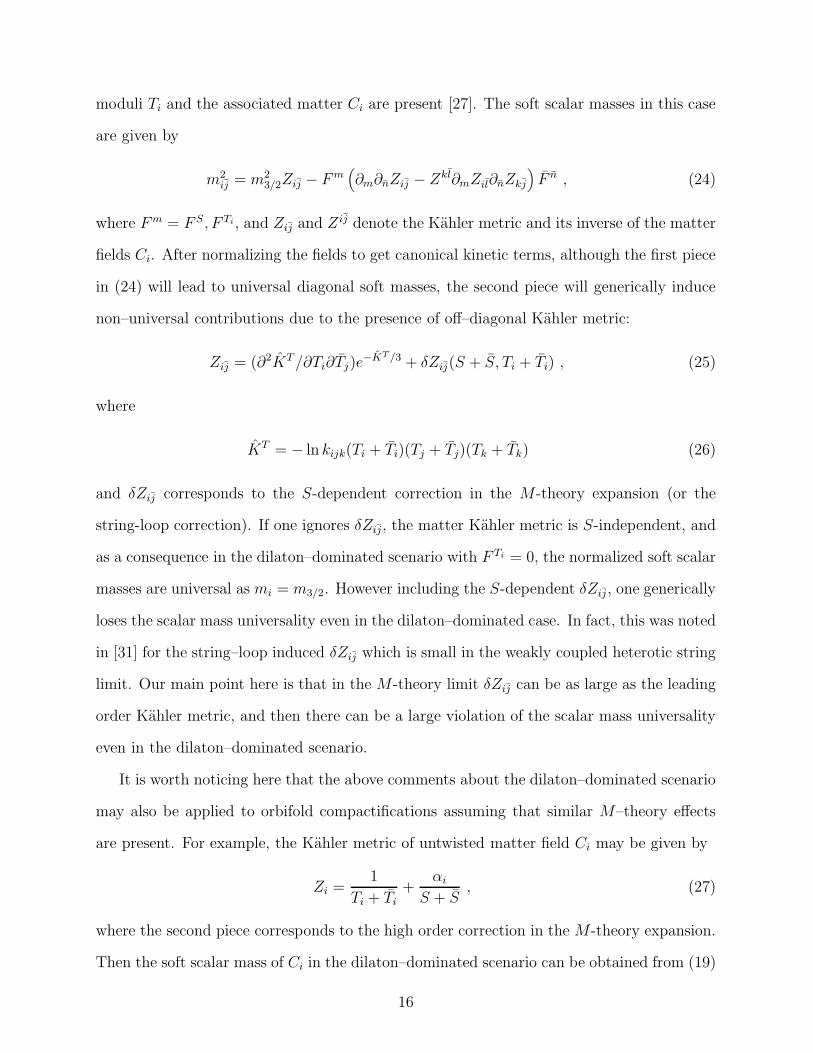
In order to discuss the SUSY spectra further, it is worth noticing that scalar masses are
always smaller than gaugino masses. This is shown in Fig. 3 where the ratio m/|M | versus
θ is plotted for different values of α(T + T ). Notice that in the heterotic string limit which
corresponds to the straight line m/|M | = 1/√
3, the limit sin θ → 0 is not well defined since
all M , A, m vanish in that limit. One then has to include the string one–loop corrections
(or the sigma–model corrections) to the Kahler potential and gauge kinetic functions which
would modify the boundary conditions (21). This problem is not present in the M–theory
limit since gaugino masses are always different from zero.
Finally, given the numerical results and also Fig. 1 and Fig. 2, it is straightforward to
compare the M–theory limit with the weakly coupled heterotic string limit in the dilaton–
dominated case with | sin θ| = 1. For example, whereas m2 = m23/2 in the heterotic string
limit, now in the M-theory limit, m2 can be much smaller and even negative. See Fig. 1(a)
with respect to the possibility of a negative m2 in the dilaton–dominated scenario, where
| sin θ| = 1 is excluded. For a further comparison, let us consider the case when several
15
moduli Ti and the associated matter Ci are present [27]. The soft scalar masses in this case
are given by
m2ij = m2
3/2Zij − F m(
∂m∂nZij − Zkl∂mZil∂nZkj
)
F n , (24)
where F m = F S, F Ti, and Zij and Z ij denote the Kahler metric and its inverse of the matter
fields Ci. After normalizing the fields to get canonical kinetic terms, although the first piece
in (24) will lead to universal diagonal soft masses, the second piece will generically induce
non–universal contributions due to the presence of off–diagonal Kahler metric:
Zij = (∂2KT /∂Ti∂Tj)e−KT /3 + δZij(S + S, Ti + Ti) , (25)
where
KT = − ln kijk(Ti + Ti)(Tj + Tj)(Tk + Tk) (26)
and δZij corresponds to the S-dependent correction in the M-theory expansion (or the
string-loop correction). If one ignores δZij, the matter Kahler metric is S-independent, and
as a consequence in the dilaton–dominated scenario with F Ti = 0, the normalized soft scalar
masses are universal as mi = m3/2. However including the S-dependent δZij, one generically
loses the scalar mass universality even in the dilaton–dominated case. In fact, this was noted
in [31] for the string–loop induced δZij which is small in the weakly coupled heterotic string
limit. Our main point here is that in the M-theory limit δZij can be as large as the leading
order Kahler metric, and then there can be a large violation of the scalar mass universality
even in the dilaton–dominated scenario.
It is worth noticing here that the above comments about the dilaton–dominated scenario
may also be applied to orbifold compactifications assuming that similar M–theory effects
are present. For example, the Kahler metric of untwisted matter field Ci may be given by
Zi =1
Ti + Ti+
αi
S + S, (27)
where the second piece corresponds to the high order correction in the M-theory expansion.
Then the soft scalar mass of Ci in the dilaton–dominated scenario can be obtained from (19)
16
with the substitution α(T + T ) → 3αi(Ti + Ti) and | sin θ| = 1, which shows clearly that the
scalar mass universality is lost. This is also true for αi = α since still the VEVs of the Ti’s
will be different in general.
Let us now discuss the predictions for the low–energy (≈ MW ) sparticle spectra in this
M–theory scenario. As is well known there are several particles whose masses are rather
independent of the details of SU(2)L × U(1)Y radiative breaking and are mostly given by
the boundary conditions and the renormalization group running [29]. In particular, that is
the case of the gluino g, all the sleptons l and first and second generation squarks q. Since,
as discussed above, always m < |M | at the GUT scale, the qualitative mass relations at the
electroweak scale in the M-theory scenario turn out to be
Mg ≈ mq > ml , (28)
where gluinos are slightly heavier than squarks. We recall that slepton masses are smaller
than squark masses because they do not feel the important gluino contribution in the renor-
malization. The precise values in (28) depend on the ratio r ≡ m/|M |:
Mg : mQL: muR
: mdR: mLL
: meR
≈ 1 :1
3
√7.6 + r2 :
1
3
√7.17 + r2 :
1
3
√7.14 + r2 :
1
3
√0.53 + r2 :
1
3
√0.15 + r2. (29)
For example for r = 1/√
3, which is always the case of the weakly coupled heterotic string
limit, one obtains 1 : 0.94 : 0.92 : 0.91 : 0.3 : 0.23, whereas for the extreme case of r = 0
the result is 1 : 0.92 : 0.89 : 0.88 : 0.24 : 0.13. Clearly, this type of analysis would allow
us to distinguish the M–theory limit from the weakly coupled heterotic string limit. If the
observed SUSY spectrum is inconsistent with the above results for r = 1/√
3, the M–theory
limit may be the answer. On the other hand, we see in Fig. 3 that r = 1/√
3 can be obtained
for particular values of θ in the M–theory limit also. Thus if the SUSY spectrum turns out to
be consistent with r = 1/√
3, one should analyze the rest of the SUSY mass spectra, taking
into account the details of the electroweak radiative breaking. This more detailed analysis
would allow us to distinguish clearly between both limits. To this respect, we note that even
17
for r which is close to 1/√
3, the pattern of soft terms in the M–theory limit significantly
differs from that in the heterotic string limit (see Figs. 1, 2). Although most of our analysis
has been made for the simple case that only S and one of the possible T -moduli participate
in SUSY breaking, this kind of analysis can be easily generalized to a more general case.
Acknowledgments: This work is supported in part by KAIST Basic Science Research
Program (KC), KAIST Center for Theoretical Physics and Chemistry (KC, HBK), KOSEF
through CTP of Seoul National University (KC), the KRF under the Distinguished Scholar
Exchange Program (KC), Basic Science Research Institutes Program BSRI-97-2434 (KC),
the KOSEF under the Brainpool Program (CM), and the CICYT under contract AEN97-
1678-E (CM).
18
REFERENCES
[1] P. Horava and E. Witten, Nucl. Phys. B460, 506 (1996); Nucl. Phys. B475, 94 (1996).
[2] P. Horava, Phys. Rev. D54, 7561 (1996).
[3] E. Witten, Nucl. Phys. B471, 135 (1996).
[4] T. Banks and M. Dine, Nucl. Phys. B479, 173 (1996).
[5] K. Choi, Phys. Rev. D56, 6588 (1997).
[6] E. Caceres, V. S. Kaplunovsky and I. M. Mandelberg, Nucl. Phys. B493, 73 (1997).
[7] E. Dudas and J. Mourad, Phys. Lett. B400, 71 (1997)
[8] T. Li, J. L. Lopez and D. V. Nanopoulos, Phys. Rev. D56 2602 (1997); “M-theory
Inspired No-scale Supergravity” CTP-TAMU-07/97, hep-ph/9702237.
[9] E. Dudas and C. Grojean, “Four-Dimensional M-theory and Supersymmetry Breaking”,
CERN-TH/97-79, hep-th/9704177.
[10] I. Antoniadis and M. Quiros, Phys. Lett. B392, 61 (1997); “Supersymmetry Breaking
in M-theory and Gaugino Condensation”, CERN-TH/97-90, hep-th/9705037; “On the
M-theory Description of Gaugino Condensation”, CERN-TH/97-165, hep-th/9707208.
[11] H. P. Nilles, M. Olechowski and M. Yamaguchi, “Supersymmetry Breaking and Soft
Terms in M-theory”, TUM-HEP-282/97, hep-th/9707143.
[12] Z. Lalak and S. Thomas, ”Gaugino Condensation, Moduli Potential and Supersymmetry
Breaking in M-theory Models”, QMW-PH-97-23, hep-th/9707223.
[13] E. Dudas, “Supersymmetry Breaking in M-theory and Quantization Rules”, CERN-
TH/97-236, hep-th/9709043.
[14] J. Ellis, A. E. Faraggi and D. V. Nanopoulos, “M-theory Model-Building and Proton
Stability”, CERN-TH-97/237, hep-th/9709049.
19
[15] A. Lukas, B. A. Ovrut and D. Waldram, “On the Four-Dimensional Effective Action of
Strongly Coupled Heterotic String Theory”, hep-th/9710208.
[16] M. Green, J. Schwarz and E. Witten, Superstring Theory (Cambridge University Press,
Cambridge, England, 1987).
[17] H. P. Nilles and S. Stieberger, “String-Unification, Universal One-Loop Corrections and
Strongly Coupled Heterotic String Theory”, hep-th/9702110.
[18] This was noted by H. P. Nilles, Phys. Lett. B180, 240 (1986) for the heterotic string
loop and sigma model expansion of the 4–dimensional effective action.
[19] K. Choi and J. E. Kim, Phys. Lett. B165, 71 (1985).
[20] L. E. Ibanez and P. Nilles, Phys. Lett. B169, 354 (1986); J. P. Derendinger, L. E. Ibanez
and H. P. Nilles, Nucl. Phys. B267, 365 (1986).
[21] J.P. Derendinger, S. Ferrara, C. Kounnas and F. Zwirner, Nucl. Phys. B372, 145 (1992);
Phys. Lett. B271, 307 (1991);
[22] D. Lust and C. Munoz, Phys. Lett. B279, 272 (1992).
[23] I. Antoniadis, E. Gava, K.S. Narain and T.R. Taylor, Nucl. Phys. B432, 187 (1994).
[24] K. Choi, Z. Phys. C39, 219 (1988).
[25] A. Klemm and S. Theisen, Nucl. Phys. B389, 153 (1993).
[26] A. Font, Nucl. Phys. B391, 358 (1993).
[27] H.B. Kim and C. Munoz, Z. Phys. C75, 367 (1997).
[28] S.K. Soni and H.A. Weldon, Phys. Lett. B126, 215 (1983).
[29] For a recent review, see A. Brignole, L.E. Ibanez and C. Munoz, “Soft Supersymmetry–
Breaking Terms from Supergravity and Superstring Models”, FTUAM 97/7, hep-
ph/9707209.
20
[30] A. Brignole, L. E. Ibanez and C. Munoz, Nucl. Phys. B422, 125 (1994).
[31] J. Louis and Y. Nir, Nucl. Phys. B447, 18 (1995).
21
0 12π π 3
2π 2π
-2
-1
0
1
2
.....................................................................................................................................................................................................................................................................................................................................................................................................................................................................................................................
(a) α(T + T ) = 2.0
M
m
AM
m
A..........
............
.......................
.................................................................................................................................. ................
...........................................
................................................................................................ ...........................
............................................................
.............................................................
......
0 12π π 3
2π 2π
-2
-1
0
1
2
.....................................................................................................................................................................................................................................................................................................................................................................................................................................................................................................................
(b) α(T + T ) = 1.5
M
m
AM
m
A..................
.................
....................................
................................................
.................................................................................................................................... ................................................................
..................................................................................................................................... ...................
.................................................................................................
............................................
........................................................
...
0 12π π 3
2π 2π
-2
-1
0
1
2
.....................................................................................................................................................................................................................................................................................................................................................................................................................................................................................................................
(c) α(T + T ) = 1.0
Mm
A M
mA
..........................
...............................
..........................................................
......................................................................
...................................................................................................................................................................................... .............................................................................................
......................................................................................................................................................................... ...........
......................................................................................................................................................................
..............................................................................
..........................................................................................
...
0 12π π 3
2π 2π
-2
-1
0
1
2
.....................................................................................................................................................................................................................................................................................................................................................................................................................................................................................................................
(d) α(T + T ) = 0.5M
m
A M
m
A
.................................
.........................................................................................
..............................
.....................................................................................................................
....................................................................................................................................................................................... ................................................................................................................
.................................................................................................................................................................................................. ............................................................................................................................................................................................................................................................................................................................................
...........................................................................................................................
Figure 1: Soft parameters in unit of m3/2 versus θ for different values of α(T + T ) in the
M–theory limit. Here M , m and A are the gaugino mass, the scalar mass and the trilinear
parameter respectively.
22
0 12π π 3
2π 2π
-2
-1
0
1
2
.....................................................................................................................................................................................................................................................................................................................................................................................................................................................................................................................
M
m
A M
m
A
.............................................................................................................................................
........................................................
...............................................................................................................
............................................................................................................................................................................................................................................................................................................................................
............................................................................................................................................................................................................................................................................................................................................................................................................................................................................................................................................................................................................
.................................................................................................................................................
Figure 2: Soft parameters in unit of m3/2 versus θ in the weakly coupled heterotic string
limit.
0 12π π 3
2π 2π
0
0.2
0.4
0.6
m
|M |
..........................................................................................................................................................................................................................................................................................................................................................................................................................................................................................................................................................................................................................
..
..
..
..
...
...
....
.............................................................................................................................................................. ..
..
..
...
...
...
...
....
....
.....
.......
...
...
...
..........
.....
....
...
..
..
..
..
..
.............................................................................................................................................
..........
..
..........
...........
............
.......................................................................................................................................................................................................................................................................................................................................................................... .............................
...............
.............
..........
..........
...........
...........
...........
...........
...........
..........
.
..........
.
.........
..
..........
..
..........
...........
............
.......................................................................................................................................................................................................................................................................................................................................................................... .............................
...............
.............
..........
..........
...........
...........
...........
...........
...........
..........
.
..........
.
.........
..
..................................................................................................................................................................................................................................................................................................................................................................................................... ............
............
...........
.......
...........
.......
............
...........
.......
...........
........
...........
...........
.......
...................................
.......
........
.....
.....
......
............
...........
.......
...........
............................................................................................................................................................................................................................................................................................................................................................ ............
............
...........
.......
...........
.......
............
...........
.......
...........
........
...........
...........
.......
...................................
.......
........
.....
.....
......
..
................
...............
.............................................................................................................................................................................................................................................................................................................................................................................................................................................................................................................................................................................................. ................
...............
...............
...............
...............
................
................
...............
...............
................
...............
...............
...............
................
...............
.................
..................
................
...............
..............
..............
..............
...............
.................
.................
...............
................................................................................................................................................................................................................................................................................................................................................................................................................................................................................................................................................................................................... ................
...............
...............
...............
...............
................
................
...............
...............
................
...............
...............
...............
................
...............
.................
..................
................
...............
..............
..............
..............
...............
.................
......
21.5
1
0.5
21.5
1
0.5
Figure 3: m/|M | versus θ for different values of α(T + T ). The straight line corresponds to
the weakly coupled heterotic string limit.
23