arX

iv:c

ond-

mat

/030

1608

v2 [

cond

-mat

.mes

-hal

l] 1

1 Ju

n 20

03

Formulae for zero-temperature ondu tan e through a region with intera tion

T. Reje

1and A. Ram²ak

1,2

1Joºef Stefan Institute, Jamova 39, SI-1000 Ljubljana, Slovenia

2Fa ulty of Mathemati s and Physi s, University of Ljubljana, Jadranska 19, SI-1000 Ljubljana, Slovenia

The zero-temperature linear response ondu tan e through an intera ting mesos opi region at-

ta hed to nonintera ting leads is investigated. We present a set of formulae expressing the ondu -

tan e in terms of the ground-state energy or persistent urrents in an auxiliary system, namely a

ring threaded by a magneti ux and ontaining the orrelated ele tron region. We rst derive the

ondu tan e formulae for the nonintera ting ase and then give arguments why the formalism is

also orre t in the intera ting ase if the ground state of a system exhibits Fermi liquid properties.

We prove that in su h systems, the ground-state energy is a universal fun tion of the magneti ux,

where the ondu tan e is the only parameter. The method is tested by omparing its predi tions

with exa t results and results of other methods for problems su h as the transport through sin-

gle and double quantum dots ontaining intera ting ele trons. The omparisons show an ex ellent

quantitative agreement.

I. INTRODUCTION

The measurements of the ondu tivity and the ele -

tron transport in general are one of the most dire t and

sensitive probes in solid state physi s. In su h measure-

ments many interesting new phenomena were signaled,

in parti ular super ondu tivity, transport in metals with

embedded magneti impurities and the related Kondo

physi s, heavy fermion phenomena and the physi s of the

Mott-Hubbard transition regime. In the last de ade te h-

nologi al advan es enabled ontrolled fabri ation of small

regions onne ted to leads and the ondu tan e, relating

the urrent through su h a region to the voltage applied

between the leads, also proved to be a relevant property

of su h systems. There is a number of su h examples, e.g.

metalli islands prepared by e-beam lithography or small

metalli grains

1

, semi ondu tor quantum dots

2

, or a sin-

gle large mole ule su h as a arbon nanotube or DNA. It

is possible to break a metalli onta t and measure the

transport properties of an atomi -size bridge that forms

in the break

3

, or even measure the ondu tan e of a single

hydrogen mole ule, as reported re ently in Ref.

4

. In all

su h systems, strong ele tron orrelations are expe ted

to play an important role.

The transport in nonintera ting mesos opi systems

is theoreti ally well des ribed in the framework of the

Landauer-Büttiker formalism. The ondu tan e is deter-

mined with the Landauer-Büttiker formula

57

, where the

key quantity is the single parti le transmission amplitude

t(ε) for ele trons in the vi inity of the Fermi energy. The

formula proved to be very useful and reliable, as long as

ele tron-ele tron intera tion in a sample is negligible.

Although the Landauer-Büttiker formalism provides a

general des ription of the ele tron transport in noninter-

a ting systems, it normally annot be used if the intera -

tion between ele trons plays an important role. Several

approa hes have been developed to allow one to treat also

su h systems. First of all, the Kubo formalism provides

us with a ondu tan e formula whi h is appli able in the

linear response regime and has, for example, been used

to al ulate the ondu tan e in Refs.

8,9

. A mu h more

general approa h was developed by Meir and Wingreen

in Ref.

10

. Within the Keldysh formalism they manage

to express the ondu tan e in terms of nonequilibrium

Green's fun tions for the sample part of the system. The

formalism an be used to treat systems at a nite sour e-

drain voltage and an also be extended to des ribe time-

dependent transport phenomena

11

. The main theoreti al

hallenge in these approa hes is to al ulate the Green's

fun tion of a system. Ex ept in some rare ases where

exa t results are available, perturbative approa hes or

numeri al renormalization group studies are employed.

In this paper we propose an alternative method for

al ulating the ondu tan e through su h orrelated sys-

tems. The method is appli able only to a ertain lass of

systems, namely to those exhibiting Fermi liquid prop-

erties, at zero temperature and in the linear response

regime. However, in this quite restri tive domain of va-

lidity, the method promises to be easier to use than the

methods mentioned above. We show that the ground-

state energy of an auxiliary system, formed by onne ting

the leads of the original system into a ring and threaded

by a magneti ux, provides us with enough informa-

tion to determine the ondu tan e. The main advantage

of this method is the fa t that it is often mu h easier

to al ulate the ground-state energy (for example, using

variational methods) than the Green's fun tion, whi h

is needed in the Kubo and Keldysh approa hes. The

ondu tan e of a Hubbard hain onne ted to leads was

studied re ently using a spe ial ase of our method and

DMRG

12,13

and a spe ial ase of our approa h was ap-

plied in the Hartree-Fo k analysis of anomalies in the

ondu tan e of quantum point onta ts

14

. The method

is related to the study of the harge stiness and persis-

tent urrents in one-dimensional systems

1518

.

The paper is organized as follows. In Se tion II we

present the model Hamiltonian for whi h the method is

appli able. In Se tion III we derive general formulae for

the zero-temperature ondu tan e through a mesos opi

region with nonintera ting ele trons onne ted to leads.

In Se tion IV we extend the formalism to the ase of in-

2

tera ting ele trons. We give arguments why the formal-

ism is orre t as long as the ground state of the system

exhibits Fermi liquid properties. In Se tion V onver-

gen e tests for a typi al nonintera ting system are rst

presented. Then we support our formalism also with nu-

meri al results for the ondu tan e of some non-trivial

problems, su h as the transport through single and dou-

ble quantum dots ontaining intera ting ele trons and

onne ted to nonintera ting leads. These omparisons,

in luding the omparison with the exa t results for the

Anderson model, demonstrate a good quantitative agree-

ment. After the on lusions in Se tion VI we present

some more te hni al details in Appendix A. In Appendix

B we des ribe the numeri al method used in Se tion V.

II. MODEL HAMILTONIAN

sample

n n’

left lead right lead

Figure 1: S hemati pi ture of the system des ribed by Hamil-

tonian (1).

In this Se tion we introdu e a general Hamiltonian de-

s ribing a mesos opi sample oupled to leads as shown

in Fig. 1. The Hamiltonian is a generalization of the well

known Anderson impurity model

19

. We split the Hamil-

tonian into ve pie es

H = HL + VL +HC + VR +HR, (1)

whereHC models the entral region,HL andHR des ribe

the left and the right lead, and VL and VR are the tunnel-

ing ouplings between the leads and the entral region.

We an also split the Hamiltonian into a term H(0)de-

s ribing independent ele trons and a term U des ribing

the Coulomb intera tion between them

H = H(0) + U. (2)

One an often negle t the intera tion in the leads and

between the sample and the leads. We assume this is

the ase. Then the entral region is the only part of the

system where one must take the intera tion into a ount

HC = H(0)C + U. (3)

Here H(0)C des ribes a set of nonintera ting levels

H(0)C =

∑

i,j∈Cσ

H(0)Cjid

†jσdiσ , (4)

where d†iσ (diσ) reates (destroys) an ele tron with spin

σ in the state i. The states introdu ed here an have

various physi al meanings. They ould represent the

true single-ele tron states of the sample, for example dif-

ferent energy levels of a multi-level quantum dot or a

mole ule. In this ase, the matrix H(0)Cji is diagonal and

its elements are the single-ele tron energies of the sys-

tem. Another possible interpretation of Hamiltonian (4)

is that the states i are lo al orbitals at dierent sites ofthe system. In this ase, the diagonal matrix elements

of H(0)C are the on-site energies for these sites, while the

o-diagonal matrix elements des ribe the oupling be-

tween dierent sites of the system. The sites ould have

a dire t physi al interpretation, su h as dots in a dou-

ble quantum dot system or atoms in a mole ule, or they

ould represent titious sites obtained by dis retization

of a ontinuous system. There are other possible hoi es

of basis states for the entral region. For example, in a

system onsisting of two multi-level quantum dots one

ould use single-ele tron basis states for ea h of the dots

and des ribe the oupling between the dots with tunnel-

ing matrix elements.

The Coulomb intera tion between ele trons in the sam-

ple is given by an extended Hubbard-type oupling

U =1

2

∑

i,j∈C

σ,σ′

Uσσ′

ji njσniσ′ , (5)

where niσ = d†iσdiσ is the operator ounting the number

of ele trons with spin σ at site i. For onvenien e, we

wrote down only the expression for the Coulomb inter-

a tion in the ase, where basis states represent dierent

sites in real spa e. The expression be omes more om-

pli ated if a more general basis set is used.

We des ribe the leads or onta ts as two semi-innite,

tight-binding hains

HL(R) = −t0∑

i,i+1∈L(R)σ

c†iσci+1σ + h.c., (6)

where c†iσ (ciσ) reates (destroys) an ele tron with spin

σ on site i and t0 is the hopping matrix element between

neighboring sites. Su h a model adequately, at least for

energies low or omparable to t0, des ribes a nonintera t-ing, single-mode and homogeneous lead. It would be easy

to generalize the lead Hamiltonian to des ribe a more

realisti system, for example by modeling the true ge-

ometry or allowing for a self- onsistent potential due to

intera tion between ele trons. However, the physi s we

are interested in, is usually not hanged dramati ally by

not in luding these details into the model Hamiltonian

and therefore, we will not dis uss this issue into detail.

Finally, there is a term des ribing the oupling between

the sample and the leads,

VL(R) =∑

j∈L(R)i∈C

σ

VL(R)jic†jσdiσ + h.c., (7)

3

where VL(R)ji is the hopping matrix element between

state i in the sample and site j in a lead.

sample

Φ

i

0

0

i +1

Figure 2: The sample embedded in a ring formed by joining

the left and right leads of the system in Fig. 1. Magneti ux

Φ penetrates the ring.

In the following Se tions we dis uss the ondu tan e

through the system introdu ed above. To derive the on-

du tan e formulae, we will need a slightly modied sys-

tem. This auxiliary system is a ring formed by onne ting

the ends of the left and right leads of the original system

as shown in Fig. 2. The ring is threaded by a magneti

ux Φ in su h a way that there is no magneti eld in the

region where ele trons move. We an then perform the

standard Peierls substitution

20

and transform the hop-

ping matrix elements of the Hamiltonian (1) a ording

to

tji → tjiei e

~

∫ xjxi

A·dx, (8)

where xi is the position of site i and A is the ve tor

potential due to the ux, obeying

Φ =~

eφ =

∮

A · dx. (9)

Here we dened a dimensionless magneti ux φ. The

energy of the system is periodi in φ with a period of 2πand depends only on value of φ and not on any details of

how the ux is produ ed. If the original Hamiltonian (1)

obeys the time-reversal symmetry, the energy does not

hange if the magneti eld is reversed,

E (−φ) = E (φ) . (10)

III. CONDUCTANCE OF A

NONINTERACTING SYSTEM

In this Se tion we limit the dis ussion to nonintera t-

ing systems, i.e. we set U = 0 in Eq. (2). In su h systems,

the Landauer-Büttiker formula

57

G = G0 |t (εF )|2 , (11)

whi h relates the zero-temperature ondu tan e G to

the transmission probability |t (εF )|2 for ele trons at the

Fermi energy ǫF , an be applied. The proportionality

oe ient, G0 = 2e2

h , is the quantum of ondu tan e.

Below we rst derive a set of formulae, whi h relate the

transmission probability, and onsequently the ondu -

tan e, to single-ele tron energy levels of the auxiliary ring

system introdu ed in the previous Se tion. Then we de-

rive another set of formulae, relating the ondu tan e to

the ground-state energy of the auxiliary system. One of

these formulae was derived before in Ref.

14

, and a limit-

ing ase of another one was dis ussed in Refs.

12,13

. Here

we present a unied approa h to the problem, from whi h

these results emerge as spe ial ases.

A. Formulae relating ondu tan e to

single-ele tron energy levels

Let us onsider eigenstates of an ele tron moving on a

ring system introdu ed in the previous Se tion. We will

be interested only in energies of these states and not in

the pre ise form of wavefun tions. The energy of an ele -

tron on a ring penetrated by a magneti ux φ depends

only on the magnitude of the ux and therefore, any ve -

tor potential fullling ondition (9) is good for our pur-

pose. We hoose a ve tor potential onstant everywhere

ex ept between sites i0 and i0+1, both in the lead part of

the ring as shown in Fig. 2. The hopping matrix element

between the two sites is thus modied to t0eiφ. With

no ux penetrating the ring, the ele tron's wavefun tion

in the lead part of the system is aeiki + be−iki, where k

is the ele tron's waveve tor and a and b are amplitudes

determined by properties of the entral region. If there

is a ux through the ring, the wavefun tion is modied.

The S hrödinger equations for sites i0 and i0 + 1 show

us that the appropriate form is aeiki + be−ikifor i ≤ i0

and ae−iφeiki + be−iφe−ikifor i > i0. The s attering

matrix of the entral region provides a relation between

oe ients a and b,(

be−iφeikN

a

)

=

(

rk t′ktk r′k

)(

ae−iφe−ikN

b

)

. (12)

The elements of the s attering matrix, tk and rk (t′k and

r′k), are the transmission and ree tion amplitudes for

ele trons oming from the left (right) lead, and N is the

number of sites in the lead part of the ring. We added

phase fa tors e±ikNto the left lead amplitudes to om-

pensate for the phase dieren e an ele tron a umulates

as it travels through the lead part of the ring. The s at-

tering matrix dened this way does not depend on Nand φ, and equals the s attering matrix of the original,

two-lead system. Eq. (12) is a homogeneous system of

linear equations, solvable only if the determinant is zero.

Using the unitarity property of the s attering matrix, the

eigenenergy ondition be omes

t′keiφ + tke

−iφ = eikN +tkt′∗ke−ikN . (13)

4

We assume the Hamiltonian of the original, two lead sys-

tem obeys the time-reversal symmetry and therefore, the

s attering matrix is symmetri

21

, tk = t′k. Expressing

the transmission amplitude in terms of its absolute value

and the s attering phase shift tk = |tk| eiϕk, we arrive at

the nal form of the eigenenergy equation

|tk| cosφ = cos (kN − ϕk) . (14)

In Fig. 3 a graphi al representation of this equation is

presented.

0 π/3k−1

0

1

Figure 3: A graphi al representation of the eigenvalue equa-

tion (14). The shaded region represents the allowed values

of the left hand side of the equation for dierent values of

magneti ux (for example, the dashed line shows the values

for φ =π

4). The full line represents the right hand side of

the eigenvalue equation. The system is presented in Fig. 7,

N = 100.

To extra t the transmission probability |tk|2, we pro-

eed by dierentiating the eigenvalue equation with re-

spe t to cosφ

∂ |tk|∂ cosφ

cosφ+ |tk| =

= − sin (kN + ϕk)

(

N∂k

∂ cosφ+

∂ϕk

∂ cosφ

)

=

= ±√

1 − |tk|2 cos2 φ

(

N∂k

∂ cosφ+

∂ϕk

∂ cosφ

)

. (15)

The sign of the last expression depends on weather kbelongs to a de reasing (+) or an in reasing (−) bran hof the osine fun tion in Eq. (14), or equivalently, if we

are interested in an eigenstate with odd (+) or even (−)n, where n indexes the eigenstates from the one with the

lowest energy upward. Let us hoose an eigenstate and

onsider how the orresponding waveve tor k hanges as

the magneti ux φ is varied from 0 to π. It is evident

that the variation in k is of the order of

1N as the osine

fun tion in the right hand side of Eq. (14) os illates with

su h a period. Let as assume that the number of sites

in the ring is large enough that transmission amplitude

does not hange appre iably in this interval

∣

∣

∣

∣

∂tk∂k

∣

∣

∣

∣

π

N≪ 1. (16)

Then the derivatives

∂k∂ cos φ ,

∂|tk|∂ cos φ and

∂ϕk

∂ cos φ are of the

order of

1N and Eq. (15) simplies to

|tk| = ±√

1 − |tk|2 cos2 φN∂k

∂ cosφ+ O

(

1

N

)

. (17)

Introdu ing the density of states in the leads ρ (ε) =1π

∂k∂ε , whi h for example, for a tight-binding lead with

only nearest-neighbor hopping t0 and dispersion εk =−2t0 cos k equals 1/

(

π√

4t20 − ε2k)

, we nally obtain

∂ arccos (∓ |t (εk)| cosφ)

∂ cosφ= πNρ (εk)

∂εk

∂ cosφ, (18)

where t (εk) = tk. The ondition Eq. (16) of validity an

also be expressed in a form involving energy as a variable

N ≫ 1

ρ (ε)

∣

∣

∣

∣

∂t (ε)

∂ε

∣

∣

∣

∣

. (19)

Eq. (18) is the entral result of this work. It expresses the

transmission probability |t (ε)|2 of a sample onne ted

to two leads in terms of the variation of single-ele tron

energy levels with magneti ux penetrating the auxiliary

ring system. Employing the Landauer-Büttiker formula

Eq. (11), this result also provides the zero-temperature

ondu tan e of the system. From the derivation it is

evident that the method be omes exa t as we approa h

the thermodynami limit N → ∞.

In general Eq. (18) has to be solved numeri ally to

obtain the transmission probability on a dis rete set of

energy points, one for ea h energy level of a system. By

in reasing the system size N , the density of these points

in reases and the errors de rease, as the ondition (19) is

fullled better. We will return to this point in Se tion V

where we onsider the onvergen e issues in detail. Here

we present some spe ial ases of Eq. (18) where analyti

expressions an be obtained. By averaging the equation

over values of ux φ between φ = 0 and φ = π (note

that we may treat |t (εk)| and ρ (εk) as onstant while

averaging as the resulting error is of the order of

1N ),

we an relate the transmission probability to the average

magnitude of the derivative of a single-ele tron energy

with respe t to the ux:

|t (εk)|2 = sin2

(

π2

2Nρ (εk)

∣

∣

∣

∣

∂εk

∂φ

∣

∣

∣

∣

)

. (20)

Note that it is enough to al ulate the energy levels at

φ = 0 and φ = π to al ulate the transmission proba-

bility as |∂εk/∂φ| = 1π |εk (π) − εk (0)|. In Fig. 4(a) it is

illustrated how a large variation of single-ele tron energy

as the ux is hanged from φ = 0 to φ = π orresponds

to a large ondu tan e and vi e versa. The transmission

probability an also be al ulated from the derivative at

φ = π2 resulting in the se ond formula

|t (εk)|2 =

(

πNρ (εk)∂εk

∂φ

∣

∣

∣

∣

φ= π2

)2

. (21)

5

Again, Fig. 4(a) shows that there is a orresponden e

between a large sensitivity of a single-ele tron energy to

the ux at φ = π2 , and a large ondu tan e. Finally, we

observe that the urvature of energy levels at φ = 0 and

φ = π also gives information of ondu tan e. The third

formula reads

|t (εk)|2 = 1 − 1

1 +

(

πNρ (εk) ∂2εk

∂φ2

∣

∣

∣

φ=0,π

)2 . (22)

−π

−π/2

0

π/2

π

φ

−2 −1ε

0

1

|t|

(a)

−π/2 0 π/2 π 3π/2φ

−0.25

0.00

0.25

0.50

0.75

Nρ(

ε F)[

E(φ

)−E

(π/2)

]

−π/2 0 π/2 π 3π/2φ

−0.25

0.00

0.25

0.50

0.75

Nρ(

ε F)[

E(φ

)−E

(π/2)

]

(b) (c)

|t| = 0

|t| = 1

|t| = 1

|t| = 0

Figure 4: (a) Single-ele tron energy levels (full lines) and the

ground-state energies when a given single-ele tron level is at

the Fermi energy (dashed lines). Ground-state energies are

shifted so that both urves oin ide for φ =π

2. Note that

the energy urves are symmetri about φ = 0 as required by

Eq. (10). The shaded area represents the magnitude of the

transmission amplitude. The system and the energy interval

is the same as in Fig. 3. (b, ) The large N universal form of

the ground-state energy vs. ux urve for an even (b) and an

odd ( ) number of ele trons in a system. The magnitude of

the transmission amplitude goes from 0 to 1 in steps of 0.1.

B. Formulae relating ondu tan e to the

ground-state energy

Above we showed how the ux variation of the en-

ergy of the last o upied single-ele tron state allows one

to al ulate the zero-temperature ondu tan e through

a nonintera ting sample. The goal of this se tion is to

derive an alternative set of formulae, expressing the zero-

temperature ondu tan e in terms of the ux variation

of the ground-state energy E, whi h for an even num-

ber of ele trons in a nonintera ting system is simply a

sum of single-ele tron energies up to the Fermi energy

εF , multiplied by 2 be ause of the ele tron's spin

E = 2∑

εn≤εF

εn. (23)

We will show that the transmission probability at the

Fermi energy |t (εF )|2 is related to the ground-state en-

ergy of the ring system

1

π

∂ arccos2 (∓ |t (εF )| cosφ)

∂ cosφ= πNρ (εF )

∂E

∂ cosφ, (24)

where the sign is − and + for an odd and an even num-

ber of o upied single-ele tron states, respe tively. The

expression Eq. (24) is evidently orre t if there are no

ele trons in the system, as it gives a zero ondu tan e in

this ase. To prove the formula for other values of the

Fermi energy, we use the prin iple of the mathemati al

indu tion. To simplify the notation we introdu e

fs (εn) = N∂εn

∂ cosφ=

1

πρ (εn)

∂ arccos (s |t (εn)| cosφ)

∂ cosφ,

(25)

Fs (εn) = N∂En

∂ cosφ=

1

π2ρ (εn)

∂ arccos2 (s |t (εn)| cosφ)

∂ cosφ,

(26)

where En is the ground-state energy of a system with

the Fermi energy at εn and s is either 1 or −1, depend-ing on the signs in Eqs. (18) and (24). Dierentiating the

relation En = En−1 + 2εn with respe t to cosφ, express-ing the result in terms of fun tions fs and Fs introdu ed

above, and making use of the fa t that the sign s alter-nates with n, we obtain

Fs (εn) = F−s (εn−1) + 2fs (εn) . (27)

If we manage to show that this really is an identity, we

have a proof of Eq. (24). Using the exa t relation Fs (ε)−F−s (ε) = 2fs (ε), the expression transforms into

Fs (εn) = Fs (εn) − [F−s (εn) − F−s (εn−1)] . (28)

For a large number of sites N in the ring and orre-

spondingly, a small separation of single-ele tron energy

levels whi h is of the order of

1N , the term in parenthe-

sis equals F ′−s (εn) (εn − εn−1). F

′−s (εn) an be fa tored

into sF (εn) where F (εn) does not depend on sign s.Therefore, although the term in parenthesis in of the or-

der of

1N , its sign alternates for su essive energy levels

while its amplitude stays the same. Thus the error in-

du ed by this term does not a umulate, it just adds an

additional error of the order of

1N to the nal result.

In Fig. 4(a), the variation of the ground-state energies

with magneti ux is ompared to the variation of the

orresponding single-ele tron energies. Note that as a

onsequen e of Eq. (24), the ground-state energy in the

large N limit takes a universal form (see Fig. 4(b))

6

E (φ) − E(π

2

)

=

=1

π2Nρ (εF )

(

arccos2 (∓ |t (εF )| cosφ) − π2

4

)

. (29)

For systems with an odd number of ele trons, the ground-

state energy is obtained by adding a single-ele tron en-

ergy orresponding to Eq. (18) and the universal form

reads (see Fig. 4( ))

E (φ) − E(π

2

)

=1

π2Nρ (εF )arcsin2 (|t (εF )| cosφ) .

(30)

In general, Eq. (24) an only be solved numeri ally

to obtain the transmission probability. However, as was

the ase for single-ele tron energies, analyti solutions

an be found in ertain spe ial ases. The derivative of

the ground-state energy with respe t to ux gives the

persistent urrent in the ring j = e~

∂E∂φ

22,23

. Using the

Landauer-Büttiker formula Eq. (11), one an al ulate

the ondu tan e from the ux averaged magnitude of the

persistent urrent in the system

|t (εF )|2 = sin2

(

π2~

2eNρ (εF ) |j (φ)|

)

. (31)

Only two ground-state energy al ulations need to be

performed to obtain the ondu tan e as

~

e |j (φ)| =1π |E (π) − E (0)|. This formula was also dis ussed in

Refs.

12,13

for the ase where the transmission probability

is small. The se ond formula relates the ondu tan e to

the persistent urrent at φ = π214,24

,

|t (εF )|2 =

(

π~

eNρ (εF ) j

(π

2

)

)2

. (32)

The third formula, orresponding to Eq. (22) in the

single-ele tron ase, turns out to be more ompli ated

and gives an impli it relation for |t (εF )|

πNρ (εF )∂2E

∂φ2

∣

∣

∣

∣

min,max

=

= ± 2 |t (εF )|

π

√

1 − |t (εF )|2arccos (± |t (εF )|) . (33)

Here the upper and the lower signs orrespond to the se -

ond derivative at a minimum and at a maximum of the

energy vs. ux urve, respe tively. Minima (maxima)

o ur at φ = 0 (π) if an odd number of single-ele tron

levels is o upied and at φ = π (0) if an even number of

levels is o upied. The se ond derivative in a minimum is

proportional to the harge stiness D = N2 ∂2E/∂φ2

∣

∣

min

of the system

18,25

. We an also dene the orresponding

quantity for a maximum as D = −N2 ∂2E/∂φ2

∣

∣

max. In

general, Eq. (33) has to be solved numeri ally. However,

in the limit of a very small ondu tan e and in the vi in-

ity of the unitary limit, additional analyti formulae are

valid

|t (εF )| =

2πρ (εF )D, |t (εF )| → 0,12 + 3π

4 2πρ (εF )D, |t (εF )| → 1.(34)

Note that there is a quadrati relation between the on-

du tan e and the harge stiness in the low ondu tan e

limit. The orresponding formulae for the maximum of

the energy vs. ux urve are

|t (εF )| =

2πρ (εF ) D, |t (εF )| → 0,1 − 2

(2πρ(εF )D)2 , |t (εF )| → 1. (35)

A detailed analysis of onvergen e properties of the for-

mulae derived in this Se tion is presented Se tion V.

We stress again that the validity of these formulae

is based on an assumption that the number of sites in

the ring is su iently large a ording to the ondition

Eq. (19). This means that if t(ε) exhibits sharp reso-

nan es, the al ulation has to be performed on su h a

large auxiliary ring system that in the energy interval

of interest (the width of the resonan e) there is a large

number of eigenenergies εn. Then t(ε) ∼ t(εn′), whereεn′

is the eigenenergy losest to ε. Su h sharp resonan es

in t(ε) are expe ted e.g. in haoti systems

26,27

. The

present method might be impra ti al (but still orre t)

in this ase.

IV. CONDUCTANCE OF AN INTERACTING

SYSTEM

The zero-temperature ondu tan e of a nonintera t-

ing system an thus be determined with the transmission

probability obtained from one of the formulae we derived

in the previous Se tion, and the Landauer-Büttiker for-

mula. The main hallenge, however, remains the ques-

tion of the validity of this type of approa h for intera t-

ing systems. In this Se tion we give arguments why the

approa h is orre t for a lass of intera ting systems ex-

hibiting Fermi liquid properties. In order to rea h this

goal, we present four essential steps as follows.

Step 1: Condu tan e of a Fermi liquid system at

T = 0

The basi property that hara terizes Fermi liquid

systems

28

is that the states of a nonintera ting system of

ele trons are ontinuously transformed into states of the

intera ting system as the intera tion strength in reases

from zero to its a tual value. One an then study the

properties of su h a system by means of the perturba-

tion theory, regarding the intera tion strength as the per-

turbation parameter. The on ept of the Fermi liquid

was rst introdu ed for translation-invariant systems by

7

Landau

29,30

, and was later also extended to systems of

the type we study here

31

.

The linear response ondu tan e of a general intera t-

ing system of the type shown in Fig. 1 an be al ulated

from the Kubo formula

9,32

G = limω→0

ie2

ω + iδΠII (ω + iδ) , (36)

where ΠII (ω + iδ) is the retarded urrent- urrent orre-

lation fun tion

ΠII (t− t′) = −iθ (t− t′) 〈[I (t) , I (t′)]〉 . (37)

For Fermi liquid systems at T = 0, the urrent- urrent

orrelation fun tion an be expressed in terms of the

Green's fun tion Gn′n (z) of the system and the ondu -

tan e is given with

9

G =2e2

h

∣

∣

∣

∣

1

−iπρ (εF )e−ikF (n′−n′)Gn′n (εF + iδ)

∣

∣

∣

∣

2

, (38)

where n and n′are sites in the left and the right lead,

respe tively. One an dene the transmission amplitude

as

t (ε) ≡ 1

−iπρ (ε)e−ik(n′−n)Gn′n (ε+ iδ) , (39)

and the ondu tan e formula Eq. (38) then reads

G =2e2

h|t (εF )|2 . (40)

For non-intera ting systems, t (ε) dened this way re-

du es to the standard transmission amplitude (Fisher-

Lee relation

33

) and Eq. (40) represents the Landauer-

Büttiker formula. In the next step, we will show that

the transmission amplitude Eq. (39) has a dire t physi-

al interpretation also for intera ting systems, being the

transmission amplitude of Fermi liquid quasiparti les.

Step 2: Quasiparti le Hamiltonian

In this step, we generalize the quasiparti le approxi-

mation to the Green's fun tion, presented for the single-

impurity Anderson model in Ref.

34

, to the ase where the

intera tion is present in more than a single site.

In Fermi liquid systems obeying the time-reversal sym-

metry, the imaginary part of the retarded self-energy at

T = 0 vanishes at the Fermi energy and is quadrati

for frequen ies lose to the Fermi energy

35,36

. Using

the Fermi energy as the origin of the energy s ale, i.e.

ω − εF → ω, we an express this as

ImΣ (ω + iδ) ∝ ω2. (41)

Close to the Fermi energy, the self-energy an be ex-

panded in powers of ω resulting in an approximation to

the Green's fun tion,

G−1 (ω + iδ) = ω1− H(0) − Σ (0 + iδ) − (42)

−ω ∂Σ (ω + iδ)

∂ω

∣

∣

∣

∣

ω=0

+ O(

ω2)

. (43)

Here H(0) ontains matrix elements of the nonintera ting

part of the Hamiltonian (2). Note that expansion oe-

ients are real be ause of Eq. (41). Let us introdu e the

renormalization fa tor matrix Z as

Z−1 = 1− ∂Σ (ω + iδ)

∂ω

∣

∣

∣

∣

ω=0

. (44)

The Green's fun tion for ω lose to the Fermi energy an

then be expressed as

G−1 (ω + iδ) = Z−1/2G−1 (ω + iδ)Z−1/2+O(

ω2)

, (45)

where we dened the quasiparti le Green's fun tion

G−1 (ω + iδ) = ω1− H (46)

as the Green's fun tion of a nonintera ting quasiparti le

Hamiltonian

H = Z1/2[

H(0) + Σ (0 + iδ)]

Z1/2. (47)

Note that fa toring the renormalization fa tor matrix

as we did above ensures the hermiti ity of the resulting

quasiparti le Hamiltonian.

Matrix elements of Z dier from those of an identity

matrix only if they orrespond to sites of the entral re-

gion. In other ases, as the intera tion is limited to the

entral region, the orresponding self-energy matrix el-

ement is zero. Therefore, omparing the quasiparti le

Hamiltonian to the nonintera ting part of the real Hamil-

tonian, we observe that the ee t of the intera tion is

to renormalize the matrix elements of the entral region

Hamiltonian (4) and those orresponding to the hopping

between the entral region and the leads (7). The values

of the renormalized matrix elements depend on the value

of the Fermi energy of the system.

Let us illustrate the ideas introdu ed above for the

ase of the standard Anderson impurity model

34

. We al-

ulated the self-energy in the se ond-order perturbation

theory approximation

3739

and onstru ted the quasipar-

ti le Hamiltonian a ording to Eq. (47). In Fig. 5 the lo-

al spe tral fun tions orresponding to both the original

intera ting Hamiltonian and the nonintera ting quasipar-

ti le Hamiltonian are presented. The agreement of both

results is perfe t in the vi inity of the Fermi energy where

the expansion (42) is valid.

The reason for introdu ing the quasiparti le Hamilto-

nian is to obtain an alternative expression for the on-

du tan e in terms of the quasiparti le Green's fun tion.

Eq. (45) relates the values of the true and the quasipar-

ti le Green's fun tion at the Fermi energy,

G (0 + iδ) = Z1/2G (0 + iδ)Z1/2. (48)

8

−3 −2 −1 0 1 2 3ω / t

0

0

1

Ad(ω

) / A

d(0)

Gd(ω)

ZG~

d(ω)

Figure 5: The T = 0 lo al spe tral fun tion and the orre-

sponding quasiparti le approximation for the Anderson im-

purity model as shown in Fig. 9. The values of parameters

are t1 = 0.4t0, U = 1.92t0 and εd = −

U

2. The al ulations

were performed within the se ond-order perturbation theory

as des ribed in Appendix A.

Spe i ally, if both n and n′are sites in the leads,

Gn′n (0 + iδ) = Gn′n (0 + iδ) as a onsequen e of the

properties of the renormalization fa tor matrix Z dis-

ussed above. Eq. (39) then tells us that the zero-

temperature ondu tan e of a Fermi liquid system is

identi al to the zero-temperature ondu tan e of a non-

intera ting system dened with the quasiparti le Hamil-

tonian for a given value of the Fermi energy.

Step 3: Quasiparti les in a nite system

The on lusions rea hed in the rst two steps are based

on an assumption of the thermodynami limit, i.e. they

are valid if the entral region is oupled to semiinnite

leads. Here we generalize the on ept of quasiparti les

to a nite ring system with N sites and M ele trons,

threaded by a magneti ux φ. Let us dene the quasi-

parti le Hamiltonian for su h a system,

H (N,φ;M) = Z1/2[

H(0) (N,φ) + Σ (0 + iδ)]

Z1/2.

(49)

Here the self-energy and the renormalization fa tor ma-

trix are determined in the thermodynami limit where,

as we prove in Appendix A, they are independent of φand orrespond to those of an innite two-lead system.

Suppose now that we knew the exa t values of the

renormalized matrix elements in the quasiparti le Hamil-

tonian (49). As this is a nonintera ting Hamiltonian, we

ould then apply the ondu tan e formulae of the pre-

vious Se tion to al ulate the zero-temperature ondu -

tan e of an innite two-lead system with the same entral

region and entral region-lead hopping matrix elements,

i.e. of a system des ribed with the quasiparti le Hamil-

tonian (47). As shown in step 2, this pro edure would

provide us with the exa t ondu tan e of the original in-

tera ting system. However, to obtain the values of the

renormalized matrix elements, one needs to al ulate the

self-energy of the system, whi h is a di ult many-body

problem. In the next step, we will show, that there is an

alternative and easier way to a hieve the same goal.

In Fig. 6 we ompare the spe tral density of an Ander-

son impurity embedded in a nite ring system to that of

the orresponding quasiparti le Hamiltonian (49). Note

that the spe tral density of the quasiparti le Hamilto-

nian orre tly des ribes the true spe tral density in the

vi inity of the Fermi energy.

−0.15 −0.1 −0.05 0 0.05 0.1 0.15ω / t

0

Ad(ω

)ZG

~d(ω)

Gd(ω)

−2 −1 0 1 2

Ad(ω

)

(a)

(b)

Figure 6: (a) The T = 0 lo al spe tral fun tion as in Fig. 5,

but for a ring system with N = 400 sites and ux φ =3π

4.

(b) The spe tral fun tion in the vi inity of the Fermi energy

(dashed lines) ompared to that orresponding to the quasi-

parti le Hamiltonian (49). Both the spe tral density of the

intera ting system and the matrix elements of the quasiparti-

le Hamiltonian were al ulated within the se ond order per-

turbation theory.

Step 4: Validity of the ondu tan e formulae

In this last step we nally show how to al ulate the

ondu tan e of an intera ting system. In Appendix A

we study the ex itation spe trum of a nite ring system

threaded with a magneti ux and ontaining a region

with intera tion. We show that

E [N,φ;M + 1] − E [N,φ;M ] =

= ε (N,φ;M ; 1) + O(

N− 32

)

, (50)

where E (N,φ;M) and E (N,φ;M + 1) are the ground-

state energies of the intera ting Hamiltonian for a ring

9

system with N sites and ux φ, ontainingM andM +1ele trons, respe tively, and ε (N,φ;M ; 1) is the energy

of the rst single-ele tron level above the Fermi en-

ergy of the nite ring quasiparti le Hamiltonian (49).

This estimation allows one to use single-ele tron for-

mulae of Se . III A to al ulate the zero-temperature

ondu tan e for a Fermi liquid system. We showed in

step 3 that inserting ε (N,φ;M ; 1) into these formu-

lae would give us the orre t ondu tan e. Eq. (50)

proves, that the same result is obtained if the dier-

en e of the ground state energies of an intera ting system

E [N,φ;M + 1]−E [N,φ;M ] is inserted into a formula in-

stead. The estimated error, whi h is of the order of N− 32,

is for a largeN negligible, be ause it is mu h smaller than

the quasiparti le level spa ing, whi h is of the order of

1N .

As demonstrated in Se . III B, the ondu tan e of a

nonintera ting system an also be al ulated from the

variation of the ground-state energy with ux through

the ring. The proof of the formulae involved only the

properties of a set of neighboring single-ele tron energy

levels. We assumed the validity of single-ele tron on-

du tan e formulae for ea h of these levels and made use

of the fa t that the ground-state energy of the system

in reases by a sum of the relevant single-ele tron ener-

gies as the levels be ome o upied with additional ele -

trons. For Fermi liquid systems, the rst assumption

was proved above. The se ond assumption, whi h for

nonintera ting systems is obvious, is proved in Appendix

A. There we show that as a nite number of additional

ele trons is added to an intera ting system, the su es-

sive ground-state energies are determined by the single-

ele tron energy levels of the same quasiparti le Hamil-

tonian with a very good a ura y (A1). Therefore, the

proof of Se . III B is also valid for intera ting Fermi liq-

uid systems, provided a system is the Fermi liquid for all

values of the Fermi energy below its a tual value.

V. NUMERICAL TESTS OF THE METHOD

A. Nonintera ting system

Figure 7: A double barrier nonintera ting system. The height

of the barriers is 0.5t0, where t0 is the hopping matrix element

between neighboring sites.

In this Se tion we dis uss the onvergen e properties

of the ondu tan e formulae derived in Se . III. As a

test system we use a double-barrier potential s attering

problem presented in Fig. 7. Results of various formulae

for dierent number of sites in the ring are presented in

Fig. 8. The exa t zero-temperature ondu tan e for this

system exhibits a sharp resonan e peak superimposed on

a smooth ba kground ondu tan e. We noti e immedi-

ately that as the number of sites in the ring in reases,

the onvergen e is generally faster in the region where

the ondu tan e is smooth than in the resonan e region,

whi h is onsistent with the ondition (19). Comparing

the results obtained employing dierent ondu tan e for-

mulae we observe that the onvergen e is the fastest in

both the single-ele tron and the ground-state energy ase

if the formulae of Eqs. (22) and (33) are applied to the

maximum of the energy vs. ux urve (or to the mini-

mum in the single-ele tron ase). Formulae of Eqs. (20)

and (31) expressing the ondu tan e in terms of the dif-

feren e of the energies at φ = 0 and φ = π onverge

somewhat slower. Note however that in the former ase

the se ond derivative of the energy with respe t to the

ux has to be evaluated while in the later, the energy

dieren e is large and be ause of that, the al ulation is

mu h more well behaved. From the omputational point

of view there is another advantage of the energy dier-

en e formulae. In this ase, all the matrix elements an

be made real if one hooses su h a ve tor potential that

only one hopping matrix element if modied by the ux

as then the additional phase fa tor is e±iπ = −1. Finally,the remaining formulae, employing the slope of the en-

ergy vs. ux urve at φ = π2 and the urvature in the

minimum of the ground-state energy vs. ux urve, do

not show onvergen e properties omparable to those of

the formulae dis ussed above.

B. Anderson impurity model

In 1980s several theories

40,41

were put forward propos-

ing a realization of the Anderson impurity model

19

in

systems onsisting of a quantum dot oupled to two leads

(see Fig. 9). These theories show that the topmost o u-

pied energy level in a quantum dot with an odd number

of ele trons an be asso iated with the Anderson model

εd level and su h a system should mimi the old Kondo

problem of a magneti spin

12 impurity in a metal host. In

re ent years signatures of the Kondo physi s in ele tron

transport through quantum dots have also been found

experimentally

42,43

. The Anderson model is well dened

and is an attra tive testing ground for new numeri al

and analyti al methods that are developed to ta kle other

hallenging many-body problems. Therefore, we will also

take it as a nontrivial example to test results of the on-

du tan e formulae we derived in this paper.

There are three distin t parameter regimes of the An-

derson model. If εd < εF < εd +U with |εd + U − εF | ≫∆ and |εd − εF | ≫ ∆, where ∆ is the oupling of the

quantum dot to leads, we are in the Kondo regime. In this

regime, a narrow Kondo resonan e is formed in the spe -

tral fun tion at the Fermi energy for temperatures below

and lose to the Kondo temperature, whi h orresponds

to the width of the resonan e. The zero-temperature

10

1

G/G

0

N=50N=100N=200N=400

1

G/G

0

1

G/G

0

−2 −1.5 −1

εF / t

0

0

1

G/G

0

(a1)

(b1)

(c1)

(d1)

1

G/G

0

1

G/G

0

1

G/G

0

−2 −1.5 −1

εF / t

0

0

1

G/G

0

(a2)

(b2)

(c2)

(d2)

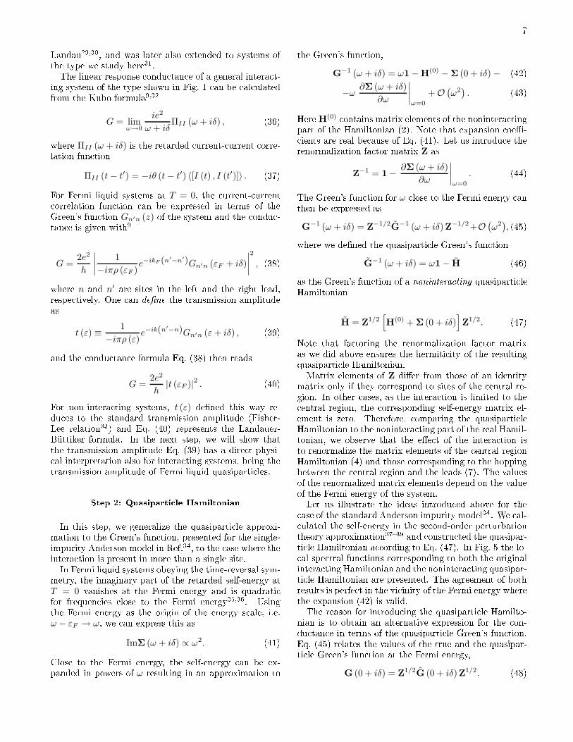
Figure 8: Exa t and approximate zero-temperature ondu tan e vs. Fermi energy urves for the system in Fig. 7. The shaded

area shows the exa t result. The left set of gures shows the approximations obtained using the single-ele tron formulae of

Se . IIIA while the right set of gures orresponds to the ground-state energy formulae of Se . IIIB. Dierent urves orrespond

to dierent number of sites N in the ring. In gures (a1) and (a2) the ondu tan e was al ulated using Eqs. (20) and (31), in

gures (b1) and (b2) using Eqs. (21) and (32), while in the other gures Eqs. (22) and (33) were used, in (c1) and (c2) applied

to the maximum and in (d1) and (d2) to the minimum of energy vs. ux urves.

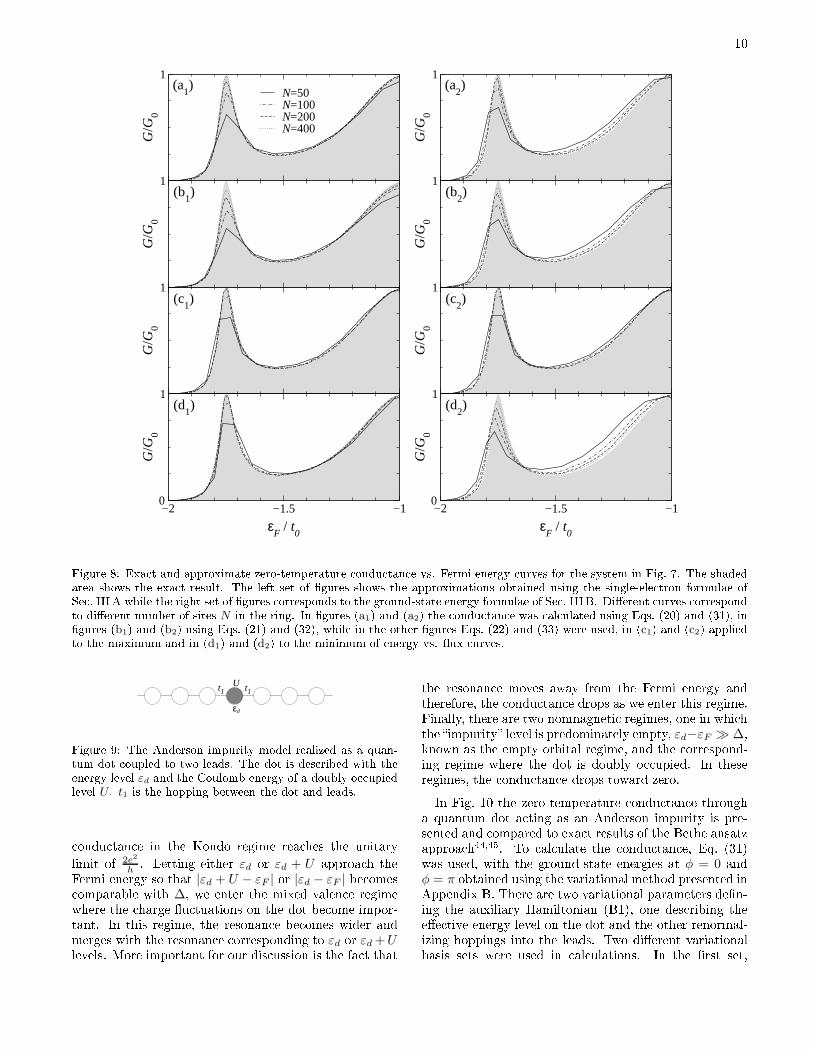
t1t1

εd

U

Figure 9: The Anderson impurity model realized as a quan-

tum dot oupled to two leads. The dot is des ribed with the

energy level εd and the Coulomb energy of a doubly o upied

level U . t1 is the hopping between the dot and leads.

ondu tan e in the Kondo regime rea hes the unitary

limit of

2e2

h . Letting either εd or εd + U approa h the

Fermi energy so that |εd + U − εF | or |εd − εF | be omes

omparable with ∆, we enter the mixed valen e regime

where the harge u tuations on the dot be ome impor-

tant. In this regime, the resonan e be omes wider and

merges with the resonan e orresponding to εd or εd +Ulevels. More important for our dis ussion is the fa t that

the resonan e moves away from the Fermi energy and

therefore, the ondu tan e drops as we enter this regime.

Finally, there are two nonmagneti regimes, one in whi h

the impurity level is predominately empty, εd−εF ≫ ∆,

known as the empty orbital regime, and the orrespond-

ing regime where the dot is doubly o upied. In these

regimes, the ondu tan e drops toward zero.

In Fig. 10 the zero-temperature ondu tan e through

a quantum dot a ting as an Anderson impurity is pre-

sented and ompared to exa t results of the Bethe ansatz

approa h

44,45

. To al ulate the ondu tan e, Eq. (31)

was used, with the ground-state energies at φ = 0 and

φ = π obtained using the variational method presented in

Appendix B. There are two variational parameters den-

ing the auxiliary Hamiltonian (B1), one des ribing the

ee tive energy level on the dot and the other renormal-

izing hoppings into the leads. Two dierent variational

basis sets were used in al ulations. In the rst set,

11

the basis onsisted of wavefun tions (B2). As a result

of the rotational symmetry in the spin degree of free-

dom, two of the basis fun tions may be merged into one.

Therefore, the basis set onsisted of proje tions of the

auxiliary Hamiltonian ground state

∣

∣0⟩

to states with

empty P0

∣

∣0⟩

, singly o upied P1

∣

∣0⟩

= P↑∣

∣0⟩

+ P↓∣

∣0⟩

and doubly o upied P2

∣

∣0⟩

dot level. In the se ond ba-

sis set, wavefun tions P1V P0

∣

∣0⟩

, P0V P1

∣

∣0⟩

, P2V P1

∣

∣0⟩

and P1V P2

∣

∣0⟩

(B7) were added to those of the rst set,

with V = VL +VR being the operator des ribing the hop-

ping between the dot and the leads (7). For ea h position

of the εd level relative to the Fermi energy, we in reased

the number of sites in the ring until the ondu tan e on-

verged. The number of sites needed to a hieve onver-

gen e (see Fig. 11a) was the lowest in the empty orbital

regime and the highest (about 1000 for the system shown

in Fig. 10) in the Kondo regime. This is a onsequen e

of Eq. (19) as a narrow resonan e related to the Kondo

resonan e appears in the transmission probability of the

quasiparti le Hamiltonian (47) in the Kondo regime. In

the mixed valen e regime, the width of the resonan e be-

omes omparable to ∆, whi h is mu h larger than the

Kondo temperature and the onvergen e is thus faster.

In the empty orbital regime the resonan e moves away

from the Fermi energy and an even smaller number of

sites is needed to a hieve onvergen e.

−0.8 0 0.8(ε

d+U/2)/t

0

0

1

G/G

0

Bethe ansatzVariational, 3Variational, 7

Figure 10: The zero-temperature ondu tan e al ulated

from ground-state energy vs. magneti ux in a nite ring

system using the variational method of Appendix B with 3

and 7 basis fun tions. For omparison, the exa t Bethe ansatz

result is presented with a dashed line. The system shown in

Fig. 9 was used, with U = 0.64t0 and t1 = 0.2t0.

Let us return to results shown in Fig. 10. Note that

extending the variational spa e from 3 to 7 basis fun -

tions signi antly improves the agreement with the exa t

result. The remaining dis repan y at the larger basis set

an be attributed to the approximate nature of the varia-

tional method. Another sour e of error ould be the fa t

that the Bethe ansatz solution assumes there is a on-

−0.8 0 0.8

(εd+U/2)/t

0

0

1

G/G

0

0 0.11/N

0

1

G/G

0

Bethe AnsatzVariational

(εd+U/2)/t

0 = 0.2

0.1

0

0.3

0.4

0.5

0.6

N = 10

20

50

100

200500 (a)

(b)

Figure 11: (a) Results of ondu tan e al ulations using

Eq. (31) for the system presented in Fig. 10 as the number

of sites in the ring in reases. Note that the onvergen e is

the fastest in the empty orbital regime and the slowest in the

Kondo regime. (b) Finite-size s aling analysis of the same

results for various values of εd. With bla k dots, the Bethe

ansatz values are shown. Energies were al ulated using the

variational method of Appendix B with 7 variational basis

fun tions.

stant oupling to an innitely wide ondu tion band. In

our ase, the ondu tion band is formed by the states in a

tight-binding ring, the oupling to whi h is not onstant.

However, it is almost onstant in the energy interval we

are interested in, i.e. near the enter of the band. In

order to estimate the ee t of the non onstant oupling

on the ondu tan e, we al ulated the dot o upation

number within the se ond order perturbation theory for

both the ase of a onstant oupling and for the ase

of a tight-binding ring. We then al ulated the ondu -

tan e in ea h ase making use of the Friedel sum rule

46

.

The agreement is signi antly better than the dieren e

between the Bethe ansatz and variational ondu tan e

urves in Fig. 10. Therefore, we believe that the use of

12

Bethe ansatz results is justied for this parti ular prob-

lem.

In Fig. 11b a nite-size s aling analysis of the on-

vergen e is presented. Note that for rings with a large

number of sites N , the error s ales approximately as

1N .

C. Double quantum dot

The next logi al step after studying individual quan-

tum dots is to onsider systems of more than one dot.

Single quantum dots are often regarded as arti ial atoms

be ause of a similar ele troni stru ture and omparable

number of ele trons in them. By oupling several quan-

tum dots one is thus reating arti ial mole ules. Here

we will not go into detail in des ribing the physi s of su h

systems. Our goal is to ompare results of our ondu -

tan e formulae to results of other methods for a double

quantum dot system presented in Fig. 12.

In the al ulation we again employed the ondu -

tan e formula (31) and al ulated the ground-state en-

ergies with the variational approa h of Appendix B with

the variational basis set (B2). In Fig. 13 the zero-

temperature ondu tan e for the ase where the inter-

dot and the on-site Coulomb repulsions V and U are of

the same size, are plotted as a fun tion of the position

of dot energy levels relative to the Fermi energy for var-

ious values of the inter-dot hopping matrix element t2.The same problem in the parti le-hole symmetri ase

εd + U2 + V = 0 was studied re ently in Ref.

8

. The Mat-

subara Green's fun tion was al ulated with the quantum

Monte Carlo method and the values on dis rete frequen-

ies were extrapolated to obtain the retarded Green's

fun tion at the Fermi energy. Then Eqs. (40) and (39)

were used to al ulate the zero-temperature ondu tan e.

The results are presented in Fig. 14, together with the

ondu tan e al ulated within the Hartree-Fo k approx-

imation and results of our method. The agreement with

the QMC results is ex ellent, while the Hartree-Fo k

approximation gives a qualitatively wrong ondu tan e

urve, espe ially at low values of the inter-dot oupling,

indi ating strong ele tron-ele tron orrelations in the sys-

tem. The results of our method for lower values of V are

also shown in Fig. 14.

2tt1 t1

εd

U U

εdV

Figure 12: A double quantum dot system. Ea h of the dots

with energy level εd and on-site Coulomb repulsion U is ou-

pled to a lead with a hopping matrix element t1. The inter-dothopping t2 is also present as is the inter-dot Coulomb repul-

sion V .

−2 −1 0 1 2(ε

d+U/2+V)/t

0

0

1

G/G

0

t2/t

0 = 0.025

0.05

0.075

0.1

0.150.

30.5

Figure 13: The zero-temperature ondu tan e of the system

in Fig. 12 as a fun tion of the position of the dot energy level

εd and inter-dot hopping matrix element t2. The remaining

parameters are U = V = t0 and t1 = 0.5t0.

0 0.5 1t2/t

0

0

1G

/G0

V/t0 = 0

V/t0 = 0.5

V/t0 = 1

V/t0 = 1, HF

V/t0 = 1, QMC

Figure 14: The zero-temperature ondu tan e of the double

quantum dot system of Fig. 12 at εd +U

2+ V = 0 as a fun -

tion of the inter-dot hopping matrix element t2 for various

values of the inter-dot Coulomb intera tion V . As a ompari-

son, the Hartree-Fo k and quantum Monte Carlo results

8

are

presented for V/t0 = 1. Other parameters are the same as in

Fig. 13.

VI. SUMMARY AND CONCLUSIONS

We have demonstrated how the zero-temperature on-

du tan e of a sample with ele tron-ele tron orrelations

and onne ted between nonintera ting leads an be de-

termined. The method is extremely simple and is based

on several formulae onne ting the ondu tan e to per-

sistent urrents in an auxiliary ring system. The ondu -

tan e is determined only from the ground-state energy

13

of an intera ting system, while in more traditional ap-

proa hes, one needs to know the Green's fun tion of the

system. The Green's fun tion approa hes are often mu h

more general, allowing the treatment of transport at -

nite temperatures and for a nite sour e-drain voltage ap-

plied a ross the sample, whi h in our method is not possi-

ble. However, the advantage of the present method omes

from the fa t that the ground-state energy is often rela-

tively simple to obtain by various numeri al approa hes,

in luding variational methods, and ould therefore, for

zero-temperature problems, be more appropriate.

Let us summarize the key points of the method:

(1) The open problem of the ondu tan e through a

sample oupled to semiinnite leads is mapped on to a

losed problem, namely a ring threaded by a magneti

ux and ontaining the same orrelated ele tron region.

(2) For a nonintera ting sample, it is shown that the

zero-temperature ondu tan e an be dedu ed from the

variation of the energy of the single-ele tron level at the

Fermi energy with the ux in a large, but nite ring sys-

tem. The ondu tan e is given with Eq. (18), or with

three simple formulae Eq. (20), Eq. (21) and Eq. (22).

(3) Alternatively, the ondu tan e of a nonintera t-

ing system is expressed in terms of the variation of the

ground-state energy with ux, Eq. (24). Three additional

ondu tan e formulae, Eq. (31), Eq. (32) and Eq. (33),

are derived.

(4) The method is primarily appli able to orrelated

systems exhibiting Fermi liquid properties at zero tem-

perature. In order to prove the validity of the method for

su h systems, the on ept of Fermi liquid quasiparti les

is extended to nite, but large systems. The ondu tan e

formulae give the ondu tan e of a system of noninter-

a ting quasiparti les, whi h is equal to the ondu tan e

of the original intera ting system. We also proved that

for su h systems, the ground-state energy of a large ring

system is a universal fun tion of the magneti ux, with

the ondu tan e being the only parameter [Eqs. (29) and

(30).

(5) The results of our method are ompared to results

of other approa hes for problems su h as the transport

through single and double quantum dots ontaining in-

tera ting ele trons. The omparison shows an ex ellent

quantitative agreement with exa t Bethe ansatz results

in the single quantum dot ase. The results for a double

quantum dot system also perfe tly mat h QMC results

of Ref.

8

.

(6) One should additionally point out that in the

derivation presented in this paper we assumed the in-

tera tion in the leads to be absent. It is lear that this

assumption is not justied for all systems. The method

annot be dire tly applied to systems where the intera -

tion in the leads is essential, as are e.g. systems exhibit-

ing Luttinger liquid properties.

(7) The validity of the method is not limited to systems

that do not break the time-reversal symmetry. A general-

ization to systems with a broken time-reversal symmetry,

su h as Aharonov-Bohm rings oupled to leads, is possi-

ble and will be presented elsewhere

47

.

(8) Another important limitation of the present

method is the single hannel approximation for the leads.

It might be possible to extend the appli ability of the

method to systems with multi- hannel leads by studying

the inuen e of several magneti uxes that ouple dif-

ferently to separate hannels. This way, one might be

able to probe individual matrix elements of the s atter-

ing matrix and derive ondu tan e formulae relevant for

su h more omplex systems.

Note added. After the present work was ompleted

the authors met R. A. Molina and R. A. Jalabert who

reported about their re ent unpublished work where an

approa h similar to our work is presented

13,48

.

A knowledgments

The authors wish to a knowledge P. Prelov²ek and X.

Zotos for helpful dis ussions and for drawing our atten-

tion to the problem of persistent urrents in orrelated

systems. We a knowledge V. Zlati¢ for dis ussions re-

lated to perturbative treatment of the Anderson model

and J. H. Jeerson for useful remarks and the nan ial

support of QinetiQ.

Appendix A: FERMI LIQUID IN A FINITE

SYSTEM

In Se . IV we based the proof of the validity of the

ondu tan e formulae for Fermi liquid systems on the

assumption that

E (N,φ;M +m) = E (N,φ;M) +

+m∑

i=1

ε (N,φ;M ; i) + O(

N− 32

)

. (A1)

Here E (N,φ;M +m) and E (N,φ;M) are the ground-

state energies of an intera ting N -site ring with ux

φ, ontaining M + m and M ele trons, respe tively.

ε (N,φ;M ; i) is a single-ele tron energy of the ring quasi-

parti le Hamiltonian H (N,φ;M) as dened in Eq. (49),

with the Fermi energy orresponding to M ele trons in

the system. The index i labels su essive single-ele tronenergy levels above the Fermi energy. We assume m to

be nite and N approa hing the thermodynami limit.

In this Appendix we will give arguments showing that

the assumption of Eq. (A1) is indeed valid. In Se . 1 we

rst express the problem in terms of the Green's fun tion

of the system. In Se . 2 we study the properties of the

self-energy due to intera tion in nite ring systems and

then use this results to omplete the proof in Se . 3.

14

1. Relation to the Green's fun tion

Assume we manage to prove Eq. (A1) for m = 1, i.e.

E (N,φ;M + 1) = E (N,φ;M) +

+ε (N,φ;M ; 1) + O(

N− 32

)

. (A2)

Then we an use the same result to relate the energy of a

system withM+2 ele trons to that withM+1 ele trons,

E (N,φ;M + 2) = E (N,φ;M) +

+ε (N,φ;M ; 1) + ε (N,φ;M + 1; 1) + O(

N− 32

)

.(A3)

Now the matrix elements of quasiparti le Hamiltonians

H (N,φ;M + 1) and H (N,φ;M) dier by an amount of

the order of

1N . To see this, note that the shift of the

Fermi energy as an ele tron is added to the system is of

the order of

1N , produ ing a shift of the same order in the

self-energy and it's derivative at the Fermi energy, whi h

dene the quasiparti le Hamiltonian through Eq. (49).

As the dieren e of the Hamiltonians ∆H is small, we

an use the rst order perturbation theory,

ε (N,φ;M + 1; 1) =

= ε (N,φ;M ; 2) +⟨

N,φ;M ; 2∣

∣

∣∆H

∣

∣

∣N,φ;M ; 2

⟩

=

= ε (N,φ;M ; 2) + O(

N−2)

. (A4)

In the last step we made use of the fa t that the quasi-

parti le Hamiltonians dier only in a nite number of

sites in and in the vi inity of the entral region, and of

the fa t that the amplitude of the quasiparti le single-

ele tron wavefun tion |N,φ;M ; 2〉 is of the order of 1√N.

Thus we have proved Eq. (A1) for m = 2 and using the

same pro edure, we an extend the proof to any nite m.

To omplete the proof, we still need to show the va-

lidity of Eq. (A2). As a rst step, onsider the Lehmann

representation of the zero-temperature entral region

Green's fun tion

Gji (t, t′) = −iθ (t− t′)⟨

0∣

∣

[

dj (t) , d†i (t′)]∣

∣0⟩

(A5)

of a ring system hara terized with N and φ, ontainingM ele trons,

Gji (N,φ;M ; z) =

=∑

n

⟨

0∣

∣dj

∣

∣n⟩⟨

n∣

∣d†i∣

∣0⟩

z −(

EM+1n − EM

0

) +

+∑

n

⟨

0∣

∣d†i∣

∣n⟩⟨

n∣

∣dj

∣

∣0⟩

z −(

EM0 − EM−1

n

) . (A6)

The rst sum runs over all basis states with M + 1 ele -

trons, while the se ond sum runs over the states with

M − 1 ele trons. The dieren e in the ground-state en-

ergies of systems with M + 1 and M ele trons is evi-

dently equal to the position of the rst δ-peak above the

Fermi energy in the spe tral density orresponding to the

Green's fun tion. In what follows, we will try to deter-

mine the energy of this δ-peak.

2. Self-energy due to intera tion

To a hieve the goal we have set in the previous Se tion,

we rst need to study the stru ture of the self-energy due

to intera tion in a nite ring with ux. Let us again on-

sider the Lehmann representation (A6) and to be spe i ,

limit ourselves to states above the Fermi energy. Intro-

du ing ϕnj = 〈0 |dj |n〉 and εn = EM+1

n − EMn , we an

express the Green's fun tion as

Gji (N,φ;M ; z) =∑

n

ϕnj ϕ

n∗i

z − εn. (A7)

This expression an also be interpreted as a lo al Green's

fun tion of a larger nonintera ting system, onsisting of

the entral region and a bath of nonintera ting energy

levels, the number of whi h is equal to the number of

multi-ele tron states with M + 1 and M − 1 ele trons of

the original intera ting system. The self-energy due to

hopping out of the entral region, whi h in ludes both

the ee ts of the intera tion as well as those due to the

hopping into the ring, an then be expressed as

Σji (N,φ;M ; z) =∑

n

VjnVni

z − εn, (A8)

where Vjn are the hopping matrix elements between the

entral region and the bath. Thus we have shown that,

as far as the single-ele tron Green's fun tion is on erned,

the intera ting system an be mapped on a larger, but

nonintera ting system.

To further larify the on epts introdu ed above, we

al ulated the self-energy due to intera tion within the

se ond-order perturbation theory. Following the al ula-

tions by Horvati¢, ok£evi¢ and Zlati¢

3739

for the Ander-

son model, we sum the se ond order self-energy diagrams

shown in Fig. 15, in luding Hartree and Fo k terms into

the unperturbed Hamiltonian. A lengthy but straight-

forward al ulation, whi h we do not repeat here, shows

that one an identify the states n of Eq. (A8) with three

Hartree-Fo k single-ele tron state indi es q = (q1, q2, q3)su h that q1 and q2 are above the Fermi energy and q3 is

below it (or vi e versa), and a spin index s. The bathenergy levels

εqs = εq1 + εq2 − εq3 (A9)

and the hopping matrix elements related to the self-

energy for ele trons with spin σ

Vjqs =

∑

k′ Uσσjk′ϕ

q1

j ϕq2

k′ϕq3∗k′ , s = σ,

1√2

∑

k′ Uσσjk′

[

ϕq1

j ϕq2

k′ − ϕq2

j ϕq1

k′

]

ϕq3∗k′ , s = σ

(A10)

are then expressed in terms of the Coulomb intera tion

matrix elements (5), and the Hartree-Fo k single-ele tron

energies εq (N,φ;M) and the orresponding wavefun -

tions |ϕq (N,φ;M)〉. In Fig. 16 the positions of δ-peaksin the imaginary part of the self-energy as a fun tion of

magneti ux through the ring are plotted. Note that as

15

the ux is varied, the positions of the peaks u tuate by

an amount of the order of the single-ele tron level spa -

ing whi h is of the order of

1N . The weights of the peaks

also depend on the ux. A similar behavior is expe ted

if higher order pro esses are also taken into a ount.

+

!

k

k

0

i j

0

!

0

!

!

0

k

k

0

i j

i

k

!

i

j

+

!

k

k

0

i j

0

!

0

!

!

0

k

k

0

i j

i

k

!

i

j

Figure 15: Se ond-order self-energy diagrams.

0

π

φ

0ω

Figure 16: Dashed lines show the positions of δ-peaks (A9) inthe se ond-order self-energy orresponding to single-ele tron

energy levels of an unperturbed system presented with gray

lines.

Finally, let us study the self-energy in the thermody-

nami limit. We will show that in this ase, the self-

energy is independent of ux and is equal to the self-

energy of the original, two-lead system, shown in Fig. 1.

To prove this statement, we onsider a self-energy Feyn-

man diagram for the entral region de oupled from the

ring, whi h then is obviously independent of ux. To

al ulate the self-energy for the full system, one should

insert the self-energy due to hopping into the ring into

ea h propagator of the diagram. The self-energy due to

hopping into the ring is

Σ(0)ji (N,φ; z) =

∑

k

VjkVki

z − εk, (A11)

where εk are the single-ele tron energy levels of the ring

de oupled from the entral region and Vki = −ψkLtLi −

ψkRtRi is the hopping matrix element between site i in the

entral region and the single-ele tron state k in the ring.

Vki is expressed in terms of the hopping matrix element

tLi between the site i and the ring site L adja ent to

the entral region and the single-ele tron wavefun tion

ψkL =

√2

N+1 sink at site L, whereN is the number of sites

in the ring. There is also a similar ontribution to Vki

orresponding to the hopping into the right lead. In the

ring system, the right lead wavefun tion an be expressed

in terms of the left lead one as ψkR = (−1)

ne−iφψk

L with

k = nπN+1 , if one takes into a ount the parity of the

wavefun tions and the ee t of the ux. Thus, Eq. (A11)

transforms into

Σ(0)ji (N,φ; z) = Σ

(L)ji (N ; z) + Σ

(R)ji (N ; z) +

+2(

tjLtRie−iφ + tjRtLie

iφ)

N + 1

∑

k

(−1)n

sin2 k

z − εk, (A12)

where Σ(L)ji (N ; z) and Σ

(R)ji (N ; z) are the self-energies

due to hopping into the left and the right leads (ea h

with N sites) of the two-lead system. In the third term,

one an perform the sum over odd n-s and over even n-sseparately. The sums dier only in sign in the N → ∞limit and therefore, this term vanishes. Therefore, in the

thermodynami limit the self-energy due to intera tion is

the same in both two-lead and ring systems.

3. Proof of Eq. (A2)

Positions of δ-peaks in the spe tral density of the in-

tera ting system orrespond to the single-ele tron energy

levels of the nonintera ting part of the ring Hamiltonian

oupled to the bath a ording to Eq. (A8). These en-

ergies an be obtained by solving for zeroes of the deter-

minant of the inverse of the lo al Green's fun tion

det[

ω1− H(0) (N,φ) − Σ (N,φ;M ;ω + iδ)]

= 0.

(A13)

What we are going to prove in this Se tion is that the

lowest positive solution of this equation orresponds to

ε (N,φ;M ; 1) as required by Eq. (A2).

We begin by separating the self-energy at frequen ies

lose to the Fermi energy into two ontributions, one

(Σ′′) due to the bath states lose to the Fermi en-

ergy and the other (Σ′) of all the other states with en-

ergies whi h are separated from the expe ted solution

of Eq. (A13) by at least an amount of the order of the

single-ele tron level spa ing ∆, whi h is of the order of

1N . We rst estimate the se ond term. Let us divide

the frequen y axis into intervals of width ∆, ea h on-

tributing to the self-energy at |ω| < ∆ an amount given

by

∫ ε+∆

ε

ρ (ε)

ω − εdε, (A14)

where ρji (ε) =∑

n VjnVniδ (ε− εn) if the notation of

Eq. (A8) is used. On average, this ontribution orre-

sponds to that of a system in the thermodynami limit

where ρ (ε) is a ontinuous fun tion and the magnitude

of ea h ontribution is at most of the order of

1N . To

see this, let us assume ρ (ε) is proportional to ε2 (41)

for all values of ε up to a uto of the order of 1. Su h

16

an approximation an be onsidered as the upper limit

of possible values of ρ (ε) in Fermi liquid systems, if one

does not take into a ount the rapidly de reasing tails

at higher energies, whi h ontribute a negligible amount

to the self-energy at the Fermi energy. Evaluating the

above integral, we nd that ontributions of the intervals

lose to the Fermi energy are of the order of

1N2 and on-

tributions of the intervals near the uto are of the order

of

1N . Using an analogous pro edure, we an also eval-

uate the derivative of the self-energy lose to the Fermi

energy, with ontributions

−∫ ε+∆

ε

ρ (ε)

(ω − ε)2dε. (A15)

In this ase, also ontributions orresponding to intervals

lose to the Fermi energy are of the order of

1N . If ρ (ε)

for a nite N is used instead, there are large u tuations

about the average value (see the dis ussion in the pre-

vious Se tion) with the amplitude of u tuations of the

same order of magnitude as the average value itself. To

estimate the dieren e between the nite-system's real

part of the self-energy (or its derivative) lose to the

Fermi energy and the orresponding quantity for a sys-

tem in the thermodynami limit, we note that a sum

of N quantities, ea h of them of the order of

1N with a

standard deviation of the same order of magnitude, has

a standard deviation of the order of N− 12, and therefore,

we an estimate that for |ω| < ∆

Σ′ (N,φ;M ;ω + iδ) =

= Σ (0 + iδ) + O(

N− 12

)

, (A16)

∂Σ′ (N,φ;M ;ω + iδ)

∂ω

∣

∣

∣

∣

ω

=

=∂Σ (ω + iδ)

∂ω

∣

∣

∣

∣

ω=0

+ O(

N− 12

)

. (A17)

Note that we do not need to ex lude the ontribution of

the interval at the Fermi energy (the one orresponding

to Σ′′) from self-energies in the right hand sides of these

equations, be ause the orresponding ontributions are

smaller than N− 12as dis ussed above. Also the errors

arising from the fa t that the right hand sides are evalu-

ated at ω = 0 instead of at ω are only of the order of

1N ,

as dis ussed in the previous Se tion. In Fig. 17 a om-

parison of the self-energies at a nite N and in the ther-

modynami limit is presented. Note that in the vi inity

of the Fermi energy, the real parts of both self-energies

oin ide.

One an now pro eed as in Eqs. (44) and (47), dening

the renormalization matrix Z′ (N,φ;M) = Z + O(

N− 12

)

and the quasiparti le Hamiltonian H′ (N,φ;M) =

H (N,φ;M) +O(

N− 12

)

orresponding to the self-energy

Σ′. As shown in the previous Se tion, the self-energies

of an innite two-lead system and the orresponding ring

system are the same and therefore, the renormalized ma-

trix elements of H (N,φ;M) orrespond to those of a

two-lead system. For |ω| < ∆, Eq. (A13) transforms into

−0.5 0 0.5ω/t

0

−2

−1

0

1

2

ReΣ

(ω)/t

0

N = 400N = ∞

−0.5 0 0.5ω/t

0

−2

−1

0

ImΣ(

ω)/t

0

(a) (b)

Figure 17: The (a) real and (b) imaginary parts of the self-

energy of an intera ting system in the thermodynami limit

and for N = 400 with φ =3π

4. The system is des ribed in

Fig. 5.

det[

ω1− H′ (N,φ;M) − Σ′′ (N,φ;M ;ω + iδ)]

= 0,

(A18)

where the oupling to the remaining bath levels has

been renormalized as Σ′′ = Z′1/2Σ′′Z′1/2. Let us for a

moment negle t this term in Eq. (A18). As the dieren e

∆H between Hamiltonians H(N,φ;M) and H ′ (N,φ;M)is small for a largeN , one is justied to relate their single-

ele tron energy levels using the rst order perturbation

formula

ε′ (N,φ;M ; 1) =

= ε (N,φ;M ; 1) +⟨

N,φ;M ; 1∣

∣

∣∆H

∣

∣

∣N,φ;M ; 1

⟩

=

= ε (N,φ;M ; 1) + O(

N− 32

)

. (A19)

In the last step we made use of arguments similar to those

in deriving Eq. (A4).

The energy (A19) an a quire an additional shift be-

ause of the oupling Σ′′. To estimate this shift we rst

note that in the worst ase s enario, i.e. when there is a

single bath energy level whi h oin ides with the quasi-

parti le energy level (A19), the oupling matrix elements

Vjn in Eq. (A8) must be at most of the order of N− 32for

Eq. (41) to be satised in the thermodynami limit. Then

one an make use of the degenerate rst order perturba-

tion theory, whi h shows that the quasiparti le energy

level is shifted by an additional amount of the order of

1N2 . This ompletes the proof of Eq. (A1).

As a on lusion, in Fig. 18 we present a omparison of

the total densities of states for a nite ring intera ting

system within the se ond order perturbation theory and

in the quasiparti le Hamiltonian approximation. Note

that the states near the Fermi energy are well des ribed

with the quasiparti le approximation, while the states

further away from the Fermi energy are split in the in-

tera ting ase. Similar results were reported in Ref.

49

.

17

-0.15 -0.1 -0.05 0 0.05 0.1 0.15

Ωt0

0

Π

Φ

HbL

-0.15 -0.1 -0.05 0 0.05 0.1 0.15

Ωt0

0

Π

Φ

HaL

Figure 18: (a) The total density of states of an intera ting ring

system within the se ond-order perturbation theory. (b) Total

density of states orresponding to the quasiparti le Hamilto-

nian. The system is des ribed in Fig. 5.

Appendix B: VARIATIONAL GROUND-STATE

ENERGY

In order to al ulate the ondu tan e for intera ting

systems, we rst need to devise a robust method that

would allow us to e iently al ulate the ground-state

energy of su h systems. Note that we need a method that

would provide us with the energy of a system with a very

large number of sites in the ring. However, the number

should still be nite - i.e. we must not perform the al u-

lations in the thermodynami limit. We made use of the

proje tion method of Gunnarson and S hönhammer

5052

,

introdu ed originally to al ulate the ground-state energy

of the Anderson impurity model, and extended it to treat

the more general Hamiltonian (1).

Let us introdu e an auxiliary nonintera ting Hamilto-

nian,

H = HL + VL + H(0)C + VR +HR, (B1)

with arbitrary matrix elements des ribing the hopping

between the leads and the entral region, and the en-

tral region itself. Note that these are the same matrix

elements as the ones being renormalized in the Fermi liq-

uid quasiparti le Hamiltonian (47). Let us also dene a

Hilbert spa e spanned by a set of 4Mbasis fun tions

|ψα〉 ≡ Pα

∣

∣0⟩

≡∏

i∈C

P iαi

∣

∣0⟩

, (B2)

where M is the number of sites in the entral region,

∣

∣0⟩

is the ground-state of the auxiliary Hamiltonian (B1)

ontaining the same number of ele trons as there are in

the ground state of the original Hamiltonian, and

P i0 = (1 − ni↑) (1 − ni↓) , (B3)

P iσ = niσ (1 − niσ) , (B4)

P i2 = ni↑ni↓ (B5)

are proje tion operators on uno upied, singly o upied

and doubly o upied site i. The original Hamiltonian is

diagonalized in the redu ed basis set introdu ed above,

Hβα = ESβα, (B6)

with Hβα = 〈ψβ |H |ψα〉 being the matrix elements of

the Hamiltonian and Sβα = 〈ψβ | ψα〉 take into a ount

the fa t that the basis fun tions do not form an orthonor-

mal basis set. The eigenstate with the lowest energy EHof this eigenvalue problem is an approximation to the

ground-state energy of the original Hamiltonian. Varying

the parameters of the auxiliary Hamiltonian, one an nd

their optimal values whi h minimize EH . The solution

of this minimization problem is the nal approximation

to the ground-state energy.

Let us onsider some simple limits of the problem. In

the nonintera ting ase where U = 0, one an hoose the

auxiliary Hamiltonian to be equal to the true Hamilto-

nian H = H . Then the wavefun tion |ψ〉 =∑

α Pα

∣

∣0⟩

=∣

∣0⟩

= |0〉 is the exa t ground-state wavefun tion of

the system. Note that applying the same wavefun tion

ansatz to the intera ting ase and allowing the matrix

elements of the auxiliary Hamiltonian to be renormal-

ized, provides us with the Hartree-Fo k solution of the

problem. Therefore, the variational method introdu ed

above always gives the ground-state energy whi h is lower

or equal to the orresponding Hartree-Fo k ground-state

energy. In the limit of the entral region being de oupled

from the ring, i.e. VL = VR = 0, the variational method

also yields the exa t ground-state energy. To prove this

statement, let us sele t the matrix elements of H in su h

a way that in its ground state there are m ele trons in

the entral region. Then the basis set (B2) spans the

full Hilbert spa e for m ele trons in the entral region.

As there is no oupling to the states in the ring, solving

the eigenvalue problem (B6) provides us with the exa t

ground state of the problem with a onstraint of a xed

number of ele trons in the entral region. By varying H ,

all the possible values of m an be tested and the one

yielding the lowest ground-state energy orresponds to

the orre t ground state of the system.

The variational wavefun tion ansatz an be improved

by extending the Hilbert spa e with additional basis fun -

tions, the most promising andidates being of type

52

|ψβλjiσα〉 = PβVλjiσPα

∣

∣0⟩

, (B7)

where Vλjiσ = Vλjic†jσdiσ + h.c. and λ is a lead index,

i.e. either L or R. On the other hand, as the size of the

18

Hilbert spa e in reases exponentially with the number

of sites in the entral region, it might be onvenient to

limit the basis set to the states obtained by proje ting

to the entral region's many body states between whi h

u tuations are possible.

Finally, we state some te hni al details on erning the

evaluation of Hβα and Sβα. It is onvenient to express

these matrix elements only in terms of quantities related

to the entral region and the neighboring sites in the

leads. As

Sβα =⟨

0 |PβPα| 0⟩

=⟨

0 |Pα| 0⟩

δβα, (B8)

the s alar produ ts between the basis fun tions are evi-

dently expressed with the entral region quantities. The

matrix elements of the Hamiltonian an be expressed as

Hβα =⟨

0 |PβHPα| 0⟩

=

=⟨

0∣

∣

∣HPβPα

∣

∣

∣0⟩

+⟨

0 |PβHPα| 0⟩

−

−⟨

0∣

∣

∣HPβPα

∣

∣

∣0⟩

=

= ESβα +⟨

0 |Pβ (VL +HC + VR)Pα| 0⟩

−

−⟨

0∣

∣

∣

(

VL + H(0)C + VR

)

Pα

∣

∣

∣0⟩

δβα, (B9)

where E is the ground-state energy of the auxiliary

Hamiltonian H . In the se ond and the third term we

made use of the fa t that lead Hamiltonians HL and HR

ommute with the entral region proje tors and there-

fore, they an el out. Again, we su eeded in expressing

the matrix elements in terms of entral region quantities

together with quantities related to the neighboring sites

in the leads. Similar results are obtained if the extended

basis set of Eq. (B7) is used. The matrix elements in

Eqs. (B8) and (B9) need to be al ulated in a noninter-

a ting state. Therefore, we an make use of the Wi k's

theorem to de ompose the expressions into two-operator

averages of type

⟨

0∣

∣

∣d†jσdiσ

∣

∣

∣0⟩

. As a huge number of

terms is generated in this pro edure, the de omposition

was performed automati ally by symboli manipulation

of operators. The ground-state energy of the auxiliary

Hamiltonian and the two-operator averages an be ex-

pressed in terms of the single-ele tron energies εk and

wavefun tions

∣

∣ϕk⟩

of H as

E = 2∑

k occ.

εk, (B10)

⟨

0∣

∣

∣d†jσdiσ

∣

∣

∣0⟩

=∑

k occ.

ϕk∗j ϕk

i . (B11)

The sums run only over the single-ele tron states o u-

pied in the ground state

∣

∣0⟩

. The eigenvalues εk were

al ulated in a basis in whi h the Hamiltonian matrix

is banded, i.e. linear ombinations of lo al basis fun -

tions orresponding to the left lead and right lead sites

were introdu ed to move the hopping matrix elements

in orners of the matrix lose to the diagonal. For ea h

eigenvalue, only the omponents of the eigenve tor re-

lated to the entral region and neighboring sites were

al ulated, again taking the spe ial stru ture of the ma-

trix into a ount. The pro edure used s ales with the

number of sites in the ring as O(

N2)

, whi h allows one

to treat systems with up to 10000 sites in the ring.

1

J. von Delft and D. C. Ralph, Phys. Rep. 345, 61 (2001).

2

L. P. Kouwenhoven et al., in Mesos opi Ele tron Trans-

port, edited by L. L. Sohn, L. P. Kouwenhoven, and G.

S hön (Kluwer A ademi , New York, 1997).

3

N. Agraït, A. L. Yeyati, and J. M. van Ruitenbeek, ond-

mat/0208239 (unpublished).

4

R. H. M. Smit et al., Nature 419, 906 (2002).

5

R. Landauer, IBM J. Res. Dev. 1, 233 (1957).

6

R. Landauer, Philos. Mag. 21, 863 (1970).

7

M. Büttiker, Phys. Rev. Lett. 57, 1761 (1986).

8

A. Oguri, Phys. Rev. B 56, 13422 (1997).

9

A. Oguri, J. Phys. So . Jpn. 70, 2666 (2001).

10

Y. Meir and N. S. Wingreen, Phys. Rev. Lett. 68, 2512

(1992).

11

A.-P. Jauho, N. S. Wingreen, and Y. Meir, Phys. Rev. B

50, 5528 (1994).

12

J. Favand and F. Milla, Eur. Phys. J. B 2, 293 (1998).

13

R. A. Molina et al., ond-mat/0209552 (unpublished).

14

O. P. Sushkov, Phys. Rev. B 64, 155319 (2001).

15

H.-F. Cheung, Y. Gefen, E. K. Riedel, and W.-H. Shih,

Phys. Rev. B 37, 6050 (1988).

16

A. O. Gogolin and N. V. Prokof'ev, Phys. Rev. B 50, 4921

(1994).

17

A. A. Aligia, PRB 66, 165303 (2002).

18

P. Prelov²ek and X. Zotos, in Le tures on the Physi s

of Highly Correlated Ele tron Systems VI, edited by F.

Man ini (Ameri an Institute of Physi s, New York, 2002).

19

P. W. Anderson, Phys. Rev. 124, 41 (1961).

20

R. E. Peierls, Z. Phys. B 80, 763 (1933).

21

S. Datta, Ele troni Transport in Mesos opi Systems

(Cambridge University Press, Cambridge, 1995).

22

F. Blo h, Phys. Rev. 137, A787 (1965).

23

M. Büttiker, Y. Imry, and R. Landauer, Phys. Lett. 96A,

365 (1983).

24

V. Meden and U. S hollwoe k, ond-mat/0210515 (unpub-

lished).

25

W. Kohn, Phys. Rev. 133, A171 (1964).

26

R. A. Jalabert, A. D. Stone, and Y. Alhassid, PRL 68,

3468 (1992).

27

J. A. Verges, E. Cuevas, M. Ortuño, and E. Louis, PRB

58, R10143 (1998).

28

P. Nozières, Theory of intera ting Fermi systems (W. A.

Bejnamin, In ., New York, 1964).

29

L. D. Landau, Pis'ma Zh. Eksp. Teor. Fiz. 3, 920 (1956).

30

L. D. Landau, Pis'ma Zh. Eksp. Teor. Fiz. 5, 101 (1957).

31

P. Nozières, J. Low Temp. Phys. 17, 31 (1974).

32

H. Bruus and K. Flensberg, Introdu tion to many-body

quantum theory in ondensed matter physi s (Oersted Lab-

19

oratory, Niels Bohr Institute, Copenhagen, 2002).

33

D. S. Fisher and P. A. Lee, Phys. Rev. B 23, 6851 (1981).

34

A. C. Hewson, The Kondo Problem to Heavy Fermions

(Cambridge University Press, Cambridge, 1993).

35

K. Yamada and K. Yosida, Prog. Theor. Phys. 76, 621

(1986).

36

A. Oguri, J. Phys. So . Jpn. 66, 1427 (1997).

37

B. Horvati¢ and V. Zlati¢, Phys. Status Solidi B 99, 251

(1980).

38

B. Horvati¢ and V. Zlati¢, Solid State Commun. 54, 957

(1985).

39

B. Horvati¢, D. ok£evi¢, and V. Zlati¢, Phys. Rev. B 36,

675 (1987).

40

L. I. Glazman and M. E. Raikh, Pis'ma Zh. Eksp. Teor.

Fiz. 47, 378 (1988).

41

T. K. Ng and P. A. Lee, Phys. Rev. Lett. 61, 1768 (1988).

42

D. Goldhaber-Gordon et al., Nature 391, 156 (1988).

43

W. G. van der Wiel et al., S ien e 289, 2105 (2000).

44

P. B. Wiegman and A. M. Tsveli k, Pis'ma Zh. Eksp. Teor.

Fiz. 35, 100 (1982).

45

P. B. Wiegman and A. M. Tsveli k, J. Phys. C 16, 2281

(1983).

46

D. C. Langreth, Phys. Rev. 150, 516 (1966).

47

T. Reje and A. Ram²ak, ond-mat/0303258 (to be pub-

lished in Phys. Rev. B).

48

R. A. Molina and R. A. Jalabert, private ommuni ation.

49

B. L. Altshuler, Y. Gefen, A. Kamenev, and L. S. Levitov,

Phys. Rev. Lett. 78, 2803 (1997).

50

K. S hönhammer, Z. Phys. B 21, 389 (1975).

51

K. S hönhammer, Phys. Rev. B 13, 4336 (1976).

52

O. Gunnarson and K. S hönhammer, Phys. Rev. B 31,

4815 (1985).