CSL Technical Report • January 2002

Formal Verification of Marzullo’s Sensor Fusion Interval

John RushbyComputer Science LaboratorySRI InternationalMenlo Park CA 94025 USA

This research was supported by NASA Langley Research Center under contractNAS1-20334 and Cooperative Agreement NCC-1-377 with Honeywell Tucson, andby the DARPA MoBIES program under contract F33615-00-C-1700 with US AirForce Research Laboratory.

Computer Science Laboratory • 333 Ravenswood Ave. • Menlo Park, CA 94025 • (650) 326-6200 • Facsimile: (650) 859-2844

Abstract

We examine the problem of selecting a best value from a collection of sensor readings,and diagnosing faulty readings in such a collection. We focus on sensor interfaces that re-turn arangeof values and describe the “fusion functions”

⋂f,n(S) of Marzullo andFfn (S)

of Schmid and Schossmaier. We use PVS formally to prove the soundness of⋂f,n(S) (i.e.,

it always contains the correct value), from which soundness ofFfn (S) also follows.Ffn (S)is generally to be preferred to

⋂f,n(S) because it satisfies a “Lipschitz Condition” (small

changes in sensor readings produce small changes in its output), and is optimal among allsuch functions.

i

ii

Contents

Contents iii

List of Figures v

1 Introduction 1

2 Formalization of Sensor Fusion Functions 52.1 Formal Specification and Verification in PVS. . . . . . . . . . . . . . . . 9

3 Conclusion 17

Bibliography 19

iii

iv

List of Figures

1.1 Sensor Fusion Problem. . . . . . . . . . . . . . . . . . . . . . . . . . . . 21.2 Resulting Fusion Interval. . . . . . . . . . . . . . . . . . . . . . . . . . . 31.3 Sensor Fusion Problem with Unclear Diagnosis. . . . . . . . . . . . . . . 41.4 Precision Sacrificed to Preserve Soundness. . . . . . . . . . . . . . . . . 4

2.1 FTI Fusion Interval. . . . . . . . . . . . . . . . . . . . . . . . . . . . . . 82.2 Marzullo’s Fusion Interval with Diagnosis. . . . . . . . . . . . . . . . . . 9

v

vi

Chapter 1

Introduction

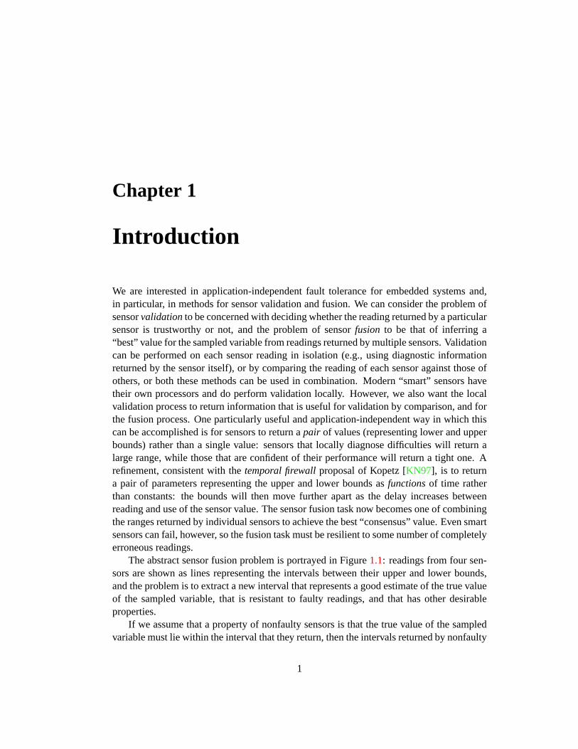
We are interested in application-independent fault tolerance for embedded systems and,in particular, in methods for sensor validation and fusion. We can consider the problem ofsensorvalidationto be concerned with deciding whether the reading returned by a particularsensor is trustworthy or not, and the problem of sensorfusion to be that of inferring a“best” value for the sampled variable from readings returned by multiple sensors. Validationcan be performed on each sensor reading in isolation (e.g., using diagnostic informationreturned by the sensor itself), or by comparing the reading of each sensor against those ofothers, or both these methods can be used in combination. Modern “smart” sensors havetheir own processors and do perform validation locally. However, we also want the localvalidation process to return information that is useful for validation by comparison, and forthe fusion process. One particularly useful and application-independent way in which thiscan be accomplished is for sensors to return apair of values (representing lower and upperbounds) rather than a single value: sensors that locally diagnose difficulties will return alarge range, while those that are confident of their performance will return a tight one. Arefinement, consistent with thetemporal firewallproposal of Kopetz [KN97], is to returna pair of parameters representing the upper and lower bounds asfunctionsof time ratherthan constants: the bounds will then move further apart as the delay increases betweenreading and use of the sensor value. The sensor fusion task now becomes one of combiningthe ranges returned by individual sensors to achieve the best “consensus” value. Even smartsensors can fail, however, so the fusion task must be resilient to some number of completelyerroneous readings.

The abstract sensor fusion problem is portrayed in Figure1.1: readings from four sen-sors are shown as lines representing the intervals between their upper and lower bounds,and the problem is to extract a new interval that represents a good estimate of the true valueof the sampled variable, that is resistant to faulty readings, and that has other desirableproperties.

If we assume that a property of nonfaulty sensors is that the true value of the sampledvariable must lie within the interval that they return, then the intervals returned by nonfaulty

1

S(2)

S(3)

S(4)

S(1)

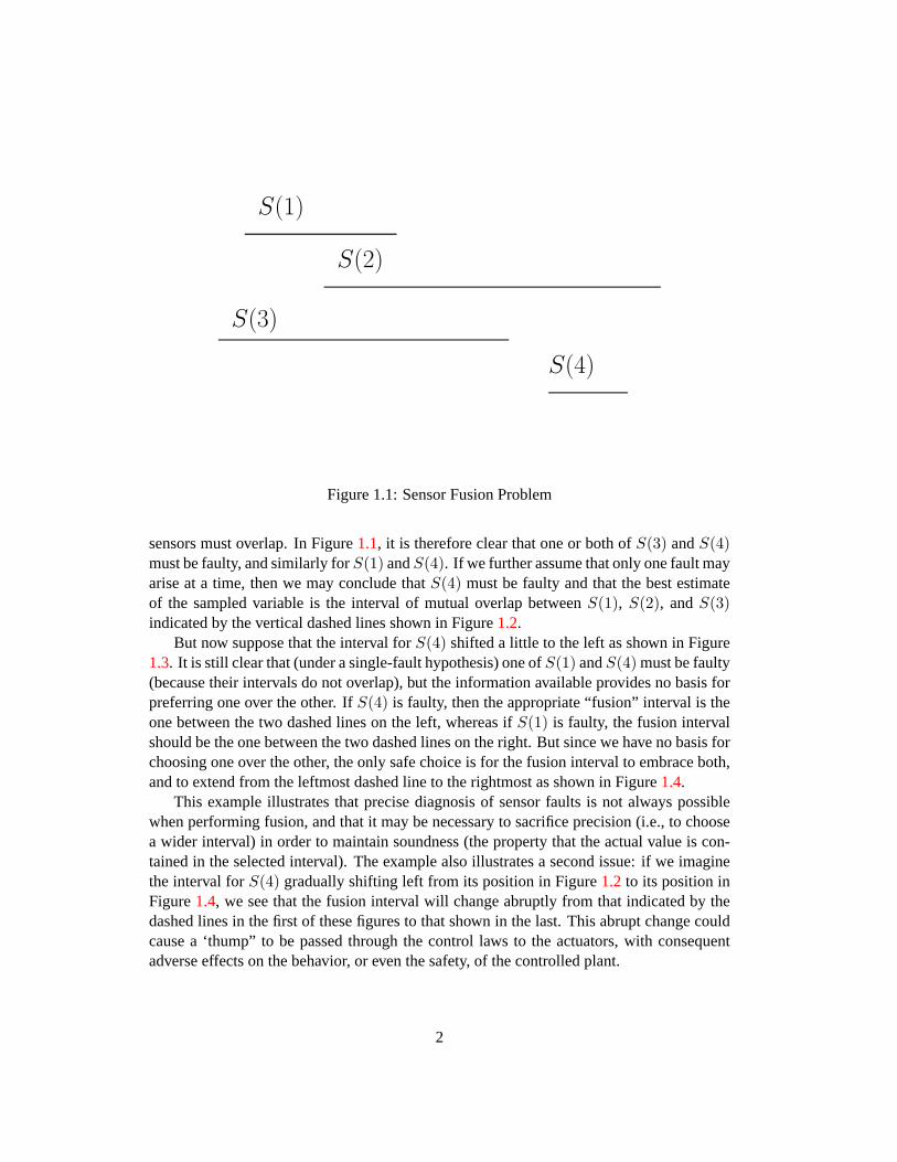
Figure 1.1: Sensor Fusion Problem

sensors must overlap. In Figure1.1, it is therefore clear that one or both ofS(3) andS(4)must be faulty, and similarly forS(1) andS(4). If we further assume that only one fault mayarise at a time, then we may conclude thatS(4) must be faulty and that the best estimateof the sampled variable is the interval of mutual overlap betweenS(1), S(2), andS(3)indicated by the vertical dashed lines shown in Figure1.2.

But now suppose that the interval forS(4) shifted a little to the left as shown in Figure1.3. It is still clear that (under a single-fault hypothesis) one ofS(1) andS(4) must be faulty(because their intervals do not overlap), but the information available provides no basis forpreferring one over the other. IfS(4) is faulty, then the appropriate “fusion” interval is theone between the two dashed lines on the left, whereas ifS(1) is faulty, the fusion intervalshould be the one between the two dashed lines on the right. But since we have no basis forchoosing one over the other, the only safe choice is for the fusion interval to embrace both,and to extend from the leftmost dashed line to the rightmost as shown in Figure1.4.

This example illustrates that precise diagnosis of sensor faults is not always possiblewhen performing fusion, and that it may be necessary to sacrifice precision (i.e., to choosea wider interval) in order to maintain soundness (the property that the actual value is con-tained in the selected interval). The example also illustrates a second issue: if we imaginethe interval forS(4) gradually shifting left from its position in Figure1.2 to its position inFigure1.4, we see that the fusion interval will change abruptly from that indicated by thedashed lines in the first of these figures to that shown in the last. This abrupt change couldcause a ‘thump” to be passed through the control laws to the actuators, with consequentadverse effects on the behavior, or even the safety, of the controlled plant.

2

S(2)

S(3)

S(4)

S(1)

Figure 1.2: Resulting Fusion Interval

In the next chapter, we will consider two fusion functions that guarantee soundness oftheir fusion intervals, and will then examine the extent to which they satisfy a “LipschitzCondition” and avoid the abrupt change illustrated in the example above.

3

S(2)

S(3)

S(1)

S(4)

Figure 1.3: Sensor Fusion Problem with Unclear Diagnosis

S(2)

S(3)

S(1)

S(4)

Figure 1.4: Precision Sacrificed to Preserve Soundness

4

Chapter 2

Formalization of Sensor FusionFunctions

We assume a collectionS of n sensor readings that are intended to sample some physicalvariableV at a timet. The reading of thej’th sensor is given byS(j) and consists of a pairrepresenting an interval; the lower bound of the interval is denotedS(j)lo and the upper byS(j)hi. Some sensors may befaulty; the maximum number of faulty sensors is denotedf(wheref < n). Nonfaulty sensors satisfy the following property.

Definition 1 (Accuracy) If j is a nonfaulty sensor, thenS(j)lo ≤ V ≤ S(j)hi.

Marzullo [Mar90] introduces the sensor fusion interval⋂f,n(S) as the smallest interval

that is guaranteed to contain the correct valueV . It is defined as follows.

Definition 2 (Marzullo fusion interval) Let l be the smallest value contained in at leastn−f of the intervalsS(j), j = 1, . . . , n, and leth be the largest value contained in at leastn− f such intervals. Then

⋂f,n(S) is the interval[l . . . h].

Marzullo’s interval can be computed as follows. First we sort the lower and upperbounds of all the sensor readings into ascending order (this takesO(n log n) time). Thenwe scan the sorted list from smallest to largest, maintaining an intersection count (initiallyzero): this increments by one for every lower bound and decrements by one for every upperbound; the lower boundl of the fusion interval is the first value where the count reachesn− f . The upper boundh is similarly foundmutatis mutandis, by scanning in the oppositedirection.

If we taken = 4 andf = 1, then Marzullo’s interval for the example shown in Figure1.1 is the interval between the dashed lines in Figure1.2. When the interval correspondingto the sensorS(4) shifts a little to the left, Marzullo’s interval becomes that shown in Figure1.4.

5

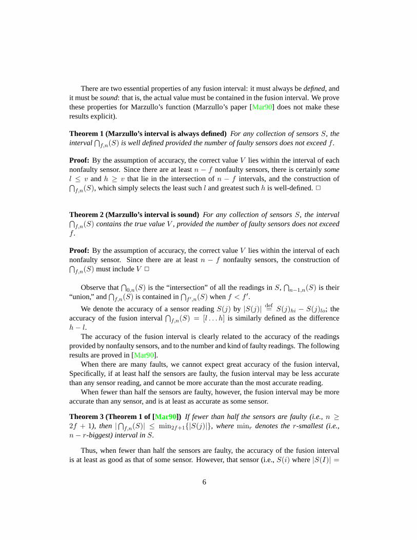
There are two essential properties of any fusion interval: it must always bedefined, andit must besound: that is, the actual value must be contained in the fusion interval. We provethese properties for Marzullo’s function (Marzullo’s paper [Mar90] does not make theseresults explicit).

Theorem 1 (Marzullo’s interval is always defined) For any collection of sensorsS, theinterval

⋂f,n(S) is well defined provided the number of faulty sensors does not exceedf .

Proof: By the assumption of accuracy, the correct valueV lies within the interval of eachnonfaulty sensor. Since there are at leastn − f nonfaulty sensors, there is certainlysomel ≤ v andh ≥ v that lie in the intersection ofn − f intervals, and the construction of⋂f,n(S), which simply selects the least suchl and greatest suchh is well-defined.2

Theorem 2 (Marzullo’s interval is sound) For any collection of sensorsS, the interval⋂f,n(S) contains the true valueV , provided the number of faulty sensors does not exceed

f .

Proof: By the assumption of accuracy, the correct valueV lies within the interval of eachnonfaulty sensor. Since there are at leastn − f nonfaulty sensors, the construction of⋂f,n(S) must includeV 2

Observe that⋂

0,n(S) is the “intersection” of all the readings inS,⋂n−1,n(S) is their

“union,” and⋂f,n(S) is contained in

⋂f ′,n(S) whenf < f ′.

We denote the accuracy of a sensor readingS(j) by |S(j)| def= S(j)hi − S(j)lo; theaccuracy of the fusion interval

⋂f,n(S) = [l . . . h] is similarly defined as the difference

h− l.The accuracy of the fusion interval is clearly related to the accuracy of the readings

provided by nonfaulty sensors, and to the number and kind of faulty readings. The followingresults are proved in [Mar90].

When there are many faults, we cannot expect great accuracy of the fusion interval,Specifically, if at least half the sensors are faulty, the fusion interval may be less accuratethan any sensor reading, and cannot be more accurate than the most accurate reading.

When fewer than half the sensors are faulty, however, the fusion interval may be moreaccurate than any sensor, and is at least as accurate as some sensor.

Theorem 3 (Theorem 1 of [Mar90]) If fewer than half the sensors are faulty (i.e.,n ≥2f + 1), then |

⋂f,n(S)| ≤ min2f+1{|S(j)|}, whereminr denotes ther-smallest (i.e.,

n− r-biggest) interval inS.

Thus, when fewer than half the sensors are faulty, the accuracy of the fusion intervalis at least as good as that of some sensor. However, that sensor (i.e.,S(i) where|S(I)| =

6

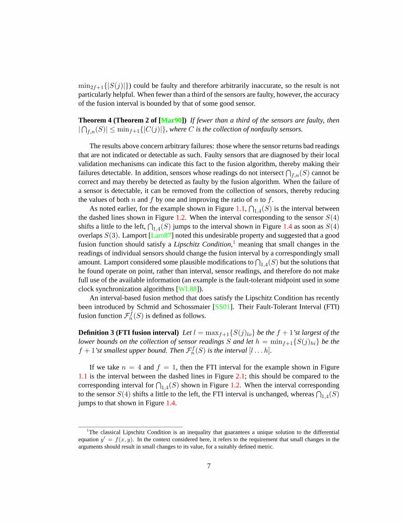
min2f+1{|S(j)|}) could be faulty and therefore arbitrarily inaccurate, so the result is notparticularly helpful. When fewer than a third of the sensors are faulty, however, the accuracyof the fusion interval is bounded by that of some good sensor.

Theorem 4 (Theorem 2 of [Mar90]) If fewer than a third of the sensors are faulty, then|⋂f,n(S)| ≤ minf+1{|C(j)|}, whereC is the collection of nonfaulty sensors.

The results above concern arbitrary failures: those where the sensor returns bad readingsthat are not indicated or detectable as such. Faulty sensors that are diagnosed by their localvalidation mechanisms can indicate this fact to the fusion algorithm, thereby making theirfailures detectable. In addition, sensors whose readings do not intersect

⋂f,n(S) cannot be

correct and may thereby be detected as faulty by the fusion algorithm. When the failure ofa sensor is detectable, it can be removed from the collection of sensors, thereby reducingthe values of bothn andf by one and improving the ratio ofn to f .

As noted earlier, for the example shown in Figure1.1,⋂

1,4(S) is the interval betweenthe dashed lines shown in Figure1.2. When the interval corresponding to the sensorS(4)shifts a little to the left,

⋂1,4(S) jumps to the interval shown in Figure1.4as soon asS(4)

overlapsS(3). Lamport [Lam87] noted this undesirable property and suggested that a goodfusion function should satisfy aLipschitz Condition,1 meaning that small changes in thereadings of individual sensors should change the fusion interval by a correspondingly smallamount. Lamport considered some plausible modifications to

⋂1,4(S) but the solutions that

he found operate on point, rather than interval, sensor readings, and therefore do not makefull use of the available information (an example is the fault-tolerant midpoint used in someclock synchronization algorithms [WL88]).

An interval-based fusion method that does satisfy the Lipschitz Condition has recentlybeen introduced by Schmid and Schossmaier [SS01]. Their Fault-Tolerant Interval (FTI)fusion functionFfn (S) is defined as follows.

Definition 3 (FTI fusion interval) Let l = maxf+1{S(j)lo} be thef + 1’st largest of thelower bounds on the collection of sensor readingsS and leth = minf+1{S(j)hi} be thef + 1’st smallest upper bound. ThenFfn (S) is the interval[l . . . h].

If we taken = 4 andf = 1, then the FTI interval for the example shown in Figure1.1 is the interval between the dashed lines in Figure2.1; this should be compared to thecorresponding interval for

⋂1,4(S) shown in Figure1.2. When the interval corresponding

to the sensorS(4) shifts a little to the left, the FTI interval is unchanged, whereas⋂

1,4(S)jumps to that shown in Figure1.4.

1The classical Lipschitz Condition is an inequality that guarantees a unique solution to the differentialequationy′ = f(x, y). In the context considered here, it refers to the requirement that small changes in thearguments should result in small changes to its value, for a suitably defined metric.

7

S(2)

S(3)

S(4)

S(1)

Figure 2.1: FTI Fusion Interval

Relationships between⋂f,n(S) andFfn (S) are established in the following theorem.

Theorem 5 (Lemma 2 of [SS01])

1. Ffn (S) ⊇⋂f,n(S)

2. Ffn (S) =⋂f,n(S) if there is noS(j) disjoint from

⋂f,n(S)

3. Fn−1n (S) =

⋂f−1,n(S)

4. F0n(S) =

⋂0,n(S)

Notice that Result 2 in the list above does not mean that Marzullo’s method plus diag-nosis and exclusion of anyS(j) disjoint from

⋂f,n(S) produces the same result asFfn (S).

Certainly, as noted on Page7, anyS(j) disjoint from⋂f,n(S) must be faulty: in the case of

Figure1.1, this means we could discardS(4) and calculate⋂

1,3(S\{S(4)}). But the resultwould be that shown in Figure2.2, which is not the same asF1

4 (S) of Figure2.1. (It is thesame asF1

3 (S\{S(4)}), as required by the theorem.)Result 1 in the list above serves to establish soundness of the FTI construction.

Theorem 6 (The FTI interval is sound) For any collection of sensorsS, the intervalFfn (S) contains the true valueV , provided the number of faulty sensors does not exceedf .

Proof: This follows from the soundness of⋂f,n(S) and the inclusion established in result

1 of the previous Theorem.2

8

S(2)

S(1)

S(3)

Figure 2.2: Marzullo’s Fusion Interval with Diagnosis

Schmid and Schossmaier [SS01] establish that their functionFfn (S) does satisfy theLipschitz Condition, and that it is optimal (i.e., the intervals produced by any fusion func-tion that satisfies the Lipschitz Condition must includeFfn (S)).

Schmid and Schossmaier also establish bounds on the accuracy ofFfn (S); they showthat it has exactly the same worst-case behavior as

⋂f,n(S), but may produce slightly less

accurate results in non-worst-case scenarios.

2.1 Formal Specification and Verification in PVS

We present a formal specification and verification for some of the concepts introducedabove. The formalization uses PVS [ORSvH95].

To begin, we define a theory parameterized by the constantsn andf , where the formeris required to be a positive natural number, and the latter is a natural number strictly lessthann (notice this exploits PVS’s support fordependent typing). We then define theindextype that will identify sensors as the numeric range1, ..., n

9

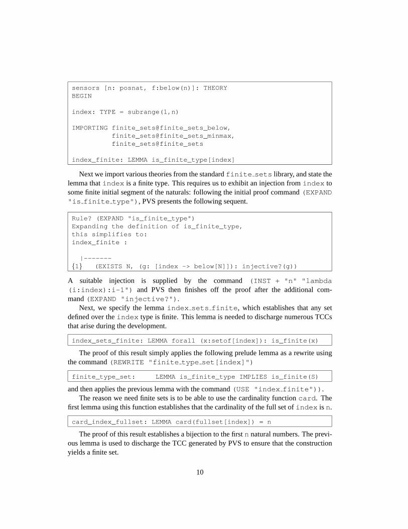
sensors [n: posnat, f:below(n)]: THEORYBEGIN

index: TYPE = subrange(1,n)

IMPORTING finite_sets@finite_sets_below,finite_sets@finite_sets_minmax,finite_sets@finite_sets

index_finite: LEMMA is_finite_type[index]

Next we import various theories from the standardfinite sets library, and state thelemma thatindex is a finite type. This requires us to exhibit an injection fromindex tosome finite initial segment of the naturals: following the initial proof command(EXPAND"is finite type") , PVS presents the following sequent.

Rule? (EXPAND "is_finite_type")Expanding the definition of is_finite_type,this simplifies to:index_finite :

|-------{1} (EXISTS N, (g: [index -> below[N]]): injective?(g))

A suitable injection is supplied by the command(INST + "n" "lambda(i:index):i-1") and PVS then finishes off the proof after the additional com-mand(EXPAND "injective?") .

Next, we specify the lemmaindex sets finite , which establishes that any setdefined over theindex type is finite. This lemma is needed to discharge numerous TCCsthat arise during the development.

index_sets_finite: LEMMA forall (x:setof[index]): is_finite(x)

The proof of this result simply applies the following prelude lemma as a rewrite usingthe command(REWRITE "finite type set[index]")

finite_type_set: LEMMA is_finite_type IMPLIES is_finite(S)

and then applies the previous lemma with the command(USE "index finite")) .The reason we need finite sets is to be able to use the cardinality functioncard . The

first lemma using this function establishes that the cardinality of the full set ofindex is n.

card_index_fullset: LEMMA card(fullset[index]) = n

The proof of this result establishes a bijection to the firstn natural numbers. The previ-ous lemma is used to discharge the TCC generated by PVS to ensure that the constructionyields a finite set.

10

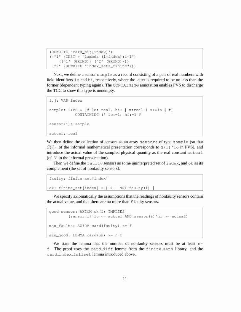
(REWRITE "card_bij[index]")(("1" (INST + "lambda (i:index):i-1")

(("1" (GRIND)) ("2" (GRIND))))("2" (REWRITE "index_sets_finite")))

Next, we define a sensorsample as a record consisting of a pair of real numbers withfield identifierslo andhi , respectively, where the latter is required to be no less than theformer (dependent typing again). TheCONTAININGannotation enables PVS to dischargethe TCC to show this type is nonempty.

i,j: VAR index

sample: TYPE = [# lo: real, hi: { x:real | x>=lo } #]CONTAINING (# lo:=1, hi:=1 #)

sensor(i): sample

actual: real

We then define the collection of sensors as an arraysensors of type sample (so thatS(i)lo of the informal mathematical presentation corresponds toS(i)‘lo in PVS), andintroduce the actual value of the sampled physical quantity as the real constantactual(cf. V in the informal presentation).

Then we define thefaulty sensors as some uninterpreted set ofindex , andok as itscomplement (the set of nonfaulty sensors).

faulty: finite_set[index]

ok: finite_set[index] = { i | NOT faulty(i) }

We specify axiomatically the assumptions that the readings of nonfaulty sensors containthe actual value, and that there are no more thanf faulty sensors.

good_sensor: AXIOM ok(i) IMPLIES(sensor(i)‘lo <= actual AND sensor(i)‘hi >= actual)

max_faults: AXIOM card(faulty) <= f

min_good: LEMMA card(ok) >= n-f

We state the lemma that the number of nonfaulty sensors must be at leastn-f . The proof uses thecard diff lemma from thefinite sets library, and thecard index fullset lemma introduced above.

11

(EXPAND "ok")(LEMMA "card_diff_subset[index]")(INST - "faulty" "fullset[index]")(("1"

(GROUND)(("1"

(CASE-REPLACE"difference(fullset[index], faulty)

= { i | NOT faulty(i) }" :HIDE? T)(("1" (USE "max_faults")

(REWRITE "card_index_fullset")(ASSERT))

("2" (HIDE -1 2) (GRIND) (APPLY-EXTENSIONALITY :HIDE? T))))("2" (GRIND))))

("2" (REWRITE "index_sets_finite")))

For an arbitrary real valuev , we defineintersect(v) to be the set of sensors whoseinterval containsv .

v: VAR realintersect(v): finite_set[index] =

{ i |sensor(i)‘lo <= v AND sensor(i)‘hi >= v }

Now we are able to state the first important result: theactual value is in the intersec-tion of at leastn-f intervals.

actual_intersect: THEOREM card(intersect(actual)) >= n-f

The proof is fairly straightforward: we split the intervals containing theactual value intothose that are faulty and those that are nonfaulty; we usemin good to establish that thereare leastn-k of the latter, and we are done.

(AUTO-REWRITE "index_sets_finite")(EXPAND "intersect")(CASE-REPLACE

" {i | sensor(i)‘lo <= actual AND sensor(i)‘hi >= actual } =union(ok,{i | faulty(i) AND sensor(i)‘lo <= actual

AND sensor(i)‘hi >= actual })" :HIDE? T)(("1"

(REWRITE "card_disj_union")(("1" (USE "min_good") (ASSERT)) ("2" (HIDE 2) (GRIND))))

("2"(HIDE 2)(APPLY-EXTENSIONALITY :HIDE? T)(EXPAND* "union" "member")(REWRITE "good_sensor")(("1" (GRIND)) ("2" (GRIND)))))

12

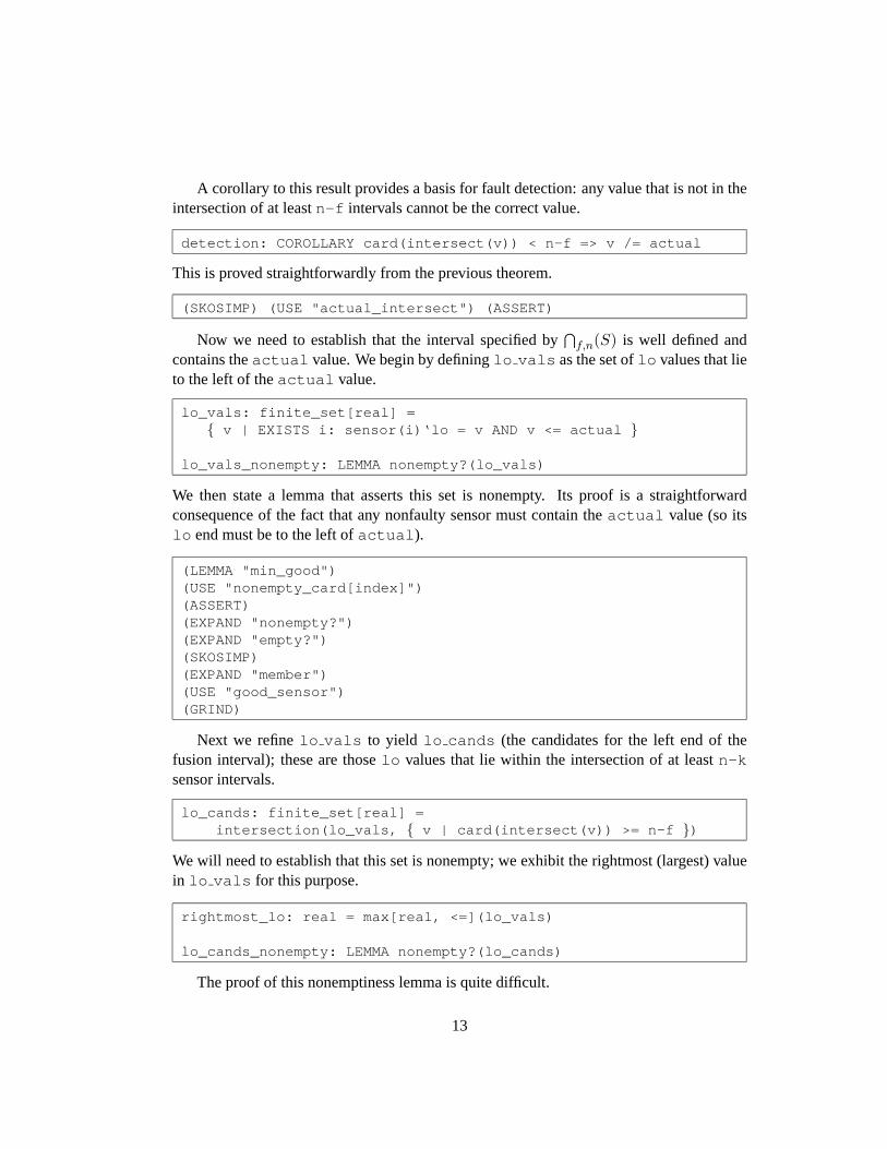
A corollary to this result provides a basis for fault detection: any value that is not in theintersection of at leastn-f intervals cannot be the correct value.

detection: COROLLARY card(intersect(v)) < n-f => v /= actual

This is proved straightforwardly from the previous theorem.

(SKOSIMP) (USE "actual_intersect") (ASSERT)

Now we need to establish that the interval specified by⋂f,n(S) is well defined and

contains theactual value. We begin by defininglo vals as the set oflo values that lieto the left of theactual value.

lo_vals: finite_set[real] ={ v | EXISTS i: sensor(i)‘lo = v AND v <= actual }

lo_vals_nonempty: LEMMA nonempty?(lo_vals)

We then state a lemma that asserts this set is nonempty. Its proof is a straightforwardconsequence of the fact that any nonfaulty sensor must contain theactual value (so itslo end must be to the left ofactual ).

(LEMMA "min_good")(USE "nonempty_card[index]")(ASSERT)(EXPAND "nonempty?")(EXPAND "empty?")(SKOSIMP)(EXPAND "member")(USE "good_sensor")(GRIND)

Next we refinelo vals to yield lo cands (the candidates for the left end of thefusion interval); these are thoselo values that lie within the intersection of at leastn-ksensor intervals.

lo_cands: finite_set[real] =intersection(lo_vals, { v | card(intersect(v)) >= n-f })

We will need to establish that this set is nonempty; we exhibit the rightmost (largest) valuein lo vals for this purpose.

rightmost_lo: real = max[real, <=](lo_vals)

lo_cands_nonempty: LEMMA nonempty?(lo_cands)

The proof of this nonemptiness lemma is quite difficult.

13

(EXPAND "nonempty?")(EXPAND "empty?")(REWRITE "forall_not")(EXPAND "member")(INST + "rightmost_lo")(EXPAND "lo_cands")(EXPAND "intersection")(SPLIT)(("1" (GRIND))

("2"(EXPAND "member")(LEMMA "rightmost_lo")(USE "max_lem[real,<=]")(("1"

(GROUND)(USE "actual_intersect")(CASE "subset?(intersect(actual),intersect(rightmost_lo))")(("1" (USE "card_subset[index]") (ASSERT))

("2"(HIDE -1 -2 -5 2)(EXPAND "subset?")(SKOSIMP)(EXPAND "member")(EXPAND "intersect")(EXPAND "lo_vals")(SKOSIMP)(ASSERT)(INST - "sensor(x!1)‘lo")(EXPAND "lo_vals")(INST + "x!1"))))

("2" (USE "lo_vals_nonempty") (EXPAND "nonempty?") (PROPAX))("3" (USE "total_le")))))

Given thatlo cands is nonempty, we can now define theleftedge of the fusioninterval as its minimum value.

leftedge: real = min[real, <=](lo_cands)

left_soundness: THEOREM leftedge <= actual

We then prove the “left half” of the soundness theorem: theleftedge lies to the leftof theactual value. The proof is straightforward given properties of themin function.

14

(LEMMA "min_lem[real,<=]")(("1"

(INST - "lo_cands" "leftedge")(("1" (GRIND))

("2" (LEMMA "lo_cands_nonempty") (EXPAND "nonempty?") (PROPAX))))("2" (LEMMA "total_le") (PROPAX)))

The construction for the “rightedge” of the fusion interval is exactly the dual of that forleftedge and is omitted.

15

16

Chapter 3

Conclusion

Modern smart sensors provide diagnostic information on their own performance and anestimate of the error in their sampled value. To allow higher-level sensor validation andfusion to be performed in an application-independent manner, it is convenient to integratethese items of information into a sensor reading that represents arangeof values (given bythe lower and upper bounds of the range). The sensor fusion problem is then to combineseveral such readings from different sensors into a best consensus value and, optionally,to perform higher-level validation by comparing the reading from one sensor against thosefrom others.

We described the “fusion functions”⋂f,n(S) of Marzullo [Mar90] and Ffn (S) of

Schmid and Schossmaier [SS01] and presented some of their properties.Ffn (S) is gener-ally to be preferred to

⋂f,n(S) because it satisfies a “Lipschitz Condition” (small changes

in sensor readings produce small changes in its output), and is optimal among all suchfunctions.

We used PVS formally to prove the well-definedness and soundness of⋂f,n(S) (i.e., it

always contains the correct value), from which soundness ofFfn (S) also follows.

17

18

Bibliography

[KN97] Herman Kopetz and R. Nossal. Temporal firewalls in large distributed real-time systems. In6th IEEE Workshop on Future Trends in Distributed Comput-ing, pages 310–315, Tunis, Tunisia, October 1997. IEEE Computer Society.1

[Lam87] Leslie Lamport. Synchronizing time servers. Technical Report 18, DEC Sys-tems Research Center, Palo Alto, CA, June 1987.7

[Mar90] Keith Marzullo. Tolerating failures of continuous-valued sensors.ACM Trans-actions on Computer Systems, 8(4):284–304, November 1990.5, 6, 7, 17

[ORSvH95] Sam Owre, John Rushby, Natarajan Shankar, and Friedrich von Henke. For-mal verification for fault-tolerant architectures: Prolegomena to the design ofPVS. IEEE Transactions on Software Engineering, 21(2):107–125, February1995. 9

[SS01] Ulrich Schmid and Klaus Schossmaier. How to reconcile fault-tolerant in-terval intersection with the Lipschitz condition.Distributed Computing,14(2):101–111, May 2001.7, 8, 9, 17

[WL88] J. Lundelius Welch and N. Lynch. A new fault-tolerant algorithm for clocksynchronization.Information and Computation, 77(1):1–36, April 1988.7

19