1

FOREIGN WORKERS IN ITALY:Are They Assimilating to Natives? Are They Competing Against Natives?

An Analysis by the SSA dataset.

Alessandra Venturini, University of Bergamo,e-mail:venturin@ibguniv.unibg.it, fax: 39-35-249975Claudia Villosio, R & P, Ricerche e Progetti, TorinoVia Bava 6, 10124 Torino Italye-mail: rep@inrete.it, tel: 39-11-888100, fax: 39-11-8123028

We would like to thank M. Abella, B. Contini, D. Del Boca, A. Gavosto, D. Gabrielli, L. Pacelli, U.Panizza, R.Revelli, S. Strozza and M. Filippi for their helps and encouragement.This research has been financed by the ILO Migration Branch and by the Funding ex-60% of the Italian Ministry ofEducation.

2

INTRODUCTION

A lot has been written about recent immigration into the Southern European Countries, but very little is known aboutwhat effect these immigrants have on the labour market in the countries of arrival. This is especially true in Italy,where the debate has been heated and the discussion has been based mainly on emotional grounds with very little andonly descriptive evidence being offered. No specific empirical research has investigate the issue because anappropriate dataset was not available.

Our intention in this paper is to show that it is possible to derive from the Social Security Archive (SSA) onEmployees an appropriate data set on the foreigners who are regularly employed in Italy, and with this information wecan answer questions such as:-Are the immigrants competitive or complementary to the native workers?-Are the immigrants assimilating to native workers in wages and employment?

The paper proceeds as follows : Section 1 describes the SSA from which our dataset is derived, section 2 comparesthis dataset with other information on immigrants, section 3 looks at the degree to which foreigners are assimilatedinto the labour market while section 4 considers the degree of wage assimilation. Section 5 discusses the wagecomplementarity or competition of the foreigners and some concluding comments close the research.

1. SOCIAL SECURITY DATASET

In fulfilling its institutional role of collecting social contributions the Italian Social Security Institute (I.N.P.S.) alsoregisters data on employment. These records cover 78.5% of total Italian employment, because Public Administrationand people employed in the professions have different funds.There are three archives: a main archive on private employment which covers roughly 11.5 million employees and1.2 million firms, a second archive on self-employment in the crafts and trade activities and on minor occupationssuch as Family workers (house-keeping, etc.) which covers about 3.5 million and a third archive on employees andself-employed in the agricultural sector which covers 1.1 million of workers.

The data we will use refers to the main archive on private employment which represents 56.1% of total Italianemployment and 71.4% of those registered with INPS. As immigrants are foreigners, they are not employed in thePublic Administration and very few of them are able to work in the professions, so the limitations of the INPS dataset are not relevant for our analysis, while the exclusion of the second (Family workers) and third archive(Agriculture) from our analysis is unfortunately not readily avoidable; this fact should be kept in mind when theresults of our research are being considered.

The main archive on private employment includes information both on employers (firms) and on individualemployees and is possible to derive from it a longitudinal (panel) dataset on private employment in Italy.

The information at firm level includes the firm identification code, its location, a 3-digit industry code, dates ofopening and closure, monthly employment1 levels, yearly data on the number of employees broken down into manualand non-manual workers, the yearly wage-bill of manual and non-manual workers. The employee records containdata identifying the worker and the firm, personal data (place of birth, nationality, age, sex, etc.), the place of work,yearly wage (before tax), number of months, weeks and days for which the wage is paid by the employer, kind ofcontracts (full-time, part-time, training contracts) and occupation (defined in 6 broad categories).

1Hence job creation and destruction (measured by employment changes at one-year intervals) and worker turnover (measured bypositive and negative monthly changes of employment) can be computed at firm level. Administrative data sets usually underestimatetenure because legal transformations of firms are recorded as firm closures. This is not a problem for our analysis because we are onlycomparing the employment behaviour of native workers and foreigner workers within the same dataset.

3

No retrospective information is recorded in this administrative archive2, there is one record for each spell ofemployment in the year and two forms will be recorded if during year t the worker moves to a new firm. Each workermay be connected - at any point in time - with the relevant firm by the identification code of the employer and thus itis possible to assign the firm's attributes to the employee.

A random sample (1:90) of the dataset was taken up by extracting the workers born on 10th March, 10th June, 10thSeptember and 10th December from 1986 to 1993, and was then reorganised into a longitudinal dataset, where theunit of observation is the work-history of the selected employees3.

Up to now the information on the foreigners employed derived from the SSA was very limited (only averageaggregate numbers) and the number of workers reported was much smaller than the number registered in othersources. An example is given in the research of Natale and Strozza (1997) where the number of foreigners reported inthe SSA in 1991 was on average 44.5% of the foreign employees reported in the ISTAT revised dataset (p.118).

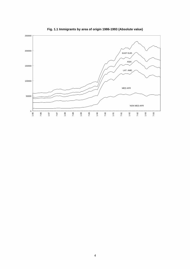
This under-reporting can partly be attributed to the way foreign labour was identified in the previous statistics: fromthe workers archive it was used the nationality which is not always reliable because in many forms it is left blank oruncompleted, from the firms archive the information used was the amount of special charges paid for hiring extra-Europeans workers4.To avoid the under-reporting of theses two sources we tried another way. We selected the workers born abroad,checked their age and entrance into the labour market. Further, in order to avoid computing the Italians born abroadwe selected only those immigrants who came from outside the European Union (EU) and Economic Advanced (EA)countries. In this way we exclude the countries where there has been a lot of Italian emigration and anyway countrieswhich contributes very little to the Italian immigration stock and even less to the recent inflows.The data-set constructed in this way provides a much higher total number of immigrants than the previous ones andemphasises the important role played by the 1990-91 legalisation in reshaping the nationality components of theimmigrants in Italy (see Fig.1.1).

2For example we can compute tenure in the current firm only if the accession occurs within the observation period, otherwise themeasure of tenure is truncated.

3For more information about the data set and its development see Contini B., Revelli R. 1992, Contini et al. 1994, Revelli 1996

4These arguments were reported in different Caritas reports and ISTAT(1997).

4

Fig. 1.1 Immigrants by area of origin 1986-1993 (Absolute value)

NON MED-AFR

MED AFR

LAT. AME.

ASIA

EAST EUR.

0

50000

100000

150000

200000

250000

1-86

7-86

1-87

7-87

1-88

7-88

1-89

7-89

1-90

7-90

1-91

7-91

1-92

7-92

1-93

7-93

5

2. COMPARISON AND DESCRIPTION OF THE DATASET

This section focuses on the presentation of the dataset used in the subsequent analyses.In Table 2.1 it is possible to compare the number of Residency-Work Permits issued by the Ministry of the Interior(Caritas, 1997) with ISTAT’s revised version of the number of valid residency permits (ISTAT, 1998). ISTAT’sestimates deduct expired permits from the total number of residency permits5 and is a better proxy of the size of theforeigners employed, while the Ministry of the Interior’s information on Residency-Work Permits includes theexpired permits and so over-estimates legal employment but it is a better proxy of total foreign employmentregistering the very common passage into illegal employment of foreigner workers with expired residency and workpermits.

Table 2.1 shows, as it should, that the SSA figure for foreigners in employment are lower than the work-permits foremployees6. This result is to be expected because the available SSA dataset do not cover Agriculture and Familywork which is very diffused among foreigners, but it is much closer to the ISTAT’s revised information of total workpermits for payroll workers (73-83%).The regional comparisons between the SSA dataset and ISTAT’s revised estimate of regular employees is unevenlydistributed (see Section b)7. Where industrial employment prevails the SSA is more representative, while in areaswhere the agriculture and the domestic employment prevail, namely in some Southern regions, the SSA data set isless representative.The national composition of the SSA dataset shows that the criteria could be improved. The Asian group is under-represented because, as is well-known, Asian workers are mostly employed as domestic workers and this category ofworkers is not included in our dataset, while the number of African workers is higher than that of ISTAT dataset. Inparticular the under-reporting of the ISTAT series is concentrated on the Senegalese' group which is about half theamount present in the SSA dataset. We did not find an explanation for this difference, but there is no reason toimagine any miss-reporting by the Social Security Institute limited to this group.A probable over-representation takes place in the Latin American group and this is easy to explain because manyItalians emigrated to South America and their descendents still hold Italian passports. Our checks on the place ofbirth by the age and the period of entry into the country were not sufficient to avoid the inclusion of immigrants ofItalian origin. However, instead of eliminating the Argentineans and the Brazilians from our dataset, we have decidedto keep them on the underlying assumption that even if some of them could have an Italian passport, theirqualifications are very low, thus they are more similar to immigrants than to natives.

5This represents the Hypothesis B of the Istat revision. Either the Census or Hypothesis A of the ISTAT revision of residency permitsunderestimated the foreigners legal presence in the country. The Census because it was difficult to approach the foreigners by the samequestionnaire and system of survey used for the Italian. The ISTAT A Hypothesis of revision of the residency permits issued by theMinistry of the Interiors excluding the expired ones, counted only permits valid at the beginning of the month while some of them wererenewed retroactively. The ISTAT B Hypothesis corrects for this systematic error.

6The information presented in the following tables are derived by our sample and reported to the total population of the Social Securitydataset.

7 In the SSA dataset the information recorded is the place of work of the worker, while ISTAT ‘s estimates report the place ofissue of the recidency permit which can be different from the place where the workers is employed.

6

Table 2.1 Comparison of Different Sources

Section a. Aggregate data

1986 1987 1988 1989 1990 1991 1992 1993Ministry of the InteriorResidency permits 450.227 572.103 645.423 490.388 781.138 852.977 927.807 987.405Total Work permits 125.049 160.550 188.018 153.473 384.782 455.963 516.359 559.294a.employees 115.158 149.004 169.004 126.602 177.212 228.229 310.438 376.382

ISTATResidency permits 645.935 589.457 649.102Total Work permits 285.318 358.621 399.940b.employees 255.233 268.026 275.774

SSAc. Foreign Workers 58.734 68.839 70.998 84.455 137.010 187.271 224.347 209.894

%ISTAT/M.I. (100*b/a) 89.4 86.3 82.0%SSA/ISTAT (100*c/b) 73.4 83.0 76.0

Section b. Regions 1993

SSA a ISTAT b %(a/b)

Piemonte 15919 15589 102.12

Valle Aosta 491 953 51.52

Liguria 4829 8167 59.13

Lombardia 59958 63397 94.58

Trentino 6927 8475 81.73

Veneto 27769 24703 112.41

Friuli 7717 8027 96.14

Emilia-R 28266 24980 113.15

Marche 5344 5709 93.61

Toscana 9931 18368 54.07

Umbria 2174 7039 30.89

Lazio 22309 48961 45.56

Campania 2794 10817 25.83

Abruzzo 4539 4337 104.66

Molise 311 291 106.87

Puglia 3570 6247 57.15

Basilicata 617 639 96.56

Calabria 686 2645 25.94

Sicilia 4739 16106 29.42

Sardegna 1005 1827 55.01

Section c. Areas of Origins 1993

SSA c ISTAT d %(c/d)Africa 117.046 110.511 105.9Asia 25.535 64.132 39.8Lat.Am. 30.265 16.243 186.3East Eu. 37.048 45.693 81.1

In the following section we examine the dataset more closely. Given the above mentioned differences by nationalitiesthe distinction by area of origins is kept.

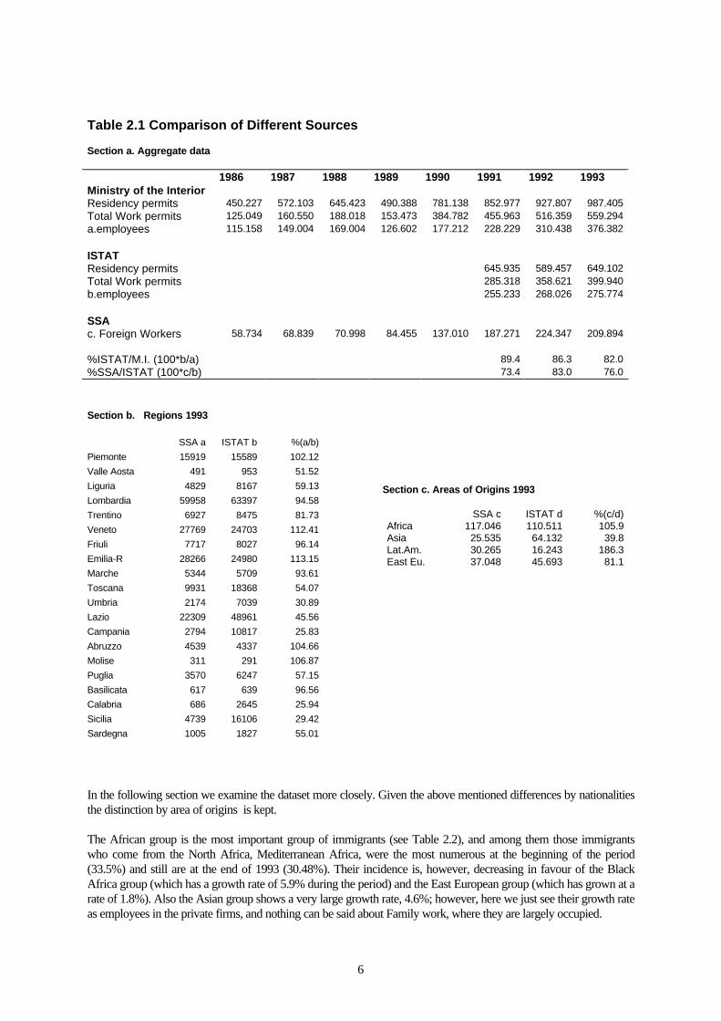
The African group is the most important group of immigrants (see Table 2.2), and among them those immigrantswho come from the North Africa, Mediterranean Africa, were the most numerous at the beginning of the period(33.5%) and still are at the end of 1993 (30.48%). Their incidence is, however, decreasing in favour of the BlackAfrica group (which has a growth rate of 5.9% during the period) and the East European group (which has grown at arate of 1.8%). Also the Asian group shows a very large growth rate, 4.6%; however, here we just see their growth rateas employees in the private firms, and nothing can be said about Family work, where they are largely occupied.

7

Table 2.2 Immigrants by area of originAbsolute values

YEARSOrigin 1986 1987 1988 1989 1990 1991 1992 1993Non Med. Africa 7593 8238 8544 13048 39409 53245 58444 53078Medit. Afr. 19652 23649 24710 27176 45458 63209 74437 63968Lat. Amer. 13546 15860 16801 19312 21568 27968 30446 30265Asia 4523 7408 8497 10554 14490 21022 26108 25535East Europe 13420 13685 12446 14365 16085 21827 34912 37048Total 58734 68839 70998 84455 137010 187271 224347 209894

PercentagesYEARS

Origin 1986 1987 1988 1989 1990 1991 1992 1993Non Med. Africa 12.93 11.97 12.03 15.45 28.76 28.43 26.05 25.29Medit. Afr. 33.46 34.35 34.80 32.18 33.18 33.75 33.18 30.48Lat. Amer. 23.06 23.04 23.66 22.87 15.74 14.93 13.57 14.42Asia 7.70 10.76 11.97 12.50 10.58 11.23 11.64 12.17East Europe 22.85 19.88 17.53 17.01 11.74 11.66 15.56 17.65

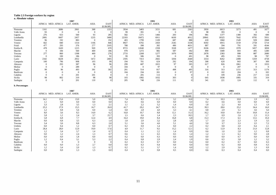
The territorial distribution of foreigners presented in Table 2.3 shows the prevalence of employment in North andCentral Italy. This is the result of two self-reinforcing phenomena: the first is related to the fact that foreign workersare concentrated in North and Central Italy where more jobs are available, second to the characteristics of our datasetwhich refers to employment in private firms which is also concentrated in the North-Central Italy. An analysis overtime stresses, for instance, that while in 1987 the non-Mediterranean Africans were in only two regions, Lombardiaand Lazio, (and in the latter region just in city of Rome), when the immigration increased the number of Africans inLazio decreased to the advantage of other more industrialised regions: Veneto, Emilia Romagna and Piemonte. Sucha trend stresses the recent flows of immigrants were labour oriented in fact they went where jobs were available.The Asian group in this dataset, instead, shows a gradual concentration in Lombardia which is an attraction for allimmigrant workers.

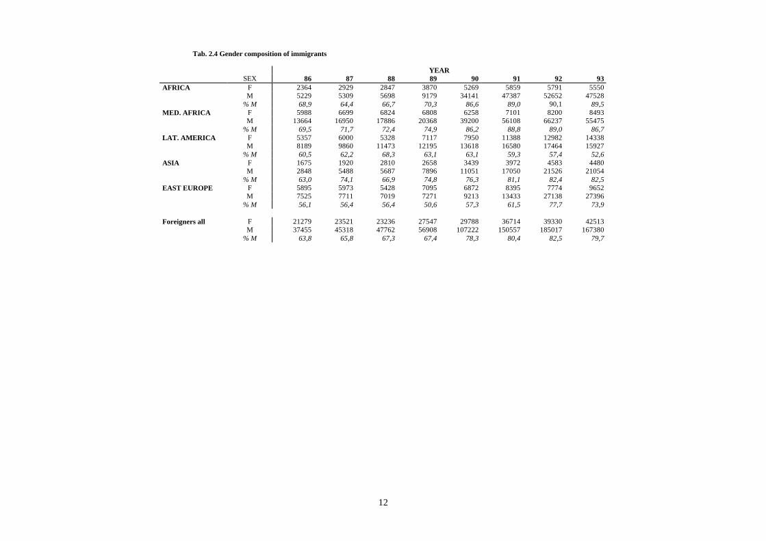
The sex distribution (see Table 2.4) shows a prevalence of male immigrants, and with the exception of the LatinAmerican group, this trend is reinforced over time. It is unusual to see a larger number of males among the Asiangroup, because the residency permits dataset shows a prevalence of females employed in the Family services.

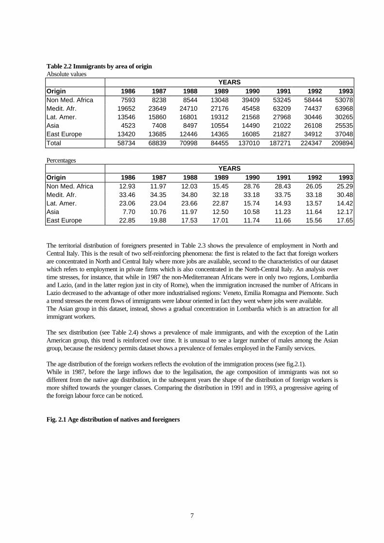
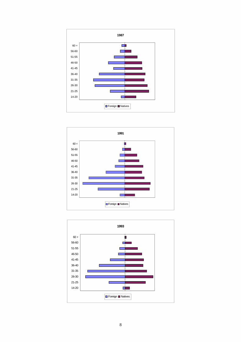
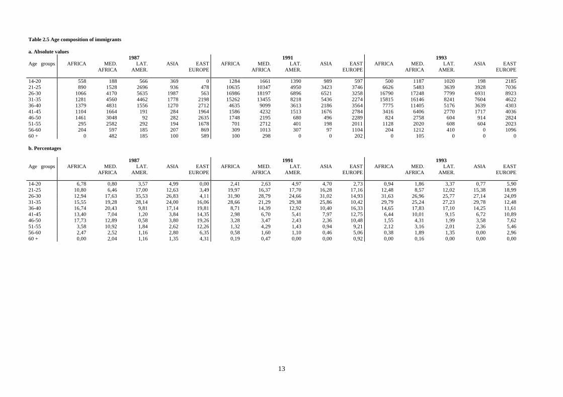
The age distribution of the foreign workers reflects the evolution of the immigration process (see fig.2.1).While in 1987, before the large inflows due to the legalisation, the age composition of immigrants was not sodifferent from the native age distribution, in the subsequent years the shape of the distribution of foreign workers ismore shifted towards the younger classes. Comparing the distribution in 1991 and in 1993, a progressive ageing ofthe foreign labour force can be noticed.

Fig. 2.1 Age distribution of natives and foreigners

8

1987

14-20

21-25

26-30

31-35

36-40

41-45

46-50

51-55

56-60

60 +

Foreign Natives

1991

14-20

21-25

26-30

31-35

36-40

41-45

46-50

51-55

56-60

60 +

Foreign Natives

1993

14-20

21-25

26-30

31-35

36-40

41-45

46-50

51-55

56-60

60 +

Foreign Natives

9

Table 2.5 discriminates by area of origin. The first column of the table reveals that the Africans working in Italy in1987 did not belong to the same groups as those who came in the more recent waves. All age groups were importantbut the 46-50 were more important than the 21-25 and the 26-30. The same is true for the East-Europeans who showa similar age distribution and for the Mediterranean Africans. These three groups belonged to an older migrationwave. The scenario changes in 1991 when the 26-30 age group becomes the most important group for the Africansand the Mediterranean Africans, and in 1993 when the 26-30 age bracket is the most important group for theAfricans, the Mediterranean Africans and the East Europeans. It is worth noting that the East European belong to amore recent wave of immigration because in 1991 the 20/25 cohort was the largest. Instead the Asian and the LatinAmerican immigrants, who are more numerous in the 31-35 cohort, are part of much more established wave.The Italian age distribution also has its peak for the 26-30 cohort, but the percentage is much lower, only 17%,because the population is more evenly distributed.

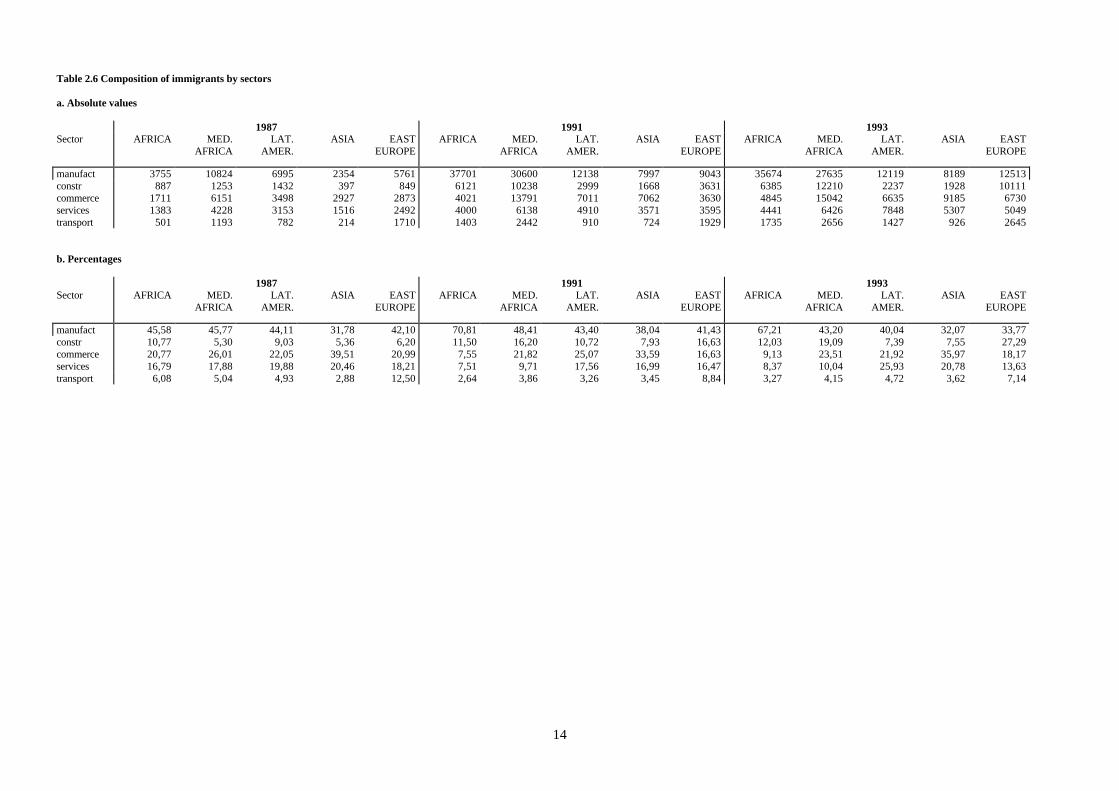
The sectorial distribution of employment of foreigners reveals a national specialisation (see Table 2.6).Manufacturing employment is the most important for all groups except the Asians for whom commercial activities arethe most important. Construction activities has increased in importance over time, expecially for immigrants fromEast Europe, while transport activities, even if it has increased in absolute numbers, it has not increased inpercentages. Service activities have increased in importance for all the groups but in particular for the LatinAmericans who find services offers them their second best employment opportunity.

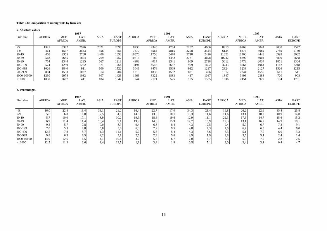
Foreigners are also employed in small scale firms, 21% in firms with fewer than 5 employees and 70% are in firmswith not more than 50 employees (Fig. 2.2).

10

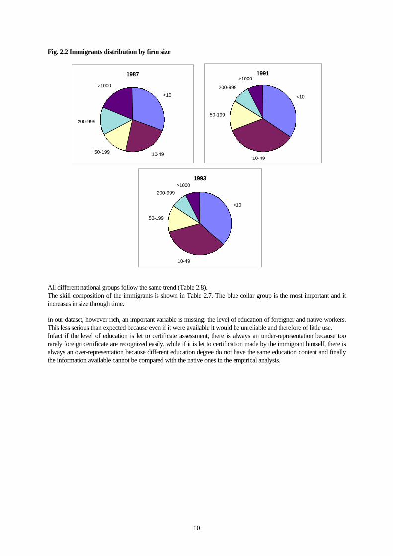
Fig. 2.2 Immigrants distribution by firm size

1987

<10

10-4950-199

200-999

>1000

1991

<10

10-49

50-199

200-999

>1000

1993

<10

10-49

50-199

200-999

>1000

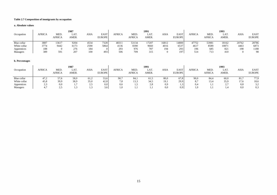
All different national groups follow the same trend (Table 2.8).The skill composition of the immigrants is shown in Table 2.7. The blue collar group is the most important and itincreases in size through time.

In our dataset, however rich, an important variable is missing: the level of education of foreigner and native workers.This less serious than expected because even if it were available it would be unreliable and therefore of little use.Infact if the level of education is let to certificate assessment, there is always an under-representation because toorarely foreign certificate are recognized easily, while if it is let to certification made by the immigrant himself, there isalways an over-representation because different education degree do not have the same education content and finallythe information available cannot be compared with the native ones in the empirical analysis.

11

Table 2.3 Foreign workers by regiona. Absolute values

1987 1991 1993AFRICA MED. AFRICA LAT. AMER. ASIA EAST

EUROPE.AFRICA MED. AFRICA LAT. AMER. ASIA EAST

EUROPE.AFRICA MED. AFRICA LAT. AMER. ASIA EAST

EUROPE.Piemonte 1161 3686 2061 368 1353 3934 5403 3151 681 2363 3950 6613 3273 491 1677Valle Aosta 93 0 0 0 0 99 391 0 0 0 98 393 0 0 0Liguria 276 653 560 93 285 582 1371 1466 293 196 981 1377 1380 392 690Lombardia 2081 6607 2457 1235 3680 22183 18472 6911 6630 4012 20841 18325 7642 8795 5931Trentino 96 192 883 0 192 403 1799 1109 687 888 418 1860 1549 928 2068Veneto 662 840 1314 1106 846 8927 6765 2450 2545 3338 8592 6915 3159 2758 5714Friuli 477 293 376 277 3105 788 398 392 490 4031 887 594 791 591 4544Emilia-R. 478 1620 1215 920 670 8715 12040 2358 3528 1477 8106 11043 1978 3457 3858Marche 0 184 560 469 186 978 1272 882 587 392 890 1680 693 495 1280Toscana 277 860 1398 469 276 2733 2268 1277 1076 999 2678 2383 998 887 2680Umbria 0 100 186 0 92 99 586 393 0 491 98 495 593 98 787Lazio 2342 6628 2052 1472 2405 2595 7413 2665 3204 2640 3314 8262 2498 5359 4758Campania 100 796 908 103 99 194 701 624 292 194 308 620 843 307 309Abruzzo 0 293 387 96 96 299 687 1815 97 305 617 826 1861 0 1033Molise 0 0 289 0 0 104 0 97 0 0 0 0 207 0 0Puglia 99 96 493 391 302 201 514 817 498 405 316 313 1151 313 1174Basilicata 0 0 0 0 0 104 194 201 0 97 0 102 204 0 102Calabria 0 0 201 201 0 0 205 113 0 0 0 109 236 217 124Sicilia 98 802 319 98 98 103 1982 1032 303 0 645 1838 1085 335 319Sardegna 0 0 201 110 0 205 748 216 111 0 341 221 124 112 0

b. Percentages

1987 1991 1993AFRICA MED. AFRICA LAT. AMER. ASIA EAST

EUROPE.AFRICA MED. AFRICA LAT. AMER. ASIA EAST

EUROPE.AFRICA MED. AFRICA LAT. AMER. ASIA EAST

EUROPE.Piemonte 14,1 15,6 13,0 5,0 9,9 7,4 8,5 11,3 3,2 10,8 7,4 10,3 10,8 1,9 4,5Valle Aosta 1,1 0,0 0,0 0,0 0,0 0,2 0,6 0,0 0,0 0,0 0,2 0,6 0,0 0,0 0,0Liguria 3,3 2,8 3,5 1,3 2,1 1,1 2,2 5,2 1,4 0,9 1,8 2,2 4,6 1,5 1,9Lombardia 25,3 27,9 15,5 16,7 26,9 41,7 29,2 24,7 31,5 18,4 39,3 28,6 25,2 34,4 16,0Trentino 1,2 0,8 5,6 0,0 1,4 0,8 2,8 4,0 3,3 4,1 0,8 2,9 5,1 3,6 5,6Veneto 8,0 3,6 8,3 14,9 6,2 16,8 10,7 8,8 12,1 15,3 16,2 10,8 10,4 10,8 15,4Friuli 5,8 1,2 2,4 3,7 22,7 1,5 0,6 1,4 2,3 18,5 1,7 0,9 2,6 2,3 12,3Emilia-R. 5,8 6,8 7,7 12,4 4,9 16,4 19,0 8,4 16,8 6,8 15,3 17,3 6,5 13,5 10,4Marche 0,0 0,8 3,5 6,3 1,4 1,8 2,0 3,2 2,8 1,8 1,7 2,6 2,3 1,9 3,5Toscana 3,4 3,6 8,8 6,3 2,0 5,1 3,6 4,6 5,1 4,6 5,0 3,7 3,3 3,5 7,2Umbria 0,0 0,4 1,2 0,0 0,7 0,2 0,9 1,4 0,0 2,2 0,2 0,8 2,0 0,4 2,1Lazio 28,4 28,0 12,9 19,9 17,6 4,9 11,7 9,5 15,2 12,1 6,2 12,9 8,3 21,0 12,8Campania 1,2 3,4 5,7 1,4 0,7 0,4 1,1 2,2 1,4 0,9 0,6 1,0 2,8 1,2 0,8Abruzzo 0,0 1,2 2,4 1,3 0,7 0,6 1,1 6,5 0,5 1,4 1,2 1,3 6,1 0,0 2,8Molise 0,0 0,0 1,8 0,0 0,0 0,2 0,0 0,3 0,0 0,0 0,0 0,0 0,7 0,0 0,0Puglia 1,2 0,4 3,1 5,3 2,2 0,4 0,8 2,9 2,4 1,9 0,6 0,5 3,8 1,2 3,2Basilicata 0 0 0 0 0 0,2 0,3 0,7 0,0 0,4 0,0 0,2 0,7 0,0 0,3Calabria 0,0 0,0 1,3 2,7 0,0 0,0 0,3 0,4 0,0 0,0 0,0 0,2 0,8 0,8 0,3Sicilia 1,2 3,4 2,0 1,3 0,7 0,2 3,1 3,7 1,4 0,0 1,2 2,9 3,6 1,3 0,9Sardegna 0,0 0,0 1,3 1,5 0,0 0,4 1,2 0,8 0,5 0,0 0,6 0,3 0,4 0,4 0,0

12

Tab. 2.4 Gender composition of immigrants

YEARSEX 86 87 88 89 90 91 92 93

AFRICA F 2364 2929 2847 3870 5269 5859 5791 5550M 5229 5309 5698 9179 34141 47387 52652 47528

% M 68,9 64,4 66,7 70,3 86,6 89,0 90,1 89,5MED. AFRICA F 5988 6699 6824 6808 6258 7101 8200 8493

M 13664 16950 17886 20368 39200 56108 66237 55475% M 69,5 71,7 72,4 74,9 86,2 88,8 89,0 86,7

LAT. AMERICA F 5357 6000 5328 7117 7950 11388 12982 14338M 8189 9860 11473 12195 13618 16580 17464 15927

% M 60,5 62,2 68,3 63,1 63,1 59,3 57,4 52,6ASIA F 1675 1920 2810 2658 3439 3972 4583 4480

M 2848 5488 5687 7896 11051 17050 21526 21054% M 63,0 74,1 66,9 74,8 76,3 81,1 82,4 82,5

EAST EUROPE F 5895 5973 5428 7095 6872 8395 7774 9652M 7525 7711 7019 7271 9213 13433 27138 27396

% M 56,1 56,4 56,4 50,6 57,3 61,5 77,7 73,9

Foreigners all F 21279 23521 23236 27547 29788 36714 39330 42513M 37455 45318 47762 56908 107222 150557 185017 167380

% M 63,8 65,8 67,3 67,4 78,3 80,4 82,5 79,7

13

Table 2.5 Age composition of immigrants

a. Absolute values1987 1991 1993

Age groups AFRICA MED.AFRICA

LAT.AMER.

ASIA EASTEUROPE

AFRICA MED.AFRICA

LAT.AMER.

ASIA EASTEUROPE

AFRICA MED.AFRICA

LAT.AMER.

ASIA EASTEUROPE

14-20 558 188 566 369 0 1284 1661 1390 989 597 500 1187 1020 198 218521-25 890 1528 2696 936 478 10635 10347 4950 3423 3746 6626 5483 3639 3928 703626-30 1066 4170 5635 1987 563 16986 18197 6896 6521 3258 16790 17248 7799 6931 892331-35 1281 4560 4462 1778 2198 15262 13455 8218 5436 2274 15815 16146 8241 7604 462236-40 1379 4831 1556 1270 2712 4635 9099 3613 2186 3564 7775 11405 5176 3639 430341-45 1104 1664 191 284 1964 1586 4232 1513 1676 2784 3416 6406 2770 1717 403646-50 1461 3048 92 282 2635 1748 2195 680 496 2289 824 2758 604 914 282451-55 295 2582 292 194 1678 701 2712 401 198 2011 1128 2020 608 604 202356-60 204 597 185 207 869 309 1013 307 97 1104 204 1212 410 0 109660 + 0 482 185 100 589 100 298 0 0 202 0 105 0 0 0

b. Percentages

1987 1991 1993Age groups AFRICA MED.

AFRICALAT.

AMER.ASIA EAST

EUROPEAFRICA MED.

AFRICALAT.

AMER.ASIA EAST

EUROPEAFRICA MED.

AFRICALAT.

AMER.ASIA EAST

EUROPE

14-20 6,78 0,80 3,57 4,99 0,00 2,41 2,63 4,97 4,70 2,73 0,94 1,86 3,37 0,77 5,9021-25 10,80 6,46 17,00 12,63 3,49 19,97 16,37 17,70 16,28 17,16 12,48 8,57 12,02 15,38 18,9926-30 12,94 17,63 35,53 26,83 4,11 31,90 28,79 24,66 31,02 14,93 31,63 26,96 25,77 27,14 24,0931-35 15,55 19,28 28,14 24,00 16,06 28,66 21,29 29,38 25,86 10,42 29,79 25,24 27,23 29,78 12,4836-40 16,74 20,43 9,81 17,14 19,81 8,71 14,39 12,92 10,40 16,33 14,65 17,83 17,10 14,25 11,6141-45 13,40 7,04 1,20 3,84 14,35 2,98 6,70 5,41 7,97 12,75 6,44 10,01 9,15 6,72 10,8946-50 17,73 12,89 0,58 3,80 19,26 3,28 3,47 2,43 2,36 10,48 1,55 4,31 1,99 3,58 7,6251-55 3,58 10,92 1,84 2,62 12,26 1,32 4,29 1,43 0,94 9,21 2,12 3,16 2,01 2,36 5,4656-60 2,47 2,52 1,16 2,80 6,35 0,58 1,60 1,10 0,46 5,06 0,38 1,89 1,35 0,00 2,9660 + 0,00 2,04 1,16 1,35 4,31 0,19 0,47 0,00 0,00 0,92 0,00 0,16 0,00 0,00 0,00

14

Table 2.6 Composition of immigrants by sectors

a. Absolute values

1987 1991 1993Sector AFRICA MED.

AFRICALAT.

AMER.ASIA EAST

EUROPEAFRICA MED.

AFRICALAT.

AMER.ASIA EAST

EUROPEAFRICA MED.

AFRICALAT.

AMER.ASIA EAST

EUROPE

manufact 3755 10824 6995 2354 5761 37701 30600 12138 7997 9043 35674 27635 12119 8189 12513constr 887 1253 1432 397 849 6121 10238 2999 1668 3631 6385 12210 2237 1928 10111commerce 1711 6151 3498 2927 2873 4021 13791 7011 7062 3630 4845 15042 6635 9185 6730services 1383 4228 3153 1516 2492 4000 6138 4910 3571 3595 4441 6426 7848 5307 5049transport 501 1193 782 214 1710 1403 2442 910 724 1929 1735 2656 1427 926 2645

b. Percentages

1987 1991 1993Sector AFRICA MED.

AFRICALAT.

AMER.ASIA EAST

EUROPEAFRICA MED.

AFRICALAT.

AMER.ASIA EAST

EUROPEAFRICA MED.

AFRICALAT.

AMER.ASIA EAST

EUROPE

manufact 45,58 45,77 44,11 31,78 42,10 70,81 48,41 43,40 38,04 41,43 67,21 43,20 40,04 32,07 33,77constr 10,77 5,30 9,03 5,36 6,20 11,50 16,20 10,72 7,93 16,63 12,03 19,09 7,39 7,55 27,29commerce 20,77 26,01 22,05 39,51 20,99 7,55 21,82 25,07 33,59 16,63 9,13 23,51 21,92 35,97 18,17services 16,79 17,88 19,88 20,46 18,21 7,51 9,71 17,56 16,99 16,47 8,37 10,04 25,93 20,78 13,63transport 6,08 5,04 4,93 2,88 12,50 2,64 3,86 3,26 3,45 8,84 3,27 4,15 4,72 3,62 7,14

15

Table 2.7 Composition of immigrants by occupation

a. Absolute values

1987 1991 1993Occupation AFRICA MED.

AFRICALAT.

AMER.ASIA EAST

EUROPEAFRICA MED.

AFRICALAT.

AMER.ASIA EAST

EUROPEAFRICA MED.

AFRICALAT.

AMER.ASIA EAST

EUROPE

Blue collar 3887 13617 9204 4534 7328 48311 53134 17207 16812 14800 47752 53981 18162 20762 28786White collar 3774 9442 6173 2590 5864 4136 8390 9660 4016 6537 4617 8589 10871 4463 6873Apprentices 188 0 276 184 0 293 976 787 194 293 196 685 821 198 1188Managers 389 591 207 100 493 506 709 315 0 197 514 713 410 0 98

b. Percentages

1987 1991 1993Occupation AFRICA MED.

AFRICALAT.

AMER.ASIA EAST

EUROPEAFRICA MED.

AFRICALAT.

AMER.ASIA EAST

EUROPEAFRICA MED.

AFRICALAT.

AMER.ASIA EAST

EUROPE

Blue collar 47,2 57,6 58,0 61,2 53,6 90,7 84,1 61,5 80,0 67,8 90,0 84,4 60,0 81,7 77,9White collar 45,8 39,9 38,9 35,0 42,8 7,8 13,3 34,5 19,1 29,9 8,7 13,4 35,9 17,6 18,6Apprentices 2,3 0,0 1,7 2,5 0,0 0,6 1,5 2,8 0,9 1,3 0,4 1,1 2,7 0,8 3,2Managers 4,7 2,5 1,3 1,3 3,6 1,0 1,1 1,1 0,0 0,9 1,0 1,1 1,4 0,0 0,3

16

Table 2.8 Composition of immigrants by firm size

a. Absolute values1987 1991 1993

Firm size AFRICA MED.AFRICA

LAT.AMER.

ASIA EASTEUROPE

AFRICA MED.AFRICA

LAT.AMER.

ASIA EASTEUROPE

AFRICA MED.AFRICA

LAT.AMER.

ASIA EASTEUROPE

<5 1321 5392 2926 2821 2898 8738 14343 4764 7202 4666 8918 16769 6844 9030 95726-9 464 1597 2543 556 656 7870 8564 2815 3208 2524 6134 8376 3082 2789 518910-19 468 2355 2708 1400 1398 10576 11756 5470 2718 2426 11821 11460 4443 3993 563220-49 568 2685 1804 769 1252 10616 9180 4452 3731 3698 10242 8397 4904 3800 668850-99 754 1344 1235 667 1218 4983 4014 2341 909 2718 5012 3773 2034 1851 3364100-199 574 1259 1262 371 764 3194 4546 2657 999 1602 3733 4064 1964 1112 2218200-499 1026 1840 911 100 1522 3046 3476 1509 912 1217 2824 3238 2127 1526 1215500-999 804 1533 1027 314 704 1313 1838 1552 821 406 1512 2244 1556 611 5111000-10000 1230 2978 1032 307 1426 1966 3322 1883 417 1017 1847 3496 2383 720 908>10000 1030 2667 411 104 1847 944 2171 525 105 1555 1036 2151 929 104 1751

b. Percentages

1987 1991 1993Firm size AFRICA MED.

AFRICALAT.

AMER.ASIA EAST

EUROPEAFRICA MED.

AFRICALAT.

AMER.ASIA EAST

EUROPEAFRICA MED.

AFRICALAT.

AMER.ASIA EAST

EUROPE

<5 16,0 22,8 18,4 38,1 21,2 16,4 22,7 17,0 34,3 21,4 16,8 26,2 22,6 35,4 25,86-9 5,6 6,8 16,0 7,5 4,8 14,8 13,5 10,1 15,3 11,6 11,6 13,1 10,2 10,9 14,010-19 5,7 10,0 17,1 18,9 10,2 19,9 18,6 19,6 12,9 11,1 22,3 17,9 14,7 15,6 15,220-49 6,9 11,4 11,4 10,4 9,1 19,9 14,5 15,9 17,7 16,9 19,3 13,1 16,2 14,9 18,150-99 9,2 5,7 7,8 9,0 8,9 9,4 6,3 8,4 4,3 12,5 9,4 5,9 6,7 7,2 9,1100-199 7,0 5,3 8,0 5,0 5,6 6,0 7,2 9,5 4,8 7,3 7,0 6,4 6,5 4,4 6,0200-499 12,5 7,8 5,7 1,3 11,1 5,7 5,5 5,4 4,3 5,6 5,3 5,1 7,0 6,0 3,3500-999 9,8 6,5 6,5 4,2 5,1 2,5 2,9 5,6 3,9 1,9 2,8 3,5 5,1 2,4 1,41000-10000 14,9 12,6 6,5 4,1 10,4 3,7 5,3 6,7 2,0 4,7 3,5 5,5 7,9 2,8 2,5>10000 12,5 11,3 2,6 1,4 13,5 1,8 3,4 1,9 0,5 7,1 2,0 3,4 3,1 0,4 4,7

17

3. EMPLOYMENT ASSIMILATION

Foreign workers often have lower professional careers than native workers. This inferior performance can be traced insome cases to their lower qualifications and to the fact that unskilled work offers few opportunities of improvement.In other cases the highly unstable nature of foreigners' work is probably due to three factors: they are not as familiarwith the labour market as native workers; they need an income and thus accept any job offered, even the mostunstable; the employer who takes on foreign workers cannot easily judge their qualifications so he tends tounderestimate the worker’s productivity. For these reasons the employer would employ the foreign workers in jobswith low labour turnover costs, thus reducing the risk of employing unproductive workers

If foreign worker job instability is due to the last three factors then it should be found only during the early stages ofimmigration, for the longer the immigrants remain in a country, job instability should be reduced and theiremployment pattern should become similar to that of native workers with the same qualifications.If this does happen then we can speak of employment assimilation to describe employment behaviour which issimilar to that of a native worker, under-assimilation if it less and over-assimilation if it is better.Our data set enables us to consider this topic and analyse foreign worker job instability.

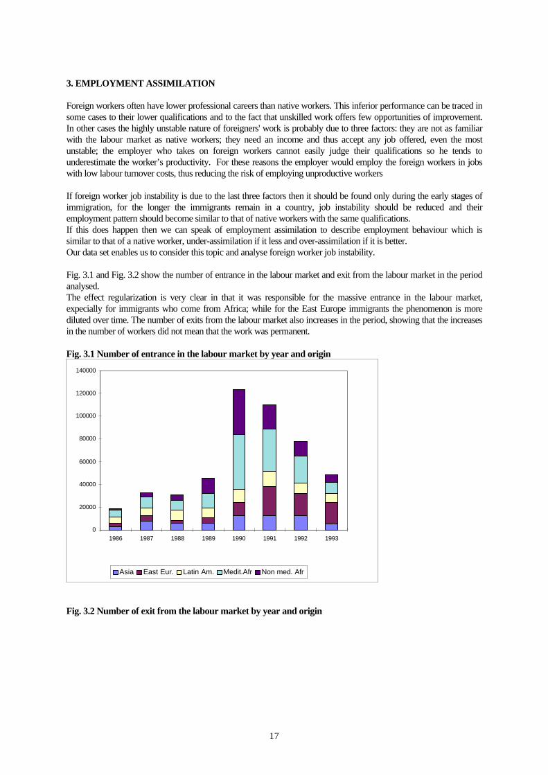
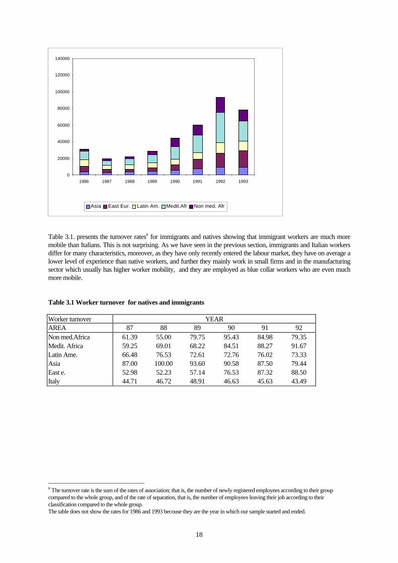
Fig. 3.1 and Fig. 3.2 show the number of entrance in the labour market and exit from the labour market in the periodanalysed.The effect regularization is very clear in that it was responsible for the massive entrance in the labour market,expecially for immigrants who come from Africa; while for the East Europe immigrants the phenomenon is morediluted over time. The number of exits from the labour market also increases in the period, showing that the increasesin the number of workers did not mean that the work was permanent.

Fig. 3.1 Number of entrance in the labour market by year and origin

0

20000

40000

60000

80000

100000

120000

140000

1986 1987 1988 1989 1990 1991 1992 1993

Asia East Eur. Latin Am. Medit.Afr Non med. Afr

Fig. 3.2 Number of exit from the labour market by year and origin

18

0

20000

40000

60000

80000

100000

120000

140000

1986 1987 1988 1989 1990 1991 1992 1993

Asia East Eur. Latin Am. Medit.Afr Non med. Afr

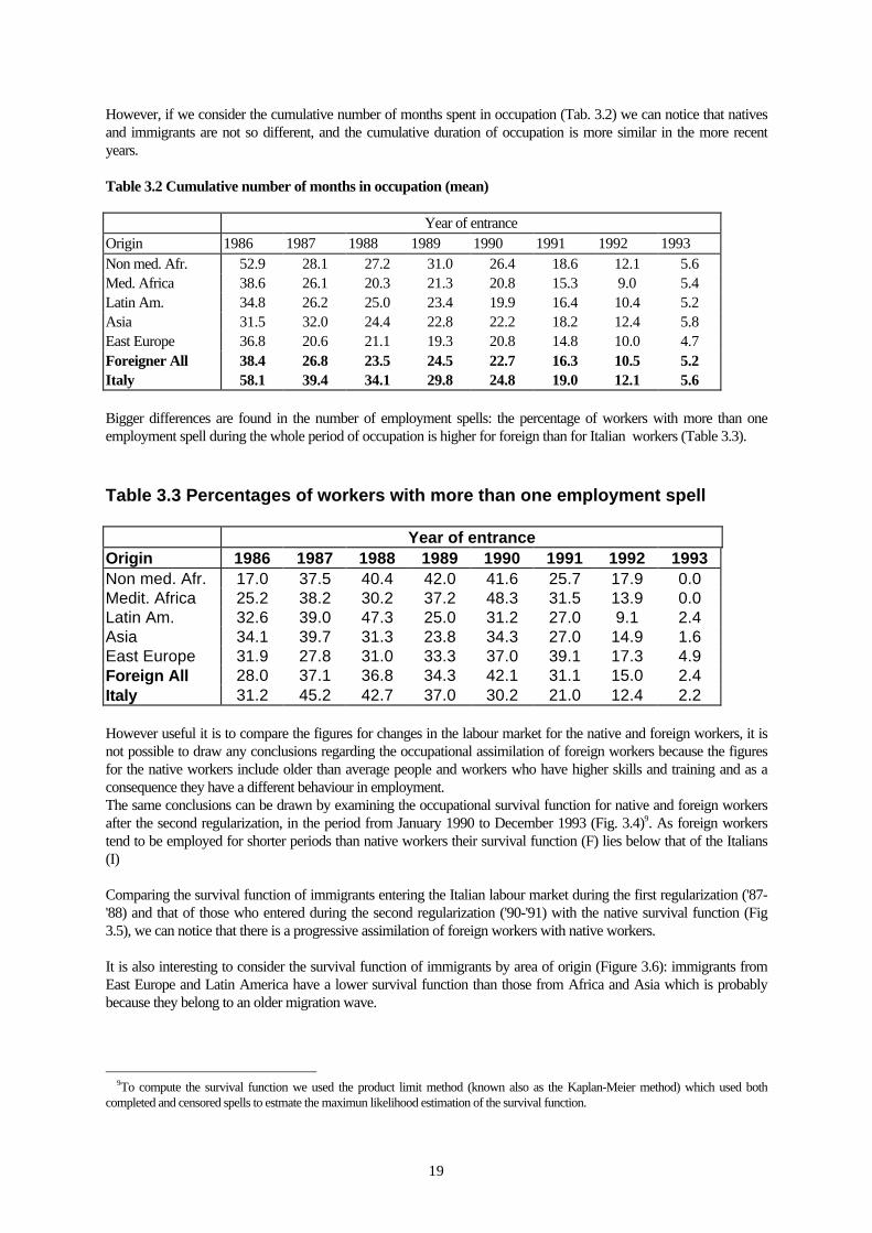
Table 3.1. presents the turnover rates8 for immigrants and natives showing that immigrant workers are much moremobile than Italians. This is not surprising. As we have seen in the previous section, immigrants and Italian workersdiffer for many characteristics, moreover, as they have only recently entered the labour market, they have on average alower level of experience than native workers, and further they mainly work in small firms and in the manufacturingsector which usually has higher worker mobility, and they are employed as blue collar workers who are even muchmore mobile.

Table 3.1 Worker turnover for natives and immigrants

Worker turnover YEARAREA 87 88 89 90 91 92Non med.Africa 61.39 55.00 79.75 95.43 84.98 79.35Medit. Africa 59.25 69.01 68.22 84.51 88.27 91.67Latin Ame. 66.48 76.53 72.61 72.76 76.02 73.33Asia 87.00 100.00 93.60 90.58 87.50 79.44East e. 52.98 52.23 57.14 76.53 87.32 88.50Italy 44.71 46.72 48.91 46.63 45.63 43.49

8 The turnover rate is the sum of the rates of association; that is, the number of newly registered employees according to their groupcompared to the whole group, and of the rate of separation, that is, the number of employees leaving their job according to theirclassification compared to the whole group.The table does not show the rates for 1986 and 1993 becouse they are the year in which our sample started and ended.

19

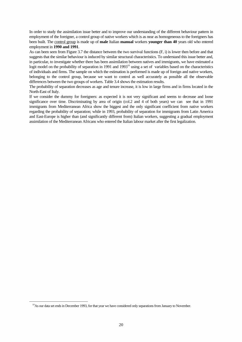
However, if we consider the cumulative number of months spent in occupation (Tab. 3.2) we can notice that nativesand immigrants are not so different, and the cumulative duration of occupation is more similar in the more recentyears.

Table 3.2 Cumulative number of months in occupation (mean)

Year of entranceOrigin 1986 1987 1988 1989 1990 1991 1992 1993Non med. Afr. 52.9 28.1 27.2 31.0 26.4 18.6 12.1 5.6Med. Africa 38.6 26.1 20.3 21.3 20.8 15.3 9.0 5.4Latin Am. 34.8 26.2 25.0 23.4 19.9 16.4 10.4 5.2Asia 31.5 32.0 24.4 22.8 22.2 18.2 12.4 5.8East Europe 36.8 20.6 21.1 19.3 20.8 14.8 10.0 4.7Foreigner All 38.4 26.8 23.5 24.5 22.7 16.3 10.5 5.2Italy 58.1 39.4 34.1 29.8 24.8 19.0 12.1 5.6

Bigger differences are found in the number of employment spells: the percentage of workers with more than oneemployment spell during the whole period of occupation is higher for foreign than for Italian workers (Table 3.3).

Table 3.3 Percentages of workers with more than one employment spell

Year of entranceOrigin 1986 1987 1988 1989 1990 1991 1992 1993Non med. Afr. 17.0 37.5 40.4 42.0 41.6 25.7 17.9 0.0Medit. Africa 25.2 38.2 30.2 37.2 48.3 31.5 13.9 0.0Latin Am. 32.6 39.0 47.3 25.0 31.2 27.0 9.1 2.4Asia 34.1 39.7 31.3 23.8 34.3 27.0 14.9 1.6East Europe 31.9 27.8 31.0 33.3 37.0 39.1 17.3 4.9Foreign All 28.0 37.1 36.8 34.3 42.1 31.1 15.0 2.4Italy 31.2 45.2 42.7 37.0 30.2 21.0 12.4 2.2

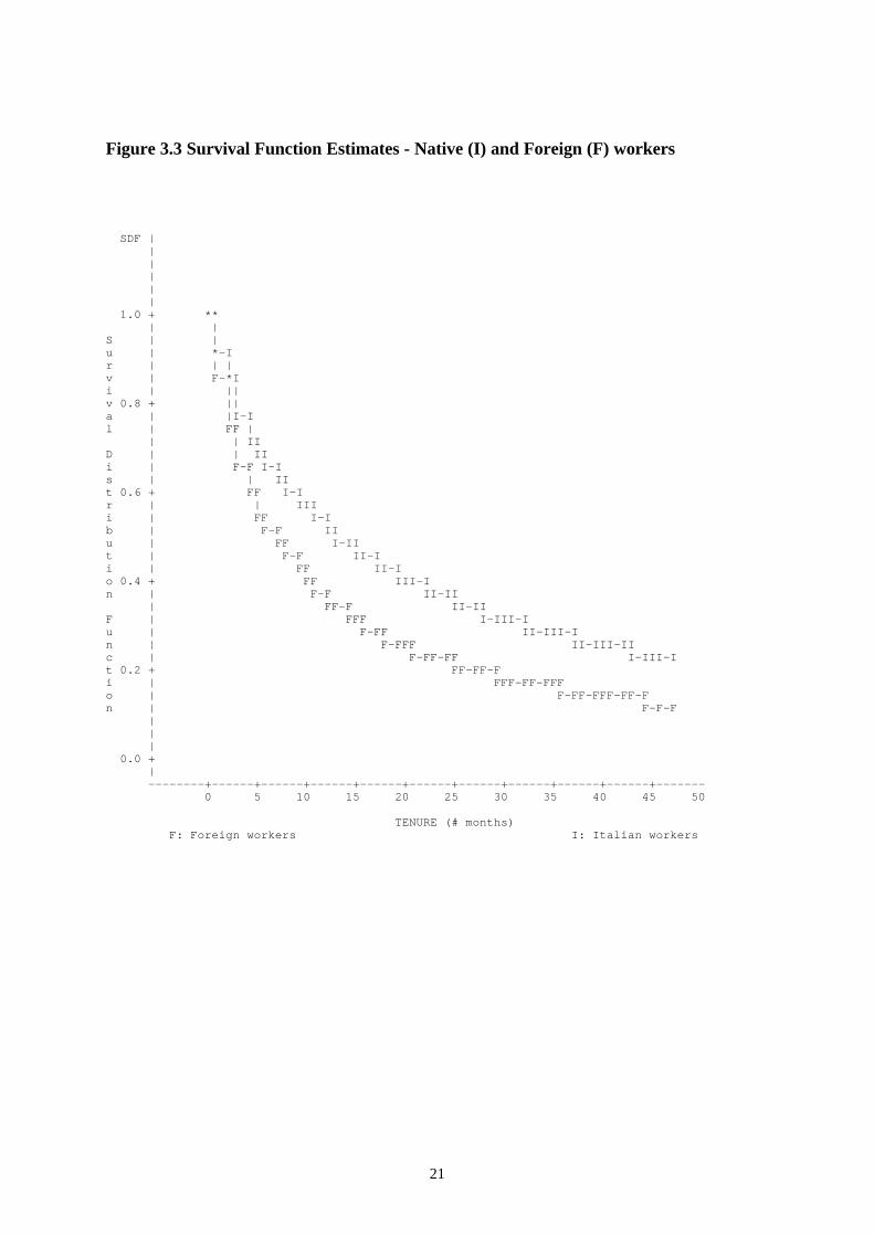
However useful it is to compare the figures for changes in the labour market for the native and foreign workers, it isnot possible to draw any conclusions regarding the occupational assimilation of foreign workers because the figuresfor the native workers include older than average people and workers who have higher skills and training and as aconsequence they have a different behaviour in employment.The same conclusions can be drawn by examining the occupational survival function for native and foreign workersafter the second regularization, in the period from January 1990 to December 1993 (Fig. 3.4)9. As foreign workerstend to be employed for shorter periods than native workers their survival function (F) lies below that of the Italians(I)

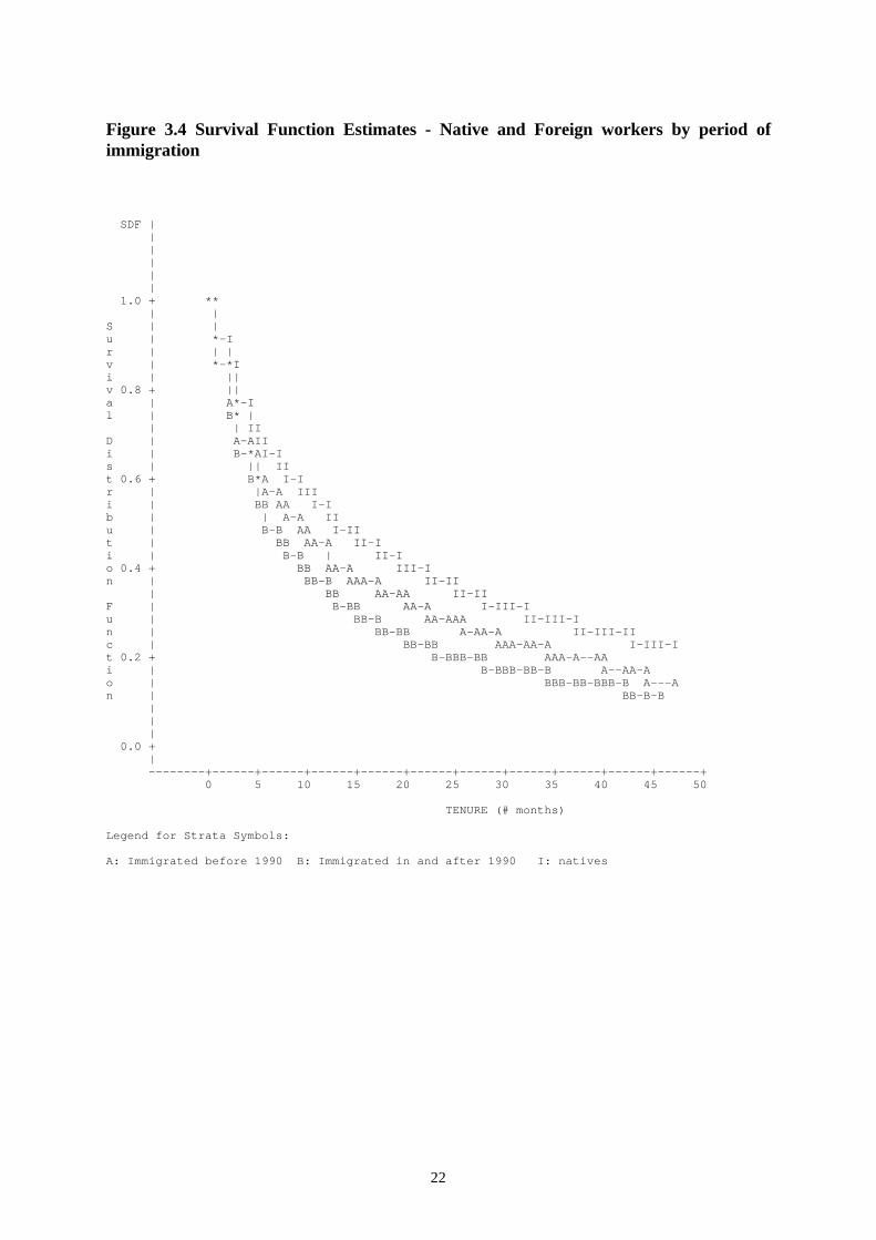
Comparing the survival function of immigrants entering the Italian labour market during the first regularization ('87-'88) and that of those who entered during the second regularization ('90-'91) with the native survival function (Fig3.5), we can notice that there is a progressive assimilation of foreign workers with native workers.

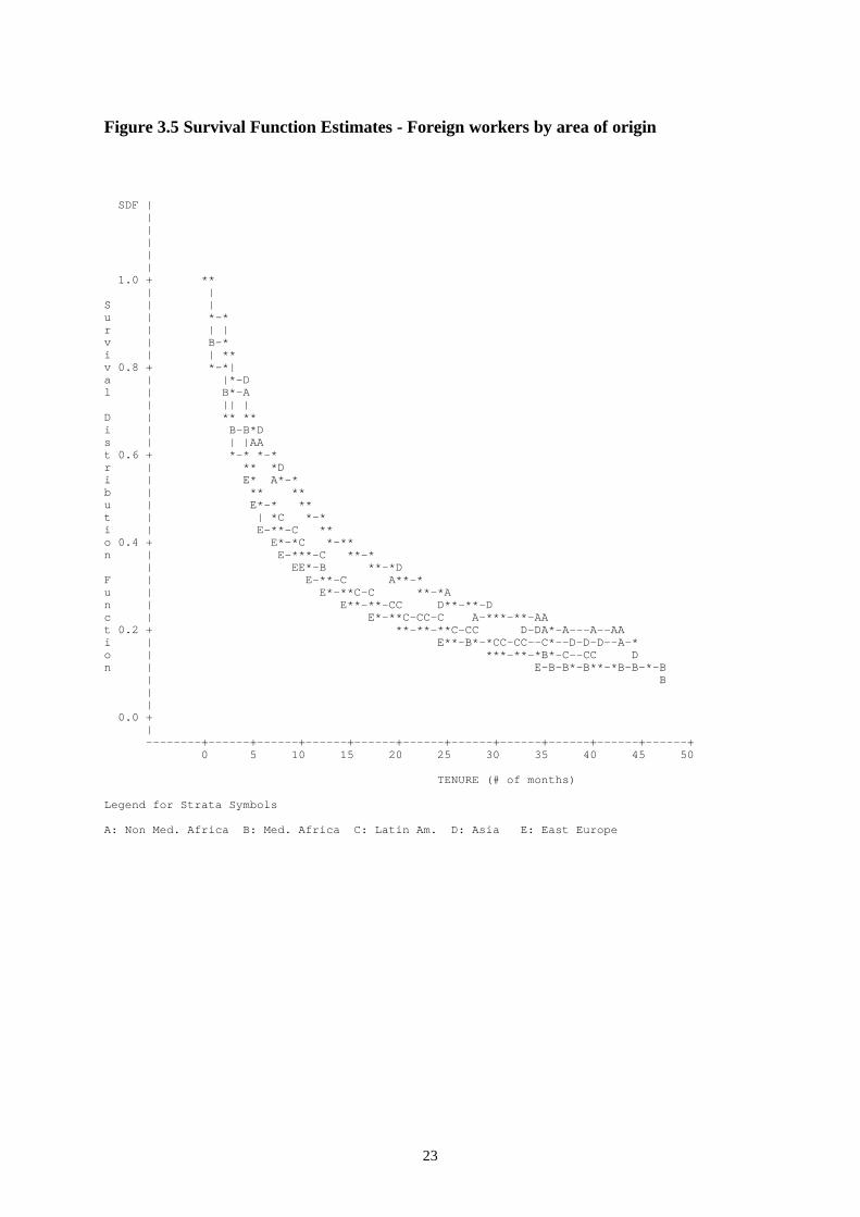
It is also interesting to consider the survival function of immigrants by area of origin (Figure 3.6): immigrants fromEast Europe and Latin America have a lower survival function than those from Africa and Asia which is probablybecause they belong to an older migration wave.

9To compute the survival function we used the product limit method (known also as the Kaplan-Meier method) which used bothcompleted and censored spells to estmate the maximun likelihood estimation of the survival function.

20

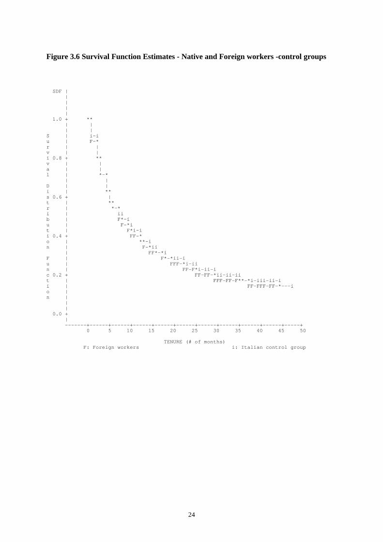
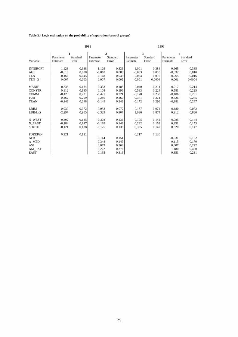
In order to study the assimilation issue better and to improve our understanding of the different behaviour pattern inemployment of the foreigner, a control group of native workers which is as near as homogeneous to the foreigners hasbeen built. The control group is made up of male Italian manual workers younger than 40 years old who enteredemployment in 1990 and 1991.As can been seen from Figure 3.7 the distance between the two survival functions (F, i) is lower then before and thatsuggests that the similar behaviour is induced by similar structural characteristics. To understand this issue better and,in particular, to investigate whether there has been assimilation between natives and immigrants, we have estimated alogit model on the probability of separation in 1991 and 199310 using a set of variables based on the characteristicsof individuals and firms. The sample on which the estimation is performed is made up of foreign and native workers,belonging to the control group, because we want to control as well accurately as possible all the observabledifferences between the two groups of workers. Table 3.4 shows the estimation results.The probability of separation decreases as age and tenure increase, it is low in large firms and in firms located in theNorth-East of Italy.If we consider the dummy for foreigners: as expected it is not very significant and seems to decrease and loosesignificance over time. Discriminating by area of origin (col.2 and 4 of both years) we can see that in 1991immigrants from Mediterranean Africa show the biggest and the only significant coefficient from native workersregarding the probability of separation; while in 1993, probability of separation for immigrants from Latin Americaand East-Europe is higher than (and significantly different from) Italian workers, suggesting a gradual employmentassimilation of the Mediterranean Africans who entered the Italian labour market after the first legalization.

10As our data set ends in December 1993, for that year we have considered only separations from January to November.

21

Figure 3.3 Survival Function Estimates - Native (I) and Foreign (F) workers

SDF | | | | | | 1.0 + ** | |S | |u | *-Ir | | |v | F-*Ii | ||v 0.8 + ||a | |I-Il | FF | | | IID | | IIi | F-F I-Is | | IIt 0.6 + FF I-Ir | | IIIi | FF I-Ib | F-F IIu | FF I-IIt | F-F II-Ii | FF II-Io 0.4 + FF III-In | F-F II-II | FF-F II-IIF | FFF I-III-Iu | F-FF II-III-In | F-FFF II-III-IIc | F-FF-FF I-III-It 0.2 + FF-FF-Fi | FFF-FF-FFFo | F-FF-FFF-FF-Fn | F-F-F | | | 0.0 + | --------+------+------+------+------+------+------+------+------+------+------- 0 5 10 15 20 25 30 35 40 45 50

TENURE (# months) F: Foreign workers I: Italian workers

22

Figure 3.4 Survival Function Estimates - Native and Foreign workers by period ofimmigration

SDF | | | | | | 1.0 + ** | |S | |u | *-Ir | | |v | *-*Ii | ||v 0.8 + ||a | A*-Il | B* | | | IID | A-AIIi | B-*AI-Is | || IIt 0.6 + B*A I-Ir | |A-A IIIi | BB AA I-Ib | | A-A IIu | B-B AA I-IIt | BB AA-A II-Ii | B-B | II-Io 0.4 + BB AA-A III-In | BB-B AAA-A II-II | BB AA-AA II-IIF | B-BB AA-A I-III-Iu | BB-B AA-AAA II-III-In | BB-BB A-AA-A II-III-IIc | BB-BB AAA-AA-A I-III-It 0.2 + B-BBB-BB AAA-A--AAi | B-BBB-BB-B A--AA-Ao | BBB-BB-BBB-B A---An | BB-B-B | | | 0.0 + | --------+------+------+------+------+------+------+------+------+------+------+ 0 5 10 15 20 25 30 35 40 45 50

TENURE (# months)

Legend for Strata Symbols:

A: Immigrated before 1990 B: Immigrated in and after 1990 I: natives

23

Figure 3.5 Survival Function Estimates - Foreign workers by area of origin

SDF | | | | | | 1.0 + ** | |S | |u | *-*r | | |v | B-*i | | **v 0.8 + *-*|a | |*-Dl | B*-A | || |D | ** **i | B-B*Ds | | |AAt 0.6 + *-* *-*r | ** *Di | E* A*-*b | ** **u | E*-* **t | | *C *-*i | E-**-C **o 0.4 + E*-*C *-**n | E-***-C **-* | EE*-B **-*DF | E-**-C A**-*u | E*-**C-C **-*An | E**-**-CC D**-**-Dc | E*-**C-CC-C A-***-**-AAt 0.2 + **-**-**C-CC D-DA*-A---A--AAi | E**-B*-*CC-CC--C*--D-D-D--A-*o | ***-**-*B*-C--CC Dn | E-B-B*-B**-*B-B-*-B | B | | 0.0 + | --------+------+------+------+------+------+------+------+------+------+------+ 0 5 10 15 20 25 30 35 40 45 50

TENURE (# of months)

Legend for Strata Symbols

A: Non Med. Africa B: Med. Africa C: Latin Am. D: Asia E: East Europe

24

Figure 3.6 Survival Function Estimates - Native and Foreign workers -control groups

SDF | | | | | 1.0 + ** | | | |S | i-iu | F-*r | |v | |i 0.8 + **v | |a | |l | *-* | |D | |i | **s 0.6 + |t | **r | *-*i | iib | F*-iu | F-*it | F*i-ii 0.4 + FF-*o | **-in | F-*ii | FF*-*iF | F*-*ii-iu | FFF-*i-iin | FF-F*i-ii-ic 0.2 + FF-FF-*ii-ii-iit | FFF-FF-F**-*i-iii-ii-ii | FF-FFF-FF-*---io |n | | | 0.0 + | -------+------+------+------+------+------+------+------+------+------+-----+ 0 5 10 15 20 25 30 35 40 45 50

TENURE (# of months) F: Foreign workers i: Italian control group

25

Table 3.4 Logit estimation on the probability of separation (control groups)

1991 1993

1 2 3 4Parameter Standard Parameter Standard Parameter Standard Parameter Standard

Variable Estimate Error Estimate Error Estimate Error Estimate Error

INTERCPT 1,128 0,338 1,129 0,339 1,001 0,384 0,965 0,385AGE -0,010 0,008 -0,010 0,008 -0,033 0,010 -0,032 0,010TEN -0,166 0,045 -0,168 0,045 -0,064 0,016 -0,065 0,016TEN_Q 0,007 0,003 0,007 0,003 0,001 0,0004 0,001 0,0004

MANIF -0,335 0,184 -0,333 0,185 -0,040 0,214 -0,017 0,214CONSTR 0,112 0,195 0,108 0,196 0,583 0,224 0,581 0,225COMM -0,423 0,221 -0,421 0,221 -0,178 0,250 -0,186 0,251PUB 0,262 0,259 0,246 0,260 0,371 0,274 0,326 0,275TRAN -0,146 0,248 -0,149 0,249 -0,172 0,296 -0,181 0,297

LDIM 0,030 0,072 0,032 0,072 -0,187 0,071 -0,180 0,072LDIM_Q -2,297 0,905 -2,329 0,907 1,036 0,874 0,912 0,880

N_WEST -0,302 0,135 -0,303 0,136 -0,105 0,142 -0,085 0,144N_EAST -0,184 0,147 -0,199 0,148 0,232 0,152 0,251 0,153SOUTH -0,121 0,138 -0,125 0,138 0,325 0,147 0,320 0,147

FOREIGN 0,221 0,111 0,217 0,120AFR 0,144 0,151 -0,031 0,182A_MED 0,348 0,149 0,115 0,170ASI 0,079 0,268 0,607 0,272AM_LAT 0,222 0,376 1,180 0,420EAST 0,135 0,316 0,351 0,231

26

4. WAGE DIFFERENTIALS AND WAGE ASSIMILATION

If employment differentials are limited let us examine those for wages. We concentrate our analysis on thedifferentials in 1991, after the end of the second regularization procedure, and in 1993, two years later. Unfortunately,in our data set for the earlier period there were too few non-EU-EAC immigrants to consider it.

Table 4.1 Wage differentials between native and foreign workers (log dailywage) by branches and origin

1991 1993 1991 1993Section a ALL ALL Control

groupControlgroup

Branches

Mining -0.468 -0.261 0.097 0.062Metal works 0.260 1.074 0.030 0.115Non metal products 0.211 0.147 0.035 0.016Metal products and machinery 0.248 0.293 0.087 0.079Chemicals, rubber and plastic 0.185 0.133 -0.055 0.044Electronics and office equipment -0.093 -0.011 0.076 0.076Automobile 0.087 0.111 0.040 -0.161Food and beverages 0.175 0.193 0.201 0.074Textiles 0.003 0.052 -0.037 -0.072Lumber and wood products 0.088 0.094 0.156 0.062Paper and printing 0.035 0.159 -0.029 0.006Construction 0.122 0.059 0.091 0.044Wholesale trades 0.089 0.062 0.213 0.054Retailing 0.094 0.042 -0.035 -0.038Transports 0.102 0.224 0.221 0.238Communications -0.178 -0.182Banking, insurances -0.067 -0.068Business services 0.025 0.016 0.047 0.082Energy, gas and water 0.031 0.006 -0.155 -0.089Other services 0.137 0.116 0.038 0.035

Section bAreas of origin

Non-Med. Africa 0.210 0.196 0.054 0.012Med. Africa 0.161 0.187 0.052 0.063Asia 0.122 0.212 -0.022 0.044East Europe 0.136 0.132 0.075 0.026Latin America -0.181 0.143 -0.234 0.047

ALL 0.145 0.153 0.057 0.035

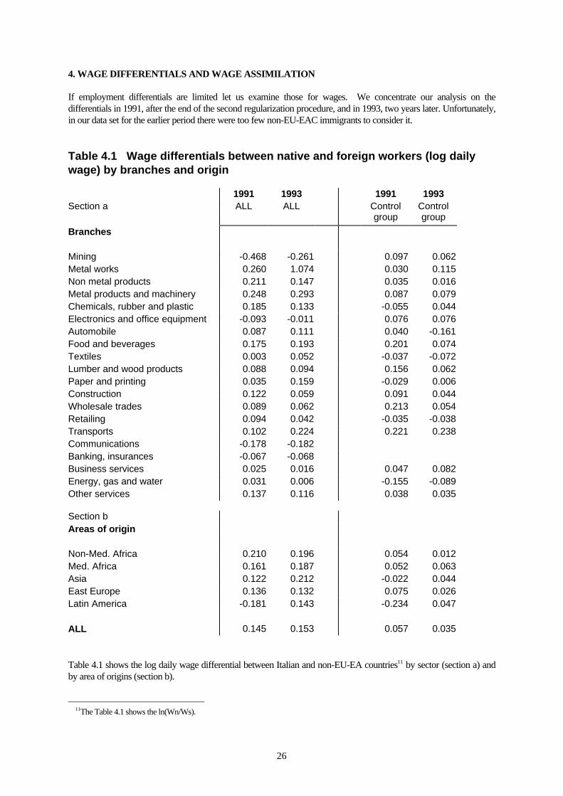
Table 4.1 shows the log daily wage differential between Italian and non-EU-EA countries11 by sector (section a) andby area of origins (section b).

11The Table 4.1 shows the ln(Wn/Ws).

27

In the first and second columns the wage comparison is between the overall workers wage and the non-UE-EAC one,while in the third and fourth columns the reference group is the control group.In 1991 the log wage differential is on average 0.145 and shows a very large variance among the industrial branches(0.26 /-0.47), larger than among the service branches. Wage differences are again large among areas of origin: while the immigrants who came from non-MediterraneanAfrica have the lowest wage, the workers came from Latin America receive a wage rate which is higher than thenative workers (negative sign of the ratio). This disappears in time, and the new immigrants who also came from theLatin American countries have a lower wage than the native workers (Table 4.1, Section b, Column 2). This overallresult is to be expected because the immigrants are employed in manual jobs at the lowest level and have little tenurebecause most of them have been employed regularly only since the end of the '80s.

The analysis of the time factor 1991 and 1993 is a little puzzling. On aggregate the difference increases over time andreaches 0.153, but there is not a clear-cut trend in the branches examined. And even in the area of origin section theAsian group shows an increase in the wage differential while the other groups show a small reduction. This effect isdue to a change in the composition of the two groups, native workers being more skilled and immigrant workersbeing less skilled.

The right side of Table 4.1 compares the native workers’ wage of the "control" group with that of the foreign workersand, as expected, there is a smaller wage differential which is 0.057 in 1991 and 0.035 in 1993. In few branches thesmaller wages gap become negative but on average it is positive. The specification by areas of origin shows the sametrend, the positive coefficients are smaller in size than before because the two groups are more similar, and for theLatin Americans and the Asian workers the wage gap is negative (higher wage for the foreigners).A comparison over time for 1991 and 1993 for the wages of the control group and those of the immigrants has adifferent meaning, because the native workers in the control group and the foreigner workers both entered into thelabour market during 1990 and 1991 and persisted in the labour market until 1993, thus the variation of the wagegap in this time dimension suggests an increase or decrease in the foreigners' wage integration.If it is assumed that the employer is not able to asses a foreign worker's productivity, before he or she is hired, in orderto reduce risk he will hire the immigrant at the lowest possible level and wage, and in this way he initiallydiscriminate against the foreign worker. However, as soon as the employer sees the ability of the worker, he willadjusts his position and wage to his productivity and thus he will reduce the initial discrimination. In general this iswhat the data shows, the wage gap with the control group decreases and reaches 0.035. Each branch shows this trend- with as usual some exceptions - while this pattern does not appear in the distinction by country of origin.

Another measure to analyse the wage gap between foreign and native workers is total annual earnings. Thismeasure adds up the daily wage and the number of days worked and thus is much lower for the workers who have aless stable job in the labour market, as is the case for the immigrants. The results not shown in the table reveal that in1991 there was an aggregate wage gap of 0.425 and in 1993 it was 0.353. Given the previous increasing trend on thewage gap, the reduction in the earning gap is due to the increase in length in employment by immigrants. This effectis even stronger if the control group is taken into account, immigrants show a negative - thus higher wage - gap -0.095 in 1991 and -0.081 in 1993.

The comparison with a control group was meant to control the etherogenity of the workers but the Oaxaca (1973)index provides a synthetic measure of the wage gap. It is divided into two parts: one which is explained by thedifferent characteristics of the two worker groups and the other part unexplained. This measure is generally used ingender literature and was applied by Bonjour and Pacelli (1997) on the same dataset to study gender wagedifferences.

Let us briefly recall the wage gap specification.The wage (w) of the worker (i) of type (n) for a native worker and (f) for a foreign worker, is determined by a series ofhuman capital and efficiency wage variables (X).Thus we have two testable equations, the first for native workers and the second for foreign workers which will resultin two different estimated vectors of coefficients b^

n and b^f.

1.n n ni n i iw = b X + ∈Error! Switch argument not specified.

2.f f fi f i iw = b X + ∈Error! Switch argument not specified.

28

Given the average characteristics of native workers Xn and foreign workers Xf

and the estimated coefficients

$bn and $bf , the average wage for native and foreign workers can be computed as:

3. n n nw = X b$Error! Switch argument not specified.4. f f fw = X b$Error! Switch argument not specified.

but also the counter factual average wage for foreign workers w fc - resulting from the product of the foreigners

characteristics X f and the native parameter $bn - and viceversa for native workers wnc .

The wage gap can thus be broken up into two parts: the first one explained by the different characteristics of the twogroups, and the second unexplained frequently called discrimination.

5. n f N fc

fc

f n f n N f fW -W = (W -W )+(W -W )= ( X - X )b +( b - b )X$ $ $

Breaking up the figures in this way does not mean we intend to examine the discrimination against foreign workersbut on the contrary their integration into the labour market. As previously explained, the initial low wage entrance dueto the underestimate of the foreign worker productivity will be revised by checking the foreign workers productivityon the job, and by reducing the "unexplained wage gap". By applying the Oaxaca decomposition in 1991 and twoyears later, in 1993, a reduction of the differential due to the better appreciation of the foreigner productivity is to beexpected.

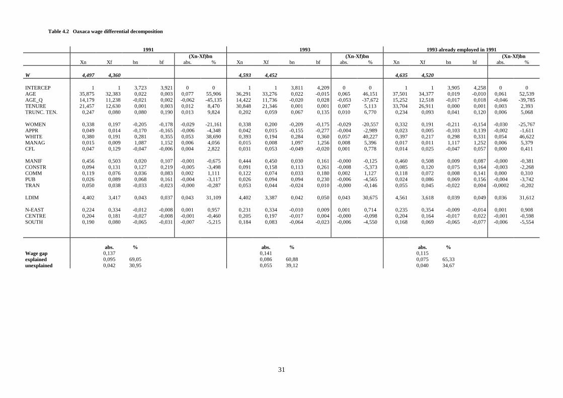
The empirical tests in Table 4.2 shows the results of the 6 cross-section OLS regressions while the computation ofthe index is shown in the lower part of the table12.

If we examine section a of Table 4.2. The first and second columns, of this and also of the other sections, show themean value of the logwage and of all the explicative variables (Xi) used in the OLS regression - age, agesquare, sex,type of contract, tenure, truncated tenure, sector, log size of the firm and macro-areas - in the Italian and Foreigngroups. The third and the fourth columns report the coefficients of the logwage OLS regression run for the Italiansand the Foreigners separately. The fifth column reports the wage gap as explained by the differences in thecharacteristics between the two groups [(Xn-Xf)bn] while the percentage of the total logwage gap explained by themare shown in column six.

In 1991 69% of the total wage gap between native workers and foreign workers, 0.1369, was explained by thedifferent average characteristics between the two groups and 31% was unexplained, 0.0424.The age component explains 11% of the logwage gap (55%-45%), immigrant workers, as is well known, are youngerthan native workers; the firm size 31%, immigrants work mainly for small firms; the tenure 8.47%, immigrants havejust entered the Italian labour market thus they have little or no tenure.The negative sign of the absolute differences for the sex composition simply stresses that the male group prevailsamong the immigrants, thus the lower share of female workers in the foreign group adjust the foreign wage upward,the same happens in the construction sector and for the territorial distribution. The immigrants are mainly located in North and Central Italy, thus the negative sign of the Southern dummy stresses that their wage has been adjustedupward.

This result can be compares with the one obtained by the research of Bonjour and Pacelli (1997) on the female-maledifferential with the same data set in the same year, 1991. The total log wage gap in the male-female analysis is

12 The complete output of the 6 OLS regressions is presented in table 4.a in the appendix

29

0.225, which is lager than that for native-foreign workers (0.137). The age variable is also very important in themale-female case and explains 11% of the wage gap, the firm size is also important (11%) but much less so than inthe native-foreign case (31%).Even though the two results are not comparable directly because the specification used in the Italian case is a littledifferent from the one used for the native-foreigner case, the explained part of the total gap is much smaller, neverabove 25% (0.072), while in the specification more similar to ours it is 15% (0.04) and thus the unexplained part ismuch larger.

In 1993 the wage gap increased to 0.14 and the explained part decreased to 61% and thus the unexplained partincreased to 39% (0.055). The age variable looses some of its significance, now it explains only 9% of the wage gap,and also the impact of the tenure variable is reduced, while the other variables keep the same role in explaining thewage gap.There is no evidence in the wage data of wage assimilation in this short period of time. Probably the analysis cross-section even though is at an individual level are not sufficiently detailed to identify changes in the appreciation of theforeign workers in the labour market 13.

In order to identify a possible wage assimilation of the foreigners, section c of the Table 4.2 presents the result of thewage differential of the workers present in the labour market in 1991 and still employed in 1993. From thiscomparison we analyse the different degrees of wage assimilation between native and foreign workers. The wage gapfalls to 0.1152, and 65% of it is explained by the different characteristics of the two groups and 34.7% remainsunexplained. Thus the total wage gap is reduced and the unexplained part is smaller than it was in 1993 (0.0399).But what is more important it is smaller than the 1991 share, when it was 0.0424, supporting the interpretation of awage assimilation by foreigners.

To check the wage gap we also calculated the wage differentials against the control group which is, as alreadymentioned, made up of native workers whose characteristics are very similar to the foreign workers - under 40, male,blue collar and entered the labour market in 1991.The wage differential between the two groups in 1993 is 0.0437, a value which is very close to the previous one,97% of which is unexplained because the characteristics of the two groups are similar and therefore the explained partis already present in the selection of the two groups 14.

In the article by Bonjour and Pacelli (1997) the Oaxaca traditional decomposition is revised by the introduction of asubdivision into branches. The underlying hypothesis is that there is a possible differential behaviour of the wage gapby economic activity15.

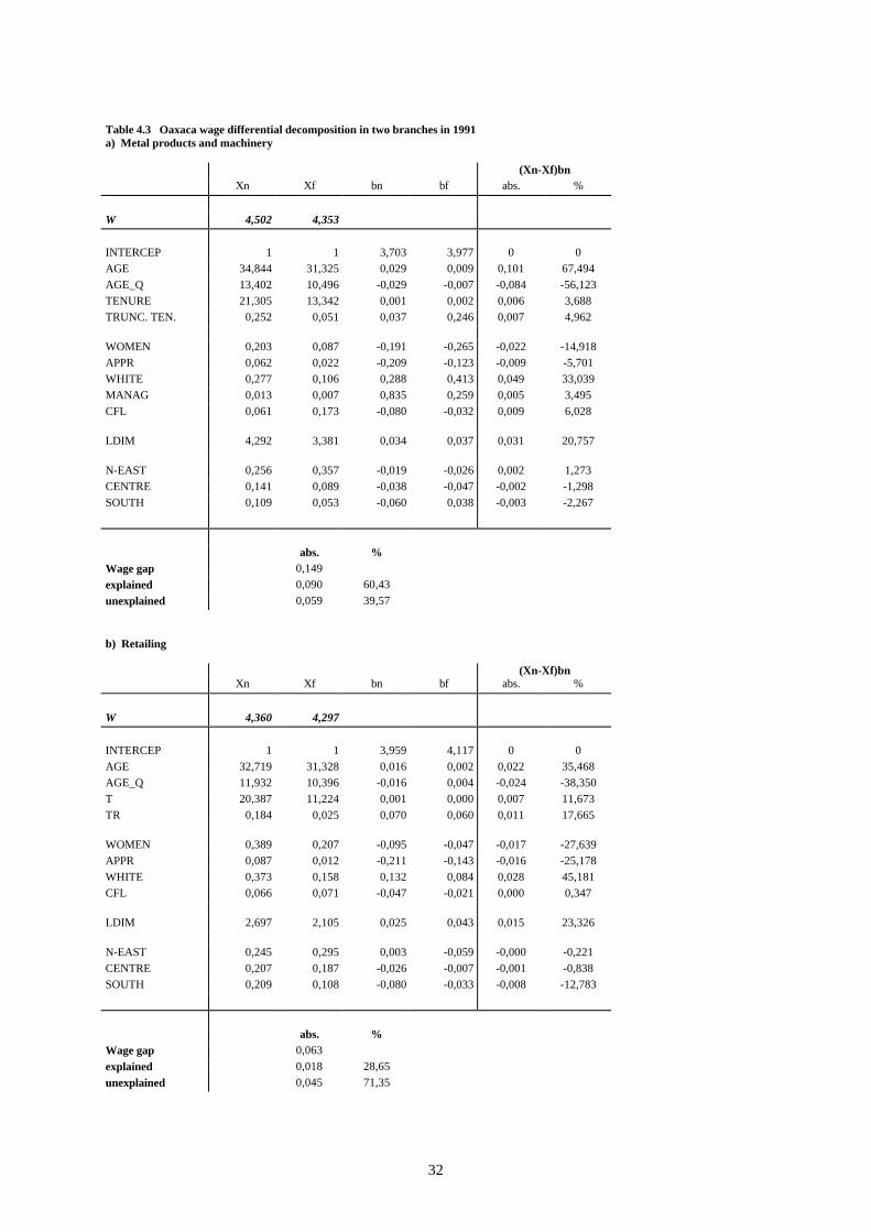
For 1991 we have specified the index for two branches in which foreign workers accounted for an important share:one in the industrial production sector, Metal Products and Machinery (MPM), and the other in the service sector,Retailing.Table 4.3 shows that the wage gaps are different: 0.149 in the Metal Products and Machinery Industry and 0.06 inRetailing. The first gap results above the national average and the second one below. The explained part is howeverlarger in the first case 60%, while in the second case it is only 29%. There are differences in the explicative power ofthe characteristics of the two groups, for instance the age variable explains 11% of the wage gap in the MPM branchand -3% in the Retailing branch. The tenure effect is 3% in the MPM branch and 12% in Retailing. These differentrelationships stress that the overall picture is the result of composite effects. The unexplained parts - which are inpercentages the complement to the explained part and thus are very different - in reality when analyzed in absolutevalue are much more similar, 0.059 in the industrial branch and 0.045 in the services branch and they are also verysimilar to the overall picture.

13This effect could be also the result of variables omitted from our dataset.

14 For the control group in 1991 the wage gap was only 0.021, of which 162 unexplained. This result is induced by a negative sign of theexplained part (-62%) that implies that the characteristics favoured the foreigners, (for instance the average age of the Italian workers waslower than for the foreign workers and the age variable accounted for -93% of the explained gap).

15In their analysis the specification by branches only capture 11% of the wage differential.

30

A final comment on the Blau and Kahn (1992) specification used in their international comparison and by Del Boca(1993) in a bilateral countries. This specification introduces the standard residual of the regression and its standarddeviation into the calculation of the Oaxaca index. This specification is not only a test for the differences in the pricesof the workers' characteristics (different bn, bf) but also for their change. In the Blau and Kahn study it was used bycountry, in our case it could be used over time. Initially we planned to use this specification to identify whether ashock such as a regularization has produced a change in the non observed prices of the workers' characteristics.Finally the small number of immigrants before the legalization, the still small number of foreign workers after thelegalization and the short time span covered suggests it should be left for future research.

31

Table 4.2 Oaxaca wage differential decomposition

1991 1993 1993 already employed in 1991(Xn-Xf)bn (Xn-Xf)bn (Xn-Xf)bn

Xn Xf bn bf abs. % Xn Xf bn bf abs. % Xn Xf bn bf abs. %

W 4,497 4,360 4,593 4,452 4,635 4,520

INTERCEP 1 1 3,723 3,921 0 0 1 1 3,811 4,209 0 0 1 1 3,905 4,258 0 0AGE 35,875 32,383 0,022 0,003 0,077 55,906 36,291 33,276 0,022 -0,015 0,065 46,151 37,501 34,377 0,019 -0,010 0,061 52,539AGE_Q 14,179 11,238 -0,021 0,002 -0,062 -45,135 14,422 11,736 -0,020 0,028 -0,053 -37,672 15,252 12,518 -0,017 0,018 -0,046 -39,785TENURE 21,457 12,630 0,001 0,003 0,012 8,470 30,848 21,346 0,001 0,001 0,007 5,113 33,704 26,911 0,000 0,001 0,003 2,393TRUNC. TEN. 0,247 0,080 0,080 0,190 0,013 9,824 0,202 0,059 0,067 0,135 0,010 6,770 0,234 0,093 0,041 0,120 0,006 5,068

WOMEN 0,338 0,197 -0,205 -0,178 -0,029 -21,161 0,338 0,200 -0,209 -0,175 -0,029 -20,557 0,332 0,191 -0,211 -0,154 -0,030 -25,767APPR 0,049 0,014 -0,170 -0,165 -0,006 -4,348 0,042 0,015 -0,155 -0,277 -0,004 -2,989 0,023 0,005 -0,103 0,139 -0,002 -1,611WHITE 0,380 0,191 0,281 0,355 0,053 38,690 0,393 0,194 0,284 0,360 0,057 40,227 0,397 0,217 0,298 0,331 0,054 46,622MANAG 0,015 0,009 1,087 1,152 0,006 4,056 0,015 0,008 1,097 1,256 0,008 5,396 0,017 0,011 1,117 1,252 0,006 5,379CFL 0,047 0,129 -0,047 -0,006 0,004 2,822 0,031 0,053 -0,049 -0,020 0,001 0,778 0,014 0,025 -0,047 0,057 0,000 0,411

MANIF 0,456 0,503 0,020 0,107 -0,001 -0,675 0,444 0,450 0,030 0,161 -0,000 -0,125 0,460 0,508 0,009 0,087 -0,000 -0,381CONSTR 0,094 0,131 0,127 0,219 -0,005 -3,498 0,091 0,158 0,113 0,261 -0,008 -5,373 0,085 0,120 0,075 0,164 -0,003 -2,268COMM 0,119 0,076 0,036 0,083 0,002 1,111 0,122 0,074 0,033 0,180 0,002 1,127 0,118 0,072 0,008 0,141 0,000 0,310PUB 0,026 0,089 0,068 0,161 -0,004 -3,117 0,026 0,094 0,094 0,230 -0,006 -4,565 0,024 0,086 0,069 0,156 -0,004 -3,742TRAN 0,050 0,038 -0,033 -0,023 -0,000 -0,287 0,053 0,044 -0,024 0,010 -0,000 -0,146 0,055 0,045 -0,022 0,004 -0,0002 -0,202

LDIM 4,402 3,417 0,043 0,037 0,043 31,109 4,402 3,387 0,042 0,050 0,043 30,675 4,561 3,618 0,039 0,049 0,036 31,612

N-EAST 0,224 0,334 -0,012 -0,008 0,001 0,957 0,231 0,334 -0,010 0,009 0,001 0,714 0,235 0,354 -0,009 -0,014 0,001 0,908CENTRE 0,204 0,181 -0,027 -0,008 -0,001 -0,460 0,205 0,197 -0,017 0,004 -0,000 -0,098 0,204 0,164 -0,017 0,022 -0,001 -0,598SOUTH 0,190 0,080 -0,065 -0,031 -0,007 -5,215 0,184 0,083 -0,064 -0,023 -0,006 -4,550 0,168 0,069 -0,065 -0,077 -0,006 -5,554

abs. % abs. % abs. %Wage gap 0,137 0,141 0,115explained 0,095 69,05 0,086 60,88 0,075 65,33unexplained 0,042 30,95 0,055 39,12 0,040 34,67

32

Table 4.3 Oaxaca wage differential decomposition in two branches in 1991a) Metal products and machinery

(Xn-Xf)bnXn Xf bn bf abs. %

W 4,502 4,353

INTERCEP 1 1 3,703 3,977 0 0AGE 34,844 31,325 0,029 0,009 0,101 67,494AGE_Q 13,402 10,496 -0,029 -0,007 -0,084 -56,123TENURE 21,305 13,342 0,001 0,002 0,006 3,688TRUNC. TEN. 0,252 0,051 0,037 0,246 0,007 4,962

WOMEN 0,203 0,087 -0,191 -0,265 -0,022 -14,918APPR 0,062 0,022 -0,209 -0,123 -0,009 -5,701WHITE 0,277 0,106 0,288 0,413 0,049 33,039MANAG 0,013 0,007 0,835 0,259 0,005 3,495CFL 0,061 0,173 -0,080 -0,032 0,009 6,028

LDIM 4,292 3,381 0,034 0,037 0,031 20,757

N-EAST 0,256 0,357 -0,019 -0,026 0,002 1,273CENTRE 0,141 0,089 -0,038 -0,047 -0,002 -1,298SOUTH 0,109 0,053 -0,060 0,038 -0,003 -2,267

abs. %Wage gap 0,149

explained 0,090 60,43

unexplained 0,059 39,57

b) Retailing

(Xn-Xf)bnXn Xf bn bf abs. %

W 4,360 4,297

INTERCEP 1 1 3,959 4,117 0 0AGE 32,719 31,328 0,016 0,002 0,022 35,468AGE_Q 11,932 10,396 -0,016 0,004 -0,024 -38,350T 20,387 11,224 0,001 0,000 0,007 11,673TR 0,184 0,025 0,070 0,060 0,011 17,665

WOMEN 0,389 0,207 -0,095 -0,047 -0,017 -27,639APPR 0,087 0,012 -0,211 -0,143 -0,016 -25,178WHITE 0,373 0,158 0,132 0,084 0,028 45,181CFL 0,066 0,071 -0,047 -0,021 0,000 0,347

LDIM 2,697 2,105 0,025 0,043 0,015 23,326

N-EAST 0,245 0,295 0,003 -0,059 -0,000 -0,221CENTRE 0,207 0,187 -0,026 -0,007 -0,001 -0,838SOUTH 0,209 0,108 -0,080 -0,033 -0,008 -12,783

abs. %Wage gap 0,063

explained 0,018 28,65

unexplained 0,045 71,35

33

5. COMPETITION OR COMPLEMENTARITY

This section of the paper examines the effect of the immigrants on the wages of the native workers.To detect such effects the literature suggests two lines of analysis: either by taking a cross-section of the wages ofnative workers in branches with different intensities of foreign labour or by taking a cross-section of native wages inareas or cities with different intensities of foreign employment.The empirical test of both these approaches relies on the hypothesis that workers do not move, thus they are affectedby the increase in the supply of labour. This hypothesis looks very unlikely in the case of foreign people whofrequently get residence permits in one area and then register at a job-placing office in another area. It is howevermuch more likely in the case of foreign workers already employed, who usually move within a given area, and in thecase of natives who show a very low territorial mobility.

The available data set enables us to carry out the test in both directions: territorial and sectorial.The entry of immigrants into the labour market followed the rhythm of subsequent legalizations, producing a series ofsupply shocks to the Italian labour market. In particular, the legalization of 1991 is comparable to the shock that theFrench labour market received in 1962 when there was the Algerian repatriation (Hunt, 1992) or to the shock that thePortuguese labour market received in mid '70 when the repatriation from Angola and Mozambic took place(Carrington and De Lima, 1996) or to what Miami had to bear when in 1980 the Mariel Boatlift people fled fromCuba (Card, 1990).

The origins of the phenomenon are different but the shocks for the labour market were very similar. In France therepatriated increased the labour force by 1.6%, and in the Var Department by 6%, in Miami the labour forceincreased by 7% and in Portugal the "retournados" represented 10% of the Labour force. In Italy, before legalizationforeign employment represented less than 1% of total employment but after 1991 it had reached 2% (see Table 2.2)and in the province of Gorizia 5.5% and more than 4% in the provinces of Bergamo, Brescia, Parma, Vicenza eReggio Emilia.

Table 5.1 ratio of foreign workers to native workers by provinces and branches

Section aRatio of foreign workers to native workers -STOCK-

YEARS1986 1987 1988 1989 1990 1991 1992 1993

mean by provinces 0.606 0.733 0.732 0.830 1.290 1.889 2.354 2.227var prov. 0.601 0.707 0.539 0.526 0.914 1.773 2.172 1.862mean top 10 prov. 2.280 2.417 2.264 2.338 3.299 4.595 5.157 4.766% prov. above mean prov. 34.74 36.84 35.79 42.11 43.16 41.05 45.26 49.47

mean by branches 0.734 0.814 0.809 0.891 1.381 1.810 2.128 2.182var branches 0.120 0.111 0.094 0.093 0.225 0.579 1.074 1.005mean top 5 branches 1.138 1.252 1.187 1.281 2.000 2.787 3.553 3.491% branches above mean br. 55.0 50.0 60.0 50.0 45.0 45.0 45.0 45.0

34

Section bRatio of foreign workers to native workers -INFLOW-

YEARS1986 1987 1988 1989 1990 1991 1992 1993

mean by provinces 0.770 1.179 1.098 1.624 4.237 4.738 4.577 4.111var prov. 0.867 1.993 1.236 2.358 14.564 9.922 9.612 10.964mean top 10 prov. 2.89 3.99 3.39 5.10 12.57 10.75 9.88 10.95% prov. above mean prov. 38.95 43.16 46.32 36.84 40.00 49.47 46.32 43.16

mean by branches 0.732 1.004 1.102 1.721 4.510 4.165 4.522 4.071var branches 0.192 0.379 0.682 0.974 8.559 6.242 6.013 5.254mean top 5 branches 1.266 1.814 2.144 3.013 8.086 7.363 7.225 7.044% branches above mean br. 47.37 42.11 52.63 47.37 47.37 52.63 57.89 42.11

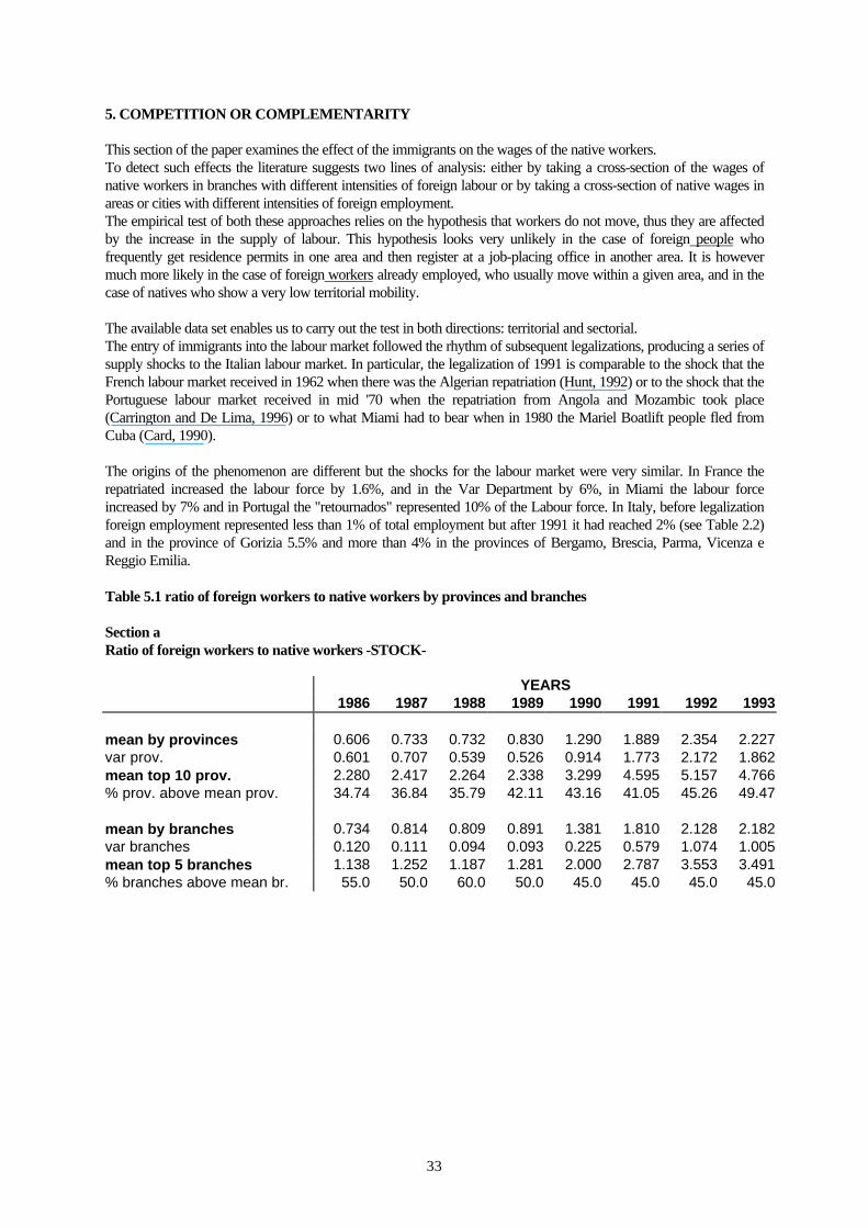
Table 5.1 shows the strong impact of legalization on the Italian labour market and its territorial and sectorialdistribution.The first part of the Table, section a, refers to the stock of foreign workers compared to native workers and stresses ageneral increase, but in particular the larger increase in some of the 95 provinces and of the 19 branches ofproduction.Just to name a few provinces: Bergamo, Brescia, Piacenza, Como, Parma, Reggio Emilia, Rimini, Modena, Bologna,Lucca, Verona Vicenza, Treviso, Trento, Trieste, Gorizia e l'Aquila - with the exception of the last one they are all inthe North, North-East and Center-North - and a few branches: Non-metal products, Timber and wood products,Construction and Retailing.

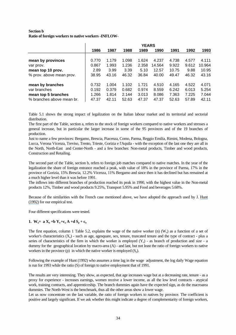
The second part of the Table, section b, refers to foreign job matches compared to native matches. In the year of thelegalization the share of foreign entrance reached a peak, with value of 18% in the province of Parma, 17% in theprovince of Gorizia, 15% Brescia, 12.2% Vicenza, 11% Bergamo and since then it has declined but has remained ata much higher level than it was before 1991.The inflows into different branches of production reached its peak in 1990, with the highest value in the Non-metalproducts 12%, Timber and wood products 9.25%, Transport 5.95% and Food and beverages 5.68%.

Because of the similarities with the French case mentioned above, we have adopted the approach used by J. Hunt(1992) for our empirical test.

Four different specifications were tested.

1. Wn= a Xn +b Yn +ca A +d Sp + cn

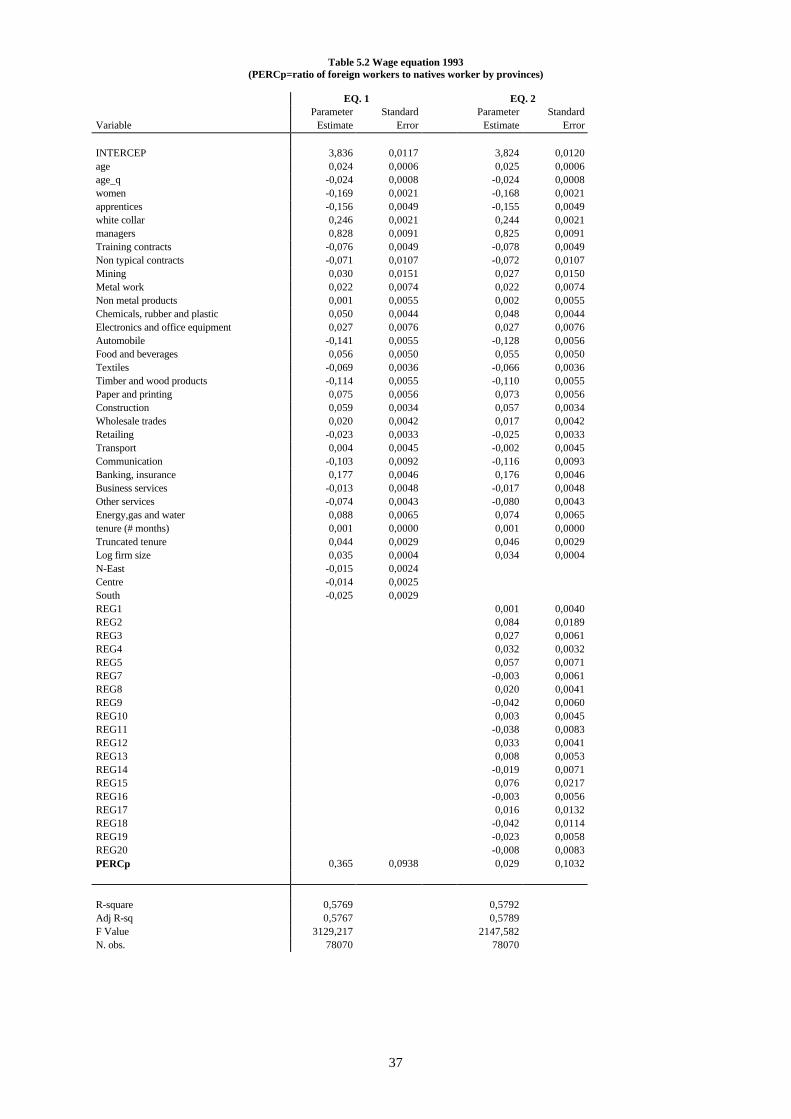
The first equation, column 1 Table 5.2, explains the wage of the native worker (n) (Wn) as a function of a set ofworker's characteristics (Xn) - such as age, agesquare, sex, tenure, truncated tenure and the type of contract - plus aseries of characteristics of the firm in which the worker is employed (Yn) - as branch of production and size - adummy for the geographical location by macro-area (A) - and last, but not least the ratio of foreign workers to nativeworkers in the province (p) in which the native worker is employed (Sp).

Following the example of Hunt (1992) who assumes a time lag in the wage adjustment, the log daily Wage equationis run for 1993 while the ratio (S) of foreign to native employment that of 1991.

The results are very interesting. They show, as expected, that age increases wage but at a decreasing rate, tenure - as aproxy for experience - increases earnings, women receive a lower income, as all the low level contracts - atypicalwork, training contracts, and apprenticeship. The branch dummies again have the expected sign, as do the macroareadummies. The North-West is the benchmark, thus all the other areas show a lower wage.Let us now concentrate on the last variable, the ratio of foreign workers to natives by province. The coefficient ispositive and largely significant. If we ask whether this might indicate a degree of complementarity of foreign workers,

35

the answer is no for it only suggests that immigrants are employed in the provinces where the demand for labour ishigher, and wages are higher than in other areas.The foreign ratio variable is the only provincial variable in the equation and thus it only indicates the fixed provincialeffect that could probably be replaced by an excess demand proxy.This finding is similar to Hunt's results for the Algerian repatriation when she found a fixed departmental effect.

This result is also in line with previous descriptive analyses by Livi Bacci (1996) and Venturini (1996). The twoauthors, the first by a Graph, the second by a correlation test (0.7) stressed the presence of foreign workers only in theregions with low native unemployment and high excess demand for labour and that this evidence supports acomplementary role for the immigrants who do not displace native workers. No evidence is presented in these workson wage competition or complementarity, except in Venturini (1997) while a nihil effect is suggested for variousstructural reasons which characterize the Italian labour market: wages are set by Centralized Bargaining, the impactof the foreigners is too recent and too limited to effect wages and decentralized bargaining is a very recentphenomenon which at the moment has had little or no effect.

To better control territorial size we have replaced in eq.2 the macro areas dummies with regional dummies while theother variables were kept the same.

2. Wn= a Xn +b Yn + cr R + d Sp + cn

The results of the test, shown in Table 5.2 Column 2 reveal that the coefficients of the workers and the firms'characteristics were very similar. The regional dummies are significant with different coefficients. The benchmark inthe regional analysis is the "Veneto" and it shows that the regions 1-5 (North-West) have higher wage coefficients,while in the South there is a negative or a non-significant coefficient.This result was to be expected but what is more important is the finding that the provincial foreign workers ratio is nolonger significant, stressing that the variance of the territorial wage distribution is accounted for by the regionaldummies and that neither the provincial size nor the foreign ratio variable are important.

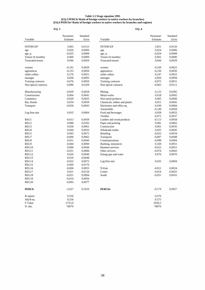
The third equation, column 3 Table 5.2 proposes a cross-branch analyses.

3. Wn= a Xn + b Zn + cr R + d Sb + cn

The wage of the native worker (Wn) is the function of the previously mentioned worker characteristics (Xn) - age,experience and job contract - and the firm's characteristics (Zn ) which are the firm size, and the (large) sectors - theregional location (R) and the ratio of foreign workers to native workers by branches (Sb) plus an error term.

The results for the individual characteristics and the firm characteristics are similar to the previous ones, while theforeign ratio coefficient is negative, significant and high.This does not necessarily mean that immigrants compete strongly with native workers for in this case even when wecontrol the result by a sector dummy, the negative coefficient mainly stresses that immigrants are employed in lowwage branches of production.

The fourth equation controls for the high wage area and the low wage sector and test the following equation.

4. Wn= a Xn +bYn + ca A + Sbr + cn

The wage of the native worker (n) (Wn) is the function of the characteristics (Xn) - age, experience, sex and contract -and of the firm characteristics (Yn) - size, branch- and macro-areas (A) plus the ratio of foreign workers in the samebranch (b) and region (r) (Sbr).Unfortunately, given the small number of foreign workers in many provinces, it was impossible to control by branchand province, but as was shown by the previous results of eq.2 the regional variable (20 regions) covers theprovincial dimension (95 provinces) pretty well given the homogeneity of the two groups.The results of the test, column 4 Table 5.2, present the same coefficient of previous specifications and a negativesignificant coefficient for the foreign employment share equal to -0.169.

36

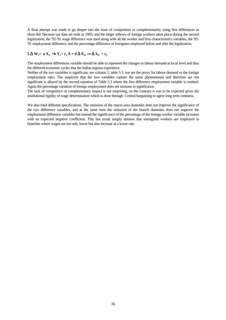
A final attempt was made to go deeper into the issue of competition or complementarity using first differences asHunt did. Because our data set ends in 1993, and the larger inflows of foreign workers takes place during the secondlegalization, the '92-'91 wage difference was used along with all the worker and firm characteristics variables, the '92-'91 employment difference, and the percentage difference of foreigners employed before and after the legalization.

5 ∆∆∆∆ Wn= a Xn +b Yn + ca A + d ∆∆∆∆ Ebr +e ∆∆∆∆ Sbr + cn

The employment differences variable should be able to represent the changes in labour demand at local level and thusthe different economic cycles that the Italian regions experience.Neither of the two variables is significant, see column 1, table 5.3, nor are the proxy for labour demand or the foreignemployment ratio. The suspicion that the two variables capture the same phenomenon and therefore are notsignificant is allayed by the second equation of Table 5.3 where the first difference employment variable is omitted.Again the percentage variation of foreign employment does not increase in significance.The lack of competitive or complementary impact is not surprising, on the contrary it was to be expected given theinstitutional rigidity of wage determination which is done through Central bargaining to agree long term contracts.

We also tried different specifications. The omission of the macro-area dummies does not improve the significance ofthe two difference variables, and at the same time the omission of the branch dummies does not improve theemployment difference variables but instead the significance of the percentage of the foreign worker variable increaseswith an expected negative coefficient. This last result simply stresses that immigrant workers are employed inbranches where wages are not only lower but also increase at a lower rate.

37

Table 5.2 Wage equation 1993(PERCp=ratio of foreign workers to natives worker by provinces)

EQ. 1 EQ. 2Parameter Standard Parameter Standard

Variable Estimate Error Estimate Error

INTERCEP 3,836 0,0117 3,824 0,0120age 0,024 0,0006 0,025 0,0006age_q -0,024 0,0008 -0,024 0,0008women -0,169 0,0021 -0,168 0,0021apprentices -0,156 0,0049 -0,155 0,0049white collar 0,246 0,0021 0,244 0,0021managers 0,828 0,0091 0,825 0,0091Training contracts -0,076 0,0049 -0,078 0,0049Non typical contracts -0,071 0,0107 -0,072 0,0107Mining 0,030 0,0151 0,027 0,0150Metal work 0,022 0,0074 0,022 0,0074Non metal products 0,001 0,0055 0,002 0,0055Chemicals, rubber and plastic 0,050 0,0044 0,048 0,0044Electronics and office equipment 0,027 0,0076 0,027 0,0076Automobile -0,141 0,0055 -0,128 0,0056Food and beverages 0,056 0,0050 0,055 0,0050Textiles -0,069 0,0036 -0,066 0,0036Timber and wood products -0,114 0,0055 -0,110 0,0055Paper and printing 0,075 0,0056 0,073 0,0056Construction 0,059 0,0034 0,057 0,0034Wholesale trades 0,020 0,0042 0,017 0,0042Retailing -0,023 0,0033 -0,025 0,0033Transport 0,004 0,0045 -0,002 0,0045Communication -0,103 0,0092 -0,116 0,0093Banking, insurance 0,177 0,0046 0,176 0,0046Business services -0,013 0,0048 -0,017 0,0048Other services -0,074 0,0043 -0,080 0,0043Energy,gas and water 0,088 0,0065 0,074 0,0065tenure (# months) 0,001 0,0000 0,001 0,0000Truncated tenure 0,044 0,0029 0,046 0,0029Log firm size 0,035 0,0004 0,034 0,0004N-East -0,015 0,0024Centre -0,014 0,0025South -0,025 0,0029REG1 0,001 0,0040REG2 0,084 0,0189REG3 0,027 0,0061REG4 0,032 0,0032REG5 0,057 0,0071REG7 -0,003 0,0061REG8 0,020 0,0041REG9 -0,042 0,0060REG10 0,003 0,0045REG11 -0,038 0,0083REG12 0,033 0,0041REG13 0,008 0,0053REG14 -0,019 0,0071REG15 0,076 0,0217REG16 -0,003 0,0056REG17 0,016 0,0132REG18 -0,042 0,0114REG19 -0,023 0,0058REG20 -0,008 0,0083PERCp 0,365 0,0938 0,029 0,1032

R-square 0,5769 0,5792Adj R-sq 0,5767 0,5789F Value 3129,217 2147,582N. obs. 78070 78070

38

Table 5.3 Wage equation 1993(EQ.3 PERCb=Ratio of foreign workers to native workers by branches)

(EQ.4 PERCbr=Ratio of foreign workers to native workers by branches and regions)

EQ. 3 EQ. 4

Parameter Standard Parameter StandardVariable Estimate Error Variable Estimate Error

INTERCEP 3,865 0,0123 INTERCEP 3,851 0,0120age 0,026 0,0006 age 0,024 0,0006age_q -0,025 0,0008 age_q -0,024 0,0008Tenure (# months) 0,000 0,0000 Tenure (# months) 0,001 0,0000Truncated tenure 0,046 0,0029 Truncated tenure 0,044 0,0029

women -0,191 0,0020 women -0,169 0,0022apprentices -0,153 0,0050 apprentices -0,156 0,0050white collars 0,270 0,0021 white collars 0,247 0,0022manager 0,838 0,0093 manager 0,826 0,0094Training contracts -0,076 0,0050 Training contracts -0,075 0,0051Non tipical contracts -0,086 0,0109 Non tipical contracts -0,063 0,0111

Manufacturing -0,020 0,0028 Mining 0,123 0,0385Constructions 0,064 0,0041 Metal works 0,018 0,0092Commerce -0,029 0,0035 Non metal products 0,005 0,0060Bar, Hotels 0,034 0,0059 Chemicals, rubber and plastic 0,051 0,0045Transport -0,056 0,0043 Electronics and office eq. 0,030 0,0084

Automobile -0,149 0,0058Log firm size 0,035 0,0004 Food and beverages 0,058 0,0052

Textiles -0,071 0,0037REG1 -0,013 0,0039 Lumber and wood products -0,113 0,0058REG2 0,088 0,0193 Paper and printing 0,081 0,0062REG3 0,036 0,0061 Construction 0,061 0,0035REG4 0,044 0,0033 Wholesale trades 0,025 0,0045REG5 0,065 0,0072 Retailing -0,023 0,0034REG7 -0,006 0,0062 Transports -0,007 0,0048REG8 0,031 0,0040 Communications -0,098 0,0094REG9 -0,044 0,0060 Banking, insurances 0,169 0,0051REG10 0,000 0,0044 Business services -0,012 0,0051REG11 -0,031 0,0084 Other services -0,074 0,0043REG12 0,026 0,0040 Energy,gas and water 0,070 0,0070REG13 0,010 0,0048REG14 -0,022 0,0072 Log firm size 0,035 0,0004REG15 0,069 0,0176REG16 -0,006 0,0053 N-East -0,011 0,0024REG17 0,021 0,0134 Centre -0,014 0,0025REG18 -0,021 0,0094 South -0,031 0,0032REG19 -0,010 0,0056REG20 -0,003 0,0077

PERCb -2,627 0,1616 PERCbr -0,174 0,0927

R-square 0,556 0,576Adj R-sq 0,556 0,575F Value 2733,9 2930,2N. obs. 78070 78070

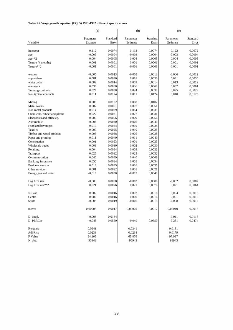
39

Table 5.4 Wage growth equation (EQ. 5) 1991-1992 different specifications

(a) (b) (c)

Parameter Standard Parameter Standard Parameter StandardVariable Estimate Error Estimate Error Estimate Error

Intercept 0,112 0,0074 0,113 0,0074 0,122 0,0072age -0,003 0,0004 -0,003 0,0004 -0,003 0,0004age**2 0,004 0,0005 0,004 0,0005 0,004 0,0005Tenure (# months) 0,001 0,0001 0,001 0,0001 0,001 0,0001Tenure**2 -0,001 0,0001 -0,001 0,0001 -0,001 0,0001

women -0,005 0,0013 -0,005 0,0013 -0,006 0,0012apprentices 0,081 0,0030 0,081 0,0030 0,081 0,0030white collar 0,009 0,0014 0,009 0,0014 0,013 0,0012managers 0,036 0,0060 0,036 0,0060 0,037 0,0061Training contracts 0,024 0,0030 0,024 0,0030 0,025 0,0029Non typical contracts 0,011 0,0124 0,011 0,0124 0,010 0,0125

Mining 0,008 0,0102 0,008 0,0102Metal works 0,007 0,0051 0,007 0,0051Non metal products 0,014 0,0039 0,014 0,0039Chemicals, rubber and plastic 0,027 0,0031 0,027 0,0031Electronics and office eq. 0,009 0,0056 0,009 0,0056Automobile -0,006 0,0040 -0,005 0,0040Food and beverages 0,019 0,0034 0,019 0,0034Textiles 0,009 0,0025 0,010 0,0025Timber and wood products 0,005 0,0038 0,005 0,0038Paper and printing 0,011 0,0040 0,011 0,0040Construction 0,001 0,0023 0,001 0,0023Wholesale trades 0,003 0,0030 0,002 0,0030Retailing 0,004 0,0024 0,003 0,0023Transport 0,025 0,0032 0,025 0,0032Communication 0,040 0,0069 0,040 0,0069Banking, insurance 0,055 0,0034 0,055 0,0034Business services 0,016 0,0035 0,016 0,0035Other services 0,001 0,0022 0,001 0,0021Energy,gas and water -0,016 0,0050 -0,017 0,0049

Log firm size -0,003 0,0008 -0,003 0,0008 -0,002 0,0007Log firm size**2 0,021 0,0076 0,021 0,0076 0,021 0,0064

N-East 0,002 0,0016 0,002 0,0016 0,004 0,0015Centre 0,000 0,0016 0,000 0,0016 0,001 0,0015South -0,005 0,0019 -0,005 0,0019 -0,008 0,0017

mover 0,00003 0,0017 0,00005 0,0017 -0,00010 0,0017

D_empl. -0,008 0,0134 -0,011 0,0115D_PERCbr -0,048 0,0550 -0,049 0,0550 -0,281 0,0474

R-square 0,0241 0,0241 0,0181Adj R-sq 0,0238 0,0238 0,0179F Value 64,105 65,876 97,987N. obs. 95943 95943 95943

40

6. CONCLUDING COMMENTS

The research has shown that it is possible to derive a dataset on foreign workers from the Social Security Archive byusing the place of birth as a selecting device. Controlling for the age and the date of entry and selecting only thoseforeigners who come from non-European and developing countries we get a good proxy of the immigrant inflow. Thisis also the best proxy of the number of foreign workers derived from the same dataset. It is closer to ISTAT’s revisedestimates of the number of work permits issued for employees and is the only dataset with individual data.

Three main issues have been analysed in the paper: the employment behaviour of foreign workers and the degree oftheir employment assimilation; their wage differential and their wage assimilation, as well as their competitive orcomplementary role in the labour market.

Migrant workers are more mobile than native workers. Their turnover rates increases, indicating that foreign workershave not gained a stable role in the labour market, however the cumulative duration of occupation of foreigners andnatives is more similar.When the employment behaviour of foreigners is compared with a group of workers with similar characteristics, the“control group”, differences are smaller. In this case the survival functions in each spell of occupation for the twogroups are very close. A comparison of the pattern of pre-legalisation and post-legalisation immigrants suggests thatthere is gradual assimilation which takes place among foreign workers in that the survival function of the first grouplies between that of native workers and that of more recent immigrants.

The analysis of the wage differential using the Oaxaca decomposition reveals a small wage gap in 1991; 70% of it isexplained by the different characteristics of the native and foreign workers and only the remainder is due tounobserved characteristics or discrimination.In 1993 the total wage differential increases in absolute terms indicating a larger heterogeneity among the two groups,moreover the explained part falls to 61% and the unexplained part increases to 39%. The analysis of the wage gap in1993 of workers already employed in 1991, shows a lower wage differential in absolute terms and a smallerunexplained part. What is more relevant, however, is that the total wage differential is much smaller than in themale/female case both in absolute and relative terms.

The approach used by Bonjour and Pacelli (1997) was used to analyse some different branches; large differences inthe absolute wage gap and in the explained part were revealed. However, the absolute value of the unexplained wagegap is the same among different branches.

Last but not least the competitive or complementary role of foreign workers in the labour market is explored and theanalysis was carried out at branch and provincial levels. The empirical tests suggest that foreign workers are presentin low wage branches and in high wage areas, and that the regional dummy is a good proxy of the territorialdistribution of foreign employment and can replace the provincial one. Following Jennifer Hunt’s (1992) approach tothe Algerian repatriation to France, the effect of legalisation on native wage levels was examined. The legalisationmeasures led to the inflow of immigrants increasing to such an extent that their share of the labour market rose by 1%in one and a half years, in a few areas the increase in foreign workers was more than 4%.The first difference estimates of the native workers’ wage do not appear to be affected by variations in local demandor by the share of foreign workers and this result was to be expected because the institutionalised system ofdetermining wages is not sufficiently flexible to react quickly to external changes such as an increase in the supply oflabour

The paper should be considered as only a preliminary report as we plan to do further research into the phenomena. Assoon as the samples taken from the SSA are updated we will first re-run a test for the complementary role ofimmigrants which will cover a longer time span and the longer time span will also facilitate a more accurate analysisof the employment and wage assimilation pattern, specified by the areas of origin of immigrants.

41

REFERENCES

Altonji J., Card D., 1991, The Effects of Immigration on the Labor Market Outcomes of Natives, in Abowd J.,Freeman R. (eds) Immigration, Trade and Labor, Chicago: University of Chicago Press, pp.201-34.

Bonjour D., Pacelli L., 1997, Wage Formation and the Gender Wage Gap in Italy and Switzerland, paper presentedat the ESPE Conference, Colchester.

Blau D., Kahn F.L., 1992, The Gender Earnings Gap:learning from International Comparison, American EconomicReview, 82, 2.

Bruni M., Venturini A., 1995, Preassure to migrate and propensity to migrate. The case of the Mediterranean Basin,Interntional Labour Review, n.3, pp.377-400.

Card D., 1990, The Impact of the Mariel Boatlift on the Miami Labor Market, Industrial and Labor RelationsReview, vol.43, n.2, pp.245-57.

Caritas, 1997, Rapporto sull'Immigrazione '97, ANTEREM.

Contini B., Pacelli L., Revelli R. 1994 "Struttura occupazionale e retribuzioni dai dati individuali degli archiviINPS", Norme e metodi CNEL, Quaderno n. 26, Roma

Contini B., Revelli R. 1992 "I dati su imprese, occupazione e retribuzioni di fonte INPS", Padova Ricerche,Quaderno n. 13, luglio.

Del Boca D., 1993, Offerta di lavoro e politiche pubbliche, NIS, Roma.

De Lima P., Carrington W., 1996, The impact of 1970's Repatriates from Africa on the Portuguise Labor Market,Industrial and Labor Relations Review, vol.49, n.2, pp.330-347.

Filippi M., Villosio C., 1997, Il lavoro regolare degli stranieri in Italia, paper presented at the AIEL Conference,Cagliari.

Hunt J., 1992, The Impact of the 1962 Repatriates from Algeria on the French Labor Market, Industrial and LaborRelations Review, vol.53, n.3, pp.556-572.

ISTAT, 1996, Notiziario statistico " Statistiche sui permessi di soggiorno degli stranieri: Analisi dei dati al 31dicembre 1991, 1992, 1993 e 1994", serie 4, Foglio 41, anno XVII, n1, Febbraio.

ISTAT, 1998, La presenza straniera in Italia negli anno '90, a cura di Gabrielli D., Bisogni E., Collana Informazionen.61.

ISTAT, 1997 Rapporto Annuale. La situazione del Paese 1996, Roma

LaLonde R., Topel R, 1991, Labor Market Adjustments to Increased Immigration, in Abowd J., Freeman R. (eds)Immigration, Trade and Labor, Chicago: University of Chicago Press, pp. 167-99.

Livi Bacci M., 1996, "Immigrazione e mobilita'", Galli G.(ed.) La mobilita' della Societa' Italiana, ConfindustriaCentro Studi, SIPI, Roma.

Natale M., Strozza S., 1997, Gli immigrati stranieri in Italia Quanti sono , chi sono , come vivono?, Cacucci Editore,Bari.

Oaxaca R., 1973, Male-Female Wage Differentials in Urban Labour Market, International Economic Review, 14.

42

Revelli R. 1996 "Statistics on Job Creation: Issues in the Use of Administrative Data", in OECD Job Creation andLoss: Analysis, Policy and Data Development, Paris.

Venturini A., 1996, Complementarita’ e sostituzione tra lavoratori nazionali e stranieri: il caso italiano, Relazionepresentata alla Sociata’ degli Economisti, Bologna.

Venturini A., 1996a, Extent of Competition between and Complementarity among National and Third-WorldMigrant workers in the Labour Market: An Exploration of the Italian Case, Internationa Migration Papers , ILO, n.11.

Venturini A., 1997, Do immigrants working illegaly reduce the natives’ legal empployment? Evidence from Italy, submitted to the Journal of Population Economics.

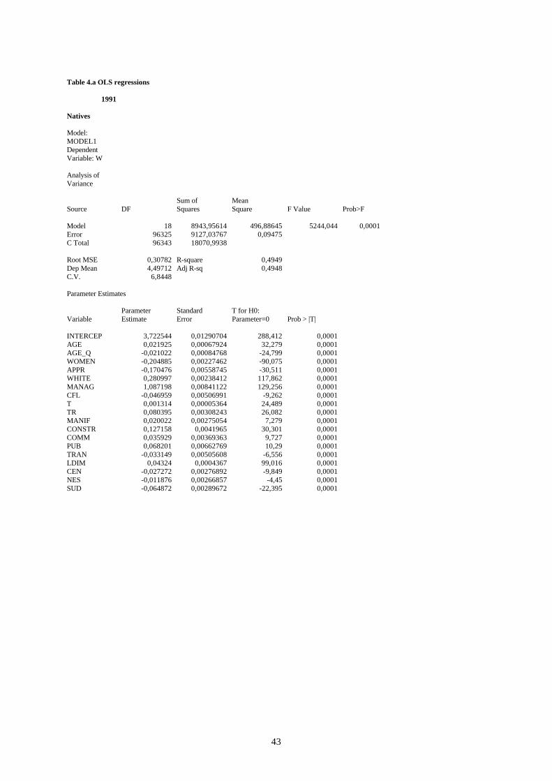
43

Table 4.a OLS regressions

1991

Natives

Model:MODEL1DependentVariable: W

Analysis ofVariance

Sum of MeanSource DF Squares Square F Value Prob>F

Model 18 8943,95614 496,88645 5244,044 0,0001Error 96325 9127,03767 0,09475C Total 96343 18070,9938

Root MSE 0,30782 R-square 0,4949Dep Mean 4,49712 Adj R-sq 0,4948C.V. 6,8448

Parameter Estimates

Parameter Standard T for H0:Variable Estimate Error Parameter=0 Prob > |T|

INTERCEP 3,722544 0,01290704 288,412 0,0001AGE 0,021925 0,00067924 32,279 0,0001AGE_Q -0,021022 0,00084768 -24,799 0,0001WOMEN -0,204885 0,00227462 -90,075 0,0001APPR -0,170476 0,00558745 -30,511 0,0001WHITE 0,280997 0,00238412 117,862 0,0001MANAG 1,087198 0,00841122 129,256 0,0001CFL -0,046959 0,00506991 -9,262 0,0001T 0,001314 0,00005364 24,489 0,0001TR 0,080395 0,00308243 26,082 0,0001MANIF 0,020022 0,00275054 7,279 0,0001CONSTR 0,127158 0,0041965 30,301 0,0001COMM 0,035929 0,00369363 9,727 0,0001PUB 0,068201 0,00662769 10,29 0,0001TRAN -0,033149 0,00505608 -6,556 0,0001LDIM 0,04324 0,0004367 99,016 0,0001CEN -0,027272 0,00276892 -9,849 0,0001NES -0,011876 0,00266857 -4,45 0,0001SUD -0,064872 0,00289672 -22,395 0,0001

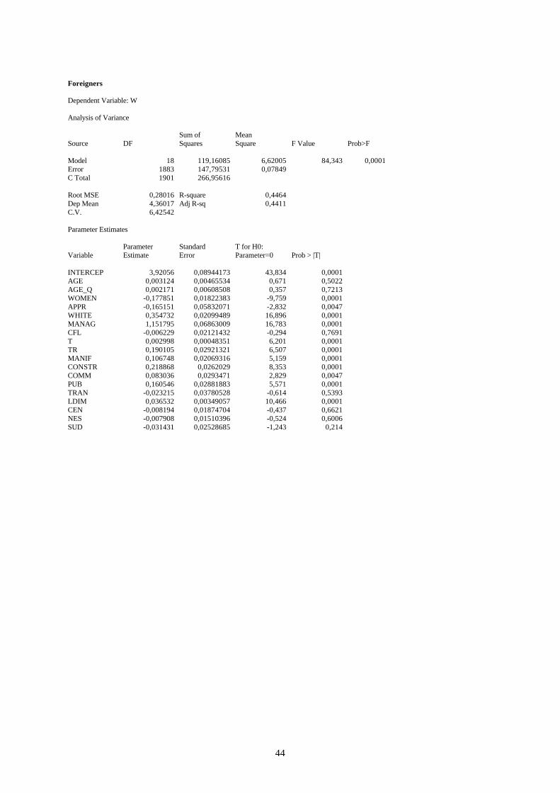
44

Foreigners

Dependent Variable: W

Analysis of Variance

Sum of MeanSource DF Squares Square F Value Prob>F

Model 18 119,16085 6,62005 84,343 0,0001Error 1883 147,79531 0,07849C Total 1901 266,95616

Root MSE 0,28016 R-square 0,4464Dep Mean 4,36017 Adj R-sq 0,4411C.V. 6,42542

Parameter Estimates

Parameter Standard T for H0:Variable Estimate Error Parameter=0 Prob > |T|

INTERCEP 3,92056 0,08944173 43,834 0,0001AGE 0,003124 0,00465534 0,671 0,5022AGE_Q 0,002171 0,00608508 0,357 0,7213WOMEN -0,177851 0,01822383 -9,759 0,0001APPR -0,165151 0,05832071 -2,832 0,0047WHITE 0,354732 0,02099489 16,896 0,0001MANAG 1,151795 0,06863009 16,783 0,0001CFL -0,006229 0,02121432 -0,294 0,7691T 0,002998 0,00048351 6,201 0,0001TR 0,190105 0,02921321 6,507 0,0001MANIF 0,106748 0,02069316 5,159 0,0001CONSTR 0,218868 0,0262029 8,353 0,0001COMM 0,083036 0,0293471 2,829 0,0047PUB 0,160546 0,02881883 5,571 0,0001TRAN -0,023215 0,03780528 -0,614 0,5393LDIM 0,036532 0,00349057 10,466 0,0001CEN -0,008194 0,01874704 -0,437 0,6621NES -0,007908 0,01510396 -0,524 0,6006SUD -0,031431 0,02528685 -1,243 0,214

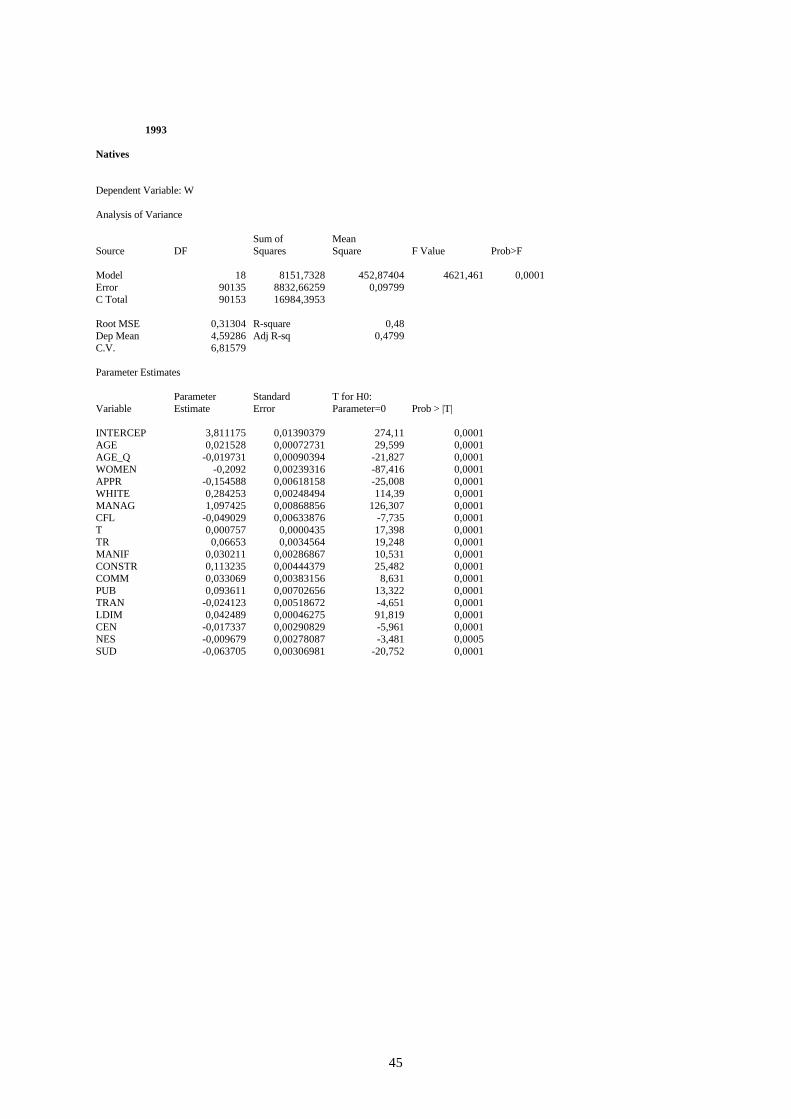
45

1993

Natives

Dependent Variable: W

Analysis of Variance

Sum of MeanSource DF Squares Square F Value Prob>F

Model 18 8151,7328 452,87404 4621,461 0,0001Error 90135 8832,66259 0,09799C Total 90153 16984,3953

Root MSE 0,31304 R-square 0,48Dep Mean 4,59286 Adj R-sq 0,4799C.V. 6,81579

Parameter Estimates

Parameter Standard T for H0:Variable Estimate Error Parameter=0 Prob > |T|

INTERCEP 3,811175 0,01390379 274,11 0,0001AGE 0,021528 0,00072731 29,599 0,0001AGE_Q -0,019731 0,00090394 -21,827 0,0001WOMEN -0,2092 0,00239316 -87,416 0,0001APPR -0,154588 0,00618158 -25,008 0,0001WHITE 0,284253 0,00248494 114,39 0,0001MANAG 1,097425 0,00868856 126,307 0,0001CFL -0,049029 0,00633876 -7,735 0,0001T 0,000757 0,0000435 17,398 0,0001TR 0,06653 0,0034564 19,248 0,0001MANIF 0,030211 0,00286867 10,531 0,0001CONSTR 0,113235 0,00444379 25,482 0,0001COMM 0,033069 0,00383156 8,631 0,0001PUB 0,093611 0,00702656 13,322 0,0001TRAN -0,024123 0,00518672 -4,651 0,0001LDIM 0,042489 0,00046275 91,819 0,0001CEN -0,017337 0,00290829 -5,961 0,0001NES -0,009679 0,00278087 -3,481 0,0005SUD -0,063705 0,00306981 -20,752 0,0001

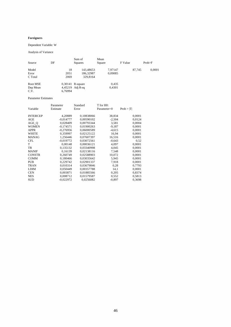
46

Foreigners

Dependent Variable: W

Analysis of Variance

Sum of MeanSource DF Squares Square F Value Prob>F

Model 18 143,48653 7,97147 87,745 0,0001Error 2051 186,32987 0,09085C Total 2069 329,8164

Root MSE 0,30141 R-square 0,435Dep Mean 4,45219 Adj R-sq 0,4301C.V. 6,76994

Parameter Estimates

Parameter Standard T for H0:Variable Estimate Error Parameter=0 Prob > |T|

INTERCEP 4,20889 0,10838066 38,834 0,0001AGE -0,014777 0,00590102 -2,504 0,0124AGE_Q 0,028409 0,00793344 3,581 0,0004WOMEN -0,174571 0,01900263 -9,187 0,0001APPR -0,276956 0,06000589 -4,615 0,0001WHITE 0,359997 0,02125122 16,94 0,0001MANAG 1,256446 0,07607397 16,516 0,0001CFL -0,019772 0,03072561 -0,643 0,52T 0,00148 0,00036121 4,097 0,0001TR 0,135132 0,03340998 4,045 0,0001MANIF 0,16139 0,02138116 7,548 0,0001CONSTR 0,260749 0,02588903 10,072 0,0001COMM 0,180466 0,03035642 5,945 0,0001PUB 0,229742 0,02901337 7,918 0,0001TRAN 0,010314 0,03679846 0,28 0,7793LDIM 0,050449 0,00357788 14,1 0,0001CEN 0,003871 0,01885566 0,205 0,8374NES 0,008712 0,01579587 0,552 0,5813SUD -0,022972 0,0256082 -0,897 0,3698

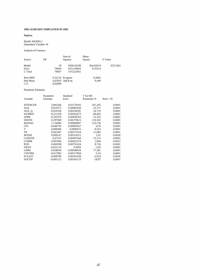
47

1993 ALREADY EMPLOYED IN 1991

Natives

Model: MODEL1Dependent Variable: W

Analysis of Variance

Sum of MeanSource DF Squares Square F Value

Model 18 6568,56249 364,92014 3537,963Error 79049 8153,44063 0,10314C Total 79067 14722,0031

Root MSE 0,32116 R-square 0,4462Dep Mean 4,63503 Adj R-sq 0,446C.V. 6,92898

Parameter Estimates

Parameter Standard T for H0:Variable Estimate Error Parameter=0 Prob > |T|

INTERCEP 3,905266 0,01579193 247,295 0,0001AGE 0,019375 0,00081656 23,727 0,0001AGE_Q -0,016766 0,00100281 -16,719 0,0001WOMEN -0,211359 0,00262673 -80,465 0,0001APPR -0,103379 0,00838763 -12,325 0,0001WHITE 0,297949 0,00270613 110,102 0,0001MANAG 1,116606 0,00906807 123,136 0,0001CFL -0,046793 0,00983057 -4,76 0,0001T 0,000406 0,0000475 8,553 0,0001TR 0,041407 0,00373524 11,085 0,0001MANIF 0,009147 0,00314315 2,91 0,0036CONSTR 0,07522 0,00497644 15,115 0,0001COMM 0,007844 0,00425379 1,844 0,0652PUB 0,069298 0,00791424 8,756 0,0001TRAN -0,022119 0,0056 -3,95 0,0001LDIM 0,038639 0,00049934 77,381 0,0001CENTRE -0,017005 0,00317858 -5,35 0,0001N-EAST -0,008789 0,00301638 -2,914 0,0036SOUTH -0,065123 0,00345119 -18,87 0,0001

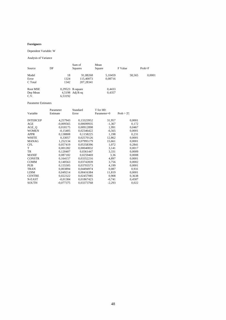
48

Foreigners

Dependent Variable: W

Analysis of Variance

Sum of MeanSource DF Squares Square F Value Prob>F

Model 18 91,88268 5,10459 58,565 0,0001Error 1324 115,40073 0,08716C Total 1342 207,28341

Root MSE 0,29523 R-square 0,4433Dep Mean 4,5198 Adj R-sq 0,4357C.V. 6,53192

Parameter Estimates

Parameter Standard T for H0:Variable Estimate Error Parameter=0 Prob > |T|

INTERCEP 4,257943 0,13323952 31,957 0,0001AGE -0,009565 0,00699935 -1,367 0,172AGE_Q 0,018175 0,00912898 1,991 0,0467WOMEN -0,15405 0,02346422 -6,565 0,0001APPR 0,138808 0,1158225 1,198 0,231WHITE 0,33057 0,02570126 12,862 0,0001MANAG 1,252134 0,07995179 15,661 0,0001CFL 0,057419 0,05358396 1,072 0,2841T 0,001282 0,00040832 3,141 0,0017TR 0,120407 0,0361447 3,331 0,0009MANIF 0,087182 0,0259469 3,36 0,0008CONSTR 0,164157 0,03352216 4,897 0,0001COMM 0,140563 0,03742839 3,756 0,0002PUB 0,155505 0,03703573 4,199 0,0001TRAN 0,003894 0,04494974 0,087 0,931LDIM 0,049214 0,00416384 11,819 0,0001CENTRE 0,022322 0,02457085 0,908 0,3638N-EAST -0,01384 0,01867423 -0,741 0,4587SOUTH -0,077375 0,03373768 -2,293 0,022