
Forecasting volatility with asymmetric smooth transition dynamic range models
16
International Journal of Forecasting 28 (2012) 384–399 Contents lists available at SciVerse ScienceDirect International Journal of Forecasting journal homepage: www.elsevier.com/locate/ijforecast Forecasting volatility with asymmetric smooth transition dynamic range models Edward M.H. Lin a , Cathy W.S. Chen a,∗ , Richard Gerlach b a Department of Statistics, Feng Chia University, Taiwan b Discipline of Operations Management and Econometrics, University of Sydney, Australia article info Keywords: Smooth transition Volatility model Threshold variable Bayesian inference MCMC methods abstract We propose a nonlinear smooth transition conditional autoregressive range (CARR) model for capturing smooth volatility asymmetries in international financial stock markets, build- ing on recent work on smooth transition conditional duration modelling. An adaptive Markov chain Monte Carlo scheme is developed for Bayesian estimation, volatility fore- casting and model comparison for the proposed model. The model can capture sign or size asymmetry and heteroskedasticity, such as that which is commonly observed in financial markets. A mixture proposal distribution is developed in order to improve the acceptance rate and the mixing issues which are common in random walk Metropolis-Hastings meth- ods. Further, the logistic transition function is employed and its main properties are con- sidered and discussed in the context of the proposed model, which motivates a suitable, weakly informative prior which ensures a proper posterior distribution and identification of the estimators. The methods are illustrated using simulated data, and an empirical study also provides evidence in favour of the proposed model when forecasting the volatility in two financial stock markets. In addition, the deviance information criterion is employed to compare the proposed models with their limiting classes, the nonlinear threshold CARR models and the symmetric CARR model. © 2011 International Institute of Forecasters. Published by Elsevier B.V. All rights reserved. 1. Introduction Dynamic time series models play an important role in describing, estimating and forecasting asset volatility in financial markets. In this paper, we examine whether the volatility asymmetry, combined with range-based models, might be able to be modeled better via a smooth transition function, and whether this model allows more accurate forecasts of daily asset volatility than standard competing models. As such, a range-based heteroskedastic, asymmetric model, with a smooth transition function, is proposed and assessed here. It is well known and accepted that squared daily re- turns, as employed by generalised autoregressive condi- tionally heteroskedastic (GARCH) models (see Bollerslev, ∗ Corresponding author. E-mail address: [email protected] (C.W.S. Chen). 1986; Engle, 1982), are not the most efficient measure of the daily volatility. The recent literature has focused on the realized volatility, employing intra-day return data, and autoregressive-type models (for example, see Andersen, Bollerslev, Diebold, & Labys, 2003; Liu & Maheu, 2008), in- cluding the incorporation of jumps in returns and volatil- ity (e.g. Andersen, Bollerslev, & Diebold, 2007). However, issues such as biases and inefficiencies from market micro- structure effects are also well documented, e.g., see Hansen and Lunde (2006). Daily stock ranges are also known to be more efficient measures of return volatility than daily returns (see Alizadeh, Brandt, & Diebold, 2002; Ander- sen & Bollerslev, 1998; Garman & Klass, 1980; Parkin- son, 1980), since they employ all price changes during the day (though not in a direct manner: only the mini- mum and maximum prices are employed), and not sim- ply the closing or opening prices, which can miss large intra-day movements. Thus, using financial range data has 0169-2070/$ – see front matter © 2011 International Institute of Forecasters. Published by Elsevier B.V. All rights reserved. doi:10.1016/j.ijforecast.2011.09.002
Transcript of Forecasting volatility with asymmetric smooth transition dynamic range models
International Journal of Forecasting 28 (2012) 384–399
Contents lists available at SciVerse ScienceDirect
International Journal of Forecasting
journal homepage: www.elsevier.com/locate/ijforecast
Forecasting volatility with asymmetric smooth transition dynamicrange modelsEdward M.H. Lin a, Cathy W.S. Chen a,∗, Richard Gerlach b
a Department of Statistics, Feng Chia University, Taiwanb Discipline of Operations Management and Econometrics, University of Sydney, Australia
a r t i c l e i n f o
Keywords:Smooth transitionVolatility modelThreshold variableBayesian inferenceMCMC methods
a b s t r a c t
We propose a nonlinear smooth transition conditional autoregressive range (CARR) modelfor capturing smooth volatility asymmetries in international financial stockmarkets, build-ing on recent work on smooth transition conditional duration modelling. An adaptiveMarkov chain Monte Carlo scheme is developed for Bayesian estimation, volatility fore-casting and model comparison for the proposed model. The model can capture sign or sizeasymmetry and heteroskedasticity, such as that which is commonly observed in financialmarkets. A mixture proposal distribution is developed in order to improve the acceptancerate and the mixing issues which are common in randomwalk Metropolis-Hastings meth-ods. Further, the logistic transition function is employed and its main properties are con-sidered and discussed in the context of the proposed model, which motivates a suitable,weakly informative prior which ensures a proper posterior distribution and identificationof the estimators. Themethods are illustrated using simulated data, and an empirical studyalso provides evidence in favour of the proposed model when forecasting the volatility intwo financial stock markets. In addition, the deviance information criterion is employedto compare the proposed models with their limiting classes, the nonlinear threshold CARRmodels and the symmetric CARR model.© 2011 International Institute of Forecasters. Published by Elsevier B.V. All rights reserved.
s. P
1. Introduction
Dynamic time series models play an important rolein describing, estimating and forecasting asset volatilityin financial markets. In this paper, we examine whetherthe volatility asymmetry, combined with range-basedmodels, might be able to be modeled better via a smoothtransition function, and whether this model allows moreaccurate forecasts of daily asset volatility than standardcompetingmodels. As such, a range-basedheteroskedastic,asymmetric model, with a smooth transition function, isproposed and assessed here.
It is well known and accepted that squared daily re-turns, as employed by generalised autoregressive condi-tionally heteroskedastic (GARCH) models (see Bollerslev,
∗ Corresponding author.E-mail address: [email protected] (C.W.S. Chen).
0169-2070/$ – see front matter© 2011 International Institute of Forecasterdoi:10.1016/j.ijforecast.2011.09.002
1986; Engle, 1982), are not the most efficient measure ofthe daily volatility. The recent literature has focused on therealized volatility, employing intra-day return data, andautoregressive-type models (for example, see Andersen,Bollerslev, Diebold, & Labys, 2003; Liu & Maheu, 2008), in-cluding the incorporation of jumps in returns and volatil-ity (e.g. Andersen, Bollerslev, & Diebold, 2007). However,issues such as biases and inefficiencies frommarketmicro-structure effects are alsowell documented, e.g., seeHansenand Lunde (2006). Daily stock ranges are also known tobe more efficient measures of return volatility than dailyreturns (see Alizadeh, Brandt, & Diebold, 2002; Ander-sen & Bollerslev, 1998; Garman & Klass, 1980; Parkin-son, 1980), since they employ all price changes duringthe day (though not in a direct manner: only the mini-mum and maximum prices are employed), and not sim-ply the closing or opening prices, which can miss largeintra-day movements. Thus, using financial range data has
ublished by Elsevier B.V. All rights reserved.
E.M.H. Lin et al. / International Journal of Forecasting 28 (2012) 384–399 385
become a viable option andwe employ intra-day high–lowprice ranges in this study. Range-based volatility modelsinclude the conditional autoregressive rangemodel (CARR)of Chou (2005), motivated by the autoregressive condi-tional duration models (ACD) of Engle and Russell (1998);the range-based stochastic volatility model of Alizadehet al. (2002); and the range EGARCH model of Brandt andJones (2006). These authors, backed up by Shu and Zhang(2006), also found that range estimators are quite ro-bust towardmicrostructure effects. Fernandes, de SaMota,and Rocha (2005) developed a multivariate range-basedMCARR model. Chou, Chou, and Liu (2009) present a thor-ough review of range-based models.
Asymmetric volatility, where higher volatility followsnegative shocks to asset returns, called the leverage effectand discovered by Black (1976), is typically allowed forin volatility modelling (see for example the GJR-GARCHmodel of Glosten, Jagannathan, & Runkle, 1993). Chou(2006) considered separate CARR models for the positiveand negative price ranges, while Chen, Gerlach, and Lin(2008),motivated by the asymmetric threshold ACDmodelof Zhang, Russell, and Tsay (2001), allowed for exogenousthreshold variables in order to examine fully asymmetricrange effects in a threshold CARR (TARR) model. Moreflexible and general asymmetric volatility models includethe smooth transition GARCH (ST-GARCH) model (see,e.g. Anderson, Nam, & Vahid, 1999; Gerlach & Chen,2008; González-Rivera, 1998; Lubrano, 2001). This model,building on thework of Chan and Tong (1986) and Grangerand Teräsvirta (1993) for AR models, allows a continuoustransition function to describe the regime switchingdynamics of volatility. The ST-GARCH of González-Rivera(1998) enables a smooth transition between the twovolatility regimes in the GJR-GARCH model, capturing asmooth leverage effect. Our proposed smooth transitionnonlinear range-based model is motivated by these, andalso by the smooth transition ACD (STACD) model of Meitzand Teräsvirta (2006). The essence of these models is thatthe volatility, or trading duration, is a continuous functionof a threshold or transition variable.
Most work on asymmetric models considers signasymmetry, or the leverage effect, where the volatilityincreases following negative asset returns. When an assetreturn, or a model error term, is used as the thresholdvariable, then sign asymmetry is being captured, since itis usually positive or negative movements which controlthe asymmetric affects on volatility, e.g. the GJR-GARCHmodel. However, if a positive valued variable, such as aprice range or variance, is used as the threshold variable,then the asymmetric volatility response is driven by thesize of the threshold variable, not its sign. For example, ifthe response of the volatility to previous squared shocksis larger if the squared shock itself is larger, or if theintra-day price range is larger that day, then that is sizeasymmetry. Chen, Gerlach, Choy, and Lin (2010), Chenet al. (2008), Leeves (2007) and Sarantis (1999) illustratedhow to model size asymmetry, using the intra-day rangeas a threshold variable, and its importance in volatilityestimation and forecasting. The TCARRmodel of Chen et al.(2008) considered both sign and size asymmetry, findingthat size asymmetry, in the form of the daily lagged price
range of the US market, was generally the most importantregarding the accuracy of range-based volatility forecastsacross six financial markets over a six month period. Ourproposed model directly extends the TCARR of Chen et al.(2008).
A Bayesian approach is adopted for estimating the pro-posed model, including the speed of transition param-eter (γ , which reflects the sharpness of the transitionfunction between the two regimes), the threshold limitvalue (c , which shows where the transition function is ex-actly 0.5, the mid-point between two regimes), and thedelay lag (d). Frequentist estimation of these parameterscan be problematic, especially under a numerical (likeli-hood) optimisation approach, since: (i) the likelihood isnon-integrable in γ , since it is well-defined for the valueγ = ∞, corresponding to a step transition function;(ii) γ can take the value 0, which presents an identificationproblem, as is discussed in Section 3; (iii) the likelihood isnon-differentiable and oftenmulti-modal (Giordani, Kohn,& vanDijk, 2007) in terms of the threshold limit (c), leadingBauwens, Lubrano, and Richard (1999, p. 239) to remark:‘‘any classical measure of uncertainty for c seems unfea-sible’’; and (iv) the delay lag d is discrete, making nu-merical likelihood optimisation and inference a challenge.Frequentist approaches for estimating threshold nonlinearmodels usually involve setting the threshold limit and de-lay lag in advance (e.g. to 0 and 1 respectively), or choosingthem via a grid search (e.g. Zhang et al., 2001) or an infor-mation criterion (e.g. Li & Li, 1996), then estimating param-eters conditional upon these choices, without accountingfor the uncertainty in their estimation, or providing infer-ences on them. Further, both frequentist and Bayesian es-timates of the speed of transition are often large, so that astep transition is implied (e.g. Lopes & Salazar, 2006; Nam,Pyun, & Avard, 2001), and many reported estimates havevery large standard errors regardless (e.g. Chelley-Steeley,2005; Lubrano, 2001; Sarantis, 1999), so that the questionas towhethermore than one regime is required is also per-tinent, but often left unanswered. All of these issues arequitemanageable and solvable under a Bayesian approach,as taken in this paper, but require some set-up work, asis discussed in Sections 2.3 and 3. Further, in a forecastingcontext, a Bayesian approach allows the inclusion of pa-rameter uncertainty in the forecasts, since point forecastsare averaged over the posterior distribution, not obtainedby plugging in parameter estimates, and also allows theestimation and assessment of the entire posterior distri-bution of any forecasted quantity, rather than simply pro-viding point estimates.
Thus, Bayesian Markov chain Monte Carlo (MCMC)methods are developed for estimation and forecasting us-ing the proposed model, including the development of anovel mixture of proposal density idea in the Metropolis-Hastings framework, which is subsequently shown to in-crease the mixing and efficiency of the sampling scheme.
Section 2 reviews some range-based and other volatilitymodels and presents the proposed smooth transitionmodel; Section 3 discusses the Bayesian method forestimation and inferencewith the adaptiveMCMCmethodand the prior choices. A simulation study is presentedin Section 4. Section 5 discusses model comparison andout-of-sample volatility forecasting. Section 6 presentsvolatility forecast studies of two international marketindices, while Section 7 offers conclusions.

386 E.M.H. Lin et al. / International Journal of Forecasting 28 (2012) 384–399
2. Range-based and volatility models
This section reviews some models which provide themotivation for our proposed range-based model.
2.1. Smooth transition GARCH
The first model presented is the smooth transitionST-GARCH(1, 1) model which was developed by Andersonet al. (1999), and is written as:
yt = atat =
htεt , εt ∼ D(0, 1)
ht = (1 − F(zt−d))h(1)t + F(zt−d)h
(2)t
h(l)t = α
(l)0 + α
(l)1 ε2
t−1 + β(l)1 ht−1,
where D(0, 1) is a distribution with mean 0 and variance1. The transition function, which is usually assumed to bea cumulative distribution function (cdf), such as the logis-tic or exponential, is defined on [0, 1], so that the modelis a continuous mixture of two regime volatility processes.The transition variable zt can be chosen as lagged observa-tions (yt−d) or an exogenous variable in order to allow fora more flexible dynamic volatility process, e.g. an interna-tionalmarket return, or a combination of variables (Chen &So, 2006). These choices capture sign asymmetry. Alterna-tively, zt could be chosen as a positive-valued variable suchas the lagged volatility or lagged price range, which wouldcapture the size asymmetry.
2.2. Threshold nonlinear range-based models
Chen et al. (2008) proposed the nonlinear thresholdTCARR model, directly extending the CARR model of Chou(2005), which for two regimes can be written:
Rt = λtεt , εt ∼ f (·) ,
λt =
α
(1)0 +
pi=1
α(1)i Rt−i +
qi=1
β(1)i λt−i, if zt−d ≤ c,
α(2)0 +
pi=1
α(2)i Rt−i +
qi=1
β(2)i λt−i, if zt−d > c.
(1)
Here, the intra-period asset price range Rt is the differencebetween the highest and lowest logged prices (MaxPit,MinPit), defined as Rt = (MaxPit − MinPit) × 100,where Pit is the log price index at time t, t − 1 < i ≤ t ,and the subscript i orders the intra-period measurements.The conditional mean λt ≡ E[Rt | It−1] is dependenton past information It−1, and f (·) is a distribution withsupport (0, ∞) and a unit mean. The threshold value c isconstrained to liewithin the range of the threshold variablezt−d, so that the regimes form a partition of the space ofzt−d, with delay lag d. The volatility estimates and forecastsof TARRmodels can bemore efficient than those of modelsusing squared or absolute returns, and more accurate thanthe symmetric CARRmodel, as shownby Chen et al. (2008).Once again, zt could be chosen to capture either sign or sizeasymmetry. Chen et al. (2008) considered three choices:the local market lagged price range, the US market lagged
price range (both of which capture size asymmetry) andthe US market return. For six markets, including Japan andHong Kong, they found that the most accurate volatilityforecasts, among a range of competing GARCH and range-based models, were generated by the TCARR with the USmarket lagged price range as the threshold variable; i.e. thedynamics and average range seemed to vary in response tohigh or low lagged US market price ranges.
The model which we propose extends the TCARR sothat the nonlinearity and potential volatility asymmetry ismodelled more flexibly, via a smooth transition function.
2.3. The smooth transition dynamic range model
Motivated by the smooth transition ACD models ofMeitz and Teräsvirta (2006) and the smooth transitionGARCH model of Gerlach and Chen (2008), we proposethe following smooth transition conditional autoregressiverange (STARR) model:
λt = (1 − F(zt−d; γ , c)) λ(1)t + F(zt−d, γ )λ
(2)t , (2)
λ(j)t = α
(j)0 +
pi=1
α(j)i Rt−i +
qi=1
β(j)i λt−i,
where j = 1, 2 and the delay lag d is a positive integer. Thismodel extends that ofMeitz and Teräsvirta (2006), since allparameters are allowed to change between regimes andthe threshold variable can be any exogenous variable orlagged values of the range. The logistic smooth transitionfunction F(zt−d; γ , c) is considered:
F(zt−d; γ , c) =
1 + exp
−γ
zt−d − c
sz
−1
, (3)
where γ > 0 is the smoothness or speed of transitionparameter; c is the location or threshold parameter, andsz is the (sample) standard deviation of the observedthreshold variable zt . This specification allows γ to bescale-free, and hence comparable across different assets,which is quite important both aesthetically and for settingthe prior distribution. The methods can be adapted toother transition functions in a straightforward manner;see for example Chen et al. (2010). Model (2) is a smoothtransition CARR model, with F(zt−d; γ , c) controlling thespeed of transition between regimes, via zt−d.
The linear CARR model is a special case of the proposedSTARR model: as γ → 0, F(zt−d; γ , c) approaches 0.5and the model reduces to a symmetric single regime CARRmodel. Thus, as γ → 0, a serious identification issue exists.Instead, as γ goes to infinity, the behavior of λt is
λt =
α
(1)0 +
pi=1
α(1)i Rt−i +
qi=1
β(1)i λt−i, if zt−d ≤ c,
α(2)0 +
pi=1
α(2)i Rt−i +
qi=1
β(2)i λt−i, if zt−d > c.
(4)
Thus, as γ goes to infinity, F(zt−d; γ , c) → 0 andF(zt−d; γ , c) → 1 for zt−d < c and zt−d > c respectively,which is exactly the step transition TARRmodel of Gerlachand Chen (2008).
E.M.H. Lin et al. / International Journal of Forecasting 28 (2012) 384–399 387
Sufficient conditions for stationarity for smooth tran-sition models are problematic, since in general theyinvolve E [F(zt−d; γ , c)]. If we approximate by settingE [F(zt−d; γ , c)] = 0.5, theoretically, which is likely to bea reasonably good approximation since F(·) is a cdf, thenthe conditions for positivity and stationarity are:
i. Positivity
α(j)0 > 0, α
(j)i ≥ 0, β
(j)i ≥ 0. (5)
ii. Stationarityp
i=1
0.5(α(1)i + α
(2)i ) +
qi=1
0.5(β(1)i + β
(2)i ) < 1. (6)
In practice, the second condition should depend onF(zt−d; γ , c). Though the true expression E [F(zt−d; γ , c)]is likely to be close to 0.5, it is problematic to derive,since F(·) depends on an observed threshold variable,whose distribution may not be specified, and on unknownparameters.
We denote the data vector Rs+1,T= (Rs+1, . . . , RT )
′
with sample size n; s = max(p, q, d0); and d0 is the max-imum delay. The distribution of the unit mean error termmust have a positive value, and is often chosen to be ex-ponential or Weibull. We employ a Weibull distributionwith a shape parameter η, so that the conditional likeli-hood function is:
L(Rs+1,T|θ) =
Tt=s+1
η
Rt
0 (1 + 1/η) Rt
λt
η
× exp
−
0 (1 + 1/η) Rt
λt
η, (7)
where 0 is the Gamma function, and θ = (α1, α2, η, γ ,
c, d) is a vector of all unknownparameters;αj = (α(j)0 , . . . ,
α(j)p , β
(j)1 , . . . , β
(j)q )′ are the mean parameter vectors, j =
1, 2.
3. Priors and Bayesian inference
Prior distributions on parameters must be assumedin Bayesian inference. However, conjugate prior distribu-tions are not available for the STARR (or CARR) modelparameters under the Weibull (or other common) errordistribution. As such, the posteriors must be obtainedthrough computational methods, such as MCMC sam-pling and acceptance–rejection methods, e.g. MetropolisorMetropolis-Hastings (MH) algorithms. Gerlach andChen(2008) illustrate the favourable performance of Bayesianinference via MCMC methods for double smooth transi-tion GARCH models, and we extend their MCMC samplingscheme here. Further, we choose a weakly informativeprior which: (i) includes shrinkage adjustments in order toavoid the identification issue as γ → 0, (ii) enforces theparameter constraints in Eqs. (5) and (6), and finally (iii)ensures a proper posterior while being only weakly infor-mative.
A constrained uniform prior is taken for p(α), theconstraint defined by the indicator I(S), where S defines
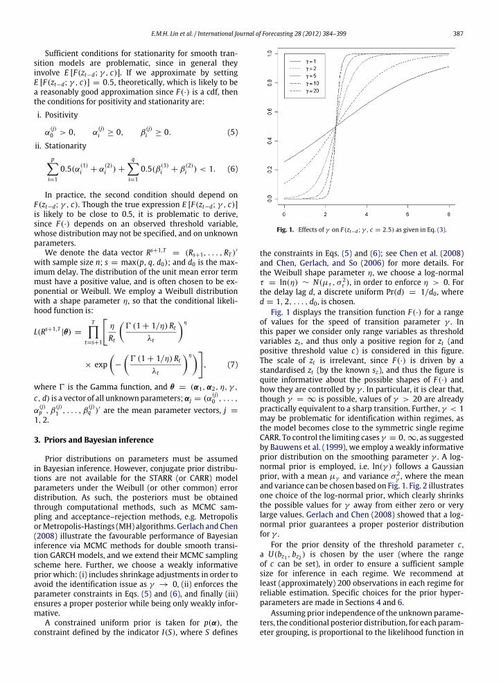
Fig. 1. Effects of γ on F(zt−d; γ , c = 2.5) as given in Eq. (3).
the constraints in Eqs. (5) and (6); see Chen et al. (2008)and Chen, Gerlach, and So (2006) for more details. Forthe Weibull shape parameter η, we choose a log-normalτ = ln(η) ∼ N(µτ , σ
2τ ), in order to enforce η > 0. For
the delay lag d, a discrete uniform Pr(d) = 1/d0, whered = 1, 2, . . . , d0, is chosen.
Fig. 1 displays the transition function F(·) for a rangeof values for the speed of transition parameter γ . Inthis paper we consider only range variables as thresholdvariables zt , and thus only a positive region for zt (andpositive threshold value c) is considered in this figure.The scale of zt is irrelevant, since F(·) is driven by astandardised zt (by the known sz), and thus the figure isquite informative about the possible shapes of F(·) andhow they are controlled by γ . In particular, it is clear that,though γ = ∞ is possible, values of γ > 20 are alreadypractically equivalent to a sharp transition. Further, γ < 1may be problematic for identification within regimes, asthe model becomes close to the symmetric single regimeCARR. To control the limiting cases γ = 0, ∞, as suggestedby Bauwens et al. (1999), we employ a weakly informativeprior distribution on the smoothing parameter γ . A log-normal prior is employed, i.e. ln(γ ) follows a Gaussianprior, with a mean µγ and variance σ 2
γ , where the meanand variance can be chosen based on Fig. 1. Fig. 2 illustratesone choice of the log-normal prior, which clearly shrinksthe possible values for γ away from either zero or verylarge values. Gerlach and Chen (2008) showed that a log-normal prior guarantees a proper posterior distributionfor γ .
For the prior density of the threshold parameter c ,a U(bz1 , bz2) is chosen by the user (where the rangeof c can be set), in order to ensure a sufficient samplesize for inference in each regime. We recommend atleast (approximately) 200 observations in each regime forreliable estimation. Specific choices for the prior hyper-parameters are made in Sections 4 and 6.
Assuming prior independence of the unknown parame-ters, the conditional posterior distribution, for each param-eter grouping, is proportional to the likelihood function in

388 E.M.H. Lin et al. / International Journal of Forecasting 28 (2012) 384–399
Fig. 2. Log-normal prior on γ , with µ = ln(5), σ 2= (ln(10))2/3.
Eq. (7), multiplied by the prior:
p(φ|Rs+1,T , θ−φ) ∝ L(Rs+1,T|θ)p(φ), (8)
where φ is one of α1, α2, τ , d, γ , or c , and θ−φ is the vectorof all model parameters θ, excluding the element φ.
To simulate the delay parameter d, we draw from itsconditional posterior multinomial distribution:
Pr(d = j|Rs+1,T , θ−d)
=L(Rs+1,T
|d = j, θ−d) Pr(d = j)d0i=1
L(Rs+1,T |d = i, θ−d) Pr(d = i)
, (9)
where j = 1, . . . , d0.In order to draw from Eq. (8) for all parameters except
d, we apply adaptive MHmethods, but instead of the usualGaussian proposal distributions, we employ a mixtureof Gaussian proposals. Gaussian random walk (RW) MHalgorithms, which are now standard for Bayesian GARCHmodels, can get stuck in local modes and experiencevery slow convergence, and also low acceptance rates.Further, adaptive sampling schemes often rely on the burn-in sample covering the posterior distribution sufficiently.Employing a mixture of Gaussians proposal, where oneor two of the mixtures have very large variances, shouldhelp to avoid or improve all of these issues, and thusincrease the mixing rate of the MCMC sampler and speedconvergence, mainly by allowing occasional ‘‘large’’ jumpsin the MCMC iterates. This method, while developedindependently by us, is a simplification of the moreflexible adaptive mixture of Student-t proposal method ofHoogerheide, Kaashoek, and van Dijk (2007), which maybe more robust and efficient in the case of highly non-elliptical posterior shapes.
For the groups αj, j = 1, 2, we use the RW MH algo-rithm for the first M MCMC iterations as a burn-in, usinga mixture of three Gaussians as a proposal. We then em-ploy an independent kernel (IK) MH algorithm for the lastN −M iterations as the sampling period, now employing adifferent, adaptedmixture of threeGaussians as a proposal,where the adaptivity comes from employing the samplemean and covariance of the burn-in sample in the sam-pling period proposal mixture. Consider a general parame-ter vector θ|k ∼ N(µ, kiΩ), i = 1, 2, 3, where the mixingis done over k. The innovation comes in the choices of k andthe associated mixture probabilities. We set:
k =
1 w.p. 0.859 w.p. 0.181 w.p. 0.05.
Fig. 3. Probability density plot based on the mixture Gaussian, Gaussianand Student-t distributions.
The choices of k are very similar to those made in a mix-ture of Gaussian state space model capturing certain typesof outliers, as used by Gerlach, Carter, and Kohn (2000),and are made to ensure that a very fat-tailed proposal dis-tribution results, ensuring that low probability jumps outof local modes in the MCMC scheme are possible, if neces-sary, as discussed earlier. Fig. 3 compares three differentdistributions, including the proposed mixture of threeGaussians, a simple standardGaussian, and a Student-t dis-tribution with six degrees of freedom. The mixture pro-posal density can flexibly allow for quite fat tails comparedto the other two distributions. We conjecture that this willlead to better and more efficient MCMC samples, whichwill be analyzed in the simulation study.
4. Simulation study
The estimation methods are illustrated for simulateddata from various parameter settings. Five hundred datareplications are used, with a sample size of n = 2000,from three models: two with a smooth transition functionunder different transition variables and one with a stepfunction. All error terms, εt , are generated from a Weibulldistribution with a unit mean and shape η.
Model 1: The true model is STARR (1, 1):
Rt = λtεt ,
λt = (1 − F(Rt−1, γ )) λ(1)t + F(Rt−1, γ )λ
(2)t ,
λ(1)t = 0.03 + 0.06Rt−1 + 0.91λt−1,
λ(2)t = 0.10 + 0.21Rt−1 + 0.75λt−1,
F(Rt−1; γ ) =1
1 + exp−γ
Rt−1−2.0
sR
.
In turn, γ = 2, 5.Model 2: The true model is STARRX (1, 1):
Rt = λtεt ,
λt = (1 − F(zt−1, γ )) λ(1)t + F(zt−1, γ )λ
(2)t ,

E.M.H. Lin et al. / International Journal of Forecasting 28 (2012) 384–399 389
Table 1Simulation results of a STARR model obtained from 500 replications with n = 2000.
γ = 2 Real Mixtureb Gaussian Student-tMed Std. 2.5% 97.5% Med Std. 2.5% 97.5% Med Std. 2.5% 97.5%
α(1)0 0.03 0.031 (88.2%)c 0.012 0.009 0.056 0.025 (62.4%) 0.010 0.007 0.043 0.025 (57.8%) 0.010 0.007 0.043
α(1)1 0.06 0.073 (85.8%) 0.022 0.032 0.115 0.083 (60.4%) 0.017 0.053 0.117 0.082 (57.0%) 0.017 0.052 0.116
β(1)1 0.91 0.887 (76.8%) 0.020 0.849 0.927 0.878 (61.4%) 0.017 0.848 0.912 0.872 (62.0%) 0.017 0.841 0.905
α(2)0 0.10 0.183 (87.4%) 0.103 0.034 0.414 0.158 (57.2%) 0.068 0.046 0.284 0.150 (55.6%) 0.066 0.047 0.276
α(2)1 0.21 0.187 (89.6%) 0.048 0.106 0.293 0.182 (64.2%) 0.036 0.122 0.256 0.182 (65.8%) 0.036 0.118 0.253
β(2)1 0.75 0.710 (86.4%) 0.069 0.551 0.818 0.729 (64.6%) 0.050 0.627 0.815 0.741 (64.2%) 0.050 0.643 0.827
η 2.20 2.197 (94.4%) 0.038 2.123 2.273 2.196 (94.0%) 0.038 2.121 2.271 2.195 (93.4%) 0.038 2.121 2.271γ 2 3.446 (87.8%) 3.940 1.353 15.020 3.111 (73.0%) 3.402 1.209 13.014 3.008 (69.0%) 3.266 1.160 12.582c 2.00 2.233 (88.4%) 0.297 1.647 2.744 2.186 (83.8%) 0.281 1.657 2.691 2.174 (86.0%) 0.290 1.631 2.692d 1 1 (89.8%)a – – – 1 (84.0%) – – – 1 (84.2%) – – –
γ = 5 Real Mixtureb Gaussian Student-tMed Std. 2.5% 97.5% Med Std. 2.5% 97.5% Med Std. 2.5% 97.5%
α(1)0 0.03 0.027 (87.2%) 0.008 0.013 0.043 0.026 (80.8%) 0.008 0.012 0.042 0.026 (79.4%) 0.008 0.012 0.041
α(1)1 0.06 0.057 (91.6%) 0.016 0.028 0.088 0.060 (86.2%) 0.015 0.032 0.091 0.061 (85.0%) 0.015 0.034 0.092
β(1)1 0.91 0.905 (89.6%) 0.013 0.879 0.929 0.903 (86.2%) 0.013 0.877 0.926 0.902 (85.4%) 0.013 0.877 0.925
α(2)0 0.10 0.269 (73.4%) 0.131 0.072 0.574 0.260 (67.0%) 0.115 0.071 0.491 0.257 (67.8%) 0.114 0.067 0.486
α(2)1 0.21 0.191 (89.8%) 0.045 0.111 0.288 0.187 (80.6%) 0.041 0.117 0.274 0.189 (81.6%) 0.042 0.115 0.275
β(2)1 0.75 0.672 (74.8%) 0.069 0.514 0.780 0.681 (69.8%) 0.060 0.553 0.780 0.680 (71.0%) 0.061 0.551 0.782
η 2.20 2.196 (93.4%) 0.038 2.121 2.272 2.195 (92.8%) 0.038 2.120 2.271 2.194 (92.6%) 0.038 2.120 2.270γ 5 4.920 (99.0%) 1.868 2.759 9.901 4.886 (96.0%) 1.840 2.750 9.788 4.841 (95.0%) 1.823 2.737 9.703c 2.00 2.181 (85.2%) 0.217 1.800 2.646 2.162 (84.2%) 0.211 1.784 2.601 2.165 (84.8%) 0.211 1.785 2.603d 1 1 (95.4%) – – – 1 (92.2%) – – – 1 (93.8%) – – –a The percentage of datasets where the delay lag d was chosen is in parentheses, d = 1, 2, 3.b ‘Mixture’ means that the mixture Gaussian proposal distribution was used.c The percentage of datasets where the true parameter value was inside the 95% posterior interval is in parentheses, except for d.
λ(1)t = 0.04 + 0.17Rt−1 + 0.79λt−1,
λ(2)t = 0.30 + 0.30Rt−1 + 0.60λt−1,
F(zt−1; γ ) =1
1 + exp−γ (
zt−1−2.0sz
) ,
zt = λz,tεz,t ,
λz,t = 0.09 + 0.17zt−1 + 0.79λz,t−1.
In turn, γ = 2, 5.Model 3: The true model is TARR (1, 1):
Rt = λtεt ,
λt =
0.10 + 0.20Rt−1 + 0.70λt−1, zt−1 ≤ 1.60.45 + 0.20Rt−1 + 0.65λt−1, zt−1 > 1.6.
Note that model 3 is a STARR model with a step transitionfunction. We fit a STARR model in order to examine therobustness to departures from a smooth transition underthis model.
For the blocks of αj, j = 1, 2, themixture of three Gaus-sians proposal distribution is employed. For comparison,estimates of αj using Gaussian and Student-t proposal dis-tributions are also obtained using the same data sets. Themaximum delay lag is set to d0 = 3, and c ∼ U(Q1,Q3),where Q1 and Q3 are set as the first and third quantiles ofthe observed threshold variable zt . The hyperparameters inthe prior for ln(γ ) are set to (µγ = ln 5, σ 2
γ =(ln 10)
32), as
suggested by Gerlach and Chen (2008). For each data set,N = 30,000MCMC iterations are used, including a burn-inof the firstM = 10,000 iterations. Convergence is assessedby viewing many trace plots of parameters from different
starting positions over many different data sets: conver-gence is always evident well before 10,000 iterations.
Since some of the posterior distributions are skewed,posterior medians are chosen as the point estimator foreach parameter. The true parameter values, average pos-terior medians, standard deviations of the 500 posteriormedians, and 95% intervals for 500 posterior median es-timates of the model parameters in Models 1–3 are shownin Tables 1–3. Further, for each dataset, the 95% Bayesiancredible interval is calculated for each parameter, usingthe 2.5th and 97.5th percentiles of the MCMC samplingperiod. The frequentist coverages, i.e. the percentage ofcredible intervals that contained the true parameter value,are displayed in parentheses for each parameter. The re-sults are shown under the three types of proposal distribu-tion: mixture of three Gaussians, Gaussian and Student-twith 5 degrees of freedom. Broadly speaking, the methodsused for estimation show little or no clear bias and a rea-sonable standard deviation. Further, the delay lag is cor-rectly chosen as 1, by maximum posterior probability, inat least 84% of datasets in each case, and usually closer to95%–100%. Perhaps the estimate of γ when the true valueis 2 is slightly concerning, no doubt shrunk away from 0 bythe log-normal prior:while the estimates average between3 and 3.45, the 95% interval of posterior medians rangesfrom about 1–15. Clearly this parameter is difficult to esti-mate for low true values. However, when the true value is5, the estimates are close to unbiased and have a smallerstandard deviation and a tighter interval of estimation.
Tables 1–2 reveal that there are no clear differences inthe results over the three choices for proposal distribution

390 E.M.H. Lin et al. / International Journal of Forecasting 28 (2012) 384–399
Table 2Simulation results of a STARRX model obtained from 500 replications with n = 2000.
γ = 2 Real Mixtureb Gaussian Student-tMed Std. 2.5% 97.5% Med Std. 2.5% 97.5% Med Std. 2.5% 97.5%
α(1)0 0.04 0.051 (92.6%)c 0.019 0.015 0.089 0.048 (78.8%) 0.017 0.014 0.081 0.048 (79.4%) 0.018 0.014 0.081
α(1)1 0.17 0.158 (89.4%) 0.023 0.111 0.203 0.156 (82.0%) 0.022 0.112 0.196 0.158 (81.8%) 0.022 0.114 0.198
β(1)1 0.79 0.759 (85.6%) 0.031 0.695 0.815 0.767 (81.6%) 0.028 0.712 0.820 0.765 (83.4%) 0.029 0.709 0.818
α(2)0 0.30 0.260 (88.2%) 0.063 0.148 0.388 0.265 (90.0%) 0.067 0.147 0.399 0.269 (90.8%) 0.068 0.149 0.403
α(2)1 0.30 0.264 (85.8%) 0.048 0.180 0.367 0.267 (84.0%) 0.048 0.183 0.371 0.265 (86.4%) 0.049 0.179 0.371
β(2)1 0.60 0.616 (90.6%) 0.068 0.476 0.740 0.605 (90.8%) 0.070 0.462 0.731 0.606 (91.6%) 0.071 0.460 0.734
η 2.20 2.197 (94.4%) 0.038 2.122 2.273 2.196 (94.0%) 0.038 2.121 2.271 2.197 (94.2%) 0.038 2.122 2.272γ 2 3.121 (90.6%) 3.063 1.199 11.878 3.011 (86.6%) 2.921 1.194 11.296 3.015 (86.6%) 2.914 1.191 11.263c 2.00 1.957 (96.2%) 0.200 1.578 2.342 1.962 (95.6%) 0.207 1.570 2.347 1.973 (95.4%) 0.207 1.578 2.355d 1 1 (95.6%)a – – – 1 (94.4%) – – – 1 (94.4%) – – –
γ = 5 Real Mixtureb Gaussian Student-tMed Std. 2.5% 97.5% Med Std. 2.5% 97.5% Med Std. 2.5% 97.5%
α(1)0 0.04 0.041 (92.0%) 0.011 0.021 0.063 0.041 (92.2%) 0.012 0.020 0.065 0.040 (91.0%) 0.011 0.020 0.064
α(1)1 0.17 0.156 (85.8%) 0.017 0.125 0.190 0.156 (86.8%) 0.017 0.123 0.191 0.156 (85.4%) 0.017 0.123 0.190
β(1)1 0.79 0.778 (89.2%) 0.022 0.733 0.818 0.778 (90.4%) 0.023 0.730 0.820 0.778 (89.0%) 0.023 0.731 0.819
α(2)0 0.30 0.284 (92.2%) 0.052 0.187 0.388 0.285 (95.0%) 0.058 0.179 0.400 0.286 (95.2%) 0.058 0.179 0.399
α(2)1 0.30 0.274 (88.6%) 0.042 0.198 0.361 0.274 (89.6%) 0.044 0.194 0.368 0.274 (90.2%) 0.044 0.194 0.368
β(2)1 0.60 0.584 (93.2%) 0.059 0.464 0.692 0.583 (94.6%) 0.063 0.452 0.700 0.583 (94.8%) 0.063 0.454 0.700
η 2.20 2.197 (94.4%) 0.038 2.122 2.273 2.196 (94.4%) 0.038 2.122 2.272 2.196 (94.2%) 0.038 2.122 2.272γ 5 5.164 (100.0%) 1.809 2.864 9.848 5.095 (99.6%) 1.824 2.766 9.802 5.063 (99.0%) 1.804 2.760 9.726c 2.00 2.024 (93.2%) 0.101 1.834 2.232 2.027 (94.4%) 0.108 1.825 2.252 2.026 (94.4%) 0.108 1.823 2.249d 1 1 (99.0%) – – – 1 (99.0%) – – – 1 (98.8%) – – –a The percentage of datasets where the delay lag dwas chosen is in parentheses, d = 1, 2, 3.b ‘Mixture’ means that the mixture Gaussian proposal distribution was used.c The percentage of datasets where the true parameter value was inside the 95% posterior interval is in parentheses, except for d.
with respect to point estimation. However, there areclear differences in the coverage percentages, i.e., withrespect to inference. If a correct 95% frequentist coverageis a goal of inference (which is often not the case forBayesian methods, especially under informative priors),then for Model 1 the coverages are vastly superiorunder the mixture of Gaussians proposal density in theMH method. Surprisingly, the Student-t method did notimprove much on the Gaussian proposal with respect tocoverage; however, in each case in Table 1, the frequentistcoverage is much closer to the nominal 95% under themixture proposal method. The results are mixed for theSTARRX model in Table 2, with the coverages from allmethods generally being closer to 95% than those for theSTARR model. Naturally, with fixed true parameter values,informative priors will generally lead to a coverage whichdiffers from nominal. Our prior is weakly informative,which at least partly explains the remaining differencesobserved here.
The data for Model 3 are generated by a TARR model,but are fitted by the misspecified STARR model. The rangeequation parameters seem to be estimated well, with littleor no obvious bias, and even with coverage rates whichare reasonably close to the nominal rates. Both the averageposterior median and posterior mean for the speed oftransition parameter estimates are displayed in Table 3.While the truth is γ = ∞, the estimates are generallyquite large, with large variances. Here we see the effect ofthe informative log-normal prior on γ : a proper posteriormeans that very large values of γ will have estimateswhich are biased downwards (as they must be), but still
usually large enough to hint that a sharp transition modelis likely.
5. Model comparison and volatility forecasting
In order to compare competing STARRmodels and otherrange-based or return-based volatility models, we usethe deviance information criterion (DIC, see Spiegelhalter,Best, Carlin, & Van der Linde, 2002) for in-sampleperformances, and volatility forecasting for out-of-sampleperformances. Further, the Diebold-Mariano (DM) test(Diebold & Mariano, 1995) is employed to formally testdifferent volatility models, pairwise, for equal forecastaccuracy. The superior predictive ability (SPA) test ofHansen (2005) is also applied for comparing the forecastaccuracy jointly among the competing models.
The DIC is an information criterion (IC) which canbe estimated in a Bayesian framework and which actssimilarly to the standard AIC and BIC, in that a measureof fit is contrasted with a penalty function, related to thenumber of parameters in themodel, in an additivemanner.The DIC uses the deviance for a model, defined by Gelman,Carlin, Stern, and Rubin (2004, p. 180–183) as:
deviance : D(y, θ) = −2 ln f (y|θ).
The posterior expected deviance, Eθ |y[D(θ)] = D, is pro-portional to the Kullback-Leibler (K-L) information of themodel, and hence the model with the lowest expected de-viancewill have the highest posterior probability. Thus, thedeviance is ameasure of the fit,whichdecreaseswith a bet-ter fit (higher posterior probability, lowerK-L information).
E.M.H. Lin et al. / International Journal of Forecasting 28 (2012) 384–399 391
Table 3Simulation results of a misspecified model (TARR) obtained from 500 replications with n = 2000. The threshold value of the TARR model is r = 1.6.
Real Mean Med Std. 2.5% 97.5%
α(1)0 0.10 0.092 0.092 (88.4%)b 0.014 0.066 0.121
α(1)1 0.20 0.176 0.177 (81.0%) 0.024 0.126 0.221
β(1)1 0.70 0.695 0.695 (92.6%) 0.022 0.651 0.735
α(2)0 0.45 0.514 0.515 (92.8%) 0.107 0.304 0.714
α(2)1 0.20 0.181 0.179 (94.4%) 0.054 0.082 0.293
β(2)1 0.65 0.606 0.609 (92.0%) 0.061 0.478 0.716
η 2.20 2.211 2.211 (94.8%) 0.039 2.136 2.287γ 13.628 11.517 8.362 4.577 35.309c 1.634 1.630 0.078 1.494 1.802d 1 1 (98.0%)a – – –a The percentage of datasets where the delay lag d was chosen is in parentheses, d = 1, 2, 3.b The percentage of datasets where the true parameter value was inside the 95% posterior interval is in parentheses, except for d.
The DIC is defined as:
DIC = D(θ) + 2pD,
where pD is a measure of the effective number of param-eters in the model and uses the posterior mean of the pa-rameters θ = Eθ |y[θ ] to estimate it via:
pD = Eθ |y[D(θ)] − D(Eθ |y[θ ]) = D − D(θ).
This is actually a measure of model complexity that in-creases with the ease of fitting the model to the data. Infact, for a linear model with Gaussian errors, pD equals thenumber of parameters in the model. Adding the averagedeviance and the effective number of parameters, pD, thusgives a measure of model fit, penalised by the complexityof the model; where the complexity is related to the num-ber of parameters in the model. The DIC can be defined inanother form: DIC = D+ pD = 2D−D(θ). The model withthe smallest DIC value is the one with the best fit.
5.1. Out-of-sample forecasting
For an out-of-sample forecast period of size n, let σt
be a time series and let σ1,t+h|t and σ2,t+h|t denote twocompetitive forecasts of σt+h, where h = 1, . . . , n. Theforecast error from the ith fitted model is ei,t+h|t = σt+h −
σi,t+h|t , i = 1, 2. Two popular error measures are themeansquare error (MSE) and mean absolute deviation (MAD),calculated as follows:
MSE : g(ei,t+h|t) = n−1n
h=1
ei,t+h|t
2,
MAD : g(ei,t+h|t) = n−1n
h=1
ei,t+h|t ,
where i = 1, 2. TheDMtest statistic evaluates the forecastsin terms of an arbitrary loss metric g(·):
DM =
n−1n
t=1
g(e1,t+h|t) − g(e2,t+h|t)
√S/n
,
where S is an estimator of the variance of the samplemean loss differential n−1 n
t=1(g(e1,t+h|t) − g(e2,t+h|t))and can be estimated using an approximate normal densityof g(e1,t+h|t) − g(e2,t+h|t) evaluated at zero.
Hansen (2005) proposed the joint test for superiorpredictive ability (SPA) to allow comparisons across arange ofmodels, compared to a benchmarkmodel. The testallows the loss function, e.g. MAD or MSE, to be specified,and tests whether a benchmark has a significantly lowerexpected loss than a range of competing models. Undera general loss measure L(ei,t+h|t), where i subscriptsindicate each of the competing forecast models, withthe benchmark model denoted i = 0, Hansen (2005)considered the loss comparisons di,t = L(e0,t+h|t) −
L(ei,t+h|t). These were placed into a vector, containing eachmodel’s loss compared to the benchmark, and a test wasdeveloped that the average of this vector µd satisfies thehypothesis µd ≤ 0, in which case the benchmark model isjointly superior to all of the other models considered. Weemploy the studentized version of the test, with the teststatistic:
√nmax
max
diωi
, 0
,
where di is the sample average of the loss comparisons di,tfor model i and ωi is an estimate of std(
√ndi).
5.2. Volatility proxies
In general, the volatility is an unobserved process: thetrue volatility for financial market data is simply not avail-able. Many different variables have been suggested to sub-stitute or proxy for the true volatility. Following the recentliterature, we forecast the standard deviation (σt ) and con-sider two proxy variables for the unobservable true σt :
1. σ1,t =m
i=1 y2i,t
0.52. σ2,t = exp[ln(Rt) − 0.43 + 0.292/2] (Alizadeh et al.,
2002).
The first proxy is the square root of the well-knownrealized volatilitymeasure, being the sum of the squares ofintra-day returns, where yi,t is the ith intra-day return onday t . Fifteen minute intra-day prices were employed forthis purpose. The second proxy is based on the intra-dayrange data and is derived from a result by Alizadeh et al.(2002), linking the quadratic variation with range data viaan empirical result and a relationship from the log-normaldistribution.

392 E.M.H. Lin et al. / International Journal of Forecasting 28 (2012) 384–399
Table 4Summary statistics of daily intra-day ranges from January 5, 1998 to December 31, 2009.
Obs. Mean Min. Max. Std. dev. Skewness Excess kurtosis Jarque-Bera test Q(10)
Japan 2845 1.637 0.299 11.743 0.975 3.016 18.351 44,234.625 5484.820(<0.001) (<0.001)
Hong Kong 2880 1.716 0.285 17.647 1.124 3.125 23.020 68,276.283 7408.287(<0.001) (<0.001)
6. Empirical study
We illustrate ourmethods using the intra-day high–lowprices from two stock markets obtained from the websitefinance.yahoo.com: Nikkei 225 (Japan) and the HANGSENG Index (HSI, Hong Kong) for the period from January5, 1998 to December 31, 2009. This period is chosen inorder to provide an accurate picture from after the Asianfinancial crisis and to include the global financial crisis(GFC) period. Summary statistics from the Nikkei 225and HSI daily range data are displayed in Table 4: thedaily range is heavily right skewed and has extremelyheavy tails, with all range series failing the Jarque-Beranormality test at the 1% level. Both market ranges showclear autocorrelation, which is confirmed by the Ljung-Box test showing high significance for the first 10 lags inTable 4. Further, the effect of the GFC is clear, from August2008 to October 2008, in an increasing volatility (ranges).
Naturally, intra-day range data may be affected byoutliers in returns or volatilities. There is a growing body ofliterature on measuring jumps in volatility, e.g. Andersenet al. (2007) and Barndorff-Nielsen and Shephard (2004).If jumps exist and are present in our data, then theyplay a role in the actual price movements that investorsexperience, and we believe that models should be robustto such movements; if they are not, then these modelsmay be of little practical value. As such, we follow Liuand Maheu (2008) and simply use the realized volatilitywithout correcting for outliers or jumps. In terms ofoutliers, the models we propose should be robust to manytypes of outliers/jumps through the heavy-tailed right-skewed Weibull error distribution.
First, in-sample estimation is considered, focusing onrange-based models only. Five STARR-type models areconsidered: the self-exciting STARR (using the laggedrange as the transition variable), the STARRX usingthe US S&P500 daily lagged range as the transitionvariable, the symmetric CARR, and the sharp transitionTARR and TARRX models. The priors have the samesettings as in the simulation study, and the estimationis again based on a total of 30,000 MCMC iterations,including 10,000 iterations which form the burn-inperiod. Again, convergence is checked for each model byextensively examiningmultiple trace plots and confirmingconvergence to the same posterior well inside the burn-in period. Table 5 contains the posterior median estimatesand standard errors for all five dynamic range modelsapplied to each market. The results from all models agreethat the range persistence (α1 + β1) is high (i.e. close to1) in both markets and in both regimes for the STARRand TARR models. Since the persistence estimates arecomparable in each regime, the fact that α0 is estimated
to be higher in the large range regime, zt−d > c , indicatesthat the average range (volatility) is estimated to be higherfollowing large ranges (volatility) in the Asian markets orin the US market. The posterior mode for the delay d (theposterior probability, as a percentage, is in parentheses)is one day for all nonlinear range models with the USrange as the transition value; however, the self-excitingTARR and STARR models chose a two day delay lag, d =
2, in Hong Kong. In Japan, there is clear evidence of asmooth transition between regimes, with both the STARRand STARRXmodels estimating almost all posterior weightbelow γ = 5. However, the models in Hong Kong showa possibly sharper transition, with most of the posteriorweight above γ = 5.
To evaluate the fit of eachmodel, Ljung-BoxQ -statisticsare calculated and shown in Table 6. We transformed theresiduals that are obtained from a Weibull distributionin order to achieve standard normality, using a standardprobability transform. No model can be rejected via theQ -statistics up to the 20th lag: all models seem to fit thedata adequately in-sample, at the 5% level of significance.
From Table 7, in order to assess the Markov chainconvergence and mixing efficiency, six MCMC chainsare initialized from widely varying positions, under themixture of Gaussians and the Gaussian proposal methods,yielding results for the Gelman and Rubin efficiencymeasure (Gelman & Rubin, 1992) which should be closerto one for more efficient MCMC sampling schemes. Whileboth methods mostly give acceptable levels of efficiency,the improvement under the mixture proposal method isclear, in both markets.
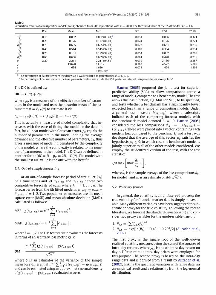
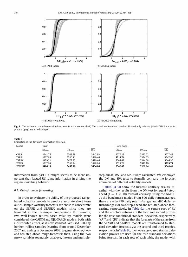
The estimated logistic transition function F(zt−d; γ , c)for eachmarket is displayed in Fig. 4 (dark crosses). A visualapproximation of the estimation uncertainty is given byshowing some estimated functions based on 30 randomlyselected MCMC iterates for (γ , c) (grey crosses). Fig. 4indicates that smooth transitions rather than sharp arefavoured in estimating this function, in both markets. Thefunctions are estimated to be steeper in the Hong Kongmarket, agreeing with the estimation results in Table 5.
The DIC is used to compare the in-sample performancesof the five models. Table 8 presents the smallest, largestand average values of the DIC for each model. Asymmetricmodels are clearly preferred in each market, i.e. the sym-metric CARR model is least favoured in each case. Amongthese nonlinear dynamic rangemodels, the STARRXmodelis clearly preferred in Japan, followed by the TARRXmodel.The effect of the US market on the Japanese daily rangedata seems strong and clear in this period. However, inHong Kong, the favored model under the maximum andmean DIC is the STARR, but under the minimum DIC mea-sure it is the TARR. Under the four nonlinear rangemodels,
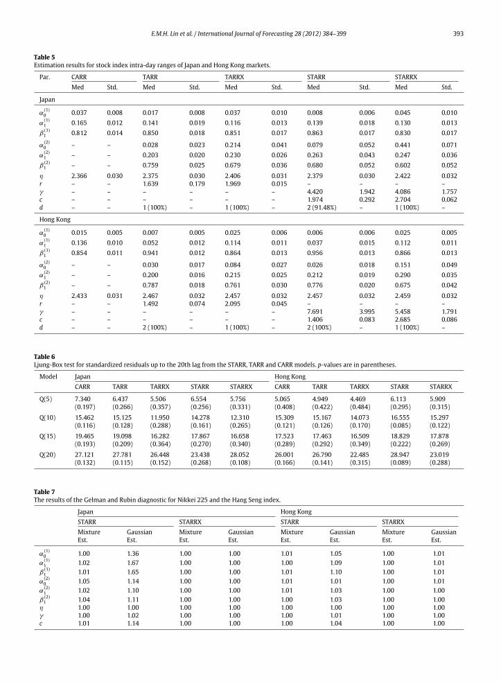
E.M.H. Lin et al. / International Journal of Forecasting 28 (2012) 384–399 393
Table 5Estimation results for stock index intra-day ranges of Japan and Hong Kong markets.
Par. CARR TARR TARRX STARR STARRXMed Std. Med Std. Med Std. Med Std. Med Std.
Japan
α(1)0 0.037 0.008 0.017 0.008 0.037 0.010 0.008 0.006 0.045 0.010
α(1)1 0.165 0.012 0.141 0.019 0.116 0.013 0.139 0.018 0.130 0.013
β(1)1 0.812 0.014 0.850 0.018 0.851 0.017 0.863 0.017 0.830 0.017
α(2)0 – – 0.028 0.023 0.214 0.041 0.079 0.052 0.441 0.071
α(2)1 – – 0.203 0.020 0.230 0.026 0.263 0.043 0.247 0.036
β(2)1 – – 0.759 0.025 0.679 0.036 0.680 0.052 0.602 0.052
η 2.366 0.030 2.375 0.030 2.406 0.031 2.379 0.030 2.422 0.032r – – 1.639 0.179 1.969 0.015 – – – –γ – – – – – – 4.420 1.942 4.086 1.757c – – – – – – 1.974 0.292 2.704 0.062d – – 1 (100%) – 1 (100%) – 2 (91.48%) – 1 (100%) –
Hong Kong
α(1)0 0.015 0.005 0.007 0.005 0.025 0.006 0.006 0.006 0.025 0.005
α(1)1 0.136 0.010 0.052 0.012 0.114 0.011 0.037 0.015 0.112 0.011
β(1)1 0.854 0.011 0.941 0.012 0.864 0.013 0.956 0.013 0.866 0.013
α(2)0 – – 0.030 0.017 0.084 0.027 0.026 0.018 0.151 0.049
α(2)1 – – 0.200 0.016 0.215 0.025 0.212 0.019 0.290 0.035
β(2)1 – – 0.787 0.018 0.761 0.030 0.776 0.020 0.675 0.042
η 2.433 0.031 2.467 0.032 2.457 0.032 2.457 0.032 2.459 0.032r – – 1.492 0.074 2.095 0.045 – – – –γ – – – – – – 7.691 3.995 5.458 1.791c – – – – – – 1.406 0.083 2.685 0.086d – – 2 (100%) – 1 (100%) – 2 (100%) – 1 (100%) –
Table 6Ljung-Box test for standardized residuals up to the 20th lag from the STARR, TARR and CARR models. p-values are in parentheses.
Model Japan Hong KongCARR TARR TARRX STARR STARRX CARR TARR TARRX STARR STARRX
Q(5) 7.340 6.437 5.506 6.554 5.756 5.065 4.949 4.469 6.113 5.909(0.197) (0.266) (0.357) (0.256) (0.331) (0.408) (0.422) (0.484) (0.295) (0.315)
Q(10) 15.462 15.125 11.950 14.278 12.310 15.309 15.167 14.073 16.555 15.297(0.116) (0.128) (0.288) (0.161) (0.265) (0.121) (0.126) (0.170) (0.085) (0.122)
Q(15) 19.465 19.098 16.282 17.867 16.658 17.523 17.463 16.509 18.829 17.878(0.193) (0.209) (0.364) (0.270) (0.340) (0.289) (0.292) (0.349) (0.222) (0.269)
Q(20) 27.121 27.781 26.448 23.438 28.052 26.001 26.790 22.485 28.947 23.019(0.132) (0.115) (0.152) (0.268) (0.108) (0.166) (0.141) (0.315) (0.089) (0.288)
Table 7The results of the Gelman and Rubin diagnostic for Nikkei 225 and the Hang Seng index.
Japan Hong KongSTARR STARRX STARR STARRXMixture Gaussian Mixture Gaussian Mixture Gaussian Mixture GaussianEst. Est. Est. Est. Est. Est. Est. Est.
α(1)0 1.00 1.36 1.00 1.00 1.01 1.05 1.00 1.01
α(1)1 1.02 1.67 1.00 1.00 1.00 1.09 1.00 1.01
β(1)1 1.01 1.65 1.00 1.00 1.01 1.10 1.00 1.01
α(2)0 1.05 1.14 1.00 1.00 1.01 1.01 1.00 1.01
α(2)1 1.02 1.10 1.00 1.00 1.01 1.03 1.00 1.00
β(2)1 1.04 1.11 1.00 1.00 1.00 1.03 1.00 1.00
η 1.00 1.00 1.00 1.00 1.00 1.00 1.00 1.00γ 1.00 1.02 1.00 1.00 1.00 1.01 1.00 1.00c 1.01 1.14 1.00 1.00 1.00 1.04 1.00 1.00
394 E.M.H. Lin et al. / International Journal of Forecasting 28 (2012) 384–399
(a) STARR-Japan. (b) STARRX-Japan.
(c) STARR-Hong Kong. (d) STARRX-Hong Kong.
Fig. 4. The estimated smooth transition functions for each market (dark). The transition functions based on 30 randomly selected joint MCMC iterates forγ and c (grey) are also displayed.
Table 8Evaluation of the deviance information criterion.
Model Japan Hong KongDICmin DICmax DIC DICmin DICmax DIC
CARR 5542.76 5542.99 5542.88 5577.29 5577.52 5577.44TARR 5527.85 5530.11 5529.46 5518.74 5554.03 5547.90TARRX 5479.21 5479.95 5479.46 5544.42 5544.58 5544.50STARR 5517.95 5533.74 5528.04 5528.79 5531.79 5529.71STARRX 5404.19 5455.86 5434.66 5540.47 5568.94 5548.41
information from past HK ranges seems to be more im-portant than lagged US range information in driving theregime switching behavior.
6.1. Out-of-sample forecasting
In order to evaluate the ability of the proposed range-based volatility models to produce accurate short termout-of-sample volatility forecasts, we chose to concentrateon the STARR and STARRX models, since they arefavoured in the in-sample comparisons. Furthermore,two well-known returns-based volatility models wereconsidered: the GARCH and GJR-GARCHmodels, both witht-distributed errors, as is now standard. We used 500-dayhorizon rolling samples (starting from around December2007 and ending in December 2009) to generate one-, two-and ten-step-ahead range forecasts; then, using the twoproxy variables separately, as above, the one andmultiple-
step-ahead MSE and MAD were calculated. We employedthe DM and SPA tests to formally compare the forecastaccuracies of different volatility models.
Tables 9a–9b show the forecast accuracy results, to-gether with the results from the DM test for equal l-step-ahead (l = 1, 2, 10) forecast accuracy, using the GARCHas the benchmark model. From 500 daily returns/ranges,there are only 499 daily returns/ranges and 490 daily re-turns/ranges for two-step-ahead and ten-step-ahead fore-casting, respectively. In Table 9a, the square root of RVand the absolute returns are the first and second proxiesfor the true conditional standard deviation, respectively.‘‘(A)’’ and ‘‘(B)’’ indicate that the forecasts of the range fromthe STARR and STARRX models are transformed to stan-dard deviation forecasts via the second and third proxies,respectively. In Table 9b, the two range-based standard de-viation proxies are used for the true standard deviationsbeing forecast. In each row of each table, the model with

E.M.H. Lin et al. / International Journal of Forecasting 28 (2012) 384–399 395
Table 9aAccuracymeasures and results of theDiebold-Mariano (DM) test for equal l-step-ahead forecast accuracy using the first proxy,with p-values in parentheses.The benchmark is the GARCH model.
Horizon GARCH GJR STARR STARRX
Japan
σ1,t MSE 1 1.203 1.185 0.315a 0.356(0.240) (0.000) (0.000)
MSE 2 1.232 1.212 0.381a 0.480(0.236) (0.000) (0.000)
MSE 10 1.443 1.351 0.499a 0.642(0.000) (0.000) (0.000)
MAD 1 0.889 0.873 0.336a 0.347(0.026) (0.000) (0.000)
MAD 2 0.900 0.882 0.356a 0.375(0.015) (0.000) (0.000)
MAD 10 0.956 0.913 0.395a 0.426(0.000) (0.000) (0.000)
Hong Kong
σ1,t MSE 1 2.394 2.302 0.501a 0.519(0.000) (0.000) (0.000)
MSE 2 2.455 2.363 0.373 0.368a
(0.000) (0.000) (0.000)MSE 10 2.632 2.552 0.493 0.480a
(0.003) (0.000) (0.000)MAD 1 1.360 1.324 0.563 0.559a
(0.000) (0.000) (0.000)MAD 2 1.373 1.334 0.428 0.412a
(0.000) (0.000) (0.000)MAD 10 1.398 1.361 0.481 0.442a
(0.000) (0.000) (0.000)1. The volatility proxy in each market is σ1,t , the square root of realized volatility; 2. Statistics which are significant at the 10% level are in boldface;
3. For the STARR and STARRX models, the estimated values ofht are given by exp[ln(Rt ) − 0.43 + 0.292/2].
a Indicates the minimumMSE or MAD in each row.
the lowestMSE orMAD is indicated by an asterisk,while allmodels with MSE or MAD values significantly lower thanthose of the GARCH model, at the 10% significance level,are in bold.
First, for theRVproxy in Table 9a, theGJR-GARCHmodelforecasts the volatility significantly better than the GARCHmodel in all cases, providing some confirmatory evidencefor the well-known leverage effect, which is captured bythe GJR but not the GARCH model. However, under boththe MSE and MAD measures, in both markets and at allhorizons, one of the STARR models is the most accurate atforecasting the volatility, and all of the STARR and STARRXare more accurate forecasters than either the GARCH orGJR-GARCH models, and are significantly more accuratethan the GARCH model’s forecasts.
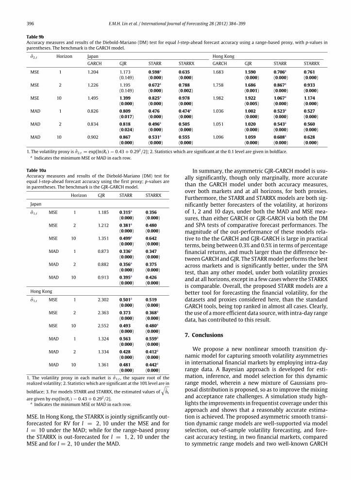
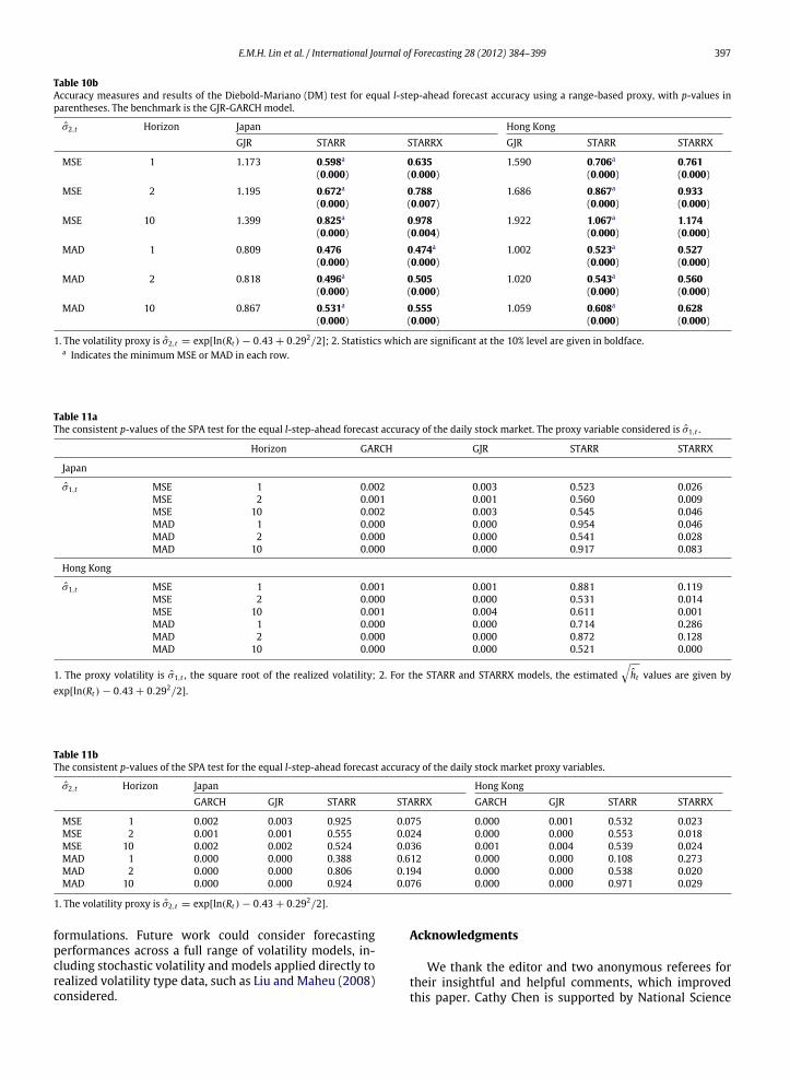
Table 9b displays the DM test results for equal forecastaccuracy via the range-based proxy σ2,t . The volatilityforecasts using either the STARR or STARRX models aresignificantly more accurate than those from the GARCHmodel, and are also clearly more accurate than those fromthe GJR-GARCH model, in both markets and at all forecasthorizons. In both markets the best model is the STARR,which captures the local size asymmetry.
Tables 10a–10b show results from the same sets of fore-casts as in Tables 9a–9b, but the benchmark model for theDM tests has now changed to the GJR-GARCH model, and
the results of theGARCHmodel are left out in order to avoidrepetition. The results are very similar to those when usingthe GARCH as the benchmarkmodel. Under the RV and therange-based proxy for volatility, the STARR and STARRXmodels are both significantly more accurate than theGJR-GARCHmodel in bothmarkets and at all forecast hori-zons. Again, the STARR is the preferred model overall.
TheDiebold-Mariano test is only a pairwisemodel com-parison procedure. The joint test for superior predictiveability (SPA) is now considered. Tables 11a–11b containconsistent p-values from the Hansen test for SPA. Each col-umn shows the benchmark model, and the p-value is thatwhich tests whether all other models jointly have lowerexpected loss, where MSE and MAD are considered andmark each row. l = 1-, 2- and 10-step-ahead forecastsare considered. The results are clear and reasonably con-sistent across proxies, loss (accuracy) measures, horizonsand markets. In each case, the other three models jointlyout-perform the GARCH and the GJR models, and forecastsignificantly more accurately than these twomodels. In nocases do any of the other three models significantly out-forecast the STARR model, since all its p-values are wellabove 0.05. The STARRX model is jointly significantly out-forecasted for RV in Japan for l = 1, 2, 10 under the MSEand for l = 1, 2 under the MAD; while for the range-basedproxy the STARRX is out-forecasted for l = 2, 10 under
396 E.M.H. Lin et al. / International Journal of Forecasting 28 (2012) 384–399
Table 9bAccuracy measures and results of the Diebold-Mariano (DM) test for equal l-step-ahead forecast accuracy using a range-based proxy, with p-values inparentheses. The benchmark is the GARCH model.
σ2,t Horizon Japan Hong KongGARCH GJR STARR STARRX GARCH GJR STARR STARRX
MSE 1 1.204 1.173 0.598a 0.635 1.683 1.590 0.706a 0.761(0.149) (0.000) (0.000) (0.000) (0.000) (0.000)
MSE 2 1.226 1.195 0.672a 0.788 1.758 1.686 0.867a 0.933(0.149) (0.000) (0.002) (0.001) (0.000) (0.000)
MSE 10 1.495 1.399 0.825a 0.978 1.982 1.922 1.067a 1.174(0.000) (0.000) (0.000) (0.005) (0.000) (0.000)
MAD 1 0.826 0.809 0.476 0.474a 1.036 1.002 0.523a 0.527(0.017) (0.000) (0.000) (0.000) (0.000) (0.000)
MAD 2 0.834 0.818 0.496a 0.505 1.051 1.020 0.543a 0.560(0.024) (0.000) (0.000) (0.000) (0.000) (0.000)
MAD 10 0.902 0.867 0.531a 0.555 1.096 1.059 0.608a 0.628(0.000) (0.000) (0.000) (0.000) (0.000) (0.000)
1. The volatility proxy is σ2,t = exp[ln(Rt ) − 0.43 + 0.292/2]; 2. Statistics which are significant at the 0.1 level are given in boldface.a Indicates the minimumMSE or MAD in each row.
Table 10aAccuracy measures and results of the Diebold-Mariano (DM) test forequal l-step-ahead forecast accuracy using the first proxy; p-values arein parentheses. The benchmark is the GJR-GARCH model.
Horizon GJR STARR STARRX
Japan
σ1,t MSE 1 1.185 0.315a 0.356(0.000) (0.000)
MSE 2 1.212 0.381a 0.480(0.000) (0.000)
MSE 10 1.351 0.499a 0.642(0.000) (0.000)
MAD 1 0.873 0.336a 0.347(0.000) (0.000)
MAD 2 0.882 0.356a 0.375(0.000) (0.000)
MAD 10 0.913 0.395a 0.426(0.000) (0.000)
Hong Kong
σ1,t MSE 1 2.302 0.501a 0.519(0.000) (0.000)
MSE 2 2.363 0.373 0.368a
(0.000) (0.000)MSE 10 2.552 0.493 0.480a
(0.000) (0.000)MAD 1 1.324 0.563 0.559a
(0.000) (0.000)MAD 2 1.334 0.428 0.412a
(0.000) (0.000)MAD 10 1.361 0.481 0.442a
(0.000) (0.000)1. The volatility proxy in each market is σ1,t , the square root of therealized volatility; 2. Statistics which are significant at the 10% level are in
boldface; 3. For models STARR and STARRX, the estimated values ofht
are given by exp[ln(Rt ) − 0.43 + 0.292/2].a Indicates the minimumMSE or MAD in each row.
MSE. In Hong Kong, the STARRX is jointly significantly out-forecasted for RV for l = 2, 10 under the MSE and forl = 10 under the MAD; while for the range-based proxythe STARRX is out-forecasted for l = 1, 2, 10 under theMSE and for l = 2, 10 under the MAD.
In summary, the asymmetric GJR-GARCHmodel is usu-ally significantly, though only marginally, more accuratethan the GARCH model under both accuracy measures,over both markets and at all horizons, for both proxies.Furthermore, the STARR and STARRX models are both sig-nificantly better forecasters of the volatility, at horizonsof 1, 2 and 10 days, under both the MAD and MSE mea-sures, than either GARCH or GJR-GARCH via both the DMand SPA tests of comparative forecast performances. Themagnitude of the out-performance of these models rela-tive to the the GARCH and GJR-GARCH is large in practicalterms, being between 0.3% and 0.5% in terms of percentagefinancial returns, and much larger than the difference be-tweenGARCH andGJR. The STARRmodel performs the bestacross markets and is significantly better, under the SPAtest, than any other model, under both volatility proxiesand at all horizons, except in a few caseswhere the STARRXis comparable. Overall, the proposed STARR models are abetter tool for forecasting the financial volatility, for thedatasets and proxies considered here, than the standardGARCH tools, being top ranked in almost all cases. Clearly,the use of amore efficient data source,with intra-day rangedata, has contributed to this result.
7. Conclusions
We propose a new nonlinear smooth transition dy-namic model for capturing smooth volatility asymmetriesin international financial markets by employing intra-dayrange data. A Bayesian approach is developed for esti-mation, inference, and model selection for this dynamicrange model, wherein a new mixture of Gaussians pro-posal distribution is proposed, so as to improve the mixingand acceptance rate challenges. A simulation study high-lights the improvements in frequentist coverage under thisapproach and shows that a reasonably accurate estima-tion is achieved. The proposed asymmetric smooth transi-tion dynamic range models are well-supported via modelselection, out-of-sample volatility forecasting, and fore-cast accuracy testing, in two financial markets, comparedto symmetric range models and two well-known GARCH
E.M.H. Lin et al. / International Journal of Forecasting 28 (2012) 384–399 397
Table 10bAccuracy measures and results of the Diebold-Mariano (DM) test for equal l-step-ahead forecast accuracy using a range-based proxy, with p-values inparentheses. The benchmark is the GJR-GARCH model.
σ2,t Horizon Japan Hong KongGJR STARR STARRX GJR STARR STARRX
MSE 1 1.173 0.598a 0.635 1.590 0.706a 0.761(0.000) (0.000) (0.000) (0.000)
MSE 2 1.195 0.672a 0.788 1.686 0.867a 0.933(0.000) (0.007) (0.000) (0.000)
MSE 10 1.399 0.825a 0.978 1.922 1.067a 1.174(0.000) (0.004) (0.000) (0.000)
MAD 1 0.809 0.476 0.474a 1.002 0.523a 0.527(0.000) (0.000) (0.000) (0.000)
MAD 2 0.818 0.496a 0.505 1.020 0.543a 0.560(0.000) (0.000) (0.000) (0.000)
MAD 10 0.867 0.531a 0.555 1.059 0.608a 0.628(0.000) (0.000) (0.000) (0.000)
1. The volatility proxy is σ2,t = exp[ln(Rt ) − 0.43 + 0.292/2]; 2. Statistics which are significant at the 10% level are given in boldface.a Indicates the minimumMSE or MAD in each row.
Table 11aThe consistent p-values of the SPA test for the equal l-step-ahead forecast accuracy of the daily stock market. The proxy variable considered is σ1,t .
Horizon GARCH GJR STARR STARRX
Japan
σ1,t MSE 1 0.002 0.003 0.523 0.026MSE 2 0.001 0.001 0.560 0.009MSE 10 0.002 0.003 0.545 0.046MAD 1 0.000 0.000 0.954 0.046MAD 2 0.000 0.000 0.541 0.028MAD 10 0.000 0.000 0.917 0.083
Hong Kong
σ1,t MSE 1 0.001 0.001 0.881 0.119MSE 2 0.000 0.000 0.531 0.014MSE 10 0.001 0.004 0.611 0.001MAD 1 0.000 0.000 0.714 0.286MAD 2 0.000 0.000 0.872 0.128MAD 10 0.000 0.000 0.521 0.000
1. The proxy volatility is σ1,t , the square root of the realized volatility; 2. For the STARR and STARRX models, the estimatedht values are given by
exp[ln(Rt ) − 0.43 + 0.292/2].
Table 11bThe consistent p-values of the SPA test for the equal l-step-ahead forecast accuracy of the daily stock market proxy variables.
σ2,t Horizon Japan Hong KongGARCH GJR STARR STARRX GARCH GJR STARR STARRX
MSE 1 0.002 0.003 0.925 0.075 0.000 0.001 0.532 0.023MSE 2 0.001 0.001 0.555 0.024 0.000 0.000 0.553 0.018MSE 10 0.002 0.002 0.524 0.036 0.001 0.004 0.539 0.024MAD 1 0.000 0.000 0.388 0.612 0.000 0.000 0.108 0.273MAD 2 0.000 0.000 0.806 0.194 0.000 0.000 0.538 0.020MAD 10 0.000 0.000 0.924 0.076 0.000 0.000 0.971 0.029
1. The volatility proxy is σ2,t = exp[ln(Rt ) − 0.43 + 0.292/2].
formulations. Future work could consider forecastingperformances across a full range of volatility models, in-cluding stochastic volatility andmodels applied directly torealized volatility type data, such as Liu and Maheu (2008)considered.
Acknowledgments
We thank the editor and two anonymous referees fortheir insightful and helpful comments, which improvedthis paper. Cathy Chen is supported by National Science
398 E.M.H. Lin et al. / International Journal of Forecasting 28 (2012) 384–399
Council (NSC) of Taiwan grants NSC99-2118-M-035-001-MY2 and NSC96-2118-M-035-002-MY3. Edward Lin issupported by NSC’s Graduate Students Study Abroadprogram (NSC97-2917-I-035-101).
Appendix
For a comparison with the volatility forecast of theSTARRmodels,we considerGARCH,GJR-GARCH, TARR, andTARRX models in the out-of-sample forecast:
GARCH model:
yt = at ,
at =
htεt , εt ∼ tν,
ht = α0 + α1a2t−1 + β1ht−1.
GJR-GARCH model:
yt = at ,
at =
htεt , εt ∼ tν,
ht = α0 + (α1 + δI−t−1)a2t−1 + β1ht−1,
I−t−1 =
1 if at−1 ≤ 0,0 if at−1 > 0.
TARR model:
Rt = λtεt , εt ∼ Weibull(η),
λt =
α
(1)0 + α
(1)1 Rt−1 + β
(1)1 λt−1 if Rt−d ≤ r,
α(2)0 + α
(2)1 Rt−1 + β
(2)1 λt−1 if Rt−d > r.
TARRX model:
Rt = λtεt , εt ∼ Weibull(η),
λt =
α
(1)0 + α
(1)1 Rt−1 + β
(1)1 λt−1 if RUS
t−d ≤ r,α
(2)0 + α
(2)1 Rt−1 + β
(2)1 λt−1 if RUS
t−d > r.
References
Alizadeh, S., Brandt, M. W., & Diebold, F. X. (2002). Range-basedestimation of stochastic volatility models. Journal of Finance, 57,1047–1092.
Andersen, T., & Bollerslev, T. (1998). Answering the skeptics: yes,standard volatilitymodels do provide accurate forecasts. InternationalEconomic Review, 39, 885–905.
Andersen, T. G., Bollerslev, T., & Diebold, F. X. (2007). Roughing it up:including jump components in the measurement, modeling andforecasting of return volatility. The Review of Economics and Statistics,89, 701–720.
Andersen, T., Bollerslev, T., Diebold, F., & Labys, P. (2003). Modelling andforecasting realized volatility. Econometrica, 71(2), 579–625.
Anderson, H. M., Nam, K., & Vahid, F. (1999). Asymmetric nonlinearsmooth transition GARCHmodels. In P. Rothman (Ed.), Nonlinear timeseries analysis of economic and financial data (pp. 191–207). Boston:Kluwer.
Barndorff-Nielsen, O. E., & Shephard, N. (2004). Power and bipowervariation with stochastic volatility and jumps (with discussion).Journal of Financial Econometrics, 2, 1–48.
Bauwens, L., Lubrano, M., & Richard, J.-F. (1999). Bayesian inference indynamic econometric models. Oxford University Press.
Black, F. (1976). Studies in stock price volatility changes. In Proceedingsof the 1976 business section (pp. 177–181). American StatisticalAssociation.
Bollerslev, T. (1986). Generalized autoregressive conditional het-eroskedasticity. Journal of Econometrics, 31, 307–327.
Brandt, M., & Jones, C. (2006). Volatility forecasting with range-basedEGARCH models. Journal of Business and Economic Statistics, 24,470–486.
Chan, K. S., & Tong, H. (1986). On estimating thresholds in autoregressivemodels. Journal of Time Series Analysis, 7, 179–190.
Chelley-Steeley, P. L. (2005). Modeling equity market integration usingsmooth transition analysis: a study of eastern European stockmarkets. Journal of International Money and Finance, 24, 818–831.
Chen, C. W. S., Gerlach, R. H., Choy, S. T., & Lin, C. (2010). Estimationand inference for exponential smooth transition nonlinear volatilitymodels. Journal of Statistical Planning and Inference, 140, 719–733.
Chen, C.W. S., Gerlach, R. H., & Lin, E. M. H. (2008). Forecast volatility fromthreshold heteroskedastic range models. Computational Statistics andData Analysis, 52, 2990–3010.
Chen, C. W. S., Gerlach, R., & So, M. K. P. (2006). Comparison of non-nested asymmetric heteroskedastic models. Computational Statisticsand Data Analysis, 51, 2164–2178.
Chen, C.W. S., & So, M. K. P. (2006). On a threshold heteroskedastic model.International Journal of Forecasting , 22, 73–89.
Chou, R. (2005). Forecasting financial volatilities with extreme values,the conditional autoregressive range (CARR) model. Journal of Money,Credit and Banking , 37, 561–582.
Chou, R. (2006). Modeling the asymmetry of stockmovements using priceranges. Advances in Econometrics, 20A, 231–257.
Chou, R., Chou, H., & Liu, N. (2009). Range volatility models and theirapplications in finance. In The handbook of quantitative finance and riskmanagement . Springer.
Diebold, F. X., & Mariano, R. S. (1995). Comparing predictive accuracy.Journal of Business and Economic Statistics, 13, 253–263.
Engle, R. F. (1982). Autoregressive conditional heteroscedasticity withestimates of the variance of United Kingdom inflation. Econometrica,50, 987–1008.
Engle, R. F., & Russell, J. R. (1998). Autoregressive conditional duration:a new model for irregular spaced transaction data. Econometrica, 66,1127–1162.
Fernandes, M., de Sa Mota, B., & Rocha, G. (2005). A multivariateconditional autoregressive range model. Economics Letters, 86,435–440.
Garman, M. B., & Klass, M. J. (1980). On the estimation of price volatilityfrom historical data. Journal of Business, 53, 67–78.
Gelman, A., Carlin, J. B., Stern, H. S., & Rubin, D. B. (2004). Bayesian dataanalysis (2nd ed.). Chapman and Hall.
Gelman, A., &Rubin, D. B. (1992). Inference from iterative simulationusingmultiple sequences. Statistical Science, 7, 457–511.
Gerlach, R., Carter, C., & Kohn, R. (2000). Efficient Bayesian inferencefor dynamic mixture models. Journal of the American StatisticalAssociation, 95(451), 819–828.
Gerlach, R., & Chen, C.W. S. (2008). Bayesian inference andmodel compar-ison for asymmetric smooth transition heteroskedasticmodels. Statis-tics and Computing , 18, 391–408.
Giordani, P., Kohn, R., & van Dijk, D. (2007). A unified approach tononlinearity, structural change, and outliers. Journal of Econometrics,137(1), 112–133.
Glosten, L. R., Jagannathan, R., & Runkle, D. E. (1993). On the relationbetween the expected value and the volatility of the nominal excessreturn on stocks. Journal of Finance, 487, 1779–1801.
González-Rivera, G. (1998). Smooth-transition GARCH models. Studies inNonlinear Dynamics and Econometrics, 3, 61–78.
Granger, C. W. J., & Teräsvirta, T. (1993). Modelling nonlinear economicrelationships. In Advanced texts in econometrics. New York, Toronto,Melbourne: Oxford University Press.
Hansen, P. R. (2005). A test for superior predictive ability. Journal ofBusiness and Economic Statistics, 4, 365–380.
Hansen, P. R., & Lunde, A. (2006). Realized variance and marketmicrostructure noise. Journal of Business and Economic Statistics, 24(2),127–161.
Hoogerheide, L. F., Kaashoek, J. F., & van Dijk, H. K. (2007). On theshape of posterior densities and credible sets in instrumental variableregression models with reduced rank: an application of flexiblesampling methods using neural networks. Journal of Econometrics,139, 154–180.
Leeves, G. (2007). Asymmetric volatility of stock returns during the Asiancrisis: evidence from Indonesia. International Review of Economics andFinance, 16, 272–286.
Li, C. W., & Li, W. K. (1996). On a double-threshold autoregressiveheteroscedastic time series model. Journal of Applied Econometrics, 11,253–274.
Liu, C., & Maheu, J. (2008). Are there structural breaks in realizedvolatility? Journal of Financial Econometrics, 6, 326–360.
Lopes, H. F., & Salazar, E. (2006). Bayesian model uncertainty in smoothtransition autoregressions. Journal of Time Series Analysis, 27, 99–117.

E.M.H. Lin et al. / International Journal of Forecasting 28 (2012) 384–399 399
Lubrano, M. (2001). Smooth transition GARCH models, a Bayesianperspective. Recherches Economiques de Louvain, 67, 257–287.
Meitz, M., & Teräsvirta, T. (2006). Evaluating models of autoregressiveconditional duration. Journal of Business and Economic Statistics, 24,104–124.
Nam, N., Pyun, C. S., & Avard, S. L. (2001). Asymmetric revertingbehavior of short-horizon stock returns: an evidence of stock marketoverreaction. Journal of Banking and Finance, 25, 807–824.
Parkinson, M. (1980). The extreme value method for estimating thevariance of the rate of return. Journal of Business, 53, 61–65.
Sarantis, N. (1999). Modeling non-linearities in real effective exchangerates. Journal of International Money and Finance, 18, 27–45.
Shu, J. H., & Zhang, J. E. (2006). Testing range estimators of historicalvolatility. Journal of Futures Markets, 26, 297–313.
Spiegelhalter, D. J., Best, N. G., Carlin, B. P., & Van der Linde, A. (2002).Bayesian measures of model complexity and fit (with discussion).Journal of the Royal Statistical Society, Series B, 64, 583–616.
Zhang, M. Y., Russell, J., & Tsay, R. S. (2001). A nonlinear autoregressiveconditional duration model with applications to financial transactiondata. Journal of Econometrics, 104, 179–207.