Bouakez : Corresponding author. Institute of Applied Economics and CIRPÉE, HEC Montréal, 3000 chemin de la Côte-Sainte-Catherine, Montréal, Québec, Canada H3T 2A7 Tel.: 1-514-340-7003; Fax: 1-514-340-6469 hafedh.bouakez@hec.ca Normandin: Institute of Applied Economics and CIRPÉE, HEC Montréal, 3000 chemin de la Côte-Sainte-Catherine, Montréal, Québec, Canada H3T 2A7 Tel.: 1-514-340-6841 ; Fax: 1-514-340-6469 michel.normandin@hec.ca We thank seminar participants at the Bank of Canada and the Paris School of Economics for helpful comments and suggestions. Financial support from FQRSC, SSHRC, and IFM2 is gratefully acknowledged.

Cahier de recherche/Working Paper 08-18 Fluctuations in the Foreign Exchange Market: How Important are Monetary Policy Shocks?

Hafedh Bouakez Michel Normandin Septembre/September 2008

Abstract: We study the effects of U.S. monetary policy shocks on the bilateral exchange rate between the U.S. and each of the G7 countries. We also estimate deviations from uncovered interest rate parity and exchange rate pass-through conditional on these shocks. The analysis is based on a structural vector autoregression in which monetary policy shocks are identified through the conditional heteroscedasticity of the structural disturbances. Unlike earlier work in this area, our empirical methodology avoids making arbitrary assumptions about the relevant policy indicator or transmission mechanism in order to achieve identification. At the same time, it allows us to assess the implications of imposing invalid identifying restrictions. Our results indicate that the nominal exchange rate exhibits delayed overshooting in response to a monetary expansion, depreciating for roughly ten months before starting to appreciate. The shock also leads to large and persistent departures from uncovered interest rate parity, and to a prolonged period of incomplete pass-through. Variance-decomposition results indicate that monetary policy shocks account for a non-trivial proportion of exchange rate fluctuations. Keywords: Conditional heteroscedasticity, Delayed overshooting, Exchange rate pass-through, Identification, Structural vector autoregression, Uncovered interest rate parity JEL Classification: C32, E52, F31, F41

1. Introduction

The dominant view in the literature on exchange rate determination is based on the premises

that prices are sticky in the short run and that uncovered interest rate parity (UIP) holds

continuously. As first established by Dornbusch (1976), these assumptions together imply

that the nominal exchange rate must immediately overshoot its long-run level in response to

a monetary policy shock. Price stickiness also implies that, conditional on a monetary policy

shock, exchange rate pass-through to domestic prices is incomplete in the short run, which

translates into violations of the law of one price and, therefore, deviations from purchasing

power parity. Following the seminal work of Obstfeld and Rogoff (1995), recent theoretical

studies on exchange rate determination have sought to incorporate these features into fully

optimizing, rational-expectation models. Despite being more sophisticated, however, these

models preserve the essence of the Dornbusch model, continuing to emphasize the interaction

of nominal rigidities and monetary policy shocks as the main mechanism driving exchange-

rate fluctuations.

The purpose of this paper is to evaluate the empirical relevance of this view. More

specifically, we estimate the effects of U.S. monetary policy shocks on the bilateral exchange

rate between the U.S. and each of the remaining G7 countries. We also estimate deviations

from UIP and exchange rate pass-through to U.S. domestic prices conditional on these

shocks. Finally, we measure the importance of monetary policy shocks in accounting for

the variability of each of these variables.

Surprisingly, little empirical work has been done to measure the effects of monetary

policy shocks on exchange rates. Furthermore, the handful of empirical studies that have

attempted to examine this issue using vector autoregressions (VAR) did not reach a con-

sensus regarding the direction in which and the extent to which monetary policy shocks

affect the exchange rate. Indeed, some studies find that the nominal exchange rate does not

immediately overshoot its long-run level in response to a monetary policy shock. Instead,

it exhibits a hump-shaped profile, reaching its maximal response several months after the

shock; a pattern often referred to as delayed overshooting (e.g., Eichenbaum and Evans

1995, Grilli and Roubini 1995, 1996). Others, in contrast, find that the exchange rate over-

shooting is nearly immediate (e.g., Kim and Roubini 2000 and Kalyvitisa and Michaelides

2001). Similarly, there is little agreement on the importance of monetary policy shocks in

1

accounting for exchange-rate movements: estimates of the fraction of exchange rate vari-

ability that is attributed to monetary policy shocks range from essentially zero (e.g., Scholl

and Uhlig 2005) to over 50 percent (e.g., Kim and Roubini 2000).

In the same vein, although it is now well established that there are significant departures

from UIP, which imply the existence of predictable excess returns on the foreign-exchange

market, there is little and mixed evidence on the extent to which these departures are due

to unexpected changes in monetary policy. Deviations from UIP conditional on monetary

policy shocks and the importance of these shocks in accounting for the variability of excess

returns are found to be large in some studies (e.g., Eichenbaum and Evans 1995 and Faust

and Rogers 2003) but fairly small in others (e.g., Kim and Roubini 2000).

To some extent, the discrepancy in results across these earlier studies is attributed to

the method used to identify monetary policy shocks within structural vector autoregressions

(SVAR). Although most of existing studies measure monetary policy shocks with innovations

to the short term interest rate, they differ in the restrictions imposed on the interactions be-

tween the variables included in the SVAR, which in turn determine the mechanism through

which shocks propagate. Four types of restrictions can be found in the literature: recursive

zero restrictions (e.g., Eichenbaum and Evans 1995, Grilli and Roubini 1995, 1996), non-

recursive zero restrictions (e.g., Kim and Roubini 2000), sign and shape restrictions (e.g.,

Faust and Rogers 2003 and Scholl and Uhlig 2005), and long-run restrictions (e.g., Clarida

and Gali 1994 and Rogers 1999).1

These different types of restrictions have in common that they are arbitrary in nature.

Faust and Rogers (2003) further argue that some of the commonly used zero restrictions

are highly stylized and, therefore, unlikely to provide a plausible description of the trans-

mission channels of monetary policy shocks. Based on an empirical exercise in which they

eliminate all dubious identifying assumptions, they conclude that the peak response of the

nominal exchange rate to a monetary policy shock may be delayed or nearly immediate,

and that monetary policy may or may not be important in accounting for exchange-rate

fluctuations. While this study provides useful insights into the consequences of imposing

dubious identifying assumptions, it does not resolve the uncertainty surrounding the effects

of monetary policy shocks on foreign-exchange variables. Scholl and Uhlig (2005) attribute

this inconclusiveness to the fact that the restrictions imposed by Faust and Rogers (2003)

1Studies based on long-run restrictions have focused on the real rather than the nominal exchange rate.

2

are too weak to narrow down the range of plausible monetary policy shocks. Put differently,

these restrictions lead to under-identified SVARs, so that monetary policy shocks are not

uniquely determined. This in turn implies that the underlying restrictions are not testable.

This paper is in the spirit of the work of Faust and Rogers, but differs from it in

several important respects. It estimates a flexible SVAR where monetary policy shocks are

identified by exploiting the conditional heteroscedasticity of the structural innovations, a

procedure that has recently been proposed by Normandin and Phaneuf (2004). Unlike the

identification procedures used in earlier studies, which impose conditional homoscedasticity

of the innovations, this data-based approach does not rely on any arbitrary assumption

about the relevant indicator or transmission mechanism of monetary policy. It is therefore

a judgement-free approach which, in addition, allows one to formally test the commonly used

restrictions, including recursive zero restrictions, which are predominant in the literature.

Our results indicate that following an unanticipated monetary expansion, the nominal

exchange rate exhibits delayed but rapid overshooting, reaching its maximal depreciation

between 8 and 11 months after the shock. The monetary policy shock also triggers significant

and persistent departures from UIP as well as a prolonged period of incomplete exchange

rate pass-through, which exhibits a non-monotonic pattern. Interestingly, our approach

generates empirically plausible results for all the variables included in the SVAR without

having to impose arbitrary restrictions on their dynamic responses. Variance-decomposition

results reveal that monetary policy shocks are relatively important in explaining the vari-

ability of the nominal exchange rate, with a contribution that exceeds 30 percent at the

36-month horizon in some cases. In contrast, there is no clear evidence that the empirical

failure of UIP is mainly driven by monetary disturbances, at least at short horizons. Com-

pared with the results reported by Faust and Rogers, our findings provide more conclusive

evidence on the effects of monetary policy shocks. This is mainly because our identification

procedure tightly identifies these shocks.

We also find that imposing invalid identifying restrictions may lead to misleading impulse-

response and variance-decomposition results. In particular, when monetary policy shocks

are identified with orthogonalized innovations to the federal funds rate, as is frequently

assumed, the dynamic response of the nominal exchange rate to a monetary policy shock

is counterfactually small and lacks the delayed overshooting pattern. The restrictions asso-

ciated with the federal funds rate also result in a severe understatement of the importance

3

of monetary policy shocks in accounting for the variability of the nominal exchange rate.

The rest of the paper is organized as follows. Section 2 describes the empirical methodol-

ogy. Section 3 performs a preliminary analysis of the data. Section 4 discusses the estimated

effects of monetary policy shocks on the nominal exchange rate, deviations from UIP, and

exchange rate pass-through. Section 5 performs a robustness analysis. Section 6 concludes.

2. Empirical Methodology

2.1 Specification

The SVAR system (in innovation form) is:

Aνt = ǫt, (1)

where νt are the statistical innovations, ǫt are the structural innovations, and A captures

the interactions between current statistical innovations. The SVAR includes variables that

belong to the goods market, reserve market, and foreign-exchange market. The goods

variables are U.S. total output, yt, the U.S. price index, pt, and the world commodity-price

index, cpt. The reserve variables are the U.S. non-borrowed reserves, nbrt, total reserves, trt,

and the federal funds rate, fft. The foreign-exchange variables are the differential between

the foreign and U.S. nominal short-term interest rates, drt, and the nominal exchange rate

measuring the number of U.S. dollars needed to buy one unit of foreign currency, et.2

Following Bernanake and Mihov (1998), the market for U.S. bank reserves is further

developed via the simple formulation:

νnbr,t = φdσdǫd,t − φbσbǫb,t + σsǫs,t, (2)

νtr,t = −ανff,t + σdǫd,t, (3)

νtr,t − νnbr,t = βνff,t − φbσbǫb,t, (4)

where ǫs,t is a shock representing an exogenous policy action taken by the Fed, or mon-

etary policy shock, while ǫd,t and ǫb,t denote respectively the shocks of demand for total

reserves and for borrowed reserves by commercial banks. The parameters σs, σd, and σb

are the standard deviations scaling the structural innovations of interest, while φd and φb

are unrestricted parameters, and α and β are positive parameters. Equation (2) describes

2The choice of these variables is further discussed in Section 2.3.

4

the procedures which may be used by the Fed to select its monetary policy instruments.

Equation (3) represents the banks’ demand for total reserves in innovation form. Equation

(4) is the banks’ demand for borrowed reserves in innovation form, under the assumption

of a zero discount-rate innovation.

Inserting the equilibrium solution of the model (2)–(4) in system (1) gives:

a11 a12 a13 a14 a15 a16 a17 a18

a21 a22 a23 a24 a25 a26 a27 a28

a31 a32 a33 a34 a35 a36 a37 a38

a41 a42 a431+φb

σs−

φb+φd

σs

βφb−αφd

σsa47 a48

a51 a52 a53 0 1

σd

ασd

a57 a58

a61 a62 a631

σb−

1

σb

βσb

a67 a68

a71 a72 a73 a74 a75 a76 a77 a78

a81 a82 a83 a84 a85 a86 a87 a88

νy,t

νp,t

νcp,t

νnbr,t

νtr,t

νff,t

νdr,t

νe,t

=

ǫ1,t

ǫ2,t

ǫ3,t

ǫs,t

ǫd,t

ǫb,t

ǫ7,t

ǫ8,t

, (5)

where aij (i, j = 1, ...8) are unconstrained parameters. The system (5) allows interactions

between the terms within and across the blocks of goods, reserve and foreign-exchange

variables. As a result, all variables may be contemporaneously affected by the structural

innovations and, in particular, by monetary policy shocks.

It is instructive to rewrite the fourth equation in (5) as

νs,t = [ρ41νy,t + ρ42νp,t + ρ43νcp,t + ρ47νdr,t + ρ48νe,t] + σsǫs,t, (6)

where ρ4j = −a4jσs (for j = 1, 2, 3, 7, 8) and νs,t = (1 + φb)νnbr,t − (φd + φb)νtr,t + (βφb −

αφd)νff,t. Equation (6) is interpreted as the Fed’s feedback rule. The term νs,t measures

the statistical innovation of the monetary policy indicator. This indicator is expressed as a

combination of the reserve variables, reflecting the notion that the Fed might be adopting

a mixed procedure whereby it targets neither the interest rate nor a monetary aggregate

exclusively. The expression in brackets in equation (6) captures the systematic response of

the Fed to changes in the non-reserve variables. More precisely, the feedback rule implies

that the Fed designs its policy by taking into account current values of output, the price

level, commodity prices, the interest differential, and the exchange rate. Finally, the term

σsǫs,t is the scaled monetary policy shock.

The conditional scedastic structure of system (5) is:

AΣtA′ = Γt. (7)

5

The matrix Σt = Et−1(νtν′t) measures the conditional non-diagonal covariance matrix of

the non-orthogonal statistical innovations, Γt = Et−1(ǫtǫ′t) is the conditional diagonal co-

variance matrix of the orthogonal structural innovations, while I = E(ǫtǫ′t) normalizes the

unconditional variances of the structural innovations. The dynamics of the conditional

variances of the structural innovations are determined by

Γt = (I − ∆1 − ∆2) + ∆1 • (ǫt−1ǫ′t−1) + ∆2 • Γt−1. (8)

The operator • denotes the element-by-element matrix multiplication, while ∆1 and ∆2

are diagonal matrices of parameters. Equation (8) involves intercepts that are consistent

with the normalization I = E(ǫtǫ′t). Also, (8) implies that all the structural innovations are

conditionally homoscedastic if ∆1 and ∆2 are null. On the other hand, some structural in-

novations display time-varying conditional variances characterized by univariate generalized

autoregressive conditional heteroscedastic [GARCH(1,1)] processes if ∆1 and ∆2 — which

contain the ARCH and GARCH coefficients, respectively — are positive semi-definite and

(I −∆1 −∆2) is positive definite. Finally, all the conditional variances follow GARCH(1,1)

processes if ∆1, ∆2, and (I − ∆1 − ∆2) are positive definite.

2.2 Identification

Under conditional heteroscedasticity, system (5) and, in particular, the monetary policy

shocks and their effects on macroeconomic variables can be identified. The sufficient (rank)

condition for identification states that the conditional variances of the structural innova-

tions are linearly independent. That is, λ = 0 is the only solution to Γλ = 0, such that

(Γ′Γ) is invertible — where Γ stacks by column the conditional volatilities associated with

each structural innovation. The necessary (order) condition requires that the conditional

variances of (at least) all but one structural innovations are time-varying. In practice, the

rank and order conditions lead to similar conclusions, given that the conditional variances

are parameterized by GARCH(1,1) processes (see Sentana and Fiorentini 2001).3

3Rigobon (2003) develops an alternative identification method which also exploits the conditional het-eroscedasticity of the structural innovations. His method and the procedure used in this paper share thesame intuition: the conditional heteroscedasticity adds equations to the system, allowing the number ofunknown parameters to match the number of equations. However, the estimation strategies are different:In Rigobon’s paper, the conditional variances of the structural innovations are estimated for each of thepre-selected volatility regimes, rather than from a parametric specification such as a GARCH process.

6

Under conditional homoscedasticity, system (5) is not identified. In this environment,

certain targeting restrictions and orthogonality conditions must be imposed to identify the

monetary policy shocks (rather than the entire system). The usual targeting restrictions,

which define the monetary policy indicator, are the following:

• Non-borrowed reserve (NBR) indicator: φd = φb = 0. The Fed targets the non-

borrowed reserves. Thus, the non-borrowed reserves are the single policy variable and

νs,t = νnbr,t.

• Borrowed reserve (BR) indicator: φd = 1 and φb = α/β. The Fed targets borrowed

reserves. The policy variables are the non-borrowed reserves and total reserves, and

the policy indicator is νs,t = −(1 + α/β)(νtr,t − νnbr,t).

• Adjusted non-borrowed reserve (ANBR) indicator: α = φb = 0. In this case, shocks

to total reserves are purely demand shocks which are fully accommodated by the

Fed in the short run. The policy indicator is the adjusted non-borrowed reserves or

the portion of non-borrowed reserves which is orthogonal to total reserves: νs,t =

νnbr,t − φdνtr,t.

• Federal funds rate (FFR) indicator: φd = 1 and φb = −1. The Fed targets the federal

funds rate and decides to fully offset shocks to total reserves and borrowing demand.

The federal funds rate is the single policy variable and νs,t = −(β + α)νff,t.

The usual orthogonality conditions are the following:

• No impact effects: aij = 0 (for i = 1, . . . , 3 and j = 4, . . . , 8). These restrictions

impose the absence of contemporaneous effects of policy variables on goods variables.

In this case, the policy shocks in (6) are orthogonal to the goods variables. Note that

these effects can be direct or indirect. The direct effects are captured, for example, by

ai,4 (for i = 1, . . . , 3) for the NBR indicator. The policy variables can indirectly affect

the goods variables through their current effects on non-policy reserve variables and

on foreign-exchange variables. For example, these indirect effects are captured by ai,j

(for i = 1, . . . , 3 and j = 5, . . . , 8) for the NBR indicator.

• No feedback effects: aij = 0 (for i = 4, . . . , 6 and j = 7, 8). These restrictions imply

that ρ4j = 0 (for j = 7, 8). This means that the Fed does not adjust endogenously

7

the monetary policy to current changes of interest differential and exchange rate. In

this context, there is no systematic response of the monetary authority to movements

in foreign-exchange variables.

Under conditional homoscedasticity, combining one set of targeting restrictions with all

the sets of orthogonality conditions presented above ensures exact identification of monetary

policy shocks. In this case, the shocks are generated from a standard VAR-based procedure

that imposes the conditional homoscedasticity of the VAR residuals as well as non-testable

identifying restrictions. Specifically, with a single policy variable, the shocks are computed

from a Choleski decomposition of the VAR-residual covariance matrix. This decomposition

is typically obtained by ordering the goods variables first, followed by the policy variable,

by the other reserve variables, and by the foreign-exchange variables. This strategy has

been used, for example, by Eichenbaum and Evans (1995), who combine the restrictions

associated with either the FFR or NBR indicator along with the orthogonality conditions

in order to achieve identification. Faust and Rogers (2003), on the other hand, impose the

FFR targeting restrictions, but relax some of the orthogonality conditions, which leads to

under-identification.

2.3 Estimation strategy and data

We estimate system (5) using a two-step procedure. The first step consists in estimating, by

ordinary least squares (OLS), a τ -order VAR that includes output, consumer and commodity

prices, non-borrowing and total reserves, the federal funds rate, the interest rate differential,

and the nominal exchange rate. From this regression, we extract estimates of the statistical

innovations νt for t = τ +1, ..., T. For given values of the (non-zero) elements of the matrices

A,∆1, and ∆2, it is then possible to construct an estimate of the conditional covariance

matrix Σt recursively, using equations (7) and (8) and the initialization Γτ = I. The second

step consists in estimating the (non-zero) elements of the matrices A,∆1, and ∆2 using

full-information maximum likelihood (FIML). This method assumes that the statistical

innovations are conditionally normally distributed.

Our empirical analysis is based on monthly data taken from the International Financial

Statistics, the Board of Governors of the Federal Reserve System, the Federal Reserve Bank

of Saint-Louis, and the Bureau of Labor Statistics databases. Following Eichenbaum and

Evans (1995), we study the effects of U.S. monetary policy shocks on several exchange rates

8

vis-a-vis the U.S. dollar. Therefore, six different SVARs are estimated, corresponding to

the currencies of the remaining G7 countries: Canada (Canadian Dollar), France (French

Franc), Germany (Deutschmark), Italy (Lira), Japan (Yen), and the U.K. (British Pound).

Each of these SVARs also includes the interest rate differential between the U.S. and one

of the afore-mentioned countries. Since France, Italy, and Germany joined the European

Monetary Union in 1999, results for these countries are based on the sample period 1982:11

to 1998:12. For the remaining countries, the sample extends to 2004:10. The starting date

of the sample is widely believed to have marked the beginning of an era of stable monetary

policy in the U.S.

The variables used in the analysis are constructed as follows: yt is measured by the

U.S. industrial-production index; pt is measured by the U.S. consumer-price index, cpt is

measured by the world-export commodity-price index; nbrt and trt correspond to the U.S.

non-borrowed and total reserves, respectively, and fft is measured by the federal funds rate.

The interest rate differential, drt, is constructed as the difference between the U.S. three-

month Treasury Bill rate and its foreign counterpart.4 The exchange rate, et, is defined as

the number of U.S. dollars required to purchase one unit of foreign currency. All series,

except the federal funds rate and the interest rate differential are seasonally adjusted and

expressed in logarithm.5

Our empirical analysis does not take into account the foreign counterparts of yt and

pt. While, admittedly, this omission implies an asymmetric treatment of the U.S. and the

foreign country, it is largely dictated by the computational burden involved in estimating

GARCH processes with a large number of variables. When we added foreign output and the

foreign price index to the list of variables used in estimation, the extended SVAR proved

to be difficult to estimate by FIML. To circumvent this problem, and as a robustness check

of our results, we estimated the extended SVAR using a conditional (limited-information)

maximum-likelihood procedure.6 The details and results of this estimation are discussed in

Section 5.

4The short-term interest rate is measured by the three-month Treasury Bill rate for Canada, France, andthe U.K., by the Call money rate for Germany and Japan, and by the money market rate for Italy.

5Exchange-rate series are not seasonally adjusted but are expressed in logarithm.6An alternative strategy to treat the U.S. and the foreign country in a more symmetric manner would be

to express output and prices in terms of differences between the U.S. and each of the remaining G7 countries.This approach would not allow us, however, to compute the response of U.S. variables to a U.S. monetarypolicy shock, and therefore to compare our results to those reported in existing studies.

9

3. Preliminary Analysis

3.1 Specification tests

For each system, the VAR process includes six lags (τ = 6).7 The McLeod and LM test

statistics are often significant for p-order autocorrelations of the squared VAR residuals

and ARCH(p) effects (with p = 1, 3, 6). These results suggest the presence of conditional

heteroscedasticity in some statistical innovations, which is likely to translate into time-

varying conditional variances of the structural innovations.

Table 1 reports estimates of the GARCH(1,1) parameters. These estimates indicate

that the U.S. monetary policy shock has a highly persistent conditional variance, as the

sum of the ARCH and GARCH coefficients exceeds 0.95 in all cases. More importantly, the

estimates imply that the order condition for identification is always satisfied, since seven of

the eight structural innovations are heteroscedastic. Likewise, the rank condition is always

satisfied given that (Γ′Γ) is systematically invertible. These results mean that monetary

policy shocks can be identified through the conditional heteroscedasticity of the structural

innovations.8

Table 2 reports estimates of the reserve-market parameters. With few exceptions, the

estimates are fairly similar across the six systems.9 This is somewhat reassuring given that

the six systems share the same U.S. reserve-market variables. The slope of demand for total

reserves, α, has the correct sign in all cases, while that of the supply of borrowed reserves, β,

has the predicted sign in all but one case. Both parameters, however, are often imprecisely

estimated.

Recall that the specification (2)–(4) leads to the following linear restrictions in (5):

a54 = 0 and a64 = −a65. These restrictions are tested individually and jointly using a Wald

test. The results, reported in Panel A of Table 3, indicate that the restrictions cannot be

rejected at any conventional level of significance, which suggests that the specification (2)–

7In all cases, the Ljung-Box and heteroscedastic-robust Lagrange-Multiplier (LM) test statistics are neversignificant (at the 1% level) for p-order autocorrelations and AR(p) processes of the VAR residuals (withp = 1, 3, 6).

8In all cases, the McLoed and LM test statistics are never significant for p-order autocorrelations ofthe squared structural innovations (relative to their conditional variances) and GARCH(p,q) effects (withp = 3, and 6 and q = 1). This suggests that the estimates of the GARCH(1,1) coefficients provide anadequate description of the conditional heteroscedasticity of all structural innovations, including monetarypolicy shocks.

9The only notable exceptions are the estimate of σb in the system involving Japan and those of β in thesystems involving Germany and Japan.

10

(4) provides an empirically plausible description of the U.S. reserve market.10 We therefore

refer to the SVAR (5) as the unrestricted system, and to the dynamic responses and variance

decompositions it generates as the valid ones.

Panel B of Table 3 reports for each estimated system the p-value of the Wald statistic for

the joint test of the targeting and orthogonality restrictions associated with each monetary

policy indicator. The results indicate that these restrictions are soundly rejected in all

cases, thus implying that it is inappropriate to account for the stance of U.S. monetary

policy using a framework in which the Fed focuses on a single reserve variable, and which

imposes the orthogonality of the policy shock to a set of economic variables.

3.2 Monetary policy shocks

From the monetary authority’s feedback rule (6), it is possible to extract the sequence

of U.S. monetary policy shocks, ǫs,t, implied by the unrestricted system (5). Smoothed

measures of these shocks (computed as five-month centered moving averages) are depicted in

Figure 1. A negative (positive) value of the smoothed measure represents an unanticipated

contractionary (expansionary) policy by the Fed. The shaded vertical areas represent the

1991 and 2001 contractions as identified by the National Bureau of Economic Research.

The smoothed policy shocks exhibit a similar pattern across the six estimated systems.

In particular, there is an episode of very large negative policy shocks in the mid-1980s,

which coincides with the period in which the Fed decreased substantially its non-borrowed

reserves in order to sterilize the effects of its extensive lending to the Continental Illinois

Bank on total reserves (see Benston et al. 1986). Similarly, there is a sequence of contrac-

tionary policy shocks in 1988, which coincides with the exogenous and unpredictable policy

tightening in December 1988 identified by Romer and Romer (1994) based on their narrative

analysis of the minutes of the Federal Open Market Committee meetings. The figure also

shows that the 1991 contraction was preceded by contractionary policy shocks, while the

2001 contraction was preceded by expansionary ones. During both contractions, however,

monetary policy shocks were fairly small. More generally, policy shocks appear to be much

less volatile in 1990s and 2000s than in the 1980s. This observation is consistent with the

view that U.S. monetary policy has become more effective in stabilizing the economy in

recent years.

10These restrictions were also tested using a likelihood-ratio test and were not rejected.

11

3.3 Dynamic responses of selected U.S. variables

In this section, we analyze the dynamic effects of U.S. monetary policy shocks on output,

the price level, and the nominal interest rate. The aim of this exercise is to demonstrate

that our approach yields sensible results regarding the effects of monetary policy on U.S.

economic activity.

Figure 2 depicts the unrestricted response of output (first row), the price index (second

row), and the federal funds rate (sixth row) to an expansionary monetary policy shock, along

with their corresponding confidence intervals.11 The size of the shock is normalized to its

unconditional standard deviation. Following a monetary expansion, U.S. output increases in

all of the estimated systems. In four of the six cases, the response is hump shaped, reaching

its peak between 15 and 20 months after the shock. This non-monotonic pattern has been

documented by several empirical VAR-based studies using various identification schemes

(e.g., Christiano, Eichenbaum, and Evans 1999). The shock also triggers an increase in the

price level in all but one system (the United Kingdom). While the response is relatively

muted in the first months following the shock, the price index converges to a higher long-run

level. The initial inertia of the price level in response to a monetary policy shock has also

been observed by Christiano et al. (1999).

The monetary expansion leads to an initial decline in the federal funds rate, which

persists for five months in most of the systems, followed by a sharp increase in the subsequent

months. That is, the unrestricted system generates a short-lived liquidity effect. This result

tends to support the so-called vanishing-liquidity-effect hypothesis, according to which the

fall in the nominal interest rate following an expansionary monetary policy shock has become

smaller in the post-1982 period (see also Pagan and Robertson 1995 and Christiano 1995).

In sum, the unrestricted system (5) generates empirically plausible dynamic responses

of output, the price level, and the federal funds rate to a U.S. monetary policy shock. In

particular, it does not lead to a price puzzle, namely, a negative response of the price level

to an expansionary monetary policy shock, as is the case with some earlier studies.12

11These (possibly asymmetric) 68% confidence intervals are computed using the Bayesian procedure sug-gested by Sims and Zha (1999).

12Grilli and Roubini (1995) find a sizable price puzzle in the G7 countries. Furthermore, Scholl and Uhlig(2005) show that applying the recursive identification scheme adopted by Eichenbaum and Evans (1995) toan updated dataset leads to a price puzzle, although there was none in the original study.

12

4. Results

This section studies the predictions of system (5) regarding the dynamic effects of U.S.

monetary policy shocks on the nominal exchange rate, deviations from UIP, and the degree

of exchange rate pass-through. It also evaluates the relative importance of monetary policy

shocks in accounting for exchange-rate and excess-return variability. In each case, we discuss

the consequences of imposing counterfactual identifying assumptions. More specifically, we

compare the valid dynamic responses and variance decompositions with those obtained upon

imposing various sets of recursive zero restrictions.

4.1 The nominal exchange rate

The dynamic responses of the nominal exchange rate are depicted in Figure 3. The first

row shows the unrestricted response of the U.S. dollar (vis-a-vis the currencies of the G7

countries) to an unanticipated U.S. monetary expansion and its confidence interval. The

remaining rows superpose on the unrestricted response those obtained by imposing the

restrictions associated with the ANBR, BR, FFR, and NBR indicators along with the or-

thogonality conditions. The unrestricted system implies that following a positive monetary

policy shock, the U.S. dollar depreciates significantly and persistently against all the six

currencies, as theory predicts. In general, the exchange rate exhibits delayed overshooting,

attaining its maximum response between 8 and 11 months after the shock. This result vio-

lates Dornbusch’s overshooting model according to which the nominal exchange rate should

immediately exceed its long-run level in response to a monetary policy shock. On the other

hand, our findings suggest that the peak response of the nominal exchange rate occurs much

earlier than reported by Eichenbaum and Evans (1995).13 The only exception occurs in the

system involving Canada, where the response of the nominal exchange rate is muted at all

horizons.

What are the implications of imposing invalid identifying restrictions on the system (5)

for the dynamic response of the nominal exchange rate? The second, third, and fourth rows

of Figure 3 show that imposing the restrictions associated with the NBR, BR, and ANBR

indicators along with the orthogonality conditions yields qualitatively similar predictions to

13Eichenbaum and Evans (1995) find that in response to a contractionary shock to U.S. monetary policy,the U.S. dollar reaches its maximum appreciation between 24 and 39 months after the shock, before startingto depreciate.

13

those implied by the unrestricted specification. The three sets of restrictions imply that the

nominal exchange rate reaches its peak with a delay in five of the six estimated systems. In

each of these cases, however, the magnitude of the exchange rate response is relatively small

compared with its unrestricted counterpart. On the other hand, imposing the restrictions

associated with the FFR indicator and the orthogonality conditions generates results that

deviate significantly from the valid ones. Under these restrictions, the response of the U.S.

dollar is essentially flat and, with one exception (Japan), does not exhibit any clear delayed

overshooting. In addition, the estimated response of the U.S.–Canada bilateral exchange

rate is negative on impact, an anomaly often called the exchange rate puzzle (see, for

example, Grilli and Roubini 1995, 1996).

These results suggest that the delayed overshooting of the exchange rate is robust to

imposing invalid identifying restrictions, except when the monetary policy shock is identified

with orthogonalized innovations to the federal funds rate. These restrictions, however,

generate counterfactually weak effects of monetary policy shocks on the nominal exchange

rate. Interestingly, our results are quantitatively close to those reported by Scholl and

Uhlig (2005) who adopt an agnostic identification procedure based on sign restrictions.

Consistently with our results, they find that the maximum response of the nominal exchange

rate to a monetary policy shock takes place within a year. In contrast to their methodology

which, by construction, allows them to avoid the price puzzle discussed above, our procedure

resolves this puzzle without imposing any a priori restrictions on the response of relevant

variables.

Variance-decomposition results are shown in Figure 4, which reports the fraction of the

variance of the k-step ahead forecast error of the nominal exchange rate that is attributed

to monetary policy shocks. The figure indicates that for very short horizons (of less than

three months), monetary policy shocks explain less than 10 percent of exchange rate vari-

ability. At the one-year horizon, this fraction increases significantly, reaching 40 percent in

four of the six cases. For longer horizons, it decreases slightly, but remains larger than 30

percent and statistically significant. The only case in which monetary policy shocks seem

to be irrelevant for exchange rate fluctuations is the U.S.–Canada bilateral exchange rate.

Overall, these findings suggest that monetary policy shocks are relatively important in ac-

counting for exchange-rate variability. This conclusion is in line with the evidence reported

by Eichenbaum and Evans (1995), but conflicts with the conclusion reached by Scholl and

14

Uhlig (2005).

The remaining rows of Figure 4 show that imposing the restrictions associated with the

NBR, BR, ANBR, and FFR indicators leads to an important understatement of the impor-

tance of monetary policy shocks in accounting for exchange rate movements. In particular,

identifying monetary policy shocks with orthogonalized innovations to the federal funds

rate conveys the impression that these shocks play little role in accounting for exchange-

rate variability. Among the four sets of restrictions, those associated with the NBR indicator

seem to be the least harmful, although they still lead to sizable departures from the valid

variance-decomposition results in some cases. The BR and ANBR indicators, on the other

hand, yield virtually identical results.

4.2 Deviations from UIP

The last row of Figure 2 shows that, in four of the six systems, an unanticipated U.S.

monetary expansion drives a positive wedge between the foreign interest rate and its U.S.

counterpart, at least in the first few months following the shock. Together with the delayed

overshooting of the nominal exchange rate, this positive interest rate differential implies

a violation of UIP. Indeed, UIP requires that a positive interest rate differential be asso-

ciated with an appreciating exchange rate, meaning that the dollar should have immedi-

ately depreciated following the shock, before subsequently appreciating towards its long-run

equilibrium. Deviations from UIP imply that there are predictable excess returns in the

foreign-exchange market. Following Eichenbaum and Evans (1995), we construct a measure

of excess return, Ψt, as

Ψt = drt + et+1 − et.

Hence, if UIP holds, the conditional expectation EtΨt+k must be identically zero at any

horizon k. The effect of a monetary policy shock on this conditional expectation is straight-

forward to compute from the impulse responses of the interest rate differential and the

nominal exchange rate. The dynamic path of expected excess return obtained from the

unrestricted and restricted systems are shown in Figure 5.

The unrestricted system predicts that a positive monetary policy shock leads to sizable

and persistent departures from UIP. In some cases (France, Italy, and Japan), the expected

excess return exceeds 20 basis points on impact. In other cases (Germany and the U.K.),

deviations from UIP take more than three years to die away. These results are consistent

15

with the evidence reported by Eichenbaum and Evans (1995) and Faust and Rogers (2003),

which points to large conditional deviations from UIP, thus questioning the validity of

models of exchange rate determination that embed the UIP condition. For Canada, however,

expected excess return is small and statistically indistinguishable from zero. This outcome

is a direct consequence of the muted response of the nominal exchange rate and the interest

rate differential between the U.S. and Canada. A plausible explanation for this result is the

high degree of financial integration between the U.S. and Canada.14

Figure 5 shows that imposing the restrictions associated with the different policy indica-

tors and orthogonality conditions leads to roughly similar deviations from UIP on impact.

For longer horizons, however, imposing these invalid restrictions is less innocuous, as they

underestimate excess return in most cases. When monetary policy shocks are identified

with orthogonalized innovations to the federal funds rate, even the sign of the implied

excess return is sometimes incorrect.

How important are monetary policy shocks in accounting for deviations from UIP?

Variance-decomposition results, displayed in Figure 6 indicate that the contribution of mon-

etary policy shocks to the variability of excess return is less than 10 percent in the short

run. For longer horizons, however, the evidence is rather mixed: In two cases (Germany

and the United Kingdom), the fraction of variance attributed to monetary policy shocks

reaches roughly 50 percent at the 36-month horizon. In three other cases, this fraction is less

than 10 percent. Based on these observations, it is unclear whether the well-documented

empirical failure of UIP (see surveys by Froot and Thaler 1990 and Isard 1995) is driven by

monetary policy shocks.

A much more conclusive (but incorrect) evidence is obtained by imposing the restrictions

associated with the different policy indicators and orthogonality conditions. The results ob-

tained upon imposing these restrictions clearly suggest that monetary policy shocks cannot

be responsible for deviations from UIP. In other words, these restrictions lead to under-

estimating the contribution of monetary policy shocks to the variability of excess return.

14See Normandin (2004) for a discussion of the factors that could have contributed to the high degree ofintegration between Canadian and U.S. financial markets.

16

4.3 Exchange rate pass-through

A question that has received considerable attention in recent years is the extent to which

exchange rate movements are passed through to domestic prices. Traditionally, exchange

rate pass-through is measured as the regression coefficient of domestic inflation on changes

in the nominal exchange rate. This reduced-form approach treats pass-through as an un-

conditional phenomenon. Bouakez and Rebei (2008) argue, however, that the degree of

exchange rate pass-through depends on the nature of the structural shocks impinging on

the economy, and suggest instead to compute conditional estimates of pass-through. One

obvious advantage of this approach is that it does not treat exchange rate movements as

being exogenous, which would be an inappropriate assumption for a large economy like the

United States. Bouakez and Rebei define pass-through conditional on a given shock as the

ratio of the response of the price level to that of the nominal exchange rate. In this paper,

we find it convenient to compute exchange rate pass-through conditional on a monetary

policy shock, ρt, as the dynamic response of the following variable:

ρt = pt − et.

With this definition, exchange rate pass-through is incomplete when the response of ρt is

negative and complete when the response is equal to zero. One advantage of this measure

of pass-through compared with the ratio-based measure is that it is less erratic in regions

where the response of the nominal exchange rate is close to zero. The ratio-based measure

implies that pass-through is infinite when the response of the exchange rate changes sign.

The unrestricted and restricted measures of pass-through conditional on a U.S. monetary

policy shock are depicted in Figure 7.15 The unrestricted system implies that the monetary

policy shock is followed by a prolonged period of incomplete pass-through, which lasts for

more than 15 months in five of the six systems. Only in the system involving Canada,

does exchange rate pass-through appear to be complete at all horizons. It is worth noting

that because the response of the price index is relatively muted, the shape of exchange rate

pass-through is largely determined by the response of the nominal exchange rate. In cases

where the exchange rate exhibits delayed overshooting, pass-through has an inverted hump-

shaped pattern, with a trough occurring between 8 and 11 months after the shock. This

15Since pass-through is measured as a dynamic response (which is constant for a given horizon), its variancedecomposition is not defined.

17

observation suggests that exchange rate delayed overshooting and incomplete pass-through

are two different manifestations of the same effect.

Results obtained under the restrictions associated with the NBR, BR, and ANBR indica-

tors yield similar conclusions regarding the length of the period of incomplete pass-through.

Imposing these restrictions, however, lead to overestimating the degree of pass-through dur-

ing that period, especially in the systems involving Italy and Japan. Identifying monetary

policy shocks with orthogonalized innovations to the federal funds rate, on the other hand,

leads to a totally different pattern of exchange rate pass-through, indicating that it is nearly

complete at all horizons.

5. Robustness Analysis

The purpose of this section is to study the robustness of our results to an alternative

specification of the SVAR that treats the U.S. and the foreign country more symmetrically,

as in Grilli and Roubini (1995, 1996). More specifically, we extend the baseline system

(5) to an 11-variable system by adding foreign output and the foreign price index to the

list of variables used in estimation and by including the U.S. and the foreign short-term

interest rates separately (rather than their difference).16 Given the difficulty to estimate

the extended system by FIML, we instead use a limited-information maximum-likelihood

procedure that consists of three steps. The first step is similar to that described in Section

2.3. That is, we estimate by OLS a reduced-form VAR with the 11 variables discussed above

and six lags to extract the associated statistical innovations and construct an estimate of

their conditional covariance matrix. In the second step, we estimate by maximum likelihood

the elements of A, ∆1, and ∆2 that are related to the variables included in the baseline

SVAR (where the interest rate differential is replaced with the U.S. interest rate). Finally,

conditional on these estimates, we select the remaining elements of A, ∆1, and ∆2 that

maximize the log-likelihood of the sample.

As in the baseline case, estimates of the GARCH(1,1) parameters obtained in the ex-

tended case imply that the order and rank conditions for identification are fulfilled. Es-

timates of the reserve-market parameters are also similar to those reported in Table 2.

16Foreign output and the foreign price index are respectively measured by the industrial-production indexand the consumer-price index in each of the non-U.S. G7 countries. Both series are seasonally adjusted andexpressed in logarithm.

18

Moreover, test results indicate that the restrictions a54 = 0 and a64 = −a65 cannot be

rejected at conventional significance levels whereas the targeting and orthogonality restric-

tions discussed in Section 2.2 are soundly rejected by the data.17 Below, we discuss the

predictions of the extended SVAR regarding the effects of monetary policy shocks on the

nominal exchange rate, excess return, and exchange rate pass-through. To conserve space,

we only report the unrestricted results and those obtained upon imposing the restrictions

associated with the FFR indicator and the orthogonality conditions, since those restrictions

yield the largest departures from the unrestricted results.

The top panels of Figure 8 show the unrestricted response of the nominal exchange rate

to an expansionary monetary policy shock. As before, the nominal exchange rate depreciates

and exhibits delayed overshooting in five of the six estimated systems, with a peak occurring

between 8 to 12 months after the shock. Canada is again an outlier in that the response of its

bilateral exchange rate with the U.S. is muted and mostly statistically insignificant. When

identification is achieved by imposing the restrictions associated with the FFR indicator,

the resulting dynamic responses deviate substantially from their unrestricted counterparts,

especially in the case of France, Germany, and Italy (see the bottom panels of Figure

8). Variance-decomposition results for the nominal exchange rate are shown in Figure 9.

Because the extended SVAR involves more shocks than the baseline SVAR, the contribution

of monetary policy shocks to exchange rate variability is, by construction, smaller in the

former than in the latter.18 Nonetheless, the top panels of Figure 9 indicate that monetary

policy shocks still explain a non-trivial share of exchange-rate movements. For example, the

contribution of these shocks to the conditional variance of the one-year step ahead forecast

error of the nominal exchange rate exceeds 10 percent in most cases and reaches 30 percent

in the case of France and Italy.

The unrestricted dynamic responses of excess return, depicted in the top panels of

Figure 10, are similar in shape to those obtained in the baseline SVAR, but are smaller

in magnitude. Excess return is statistically significant on impact only in two of the six

estimated systems (France and Japan). In the systems involving Germany, Japan and the

U.K., there is a sizable and statistically significant excess return (exceeding 20 basis points

in the latter case) at horizons between one and two years after the shock. Hence, there is

17Estimation and test results are not reported but are available upon request.18This can easily be verified by comparing the top panels of Figures 4 and 9.

19

clear evidence of deviations from UIP conditional on U.S. monetary policy shocks, although

not to the extent suggested by the baseline SVAR. The bottom panels of Figure 10 show

that the size and, perhaps more importantly, the sign of excess return are often incorrect

when predicted by a restricted SVAR in which monetary policy shocks are identified with

orthogonalized innovations to the federal funds rate. Variance-decomposition results, shown

in Figure 11, indicate that monetary policy shocks explain very little (less than 5 percent)

of the variability of excess return at all horizons, thus reinforcing the view that deviations

from UIP are unlikely to be driven by monetary policy shocks.

Exchange rate pass-through conditional on a U.S. monetary policy shock is reported

in Figure 12. As in the baseline case, conditional pass-through is a mirror image of the

dynamic response of the nominal exchange rate. The unrestricted SVAR predicts that a

monetary policy shock triggers a significant departure from complete pass-through (except

for Canada), which attains its maximum between 8 and 12 months after the shock and which

persists for several months. In contrast, the results obtained by imposing the restrictions

associated with the FFR indicator convey the misleading impression that pass-through is

much more complete.

Overall, these results closely resemble those implied by the baseline SVAR. In particular,

our main findings regarding the delayed overshooting of the nominal exchange rate, the

existence of excess returns and the delayed pass-through conditional on a monetary policy

shock appear to be very robust.

6. Conclusion

This paper has estimated the effects of monetary policy shocks on the nominal exchange

rate, excess return, and exchange rate pass-through using a flexible SVAR approach that

relaxes arbitrary identifying assumptions associated with the choice of the policy indicator

and orthogonality conditions. Our approach identifies monetary policy shocks through the

conditional heteroscedasticity of the structural innovations, thus enabling us to test the

restrictions commonly imposed in the literature in order to achieve identification.

Our results indicate that a monetary policy expansion leads to a delayed overshooting

of the nominal exchange rate, with a peak occurring at around 10 months after the shock,

to large deviations from UIP, and to several months of incomplete pass-through. We also

show that imposing invalid identifying restrictions may deliver misleading results regarding

20

the effects of monetary policy shocks. Finally, we find that monetary policy shocks account

for a non-trivial proportion of the variability of the exchange rate and exchange rate pass-

through. While the latter observation lends support to standard sticky-price models of

exchange rate determination, the delayed overshooting of the nominal exchange rate and

the existence of predictable excess returns on the foreign exchange market are clearly at

odds with the predictions of these models. This paper’s results, therefore, provide guidance

about the direction in which models of exchange rate determination should be amended to

better fit the data.

21

References

[1] Benston, G. J., R.A. Eisenbeis, P.M. Horvitz, E.J. Kane, and G.G. Kaufman (1986),

Perspectives on Safe and Sound Banking: Past, Present, and Future, Cambridge: MIT

Press.

[2] Bernanke, B. and I. Mihov (1998), “Measuring Monetary Policy”, Quarterly Journal

of Economics, 113, 869–902.

[3] Bouakez, H. and N. Rebei (2008), “Has Exchange Rate Pass-Through Really Declined?

Evidence from Canada”, Journal of International Economics 75, 249–267.

[4] Christiano, L.J. (1995), “Commentary on “Resolving the Liquidity Effect” by Pagan

and Robertson”, Federal Reserve Bank of St-Louis Review, 77, 55–61

[5] Christiano, L.J., Eichenbaum, M. and C.L. Evans (1999), “Monetary Shocks: What

Have We Learned and to What End ?” in J. B. Taylor and M. Woodford, eds., Handbook

of Macroeconomics, Amsterdam: North-Holland.

[6] Clarida, R., and Gali, J. (1994), “Sources of Real Exchange Rate Fluctuations: How

Important are Nominal Shocks?” Carnegie-Rochester Conference Series on Public Pol-

icy, 41, 1–56

[7] Dornbusch, R. (1976), “Expectations and Exchange Rate Dynamics”, Journal of Po-

litical Economy, no. 84, 1161–1176.

[8] Eichenbaum, M. and C.L. Evans (1995), “Some Empirical Evidence of Shocks to Mone-

tary Policy on Exchange Rates”, Quarterly Journal of Economics, 1995, 110, 975–1010.

[9] Faust, J. and J.H. Rogers (2003), “Monetary Policy’s Role in Exchange Rate Behavior”,

Journal of Monetary Economics, 50, 1403–1622.

[10] Froot, K.A. and R.H. Thaler (1990), “Foreign Exchange”, Journal of Economic Per-

spectives, 4, 179–192.

[11] Grilli, V. and N. Roubini (1995), “Liquidity and Exchange Rates: Puzzling Evidence

from the G-7 countries”, mimeo, Yale University.

22

[12] Grilli, V. and N. Roubini (1996), “Liquidity Models in Open Economies: Theory and

Empirical Evidence”, European Economic Review, 1996, 847-859.

[13] Isard, P. (1995), Exchange Rate Economics, Cambridge: University Press.

[14] Kalyvitisa, S. and A. Michaelides, (2001), “New Evidence on the Effects of U.S. Mon-

etary Policy on Exchange Rates”, Economics Letters 71, 255–263.

[15] Kim, S. and N. Roubini (2000), “Exchange Rate Anomalies in the Industrial Countries;

A Solution with a Structural VAR Approach”, Journal of Monetary Economics 45,

2000, 561–586.

[16] Normandin, M. (2004), “Canadian and U.S. Financial Markets: Testing the Interna-

tional Integration Hypothesis Under Time-Varying Conditional Volatility”, Canadian

Journal of Economics 37, 1021–1041.

[17] Normandin, M. and L. Phaneuf (2004), “Monetary Policy Shocks: Testing Identifi-

cation Conditions Under Time-Varying Conditional Volatility”, Journal of Monetary

Economics 51, 1217–1243.

[18] Obstfeld, M. and K. Rogoff (1995), “Exchange Rate Dynamics Redux”, Journal of

Political Economy 103, 624–660.

[19] Pagan, A.R. and J.C. Robertson (1995), “Resolving the Liquidity Effect”, Federal

Reserve Bank of St-Louis Review 77, 33-54.

[20] Rigobon, R. (2003), “Identification Through Heteroskedasticity,” Review of Economics

and Statistics, 85, 777-792.

[21] Rogers, J. (1999), “Monetary Shocks and Real Exchange Rates”, Journal of Interna-

tional Economics 48, 269–288.

[22] Romer, C.D. and D.H. Romer (1994), “Monetary Policy Matters.” Journal of Monetary

Economics 34, 75–88.

[23] Sentana, E. and G. Fiorentini (2001), “Identification, Estimation and Testing of Con-

ditionally Heteroskedastic Factor Models”, Journal of Econometrics 102, 143–164.

23

[24] Scholl, A. and H. Uhlig (2005), “New Evidence on the Puzzles: Results from Agnostic

Identification on Monetary Policy and Exchange Rates”, mimeo.

[25] Sims, C. and T. Zha (1999), “Error Bands for Impulse Responses”, Econometrica, 67

1113–1157.

24

Table 1. Estimates of the GARCH(1,1) Parameters

Canada France Germany Italy Japan U.K.

ǫ1,t − − − − − −

− − − − − −

ǫ2,t 0.331 0.126 0.091 0.133 0.043 0.067(0.122) (0.079) (0.042) (0.114) (0.022) (0.028)0.569 0.844 0.905 0.776 0.950 0.932

(0.107) (0.088) (0.047) (0.205) (0.023) (0.031)

ǫ3,t 0.222 0.472 0.073 0.276 0.460 0.288(0.122) (0.205) (0.061) (0.214) (0.142) (0.124)0.434 0.279 0.890 0.519 0.427 0.375

(0.289) (0.183) (0.107) (0.306) (0.094) (0.253)

ǫs,t 0.193 0.540 0.600 0.207 0.211 0.253(0.037) (0.163) (0.189) (0.044) (0.050) (0.047)0.805 0.424 0.357 0.790 0.788 0.744

(0.037) (0.147) (0.130) (0.044) (0.050) (0.046)

ǫd,t 0.279 0.350 0.302 0.361 0.190 0.360(0.123) (0.215) (0.182) (0.236) (0.124) (0.136)

− − − − − −

ǫb,t 0.367 0.144 0.309 0.263 0.143 0.235(0.174) (0.172) (0.254) (0.207) (0.068) (0.128)

− − − − − −

ǫ7,t 0.589 0.688 0.129 0.623 0.108 0.458(0.159) (0.200) (0.164) (0.267) (0.048) (0.129)0.358 0.229 0.711 0.265 0.878 −

(0.154) (0.177) (0.384) (0.202) (0.051) −

ǫ8,t 0.369 0.181 0.362 0.093 0.474 0.203(0.150) (0.187) (0.211) (0.187) (0.177) (0.137)

− − − − − −

-

Notes: Entries are the estimates (standard errors) of the parameters of the GARCH(1,1)

processes. For each structural innovation, the first and second rows refer to the ARCH and

GARCH coefficients, respectively. A dash (−) indicates that zero-restrictions are imposed

to ensure that ∆1 and ∆2 are non-negative definite.

25

Table 2. Estimates of the Reserve-Market Parameters

Canada France Germany Italy Japan U.K.

σs 0.042 0.022 0.019 0.035 0.027 0.022(0.032) (0.084) (0.124) (0.141) (0.215) (0.016)

σd 0.119 0.012 0.011 0.059 0.100 0.014(0.132) (0.004) (0.003) (0.104) (0.086) (0.002)

σb 0.035 0.0113 −0.243 0.088 4.144 0.098(0.010) (0.145) (0.654) (0.073) (25.539) (0.088)

α 0.083 0.045 0.035 0.206 0.045 0.001(0.137) (0.022) (0.025) (0.105) (0.098) (0.008)

β 0.181 0.366 −0.897 0.357 3.458 0.480(0.051) (0.517) (2.415) (0.304) (19.155) (0.426)

φd 0.883 0.978 0.868 0.762 0.902 0.896(0.269) (0.446) (0.760) (1.058) (7.644) (0.250)

φb 0.375 0.152 −0.046 0.452 0.011 0.002(0.595) (0.810) (0.780) (0.983) (7.923) (0.038)

Notes: Entries are the estimates of the structural parameters of the U.S. reserve market.

Numbers in parentheses are standard errors.

26

Table 3. Test Results

Canada France Germany Italy Japan U.K.

Panel A: Tests of theoretical restrictions

a54 = 0 [0.868] [0.982] [0.868] [0.535] [0.903] [0.749]

a64 = −a65 [0.967] [0.317] [0.880] [0.386] [0.912] [0.649]

Joint [0.985] [0.590] [0.978] [0.529] [0.986] [0.858]

Panel B : Tests of identification conditionsTargeting andOrthogonality [0.000] [0.000] [0.000] [0.000] [0.000] [0.000]

Targeting, Orthogonality,and Homoscedasticity [0.000] [0.000] [0.000] [0.000] [0.000] [0.000]

Note: Entries are the p-values of the χ2-distributed Wald test statistics. Targeting restric-

tions refer to the sets of restrictions associated with the NBR, BR, ANBR, or FFR indicator.

Identical p-values are obtained when each of these sets is combined with (i) orthogonality

conditions and (ii) orthogonality conditions and homoscedasticity.

27

Canada

Unr

estr

icte

d

1983 1985 1987 1989 1991 1993 1995 1997 1999 2001 2003-2.5

-2.0

-1.5

-1.0

-0.5

0.0

0.5

1.0

1.5

Germany

Unr

estr

icte

d

1983 1985 1987 1989 1991 1993 1995 1997 1999 2001 2003-2.5

-2.0

-1.5

-1.0

-0.5

0.0

0.5

1.0

1.5

Japan

Unr

estr

icte

d

1983 1985 1987 1989 1991 1993 1995 1997 1999 2001 2003-2.5

-2.0

-1.5

-1.0

-0.5

0.0

0.5

1.0

1.5

France

Unr

estr

icte

d

1983 1985 1987 1989 1991 1993 1995 1997 1999 2001 2003-2.5

-2.0

-1.5

-1.0

-0.5

0.0

0.5

1.0

1.5

ItalyU

nres

tric

ted

1983 1985 1987 1989 1991 1993 1995 1997 1999 2001 2003-2.5

-2.0

-1.5

-1.0

-0.5

0.0

0.5

1.0

1.5

United Kingdom

Unr

estr

icte

d

1983 1985 1987 1989 1991 1993 1995 1997 1999 2001 2003-2.5

-2.0

-1.5

-1.0

-0.5

0.0

0.5

1.0

1.5

Figure 1: Monetary Policy Shocks

Solid lines: unrestricted monetary policy shocks, shaded areas: NBER contractions

28

Canada

y

5 10 15 20 25 30 35 40

-0.005

0.000

0.005

0.010

0.015

0.020

Canada

p

5 10 15 20 25 30 35 40

-0.003

-0.002

-0.001

0.000

0.001

0.002

0.003

0.004

0.005

Canada

cp

5 10 15 20 25 30 35 40-0.024

-0.016

-0.008

0.000

0.008

0.016

0.024

Canada

nb

r

5 10 15 20 25 30 35 40

-0.06

-0.04

-0.02

0.00

0.02

0.04

0.06

Canada

tr

5 10 15 20 25 30 35 40

-0.05

-0.04

-0.03

-0.02

-0.01

0.00

0.01

0.02

Canada

ff

5 10 15 20 25 30 35 40-0.4

-0.3

-0.2

-0.1

-0.0

0.1

0.2

0.3

0.4

0.5

Canada

dr

5 10 15 20 25 30 35 40

-1.00

-0.75

-0.50

-0.25

0.00

0.25

0.50

0.75

France

y

5 10 15 20 25 30 35 40

-0.005

0.000

0.005

0.010

0.015

0.020

Francep

5 10 15 20 25 30 35 40

-0.003

-0.002

-0.001

0.000

0.001

0.002

0.003

0.004

0.005

France

cp

5 10 15 20 25 30 35 40-0.024

-0.016

-0.008

0.000

0.008

0.016

0.024

France

nb

r

5 10 15 20 25 30 35 40

-0.06

-0.04

-0.02

0.00

0.02

0.04

0.06

France

tr

5 10 15 20 25 30 35 40

-0.05

-0.04

-0.03

-0.02

-0.01

0.00

0.01

0.02

France

ff

5 10 15 20 25 30 35 40-1.00

-0.75

-0.50

-0.25

0.00

0.25

0.50

France

dr

5 10 15 20 25 30 35 40

-0.50

-0.25

0.00

0.25

0.50

0.75

Germany

y

5 10 15 20 25 30 35 40

-0.005

0.000

0.005

0.010

0.015

0.020

Germany

p

5 10 15 20 25 30 35 40

-0.003

-0.002

-0.001

0.000

0.001

0.002

0.003

0.004

0.005

Germanycp

5 10 15 20 25 30 35 40-0.024

-0.016

-0.008

0.000

0.008

0.016

0.024

Germany

nb

r

5 10 15 20 25 30 35 40

-0.06

-0.04

-0.02

0.00

0.02

0.04

0.06

Germany

tr

5 10 15 20 25 30 35 40

-0.05

-0.04

-0.03

-0.02

-0.01

0.00

0.01

0.02

Germany

ff

5 10 15 20 25 30 35 40-0.4

-0.3

-0.2

-0.1

-0.0

0.1

0.2

0.3

0.4

0.5

Germany

dr

5 10 15 20 25 30 35 40

-1.00

-0.75

-0.50

-0.25

0.00

0.25

0.50

0.75

Italy

y

5 10 15 20 25 30 35 40

-0.005

0.000

0.005

0.010

0.015

0.020

Italy

p

5 10 15 20 25 30 35 40

-0.003

-0.002

-0.001

0.000

0.001

0.002

0.003

0.004

0.005

Italy

cp

5 10 15 20 25 30 35 40-0.024

-0.016

-0.008

0.000

0.008

0.016

0.024

Italy

nb

r

5 10 15 20 25 30 35 40

-0.06

-0.04

-0.02

0.00

0.02

0.04

0.06

Italy

tr

5 10 15 20 25 30 35 40

-0.05

-0.04

-0.03

-0.02

-0.01

0.00

0.01

0.02

Italy

ff

5 10 15 20 25 30 35 40-0.4

-0.3

-0.2

-0.1

-0.0

0.1

0.2

0.3

0.4

0.5

Italy

dr

5 10 15 20 25 30 35 40

-1.00

-0.75

-0.50

-0.25

0.00

0.25

0.50

0.75

Japan

y

5 10 15 20 25 30 35 40

-0.005

0.000

0.005

0.010

0.015

0.020

Japan

p

5 10 15 20 25 30 35 40

-0.003

-0.002

-0.001

0.000

0.001

0.002

0.003

0.004

0.005

Japan

cp

5 10 15 20 25 30 35 40-0.024

-0.016

-0.008

0.000

0.008

0.016

0.024

Japan

nb

r

5 10 15 20 25 30 35 40

-0.06

-0.04

-0.02

0.00

0.02

0.04

0.06

Japan

tr

5 10 15 20 25 30 35 40

-0.05

-0.04

-0.03

-0.02

-0.01

0.00

0.01

0.02

Japan

ff

5 10 15 20 25 30 35 40-0.4

-0.3

-0.2

-0.1

-0.0

0.1

0.2

0.3

0.4

0.5

Japan

dr

5 10 15 20 25 30 35 40

-1.00

-0.75

-0.50

-0.25

0.00

0.25

0.50

0.75

United Kingdom

y

5 10 15 20 25 30 35 40

-0.005

0.000

0.005

0.010

0.015

0.020

United Kingdom

p

5 10 15 20 25 30 35 40

-0.003

-0.002

-0.001

0.000

0.001

0.002

0.003

0.004

0.005

United Kingdom

cp

5 10 15 20 25 30 35 40-0.024

-0.016

-0.008

0.000

0.008

0.016

0.024

United Kingdom

nb

r

5 10 15 20 25 30 35 40

-0.06

-0.04

-0.02

0.00

0.02

0.04

0.06

United Kingdom

tr

5 10 15 20 25 30 35 40

-0.05

-0.04

-0.03

-0.02

-0.01

0.00

0.01

0.02

United Kingdom

ff

5 10 15 20 25 30 35 40-0.4

-0.3

-0.2

-0.1

-0.0

0.1

0.2

0.3

0.4

0.5

United Kingdom

dr

5 10 15 20 25 30 35 40

-1.00

-0.75

-0.50

-0.25

0.00

0.25

0.50

0.75

Figure 2: Unrestricted Dynamic Responses to an Expansionary Monetary Policy Shock

Solid lines: unrestricted, dashed lines: confidence intervals

29

Canada

Unr

estr

icte

d

5 10 15 20 25 30 35 40

-0.025

0.000

0.025

0.050

0.075

Canada

NB

R

5 10 15 20 25 30 35 40

-0.016

-0.008

0.000

0.008

0.016

0.024

0.032

0.040

Canada

BR

5 10 15 20 25 30 35 40

-0.016

-0.008

0.000

0.008

0.016

0.024

0.032

0.040

Canada

AN

BR

5 10 15 20 25 30 35 40

-0.016

-0.008

0.000

0.008

0.016

0.024

0.032

0.040

Canada

FF

R

5 10 15 20 25 30 35 40

-0.016

-0.008

0.000

0.008

0.016

0.024

0.032

0.040

France

Unr

estr

icte

d

5 10 15 20 25 30 35 40

-0.025

0.000

0.025

0.050

0.075

France

NB

R

5 10 15 20 25 30 35 40

-0.016

-0.008

0.000

0.008

0.016

0.024

0.032

0.040

France

BR

5 10 15 20 25 30 35 40

-0.016

-0.008

0.000

0.008

0.016

0.024

0.032

0.040

France

AN

BR

5 10 15 20 25 30 35 40

-0.016

-0.008

0.000

0.008

0.016

0.024

0.032

0.040

France

FF

R

5 10 15 20 25 30 35 40

-0.016

-0.008

0.000

0.008

0.016

0.024

0.032

0.040

Germany

Unr

estr

icte

d

5 10 15 20 25 30 35 40

-0.025

0.000

0.025

0.050

0.075

Germany

NB

R

5 10 15 20 25 30 35 40

-0.016

-0.008

0.000

0.008

0.016

0.024

0.032

0.040

Germany

BR

5 10 15 20 25 30 35 40

-0.016

-0.008

0.000

0.008

0.016

0.024

0.032

0.040

Germany

AN

BR

5 10 15 20 25 30 35 40

-0.016

-0.008

0.000

0.008

0.016

0.024

0.032

0.040

Germany

FF

R

5 10 15 20 25 30 35 40

-0.016

-0.008

0.000

0.008

0.016

0.024

0.032

0.040

Italy

Unr

estr

icte

d

5 10 15 20 25 30 35 40

-0.025

0.000

0.025

0.050

0.075

Italy

NB

R5 10 15 20 25 30 35 40

-0.016

-0.008

0.000

0.008

0.016

0.024

0.032

0.040

Italy

BR

5 10 15 20 25 30 35 40

-0.016

-0.008

0.000

0.008

0.016

0.024

0.032

0.040

Italy

AN

BR

5 10 15 20 25 30 35 40

-0.016

-0.008

0.000

0.008

0.016

0.024

0.032

0.040

Italy

FF

R

5 10 15 20 25 30 35 40

-0.016

-0.008

0.000

0.008

0.016

0.024

0.032

0.040

Japan

Unr

estr

icte

d

5 10 15 20 25 30 35 40

-0.025

0.000

0.025

0.050

0.075

Japan

NB

R

5 10 15 20 25 30 35 40

-0.016

-0.008

0.000

0.008

0.016

0.024

0.032

0.040

Japan

BR

5 10 15 20 25 30 35 40

-0.016

-0.008

0.000

0.008

0.016

0.024

0.032

0.040

Japan

AN

BR

5 10 15 20 25 30 35 40

-0.016

-0.008

0.000

0.008

0.016

0.024

0.032

0.040

Japan

FF

R

5 10 15 20 25 30 35 40

-0.016

-0.008

0.000

0.008

0.016

0.024

0.032

0.040

United Kingdom

Unr

estr

icte

d

5 10 15 20 25 30 35 40

-0.025

0.000

0.025

0.050

0.075

United Kingdom

NB

R

5 10 15 20 25 30 35 40

-0.016

-0.008

0.000

0.008

0.016

0.024

0.032

0.040

United Kingdom

BR

5 10 15 20 25 30 35 40

-0.016

-0.008

0.000

0.008

0.016

0.024

0.032

0.040

United Kingdom

AN

BR

5 10 15 20 25 30 35 40

-0.016

-0.008

0.000

0.008

0.016

0.024

0.032

0.040

United Kingdom

FF

R

5 10 15 20 25 30 35 40

-0.016

-0.008

0.000

0.008

0.016

0.024

0.032

0.040

Figure 3: Dynamic Responses of the Nominal Exchange Rate to an Expansionary Monetary Policy Shock

Solid lines: unrestricted, dashed lines: confidence intervals, dotted lines: restricted (targeting+orthogonality)

30

Canada

Unr

estr

icte

d

5 10 15 20 25 30 35 40

0

10

20

30

40

50

60

70

80

Canada

NB

R

5 10 15 20 25 30 35 40

0

10

20

30

40

50

60

70

Canada

BR

5 10 15 20 25 30 35 40

0

10

20

30

40

50

60

70

Canada

AN

BR

5 10 15 20 25 30 35 40

0

10

20

30

40

50

60

70

Canada

FF

R

5 10 15 20 25 30 35 40

0

10

20

30

40

50

60

70

France

Unr

estr

icte

d

5 10 15 20 25 30 35 40

0

10

20

30

40

50

60

70

80

France

NB

R

5 10 15 20 25 30 35 40

0

10

20

30

40

50

60

70

France

BR

5 10 15 20 25 30 35 40

0

10

20

30

40

50

60

70

France

AN

BR

5 10 15 20 25 30 35 40

0

10

20

30

40

50

60

70

France

FF

R

5 10 15 20 25 30 35 40

0

10

20

30

40

50

60

70

Germany

Unr

estr

icte

d5 10 15 20 25 30 35 40

0

10

20

30

40

50

60

70

80

Germany

NB

R

5 10 15 20 25 30 35 40

0

10

20

30

40

50

60

70

Germany

BR

5 10 15 20 25 30 35 40

0

10

20

30

40

50

60

70

Germany

AN

BR

5 10 15 20 25 30 35 40

0

10

20

30

40

50

60

70

Germany

FF

R

5 10 15 20 25 30 35 40

0

10

20

30

40

50

60

70

Italy

Unr

estr

icte

d

5 10 15 20 25 30 35 40

0

10

20

30

40

50

60

70

80

Italy

NB

R5 10 15 20 25 30 35 40

0

10

20

30

40

50

60

70

Italy

BR

5 10 15 20 25 30 35 40

0

10

20

30

40

50

60

70

Italy

AN

BR

5 10 15 20 25 30 35 40

0

10

20

30

40

50

60

70

Italy

FF

R

5 10 15 20 25 30 35 40

0

10

20

30

40

50

60

70

Japan

Unr

estr

icte

d

5 10 15 20 25 30 35 40

0

10

20

30

40

50

60

70

80

Japan

NB

R

5 10 15 20 25 30 35 40

0

10

20

30

40

50

60

70

Japan

BR

5 10 15 20 25 30 35 40

0

10

20

30

40

50

60

70

Japan

AN

BR

5 10 15 20 25 30 35 40

0

10

20

30

40

50

60

70

Japan

FF

R

5 10 15 20 25 30 35 40

0

10

20

30

40

50

60

70

United Kingdom

Unr

estr

icte

d

5 10 15 20 25 30 35 40

0

10

20

30

40

50

60

70

80

United Kingdom

NB

R

5 10 15 20 25 30 35 40

0

10

20

30

40

50

60

70

United Kingdom

BR

5 10 15 20 25 30 35 40

0

10

20

30

40

50

60

70

United Kingdom

AN

BR

5 10 15 20 25 30 35 40

0

10

20

30

40

50

60

70

United KingdomF

FR

5 10 15 20 25 30 35 40

0

10

20

30

40

50

60

70

Figure 4: Contribution of Monetary Policy Shocks to the Conditional Variance of the k-Step Ahead Forecast Errorof the Nominal Exchange Rate

Solid lines: unrestricted, dashed lines: confidence intervals, dotted lines: restricted (targeting+orthogonality)

31

Canada

Unr

estr

icte

d

5 10 15 20 25 30 35 40

-1.0

-0.8

-0.6

-0.4

-0.2

-0.0

0.2

0.4

0.6

Canada

NB

R

5 10 15 20 25 30 35 40

-0.50

-0.25

0.00

0.25

0.50

Canada

BR

5 10 15 20 25 30 35 40

-0.50

-0.25

0.00

0.25

0.50

Canada

AN

BR

5 10 15 20 25 30 35 40

-0.50

-0.25

0.00

0.25

0.50

Canada

FF

R

5 10 15 20 25 30 35 40

-0.50

-0.25

0.00

0.25

0.50

France

Unr

estr

icte

d

5 10 15 20 25 30 35 40

-1.0

-0.8

-0.6

-0.4

-0.2

-0.0

0.2

0.4

0.6

France

NB

R

5 10 15 20 25 30 35 40

-0.50

-0.25

0.00

0.25

0.50

France

BR

5 10 15 20 25 30 35 40

-0.50

-0.25

0.00

0.25

0.50

France

AN

BR

5 10 15 20 25 30 35 40

-0.50

-0.25

0.00

0.25

0.50

France

FF

R

5 10 15 20 25 30 35 40

-0.50

-0.25

0.00

0.25

0.50

Germany

Unr

estr

icte

d

5 10 15 20 25 30 35 40

-1.0

-0.8

-0.6

-0.4

-0.2

-0.0

0.2

0.4

0.6

Germany

NB

R

5 10 15 20 25 30 35 40

-0.50

-0.25

0.00

0.25

0.50

Germany

BR

5 10 15 20 25 30 35 40

-0.50

-0.25

0.00

0.25

0.50

Germany

AN

BR

5 10 15 20 25 30 35 40

-0.50

-0.25

0.00

0.25

0.50

Germany

FF

R

5 10 15 20 25 30 35 40

-0.50

-0.25

0.00

0.25

0.50

Italy

Unr

estr

icte

d

5 10 15 20 25 30 35 40

-1.0

-0.8

-0.6

-0.4

-0.2

-0.0

0.2

0.4

0.6

Italy

NB

R5 10 15 20 25 30 35 40

-0.50

-0.25

0.00

0.25

0.50

Italy

BR

5 10 15 20 25 30 35 40

-0.50

-0.25

0.00

0.25

0.50

Italy

AN

BR

5 10 15 20 25 30 35 40

-0.50

-0.25

0.00

0.25

0.50

Italy

FF

R

5 10 15 20 25 30 35 40

-0.50

-0.25

0.00

0.25

0.50

Japan

Unr

estr

icte

d

5 10 15 20 25 30 35 40

-1.0

-0.8

-0.6

-0.4

-0.2

-0.0

0.2

0.4

0.6

Japan

NB

R

5 10 15 20 25 30 35 40

-0.50

-0.25

0.00

0.25

0.50

Japan

BR

5 10 15 20 25 30 35 40

-0.50

-0.25

0.00

0.25

0.50

Japan

AN

BR

5 10 15 20 25 30 35 40

-0.50

-0.25

0.00

0.25

0.50

Japan

FF

R

5 10 15 20 25 30 35 40

-0.50

-0.25

0.00

0.25

0.50

United Kingdom

Unr

estr

icte

d

5 10 15 20 25 30 35 40

-1.0

-0.8

-0.6

-0.4

-0.2

-0.0

0.2

0.4

0.6

United Kingdom

NB

R

5 10 15 20 25 30 35 40

-0.50

-0.25

0.00

0.25

0.50

United Kingdom

BR

5 10 15 20 25 30 35 40

-0.50

-0.25

0.00

0.25

0.50

United Kingdom

AN

BR

5 10 15 20 25 30 35 40

-0.50

-0.25

0.00

0.25

0.50

United Kingdom

FF

R

5 10 15 20 25 30 35 40

-0.50

-0.25

0.00

0.25

0.50

Figure 5: Dynamic Responses of Excess Return to an Expansionary Monetary Policy Shock

Solid lines: unrestricted, dashed lines: confidence intervals, dotted lines: restricted (targeting+orthogonality)

32

Canada

Unre

strict

ed

5 10 15 20 25 30 35 40

0

10

20

30

40

50

60

70

Canada

NB

R

5 10 15 20 25 30 35 40

0

8

16

24

32

40

48

56

Canada

BR

5 10 15 20 25 30 35 40

0

8

16

24

32

40

48

56

Canada

AN

BR

5 10 15 20 25 30 35 40

0

8

16

24

32

40

48

56

Canada

FF

R

5 10 15 20 25 30 35 40

0

8

16

24

32

40

48

56

FranceU

nre

strict

ed

5 10 15 20 25 30 35 40

0

10

20

30

40

50

60

70

France

NB

R

5 10 15 20 25 30 35 40

0

8

16

24

32

40

48

56

France

BR

5 10 15 20 25 30 35 40

0

8

16

24

32

40

48

56

France

AN

BR

5 10 15 20 25 30 35 40

0

8

16

24

32

40

48

56

France

FF

R

5 10 15 20 25 30 35 40

0

8

16

24

32

40

48

56

Germany

Unre

strict

ed

5 10 15 20 25 30 35 40

0

10

20

30

40

50

60

70

Germany

NB

R

5 10 15 20 25 30 35 40

0

8

16

24

32

40

48

56

Germany

BR

5 10 15 20 25 30 35 40

0

8

16

24

32

40

48

56

Germany

AN

BR

5 10 15 20 25 30 35 40

0

8

16

24

32

40

48

56

Germany

FF

R

5 10 15 20 25 30 35 40

0

8

16

24

32

40

48

56

Italy

Unre

strict

ed

5 10 15 20 25 30 35 40

0

10

20

30

40

50

60

70

Italy

NB

R5 10 15 20 25 30 35 40

0

8

16

24

32

40

48

56

Italy

BR

5 10 15 20 25 30 35 40

0

8

16

24

32

40

48

56

Italy

AN

BR

5 10 15 20 25 30 35 40

0

8

16

24

32

40

48

56

Italy

FF

R

5 10 15 20 25 30 35 40

0

8

16

24

32

40

48

56

Japan

Unre

strict

ed

5 10 15 20 25 30 35 40

0

10

20

30

40

50

60

70

Japan

NB

R

5 10 15 20 25 30 35 40

0

8

16

24

32

40

48

56

Japan

BR

5 10 15 20 25 30 35 40

0

8

16

24

32

40

48

56

Japan

AN

BR

5 10 15 20 25 30 35 40

0

8

16

24

32

40

48

56

Japan

FF

R

5 10 15 20 25 30 35 40

0

8

16

24

32

40

48

56

United Kingdom

Unre

strict

ed

5 10 15 20 25 30 35 40

0

10

20

30

40

50

60

70

United Kingdom

NB

R

5 10 15 20 25 30 35 40

0

8

16

24

32

40

48

56

United Kingdom

BR

5 10 15 20 25 30 35 40

0

8

16

24

32

40

48

56

United Kingdom

AN

BR

5 10 15 20 25 30 35 40

0

8

16

24

32

40

48

56

United Kingdom

FF

R

5 10 15 20 25 30 35 40

0

8

16

24

32

40

48

56

Figure 6: Contribution of Monetary Policy Shocks to the Conditional Variance of the k-Step Ahead Forecast Errorof Excess Return

Solid lines: unrestricted, dashed lines: confidence intervals, dotted lines: restricted (targeting+orthogonality)

33

Canada

Unr

estr

icte

d

5 10 15 20 25 30 35 40

-0.07

-0.06

-0.05

-0.04

-0.03

-0.02

-0.01

0.00

0.01

0.02

Canada

NB

R

5 10 15 20 25 30 35 40

-0.030

-0.025

-0.020

-0.015

-0.010

-0.005

0.000

0.005

0.010

0.015

Canada

BR

5 10 15 20 25 30 35 40

-0.030

-0.025

-0.020

-0.015

-0.010

-0.005

0.000

0.005

0.010

0.015

Canada

AN

BR

5 10 15 20 25 30 35 40

-0.030

-0.025

-0.020

-0.015

-0.010

-0.005

0.000

0.005

0.010

0.015

Canada

FF

R

5 10 15 20 25 30 35 40

-0.030

-0.025

-0.020

-0.015

-0.010

-0.005

0.000

0.005

0.010

0.015

France

Unr

estr

icte

d

5 10 15 20 25 30 35 40

-0.07

-0.06

-0.05

-0.04

-0.03

-0.02

-0.01

0.00

0.01

0.02

France

NB

R

5 10 15 20 25 30 35 40

-0.030

-0.025

-0.020

-0.015

-0.010

-0.005

0.000

0.005

0.010

0.015

France

BR

5 10 15 20 25 30 35 40

-0.030

-0.025

-0.020

-0.015

-0.010

-0.005

0.000

0.005

0.010

0.015

France

AN

BR

5 10 15 20 25 30 35 40

-0.030

-0.025

-0.020

-0.015

-0.010

-0.005

0.000

0.005

0.010

0.015

France

FF

R

5 10 15 20 25 30 35 40

-0.030

-0.025

-0.020

-0.015

-0.010

-0.005

0.000

0.005

0.010

0.015

Germany

Unr

estr

icte

d

5 10 15 20 25 30 35 40

-0.07

-0.06

-0.05

-0.04

-0.03

-0.02

-0.01

0.00

0.01

0.02

Germany

NB

R

5 10 15 20 25 30 35 40

-0.030

-0.025

-0.020

-0.015

-0.010

-0.005

0.000

0.005

0.010

0.015

Germany

BR

5 10 15 20 25 30 35 40

-0.030

-0.025

-0.020

-0.015

-0.010

-0.005

0.000

0.005

0.010

0.015

Germany

AN

BR

5 10 15 20 25 30 35 40

-0.030

-0.025

-0.020

-0.015

-0.010

-0.005

0.000

0.005

0.010

0.015

Germany

FF

R

5 10 15 20 25 30 35 40

-0.030

-0.025

-0.020

-0.015

-0.010

-0.005

0.000

0.005

0.010

0.015

Italy

Unr

estr

icte

d

5 10 15 20 25 30 35 40

-0.07

-0.06

-0.05

-0.04

-0.03

-0.02

-0.01

0.00

0.01

0.02

Italy

NB

R5 10 15 20 25 30 35 40

-0.030

-0.025

-0.020

-0.015

-0.010

-0.005

0.000

0.005

0.010

0.015

Italy

BR

5 10 15 20 25 30 35 40

-0.030

-0.025

-0.020

-0.015

-0.010

-0.005

0.000

0.005

0.010

0.015

Italy

AN

BR

5 10 15 20 25 30 35 40

-0.030

-0.025

-0.020

-0.015

-0.010

-0.005

0.000

0.005

0.010

0.015

Italy

FF

R

5 10 15 20 25 30 35 40

-0.030

-0.025

-0.020

-0.015

-0.010

-0.005

0.000

0.005

0.010

0.015

Japan

Unr

estr

icte

d

5 10 15 20 25 30 35 40

-0.07

-0.06

-0.05

-0.04

-0.03

-0.02

-0.01

0.00

0.01

0.02

Japan

NB

R

5 10 15 20 25 30 35 40

-0.030

-0.025

-0.020

-0.015

-0.010

-0.005

0.000

0.005

0.010

0.015

Japan

BR

5 10 15 20 25 30 35 40

-0.030

-0.025

-0.020

-0.015

-0.010

-0.005

0.000

0.005

0.010

0.015

Japan

AN

BR

5 10 15 20 25 30 35 40

-0.030

-0.025

-0.020

-0.015

-0.010

-0.005

0.000

0.005

0.010

0.015

Japan

FF

R

5 10 15 20 25 30 35 40

-0.030

-0.025

-0.020

-0.015

-0.010

-0.005

0.000

0.005

0.010

0.015

United Kingdom

Unr

estr

icte

d

5 10 15 20 25 30 35 40

-0.07

-0.06

-0.05

-0.04

-0.03

-0.02

-0.01

0.00

0.01

0.02

United Kingdom

NB

R

5 10 15 20 25 30 35 40

-0.030

-0.025

-0.020

-0.015

-0.010

-0.005

0.000

0.005

0.010

0.015

United Kingdom

BR

5 10 15 20 25 30 35 40

-0.030

-0.025

-0.020

-0.015

-0.010

-0.005

0.000

0.005

0.010

0.015

United Kingdom

AN

BR

5 10 15 20 25 30 35 40

-0.030

-0.025

-0.020

-0.015

-0.010

-0.005

0.000

0.005

0.010

0.015

United Kingdom

FF

R

5 10 15 20 25 30 35 40

-0.030

-0.025

-0.020

-0.015

-0.010

-0.005

0.000

0.005

0.010

0.015

Figure 7: Exchange Rate Pass-Through Conditional on an Expansionary Monetary Policy Shock

Solid lines: unrestricted, dashed lines: confidence intervals, dotted lines: restricted (targeting+orthogonality)

34

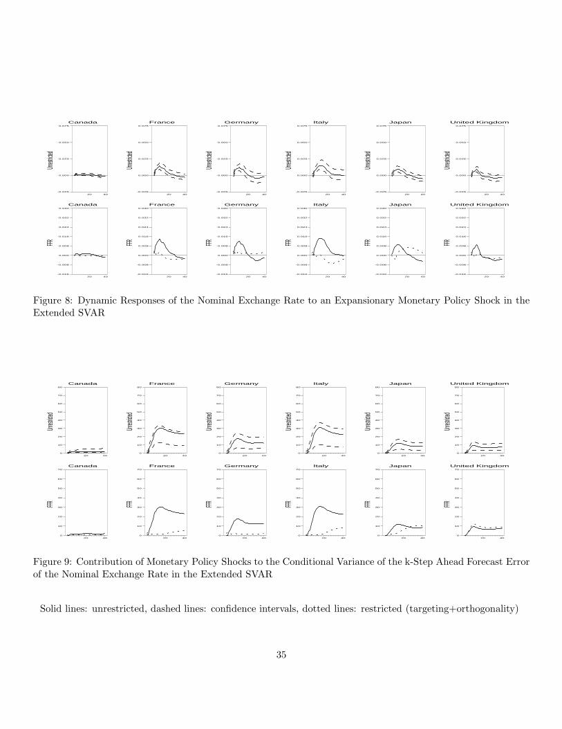
Canada

Unrestr

icted

20 40-0.025

0.000

0.025

0.050

0.075

Canada

FFR

20 40-0.016

-0.008

0.000

0.008

0.016

0.024

0.032

0.040

France

Unrestr

icted

20 40-0.025

0.000

0.025

0.050

0.075

France

FFR

20 40-0.016

-0.008

0.000

0.008

0.016

0.024

0.032

0.040

Germany

Unrestr

icted

20 40-0.025

0.000

0.025

0.050

0.075

Germany

FFR

20 40-0.016

-0.008

0.000

0.008

0.016

0.024

0.032

0.040

Italy

Unrestr

icted

20 40-0.025

0.000

0.025

0.050

0.075

Italy

FFR

20 40-0.016

-0.008

0.000

0.008

0.016

0.024

0.032

0.040

Japan

Unrestr

icted

20 40-0.025

0.000

0.025

0.050

0.075

Japan

FFR

20 40-0.016

-0.008

0.000

0.008

0.016

0.024

0.032

0.040

United Kingdom

Unrestr

icted

20 40-0.025

0.000

0.025

0.050

0.075

United Kingdom

FFR

20 40-0.016

-0.008

0.000

0.008

0.016

0.024

0.032

0.040

Figure 8: Dynamic Responses of the Nominal Exchange Rate to an Expansionary Monetary Policy Shock in theExtended SVAR

Canada

Unrestr

icted

20 400

10

20

30

40

50

60

70

80

Canada

FFR

20 400

10

20

30

40

50

60

70

France

Unrestr

icted

20 400

10

20

30

40

50

60

70

80

France

FFR

20 400

10

20

30

40

50

60

70

Germany

Unrestr

icted

20 400

10

20

30

40

50

60

70

80

Germany

FFR

20 400

10

20

30

40

50

60

70

Italy

Unrestr

icted

20 400

10

20

30

40

50

60

70

80

Italy

FFR

20 400

10

20

30

40

50

60

70

Japan

Unrestr

icted

20 400

10

20

30

40

50

60

70

80

Japan

FFR

20 400

10

20

30

40

50

60

70

United Kingdom

Unrestr

icted

20 400

10

20

30

40

50

60

70

80

United Kingdom

FFR

20 400

10

20

30

40

50

60

70

Figure 9: Contribution of Monetary Policy Shocks to the Conditional Variance of the k-Step Ahead Forecast Errorof the Nominal Exchange Rate in the Extended SVAR

Solid lines: unrestricted, dashed lines: confidence intervals, dotted lines: restricted (targeting+orthogonality)

35

Canada

Unrestr

icted

20 40-1.0

-0.8

-0.6

-0.4

-0.2

-0.0

0.2

0.4

0.6

Canada

FFR

20 40-0.50

-0.25

0.00

0.25

0.50

France

Unrestr

icted

20 40-1.0

-0.8

-0.6

-0.4

-0.2

-0.0

0.2

0.4

0.6

France

FFR

20 40-0.50

-0.25

0.00

0.25

0.50

Germany

Unrestr

icted

20 40-1.0

-0.8

-0.6

-0.4

-0.2

-0.0

0.2

0.4

0.6

Germany

FFR

20 40-0.50

-0.25

0.00

0.25

0.50

Italy

Unrestr

icted

20 40-1.0

-0.8

-0.6

-0.4

-0.2

-0.0

0.2

0.4

0.6

Italy

FFR

20 40-0.50

-0.25

0.00

0.25

0.50

Japan

Unrestr

icted

20 40-1.0

-0.8

-0.6

-0.4

-0.2

-0.0

0.2

0.4

0.6

Japan

FFR

20 40-0.50

-0.25

0.00

0.25

0.50

United Kingdom

Unrestr

icted

20 40-1.0

-0.8

-0.6

-0.4

-0.2

-0.0

0.2

0.4

0.6

United Kingdom

FFR

20 40-0.50

-0.25

0.00

0.25

0.50

Figure 10: Dynamic Responses of Excess Return to an Expansionary Monetary Policy Shock in the ExtendedSVAR

Canada

Unrestr

icted

20 400

10

20

30

40

50

60

70

Canada

FFR

20 400

8

16

24

32

40

48

56

France

Unrestr

icted

20 400

10

20

30

40

50

60

70

France

FFR

20 400

8

16

24

32

40

48

56

Germany

Unrestr

icted

20 400

10

20

30

40

50

60

70

Germany

FFR

20 400

8

16

24

32

40

48

56

Italy

Unrestr

icted

20 400

10

20

30

40

50

60

70

Italy

FFR

20 400

8

16

24

32

40

48

56

Japan

Unrestr

icted

20 400

10

20

30

40

50

60

70

Japan

FFR

20 400

8

16

24

32

40

48

56

United Kingdom

Unrestr

icted

20 400

10

20

30

40

50

60

70

United Kingdom

FFR

20 400

8

16

24

32

40

48

56

Figure 11: Contribution of Monetary Policy Shocks to the Conditional Variance of the k-Step Ahead ForecastError of Excess Return in the Extended SVAR

Solid lines: unrestricted, dashed lines: confidence intervals, dotted lines: restricted (targeting+orthogonality)

36

Canada

Unrestr

icted

20 40-0.07

-0.06

-0.05

-0.04

-0.03

-0.02

-0.01

0.00

0.01

0.02

Canada

FFR

20 40-0.030

-0.025

-0.020

-0.015

-0.010

-0.005

0.000

0.005

0.010

0.015

France

Unrestr

icted

20 40-0.07

-0.06

-0.05

-0.04

-0.03

-0.02

-0.01

0.00

0.01

0.02

France

FFR

20 40-0.030

-0.025

-0.020

-0.015

-0.010

-0.005

0.000

0.005

0.010

0.015

Germany

Unrestr

icted

20 40-0.07

-0.06

-0.05

-0.04

-0.03

-0.02

-0.01

0.00

0.01

0.02

Germany

FFR

20 40-0.030

-0.025

-0.020

-0.015

-0.010

-0.005

0.000

0.005

0.010

0.015

Italy

Unrestr

icted

20 40-0.07

-0.06

-0.05

-0.04

-0.03

-0.02

-0.01

0.00

0.01

0.02

Italy

FFR

20 40-0.030

-0.025

-0.020

-0.015

-0.010

-0.005

0.000

0.005

0.010

0.015

Japan

Unrestr

icted

20 40-0.07

-0.06

-0.05

-0.04

-0.03

-0.02

-0.01

0.00

0.01

0.02

Japan

FFR

20 40-0.030

-0.025

-0.020

-0.015

-0.010

-0.005

0.000

0.005

0.010

0.015

United Kingdom

Unrestr

icted

20 40-0.07

-0.06

-0.05

-0.04

-0.03

-0.02

-0.01

0.00

0.01

0.02

United Kingdom

FFR

20 40-0.030

-0.025

-0.020

-0.015

-0.010

-0.005

0.000

0.005

0.010

0.015

Figure 12: Exchange Rate Pass-Through Conditional on an Expansionary Monetary Policy Shock in the ExtendedSVAR

Solid lines: unrestricted, dashed lines: confidence intervals, dotted lines: restricted (targeting+orthogonality)

37