Flexible automatic motion blending with registration curves

Eurographics/SIGGRAPH Symposium on Computer Animation (2003)D. Breen, M. Lin (Editors)

Flexible Automatic Motion Blending with Registration Curves

Lucas Kovar1 and Michael Gleicher1

1 University of Wisconsin, Madison

AbstractMany motion editing algorithms, including transitioning and multitarget interpolation, can be represented asinstances of a more general operation called motion blending. We introduce a novel data structure called a regis-tration curve that expands the class of motions that can be successfully blended without manual input. Registrationcurves achieve this by automatically determining relationships involving the timing, local coordinate frame, andconstraints of the input motions. We show how registration curves improve upon existing automatic blendingmethods and demonstrate their use in common blending operations.

Categories and Subject Descriptors (according to ACM CCS): I.3.7 [Computer Graphics]: Animation

1. Introduction

Motion capture has been a successful technique for creatingrealistic animations of humans, in large part because of theavailability of motion editing methods. Since capture is fun-damentally limited to producing a finite set of clips, by itselfit offers little flexibility. However, through motion editingthese clips can be adapted to meet the demands of a partic-ular situation. Some of the most successful editing methodsare based on the idea of motion blending, which producesnew motions (blends) by combining multiple clips accord-ing to time-varying weights. Motion blending has severalapplications. For example, blending can be used to createseamless transitions between motions, allowing one to buildlengthy, complicated motions out of simpler actions. An-other application is interpolation, or creating motions “in-between” the initial set to produce a parameterized space ofmotions. Blending operations such as these have significantpractical importance and have proven useful in commercialapplications like video games 13, 21.

While blending is a powerful tool, it will not produce re-alistic results unless the input motions are chosen with somecare. The range of motions that can be successfully blendeddepends heavily on how much information about the mo-tions is given to the algorithm. If nothing is known about theinput other than the raw motion parameters (e.g., the root po-sition and joint angles at each frame), then existing blendingalgorithms are reliable only if the motions are quite similar.

Our goal is to expand the range of motions that can besuccessfully blended without requiring manual intervention.Toward this end we introduce registration curves. A registra-tion curve is an automatically constructed data structure thatencapsulates relationships involving the timing, local coor-dinate frame, and constraint states of an arbitrary number ofinput motions. These relationships are used to improve thequality of blended motion and allow blends that were previ-ously beyond the reach of automatic methods.

In the remainder of this paper we describe how to con-struct and use registration curves. The next section startswith an overview of registration curves. Section 3 reviewsrelated work. Section 4 explains how to construct registra-tion curves, and Section 5 presents a blending algorithm thatexploits the information contained in registration curves. Fi-nally, Section 6 demonstrates our technique in common ap-plications and Section 7 concludes with a discussion of theadvantages and limitations of registration curves.

2. Overview of Registration Curves

We represent motions in the standard skeletal format. For-mally, a motion is defined as a continuous function M( f ) =(pR( f ),q1...n( f )), where pR is the global position of the rootand qi is the orientation of the ith joint in its parent’s coordi-nate system. Each parameter vector M( f ) is called a frameand f is the frame index. Motions are assumed to be an-notated with constraint information, e.g., that the left heel

c© The Eurographics Association 2003.

L. Kovar and M. Gleicher / Flexible Automatic Motion Blending with Registration Curves

should be planted over some range of frames. Constraintsmay be generated automatically using techniques as in 4; inour experiments we used automated methods and tuned theresults by hand. While motions are continuous functions, inpractice one has access only to discrete samples. We mapthese samples to integer frames and generate skeletal posesat non-integer frames through interpolation.

A blend B(t) is a motion constructed from N input mo-tions M1, . . . ,MN and an N-dimensional weight functionw(t). While the specific form of B(t) depends on the blend-ing algorithm, if wi = 1 at t0 and all the other weights are 0,then B(t0) is identical to a frame from Mi. In this framework,a transition involves two motions and a weight function thatstarts at (1,0) and smoothly changes to (0,1), and an inter-polation combines an arbitrary number of motions accordingto a constant weight function.

When the only available information is the input motionsthemselves, the standard blending method is linear blend-ing. The ith frame of a linear blend is a weighted average ofthe skeletal parameters at the ith frame of each input motion.Specifically, the blended root position is calculated either byaveraging root positions or velocities, and blended joint an-gles can be calculated by averaging Euler angles or comput-ing the exponential map of averaged logarithmic maps 14.Constraints are not handled directly by linear blending, al-though often they are enforced as a postprocess.

Linear blending produces reasonable results when the in-put motions are sufficiently similar. Our strategy is thusto still combine frames via averaging, but to automaticallyextract information from the input motions to help decidewhich frames to combine, how to position and orient themprior to averaging, and what constraints should exist on theresult. This information is used to create a timewarp curve, acoordinate alignment curve, and a set of constraint matches,which together form a registration curve. The rest of this sec-tion provides an overview of these data structures and howthey are merged into a registration curve.

2.1. Timing

Linear blending can fail when motions have different tim-ing, that is, when corresponding events occur at different ab-solute times. See Figure 1 for examples and Bruderlin andWilliams 5 for a discussion. A solution is to timewarp the in-put motions so corresponding events occur simultaneously.This involves determining a timewarp curve S(u) that returnssets of frame indices, one from each input motion, such thatthe corresponding frames are all logically related. For ex-ample, given a walking motion and a jogging motion, S(u)would be constructed so S1(u) and S2(u) are at the samepoint in the locomotion cycle. It is also useful if the timewarpcurve is continuous and strictly increasing (that is, if u1 > u0then Si(u1) > Si(u0)). If these properties hold, then the in-verse functions u(Si) are well-defined, and given a frame ofan input motion we can uniquely determine the related point

Figure 1: Top: A transition between walking and joggingthat spans two locomotion cycles. For clarity, only the rightleg is shown. Without timewarping, out-of-phase frames arecombined and the character floats above the ground withits legs nearly straight. Bottom: an interpolation between ajab and a slower, stronger punch. Without timewarping, thecharacter’s arm wobbles.

on the timewarp curve and vice-versa. The parameter u thendefines a reference time system: each input motion may bethought of as a realization of some canonical motion, andwhen this canonical motion is at frame u then Mi is at frameSi(u) and vice-versa.

A registration curve is built around a continuous, strictlyincreasing timewarp curve S(u). This timewarp curve is gen-erated automatically for an arbitrary number of motions; de-tails are in Section 4.2. During blending, the set of framescombined at any given time always corresponds to somepoint on S(u). Since we have no information other than theinput data to work with, to create the timewarp curve weuse the heuristic that frames are more likely to correspondif they are similar. This complements the way we actuallycombine frames: since it is more reliable to average skeletalparameters when poses are similar, we time-align motionsso corresponding frames are as similar as possible.

2.2. Coordinate Frame Alignment

Linear blending can fail even when frames occurring at thesame time are quite similar. Imagine that we have two walk-ing motions that are in phase, one curving to the left and theother to the right (Figure 2). Since the root position is lin-early interpolated, the blended root path collapses. Also, the



Figure 2: An interpolation of two walking motions thatcurve in different directions. The black paths show the pro-jection of the root onto the ground, and the triangles indicatethe position and orientation of the root at selected frames.Linear blending causes the root trajectory to collapse. Notethat the root orientation changes suddenly at the end of themotion, when the accumulated angle between the roots ex-ceeds 180◦.

character suddenly flips around near the end of the motion;this is because standard orientation averaging schemes likespherical linear interpolation have discontinuities when theangles change by more than 180◦.

To solve this problem, we observe that motions are funda-mentally unchanged by rotations about the vertical axis andtranslations in the floor plane 7, 9, 11. For example, a walk-ing motion looks the same whether it starts at the origin andheads east or starts ten feet to the side and heads southwest.This implies that we are free to apply rigid 2D transfor-mations to a motion, effectively changing its local coordi-nate frame. In particular, we can choose transformations thatmake motions as similar as possible at specified frames. Werefer to this process as coordinate frame alignment.

Coordinate frame alignment can successfully blend mo-tions with nontrivially distinct paths. Say we are blendingthe frames M1( f1), . . . ,Mn( fn). These frames are aligned toform a single, abstract frame F which may itself be rigidlytransformed. Each Mi votes on the position and orientationof F , and these votes are combined according to the blendweights. This allows the blended root trajectory to be deter-mined incrementally. Once F is situated, the final blendedframe is a weighted average of the input frames. Registrationcurves implement this idea by containing alignment curves.An alignment curve is a function A(u) that gives a set oftransformations which align the frames at each point S(u)on the timewarp curve. Section 4.3 explains how to constructan alignment curve and Section 5.2 provides details on us-ing them in blending. Figure 2 shows that blending with an

alignment curve correctly handles the example at the start ofthis section.

2.3. Constraint Matches

Since we combine frames via averaging, constraints on theblend may not be satisfied. However, if we can simply de-termine what these constraints are, then a variety of methodsexist for adjusting the motion to enforce them 6, 12, 10. Evenif the blend looks fine, it is still desirable to know its con-straints since it may be further edited.

Determining constraints on the blend takes some care be-cause the input motions may have fundamentally differentconstraint states. For example, while a walking motion al-ways has at least one foot planted, a running motion containsflight stages where no constraints exist. Even if the motionsare timewarped, the intervals over which constraints are ac-tive will not match. Also, we may be interested in blendingmotions that have different numbers of constraints. For in-stance, to create a space of parameterized turning motionswe might interpolate a motion where a character stands stillwith one where it turns in place (and hence picks up its feet).

If we represent the interval of a constraint in terms of theglobal time parameter u, then it is reasonable to presumethat constraints which are nearby “mean” roughly the samething, even if they do not span identical regions. Registrationcurves employ this idea to create constraint matches. Eachconstraint match contains a set of related constraints, onefrom each motion. The start and end of these constraints inglobal time are treated as parameters which may themselvesbe blended. Our algorithm for finding constraint matches isdiscussed in detail in Section 4.4.

3. Related Work

Motion blending has been an integral part of several re-search efforts. One of the earliest was due to Perlin 15,who presented a real-time system based on procedurally-generated motions. After a user manually constructed basemotions, blending operations were used to create new mo-tions and transition between existing ones. The languagefor constructing motions contained built-in timing and con-straint models, simplifying the related blending issues. Sev-eral systems have leveraged multitarget blending to createintuitively parameterized spaces of motions 23, 18, 20. Multipleresearch groups have used general blending (that is, blend-ing with arbitrary weight functions) to provide continuouscontrol of locomotion 8, 2, 14. Blend-based transitions havebeen incorporated into various systems for graph-based mo-tion synthesis 18, 9.

Techniques for certain blending operations have been de-veloped outside of the framework presented in Section 2.Instead of averaging skeletal parameters directly, Unuma etal. 22 used weighted averages in the Fourier domain. Rose etal. 19 used spacetime optimization to create transitions thatminimize joint torque. Other researchers 11, 1, 16 have gener-



ated transitions by concatenating motions and eliminatingdiscontinuities with displacement mapping techniques 24.

Timewarping has been an important part of previous workon motion blending. Some systems required the user to marksparse “key times” in the input motions, which were lin-early interpolated to form a timewarp curve 18, 14. Our tech-nique requires no user intervention. Ashraf and Wong 2

semi-automatically labelled motions with sparse timing in-formation, such as zero-crossings of the second derivative ofuser-specified joint angles. Timewarp curves were generatedthrough a greedy algorithm that matched identical labels.Our algorithm generates dense correspondences and uses adynamic programming technique with stronger optimalityproperties. The method of Bruderlin and Williams 5 is themost similar to our own, as it also is based on dynamic pro-gramming. However, their algorithm will not in general yielda strictly increasing timewarp curve, and it is only designedto handle two motions. We extend this method to producestrictly increasing timewarp curves for an arbitrary numberof motions.

Most previous motion blending efforts used linear inter-polation to compute root parameters. A notable exceptionis the work of Park et al. 14, where the root was positionedand oriented according to a user-specified path (Gleicher 7

used a similar method to interactively edit individual mo-tions). Blending was then used to determine a skeletal poseappropriate for the local speed and curvature of the root tra-jectory. We blend root parameters directly, so there is noneed to specify the root path. Also, Park et al.’s method wasbased on the assumption that the input motions were suffi-ciently smooth that the root path could be well approximatedby a circular arc. Our method is applicable to motions withsharply varying path curvatures (see Figure 8).

Bindiganavale and Badler 4 developed a method for auto-matically detecting constraints satisfied by a motion. How-ever, for blends we are interested in the constraints thatshould be satisfied, not the ones that are satisfied. Rose etal 18 manually specified the starting and ending times ofcorresponding constraints in the input motions and blendedthe interval bounds. Our method is similar, except corre-sponding constraints are identified automatically. Ashraf andWong 3 and Kovar et al. 9 copied the constraints from the in-put motion with the currently highest blending weight. Thisapproach works well for the special case of transitions, butcan produce artifacts with other blending operations suchas interpolation. In particular, when the blend weights arenearly equal a small change in the weights may producelarge changes in the constraints. Our technique ensures thatconstraints change smoothly if the blend weights changesmoothly.

4. Constructing Registration Curves

To build a registration curve, we start by constructing a time-warp curve S(u). An alignment curve A(u) is then builtaround S(u), and constraint matches are identified by us-

ing S(u) to map constraint intervals into a standard timeframe. Fundamental to our approach is a function D(F1,F2)which simultaneously determines the “distance” betweentwo frames of motion and an aligning rigid 2D transforma-tion. We now describe D and discuss the creation of the time-warp curve, the alignment curve, and the constraint matches.

4.1. A Coordinate-Invariant Distance Function

We use the same distance function as Kovar et al. 9; see thispaper for a discussion of its motivation. Briefly, computingD(F1,F2) involves three steps (Figure 3). First, small win-dows of nearby frames are extracted around F1 and F2. Weused neighborhoods of five frames, which has the effect ofincorporating velocity and acceleration information. Next,each frame is converted to a point cloud by attaching markersto the joints of the skeleton, forming two larger point clouds.Finally, the optimal sum of squared distances between cor-responding points is computed over all rigid 2D transforma-tions of the second point cloud. That is, we compute

D(F1,F2) = minθ,x0,z0

n

∑i=1

wi‖pi −Tθ,x0,z0 p′i‖2 (1)

where pi and p′i are respectively the ith point of the first andsecond point clouds, Tθ,x0,z0 is a rotation by θ about the y(vertical) axis followed by a translation in the floor plane by(x0,z0), and wi may be used to preferentially weight differ-ent joints. In our experiments the wi were equal and eachpoint cloud had 200 points (40 points per frame for fiveframes).

Assuming the wi sum to unity, the optimal solution toEquation 1 is achieved under the following transformation:

θ = tan−1

(∑i wi(xiz

′i − x′i zi)− (xz′− x′z)

∑i wi(xix′i + ziz′i)− (xx′ + zz′)

)(2)

x0 = x− x′i cosθ− z′i sinθ (3)

z0 = zi + x′i sinθ− z′i cosθ (4)

where we use the shorthand notation α = ∑ni=1 wiαi.

Figure 3: Computing D(F1,F2).



4.2. Creating the Timewarp Curve

The timewarp curve is generated by creating a dense set offrame correspondences, fitting a spline to these frame corre-spondences, and adjusting the spline so it is strictly increas-ing. We first consider the case of just two motions and thengeneralize to more motions.

4.2.1. Timewarp Curves for Two Motions

Using the distance function in Equation 1, we can create agrid where columns correspond to frames from the first mo-tion, rows correspond to frames from the second motion, andeach cell contains the distance between the correspondingpair of frames. Given two cells in this grid, we can use thedynamic timewarping algorithm to find a minimal-cost con-necting path (Figure 4), where the cost of a path is found bysumming its cells. This path corresponds to an optimal time-alignment that starts and ends at the bounding cells. We onlyconsider paths having three properties:

1. Continuity. Each cell on the path must share a corner oredge with another cell on the path.

2. Causality. Paths must not reverse direction; they shouldeither go entirely forward or entirely backward in time.

3. Slope Limit. At most L consecutive horizontal steps orconsecutive vertical steps may be taken.

These properties are illustrated in Figure 4. Slope limits areuseful because very large slopes typically indicate that themotions are (at least locally) so different that there are nogood frame matches. In this case it is preferable to limit thetimewarping and accept the fact that corresponding poseswill not be particularly similar. We have found a slope limitof 2 or 3 to produce good results.

Dynamic timewarping is based on well-known dynamicprogramming methods; refer to the literature 17, 5 for details.From a given starting point, dynamic timewarping can beused to find optimal paths leading to all points on the bound-ary of the grid. The only question is which boundary pointto select. In some cases, this will be known a priori. For ex-ample, if the entire motions are to be time-aligned — thatis, both the first frames and the last frames must correspond— then the path must pass through the lower-left and upper-right corners of the grid. In many cases, however, there is nopreferred boundary point. In this case we select the one thatminimizes the average cell cost.

The frame correspondences generated by dynamic time-warping could be used directly to form a piecewise-lineartimewarp curve. However, though monotonic, this curvewould not be strictly increasing; multiple frames of one mo-tion may be matched to a single frame of the other. More-over, while the slope limits place global restrictions on howsteep or shallow this timewarp curve can be, they do not en-sure any smoothness properties. For these reasons we insteadcreate the timewarp curve by fitting a smooth, strictly in-creasing function to the frame correspondences. If we onlycared about smoothness, then a simple solution would be

Sneaking

Wal

king

Legal Not continuous Not causal Breaks slope limit (L = 2)

Legal and Illegal Paths

Dynamic Timewarping Example

Figure 4: Left: Dynamic timewarping applied to a walkingmotion and a sneaking motion. The background image showsframe distances; larger distances correspond to whiter cells.The central grey circle is the starting point and the generatedpath is in bright white. The local slope variations arise be-cause the character pauses slightly at each footstep in thesneaking motion but travels at a steady pace in the walkingmotion. Right: Legal and illegal dynamic timewarping paths(L = 2).

to fit a spline, which only requires solving a linear system.Adding in the constraint that the spline be strictly increas-ing produces a significantly more expensive quadratic pro-gramming problem. However, given the causality and slopelimit restrictions, it is likely that a spline fit without any con-straints will be approximately strictly increasing.

In light of this, our strategy is to fit a uniform quadraticB-spline as an unconstrained optimization and then adjustthe knots. The result is the final timewarp curve S(u). Due tothe convex hull property of B-splines, we need only ensurethat the knots p1, . . . ,pn are strictly increasing. We do thisby selecting a “base” motion Mbase and for the other motionM j enforcing the property

ε ≤ pi, j − pi−1, j

pi,base − pi−1,base≤ 1

ε, 1 < i ≤ n (5)

for some ε > 0. It is easy to show that this implies ε2 ≤ dSidS j

≤1ε2 . Appendix A gives an algorithm for enforcing Equation 5.Mbase is selected implicitly by running this algorithm with



each motion as the base and keeping the result with thesmallest adjustment.

4.2.2. Timewarp Curves For More Than Two Motions

Directly applying the methods of Section 4.2.1 to morethan two motions is computationally expensive. The gener-alization of Equation 1 yields a nonlinear optimization forwhich there is no closed-form solution, and since dynamictimewarping requires filling a k-dimensional grid for k mo-tions, it scales exponentially. However, we can design a sim-ple and efficient algorithm by combining multiple timewarpcurves relating pairs of motions. Say we have three mo-tions M1, M2, and M3 and timewarp curves S1→2, S1→3,and S2→3, one for each pair. Then if S1→2( f1) = f2 andS1→3( f1) = f3, it is likely that S2→3( f2) is also approxi-mately f3. Hence we might simply remove S2→3 and com-bine S1→2 and S1→3 into a single timewarp curve.

More generally, given a set of motions M1, . . . ,Mk, a mo-tion Mre f is selected to serve as a reference. Mre f maybe chosen to minimize the average distance to the othermotions, where the distance between Mi and M j is de-fined as the average distance between the correspondingframes generated by dynamic timewarping. Let Si(u) =(Si,1(u),Si,2(u)) be the timewarp curve between Mre f andMi. For convenience and without loss of generality, we as-sume Si,1(u) returns frame indices of Mre f and Si,2(u) re-turns corresponding frame indices from Mi. We sample theframe indices of Mre f and for each sample use the inversefunctions u(Si,1) to determine the corresponding frames in

each other motion. Specifically, the ith motion’s frame isSi,2(u(Si,1)). To form the final timewarp curve, we fit a k-dimensional quadratic spline to these samples and adjust theknots to enforce Equation 5 (see Appendix A), just as in thetwo-dimensional case.

4.3. Creating the Alignment Curve

Given the timewarp curve, the alignment curve is simple toconstruct. Consider first the case of two motions. For eachframe correspondence generated via dynamic timewarping,Equation 1 specifies a rigid 2D transformation {θi,x0i ,z0i}that aligns the second frame with the first. A 3D quadraticspline is fit to these transformations, yielding an alignmentcurve A(u) = (A1(u),A2(u)) where every A1(u) is the iden-tity transformation and A2(u) = {θ(u),x0(u),z0(u)} is theresult of the spline fit. To avoid angle discontinuities, prior tofitting the spline the θi should be adjusted so |θi−θi−1| ≤ π.Also, there are sometimes small spikes in the transformationparameters when the dynamic timewarping algorithm shiftsfrom one kind of step (vertical, horizontal, or diagonal) toanother and then back again. We have found it useful to treatthese spikes as high-frequency noise and remove them witha short median filter (kernel width of 3 to 5) prior to fittingthe spline. Finally, it is important that the knot spacing onthe spline be sufficiently small that it remains close to the

Connected Connected Disconnected

Constraint Matching Example

Definition of Connected Constraints

1 2

3 4

Figure 5: Top: Examples of connected and disconnectedconstraints. Bottom: The steps taken by the constraintmatching algorithm on a sample input. Note that a constraintis removed from the second motion and split in the first mo-tion.

(filtered) samples; we have found that a knot for every 3 to 5samples yields good results.

The case of more than two motions is handled in directanalogy to Section 4.2.2. We start with a timewarp curve forthe entire set of motions and a collection of alignment curvesrelating pairs of motions. A reference motion is selected andframes are sampled from it. For each sample, the timewarpcurve is used to create a set of corresponding frames, andfrom the alignment curves we find a set of mutually align-ing coordinate transformations. A spline is then fit to thesesamples as in the two-motion case.

4.4. Identifying Constraint Matches

The final step in building a registration curve is to identifyconstraint matches. Each kind of constraint is treated inde-pendently (e.g., we might first consider left heelplants, thenright toeplants, and so on). For each motion, the intervalsof a given kind of constraint are assumed to be disjoint.The algorithm starts by mapping the duration of each con-straint into a standard time frame via the timewarp curve. Itthen groups constraints into constraint matches based on twoguidelines. First, each constraint match must contain exactlyone constraint from each motion. Second, the elements ofa constraint match must be connected in the sense that theunion of all the constraint intervals must form a single con-tinuous interval (Figure 5). This is based on the heuristic thatcorresponding constraints ought to occur at similar points inthe motions.

Some constraints may not be able to belong to any con-straint match; for example, a constraint may overlap with noother constraints. In this case that constraint is eliminated.That is, if a constrained region is logically associated withan unconstrained region, that constraint is broken. To illus-trate, say we blend a motion where a character stands on itsleft leg with a motion where it stands on both legs. We ex-pect the character to stand on its left leg and vary the heightof his right foot according to the blend parameters — thatis, the constraint on the right foot from the second motion



should be broken. For similar reasons, if a constraint of onemotion overlaps two or more constraints of another motion,we consider adding a gap to it, thereby splitting it into twoshorter constraints.

Let Ci, j be the jth constraint of ith motion. Our algorithmprocesses the constraints sequentially: Ci, j is either elimi-nated or added to a constraint match before Ci, j+1 is con-sidered. Each iteration starts by checking whether the earli-est unprocessed constraints of each motion are connected. Ifnot, the constraint which starts the earliest cannot be part ofany constraint match, so we discard it and proceed to thenext iteration. Otherwise we can form a constraint matchfrom these constraints. We first decide whether any of themshould be split (see Appendix B), and then we build a con-straint match from the constraints that were not split and thefirst portion of the constraints that were split. Figure 5 showsour constraint matching algorithm on a sample input.

5. Blending With Registration Curves

Creating a single frame B(ti) of a blend involves four steps:

1. Determine a position S(ui) on the timewarp curve2. Position and orient the frames at S(ui).3. Combine the frames based on the blending weights w(ti).4. Determine the constraints on the resulting frame

We assume that for some frame B(t0), u0 is known. If thishappens to be the first frame of the blend, then we generatein order B(t1), then B(t2), and so on. If B(t0) is not the firstframe, we first generate these forward frames and then createB(t−1),B(t−2), . . .. We require that ui > ui−1, i.e., movingforward in time is equivalent to moving forward in u.

We now discuss how to create an individual frame of theblend. To simplify matters, we only discuss the case of mov-ing forward in u; moving backward is handled similarly.

5.1. Advancing Along the Timewarp Curve

For B(t0), this step is skipped, since u0 is given to us. Oth-erwise, we are at some point S(ui−1) on the timewarp curveand want to move to a new location S(ui). Consider the sit-uation where wj(t) = 1 and the other weights are always 0.In this case B should be identical to M j , and so time shouldflow such that M j is played at its normal rate. So, for exam-ple, if we wanted to advance ∆t units of time, then we shouldpick ∆u = ui − ui−1 such that S j(ui−1 + ∆u)− S j(ui−1) =∆t. Taking the limit as (∆t,∆u) → 0 and exploiting the factthat S j(u) and u(t) are both strictly increasing, this yieldsdudt = du

dS j.

For general w(t), we extend this equation as follows:

dudt

=k

∑j=1

wj(t)dudS j

(6)

Intuitively, each motion votes on how fast the global timeparameter u should flow, and these votes are combined based

upon the blend weights. In general this differential equationmust be solved numerically. However, since the time stepbetween frames is small and w and S are smooth, we havefound that we can advance a frame in a single Euler step:

∆u =

(k

∑j=1

wj(ti−1)dudS j

)∆t (7)

A similar strategy was used in 14. For convex weights, whichare commonly viewed as natural choices for blending oper-ations, Equation 7 will always yield ∆u > 0 and hence timewill always flow forward. Systems which do not limit them-selves to arbitrary blend weights can replace wj(ti−1) with|wj(ti−1)|

∑r |wr(ti−1)| in Equation 7, ensuring ∆u > 0.

Figure 6: Top: Given any set of corresponding frames, thecoordinate alignment curve specifies rigid 2D transforma-tions that mutually align them. This group of aligned framescan itself be rigidly transformed. Bottom: Based on the po-sition and orientation of the previous blended frame, eachmotion votes on a new position and orientation for the cur-rent blended frame. These votes are combined according tothe blend weights; here we show the case w1 = w2 = 0.5.

5.2. Positioning and Orienting Frames

Now that the value of ui is known, we extract the frameM j(S j(ui)) from the jth motion and transform it by A j(ui).This yields a set of mutually aligned frames that, just as witha single frame of motion, we are free to position and orienton the ground plane (Figure 6). Our task is to find an appro-priate rigid 2D transformation T(ti) to apply to this group offrames, making T(ti)A j(ui) the total transformation appliedto M j(S j(ui)). For the first frame of the blend, T(t0) may be



chosen arbitrarily. For the other frames, we need to chooseT(ti) so the position and orientation of B(ti) is consistentwith the preceding frame. To see how to do this, consider thecase where wj(t) is 1 and the other blending weights are 0for all t > ti−1. In this case the remainder of the blend shouldsimply be a copy of a portion of M j , transformed rigidly byT(ti−1)A j(ui−1) so it connects seamlessly with B(ti−1). Ifwe define

∆T j(ti) = T(ti−1)A j(ui−1)A j−1(ui) (8)

then setting T(ti) = ∆T j(ti) yields this result.

More generally, we compute T(ti) by averaging the coor-dinate transformations ∆T j(ti) according to the wj(ti); seeFigure 6. Each motion votes for the T(ti) that leaves itscoordinate system unchanged, and we average these votesaccording to the blend weights. To perform this averag-ing, we need to choose parameters to represent ∆T j(ti).We start by choosing an origin that is near the transformedframes. This is done by transforming each M j(S j(ui))by ∆T j(ti)A j(ui−1), projecting the root position onto theground, and averaging over all the motions. ∆T j(ti) is thenrepresented by the parameter set {φ j,(x j,z j)}, which corre-sponds to a rotation by φ j about this origin followed by atranslation (x j,z j). Finally, T(ti) is:

T(ti) =

{∑

jw jφ j,

(∑

jw jx j,∑

jw jz j

)}(9)

5.3. Making the Blended Frame

Using these transformed frames, we compute the skeletalpose of the blend frame by computing a weighted averageof the root positions and averaging the joint orientations us-ing the method presented by Park et al 14. Our final task is todetermine the constraints on this new frame. For each con-straint match M we determine an interval IM based on thecurrent blend weights. If the ith constraint Ci of M is ac-tive over the interval [Cs

i ,CeI ], then IM = [∑wiC

si , ∑wiC

ei ].

If ui is inside this interval, then the corresponding constraintis applied to the blend frame. Actually enforcing the con-straints is up to the implementation; we used the method ofKovar et al 10.

6. Results and ApplicationsThe most expensive part of constructing a registration curveis filling in the dynamic timewarping grid. Computing thefull grid for two 20 second motions (600 frames eachand 360,000 cell evaluations) takes 3.43 seconds on a 1.3gHz Athlon processor using point clouds with two hundredpoints. The remainder of the construction process takes 0.03seconds. A registration curve is computed once and storedfor future blending operations. A full 5 second output mo-tion (150 frames) can be generated at interactive rates.

Registration curves fit seamlessly into common blending

applications. The rest of this section discusses using registra-tion curves for transitioning, interpolating, and continuousmotion control.

6.1. Transitions

To create a transition, a user specifies its length and whereit takes place. Our algorithm thus takes as input two framesM1( f1) and M2( f2) defining the center of the transition plusthe half-width h of the transition (the entire width is 2h + 1frames). M1( f1) and M2( f2) serve as the starting point forthe dynamic timewarping algorithm (Section 4.2.1).

To find the starting position S(u0) of the blend on thetimewarp curve, we average the u values that correspondto M1( f1) and M2( f2): u0 = 1

2 (u(S1( f1))+u(S2( f2))). Wethen generate h frames going both forward in time and back-ward in time, using a weight function that smoothly changesfrom (0,1) to (1,0). An example transition is shown in Fig-ure 7.

In general, the first and last frames of the transitionwill not occur at integer times, and so M1 and M2 haveto be resampled if they are to connect smoothly to thetransition boundaries. If this is undesirable, then we canforce the boundaries to occur at integer times by generatingu−h, . . . ,uh as described in Section 5.1, applying a smoothdisplacement map that rounds u−h and uh to the nearest in-tegers, and using these new values in place of the originals.

Figure 7: A transition between jogging and a significantlyslower sneaking motion.

6.2. Interpolations

An interpolation can be created by specifying a set of mo-tions and a fixed set of blend weights. It is presumed that theentirety of each input motion is to be blended, which meansthat when we execute the dynamic timewarping algorithmwe force it to match the first frames and last frames together.Once a registration curve for these motions is built, we createthe blend by setting u0 to be the first point on the timewarpcurve and stepping forward until the end of the timewarpcurve is reached.

We have used interpolations to generate several parame-terized clips (see Figure 8), including ones that allow controlof the angle of a turn (both in place and while walking), thedirection and force of a punch, and the “snap” and follow-through of a lunging front kick.



6.3. Continuous Motion Control

For certain kinds of motions, it makes sense to use blendweights that vary continuously. This is a simple generaliza-tion of interpolation; we merely replace the constant weightfunction with a user-specified weight function. To demon-strate this application, we obtained a set of walking, jogging,and sneaking motions. For each locomotion style there wasa motion that travelled straight ahead, one that curved to theleft, and one that curved to the right. We generated a regis-tration curve out of these nine motions and used it to con-tinuously control the speed, curvature, and “sneakiness” of acharacter. An example motion is shown in Figure 9.

Figure 8: Top: a parameterized clip built from a straightwalk (far right) and one with a sharp 180 degree turn (farleft) is used to create sharp path changes in a continuumof directions. Bottom: a parameterized clip built from threekicking motions is sampled to create a large number of sim-ilar but distinct kicks.

7. Discussion

In this paper we have introduced registration curves, a toolfor automatically generating blends between an arbitrarynumber of motions. Registration curves improve upon exist-ing automatic methods by explicitly addressing differencesin timing, path, and constraint state, expanding the rangeof motions that can be successfully blended. At the sametime, registration curves offer a simple interface for com-mon blending operations like transitions, interpolations, andcontinuous control.

While we have presented registration curves as a tool formanipulating motion capture data, they work equally wellwith other motion sources, such as keyframed or physi-cally modelled animation. Moreover, our method is readily

Figure 9: A sample motion from a registration curve builtautomatically for nine motions. These input motions wereof a character walking, jogging, and sneaking at differentcurvatures. By continuously varying blends weights, a userwas able to control the speed, curvature, and sneakiness ofthe character.

adapted to data that is not in skeletal format, since the time-warping and coordinate frame alignment algorithms only re-quire point data.

No blending method is perfect, and so it is important tounderstand when it is likely to succeed and when it willprobably fail. Registration curves assume that structurallyrelated parts of motions look more similar than unrelatedparts. For a large class of motions, this assumption is valid.Corresponding points in a locomotion cycle, for example,do in fact look more similar than frames which are out ofphase. Similarly, registration curves are appropriate for mo-tions which perform the same action in different styles, suchas casually picking up a glass versus forcefully snatchingit. On the other hand, in some cases logically correspond-ing parts of motions have the most dissimilar poses. Say wehave two motions where a character reaches for a glass, butin the first it reaches above its head and in the second it bendsdown to the ground. While the apexes of each reach are log-ically identical, they are also the most dissimilar poses inthe two motions. In this case the timewarp curve our methodgenerates would not be nearly as accurate as manually la-belling correspondences. However, this does not imply thatour framework is unable to handle motions like reaching. Ifthe set of desired motions is sampled sufficiently densely,then motions which reach to nearby locations do in fact lookmost similar at corresponding parts of the reach. Using mul-tiple registration curves, the entire space could then still bespanned.

Our method currently does not enforce any physical con-straints like balance. However, we expect these physicalrequirements could be enforced as a post-process once ablend is generated. Incorporating physical constraints intoour methods is left for future work.

Acknowledgements

We thank House of Moves, Demian Gordon, and The OhioState University for donating motion capture data. This workwas supported in part by NSF grants CCR-9984506 and



CCR-0204372, along with equipment donations from Intel.Lucas Kovar is supported by an Intel Foundation Fellowship.

References1. O. Arikan and D. A. Forsyth. Interactive motion generation

from examples. In Proceedings of ACM SIGGRAPH 2002,Annual Conference Series. ACM SIGGRAPH, July 2002.

2. G. Ashraf and K. C. Wong. Generating consistent motiontransition via decoupled framespace interpolation. ComputerGraphics Forum, 2000.

3. G. Ashraf and K. C. Wong. Constrained framespace interpo-lation. In Computer Animation 2001, 2001.

4. Rama Bindiganavale and Norman Badler. Motion abstrac-tion and mapping with spatial constraints. In Modellingand Motion Capture Techniques for Virtual Environments,CAPTECH’98, pages 70–82, November 1998.

5. A. Bruderlin and L. Williams. Motion signal processing. InProceedings of ACM SIGGRAPH 95, Annual Conference Se-ries, pages 97–104. ACM SIGGRAPH, August 1995.

6. M. Gleicher. Retargeting motion to new characters. In Pro-ceedings 0f ACM SIGGRAPH 98, Annual Conference Series,pages 33–42. ACM SIGGRAPH, July 1998.

7. M. Gleicher. Motion path editing. In Proceedings 2001 ACMSymposium on Interactive 3D Graphics. ACM, March 2001.

8. S. Guo and J. Roberge. A high-level control mechanism forhuman locomotion based on parametric frame space interpola-tion. In Proceedings of Eurographics Workshop on ComputerAnimation and Simulation ’96, 1996.

9. L. Kovar, M. Gleicher, and F. Pighin. Motion graphs. In Pro-ceedings of ACM SIGGRAPH 2002, Annual Conference Se-ries. ACM SIGGRAPH, July 2002.

10. L. Kovar, J. Schreiner, and M. Gleicher. Footskate cleanup formotion capture editing. In Proceedings of ACM SIGGRAPHSymposium on Computer Animation 2002. ACM SIGGRAPH,July 2002.

11. J. Lee, J. Chai, P. Reitsma, J. Hodgins, and N. Pollard. In-teractive control of avatars animated with human motion data.In Proceedings of ACM SIGGRAPH 2002, Annual ConferenceSeries. ACM SIGGRAPH, July 2002.

12. J. Lee and S. Y. Shin. A hierarchical approach to interac-tive motion editing for human-like figures. In Proceedingsof ACM SIGGRAPH 99, Annual Conference Series, pages 39–48. ACM SIGGRAPH, August 1999.

13. M. Mizuguchi, J. Buchanan, and T. Calvert. Data driven mo-tion transitions for interactive games. In Eurographics 2001Short Presentations, September 2001.

14. S. I. Park, H. J. Shin, and S. Y. Shin. On-line locomotiongeneration based on motion blending. In Proceedings of ACMSIGGRAPH Symposium on Computer Animation 2002. ACMSIGGRAPH, July 2002.

15. K. Perlin. Real time responsive animation with personality.IEEE Transactions on Visualization and Computer Graphics,1(1):5–15, March 1995.

16. Katherine Pullen and Christoph Bregler. Motion capture as-sisted animation: Texturing and synthesis. In Proceedingsof ACM SIGGRAPH 2002, Annual Conference Series. ACMSIGGRAPH, July 2002.

17. L. Rabiner and B.H. Juang. Fundamentals of Speech Recog-nition. Prentice Hall, Englewood Cliffs, NJ 07632, 1993.

18. C. Rose, M. Cohen, and B. Bodenheimer. Verbs and ad-verbs: Multidimensional motion interpolation. IEEE Com-puter Graphics and Application, 18(5):32–40, 1998.

19. C. Rose, B. Guenter, B. Bodenheimer, and M. Cohen. Efficientgeneration of motion transitions using spacetime constraints.In Proceedings of ACM SIGGRAPH 1996, Annual ConferenceSeries, pages 147–154. ACM SIGGRAPH, August 1996.

20. C. Rose, P. Sloan, and M. Cohen. Artist-directed inverse-kinematics using radial basis function interpolation. Proceed-ings of Eurographics 2001, 20(3), 2001.

21. S. Theodore. Understanding animation blending. Game De-veloper, pages 30–35, May 2002.

22. M. Unuma, K. Anjyo, and T. Tekeuchi. Fourier principlesfor emotion-based human figure animation. In Proceedingsof ACM SIGGRAPH 95, Annual Conference Series, pages 91–96. ACM SIGGRAPH, 1995.

23. D. Wiley and J. Hahn. Interpolation synthesis of articulatedfigure motion. IEEE Computer Graphics and Application,17(6):39–45, 1997.

24. A. Witkin and Z. Popovic. Motion warping. In Proceedings ofACM SIGGRAPH 95, Annual Conference Series, pages 105–108. ACM SIGGRAPH, August 1995.

Appendix A

This appendix describes how to adjust a set of n-dimensionalvectors p1, . . . ,pk such that Equation 5 holds. Without lossof generality, we assume Mbase = M1.

Refer to Figure 10. We process each knot in order fromp2 to pk, adjusting it if Equation 5 is violated. For j ∈ [2,n],let c j be defined such that c j1 =−1, c j j = ε, and every othercomponent is 0; also let c′j be defined such that c′j1 = ε, c′j j =−1, and every other component is 0. If we define di = pi −pi−1, then Equation 5 holds if and only if di · c j ≤ 0 anddi · c′j ≤ 0 for 2 ≤ j ≤ n.

Let S1 and S2 be sets of indices. For 2 ≤ j ≤ n, we put jinto S1 if di · c j > 0 and into S2 if di · c′j > 0 †. If S1 and S2are empty, no adjustment needs to be made to pi. Otherwisewe project di onto the linear subspace defined by the equa-tions x · c j = 0 and x · c′k = 0, where j ∈ S1 and k ∈ S2. Todo this, we create an orthogonal basis V = {v1, . . . ,vm} forthis space. Define v′1 such that v′11 = 1, v′1 j = 1

ε if j ∈ S1,v′1 j = ε if j ∈ S2, and v′1 j = 0 otherwise. The desired basis

† At least one of the conditions will hold for reasonable knot se-quences. For example, in Figure 10, pi would be in the bottom-leftquadrant if both conditions were violated.



has v1 = v′1‖v′1‖ and the other vi set to the coordinate axis vec-

tors corresponding to the indices that are not in S1 or S2.The projection of di onto this subspace yields a new vectordi +∆di, where ∆di = (I−VV T )di.

To minimize the overall disturbance, we would like tosplit the change ∆di across pi and pi−1 (Figure 10). We re-place pi with pi +(1−λ)∆di and pi−1 with pi −λ∆di. Hereλ is a positive number no larger than 0.5 and as large as pos-sible such that replacing pi−1 with pi −λ∆di does not leadto a violation of Equation 5.

(ε,1)

(1,ε)c2 = (-1,ε)

c2' = (ε,-1)

pi

pi-1

pi

pi-1

pi-2

d

Figure 10: Right: a diagram showing the relationship be-tween pi, c, c′, and the slope bounds in two dimensions. Left:pi and pi−1 are adjusted to satisfy Equation 5

Appendix B

A A A

B B BA does not subsume B A does not subsume BA subsumes B

p p

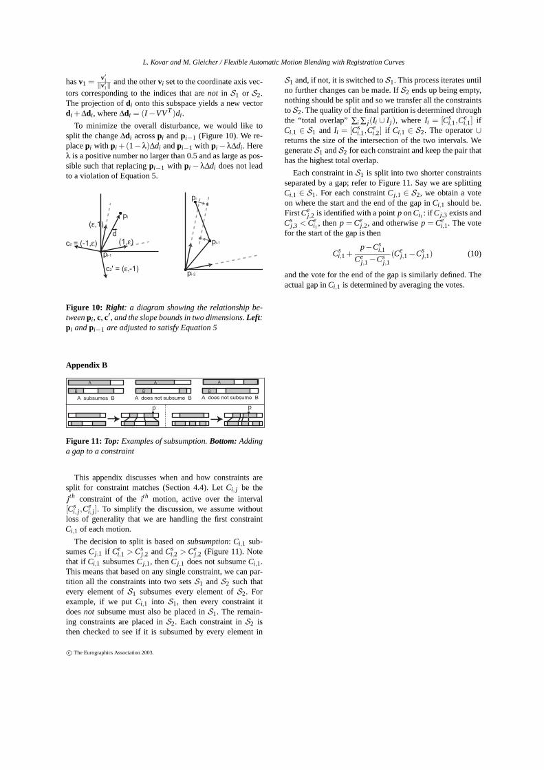
Figure 11: Top: Examples of subsumption. Bottom: Addinga gap to a constraint

This appendix discusses when and how constraints aresplit for constraint matches (Section 4.4). Let Ci, j be thejth constraint of the ith motion, active over the interval[Cs

i, j,Cei, j]. To simplify the discussion, we assume without

loss of generality that we are handling the first constraintCi,1 of each motion.

The decision to split is based on subsumption: Ci,1 sub-sumes Cj,1 if Ce

i,1 > Csj,2 and Cs

i,2 > Cej,2 (Figure 11). Note

that if Ci,1 subsumes Cj,1, then Cj,1 does not subsume Ci,1.This means that based on any single constraint, we can par-tition all the constraints into two sets S1 and S2 such thatevery element of S1 subsumes every element of S2. Forexample, if we put Ci,1 into S1, then every constraint itdoes not subsume must also be placed in S1. The remain-ing constraints are placed in S2. Each constraint in S2 isthen checked to see if it is subsumed by every element in

S1 and, if not, it is switched to S1. This process iterates untilno further changes can be made. If S2 ends up being empty,nothing should be split and so we transfer all the constraintsto S2. The quality of the final partition is determined throughthe “total overlap” ∑i ∑ j(Ii ∪ I j), where Ii = [Cs

i,1,Cei,1] if

Ci,1 ∈ S1 and Ii = [Csi,1,C

ei,2] if Ci,1 ∈ S2. The operator ∪

returns the size of the intersection of the two intervals. Wegenerate S1 and S2 for each constraint and keep the pair thathas the highest total overlap.

Each constraint in S1 is split into two shorter constraintsseparated by a gap; refer to Figure 11. Say we are splittingCi,1 ∈ S1. For each constraint Cj,1 ∈ S2, we obtain a voteon where the start and the end of the gap in Ci,1 should be.First Ce

j,2 is identified with a point p on Ci1 : if Cj,3 exists andCs

j,3 < Cei1 , then p = Ce

j,2, and otherwise p = Cei,1. The vote

for the start of the gap is then

Csi,1 +

p−Csi,1

Cej,1 −Cs

j,1(Ce

j,1 −Csj,1) (10)

and the vote for the end of the gap is similarly defined. Theactual gap in Ci,1 is determined by averaging the votes.


Flexible automatic motion blending with registration curves

Documents

Transcript of Flexible automatic motion blending with registration curves