Mental chronometry, the study of psychological processes through observed response times (RTs), is one of the most prevalent approaches in cognitive psychology. As early as 1868, Donders (1868/1969) used RT measurements in order to investigate differences between mental processes. Since then, RT studies have been used in perhaps all fields of cog-nitive science. Such is the importance of RT data to cognitive psychology that methods for analyzing them have become an object of study in their own right (e.g., Luce, 1986).

Continuing this trend, considerable attention has been lent to the combination of RT and accuracy data (a ubiquitous combination often referred to as two-choice response time data). For the analysis of this type of data, several nonlinear statistical models have been developed, often with substan-tive interpretations attached to the parameters and underlying processes (e.g., the discrete random walk model: Laming, 1968; Link & Heath, 1975). A more advanced model, and the one that is at the heart of the present article, is the Ratcliff diffusion model (RDM; Ratcliff, 1978; Ratcliff, Van Zandt, & McKoon, 1999). The latter model, which will be described in detail in the next section, has performed remarkably well in the analysis of two-choice RT data. It has successfully been applied to experiments in many different fields, such as memory (Ratcliff, 1978, 1988), letter matching (Ratcliff, 1981), lexical decision (Ratcliff, Gomez, & McKoon, 2004; Wagenmakers, Ratcliff, Gomez, & McKoon, in press), sig-nal detection (Ratcliff & Rouder, 1998; Ratcliff, Thapar, & McKoon, 2004; Ratcliff et al., 1999), visual search (Strayer & Kramer, 1994), and perceptual judgment (Ratcliff, 2002; Ratcliff & Rouder, 2000; Thapar, Ratcliff, & McKoon, 2003; Voss, Rothermund, & Voss, 2004). In particular, the RDM succeeds in explaining characteristic aspects of two-choice

RT data such as the occurrence of both fast and slow errors. With the RDM, it is possible to make statements about entire distributions of correct and error latencies, and the param-eter estimates allow for much more detailed inferences than those provided by classical models such as ANOVA or curve fitting. In particular, the RDM’s parameters, which will be described in detail in the next section, can provide insight into the relative contributions of different factors, such as quality of the input stimulus, conservativeness of the participant, and time spent on processes other than deciding.

In spite of its advantages, the RDM has not yet become a popular or widely used method to analyze two-choice RT data. The reasons for this lack of dispersion have to do with numerical, statistical, and software issues (see also W. Schwarz, 2001). The first set of reasons concerns the fact that the model is prohibitively difficult to implement for ap-plied researchers because of numerical difficulties. One has to deal with an infinite oscillating series in the expression for the cumulative distribution function (CDF) or probability density function (PDF; see Ratcliff & Tuerlinckx, 2002). In addition, some of the parameters are allowed to vary from trial to trial and this leads to (partly) intractable integrals (Rat-cliff & Tuerlinckx, 2002; Tuerlinckx, 2004). Recently, Voss and Voss (2007b) have proposed a method to circumvent the problem, but their solution requires a numerical solution of a partial differential equation. However, once the CDF or PDF have been computed, the task of estimating the parameters still requires some skill in function optimization, because no analytical estimators exist. In sum, some experience with nu-merical methods is needed to implement the model.

The second group of reasons to have forestalled wide-spread use of the RDM is related to statistical issues. The

1011 Copyright 2007 Psychonomic Society, Inc.

TheoreTical and review arTicles

Fitting the Ratcliff diffusion model to experimental data

Joachim vandekerckhove and Francis TuerlinckxUniversity of Leuven, Leuven, Belgium

Many experiments in psychology yield both reaction time and accuracy data. However, no off-the-shelf meth-ods yet exist for the statistical analysis of such data. One particularly successful model has been the diffusion process, but using it is difficult in practice because of numerical, statistical, and software problems. We pre sent a general method for performing diffusion model analyses on experimental data. By implementing design ma-trices, a wide range of across-condition restrictions can be imposed on model parameters, in a flexible way. It becomes possible to fit models with parameters regressed onto predictors. Moreover, data analytical tools are discussed that can be used to handle various types of outliers and contaminants. We briefly present an easy- to-use software tool that helps perform diffusion model analyses.

Psychonomic Bulletin & Review2007, 14 (6), 1011-1026

J. Vandekerckhove, joachim.vandekerckhove@psy.kuleuven.be

1012 VandekerckhoVe and Tuerlinckx

cal methods for testing substantive hypotheses and compar-ing different models. We then briefly introduce our DMAT for MATLAB. We present results from simulation studies where properties of these statistical methods are investi-gated. Finally, we demonstrate the use of our methods and software in two example applications.

The RaTcliFF DiFFusion MoDel

Parameters of the Model

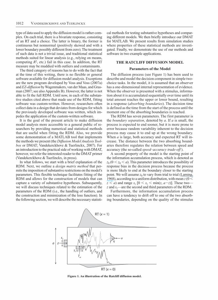
The diffusion process (see Figure 1) has been used to describe and model the decision component in simple two-choice tasks. In the model, it is assumed that an observer has a one-dimensional internal representation of evidence. When the observer is presented with a stimulus, informa-tion about it is accumulated sequentially over time until its total amount reaches the upper or lower bound, resulting in a response (absorbing boundaries). The decision time is defined as the time from the start of the process until the moment one of the absorbing boundaries is reached.

The RDM has seven parameters. The first parameter is the boundary separation, denoted by a. If a is small, the process is expected to end sooner, but it is more prone to error because random variability inherent to the decision process may cause it to end up at the wrong boundary. When a is large, both accuracy and expected RT will in-crease. The distance between the two absorbing bound-aries therefore regulates the relation between speed and accuracy (the so-called speed–accuracy trade-off ).

A second property of the model is the starting point of the information accumulation process, which is denoted as z0 (0 z0 a). This parameter introduces the possibility of response bias in the decision process because the process is more likely to end at the boundary closer to the starting point. We will assume z0 to vary from trial to trial (Laming, 1968), according to a uniform distribution, with mean z (0 z a) and range sz [0 sz min(z, az)]. These two— z and sz—are the second and third parameters of the RDM.

Furthermore, the information accumulation process can have a tendency to drift off to one of the two absorb-ing boundaries, depending on the quality of the stimulus

type of data used to apply the diffusion model is rather com-plex. On each trial, there is a bivariate response, consisting of an RT and a choice. The latter is binary, the former is continuous but nonnormal (positively skewed and with a lower boundary possibly different from zero). The treatment of such data is not a trivial issue, and traditional statistical methods suited for linear analysis (e.g., relying on means, computing R2, etc.) fail in this case. In addition, the RT measure may be muddied with outliers and contaminants.

The third category of reasons has to do with the fact that at the time of this writing, there is no flexible or general software available for diffusion model analysis. Exceptions are the new program developed by Voss and Voss (2007a) and EZ-diffusion by Wagenmakers, van der Maas, and Gras-man (2007; see also Appendix B). However, the latter is not able to fit the full RDM. Until now, in each of the substan-tive studies cited above that made use of the RDM, fitting software was custom-written. However, researchers often collect data in a design that deviates from designs for which the previously developed software was written, which im-pedes the application of the custom-written software.

It is the goal of the present article to make diffusion model analysis more accessible to a general public of re-searchers by providing numerical and statistical methods that are useful when fitting the RDM. Also, we provide some demonstration of a MATLAB tool that implements the methods we present (the Diffusion Model Analysis Tool-box or DMAT; Vandekerckhove & Tuerlinckx, 2007). For an introduction to the practical side of working with DMAT, however, we refer the interested reader to the DMAT primer (Vandekerckhove & Tuerlinckx, in press).

In what follows, we start with a brief explanation of the RDM. Next, we outline a design matrix method that per-mits the imposition of substantive restrictions on the model’s parameters. This flexible technique facilitates fitting of the RDM and allows for the construction of models that can capture a variety of substantive hypotheses. Subsequently, we will discuss techniques related to the estimation of the parameters of the RDM (i.e., the handling of outliers, and the construction and minimization of the loss function). In the following section, we will describe the necessary statisti-

a z

sz

st

Ter

ηv

RT (x = 0)

RT (x = 1)

Figure 1. an illustration of the Ratcliff diffusion model.

FiTTing The raTcliFF diFFusion Model 1013

Second, and more importantly, in many situations one may want to impose substantive restrictions on the param-eters, in effect leading to a reduction in the number of pa-rameters. An obvious example of such a restriction is the requirement that a certain parameter equals a known con-stant. For example, it can be hypothesized that the range of nondecision time, st, equals zero for all conditions (st(c) 0 for c 1, . . . , C ). In this way, st has been dropped from the model (see below for an evaluation of this restriction). Another popular substantive restriction in the context of the diffusion model is the requirement of a symmetric dif-fusion process (z(c) a(c)/2 for c 1, . . . , C ).

However, we can go a step further by carrying out a regres-sion of the parameters onto a set of predictors. To elucidate this concept, assume that a researcher has set up a bright-ness discrimination task (Ratcliff & Rouder, 1998; see also Example 2 in this article); assume also that there are 33 lev-els of brightness defined by increasing the number of white pixels in each step with an equal number. For the moment, the focus will be on the drift rates. Not restricting the drifts in any way will lead to 33 drift parameters to be estimated. However, the researcher may want to test the hypothesis that the drift rate varies linearly with brightness level:

v(c) v*(1) 1 B(c) v

*(2),

where B(c) refers to the brightness level in condition c and c 1, . . . , C. In this example, we have reduced the number of parameters to be estimated from 33 to 2. (Note also that we have introduced a new notation here: basic or design parameters are marked with an asterisk.)

In general, the drift rate in condition c can be decom-posed into a weighted linear combination of M known predictor values:

v d vc cj j

j

M

( ) ( )* ,=

=∑

1

(1)

where dcj is the value of the jth predictor in condition c. In the aforementioned example, M 2, dc1 1 and dc2 B(c). Because we have C linear equations, as in Equation 1 (one for each drift rate), we can make use of matrices and vectors to represent them all at once:

ψψv c

C

j j

v

v

v

d v

=

=

( )

( )

( )

( )

1

1

**

( )*

( )*

j

M

cj jj

M

Cj jj

M

d v

d v

=

=

=

∑

∑

∑

1

1

1

=

d d

d d d

d

M

c cj cM

11 1

1

CC CM

j

Md

v

v

v1

1

×

( )*

( )*

( )*

= ×D vv*.

presented. This information accumulation rate, or drift rate, is assumed to vary not only within a trial, following a Gaussian distribution with mean ξ and standard devia-tion s, but also across trials (Ratcliff, 1978), such that ξ fol-lows a Gaussian distribution with mean v and standard de-viation . An experimental condition with nonambigu ous stimuli will lead to a large positive mean drift rate v and thus a high probability of hitting the upper boundary (in-dicating a correct response) in a short time. The standard deviation s, which indicates the volatility in drift rate in a single trial, is a nonidentified parameter in the model, so we fixed it to the arbitrary value 0.1, which is a consensus value in the literature (e.g., Ratcliff et al., 1999). Thus, we added a fourth and fifth parameter to the model, namely the mean drift rate v and its intertrial standard deviation .

Finally, another component of the model is the time needed to perform nondecision processes such as encod-ing of the stimulus, response preparation and execution of the motor response (Luce, 1986). We denote the nondeci-sion part of the observed RT as ter. This ter is assumed to vary from trial to trial, according to a uniform distribution with mean Ter and range st. These two are the sixth and seventh parameters of the RDM.

some notational conventions

In the preceding section, we defined the seven key pa-rameters of the diffusion model. We will sometimes cap-ture all of these parameters in a parameter vector q(c) (a(c), Ter(c), (c), z(c), sz(c), st(c), v(c)), where the bracketed subscript (c) refers to the cth condition in an experiment, and c 1, . . . , C. When working with different conditions in an experiment (and thus different parameter vectors), we will vertically concatenate the parameter vectors into a parameter matrix, P. Thus, if we have C conditions,

P=

a

a

T

TC

er

er C

( )

( )

( )

( )

,

1 1

, ,

( )

( )

( )

( )

η

η

1 1

C C

z

z

,, ,

( )

( )

( )

( )

s

s

s

s

z

z C

t

t C

1 1

, .

( )

( )

v

v C

1

A single column in such a parameter matrix then contains estimates of one specific parameter over conditions, and such a column vector will be denoted with a ψ. For ex-ample, the nondecision time in condition c will be denoted as Ter(c), which is the cth element of ψTer (the second column of P) and the second element of q(c) (the cth row of P).

Finally, we will often use a plain q to refer to a generic (i.e., any) parameter.

The Design MaTRix MeThoD

There are several reasons why a researcher might not be interested in fitting a model with all parameters free. First, there is the issue of parsimony. Fitting the RDM to an exper-iment with C conditions would leave us with 7 C distinct parameters to estimate. Even if the number of conditions is moderate, for example C 5, this leads to many param-eters to be estimated (i.e., 35 parameters to be estimated). Therefore, it seems that some reduction in the number of parameters is needed from a pragmatic point of view.

1014 VandekerckhoVe and Tuerlinckx

Creative use of design matrices makes it possible to impose substantive restrictions on parameter sets, and will enable researchers to test specific substantive hy-potheses. Extending the diffusion model with the design matrix methodology, it becomes possible to build a type of “ANOVA/multiple regression” diffusion model.

Using the design matrix method entails two restrictions, however. First, only linear decompositions (i.e., linear in the basic parameters) can be represented by matrices. Second, only restrictions across conditions are possible, whereas restrictions across parameters (e.g., restricting z to be equal to a/2) require a different strategy. Nonethe-less, implementing restrictions using design matrices is a very flexible and powerful tool that has gained some atten-tion in other areas (e.g., see De Boeck & Wilson, 2004, for a wide variety of applications in psychometrics).

sTaTisTical inFeRence: esTiMaTion

Finding the parameters of the RDM, given a data set, is something of a challenge. Before starting, several nontriv-ial choices need to be made, in particular regarding how to deal with outliers and other contaminant RTs, the objec-tive function to use in the estimation step, and the precise method of optimization of the latter function. In this sec-tion, we discuss each of these choices, but for details we will refer the reader to Appendices A and B. A crucial part of any algorithm to fit the diffusion model is the efficient computation of its CDF. For this, we rely heavily on the methods described in Tuerlinckx (2004).

outlier handling strategiesAn important issue to consider when applying a statisti-

cal model to RT data is that of contaminants, data points that appear in the data sets but are somehow not germane to the research question. A well-known class of contami-nants is that of outliers (data points that are outside the range of normal observations); other examples are ran-dom guesses (data from trials where the participant some-how missed the stimulus and guessed), delayed start-ups (where the participant was somehow inappropriately de-layed in responding), and fast guesses (where the partici-pant executed a response before having actually inspected the stimulus).

Each of these types of contaminants can severely muddy the data (Ratcliff, 1993; Ratcliff & Tuerlinckx, 2002; Ul-rich & Miller, 1994), possibly resulting in biased param-eter estimates and incorrect standard errors of estimation. A fitting procedure for an RT model such as the one con-sidered in this article should therefore always be equipped with a proper strategy for handling these contaminants. We opt for a combination of two methods: First, the data are preprocessed with an exponentially weighted moving average (EWMA) control method that gives the minimal RT necessary for inclusion in the data analysis; and sec-ond, a mixture model is fitted to the data.

The EWMA method is an optional new method used in a preprocessing step in order to filter out RTs suspected of being fast guesses. The idea behind this method is that the identification of fast guesses is made possible because

The design matrix D is a C M matrix where each column represents a predictor (e.g., an intercept, an experimental treatment, a measured variable, etc.). The design matrix D is then multiplied with an M 1 design parameter vector, to recover a C 1 model parameter vector ψ.

The idea of regressing the parameters onto a set of pre-dictors can be applied to all parameters in the model and is by no means restricted to the drift rates. Because a differ-ent design matrix can be used for each parameter, D is in-dexed with the parameter symbol in order to make it clear to which parameter the design corresponds. The entire param-eter matrix P can be described in terms of only the seven (known) design matrices D and the seven design parameter vectors ψ. The result is that, when fitting the model to the data, only the elements of the parameter vectors (as opposed to all the diffusion parameters) have to be estimated.

Two special and interesting cases of design matrices D are worth mentioning. The first special case is where D consists of a column of ones. This can be illustrated for the parameter Ter as follows:

T

T

T

er

er c

er C

( )

( )

( )

1 1

1

=

11

1

× Ter( )* .

The result of this is that the C conditions have the same Ter. In a second special case, D equals the C C identity matrix; each of the C conditions, therefore, has a different value for a certain parameter. In the case of an identity matrix as the design matrix, there is no restriction of pa-rameters across conditions.

To illustrate the usefulness of the design matrix method, let us consider a final example. Suppose we want to fit a drift rate to the first condition and allow the drift rates of the other conditions to deviate from the first condition (but all in the same way). This can be implemented by defining the design matrix

Dv =

1 0

1 1

1 1

with

ψψv v

v

v= ×

D( )*

( )*

,1

2

and therefore v(1) v*(1) and v(c) v*

(1) 1 v*(2) for all c 1

(see chap. 6 in Littell, Stroup, & Freund, 2002, for more details on the construction of design matrices).

In general, we formulate the parameter matrix P {Da a*, DTer T*

er, D  η*, Dz z*, Dsz s*

z, Dst s*

t, Dv v*}. Then, all the elements of a*, T*

er, η*, z*, s*z, s*

t, and v* are the parameters over which we want to optimize the fit to data.

FiTTing The raTcliFF diFFusion Model 1015

the observed number of data points in each of a set of pre-defined “RT bins.” We call this statistic Λ. Details regard-ing Λ and its optimization are provided in Appendix B.

sTaTisTical inFeRence: TesTing anD MoDel selecTion

After having estimated the parameters of one or more models, the researcher may want to test hypotheses about the parameters, and/or compare models. We distinguish between testing a hypothesis about a single parameter with the Wald test, comparing two nested models, and comparing nonnested models.

The Wald Test for a hypothesis about single Parameters

The univariate Wald test can be used to test the null hypothesis that q q0 (vs. the alternative q q0). It starts from the Wald statistic

Zse

=−ˆ

,ˆ

θ θ

θ

0

where q is the point estimate of some parameter q and seˆq

the standard error. Under the null hypothesis and under some regularity conditions, Z follows approximately a standard normal distribution (or, equivalently, Z2 follows a χ2

1 distribution; Bishop, Fienberg, & Holland, 1975; the univariate Wald test is equivalent to a “Z test”).

Although the regularity conditions are fairly general, one of them is noteworthy. The Wald statistic should not be used if the test value q0 is at a boundary of the param-eter space (Bishop et al., 1975; but see also Stram & Lee, 1994, for an adaptation of the reference distribution). As a consequence, it cannot be used to test the null hypothesis that, for example, 0, since is bounded at 0.

Note also that a multivariate Wald test is possible to test a composite null hypothesis about several parameters (Bishop et al., 1975).

comparing Two nested Models

A model called the reduced model is nested in another model called the full model, if the reduced model can be reached by setting restrictions on the parameters of the full one (e.g., setting some of the parameters to zero). Such nested models can be compared through the likelihood ratio test (LRT). In this way, joint hypotheses about several parameters can be tested simultaneously. The LRT is very helpful in combination with the design matrix approach, because Model 1 is nested in Model 2, if for a given param-eter the columns of the design matrix of Model 1 (D1) lie in the space spanned by the columns of the design matrix of Model 2 (D2) (where we assume that the design matrices for the other parameters are kept constant); that is, the models are nested if each column of D1 can be represented as a linear combination of the columns of D2.

For example, a researcher might want to test whether an experimental manipulation has had some influence on drift rate. To that end, one could compare a model in

they tend to have a specific signature, being responses with a very short RT and chance level performance. A method suggested by this property of fast guesses sorts the data points according to the RTs and finds the minimal RT at which the responses begin to deviate from what we expect when guessing. This minimal RT is used as a lower cutoff value, such that all observations with shorter RTs are cen-sored. More technical detail is provided in Appendix A.

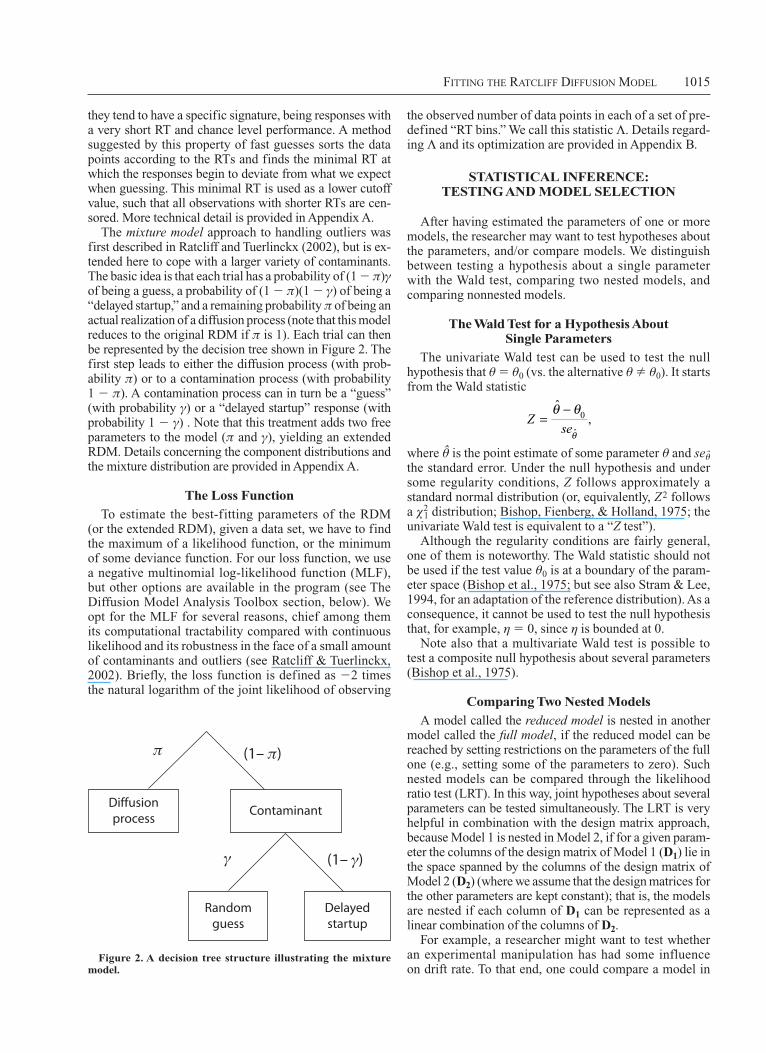
The mixture model approach to handling outliers was first described in Ratcliff and Tuerlinckx (2002), but is ex-tended here to cope with a larger variety of contaminants. The basic idea is that each trial has a probability of (1 π)γ of being a guess, a probability of (1 π)(1 γ) of being a “delayed startup,” and a remaining probability π of being an actual realization of a diffusion process (note that this model reduces to the original RDM if π is 1). Each trial can then be represented by the decision tree shown in Figure 2. The first step leads to either the diffusion process (with prob-ability π) or to a contamination process (with probability 1 π). A contamination process can in turn be a “guess” (with probability γ) or a “delayed startup” response (with probability 1 γ) . Note that this treatment adds two free parameters to the model (π and γ), yielding an extended RDM. Details concerning the component distributions and the mixture distribution are provided in Appendix A.

The loss Function

To estimate the best-fitting parameters of the RDM (or the extended RDM), given a data set, we have to find the maximum of a likelihood function, or the minimum of some deviance function. For our loss function, we use a negative multinomial log-likelihood function (MLF), but other options are available in the program (see The Diffusion Model Analysis Toolbox section, below). We opt for the MLF for several reasons, chief among them its computational tractability compared with continuous likelihood and its robustness in the face of a small amount of contaminants and outliers (see Ratcliff & Tuerlinckx, 2002). Briefly, the loss function is defined as 2 times the natural logarithm of the joint likelihood of observing

π (1– π)

γ (1– γ)

Diffusionprocess

Contaminant

Randomguess

Delayedstartup

Figure 2. a decision tree structure illustrating the mixture model.

1016 VandekerckhoVe and Tuerlinckx

with less technical background to use the diffusion model in practice. The program, DMAT, can be freely down-loaded from the Web site of the K.U. Leuven Research Group for Quantitative and Personality Psychology (ppw .kuleuven.be/okp/dmatoolbox).

In creating DMAT, we had two main goals in mind. The program should be (1) accurate and efficient, and (2) user friendly. We believe that we have achieved both goals to a satisfactory degree. Regarding accuracy and efficiency, DMAT performs well in simulations (see below) test-ing the recovery of model and design parameters from simulated data (estimation biases are generally low, and standard errors small). In addition, on our desktop PCs the algorithm typically converges in less than 1 min. The program is developed to make use of all fitting and model-ing strategies we have discussed above (and more).

Regarding flexibility and ease of use, we have added a graphical user interface. (Note that a MATLAB command interface is also available and offers more flexibility.) Also, wherever possible, we have provided default settings that we believe will perform well in most cases, and we have written an instructional primer to the use of the toolbox (Vandekerckhove & Tuerlinckx, in press).

simulations

To evaluate aspects of the tools described above, we performed many Monte Carlo simulations, of which we report here a selection. We discuss the results of three sim-ulation studies in which the performance of the estimation method is tested and two more simulations are carried out to evaluate properties of the inferential statistics associ-ated with using the RDM.

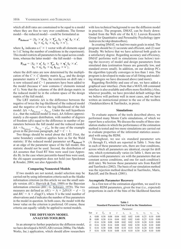
Throughout, we use six standard parameter sets (A through F), which are reported in Table 1. Note that in each of these parameter sets, there are four conditions, across which all parameters are identical, except for drift rate, which systematically varies (in Table 1, there are ten columns with parameters: six with the parameters that are constant across conditions, and one for each condition’s drift rate). We borrow these parameter sets from Ratcliff and Tuerlinckx (2002). The basis of our simulation method was the rejection method described in Tuerlinckx, Maris, Ratcliff, and De Boeck (2001).

asymptotic Parameter RecoveryAs a first test of the estimation algorithm, we used it to

estimate RDM parameters, given the true (i.e., expected) proportions in each of the bins of the likelihood function

which all drift rates are constrained to be equal to a model where they are free to vary over conditions. The former model—the reduced model—could be formulated as

PReduced {1c a*, 1c T*er, 1c η*, 1c z*,

1c s*z, 1c s*

t, 1c v*},

where 1c indicates a C 1 vector with all elements equal to 1 (C being the number of conditions in the experiment). This model restricts all parameters to be equal across condi-tions, whereas the latter model—the full model—is then

PFull {1c a*, 1c T*er, 1c η*, 1c z*,

1c s*z, 1c s*

t, icc v*},

where the drift rates are now determined by the multipli-cation of the C C identity matrix icc and the design parameter matrix v*. Thus, the restriction on drift rate v is now released and C1 parameters have been added to the model (because v* now contains C elements instead of 1). Note that the columns of the drift design matrix in the reduced model lie in the column space of the design matrix of the full model.

The LRT statistic ∆Λ is the difference between the negative of twice the log-likelihood of the reduced model and the negative of twice the log-likelihood of the full model: ∆Λ ΛPReduced

ΛPFull. Under the null hypothesis

(i.e., that the reduced model is true), ∆Λ follows approxi-mately a chi-square distribution, with number of degrees of freedom (dfs) equal to the difference in number of pa-rameters between the full model and the reduced model: ∆Λ ΛPReduced

ΛPFull ∼ χ2

∆df. In the case of the example given in the previous paragraph, ∆df C 1.

Two things should be noted about the LRT. First, the same boundary condition applies here as for the Wald statistic: If the reduced model parameter set PReduced is at an edge of the parameter space of the full model, this statistic should not be used. Second, the distribution of ∆Λ assumes that fixed RT bins were used (see Appen-dix B). In the case where percentile-based bins were used, the chi-square assumption does not hold (see Speckman & Rouder, 2004; see also Appendix B).

comparing nonnested Models

If two models are not nested, model selection may be carried out by using information criteria such as the Akaike information criterion (in this article we use the small sam-ple version AICc; Hurvich & Tsai, 1989) or the Bayesian information criterion (BIC; G. Schwarz, 1978). The two measures are defined as AICc Λ 1 2dN/(N d 1) and BIC Λ 1 d log(N ), where N is the total number of observations and d indicates the number of free parameters in the model in question. In both cases, the model with the lower value on the criterion is preferred. Of course, these criteria can equally validly be applied to nested models.

The DiFFusion MoDel analysis Toolbox

In an attempt to further popularize the diffusion model, we have developed a MATLAB (version 2006a; The Math-Works, Inc.) application, which should allow researchers

Table 1 standard Parameter sets used in the simulations

Parameter

Set a Ter z sz st v1 v2 v3 v4

A 0.08 0.30 0.08 0.04 0.02 0.02 0.40 0.25 0.10 0.00B 0.08 0.30 0.16 0.04 0.02 0.02 0.40 0.25 0.10 0.00C 0.16 0.30 0.08 0.08 0.02 0.02 0.30 0.20 0.10 0.00D 0.16 0.30 0.16 0.08 0.02 0.02 0.30 0.20 0.10 0.00E 0.16 0.30 0.08 0.08 0.10 0.10 0.30 0.20 0.10 0.00F 0.16 0.30 0.16 0.08 0.10 0.10 0.30 0.20 0.10 0.00

FiTTing The raTcliFF diFFusion Model 1017

abled the outlier treatment or did not. When we did add outliers, 2.5% were fast guesses (RTs were draws from a uniform distribution between 200 and 400 msec, and accu-racy was about 50%) and an additional 2.5% were delayed startups (RT draws from a uniform distribution between 500 and 3,000 msec, but with accuracy as expected under the diffusion model). We then estimated the parameters for each data set with DMAT and compared parameter recov-ery. In Table 4, the results are shown for Parameter Set A. As can be seen, if the data set did contain outliers with the aforementioned properties, and they are not accounted for, estimation biases increase dramatically to over 100% for some drift values. When the combined EWMA/mixture model method is applied, relative biases return to the same magnitude as in the condition where no outliers existed.

To conserve space, we do not report results for the other parameter sets here; but, as it turns out, our outlier treat-ment succeeds in alleviating the influence of outliers and contaminants on parameter estimates. Biases and stan-dard errors of the parameters that the adapted algorithm returned from the contaminated data set are closer to those of the parameters that the original algorithm returned from a “clean” data set, and they are lower than those from the original algorithm on the contaminated data set.

(see Equation B1 in Appendix B). In other words, as input we use the exact proportions of observations that each RT bin would have, given a certain set of parameters. Under this condition, there should be perfect recovery of the parameter values. This test was carried out under many different parameter sets, including the ones in Table 1. In each case, the algorithm returned the exact parameter val-ues to the requested accuracy (this was the case for each objective function DMAT allows).

Preasymptotic Parameter RecoveryAs a second test of the estimation algorithm, we per-

formed a series of simple simulations to investigate biases and standard errors of the parameter estimates. We define the relative bias of each parameter as

ˆ%,θ θ

θ− × 100

and the standard error as

1

1

2

R jj

R

−−( )∑ ˆ ˆ ,θ θ

with R the number of replications, and q and q–

respectively the estimate and the mean estimate of the parameter q.

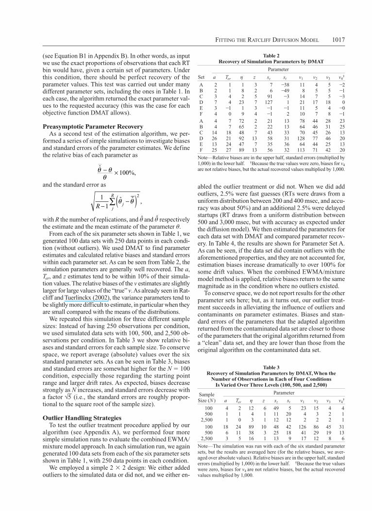
From each of the six parameter sets shown in Table 1, we generated 100 data sets with 250 data points in each condi-tion (without outliers). We used DMAT to find parameter estimates and calculated relative biases and standard errors within each parameter set. As can be seen from Table 2, the simulation parameters are generally well recovered. The a, Ter, and z estimates tend to be within 10% of their simula-tion values. The relative biases of the v estimates are slightly larger for large values of the “true” v. As already seen in Rat-cliff and Tuerlinckx (2002), the variance parameters tend to be slightly more difficult to estimate, in particular when they are small compared with the means of the distributions.

We repeated this simulation for three different sample sizes: Instead of having 250 observations per condition, we used simulated data sets with 100, 500, and 2,500 ob-servations per condition. In Table 3 we show relative bi-ases and standard errors for each sample size. To conserve space, we report average (absolute) values over the six standard parameter sets. As can be seen in Table 3, biases and standard errors are somewhat higher for the N 100 condition, especially those regarding the starting point range and larger drift rates. As expected, biases decrease strongly as N increases, and standard errors decrease with a factor √ 

__ 5 (i.e., the standard errors are roughly propor-

tional to the square root of the sample size).

outlier handling strategiesTo test the outlier treatment procedure applied by our

algorithm (see Appendix A), we performed four more simple simulation runs to evaluate the combined EWMA/mixture model approach. In each simulation run, we again generated 100 data sets from each of the six parameter sets shown in Table 1, with 250 data points in each condition.

We employed a simple 2 2 design: We either added outliers to the simulated data or did not, and we either en-

Table 2 Recovery of simulation Parameters by DMaT

Parameter

Set a Ter z sz st v1 v2 v3 v4†

A 2 1 1 3 7 38 11 4 5 2B 2 1 8 2 6 49 8 5 5 1C 3 4 2 5 91 3 14 7 5 3D 7 4 23 7 127 1 21 17 18 0E 3 1 1 3 1 1 11 5 4 0F 4 0 9 4 1 2 10 7 8 1

A 4 7 72 2 21 13 78 44 28 23B 4 7 65 2 22 13 64 46 31 25C 14 18 48 7 43 33 70 45 26 13D 26 21 92 13 58 31 128 77 46 20E 13 24 47 7 35 36 64 44 25 13F 25 27 89 13 56 32 113 71 42 20

Note—Relative biases are in the upper half, standard errors (multiplied by 1,000) in the lower half. †Because the true values were zero, biases for v4 are not relative biases, but the actual recovered values multiplied by 1,000.

Table 3 Recovery of simulation Parameters by DMaT, When the

number of observations in each of Four conditions is Varied over Three levels (100, 500, and 2,500)

Sample Parameter

Size (N ) a Ter z sz st v1 v2 v3 v4†

100 4 2 12 6 49 5 23 15 4 4 500 1 1 4 1 11 20 4 3 2 12,500 1 0 3 1 12 12 2 2 2 1

100 18 24 89 10 48 42 126 86 45 31 500 6 11 38 3 25 18 41 29 19 132,500 3 5 16 1 13 9 17 12 8 6

Note—The simulation was run with each of the six standard parameter sets, but the results are averaged here (for the relative biases, we aver-aged over absolute values). Relative biases are in the upper half, standard errors (multiplied by 1,000) in the lower half. †Because the true values were zero, biases for v4 are not relative biases, but the actual recovered values multiplied by 1,000.

1018 VandekerckhoVe and Tuerlinckx

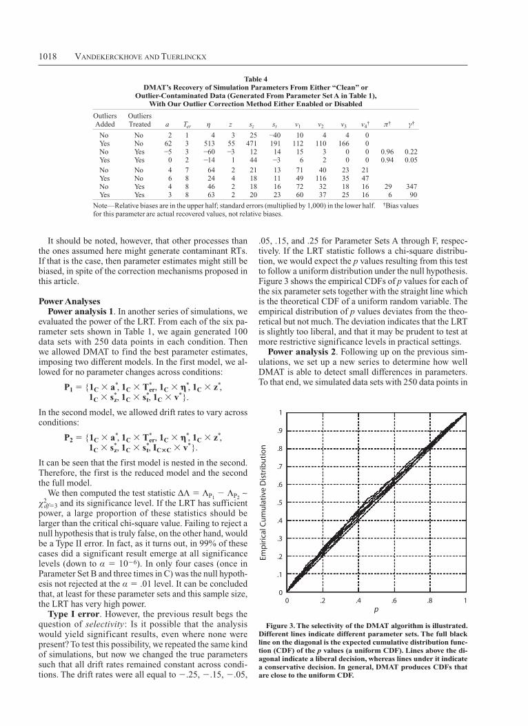
.05, .15, and .25 for Parameter Sets A through F, respec-tively. If the LRT statistic follows a chi-square distribu-tion, we would expect the p values resulting from this test to follow a uniform distribution under the null hypothesis. Figure 3 shows the empirical CDFs of p values for each of the six parameter sets together with the straight line which is the theoretical CDF of a uniform random variable. The empirical distribution of p values deviates from the theo-retical but not much. The deviation indicates that the LRT is slightly too liberal, and that it may be prudent to test at more restrictive significance levels in practical settings.

Power analysis 2. Following up on the previous sim-ulations, we set up a new series to determine how well DMAT is able to detect small differences in parameters. To that end, we simulated data sets with 250 data points in

It should be noted, however, that other processes than the ones assumed here might generate contaminant RTs. If that is the case, then parameter estimates might still be biased, in spite of the correction mechanisms proposed in this article.

Power analysesPower analysis 1. In another series of simulations, we

evaluated the power of the LRT. From each of the six pa-rameter sets shown in Table 1, we again generated 100 data sets with 250 data points in each condition. Then we allowed DMAT to find the best parameter estimates, imposing two different models. In the first model, we al-lowed for no parameter changes across conditions:

P1 {1c a*, 1c T*er, 1c η*, 1c z*,

1c s*z, 1c s*

t, 1c v*}.

In the second model, we allowed drift rates to vary across conditions:

P2 {1c a*, 1c T*er, 1c η*, 1c z*,

1c s*z, 1c s*

t, icc v*}.

It can be seen that the first model is nested in the second. Therefore, the first is the reduced model and the second the full model.

We then computed the test statistic ∆Λ ΛP1 ΛP2

∼ χ2

df3 and its significance level. If the LRT has sufficient power, a large proportion of these statistics should be larger than the critical chi-square value. Failing to reject a null hypothesis that is truly false, on the other hand, would be a Type II error. In fact, as it turns out, in 99% of these cases did a significant result emerge at all significance levels (down to α 106). In only four cases (once in Parameter Set B and three times in C) was the null hypoth-esis not rejected at the α .01 level. It can be concluded that, at least for these parameter sets and this sample size, the LRT has very high power.

Type i error. However, the previous result begs the question of selectivity: Is it possible that the analysis would yield significant results, even where none were pres ent? To test this possibility, we repeated the same kind of simulations, but now we changed the true parameters such that all drift rates remained constant across condi-tions. The drift rates were all equal to .25, .15, .05,

1

.9

.8

.7

.6

.5

.4

.3

.2

.1

00 .2 .4 .6

p.8 1

Emp

iric

al C

um

ula

tive

Dis

trib

uti

on

Figure 3. The selectivity of the DMaT algorithm is illustrated. Different lines indicate different parameter sets. The full black line on the diagonal is the expected cumulative distribution func-tion (cDF) of the p values (a uniform cDF). lines above the di-agonal indicate a liberal decision, whereas lines under it indicate a conservative decision. in general, DMaT produces cDFs that are close to the uniform cDF.

Table 4 DMaT’s Recovery of simulation Parameters From either “clean” or

outlier-contaminated Data (generated From Parameter set a in Table 1), With our outlier correction Method either enabled or Disabled

Outliers OutliersAdded Treated a Ter z sz st v1 v2 v3 v4

† π† γ†

No No 2 1 4 3 25 40 10 4 4 0Yes No 62 3 513 55 471 191 112 110 166 0No Yes 5 3 60 3 12 14 15 3 0 0 0.96 0.22Yes Yes 0 2 14 1 44 3 6 2 0 0 0.94 0.05

No No 4 7 64 2 21 13 71 40 23 21Yes No 6 8 24 4 18 11 49 116 35 47No Yes 4 8 46 2 18 16 72 32 18 16 29 347Yes Yes 3 8 63 2 20 23 60 37 25 16 6 90

Note—Relative biases are in the upper half; standard errors (multiplied by 1,000) in the lower half. †Bias values for this parameter are actual recovered values, not relative biases.

FiTTing The raTcliFF diFFusion Model 1019

example 1: an incomplete Factorial anoVa Design

The experiment by Vandekerckhove et al. (in press) is in the domain of visual shape perception and change de-tection in particular. The basic effect of interest is that if observers are shown a succession of two 2-D shapes which are different in only one vertex (an angle or a curvature extreme), this difference is easier to detect if it is adding or removing a concavity than if it is adding or removing a con-vexity (Barenholtz, Cohen, Feldman, & Singh, 2003). The substantive research question in this experiment is: Does the effect occur when the change is not adding or removing a new vertex, but increasing or decreasing an existing one? The paradigm is a two-interval forced choice task.

In the experiment, three variables are manipulated: (1) change—was there any difference between the two shapes? (2) quality—did the number of vertices change? (3) type—if there was a change, was it in a concavity (curvature with negative sign) or in a convexity (positive sign)? As is obvious from Variables 2 and 3, this is not a fully crossed design (properties of the change cannot be manipulated if there has been no change; as a result, each “change” condition had 80 data points but each “no-change” condition had 320). Table 6 lists all the con-ditions between which we would want to differentiate. Because the manipulations are all intended to affect the quality of the stimulus, we expect changes in drift rate, but not in any other variable. Writing the design as we do in Table 6 simplifies construction of a design matrix: The complete design matrix is simply the last three columns in the table, plus one column with ones for an intercept.

The goal of this experiment (and thus of the data analy-sis) is twofold. Primarily, it was to find out whether the type variable contributes anything above and beyond the quality variable. Additionally, if type has an effect, we would want to know whether it is independent of quality; that is, is there an interaction? To this end, we defined

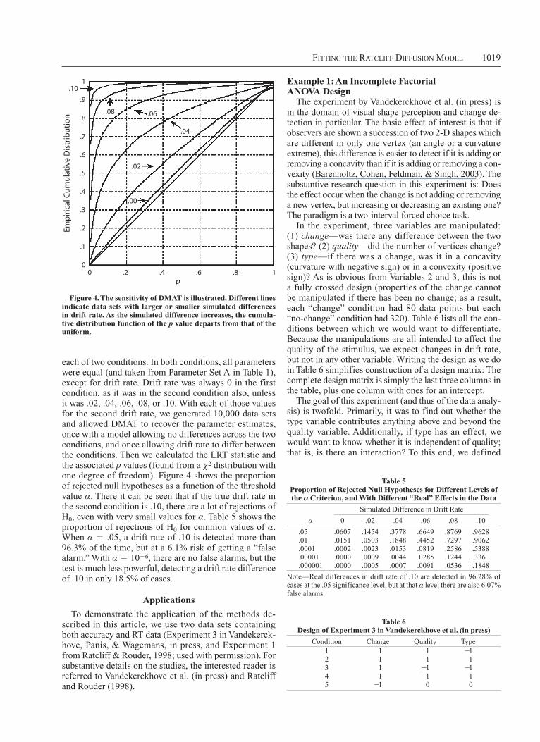
each of two conditions. In both conditions, all parameters were equal (and taken from Parameter Set A in Table 1), except for drift rate. Drift rate was always 0 in the first condition, as it was in the second condition also, unless it was .02, .04, .06, .08, or .10. With each of those values for the second drift rate, we generated 10,000 data sets and allowed DMAT to recover the parameter estimates, once with a model allowing no differences across the two conditions, and once allowing drift rate to differ between the conditions. Then we calculated the LRT statistic and the associated p values (found from a χ2 distribution with one degree of freedom). Figure 4 shows the proportion of rejected null hypotheses as a function of the threshold value α. There it can be seen that if the true drift rate in the second condition is .10, there are a lot of rejections of H0, even with very small values for α. Table 5 shows the proportion of rejections of H0 for common values of α. When α .05, a drift rate of .10 is detected more than 96.3% of the time, but at a 6.1% risk of getting a “false alarm.” With α 106, there are no false alarms, but the test is much less powerful, detecting a drift rate difference of .10 in only 18.5% of cases.

applications

To demonstrate the application of the methods de-scribed in this article, we use two data sets containing both accuracy and RT data (Experiment 3 in Vandekerck-hove, Panis, & Wagemans, in press, and Experiment 1 from Ratcliff & Rouder, 1998; used with permission). For substantive details on the studies, the interested reader is referred to Vandekerckhove et al. (in press) and Ratcliff and Rouder (1998).

1

.9

.8

.7

.6

.5

.4

.3

.2

.1

00 .2 .4 .6

p.8 1

Emp

iric

al C

um

ula

tive

Dis

trib

uti

on

.10

.08 .06

.04

.02

.00

Figure 4. The sensitivity of DMaT is illustrated. Different lines indicate data sets with larger or smaller simulated differences in drift rate. as the simulated difference increases, the cumula-tive distribution function of the p value departs from that of the uniform.

Table 5 Proportion of Rejected null hypotheses for Different levels of the α criterion, and With Different “Real” effects in the Data

Simulated Difference in Drift Rate

α 0 .02 .04 .06 .08 .10

.05 .0607 .1454 .3778 .6649 .8769 .9628

.01 .0151 .0503 .1848 .4452 .7297 .9062

.0001 .0002 .0023 .0153 .0819 .2586 .5388

.00001 .0000 .0009 .0044 .0285 .1244 .336

.000001 .0000 .0005 .0007 .0091 .0536 .1848

Note—Real differences in drift rate of .10 are detected in 96.28% of cases at the .05 significance level, but at that α level there are also 6.07% false alarms.

Table 6 Design of experiment 3 in Vandekerckhove et al. (in press)

Condition Change Quality Type 1 1 1 12 1 1 13 1 1 14 1 1 1

5 1 0 0

1020 VandekerckhoVe and Tuerlinckx

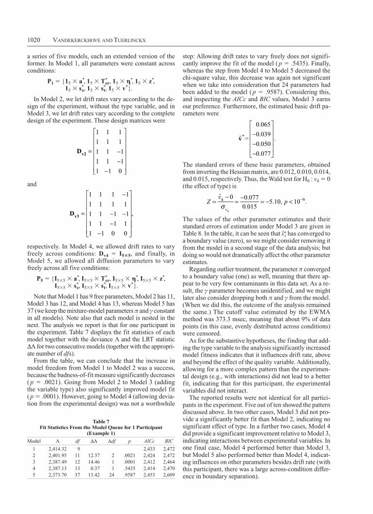
step: Allowing drift rates to vary freely does not signifi-cantly improve the fit of the model ( p .5435). Finally, whereas the step from Model 4 to Model 5 decreased the chi-square value, this decrease was again not significant when we take into consideration that 24 parameters had been added to the model ( p .9587). Considering this, and inspecting the AICc and BIC values, Model 3 earns our preference. Furthermore, the estimated basic drift pa-rameters were

ˆ

.

.

.

.

.v* =

0 065

0 039

0 050

0 077

−−−

The standard errors of these basic parameters, obtained from inverting the Hessian matrix, are 0.012, 0.010, 0.014, and 0.015, respectively. Thus, the Wald test for H0 : v4 0 (the effect of type) is

Zv

pv

=−

= − = − < −ˆ .

.. , .4 60 0 077

0 0155 10 10

4σ

The values of the other parameter estimates and their standard errors of estimation under Model 3 are given in Table 8. In the table, it can be seen that s*z has converged to a boundary value (zero), so we might consider removing it from the model in a second stage of the data analysis; but doing so would not dramatically affect the other parameter estimates.

Regarding outlier treatment, the parameter π converged to a boundary value (one) as well, meaning that there ap-pear to be very few contaminants in this data set. As a re-sult, the γ parameter becomes unidentified, and we might later also consider dropping both π and γ from the model. (When we did this, the outcome of the analysis remained the same.) The cutoff value estimated by the EWMA method was 373.3 msec, meaning that about 9% of data points (in this case, evenly distributed across conditions) were censored.

As for the substantive hypotheses, the finding that add-ing the type variable to the analysis significantly increased model fitness indicates that it influences drift rate, above and beyond the effect of the quality variable. Additionally, allowing for a more complex pattern than the experimen-tal design (e.g., with interactions) did not lead to a better fit, indicating that for this participant, the experimental variables did not interact.

The reported results were not identical for all partici-pants in the experiment. Five out of ten showed the pattern discussed above. In two other cases, Model 3 did not pro-vide a significantly better fit than Model 2, indicating no significant effect of type. In a further two cases, Model 4 did provide a significant improvement relative to Model 3, indicating interactions between experimental variables. In one final case, Model 4 performed better than Model 3, but Model 5 also performed better than Model 4, indicat-ing influences on other parameters besides drift rate (with this participant, there was a large across-condition differ-ence in boundary separation).

a series of five models, each an extended version of the former. In Model 1, all parameters were constant across conditions:

P1 {15 a*, 15 T*er, 15 η*, 15 z*,

15 s*z, 15 s*

t, 15 v*}.

In Model 2, we let drift rates vary according to the de-sign of the experiment, without the type variable, and in Model 3, we let drift rates vary according to the complete design of the experiment. These design matrices were

Dv2 = −−

−

1 1 1

1 1 1

1 1 1

1 1 1

1 1 0

and

Dv3 =

−

− −−

−

1 1 1 1

1 1 1 1

1 1 1 1

1 1 1 1

1 1 0 0

,

respectively. In Model 4, we allowed drift rates to vary freely across conditions: Dv4 i55, and finally, in Model 5, we allowed all diffusion parameters to vary freely across all five conditions:

P5 {i55 a*, i55 T*er, i55 η*, i55 z*,

i55 s*z, i55 s*

t, i55 v*}.

Note that Model 1 has 9 free parameters, Model 2 has 11, Model 3 has 12, and Model 4 has 13, whereas Model 5 has 37 (we keep the mixture-model parameters π and γ constant in all models). Note also that each model is nested in the next. The analysis we report is that for one participant in the experiment. Table 7 displays the fit statistics of each model together with the deviance Λ and the LRT statistic ∆Λ for two consecutive models (together with the appropri-ate number of dfs).

From the table, we can conclude that the increase in model freedom from Model 1 to Model 2 was a success, because the badness-of-fit measure significantly decreases ( p .0021). Going from Model 2 to Model 3 (adding the variable type) also significantly improved model fit ( p .0001). However, going to Model 4 (allowing devia-tion from the experimental design) was not a worthwhile

Table 7 Fit statistics From the Model Queue for 1 Participant

(example 1)

Model Λ df ∆Λ ∆df p AICc BIC

1 2,414.32 9 2,433 2,4722 2,401.95 11 12.37 2 .0021 2,424 2,4723 2,387.49 12 14.46 1 .0001 2,412 2,4644 2,387.13 13 0.37 1 .5435 2,414 2,4705 2,373.70 37 13.42 24 .9587 2,453 2,609

FiTTing The raTcliFF diFFusion Model 1021

To perform the analysis, we defined a series of three models, each a more complex version of the former. In all models, we determined that there should be two different levels of the parameters a, z, and sz: one for the conditions with accuracy instruction, and one for those with speed in-struction. To do this, we constructed the following design matrix for these parameters:

D D D1 0

0 1a z s25 25

25 25z

= = =

,

which has two columns with 25 ones and 25 zeros each. Additionally, in Model 1 we will allow v to evolve linearly with the brightness manipulation, while allowing differ-ent regression slopes and intercepts for different speed–accuracy instructions:

D1 l 0 0

0 0 1 lv25 25 25

25 25 25

=

,

where l [3 6 7 . . . 27 28 31]T represents the 25 bright-ness levels (with the first and last values adapted to reflect the average of the five groups pooled there). The other design matrices impose the requirement that there be no change across conditions:

P2 {Da a*, 150 T*er, 150 η*, Dz z*,

Dsz s*

z, 150 s*t, Dv v*}.

However, the restriction that drift rates should increase linearly with the brightness manipulation is hardly ten-able, both on theoretical grounds (because performance has upper and lower bounds) and due to opportunistic in-spection of Ratcliff and Rouder’s (1998) results. In fact, in their article, drift rate increases with brightness like a sigmoid function. Thus, in Model 2, we add a quadratic, cubic, and quartic component to the design, to mimic an S-shaped function. Now,

D

1 l l l l 0 0 0 0 0

0 0 0 0 0

v

25 25 25 25 25 25

25 25 25 25 25

=2 43

11 l l l l252 3 4

,

where the exponents indicate the element-wise power func-tion (i.e., each element of the vector l is taken to that pow- er). The other design matrices are the same as in Model 1. Note that, for numerical reasons, we rescaled each column of Dv so that the values were in the range (0, 0.5).

In Model 3, we allowed drift rates to vary freely:

P3 {Da a*, 150 T*er, 150 η*, Dz z*,

Dsz s*

z, 150 s*t, i5050 v*}.

Finally, in Model 4, all diffusion parameters can vary freely across conditions.

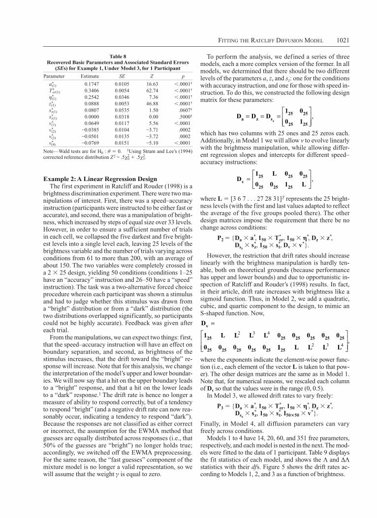
Models 1 to 4 have 14, 20, 60, and 351 free parameters, respectively, and each model is nested in the next. The mod-els were fitted to the data of 1 participant. Table 9 displays the fit statistics of each model, and shows the Λ and ∆Λ statistics with their dfs. Figure 5 shows the drift rates ac-cording to Models 1, 2, and 3 as a function of brightness.

example 2: a linear Regression DesignThe first experiment in Ratcliff and Rouder (1998) is a

brightness discrimination experiment. There were two ma-nipulations of interest. First, there was a speed– accuracy instruction (participants were instructed to be either fast or accurate), and second, there was a manipulation of bright-ness, which increased by steps of equal size over 33 levels. However, in order to ensure a sufficient number of trials in each cell, we collapsed the five darkest and five bright-est levels into a single level each, leaving 25 levels of the brightness variable and the number of trials varying across conditions from 61 to more than 200, with an average of about 150. The two variables were completely crossed in a 2 25 design, yielding 50 conditions (conditions 1–25 have an “accuracy” instruction and 26–50 have a “speed” instruction). The task was a two-alternative forced choice procedure wherein each participant was shown a stimulus and had to judge whether this stimulus was drawn from a “bright” distribution or from a “dark” distribution (the two distributions overlapped significantly, so participants could not be highly accurate). Feedback was given after each trial.

From the manipulations, we can expect two things: first, that the speed–accuracy instruction will have an effect on boundary separation, and second, as brightness of the stimulus increases, that the drift toward the “bright” re-sponse will increase. Note that for this analysis, we change the interpretation of the model’s upper and lower boundar-ies. We will now say that a hit on the upper boundary leads to a “bright” response, and that a hit on the lower leads to a “dark” response.1 The drift rate is hence no longer a measure of ability to respond correctly, but of a tendency to respond “bright” (and a negative drift rate can now rea-sonably occur, indicating a tendency to respond “dark”). Because the responses are not classified as either correct or incorrect, the assumption for the EWMA method that guesses are equally distributed across responses (i.e., that 50% of the guesses are “bright”) no longer holds true; accordingly, we switched off the EWMA preprocessing. For the same reason, the “fast guesses” component of the mixture model is no longer a valid representation, so we will assume that the weight γ is equal to zero.

Table 8 Recovered basic Parameters and associated standard errors

(SEs) for example 1, under Model 3, for 1 Participant

Parameter Estimate SE Z p

a*(1) 0.1747 0.0105 16.63 .0001†

T*er(1) 0.3406 0.0054 62.74 .0001†

*(1) 0.2542 0.0346 7.36 .0001†

z*(1) 0.0888 0.0053 46.88 .0001†

s*z(1) 0.0807 0.0535 1.50 .0607†

s*t(1) 0.0000 0.0318 0.00 .5000†

v*(1) 0.0649 0.0117 5.56 .0001

v*(2) 0.0385 0.0104 3.71 .0002

v*(3) 0.0501 0.0135 3.72 .0002

v*(4) 0.0769 0.0151 5.10 .0001

Note—Wald tests are for H0 : q 0. †Using Stram and Lee’s (1994) corrected reference distribution Z2 ~ .5χ2

0 1 .5χ21.

1022 VandekerckhoVe and Tuerlinckx

an experiment and discussed the use of the likelihood ratio statistic ∆Λ for statistical inference and model selection. With this statistical framework to complement diffusion modeling, the simultaneous analysis of RT and accuracy data moves closer to the realm of well-known statistical procedures such as ANOVA and multiple linear regression. We presented simulation studies where the small-sample behavior of the likelihood ratio statistic was found suitable. We also presented outlier treatment methods and showed that they perform well. Furthermore, we have implemented these methods in a freely available software tool, DMAT (Vandekerckhove & Tuerlinckx, 2007, in press).

Some further extensions of the RDM now present themselves. A first extension that readily flows from the present study is to implement other (nonlinear) constraints on model parameters than the ones permitted by the de-sign matrix method. For example, in our second applica-tion we implemented an ad hoc imitation of a sigmoid function (with a polynomial of a high degree), whereas a better solution would be to simply use a nonlinear link function, such as a logit or probit link. A second possibil-ity for advancement is to move from classical frequen-tist parameter estimation to a Bayesian framework, as in Lee, Fuss, and Navarro (2007). Finally, further research is needed to investigate the statistical qualities of quan-tile probability products estimators (Brown & Heathcote,

As can be seen from the table, Model 2 greatly outper-forms Model 1, indicating deviations from linearity (as is obvious from Figure 5). Moreover, Model 3 performs slightly better than Model 2. Finally, Model 4 does not per-form significantly better than Model 3, indicating that it is not necessary to free all parameters in the model across conditions. The AICc and BIC statistics, in Table 9, show a preference for Model 2, where a polynomial regression was imposed on the drift rates. In this case, we would opt for Model 2, both because the information criteria point in that direction, and also because the LRT does not give convincing evidence against Model 2.

The recovered basic parameters and their standard er-rors of estimation under Model 2 are given in Table 10, in which it can be seen that—as opposed to Example 1—all parameters significantly deviate from 0 (or from 1, in the case of π). With π 0.9606, about 4% of the data (across conditions) are estimated to be contaminants.

For the two other participants, AICc and BIC values did not agree, but the pattern of significance between models was identical to that in Table 9.

conclusion

In the present article, we investigated and enhanced the practical applicability of the diffusion model for RT and accuracy data and explored several avenues of improve-ment. We suggested the use of design matrices in order to regress diffusion model parameters onto covariates from

2

1.5

1

0.5

0

–0.5

–1

–1.5

–2

Dri

ft R

ate

Model Fits for Example 2

Model 1 for accuracyModel 1 for speedModel 2 for accuracyModel 2 for speedModel 3 for accuracyModel 3 for speed

0 5 10 15 20 25 30

Brightness Level

Figure 5. Drift rates of 1 participant in experiment 1 of Rat-cliff and Rouder (1998). Drifts recovered by Model 1 are shown as dashed lines, with the steeper line indicating the speed condi-tion. Drifts from Model 2 are full curves, and drifts from Model 3 are stars. as can be seen, Model 1 provides a poor fit, whereas Model 2 is much closer to the separate drift rates, though still with some deviation left.

Table 10 Recovered basic Parameters and associated standard errors

(SEs) for example 2, under Model 2, for 1 Participant

Parameter Estimate SE Z pa*

(1) 0.1688 0.0016 103.50 .0001†

a*(2) 0.0436 0.0000 .106 .0001†

T*er(1) 0.3065 0.0008 369.61 .0001†

*(1) 0.0252 0.0085 2.95 .0016†

z*(1) 0.0821 0.0012 71.13 .0001†

z*(2) 0.0218 0.0000 .106 .0001†

s*z(1) 0.0476 0.0078 6.12 .0001†

s*z(2) 0.0426 0.0000 .106 .0001†

s*t(1) 0.1427 0.0023 62.27 .0001†

v*(1) 0.5892 0.0155 37.96 .0001

v*(2) 3.9174 0.2829 13.85 .0001

v*(3) 0.8681 0.0336 25.86 .0001

v*(4) 6.4215 0.6207 10.35 .0001

v*(5) 0.1671 0.0188 8.90 .0001

v*(6) 2.0014 0.3373 5.93 .0001

π*(1) 0.9582 0.0041 10.28‡ .0001†

Note—Wald tests are for H0 : q 0 unless indicated otherwise. Basic drift parameters (1), (2), and (3) refer to the accuracy condition, and (4), (5), and (6) refer to the speed condition. Other parameters indexed with a (1) apply to the accuracy condition and with a (2) to the “speed” condi-tion. †Using Stram and Lee’s (1994) corrected reference distribution Z2 ∼ .5χ2

0 1 .5χ21. ‡Testing H0 : π*

(1) 1.

Table 9 Fit statistics From the Model Queue

for 1 Participant (example 2)

Model Λ df ∆Λ ∆df p AICc BIC

1 23,516.8 14 23,545 23,6422 23,213.64 20 303.14 6 .0001 23,254 23,3933 23,153.26 60 60.38 40 .0202 23,274 23,6924 23,086.12 351 67.14 291 .9999 23,821 26,236

FiTTing The raTcliFF diFFusion Model 1023

Ratcliff, R., & Rouder, J. N. (2000). A diffusion model account of masking in letter identification. Journal of Experimental Psychology: Human Perception & Performance, 26, 127-140.

Ratcliff, R., Thapar, A., & McKoon, G. (2004). A diffusion model analysis of the effects of aging on recognition memory. Journal of Memory & Language, 50, 408-424.

Ratcliff, R., & Tuerlinckx, F. (2002). Estimating parameters of the diffusion model: Approaches to dealing with contaminant reaction times and parameter variability. Psychonomic Bulletin & Review, 9, 438-481.

Ratcliff, R., Van Zandt, T., & McKoon, G. (1999). Connectionist and diffusion models of reaction time. Psychological Review, 106, 261-300.

Read, T., & Cressie, N. (1988). Goodness-of-fit statistics for discrete multivariate data. New York: Springer.

Roberts, S. (1959). Control chart tests based on geometric moving aver-ages. Technometrics, 1, 239-250.

Schwarz, G. (1978). Estimating the dimension of a model. Annals of Statistics, 6, 461-464.

Schwarz, W. (2001). The ex-Wald distribution as a descriptive model of response times. Behavior Research Methods, Instruments, & Comput-ers, 33, 457-469.

Speckman, P. L., & Rouder, J. N. (2004). A comment on Heathcote, Brown, and Mewhort’s QMLE method for response time distributions. Psychonomic Bulletin & Review, 11, 574-576.

Stram, D. O., & Lee, J. W. (1994). Variance components testing in the longitudinal mixed effects model. Biometrics, 50, 1171-1177.

Strayer, D. L., & Kramer, A. F. (1994). Strategies and automaticity: I. Basic findings and conceptual framework. Journal of Experimental Psychology: Learning, Memory, & Cognition, 20, 318-341.

Thapar, A., Ratcliff, R., & McKoon, G. (2003). A diffusion model analysis of the effects of aging on letter discrimination. Psychology & Aging, 18, 415-429.

Tuerlinckx, F. (2004). The efficient computation of the cumulative dis-tribution and probability density functions in the diffusion model. Be-havior Research Methods, Instruments, & Computers, 36, 702-716.

Tuerlinckx, F., Maris, E., Ratcliff, R., & De Boeck, P. (2001). A comparison of four methods for simulating the diffusion process. Be-havior Research Methods, Instruments, & Computers, 33, 443-456.

Ulrich, R., & Miller, J. (1994). Effects of truncation on reaction time analysis. Journal of Experimental Psychology: General, 123, 34-80.

Vandekerckhove, J., Panis, S., & Wagemans, J. (in press). The con-cavity effect is a compound of local and global effects. Perception & Psychophysics.

Vandekerckhove, J., & Tuerlinckx, F. (2007). The Diffusion Model Analysis Toolbox [Software and manual]. Retrieved from ppw.kuleuven .be/okp/dmatoolbox.

Vandekerckhove, J., & Tuerlinckx, F. (in press). Diffusion model analysis with MATLAB: A DMAT primer. Behavior Research Methods.

Voss, A., Rothermund, K., & Voss, J. (2004). Interpreting the param-eters of the diffusion model: An empirical validation. Memory & Cog-nition, 32, 1206-1220.

Voss, A., & Voss, J. (2007a). Fast-dm: A free program for efficient diffu-sion model analysis. Behavior Research Methods, 39, 767-775.

Voss, A., & Voss, J. (2007b). A fast numerical algorithm for the esti-mation of diffusion-model parameters. Manuscript submitted for publication.

Wagenmakers, E.-J., Ratcliff, R., Gomez, P., & McKoon, G. (in press). A diffusion model account of criterion manipulations in the lexical decision task. Journal of Memory & Language.

Wagenmakers, E.-J., van der Maas, H. L., & Grasman, R. P. (2007). An EZ-diffusion model for response time and accuracy. Psychonomic Bulletin & Review, 14, 3-22.

noTe

1. Changing the response coding is in general only necessary if there is a very high proportion of correct—or error—responses, so that one of the marginal distributions of the model is represented by only a few data points. Here there is no substantive or statistical reason that compels us to do this; we merely take this approach for illustrative reasons.

2003; Heathcote & Brown, 2004; Heathcote, Brown, & Mewhort, 2002; Speckman & Rouder, 2004), since this estimation method seems preferable if the range of the RT distribution is unknown, but its qualities for statistical inference are not yet explored.

auThoR noTe

This research was supported by Grants GOA/00/02-ZKA4511, GOA/2005/04-ZKB3312, and IUAP P5/24. J.V. and F.T. thank Jeff Rouder for providing the data used in the second application example, and Eric-Jan Wagenmakers and Andrew Heathcote for helpful comments on ear-lier drafts of this article. Correspondence concerning this article should be addressed to J. Vandekerckhove, Department of Psychology, Tienses-traat 102, B-3000 Leuven, Belgium (e-mail: joachim.vandekerckhove@ psy.kuleuven.be).

ReFeRences

Barenholtz, E., Cohen, E., Feldman, J., & Singh, M. (2003). De-tection of change in shape: An advantage for concavities. Cognition, 89, 1-9.

Bishop, Y., Fienberg, S., & Holland, P. (1975). Discrete multivariate analysis: Theory and practice. Cambridge, MA: MIT Press.

Brown, S., & Heathcote, A. (2003). QMLE: Fast, robust and efficient estimation of distribution functions based on quantiles. Behavior Re-search Methods, Instruments, & Computers, 35, 485-492.

Chandra, M. (2001). Statistical quality control. New York: CRC Press.De Boeck, P., & Wilson, M. (2004). Explanatory item response models:

A generalized linear and nonlinear approach. New York: Springer.Donders, F. C. (1969). On the speed of mental processes. Acta Psy-

chologica, 30, 412-431. (Translation of Die Schnelligkeit psychischer Processe, first published in 1868)

Heathcote, A., & Brown, S. (2004). Reply to Speckman and Rouder: A theoretical basis for QML. Psychonomic Bulletin & Review, 11, 577-578.

Heathcote, A., Brown, S., & Mewhort, D. J. K. (2002). Quan-tile maximum likelihood estimation of response time distributions. Psychonomic Bulletin & Review, 9, 394-401.

Hurvich, C. M., & Tsai, C.-L. (1989). Regression and time series model selection in small samples. Biometrika, 76, 297-307.

Laming, D. (1968). Information theory of choice reaction time. New York: Wiley.

Lee, M. D., Fuss, I. G., & Navarro, D. J. (2007). A Bayesian ap-proach to diffusion models of decision-making and response time. In B. Schölkopf, J. C. Platt, & T. Hoffman (Eds.), Advances in neural in-formation processing systems, Vol. 19. Cambridge, MA: MIT Press.

Link, S., & Heath, R. (1975). A sequential theory of psychological discrimination. Psychometrika, 40, 77-105.

Littell, R. C., Stroup, W., & Freund, R. J. (2002). SAS system for linear models (4th ed.). Cary, NC: SAS Institute.

Luce, D. (1986). Response times. New York: Oxford University Press.Nelder, J. A., & Mead, R. (1965). A simplex method for function mini-

mization. Computer Journal, 7, 308-313.Ratcliff, R. (1978). A theory of memory retrieval. Psychological Re-

view, 85, 59-108.Ratcliff, R. (1981). A theory of order relations in perceptual matching.

Psychological Review, 88, 552-572.Ratcliff, R. (1988). Continuous versus discrete information process-

ing: Modeling the accumulation of partial information. Psychological Review, 95, 238-255.

Ratcliff, R. (1993). Methods for dealing with reaction time outliers. Psychological Bulletin, 114, 510-532.

Ratcliff, R. (2002). A diffusion model account of response time and ac-curacy in a brightness discrimination task: Fitting real data and failing to fit fake but plausible data. Psychonomic Bulletin & Review, 9, 278-291.

Ratcliff, R., Gomez, P., & McKoon, G. (2004). A diffusion model ac-count of the lexical-decision task. Psychological Review, 111, 159-182.

Ratcliff, R., & Rouder, J. N. (1998). Modeling response times for two-choice decisions. Psychological Science, 9, 347-356.

1024 VandekerckhoVe and Tuerlinckx

aPPenDix a outlier Treatment Methods

exponentially Weighted Moving average FilterThe exponentially weighted moving average method (EWMA; Chandra, 2001; Roberts, 1959) is a statistical

quality control method that can detect shifts in performance as RTs increase. A cutoff threshold is set where the performance is judged to be above chance level.

The first step in the application of the method is sorting the RTs from short to long. In effect, we will then look at our data set as if it described a binary process that unfolds (and changes) over time. As time progresses (i.e., as RT increases), the process will start to shift away from its “control state” (with 50% accuracy) and tend toward a biased process (with accuracy . 50%). The control process describes our expectation regarding fast guesses, which is straightforward: Guesses are draws from a Bernoulli process at chance level. Formally, if the sth observation (that is, the response X(s), corresponding to the sth sorted RT T(s)) is a guess, then X(s) ~ Bernoulli(0.5). The control process should be a credible representation of fast guesses, otherwise this method will not work. However, usually trials in an experiment are counterbalanced and randomized in such a way that participants cannot significantly exceed chance level accuracy without paying proper attention to the stimuli presented. If measures have been taken to avoid participants from being “cued” to a correct (or error) response even when guessing, it is reasonable to expect accuracy to be around 50% for fast guesses in a two-alternative forced choice task.

To determine the minimal RT at which the system no longer follows this control process, we take the RTs from all conditions (all RTs still sorted fast to slow), and analyze their corresponding responses. Of these responses, we iteratively compute the EWMA statistic cs λxs 1 (1 λ)cs1, where xs 1 if the response corresponding to the sth sorted RT was correct and 0 otherwise, and λ ∈ (0, 1) is a weight parameter that controls how many of the last observations are used. If λ is 1, only the sth observation is used, and if λ approaches 0, all observations from the first to the sth are weighted equally. We will then, at each iteration, calculate the upper control limit (UCL) of this process, and check whether the EWMA statistic cs exceeds this value.

In practice, some constants need to be defined. The first is the in-control mean of the process, which in this context represents the expected average performance of a fast guess. We denote this parameter c0, and initialize it to 0.5. Second is the in-control standard deviation σ0 (standard deviation of X ), which is also equal to 0.5 (this follows from the properties of the Bernoulli distribution). A third constant for EWMA is the weight parameter λ. We choose λ 0.01, thereby accounting for many previous data points. The final constant is the width of the control limits (in standard deviations). To ensure a sensitive test, we set L to 1.5 (a relatively low value).

Given these parameters, we now compute cs and check whether it is smaller than the UCL:

c UCL c Ls ss< = +

−− −

0 0

2

21 1σ λ

λλ( ) . (A1)

If this inequality is true, the process is judged to be within the limits of the control model, and we label observa-tion s as a “fast guess.” When the UCL is exceeded, we decide that the probability of giving a correct response significantly exceeds 0.5 from this RT on, and stop the iteration process. The RT at which the UCL was breached is then taken as the threshold, and all RTs below it are censored.

0.9

0.85

0.8

0.75

0.7

0.65

0.6

0.55

0.5

0.45

0.4

Stat

e o

f th

e Sy

stem

(c)

EWMA Control Chart (λ = 0.01, L = 1.5)

0 0.2 0.4 0.6 0.8 1 1.2 1.4

Reaction Time

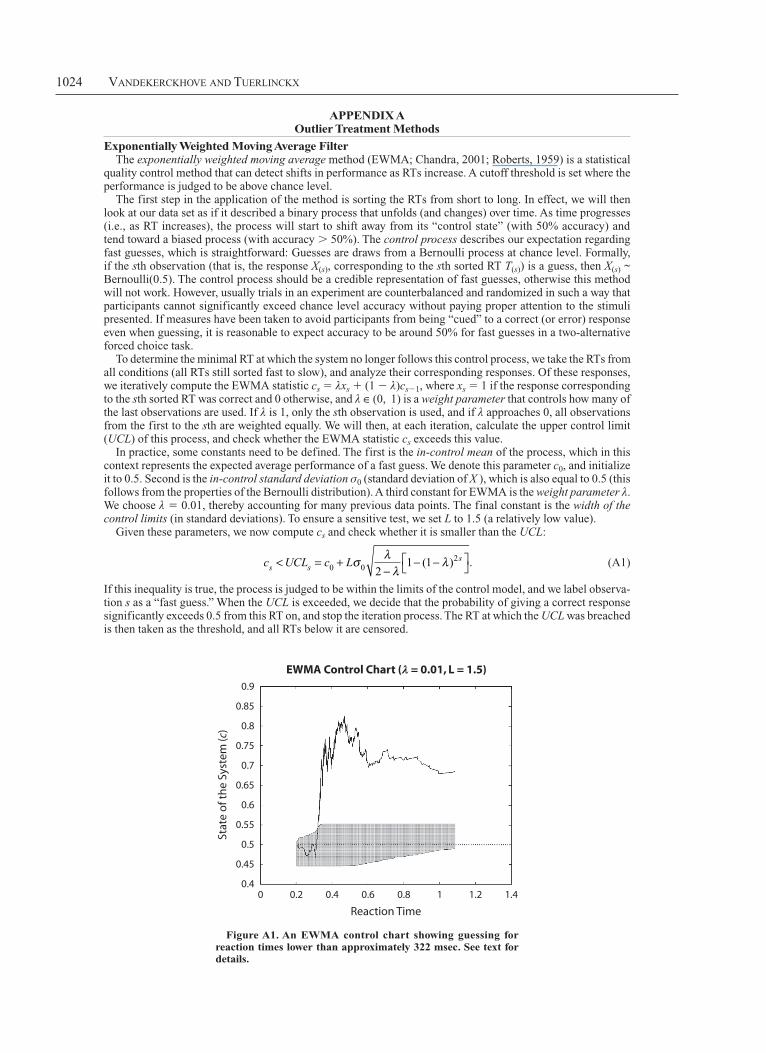
Figure a1. an eWMa control chart showing guessing for reaction times lower than approximately 322 msec. see text for details.

FiTTing The raTcliFF diFFusion Model 1025

aPPenDix a (continued)

The EWMA method is commonly illustrated with a control chart, which depicts the evolution of cs as a func-tion of increasing RT. Figure A1 shows an example control chart, with the EWMA statistic indicated by a full line, the control state by a dotted line, and the control limits by a shaded region around the control state. This control chart is based on data that were generated from the parameters shown in Table 1 (Set A), with 250 data points in each condition, and 5% fast outliers added to the 200- to 400-msec domain, uniformly distributed and with 50% accuracy. The EWMA algorithm returns a cutoff value of 322 msec, which is reasonable considering that the diffusion process with these parameters starts around 300 msec, but there are contaminants between 200 and 400 msec.

Mixture Model approachThe CDF of the diffusion model extended with the mixture model approach is

FX,T (x, t, q) πDiff(x, t, q) 1 (1 π)γ  1–2U(t, T, T1)1 (1 π)(1 γ)Pr(X x | q)U(t, T, T1), (A2)

where U(t, A, B) indicates the cumulative density function of a uniform distribution from A to B, evaluated at t. DiffX,T (x, t, q) is the joint probability that the response equals x (x 0 for an error and x 1 for a correct response) and that the response is given at time t or before, under a Ratcliff diffusion model with parameter vector q [thus, DiffX,T (x, t, q) Pr(X x, T t | q]. The exact formula for this joint probability is provided in Tuerlinckx (2004, Equations 1, 2, and 3). Further, T and T1 are the minimum and maximum of the assumed RT distributions for contaminants. Technically, T and T1 are parameters, but in the remainder of this article we will not treat them as such. They are not included in the parameter estimation routine, but are directly estimated with the observed minimum and maximum RTs (for each condition and each participant), respectively.

aPPenDix b Minimizing the Multinomial log-likelihood Function

loss FunctionDMAT uses a multinomial likelihood function (MLF), which expresses the likelihood of observing a certain

proportion of responses in a given number of RT bins, and should therefore be maximized in order to find good parameter estimates.

To define B RT bins, we select B1 monotonically increasing bin edges q1, . . . , qB1 and define q0 0 and qB 1. The observed frequency in bin b, in condition c, for response x, is then simply

O I q t qcxb b cxj bj

ncx

= < ≤( )−=

∑ 11

,

with ncx being the number of data points with response x in condition c. I() is the indicator function (which takes the value 1 if its argument is true and 0 otherwise). The predicted (or expected) proportion of x responses in bin b of condition c equals Pcxb FX,T(x, qb, qc) FX,T(x, qb1, qc), where qc indicates the parameter vector for condition c, and FX,T is the CDF of the RDM or of the extended RDM (see Equation A2).

The negative log of the MLF that needs to be minimized is then defined as:

Λ

= − = −

= −===

∏∏∏2 2 210

1

1

log P OcxbO

b

B

xc

Ccxb

ccxb cxbb

B

xc

C

Plog( ).===

∑∑∑10

1

1 (B1)

We will henceforth refer to Equation B1 as the multinomial (log) likelihood function (MLF). During parameter estimation this will be the loss function we will be minimizing. An alternative to the MLF is the more common chi-square loss function as described by Ratcliff and Tuerlinckx (2002). It is shown by Read and Cressie (1988) that both are intimately related. DMAT allows the user to choose between these two, but the MLF is the default option.

We give two final remarks about the loss function. First, in light of the recent discussion about the appropriate-ness of fixed versus percentile-based boundaries to define the bins (see Brown & Heathcote, 2003; Heathcote & Brown, 2004; Heathcote, Brown, & Mewhort, 2002; Speckman & Rouder, 2004), in DMAT we have left the choice to the user. To briefly summarize this discussion: A statistic computed using percentile-based (data- dependent) bin edges is not a true chi-square statistic. The practical consequence of this is that the ( p value of the) test statistic ∆Λ cannot be used for inference. There is also the third option of using fixed bin edges calcu-lated from the average percentile-based bins over a wide range of parameter values (and this is the default choice in DMAT). The fits reported in this article are based on these realistic bin boundary values but as said before, the user can opt for another method.

A second remark is that some parameters in the model cannot take all possible real values and this may lead to numerical difficulties during the optimization. There are several possible strategies to avoid these problems, but in the estimation algorithm we simply define that Λq 1010 if the parameter set q is outside the allowable parameter space. This penalty value ensures that the optimization algorithm will remain inside the parameter space.

1026 VandekerckhoVe and Tuerlinckx

aPPenDix b (continued)

optimizationIn this subsection, we discuss three aspects of our optimization procedure: the starting points, the algorithm,

and ways to avoid local minima.First, we use a method of moments to produce a good initial estimate of the parameters. If the user of DMAT

did not provide the algorithm with a starting guess, DMAT uses the estimates from the EZ-diffusion model (Wagenmakers et al., 2007) to generate a plausible starting point for the first model in the queue. For subsequent models in a queue, DMAT uses the final estimates of the previous model as starting point (if necessary, a linear transformation or regression will be applied to ensure that this initial guess does not violate any restrictions of the present model). For the parameters of the RDM that are not represented in the EZ-diffusion model, we make the following (arbitrary) guesses: 0.2, z 1–2a, sz 9–20a, and st 9–10Ter.

Second, the algorithm we use to find the optimum of the loss function is the Nelder–Mead simplex algorithm (NMS algorithm; Nelder & Mead, 1965), with a few adaptations. In our algorithm, we allow a single NMS run to proceed for 200 steps, after which the size of the simplex shape is reset to its original size. We do this because we have observed that (due to numerical issues) the optimizer sometimes converges in a local minimum. Resetting the simplex size allows the algorithm to escape from such local minima. Usually, the simplex size is reset three times, thus performing four runs with maximally 200 steps. When these are finished, we start a fifth, longer, NMS run with maximally 5,000 iterations; usually, however, the last NMS run converges before that. DMAT users can change the number of NMS runs, as well as the maximum number of iterations allowed. The final phase of the algorithm is a single quasi-Newton step, where the first and second derivatives of the objective are numerically approximated and used to find the local minimum near the point where the NMS run converged. This provides us with a numerical approximation to the Hessian matrix (the matrix of second derivatives) at the minimum, which is then used to verify that the solution point is in fact a minimum (the Hessian should be positive definite), and to calculate estimates of parameter standard errors.

Third, we incorporate another strategy for identifying and escaping suspected local minima. The fact that the algorithm has converged to a minimum is still no guarantee that we have in fact found optimal parameter esti-mates. A better parameter set might still exist in a region that our algorithm has not visited. This is a very difficult problem and it is not possible in general to give strong guarantees about the optimality of a set of estimated pa-rameters. Local minima seem to exist near those boundaries of the parameter space where any of the variability parameters , st, or sz are zero (although it is possible that this is a true minimum for some data sets).

To avoid local minima, the algorithm performs a jump when the variance parameters are estimated to zero (sz and st will be changed to half of their maximal value, and will be, arbitrarily, reset to 0.2). After making this jump, the NMS is restarted. In our experience, with this identify-and-jump strategy the algorithm often succeeds in locating a better point in the parameter space.

(Manuscript received October 3, 2006; revision accepted for publication June 6, 2007.)