arX

iv:a

stro

-ph/

9806

143v

2 2

6 O

ct 1

998

First Comparison of Ionization and Metallicity in Two Lines of Sight Toward

HE 1104–1805 AB at z = 1.661

Sebastian Lopez and Dieter Reimers

Hamburger Sternwarte, Universitat Hamburg, Gojenbergsweg 112, 21029 Hamburg, Germany;

slopez@hs.uni-hamburg.de

Michael Rauch2 and Wallace L. W. Sargent

Astronomy Department, 105-25 California Institute of Technology, 1200 E. California Blvd.,

Pasadena, CA 91125, USA; mr@astro.caltech.edu

and

Alain Smette3

Kapteyn Astronomical Institute, PO Box 800, NL-9700 AV Groningen, The Netherlands.

ABSTRACT

Using new Hubble Space Telescope Faint Object Spectrograph, New Technology

Telescope EMMI, and Keck HIRES spectra of the gravitationally-lensed double QSO

HE 1104–1805 AB (zem = 2.31), and assuming UV photoionization by a metagalactic

radiation field, we derive physical conditions (ionization levels, metal abundances and

cloud sizes along the lines of sight) in five C iv+Mg ii absorption systems clustered

around z = 1.66 along the two lines of sight. Three of these systems are associated

with a damped Lyα (DLA) system with log N(H i) = 20.85, which is observed in the

ultraviolet spectra of the bright QSO image (A). The other two systems are associated

with a Lyman-limit system with log N(H i) = 17.57, seen in the fainter image (B). The

C iv and Mg ii line profiles in A resemble those in the B spectra, and span ∆v ≈ 360

km s−1. The angular separation θ = 3.195′′ between A and B corresponds to a

transverse proper separation of S⊥ = 8.3 h−150 kpc, for q0 = 0.5 and a lens at z = 1.

Assuming that the relative metal abundances in these absorption systems are the

same as observed in the DLA system, we find that the observed N(C iv)/N(Mg ii)

1 Based on observations made at ESO, La Silla, Chile. Based on observations made at the Anglo Australian

Telescope. Based on observations with the NASA/ESA Hubble Space Telescope, obtained at the STScI, which is

operated by AURA, Inc., under NASA contract NAS5–26 555. Based on observations made at the W. M. Keck

Observatory, which is operated as a scientific partnership between the California Institute of Technology and the

University of California; it is made possible by the generous support of the W. M. Keck Foundation.

2Hubble Fellow

3Now at Laboratory of Astronomy and Solar Physics, NASA-Goddard Space Flight Center, Code 681, Greenbelt

MD 20771, USA, and National Optical Astronomy Observatories, P.O. Box 26732, 950 N. Cherry Ave., Tucson, AZ

85726-6732; asmette@band3.gsfc.nasa.gov

– 2 –

ratios imply ionization parameters of log Γ = −2.95 to −2.35. Consequently, these

clouds should be small (0.5–1.6 kpc with a hydrogen density nH ∼< 0.01 cm−3) and

relatively highly ionized. The absorption systems to B are found to have a metallicity

0.63 times lower than the metallicity of the gas giving rise to the DLA system,

ZDLA ≃ 1/10 Z⊙.

We detect Ovi at z = 1.66253 in both QSO spectra, but no associated Nv. Our

model calculations lead us to conclude that the C iv clouds should be surrounded

by large (∼ 100 kpc) highly ionized low-density clouds (nH ∼ 10−4 cm−3), in which

Ovi, but only weak C iv absorption occurs. In this state, log Γ ≥ −1.2 reproduces the

observed ratio of N(Ovi)/N(N v) > 60.

These results are discussed in view of the disk/halo and hierarchical structure

formation models.

Subject headings: galaxies: abundances — gravitational lensing — quasars: absorption

lines — quasars: individual (HE 1104–1805 AB)

1. Introduction

The physical nature of the ionized gas observed in high redshift QSO absorption systems

has not been clearly determined so far. One possible mechanism capable of ionizing this gas is

ultraviolet (UV) photoionization by the background field of distant active galactic nuclei and of

local sources associated with the absorption systems. In this model, two gas phases with different

ionization parameters Γ (ratio of hydrogen ionizing photon density to total hydrogen density nH)

are commonly invoked in order to explain the presence of low and high ionization species, e.g.,

Mg ii, C iv, and Ovi (Bergeron et al. 1994; Lu & Savage 1993). As Γ is defined by nH for a

given ionizing field, one can also estimate the spatial extent of the ionized clouds along the line

of sight (LOS) if the total hydrogen column density N(H) is known. In general, the reliability

of these models strongly depends on a good knowledge of the metal abundances involved. On

the other hand, double LOSs toward background QSOs offer a unique possibility to resolve such

clouds geometrically and determine transverse sizes. For instance, Smette et al. (1992) report

lower limits of D = 0.7 to 2.2 h−150 kpc for the diameters of two metal systems at z ≈ 2 toward

UM 673 AB, from the analysis of the line strengths in both QSO spectra. A somewhat different

result, although with large uncertainties, is achieved through statistical simulations by Smette et

al. (1995, hereafter Paper I), who infer 25 < D < 300 h−150 kpc for C iv clouds in the LOSs to HE

1104–1805 AB. At higher resolution, Rauch (1997b) has recently shown that density gradients on

sub-kpc scales in gas associated with metal systems are not uncommon. These results suggest that

C iv absorbers are composed of a large number of small cloudlets.

HE 1104–1805 AB (zem = 2.31, mB(A) = 16.7, mB(B) = 18.6, angular separation θ = 3.195′′)

was discovered in the course of the Hamburg/ESO Survey (Wisotzki et al. 1993), and has been

– 3 –

already studied at medium resolution by Smette et al. (Paper I). There is wide evidence for this

QSO to be gravitationally lensed (Paper I; Wisotzki et al. 1995; Courbin, Lidman, & Magain 1998),

so the proper separation between LOSs will depend on the (hitherto not well established) redshift

of the lensing agent. Two papers aimed at detecting the lensing galaxy of HE 1104–1805 with

somewhat different results have recently appeared. Using IR direct imaging observations, Courbin

et al. (1998) estimate the lensing galaxy to be at zlens = 1.66, while Remy et al. (1998) find that

their Hubble Space Telescope (HST) and ground-based direct imaging observations are consistent

with zlens = 1.32. Neither of these results influences our photoionization models. Nevertheless,

the small velocity differences and the similar line profiles between absorption lines in A and B at

z = 1.66 (see § 5) probably exclude the damped Lyα (DLA) system observed in A as the lensing

agent, thus excluding the zlens = 1.66 result.

The primary aim of this study is to compare ionization conditions and metallicities in clouds

at zabs = 1.66 for the two LOSs toward HE1104–1805. We use new HST Faint Object Spectrograph

(FOS), and ground-based New Technology Telescope (NTT) and Keck spectra. The C iv systems

observed in the UV and optical spectra of A and B at redshifts close to zDLA are very well suited

to determine whether this gas is indeed photoionized: it can be assumed that they are associated

with the high-density gas giving rise to the DLA system observed in A at z = 1.66162 and have

therefore a common chemical history. Consequently, the relative element abundances should be the

same in all these systems. Since the DLA gas is expected to be opaque to the ionizing radiation,

it is possible to derive these element abundances without ionization corrections.

To investigate the issue of ionization in the C iv systems, we have used the photoionization

code CLOUDY (Ferland 1993) and the ionizing radiation field proposed by Haardt & Madau

(1996). We have assumed that this radiation field also ionizes the gas that gives rise to the

strong Ovi absorption observed along both LOSs. We have made a distinction between two

gas phases with different ionization states: a low ionization phase, where both Mg ii and C iv

absorption occur, and a high ionization phase, where Ovi but weak C iv absorption occurs. The

photoionization models for each of these two gas phases are constrained by the observed column

density ratios N(C iv) to N(Mg ii) and N(Ovi) to N(Nv), respectively.

Our paper is organized basically in two parts: estimation of the metal abundances in the

DLA gas, and photoionization models for the C iv systems. The spectra are described in § 2.

In § 3 we describe the line fitting method used, and discuss the important role played by the

continuum fitting to the HST spectra. § 4 is devoted to the metal abundances determined for

the DLA system observed in QSO component A. § 5 presents possible physical scenarios for the

C iv systems observed in A and B based on their association with the DLA system and on the

line profiles. The CLOUDY models and the resulting physical parameters for the C iv and Ovi

absorbers are described in § 6. Finally, we outline our conclusions in § 7.

– 4 –

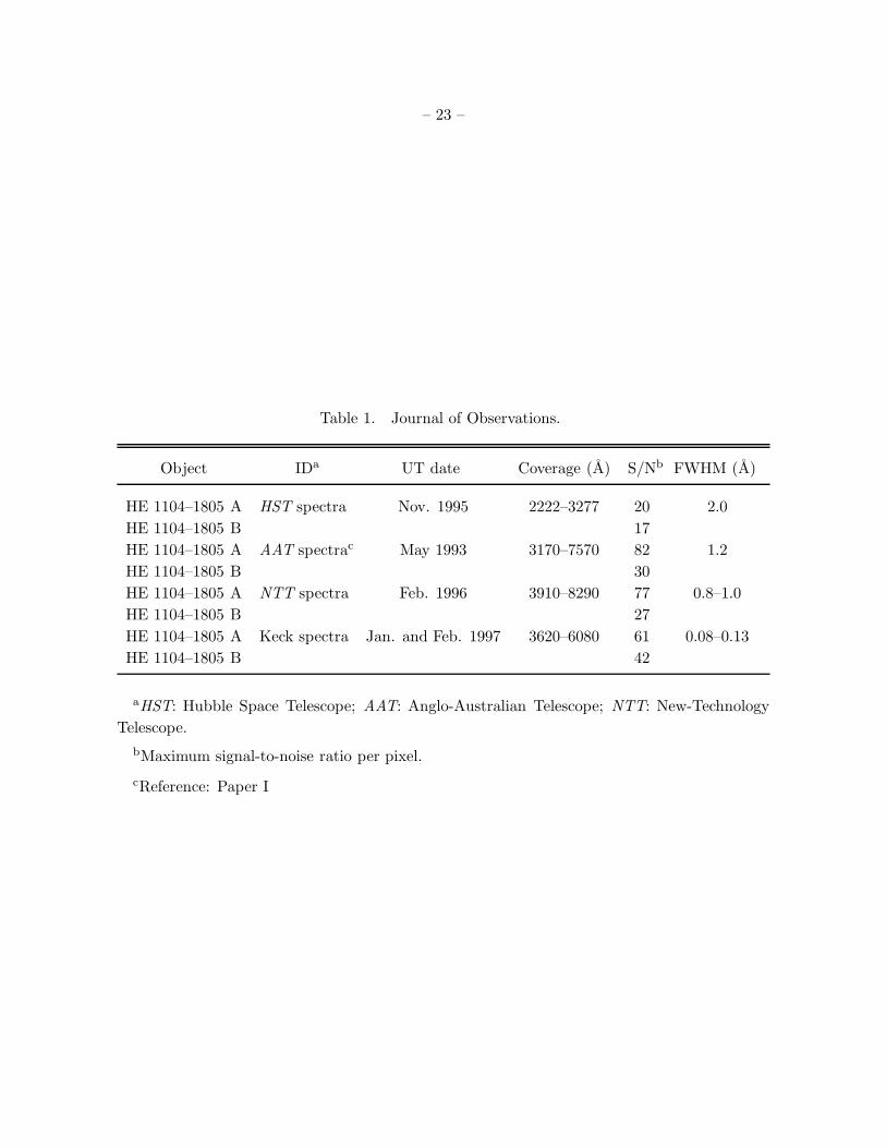
2. Observations and Data Reduction

An overview of the spectra used in this paper is displayed in Table 1. We now detail the

observations.

2.1. HST Spectra

UV spectra of HE 1104–1805 A and B were taken in November 1995 with the Faint Object

Spectrograph onboard the Hubble Space Telescope. Target acquisition and spectroscopy were

done using Grating G270H with the red detector and the 3.′′7 × 3.′′7 aperture. This configuration

yields a spectral resolution of FWHM = 2 A and a wavelength coverage from 2222 A to 3277 A

(Schneider et al. 1993). Total integration times of 1790 and 6690 seconds for QSO component A

and B, respectively, resulted in variance weighted spectra of maximum signal-to-noise ratios S/N

= 20 (A) and 17 per ∼ 0.5 A pixel.

2.2. Keck HIRES Spectra

Optical spectra of HE 1104–1805 A and B were taken in January and February 1997 with the

Keck High Resolution Spectrograph HIRES (Vogt et al. 1994) and an 0.86′′ slit at FWHM = 6.6

km s−1. They range from 3620 to 6080 A. A full description of the observations and extraction

method, as well as the spectra themselves will be presented elsewhere. In short, an image rotator

was used to keep the slit off the second image, and as close as possible to the parallactic angle.

The continua were matched by using the brighter A image continuum as a template, i.e., the

continuum points of the B image spectrum were, in a sense, ”stapled” to the A image continuum.

This was done using polynomial fits in such a way that differences between the continua on scales

larger than at average 300 km s−1 are divided out, but regions smaller than that retain their

differences between the LOSs. The typical absorption line or absorption complexes between the

spectra (which were omitted from the fit anyway) are not affected as can be seen from the strong

differences in the metal lines despite the very similar Lyα forest. We have also taken special care

to omit the metal absorption line complexes from the continuum points, to be sure that we do not

wipe out the differences. One-sigma arrays were derived from the Poissonian photon error, and

rebinned onto the 0.04 A/pixel constant wavelength scale.

2.3. NTT Spectra

Optical spectra of HE 1104–1805 A and B were obtained in February 1996 with the echelle

spectrograph of EMMI on the ESO New Technology Telescope in the Red Medium Dispersion

mode under subarcsecond seeing conditions. The wavelength coverage is 3910 to 8290 A. Both

– 5 –

images were simultaneously centered in a 1′′ slit. Grating #9, grism 3 as cross-disperser, a F/5.2

camera and a TEK 20482 CCD were used. This CCD provides 24µm pixels, corresponding to 0.′′27

in the sky. The total integration time was 16 hours. The echelle orders were optimally extracted

with a version of the extraction algorithm used in Paper I, modified to extract cross-dispersed

spectra. The algorithm attempts to reduce the statistical noise in the extracted spectra to a

minimum, and allows the correct separation of the two seeing profiles. It basically consists of

the following steps: (i) a variance (Poisson statistics, read-out noise and cosmics) is assigned

to each pixel. For each flat-fielded two-dimensional spectrum, two Gaussians of common width

are simultaneously fitted to the profiles at each wavelength channel along the previously defined

echelle orders using the Levenberg-Marquardt method (Press et al. 1986); (ii) the variation of the

width and the position of the brighter component with respect to the orders in the dispersion

direction is then fitted with low order polynomials; (iii) step (i) is repeated, this time with fixed

width and position—given by the polynomial fits—thus allowing only the amplitudes to vary. The

final, variance-weighted coadded spectra have FWHM = 0.8 to 1.0 A and maximum S/N ≃ 77 (A)

and ≃ 27 (B). The continuum level was estimated separately in each order—skipping corrections

for the blaze function—and for each QSO image. This was done by fitting low-order polynomials

and cubic splines to featureless spectral regions.

2.4. AAT Spectra

Additional FWHM = 1.2 A resolution spectra of both QSO images taken with the 3.9m

Anglo-Australian Telescope and covering the wavelength range 3170 to 7570 A were also used.

They have already been presented in Paper I.

2.5. Wavelength calibration of the HST spectra

Special care has been taken to re-define the absolute zero point of the wavelength scale in

the HST spectra. An off-center position of the targets in the aperture of the FOS may cause

differences in the wavelength scale between the A and B spectra. By measuring wavelength

positions of the galactic Mg ii λλ2796, 2803 lines, and assuming that this absorption takes place

in the same cloud along both LOSs we found an offset of ∆λ(A − B) = −0.42 A. This correction

was applied to the B spectrum. Additionally, an overlapping 100 A wide spectral region around

λ = 3220 A in the HST and AAT spectra allowed for a correction of the FOS wavelength scale

to vacuum-heliocentric values. This was done by comparing the central wavelength differences of

absorption lines in the A spectrum thought not to be blended. A relatively small correction of

∆λ(AAT − HST ) = +0.04 A was then applied to both HST spectra.

– 6 –

3. Absorption Line Analysis

3.1. Continuum Definition in the HST Spectra

Owing to the low FOS resolution, line blending introduces a serious problem when performing

continuum fitting. This is particularly marked in the Lyα forest, because of the lack of spectral

regions free of absorption lines. For this reason, we decided to first determine the absorbed

continuum—clearly dominated by two optically thin Lyman-limit systems (LLS) at z = 2.20 and

2.30 and the DLA system (A) and a LLS at z = 1.66 (B)—before describing the intrinsic QSO

continuum. Both spectra were corrected for galactic extinction (Seaton 1979) with E(B−V)=0.09

(Reimers et al. 1995). The Lyman edges, arising from the superposition and blending of

corresponding high-order H i Lyman series lines, were modeled with Voigt profiles convolved

with a FWHM = 2 A Gaussian describing the instrumental profile. The optical depth τ at each

Lyman break, given by the ratio of the extrapolated continuum to the Lyman one, determined

N(H i), whereas b was mainly constrained by the shape of the edge. These parameters are listed

in Table 2. The total optical depth at each LLS is given by the Lyman continuum and the lines of

the Lyman series. Note that the flux for λ < 2200 A in the B spectrum is not completely absorbed

(see Fig. 1).

The intrinsic QSO continuum of HE 1104–1805 A and B in the HST spectra for λobs ≤ 3277

A was found to be very well represented by two power laws (f ∝ να) with a break at λ = 2917

A. To determine the power law parameters, a maximum likelihood fit was performed, matching

simultaneously the intrinsic and the H i absorption continuum with the observed flux at selected

absorption-free spectral regions including some regions dominated by significant H i absorption

lines. This led to the best-fit spectral indices α = −0.8, −1.5 for A, and −0.8, −0.9 for B (see

Fig. 1). We believe this continuum estimation is a good one, since an extrapolation to longer

wavelengths fits the scaled AAT spectra to well within 1σ in regions of low Lyα line density.

Moreover, expected emission lines by Lyα, Nv, and Ovi stand out well against the continuum

as can be seen in Fig. 1. Division of the flux by this continuum resulted in the normalized HST

spectra shown in Fig. 2.

The different continuum slopes of A and B, already pointed out in the discovery paper, might

be a consequence of QSO component A being microlensed (Wisotzki et al. 1993). Furthermore,

we find the spectrum of A bluewards of Lyα emission to be softer than that of B, in agreement

with the variability in the spectral slopes reported by Wisotzki et al. (1995) from the analysis of

low resolution observations in the optical range made one and two years before ours. However,

an alternative explanation for the different slopes might be differential reddening by dust grains

in the DLA system observed in A, a possibility recently considered for the gravitationally lensed

QSO 0957+561 (Zuo et al. 1997).

– 7 –

3.2. Line Profile Fitting

In this section we describe the line fitting procedures used to obtain column densities

of lines associated with the z = 1.66 absorption systems in A and B. In general, this is a

nontrivial task because of the limited resolution of our spectra other than Keck HIRES, so that

assumptions concerning line widths must be made. The lines were modelled with Voigt profiles.

We distinguish between maximum likelihood fits, performed to lines in the Keck and NTT spectra,

and “interactive” fits, performed to lines in the AAT and HST spectra (aside from H i lines).

3.2.1. Keck Spectra

To determine column densities N and Doppler parameters b of lines in the Keck HIRES

spectra, we χ2-fitted Voigt profiles convolved with the instrumental profile to lines in the Keck

spectra using the MIDAS program FITLYMAN (Fontana & Ballester 1995). These lines lie

longward of Lyα emission. Line parameters, i.e., rest-frame vacuum wavelengths, damping

constants and oscillator strengths, were taken from Morton (1991), and from Verner et al. (1994)

for lines with revised f -values.

Most of the column density errors σlogN range from 0.01 to 0.10 dex; however, the smoothing

introduced by rebinning the 1σ-arrays sometimes underestimates the true flux uncertainties,

making σlogN systematically too low. Thus, we made the following correction to the fit errors:

for each line, we measured the amount of smoothing by calculating the ratio of the flux standard

deviation from 41-pixel wide featureless regions in the data to the sigma from the error array. In

the (few) cases where this ratio was larger than one, σlogN was corrected by this factor. Clearly,

this applies only to unsaturated, resolved lines; a similar treatment to non-resolved complexes is

less obvious because the σlogN ’s result from a more complicated Hessian matrix, and are no longer

independent. We did not allow for this effect.

Special attention must be given to the fits of lines associated with the DLA system observed

in the spectrum of QSO component A because they will determine the metal abundances. To look

for possible hidden saturation, we used the apparent optical depth method to compare apparent

column densities Napp(v) of different transitions of a given ion in velocity space (e.g. eq. [1] in

Lu et al. 1996; Savage & Sembach 1991, for a description of the method). Although some lines

are probably saturated (e.g. Al ii λ1670), in most of the cases where more than one transition is

available we do not find significantly saturated structures, and the agreement between the fit and

integration results is remarkable (cf. Table 4).

– 8 –

3.2.2. NTT Spectra

In the NTT spectrum, the Mg ii profiles at zDLA are slightly asymmetric, suggesting that

this system will also split into more components at higher resolution. Consequently, we fitted

four-component Voigt profiles to these lines, with b-parameters fixed at values found for the Si ii

lines in the Keck spectra.

3.2.3. HST and AAT Spectra

At even lower resolution, one cannot expect to recognize the line profiles properly; hence,

to derive column densities of lines in the HST and AAT spectra, turbulence dominated line

broadening was considered. Voigt profiles were interactively created and superimposed to the

spectra using XVOIGT (Mar & Bailey 1995), while attempting to minimize the residuals. The

redshift and Doppler widths used to create such line profiles were those found in a second fit with

FITLYMAN of lines present both in the AAT and Keck spectra. Lines with asymmetric profiles

were considered to be single, and the total column densities were fixed to the known Keck-values.

In this fashion, the low and high-ionization species were distinguished using “low-resolution”

Doppler parameters determined by the fits to Fe ii λ1608 (b = 20 km s−1) and C iv λ1548 (b = 44

km s−1) lines in A, respectively. For B, the lines used were Al ii λ1670 (b = 20 km s−1) and C iv

λ1548 (b = 37 km s−1).

To estimate the uncertainties of our column densities we smoothed and rebinned lines

observed in the NTT spectra to HST FOS resolution, and re-computed column densities with

the procedure described above. The new column densities showed deviations of the order 0.1

to 0.2 dex from the original, better determined values. Another source of error is our limited

ability to de-blend metal lines from Lyα forest lines. On the other hand, most column densities of

transitions in the UV that contribute to the metal abundances are based on one line in the HST

spectra and another in the AAT ones, e.g., C ii λλ1036,1334; O i λλ988,1302 (see Fig. 2). If these

two effects compensate, we think that taking σlogN = 0.2 dex for these ions is appropriate.

3.2.4. Detection Limits

We defined 3 σ detection limits for metal lines in the HST and AAT spectra according to the

formula (Caulet 1989)

σW =FWHM

< S/N >, (1)

where FWHM is the width of the spectral point spread function and <S/N> is the mean local

signal to noise expected at the position of the line (measured as the inverse standard deviation

of the normalized flux in small featureless stretches adjacent to the line). They range between

Wobs = 0.13 and 1.00 A in the B spectra.

– 9 –

3.2.5. H i Column Densities at z = 1.66

To derive more accurate column densities for H i, we used the normalized HST spectra.

Because they completely cover the rest-frame spectral range down to 912 A for the z = 1.66

systems, it is possible to measure N(H i) in both spectra more accurately than in previous

studies on damped systems, by using higher Lyman series transitions. We simultaneously fitted

two-component Voigt profiles to 11 resolved H i lines in the normalized spectra of A and B using

FITLYMAN. The fit solutions to lines in B were constrained by τ = 2.34 at the Lyman edge. We

estimate the neutral hydrogen column density of the DLA gas (spectrum A) to be log N(H i) =

20.85±0.01; for the LLS (B) we obtained log N(H i) = 17.57±0.10. Notice that these values are

independent of the ones estimated for placing the continuum and shown in Table 2.

4. The Damped Lyα System Toward HE 1104–1805 A at zDLA = 1.66162

Table 3 displays the fit results for lines associated with the DLA system toward HE 1104–1805

A at zDLA = 1.66162. A wide variety of singly and doubly ionized species is observed in this

DLA system, but C iv and Si iv are also present. We now describe the Keck HIRES line profiles,

referring to the left-hand panels of Figures 3, 5 and 4, throughout this section.

4.1. Low Ion Profiles

The left-hand panel of Fig. 3 shows the line profiles of strongest low-ionization species in

velocity space, relative to v = 0 at z = 1.66164, the redshift of Mg ii in the DLA system. These

lines lie redward of the Lyα forest. In each line complex, we have fitted four Voigt profiles with

independent z, b and N values. The Ni ii and Fe ii results are based upon simultaneous fits to 3

transitions; the Si ii and Al iii fits on 2 transitions; the Al ii fit on 1 transition; and the Mg ii fit on

2 transitions (cf. Table 3). We fitted 4 components to the Mg ii lines in the NTT spectra, with z

and b tied to the values found for Si ii. Only the three bluemost components show associated Zn ii

and Cr ii (see 4.3.1).

From the high-resolution plots, we see that the low ions track each other quite closely,

suggesting they occur in the same gas clouds. The whole profile is characterized by one cloud at

v ≈ −30 km s−1 with the strongest absorption, one cloud at v ≈ +40 km s−1 with the smallest

column densities, and two clouds with intermediate column density clouds lying in between.

This “edge-leading asymmetry” seems to be a common feature of low-ionization absorption lines

associated with damped Lyα systems. It has been variously interpreted as a consequence of

absorption by rotating gaseous disks (e.g., Wolfe et al. 1995b) or as the signature of merging

protogalactic clumps in hierarchical structure formation (Rauch et al. 1997a). The different

column density ratios at each velocity indicate clouds with different physical conditions (gas

– 10 –

density, metallicity, or even ionization) within 70 km s−1.

4.1.1. Line Widths

Remarkably, and despite the independent fits performed to each ion profile, we obtain fit

solutions that uniquely characterize each cloud in redshift and broadening parameter (cf. Table 3

and Fig. 3). For instance, for the clouds at v ∼ −30, −10, 10 and 40 km s−1 we find respective

mean widths and standard deviations of 〈b〉 = 3.5 ± 0.7, 12.6 ± 2.7, 9.1 ± 2.2 and 7.6 ± 1.8 km s−1

(fourth Ni ii component excluded due to large b-uncertainties; fit to Zn ii, Cr ii and Ti ii lines not

included). Thus, we find a similar line-broadening mechanism in each of these absorption systems

and, based on the small Doppler-parameter dispersions, cautiously favor turbulent gas motions as

the dominant line-broadening mechanism.

4.2. High Ion Profiles

The left-hand panel of Fig. 4 shows the C iv λ1548, 1550, Si iv λ1393, 1402 and, for comparison

purposes, Al ii λ1670 velocity profiles associated with the DLA system. For the C iv absorption

lines between [-80,+80] km s−1, only four-component Voigt profile fits succeeded. Unfortunately,

the poor S/N at the position of the Si iv lines and contamination by Lyα forest lines do not allow

a clear comparison with the C iv profiles. We decided not to fit these Si iv lines. Instead, we

give upper limits for column densities based on the apparent optical depth method. The high ion

profiles do not exactly track the low ion profiles: the data rather suggest at least part of the C iv

absorption (velocity component 1) occurs in clouds without low ionization species. On the other

hand, C iv velocity components 2 to 4 show a certain resemblance to the edge-leading asymmetry

of the low ion profiles; however, our fit solution yields relatively large b-values, suggesting

that C iv, regardless of which line broadening mechanism dominates—thermal or turbulent gas

motion—occurs in hotter gas regions than the low ion clouds.

4.3. Abundances

Metal abundances in the DLA system, normalized to solar values and defined by

[M/H] ≡ log(N(M)/N(H)) − log(N(M)/N(H))⊙ (2)

were computed using the column densities integrated between [-50,60] km s−1. They are listed in

Table 4. Solar abundances were taken from Verner et al. (1994). Singly ionized species provide the

bulk of the total element column densities, except for O i, assumed to be the dominant ionization

stage of oxygen.

– 11 –

4.3.1. Zn, Cr and Ti Abundances and Dust

Fig. 5 shows the Keck velocity profiles of the most outstanding Zn ii and Cr ii transitions.

The fit solutions lead to three-component profiles for the Cr ii complex at v = −29.1, −7.3 and

7.4 km s−1, and two-component profiles for Zn ii at v = −30.0 and −9.0 km s−1, relative to

z = 1.66164. The column density ratios relative to solar vary from N(Zn ii)/N(Cr ii) = 3.47

(bluemost component) to 1.73. If the Zn and Cr abundances as well as the ionization level were

the same in these clouds (which is very probable), then this variation would indicate that the

dust-to-gas ratio in this DLA gas is inhomogeneous within 20 km s−1, with a higher dust content

in the higher density Zn ii component.

The variation of the abundance ratios of refractory elements among different clouds associated

with the DLA gas provide insights into the presence of dust in the disk of damped Lyα galaxies

(Lu et al. 1996), because dust grains can be locally destroyed by passage of supernova shocks

(Sembach & Savage 1996, and references therein). We can extend our analysis of elemental

abundance ratios to iron and nickel, also expected to be depleted into dust. The column density

ratios Zn ii to Fe ii and Zn ii to Ni ii relative to solar are respectively Zn/Fe = 5.5 and Zn/Ni

= 7.9 for velocity component 1, and Zn/Fe = 2.5 and Zn/Ni = 2.8 for velocity component 2,

thus in concordance with what one observes for Cr in the corresponding clouds (we estimate the

corresponding uncertainties to be no larger than 0.4). Although these variations are small, 0.3 –

0.4 dex, it seems that in the v ∼ −30 km s−1 cloud the effect of dust depletion is more important

than in the cloud at v ∼ −10 km s−1. On the other hand, as pointed out in section 4.1.1,

the bluemost component is characterized by narrower lines than component 2 in all the ions

considered (including Zn ii and Cr ii). It would be of great interest to discern whether such line

width differences have a thermal origin (contrary to what was stated in 4.1.1, however), because it

would give evidence for dust depletion being more effective in cooler gas.

Lu et al. (1996) have presented arguments for a pure nucleosynthetic origin of the elemental

abundance pattern observed in Lyα damped systems at low metallicity. These arguments are:

the low N/O ratio, which we also find in this DLA system (see next section); the α-element

overabundance relative to Fe-peak elements, also observed for the abundance ratios of Si to Fe,

Cr, Mn and Ni in our Keck HIRES data; and the underabundance of Al relative to Si and Mn

relative to Fe (the “odd-even effect”; see Lu et al. 1996 for details), which we do not find in this

DLA system. Instead, we derive [Al/Si]= +0.25 ± 0.15, and [Mn/Fe]= −0.02 ± 0.14 (cf. Table 4),

although we recall that the Al abundance is only based on the Al ii λ1670 line. Given the high

Mn/Fe ratio and the argument given in the last paragraph, we suggest that stellar nucleosynthesis

alone is not likely to produce the relative abundance pattern observed in this DLA gas.

Based on the total zinc abundance [Zn/H] = −1.02 ± 0.01 relative to the solar value, we

derive a metallicity ZDLA ≃ 1/10 Z⊙ for this system. This zinc abundance is somewhat lower than

the value [Zn/H] = −0.8 reported by Pettini et al. (1997) [same data as in Paper I], who also

used log (Zn/H)⊙ = −7.35, and more accurate since it is based on a simultaneous fit to two Zn ii

– 12 –

lines.4 Additionally, we deduce from [Cr/H] = −1.46 ± 0.02 a dust-to-gas ratio of ∼ 0.11, using

the definition given by Vladilo (1998), eq. [19], and considering that most of chromium should

be incorporated into dust grains in the ISM of galaxies showing damped H i absorption (e.g.

Pettini et al. 1990). Furthermore, titanium, another refractory element, is found to have [Ti/H]

= −1.50 ± 0.07, based upon the unsaturated Ti ii λλ1910.6, 1910.9 lines. This is in full agreement

with the incorporation of Ti and Cr into a dust phase in the neutral ISM of this damped Lyα

galaxy. Thus, based on these abundances, we conclude that (1) this DLA system does not differ

too much from other ones at higher redshifts, given the scatter observed in [Zn/H] (cf. Fig. 3 in

Pettini et al. 1997); (2) there is evidence for the presence of dust.

4.3.2. The Abundance Ratio O/N

The crucial abundance ratios in this work are [O/N] and [C/Mg].

Based on the O i λλ988,1302 lines, we find [O/H] = −0.98±0.20, in very good agreement with

the abundance ratio of Zn. This supports O i as a very good tracer of H i— as can be expected

from its ionization potential, 13.62 eV— and suggests that O is not depleted into dust in the ISM

of this damped Lyα galaxy, in agreement with observations in the local ISM (Cardelli et al. 1991).

Moreover, since both O and Si have been observed to have solar abundance ratios in Galactic

halo stars and in metal-poor dwarf galaxies, one would expect [Si/O] ≃ 0 in DLA systems (Lu et

al. 1996 and references therein). We do obtain the same abundance ratios for O and Si within the

errors, and [Si/H] is based on reliable column-density measurements of two Si ii lines (observed

in the Keck HIRES spectrum), making our oxygen abundance estimation yet more confident.

Concerning the abundance ratio of nitrogen, the bulk of [N/H] is provided by the column density

of N ii λ1083. This line is very probably not contaminated by a Lyα forest interloper, given the

absence of absorption at the same wavelength in the spectrum of B (see Fig. 2). In addition,

nitrogen—like oxygen—is also expected not to be depleted in the ISM (Cardelli et al. 1991). In

consequence, we are confident of an abundance ratio of [O/N]= 0.88 in this DLA gas, that is,

O/N is 8 times greater than the solar ratio. This is in qualitative agreement with observations of

damped Lyα galaxies at higher redshifts (Pettini et al. 1995; Lu et al. 1996), and with galactic

chemical evolution models, because these two elements have different nucleosynthetic origins,

oxygen being produced in much shorter timescales than nitrogen.

4However, our 40 km s−1 resolution NTT spectra yield Zn and Cr abundances completely consistent with the

Keck results, thus validating abundance studies of Zn at medium resolution.

– 13 –

4.3.3. The Abundance Ratio C/Mg

The carbon abundance is based on the fits to the C ii λλ1036, 1334 lines. C/Mg is found to

have the solar value within the errors, but N(Mg) might be underestimated through saturation of

the Mg ii lines in A.

5. Geometry of the Absorbers at z = 1.66

Fig. 6 shows the velocity profiles of the C iv λ1548,1550 and Mg ii λ2796,2803 doublets (at 7

and 40 km s−1 resolution, respectively) toward HE1104–1805 A (left) and B. In both panels, v = 0

km s−1 corresponds to z = 1.66164, which is the redshift of Mg ii in the DLA system. We have

arbitrarily numbered the C iv complexes at z = 1.66143 (1), z = 1.66280 (2) and z = 1.66465 (3)

in the A spectra, and at z = 1.66184 (4), z = 1.66284 (5) and z = 1.66493 (6) in the B spectra, so

they will be refered to as systems 1 to 6 throughout the following sections. Also shown in Fig. 6,

covering a larger range of velocities, are the profiles of the Lyα, Lyβ and Lyγ H i lines. Note that

H i presents (at least) two components both in A and B.

C iv systems 1 to 4 show associated Mg ii, although shifted in velocity, as is more evident in

systems 1 and 4 (the line shapes suggest that either of these systems will probably split into more

components at even higher resolution). However, most of the Mg ii seen in A at v = 0 is due to

the DLA system. In B, system 4 is identified with the LLS. The presence of Mg ii in absorption

systems 2 and 6 is less evident at this S/N, so only upper limits can be derived. C iv system 5 will

not be considered here.

Do C iv and Mg ii occur in the same clouds? Although the present data show a correspondence

in velocity, there might not be a physical association between both ions. However, we will show in

the next section that photoionization simulations of these clouds do indeed predict the presence

of both ions in a common gas phase, in agreement with our observations. Furthermore, we know

from studies at high resolution that line profiles of low and high ions do track one another in

Lyman-limit systems (Prochaska & Wolfe 1996). As discussed in § 6.2 it is also possible that part

of the C iv arises in the same highly ionized gas that gives rise to Ovi. In any case, the velocity

profiles of system 4 (LLS) show that, if a physical association of both ions is correct, at least part

of the C iv arises in clouds where no Mg ii is present (see also the right-hand panel of Fig. 4).

From inspection of Fig. 6, it seems likely that LOSs A and B cross common absorbers. This

is suggested by the similar line profile pattern in both spectra. If a common absorption complex

gives rise to systems 1 (A) and 4 (B), then the different equivalent widths of the Mg ii lines in

A and B, in contrast to the more similar C iv equivalent widths, suggest gas inhomogeneities on

spatial scales smaller than the linear separation between LOSs S⊥ = 8.3 h−150 kpc, for q0 = 0.5 and

a lens at z = 1, thus suggesting that C iv arises in a more extended region than Mg ii. However,

we find that the velocity difference between the C iv clouds in A and B is 〈∆v〉 = −11 ± 2 km s−1

– 14 –

while 〈∆v〉 = −1 ± 1 km s−1 for the corresponding Mg ii clouds. If these velocity differences are

a consequence of peculiar cloud motions, then a physical association of C iv and Mg ii is still

compatible with the data. Since it is not the aim of this study to determine the origin of both this

velocity difference and the ∼360 km s−1 velocity span of the C iv absorbers along both LOSs, we

have analyzed each system separately.

There are two alternative interpretations for the H i column densities in A and B: (1) the DLA

system arises in a disk-type galaxy (Wolfe 1995a) with the LOS to A passing through the gas in

the halo and the disk and LOS B passing through the halo gas only, or (2) in models of hierarchical

structure formation the DLA system arises in the central region of a protogalactic clump and

LOS B crosses the surrounding less dense gas at an impact parameter of a few kpc (Rauch et

al. 1997a). Our data do not allow us to discriminate between these two models. Consequently,

in the following we will simply consider C iv absorption systems 2 to 6 to arise in clouds in the

extended halo of the cloud giving rise to the DLA system (system 1), giving explicit references to

one of these models.

6. Ionization State and Chemical Composition

We have used the photoionization code CLOUDY (version 84.12a; Ferland 1993) to investigate

the ionization state and metallicity in the LLS observed in the B spectra of HE 1104–1805

(system number 4 in Fig. 6) and in three further C iv-Mg ii systems observed in A (systems 2,

3) and B (system 6). The clouds giving rise to these systems are represented by parallel slabs

illuminated on one side by the radiation field Jν proposed by Haardt & Madau (1996), consisting

of the background flux contributed by QSOs and AGNs, which is attenuated by H and He

absorption in Lyman-limit systems and Lyα forest clouds. This radiation field also has a diffuse

component due to recombination continuum radiation. Our model assumes J(912) = 0.37 × 10−21

erg s−1 cm−2 Hz−1 sr−1 at z = 1.66. Although this geometry does not perfectly describe a cloud

being illuminated by an isotropic incident radiation field, it should not introduce errors larger than

a factor of ∼ 2 (Bergeron and Stasinska 1986). In particular, cloud sizes along the LOSs resulting

from this model need to be considered upper limits, because considering slabs illuminated only on

one side underestimates the true ionizing radiation field.

As we argue below, the wide variety of low- and high-ionization stages present in these

systems makes it necessary to model the gas clouds with two zones of different ionization levels:

(1) a “low-ionization phase”, where absorption by singly, doubly, but also triply ionized atoms

occurs5; (2) a “high-ionization phase”, where Ovi absorption occurs. However, we will also discuss

the possible existence of a third, “intermediate-ionization phase”.

The CLOUDY simulations predict column densities of the expected ionization stages, suitable

5The term “low” has specifically the purpose to distinguish both gas phases.

– 15 –

to be compared with the observations. As a general strategy, we attempt to reproduce the

observed ionic column density ratios N(C iv) to N(Mg ii) in systems 2, 3, 4 and 6, and the ratio

N(Ovi) to N(Nv) in the high-ionization phase by varying the ionization parameter Γ. We assume

that both gas zones are ionized by the Haardt & Madau radiation field, and have the same relative

abundances as found in the DLA gas. Since the column density ratios are quite insensitive to the

metallicity of the gas [M/H] for a wide range of ionization parameters, we can constrain [M/H]

using the individual observed column densities.

Clearly, the assumption of same relative abundances in A and B must not hold for gas-phase

abundances of elements known to be depleted by condensation into dust grains. If the dust-to-gas

ratio in the halo of this damped Lyα galaxy were considerably lower than in its DLA region (or

even zero), photoionization models should arrive at ionic column densities of refractory elements

that are underestimated, compared with the observed value. We observe this effect for Fe ii (see

next section).

6.1. Low-ionization Phase

6.1.1. The Lyman-limit System at z = 1.66184 toward HE 1104–1805 B

Table 5 displays the observed column densities of ions associated with the LLS at z = 1.66184.

The low and high ion velocity profiles are shown in Figures 3 and 4, respectively (right-hand

panels). Besides the DLA system, this is the second most metal-rich system. Prominent ions

observed are: Mg ii, Al ii, Al iii, Si ii, Si iii, C ii, N iii and Fe ii. The detection of Fe ii is marginal

but significant. Due to the low S/N and extraction artifacts at the position of Fe ii λ1608 (Fig. 3,

top right spectrum), we decided to fit one-component Voigt profiles to the three strongest Fe ii

lines in the NTT spectra. The detection of Al ii and Al iii is qualitatively consistent with the

assumption of DLA relative metal abundances in the LLS.

Taking the arguments given in § 5 into account, in order to perform photoionization

simulations for the LLS we have to first determine the range of possible values within which

N(C iv)/N(Mg ii) is likely to vary. Since the line profiles of Mg ii do not trace the whole velocity

range of C iv, a very conservative upper limit of ∼ 20 for the ratios is given by the total column

densities of the fitted Voigt profiles. However, from the right-hand panel of Fig. 4 we see that the

low ion profiles (here represented by Al ii λ1670) coincide quite well in velocity space with C iv fit

components 2 and 3. Considering that these Mg ii line profiles at Keck HIRES resolution would

not differ too much from the Al ii λ1670 ones, and taking the column densities integrated over

these components leads to N(C iv)/N(Mg ii)= 5.3, a much more realistic column density ratio.

Table 6 displays the column densities predicted by CLOUDY for the LLS using the Haardt

& Madau ionizing radiation field (column labelled MODEL 1). Assuming for this system DLA

gas-phase abundances, a column density ratio N(C iv)/N(Mg ii)= 5.3 implies log nH = −1.8 cm−3

– 16 –

(or log Γ = −2.95 for this radiation field); in other words, the gas is relatively highly ionized

with N(H ii)/N(H i)≈ 200, but Mg ii is still present. The observed log N(H i) = 17.57 leads to a

typical (model dependent) cloud size along the LOSs of S‖ ≤ 1.6 kpc. For comparison purposes,

a power law of the form f ∝ ν−2 was also used as ionizing background (column labeled MODEL

2 in Table 6). A harder radiation field is not able to reproduce N(C iv)/N(Mg ii)= 5.3 with the

assumed element abundances. However, even the selected power law model fails to simultaneously

reproduce C ii and C iv, while the Haardt & Madau model does, due to the continuum break at

the He ii edge.

Our model assumes that the LLS gas is in photoionization equilibrium. Deviations from this

equilibrium can lead to dramatic underestimations of the cloud lengths parallel to the LOSs by

photoionization simulations, because the neutral hydrogen fraction is overestimated (Haehnelt et

al. 1996a). However, at the density derived for this LLS, nH ∼ 0.01 cm−3, significant departures

from the equilibrium temperature (T = 1.5 × 104 K) are rare, as is shown by Smoothed Particle

Hydrodynamics simulations (Rauch et al. 1997a, Haehnelt et al. 1996b). Thus, the hydrogen

recombination timescale in this regime, ∼ 6 Myr, is short enough to allow line cooling to balance

photoheating processes. Consequently, we believe the CLOUDY sizes derived for this LLS to be

reliable.

Gas Metallicity in the Lyman-limit System. The photoionization models described above

are quite independent of the gas metallicity [M/H] over the whole range of possible gas densities;

therefore, [M/H] can be determined by matching predicted and observed column densities. We

find that, regardless of which model is assumed, [M/H]LLS = [M/H]DLA − 0.2 represents the best

prediction for nine ions observed in this system (Al ii, Al iii and Fe ii are not considered). In

particular, N(C ii), N(C iv), N(Mg ii), and N(Si iii) are simultaneously very well reproduced if

ZLLS = 0.63 ZDLA. This is an upper limit for ZLLS because due to saturation of the Mg ii lines

in A, we obtain only a lower limit for [Mg/H]; hence, to reproduce N(Mg ii) in B, a larger Mg

content would require an even lower metallicity in the LLS relative to the DLA gas. Varying the

relative abundances within the observational errors in the column densities leads us to estimate

that this result is significant at the 2σ level (for comparison, considering solar relative abundances

in the LLS leads to [M/H]LLS = −1.5).

Studies of our galaxy halo gas show no systematic differences in the gas-phase abundances

within galactocentric distances of 7 to 10 kpc in various directions, suggesting uniform physical

properties over these radii. In addition, warm disk clouds show gas abundances that are 0.2 to 0.6

dex lower than those in warm halo clouds (Sembach & Savage 1996, and references therein; Savage

& Sembach 1996, but see Cardelli et al. 1995). If we assume that the LLS observed at z = 1.66184

in HE 1104–1805 B arises in the halo of the z = 1.66162 damped Lyα galaxy seen in A, a negative

gradient in metallicity from DLA to halo gas implies that this halo gas has not yet been fully

enriched with metals. This might be a consequence of different star-formation rates, in which case

LOS B would be probing gas regions of lower star-formation rate than LOS A. Alternatively, such

– 17 –

an abundance gradient could also be explained by a disk-to-halo gas (and dust) transfer yet in

early stages, if gas in the halo originates in the disk.

Fe and Al Abundances in the Lyman-limit System. Singly ionized iron is the most

outstanding outlier in our model, yielding an Fe ii abundance one order of magnitude lower

than observed (cf. Table 6). We conclude that this difference can only be due to different

iron gas abundances between A and B, qualitatively consistent with the absence of dust in

the halo of this damped Lyα galaxy. This situation resembles that in our Galaxy, where the

degree of dust depletion in halo clouds is smaller than in Disk clouds (Sembach & Savage 1996).

Further CLOUDY simulations show that the observed log N(Fe ii)= 12.47 can be reproduced if

[Fe/H]LLS = −0.8 (Haardt & Madau 1996) or −1.0 (fν ∝ ν−2). An opposite effect is found for

aluminum, where our model reproduces Al iii only if [Al/H]= −1.0, that is, if the Al overabundance

is limited to the DLA gas (but such overabundance might be a consequence of a saturated Al ii

λ1670 line in A [see also section 3.2.1]).

A third ionization phase? N(C iv)/N(Mg ii)= 5.3 also requires N(C iii) to be lower by 1.5 σ

than observed. This suggests that there might in fact be a third “intermediate-ionization gas

phase”, where part of the C iv, C iii, N iii and Si iv but no singly ionized species occur (neither

does Si iii, whose ionizing potential of 33.5 eV is considerably lower than that of C iii). We would

be thus observing blends of lines arising in two phases at similar redshifts. The existence of such

a gas phase is fully consistent with the model predictions for Si iii and Al iii in the low-ionization

phase (provided the Al relative abundance is lower than in the DLA gas), and with the C iv line

profiles, showing a much wider velocity span than the low ions (Fig 4). Unfortunately, the HST

spectral resolution does not allow an appropriate analysis of the C iii and N iii line profiles.

6.1.2. The C iv Systems at z = 1.66280 and z = 1.66465 toward HE 1104–1805 A

The N(C iv)/N(Mg ii) ratios in the C iv systems at z = 1.66280 and z = 1.66460 in A

(systems 2 and 3 in Fig. 6) are relatively well constrained by the observations, so we basically

repeated the procedure described in the previous section, i.e., we searched for CLOUDY solutions

that reproduce these ratios by varying Γ and Z. Since only the total neutral hydrogen column

density is known, N(H i) was distributed according to the N(Mg ii) ratios.

Table 8 displays the column densities predicted by CLOUDY for System 3. Again assuming

DLA gas-phase abundances, and the Haardt & Madau metagalactic radiation field, we find for

this system that the observed N(C iv)/N(Mg ii)= 70.8 can be well reproduced if log nH = −2.21

cm−3 (or log Γ = −2.54 for this radiation field), implying a longitudinal cloud size of S‖ ≤ 0.9 kpc,

where the inequality stands for [Mg/H] > −0.97. This size estimate assumes both C iv and Mg ii

to arise from the same density region in photoionization equilibrium.

– 18 –

In System 2, the detection of Mg ii is uncertain, and we can only derive

N(C iv)/N(Mg ii)> 117.5, which requires that log nH < −2.30 (log Γ > −2.45), or S‖ ∼>

0.5 kpc for N(H i)= 16.05. Predicted column densities for system 2 are shown in Table 7. The

disagreement for N(C iii) arises as a consequence of a bad fit to the C iii λ977 line.

None of these photoionization models necessarily requires that Z < ZDLA.

6.1.3. The C iv Systems at z = 1.66493 toward HE 1104–1805 B

Observed and predicted column densities for the C iv system at z = 1.66493 in B (system 6)

are shown in Table 9. Because the detection of Mg ii is very uncertain, our model was required

to reproduce C iv assuming Z = 0.63 ZDLA. We arrived at log nH = −2.40 (or log Γ = −2.35),

implying S‖ ∼ 0.6 kpc.

6.2. Ovi-phase

Possibly the most interesting result of this study is the significant detection of strong Ovi

absorption at z = 1.66 in both LOSs toward HE 1104–1805. Fig. 7 shows the corresponding section

of the HST spectra of the A and B images with tickmarks above the spectrum indicating the Ovi

λλ1031,1037 doublet at z = 1.66253 and the C ii λ1036 lines associated with the damped Lyα and

Lyman-limit systems. Tickmarks below the flux level indicate lines identified with other systems.

The Ovi λ1031 lines at λ = 2747 A have similar rest-frame equivalent widths of Wr = 0.93 ± 0.07

A (A) and 0.86 ± 0.10 A. Besides Si iii λ1206 at z = 1.28, neither further metal lines nor a Lyβ

line has been identified at this wavelength, but contamination by a weak Lyα line is not ruled

out.6 Voigt profiles convolved with the instrumental profile have been overplotted in the spectra

of A and B. They have Doppler parameters b = 180 km s−1 (A) and 110 km s−1 (B) (obtained

from Gaussian profile fits to the Ovi λ1031 lines) and common column density log N = 14.95. N

shows little variation with b within 110–180 km s−1 in this region of the curve of growth. Clearly,

these large Doppler values do not necessarily represent the true line widths. Rather, the observed

line profiles are probably made up of more than one Ovi line (but see next paragraphs). For

comparison, the dotted lines show the resulting profiles of 3 (A) and 2 (B) Ovi doublets with

common b = 50 km s−1 and total column density log N = 15.1 (A) and 15.0 (B). The doublets are

placed at redshifts corresponding to systems 1, 2, and 3 in A, and 4 and 5 in B (cf. Fig. 6).

Although Ovi has been shown to be relatively common in QSO absorption systems (Bahcall

et al. 1993; Bergeron et al. 1994; Burles & Tytler 1996), its detection along the two LOSs to

6It seems very unlikely that the absorption feature at λ ∼ 2747 A is entirely due to a Lyα forest interloper. In

such a case, two Lyα lines with N(H i) ∼ 1016 cm−2 (b = 30 km s−1) would be required to reproduce the absorption

profiles; however, no associated C iv is found, as it would be expected in this class of Lyα clouds.

– 19 –

HE 1104–1805 at z = 1.66 allows us to directly prove for the first time that this ion does indeed

arise in very extended gas clouds. There were indications of this for systems at lower redshift

(e.g. Bergeron et al. 1994; Lu & Savage 1993) but no firm evidence. Large, low-density Ovi

gas clouds confirms the prediction by Rauch et al. (1997a) based on simulations of protogalactic

clumps (PGCs). In this model, PGCs with a few times 109 M⊙ (in baryons) are embedded in a

filamentary, low density and largely featureless Ovi phase with spatial extent of up to several

hundreds kpc at the N(Ovi) = 1013 cm−2 column density contour (cf. Fig. 3 in Rauch et al.).

Detectable Ovi is indeed expected to be more extended than C iv. The gas is photoionized, and

the lines are bulk motion broadened and wider than C iv, as they sample the peculiar velocities

over a larger volume.

Observational evidence for the physical processes giving rise to Ovi—collisional or

photoionization—remain, however, debatable so far, basically because contamination by Lyα lines

makes it difficult to resolve the Ovi λλ1032, 1036 doublet profiles appropriately. In our case, a

quantitative assessment of the nature of this gas phase is possible, since no Nv is detected at this

redshift (Fig. 8), and photoionization models can be well constrained under certain assumptions.

At the hydrogen density nH ∼ 0.01 cm−3 derived for the C iv+Mg ii clouds, the fraction of

ionizing photons with the E > 114 eV necessary to ionize enough Ov into “observable” Ovi is

too small. Consequently, an additional, less dense phase is required to explain the strong Ovi

absorption observed in A and B. Since a unique interpretation of the line profiles is difficult

with the present HST data, we made the following, simplifying assumptions: (1) both LOSs

pass through a common phase giving rise to the Ovi absorption lines, suggested by the similar

equivalent widths and the zero velocity difference between lines in A and B; and (2) the absorption

lines arise in one cloud, suggested by the line profile symmetry (this assumption may not be valid,

but it is equivalent to integrating N(Ovi) over several line components). A 3σ upper limit of

Wr = 0.034 A for the Nv λ1238.8210 line (the stronger line of the Nv doublet) measured in the

AAT spectrum of A leads to a 3σ upper limit of log N(Nv) < 13.2. The non-detection of Nv

places the stringent (but otherwise very conservative) lower limit of N(Ovi)/N(N v) > 60. This

ratio requires densities lower than log nH = −3.55, or a large ionization parameter log Γ ≥ −1.2,

if we assume the same relative abundances as found in the DLA gas. This is a striking result,

given that a lower (closer to solar) [O/N] ratio would lead to even less dense Ovi clouds. In this

regard, we must bear in mind that the CLOUDY simulations above depend partly on the relative

abundances assumed. For instance, variations of the [O/N] ratio within the estimated column

density uncertainties will lead to differences in the predicted parameters.

It is nontrivial to obtain an overall picture of this phase because the total hydrogen column

density is not known. As a consequence, photoionization models will not reproduce the individual

observed column densities N(Ovi) and N(Nv) uniquely, but both N(H) and the gas metallicity

Z will determine them. This is shown in Fig. 9, where we have plotted all the pairs (Z,N(H))

that reproduce log N(Ovi) = 15.0 and log N(Nv) = 13.2. We can see that, in general, a lower

metallicity of the highly ionized gas relative to that of the DLA gas, say Z < 0.63ZDLA, will

– 20 –

be compatible with the observations if N(H) is large, log N(H) > 20.0. Additionally, we find

that, regardless of the gas metallicity, the clouds where this phase occurs must be at least one

to two orders of magnitude larger than the systems giving rise to Mg ii absorption. These cloud

sizes (S‖ >∼ 100 kpc), if representative of transverse dimensions, are widely consistent with the

detection of Ovi of similar strength in both LOSs. Typical masses derived from these models are

∼ 109 M⊙.

To see if C iv is expected in such a model, we performed further ionization simulations for

larger ionization parameters, requiring that the assumed total hydrogen column density and

metallicity always led to log N(Ovi) = 15.0, i.e., curves departing from points on the Z vs. N(H)

curve in Fig. 9. The predicted N(C iv) column densities in such models are shown in Fig. 10 for

the Haardt & Madau (solid line) and a power-law radiation field (dashed line). At the minimum

value of Γ allowed by the observations log Γ = −1.2, and for a wide range of gas metallicities,

CLOUDY predicts log N(C iv)≈ 14.4, in agreement with the observed value. However, at higher

ionization parameters, e.g., N(Ovi)/N(N v) ∼ 90 or log Γ = −1.0 (corresponding to a 2σ

significant non-detection of Nv), N(C iv) becomes ∼ 40% smaller, independently of Z. This

result in turn indicates that at least part of the observed C iv arises in highly ionized gas, with the

remaining contribution coming from the low-ionization gas phase. The present HST data do not

enable us to quantitatively assess this issue and we can only conclude that C iv is likely to occur

in both phases.

Collisional ionization of gas in thermal equilibrium can also reproduce the observed

N(Ovi)/N(N v) ratio at T = 105.45 K if one assumes solar relative abundances (Sutherland &

Dopita 1993), so we cannot rule out this process as responsible for ionizing Ov into Ovi. In

such a case, the line broadening would be mostly due to macro-turbulence. Collisionally ionized

Ovi gas in a Lyman-limit system at z ≃ 3.4 has been recently proposed by Kirkman & Tytler

(1997), who detect both C iv and Ovi at the same redshift in high resolution data. These authors

favor collisional ionization due to the high kinetic temperatures implied by the line widths of both

ions. In the case of HE 1104–1805 AB, additional, higher resolution (R ∼ 23 000) UV spectra are

needed, in order to finally discriminate between collisional and photoionization as the dominant

ionization mechanism in the Ovi-phase.

7. Conclusions and Final Remarks

We outline our conclusions as follows:

1. The damped Lyα system observed at z = 1.66162 in the ultraviolet and optical spectra

of HE 1104–1805 A has a neutral hydrogen column density of log N(H i)= 20.85 ± 0.01.

The 6.6 km s−1 resolution line profiles show that this high-density gas is distributed

in four clouds spanning ∼ 80 km s−1. Since the low ionization and Al iii line profiles

are observed to track fairly well, these ions are likely to arise in common clouds. Their

– 21 –

b-values are consistent if the broadening mechanism is not purely thermal. The C iv

line profiles show that at least some of C iv absorption occurs in clouds with no singly

ionized species. We find a metallicity of ZDLA ≃ 1/10 Z⊙ and a dust-to-gas ratio

of ∼ 0.11, based on [Zn/H]= −1.02 and [Cr/H]= −1.46. Other element abundances

are: [C/H]= −0.91, [N/H]= −1.86, [O/H]= −0.98, [Mg/H]= −0.97, [Al/H]= −0.77,

[Si/H]= −1.02, [Ti/H]= −1.50, [Mn/H]= −1.61, [Fe/H]= −1.59 and [Ni/H]= −1.68.

The O/N ratio, 8 times larger than the solar value, is consistent with galactic chemical

evolution models. However, the observed elemental abundance pattern must be modified by

condensation into dust grains given (a) the underabundance of Cr and Ti relative to Zn;

and (b) the variation of the abundance ratios of these and other refractory elements among

different clouds associated with the DLA system.

2. Photoionization by the metagalactic radiation field proposed by Haardt & Madau (1996)

implies that the Lyman-limit System observed at z = 1.66184 in the spectra of HE 1104–1805

B and the three further C iv systems observed at similar redshifts in A and B all belong to

the same category of absorbers, namely small (LOS sizes 0.5 to 1.6 kpc) and relatively dense

(nH = 0.01 cm−3) clouds where both C iv and Mg ii absorption occurs.

3. We find evidence for the LLS and one further C iv absorption system observed in B to have

lower metallicities than observed in the DLA gas, Z = 0.63 ZDLA. This result is significant

at the 2 σ confidence level if the column density uncertainties are not underestimated.

4. In the context of galaxy formation, the observed H i column densities suggest that LOS B

intercepts gas in the “halo” of a protogalaxy at z = 1.66, while LOS A crosses its denser,

central gas regions. If this picture is correct, then we are observing metal-poor gas in the

halo of such a galaxy, compared to the high-density gas (within a transverse separation of

∼8 h−150 kpc). This in turn suggests regions of different star-formation rates or, alternatively,

metal enrichment through gas transfer from the inner to the outer regions of the protogalaxy

still in early stages.

5. The presence of a highly ionized gas phase giving rise to the observed Ovi absorption of

similar strength in both spectra is evident. If photoionization is assumed, the observed

log N(Ovi) = 15.0, and the non-detection of Nv implies large (∼ 100–200 kpc), low-density

(∼10−4 cm−3) clouds where strong Ovi but weak C iv absorption occurs. On the basis of

these results, we suggest that this highly ionized gas surrounds the clouds giving rise to the

damped Lyα and Lyman-limit systems. Such an extended low-density Ovi phase confirms

the predictions of simulations of protogalactic clumps (Rauch et al. 1997a).

Concerning the negative gradient in metallicity from gas crossed by LOS A to gas crossed

by LOS B, it must be pointed out that such an effect, if real, does not necessarily support the

disk/halo scenario. Indeed, it is still not clear whether present-day rotating disk-like galaxies

should have had a similar appearance in their early stages of formation, nor is it well understood

– 22 –

what we should define as protogalactic “halos”. A good deal of progress is being made to resolve

this paradigm: a link between metallicity and kinematics can improve our understanding of

DLA systems (Wolfe et al. 1998); hydrodynamic simulations of merging protogalactic clumps are

capable of explaining the large velocity spans seen in this class of absorption systems (Haehnelt

et al. 1998). Here we have demonstrated the powerful tool which double LOSs can provide us. A

convincing interpretation of our result, however, has to await a larger sample of such cases.

Finally, let us emphasize that the scenario of small and compact C iv clouds surrounded by

extended Ovi gas can indeed be theoretically understood and is in good agreement with the

predictions of a cold-dark-matter based model (Rauch et al. 1997a). Furthermore, in a hierarchical

structure formation scenario damped Lyα and Lyman limit systems can arise from relatively

small (Mbaryon ∼ 109 M⊙) merging protogalactic clumps. Even if the sizes derived using our

photoionization models are not representative of transverse cloud sizes, the similar C iv line

profiles and equivalent widths in A and B are still consistent with filamentary structures, which is

also a prediction of hierarchical structure formation. Such a correlation between line profiles in A

and B is, on the other hand, less evident for Mg ii, implying gas inhomogeneities on spatial scales

similar to the separation between LOSs, and in concordance with Mg ii arising in smaller regions

than C iv and Ovi.

S. L. thanks the BMBF (DARA) for support under grant No. 50OR96016; M. R. thanks

NASA for support through grant HF-0107501-94A from the Space Telescope Science Institute;

W. L. W. S. was supported by grant AST 9529073 from the National Science Foundation. A. S.

thanks the financial support under grant no. 781-73-058 from the Netherlands Foundation for

Research in Astronomy (ASTRON), which receives its funds from the Netherlands Organisation

for Scientific Research (NWO). We thank the anonymous referee for many helpful suggestions.

– 23 –

Table 1. Journal of Observations.

Object IDa UT date Coverage (A) S/Nb FWHM (A)

HE 1104–1805 A HST spectra Nov. 1995 2222–3277 20 2.0

HE 1104–1805 B 17

HE 1104–1805 A AAT spectrac May 1993 3170–7570 82 1.2

HE 1104–1805 B 30

HE 1104–1805 A NTT spectra Feb. 1996 3910–8290 77 0.8–1.0

HE 1104–1805 B 27

HE 1104–1805 A Keck spectra Jan. and Feb. 1997 3620–6080 61 0.08–0.13

HE 1104–1805 B 42

aHST: Hubble Space Telescope; AAT: Anglo-Australian Telescope; NTT: New-Technology

Telescope.

bMaximum signal-to-noise ratio per pixel.

cReference: Paper I

– 24 –

Table 2. Lyman-edges in HE 1104-1805 A and B.

zLLS τa log NH i(cm−2) b (km s−1)

A 1.66162 · · · 20.84b 27

2.20016 0.29±0.08 16.67±0.12 35

2.29880 0.14±0.07 16.36±0.23 40

B 1.66184 2.34±0.51 17.57±0.10 30

2.20099 0.63±0.11 17.00±0.08 40

2.29877 0.21±0.11 16.53±0.23 35

aOptical depth τ = ln(f+/f−), where f+ is the

extrapolated continuum redward of 912 × (1 + zLLS), and

f− the absorbed continuum.

bColumn density constrained by the damped Lyα wings.

– 25 –

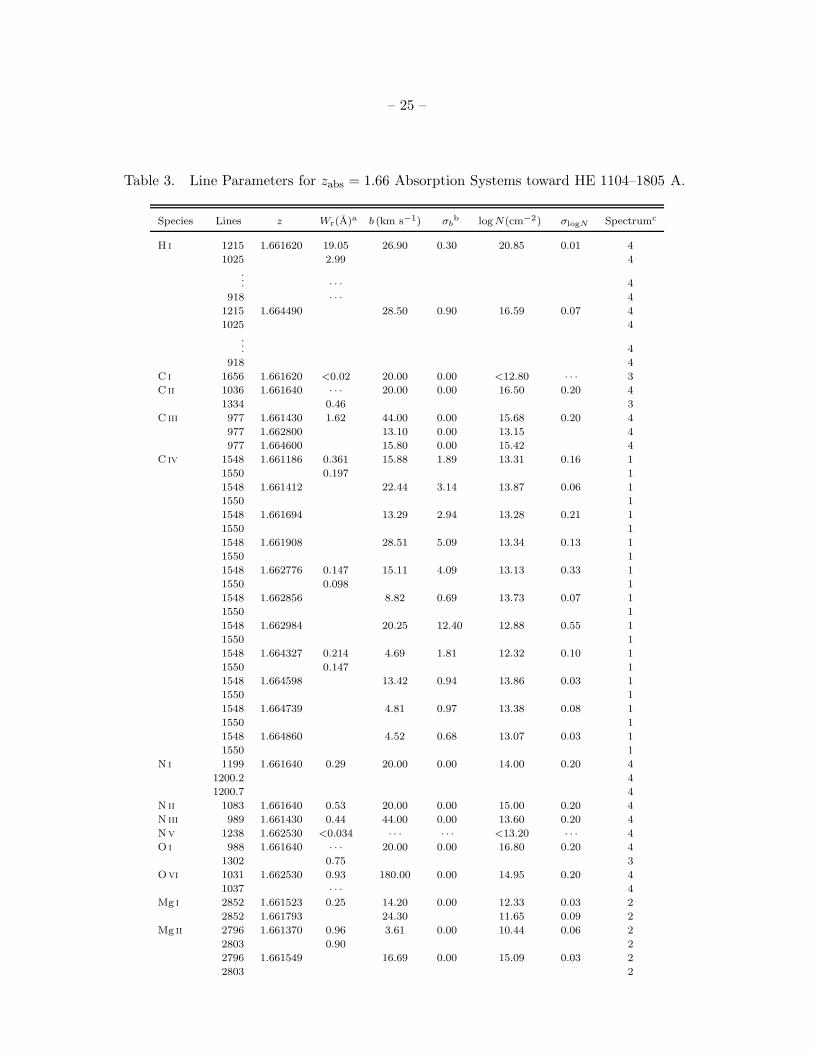
Table 3. Line Parameters for zabs = 1.66 Absorption Systems toward HE 1104–1805 A.

Species Lines z Wr(A)a b (km s−1) σbb log N(cm−2) σlogN Spectrumc

H i 1215 1.661620 19.05 26.90 0.30 20.85 0.01 4

1025 2.99 4... · · · 4

918 · · · 4

1215 1.664490 28.50 0.90 16.59 0.07 4

1025 4

... 4

918 4

C i 1656 1.661620 <0.02 20.00 0.00 <12.80 · · · 3

C ii 1036 1.661640 · · · 20.00 0.00 16.50 0.20 4

1334 0.46 3

C iii 977 1.661430 1.62 44.00 0.00 15.68 0.20 4

977 1.662800 13.10 0.00 13.15 4

977 1.664600 15.80 0.00 15.42 4

C iv 1548 1.661186 0.361 15.88 1.89 13.31 0.16 1

1550 0.197 1

1548 1.661412 22.44 3.14 13.87 0.06 1

1550 1

1548 1.661694 13.29 2.94 13.28 0.21 1

1550 1

1548 1.661908 28.51 5.09 13.34 0.13 1

1550 1

1548 1.662776 0.147 15.11 4.09 13.13 0.33 1

1550 0.098 1

1548 1.662856 8.82 0.69 13.73 0.07 1

1550 1

1548 1.662984 20.25 12.40 12.88 0.55 1

1550 1

1548 1.664327 0.214 4.69 1.81 12.32 0.10 1

1550 0.147 1

1548 1.664598 13.42 0.94 13.86 0.03 1

1550 1

1548 1.664739 4.81 0.97 13.38 0.08 1

1550 1

1548 1.664860 4.52 0.68 13.07 0.03 1

1550 1

N i 1199 1.661640 0.29 20.00 0.00 14.00 0.20 4

1200.2 4

1200.7 4

N ii 1083 1.661640 0.53 20.00 0.00 15.00 0.20 4

N iii 989 1.661430 0.44 44.00 0.00 13.60 0.20 4

Nv 1238 1.662530 <0.034 · · · · · · <13.20 · · · 4

O i 988 1.661640 · · · 20.00 0.00 16.80 0.20 4

1302 0.75 3

Ovi 1031 1.662530 0.93 180.00 0.00 14.95 0.20 4

1037 · · · 4

Mg i 2852 1.661523 0.25 14.20 0.00 12.33 0.03 2

2852 1.661793 24.30 11.65 0.09 2

Mg ii 2796 1.661370 0.96 3.61 0.00 10.44 0.06 2

2803 0.90 2

2796 1.661549 16.69 0.00 15.09 0.03 2

2803 2

– 26 –

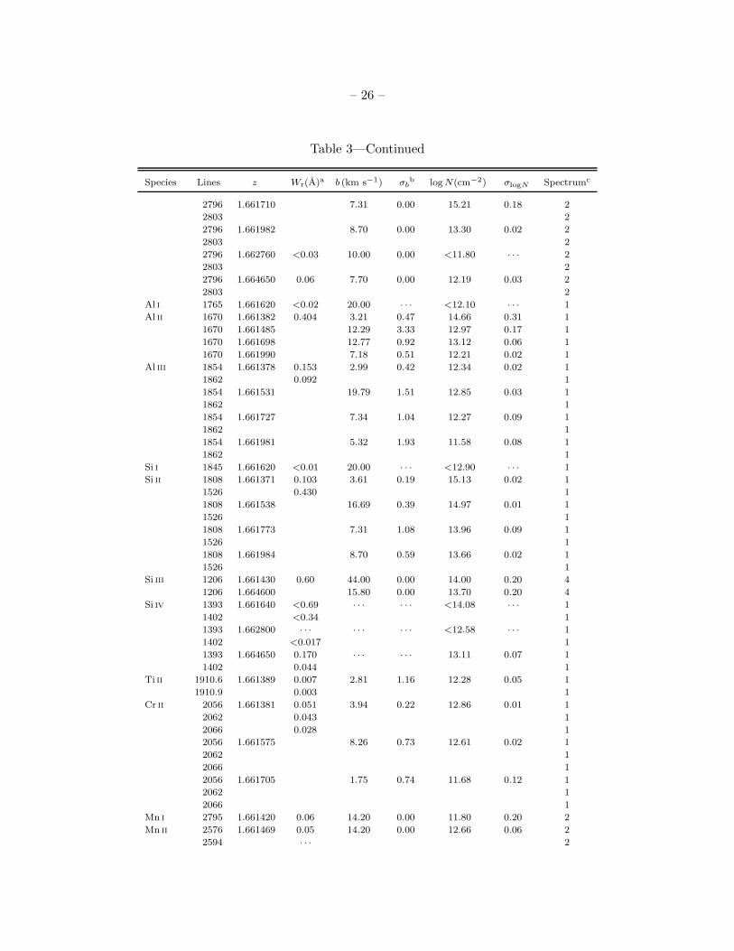
Table 3—Continued

Species Lines z Wr(A)a b (km s−1) σbb log N(cm−2) σlogN Spectrumc

2796 1.661710 7.31 0.00 15.21 0.18 2

2803 2

2796 1.661982 8.70 0.00 13.30 0.02 2

2803 2

2796 1.662760 <0.03 10.00 0.00 <11.80 · · · 2

2803 2

2796 1.664650 0.06 7.70 0.00 12.19 0.03 2

2803 2

Al i 1765 1.661620 <0.02 20.00 · · · <12.10 · · · 1

Al ii 1670 1.661382 0.404 3.21 0.47 14.66 0.31 1

1670 1.661485 12.29 3.33 12.97 0.17 1

1670 1.661698 12.77 0.92 13.12 0.06 1

1670 1.661990 7.18 0.51 12.21 0.02 1

Al iii 1854 1.661378 0.153 2.99 0.42 12.34 0.02 1

1862 0.092 1

1854 1.661531 19.79 1.51 12.85 0.03 1

1862 1

1854 1.661727 7.34 1.04 12.27 0.09 1

1862 1

1854 1.661981 5.32 1.93 11.58 0.08 1

1862 1

Si i 1845 1.661620 <0.01 20.00 · · · <12.90 · · · 1

Si ii 1808 1.661371 0.103 3.61 0.19 15.13 0.02 1

1526 0.430 1

1808 1.661538 16.69 0.39 14.97 0.01 1

1526 1

1808 1.661773 7.31 1.08 13.96 0.09 1

1526 1

1808 1.661984 8.70 0.59 13.66 0.02 1

1526 1

Si iii 1206 1.661430 0.60 44.00 0.00 14.00 0.20 4

1206 1.664600 15.80 0.00 13.70 0.20 4

Si iv 1393 1.661640 <0.69 · · · · · · <14.08 · · · 1

1402 <0.34 1

1393 1.662800 · · · · · · · · · <12.58 · · · 1

1402 <0.017 1

1393 1.664650 0.170 · · · · · · 13.11 0.07 1

1402 0.044 1

Ti ii 1910.6 1.661389 0.007 2.81 1.16 12.28 0.05 1

1910.9 0.003 1

Cr ii 2056 1.661381 0.051 3.94 0.22 12.86 0.01 1

2062 0.043 1

2066 0.028 1

2056 1.661575 8.26 0.73 12.61 0.02 1

2062 1

2066 1

2056 1.661705 1.75 0.74 11.68 0.12 1

2062 1

2066 1

Mn i 2795 1.661420 0.06 14.20 0.00 11.80 0.20 2

Mn ii 2576 1.661469 0.05 14.20 0.00 12.66 0.06 2

2594 · · · 2

– 27 –

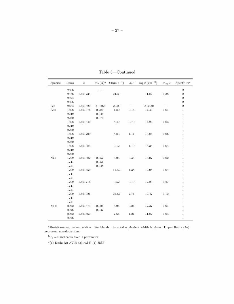
Table 3—Continued

Species Lines z Wr(A)a b (km s−1) σbb log N(cm−2) σlogN Spectrumc

2606 · · · 2

2576 1.661734 24.30 11.82 0.38 2

2594 2

2606 2

Fe i 2484 1.661620 < 0.02 20.00 · · · <12.30 · · · 2

Fe ii 1608 1.661376 0.280 4.80 0.16 14.49 0.01 1

2249 0.045 1

2260 0.079 1

1608 1.661549 8.49 0.70 14.29 0.03 1

2249 1

2260 1

1608 1.661709 8.83 1.11 13.85 0.06 1

2249 1

2260 1

1608 1.661983 9.12 1.10 13.34 0.04 1

2249 1

2260 1

Ni ii 1709 1.661382 0.052 3.05 0.35 13.07 0.02 1

1741 0.051 1

1751 0.048 1

1709 1.661559 11.52 1.38 12.98 0.04 1

1741 1

1751 1

1709 1.661716 0.52 0.19 12.29 0.27 1

1741 1

1751 1

1709 1.661921 21.67 7.71 12.47 0.12 1

1741 1

1751 1

Zn ii 2062 1.661373 0.026 3.04 0.24 12.37 0.01 1

2026 0.042 1

2062 1.661560 7.64 1.21 11.82 0.04 1

2026 1

aRest-frame equivalent widths. For blends, the total equivalent width is given. Upper limits (3σ)

represent non-detections.

bσb = 0 indicates fixed b parameter.

c(1) Keck; (2) NTT; (3) AAT; (4) HST

– 28 –

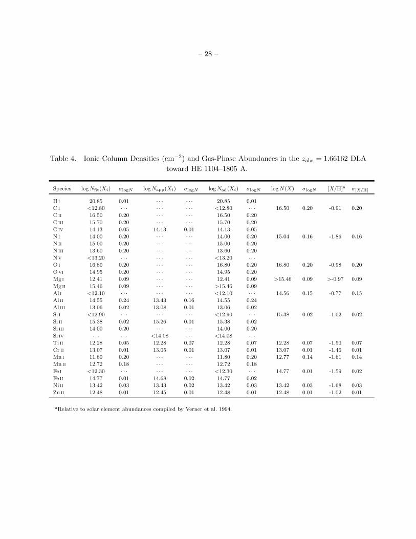
Table 4. Ionic Column Densities (cm−2) and Gas-Phase Abundances in the zabs = 1.66162 DLA

toward HE 1104–1805 A.

Species log Nfit(Xi) σlogN log Napp(Xi) σlogN log Nad(Xi) σlogN log N(X) σlogN [X/H]a σ[X/H]

H i 20.85 0.01 · · · · · · 20.85 0.01

C i <12.80 · · · · · · · · · <12.80 · · · 16.50 0.20 -0.91 0.20

C ii 16.50 0.20 · · · · · · 16.50 0.20

C iii 15.70 0.20 · · · · · · 15.70 0.20

C iv 14.13 0.05 14.13 0.01 14.13 0.05

N i 14.00 0.20 · · · · · · 14.00 0.20 15.04 0.16 -1.86 0.16

N ii 15.00 0.20 · · · · · · 15.00 0.20

N iii 13.60 0.20 · · · · · · 13.60 0.20

Nv <13.20 · · · · · · · · · <13.20 · · ·

O i 16.80 0.20 · · · · · · 16.80 0.20 16.80 0.20 -0.98 0.20

Ovi 14.95 0.20 · · · · · · 14.95 0.20

Mg i 12.41 0.09 · · · · · · 12.41 0.09 >15.46 0.09 >-0.97 0.09

Mg ii 15.46 0.09 · · · · · · >15.46 0.09

Al i <12.10 · · · · · · · · · <12.10 · · · 14.56 0.15 -0.77 0.15

Al ii 14.55 0.24 13.43 0.16 14.55 0.24

Al iii 13.06 0.02 13.08 0.01 13.06 0.02

Si i <12.90 · · · · · · · · · <12.90 · · · 15.38 0.02 -1.02 0.02

Si ii 15.38 0.02 15.26 0.01 15.38 0.02

Si iii 14.00 0.20 · · · · · · 14.00 0.20

Si iv · · · · · · <14.08 · · · <14.08 · · ·

Ti ii 12.28 0.05 12.28 0.07 12.28 0.07 12.28 0.07 -1.50 0.07

Cr ii 13.07 0.01 13.05 0.01 13.07 0.01 13.07 0.01 -1.46 0.01

Mn i 11.80 0.20 · · · · · · 11.80 0.20 12.77 0.14 -1.61 0.14

Mn ii 12.72 0.18 · · · · · · 12.72 0.18

Fe i <12.30 · · · · · · · · · <12.30 · · · 14.77 0.01 -1.59 0.02

Fe ii 14.77 0.01 14.68 0.02 14.77 0.02

Ni ii 13.42 0.03 13.43 0.02 13.42 0.03 13.42 0.03 -1.68 0.03

Zn ii 12.48 0.01 12.45 0.01 12.48 0.01 12.48 0.01 -1.02 0.01

aRelative to solar element abundances compiled by Verner et al. 1994.

– 29 –

Table 5. Line Parameters for the zabs = 1.66 Absorption Systems toward HE 1104–1805 B.

Species Lines z Wr (A)a b (km s−1) σbb log N(cm−2) σlogN Spectrumc

H i 1215 1.661840 1.690 30.00 0.00 17.57 0.00 4

1025 0.790 4... · · · 4

918 · · · 4

1215 1.664970 30.00 0.00 15.90 0.13 4

1025 4

... 4

918 4

C i 1656 1.661650 <0.09 20.00 0.00 <13.50 3

C ii 1036 1.661650 · · · 20.00 0.00 14.50 0.20 4

1334 0.18 3

C iii 977 1.664480 0.95 37.00 0.00 15.50 0.20 4

977 1.661830 29.30 0.00 14.00 0.20 4

C iv 1548 1.661130 0.630 19.93 2.33 13.24 0.04 1

1550 0.361 1

1548 1.661512 8.82 0.88 13.56 0.06 1

1550 1

1548 1.661759 21.96 4.49 13.81 0.10 1

1550 1

1548 1.662036 12.62 1.74 13.77 0.09 1

1550 1

1548 1.662250 47.39 4.03 13.71 0.15 1

1550 1

1548 1.662878 20.75 3.44 13.31 0.10 1

1550 1

1548 1.663167 5.89 2.53 12.38 0.16 1

1550 1

1548 1.663384 8.02 2.11 12.55 0.08 1

1550 1

1548 1.664721 0.077 3.54 1.49 12.61 0.07 1

1550 0.067 1

1548 1.664887 5.43 0.36 13.63 0.03 1

1550 1

N i 1199 1.661650 <0.11 20.00 · · · <14.00 · · · 4

N ii 1083 1.661650 <0.13 20.00 · · · <13.70 · · · 4

N iii 989 1.661830 0.27 37.00 0.00 14.00 0.20 4

989 1.662840 29.90 0.00 13.70 0.20 4

989 1.665070 0.27 37.20 0.00 14.20 0.20 4

Nv 1238 1.662530 <0.19 · · · <14.00 · · · 4

O i 988 1.661650 <0.13 20.00 · · · <14.10 · · · 4

1302 <0.19 3

Ovi 1031 1.662530 0.86 110.00 0.00 14.95 0.20 4

1037 4

Mg i 2853 1.661650 <0.10 20.00 · · · <11.90 · · · 2

Mg ii 2796 1.661557 0.343 7.83 0.00 13.14 0.13 2

2803 0.239 2

2796 1.661783 26.52 0.00 12.73 0.09 2

2803 2

2796 1.664930 <0.09 10.00 <12.40 2

2803 2

Al i 1765 1.661650 <0.10 20.00 · · · <12.60 · · · 1

Al ii 1670 1.661556 0.097 7.70 0.00 12.26 0.03 1

– 30 –

Table 5—Continued

Species Lines z Wr (A)a b (km s−1) σbb log N(cm−2) σlogN Spectrumc

1670 1.661781 14.10 0.00 11.80 0.06 1

1670 1.661990 8.10 0.00 11.45 0.10 1

Al iii 1854 1.661564 0.041 7.75 1.29 12.08 0.11 1

1862 0.036 1

1854 1.661784 14.07 13.05 11.98 0.35 1

1862 1

1854 1.661956 8.15 11.22 11.81 0.46 1

1862 1

Si i 1845 1.661650 <0.08 20.00 · · · <13.20 · · · 1

Si ii 1526 1.661552 0.076 8.30 0.94 13.29 0.03 1

1526 1.661747 7.72 3.94 12.80 0.15 1

1526 1.661941 8.99 3.69 12.89 0.12 1

Si iii 1206 1.661830 0.55 37.00 14.10 0.20 4

Si iv 1393 1.661840 1.166 · · · · · · <14.28 · · · 1

1402 0.580 1

1393 1.664930 · · · · · · · · · <12.86 · · · 1

1402 <0.033 1

Fe ii 2344 1.661578 0.012 7.86 4.30 12.47 0.08 2

2382 0.030 2

2600 0.045 2

aRest-frame equivalent widths. For blends, the total equivalent width is given. Upper limits (3σ)

represent non-detections.

bσb = 0 indicates fixed b parameter.

c(1) Keck; (2) NTT; (3) AAT; (4) HST

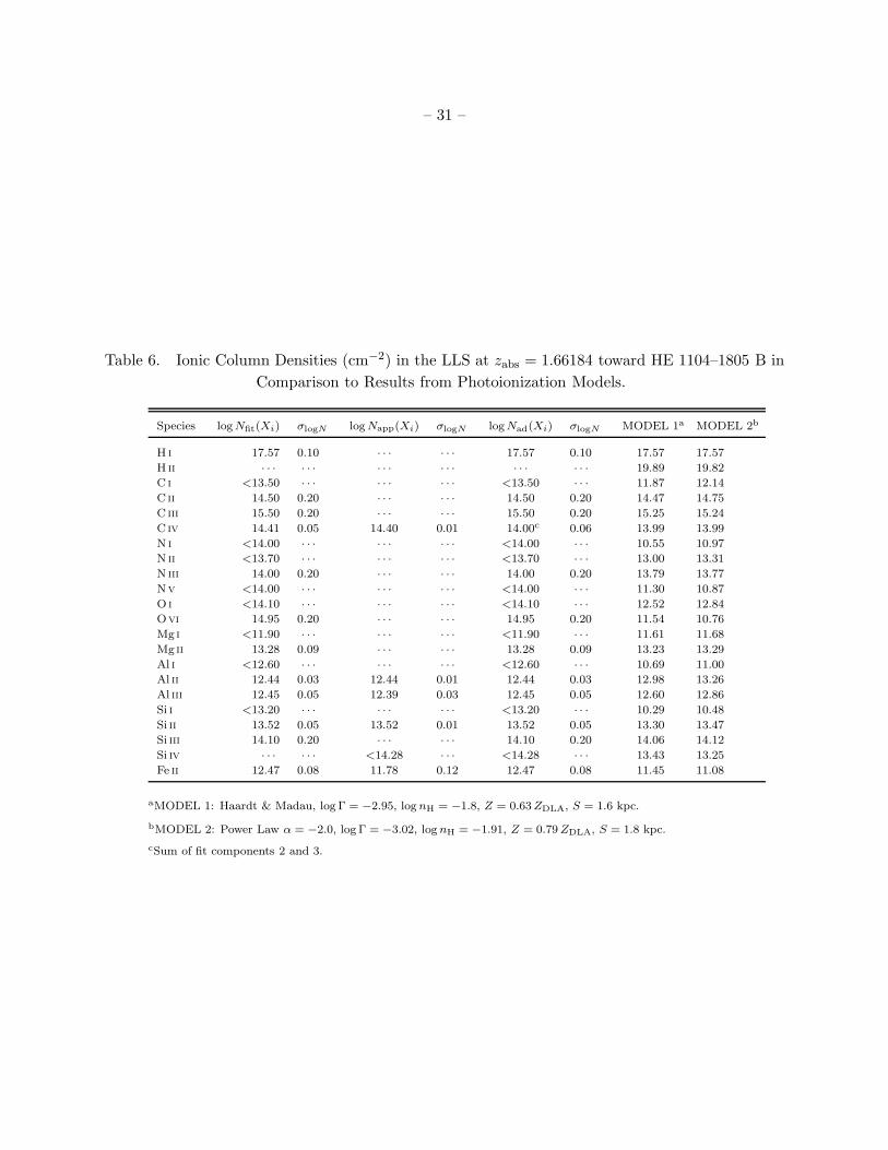
– 31 –

Table 6. Ionic Column Densities (cm−2) in the LLS at zabs = 1.66184 toward HE 1104–1805 B in

Comparison to Results from Photoionization Models.

Species log Nfit(Xi) σlogN log Napp(Xi) σlogN log Nad(Xi) σlogN MODEL 1a MODEL 2b

H i 17.57 0.10 · · · · · · 17.57 0.10 17.57 17.57

H ii · · · · · · · · · · · · · · · · · · 19.89 19.82

C i <13.50 · · · · · · · · · <13.50 · · · 11.87 12.14

C ii 14.50 0.20 · · · · · · 14.50 0.20 14.47 14.75

C iii 15.50 0.20 · · · · · · 15.50 0.20 15.25 15.24

C iv 14.41 0.05 14.40 0.01 14.00c 0.06 13.99 13.99

N i <14.00 · · · · · · · · · <14.00 · · · 10.55 10.97

N ii <13.70 · · · · · · · · · <13.70 · · · 13.00 13.31

N iii 14.00 0.20 · · · · · · 14.00 0.20 13.79 13.77

Nv <14.00 · · · · · · · · · <14.00 · · · 11.30 10.87

O i <14.10 · · · · · · · · · <14.10 · · · 12.52 12.84

Ovi 14.95 0.20 · · · · · · 14.95 0.20 11.54 10.76

Mg i <11.90 · · · · · · · · · <11.90 · · · 11.61 11.68

Mg ii 13.28 0.09 · · · · · · 13.28 0.09 13.23 13.29

Al i <12.60 · · · · · · · · · <12.60 · · · 10.69 11.00

Al ii 12.44 0.03 12.44 0.01 12.44 0.03 12.98 13.26

Al iii 12.45 0.05 12.39 0.03 12.45 0.05 12.60 12.86

Si i <13.20 · · · · · · · · · <13.20 · · · 10.29 10.48

Si ii 13.52 0.05 13.52 0.01 13.52 0.05 13.30 13.47

Si iii 14.10 0.20 · · · · · · 14.10 0.20 14.06 14.12

Si iv · · · · · · <14.28 · · · <14.28 · · · 13.43 13.25

Fe ii 12.47 0.08 11.78 0.12 12.47 0.08 11.45 11.08

aMODEL 1: Haardt & Madau, log Γ = −2.95, log nH = −1.8, Z = 0.63 ZDLA, S = 1.6 kpc.

bMODEL 2: Power Law α = −2.0, log Γ = −3.02, log nH = −1.91, Z = 0.79 ZDLA, S = 1.8 kpc.

cSum of fit components 2 and 3.

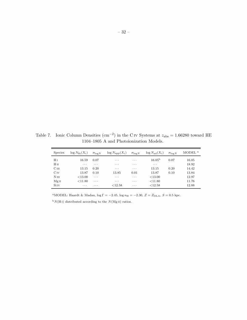
– 32 –

Table 7. Ionic Column Densities (cm−2) in the C iv Systems at zabs = 1.66280 toward HE

1104–1805 A and Photoionization Models.

Species log Nfit(Xi) σlogN log Napp(Xi) σlogN log Nad(Xi) σlogN MODEL a

H i 16.59 0.07 · · · · · · 16.05b 0.07 16.05

H ii · · · · · · · · · · · · · · · 18.92

C iii 13.15 0.20 · · · · · · 13.15 0.20 14.42

C iv 13.87 0.10 13.85 0.01 13.87 0.10 13.84

N iii <13.00 · · · · · · · · · <13.00 12.97

Mg ii <11.80 · · · · · · · · · <11.80 11.76

Si iv · · · · · · <12.58 · · · <12.58 12.88

aMODEL: Haardt & Madau, log Γ = −2.45, log nH = −2.30, Z = ZDLA, S = 0.5 kpc.

bN(H i) distributed according to the N(Mg ii) ratios.

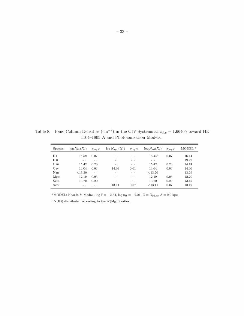
– 33 –

Table 8. Ionic Column Densities (cm−2) in the C iv Systems at zabs = 1.66465 toward HE

1104–1805 A and Photoionization Models.

Species log Nfit(Xi) σlogN log Napp(Xi) σlogN log Nad(Xi) σlogN MODEL a

H i 16.59 0.07 · · · · · · 16.44b 0.07 16.44

H ii · · · · · · · · · · · · · · · 19.22

C iii 15.42 0.20 · · · · · · 15.42 0.20 14.74

C iv 14.04 0.03 14.03 0.01 14.04 0.03 14.06

N iii <13.20 · · · · · · · · · <13.20 13.29

Mg ii 12.19 0.03 · · · · · · 12.19 0.03 12.20

Si iii 13.70 0.20 · · · · · · 13.70 0.20 13.42

Si iv · · · · · · 13.11 0.07 <13.11 0.07 13.19

aMODEL: Haardt & Madau, log Γ = −2.54, log nH = −2.21, Z = ZDLA, S = 0.9 kpc.

bN(H i) distributed according to the N(Mg ii) ratios.

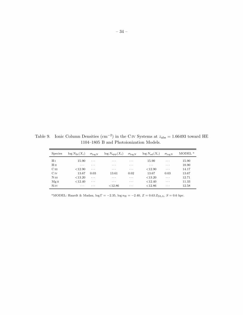
– 34 –

Table 9. Ionic Column Densities (cm−2) in the C iv Systems at zabs = 1.66493 toward HE

1104–1805 B and Photoionization Models.

Species log Nfit(Xi) σlogN log Napp(Xi) σlogN log Nad(Xi) σlogN MODEL a

H i 15.90 · · · · · · · · · 15.90 · · · 15.90

H ii · · · · · · · · · · · · · · · · · · 18.90

C iii <12.90 · · · · · · · · · <12.90 · · · 14.17

C iv 13.67 0.03 13.61 0.02 13.67 0.03 13.67

N iii <13.20 · · · · · · · · · <13.20 · · · 12.71

Mg ii <12.40 · · · · · · · · · <12.40 · · · 11.33

Si iv · · · · · · <12.86 · · · <12.86 · · · 12.58

aMODEL: Haardt & Madau, log Γ = −2.35, log nH = −2.40, Z = 0.63 ZDLA, S = 0.6 kpc.

– 35 –

REFERENCES

Bahcall, J. N., et al. 1993, ApJS, 87, 1

Bergeron, J., & Stasinska, G. 1986, A&A, 169, 1

Bergeron, J., et al. 1994, ApJ, 436, 33

Burles, S., & Tytler, D. 1996, ApJ, 460, 584

Cardelli, J. A., Savage, B. D., & Ebbets, D. C. 1991, ApJ, 383, L23

Cardelli, J. A., Sembach, K. R. & Savage, B. D. 1995, ApJ, 440, 241

Caulet, A. 1989, ApJ, 340, 90

Courbin, F., Lidman, C. & Magain, P. 1998, A&A, 330, 57

Ferland, G. J. 1993, University of Kentucky, Physics Department Internal Report

Fontana, A. & Ballester, P. 1995, ESO Messenger 80, 37

Haardt, F., & Madau, P. 1996, ApJ, 461, 20

Haehnelt, M. G., Rauch, M., & Steinmetz, M. 1996a, MNRAS, 283, 1055

Haehnelt, M. G., Steinmetz, M. & Rauch, M. 1996b, ApJ, 465, L95

Haehnelt, M. G., Steinmetz, M. & Rauch, M. 1998, ApJ, 495, 647

Kirkman, D., & Tytler, D. 1997, ApJ, 489, L123

Lu, L., & Savage, B. D. 1993, ApJ, 403, 127

Lu, L., Sargent, W. L. W., Barlow, T. A., Churchill, C. W., & Vogt, S. S. 1996, ApJS, 107, 475

Mar, D. P., & Bailey, G. 1995, PASA, 12, 239

Morton, D. C. 1991, ApJS, 77, 119

Pettini, M., Boksenberg, A., & Hunstead, R.W. 1990, ApJ, 348, 48

Pettini, M., Lipman, K., & Hunstead, R.W. 1995, ApJ, 451, 100

Pettini, M., Smith, L. J., Kink, D. L., & Hunstead, R.W. 1997, ApJ, 486, 665

Press, W. H., Flannery, B. P., Teukolsky, S. A., & Vetterling, W. T. 1986, Numerical Recipes,

Cambridge University Press.

Prochaska, J. X., & Wolfe, A. M. 1996, ApJ, 470, 403

– 36 –

Prochaska, J. X., & Wolfe, A. M. 1997, ApJ, 474, 140

Rauch, M., Haehnelt, M. G., & Steinmetz, M. 1997a, ApJ, 481, 601

Rauch, M. 1997b, in Structure and Evolution of the IGM from QSO Absorption Lines, Proc. 13th

IAP Colloquium, ed. P. Petitjean, S. Charlot (Paris: Editions Frontieres), 109

Reimers, D., Rodriguez-Pascual, P., Hagen, H.-J., & Wisotzi, L. 1995, A&A, 293, L21

Remy, M., Claeskens, J.-F., Surdej, J., et al. 1998, New Astronomy, in press.

Savage, B. D. & Sembach, K. R. 1991, ApJ, 379, 245

Savage, B. D. & Sembach, K. R. 1996, ApJ, 470, 893

Schneider, D. P., et al. 1993, ApJS, 87, 45

Seaton, M. J. 1979, MNRAS, 187, 73

Sembach, K. R. & Savage, B. D. 1996, ApJ, 457, 211

Smette, A., Surdej, J., Shaver, P. A., Foltz, C. B., Chaffee, F. H., Weymann, R. J., Williams, R.

E. & Magain, P. 1992, ApJ, 389, 39

Smette, A., Robertson, J. G., Shaver, P. A., Reimers, D., Wisotzki, L. & Kohler T. (Paper I) 1995,

A&AS, 113, 199

Sutherland, R. S. & Dopita, M. A. 1993, ApJS, 88, 253

Verner, D. A., Barthel, P. D. & Tytler, D. 1994, A&AS, 108, 287

Vladilo, G., 1998, ApJ, 493, 583

Vogt, S. S., Allen, S. L., Bigelow, B. C., Bresee, L., Brown, B., et al. 1994, S.P.I.E. 2198:362

Wisotzki, L., Kohler, T., Kayser, R., & Reimers, D. 1993, A&A, 278, L15

Wisotzki, L., Kohler, T., Ikonomou, M., & Reimers, D. 1995, A&A, 297, L59

Wolfe, A. M. 1995a, in QSO Absorption Lines, Proc. ESO Workshop, ed. G. Meylan (Heidelberg:

Springer), 13

Wolfe, A. M., Lanzetta, K. M., Foltz, C. B., & Chaffee F. H. 1995b, ApJ, 454, 698

Wolfe, A. M., & Prochaska, J. X. 1998, ApJ, 494, L15

Zuo, L., Beaver, E. A., Burbidge, E. M., Cohen, R. D., Junkkarinen, V. T., & Lyons, R. W. 1997,

ApJ, 477, 568

This preprint was prepared with the AAS LATEX macros v4.0.

– 37 –

Fig. 1.— HST FOS spectra of HE 1104–1805 A and B and their 1σ errors. Fluxes have been

corrected for galactic extinction (Seaton 1979) with E(B − V)=0.09 (Reimers et al. 1995). Also

shown are the AAT spectra which have been scaled to the HST flux levels, smoothed and rebinned

to the FOS resolution, and plotted for λ ≥ 3277 A. Metal absorption lines lying longward of Lyα

emission were covered by the NTT and Keck spectra. The power law and the QSO continuum

derived as described in the text have been overplotted. Expected positions of emission lines by

Lyα, Lyβ, Nv, Ovi, and Svi are indicated.

Fig. 2.— Sections of the normalized HST FOS (FWHM ∼ 2 A) and AAT (FWHM ∼ 1.2 A)

spectra of HE 1104–1805 A (upper panels) and B, showing synthetic Voigt profiles of the high-

order H i Lyman-series lines (top) and most relevant metal lines belonging to the damped Lyα

system (A) and Lyman-limit System (B) at z = 1.66. Tickmarks (from upper panel to right-lower

panel) indicate the positions of H i λλ918 to 949, C ii λλ1036, 1334, N ii λ1083 and O i λλ988, 1302.

Fig. 3.— Low ions: Velocity profiles at 6.6 km s−1 resolution of lines associated with the damped

Lyα system toward HE 1104–1805 A (left-hand panel), and the Lyman-limit System toward HE

1104–1805 B. The Mg ii line profiles are at 40 km s−1 resolution. The zero velocity scale in both

panels corresponds to z = 1.66164. The smoothed lines represent the best-fit Voigt profiles and

ticks mark the line positions.

Fig. 4.— High ions: Velocity profiles at 6.6 km s−1 resolution of lines associated with the damped

Lyα system toward HE 1104–1805 A (left-hand panel), and the Lyman-limit System toward HE

1104–1805 B. The Al ii λ1670 velocity profiles are also shown for comparison purposes (see text).

The zero velocity scale in both panels corresponds to z = 1.66164. The smoothed lines represent

the best-fit Voigt profiles and ticks mark the line positions. The absorption feature at v ∼ +110

km s−1 in the C iv λ1548 B plot is identified with Si ii λ1808 at z = 1.28.

Fig. 5.— Left: Velocity profiles at 6.6 km s−1 resolution of Cr ii, Zn ii and Ti ii lines associated

with the damped Lyα system toward of HE 1104–1805 A. Right: Expected positions of the same

ions in HE 1104–1805 B. The zero velocity scale in both panels corresponds to z = 1.66164. The

smoothed lines represent the best-fit Voigt profiles and ticks mark the line positions.

Fig. 6.— Bottom: Velocity profiles of the C iv λλ1548,1550 (at 6.6 km s−1 resolution) and Mg ii

λλ2796,2803 (at 40 km s−1 resolution) doublets in A (left) and B. In both panels v = 0 km s−1

corresponds to z = 1.66164. In the Mg ii λ2796 plot, the feature at −100 km s−1 is identified with

Mn i λ2795. Top: HST velocity profiles of the corresponding Lyα, Lyβ and Lyγ H i lines (note the

different velocity scales).

Fig. 7.— Section of the HST spectra A and B showing the Ovi λλ1031,1037 doublet at z =

1.66253. Solid lines: Voigt profiles—convolved with a FWHM = 2 A Gaussian—with b = 180

km s−1 (A) and 110 km s−1 (B), and column density log N = 14.95. Dotted lines: Voigt profiles of

3 (A) and 2 (B) Ovi lines with common b = 50 km s−1 and total column density log N = 15.1 (A)

– 38 –

and 15.0 (B). The lines are placed at redshifts labeled 1, 2 and 3 (A), and 4 and 5 (B) in Fig. 6.

Fig. 8.— Section of the AAT spectra A and B. Tickmarks indicate the positions at which the Nv

λλ1238, 1242 doublet lines would appear if Nv were present at z = 1.66253. Part of the red wing

of the damped Lyα line appears in the overplotted synthetic spectrum A. In B, the absorption at

λ = 3308 A is identified with a Lyα line, supported by the detection of Lyβ at the same redshift

in the HST spectrum.

Fig. 9.— Hydrogen column density vs. metallicity in the Ovi-phase for different CLOUDY models

assuming the Haardt & Madau continuum (solid line) and a power law as ionizing background.

The relative abundances are the same as in the DLA gas. These models yield throughout

log N(Ovi)= 15.0 and log N(Nv)= 13.2.

Fig. 10.— Column densities vs. ionization parameter Γ in the Ovi-phase for different CLOUDY

models. Solid line: Haardt & Madau radiation field as ionizing background, and Z = ZDLA. Dotted

line: Same radiation field, with Z = 0.4 ZDLA. Dashed line: Power law and Z = ZDLA. The relative

abundances are the same as in the DLA gas. These models yield throughout log N(O vi)= 15.0.

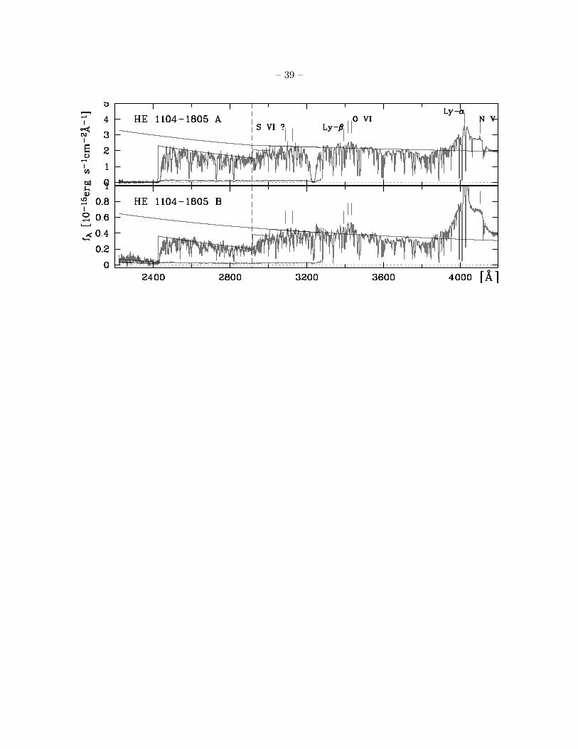
– 39 –

– 40 –

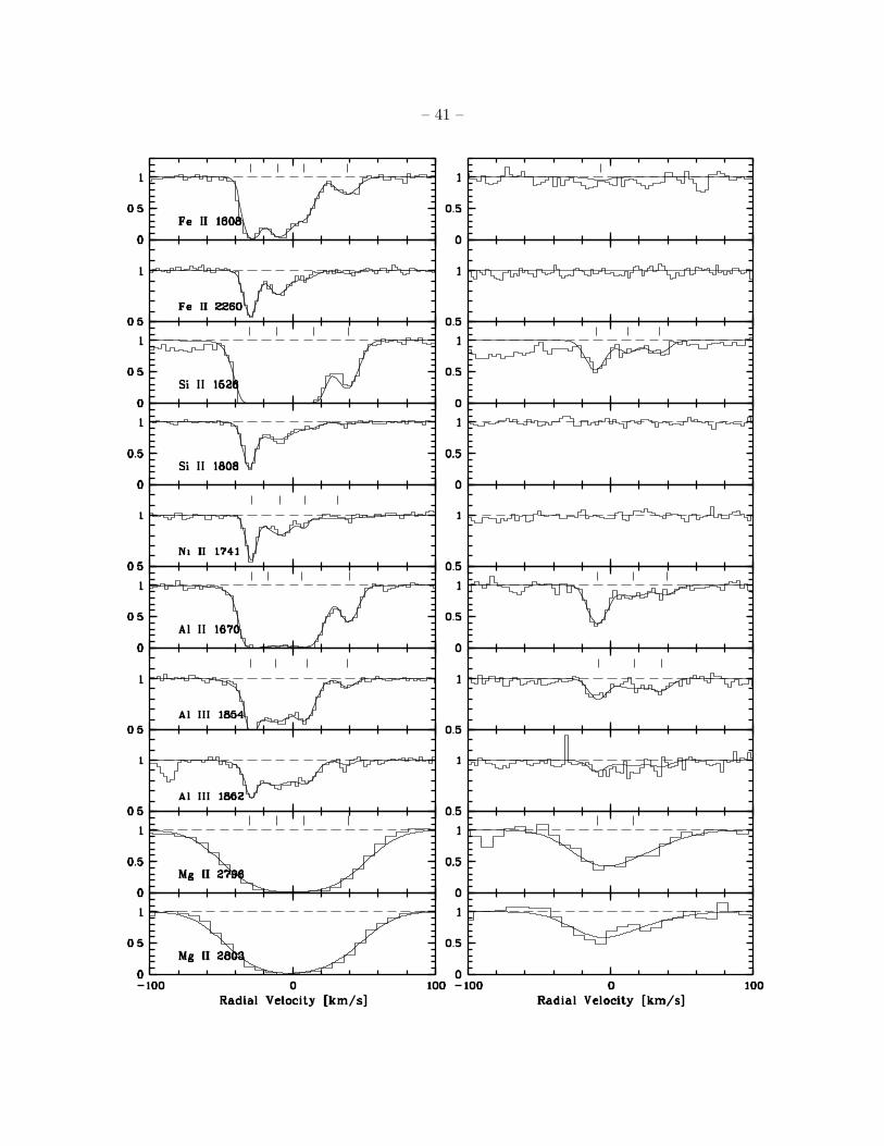
– 41 –

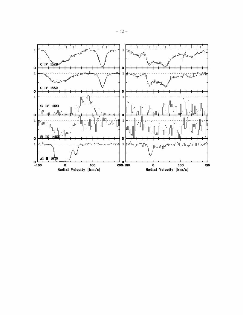
– 42 –

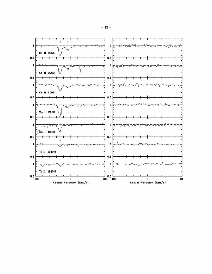
– 43 –

– 44 –

– 45 –

– 46 –

– 47 –

– 48 –

– 49 –