Finite volume solutions for electromagnetic induction processing

Applied Mathematical Modelling xxx (2015) xxx–xxx

Contents lists available at ScienceDirect

Applied Mathematical Modelling

journal homepage: www.elsevier .com/locate /apm

Finite volume solutions for electromagnetic inductionprocessing

http://dx.doi.org/10.1016/j.apm.2015.03.0590307-904X/� 2015 Elsevier Inc. All rights reserved.

⇑ Corresponding author. Tel.: +44 2083319589.E-mail address: [email protected] (G. Djambazov).

Please cite this article in press as: G. Djambazov et al., Finite volume solutions for electromagnetic induction processing, Appl. Mathell. (2015), http://dx.doi.org/10.1016/j.apm.2015.03.059

G. Djambazov a,⇑, V. Bojarevics a, K. Pericleous a, N. Croft b

a Centre for Numerical Modelling and Process Analysis, University of Greenwich, UKb College of Engineering, Swansea University, UK

a r t i c l e i n f o a b s t r a c t

Article history:Received 5 November 2014Received in revised form 10 March 2015Accepted 16 March 2015Available online xxxx

Keywords:Electromagnetic fieldInduction processingNumerical solution of partial differentialequationsPseudo-steady stateIntegral boundary conditionFinite volume discretisation

A new method is presented for numerically solving the equations of electromagneticinduction in conducting materials using native, primary variables and not a magneticvector potential. Solving for the components of the electric field allows the meshed domainto cover only the processed material rather than extend further out in space. Togetherwith the finite volume discretisation this makes possible the seamless coupling of theelectromagnetic solver within a multi-physics simulation framework. After validation forcases with known results, a 3-dimensional industrial application example of inductionheating shows the suitability of the method for practical engineering calculations.

� 2015 Elsevier Inc. All rights reserved.

1. Introduction

Induction heating and stirring is often used in the processing of conductive materials: melting of metals and alloys,controlling the temperature and stirring of liquid silicon, etc. Magnetic fields are also used to melt levitated samples forprecise measurements of material properties. For chemically reactive alloys the magnetic field can help contain the meltin ‘semi-levitation’ or ‘cold crucible’ induction furnaces.

Computer modelling of those processes can be very useful for their optimisation. The process usually involves severalintertwined physical phenomena such as electromagnetic induction, heat transfer, phase change, elasto-plasticity, fluid flowwith free surface, and magnetohydrodynamics.

An efficient way to capture the true interactions among all those phenomena can be the simulation by a single computerprogram [1] where the values of the solved variables are advanced simultaneously at each iteration and at each time step ofthe solution process. Some authors [2] also include thermo-mechanical (stress analysis) computations at each step of thealgorithm for cases where the deformation of the material affects the electromagnetic field.

The electromagnetic fields involved in induction metal processing are three dimensional, and eddy currents are inducedin the conducting objects. Their calculation has been addressed in various ways, with or without magnetic potentials, infinite element (FEM) and other formulations [4–7]. Combining FEM and boundary element methods helps reduce the sizeof the meshed computational domain and, hence, the computational time [8]. This work does not attempt to include a more

. Mod-

http://dx.doi.org/10.1016/j.apm.2015.03.059

mailto:[email protected]


http://www.sciencedirect.com/science/journal/0307904X

http://www.elsevier.com/locate/apm


2 G. Djambazov et al. / Applied Mathematical Modelling xxx (2015) xxx–xxx

comprehensive review of the numerous formulations, algorithms and software implementations for modelling 3D electro-magnetic phenomena.

In this work the finite volume method is used to discretise and solve the governing equations of electromagnetic induc-tion. Such a formulation is compatible with the solution procedures for the other variables in a thermo-fluid computationalmodel. The resulting computer code readily fits into the PHYSICA framework [3]. It can also be used in combination with otherfinite volume PDE codes.

The algorithm described below is formulated in primary variables for the electric and the magnetic field and does notinvolve a magnetic vector potential. This presents an alternative to the potential formulation and allows a more ‘natural’representation of the governing equations and of the boundary conditions on the conductor surfaces.

The implementation of the new method described here was added to a multi-physics computational environment [3] butthe method itself is generic and can be attached to other partial differential equation (PDE) solvers.

The paper is organised as follows: first, the governing equations of electromagnetic induction are presented, then specialattention is paid to the source term linearisation in the quasi-steady case. Various aspects of the boundary treatment areconsidered, and finally validation and sample results illustrate the applicability of the method.

2. Equations

Maxwell’s equations in differential form describe the local relationship between the variables of the electromagnetic field.In the case of non-magnetic materials (non-ferrous metals or steel in a certain temperature range) the magnetic permeabilityl may be assumed constant throughout the spatial domain of interest. On the other hand, in sufficiently conductingmaterials (including molten metals) there are no localised electric charges, and Maxwell’s equations can be simplified toform the basis of the theory of electromagnetism [9]:

Pleaseell. (2

div B ¼ 0; ð1Þcurl E ¼ �@B=@t; ð2Þcurl B ¼ lJ; ð3Þdiv E ¼ 0; ð4Þ

where B is the magnetic induction, E is the electric field intensity, t is time, and J is the electric current density. Ohm’s lawprovides an algebraic relation between J and E, and for isotropic electrical conductivity r it can be written as J ¼ rE.

Assuming that B is sufficiently continuous so that its temporal and spatial derivatives may be swapped, taking the curl of(2), after substitution only one variable is left:

curl ðcurl EÞ ¼ �l@ðrEÞ=@t: ð5Þ
The electrical conductivity r depends on the temperature which changes with time. However, on the time scale of theelectromagnetic processes, r may be assumed constant in time. Then, using the mathematical identitycurl ðcurl EÞ ¼ gradðdiv EÞ � r2E and (4), Eq. (5) may be simplified into:
r2E ¼ lr @E@t: ð6Þ

The transient term and the diffusion term of the general conservation equation usually solved by Computational FluidDynamics (CFD) codes can easily be recognised in the above Eq. (6). So CFD codes may be used directly for transient simulationsof electromagnetic phenomena just by switching off the convection term and providing the necessary boundary conditions.

In induction melting only alternating currents are used with typical frequencies in the range 1–10 kHz. The time scale ofthe electromagnetic phenomena is at least 50 times smaller than the time scale of the fluid phenomena. Consequently, themodelling of the fluid flow in the process requires the pseudo-steady solutions of the electric and the magnetic fields ratherthan their time-dependent behaviour.

Assuming that a periodic solution exists with a circular frequency x: E ¼ ER cos xt þ EI sin xt, and substituting into (6),the following system results:

r2ER ¼ lrxEI; ð7Þr2EI ¼ �lrxER: ð8Þ

This system consists of six scalar equations for six unknown functions. The transient terms have disappeared and havebeen replaced by source terms. The magnitude of these source terms is substantial and they need to be linearised withrespect to the unknown variables in order to achieve convergence within the CFD code; this is discussed in the next section.

From the solved values of ER and EI the components of the magnetic field B can be recovered according to (2) as

BR ¼ �1x

curl EI; ð9Þ

BI ¼1x

curl ER; ð10Þ

with the curl operators evaluated numerically from the partial spatial derivatives of E.

cite this article in press as: G. Djambazov et al., Finite volume solutions for electromagnetic induction processing, Appl. Math. Mod-015), http://dx.doi.org/10.1016/j.apm.2015.03.059


G. Djambazov et al. / Applied Mathematical Modelling xxx (2015) xxx–xxx 3

The charge conservation constraint (4) results in two more equations for the same variables: div ER ¼ 0 and div EI ¼ 0.One way of insuring non-divergence of the electric field vectors is by solving separately for their irrotational part (�ruR;I)

and rotational part (E0R;I), the final solution being the sum of the two fields:

Pleaseell. (2

ER ¼ E0R �ruR; ð11ÞEI ¼ E0I �ruI: ð12Þ

The equations for the two scalar electric potentials uR and uI that are obtained from (11), (12) and (4)

div ðruR;IÞ ¼ r2uR;I ¼ div E0R;I; ð13Þ

can easily be solved in the same finite volume framework.When (11) and (12) are substituted into (7) and (8) additional source terms appear and the equations for the rotational

components become

r2E0R ¼ lrxE0I þr2ðruRÞ � lrxruI; ð14Þr2E0I ¼ �lrxE0R þr2ðruIÞ þ lrxruR: ð15Þ

Hence, the PDE system to solve will have eight Eqs. (13)–(15) with the eight unknowns being all three components of E0Rand E0I plus uR and uI . These are second order diffusion type equations where the right-hand side (RHS) of each one dependson unknowns ‘belonging’ to other equations from the system. An iterative approach to the numerical solution of the systemis followed, i.e. the RHS is calculated from the values of the unknowns at the previous iteration. For better stability andconvergence of the algorithm, partial linearisation of the RHS is done which transfers part of the RHS to the diagonal ofthe system matrix (solved at each iteration) and which is discussed in the following section.

2.1. Force and heat

The purpose of treating a metal charge or a conducting liquid (e.g. molten silicon) with electromagnetic induction is toadd heat and to stir the melt, so it is essential to accurately predict the forces acting and the heat released in the liquid mate-rial. In a unit of conducting volume the electromagnetically generated instantaneous Lorentz force F and Joule heat Q are [9]

F ¼ J� B; ð16ÞQ ¼ J � E ¼ rE2: ð17Þ

Time-averaging of these sinusoidal quantities over one period yields the mean (quasi-steady) values

Fmean ¼ 0:5ðJR � BR þ JI � BIÞ; ð18ÞQ mean ¼ 0:5rðE2

R þ E2I Þ: ð19Þ

2.2. Useful particular cases

The number of unknown variables can be reduced in two-dimensional models. Let us assume that the magnetic induc-tion B has only one component in the z-direction Bz ¼ B, and the other two components are zero. Then from Eqs. (1)–(3) wecan obtain:

@B@z¼ @Ex

@z¼ @Ey

@z¼ Ez ¼ 0; ð20Þ

@Ey

@x� @Ex

@y¼ � @B

@t; ð21Þ

lrEx ¼@B@y; lrEy ¼ �

@B@x: ð22Þ

Note that (4) is automatically satisfied when (22) is true. Also, in non-conducting areas (r ¼ 0), @B=@x ¼ @B=@y ¼ 0 whichmeans

B ¼ const: ð23Þ

For regions with r ¼ const a single time-dependent equation for the magnetic induction may be obtained by further differ-entiating (22) and substituting into (21):

@2B@x2 þ

@2B@y2 ¼ lr @B

@t: ð24Þ

In the quasi-steady case a convenient set of two differential equations for the magnetic induction variables results which is atwo-dimensional scalar version of (7) and (8):




Pleaseell. (2

B ¼ BR cos xt þ BI sin xt; ð25Þ@2BR

@x2 þ@2BR

@y2 ¼ lrxBI; ð26Þ

@2BI

@x2 þ@2BI

@y2 ¼ �lrxBR: ð27Þ

Further simplification is possible in the one-dimensional case which can be useful for a surface parallel to the magnetic fieldvector lines. In (22) if it is assumed that Ex ¼ 0, it follows that @B=@y ¼ 0, and (26) and (27) are reduced to ordinarydifferential equations along x. It can be verified by substitution that their solution will be

BR ¼ B0 exp � xd

� �cos

xd; BI ¼ B0 exp � x

d

� �sin

xd; ð28Þ

where d is defined by the equation lrxd2 ¼ 2, and B0 is the magnetic induction on the surface at the beginning of each cycle.Then from (22) we obtain

ER ¼xd2ðBR þ BIÞ; EI ¼

xd2ðBI � BRÞ: ð29Þ

One-dimensional approximation is appropriate for analysis of higher-frequency cases (with thinner electromagnetic skindepth d) and where the curvature of the surface is not great with the magnetic field lines parallel (or almost parallel) toit. Two-dimensional computation can be applied to non-axisymmetric middle cross-sections of longer billets or crucibleswhere the magnetic field lines become parallel to the treated surfaces. The above particular cases are also very useful forvalidating the general, 3-dimensional implementations as this can be seen in Section 5.

3. Source terms linearisation

The general conservation equation solved by most CFD codes is in the form

@ðq/Þ@t

þ div ðqu/Þ ¼ div ðC/ grad/Þ þ S/: ð30Þ

where q is the fluid density, u is the fluid velocity, C/ is the diffusion coefficient, / is the unknown conserved variable, and S/

is the source term. To achieve convergence of the iterative solution process in many cases it is necessary to represent thesource term in the form

S/ ¼ SC � SP/; ð31Þ

with SP > 0. This technique is called linearisation of the source term, and it often represents the physical dependence of thesource term on its variable [10].

Consider the pair of Eqs. (26) and (27); the result will apply also to the three components of the vector equations (7) and(8). These equations are particular cases of the general conservation Eq. (30) where the transient term and the convectionterm on the left-hand side are set to zero and the diffusion coefficient is C/ ¼ 1.

Examining the source terms, it can be seen that each of the unknown variables, BR and BI , appears in the source term ofthe other variable’s equation. Also, each variable may have its own sources due to the boundary conditions. Assume that eachvariable’s own sources can be represented in the form (31). The discretised finite volume forms of the complete Eqs. (26) and(27) will then be:

Xn

f¼1

AfBR;f � BR

dfþ cR � pRBR � qBI ¼ 0; ð32Þ

Xn

f¼1

AfBI;f � BI

dfþ cI � pIBI þ qBR ¼ 0: ð33Þ

Here the summation is done over all the n faces (f) bounding a given cell in the mesh, Af are the face areas, BR;f and BI;f are thevalues of the variables in the neighbouring cells across f ; df are the distances between the neighbouring cell centres,q ¼ lrxV where V is the cell volume; cR ¼ ðSCÞBR

V , pR ¼ ðSPÞBRV , cI ¼ ðSCÞBI

V , and pI ¼ ðSPÞBIV are the respective linearised

sources.Eq. (32) may be rearranged to form an expression for BR. This expression can be used to remove BR from Eq. (33). Likewise

(33) can be used to enable the removal of BI from (32). If the sums are split, denoting

RR ¼Xn

f¼1

AfBR;f

df; RI ¼

Xn

f¼1

AfBI;f

df; R0 ¼

Xn

f¼1

Af

df;




the discretised finite volume equations (32) and (33) can be written in the form:

Pleaseell. (2

Xn

f¼1

AfBR;f � BR

dfþ cR � q

RI þ cI

R0 þ pI

� �� pR þ

q2

R0 þ pI

� �BR ¼ 0; ð34Þ

Xn

f¼1

AfBI;f � BI

dfþ cI þ q

RR þ cR

R0 þ pR

� �� pI þ

q2

R0 þ pR

� �BI ¼ 0: ð35Þ

The terms RI (in the BR-equation) and RR (in the BI-equation) each contain the other unknown variable. In the implementa-tion, those values are taken from the previous iteration of the non-linear iteration loop. This means the linearisation of thesource terms shown above is only partial but it helps transfer part of the magnitude of the source term onto the systemmatrix diagonal which makes the iterative solution of the linear system more stable. This form of the linearised sourceexpressions is not ideal because one of the equations still contains a negative coefficient in front of neighbouring valuesof the other variable. However, with a relaxation factor in the range 0.75–0.95, converged solutions have been obtainedfor most sets of boundary conditions.

4. Boundary conditions

Boundary conditions may be specified on the surface of the conducting objects. In this way the computational domainonly covers the bodies with induced currents, and the action of the external driving coil is taken into account viaBiot–Savart integration for the points on the surface. Symmetry may be used to reduce the size of the computational domain.In most cases that is azimuthal symmetry, and for vector quantities boundary expressions are also presented in this section.

4.1. Surface boundaries

Faraday’s Eq. (2) and the condition that there is no normal current through the surface provide the necessary boundaryconditions.

4.1.1. Induction conditionIn the quasi-steady case (25) Faraday’s law of electromagnetic induction is represented by two vector equations:

curl ER ¼ �xBI; curl EI ¼ xBR: ð36Þ
The two vectors of the magnetic induction BR and BI can be evaluated separately using the Biot–Savart formula (43) with thecorresponding current density fields JR ¼ rER and JI ¼ rEI .
A local coordinate system is considered ðn; a; bÞ with an origin in the middle of a given cell face on the surface. Axis n isdefined by the outward normal vector to the face, axis a has the direction of the vector defined by the first and the secondcorner points of the face, and axis b is in the direction of the cross product n� a of the first two unit vectors. After expandingcurl ER and curl EI in the local coordinate frame the induction boundary condition (36) becomes:

@EnR

@b� @EbR

@n¼ �xBaI;

@EnI

@b� @EbI

@n¼ xBaR; ð37Þ

@EaR

@n� @EnR

@a¼ �xBbI;

@EaI

@n� @EnI

@a¼ xBbR: ð38Þ

The components of J and E normal to the surface of the conducting bodies are zero. However, the quantities EnR, and EnI areequal to zero only for the given cell face on the surface. (If the surface is not flat, the n-components of the neighbouring facesare nonzero with respect to the local coordinates.) This means that their derivatives with respect to a and b are not zero andhave to be evaluated. This may be done in the following way. Let ra is the curvature radius of the surface in the plane ða;nÞ. Inthe vicinity of the observation point on the surface the intersection of plane ða;nÞ with the surface is a circular arc. Let a bethe central angle sweeping that arc. Then the projection onto axis n of the tangential vector of magnitude Ea turning alongthe arc will be En ¼ �Ea sin a. Differentiating this with respect to a, bearing in mind that a ¼ raa, the equation@En=@a ¼ �ðEa=raÞ cos a is obtained which for the location of interest, a ¼ 0, gives

@En

@a¼ �Ea

ra; ð39Þ

@En

@b¼ �Eb

rb: ð40Þ

The second Eq. (40) can be derived for the plane ðb;nÞ in exactly the same way as (39); then these equations can be applied tothe R and I parts in (37) and (38) in order to obtain expressions for the normal derivatives of the tangential components:

@EbR

@n¼ xBaI �

EbR

rb;

@EbI

@n¼ �xBaR �

EbI

rb; ð41Þ

@EaR

@n¼ �xBbI �

EaR

ra;

@EaI

@n¼ xBbR �

EaI

ra: ð42Þ




It can be seen that the above boundary sources are in a linearised form (31). The only difficulty is that they are in local coor-dinates, and the solved variables are global components of the field vectors. This means that it may not be possible to takeadvantage of the linearisation. This should not be a problem if the surface curvature is not to high. A backward transforma-tion is done from local to global coordinates to determine the actual fluxes of the x, y, and z components of the solvedvariables. Usually the Biot–Savart evaluation of the magnetic induction will be implemented in global coordinates, thenthe forward transformation will provide the necessary local components of BR and BI .

4.1.2. The singular integral of Biot–SavartGiven the electric current density (JR; JI) within the time-harmonic (pseudo-steady) approximation, the corresponding

induced magnetic field can be calculated as

Pleaseell. (2

BR;I ¼l

4p

Zspace

JR;I � rr3 dV ;

r ¼ robservation � rsource;

ð43Þ

where the volume integral is taken over all space, i.e. all conducting bodies including the excitation coil. On the surfacewhere it is needed for the boundary conditions the integral is singular as r tends to zero.

On a cell-centred mesh, like the one PHYSICA uses, it may be possible to avoid the singularity by evaluating the integral forthe nodes (vertices) of the mesh and then interpolating for the face centres. In most cases, however, finer meshes are needed,and the accuracy of this approach is not sufficient.

An alternative method was developed based on a derived analytical expression for the integral value induced by a thincylindrical slab (like a coin) at the points of its axis. The mesh cells lying immediately below the surface observation point(down to a certain specified depth) are processed in this way, and the contributions of all the other cells are calculateddirectly with the Biot–Savart formula (43). This approach was observed to give improved results. Problems still exist forneighbouring cells that lie off the normal axis and are still very close to the observation point since no analytical expressionis used for their contributions.

Local mesh refinement around the singularity is the third approach that has been investigated. When the contribution ofeach element of the mesh is being calculated, the ratio between its size and the distance from the element centroid to theobservation point is considered. If that ratio is lower than a certain limit (0.35 was found to give sufficient accuracy at areasonable computational cost) the usual piecewise constant integration is performed, else the element is split into eight(for a hexahedral element) equal volumes, each with their own centroid, and their contributions are evaluated separately.The density of the finite volume mesh depends on the ‘skin layer’ of the electromagnetic field, and the thickness of the skinlayer depends on the frequency and the electrical conductivity. For the cases of induction heating considered in this work,one-level local mesh refinement was found to perform best of the three methods described.

Another issue with the Biot–Savart integral is the computational cost of its evaluation for large problems. Every cell of themesh has to be visited for every cell face on the surface at every iteration. Unlike with the differential equations, symmetrycannot be used here to save computation. Clustering the cells into sub-domains can help: for each cluster, depending on thedistance to the observation point, either its average values are used or the individual contributions of its cells are calculated.This is straightforward to describe in words but needs careful coding.

4.1.3. Normal current conditionNo electric current can flow out of a conductor into an insulator. Consequently, the normal to the surface components of

the electric field vectors ER and EI must reduce to zero on the conductor surface. On a cell-centred mesh a linear profile canbe assumed

@En

@n¼ 0� En

df¼ � 1

dfExnx þ Eyny þ Eznz� �

; ð44Þ

where n is the direction of the outward to the surface unit normal vector nðnx;ny;nzÞ, df is the distance from the cell centreimmediately below the surface to the cell face on the surface, En is the local normal component of either of the vectors ER andEI , and ðEx; Ey; EzÞ are the solved global components of those vectors, all cell-centre values.

As with (41) and (42), the normal current condition (44) also needs to be transformed from local to global coordinates beforeit can be used. This can be done by differentiating with respect to n the transformation equations for Ex; Ey, and Ez. The result isin linearised form (31) with the previous iteration values of the other two vector components appearing in the SC part.

4.2. Symmetry and material boundaries

For the usual symmetry boundary condition the normal derivatives of the solved quantities are set to zero. With azi-muthal symmetry in a cylindrical geometry the above is quite correct for the scalar variables and the axial componentsof the vector variables. However, the remaining two vector components need special attention in this case.

In fact, what is required is to make the radial (Er) and the azimuthal (Ea) components of a given vector EðEx; Ey; EzÞ stayconstant across the azimuthal symmetry plane, i.e. to ensure




Pleaseell. (2

@Er

@a¼ 0;

@Ea

@a¼ 0: ð45Þ

where a is the azimuthal angle in cylindrical coordinates. By differentiating with respect to a the transformation expressionsEr ¼ Ex cosaþ Ey sin a and Ea ¼ Ey cos a� Ex sin a it can be shown that the equations

@Ex

@a¼ �Ey;

@Ey

@a¼ Ex; ð46Þ

are equivalent to (45). The above relations express the azimuthal symmetry condition in terms of the solved quantities in theglobal Cartesian coordinate frame. At implementation it would be best to use the outward normal derivatives at the sym-metry planes instead of the a-derivatives, then n ¼ �ra with r being the cylindrical radius of the centre of the given faceon the symmetry plane, and the sign depends on which side of the sector domain is being considered. Strictly speaking,expressions (46) use the face values, and on a cell-centred mesh the solved quantities are available at the cell centroids.Assuming linear variation from the centroid to the face centre, new expressions involving only the cell values can be derived.

-40

-35

-30

-25

-20

-15

-10

-5

0

5

0 0.01 0.02 0.03 0.04 0.05 0.06

x (m)

Electric field, Real

exactsolve Esolve B

-10

-5

0

5

10

15

20

25

30

35

40

0 0.01 0.02 0.03 0.04 0.05 0.06

x (m)

Electric field, Imag

exactsolve Esolve B

-0.05

0

0.05

0.1

0.15

0.2

0 0.01 0.02 0.03 0.04 0.05 0.06

x (m)

Magnetic field, Real

exactsolve B

-0.01

0

0.01

0.02

0.03

0.04

0.05

0.06

0.07

0 0.01 0.02 0.03 0.04 0.05 0.06

x (m)

Magnetic field, Imag

exactsolve B

Fig. 1. Validation results for 1D test problem.




They appear in the form (31) with SP ¼ df =ðr2 þ d2f Þ where df is the small distance between the cell centroid and the

azimuthal symmetry face.Discontinuities arise at material boundaries between two conductors with different electrical conductivity. The principle

of charge conservation requires that the normal electric current should be the same either side of any face in the mesh. Thismeans that

Pleaseell. (2

r1E1n ¼ r2E2n; ð47Þ

where E1n and E2n are the face values of the solved electric field vectors in the two materials. If (47) is ignored and the mesh iscontinuous, the diffusive Eqs. (7) and (8) will smear the jump over several cells across the interface. If that is undesirable,source terms need to be introduced in every pair of cells across the material boundary. Again a transformation from localto global coordinates is needed for the implementation of this boundary condition.

Y

X

Z

-5e+06

-4e+06

-3e+06

-2e+06

-1e+06

0

0 0.005 0.01 0.015 0.02 0.025 0.03 0.035

r (m)

Current Density (A/m**2), t=0 (real part)

solve Eanalytic

-1e+06

0

1e+06

2e+06

3e+06

4e+06

5e+06

6e+06

0 0.005 0.01 0.015 0.02 0.025 0.03 0.035

r (m)

Current Density (A/m**2), t = 1/4 cycle (imag. part)

solve Eanalytic

Fig. 2. Axisymmetric solution for test sphere: computational ‘wedge’ domain, current loop and results on equatorial plane.




5. Validation

It is natural to start testing the numerical procedures with simple cases that are easily verifiable. The one-dimensionaltest with analytical solution (28) and (29) is presented in Fig. 1. The 1D computational domain of length 55 mm is dividedinto 20 mesh cells clustered towards the right end which represents the metal charge surface. This variable mesh spacingallows better resolution within the electromagnetic skin depth (d = 8.5 mm in this case) without using fine mesh everywherein the domain. (Such clustering of the mesh becomes especially important in 3-dimensional cases since it leads to significantsavings in computational time.) Sinusoidal in time magnetic field is prescribed with amplitude 0.2 T on the charge surfaceand frequency 7000 Hz. The Biot–Savart integral is not used in this test. Two different numerical results are compared withthe exact solution: the result of solving (7) and (8) with boundary conditions (42) is marked ‘‘solve E’’, and the result ofsolving (26) and (27) with fixed-value boundary conditions is marked ‘‘solve B’’. Excellent agreement is observed with onlya minor error where numerical differentiation is used (22) to post-process results.

An axisymmetric test case relevant to magnetic levitation has been used to verify a pseudospectral method for modellinginduction melting [11]. The test case, which also has an analytical solution, is of the electric current induced in a conductingsphere by a coaxial current ring. The presented results are for frequency 6000 Hz, electrical conductivity of the sphere4� 106 S/m, electromagnetic skin depth d = 3.25 mm, radius of the sphere 37.5 mm, radius of the single current loop60 mm and amplitude of the current 1000 A. The finite-volume computational domain covers a 9o wedge (slice) of the spherewith its axis of symmetry being the axis of the current-carrying ring. Azimuthal symmetry boundary conditions, as describedin the previous section, are applied on the meridional planes either side of the wedge. The Biot–Savart integral boundarycondition is applied on the outer surface of the wedge. When doing this, the remaining 39 spherical sectors which arenot in the computational mesh are taken into account by rotating the vectors of the electric current density of the main sliceaccordingly around the axis of symmetry. In Fig. 2 the electric current density along the radius in the equatorial plane of thesphere is shown at the beginning of a cycle and at a quarter of a cycle. The numerical solution ‘‘solve E’’ was obtained asdescribed above, however, here the magnetic field on the surface is not known, and it was calculated using (43). It can beseen that the agreement is very good, but it is not perfect. This is due to the accuracy with which the particular implemen-tation of the software handles the singularity of (43).

0

0.005

0.01

0.015

0.02

0.045 0.05 0.055 0.06 0.065 0.07 0.075 0.08 0.085

Electric field (real part) with boundary B = 0.1 T

20 V/m

0

0.005

0.01

0.015

0.02

0.045 0.05 0.055 0.06 0.065 0.07 0.075 0.08 0.085

E-difference (real part) with boundary B = 0.1 T

2 %

Fig. 3. 2D test (horizontal section of ‘cold-crucible’ induction furnace): above - solved electric field; below - difference between ‘‘solve E’’ and ‘‘solve B’’.

Please cite this article in press as: G. Djambazov et al., Finite volume solutions for electromagnetic induction processing, Appl. Math. Mod-ell. (2015), http://dx.doi.org/10.1016/j.apm.2015.03.059


Y

X

Z

JHeat

1.7E+071.5E+071.3E+071.1E+079E+067E+065E+063E+061E+06

65000 N/m3

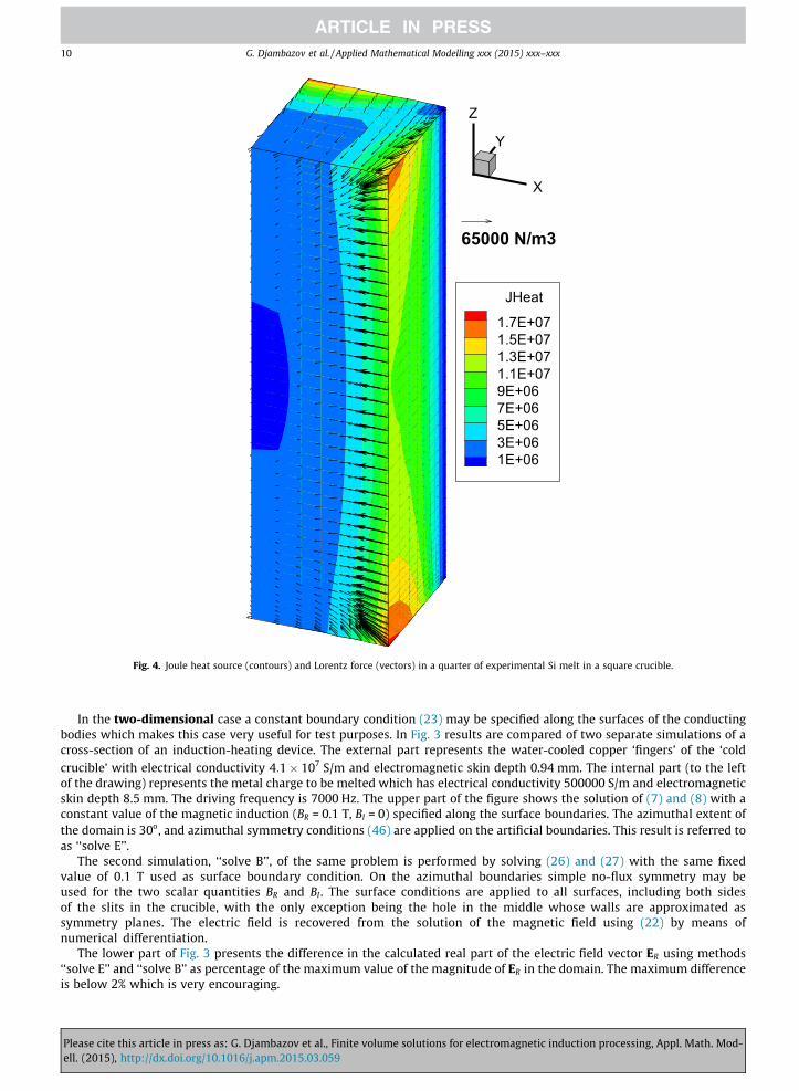
Fig. 4. Joule heat source (contours) and Lorentz force (vectors) in a quarter of experimental Si melt in a square crucible.


In the two-dimensional case a constant boundary condition (23) may be specified along the surfaces of the conductingbodies which makes this case very useful for test purposes. In Fig. 3 results are compared of two separate simulations of across-section of an induction-heating device. The external part represents the water-cooled copper ‘fingers’ of the ‘coldcrucible’ with electrical conductivity 4:1� 107 S/m and electromagnetic skin depth 0.94 mm. The internal part (to the leftof the drawing) represents the metal charge to be melted which has electrical conductivity 500000 S/m and electromagneticskin depth 8.5 mm. The driving frequency is 7000 Hz. The upper part of the figure shows the solution of (7) and (8) with aconstant value of the magnetic induction (BR = 0.1 T, BI = 0) specified along the surface boundaries. The azimuthal extent ofthe domain is 30o, and azimuthal symmetry conditions (46) are applied on the artificial boundaries. This result is referred toas ‘‘solve E’’.

The second simulation, ‘‘solve B’’, of the same problem is performed by solving (26) and (27) with the same fixedvalue of 0.1 T used as surface boundary condition. On the azimuthal boundaries simple no-flux symmetry may beused for the two scalar quantities BR and BI . The surface conditions are applied to all surfaces, including both sidesof the slits in the crucible, with the only exception being the hole in the middle whose walls are approximated assymmetry planes. The electric field is recovered from the solution of the magnetic field using (22) by means ofnumerical differentiation.

The lower part of Fig. 3 presents the difference in the calculated real part of the electric field vector ER using methods‘‘solve E’’ and ‘‘solve B’’ as percentage of the maximum value of the magnitude of ER in the domain. The maximum differenceis below 2% which is very encouraging.



XY

Z

magBR_W

0.0380.0360.0340.0320.03

Fig. 5. Vertical component of the computed 3D magnetic field.


6. Results and discussion

A three-dimensional example is taken from a project on recycling silicon processing waste [12] where the non-conductingcrucible often has square cross-section (Fig. 4).

The meshed computational domain covers 1/4 of the volume of molten silicon inside the crucible with y ¼ 0 andx ¼ 0 being symmetry planes. The side of the square cross-section is 35.4 mm and the height of the melt volume is65 mm. The external coil is represented as 10 rings of electrical current lines with radius 47 mm spaced verticallyat 17 mm from each other with the lowest turn located 50 mm below the lower end of the meshed volume. Theamplitude of the coil current is 544.5 A and its frequency is 3000 Hz. The electromagnetic skin depth in this caseis 8.3 mm.

The 3-dimensional calculation according to (7)–(10) shows the amplitude of the vertical z-component of the magneticinduction on the inner crucible wall (the outer surface of the meshed volume) is around 38 mT on average (Fig. 5). For com-parison, this value was prescribed as the boundary condition of the ‘‘solveB’’ 2-dimensional implementation based on (26)and (27) in a square domain with the same side length as the 3D one. As it can be seen in Fig. 6 and 7, the resultingelectromagnetic field, force field and heat sources are quite similar. Both comparisons are between values at height 1/3 fromthe top of the domain in the 3D case ‘‘solve E’’ and the corresponding 2D results ‘‘solve B’’.

The similar cross-section values are expected as the electromagnetic field has nearly 2-dimensional structure at thechosen height. However, near the top and the bottom of the domain, significant deviation from the 2D pattern is observed(Figs. 4 and 5) which justifies the need for 3D modelling capability.



Real part B [mT] & J (3D)

0.00 2.00 4.00 6.00 8.00 10.0 12.0 14.0 16.0 x,mm0.00

2.00

4.00

6.00

8.00

10.0

12.0

14.0

16.0

y,mm

5.00

35.0

3.0 MA/m2 Real part B [mT] & J

0.00 2.00 4.00 6.00 8.00 10.0 12.0 14.0 16.0 x,mm0.00

2.00

4.00

6.00

8.00

10.0

12.0

14.0

16.0

y,mm

5.00

35.0

3.0 MA/m2

Fig. 6. Comparison of ‘‘solve E’’ (left) and ‘‘solve B’’ (right) electromagnetic field.

EM Force & Heat (3D)

0.00 2.00 4.00 6.00 8.00 10.0 12.0 14.0 16.0 x,mm0.00

2.00

4.00

6.00

8.00

10.0

12.0

14.0

16.0

y,mm

2.00

10.0

HeatE-6

0.1 MN/m3 EM Force & Heat

0.00 2.00 4.00 6.00 8.00 10.0 12.0 14.0 16.0 x,mm0.00

2.00

4.00

6.00

8.00

10.0

12.0

14.0

16.0

y,mm

2.00

10.0

HeatE-6

0.1 MN/m3

Fig. 7. Comparison of ‘‘solve E’’ (left) and ‘‘solve B’’ (right) Joule heating and electromagnetic (Lorentz) force field.


7. Conclusions

The finite volume method has been applied to the solution of the equations of electromagnetic induction. Primitive vari-ables have been used rather than a magnetic vector potential. Only the charge of the induction furnace (the conducting bodyor liquid where eddy currents are induced) is included in the meshed computational domain, and the influence of the drivingcoil current is accounted for by means of integral equations. In this way the same mesh can be used simultaneously for allaspects of the modelled physics: electromagnetism, fluid flow, turbulence, heat transfer, etc. This common mesh would alsobe very useful in true magnetohydrodynamic cases where the induction and the flow are closely coupled (inter-dependenton each other).

In two-dimensional quasi-steady simulations for the cross-sections of induction furnaces, selecting the real and imaginarypart of the magnetic induction as solved variables is the most accurate and computationally efficient approach. This optionneeds an estimate of the magnetic field strength between the coil and the charge to be prescribed as boundary condition(and the solution re-iterated if necessary). Solving for the electric field vector and for an additional scalar potential (realand imaginary parts) is a generic option for 3-dimensional quasi-steady models. This full model does require calculationof the magnetic field integral for all cell faces on the surface of the charge which may lead to longer computational timesbut a clustering approach to the implementation of the integral evaluation (where cells further away from the observationpoint are clustered together and only their average is used in the calculation) helps reducing the run time even withoutparallel computation.




Extensive validation of the new 3-dimensional method was accomplished by comparing with (a) 1D theoretical results,(b) 2D cross-section results and (c) 2D axisymmetric analytical results in a vertical plane perpendicular to the cross-section-ing plane. A fully 3-dimensional example shows the applicability of the method to real industrial problems, in this case - theelectromagnetic field in a volume of silicon remelted in a crucible with a square cross-section with the aim of purifying it andreusing it in photo-voltaic cells.

The procedures described in this paper provide a method for modelling the operation of induction furnaces, as well asclosely coupled magnetohydrodynamic phenomena in complex geometries. They are most useful in cases of visible penetra-tion of the magnetic field into the heated charge, e.g. more than 2% of the radius or equivalent size parameter. The smallerthe electromagnetic skin depth, the more clustered towards the surface of the charge the computational mesh needs to be inorder to achieve adequate resolution. For even higher frequencies when the mesh at the surface would become impracticallyfine, there is no need to solve numerically the PDEs of the electromagnetic field; instead, the 1-dimensional analytical result(28, 29) can be integrated over a chosen suitable depth and the resulting force and heat applied as source terms in thecorresponding fluid and thermal PDEs.

Acknowledgments

This work was financed through two separate research projects: (1) Grant GR/N14316/01 by EPSRC (Net-shape casting ofTiAl components) and (2) SIKELOR[12] - a project funded by the 7th Framework Programme of the European Commission,subprogramme: ENV.2013.6.3–1, project reference 603718.

References

[1] S.L. Ho, Y. Li, X. Lin, E.W.C. Lo, K.W.E. Cheng, K.F. Wong, Calculations of eddy current, fluid, and thermal fields in an air insulated bus duct system, IEEETrans. Magn. 43 (4) (2007) 1433–1436.

[2] F. Bay, V. Labbe, Y. Favennec, J. Chenot, A numerical model for induction heating processes coupling electromagnetism and thermomechanics, Int. J.Numer. Method Eng. 58 (2003) 839–867, http://dx.doi.org/10.1002/nme.796.

[3] N. Croft, K. Pericleous, M. Cross, PHYSICA: A multiphysics environment for complex flow processes, in: C. Taylor (Ed.), Numerical Methods in Laminarand Turbulent Flow Part 2, vol. 9, Pineridge Press, U.K., 1995, pp. 1269–1280. http://staffweb.cms.gre.ac.uk/physica.

[4] A. Kalimov, S. Vaznov, T. Voronina, Eddy current calculation using finite element method with boundary conditions of integral type, IEEE Tran. Magn.33 (2) (1997) 1326–1329, http://dx.doi.org/10.1109/20.582500.

[5] Q. Chen, A. Konrad, P. Biringer, A finite element - Green’s function method for the solution of unbounded three-dimensional eddy current problems,IEEE Trans. Magn. 30 (5) (1994) 3048–3051, http://dx.doi.org/10.1109/20.312580.

[6] J. Ruan, X. Chen, K. Zhou, Z. Ren, 3D transient eddy current calculation by the hybrid FE-BE method using magnetic field intensity H, IEEE Trans. Magn.31 (3) (1995) 1408–1411, http://dx.doi.org/10.1109/20.376291.

[7] E. Haber, U. Ascher, D. Aruliah, D. Oldenburg, Fast simulation of 3D electromagnetic problems using potentials, J. Comput. Phys. 163 (2000) 150–171,http://dx.doi.org/10.1006/jcph.2000.6545.

[8] F. Matsuoka, A. Kameari, Calculation of three-dimensional eddy current by FEM–BEM coupling method, IEEE Trans. Magn. 24 (1) (1988) 183–185.[9] R. Moreau, Magnetohydrodynamics, Kluwer Academic Publishers, 1990.

[10] S.V. Patankar, Numerical Heat Transfer and Fluid Flow, Hemishere Publishing Co., 1980.[11] V. Bojarevics, K. Pericleous, M. Cross, Modeling the dynamics of magnetic semilevitation melting, Metall. Mater. Trans. B 31B (2000) 179–189.[12] SiKELOR, http://cordis.europa.eu/project/rcn/110318en.html, http://www.sikelor.eu, accessed: 28 Oct (2014)


http://refhub.elsevier.com/S0307-904X(15)00260-7/h0005


http://dx.doi.org/10.1002/nme.796

http://staffweb.cms.gre.ac.uk/physica

http://dx.doi.org/10.1109/20.582500

http://dx.doi.org/10.1109/20.312580

http://dx.doi.org/10.1109/20.376291

http://dx.doi.org/10.1006/jcph.2000.6545







http://cordis.europa.eu/project/rcn/110318en.html

http://www.sikelor.eu


Finite volume solutions for electromagnetic induction processing

Documents

Transcript of Finite volume solutions for electromagnetic induction processing