Finite element and b-spline methods for one-dimensional non-local elasticity

European Congress on Computational Methodsin Applied Sciences and Engineering (ECCOMAS 2012)

J. Eberhardsteiner et.al. (eds.)Vienna, Austria, September 10-14, 2012

FINITE ELEMENT AND B-SPLINE METHODS FORONE-DIMENSIONAL NON-LOCAL ELASTICITY

M. Malagu1,2, E. Benvenuti1 and A. Simone2

1Engineering Department, University of FerraraVia Saragat 1, I-44100 Ferrara, Italy

e-mail: [email protected], [email protected]

2 Faculty of Civil Engineering and Geosciences, Delft University of TechnologyStevinweg 1, 2628 CN Delft, The Netherlands

e-mail: [email protected]

Keywords: non-local elasticity, FEM, B-spline

Abstract. Non-local elasticity theories have been intensively applied to a wide range of prob-lems in physics and applied mechanics such as fracture mechanics, damage mechanics, strainsoftening materials, dislocation dynamics and nanostructures. Most applications are basedeither on the integro-differential constitutive law proposed by Eringen or on the gradient con-stitutive law developed by Aifantis and co-workers. In this work, we study a one-dimensionalnon-local elastic tensile bar, where Eringen’s and Aifantis’s constitutive laws are used. Theproblem is solved by means of standard finite elements and B-splines elements with high conti-nuity. The results are compared with the C∞ exact solution of the problem.

M. Malagu, E. Benvenuti and A. Simone

1 INTRODUCTION

The growing interest in nanotechnology has fuelled the study of nanostructures such as nano-trusses, nanobeams and nanoshells [1, 2, 3]. Classical continuum mechanics cannot fully de-scribe the mechanical behavior of these structures due to the absence of an internal materiallength scale in the constitutive law. Since the works of Tupin [4] and Mindlin [5], higher-ordergradient terms and internal length scale parameters have allowed the study of size effects atmicro- and nanoscale. Eringen’s studies on non-local elasticity introduced integro-differentialconstitutive equations to account the effect of long-range interatomic forces [6]. Furthermore,Aifantis and coworkers developed a strain gradient theory [7] in which microscale deformationis introduced by means of a higher-order strain tensor in the governing equations.The numerical solution of the two previous formulations presents some drawbacks. The non-local elasticity leads to high computational cost since the integral form of the constitutive equa-tions. On the other hand, the increased order of the strain gradient model involves a highernumber of boundary conditions and the higher-continuity requirement is the main issue for thestandard finite elements.

2 CONSTITUTIVE EQUATIONS

In an isotropic and homogeneous rod with Young’s modulus E and cross section A, Eringen’snon-local elasticity theory assumes the stress σ at point x as the nonlocal function of the strainε at the surrounding points x [6].

In the present work, we adopt the following constitutive law proposed by Eringen [8] andlater investigated, among others, by Polizzotto [9]:

σ(x) = Eξ1ε(x) + Eξ2

∫Ω

α(|x− x|, ℓ)E ε(x) dx, (1)

where the weighting function α(|x− x|, ℓ) is defined as

α(|x− x|, ℓ) = g0 e− |x−x|

ℓ (2)

The normalization factor g0 is equal to g0 = (2ℓ)−1, ℓ is the constant material characteristiclength and the two constant constitutive parameters ξ1 and ξ2 are chosen to obey the relationξ1 + ξ2 = 1 [10].It can be shown [10] that, when a tensile bar subjected to constant stress is considered, theintegral stress-strain (1) turns out being equivalent to the Aifantis strain gradient constitutivelaw [7]

σ(x) = E(ε(x)− g2 ∇2ε(x)

), (3)

provided that g = ℓ√ξ1.

3 GOVERNING EQUATIONS

The governing equations of the nonlocal elasticity formulations based on the Eringen’s (1)and Aifantis’s (3) models are derived by imposing the vanishing of the first variation of thetotal potential energy

Π(u) = Wi(u)−We(u) (4)

where u is the axial displacement, while Wi and We are the virtual work of internal and externalforces, respectively.

2


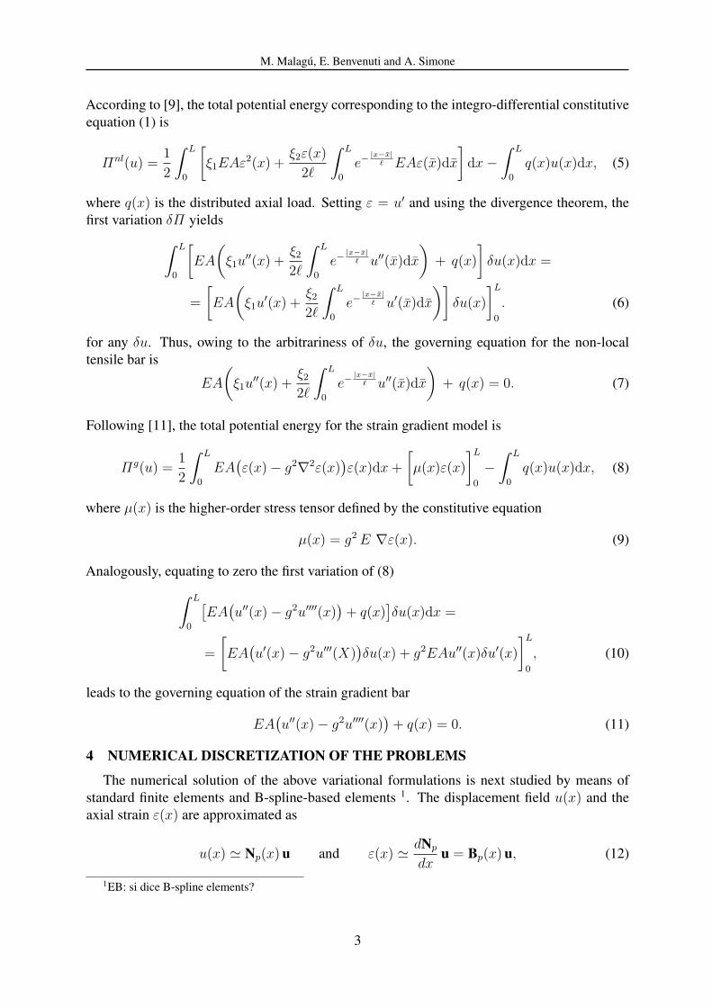
According to [9], the total potential energy corresponding to the integro-differential constitutiveequation (1) is

Πnl(u) =1

2

∫ L

0

[ξ1EAε2(x) +

ξ2ε(x)

2ℓ

∫ L

0

e−|x−x|

ℓ EAε(x)dx

]dx−

∫ L

0

q(x)u(x)dx, (5)

where q(x) is the distributed axial load. Setting ε = u′ and using the divergence theorem, thefirst variation δΠ yields∫ L

0

[EA

(ξ1u

′′(x) +ξ22ℓ

∫ L

0

e−|x−x|

ℓ u′′(x)dx

)+ q(x)

]δu(x)dx =

=

[EA

(ξ1u

′(x) +ξ22ℓ

∫ L

0

e−|x−x|

ℓ u′(x)dx

)]δu(x)

]L0

. (6)

for any δu. Thus, owing to the arbitrariness of δu, the governing equation for the non-localtensile bar is

EA

(ξ1u

′′(x) +ξ22ℓ

∫ L

0

e−|x−x|

ℓ u′′(x)dx

)+ q(x) = 0. (7)

Following [11], the total potential energy for the strain gradient model is

Πg(u) =1

2

∫ L

0

EA(ε(x)− g2∇2ε(x)

)ε(x)dx+

[µ(x)ε(x)

]L0

−∫ L

0

q(x)u(x)dx, (8)

where µ(x) is the higher-order stress tensor defined by the constitutive equation

µ(x) = g2E ∇ε(x). (9)

Analogously, equating to zero the first variation of (8)∫ L

0

[EA

(u′′(x)− g2u′′′′(x)

)+ q(x)

]δu(x)dx =

=

[EA

(u′(x)− g2u′′′(X)

)δu(x) + g2EAu′′(x)δu′(x)

]L0

, (10)

leads to the governing equation of the strain gradient bar

EA(u′′(x)− g2u′′′′(x)

)+ q(x) = 0. (11)

4 NUMERICAL DISCRETIZATION OF THE PROBLEMS

The numerical solution of the above variational formulations is next studied by means ofstandard finite elements and B-spline-based elements 1. The displacement field u(x) and theaxial strain ε(x) are approximated as

u(x) ≃ Np(x)u and ε(x) ≃ dNp

dxu = Bp(x)u, (12)

1EB: si dice B-spline elements?

3


where the subscript p denotes the polynomial degree of the basis functions. If the basis functionsrelated to a single element are connoted by the superscript e, the discrete element field can becast as

ue(x) ≃ Nep(x) ue and εe(x) ≃

dNep

dxue = Be

p(x) ue (13)

In the non-local case, the global stiffness matrix of the bar reads

Knl =

nel∧e=1

∫ xe1

xe1

(ξ1 Be T

p (x)EABep(x)dx+

ξ22ℓ

∫ L

0

e|x−x|

ℓ Be Tp (x)EABe

p(x)dx

)dx, (14)

Analogously, in the strain gradient case, the global stiffness yields

Kg =

nel∧e=1

∫ xe1

xe1

(Be T

p (x)EABep(x) + g2Ce T

p (x)EACep(x)

)dx, (15)

where Cp are the second derivatives of Np with respect to x.The integro-differential formulation is computationally burdensome since the computation

of the elemental stiffness matrix (14) requires the evaluation of the stiffness contributions fromthe whole domain. On the other hand, the computation of (15) for the strain gradient case re-quires high-continuity of the displacement field formulation. The high-continuity requirementwas overcome in different ways, such as by using C1 Hermite finite elements, the element-free Galerkin method or the staggered method [12]. The Hermite basis functions possess in-deed increasing inter-elemental continuity for increasing polynomial degree, as displayed inFigures 1(a)- (d), in contrast to C0 Lagrange interpolation functions. In the present study, as al-ternative candidates to standard interpolation functions, B-spline basis functions are consideredbecause they are suitable for the construction of higher-order basis functions. In particular, byincreasing the number of the degrees of freedom and the polynomial order of the B-spline ba-sis functions–the so called k-refinement method [13]–, the continuity order increases. The useof the B-splines leads to a homogeneous structure of highly continuous basis functions alongthe whole one-dimensional domain as shown in Figures 1(e) and 1(f). Robust and efficient al-gorithms to compute high-order NURBS and B-spline basis functions are well known in theliterature (i.e. [14, 15]).

5 APPLICATION AND RESULTS

Let us consider an elastic bar with length L = 100 cm, cross area A = 1 cm2 and Young’smodulus E = 210 GPa loaded by two unit axial forces as presented in Figure 2.The analytical solution [10] corresponding to the nonlocal stress-strain law (1) is shown inFigure 3. In this case, the analytical solutions [10] corresponding to the nonlocal stress-strainlaws (1) and (3) coincide if g = ℓ

√ξ1. The boundary layers increase by increasing the value

of |1 − ξ1| and become sharper for decreasing ℓ. Furthermore, if ξ1 < 1, the strain energyassociated with the nonlocal solution is larger than that predicted by the classical elasticitytheory, whereas for ξ1 > 1 we have the opposite trend, according to the experimental results [16].The imposition of the boundary conditions, which is not discussed in the present paper, is treatedin [10].In Figure 4 the numerical solutions of the integral non-local model for the Lagrange, Hermiteand B-spline interpolations with 50 and 100 degrees of freedom are compared to the analyticalsolution. The strain field displayed in Figures 4(a) and 4(b) are affected by diffused oscillations,

4


−1 −0.5 0 0.5 1−0.5

0

0.5

1

1.5

(a) Lagrange basis functions (p=2)

−1 −0.5 0 0.5 1−0.5

0

0.5

1

1.5

(b) Lagrange basis functions (p=4)

−1 −0.5 0 0.5 1−0.5

0

0.5

1

(c) Hermite basis functions (p=3)

−1 −0.5 0 0.5 1−1

−0.5

0

0.5

1

(d) Hermite basis functions (p=5)

0 0.2 0.4 0.6 0.8 10

0.2

0.4

0.6

0.8

1

(e) B-spline basis functions (p=2)

0 0.2 0.4 0.6 0.8 10

0.2

0.4

0.6

0.8

1

(f) B-spline basis functions (p=4)

Figure 1: basis functions used for the interpolation of the displacement field.

F = 1 kN

L = 1 m

A = 1 cm2E = 210 GPaF = 1 kN

Figure 2: Homogeneous bar with unitary tip forces.

5


0 10 20 30 40 50 60 70 80 90 1004

4.5

5x 10

−5

x [cm]

ε [−

]

l=0 cm l=5 cm l=10 cm l=15 cm l=20 cm

(a) ξ1 = 1.3

0 10 20 30 40 50 60 70 80 90 100

4

5

6

7x 10

−5

x [cm]

ε [−

]

ξ

1=0.5 ξ

1=0.7 ξ

1=1 ξ

1=1.3 ξ

1=1.5

(b) ℓ = 5 cm

Figure 3: strain field of a tensile bar with E = 210 GPa, A = 1 cm2 and L = 100 cm.

whose entity increases by increasing the polynomial degree. The oscillations attenuate whenthe Hermite basis functions are employed, though they still persist along the whole domain, anddo not vanish by increasing the polynomial order, as it can be seen in Figures 4(c)-(d).On the other hand, Figures 4(e) and 4(f) show that, by increasing the polynomial degree and,consequently, the continuity of the B-spline basis functions, the numerical solution improves.Therefore, the wide support of the B-spline basis functions considerably improve the accuracyof the numerical solution.The case of the strain gradient stress-strain law is next taken into account. The Lagrange in-terpolation is not feasible to this formulation since the increased order of the weak form of theproblem.In Figure 5, the results for the strain gradient model are plotted for the Hermite and B-spline interpolations. In Figures 5(a) and 5(c), oscillations appear at the boundaries when a verycoarse discretization is adopted consisting of 10 degrees of freedom. After refining the mesh,both the numerical solutions obtained by means of the Hermite and the B-spline interpolationsoverlap the exact solution as it can be seen in Figures 5(b) and 5(d) corresponding to 20 degreesof freedom.

The relative strain energy error for the non-local formulation in Figure 6(a) shows that theerror associated with the Hermite basis functions decreases slightly if compared to the C0 La-grange basis functions. The accuracy dramatically improves when B-spline basis functionsare exploited, owing to the combined beneficial effects of the wide support and the high-ordercontinuity.On the other hand, Figure 6(b) shows that in the case of the strain gradient formulation, theconvergence rate significantly increases both for the Hermite and the B-spline interpolations.A synthesis of the pros and cons of the adopted numerical procedures for the non-local and the

6


0 20 40 60 80 100

3.5

4

4.5

5

x 10−5

x [cm]

ε [−

]

(a) Lagrange finite elements (50 dofs)

0 20 40 60 80 100

3.5

4

4.5

5

x 10−5

x [cm]

ε [−

]

(b) Lagrange finite elements (100 dofs)

0 20 40 60 80 100

3.5

4

4.5

5

x 10−5

x [cm]

ε [−

]

(c) Hermite finite elements (50 dofs)

0 20 40 60 80 100

3.5

4

4.5

5

x 10−5

x [cm]

ε [−

]

(d) Hermite finite elements (100 dofs)

0 20 40 60 80 100

3.5

4

4.5

5

x 10−5

x [cm]

ε [−

]

(e) B-spline elements (50 dofs)

0 20 40 60 80 100

3.5

4

4.5

5

x 10−5

x [cm]

ε [−

]

(f) B-spline elements (100 dofs)

Figure 4: tensile bar with Eringen’s formulation, ξ1 = 2 and ℓ = 3 cm. Exact solution (solid black line) andnumerical solutions (dash-dot lines). Lagrange finite elements: quadratic (red), cubic (green) and quartic (blue)basis functions. Hermite finite elements: cubic (red), quintic (green) and septic(blue) basis functions. B-splineelements: quadratic (red), cubic (green) and quartic (blue) basis functions.

7


0 20 40 60 80 100

3.5

4

4.5

5

x 10−5

x [cm]

ε [−

]

(a) Hermite basis functions (10 dofs)

0 20 40 60 80 100

3.5

4

4.5

5

x 10−5

x [cm]

ε [−

]

(b) Hermite basis functions (20 dofs)

0 20 40 60 80 100

3.5

4

4.5

5

x 10−5

x [cm]

ε [−

]

(c) B-spline basis functions (10 dofs)

0 20 40 60 80 100

3.5

4

4.5

5

x 10−5

x [cm]

ε [−

]

(d) B-spline basis functions (20 dofs)

Figure 5: tensile bar with Aifantis’s formulation, ξ1 = 2 and ℓ = 3 cm. Exact solution (solid black line) andnumerical solutions (dash-dot lines). Hermite finite elements: cubic (red), quintic (green) and septic (blue) basisfunctions. B-spline elements: quadratic (red), cubic (green) and quartic (blue) basis functions.

8


100

101

102

103

10−10

10−8

10−6

10−4

10−2

100

log(Degrees of freedom)

log(

Str

ain

ener

gy r

elat

ive

erro

r)

Lag p=2

Lag p=3

Lag p=4

Her p=3

Her p=5

Her p=7

Bsp p=2

Bsp p=3

Bsp p=4

(a) Non-local formulation

100

101

102

103

10−10

10−8

10−6

10−4

10−2

100

log(Degrees of freedom)

log(

Str

ain

ener

gy r

elat

ive

erro

r)

Her p=3

Her p=5

Her p=7

Bsp p=3

Bsp p=5

Bsp p=7

(b) Strain gradient formulation

Figure 6: strain energy convergence rate.

9


Basis functions Polynomial order Continuity Oscillations Convergence2 C0 no

Lagrangian 3 C0 yes bad4 C0 yes3 C1 yes

Hermite 5 C2 yes bad7 C3 yes2 C1 no

B-spline 3 C2 no medium4 C3 no

Table 1: resume of the numerical results from the Eringen’s formulation.

Basis functions Polynomial order Continuity Oscillations Convergence3 C1 at the

Hermite 5 C2 boundaries good7 C3 for few dofs3 C2 at the

B-spline 5 C4 boundaries good7 C6 for few dofs

Table 2: resume of the numerical results from the Aifantis’s formulation.

strain gradient formulations is reported in Table 1 and Table 2, respectively.

6 CONCLUSIONS

The numerical solution of the problem of a tensile bar governed by non-local and strain gra-dient based nonlocal elastic stress-strain laws is computationally burdensome because of thenonlocal structure of the stiffness equation and the high inter-elemental continuity requirement,respectively. We used Hermite and B-spline interpolations for both constitutive laws, and La-grange interpolation functions for the nonlocal model only. In the nonlocal case, the numericalresults obtained by means of Lagrange and Hermite basis functions are affected by oscilla-tions along the whole domain and exhibit slow convergence in terms of strain energy relativeerror. Accuracy significantly improves when B-spline basis function are used. In the straingradient case, Hermite and B-spline polynomials lead to almost equivalent results, as oscilla-tions decrease and the strain energy convergence rate improve significantly. In short, B-splineinterpolation is a robust and accurate tool for the numerical solution of problems in nonlocalelasticity governed by integral and strain gradient stress-strain laws.

REFERENCES

[1] S. Papargyri-Beskou, K. G. Tsepoura, D. Polyzos, and D. E. Beskos. Bending and stabilityanalysis of gradient elastic beams. International Journal of Solids and Structures.

[2] K. G. Tsepoura, S. Papargyri-Beskou, D. Polyzos, and D. E. Beskos. Static and dynamicanalysis of a gradient-elastic bar in tension. Archive of Applied Mechanics.

10


[3] J. Peddieson, G. R. Buchanan, and R. P. McNitt. Application of nonlocal continuummodels to nanotechnology. International Journal of Engineering Science.

[4] R. Tupin. Elastic materials with couple-stresses. Archive for Rational Mechanics andAnalysis, 11:385–414, 1962.

[5] R. D. Mindlin. Micro-structure in linear elasticity. Archive for Rational Mechanics andAnalysis, 16:51–78, 1961.

[6] A. C. Eringen. On differential equations of nonlocal elasticity and solutions of screwdislocation and surface waves. Archive of Applied Mechanics, 54:4703–4710, 1983.

[7] E. Aifantis. On the role of gradients in the localization of deformation and fracture. Inter-national Journal of Engineering Science, 30:1279–1299, 1992.

[8] A. C. Eringen. Nonlocal continuum field theories. Springer, 2001.

[9] C. Polizzotto. Nonlocal elasticity and related variational principles. International Journalof Solids and Structures, 38:7359–7380, 2001.

[10] E. Benvenuti and A. Simone. Closed form solutions for eringen integral and aifantisgradient models in nonlocal elasticity. 2012.

[11] I. Vardoulakis and J. Sulem. Bifurcation analysis in geomechanics. Chapman and Hall,1995.

[12] H. Askes and E. C. Aifantis. Gradient elasticity in statics and dynamics: An overview offormulations, length scale identification procedures, finite element implementations andnew results. International Journal of Solids and Structures, 48:1962–1990, 2011.

[13] T. J. R. Hughes, J. A. Cottrell, and Y. Bazilevs. Isogeometric analysis: CAD, finite el-ements, NURBS, exact geometry and mesh refinement. Computer Methods in AppliedMechanics and Engineering, 194:4135–4195, 2005.

[14] L. A. Piegl and W. Tiller. The NURBS book. Springer, 1997.

[15] C. de Falco, A. Reali, and R. Vazquez. Geopdes: A research tool for isogeometric analysisof pdes. Advances in Engineering Software, 42:1020–1034, 2011.

[16] W. D. Nix and H. Gao. Indentation size effects in crystalline materials: A law for straingradient plasticity.

11

Finite element and b-spline methods for one-dimensional non-local elasticity

Documents

Transcript of Finite element and b-spline methods for one-dimensional non-local elasticity