Quality Technology & Quantitative Management Vol. 5, No. 1, pp. 1-20, 2008

QQTTQQMM © ICAQM 2008

Finite Buffer Vacation Queue under E-limited with Limit Variation Service and Batch Markovian Arrival Process

A. D. Banik and U. C. Gupta

Department of Mathematics, Indian Institute of Technology, Kharagpur, India (Received June 2006, accepted January 2007)

______________________________________________________________________

Abstract: We consider a finite-buffer single server queue with single (multiple) vacation(s) under batch Markovian Arrival Process (BMAP). The service discipline is varying number limited service, also called E-limited with limit variation (ELV) where the server serves until either the system is emptied or a randomly chosen limit of l customers have been served. Queue length distributions at various epochs such as, pre-arrival, arbitrary, departure etc. have been obtained. Several other service disciplines like, Bernoulli scheduling, non-exhaustive service and E-limited service can be treated as special cases of the ELV service. Such a queueing system finds applications in the token ring or token bus of local area network (LAN) in which the vacation would correspond to the time the token is away to the other stations.

Keywords: Batch Markovian arrival process, finite buffer queue, limited service discipline, multiple vacations, single server, single vacation. ______________________________________________________________________

1. Introduction

ueueing systems with vacations have found wide applications in the modelling and analysis of computer and communication networks, and several other engineering

systems in which single server is attached to one or more workstations. Modelling such systems as single server queues with vacations allows one to analyze each workstation in relative isolation since the time the server is attending to other stations in the system may be modeled as vacation. For more detail and versatile implementation of vacation models one can refer to the comprehensive survey by Doshi [4]. Vacation models are distinguished by their scheduling disciplines, that is, the rules governing when a service stops and a vacation begins. Several service disciplines in combination with vacations are possible, e.g., exhaustive, limited, gated, exhaustive limited (E-limited), gated limited (G-limited) etc. In fact there is an extensive amount of literature available on infinite and finite buffer 1M G/ / type vacation models that can be found in Takagi [17],[18], respectively.

Traditional teletraffic analysis using Poisson process is not powerful enough to capture the correlated and bursty nature of traffic arising in the present high-speed networks, e.g., ATM networks where packets or cells of voice, video, image and data are sent over a common transmission channel on statistical multiplexing basis. The performance analysis of statistical multiplexers whose input consists of superposition of several packetized sources have been done through some analytically tractable arrival process, e.g., Markovian arrival process ( )MAP , see Lucantoni et al. [13] and batch Markovian arrival process ( )BMAP , see Lucantoni [12]. In [13] the analysis of 1MAP G/ / queue with multiple vacations has been carried out. Later in [12] the detailed analysis of 1BMAP G/ / queue

Q

2 Banik and Gupta

has been carried out. This type of arrival process includes many familiar input processes such as Markovian arrival process ( )MAP [13], Markov modulated Poisson process ( )MMPP , PH-type renewal process, Interrupted Poisson process ( )IPP , Poisson process etc. Further Matendo [14], Ferrandiz [5] etc. have discussed 1BMAP G/ / queue with vacations. As queueing analysis of finite systems are more realistic in applications than infinite systems, the detailed study of finite capacity vacation model 1BMAP G N/ / / queue under exhaustive service discipline was performed by Niu et al. [16] where they have included setup time, close-down time, single/multiple vacations.

In this paper we analyze 1BMAP G N/ / / queue where the server serves until either the system empties or a randomly chosen limit of (0 )l l L≤ ≤ customers have been served, whichever occurs first. The server then goes for a vacation of random length of time before returning to serve the queue again. Returning from a vacation if the queue is empty then according to the acting vacation policy the server will decide whether he remains dormant in the queue waiting for a customer (single vacation) or he takes another vacation (multiple vacation). This type of service discipline is known as E-limited with limit variation (ELV) and was earlier studied by Lamaire [9],[10] for the case of 1M G/ / infinite and finite buffer queue, respectively.

A batch which upon arrival does not find enough space in the buffer is, either fully rejected, or a part of that batch is rejected. Some queueing protocols are based on the former strategy and they are known as total batch rejection policy. A more recent protocol is known as the partial batch rejection policy. We analyze only partial batch rejection strategy and obtain queue length distributions at various epochs using a combination of embedded Markov chain and supplementary variable method. We present an unified approach to analyze both single and multiple vacation models together and for that we define an indicator function ( )Sδ as follows:

1, for single vacation policy

0, for multiple vacation policySδ,⎧

= ⎨ ,⎩

i.e., by fixing 1Sδ = one can get the results for single vacation policy and similarly, 0Sδ = gives the results for multiple vacation policy. One may note here that results of several vacation policies viz. Bernoulli scheduling, exhaustive service, pure limited service and E-limited service can be obtained as special cases of ELV model. Moreover the results of

1M G N/ / / queue with ELV service, earlier studied in [10] and the same queue with limited service studied by Lee [11] can be obtained as special cases of our model. Finally, it may be remarked here that the analysis of 1MAP G N/ / / queue with limited service discipline is carried out by Blondia [3], Gupta et al.[7], and recently Banik et al. [1] analyzed the same queue under ELV service discipline. Also Banik et al. [2] discussed 1BMAP G N/ / / queue under limited service discipline. The methodology involved in this paper is similar to that of [7],[1],[2], but dealing with BMAP arrival and ELV service discipline together made the model more complex and forced significant extension both in terms of theoretical and computational aspects. As a final remark it may be mentioned here that to the best of authors knowledge there are no previous work on finite or infinite buffer 1BMAP G/ / queue under E-limited with limit variation service.

2. Description of the Model

Let us consider a 1BMAP G N/ / / queue wherein the server is allowed to serve a maximum of (0 )l l L≤ ≤ customers during each visit to the queue, i.e., the server goes

Finite Buffer Vacation Queue under E-limit 3

for a vacation if either the queue has been emptied or l customers have been served, whichever occurs earlier. On return from a vacation if the queue is empty or a limit of zero is chosen, the server immediately goes on another vacation in the case of multiple vacation policy, whereas the server remains dormant and waiting for a customer to serve in case of single vacation policy. The limit l is a random variable whose mass function is denoted by (0 )lp l L≤ ≤ and cumulative distribution function is ( )P l . The limit for number of customers to be served during a service interval (i.e. the busy period) is determined at the preceding vacation termination instant. The sequence of limits chosen at these instants are independent and identically distributed random variables (i.i.d.r.vs.). By suitably choosing

lp one can obtain results for several other service disciplines, including Bernoulli scheduling, exhaustive service, pure limited service and E-limited service, e.g., if we take

1Lp = and 0 (0 )lp l L= ≤ < then the service system is equivalent to E-limited service. If ( 1)L = ∞ = in the above assumption, the service system is equivalent to exhaustive

service system (=pure limited service). Bernoulli scheduling system can be thought of as a special case of ELV service system with 0 0L p= ∞, = and 1(1 ) 0 1l

lp p p p−= − , < < for 1,2,....l =

Input process is BMAP where arrivals are governed by an underlying m -state Markov chain. The arrival process is characterized by m m× matrices 0k k, ≥D where ( )i j, -th (1 )i j m≤ , ≤ element of 0D , is the state transition rate from state i to state j in the underlying Markov chain without an arrival and ( )i j, -th element of 1k k, ≥D , is the state transition rate from state i to state j in the underlying Markov chain with an arrival of batch size k . The matrix 0D has nonnegative off-diagonal and negative diagonal elements, and the matrix 1, ≥ ,kD k has nonnegative elements. Let ( )N t denote the number of arrivals in (0, ]t and ( )J t be the state of the underlying Markov chain at time t with state space :1 i i m≤ ≤ . Then ( ), ( )N t J t is a two-dimensional Markov process of BMAP with state space ( , ) : 0, 1 n i n i m≥ ≤ ≤ . The infinitesimal generator of BMAP is given by

⎛ ⎞⎜ ⎟⎜ ⎟=⎜ ⎟⎜ ⎟⎝ ⎠

0 1 2 3

0 1 2

0 1

D D D D

0 D D DQ

0 0 D D.

As Q is the infinitesimal generator of the BMAP , we have ∞= =∑ 0 0k kD e , where e is

an 1m× column vector with all its elements equal to 1. Further since 0k k∞== ∑D D is the

infinitesimal generator of the underlying Markov chain ( )J t , there exists a stationary probability vector π such that = , = .π π0 e 1D Then the average arrival rate λ∗ and average batch arrival rate gλ of the stationary BMAP are given by λ∗ ∞

== ∑π 1k kkD e and π 1kg kλ ∞

== ,∑ D e respectively.

Let *( ) ( )[ ( )]S x s x S θ be the distribution function (DF) probability density function (pdf)[Laplace-Stieltjes transform (LST)] of the service time S of a typical customer. Similarly, *( ) ( )[ ( )]V x v x V θ be the DF pdf [LST] of a typical vacation time V of the server. The mean service [vacation] time is (1)( ) (0)E S S∗= − [ (1)( ) (0)E V V ∗= − ], where

( ) ( )jf ζ∗ is the ( 1)thj j ≥ derivative of ( )f θ∗ at θ ζ= . The service-, vacation- times are assumed to be i.i.d. r.vs. and each is independent of the arrival process. The traffic intensity is given by ( )E Sρ λ∗= . Further, let ρ′ be the probability that the server is busy. The state of the system at time t is described by the r.v.s., namely

4 Banik and Gupta

•

( , ) if the server is serving -th (1 ) customer in the service period

consisting of services of at the most (1 ) customers

( ) 0 on vacation

( , ) server is on dormancy and

k l k k l

l l L

t

d l

ξ

≤ ≤≤ ≤

= dormancy period started with a limit value

chosen as l

⎧⎪⎪⎪⎨⎪⎪⎪⎩

• ( )qN t = number of customers present in the queue excluding the one in service

• ( )J t = state of the underlying Markov chain of BMAP

• ( )S t = remaining service time of the customer in service

• ( )V t = remaining vacation time of the server.

We define for 1 i m≤ ≤ the joint probability densities of queue length ( )qN t , state of the server ( )tξ and the remaining service (vacation) time ( )S V , respectively, by

π ξΔ = = = < < + Δ =[ ], ( , ; ) ( ) , ( ) , ( ) , ( ) ( , ),k

i l qn x t x P N t n J t i x S t x x t k l

0 1 1 0n N l L k l x≤ ≤ , ≤ ≤ , ≤ ≤ , ≥ ,

ω ξ, ; Δ = = , = , < < + Δ , = , ≤ ≤ , ≥ ,( ) ( ) ( ) ( ) ( ) 0 0 0i qn x t x P N t n J t i x V t x x t n N x

ν ξ, ; = = , = , = , , ≤ ≤ .(0 ) ( ) 0 ( ) ( ) ( ) 1i l qt P N t J t i t d l l L

As we shall discuss the model in limiting case, i.e., when t →∞ the above probabilities will be denoted by π ω, , , , ,[ ] ( ) ( )k

i l in x n x and (0)i lν , , respectively. Let us further define the row vectors of order 1 m×

π[ ] [ ]( ) [ ( )] and ( ) [ ( )]k kl i l in x n x n x n x,, = , , = , ,ωπ ω

and (0) [ (0)] 1l i l i m,= , ≤ ≤ ,νν

where π , ,[ ] ( )ki l n x denotes the arbitrary epoch probability that there are n customers in the

queue and the state of the arrival process is i when the server is serving the -thk customer whose remaining service time is x in the present busy period consisting of the sum of the service times of l or lesser number of customers. Similarly, ω ,( )i n x denotes the arbitrary epoch probability that n customers are in the queue and state of the arrival process is i when the server is on vacation with remaining vacation time x , and ν , (0)i l denotes the arbitrary epoch probability that the server is on dormancy state which started with a limit value chosen l and of course zero customer in the system, and phase of the arrival process is i .

3. Queue Length Distributions at Various Epochs

3.1. Queue Length Distribution at Service Completion and Vacation Termination Epochs

Consider the system at service completion/vacation termination epochs which are taken as embedded points. Let 0 1 2 t t t, , ,... be the time epochs at which either service

Finite Buffer Vacation Queue under E-limit 5

completion or vacation termination occurs. 0it i+ , ≥ denotes the time epoch just after a service completion or vacation termination occurs. The state of the system at it

+ is defined as ( ) ( ) ( )q i i iN t t J tξ+ + +, , , where ( ) ( )q i iN t tξ+ +, and ( )iJ t + are defined earlier. Therefore,

( ) 0itξ + = indicates that the embedded point is a vacation termination instant, whereas ( ) ( ) (1 1 )it k l l L k lξ + = , ≤ ≤ , ≤ ≤ indicates the embedded point is a service completion

instant of the k -th customer in the present busy period consisting of services of l or lesser number of customers. In limiting case these probability distributions are

[ ] ( ) lim ( ( ) ( ) ( ) ( ) ) 0 1 1 1kj l q i i i

ig n P N t n t k l J t j n N k l l L j mξ+ + +

, →∞= = , = , , = , ≤ ≤ , ≤ ≤ , ≤ ≤ , ≤ ≤ ,

ξ+ + +

→∞= = , = , = , ≤ ≤ , ≤ ≤ ,( ) lim ( ( ) ( ) 0 ( ) ) 0 1j q i i i

if n P N t n t J t j n N j m

where [ ]( )kj lg n, represents the probability that there are n customers in the queue and the

state of the arrival process is j at service completion epoch of the k -th customer in the service period consisting of services of at the most l customers. Similarly, let ( )jf n represents the probability that there are n customers in the queue and the state of the arrival process is j at vacation termination epoch. Further, let us denote the row vectors of order 1 m×

g f,= , = , ≤ ≤ .[ ] [ ]( ) [ ( )] ( ) [ ( )] 1k kl j l jn n n n j mg f

Let ( ) 0n n n, ≥A V denote an m m× matrix whose ( )i j, -th element represents the conditional probability that n customers have been accepted during a service (vacation) time of a customer and the underlying Markov chain is in phase j at the end of the service (vacation) time given that the underlying Markov chain was in phase i at the beginning of the service (vacation). Further, let us denote c

nA and cnV by

0N N

c cn k n k

k n k nn N

= == , = , ≤ ≤ .∑ ∑A A V V

Obviously, 1ci i N, ≥ +A will be equal to null matrix of order m m× and similarly, for

1ci i N, ≥ + .V

Observing the system immediately after each embedded point, we have the transition probability matrix (TPM) P with four block matrices of the form:

( 1) ( 1)( 1) 1 ( 1) 1 .

2 2

( 1) ( 1) ( 1)( 1) ( 1) ( 1) ( 1)

2 2 2

( 1) ( 1) ( 1)( 1) ( 1)

2L L L L

N m N m

L L L L L LN m N m N m N m

L L N m N mN m N m

+ +⎛ ⎞ ⎛ ⎞+ + × + +⎜ ⎟ ⎜ ⎟⎝ ⎠ ⎝ ⎠

+ + ++ × + + × +

+ + × ++ × +

⎡ ⎤⎢ ⎥= ⎢ ⎥⎢ ⎥⎣ ⎦

P

Ξ Ω

Δ Φ

First we will explain these block matrices for multiple vacation model. Ξ describes the probability of transitions among the service completion epochs. A typical service completion epoch will be denoted by the triplet ξ+ + +, , ( ) ( ) ( )q i i iN t t J t of which we first consider the change in ( )q iN t + , i.e., (0 )n n N≤ ≤ and the second element of

( ) ( )it k lξ + = , , i.e., (1 )l l L≤ ≤ to describe the construction of the first block of the TPM. Then the elements of Ξ can be written as follows:

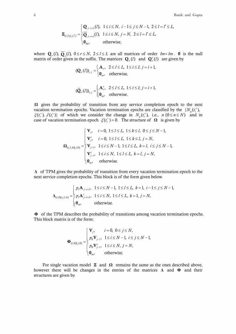
6 Banik and Gupta

− +

′, , , − +

′⎧ ≤ ≤ , − ≤ ≤ − , ≤ = ≤ ,⎪

′= , ≤ ≤ , = , ≤ = ≤ ,⎨⎪

,⎩

Ξ1

( ) ( ) 1

( ), 1 1 1 2

( ) 1 2

otherwise,

j i

i l j l j i

lm

l i N i j N l l L

l i N j N l l L

Q

Q

0

where ( ) ( ) 0 2r rl l r N l L, , ≤ ≤ , ≤ ≤Q Q are all matrices of order lm lm× . 0 is the null

matrix of order given in the suffix. The matrices ( )r lQ and ( )cr lQ are given by

,

, ≤ ≤ , ≤ ≤ ; = + ,⎧= ⎨ , ,⎩

2 1 1( ( ))

otherwiser

r i jm

l L i l j il

AQ

0

,

⎧ , ≤ ≤ , ≤ ≤ ; = + ,⎪= ⎨,⎪⎩

2 1 1( ( ))

otherwise.

cr

r i jm

l L i l j il

AQ

0

Ω gives the probability of transition from any service completion epoch to the next vacation termination epochs. Vacation termination epochs are classified by the ( ) q iN t + ,

( ) ( )i it J tξ + +, of which we consider the change in ( )q iN t + , i.e., ≤ ≤ (0 )n n N and in case of vacation termination epoch ( ) 0itξ + = . The structure of Ω is given by

, , , −

−

, = , ≤ ≤ , ≤ ≤ , ≤ ≤ − ,⎧⎪

, = , ≤ ≤ , ≤ ≤ , = ,⎪⎪= , ≤ ≤ − , ≤ ≤ , = , ≤ ≤ − ,⎨⎪

, ≤ ≤ , ≤ ≤ , = , = ,⎪⎪ , .⎩

Ω( )( 0)

0 1 1 0 1

0 1 1

1 1 1 1

1 1

otherwise

j

cj

i l k j j i

cj i

m

i l L k l j N

i l L k l j N

i N l L k l i j N

i N l L k l j N

V

V

V

V

0

Δ of TPM gives the probability of transition from every vacation termination epoch to the next service completion epochs. This block is of the form given below.

− +

, , , − +

, ≤ ≤ − , ≤ ≤ , = , − ≤ ≤ − ,⎧⎪⎪= , ≤ ≤ , ≤ ≤ , = , = ,⎨⎪ , .⎪⎩

Δ1

( 0)( ) 1

1 1 1 1 1 1

1 1 1

otherwise

l j i

ci j l k l j i

m

p i N l L k i j N

p i N l L k j N

A

A

0

Φ of the TPM describes the probability of transitions among vacation termination epochs. This block matrix is of the form:

−, ,

−

, = , ≤ ≤ ,⎧⎪

, ≤ ≤ − , ≤ ≤ − ,⎪= ⎨, ≤ ≤ , = ,⎪

⎪ , .⎩

Φ 0

( 0)( 0)

0

0 0

1 1 1

1

otherwise

j

j ii j c

j i

m

i j N

p i N i j N

p i N j N

V

V

V

0

For single vacation model Ξ and Ω remains the same as the ones described above, however there will be changes in the entries of the matrices Δ and Φ and their structures are given by

Finite Buffer Vacation Queue under E-limit 7

11 1

1

( 0)( ) 1

1

0 1 1 0 2

0 1 1 1

1 1 1 1 1 1

1 1

jrl j rr

r Nl j Nr

i j l k l j i

cl j i

p i l L k j N

p i l L k j N N

p i N l L k i j N

p i N l L

+= − +

∞= − +

, , , − +

− +

, = , ≤ ≤ , = , ≤ ≤ − ,∑

, = , ≤ ≤ , = , = − , ,∑

= , ≤ ≤ − , ≤ ≤ , = , − ≤ ≤ − ,

, ≤ ≤ , ≤ ≤ ,

AD

ADA

A

Δ

1 ,

otherwise m

k j N

⎧⎪⎪⎪⎨⎪

= , =⎪⎪ , ,⎩0

and

0

0

( 0)( 0)

0

0 0

1 1 1

1

otherwise

j

j ii j c

j i

m

p i j N

p i N i j N

p i N j N

−, ,

−

, = , ≤ ≤ ,⎧⎪

, ≤ ≤ − , ≤ ≤ − ,⎪= ⎨, ≤ ≤ , = ,⎪

⎪ , .⎩

V

V

V

0

Φ

Note that the factor 10( ) 1r r r−= − , ≥D DD represents the phase transition matrix during

an inter-batch arrival time, for detail see Lucantoni [12]. Now the unknown probability vectors [ ] ( )k

l ng and ( )nf can be obtained by solving the system of equations:

[ ] [ ]( ( ) ( )) ( ( ) ( ))k kl ln n n n, = , Pg f g f .

One may note here that queue length distributions at departure epoch can be obtained through the relations between distributions of number of customers in the queue at service completion and departure epochs. Let ,[ ]u ( )k

l n denotes row vector whose i -th element represents steady state probability that there are (0 )n n N≤ ≤ customers in the queue and phase of the arrival process is (1 )i i m≤ ≤ at departure epoch of the k -th (1 )k l≤ ≤ customer in the service period consisting of services of (1 )l l L≤ ≤ or lesser number of customers. Since [ ]u ( )k

l n is proportional to [ ] ( )kl ng and = = = =∑ ∑ ∑ [ ]

0 1 1u ( )e 1kN L ln l k l n , we get

= = =

= , ≤ ≤ , ≤ ≤ , ≤ ≤ .∑ ∑ ∑

[ ][ ]

[ ]

0 1 1

( )u ( ) 0 1 1

( )

kk l

l N L l kl

i l k

nn n N l L k l

n e

g

g (1)

3.2. Queue Length Distribution at Arbitrary Epoch

To determine queue length distribution at arbitrary epoch we will develop relations between distributions of number of customers in the queue at service completion (vacation termination) and arbitrary epochs. Supplementary variable method has been used and for that we relate the states of the system at two consecutive time epochs t and +Δt t and using probabilistic arguments, we have a set of partial differential equations for each phase

(1 )i i m, ≤ ≤ . Taking limit as t →∞ and using matrices and vector notations, we obtain

δ− , = , + , + , ≤ ≤π π[1] [1]0 1(0 ) (0 ) (1 0) ( ) (0) ( ) 1l l l S l

dx x p s x s x l L

dxD Dω ν (2)

−− , = , + , , ≤ ≤ , ≤ ≤π π π[ ] [ ] [ 1]0(0 ) (0 ) (1 0) ( ) 2 2 ,k k k

l l ld

x x s x l L k ldx

D (3)

8 Banik and Gupta

=− , = , + − , + + ,∑π π π[1] [1] [1]

01

( ) ( ) ( ) ( 1 0) ( )n

l l l i li

dn x n x n i x p n s x

dxD D ω

δ ++ , ≤ ≤ − , ≤ ≤1(0) ( ) 1 2 1 ,S l n s x n N l LDν (4)

=− , = , + − , + + ,∑π π π[1] [1] [1]

01

( ) ( ) ( ) ( 1 0) ( )n

l l l i li

dn x n x n i x p n s x

dxD D ω

δ ′+ , = − ≤ ≤(0) ( ) 1, 1 , S l N s x n N l LDν (5)

[ ] [ ] [ ] [ 1]0

1( ) ( ) ( ) ( 1 0) ( ),

nk k k k

l l l i li

dn x n x n i x n s x

dx−

=− , = , + − , + ,∑D Dπ π π + π

1 1 2 2n N l L k l≤ ≤ − , ≤ ≤ , ≤ ≤ , (6)

π=

′− , = , + − , , ≤ ≤ , ≤ ≤ ,∑π π[ ] [ ] [ ]0

1( ) ( ) ( ) 1 1

Nk k k

l l l ii

dN x N x N i x l L k l

dxD D (7)

δ δ= =

− , = , + , + − , + , ,∑ ∑ π[ ]0 0

1 1(0 ) (0 ) ( (0 0) (1 ) (0 0) (0 0)) ( )

L lk

l S Sl k

dx x p x

dxDω ω ω ω ν (8)

= =− , , + − , + ,∑ ∑ π[ ]

01 1

( )= ( ) ( ) ( ( 0)n L

li l

i l

dn x n x n i x n

dxD Dω ω ω

0 ( 0)) ( ) 1 1p n x n N+ , , ≤ ≤ − ,ω ν (9)

= =

′− , = , + − , + , + , ,∑ ∑ π[ ]0 0

1 1( ) ( ) ( ) ( ( 0) ( 0)) ( )

N Ll

i li l

dN x N x N i x N p N x

dxD Dω ω ω ω ν (10)

δ δ= + , , ≤ ≤ ,0(0) (0 0) 1S l S lp l L0 Dν ω (11)

where ∞=′ ′= , ≥∑ ( 0)j ii j iD D and , ,π[ ] ( 0)( ( 0))k

l n nω are the respective probabilities when remaining service time (remaining vacation time) is zero. Let us define the Laplace transform of ,π[ ] ( )k

l n x and ,( )n xω as

θ θθ θ∞ ∞∗ − ∗ −, = , , , = , ,∫ ∫π π[ ] [ ]0 0( ) ( ) ( ) ( )k x k x

l ln e n x dx n e n x dxω ω

θ≤ ≤ , ≤ ≤ , ≤ ≤ , ≥ ,0 1 1 Re 0n N l L k l so that

∞ ∞∗ ∗≡ , = , , ≡ , = , .∫ ∫π π π[ ] [ ] [ ]0 0( ) ( 0) ( ) ( ) ( 0) ( )k k k

l l ln n n x dx n n n x dxω ω ω (12)

Multiplying Equations (2)-(10) by xe θ− and integrating w.r.t. x over 0 to ∞ , we obtain

θ θ θ θ δ θ∗ ∗ ∗ ∗− , + , = , + , + , ≤ ≤ ,π π π[1] [1] [1]0 1(0 ) (0 0) (0 ) (1 0) ( ) (0) ( ) 1l l l l S lp S S l LD Dω ν (13)

θ θ θ θ∗ ∗ − ∗− , + , = , + , , ≤ ≤ , ≤ ≤ ,π π π π[ ] [ ] [ ] [ 1]0(0 ) (0 0) (0 ) (1 0) ( ) 2 2k k k k

l l l l S l L k lD (14)

Finite Buffer Vacation Queue under E-limit 9

θ θ θ θ θ∗ ∗ ∗ ∗

=− , + , = , + − , + + ,∑π π π π[1] [1] [1] [1]

01

( ) ( 0) ( ) ( ) ( 1 0) ( )n

l l l l i li

n n n n i p n SD D ω

δ θ∗++ , ≤ ≤ − , ≤ ≤ ,1(0) ( ) 1 2 1S l n S n N l LDν (15)

θ θ θ θ θ∗ ∗ ∗ ∗

=− , + , = , + − , + + ,∑π π π π[1] [1] [1] [1]

01

( ) ( 0) ( ) ( ) ( 1 0) ( )n

l l l l i li

n n n n i p n SD D ω

δ θ∗′+ , = − , ≤ ≤ ,(0) ( ) 1 1S l N S n N l LDν (16)

θ θ θ θ θ∗ ∗ ∗ − ∗

=− , + , = , + − , + + , ,∑π π π π π[ ] [ ] [ ] [ ] [ 1]

01

( ) ( 0) ( ) ( ) ( 1 0) ( )n

k k k k kl l l l i l

in n n n i n SD D

1 1 2 2n N l L k l≤ ≤ − , ≤ ≤ , ≤ ≤ , (17)

θ θ θ θ∗ ∗ ∗

=′− , + , = , + − , , ≤ ≤ , ≤ ≤ ,∑π π π π[ ] [ ] [ ] [ ]0

1( ) ( 0) ( ) ( ) 1 1

Nk k k k

l l l l ii

N N N N i l L k lD D (18)

θ θ θ δ∗ ∗

= =− , + , = , + , + − ,∑ ∑ π[ ]

01 1

(0 ) (0 0) (0 ) ( (0 0) (1 ) (0 0)L l

kl S

l kDω ω ω ω

0 (0 0)) ( ),S p Vδ θ∗+ ,ω (19)

θ θ θ θ∗ ∗ ∗

= =− , + , = , + − , + ,∑ ∑ π[ ]

01 1

( ) ( 0) ( ) ( ) ( ( 0)n L

li l

i ln n n n i nD Dω ω ω ω

0 ( 0)) ( ) 1 1p n V n Nθ∗+ , , ≤ ≤ − ,ω (20)

θ θ θ θ∗ ∗ ∗

=− , + , = , + − ,∑0

1( ) ( 0) ( ) ( )

N

ii

N N N N iD Dω ω ω ω

θ∗

=+ , + , .∑ π[ ]

01

( ( 0) ( 0)) ( )L

ll

lN p N Vω (21)

Using Equations (13)-(21), we will derive certain results in the form of lemmas and theorems.

Lemma 1

δ−

= = = = = = =, + , = , + , .∑ ∑ ∑ ∑ ∑ ∑ ∑π π

1[ ] [ ]

2 1 0 1 1 1 1(0 0)e ( 0)e (0 0)e ( 0)e

L l N L L N Lk l

l l S l ll k n l l n l

n p p nω ω (22)

The left hand side is the mean number of entrances into the vacation states per unit of time and the right hand side is the mean number of departure from the vacation states per unit of time.

Proof. Setting 0θ = in (13)-(18) and using (12), then post-multiplying all the equations by the vector e and adding them, using =0eD 0 and (11), after simplification we obtain the result.

10 Banik and Gupta

Theorem 3.1

π[ ] [ ]

0 1 1 0 1 1( ) ( 0)e ( )e

N L l N L lk k

l ln l k n l k

E S n n ρ= = = = = =

′, = = ,∑ ∑ ∑ ∑ ∑ ∑π (23)

N

0 1 n=0 1( ) ( ,0)e (0)e= ( )e (0)e 1 .

N L L

S l S ln l l

E V n v nδ δ ρ= = =

′+ + = −∑ ∑ ∑ ∑ω ω ν (24)

= = = ,∑ ∑ ∑ π[ ]0 1 1 ( 0)ekN L l

n l k l n denotes the mean number of service completions per unit of time and multiplying this by ( )E S will give ρ′ . Similarly, the other result can be interpreted.

Proof. Differentiating (13)-(18) w.r.t. θ , setting 0θ = in those equations and post-multiplying by e, adding them, using ′ =0eD 0 and (11), and Lemma 1, after simplification we obtain (23). Similarly, post-multiplying (19)-(21) by e , differentiating these equations w.r.t. θ and setting 0θ = , after some algebraic manipulation we obtain

= =, = .∑ ∑0 0( ) ( 0)e ( )eN Nn nE V n nω ω

3.2.1. Relation Between Queue Length Distribution at Arbitrary and Service Completion (Vacation Termination) Epochs

We first relate the service completion (vacation termination) epoch probabilities, [ ] ( )kl ng and ( )nf with the probabilities ,π[ ] ( 0)k

l n and ,( 0)nω which are given by

π ,,

= = = =

,=

, + ,∑ ∑ ∑ ∑π

[ ][ ]

[ ]

0 1 1 0

( 0)( )

( 0)e ( 0)e

ki lk

i l N L l Nk

ln l k n

ng n

n nω

πσ ,= , , ≤ ≤ , ≤ ≤ , ≤ ≤ , ≤ ≤ ,[ ]1

( 0) 0 1 1 1ki l n n N l L k l i m (25)

and similarly,

ωσ

= , , ≤ ≤ , ≤ ≤ .1

( ) ( 0) 0 1i if n n n N i m (26)

where σ = = = == , + ,∑ ∑ ∑ ∑π[ ]0 1 1 0( 0)e ( 0)ekN L l N

n l k nl n nω . Employing the above relations we will determine arbitrary epoch probabilities in terms of service completion or vacation termination epoch probabilities. Setting 0θ = in the Equations (13)-(17) and (19)-(20), using (25) and (26) we obtain the following relations:

σ δ −= − + − ≤ ≤π[1] [1] 11 0(0) ( ( (1) (0)) (0) )( ) , 1 ,l l l lp l LS D Df g ν (27)

σ − −= − − , ≤ ≤ , ≤ ≤ ,π[ ] [ 1] [ ] 10(0) ( (1) (0))( ) 2 2k k k

l l l l L k lDg g (28)

σ=

= − + + −∑π π[1] [1] [1]

1( ) ( ( ) ( ( 1) ( ))

n

l l i l li

n n i p n nD f g

11 0(0) )( ) ,S l nδ −++ −D Dν ≤ ≤ − , ≤ ≤ ,1 2 1n N l L (29)

σ=

= − + + −∑π π[1] [1] [1]

1( ) ( ( ) ( ( 1) ( ))

n

l l i l li

n n i p n nD g g

10(0) )( )S l Nδ −′+ − ,D Dν = − , ≤ ≤ ,1 1n N l L (30)

Finite Buffer Vacation Queue under E-limit 11

σ −

== − + +∑π π[ ] [ ] [ 1]

1( ) ( ( ) ( ( 1)

nk k k

l l i li

n n i nD g

[ ] 10( )))( )k

l n −− − ,Dg ≤ ≤ − , ≤ ≤ , ≤ ≤ ,1 1 2 2n N l L k l (31)

σ δ δ −

= == + − + − − ,∑ ∑ [ ] 1

0 01 1

(0) ( (0) (1 ) (0) (0) (0))( )L l

kl S S

l kp Dω g f f f (32)

σ −

= == − + + − − ≤ ≤ −∑ ∑ [ ] 1

0 01 1

( ) ( ( ) ( ( ) ( ) ( )))( ) , 1 1.n L

li l

i ln n i n p n n n ND Dω ω g f f (33)

It may be noted here that we do not have such expression for π[ ] ( )kl N and ( )Nω .

However, one can compute = =∑ ∑ π[ ]1 1 ( )ekL l

l k l N and ( )eNω by using Theorem 3.1 and is given by ρ −

= = = = =′= −∑ ∑ ∑ ∑ ∑π π[ ] [ ]11 1 0 1 1( )e ( )ek kL l N L l

l k n l kl lN n and 10( )e (1 ) ( )eN

nN nρ −=′= − − ∑ω ω

1 (0)Ll l=− ,∑ ν respectively. Though the vectors π[ ] ( )k

l N and ( )Nω are not obtained componentwise, but = =∑ ∑ π[ ]

1 1 ( )ekL ll k l N and ( )eNω are sufficient to determine key

performance measures (Section 4).

Lemma 2 ρ′ (probability that the server is busy) is given by

ρδ

= = =

−

= = = = =

∑ ∑ ∑′ = .

+ + −∑ ∑ ∑ ∑ ∑

[ ]

0 1 1

[ ] 10

0 0 1 0 1

( ) ( )e

( ) ( )e ( ) ( ) (0)( )

N L lk

ln l k

N L l N Lk

l S ln l k n l

E S n

E S n E V n pe D e

g

g f f (34)

Proof. Let bΘ iΘ be the random variable denoting the length of busy idle period and bθ iθ be the mean length of a busy idle period, then we have

θ θρ

θ θ θ δ= = =

= =

∑ ∑ ∑′ = = .

+ +∑ ∑

π[ ]

0 1 1

0 1

( )e

( )e (0)e

N L lk

lb b n l k

N Lb i i

S ln l

nand

nω ν

Applying Theorem 3.1, and then dividing numerator and denominator by σ , using (25) and (26), we can write the above ratio as

θθ δ

= = =

−

= =

∑ ∑ ∑= .

+ −∑ ∑

[ ]

0 1 1

10

0 1

( ) ( )e

( ) ( ) (0)( )

N L lk

lb n l k

N Li

S ln l

E S n

E V n pe D e

g

f f

The above ratio yields the result. Lemma 3 Probability that the server is in dormancy is given by

10

1 1( ) (0)e (0)( )

L L

l ll l

P server is in dormancy pσ −

= == = .∑ ∑ − eDν f (35)

Proof. Putting 1Sδ = and then multiplying (11) by 1σ − , using (26) and then post- Multiplying by e we obtain the result.

12 Banik and Gupta

Remark: One may note here that σ is frequently needed for calculation of the state probabilities and it can be obtained by using ρ′ and (25) in (23).

Let ( )nq denote the row vector of order 1 m× whose i -th component is the probability of (0 )n n N≤ ≤ customers in the queue at arbitrary epoch and state of the arrival process is (1 )i i m≤ ≤ . ( )nq is given by

δ= = =

= + + ,∑ ∑ ∑π[ ]

1 1 1(0) (0) (0) (0)

L l Lk

l S ll k l

q ω ν (36)

= =

= + , ≤ ≤ −∑ ∑ π[ ]

1 1( ) ( ) ( ) 1 1

L lk

ll k

n n n n Nq ω (37)

−

= = =

⎛ ⎞= − +∑ ∑ ∑⎜ ⎟⎝ ⎠

π π1

[ ]

0 1 1( ) ( ) ( )

N L lk

ln l k

N n nq ω (38)

3.3. Queue Length Distribution at Pre-Arrival Epoch

Let − ( )np be the 1 m× vectors whose j th components are given by ( )jp n− which gives the probability that an arrival finds (0 )n n N≤ ≤ customers in the queue and the arrival process is in state j . The vectors − ( )np is given by

λ λ

∞

− =∑ ′

= = , ≤ ≤ .1 1( ) ( )

( ) 0i

i

g g

n nn n N

q D q Dp (39)

4. Performance Measures

In this section we discuss the various performance measures which are often needed for investigating the behaviour of a queueing system. As the state probabilities at departure-, arbitrary- and pre-arrival epochs are known, the corresponding mean queue lengths can be easily obtained. For example, the average number in the queue at any arbitrary epoch

== = ∑ 0 ( )eNiLq i iq , the average number in the queue when the server is busy = = == = ∑ ∑ ∑ π[ ]

0 1 11 [ ( )]ekN L li l k lLq i i , the average number in the queue when the server is on

vacation == = ∑ 02 ( )eNiLq i iω . It may be remarked here that for large values of N the

computation of qL may pose some problems because of the storage of large number of probability vectors π[ ] ( )k

l n . The problem can be resolved by using main frame computer and applying efficient memory management technique. One useful performance measure is the blocking probability which is discussed below.

4.1. Blocking Probabilities

Since pre-arrival epoch probabilities are known, the blocking probability of the first customer of an arriving batch is given by

λ− ′

= = 1( ) e( )e .F

g

NPBL N

q Dp (40)

Let Gk be the matrix of order m m× whose element [ ]k ijG is the probability that the position of an arbitrary customer in an accepted batch is k with phase changes from i to j . The probability that in an accepted batch has n customers with phase changes from

Finite Buffer Vacation Queue under E-limit 13

i to j is given by the ij -th element of the matrix /nn λ∗D . Hence the probability that the position of an arbitrary customer in a batch of size n is k is equal to (1/ ) ( / )nn n λ∗⋅ ,D 1 2 3k n= , , , ..., , where 1/n denotes the probability that an arbitrary customer belongs to a batch of size n. Therefore,

1 2 3nk

n kk

λ

∞

∗=

= , = , , ,.........∑D

G

Hence the blocking probability of an arbitrary customer ( )APBL is given by

0 1

( ) eN

A kn k N n

PBL n∞

= = − += .∑ ∑q G (41)

Finally, the blocking probability of the last customer of a batch ( )EPBL is given by

λ

∞

= = − += .∑ ∑

0 1

( ) eN

Ei j N i

i jPBLg

q D (42)

One may note that mean waiting time qW (in queue) of an arbitrary customer can be obtained using Little’s rule and it is given by qW Lq λ′= / , λ′ = effective arrival rate

(1 )APBLλ∗= − .

This completes analytic analysis of the model. Now we present computational procedures and discussion of numerical results in Section 5 and 6, respectively.

5. Computational Procedures

In this section we shall briefly discuss the necessary steps required for the computation of the matrices nA , nV of TPM P . The evaluation of ( )n nA V , in general, for arbitrary service (vacation) time distribution requires numerical integration or infinite summation and it can be carried out along the lines proposed by Lucantoni [12]. However, when the service-, vacation- time distributions are of phase type (PH-distribution), these matrices can be evaluated without any numerical integration, e.g., Neuts [15, pp.60-70]. It may be noted here that various service (vacation) time distributions arising in practical applications can be approximated by PH-distribution. The following theorem gives a procedure for the computation of the matrices nA and nV . Thereafter we can construct the TPM as described in the previous Subsection 3.1 and then solve the system of equations through GTH algorithm, Grassmann et al. [8].

Theorem 5.1 Let ( )S x follow PH-distribution with irreducible representation ,( )Uβ , where β and U are of dimension γ , then the matrices An are given by

= ⊗ , ≤ ≤ ,0( ) 0n n m n NA B I U (43)

γ−= − ⊗ ⊗ + ⊗ ,1

0 0 ( )[ ]m mwhere B I D I I Uβ (44)

γ γ

− −−

== − ⊗ ⊗ + ⊗ , ≤ ≤ − ,∑

11

00

( )[ ] 1 1n

n i n i mi

n NB B D I D I I U (45)

γ γ

− −−

=′= − ⊗ ⊗ + ⊗ ,∑

11

0[ ]( )

N

N i N i mi

B B D I D I I U (46)

14 Banik and Gupta

where = −0 eU U , mI and γI are the identity matrices of order given in suffix, and the symbol ⊗ denotes the Kronecker product of two matrices. Similarly, let ( )V x follow a PH-distribution with irreducible representation ,( )Tα , where α and T are of dimension μ , then the matrices

nV are given by = ⊗ , ≤ ≤ ,0( ) 0n n m n NV R I T (47)

where μ−= − ⊗ ⊗ + ⊗ ,1

0 0( )[ ]m mR I D I I Tα (48)

μ μ

− −−

== − ⊗ ⊗ + ⊗ , ≤ ≤ − ,∑

11

00

( )[ ] 1 1n

n i n i mi

n NR R D I D I I T (49)

μ μ

− −−

=′= − ⊗ ⊗ + ⊗ ,∑

11

0[ ](D )

N

N i N i mi

R R D I I I T (50)

where = − .0 eT T

Proof is the straightforward extension of Neuts ([15], 60-70), Gupta and Laxmi [6]. However, for the sake of completeness we have given the proof in appendix.

6. Numerical Results

To demonstrate the applicability of the results obtained in the previous sections, some numerical results have been presented in the form of graphs showing the nature of some performance measures against the variation of some critical model parameters. We have conducted an experiment on the 2 1 20BMAP E/ / / queue with multiple vacations (vacation time follows PH-distribution) for the following input parameters: The 2-state BMAP representation is taken as

−⎡ ⎤= ,⎢ ⎥−⎣ ⎦

0

1.5125 0.7500

0.8750 1.0250D

⎡ ⎤= ,⎢ ⎥⎣ ⎦

1

0.3812 0.0000

0.0625 0.0125D

⎡ ⎤= ,⎢ ⎥⎣ ⎦

2

0.1525 0.0000

0.0250 0.0050D

⎡ ⎤= ,⎢ ⎥⎣ ⎦

3

0.1525 0.0000

0.0250 0.0050D

⎡ ⎤= ,⎢ ⎥⎣ ⎦

5

0.0762 0.0000

0.0125 0.0025D

where 1 0000λ∗ = . . PH-type representation of vacation time is taken as

[ ] −⎡ ⎤= , = ⎢ ⎥−⎣ ⎦

1.098 1.0990.7 0.3

0.071 1.832Tα

with ( )E V =1.242509. For 2E service time, PH-type representation is taken as

[ ]1.0 0.0β = , γ γ

γ−⎡ ⎤

= ⎢ ⎥−⎣ ⎦S

0.0

with ( ) 2 0E S γ= . / and by suitably varying γ one can get various values of ρ which is equal to ( )E Sλ∗ . We take the maximum value of the limit 5L = and the following four limit mass functions are examined, where ( )δ . denotes Dirac delta function:

• Uniform: 1 6 for 0,1,2,...,5lp l= / , =

• 10Geometric: 2 3(1 3) for 1,2,... and 0l

lp l p−= / / , = =

• Constant: ( 5)lp lδ= −

Finite Buffer Vacation Queue under E-limit 15

• Bimodal: (1 2) ( 3) (1 2) ( 5)lp l lδ δ= / − + / −

Figure 1(a) shows the effect of ρ on ρ′ for the above four types of limit mass functions and it is observed that when 0 5ρ < . server utilization remains same for all the limit distributions except for the case of geometric limit mass function, and after that they significantly vary as 0 5ρ > . . Further, for the case of constant and bimodal limit mass functions, server utilization becomes higher than geometric and uniform limit mass functions when traffic load is larger than 0.5. In Figure 1(b), we have checked the influence of ρ on APBL for the above four types of limit mass functions. It is seen that APBL is quite low throughout all the values of ρ for case of constant and bimodal limit mass functions. But it is not so for the other two. Specially geometric case shows very high blocking probability in possible values of ρ.

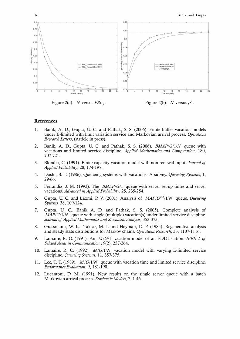
In Figures 2(a) and 2(b), we have plotted APBL and ρ′ against queue capacity in a 1BMAP PH N/ / / queue with multiple vacations (Vacation time follow phase type

distribution as we have taken for Figure 1(a)). BMAP representation is taken same as the one taken in Figure 1(a). Service time is of phase type with representation

[ ]β−⎡ ⎤

= , = ⎢ ⎥−⎣ ⎦S

19.683 2.4530.4 0.6

1.367 8.086

with ( )E S =0.108121. Figure 2(a) gives the blocking probabilities of an arbitrary customer where N varies from 2 to 24 and it is done for two types of limit mass functions (constant and bimodal as given in Figure 1(a)).

It can be seen that as N increases the blocking probabilities are asymptotically approaching towards zero. As expected the blocking probability for uniform limit mass function is higher than bimodal limit mass function.

In Figure 2(b), we have carried out the same type of comparison as we did in Figure 2(a) except that here we have plotted the probability that the server is busy against the queue capacity ( N ). It is seen that as N increases ρ′ asymptotically approaches towards ρ as for infinite buffer queue ρ ρ′ = . This is to some extent a valid check for the analytical and numerical results.

Figure 1(a). versus ρ ρ′ . Figure 1(b). versus APBLρ .

16 Banik and Gupta

Figure 2(a). versus AN PBL . Figure 2(b). versus N ρ′ .

References

1. Banik, A. D., Gupta, U. C. and Pathak, S. S. (2006). Finite buffer vacation models under E-limited with limit variation service and Markovian arrival process. Operations Research Letters, (Article in press).

2. Banik, A. D., Gupta, U. C. and Pathak, S. S. (2006). 1BMAP G N/ / / queue with vacations and limited service discipline. Applied Mathematics and Computation, 180, 707-721.

3. Blondia, C. (1991). Finite capacity vacation model with non-renewal input. Journal of Applied Probability, 28, 174-197.

4. Doshi, B. T. (1986). Queueing systems with vacations- A survey. Queueing Systems, 1, 29-66.

5. Ferrandiz, J. M. (1993). The 1BMAP G/ / queue with server set-up times and server vacations. Advanced in Applied Probability, 25, 235-254.

6. Gupta, U. C. and Laxmi, P. V. (2001). Analysis of 1a bMAP G N,/ / / queue, Queueing Systems. 38, 109-124.

7. Gupta, U. C., Banik A. D. and Pathak, S. S. (2005). Complete analysis of 1MAP G N/ / / queue with single (multiple) vacation(s) under limited service discipline.

Journal of Applied Mathematics and Stochastic Analysis, 353-373.

8. Grassmann, W. K., Taksar, M. I. and Heyman, D. P. (1985). Regenerative analysis and steady state distributions for Markov chains. Operations Research, 33, 1107-1116.

9. Lamaire, R. O. (1991). An 1M G/ / vacation model of an FDDI station. IEEE J. of Selcted Areas in Communication , 9(2), 257-264.

10. Lamaire, R. O. (1992). 1M G N/ / / vacation model with varying E-limited service discipline. Queueing Systems, 11, 357-375.

11. Lee, T. T. (1989). 1M G N/ / / queue with vacation time and limited service discipline. Performance Evaluation, 9, 181-190.

12. Lucantoni, D. M. (1991). New results on the single server queue with a batch Markovian arrival process. Stochactic Models, 7, 1-46.

Finite Buffer Vacation Queue under E-limit 17

13. Lucantoni, D. M., Meier-Hellstern, K. S. and Neuts, M. F. (1990). A single-server queue with server vacations and a class of non-renewal processes. Advanced in Applied Probability, 22, 676-705.

14. Matendo, S. K. (1994). Some performance measures for vacation models with a batch Markovian arrival process. Journal of Applied Mathematics and Stochastic Analysis, 7, 111-124.

15. Neuts, M. F. (1981). Matrix-Geometric Solutions in Stochastic Models: An Algorithmic Approach. Johns Hopkins Univ. Press, Baltimore, MD.

16. Niu, Z., Shu, T. and Takahashi, Y. (2003). A vacation queue with set up and close-down times and batch Markovian arrival processes. Performance Evaluation, 54, 225-248.

17. Takagi, H. (1991). Queueing Analysis - A Foundation of Performance Evaluation, Vacation and Priority Systems: Volume 1. New York: North-Holland.

18. Takagi, H. (1993). Queueing Analysis - A Foundation of Performance Evaluation, Finite Systems: Volume 2. New York: North-Holland.

Appendix

Proof of Theorem 5.1: As ( )S x follows a PH - distribution with representation ,( )Uβ , its probability distribution and density functions are given by

− , ≥ ,( )=1 exp( ) for 0S x x xU eβ

− = ,(1) 0and ( )= exp( ) exp( )S x x xU Ue U Uβ β (51)

where 0U is non-negative vector and satisfies + =0 0Ue U . We know that BMAP is a 2-dimensional Markov process and defines a batch arrival process, e.g., transition from state ( )i j, to state ( ) 1 1 i k l k j l m+ , , ≥ , ≤ , ≤ , indicates a batch arrival of size k . Now let

, = = , = | = , =( , ) Pr ( ) ( ) (0) 0 (0) i jP n t N t n J t j N J i (52)

be the ( )i j, th element of an m m× matrix , .( )n tP Since we are considering the finite systems, therefore combining the partial and total rejection policies, we obtain the following Chapman-Kolmogorov equation:

=(0,0) ,mP I (53)

−

−=

, = , + , , ≤ ≤ − ,∑1

(1)0

0( ) ( ) ( ) 0 1

n

n kk

n t n t k t n NP P D P D (54)

−

−=

′ ′, = , + , ,∑1

(1)0

0( ) ( ) ( )

N

N kk

N t N t k tP P D P D (55)

The following is a useful property of frequent use in calculations with Kronecker product. If and X Y Z W, , are rectangular matrices such that the ordinary matrix products XY and ZW are defined, then

⊗ = ⊗ ⊗ .( )( )XY ZW X Z Y W (56)

18 Banik and Gupta

The matrices nA as defined in subsection 3.1 are given by

∞= , ,∫0 ( ) ( )n n x dS xA P

00 ( ) exp( ) (using (51))n x x dx∞= , ,∫ P U Uβ

∞= , ⊗ ,∫ 00 ( ) exp( )mn x x dxP I U Uβ

00 ( ( ) exp( ))( ) (using (56))mn x x dx∞= , ⊗ ⊗ ,∫ P U I Uβ

= ⊗ ,0( )n mB I U

∞= , ⊗ .∫0where, ( ) exp( )n n x x dxB P Uβ (57)

Integration by parts of the right hand side of nB gives

∞− ∞ −= , ⊗ − , ⊗ .∫1 (1) 10 0[ ( ) exp( ) ] ( ) exp( )n n x x n x x dxB P U U P U Uβ β (58)

As x →∞ , ( ) 0n x, →P and 0( 0) n mn δ, =P I , where

δ, =⎧

= ⎨ , ≠ .⎩0

1 if 0,

0 if 0n

n

n (59)

Therefore

∞− −= − , ⊗ − , ⊗ ,∫1 (1) 10( 0) ( ) exp( )n n n x x dxB P U P U Uβ β

δ ∞− −= − ⊗ − , ⊗ .∫1 (1) 10 0( ) ( ) exp( )n m n x x dxI U P U Uβ β (60)

For 1 1n N≤ ≤ − , from (60),

∞ −= − , ⊗ ,∫ (1) 10 ( ) exp( )n n x x dxB P U Uβ

11

000

[ ( ) ( ) ] exp( ) (using (54))n

n kk

n x k x x dx−∞ −

−=

= − , + , ⊗ ,∑∫ P D P D U Uβ

−∞ ∞− −−

== − , ⊗ − , ⊗ ,∑∫ ∫

11 1

00 00

( ) exp( ) ( ) exp( )n

n kk

n x x dx k x x dxP D U U P D U Uβ β

Finite Buffer Vacation Queue under E-limit 19

∞ −= − , ⊗ ⊗∫ 100 ( ( ) exp( ))( )n x x dxP U D Uβ

11

00

( ( ) exp( ))( ) (using (56))n

n kk

k x x dxβ−∞ −

−=

− , ⊗ ⊗ ,∑∫ P U D U

11 1

00

( ) ( ) (using (57))n

n i n ii

−− −−

== − ⊗ − ⊗ , ,∑B D U B D U (61)

γ

−− −−

=+ ⊗ = − ⊗ ,∑

11 1

00

or, ( ) ( )n

n m i n i mi

B I D U B D I I U

11 1

00

or, ( ) ( )( ) (using (56))n

n m i n i mi

γ

−− −−

=+ ⊗ = − ⊗ ⊗ , ,∑B I D U B D I I U

γ

− − − −−

== − ⊗ ⊗ + ⊗ ,∑

11 1 1

00

or, ( )( )( )n

n i n i m mi

B B D I I U I D U

γ

− − − − − − − −−

== − ⊗ + ⊗ ⊗ ,∑

11 1 1 1 1 1 1

00

or, ( )[( )( ) ] (as, ( ) = ),n

n i n i m mi

B B D I I D U I U AB B A

γ

− − − − − −−

== − ⊗ + ⊗ ⊗ , ⊗ ⊗∑

11 1 1 1 1

00

or, ( )[( )( )] (as, ( ) = ),n

n i n i m mi

B B D I I D U I U A B A B

γ

− − −−

== − ⊗ ⊗ + ⊗ ⊗ .∑

11 1

00

or, ( )[( ) ( )( )]n

n i n i m mi

B B D I I U D U I U (62)

Using (56) in (62), after simplification we obtain (45).

For 0n = , from (60),

∞− −= − ⊗ − , ⊗ ,∫1 (1) 10 0( ) (0 ) exp( )m x x dxB I U P U Uβ β

1 100( ) [ (0 ) ] exp( ) (using (54))m x x dx∞− −= − ⊗ − , ⊗ ,∫I U P D U Uβ β

∞− −= − ⊗ − , ⊗ ⊗ ,∫1 100( ) ( (0 ) exp( ))( )m x x dxI U P U D Uβ β

− −= − ⊗ − ⊗ ,1 10 0( ) ( )mI U B D Uβ

− −+ ⊗ = − ⊗ ⊗ ,1 10 0or, ( ( )) ( )( )m m mB I D U I I Uβ

− − −= − ⊗ ⊗ + ⊗ ,1 1 10 0or, ( )( )[ ( )]m m mB I I U I D Uβ

− − − −= − ⊗ + ⊗ ⊗ ,1 1 1 10 0or, ( )[( ( ))( ) ]m m mB I I D U I Uβ

− − − −= − ⊗ + ⊗ ⊗ ⊗ ,1 1 1 10 0or, ( )[( ( )( ))( ) ]m m m m mB I I D I I U I Uβ

20 Banik and Gupta

− − − − − −= − ⊗ ⊗ + ⊗ ⊗ ⊗ .1 1 1 1 1 10 0or, ( )[( ) ( )( )( ) ]m m m m mB I I U D I I U I Uβ

Few more steps will give (44). For n N= , from (60) in the similar way one can obtain (46). Using the same procedure, one can have the results (48)-(50).

Authors’ Biographies:

A. D. Banik was born in West Bengal, India, in 1977. He received the B.Sc. and M.Sc. degrees in Mathematics from the Jadavpur University, West Bengal, India, in 1998 and 2000, respectively. Since June 2002, he is working as a Ph.D. student at the Department of Mathematics, Indian Institute of Technology, Kharagpur, India. His main research interests include continuous-time queueing theory and its applications. He has published research articles in Operations Research Letters, Applied Mathematics and Computation, Journal of Applied Mathematics and Stochastic Analysis, Applied Mathematical Modelling.

U. C. Gupta is currently Professor in the Department of Mathematics at Indian Institute of Technology, Kharagpur. He did his masters in Statistics from Banaras Hindu University, Varanasi, in the year 1978. Further he completed his Ph.D. from Indian Institute of Technology, Delhi, in 1982. For a short stint (Dec. 1982-Oct 1985) Dr. Gupta was in Indian Statistical Services (ISS) and worked with Govt. of India in various capacities. Since Nov. 1985, Dr. Gupta has been teaching various courses at IIT Kharagpur. He has contributed significantly in the area of modeling and analysis of continuous- and discrete- time queueing systems. He has published several research articles in various journals such as Stochastic Processes and Their Applications, Queueing Systems, European Jl. of Operational Research, Performance Evaluation, Jl. of Applied Probability, Probability Engineering and Informational Sci., Operational Research Letters, Journal of the Operational Research Society, Informs Jl. of Computing, Journal of Applied Mathematics and Stochastic Analysis, Journal of Operations Research of the Spanish Society of Statistics and Operations Research (TOP), Applied Mathematical Modelling, RAIRO.