Fine structure of the low-latitude mesospheric turbulence

Uma Das,1 H. S. S. Sinha,1 Som Sharma,1 H. Chandra,1 and Sanat K. Das1,2

Received 17 October 2008; revised 25 March 2009; accepted 2 April 2009; published 30 May 2009.

[1] Rocket-borne measurements of electron density were conducted from Sriharikota(13.7�N, 80.2�E) to study the fine structure of low-latitude mesospheric neutralturbulence. Spectra of electron density fluctuations were obtained using the continuouswavelet transform (CWT), and the turbulence parameters were estimated. The presentstudy shows that turbulence is not present continuously in the mesosphere but exists inlayers of different thicknesses varying from 100 m to 3 km, interspersed by regions ofstability. The most important results are the following: (1) Identification of thin layersof turbulence with 100–200 m of thickness over low latitudes. These thin layers arefound to lie on the edges of the thick layers of turbulence. (2) Sharp gradients inturbulence parameters at the edge regions are detected from experimental observationsfor the first time. This was seen earlier in simulation studies only. (3) Satellite-observedtemperatures show enhanced gravity wave activity, and it is suggested that deepconvections over the continental landmass in the lower atmosphere are the major sourceof these gravity waves responsible for generation of turbulence.

Citation: Das, U., H. S. S. Sinha, S. Sharma, H. Chandra, and S. K. Das (2009), Fine structure of the low-latitude mesospheric

turbulence, J. Geophys. Res., 114, D10111, doi:10.1029/2008JD011307.

1. Introduction

[2] The past twenty years have seen considerable prog-ress in understanding various processes related to meso-spheric turbulence. As the mesospheric region is collisiondominated, turbulence in the neutral atmosphere is trans-ferred to the electrons and ions, making them effectivepassive tracers of neutral turbulence. This aspect is exploitedby the radars and rocket techniques that probe this part of theatmosphere. Remote sensing studies using radars [Hocking,1990; Hocking and Rottger, 2001; Rao et al., 2001; Sasi andVijayan, 2001; Chakravarty et al., 2004; Sheth et al., 2006],in situ measurements of neutral density [Lubken, 1992;Lubken et al., 1993; Rapp et al., 2004], ion and electrondensities [Sinha, 1976; Thrane and Grandal, 1981; Thrane etal., 1985, 1987; Blix et al., 1990; Sinha, 1992; Goldberg etal., 1997; Lehmacher et al., 1997, 2006] and chemical releaseexperiments [Larsen, 2002] have contributed largely to theunderstanding of the spatial and the temporal variation of theturbulence parameters in the mesosphere. It is very wellestablished that the Kolmogorov’s theory explains the neutralturbulence and the energy cascade process in the mesosphereand the lower thermosphere.What needs to be understood arethe morphological characteristics of the turbulence, its finestructure and the impact of turbulence on the energy budgetof this region.

[3] One of the most important studies of mesosphericturbulence using rocket-borne measurements was byLubken [1997] over high latitudes, mostly from Andoya(69�N, 16�E), using neutral density fluctuations as tracers.A significant and systematic seasonal variation was found,where, turbulence was confined to a relatively small heightregion of 78–97 km during summer but covered the entiremesosphere from 60 to 100 km during winter. The turbu-lence is generated due to gravity waves that are produced inthe lower atmosphere, which travel upward and break atmesospheric heights and/or due to Kelvin Helmholtz insta-bility which occurs in situ in the presence of strong windshears. As the gravity waves travel upward they are filteredby season-dependent prevailing winds and result in theobserved seasonal variation of the turbulent activity. Duringthe MaCWAVE/MIDAS summer campaign conducted fromAndoya during July 2002, turbulence was observed below80 km also [Rapp et al., 2004]. This was a result of largegravity wave amplitudes, because of which the waves reachtheir breaking levels at lower altitudes and produce turbu-lence at altitudes lower than normal. Near continuousturbulent layers were found from 72 to 90 km altitudeduring this campaign. Rocket-borne measurements of elec-tron density were made from the equatorial latitudes atAlcantara (2.5�S, 44.4�W) in Brazil [Goldberg et al., 1997;Lehmacher et al., 1997] during the CADRE/MALTEDcampaign in August 1994, where turbulence was foundbetween 85 and 90 km during the daytime. Mesosphericturbulence was also studied extensively using MST radars[Gage and Balsley, 1980; Kubo et al., 1997; Sasi andVijayan, 2001; Rao et al., 2001; Kamala et al., 2003;Kumar et al., 2007]. Strongest echoes are seen duringJune/July months and the weakest during winter [Kamala

JOURNAL OF GEOPHYSICAL RESEARCH, VOL. 114, D10111, doi:10.1029/2008JD011307, 2009ClickHere

for

FullArticle

1Space and Atmospheric Sciences Division, Physical ResearchLaboratory, Ahmedabad, India.

2Now at GeosciencesDivision, PhysicalResearchLaboratory,Ahmedabad,Gujarat, India.

Copyright 2009 by the American Geophysical Union.0148-0227/09/2008JD011307$09.00

D10111 1 of 11

et al., 2003]. Observations by Thomas et al. [1996] usingVHF radar and lidar showed that radar echoes were ob-served above and below the maxima in mesospheric tem-perature inversions, which was observed at �85 km overthe midlatitudes. [Hauchecorne et al., 1987] suggested thatgravity wave breaking may account for such inversions.Lehmacher et al. [2006] also found large energy dissipationrates over an equatorial station at 90 km, where a meso-spheric inversion layer was observed.[4] Using the electron density irregularity data obtained

from earlier sounding rocket flights from Sriharikota(13.7�N, 80.2�E), and 3 m irregularity data obtained bythe MST radar at Gadanki (13.5�N, 79.2�E), which islocated about 100 km west of Sriharikota, Chakravarty etal. [2004] have shown that the fine structures in the electrondensity irregularities are often present in the height region of�75 km over Sriharikota, which match quite well with theradar observed structures of the main scattering layer (70 ±5 km) over Gadanki. The altitude resolution of radar back-scattered echoes is limited by the finite pulse width. With a16 ms uncoded pulse, a resolution of 2.4 km was obtained[Kumar et al., 2007], but the use of smaller pulse widths cangive better altitude resolutions. Observations using narrowpulse widths indicated presence of scattering layers down to�600 m embedded in a broad turbulence field of 4–5 kmthickness at 75 ± 5 km [Chakravarty et al., 2004]. Using iondensity measurements over high latitudes, Blix et al. [1990]also showed earlier that the turbulence tends to occur in thinlayers (Dz < 1 km). Sheth et al. [2006] obtained a resolutionof 150 m using pulses of 1 ms baud length. This high-resolution study of mesospheric fine structure with theJicamarca MST radar showed many interesting features.Spectral widths and backscattered power showed positivecorrelations at upper mesospheric heights in agreement withearlier findings [Fukao et al., 1980] that upper mesosphericechoes are dominated by isotropic Bragg scatter. In manyinstances in the upper mesosphere, a weakening of positivecorrelation away from layer centers (towards top and bottomboundaries) was observed with the aid of improved heightresolution. This finding supports the idea that layer edgesare dominated by anisotropic turbulence [Sheth et al.,2006].[5] Fritts et al. [2003] showed through direct numerical

simulation studies that there are sharp gradients in theturbulence parameters at the edges of the broad turbulencefield. This is because of the efficient mixing of constituentswithin the turbulent region. Traditional spectral analysismethods of rocket data, like the Fourier transform, typicallyuse data of over 1 km for getting one spectrum. Thesemethods smear out any such sharp gradients and also do notallow one to look into the fine structure of the turbulencefield. Recent advances in mathematical tools have seen thegrowth of a mathematical microscope, the continuouswavelet transform (CWT), which is described in detail inliterature [Farge, 1992; Torrence and Compo, 1998]. Today,CWT has become a more powerful tool to understand thegeophysical phenomena both in the frequency and the timedomains, simultaneously. This technique has been usedsince many years for the study of turbulence produced inwind tunnels, near heated walls, in numerical simulations,etc. [Farge, 1992 and references therein]. It is also used invarious other geophysical studies including long-term me-

sospheric airglow variations [Das and Sinha, 2008], meso-spheric turbulence using neutral density measurements[Strelnikov et al., 2003; Rapp et al., 2004], etc.

2. Experimental Details

[6] A coordinated campaign was conducted in India tostudy the mesospheric neutral turbulence at low latitudes.The major experiments conducted during the campaignwere rocket-borne measurements of electron density fromSriharikota in coordination with ground based mesosphere-stratosphere-troposphere (MST) radar observations fromGadanki. Launch criterion was decided based on the meso-spheric echo strength observed in the MST radar observa-tions. The rocket was launched from Satish Dhawan SpaceCenter (SDSC), Sriharikota at 1142 hours LT, on 23 July2004. The nose cone ejection was at 60 km and the rocketreached an apogee of 109 km. A hemispherical LangmuirProbe (LP) sensor, biased at +4 V, was used to measure theelectron density fluctuations. For studying the electrondensity fluctuations in different scale sizes the currentcollected by the LP sensor was processed onboard in threechannels with different gains having frequency response ofDC–100 Hz (Main channel), 30–150 Hz (Medium Fre-quency [MF] channel) and 70–1000 Hz (High Frequency[HF] channel), with a sampling frequency of 520, 1040,5200 Hz, respectively. The consolidated power spectra ofthe irregularities were constructed from the electron densityvalues obtained from these three channels. The MST radarlocated at Gadanki operates at 53 MHz [Rao et al., 1995].For the present campaign, the month of July was chosenbased on the earlier studies of mesospheric echoes fromGadanki as the occurrence and the strength of echoes werefound to be highest during June–July [Kamala et al., 2003].On 23 July 2004 the MST radar was operated during08:30–16:00 LT.[7] Preliminary results and the technical details of all

experiments of the campaign were reported by Chandra etal. [2008]. Turbulence parameters were estimated from theelectron density data from LP, using the Fourier transform,and also from the radar observations and have been pre-sented and discussed by Chandra et al. [2008]. Furtherresults obtained from the electron density measurementswhen subjected to the CWT are described in this paper.Some new features of neutral turbulence such as existenceof extremely thin layers of turbulence and sharp gradients ofturbulence parameters at the edge regions are discussed.

3. Data Analysis

[8] The CWTwas applied to the electron density obtainedfrom the main channel (DC–100 Hz) of LP. The Morletwavelet (with a frequency of 6), which is a plane wavemodulated by a gaussian, was used as the mother wavelet.Complete description of the CWT and the different waveletscan be found in the work of Farge [1992] and Torrence andCompo [1998]. The software written in IDL, provided byTorrence and Compo [1998], was used for the presentanalysis. The wavelet power spectrum obtained is a com-posite of more than 50000 individual spectra. However,averages of horizontal slabs of 100 m thickness have beencomputed to obtain altitude-averaged power spectra. A

D10111 DAS ET AL.: MESOSPHERIC TURBULENCE

2 of 11

D10111

range of 100 m is chosen to make sure that the breakpointsobserved in the spectra due to turbulence are indeed presentin the data set and any statistical noise is also removed.Moreover, averaging over 100 m ensures the fact thatconsecutive spectra contain independent information ofscales up to 100 m [Strelnikov et al., 2003]. Wavelet powerspectra of data from the other two channels. i.e., the MF(30–150 Hz) and the HF (70–1000 Hz) channels also havebeen computed. The altitude-averaged power spectra forevery 100 m in the same altitude regions as in the case ofmain channel are then computed. The main channel and theMF channel spectra have been normalized at 50 Hz and laterwith the HF channel spectra at 100 Hz to get compositespectra ranging from DC to 1000 Hz. With a typical rocketvelocity of 1000 ms�1, in the region of interest, thespectrum, therefore, gives information about the irregular-ities having scale sizes in the range of approximately 1m to1 km.[9] The characteristic slopes of a turbulent power spec-

trum are �5/3 in the inertial subrange and �7 in the viscousdissipation regime. The Heisenberg model exhibits theseclassical k�5/3 and the k�7 power laws with a smoothtransition taking place between them [Heisenberg, 1948].This theoretical spectral model was fitted to the altitude-averaged power spectra and the value of the inner scale (l0)was obtained from the best fit, from which the otherturbulent parameters can be estimated [Lubken, 1992]. Eachof the altitude-averaged power spectra has been verifiedwhether the Heisenberg model can be fitted, since the fittingcan be done only if the measured spectra show the nature ofthe inertial subrange with slope �5/3 as well as the viscousdissipation range with slope �7.[10] Once the inner scale has been identified for those

spectra where the Heisenberg model could be fitted, theother turbulence parameters are estimated by the usualprocedures [Sinha, 1992; Lubken, 1992]. The energy dissi-

pation rate is given by � = n3/h4, where h is the Kolmogorovmicroscale given by h = l0/9.9 and n is the kinematicviscosity, derived using the densities and the temperaturefrom the MSISE-90 model [Hedin, 1991] for the launchconditions. The corresponding heating rate is dT/dt =0.0864� K/day [Lubken, 1997].

4. Results

[11] The electron density measured by the LP main chan-nel during the ascent of the rocket is shown in Figure 1 (left).The variations below 68.5 km are not real and are an artifactof the rocket spin and due to extremely small electron densityin this region these appear very prominently on a log scale.The variations in the electron density in the 68.5 to 71 kmregion seem to be real. The electron density increases withaltitude as is expected. A peak electron density of �1.5 �105 cm�3 is found at �98 km. Figure 1 (right) shows thewavelet power spectra computed from LP data, spanning thecomplete frequency range from DC to 1000 Hz. The contouris a composite of all the altitude-averaged power spectra,normalized with the square of the electron density, so that thepower spectra are comparable at all altitudes. The power at allaltitudes is decreasing with frequency, as is expected for anygeophysical process. The white long dashed lines in Figure 1show the variation of power of various scale sizes withaltitude. As the rocket velocity decreases with altitude, thefrequency at which these scale sizes appear decreases ac-cordingly resulting in the bend in these lines towards thelower frequencies. The two vertical black dashed lines at4.6 Hz and 9.2 Hz are the rocket spin frequency and itssecond harmonic, respectively. Large power (bursts of redand orange) is seen at all scale sizes in the altitude ranges of68–71 km, 75–89 km and 100–105 km at frequenciesgreater than 10 Hz, i.e., beyond the spin frequency and itssecond harmonic and these are the regions of interest in the

Figure 1. (left) Electron density profile during ascent of the rocket from the fixed bias Langmuir probe.(right) The composite of all altitude-averaged wavelet power spectra normalized with the averageelectron density. The white long dashed lines show the variation of power of various scale sizes withaltitude. Two vertical black dashed lines at 4.6 and 9.2 Hz are the rocket spin frequency and its secondharmonic, respectively. See text for more details.

D10111 DAS ET AL.: MESOSPHERIC TURBULENCE

3 of 11

D10111

present study. Figure 2 shows the electron density gradientscale length, L�1 [1/L = (1/ne)(dne/dh)] calculated over analtitude interval of 300 m. It can be seen that very strongpositive and negative gradients are present below 71 kmregion, moderate positive gradients in the 79–89 km regionand weak gradients in the intervening region. The gradient inthe region of 79–89 km is ranging from 0 to 0.5 km�1. Theseregions of strong gradients are the regions where largepowers (bursts of red and orange) are seen in the waveletspectra in Figure 1.[12] A total of 405 altitude-averaged power spectra were

computed from all the available data; out of which 102spectra showed the characteristic slopes of neutral turbu-lence, i.e., a slope of �5/3 in the inertial subrange and a �7slope in the viscous dissipation regime, in the altitude

region from 75 to 89 km. Some intermediate regions didnot show these slopes and therefore are considered asregions of no turbulence. The inner scales were identifiedby fitting the Heisenberg model to the spectra that showedcharacteristic turbulence slopes. The inner scales increasedfrom 10 to 50 m with increasing altitude in this regionfrom 75 to 89 km. Assuming an energy dissipation rate of100mW/kg, Lubken et al. [1993] estimated inner scales in themesospheric and the lower thermospheric altitudes. Theinner scales obtained in the present study compare verywell with these theoretical estimates of Lubken et al. [1993].In the region from 68.5 to 71 km, a few altitude-averagedspectra showed the slope of �5/3, which is characteristic ofneutral turbulence and no viscous dissipation regime hasbeen seen. At an altitude of �70 km, the theoretical value ofthe inner scale is of the order of 5 m and can be muchsmaller for smaller energy dissipation rates. Because of thecombined effect of the lower value of the inner scale and thedetection limit of the instrument, the inner scales could notbe identified in the altitude region from 68.5 to 71 km in thepresent experiment. Above 100 km, electron density irreg-ularities could be produced due to plasma instabilities andare beyond the scope of the present study. At other altitudesbelow 100 km, that are not discussed above, no irregular-ities have been observed.[13] Figure 3 shows two examples of the altitude-aver-

aged power spectra at 70 ± 0.05 and 81 ± 0.05 km. At70 km, the viscous dissipation regime could not be observed.The linear regression shows that the power spectrum fol-lows a power law with a spectral index of �1.96. At 81 km,both the inertial subrange and the viscous dissipation regimecan be seen, and hence the Heisenberg model could be fittedand is given by the solid line. The inner scale (l0) obtainedfrom the fit is 25.2 m. This corresponds to an energydissipation rate of 14 mW/kg. Figure 4a gives the profileof the estimated energy dissipation rate, �, in the altituderegion from 75 to 89 km, from all the 102 altitude-averagedpower spectra, which showed the characteristic slopes ofneutral turbulence. It shows an increasing trend with alti-tude. It is found that turbulence was not present continu-

Figure 2. The electron density gradient scale lengthcomputed over 300 m, during the ascent of the rocket.

Figure 3. The altitude-averaged wavelet power spectrum at (left) 70.0 ± 0.5 km and (right) 81.0 ± 0.5 km.The solid line in the spectrum in the right is the best Heisenberg fit, with l0 = 25.2 m.

D10111 DAS ET AL.: MESOSPHERIC TURBULENCE

4 of 11

D10111

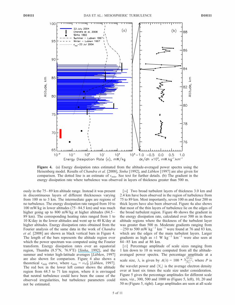
ously in the 75–89 km altitude range. Instead it was presentin discontinuous layers of different thicknesses varyingfrom 100 m to 3 km. The intermediate gaps are regions ofno turbulence. The energy dissipation rate ranged from 10 to100 mW/kg in lower altitudes (75–84.5 km) and was muchhigher going up to 800 mW/kg at higher altitudes (84.5–89 km). The corresponding heating rates ranged from 1 to10 K/day in the lower altitudes and went up to 40 K/day athigher altitudes. Energy dissipation rates obtained from theFourier analysis of the same data in the work of Chandraet al. [2008] are shown as black vertical bars in Figure 4.The length of the bars represents the altitude region overwhich the power spectrum was computed using the Fouriertransform. Energy dissipation rates over an equatorialregion, Thumba (8.5�N, 76.9�E) [Sinha, 1992], and thesummer and winter high-latitude averages [Lubken, 1997]are also shown for comparison. Figure 4 also shows atheoretical �min curve, where �min = nwB

2 [Lubken, 1997].The red box in the lower left corner shows the altituderegion from 68.5 to 71 km region, where it is envisagedthat neutral turbulence could have been the cause of theobserved irregularities, but turbulence parameters couldnot be estimated.

[14] Two broad turbulent layers of thickness 3.0 km and2.4 km have been observed in the region of turbulence from75 to 89 km. Most importantly, seven 100 m and four 200 mthick layers have also been observed. Figure 4a also showsthat most of the thin layers of turbulence lie on the edges ofthe broad turbulent region. Figure 4b shows the gradient inthe energy dissipation rate, calculated over 500 m in thosealtitude regions where the thickness of the turbulent layerwas greater than 500 m. Moderate gradients ranging from�250 to 500 mW kg�1 km�1 were found at 76 and 83 km,which are the edges of the main turbulent layers. Largergradients as high as ±1 W kg�1 km�1 were also seen at84–85 km and at 86 km.[15] Percentage amplitude of scale sizes ranging from

1 km down to 10 m were computed from all the altitude-averaged power spectra. The percentage amplitude at a

scale size, l, is given by A(l) = 100 *

ffiffiffiffiffiffiffi

P lð ÞphNei , where P is

the wavelet power and hNei is the average electron densityover at least six times the scale size under consideration.Figure 5 gives the percentage amplitudes for different scalesizes, viz., 300, 500 and 1000 m (Figure 5, left), 10, 20 and50 m (Figure 5, right). Large amplitudes are seen at all scale

Figure 4. (a) Energy dissipation rates estimated from the altitude-averaged power spectra using theHeisenberg model. Results of Chandra et al. [2008], Sinha [1992], and Lubken [1997] are also given forcomparison. The dotted line is an estimate of �min. See text for further details. (b) The gradient in theenergy dissipation rate where turbulence was observed in layers of thickness greater than 500 m.

D10111 DAS ET AL.: MESOSPHERIC TURBULENCE

5 of 11

D10111

sizes below 71 km. The amplitudes are in the range of 10–100% for the large scale sizes from 300 m to 1 km and inthe range of 10–30% for the smaller scales. At 70.5 km, thepercentage amplitude for the scale size of 500 m is almost200%. The altitude region from 78 to 89 km also showedhigh amplitudes of 5–50% and 0.1–5% for large and smallscale sizes, respectively. Also, the amplitudes of the smallscale sizes decrease very rapidly with scale size, which isdue to the steep �7 slope of the VDR in the altitude regionfrom 75 to 89 km.

5. Discussion

[16] In situ measurements of electron density in the �70to 110 km region over low latitudes showed the presence ofstrong fluctuations over a large scale size range. Largepercentage amplitudes of these electron density fluctuationsare a result of various causative mechanisms operating inthe mesosphere and lower thermosphere. At altitudes belowabout 90 km, the only known process which could producesuch irregularities in the electron density is the neutralturbulence. There have been very few daytime flights fromSriharikota in the past to study the electron density irregu-larities in the low-latitude mesosphere [Sinha and Prakash,1995; Chakravarty et al., 2004 and references therein].These flights were primarily intended to study the E andF region of the ionosphere. The present flight from Srihar-ikota thus provides valuable measurements to study theelectron density irregularities in the mesosphere over lowlatitudes. This region was observed more closely from�70 km and above during this campaign.[17] Large amplitudes of the larger scale sizes were

observed in 78–89 km and of smaller scales in 75–89 kmregion (Figure 5). This is also the region of moderateelectron density gradients (Figure 2). The altitudes of peakamplitudes of the large scale sizes and the peak gradients in

the electron density match exactly. During the calculation ofthe wavelet coefficients, the scales are increased in frac-tional steps of power of two while the translation is a linearprocess only [Farge, 1992; Torrence and Compo, 1998].Also, so the large-scale wavelet coefficients are redundant,which cause the modulations in the percentage amplitude, ascan be seen in Figure 5. The turbulent layers are alsoobserved in the same altitude region from 75 to 89 km.Chandra et al. [2008] suggested that the electron densityirregularities seen during this flight, produced due to neutralturbulence could be the result of breaking of gravity waves.[18] A reanalysis of the electron density data with the new

technique, CWT, has revealed some new and interestingresults. The most important result this study brings out isthat the turbulence can exist in thin layers with thickness of100–200 m. These thin layers are observed at the edgesof the broad turbulent regions which show that these layersof stratification could be part of a system restoring to laminarflow which surround the larger regions of turbulence. Thegaps that can be seen in Figure 4 are the regions of stabilitywhere the power spectra do not show the turbulencecharacteristics. Mesospheric turbulence thus exists in layerswith interspersed regions of stability. During this campaign,simultaneous MST radar observations were also carriedout and backscattered echoes were observed from 73.5 to77.5 km [Chandra et al., 2008]. The strength of the back-scattered echoes, which is a measure of the turbulence, wasstrongest during 1100 to 1130 hours LT. Later, the strengthreduced, which indicates that the turbulence started todecay. The rocket-borne LP launched at 1142 hours hencemeasured the electron density fluctuations during the start ofthe decay phase of the turbulence. The strength of the radarechoes during this time was still strong enough. Thisconfirms that the observed thin layers of turbulence werepart of the system restoring to laminar flow. Such thin layerscould not be detected earlier due to the limitation of analysis

Figure 5. Percentage amplitude of electron density fluctuations of various scale sizes. For the 10-mscale size, the variation in the 70- to 80-km region is below the detection limit of the instrument, and the50-m scale size is contaminated by the rocket spin above 87 km and hence is not shown.

D10111 DAS ET AL.: MESOSPHERIC TURBULENCE

6 of 11

D10111

techniques of rocket data, which so far had a typicaldetection limit of layer thickness of about 1 km. Thedetection of these thin layers of turbulence and their exactlocation is thus made for the first time in the present studyusing rocket-borne electron density measurements over lowlatitudes and was possible due to the use of CWT foranalyzing the electron density fluctuations. Strelnikov etal. [2003] had applied the same technique to mesosphericneutral density fluctuations measured by rocket-borne ion-ization gauges. They also found thin layers of turbulence of100 m thickness. Scattering layers down to 600 m embed-ded in the broad turbulence field of about 4–5 km thicknessaround 75 km were observed by the MST radar at Gadanki[Chakravarty et al., 2004]. The Jicamarca radar also ob-served thin sheets of turbulence with a resolution of 150 m[Sheth et al., 2006]. It can also be clearly seen that thepresent results obtained using the CWT and those obtainedby the Fourier transform [Chandra et al., 2008] are verysimilar, with CWT giving much better altitude resolution ofthe turbulence parameters thereby resolving the fine struc-tures of the turbulent region.[19] Direct numerical simulation studies showed that

there are large gradients in the turbulent parameters at thelayer edges [Fritts et al., 2003]. This is due to the efficientmixing within the turbulent layer. With the use of the CWTit was possible to compute these gradients in the presentstudy (Figure 4). This is the first experimental evidence for

the presence of such gradients at the layer edges in theturbulence parameters. It is therefore contemplated that therocket had traversed the complete turbulent region and thatwe have a complete snapshot of the processes going on. Inaddition, studies by the Jicamarca radar [Sheth et al., 2006]show that layer edges are dominated by anisotropic turbu-lence. Anisotropy was observed in the MST radar echoes inthe present campaign also, wherein the echo strength of thevarious beams in different directions varied significantly[Chandra et al., 2008]. Though the gradients show efficientmixing within the layer, the anisotropic echoes show thatthis mixing is homogeneous vertically along the direction ofrocket observations and horizontal anisotropies can stillexist.[20] The high-latitude summer energy dissipation rates

given by Lubken [1997] range from 1 to 160 mW/kg in 79to 97 km, with a peak at around 90 km. The present summerresults are in conformity with this high-latitude average, butare computed at a better resolution. It should be noted thatthe energy dissipation rate at the higher altitudes above84 km are considerably higher, going up to 800 mW/kg andthe gradients in the energy dissipation rates are also large.Rapp et al. [2004] also observed high-energy dissipationrates and at �89 km a rate of 1 W/kg was observed and itcorresponds to a heating rate of�100 K/day. This large valueof � coincided with a strong positive temperature gradient ofthe order of +40 K/km. Lehmacher et al. [2006] also found a

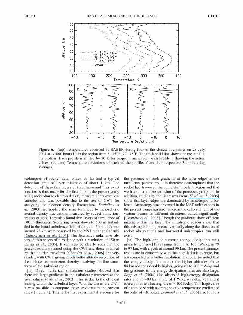
Figure 6. (top) Temperatures observed by SABER during four of the closest overpasses on 23 July2004 at �1000 hours LT in the region from 5–15�N, 72–75�E. The thick solid line shows the mean of allthe profiles. Each profile is shifted by 30 K for proper visualization, with Profile 1 showing the actualvalues. (bottom) Temperature deviations of each of the profiles from their respective 3-km runningaverages.

D10111 DAS ET AL.: MESOSPHERIC TURBULENCE

7 of 11

D10111

large energy dissipation rate of 170 mW/kg over an equa-torial station at 90 km, where a mesospheric inversion layerwas observed. These high-energy dissipation rates and thecorresponding high heating rates in the earlier and thepresent works show that turbulence has a much moreimportant role to play in the energy budget of the meso-spheric region. This study also supports the idea that gravitywave breaking and turbulence could produce the meso-spheric temperature inversions. At slightly lower altitudes,the present results are also in agreement with the value of50 mW/kg at 86 km altitude reported over the equator atPeru by Royrvik and Smith [1984], using coordinated experi-ments of the Jicamarca radar and in situ measurements ofelectron density. The present summer results match quietwell with the high-latitude summer average above 84 km.However turbulence is also seen below 84 km in contrast tothe earlier high-latitude summer results [Lubken, 1997] andmatch quite well with later experiments and campaigns thatshowed that turbulence was present in the high-latitudesummer lower mesosphere also [Rapp et al., 2004]. It canalso be seen in Figure 4 that the energy dissipation rates

obtained by Sinha [1992] over an equatorial station Thumbaare underestimated. It should be remembered that the resultsby Sinha are from more than one flight, none of which wasconducted with a view to study neutral turbulence. Hence itis quite possible that results of Sinha pertain to epochs ofweak turbulence.[21] The zonal and meridional winds measured by the

MST radar at Gadanki in 75–77 km region showed thepresence of a 10-min periodicity, which pointed towardsthe presence of gravity waves at those altitudes [Chandra etal., 2008]. It is possible that these gravity waves got amplifiedas they propagated upward resulting in the observed turbu-lence. The presence of gravity waves is seen in the temper-atures observed by satellites. Temperatures observed bySABER during four of the closest overpasses on 23 July2004 at �1000 hours LT in the region of 5–15�N, 72–75�Eare shown in Figure 6. The thick solid line shows the meanof all the profiles. Each profile is shifted by 30 K for propervisualization with Profile 1 showing the actual values.Figure 6 (bottom) shows the temperature deviations fromtheir respective 3-km running averages. These temperature

Figure 7. (top) Temperatures observed by HALOE onboard UARS during two of the closest overpasseson 26 and 27 July, The thick solid line shows the mean of the profiles. (bottom) Temperature deviationsof each of the profiles from their respective 3-km running averages.

D10111 DAS ET AL.: MESOSPHERIC TURBULENCE

8 of 11

D10111

profiles show intense dynamic activity on 23 July 2004 inthe region from 65 to 90 km. The vertical wavelength ofthese waves is �5–6 km and the amplitude of thesetemperature deviations was in the range of ±4–10K. Tem-peratures observed by HALOE onboard UARS during theclosest overpasses over Sriharikota within ±5� on 26–27 Julyare shown in Figure 7 (top) and the deviations from theirrespective 3-km running averages are shown in Figure 7(bottom). On 26 July, the temperature profile showsgravity wave features of vertical wavelength �5–6 kmand deviations in the range �±6 K. On the next day theactivity was much lower with deviations of �±2 K, exceptat 65–70 km. The activity on these later days was compar-atively lower. These satellite observations provide furthersupporting evidence and hence it is concluded in the presentwork that, on 23 July 2004 breaking of gravity waves couldhave caused the observed turbulence and the large values ofthe energy dissipation rate in conformity with the results ofChandra et al. [2008]. Unfortunately, wind measurementswere not available in the altitude region of interest duringthe period of rocket launch. Hence it cannot be completelyruled out that the Kelvin Helmholtz instability could nothave operated at these altitudes. If the conditions wereconducive it could also have contributed to the observedturbulence. However, breaking of gravity waves seems to bea more plausible explanation for the generation of theobserved turbulence.[22] Gravity waves can be produced by a variety of

mechanisms like topography, convections, troposphericjets, thunderstorms, severe weather, etc [Fritts, 1984].Figure 8 shows the horizontal wind vectors from theNCEP/NCAR reanalysis data at 500 hPa over the Indiansubcontinent on 23 July 2004 at 0600 hours UT (1130 hoursLT). No jet streams are observed in these winds in thepresent study over the region of interest. Hence jet streamscould not have caused the observed gravity waves. Theweather was quiet on the day of the rocket launch and sothunderstorms and severe weather conditions can also be

ruled out. It is therefore speculated that the gravity wavesare either of topographic origin or produced due to deepconvections. A study using a Microwave Limb Sounder(MLS) onboard the Upper Atmosphere Research Satellite(UARS) by McLandress et al. [2000] showed that duringthe northern hemispheric summer (June to August), gravitywave activity at the 38 km level has a maximum over Africaand Southeast Asia at 10�–15�N and over North America at30�N. The Indian subcontinent which is the region ofinterest in the present study is a part of these zones.McLandress et al. [2000] suggested that these continentallandmasses were geographically fixed sources of gravitywaves and deep convections in summer and forced flowover mountains in winter could be the mechanisms. Thisenhanced gravity wave activity can propagate upward andcause high turbulence in the mesosphere. The study ofmesospheric turbulence by Sasi and Vijayan [2001] usingthe MST radar at Gadanki showed that the energy dissipa-tion rate peaks in summer months from June to Septemberand varies from 7 to 100 mW/kg from the lower altitudes at65 km to mesopause altitudes at 90–95 km. These high-energy dissipation rates were related to the enhanced gravitywave activity due to deep convections over the low-latitudeIndian subcontinent during the summer monsoon season(June to September). The gravity waves thus observed in theupper atmosphere during the period of study in the SABERand HALOE temperature profiles could thus have beengenerated by deep convections over the continental land-mass as suggested by McLandress et al. [2000]. Also, thesewaves could have traveled upward and their eventualbreaking could have produced the observed turbulence.

6. Summary and Conclusions

[23] Electrons and ions are effective passive tracers tostudy the mesospheric turbulence and have been used inmany rocket and radar studies. In situ measurements ofelectron density over Sriharikota on 23 July 2004 showed

Figure 8. Horizontal wind vectors from NCEP/NCAR reanalysis data at (a) 500 hPa and (b) 200 hPa on23 July 2004 at 0600 hours UT. Blue star shows the location of Sriharikota.

D10111 DAS ET AL.: MESOSPHERIC TURBULENCE

9 of 11

D10111

the presence of strong electron density fluctuations in thealtitude regions below 71 km and from 75–89 km. At thesealtitudes neutral turbulence is the mechanism that canproduce such fluctuations. The continuous wavelet trans-form has been used to analyze the data which yielded somenew and interesting results.[24] 1. Mesospheric turbulence exists in layers with

regions of stability interspersed between the turbulent layers.[25] 2. Thin layers of turbulence with 100–200 m thick-

ness are detected over low latitudes and these layers lie onthe edges of the broad turbulent regions.[26] 3. Sharp gradients in the turbulence parameters at the

edge regions of turbulence are seen in experimental obser-vations for the first time. This shows the efficient mixingwithin the turbulent layer. However, radar observationsshowed that the turbulence observed on 23 July 2004 wasanisotropic. This implies that vertical mixing was homoge-neous but horizontal anisotropies could still exist.[27] 4. Enhanced gravity wave activity was seen by

MST radar and satellite-observed temperatures in the regionfrom 65 to 90 km which could have generated the observedturbulence.[28] 5. These gravity waves could have been produced

due to deep convections over the continental landmass ofthe Indian subcontinent.

[29] Acknowledgments. The authors are immensely grateful to P.Panigrahi for the highly valuable discussions on wavelets and D.C. Frittsfor the very helpful discussions on turbulence. The authors thank R.N.Misra and M.B. Dadhania for their efforts in payload fabrication. Thanksare also due to the RSR group of VSSC, Trivandrum and SDSC,Sriharikota, for payload integration and necessary launch support. NCEPreanalysis data are provided by the NOAA/OAR/ESRL PSD, Boulder,Colorado, USA. The authors also thank SABER and HALOE teams forproviding free access to temperature data. Wavelet software was providedby C. Torrence and G. Compo and is available at URL http://paos.colorado.edu/research/wavelets/. This work was supported by the Department ofSpace, Government of India.

ReferencesBlix, T. A., E. V. Thrane, and Ø. Andreassen (1990), In situ measurementsof the fine-scale structure and turbulence in the mesosphere and lowerthermosphere by means of electrostatic positive ion probes, J. Geophys.Res., 95, 5533–5548.

Chakravarty, S. C., J. Datta, S. Kamala, and S. P. Gupta (2004), High-resolution mesospheric layer structures from MST radar backscatterechoes over low latitude, J. Atmos. Sol. Terr. Phys., 66, 859–866,doi:10.1016/j.jastp.2004.02.003.

Chandra, H., H. S. S. Sinha, R. N. Misra, U. Das, S. R. Das, J. Datta, S. C.Chakravarty, A. K. Patra, N. Venkateswara Rao, and D. Narayana Rao(2008), First mesospheric turbulence study made using coordinated rocketand MST radar measurements over Indian low latitude region, Ann.Geophys., 26, 2725–2738.

Das, U., and H. S. S. Sinha (2008), Long term variations in oxygen greenline emission over Kiso, Japan from ground photometric observationsusing continuous wavelet transform, J. Geophys. Res., 113, D19115,doi:10.1029/2007JD009516.

Farge, M. (1992), Wavelet transforms and their applications to turbulence,Annu. Rev. Fluid Mech., 24, 395–457.

Fritts, D. C. (1984), Gravity wave saturation in the middle atmosphere:A review of theory and observations, Rev. Geophys., 22, 275–308.

Fritts, D. C., C. Bizon, J. A. Werne, and C. K. Meyer (2003), Layeringaccompanying turbulence generation due to shear instability and gravity-wave breaking, J. Geophys. Res., 108(D8), 8452, doi:10.1029/2002JD002406.

Fukao, S., T. Sato, R. M. Harper, and S. Kato (1980), Radio waves scatter-ing from the tropical mesosphere observed with the Jicamarca radar,Radio Sci., 15, 447–457.

Gage, K. S., and B. B. Balsley (1980), On the scattering and reflectionmechanisms contributing to clear air radar echoes from the troposphere,stratosphere and mesosphere, Radio Sci., 15, 243–257.

Goldberg, R. A., G. A. Lehmacher, F. J. Schmidlin, D. C. Fritts, J. D.Mitchell, C. L. Croskey, M. Friedrich, and W. E. Swartz (1997), Equa-torial dynamics observed by rocket, radar and satellite during theCADRE/MALTED campaign: 1. Programmatics and small-scale fluctua-tions, J. Geophys. Res., 102, 26,179–26,190.

Hauchecorne, A., M. L. Chanin, and R. Wilson (1987), Mesospheric tem-perature inversion and gravity wave breaking, Geophys. Res. Lett., 14,933–936.

Hedin, A. E. (1991), Extension of the MSIS thermosphere model into themiddle and lower atmosphere, J. Geophys. Res., 96, 1159–1172.

Heisenberg, W. (1948), Zur statistischen theorie der turbulenz, Z. Physik.,124, 628–657.

Hocking, W. K. (1990), Turbulence in the region 80–120 km, Adv. SpaceRes., 10, 12,153–12,161.

Hocking, W. K., and J. Rottger (2001), The structure of turbulence in themiddle and lower atmosphere seen by and deduced from MF, HF andVHF radar, with special emphasis on small-scale features and anisotropy,Ann. Geophys., 19, 933–944.

Kamala, S., D. NarayanaRao, S. C. Chakravarty, J. Datta, and B. S. N.Prasad (2003), Vertical structure of mesospheric echoes from the IndianMST radar, J. Atmos. Sol. Terr. Phys., 65, 71–83.

Kubo, K., T. Sugiyama, T. Nakamura, and S. Fukao (1997), Seasonal andinterannual variability of mesospheric echoes observed with the middleand upper atmosphere radar during 1986–1995, Geophys. Res. Lett., 24,1211–1214.

Kumar, G. K., M. V. Ratnam, A. K. Patra, V. J. Rao, S. V. B. Rao, and D. N.Rao (2007), Climatology of the low-latitude mesospheric echo character-istics observed by Indian MST radar, J. Geophys. Res., 112, D06109,doi:10.1029/2006JD007609.

Larsen, M. F. (2002), Winds and shears in the mesosphere and lowerthermosphere: Results from four decades of chemical release wind mea-surements, J. Geophys. Res., 107(A8), 1215, doi:10.1029/2001JA000218.

Lehmacher, G. A., R. A. Goldberg, F. J. Schmidlin, C. L. Croskey, J. D.Mitchell, and W. E. Swartz (1997), Electron density fluctuations in theequatorial mesosphere: Neutral turbulence or plasma instabilities, Geo-phys. Res. Lett., 24, 1715–1718.

Lehmacher, G. A., C. L. Croskey, J. D. Mitchell, M. Friedrich, F.-J. Lub-ken, M. Rapp, E. Kudeki, and D. C. Fritts (2006), Intense turbulenceobserved above a mesospheric temperature inversion at equatorial lati-tude, Geophys. Res. Lett., 33, L08808, doi:10.1029/2005GL024345.

Lubken, F. J. (1992), On the extraction of turbulent parameters from atmo-spheric density fluctuations, J. Geophys. Res., 97, 20,385–20,395.

Lubken, F. J. (1997), Seasonal variation of turbulent energy dissipationrates at high latitudes as determined by in situ measurements of neutraldensity fluctuations, J. Geophys. Res., 102, 13,441–13,456.

Lubken, F.-J., W. Hillert, G. Lehmacher, and U. von Zahn (1993), Ex-periments revealing small impact of turbulence on the energy budget ofthe mesosphere and the lower thermosphere, J. Geophys. Res., 98,20,369–20,384.

McLandress, C., M. J. Alexander, and D. L. Wu (2000), Microwave LimbSounder observations of gravity waves in the stratosphere: A climatologyand interpretation, J. Geophys. Res., 105, 11,947–77,967.

Rao, P. B., A. R. Jain, P. Kishore, P. Balamuralidhar, S. H. Damle, andG. Viswanathan (1995), IndianMST radar, I: System description and samplevector wind measurements in ST mode, Radio Sci., 30, 1125–1138.

Rao, D. N., M. V. Ratnam, T. N. Rao, and S. V. B. Rao (2001), Seasonalvariation of vertical eddy diffusivity in the troposphere, lower strato-sphere and mesosphere over a tropical station, Ann. Geophys., 19,975–984.

Rapp, M., B. Strelnikov, A. Mullemann, F.-J. Lubken, and D. C. Fritts(2004), Turbulence measurements and implications for gravity wave dis-sipation during the MaCWAVE/MIDAS rocket program, Geophys. Res.Lett., 31, L24S07, doi:10.1029/2003GL019325.

Royrvik, O., and L. G. Smith (1984), Comparison of mesospheric VHFradar echoes and rocket probe electron concentration measurements,J. Geophys. Res., 89, 9014–9022.

Sasi, M. N., and L. Vijayan (2001), Turbulence characteristics in the tro-pical mesosphere as obtained by MST radar at Gadanki (13.5�N, 79.2�E),Adv. Space Res., 19, 1019–1025.

Sheth, R., E. Kudeki, G. Lehmacher, M. Sarango, R. Woodman, J. Chau,L. Guo, and P. Reyes (2006), A high-resolution study of mesospheric finestructure with the Jicamarca MST radar, Ann. Geophys., 24, 1281–1293.

Sinha, H. S. S. (1976), Studies in equatorial aeronomy, Ph.D. dissertation,Gujarat Univ., Ahmedabad, India.

Sinha, H. S. S. (1992), Plasma density irregularities in the equatorialD-region produced by neutral turbulence, J. Atmos. Terr. Phys., 54,49–61.

Sinha, H. S. S., and S. Prakash (1995), Electron densities in the equatoriallower ionosphere over Thumba and Shar, Adv. Space Res., 18, 311–318.

D10111 DAS ET AL.: MESOSPHERIC TURBULENCE

10 of 11

D10111

Strelnikov, B., M. Rapp, and F.-J. Lubken (2003), A new technique for theanalysis of neutral air density fluctuations measured in situ in the middleatmosphere,Geophys. Res. Lett., 30(20), 2052, doi:10.1029/2003GL018271.

Thomas, L., A. K. P. Marsh, D. P. Wareing, I. Astin, and H. Chandra(1996), VHF echoes from the midlatitude mesosphere and the thermalstructure observed by lidar, J. Geophys. Res., 101, 12,867–12,877.

Thrane, E. V., and B. Grandal (1981), Observations of the fine scale struc-ture in the mesosphere and lower thermosphere, J. Atmos. Terr. Phys., 43,179–189.

Thrane, E. V., et al. (1985), Neutral air turbulence in the upper atmosphereobserved during the energy budget campaign, J. Atmos. Terr. Phys., 47,243–264.

Thrane, E. V., et al. (1987), Small scale structure and turbulence in themesosphere and lower thermosphere at high latitudes in winter, J. Atmos.Terr. Phys., 49, 751–762.

Torrence, C., and G. P. Compo (1998), A practical guide to wavelet ana-lysis, Bull. Am. Meteorol. Soc., 79, 61–78.

�����������������������H. Chandra, U. Das, S. Sharma, and H. S. S. Sinha, Space and

Atmospheric Sciences Division, Physical Research Laboratory, Navrangpura,Ahmedabad-380009, Gujarat, India. (umakota@prl.res.in)S.K.Das,GeosciencesDivision, PhysicalResearchLaboratory,Navrangpura,

Ahmedabad-380009, Gujarat, India.

D10111 DAS ET AL.: MESOSPHERIC TURBULENCE

11 of 11

D10111