Accepted Manuscript

Finding fibres and their contacts within 3D images of disordered fibrous media

J. Viguié, P. Latil, L. Orgéas, P.J.J. Dumont, S. Rolland du Roscoat, J.-F. Bloch,

C. Marulier, O. Guiraud

PII: S0266-3538(13)00385-0

DOI: http://dx.doi.org/10.1016/j.compscitech.2013.09.023

Reference: CSTE 5631

To appear in: Composites Science and Technology

Received Date: 16 July 2013

Revised Date: 25 September 2013

Accepted Date: 28 September 2013

Please cite this article as: Viguié, J., Latil, P., Orgéas, L., Dumont, P.J.J., Rolland du Roscoat, S., Bloch, J.-F.,

Marulier, C., Guiraud, O., Finding fibres and their contacts within 3D images of disordered fibrous media,

Composites Science and Technology (2013), doi: http://dx.doi.org/10.1016/j.compscitech.2013.09.023

This is a PDF file of an unedited manuscript that has been accepted for publication. As a service to our customers

we are providing this early version of the manuscript. The manuscript will undergo copyediting, typesetting, and

review of the resulting proof before it is published in its final form. Please note that during the production process

errors may be discovered which could affect the content, and all legal disclaimers that apply to the journal pertain.

1

Finding fibres and their contacts

within 3D images of disordered fibrous media.

J. Viguié1,2,3,4, P. Latil1,2,3,4, L. Orgéas1,2, P.J.J. Dumont3,4, S. Rolland du Roscoat1,2,5,*, J.-F. Bloch3,4

, C. Marulier1,2,3,4 and O. Guiraud1,2,3,4

1CNRS, 3SR Lab, BP 53, 38041 Grenoble cedex 9, France

2Université de Grenoble Alpes, 3SR Lab, BP 53, 38041 Grenoble cedex 9, France 3CNRS, LGP2, CS 10065, 38402 Saint-Martin-d’Hères, France

4Université de Grenoble Alpes, LGP2, CS 10065, 38402 Saint-Martin-d’Hères, France 5ESRF, ID 19 Topography and Microtomography Group, 38043 Grenoble cedex, France

*Corresponding author’s email: laurent.orgeas@3sr-grenoble.fr

Keywords: A - Fibres, A - Polymer-matrix composites (PMCs), D - Non-destructive testing, D - Microtomography

Abstract: Modelling physical and mechanical properties of fibrous materials requires a relevant

description of their microstructures, e.g. the descriptors of fibres and fibre-fibre contacts. In this

work, a method is proposed to identify fibres with complex cross sections and their contacts from

3D images of disordered fibrous media, obtained from X-ray microtomography. The image

analysis procedrue first consists in obtaining a map of the local fibre orientation. Fibres are then

detected by deleting regions of high local orientation gradients. Therewith, dilatation operations

using slender orientated structuring elements are performed to retrieve deleted fibre parts. The

procedure thus provides 3D images with labelled fibres and fibre-fibre contacts. Its relevance is

assessed by analysing the microstructures of three typical fibrous media used in short fibre

reinforced polymer composites or as paper materials: mats of (i) mono-disperse copper fibres

with circular cross sections, (ii) glass fibres bundles, (iii) wood fibres.

2

1. INTRODUCTION

Fibrous materials are of great interest as their physical and mechanical properties can be tailored

by tuning the nature, content, geometry, orientation and position of fibres, as well as by changing

the morphology or the nature of contacts between fibres. However, the full potential of fibrous

materials such as fibre reinforced polymer composites or papers is still not completely exploited

because the relations between their fibrous microstructure, the mechanical or physical micro-

mechanisms activated at the fibre scale and their macroscale behaviour often remain

misunderstood.

X-ray microtomography images are very useful to obtain 3D and appropriate descriptions of the

complex microstructures of fibrous materials and their evolutions under varying physical loading

conditions. For instance, the measurement of microstructure parameters such as porosity,

specific surface or mean chord lengths can provide some relevant information on the global

evolution of fibrous microstructures during physical or mechanical loadings (Rolland du Roscoat

et al., 2008; Delisée et al., 2009). Such analyses can be refined by measuring kinematic fields

using digital image correlation (Hild et al., 2009, Viguié et al., 2011). However, to finely analyse

fibre scale mechanisms at the fibre scale, additional information covering the positions,

orientations, geometries of the fibre centrelines and of the fibre-fibre contacts must be extracted

from the 3D micrographs (Latil et al., 2011, Malmberg et al., 2011; Marulier et al., 2012,

Guiraud et al., 2012). As a first requirement to achieve this, one has to recognise, automatically if

possible, fibres and fibre-fibre contacts. This is still problematic.

To date, several methods have been investigated. One of them consists in extracting the

geometrical fibrous skeleton by using homotopic thinning algorithm (Yang and Lindquist, 2000,

Lux et al., 2006, Masse et al., 2006, Tan et al., 2006). Once the skeleton is extracted, the

3

principal branches are identified by classifying the skeleton voxels into branches and nodes and

by merging branches with the most similar orientation (Lux et al., 2006). In the special case of

monodisperse fibres with circular cross sections, another method consists in extracting principal

branches by using threshold operations on the distance (transform) map before applying the

homotopic thinning algorithm (Orgéas et al., 2012).

Once the principal branches are extracted, the final labelled image can be obtained by dilation of

the segmented skeleton inside the original image (Lux et al., 2006, Lux, 2013) or by

reconstructing volumes from CAD operations, if possible (Orgéas et al., 2012). However,

skeletonization methods are often restricted to low fibre contents and to fibres exhibiting

sufficiently simple and isotropic cross sections from a geometrical standpoint.

Another largely investigated method consists in tracking fibres by following the centre of mass of

the fibre cross sections (see for example Latil et al. (2011) in the case of a bundle of aligned

fibres) or the centre of lumens in the case of wood hollow fibres (Svensson and Aronsson, 2003).

This method necessitates the recognition of the fibre cross sections from 2D or 3D images

(Walther et al., 2006; Wernersson et al., 2009; Malmberg et al., 2011). In the case of wood

fibres, another method uses the Radon transform to find the position and the orientation of the

fibre wall (Axelsson et al., 2007).

However, the recognition and the tracking of fibres with more complex cross sections remain a

very tough task using the above methods. Instead, methods based on the use of local fibre

orientation maps provide some relevant information to overcome this challenging issue. Such

maps can be obtained by several methods, applied on binarised or grey level images, as the chord

length (transform) maps (Eberhardt and Clarke, 2002; Sandau and Ohser, 2007), the anisotropic

gaussian orientation space (Robb et al., 2007) or by using the inertia moments of directional

distance maps. The latter has the advantage of inspecting a limited number of directions

4

(Axelsson, 2008; Altendorf and Jeulin, 2009; Krause et al., 2010). Doing so, Altendorf and Jeulin

(2009) identified cylindrical fibres inside fibrous networks by analysing the local fibre radius

provided by the local fibre orientation map. Nevertheless, the use of the local fibre radius seems

to restrain the analyses to fibres with rather isotropic cross sections.

In this work, we propose a method to identify fibres with more complex and anisotropic cross

sections, by further exploiting the information provided by the local fibre orientation map, i.e. by

analysing finely the variations of the local fibre orientation. Fibres are detected by deleting

regions of high misorientation, as these zones correspond to the vicinities of fibre-fibre contacts.

To retrieve the removed fibre parts, dilatation operations using slender orientated structuring

elements are then performed. This finally yields to the labelling and to the characterisation of

fibres and fibre-fibre contacts. The method is described in details in the section 3. Its relevance is

gauged from 3D images of four real fibrous architectures, the fibre geometries of which

exhibiting increasing complexity (section 4).

2. CONSIDERED FIBROUS MATERIALS

The fibrous architectures of two short fibre reinforced polymer composites and two handmade

papers were analysed with the method proposed in the next section. The studied fibrous networks

are depicted in the 3D images given in Fig. 1.

• The first fibrous network was composed of conductive copper fibres with circular cross

section (diameter of 0.2 mm, length of 10 mm) exhibiting a fibre volume fraction of 0.17 and

planar fibre orientation (along the (e1, e2) plane) with a moderate preferential fibre orientation

along the e1 direction. This sample was investigated in detail in Orgéas et al. (2012). The 3D

5

image (Fig. 1(a)) had a size of 360 × 360 × 88 voxels for a specimen of 6.1 × 6.1 × 1.5 mm3,

i.e. the voxel size was 173 µm3. As a result, fibres had a cross section diameter of 11.7 voxels.

Fibres were detected and counted following the procedure described in Orgéas et al. (2012),

which consisted in separating contacting fibres by performing a thresholding operation on the

3D Euclidian distance map and detecting the centreline of each individual fibre by applying

the homotopic algorithm. Nf = 133 fibres were identified. Fibre-fibre contacts were obtained

by regenerating numerically fibres from their centrelines (Latil et al., 2011). A contact was

considered relevant each time a couple of regenerated fibres overlapped: Nc = 214 contacts

were found.

• The second fibrous media was a network of glass fibre bundles commonly used as

reinforcement in Sheet Moulding Compounds (SMC) and Glass or Carbon Mat

Thermoplastics (G/CMT). This network was investigated in detail in Guiraud et al. (2012).

The bundles had a length of 13 mm and exhibited a planar random orientation: fibre bundles

were mostly orientated along the (e1, e2) plane. The fibre bundle volume fraction was equal to

0.13. Fibre bundles exhibited irregular and flat cross sections, their typical thickness and

width were approximately equal to 0.2 mm and 1 mm, respectively. The corresponding 3D

image displayed in Fig. 1(b) had a size of 500 × 500 × 146 voxels for a specimen volume of

15.6 × 15.6 × 4.5 mm3, i.e. the voxel size was 31.23 µm3. As a result, the cross sections of

bundles had typical thicknesses and widths of 3 and 15 voxels, respectively. The bundle

centrelines were manually detected (Le et al., 2008, Guiraud et al., 2012). A number Nf = 148

bundles was determined. To estimate the number of bundle-bundle contacts, Guiraud et al.

(2012) regenerated numerically the bundles from their centrelines by assuming that their

cross sections were elliptical, constant with major axes orientated along the (e1, e2) plane.

Nc = 116 contacts were found.

6

• The third studied material (see Fig. 1(c)) was a network of cellulosic (wood pulp) fibres

obtained by laboratory papermaking operations using low pressing conditions (Marulier et al.,

2012) to obtain a final basis weight of 40 g m-2. The fibre length was about 1 to 2-3 mm.

Fibres were mostly orientated in the (e1, e2) plane. The fibre volume fraction was close to

0.15. Their cross sections were irregular, rather flat but exhibited pronounced twist along the

fibre centrelines. Their minimal thickness was around 5 µm and their mean maximal width

was close to 33 µm (Marulier et al., 2012). Notice that some of the fibres exhibited some

hollow cross sections, which corresponds to fibres with partially opened lumens. The 3D

image had a size of 300 × 300 × 200 voxels for a specimen volume of 210 × 210 × 140 µm 3,

i.e. the voxel size was 0.73 µm3. Hence, the minimal fibre thickness was higher than 7 voxels.

• The fourth studied material (see Fig. 1(d)) was also a network of cellulosic (wood pulp) fibres

obtained by a laboratory papermaking process and standard pressing conditions (Marulier et

al., 2012) for a basis weight of 15 g m-2. The fibres have the same morphological features as

those of the previous network. However, due to higher pressing conditions, the maximal

widths of the fibre cross sections mostly lay along the (e1, e2) plane (Marulier et al., 2012).

The 3D image had a size of 450 × 450 × 65 voxels for a specimen volume of

315 × 315 × 45 µm 3, i.e. the voxel size was 0.73 µm3.

3. DESCRIPTION OF THE METHOD

By analysing data provided from the local fibre orientation map, the proposed method is an

extension of the work suggested by Altendorf and Jeulin (2009). Starting from segmented and

binarised 3D image, it requires three steps. In step (i), a map of the local fibre orientation is

7

constructed. In step (ii), fibres are separated by detecting regions of high orientation gradients.

Dilatation operations using slender orientated structuring elements are finally performed in step

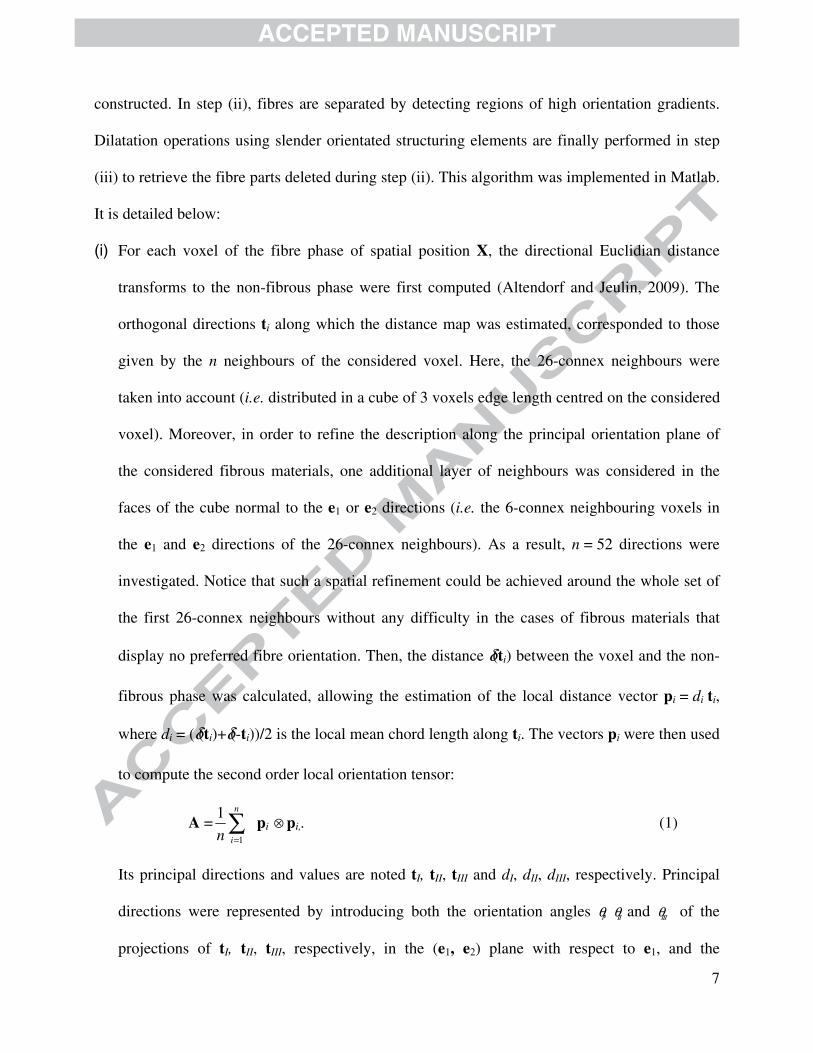
(iii) to retrieve the fibre parts deleted during step (ii). This algorithm was implemented in Matlab.

It is detailed below:

(i) For each voxel of the fibre phase of spatial position X, the directional Euclidian distance

transforms to the non-fibrous phase were first computed (Altendorf and Jeulin, 2009). The

orthogonal directions ti along which the distance map was estimated, corresponded to those

given by the n neighbours of the considered voxel. Here, the 26-connex neighbours were

taken into account (i.e. distributed in a cube of 3 voxels edge length centred on the considered

voxel). Moreover, in order to refine the description along the principal orientation plane of

the considered fibrous materials, one additional layer of neighbours was considered in the

faces of the cube normal to the e1 or e2 directions (i.e. the 6-connex neighbouring voxels in

the e1 and e2 directions of the 26-connex neighbours). As a result, n = 52 directions were

investigated. Notice that such a spatial refinement could be achieved around the whole set of

the first 26-connex neighbours without any difficulty in the cases of fibrous materials that

display no preferred fibre orientation. Then, the distance δ(ti) between the voxel and the non-

fibrous phase was calculated, allowing the estimation of the local distance vector pi = di ti,

where di = (δ(ti)+δ(-ti))/2 is the local mean chord length along ti. The vectors pi were then used

to compute the second order local orientation tensor:

A = ∑=

n

in 1

1pi ⊗ pi,. (1)

Its principal directions and values are noted tI, tII, tIII and dI, dII, dIII, respectively. Principal

directions were represented by introducing both the orientation angles θΙ, θΙΙ and θΙΙΙ of the

projections of tI, tII, tIII, respectively, in the (e1, e2) plane with respect to e1, and the

8

orientation angles ΨΙ, ΨΙΙ and ΨΙΙΙ of the projections of tI, tII, tIII, respectively, in the (e1, e3) plane

with respect to e1. To illustrate the evolution of these parameters inside a fibrous medium,

Fig. 2 gives 2D maps of their values within a 3D zone extracted from the volume of Fig. 1(b).

From this figure, it is worth noting that regions close to a contact between fibres are

systematically related to high gradients (i) of the local fibre orientation angle (here only sharp

variations of θΙ are observed, since fibres are mostly orientated in the (e1, e2) plane) and (ii) of

the eigenvalues related to the two other perpendicular principal directions (dII and dIII). It is

also interesting to note that the gradients recorded in the case of the θΙ map are sharper than

those observed for the dII or dIII ones, which are spread in larger zones around the contact

interface. This yields to consider in the following the first principal direction θΙ as the most

relevant parameter to identify contact surfaces.

(ii) In order to identify such particular zones, the mean local angular deviation Cp between the

first principal local orientation vector tI(X) and the first principal local orientation vectors of

its n neighbours tI(X+dXi) was calculated:

Cp(X) = ∑=

n

in 1

1|tI(X)·tI(X+dXi)|. (2)

In the case of the glass fibre bundle network displayed in Fig. 3(a), the resulting map of Cp is

depicted in Fig. 3(b). This image highlights obvious differences between contact zones and

most of the rest of fibres. Thus, to disconnect contacting fibres with different mean

orientations, a segmentation using an appropriate threshold of Cp could be achieved. For the

considered fibrous materials, typical threshold values of Cp ranging between 0.9 and 1

produced proper segmentations, i.e. that could both preserve most of the portions of fibres

outside contacting zones and separate contacting fibres (as depicted in Fig. 3(c)).

9

Then all the 26-connex voxels were grouped and labelled. At this step, some “small” fibre

portions were disconnected from the fibre they belonged to. If these volumes were lower

than an arbitrary minimum number of voxels (typical user-defined values ranging from 500

to 2000 voxels were here chosen), these small volumes were deleted. They were easily

retrieved during the next dilatation operation (iii, see below), together with the small

volumes deleted by global Cp thresholding (cf. Fig. 3(c)). Thereafter, 90% of labels

corresponded to individual fibres. For the remaining 10%, two problems were identified:

either some contacting fibres were not well separated or individual “big” portions that should

belong to the same fibre were disconnected. To treat these two cases, the threshold value of

Cp was reconsidered for the concerned labels (i.e. “locally”), in order either to separate not

well-separated fibres or to reconnect individual portions that should belong to the same fibre.

At this stage, an estimation of the total number of fibres Nf was obtained.

It is important to notice that the proposed individualisation method is exclusively based on

the detection of the local orientation angle variations. As a result, it does not enable one to

detect (nearly) parallel fibres. In the particular cases where parallel fibres could not be

separated, the as-treated volumes were subjected to an additional and successful thresholding

operation using the distance transform map, as already proposed in Orgéas et al. (2012).

(iii) At the end of step (ii), some voxels of the initial fibrous phase were not attributed to labelled

fibres (see Fig. 3(c)). To associate them with a proper label, each labelled fibre was subjected

to a dilatation using an anisotropic slender structuring element. In the case of the tested

fibrous media for which the fibre centrelines were weakly wavy, it was possible to ascribe

the mean orientation of the considered fibre to the element orientation, i.e. the mean value of

the tI’s within the considered segmented fibre. However, this is not a restriction of the

10

proposed method: for more tortuous fibres, the structuring element could be aligned with the

local direction of the tI’s. The structuring element was defined as a column of one voxel

thick with a length similar to the characterisitic fibre width. The dilatation was restricted to

the fibrous phase of the initial image. The operation was achieved once, to each voxel, label

by label. The procedure was repeated until reaching a stabilisation of the dilatation process

(≈ 15 iterations). After this sequence, either few voxels were not labelled or the voxels close

to contact regions had two labels, as highlighted with the white voxels in the example shown

in Fig. 3(d). In both cases, these voxels were associated with the main label of its 26-

neighbours. The image obtained after this last operation is displayed in Fig. 3(e).

Hence, the described image treatment procedure provides a 3D image with labelled fibres. The

numbers of fibre-fibre contacts Nc can thereafter be estimated by identifying the labels the fibres

of which were in contact. It was also possible to obtain rough estimates of contact surfaces, by

considering that a voxel belonged to a fibre-fibre contact surface if one of its 26-connex

neighbouring voxels belonged to another fibre (a contact zone has thus a thickness of two

voxels). A contact region between two connected fibres gathered all voxels of the contact zone

between these fibres. As a consequence, it could be split into several voxel subsets, i.e. a contact

zone can appear as a set of disconnected sub-surfaces.

4. VALIDATION

Figs. 4(a) and 4(b) exhibit the original 3D image of the network of copper fibres and the same 3D

11

image with coloured labelled fibres after the identification procedure, respectively. By visually

inspecting the obtained image, the identification of fibres seems fairly accurate. It can be noticed

that a negligible number of voxels was not correctly attributed (i.e. labelled differently from the

fibre they belong to). This particularly occurred in zones where fibres were locally nearly

parallel. As shown in the zoom of Fig. 4(c), fibre-fibre contacts were also properly detected using

the proposed algorithm. As revealed from Figs. 5-7, identical qualitative observations can be

established for the network of glass fibre bundles (Figs. 5(a-c)), but also for the two tested

networks of cellulosic fibres (see Figs. 6(a-c) and 7(a-c)). To further validate the method, more

quantitative results could also be extracted from the analysis. They are briefly summarised and

discussed below:

• For the network of copper fibres (Fig. 4), the total number of fibres is found to be

Nf = 133. This estimate is equal to the number of fibres counted in Orgéas et al. (2012)

from either a manual detection of fibres or by a thresholding based on the 3D Euclidian

distance map (see section 2). Moreover, the measured number of fibre-fibre contacts

reaches Nc = 218. This result is very close to the value of 214 assessed in Orgéas et al.

(2012) from an homotopic thinning followed by a 3D reconstruction of the fibrous

microstructure (see section 2). It can thus be concluded that to identify cylindrical fibres

with circular and constant cross-section and their contacts, the proposed procedure can

fairly be considered as efficient as classical geometrical skeletonisation methods. The

observed slight discrepancy may be attributed to a less accurate separation of parallel

fibres in the case of the present method.

• As in the case of copper fibres, the identification of glass fibre bundles inside the fibrous

12

media displayed in Fig. 5 is also accurate. Indeed, the number of labelled fibres is

Nf = 148: it is equal to the number of fibres manually counted by Guiraud et al. (2012)

(see section 2). Likewise, the estimated number of bundle-bundle contacts reaches Nc =

108. This value slightly differs from the value of 116 assessed by Guiraud et al. (2012)

(see section 2). This difference may probably be attributed to the method proposed in

Guiraud et al. (2012). Since the authors assumed constant elliptical cross section of the

bundles in order to detect bundle-bundle contacts, their method could yield to erroneous

estimation of Nc. Conversely, the identification procedure here proposed does not support

such a strong hypothesis and can hence handle fibres with flat but also variable cross

sections.

• A similar quantitative analysis was also carried out with the two cellulosic fibrous

networks depicted in Figs. 6 and 7. The number of fibres Nf was respectively estimated to

30 and 15. Such estimates exactly fit those that were obtained from a manual fibre

picking. Furthermore, the number of fibre-fibre contacts Nc was found to reach 32 and 18,

respectively. Here again, these results are very close to those assessed from a manual

observations of the considered images, i.e. 32±1 and 18, respectively.

Thus, by performing an appropriate finding and labelling of fibres and their contacts inside a 3D

segmented image with reasonable computation time (calculations for the analysed volumes

approximately lasted 10 h on a standard workstation), the proposed method constitutes a first and

required step to carry out a deeper analysis of the fibre morphologies and geometries: positions,

local orientations, curvatures and twists of the fibre centrelines (Latil et al, 2011), shape and

orientation of the fibre cross sections. It can also bring useful information about the position,

orientation, morphology and the geometry of fibre-fibre contacts. For instance, contact

13

orientation tensors built from the normal of each mean contact plane could be estimated (Latil et

al, 2011, Guiraud et al 2012, Orgéas et al, 2012). Similarly, graphs (c-d) shown in Figs. 4-7 also

illustrated some of the useful and original information that could be extracted about the

morphology and the geometry of contacts:

• As evidenced from the graphs (c) of these figures, fibre-fibre contacts display various

morphologies depending on the complexity of the fibre geometry: single contact surfaces or

contact zones with multiple sub-surfaces. The first ones are preferred morphologies in the

case of fibres with simple and convex cross sections (see Fig.4(c)), whereas the first and the

second morphologies can be encountered if the fibres cross sections become more complex,

as in the cases of the glass fibre bundles or the wood fibres (see Fig. 5-7(c)).

• The graphs (d) of these figures also provide the distributions of the estimated areas of contact

zones inside the scanned volumes. On each of these graphs, the areas have been normalised

by a characteristic contact surface area which corresponds to the square of the mean principal

width of the considered fibres or fibre bundles:

o Whatever the considered fibrous microstructure, the median value of the normalised

contact surface area is always below 1: it is equal to 0.48, 0.38, 0.19 and 0.37 for the

fibrous microstructures shown in Figs. 4, 5, 6 and 7, respectively.

o For the fibrous media with planar random fibre orientation, i.e. for fibrous media

plotted in Figs. 5-7, the normalised contact surface areas range between 0 and 3.

Conversely, for the Copper fibrous media (Fig. 4), the contact area distribution is

wider : this is related to the preferred fibre orientation along one direction that yields

to increase contact surfaces between fibres (Toll, 1993, Latil et al., 2011)

14

o The influence of processing conditions on contact surfaces can also be clearly

highlighted: as evident from the graphs of Figs. 6(d) and 7(d), the higher the pressure

during the paper processing, the larger the fibre-fibre contact surface areas.

Contact surfaces often play a critical role on the macroscale physical properties of fibrous

networks. As a consequence, having an automatic access to their number, position, morphology

and geometry may significantly contribute to the understanding and modelling of these

properties.

5. CONCLUDING REMARKS

In this work, we have proposed a novel method to identify and tag fibres with complex

anisotropic cross sections together with their contacts within 3D images of disordered fibrous

materials. The method relies upon a fine analysis of the local orientation map obtained from the

3D directional distance map. The reliability of the method was proved for real networks of

slightly wavy fibres exhibiting simple (circular) or very complex cross sections (with variable

irregular and slender shapes that could also be twisted along the fibre centrelines).

• The thresholding operation based on the local and intrinsic angular deviation parameter Cp

which is directly deduced from the 3D directional distance map seems to be relevant for

the considered fibrous materials and their associated 3D images, i.e. (i) for images that

had rather low the spatial resolutions (down to only 3-5 voxels along the smallest

thickness of the fibres), (ii) for low to moderate fibre contents, and (iii) for slightly wavy

fibres that were not (nearly) parallel. At such spatial resolutions, fibre contents and

orientations, it is expected to be still efficient for more tortuous fibres. Other existing

15

solutions can be used to tackle the case of (nearly) parallel fibres, for which the proposed

method is inappropriate.

• The dilatation operation that follows the Cp thresholding is another key point of the

method. Its efficiency and accuracy greatly depends on the shape, the dimensions and the

orientation of the selected structuring element. In this work, for the sake of simplicity, the

dilatation operation was successfully performed using a unique structuring element whose

orientation was set as a function of the mean orientation of each fibre. However, in view

of treating highly tortuous fibres and improving the identification accuracy in contact

zones, the shape, dimensions and orientation of the structuring element should be

continuously adapted by using the local fibre information.

The automatic identification of fibres with complex anisotropic cross sections together with their

contacts inside 3D images of disordered fibrous networks is the first requirement to obtain

quantitative microstructural data on the morphologies and geometries of fibres and fibre-fibre

contacts. If further studies are still required to improve this identification, the method proposed in

this paper demonstrates that such valuable data are now accessible. If the 3D images were

obtained from fibrous materials subjected to macroscale physical or mechanical loading, the

evolution of the underlying deformation micro-mechanisms of the fibres and the fibre-fibre

contacts could be better assessed.

ACKNOWLEDGEMENTS

This work was performed within the ANR research program “3D discrete analysis of deformation

micromechanisms in highly concentrated fiber suspensions” (ANAFIB, ANR-09-JCJC-0030-01),

the ESRF Long Term Project “Heterogeneous Fibrous Materials” (exp. MA127). J. Viguié also

16

thanks Grenoble INP together with the PowerBonds and WoodWisdom ERA-NET project for his

research grant.

REFERENCES

(1) Altendorf, H. and Jeulin, D. “3D directional mathematical morphology for analysis of fiber

orientations” Image Analysis Stereol 28 (2009) 143-153.

(2) Axelsson, M. “3D Tracking of cellulose fibres in volume images” Proc. Int Conf Image Process 4

(2007) 309-312.

(3) Axelsson, M. “Estimating 3D fibre orientation in volume images. Pattern Recognition” Proc. Int

Conf Pattern Recognition, (2008) 1-4.

(4) Eberhardt, C.N. and Clarke, A.R. “Automated reconstruction of curvilinear fibres from 3D dataset

acquired by X-Ray Microtomography” J Microscopy 206 (2002) 41-53.

(5) Guiraud, O., Orgéas, L., Dumont, P.J.J., Rolland du Roscoat, S. “Microstructure and deformation

micromechanisms of concentrated fiber bundle suspensions: An analysis combining x-

raymicrotomography and pull-out tests” J Rheol 56 (2012) 592-23.

(6) Hild, F., Maire, E., Roux, S., Witz, J.F. “Three-dimensional analysis of a compression test on stone

wool” Acta Mater 57 (2009) 3310-3320.

(7) Krause M., Hausherr J.M., Burgeth B., Herrmann C. and Krenkel W. “Determination of the fibre

orientation in composites using the structure tensor and local X-ray transform” J Mater Sci 45 (2010)

888-896.

(8) Latil, P., Orgéas, L., Geindreau, C., Dumont, P.J.J. and Rolland du Roscoat, S. “Towards the 3D in

situ characterisation of deformation micro-mechanisms within a compressed bundle of fibres”

Compos Sci Technol 71 (2011) 480-488.

(9) Le, T.-H., Dumont, P.J.J., Orgéas, L., Favier, D., Salvo, L., E. Boller, E. “X-ray phase contrast

microtomography for the analysis of the fibrous microstructure of SMC composites” Compos Part A

39 (2008) 91-103.

(10) Lux, J., Delisée, C. and Thibault, X. “3D characterisation of wood based fibrous materials: an

application” Image Anal Stereol 25 (2006) 25-35.

(11) Lux, J. “Automatic segmentation and structural characterization of low density fibreboards” Image

Anal Stereol, 32 (2013) 13-25.

(12) Malmberg F., Lindblad J., Östlund C., Almgren K.M. and Gamstedt E.K. Nucl Instr Meth Phys Res A

637 (2011) 143-148.

17

(13) Marulier C., Dumont P.J.J., Orgéas L., Caillerie D. and Rolland du Roscoat S. “Towards 3D analysis

of pulp fibre networks at the fibre and at the bond levels” Nordic Pulp Paper Res J 28 (2012) 245-

255.

(14) Masse, J.P., Salvo, L., Rodney, D., Bréchet, Y., Bouaziz, O. “Influence of relative density on the

architecture and mechanical behaviour of a steel metallic wool” Scripta Mater 54 (2006) 1379-1383.

(15) Palágyi, K. and Kuba, A. “A 3D 6-subiteration thinning algorithm for extracting medial lines”

Pattern Recogn Letters 19 (1998) 613-627.

(16) Orgéas L., Dumont P.J.J., Vassal J.P., Guiraud O., Michaud V. and Favier D. “In-plane conduction of

polymer composite plates reinforced with architectured networks of Copper fibres” J Mater Sci 47

(2012) 2932-2942.

(17) Sandau, K. and Ohser, J. “The chord length transform and the segmentation of crossing fibres” J

Microscopy 226 (2007) 43-53.

(18) Svensson, S. and Aronsson, M. “Using distance transform based algorithms for extracting measures

of the fibre network in volume images of paper” IEEE Trans Syst Man Cyber-Part B 33 (2003) 562-

571.

(19) Tan J.C., Elliott J.A. and Clyne T.W. “Analysis of tomography images of bonded fibre networks to

measure distributions of fibre segment length and fibre orientation” Adv Eng Mater 8 (2006) 495-

500.

(20) Toll, S. “Note on the tube model” J Rheol 37 (1993) 123-125

(21) Walther, T., Terzic K., Donath T., Meine H., Beckman F., Thoemen H. “Microstructural analysis of

lignocellulosic fiber networks” Developments in X-ray Tomography V (2006) 6318.

(22) Wernersson L.G., Brun A. and Luengo Hendricks C.L. “Segmentation of wood fibres in 3D CT

images using graph cuts” Lecture Notes Comput Sci 5716 (2009) 92-102.

(23) Yang H. and Lindquist B.W. “Three-dimensional image analysis of fibrous materials” Proc

Applications of Digital Image Processing XXIII (2000) 4115.

18

(c)(c)

210 µm

(a) (b)

15.6 mm6.1 mm

e1

e2

e3

(d)

315 µm

Figure 1: 3D images obtained by X-ray tomography of (a) a network of Copper fibres reinforcing a PMMA polymer matrix (360 × 360 × 88 voxels, 1 voxel = 173 μm3), (b) a network of glass fibre bundles reinforcing a thermoset polyester matrix with mineral fillers (500 × 500 × 146 voxels, 1 voxel = 31.23 μm3) and (c) a network of cellulosic fibres with a basis weight of 40 g m-2 obtained by a papermaking process under low pressing conditions (300 × 300 × 200 voxels, 1 voxel = 0.73 μm3) and (d) a network of cellulosic fibres with a basis weight of 15 g m-2 obtained by a papermaking process under standard pressing conditions (450 × 450 × 65 voxels, 1 voxel = 0.73 μm3).

19

θI(rad) Ψ

I (rad)

θII(rad) Ψ

II (rad)

θIII(rad) Ψ

III (rad)

dI(voxels)

dII(voxels)

dIII(voxels)

e2

e1

Figure 2: Maps of the orientation angles θI, θII and θIII and of the projections of the principal directions in the (e1, e2) plane with respect to e1, of the orientation angles ΨI, ΨII and ΨIII of the projections of the principal directions in

the (e1, e3) plane with respect to e1, and of the eigenvalues dI, dII and dIII, along the (e1, e2) plane of a small segmented 3D image extracted from the volume shown in Fig. 1(b) (160 x 160 x 100 voxels, 1 voxel = 183 μm3).

20

(a) (b)

(c) (d) (e)

Cp > 0.98

Cp

Figure 3: (a) Slice along the (e1, e2) plane of a small segmented 3D image of a network of glass fibre bundles (160 x 160 x 100 voxels, 1 voxel = 183 µm3), (b) map of the mean angular deviation Cp, (c) labelled image after thresholding of Cp, (d) image after the successive dilatations with a 2D elliptic structuring element and (e) image at the end of the identification procedure.

21

(a) (b)

1.5 mm(= 88 voxels)

(c)

6.1 mm(= 360 voxels)

x (voxels)y (voxels)

z (v

oxe

ls)

y (voxels)

z (v

oxe

ls)

(d)

x (voxels)

Figure 4: (a) Original 3D image obtained by X-ray tomography of a network of Copper fibres reinforcing a polymer composite (360 x 360 x 88 voxels, 1 voxel = 173 μm3). (b) 3D image with labelled fibres after the identification procedure. (c) 3D image of fibre-fibre contact surfaces represented in red along a fibre extracted from the labelled image. (d) Area distribution of fibre-fibre contacts.

(a) (b)

15.6 mm(= 500 voxels)4.5 mm

(=160 voxels)

(c) (d)

x (voxels)y (voxels)

z (v

oxe

ls)

x (voxels)

y (voxels)

z (v

oxe

ls)

Figure 5: (a) 3D image obtained by X-ray tomography of a network of glass fibre bundles reinforcing a polymer composite (500 x 500 x 146 voxels, 1 voxel = 31.23 μm3). (b) 3D image with labelled bundles after the identification procedure. (c) Same 3D image with fibre-fibre contact zones represented in red. (d) Area distribution of fibre-fibre contacts.

22

210 μm

(= 300 voxels)

140 μm

(= 200 voxels)

(a) (b)

(c)

x (voxels)y (voxels)

z (v

oxe

ls)

x (voxels)y (voxels)

z (v

oxe

ls)

(d)

Figure 6: (a) 3D image obtained by X-ray tomography of a network of cellulosic fibres obtained by a papermaking process (300 x 300 x 200 voxels, 1 voxel = 0.73 μm3). (b) 3D image with labelled fibres after the identification procedure. (c) 3D image of fibre-fibre contact zones represented in red along a fibre extracted from the labelled image. (d) Area distribution of fibre-fibre contacts.

(a) (b)

(c)

315 μm

(= 450 voxels)

45 μm

(= 65 voxels)

x (voxels)

y (voxels)

z (v

oxe

ls)

x (voxels)

y (voxels)

z (v

oxe

ls)

(d)

Figure 7: (a) 3D image obtained by X-ray tomography of a network of cellulosic fibres obtained by a papermaking process (450 x 450 x 65 voxels, 1 voxel = 0.73 μm3). (b) 3D image with labelled fibres after the identification procedure. (c) Same 3D image with fibre-fibre contact zones represented in red. (d) Area distribution of fibre-fibre contacts.