Financial Management of Firms and Financial Institutions
320
VŠB - TECHNICAL UNIVERSITY OF OSTRAVA Faculty of Economics, Department of Finance Financial Management of Firms and Financial Institutions 11 th International Scientific Conference PROCEEDINGS (Part I.) 6 th – 7 th September 2017 Ostrava, Czech Republic
-
Upload
khangminh22 -
Category
Documents
-
view
0 -
download
0
Transcript of Financial Management of Firms and Financial Institutions

VŠB - TECHNICAL UNIVERSITY OF OSTRAVA
Faculty of Economics, Department of Finance
Financial Management of Firms and
Financial Institutions
11th International Scientific Conference
PROCEEDINGS
(Part I.)
6th – 7th September 2017
Ostrava, Czech Republic
ORGANIZED BY
VŠB - Technical University of Ostrava, Faculty of Economics, Department of Finance
EDITED BY
Miroslav Čulík
TITLE
Financial Management of Firms and Financial Institutions
ISSUED IN
Ostrava, Czech Republic, 2017, 1st Edition
PAGES
960
ISSUED BY
VŠB - Technical University of Ostrava
PRINTED IN
BELISA Advertising, s.r.o., Hlubinská 32, 702 00 Ostrava, Czech Republic
ORGANIZÁTOR
VŠB - Technická univerzita Ostrava, Ekonomická fakulta, Katedra financí
EDITOR
Miroslav Čulík
NÁZEV
Finanční řízení podniků a finančních institucí
MÍSTO, ROK, VYDÁNÍ
Ostrava, 2017, 1. vydání
POČET STRAN
960
VYDAL
VŠB - Technická univerzita Ostrava
TISK
BELISA Advertising, s.r.o., Hlubinská 32, 702 00 Ostrava, Česká Republika
ISBN 978-80-248-4138-0 (book of proceedings)
ISBN 978-80-248-4139-7 (CD)
ISSN 2336-162X
PROGRAM COMMITTEE
prof. Dr. Ing. Dana Dluhošová VŠB - Technical University of Ostrava,
Czech Republic
doc. Ing. Petr Dvořák, Ph.D. University of Economics Prague, Czech
Republic
doc. RNDr. Jozef Fecenko, CSc. University of Economics in Bratislava,
Slovakia
prof. Dr. Ing. Jan Frait Czech National Bank Prague,
Czech Republic
doc. RNDr. Galina Horáková, CSc. University of Economics in Bratislava,
Slovakia
prof. Ing. Eva Kislingerová, CSc. University of Economics Prague,
Czech Republic
prof. Ing. Bohumil Král, CSc. University of Economics Prague,
Czech Republic
doc. Ing. Peter Krištofík, Ph.D. Matej Bel University in Banská
Bystrica, Slovakia
prof. Ing. Anna Majtánová, Ph.D. University of Economics in Bratislava,
Slovakia
prof. Ing. Dušan Marček, CSc. VŠB - Technical University of Ostrava,
Czech Republic
prof. Ing. Miloš Mařík, CSc. University of Economics Prague,
Czech Republic
doc. Ing. Ladislav Mejzlík, Ph.D. University of Economics Prague,
Czech Republic
prof. Ing. Petr Musílek, Ph.D. University of Economics Prague,
Czech Republic
doc. RNDr. Valéria Skřivánková, CSc. Pavol Jozef Šafárik University in
Košice, Slovakia
doc. Ing. Tomáš Tichý, Ph.D. VŠB - Technical University of Ostrava,
Czech Republic
prof. Ing. Miloš Tumpach, Ph.D. University of Economics in Bratislava,
Slovakia
prof. Dr. Ing. Zdeněk Zmeškal VŠB - Technical University of Ostrava,
Czech Republic
EDITED BY
doc. Ing. Miroslav Čulík, Ph.D. VŠB - Technical University of Ostrava,
Czech Republic
REVIEWED BY
doc. Ing. Miroslav Čulík, Ph.D. VŠB - Technical University of Ostrava,
Czech Republic
prof. Dr. Ing. Dana Dluhošová VŠB - Technical University of Ostrava,
Czech Republic
Ing. Petr Gurný, Ph.D. VŠB - Technical University of Ostrava,
Czech Republic
doc. Ing. Aleš Kresta, Ph.D. VŠB - Technical University of Ostrava,
Czech Republic
prof. Ing. Lumír Kulhánek, CSc. VŠB - Technical University of Ostrava,
Czech Republic
prof. Dr. Sergio Ortobelli Lozza University of Bergamo,
Italy
prof. Ing. Martin Macháček, Ph.D. et Ph.D. VŠB - Technical University of Ostrava,
Czech Republic
Ing. Martina Novotná, Ph.D. VŠB - Technical University of Ostrava,
Czech Republic
doc. Ing. Martin Svoboda, Ph.D. Masaryk University in Brno,
Czech Republic
doc. Ing. Tomáš Tichý, Ph.D. VŠB - Technical University of Ostrava,
Czech Republic
Ing. Jiří Valecký, Ph.D. VŠB - Technical University of Ostrava,
Czech Republic
prof. Dr. Ing. Zdeněk Zmeškal VŠB - Technical University of Ostrava,
Czech Republic
CONTENTS
Part I.
Andrejovská Alena, Gavurová Beáta
Meta - Analysis of the Categorization of EU Countries in the Context of Tax Competition 14
Barczak Stanisław
The gray GM(1,1) model applications in time series analysis - selected issues 22
Baštincová Anna, Benko Ján
Dividends as risk subject of taxation in Slovak republic 33
Belanová Katarína
Firm Investment under Financial Market Imperfections 39
Bělušová Kristýna, Brychta Karel
CFC Rules as stated in the standards of the OECD and EU – a comparative study 46
Blahušiaková Miriama
The Analysis of the Golden Rule in the Balance Sheet of Selected Business Accounting
Entities 54
Blajer-Gołębiewska Anna
Corporate reputation, ownership structure and market value in the banking sector in Poland 62
Bohušová Hana, Svoboda Patrik, Solilová Veronika, Nerudová Danuše
Materiality of Deferred Tax Reporting – Case of Czech Listed Companies 70
Bokšová Jiřina, Horák Josef
Reporting ability of financial statements of micro and small accounting entities after amendment
of Act on Accounting 79
Borovcová Martina
Selection of the optimal solution of the decision-making problem 87
Borovcová Martina, Richtarová Dagmar
Analysis of the financial performance by applying multi-level decomposition method 96
Borovička Adam
Non-traditional approach using mathematical programming to a stock investment portfolio
making 106
Borovička Adam, Tomsa Jan
Modified KSU-STEM as an appropriate tool for making a portfolio of open unit trusts 114
Brychta Karel, Bělušová Kristýna
International Taxation of Dividends as Regulated in Double Tax Treaties – a Case of the Czech
Republic 122
Buła Rafał
Modified method of area division in fractal dimension estimation 131
Butek Michal, Bakeš Vladimír
Potential of blockchain technology 143
Buus Tomáš
P/E, dividend yield and GDP growth in U.S.A.: The story of stock market valuation 151
Leszek Czerwonka, Jacek Jaworski
Capital Structure Determinants of Industrial Companies Listed on the Warsaw Stock
Exchange 157
Černá Dana
Adaptive wavelet method for pricing options under the Stein-Stein stochastic volatility
model 165
Čulík Miroslav
Valuation of the Two-Color Rainbow Real Options 173
Čulík Miroslav, Jurčicová Andrea
Application and Comparison of the Methods for Influences Quantification Including Sensitivity
Analysis 185
Daníšek Matušková Petra
Location Factors of Headquarters of Largest Czech Enterprises 195
Doś Anna
Financial performance and bankruptcy risk of socially responsible and „irresponsible” companies
– the Polish case 201
Drugdová Barbora
On the Issue of Commercial Insurance and Commercial Insurance Market in
the Slovak Republik 209
Durica Marek, Zvarikova Katarina
MDA vs. Logit bankruptcy models in the Slovak Republic 214
Dvořáčková Hana, Jochec Marek
Evaluation of the Behavioral Differences in the FX Trading Approach with Regard to
the Gender 222
Fleischmann Luboš
Unconventional monetary policy tools in central banking globally and within the Czech
Republic 230

Foffová Nikola, Hrdý Milan, Marek Petr
Leverage of European Firms 237
Frączkiewicz-Wronka Aldona, Kozak Anna
The comparsion of various types of public-social partnerships in Poland in the light of the
empirical reasearch 246
Glova Jozef
Intangible Assets and Their Valuation Using Direct Intellectual Capital Methods: Pros and
Cons 255
Guo Haochen
Hedging portfolio risk management with VaR 264
Gurný Petr
Estimation and analysis of value multipliers within processing industry in Czech Republic 270
Gurný Petr, Slezáková Klára
Application of Sensitivity Analysis within Determination of Chosen Partial Effects on Company's
Value 277
Havelka Jiří
Business Strategy Management: The Importance of Employees During Implementation of
Strategic Changes 284
Horák Josef, Bokšová Jiřina
The use of Big Data in terms of overhead costs 294
Hornická Renáta
The nature and importance of dislosing information about interests in any subsidiaries, joint
ventures and associates according to IFRSs 301
Hospodka Jan, Randáková Monika
Indicating Insolvency in Firms 312
Part II.
Hozman Jiří, Tichý Tomáš
DG method for the Hull-White option pricing model 320
Chlíbek Adam
Managing foreign exchange exposures in the context of ending the currency commitment of the
CNB 328
Chmelíková Barbora, Svoboda Martin
Is the Financial Literacy Level of Finance and Law Students the Same? 336
Chytilová Lucie
Efficiency of financial institutions in the Visegrad Group according to Data Envelopment Analysis
with dual-role variable 342
Ilavska Iveta, Durica Marek
Delta and Gamma for Gap Options 350
Janáčková Hana, Kořená Kateřina
Development and application of the Industry 4.0 principles in the selected firms and areas in the
Czech Republic 357
Jančíková Eva, Pásztorová Janka, Raneta Leonid
Impact of Banking Union on the Banking industry in Slovak Republic 364
Kalouda František
Inflation forecasting in company financial management (use and reliability) 372
Kashi Kateřina
Employees' Performance Management by Using MCDM Methods 383
Kolková Andrea
Back-test of efficiency by combining technical indicators on the EUR/JPY 391
Kopa Miloš
SD portfolio enhancement with and without short sales 400
Kopecká Lucie, Pacáková Viera
Bayesian Estimation of Probability of Incidences of the Most Serious Oncological Diseases in the
Czech Republic 407
Kostalova Jana
Use of Financial Instruments in the Czech Republic within the European Structural and
Investment Funds in the Programming Period 2014-2020 415
Kouaissah Noureddine, Ortobelli Lozza Sergio
Multivariate Dominance among financial sectors 423
Krajíček Jan
Banking sector 432
Kresta Aleš, Lisztwanová Karolina
Break-even analysis under normally distributed input variables 440
Krištofík Peter, Ištok Michal
A corporation structure draft for the selected Slovak companies 446
Kubaščíková Zuzana
Application the Binomial Distribution, Hypergeometric Distribution and Poisson Probability
Distribution in Accounting 455
Kubicová Jana
Offshore Financial Centres, Tax Havens and Location of Banks’ Claims 459
Kuna-Marszalek Anetta, Marszalek Jakub
Greening the Green - Environmental and Financial Aspects of the American Green Bond Market
Development 468
Kuzior Anna, Rówińska Małgorzata
Performance management of business entities in light of comprehensive income concept 476
Lando Tommaso, Bertoli-Barsotti Lucio
Income inequality and intersecting Lorenz curves: an empirical study 484
Lisztwanová Karolina, Kresta Aleš
Comparison of valuation approaches of finished goods and work in progress 491
Lisztwanová Karolina, Ratmanová Iveta
Assessment of Impact of Items Reducing Tax Base and Tax on Total Amount of Corporate Income
Tax in the Czech Republic in Selected Sectors 498
Malavasi Matteo, Ortobelli Sergio
Semiparametric Tests for Behavioral Finance Efficiency 507
Málek Jiří, van Tran Quang
Investigating the Distributional Properties of Highly Volatile Bitcoin Exchange Rate 514
Marček Dušan, Falát Lukáš
Optimal Strategy for Homeowners about Mortgages in Eurozone in 2017 522
Marek Patrice, Šedivá Blanka
Optimization and Testing of RSI 530
Mareš David, Kotěšovcová Jana
The impact of macroeconomic indicators on sovereign rating 538
Mastalerz-Kodzis Adrianna
Multidimensional phenomena analysis with the use of Hölder function properties 543
Mazanec Jaroslav, Bartošová Viera
The Quantification of Effectiveness as Precondition for Facility Management 552
Meluchová Jitka, Mateášová Martina
Benefits and risks of using outsourcing of economic activities 560
Mihola Jiří, Wawrosz Petr
The relationship between profitability and efficiency 568
Michalkova Lucia, Kliestik Tomas
Determinants of value of tax shield in the Slovak Republic 574

Mikulec Ondřej
Analysis of Blue-Collars and White-Collars Approach to Company's Attendance 583
Miśkiewicz-Nawrocka Monika, Zeug-Żebro Katarzyna
The evaluation of the effectiveness of a long-term stocks investment strategy based on the largest
Lyapunov exponent 590
Mokošová Daša, Subačienė Rasa, Hladika Mirjana, Molín Jan
Impact of changes in accounting regulation on sanctions for its violation in selected countries 599
Moravcikova Dominika, Kliestikova Jana
Brand valuation and recognition of Sedita with using a licence analogue method and the possibility
of its use in creating the value of the enterprise 609
Musa Hussam, Stroková Zuzana, Musová Zdenka
Comparative analysis of traditional and alternative financing of SMEs in Slovakia 617
Part III.
Musílek Petr
Investment Bubbles 625
Niklová Petra, Bokšová Jiřina, Horák Josef
The possibility of identification of high-risk suppliers from financial statements 636
Novotná Martina
The Use and Comparison of Survival Models for Corporate Bankruptcies 644
Novotný Josef, Tian Yuan
Determination of Credit Risk for Debt Assets Portfolio between 2016 and 2017 653
Ondrušová Lucia
Company in crisis 661
Paleta Vojtěch
The Impact of Digitalization and Connectivity on Automotive OEM: Sustainability
Dashboard 668
Paliderová Martina
Comparison of the tax and contribution burden on the entrepreneur in Slovak legislation 678
Parajka Branislav, Kňažková Veronika
Possibilities of Financial Statements Presentation for Micro Accounting Entities in the Slovak
Republic 687
Podhorska Ivana, Misankova Maria
Searching for significant variables in the area of company´s financial health prediction: A case
study in Slovakia 692
Pośpiech Ewa
Multi-criteria fuzzy modelling in the issue of portfolio selection 700
Ptáčková Barbora
Analysis of the Value Drivers of the Company’s Financial Performance 708
Randáková Monika, Bokšová Jiřina
Tax Implications of Non-monetary Capital Contributions in Corporations 716
Reuse Svend, Svoboda Martin
Czech PX-TR – Derivation of Historical Data for the Performance Index and Analysis of two
Trading Strategies 723
Richtarová Dagmar
Analysis of Variance of Economic Value Added to Chosen Industry in the Czech Republic 732
Siekelova Anna, Svabova Lucia
Decision to provide trade credit based on selected models of financial health prediction in the
chosen sector 740
Skřivánková Valéria, Hajdu Matej
Strategies of Portfolio Insurance at Extremal Risks 747
Sroczyńska-Baron Anna
The efficiency of online auction market in Poland for chosen category of items 755
Stádník Bohumil
Framework for Valuation of CAT Bonds 763
Staníčková Michaela, Melecký Lukáš
Impact Analysis of the European Structural Funds on Efficiency of Employment Issues in Euro
Area 773
Staniek Dušan
The significance of cross-currency basis in corporate finance 781
Steinerowska-Streb Izabella
The impact of capital shortages on the financial investment sources of family firms 790
Strouhal Jiří, Štamfestová Petra
EBIT Construction and Its Impact on ROA: Does it Affect Corporate Rating? 798
Svítil Martin
Acquisition of the company: plan for the first 100 days 805
Šimůnek Jiří
Quality of the reporting under IFRS 8 of issuers of the quoted securities in the Czech
Republic 814
Špačková Adéla
Estimation of Claim Frequency by Generalized Linear Models 821
Tarišková Natália, Skorková Zuzana
Human Capital Accounting 831
Tian Yuan, Novotný Josef
Application of the CreditGrades™ Model to Sovereign Credit Default Swaps 843
Tichý Tomáš, Holčapek Michal, Hozman Jiří, Kresta Aleš
Comparison of several alternatives to numerical pricing of options 851
Torri Gabriele, Giacometti Rosella, Rachev Svetlozar
Option Pricing in Non-Gaussian Ornstein-Uhlenbeck Markets 857
Tworek Piotr
Methods of Risk Identification in Management of Public Sector Organizations 866
Urminský Jaroslav, Vyskočilová Štěpánka
Spatial Structure of Headquarters of Largest Enterprises in the Czech Republic 874
Valachová Viera, Kráľ Pavol
The Importance of Brand Portfolio Optimization 883
Valaskova Katarina
Slovak Prediction Models in Economic Practice 891
Valecký Jiří
Setting optimal limit of cover by stochastic optimisation 901
Vávra František, Ťoupal Tomáš
Concordance Rate between Time Series of Exchange Rates, Statistical and
Probabilistic view 907
Vitali Sebastiano, Moriggia Vittorio
Pension fund ALM models with stochastic dominance 915
Vokoun Marek
Impact of Innovation Outsourcing on the Financial Situation of Companies in
the Czech Republic 923
Wójcicka Aleksandra
The impact of financial ratios dynamics on company’s performance 931
Zelinková Kateřina
Determination of Risk Measure by Assuming Laplace Distribution 937
Zeug-Żebro Katarzyna, Miśkiewicz-Nawrocka Monika
Risk Analysis of Fundamental Portfolio of Investment 944

Zmeškal Zdeněk, Dluhošová Dana
Bond valuation under risk, flexibility and interaction on a game theory basis 951
11th International Scientific Conference on Financial Management of Firms and Financial Institutions Ostrava
VŠB-TU of Ostrava, Faculty of Economics, Department of Finance 6th – 7th September 2017
14
Meta - Analysis of the Categorization of EU Countries in the Context of Tax Competition
Alena Andrejovská1, Beáta Gavurová2
Abstract
Market economy, capital mobility, and corporate tax efficiency are concepts that are related to
each other and are currently putting strong pressure on investors and increasing tax
competition. The paper identifies, analyzes and evaluates a group of EU Member States in the
context of tax competition and classifies these countries in economically meaningful groups
based on similarities in corporate taxation. Several methodical approaches of hierarchical and
non-hierarchical cluster analysis are used and compared in the framework of the meta-analysis.
The result of this analysis is four groups of multidimensional objects that have shown that
member states have been divided into a group of new and old member states in terms of tax
burden and other macroeconomic factors. The analysis has also highlighted the differences in
corporate taxation in the European area.
Key words
Tax competition, corporate tax, tax burden, cluster analysis, nominal and effecitve corporate
tax rate
JEL Classification: H21, H25
1. Úvod
Druhá polovica 20. storočia bola charakterizovaná nástupom globalizácie a prechodu od
regionálnych trhových systémov k celosvetovým. Široký (2012) uvádza, že v tomto období
dochádzalo k výraznému pohybu v medzinárodnom obchode a k mobilite daňových základov,
čo málo za následok prelínanie rôznych daňových systémov a vytvorenie súťaživého
a konkurenčného prostredie medzi daňovými systémami jednotlivých krajín EÚ. Z pohľadu
Sinna (1990) existujú dva základné pohľady na meranie úrovne daňového zaťaženia a
prístupy k celkovému daňovému zaťaženiu a daňovej konkurencii. Prvý pohľad preferuje
daňovú konkurenciu ako daňovú hru kvôli pozitívnemu vplyvu na verejné výdavky a zníženiu
neefektívnych aktivít Salin (1998) a Tiebout (1956). Druhý pohľad poukazuje na vplyv
daňovej konkurencie v negatívnom svetle Wilson (1999) a Stiglitz a kol. (2015) alebo Griffith
a kol. (2004). Autori poukazujú na okolnosti, že vo verejných financiách trh zlyháva, preto
preferujú daňovú harmonizáciu, pričom kladú dôraz na negatívny účinok mobility kapitálu na
kapitálových daňových sadzbách a na úroveň verejných výdavkov. V Európe sa problém
daňovej konkurencie prejavuje už od začiatku šesťdesiatych rokov 20-teho storočia.
Vo viacerých krajinách sa v tomto období začalo s poklesom nominálnych sadzieb daní, čo
malo za následok negatívny vplyv na fiškálne externality, ktoré vychádzali z nezávislej súťaže
1 doc. Ing. Alena Andrejovská, PhD., Technical University of Košice, Faculty of Economics, e-mail:
[email protected]. 2 doc. Ing. Beáta Gavurová, PhD., MBA. Technical University of Košice, Faculty of Economics, e-
mail: [email protected].
Acknowledgement: This research was supported by VEGA project No. 1/0311/17 on Measuring and
Reporting Intangible Assets
11th International Scientific Conference on Financial Management of Firms and Financial Institutions Ostrava
VŠB-TU of Ostrava, Faculty of Economics, Department of Finance 6th – 7th September 2017
15
mobilných základov dane. Je nevyhnutné zdôrazniť, že od polovice roku 1980, boli vo
všetkých krajinách podstatne znížené štatutárne korporátne daňové sadzby. Tento jav
pretrváva dodnes a ich klesajúca tendencia je permanentne viditeľná hlavne pri použití
efektívnej priemernej daňovej sadzby, čo má za následok rozšírenie daňového základu, ku
ktorému došlo v mnohých krajinách. Nesmie sa však zabúdať, že okrem zníženia štatutárnych
a efektívnych korporátnych sadzieb na daňové zaťaženie vplýva celý rad ďalších
makroekonomických ukazovateľov, ktoré sa rozhodujúcou mierou podieľajú na vytváraní
konkurenčného prostredia medzi členskými krajinami EÚ.
Cieľom príspevku je vytvoriť ekonomickú kategorizáciu krajín EÚ v kontexte daňovej
konkurencie so zreteľom na vopred určené segmentačné kritériá využívajúce hierarchické
a nehierarchické metódy zhlukovania.
Výber makroekonomických ukazovateľov bol zrealizovaný na základe teoretických
poznatkov autorov Barro (1979) a Devereux a kol. (2002), ktorí skúmali pôsobenie týchto
faktorov na oblasť daňových príjmov právnických osôb, ako aj spätné pôsobenie dane na
faktory v budúcom období. Autori pomocou multidimenzionálneho škálovania zisťovali
rozdielnosti medzi skúmanými objektmi a sledovali pôsobenie vybraných ukazovateľov na
daňovú oblasť. Pri sledovaní vplyvu makroekonomických determinantov na kategorizáciu
členských krajín boli použité dáta z Eurostatu a KPMG.
nominálna štatutárna sadzba dane z príjmov PO v %,
efektívna sadzba dane z príjmov PO v %,
HDP - vyjadrený v bežných cenách v mil. €,
miera zamestnanosti - predstavuje podiel zamestnaných vo veku od 15 do 64 rokov,
miera inflácie - meraná na základe harmonizovaného indexu spotrebiteľských cien,
saldo štátneho rozpočtu - deficit/prebytok ŠR vyjadrený v pomere k HDP v %,
verejný dlh - verejný dlh ako pomer dlhu k HDP v %,
celkové daňové zaťaženie - pomer príjmov zo všetkých druhov daní a sociálnych
príspevkov vo forme daní k HDP v %,
vládne výdavky -v bežných cenách v mil. €,
celkové daňové príjmy - celkové daňové príjmy z priamych a nepriamych daní
v bežných cenách v mil. €.
Kategorizácia bola uskutočnená pomocou viacerých metodických prístupov k štúdiu dát,
ktoré sú založené na koncepcii euklidovskej metriky (Halkidi a kol., 2001). V súlade so
stanoveným zámerom boli v rámci metodológie zhlukovej analýzy využité hierarchické aj
nehierarchické metódy klastrovania. Z hierarchických metód bola zvolená analýza Wardovou
linkage (v praxi najčastejšie využívaná) s mediánovou metódou, obidve pomocou funkcie
hclust() (Ferreira a kol., 2009). Z nehirerarchických metód bola využitá metóda k-means a
fuzzy c-means, ktorá je oproti ostatným metódam špecifická a umožňuje odhaliť tzv.
klasifikačné neurčité objekty pomocou funkcie kmeans() a fanny()(Charrad a kol., 2012).
Analýzy boli vykonané v štatistickom jazyku R za rok 2015. Pri všetkých sledovaných
metódach bol určený optimálny počet štyroch zhlukov.
1.1 Daňová konkurencia z pohľadu hierarchického a nehierarchického zhlukovania
Wardova metóda
Ide o najviac využívanú a u ekonómov Cunninghama a kol. (1972) veľmi obľúbenú
hierarchickú metódu, ktorú autori považujú za najúčinnejšiu. Wardova metóda vytvára
kompaktné zhluky rovnakej početnosti.

11th International Scientific Conference on Financial Management of Firms and Financial Institutions Ostrava
VŠB-TU of Ostrava, Faculty of Economics, Department of Finance 6th – 7th September 2017
16
Obrázok 1 Dendrogram: Wardova metóda
Prvý zhluk tvorili: Španielsko a Taliansko. Druhý zhluk tvorili rovnako 2 krajiny:
Francúzsko a Spojené kráľovstvo. Tretí zhluk samostatne tvorilo iba Nemecko. Posledný
štvrtý zhluk bol tvorený: Rumunskom, Maďarskom, Slovenskou republikou, Bulharskom,
Lotyšskom, Švédskom, Írskom, Dánskom, Fínskom, Poľskom, Belgickom, Holandskom,
Portugalskom, Gréckom, Rakúskom, Luxemburskom, Litvou, Chorvátskom, Cyprom,
Estónskom, Slovinskom, Českou republikou a Maltou. V tomto zhluku môžeme sledovať
vzájomné zoskupenie nových členských krajín, ktoré sa zoskupili v prvej a druhej vetve tohto
zhluku. Staré členské krajiny naopak vyjadrili svoju vzájomnú blízkosť v tretej a vo štvrtej
vetve daného zhluku. Dôvod vzájomnej blízkosti a rozdelenia vo štvrtom zhluku je vyjadrený
hlavne v podobnosti výšky hodnôt sledovaných ukazovateľov. Rozdiel medzi hodnotami
ukazovateľov starých a nových členských krajín je v tomto zhluku rádovo desať násobný.
Nové členské krajiny pri korporátnom zdanení sú, ako uvádza Kubátová (2009), viac
konkurencieschopné a to hlavne z dôvodu nižších štatutárnych sadzieb (od 10 % do 22 %)
a efektívnych sadzieb ( od 11,33 % do 24,2 %). Výsledky zhlukovej analýzy pri tejto metóde
vykazujú uspokojivý záver, nakoľko žiadne zo zhlukov sa vzájomne neprekrýva a nemajú ani
spoločný prienik.
Mediánová metóda
Druhou metódou hierarchického zhlukovania bola mediánová metóda. Štruktúra aj
početnosť zhlukov pri tejto metóde je identická so štruktúrou a početnosťou zhlukov
pri Wardovej metóde (Obrázok 1). Rozloženie krajín v štyroch zhlukoch môžeme hodnotiť
ako nerovnomerné, nakoľko prvý zhlukoval iba dve staré členské krajiny a to: Španielsko
a Taliansko, podobne ako druhý zhluk, ktorého početnosť bola rovnaká. Tvorili ho dve staré
členské krajiny Francúzsko a Spojené kráľovstvo. Tretí samostatný zhluk bol tvorený iba
jednou krajinou, ktorá tiež patrí medzi staré členské štáty a to Nemecko.
Najpočetnejšiu skupinu tvoril posledný štvrtý zhluk, ktorý bol tvorený mixom starých
a nových členských krajín. Spoločné pre tieto krajiny je najnižšia štatutárna a efektívna sadzba

11th International Scientific Conference on Financial Management of Firms and Financial Institutions Ostrava
VŠB-TU of Ostrava, Faculty of Economics, Department of Finance 6th – 7th September 2017
17
korporátnej dane, deflácia (-1,5 %) a nízky deficit ŠR (-3,2 %). Druhú skupinu v danom
zhluku tvoria staré členské krajiny, ktoré boli zastúpené v tretej a štvrtej vetve: Portugalsko,
Grécko, Luxembursko, Belgicko, Holandsko, Írsko, Švédsko, Rakúsko, Dánsko a Fínsko.
Charakteristické pre tieto krajiny je síce vyššia štatutárna (až do výšky 33,99 %) a efektívna
sadzba korporátnej dane (do výšky 28 %), ale ich makroekonomické ukazovatele vykazujú
lepšie hodnoty. Rast takmer nulovej inflácie (0,2 %), HDP na úrovni 3,5 %, s výnimkou Írska,
ktoré v roku 2015 dosahovalo rast až vo výške 26,3 % a zároveň dosiahlo pokles dlhu na
úroveň 93 % HDP zabezpečili opatrenia v podobe prísnejšej kontroly výdavkov a posilnenie
rastu ekonomiky.
Metóda k-means
Metóda k-priemerov (k-means) je významnou a v praxi často využívanou metódou, ktorá
sa uplatňuje hlavne pri sledovaní väčšieho množstva pozorovaní, ktoré sú rozdelené do
malého počtu zhlukov. Hodnotenie vykazuje znaky prekryvu, ktorý nastal v prvom a štvrtom
zhluku, pričom krajiny Portugalsko, Írsko, Fínsko, Rakúsko, Malta sú súčasťou oboch
spomínaných zhlukov. Tretí zhluk je tvorený Nemeckom, ako samostatnou krajinou, podobne
ako predchádzajúcich metódach. Súčasťou druhého zhluku bolo Francúzsko, Spojené
kráľovstvo, Taliansko a Španielsko (Obrázok 2). Prvý najpočetnejší zhluk bol tvorený mixom
starých a nových členských krajín, pričom staré členské krajiny vyjadrovali vzájomnú blízkosť
a prekryv so štvrtým zhlukom. Aj v tomto prípade môžeme zhodnotiť, že zatriedenie krajín do
zhlukov nebolo jednoznačné.
Obrázok 2 K-means metóda
Metóda neurčitého zhlukovania: fuzzy c-means
Metóda fuzzy c-means - neurčitého zhlukovania sa podstatne líši od ostatných metód, má
v praxi praktické využitie najmä pri odhaľovaní rôznych druhov podvodov. Táto metóda
využíva pravdepodobnostné výpočty a umožňuje, aby krajiny (objekty) patrili naraz viacerým
zhlukom, vždy s určitou alebo neurčitou percentuálnou pravdepodobnosťou. Neurčité krajiny
predstavovali krajiny, ktorých podiel v jednotlivých klastroch bol približne rovnaký (v súčte
100 %). Príslušnosť určitých krajín bola viac ako 50 %. Pri analýze bol vizuálne znázornený
11th International Scientific Conference on Financial Management of Firms and Financial Institutions Ostrava
VŠB-TU of Ostrava, Faculty of Economics, Department of Finance 6th – 7th September 2017
18
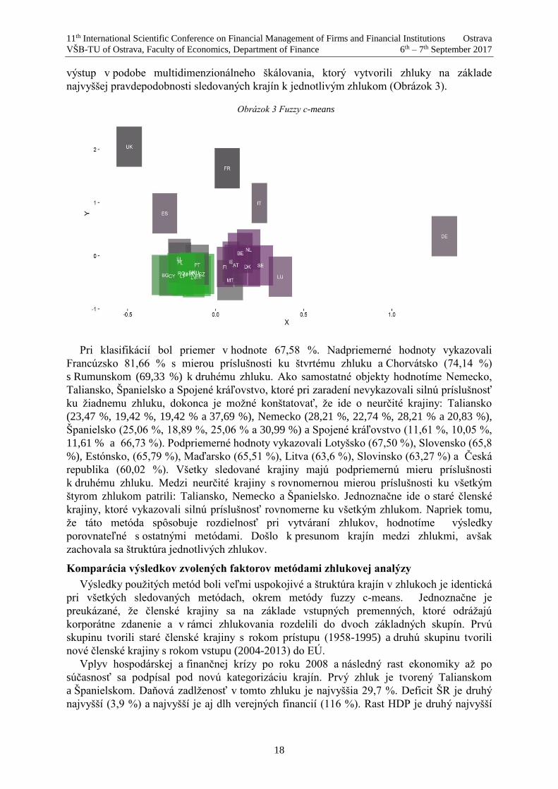
výstup v podobe multidimenzionálneho škálovania, ktorý vytvorili zhluky na základe
najvyššej pravdepodobnosti sledovaných krajín k jednotlivým zhlukom (Obrázok 3).
Obrázok 3 Fuzzy c-means
Pri klasifikácií bol priemer v hodnote 67,58 %. Nadpriemerné hodnoty vykazovali
Francúzsko 81,66 % s mierou príslušnosti ku štvrtému zhluku a Chorvátsko (74,14 %)
s Rumunskom (69,33 %) k druhému zhluku. Ako samostatné objekty hodnotíme Nemecko,
Taliansko, Španielsko a Spojené kráľovstvo, ktoré pri zaradení nevykazovali silnú príslušnosť
ku žiadnemu zhluku, dokonca je možné konštatovať, že ide o neurčité krajiny: Taliansko
(23,47 %, 19,42 %, 19,42 % a 37,69 %), Nemecko (28,21 %, 22,74 %, 28,21 % a 20,83 %),
Španielsko (25,06 %, 18,89 %, 25,06 % a 30,99 %) a Spojené kráľovstvo (11,61 %, 10,05 %,
11,61 % a 66,73 %). Podpriemerné hodnoty vykazovali Lotyšsko (67,50 %), Slovensko (65,8
%), Estónsko, (65,79 %), Maďarsko (65,51 %), Litva (63,6 %), Slovinsko (63,27 %) a Česká
republika (60,02 %). Všetky sledované krajiny majú podpriemernú mieru príslušnosti
k druhému zhluku. Medzi neurčité krajiny s rovnomernou mierou príslušnosti ku všetkým
štyrom zhlukom patrili: Taliansko, Nemecko a Španielsko. Jednoznačne ide o staré členské
krajiny, ktoré vykazovali silnú príslušnosť rovnomerne ku všetkým zhlukom. Napriek tomu,
že táto metóda spôsobuje rozdielnosť pri vytváraní zhlukov, hodnotíme výsledky
porovnateľné s ostatnými metódami. Došlo k presunom krajín medzi zhlukmi, avšak
zachovala sa štruktúra jednotlivých zhlukov.
Komparácia výsledkov zvolených faktorov metódami zhlukovej analýzy
Výsledky použitých metód boli veľmi uspokojivé a štruktúra krajín v zhlukoch je identická
pri všetkých sledovaných metódach, okrem metódy fuzzy c-means. Jednoznačne je
preukázané, že členské krajiny sa na základe vstupných premenných, ktoré odrážajú
korporátne zdanenie a v rámci zhlukovania rozdelili do dvoch základných skupín. Prvú
skupinu tvorili staré členské krajiny s rokom prístupu (1958-1995) a druhú skupinu tvorili
nové členské krajiny s rokom vstupu (2004-2013) do EÚ.
Vplyv hospodárskej a finančnej krízy po roku 2008 a následný rast ekonomiky až po
súčasnosť sa podpísal pod novú kategorizáciu krajín. Prvý zhluk je tvorený Talianskom
a Španielskom. Daňová zadlženosť v tomto zhluku je najvyššia 29,7 %. Deficit ŠR je druhý
najvyšší (3,9 %) a najvyšší je aj dlh verejných financií (116 %). Rast HDP je druhý najvyšší

11th International Scientific Conference on Financial Management of Firms and Financial Institutions Ostrava
VŠB-TU of Ostrava, Faculty of Economics, Department of Finance 6th – 7th September 2017
19
vo výške 2 %. Sledované krajiny sú si geograficky ale aj ekonomicky blízke, čomu
nasvedčujú podobné makroekonomické ukazovatele. Druhý zhluk v sledovanom období bol
tvorený Francúzskom a Spojeným kráľovstvom. Daňové zaťaženie bolo na úrovni 26,67 %,
deficit ŠR bol najvyšší spomedzi všetkých sledovaných zhlukov, na úrovní 4 %. Najvyšší bol
aj dlh verejných financií vo výške 92,5 %. Rast HDP bol na úrovni 1,8 %. Francúzsko
zaznamenalo stabilný rast ekonomiky, ktorý odštartovala rastúca domáca spotreba.
Problémom bol zahraničný obchod, ktorý brzdil ekonomickú aktivitu a to najmä zníženým
vývozom. V súčasnosti Britská ekonomika je druhou najväčšou ekonomikou po Nemecku a
najvýznamnejšou obchodnou veľmocou. Ekonomika Veľkej Británie zaznamenala a
posledných osem rokoch medziročný nárast v priemere o takmer 2,6 % (priemer EÚ je 2,3 %).
Tento rast je podporený najmä priemyselnou výrobou. Tretí zhluk je tvorený Nemeckom.
Výška daňového zaťaženia v tomto zhluku je 29,65 %. Nemecko hospodárilo s prebytkom vo
výške 0,7 % a celkový dlh verejných financií bol na úrovni 71,2 %. Miera inflácie je podobná
ako v predchádzajúcom zhluku, na úrovni 0,1 %. Nemecká ekonomika je najväčšou
ekonomikou v Európe a štvrtou najväčšou vo svete. Nemecká ekonomika v roku 2015 rástla
najrýchlejšie za posledné štyri roky a posilnila o 1,7 %, najvyšší podiel na tomto ukazovateli
mala súkromná spotreba. Spotrebu domácnosti podporil hlavne rast miezd a nízka inflácia 0,1
%. Rast hospodárstva priniesol do rozpočtu aj vyššie príjmy z daní, ktoré tvorili 1 153 mil. €.
Posledný štvrtý zhluk je tvorený mixom starých a nových členských krajín. Daňové zaťaženie
v tomto zhluku vyjadruje najnižšiu mieru vo výške 20,90 %. Najnižší je aj ukazovateľ
verejného dlhu na úrovni 67,1 % a deficit ŠR (1,9 %). Podobne ako v prvom zhluku, aj v
tomto prípade ide o defláciu na úrovni 0,1 %. Ako pozitívum môžeme hodnotiť rast HDP,
ktorý je najvyšší s pomedzi všetkých sledovaných zhlukov (3,5 %). Najväčšou mierou sa na
tom podieľali Írsko (26,3 %), Malta (6,2 %), Česká republika (4,5 %), Poľsko (3,9 %),
Slovenská republika (3,8 %) a Bulharsko (3,6 %). Všetky ostatné krajiny boli podpriemerné.
Najnižšie daňové zaťaženie bolo v Bulharsku (10 %), Írsku a Cypre (12,5 %). Írsko,
Chorvátsko, Lotyšsko, Litva, Malta a Poľsko boli krajiny, u ktorých za sledované obdobie
nedošlo k zmene štatutárnej sadzby. Najvýraznejšia zmena v podobe zníženia sadzieb bola
v Bulharsku o (9,5 %), v Českej republike o (9,0 %), v Rakúsku o (9,0 %), Fínsku o (9,0 %),
Slovinsku o (8,0 %), Dánsku o (6,5 %), Švédsku, Estónsku a Grécku o (6 %). Na druhej strane
k zvýšeniu došlo na Slovensku o 3,0 % a v Maďarsku o 1,4 %. Výška celkového zaťaženia
verejných financií bola najvýraznejšia v Grécku (179,6 %), Portugalsku (129 %) a Írsku (93,8
%). Sledované krajiny prekročili limitované Maastrichtské kritéria (60 %). Lepšie vyhliadky
malo Írsko, ktoré v roku 2015 malo rast HDP vo výške 26,3 %. Na druhej strane najnižšie
zaťaženie verejných financií bolo v Estónsku (9,7 %) a v Bulharsku (26,7 %). Naopak, vlády
sa zasadzovali za nízke sadzby priamych daní, čím podporili rozvoj podnikateľskej sféry,
zvýšili zamestnanosť a celkovú kúpyschopnosť obyvateľstva. Najvyššie daňové príjmy získali
krajiny Belgicko 195 mil. €, Dánsko 128 mil. €, Holandsko 254 mil. €, Rakúsko 146 mil. €
a Švédsko 195 mil. €. Vo všetkých sledovaných krajinách sa výška sadzieb pohybovala od 22
% do 25 %, okrem Belgicka, kde bola výška 33,99 %. Na druhej strane najnižšie daňové
príjmy boli v Lotyšsku 966 tis. €, v Slovinsku 14 mil. €, na Cypre 9 mil. €, v Litve a v
Chorvátsku 2 mil. €. Daňová sadzba v sledovaných krajinách bolo od 12,5 % do 17 %.
Posledný štvrtý zhluk hodnotíme s najnižším daňovým, ale aj verejným zaťažením
a najvyššou mierou rastu HDP. Záverom môžeme skonštatovať, že rozloženosť krajín na
základe makroekonomických ukazovateľov bola jednoznačná. Ako uvádza Clausing (2011),
nízke daňové sadzby a celkové daňové zaťaženie zatraktívňuje podnikanie a aj investovanie,
čím dochádza ku vzniku konkurenčnej výhody pre spoločnosti v uvedených krajinách. Podľa
Teathera (2005) fungujúca daňová konkurencia medzi jednotlivými krajinami je postavená na
veľmi jednoduchých základných princípoch. Existencia daňovej konkurencie prináša dva

11th International Scientific Conference on Financial Management of Firms and Financial Institutions Ostrava
VŠB-TU of Ostrava, Faculty of Economics, Department of Finance 6th – 7th September 2017
20
základné efekty pre daňové systémy jednotlivých krajín. Ak si môžu krajiny medzi sebou
navzájom daňovo konkurovať, bude prvým dôsledkom zníženie daňových sadzieb, čím
krajiny prilákajú zahraničný kapitál z ostatných krajín. Druhý efekt je, že ostatné krajiny budú
nútené reformovať svoje daňové systémy a snažiť sa znižovať daňové sadzby, aby získali
kapitál späť. Práve tieto efekty aj podľa našej analýzy zabezpečili najvyššiu
konkurencieschopnosť, ktorú majú krajiny v zhluku, ktorý bol tvorený mixom starých
a nových členských krajín, kde rozhodujúcu početnosť mali nové členské krajiny. Na základe
zhlukovej analýzy bolo preukázané, že členské krajiny sa z pohľadu daňového zaťaženia a z
pohľadu ostatných makroekonomických faktorov rozdelili na nové a staré členské štáty.
2. Záver
Analýzou sa tak preukázalo, že napriek pokračujúcej integrácii v rámci EÚ a snahám
o harmonizáciu daňových systémov, stále pretrvávajú významné diferencie medzi vybranými
krajinami. Rozdiely sú významné najmä v úrovni nominálneho a efektívneho zdanenia
korporácií, ktoré v sebe agreguje rozdielnosť aj v oblasti ekonomickej vyspelosti krajín a ich
fiškálneho hospodárenia. Analýza poukázala zároveň na významné rozdiely medzi starými
a novými členskými krajinami. Štvrtý zhluk krajín je tvorený novými pristupujúcimi krajinami
(s dátumom prístupu 2004–2013). Z pohľadu zdaňovania korporácií sú divergentné voči
krajinám v zhlukoch 1, 2 a 3. V týchto zhlukoch sú zakladajúce, pôvodné a staršie krajiny (s
dátumom prístupu 1957-2003). Úroveň efektívneho zdanenia korporácií medzi týmito dvoma
skupinami dosahuje rozdiel v intervale 3,8 %–10,5 %. Kým krajiny zhlukov 1, 2 a 3 možno
považovať za daňovo najmenej príťažlivé, krajiny v zhluku 4 sú pre daňových poplatníkov
z pohľadu daňovej konkurencie zaujímavejšie.
References
[1] Barro, R. J. (1979). On the determination of the public debt. The Journal of Political
Economy, 940-971.
[2] Clausing, K. A. (2007). In search of corporate tax incidence. Tax Law Review, 65, 433-
472.
[3] CumminS, J. G. and Hubbard, R. G. (1995). The tax sensitivity of foreing direct
investment: Evidence from firm level panel data. In FELDSTEIN, M. (ed.) The Effects
of Taxationon Multinational Corpotrations.Chicago : University of Chicago Press, 123-
147.
[4] Devereux, M. P., Griffith, R. and Klemm, A. (2002). Corporate income tax reforms and
international tax competition, Economic Policy, 17, 451-495.
[5] Ferreira, L. and HitchcocK, D.B. (2009). A comparison of hierarchical methods for
clustering functional data. Communications in Statistics - Simulation and Computation,
38(9), 1925-1949.
[6] Griffith, R. a Klemm, A. (2004). What has been the tax competition experience of the
last 20 years? The institute for Fiscal Studies. WP04/05.
[7] Halkidi, M., Batistakis, Y. and Vazirgiannis, M. (2001). On clustering validation
techniques. Journal of intelligent information systems, 17(2), 107-145.
[8] Charrad, M., Ghazzali, N., Boiteau, V. a Niknafs, A. (2012). NbClust Package: finding
the relevant number of clusters in a dataset. UseR! 2012.
11th International Scientific Conference on Financial Management of Firms and Financial Institutions Ostrava
VŠB-TU of Ostrava, Faculty of Economics, Department of Finance 6th – 7th September 2017
21
[9] Kubátová, K. (2008). Analýza daňové konkurenceschopnosti u daně z příjmu korporací
v EU [online]. Available at: http://kvf.vse.cz/storage/1239724949_sb_kubatova.pdf
[Accessed 2 July 2017].
[10] Salin, P. (1998). Harmful Tax Competition: An Emerging Global Issue. OECD
Publications, 2, rue Andr´e-Pascal, 75775 Paris Cedex 16. Printed in France.
[11] Sinn, H. W. (1990). Tax harmonization and tax competition in Europe. European
Economic Review, 34(2-3), 489-504.
[12] Stiglitz, J.E. a Rosengard, J.K. (2015). Economic of the Public Sector. W.W. Norton &
Company, 923.
[13] Široký, J. (2012). Daně v Evropské unii: daňové systémy všech 27 členských států EU a
Chorvatska, legislativní základy daňové harmonizace včetně judikátů SD, odraz
ekonomické krize v daňové politice EU. 400.
[14] Teather, E. K. (Ed.). (2005). Embodied geographies. Routledge.
[15] Tiebout, CH. (1956). A Pure Theory of Local Expenditures. The Journal of Political
Economy, 64(5), 416-424.
[16] Wilson, J. (1999). Theories of tax competition. National Tax Journal, 52, 269-304.
11th International Scientific Conference on Financial Management of Firms and Financial Institutions Ostrava
VŠB-TU of Ostrava, Faculty of Economics, Department of Finance 6th – 7th September 2017
22
The gray GM(1,1) model applications in time series analysis - selected issues
Stanisław Barczak1
Abstract
This article will present selected models related to time series analysis. Those are ARMA
model, Grey Model GM(1,1), Grey Model RGM(1,1) and the Holt’s mechanic model. The
purpose of this article is to point out practical aspects of time series models usage under
incomplete information conditions – ultra-short history of the process. Additionally, processes
identification problem has been considered for the so-called levels and differences in case of
ultra-short time series – four observations. The considerations are made on the example of
investment gold price in USD for one troy ounce.
Key words
Econometrics, Time Series, Grey Models, Grey Informations, Grey Systems
JEL Classification: C1, C2, C32, C44
1. Introduction
The elemental econometrical model, considered in the grey system theory, is the so-called
grey NGM ,1 2 model. The essence of grey modeling is the use of very short time series. The
assumption of a short time series alone presents the essence and the purpose of grey modeling
– a modeling under incomplete information conditions.
Two targets have been set in consideration included in the article I) the problem of time
series non-stationarity for new processes – subjective process qualification for trend-
stationary or incremental-stationary groups under ultra-short time series conditions, II)
estimation of forecasts obtained by selected methods of time series analysis with forecasts
obtained by the 1,1GM model, by the prism of ex post errors in forecasts and under
conditions of misidentification of process evolution [1],[2],[3].
Two hypothesis have been put forward in the considerations: I) First realizations of a new
process (ultra-short time series) do not directly determine its trend-stationary or incremental-
stationary nature which allows using grey models for any process at the earliest stages of its
evolution irrespective of its nature, II) GM(1,1), model usage, for short time series gives a
line/row of magnitude of ex post errors, comparable to the classical methods used in time
series analysis and classical forecast theory for long time series.
In the subject literature, the form of the gray GM(1,1) model is often under considerations
with some of its modifications. Its basic modifications include: discretization of the model for
discrete variables, model residues modification using Fourier transform and “S” shaped
processes modeling by the grey Verhulst model prism [2]. In time series analysis GM(1,1)
model is applied to the process of specifying the autoregressive AR(p) models and the wide
range of variants of the GARCH class.
1Stanisław Barczak, PhD, The Univercity of Economics in Katowice,
[email protected] 2 NGM ,1 – Grey Model, where: 1 – first-order differential equation , N - a number of explanatory
variables.

11th International Scientific Conference on Financial Management of Firms and Financial Institutions Ostrava
VŠB-TU of Ostrava, Faculty of Economics, Department of Finance 6th – 7th September 2017
23
The article will present selected methods of time series analysis and forecast theory against
the grey GM(1,1) model using real empirical data – gold rating in USD3 for one troy ounce4.
2. ARMA(p,q) process vs GM(1,1) model
In both the classic econometric forecasting theory and the time series analysis, time series
with a relatively large number of observations are modeled. The situation changes radically
when using grey models, where the number of observations used is extremely low. A natural
conclusion comes to light. Time series models and models derived from classical forecasting
theories are built for processes whose history / evolution is observed over an extended period
of time. It can, therefore, be assumed that the portion of the information required for their
specification, estimation, and validation is satisfactory [10]. Although there are certain
exogenous variables that influence the process under investigation but are not quantified or
there is no certainty as to their significant effect on the endogenous / predicted variable. It
seems natural then that to shorten the time series / process history is to lose a large portion of
information. If we assume that the process under consideration is a new process without a
sufficiently long history, then the use of classical time series analysis methods and classical
forecasting theories is questionable. The solution to the problem may be the search for a
similar process whose evolution is well known. An alternative to this approach may be the use
of grey models, the essence of which is the description and prediction of the process under
extreme information deficit conditions. This approach is not without flaws and questions.
The classical time series formula qpARMA , , given the following formula, will be
considered first [11], [7]:
p
i
q
i
itititit yy1 1
0 (1)
where: t - white noise process, p - a positive integer representing the autoregressive
pAR process delay order, q - a positive integer representing the qMA moving average
delay order.
By using the pB backshift operator, the ARMA (p,q) model can be represented as:
t
q
qt
p
p BByBB 101 11 (2)
where: pt
p yB - backshift operator, p
pBB 11 - polynomial of the
autoregressive pAR model part, q
qBB 11 - polynomial of the moving average
qMA model part.
qpARMA , process identification directly relates to the observation of the ACF
autocorrelation function in the case of the moving average part and the PACF partial
autocorrelation function in the case of an autoregressive part. Deciding to identify model
delays requires simultaneous observation of ACF and PACF functions. In addition, it is
important to evaluate the existence of unitary elements of a characteristic polynomial model.
Their existence means non-stationarity of the process and the necessity of constructing the
model for the difference of the predicted variable: an integrated process of the order d :
qdpARIMA ,, .
Example 1 qpARMA , Model
Consider the daily gold prices per ounce in the 2014-01-02 to 2014-04-24 period.
3 http://www.mennicawroclawska.pl/Ceny-Zlota-cinfo-pol-47.html 4 Troy ounce – designation: „oz” or „t oz”. conversion: 1oz=31,1035 gram.

11th International Scientific Conference on Financial Management of Firms and Financial Institutions Ostrava
VŠB-TU of Ostrava, Faculty of Economics, Department of Finance 6th – 7th September 2017
24
The pricing process is shown in Figure 1.
Figure 1: Gold prices in USD for 1 troy ounce in the 2014-01-02 to 2014-04-24 period
ACF autocorrelation functions and PACF partial autocorrelation are shown in Figure 2.
Additionally, it is assumed that the number of observed delays is :
448,4)88ln()ln( Tm , where: T - the number of observations in a time series.
Figure 2: ACF and PACF functions for gold prices
As shown in Figure 1, PACF partial autocorrelation is only relevant for the first delay,
which may wrongly suggest the autoregression process of the first order AR (p). This
conclusion is entirely wrong if the results obtained for the ACF autocorrelation function are
taken into account, which for all four considered delays is statistically significant.
Additionally, the confirmation itself is the result of the estimation given in the form:
0235,0 5771,29
9688,029,1279 1 ttt yy
Assuming a 5% significance level, all model parameters are statistically significant. The
stationary condition of the process is completed such that: 19688,01 . It is well known
from research practice that price processes, including ore prices, are integrated processes. As
it might be seen, the value of a 1 parameter for a module is very close to unity, which may
indicate that the process is cumulative. Running an ADF test for daily gold prices from 2014-
01-02 to 2014-04-24 confirms the validity of the decision on non-stationarity occurrence. As a
result of the ADF test [6] test statistic has been obtained: 7303,0t . Assuming a 5%
significance level and comparing it with a 445,0p value decision is made that there is no
reason to reject the null hypothesis, which states the integration of the first degree:
)1(~: IyH to . Consider, for the sake of simplicity, that further integration orders are not
considered. Consistent with the above, in the first-order integration the essence of the problem
1 200,00
1 250,00
1 300,00
1 350,00
1 400,00
201
4.0
1.0
22
01
4.0
1.0
72
01
4.0
1.1
22
01
4.0
1.1
72
01
4.0
1.2
22
01
4.0
1.2
72
01
4.0
2.0
12
01
4.0
2.0
62
01
4.0
2.1
12
01
4.0
2.1
62
01
4.0
2.2
12
01
4.0
2.2
62
01
4.0
3.0
32
01
4.0
3.0
82
01
4.0
3.1
32
01
4.0
3.1
82
01
4.0
3.2
32
01
4.0
3.2
82
01
4.0
4.0
22
01
4.0
4.0
72
01
4.0
4.1
22
01
4.0
4.1
72
01
4.0
4.2
2
US
D/1
oz
t
-1
-0.5
0
0.5
1
0 1 2 3 4 5
lag
ACF for CENA_ZLOTO
+- 1.96/T^0.5
-1
-0.5
0
0.5
1
0 1 2 3 4 5
lag
PACF for CENA_ZLOTO
+- 1.96/T^0.5
11th International Scientific Conference on Financial Management of Firms and Financial Institutions Ostrava
VŠB-TU of Ostrava, Faculty of Economics, Department of Finance 6th – 7th September 2017
25
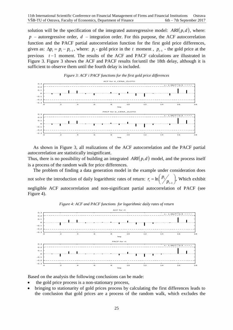
solution will be the specification of the integrated autoregressive model: dpARI , , where:
p – autoregressive order, d – integration order. For this purpose, the ACF autocorrelation
function and the PACF partial autocorrelation function for the first gold price differences,
given as: 1 ttt ppp , where: tp - gold price in the t moment , 1tp - the gold price at the
previous 1t moment. The results of the ACF and PACF calculations are illustrated in
Figure 3. Figure 3 shows the ACF and PACF results for/until the 18th delay, although it is
sufficient to observe them until the fourth delay is included.
Figure 3: ACF i PACF functions for the first gold price differences
As shown in Figure 3, all realizations of the ACF autocorrelation and the PACF partial
autocorrelation are statistically insignificant.
Thus, there is no possibility of building an integrated dpARI , model, and the process itself
is a process of the random walk for price differences.
The problem of finding a data generation model in the example under consideration does
not solve the introduction of daily logarithmic rates of return:
1
lnt
tt p
pr , Which exhibit
negligible ACF autocorrelation and non-significant partial autocorrelation of PACF (see
Figure 4).
Figure 4: ACF and PACF functions for logarithmic daily rates of return
Based on the analysis the following conclusions can be made:
the gold price process is a non-stationary process,
bringing to stationarity of gold prices process by calculating the first differences leads to
the conclusion that gold prices are a process of the random walk, which excludes the
-0.3
-0.2
-0.1
0
0.1
0.2
0.3
0 2 4 6 8 10 12 14 16 18
lag
ACF for d_CENA_ZLOTO
+- 1.96/T^0.5
-0.3
-0.2
-0.1
0
0.1
0.2
0.3
0 2 4 6 8 10 12 14 16 18
lag
PACF for d_CENA_ZLOTO
+- 1.96/T^0.5
-0.3
-0.2
-0.1
0
0.1
0.2
0.3
0 2 4 6 8 10 12 14 16 18
lag
ACF for rt
+- 1.96/T^0.5
-0.3
-0.2
-0.1
0
0.1
0.2
0.3
0 2 4 6 8 10 12 14 16 18
lag
PACF for rt
+- 1.96/T^0.5

11th International Scientific Conference on Financial Management of Firms and Financial Institutions Ostrava
VŠB-TU of Ostrava, Faculty of Economics, Department of Finance 6th – 7th September 2017
26
construction of the class qpARMA , . The random walk mechanic allows to simulate the
trajectory of the price at the set initial values,
bringing to stationarity of gold prices process by the use of logarithmic transformation
(logarithmic daily rates of return) leads to the conclusion that they are a purely random
process, and thus the construction of a class qpARMA , model is impossible.
An alternative approach to the problem of gold price modeling is the use of a gray model
for ultra-short time series. Grey 1,1GM is given as a heterogeneous first-order differential
equation and expressed in the following formula [8]:
baxdt
dx 1
1
, 0b (3)
where: a ,b - parameters of the equation.
Assuming that: nxxxX 0000 ,,2,1 - is a line-by-line implementation of the
predicted 0X variable. Continuing that: nxxxX 1111 ,,2,1 - is a line vector that
arose from the AGO5 procedure. Thus, the basic form of the gray model is given by the
following formula [8]:
bkazkx 10 (4)
where: nzzzZ 1111 ,,2,1 is a series of moving averages designated for a 1X
variable and given as:
12
1 111 kxkxkz for nk ,,1 (5)
Structural parameters a ,b of the model (2) are estimated by the least squares method:
YB'BB'a1
ˆ (6)
where:
nx
x
x
0
0
0
3
2
Y ,
1
13
12
1
1
1
nz
z
z
B (7)
Time response equation is given as [8]:
a
be
a
bXkX ak
11ˆ 01 for 0a , nk ,,2,1 (8)
The theoretical values of the model are derived from the following equation [8]:
aka ea
bxekxkxkxkx
11ˆ1ˆ1ˆ1ˆ 011110 (9)
5 AGO – Accumulating Generation Operator.

11th International Scientific Conference on Financial Management of Firms and Financial Institutions Ostrava
VŠB-TU of Ostrava, Faculty of Economics, Department of Finance 6th – 7th September 2017
27
for 0a , nk ,,2,1
The following possibilities of the grey 1,1GM model should be included to its advantages:
modeling of short time series (maximum of four realizations) - incomplete information
about the process - new processes,
construction of short-term forecasts, in the case of construction of which it is assumed that
there are changes in the forecast of the only quantitative variable,
smoothing time series,
using the gray model as a tool to support time series analysis based on classic models such
as ARMA and GARCH models..
The limitations of the gray 1,1GM model include:
the model can be used only for a time series consisting of the positive effects of the
predicted variable,
due to the use of very short time series, it is not possible to analyze the stochastic structure
of the model – evaluation of the formal fulfillment of assumptions about the random t
component, in relation to the least squares method.
the use of short time series makes it impossible to assess the quality of a model by using
classical measures such as the determination coefficient, the coefficient of random
variation.
assuming that the observed process is a new process represented by a short time series, it
is impossible to evaluate the considered process for its stationary or non-stationary.
Example 2 Basic 1,1GM model
The time series considered will still be the daily gold prices per ounce in the period: 2014-
01-02 to 2014-01-07 used in Example 1. In the case of the gray 1,1GM model, a length of
time series consisting of four observations ( 4T ) has been adopted a priori . Only prices not
rates of return will be modelised. There are two reasons for this approach: i) Calculating daily
rates of return will result in a loss of four to three-time series, ii) grey 1,1GM model requires
that the time series realizations be positive, which in a broader context of analyze using the
gray model with the rate of return is not guaranteed. For estimating the fit of the model to the
actual data, the average relative percentage error of the expired forecasts was used - MAPE,
given in the following formula:
t
t
xmMAPE 100
ˆ
10
(10)
where: m - pair’s number: actual value 0x and theoretical value 0x̂ , t - forecast
verification period, 00 x̂xt .
The basic grey 1,1GM model will be estimated based on time series from 2014-01-02 to
2014-01-07. Additionally, it was assumed that the forecast verification period is the period
from 2014-01-03 to 2014-01-07. Thus, the theoretical implementation of the MAPE error of
2014-01-02 was omitted. This is due to the fact that the first theoretical implementation of the
gray model is always equal to the first real implementation: 00 x̂x . So its inclusion would
underestimate the falsehood of the forecast.
The gray 1,1GM model obtained by the least squares estimation can be written as a
differential equation as:
11th International Scientific Conference on Financial Management of Firms and Financial Institutions Ostrava
VŠB-TU of Ostrava, Faculty of Economics, Department of Finance 6th – 7th September 2017
28
1,1214006,0 1
1
xdt
dx
The equation of theoretical values is given by the following formula:
kexekx 006,00006,00
)006,0(
1,1214111ˆ
, for nk ,...,2,1
In the example under discussion, the MAPE forecast error is 0.24% and can be assumed in
the ex post sense as too low. Further analysis of the model in terms of stochastic structure and
model quality is impossible due to the low number of observations. The only measure that
characterizes model quality is an acceptable level of arbitrary ex-post error of expired
forecasts. In applications of gray 1,1GM models it should be remembered that the increasing
the number of executions in a time series results in an increase of forecast error [1], [3]. The
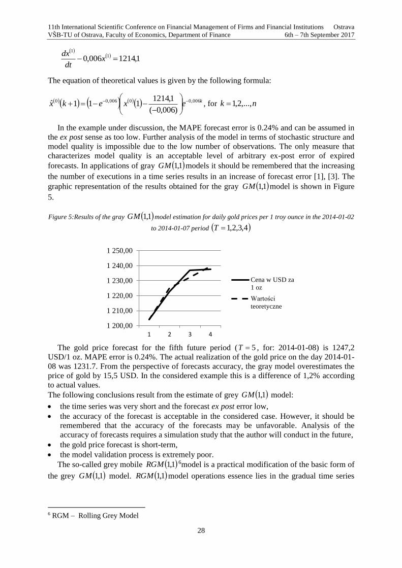
graphic representation of the results obtained for the gray 1,1GM model is shown in Figure
5.
Figure 5:Results of the gray 1,1GM model estimation for daily gold prices per 1 troy ounce in the 2014-01-02
to 2014-01-07 period 4,3,2,1T
The gold price forecast for the fifth future period ( 5T , for: 2014-01-08) is 1247,2
USD/1 oz. MAPE error is 0.24%. The actual realization of the gold price on the day 2014-01-
08 was 1231.7. From the perspective of forecasts accuracy, the gray model overestimates the
price of gold by 15,5 USD. In the considered example this is a difference of 1,2% according
to actual values.
The following conclusions result from the estimate of grey 1,1GM model:
the time series was very short and the forecast ex post error low,
the accuracy of the forecast is acceptable in the considered case. However, it should be
remembered that the accuracy of the forecasts may be unfavorable. Analysis of the
accuracy of forecasts requires a simulation study that the author will conduct in the future,
the gold price forecast is short-term,
the model validation process is extremely poor.
The so-called grey mobile 1,1RGM 6model is a practical modification of the basic form of
the grey 1,1GM model. 1,1RGM model operations essence lies in the gradual time series
6 RGM – Rolling Grey Model
1 200,00
1 210,00
1 220,00
1 230,00
1 240,00
1 250,00
1 2 3 4
Cena w USD za
1 oz
Wartości
teoretyczne
11th International Scientific Conference on Financial Management of Firms and Financial Institutions Ostrava
VŠB-TU of Ostrava, Faculty of Economics, Department of Finance 6th – 7th September 2017
29
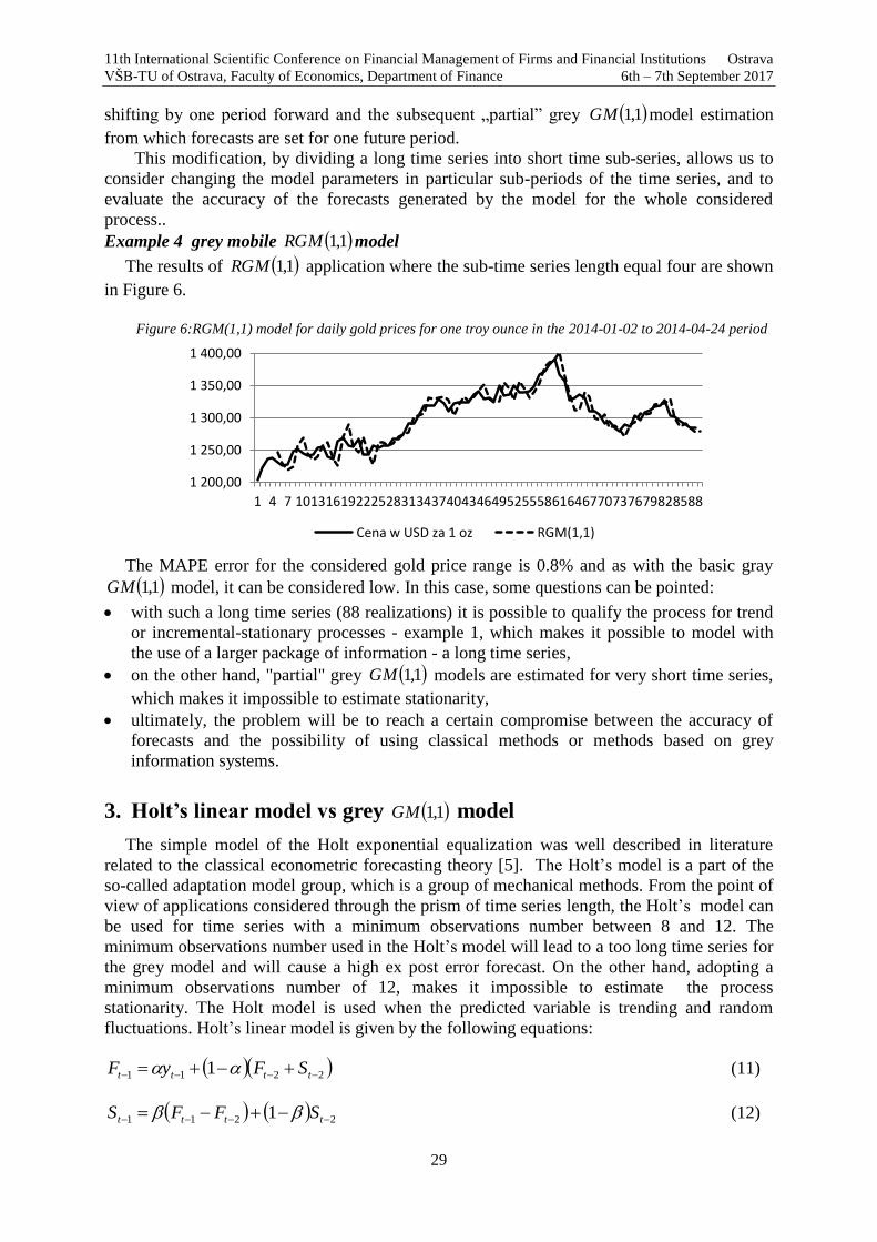
shifting by one period forward and the subsequent „partial” grey 1,1GM model estimation
from which forecasts are set for one future period.
This modification, by dividing a long time series into short time sub-series, allows us to
consider changing the model parameters in particular sub-periods of the time series, and to
evaluate the accuracy of the forecasts generated by the model for the whole considered
process..
Example 4 grey mobile 1,1RGM model
The results of 1,1RGM application where the sub-time series length equal four are shown
in Figure 6.
Figure 6:RGM(1,1) model for daily gold prices for one troy ounce in the 2014-01-02 to 2014-04-24 period
The MAPE error for the considered gold price range is 0.8% and as with the basic gray
1,1GM model, it can be considered low. In this case, some questions can be pointed:
with such a long time series (88 realizations) it is possible to qualify the process for trend
or incremental-stationary processes - example 1, which makes it possible to model with
the use of a larger package of information - a long time series,
on the other hand, "partial" grey 1,1GM models are estimated for very short time series,
which makes it impossible to estimate stationarity,
ultimately, the problem will be to reach a certain compromise between the accuracy of
forecasts and the possibility of using classical methods or methods based on grey
information systems.
3. Holt’s linear model vs grey 1,1GM model
The simple model of the Holt exponential equalization was well described in literature
related to the classical econometric forecasting theory [5]. The Holt’s model is a part of the
so-called adaptation model group, which is a group of mechanical methods. From the point of
view of applications considered through the prism of time series length, the Holt’s model can
be used for time series with a minimum observations number between 8 and 12. The
minimum observations number used in the Holt’s model will lead to a too long time series for
the grey model and will cause a high ex post error forecast. On the other hand, adopting a
minimum observations number of 12, makes it impossible to estimate the process
stationarity. The Holt model is used when the predicted variable is trending and random
fluctuations. Holt’s linear model is given by the following equations:
2211 1 tttt SFyF (11)
2211 1 tttt SFFS (12)
1 200,00
1 250,00
1 300,00
1 350,00
1 400,00
1 4 7 101316192225283134374043464952555861646770737679828588
Cena w USD za 1 oz RGM(1,1)
11th International Scientific Conference on Financial Management of Firms and Financial Institutions Ostrava
VŠB-TU of Ostrava, Faculty of Economics, Department of Finance 6th – 7th September 2017
30
where: tF - trend estimation in a t moment, tS - smoothed value evaluation of the trend
increase in a t period , , - smoothing parameters taking values from the range: 10
and 10 , ty - the realization of the predicted variable in a t moment.
Holt's linear model equation is given by the following formula:
nnt SntFy * , nt (13)
where: nt - time advance, *
ty - theoretical implementation of the model in a t moment.
The initial values for the simulation are assumed to be at the level: 11 yF i 121 yyS .
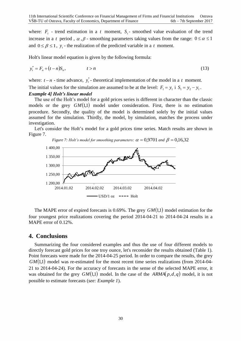
Example 4] Holt’s linear model
The use of the Holt’s model for a gold prices series is different in character than the classic
models or the grey 1,1GM model under consideration. First, there is no estimation
procedure. Secondly, the quality of the model is determined solely by the initial values
assumed for the simulation. Thirdly, the model, by simulation, matches the process under
investigation.
Let's consider the Holt’s model for a gold prices time series. Match results are shown in
Figure 7. Figure 7: Holt’s model for smoothing parameters: 9701,0 and 32,16,0
The MAPE error of expired forecasts is 0.69%. The grey 1,1GM model estimation for the
four youngest price realizations covering the period 2014-04-21 to 2014-04-24 results in a
MAPE error of 0.12%.
4. Conclusions
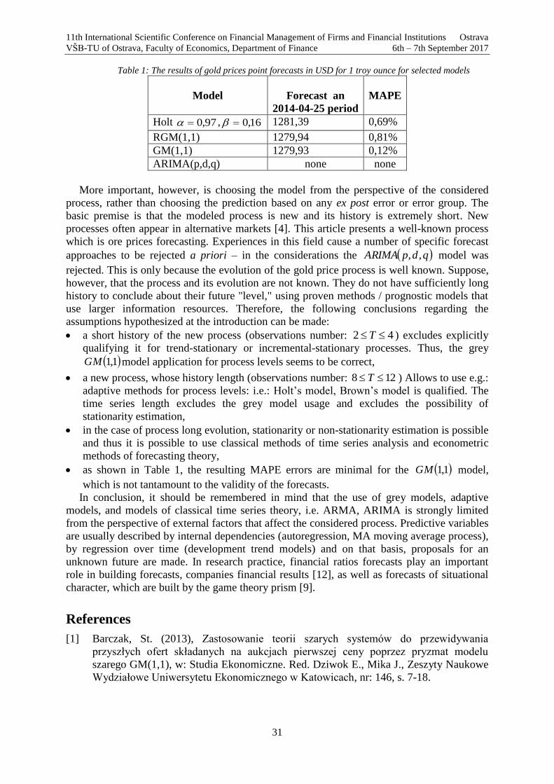
Summarizing the four considered examples and thus the use of four different models to
directly forecast gold prices for one troy ounce, let's reconsider the results obtained (Table 1).
Point forecasts were made for the 2014-04-25 period. In order to compare the results, the grey
1,1GM model was re-estimated for the most recent time series realizations (from 2014-04-
21 to 2014-04-24). For the accuracy of forecasts in the sense of the selected MAPE error, it
was obtained for the grey 1,1GM model. In the case of the qdpARMA ,, model, it is not
possible to estimate forecasts (see: Example 1).
1 200,00
1 250,00
1 300,00
1 350,00
1 400,00
2014.01.02 2014.02.02 2014.03.02 2014.04.02
USD/1 oz Holt
11th International Scientific Conference on Financial Management of Firms and Financial Institutions Ostrava
VŠB-TU of Ostrava, Faculty of Economics, Department of Finance 6th – 7th September 2017
31
Table 1: The results of gold prices point forecasts in USD for 1 troy ounce for selected models
Model
Forecast an
2014-04-25 period
MAPE
Holt 97,0 , 16,0 1281,39 0,69%
RGM(1,1) 1279,94 0,81%
GM(1,1) 1279,93 0,12%
ARIMA(p,d,q) none none
More important, however, is choosing the model from the perspective of the considered
process, rather than choosing the prediction based on any ex post error or error group. The
basic premise is that the modeled process is new and its history is extremely short. New
processes often appear in alternative markets [4]. This article presents a well-known process
which is ore prices forecasting. Experiences in this field cause a number of specific forecast
approaches to be rejected a priori – in the considerations the qdpARIMA ,, model was
rejected. This is only because the evolution of the gold price process is well known. Suppose,
however, that the process and its evolution are not known. They do not have sufficiently long
history to conclude about their future "level," using proven methods / prognostic models that
use larger information resources. Therefore, the following conclusions regarding the
assumptions hypothesized at the introduction can be made:
a short history of the new process (observations number: 42 T ) excludes explicitly
qualifying it for trend-stationary or incremental-stationary processes. Thus, the grey
1,1GM model application for process levels seems to be correct,
a new process, whose history length (observations number: 128 T ) Allows to use e.g.:
adaptive methods for process levels: i.e.: Holt’s model, Brown’s model is qualified. The
time series length excludes the grey model usage and excludes the possibility of
stationarity estimation,
in the case of process long evolution, stationarity or non-stationarity estimation is possible
and thus it is possible to use classical methods of time series analysis and econometric
methods of forecasting theory,
as shown in Table 1, the resulting MAPE errors are minimal for the 1,1GM model,
which is not tantamount to the validity of the forecasts.
In conclusion, it should be remembered in mind that the use of grey models, adaptive
models, and models of classical time series theory, i.e. ARMA, ARIMA is strongly limited
from the perspective of external factors that affect the considered process. Predictive variables
are usually described by internal dependencies (autoregression, MA moving average process),
by regression over time (development trend models) and on that basis, proposals for an
unknown future are made. In research practice, financial ratios forecasts play an important
role in building forecasts, companies financial results [12], as well as forecasts of situational
character, which are built by the game theory prism [9].
References
[1] Barczak, St. (2013), Zastosowanie teorii szarych systemów do przewidywania
przyszłych ofert składanych na aukcjach pierwszej ceny poprzez pryzmat modelu
szarego GM(1,1), w: Studia Ekonomiczne. Red. Dziwok E., Mika J., Zeszyty Naukowe
Wydziałowe Uniwersytetu Ekonomicznego w Katowicach, nr: 146, s. 7-18.

11th International Scientific Conference on Financial Management of Firms and Financial Institutions Ostrava
VŠB-TU of Ostrava, Faculty of Economics, Department of Finance 6th – 7th September 2017
32
[2] Barczak, St. (2013), Zastosowania modeli szarych do prognozowania procesów S
kształtnych na przykładzie prognozy na rok akademicki 2011/2012 liczby studentów
wszystkich typów studiów w Polsce, w: Zastosowanie metod ilościowych w
zarządzaniu ryzykiem w działalności inwestycyjnej, red. Barczak A. St., Tworek P.,
Wydawnictwo Uniwersytetu Ekonomicznego w Katowicach, Katowice, s. 482-496.
[3] Barczak St. (2014), Applications of Grey Models in the Analysis of Financial Time
Series. The FOREX Market Example, w: Proceedings of the 11th International
Scientific Conference. European Financial Systems 2014, red. O. Deev, V. Ksjurova &
J. Krajicek Masaryk University, Brno, s. 26-34
[4] Borowski K. (2011), Teoria i praktyka Bechmarków, Wyd. Difin, Warszawa
[5] Dittmann, P. (2003), Prognozowanie w przedsiębiorstwie. metody, zastosowania, Wyd.
Oficyna Ekonomiczna, Kraków
[6] Kufel T. (2004), Ekonometria. Rozwiązywanie problemów z wykorzystaniem programu
Gretl, PWN, Warszawa
[7] Lutkepohl, H., Kratzig, M. (2004), Applied Time Series Econometrics. Wyd.
Cambridge University Press, Cambridge
[8] Sifeng, L., Yi, L. (2010), Grey Information. Theory and Practical Applications. Wyd.
Springer-Verlag, London.
[9] Sroczyńska-Baron, A. (2013), The choice of portfolio based on the theory of
cooperative games, w: European Financial Systems 2013, red. O. Deev, V. Ksjurova &
J. Krajicek, Proceedings of the 10th International Scientific Conference Brno: Masaryk
University, s.305-311
[10] Starzeński O. (2006), Elementy analizy rynków finansowych, Wyd. Górnośląska
Wyższa Szkoła Handlowa im. Wojciecha Korfantego, Katowice
[11] Tsay R.S. (2010), Analysis of Financial Time Series, wyd. 3 zm., Wyd. John Wiley &
Sons, New Jersey
[12] Węgrzyn, T. (2013), Stock selection on the warsaw stock exchange financial ratios or
profitability ratios. analysis between 2001 and 2011, w: The 7th International Days of
Statistics and Economics, red. T. Löster & T. Pavelka, Conference Proceedings, Prague,
s. 1554-1564.
11th International Scientific Conference on Financial Management of Firms and Financial Institutions Ostrava
VŠB-TU of Ostrava, Faculty of Economics, Department of Finance 6th – 7th September 2017
33
Dividends as risk subject of taxation in Slovak republic
Anna Baštincová, Ján Benko1
Abstract
Dividends represent income distributed to natural persons and legal entities on the base of their
property rights in business entities. In Slovak legislation regarding to taxation of dividends,
several fundamental changes have been made in past taxable periods. Since 2017 dividends are
subject to income tax, but not subject to health insurance charges. Article deals with difficulties
of dividend taxation, which have been recognized in past particular taxable periods and are
distributed at present, factors and context to be respected to meet legislation. This article is
primarily about identification of benericiary of dividends, source of dividends, tax residency,
taxation and applicable tax rate, depending on period of dividends recognition.
Key words
dividends, taxation, natural persons, legal entities, business entity
JEL Classification: M41, H25
1. Úvod
Podiel na zisku sa nadobúda vkladom spoločníka do obchodnej spoločnosti a vyjadruje
mieru jeho účasti na čistom obchodnom imaní. Pri zdaňovaní podielov na zisku v SR
dochádzalo počas jednotlivých zdaňovacích období k viacerým zásadným zmenám. V tých
obdobiach, keď neboli podiely na zisku predmetom dane z príjmov, podliehali platbe
poistného na zdravotné poistenie. Pri zdaňovaní podielov na zisku, ktorý bol vytvorený v
rôznych zdaňovacích obdobiach a bude vyplácaný fyzickým a právnickým osobám po 1.
januári 2017, bude potrebné zohľadňovať veľa rôznych faktorov a súvislostí.
2. Vznik nároku na podiel na zisku v obchodnej spoločnosti
Podiely na zisku predstavujú príjmy, ktoré plynú fyzickým osobám a právnickým osobám
z ich majetkových práv v obchodnej spoločnosti. Majetkové právo znamená právo participácie
na výsledku hospodárenia, na vyrovnávacom podiele a na likvidačnom zostatku spoločnosti.
Výška podielu na zisku sa určuje pomerom vkladu spoločníka k základnému imaniu
spoločnosti. Právo na podiel na zisku vzniká rozhodnutím spoločníkov (akcionárov) o tom, že
vytvorený zisk po zdanení, t. j. čistý zisk, sa použije na rozdelenie vlastníkom.
V akciovej spoločnosti majú právo na podiel na zisku akcionári, členovia predstavenstva a
dozornej rady. U akcionára sa tento podiel (dividenda) určuje pomerom menovitej hodnoty
jeho akcií k menovitej hodnote akcií všetkých akcionárov (s výnimkou akcií s odlišným
nárokom na podiel na zisku vymedzených v stanovách). Podiel členov predstavenstva a
1 Prof. Ing. Anna Baštincová, CSc., Ekonomická univerzita v Bratislave, Fakulta hospodárskej
informatiky, Katedra účtovníctva a audítorstva, Ing. Ján Benko, interný doktorand Katedry
účtovníctva a audítorstva, Dolnozemská cesta 1, 852 35 Bratislava, e-mail: [email protected],

11th International Scientific Conference on Financial Management of Firms and Financial Institutions Ostrava
VŠB-TU of Ostrava, Faculty of Economics, Department of Finance 6th – 7th September 2017
34
členov dozornej rady na zisku (tantiemy) určuje valné zhromaždenie. Na rozdelení zisku sa
môžu v súlade so stanovami podieľať aj zamestnanci akciovej spoločnosti.
V spoločnosti s ručením obmedzeným má nárok na podiel na zisku spoločník. Výška
podielu jednotlivých spoločníkov sa určí v pomere zodpovedajúcom ich splateným vkladom.
V komanditnej spoločnosti základné imanie vytvárajú len vklady komanditistov,
komplementári nemajú vkladovú povinnosť. Zisk komanditnej spoločnosti sa delí na časť
pripadajúcu na komanditistov a časť pripadajúcu komplementárom pomerom, ktorý je
stanovený v spoločenskej zmluve.
Vo verejnej obchodnej spoločnosti majú spoločníci povinnosť splatiť vklady len v tom
prípade, ak sa k tomu zaviazali v spoločenskej zmluve. Zisk spoločnosti sa rozdeľuje medzi
spoločníkov v rovnakej výške bez ohľadu na výšku vkladov (ak spoločenská zmluva
nestanovuje inak).
Na podnikaní v obchodnej spoločnosti sa môže svojím vkladom podieľať aj tichý
spoločník, ktorý sa zmluvne zaväzuje, že poskytne určitý vklad; obchodná spoločnosť sa zase
zaväzuje, že bude tichému spoločníkovi vyplácať časť zisku z jeho podielu na výsledku
podnikania.
3. Zdaňovanie podielov na zisku v Slovenskej republike
Zákonná úprava zdanenia príjmov významným spôsobom zasahuje aj do zdanenia podielov
na zisku, t. j. príjmov, ktoré plynú fyzickým osobám a právnickým osobám z ich majetkových
práv v obchodných spoločnostiach (Vanková, 2017). Podiely zo ziskov vytvorených do roku
2003 boli predmetom dane z príjmov, v rokoch 2004-2016 sa podiely nezdaňovali daňou
z príjmov, ale podliehali platbám poistného na zdravotné poistenie (zdravotným odvodom);
od roku 2017 sú podiely na zisku znova predmetom dane z príjmov, ale súčasne boli zrušené
zdravotné odvody ako neštandardný nástroj, ktorý sa uplatňoval na tento druh príjmov v SR.
Všeobecný prehľad o zdaňovaní podielov zo ziskov vytvorených v rokoch 2003-2017 v SR
obsahuje tabuľka č. 1:
Tabuľka 1: Všeobecný prehľad o zdaňovaní podielov zo ziskov vytvorených v r.2003-2017 v SR
Podiely na zisku, ktorý bol vytvorený do r. 2003
Podiely na zisku, ktorý bol vytvorený v r. 2004-2016
Podiely na zisku, ktorý bude vytvorený po 1.1. 2017
‒ boli predmetom dane z príjmov
‒ nepodliehali zdravotným
odvodom
‒ neboli predmetom dane z príjmov
‒ podliehali zdravotným odvodom
(vo výške 10 % a 14 %)
‒ sú predmetom dane z príjmov
‒ nepodliehajú zdravotným
odvodom
Zdroj: vlastné spracovanie
Zdanenie podielov na zisku vyplatených po 1. januári 2017 ovplyvňuje veľa rôznych
faktorov a závisí najmä od:
- príjemcu podielu (či je príjemcom fyzická osoba alebo právnická osoba),
- zdroja príjmu (či plynú z tuzemska, zo zmluvného štátu, s ktorým má SR uzavretú
zmluvu o zamedzení dvojitého zdanenia alebo z nezmluvného štátu, s ktorým nemá SR
uzavretú zmluvu o zamedzení dvojitého zdanenia),
- daňovej rezidencie (či príjemcom týchto príjmov je daňový rezident SR, rezident
zmluvného štátu alebo rezident nezmluvného štátu),
- obdobia, v ktorom boli podiely na zisku vytvorené.
Pri zdaňovaní podielov na zisku sa uplatňujú dva spôsoby zdanenia. Prvým spôsobom je
zdanenie zrážkou pri ich výplate, pričom za ich zrazenie a odvedenie správcovi dane je
zodpovedný platiteľ dane, t. j. obchodná spoločnosť, ktorá podiel na zisku vyplatila. Druhým

11th International Scientific Conference on Financial Management of Firms and Financial Institutions Ostrava
VŠB-TU of Ostrava, Faculty of Economics, Department of Finance 6th – 7th September 2017
35
spôsobom je zdanenie prostredníctvom daňového priznania, pričom zodpovednosť za
zdanenie a odvedenie dane má príjemca podielu z majetkovej účasti.
3.1 Zdaňovanie podielov na zisku vyplatených fyzickým osobám
Príjmy fyzických osôb z majetkových účastí na obchodných spoločnostiach sú od roku
2017 predmetom dane z príjmov. Medzi príjmy plynúce fyzickým osobám formou podielov
na zisku, v závislosti od právnej formy spoločnosti, ktorá ich vypláca, patria:
- podiely na zisku vyplácané zo zisku akciovej spoločnosti a spoločnosti s ručením
obmedzeným,
- podiely na zisku vyplácané verejnou obchodnou spoločnosťou a komanditnou
spoločnosťou.
Na základe rozhodnutia valného zhromaždenia akciovej spoločnosti a spoločnosti s
ručením obmedzeným podiely na zisku môžu byť vyplatené:
- osobám, ktoré sa podieľajú na základnom imaní,
- členom štatutárneho orgánu a členom dozorného orgánu,
- tichému spoločníkovi (podiel na výsledku podnikania).
Podiely na zisku, ktoré plynú fyzickým osobám - rezidentom SR, podliehajú zdaneniu, ak
budú vyplácané zo zisku obchodnej spoločnosti vytvoreného za zdaňovacie obdobie roku
2017 alebo neskôr. Uvedené príjmy budú zdanené daňou vyberanou zrážkou, sadzbou dane vo
výške 7 %. Daň vyberá obchodná spoločnosť, ktorá podiely vyplatila; základom dane pre daň
vyberanú zrážkou z podielov na zisku je hrubý príjem neznížený o výdavky.
Medzi podiely na zisku vyplácané fyzickým osobám verejnou obchodnou spoločnosťou a
komanditnou spoločnosťou patrí:
- podiel na zisku spoločníka verejnej obchodnej spoločnosti,
- podiel na zisku komplementára komanditnej spoločnosti,
- podiel na výsledku podnikania tichého spoločníka verejnej obchodnej spoločnosti.
Zisk dosiahnutý verejnou obchodnou spoločnosťou nepodlieha zdaneniu daňou z príjmov
právnickej osoby tejto spoločnosti. Verejná obchodná spoločnosť zisťuje základ dane za
spoločnosť ako celok a tento sa rozdelí medzi jednotlivých spoločníkov v takom pomere, v
akom sa medzi nich rozdeľuje zisk podľa spoločenskej zmluvy. Podiel na zisku spoločníkov
verejnej obchodnej spoločnosti, ktorými sú fyzické osoby, tvorí čiastkový základ dane
z príjmov z podnikania (ZDP,§ 6 ods. 7).
V komanditnej spoločnosti sa zisťuje základ dane za spoločnosť ako celok a od takto
zisteného základu dane sa odpočíta podiel pripadajúci na jednotlivých komplementárov podľa
spoločenskej zmluvy, u ktorých tvorí čiastkový základ dane (ZDP, § 6 ods. 8). Zostávajúci
základ dane je základom dane komanditnej spoločnosti.
Podiel na výsledku podnikania tichého spoločníka verejnej obchodnej spoločnosti tvorí
čiastkový základ dane z ostatných príjmov (ZDP, § 8); u tohto subjektu nejde o príjem
z podnikania, pretože priamo nevykonáva podnikateľskú činnosť (poskytuje len určitý vklad
na podnikanie obchodnej spoločnosti).
Osobitnú skupinu tvoria podiely na zisku vyplácané obchodnou spoločnosťou
zamestnancom bez účasti na základnom imaní. Tento príjem zamestnanca sa považuje za
príjem zo závislej činnosti (ZDP, § 5), ktorý sa zdaňuje spolu s ostatnými príjmami zo závislej
činnosti preddavkovo v tom mesiaci, v ktorom bol vyplatený zamestnancom a to sadzbou
dane vo výške 19 % (resp. 25 % z tej časti základu dane, ktorá presiahne 176,8-násobok
platného životného minima - v roku 2017 ide o sumu 35 022,31 eur).
Na základe uvedených skutočností budú podiely na zisku vytvorené po 1. januári 2017 a
vyplatené fyzickým osobám (FO) zdanené tak, ako uvádza tabuľka č. 2:
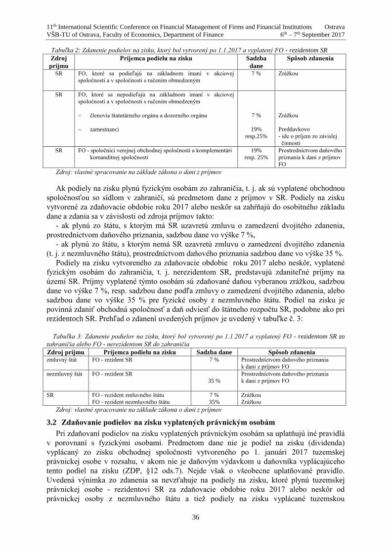
11th International Scientific Conference on Financial Management of Firms and Financial Institutions Ostrava
VŠB-TU of Ostrava, Faculty of Economics, Department of Finance 6th – 7th September 2017
36
Tabuľka 2: Zdanenie podielov na zisku, ktorý bol vytvorený po 1.1.2017 a vyplatený FO - rezidentom SR
Zdroj
príjmu
Príjemca podielu na zisku Sadzba
dane
Spôsob zdanenia
SR FO, ktoré sa podieľajú na základnom imaní v akciovej
spoločnosti a v spoločnosti s ručením obmedzeným
7 % Zrážkou
SR FO, ktoré sa nepodieľajú na základnom imaní v akciovej
spoločnosti a v spoločnosti s ručením obmedzeným
‒ členovia štatutárneho orgánu a dozorného orgánu
‒ zamestnanci
7 %
19%
resp.25%
Zrážkou
Preddavkovo
- ide o príjem zo závislej
činnosti
SR FO - spoločníci verejnej obchodnej spoločnosti a komplementári
komanditnej spoločnosti
19%
resp. 25%
Prostredníctvom daňového
priznania k dani z príjmov
FO
Zdroj: vlastné spracovanie na základe zákona o dani z príjmov
Ak podiely na zisku plynú fyzickým osobám zo zahraničia, t. j. ak sú vyplatené obchodnou
spoločnosťou so sídlom v zahraničí, sú predmetom dane z príjmov v SR. Podiely na zisku
vytvorené za zdaňovacie obdobie roku 2017 alebo neskôr sa zahŕňajú do osobitného základu
dane a zdania sa v závislosti od zdroja príjmov takto:
- ak plynú zo štátu, s ktorým má SR uzavretú zmluvu o zamedzení dvojitého zdanenia,
prostredníctvom daňového priznania, sadzbou dane vo výške 7 %,
- ak plynú zo štátu, s ktorým nemá SR uzavretú zmluvu o zamedzení dvojitého zdanenia
(t. j. z nezmluvného štátu), prostredníctvom daňového priznania sadzbou dane vo výške 35 %.
Podiely na zisku vytvoreného za zdaňovacie obdobie roku 2017 alebo neskôr, vyplatené
fyzickým osobám do zahraničia, t. j. nerezidentom SR, predstavujú zdaniteľné príjmy na
území SR. Príjmy vyplatené týmto osobám sú zdaňované daňou vyberanou zrážkou, sadzbou
dane vo výške 7 %, resp. sadzbou dane podľa zmluvy o zamedzení dvojitého zdanenia, alebo
sadzbou dane vo výške 35 % pre fyzické osoby z nezmluvného štátu. Podiel na zisku je
povinná zdaniť obchodná spoločnosť a daň odviesť do štátneho rozpočtu SR, podobne ako pri
rezidentoch SR. Prehľad o zdanení uvedených príjmov je uvedený v tabuľke č. 3:
Tabuľka 3: Zdanenie podielov na zisku, ktorý bol vytvorený po 1.1.2017 a vyplatený FO - rezidentom SR zo
zahraničia alebo FO - nerezidentom SR do zahraničia
Zdroj príjmu Príjemca podielu na zisku Sadzba dane Spôsob zdanenia zmluvný štát FO - rezident SR 7 % Prostredníctvom daňového priznania
k dani z príjmov FO
nezmluvný štát FO - rezident SR
35 %
Prostredníctvom daňového priznania
k dani z príjmov FO
SR FO - rezident zmluvného štátu
FO - rezident nezmluvného štátu
7 %
35%
Zrážkou
Zrážkou
Zdroj: vlastné spracovanie na základe zákona o dani z príjmov
3.2 Zdaňovanie podielov na zisku vyplatených právnickým osobám
Pri zdaňovaní podielov na zisku vyplatených právnickým osobám sa uplatňujú iné pravidlá
v porovnaní s fyzickými osobami. Predmetom dane nie je podiel na zisku (dividenda)
vyplácaný zo zisku obchodnej spoločnosti vytvoreného po 1. januári 2017 tuzemskej
právnickej osobe v rozsahu, v akom nie je daňovým výdavkom u daňovníka vyplácajúceho
tento podiel na zisku (ZDP, §12 ods.7). Nejde však o všeobecne uplatňované pravidlo.
Uvedená výnimka zo zdanenia sa nevzťahuje na podiely na zisku, ktoré plynú tuzemskej
právnickej osobe - rezidentovi SR za zdaňovacie obdobie roku 2017 alebo neskôr od
právnickej osoby z nezmluvného štátu a tiež podiely na zisku vyplácané tuzemskou
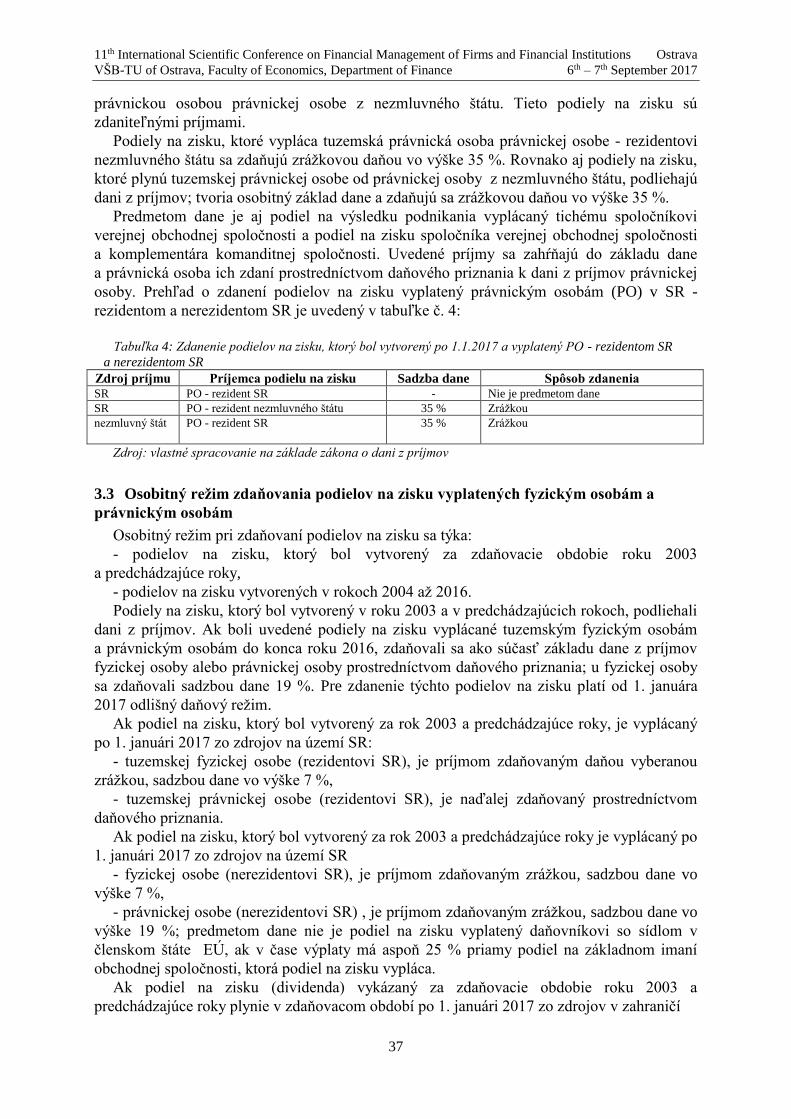
11th International Scientific Conference on Financial Management of Firms and Financial Institutions Ostrava
VŠB-TU of Ostrava, Faculty of Economics, Department of Finance 6th – 7th September 2017
37
právnickou osobou právnickej osobe z nezmluvného štátu. Tieto podiely na zisku sú
zdaniteľnými príjmami.
Podiely na zisku, ktoré vypláca tuzemská právnická osoba právnickej osobe - rezidentovi
nezmluvného štátu sa zdaňujú zrážkovou daňou vo výške 35 %. Rovnako aj podiely na zisku,
ktoré plynú tuzemskej právnickej osobe od právnickej osoby z nezmluvného štátu, podliehajú
dani z príjmov; tvoria osobitný základ dane a zdaňujú sa zrážkovou daňou vo výške 35 %.
Predmetom dane je aj podiel na výsledku podnikania vyplácaný tichému spoločníkovi
verejnej obchodnej spoločnosti a podiel na zisku spoločníka verejnej obchodnej spoločnosti
a komplementára komanditnej spoločnosti. Uvedené príjmy sa zahŕňajú do základu dane
a právnická osoba ich zdaní prostredníctvom daňového priznania k dani z príjmov právnickej
osoby. Prehľad o zdanení podielov na zisku vyplatený právnickým osobám (PO) v SR -
rezidentom a nerezidentom SR je uvedený v tabuľke č. 4:
Tabuľka 4: Zdanenie podielov na zisku, ktorý bol vytvorený po 1.1.2017 a vyplatený PO - rezidentom SR
a nerezidentom SR
Zdroj príjmu Príjemca podielu na zisku Sadzba dane Spôsob zdanenia SR PO - rezident SR - Nie je predmetom dane
SR PO - rezident nezmluvného štátu 35 % Zrážkou
nezmluvný štát PO - rezident SR
35 % Zrážkou
Zdroj: vlastné spracovanie na základe zákona o dani z príjmov
3.3 Osobitný režim zdaňovania podielov na zisku vyplatených fyzickým osobám a
právnickým osobám
Osobitný režim pri zdaňovaní podielov na zisku sa týka:
- podielov na zisku, ktorý bol vytvorený za zdaňovacie obdobie roku 2003
a predchádzajúce roky,
- podielov na zisku vytvorených v rokoch 2004 až 2016.
Podiely na zisku, ktorý bol vytvorený v roku 2003 a v predchádzajúcich rokoch, podliehali
dani z príjmov. Ak boli uvedené podiely na zisku vyplácané tuzemským fyzickým osobám
a právnickým osobám do konca roku 2016, zdaňovali sa ako súčasť základu dane z príjmov
fyzickej osoby alebo právnickej osoby prostredníctvom daňového priznania; u fyzickej osoby
sa zdaňovali sadzbou dane 19 %. Pre zdanenie týchto podielov na zisku platí od 1. januára
2017 odlišný daňový režim.
Ak podiel na zisku, ktorý bol vytvorený za rok 2003 a predchádzajúce roky, je vyplácaný
po 1. januári 2017 zo zdrojov na území SR:
- tuzemskej fyzickej osobe (rezidentovi SR), je príjmom zdaňovaným daňou vyberanou
zrážkou, sadzbou dane vo výške 7 %,
- tuzemskej právnickej osobe (rezidentovi SR), je naďalej zdaňovaný prostredníctvom
daňového priznania.
Ak podiel na zisku, ktorý bol vytvorený za rok 2003 a predchádzajúce roky je vyplácaný po
1. januári 2017 zo zdrojov na území SR
- fyzickej osobe (nerezidentovi SR), je príjmom zdaňovaným zrážkou, sadzbou dane vo
výške 7 %,
- právnickej osobe (nerezidentovi SR) , je príjmom zdaňovaným zrážkou, sadzbou dane vo
výške 19 %; predmetom dane nie je podiel na zisku vyplatený daňovníkovi so sídlom v
členskom štáte EÚ, ak v čase výplaty má aspoň 25 % priamy podiel na základnom imaní
obchodnej spoločnosti, ktorá podiel na zisku vypláca.
Ak podiel na zisku (dividenda) vykázaný za zdaňovacie obdobie roku 2003 a
predchádzajúce roky plynie v zdaňovacom období po 1. januári 2017 zo zdrojov v zahraničí

11th International Scientific Conference on Financial Management of Firms and Financial Institutions Ostrava
VŠB-TU of Ostrava, Faculty of Economics, Department of Finance 6th – 7th September 2017
38
- tuzemskej fyzickej osobe, je príjmom zahrnovaným do osobitného základu dane, pri
použití sadzby dane 7 %,
- tuzemskej právnickej osobe, je zdaňovaný prostredníctvom daňového priznania;
predmetom dane nie je podiel na zisku vyplatený daňovníkom so sídlom v členskom štáte EÚ,
ak v čase výplaty má tuzemský daňovník aspoň 25 % podiel na základnom imaní obchodnej
spoločnosti, ktorá podiel na zisku vypláca.
Podiely na zisku, ktorý bol vytvorený v rokoch 2004 až 2016, vyplácané fyzickým osobám
a právnickým osobám, nie sú predmetom dane z príjmov, ak k ich výplate dôjde po 1. januári
2017. Ak sú uvedené podiely na zisku vyplácané právnickou osobou osobám so sídlom alebo
bydliskom v zahraničí, tak ako pri tuzemských osobách, nejde o zdaniteľný príjem.
Podiely na zisku vyplatené zamestnancom bez majetkovej účasti na základom imaní sú
predmetom dane, ide však o príjmy oslobodené od dane.
4. Záver
Nová právna úprava zdanenia príjmov fyzických osôb a právnických osôb v Slovenskej
republike významným spôsobom ovplyvnila aj zdanenie podielov na zisku, ktoré plynú týmto
osobám z ich majetkových práv v obchodných spoločnostiach. Po mnohých rokoch podiely na
zisku znovu podliehajú dani z príjmov a neuplatňuje sa poistné na zdravotné poistenie ako
neštandardný nástroj, ktorý sa vzťahoval na tento druh príjmov. Pri zdaňovaní podielov na
zisku vyplácaných po 1. januári 2017 je potrebné zohľadňovať veľa rôznych faktororov a
súvislostí, predovšetkým príjemcu podielu a jeho daňovú rezidenciu, zdroj týchto príjmov a
tiež zdaňovacie obdobie, v ktorom boli podiely na zisku vytvorené. Pri ich zdaňovaní sa
uplatňujú rôzne sadzby dane a rôzne spôsoby zdanenia, z čoho rezultuje aj riziko a
diferencovaná zodpovednosť za správne zdanenie a odvedenie dane daňovému úradu.
Potvrdenie
Príspevok bol spracovaný ako jeden z výstupov riešenia projektu grantovej agentúry
Vedecká grantová agentúra Ministerstva školstva SR a Slovenskej akadémie vied (VEGA)
č. 1/0512/16 (2016-2018) "Zachovanie a rast majetkovej podstaty ako relevantný nástroj
trvalo udržateľného rozvoja podniku".
References
[1] Baštincová, A. (2016). Účtovníctvo a dane právnických osôb. 1. vydanie. Bratislava:
Wolters Kluwer.
[2] Mezeiová, V., Horniaček, P. (2017). Novela zákona o dani z príjmov účinná od 1.
januára 2017. Dane a účtovníctvo 2/2017. Bratislava: Wolters Kluwer.
[3] Solíková, V. (2017). Zdaňovanie podielov na zisku (dividend) od roku 2017. Dostupné na
internete:https://www.podnikajte.sk/dane-a-účtovníctvo/c/2965/category/dan-z-prijmov...
z 11.6.2017.
[4] Vanková, L. (2017). Podiel na zisku a daň z príjmov od roku 2017. Dane a účtovníctvo
4/2017. Bratislava: Wolters Kluwer.
[5] Zákon č. 513/1991 Zb. Obchodný zákonník v znení neskorších predpisov.
[6] Zákon č. 595/2003 Z. z. o dani z príjmov v znení neskorších predpisov

8th International Scientific Conference Managing and Modelling of Financial Risks Ostrava
VŠB-TU of Ostrava, Faculty of Economics, Department of Finance 6th – 7th September 2017
39
Firm Investment under Financial Market Imperfections1
Katarína Belanová 2
Abstract
A company can fund its investments by the use of internal and/or external funds. Especially
SMEs have difficulties in getting external financial sources. One of the main reasons is that
financial markets are imperfect, which results from the underdevelopment of the financial
systems. The aim of the article is to survey the impact of financial market imperfections on firm
investment on the sample of 53 automotive companies in the SR. The survey was carried out
during the year 2011. We find supportive evidence for the fact that companies surveyed face
credit rationing.
Key words
Financial sources, credit rationing, firm investment
JEL Classification: E22, D92
1. Introduction
Companies need finance to operate and undertake investment projects. It is obvious that if
finance is inadequate, they will not invest. A company can fund its investment projects by the
use of internal and/or external funds. It usually has to get at least part of its financing from
financial markets. Especially small and medium – sized enterprises (SMEs) have difficulties
in getting external financial sources. One of the main reasons is that financial markets are
imperfect. They are imperfect in a way that external funds suppliers encounter assymetric
information, i.e. they have less information about the profitability and risks of investment
projects than firms have. Information is important in firm financing transactions, since firms
receive capital today and only provide returns on the capital in the future. Moreover, financial
systems are underdeveloped. If credit rationing is prevalent, a company can not borrow as
much as it would like to or may even be denied access to credit. The theoretical contributions
state that if it is credit – rationed, it may have to rely on internal funds to finance its
investment. As a result, its investment is sensitive to the amount of internal funds. The aim of
the article is to survey the impact of financial market imperfections on firm investment. The
empirical analysis uses firm – level data and is based on a survey of 53 automotive suppliers
in the Slovak republic, which was carried out during the year 2011.
The results show that the availability of internal funds has a positive and statistically
significant effect on investment of the entire sample, suggesting that automotive companies
face financing constraints.
1 The paper is a part of VEGA project No. 1/0776/16 Taxation of the financial sector and harmonizing
tendencies in the European Union. 2 Assoc. Prof. Ing. Katarína Belanová, PhD., University of Economics in Bratislava, Faculty of
National Economy, Dpt. of Finance, e-mail: [email protected].

8th International Scientific Conference Managing and Modelling of Financial Risks Ostrava
VŠB-TU of Ostrava, Faculty of Economics, Department of Finance 6th – 7th September 2017
40
2. Literature review
According to the source, where the capital comes from, a company can finance its
investments using internal and/or external funds. As figure 1 shows, internal funds are the
ones which arose and are used in a company. External funds come from various borrowing
sources as well as from issuing shares.
Figure 1: Classification of financial sources
According to the neoclassical theory of firm investment, since financial markets are
perfect, i.e., there are neither transaction nor information costs, internal and external funds are
perfect substitutes in terms of financing investment; and, firms have access to unlimited
sources of funds. Therefore, firm investments should not be constrained by lack of funds
(Modigliani and Miller, 1958). However, this hypothesis fails in the presence of assymetric
information, which can lead to credit rationing. The basic intuition of Stiglitz and Weiss
(1981) is that moderate increases of interest rate would elicit a higher supply of funds;
however, further increases of the interest rate will worsen the quality of the applicant pool,
thus reducing the expected return to the bank. As a result, the bank rations credit instead of
raising the interest rate. Collateral can contribute to relaxing credit rationing. However, this
contribution may be impeded if it is costly for banks to write a number of loan contracts
involving different amounts of interest rates and collateral or if the regulation system is
rudimentary.
When companies are involved in a financial imperfect surrounding, they are concerned
about how to finance their investment because different financing sources have different costs.
The pecking order theory states that firms have an ordering in preferences regarding sources
of investment funds (Myers, 1984). This theory argues that firms prefer internal funds to
external funds because external funds are more expensive (Gelos and Werner, 2002). If firms
need external funds after exhausting internal funds, they will start with the least risky security,

8th International Scientific Conference Managing and Modelling of Financial Risks Ostrava
VŠB-TU of Ostrava, Faculty of Economics, Department of Finance 6th – 7th September 2017
41
i.e., debt. Hybrids (like convertibiles) follow debt in the pecking order. Equity is ultimately
below as the last resort. Firms are in favour of debt over equity because debt has lower
information cost than equity (Myers, 1984).
The theory concludes that since financial markets are imperfect, firm investment may be
sensitive to internal funds, i.e., firms having higher investment – internal sensitivities are
considered as more financially constrained.
3. Empirical testing of firm investment under financial market
imperfections
The recognition of the effect of financial market imperfections on firm investment suggests
that internal funds should be accounted for when estimating firm investment. Despite the
theoretical plausibility of a relationship between capital market imperfections and real
investments, the empirical literature has found it difficult to identify this channel.
Moreover, number of the empirical studies on firm investment in the presence of financial
market imperfections which focus on firms in developing and transition countries, is relatively
limited. The relevant studies have similar scenario: they identify a priori proxy for the
financial constraints and then use this proxy to sort the firms in question into groups of
different degrees of financial constraints. In addition, according to Fazzari et al. (1988) they
compare the investment – internal funds sensitivities across these groups of firms based on the
outcomes of the tests using the augmented version of the accelerator or Tobin`s Q model. The
investment – internal funds sensitivity should be greater for (groups of) firms facing higher
degrees of financial constraints. The sorting criteria that the empirical studies have used are:
Size (e.g., Agung; etc.);
Age (e.g. Schaller, 1993; Jaramillo et al., 1996);
Membership of business/financial groups (e.g., Hoshi et al., 1991;
Agung, 2000);
The presence of bond ratings (e.g. Whited, 1992);
The degree of shareholder concentration (e.g. Schaller, 1993);
Dividend payout ratio (e.g., Hubbard et al., 1995); and so on.
Among these criteria, firm size and age are most widely used. Since lending and
monitoring costs have economies of scale (Bernanke, 1996), it is cheaper (for lenders) to lend
to larger firms, which tend to apply for larger loans, as compared to smaller ones. Therefore,
large firms should have better access to loans than small ones. Larger firms may also have
better access to credit because they usually have more acceptable collateral. In addition, larger
firms may have better track records, which may help diminish information assymetry and
improve their access to credit. Moreover, in so far as size of the firm is related to its
possibility to be listed on stock markets large listed firms may emit more inside information to
lenders through the stock markets in which they operate. Hence, we can assume that large
firms are less financially constrained than small ones. As for age, it is usually argued that
banks should have better information about older (more mature) firms due to longer
relationships and repeated contacts. Moreover, older firms may have accumulated more assets,
which could be pledged as collateral for loans, which facilitates their access to loans. Older
firms may also have more experience with lenders, which helps these firms to find better ways
to obtain credit from lenders. Therefore, older firms shoulsd be less financially constrained
because they may have better Access to credit. The empirical studies that use size criterion
come up with mixed findings (Gelos and Werner, 2002; Driffield and Pal, 2001), whereas the
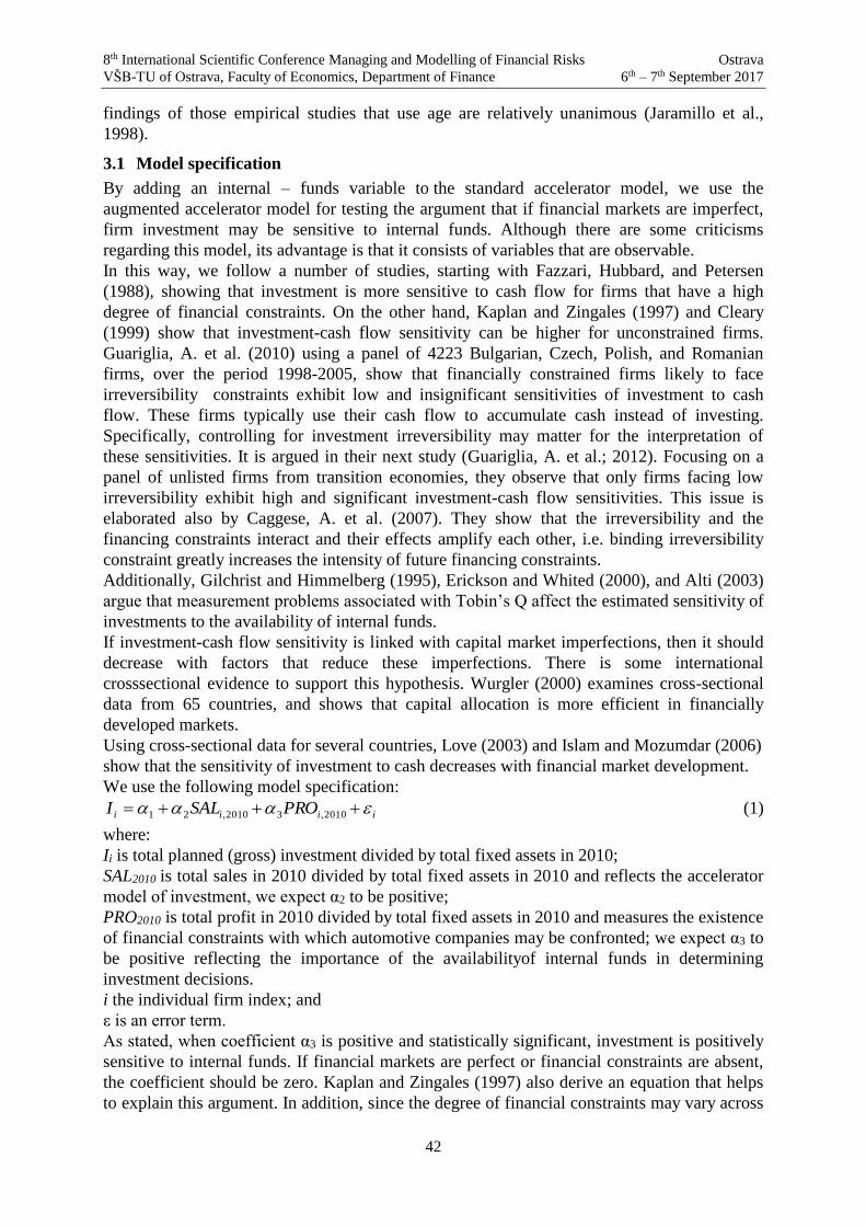
8th International Scientific Conference Managing and Modelling of Financial Risks Ostrava
VŠB-TU of Ostrava, Faculty of Economics, Department of Finance 6th – 7th September 2017
42
findings of those empirical studies that use age are relatively unanimous (Jaramillo et al.,
1998).
3.1 Model specification
By adding an internal – funds variable to the standard accelerator model, we use the
augmented accelerator model for testing the argument that if financial markets are imperfect,
firm investment may be sensitive to internal funds. Although there are some criticisms
regarding this model, its advantage is that it consists of variables that are observable.
In this way, we follow a number of studies, starting with Fazzari, Hubbard, and Petersen
(1988), showing that investment is more sensitive to cash flow for firms that have a high
degree of financial constraints. On the other hand, Kaplan and Zingales (1997) and Cleary
(1999) show that investment-cash flow sensitivity can be higher for unconstrained firms.
Guariglia, A. et al. (2010) using a panel of 4223 Bulgarian, Czech, Polish, and Romanian
firms, over the period 1998-2005, show that financially constrained firms likely to face
irreversibility constraints exhibit low and insignificant sensitivities of investment to cash
flow. These firms typically use their cash flow to accumulate cash instead of investing.
Specifically, controlling for investment irreversibility may matter for the interpretation of
these sensitivities. It is argued in their next study (Guariglia, A. et al.; 2012). Focusing on a
panel of unlisted firms from transition economies, they observe that only firms facing low
irreversibility exhibit high and significant investment-cash flow sensitivities. This issue is
elaborated also by Caggese, A. et al. (2007). They show that the irreversibility and the
financing constraints interact and their effects amplify each other, i.e. binding irreversibility
constraint greatly increases the intensity of future financing constraints.
Additionally, Gilchrist and Himmelberg (1995), Erickson and Whited (2000), and Alti (2003)
argue that measurement problems associated with Tobin’s Q affect the estimated sensitivity of
investments to the availability of internal funds.
If investment-cash flow sensitivity is linked with capital market imperfections, then it should
decrease with factors that reduce these imperfections. There is some international
crosssectional evidence to support this hypothesis. Wurgler (2000) examines cross-sectional
data from 65 countries, and shows that capital allocation is more efficient in financially
developed markets.
Using cross-sectional data for several countries, Love (2003) and Islam and Mozumdar (2006)
show that the sensitivity of investment to cash decreases with financial market development.
We use the following model specification:
iiii PROSALI 2010,32010,21 (1)
where:
Ii is total planned (gross) investment divided by total fixed assets in 2010;
SAL2010 is total sales in 2010 divided by total fixed assets in 2010 and reflects the accelerator
model of investment, we expect α2 to be positive;
PRO2010 is total profit in 2010 divided by total fixed assets in 2010 and measures the existence
of financial constraints with which automotive companies may be confronted; we expect α3 to
be positive reflecting the importance of the availabilityof internal funds in determining
investment decisions.
i the individual firm index; and
ε is an error term.
As stated, when coefficient α3 is positive and statistically significant, investment is positively
sensitive to internal funds. If financial markets are perfect or financial constraints are absent,
the coefficient should be zero. Kaplan and Zingales (1997) also derive an equation that helps
to explain this argument. In addition, since the degree of financial constraints may vary across
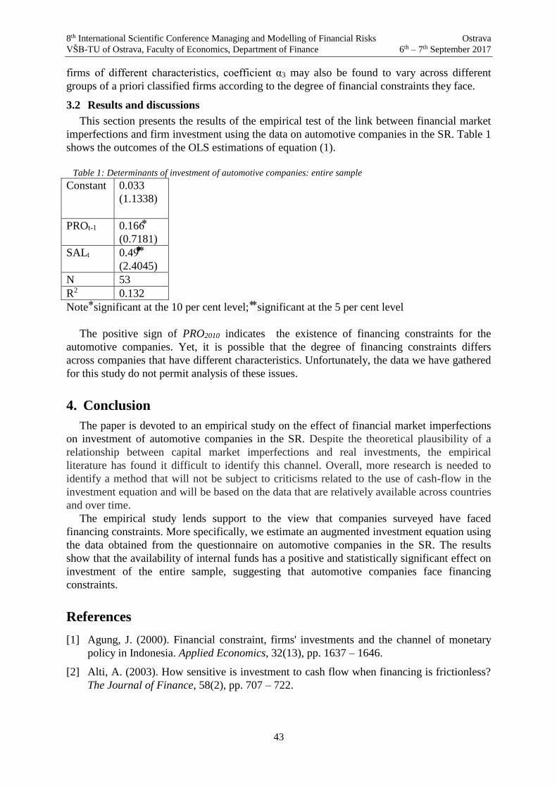
8th International Scientific Conference Managing and Modelling of Financial Risks Ostrava
VŠB-TU of Ostrava, Faculty of Economics, Department of Finance 6th – 7th September 2017
43
firms of different characteristics, coefficient α3 may also be found to vary across different
groups of a priori classified firms according to the degree of financial constraints they face.
3.2 Results and discussions
This section presents the results of the empirical test of the link between financial market
imperfections and firm investment using the data on automotive companies in the SR. Table 1
shows the outcomes of the OLS estimations of equation (1).
Table 1: Determinants of investment of automotive companies: entire sample
Constant 0.033
(1.1338)
PROt-1 0.166⃰
(0.7181)
SALt 0.49⃰⃰⃰⃰⃰⃰⃰⃰ ⃰
(2.4045)
N 53
R2 0.132
Note ⃰ significant at the 10 per cent level; ⃰ ⃰ significant at the 5 per cent level
The positive sign of PRO2010 indicates the existence of financing constraints for the
automotive companies. Yet, it is possible that the degree of financing constraints differs
across companies that have different characteristics. Unfortunately, the data we have gathered
for this study do not permit analysis of these issues.
4. Conclusion
The paper is devoted to an empirical study on the effect of financial market imperfections
on investment of automotive companies in the SR. Despite the theoretical plausibility of a
relationship between capital market imperfections and real investments, the empirical
literature has found it difficult to identify this channel. Overall, more research is needed to
identify a method that will not be subject to criticisms related to the use of cash-flow in the
investment equation and will be based on the data that are relatively available across countries
and over time.
The empirical study lends support to the view that companies surveyed have faced
financing constraints. More specifically, we estimate an augmented investment equation using
the data obtained from the questionnaire on automotive companies in the SR. The results
show that the availability of internal funds has a positive and statistically significant effect on
investment of the entire sample, suggesting that automotive companies face financing
constraints.
References
[1] Agung, J. (2000). Financial constraint, firms' investments and the channel of monetary
policy in Indonesia. Applied Economics, 32(13), pp. 1637 – 1646.
[2] Alti, A. (2003). How sensitive is investment to cash flow when financing is frictionless?
The Journal of Finance, 58(2), pp. 707 – 722.
8th International Scientific Conference Managing and Modelling of Financial Risks Ostrava
VŠB-TU of Ostrava, Faculty of Economics, Department of Finance 6th – 7th September 2017
44
[3] Bernanke, B. et al. (1996). The financial accelerator and the flight to quality. The Review
of Economics and Statistics, 78(1), pp. 1 – 15.
[4] Brealey, R.A. and Myers, S.C. (1984). Principles of Corporate Finance. 2nd ed. New
York: McGraw-Hill Book Co.
[5] Caggese, A. et al. (2007). Financing constraints, irreversibility and investment dynamics.
Journal of Monetary Economics, 54(2007), pp. 2102 – 2130.
[6] Cleary, S. (1999). The relationship between firm investment and financial status. The
Journal of Finance, 54(2), pp. 673 – 692.
[7] Driffield, N. and Pal, S. (2001). The East Asian Crisis and Financing Corporate
Investment: Is There A Cause for Concern? Journal of Asian Economics, 12(4), pp. 507 –
527.
[8] Erickson, T. and Whited, T.M. (2000). Measurement error and the relationship between
investment and q. Journal of Political Economy, 108(5), pp. 1027 – 1057.
[9] Fazzari, S, Hubbard, R.G. and Petersen, B. (1988). Financing constraints and corporate
investment. Brooking Papers on Economic Activity, 1, pp. 141 – 1195. Washington D.C.:
The Brookings Institution.
[10] Gelos, R.G. and Werner, A. M. (2002). Financial liberalization, credit constraints and
collateral. Journal of Development Economics, 67(1), pp. 1 – 27.
[11] Gilchrist, S. and Himmelberg, C.P. (1995). Evidence on the role of cash flow for
investment. Journal of Monetary Economics, 36(3), pp. 541 – 572.
[12] Guariglia, A. et al. (2010). Investment and Financing Constraints in China. Discussion
paper series, Nr. 521. Oxford: University of Oxford.
[13] Guariglia, A. et al. (2012). Negative investment in China. Research paper Nr. 2012/01.
Nottingham: The University of Nottingham.
[14] Hishi et al. (1991). Corporate structure, liquidity and investment. The Quarterly Journal
of Economics, 106(1), pp. 33 – 60.
[15] Hubbard et al.(1995). Internal finance and firm investment. Journal of Money, Credit and
Banking, 27(3), pp. 683 – 701.
[16] Islam, S. and Mozumdar, A. (2006). Financial development and the importance of
internal cash: Evidence from international data. Journal of Banking and Finance, 31(3),
pp.641 – 658.
[17] Jaramillo, F. et al. (1996). Capital market imperfections before and after financial
liberalization. Journal of Development Economics, 51(3), pp. 367 – 386.
[18] Kaplan, S.N. and Zingales, L. (1997). Do investment-cash flow sensitivities provide
useful measures of financing constraints? The Quarterly Journal of Economics, 112(1),
pp. 169 – 215.
[19] Love, J. (2003). Financial development and financing constraints: International evidence
from the structural investment model. Rev. Financ.Studies, 16(3), pp. 765 – 791.
[20] Modigliani, F. and Miller, M.H. (1958). The cost of capital, corporation finance and the
theory of Investment. The American Economic Review, 48(3), pp. 261 – 297.

8th International Scientific Conference Managing and Modelling of Financial Risks Ostrava
VŠB-TU of Ostrava, Faculty of Economics, Department of Finance 6th – 7th September 2017
45
[21] Schaller, H. (1993). The risky spread, investment, and monetary transmission: Evidence
on the role of assymetric information. The Review of Economics and Statistics, 78(3), pp.
375 – 383.
[22] Stiglitz, J.E. and Weiss, A. (1981). Credit rationing in markets with imperfect
information. The American Economic Review, 71(3), pp. 393 – 410.
[23] Whited, T.M. (1992). Debt, liquidity constraints, and corporate investment: Evidence
from panel data. The Journal of Finance, 47(4), pp. 1425 – 1460.
[24] Wurgler, J. (2000). Financial markets and the allocation of capital. Journal of Financial
Economics, 58(1-2), pp. 187 – 214.
11th International Scientific Conference on Financial Management of Firms and Financial Institutions Ostrava
VŠB-TU of Ostrava, Faculty of Economics, Department of Finance 6th – 7th September 2017
46
CFC Rules as stated in the standards of the OECD and EU – a comparative study
Kristýna Bělušová1 , Karel Brychta2
Abstract
This paper deals with the issue of Controlled Foreign Company rules as stated in the OECD BEPS
project and in the ATAD Directive implementing the rules in European Union law. The aim of
this paper is to describe and compare basic CFC rules in the form as stipulated by the OECD in
its BEPS project and the form as enshrined in the ATAD Directive. For the comparison made six
attributes were followed. The research is based on qualitative research (a case study). The method
of data collection was the content analysis of the text; selected texts published by the OECD, and
the text of the ATAD Directive, were the objects of the research carried out. The findings reached
suggest that the ATAD Directive, which is legally binding for individual EU Member States,
enshrines the CFC rules in a somewhat stricter manner than the BEPS recommendations.
Key words
BEPS, ATAD, comparison, CFC rules
JEL Classification: H25, H26, K34
1 Introduction
In order to prevent tax evasion and introduce more just taxation consisting of the fairer
allocation of tax bases, the OECD commenced work on a project aimed at fighting Tax Base
Erosion and the Transfer of Profits project (hereinafter referred to as BEPS). The project was
commenced in June 2013 by the publication of the BEPS Action Plan; the document consists
of 15 mutually interconnected actions which respond to current issues in the area of taxation
(Herrington, 2015). The aim of the BEPS Action Plan is to identify steps and measures which
must be adopted in order to tackle BEPS effectively in both international and national contexts.
However, measures proposed in the OECD materials only present recommendations (Flipsen
and Duteweert, 2014), whose efficiency is contingent upon their wide acceptance and actual
enforcement. The BEPS project covers a number of interrelated areas. This contribution is
specifically aimed at an area which is covered by Action Plan no. 3 – i.e. at Controlled Foreign
Company Rules (hereinafter referred to as the CFC rules).
1.1 Aim and methodology
The aim of this contribution is to describe and compare the CFC rules in the form stipulated
by the OECD in its BEPS project and the form enshrined in a directive adopting the CFC rules
to EU law, namely in the Council Directive (EU) 2016/1164 of 12 July 2016 laying down rules
against tax avoidance practices that directly affect the functioning of the internal market
(hereinafter referred to as the ATAD Directive). The comparison was performed for:
rules for defining CFC,
CFC exemption,
1 Ing. et Ing. Kristýna Bělušová, Brno University of Technology, Faculty of Business and Management,
Kolejní 2906/4, 612 00 Brno, the Czech Republic, [email protected]. 2doc. Mgr. Ing. Karel Brychta, Ph.D., Brno University of Technology, Faculty of Business and
Management, Kolejní 2906/4, 612 00 Brno, the Czech Republic, [email protected].

11th International Scientific Conference on Financial Management of Firms and Financial Institutions Ostrava
VŠB-TU of Ostrava, Faculty of Economics, Department of Finance 6th – 7th September 2017
47
rules for defining a CFC,
rules for computing income,
rules for attributing income
rules to prevent or eliminate double taxation for the situations where the attributed
CFC income is also subject to foreign corporation.
This contribution is based on qualitative research (a case study), as follows from
the stipulated objective. The method of data collection was the content analysis of the text;
selected texts published by the OECD, and the text of the ATAD Directive, were
the objects of the research. The contribution itself has the following structure. The next section
describes the CFC rules as stipulated by the OECD. Afterwards, the authors' attention is focused
on the relevant standards enshrined in the ATAD Directive. In the discussion section,
the authors present selected results focusing on the evaluation of the standards given by the EU
law in comparison with the standards anticipated by the OECD. The final chapter contains
an overall summary.
2 BEPS Action 3 – CFC rules
Action 3 deals with the introduction of effective rules for the taxation of controlled foreign
companies. According to the OECD, these CFC rules should be used by governments as
a discouraging measure and not a method for increasing tax revenues (Feinschreiber and Kent,
2015). The CFC rules are only applied to passive income, and the amounts of income should
be calculated in accordance with the rules of the domestic jurisdiction for the calculation of
income. Passive income should be attributed to domestic companies according to the amounts
of their share in foreign controlled entities, and double taxation should be eliminated through
an offset of tax paid abroad against domestic tax (OECD, 2015). As stated by Dourado (2015,
p. 343), „CFC rules deny deferral of taxation on income accrued to a CFC or a similar entity
that would escape taxation in the residence country. CFC rules are designed in many countries
as an exception to the above-mentioned deferral.“. CFC rules within the BEPS project consist
of 6 fundamental elements (PWC, 2015a; OECD, 2015) as specified below.
2.1 Rule for defining a CFC
According to the OECD’s recommendation, a controlled entity under the CFC rules is
a permanent establishment or a company controlled by resident shareholders, provided that
the share in the capital or in the voting rights of the controlled foreign company is at least
50 %. If the definition of a controlled company is met, the CFC rules should not apply in case
the controlled entities are located in jurisdictions whose tax rate is not markedly lower than that
of the domestic jurisdiction, or if the income of the controlled entity does not exceed a certain
threshold (the aim is to mitigate administrative burden in entities where the additional revenue
would be low), or in case the income of the controlled entity was not achieved as a result of
avoidance of tax obligation (however, such a rule is administratively difficult to prove) (OECD,
2015). The Czech Ministry of Finance also regards the limit of 50 % as sufficient (Ministerstvo
financí ČR, 2017). For example, the afore-mentioned limit of the share of the capital or of
the voting rights for meeting the CFC definition was introduced in Argentina, Australia and
China; on the other hand, in Italy the limit is 20 %, and 10 % for a company listed on the stock
exchange. (Deloitte, 2014).
2.2 CFC exemptions
Those controlled foreign companies that are subject to a sufficiently similar effective
corporate income tax rate applied in the jurisdiction of the parent company are exempted from
the CFC rules (OECD, 2015). For example, this condition was supported by PWC (2015b).
Therefore, the subjects of the CFC rules are corporations located in the jurisdictions where
11th International Scientific Conference on Financial Management of Firms and Financial Institutions Ostrava
VŠB-TU of Ostrava, Faculty of Economics, Department of Finance 6th – 7th September 2017
48
the tax rate is significantly lower than in the country of the parent company. However, an
exception from the CFC rules depends not only on the level of the tax rate; it is also derived
from the minimum threshold value or the level of income. This was stipulated in order to reduce
administrative burden, and to effectively focus the CFC rules on certain companies. . In this
respect, the OECD (2015) points out that, „An anti-avoidance threshold requirement would
only subject transactions and structures that were the result of tax avoidance to CFC rules.
This could narrow the effectiveness of CFC rules as preventative measures, and it could also
increase the administrative and compliance burdens of CFC rules if it were administrated as
an up-front rule.“.
2.3 Definition of CFC income
The subject of the CFC rules includes dividends, interest, insurance income, royalties
and intellectual property income, as well as sales and services income. The specific definitions
of these types of income relate to domestic legal regulations. Nevertheless, the OECD materials
specify income categories excluded from the CFC rules. For example, in the case of dividends,
these are:
1. if the dividends are paid out as the active income of the branch;
2. if the dividends are exempt from taxation in the jurisdiction of the controlled foreign
company and in the parent country; and
3. if the dividends are paid to the controlled foreign company and come from active
securities trading (OECD, 2015).
2.4 Rules for computing income
The level of income is calculated according to the rules of the jurisdiction in which the
parent company is established. This option also enables tax administration costs to be reduced,
which is one of the objectives of the BEPS project. However, the OECD also dealt with
the issue of handling loss. In this respect, it was considered that loss should be limited by
the amount of profit of a similar nature, i.e. CFC’s passive losses should be offset against
passive income. The other option was that the loss would be offset against the profit achieved
by the parent company. However, the option of deducting loss falls under the jurisdiction of the
internal legal regulations of the parent companies (OECD, 2015). In relation to the application
of loss, there is, according to the opinion presented by PWC (2015b), no political reason why
loss by one CFC should not be offset against the profits of other CFCs.
2.5 Rules for attributing income
According to the OECD (2015) attributing income is realised in five steps, which determine:
1. which taxpayers will have the income attributed to them;
2. what level of income will be attributed;
3. if the income will be included in the revenues of the CFC;
4. how the income will be handled; and
5. what tax rate will be applied to the given income.
The conditions under which the income shall be included into the revenues of the parent
company are determined by domestic law, and the tax rate shall be identical to the tax rate
levied on the parent company (OECD, 2015). However, there are opinions that third parties not
acting in concord should not be covered by the definition of control set out in the BEPS, i.e.
that income under these circumstances should not be attributed to shareholders (PWC, 2015b).
2.6 Rules to prevent or eliminate double taxation
Double taxation may occur in three situations. First, situations in which the income from
the CFC is subject to foreign corporate income tax. Second, situations in which CFC rules in
more than one jurisdiction apply to the same CFC income. Third, situations in which a CFC
distributes dividends that have been attributed to its shareholders under the CFC rules, or
11th International Scientific Conference on Financial Management of Firms and Financial Institutions Ostrava
VŠB-TU of Ostrava, Faculty of Economics, Department of Finance 6th – 7th September 2017
49
a resident shareholder possesses the shares in the CFC. For the first two situations, double
taxation shall be prevented by the offset method. Regarding the third situation, double taxation
shall be prevented by exempting dividends and profit from tax, if the income was previously
the subject of CFC, but the afore-mentioned taxation was left to individual jurisdictions (in
accordance with the provisions of domestic law) (OECD, 2015). The CFC rules should allow
for an offset of tax paid in foreign jurisdictions even in the case of intermediary companies,
provided that the same CFC income is subject to the CFC rules in more than one jurisdiction
(Deloitte, 2015).
3 Reflection of BEPS Action 3 in EU law: ATAD Directive
The current political priorities in the area of international taxation emphasize the need to
ensure that taxes are paid in the location where profit and value were generated (European
Commission, 2016). In this context, the European Commission adopted the ATAD Directive in
2016, which represents another important step toward the introduction of the BEPS, and must
be transposed into the Member States’ legislation by 1 January 2019 (Duffy and Hogan, 2016).
The implementation period has been extended regarding Article 4 (Interest limitation rule) and
Article 5 (Exit taxation) of this Directive (see Article 11 of the ATAD Directive). The ATAD
Directive responds to situations where corporate groups misuse the differences of national tax
systems, with the aim of reducing their overall tax obligation using low tax rates, deductions
on the grounds of double taxation, or ensuring that income categories are not taxable in one
jurisdiction by their deduction from the tax base, while they would not even be included in the
tax base in the other jurisdiction (Bondaerts and Ijzerman, 2016). The rules which will be
stipulated on the basis of this Directive are essential for protection against aggressive tax
planning within the internal market, due to the fact that corporate groups have been increasingly
resorting to BEPS in order to reduce their global tax obligation. Therefore, the main goal of the
Directive is to increase the resistance of the internal market as a whole against cross-border tax
evasion practices.
The ATAD Directive consists of three sections (13 articles), whereby the CFC rules are
covered in Articles 7 and 8 of the ATAD Directive (Eur-lex, 2017b).
3.1 Rules for defining a CFC
According to the ATAD Directive, a controlled foreign entity is considered to be an entity,
in which the taxpayer themselves, or together with affiliated enterprises, holds a direct or
indirect share representing more than 50 % of the voting rights in this entity, or owns more than
50 % of this entity, and the actual corporate income tax paid by the entity is lower than the
difference between the corporate income tax paid by the entity and the corporate income tax
paid by the taxpayer. Under this Directive, the CFC rules also apply to permanent
establishments. (Eur-lex, 2017b)
3.2 Definition of income
The CFC rules apply to interest or any other income from financial assets, royalties and
intellectual property income, dividends and income from the disposal of shares, income from
financial leasing, income from insurance, banking and other financial activities, and sales and
services income or income from operations which are not real. (Eur-lex, 2017b)
3.3 CFC exemptions
The Member State can decide that the afore-mentioned entity shall not be treated as a CFC,
if such an entity has income (with the exception income from artificial transactions) not
exceeding one third of the given entity’s income. The condition of one third of income also
applies to financial enterprises, but it concerns income from transactions between the taxpayer
11th International Scientific Conference on Financial Management of Firms and Financial Institutions Ostrava
VŠB-TU of Ostrava, Faculty of Economics, Department of Finance 6th – 7th September 2017
50
and its affiliated enterprises. In the event of artificial transactions undertaken with the intention
of obtaining a tax advantage, the entity may not be subject to the CFC rules if its accounting
profit is lower than EUR 750,000 and income from other operations is lower than EUR 75,000,
or if the accounting profit does not exceed 10 % of its operating costs for the given tax period.
(Eur-lex, 2017b)
3.4 Rules for computing income
The level of income is calculated in accordance with the regulations of the Member State
where the parent company is a tax resident. If case the CFC is in loss, the tax base of the parent
company is not reduced by the loss; under national laws, the loss may be transferred to the
following accounting period, where it can be applied. In the case of artificial transactions,
income is calculated in accordance with the principle of normal market conditions. (Eur-lex,
2017b)
3.5 Rules for attributing income
The income to be included in the tax base shall be calculated in proportion to the taxpayer's
participation in the given entity (Eur-lex, 2017).
3.6 Rules to prevent or eliminate double taxation
For situations where CFC income was subject to taxation in the jurisdiction of the CFC, the
Member State of the resident company shall allow the tax paid by the CFC to be deducted from
this payer's tax obligation. The deduction shall be made in accordance with the regulations of
the Member State. (Eur-lex, 2017)
4 Results
In the first structural block, namely the definition of the controlled foreign entity, we can say
that the ATAD Directive applicable for the European Union Member States adopted
the recommended limit regarding the minimum amount of the share held in a foreign company
stipulated in the BEPS. The ATAD Directive expands the CFC definition to include a fact
regarding a low tax rate, which is also specified here, whereas the OECD reflects this situation
in the section describing exceptions to CFC rules.
In the second structural block – exceptions to CFC rules – BEPS OECD recommends
an exception to the application of CFC rules in the event of a similar effective tax rate in the
CFC’s jurisdiction, or if the income does not exceed the stipulated threshold value. However,
income from artificial transactions is always subject to CFC rules. However, the BEPS does not
specifically stipulate any rules for the determination of the level of the effective tax rate.
The ATAD Directive enshrined more lenient rules for exceptions, which may but need not be
implemented by the Member States into their national laws. This concerns an exception to CFC
rules where the CFC income is no higher than one third of the given entity’s income, and the
exception is also stipulated for artificial transactions where the CFC rules do not apply to
an entity whose accounting profit is lower than EUR 750,000 and income from other operations
lower than EUR 75,000, or if the accounting profit amounts to no more than 10 % of its costs
for the given tax period. The definition of a low rate (as mentioned above) is set forth in the
previous structural block.
The directive contains a broader range of explicitly stated types of income subject to
the CFC rules. The extra items include, for example, income from the disposal of a share,
income from financial leasing and income relating to artificial transactions. However, in
the case of both standards, the specific definition of individual incomes is left to the state's
legislation.
11th International Scientific Conference on Financial Management of Firms and Financial Institutions Ostrava
VŠB-TU of Ostrava, Faculty of Economics, Department of Finance 6th – 7th September 2017
51
Within the scope of the BEPS, the calculation of the level of income dealing with loss is also
left to the individual states' internal legislations. In the case of the ATAD Directive,
the calculation of the level of income is performed in same way, i.e. it leaves it to the individual
Member States' legislations. However, regarding dealing with loss, the ATAD Directive's
definition is stricter. If the CFC is in loss, the tax base of the parent company cannot be
decreased by the loss incurred in the tax period concerned. However, Member States can
stipulate the transfer and application of the loss in the following tax period in their legislations.
In terms of the prevention of double taxation, the BEPS recommends the credit method and the
tax exemption method. The ATAD Directive, on the other hand, leaves the deduction of the tax
paid to the Member States' legislations.
Based on the above, we can say that the CFC rules enshrined in the ATAD Directive have
been made stricter than those in the BEPS recommendation. Nevertheless, we must bear in mind
that most of the structural blocks concerning the CFC rules represent mere recommendations
for individual states. The only exception is the criterion of the CFC income definition, which
does not contain recommendation for implementation into the laws of individual states'
legislations; instead, it offers several possibilities (PWC, 2015c). On the other hand, the ATAD
Directive enshrines rules that must be implemented by the EU Member States.
Although the CFC rules already exist in many countries, they have not been processed in
a comprehensive manner (Burmester and Smiley, 2013). This main objective cannot be
achieved while Member States act individually, because aggressive tax planning is based on
differences between national legal regulations and measures (European Commission, 2016). In
spite of this, the CFC rules introduced in the European Union must not disrupt the functioning
of the single internal market, or the free movement of capital under Article 63 of the Treaty on
the Functioning of the European Union (hereinafter referred to as TFEU), or the freedom of
establishment under Article 49 TFEU. This conclusion was reached by the European Court of
Justice in its decision in the case of Cadbury Schweppes plc and Cadbury Schweppes Overseas
Ltd v Commissioners of Inland Revenue C-196/04 (Eur-lex, 2017a). At the time of the judicial
proceedings in question, the CFC rules had been stipulated in 11 European Union countries,
and they had to be amended following this decision (Cussons, 2006).
Within the scope of maintaining the competitiveness of the Czech Republic, it is important
that the Czech Republic does not voluntarily go beyond the mandatory implementation of the
ATAD Directive (SP ČR, 2017). This is confirmed by the basis for public consultation
regarding the implementation of the ATAD, issued by the Ministry of Finance of the Czech
Republic (Ministerstvo financí ČR, 2017).
To conclude this article, examples of CFC rules in various countries are listed for a
comparison. The scope of application of the CFC rules in Italy is restricted to controlled
companies, whereas affiliated companies (i.e. companies holding a share of at least 20%) are
not subject to the CFC legal regulations (Foglia, Emma, 2015). Income falling under CFC rules
is generated in Germany if German shareholders obtain a passive income with low tax rate from
the foreign controlled company. The threshold value for a low tax rate is stipulated at 25 %,
although the corporate income tax rate is 15 % (Linn, Braun, 2015). However, the CFC rules
do not apply to foreign subsidiaries, provided that such subsidiaries meet three cumulative
conditions: the revenue from passive investment must not exceed 10 % of the total revenue, the
passive income at the level of the subsidiary must not exceed EUR 80,000, and passive income
from all the foreign affiliated enterprises must not exceed a value of EUR 80,000 (Egger,
Wamser, 2015). Under Polish CFC rules, a controlled company is considered to be every
company that is owned by a resident shareholder and whose registered office is in a tax haven,
with no further exceptions (Glowacki, 2014).

11th International Scientific Conference on Financial Management of Firms and Financial Institutions Ostrava
VŠB-TU of Ostrava, Faculty of Economics, Department of Finance 6th – 7th September 2017
52
5 Conclusion
The aim of this article was to compare the BEPS project, created by the OECD, and
the ATAD Directive, which is based on the afore-mentioned BEPS. Given the extent of
the issue, the authors focused only on Action 3 of the CFC rules. On the basis of qualitative
research - text content analysis, individual documents were first analysed and a comparison was
then performed. The research carried out has resulted in the finding that the ATAD Directive,
which is legally binding for individual EU Member States, enshrines the CFC rules in
a somewhat stricter manner than the BEPS recommendations.
Acknowledgement
The paper was supported by the internal project International Taxation of Dividends in
the Context of Multinational Enterprise Tax Management (FP-J-17-4224), realized at the Brno
University of Technology, Faculty of Business and Management.
References
[1] Bongaerts, W., Ijzerman, I. (2016). EC anti-tax-avoidance package: Responses from
european tax practices. NewsQuarterly. ABA Section of Taxation; Washington, 35(3),
pp.26-34.
[2] Burmester, K., Smiley, S. (2013). OVERVIEW OF THE OECD'S ACTION PLAN ON
BASE EROSION AND PROFIT SHIFTING. Corporate Taxation, 40(6), pp.49-54.
[3] Cussons, P. (2006). European Court opposes UK's CFC rules in Cadbury Schweppes.
International Tax Review, pp.69-71.
[4] Deloitte (2014). Guide to controlled foreign company regimes. [online] London: Deloitte.
Available at: <
https://www2.deloitte.com/content/dam/Deloitte/global/Documents/Tax/dttl-tax-guide-
to-cfc-regimes-120314.pdf> [Accessed 01 August 2017].
[5] Deloitte (2015). International Tax Alert: Stay informed of new development: BEPS Action
3: Strengthening CFC rules. [online] Singapore: Deloitte. Available at: <
https://www2.deloitte.com/content/dam/Deloitte/sg/Documents/tax/sg-tax-deloitte-
international-tax-alert-april2015-beps-action-3-noexp.pdf> [Accessed: 5 August 2017].
[6] Dourado, A. (2015). The Role of CFC Rules in the BEPS Initiative and in the EU. British
Tax Review, (3), pp.341-363.
[7] Duffy, J., Hogan, S. (2016). Ireland: Ireland updates its international tax strategy.
International Tax Review, pp.29-29Egger, P.H., Wamser, G., 2015. The impact of
controlled foreign company legislation on real investments abroad. A multi-dimensional
regression discontinuity design. Journal of Public Economics, 129, pp.77-91.
[8] EUR-LEX (2017b). Council Directive (EU) 2016/1164 of 12 July 2016 laying down rules
against tax avoidance practices that directly affect the functioning of the internal market,
as amended. Eur-lex.europe.eu [online]. Available at: < http://eur-lex.europa.eu/legal-
content/en/TXT/?uri=CELEX%3A32016L1164> [Accessed: 1 August 2017].
11th International Scientific Conference on Financial Management of Firms and Financial Institutions Ostrava
VŠB-TU of Ostrava, Faculty of Economics, Department of Finance 6th – 7th September 2017
53
[9] EUR-LEX (2017a). Judgement of the Court of Justice of the European Union of 12
September Case C-194/06 Cadbury Schweppes plc and Cadbury Schweppes Overseas Ltd
v Commissioners of Inland Revenue. Eur-lex.europe.eu [online]. 2016 Available at: <
http://eur-lex.europa.eu/legal-
content/EN/TXT/?qid=1500323980986&uri=CELEX%3A62004CJ0196> [Accessed: 5
August 2017].
[10] Feinschreiber, R., Kent, M. (2015). OECD BEPS: How action 3 would strengthen CFC
rules. Journal of International Taxation, 26(9), pp.42-48.
[11] Flipsen, P.H.M., Duteweert, P. (2014). BEPS Developments and EU Parent Subsidiary
Directive Changes Analyzed from a Dutch Perspective. International Tax Journal, 40(6),
pp.7-12.
[12] Foglia, G., Emma, M. (2015). Italy: Italian Cabinet approves the Internationalisation
Decree's tax package. International Tax Review, pp.20.
[13] Glowacki, 2014. Poland: Introducing one of most unorthodox CFC systems in the world?
No local capital gains participation exemption. International Tax Review, 25(5), pp.1-1.
[14] Herrington, M. (2015). The OECD BEPS Project-- A Status Update. International Tax
Journal, 41(3), pp.25-28.
[15] Linn, A., Braun, T. (2015). Germany: Federal Tax Court rules CFC income is not subject
to trade tax. International Tax Review, pp.27.
[16] Ministerstvo financí ČR (2017). Implementace směrnice EU proti vyhýbání se daňovým
povinnostem do českého právního řádu: podklad pro veřejnou konzultaci. [online] Praha:
Ministerstvo Financí ČR. Available at:< http://www.mfcr.cz/cs/o-ministerstvu/verejne-
diskuze/2017/verejna-konzultace-implementace-smernice-28011> [Accessed 12 July
2017].
[17] OECD (2015). Designing Effective Controlled Foreign Company Rules, Action 3 – 2015
Final Report. [online] OECD Publishing, Paris. Available at:
<http://dx.doi.org/10.1787/9789264241152-en> [Accessed 18 July 2017].
[18] PWC (2015b). BEPS Discussion Draft: Action 3: Strengthening CFC rules. [online]
London: PricewaterhouseCoopers. Available at: < https://www.pwc.com/gx/en/tax/tax-
policy-administration/beps/assets/pwc-beps-action-3-cfc-pwc-response-may-2015.pdf>
[Accessed 03 August 2017].
[19] PWC (2015c). Multinationals will be concerned about additional complexity in controlled
foreign company proposals. [online] London: PricewaterhouseCoopers. Available at: <
https://www.pwc.com/gx/en/tax/newsletters/tax-policy-bulletin/assets/pwc-additional-
complexity-controlled-foreign-company-proposals.pdf> [Accessed 07 August 2017].
[20] PWC (2015a). OECD ISSUES FINAL BEPS RECOMMENDATIONS. Journal of
International Taxation, 26(12), pp.52-58.
[21] SP ČR (2017). Stanovisko k implementaci směrnice ATAD do českého právního řádu.
[online] Praha: Svaz průmyslu a dopravy ČR. Available at: <
http://www.spcr.cz/images/ATAD_stanovisko_na_web.pdf> [Accessed 05 August 2017].

11th International Scientific Conference on Financial Management of Firms and Financial Institutions Ostrava
VŠB-TU of Ostrava, Faculty of Economics, Department of Finance 6th – 7th September 2017
54
The Analysis of the Golden Rule in the Balance Sheet of Selected Business Accounting Entities
Miriama Blahušiaková 1
Abstract
Accounting entities need assets, liabilities and equity for their business activities. According to
the Golden Rule the proportion between long-term sources and long-term assets should be
equal to 1. Based on the analysis of the Golden rule the accounting entity can be overcapitalised
or undercapitalised. The paper focuses on the definition of the Golden rule from various points
of view, its detailed analysis in particular business accounting entities. The aim of the paper is
to verify the hypothesis that the business accounting entities are characterised by certain level
of undercapitalisation, although it can be risky for the accounting entity´s financial stability.
Key words
the Golden Rule, balance sheet, short-term, long-term, assets, liabilities, equity, financial
analysis, financial position, liquidity
JEL Classification: M40, M41
1. Podstata zlatého bilančného pravidla
Každá podnikateľská účtovná jednotka potrebuje k uskutočňovaniu svojej činnosti určitý
majetok a zdroje majetku. Stav majetku a zdrojov majetku sa počas jednotlivých účtovných
období mení, dochádza k premene majetku z jednej formy na druhú a rovnako sa mení aj
štruktúra zdrojov majetku, z ktorých je tento majetok obstarávaný.
Majetok a zdroje majetku môžeme členiť podľa viacerých hľadísk a kritérií. V prípade
majetku sú takýmito hľadiskami hľadisko vzťahu k prevádzkovému cyklu, hľadisko času,
hľadisko charakteru majetku a hľadisko likvidnosti. V prípade zdrojov majetku sú základnými
hľadiskami ich členenia hľadisko vlastníctva a taktiež hľadisko času.
1.1 Časové hľadisko členenia majetku a zdrojov majetku
Jedným zo základných hľadísk členenia majetku a zdrojov majetku je hľadisko času, na
základe ktorého sa majetok a zdroje majetku členia na dlhodobé a krátkodobé. Účtovná
jednotka v priebehu svojho podnikania obstaráva alebo jej vzniká majetok dlhodobého
charakteru (napr. stroje, pozemky, budovy, výrobné zariadenia, dopravné prostriedky, softvér,
dlhodobé pohľadávky a pod.), ktorý je charakteristický tým, že jeho doba použiteľnosti,
dohodnutá doba splatnosti alebo vyrovnania iným spôsobom pri vzniku účtovného prípadu je
dlhšia ako jeden rok. Ostatný majetok (napr. zásoby, krátkodobé pohľadávky, finančné účty,
krátkodobý finančný majetok a pod.) je považovaný za krátkodobý. Všeobecne by sme za
dlhodobý majetok mohli považovať neobežný majetok a časť obežného majetku, ktorým sú
dlhodobé pohľadávky. Obežný majetok s výnimkou dlhodobých pohľadávok je majetkom
krátkodobým.
1 Ing. Miriama Blahušiaková, Phd., Department of Accounting and Auditing, The Faculty of
Economic Informatics, University of Economics in Bratislava, [email protected].

11th International Scientific Conference on Financial Management of Firms and Financial Institutions Ostrava
VŠB-TU of Ostrava, Faculty of Economics, Department of Finance 6th – 7th September 2017
55
Podobne by sme mohli postupovať aj v prípade zdrojov majetku, ktoré môžeme rozdeliť
z hľadiska času na dlhodobé a krátkodobé zdroje majetku. K dlhodobým zdrojom majetku
okrem vlastného imania (ako vlastného dlhodobého zdroja krytia majetku) zaraďujeme
dlhodobé záväzky, ktoré môžeme charakterizovať ako záväzky, ktorých dohodnutá doba
splatnosti alebo vyrovnania iným spôsobom pri vzniku účtovného prípadu je dlhšia ako jeden
rok. Ostatné záväzky sú považované za krátkodobé. Ak pri niektorom druhu majetku alebo
záväzku nie je možné členenie podľa vyššie uvedených kritérií, rozhodujúci pre členenie
majetku a záväzkov je zámer, s akým účtovná jednotka majetok obstarala, resp. zámer, s akým
záväzok vznikol.
Pre účely finančnej analýzy sa spravidla pri pohľadávkach a záväzkoch vychádza nie
z dohodnutej doby splatnosti, podľa ktorej sa pohľadávky a záväzky účtujú pri vzniku
účtovného prípadu a ktorá predstavuje dobu dohodnutú v zmluve alebo iným spôsobom, v
ktorej sa majú pohľadávky a záväzky splatiť, ale zo zostatkovej doby splatnosti, ktorá sa
rovná rozdielu medzi dohodnutou dobou splatnosti a dňom, ku ktorému sa zostavuje účtovná
závierka. Je to z toho dôvodu, že pri finančnej analýze je základným a veľakrát jediným
zdrojom informácií účtovná závierka, ktorá sa zostavuje k poslednému dňu účtovného
obdobia a v ktorej sú vykázané stavy majetku a zdrojov majetku k tomuto dátumu.
1.2 Zlaté bilančné pravidlo
Z hľadiska zachovania rovnováhy a finančnej stability účtovnej jednotky by mal byť
„každý druh majetku financovaný zdrojom majetku s takou dobou splatnosti, ktorá zodpovedá
dobe efektívneho využívania príslušného majetku“ (Šlosárová, A. a Blahušiaková, M., 2017,
s. 348). Toto pravidlo sa označuje ako zlaté bilančné pravidlo, ktoré je považované za veľmi
významný nástroj na posúdenie finančného zdravia účtovnej jednotky, a to najmä z hľadiska
jej stability. Stabilita účtovnej jednotky je závislá od štruktúry finančných zdrojov účtovnej
jednotky a vzájomného vzťahu medzi majetkom a zdrojmi majetku.
Podľa zlatého bilančného pravidla by mala účtovná jednotka na krytie dlhodobo viazaného
majetku (t. j. neobežného majetku a dlhodobých pohľadávok) použiť také finančné zdroje,
ktoré má dlhodobo k dispozícii a na krytie krátkodobého majetku by mala použiť krátkodobé
zdroje majetku.
Z historického hľadiska najstaršie chápanie zlatého bilančného pravidla vychádzalo zo
skutočnosti, že suma neobežného majetku by mala byť približne v rovnakej výške ako suma
vlastného imania. Neskôr sa v súlade s týmto pravidlom vyžadovalo, aby suma dlhodobého
majetku, ktorý okrem neobežného majetku tvoria aj dlhodobé pohľadávky (ako súčasť
obežného majetku), bola približne na takej istej úrovni ako suma dlhodobých zdrojov
majetku, ku ktorým sa okrem vlastného imania zaradili aj dlhodobé záväzky v širšom zmysle.
Iná aplikácia zlatého bilančného pravidla dáva do pomeru dlhodobé zdroje (t. j. vlastné imanie
a dlhodobé záväzky v širšom zmysle) a neobežný majetok (t. j. nie všetok majetok
dlhodobého charakteru).
Podľa nášho názoru, vychádzajúc z definície zlatého bilančného pravidla uvedenej vyššie,
najpresnejšie vyjadruje podstatu zlatého bilančného pravidla pomer medzi dlhodobými
zdrojmi majetku a dlhodobým majetkom. Z tohto vzájomného pomeru, ktorý by mal byť 1:1,
budeme vychádzať aj pri spracovaní tohto príspevku.
1
1
dávkydlhodpohlajetokneobežnýma
kydlhodzáväznievlastnéima
jetokdlhodobýma
rojedlhodobézd (1)

11th International Scientific Conference on Financial Management of Firms and Financial Institutions Ostrava
VŠB-TU of Ostrava, Faculty of Economics, Department of Finance 6th – 7th September 2017
56
V reálnych podmienkach však tento ideálny pomer neexistuje. Suma dlhodobých zdrojov je
spravidla väčšia alebo menšia ako suma dlhodobého majetku, ktorý je týmito dlhodobými
zdrojmi krytý.
Ak je suma dlhodobých zdrojov krytia väčšia ako suma dlhodobého majetku, podnik je
prekapitalizovaný. Znamená to, že časť dlhodobých zdrojov je použitá aj na krytie
krátkodobého majetku.
Naopak, ak je suma dlhodobých zdrojov krytia nižšia ako suma dlhodobého majetku,
podnik je podkapitalizovaný a dlhodobý majetok je čiastočne krytý aj krátkodobými zdrojmi
krytia majetku. Vzniká tak nekrytý dlh, ktorý môže byť veľmi nebezpečný z hľadiska
ohrozenia stability účtovnej jednotky, pretože povinnosť vrátiť cudzí kapitál vznikne skôr,
ako dôjde k návratnosti tohto majetku.
Žiaduci stav je prekapitalizácia, ktorá je predpokladom stability, podkapitalizácia totiž
kvôli vzniku nekrytého dlhu stabilitu ohrozuje.
Z bilančnej rovnováhy, ktorá musí byť v súvahe zachovaná, vyplýva, že vzťah medzi
dlhodobým majetkom a dlhodobými zdrojmi majetku ovplyvňuje následne aj vzťah medzi
krátkodobým majetkom a krátkodobými zdrojmi krytia majetku. V prípade prekapitalizácie je
suma krátkodobého majetku vyššia ako suma krátkodobých záväzkov, a krátkodobý majetok
je teda čiastočne krytý dlhodobými zdrojmi krytia (ide najmä o krytie trvalej potreby zásob).
Rozdiel, o ktorý krátkodobý majetok prevyšuje krátkodobé záväzky, sa označuje ako čistý
pracovný kapitál (vo všeobecnosti je to rozdiel medzi obežným majetkom a krátkodobými
záväzkami). Ak je účtovná jednotka podkapitalizovaná, suma krátkodobého majetku je nižšia
ako suma krátkodobých záväzkov a vzniká nekrytý dlh, ktorý môže znamenať, že účtovná
jednotka použila na financovanie dlhodobého majetku krátkodobé zdroje krytia, čo môže byť
rizikové z hľadiska dlhodobej stability účtovnej jednotky. Účtovná jednotka môže mať
problémy s likviditou, pretože nemá dostatok krátkodobých prostriedkov (majetku) na úhradu
krátkodobých záväzkov.
Každá účtovná jednotka by mala venovať dostatočnú pozornosť hľadaniu a udržiavaniu
svojej optimálnej finančnej štruktúry zodpovedajúcej jej špecifickým podmienkam v danom
čase. Až hlbší a komplexnejší rozbor v konkrétnych podmienkach účtovnej jednotke ukáže, či
je štruktúra zdrojov krytia majetku optimálna, alebo je účtovná jednotka podkapitalizovaná, t.
j. má nedostatočnú sumu vlastného imania vzhľadom k sume majetku, je príliš zadlžená
vrátane všetkých dôsledkov z toho plynúcich. Ak je účtovná jednotka prekapitalizovaná, môže
to znamenať, že nedostatočne využíva cudzie zdroje majetku z dôvodu príliš veľkej opatrnosti
a preto udržuje nadmerne vysokú sumu vlastného imania (Kovanicová, 2005).
2. Aplikácia zlatého bilančného pravidla v konkrétnych účtovných
jednotkách
Pre analýzu uplatňovania zlatého bilančného pravidla v súvahe konkrétnych vybraných
účtovných jednotiek sme z portálu www.finstat.sk vybrali po 3 účtovné jednotky
z veľkoobchodu a 3 účtovné jednotky z automobilového priemyslu (ktoré zostavujú účtovnú
závierku podľa slovenskej právnej úpravy účtovníctva), pričom sme sa zamerali na účtovné
jednotky dosahujúce vyššie tržby v sume 150 000 000 € a viac (ďalej v príspevku označované
ako účtovná jednotka 1 až účtovná jednotka 6). Taktiež sme vybrali po tri účtovné jednotky
z týchto dvoch odvetví dosahujúce nižšie tržby v hodnote do 500 000 € (ďalej v príspevku
označované ako účtovná jednotka 7 až účtovná jednotka 12). Následne sme z portálu
www.registeruz.sk stiahli účtovné závierky vybraných účtovných jednotiek za účtovné
obdobie 2016. V týchto účtovných jednotkách sme uskutočnili analýzu dodržiavania zlatého
bilančného pravidla vychádzajúc z hypotézy, že pre podnikateľské účtovné jednotky je typická
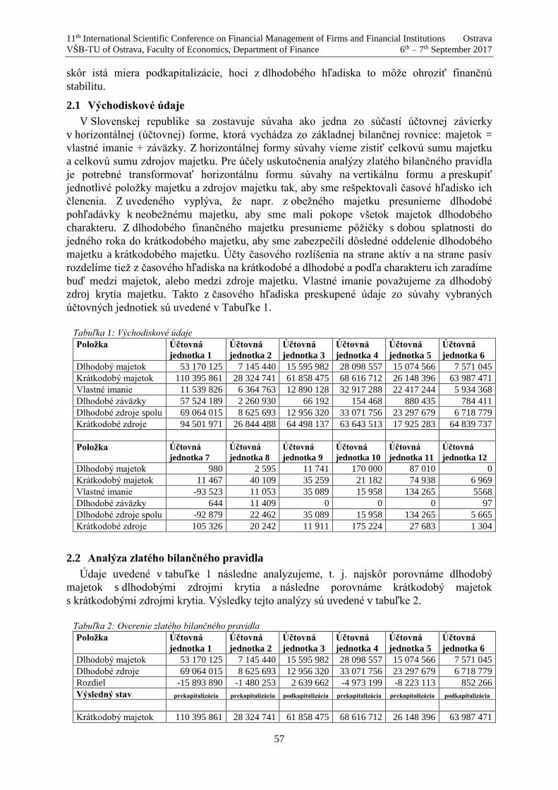
11th International Scientific Conference on Financial Management of Firms and Financial Institutions Ostrava
VŠB-TU of Ostrava, Faculty of Economics, Department of Finance 6th – 7th September 2017
57
skôr istá miera podkapitalizácie, hoci z dlhodobého hľadiska to môže ohroziť finančnú
stabilitu.
2.1 Východiskové údaje
V Slovenskej republike sa zostavuje súvaha ako jedna zo súčastí účtovnej závierky
v horizontálnej (účtovnej) forme, ktorá vychádza zo základnej bilančnej rovnice: majetok =
vlastné imanie + záväzky. Z horizontálnej formy súvahy vieme zistiť celkovú sumu majetku
a celkovú sumu zdrojov majetku. Pre účely uskutočnenia analýzy zlatého bilančného pravidla
je potrebné transformovať horizontálnu formu súvahy na vertikálnu formu a preskupiť
jednotlivé položky majetku a zdrojov majetku tak, aby sme rešpektovali časové hľadisko ich
členenia. Z uvedeného vyplýva, že napr. z obežného majetku presunieme dlhodobé
pohľadávky k neobežnému majetku, aby sme mali pokope všetok majetok dlhodobého
charakteru. Z dlhodobého finančného majetku presunieme pôžičky s dobou splatnosti do
jedného roka do krátkodobého majetku, aby sme zabezpečili dôsledné oddelenie dlhodobého
majetku a krátkodobého majetku. Účty časového rozlíšenia na strane aktív a na strane pasív
rozdelíme tiež z časového hľadiska na krátkodobé a dlhodobé a podľa charakteru ich zaradíme
buď medzi majetok, alebo medzi zdroje majetku. Vlastné imanie považujeme za dlhodobý
zdroj krytia majetku. Takto z časového hľadiska preskupené údaje zo súvahy vybraných
účtovných jednotiek sú uvedené v Tabuľke 1.
Tabuľka 1: Východiskové údaje
Položka Účtovná
jednotka 1
Účtovná
jednotka 2
Účtovná
jednotka 3
Účtovná
jednotka 4
Účtovná
jednotka 5
Účtovná
jednotka 6
Dlhodobý majetok 53 170 125 7 145 440 15 595 982 28 098 557 15 074 566 7 571 045
Krátkodobý majetok 110 395 861 28 324 741 61 858 475 68 616 712 26 148 396 63 987 471
Vlastné imanie 11 539 826 6 364 763 12 890 128 32 917 288 22 417 244 5 934 368
Dlhodobé záväzky 57 524 189 2 260 930 66 192 154 468 880 435 784 411
Dlhodobé zdroje spolu 69 064 015 8 625 693 12 956 320 33 071 756 23 297 679 6 718 779
Krátkodobé zdroje 94 501 971 26 844 488 64 498 137 63 643 513 17 925 283 64 839 737
Položka Účtovná
jednotka 7
Účtovná
jednotka 8
Účtovná
jednotka 9
Účtovná
jednotka 10
Účtovná
jednotka 11
Účtovná
jednotka 12
Dlhodobý majetok 980 2 595 11 741 170 000 87 010 0
Krátkodobý majetok 11 467 40 109 35 259 21 182 74 938 6 969
Vlastné imanie -93 523 11 053 35 089 15 958 134 265 5568
Dlhodobé záväzky 644 11 409 0 0 0 97
Dlhodobé zdroje spolu -92 879 22 462 35 089 15 958 134 265 5 665
Krátkodobé zdroje 105 326 20 242 11 911 175 224 27 683 1 304
2.2 Analýza zlatého bilančného pravidla
Údaje uvedené v tabuľke 1 následne analyzujeme, t. j. najskôr porovnáme dlhodobý
majetok s dlhodobými zdrojmi krytia a následne porovnáme krátkodobý majetok
s krátkodobými zdrojmi krytia. Výsledky tejto analýzy sú uvedené v tabuľke 2.
Tabuľka 2: Overenie zlatého bilančného pravidla
Položka Účtovná
jednotka 1
Účtovná
jednotka 2
Účtovná
jednotka 3
Účtovná
jednotka 4
Účtovná
jednotka 5
Účtovná
jednotka 6
Dlhodobý majetok 53 170 125 7 145 440 15 595 982 28 098 557 15 074 566 7 571 045
Dlhodobé zdroje 69 064 015 8 625 693 12 956 320 33 071 756 23 297 679 6 718 779
Rozdiel -15 893 890 -1 480 253 2 639 662 -4 973 199 -8 223 113 852 266
Výsledný stav prekapitalizácia prekapitalizácia podkapitalizácia prekapitalizácia prekapitalizácia podkapitalizácia
Krátkodobý majetok 110 395 861 28 324 741 61 858 475 68 616 712 26 148 396 63 987 471
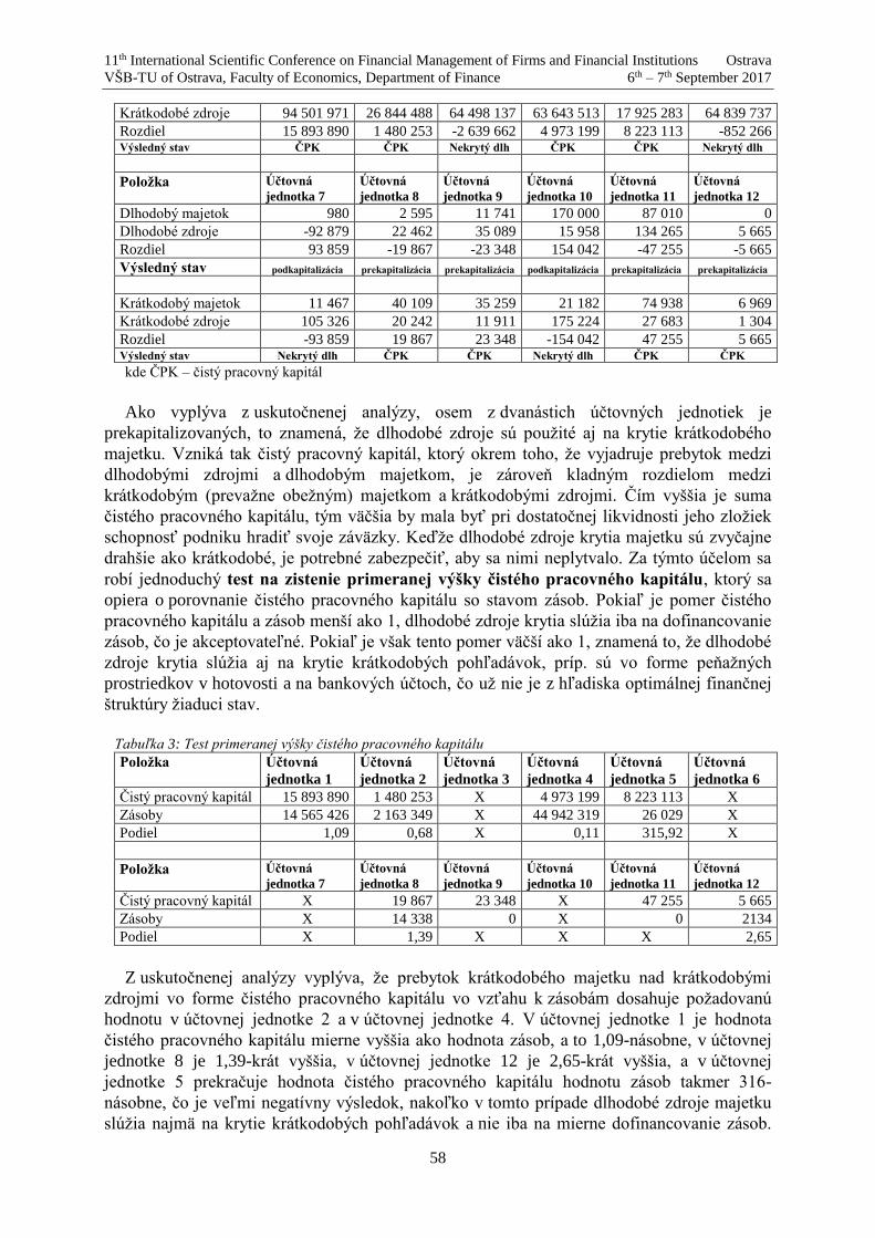
11th International Scientific Conference on Financial Management of Firms and Financial Institutions Ostrava
VŠB-TU of Ostrava, Faculty of Economics, Department of Finance 6th – 7th September 2017
58
Krátkodobé zdroje 94 501 971 26 844 488 64 498 137 63 643 513 17 925 283 64 839 737
Rozdiel 15 893 890 1 480 253 -2 639 662 4 973 199 8 223 113 -852 266 Výsledný stav ČPK ČPK Nekrytý dlh ČPK ČPK Nekrytý dlh
Položka Účtovná
jednotka 7
Účtovná
jednotka 8
Účtovná
jednotka 9
Účtovná
jednotka 10
Účtovná
jednotka 11
Účtovná
jednotka 12
Dlhodobý majetok 980 2 595 11 741 170 000 87 010 0
Dlhodobé zdroje -92 879 22 462 35 089 15 958 134 265 5 665
Rozdiel 93 859 -19 867 -23 348 154 042 -47 255 -5 665
Výsledný stav podkapitalizácia prekapitalizácia prekapitalizácia podkapitalizácia prekapitalizácia prekapitalizácia
Krátkodobý majetok 11 467 40 109 35 259 21 182 74 938 6 969
Krátkodobé zdroje 105 326 20 242 11 911 175 224 27 683 1 304
Rozdiel -93 859 19 867 23 348 -154 042 47 255 5 665 Výsledný stav Nekrytý dlh ČPK ČPK Nekrytý dlh ČPK ČPK
kde ČPK – čistý pracovný kapitál
Ako vyplýva z uskutočnenej analýzy, osem z dvanástich účtovných jednotiek je
prekapitalizovaných, to znamená, že dlhodobé zdroje sú použité aj na krytie krátkodobého
majetku. Vzniká tak čistý pracovný kapitál, ktorý okrem toho, že vyjadruje prebytok medzi
dlhodobými zdrojmi a dlhodobým majetkom, je zároveň kladným rozdielom medzi
krátkodobým (prevažne obežným) majetkom a krátkodobými zdrojmi. Čím vyššia je suma
čistého pracovného kapitálu, tým väčšia by mala byť pri dostatočnej likvidnosti jeho zložiek
schopnosť podniku hradiť svoje záväzky. Keďže dlhodobé zdroje krytia majetku sú zvyčajne
drahšie ako krátkodobé, je potrebné zabezpečiť, aby sa nimi neplytvalo. Za týmto účelom sa
robí jednoduchý test na zistenie primeranej výšky čistého pracovného kapitálu, ktorý sa
opiera o porovnanie čistého pracovného kapitálu so stavom zásob. Pokiaľ je pomer čistého
pracovného kapitálu a zásob menší ako 1, dlhodobé zdroje krytia slúžia iba na dofinancovanie
zásob, čo je akceptovateľné. Pokiaľ je však tento pomer väčší ako 1, znamená to, že dlhodobé
zdroje krytia slúžia aj na krytie krátkodobých pohľadávok, príp. sú vo forme peňažných
prostriedkov v hotovosti a na bankových účtoch, čo už nie je z hľadiska optimálnej finančnej
štruktúry žiaduci stav.
Tabuľka 3: Test primeranej výšky čistého pracovného kapitálu
Položka Účtovná
jednotka 1
Účtovná
jednotka 2
Účtovná
jednotka 3
Účtovná
jednotka 4
Účtovná
jednotka 5
Účtovná
jednotka 6
Čistý pracovný kapitál 15 893 890 1 480 253 X 4 973 199 8 223 113 X
Zásoby 14 565 426 2 163 349 X 44 942 319 26 029 X
Podiel 1,09 0,68 X 0,11 315,92 X
Položka Účtovná
jednotka 7
Účtovná
jednotka 8
Účtovná
jednotka 9
Účtovná
jednotka 10
Účtovná
jednotka 11
Účtovná
jednotka 12
Čistý pracovný kapitál X 19 867 23 348 X 47 255 5 665
Zásoby X 14 338 0 X 0 2134
Podiel X 1,39 X X X 2,65
Z uskutočnenej analýzy vyplýva, že prebytok krátkodobého majetku nad krátkodobými
zdrojmi vo forme čistého pracovného kapitálu vo vzťahu k zásobám dosahuje požadovanú
hodnotu v účtovnej jednotke 2 a v účtovnej jednotke 4. V účtovnej jednotke 1 je hodnota
čistého pracovného kapitálu mierne vyššia ako hodnota zásob, a to 1,09-násobne, v účtovnej
jednotke 8 je 1,39-krát vyššia, v účtovnej jednotke 12 je 2,65-krát vyššia, a v účtovnej
jednotke 5 prekračuje hodnota čistého pracovného kapitálu hodnotu zásob takmer 316-
násobne, čo je veľmi negatívny výsledok, nakoľko v tomto prípade dlhodobé zdroje majetku
slúžia najmä na krytie krátkodobých pohľadávok a nie iba na mierne dofinancovanie zásob.

11th International Scientific Conference on Financial Management of Firms and Financial Institutions Ostrava
VŠB-TU of Ostrava, Faculty of Economics, Department of Finance 6th – 7th September 2017
59
Táto skutočnosť je pre účtovnú jednotku 5 veľmi negatívna a nežiaduca z hľadiska jej
finančnej stability. Účtovné jednotky 9 a 11 nevykazujú žiaden stav zásob, čo je taktiež
negatívny jav z hľadiska hodnoty tohto ukazovateľa, pretože v tomto prípade sú dlhodobé
zdroje použité na financovanie krátkodobých pohľadávok a krátkodobého finančného majetku
vo forme peňažných prostriedkov v hotovosti a na bankových účtoch, čo je pre účtovnú
jednotku neefektívne.
Účtovné jednotky 3, 6, 7 a 10 sú podkapitalizované, to znamená, že na krytie dlhodobého
majetku používajú aj krátkodobé zdroje krytia. Zároveň je suma krátkodobého majetku nižšia
ako suma krátkodobých záväzkov, čím vzniká nekrytý dlh, ktorý môže mať nepriaznivé
dôsledky na finančnú situáciu účtovnej jednotky, nakoľko táto nemá dostatok prostriedkov na
úhradu krátkodobých záväzkov a je ohrozená jej likvidita. Účtovná jednotka 7 sa nachádza vo
veľmi zlej finančnej situácii vzhľadom na zápornú hodnotu vlastného imania.
Na zistenie úrovne dodržania zlatého bilančného pravidla sa používajú aj dva pomerové
ukazovatele označované ako stupne krytia majetku. Prvý, ktorý vyjadruje pomer medzi
vlastným imaním a dlhodobým majetkom, sa označuje ako stupeň krytia dlhodobého
majetku vlastným imaním. Druhý ukazovateľ vyjadrujúci pomer medzi všetkými
dlhodobými zdrojmi majetku a dlhodobým majetkom sa označuje ako stupeň krytia
dlhodobého majetku dlhodobými zdrojmi. Pri oboch ukazovateľoch je žiaduce, aby
dosahovali čo najvyššie hodnoty. Niektorí autori považujú za minimálnu hodnotu prvého
ukazovateľa hodnotu aspoň 75 % a druhého ukazovateľa hodnotu 100 %, čo je v konečnom
dôsledku aj podstata zlatého bilančného pravidla, podľa ktorého má byť dlhodobý majetok
krytý dlhodobými zdrojmi krytia a krátkodobý majetok krytý krátkodobými zdrojmi krytia.
Tabuľka 4: Overenie dodržania zlatého bilančného pravidla
Položka Účtovná
jednotka 1
Účtovná
jednotka 2
Účtovná
jednotka 3
Účtovná
jednotka 4
Účtovná
jednotka 5
Účtovná
jednotka 6
Dlhodobý majetok 53 170 125 7 145 440 15 595 982 28 098 557 15 074 566 7 571 045
Vlastné imanie 11 539 826 6 364 763 12 890 128 32 917 288 22 417 244 5 934 368
Dlhodobé zdroje 69 064 015 8 625 693 12 956 320 33 071 756 23 297 679 6 718 779
Stupeň krytia
dlhodobého majetku
vlastným imaním v % 21,70% 89,07% 82,65% 117,15% 148,71% 78,38%
Stupeň krytia
dlhodobého majetku
dlhodobými zdrojmi v
% 129,89% 120,72% 83,07% 117,70% 154,55% 88,74%
Položka Účtovná
jednotka 7
Účtovná
jednotka 8
Účtovná
jednotka 9
Účtovná
jednotka 10
Účtovná
jednotka 11
Účtovná
jednotka 12
Dlhodobý majetok 980 2 595 11 741 170 000 87 010 0
Vlastné imanie -93 523 11 053 35 089 15 958 134 265 5568
Dlhodobé zdroje -92 879 22 462 35 089 15 958 134 265 5 665
Stupeň krytia
dlhodobého majetku
vlastným imaním v % -9543,16% 425,93% 298,86% 9,39% 154,31% X
Stupeň krytia
dlhodobého majetku
dlhodobými zdrojmi v
% -9477,45% 865,59% 298,86% 9,39% 154,31% X
Ako vyplýva z uskutočnenej analýzy, v prípade ukazovateľa stupňa krytia dlhodobého
majetku vlastným imaním, kde žiaduca hodnota je približne na úrovni 75 %, je ideálny stav
v účtovnej jednotke 6, v ktorej tento ukazovateľ dosahuje hodnotu na úrovni 78,38 %. Za

11th International Scientific Conference on Financial Management of Firms and Financial Institutions Ostrava
VŠB-TU of Ostrava, Faculty of Economics, Department of Finance 6th – 7th September 2017
60
pozitívny stav môžeme považovať aj hodnotu tohto ukazovateľa v účtovných jednotkách 2
a 3, kde prekračuje ideálne hodnoty o pár percent. Veľmi nepriaznivá situácia je v účtovnej
jednotke 1, ktorá má veľmi nízku hodnotu vlastného imania v pomere ku dlhodobému
majetku. V účtovnej jednotke 5 práve naopak, stav vlastného imania až o 48,71 % prekračuje
hodnotu dlhodobého majetku, čo nemusí pôsobiť veľmi priaznivo z hľadiska ideálnej
finančnej štruktúry a stability účtovnej jednotky, nakoľko účtovná jednotka má vysoký stav
vlastných zdrojov krytia majetku (tie sú považované za drahšie). V šestici menších účtovných
jednotiek (t. j. účtovných jednotkách 7 až 12) je situácia veľmi nepriaznivá. Účtovná jednotka
7 vzhľadom na zápornú hodnotu vlastného imania, dosahuje aj zápornú hodnotu tohto
ukazovateľa, t. j. majetok nevie pokryť vlastnými zdrojmi. Účtovná jednotka 12 nemá žiaden
dlhodobý majetok, preto je výpočet týchto ukazovateľov bezpredmetný. V účtovných
jednotkách 8, 9 a 11 dosahuje ukazovateľ krytia dlhodobého majetku vlastným imaním príliš
vysoké hodnoty, čo je dôsledkom prekapitalizácie, ktorá je však v týchto účtovných
jednotkách zbytočne príliš vysoká. Vysoká miera prekapitalizácie môže byť výsledkom príliš
veľkej opatrnosti účtovnej jednotky a nedostatočného využívania cudzích zdrojov. Účtovná
jednotka 10 má hodnotu tohto ukazovateľa príliš nízku, iba na úrovní 9,39 %, čo vyplýva zo
skutočnosti, že v tejto účtovnej jednotke je vysoká suma dlhodobého majetku, avšak veľmi
nízka úroveň vlastného imania v pomere k tomuto dlhodobému majetku.
Pokiaľ porovnáme vzťah medzi celkovými dlhodobými zdrojmi a dlhodobým majetkom,
ani jedna účtovná jednotka nedosahuje ideálne hodnoty, účtovné jednotky 1, 2 a 4 mierne
prekračujú túto odporúčanú hranicu. Horšia situácia je v účtovnej jednotke 5, kde je tento
pomer o 54,55 % väčší ako odporúčaná hodnota. Účtovné jednotky 9, 10 a 11 dosahujú
hodnoty tohto ukazovateľa na rovnakej úrovni, ako boli hodnoty predchádzajúceho
ukazovateľa práve v dôsledku absencie dlhodobých záväzkov, pretože celkové dlhodobé
zdroje sú v rovnakej výške ako hodnota vlastného imania. Naopak v účtovných jednotkách 3
a 6, ktoré sú podkapitalizované, dosahuje tento ukazovateľ nižšie než odporúčané hodnoty. Je
to z dôvodu, že dlhodobý majetok je vyšší ako dlhodobé zdroje krytia a preto je časť
dlhodobého majetku krytá aj krátkodobými zdrojmi majetku. Účtovná jednotka 7 dosahuje
záporné hodnoty aj u tohto ukazovateľa vzhľadom na to, že vysokú sumu záporného vlastného
imania nedokáže kompenzovať dlhodobými záväzkami. V účtovnej jednotke 8 je hodnota
dlhodobého majetku v porovnaní s dlhodobými zdrojmi príliš nízka, preto hodnota
ukazovateľa stupňa krytia dlhodobého majetku dlhodobými zdrojmi dosahuje hodnotu 865,59
%. Účtovná jednotka tak vykazuje zbytočne vysokú mieru prekapitalizácie.
3. Vyhodnotenie výsledkov výskumu
Cieľom príspevku bolo na základe uskutočnenej analýzy aplikácie zlatého bilančného
pravidla v konkrétnych vybraných účtovných jednotkách overiť, t. j. potvrdiť alebo vyvrátiť,
hypotézu, že pre podnikateľské účtovné jednotky je charakteristická skôr mierna
podkapitalizácia, a to i napriek skutočnosti, že z dlhodobého hľadiska to môže ohrozovať
finančnú stabilitu účtovnej jednotky.
Pre overenie hypotézy sme si vybrali dvanásť účtovných jednotiek, v ktorých sme skúmali
vzájomné vzťahy medzi majetkom a zdrojmi majetku. Z analyzovaných účtovných jednotiek
sme u ôsmich účtovných jednotiek zaznamenali prekapitalizáciu, štyri účtovné jednotky boli
podkapitalizované.
Z hľadiska finančnej stability je pre účtovné jednotky výhodnejšia určitá miera
prekapitalizácie, čiže situácia, keď je suma dlhodobých zdrojov krytia vyššia ako suma
dlhodobého majetku, ktorý je týmito dlhodobými zdrojmi krytý, a účtovnej jednotke vzniká
čistý pracovný kapitál. Prekapitalizácia je však ideálna iba za podmienky, že podiel čistého

11th International Scientific Conference on Financial Management of Firms and Financial Institutions Ostrava
VŠB-TU of Ostrava, Faculty of Economics, Department of Finance 6th – 7th September 2017
61
pracovného kapitálu a zásob je menší ako 1. V tomto prípade je časť dlhodobých zdrojov
majetku použitá najmä na dočasné financovanie zásob. V opačnom prípade sú dlhodobé
zdroje majetku uložené v podobe krátkodobých pohľadávok a peňažných prostriedkov či už
v hotovosti, alebo na bankových účtoch, čo z hľadiska optimálnej finančnej štruktúry nie je
žiaduci jav. Z ôsmich účtovných jednotiek, ktoré vykazovali prekapitalizáciu, iba dve účtovné
jednotky prešli testom primeranej výšky čistého pracovného kapitálu.
Potreba čistého pracovného kapitálu je dôležitá aj z hľadiska skúmania ukazovateľov
likvidity a analýzy platobnej schopnosti účtovnej jednotky. V prípade podkapitalizácie, keď
má účtovná jednotka nedostatok krátkodobého majetku na úhradu krátkodobých záväzkov,
vzniká nekrytý dlh, ktorý môže mať za následok ohrozenie likvidity a platobnej disciplíny
účtovnej jednotky.
V nami vybraných účtovných jednotkách bola aj suma vlastného imania, t. j. vlastných
zdrojov financovania dostatočne vysoká, preto sme zaznamenali viac účtovných jednotiek,
ktoré sú skôr prekapitalizované, než podkapitalizované. Dokonca aj v účtovných jednotkách 7
až 12, ktoré boli veľkosťou skôr mikro, resp. malými, účtovnými jednotkami, dosahovalo
vlastného imanie dosť vysoké hodnoty (hoci takmer všetky tieto menšie účtovné jednotky
tvorili základné imanie iba v zákonom stanovenej výške), s výnimkou účtovnej jednotky 6,
ktorej hodnota vlastného imania bola záporná. Náš predpoklad, že pre menšie účtovné
jednotky je charakteristickým znakom podkapitalizácia práve z dôvodu, že v týchto účtovných
jednotkách je suma vlastného imania nižšia, sa nepotvrdil.
Z výskumu vyplynul záver, že podkapitalizácia v podnikateľských účtovných jednotkách
nemusí byť pravidlom a aj menšie podnikateľské účtovné jednotky vykazujú istú mieru
prekapitalizácie. Prekapitalizácia je pozitívny jav aj z hľadiska hodnotenia finančnej situácie
účtovnej jednotky, podkapitalizácia je jav skôr negatívny. Podkapitalizácia sa totiž prejaví
v tom, že účtovná jednotka má sumu krátkodobého majetku menšiu než sumu krátkodobých
záväzkov a teda je ohrozená jej likvidita a platobná schopnosť.
V tejto súvislosti je dôležité uviesť, že skúmaná vzorka účtovných jednotiek bola príliš
malá. Z hľadiska zabezpečenia vyššej vypovedacej schopnosti skúmaných skutočností by
určite pomohla analýza väčšieho počtu účtovných jednotiek.
References
[1] Kovanicová, D. (2005). Finanční účetnictví. Světový koncept. Praha: BOVA POLYGON.
[2] Šlosárová, A. and Blahušiaková, M. (2017). Analýza účtovnej závierky. Bratislava:
Wolters Kluwer.
[3] Opatrenie Ministerstva financií Slovenskej republiky č. 23054/2002-92, ktorým sa
ustanovujú podrobnosti o postupoch účtovania a rámcovej účtovej osnove pre
podnikateľov účtujúcich v sústave podvojného účtovníctva v znení neskorších predpisov.
11th International Scientific Conference on Financial Management of Firms and Financial Institutions Ostrava
VŠB-TU of Ostrava, Faculty of Economics, Department of Finance 6th – 7th September 2017
62
Corporate reputation, ownership structure and market value in the banking sector in Poland
Anna Blajer-Gołębiewska1
Abstract
The aim of this study was to identify an impact of corporate reputation, ownership structure and
selected financial characteristics on the market value of companies in the banking sector in
Poland. On the basis of a panel data model with random individual effects and fixed time
effects, we found that the main factor enhancing market value is return on equity. Other
statistically significant determinants of market valuation were: percentage of shares possessed
by institutional shareholders, the fact that a company is paying dividends, and the size of a
company. We applied two proxies for corporate reputation: points achieved in the ranking of
Responsible Businesses and inclusion into the RESPECT Index. None of them was found to be
a significant predictor of market valuation of firms from the banking sector in Poland.
Key words
Corporate reputation, ownership structure, institutional investors, market value, financial
markets.
JEL Classification: L14; G32; G23; G11; D46; D53.
1. Introduction
The market value of a company reflects a value that investors are willing to pay for this
company. It is a function not only of its financial results, but also of other factors constituting
an attitude of investors towards the company such as corporate reputation or ownership
structure.
Regarding ownership structure, there are many indicators, which can be analysed, such as
institutional ownership, governmental ownership, insider ownership, etc. These indicators are
directly observable and unequivocal.
As corporate reputation is not directly observable, there is plenty of measurement methods
and consequently, many variables representing its level. This variety of attempts results from
its definition, which states that corporate reputation (CR) is a function of collective
judgements of a given firm based on its financial, social, and environmental performance,
which changes over time (Fombrun and Van Riel, 1997; Scott and Walsham, 2005). As
specific intangible asset, corporate reputation is able to generate wealth.
Regarding corporate reputation, its impact on market value is often analysed in the case of
banking sector (Fiordelisi, Soana and Schwizer, 2013; Trotta and Cavallaro, 2012; Gillet,
Hübner and Plunus, 2010; Ebert, 2009, pp. 60-67). However, the results of some previous
studies in this relationship for the Polish banking sector, based on an event study, were not
conclusive (Blajer-Gołębiewska, 2014a).
Thus, the aim of this study is to identify an impact of corporate reputation, ownership
structure and selected financial characteristics on market valuation of companies in the
banking sector in Poland.
1 Anna Blajer-Gołębiewska, Ph.D., University of Gdansk, Faculty of Economics, [email protected].

11th International Scientific Conference on Financial Management of Firms and Financial Institutions Ostrava
VŠB-TU of Ostrava, Faculty of Economics, Department of Finance 6th – 7th September 2017
63
The article is structured as follows. The next section provides a brief overview of literature
on previous research on relationships between corporate reputation, ownership structure,
financial characteristics and market value. In the following section, the applied methodology
is outlined. In the penultimate section, findings on these relationships are presented and
discussed. The final section provides summary and conclusions.
2. Literature overview
On the one hand, corporate reputation influences investors’ behaviours creating market
value of a company, but on the other, market value could be a signal of company’s reputation
for investors (Roberts and Dowling, 2002). In the literature, one can find lots of studies
exploring an impact of CR on stock market valuation. In these studies, measures of CR were
mainly based on reputational ranking of the Most Admired Companies (Cole, 2012; Smith,
Smith and Wang, 2010; Brammer, Brooks and Pavelin, 2006; Black, Carnes and Richardson,
2000) or on other rankings such as MERCO – the ranking of Spanish listed companies:
(Fernández-Gámez, Gil-Corral and Galán-Valdivieso, 2016). Some authors use specific
measures for CR, such as perception of the general public based on surveys (Raithel and
Schwaiger, 2015) or mass-media-based CR (Agnihotri, 2014). Moreover, authors incorporate
often some financial characteristics such as: BV, ROE, ROA, total assets, total liabilities and
others (table 1).
Although higher CR is expected to increase market valuation, results of previous studies
are sometimes inconsistent or inconclusive.These studies reveal mainly a positive relationship
between CR and market value (Fernández-Gámez, Gil-Corral and Galán-Valdivieso, 2016;
Raithel and Schwaiger, 2015; Agnihotri, 2014; Cole, 2012; Smith, Smith and Wang, 2010;
Brammer, Brooks and Pavelin, 2006; Vergin and Qoronfleh, 1998 and others; table 1). Black,
Carnes and Richardson (2000) decomposed CR into a non-financial component and a
financial component and they found a positive relationship with market value for both
components. Brammer, Brooks and Pavelin (2006) found that not only an increase, but also a
decrease in CR can cause higher market value, so it seems that for investors ‘any news is a
good news’.
As mentioned above, regarding CR problems, banking sector is the one which is very often
analysed (Blajer-Gołębiewska, 2014a; Fiordelisi, Soana and Schwizer, 2013; Trotta and
Cavallaro, 2012; Gillet, Hübner and Plunus, 2010; Ebert, 2009). Previous studies on CR in the
banking sector in Poland revealed that more effective management (expressed in higher levels
of ROE and ROA) leads to higher levels of ‚reputational characteristics‘, such as responsible
leadership, dialogue with shareholders, social commitment, responsible management, and
social innovation, in the next few years (Blajer-Gołębiewska, 2014a). An event study on
importance of CR for investors revealed that an effect of an increase in reputation has no
conclusive impact on investors’ interest in a company, i.e. on higher abnormal returns not only
in the banking sector, but also in other sectors in Poland (Blajer-Gołębiewska, 2014 a, 2014b).
According to literature about descriptors of market value of a company, ownership
structure and dividend yield are often mentioned. Desender, Garcia Cestona and Crespi
Cladera (2008) found that insider ownership and the number of foreign shareholders are
positively related to market value. However, ownership concentration and the number of
financial shareholders are negatively related to market value. Stock market performance of
family controlled firms is better than in cases of non-family controlled firms, especially when
it comes to founding families. Furthermore, during periods of crisis ‘insider ownership and
ownership concentration are important to explain stock price adjustments‘ (Desender, Garcia
Cestona and Crespi Cladera, 2008, p. 1).
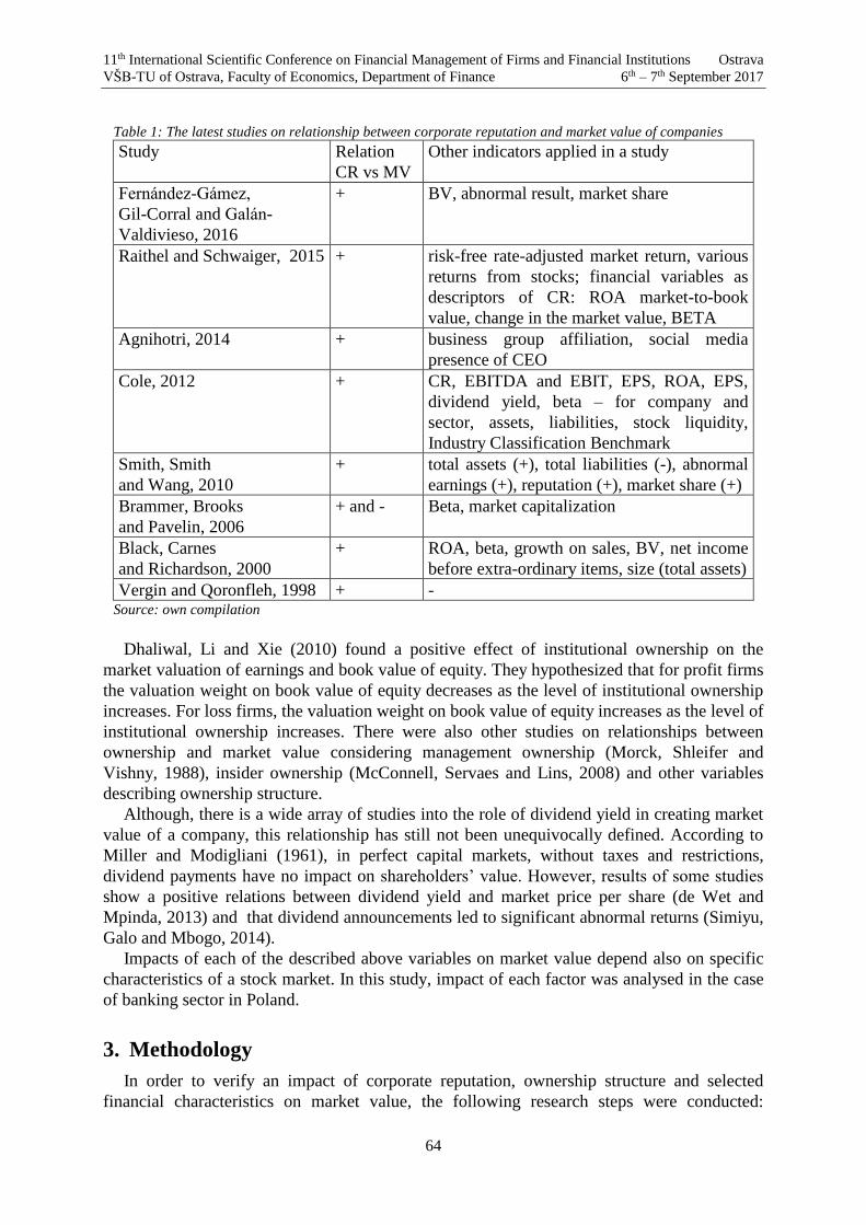
11th International Scientific Conference on Financial Management of Firms and Financial Institutions Ostrava
VŠB-TU of Ostrava, Faculty of Economics, Department of Finance 6th – 7th September 2017
64
Table 1: The latest studies on relationship between corporate reputation and market value of companies
Study Relation
CR vs MV
Other indicators applied in a study
Fernández-Gámez,
Gil-Corral and Galán-
Valdivieso, 2016
+ BV, abnormal result, market share
Raithel and Schwaiger, 2015 + risk-free rate-adjusted market return, various
returns from stocks; financial variables as
descriptors of CR: ROA market-to-book
value, change in the market value, BETA
Agnihotri, 2014 + business group affiliation, social media
presence of CEO
Cole, 2012 + CR, EBITDA and EBIT, EPS, ROA, EPS,
dividend yield, beta – for company and
sector, assets, liabilities, stock liquidity,
Industry Classification Benchmark
Smith, Smith
and Wang, 2010
+ total assets (+), total liabilities (-), abnormal
earnings (+), reputation (+), market share (+)
Brammer, Brooks
and Pavelin, 2006
+ and - Beta, market capitalization
Black, Carnes
and Richardson, 2000
+ ROA, beta, growth on sales, BV, net income
before extra-ordinary items, size (total assets)
Vergin and Qoronfleh, 1998 + - Source: own compilation
Dhaliwal, Li and Xie (2010) found a positive effect of institutional ownership on the
market valuation of earnings and book value of equity. They hypothesized that for profit firms
the valuation weight on book value of equity decreases as the level of institutional ownership
increases. For loss firms, the valuation weight on book value of equity increases as the level of
institutional ownership increases. There were also other studies on relationships between
ownership and market value considering management ownership (Morck, Shleifer and
Vishny, 1988), insider ownership (McConnell, Servaes and Lins, 2008) and other variables
describing ownership structure.
Although, there is a wide array of studies into the role of dividend yield in creating market
value of a company, this relationship has still not been unequivocally defined. According to
Miller and Modigliani (1961), in perfect capital markets, without taxes and restrictions,
dividend payments have no impact on shareholders’ value. However, results of some studies
show a positive relations between dividend yield and market price per share (de Wet and
Mpinda, 2013) and that dividend announcements led to significant abnormal returns (Simiyu,
Galo and Mbogo, 2014).
Impacts of each of the described above variables on market value depend also on specific
characteristics of a stock market. In this study, impact of each factor was analysed in the case
of banking sector in Poland.
3. Methodology
In order to verify an impact of corporate reputation, ownership structure and selected
financial characteristics on market value, the following research steps were conducted:
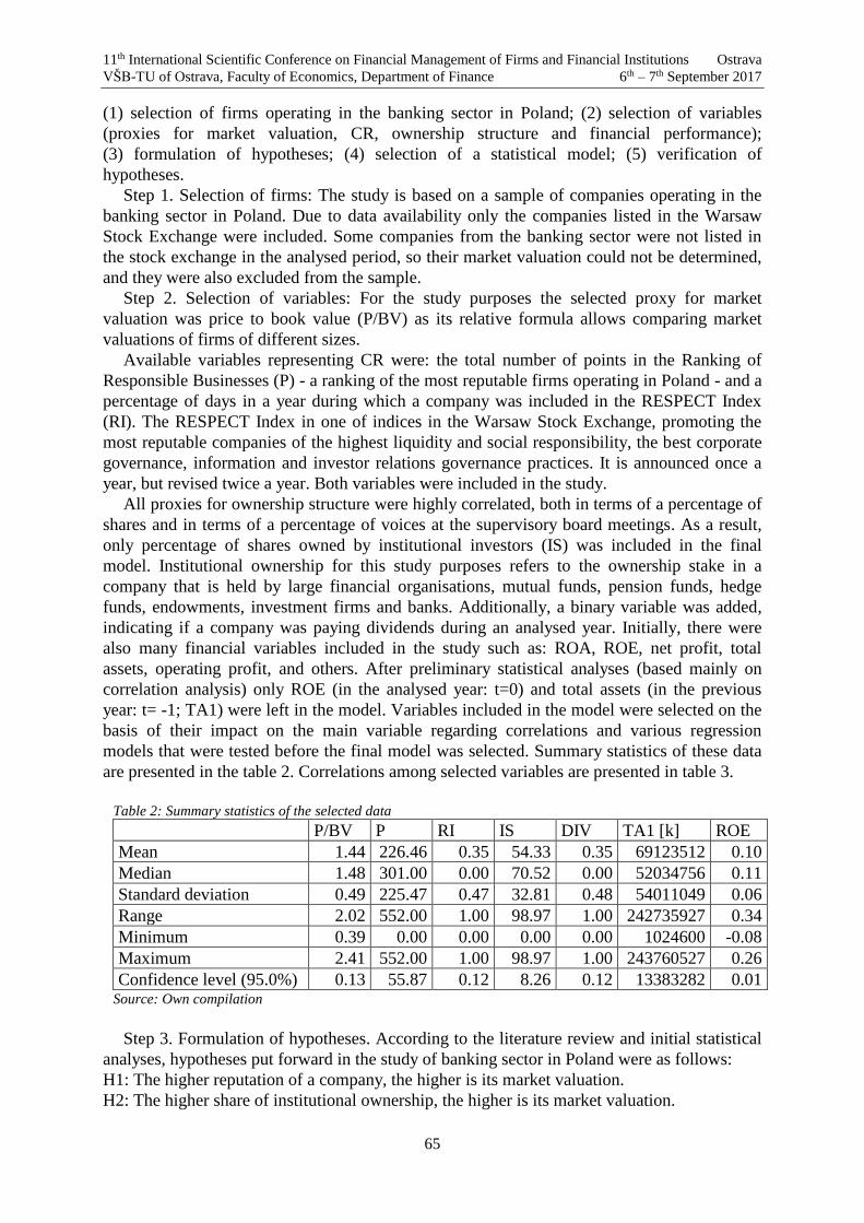
11th International Scientific Conference on Financial Management of Firms and Financial Institutions Ostrava
VŠB-TU of Ostrava, Faculty of Economics, Department of Finance 6th – 7th September 2017
65
(1) selection of firms operating in the banking sector in Poland; (2) selection of variables
(proxies for market valuation, CR, ownership structure and financial performance);
(3) formulation of hypotheses; (4) selection of a statistical model; (5) verification of
hypotheses.
Step 1. Selection of firms: The study is based on a sample of companies operating in the
banking sector in Poland. Due to data availability only the companies listed in the Warsaw
Stock Exchange were included. Some companies from the banking sector were not listed in
the stock exchange in the analysed period, so their market valuation could not be determined,
and they were also excluded from the sample.
Step 2. Selection of variables: For the study purposes the selected proxy for market
valuation was price to book value (P/BV) as its relative formula allows comparing market
valuations of firms of different sizes.
Available variables representing CR were: the total number of points in the Ranking of
Responsible Businesses (P) - a ranking of the most reputable firms operating in Poland - and a
percentage of days in a year during which a company was included in the RESPECT Index
(RI). The RESPECT Index in one of indices in the Warsaw Stock Exchange, promoting the
most reputable companies of the highest liquidity and social responsibility, the best corporate
governance, information and investor relations governance practices. It is announced once a
year, but revised twice a year. Both variables were included in the study.
All proxies for ownership structure were highly correlated, both in terms of a percentage of
shares and in terms of a percentage of voices at the supervisory board meetings. As a result,
only percentage of shares owned by institutional investors (IS) was included in the final
model. Institutional ownership for this study purposes refers to the ownership stake in a
company that is held by large financial organisations, mutual funds, pension funds, hedge
funds, endowments, investment firms and banks. Additionally, a binary variable was added,
indicating if a company was paying dividends during an analysed year. Initially, there were
also many financial variables included in the study such as: ROA, ROE, net profit, total
assets, operating profit, and others. After preliminary statistical analyses (based mainly on
correlation analysis) only ROE (in the analysed year: t=0) and total assets (in the previous
year: t= -1; TA1) were left in the model. Variables included in the model were selected on the
basis of their impact on the main variable regarding correlations and various regression
models that were tested before the final model was selected. Summary statistics of these data
are presented in the table 2. Correlations among selected variables are presented in table 3.
Table 2: Summary statistics of the selected data
P/BV P RI IS DIV TA1 [k] ROE
Mean 1.44 226.46 0.35 54.33 0.35 69123512 0.10
Median 1.48 301.00 0.00 70.52 0.00 52034756 0.11
Standard deviation 0.49 225.47 0.47 32.81 0.48 54011049 0.06
Range 2.02 552.00 1.00 98.97 1.00 242735927 0.34
Minimum 0.39 0.00 0.00 0.00 0.00 1024600 -0.08
Maximum 2.41 552.00 1.00 98.97 1.00 243760527 0.26
Confidence level (95.0%) 0.13 55.87 0.12 8.26 0.12 13383282 0.01 Source: Own compilation
Step 3. Formulation of hypotheses. According to the literature review and initial statistical
analyses, hypotheses put forward in the study of banking sector in Poland were as follows:
H1: The higher reputation of a company, the higher is its market valuation.
H2: The higher share of institutional ownership, the higher is its market valuation.

11th International Scientific Conference on Financial Management of Firms and Financial Institutions Ostrava
VŠB-TU of Ostrava, Faculty of Economics, Department of Finance 6th – 7th September 2017
66
H3: The higher level of financial performance (ROE), the higher is its market valuation.
H4: Firms paying dividends are expected to have higher value in the market.
H5: The bigger the company, the higher is its market valuation.
Table 3: Correlations among selected variables
P/BV P RI IS DIV TA1
P 0.213 1.000
RI 0.173 0.684 1.000
IS 0.331 0.640 0.540 1.000
DIV 0.421 0.289 0.177 0.115 1.000
TA1 0.389 0.087 -0.118 -0.098 0.425 1.000
ROE 0.579 0.069 0.037 0.049 0.398 0.262 Source: Own compilation
Step 4. Considering the nature of the dataset, the panel data methods were chosen to verify
hypotheses. To test whether a fixed or a random individual effects model is more suitable for
our data set, we performed the Hausman tests (Hausman, 1978, pp. 1251-1271). In this test,
the null hypothesis states that coefficients in both (fixed and random effects) models are
consistent, but the random effects model is preferred due to higher efficiency. Regarding
results of the test [H = 3.1255; p-value = prob(χ2 (10) > 3.1255) = 0.9783], the null
hypothesis should be not be rejected, so we chose the random individual effects model.
Next, we conducted the Lagrange multiplier (LM) test. For random effects it is the
Breusch-Pagan test. The null hypothesis is that the variance across entities is constant, so data
should be treated as homogeneous and the simple pooled model would be adequate.
According to results achieved [LM = 42.2037; p-value = prob(χ2 (1) > 42.2037) = 4.93e-011],
p-value is small, so the null hypothesis should be rejected. In other words, the individual
effects are significant.
Furthermore, in order to check if time effects should be included in the model, we
conducted the Wald joint test on time dummies where the null hypothesis states that there are
no time effects. Regarding results of the test [χ2(4) = 19.3624; p-value = 0.0013], the null
hypothesis should be rejected, so the time-dummies should be included in the model.
As a result, we applied a panel data model with random individual effect and fixed time
effects. The final dataset should consist of 455 unit observations: 7 variables analysed for 13
companies from the banking sector in Poland listed on the Warsaw Stock Exchange in years
2011-2015. However, 8 observations concerning market valuation were missing, because not
all companies included in the data set were listed on the stock exchange during the whole
period of analysis. Moreover, 2 observations on ownership structure were unavailable. These
resulted in unbalanced panel data.
Verification of hypotheses (step 5) is presented in the next section.
4. Findings
Coefficients estimated in the described above model for the banking sector are presented in
table 4. The dependent variable was price to book value ratio (P/BV). In cases of 84% of all
observations price value was higher than book value (P/BV > 1). According to the model,
significant determinants of P/BV are return on equity (ROE), percentage of shares possessed
by institutional shareholders (IS), the fact that a company is paying dividends (DIV) and the
size of a company (TA1; table 4). The highest impact occurs in the case of ROE (ROE;
coeff.= 2.9882, p-value=0.0097). Percentage of shares possessed by institutional shareholders,

11th International Scientific Conference on Financial Management of Firms and Financial Institutions Ostrava
VŠB-TU of Ostrava, Faculty of Economics, Department of Finance 6th – 7th September 2017
67
dividends, and the size of a company are significant with p-value lower than 0.05. The model
could be better fitted to the data, R2 coefficient equals 0.5174.
Table 4: Individual random effects model (GLS)
Dependent variable: P/BV
variable coefficient std. error z p-value
const. 0.7267 0.2065 3.5190 0.0004 ***
RI -0.0257 0.1507 -0.1707 0.8645
P -0.0001 0.0003 -0.4277 0.6689
IS 0.0046 0.0025 1.8400 0.0658 *
DIV 0.1479 0.0876 1.6890 0.0913 *
TA1 0.0000 0.0000 1.6510 0.0988 *
ROE 2.9882 1.1559 2.5850 0.0097 ***
dt_2 -0.1523 0.0960 -1.5860 0.1126
dt_3 0.0150 0.0964 0.1553 0.8766
dt_4 0.2036 0.0971 2.0980 0.0359 **
dt_5 -0.0792 0.1158 -0.6836 0.4942
corr(y,yhat)^2 = 0.5174
Statistical tests for individual effects
test statistics (χ2) df p-value
Hausman tests for panel model (random vs. fixed
effects) 3.1255 10 0.9783
Lagrange multiplier (Breush-Pagan) tests for
individual and time effects 43.2037 1 4.93e-011
Wald joint test on time dummies 19.3624 4 0.0007
Joint test on named regressors 21.8901 6 0.0013
Other statistics
Sum of squared residuals 6.5199 Standard Error of regression 0.3725
Log-likelihood -19.0862 Akaike criterion 60.1723
Bayes. Schwarz criterion 82.6459 Hannan-Quinn 68.9063 Source: Own compilation
An interesting fact is that none of variables representing CR was significant in the model.
In other words, neither the number of points in the reputational ranking, not the inclusion in
the RESPECT Index has an impact on firm’s market value. This fact is consistent with
previous studies that revealed that an effect of an increase in CR has no conclusive impact on
investors’ interest in a company (Blajer-Gołębiewska, 2014a, 2014b).
5. Summary and conclusions
We contribute to the current literature, firstly, by analysing investors decisions reflected in
market valuations of banks in the relatively young stock exchange. Moreover, we combined
not only financial factors with corporate reputation (which is quite common in the literature),
but also included ownership structure and dividends in the model.
On the basis of a panel data model with random individual effect and fixed time effects, we
found that in the case on banks listed in the Warsaw Stock Exchange there is no impact of
corporate reputation on their market valuation, so the first hypothesis should be rejected. The
remaining four hypotheses were verified positively. In other words, higher institutional
ownership, ROE, value of assets and dividends payments are statistically significant predictors
11th International Scientific Conference on Financial Management of Firms and Financial Institutions Ostrava
VŠB-TU of Ostrava, Faculty of Economics, Department of Finance 6th – 7th September 2017
68
of market values of firms in the banking sector. No relationship between variables
representing corporate reputation and market values of companies is a bit surprising; however,
this could occur due to the fact that Warsaw Stock Exchange is relatively young and small.
Limitations of the study arise mainly from data availability which was also reflected in the
narrow sample. Quality and validity of CR indicators can also be controversial as there is no
generally approved measure of CR, but this issue is a subject of a separate study (Blajer-
Gołębiewska, 2017).
Concluding, in the Warsaw Stock Exchange, decisions of investors in the banking sector
are rather based on financial factors (ROE, TA, dividends). Even a higher level of institutional
ownership may also be perceived as an implication or a signal of high financial performances.
Further research could reveal if relationships found in this study also hold true for other
sectors or if these are specific relationships, occurring just in the case of the banking sector.
References
[1] Agnihotri, A. (2014). Mass-media-based corporate reputation and firms’ market valuation
– Evidence from emerging markets. Corporate Reputation Review. 17(3), pp. 206-218.
[2] Black, E.L., Carnes, T.A. and Richardson, V.J. (2000). The market valuation of corporate
reputation. Corporate Reputation Review. 3(1), pp. 31-42.
[3] Blajer-Gołębiewska, A. (2014a). The importance of corporate reputation for investors in
the banking sector in Poland. Journal on Legal and Economic Issues of Central Europe.
5(2), pp. 25-35.
[4] Blajer-Gołębiewska, A. (2014b). Do stock exchange indices based on reputational factors
matter? International Journal of Academic Research, Part B, 6(4), pp. 231-237.
[5] Blajer-Gołębiewska, A. (2017). Pomiar postrzeganej przez inwestorów reputacji
przedsiębiorstwa. Studia i Prace Wydziału Nauk Ekonomicznych i Zarządzania
Uniwersytetu Szczecińskiego, 48(2), pp. 23-36.
[6] Brammer, S.J., Brooks, C. and Pavelin, S. (2006). Corporate reputation and stock returns:
are good firms good for investors? ICMA Centre Discussion Papers in Finance. DP2006-
05, pp. 1-28.
[7] Cole, S. (2012). The impact of reputation on market value, World Economics, 13(3), pp.
47-68.
[8] Desender, K., Garcia Cestona, M. and Crespi Cladera, R. (2008). Stock price performance
and ownership structure during periods of stock market crisis: the Spanish case working
paper, University of the Balearic Islands website
<http://www.uib.cat/depart/deeweb/demo/pdfs/PapersJun08/Kurt.pdf> [Accessed 12 May
2017].
[9] De Wet, J. and Mpinda, M. (2013). The impact of dividend payments on shareholders'
wealth: evidence from the Vector error correction model. International Business and
Economics Research Journal, 12(11), pp. 1451-1465.
[10] Dhaliwal, D. S., Li, O. Z. and Xie, H. (2010). Institutional investors, financial health, and
equity valuation. Asia-Pacific Journal of Accounting & Economics, 17, pp. 151-173.
[11] Ebert, T. (2009). Trust as the key to loyalty in business-to-consumer exchanges: trust
building measures in the banking industry, Wiesbaden: Gabler.
11th International Scientific Conference on Financial Management of Firms and Financial Institutions Ostrava
VŠB-TU of Ostrava, Faculty of Economics, Department of Finance 6th – 7th September 2017
69
[12] Fernandez-Gamez, M.A., Gil-Corral, A.M. and Galan-Valdivieso, F. (2015). Corporate
reputation and market value: Evidence with generalized regression neural networks.
Expert Systems with Applications. 46, pp. 69-76.
[13] Fiordelisi, F., Soana, M. and Schwizer, P. (2013). The determinants of Reputational Risk
in the Banking Sector. Journal of Banking and Finance. 37(5), pp. 1359-1371.
[14] Fombrun, C.J. and van Riel, C.B.M. (1997). The Reputational Landscape. Corporate
Reputation Review, 1(1/2), pp. 5-13.
[15] Gillet, R., Hübner, G. and Plunus, S. (2010). Operational risk and reputation in the
financial industry. Journal of Banking and Finance, 34, pp. 224-235.
[16] McConnell, J.J., Servaes, H. and Lins, K.V. (2008). Changes in insider ownership and
changes in the market value of the firm. Journal of Corporate Finance, 14(2), pp. 92-
106.
[17] Miller, M. and Modigliani, F. (1961). Dividend Policy, Growth, and the Valuation of
Shares. The Journal of Business, 34(4), pp. 411-433.
[18] Morck, R., Shleifer, A. and Vishny, R. (1988). Management ownership and market
valuation: an empirical analysis. Journal of Financial Economics, 20, pp. 293-316.
[19] Raithel, S. and Schwaiger, M. (2015). The effects of corporate reputation perceptions of
the general public on shareholder value. Strategic Management Journal, 36(6), pp. 945-
956.
[20] Roberts, P.W. and Dowling, G.R. (2002). Corporate reputation and sustained superior
financial performance. Strategic Management Journal, 2(12), pp. 1077-1093.
[21] Scott, S. V. and Walsham, G. (2005). Reconceptualizing and managing reputation risk in
the knowledge economy: towards reputable action. Organizational Science, 16(3), pp.
308-322.
[22] Smith, K.T., Smith, M. and Wang, K. (2010). Does corporate reputation translate into
higher market value? Journal of Strategic Management, 18(3), pp. 201-221.
[23] Simiyu, K.N., Galo, J.N. and Mbogo, J. (2014). The effect of dividend announcement on
share price changes for companies listed at Nairobi Securities Exchange, Kenya,
Research Journal of Finance and Accounting, 5(17), pp. 243-255.
[24] Trotta, A. and Cavallaro, G. (2012). Measuring corporate reputation: a framework for
Italian banks, International Journal of Economics and Finance Studies, 4(2), 2012, pp.
21-30.
[25] Smith, K.T., Smith, M. and Wang, K. (2010). Does corporate reputation translate into
higher market value? Journal of Strategic Management, 18(3), pp. 201-221.
[26] Vergin, R.C. and Qoronfleh, M.W. (1998). Corporate reputation and the stock market,
Business Horizons, 4(1), pp. 19-26.

11th International Scientific Conference on Financial Management of Firms and Financial Institutions Ostrava
VŠB-TU of Ostrava, Faculty of Economics, Department of Finance 6th – 7th September 2017
70
Materiality of Deferred Tax Reporting – Case of Czech Listed Companies
Hana Bohušová, Patrik Svoboda, Veronika Solilová, Danuše Nerudová1
Abstract
The reporting of a deferred tax is an instrument for distributable profit regulation. The current
research aimed at deferred tax in European companies is very limited. The majority of studies
in deferred tax concerns the US firms and covers period beginning in 1994. The paper is
concerned to non US companies reporting according to the IFRS. The materiality and structure
of deferred tax category in the case of publicly traded companies operating in power and
utilities sector in the Czech Republic is subject of the analysis. The research is built on results
of the authors´ previous research concerning the Czech companies reporting according to the
Czech Accounting Legislation. The materiality, structure and the impact on selected financial
analysis ratios due to deferred tax reporting in period after the IFRS adoption are analyzed. The
results of the analysis revealed the similar impact of the deferred tax category regardless to
financial reporting system used.
Key words
Deferred tax, materiality, profit or loss, tax base.
JEL Classification: M40, M41.
1. Introduction
The objectives of the financial reporting and taxation are different. While the aim of the
financial reporting is concentrated on the fair reporting to users, it means the financial results
must not be overestimated; the aim of taxation is to fill the state budget. From the perspective
of business entities, there are efforts to minimalize the income tax base. Due to these facts, the
reported profit or loss could differ from the income tax base in majority states.
The level of difference is dependent on relationship between the tax system and the
financial reporting system in a particular country. The deferred tax category reflects the fact
that the tax and rules for financial reporting in most countries differ.
Probability and time of realization of deferred tax assets (DTA) and deferred tax liabilities
(DTL) are estimated for the most accurate deferred tax reporting. Reporting in accordance
with a deferred taxes model is a subject of challenge on several areas of the research. The
majority of studies deal with the relationship of tax and accounting rules for the income
measurement, the most significant were carried out by Lamb, Nobes, Roberts (1998),
Friedman, MacDonald (2007), Eberhartinger, Klostermann (2007).
1 Doc. Ing. Hana Bohušová, Ph.D., doc. Ing. Patrik Svoboda, Ph.D., Ing. Veronika Solilová, Ph.D.,
prof. Ing. Danuše Nerudová, Ph.D. Department of Accounting and Taxes, FBE, Mendel University in
Brno, Zemědělská 1, 613 00 Brno, [email protected].

11th International Scientific Conference on Financial Management of Firms and Financial Institutions Ostrava
VŠB-TU of Ostrava, Faculty of Economics, Department of Finance 6th – 7th September 2017
71
2. Literature and theory
The deferred tax is only a financial reporting category. The reporting of deferred tax is an
instrument for a distributable profit or loss regulation in a form of an accrual or a deferral.
The treatments for a deferred tax reporting (for companies obliged for a deferred tax
reporting) do not differ significantly in particular financial reporting systems, while the
income tax rules could be significantly different in particular countries. The deferred tax
reporting issue is a main subject of IAS 12 – Income taxes within the IFRS. There is the
similar treatment the US GAAP: ASC Topic 740 – 10 Income taxes.
According to IAS 12 the temporary differences are differences between the carrying
amount of an asset or liability in the statement of financial position and its tax base. The tax
base of an asset or a liability is the amount attributed to that asset or liability for tax purposes.
These differences result in taxable or deductible amounts in future years: the deferred tax
liability (DTL) or deferred tax asset. In the case of DTL, the company makes a “provision” in
a form of DTL for this part of the income tax payment and decreases the profit account. In the
case of DTA, the company saves on a payable income tax in a future, and it increases the
profit or loss for distribution to owners.
3. Related works
There is a lot of empirical studies concerning the deferred tax and its impact on financial
situation of the firm: Desai (2003), Manzon, Plesko (2002), Plesko (2004), Phillips, Pincus,
Rego (2003), Hanlon, Hoopes, Shroff (2014), Chi, Pincus, Teoh (2014), Noga, Shnader
(2013), Laux (2013), Blaylock, Shevlin, Wilson (2012), Donohoe, Gill (2011), Comprix,
Graham, Moore (2011), Colley et al. (2012), Crabtree, Maher (2009), Jackson (2015). The
main aim of these studies is to realize the size and sources of a deferred tax. For example,
there are studies of Poterba et al. (2007), and Haskins, Simko (2011) for companies
incorporated in the U.S.A, and the study of Vučković Milutinović, Lukić (2013) for Serbian
non-financial and financial companies. The further aim of above mentioned studies is to
research impacts of a deferred tax reporting in different areas. These could be a future tax
payment, earning persistence, firm valuation, shares price or financial distress. The share of
deferred taxes in financial statements determines how important they are for companies`
performances evaluation.
The majority of studies (Phillips, Pincus, Rego, 2003, Blaylock, Shevlin, Wilson, 2012
Crabtree, Maher, 2009, Noga, Shnader, 2013) is concerned with the relation between the book
and tax reporting and firms' incentives to engage in earnings management activities. They
used similar samples of firms incorporated in the U.S. The datasets cover the similar periods
1994–2000 and 1993 –2005. The conclusions of the studies are similar: suggest that a deferred
tax expense reporting can supplement accrual measures in a detecting earnings management to
avoid an earnings decline and to avoid a loss in future periods.
Some of the most recent studies link characteristics of BTDs with certain negative
economic outcomes (Ayers et al., 2009, Dhaliwal et al., 2008, Jackson, 2015).
It is difficult to find similar studies carried out for European firms. There are only studies
of Gordon, Joos (2004), Bohušová, Svoboda (2005), and Chludek (2011), Vučković-
Milutinović, Lukić (2013). As the most complex, the research of Chludek (2011) can be
considered.
As can be clearly seen from the review of current results of research concerning the
deferred tax, the research aimed at European companies is very limited. Moreover, the
majority of studies covers period beginning 1994 and concerns firms incorporated in the USA.
11th International Scientific Conference on Financial Management of Firms and Financial Institutions Ostrava
VŠB-TU of Ostrava, Faculty of Economics, Department of Finance 6th – 7th September 2017
72
The year 1994 is the first year when the change of deferred tax can be computed due to
effectiveness of SFAS 109 (respectively ASC 740). It means that the conclusions of all studies
are based on similar dataset.
According to results of deferred tax research carried out in the U.S.A., the deferred tax
category can be considered as material and necessary to meet the elementary quality
characteristics and principles of financial reporting (accrual principle, the principle of
prudence, faithful representation).
4. Aim and methodology
The paper is concerned with the deferred tax issue in the Czech Republic context. The
materiality and structure of deferred tax is necessary to be examined (the extent to which
deferred taxes appear in financial statements determines how important they are for evaluation
of companies` performances).
The paper concerns the impact of financial reporting system used on the level of materiality
of a deferred tax reporting. The case of the Czech Republic was chosen due to the fact that
publicly traded companies reported according to the Czech national GAAP until the end 2004
and they are obliged to prepare their financial statements in an accord with the IFRS since
2005 according to the EC Regulation No. 1602/2002 (EC, 2002).
The results g the research are compared to the results of the previous study carried out by
Bohušová, Svoboda (2005) concerning the deferred tax reporting by listed companies before
the IFRS adoption. The materiality and the structure of reported deferred tax of non-financial
publicly traded companies listed on Prague Stock Exchange operating in the sector Power &
utilities in 2013 is the subject of the research. The companies were identified in the
CreditRiskMonitor database. The dataset includes financial statements and notes to financial
statements (amounts and components of deferred tax) of 4 companies (all listed companies
operating in this sector in the Czech Republic) after the IFRS adoption (2005–2014). Firm-
years for which financial data are not available have been excluded. Thus, after eliminating
these, we obtain data for 36 firm-years for the period 2005 to 2014.
Our research is divided into three parts. First, we evaluate the materiality of deferred tax
category within our sample and we provide average structure and the most significant
components of temporary differences in the Czech listed companies operating in power and
utilities sector. Information is material if omitting or misstating it could influence decisions
that users make on the basis of financial information about a specific reporting entity.
According to McKee (2000) the IASB does not set any quantitative criteria of materiality.
Several rules for materiality quantification have been set out by the academic sphere.
The study funded by Norwegian Research Council carried out by McKee et al. in 2000
presents single rule methods and variable size rule methods. According to single rule
methods, there are the following quantitative criteria for calculation of materiality:
5% of pre-tax income;
0.5% of total assets;
1% of equity;
0.5% of total revenue.
The gross profit, total assets and equity quantitative criteria are used for materiality
calculation in analyzed sample. We are also concerned with the structure of the deferred tax
asset or liability and in their changes due to change in financial reporting system. The
comparison of deferred tax reporting due to change in financial reporting system is based on
results of authors´ previous research in deferred tax reporting in the Czech Republic before
obligatory adoption of the IFRS by publicly traded companies.
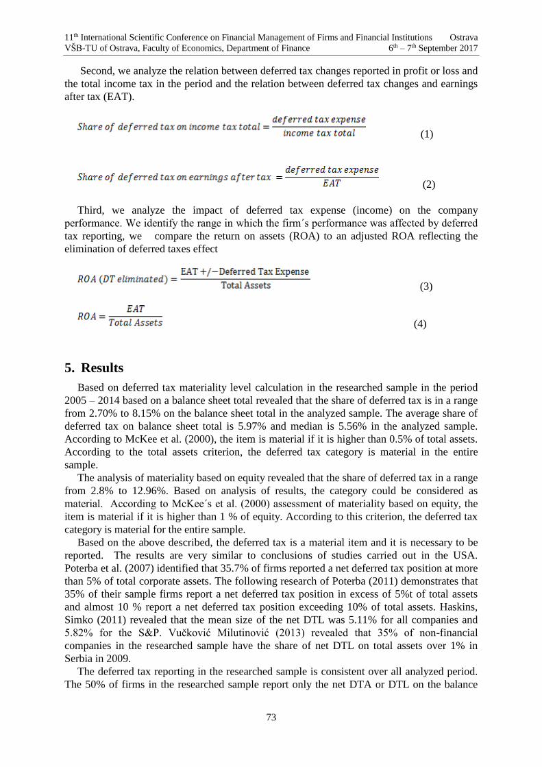
11th International Scientific Conference on Financial Management of Firms and Financial Institutions Ostrava
VŠB-TU of Ostrava, Faculty of Economics, Department of Finance 6th – 7th September 2017
73
Second, we analyze the relation between deferred tax changes reported in profit or loss and
the total income tax in the period and the relation between deferred tax changes and earnings
after tax (EAT).
(1)
(2)
Third, we analyze the impact of deferred tax expense (income) on the company
performance. We identify the range in which the firm´s performance was affected by deferred
tax reporting, we compare the return on assets (ROA) to an adjusted ROA reflecting the
elimination of deferred taxes effect
(3)
(4)
5. Results
Based on deferred tax materiality level calculation in the researched sample in the period
2005 – 2014 based on a balance sheet total revealed that the share of deferred tax is in a range
from 2.70% to 8.15% on the balance sheet total in the analyzed sample. The average share of
deferred tax on balance sheet total is 5.97% and median is 5.56% in the analyzed sample.
According to McKee et al. (2000), the item is material if it is higher than 0.5% of total assets.
According to the total assets criterion, the deferred tax category is material in the entire
sample.
The analysis of materiality based on equity revealed that the share of deferred tax in a range
from 2.8% to 12.96%. Based on analysis of results, the category could be considered as
material. According to McKee´s et al. (2000) assessment of materiality based on equity, the
item is material if it is higher than 1 % of equity. According to this criterion, the deferred tax
category is material for the entire sample.
Based on the above described, the deferred tax is a material item and it is necessary to be
reported. The results are very similar to conclusions of studies carried out in the USA.
Poterba et al. (2007) identified that 35.7% of firms reported a net deferred tax position at more
than 5% of total corporate assets. The following research of Poterba (2011) demonstrates that
35% of their sample firms report a net deferred tax position in excess of 5%t of total assets
and almost 10 % report a net deferred tax position exceeding 10% of total assets. Haskins,
Simko (2011) revealed that the mean size of the net DTL was 5.11% for all companies and
5.82% for the S&P. Vučković Milutinović (2013) revealed that 35% of non-financial
companies in the researched sample have the share of net DTL on total assets over 1% in
Serbia in 2009.
The deferred tax reporting in the researched sample is consistent over all analyzed period.
The 50% of firms in the researched sample report only the net DTA or DTL on the balance
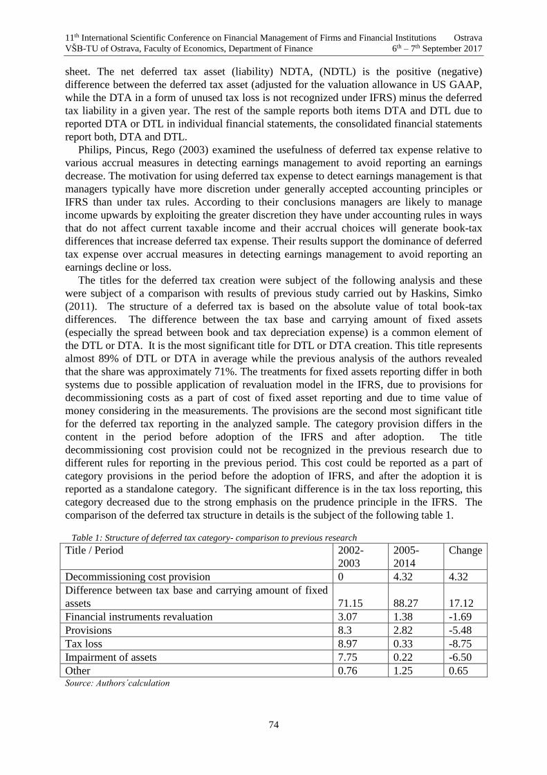
11th International Scientific Conference on Financial Management of Firms and Financial Institutions Ostrava
VŠB-TU of Ostrava, Faculty of Economics, Department of Finance 6th – 7th September 2017
74
sheet. The net deferred tax asset (liability) NDTA, (NDTL) is the positive (negative)
difference between the deferred tax asset (adjusted for the valuation allowance in US GAAP,
while the DTA in a form of unused tax loss is not recognized under IFRS) minus the deferred
tax liability in a given year. The rest of the sample reports both items DTA and DTL due to
reported DTA or DTL in individual financial statements, the consolidated financial statements
report both, DTA and DTL.
Philips, Pincus, Rego (2003) examined the usefulness of deferred tax expense relative to
various accrual measures in detecting earnings management to avoid reporting an earnings
decrease. The motivation for using deferred tax expense to detect earnings management is that
managers typically have more discretion under generally accepted accounting principles or
IFRS than under tax rules. According to their conclusions managers are likely to manage
income upwards by exploiting the greater discretion they have under accounting rules in ways
that do not affect current taxable income and their accrual choices will generate book-tax
differences that increase deferred tax expense. Their results support the dominance of deferred
tax expense over accrual measures in detecting earnings management to avoid reporting an
earnings decline or loss.
The titles for the deferred tax creation were subject of the following analysis and these
were subject of a comparison with results of previous study carried out by Haskins, Simko
(2011). The structure of a deferred tax is based on the absolute value of total book-tax
differences. The difference between the tax base and carrying amount of fixed assets
(especially the spread between book and tax depreciation expense) is a common element of
the DTL or DTA. It is the most significant title for DTL or DTA creation. This title represents
almost 89% of DTL or DTA in average while the previous analysis of the authors revealed
that the share was approximately 71%. The treatments for fixed assets reporting differ in both
systems due to possible application of revaluation model in the IFRS, due to provisions for
decommissioning costs as a part of cost of fixed asset reporting and due to time value of
money considering in the measurements. The provisions are the second most significant title
for the deferred tax reporting in the analyzed sample. The category provision differs in the
content in the period before adoption of the IFRS and after adoption. The title
decommissioning cost provision could not be recognized in the previous research due to
different rules for reporting in the previous period. This cost could be reported as a part of
category provisions in the period before the adoption of IFRS, and after the adoption it is
reported as a standalone category. The significant difference is in the tax loss reporting, this
category decreased due to the strong emphasis on the prudence principle in the IFRS. The
comparison of the deferred tax structure in details is the subject of the following table 1.
Table 1: Structure of deferred tax category- comparison to previous research
Title / Period 2002-
2003
2005-
2014
Change
Decommissioning cost provision 0 4.32 4.32
Difference between tax base and carrying amount of fixed
assets 71.15 88.27 17.12
Financial instruments revaluation 3.07 1.38 -1.69
Provisions 8.3 2.82 -5.48
Tax loss 8.97 0.33 -8.75
Impairment of assets 7.75 0.22 -6.50
Other 0.76 1.25 0.65 Source: Authors´calculation
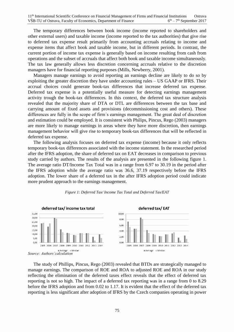
11th International Scientific Conference on Financial Management of Firms and Financial Institutions Ostrava
VŠB-TU of Ostrava, Faculty of Economics, Department of Finance 6th – 7th September 2017
75
The temporary differences between book income (income reported to shareholders and
other external users) and taxable income (income reported to the tax authorities) that give rise
to deferred tax expense result primarily from accounting accruals relating to income and
expense items that affect book and taxable income, but in different periods. In contrast, the
current portion of income tax expense is generally based on income resulting from cash from
operations and the subset of accruals that affect both book and taxable income simultaneously.
The tax law generally allows less discretion concerning accruals relative to the discretion
managers have for financial reporting purposes (Mills, Newberry, 2001).
Managers manage earnings to avoid reporting an earnings decline are likely to do so by
exploiting the greater discretion they have under accounting rules – US GAAP or IFRS. Their
accrual choices could generate book-tax differences that increase deferred tax expense.
Deferred tax expense is a potentially useful measure for detecting earnings management
activity trough the book-tax differences. In this context, the deferred tax structure analysis
revealed that the majority share of DTA or DTL are differences between the tax base and
carrying amount of fixed assets and provisions (decommissioning cost and others). These
differences are fully in the scope of firm´s earnings management. The great deal of discretion
and estimation could be employed. It is consistent with Philips, Pincus, Rego (2003) managers
are more likely to manage earnings in areas where they have more discretion, then earnings
management behavior will give rise to temporary book-tax differences that will be reflected in
deferred tax expense.
The following analysis focuses on deferred tax expense (income) because it only reflects
temporary book-tax differences associated with the income statement. In the researched period
after the IFRS adoption, the share of deferred tax on EAT decreases in comparison to previous
study carried by authors. The results of the analysis are presented in the following figure 1.
The average ratio DT/Income Tax Total was in a range from 6.97 to 30.19 in the period after
the IFRS adoption while the average ratio was 36.6, 37.19 respectively before the IFRS
adoption. The lower share of a deferred tax in the after IFRS adoption period could indicate
more prudent approach to the earnings management.
Figure 1: Deferred Tax/ Income Tax Total and Deferred Tax/EAT
Source: Authors´calculation
The study of Phillips, Pincus, Rego (2003) revealed that BTDs are strategically managed to
manage earnings. The comparison of ROE and ROA to adjusted ROE and ROA in our study
reflecting the elimination of the deferred taxes effect reveals that the effect of deferred tax
reporting is not so high. The impact of a deferred tax reporting was in a range from 0 to 8.29
before the IFRS adoption and from 0.02 to 1.17. It is evident that the effect of the deferred tax
reporting is less significant after adoption of IFRS by the Czech companies operating in power

11th International Scientific Conference on Financial Management of Firms and Financial Institutions Ostrava
VŠB-TU of Ostrava, Faculty of Economics, Department of Finance 6th – 7th September 2017
76
and utilities sector. The reasons for these changes are subject of the following research. The
results of the analysis are a subject of the following table 2.
Table 2: Impact of deferred tax reporting on ROA 2005-2014
Ratio/Year 2005 2006 2007 2008 2009 2010 2011 2012 2013 2014
ROA(DT eliminated)
Average 7.22 10.60 9.96 8.95 11.92 12.73 10.79 8.90 9.11 7.89
Median 7.24 10.60 10.58 9.83 10.74 10.79 10.64 7.60 9.45 9.12
ROA
Average 6.77 10.09 10.05 8.68 11.50 12.43 10.42 8.61 8.96 7.65
Median 6.87 10.09 11.53 9.51 10.41 10.42 10.28 7.34 9.47 9.00 Source: Authors´calculation
Figure 2: ROA (DT eliminated) and ROA
Source: Authors´calculation
6. Conclusion and future work
The results presented in the paper are initial part of the research concerning the deferred tax
reporting within the EU companies. We have investigated the materiality, structure and impact
of deferred tax according to IAS 12 reporting. We have made a comparison of deferred tax
according to the CAL and IFRS reporting effect. The data in a form of financial statements of
all publicly listed companies in the Czech Republic operating in Power and Utilities sector
were processed. We have found that the structure of deferred tax differs due to changes in
accounting rules, the most common title for DTA or DTL creation is difference between tax
base and carrying amount of long–term assets (property, plant and equipment and intangible
assets) in both systems (CAL and IFRS). The share of the net DTA or DTL on a balance sheet
total is material as well as the share of the net DTA or DTL on equity. The category deferred
tax was identified as a material category and it is necessary to be reported. The analysis
showed that this share is not significantly different regardless to reporting system (5.78 % in
average for analyzed sample reporting according to IFRS, 5.11%, 5.82 % respectively for
sample reporting according to US GAAP (Poterba, Rao, Seidman, 2011). The average ratio
DT/Income Tax Total was in a range from 6.97 to 30.19 in the period after the IFRS adoption
while the average ratio was 36.6, 37.19 respectively before the IFRS adoption. The lower
share of a deferred tax in the after IFRS adoption period could indicate the more prudent
approach to the earnings management. The comparison of ROA to adjusted ROA in our study
reflecting the elimination of the deferred taxes effect reveals that the effect of deferred tax
reporting is not so high in the Czech Republic after the IFRS adoption.
11th International Scientific Conference on Financial Management of Firms and Financial Institutions Ostrava
VŠB-TU of Ostrava, Faculty of Economics, Department of Finance 6th – 7th September 2017
77
The conclusion is based on limited dataset. It is supposed, the future research involved in
this issue will be submitted by more robust dataset concerning the financial data for majority
of EU-listed companies. The issue will be researched also in context of European Small and
Medium companies and their reporting.
Acknowledgements
The paper is the result of the GA ČR no. 15-24867S „Small and medium size enterprises in
global competition: Development of specific transfer pricing methodology reflecting their
specificities .
References
[1] Ayers, B. C., Jiang, J., Laplante, S. K. (2009). Taxable income as a performance measure:
The effects of tax planning and earnings quality. Contemporary Accounting Research, 26
(1), p. 15-54.
[2] Blaylock, B. Shevlin, T., Wilson, R.J. (2012). Tax Avoidance, Large Positive
Temporary Book-Tax Differences, and Earnings Persistence. The Accounting Review, 87
(1), p. 91-120.
[3] Bohušová, H., Svoboda, P. (2005). Analýza odložené daně z příjmů a její vliv na
ukazatele charakterizující ekonomickou výkonnost podniku. Acta Universitatis Agric. et
Silvic, Mend. Brun., 53(6), p. 33-44.
[4] Colley, R., Rue, J., Valencia, A. (2012). Accounting for Deferred Taxes: Time for a
Change. Journal of Business and Economic Research, 10 (3), p. 149-156.
[5] Comprix, J., Graham, R., Moore, J. (2011). Empirical Evidence on the Impact of Book-
Tax Differences on Divergence of Opinion among Investors. The Journal of the
American Taxation Association, 33(1), p. 51-78.
[6] Crabtree, A, Maher, J. J. (2009). The Influence of Differences in Taxable Income and
Book Income on the Bond Credit Market. The Journal of the American Taxation
Association, 31(1), p. 75-99.
[7] Desai, M. (2003). The Divergence between Book and Tax Income. Tax Policy and the
Economy, 17, p. 169-206.
[8] Dhaliwal, D. S., Huber, R. E., Lee, H.S., Pincus, M. (2008). Social Science Research
Network Book-Tax Differences, Uncertainty about Fundamentals and Information
Quality, and Cost of Capital.
[9] Donohoe, M.P., McGill, G. A. (2011). The Effects of Increased Book-Tax Difference
Tax Return Disclosures on Firm Valuation and Behavior. The Journal of the American
Taxation Association, 33(2), p. 35-65.
[10] Eberhartinger, E., Klostermann, M. (2007). What if IFRS were a Tax Base? New
Empirical Evidence from an Austrian Perspective. Accounting in Europe, 4(2).
[11] European Commission (2002). Regulation (EC) No. 1606/2002.
[12] Freedman, J., MacDonald, G. (2007). The Tax Base for CCCTB: The Role of Principles,
Working paper, Oxford University Centre for Business Taxation.
11th International Scientific Conference on Financial Management of Firms and Financial Institutions Ostrava
VŠB-TU of Ostrava, Faculty of Economics, Department of Finance 6th – 7th September 2017
78
[13] Gordon, E., Joos, P. R. (2004). Unrecognized Deferred Taxes: Evidence from the U.K.
The Accounting Review. 79(1), p. 97-124.
[14] Hanlon, M., Hoopes, J.L., Shroff, N. (2014). The Effect of Tax Authority Monitoring and
Enforcement on Financial Reporting Quality, The Journal of the American Taxation
Association, 36(2), p. 137-170.
[15] Haskins, M., Simko, P. (2011). What a Corporate Tax Cut Might Mean: An Analysis of
Deferred Taxes. Working paper, University of Virginia.
[16] Chi, S. S., Pincus, M., Teoh, S. H. (2014). Mispricing of Book-Tax Differences and the
Trading Behavior of Short Sellers and Insiders. The Accounting Review, 89(2), p. 511-
543.
[17] Chludek, A., K. (2011). Dissertation The Impact of Deferred Taxes on Firm Value.
Wirtschafts- und Sozialwissenschaftlichen Fakultät der Universität, Köln.
[18] Jackson, M. (2015). Book-Tax Differences and Future Earnings Changes. The Journal of
the American Taxation Association. 37(2), p. 49-73.
[19] Laux, R. C. (2013). The Association between Deferred Tax Assets and Liabilities and
Future Tax Payments. The Accounting Review. 88(4), p. 1357-1383.
[20] Lamb, M., Nobes, Ch., Roberts, A. (1998). International Variations in the Connections
Between Tax and Financial Reporting. Accounting and Business Research. 28(3), p.
173-188.
[21] Manzon, G. B., Plesko, G.A. (2002), The Relation Between Financial and Tax Reporting
Measures of Income, Tax Law Review, 55(2), p. 175-214.
[22] Mills, L., Newberry, K. (2001). The influence of tax and nontax costs on book-tax
reporting differences: Public and private firms. The Journal of the American Taxation
Association. 23 (1), p. 1-19.
[23] McKee, T.E. (2000). Current materiality guidance for auditors. Working
paper. Foundation for Research in Economic and Business Administration.
[24] Noga, T., J., Schnader, A. L. (2013). Book-Tax Differences as an Indicator of Financial
Distress. Accounting Horizons, 27(3), p.469-489.
[25] Phillips, J., Pincus, M., Rego, S. O. (2003). Earnings Management: New Evidence Based
on Deferred Tax Expense. The Accounting Review. 78(2), p. 491-521.
[26] Plesko, G.A. (2004). Corporate Tax Avoidance and the Properties of Corporate Earnings.
National Tax Journal, 57(3). p. 729-737.
[27] Poterba, J., Nirupama, R., Seidman, J. (2007). The significance and composition of
deferred tax assets and liabilities, Working Paper, Cambridge, MA: National Bureau of
Economic Research.
[28] Poterba, J., Nirupama, R., Seidman, J. (2011). Deferred Tax Positions and Incentives for
Corporate Behavior Around Corporate Tax Changes, National Tax Journal, 64(1), p. 27-
57.
[29] Vučković Milutinović, S., Lukić, R. (2013). Analysis of Deferred Taxes in the Business
Environment in Serbia. Economia. Seria Management, 16(1), p.25-37.

11th International Scientific Conference on Financial Management of Firms and Financial Institutions Ostrava
VŠB-TU of Ostrava, Faculty of Economics, Department of Finance 6th – 7th September 2017
79
Reporting ability of financial statements of micro and small accounting entities after amendment of
Act on Accounting
Jiřina Bokšová, Josef Horák 1
Abstract
The submitted paper deals with the reporting ability of the financial statements of micro and
small accounting entities after the amendment of the Act on Accounting. Firstly, the content of
the individual financial statements will be defined and assessed, secondly the structure and
reporting ability of the Notes to the financial statements including comments on realised
changes will be discussed. At the end of the paper the comparative analysis of the reporting
ability of the financial statements of small and micro accounting entities for the users of the
accounting information before and after the amendment of the Act on Accounting. The
submitted analysis is very actual because of more than 80 % of all accounting entities are just
micro and small accounting entities.
Key words
financial statements, micro accounting entity, notes to the financial statements, small
accounting entity, users of the accounting information
JEL Classification: M41
1. Úvod
Účetní závěrka společnosti by měla poskytovat uživatelům účetních informací ucelený
pohled na podnik jako ekonomický celek za konkrétní účetní období. Informace získané
z účetní závěrky podniků by měly sloužit uživatelům při jejich ekonomických rozhodnutích.
Dle zákona o účetnictví se rozlišuje několik druhů účetní závěrky – řádná, mimořádná a
mezitímní. Součástí účetní závěrky je rozvaha, výkaz zisku a ztráty, příloha, výkaz o změnách
peněžních toků a výkaz o změnách ve vlastním kapitálu. [8] Složky účetní závěrky slouží k
poskytnutí informací o finanční pozici, zdrojích účetní jednotky a výkonnosti společnosti za
účetní období. Informace v účetních závěrkách obsažené, by měly být pravdivé. [6, 7] Účetní
jednotka je povinna dle zákona č. 563/1991 Sb., o účetnictví dodržovat zásadu věrného a
poctivého zobrazení předmětu účetnictví a finanční situace. [10] Nedílnou součástí účetní
závěrky je příloha. V příloze by měly být vysvětleny a blíže okomentovány součtové řádky
rozvahy a výkazu zisku a ztráty. Dále se zde uvádějí informace, které se z jiných výkazů
vyčíst nedají, například výše zástav, bankovní záruk, podmíněných závazků apod. Příloha k
účetní závěrce je přidanou hodnotou uvedených čísel v rozvaze a ve výkazu zisku a ztráty,
zvyšuje jejich užitnou hodnotu pro uživatele účetních výkazů. [1]
K 1. 1. 2016 vstoupila v účinnost velká novela zákona o účetnictví č. 563/1991 Sb., ve
znění pozdějších předpisů. Ta vychází ze Směrnice Evropského parlamentu a Rady
2013/34/EU o ročních účetních závěrkách, konsolidovaných účetních závěrkách a
souvisejících zprávách některých forem podniků, která svým vydáním zrušila směrnici č. 4 a
1 doc. Ing. Jiřina Bokšová, Ph.D., ŠKODA AUTO UNIVERSITY, [email protected],
Ing. Josef Horák, Ph.D., ŠKODA AUTO UNIVERSITY, [email protected]
11th International Scientific Conference on Financial Management of Firms and Financial Institutions Ostrava
VŠB-TU of Ostrava, Faculty of Economics, Department of Finance 6th – 7th September 2017
80
č. 7. Členským státům byla Evropskou unií uvalena povinnost, aby právní a správní předpisy
nezbytné pro dosažení souladu se směrnicí 2013/34/EU, byly účinné do 20. července 2015.
Členské státy si mohou stanovit, že předpisy se použijí na účetní závěrky za účetní období
počínaje 1. 1. 2016 nebo v průběhu roku 2016.
Mezi nejvýznamnější změny novely patří kategorizace účetních jednotek dle jejich
velikosti, kategorizace konsolidačních skupin, definice účelu účetnictví, úprava ocenění
zásob vytvořených vlastní činností, úprava definice událostí po rozvahovém dni, zrušení
mimořádného výsledku hospodaření včetně souvisejících nákladů a výnosů, změna účtování
Aktivace a Změn stavu zásob vlastní činností, či znovuzavedení jednoduchého účetnictví.
Článek 4, odst. 2 Směrnice 2013/34/EU nařídil, aby do právních předpisů byl transponován
účel účetní závěrky. Uvádí, že roční účetní závěrka má být sestavena jasně a v souladu s
danou směrnicí. Byl doplněn do § 7, odst. 1, který říká, že „účetní jednotky jsou povinny vést
účetnictví tak, aby účetní závěrka byla sestavena na jeho základě srozumitelně̌ a podávala
věrný a poctivý obraz předmětu účetnictví a finanční situace účetní jednotky tak, aby na jejím
základě mohla osoba, která tyto informace využívá (dále jen „uživatel“), činit ekonomická
rozhodnutí.“ Doplnění účelu účetní závěrky by mělo být vodítkem při výběru účetních zásad a
metod a dalších účetních postupů. [2]
Účetnictví je možné dle české legislativy vést v plném nebo ve zjednodušeném rozsahu.
Obchodní korporace vedou účetnictví v plném rozsahu. Ve zjednodušeném rozsahu dle
zákona o účetnictví § 9, odst. 3 vedou účetnictví mikro a malé účetní jednotky, které nemají
povinnost ověření účetní závěrky auditorem, avšak zároveň se musí jednat o spolek, církev,
odborovou organizaci, apod. Zjednodušený rozsah vedení účetnictví spočívá v tom, že účetní
jednotky mohou spojit účtování v hlavní knize a v deníku, nepoužijí ocenění metodou
ekvivalence a reálnou hodnotou nebo neúčtují o opravných položkách a rezervách s výjimkou
těch, které jsou tvořeny na základě zvláštních právních předpisů – zákona o rezervách.
Zákon o účetnictví dle § 7, odst. 1 účetním jednotkám ukládá „vést účetnictví tak, aby
účetní závěrka byla sestavena na jeho základě srozumitelně a podávala věrný a poctivý obraz
předmětu účetnictví a finanční situace tak, aby na jejím základě mohla osoba, která tyto
informace využívá (dále je „uživatel“) činit ekonomická rozhodnutí.“
Účetní závěrka je sestavována v plném nebo ve zkráceném rozsahu. Všechny účetní
jednotky mají povinnost sestavit účetní závěrku v plném rozsahu (plný rozsah účetní závěrky
znamená plná sada účetních výkazů a příloha). Ve zkráceném rozsahu mohou sestavovat
účetní závěrku pouze mikro a malé účetní jednotky bez auditu. Zde je na místě upozornit na
skutečnost, že ne všechny mikro a malé účetní jednotky bez auditu však mohou vést účetnictví
ve zjednodušeném rozsahu.
Zkrácený rozsah sestavení účetní závěrky mikro a malých podniků bez auditu znamená, že
a v případě výkazu rozvaha se využívá pro zkrácený rozsah tzv. základní a rozšířená varianta
výkazu rozvaha, jak je uvedeno v Tabulce 1.
Výkaz zisku a ztráty musí všechny obchodní společnosti sestavit vždy v plném rozsahu. Ve
zkráceném rozsahu sestavují jen ty účetní jednotky, které nejsou obchodními společnostmi, a
jejich sestavená účetní závěrka nepodléhá ověření auditorem. Mikro a malé účetní jednotky
bez povinnosti auditu však výkaz zisku a ztráty uživatelům účetních informací účinností
novely zákona o účetnictví již nezveřejňují, viz Tabulka 2.

11th International Scientific Conference on Financial Management of Firms and Financial Institutions Ostrava
VŠB-TU of Ostrava, Faculty of Economics, Department of Finance 6th – 7th September 2017
81
Tabulka 1: Základní verze rozvahy a rozšířená verze rozvahy pro mikro a male účetní jednotky bez auditu
Řádek
Položka
Řádek
Položka
AKTIVA CELKEM AKTIVA CELKEM
A. Pohledávky za upsaný ZK A. Pohledávky za upsaný ZK
B. Dlouhodobý majetek B. Dlouhodobý majetek
C. Oběžná aktiva B. I. Dlouhodobý nehmotný majetek
D. Časové rozlišení aktiv B. II. Dlouhodobý hmotný majetek
PASIVA CELKEM B. III. Dlouhodobý finanční majetek
A. Vlastní kapitál C. Oběžná aktiva
B. +
C.
CIZÍ ZDROJE C. I. Zásoby
B. Rezervy C. II. Pohledávky
C. Závazky C. II. 1 Dlouhodobé pohledávky
D. Časové rozlišení pasiv C. II. 2 Krátkodobé pohledávky
C. III. Krátkodobý finanční majetek
C. IV. Peněžní prostředky
D. Časové rozlišení aktiv
PASIVA CELKEM
A. Vlastní kapitál
A.I. Základní kapitál
A.II. Ážio a kapitálové fondy
A.III Fondy ze zisku
A.IV. Výsledek hospodaření minulých let
A.V. Výsledek hospodaření běžného účetního období
A.VI. Rozhodnuto o zálohové výplatě podílů na zisku
B.+C. CIZÍ ZDROJE
B. Rezervy
C. Závazky
C.I. Dlouhodobé závazky
C.II. Krátkodobé závazky
D. Časové rozlišení pasiv
Zdroj: vlastní zpracování v souladu s § 1b zákona o účetnictví č. 563/1991 Sb.
Tabulka 2: Rozsah zveřejnění účetní závěrky mikro a malých obchodních účetních jednotek
Kategorie
Rozvaha
základní
verze
Rozvaha
rozšířená
verze
Rozvaha
plná
verze
Výkaz
zisku a
ztráty plná
verze
Příloha
Výkaz
CF
Výkaz o
změnách
ve VK
Mikro bez auditu
Mikro auditovaná
Malá ÚJ bez auditu
Malá ÚJ auditovaná
Zdroj: vlastní zpracování v souladu se zákonem o účetnictví č. 563/1991 Sb.
Do skupiny mikro účetních jednotek jsou zařazeny podniky, které splňují podmínku obratu
do 18 mil. Kč, výši aktiv netto 9 mil. Kč a 10 přepočtených zaměstnanců. Mikro účetní
jednotky, které nemají povinnost ověřit účetní závěrku auditorem, sestavují rozvahu
v základní verzi. Výkaz zisku a ztráty mikro podniky bez auditu sice sestavují v plném
rozsahu, ale nově uživatelům nezveřejňují, příloha k účetní závěrce poskytuje pouze
minimální informace. [4]

11th International Scientific Conference on Financial Management of Firms and Financial Institutions Ostrava
VŠB-TU of Ostrava, Faculty of Economics, Department of Finance 6th – 7th September 2017
82
Proč došlo ke snížení vykazovaných informací pro uživatele účetních závěrek? Důvod byl
uveden v důvodové zprávě předkládaného návrhu vlády novelizace zákona o účetnictví a má
jím být snížení administrativní zátěže a zlepšení konkurenčního prostředí. Zde je nutné
kriticky tento důvod posoudit. Je otázkou, zda dojde ke zlepšení konkurenčního prostředí tím,
že uživatelům účetní závěrky zůstávají skryty důležité informace ohledně výše závazků z
obchodních vztahů, pohledávek z obchodních vztahů, peněžních prostředků, informace o výši
výsledku hospodaření za účetní období apod.
V případě mikro účetních jednotek bez auditu není ani možné provést základní kontrolu, že
výsledek hospodaření za běžné účetní období v rozvaze souhlasí na hodnotu uvedenou ve
výkazu zisku a ztráty. U mikro účetních jednotek bez auditu není možné zjistit rentabilitu
podniku. Podle názoru autorů naopak u mikro účetních jednotek bez auditu došlo změnou
zákona ke zhoršení konkurenčního prostředí, protože řada důležitých ekonomických informací
se stala informacemi nedostupnými pro uživatele účetní závěrky.
Do skupiny malých účetních jednotek jsou zařazeny podniky, které splňují podmínku
obratu do 200 mil. Kč, výši aktiv netto 100 mil. Kč a 50 přepočtených zaměstnanců. Malé
účetní jednotky, které nemají povinnost ověřit účetní závěrku auditorem, sestavují rozvahu
v rozšířené verzi. Výkaz zisku a ztráty malé podniky bez auditu sestavují v plném rozsahu,
nově však již nezveřejňují, příloha k účetní závěrce poskytuje pouze malé množství
doplňujících informací. [5]
Stejně jako u základní verze uživatelé nemají možnosti z výkazu rozvaha vyčíst hodnotu
zadlužení společnosti, výši poskytnutých a přijatých půjček mezi spřízněnými osobami nebo
určit strukturu zásob. Tyto a jiné doplňující informace by měly být následně uvedeny v příloze
účetní závěrky, která blíže vysvětluje a rozšiřuje jednotlivé položky z výkazu rozvahy a
výkazu zisku a ztráty.
Příloha k účetní závěrce může být stejně jako účetní výkazy sestavována v plném rozsahu
nebo ve zkráceném rozsahu. Požadavky na její rozsah je dán kaskádovitě. Základní ustanovení
v § 39 v prováděcí vyhlášce pro podnikatele jsou povinná pro všechny kategorie účetní
jednotky. [9] Nicméně ustanovení v § 39a - § 39c jsou závazná s ohledem na danou kategorii
účetní jednotky tak, jak je uvedeno v Tabulce 3.
Tabulka 3: Rozsah sestavení přílohy k účetní závěrce dle jednotlivých kategorií
Kategorie účetní jednotky Příloha k účetní závěrce
Rozsah Obsah
Mikro bez auditu Příloha ve zkráceném rozsahu § 39
Mikro auditovaná Příloha v plném rozsahu pro mikro a malé ÚJ § 39 + § 39a
Malá ÚJ bez auditu Příloha ve zkráceném rozsahu § 39
Malá ÚJ auditovaná Příloha v plném rozsahu pro mikro a malé ÚJ § 39 + § 39a
Zdroj: vlastní zpracování v souladu se zákonem o účetnictví č. 563/1991 Sb.
2. Metodologie výzkumu
Pro potvrzení výše uvedených teoretických poznatků byla vybrána 1 společnost, která
splňovala podmínky pro zařazení „malá účetní jednotka bez auditu“ z odvětví
automobilového průmyslu, na které byla ověřována hypotéza: „Změna zákona o účetnictví ve
vztahu k vykazovaným informacím v účetních závěrkách mikro a malých účetních jednotek
bez auditu povede ke zvýšení konkurenceschopnosti na trhu“. Výzkum společnosti
Semperflex A.H., s.r.o. provedla Ing. Kamila Marešová, která porovnala vypovídací
schopnost účetní závěrky za rok 2015 a změny ve vypovídací schopnosti účetní závěrky při
platné účetní legislativě 2016. [3]
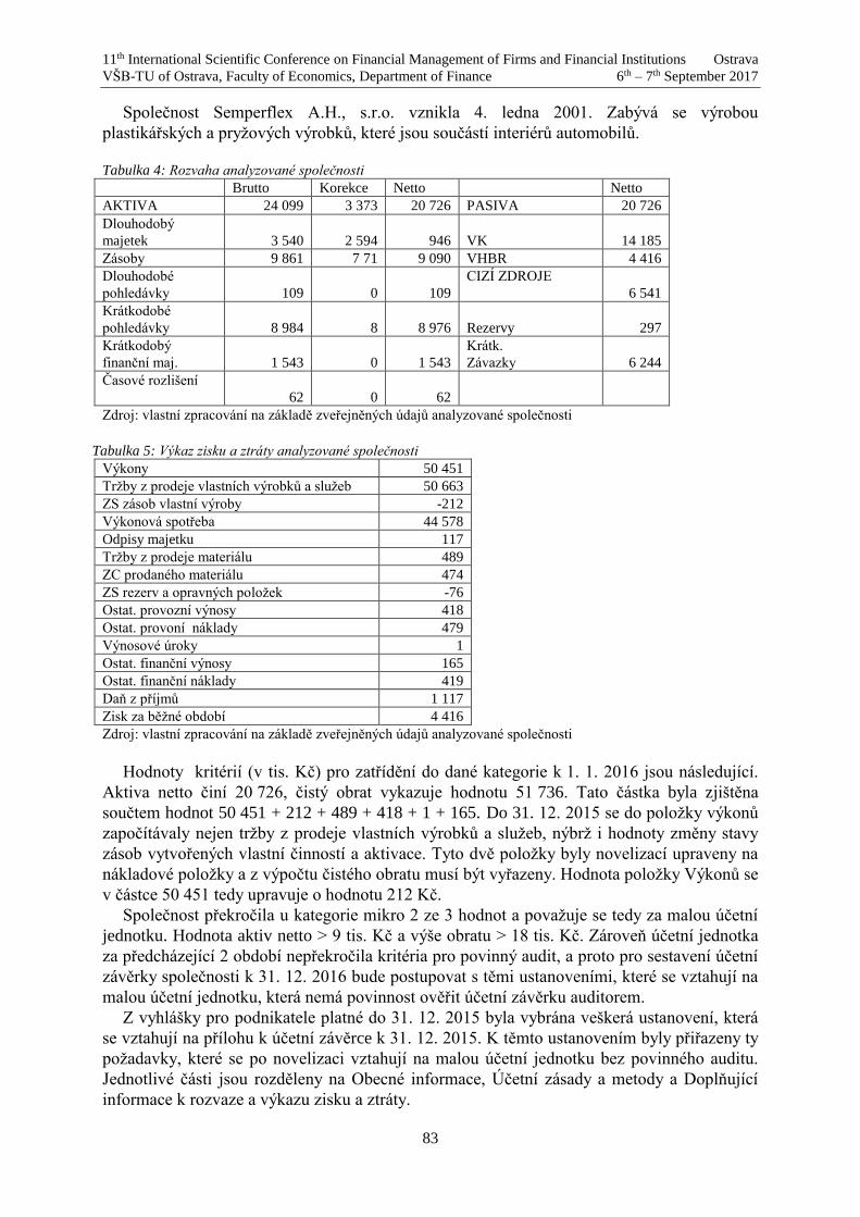
11th International Scientific Conference on Financial Management of Firms and Financial Institutions Ostrava
VŠB-TU of Ostrava, Faculty of Economics, Department of Finance 6th – 7th September 2017
83
Společnost Semperflex A.H., s.r.o. vznikla 4. ledna 2001. Zabývá se výrobou
plastikářských a pryžových výrobků, které jsou součástí interiérů automobilů.
Tabulka 4: Rozvaha analyzované společnosti
Brutto Korekce Netto Netto
AKTIVA 24 099 3 373 20 726 PASIVA 20 726
Dlouhodobý
majetek
3 540
2 594
946
VK
14 185
Zásoby 9 861 7 71 9 090 VHBR 4 416
Dlouhodobé
pohledávky
109
0
109
CIZÍ ZDROJE
6 541
Krátkodobé
pohledávky
8 984
8
8 976
Rezervy
297
Krátkodobý
finanční maj.
1 543
0
1 543
Krátk.
Závazky
6 244
Časové rozlišení
62
0
62
Zdroj: vlastní zpracování na základě zveřejněných údajů analyzované společnosti
Tabulka 5: Výkaz zisku a ztráty analyzované společnosti
Výkony 50 451
Tržby z prodeje vlastních výrobků a služeb 50 663
ZS zásob vlastní výroby -212
Výkonová spotřeba 44 578
Odpisy majetku 117
Tržby z prodeje materiálu 489
ZC prodaného materiálu 474
ZS rezerv a opravných položek -76
Ostat. provozní výnosy 418
Ostat. provoní náklady 479
Výnosové úroky 1
Ostat. finanční výnosy 165
Ostat. finanční náklady 419
Daň z příjmů 1 117
Zisk za běžné období 4 416
Zdroj: vlastní zpracování na základě zveřejněných údajů analyzované společnosti
Hodnoty kritérií (v tis. Kč) pro zatřídění do dané kategorie k 1. 1. 2016 jsou následující.
Aktiva netto činí 20 726, čistý obrat vykazuje hodnotu 51 736. Tato částka byla zjištěna
součtem hodnot 50 451 + 212 + 489 + 418 + 1 + 165. Do 31. 12. 2015 se do položky výkonů
započítávaly nejen tržby z prodeje vlastních výrobků a služeb, nýbrž i hodnoty změny stavy
zásob vytvořených vlastní činností a aktivace. Tyto dvě položky byly novelizací upraveny na
nákladové položky a z výpočtu čistého obratu musí být vyřazeny. Hodnota položky Výkonů se
v částce 50 451 tedy upravuje o hodnotu 212 Kč.
Společnost překročila u kategorie mikro 2 ze 3 hodnot a považuje se tedy za malou účetní
jednotku. Hodnota aktiv netto > 9 tis. Kč a výše obratu > 18 tis. Kč. Zároveň účetní jednotka
za předcházející 2 období nepřekročila kritéria pro povinný audit, a proto pro sestavení účetní
závěrky společnosti k 31. 12. 2016 bude postupovat s těmi ustanoveními, které se vztahují na
malou účetní jednotku, která nemá povinnost ověřit účetní závěrku auditorem.
Z vyhlášky pro podnikatele platné do 31. 12. 2015 byla vybrána veškerá ustanovení, která
se vztahují na přílohu k účetní závěrce k 31. 12. 2015. K těmto ustanovením byly přiřazeny ty
požadavky, které se po novelizaci vztahují na malou účetní jednotku bez povinného auditu.
Jednotlivé části jsou rozděleny na Obecné informace, Účetní zásady a metody a Doplňující
informace k rozvaze a výkazu zisku a ztráty.

11th International Scientific Conference on Financial Management of Firms and Financial Institutions Ostrava
VŠB-TU of Ostrava, Faculty of Economics, Department of Finance 6th – 7th September 2017
84
U společnosti bylo ověřeno, zda při sestavení přílohy k účetní závěrce k 31. 12. 2016 byly
vysvětleny ty položky, který ji ukládaly platné právní předpisy. Rozbor je uveden pro každou
položku a zaznamenán do sloupce ANO, NE a N/A. Ano je zaškrtnuto tehdy, pokud byla
informace zaznamenána do přílohy. N/A je označeno, v případě, že dané ustanovení není pro
společnost relevantní (např. společnost nemá dlouhodobé investice, proto nevykazuje
požadované informace). Zjištěné výsledky jsou uvedeny v Tabulce 6.
Tabulka 6: Výsledky analýzy účetní závěrky za rok 2015
Zdroj: vlastní zpracování na základě provedené analýzy
Z provedeného rozboru byla zjištěna pochybení v podobě informací, které účetní jednotka
měla uživatelům sdělit, ale neučinila tak. V sekci Obecné informace se jedná o neuvedení
výše vkladu společníka společnosti, o nezobrazení organizační struktury, o nesdělení změn v
obchodním rejstříku za rok 2015. V sekci Účetní zásady a metody nebyl zveřejněn způsob
stanovení opravné položky k zásobám a pohledávkám. V sekci Doplňující informace k
rozvaze a výkazu zisku a ztráty chybí informace o výši pohledávek s dobou splatnosti delší
než 5 let, o výši závazků s dobou splatností delší než 5 let, informace o výdajích na výzkum a
vývoj, informace o popisu významných událostí mezi rozvahovým dnem a datem sestavení
účetní závěrky apod. Jelikož se jedná o výrobní společnost, tak uživatel účetních informací
může předpokládat, že velká část hodnoty bilanční sumy bude vázána v hodnotě zásob. V
případě zkoumané společnosti se dokonce jedná o 44 %, a proto je neuvedení stanovení
metody opravné položky k zásobám možné považovat za skutečnost, která má vliv na
rozhodování uživatele účetních informací. V oblasti ocenění zásob zapomněla účetní jednotka
sdělit metodu účtování o zásobách – metodu A nebo metodu B.
Z Tabulky 6 vyplývá, že malá účetní jednotka v příloze k účetní závěrce k 31. 12. 2016
sníží počet posuzovaných ustanovení, jež mají do přílohy být promítnuty. Na jedné straně se
informovanost uživatelů účetní závěrky snížila o 71 dříve poskytovaných informací. Na druhé
straně v části doplňujících informací bude muset nově povinně sdělit 5 nových informací jako
např. zda v účetním období společnost nabyla nové vlastní podíly; jestli jsou pohledávky a
závazky kryty věcnými zárukami nebo výši nákladů a výnosů, které jsou mimořádné svým
původem nebo objemem.
3. Diskuze
Účetní závěrka představuje zdroj informací pro uživatele účetních informací. Z provedené
analýzy je zřejmé, že u mikro a malých účetních jednotek, které nemají povinnost ověřit
účetní závěrku auditorem, se po novele zákona o účetnictví sníží počet zveřejňovaných
informací v příloze k účetní závěrce.
Při rozboru účetní závěrky malé účetní jednotky, jejíž účetní závěrka nepodléhá povinnému
auditu, společnost Semperflex A.H., s.r.o., vykázala v příloze k účetní závěrce k 31. 12. 2015
celkem 9 pochybení (společnost nezveřejnila informace ohledně organizační struktury; výše
podílu na základním kapitálu společníka; změny v obchodním rejstříku; informace o výši
Rozsah přílohy Ano NE N/A Celkem
ustanovení
Nová
ustanovení
Novelou vypuštěná
ustanovení
Obecné informace 14 3 21 38 0 25
Účetní zásady 6 1 11 18 0 3
Doplňující informace 18 5 30 53 5 43
Celkem nezveřejňované
informace od r. 2016
71

11th International Scientific Conference on Financial Management of Firms and Financial Institutions Ostrava
VŠB-TU of Ostrava, Faculty of Economics, Department of Finance 6th – 7th September 2017
85
pohledávek a dluhů s dobou splatností delší než 5 let; informace o výši nákladů na výzkum a
vývoj a o informaci ohledně významných událostí mezi rozvahovým dnem a datem sestavení
účetní závěrky).
Z analýzy vyplynulo, že pokud by účetní jednotka sestavovala danou účetní závěrku za
podmínek platných po novelizaci zákona o účetnictví, tak by se v příloze k účetní závěrce
podstatně snížily zveřejňované informace, zejména v části obecných informací o společnosti o
25 informací, v části účetních zásad o 3 informace a v části doplňujících informací o 42
informací.
4. Závěr
Důvodem novelizace zákona o účetnictví měla být „zvýšená konkurenceschopnost“. Ve
skutečnosti však nastává pravý opak. Mikro a malé účetní jednotky bez auditu zveřejňují
rozvahu ve zkrácené nebo rozšířené formě (tím je již značně omezena vypovídací schopnost
účetní závěrky), výkaz zisku a ztráty není zveřejňován vůbec a množství dříve zveřejňovaných
informací v příloze k účetní závěrce se stalo novelou zákona informacemi utajenými. Tyto
legislativní kroky vedou bezesporu ke snížení konkurenceschopnosti na našem trhu. Ještě
jednou je důležité na tomto místně vzpomenout, že uživatelé u těchto společností nebudou mít
nově informace o výši závazků z obchodních vztahů, výši pohledávek z obchodních vztahů,
výši peněžních prostředků, informace o výši výsledku hospodaření za účetní období, výši
zadluženosti společnosti, výši poskytnutých a přijatých půjček mezi spřízněnými osobami
nebo určit strukturu zásob.
Tento závěr je alarmující, neboť dle informací ministerstva financí k 10. 4. 2014, tvoří
naprostou většinu účetní jednotek v České republice (94,5 % ze všech registrovaných
účetních jednotek) právě mikro a malé účetní jednotky. Otázkou zůstává, pro koho je
„nezveřejňování informací a zatajování informací ve výkazu zisku a ztráty“ v účetních
závěrkách společností na ekonomickém trhu vlastně výhodou?
References
[1] Bokšová, J. (2010). Účetní výkazy pod lupou I – Základy účetního výkaznictví. Praha:
LINDE.
[2] Directive 2013/34/EU of the European Parliament and of the Council of 26 June 2013 on
the annual financial statements, consolidated financial statements and related reports of
certain types of undertakings, amending Directive 2006/43/EC of the European
Parliament and of the Council and repealing Council Directives 78/660/EEC and
83/349/EEC
[3] Marešová, K. (2016). Vypovídací schopnost přílohy v účetní závěrce v České republice.
Ing. VŠE.
[4] Müllerová, L. (2016). Vliv kategorizace účetních jednotek na účetní závěrku. Účetnictví v
praxi, 2016(4).
[5] Pilátová, J. (2017). Zákon o účetnictví 2017 s komentářem. Praha: GRADA.
[6] Strouhal, J. (2012). Applicability Of Ifrs For Smes In The Czech Republic. Ecoman
ECONOMICS AND MANAGEMENT, 17(2).
[7] Strouhal, J. (2016). Rozdíly v účetních výkazech po novele účetních předpisů. Účetnictví
v praxi, 2016(1).

11th International Scientific Conference on Financial Management of Firms and Financial Institutions Ostrava
VŠB-TU of Ostrava, Faculty of Economics, Department of Finance 6th – 7th September 2017
86
[8] Strouhal, J., & Bonaci C. G. 2014. Facing current trends in accounting harmonization:
on case of Czech professional accountants. 8th International conference on accounting,
auditing, and taxation (ICAAT 2014).
[9] Vyhláška č. 502/2002 Sb., kterou se provádějí některá ustanovení zákona č. 563/1991
Sb., o účetnictví, ve znění platném do 31. 12. 2015, pro účetní jednotky, které jsou
podnikateli účtujícími v soustavě̌ podvojného účetnictví
[10] Zákon č. 563/1991 Sb., o účetnictví
11th International Scientific Conference on Financial Management of Firms and Financial Institutions Ostrava
VŠB-TU of Ostrava, Faculty of Economics, Department of Finance 6th – 7th September 2017
87
Selection of the optimal solution of the decision-making problem
Martina Borovcová 1
Abstract
This paper is focused on the selection of the optimal solution of the decision-making problem
in the field of automobile collision insurance. The content of the paper is the description,
verification and application of the multi-level decomposition method AHP on the Saaty pair
comparison approach. The AHP method is described in the case of preferences determination.
This method is applied for the selection of the optimal product of the automobile collision
insurance.
Key words
Multi-attribute methods, AHP (analytic hierarchy process), Saaty pair comparison approach,
automobile collision insurance
JEL Classification: C4, C61, G22
1. Úvod
Hledání optimálního řešení je součástí řešení rozhodovacích problémů. Aby bylo možné
optimální variantu nalézt, musí mít rozhodovací problém více variant řešení. Optimální
variantou je potom taková varianta, která vyhovuje nejlépe ve všech posuzovaných kritériích.
Jednotlivé varianty řešení jsou posuzovány dle intenzity či míry splnění určitých
požadavků, kritérií, které jsou na varianty kladeny. Protože rozhodování o výběru varianty
zpravidla nezávisí pouze na jednom posuzovaném kritériu, jeví se vhodným využívat metody
vícekriteriálního hodnocení variant. Takovéto rozhodování o výběru je bezesporu vhodnější a
komplexnější. Může sice nastat situace, kdy by k výběru varianty bylo použito pouze jediného
kritéria hodnocení a za podmínky kvantitativního charakteru kritéria by pak stačilo uspořádat
varianty podle hodnot tohoto kritéria a varianta s nejvyšší, či nejnižší hodnotou by byla
variantou optimální. Existuje však poměrně málo rozhodovacích problémů, které by měly
monokriteriální charakter. Podstatně častěji je možné setkat se s problémy, kdy varianty řešení
je třeba posuzovat pomocí většího počtu kritérií hodnocení. Takovéto rozhodovací problémy
pak mají charakter vícekriteriální, multikriteriální.
Cílem příspěvku je výběr optimálního produktu havarijního pojištění. K výběru optimální
varianty bude použito víceúrovňové dekompoziční metody AHP, proto bude nejdříve popsána
podstata rozhodovacího procesu a princip vícekriteriálního rozhodování a následně metoda
AHP samotná. Tato bude následně aplikována při výběru konkrétního produktu havarijního
pojištění. Variantami rozhodování bude produkt havarijního pojištění kategorizovaný dle
požadavků klienta na výši pojistného plnění, výši pojistného a výši spoluúčasti na pojistném
plnění.
1 1 Ing. Martina Borovcová, Ph.D., VŠB-Technická univerzita Ostrava, Ekonomická fakulta, katedra
financí, Sokolská třída 33, 701 21 Ostrava. Email: [email protected]..

11th International Scientific Conference on Financial Management of Firms and Financial Institutions Ostrava
VŠB-TU of Ostrava, Faculty of Economics, Department of Finance 6th – 7th September 2017
88
2. Popis metod vícekriteriálního hodnocení variant
Úlohy vícekriteriálního hodnocení variant jsou zaměřeny především na nalezení nejlepší
(optimální) varianty a uspořádání variant od nejlepší po nejhorší. Optimální variantou je
taková varianta, která nejlépe splňuje každé z posuzovaných kritérií. Taková varianta však
nemusí být mezi posuzovanými variantami vůbec obsažena. Nejlepší varianta je tak zpravidla
variantou kompromisní, tedy variantou hodnocenou nejlépe dle nejdůležitějších kritérií nebo
dle největšího množství posuzovaných kritérií. Je tak vždy nejméně vzdálena od ideální
varianty nebo nejdále vzdálena od varianty bazální, přičemž ideální variantou je taková
varianta, která nabývá v hodnoceném kritériu nejlepší možné hodnoty. Naopak, varianta s
nejhoršími hodnotami kritérií je bazální variantou. Ideální a bazální varianty bývají obvykle
hypotetické. Pokud by ideální varianta opravdu existovala, byla by zároveň variantou
optimální. Jak již bylo uvedeno výše, tato situace však zpravidla nenastává a proto jakékoli
vybrané řešení je řešením kompromisním. Ve všech úlohách musí být kompromisní varianta
nedominovaná, což znamená, že mezi variantami rozhodování tedy neexistuje varianta, která
ji dominuje.
Úlohy vícekriteriálního rozhodování je možné dělit dle typu informací, které vyjadřují
preference kritérií nebo variant na úlohy kdy nejsou vyžadovány informace o důležitosti
kritérií nebo úlohy ve kterých jsou vyžadovány informace. Vyžadovány pak mohou být
ordinální či kardinální informace o kritériích nebo o aspirační úrovni kritérií. Řešení
optimalizačních úloh je rovněž závislé na dalších předpokladech, jak uvádí např. Valecký
(2017).
V závislosti na kombinaci způsobu stanovení preference kritérií a hodnot kritérií lze použít
řadu metod, viz Tabulka 1. Je patrné, že je možné rozlišit čtyři skupiny kombinací. I. skupina
obsahuje úlohy bez preference kritérií, II. skupina je tvořena úlohami s kvantitativně určenými
kritérii (např. finanční, ekonomická), do III. skupiny patří úlohy, u nichž jak preference
kritérií, tak hodnoty kritérií jsou stanoveny stejnou metodou, IV. skupina zahrnuje ostatní
kombinace.
Tabulka 1: Vícekriteriální kombinace způsobů stanovení hodnot a preferencí kritérií
Kombinace způsobů stanovení hodnot a
preferencí kritérií
Preference dílčích kritérií
bez ordinální kardinální párové
pořadí bodová Fuller Saaty
A B C D E
Ho
dn
oty
kri
terií
u
va
ria
nt
kardinální kvantitativní a
I.
II.
ordinální pořadí b III. IV.
kardinální bodová c III.
párové Fuller d
IV. III.
Saaty e III.
Zdroj: Zmeškal (2013)
Jednu ze skupin vícekriteriálních metod tvoří vícestupňové dekompoziční metody
vycházející ze Saatyho metody párového porovnání. Patří sem metoda AHP (analytic
hierarchy proces) a ANP (analytic network proces). U těchto metod jsou preference (váhy)
stanoveny postupnou dekompozicí. Přitom metoda AHP je lineární metodou bez zpětných
vazeb. Metoda ANP je nelineární složitější metodou obsahující zpětné vazby a je možné
v komplexní variantě zachytit vztah mezi variantami a preferencemi. Metoda AHP je
zvláštním případem (podmnožinou) metody ANP.
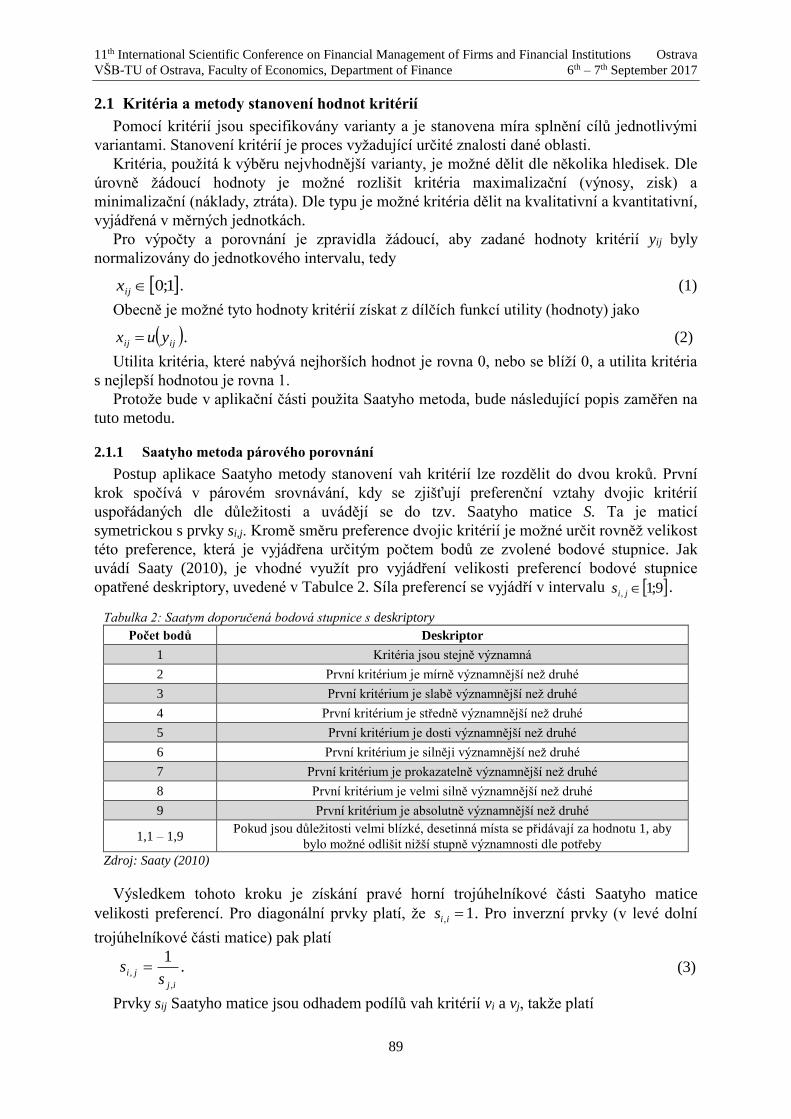
11th International Scientific Conference on Financial Management of Firms and Financial Institutions Ostrava
VŠB-TU of Ostrava, Faculty of Economics, Department of Finance 6th – 7th September 2017
89
2.1 Kritéria a metody stanovení hodnot kritérií
Pomocí kritérií jsou specifikovány varianty a je stanovena míra splnění cílů jednotlivými
variantami. Stanovení kritérií je proces vyžadující určité znalosti dané oblasti.
Kritéria, použitá k výběru nejvhodnější varianty, je možné dělit dle několika hledisek. Dle
úrovně žádoucí hodnoty je možné rozlišit kritéria maximalizační (výnosy, zisk) a
minimalizační (náklady, ztráta). Dle typu je možné kritéria dělit na kvalitativní a kvantitativní,
vyjádřená v měrných jednotkách.
Pro výpočty a porovnání je zpravidla žádoucí, aby zadané hodnoty kritérií yij byly
normalizovány do jednotkového intervalu, tedy
1;0ijx . (1)
Obecně je možné tyto hodnoty kritérií získat z dílčích funkcí utility (hodnoty) jako
ijij yux . (2)
Utilita kritéria, které nabývá nejhorších hodnot je rovna 0, nebo se blíží 0, a utilita kritéria
s nejlepší hodnotou je rovna 1.
Protože bude v aplikační části použita Saatyho metoda, bude následující popis zaměřen na
tuto metodu.
2.1.1 Saatyho metoda párového porovnání
Postup aplikace Saatyho metody stanovení vah kritérií lze rozdělit do dvou kroků. První
krok spočívá v párovém srovnávání, kdy se zjišťují preferenční vztahy dvojic kritérií
uspořádaných dle důležitosti a uvádějí se do tzv. Saatyho matice S. Ta je maticí
symetrickou s prvky si,j. Kromě směru preference dvojic kritérií je možné určit rovněž velikost
této preference, která je vyjádřena určitým počtem bodů ze zvolené bodové stupnice. Jak
uvádí Saaty (2010), je vhodné využít pro vyjádření velikosti preferencí bodové stupnice
opatřené deskriptory, uvedené v Tabulce 2. Síla preferencí se vyjádří v intervalu 9;1, jis .
Tabulka 2: Saatym doporučená bodová stupnice s deskriptory
Počet bodů Deskriptor
1 Kritéria jsou stejně významná
2 První kritérium je mírně významnější než druhé
3 První kritérium je slabě významnější než druhé
4 První kritérium je středně významnější než druhé
5 První kritérium je dosti významnější než druhé
6 První kritérium je silněji významnější než druhé
7 První kritérium je prokazatelně významnější než druhé
8 První kritérium je velmi silně významnější než druhé
9 První kritérium je absolutně významnější než druhé
1,1 – 1,9 Pokud jsou důležitosti velmi blízké, desetinná místa se přidávají za hodnotu 1, aby
bylo možné odlišit nižší stupně významnosti dle potřeby
Zdroj: Saaty (2010)
Výsledkem tohoto kroku je získání pravé horní trojúhelníkové části Saatyho matice
velikosti preferencí. Pro diagonální prvky platí, že 1, iis . Pro inverzní prvky (v levé dolní
trojúhelníkové části matice) pak platí
.1
,
,
ij
jis
s (3)
Prvky sij Saatyho matice jsou odhadem podílů vah kritérií vi a vj, takže platí
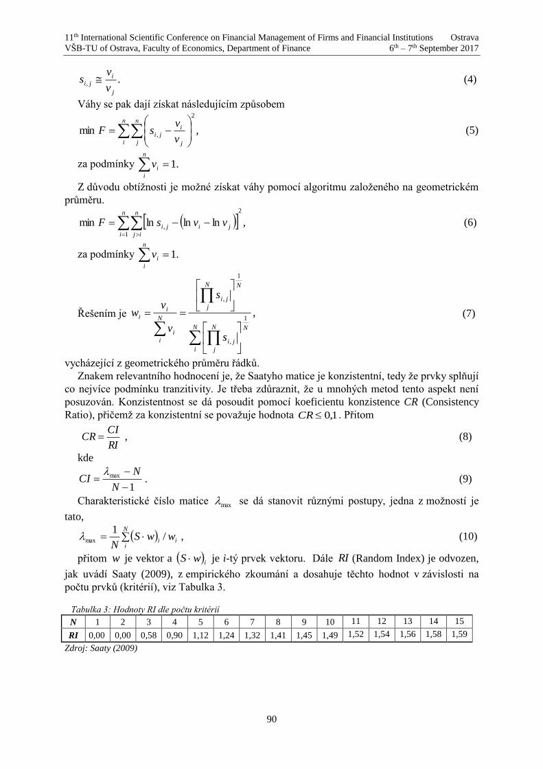
11th International Scientific Conference on Financial Management of Firms and Financial Institutions Ostrava
VŠB-TU of Ostrava, Faculty of Economics, Department of Finance 6th – 7th September 2017
90
.,
j
iji
v
vs (4)
Váhy se pak dají získat následujícím způsobem
,min
2
,
n
i
n
j j
iji
v
vsF (5)
za podmínky .1n
i
iv
Z důvodu obtížnosti je možné získat váhy pomocí algoritmu založeného na geometrickém
průměru.
,lnlnlnmin
2
1
,
n
i
n
ij
jiji vvsF (6)
za podmínky .1n
i
iv
Řešením je ,1
,
1
,
N
i
NN
j
ji
NN
j
ji
N
i
i
i
i
s
s
v
vw (7)
vycházející z geometrického průměru řádků.
Znakem relevantního hodnocení je, že Saatyho matice je konzistentní, tedy že prvky splňují
co nejvíce podmínku tranzitivity. Je třeba zdůraznit, že u mnohých metod tento aspekt není
posuzován. Konzistentnost se dá posoudit pomocí koeficientu konzistence CR (Consistency
Ratio), přičemž za konzistentní se považuje hodnota 1,0CR . Přitom
RI
CICR , (8)
kde
1
max
N
NCI
. (9)
Charakteristické číslo matice max se dá stanovit různými postupy, jedna z možností je
tato,
N
iii wwS
N/
1max , (10)
přitom w je vektor a iwS je i-tý prvek vektoru. Dále RI (Random Index) je odvozen,
jak uvádí Saaty (2009), z empirického zkoumání a dosahuje těchto hodnot v závislosti na
počtu prvků (kritérií), viz Tabulka 3.
Tabulka 3: Hodnoty RI dle počtu kritérií
N 1 2 3 4 5 6 7 8 9 10 11 12 13 14 15
RI 0,00 0,00 0,58 0,90 1,12 1,24 1,32 1,41 1,45 1,49 1,52 1,54 1,56 1,58 1,59
Zdroj: Saaty (2009)
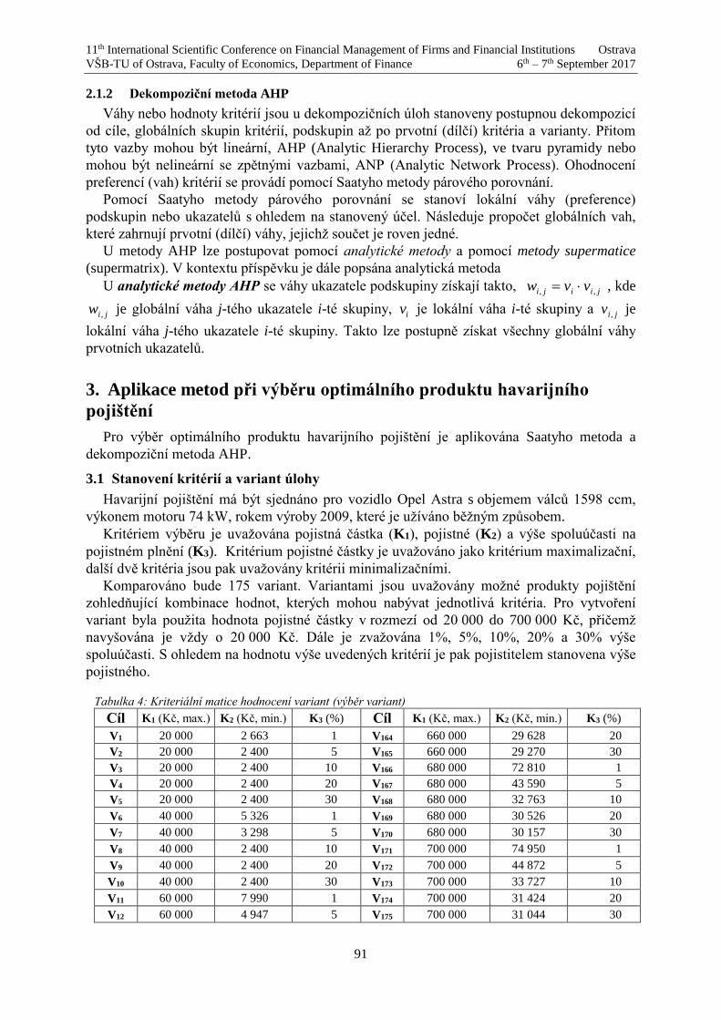
11th International Scientific Conference on Financial Management of Firms and Financial Institutions Ostrava
VŠB-TU of Ostrava, Faculty of Economics, Department of Finance 6th – 7th September 2017
91
2.1.2 Dekompoziční metoda AHP
Váhy nebo hodnoty kritérií jsou u dekompozičních úloh stanoveny postupnou dekompozicí
od cíle, globálních skupin kritérií, podskupin až po prvotní (dílčí) kritéria a varianty. Přitom
tyto vazby mohou být lineární, AHP (Analytic Hierarchy Process), ve tvaru pyramidy nebo
mohou být nelineární se zpětnými vazbami, ANP (Analytic Network Process). Ohodnocení
preferencí (vah) kritérií se provádí pomocí Saatyho metody párového porovnání.
Pomocí Saatyho metody párového porovnání se stanoví lokální váhy (preference)
podskupin nebo ukazatelů s ohledem na stanovený účel. Následuje propočet globálních vah,
které zahrnují prvotní (dílčí) váhy, jejichž součet je roven jedné.
U metody AHP lze postupovat pomocí analytické metody a pomocí metody supermatice
(supermatrix). V kontextu příspěvku je dále popsána analytická metoda
U analytické metody AHP se váhy ukazatele podskupiny získají takto, jiiji vvw ,, , kde
jiw , je globální váha j-tého ukazatele i-té skupiny, iv je lokální váha i-té skupiny a jiv , je
lokální váha j-tého ukazatele i-té skupiny. Takto lze postupně získat všechny globální váhy
prvotních ukazatelů.
3. Aplikace metod při výběru optimálního produktu havarijního
pojištění
Pro výběr optimálního produktu havarijního pojištění je aplikována Saatyho metoda a
dekompoziční metoda AHP.
3.1 Stanovení kritérií a variant úlohy
Havarijní pojištění má být sjednáno pro vozidlo Opel Astra s objemem válců 1598 ccm,
výkonem motoru 74 kW, rokem výroby 2009, které je užíváno běžným způsobem.
Kritériem výběru je uvažována pojistná částka (K1), pojistné (K2) a výše spoluúčasti na
pojistném plnění (K3). Kritérium pojistné částky je uvažováno jako kritérium maximalizační,
další dvě kritéria jsou pak uvažovány kritérii minimalizačními.
Komparováno bude 175 variant. Variantami jsou uvažovány možné produkty pojištění
zohledňující kombinace hodnot, kterých mohou nabývat jednotlivá kritéria. Pro vytvoření
variant byla použita hodnota pojistné částky v rozmezí od 20 000 do 700 000 Kč, přičemž
navyšována je vždy o 20 000 Kč. Dále je zvažována 1%, 5%, 10%, 20% a 30% výše
spoluúčasti. S ohledem na hodnotu výše uvedených kritérií je pak pojistitelem stanovena výše
pojistného.
Tabulka 4: Kriteriální matice hodnocení variant (výběr variant)
Cíl K1 (Kč, max.) K2 (Kč, min.) K3 (%) Cíl K1 (Kč, max.) K2 (Kč, min.) K3 (%)
V1 20 000 2 663 1 V164 660 000 29 628 20
V2 20 000 2 400 5 V165 660 000 29 270 30
V3 20 000 2 400 10 V166 680 000 72 810 1
V4 20 000 2 400 20 V167 680 000 43 590 5
V5 20 000 2 400 30 V168 680 000 32 763 10
V6 40 000 5 326 1 V169 680 000 30 526 20
V7 40 000 3 298 5 V170 680 000 30 157 30
V8 40 000 2 400 10 V171 700 000 74 950 1
V9 40 000 2 400 20 V172 700 000 44 872 5
V10 40 000 2 400 30 V173 700 000 33 727 10
V11 60 000 7 990 1 V174 700 000 31 424 20
V12 60 000 4 947 5 V175 700 000 31 044 30

11th International Scientific Conference on Financial Management of Firms and Financial Institutions Ostrava
VŠB-TU of Ostrava, Faculty of Economics, Department of Finance 6th – 7th September 2017
92
3.2 Vstupní data a výpočty
Na základě vstupních dat jsou pomocí Saatyho metody párovného porovnání, popsané v
subkapitole 2.1.1, vypočteny váhy jednotlivých kritérií a ověřena konzistence vytvořené
matice.
Obrázek 2: Váhy kritérií dle Saatyho metody párového porovnání
Cíl K1 K2 K3 geomean váhy wi (S . w) (S . w)i/wi
K1 1 3 5 2,46621 0,64833 1,9474 3,0037
K2 1/3 1 2 0,87358 0,22965 0,6898 3,0037
K3 1/5 1/2 1 0,46416 0,12202 0,3665 3,0037
3,80395 1,00000 λmax = 3,0037
CI = 0.00185
CR=CI/RI 0.0032
RI= 0,5800
N= 3,0000
Proces rozhodování a výběru optimální varianty je realizován na vzorku 175 variant.
Protože by Saatyho matice konstruovaná pro takové množství variant byla příliš složitou, jsou
vytvořeny a použity hodnotové škály. Pro kritéria K1 a K2 je vytvořeno vždy devět
hodnotových pásem.
Obrázek 3: Váhy skupin variant pro K1
K1 V1 V2 V3 V4 V5 V6 V7 V8 V9 geomean váhy w
V1 1 1/2 1/3 1/4 1/5 1/6 1/7 1/8 1/9 0,333333 0,030147
V2 2 1 1/2 1/3 1/4 1/5 1/6 1/7 1/8 0,5 0,045221
V3 3 2 1 1/2 1/3 1/4 1/5 1/6 1/7 0,654654 0,059208
V4 4 3 2 1 1/2 1/3 1/4 1/5 1/6 0,816497 0,073846
V5 5 4 3 2 1 1/2 1/3 1/4 1/5 1 0,090442
V6 6 5 4 3 2 1 1/2 1/3 1/4 1,224745 0,110769
V7 7 6 5 4 3 2 1 1/2 1/3 1,527525 0,138153
V8 8 7 6 5 4 3 2 1 1/2 2 0,180885
V9 9 8 7 6 5 4 3 2 1 3 0,271327
11,05675 1,000000
RI= 1.4500
N= 9,0000
Obrázek 4: Váhy skupin variant pro K2
K2 V1 V2 V3 V4 V5 V6 V7 V8 V9 geomean váhy w
V1 1 2 3 4 5 6 7 8 9 3 0,271327
V2 1/2 1 2 3 4 5 6 7 8 2 0,180885
V3 1/3 1/2 1 2 3 4 5 6 7 1,527525 0,138153
V4 1/4 1/3 1/2 1 2 3 4 5 6 1,224745 0,110769
V5 1/5 1/4 1/3 1/2 1 2 3 4 5 1 0,090442
V6 1/6 1/5 1/4 1/3 1/2 1 2 3 4 0,816497 0,073846
V7 1/7 1/6 1/5 1/4 1/3 1/2 1 2 3 0,654654 0,0059208
V8 1/8 1/7 1/6 1/5 1/4 1/3 1/2 1 2 0,5 0,045221
V9 1/9 1/8 1/7 1/6 1/5 1/4 1/3 1/2 1 0,333333 0,030147
11,05675 1,0000
RI= 1.4500
N= 9,0000
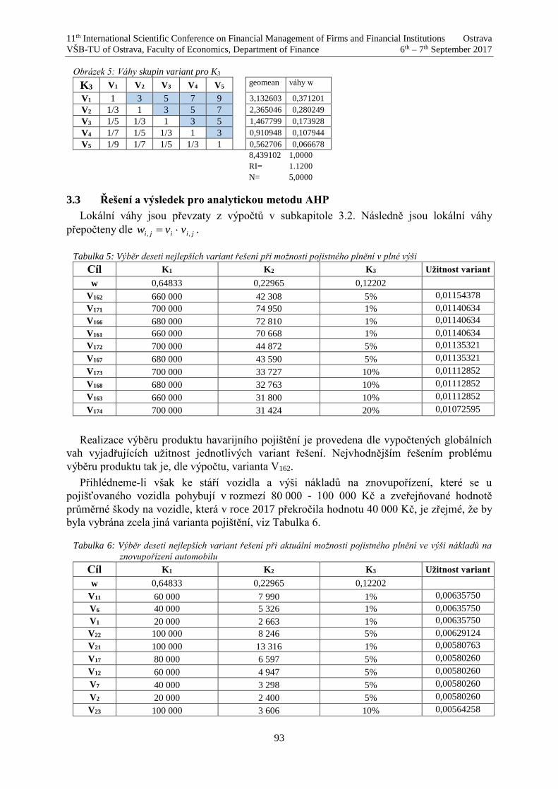
11th International Scientific Conference on Financial Management of Firms and Financial Institutions Ostrava
VŠB-TU of Ostrava, Faculty of Economics, Department of Finance 6th – 7th September 2017
93
Obrázek 5: Váhy skupin variant pro K3
K3 V1 V2 V3 V4 V5 geomean váhy w
V1 1 3 5 7 9 3,132603 0,371201
V2 1/3 1 3 5 7 2,365046 0,280249
V3 1/5 1/3 1 3 5 1,467799 0,173928
V4 1/7 1/5 1/3 1 3 0,910948 0,107944
V5 1/9 1/7 1/5 1/3 1 0,562706 0,066678
8,439102 1,0000
RI= 1.1200
N= 5,0000
3.3 Řešení a výsledek pro analytickou metodu AHP
Lokální váhy jsou převzaty z výpočtů v subkapitole 3.2. Následně jsou lokální váhy
přepočteny dle jiiji vvw ,, .
Tabulka 5: Výběr deseti nejlepších variant řešení při možnosti pojistného plnění v plné výši
Cíl K1 K2 K3 Užitnost variant
w 0,64833 0,22965 0,12202
V162 660 000 42 308 5% 0,01154378
V171 700 000 74 950 1% 0,01140634
V166 680 000 72 810 1% 0,01140634
V161 660 000 70 668 1% 0,01140634
V172 700 000 44 872 5% 0,01135321
V167 680 000 43 590 5% 0,01135321
V173 700 000 33 727 10% 0,01112852
V168 680 000 32 763 10% 0,01112852
V163 660 000 31 800 10% 0,01112852
V174 700 000 31 424 20% 0,01072595
Realizace výběru produktu havarijního pojištění je provedena dle vypočtených globálních
vah vyjadřujících užitnost jednotlivých variant řešení. Nejvhodnějším řešením problému
výběru produktu tak je, dle výpočtu, varianta V162.
Přihlédneme-li však ke stáří vozidla a výši nákladů na znovupořízení, které se u
pojišťovaného vozidla pohybují v rozmezí 80 000 - 100 000 Kč a zveřejňované hodnotě
průměrné škody na vozidle, která v roce 2017 překročila hodnotu 40 000 Kč, je zřejmé, že by
byla vybrána zcela jiná varianta pojištění, viz Tabulka 6.
Tabulka 6: Výběr deseti nejlepších variant řešení při aktuální možnosti pojistného plnění ve výši nákladů na
znovupořízení automobilu
Cíl K1 K2 K3 Užitnost variant
w 0,64833 0,22965 0,12202
V11 60 000 7 990 1% 0,00635750
V6 40 000 5 326 1% 0,00635750
V1 20 000 2 663 1% 0,00635750
V22 100 000 8 246 5% 0,00629124
V21 100 000 13 316 1% 0,00580763
V17 80 000 6 597 5% 0,00580260
V12 60 000 4 947 5% 0,00580260
V7 40 000 3 298 5% 0,00580260
V2 20 000 2 400 5% 0,00580260
V23 100 000 3 606 10% 0,00564258

11th International Scientific Conference on Financial Management of Firms and Financial Institutions Ostrava
VŠB-TU of Ostrava, Faculty of Economics, Department of Finance 6th – 7th September 2017
94
Tabulka 7: Vypočtené váhy dle analytické metody AHP
Položka Lokální Globální
Cíl 0
K1 64,833 %
K2 22,965 %
K3 12,202 %
V1 0,64 %
V2 0,58 %
V3 0,52 %
V4 0,48 %
V5 0,45 %
⁞ ⁞
⁞ ⁞
V172 1,11 %
V173 1,11 %
V174 1,07 %
V175 1,05 %
Ʃ 100,00 %
4. Závěr
Cílem příspěvku bylo nalezení optimálního produktu havarijního pojištění. Proces
posuzování jednotlivých variant byl založen na zohlednění pojistné částky, pojistného a
intenzity spoluúčasti. Optimální produkt pak měl kombinovat vhodnou míru naplnění těchto
kritérií.
Pro výběr optimální varianty byla použita dekompoziční metoda, Saatyho analytická
metoda AHP, založená na párovém porovnání. V textu byla tato metoda nejprve popsána.
Následně byly vytvořeny kombinacemi možných reálných hodnot, pojistné částky, pojistného
a spoluúčasti, nabízených pojistitelem jednotlivé varianty. Proces rozhodování pak probíhal na
bázi posouzení 175 variant. Takový počet variant je pro použití principu párového
porovnávání, na jehož základě je postavena metoda AHP dosti velký, proto bylo pro
porovnávání využito hodnotových škál.
Pokud by šlo o nový vůz, kdy při pojistné události může nastat totální škoda, byla by jako
nejlepší vybrána varianta pojištění V162 s hodnotou pojistné částky 660 000 Kč při pojistném
42 308 Kč a výši spoluúčasti 5%. Je-li však skutečností, že pojišťováno je vozidlo již několik
let používané, není logické pracovat s hodnotou pojistné částky v takové výši. Vodítkem pro
výběr ideální varianty pojištění pak mohou být také informace o průměrných hodnotách škod
v jednotlivých letech, či informace o hodnotě nákladů na znovupořízení příslušného typu
automobilu s ohledem na dobu používání a dalších faktorech.
References
[1] Borovcová, M. (2010). Metody vícekriteriálního hodnocení variant a jejich využití při
výběru produktu finanční instituce. Řízení a modelování finančních rizik. 1. vyd. pp. 20-
28. Ostrava: VŠB – Technická univerzita Ostrava.

11th International Scientific Conference on Financial Management of Firms and Financial Institutions Ostrava
VŠB-TU of Ostrava, Faculty of Economics, Department of Finance 6th – 7th September 2017
95
[2] Česká pojišťovna. (2017). Sjednejte si pojištění auta [online]. ČP [1.9.2017]. Dostupné z:
https://www.ceskapojistovna.cz/pojisteni-vozidel
[3] Fotr, J., Dědina, J. a Hrůzová, H. (2010). Manažerské rozhodování. 2. aktualiz. vyd.
Praha: Ekopress.
[4] Fotr, J., Švecová L. a kol. (2010). Manažerské rozhodování: postupy, metody a nástroje.
2. vyd. Praha: EKOPRESS.
[5] Ramík, J. (1999). Vícekriteriální rozhodování – analytický hierarchický process (AHP).
1. vyd. Karviná: Slezská univerzita v Opavě.
[6] Saaty, T. L. (2010). Principia Mathematica Decernendi: Mathematical Principles of
Decision Making. 1st printing. Pittsburgh: RWS Publications.
[7] Saaty,T. L. (2009). Theory and Applications of the Analytic Network Process. 2nd printing
with correction. Pittsburgh: RWS Publications.
[8] Valecký, J. (2017). Setting optimal limit of cover by stochastic optimisation. Proceedings
11th Internationl Scientific Conference Financial Management of Firms and Financial
Institutions. pp. 901-906. Ostrava: VŠB-TU Ostrava, Ekf.
[9] Zmeškal, Z., D. Dluhošová a T. Tichý (2013). Finanční modely: koncepty, metody,
aplikace. 3. Přeprac. A rozšíř. Vyd. Praha: Ekopress.
11th International Scientific Conference on Financial Management of Firms and Financial Institutions Ostrava
VŠB-TU of Ostrava, Faculty of Economics, Department of Finance 6th – 7th September 2017
96
Analysis of the financial performance by applying multi-level decomposition method
Martina Borovcová, Dagmar Richtarová 1
Abstract
The paper is focused on the financial performance analysis by applying multi-level
decomposition method. In the theoretical part, the multi-level decomposition method AHP on
the Saaty pair comparison approach, Economic Value Added and analysis of deviation are
presented. In the application part, the analysis of the performance of the sector is reviewed over
the period from 2007 to 2015. Next, factors affecting the Economic Value Added are analysed
by using the analysis of deviation, verification and application of the multi-level decomposition
method. In the end, comments on the results of the influence quantification are provided.
Key words
Financial Performance, Economic Value Added, Analysis of Deviation, Analytic Hierarchy
Proces
JEL Classification: C1, C4, G3
1. Úvod
Ekonomická přidaná hodnota je jedním z hlavních ukazatelů, které lze využít pro
hodnocení výkonnosti finančních i nefinančních institucí, ale také ekonomiky jako celku.
Jednou z možností, jak zjistit faktory, které ovlivňují úroveň výkonnosti je aplikace
pyramidového rozkladu daného ukazatele s využitím analýzy odchylek, kterou lze rozdělit na
statickou a dynamickou analýzu, jak uvádí Ptáčková (2016), Dluhošová, Ptáčková, Richtarová
(2017). Výkonnost je vždy ovlivňována několika faktory, proto má hodnocení výkonnosti
multikriteriální charakter.
Cílem příspěvku je ověřit výsledky hodnocení finanční výkonnosti vybraného odvětví
pomocí dekompozičních metod vícekriteriálního rozhodování. Výkonnost bude hodnocena dle
ekonomické přidané hodnoty a hlavní generátory hodnoty budou stanoveny dle analýzy
odchylek. Saatyho metodou párového porovnání bude pak ověřen vliv hlavních generátorů.
Následně bude stanoveno pořadí jednotlivých období s ohledem na zjištěné změny generátorů
a jejich preference.
2. Popis metod vícekriteriálního hodnocení variant
Úlohy vícekriteriálního hodnocení variant jsou zaměřeny především na nalezení nejlepší
(optimální) varianty a uspořádání variant od nejlepší po nejhorší. Optimální variantou je
taková varianta, která nejlépe splňuje každé z posuzovaných kritérií. Jak uvádí Borovcová
1 Ing. Martina Borovcová, Ph.D., VŠB - TU Ostrava, Ekonomická fakulta, Sokolská třída 33, Ostrava.
email: martina. [email protected].
Ing. Dagmar Richtarová, Ph.D., VŠB - TU Ostrava, Ekonomická fakulta, Sokolská třída 33, Ostrava.
email: [email protected].
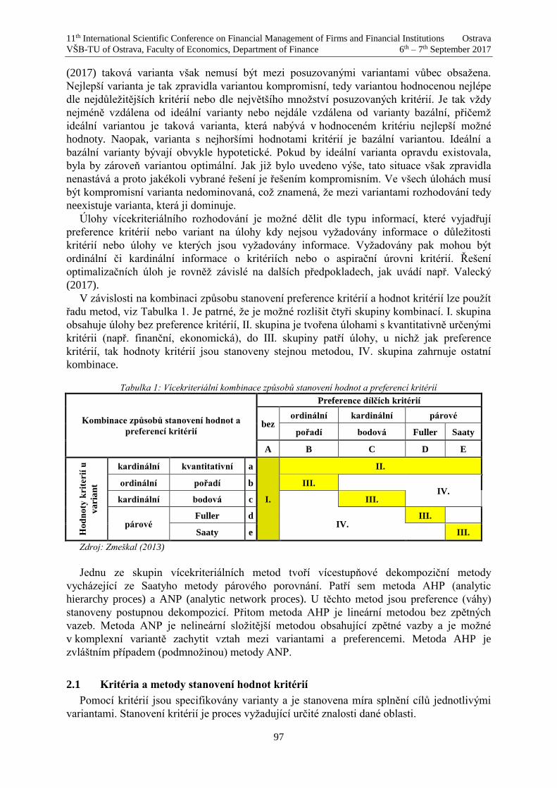
11th International Scientific Conference on Financial Management of Firms and Financial Institutions Ostrava
VŠB-TU of Ostrava, Faculty of Economics, Department of Finance 6th – 7th September 2017
97
(2017) taková varianta však nemusí být mezi posuzovanými variantami vůbec obsažena.
Nejlepší varianta je tak zpravidla variantou kompromisní, tedy variantou hodnocenou nejlépe
dle nejdůležitějších kritérií nebo dle největšího množství posuzovaných kritérií. Je tak vždy
nejméně vzdálena od ideální varianty nebo nejdále vzdálena od varianty bazální, přičemž
ideální variantou je taková varianta, která nabývá v hodnoceném kritériu nejlepší možné
hodnoty. Naopak, varianta s nejhoršími hodnotami kritérií je bazální variantou. Ideální a
bazální varianty bývají obvykle hypotetické. Pokud by ideální varianta opravdu existovala,
byla by zároveň variantou optimální. Jak již bylo uvedeno výše, tato situace však zpravidla
nenastává a proto jakékoli vybrané řešení je řešením kompromisním. Ve všech úlohách musí
být kompromisní varianta nedominovaná, což znamená, že mezi variantami rozhodování tedy
neexistuje varianta, která ji dominuje.
Úlohy vícekriteriálního rozhodování je možné dělit dle typu informací, které vyjadřují
preference kritérií nebo variant na úlohy kdy nejsou vyžadovány informace o důležitosti
kritérií nebo úlohy ve kterých jsou vyžadovány informace. Vyžadovány pak mohou být
ordinální či kardinální informace o kritériích nebo o aspirační úrovni kritérií. Řešení
optimalizačních úloh je rovněž závislé na dalších předpokladech, jak uvádí např. Valecký
(2017).
V závislosti na kombinaci způsobu stanovení preference kritérií a hodnot kritérií lze použít
řadu metod, viz Tabulka 1. Je patrné, že je možné rozlišit čtyři skupiny kombinací. I. skupina
obsahuje úlohy bez preference kritérií, II. skupina je tvořena úlohami s kvantitativně určenými
kritérii (např. finanční, ekonomická), do III. skupiny patří úlohy, u nichž jak preference
kritérií, tak hodnoty kritérií jsou stanoveny stejnou metodou, IV. skupina zahrnuje ostatní
kombinace.
Tabulka 1: Vícekriteriální kombinace způsobů stanovení hodnot a preferencí kritérií
Kombinace způsobů stanovení hodnot a
preferencí kritérií
Preference dílčích kritérií
bez ordinální kardinální párové
pořadí bodová Fuller Saaty
A B C D E
Ho
dn
oty
kri
terií
u
va
ria
nt
kardinální kvantitativní a
I.
II.
ordinální pořadí b III. IV.
kardinální bodová c III.
párové Fuller d
IV. III.
Saaty e III.
Zdroj: Zmeškal (2013)
Jednu ze skupin vícekriteriálních metod tvoří vícestupňové dekompoziční metody
vycházející ze Saatyho metody párového porovnání. Patří sem metoda AHP (analytic
hierarchy proces) a ANP (analytic network proces). U těchto metod jsou preference (váhy)
stanoveny postupnou dekompozicí. Přitom metoda AHP je lineární metodou bez zpětných
vazeb. Metoda ANP je nelineární složitější metodou obsahující zpětné vazby a je možné
v komplexní variantě zachytit vztah mezi variantami a preferencemi. Metoda AHP je
zvláštním případem (podmnožinou) metody ANP.
2.1 Kritéria a metody stanovení hodnot kritérií
Pomocí kritérií jsou specifikovány varianty a je stanovena míra splnění cílů jednotlivými
variantami. Stanovení kritérií je proces vyžadující určité znalosti dané oblasti.

11th International Scientific Conference on Financial Management of Firms and Financial Institutions Ostrava
VŠB-TU of Ostrava, Faculty of Economics, Department of Finance 6th – 7th September 2017
98
Kritéria použitá k výběru nejvhodnější varianty je možné dělit dle několika hledisek. Dle
úrovně žádoucí hodnoty je možné rozlišit kritéria maximalizační (výnosy, zisk) a
minimalizační (náklady, ztráta). Dle typu je možné kritéria dělit na kvalitativní a kvantitativní,
vyjádřená v měrných jednotkách.
Pro výpočty a porovnání je zpravidla žádoucí, aby zadané hodnoty kritérií yij byly
normalizovány do jednotkového intervalu, tedy
1;0ijx . (1)
Obecně je možné tyto hodnoty kritérií získat z dílčích funkcí utility (hodnoty) jako
ijij yux . (2)
Utilita kritéria, které nabývá nejhorších hodnot je rovna 0, nebo se blíží 0, a utilita kritéria
s nejlepší hodnotou je rovna 1.
Protože bude v příspěvku aplikována Saatyho metoda párového porovnání, bude
následující popis zaměřen na tuto metodu.
2.1.1 Saatyho metoda párového porovnání
Postup aplikace Saatyho metody stanovení vah kritérií lze rozdělit do dvou kroků. První
krok spočívá v párovém srovnávání, kdy se zjišťují preferenční vztahy dvojic kritérií
uspořádaných dle důležitosti a uvádějí se do tzv. Saatyho matice S. Ta je maticí
symetrickou s prvky si,j. Kromě směru preference dvojic kritérií je možné určit rovněž velikost
této preference, která je vyjádřena určitým počtem bodů ze zvolené bodové stupnice. Jak
uvádí Saaty (2010), je vhodné využít pro vyjádření velikosti preferencí bodové stupnice
opatřené deskriptory, uvedené v Tabulce 2. Síla preferencí se vyjádří v intervalu 9;1, jis .
Tabulka 2: Saatym doporučená bodová stupnice s deskriptory
Počet bodů Deskriptor
1 Kritéria jsou stejně významná
2 První kritérium je mírně významnější než druhé
3 První kritérium je slabě významnější než druhé
4 První kritérium je středně významnější než druhé
5 První kritérium je dosti významnější než druhé
6 První kritérium je silněji významnější než druhé
7 První kritérium je prokazatelně významnější než druhé
8 První kritérium je velmi silně významnější než druhé
9 První kritérium je absolutně významnější než druhé
1,1 – 1,9 Pokud jsou důležitosti velmi blízké, desetinná místa se přidávají za hodnotu 1, aby
bylo možné odlišit nižší stupně významnosti dle potřeby
Zdroj: Saaty (2010)
Výsledkem tohoto kroku je získání pravé horní trojúhelníkové části Saatyho matice
velikosti preferencí. Pro diagonální prvky platí, že 1, iis . Pro inverzní prvky (v levé dolní
trojúhelníkové části matice) pak platí
.1
,
,
ij
jis
s (3)
Prvky sij Saatyho matice jsou odhadem podílů vah kritérií vi a vj, takže platí
.,
j
iji
v
vs (4)
Váhy se pak dají získat následujícím způsobem
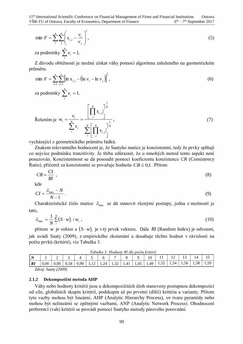
11th International Scientific Conference on Financial Management of Firms and Financial Institutions Ostrava
VŠB-TU of Ostrava, Faculty of Economics, Department of Finance 6th – 7th September 2017
99
,min
2
,
n
i
n
j j
iji
v
vsF (5)
za podmínky .1n
i
iv
Z důvodu obtížnosti je možné získat váhy pomocí algoritmu založeného na geometrickém
průměru.
,lnlnlnmin
2
1
,
n
i
n
ij
jiji vvsF (6)
za podmínky .1n
i
iv
Řešením je ,1
,
1
,
N
i
NN
j
ji
NN
j
ji
N
i
i
i
i
s
s
v
vw (7)
vycházející z geometrického průměru řádků.
Znakem relevantního hodnocení je, že Saatyho matice je konzistentní, tedy že prvky splňují
co nejvíce podmínku tranzitivity. Je třeba zdůraznit, že u mnohých metod tento aspekt není
posuzován. Konzistentnost se dá posoudit pomocí koeficientu konzistence CR (Consistency
Ratio), přičemž za konzistentní se považuje hodnota 1,0CR . Přitom
RI
CICR , (8)
kde
1
max
N
NCI
. (9)
Charakteristické číslo matice max se dá stanovit různými postupy, jedna z možností je
tato,
N
iii wwS
N/
1max , (10)
přitom w je vektor a iwS je i-tý prvek vektoru. Dále RI (Random Index) je odvozen,
jak uvádí Saaty (2009), z empirického zkoumání a dosahuje těchto hodnot v závislosti na
počtu prvků (kritérií), viz Tabulka 3.
Tabulka 3: Hodnoty RI dle počtu kritérií
N 1 2 3 4 5 6 7 8 9 10 11 12 13 14 15
RI 0,00 0,00 0,58 0,90 1,12 1,24 1,32 1,41 1,45 1,49 1,52 1,54 1,56 1,58 1,59
Zdroj: Saaty (2009)
2.1.2 Dekompoziční metoda AHP
Váhy nebo hodnoty kritérií jsou u dekompozičních úloh stanoveny postupnou dekompozicí
od cíle, globálních skupin kritérií, podskupin až po prvotní (dílčí) kritéria a varianty. Přitom
tyto vazby mohou být lineární, AHP (Analytic Hierarchy Process), ve tvaru pyramidy nebo
mohou být nelineární se zpětnými vazbami, ANP (Analytic Network Process). Ohodnocení
preferencí (vah) kritérií se provádí pomocí Saatyho metody párového porovnání.

11th International Scientific Conference on Financial Management of Firms and Financial Institutions Ostrava
VŠB-TU of Ostrava, Faculty of Economics, Department of Finance 6th – 7th September 2017
100
Pomocí Saatyho metody párového porovnání se stanoví lokální váhy (preference)
podskupin nebo ukazatelů s ohledem na stanovený účel. Následuje propočet globálních vah,
které zahrnují prvotní (dílčí) váhy, jejichž součet je roven jedné.
U metody AHP lze postupovat pomocí analytické metody a pomocí metody supermatice
(supermatrix). V kontextu příspěvku je dále popsána analytická metoda
U analytické metody AHP se váhy ukazatele podskupiny získají takto, jiiji vvw ,, , kde
jiw , je globální váha j-tého ukazatele i-té skupiny, iv je lokální váha i-té skupiny a jiv , je
lokální váha j-tého ukazatele i-té skupiny. Takto lze postupně získat všechny globální váhy
prvotních ukazatelů.
3. Analýza odchylek
Jedním z přístupů k analýze odchylek je metoda pyramidového rozkladu. Pyramidový
rozklad umožňuje stanovit vzájemné vazby mezi jednotlivými ukazateli a identifikovat vliv
těchto dílčích ukazatelů na vrcholový ukazatel.
Souvislost mezi vrcholovým ukazatelem x a dílčími ukazateli ai lze vyjádřit pomocí funkce
x = f (a1, a2……… an), která umožňuje kvantifikovat míru vlivu dílčích ukazatelů jako
příčinných faktorů na změnu zvoleného vrcholového ukazatele (Dluhošová, 2010).
Odchylku vrcholového ukazatele lze vyjádřit jako součet odchylek vybraných dílčích
ukazatelů,
i
ax ixy , (11)
kde x je analyzovaný ukazatel, xy je přírůstek vlivu analyzovaného ukazatele, ai je dílčí
vysvětlující ukazatel, iax je vliv dílčího ukazatele ai na analyzovaný ukazatel x.
Změny hodnot ukazatelů mohou být vyjádřeny pomocí relativních a absolutních odchylek.
Pro rozklad se využívají zpravidla dvě základní vazby, aditivní a multiplikativní vazba,
výjimečně se vyskytují exponenciální vazby.
Při aditivních vazbách jsou přímo souměřitelné absolutní rozdíly činitelů. Podle toho, jak
je řešena multiplikativní vazba, se rozlišuje pět metod: metoda postupných změn, metoda
rozkladu se zbytkem, logaritmická metoda rozkladu, funkcionální a integrální metoda
rozkladu, jejich odvození lze najít například v Zmeškal a kol. (2013), Dluhošová (2010).
V příspěvku bude aplikována integrální metoda, která pracuje s diskrétními výnosy. Vyčíslení
vlivů dle integrální metody je obdobné jako u metody funkcionální, ale je aplikována pouze
lineární složka Taylorova rozvoje 1. stupně.
Za předpokladu 3 faktorů:
.
,,,,,,0
0
0,30,20,1
ˇ
0,30,20,1
0
00,30,20,1
xxx yx
x
x
aaaxy
x
aaax
x
xy
x
aaaxy
(12)
Po úpravě pak
.1
321 x
x
aaax yR
RRRy
(13)
,,
1
1 x
x
a
a yR
Rx ,
,
2
2 x
x
a
a yR
Rx .
,
3
3 x
x
a
a yR
Rx (14)
kde xR a iaR jsou diskrétní výnosy ukazatelů x a ai.
Dle Zmeškal (2013) pro jakýkoliv počet prvků platí, že
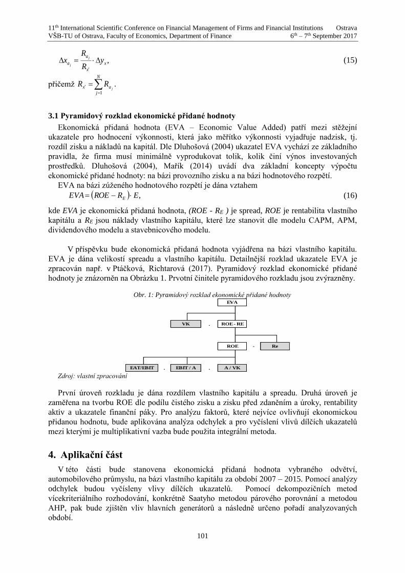
11th International Scientific Conference on Financial Management of Firms and Financial Institutions Ostrava
VŠB-TU of Ostrava, Faculty of Economics, Department of Finance 6th – 7th September 2017
101
,x
x
a
a yR
Rx
j
j
(15)
přičemž
N
j
ax jRR
1
.
3.1 Pyramidový rozklad ekonomické přidané hodnoty
Ekonomická přidaná hodnota (EVA – Economic Value Added) patří mezi stěžejní
ukazatele pro hodnocení výkonnosti, která jako měřítko výkonnosti vyjadřuje nadzisk, tj.
rozdíl zisku a nákladů na kapitál. Dle Dluhošová (2004) ukazatel EVA vychází ze základního
pravidla, že firma musí minimálně vyprodukovat tolik, kolik činí výnos investovaných
prostředků. Dluhošová (2004), Mařík (2014) uvádí dva základní koncepty výpočtu
ekonomické přidané hodnoty: na bázi provozního zisku a na bázi hodnotového rozpětí.
EVA na bázi zúženého hodnotového rozpětí je dána vztahem
,ERROEEVA E (16)
kde EVA je ekonomická přidaná hodnota, (ROE - RE ) je spread, ROE je rentabilita vlastního
kapitálu a RE jsou náklady vlastního kapitálu, které lze stanovit dle modelu CAPM, APM,
dividendového modelu a stavebnicového modelu.
V příspěvku bude ekonomická přidaná hodnota vyjádřena na bázi vlastního kapitálu.
EVA je dána velikostí spreadu a vlastního kapitálu. Detailnější rozklad ukazatele EVA je
zpracován např. v Ptáčková, Richtarová (2017). Pyramidový rozklad ekonomické přidané
hodnoty je znázorněn na Obrázku 1. Prvotní činitele pyramidového rozkladu jsou zvýrazněny.
Obr. 1: Pyramidový rozklad ekonomické přidané hodnoty
.
-
. .
Re
EAT/EBIT EBIT / A A / VK
EVA
VK ROE - RE
ROE
Zdroj: vlastní zpracování
První úroveň rozkladu je dána rozdílem vlastního kapitálu a spreadu. Druhá úroveň je
zaměřena na tvorbu ROE dle podílu čistého zisku a zisku před zdaněním a úroky, rentability
aktiv a ukazatele finanční páky. Pro analýzu faktorů, které nejvíce ovlivňují ekonomickou
přidanou hodnotu, bude aplikována analýza odchylek a pro vyčíslení vlivů dílčích ukazatelů
mezi kterými je multiplikativní vazba bude použita integrální metoda.
4. Aplikační část
V této části bude stanovena ekonomická přidaná hodnota vybraného odvětví,
automobilového průmyslu, na bázi vlastního kapitálu za období 2007 – 2015. Pomocí analýzy
odchylek budou vyčísleny vlivy dílčích ukazatelů. Pomocí dekompozičních metod
vícekriteriálního rozhodování, konkrétně Saatyho metodou párového porovnání a metodou
AHP, pak bude zjištěn vliv hlavních generátorů a následně určeno pořadí analyzovaných
období.
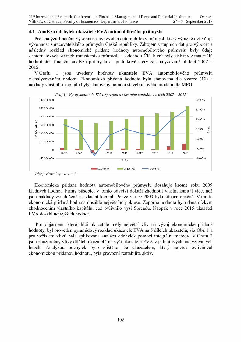
11th International Scientific Conference on Financial Management of Firms and Financial Institutions Ostrava
VŠB-TU of Ostrava, Faculty of Economics, Department of Finance 6th – 7th September 2017
102
4.1 Analýza odchylek ukazatele EVA automobilového průmyslu
Pro analýzu finanční výkonnosti byl zvolen automobilový průmysl, který výrazně ovlivňuje
výkonnost zpracovatelského průmyslu České republiky. Zdrojem vstupních dat pro výpočet a
následný rozklad ekonomické přidané hodnoty automobilového průmyslu byly údaje
z internetových stránek ministerstva průmyslu a odchodu ČR, které byly získány z materiálů
hodnotících finanční analýzu průmyslu a podnikové sféry za analyzované období 2007 –
2015.
V Grafu 1 jsou uvedeny hodnoty ukazatele EVA automobilového průmyslu
v analyzovaném období. Ekonomická přidaná hodnota byla stanovena dle vzorce (16) a
náklady vlastního kapitálu byly stanoveny pomocí stavebnicového modelu dle MPO.
Graf 1: Vývoj ukazatele EVA, spreadu a vlastního kapitálu v letech 2007 – 2015
Zdroj: vlastní zpracování
Ekonomická přidaná hodnota automobilového průmyslu dosahuje kromě roku 2009
kladných hodnot. Firmy působící v tomto odvětví dokáží zhodnotit vlastní kapitál více, než
jsou náklady vynaložené na vlastní kapitál. Pouze v roce 2009 byla situace opačná. V tomto
ekonomická přidaná hodnota dosáhla největšího poklesu. Záporná hodnota byla dána nízkým
zhodnocením vlastního kapitálu, což ovlivnilo výši Spreadu. Naopak v roce 2015 ukazatel
EVA dosáhl nejvyšších hodnot.
Pro objasnění, které dílčí ukazatele měly největší vliv na vývoj ekonomické přidané
hodnoty, byl proveden pyramidový rozklad ukazatele EVA na 5 dílčích ukazatelů, viz Obr. 1 a
pro vyčíslení vlivů byla aplikována analýza odchylek pomocí integrální metody. V Grafu 2
jsou znázorněny vlivy dílčích ukazatelů na výši ukazatele EVA v jednotlivých analyzovaných
letech. Analýzou odchylek bylo zjištěno, že ukazatelem, který nejvíce ovlivňoval
ekonomickou přidanou hodnotu, byla provozní rentabilita aktiv.

11th International Scientific Conference on Financial Management of Firms and Financial Institutions Ostrava
VŠB-TU of Ostrava, Faculty of Economics, Department of Finance 6th – 7th September 2017
103
Graf 2: Vliv dílčích ukazatelů na ukazatel EVA
Zdroj: vlastní zpracování
4.2 Aplikace Saatyho metody párového porovnání
Pomocí dekompoziční metody vícekriteriálního rozhodování, konkrétně Saatyho metody je
zjištěno období s nejpodstatnějšími změnami ukazatelů.
Ke splnění stanoveného cíle je nezbytné stanovit kritéria a varianty rozhodování. Kritériem
výběru je uvažován ukazatel EBIT/A (K1), ukazatel A/VK (K2), ukazatel EAT/EBIT (K3),
ukazatel RE (K4) a ukazatel VK (K5), viz Obr. 2. Kritéria již jsou seřazena dle důležitosti.
Tabulka 4: Váhy kritérií dle Saatyho metody párového porovnání
K1 K2 K3 K4 K5 geomean váhy w
K1 1 2 3 4 5 2,605171 0,417419
K2 1/2 1 2 3 4 1,643752 0,263374
K3 1/3 1/2 1 2 3 1 0,160227
K4 1/4 1/3 1/2 1 2 0,608364 0,097476
K5 1/5 1/4 1/3 1/2 1 0,383852 0,061504
∑ 6,241139 1
Zdroj: vlastní zpracování
Variantami jsou uvažovány jednotlivé roky analyzovaného období. Pro splnění
stanoveného cíle jsou nejprve vypočteny hodnoty užitnosti variant pro jednotlivá kritéria.
Následně jsou po zohlednění vah jednotlivých kritérií vypočteny výsledné hodnoty vážených
užitností konkrétních variant. Výsledné hodnoty jsou zachyceny v Tabulce 5. Zvýrazněny jsou
vždy nejvyšší hodnoty naplnění kritéria příslušnou variantou.
Tabulka 5: Stanovení pořadí jednotlivých let dle intenzity změn
07_08 08_09 09_10 10_11 11_12 12_13 13_14 14_15
K1 0,029742 0,136909 0,066167 0,019991 0,013664 0,009662 0,096809 0,044475
K2 0,008621 0,061083 0,006096 0,028062 0,041748 0,018766 0,012614 0,086384
K3 0,003709 0,03716 0,007674 0,005245 0,025398 0,017072 0,011417 0,052553
K4 0,002256 0,031971 0,015451 0,003191 0,006945 0,004668 0,022607 0,010386
K5 0,002946 0,006553 0,014264 0,002013 0,009749 0,004382 0,001424 0,020173
∑ 0,047274 0,273677 0,109652 0,058502 0,097505 0,05455 0,14487 0,21397
Pořadí 8 1 4 6 5 7 3 2
Zdroj: vlastní zpracování
11th International Scientific Conference on Financial Management of Firms and Financial Institutions Ostrava
VŠB-TU of Ostrava, Faculty of Economics, Department of Finance 6th – 7th September 2017
104
Z výsledků zachycených v Tabulce 5 je zřejmé, že zcela zásadními změnami vývoje hodnot
se vyznačuje období let 2008-2009. Ve dvou z pěti sledovaných kritérií, K1 a K4 jsou roční
změny nejpodstatnější. Kritérium K1 (ukazatel EBIT/A) je kritériem nejdůležitějším, tedy
s nejvyšší vahou, proto je toto období hodnoceno v souvislosti se změnami jako důležitější
než období 2014-2015, které je sice nejdůležitější hned ve třech posuzovaných kritériích, ale
s nižší preferencí.
5. Závěr
Cílem příspěvku bylo ověřit výsledky hodnocení finanční výkonnosti vybraného odvětví
pomocí dekompozičních metod vícekriteriálního rozhodování. Výkonnost byla hodnocena dle
ekonomické přidané hodnoty a hlavní generátory hodnoty byly staveny dle analýzy odchylek.
Saatyho metodou párového porovnání pak byl ověřen vliv hlavních generátorů. Následně bylo
stanoveno pořadí jednotlivých období s ohledem na zjištěné změny generátorů a jejich
preference. Z provedené analýzy vyplývá, že obdobím s nejvýraznějšími změnami bylo období
let 2008 – 2009. Důvodem je největší změna generátoru EBIT/A s nejvyšší preferencí.
Závěrem je možné konstatovat, že použití dekompozičních metod vícekriteriálního
rozhodování je vhodnou součástí hodnocení výkonnosti.
References
[1] Borovcová, M. (2017). Selection of the optimal solution of the decision-making problem.
In: Proceedings 11th Internationl Scientific Conference Financial Management of Firms
and Financial Institutions. pp. 87-95. Ostrava: VŠB-TU Ostrava, Ekf.
[2] Borovcová, M., Špačková, A. Indicators Preference Determination of the Level Insurance
Market Assessment by Applying the AHP and ANP Decomposition Multi-Attribute
Methods. In: Proceedings of the 8th International Scientific Conference. Zlín: Tomas Bata
University in Zlín, pp. 98-109. ISBN 978-80-7454-653-2.
[3] Dluhošová, D. (2004). Přístupy k analýze finanční výkonnosti firem a odvětví na bázi
metody EVA – Economic Value Added. Finance a úvěr - Czech Journal of Economics and
Finance, 11-12 2004, roč. 54.
[4] Dluhošová, D. (2010). Finanční řízení a rozhodování podniku. Praha: EKOPRESS, 2010.
[5] Dluhošová, D., Ptáčková, B., Richtarová, D. (2017). Application of selected financial
performance methods to chosen industry in the Czech Republic. In: European Financial
Systems, 14thInternational Scientific Conference. Brno: Masaryk University. 2017.
[6] Maříková, P., Mařík, M. (2005). Moderní metody hodnocení výkonnosti a oceňování
podniku. Praha: Ekopress.
[7] Ptáčková, B. (2016). Identifikace generátorů finanční výkonnosti metodou dekompozice
rozptylu. In: Managing and Modelling of Financial Risks: proceedings of the 8th
international scientific conference: September 5-6, 2016, Ostrava, Czech Republic.
Ostrava: VŠB - Technical University of Ostrava, 2016.
[8] Ptáčková, B., Richtarová, D. (2017). Analysis of the generators of the company´s
financial performance. In: Proceedings of the 8th International Scientific Conference.
Zlín: Tomas Bata University in Zlín, pp. 942-950. ISBN 978-80-7454-653-2.

11th International Scientific Conference on Financial Management of Firms and Financial Institutions Ostrava
VŠB-TU of Ostrava, Faculty of Economics, Department of Finance 6th – 7th September 2017
105
[9] Saaty, T. L. (2010). Principia Mathematica Decernendi: Mathematical Principles of
Decision Making. 1st printing. Pittsburgh: RWS Publications.
[10] Saaty,T. L. (2009). Theory and Applications of the Analytic Network Process. 2nd printing
with correction. Pittsburgh: RWS Publications.
[11] Valecký, J. (2017). Setting optimal limit of cover by stochastic optimisation. In:
Proceedings 11th Internationl Scientific Conference Financial Management of Firms and
Financial Institutions. pp. 901-906. Ostrava: VŠB-TU Ostrava, Ekf.
[12] Zmeškal, Z., D. Dluhošová a T. Tichý (2013). Finanční modely: koncepty, metody,
aplikace. Praha: Ekopress.
[13] Analytické materiály a statistiky – finanční analýza podnikové sféry se zaměřením na
konkurenceschopnost sledovaných odvětví za roky 2007 – 2015. MPO. Dostupné z:
http://www.mpo.cz/ministr-a-ministerstvo/analyticke-materialy.

11th International Scientific Conference on Financial Management of Firms and Financial Institutions Ostrava
VŠB-TU of Ostrava, Faculty of Economics, Department of Finance 6th – 7th September 2017
106
Non-traditional approach using mathematical programming to a stock investment portfolio making
Adam Borovička 1
Abstract
In most cases, the investment portfolio is made based on partial indicators of fundamental or
technical analysis, actual mood in the capital market or investor’s intuition and feelings. These
partial approaches cannot offer a comprehensive analysis with a consequent quantitative
determination of the shares of the investment instruments in the portfolio. To eliminate this
drawback, I propose a complex multi-factors analysis using multiple objective mathematical
programming. This approach is able to take into account many factors influencing investment
decision (yield, risk, dividend, cost, volume of trades, mood etc.). The result is shares of the
investment instruments in the portfolio. Applicability of this non-traditional approach is
demonstrated on an investment decision making on the RM-System Czech Stock Exchange.
Two typical investment strategies are specified. Stock portfolios for both strategies are analysed
and compared.
Key words
Multiple objective mathematical programming, portfolio making, RM-System, stock.
JEL Classification: C61, G11
1. Introduction
Many people over the world have some free funds. One way how to use them is the
investment. This way is increasingly popular in the Czech Republic. Selection of the suitable
investment instruments and determination of their shares in the portfolio can be very difficult
process. The investment decision can be supported by the results of fundamental or technical
analysis, expert estimations or investor’s human intuition. Based on these partial outputs, the
portfolio is actually intuitively made.
I think that the (potential) investor (namely with little experience) would welcome
a comprehensive investment portfolio making procedure which enable to consider all
monitored investment characteristics (yield, risk, dividend, volume of trades, cost etc.) and
investor preferences (risk attitude, diversification, yield requirements etc.). On this base, such
an approach would provide the most suitable structure of the portfolio, i.e. shares of the
particular investment instruments.
So, the main aim of this article is to propose such an investment portfolio making
procedure. Developed approach uses multiple objective mathematical programming concept
which is non-traditional for a decision making on the capital market. However, this article
wants to show that not commonly used (multi-objective) mathematical programming can be
reasonably applicable for making an investment portfolio. The mathematical model is
primarily formulated for a portfolio making on the stock exchange, where the investment
instruments are traded in the standardized unit (lots). However, it is very flexible for any
1 Ing. Adam Borovička, Ph.D., University of Economics, Department of Econometrics, W. Churchill
Sq. 4, Prague, Czech Republic, e-mail: [email protected].

11th International Scientific Conference on Financial Management of Firms and Financial Institutions Ostrava
VŠB-TU of Ostrava, Faculty of Economics, Department of Finance 6th – 7th September 2017
107
changes. Significant applicability of the proposed approach is demonstrated on the RM-
System Czech Stock Exchange, where the investors with smaller capital can trade through the
user-friendly online system. The portfolio is made for two different typical investment
strategies. The results are analysed and interpreted in detail.
The article has the following structure. After the introduction, the proposed portfolio
making procedure using the multiple objective mathematical programming is closely
described. The next section deals with making a portfolio for two types of investors on the
RM-System Czech Stock Exchange. Finally, the article is summarized and some ideas for
future research are outlined.
2. Portfolio making procedure using multiple objective programming
If the (potential) investor wants to invest his/her free funds, an appropriate investment
policy (strategy) should be specified (Steigauf, 2003). It contains purpose of the investment,
investment time horizon, risk attitude, yield preferences, style of an investment management
etc. Then the portfolio from the preselected investment instruments (e.g. stocks traded on the
RM-System Czech Stock Exchange) can be made. For a partial analysis, the principles
(namely based on the price or yield of stock) of fundamental (Graham and Dodd, 2008) or
technical (Murphy, 1999) analysis can be used. Further, the investment decision can be
influenced an expert estimations, human intuition or mass behaviour. Then to make
a portfolio, all analysis, percepts and attitudes must be put together. In practice, this
compilation is performed by some intuitive (qualitative) approach. Then, shares of the
investment instruments in the portfolio are actually estimated. To simplify and quantify the
approach, I propose a complex portfolio making procedure using multiple objective
mathematical programming. The main advantage of this multifactor approach is that enables
to include all important investment perspectives (yield, risk, cost, dividend, volume of trades,
diversification etc.). Result of this approach is a final structure of the investment portfolio (i.e.
with particular shares) which is very significant support for an investor’s decision making.
After a specification of the investment policy and a preselection of the investment
instruments (further stocks), the mathematical model is formulated to make a portfolio. This
model can be inspired by the Markowitz portfolio theory (Markowitz, 1952). However, it is
more complexly specified as multiobjective. At first, all selected characteristics of the
portfolio are specified as the objective functions (criteria). The maximizing (minimizing)
objective function can be formulated as a weighted average 1
1 1
( ..., ) /n n
j n i i i
i i
f x x c x x
, where
( 1,2,..., )ic i n is some characteristic of the i-th stock (from n stocks) and
1
/ ( 1,2,..., )n
i i
i
x x i n
is a share of the i-th in the portfolio. Variable ix denotes only
approximate share because the sum of these variables may not equal 1. This formulation is
required because the stocks can be traded only in standardized units (lots), not by piece.
Further, the set of feasible solution X representing all demands on the portfolio is specified.
It can include a “diversification” condition which is represented by minimum and maximum
number of stocks in the portfolio, or (minimum) maximum level of a share of one stock. This
can be mathematically formulated as
1
1
, * * , 0,1 1,2,...,i
n
i
i
nx
i i i ixi
lower y upper mins y maxs y y i n
,

11th International Scientific Conference on Financial Management of Firms and Financial Institutions Ostrava
VŠB-TU of Ostrava, Faculty of Economics, Department of Finance 6th – 7th September 2017
108
where lower, or upper is a minimum, or maximum number of stocks in the portfolio, mins , or
maxs is a minimum, or maximum share of one stock in the portfolio and ( 1,2,..., )iy i n is
a binary variable representing absence/presence of the i-th stock in the portfolio. Other
conditions must ensure that the resulting shares exactly match the investment in the
appropriate number of the whole lots. This fact is ensured by the following formulae
0
1
*1 1 , , 1,2,..., ,
ni i
i i i i
i
price lottol x tol x p p Z i n
invest
where ( 1,2,..., )iprice i n is an actual market price of the i-th stock, ( 1,2,..., )ilot i n
represents a number of stocks in the lot, ( 1,2,..., )ip i n denotes a number of purchased lot of
the i-th stock, invest is an approximate amount of invested money and tol represents very
small deviation from 1. These conditions respect a trade in the standardized units under the
limits of the amount of invested money. Similarly, other requirements can be included.
In the next step, the optimum of the minimizing, or maximizing objective functions on the
bounded set X must be found. Because of nonlinearities in the model, only local optimum is
usually found. To make a (stock) portfolio, the following mathematical model is formulated *
*
max min
( )
( )max j j
jj
f f
j j ffj I j I
z w w
X
x
x
x
, (1)
where 1 2( , ,..., )T
nx x xx , maxI , or
minI is a set of indices of the maximizing, or minimizing
objective functions, ( 1,2,..., )jw j k is a weight of the j-th objective function (criterion)
and* ( 1,2,..., )jf j k is the (locally) optimal value of the j-th objective function.
Transformation of the multi-objective view to the one-objective is made by a well-known
weighted sum approach (Fishburn, 1967). Then the value of this aggregate objective function
actually represents a rate of obtaining the optimal value of all criteria on average. In other
words, it is a rate of utility (from 0 to 1) of the solution for the decision maker. The optimal
solution represents the most suitable structure of the stock portfolio and determines the values
of all watched portfolio characteristics.
3. Stock portfolio making on the RM-System Czech Stock Exchange
This part shows two cases of a decision making on the stock exchange in order to make
a stock portfolio. These cases should reflect the real decision making situations of the
investors who are able to independently trade with stocks in terms of the online trading system
of the Czech exchange RM-System. These investors are able to specify their investment policy
(purpose of the investment, time horizon, risk attitude or yield preferences). Then the stock
portfolio for both types of investors can be made by the proposed approach using
mathematical programming.
3.1 RM-System Czech Stock Exchange
RM-System Czech Stock Exchange is a market where the stocks of the best-known Czech
and foreign companies (e.g. ČEZ, Unipetrol, Erste Bank or Microsoft) are traded. This stock
exchange is primarily focused on small and medium investors. Among the greatest advantages
of the trading on the Czech RM-System exchange is a wide offer of stocks traded in the Czech
crowns, the longest trading time in the Czech Republic or user-friendly online trading system
with EasyClick (RM-System, 2017b).
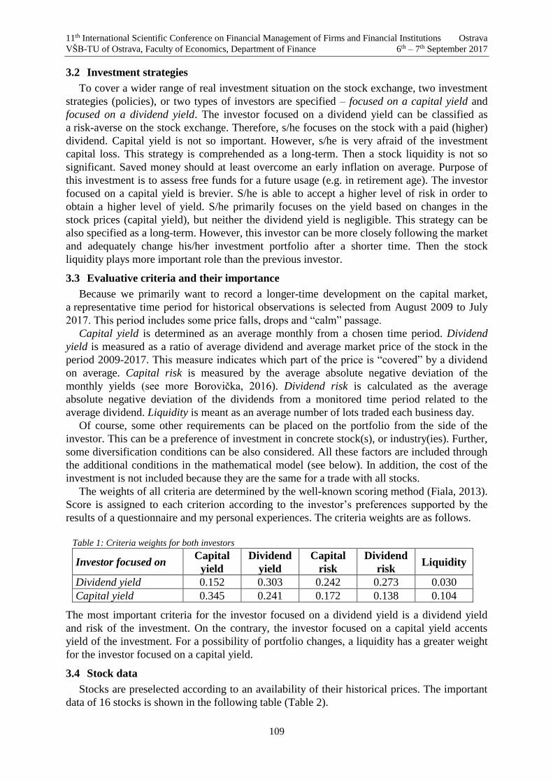
11th International Scientific Conference on Financial Management of Firms and Financial Institutions Ostrava
VŠB-TU of Ostrava, Faculty of Economics, Department of Finance 6th – 7th September 2017
109
3.2 Investment strategies
To cover a wider range of real investment situation on the stock exchange, two investment
strategies (policies), or two types of investors are specified – focused on a capital yield and
focused on a dividend yield. The investor focused on a dividend yield can be classified as
a risk-averse on the stock exchange. Therefore, s/he focuses on the stock with a paid (higher)
dividend. Capital yield is not so important. However, s/he is very afraid of the investment
capital loss. This strategy is comprehended as a long-term. Then a stock liquidity is not so
significant. Saved money should at least overcome an early inflation on average. Purpose of
this investment is to assess free funds for a future usage (e.g. in retirement age). The investor
focused on a capital yield is brevier. S/he is able to accept a higher level of risk in order to
obtain a higher level of yield. S/he primarily focuses on the yield based on changes in the
stock prices (capital yield), but neither the dividend yield is negligible. This strategy can be
also specified as a long-term. However, this investor can be more closely following the market
and adequately change his/her investment portfolio after a shorter time. Then the stock
liquidity plays more important role than the previous investor.
3.3 Evaluative criteria and their importance
Because we primarily want to record a longer-time development on the capital market,
a representative time period for historical observations is selected from August 2009 to July
2017. This period includes some price falls, drops and “calm” passage.
Capital yield is determined as an average monthly from a chosen time period. Dividend
yield is measured as a ratio of average dividend and average market price of the stock in the
period 2009-2017. This measure indicates which part of the price is “covered” by a dividend
on average. Capital risk is measured by the average absolute negative deviation of the
monthly yields (see more Borovička, 2016). Dividend risk is calculated as the average
absolute negative deviation of the dividends from a monitored time period related to the
average dividend. Liquidity is meant as an average number of lots traded each business day.
Of course, some other requirements can be placed on the portfolio from the side of the
investor. This can be a preference of investment in concrete stock(s), or industry(ies). Further,
some diversification conditions can be also considered. All these factors are included through
the additional conditions in the mathematical model (see below). In addition, the cost of the
investment is not included because they are the same for a trade with all stocks.
The weights of all criteria are determined by the well-known scoring method (Fiala, 2013).
Score is assigned to each criterion according to the investor’s preferences supported by the
results of a questionnaire and my personal experiences. The criteria weights are as follows.
Table 1: Criteria weights for both investors
Investor focused on Capital
yield
Dividend
yield
Capital
risk
Dividend
risk Liquidity
Dividend yield 0.152 0.303 0.242 0.273 0.030
Capital yield 0.345 0.241 0.172 0.138 0.104
The most important criteria for the investor focused on a dividend yield is a dividend yield
and risk of the investment. On the contrary, the investor focused on a capital yield accents
yield of the investment. For a possibility of portfolio changes, a liquidity has a greater weight
for the investor focused on a capital yield.
3.4 Stock data
Stocks are preselected according to an availability of their historical prices. The important
data of 16 stocks is shown in the following table (Table 2).
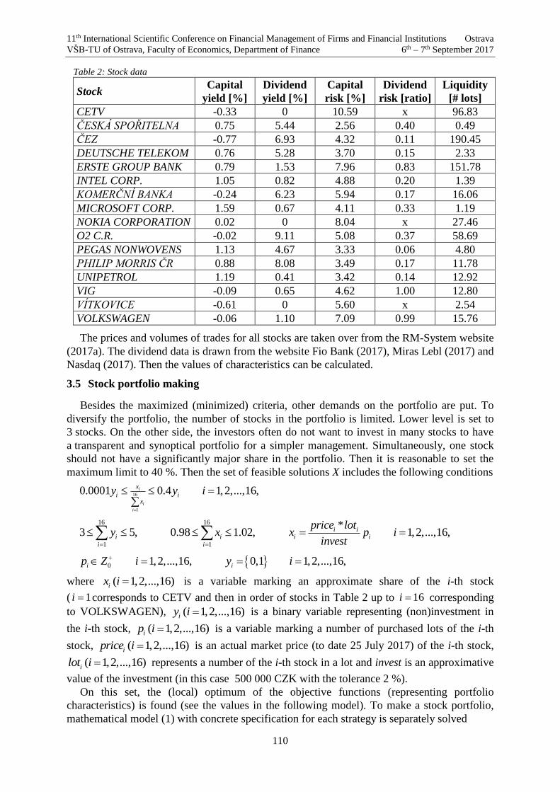
11th International Scientific Conference on Financial Management of Firms and Financial Institutions Ostrava
VŠB-TU of Ostrava, Faculty of Economics, Department of Finance 6th – 7th September 2017
110
Table 2: Stock data
Stock Capital
yield [%]
Dividend
yield [%]
Capital
risk [%]
Dividend
risk [ratio]
Liquidity
[# lots]
CETV -0.33 0 10.59 x 96.83
ČESKÁ SPOŘITELNA 0.75 5.44 2.56 0.40 0.49
ČEZ -0.77 6.93 4.32 0.11 190.45
DEUTSCHE TELEKOM 0.76 5.28 3.70 0.15 2.33
ERSTE GROUP BANK 0.79 1.53 7.96 0.83 151.78
INTEL CORP. 1.05 0.82 4.88 0.20 1.39
KOMERČNÍ BANKA -0.24 6.23 5.94 0.17 16.06
MICROSOFT CORP. 1.59 0.67 4.11 0.33 1.19
NOKIA CORPORATION 0.02 0 8.04 x 27.46
O2 C.R. -0.02 9.11 5.08 0.37 58.69
PEGAS NONWOVENS 1.13 4.67 3.33 0.06 4.80
PHILIP MORRIS ČR 0.88 8.08 3.49 0.17 11.78
UNIPETROL 1.19 0.41 3.42 0.14 12.92
VIG -0.09 0.65 4.62 1.00 12.80
VÍTKOVICE -0.61 0 5.60 x 2.54
VOLKSWAGEN -0.06 1.10 7.09 0.99 15.76
The prices and volumes of trades for all stocks are taken over from the RM-System website
(2017a). The dividend data is drawn from the website Fio Bank (2017), Miras Lebl (2017) and
Nasdaq (2017). Then the values of characteristics can be calculated.
3.5 Stock portfolio making
Besides the maximized (minimized) criteria, other demands on the portfolio are put. To
diversify the portfolio, the number of stocks in the portfolio is limited. Lower level is set to
3 stocks. On the other side, the investors often do not want to invest in many stocks to have
a transparent and synoptical portfolio for a simpler management. Simultaneously, one stock
should not have a significantly major share in the portfolio. Then it is reasonable to set the
maximum limit to 40 %. Then the set of feasible solutions X includes the following conditions
16
1
16 16
1 1
0
0.0001 0.4 1,2,...,16,
*3 5, 0.98 1.02, 1,2,...,16,
1,2,...,16, 0,1 1,2,...,16,
i
i
i
x
i ix
i ii i i i
i i
i i
y y i
price loty x x p i
invest
p Z i y i
where ( 1,2,...,16)ix i is a variable marking an approximate share of the i-th stock
( 1i corresponds to CETV and then in order of stocks in Table 2 up to 16i corresponding
to VOLKSWAGEN), ( 1,2,...,16)iy i is a binary variable representing (non)investment in
the i-th stock, ( 1,2,...,16)ip i is a variable marking a number of purchased lots of the i-th
stock, ( 1,2,...,16)iprice i is an actual market price (to date 25 July 2017) of the i-th stock,
( 1,2,...,16)ilot i represents a number of the i-th stock in a lot and invest is an approximative
value of the investment (in this case 500 000 CZK with the tolerance 2 %).
On this set, the (local) optimum of the objective functions (representing portfolio
characteristics) is found (see the values in the following model). To make a stock portfolio,
mathematical model (1) with concrete specification for each strategy is separately solved
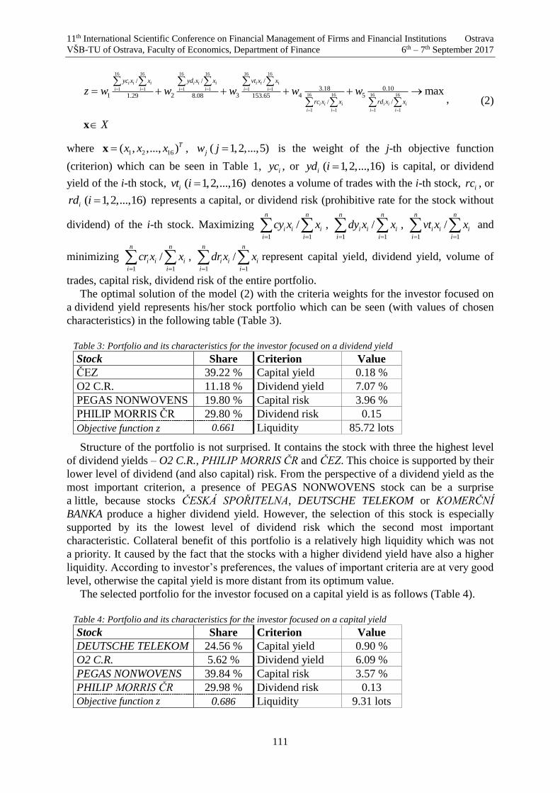
11th International Scientific Conference on Financial Management of Firms and Financial Institutions Ostrava
VŠB-TU of Ostrava, Faculty of Economics, Department of Finance 6th – 7th September 2017
111
16 16 16 16 16 16
1 1 1 1 1 1
16 16 16 16
1 1 1 1
/ / /
3.18 0.101 2 3 4 51.29 8.08 153.65
/ /
maxi i i i i i i i i
i i i i i i
i i i i i i
i i i i
yc x x yd x x vt x x
rc x x rd x x
z w w w w w
X
x
, (2)
where 1 2 16( , ,..., )Tx x xx , ( 1,2,...,5)jw j is the weight of the j-th objective function
(criterion) which can be seen in Table 1, iyc , or ( 1,2,...,16)iyd i is capital, or dividend
yield of the i-th stock, ( 1,2,...,16)ivt i denotes a volume of trades with the i-th stock, irc , or
( 1,2,...,16)ird i represents a capital, or dividend risk (prohibitive rate for the stock without
dividend) of the i-th stock. Maximizing 1 1
/n n
i i i
i i
cy x x
, 1 1
/n n
i i i
i i
dy x x
, 1 1
/n n
i i i
i i
vt x x
and
minimizing 1 1
/n n
i i i
i i
cr x x
, 1 1
/n n
i i i
i i
dr x x
represent capital yield, dividend yield, volume of
trades, capital risk, dividend risk of the entire portfolio.
The optimal solution of the model (2) with the criteria weights for the investor focused on
a dividend yield represents his/her stock portfolio which can be seen (with values of chosen
characteristics) in the following table (Table 3).
Table 3: Portfolio and its characteristics for the investor focused on a dividend yield
Stock Share Criterion Value
ČEZ 39.22 % Capital yield 0.18 %
O2 C.R. 11.18 % Dividend yield 7.07 %
PEGAS NONWOVENS 19.80 % Capital risk 3.96 %
PHILIP MORRIS ČR 29.80 % Dividend risk 0.15
Objective function z 0.661 Liquidity 85.72 lots
Structure of the portfolio is not surprised. It contains the stock with three the highest level
of dividend yields – O2 C.R., PHILIP MORRIS ČR and ČEZ. This choice is supported by their
lower level of dividend (and also capital) risk. From the perspective of a dividend yield as the
most important criterion, a presence of PEGAS NONWOVENS stock can be a surprise
a little, because stocks ČESKÁ SPOŘITELNA, DEUTSCHE TELEKOM or KOMERČNÍ
BANKA produce a higher dividend yield. However, the selection of this stock is especially
supported by its the lowest level of dividend risk which the second most important
characteristic. Collateral benefit of this portfolio is a relatively high liquidity which was not
a priority. It caused by the fact that the stocks with a higher dividend yield have also a higher
liquidity. According to investor’s preferences, the values of important criteria are at very good
level, otherwise the capital yield is more distant from its optimum value.
The selected portfolio for the investor focused on a capital yield is as follows (Table 4).
Table 4: Portfolio and its characteristics for the investor focused on a capital yield
Stock Share Criterion Value
DEUTSCHE TELEKOM 24.56 % Capital yield 0.90 %
O2 C.R. 5.62 % Dividend yield 6.09 %
PEGAS NONWOVENS 39.84 % Capital risk 3.57 %
PHILIP MORRIS ČR 29.98 % Dividend risk 0.13
Objective function z 0.686 Liquidity 9.31 lots

11th International Scientific Conference on Financial Management of Firms and Financial Institutions Ostrava
VŠB-TU of Ostrava, Faculty of Economics, Department of Finance 6th – 7th September 2017
112
In this portfolio, it was not possible to expect that it will contain the stocks with the highest
capital yield, because the importance of the dividend yield is perceptible. Then the result is
a compromise namely between capital and dividend yield. As we can see, the stock O2 C.R.
actually provides a zero capital yield. Nevertheless, this stock is in the portfolio because of its
the highest dividend yield. The capital yield of the entire portfolio is quite close to the optimal
value. The portfolio liquidity is low which is namely caused by the pressure on higher capital
and dividend yield. To increase the portfolio liquidity, the weight of this criterion would have
to be increased.
3.6 More detailed results discussion
Through two investment strategies, we can see a sensitivity of the solution (portfolio
structure) on the criteria importance (investor’s preferences). It was no doubt that the portfolio
for the investor focused on a dividend, or capital yield will produce higher dividend, or capital
yield. Although the importance of a dividend risk is higher for the investor focused on
a dividend yield, a dividend risk of this portfolio is slightly higher than for the investor
focused on a capital yield. We can see that a higher dividend risk produces a higher dividend
yield. This fact does not hold for a relationship of the capital yield and risk because a higher
capital yield of the portfolio for the investor focused on a capital yield is supported by a lower
level of capital risk. This situation is caused by the fact that a higher level of capital risk rather
corresponds to the stock with a lower average monthly return. Although a liquidity is more
important criterion for the investor focused on a capital yield, his/her investment portfolio
produces a much lower level of liquidity. It is especially influenced by the stocks representing
both higher dividend yield and greater liquidity. Optimal value of the objective function is
similar for both investment strategy. It is possible to say that the values of all portfolio
characteristics are satisfied from the level 66,1 %, or 68,6 % for the investor focused on
a dividend, or capital yield. Both investments are slightly higher than 500 000 CZK.
The proposed mathematical model is flexible. Through the additional conditions, other
investor’s demands on the portfolio can be considered. The investor can express a preference
of the investment in concrete industry, a minimum share of the selected stock(s) etc. Further,
any indicator of fundamental or technical analysis can be also taken into account as other
stock characteristic. Not only the historical conditions, but also the actual ones on the capital
market can be included in the model (e.g. last paid dividend, recent price developments or
volume of trades). These factors should rather important for a short-time, or speculative
investment. Then the time series of the historical prices (yields) would be adequately
modified. Further, the proposed procedure using multiple objective mathematical
programming model can be also applied for required changes in the investment portfolio.
Based on the actual data and development on the capital market, a solution of the model
provides a new (actual) structure of the portfolio.
The proposed procedure may not be used only on the stock exchange. It can make
a portfolio of other investment instruments (bonds, investment certificates, open unit trusts
etc.). However, the application can be also possible outside the capital market, for instance to
project portfolio making or service supply.
At the end, one note should be mentioned. The analysis is primarily based on the historical
data. History may not have repeated! However, a historical time period is chosen based on
experiences so as to best reflect developments within the required time horizon. Nevertheless,
the investor should keep in mind that it is rather the estimation of the development of the
monitored characteristics.

11th International Scientific Conference on Financial Management of Firms and Financial Institutions Ostrava
VŠB-TU of Ostrava, Faculty of Economics, Department of Finance 6th – 7th September 2017
113
4. Conclusion
This article provides the non-traditional approach to a stock portfolio making. The
procedure using a multiple objective mathematical programming is proposed. Applicability of
this approach is illustrated on two stock portfolio making situations on the RM-System Czech
Stock Exchange. The article clearly declares that mathematical programming concept is fully
useable for a portfolio making. It provides a complex analysis enabling to take into account
various perspectives to the stocks. The major result of this procedure is an exact structure of
the portfolio which is significant support for an investment decision making.
Of course, a few ideas for future research can be outlined. Firstly, re-optimization
procedure for a prospective portfolio change should be practically performed. Secondly, some
typical elements of uncertainty should be also considered. Then the return would be expressed
as stochastic element or fuzzy number. Imperfect information (vague preferences) of the
investor can be also included via the concept of fuzzy sets. Then the mathematical model
would lead to the stochastic or fuzzy programming which is very interesting area for research.
Acknowledgements
The research project was supported by Grant No. IGA F4/57/2017 of the Internal Grant
Agency, Faculty of Informatics and Statistics, University of Economics, Prague.
References
[1] Borovička, A., 2016. Possible concepts of risk measurement in investment portfolio
made by the mathematical programming. In: Hradec Králové University, Hradec
Economic Days. Hradec Králové, Czech Republic, 2-3 February 2016. Hradec Králové:
Hradec Králové University.
[2] Fiala, P., 2013. Modely a metody rozhodování. 3rd ed. Prague: Oeconomica.
[3] Fio Bank, 2017. Dividendy. [online] Available at:
<https://www.fio.cz/zpravodajstvi/dividendy> [Accessed 5 August 2017].
[4] Fishburn, P.C., 1967. Letter to the editor ̶ additive utilities with incomplete product sets:
Application to priorities and assignments. Operations Research, 15(3), pp. 537-542.
[5] Graham, B. and Dodd, D., 2008. Security analysis. 6th ed. Columbus: McGraw-Hill
Education.
[6] Markowitz, H.M., 1952. Portfolio Selection. Journal of Science, 7(1), pp. 77-91.
[7] Miras Lebl, 2017. Historický přehled dividend. [online] Available at:
<http://www.miras.cz/akcie/dividendy.php> [Accessed 5 August 2017].
[8] Murphy, J.J., 1999. Technical analysis of the financial markets: a comprehensive guide
to trading methods and applications. 2nd ed. New York: New York Institute of Finance.
[9] Nasdaq, 2017. Dividend History. [online] Available at:
<http://www.nasdaq.com/quotes/dividend-history.aspx> [Accessed 5 August 2017].
[10] RM-System, 2017a. Akcie EasyClick on-line. [online] Available at:
<http://www.rmsystem.cz/kurzy-online/akcie/easyclick> [Accessed 5 August 2017].
[11] RM-System, 2017b. Basic information. [online] Available at:
<http://www.rmsystem.cz/spolecnost/zakladni-informace> [Accessed 15 August 2017].
[12] Steigauf, S., 2003. Fondy – jak vydělávat pomocí fondů. Prague: Grada Publishing.
11th International Scientific Conference on Financial Management of Firms and Financial Institutions Ostrava
VŠB-TU of Ostrava, Faculty of Economics, Department of Finance 6th – 7th September 2017
114
Modified KSU-STEM as an appropriate tool for making a portfolio of open unit trusts
Adam Borovička, Jan Tomsa 1
Abstract
Investment decision is usually influenced by a few factors (expected yield, risk, cost, mood,
intuition etc.). Commonly used techniques of fundamental, technical, psychological analysis or
some intuition approaches are able to take into account only some factors. Moreover, the capital
market is a place with unstable (changing) conditions, then the investor’s preferences can be
vague (uncertain). If the investment decision is to be complex, then all these typical factors
must be included. Therefore, I propose to apply fuzzy multiple objective programming method
KSU-STEM with proposed improving modifications that meets all requirements for investment
decision making. This method is described and discussed in detail. Modified method is
illustratively applied to making a portfolio of open unit trusts which are increasingly popular in
the Czech Republic. The results are deeply analysed.
Key words
KSU-STEM, open unit trust, portfolio making, triangular fuzzy number.
JEL Classification: C61, G11
1. Introduction
Making an investment decision can be very difficult. Firstly, most people do not have
enough information and knowledge from the world of finance. Secondly, this type of decision
should be complex. Then the possible investments should be evaluated from more than one
perspective (purpose of the investment, investment horizon, amount of invested money, yield,
risk and cost of the investment, risk attitude, mood in the capital market etc.). Most of
(potential) investors goes for advice to the investment counsel. Together they create the
investment strategy (policy). On this base, particular investment instruments are preselected.
According to my experiences, the portfolio is usually made rather intuitively, without deep
quantitative analysis of price development or cost attitude. Even real level of cost is often
hidden for the client. Further, approaches of the fundamental or technical analysis are
sometimes applied. However, these principles can provide various analysis namely focused on
a price (or return) development. Then for complex multi-criteria analysis, the others must be
done. Moreover, these methods are not able to make a portfolio as a whole.
The negative facts mentioned above inspired me to introduce the method that can make an
investment portfolio complexly based on all important criteria and investor’s (vague)
preferences. As a suitable method, KSU-STEM is selected. This interactive fuzzy multiple
objective programming method is developed by Lai and Hwang (1996). Advantage of this
concept is an interactive procedure which enables appropriate consideration of the investor’s
1 Ing. Adam Borovička, Ph.D., Ing. Jan Tomsa, Czech Technical University in Prague, Department of
Software Engineering, Trojanova 13, Prague, Czech Republic, e-mail: [email protected],
11th International Scientific Conference on Financial Management of Firms and Financial Institutions Ostrava
VŠB-TU of Ostrava, Faculty of Economics, Department of Finance 6th – 7th September 2017
115
preferences. Further, I indicated some drawbacks of the algorithm and imperfections related to
the investment application. Therefore, some improving modifications are proposed.
The main aim of this article is to propose an effective (non-traditional) methodical concept
how to make a comprehensive portfolio based on the specified investment strategy. The
proposed approach using modified fuzzy multiple objective programming method is
a significant support for a (potential) investor. The second aim is to show an application
ability of the proposed concept. It is demonstrated on the capital market with open unit trusts.
This type of investment becomes more and more popular in the Czech Republic. For specified
typical investment strategy, the portfolio of open unit trusts offered by ERSTE-SPARINVEST
is made. The result is analysed, namely from the perspective of preference sensitivity analysis.
Structure of the article is follows. After the introduction, interactive multiple objective
programming methods are briefly introduced. Attention is directed to the KSU-STEM method
whose algorithm with some improving modifications is described in detail. The next section
contains the practical application of making a portfolio of open unit trusts. In conclusion, the
article is summarized and a few ideas for future research are outlined.
2. Interactive multiple objective programming methods
Interactive multiple objective programming methods enable to find a compromise solution
based on the continuously expressed investor’s preferences. I am convinced that interactive
procedure is very usable just in an investment decision making process where the investment
portfolio is guardedly made step by step.
Interactive methods have been developed since the 1970s. One of the first methods was
proposed by Benayoun et al. (1971) which is called Step Method (STEM). Research in this
area has begun to expand, for instance methods proposed by Geoffriona, Deyra a Feinberga
(1972), Sakawa (1981) or Steuer a Choo (1983). In 1980s, a stochastic form of these
interactive methods was developed (e.g. Teghem et al., 1986). Leung (1987) proposed
a method based on the interactive changes of goal values. Of course, interactive methods
using fuzzy elements were also developed (e.g. Sakawa, 1993). Liang (2006) proposed fuzzy
multiple objective programming method using the α-cut approach. In the end, some current
methods were modified to the fuzzy form. A representative of these methods is a fuzzy
modification of STEM, called KSU-STEM developed by Lai and Hwang (1996).
Selection of a suitable method is especially influenced by character of the solved problem.
The investment portfolio making problem is widespread. Algorithm of the applied method
should therefore be as understandable as possible for a wide range of potential investors or
investment counsels. Then the algorithm should not require any information that is difficult to
access by a decision maker. Many methods (not only) mentioned above require such an
information (goal value, α-level, or substitution relationship between criteria values). Under
these my reasonable requirements, KSU-STEM method is selected to make properly an
investment portfolio. However, it does not have to mean that this method is totally perfect for
solving a specified (or another) decision making problem as we can see in section 2.1.1.
2.1 KSU-STEM
Interactive multiple objective programming method KSU-STEM is a modification of
STEM method. The main benefits are as follows. The weights of criteria can be determined
by a decision maker, not by the algorithm itself. Further, the objective functions do not have to
be transformed to “max” or “min” character. The basal value of objective functions is also
considered.

11th International Scientific Conference on Financial Management of Firms and Financial Institutions Ostrava
VŠB-TU of Ostrava, Faculty of Economics, Department of Finance 6th – 7th September 2017
116
2.1.1 Algorithm and its proposed improving modifications
Now, the KSU-STEM algorithm with some improving modifications can be described in
the following several steps.
Step 1: Define k criteria as the objective functions 1 2( ) , ( ) ,..., ( )kf f f T T T
1 2 kx c x x c x x c x ,
where 1 2( , ,..., ), 1,2,..., ,nc c c i k T
ic is a vector of n (price) coefficients of the i-th objective
function and 1 2( , ,..., )T
nx x xx is a vector of n variables. Two sets of indices labelling the
objective functions are determined, minI for minimizing and maxI for maximizing objective
functions. Ideal value of minimizing, or maximizing objective function is denoted as min max( ) ( )U
i if f i I I U
ix , where U
ix is a solution corresponding to minimum, or
maximum of the i-th minimizing, or maximizing objective function on the set of feasible
solutions X representing all conditions. In other words, the following holds
argmin ( )if
X
U
ix x
x, or
argmax ( )if
X
U
ix x
x. (1)
To find the extreme of any objective function, the set X should be bounded. In a portfolio
making problem, this set is bounded at least due to “portfolio” condition. The original
approach of a determination of the basal values is unnecessarily pessimistic (see more Lai and
Hwang 1996). More reasonable concept is that the basal value of the objective functions is
determined with respect to the optimal solution by all other objective functions. This approach
can be seen (e.g.) in STEM method. Then the basal value of the i-th minimizing, or
maximizing objective function is specified as
min max
minmax ( )L
i ij I I
f f i I
U
jx , or min max
maxmin ( )L
i ij I I
f f i I
U
jx . (2)
Step 2: According to Bellman and Zadeh (1970), fuzzy goal representing a preference of
acquisition of the particular function values is determined for each objective function. Fuzzy
goal corresponding to minimizing, or maximizing objective function is represented by a fuzzy
set ( )ifF x with the following membership function
( )
1
( )
0
Li
L Uf i ii
U
i
f U L
i iF f fL
i
f
f f
f
Ti
x
T
i
c xT T
i i
T
i
c x
c x c x
c x
, or ( )
1
( )
0
Li
U Lf i ii
U
i
f L U
i iF f fL
i
f
f f
f
Ti
x
T
i
c xT T
i i
T
i
c x
c x c x
c x
.
The fuzzy set for minimizing, or maximizing objective function is actually right-handed, or
left-handed triangular fuzzy number.
Step 3: According to (Zimmermann, 1978), fuzzy multiple objective mathematical model
is transformed to the strict form by means of a fuzzy goals concept as follows.
min max
max
(1 ) , (1 ) ,
, 0.
L L
i ii iL U U L
i i i i
z
f fv i I v i I
f f f f
X
T T
i ic x c x
x
(3)
This proposed model better reflects the importance of objective functions due to weight
expression (1 )*iv fraction against the original concept *iv fraction . Model (3) actually
maximizes a minimum weighted deviation of the basal value (over all objective functions).
The optimal solution *x with values of the objective functions ( ), 1,2,..., ,if i k*x is found. If
values of all objective functions are acceptable for a decision maker, a compromise solution is
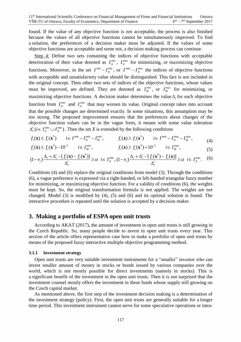
11th International Scientific Conference on Financial Management of Firms and Financial Institutions Ostrava
VŠB-TU of Ostrava, Faculty of Economics, Department of Finance 6th – 7th September 2017
117
found. If the value of any objective function is not acceptable, the process is also finished
because the values of all objective functions cannot be simultaneously improved. To find
a solution, the preferences of a decision maker must be adjusted. If the values of some
objective functions are acceptable and some not, a decision making process can continue.
Step 4: Define two sets containing the indices of objective functions with acceptable
deterioration of their value denoted as min
AI , max
AI for minimizing, or maximizing objective
functions. Moreover, in the set min min
AI I , or max max
AI I the indices of objective functions
with acceptable and unsatisfactory value should be distinguished. This fact is not included in
the original concept. Then other two sets of indices of the objective functions, whose values
must be improved, are defined. They are denoted as min
MI , or max
MI for minimizing, or
maximizing objective functions. A decision maker determines the valuei for each objective
function from min
AI and max
AI that may worsen its value. Original concept takes into account
that the possible changes are determined exactly. In some situations, this assumption may be
too strong. The proposed improvement ensures that the preferences about changes of the
objective function values can be in the vague form, it means with some value toleration min min( )i A Ai I I . Then the set X is extended by the following conditions
max
5 5 max
min max
( ) ( ) , ( ) ( ) ,
( ) ( ) 10 , ( ) ( ) 10 ,
[ ( ) ( )] [ ( ) ( )](1 ) , (1 ) .
min min min max max
i i A M i i A M
min
i i M i i M
i i i i i i i ii A i A
i i
f f i I I I f f i I I I
f f i I f f i I
f f f fv i I v i I
* *
* *
* *
x x x x
x x x x
x x x x
(4)
(5)
(6)
Conditions (4) and (6) replace the original conditions from model (3). Through the conditions
(6), a vague preference is expressed via a right-handed, or left-handed triangular fuzzy number
for minimizing, or maximizing objective function. For a validity of conditions (6), the weights
must be kept. So, the original transformation formula is not applied. The weights are not
changed. Model (3) is modified by (4), (5) and (6) and its optimal solution is found. The
interactive procedure is repeated until the solution is accepted by a decision maker.
3. Making a portfolio of ESPA open unit trusts
According to AKAT (2017), the amount of investment in open unit trusts is still growing in
the Czech Republic. So, many people decide to invest in open unit trusts every year. This
section of the article offers representative case how to make a portfolio of open unit trusts by
means of the proposed fuzzy interactive multiple objective programming method.
3.1.1 Investment strategy
Open unit trusts are very suitable investment instruments for a “smaller” investor who can
invest smaller amount of money in stocks or bonds issued by various companies over the
world, which is not mostly possible for direct investments (namely in stocks). This is
a significant benefit of the investment in the open unit trusts. Then it is not surprised that the
investment counsel mostly offers the investment in these funds whose supply still growing on
the Czech capital market.
As mentioned above, the first step of the investment decision making is a determination of
the investment strategy (policy). First, the open unit trusts are generally suitable for a longer
time period. This investment instrument cannot serve for some speculative operations or intra-

11th International Scientific Conference on Financial Management of Firms and Financial Institutions Ostrava
VŠB-TU of Ostrava, Faculty of Economics, Department of Finance 6th – 7th September 2017
118
day trading because of its limited liquidity. A typical investment strategy is a conservative
longer-time investment in order to use a capitalized money in the distant future (e.g. in
the retirement age). This investor is rather risk-averse. S/he is not able to take such a risk to
obtain a higher yield. S/he prefers investment instruments with a lower volatility of their
yields. So, s/he rather invest in a period of “calm” on the capital market when there are no
huge drops or rises of prices. This strategy is just supported by a longer investment horizon.
3.1.2 Evaluative criteria and investor’s preferences
Open unit trusts are evaluated by a few criteria. The first one is yield of the open unit trust.
Because this investment is rather for a longer time horizon, the yield is representatively
computed from a period August 2008 - June 2017. This period including various price
developments could well represent a longer-time development on the capital market with open
unit trusts. Then (expected) yield is determined as an average monthly. Risk of the unit trust is
expressed as an absolute average negative deviation of the historical yields from a monitored
time period. This measure is representative indicator of negative yield volatility of the open
unit trust. Cost includes all fees connected with the investment in the open unit trust (entry,
management, licence fee etc.). This is three most important criteria. However, we can specify
other criteria as geographical location of the investment, type of capital market (emerging,
“advanced” market), type of open unit trusts, mood on the capital market or personal intuition.
These factors can relate to return and risk. They can be considered trough other demands on
the portfolio expressed as conditions in the model (see below).
Weights of three essential specified characteristics representing the investor’s preferences
mentioned above are determined by a well-known scoring method (Fiala, 2013). Score is
assigned to the criteria based on the results of questionnaire and my investment experiences.
The weights are as follows: yield – 0.35, risk – 0.5, cost – 0.15. It is not surprised that the risk
is the most important criterion and the cost does not play such a significant role compared to
the risk and yield.
3.1.3 ESPA funds data
For investment, the ESPA open unit trust with a required history are selected (4 bond and 7
stock). These funds are managed by ERSTE-SPARINVEST. In the Czech Republic, these
open unit trusts are offered by Česká spořitelna Investment company which plays a key role
on the Czech market of collective investment. Cost and prices data of the ESPA funds are
selected on the web site of Česká spořitelna Investment centrum (2017). Other necessary data
is calculated. All data of ESPA open unit trusts are shown in the following table (Table 1).
Table 1: ESPA open unit trusts data
Cat. Fund Yield [%] Risk [%] Cost [%]
Bond ESPA Portfolio Bond Europe 0.44 1.44 4.21
ESPA Český fond státních dluhopisů 0.26 0.78 3.61
ESPA Český fond firemních dluhopisů 0.05 0.16 1.54
ESPA Bond Europe High Yield 0.68 1.92 4.59
Sto
ck
ESPA Stock Russia 0.31 6.71 6.16
ESPA Stock Japan 0.62 4.48 6.07
ESPA Stock Istanbul 0.46 6.05 6.10
ESPA Stock Global 0.65 3.90 6.05
ESPA Stock Europe Property 0.65 4.37 6.02
ESPA Stock Europe Emerging -0.17 4.93 6.08
ESPA Stock Europe 0.48 3.43 6.63
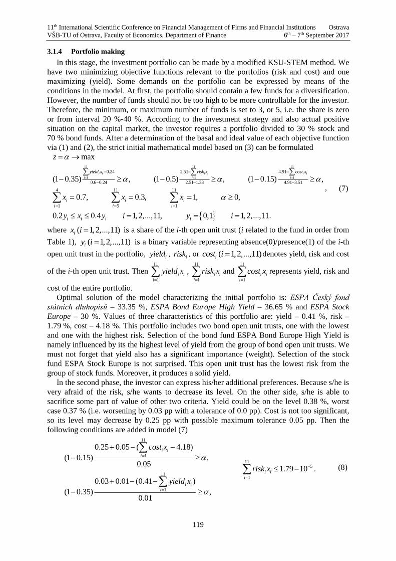
11th International Scientific Conference on Financial Management of Firms and Financial Institutions Ostrava
VŠB-TU of Ostrava, Faculty of Economics, Department of Finance 6th – 7th September 2017
119
3.1.4 Portfolio making
In this stage, the investment portfolio can be made by a modified KSU-STEM method. We
have two minimizing objective functions relevant to the portfolios (risk and cost) and one
maximizing (yield). Some demands on the portfolio can be expressed by means of the
conditions in the model. At first, the portfolio should contain a few funds for a diversification.
However, the number of funds should not be too high to be more controllable for the investor.
Therefore, the minimum, or maximum number of funds is set to 3, or 5, i.e. the share is zero
or from interval 20 %-40 %. According to the investment strategy and also actual positive
situation on the capital market, the investor requires a portfolio divided to 30 % stock and
70 % bond funds. After a determination of the basal and ideal value of each objective function
via (1) and (2), the strict initial mathematical model based on (3) can be formulated
11 11 11
1 1 1
0.24 2.51 4.91
0.6 0.24 2.51 1.33 4.91 3.51
4 11 11
1 5 1
max
(1 0.35) , (1 0.5) , (1 0.15) ,
0.7, 0.3, 1, 0,
0.2 0.4 1,2,...,11, 0,1 1,2,.
i i i i i i
i i i
yield x risk x cost x
i i i
i i i
i i i i
z
x x x
y x y i y i
..,11.
, (7)
where ( 1,2,...,11)ix i is a share of the i-th open unit trust (i related to the fund in order from
Table 1), ( 1,2,...,11)iy i is a binary variable representing absence(0)/presence(1) of the i-th
open unit trust in the portfolio, iyield ,
irisk , or ( 1,2,...,11)icost i denotes yield, risk and cost
of the i-th open unit trust. Then 11
1
i i
i
yield x
, 11
1
i i
i
risk x
and 11
1
i i
i
cost x
represents yield, risk and
cost of the entire portfolio.
Optimal solution of the model characterizing the initial portfolio is: ESPA Český fond
státních dluhopisů – 33.35 %, ESPA Bond Europe High Yield – 36.65 % and ESPA Stock
Europe – 30 %. Values of three characteristics of this portfolio are: yield – 0.41 %, risk –
1.79 %, cost – 4.18 %. This portfolio includes two bond open unit trusts, one with the lowest
and one with the highest risk. Selection of the bond fund ESPA Bond Europe High Yield is
namely influenced by its the highest level of yield from the group of bond open unit trusts. We
must not forget that yield also has a significant importance (weight). Selection of the stock
fund ESPA Stock Europe is not surprised. This open unit trust has the lowest risk from the
group of stock funds. Moreover, it produces a solid yield.
In the second phase, the investor can express his/her additional preferences. Because s/he is
very afraid of the risk, s/he wants to decrease its level. On the other side, s/he is able to
sacrifice some part of value of other two criteria. Yield could be on the level 0.38 %, worst
case 0.37 % (i.e. worsening by 0.03 pp with a tolerance of 0.0 pp). Cost is not too significant,
so its level may decrease by 0.25 pp with possible maximum tolerance 0.05 pp. Then the
following conditions are added in model (7)
11
1
115
111
1
0.25 0.05 ( 4.18)
(1 0.15) ,0.05
1.79 10 .
0.03 0.01 (0.41 )
(1 0.35) ,0.01
i i
i
i i
i
i i
i
cost x
risk x
yield x
(8)
11th International Scientific Conference on Financial Management of Firms and Financial Institutions Ostrava
VŠB-TU of Ostrava, Faculty of Economics, Department of Finance 6th – 7th September 2017
120
Conversely, these two conditions are excluded from model (7)
11 11
1 1
4.91 0.24
(1 0.15) , (1 0.35) .4.91 3.51 0.6 0.24
i i i i
i i
cost x yield x
(9)
Model (7) with modifications (8) and (9) is solved to find a new structure of the portfolio.
Its form is as follows: ESPA Český fond státních dluhopisů – 38.67 %, ESPA Bond Europe
High Yield – 31.33 % and ESPA Stock Europe – 30 %. Portfolio characteristics are: yield –
0.38 %, risk – 1.69 %, cost – 4.02 %. It is obvious that the funds have not changed. Only
shares are partly different. It was clear that the stock fund share would not change. In order to
decrease the portfolio risk, a share of the unit trust with the lowest level of risk increased
(38.67 % vs. 33.35 %). Cost reduction is caused by the fact that this fund also brings the least
cost. The investor no longer wants to reduce the yield. If s/he still allowed a reduction of 0.01
pp, the risk would fall slightly (from 1.69 % to 1.67 %). If s/he wanted to get closer to the
ideal risk level, he would have to accept a significant reduction in yield. For instance, the risk
at 1.47 % would mean a drop of yield to 0.29 % which is not acceptable for the investor.
Thus, the current portfolio mentioned above is accepted. The interactive procedure is over.
3.1.5 Final results discussion
Described investment decision making process with the open unit trusts shows how should
portfolio making look like. The process or its parts is inspired by my personal investment
experiences and the results of a questionnaire focused on the investor’s preferences for
making a portfolio of the open unit trusts. Of course, next to the risk-averse investor, another
typical strategy is risk-seeking that was no longer a space in this article. However, it is clear
that higher importance of the yield would produce higher yield of the entire portfolio which is
likely to involve higher risk and cost. These results are obvious from a data set and confirmed
by my performed multi-criteria analysis. It can be seen that the model, or portfolio structure, is
sensitive to the weights (or importance) of the criteria. It follows that investor’s preferences
must be expressed very cautiously. In the end, we should keep in mind that the analysis is
dependent on the historical data. History does not necessarily have to be repeated. However,
historical developments can very well serve to make a vision of possible future developments.
However, it must not be considered as the only possible.
The proposed modified KSU-STEM method can be applied to other decision making
situations. Of course, it can be used for making a portfolio of other financial assets (stocks,
bonds, or investment certificates). Another area of use may be project portfolio making or
project management.
4. Conclusion
This article deals with a very important and interesting topic. Investment decision making
pertains to many people around the world. But making an investment portfolio may not be
easy. Therefore, the modified fuzzy multiple objective programming method KSU-STEM is
proposed as a very effective support for the (potential) investor. This method is an improved
version of the original concept KSU-STEM which can consider all important criteria of
investment instruments evaluation and (vague) investor’s preferences. These positive features
can be effectively used in making the portfolio of open unit trusts as was illustrated.
This article shows that the use of mathematical programming methods in an investment
decision making can be very beneficial. Of course, these methods and principles can be
further improved. KSU-STEM method would be extended by the objective functions with
11th International Scientific Conference on Financial Management of Firms and Financial Institutions Ostrava
VŠB-TU of Ostrava, Faculty of Economics, Department of Finance 6th – 7th September 2017
121
fuzzy or stochastic (price) coefficients. Usage of another fuzzy numbers would be also
studied. These proposals open up space for future research.
Acknowledgements
The research project was supported by Grant No. SGS14/210/OHK4/3T/14.
References
[1] AKAT ČR. 2017. Prezentace AKAT ke konci roku 2016. [pdf] AKAT ČR. Available at:
<https://www.akatcr.cz/public/vypisUniversal.do?typZpravy=8> [Accessed 10 July
2017]
[2] Bellman, R.E. and Zadeh, L.A., 1970. Decision making in a fuzzy environment.
Management Science, 17(4), pp. 141-164.
[3] Benayoun, R., de Montgolfier, J., Tergny, J. and Laritchev, O.I., 1971. Linear
programming with multiple objective functions: STEP Method (STEM). Mathematical
Programming, 1(1), pp. 366-375
[4] Česká spořitelna Investment centrum, 2017. Podílové fondy. [online] Available at:
<https://cz.products.erstegroup.com/Retail/cs/index.phtml> [Accessed 15 July 2017].
[5] Fiala, P., 2013. Modely a metody rozhodování. 3rd ed. Prague: Oeconomica.
[6] Geoffrion, A.M., Dayer, J.S. and Feinberg, A., 1972. An interactive approach for
multicriterion optimization, with an application to the operation an academic department.
Management Science, 19(4), pp. 357-367.
[7] Lai, Y.J. and Hwang, C.L., 1996. Fuzzy multiple objective decision making: Methods and
applications. 2sd ed. Berlin: Springer.
[8] Leung, Y., 1987. Hierarchical programming with fuzzy objective and constraints. In: J.
Kacprzyk and S. A. Orlovski, eds. Optimization Models Using Fuzzy Sets and Possibility
Theory. Dordrecht: D. Reidel. pp. 245-257.
[9] Liang, T-F., 2006. Distribution planning decisions using interactive fuzzy multi-objective
linear programming. Fuzzy Sests and Systems, 157(10), pp. 1303-1316.
[10] Sakawa, M., 1981. An interactive computer program for multiobjective decision making
by the sequential proxy optimization technique. International Journal of Man-Machine
Studies, 14(2), pp. 193-213.
[11] Sakawa, M., 1993. Fuzzy sets and interactive multiobjective optimization. New York:
Plenum Press.
[12] Steuer, R.E. and Choo, E.U., 1983. An interactive weighted Tchebycheff procedure for
multiple objective programming. Mathematical Programming, 26(6), pp. 326-344.
[13] Teghem, J., Dufrane, D., Thauvoye, M. and Kunsch, P., 1986. STRANGE: An
interactive method for multi-objective linear programming under uncertainty. European
Journal of Operations Research, 26(1), pp. 65-82.
[14] ZIMMERMANN, H.J., 1978. Fuzzy programming and linear programming with several
objective functions. Fuzzy Sets and Systems, 1(1), pp. 45-55.

11th International Scientific Conference on Financial Management of Firms and Financial Institutions Ostrava
VŠB-TU of Ostrava, Faculty of Economics, Department of Finance 6th – 7th September 2017
122
International Taxation of Dividends as Regulated in Double Tax Treaties – a Case of the Czech
Republic
Karel Brychta, Kristýna Bělušová 1
Abstract
The aim of this paper is to identify and systematize the standards governing international
taxation of dividends as stated in all 87 double tax treaties (hereinafter referred to as „DDTs“
only) in which the Czech Republic is a contracting party. Content analysis and comparison of
the legal texts were the research methods used in this respect. A matrix describing each DDT
from the view point of both nominal and numerical categories represents the output which was
put to investigation. With its help the authors identified aspects with high level of
standardization and aspects with a higher level of diversity. On the basis of results reached one
can observe that aspects contained in DDT are mostly those with high level of standardization.
However, there is a significant exception from this conclusion – it relates to the rules governing
the taxation in the country of source.
Key words
Czech Republic, dividends, double tax treaties, international taxation, taxonomy
JEL Classification: H25, K33, K34
1. Introduction
International taxation is an issue that primarily concerns multinational enterprises
(hereinafter referred to as MNEs) – i.e. enterprises that allocate their investments, or assets,
into at least two different jurisdictions (Khasbulatov, 2014). One factor for such a behaviour
is to optimize one's tax liability by utilizing different tax systems and different legal
regulations (Kavelaars, 2013). The link to international taxation of dividend incomes is more
than obvious in this respect. This article targets a specific area - it specifically deals with
standards enshrined in double tax treaties (hereinafter referred to as DDTs), to which the
Czech Republic is a contracting party.
1.1 Objective and methodology
The main objective of this paper is to identify the standards for international taxation of
dividends contained in all DDTs to which the Czech Republic is a contracting party, and to
create their taxonomy using appropriate criteria.
The conducted research is based on a qualitative research. Data was collected using content
analysis of the text. Legal regulations were the subject of the research - namely the text of
relevant Articles in all 87 DDTs to which the Czech Republic is a contracting party and which
were valid as of 01/25/2017. The authors of the paper started, in this respect, from the list of
DDTs published by the Financial Administration of the Czech Republic (Ministry of Finance
of the Czech Republic, 2017). To obtain the actual texts of the DDTs, ASPI – the
1 doc. Mgr. Ing. Karel Brychta, Ph.D., Brno University of Technology, Kolejní 2906/4, 612 00 Brno,
Czech Republic, [email protected].
Ing. et Ing. Kristýna Bělušová, Brno University of Technology, Kolejní 2906/4, 612 00 Brno, Czech
Republic, [email protected].
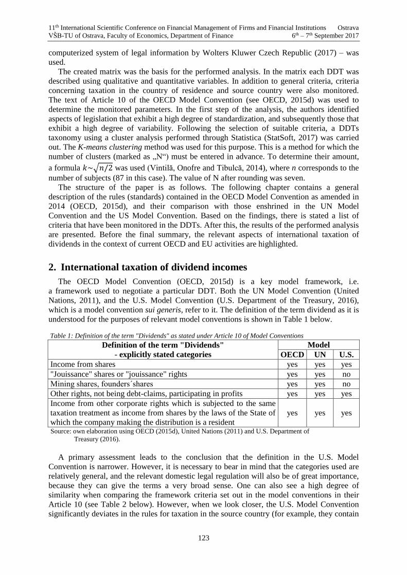
11th International Scientific Conference on Financial Management of Firms and Financial Institutions Ostrava
VŠB-TU of Ostrava, Faculty of Economics, Department of Finance 6th – 7th September 2017
123
computerized system of legal information by Wolters Kluwer Czech Republic (2017) – was
used.
The created matrix was the basis for the performed analysis. In the matrix each DDT was
described using qualitative and quantitative variables. In addition to general criteria, criteria
concerning taxation in the country of residence and source country were also monitored.
The text of Article 10 of the OECD Model Convention (see OECD, 2015d) was used to
determine the monitored parameters. In the first step of the analysis, the authors identified
aspects of legislation that exhibit a high degree of standardization, and subsequently those that
exhibit a high degree of variability. Following the selection of suitable criteria, a DDTs
taxonomy using a cluster analysis performed through Statistica (StatSoft, 2017) was carried
out. The K-means clustering method was used for this purpose. This is a method for which the
number of clusters (marked as „N“) must be entered in advance. To determine their amount,
a formula 𝑘~√𝑛/2 was used (Vintilă, Onofre and Tibulcă, 2014), where n corresponds to the
number of subjects (87 in this case). The value of N after rounding was seven.
The structure of the paper is as follows. The following chapter contains a general
description of the rules (standards) contained in the OECD Model Convention as amended in
2014 (OECD, 2015d), and their comparison with those enshrined in the UN Model
Convention and the US Model Convention. Based on the findings, there is stated a list of
criteria that have been monitored in the DDTs. After this, the results of the performed analysis
are presented. Before the final summary, the relevant aspects of international taxation of
dividends in the context of current OECD and EU activities are highlighted.
2. International taxation of dividend incomes
The OECD Model Convention (OECD, 2015d) is a key model framework, i.e.
a framework used to negotiate a particular DDT. Both the UN Model Convention (United
Nations, 2011), and the U.S. Model Convention (U.S. Department of the Treasury, 2016),
which is a model convention sui generis, refer to it. The definition of the term dividend as it is
understood for the purposes of relevant model conventions is shown in Table 1 below.
Table 1: Definition of the term "Dividends" as stated under Article 10 of Model Conventions
Definition of the term "Dividends"
- explicitly stated categories
Model
OECD UN U.S.
Income from shares yes yes yes
"Jouissance" shares or "jouissance" rights yes yes no
Mining shares, founders´shares yes yes no
Other rights, not being debt-claims, participating in profits yes yes yes
Income from other corporate rights which is subjected to the same
taxation treatment as income from shares by the laws of the State of
which the company making the distribution is a resident
yes yes yes
Source: own elaboration using OECD (2015d), United Nations (2011) and U.S. Department of
Treasury (2016).
A primary assessment leads to the conclusion that the definition in the U.S. Model
Convention is narrower. However, it is necessary to bear in mind that the categories used are
relatively general, and the relevant domestic legal regulation will also be of great importance,
because they can give the terms a very broad sense. One can also see a high degree of
similarity when comparing the framework criteria set out in the model conventions in their
Article 10 (see Table 2 below). However, when we look closer, the U.S. Model Convention
significantly deviates in the rules for taxation in the source country (for example, they contain
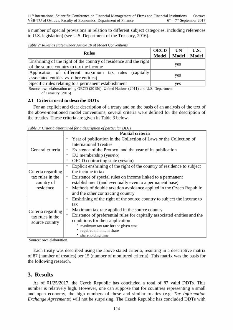
11th International Scientific Conference on Financial Management of Firms and Financial Institutions Ostrava
VŠB-TU of Ostrava, Faculty of Economics, Department of Finance 6th – 7th September 2017
124
a number of special provisions in relation to different subject categories, including references
to U.S. legislation) (see U.S. Department of the Treasury, 2016).
Table 2: Rules as stated under Article 10 of Model Conventions
Rules OECD
Model
UN
Model
U.S.
Model
Enshrining of the right of the country of residence and the right
of the source country to tax the income yes
Application of different maximum tax rates (capitally
associated entities vs. other entities) yes
Specific rules relating to a permanent establishment yes Source: own elaboration using OECD (2015d), United Nations (2011) and U.S. Department
of Treasury (2016).
2.1 Criteria used to describe DDTs
For an explicit and clear description of a treaty and on the basis of an analysis of the text of
the above-mentioned model conventions, several criteria were defined for the description of
the treaties. These criteria are given in Table 3 below.
Table 3: Criteria determined for a description of particular DDTs
Partial criteria
General criteria
Year of publication in the Collection of Laws or the Collection of
International Treaties Existence of the Protocol and the year of its publication EU membership (yes/no) OECD contracting state (yes/no)
Criteria regarding
tax rules in the
country of
residence
Explicit enshrining of the right of the country of residence to subject
the income to tax Existence of special rules on income linked to a permanent
establishment (and eventually even to a permanent base) Methods of double taxation avoidance applied in the Czech Republic
and the other contracting country
Criteria regarding
tax rules in the
source country
Enshrining of the right of the source country to subject the income to
tax Maximum tax rate applied in the source country Existence of preferential rules for capitally associated entities and the
conditions for their application maximum tax rate for the given case required minimum share shareholding time
Source: own elaboration.
Each treaty was described using the above stated criteria, resulting in a descriptive matrix
of 87 (number of treaties) per 15 (number of monitored criteria). This matrix was the basis for
the following research.
3. Results
As of 01/25/2017, the Czech Republic has concluded a total of 87 valid DDTs. This
number is relatively high. However, one can suppose that for countries representing a small
and open economy, the high numbers of these and similar treaties (e.g. Tax Information
Exchange Agreements) will not be surprising. The Czech Republic has concluded DDTs with
11th International Scientific Conference on Financial Management of Firms and Financial Institutions Ostrava
VŠB-TU of Ostrava, Faculty of Economics, Department of Finance 6th – 7th September 2017
125
all EU member states, as well as with all OECD countries. The Czech Republic, as well as
other countries, use model conventions to negotiate a particular DDT. However, this does not
in itself mean an automatic acceptance of the text of the model convention (e.g. with respect
to existing reservations for some articles or the existence of a certain degree of discretion).
This is evidenced even by the achieved results - in the evaluated DDTs, elements with a high
degree of similarity can be identified; nevertheless, elements with a high degree of variability
can be identified as well.
3.1 Highly standardized aspects contained in DDTs
It was not surprising to find (a basically empirically confirmed initial and logical
assumption) that a number of areas exhibit, if not exactly identical, a very similar legal
regulation - in all valid DDTs to which the Czech Republic is a contracting party.
3.1.1 Explicit enshrining of the right of the country of residence and the source country to
subject the income to tax
All DDTs explicitly enshrine the right of the country of residence to tax income from
dividends. The right of the source country to tax income is also enshrined - in this case,
however, the partial criteria and conditions differ. The enshrining of the right of the country of
residence and the right of the source country is no surprise. It would be more surprising if it
was not enshrined for a country/or for both contracting countries. It should be emphasized that
"only" a right granted to the contracting state, not an obligation to subject the income to tax, is
involved. Whether or not the final taxation occurs depends solely on the relevant domestic
legislation.
3.1.2 Rules relating to a permanent establishment (respectively to a permanent establishment
and a permanent base)
Another aspect that is similarly regulated in the DDTs is the existence of special rules
relating to a permanent establishment (respectively to a permanent establishment and
a permanent base). Again, these are the rules that are contained in all DDTs. This is
understandable, and in conjunction with a number of other related OECD provisions and
activities (see e.g. OECD, 2015b), it highlights the intricacy and complexity of the issue of
international taxation of the income of a permanent establishment. This is one of the key
issues, and as evidenced by practice, one of the most complicated (see e.g. Kobetsky, 2011).
The DDTs stipulate that in the case of paid dividends that are effectively connected with
a permanent establishment, general rules will not apply (for more details see Article 10, items
4 and 5 of the OECD Model Convention (OECD, 2015d)).
3.1.3 Methods for avoidance of double taxation
The method for avoidance of double taxation is a key means leading to the elimination of
double taxation of income. It is a means by which the taxpayer's country of residence takes
into account the fact that the income in question has already been taxed in the source country
(or was subject to tax, but due to investment or other incentives, a tax credit was granted - in
this case a fiction is applied where the reduced or exempt tax is treated as duly paid full tax).
Model conventions "allow" the use of both categories of methods for avoidance (elimination)
of double taxation - the credit method or the exemption method. By nature of the matter, it
was only necessary to examine which method is enshrined in particular DDT - not whether it
is enshrined at all. Based on the comparison, one can state the following:
More recent DDTs to which the Czech Republic is a party tend to enshrine a single
method for all income categories.
In the case of the Czech Republic as the tax residence country, all DDTs establish the
ordinary credit method for avoidance of double taxation.

11th International Scientific Conference on Financial Management of Firms and Financial Institutions Ostrava
VŠB-TU of Ostrava, Faculty of Economics, Department of Finance 6th – 7th September 2017
126
In the case of a method established for the other contracting state as the tax residence
country, there is a higher variability. Out of the total number of 87 DDTs, 72 of them
also enshrine the ordinary credit method. Other DDTs enshrine the full credit method (6
out of 87 DDTs) or certain specific conditions for applying the method set (or methods
set). In summary, however, we can say that there is a certain form of symmetry despite
the existing differences.
3.2 Aspects exhibiting higher degree of variability
The aspect in which DDTs differ to a higher degree are the rules of taxation in the source
country. All DDTs naturally give the source country the right to tax the income, but the other
attributes differ.
3.2.1 Enshrining the preferential regime for capitally associated entities
Out of the total number of 87 DDTs, 48 of these (i.e. 55.2 % of the total amount) set
a preferential regime for capitally associated legal entities. The rate for these entities ranges
from 0 to 12.5 %. Surprisingly, only 6 DDTs establish the minimum share-holding duration to
have the option to apply a more favourable tax rate, namely the DDT with Japan (1/2 year),
Cyprus (1 year), Lichtenstein (1 year), Luxembourg (1 year), Portugal (2 years) and
Switzerland (1 year).
3.2.2 Tax rates - others
A total of 39 DDTs do not enshrine the above stated regime - i.e. the established rates are
valid regardless of the legal form of the dividend recipient. These rates are applied also in
case of remaining 48 DDTs for the entities/persons which do not meet the criteria set (i.e. the
criterion of the legal form and eventually even the criterion for minimum duration of share-
holding). The maximum tax rates oscillate from 5 % to 15 %. Only one DDT does not
establish a maximum tax rate at all - namely the DDT with Greece. In the case of this country,
the domestic legislation applies.
3.3 Cluster analysis of DDTs
Based on the comparison carried out, it was obvious that it makes sense to perform
a cluster analysis using only the criteria for taxation in the source country, as these criteria
exhibit variability, unlike the others. The clustering was performed using information about
the existence of the preferential regime (assessed using variable 0 (no) and 1 (yes)),
information about the minimum required share for the preferential regime and information
about maximum tax rates. The results, i.e. the division of countries into relevant clusters, as
well as their brief description, are given in Table 4 below.
Table 4: Taxonomy of DDTs – results of cluster analysis.
Cluster Contracting States Description
I
(32)
Albania; Barbados; Belarus; Belgium; Colombia;
Egypt; Estonia; Finland; France; Georgia; Germany;
Hungary; China; Iceland; Ireland; Japan; Latvia;
Lithuania; Macedonia; Moldova; Netherlands;
Pakistan; Portugal; Slovenia; South Africa; Spain;
Sweden; Korean republic; Tunis; UK (United
Kingdom of Great Britain and Northern Ireland);
Ukraine; Uzbekistan
preferential regime: yes minimum required share: 25 % max. tax rate for the preferential regime:
prevalent 5 % (3 x 10 %; 1 x 0 %)
general maximum tax rate: 10% or 15%
II
(4) Australia; Indonesia; Israel; Venezuela
preferential regime: yes minimum required share: 15 % or 20 % max. tax rate for the preferential regime:
10 %
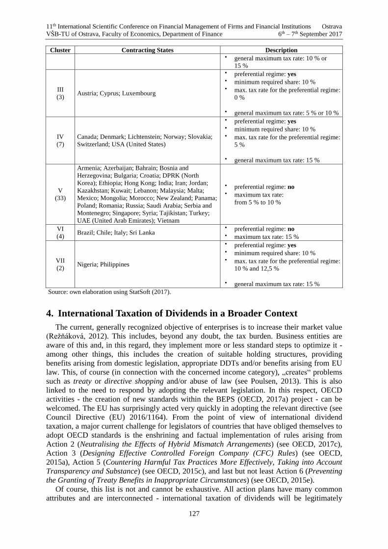
11th International Scientific Conference on Financial Management of Firms and Financial Institutions Ostrava
VŠB-TU of Ostrava, Faculty of Economics, Department of Finance 6th – 7th September 2017
127
Cluster Contracting States Description general maximum tax rate: 10 % or
15 %
III
(3) Austria; Cyprus; Luxembourg
preferential regime: yes minimum required share: 10 % max. tax rate for the preferential regime:
0 %
general maximum tax rate: 5 % or 10 %
IV
(7)
Canada; Denmark; Lichtenstein; Norway; Slovakia;
Switzerland; USA (United States)
preferential regime: yes minimum required share: 10 % max. tax rate for the preferential regime:
5 %
general maximum tax rate: 15 %
V
(33)
Armenia; Azerbaijan; Bahrain; Bosnia and
Herzegovina; Bulgaria; Croatia; DPRK (North
Korea); Ethiopia; Hong Kong; India; Iran; Jordan;
Kazakhstan; Kuwait; Lebanon; Malaysia; Malta;
Mexico; Mongolia; Morocco; New Zealand; Panama;
Poland; Romania; Russia; Saudi Arabia; Serbia and
Montenegro; Singapore; Syria; Tajikistan; Turkey;
UAE (United Arab Emirates); Vietnam
preferential regime: no maximum tax rate:
from 5 % to 10 %
VI
(4) Brazil; Chile; Italy; Sri Lanka
preferential regime: no maximum tax rate: 15 %
VII
(2) Nigeria; Philippines
preferential regime: yes minimum required share: 10 % max. tax rate for the preferential regime:
10 % and 12,5 %
general maximum tax rate: 15 %
Source: own elaboration using StatSoft (2017).
4. International Taxation of Dividends in a Broader Context
The current, generally recognized objective of enterprises is to increase their market value
(Režňáková, 2012). This includes, beyond any doubt, the tax burden. Business entities are
aware of this and, in this regard, they implement more or less standard steps to optimize it -
among other things, this includes the creation of suitable holding structures, providing
benefits arising from domestic legislation, appropriate DDTs and/or benefits arising from EU
law. This, of course (in connection with the concerned income category), „creates“ problems
such as treaty or directive shopping and/or abuse of law (see Poulsen, 2013). This is also
linked to the need to respond by adopting the relevant legislation. In this respect, OECD
activities - the creation of new standards within the BEPS (OECD, 2017a) project - can be
welcomed. The EU has surprisingly acted very quickly in adopting the relevant directive (see
Council Directive (EU) 2016/1164). From the point of view of international dividend
taxation, a major current challenge for legislators of countries that have obliged themselves to
adopt OECD standards is the enshrining and factual implementation of rules arising from
Action 2 (Neutralising the Effects of Hybrid Mismatch Arrangements) (see OECD, 2017c),
Action 3 (Designing Effective Controlled Foreign Company (CFC) Rules) (see OECD,
2015a), Action 5 (Countering Harmful Tax Practices More Effectively, Taking into Account
Transparency and Substance) (see OECD, 2015c), and last but not least Action 6 (Preventing
the Granting of Treaty Benefits in Inappropriate Circumstances) (see OECD, 2015e).
Of course, this list is not and cannot be exhaustive. All action plans have many common
attributes and are interconnected - international taxation of dividends will be legitimately
11th International Scientific Conference on Financial Management of Firms and Financial Institutions Ostrava
VŠB-TU of Ostrava, Faculty of Economics, Department of Finance 6th – 7th September 2017
128
affected (to varying degrees) by other action plans as well. Nevertheless, authors of the paper
believe that even the implementation of the above-mentioned OECD standards will not in
principle affect pro futuro the rules that have been examined in this paper. This conclusion is
also supported by the OECD (2017b) document containing a draft amendment to the model
convention, which, in contrast to the 2014 version (see OECD, 2015d), „only“ cancels the
reference to partnership, while setting a 365-day period for holding the share.
5. Conclusion
The issue of international taxation of dividends is a very topical one. This is evidenced
both by relevant OECD and EU activities, as well as the interest by practice and the academic
sphere, which seek to capture and explain certain phenomena and trends. However, neither of
the concerned parties should ignore the rules given by the legislation. International taxation of
income is a complex area that is regulated by international law, as well as EU law and,
naturally, domestic law. This in itself bears evidence of how complex the given area is.
This article targeted a relatively narrow area, namely international taxation of dividend
income in terms of the rules contained in the DDTs to which the Czech Republic is
a contracting party. The objective of this article was to identify the standard enshrined in the
above-mentioned DDTs using qualitative research and at the same time to create a taxonomy
of the DDTs based on their similarity in the rules set for taxation in the source country of the
income. For this purpose, an 87 x 15 matrix was created to provide a description of all 87
valid DDTs. Achieved results confirmed the initial empirical assumption - this is an area with
a high degree of standardization. However, rules on taxation in the source country
significantly deviate from this conclusion; they exhibit a higher degree of variability, and they
could therefore be used as criteria for creating the DDT taxonomy. As the generalized
description of the seven formed clusters shows, the main sorting point is the non/existence of
a preferential regime for capitally associated entities.
Acknowledgement
The paper represents an output of the project International Taxation of Dividends in the
Context of Multinational Enterprise Tax Management (FP-J-17-4224) supported by the Brno
University of Technology.
References
[1] Council Directive (EU) 2016/1164 of 12 July 2016 laying down rules against tax
avoidance practices that directly affect the functioning of the internal market, as
amended.
[2] Kavelaars, P. (2013). EU and OECD: Fighting against Tax Avoidance. Intertax,
International Tax Review, 41(10), pp. 507-515.
[3] Khasbulatov, R. I. (2014). Corporations, Transnational (TNC). Value Inquiry Book Series
[online]. pp. 103-104. Available at: EBSCO database [Accessed 10 July 2017].
[4] Kobetsky, M. (2011). International taxation of permanent establishments: principles and
policy. New York: Cambridge University Press.

11th International Scientific Conference on Financial Management of Firms and Financial Institutions Ostrava
VŠB-TU of Ostrava, Faculty of Economics, Department of Finance 6th – 7th September 2017
129
[5] Ministry of Finance of the Czech Republic (2017). Přehled platných smluv České
republiky o zamezení dvojímu zdanění v oboru daní z příjmu, resp. z příjmu a z majetku.
[In Czech: List of Valid Treaties of the Czech Republic on Avoidance of Double Taxation
in the Area of Income Taxes, eventually in the Area of Income and Property Taxes].
[online] Available at: <http://www.mfcr.cz/cs/legislativa/dvoji-zdaneni/prehled-platnych-
smluv> [Accessed 10 June 2017].
[6] OECD (2015a). Designing Effective Controlled Foreign Company Rules, Action 3 - 2015
Final Report. [online] OECD Publishing, Paris. Available at:
<http://dx.doi.org/10.1787/9789264241152-en> [Accessed 10 July 2017].
[7] OECD (2015b). Preventing the Artificial Avoidance of Permanent Establishment Status -
Action 7. 2015 Final Report. [online] OECD Publishing, Paris. Available at: <
http://dx.doi.org/10.1787/9789264241220-en> [Accessed 01 January 2017].
[8] OECD (2015c). Countering Harmful Tax Practices More Effectively, Taking into
Account Transparency and Substance, Action 5 - 2015 Final Report, OECD Publishing,
Paris.
Available at: <http://dx.doi.org/10.1787/9789264241190-en> [Accessed 10 July 2017].
[9] OECD (2015d). Model Tax Convention on Income and on Capital 2014 (Full Version).
[online] OECD Publishing, Paris. Available at:
<http://dx.doi.org/10.1787/9789264239081-en> [Accessed 01 July 2017].
[10] OECD (2015e). Preventing the Granting of Treaty Benefits in Inappropriate
Circumstances, Action 6 - 2015 Final Report, OECD Publishing, Paris.
Available at: <http://dx.doi.org/10.1787/9789264241695-en> [Accessed 10 July 2017].
[11] OECD (2017a). Base Erosion and Profit Shifting. [online] Available at:
<http://www.oecd.org/tax/beps/beps-actions.htm> [Accessed 17 July 2017].
[12] OECD (2017b). Draft Contents of the 2017 Update to the OECD Model Tax Convention
of 17 July 2017. [online] Available at: <http://www.oecd.org/tax/treaties/draft-contents-
2017-update-oecd-model-tax-convention.pdf> [Accessed 26 July 2017].
[13] OECD (2017c). Neutralising the Effects of Branch Mismatch Arrangements, Action 2:
Inclusive Framework on BEPS, OECD Publishing, Paris.
Available at: <http://dx.doi.org/10.1787/9789264278790-en> [Accessed 10 July 2017].
[14] Poulsen, M. (2013). Treaty/Directive Shopping and Abuse of EU Law. Intertax,
International Tax Review. 41(4), pp. 230-251.
[15] Režňáková, M. (2012). Efektivní financování rozvoje podnikání. [In Czech: Effective
Ways of Enterprise Financing]. 1st ed. Praha: Grada.
[16] StatSoft (2017). Statistica Cz (Verze 12). [computer program]. StatSoft CR s.r.o.
[17] U.S. Department of the Treasury (2016). U.S. Model Income Tax Convention (February
17, 2016). [online] Available at: < https://www.treasury.gov/resource-center/tax-
policy/treaties/Pages/treaties.aspx> [Accessed 01 July 2017].
[18] United Nations (2011). United Nations Model Double Taxation Convention between
developed and developing countries. [online] New York: United Nations. Available at: <
http://www.un.org/esa/ffd/documents/UN_Model_2011_Update.pdf> [Accessed 01 July
2017].

11th International Scientific Conference on Financial Management of Firms and Financial Institutions Ostrava
VŠB-TU of Ostrava, Faculty of Economics, Department of Finance 6th – 7th September 2017
130
[19] Vintilă, R., Onofre, M. and Tibulcă, I.-L. (2014). Fiscal Convergence in an Enlarged
European Union. Transylvantian Review of Administrative Sciences [online]. 2014, 41E,
pp. 213-223. Available at: <http://rtsa.ro/tras/index.php/tras/article/view/164/160>
[Accessed 30 August 2016].
[20] Wolters Kluwer Česká republika (2017). Automatizovaný systém právních informací. [In
Czech: Computerized System of Legal Information]. (version according to the state as
valid as to 09 April 2017). [computer program] Wolters Kluwer Česká republika.
11th International Scientific Conference on Financial Management of Firms and Financial Institutions Ostrava
VŠB-TU of Ostrava, Faculty of Economics, Department of Finance 6th – 7th September 2017
131
Modified method of area division in fractal dimensi-on estimation
Rafał Buła1
Abstract
This paper is devoted to the problem of fractal dimension estimation of financial time series.
Firstly, main drawbacks of the area-division method are revealed and described. Secondly, a
few changes are proposed in order to improve essential features of fractal dimension estimates
obtained when using this method. As a result the modified method of area division has been
created and is discussed. Finally, superiority of the modified method over its initial version is
presented.
Key words
Fractal dimension, risk assessment, segment-variation method, area-division method.
JEL Classification: G17
1. Introduction
This paper is devoted to the problem of estimating the fractal dimension of financial time
series. The conclusions drawn relate primarily to the methodological layer, but the issue of
adopting the presented methods in practice will be the subject of separate research devoted
exclusively to the analysis of empirical data.
The inspiration for the pertinent considerations was noticing the inadequacy of the
commonly used approach to measuring the riskiness of financial investments based on the
Gaussian distribution and the geometric Brownian motion. Due to historical conditions and
extensive mathematical apparatus, the use of de Moivre-Gauss-Laplace distribution has be-
come widespread, at the same time providing an impetus for many discoveries leading to the
emergence of modern science of finance and concepts such as Harry Markowitz’s mean and
variance analysis (1952; 1959), or still the dominant valuation model of capital assets by
Treynor-Sharpe-Lintner-Mossin (Treynor, 1962; Sharpe, 1964; Lintner, 1965; Mossin, 1966).
Nevertheless, over the years, apparent discrepancies between empirical rates of return and the
postulated distribution have become so substantial that the existing paradigm started to be
questioned.
Already in the 1960s doubts were raised regarding the assumption of normality, indepen-
dence, and equality (in terms of probability distribution) of rates of return on financial instru-
ments (Andreou, Pittis and Spanos, 2001). Noticing the phenomenon of leptokurtosis of empi-
rical probability distributions resulted in Benoit Mandelbrot’s modeling of -stable distributi-
ons, at the same time abandoning the assumption of normality (Mandelbrot, 1963; 1967;
1972). The next step was to deny the postulate of independence, resulting in the idea of mode-
ling using a fractal Brownian motion. The combination of these concepts led to the idea of
describing processes taking place in the financial market by means of fractal objects and using
appropriate conceptual apparatus of fractal geometry. This resulted in the fractal market theo-
1 Rafał Buła, Ph.D., Department of Investment and Real Estate, University of Economics in Katowice,
Poland, [email protected].

11th International Scientific Conference on Financial Management of Firms and Financial Institutions Ostrava
VŠB-TU of Ostrava, Faculty of Economics, Department of Finance 6th – 7th September 2017
132
ry, now developed into the theory of the multifractal market, which is based on the use of sta-
tistically self-similar (at least approximately) descriptions of series of prices or rates of return
from the financial market (Buła, 2017; Buła and Pera, 2015).
Rejection of these assumptions means that the previously used risk measures – in particu-
lar, forming the foundation of the mean and variance analysis of the Markowitz’s second cen-
tral moment – are losing their significance and their cognitive value is decreasing. In this situ-
ation, it is necessary to use additional measures to assess the level of financial investment risk.
The key quantity used to measure the investment risk in this approach is the fractal dimension
of the time series of prices and rates of return, whereas the box dimension is the most
commonly used with empirical financial time series.
An important methodological issue related to the assessment of the investment risk level is
to find an appropriate method for estimating this dimension in relation to time series origina-
ting from the financial market. Various approaches to this problem have been proposed in the
literature (Dubuc, et al., 1989; Schmittbuhl and Vilotte, 1995; Zwolankowska, 1998; 2000a),
but it cannot be regarded as solved. For this reason, the study presents the method of box di-
mension estimation – in particular the area-division method. So far, the author has shown
(Buła, 2012a; 2012b) that this method, although interesting and worth development, provides
biased and highly unstable estimates for the stochastic process which is a fractal Brownian
motion.
The main purpose of the presented analyzes was to investigate the reasons why the area-
division method, despite an interesting construction, does not lead to estimates of desirable
properties. Detection of these would allow for removing possible construction flaws of the
method and for improving the quality of the estimates obtained. Therefore, another objective
was to investigate the possibility of modifying the area-division method and to propose ap-
propriate corrections. In addition, it would be advisable in this situation to analyze the impact
of the corrections made on the quality of estimates and to evaluate the appropriateness of the
changes. The research hypothesis remains in close connection to the stated objectives of the
study. This hypothesis states that there is a possibility to modify the area-division method so
as to eliminate its essential weaknesses.
In the course of the research, the author used primarily deductive inference. MS Excel
spreadsheet and Visual Basic for Applications programming language were used for calculati-
ons.
2. Geometric method of estimating fractal dimension
Among various methods of estimating the fractal dimension, geometric methods deserve
particular attention, as referring to the essence of that dimension and its geometric interpreta-
tion. This paper is devoted to an in-depth analysis of the area-division method. The author is
of the opinion that the deficiencies shown by this method can be eliminated, if not completely,
at least in part. As a result of the introduction of appropriate modifications, it is possible to
obtain qualitatively comparable estimates by means of this estimation method with the estima-
tes obtained by using the segment-variation method (Zwolankowska, 1998; 1999; 2000a;
2000b; 2001). Therefore, constructing a modified area-division method is the ultimate goal of
the author.
2.1 Area-division method
The area-division method was first proposed as a method of estimating the fractal di-
mension of financial time series (but potentially also others) by Grzegorz Przekota (2003).
This method, according to its creator, is to merge the advantages of the segment-variation me-
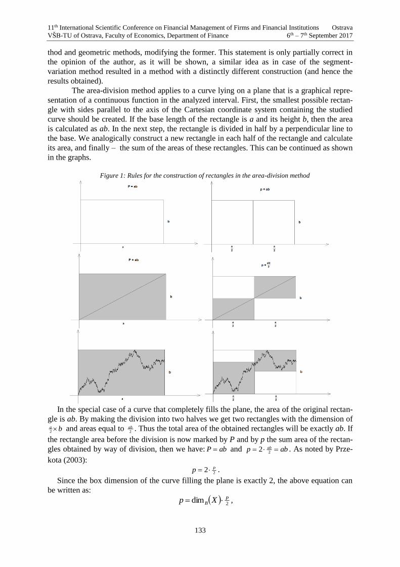
11th International Scientific Conference on Financial Management of Firms and Financial Institutions Ostrava
VŠB-TU of Ostrava, Faculty of Economics, Department of Finance 6th – 7th September 2017
133
thod and geometric methods, modifying the former. This statement is only partially correct in
the opinion of the author, as it will be shown, a similar idea as in case of the segment-
variation method resulted in a method with a distinctly different construction (and hence the
results obtained).
The area-division method applies to a curve lying on a plane that is a graphical repre-
sentation of a continuous function in the analyzed interval. First, the smallest possible rectan-
gle with sides parallel to the axis of the Cartesian coordinate system containing the studied
curve should be created. If the base length of the rectangle is a and its height b, then the area
is calculated as ab. In the next step, the rectangle is divided in half by a perpendicular line to
the base. We analogically construct a new rectangle in each half of the rectangle and calculate
its area, and finally – the sum of the areas of these rectangles. This can be continued as shown
in the graphs.
Figure 1: Rules for the construction of rectangles in the area-division method
In the special case of a curve that completely fills the plane, the area of the original rectan-
gle is ab. By making the division into two halves we get two rectangles with the dimension of
ba 2
and areas equal to 2
ab . Thus the total area of the obtained rectangles will be exactly ab. If
the rectangle area before the division is now marked by P and by p the sum area of the rectan-
gles obtained by way of division, then we have: abP and abp ab 2
2 . As noted by Prze-
kota (2003):
22 Pp .
Since the box dimension of the curve filling the plane is exactly 2, the above equation can
be written as:
2
dim PB Xp ,

11th International Scientific Conference on Financial Management of Firms and Financial Institutions Ostrava
VŠB-TU of Ostrava, Faculty of Economics, Department of Finance 6th – 7th September 2017
134
where XBdim is the box dimension. Half of the figures of the area before the division is
thus multiplied by the fractal (box) dimension of that curve to get the area of figures obtained
after the rectangle is divided. We deal with a similar situation in case of a straight line (not a
graphical representation of a constant function, which we exclude from further consideration).
In this case, the initial rectangle area will equal to abP , while after the division 2abp .
Therefore:
21 Pp ,
whereas the fractal dimension of a straight line equals to 1. Furthermore, it can be noted
that greater variation of the investigated function means larger area of figures obtained after
the rectangle is divided. Moreover, larger “fray” of the graph also means a larger fractal di-
mension, so it can be postulated (and so did the creator of the method) that there is a relation-
ship between the fractal dimension of the curve and the areas of successively obtained geo-
metric objects. In the general case the area of the initial rectangle can be calculated by using
the function range for a given interval. Then ahP , whereas hahhp a 212 , where h is
the function range for a given interval of length a, while 1h and
2h are the range in respectively
the first and second rectangles formed after the division. Thus h means the average range of
the function for the rectangles created after the division The presented relationships imply the
dependence in the form of:
22 Phhp .
At the same time, it should be noted that the quantity hh2 takes values from the interval
21, (as Pp and 2Pp ). As the ratio h to h increases, the quotient h
h2 is greater, and thus
the increase in the variation of the function is accompanied by an increase in the quotient. On
the basis of the discussed conditions the author of the method considered that the quantity hh2
can be treated as a specific fractal measure giving the degree of fluctuation of the analyzed
function.
The presented underlying idea of the area-division method had to be concretized with
respect to empirical financial time series whose graphical representation in the Cartesian co-
ordinate system is de facto a set of isolated points. In this situation, in the first place, for the
series NX,...,X,X 10 is calculated its length N. Then the series is divided into n congru-
ent rectangles, of which each has a length of nN , but the number must be even. For each of the
rectangles created in this way there must be calculated:
tXtXh
nN
nN
nN
nN k,...,ktk,...,kt
n
k11minmax
, n,...,,k 21 ,
where the range of time series in the k-th rectangle for the given n was denoted by n
kh . The
sum area can be calculated as:
n
k
n
knN
n hP1
.
In the next stage of the calculation, each of the n rectangles is divided into two congruent
ones. Then the previous step is repeated – it is necessary to calculate the range values for the
following rectangles:
tXtX'h
nN
nN
nN
nN k,...,ktk,...,kt
n
k2222
11minmax
, n,...,,k 221 ,
as well as their areas after division:
n
k
n
knN
n hp2
12
.
11th International Scientific Conference on Financial Management of Firms and Financial Institutions Ostrava
VŠB-TU of Ostrava, Faculty of Economics, Department of Finance 6th – 7th September 2017
135
The above procedure is performed for all n being divisors of N with the proviso that nN
must be divisible by 2. The result is a set of points n
Pp,n
2. As the postulated dependency has
the form ( XMADdim means the fractal dimension estimated by the area-division method):
2
dim nP
MADn Xp ,
hence the fractal dimension is obtained by estimating the regression coefficient for the
compound:
2
dim PMAD Xp .
This estimate takes the form:
m
ii
P
m
ii
Pi
MAD
p
X
1
2
2
12
dim
as there is no free term here. For this reason, it is unacceptable to use the determination co-
efficient when examining the fit of a regression line.
2.2 Authorship modification of area-division method
This section will present an authorship modification of the area-division method. In the
first place, however, one should refer to the identified shortcomings of the original method.
The creator of the area-division method demonstrates its adoption on the example of two
series: the series in which the studied quantity takes the alternating values of 1 and 2, and the
series formed by successive natural numbers starting from unity. However, the calculations
presented in all the available, to the author, works of the creator of the area-division method
are inconsistent and may be misleading for the reader (Przekota, 2003; Przekota, 2012; Prze-
kota, 2014; Przekota and Przekota, 2004; Przekota and Szczepańska-Przekota, 2008; Przekota
and Waściński, 2012).
It should be noted in the first place that the creator uses interchangeably the term “number
of observations” and “length of series,” except that the “length of series” to be correctly un-
derstood (as it is the essence of the method) is the length of the rectangle base in which the
time series is placed. Following the creator, if one simplistically assumes that the observations
appear every conventional unit of time, then the “length of series” will be equivalent to the
“number of observations” reduced by one unit.
Secondly, in the situation of dividing the original rectangle into halves, it should be borne
in mind that by analyzing a given series, we assume for the purposes of analysis that observa-
tions form a certain curve, not a set of isolated points.
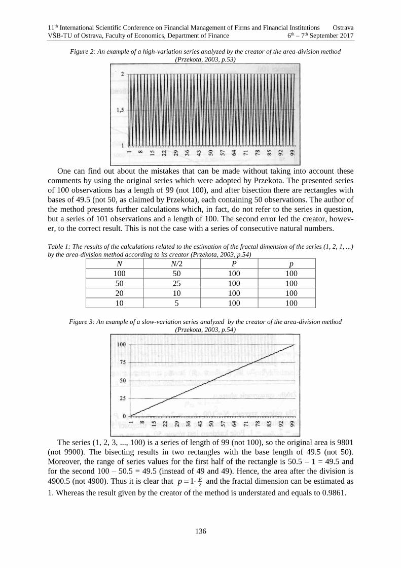
11th International Scientific Conference on Financial Management of Firms and Financial Institutions Ostrava
VŠB-TU of Ostrava, Faculty of Economics, Department of Finance 6th – 7th September 2017
136
Figure 2: An example of a high-variation series analyzed by the creator of the area-division method
(Przekota, 2003, p.53)
One can find out about the mistakes that can be made without taking into account these
comments by using the original series which were adopted by Przekota. The presented series
of 100 observations has a length of 99 (not 100), and after bisection there are rectangles with
bases of 49.5 (not 50, as claimed by Przekota), each containing 50 observations. The author of
the method presents further calculations which, in fact, do not refer to the series in question,
but a series of 101 observations and a length of 100. The second error led the creator, howev-
er, to the correct result. This is not the case with a series of consecutive natural numbers.
Table 1: The results of the calculations related to the estimation of the fractal dimension of the series (1, 2, 1, ...)
by the area-division method according to its creator (Przekota, 2003, p.54)
N N/2 P p
100 50 100 100
50 25 100 100
20 10 100 100
10 5 100 100
Figure 3: An example of a slow-variation series analyzed by the creator of the area-division method
(Przekota, 2003, p.54)
The series (1, 2, 3, ..., 100) is a series of length of 99 (not 100), so the original area is 9801
(not 9900). The bisecting results in two rectangles with the base length of 49.5 (not 50).
Moreover, the range of series values for the first half of the rectangle is 50.5 – 1 = 49.5 and
for the second 100 – 50.5 = 49.5 (instead of 49 and 49). Hence, the area after the division is
4900.5 (not 4900). Thus it is clear that 2
1 Pp and the fractal dimension can be estimated as
1. Whereas the result given by the creator of the method is understated and equals to 0.9861.
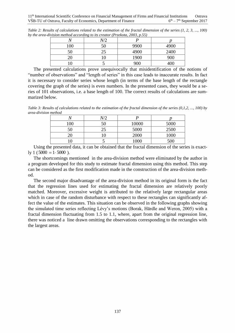
11th International Scientific Conference on Financial Management of Firms and Financial Institutions Ostrava
VŠB-TU of Ostrava, Faculty of Economics, Department of Finance 6th – 7th September 2017
137
Table 2: Results of calculations related to the estimation of the fractal dimension of the series (1, 2, 3, ..., 100)
by the area-division method according to its creator (Przekota, 2003, p.55)
N N/2 P p
100 50 9900 4900
50 25 4900 2400
20 10 1900 900
10 5 900 400
The presented calculations prove unequivocally that misidentification of the notions of
“number of observations” and “length of series” in this case leads to inaccurate results. In fact
it is necessary to consider series whose length (in terms of the base length of the rectangle
covering the graph of the series) is even numbers. In the presented cases, they would be a se-
ries of 101 observations, i.e. a base length of 100. The correct results of calculations are sum-
marized below.
Table 3: Results of calculations related to the estimation of the fractal dimension of the series (0,1,2, ..., 100) by
area-division method
N N/2 P p
100 50 10000 5000
50 25 5000 2500
20 10 2000 1000
10 5 1000 500
Using the presented data, it can be obtained that the fractal dimension of the series is exact-
ly 1 ( 500015000 ).
The shortcomings mentioned in the area-division method were eliminated by the author in
a program developed for this study to estimate fractal dimension using this method. This step
can be considered as the first modification made in the construction of the area-division meth-
od.
The second major disadvantage of the area-division method in its original form is the fact
that the regression lines used for estimating the fractal dimension are relatively poorly
matched. Moreover, excessive weight is attributed to the relatively large rectangular areas
which in case of the random disturbance with respect to these rectangles can significantly af-
fect the value of the estimates. This situation can be observed in the following graphs showing
the simulated time series reflecting Lévy’s motions (Borak, Härdle and Weron, 2005) with a
fractal dimension fluctuating from 1.5 to 1.1, where, apart from the original regression line,
there was noticed a line drawn omitting the observations corresponding to the rectangles with
the largest areas.
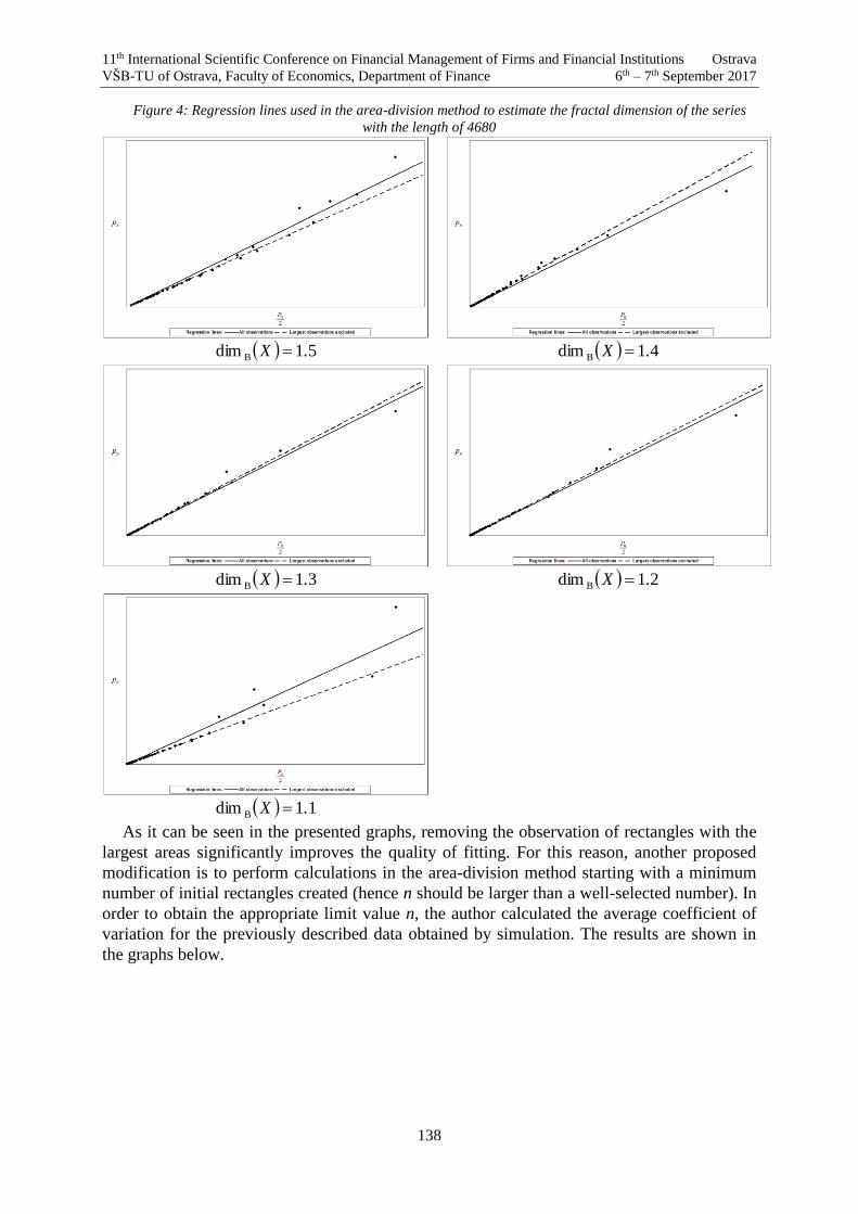
11th International Scientific Conference on Financial Management of Firms and Financial Institutions Ostrava
VŠB-TU of Ostrava, Faculty of Economics, Department of Finance 6th – 7th September 2017
138
Figure 4: Regression lines used in the area-division method to estimate the fractal dimension of the series
with the length of 4680
51dim B .X 41dim B .X
31dim B .X 21dim B .X
11dim B .X
As it can be seen in the presented graphs, removing the observation of rectangles with the
largest areas significantly improves the quality of fitting. For this reason, another proposed
modification is to perform calculations in the area-division method starting with a minimum
number of initial rectangles created (hence n should be larger than a well-selected number). In
order to obtain the appropriate limit value n, the author calculated the average coefficient of
variation for the previously described data obtained by simulation. The results are shown in
the graphs below.

11th International Scientific Conference on Financial Management of Firms and Financial Institutions Ostrava
VŠB-TU of Ostrava, Faculty of Economics, Department of Finance 6th – 7th September 2017
139
Figure 5: Random variation coefficient for the regression line used for estimating the fractal dimension
Series length 1008 Series length 2016
Series length 3024 Series length 3960
Series length 4680
As shown above, even a slight increase in the minimum number of rectangles obtained in
the first division dramatically improves the fitting of regression lines. The problem, however,
remains such a selection of the mentioned quantity so that the simultaneous reduction of the
coefficient of random variation does not lead to an excessive reduction in the number of ob-
servations used in the construction of regression line. The author decided to compromise on
the adoption of this quantity at level 10, which provides a significant improvement in the fit-
ting using the most possible number of observations.
The third modification proposed in this paper refers to the problem of correctness of the de-
termination of the fractal dimension estimator. It can be proved (Buła, 2012b) that the area-
division method in the original form actually leads to an estimate not of the fractal dimension,
but of the function values related to it:
1dim2dim X
MADBX .
As a result, the estimates obtained are understated. Therefore, the author proposes to trans-
form the estimated quantity as follows:
1dimlogdim 2 XX MADB
11th International Scientific Conference on Financial Management of Firms and Financial Institutions Ostrava
VŠB-TU of Ostrava, Faculty of Economics, Department of Finance 6th – 7th September 2017
140
thereby resulting in the box dimension. The area-division method containing the presented
modifications, taking into account their significant influence on the construction of the meth-
od and the results obtained, was called a modified area-division method by the author. Thus,
the main research hypothesis was confirmed, and the main objective of the paper was attained.
3. Conclusion
The paper discusses the area-division method and its application to estimate the fractal di-
mension of time series. At the same time, the shortcomings of the analyzed method were
pointed out, which made the estimates based on it significantly burdensome and unstable. An
in-depth analysis of the fractal dimension algorithm used in the area-division method has
found flaws in the construction of this algorithm. In addition, in order to eliminate the identi-
fied deficiencies, the author proposed incorporating correlations involving the understanding
of “length of series” and “number of observations,” improvement of the fitting of estimated
regression lines, and use of functional exponential relations between the real box dimension of
the series and its estimates obtained in the area-division method. As a result, a modified area-
division method is presented. Due to the limited scope of this paper, the author will devote a
separate paper into comparative analysis taking into account the modifications made based on
the data obtained by simulation and in empirical way.
References
[1] Andreou, E., Pittis, N. and Spanos, A. (2001). On modelling speculative prices: the em-
pirical literature. Journal of Economic Surveys, 15(2), pp.187-220.
[2] Borak, S., Härdle, W. and Weron, R. (2005). Stable distributions. SFB 649 Discussion
Papers, 8, pp.1-26.
[3] Buła, R. (2012a). Aspekty metodyczne szacowania wymiaru fraktalnego finansowych
szeregów czasowych. In: M. Kuczera, ed. (2012). Młodzi naukowcy dla polskiej nauki.
Kraków: Creativetime, pp.192-200.
[4] Buła, R. (2012b). Metoda podziału pola a metoda segmentowo-wariacyjna szacowania
wymiaru fraktalnego. In: M. Kuczera, ed. (2012). Nowe trendy w naukach human-
istycznych i społeczno-ekonomicznych. Kraków: Creativetime, pp.248-256.
[5] Buła, R. (2017). Analiza wymiaru fraktalnego spółek notowanych na Giełdzie Papierów
Wartościowych w Warszawie – aspekty metodyczne. Nauki o Finansach, 1(30), in press.
[6] Buła, R. and Pera, K. (2015). Применение концепции фрактальной размерности для
оценки инвестиционного риска на финансовых рынках. In: С. А. Белозеров, ed.
(2015). Международный экономический симпозиум - 2015: материалы
Международных научных конференций, посвященных 75-летию экономического
факультета Санкт-Петербургского государственного университета 22–25 апреля
2015 г. Сборник статей. Санкт-Петербург: Скифия-принт, pp.217-235.
[7] Dubuc, B., Quiniou, J., Roques-Carmes, C., Tricot, C. and Zucker, S. (1989). Evaluating
the fractal dimension of profiles. Physical Review A, 39(3), pp.1500-1512.
[8] Lintner, J. (1965). The Valuation of Risk Assets and the Selection of Risky Investments
in Stock Portfolios and Capital Budgets. The Review of Economics and Statistics, 47(1),
pp.13-37.
11th International Scientific Conference on Financial Management of Firms and Financial Institutions Ostrava
VŠB-TU of Ostrava, Faculty of Economics, Department of Finance 6th – 7th September 2017
141
[9] Mandelbrot, B. (1963). The Variation of Certain Speculative Prices. The Journal of Busi-
ness, 36(4), pp.394-419.
[10] Mandelbrot, B. (1967). The Variation of Some Other Speculative Prices. The Journal of
Business, 40(4), pp.393-413.
[11] Mandelbrot, B. (1972). Correction of an Error in “The Variation of Certain Speculative
Prices”. The Journal of Business, 45(4), pp.542-543.
[12] Markowitz, H. (1952). Portfolio Selection. The Journal of Finance, 7(1), pp.77-91.
[13] Markowitz, H. (1959). Portfolio Selection. Efficient Diversification of Investments. New
York: John Wiley & Sons.
[14] Mossin, J. (1966). Equilibrium in a Capital Asset Market. Econometrica, 34(4), pp.768-
783.
[15] Przekota, G. (2003). Szacowanie wymiaru fraktalnego szeregów czasowych metodą pod-
ziału pola. Zeszyty Studiów Doktoranckich Akademii Ekonomicznej w Poznaniu, 12,
pp.47-68.
[16] Przekota, G. (2012). Szacowanie ryzyka zmian cen akcji metodą podziału pola. Problemy
Zarządzania, 10(4), pp.178-187.
[17] Przekota, G. (2014). Gospodarcze aspekty ryzyka na rynkach finansowych. Koszalin:
Wyd. Ucz. Politechniki Koszalińskiej.
[18] Przekota, G. and Przekota, D. (2004). Szacowanie wymiaru fraktalnego szeregów
czasowych kursów walut metodą podziału pola. Badania operacyjne i decyzje, 3-4,
pp.67-82.
[19] Przekota, G. and Szczepańska-Przekota, A. (2008). Analiza empiryczna efektywności
polskiego rynku akcji. Warszawa: Ośrodek Analiz Statystycznych.
[20] Przekota, G. and Waściński T. (2012). Wybrane problemy oceny ryzyka zmian cen akcji
za pomocą miar klasycznych i nieklasycznych. Zeszyty Naukowe Uniwersytetu Przyrod-
niczo-Humanistycznego w Siedlcach, 95, pp.71-82.
[21] Schmittbuhl, J. and Vilotte, J.-P. (1995). Reliability of self-affine measurements. Physi-
cal Review E, 51(1), pp.131-147.
[22] Sharpe, W. (1964). Capital Asset Prices: A Theory of Market Equilibrium under Condi-
tions of Risk. The Journal of Finance, 19(3), pp.425-442.
[23] Treynor, J. (1962). Toward a Theory of Market Value of Risky Assets. [pdf] Available at:
https://papers.ssrn.com/sol3/Delivery.cfm/SSRN_ID2654579_code87814.pdf?abstractid=
628187.&mirid=1.
[24] Zwolankowska, M. (1998). Szacowanie lokalnego wymiaru fraktalnego szeregów
czasowych. Zeszyty Naukowe Uniwersytetu Szczecińskiego, 233, pp.157-163.
[25] Zwolankowska, M. (1999). Wykorzystanie wymiaru fraktalnego w ocenie ryzyka in-
westycji giełdowych. In: T. Trzaskalik, ed. (1999). Modelowanie preferencji a ryzyko
’99. Katowice: Wydawnictwo Akademii Ekonomicznej im. Karola Adamieckiego w Ka-
towicach, pp.465-476.
[26] Zwolankowska, M. (2000a). Metoda segmentowo-wariacyjna. Nowa propozycja sza-
cowania wymiaru fraktalnego. Przegląd Statystyczny, 1-2, pp.209-223.

11th International Scientific Conference on Financial Management of Firms and Financial Institutions Ostrava
VŠB-TU of Ostrava, Faculty of Economics, Department of Finance 6th – 7th September 2017
142
[27] Zwolankowska, M. (2000b). Wymiar fraktalny jako miara zmienności stopy zwrotu.
Zeszyty Naukowe Uniwersytetu Szczecińskiego, 306, pp.259-269.
[28] Zwolankowska, M. (2001). Fraktalna geometria polskiego rynku akcji. Szczecin:
Wydawnictwo Naukowe Uniwersytetu Szczecińskiego.
11th International Scientific Conference on Financial Management of Firms and Financial Institutions Ostrava
VŠB-TU of Ostrava, Faculty of Economics, Department of Finance 6th – 7th September 2017
143
Potential of blockchain technology
Michal Butek, Vladimír Bakeš1
Abstract
The aim of this article is to analyze possible areas of use of blockchain technology and
cryptocurrency systems. The emergence of this technology is linked to the emergence of the
Bitcoin system in 2008. Blockchain is a special type of a database, into which are
chronologically recorded the transactions, which are executed in cryptocurrencies such as
Bitcoin. In this article, we will examine three areas of use. The first is the possibility of
replacing the conventional "fiat" money with cryptocurrencies. The second area is to use
cryptocurrencies as a store of value. The latest area of interest is the use of blockchain
technology as a very secure and effective form of transaction records, with potential for use in
various, even non-financial, areas.
Key words
Bitcoin, blockchain
JEL Classification: E42, O33, E71,
1 Stručná charakteristika Bitcoinu a blockchain technológie
Bitcoin bol vytvorený v roku 2008, keď neznámy vedec alebo skupina vedcov vydala pod
pseudonymom Satoshi Nakamoto „white paper“ – dokument popisujúci princípy fungovania
decentralizovaného systému Bitcoin, ktorý uchováva všetky transakcie vo verejnej
decentralizovanej databáze zabezpečenej dômyselným šifrovacím mechanizmom – databáze
blockchain. Následne bol v januári roku 2009 vytvorený prvý blok v databáze, čím systém
Bitcoin reálne vznikol. Špecifikom systému je nezávislosť pravidiel na základe ktorých
funguje od akejkoľvej autority. Tento decentralizovaný peer to peer systém uchováva všetky
realizované transakcie virtuálnych jednotiek – bitcoinov. Užívateľ systému si môže
vygenerovať prakticky ľubovoľný počet adries. Pri generovaní adresy dochádza zároveň
k vytvoreniu tzv. súkromného kľúča, ktorý je potrebný na následné odoslanie bitcoinov
z príslušnej adresy. Pri realizácii transakcie dochádza k podpisu transakcie týmto súkromným
kľúčom, ktorý za normálnych okolností nie je viditeľný druhými subjektami. Vlastníctvo
bitcoinov je tak nezávislé od autority, na rozdiel od prostriedkov v banke nie je možné
bitcoinové prostriedky zabaviť. V sieti sa transakcie zhlukujú do väčších dátových celkov –
blokov, ktoré vznikajú približne raz za 10 min. a následne sa zapisujú do blockchain
databázy. Každý blok nadväzuje na predošlý blok a celá databáza je vlastne reťazou blokov.
(odtiaľ pochádza anglický názov blockchain) Vytváranie blokov si vyžaduje realizáciu
kryptografických výpočtov. Nové bitcoiny sa vytvárajú postupne na základe vopred
stanoveného algoritmu a do obehu sa dostávajú ako odmena za vytvorenie bloku, ktoré je
náročné na spotrebu elektrickej energie. Takéto subjekty sa nazvývajú míneri. Každé 4 roky
dochádza k udalosti, ktorá sa nazýva polenie (anglicky halving). Vtedy sa odmena za
vygenerovaný blok znižuje na polovicu. Prvé 4 roky bola odmena 50 bitcoinov za blok,
1 Ing. Michal Butek11, Ing. Vladimír Bakeš21 Žilinská univerzita, fakulta PEDAS, katedra ekonomiky,
Univerzitná 1, 01026 Žilina, [email protected] [email protected]
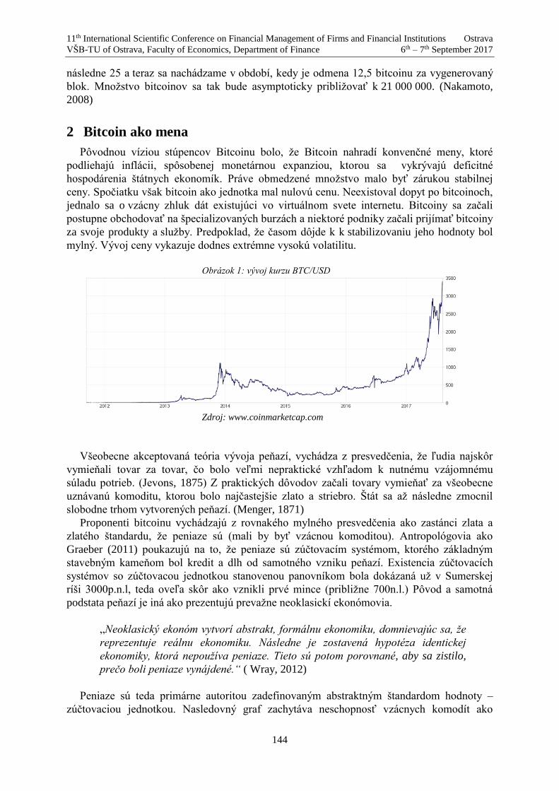
11th International Scientific Conference on Financial Management of Firms and Financial Institutions Ostrava
VŠB-TU of Ostrava, Faculty of Economics, Department of Finance 6th – 7th September 2017
144
následne 25 a teraz sa nachádzame v období, kedy je odmena 12,5 bitcoinu za vygenerovaný
blok. Množstvo bitcoinov sa tak bude asymptoticky približovať k 21 000 000. (Nakamoto,
2008)
2 Bitcoin ako mena
Pôvodnou víziou stúpencov Bitcoinu bolo, že Bitcoin nahradí konvenčné meny, ktoré
podliehajú inflácii, spôsobenej monetárnou expanziou, ktorou sa vykrývajú deficitné
hospodárenia štátnych ekonomík. Práve obmedzené množstvo malo byť zárukou stabilnej
ceny. Spočiatku však bitcoin ako jednotka mal nulovú cenu. Neexistoval dopyt po bitcoinoch,
jednalo sa o vzácny zhluk dát existujúci vo virtuálnom svete internetu. Bitcoiny sa začali
postupne obchodovať na špecializovaných burzách a niektoré podniky začali prijímať bitcoiny
za svoje produkty a služby. Predpoklad, že časom dôjde k k stabilizovaniu jeho hodnoty bol
mylný. Vývoj ceny vykazuje dodnes extrémne vysokú volatilitu.
Obrázok 1: vývoj kurzu BTC/USD
Zdroj: www.coinmarketcap.com
Všeobecne akceptovaná teória vývoja peňazí, vychádza z presvedčenia, že ľudia najskôr
vymieňali tovar za tovar, čo bolo veľmi nepraktické vzhľadom k nutnému vzájomnému
súladu potrieb. (Jevons, 1875) Z praktických dôvodov začali tovary vymieňať za všeobecne
uznávanú komoditu, ktorou bolo najčastejšie zlato a striebro. Štát sa až následne zmocnil
slobodne trhom vytvorených peňazí. (Menger, 1871)
Proponenti bitcoinu vychádzajú z rovnakého mylného presvedčenia ako zastánci zlata a
zlatého štandardu, že peniaze sú (mali by byť vzácnou komoditou). Antropológovia ako
Graeber (2011) poukazujú na to, že peniaze sú zúčtovacím systémom, ktorého základným
stavebným kameňom bol kredit a dlh od samotného vzniku peňazí. Existencia zúčtovacích
systémov so zúčtovacou jednotkou stanovenou panovníkom bola dokázaná už v Sumerskej
ríši 3000p.n.l, teda oveľa skôr ako vznikli prvé mince (približne 700n.l.) Pôvod a samotná
podstata peňazí je iná ako prezentujú prevažne neoklasickí ekonómovia.
„Neoklasický ekonóm vytvorí abstrakt, formálnu ekonomiku, domnievajúc sa, že
reprezentuje reálnu ekonomiku. Následne je zostavená hypotéza identickej
ekonomiky, ktorá nepoužíva peniaze. Tieto sú potom porovnané, aby sa zistilo,
prečo boli peniaze vynájdené.“ ( Wray, 2012)
Peniaze sú teda primárne autoritou zadefinovaným abstraktným štandardom hodnoty –
zúčtovaciou jednotkou. Nasledovný graf zachytáva neschopnosť vzácnych komodít ako

11th International Scientific Conference on Financial Management of Firms and Financial Institutions Ostrava
VŠB-TU of Ostrava, Faculty of Economics, Department of Finance 6th – 7th September 2017
145
bitcoin a zlato slúžiť ako štandard hodnoty. V grafe sú zachytená relatívna kúpna sila zlata
bitcoinu a eura vo vzťahu k tovarom a službám.
Obrázok 2: Kúpna sila eura, zlata a bitcoinu
Zdroj: vlastné spracovanie
Bitcoin, ani zlato nedokážu plniť funkciu štandardu hodnoty. Bitcoin, alebo akákoľvek iná
kryptomena je skôr digitálnou komoditou ako menou. Zo svojej podstaty nemôže plniť
funkciu zúčtovacej jednotky (Yermack, 2013). Teda je nereálne aby subjekty ekonomiky
vyjadrovali hodnotu tovarov, služieb, dlhov a miezd v bitcoinoch.
3 Bitcoin ako nástroj na uchovanie hodnoty
Bitcoin je prirovnávaný k zlatu, niekedy dokonca označovaný ako digital gold, alebo gold
2.0 (Lee, 2017) . Podobne ako na ťažbu zlata aj na “ťažbu bitcoinov“ je nevyhnutná spotreba
energia a tak rovnako ako zlato ani bitcoin nie je „zadarmo“. Množstvo bitcoinov, ktoré budú
„vyťažené“ je vopred dané podobne ako sú celkové zásoby zlata na Zemi vopred limitované.
Podmienky za akých by mohlo dôjsť k zmene tohto limitu sa budeme venovať v ďalších
častiach tohto článku. Podstatná je viera v nemožnosť zmeny týchto pravidiel. Podobne aj
v prípade zlata je viera v jeho budúcu vzácnosť podstatným faktorom určujúcim jeho cenu.
Ak by došlo v budúcnosti k objaveniu obrovských nálezísk zlata došlo by k poklesu jeho
hodnoty podobne ako sa to dialo po objavení nálezísk drahých kovov v latinskej amerike. Ak
by sa vynašla cenovo dostupná metóda nukleárnej transmutácie, kedy sa jadrovou reakciou
vyrobí stabilný izotop zlata mohla by sa trhová cena takisto znížiť. Našou snahou je poukázať
na paralelu medzi cenou zlata a bitcoinu. V obidvoch prípadoch je dôležitá viera, že
v budúcnosti ich množstvo bude obmedzené.
Logickým argumentom by bolo poukázať na fakt, že zlato má na rozdiel od bitcoinov aj
svoju úžitkovú hodnotu danú využívaním v šperkárstve a elektrotechnickom priemysle, no
zastávame názor, že hodnota zlata nie je daná primárne jeho využiteľnosťou, ale vierou
v možnosť výmeny za tovar a služby v adekvátnej hodnote v budúcnosti. Zlato je preto
označované ako komodita s monetárnym dopytom. (Karpiš, 2011) Hodnota vzácnej komodity
je daná dôležitosťou, akú jednotlivé spoločnosti pripisujú konkrétnej vzácnej komodite. Tento
argument podporuje aj nález z ostrova Yap, kde domorodé obyvateľstvo využívalo ako
peniaze kamenné kolesá, ktoré takisto nemali žiadnu úžitkovú hodnotu. (Furness, 1910) Ich
11th International Scientific Conference on Financial Management of Firms and Financial Institutions Ostrava
VŠB-TU of Ostrava, Faculty of Economics, Department of Finance 6th – 7th September 2017
146
získavanie však bolo nákladné podobne ako v prípade bitcoinu a zlata. Na druhej strane
existujú spoločnosti, ktoré hodnotu zlatu nepripisujú.
„Núbijci príliš nechápali ochotu vymieňať napríklad soľ za niečo tak nepotrebné ako je
žltý kov“ (Revenda, 2015).
Obmedzané množstvo neužitočnej komodity však nie je zárukou jeho stabilnej hodnoty.
Komodita si musí získať dôležitosť, musí sa stať symbolom spoločenského postavenia. Musí
sa stať predmetom súťaživosti. „Prebytok potravy, ktorý majú k dispozícii, im takisto dovoľuje
vynakladať jej väčšie množstvo, ako sú drahé kovy a drahokamy, v ktorých boháči medzi
sebou toľko súťažia“(Smith, 2017) „Peňažná cena diamantov, tejto najzbytočnejšej
zbytočnosti...“(Smith, 2017). Ich hodnota nie je daná ich využiteľnosťou, tieto komodity sa
stávajú konečným predmetom túžby samotnej.
Na Zemi je množstvo všetkého vyťaženého zlata približne 170 000 ton. Množstvo
vyťažených bitcoinov v čase písania článku predstavuje 16,462,625. (coinmarketcap, 2017)
Na jeden vyťažený bitcoin tak pripadá približne 10 kg vyťaženého zlata, no jeho cena je
mnohonásobne nižšia ako 10kg zlata.
Zlato priťahuje pozornosť hlavne v časoch neistoty, kedy zaniká dôvera v inštitúcie
a štandartné nástroje na uchovanie hodnoty, ktoré sú zväčša kreditnými nástrojmi. V prípade
bitcoinu sú tieto investičné úvahy rovnaké. Bitcoin bude zrejme podobne ako zlato priťahovať
záujem investorov prevažne v časoch neistoty na trhoch a nedôveryhodnosti v schopnosti
štandarndých investičných nástrojov uchovávať hodnotu. (Lis, Zvierzchlewski, 2016)
Limitovanosť množstva bitcoinov. Pravidlá na základe ktorých funguje systém Bitcoin sú
dopredu dané. Jednotliví míneri (subjekty vytvárajúce bloky obsahujúce jednotlivé transakcie)
vzájomne súťažia o vytvorenie bloku. Ak by vytvoril míner blok, ktorý by bol v rozpore
s pravidlami, väčšina by ho neprijala. Systém je bezpečný pokiaľ poctivé uzly disponujú
väčším počtom výpočtového výkonu ako spolupracujúca skupina útočníkov. (Nakamoto,
2008)
Nakamoto zrejme nepredpokladal, že by k útoku „nepoctivou väčšinou“ mohlo dojsť.
Míneri na začiatku existencie siete Bitcoin ťažili bitcoiny na bežných počítačoch, postupne sa
začali zoskupovať do tzv. poolov aby dosiahli väčší výkon. Neskôr sa začal vyrábať
a využívať špeciálny hardware, ktorého jediným využitím bolo dolovanie bitcoinov. Práve
tento technologický posun spôsobil centralizáciu dolovania bitcoinov, a presun do oblastí
s nízkou cenou elektrickej energie, prevažne do Číny. Odhaduje sa, že viac ako 70 percent
dolovania kontrolujú čínsky míneri. (Coleman, 2016) V Číne sa nachádza navyše
najúspešnejšia spoločnosť vyrábajúca spomínané špecializované zariadenia a tak sa dá
predpokladať, že koncentrácia moci bude pokračovať. Kým moc mínerov sa koncentruje
v Číne, ekonomická aktivita súvisiaca s Bitcoinom je charakteristická pre ekonomicky vyspelé
krajiny. Len niečo medzi 2-3 percentami Bitcoinových uzlov sa nachádza v Číne, kým skoro
30 percent sa nachádza v USA. (bitnodes, 2017) Táto disbalancia vytvára mocenské skupiny,
ktoré majú svoje vlastné priority a záujmy a v pôvodne decentralizovanom bitcoine sa medzi
týmito skupinami odohrávajú rokovania špecifické pre centralizované systémy.
Znižujúce sa odmeny mínerom budú viesť v budúcnosti k zásadnému dilema. Dodržať
maximálne množstvo stanovené Satoshim za cenu znižujúceho výkonu siete a teda
bezpečnosti siete, alebo umožniť emisiu nových bitcoinov, zabezpečiť dostatočný výkon siete,
ale porušiť pôvodné pravidlá a limit 21000000 bitcoinov?
Ak by sa dokázala väčšina mínerov zhodnúť je prakticky možné presadiť akúkoľvek
zmenu pravidiel vrátane 21000000 limitu na celkové množstvo bitcoinov.

11th International Scientific Conference on Financial Management of Firms and Financial Institutions Ostrava
VŠB-TU of Ostrava, Faculty of Economics, Department of Finance 6th – 7th September 2017
147
4 Technológia blockchain
Blockchain je jednou z prevratných technológií súčasnosti. (Pohulak- Zolędowska, 2016).
Bitcoin bol prvou aplikáciou blockchain technológie, no od jeho vzniku boli vyvinuté ďalšie
aplikácie využívajúce vlastnú blockchain databázu. Táto technológia bola označená mnohými
za prelomovú:
IBM: „Podobne ako internet zmenil svet poskytnutím väčšieho prístupu k informáciám,
technológia blockchain je schopná zmeniť spôsob podnikania zabezpečením dôvery“ (Lucas,
2017)
Goldman Sachs: „Blockchain môže zmeniť....všetko“(Boroujerdi, Wolf, 2015)
Deloitte (2017): „Blockchain má potenciál skutočne zmeniť viacero odvetví a robiť procesy
demokratickejšie, bezpečnejšie, transparentnejšie a efektívnejšie.“
4.1 Blockchain vs. centralizovaná databáza
Blockchain je technológia, ktorá umožňuje úplne novým spôsobom pracovať medzi
rôznymi subjektami so zdieľanými dátami. Potreba komunikovať a zdieľať dáta s inými
subjektami je neodmysliteľnou súčasťou dnešnej spoločnosti. Spočiatku si jednotlivé subjekty
uchovávali dáta vo vlastnej databáze. V prípade spolupráce s inými subjektmi, ktoré si
vyžadovali prístup k tým istým dátam dochádzalo k zdieľaniu zmien a následne si každý
subjekt aktualizoval záznamy v svojej databáze. Jednotlivé dáta tak boli uchovávané vo
viacerých databázach súčasne. Ľahko sa mohlo stať, že vplyvom pomalého aktualizovaniu
vlastných záznamov, prípadne iným problémom v komunikácii došlo medzi jednotlivými
subjektami ku konfliktom spôsobených nekonzistentnosťou jednotlivých záznamov v rôznych
databázach. (Buno, 2014) Logickým východiskom bolo spoľahnutie sa na dôveryhodného
prostredníka-centrálnu autoritu, ktorý ako jediný uchovával aktuálny stav zdieľaných dát.
Technológia blockchain umožňuje vytvorenie dôveryhodnej zdieľanej databázy bez
prítomnosti prostredníka. Všetky uzly siete vlastnia identický záznam. K aktualizovaniu
databázy dochádza súčasne na všetkých uzloch pripojených do siete. Transakcie sú schválené
a zapísané do blockchainu len v prípade že sú potvrdené dostatočným množstvom validátorov.
Výhodou blockchainu oproti štandardnej centralizovanej databáze sú:(deloitte, 2017)
Vylúčenie medzičlánkov a sprostredkovateľov
Dva subjekty môžu spraviť výmenu bez prítomnosti tretiej strany, čím sa redukuje
alebo úplne eliminuje riziko protistrany.
Zvýšenie moci uživateľov
Užívatelia majú plne pod kontrolou svoje informácie a transakcie
Kvalita dát
Dáta v Blockchaine sú úplné, konzistentné, včasné, presné a široko dostupné.
Trvácnosť a spoľahlivosť
Vďaka decentralizovanej povahe siete, nemá blockchain centrálny bod, ktorý môže
zlyhať a sieť tak môže odolávať útokom.
Integrita s nastavenými pravidlami
Užívatelia sa môžu spoľahnúť, že transakcie budú realizované v súlade s pravidlami
bez nutnosti spoliehania sa na dôveryhodný tretí subjekt.
Transparentnosť a nemennosť
Zmeny vo verejných blockchain databázach sú verejne dostupné. Blockchain uchováva
všetky svoje predošlé stavy a tak sú transakcie nemenné a nevymazateľné.
Zjednodušenie systému
Pridaním všetkých transakcií do jednej verejne dostupnej databázy sa odstraňujú
komplikácie spôsobené s manažovaním viacerých databáz.

11th International Scientific Conference on Financial Management of Firms and Financial Institutions Ostrava
VŠB-TU of Ostrava, Faculty of Economics, Department of Finance 6th – 7th September 2017
148
Rýchle spracovanie transakcií
V prípade využívania centrálnej autority sú niekedy aktualizácie záznamov v databáze
pomalé. Napríklad medzibankové prevody trvajú niekoľko dní, blockchain technológia
dokáže tento čas skrátiť na niekoľko sekúnd prípadne minút.
Znižovanie transakčných nákladov
Eliminovaním tretej strany – medzičlánku bude viesť k znižovaniu transakčných
nákladov.
4.2 Verejné vs. súkromné blockchain databázy
Verejná blockchain
Jedná sa o databázu, ktorú ktokoľvek na svete môže čítať, ktokoľvek môže vytvárať
transakcie ktoré sú zapísané do databázy ak sú v súlade s pravidlami a každý sa môže
zúčastňovať procesu validácie – procese určujúcom ktoré bloky budú zahrnuté do databázy
a aký je aktuálny stav. Namiesto dôvery v centrálnu autoritu je verejná blockchain databáza
zabezpečená validátormi - subjektami, ktoré sú ekonomicky motivované šifrovaním
zabezpečovať blockchain. (Butterin,2015)
Súkromná blockchain
Oproti verejnej blockchain databáze je skupina validátorov vopred obmedzená. Napríklad
to môže byť konzorcium 15 vybraných finančných inštitúcií z ktorých 10 musí podpísať
každý blok aby bol platný.. Právo čítať blockchain môže byť takisto obmedzené na určitú
skupinu. (Butterin, 2015)
4.3 Oblasť využitia
Predpokladá sa, že blockchain technológia nájde svoje uplatnenie hlavne nasledovných
sektoroch: finančný sektor, zdravotníctvo, dodávateľské reťazce, digitálna identita.
4.3.1 Finančný sektor
Blockchain dokáže urýchliť a znížiť náklady na cezhraničné platby. Príkladom je
medzibankový zúčtovací systém ripple využívajúci blockchain technológiu, ktorý v súčasnosti
integruje viac ako 75 klientov zahŕňajúcich viaceré významné banky ako Unicredit a
Santander. Platby v rámci systému ripple sú okamžité, bezpečné, transparentnejšie a
mnohonásobne lacnejšie.
Je predpoklad, že blockchain technológia zásadným spôsobom zmení fungovanie búrz,
obchodovanie s akciami a ostatnými finančnými nástrojmi stane rýchlejšie.
Jednou z najvýznamnejších zmien oproti pôvodným technológiam je využitie tzv. “smart
contract”. Jedná sa o program ktorý vykonáva transakcie podľa podmienok nastavených na
začiatku bez prítomnosti tretieho subjektu. Smart contract dokáže napríklad vynútiť prevod
vlastníckeho práva (napríklad nehnuteľnosti) v prípade, že boli splnené podmienky zmluvy.
Kupujúci sa v prípade uhradenia zmluvnej čiastky nemusí obávať, že autorita-prostredník
neschváli prevod predmetného vlastníckeho práva.
4.3.2 Zdravotníctvo
Blockchain technológia má potenciál transformovať zdravotnú starostlivosť, zvýšiť
bezpečnosť, súkromie a interoperabilitu zdravotných údajov. Táto technológia by mohla
poskytnúť nový model pre výmenu zdravotných informácií medzi jednotlivými oddeleniami
tým, že zdieľanie elektronických záznamov bude efektívnejšie, jednoduchšie a bezpečnejšie.
4.3.3 Dodávateľské reťazce
V súčasnej dobe sú globálne dodávateľské reťazce jedným z nosným pilierom globálnej
ekonomiky. Od objednávky tovaru po dodanie prechádza tovar mnohými spoločnosťami.

11th International Scientific Conference on Financial Management of Firms and Financial Institutions Ostrava
VŠB-TU of Ostrava, Faculty of Economics, Department of Finance 6th – 7th September 2017
149
Blockchain v oblasti dodávateľských reťazcov si sľubuje efektívnejšie spravovanie dodávok,
transparentné sledovanie zásielok, digitalizáciu celého procesu a bezpečné zdieľanie citlivých
informácií medzi partnermi. Príkladm je spoločnosť Maersk, ktorá v spolupráci s IBM
implementuje pre svoje dodávateľské reťazce blockchain technológiu. (IBM,2017)
4.3.4 Digitálna identita
Presunom osobných záznamov na blockchain má užívateľ plne pod kontrolou komu ktoré
osobné informácie budú dostupné. Viaceré spoločnosti a služby môžu využívať zdieľanú
databázu, overovať dôveryhodnosť zákazníka. (Balcerzak et al., 2017)
5 Záver
V tomto článku sme analyzovali potenciál využitia kryptomien a technológie blockchain na
ktorej je fungovanie týchto systémov založené. Kryptomeny vzhľadom k svojej povahe
nemôžu slúžiť ako štandard hodnoty a teda sa nemôžu stať peniazmi. Napriek tomu, že
kryptomeny ako bitcoin nemajú žiadnu vnútornú alebo úžitkovú hodnotu je možné, že
v prípade neistoty na finančných trhoch a nedôvery v schopnosť štandardných finančných
nástrojov uchovávať hodnotu, budú vyhľadávanou investičnou alternatívou. Najvýznamnejší
potenciál blockchain technológie vnímame v možnosti využitia v rôznych finančných aj
nefinančných oblastiach. Súkromné blockchain databázy otvárajú nové možnosti v mnohých
sférach spoločnosti.
Zdroje
[1] Balcerzak, P., Pietrzak, A., Bernard, M. (2017). Digital Economy in Visegrad Countries.
Multiple-criteria Decision Analysis at Regional Level in The Years 2012 and 2015,
Journal of Competitiveness, 9(2), pp. 5 – 18.
[2] Bitnodes, Global Bitcoin Nodes Distribution. [online] Dostupné na <
https://bitnodes.21.co/> [cit. 18. august 2017]
[3] Boroujerdi, R.D. and Wolf C., (2015). What if I Told You… [online] Dostupné na
<http://www.goldmansachs.com/our-thinking/pages/macroeconomic-insights-
folder/what-if-i-told-you/report.pdf/> [cit. 18. august 2017]
[4] Buno, M. (2014). Dimensions of the business environment V4. Ekonomicko-manazerske
spektrum, 8(1), 70-73.
[5] Butterin, V., (2015). On Public and Private Blockchains. [online] Dostupné na
<https://blog.ethereum.org/2015/08/07/on-public-and-private-blockchains/> [cit. 18.
august 2017]
[6] Coinmarketcap, (2017). CryptoCurrency Market Capitalizations. [online] Dostupné na
<https://coinmarketcap.com/> [cit. 18. august 2017]
[7] Coleman L., (2016). China’s Mining Dominance: Good Or Bad For Bitcoin? [online]
Dostupné na <https://www.cryptocoinsnews.com/chinas-mining-dominance-good-or-
bad-for-bitcoin/> [cit. 18. august 2017]
[8] Deloitte, Blockchain technology: 9 benefits & 7 challenges [online] Dostupné na
<https://www2.deloitte.com/nl/nl/pages/innovatie/artikelen/blockchain-technology-9-
benefits-and-7-challenges.html/> [cit. 18. august 2017]
11th International Scientific Conference on Financial Management of Firms and Financial Institutions Ostrava
VŠB-TU of Ostrava, Faculty of Economics, Department of Finance 6th – 7th September 2017
150
[9] Furness, W.H., (1910). The Island Of Stone Money UAP Of The Carolines, J. B.
Lippincott Company
[10] IBM, (2017). Maersk and IBM Unveil First Industry-Wide Cross-Border Supply Chain
Solution on Blockchain [online] Dostupné na < https://www-
03.ibm.com/press/us/en/pressrelease/51712.wss/> [cit. 18. august 2017]
[11] Jevons W.S., (1875). Money and the Mechanism of Exchange, London: Macmillan.
[12] Karpiš, J., (2011). Ekonomický význam zlata ako komodity s monetárnym dopytom.
Bratislava: INESS Consult , s.r.o.
[13] Lee, J., (2017) Bitcoin Is Digital Gold. But Will You Buy a Sandwich With It? .[online]
Dostupné na <https://www.bloomberg.com/news/articles/2017-06-19/bitcoin-is-digital-
gold-but-will-you-buy-a-sandwich-with-it > [cit. 18. august 2017]
[14] Lis P., Zwierzchlewski, S., (2016). The Conception and Implementation of a Model
Mechanism of Currency Crises. TRANSFORMATIONS IN BUSINESS & ECONOMICS,
15(2), pp. 148-164
[15] Lucas, M., (2017). The difference between Bitcoin and blockchain for business. [online]
Dostupné na <https://www.ibm.com/blogs/blockchain/2017/05/the-difference-between-
bitcoin-and-blockchain-for-business//> [cit. 18. august 2017]
[16] Menger, C., (1871). Principles of Economics. CreateSpace Independent Publishing
Platform
[17] Nakamoto, S., (2008). Bitcoin: A Peer-to-Peer Electronic Cash System. [pdf] Dostupné
na <https://bitcoin.org/bitcoin.pdf> [cit. 18. august 2017].
[18] Pohulak-Zołędowska, E., (2016). Innovation in Contemporary Economies. Oeconomia
Copernicana, 7(3), 451-466.
[19] Revenda, Z.,(2015) Zlatá minca, ktorá drží historický rekord: platila 700 rokov. [online]
Dostupné na <http://finweb.hnonline.sk/spravy-zo-sveta-financii/509389-zlata-minca-
ktora-drzi-historicky-rekord-platila-700-rokov> [cit. 18. august 2017]
[20] Smith, A., (2017) Bohatství národů. Praha: Grada
[21] Wray, L.R., (2012). Introduction to an Alternative History of Money. [pdf] Dostupné na
<http://www.levyinstitute.org/pubs/wp_717.pdf> [cit. 18. august 2017]
[22] Yermack, D., (2013). Is bitcoin a real currency? an economic appraisal.[pdf] Dostupné
na <http://www.nber.org/papers/w19747.pdf> [cit. 18. august 2017]
11th International Scientific Conference on Financial Management of Firms and Financial Institutions Ostrava
VŠB-TU of Ostrava, Faculty of Economics, Department of Finance 6th – 7th September 2017
151
P/E, dividend yield and GDP growth in U.S.A.: The story of stock market valuation1
Tomáš Buus 2
Abstract
Stock market participants utilize variety of valuation models and their assumptions. Some of those
features, like investors’ myopia, growth expectations or use of income valuation methods are
central to many theories in finance. We derive growth expectations and test validity of those
hypotheses (assumptions) in this paper via examination of relationship between US GDP growth
and S&P 500 P/E and dividend yield. The evidence shows that here has been major shift in
valuation techniques and/or expectations of profit growth at stock market participants. Our results
also have significant implications for efficient market hypothesis and usability of rational, resp.
adaptive expectations models in share (business) valuation.
Key words
Here write the key words (in English)
JEL Classification: Here write the JEL classification code(s)
1. Introduction
Stock market valuation multiples like P/E and dividend yield can supply us with information
about the expected growth of profits (dividends) provided that the stock markets use income
valuation of listed businesses. We use the 1930 – 2016 data on S&P 500 characteristics and US
GDP growth to yield information about the valuation techniques used by market participants.
The income valuation techniques have been available for centuries, long time before 1930s.
However, the mass utilization advanced financial forecasting models had to wait for computing
force. First the use of computers has shifted significantly practice of corporate finance. The
tedious tasks of financial planning and forecasting, formerly almost impossible or at least
difficult in the detail any student of finance provides today, became routine in 1980s and 1990s.
Recently, the neural networks took the work with spreadsheets of analysts’ shoulders.
Therefore, stock market valuation could have become increasingly informative about the
expectations implied in it.
The troubling part of digging expectations out of stock market prices is that there are at least
two unknown variables: discount rate and growth. The reason behind the growth of stock
market prices in the last 40 years could have been increasing profits as well as dropping
government bond yields, as Figure 1 shows.
Mathematical instrument, which could free us from the two-unknown problem is
straightforward: Earnings/price minus the dividend yield. Using that difference together with
disassembly of retention ratio lets us show that this difference equals to the expected permanent
growth times constant.
1 This paper is one of the outputs of the University of Economics in Prague, Faculty of Finance and
Accounting research project and has been financed by the institutional support VSE IP100040. 2 Ing. Tomáš Buus, Ph.D., University of Economics, Prague, Department of Corporate Finance and
Business Valuation, W. Churchill sq. 4, 130 67 Prague, Czech Republic; e-mail: [email protected]
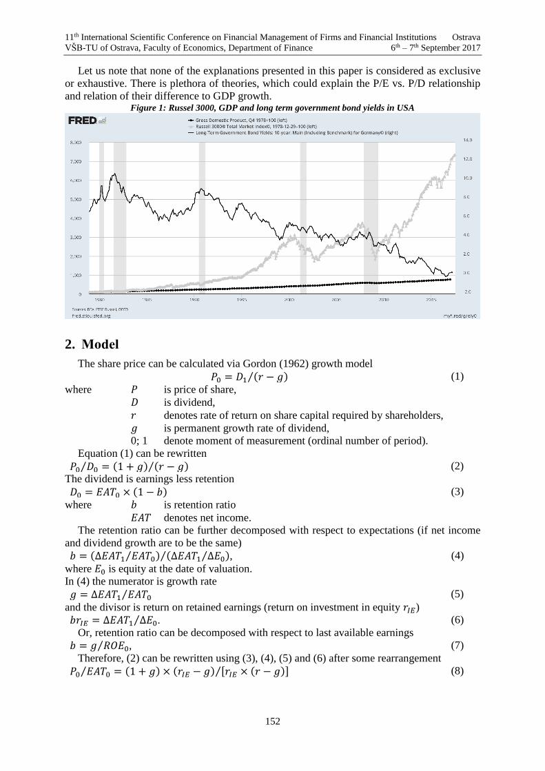
11th International Scientific Conference on Financial Management of Firms and Financial Institutions Ostrava
VŠB-TU of Ostrava, Faculty of Economics, Department of Finance 6th – 7th September 2017
152
Let us note that none of the explanations presented in this paper is considered as exclusive
or exhaustive. There is plethora of theories, which could explain the P/E vs. P/D relationship
and relation of their difference to GDP growth. Figure 1: Russel 3000, GDP and long term government bond yields in USA
2. Model
The share price can be calculated via Gordon (1962) growth model
𝑃0 = 𝐷1 (𝑟 − 𝑔)⁄ (1)
where 𝑃 is price of share,
𝐷 is dividend,
𝑟 denotes rate of return on share capital required by shareholders,
𝑔 is permanent growth rate of dividend,
0; 1 denote moment of measurement (ordinal number of period).
Equation (1) can be rewritten
𝑃0 𝐷0⁄ = (1 + 𝑔) (𝑟 − 𝑔)⁄ (2)
The dividend is earnings less retention
𝐷0 = 𝐸𝐴𝑇0 × (1 − 𝑏) (3)
where 𝑏 is retention ratio
𝐸𝐴𝑇 denotes net income.
The retention ratio can be further decomposed with respect to expectations (if net income
and dividend growth are to be the same)
𝑏 = (∆𝐸𝐴𝑇1 𝐸𝐴𝑇0⁄ ) (∆𝐸𝐴𝑇1 ∆𝐸0⁄ )⁄ , (4)
where 𝐸0 is equity at the date of valuation.
In (4) the numerator is growth rate
𝑔 = ∆𝐸𝐴𝑇1 𝐸𝐴𝑇0⁄ (5)
and the divisor is return on retained earnings (return on investment in equity 𝑟𝐼𝐸)
𝑏𝑟𝐼𝐸 = ∆𝐸𝐴𝑇1 ∆𝐸0⁄ . (6)
Or, retention ratio can be decomposed with respect to last available earnings
𝑏 = 𝑔 𝑅𝑂𝐸0⁄ , (7)
Therefore, (2) can be rewritten using (3), (4), (5) and (6) after some rearrangement
𝑃0 𝐸𝐴𝑇0⁄ = (1 + 𝑔) × (𝑟𝐼𝐸 − 𝑔) [𝑟𝐼𝐸 × (𝑟 − 𝑔)]⁄ (8)

11th International Scientific Conference on Financial Management of Firms and Financial Institutions Ostrava
VŠB-TU of Ostrava, Faculty of Economics, Department of Finance 6th – 7th September 2017
153
If the expected 𝑟𝐼𝐸 equals 𝑅𝑂𝐸0, or in other words, if investor expect the past performance
of the evaluated share (share index) to persist indefinitely even at the new projects, then (8)
equals (2) thus
𝑟𝐼𝐸 = 𝑅𝑂𝐸0 ⇔ 𝐸𝐴𝑇0 𝑃0⁄ − 𝐷0 𝑃0⁄ = 0 (9)
However, if the expected 𝑟𝐼𝐸 equals the cost of equity 𝑟 thus the new investment projects
have 𝑁𝑃𝑉 = 0, then (8) reduces after some rearrangement to
𝑃0 𝐸𝐴𝑇0⁄ = (1 + 𝑔) 𝑟⁄ (10)
thus
𝑟𝐼𝐸 = 𝑟 ⇔ 𝐸𝐴𝑇0 𝑃0⁄ − 𝐷0 𝑃0⁄ = 𝑔 (1 + 𝑔)⁄ (11)
and
𝑟𝐼𝐸 = 𝑟 ⇔ 𝑔 = (𝐸𝐴𝑇0 𝑃0⁄ − 𝐷0 𝑃0⁄ ) [1 − (𝐸𝐴𝑇0 𝑃0⁄ − 𝐷0 𝑃0⁄ )]⁄ . (12)
Investors would expect the past performance to persist if the market forces do not render any
extraordinary (either positive or negative) profits transitory. If the extraordinary profits are
considered temporary, then 𝑟𝐼𝐸 = 𝑟 and the future 𝑅𝑂𝐸1..∞ would converge to return required
by shareholders 𝑟. There is no straightforward way to express the weights assigned to expected
persistence or disappear of abnormal profits. Therefore, we have to express the relationship
between expected growth and right side of (12) by constant 𝑐:
𝑐 × 𝑔 = (𝐸𝐴𝑇0 𝑃0⁄ − 𝐷0 𝑃0⁄ ) [1 − (𝐸𝐴𝑇0 𝑃0⁄ − 𝐷0 𝑃0⁄ )]⁄ . (13)
The expected permanent growth 𝑔 should be equal to the GDP growth in the long term.
Otherwise, the stock market would shrink below any measure or expand to the size exceeding
the whole economy.
3. Data
The U.S. GDP growth data we use, are from St. Louis FRED database
(https://fred.stlouisfed.org) in two sets: 1930 – 1946 annual, not seasonally adjusted, and 1947
– III/2016 quarterly, seasonally adjusted.
The S&P 500 data on index value, earnings and dividend for 1871 – 7/2017 period come
from Robert Shiller’s (2015) Irrational Exuberance
(http://www.econ.yale.edu/~shiller/data.htm).
4. Results and conclusions
The results (Figure 2, Figure 3, Figure 4) show that there has been always connection
between real economy and implied growth expectations. The relationship was particularly
strong in times of economic turmoil and changes in 1930s and 2007-2017 period. The existence
of relationship signalizes utilization of income valuation techniques at the stock market through
the whole period. If the market participants relied only on assessment of share prices based on
securities’ supply and demand and/or on relative valuation, there would not be R2 between
implied growth and GDP growth reaching 0.7 (which means correlation at least 0.8) in certain
periods.
However, the co-movement of implied growth expectations and GDP growth has become
more visible since 1980s, which could be probably attributed to utilization of computers for
financial forecasting and valuation. Thatd has triggered use of advanced financial forecasting
techniques. Before, the relationship between implied growth and GDP growth is rather weak.
Moreover, the 𝑐 × 𝑔 in (13) was significantly lower than GDP growth, particularly in 1940s,
1960s and 1970s. That could both signalize low growth expectations and/or expectations of
persisting abnormal performance of companies. Since the market participants rather seem to be
overly optimistic, there would be no reason for systematic long-term underestimation of growth
expectations. Rather, the market participants have expected the abnormal earnings of listed
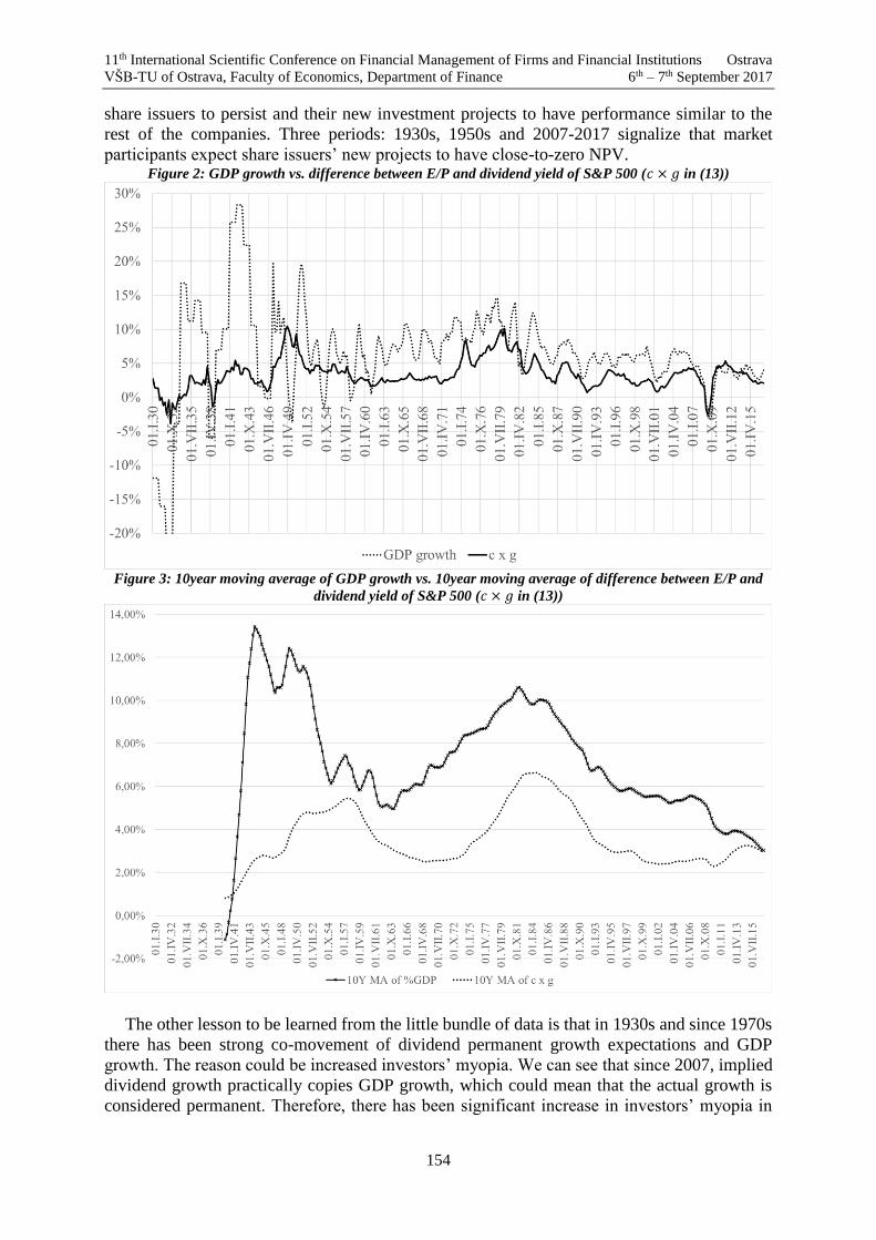
11th International Scientific Conference on Financial Management of Firms and Financial Institutions Ostrava
VŠB-TU of Ostrava, Faculty of Economics, Department of Finance 6th – 7th September 2017
154
share issuers to persist and their new investment projects to have performance similar to the
rest of the companies. Three periods: 1930s, 1950s and 2007-2017 signalize that market
participants expect share issuers’ new projects to have close-to-zero NPV. Figure 2: GDP growth vs. difference between E/P and dividend yield of S&P 500 (𝑐 × 𝑔 in (13))
Figure 3: 10year moving average of GDP growth vs. 10year moving average of difference between E/P and
dividend yield of S&P 500 (𝑐 × 𝑔 in (13))
The other lesson to be learned from the little bundle of data is that in 1930s and since 1970s
there has been strong co-movement of dividend permanent growth expectations and GDP
growth. The reason could be increased investors’ myopia. We can see that since 2007, implied
dividend growth practically copies GDP growth, which could mean that the actual growth is
considered permanent. Therefore, there has been significant increase in investors’ myopia in

11th International Scientific Conference on Financial Management of Firms and Financial Institutions Ostrava
VŠB-TU of Ostrava, Faculty of Economics, Department of Finance 6th – 7th September 2017
155
recent decades. The reason could be an both increasing unpredictability of economic
environment or shift to the rational expectations from adaptive ones.
Moreover, Figure 4 shows that financial markets have poor ability to predict future GDP
growth and that they rather rely on the last available data since the R2 between GDP growth
and 𝑐 × 𝑔 in (13) is if the 𝑐 × 𝑔 is delayed by 2 quarters. Delay of GDP growth significantly
reduces the R2 values. The observation, frequently presented in finance textbooks, that the
financial markets precede the real economy by several (usually 3) quarters is therefore probably
based on the increase of risk premiums in the evening of economic turmoils rather than by
change of the growth expectations. Figure 4: 1930 - 2017 R2 of US %GDP and the difference between E/P and dividend yield of S&P 500 (𝑐 × 𝑔
in (13)) according to GDP growth delay (by quarters)
However, the dependence of GDP growth expectations on past GDP growth lasted only till
1970s.3 Since 1980s till 2000, the closest relationship show the GDP and 𝑐 × 𝑔 both undelayed.
Figure 5: 10year moving R2 of US %GDP, resp. real GDP growth and the difference between E/P and
dividend yield of S&P 500 (𝑐 × 𝑔 in (13)); delay by quarters in parentheses
3 The R2 between GDP and 𝑐 × 𝑔 in (13) is based on past 10 years of data. Therefore, if we see the R2
of the delayed 𝑐 × 𝑔 to level out with R2 of undelayed GDP and 𝑐 × 𝑔 since 1990s, then that trend
started in 1980s.

11th International Scientific Conference on Financial Management of Firms and Financial Institutions Ostrava
VŠB-TU of Ostrava, Faculty of Economics, Department of Finance 6th – 7th September 2017
156
Until 2000, the predictive power of US stock market for GDP growth was poor. However,
since that time, the accuracy of those predictions (for 2 quarters ahead) are approximately on
par with reflection of actual GDP growth rate in share prices, as we can see on Figure 5. Such
a change can be probably attributed again to the use of computers in financial forecasting.
References
[1] Fisher, I. (1930). The theory of interest. New York: The Macmillan Company.
[2] Friday, D. (1922). An extension of value theory. The Quarterly Journal of Economics,
36(2), pp. 197-219.
[3] Gordon, Myron J. (1962). The Investment, Financing, and Valuation of the Corporation.
Homewood, IL: R. D. Irwin.
[4] Shiller, R. J. (2015). Irrational exuberance. Princeton university press.
11th International Scientific Conference on Financial Management of Firms and Financial Institutions Ostrava VŠB-TU of Ostrava, Faculty of Economics, Department of Finance 6th – 7th September 2017
157
Capital Structure Determinants of Industrial Companies Listed on the Warsaw Stock Exchange
Leszek Czerwonka, Jacek Jaworski 1
Abstract
The aim of this study is to verify whether a company's capital structure depends on the share of
fixed assets in total assets, the size and growth of a company, its profitability, liquidity and size
of non-debt tax shield. The significance of the impact of various factors on the debt of a
company was studied using linear panel models. Data for the analysis comes from the financial
statements of companies listed on the Warsaw Stock Exchange, belonging to the industry sector
(sample size: 177). The research period is 1998-2012. Analysis of the data leads to the
conclusion that shaping the capital structure of the studied companies is best explained by the
pecking order theory. To the minor extent it is explained by the agency theory.
Key words
capital structure, determinants of capital structure, financing, corporate finance, pecking order
theory
JEL Classification: G32, M20, D22.
1. Introduction
The shaping of the companies’ capital structures is the subject of many authors’ studies.
These studies are mainly focused on the identification of factors affecting the relationship
between equity and debt in financing sources and searching for a theory which adequately
explains the companies’ behaviour in this regard. This paper is part of this trend of research.
There are many theories of the capital structure in the literature. They include the agency
theory (Jensen and Meckling, 1976), the signalling theory (Ross, 1977), the pecking order
theory (Myers and Majluf, 1984) and the static trade-off theory (Kraus and Litzenberger,
1973; Myers, 1984). On this basis, the number of factors that could affect the financial
decisions of companies can be extracted (e.g. Czerwonka and Jaworski, 2017). The goal of
this paper is the empirical verification of the hypothesis claiming that the capital structure of
enterprises depends on the share of fixed assets in the total assets, the size and the growth of
the company, its profitability, liquidity and the size of the non-debt tax shield. On the basis of
the diagnosed strength and direction of the above relationships, authors decided to find among
modern capital structure theories the one, that best explains the behaviour of the studied
companies.
The research subject was the industry sector of the companies listed on the Warsaw Stock Exchange. In achieving the research aims, the authors used analysis based on
the linear panel models.
1 dr hab. Leszek Czerwonka, prof. UG, University of Gdańsk, Faculty of Economics,
dr hab. Jacek Jaworski, prof. WSB, WSB University in Gdańsk, [email protected]

11th International Scientific Conference on Financial Management of Firms and Financial Institutions Ostrava VŠB-TU of Ostrava, Faculty of Economics, Department of Finance 6th – 7th September 2017
158
2. Variable measures
The capital structure is defined in the literature in many ways. However, most definitions
attempt to explain it as the relationship between equity and debt used in financing activities of
the enterprise. Even bigger diversity concerns measures used by different authors for trying to
measure this relationship. The usefulness of these measures was analysed by Rajan and
Zingales (1995). They concluded that the choice of the proper measure should be based on the
specifics of the studied economy. In the Polish case, where trade credit is an important source
of enterprise financing, the adequate measure is the total debt ratio (DR). It is the relationship
of total liabilities to total assets. This ratio was used in the studies, among others, of Mazur
(2007), Wilimowska and Wilimowski (2010). It was also used by researchers from other
countries e.g. Cortez (2012), Abeywardana and Banda (2015), Imtiaz, Mahmud and Mallik
(2016).
On the basis of the analysis of theoretical models and empirical studies as explanatory
variables can be extracted: the share of fixed assets in total assets (TANG), size (SIZE) and
company growth (GROW), profitability (PROF), liquidity (LIQ) and the amount of non-debt
tax shield (NDTS),.
For the first of the explanatory variables (TANG) proper measure is only the share of fixed
assets in total assets (Campbell and Jerzemowska, 2001; Mazur, 2007; Rauh and Sufi, 2010;
Cortez, 2012; Imtiaz, Mahmud and Mallik, 2016). The size of the company (SIZE) is
measured by different authors in various ways. Generally it is the natural logarithm of total
assets (Campbell and Jerzemowska, 2001; Abeywardana and Banda, 2015; Imtiaz, Mahmud
and Mallik, 2016). Similarly, for measuring the growth of the company (GROW) the assets
growth rate can be used (Cortez, 2012; Imtiaz, Mahmud and Mallik, 2016).
The company’s profitability (PROF) can be measured using different methods. However,
assuming, that the main premise for searching financing sources is the operational activity of
the company, the proper measure appears to be the relationship between EBIT and the total
assets (ROA) (Campbell and Jerzemowska, 2001; Abeywardana and Banda, 2015; Imtiaz,
Mahmud and Mallik, 2016).
For measuring financial liquidity (LIQ) the most commonly used in previous studies were
static ratios. The most popular is the current liquidity ratio which is the relationship of the
current assets and the current liabilities (Campbell and Jerzemowska, 2001; Mazur, 2007;
Wilimowska and Wilimowski, 2010; Abeywardana and Banda, 2015).
The non-debt tax shield (NDTS) is a substitute of the interest tax shield and it results from
the fixed assets depreciation. Therefore, the adequate measure is the relationship of the annual
depreciation and the total assets (Mazur, 2007; Wilimowska and Wilimowski, 2010; Cortez,
2012; Abeywardana and Banda, 2015).
3. Research sample
The studied sample consisted of the financial statements of 177 companies listed on the
Warsaw Stock Exchange, belonging to the industry sector. The research period covered the
years 1998-2012. The data was taken from the Notoria base. The number of firm-period
observations for each variable ranged from 1768 to 1941. The diversity in the number of
observations results from the fact that not all companies were listed during the whole period
of the analysis. In addition, some of the variables are indices and their calculation needed data
from two successive periods. Furthermore, there was in some cases a lack of data for listed
companies from the individual years.
Table 1 presents descriptive parameters of the research sample for all studied variables.
Outliers and questionable values were explained or eliminated from the study.
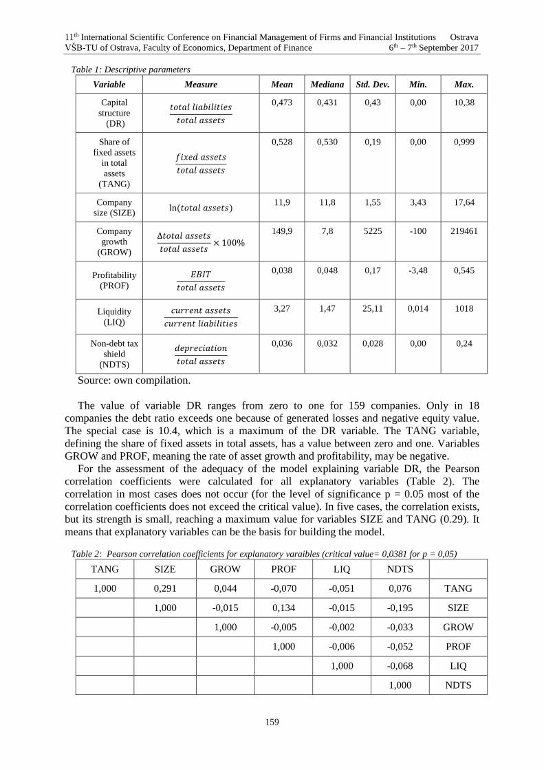
11th International Scientific Conference on Financial Management of Firms and Financial Institutions Ostrava VŠB-TU of Ostrava, Faculty of Economics, Department of Finance 6th – 7th September 2017
159
Table 1: Descriptive parameters
Variable Measure Mean Mediana Std. Dev. Min. Max.
Capital
structure
(DR)
𝑡𝑜𝑡𝑎𝑙 𝑙𝑖𝑎𝑏𝑖𝑙𝑖𝑡𝑖𝑒𝑠
𝑡𝑜𝑡𝑎𝑙 𝑎𝑠𝑠𝑒𝑡𝑠
0,473 0,431 0,43 0,00 10,38
Share of
fixed assets
in total
assets
(TANG)
𝑓𝑖𝑥𝑒𝑑 𝑎𝑠𝑠𝑒𝑡𝑠
𝑡𝑜𝑡𝑎𝑙 𝑎𝑠𝑠𝑒𝑡𝑠
0,528 0,530 0,19 0,00 0,999
Company
size (SIZE) ln (𝑡𝑜𝑡𝑎𝑙 𝑎𝑠𝑠𝑒𝑡𝑠)
11,9 11,8 1,55 3,43 17,64
Company
growth
(GROW)
∆𝑡𝑜𝑡𝑎𝑙 𝑎𝑠𝑠𝑒𝑡𝑠
𝑡𝑜𝑡𝑎𝑙 𝑎𝑠𝑠𝑒𝑡𝑠× 100%
149,9 7,8 5225 -100 219461
Profitability
(PROF)
𝐸𝐵𝐼𝑇
𝑡𝑜𝑡𝑎𝑙 𝑎𝑠𝑠𝑒𝑡𝑠
0,038 0,048 0,17 -3,48 0,545
Liquidity
(LIQ)
𝑐𝑢𝑟𝑟𝑒𝑛𝑡 𝑎𝑠𝑠𝑒𝑡𝑠
𝑐𝑢𝑟𝑟𝑒𝑛𝑡 𝑙𝑖𝑎𝑏𝑖𝑙𝑖𝑡𝑖𝑒𝑠
3,27 1,47 25,11 0,014 1018
Non-debt tax
shield
(NDTS)
𝑑𝑒𝑝𝑟𝑒𝑐𝑖𝑎𝑡𝑖𝑜𝑛
𝑡𝑜𝑡𝑎𝑙 𝑎𝑠𝑠𝑒𝑡𝑠
0,036 0,032 0,028 0,00 0,24
Source: own compilation.
The value of variable DR ranges from zero to one for 159 companies. Only in 18
companies the debt ratio exceeds one because of generated losses and negative equity value.
The special case is 10.4, which is a maximum of the DR variable. The TANG variable,
defining the share of fixed assets in total assets, has a value between zero and one. Variables
GROW and PROF, meaning the rate of asset growth and profitability, may be negative.
For the assessment of the adequacy of the model explaining variable DR, the Pearson
correlation coefficients were calculated for all explanatory variables (Table 2). The
correlation in most cases does not occur (for the level of significance p = 0.05 most of the
correlation coefficients does not exceed the critical value). In five cases, the correlation exists,
but its strength is small, reaching a maximum value for variables SIZE and TANG (0.29). It
means that explanatory variables can be the basis for building the model.
Table 2: Pearson correlation coefficients for explanatory varaibles (critical value= 0,0381 for p = 0,05)
TANG SIZE GROW PROF LIQ NDTS
1,000 0,291 0,044 -0,070 -0,051 0,076 TANG
1,000 -0,015 0,134 -0,015 -0,195 SIZE
1,000 -0,005 -0,002 -0,033 GROW
1,000 -0,006 -0,052 PROF
1,000 -0,068 LIQ
1,000 NDTS
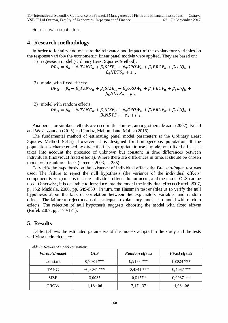
11th International Scientific Conference on Financial Management of Firms and Financial Institutions Ostrava VŠB-TU of Ostrava, Faculty of Economics, Department of Finance 6th – 7th September 2017
160
Source: own compilation.
4. Research methodology
In order to identify and measure the relevance and impact of the explanatory variables on
the response variable the econometric, linear panel models were applied. They are based on:
1) regression model (Ordinary Least Squares Method):
𝐷𝑅𝑖𝑡 = 𝛽0 + 𝛽1𝑇𝐴𝑁𝐺𝑖𝑡 + 𝛽2𝑆𝐼𝑍𝐸𝑖𝑡 + 𝛽3𝐺𝑅𝑂𝑊𝑖𝑡 + 𝛽4𝑃𝑅𝑂𝐹𝑖𝑡 + 𝛽5𝐿𝐼𝑄𝑖𝑡 +𝛽6𝑁𝐷𝑇𝑆𝑖𝑡 + 𝜀𝑖𝑡,
2) model with fixed effects:
𝐷𝑅𝑖𝑡 = 𝛽0 + 𝛽1𝑇𝐴𝑁𝐺𝑖𝑡 + 𝛽2𝑆𝐼𝑍𝐸𝑖𝑡 + 𝛽3𝐺𝑅𝑂𝑊𝑖𝑡 + 𝛽4𝑃𝑅𝑂𝐹𝑖𝑡 + 𝛽5𝐿𝐼𝑄𝑖𝑡 +𝛽6𝑁𝐷𝑇𝑆𝑖𝑡 + 𝜇𝑖𝑡,
3) model with random effects:
𝐷𝑅𝑖𝑡 = 𝛽0 + 𝛽1𝑇𝐴𝑁𝐺𝑖𝑡 + 𝛽2𝑆𝐼𝑍𝐸𝑖𝑡 + 𝛽3𝐺𝑅𝑂𝑊𝑖𝑡 + 𝛽4𝑃𝑅𝑂𝐹𝑖𝑡 + 𝛽5𝐿𝐼𝑄𝑖𝑡 +𝛽6𝑁𝐷𝑇𝑆𝑖𝑡 + 𝜀𝑖𝑡 + 𝜇𝑖𝑡.
Analogous or similar methods are used in the studies, among others: Mazur (2007), Nejad
and Wasiuzzaman (2013) and Imtiaz, Mahmud and Mallik (2016).
The fundamental method of estimating panel model parameters is the Ordinary Least
Squares Method (OLS). However, it is designed for homogeneous population. If the
population is characterised by diversity, it is appropriate to use a model with fixed effects. It
takes into account the presence of unknown but constant in time differences between
individuals (individual fixed effects). Where there are differences in time, it should be chosen
model with random effects (Greene, 2003, p. 285).
To verify the hypothesis on the existence of individual effects the Breusch-Pagan test was
used. The failure to reject the null hypothesis (the variance of the individual effects’
component is zero) means that the individual effects do not occur, and the model OLS can be
used. Otherwise, it is desirable to introduce into the model the individual effects (Kufel, 2007,
p. 166; Maddala, 2006, pp. 649-650). In turn, the Hausman test enables us to verify the null
hypothesis about the lack of correlation between the explanatory variables and random
effects. The failure to reject means that adequate explanatory model is a model with random
effects. The rejection of null hypothesis suggests choosing the model with fixed effects
(Kufel, 2007, pp. 170-171).
5. Results
Table 3 shows the estimated parameters of the models adopted in the study and the tests
verifying their adequacy.
Table 3: Results of model estimations
Variable/model OLS Random effects Fixed effects
Constant 0,7034 *** 0,9164 *** 1,8024 ***
TANG −0,5041 *** -0,4741 *** -0,4067 ***
SIZE 0,0035 -0,0177 * -0,0937 ***
GROW 1,18e-06 7,17e-07 -1,08e-06
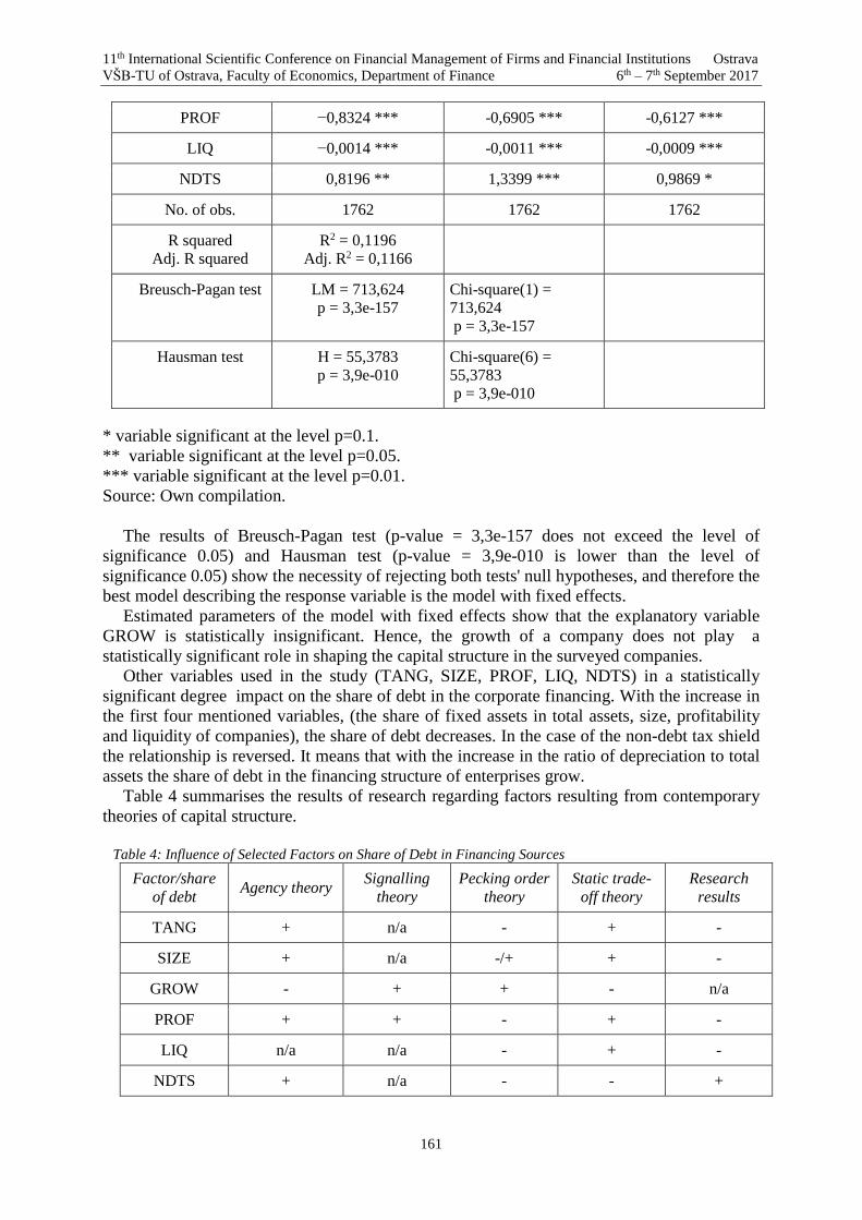
11th International Scientific Conference on Financial Management of Firms and Financial Institutions Ostrava VŠB-TU of Ostrava, Faculty of Economics, Department of Finance 6th – 7th September 2017
161
PROF −0,8324 *** -0,6905 *** -0,6127 ***
LIQ −0,0014 *** -0,0011 *** -0,0009 ***
NDTS 0,8196 ** 1,3399 *** 0,9869 *
No. of obs. 1762 1762 1762
R squared
Adj. R squared
R2 = 0,1196
Adj. R2 = 0,1166
Breusch-Pagan test LM = 713,624
p = 3,3e-157
Chi-square(1) =
713,624
p = 3,3e-157
Hausman test H = 55,3783
p = 3,9e-010
Chi-square(6) =
55,3783
p = 3,9e-010
* variable significant at the level p=0.1.
** variable significant at the level p=0.05.
*** variable significant at the level p=0.01.
Source: Own compilation.
The results of Breusch-Pagan test (p-value = 3,3e-157 does not exceed the level of
significance 0.05) and Hausman test (p-value = 3,9e-010 is lower than the level of
significance 0.05) show the necessity of rejecting both tests' null hypotheses, and therefore the
best model describing the response variable is the model with fixed effects.
Estimated parameters of the model with fixed effects show that the explanatory variable
GROW is statistically insignificant. Hence, the growth of a company does not play a
statistically significant role in shaping the capital structure in the surveyed companies.
Other variables used in the study (TANG, SIZE, PROF, LIQ, NDTS) in a statistically
significant degree impact on the share of debt in the corporate financing. With the increase in
the first four mentioned variables, (the share of fixed assets in total assets, size, profitability
and liquidity of companies), the share of debt decreases. In the case of the non-debt tax shield
the relationship is reversed. It means that with the increase in the ratio of depreciation to total
assets the share of debt in the financing structure of enterprises grow.
Table 4 summarises the results of research regarding factors resulting from contemporary
theories of capital structure.
Table 4: Influence of Selected Factors on Share of Debt in Financing Sources
Factor/share
of debt Agency theory
Signalling
theory
Pecking order
theory
Static trade-
off theory
Research
results
TANG + n/a - + -
SIZE + n/a -/+ + -
GROW - + + - n/a
PROF + + - + -
LIQ n/a n/a - + -
NDTS + n/a - - +
11th International Scientific Conference on Financial Management of Firms and Financial Institutions Ostrava VŠB-TU of Ostrava, Faculty of Economics, Department of Finance 6th – 7th September 2017
162
+ positive dependence
- negative dependence
-/+ unspecified dependence
n/a no grounds to identify the dependence
Source: Own elaboration based on (Czerwonka and Jaworski 2017).
The comparison of the data in Table 4 shows that the shaping of the capital structure on
industrial companies listed on the Warsaw Stock Exchange is best explained by the pecking
order theory. According to this theory, the increase in the share of fixed assets in total assets,
in profitability and liquidity of the company causes the debt to decrease. And that happens in
the surveyed enterprises. The pecking order theory does not indicate precisely the direction of
the relationship between the company's capital structure and company's size. It may proceed
in two directions. In the case of the surveyed companies the directions of these relations are
negative. For the variable, which according to the theory has positive impact on the share of
debt (GROW - the growth of a company), there is no correlation in the study. The impact of
NDTS - Non-debt tax shield for the investigated companies is inverse than the pecking order
theory suggests. The positive relationship between NDTS and debt corresponds to the agency
theory.
6. Conclusions
The results of the research enable us to confirm adopted hypothesis in the wider scope. The
capital structure of Polish enterprises is determined by the share of assets in the total assets,
size, profitability, liquidity and the size of non-debt tax shield. The only factor whose impact
has not been confirmed is the growth of the company.
The direction of the impact of various factors on the capital structure of the Polish
industrial companies justifies the adoption of the thesis that the pecking order theory best
explains this area of the behaviour in these organisations. It means that the management of the
Polish industrial enterprises choose internal financing as a first choice. The second is debt.
The issue of equity is chosen as the last.
Shaping of the capital structure of the surveyed enterprises also is explained by the agency
theory, and basically the part of the theory taking into account the non-debt tax shield. The
increasing depreciation is a greater free cash flow available to managers (Jensen, 1986). To
reduce the irrational spending, as well as take advantage of the phenomenon of leverage,
businesses with increasing possibilities of self-financing, are increasingly financed also by
debt.
The basic restrictions on the generalisation of the results of the study include:
the adopted list of variables probably is not complete and there are others, not
included in the study, factors affecting the rate of corporate debt,
limited number of companies (listed), their specificity (industrial) and a limited
research period does not guarantee the representativeness of all Polish companies.
These restrictions are a prerequisite for replication of the research in the future and extend the
research sample by firms from other sectors.
References
[1] Abeywardana, N.L.E. and Banda, Y.K.W. (2015). Impact of Observable Determinants
and Unobservable Effect on Capital Structure: Evidence from Quoted Public
Manufacturing Companies in Sri Lanka. The International Journal Of Business &
Management, vol. 3, iss. 6, pp. 150-158.

11th International Scientific Conference on Financial Management of Firms and Financial Institutions Ostrava VŠB-TU of Ostrava, Faculty of Economics, Department of Finance 6th – 7th September 2017
163
[2] Baza Notoria (Notoria Database), ver.: I quarter 2014.
[3] Cambell, K. and Jerzemowska, M. (2001). Capital Structure Decisions Made by
Companies in a Transitional Economy: The Case of Poland [in:] Financial
Management. Objectives – Organization – Tools, ed. D. Zarzecki, FRR w Polsce,
Warszawa.
[4] Cortez, M.A. (2012). The Determinants of Corporate Capital Structure: Evidence from
Japanese Manufacturing Companies. Journal of International Business Research, vol.
11, no. 3, pp. 121-133.
[5] Czerwonka, L. and Jaworski, J. (2017). Determinanty struktury kapitału. Przegląd
literatury (Determinants of the capital structure. review of the literature). in print.
[6] Greene, W.H. (2003). Econometric analysis. Prentice Hall, Upper Saddle River, NJ.
[7] Imtiaz, F., Mahmud, K. and Mallik, A. (2016). Determinants of Capital Structure and
Testing of Applicable Theories: Evidence from Pharmaceutical Firms of Bangladesh.
International Journal of Economics and Finance, vol. 8, no. 3, pp. 23-32.
[8] Jensen, M.C. and Meckling, W.H. (1976). Theory of the Firm: Managerial Behavior,
Agency Costs and Ownership Structure. Journal of Financial Economics, vol. 3, no. 4,
pp. 305-360.
[9] Jensen, M.C. (1986). Agency Costs of Free Cash Flow, Corporate Finance, and
Takeovers. The American Economic Review, vol. LXXVI, no. 2, pp. 323-329.
[10] Kraus, A. and Litzenberger, R.H. (1973). A State-Preference Model of Optimal Finacial
Leverage. The Journal of Finance, vol. 28, iss. 4., pp. 911-922.
[11] Kufel, T. (2007). Ekonometria. Rozwiązywanie problemów z wykorzystaniem programu
GRETL (Econometrics. Solving Problems Using GRETL). Wydawnictwo Naukowe
PWN, Warszawa. [in Polish]
[12] Maddala, G.S. (2006). Ekonometria (Econometrics). Wydawnictwo Naukowe PWN,
Warszawa. [in Polish]
[13] Mazur, K. (2007). The Determinants of Capital Structure Choice: Evidence from Polish
Companies. International Advances in Economic Research, vol. 13, iss. 4, pp. 495-514.
[14] Myers S.C. (1984). The Capital Structure Puzzle. The Journal of Finance, vol. 39, no. 3,
s. 575-592
[15] Myers, S.C. and Majluf, N.S. (1984). Corporate Financing and Investment Decisions
when Firms have Information that Investors do not have. Journal of Financial
Economics, 1984, no. 13, pp. 187-221.
[16] Nejad, N.R. and Wasiuzzaman, S. (2013). The Empirical Analysis of Capital Structure
Determinants – Evidence From Malaysia. Engineering and Technology, no. 74, pp. 466-
474.
[17] Rajan, R. G. and Zingales, L. (1995). What Do We Know about Capital Structure?
Some evidence from International Data. Journal of Finance, vol. 50, pp. 1421- 1460.
[18] Rauh, J.D. and Sufi, A. (2010). Capital Structure and Debt Structure. The Review of
Financial Studies, vol. 23, no. 12, pp. 4242-4280.
[19] Ross, S.A. (1977). The Determination of Financial Structure: The Incentive-Signalling
Approach. The Bell Journal of Economics, vol. 8, no. 1, pp. 23-40.

11th International Scientific Conference on Financial Management of Firms and Financial Institutions Ostrava VŠB-TU of Ostrava, Faculty of Economics, Department of Finance 6th – 7th September 2017
164
[20] Wilimowska, Z. and Wilimowski, M. (2010). Wpływ czynników
mikroekonomicznych na zarządzanie strukturą kapitałową polskich przedsiębiorstw
(Impact of Microeconomic Factors on Capital Structure of Polish Companies), [in:]
Komputerowo zintegrowane zarządzanie (Computer Integrated Management) T.2, ed.
R. Knosala, Ofic. Wyd. PTZP, Opole. [in Polish]
11th International Scientific Conference on Financial Management of Firms and Financial Institutions Ostrava
VŠB-TU of Ostrava, Faculty of Economics, Department of Finance 6th – 7th September 2017
165
Adaptive wavelet method for pricing options under the Stein-Stein stochastic volatility model
Dana Černá 1
Abstract
We use the Stein-Stein stochastic volatility model for calculating the theoretical price of an
option. While the Black-Scholes model assumes that the volatility of the asset is constant or a
known function, the Stein-Stein model assumes that the volatility is a random process. The
Stein-Stein model is represented by a parabolic equation. We employ wavelets for its efficient
numerical solution, because wavelets are well-known for their compression property. It means
that the representation of the solution in a wavelet basis requires a small number of coefficients
and the computation of the solution with desired accuracy can be performed with the small
number of parameters. We use the Crank-Nicolson scheme for the time discretization and an
adaptive method with a linear spline-wavelet basis for the space discretization. Numerical
examples are presented for the European put and call options.
Key words
Stein-Stein model, European option, wavelets, adaptive wavelet method, linear spline wavelet,
vanilla option, stochastic volatility.
JEL Classification: C63, G13.
1. Introduction
The paper is concerned with pricing European options. Recall that a European put option
gives its holder the right, but not the obligation, to sell a group of underlying assets at a
specific price (strike price) on a certain date (maturity date). Similarly, a European call option
gives its holder the right, but not the obligation, to buy a group of underlying assets at a
specific price on a certain date. The well-known Black-Scholes option pricing model derived
in (Black and Scholes, 1973) assumes that the volatility of the asset is constant or a known
function. Several models were derived to replace the deterministic volatility with a stochastic
volatility proces, e.g. the Heston model, the Hull-White model and the Stein and Stein model.
Wavelet methods have been already succesfully used for solving option pricing problems,
see e.g. (Finěk, 2016; Hilber et al., 2013; Rometsch, 2010). We also proposed and
implemented a wavelet method for option pricing in our previous papers. We used the Black-
Scholes model and tested the performance of the wavelet method with respect to the choice of
a wavelet basis (Černá, 2016), compared an isotropic and an anisotropic approach, studied the
convergence rate of the method and proposed a construction of a wavelet basis such that the
Black-Scholes operator represented in this basis is sparse (Černá and Finěk, 2017).
Furthermore, we have proposed and implemented adaptive wavelet method for valuation of
two-asset Asian option with floating strike and for the Heston stochastic volatility model.
In this paper, we focus on the Stein-Stein stochastic volatility model for calculating the
price of options. Up to our knowledge, methods based on wavelets have not been used for
option pricing under the Stein-Stein model. In our previous papers we used an adaptive
1 RNDr. Dana Černá, Ph.D., Department of Mathematics and Didactics of Mathematics, Faculty of
Science, Humanities and Education, Technical University of Liberec, Studentská 2, 461 17 Liberec,
Czech Republic, e-mail: [email protected].
This work was supported by grant No. GA16-09541S of the Czech Science Foundation.
11th International Scientific Conference on Financial Management of Firms and Financial Institutions Ostrava
VŠB-TU of Ostrava, Faculty of Economics, Department of Finance 6th – 7th September 2017
166
wavelet method that is a modification of the method from (Cohen et al., 2002). In this paper,
we use a different approach that is simpler and was more efficient in our numerical
experiments. The quantitative properties of any wavelet method depend on the choice of a
wavelet basis. In this paper, we adapt the piecewise linear wavelet basis with two vanishing
moments from (Černá and Finěk, 2011; Primbs, 2010) to the rectangle and boundary
conditions representing the Stein-Stein model and use it in the scheme.
2. Stein-Stein model
The Stein-Stein model assumes that the volatility is a random process and that the market
price 𝑉(𝑆, 𝑣, 𝑡) of the option can be computed as the solution of the equation (Stein and Stein,
1991): 𝜕𝑉
𝜕𝑡− 𝐿(𝑉) = 0, 𝑡 ∈ (0, 𝑇),
with the operator 𝐿 given by
𝐿(𝑉) =𝑆2𝑣2
2
𝜕2𝑉
𝜕𝑆2+
𝜎2
2
𝜕2𝑉
𝜕𝑣2+ 𝑟𝑆
𝜕𝑉
𝜕𝑆+ 𝛼(𝑚 − 𝑣)
𝜕𝑉
𝜕v− 𝑟𝑉, 𝑆 ∈ ℝ+, 𝑣 ∈ ℝ.
The variable 𝑆 is an asset price, 𝑣2 is a variance of 𝑆 and 𝑡 is time to maturity. The
parameter 𝛼 represents the mean reversion rate, 𝑚 is the long term variance, 𝜎 is the volatility
of the volatility, and 𝑟 is a risk-free rate. For more details see (Stein and Stein, 1991).
We approximate the unbounded domain (0, ∞) × (−∞, ∞) by a domain 𝛺 = (0, 𝑆𝑚𝑎𝑥 ) ×(−𝑣𝑚𝑎𝑥, 𝑣𝑚𝑎𝑥), where 𝑆𝑚𝑎𝑥 and 𝑣𝑚𝑎𝑥 are large enough. We denote the parts of the boundary
𝜕𝛺 of the domain Ω as
𝛤1 = {[𝑆, −𝑣𝑚𝑎𝑥], 𝑆 ∈ (0, 𝑆𝑚𝑎𝑥)}, 𝛤2 = {[𝑆𝑚𝑎𝑥, 𝑣], 𝑣 ∈ (−𝑣𝑚𝑎𝑥 , 𝑣𝑚𝑎𝑥)}, 𝛤3 = {[𝑆, 𝑣𝑚𝑎𝑥], 𝑆 ∈ (0, 𝑆𝑚𝑎𝑥)}, 𝛤4 = {[0, 𝑣], 𝑣 ∈ (−𝑣𝑚𝑎𝑥, 𝑣𝑚𝑎𝑥)}.
We need to prescribe appropriate initial and boundary conditions. Let 𝐾 be the strike price.
The initial condition represents the value of the option at maturity, therefore
𝑉(𝑆, 𝑣, 0) = { 𝑚𝑎𝑥(𝐾 − 𝑆, 0), for put option,
𝑚𝑎𝑥(𝑆 − 𝐾, 0), for call option.
Boundary conditions are given by
𝑉(0, 𝑣, 𝑡) = {𝐾𝑒−𝑟𝑡, for put option,
0, for call option,
𝜕𝑉
𝜕𝑆(𝑆𝑚𝑎𝑥, 𝑣, 𝑡) = {
0, for put option,1, for call option.
It remains to prescribe the boundary conditions on 𝛤1 and 𝛤3. Similarly as in (Achdou and
Pironneau, 2009; Hozman and Tichý, 2017) we prescribe the artificial boundary conditions.
We choose the homogeneous Neumann boundary conditions, i.e.
𝜕𝑉
𝜕𝑛= 0 on 𝛤1 and 𝛤3,
where 𝑛 denotes the normal vector. We set

11th International Scientific Conference on Financial Management of Firms and Financial Institutions Ostrava
VŠB-TU of Ostrava, Faculty of Economics, Department of Finance 6th – 7th September 2017
167
𝑊(𝑆, 𝑣, 𝑡) = {𝐾𝑒−𝑟𝑡, for put option,
0, for call option,
and define 𝑈 = 𝑉 − 𝑊. Since we have
𝜕𝑊
𝜕𝑡− 𝐿(𝑊) = 0,
we can restrict ourselves to the problem
𝜕𝑈
𝜕𝑡− 𝐿(𝑈) = 0, 𝑡 ∈ (0, 𝑇),
with initial conditions 𝑈(𝑆, 𝑣, 0) = 𝑉(𝑆, 𝑣, 0) − 𝑊(𝑆, 𝑣, 0), homogeneous Dirichlet boundary
conditions on 𝛤4 and boundary conditions on 𝛤1, 𝛤2, and 𝛤3 as above.
We use the Crank-Nicolson scheme for the time discretization. Let 𝑀 ∈ ℕ, 𝜏 = 𝑀−1, 𝑡𝑙 =𝑙𝜏, 𝑙 = 0, ⋯ , 𝑀, and denote 𝑈𝑙(𝑆, 𝑣) = 𝑈(𝑆, 𝑣, 𝑡𝑙). The Crank-Nicolson scheme has the form:
𝑈𝑙+1 − 𝑈𝑙
𝜏−
𝐿(𝑈𝑙+1)
2−
𝐿(𝑈𝑙)
2= 0.
3. Wavelet basis
We briefly review a concept of a wavelet basis, for more details one can see e.g. (Urban,
2009). Let us consider a separable Hilbert space 𝐻 with the norm ‖. ‖𝐻. Let ‖. ‖ and (.,.)
denote the L2-norm and the L2-inner product, respectively. Furthermore, let 𝐽 be an index set
such that each index 𝜆 ∈ 𝐽 takes the form 𝜆 = (𝑗, 𝑘), |𝜆|: = 𝑗 denotes a level and 𝑘 represents
a spatial location. For 𝐯 = {𝑣𝜆}𝜆∈𝐽, 𝑣𝜆 ∈ ℝ, we define
‖𝐯‖2 = (∑|𝑣𝜆|2
𝜆∈𝐽
)
1 2⁄
, 𝑙2( 𝐽) = {𝐯 ∶ ‖𝐯‖2 < ∞}.
Definition: A family 𝛹 = {𝜓𝜆, 𝜆 ∈ 𝐽} is called a wavelet basis of the space 𝐻 if it satisfies the
following conditions:
𝛹 is a Riesz basis for 𝐻, i.e. the closure of the span of 𝛹 is 𝐻 and there exist
constants 𝑐, 𝐶 ∈ (0, ∞) such that for all 𝐛 = {𝑏𝜆}𝜆∈𝐽 ∈ 𝑙2( 𝐽) we have
𝑐‖𝐛‖2 ≤ ‖∑ 𝑏𝜆𝜓𝜆
𝜆∈𝐽
‖
𝐻
≤ 𝐶‖𝐛‖2.
For all 𝜆 ∈ 𝐽 a diameter of the support of 𝜓𝜆 is bounded by 𝐶2−|𝜆| with 𝐶
independent on |𝜆| and at a given level the supports of only finitely many wavelets
overlap at any point 𝑥.
A wavelet basis 𝛹 has typically a hierarchical structure
11th International Scientific Conference on Financial Management of Firms and Financial Institutions Ostrava
VŠB-TU of Ostrava, Faculty of Economics, Department of Finance 6th – 7th September 2017
168
𝛹 = 𝛷𝑗0∪ ⋃ 𝛹𝑗.
∞
𝑗=𝑗0
Let 𝐼𝑗 and 𝐽𝑗 be finite index sets and
𝛷𝑗 = {𝜑𝑗,𝑘, 𝑘 ∈ 𝐼𝑗}, 𝛹𝑗 = {𝜓𝑗,𝑘, 𝑘 ∈ 𝐽𝑗}.
The functions 𝜑𝑗,𝑘 are called scaling functions and the functions 𝜓𝑗,𝑘 are called wavelets on
the level 𝑗. The set
𝛹𝑠 = 𝛷𝑗0∪ ⋃ 𝛹𝑗
𝑠
𝑗=𝑗0
is a finite dimensional subset of 𝛹 and is called a multiscale wavelet basis. We further assume
that there exists 𝐿 ≥ 1 such that wavelets 𝜓𝑗,𝑙 have 𝐿 vanishing moments, i.e. for any
polynomial 𝑝 of degree 𝑚 ≤ 𝐿 − 1 we have
∫ 𝑝(𝑥)𝜓𝑗,𝑙𝛺𝑗,𝑙
(𝑥)𝑑𝑥 = 0, 𝑙 ∈ 𝐽𝑗 , 𝑗 ≥ 𝑗0, 𝛺𝑗,𝑙 = supp 𝜓𝑗,𝑙.
In this paper, we use a linear spline-wavelet basis from (Černá and Finěk, 2011) and adapt
this basis to the rectangle 𝛺 = (0, 𝑆𝑚𝑎𝑥 ) × (−𝑣𝑚𝑎𝑥, 𝑣𝑚𝑎𝑥) and boundary conditions
formulated in the previous section. We define scaling functions as hat functions:
𝜑(𝑥) = {𝑥, 𝑥𝜖[0,1],
2 − 𝑥, 𝑥𝜖[1,2],0, otherwise,
𝜑𝑏(𝑥) = {1 − 𝑥, 𝑥𝜖[0,1],
0, otherwise.
We define scaling bases 𝛷21 = {𝜑2,𝑘
1 , 𝑘 = 1, ⋯ ,4} and 𝛷22 = {𝜑2,𝑘
2 , 𝑘 = 1, ⋯ ,5}, where
𝜑2,𝑘1 (𝑥) = 2𝜑(4𝑥 − 𝑘 + 1), 𝑘 = 1,2,3,
𝜑2,41 (𝑥) = 2𝜑𝑏(4 − 4𝑥),
𝜑2,12 (𝑥) = 2𝜑𝑏(4𝑥),
𝜑2,𝑘2 (𝑥) = 2𝜑(4𝑥 − 𝑘 + 2), 𝑘 = 2,3,4,
𝜑2,52 (𝑥) = 2𝜑𝑏(4 − 4𝑥).
We define a wavelet 𝜓 as
𝜓(𝑥) = −𝜑(2𝑥)
4−
𝜑(2𝑥 − 1)
2+
3𝜑(2𝑥 − 2)
2−
𝜑(2𝑥 − 3)
2−
𝜑(2𝑥 − 4)
4
and boundary wavelets as
𝜓𝑏1(𝑥) = 3𝜑𝑏(2𝑥)
2−
9𝜑(2𝑥)
8+
𝜑(2𝑥 − 1)
4+
𝜑(2𝑥 − 2)
8,
𝜓𝑏2(𝑥) = 3𝜑(2𝑥)
2− 𝜑(2𝑥 − 1) −
𝜑(2𝑥 − 2)
2.
11th International Scientific Conference on Financial Management of Firms and Financial Institutions Ostrava
VŠB-TU of Ostrava, Faculty of Economics, Department of Finance 6th – 7th September 2017
169
The wavelet bases on (0,1) on the level 𝑗 ≥ 2 are defined by 𝛹𝑗𝑖 = {𝜓𝑗,𝑘
𝑖 , 𝑘 = 1, ⋯ , 2𝑗} for
𝑖 = 1,2, with
𝜓𝑗,1𝑖 (𝑥) = 2𝑗/2𝜓𝑏𝑖(2𝑗𝑥),
𝜓𝑗,𝑘𝑖 (𝑥) = 2𝑗/2𝜓(2𝑗𝑥 − 𝑘 + 2), 𝑘 = 2, ⋯ , 2𝑗 − 1,
𝜓𝑗,2𝑗𝑖 (𝑥) = 2𝑗/2𝜓𝑏1(2𝑗 − 2𝑗𝑥).
We apply a linear transformation to obtain wavelet bases on (0, 𝑆𝑚𝑎𝑥) and (−𝑣𝑚𝑎𝑥, 𝑣𝑚𝑎𝑥). We define
𝜑𝑗,𝑘𝑆 (𝑆) = 𝜑𝑗,𝑘
1 (𝑆/𝑆𝑚𝑎𝑥) , 𝜓𝑗,𝑘𝑆 (𝑆) = 𝜓𝑗,𝑘
1 (𝑆/𝑆𝑚𝑎𝑥),
for 𝑆𝜖(0, 𝑆𝑚𝑎𝑥), and
𝜑𝑗,𝑘𝑣 (𝑣) = 𝜑𝑗,𝑘
2 ( 𝑣+𝑣𝑚𝑎𝑥
2𝑣𝑚𝑎𝑥 ), 𝜓𝑗,𝑘𝑣 (𝑣) = 𝜓𝑗,𝑘
2 (𝑣+𝑣𝑚𝑎𝑥
2𝑣𝑚𝑎𝑥 ),
for 𝑣𝜖(−𝑣𝑚𝑎𝑥, 𝑣𝑚𝑎𝑥). Let
𝛹𝑆 = {𝜑𝑗,𝑘𝑆 , 𝑘 = 1, ⋯ ,4} ∪ {𝜓𝑗,𝑘
𝑆 , 𝑘 = 1, ⋯ , 2𝑗+1, 𝑗 ≥ 2},
𝛹𝑣 = {𝜑𝑗,𝑘𝑣 , 𝑘 = 1, ⋯ ,5} ∪ {𝜓𝑗,𝑘
𝑣 , 𝑘 = 1, ⋯ , 2𝑗+1, 𝑗 ≥ 2},
and 𝛹 = 𝛹𝑆 ⊗ 𝛹𝑣. Then 𝛹 is a wavelet basis for the space 𝑉 = {𝑣 ∈ 𝐻1 (𝛺): 𝑣 = 0 on 𝛤4} with respect to the 𝐿2-norm and 𝛹 normalized in the 𝐻1-norm is a wavelet basis for 𝑉 with
respect to the 𝐻1-norm.
4. Adaptive wavelet method
The standard weak formulation of the scheme has the form:
(𝑈𝑙+1, 𝑣)
𝜏−
𝑎(𝑈𝑙+1, 𝑣)
2−
𝑎(𝑈𝑙, 𝑣)
2=
(𝑈𝑙, 𝑣)
𝜏,
where 𝑣 ∈ 𝑉 and 𝑎(𝑢, 𝑣) = (𝐿(𝑢), 𝑣) for 𝑢, 𝑣 ∈ 𝑉. We use an adaptive wavelet method for discretization with respect to the variables 𝑆 and 𝑣.
While the classical adaptive methods use refining a given mesh according to a-posteriori local
error estimates, the wavelet approach is different and insists in thresholding small wavelet
coefficients.
Let 𝛹 = {𝜓𝜆, 𝜆 ∈ 𝐽} be the wavelet basis from the previous section. We expand the
solution 𝑈𝑙 in the basis Ψ, i.e.
𝑈𝑙 = ∑ 𝑢𝜆𝑙
𝜆∈𝐽
𝜓𝜆.
We substitute this expansion to the variational formulation and we obtain the biinfinite matrix
equation
𝐀𝐮𝑙+1 = 𝐟𝑙
11th International Scientific Conference on Financial Management of Firms and Financial Institutions Ostrava
VŠB-TU of Ostrava, Faculty of Economics, Department of Finance 6th – 7th September 2017
170
with 𝐮𝑙 = {𝑢𝜆𝑙 }
𝜆∈𝐽, 𝐀 = {𝐴𝜇,𝜆}
𝜇,𝜆∈𝐽 , 𝐟𝑙 = {𝑓𝜇
𝑙}𝜇𝜖𝐽
, and
𝐴𝜇,𝜆 =(𝜓𝜆, 𝜓𝜇)
𝜏−
𝑎(𝜓𝜆, 𝜓𝜇)
2, 𝜆, 𝜇 ∈ 𝐽,
𝑓𝜇𝑙 =
𝑎(𝑈𝑙, 𝜓𝜇)
2+
(𝑈𝑙 , 𝜓𝜇)
𝜏, 𝜇 ∈ 𝐽.
We use the standard Jacobi diagonal preconditioner and solve the problem by the method
of generalized residuals (GMRES). The algorithm comprises the following steps:
1. Choose time step 𝜏 and the number of basis functions 𝑁. 2. Compute the vector of coefficients 𝐮0 for the function 𝑈0 and do 𝐮0 = COARSE(𝐮0, 𝑁). 3. For l = 0, 1, 2, . . . , M – 1 compute the right-hand side 𝐟𝑙, do 𝐮𝑙+1 = GMRES(𝐀, 𝐟𝑙, 𝐮𝑙),
and 𝐮𝑙+1 = COARSE(𝐮𝑙+1, 𝑁). 4. Compute the approximate solution 𝑈𝑀.
In the algorithm, 𝐮𝑙+1 = GMRES(𝐀, 𝐟𝑙, 𝐮𝑙), means that 𝐮𝑙+1 is the solution of the system of
linear algebraic equations with the matrix 𝐀 and the right-hand side 𝐟𝑙 using GMRES method
with initial vector 𝐟𝑙. The routine 𝐮𝑙+1 = COARSE(𝐮𝑙+1, 𝑁) insists in thresholding, i.e. we
take N entries from the vector 𝐮𝑙 that are largest in the absolute value and set to zero the
others. Thus the output parameter 𝐮𝑙+1 contains N nonzero entries. Each iteration of GMRES
requires multiplication of the infinite-dimensional matrix 𝐀 with a finitely supported vector. It
is computed approximately by the method from (Černá and Finěk, 2013). The matrix 𝐀 has
so-called finger structure, see e.g. (Černá and Finěk, 2017) and it is generally not sparse but
only quasi sparse.
Since we work with the sparse representation of the right-hand side and the sparse
representation of the vector representing the solution, the method is adaptive. It is known that
the coefficients in the wavelet basis are small in regions where the function is smooth and
large in regions where the function has some singularity.
5. Numerical example
We use the proposed scheme with the linear spline wavelet basis proposed in Section 3 for
computing the prices of European put and call options with the same parameters as in (Stein
and Stein, 1991; Hozman and Tichý, 2017), i.e. the mean reversion rate 𝛼 = 16, the long run
variance 𝑚 = 0.25, current variance 𝑣 = 0.25, the volatility of volatility 𝜎 = 0.4, the interest
rate 𝑟 = 0.0953 and the price 𝑆 = 100. We choose 𝑆𝑚𝑎𝑥 = 600, 𝑣𝑚𝑎𝑥 = 1, and the time step
𝜏 = 1/3650.
The graphs of the function 𝑉 that represents the price of the options for both put and call
options for time to maturity 𝑡 = 1/4 , i.e. three month to maturity, and several values of the
volatility 𝑣 are displayed in Figure 1. Since the function 𝑈(𝑆, 𝑣, 0) has not derivative on the
line 𝐾 × (−𝑣𝑚𝑎𝑥, 𝑣𝑚𝑎𝑥), the largest wavelet coefficients correspond to wavelets with
supports in the regions near this line and wavelet coefficients are small outside these regions.
Thus many wavelet coefficients are thresholded and the representation of the solution is
sparse.

11th International Scientific Conference on Financial Management of Firms and Financial Institutions Ostrava
VŠB-TU of Ostrava, Faculty of Economics, Department of Finance 6th – 7th September 2017
171
Figure 1: The value of put option (left) and call option (right) three month to maturity.
In Table 1 the values of the options are listed for time to maturity 𝑡 = 1/12 and 𝑡 = 1/4,
the number of basis functions 𝑁 = 9 600, and several values of the strike 𝐾. For comparison,
the values for the Black-Scholes model (Black and Scholes, 1973) are listed. The similar
results were obtained in (Stein and Stein, 1991; Hozman and Tichý, 2017). The main
advantage of the adaptive wavelet scheme is that the number of parameters representing the
solution was relatively small. We used 9 600 basis functions and obtained similar values as in
(Stein and Stein, 1991). To obtain the results with similar accuracy using the standard
Galerkin method with the multiscale wavelet basis 𝛹𝑠, we needed wavelets up to level 𝑠 =10, i.e. 1 049 600 basis functions. We also tested the performance of the Galerkin method
with the linear B-spline basis, i.e. FEM with linear elements and a uniform rectangular mesh.
Since the linear B-spline basis and the linear spline-wavelet basis generate the same spaces,
this method also required the basis functions on the level 𝑠 = 10 and 1 049 600 parameters to
obtain the similar results. The number of parameters for the proposed method is also smaller
than for the discontinuous Galerkin method with linear, quadratic and cubic functions, see the
results in (Hozman and Tichý, 2017).
Table 1: Prices of options for the Stein-Stein model and the Black-Scholes model for time to maturity t and
the strike K.
𝑡 = 1/12 𝑡 = 1/4
Stein-Stein Black-Scholes Stein-Stein Black-Scholes
𝐾 put call put call put call put call
85 0.035 15.707 0.020 15.693 0.413 17.414 0.340 17.342
90 0.205 10.917 0.170 10.882 1.011 13.130 0.915 13.033
95 0.854 6.605 0.812 6.563 2.133 9.370 2.025 9.262
100 2.523 3.314 2.489 3.280 3.948 6.302 3.837 6.191
105 5.523 1.353 5.482 1.312 6.524 3.996 6.411 3.883
110 9.589 0.460 9.544 0.414 9.811 2.400 9.695 2.284
6. Conclusion
We extended our research to option pricing under the Stein-Stein stochastic volatility
model. We constructed a piecewise linear wavelet basis with two vanishing moments on the
rectangle (0, 𝑆𝑚𝑎𝑥) × (−𝑣𝑚𝑎𝑥, 𝑣𝑚𝑎𝑥) that is adapted to boundary conditions. We proposed
and implemented an adaptive wavelet method with this basis for a numerical solution of the
parabolic equation representing the Stein-Stein model. We presented numerical examples for
the European put and call options and compared the results with the Black-Scholes model.

11th International Scientific Conference on Financial Management of Firms and Financial Institutions Ostrava
VŠB-TU of Ostrava, Faculty of Economics, Department of Finance 6th – 7th September 2017
172
The main advantage of the method is a small number of parameters representing the solution
with desired accuracy. Our future aim is to develop and analyze the efficient solver for other
option pricing models such as the Hull-White model and the Lévy model and to compare the
results.
References
[1] Achdou, Y., and Pironneau, O. (2009). Partial differential equations for option pricing.
Handbook of Numerical Analysis, 15, p. 369-495.
[2] Black, F., and Scholes, M. (1973). The pricing of options and corporate liabilities. J.
Polit. Econ., 81, p. 637-659.
[3] Cohen, A., Dahmen, W., and DeVore, R. (2002). Adaptive wavelet methods II - beyond
the elliptic case. Found. Math., 2, p. 203-245.
[4] Černá, D., and Finěk, V. (2011). Construction of optimally conditioned cubic spline
wavelets on the interval. Adv. Comput. Math., 34, p. 219-252.
[5] Černá, D., and Finěk, V. (2013). Approximate multiplication in adaptive wavelet
methods. Cent. Eur. J. Math., 11, p. 972-983.
[6] Černá, D. (2016). Numerical solution of the Black-Scholes equation using cubic spline
wavelets. In: 42st International Conference Applications of Mathematics in Engineering
and Economics (V. Pasheva, N. Popivanov, and G. Venkov, eds.), AIP Conference
Proceedings, 1789, No. 030001 (8 pages).
[7] Černá, D., and Finěk, V. (2017). Sparse wavelet representation of differential operators
with piecewise polynomial coefficients. Axioms, 6, (21 pages).
[8] Finěk, V. (2016). Fractional step method for wavelet based solution of Black-Scholes
equation. In: 42st International Conference Applications of Mathematics in Engineering
and Economics (V. Pasheva, N. Popivanov, and G. Venkov, eds.), AIP Conference
Proceedings, 1789, No. 030007 (4 pages).
[9] Hilber, N., Reichmann, O., Schwab, C., and Winter, C. (2013). Computational Methods
for Quantitative Finance. Springer, Berlin.
[10] Hozman, J., and Tichý, T. (2017). A DG approach to the numerical solution of the Stein-
Stein stochastic volatility option pricing model. In: 43rd International Conference
Applications of Mathematics in Engineering and Economics, AIP Conference
Proceedings.
[11] Primbs, M. (2010). New stable biorthogonal spline-wavelets on the interval. Result.
Math., 57, p. 121–162.
[12] Rometsch, M. (2010). A wavelet tour of option pricing. Ph.D. thesis, University Ulm.
[13] Stein, E.M., and Stein, J.C. (1991). Stock price distributions with stochastic volatility: An
analytic approach. Review of Financial Studies, 4, p. 727-752.
[14] Urban, K. (2009). Wavelet methods for elliptic partial differential equations, Oxford
University Press, Oxford.
11th International Scientific Conference on Financial Management of Firms and Financial Institutions Ostrava
VŠB-TU of Ostrava, Faculty of Economics, Department of Finance 6th – 7th September 2017
173
Valuation of the Two-Color Rainbow Real Options1
Miroslav Čulík 2
Abstract
This paper focuses on the valuation of real options, particularly on the options with more
underlying assets. First, real options and selected exotic real options are described. Next, case
study is provided. Here, project under risk and flexibility is evaluated. Option to abandon a
project is assumed; the cash flow generated by the project is affected by two random variables.
For valuation binomial lattice and replication strategy is applied. Results are commented and
presented.
Key words
Option, real options, replication strategy, risk-neutral, probability, exotic option, rainbow
option,
JEL Classification: G12, G32
1. Introduction
Real options methodology is an approach for solution of a wide range of valuation and
decision-making issues. This approach works with traditional methods and models used for
financial options valuation and enable to determine assets value. Compared to the traditional
passive valuation approaches (NPV, IRR etc.), real options approach takes into consideration
two important aspects: (a) riskiness of cash flow generated by the assets and (b) flexibility, i.e.
capability of management to change past decisions or to make new ones in already undertaken
projects. These future possible decisions (depends on the future state of the world) are
modelled as formal call and put options, which have their values and can be exercised by
company´s management. Real asset value determined by the real options methodology is then
given as a sum of two components: the present value of directly measurable cash flows and
the flexibility value, which captures future managerial possibilities (real options).
There are many applications in corporate finance where the financial option valuation
models are applied on the real assets valuation (real options approach). Black and Scholes
(1973) were the first authors to state that it is possible to take the equity in a levered company
as a call option on the company value. Since then, new pioneering work appeared developing
real option analysis, see for example Merton (1973) Cox, Ross and Rubinstein (1979) or
Brennan and Schwartz (1985). During the last two decades, significant increase in publishing
activities on this topic is obvious. This area has been studied and developed by many authors,
and new possible applications appear for solutions for a wide array of financial-decision and
valuation problems. The key papers and books that focus on the real options methodology
application are those of Dixit and Pindyck (1994), Smith and Nau (1995), Trigeorgis (1999),
Brennan and Trigeorgis (2000), Copeland and Antikarov (2000), Grenadier (2000), Brach
(2002), Trigeorgis and Schwartz (2001). Trigeorgis and Smit (2004) or Damodaran (2006).
1 The paper is based on research activities within the ESF Project No. CZ.1.07/2.3.00/20.0296. 2 Miroslav Čulík, associate professor, Department of Finance, Faculty of Economics, VŠB-TU
Ostrava, Sokolská třída 33, 702 00 Ostrava. e-mail: [email protected]

11th International Scientific Conference on Financial Management of Firms and Financial Institutions Ostrava
VŠB-TU of Ostrava, Faculty of Economics, Department of Finance 6th – 7th September 2017
174
This paper aims to determine the project (asset) value, which is affected by the two random
(stochastic) variables. Management has the flexibility (real option) to abandon the project at
any time during the project life-span if the conditions turn out to be unfavourable. Due to this
characteristic of the managerial flexibility (option of American type), binomial lattice and
replication strategy is applied.
The structure of the paper is as follows. First, real option methodology is shortly described;
in particular, types of managerial flexibility (real options) are described with special attention
devoted to the exotic options. Rainbow options are described and classified in the next part.
Illustrative example is provided in the application part. Here, the impact of the managerial
flexibility and correlations between random variables is studied and analysed. At last,
sensitivity analysis is performed.
2. Real options – managerial flexibility, applicability and valuation
Real options methodology represents an approach where the financial options pricing
theory and models are applied on real assets valuation.
Real options methodology application on real projects is justifiable only if:
There is risk.
Risk drives project value.
Management has flexibility.
Flexibility strategies (real options) are creditable and executable.
Management is rational in executing real options.
Future managerial investment opportunities captured in real options and quantified by
financial option valuation models represent the flexibility component (active part) of the
project value. The total project’s NPV then consists of two components: the traditional static
(passive) NPV of directly measurable expected cash flows, and the flexibility value capturing
the value of real options under active management, i.e.,
Expanded NPV = standard (static, passive) NPV of directly measurable cash flows +
flexibility value (value of real options from active management).
For flexibility quantification, traditional models for financial options pricing are employed.
These models can be classified as follows: (a) analytical (Black-Scholes model), discrete
(binomial, trinomial, multinomial), and simulation (Monte Carlo).
Because the real options are mostly the American options (decisions can be made at any
time until the investment opportunity disappears), more possible decisions can exist at a given
point of time, so the discrete valuation model on the basis of replication strategy is frequently
applied.
2.1 Types of managerial flexibility
Generally, risk is understood as an uncertainty in the future evolution of financial variables
(expected cash flows). Compared to traditional approaches, here we do not work with one, but
more possible scenarios (states) of evolution cash flows. Flexibility (adaptability) reflects the
management’s opportunities (real options) to make new future decisions or to correct the past
ones in once undertaken projects to adapt the projects to the new market conditions. These
future possible opportunities are modelled as call and put options, which can be in some
situations and states exercised either only at some point in time (European option) or at any
time during given period (American option).
The future opportunities (options) are classified primarily according to the flexibility they
provide. Options related to the project size are option to expand (management can expand the
scale of the production if the market conditions turn out to be more favourable than initially

11th International Scientific Conference on Financial Management of Firms and Financial Institutions Ostrava
VŠB-TU of Ostrava, Faculty of Economics, Department of Finance 6th – 7th September 2017
175
expected), option to contract (scale of production can be contracted if market conditions are
worse than initially expected), option to shut down and restart (production can be stopped and
restarted again when market temporarily drop down), etc. Options relating to project life and
timing include option to abandon (project can be completely abandoned if market conditions
turn overall unfavourable), option to defer (management has the right to postpone the project
initiation by next year until the uncertainty is not resolved), sequential options (project can be
abandoned during construction if investment outlay is not a single expenditure at the outset
but sequence of outlays extending throughout the project’s life) etc. Real options relating to
project operations include output mix options (product flexibility, input mix options) process
flexibility etc. Detailed description or other classification possibilities can be found in
Trigeorgis (2000), Trigeorgis and Schwartz (2001) etc.
Above mentioned options are usually named as plain vanilla (non-exotic) options; the
options with no complicated payoff function and straightforward valuation procedure.
Presence of the real options can have one of the following forms: only one individual real
option is present (only one possible opportunity exists at given time) or combinations
(portfolio) of real options (more possible opportunities exist at given time). Valuation
procedure both individual real options and portfolio of real options is identical; the main
difference is that in the case of portfolio of real options, at each decision node we choose the
best decision from more possible (with respect to prevailing conditions) to maximize project
value.3
Advanced (exotic) options are option with more complicated payoff functions. The
advanced options could have one or more of the following features:
payoff doesn´t depend only at the underlying asset value on maturity day, but the
average value over given time (Asian options), minimum or maximum value (lookback
options), if some level is reached (barrier options), the difference in price between two
underlying assets (spread options), etc.
payoff depends on the performance of the asset or assets that are in portfolio
underlying: for example, as the weighted sum or average of different (basket options),
performance of the best asset in the portfolio (Himalaian options), worst-performing
asset in the portfolio (Everest options), etc.
payoff depends on the moneyness of the option on the maturity day (cash or share
options)
options including callability and putability rights, etc.
Applications based on exotic option theory can be found in research and findings of many
authors. Geske and Johnson (1984a) use exotic multi-fold compound options for the
American put option, while Carr (1988) presents the pricing formula for sequential exchange
options. Corporate debt (Chen, 2003 and Geske and Johnson, 1984b) and chooser options
(Rubinstein, 1992), as well as capletions and floortions (options on interest rate options)
(Musiela and Rutkowski, 1998) are also priced by compound options, etc.
In this paper, attention is paid to the special group of exotic option, namely rainbow
options. Their description including classification is the contents of the following chapter.
2.1.1 Rainbow options
Rainbow options are options exposed to two or more sources of uncertainty as opposed to a
simple option that is exposed to one source of uncertainty, such as the price of underlying
asset. More generally, rainbow options are multi-asset options, sometimes referred to as the
correlation options, or basket options. Rainbow options can take various other forms but the
3 For more details se efor example Čulík (2013) pp. 123-129.
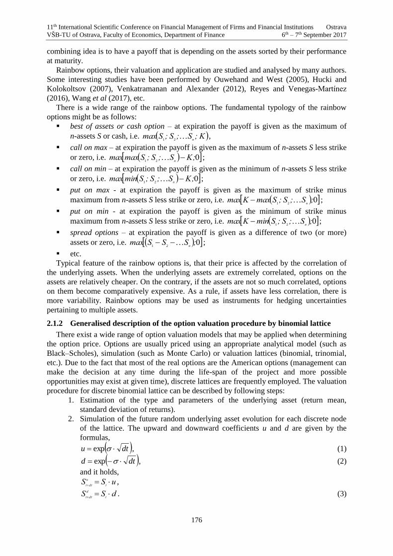
11th International Scientific Conference on Financial Management of Firms and Financial Institutions Ostrava
VŠB-TU of Ostrava, Faculty of Economics, Department of Finance 6th – 7th September 2017
176
combining idea is to have a payoff that is depending on the assets sorted by their performance
at maturity.
Rainbow options, their valuation and application are studied and analysed by many authors.
Some interesting studies have been performed by Ouwehand and West (2005), Hucki and
Kolokoltsov (2007), Venkatramanan and Alexander (2012), Reyes and Venegas-Martínez
(2016), Wang et al (2017), etc.
There is a wide range of the rainbow options. The fundamental typology of the rainbow
options might be as follows:
best of assets or cash option – at expiration the payoff is given as the maximum of
n-assets S or cash, i.e. K;S;S;Smaxn
21
,
call on max – at expiration the payoff is given as the maximum of n-assets S less strike
or zero, i.e. 021
;KS;S;Smaxmaxn ;
call on min – at expiration the payoff is given as the minimum of n-assets S less strike
or zero, i.e. 021
;KS;S;Sminmaxn ;
put on max - at expiration the payoff is given as the maximum of strike minus
maximum from n-assets S less strike or zero, i.e. 021
;S;S;SmaxKmaxn
;
put on min - at expiration the payoff is given as the minimum of strike minus
maximum from n-assets S less strike or zero, i.e. 021
;S;S;SminKmaxn
;
spread options – at expiration the payoff is given as a difference of two (or more)
assets or zero, i.e. 021
;SSSmaxn
;
etc.
Typical feature of the rainbow options is, that their price is affected by the correlation of
the underlying assets. When the underlying assets are extremely correlated, options on the
assets are relatively cheaper. On the contrary, if the assets are not so much correlated, options
on them become comparatively expensive. As a rule, if assets have less correlation, there is
more variability. Rainbow options may be used as instruments for hedging uncertainties
pertaining to multiple assets.
2.1.2 Generalised description of the option valuation procedure by binomial lattice
There exist a wide range of option valuation models that may be applied when determining
the option price. Options are usually priced using an appropriate analytical model (such as
Black–Scholes), simulation (such as Monte Carlo) or valuation lattices (binomial, trinomial,
etc.). Due to the fact that most of the real options are the American options (management can
make the decision at any time during the life-span of the project and more possible
opportunities may exist at given time), discrete lattices are frequently employed. The valuation
procedure for discrete binomial lattice can be described by following steps:
1. Estimation of the type and parameters of the underlying asset (return mean,
standard deviation of returns).
2. Simulation of the future random underlying asset evolution for each discrete node
of the lattice. The upward and downward coefficients u and d are given by the
formulas,
dtu exp , (1)
dtd exp , (2)
and it holds,
uSSt
u
dtt
,
dSSt
d
dtt
. (3)
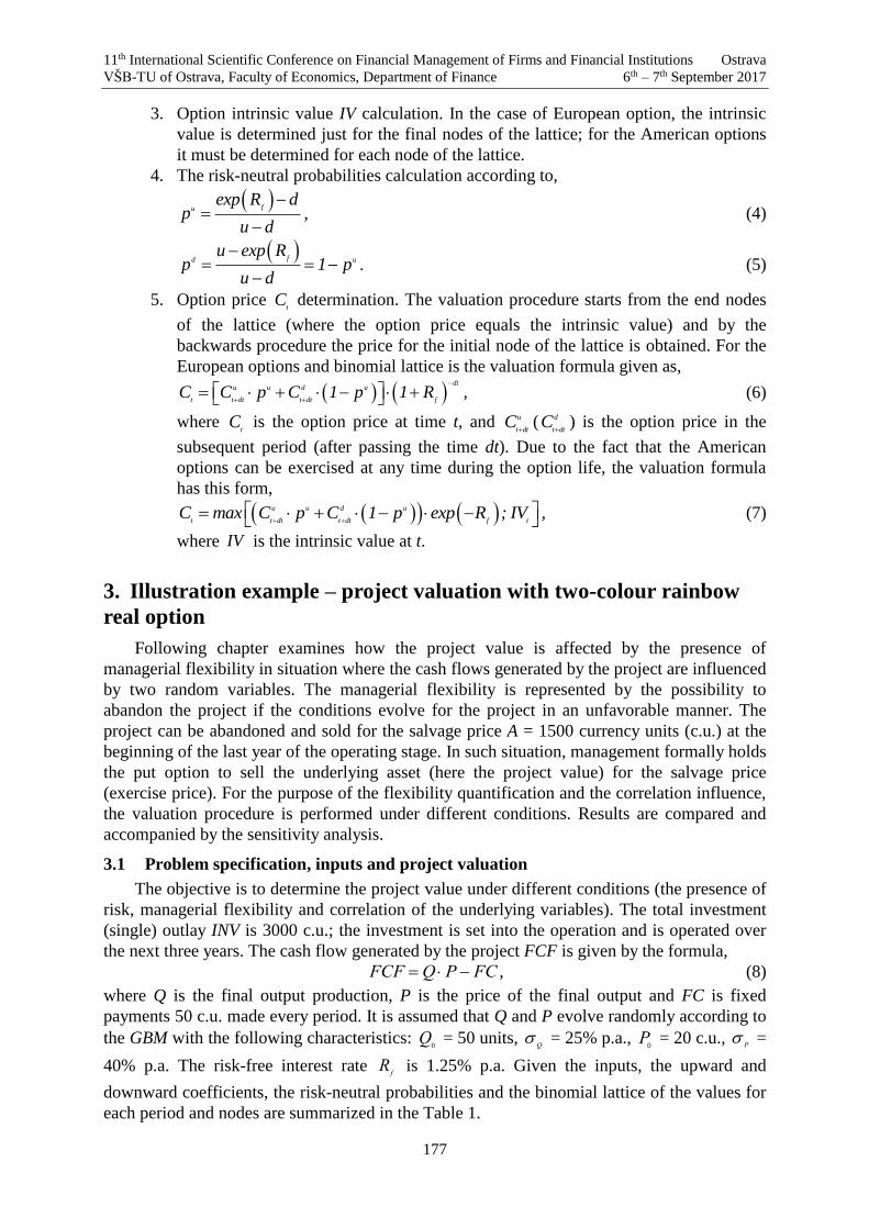
11th International Scientific Conference on Financial Management of Firms and Financial Institutions Ostrava
VŠB-TU of Ostrava, Faculty of Economics, Department of Finance 6th – 7th September 2017
177
3. Option intrinsic value IV calculation. In the case of European option, the intrinsic
value is determined just for the final nodes of the lattice; for the American options
it must be determined for each node of the lattice.
4. The risk-neutral probabilities calculation according to,
fuexp R d
pu d
, (4)
fd uu exp R
p 1 pu d
. (5)
5. Option price t
C determination. The valuation procedure starts from the end nodes
of the lattice (where the option price equals the intrinsic value) and by the
backwards procedure the price for the initial node of the lattice is obtained. For the
European options and binomial lattice is the valuation formula given as,
dt
u u d u
t t dt t dt fC C p C 1 p 1 R ,
(6)
where t
C is the option price at time t, and u
t dtC
( d
t dtC
) is the option price in the
subsequent period (after passing the time dt). Due to the fact that the American
options can be exercised at any time during the option life, the valuation formula
has this form,
u u d u
t t dt t dt f tC max C p C 1 p exp R ; IV ,
(7)
where IV is the intrinsic value at t.
3. Illustration example – project valuation with two-colour rainbow
real option
Following chapter examines how the project value is affected by the presence of
managerial flexibility in situation where the cash flows generated by the project are influenced
by two random variables. The managerial flexibility is represented by the possibility to
abandon the project if the conditions evolve for the project in an unfavorable manner. The
project can be abandoned and sold for the salvage price A = 1500 currency units (c.u.) at the
beginning of the last year of the operating stage. In such situation, management formally holds
the put option to sell the underlying asset (here the project value) for the salvage price
(exercise price). For the purpose of the flexibility quantification and the correlation influence,
the valuation procedure is performed under different conditions. Results are compared and
accompanied by the sensitivity analysis.
3.1 Problem specification, inputs and project valuation
The objective is to determine the project value under different conditions (the presence of
risk, managerial flexibility and correlation of the underlying variables). The total investment
(single) outlay INV is 3000 c.u.; the investment is set into the operation and is operated over
the next three years. The cash flow generated by the project FCF is given by the formula,
FCPQFCF , (8)
where Q is the final output production, P is the price of the final output and FC is fixed
payments 50 c.u. made every period. It is assumed that Q and P evolve randomly according to
the GBM with the following characteristics: 0Q = 50 units,
Q = 25% p.a.,
0P = 20 c.u.,
P =
40% p.a. The risk-free interest rate fR is 1.25% p.a. Given the inputs, the upward and
downward coefficients, the risk-neutral probabilities and the binomial lattice of the values for
each period and nodes are summarized in the Table 1.
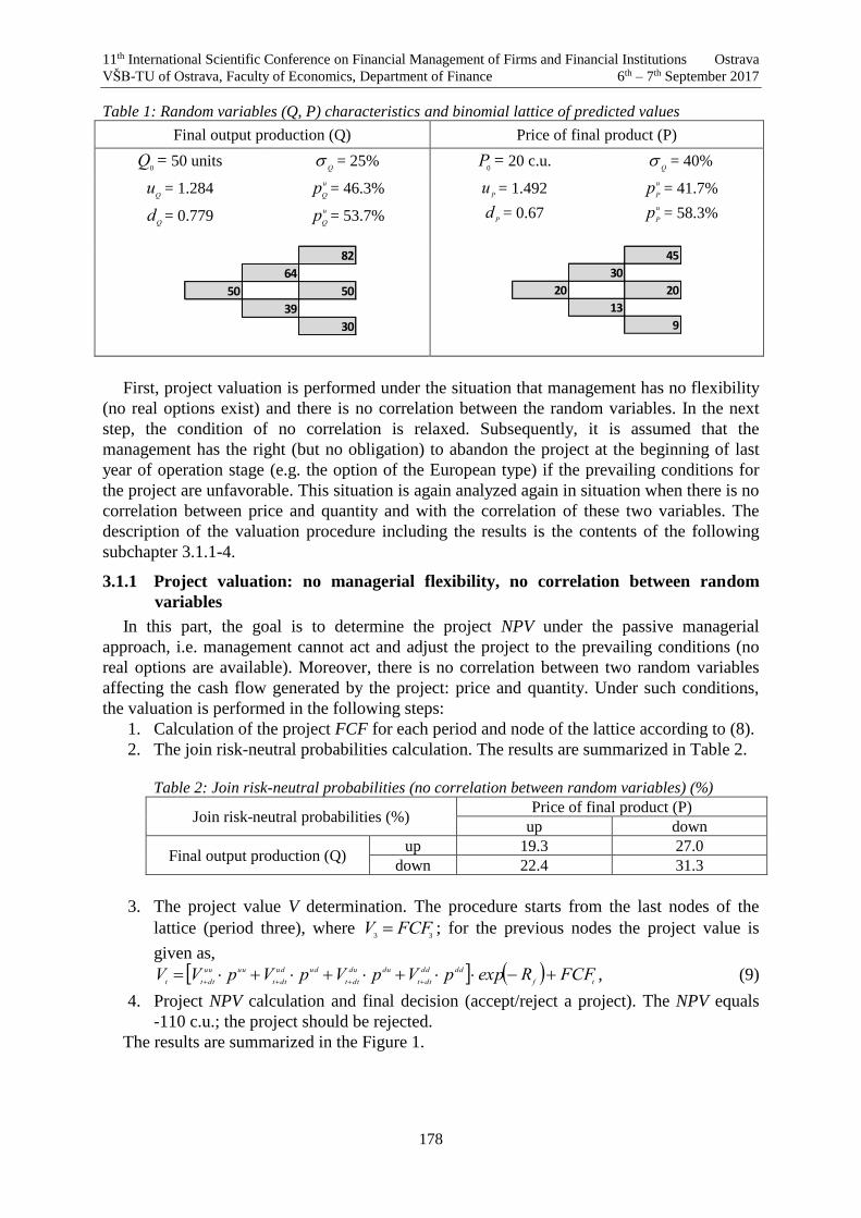
11th International Scientific Conference on Financial Management of Firms and Financial Institutions Ostrava
VŠB-TU of Ostrava, Faculty of Economics, Department of Finance 6th – 7th September 2017
178
Table 1: Random variables (Q, P) characteristics and binomial lattice of predicted values
Final output production (Q) Price of final product (P)
0Q = 50 units
Q = 25%
0P = 20 c.u.
Q = 40%
Qu = 1.284
Qd = 0.779
u
Qp = 46.3%
u
Qp = 53.7%
Pu = 1.492
Pd = 0.67
u
Pp = 41.7% u
Pp = 58.3%
82
64
50 50
39
30
45
30
20 20
13
9
First, project valuation is performed under the situation that management has no flexibility
(no real options exist) and there is no correlation between the random variables. In the next
step, the condition of no correlation is relaxed. Subsequently, it is assumed that the
management has the right (but no obligation) to abandon the project at the beginning of last
year of operation stage (e.g. the option of the European type) if the prevailing conditions for
the project are unfavorable. This situation is again analyzed again in situation when there is no
correlation between price and quantity and with the correlation of these two variables. The
description of the valuation procedure including the results is the contents of the following
subchapter 3.1.1-4.
3.1.1 Project valuation: no managerial flexibility, no correlation between random
variables
In this part, the goal is to determine the project NPV under the passive managerial
approach, i.e. management cannot act and adjust the project to the prevailing conditions (no
real options are available). Moreover, there is no correlation between two random variables
affecting the cash flow generated by the project: price and quantity. Under such conditions,
the valuation is performed in the following steps:
1. Calculation of the project FCF for each period and node of the lattice according to (8).
2. The join risk-neutral probabilities calculation. The results are summarized in Table 2.
Table 2: Join risk-neutral probabilities (no correlation between random variables) (%)
Join risk-neutral probabilities (%) Price of final product (P)
up down
Final output production (Q) up 19.3 27.0
down 22.4 31.3
3. The project value V determination. The procedure starts from the last nodes of the
lattice (period three), where 33
FCFV ; for the previous nodes the project value is
given as,
tf
dddd
dtt
dudu
dtt
udud
dtt
uuuu
dtttFCFRexppVpVpVpVV
, (9)
4. Project NPV calculation and final decision (accept/reject a project). The NPV equals
-110 c.u.; the project should be rejected.
The results are summarized in the Figure 1.

11th International Scientific Conference on Financial Management of Firms and Financial Institutions Ostrava
VŠB-TU of Ostrava, Faculty of Economics, Department of Finance 6th – 7th September 2017
179
Figure 1: Results summary: project FCF (left) and project value V (right)
3.1.2 Project valuation: no managerial flexibility, correlation between random
variables
The project valuation procedure is identical to the one described in Chapter 3.1.1. The
difference is in the join risk-neutral probabilities calculation of two correlated random
variables. Assuming Qu ( Pu ) are the upward coefficients for production (price), Qd ( Pd ) are
the downward coefficients for production (price), Q ( P ) are the volatilities of the
production (price), QP is the correlation between the production and price (
QP = 0.25) and Qg (
Pg ) is the return of the production (price)4, the join risk-neutral probabilities are given by
the following formulas:
uu Q P P Q Q P Q P QP Q Pp u u u g u g / 4 u u , .. (10)
ud Q P P Q Q P Q P QP Q Pp u u u g d g / 4 u u , (11)
du Q P P Q Q P Q P QP Q Pp u u d g u g / 4 u u , (12)
dd Q P P Q Q P Q P QP Q Pp u u d g d g / 4 u u . (13)
Table 3: Join risk-neutral probabilities (correlation between random variables) (%)
Join risk-neutral probabilities (%) Price of final product (P)
up down
Final output production (Q) up 27.73 23.98
down 25.37 22.92
Following the procedure in 3.1.1, we get the results shown in Figure 2.
4 ;/Rg;/Rg P
f
PQ
f
Q 2222

11th International Scientific Conference on Financial Management of Firms and Financial Institutions Ostrava
VŠB-TU of Ostrava, Faculty of Economics, Department of Finance 6th – 7th September 2017
180
Figure 2: Results summary: project FCF (left) and project value (right)
It is obvious that the project value V is 3284 c.u. giving the NPV of 284 c.u. The project
should be accepted.
3.1.3 Project valuation: with managerial flexibility and no correlation between random
variables
Assume the management has the possibility to abandon the project at the beginning of last
year of operation if the market conditions evolve unfavourably. The project can be sold for the
salvage value A = 1500 c.u.
The valuation procedure consists of the following steps:
1. Calculation of the project FCF for each period and node of the binomial lattice
according to (8).
2. Calculation of the project payoffs for each node of the period T with the option to
abandon *
TFCF . The payoff function is formulated as,
TT
*
TFCF;AmaxFCF , (14)
and the decision function as follows,
.FCFAifabandon
;FCFAifcontinue
T
T
T (15)
3. The join risk-neutral probabilities calculation.
4. The project value V determination according to (9).
5. NPV calculation and final decision.
Following Figure 3 shows the project free cash flow with the option to abandon (left) and
the project value evolution (right). As it is apparent, project value V equals 3525 c.u. results in
NPV of 525 c.u. Project should be accepted.

11th International Scientific Conference on Financial Management of Firms and Financial Institutions Ostrava
VŠB-TU of Ostrava, Faculty of Economics, Department of Finance 6th – 7th September 2017
181
Figure 3: Results summary: project FCF (left) and project value (right)
3.1.4 Project valuation: with managerial flexibility, correlation between random
variables
This situation represents the combination of the managerial flexibility (option to abandon a
project) and correlation between variables having impact on the cash flow generated by the
project. The valuation procedure is straightforward and clear; Figure 4 overviews the project
cash flows for each period and nodes (left) and project value development according to (9)
(right). The project value V of 3766 c.u. gives the NPV of 766 c.u.; the project should be
undertaken.
Figure 4: Results summary: project FCF (left) and project value (right)
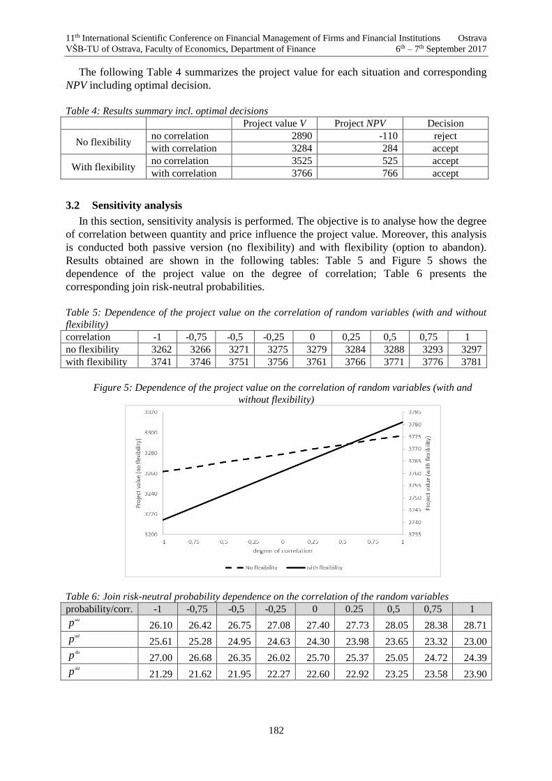
11th International Scientific Conference on Financial Management of Firms and Financial Institutions Ostrava
VŠB-TU of Ostrava, Faculty of Economics, Department of Finance 6th – 7th September 2017
182
The following Table 4 summarizes the project value for each situation and corresponding
NPV including optimal decision.
Table 4: Results summary incl. optimal decisions
Project value V Project NPV Decision
No flexibility no correlation 2890 -110 reject
with correlation 3284 284 accept
With flexibility no correlation 3525 525 accept
with correlation 3766 766 accept
3.2 Sensitivity analysis
In this section, sensitivity analysis is performed. The objective is to analyse how the degree
of correlation between quantity and price influence the project value. Moreover, this analysis
is conducted both passive version (no flexibility) and with flexibility (option to abandon).
Results obtained are shown in the following tables: Table 5 and Figure 5 shows the
dependence of the project value on the degree of correlation; Table 6 presents the
corresponding join risk-neutral probabilities.
Table 5: Dependence of the project value on the correlation of random variables (with and without
flexibility)
correlation -1 -0,75 -0,5 -0,25 0 0,25 0,5 0,75 1
no flexibility 3262 3266 3271 3275 3279 3284 3288 3293 3297
with flexibility 3741 3746 3751 3756 3761 3766 3771 3776 3781
Figure 5: Dependence of the project value on the correlation of random variables (with and
without flexibility)
Table 6: Join risk-neutral probability dependence on the correlation of the random variables
probability/corr. -1 -0,75 -0,5 -0,25 0 0.25 0,5 0,75 1 uup 26.10 26.42 26.75 27.08 27.40 27.73 28.05 28.38 28.71 udp 25.61 25.28 24.95 24.63 24.30 23.98 23.65 23.32 23.00 dup 27.00 26.68 26.35 26.02 25.70 25.37 25.05 24.72 24.39 ddp 21.29 21.62 21.95 22.27 22.60 22.92 23.25 23.58 23.90

11th International Scientific Conference on Financial Management of Firms and Financial Institutions Ostrava
VŠB-TU of Ostrava, Faculty of Economics, Department of Finance 6th – 7th September 2017
183
4. Conclusion
This paper aims at the project valuation under risk and flexibility. Particularly, option to
abandon a project is considered and exercised in situation when the market conditions evolve
in an unfavourable manner and the management may prefer to abandon the project and sell it
for salvage price if the selling price exceeds the project value if continued. The underlying
asset (cash flows generated by the project) is affected by two random variables (price and
output volume of final product).
The project valuation is performed under different conditions: with/without the presence in
managerial flexibility and with/without correlation of the variables underlying cash flows
generated by the project. Moreover, the combination of managerial flexibility and correlation
is present is subject to sensitivity analysis.
As it is apparent from the results, managerial flexibility may capture significant part of the
total asset value (here project value). Moreover, the effect of managerial flexibility is
supported by the degree of correlation between random variables. This finding is important for
long-term projects whose cash flows are associated with high degree of risk (more possible
scenarios in the future) and affected by more underlying factors (possible changes in demand
prices, operating costs etc.).
References
[1] ALEXANDER, C., VENKATRAMANAN, A. (2012). Analytic Approximation s for
Multi-Asset Option Pricing. Mathematical Finance. 22(4): pp. 667–689.
[2] BLACK, F., SCHOLES, M. (1973). The pricing of options and corporate liabilities.
Journal of Political Economy 81(3): pp. 637–654.
[3] BRACH, M. A. (2002). Real Options in Practice. New Jersey: Wiley.
[4] BRENNAN, M. J., SCHWARTZ, E. S. (1985). Evaluating natural resource investments.
Journal of Business 58(2): pp. 135–157.
[5] BRENNAN, M.J., TRIGEORIS, L. (2000). Project Flexibility, Agency and
Competition: New Developments in the Theory and Application of Real Options. 1st
Ed. London: Oxford University Press.
[6] COPELAND, T.E., ANTIKAROV, V. (2003). Real Options, Revised Edition: A
Practitioner's Guide. 2st Ed. New York: Texere.
[7] ČULÍK, M. and P. GURNÝ. (2017) ‘Assessing hard coal mining: an application with
abandonment in the Czech Republic’, Int. J. Mining and Mineral Engineering, Vol. 8,
No. 3, pp.187–206.
[8] COX, J.C., ROSS, S.A., RUBINSTEIN, M. (1979). Option pricing: A simplified
approach. Journal of Financial Economics 7(3): pp. 229–263.
[9] DAMODARAN, A. (2006). Damodaran on Valuation: Security Analysis for Investment
and Corporate Finance. 2nd Ed. New Jersey: Wiley.
[10] DIXIT, A.K., PINDYCK, R.S. (1994). Investment under Uncertainty. 1st Ed. New York:
Princeton University Press.
[11] GRENADIER, S. (2000). Game Choices: The Intersection of Real Options and Game
Theory. London: Riskbooks.
11th International Scientific Conference on Financial Management of Firms and Financial Institutions Ostrava
VŠB-TU of Ostrava, Faculty of Economics, Department of Finance 6th – 7th September 2017
184
[12] GUTHRIE, G. (2011). Learning Options and Binomial Trees. Wilmott Journal, Vol.
3(1), pp. 1–23.
[13] HAAHTELA, T. (2010). Recombining Trinomial Tree for Real Option Valuation with
Changing Volatility. In Annual Real Option Conference.
[14] HUCKI, Z., KOLOKOLTSOV, V. N. (2007) Pricing of rainbow options: game theoretic
approach. International Game Theory Review. 9(2). pp. 215–254.
[15] HOEK, J., ELLIOT, R.J. (2006). Binomial Models in Finance. New York: Springer.
[16] HULL, J.C. (2014). Options, Futures, and Other Derivatives. 9th Ed. Prentice Hall.
[17] LEE, M.Y., et all (2008). The generalized sequential compound options pricing and
sensitivity analysis. Mathematical Social Sciences, Vol. 55, Issue 1, pp. 38–54.
[18] MERTON, R. (1973). The theory of rational option pricing. Bell Journal of Economics
and Management Science 4(1): pp. 141–183.
[19] MUN, J. (2005). Real Option Analysis. Tool and Techniques for Valuing Strategic
Investments and Decisions. 2nd Ed. New Jersey: Wiley.
[20] MUN, J. (2003). Real Options Analysis Course: Business Cases and Software
Applications. New Jersey: Wiley.
[21] OUWEHAND, P., WEST, G. (2006). Pricing Rainbow Options. Willmot magazine.
[22] REYES, A.Z., MARETÍNEZ, F.V. (2016). Pricing rainbow options on baskets of assets
under mixed diffusion-jump processes. EconPapers. 61(2). pp. 374–390.
[23] SMITH, J.E., NAU, R.F. (1995). Valuing risky projects: Option pricing theory and
decision analysis. Management Science 14: pp. 795–816.
[24] TICHÝ, T. (2008). Lattice models. Pricing and hedging at (In)complete Markets. VŠB-
TU Ostrava.
[25] TRIGEORGIS, L. (1999). Real Options and Business Strategy: Applications to
Decision Making. London: Riskbooks.
[26] TRIGEORGIS, L. (2000). Real Options in Capital Investments: Models, Strategies and
Applications. London: Praeger Westport.
[27] TRIGEORGIS, L., SCHWARTZ, E. S. (2001). Real Options and Investments under
Uncertainty. Cambridge: MIT Press.
[28] TRIGEORGIS, L., SMITH, H. T. J. (2004). Strategic Investment: Real Options and
Games. New York: Princeton University Press.
[29] WANG, J.Y. et al. (2017). Rainbow trend options: valuation and applications. Review of
Derivatives Research. 20(2): pp. 91–133.
11th International Scientific Conference on Financial Management of Firms and Financial Institutions Ostrava
VŠB-TU of Ostrava, Faculty of Economics, Department of Finance 6th – 7th September 2017
185
Application and Comparison of the Methods for Influences Quantification Including Sensitivity
Analysis1
Miroslav Čulík, Andrea Jurčicová 2
Abstract
This papers deals with the application and comparison of methods for quantification of the
influence of component ratios on selected basic ratio. Method of gradual changes, logarithmic
method, functional method and integral method are applied. Results are compared and
analyzed. In addition, sensitivity analysis is performed. The goal is to how the influences vary
with respect to method applied.
Key words
pyramidal decomposition, influence quantification, financial analysis, financial ratios,
sensitivity analysis
JEL Classification: G10
1. Introduction
The financial analysis is one of the widely-used tools for analyzing the financial
performance of a company. Such analysis is crucial for successful managing of a company and
correct decision-makings. The results of the financial analysis support not only the decisions
of the management but helps to identify strong and weaknesses of the company. Moreover, the
users are not only the managers, but some other subject that might be interested such as
creditors, competitors or rating agencies.
Frequently used analysis is the application of the financial ratios. The main idea is based on
the construction of a ratio working with two or more financial variables. The result provides
some information on financial performance of the company.
There are a lot of financial ratios applicable for the financial analysis. With respect to the
subject of analysis, they may be grouped into a few subgroups: profitability ratios, liquidity
ratios, solvency ratios, assets management ratios and market ratios. When analyzing the
results of the financial ratios, it is important to understand not only the meaning the ratio
itself, but its evolution over the time, as well. If the trend in the evolution is not desirable for
the company, the first step is to analyze what is behind such evolution. A useful tool for such
analysis is the pyramidal decomposition and influence quantification. The former enables to
detect the relationships between the financial ratios; the latter one enables to quantify the
influences between them.
The goal of this paper is to describe and illustrate the possibility of the application of the
pyramidal decomposition and the influence quantification on a key profitability ratio – Return
on equity (ROE).
1 The paper is based on research activities within the ESF Project No. CZ.1.07/2.3.00/20.0296. 2 Miroslav Čulík, associate professor (corresponding author), Bc. Andrea Jurčicová, VSB-Technical
University of Ostrava, Faculty of Economics, Finance Department. Sokolská třída 33, 702 00 Ostrava.
email: [email protected], [email protected]

11th International Scientific Conference on Financial Management of Firms and Financial Institutions Ostrava
VŠB-TU of Ostrava, Faculty of Economics, Department of Finance 6th – 7th September 2017
186
The structure of the paper is as follows.
In Chapter two main idea of pyramidal decomposition is explained, relationships between
component ratios and the methods for influence quantifications.
Chapter three illustrates the usage if these methods on ROE. In the pyramidal
decomposition, this ratio is expressed as a product of three component ratio. Next, four
methods are applied to quantify how these component ratios influence during given period the
basic ratio. In the end, the sensitivity analysis is applied. Results are presented, compared and
commented.
2. Methods for influence quantification of component ratios
There is a wide range of the methods applicable in the analysis of the financial performance
of the company. With respect to the objective, reliability and the costs, the management tries
to select the most suitable. The better method selected the more reliable and accurate the
achieved results are which is necessary for the correct decision-making.
There are a lot of ways, how the methods for the financial analysis of the company can by
classify. One of the most common is the grouping them into two subgroups: deterministic and
mathematical-statistics. The deterministic methods are used primarily for general analysis of
the evolution, the horizontal and vertical analysis, the pyramidal decomposition and the
influence analysis. These methods are employed for the traditional financial analysis of
companies over a relatively shorter period. The mathematical-statistics methods are used for
the analysis over a relatively longer period, when the uncertainty in the evolution of some
financial variables is expected. The objective is usually to determine the main drivers and
factors affecting the evolution and detecting the relationships and causalities.
The financial ratios represent a tool that is frequently used by companies to analyze the
financial performance of the company. They provide useful information about the actual
financial situation of the company; on the other hand, their interpretation can be sometimes
misleading due to the fact, that each ratio incorporates many relationships which do not have
to be obvious and clear directly from the ratio itself. To analyze these (sometimes difficult and
complicated) relationships, the pyramidal decomposition is a useful tool that helps to
overcome this problem. The pyramidal decompositions enable to decompose the key (basic)
ratio into more component ratios that have the influence on its evolution. The relationships
between the component ratios may be expressed as additive or multiplicative.
The changes in the component ratios in such models have influence on the ratio on the top
of the pyramid (so called basic ratio). The total change in the basic ratio is equal to the sum of
the individual influences of all component ratios in the decomposition. This relation can be
mathematically formulated as follows,
,iax xy (1)
where x is the basic ratio, xy is the change in the basic ratio caused by the change in the
component ratios, ia is the ith component ratio and iax is the influence of the ith component
ratio ia on the basic ratio x.
2.1 Quantification of influences in decompositions with additive relationships
The additive relationship means that the basic ratio is given as a sum of the component
ratios. This relationship can be written as,
ni
i aaaax 21 , (2)
where x is the basic ratio and ia is component ratio.

11th International Scientific Conference on Financial Management of Firms and Financial Institutions Ostrava
VŠB-TU of Ostrava, Faculty of Economics, Department of Finance 6th – 7th September 2017
187
If there is an additive relationship between component ratios, then the influence of ith
component ratio is given by the following formula,
,ya
ax
x
ii
i
ai
(3)
where titii aaa ,1, , tia , . ( 1, tia ) is the value of the component ratio at time t (t+1). It is
obvious that the total change in basic ratio is distributed among the component ratios
according to their changes.
2.2 Quantification of influences in decompositions with multiplicative relationships
The multiplicative relationship means that the basic ratio is expressed as a product of n
component ratios, which is formulated mathematically as,
nii
aaaax 21 , (4)
In the pyramidal decompositions with the multiplicative relationship, the influence of each
component ratio can determine by applying some of the following methods.
2.2.1 Method of gradual changes
The method of gradual changes is the easiest to apply. The assumption for the
determination of the influence of a given component ratio is, that only one component ratio
can change whereas the others being the same. This fact might be considered as a shortcoming
because usually more ratios can change at the same time. This method is applicable regardless
of positive or negative values of changes in component ratios (changes are expressed here in
the absolute terms). Next shortcoming results from the fact that the influences may depend on
the order of component ratios in the decomposition and provide different results.
If the basic ratio is expressed as a product of three component ratios, i.e. 321 aaax , the
influence of each of them on the basic ratio is given by following formulas,
,
,
,
31,21,13
0,321,12
0,30,211
aaax
aaax
aaax
a
a
a
(5)
For this method, the equation (1) holds3.
2.2.2 Logarithmic method
The logarithmic method is the method for which formula (1) holds. The advantage of this
method (compared to the method of gradual changes) is that the influences of the component
ratios are not affected by the order of the component ratios in the pyramidal decomposition
and simultaneous changes in the component ratios are assumed. On the other hands, the usage
of this method can be limited if the changes of both basic ratio and component ratios are
negative (the changes are expressed her as the index). The influence of any component ratio
on the basic ratio is given by the following formula,
yI
Ix x
x
a
ai
i
ln
ln, (6)
where 0
1
x
xI x is the index of the change in the basic ratio,
0,
1,
i
i
aa
aI
i is the index of the
change of the ith component ratio.
3 All formulas for influence quantification assume three component ratios in the pyramidal
decomposition. General formulas for n component ratios can be found for example in [1]/
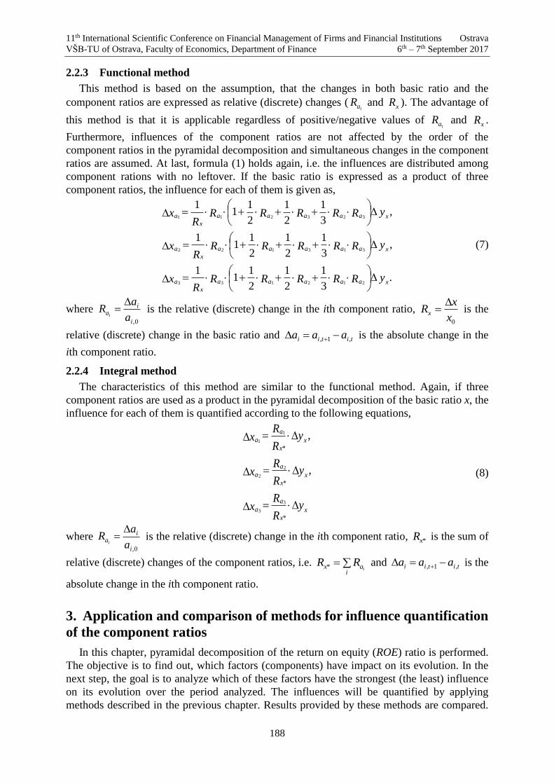
11th International Scientific Conference on Financial Management of Firms and Financial Institutions Ostrava
VŠB-TU of Ostrava, Faculty of Economics, Department of Finance 6th – 7th September 2017
188
2.2.3 Functional method
This method is based on the assumption, that the changes in both basic ratio and the
component ratios are expressed as relative (discrete) changes (iaR and xR ). The advantage of
this method is that it is applicable regardless of positive/negative values of iaR and xR .
Furthermore, influences of the component ratios are not affected by the order of the
component ratios in the pyramidal decomposition and simultaneous changes in the component
ratios are assumed. At last, formula (1) holds again, i.e. the influences are distributed among
component rations with no leftover. If the basic ratio is expressed as a product of three
component ratios, the influence for each of them is given as,
.3
1
2
1
2
11
1
,3
1
2
1
2
11
1
,3
1
2
1
2
11
1
212133
313122
323211
yRRRRRR
x
yRRRRRR
x
yRRRRRR
x
xaaaaa
x
a
xaaaaa
x
a
xaaaaa
x
a
(7)
where 0,i
ia
a
aR
i
is the relative (discrete) change in the ith component ratio,
0x
xRx
is the
relative (discrete) change in the basic ratio and titii aaa ,1, is the absolute change in the
ith component ratio.
2.2.4 Integral method
The characteristics of this method are similar to the functional method. Again, if three
component ratios are used as a product in the pyramidal decomposition of the basic ratio x, the
influence for each of them is quantified according to the following equations,
yR
Rx
yR
Rx
yR
Rx
xx
a
a
xx
a
a
xx
a
a
*
*
*
3
3
2
2
1
1
,
,
(8)
where 0,i
ia
a
aR
i
is the relative (discrete) change in the ith component ratio, *xR is the sum of
relative (discrete) changes of the component ratios, i.e. i
ax iRR * and titii aaa ,1, is the
absolute change in the ith component ratio.
3. Application and comparison of methods for influence quantification
of the component ratios
In this chapter, pyramidal decomposition of the return on equity (ROE) ratio is performed.
The objective is to find out, which factors (components) have impact on its evolution. In the
next step, the goal is to analyze which of these factors have the strongest (the least) influence
on its evolution over the period analyzed. The influences will be quantified by applying
methods described in the previous chapter. Results provided by these methods are compared.

11th International Scientific Conference on Financial Management of Firms and Financial Institutions Ostrava
VŠB-TU of Ostrava, Faculty of Economics, Department of Finance 6th – 7th September 2017
189
At last, sensitivity analysis is performed. Here, the objective is to detect how the influences
are changing with respect to the changes in input variables.
3.1 Pyramidal decomposition of key profitability ratio
Following Table 3.1 shows selected input data of the company over two years necessary for
the return on equity ratio calculation. The absolute and relative change of this ratio is
computed as well.
Table. 4.1 Input data (USD thousands)
Period t t+1
EAT 13876 5240
Equity 93355 80956
ROE (%) 14,86 6,47
Abs. change (%) -8,39
Rel. change (%) -56.45
As it is obvious from the results, ROE has decreased by 8.39% (in absolute terms) and by
56.45% (in relative terms). Such evolution of the key profitability ratio is not desirable for the
equity holders and the goal is analyzing the factors having impact on this ratio evolution and
their significance.
For this case study, we use well-known pyramidal decomposition of the ROE named
DuPont decomposition. This decomposition is based on using three component ratios (net
profit margin, assets turnover, financial leverage), with the multiplicative relation, i.e.
E
A
A
R
R
EAT
E
EATROE , (4.1)
where EAT is net profit, R is revenues (sales), E is equity and A stands for total assets.
Following table 4.2 shows the values of these component ratios over these periods; their
product provides the same values of ROE as in Table 4.1.
Table 4.2 Value of component ratios incl. ROE
Period t t+1
Net profit margin 0.051 0.028
Assets turnover 0.929 1.053
Financial leverage 3.127 2.193
ROE (%) 14.86 6.47
The next goal is find out, which of these component ratios contributed the most (or the
least) to the decrease in ROE. If the multiplicative relation between the component ratios
exists, any method described in Chapter 3 can be applied.
3.2 Quantification of influences of the component ratios on the basic ratio by applying
selected methods
Following chapter overviews the results of the quantification of the influences of the
component ratios. Methods are described in Chapter 2.
Table 4.3 reports the results of the method of gradual changes. Calculations are based on
values of the component ratios and their absolute changes; influences are quantified by
applying formula (5).

11th International Scientific Conference on Financial Management of Firms and Financial Institutions Ostrava
VŠB-TU of Ostrava, Faculty of Economics, Department of Finance 6th – 7th September 2017
190
Tab. 4.3 Influences of the component ratios on ROE by applying the method of gradual changes
Component ratio t t+1 absolute
change
Influence on
ROE (%) order
Net profit margin 0.051 0.028 -0.023 -6.72 1.
Assets turnover 0.929 1.053 0.124 1.09 3.
Financial leverage 3.127 2.193 -0.934 -2.76 2.
Sum of influences - - - -8.39 -
Table 4.4 summarizes the results of the influences if logarithmic method is applied. This
method works with index of the changes of both basic and component ratios; influences are
calculated according to (6).
Tab. 4.4 Influences of the component ratios on ROE by applying the logarithmic method
Component ratio t t+1 index of
change
Influence on
ROE (%) order
Net profit margin 0.051 0.028 0.548 -6.08 1
Assets turnover 0.929 1.053 1.134 1.27 3
Financial leverage 3.127 2.193 0.701 -3.58 2
Sum of influences - - - -8.39 -
Table 4.5 provides the results of the influences if functional method is applied. Here, the
changes are expressed as the relative (discrete) changes; influence for each component ratio is
calculated according to the formula (7).
Tab. 4.5 Influences of the component ratios on ROE by applying the functional method
Component ratio t t+1 relative
change
Influence on
ROE (%) order
Net profit margin 0.051 0.028 -0.452 -6.08 1
Assets turnover 0.929 1.053 0.134 1.33 3
Financial leverage 3.127 2.193 -0.299 -3.64 2
Sum of influences - - - -8.39 -
Table 4.6 presents the results of the integral method. Similarly, to the functional method,
the change of the component ratio is expressed here as the relative change. The influences are
quantified for each component ratio by employing formula (8).
Tab. 4.6 Influences of the component ratios on ROE by applying the integral method
Component ratio t t+1 relative
change
Influence on
ROE (%) order
Net profit margin 0.051 0.028 -0.452 -6.15 1
Assets turnover 0.929 1.053 0.134 1.82 3
Financial leverage 3.127 2.193 -0.299 -4.06 2
Sum of influences - - -0.617 -8.39 -
Figure 1 graphically summarizes and compares the results of the influences for particular
component ratio with respect to the method applied. Although the influences for each
component ratios differs across the method used, the order of the influences is the same for all
of them, i.e. the strongest effect on ROE is assigned to net profit margin, whereas the assets
turnover has the lowest influence on ROE evolution. Moreover, assets turnover is the only

11th International Scientific Conference on Financial Management of Firms and Financial Institutions Ostrava
VŠB-TU of Ostrava, Faculty of Economics, Department of Finance 6th – 7th September 2017
191
ratio that has positive impact on ROE, this positive effect was overcame by the negative
effects of the net profit margin and financial leverage. Regardless the method applied, the sum
of the individual influences always equals the change in the basic ratio.
Figure 1 Influence of component ratios on ROE according to methods used
-8.0%
-6.0%
-4.0%
-2.0%
0.0%
2.0%
EAT/R R/A A/E
infl
uen
ce o
n R
OE
(%)
Component ratio
method of gradual changes Logarithmic method Functional method Integral method
3.3 Sensitivity analysis
In this part, we are going to analyzed effect of the changes in main variables of the ROE
ratio (net profit, equity) on the influence of the component ratios. The sensitivity analysis is
performed for all methods and in this way. Firstly, it is assumed that the net profit and equity
can divert by +/- 10% and +/- 20% from their original values in period t+1. Secondly, the
values of component ratios and the changes are recalculated. Thirdly, the influences are
quantified. At last, results are compared and discussed. The sensitivity analysis is done as a
one-factor analysis.
Following Table 4.7 and Figure 2 indicates how the changes in EAT and Equity value
would influence the key ROE ratio at period t+1. It is not surprising that an increase in EAT
(Equity value being the same) will result in ROE increase; the opposite is true for the Equity
value. Again, the goal is to search the impact on the influence of each component ratio.
Tab. 4.7 Roe evolution with respect to EAT and Equity changes (period t+1)
Change from the original value (%) -20 -10 0 10 20
ROE if EAT changes (%) 7.77 7.12 6.47 5.83 5.18
ROE if Equity changes (%) 8.09 7.19 6.47 5.88 5.39
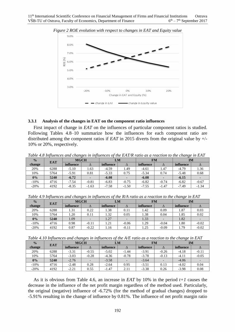
11th International Scientific Conference on Financial Management of Firms and Financial Institutions Ostrava
VŠB-TU of Ostrava, Faculty of Economics, Department of Finance 6th – 7th September 2017
192
Figure 2 ROE evolution with respect to changes in EAT and Equity value
3.3.1 Analysis of the changes in EAT on the component ratio influences
First impact of change in EAT on the influences of particular component ratios is studied.
Following Tables 4.8–10 summarize how the influences for each component ratio are
distributed among the component ratios if EAT in 2015 diverts from the original value by +/-
10% or 20%, respectively.
Table 4.8 Influences and changes in influences of the EAT/R ratio as a reaction to the change in EAT
%
change EAT
MGCH LM FM IM
influence ∆ influence ∆ influence ∆ influence ∆
20% 6288 -5.10 1.63 -4.59 1.49 -4.61 1.47 -4.79 1.36
10% 5764 -5.91 0.81 -5.33 0.75 -5.34 0.74 -5.48 0.68
0% 5240 -6.72 - -6.08 - -6.08 - -6.15 -
-10% 4716 -7.54 -0.81 -6.83 -0.75 -6.82 -0.74 -6.82 -0.67
-20% 4192 -8.35 -1.63 -7.58 -1.50 -7.55 -1.47 -7.49 -1.34
Table 4.9 Influences and changes in influences of the R/A ratio as a reaction to the change in EAT
%
change EAT
MGCH LM FM IM
influence ∆ influence ∆ influence ∆ influence ∆
20% 6288 1.31 0.22 1.38 0.11 1.42 0.09 1.87 0.03
10% 5764 1.20 0.11 1.32 0.05 1.38 0.04 1.85 0.02
0% 5240 1.09 - 1.27 - 1.33 - 1.82 -
-10% 4716 0.98 -0.11 1.21 -0.06 1.29 -0.04 1.80 -0.02
-20% 4192 0.87 -0.22 1.16 -0.11 1.25 -0.09 1.79 -0.02
Table 4.10 Influences and changes in influences of the A/E ratio as a reaction to the change in EAT
%
change EAT
MGCH LM FM IM
influence ∆ influence ∆ influence ∆ influence ∆
20% 6288 -3.31 -0.55 -5.02 -1.44 -3.91 -0.26 -4.18 -0.11
10% 5764 -3.03 -0.28 -4.36 -0.78 -3.78 -0.13 -4.11 -0.05
0% 5240 -2.76 - -3.58 - -3.64 - -4.06 -
-10% 4716 -2.48 0.28 -2.64 0.95 -3.51 0.13 -4.02 0.04
-20% 4192 -2.21 0.55 -1.47 2.11 -3.38 0.26 -3.98 0.08
As it is obvious from Table 4.6, an increase in EAT by 10% in the period t+1 causes the
decrease in the influence of the net profit margin regardless of the method used. Particularly,
the original (negative) influence of -6.72% (for the method of gradual changes) dropped to
-5.91% resulting in the change of influence by 0.81%. The influence of net profit margin ratio
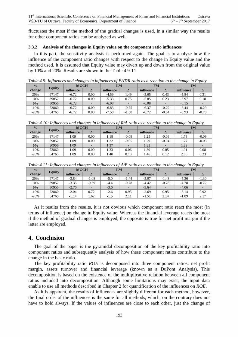
11th International Scientific Conference on Financial Management of Firms and Financial Institutions Ostrava
VŠB-TU of Ostrava, Faculty of Economics, Department of Finance 6th – 7th September 2017
193
fluctuates the most if the method of the gradual changes is used. In a similar way the results
for other component ratios can be analyzed as well.
3.3.2 Analysis of the changes in Equity value on the component ratio influences
In this part, the sensitivity analysis is performed again. The goal is to analyze how the
influence of the component ratio changes with respect to the change in Equity value and the
method used. It is assumed that Equity value may divert up and down from the original value
by 10% and 20%. Results are shown in the Table 4.9-11.
Table 4.9: Influences and changes in influences of EAT/R ratio as a reaction to the change in Equity %
change Equity
MGCH LM FM IM
influence ∆ influence ∆ influence ∆ influence ∆
20% 97147 -6.72 0.00 -4.59 1.49 -5.65 0.43 -5.84 0.31
10% 89052 -6.72 0.00 -5.33 0.75 -5.85 0.23 -5.97 0.18
0% 80956 -6.72 - -6.08 - -6.08 - -6.15 -
-10% 72860 -6.72 0.00 -6.83 -0.75 -6.37 -0.29 -6.44 -0.29
-20% 64765 -6.72 0.00 -7.58 -1.50 -6.72 -0.64 -6.93 -0.78
Table 4.10: Influences and changes in influences of R/A ratio as a reaction to the change in Equity
%
change Equity
MGCH LM FM IM
influence ∆ influence ∆ influence ∆ influence ∆
20% 97147 1.09 0.00 1.18 -0.09 1.25 -0.08 1.73 -0.09
10% 89052 1.09 0.00 1.22 -0.05 1.29 -0.04 1.77 -0.05
0% 80956 1.09 - 1.27 - 1.33 - 1.82 -
-10% 72860 1.09 0.00 1.33 0.06 1.39 0.05 1.91 0.08
-20% 64765 1.09 0.00 1.40 0.13 1.46 0.12 2.06 0.23
Table 4.11: Influences and changes in influences of A/E ratio as a reaction to the change in Equity
%
change Equity
MGCH LM FM IM
influence ∆ influence ∆ influence ∆ influence ∆
20% 97147 -3.84 -1.08 -5.0 -1.44 -5.07 -1.43 -5.36 -1.30
10% 89052 -3.35 -0.59 -4.4 -0.78 -4.42 -0.78 -4.78 -0.72
0% 80956 -2.76 - -3.6 - -3.64 - -4.06 -
-10% 72860 -2.04 0.72 -2.6 0.95 -2.69 0.95 -3.14 0.92
-20% 64765 -1.14 1.62 -1.5 2.11 -1.51 2.14 -1.89 2.17
As it results from the results, it is not obvious which component ratio react the most (in
terms of influence) on change in Equity value. Whereas the financial leverage reacts the most
if the method of gradual changes is employed, the opposite is true for net profit margin if the
latter are employed.
4. Conclusion
The goal of the paper is the pyramidal decomposition of the key profitability ratio into
component ratios and subsequently analysis of how these component ratios contribute to the
change in the basic ratio.
The key profitability ratio ROE is decomposed into three component ratios: net profit
margin, assets turnover and financial leverage (known as a DuPont Analysis). This
decomposition is based on the existence of the multiplicative relation between all component
ratios included into decomposition. Although some limitations may exist; the input data
enable to use all methods described in Chapter 2 for quantification of the influences on ROE.
As it is apparent, the results of influences are slightly different for each method, however,
the final order of the influences is the same for all methods, which, on the contrary does not
have to hold always. If the values of influences are close to each other, just the change of
11th International Scientific Conference on Financial Management of Firms and Financial Institutions Ostrava
VŠB-TU of Ostrava, Faculty of Economics, Department of Finance 6th – 7th September 2017
194
method applied might change the final order. As has been mentioned in Chapter two, the
common characteristics of all methods is the sum of the influences equals the change in the
basic ratio. Sensitivity analysis provides useful tool for deeper decision-making, particularly,
how the changes in the inputs affect the final results – here the influences on the basic ratio.
Generally, there are some limitations or shortcomings for each method. The user before
choosing the method should take into consideration the inputs, number of component ratios in
decompositions or the dependence of results on the order in decomposition into account.
References
[1] DLUHOŠOVÁ, Dana a kol. Finanční řízení a rozhodování podniku. 3. upr. vyd. Praha:
Ekopress, 2010. 225 s. ISBN 978-80-86929-68-2.
[2] HIGGINS, Robert. Analysis for Financial management. 11th ed. New York:
McGraw/Hill Education, 2016. ISBN 978-0-07-786178-0.
[3] KALOUDA, František. Finanční analýza a řízení podniku. 3. rozš. vyd. Plzeň:
Vydavatelství a nakladatelství Aleš Čeněk, s.r.o., 2017. 328 s. ISBN 978-80-7380-646-
0.
[4] KISLINGEROVÁ, Eva a Jiří HNILICA. Finanční analýza: Krok za krokem. 2. vyd.
Praha: C. H. Beck, 2008. 135 s. ISBN 978-80-7179-713-5.
[5] KNÁPKOVÁ, Adriana a Drahomíra PAVELKOVÁ. Finanční analýza: Komplexní
průvodce s příklady. 1. vyd. Praha: Grada Publishing, 2010. 205 s. ISBN 978-80-247-
3349-4.
[6] MAREK, Petr a kol. Studijní průvodce financemi podniku. 1. vyd. Praha: Ekopress,
2006. 624 s. ISBN 80-86119-37-8.
[7] MRKVIČKA, Josef a Pavel KOLÁŘ. Finanční analýza. 2. přeprac. vyd. Praha: ASPI,
2006. 228 s. ISBN 80-7357-219-2.
[8] RŮČKOVÁ, Petra. Finanční analýza. 5. vyd. Praha: Grada Publishing, 2015. ISBN
978-80-247-5534-2.
[9] SEDLÁČEK, Jaroslav. Finanční analýza podniku. 1. vyd. Brno: Computer Press, 2007.
154 s. ISBN 978-80-251-1830-6.
[10] YOUNG, David and Jacob COHEN. Corporate Financial Reporting and Analysis. 3rd
ed. Chichester: Wiley, 2013. ISBN 978-1-118-47055-8.

11th International Scientific Conference on Financial Management of Firms and Financial Institutions Ostrava
VŠB-TU of Ostrava, Faculty of Economics, Department of Finance 6th – 7th September 2017
195
Location Factors of Headquarters of Largest Czech Enterprises
Petra Daníšek Matušková 1
Abstract
Decision-making about the location of an enterprise headquarters is an essential, complex and
typically irreversible process. From a spatial point of view, the final location of an enterprise
headquarters is given by the interaction between the requirements of investors and enterprises
and by the localization factors of the individual territories. While requirements of investors and
enterprises represent spatial demand, location factors of individual territories embody spatial
supply. The aim of paper is to analyze and interpret location factors determining the collocation
of headquarters of largest companies in the Czech Republic. The analysis is based on a
questionnaire survey carried out among companies. As it turned out, hard location factors, such
as infrastructure or geographical position, still play relevant role when establishing
headquarters of the largest Czech companies, while soft location factors are regarded with
smaller intensity.
Key words
Location factors, headquarters, Czech Republic
JEL Classification: R10, R12, R39, L20
1. Úvod
Lokalizace představuje složitý proces vedoucí k výběru optimálního umístění
socioekonomických aktivit na daném území. Lokalizační teorie se řadí k nejstarším částem
regionální vědy a jejich základem je hledání lokalizačních faktorů, tedy specifických
vlastností jednotlivých území, které mohou být silně diferencovány.
Výsledné rozhodnutí o umístění sociekonomické aktivity je určeno vzájemnou interakcí
mezi preferencemi podniku či investora představujícího z prostorového pohledu poptávkovou
stranu a územně specifickými podmínkami představujícími stranu nabídky. Lokalizační
faktory působí na podnik dlouhodobě, nicméně v důsledku změn ekonomických a
technologických struktur se v čase mění jejich významnost. Výsledná lokalizace podniku je
dlouhodobé rozhodnutí, které v zásadě nelze revidovat, a když, tak za cenu vysokých nákladů
(Van Dijk a Pellenbarg, 1999).
Nabídková strana většinou nebývá předmětem lokalizačních analýz, a to i přesto, že
v současnosti probíhá konkurenční boj mezi městy a regiony o získání významných
ekonomických subjektů, což se významně projevuje v kvalitách jednotlivých území
(Urminský, Beníšková, 2015, Sucháček, 2013a, b, D. Matušková, 2016).
Mezi významné aktéry ovlivňující kvality území lze zařadit finanční instituce, justici, a
také ústředí velkých podniků. Jejich aktivity, vzájemná interakce a pravomoc rozhodování
vede ke spoluutváření kvalit území a následně k vytvoření prostorové diferenciace
ekonomické moci. Přítomnost významného aktéra na daném území může zapůsobit jako
růstový impuls aktivizující endogenní potenciál a následně ovlivnit prostorově-hospodářský
1 Ing. Petra Daníšek Matušková, VŠB-TU Ostrava, [email protected]

11th International Scientific Conference on Financial Management of Firms and Financial Institutions Ostrava
VŠB-TU of Ostrava, Faculty of Economics, Department of Finance 6th – 7th September 2017
196
význam regionů (Aksoy, Marshall, 1992, Dunning, Lundan, 2008, Lyons, 1994, Sucháček,
Baránek, 2011).
Cílem tohoto článku je analýza a interpretace lokalizačních faktorů, které určují zakládání
ústředí velkých firem na území České republiky. Článek je zaměřen na specifickou teritoriální
poptávku zastoupenou ústředími velkých podniků na území České republiky a jejich rozdílné
vnímání důležitosti vybraných lokalizačních faktorů.
2. Teoretická východiska lokalizačního procesu
První lokalizační teorie jsou založeny na předpokladech dokonalé konkurence. Na těchto
základech stojí také první systematicky pojatá lokalizační teorie a to von Thünenova teorie
lokalizace zemědělských činností, která i přesto, že se zaměřuje na řešení lokalizace
zemědělské produkce, poskytla obecný základ pro další lokalizační teorie. V této koncepci je
hlavním faktorem lokalizace vzdálenost odbytového trhu spolu se souvisejícími dopravními
náklady. Významnou teorií založenou na předpokladech dokonalé konkurence je bezpochyby
Weberova klasická teorie průmyslové lokalizace, která za nejlepší místo pro lokalizaci
podniku označuje to, jež s sebou nese nejnižší náklady (Damborský, Wokoun, 2010).
Po zpochybnění předpokladů dokonalé konkurence a prvních pokusech o ucelené závěry
týkajících se problematiky lokalizace došlo k mnoha modifikacím lokalizačních teorií, které
pracovaly například s neúplnou informovaností na trhu, transakčními náklady či možností
ovlivnění ceny produkce. Dalším významným lokalizačním přístupem jsou behavioristické
koncepce, které řeší otázku chování podniku v reálných podmínkách a hlavním aspektem je
schopnost racionálního plánování. Naopak strukturní koncepce, jež patří z chronologického
hlediska k nejmladším, vychází z regulační teorie a hlavním atributem lokalizace jsou
rámcové podmínky hospodářství a podmínky, které jsou vytvořeny ve společensko-výrobním
procesu (Maier, Tödtling, 1997, Sucháček, 2011).
Lokalizační faktory představují základ všech lokalizačních teorií a lze je definovat jako
jisté specifické vlastnosti daných území, které ovlivňují umístění socioekonomických aktivit.
Tyto faktory musí splňovat dvě základní podmínky a to, že se musí projevit v nákladech či
výnosech podniku a jsou prostorově diferencovány.
Lokalizační faktory lze členit z několika hledisek. Rozlišujeme například faktory
ekonomické a neekonomické, obecné a speciální či měkké a tvrdé. Lokalizační rozhodnutí
není ovlivňováno pouze působením jednoho faktoru, ale celým komplexem faktorů, které
v čase vznikají, zanikají či se jen mění jejich význam. Například lze pozorovat ztrátu
významu u přepravních nákladů, a naopak rostoucí důležitost tzv. měkkých lokalizačních
faktorů, do kterých řadíme např. image prostředí, kvalitu životního prostředí aj.
Lokalizace podniku patří při jeho zakládání k základním rozhodnutím a vyžaduje značné
požadavky na výzkumné, analytické a plánovací techniky. Výsledná lokalizace podniků má
poté jednoznačný vliv na současnou i budoucí prostorovou strukturu. Nejenže podoba a
kvalita území má vliv na lokalizaci podniku, ale existuje zde i obrácený efekt, kdy samotné
umístění podniku zpětně ovlivňuje podobu území a spoluvytváří podmínky pro rozmístění
dalších podniků a aktérů trhu.
3. Vstupní data a použité metody
Cílem článku je analýza a interpretace lokalizačních faktorů, které určují zakládání ústředí
velkých firem na území České republiky.
Datová základna byla získána na základě dotazníkového šetření, zaměřeného na faktory,
ovlivňující lokalizaci ústředí největších firem sídlících v České republice. V rámci dotazování
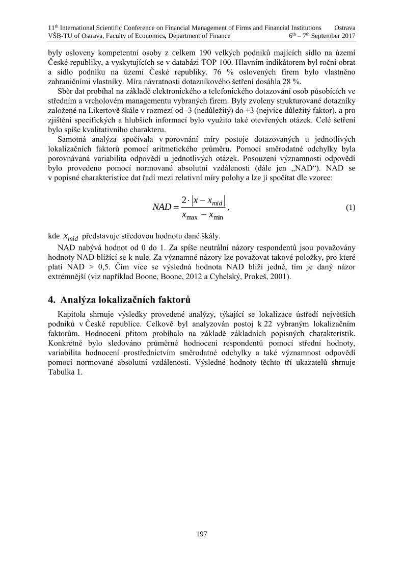
11th International Scientific Conference on Financial Management of Firms and Financial Institutions Ostrava
VŠB-TU of Ostrava, Faculty of Economics, Department of Finance 6th – 7th September 2017
197
byly osloveny kompetentní osoby z celkem 190 velkých podniků majících sídlo na území
České republiky, a vyskytujících se v databázi TOP 100. Hlavním indikátorem byl roční obrat
a sídlo podniku na území České republiky. 76 % oslovených firem bylo vlastněno
zahraničními vlastníky. Míra návratnosti dotazníkového šetření dosáhla 28 %.
Sběr dat probíhal na základě elektronického a telefonického dotazování osob působících ve
středním a vrcholovém managementu vybraných firem. Byly zvoleny strukturované dotazníky
založené na Likertově škále v rozmezí od -3 (nedůležitý) do +3 (nejvíce důležitý faktor), a pro
zjištění specifických a hlubších informací bylo využito také otevřených otázek. Celé šetření
bylo spíše kvalitativního charakteru.
Samotná analýza spočívala v porovnání míry postoje dotazovaných u jednotlivých
lokalizačních faktorů pomocí aritmetického průměru. Pomocí směrodatné odchylky byla
porovnávaná variabilita odpovědí u jednotlivých otázek. Posouzení významnosti odpovědí
bylo provedeno pomocí normované absolutní vzdálenosti (dále jen „NAD“). NAD se
v popisné charakteristice dat řadí mezi relativní míry polohy a lze ji spočítat dle vzorce:
minmax
2
xx
xxNAD
mid
, (1)
kde midx představuje středovou hodnotu dané škály.
NAD nabývá hodnot od 0 do 1. Za spíše neutrální názory respondentů jsou považovány
hodnoty NAD blížící se k nule. Za významné názory lze považovat takové položky, pro které
platí NAD > 0,5. Čím více se výsledná hodnota NAD blíží jedné, tím je daný názor
extrémnější (viz například Boone, Boone, 2012 a Cyhelský, Prokeš, 2001).
4. Analýza lokalizačních faktorů
Kapitola shrnuje výsledky provedené analýzy, týkající se lokalizace ústředí největších
podniků v České republice. Celkově byl analyzován postoj k 22 vybraným lokalizačním
faktorům. Hodnocení přitom probíhalo na základě základních popisných charakteristik.
Konkrétně bylo sledováno průměrné hodnocení respondentů pomocí střední hodnoty,
variabilita hodnocení prostřednictvím směrodatné odchylky a také významnost odpovědí
pomocí normované absolutní vzdálenosti. Výsledné hodnoty těchto tří ukazatelů shrnuje
Tabulka 1.

11th International Scientific Conference on Financial Management of Firms and Financial Institutions Ostrava
VŠB-TU of Ostrava, Faculty of Economics, Department of Finance 6th – 7th September 2017
198
Tabulka 1: Ústředí podniků – vybrané lokalizační faktory (N=190)
Zdroj: vlastní zpracování
Z dosažených výsledků je zřejmé, že z pohledu dosažených průměrných hodnot patří mezi
nejdůležitější lokalizační faktory infrastruktura, geografická poloha a kvalita podnikatelského
prostředí. Tyto položky se rovněž vyznačují relativní shodou názorů mezi jednotlivými
respondenty a vzhledem k hodnotám směrodatné odchylky lze názory na dané lokalizační
faktory považovat za relativně konzistentní.
Mezi lokalizační faktory, které díky poměrně vysoké střední hodnotě a díky významné
hodnotě NAD lze označit za podstatné při lokalizaci podniku, patří také blízkost dodavatelů,
dostupnost a množství pracovní síly, kvalita pracovní síly a blízkost zákazníků. Všechny tyto
faktory svým charakterem patří mezi tradiční tvrdé lokalizační faktory, jež v podniku přímo
působí na snižování nákladů a tím na dosahování vyššího zisku. Tvrdé lokalizační faktory se
stávají v nejrozvinutějších regionech světa obecně disponibilními, přístupnými a
homogenními, a proto relativně ztrácejí na svém výsadním významu pro prostorovou alokaci
ekonomických aktivit. Nicméně v České republice pořád sehrávají zásadní roli a měkké
lokalizační faktory (např. kvalita vzdělání, image regionu, volnočasová infrastruktura) jsou
stále málo nebo neodpovídajícím způsobem reflektovány.
Tento fakt je potvrzen i touto analýzou, konkrétně u faktorů kvalita životního prostředí či
volnočasová infrastruktura, které vykazují nízký ukazatel průměrné hodnoty i hodnoty NAD.
Stojí však za povšimnutí relativně silné postavení položky prestiž a pověst území, které je
v tomto případě věnována vyšší důležitost než například blízkosti konkurence, ceně pozemků
či celostátním politikám.
Dalším zajímavým prvkem je také poměrně velká důležitost lokalizačních faktorů
spojených s pracovní sílou, tedy s její dostupností, kvalitou, množstvím a také mzdovými
Lokalizační faktor Průměrná
hodnota
Směrodatná
odchylka NAD
Infrastruktura 2,32 0,644 0,773
Geografická poloha 2,15 0,690 0,717
Kvalita podnikatelského prostředí 1,77 0,577 0,590
Blízkost dodavatelů 1,58 1,046 0,527
Dostupnost a množství pracovní síly 1,57 0,821 0,523
Kvalita místní pracovní síly 1,56 0,998 0,520
Blízkost zákazníků 1,54 1,038 0,513
Aglomerační výhoda 1,49 0,973 0,497
Dostupnost nerostných surovin 1,32 1,504 0,440
Nízké mzdové požadavky 1,23 1,281 0,410
Blízkost a koncentrace příbuzných oborů 1,19 1,02 0,397
Prestiž a pověst území 1,19 0,786 0,397
Blízkost konkurence 1,17 1,051 0,390
Ochota manažerů ke stěhování 1,13 1,057 0,377
Blízkost decizních orgánů 1,13 1,093 0,377
Cena pozemků 1,02 0,909 0,340
Celostátní politiky 0,92 1,036 0,307
Systém veřejné správy 0,88 0,963 0,293
Kvalita životního prostředí 0,41 1,236 0,137
Dáno historicky 0,4 1,166 0,133
Možnosti kulturního vyžití -0,17 1,438 0,057
Možnosti sportovního vyžití -0,38 1,345 0,127

11th International Scientific Conference on Financial Management of Firms and Financial Institutions Ostrava
VŠB-TU of Ostrava, Faculty of Economics, Department of Finance 6th – 7th September 2017
199
požadavky. Je zřejmé, že pro podniky je velmi důležitá kvalifikovaná pracovní síla, nicméně
v rozporu s tím je přílišná akcentace nízkých mzdových požadavků, a naopak nízký zájem o
měkké lokalizační faktory. Je totiž zřejmé, že vysoká kvalita lidských zdrojů na sebe váže
požadavky v podobě nejen dobrých platových podmínek, ale také v podobě kvalitního
životního prostředí, kultury, vzdělávání apod.
Ve vazbě na nízké hodnoty u položek kulturního a sportovního vyžití, které byly zmíněny
v předchozích odstavcích, vzniká otázka, co stojí za nízkými hodnotami měkkých
lokalizačních faktorů. Nabízí se hypotéza loajality manažerů vůči svému podniku, kdy jsou
akceptovány tvrdé lokalizační faktory, a to navzdory tomu, že měkké lokalizační faktory jsou
pro ně v reálném životě důležité (Sucháček, 2015).
V rámci analýzy byla sledována také směrodatná odchylka jako ukazatel názorové shody
jednotlivých respondentů. Mezi lokalizační faktory s nejnižší variabilitou patří právě tradiční
tvrdé lokalizační faktory, které jsou současně nejvýznamnější při rozhodování o konečné
lokalizaci a potvrzují tak již výše zmíněný fakt, že tradičním lokalizačním faktorům přisuzují
podniky v České republice stále velký význam. U zbývajících lokalizačních faktorů se pak
směrodatná odchylka více méně pohybuje kolem hodnoty jedné. Největší variabilitou názorů
se pak vyznačují odpovědi u položek možnost kulturního a sportovního vyžití a dostupnost
nerostných surovin. Nicméně vzhledem k tomu, že dotazníkové šetření bylo prováděno napříč
různými obory, je vypovídací schopnost výsledků omezena na podniky s nejvyšším obratem.
5. Závěr
Rozhodování o lokalizaci se řadí mezi klíčové procesy v podniku, které následně ovlivňuje
prostorovou strukturu a rozložení dalších účastníků trhu. Základním prvkem lokalizační
analýzy je identifikace jednotlivých lokalizačních faktorů, a jejich následná interakce
s požadavky investorů a podniků na dané území.
Na základě dotazníkového šetření a následných propočtů bylo zjištěno, že lokalizace
ústředí velkých podniků na území České republiky je stále velmi ovlivněna klasickými
lokalizačními faktory, jako je infrastruktura, geografická poloha či kvalita podnikatelského
prostředí. U těchto tří faktorů byla zaznamenána také největší shoda názorů respondentů.
Zatímco zahraniční investoři vnímají nové faktory konkurenceschopnosti a jsou schopni
akcentovat tzv. měkké lokalizační faktory, podniky v České republice z různých důvodů tyto
faktory reflektují nedostatečně. To potvrzují také výsledné průměrné hodnoty či hodnoty NAD
u lokalizačních faktorů jako je kvalita životního prostředí, možnosti kulturního či sportovního
vyžití.
Poznámka
Tento článek vznikl za finanční podpory Studentské grantové soutěže EkF VŠB-TU Ostrava
v rámci projektu SP2017/76.
Literatura
[1] Aksoy, A. and Marshall, N. (1992). The Changing Corporate Head Office and Its Spatial
Implications. Regional Studies, 26(2), p. 149-162.
[2] Beníšková, T. a Urminský, J. (2015). Vybrané aspekty vztahu nabídky a poptávky v
lokalizačních analýzách. In: Klímová, V., Žítek, V. (eds.) XVIII. mezinárodní kolokvium
o regionálních vědách. Brno: Masarykova univerzita, pp. 89 - 95.
11th International Scientific Conference on Financial Management of Firms and Financial Institutions Ostrava
VŠB-TU of Ostrava, Faculty of Economics, Department of Finance 6th – 7th September 2017
200
[3] Boone, H.N. and Boone, D.A. (2012). Analyzing Likert Data. Journal of Extension,
50(2).
[4] Cyhelsky, L. a Prokes, R. (2001). Stevensova koncepce měření a z ní vyplývající
klasifikace proměnných. E+M Ekonomie a Management, Vol.4, pp. 57-61.
[5] Damborský, M., Wokoun, R. (2010). Lokalizační faktory malého a středního podnikání v
podmínkách ekonomiky ČR. E+M Ekonomie a Management, Vol. 2, pp. 32-43.
[6] Daníšek Matušková, P. (2016). Velké podniky a jejich ústředí a pobočky v České
republice. In: Klímová, V., Žítek, V. (eds.) XIX. mezinárodní kolokvium o regionálních
vědách. Brno: Masarykova univerzita, pp. 196 - 200.
[7] Dunning, J. H. and Lundan, S. M. (2008). Multinational Enterprises and the Global
Economy. Cheltenham: Edward Elgar Publishing.
[8] Lyons, D.I. (1994). Changing patterns of corporate headquarter influence 1974-89.
Environment and Planning A, Vol. 26, pp. 733-747.
[9] Maier, G., Tödtling, F. (1997). Regionálna a urbanistická ekonomika. Bratislava: Elita
[10] Sucháček, J. (2011). Globalization and Glocalization. In: The Scale of Globalization.
Think Globally, Act Locally, Change Individually in the 21st Century, Ostrava, 2011, pp.
319-324.
[11] Sucháček, J. (2013a). Urban Potential for Investment Attraction in the Czech Republic.
In: E. Jircikova, A. Knapkova and E. Pastuszkova eds. Finance and the Performance of
Firms in Science, Education, and Practice 2013. Zlin: Tomas Bata University, pp. 718-
727.
[12] Sucháček, J. (2013b). Investment Location from the Perspective of Urban and Regional
Activities in the Czech Republic. In: M. Čulík eds. Financial Management of Firms and
Financial Institutions 2013. Ostrava: VSB-Technical University, pp. 851-858.
[13] Suchacek, J. (2015). Large Enterprise Branches: The Case of the Czech Republic.
Economics and Sociology, 8(4), pp. 82-93.
[14] Sucháček, J. and Baránek, P. (2011). Headquarters of Largest Enterprises in the Czech
Republic from Regional Perspective. In: E. Jircikova, E. Pastuszkova and J. Svoboda eds.
Finance and the Performance of Firms in Science, Education, and Practice 2011. Zlin:
Tomas Bata University, pp. 469-478.
[15] Van Dijk, J. and Pellenbarg, P. (1999). The Demography of Firms: Progress and
Problems in Empirical Research. In: J., van Dijk and P., Pellenbarg eds. Demography of
firms. Spatial Dynamics of Firm Behaviour. Groningen: Rijksuniversiteit, pp. 325–337.

11th International Scientific Conference on Financial Management of Firms and Financial Institutions Ostrava
VŠB-TU of Ostrava, Faculty of Economics, Department of Finance 6th – 7th September 2017
201
Financial performance and bankruptcy risk of socially responsible and „irresponsible” companies
– the Polish case
Anna Doś 1
Abstract
Looking for relationships between firm financial performance and social performance is one of
top issues under investigation in the literature on CSR. When it comes to social performance –
financial performance correlation emerging economies are much less explored than well-
developed ones. This study contributes to the existing knowledge on social performance in the
firm’s financial context, where Polish responsible and „irresponsible” firms are compared.
Financial performance was analysed by focusing on ROE, ROA and ROS. Additionally the risk
of bankrupcy was examined basing at Z-score Altman‘s model. The effect of firm size was
examined too. It was found that there are no significant differencies between „responsible” and
„irresponsble” firm when it comes to ROE, ROS and Z-score. However there are significant
differences in ROA (responsible firms perform better) and total assets (bigger firms’ CSR
practices are ranked higher). It can be concluded, that firm size and firm operational efficiency
are drivers for CSR in Poland.
Key words
Corporate social responsibility, financial management, financial performance, corporate
sustainability,
JEL Classification: H0
1. Introduction
Contemporaneously companies often take responsibility for their impacts on society
beyond legal constraints. This means firms care for the society and the natural environment
along with focusing on maximising value for shareholders. Such business practices are named
as corporate social responsibility (CSR). Finding how corporate financial performance and
CSR are related is one of top issues investigated in modern financial literature. Most studies
try to find if engaging in corporate social responsibility helps to achieve better financial
results. Answering teh question is important to know if following social and environemntal
goals may foster achieving financial goals or contrary – cause financial distress. Authors adopt
diverse proxies for financial and social performance, choose diverse samples and statistical
tools. The results are mixed, however the positive relation between financial and social
performance are seen more often. Still the important knowledge gap exists, because studies
focus on highly developed Western countries or Asia. Poland and other CEE countries remain
largely underinvestigated when it comes to examine relationships between financial
performance and social responsibility. The main reason for this is scarce or unobtainable data.
This study aims at finding if there are differences between financial performance, bankrupcy
risk and firm size between Polish enterprises, which are considered as socially responsible
companies and firms, that are considered as socially irresponsible. The comparison between
1 Ana Doś, PhD, University of Economics in Katowice, [email protected].

11th International Scientific Conference on Financial Management of Firms and Financial Institutions Ostrava
VŠB-TU of Ostrava, Faculty of Economics, Department of Finance 6th – 7th September 2017
202
responsible and „irresponsible“ firms, which may make possible differences more
pronounced, is the first important contribution of the study. Previous studies focusing on
Poland compare responsible companies with companies seen as neutral ones in terms of social
responsibility. The second important contribution is including limited liability companies and
non-listed companies in the analysis. Previous studies focus solely on listed companies. The
third important contribution is comparing Altman Z-score togehter with most popular
financial performance metrics: ROE, ROA and ROS for Polish responsible and
„irresponsible“ companies. There are no studies, comapring bankrupcy risk of socially
responsible companies and otehrs. Altman Z-score is the most popular metrics for assessing
bankrupcy risk. Comparing Z-score of socially responsible firms and socially irresponsible
ones allows for finding if companies which face financial distress (increased risk of
bankrupcy) focus solely on improving financial results and consequenlty abandon social and
environmental goals. The effect of firm size is inlcuded in the analysis.
The method is statistical analysis of data obtained from CSR reports delivered by
independent think-thanks and from financial statements obtained from EMIS Intelligence
database. There is only one report on socially irresponsible firms in Poland. It was issued in
2015. Thereof it was the only year for which the comparative analysis between socially
responsible and socially irresponsible companies could be done.
2. The relationship between financial performance, bankrupcy risk
and social responsibility – literature review
The most widely accepted resoning for CSR is that the success of any business activity is
based on the society (providing workforce, technology, data, culture, administration etc.).
Than the consequences of business activity are widespreaded across society (products, risk,
wages, externalities, spillover effects etc.). Consequenlty companies are urged to take
responsibility for the society. Simultaneously under the CSR concept it is proclaimed that the
way any company is taking its responsibility for the society is comapny’s independent
decision [Matten, Moon 2008, p. 404-424].
From the financial point of view it is interesting how socially responsible activities are
correlated with financial management, which is traditionally seen as management oriented at
maxmimizing value for shareholders. Certainly socially responsible activities often come at a
cost (lowering pollution, reducing risk, paying fair wages etc.), which may deteriorate firm’s
competitive position. On the other hand being responsible can rewarded by the society
(increased loyalty of clients, more active workers, stable business relationship, low
reputational risk) which in turn may strneghten firm’s competitive position. It is crucial to find
if social goals and financial goals come togehter or are mutually exclusive, which makes
business choices much harder to make. The world literature reviewing existing studiens on
CSR and financial performance relationshio doesn’t bring any univocal conclusion [Peloza,
2011, s. 117-135; Malik 2015, s. 419-438]. Nevertheless examining the relationship remains
one of the main literature strands among CSR economics. One of the most impoirtant reasons
for this is that CSR and its results is highly depending on cultural settings. Argandoña and
Von Weltzien [2009] suggest that the content of CSR has evolved over time, depending on
historical, cultural, political, and socio-economic drivers and particular conditions in different
countries and also at different points in time. Therefore exploring new markets and making
cross-country comparisons may be considered as the future of CSR literature.
The novel perspective on relationsips between CSR and firms financial management is
seeing firm’s financial strenght as a condition for engaging in socially responsible activities.
Campbell [2007, s. 946-967] as a first stated that firms facing financial problems will engage

11th International Scientific Conference on Financial Management of Firms and Financial Institutions Ostrava
VŠB-TU of Ostrava, Faculty of Economics, Department of Finance 6th – 7th September 2017
203
in social responsibility to the lesser extent. Campbell [2007] didn’t provide any empirical
confirmation of his thesis. However, it seems to be a promising one since in terms of higher
bankrupcy risk key stakeholders naturally opt firstly for improving financial condition
(probably even sacrifying interestes of other stakeholders), because it is necessary for
comapny’s survival. Chan, Chou i Lon [2017, s. 241-259] empirically conformend
Campbell’s thesis. Their results confirm a significant negative association between CSR
activities and the degree of financial constraints/distress measured with both: KZ index and
Altman’s Z-score. From among financial variables that are seen as predictors for CSR firm
size is pointed as most important one [Brammer, Millington 2006]. There are two models
respresenting correlation between firm size and CSR: a linear positive relationship [Gallo,
Christensen 2011, s. 315-349] and reversed U-shaped relationship, where small and large
enterprises socially outperform middle size enterprises [Udayasankar 2008 s. 167-175]).
Therefore the effect of firm size should be included in the analysis of financial performance –
social performance relationships.
Most of studies examining relationship between financial performance and CSR compare
socially responsible companies with companies, that are seen as neutral in terms of social
responsibility. However, it is possible to compare the results of companies that are socially
responsible and companies, which cause explicit damages in society and natural environment
(socially „irresponsible“ companies). Such setting may help to demonstrate possible
differences in a more pronounced way. Stakeholder theory points, that harming business
social environement may negatively affect firm’s financial returns [Jensen 2001, s. 8-21]. It’s
been empirically confirmed that the market punishes socially irresponsible behavior [Frooman
1994]. However this not always the case. DeMaCarty [2009, s. 393-433] did a comprehensive
empirical literature review in the area. He found that the body of theory argues that CSR
produces higher returns which represents logically sound mechanisms for socially responsible
companies to contribute to strong financial success. However DeMaCarty [2009, s. 393-433]
noticed also that there are approaches that enable socially irresponsible firms to get high
returns. Consequently it is possible that average returns of socially responsible and socially
irresponsible firms would be equal.
To the author’s best knowledge the relationship between financial performance and
corporate social responsibility was empirically examined for Poland in five studies. Their
study design and methodology are presented in table 1.
Table 1: Studies covering relationship between corporate social responsibility and financial performance
among Polish companies. Study Companies
identifed as
socially responsible
Number of
firms analysed
Time scope
(number of
observations)
Financial
performance
metrics
Results
Bek-Gaik and
Rymkiewicz
(2014)
Companies
publishing
information about
their social
responsibility in
their annual reports
28 2001-2012 (233) ROE, ROA, P/BV,
DIV
No relationship
found
Bek-Gaik and
Rymkiewicz
(2015)
Companies
reporting corporate
social
responsibility
50 8 years (401) Net profit,
operational profit,
total assets, ROA,
ROE, ROS, EPS,
BV/S, LTL/E, LT/A
There is a weak
relationship
between CSR
reporting and net
proft and total
assets. No
relationshi between
CSR reporting and
other metrics.
Sobczyk Firsm indexed at No 2008-2014 (87) ROA, ROE, ROS, Indexing at WIG

11th International Scientific Conference on Financial Management of Firms and Financial Institutions Ostrava
VŠB-TU of Ostrava, Faculty of Economics, Department of Finance 6th – 7th September 2017
204
(2016) WIG RESPECT information,
approximately
13
EV, P/E, P/BV RESPECT is not
related with
financial
performance
Skrzypek and
Saadi (2016)
Firms reporting
CSR and/or
indexed at WIG
RESPECT during
at keast one year
36 resonsible
companies
compared to
otehr
companies
2009 - 2013 ROE, ROA, ROS
Responsible
companies have
higher ROS than
other big
companies in
Poland from 2010
to 2013 but not in
2009
Otola and
Tylec (2016)
Firms declaring
sepnding on CSR
58 companies
listed at
Warsaw Stock
Exchange
2013 - 2015 ROE, ROA, gross
margin
Increased financial
performance is not
translated into
increased spending
on CSR
Source: Own elaboration.
From the register presented in table 1 it can be concluded, that the relationship between
CSR and financial performance at Polish market was analyzed basing on similar samples. The
problem of possible negative social performance of Polish firm’s was not taken into
consideration yet. All analysis focus on listed companies. Therefore there are no studies,
which would focus on not listed companies and limited liability companies, which are
perceived as socially responsible (number of Polish companies covered in media for their
responsible practices are not listed companies). Only one study examined the effect of firm
size on CSR practices. Studies, which would examine how financial constraints affect Polish
firms responsibility, don’t exist. This knowledge gap was a direct inspiration for conducting
the study.
3. Study design
The study aims at comparing financial performance, bankrupcy risk and firm size of Polish
socially responsible and irresponsible companies. This requires choosing companies, which
would constitute the sample. Corporate social responsibility has become a poular and widely
discussed topic in Poland. Therefore there are many possible ways to identify responsible
companies: varying from choosing companies indexed at WIG RESPECT (Polish stock index
including only companies, that came under a detailed scrutiny for their responsibility),
companies reporting social responsibility and companies ranked highly for their CSR practices
by independent think thanks. In the study socially responsible companies were identified as
those, which are included in ranking published by Polish most prominent and independent
think thank – Forum Odpowiedzialnego Biznesu [2015]. For the purpose of the ranking not
only CSR reporting practices are evaluated, but also other ways that companies affect the
society. Consequenlty a more comprehensive picture of CSR quality is achieved. Socially
„irresponsible“ companies were identitied basing on the report prepared by other independent
think thank Centrum CSR [2015]. The report describes which Polish companies violate
commonly accepted rules and how they do it. The Centrum CSR report [2015] is the only
document reporting on irresponsible business practices that was published for Ponald.
Therefore comapring responsible and irresponsible companies is possible only for 2015.
It is justified to examine how CSR affects financial performance in short-term, because
previous studies found such relationship for other countries. Ruf et al. [2001] found that
change in corporate social performance was positively associated with growth in sales for
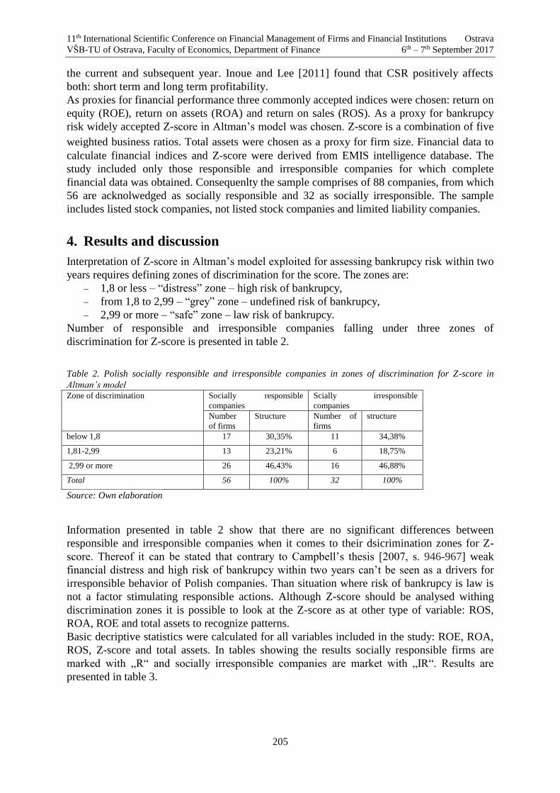
11th International Scientific Conference on Financial Management of Firms and Financial Institutions Ostrava
VŠB-TU of Ostrava, Faculty of Economics, Department of Finance 6th – 7th September 2017
205
the current and subsequent year. Inoue and Lee [2011] found that CSR positively affects
both: short term and long term profitability.
As proxies for financial performance three commonly accepted indices were chosen: return on
equity (ROE), return on assets (ROA) and return on sales (ROS). As a proxy for bankrupcy
risk widely accepted Z-score in Altman’s model was chosen. Z-score is a combination of five
weighted business ratios. Total assets were chosen as a proxy for firm size. Financial data to
calculate financial indices and Z-score were derived from EMIS intelligence database. The
study included only those responsible and irresponsible companies for which complete
financial data was obtained. Consequenlty the sample comprises of 88 companies, from which
56 are acknolwedged as socially responsible and 32 as socially irresponsible. The sample
includes listed stock companies, not listed stock companies and limited liability companies.
4. Results and discussion
Interpretation of Z-score in Altman’s model exploited for assessing bankrupcy risk within two
years requires defining zones of discrimination for the score. The zones are:
1,8 or less – “distress” zone – high risk of bankrupcy,
from 1,8 to 2,99 – “grey” zone – undefined risk of bankrupcy,
2,99 or more – “safe” zone – law risk of bankrupcy.
Number of responsible and irresponsible companies falling under three zones of
discrimination for Z-score is presented in table 2.
Table 2. Polish socially responsible and irresponsible companies in zones of discrimination for Z-score in
Altman’s model Zone of discrimination Socially responsible
companies
Scially irresponsible
companies
Number
of firms
Structure Number of
firms
structure
below 1,8 17 30,35% 11 34,38%
1,81-2,99 13 23,21% 6 18,75%
2,99 or more 26 46,43% 16 46,88%
Total 56 100% 32 100%
Source: Own elaboration
Information presented in table 2 show that there are no significant differences between
responsible and irresponsible companies when it comes to their dsicrimination zones for Z-
score. Thereof it can be stated that contrary to Campbell’s thesis [2007, s. 946-967] weak
financial distress and high risk of bankrupcy within two years can’t be seen as a drivers for
irresponsible behavior of Polish companies. Than situation where risk of bankrupcy is law is
not a factor stimulating responsible actions. Although Z-score should be analysed withing
discrimination zones it is possible to look at the Z-score as at other type of variable: ROS,
ROA, ROE and total assets to recognize patterns.
Basic decriptive statistics were calculated for all variables included in the study: ROE, ROA,
ROS, Z-score and total assets. In tables showing the results socially responsible firms are
marked with „R“ and socially irresponsible companies are market with „IR“. Results are
presented in table 3.
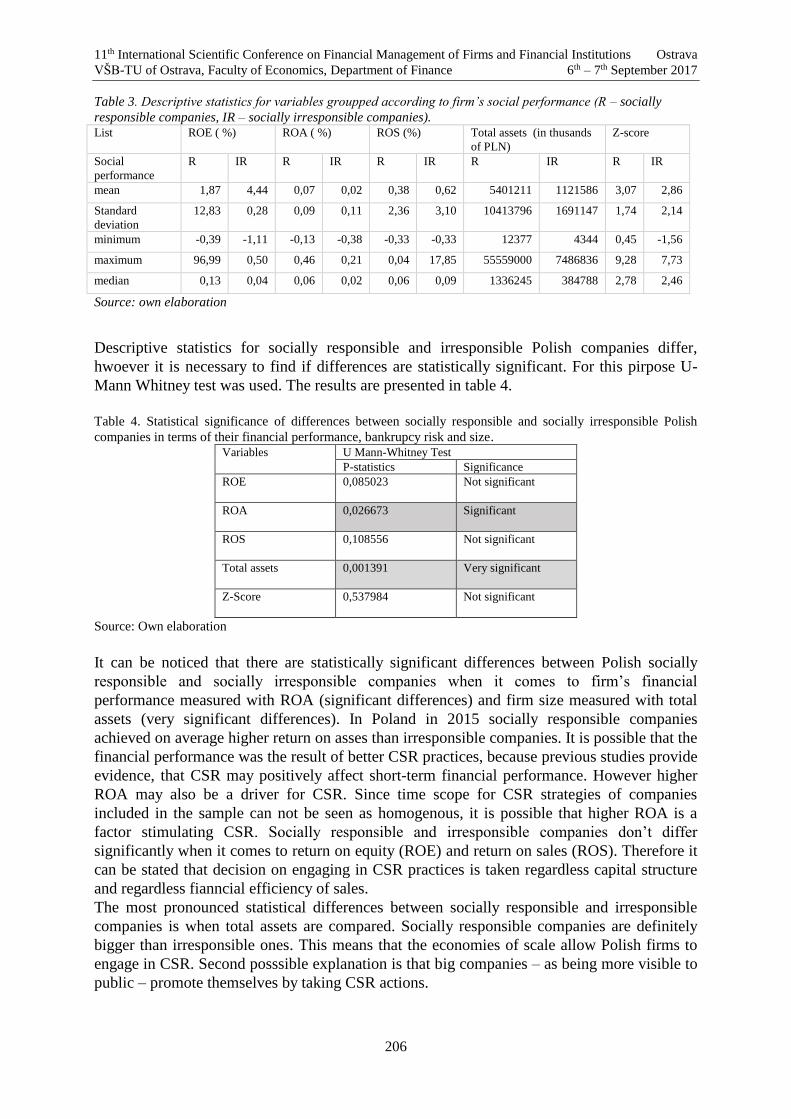
11th International Scientific Conference on Financial Management of Firms and Financial Institutions Ostrava
VŠB-TU of Ostrava, Faculty of Economics, Department of Finance 6th – 7th September 2017
206
Table 3. Descriptive statistics for variables groupped according to firm’s social performance (R – socially
responsible companies, IR – socially irresponsible companies). List ROE ( %) ROA ( %) ROS (%) Total assets (in thusands
of PLN)
Z-score
Social
performance
R IR R IR R IR R IR R IR
mean 1,87 4,44 0,07 0,02 0,38 0,62 5401211 1121586 3,07 2,86
Standard
deviation
12,83 0,28 0,09 0,11 2,36 3,10 10413796 1691147 1,74 2,14
minimum -0,39 -1,11 -0,13 -0,38 -0,33 -0,33 12377 4344 0,45 -1,56
maximum 96,99 0,50 0,46 0,21 0,04 17,85 55559000 7486836 9,28 7,73
median 0,13 0,04 0,06 0,02 0,06 0,09 1336245 384788 2,78 2,46
Source: own elaboration
Descriptive statistics for socially responsible and irresponsible Polish companies differ,
hwoever it is necessary to find if differences are statistically significant. For this pirpose U-
Mann Whitney test was used. The results are presented in table 4.
Table 4. Statistical significance of differences between socially responsible and socially irresponsible Polish
companies in terms of their financial performance, bankrupcy risk and size. Variables U Mann-Whitney Test
P-statistics Significance
ROE 0,085023
Not significant
ROA 0,026673
Significant
ROS 0,108556
Not significant
Total assets 0,001391
Very significant
Z-Score 0,537984
Not significant
Source: Own elaboration
It can be noticed that there are statistically significant differences between Polish socially
responsible and socially irresponsible companies when it comes to firm’s financial
performance measured with ROA (significant differences) and firm size measured with total
assets (very significant differences). In Poland in 2015 socially responsible companies
achieved on average higher return on asses than irresponsible companies. It is possible that the
financial performance was the result of better CSR practices, because previous studies provide
evidence, that CSR may positively affect short-term financial performance. However higher
ROA may also be a driver for CSR. Since time scope for CSR strategies of companies
included in the sample can not be seen as homogenous, it is possible that higher ROA is a
factor stimulating CSR. Socially responsible and irresponsible companies don’t differ
significantly when it comes to return on equity (ROE) and return on sales (ROS). Therefore it
can be stated that decision on engaging in CSR practices is taken regardless capital structure
and regardless fianncial efficiency of sales.
The most pronounced statistical differences between socially responsible and irresponsible
companies is when total assets are compared. Socially responsible companies are definitely
bigger than irresponsible ones. This means that the economies of scale allow Polish firms to
engage in CSR. Second posssible explanation is that big companies – as being more visible to
public – promote themselves by taking CSR actions.
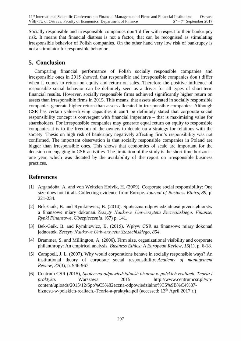
11th International Scientific Conference on Financial Management of Firms and Financial Institutions Ostrava
VŠB-TU of Ostrava, Faculty of Economics, Department of Finance 6th – 7th September 2017
207
Socially responsible and irresponsible companies don’t differ with respect to their bankrupcy
risk. It means that financial distress is not a factor, that can be recognised as stimulating
irresponsible behavior of Polish companies. On the other hand very low risk of bankrupcy is
not a stimulator for responsible behavior.
5. Conclusion
Comparing financial performance of Polish socially responsible companies and
irresponsible ones in 2015 showed, that responsible and irresponsible companies don’t differ
when it comes to return on equity and return on sales. Therefore the positive influence of
responsible social behavior can be definitely seen as a driver for all types of short-term
financial results. However, socially responsible firms achieved significantly higher return on
assets than irresponsible firms in 2015. This means, that assets alocated in socially responsible
companies generate higher return than assets allocated in irresponsible companies. Although
CSR has certain value-driving capacities it can‘t be definitely stated that corporate social
responsibility concept is convergent with financial imperiatve – that is maximising value for
shareholders. For irresponsible companies may generate equal return on equity to responsible
companies it is to the freedom of the owners to decide on a strategy for relations with the
society. Thesis on high risk of bankrupcy negatively affecting firm’s responsibility was not
confirmed. The important observation is that socially responsible companies in Poland are
bigger than irresponsible ones. This shows that economies of scale are important for the
decision on engaging in CSR activities. The limitation of the study is the short time horizon –
one year, which was dictated by the availability of the report on irresponsible business
practices.
References
[1] Argandoña, A. and von Weltzien Hoivik, H. (2009). Corporate social responsibility: One
size does not fit all. Collecting evidence from Europe. Journal of Business Ethics, 89, p.
221-234.
[2] Bek-Gaik, B. and Rymkiewicz, B. (2014). Społeczna odpowiedzialność przedsiębiorstw
a finansowe miary dokonań. Zeszyty Naukowe Uniwersytetu Szczecińskiego, Finanse,
Rynki Finansowe, Ubezpieczenia, (67) p. 141.
[3] Bek-Gaik, B. and Rymkiewicz, B. (2015). Wpływ CSR na finansowe miary dokonań
jednostek. Zeszyty Naukowe Uniwersytetu Szczecińskiego, 854.
[4] Brammer, S. and Millington, A. (2006). Firm size, organizational visibility and corporate
philanthropy: An empirical analysis. Business Ethics: A European Review, 15(1), p. 6-18.
[5] Campbell, J. L. (2007). Why would corporations behave in socially responsible ways? An
institutional theory of corporate social responsibility. Academy of management
Review, 32(3), p. 946-967.
[6] Centrum CSR (2015), Społeczna odpowiedzialność biznesu w polskich realiach. Teoria i
praktyka. Warszawa 2015. http://www.centrumcsr.pl/wp-
content/uploads/2015/12/Spo%C5%82eczna-odpowiedzialno%C5%9B%C4%87-
biznesu-w-polskich-realiach.-Teoria-a-praktyka.pdf (accessed: 13th April 2017 r.)

11th International Scientific Conference on Financial Management of Firms and Financial Institutions Ostrava
VŠB-TU of Ostrava, Faculty of Economics, Department of Finance 6th – 7th September 2017
208
[7] Chan, C. Y., Chou, D. W. and Lo, H. C. (2017). Do financial constraints matter when
firms engage in CSR?. The North American Journal of Economics and Finance, 39, p.
241-259.
[8] DeMaCarty, P. (2009). Financial returns of corporate social responsibility, and the moral
freedom and responsibility of business leaders. Business and Society Review, 114(3), p.
393-433.
[9] Forum Odpowiedzialnego Biznesu (2015), IX Ranking odpowiedzianych firm 2015.
„Dziennik Gazeta Prawna”, 22 kwietnia 2015.
[10] Frooman, J. S. (1994, July). Does the market penalize firms for socially irresponsible
behavior?. In Proceedings of the International Association for Business and Society (Vol.
5, p. 645-664).
[11] Gallo, P. J. and Christensen, L. J. (2011). Firm size matters: An empirical investigation
of organizational size and ownership on sustainability-related behaviors. Business &
Society, 50(2), p. 315-349.
[12] Inoue, Y. and Lee, S. (2011). Effects of different dimensions of corporate social
responsibility on corporate financial performance in tourism-related industries. Tourism
Management, 32(4), p. 790-804.
[13] Jensen, M. C. (2001). Value maximization, stakeholder theory, and the corporate
objective function. Journal of applied corporate finance, 14(3), 8-21.
[14] Malik, M. (2015). Value-enhancing capabilities of CSR: A brief review of contemporary
literature. Journal of Business Ethics, 127(2), p. 419-438.
[15] Matten, D. and Moon, J. (2008). “Implicit” and “explicit” CSR: A conceptual framework
for a comparative understanding of corporate social responsibility. Academy of
management Review, 33(2), p. 404-424.
[16] Otola, I. and Tylec, A. (2016). Społeczna odpowiedzialność biznesu a wyniki finansowe
przedsiębiorstw. Zeszyty Naukowe Politechniki Częstochowskiej. Zarządzanie, (24, t. 1),
p. 81-89.
[17] Peloza, J. and Shang, J. (2011). How can corporate social responsibility activities create
value for stakeholders? A systematic review. Journal of the academy of Marketing
Science, 39(1), p. 117-135.
[18] Ruf, B. M., Muralidhar, K., Brown, R. M., Janney, J. J. and Paul, K. (2001). An
empirical investigation of the relationship between change in corporate social
performance and financial performance: A stakeholder theory perspective. Journal of
business ethics, 32(2), p. 143-156.
[19] Skrzypek, A. and Saadi, N. (2016). Profitability of socially responsible public listed
companies in poland. Research Papers of the Wroclaw University of Economics/Prace
Naukowe Uniwersytetu Ekonomicznego we Wroclawiu, (423).
[20] Sobczyk, M. (2016). W poszukiwaniu wpływu dokonań CSR na wyniki finansowe.
„Prace Naukowe Uniwersytetu Ekonomicznego we Wrocławiu” 2016 (436).
[21] Udayasankar, K. (2008). Corporate social responsibility and firm size. Journal of
business ethics, 83(2), p. 167-175.

11th International Scientific Conference on Financial Management of Firms and Financial Institutions Ostrava
VŠB-TU of Ostrava, Faculty of Economics, Department of Finance 6th – 7th September 2017
209
On the Issue of Commercial Insurance and Commercial Insurance Market in the Slovak
Republik
Barbora Drugdová 1
Abstract
The insurance industry in the Slovak Republic has become an important dynamically
developing area of economy. Insurance interference with all the activities into the national
economy, touching every company, business, citizen, society and foreign countries. The Slovak
insurance market is developed. To 31.12.2016 worked on the Slovak commercial insurance
market 21 commercial insurance companies. The evolution of the market in life insurance in
recent years is more dynamic than in the non-life insurance.
Key words
insurance, commercial insurance market, life insurance, non-life insurance, indicators the
insurance market
JEL Classification: G02, G22, G23
1. Úvod
Poisťovníctvo, ako nevýrobné odvetvie má dôležitý význam v národnom hospodárstve
každej vyspelej a modernej ekonomiky. Poistenie, ako jeden zo spôsobov krytia prejavov
rizika, je súčasťou financií, a to financií všetkých subjektov národního hospodárstva. Pri
objasnení podstaty poistenia vychádzame z toho, že kľúčovými prvkami mechanizmu
fugovania poistenia sú: prenos rizika z jedného subjektu na společenstvo a spoločné znášanie
strát podľa vopred určených podmienok všetkými členmi tohoto společenstva.2
Poistenie a poisťovníctvo zasahujú priamo alebo nepriamo do všetkých oblastí ľudskej
činnosti, preto sa dotýkajú každej firmy, podniku, občana, spoločnosti aj zahraničia. Všetky
zmeny v spoločnosti sa určitým spôsobom odrážajú aj v poisťovacej činnosti. Rozvoj vedy,
techniky a kultúry prináša na trh nové moderné výrobky, nové činnosti a s tým aj nové riziká.
S týmito rizikami musia počítať a kalkulovať podniky a podnikatelia, občania, štát, ale aj
poisťovacie spoločnosti. Komerčné poisťovne musia preto stále pripravovať na poistný trh
nové poistné produkty a zároveň sledovať vývoj v celej ekonomike (napr. rast
nezamestnanosti, vývoj HDP, infláciu, rast cien, pohyb peňažných príjmov, demografické
údaje a pod.).
Slovenský poistný trh od 1. 5. 2004 je neoddeliteľnou súčasťou jednotného poistného trhu
Európskej únie. V praxi to znamená, že komerčné poisťovne všetkých členských štátov
Európskej únie majú možnosť vykonávať na území Slovenskej republiky poisťovaciu a
zaisťovaciu činnost. Platí to aj naopak – tuzemské poisťovne v Slovenskej republike môžu
ponúknuť svoje služby klientom v iných štátoch Európskej únie. V súvislosti so začlenením
do poistného trhu Európskej únie bolo potrebné prispôsobiť legislatívu Slovenskej republiky 1 Barbora Drugdová, Ing., PhD., Ekonomická unverzita v Bratislave, dolnozemská cesta č.1,
852 35 Bratislava, Slovenská republika, e-mail: barbora. [email protected] 2 VAUGHAN,E.J. – VAUGHAN, T.M. 2007,Fundamental of Risk and Insurance.New Jersey: John
Wlley and Sons, 2007, s. 34

11th International Scientific Conference on Financial Management of Firms and Financial Institutions Ostrava
VŠB-TU of Ostrava, Faculty of Economics, Department of Finance 6th – 7th September 2017
210
v oblasti poistenia, poisťovníctva a poistného trhu legislatíve Európskej únie, a to sa dotýkalo
životného aj neživotného poistenia. Posledný zákon, ktorý nadobudol účinnosť od 1.1. 2016
bol Zákon č.39/2015 Z. z. o poisťovníctve.
2. KOMERČNÝ POISTNÝ TRH A JEHO VYMEDZENIE
Poistný trh je miestom, na ktorom sa stretáva ponuka a dopyt po poistení. Poistenie je
špecifický tovar, ktorého podstatou je transfer rizika. Poistný trh funguje na základe trhových
princípov.3
V odbornej literatúre sa stretneme s niekoľkými definíciami a charakteristikami poistného
trhu.Uvedieme len niektoré, ktoré sú v českej, poľskej a slovenskej literatúre. Napríklad
v českej literatúre J. Daňhel uvádza: „Poistný trh má zhruba rovnaké rysy ako ktorýkoľvek iný
trh a pre hladké fungovanie stretu dopytu vstupujú medzi klientov a poisťovateľov tzv.
sprostredkovatelia“4. V. Čejková rozšírila definíciu o ďalší rozmer, keď použila vo svojej
monografii: „Poistný trh“ pri definovaní poistného trhu prirovnanie, že ide: „o živý a
rozvíjajúci sa organizmus, ktorý sa neustále mení a vyvíja“5. V poľskej literatúre A. Szromnik
definuje poistný trh nasledovne: „Poistný trh je priestor, kde sa stretáva ponuka a dopyt po
poistení. Stranu dopytu tvoria obyvatelia a podnikateľské subjekty, ktoré kúpou poistenia
prenášajú riziko na poisťovacie inštitúcie, ktoré predstavujú stranu ponuky“.6 V slovenskej
odbornej literatúre A. Majtánová uvádza: „ poistný trh je trhom, ktorý môžeme rozčleniť na
vecný poistný trh a investičný poistný trh“7.
Predmetom obchodu na poistnom trhu je poistenie a zaistenie. Poisťovníctvo, ako jedno z
dôležitých odvetví trhovej ekonomiky ponúka na poistnom trhu svoje služby, resp. poistenie a
zaistenie. Súčasťou poisťovníctva sú poisťovacie inštitúcie, poisťovne, poisťovne z iného
členského štátu, pobočky poisťovne z iného členského štátu, zahraničné poisťovne
a zaisťovne z iného členského štátu, sprostredkovatelia poistenia, dohľad v poisťovníctve,
asociácia poisťovní, kancelária poisťovateľov, inštitúcie zaoberajúce sa poistením popri svojej
hlavnej činnosti /banky, lízingové spoločnosti, autoservisy a pod./ a iné subjekty.
Na slovenskom komerčnom poistnom trhu podobne, ako v iných krajinách Európskej únie
a vo vyspelom svete v silne konkurenčnom prostredí sa o svojich zákazníkov – poistených,
uchádzajú komerčné poisťovne a ich sprostredkovatelia. Podobne, ako na iných trhoch je
predpokladom korektného súťaženia tvorba kvalitných poistných produktov a ich cenové
ohodnotenie.
Komerčný poistný trh, jeho rozsah, efektívnosť, význam z hľadiska národohospodárskeho je
možno charakterizovať viacerými ukazovateľmi. Medzi najčastejšie ukazovatele s ktorými sa
stretávame v odbornej literatúre patria: počet komerčných poisťovní, technické poistné, podiel
životného a neživotného poistenia na HDP, pomer životného a neživotného poistenia,
poistenosť, počet zamestnancov komerčných poisťovní (počet interných a externých
zamestnancov), ponuka poistných produktov a iné ukazovatele.
V nasledujúcej časti príspevku analyzujeme vybrané ukazovatele komerčného poistného trhu
za rok 2016.
3 MAJTÁNOVÁ, A.: Poistný trh. Bratislava: Elita, 1993, s. 11. ISBN 80-85323-32-X 4 DAŇHEL, J. a kol.: Pojistná teórie. Praha: Professional Publishing, 2005, s. 45. ISBN 80-86419-92-
0 5 ČEJKOVÁ,V.: Pojistný trh. Praha: GRADA, Publishing, s.r.o., 2002, s. 20. ISBN 80-247-0137-5 6 SZROMNIK, A.: Rynek ubezpieczeniowy. Krakov: Wydawnictwo Akademii Ekonomicznej
v Krakowie, 2001, 62 s. ISBN 83 – 7252 – 084 -4 7 MAJTÁNOVÁ, A.: Poistný trh. Bratislava: Elita, 1993, s. 11. ISBN 80-85323-32-X

11th International Scientific Conference on Financial Management of Firms and Financial Institutions Ostrava
VŠB-TU of Ostrava, Faculty of Economics, Department of Finance 6th – 7th September 2017
211
3. Analýza vybraných ukazovateľov komerčného poistného trhu
v Slovenskej republike za rok 2016
Na slovenskom poistnom trh pôsobilo v roku 2016 21 komerčných poisťovní, ktoré vytvorili
medzi sebou pomerne silné konkurenčné prostredie. Z celkového počtu poisťovní pôsobiacich
na slovenskom poistnom trhu bolo v Slovenskej asociácie poisťovní k 31.12. 2016 združených
21 komerčných poisťovní. Z členov asociácie malo 15 komerčných poisťovní univerzálnu
licenciu, životné poistenie poskytovalo 3 komerčných poisťovní a neživotné poistenie 3 komerčné
poisťovne. / Prameň: Interné materiály SAP, Bratislava 2017 /.
K najdôležitejším ukazovateľom komerčného poistného trhu patrí technické poistné.
Nasledujúca tabuľka č. 1 zobrazuje technické poistné k 31.12.2015 a k 31.12.2016 v tis. euro.
Uvádzame obidva roky, aby sme mohli porovnať vývoj tohto ukazovateľa poistného trhu.
Tab. č.1 Technické poistné k 31.12 2015 v tis. euro a k 31.12.2016.
Rok životné
poistenie
podiel neživotné
poistenie
podiel celkom
2015 1 208 481 54,25 % 1 019 218 45,75 % 2 227 700
2016 1 200 465 52,41 % 1 089 734 47,58 % 2 290 199
Zdroj: Interné materiály, SAP, Bratislava 2012
Porovnáváme rok 2015 a 2016. Celkové technické poistné k 31.12.2015 dosiahlo výšku
2 227 700 tis. euro. Z toho technické poistné životného poistenia predstavovalo 1 208 481
tis. euro a technické poistné neživotného poistenia 1 019 218 tis. euro. K 31.12. 2016 celkové
technické poistné dosiahlo výšku 2 290 199 tis. euro. Z toho technické poistné životného
poistenia predstavovalo 1 200 465 tis. euro a technické poistné neživotného poistenia bolo
1 089 734 tis. euro. Ak porovnáme obidva roky zistíme, že v roku 2016 je pokles technického
poistného v životnom poistení, a nárast technického poistného v neživotnom poistení, oproti
roku 2015.
Podiel životného poistenia na celkovom technickom poistnom v roku 2015 bol 54,25 %
a v roku 2016 bol 52, 41 % - bol mierny pokles v porovnaní s predchádzajúcim rokom.
Podiel neživotného poistenia na celkovom technickom poistnom v roku 2015 bol 45,75 %
a v roku 2016 bol 47,58 % - bol mierny nárast v porovnaní s predchádzajúcim rokom.
Pomer životného poistenia a neživotného poistenia v roku 2015 bol 54,25 : 45,75 a v roku
2016 bol 52,41 : 47,58 - bol v prospech životného poistenia.
Nasledujúca tabuľka č. 2 zobrazuje technické poistné v životnom a neživotnom poistení
k 31.12.2016 v tis. euro a zastúpenie jednotlivých komerčných poisťovní na celkovom
technickom poistnom.
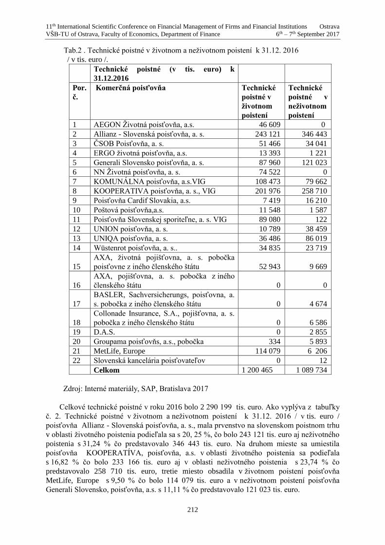
11th International Scientific Conference on Financial Management of Firms and Financial Institutions Ostrava
VŠB-TU of Ostrava, Faculty of Economics, Department of Finance 6th – 7th September 2017
212
Tab.2 . Technické poistné v životnom a neživotnom poistení k 31.12. 2016
/ v tis. euro /.
Technické poistné (v tis. euro) k
31.12.2016
Por.
č.
Komerčná poisťovňa Technické
poistné v
životnom
poistení
Technické
poistné v
neživotnom
poistení
1 AEGON Životná poisťovňa, a.s. 46 609 0
2 Allianz - Slovenská poisťovňa, a. s. 243 121 346 443
3 ČSOB Poisťovňa, a. s. 51 466 34 041
4 ERGO životná poisťovňa, a.s. 13 393 1 221
5 Generali Slovensko poisťovňa, a. s. 87 960 121 023
6 NN Životná poisťovňa, a. s. 74 522 0
7 KOMUNÁLNA poisťovňa, a.s.VIG 108 473 79 662
8 KOOPERATIVA poisťovňa, a. s., VIG 201 976 258 710
9 Poisťovňa Cardif Slovakia, a.s. 7 419 16 210
10 Poštová poisťovňa,a.s. 11 548 1 587
11 Poisťovňa Slovenskej sporiteľne, a. s. VIG 89 080 122
12 UNION poisťovňa, a. s. 10 789 38 459
13 UNIQA poisťovňa, a. s. 36 486 86 019
14 Wüstenrot poisťovňa, a. s.. 34 835 23 719
15
AXA, životná pojišťovna, a. s. pobočka
poisťovne z iného členského štátu 52 943 9 669
16
AXA, pojišťovna, a. s. pobočka z iného
členského štátu 0 0
17
BASLER, Sachversicherungs, poisťovna, a.
s. pobočka z iného členského štátu 0 4 674
18
Collonade Insurance, S.A., pojišťovna, a. s.
pobočka z iného členského štátu 0 6 586
19 D.A.S. 0 2 855
20 Groupama poisťovňs, a.s., pobočka 334 5 893
21 MetLife, Europe 114 079 6 206
22 Slovenská kancelária poisťovateľov 0 12
Celkom 1 200 465 1 089 734
Zdroj: Interné materiály, SAP, Bratislava 2017
Celkové technické poistné v roku 2016 bolo 2 290 199 tis. euro. Ako vyplýva z tabuľky
č. 2. Technické poistné v životnom a neživotnom poistení k 31.12. 2016 / v tis. euro /
poisťovňa Allianz - Slovenská poisťovňa, a. s., mala prvenstvo na slovenskom poistnom trhu
v oblasti životného poistenia podieľala sa s 20, 25 %, čo bolo 243 121 tis. euro aj neživotného
poistenia s 31,24 % čo predstavovalo 346 443 tis. euro. Na druhom mieste sa umiestila
poisťovňa KOOPERATÍVA, poisťovňa, a.s. v oblasti životného poistenia sa podieľala
s 16,82 % čo bolo 233 166 tis. euro aj v oblasti neživotného poistenia s 23,74 % čo
predstavovalo 258 710 tis. euro, tretie miesto obsadila v životnom poistení poisťovňa
MetLife, Europe s 9,50 % čo bolo 114 079 tis. euro a v neživotnom poistení poisťovňa
Generali Slovensko, poisťovňa, a.s. s 11,11 % čo predstavovalo 121 023 tis. euro.
11th International Scientific Conference on Financial Management of Firms and Financial Institutions Ostrava
VŠB-TU of Ostrava, Faculty of Economics, Department of Finance 6th – 7th September 2017
213
4. Záver
Záverom možno konštatovať, že vývoj komerčného poistného trhu v oblasti životného
poistenia je v posledných rokoch dynamickejší ako v neživotnom poistení. Podiel neživotného
poistenia v tomto roku predstavoval 47,58 % z celkového technického poistného. Pomer
životného a neživotného poistenia v roku 2016 bol 52,42 : 45,58. Slovenská republika sa
postupne približuje poistnému trhu európskeho priemeru, ktorý prestavuje zhruba 66 % v
prospech životného poistenia za rok 2016. Obyvateľstvo si postupne začína intenzívnejšie
uvedomovať životné riziká a využíva poistné produkty v oblasti životného poistenia, ktorých
ponuka prostredníctvom komerčných poisťovní na slovenskom komerčnom poistnom trhu je
flexibilná.
Acknowledgments
This paper was created on the basis of the financial support of the grant project VEGA
Ministry of Education of the Slovak Republic, no. of project 1/0236/15.
References
[1] Daňhel, J. a kol.(2005). Pojistná teórie. Praha: PROFESIONAL PUBLISHING.
[2] Čejková,V. (2002). Pojistný trh. Praha: GRADA, Publishing, s.r.o..
[3] Drugdová, B. (1995). POISTENIE A POISŤOVNÍCTVO, nemecko-slovenský
a slovensko nemecký slovník. Bratislava: ELITA.
[4] Drugdová, B. (2015). Neživotné poistenie v teórii a praxi. Bratislava: ŠEVT.
[5] Pastoráková, E., Veselovská, S., Drugdová, B. (2006). Vybrané problémy poistného a
zaistného trhu. Bratislava: Vydavateľstvo EKONÓM.
[6] Korauś, A. (2005). Bankopoisťovníctvo. Bratislava: SPRINT.
[7] Majtánová, A. (1993). Poistný trh. Bratislava: Elita, 1993.
[8] Sivák, R. a kol. (2009). Riziko a neistota vo financiách. / vybrané problémy/. Bratislava:
EKONÓM.
[9] Sivák, R. a kol. (2015). :FINANCIE. Bratislava: Wolters Kluwer.
[10] Szromnik, (2001). A. Rynek ubezpieczeniowy. Krakov: Wydawnictwo Akademii
Ekonomicznej v Krakowie.
[11] Vaughan,E.J. – Vaughan, T.M. (2007). Fundamental of Risk and Insurance. New Jersey:
John Wlley and Sons.
11th International Scientific Conference on Financial Management of Firms and Financial Institutions Ostrava
VŠB-TU of Ostrava, Faculty of Economics, Department of Finance 6th – 7th September 2017
214
MDA vs. Logit bankruptcy models in the Slovak Republic
Marek Durica1, Katarina Zvarikova2
Abstract
The issue of company financial distress and the early prediction of potential bankruptcy is one
of the most discussed issues of economists around the world in recent decades. The most
widely used method to create these models is Multidimensional Discrimination Analysis and
Logistic Regression from the first attempts in the 1960s to the present. In this paper, we focus
on comparing the prediction ability of the existing MDA bankruptcy models and the LOGIT
bankruptcy models created in various economic conditions as well as in the conditions of the
Slovak Republic. We analyze the most used models from foreign countries and also from
Slovakia and surrounding countries (V4 countries). We compare the accuracy of their
prediction of financial distress for several selected companies using real data from last years.
Key words
Financial distress, Bankruptcy prediction models, Multivariate discriminant analysis, LOGIT
model.
JEL Classification: C38, G33
1. Úvod
So zlyhávaním podnikov sa v dnešnej trhovej ekonomike stretávame stále častejšie.
Zlyhanie podniku má negatívny vplyv na všetky subjekty vstupujúce do ekonomických
vzťahov s daným podnikom. Analyzovať úverové riziko a predikovať finančnú situáciu
podniku je teda užitočné nielen pre veriteľov, ale tiež pre investorov a vlastníkov podniku,
manažment podniku alebo aj jeho zamestnancov. Na základe predpovedania finančných
ťažkostí podniku môže podnik včas prijať potrebné nápravné opatrenia. Bankrotné modely
dokážu s určitým časovým predstihom predikovať pravdepodobný úpadok podniku. Nakoľko
táto predikcia je pre každý podnik veľmi potrebná, zaoberajú sa ekonómovia na celom svete
už dlhšie obdobie tvorbou predikčných modelov, ktoré dokážu indikovať hroziace finančné
problémy podniku. V období posledných desaťročí a najmä posledných rokov bolo vytvorené
veľké množstvo bankrotných modelov, aplikovateľných najlepšie v podmienkach danej
krajiny, prípadne daného odvetvia hospodárstva, pre ktoré boli vytvorené. Väčšina
bankrotných modelov vznikla v USA, a teda bola vyvinutá pre americké podniky, avšak
bankrotné modely vznikali aj v iných krajinách po celom svete. (Cisko and Kliestik, 2013)
V Slovenskej republike skonštruovali bankrotné modely viacerí autori, napr. Chrastinová
v roku 1998, Binkert v roku 2000, Gurčík v roku 2002, Hurtošová v roku 2009, Gulka v roku
2016. (Kliestikova, Misankova and Kliestik, 2017) V ostatných krajinách V4 boli navrhnuté 1 RNDr. Marek Durica, PhD., University of Zilina, Faculty of Operation and Economics of Transport
and Communications, Department of Quantitative Methods and Economic Informatics, Univerzitna 1,
010 26 Zilina, Slovak republic, email: [email protected] 2 RNDr. Katarina Zvarikova, PhD., University of Zilina, Faculty of Operation and Economics of
Transport and Communications, Department of Economics, Univerzitna 1, 010 26 Zilina, Slovak
republic, email: [email protected]
11th International Scientific Conference on Financial Management of Firms and Financial Institutions Ostrava
VŠB-TU of Ostrava, Faculty of Economics, Department of Finance 6th – 7th September 2017
215
viaceré bankrotné modely. Autormi sú napr. Virág a Hajdu v Maďarsku v roku 1996;
Poznański v Poľsku v roku 2004, v Českej republike Neumaierová a Neumaier v rokoch
1995, 1999, 2001 a 2005 a tiež Jakubík a Teplý v roku 2006. (Kliestik, Misankova and
Adamko, 2014)
Predikčné modely sú vytvárané najmä použitím rôznych viacrozmerných štatistických
metód. Dodnes je jednou z najčastejšie využívaných metód predikcie bankrotu metóda
viacrozmernej diskriminačnej analýzy (MDA). Pomocou metódy MDA je vytvorená
diskriminačná funkcia ako lineárna kombinácia hodnôt finančných pomerových
ukazovateľov, pričom sú stanovené hraničné hodnoty tejto funkcie, pre ktoré už považujeme
podnik za neprosperujúci. Je však možné, že dosiahneme zaradenie podniku len do tzv. šedej
zóny, čo je oblasť, pri ktorej nie je možné rozhodnúť, či podnik patrí medzi prosperujúce,
alebo mu v budúcnosti hrozia finančné problémy. Cieľom tejto metódy je teda čo
najpresnejšie zaradiť analyzované podniky buď do skupiny prosperujúcich alebo
neprosperujúcich podnikov na základe poznania hodnôt finančných pomerových
ukazovateľov podniku. Predikčná schopnosť modelu je vyhodnotená na základe pomeru
správne zaradených podnikov. (Svabova and Kral, 2016)
Ďalšou často využívanou metódou pre tvorbu predikčných modelov je metóda logistickej
regresie (tzv. LOGIT modely). Cieľom aplikácie LOGIT modelu je prostredníctvom
logistického regresného modelu predikovať pravdepodobnosť, s ktorou patrí podnik do
skupiny podnikov ohrozených bankrotom. V poslednom období sa pri tvorbe predikčných
modelov často využívajú aj ďalšie moderné metódy, ako napríklad metóda neurónových sietí,
metóda rozhodovacích stromov alebo genetické algoritmy prípadne ich kombinácie. (Kliestik,
Kocisova and Misankova, 2015)
Pri aplikácií bankrotných modelov je najdôležitejšou úlohou výber tých modelov, ktoré by
čo najlepšie predpovedali možný úpadok analyzovaného podniku v daných podmienkach, teda
priniesli presné a spoľahlivé výsledky. V článku sa teda zameriavame na niekoľko vybraných
amerických modelov, ale najmä modelov vytvorených v krajinách V4 v období posledných
desaťročí. Analyzujeme ich predikčnú schopnosť na vzorke reálnych údajov vybraných
slovenských podnikov a predikčnú schopnosť MDA modelov porovnávame s predikčnou
schopnosťou LOGIT modelov.
2. Metodológia a dáta
Na Slovensku, ale aj v iných krajinách, sú bežne používané predikčné modely vytvorené
v iných ekonomických podmienkach. Stále sa používajú napr. Altmanov a Ohlsonov model,
ktoré vznikli podmienkach USA pre niekoľkými desaťročiami. Omnoho efektívnejšie je však
používanie lokálnych modelov odzrkadľujúcich lokálne ekonomické podmienky. My sme sa
zamerali na komparáciu predikčnej schopnosti bežne používaných MDA vs. LOGIT
bankrotných modelov v reálnych podmienkach SR. Zvolili sme 9 bankrotných modelov
vytvorených v krajinách V4. Ide o modely: Poznańskeho, Virágov-HajduovMDA, Virágov-
HajduovLOGIT, Jakubíkov-Teplého, Chrastinovej, Binkertov, Gurčíkov, Hurtošovej a Gulkov
model. Pre úplnosť sme do analýzy zahrnuli aj dodnes bežne používané modely vytvorené
v podmienkach USA už pred niekoľkými desaťročiami a to Altmanov MDA model v roku
1983 a tiež Ohlsonov LOGIT model z roku 1980. V Tabuľke 1 je uvedené delenie použitých
modelov podľa spôsobu ich konštrukcie a tiež roky a krajiny vzniku týchto modelov.

11th International Scientific Conference on Financial Management of Firms and Financial Institutions Ostrava
VŠB-TU of Ostrava, Faculty of Economics, Department of Finance 6th – 7th September 2017
216
Tabuľka 1: Prehľad analyzovaných bankrotných modelov
MDA modely LOGIT modely
Altman – 1983, USA Ohlson – 1980, USA
Poznański – 2014, Poľsko Jakubík-Teplý – 2004, Česká republika
Virág-HajduMDA – 1996, Maďarsko Virág-HajduLOGIT – 1996, Maďarsko
Chrastinová – 1998, Slovensko Hurtošová – 2009, Slovensko
Binkert – 2000, Slovensko Gulka – 2016, Slovensko
Gurčík – 2002, Slovensko
Altmanov Z-score model vychádzajúci z MDA je pravdepodobne stále jedným
z najpoužívanejších bankrotných modelov a to nielen na Slovensku. Pôvodný model z roku
1968 pracuje s 5 finančnými ukazovateľmi, z pôvodných 22 a bol vyvinutý pre podniky
kótované na burze. V podmienkach slovenskej ekonomiky je potrebné používať modifikáciu
z roku 1983 pre podniky, ktoré neboli kótované na burze. (Kliestik and Majerova, 2015)
Ohlson je jedným z prvých autorov, ktorí použili pri konštrukcii bankrotného modelu,
namiesto MDA, logistickú regresiu. Ohlsonov O-score model, ktorý pracuje s 9 pomerovými
ukazovateľmi, vykazuje predikčnú schopnosť až 96%. (Adamko and Svabova, 2016)
Poznańskeho model bol publikovaný v roku 2004. Bol vytvorený analyzovaním 100
poľských obchodných spoločností v rokoch 1999-2002. Je založený na 4 pomerových
ukazovateľoch. Pri konštrukcii bola použitá metóda MDA a predikčná presnosť tohto modelu
je 92,98%. (Svabova and Kral, 2016)
Maďarský bankrotný model zostrojili Virág a Hajdu v roku 1996 a to na základe databázy
154 podnikov (77 bankrotujúcich a 77 nebankrotujúcich) z údajov z rokov 1990 až 1991.
Autori vytvorili model s použitím MDA a aj logistickej regresie. (Kliestikova and Misankova,
2016)
V rokoch 1993 až 2004 Petr Jakubík a Petr Teplý analyzovali vzorku 757 českých
podnikov (606 prosperujúcich a 151 neprosperujúcich). Vytvorili bankrotný model, tzv. JT
index, s použitím logistickej regresie (LOGIT analýzy). Model pracuje so 7 pomerovými
ukazovateľmi. Autori uvádzajú predikčnú presnosť JT indexu 80,41%. Model bol v roku 2006
Českou národnou bankou zaradený do jej kvantitatívneho aparátu na vyhodnocovanie
finančnej stability nefinančných sektorov. (Jakubík and Teplý, 2011)
Model označovaný ako CH-index je prvý slovenský model publikovaný v roku 1998
Zuzanou Chrastinovou. Autorka pri jeho konštrukcii použila MDA a testovanie prebehlo na
vzorke 1 123 podnikov. CH-index zohľadňoval špecifiká poľnohospodárskych podnikov a bol
prvou metódou analýzy ex-ante v podmienkach SR orientovanou na konkrétne odvetvie,
poľnohospodárstvo. (Chrastinová, 1998)
Christian Binkert pri konštrukcii použil údaje zo slovenských (80 prosperujúcich a 80
neprosperujúcich) akciových spoločností z rôznych odborov. Čerpal údaje z účtovných
závierok, vždy za tri za sebou nasledujúce účtovné obdobia. Za pomoci MDA vyvinul modely
s 8 ukazovateľmi, z pôvodných 72 ukazovateľov. (Majerova, Kliestik and Misankova, 2015)
S cieľom rozlišovať podniky poľnohospodárskej prvovýroby na prosperujúce
a neprosperujúce zostrojil za pomoci MDA Ľubomír Gurčík svoj G-index. Na základe
náhodného výberu 60 slovenských podnikov skonštruoval model s 5 ukazovateľmi,
z pôvodných 35. (Gurčík, 2002)
Na základe údajov z reálneho bankového portfólia neidentifikovanej slovenskej komerčnej
banky vyvinula v roku 2009 svoj model Jana Hurtošová. Analyzovanú vzorku tvorilo 427
podnikateľských subjektov, z toho 94 bankrotujúcich a 333 zdravých. Pri aplikovaní
logistickej regresie skonštruovala model schopný predpovedať zlyhanie podnikateľského
subjektu rok dopredu so 4 ukazovateľmi, z pôvodných 126. (Siekelova, et al., 2017)

11th International Scientific Conference on Financial Management of Firms and Financial Institutions Ostrava
VŠB-TU of Ostrava, Faculty of Economics, Department of Finance 6th – 7th September 2017
217
V roku 2016 bola udelená cena guvernéra Národnej banky Slovenska Martinovi Gulkovi,
ktorý vyvinul bankrotný model s použitím logistickej regresie. Analyzoval vzorku 120 854
obchodných spoločností podnikajúcich v SR (120 252 obchodné spoločnosti, voči ktorým
nebolo začaté konkurzné konanie a 602, voči ktorým bolo začaté konkurzné konanie). Model
obsahuje 7 ukazovateľov, z pôvodných 25 a je schopný predpovedať default podniku rok
dopredu. (Gulka, 2016)
Budeme teda analyzovať predikčnú schopnosť 11 bankrotných modelov. Na komparáciu
predikčnej schopnosti MDA vs. LOGIT modelov máme k dispozícii 6 modelov
skonštruovaných MDA metódou a 5 bankrotných LOGIT modelov, pri konštrukcii ktorých
bola použitá metóda logistickej regresie.
Predikčná schopnosť v podmienkach SR bola overovaná na vzorke vybraných 10
podnikov, a to 5 neprosperujúcich a 5 prosperujúcich. Každá dvojica podnikov
(1 prosperujúci a 1 neprosperujúci) má rovnaké SK NACE, rovnakú právnu formu a rovnakú
veľkostnú kategóriu účtovnej jednotky. Podnik sme označili za neprosperujúci na základe
aktuálne platnej legislatívy.
Analyzovali sme reálne údaje získané z účtovných závierok vybraných spoločností.
Zdrojom informácií boli riadne účtovné závierky získane z Registra účtovných závierok
informačného systému verejnej správy SR. Jednalo sa o súvahy a výkazy ziskov a strát z
rokov 2013, 2014 a 2015.
Následne sme pre každý podnik vypočítali hodnoty všetkých finančných pomerových
ukazovateľov potrebných pre dosadenie do analyzovaných modelov. Tieto hodnoty boli pre
každý podnik a pre každý model dosadené do príslušných diskriminačných resp. logit funkcií.
Výsledky sú potom porovnávané s hraničnými hodnotami a následne je formulované
rozhodnutie o tom, či daný model považuje daný podnik za prosperujúci alebo nie. Kvalitu
modelov posudzujeme podľa počtu správne identifikovaných podnikov.
3. Výsledky analýz
Do analýzy bolo zahrnutých 5 neprosperujúcich a 5 prosperujúcich podnikov. Úpadok
neprosperujúcich spoločností potvrdila aj finančná analýza ex-post. V prípade týchto
spoločností hodnota záväzkov v sledovaných rokoch prevyšovala hodnotu majetku, koeficient
finančnej samostatnosti nadobúdal záporné hodnoty vo všetkých prípadoch a išlo o nelikvidné
podniky. K týmto neprosperujúcim podnikom bolo do analýzy zahrnutých 5 prosperujúcich
(zdravých) podnikov. S sledovanom období išlo o likvidné podniky, ktorým nehrozil úpadok.
Hodnota ich majetku prevyšovala hodnotu záväzkov. Išlo teda o finančne samostatné podniky.
Finančné pomerové ukazovatele všetkých podnikov boli dosadené do vybraných modelov.
Kompletné výsledky predikcie finančných ťažkostí prostredníctvom vybraných modelov sú
zhrnuté v Tabuľke 2. Symbolom N sú označené podniky, ktoré boli modelom identifikované
ako neprosperujúce. Predikcia prosperity podniku je označená symbolom P. MDA modely
niektoré podniky označili za priemerné resp. nachádzajúce sa v tzv. šedej zóne (označenie
GZ). Výsledky niektorých modelov pre niektoré podniky nebolo možné vypočítať (označenie
NaN) kvôli deleniu nulou.
Tabuľka 2: Výsledné predikcie analyzovaných bankrotných modelov
Model Neprosperujúce spoločnosti Prosperujúce spoločnosti
1 2 3 4 5 1 2 3 4 5
Altman GZ GZ N P GZ P P P P GZ
Ohlson N N N N N P P P P P
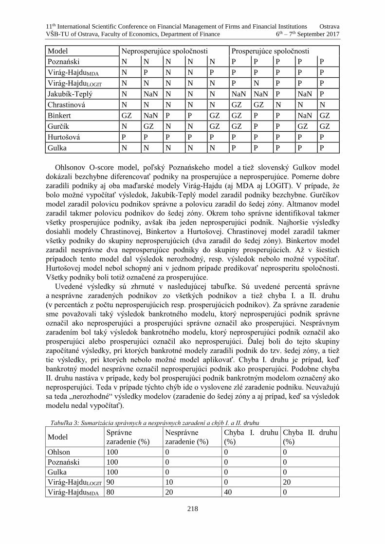
11th International Scientific Conference on Financial Management of Firms and Financial Institutions Ostrava
VŠB-TU of Ostrava, Faculty of Economics, Department of Finance 6th – 7th September 2017
218
Model Neprosperujúce spoločnosti Prosperujúce spoločnosti
Poznański N N N N N P P P P P
Virág-HajduMDA N P N N P P P P P P
Virág-HajduLOGIT N N N N N P N P P P
Jakubík-Teplý N NaN N N N NaN NaN P NaN P
Chrastinová N N N N N GZ GZ N N N
Binkert GZ NaN P P GZ GZ P P NaN GZ
Gurčík N GZ N N GZ GZ P P GZ GZ
Hurtošová P P P P P P P P P P
Gulka N N N N N P P P P P
Ohlsonov O-score model, poľský Poznańskeho model a tiež slovenský Gulkov model
dokázali bezchybne diferencovať podniky na prosperujúce a neprosperujúce. Pomerne dobre
zaradili podniky aj oba maďarské modely Virág-Hajdu (aj MDA aj LOGIT). V prípade, že
bolo možné vypočítať výsledok, Jakubík-Teplý model zaradil podniky bezchybne. Gurčíkov
model zaradil polovicu podnikov správne a polovicu zaradil do šedej zóny. Altmanov model
zaradil takmer polovicu podnikov do šedej zóny. Okrem toho správne identifikoval takmer
všetky prosperujúce podniky, avšak iba jeden neprosperujúci podnik. Najhoršie výsledky
dosiahli modely Chrastinovej, Binkertov a Hurtošovej. Chrastinovej model zaradil takmer
všetky podniky do skupiny neprosperujúcich (dva zaradil do šedej zóny). Binkertov model
zaradil nesprávne dva neprosperujúce podniky do skupiny prosperujúcich. Až v šiestich
prípadoch tento model dal výsledok nerozhodný, resp. výsledok nebolo možné vypočítať.
Hurtošovej model nebol schopný ani v jednom prípade predikovať neprosperitu spoločnosti.
Všetky podniky boli totiž označené za prosperujúce.
Uvedené výsledky sú zhrnuté v nasledujúcej tabuľke. Sú uvedené percentá správne
a nesprávne zaradených podnikov zo všetkých podnikov a tiež chyba I. a II. druhu
(v percentách z počtu neprosperujúcich resp. prosperujúcich podnikov). Za správne zaradenie
sme považovali taký výsledok bankrotného modelu, ktorý neprosperujúci podnik správne
označil ako neprosperujúci a prosperujúci správne označil ako prosperujúci. Nesprávnym
zaradením bol taký výsledok bankrotného modelu, ktorý neprosperujúci podnik označil ako
prosperujúci alebo prosperujúci označil ako neprosperujúci. Ďalej boli do tejto skupiny
započítané výsledky, pri ktorých bankrotné modely zaradili podnik do tzv. šedej zóny, a tiež
tie výsledky, pri ktorých nebolo možné model aplikovať. Chyba I. druhu je prípad, keď
bankrotný model nesprávne označil neprosperujúci podnik ako prosperujúci. Podobne chyba
II. druhu nastáva v prípade, kedy bol prosperujúci podnik bankrotným modelom označený ako
neprosperujúci. Teda v prípade týchto chýb ide o vyslovene zlé zaradenie podniku. Neuvažujú
sa teda „nerozhodné“ výsledky modelov (zaradenie do šedej zóny a aj prípad, keď sa výsledok
modelu nedal vypočítať).
Tabuľka 3: Sumarizácia správnych a nesprávnych zaradení a chýb I. a II. druhu
Model Správne
zaradenie (%)
Nesprávne
zaradenie (%)
Chyba I. druhu
(%)
Chyba II. druhu
(%)
Ohlson 100 0 0 0
Poznański 100 0 0 0
Gulka 100 0 0 0
Virág-HajduLOGIT 90 10 0 20
Virág-HajduMDA 80 20 40 0
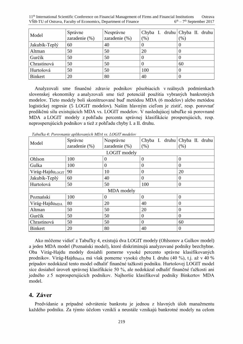
11th International Scientific Conference on Financial Management of Firms and Financial Institutions Ostrava
VŠB-TU of Ostrava, Faculty of Economics, Department of Finance 6th – 7th September 2017
219
Model Správne
zaradenie (%)
Nesprávne
zaradenie (%)
Chyba I. druhu
(%)
Chyba II. druhu
(%)
Jakubík-Teplý 60 40 0 0
Altman 50 50 20 0
Gurčík 50 50 0 0
Chrastinová 50 50 0 60
Hurtošová 50 50 100 0
Binkert 20 80 40 0
Analyzovali sme finančné zdravie podnikov pôsobiacich v reálnych podmienkach
slovenskej ekonomiky a analyzovali sme tiež potenciál použitia vybraných bankrotných
modelov. Tieto modely boli skonštruované buď metódou MDA (6 modelov) alebo metódou
logistickej regresie (5 LOGIT modelov). Naším hlavným cieľom je zistiť, resp. porovnať
predikčnú silu existujúcich MDA vs. LOGIT modelov. V nasledujúcej tabuľke sú porovnané
MDA a LOGIT modely z pohľadu percenta správnej klasifikácie prosperujúcich, resp.
neprosperujúcich podnikov a tiež z pohľadu chyby I. a II. druhu.
Tabuľka 4: Porovnanie aplikovaných MDA vs. LOGIT modelov
Model Správne
zaradenie (%)
Nesprávne
zaradenie (%)
Chyba I. druhu
(%)
Chyba II. druhu
(%)
LOGIT modely
Ohlson 100 0 0 0
Gulka 100 0 0 0
Virág-HajduLOGIT 90 10 0 20
Jakubík-Teplý 60 40 0 0
Hurtošová 50 50 100 0
MDA modely
Poznański 100 0 0 0
Virág-HajduMDA 80 20 40 0
Altman 50 50 20 0
Gurčík 50 50 0 0
Chrastinová 50 50 0 60
Binkert 20 80 40 0
Ako môžeme vidieť z Tabuľky 4, existujú dva LOGIT modely (Ohlsonov a Gulkov model)
a jeden MDA model (Poznański model), ktoré diskriminujú analyzované podniky bezchybne.
Oba Virág-Hajdu modely dosiahli pomerne vysoké percento správne klasifikovaných
prodnikov. Virág-HajduMDA má však pomerne vysokú chybu I. druhu (40 %), t.j. až v 40 %
prípadov nedokázal tento model odhaliť finančné tažkosti podniku. Hurtošovej LOGIT model
síce dosiahol úroveň správnej klasifikácie 50 %, ale nedokázal odhaliť finančné ťažkosti ani
jedného z 5 neprosperujúcich podnikov. Najhoršie klasifikoval podniky Binkertov MDA
model.
4. Záver
Predvídanie a prípadné odvrátenie bankrotu je jednou z hlavných úloh manažmentu
každého podniku. Za týmto účelom vznikli a neustále vznikajú bankrotné modely na celom

11th International Scientific Conference on Financial Management of Firms and Financial Institutions Ostrava
VŠB-TU of Ostrava, Faculty of Economics, Department of Finance 6th – 7th September 2017
220
svete. My sme zamerali na analýzu a porovnanie predikčnej schopnosti bežne používaných
MDA a LOGIT modelov v podmienkach súčasnej pokrízovej ekonomickej situácii na
Slovensku. Za týmto účelom sme analyzovali finančnú situáciu 5 vybraných prosperujúcich
a 5 neprosperujúcich podnikov. Analyzovali sme 6 MDA modelov a 5 LOGIT modelov.
Na základe výsledkov komparatívnej analýzy môžeme dospieť k záveru, že najvhodnejšie
modely na predikciu finančných ťažkostí slovenských firiem sú modely: Ohlsonov LOGIT
model z roku 1980, slovenský Gulkov LOGIT model z roku 2016 a tiež poľský Poznańskeho
MDA model z roku 2004. Tieto modely odporúčame používať pri ex-ante analýze
slovenských podnikov pomocou bankrotných modelov, pretože správne identifikovali
všetkých 5 neprosperujúcich a tiež 5 prosperujúcich firiem. Oba Virágove-Hajduove modely
(aj MDA aj LOGIT model) vytvorené v Maďarsku dosiahli pomerne vysokú predikčnú
schopnosť. Ako nevhodné na predikciu finančného zdravia sa javia viaceré slovenské modely.
Ide o MDA modely: Gurčíkov, Chrastinovej, a najmä Binkertov model (len 20 % správne
klasifikovaných podnikov), a tiež Hurtošovej LOGIT model, ktoré správne identifikovali
maximálne 50% spoločností. Z toho istého dôvodu je nevhodným tiež Altmanov model z roku
1983.
Z výsledkov analýz jednoznačne vyplýva, že lepšie výsledky predikčnej schopnosť
slovenských podnikov dosiahli LOGIT modely. Tento typ modelov má aj ďalšiu výhodu a tou
je fakt, že tieto modely jednoznačne identifikujú podnik ako prosperujúci, resp.
neprosperujúci. Na rozdiel od tohto faktu, viaceré MDA modely dosiahli slabšie výsledok
preto, lebo niektoré podniky zaradili do šedej zóny, a teda nedokázali jednoznačne predikovať
neprosperitu a ani prosperitu podnikov.
Acknowledgement
This research was financially supported by the Slovak Research and Development Agency
– Grant NO. APVV-14-0841: Comprehensive Prediction Model of the Financial Health of
Slovak Companies.
References
[1] Adamko, P. and Svabova, L. (2016). Prediction of the risk of bankruptcy of Slovak
companies. In (Culik, M. ed.) Managing and Modelling of Financial Risks: 8th
International Scientific Conference, Pts I-III. Ostrava, Czech Republic: VŠB-Technical
University of Ostrava, pp. 15-20.
[2] Chrastinová, Z. (1998). Metódy hodnotenia ekonomickej bonity a predikcie finančnej
situácie poľnohospodárskych podnikov. Bratislava: VÚEPP.
[3] Cisko, S. and Kliestik, T. (2013). Financny manazment podniku II. Zilina: EDIS
Publishers.
[4] Gulka, M. (2016). Predictive Model of Corporate Failure in the Slovak Business
Environment. Forum statisticum Slovacum, 12(1), pp. 16-22.
[5] Gurčík, Ľ. (2002). G-index – the financial situation prognosis method of agricultural
enterprises. Agricultural Economics, 48, pp. 373-378.
[6] Jakubík, P., and Teplý, P. (2011). The JT Index as an Indicator of Financial Stability of
Corporate Sector. Prague Economic Papers, 20(2), pp. 157-176.
http://dx.doi.org/10.18267/j.pep.394
11th International Scientific Conference on Financial Management of Firms and Financial Institutions Ostrava
VŠB-TU of Ostrava, Faculty of Economics, Department of Finance 6th – 7th September 2017
221
[7] Kliestik, T., Kocisova, K. and Misankova, M. (2015). Logit and Probit Model used For
Prediction of Financial Health of Company. In (Iacob, A.I. ed.) 2nd Global Conference
on Business, Economics, Management and Tourism. Procedia Economics and Finance,
23, pp. 850–855. http://dx.doi.org/10.1016/S2212-5671(15)00485-2
[8] Kliestik, T., and Majerova, J. (2015). Selected issues of selection of significant variables
in the prediction models. In (Culik, M. ed.) Financial Management of Firms and
Financial Institutions: 10th International Scientific Conference, Pts I-IV. Ostrava, Czech
Republic: VŠB-Technical University of Ostrava, pp. 537-543.
[9] Kliestik, T., Misankova, M., and Adamko, P. (2014). Sensitivity Analysis of Credit Risk
Models Based on Greeks. In (Zhang, Y. ed.) 2nd International Conference on
Management Innovation and Business Innovation (ICMIBI 2014). Lecture Notes in
Management Science, 44, pp. 99-104. http://dx.doi.org/10.5729/lnms.vol44.99
[10] Kliestikova, J. and Misankova, M., (2016). European Insolvency Law Harmonisation in
Terms of Global Challenges. In (Kliestik, T. ed.) Globalization and Its Socio-economic
Consequence:16th International Scientific Conference, Part I-V. Zilina, Slovakia:
University of Zilina, pp. 914–921.
[11] Kliestikova, J., Misankova, M., and Kliestik, T. (2017). Bankruptcy in Slovakia:
international comparison of the creditor´s position. Oeconomia Copernicana, 8(2), pp.
221-237. http://dx.doi.org/10.24136/oc.v8i2.14
[12] Majerova, J., Kliestik, T., and Misankova, M. (2015). Analysis of Convergences and
Divergences of Bankruptcy Law Institutes in the Slovak Republic and in the World. In
(Lee, G. ed.) 2015 5th International Conference on Applied Social Sciences (ICASS
2015), PT 1. Advances in Education Research, 80, pp. 34-39.
[13] Siekelova, A., Kliestik, T., Svabova, L., Androniceanu, A., and Schonfeld, J. (2017).
Receivables Management: The Importance of Financial Indicators in Assessing the
Creditworthiness. Political Journal of Management Studies, 15(2), pp. 217-228.
http://dx.doi.org/10.17512/pjms.2017.15.2.20
[14] Svabova, L., and Kral, P. (2016). Selection of Predictors in Bankruptcy Prediction
Models for Slovak Companies. In (Loster, T. and Pavelka, T. eds.) 10th International
Days of Statistics and Economics: Conference Proceedings, pp. 1759-1768.
11th International Scientific Conference on Financial Management of Firms and Financial Institutions Ostrava
VŠB-TU of Ostrava, Faculty of Economics, Department of Finance 6th – 7th September 2017
222
Evaluation of the Behavioral Differences in the FX Trading Approach with Regard to the Gender
Hana Dvořáčková 1, Marek Jochec2
Abstract
This paper is focused on behavioral finance, specifically on the gender differences in the forex
trading approach. The logistic regression model was built up on the data set, including over twelve
thousand trades, which were made by almost three hundred traders. Using those models was
evaluated and compared the impact of selected variables on the profit making of males and
females. Those variables are for example length of trade, risk approach of the trader or the value
of the trade. Both models were statistically significant and made up for the differences in the
impact of variables on the profit/loss making.
Key words:
behavioral finance, logistic regression, financial markets, fx trading
JEL Classification: C12, G02
1. Introduction
The contribution is focused on the behavioral finance. The data set, collected since 2009 to
2014, contains the trading history of almost three hundred students from different countries
(e.g. USA, Czech Republic, Slovakia, Portugal, New Zealand or Poland). Students were trading
during the standardized period (three months) on the OANDA FX Trade Practice platform,
which allows trading on forex market and also with CFD contracts and selected commodities.
In total more than twelve thousand trades were collected to create the data set, counting plenty
of variables.
There are many studies focused on the behavioral finance examining the gender differences
in trading approach, for example, Jacobsen et al. (2014) compared the optimism of males and
females in many fields including the economy and financial markets. According to his research
males tend to be significantly more optimistic than women. (Halko 2012, Dwyera, P. D. 2002
and Barber and Odean 2000) confirmed that females are more risk averse than man. Moreover,
Nicolosi, G. et al. (2009) confirmed that traders are able to learn and improve their trading skills
based on experience. The aim of the paper is to compare the impact of selected variables on the profit/loss making,
taking into account the gender of traders. Those variables, whose impact is tested are for example length of trade, value of the trade or subjective feeling of addiction on trading. The addiction feelings result was compared to the study Tavares et al. (2001), which confirmed males as more prone to gambling than females. The differences in strategy of business games was tested by Garber, Hyatt, Boya (2017), according to their study female participants of serious business games prefer accepting feelings, receptive graspers of experience and tend to
1VŠB-TUO, Faculty of Economics, Department of Finance, Sokolská třída 33, 702 00 Ostrava, Czech
Republic, E-mail: [email protected] 2 Correspondence to: Nazarbayev University, Graduate School of Business, Kabanbay Batyr 53, Astana,
Kazakhstan. E-mail address: [email protected]
11th International Scientific Conference on Financial Management of Firms and Financial Institutions Ostrava
VŠB-TU of Ostrava, Faculty of Economics, Department of Finance 6th – 7th September 2017
223
collaborate. On the other hand, males are more logical, analytical, competitive and present oriented graspers of experience.
The impact of those variables was tested using the logistic regression modelling, the method is described in detail in the chapter 2 together with the methods of the statistical verification. In this chapter is also specification of the data set and those variables, which were selected to be tested.
There were two logistic regression models estimated, which are described in the chapter 3 where one was made for female traders and the other one for male traders. As both models were found statistically significant, there was made a comparison of the resulting influence of variables on the profit/loss of the trader.
2. Data description
The data was collected by Ing. Marek Jochec Ph.D. from 2009 to 2015 during his lectures.
Students were trading on the OANDA FX Trade Practice platform with currency pairs and
CDFs. Initially, the students were given 100 000 US, meanwhile the trading period was
standardized and it took three months. As the students did not trade with real money, they were
motivated to achieve as good result as possible by a financial reward and also extra points for
the exam for the winner (student with the highest account balance at the end of the trading
period). There were 292 students involved in the research over the time, who made in total 12 416
trades with the total volume of over three billion units. From the above mentioned students,
43% (125 students) became profit makers. That is to say that their account balance at the end
of trading period was higher than 100 000 USD. Regarding the gender diversity of traders,
there were involved 120 females and 172 males. All in all, there were 29% of trades made by
females, 71% by males. From the collected data set were selected following variables to evaluate their impact on
the profit/loss making of traders:
value of the trade ( amount of traded units * price for the unit) (value) length of the trade (duration)
gender of the student (gender) Moreover, students were completing questionnaires including sixteen questions, in which
required answers were “YES” or “NO”. Subsequent questions were selected for this paper:
nr. 3: Have you ever had a feeling that you became addicted to the game? (addiction)
nr. 5: Do you think that you are a person that enjoys taking risks? (risk)The data was divided into two groups regarding the gender of traders to compare the
differences in the impact of variables on the profit or loss in trading. The data set was statistically tested and was found stationary.
3. Results and Discussion
Data were spilt into two groups based on the gender-males and females and for each group
separately was created model using the logistic regression, method enter. In following chapters are described both models and compared the impact of variables on the profit making.
Logistic Regression model for females
The data set for female traders counted in total 3 701 transactions, where 198 transactions
(5, 3 %) includes missing cases in some variables. However, all transactions were selected for
the model estimation. During the first step was estimated the baseline model, which did not
include any explanatory variable. Prediction are made on whichever category occurred more

11th International Scientific Conference on Financial Management of Firms and Financial Institutions Ostrava
VŠB-TU of Ostrava, Faculty of Economics, Department of Finance 6th – 7th September 2017
224
often in the data set, therefore the model always predicted all transactions as loss making and it
was 55,2% correct prediction. The test of significance, showed in the Table 1 proves the model
as statistically significant, the baseline model is slightly better than coin tossing.
Table 1. Variables in the Equation
B S.E. Wald df Sig. Exp(B)
Step 0Constant -,207 ,034 37,070 1 ,000 ,813
After the baseline model estimation follows adding of explanatory variables to the
model. There is the Omnibus test of model coefficients presented in the Table 2, which is checking whether the new model, including the explanatory variables is an improvement
comparing to the baseline model. For the testing is used the Chi-square test to see if there is a significant difference between -2LL of the baseline and new model.
Table 2. The Omnibus Test of Model Coefficients
Chi-square df Sig.
Model 168,079 5 ,000
As the Chi-square is significant in this case, the new model is significantly better than the
baseline as the -2LL is reduced to the value 4650,841. Regarding the predictive ability of the
model, the Nagelkerke R2 expresses how many variations of dependent variable can be
explained by the model. In this case the value is just 6, 3%. In the Classification Table (Table 3.) is calculated the percentage of correct predictions for profitmakers and lossmakers. From total amount of 1932 lossmakers was 77, 5 % predicted correctly, meanwhile the percentage correct of profitmakers is 43, 5%. It follows the overall percentage of correct predictions is 62, 3 %, which is slightly higher than predictive ability of the baseline model (55, 2 %).
Table 3. The Classification Table Predicted
profitmaker(=1)/lossmaker(=0) Percentage
Observed 0 1 Correct
profitmaker(=1)/lossmaker(=0) 0 1 498 434 77,5
1 888 683 43,5
Overall Percentage 62,3 Note: a. The cut value is ,500
Variables inserted to the model are described in the Table 4. The significance of variables is
tested in the row called Sig. As the condition for variables significance is the Sig. value below
0,001, variables duration and risk are classified as insignificant, which implies that the duration
of trade and subjective risk attitude do not have significant impact on the profit making for
females. The only influential variables are active/passive, where in case of active end of trade
is increasing the probability of profit, and also the variable addiction and constant. According
to the variable Addiction is increasing the probability of profit making together with the
subjective feeling of addiction to trading. The variable value is statistically significant but with
zero impact on the dependent variable.

11th International Scientific Conference on Financial Management of Firms and Financial Institutions Ostrava
VŠB-TU of Ostrava, Faculty of Economics, Department of Finance 6th – 7th September 2017
225
Table 4. Variables in the Equation Females
B S.E. Wald df Sig. Exp(B)
Value ,000 ,000 27,217 1 ,000 1,000
Duration ,010 ,003 11,682 1 ,001 1,010
Active/Passive ,286 ,074 14,958 1 ,000 1,331
Addiction ,731 ,087 71,190 1 ,000 2,078
Risk ,094 ,079 1,405 1 ,236 1,099
Constant -,811 ,071 129,345 1 ,000 ,444 Note: a. Variables entered on step 1: value, origin to link time (in days), active/passive, addiction, risk.
Following equation 3.1 is the final appearance of the logistic regression model
determining the influence of variables on profit for female traders.
𝑙𝑜𝑔 (𝑝
1−𝑝) = −0,811 + 0,286
𝑎𝑐𝑡𝑖𝑣𝑒
𝑝𝑎𝑠𝑠𝑖𝑣𝑒+ 0,731 𝑎𝑑𝑑𝑖𝑐𝑡𝑖𝑜𝑛. (3.1)
Logistic Regression model for males
The same model as for females was created for male traders. They made more trades than
females, in total 9 238, where 451 (4, 9 %) items included some missing cases, but also in this
case all items were selected for the model. The baseline model classified all trades as lossmaking, with 5 379 observed Lossmakers it was able to predict with 61, 2% accuracy
without any explanatory variable. According to the test of significance, presented in the Table 5. the model is significant.
Table 5. Variables in Equation
B S.E. Wald df Sig. Exp(B)
Constant -,456 ,022 434,518 1 ,000 ,634
Concerning the omnibus test of model coefficients (Table 6.), which is comparing the improvement of the model including variables to the baseline model, it considers the improvement statistically significantly better. The -2LL of the model with variables is 11 330, 51, as compared to the females model the result is not very sufficient. However, the Nagelkerke
R2 is comparable, result for males model is 6, 1% of variations of dependent variables can be
explained by the model.
Table 6. Omnibus Test of Model Coefficients
Chi-square df Sig.
Model 404,961 5 ,000
The overall percentage of correct predictions is 63,5 %, which is almost the same as for the baseline model (61,2 %), the model is able to classified correctly 94,2 % of loss makers, but just 15,1 % of profit makers, as is shown in the Table 7.
Table 7. The Classification Table Predicted
profitmaker(=1)/lossmaker(=0) Percentage
Observed 0 1 Correct
profitmaker(=1)/lossmaker(=0) 0 5 066 313 94,2
1 2 894 514 15,1
Overall Percentage 63,5 Note: a. The cut value is ,500
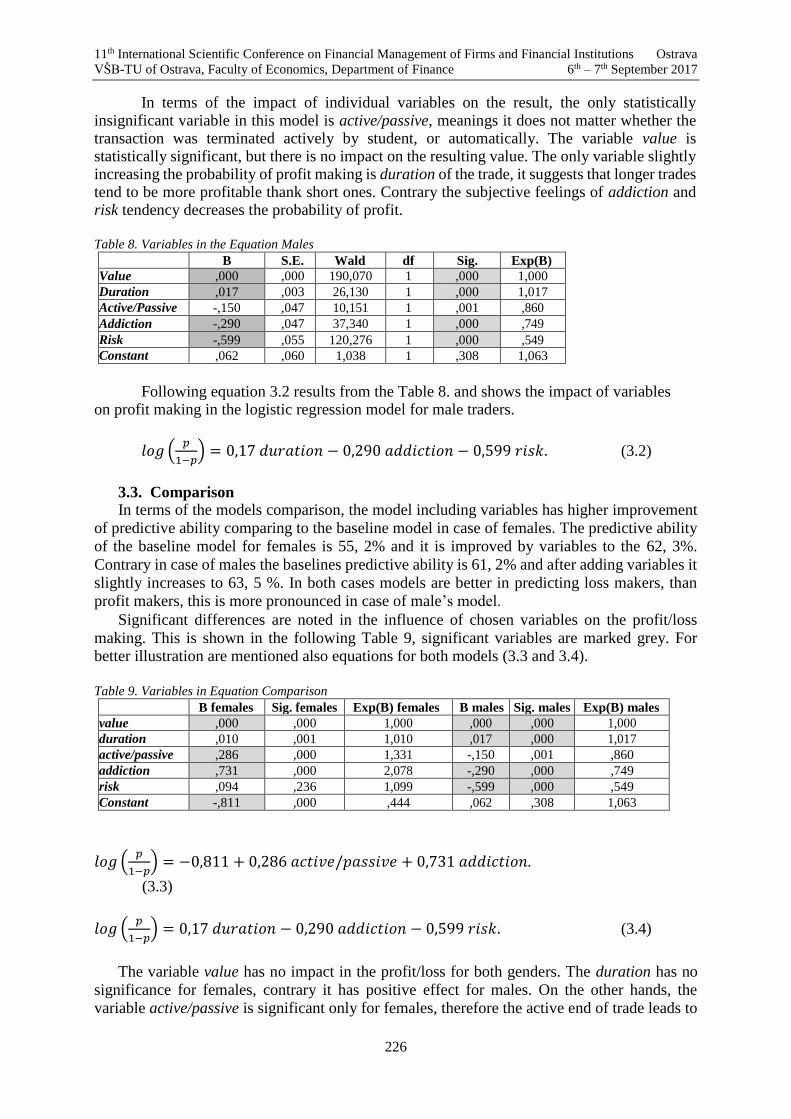
11th International Scientific Conference on Financial Management of Firms and Financial Institutions Ostrava
VŠB-TU of Ostrava, Faculty of Economics, Department of Finance 6th – 7th September 2017
226
In terms of the impact of individual variables on the result, the only statistically insignificant variable in this model is active/passive, meanings it does not matter whether the transaction was terminated actively by student, or automatically. The variable value is statistically significant, but there is no impact on the resulting value. The only variable slightly increasing the probability of profit making is duration of the trade, it suggests that longer trades tend to be more profitable thank short ones. Contrary the subjective feelings of addiction and risk tendency decreases the probability of profit.
Table 8. Variables in the Equation Males
B S.E. Wald df Sig. Exp(B)
Value ,000 ,000 190,070 1 ,000 1,000
Duration ,017 ,003 26,130 1 ,000 1,017
Active/Passive -,150 ,047 10,151 1 ,001 ,860
Addiction -,290 ,047 37,340 1 ,000 ,749
Risk -,599 ,055 120,276 1 ,000 ,549
Constant ,062 ,060 1,038 1 ,308 1,063
Following equation 3.2 results from the Table 8. and shows the impact of variables
on profit making in the logistic regression model for male traders.
𝑙𝑜𝑔 (𝑝
1−𝑝) = 0,17 𝑑𝑢𝑟𝑎𝑡𝑖𝑜𝑛 − 0,290 𝑎𝑑𝑑𝑖𝑐𝑡𝑖𝑜𝑛 − 0,599 𝑟𝑖𝑠𝑘. (3.2)
3.3. Comparison In terms of the models comparison, the model including variables has higher improvement
of predictive ability comparing to the baseline model in case of females. The predictive ability
of the baseline model for females is 55, 2% and it is improved by variables to the 62, 3%.
Contrary in case of males the baselines predictive ability is 61, 2% and after adding variables it
slightly increases to 63, 5 %. In both cases models are better in predicting loss makers, than
profit makers, this is more pronounced in case of male’s model. Significant differences are noted in the influence of chosen variables on the profit/loss
making. This is shown in the following Table 9, significant variables are marked grey. For better illustration are mentioned also equations for both models (3.3 and 3.4).
Table 9. Variables in Equation Comparison
B females Sig. females Exp(B) females B males Sig. males Exp(B) males
value ,000 ,000 1,000 ,000 ,000 1,000
duration ,010 ,001 1,010 ,017 ,000 1,017
active/passive ,286 ,000 1,331 -,150 ,001 ,860
addiction ,731 ,000 2,078 -,290 ,000 ,749
risk ,094 ,236 1,099 -,599 ,000 ,549
Constant -,811 ,000 ,444 ,062 ,308 1,063
𝑙𝑜𝑔 (𝑝
1−𝑝) = −0,811 + 0,286 𝑎𝑐𝑡𝑖𝑣𝑒/𝑝𝑎𝑠𝑠𝑖𝑣𝑒 + 0,731 𝑎𝑑𝑑𝑖𝑐𝑡𝑖𝑜𝑛.
(3.3)
𝑙𝑜𝑔 (𝑝
1−𝑝) = 0,17 𝑑𝑢𝑟𝑎𝑡𝑖𝑜𝑛 − 0,290 𝑎𝑑𝑑𝑖𝑐𝑡𝑖𝑜𝑛 − 0,599 𝑟𝑖𝑠𝑘. (3.4)
The variable value has no impact in the profit/loss for both genders. The duration has no
significance for females, contrary it has positive effect for males. On the other hands, the
variable active/passive is significant only for females, therefore the active end of trade leads to

11th International Scientific Conference on Financial Management of Firms and Financial Institutions Ostrava
VŠB-TU of Ostrava, Faculty of Economics, Department of Finance 6th – 7th September 2017
227
the profit. Very interesting is the impact of the addiction, this variable is significant for both
models, but with opposite effect. In case of females the effect is positive, meanwhile for males
it is negative. In case of Forex trading the border between professional trading and gambling
very thin. In general, if the trader relies mostly on luckiness and is focused on the profit without
any strategy together with feeling of strong emotions during the trading, he tends to forgo
gambling. According to the Tavares et.al. (2001), the emergence of male’s addiction on games
is much faster than females. Regarding the age in which are people the most susceptible to
addiction, the average is 20, 4 for males and 34, 2 for females. As the age of observed traders
was between 20 and 27, it was the critical age for males. The result of the questionnaire goes
together with the Tavares’s result, males were feeling the addiction on trading more often than
females, as is illustrated in the Graph 1 and Graph 2, 38% of males confirmed feelings of
addiction, the same feelings confirmed only 19% of females.
Graph 1: Subjective Feelings of Addiction-Females
Source: Author’s illustration
Graph 2: Subjective Feelings of Addiction-Males
Source: Author’s illustration
Concerning the impact of the addiction on the profit/loss in created models, in the female’s model this variable has the most significant POSITIVE effect, on the other hand, in the model for males is addiction decreasing the probability of profit making.
In terms of the last variable called risk, which represents the subjective feeling of risk
loving, in this case the variable is significant only for males and it is decreasing the probability of profit making. According to the result of the questionnaire, males involved in the research
tend to behave more risky than females, as is shown in the Graph 2 and Graph 3. Of the total number of respondents, 46 % of females stated that do not enjoy taking risk, the
same answer gave only 26 % of males. On the other hand, 41% of females confirmed enjoying
taking risk, the same answered 60 % of males. This result is consistent with the Halko (2012),
Dwyera, P. D. (2002) and Barber and Odean (2000), who confirmed that females are more risk
averse than males. The subjective approach to the risk goes together with the Jacobsen et al.
(2014) and the optimistic approach of males.

11th International Scientific Conference on Financial Management of Firms and Financial Institutions Ostrava
VŠB-TU of Ostrava, Faculty of Economics, Department of Finance 6th – 7th September 2017
228
Graph 3: Risk Approach - Females
Source: Author’s illustration
Graph 4: Risk Approach - Males
Source: Author’s illustration
In terms of the predictive ability of both models, the model for females achieved better improvement of prediction comparing to the baseline model, however, the overall result is very similar for both models (62, 3% for females, 63, 5% for males).
4. Conclusion
In the research there was tested the impact of selected variables on the profit/loss making of
traders, taking into account their gender. Data set includes over twelve thousand trades of
students, who were trading on the FX trade platform during their course. As they were not
trading with the real money, they were motivated to achieve as good result as possible by the
financial reward (real money) and also by extra points to their exam. Students also had to fill in
a questionnaire, including behavioural questions about their risk attitude, feelings during
trading etc.
The logistic regression models were created based on the selected data and there were created
two models, one for females, second one for males. For the paper were selected variables value,
duration, gender of the student/trader, subjective feelings of addiction, active/passive end of the
trade and the risk attitude of the student/trader. From those models follows that selected
variables have different impact for both genders. In case of the females, the only variables
having some impact on the profit/loss making are active/passive and addiction, both have the
positive effect, so they are increasing the probability of the profit making. On the other hand,
in case of males the variables with impact are duration, addiction and risk, the only variable
increasing the probability of profit making is duration, the longer trade, the higher probability
of profit. Remaining variables are decreasing the probability of the profit. The research also confirmed the Halko (2012), Dwyera, P. D. (2002) and Barber and Odean
(2000), who described that females are more risk averse than males. The subjective approach
to the risk goes together with the Jacobsen et al. (2014) and the optimistic approach of males.

11th International Scientific Conference on Financial Management of Firms and Financial Institutions Ostrava
VŠB-TU of Ostrava, Faculty of Economics, Department of Finance 6th – 7th September 2017
229
As well the Tavares et.al. (2001), and his research on the gender and addiction was confirmed
on this data set.
Acknowledgement
The research was supported through the Czech Science Foundation (GAČR) under project 16-09541S and through SP2017/32, an SGS research project of VŠB-TU Ostrava. The research was also supported by scholarships awarded by the Ostrava city and the Moravian-Silesian region. The support is greatly acknowledged.
References
[1] Barberb, B.M. and Odean T. (2000). Boys will be boys: Gender, overconfidence, and
common stock investment. The Quarterly Journal of Economics, (116)55, p. 261–292
[2] Dwyera, P. D. et al. (2002). Gender differences in revealed risk taking: evidence from
mutual fund investors. Economics Letters. 76(2), p. 151–158
[3] Field, A. (2013). Discovering Statistics Using SPSS. London: Sage
[4] Hair, J. F. et al. (2009). Multivariate Data Analysis. New Jersey: Prentice Hall.
[5] Halko M.L. et al. (2012). The gender effect in risky asset holding. Journal of Economic
Behavior & Organisation. 83(1), p. 66–81.
[6] Hosmer, D., Lemeshow, S. W. and Sturdivant, X.R. (2013). Applied Logistic Regression.
New Jersey: John Wiley & Sons.
[7] Jacobsen B. et al. (2014). Gender differences in optimism and asset allocation. Journal of
Economic Behavior & Organisation, 107, p. 630–651.
[8] Nicolosi, G. et al. (2009). Do individual investors learn from their trading experience?
Journal of Financial Markets, 12(2) p. 317–336.
[9] Tavares, H. et al. (2001). Gender differences in gambling progression. Journal of
Gambling, 17(2), p. 151-159.
11th International Scientific Conference on Financial Management of Firms and Financial Institutions Ostrava
VŠB-TU of Ostrava, Faculty of Economics, Department of Finance 6th – 7th September 2017
230
Unconventional monetary policy tools in central banking globally and within the Czech Republic
Luboš Fleischmann 1
Abstract
The period following the most recent global crisis has forced central banks in many countries to
exploit unconventional monetary policy tools in order to secure macroeconomic stability. This
study summarises the reasons for selected central banks in the advanced economies to exploit
unconventional currency and policy tools, and how the global environment has changed for the
implementation of monetary policies. It also describes the use of unconventional tools in selected
countries and investigates the Czech National Bank’s approach in more detail.
Key words
unconventional tools, monetary policy, central bank, macroeconomic stability
JEL Classification: E44, E52, E58
1. Úvod
Problémy americké investiční banky Lehman Brothers v září roku 2008, a následná globální
bankovní a finanční krize, otevřely cestu k novým přístupům centrálních bank k zajištění
měnové stability ve svých zemích. Ruku v ruce s finanční krizí nastala v roce 2010 krize
dluhová, provázená zeslabením agregátní poptávky a sílícími dezinflačními tlaky.
Hlavním cílem používání nekonvenčních nástrojů tedy bylo primárně oživení agregátní
poptávky a zvýšení inflace, snaha čelit deflaci/dezinflaci a v neposlední řadě obnovit krizí
narušený transmisní mechanismus. Ve svém důsledku mají uvedené cíle společný jmenovatel,
kterým byla náprava postkrizových negativních jevů a zajištění makroekonomické stability.
Zvolení nekonvenční politiky centrální banky směřovaly na snížení dlouhého konce výnosové
křivky.
Centrální banky ve vyspělých zemích na globální úrovni reagovaly na vzniklou situaci
v použití nekonvenční politiky po roce 2008 různě. V příspěvku popíšeme přístupy v obecné
rovině ve vybraných vyspělých ekonomikách – BoJ, která sledované postupy použila dříve než
ostatní, FED, ECB, Bank of England a samostatná část popisuje nástroj kurzového závazku
ČNB. Budou zodpovězeny primární otázky:
1) Proč začaly centrální banky vyspělých ekonomik používat nekonvenční měnové nástroje?
2) Jaké nástroje nekonvenčních politik byly kde implementovány?
3) Jaké nekonvenční nástroje použila ČNB?
2. Teoretická východiska pro použití nekonvenčních měnových
nástrojů
Tématu nekonvenční politiky měnové politiky bylo věnováno mnoho prostoru ve vědeckých
pracích. Nejčastěji jsou v nich zmiňovány důvody pro její použití ve vztahu ke globální finanční
1 Ing. Luboš Fleischmann, Vysoká škola ekonomická v Praze, Fakulta financí a účetnictví, Katedra
bankovnictví a pojišťovnictví, nám. W. Churchilla 1938/4, 130 67 Praha 3 – Žižkov, e-mail:

11th International Scientific Conference on Financial Management of Firms and Financial Institutions Ostrava
VŠB-TU of Ostrava, Faculty of Economics, Department of Finance 6th – 7th September 2017
231
krizi po roce 2008. Úvodem si v krátkosti připomeňme historický diskurs o činnosti centrálních
bank mezi významnými ekonomickými směry.
Pro ilustraci a zařazení nekonvenčních politik do pohledu na měnovou politiku v historické
souvislosti uvádíme nejprve celosvětový spor z 20. a 30. let minulého století. V České republice
se neshoda identifikovala s přívržencem Rakouské ekonomické školy Karlem Englišem a
obdivovatelem učení J. M. Keyenese, Josefem Mackem. Engliš zastával názor konzervativního
centrálního bankéře, který tvrdil, že emisní politika může souviset pouze s reeskontem reálné
směnky, za kterou stojí skutečně výroba a prodej. Jeho koncepce tedy znamenala, že centrální
banka půjčuje peníze subjektům, za kterými stojí skutečná výroba a obchod. Macek prosazoval
keynesovské myšlenky ve formě operací na volném trhu (OVT2) a nákupu státních cenných
papírů. Byl tedy přesvědčen, že centrální banka musí poskytovat dlouhodobé peníze.
Po druhé světové válce můžeme problém identifikovat na sporu mezi monetaristickou a
(post)keynesiovskou školou. Mezi oběma směry nepanoval spor ohledně nákupu státních
cenných papírů při OVT. Naopak vážné spory vedly o hlavní cíle měnové politiky při OVT, o
množství nákupu státních cenných papírů při OVT a o možnost nákupu privátních cenných
papírů při OVT. (Tomšík, Mandel, 2012).
V soudobé literatuře se tématu nekonvenční měnové politiky věnuje mnoho autorů, kteří si
všímají jak důvodů, principů a možných dopadů využívání nestandardních nebo nových
měnových nástrojů. V obecné rovině můžeme zmínit definici nekonvenční měnové politiky
(ČNB, 2017), podle které se jedná o ovlivňování dlouhodobé reálné úrokové sazby, kdy se
nekonvenční měnová politika zaměřuje na náklady a dostupnost vnějšího financování bank,
domácností a nefinančních společností.
Nejčastěji používané nekonvenční nástroje měnové politiky zmiňuje např. (Ambler, Rumler,
2017) nebo (Stone, Fujita, & Ishi, 2011). (Bini-Smaghi, 2009) uvádí rozdělení nestandardní
politiky centrálních bank do několika základních oblastí. Účinností transmisních mechanismů
měnové politiky s použitím nestandardních nástrojů se zabývá např. (Janus, 2016).
Jednotlivé centrální banky volily vhodná opatření na základě konkrétních problémů a potřeb,
které vyvstaly během fází finanční krize. (Zamrazilová, 2014) uvádí možné rozdělení krize na
dvě základní etapy3.
Autoři v odborných prací zkoumají, popisují a analyzují jednotlivé nástroje nekonvenčních
politik. Nejčastější zmínka je o kvantitativním uvolňování, kterému se věnují např. (Williams,
2011), (Besley, Kohn, 2009), (Miskin, 2010) nebo (Revenda, 2017). Devizové intervence jako
další z nestandardních nástrojů zmiňuje např. (Svensson, 2010). Další z poměrně vysokého
počtu článků jsou věnována nástroji zaváděných záporných sazeb – např. (Anderson, Liu,
2013). Minoritní počet prací se věnuje nástroji zvanému vrtulníkové peníze. O tomto
nestandardnímu zásahu centrální banky je možné se dozvědět např. v článku (Bowdler & Radia,
2012). Jedním z důvodu malého zájmu autorů vědeckých prací o tento nástroj je skutečnost, že jej
nepoužila žádná z hlavních centrálních bank nejvyspělejších zemí.
2 (Revenda, 2011) operace na volném trhu (OVT) definuje jako nákupy nebo prodeje cenných papírů
centrální bankou obchodním a dalším bankám v domácí měně, s cílem regulace rezerv bank nebo
krátkodobé úrokové míry. Jako základní charakteristiku OVT uvádí: permanentní, operativní,
zaměřené na regulaci operativního kritéria, nepřímé. 3 První etapu krize datuje od konce roku 2009, druhou od května 2010.

11th International Scientific Conference on Financial Management of Firms and Financial Institutions Ostrava
VŠB-TU of Ostrava, Faculty of Economics, Department of Finance 6th – 7th September 2017
232
3. Nekonvenční nástroje monetární politiky vybraných centrálních
bank
3.1 Japonsko jako předobraz používání nekonvenčních nástrojů centrálních bank
Japonsko se stalo „průkopníkem“ v používání nástrojů nekonvenční politiky. I přes nepříliš
systematická řešení bylo v dalších letech možné využít zkušenosti s novými možnostmi
stabilizovat finanční trhy.
Japonsko zažilo zvláštní situaci již počátkem devadesátých let prasknutím vytvořené bubliny
na trzích aktiv, zejména pak trhu akcií a nemovitostí. Následoval nechvalně známý řetězec
počínající poklesem aktiv a hospodářské zpomalení, zhoršování ekonomických fundamentů a
růst břemene problémových úvěrů. I přes špatné signály vznikajících problémů, banky
pokračovaly v půjčování tzv. „zombie“ firmám a v listopadu 1997 odstartovala finanční krize.
Historický exkurz do doby před globální krizí po roce 2008 děláme právě z důvodu podobnosti
obou zmíněných krizí.
Od roku 1998 se projevovaly deflační tendence, nastal pokles mezd a cen. Bank of Japan
(BoJ) začala snižovat úrokové sazby k nule a v moderní historii se tak poprvé uplatnil princip
ZLB4. BoJ začala používat nástroj kvantitativního uvolňování, ale vzhledem k nedostatečnému
probádání použití nového nástroje, neměla realizace opatření příliš efektivní účinek5.
Ve sledovaném období prošlo Japonsko dvěma etapami: 1) dezinflační (1992 – 1998), kdy
se inflace, nominální úrokové sazby i reálné úrokové sazby vyvíjely souběžně a 2) deflační
(1998 – 2012), v které se inflace, nominální úrokové sazby a reálné úrokové sazby se začaly
vyvíjet protisměrně.
Japonsko zažívalo, a dosud zažívá paradoxně dodnes, mnoho různých pokusů o nastavení
nekonvenčních politik. Důvodem je dlouhotrvající perioda japonské dezinflace a deflace.
3.2 Nekonvenční nástroje monetární politiky jako řešení finanční krize po roce 2008
Do začátku roku 2008 většina centrálních bank používala standardní měnově-politické
nástroje, jak jsou krátkodobé úrokové sazby, případně měnové agregáty (spíše před dominancí
inflačního cílení). Kurzy měn a měnové agregáty se přizpůsobovaly zejména nastavení sazeb.
Po vypuknutí finanční krize centrální banky reagovaly standardně a snižovaly úrokové sazby.
Z důvodu nízkých hodnot úrokových sazeb již v období před rokem 2008 některé centrální
banky rychle snížily jejich hodnotu směrem k 0, tedy k hranici ZLB6.
Zároveň s výše uvedenou situací musely banky řešit aktuální situaci narušení finančních
trhů, kterou krize vyvolala. Cílem bylo uvolnění podmínek a obnovit transmisní mechanismus,
který byl symptomy finanční krize narušen.
Výrazně silným krizovým momentem, který zasáhl velkou část evropských zemí, bylo jejich
chronické zadlužení, což vedlo v roce 2010 k tzv. dluhové krizi. Reakcí byla snaha zvyšovat
inflaci snižováním úrokových sazeb a i další evropské země dosáhly k hranici ZLB7.
Centrální banky po dosažení hranice ZLB začaly podporovat ekonomickou aktivitu
nekonvenčními nástroji měnové politiky, kterými byly a) kvantitativní uvolňování, b) tzv.
Forward guidance (centrální bankou avizování budoucích politik), c) využití záporných
úrokových sazeb, d) kurzovými závazky. Již jsme v úvodní části příspěvku uvedli, že použití
4 ZLB – Zero Lower Bond (úroková míra na úrovni tzv. technické nuly) 5 BoJ nestanovila žádný inflační cíl, nedostatečně objasnila transmisní mechanismus a
neměla plán exitu. 6 Fed v prosinci 2008 (0-0,25%), Bank of England v březnu 2009 (0,5%). 7 Švýcarská národní banka v srpnu 2011 (0%), Dánská národní banka v květnu 2012 (0,05%), ECB
v září 2014 (repo: 0,05%), Sveriges Riksbank v říjnu 2014 (0%).

11th International Scientific Conference on Financial Management of Firms and Financial Institutions Ostrava
VŠB-TU of Ostrava, Faculty of Economics, Department of Finance 6th – 7th September 2017
233
nestandardních nástrojů měnové politiky bylo zaměřeno především na snížení sazeb dlouhého
konce výnosové křivky (kromě kurzového závazku).
Důvodem používání nekonvenčních politik byla nízká inflace měřená HICP8 bez energií.
Vývoj inflace v eurozóně zobrazuje Obrázek 1.
Důvody nízké inflace nejen v eurozóně budou známy přesněji po prozkoumání hypotéz,
které mají centrální banky k dispozici. Obecně se jako hlavní důvody v literatuře uvádí
technologický pokrok a zlevňování různých statků, globalizace, mezinárodní obchod a
mezinárodní specializace, snižování kvality produkce, vývoj cen ropy a energetických komodit,
omezování úvěrové emise, fiskální konsolidace, cyklické zpomalování hospodářského růstu
v Číně jako dezinflační tlaky pro světovou ekonomiku.
Obrázek 1: Vývoj inflace v eurozóně 2000–2016 (HICP měřené bez energií)
Zdroj: ECB (2017), dostupné z: https://www.euro-area-statistics.org/
Centrální banky ve svých zemích používaly různé nástroje nekonvenční měnové politiky.
Jedná se o širokou paletu programů, z nichž byly v jednotlivých zemích použity rozhodnutím
vlastní bankovní autority. Srovnání efektivity použití různých nástrojů je těžko proveditelné
z důvodu odlišností potřeb a měnově politické situace v každé ze zemí, kde byly použity
nestandardní přístupy k zajištění finanční stability. Tabulka 1 zobrazuje použité nástroje ve
vybraných zemích.
Tabulka 1: Použití nástrojů nekonvenčních měnových politik ve vybraných zemích
Kvantitativní
uvolňování
Forward
guidance
Záporné úrokové
sazby
Kurzové
závazky
Eurozóna ANO ANO ANO
USA ANO ANO ANO
Velká Británie ANO ANO ANO
Japonsko ANO ANO ANO
ČR ANO ANO
Zdroj: vlastní zpracování
8 Harmonizovaný index spotřebitelských cen.
0,0
0,5
1,0
1,5
2,0
2,5
3,0
2007 2008 2009 2010 2011 2012 2013 2014 2015 2016

11th International Scientific Conference on Financial Management of Firms and Financial Institutions Ostrava
VŠB-TU of Ostrava, Faculty of Economics, Department of Finance 6th – 7th September 2017
234
ECB prováděla měnovou politiku formou nákupů různých dluhových instrumentů, kterými
se snaží na trh získat likviditu. Mimo jiné se snaží vyměnit nástroje s dlouhou expozicí za
likvidní peníze, a tím dodává obchodním bankám určité uvolnění ve snaze oživit jejich
úvěrovou aktivitu. Tato situace pokračuje dodnes, ECB si dala v březnu 2017 závazek
pokračovat v nákupu dluhopisů v měsíční výši až 60 mld. EUR do prosince 2017. Role ECB je
nesnadná z důvodu nehomogennosti eurozóny, různé části měnové unie jsou v různé situaci a
nalézt vhodná řešení centrální banky jsou velmi problematická.
FED byl v této etapě první v použití nekonvenčních politik. V současné době je ve fázi exitu
a postupného zpřísňování měnově politických podmínek a dochází opakovaně ke zvyšování
úrokových sazeb. FED využíval nekonvenční nástroje velmi aktivně a radikálně, pomohly
překonat krizi zejména v letech 2008-09 a nepotvrdily se katastrofické scénáře některých
odborníků, předpovídající devalvaci dolaru nebo přílišnou inflaci. FED se choval k postiženým
finančním institucím pružně, efektivně a operativněji než evropské země.
Britská centrální banka (BoE) provádí měnovou politiku formou dodávání likvidity a nákupy
soukromých aktiv prostřednictvím programu podpory poskytování půjček domácnostem a
podnikům. Po referendu o vystoupení Velké Británie z Evropské unie přistoupila k dalšímu
kvantitativnímu uvolňování v kombinaci na britské poměry s nízkou úrokovou sazbou. BoE
v srpnu 2016 snížila úrokovou sazbu z 0,5% na 0,25%, což byla nejnižší sazba v historii, a
rozšířila rozsah kvantitativního uvolňování o 70 mld. GBP.
Počátek japonských novějších nekonvenčních zásahů v měnové politice se datuje do roku
2010 a BoJ v nich pokračuje radikálně dodnes. Efektivita je zatím stále sporná, vezmeme-li
v úvahu koordinaci opatření s japonskou vládou a poměrně expanzivní fiskální politikou nebo
průmyslovou politikou. V lednu 2016 BoJ rozhodla o snížení úrokové sazby na -0,1%, poprvé
tedy v Japonsku do záporné hodnoty.
Fenomén záporných úrokových sazeb se začal naplno projevovat od konce roku 2014.
Zatímco před krizí představovaly spíše anomálii, během postkrizového období se staly běžnou
součástí života centrálních bank. Obrázek 2 ukazuje země, kterých se využití nástroje
záporných úrokových sazeb týká. Nejnižší úroková sazba je ve Švýcarsku, které vyměnilo
kurzový závazek za hluboce záporné úrokové sazby, především z důvodu ochrany apreciace
domácí měny, u které byly očekávány různé neblahé konsekvence. Podobně reagovala dánská
centrální banka, která má dlouhodobě navázán fixní kurz k euru a stejně jako v předchozím
případě bylo nutné posílit ochranu vlastní měny.
Tabulka 2: Výše záporných úrokových sazeb ve vybraných zemích
Zdroj: ČNB, 2017
11th International Scientific Conference on Financial Management of Firms and Financial Institutions Ostrava
VŠB-TU of Ostrava, Faculty of Economics, Department of Finance 6th – 7th September 2017
235
3.3 Devizové intervence ČNB
Proti předchozím sledovaným zemím je Česká republika malou ekonomikou, nedosahující
rozměrům žádné z nich. Přesto je v zahraničí velmi dobře hodnocena hlavní autorita měnové
politiky, tedy česká centrální banka, ČNB.
V listopadu 2012 bankovní rada avizovala skutečnost, že případné uvolnění měnových
podmínek provede prostřednictvím oslabení koruny. Během roku 2013 sílily deflační tlaky ve
formě, mimo jiné, pomalého růstu HDP, trvajícího poklesu fixních investic a záporné mezery
výstupu, nejpomalejšího růstu mezd v soukromých firmách, trvalého poklesu cen nemovitostí
nebo poklesu rychlosti obratu peněz. Deflační tlaky se projevovaly stále větším poklesem
inflace, která měla hodnotu hluboko pod inflačním cílem.
ČNB oslabila kurz koruny na hodnotu poblíž 27 Kč/euro dne 7. 11. 2013 a vyslovila
jednostranný kurzový závazek. Měnový kurz se rázem stal použitým nekonvenčním nástrojem
a převzal stabilizační úlohu měnové politiky.
Cílem devizových intervencí ČNB bylo: a) odvrácení rizika reálně hrozící deflace, b) dřívější
dosažení inflačního cíle, c) rychlejší oživení ekonomiky, d) dřívější opuštění hladiny nulových
úrokových sazeb.
Platnost kurzového závazku byla několikrát prodloužena a ukončena rozhodnutím bankovní
rady ČNB byla dne 6. 4. 2017. Celkem centrální banka intervenovala za uvedenou dobu zhruba
1,5 bilionu korun. Podle odhadů ČNB, zavedení kurzového závazku významně přispělo
k obnovení růstu české ekonomiky po několika letech recese.
Ukončení devizových intervencí by provázen diskusí nad chováním koruny. Obecně se
předpokládal výkyv oběma směry a postupné ustálení. Realita toto tvrzení nepotvrdila. Kurz se
ustálil, koruna posílila zhruba na hodnotu 26,50 Kč/euro. Z tohoto pohledu si autor tohoto
článku dovoluje vyslovit tvrzení, že navzdory kritickým komentářům k činnosti ČNB v této
záležitosti, měla centrální banka celý proces pod kontrolou a exit z kurzového závazku byl
uskutečněn správně.
4. Závěr
Příspěvek se věnoval nekonvenčním nástrojům měnové politiky. Hlavním cílem jejich
použití byla v obecné rovině snaha o zachování funkčního finančního systému a obnovení jeho
stability, která byla narušena globální finanční a bankovní krizí po roce 2008. Použití
nestandardních nástrojů měnové politiky bylo primárně zaměřeno na snížení dlouhého konce
výnosové křivky.
V jednotlivých zemích zasažených finančními problémy byly použity různé nekonvenční
politiky zvolené vlastními centrálními bankami. Největší problémy v tomto směru vykazuje
ECB, protože jednotlivé země a finanční situace jsou nehomogenní a každá z nich by
potřebovala vlastní řešení. Pro studijní účely je zajímavá situace v Japonsku, kde jsou
nekonvenční přístupy uplatňovány již od počátku 90. let minulého století.
V České republice byl použit institut kurzového závazku a zatím se jeví jeho zavedení jako
centrální bankou správné zhodnocení stavu.
Výše uvedené komentáře jsou zároveň odpověďmi na tři primární otázky stanovené v úvodu
příspěvku.
Literatura
[1] Ambler, S., Rumler, F. (2017). The Effectiveness of Unconventional Monetary Policy
Announcements in the Euro Area: An Event and Econometric Study. Working Papers
(Oesterreichische Nationalbank). Issue 212, preceding p1-54. 56p.

11th International Scientific Conference on Financial Management of Firms and Financial Institutions Ostrava
VŠB-TU of Ostrava, Faculty of Economics, Department of Finance 6th – 7th September 2017
236
[2] Anderson, R. G., & Liu, Y. (2013). How low can you go? Negative interest rates and
investors’ flight to safety. The Regional Economist, s. 12-13. [online] [2017-08-14].
Dostupné z https://www.stlouisfed.org/~/media/Files/PDFs/publications/pub_assets/pdf/r
e/2013/a/investments.pdf
[3] Besley, T., Kohn, D. L. (2009). Interpreting the Unconventional U.S. Monetary Policy of
2007–09. Brookings Papers on Economic Activity. s. 166–182.
[4] Bini-Smaghi, L. (2009). Conventional and unconventional monetary policy.
International Center for Monetary and Banking Studies. [online] [2017-08-11]. Dostupné
z: http://www.bis.org/review/r090429e.pdf
[5] ČNB (2017). Nekonvenční politika vybraných centrálních bank. Česká národní banka.
[online] [2017-08-04]. Dostupné z:
https://www.cnb.cz/cs/menova_politika/zpravy_o_inflaci/2009/2009_III/boxy_a_prilohy/
zoi_III_2009_box_I.html
[6] Janus, J. (2016). The Transmission Mechanism of Unconventional Monetary Policy.
Oeconomia Copernicana. Vol. 7 Issue 1, p7-21. 15p. DOI: 10.12775/OeC.2015.001.
[7] Mishkin, F. S. (2010). The Financial Crisis and the Federal Reserve. NBER
Macroeconomics Annual, 2010, 24(1), s. 495–508, https://doi.org/10.1086/648309
[8] Revenda, Z. (2011). Centrální bankovnictví. 3. Aktualizované vydání. Praha: Management
Press.
[9] Revenda, Z. (2017). Peníze v bankovním systému – analýza balance centrálních bank.
Politická ekonomie. [online] [2017-08-14].
Dostupné z https://www.vse.cz/polek/download.php?lang=cz&jnl=polek&pdf=1143.pdf
[10] Stone, M., Fujita, K., and Ishi, K. (2011). Should unconventional balance sheet policies
be added to the central bank toolkit? A review of the experience so far. International
Monetary Fund. [online] [2017-08-04]. Dostupné z:
http://www.imf.org/external/pubs/ft/wp/2011/wp11145.pdf
[11] Svensson, L. E. O. (2000). The zero bound in an open economy: a foolproof way of
escaping from liquidity trap. NBER Working Paper Series. [online] [2017-08-14].
Dostupné z: http://www.nber.org/papers/w7957.pdf?new_window=1
[12] Tomšík, V. a Mandel, M. (2012). Otazníky nad měnovou politikou kvantitativního
uvolňování. Bankovnictví. (8/2012), s. 19.
[13] Williams, J. C. (2011). Unconventional Monetary Policy: Lessons from the Past Three
Years. FRBSF Economic Letter. [online] [2017-08-14]. Dostupné z:
http://www.frbsf.org/our-district/press/presidents-speeches/williams-
speeches/2011/september/williams-unconventional-monetary-policy/

11th International Scientific Conference on Financial Management of Firms and Financial Institutions Ostrava
VŠB-TU of Ostrava, Faculty of Economics, Department of Finance 6th – 7th September 2017
237
Leverage of European Firms
Nikola Foffová, Milan Hrdý, Petr Marek1
Abstract
Paper deals with assessment of present situation and development of European firms leverage
by states and by sectors. Dependences between debt-to-equity ratio of the firms, on the one
hand, and gross debt-to-income ratio of households and general government gross debt, on the
other hand. It turns out that general conclusions cannot be adopted for all states or for all
sectors. Although the study finds out very different results, it nevertheless makes it possible to
find an explanation of some behaviors, on base of the agency theory, in the case of some
debtors (state, households and businesses).
Key words
Leverage of firms, debt to equity ratio, general government gross debt, gross debt-to-income
ratio of households, agency theory.
JEL Classification: G32, M41.
1. Úvod
Na to, jaká kapitálová struktura podniku by měla být považována za optimální, existují
různé názory. Praktické zkušenosti a četba odborné literatury nicméně naznačují, že na tuto
otázku není jednoznačná odpověď. Kapitálovou hádanku de facto, pokud věříme slovutným
odborníkům vyřešit vlastně ani není možné. Myers (1984, s. 575) tvrdí, že na otázku „Jak si
firmy volí svoji kapitálovou strukturu?“ můžeme odpovědět jen to, že „Nevíme“. Přesto však
studium této problematiky může napomoci lepšímu pochopení chování firem a způsobu jejich
rozhodování.
Tento příspěvek si klade tři cíle:
1. zhodnotit současný stav a vývoj zadluženosti evropských obchodních společností podle
jednotlivých států a podle jednotlivých odvětví;
2. testovat závislost mezi výší věřitelského rizika evropských obchodních společností a
výší hrubého státního dluhu;
3. testovat závislost mezi výší věřitelského rizika evropských obchodních společností a
mírou hrubého zadlužení domácností.
Podle teorie zastoupení vystupuje věřitel jako principál a dlužník jako jeho agent (např.
Jensen – Smith, 1983, nebo Marek, 2007). Z tohoto úhlu pohledu se firmy, veřejnost a
domácnosti nacházejí v postavení agentů vůči společnému principálovi v podobě věřitelského
1 Bc. Nikola Foffová, Fakulta financí a účetnictví, Vysoká škola ekonomická v Praze, nám.
W. Churchilla 4, 130 67 Praha 3. E-mail: [email protected]. Doc. JUDr. Ing. Milan Hrdý, Ph.D.,
Katedra financí a oceňování podniku, Fakulta financí a účetnictví, Vysoká škola ekonomická v Praze,
nám. W. Churchilla 4, 130 67 Praha 3. E-mail: [email protected]. Prof. Ing. Petr Marek, CSc.,
Katedra financí a oceňování podniku, Fakulta financí a účetnictví, Vysoká škola ekonomická v Praze,
nám. W. Churchilla 4, 130 67 Praha 3. E-mail: [email protected]. Příspěvek je zpracován v rámci projektu
Interní grantové agentury VŠE č. 48/2016 „Teoretické přístupy k optimalizaci kapitálové struktury“ a
v rámci v rámci institucionální podpory VŠE IP100040.

11th International Scientific Conference on Financial Management of Firms and Financial Institutions Ostrava
VŠB-TU of Ostrava, Faculty of Economics, Department of Finance 6th – 7th September 2017
238
sektoru. Vzájemné dluhové vazby mezi těmito sektory lze sice vyhodnotit jako nenulové, ale
jejich výši lze jinak označit jako nepodstatnou.
Firmy ve vztahu k veřejnému sektoru, jenž tvoří převážně stát, hrají roli agentů v pozici
buď daňového poplatníka, nebo příjemce daní. Na druhou stranu tím, že firmy rozhodují sami
o svém sídle a zemi svého podnikání dostávají se současně do pozice principálů a stát pak
před ně předstupuje jako jejich agent. Např. růst zadluženosti veřejného sektoru spojený
s rostoucí dluhovou službou může mít za následek pokles tempa hrubého domácího produktu,
a tím vyvolávat i větší potřebu dluhu pro firmy. Ve vztahu k domácnostem vystupují firmy na
jedné straně jako zaměstnavatelé většiny členů domácností (tj. jako principálové) a současně
na druhé straně jako výrobci a prodejci produktů (tj. jako agenti). Např. potřeba hradit dluh
firmy může vést k vyplácení nižších mezd a k růstu nezaměstnanosti, nicméně větší nabídka
firemních produktů může naopak zvyšovat poptávku po spotřebitelských úvěrech.
2. Stav a vývoj zadluženosti evropských obchodních společností
Jako zdroj dat pro zmapování zadluženosti evropských obchodních společností posloužila
databáze Amadeus (2017). Pro šetření byly vybrány všechny společnosti z odvětví A až J
(podle NACE Rev. 2) o minimálně střední velikosti, pro které byly k dispozici data za všechny
sledované roky. Celkem se jednalo o 122 597 obchodních společností z 15 zemí Evropské unie
(viz tabulka 1).
Tabulka 1: Počet vyšetřovaných obchodních společností
Země Odvětví (v %)
Celkem A B C D E F G H I J
Belgie 20 17 1 088 28 64 502 1 511 397 50 151 3 828
Bulharsko 1 395 105 4 690 380 174 1 804 5 489 1213 1 059 628 16 937
ČR 1 192 48 4 210 447 192 1 581 3 450 771 344 366 12 601
Finsko 59 12 552 105 53 172 491 179 59 54 1 736
Francie 130 96 4 628 272 317 1 729 8 512 1229 286 813 18 012
Itálie 517 78 10 346 645 528 2 031 7 151 1483 479 729 23 987
Lotyšsko 456 36 880 100 86 436 1 342 523 169 131 4 159
Lucembursko 1 1 48 3 7 84 88 33 9 10 284
Maďarsko 281 14 922 74 56 149 639 114 43 60 2 352
Německo 9 8 655 186 40 85 362 137 15 85 1 582
Polsko 26 2 41 4 3 18 40 14 1 12 161
Rumunsko 1 447 138 5 357 179 263 2 677 6 223 1616 800 517 19 217
Řecko 107 28 1 645 106 48 411 2 367 322 558 229 5 821
Slovensko 808 35 2 366 206 125 927 3 094 701 355 263 8 878
Slovinsko 32 17 987 32 50 281 1 046 341 100 156 3 042
Celkem 6 480 635 38 415 2 765 2 006 12 887 41 805 9 073 4 327 4 204 122 597 Zdroj: Amadeus (2017), Foffová (2017) a vlastní výpočty.
Legenda (sloupce): A = zemědělství, lesnictví a rybářství, B = těžba dobývání, C = zpracovatelský průmysl,
D = dodávání elektřiny, plynu, páry a klimatizovaného vzduchu, E = zásobování vodou, činnosti související
s odpadními vodami, odpady a sanacemi, F = stavebnictví, G = velkoobchod a maloobchod, opravy a údržba
motorových vozidel, H = doprava a skladování, I = ubytování, stravování a pohostinství, J = informační a
komunikační činnosti.
Pro měření zadluženosti obchodních společností byl zvolen ukazatel věřitelského rizika,
VR, počítaný jako poměr dluhu k aktivům. V databázi Amadeus (2017) jde o ukazatel debt to
equity ratio (Assets – Shareholder Funds) / Assets). Postupně bylo provedeno prostorové

11th International Scientific Conference on Financial Management of Firms and Financial Institutions Ostrava
VŠB-TU of Ostrava, Faculty of Economics, Department of Finance 6th – 7th September 2017
239
šetření současně podle zemí i podle odvětví a následně i časové šetření nejprve podle zemí a
poté i podle odvětví. Jako střední hodnota popisující vyšetřovaný soubor byl zvolen medián.
Tabulka 2: Prostorové šetření věřitelského rizika (medián)
Země Odvětví (v %)
Celkem A B C D E F G H I J
Bulharsko 39,68 48,09 43,46 80,12 43,66 44,99 52,51 51,03 57,66 41,58 48,16
Polsko 30,18 79,25 52,77 70,25 40,61 52,24 65,10 55,38 62,61 36,40 51,40
Maďarsko 27,26 41,85 52,42 66,26 68,06 54,46 57,61 58,88 57,02 56,46 52,19
ČR 37,83 48,20 51,99 78,61 44,04 60,53 55,65 61,35 82,60 55,34 56,81
Řecko 64,61 45,63 53,03 61,60 42,56 47,60 63,10 63,69 43,99 66,76 57,58
Slovinsko 57,43 67,44 56,48 39,60 62,22 63,34 59,41 60,59 60,08 49,20 58,21
Lucembursko 58,98 18,79 54,88 61,13 56,33 63,79 60,10 57,16 79,54 62,31 59,96
Finsko 66,61 72,45 57,54 60,34 55,98 66,33 61,31 66,07 82,18 66,04 61,46
Rumunsko 63,25 67,18 58,33 87,75 57,09 64,67 64,51 66,34 63,76 56,16 62,80
Belgie 49,01 56,55 58,97 45,63 53,04 68,81 65,70 69,05 74,49 68,09 64,53
Lotyšsko 54,11 47,44 62,59 73,74 73,57 61,51 68,42 67,48 83,31 64,63 64,81
Francie 55,87 56,54 59,11 89,51 73,15 77,59 68,44 73,75 74,48 69,89 67,81
Německo 58,50 64,70 68,55 60,14 68,48 75,54 76,07 79,31 84,55 74,78 70,90
Slovensko 56,67 53,76 67,22 83,98 66,02 74,02 74,12 74,51 80,91 71,49 71,18
Itálie 74,21 66,33 66,83 76,90 75,97 82,73 77,18 79,92 68,14 73,40 73,01
Celkem 56,67 56,54 57,54 70,25 57,09 63,79 64,51 66,07 74,48 64,63 62,80 Zdroj: Amadeus (2017), Foffová (2017) a vlastní výpočty.
Legenda (sloupce): A = zemědělství, lesnictví a rybářství, B = těžba dobývání, C = zpracovatelský průmysl,
D = dodávání elektřiny, plynu, páry a klimatizovaného vzduchu, E = zásobování vodou, činnosti související
s odpadními vodami, odpady a sanacemi, F = stavebnictví, G = velkoobchod a maloobchod, opravy a údržba
motorových vozidel, H = doprava a skladování, I = ubytování, stravování a pohostinství, J = informační a
komunikační činnosti, Celkem = medián ze všech společností v dané zemi. Legenda (řádky): Celkem = medián
ze všech společností v daném odvětví.
Z prostorového šetření v tabulce 2 lze pozorovat hlavně obrovskou různorodost dosažených
výsledků, která neumožňuje přijmout jednoduché závěry o typických úrovních zadluženosti za
jednotlivé země a za jednotlivá odvětví.
Ze srovnání mediánů VR podle zemí jako nejméně zadlužené země vychází Bulharsko,
Polsko a Itálie, jako nejvíce zadlužené země Itálie, Slovensko a Německo. Česká republika
obsazuje čtvrtou příčku zemí s nejnižší hodnotou VR. V případě, že by se tato studie zaměřila
pouze na první tři odvětví (sektory A, B a C), potom by Česká republika dosáhla hodnoty VR
dokonce nižší než 50 %. Nejnižší diference v hodnotách mediánů VR za odvětví v rámci jedné
země se vyskytuje u dvou zemí s nejvyšší celkovou hodnotou mediánu VR, tj. u Slovenska
(16,4 % bodů) a u Itálie (17,9 % bodů). Naopak největší diference patří Lucembursku (60,6 %
bodů) a Polsku (49,1 % bodů). Vysokou diferenci u Lucemburska lze vysvětlit patrně menším
počtem vyšetřovaných prvků. Jinými slovy řečeno v podstatě v každé zemi můžeme nalézt
vysoké rozdíly mezi nejvíce a nejméně zadluženým odvětvím.
Ze srovnání mediánů VR podle odvětví se jako nejméně zadlužené odvětví jeví sektory A
(zemědělství lesnictví a rybářství), B (těžba a dobývání) a C (zpracovatelský průmysl), neboli
z hlediska tvorby hrubého domácího produktu stěžejní odvětví. Nejvíce zadlužené odvětví
podle VR zastupují sektory I (ubytování, stravování a pohostinství), D (dodávání elektřiny,
plynu, páry a klimatizovaného vzduchu) a H (doprava a skladování). Nejnižší diferenci
v hodnotách mediánů za odvětví v rámci jedné země lze vidět u sektorů G (velkoobchod a
maloobchod, 24,7 % bodů) a C (25,1 % bodů), nejvyšší u sektorů B (60,5 % bodů) a D 49,9 %
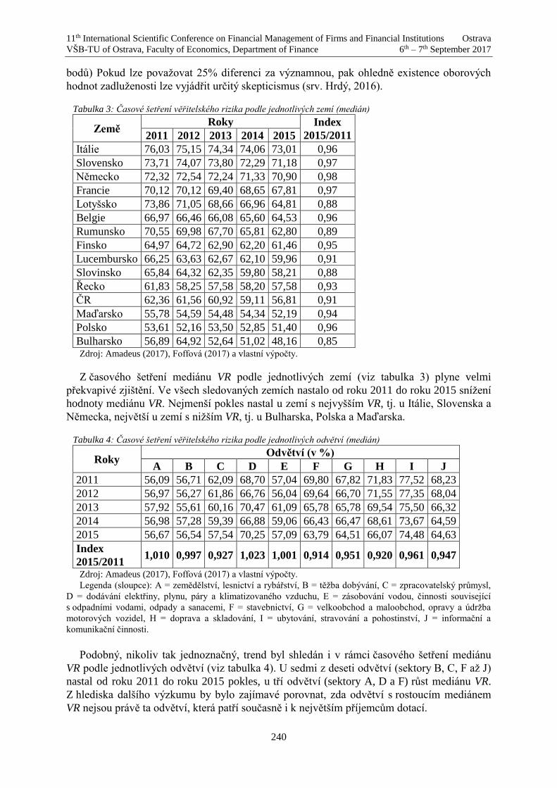
11th International Scientific Conference on Financial Management of Firms and Financial Institutions Ostrava
VŠB-TU of Ostrava, Faculty of Economics, Department of Finance 6th – 7th September 2017
240
bodů) Pokud lze považovat 25% diferenci za významnou, pak ohledně existence oborových
hodnot zadluženosti lze vyjádřit určitý skepticismus (srv. Hrdý, 2016).
Tabulka 3: Časové šetření věřitelského rizika podle jednotlivých zemí (medián)
Země Roky Index
2015/2011 2011 2012 2013 2014 2015
Itálie 76,03 75,15 74,34 74,06 73,01 0,96
Slovensko 73,71 74,07 73,80 72,29 71,18 0,97
Německo 72,32 72,54 72,24 71,33 70,90 0,98
Francie 70,12 70,12 69,40 68,65 67,81 0,97
Lotyšsko 73,86 71,05 68,66 66,96 64,81 0,88
Belgie 66,97 66,46 66,08 65,60 64,53 0,96
Rumunsko 70,55 69,98 67,70 65,81 62,80 0,89
Finsko 64,97 64,72 62,90 62,20 61,46 0,95
Lucembursko 66,25 63,63 62,67 62,10 59,96 0,91
Slovinsko 65,84 64,32 62,35 59,80 58,21 0,88
Řecko 61,83 58,25 57,58 58,20 57,58 0,93
ČR 62,36 61,56 60,92 59,11 56,81 0,91
Maďarsko 55,78 54,59 54,48 54,34 52,19 0,94
Polsko 53,61 52,16 53,50 52,85 51,40 0,96
Bulharsko 56,89 64,92 52,64 51,02 48,16 0,85 Zdroj: Amadeus (2017), Foffová (2017) a vlastní výpočty.
Z časového šetření mediánu VR podle jednotlivých zemí (viz tabulka 3) plyne velmi
překvapivé zjištění. Ve všech sledovaných zemích nastalo od roku 2011 do roku 2015 snížení
hodnoty mediánu VR. Nejmenší pokles nastal u zemí s nejvyšším VR, tj. u Itálie, Slovenska a
Německa, největší u zemí s nižším VR, tj. u Bulharska, Polska a Maďarska.
Tabulka 4: Časové šetření věřitelského rizika podle jednotlivých odvětví (medián)
Roky Odvětví (v %)
A B C D E F G H I J
2011 56,09 56,71 62,09 68,70 57,04 69,80 67,82 71,83 77,52 68,23
2012 56,97 56,27 61,86 66,76 56,04 69,64 66,70 71,55 77,35 68,04
2013 57,92 55,61 60,16 70,47 61,09 65,78 65,78 69,54 75,50 66,32
2014 56,98 57,28 59,39 66,88 59,06 66,43 66,47 68,61 73,67 64,59
2015 56,67 56,54 57,54 70,25 57,09 63,79 64,51 66,07 74,48 64,63
Index
2015/2011 1,010 0,997 0,927 1,023 1,001 0,914 0,951 0,920 0,961 0,947
Zdroj: Amadeus (2017), Foffová (2017) a vlastní výpočty.
Legenda (sloupce): A = zemědělství, lesnictví a rybářství, B = těžba dobývání, C = zpracovatelský průmysl,
D = dodávání elektřiny, plynu, páry a klimatizovaného vzduchu, E = zásobování vodou, činnosti související
s odpadními vodami, odpady a sanacemi, F = stavebnictví, G = velkoobchod a maloobchod, opravy a údržba
motorových vozidel, H = doprava a skladování, I = ubytování, stravování a pohostinství, J = informační a
komunikační činnosti.
Podobný, nikoliv tak jednoznačný, trend byl shledán i v rámci časového šetření mediánu
VR podle jednotlivých odvětví (viz tabulka 4). U sedmi z deseti odvětví (sektory B, C, F až J)
nastal od roku 2011 do roku 2015 pokles, u tří odvětví (sektory A, D a F) růst mediánu VR.
Z hlediska dalšího výzkumu by bylo zajímavé porovnat, zda odvětví s rostoucím mediánem
VR nejsou právě ta odvětví, která patří současně i k největším příjemcům dotací.

11th International Scientific Conference on Financial Management of Firms and Financial Institutions Ostrava
VŠB-TU of Ostrava, Faculty of Economics, Department of Finance 6th – 7th September 2017
241
3. Vztah mezi zadlužeností evropských obchodních společností a
zadluženosti veřejného sektoru
Jako ukazatel zadluženosti veřejného sektoru byl převzat ukazatel konsolidovaného hrubého
dluhu sektoru vládních institucí v procentech hrubého domácího produktu2, HDSVI, a to
z Eurostatu (2017a), který poskytl data za 28 členských zemí Evropské unie, dále byla využita
průměrná hodnota tohoto ukazatele za celou unii a průměrnou hodnota za eurozónu (18 zemí).
Tabulka 5: Zadluženost veřejného sektoru
Země
Roky Indexy
2011 2012 2013 2014 2015 2015/
2011
2012/
2011
2013/
2012
2014/
2013
2015/
2014
Řecko 172,1 159,6 177,4 179,7 177,4 1,031 0,927 1,112 1,013 0,987
Itálie 116,5 123,3 129,0 131,9 132,3 1,136 1,058 1,046 1,022 1,003
Portugalsko 111,4 126,2 129,0 130,6 129,0 1,158 1,133 1,022 1,012 0,988
Kypr 65,2 79,3 102,2 107,1 107,5 1,649 1,216 1,289 1,048 1,004
Belgie 102,3 104,1 105,4 106,5 105,8 1,034 1,018 1,012 1,010 0,993
Španělsko 69,5 85,7 95,4 100,4 99,8 1,436 1,233 1,113 1,052 0,994
Francie 85,2 89,5 92,3 95,3 96,2 1,129 1,050 1,031 1,033 1,009
Eurozóna (18) 86,1 89,5 91,3 92,0 90,4 1,050 1,039 1,020 1,008 0,983
Velká Británie 81,6 85,1 86,2 88,1 89,1 1,092 1,043 1,013 1,022 1,011
Chorvatsko 65,2 70,7 82,2 86,6 86,7 1,330 1,084 1,163 1,054 1,001
Rakousko 82,6 82,0 81,3 84,4 85,5 1,035 0,993 0,991 1,038 1,013
EU (28) 81,1 83,8 85,7 86,7 85,0 1,048 1,033 1,023 1,012 0,980
Slovinsko 46,6 53,9 71,0 80,9 83,1 1,793 1,157 1,317 1,139 1,027
Irsko 109,6 119,5 119,5 105,2 78,6 0,717 1,090 1,000 0,880 0,747
Maďarsko 80,7 78,2 76,6 75,7 74,7 0,926 0,969 0,980 0,988 0,987
Německo 78,7 79,9 77,5 74,9 71,2 0,905 1,015 0,970 0,966 0,951
Nizozemsko 61,6 66,4 67,7 67,9 65,1 1,057 1,078 1,020 1,003 0,959
Malta 70,0 67,6 68,4 67,0 64,0 0,914 0,966 1,012 0,980 0,955
Finsko 48,5 53,9 56,5 60,2 63,6 1,311 1,111 1,048 1,065 1,056
Slovensko 43,7 52,2 54,7 53,6 52,5 1,201 1,195 1,048 0,980 0,979
Polsko 54,1 53,7 55,7 50,2 51,1 0,945 0,993 1,037 0,901 1,018
Švédsko 37,5 37,8 40,4 45,2 43,9 1,171 1,008 1,069 1,119 0,971
Litva 37,2 39,8 38,7 40,5 42,7 1,148 1,070 0,972 1,047 1,054
Dánsko 46,4 45,2 44,7 44,8 40,4 0,871 0,974 0,989 1,002 0,902
ČR 39,8 44,5 44,9 42,2 40,3 1,013 1,118 1,009 0,940 0,955
Rumunsko 34,2 37,3 37,8 39,4 37,9 1,108 1,091 1,013 1,042 0,962
Lotyšsko 42,8 41,3 39,0 40,7 36,3 0,848 0,965 0,944 1,044 0,892
Bulharsko 15,2 16,7 17,0 27,0 26,0 1,711 1,099 1,018 1,588 0,963
Lucembursko 18,8 21,8 23,5 22,7 22,1 1,176 1,160 1,078 0,966 0,974
Estonsko 6,1 9,7 10,2 10,7 10,1 1,656 1,590 1,052 1,049 0,944 Zdroj: Eurostat (2017a), Foffová (2017) a vlastní výpočty.
Z tabulky 5 lze jako země v roce 2015 s nejzadluženějším veřejným sektorem identifikovat
Řecko, Itálii a Portugalsko, a naopak jako země s nejméně zadluženým veřejným sektorem
2 V databázi Eurostatu (2017a) je tento ukazatel uváděn jako general government gross debt as
percentage of gross domestic product.
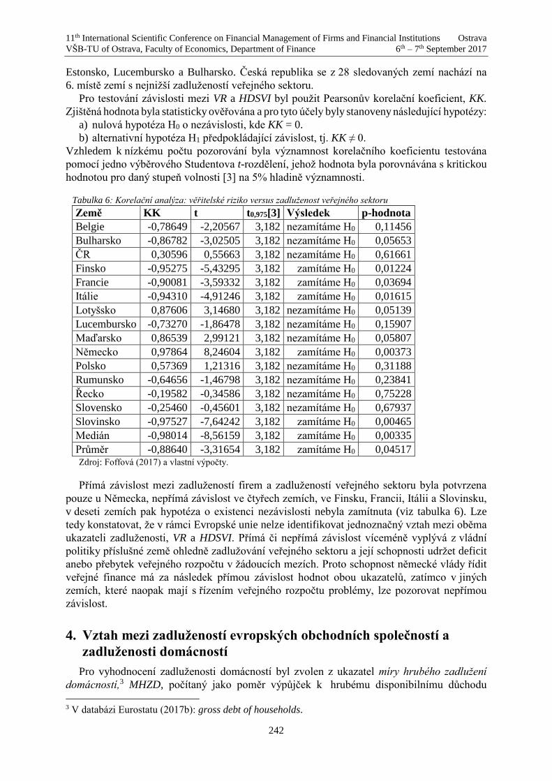
11th International Scientific Conference on Financial Management of Firms and Financial Institutions Ostrava
VŠB-TU of Ostrava, Faculty of Economics, Department of Finance 6th – 7th September 2017
242
Estonsko, Lucembursko a Bulharsko. Česká republika se z 28 sledovaných zemí nachází na
6. místě zemí s nejnižší zadlužeností veřejného sektoru.
Pro testování závislosti mezi VR a HDSVI byl použit Pearsonův korelační koeficient, KK.
Zjištěná hodnota byla statisticky ověřována a pro tyto účely byly stanoveny následující hypotézy:
a) nulová hypotéza H0 o nezávislosti, kde KK = 0.
b) alternativní hypotéza H1 předpokládající závislost, tj. KK ≠ 0.
Vzhledem k nízkému počtu pozorování byla významnost korelačního koeficientu testována
pomocí jedno výběrového Studentova t-rozdělení, jehož hodnota byla porovnávána s kritickou
hodnotou pro daný stupeň volnosti [3] na 5% hladině významnosti.
Tabulka 6: Korelační analýza: věřitelské riziko versus zadluženost veřejného sektoru
Země KK t t0,975[3] Výsledek p-hodnota
Belgie -0,78649 -2,20567 3,182 nezamítáme H0 0,11456
Bulharsko -0,86782 -3,02505 3,182 nezamítáme H0 0,05653
ČR 0,30596 0,55663 3,182 nezamítáme H0 0,61661
Finsko -0,95275 -5,43295 3,182 zamítáme H0 0,01224
Francie -0,90081 -3,59332 3,182 zamítáme H0 0,03694
Itálie -0,94310 -4,91246 3,182 zamítáme H0 0,01615
Lotyšsko 0,87606 3,14680 3,182 nezamítáme H0 0,05139
Lucembursko -0,73270 -1,86478 3,182 nezamítáme H0 0,15907
Maďarsko 0,86539 2,99121 3,182 nezamítáme H0 0,05807
Německo 0,97864 8,24604 3,182 zamítáme H0 0,00373
Polsko 0,57369 1,21316 3,182 nezamítáme H0 0,31188
Rumunsko -0,64656 -1,46798 3,182 nezamítáme H0 0,23841
Řecko -0,19582 -0,34586 3,182 nezamítáme H0 0,75228
Slovensko -0,25460 -0,45601 3,182 nezamítáme H0 0,67937
Slovinsko -0,97527 -7,64242 3,182 zamítáme H0 0,00465
Medián -0,98014 -8,56159 3,182 zamítáme H0 0,00335
Průměr -0,88640 -3,31654 3,182 zamítáme H0 0,04517 Zdroj: Foffová (2017) a vlastní výpočty.
Přímá závislost mezi zadlužeností firem a zadlužeností veřejného sektoru byla potvrzena
pouze u Německa, nepřímá závislost ve čtyřech zemích, ve Finsku, Francii, Itálii a Slovinsku,
v deseti zemích pak hypotéza o existenci nezávislosti nebyla zamítnuta (viz tabulka 6). Lze
tedy konstatovat, že v rámci Evropské unie nelze identifikovat jednoznačný vztah mezi oběma
ukazateli zadluženosti, VR a HDSVI. Přímá či nepřímá závislost víceméně vyplývá z vládní
politiky příslušné země ohledně zadlužování veřejného sektoru a její schopnosti udržet deficit
anebo přebytek veřejného rozpočtu v žádoucích mezích. Proto schopnost německé vlády řídit
veřejné finance má za následek přímou závislost hodnot obou ukazatelů, zatímco v jiných
zemích, které naopak mají s řízením veřejného rozpočtu problémy, lze pozorovat nepřímou
závislost.
4. Vztah mezi zadlužeností evropských obchodních společností a
zadluženosti domácností
Pro vyhodnocení zadluženosti domácností byl zvolen z ukazatel míry hrubého zadlužení
domácností,3 MHZD, počítaný jako poměr výpůjček k hrubému disponibilnímu důchodu
3 V databázi Eurostatu (2017b): gross debt of households.

11th International Scientific Conference on Financial Management of Firms and Financial Institutions Ostrava
VŠB-TU of Ostrava, Faculty of Economics, Department of Finance 6th – 7th September 2017
243
upravenému o změny čistého podílu domácností na rezervách penzijních fondů. Hodnoty
ukazatele byly rovněž čerpány z Eurostatu (2017b).
Tabulka 7: Zadluženost domácností
Země
Roky Indexy
2011 2012 2013 2014 2015 2015/
2011
2012/
2011
2013/
2012
2014/
2013
2015/
2014
Dánsko 265,5 262,8 253,8 264,2 243,5 0,917 0,990 0,966 1,041 0,922
Irsko 205,7 194,0 189,1 171,5 153,0 0,744 0,943 0,975 0,907 0,892
Švédsko 142,6 142,1 145,1 147,5 151,6 1,063 0,996 1,021 1,016 1,028
Velká Británie 128,0 126,2 124,9 123,2 124,0 0,969 0,986 0,990 0,986 1,006
Finsko 104,9 107,3 106,9 109,8 112,6 1,074 1,023 0,996 1,027 1,026
Španělsko 126,2 125,4 119,4 112,8 107,1 0,849 0,994 0,952 0,945 0,949
Belgie 90,5 92,6 94,6 99,1 102,1 1,128 1,023 1,022 1,047 1,031
Eurozóna (18) 97,4 96,9 95,6 94,7 94,1 0,966 0,995 0,987 0,991 0,993
Francie 83,3 84,6 86,1 86,9 88,3 1,060 1,016 1,018 1,009 1,016
Rakousko 86,7 84,1 83,8 84,3 86,4 0,997 0,970 0,997 1,005 1,026
Německo 85,9 84,5 83,7 82,8 82,2 0,957 0,983 0,991 0,989 0,993
Itálie 63,5 64,6 63,3 62,4 61,9 0,975 1,016 0,980 0,986 0,993
Polsko 56,3 54,6 56,1 58,1 60,6 1,077 0,970 1,027 1,035 1,044
ČR 54,4 55,8 57,2 55,9 57,6 1,057 1,025 1,025 0,977 1,029
Slovensko 43,3 45,4 49,3 53,6 57,6 1,330 1,050 1,086 1,087 1,073
Slovinsko 46,8 48,6 47,3 45,8 45,5 0,972 1,038 0,973 0,968 0,993
Lotyšsko 68,1 56,6 50,2 44,9 41,0 0,602 0,831 0,888 0,894 0,912
Maďarsko 64,5 54,2 48,6 45,5 39,4 0,611 0,840 0,897 0,936 0,866
Litva 39,4 37,3 35,0 34,6 35,8 0,909 0,947 0,939 0,987 1,036
Bulharsko 39,5 38,7 37,6 42,0 36,9 0,934 0,978 0,973 1,115 0,879 Zdroj: Eurostat (2017b), Foffová (2017) a vlastní výpočty.
Z tabulky 7 lze jako země s nejzadluženějšími domácnostmi v roce 2015 uvést Dánsko,
Irsko a Švédsko, zatímco země s nejméně zadluženými domácnostmi tvoří Bulharsko, Litva a
Maďarsko. Česká republika se z 18 sledovaných zemí nachází na 6. místě zemí s nejnižší
zadlužeností domácností. Pro testování závislosti mezi VR a MZHD byl zvolen stejný postup a
stejné podmínky jako při testování závislosti mezi VR a HDSVI.
Tabulka 8: Korelační analýza: věřitelské riziko versus zadluženost domácností
Země KK t t0,975[3] Výsledek p-hodnota
Belgie -0,98067 -8,68066 3,182 zamítáme H0 0,00322
Bulharsko 0,88161 3,23532 3,182 zamítáme H0 0,04802
ČR -0,71087 -1,75062 3,182 nezamítáme H0 0,17831
Finsko -0,87717 -3,16401 3,182 nezamítáme H0 0,05071
Francie -0,95279 -5,43507 3,182 zamítáme H0 0,01223
Itálie 0,77914 2,15287 3,182 nezamítáme H0 0,12038
Lotyšsko 0,99046 12,45186 3,182 zamítáme H0 0,00112
Maďarsko 0,90386 3,65916 3,182 zamítáme H0 0,03527
Německo 0,83254 2,60310 3,182 nezamítáme H0 0,08016
Polsko -0,53648 -1,10108 3,182 nezamítáme H0 0,35128
Slovensko -0,91777 -4.00307 3,182 zamítáme H0 0,02795
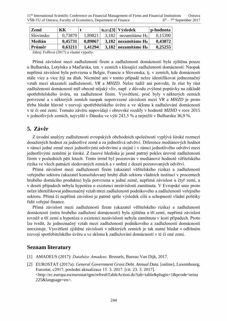
11th International Scientific Conference on Financial Management of Firms and Financial Institutions Ostrava
VŠB-TU of Ostrava, Faculty of Economics, Department of Finance 6th – 7th September 2017
244
Země KK t t0,975[3] Výsledek p-hodnota
Slovinsko 0,73870 1,89821 3,182 nezamítáme H0 0,15390
Medián 0,45731 0,89067 3,182 nezamítáme H0 0,43872
Průměr 0,63211 1,41294 3,182 nezamítáme H0 0,25255 Zdroj: Foffová (2017) a vlastní výpočty.
Přímá závislost mezi zadlužeností firem a zadlužeností domácností byla zjištěna pouze
u Bulharska, Lotyšska a Maďarska, tzn. v zemích s klesající zadlužeností domácností. Naopak
nepřímá závislost byla potvrzena u Belgie, Francie a Slovenska, tj. v zemích, kde domácnosti
stále více a více žijí na dluh. Nicméně ani v tomto případě nelze identifikovat jednoznačný
vztah mezi ukazateli zadluženosti, VR a MHZD. Nelze tudíž ani potvrdit, že růst by růst
zadluženosti domácností měl obecně nějaký vliv, např. z důvodu zvýšené poptávky na základě
spotřebitelského úvěru, na zadluženost firem. Vysvětlení, proč byly v některých zemích
potvrzené a v některých zemích naopak nepotvrzené závislosti mezi VR a MHZD je proto
třeba hledat hlavně v rozvoji spotřebitelského úvěru a ve sklonu k zadlužování domácností
v té či oné zemi. Tomuto závěru napovídají i obrovské rozdíly v hodnotě MZHD v roce 2015
v jednotlivých zemích, nejvyšší v Dánsku ve výši 243,5 % a nejnižší v Bulharsku 36,9 %.
5. Závěr
Z úvodní analýzy zadluženosti evropských obchodních společností vyplývá široké rozmezí
dosažených hodnot za jednotlivé země a za jednotlivá odvětví. Diference mediánových hodnot
v rámci jedné země mezi jednotlivými odvětvími a stejně i v rámci jednotlivého odvětví mezi
jednotlivými zeměmi je široké. Z časové hlediska je jasně patrný pokles úrovně zadluženosti
firem v posledních pěti letech. Tento trend byl pozorován v mediánové hodnotě věřitelského
rizika ve všech patnácti sledovaných zemích a v sedmi z deseti pozorovaných odvětví.
Přímá závislost mezi zadlužeností firem (ukazatel věřitelského rizika) a zadlužeností
veřejného sektoru (ukazatel konsolidovaný hrubý dluh sektoru vládních institucí v procentech
hrubého domácího produktu) byla potvrzena u jedné země, nepřímá závislost u čtyř zemí, a
v deseti případech nebyla hypotéza o existenci nezávislosti zamítnuta. V Evropské unie proto
nelze identifikovat jednoznačný vztah mezi zadlužeností podnikového a zadlužeností veřejného
sektoru. Přímá či nepřímá závislost je patrně spíše výsledek cílů a schopností vládní politiky
řídit veřejné finance.
Přímá závislost mezi zadlužeností firem (ukazatel věřitelského rizika) a zadlužeností
domácností (míra hrubého zadlužení domácností) byla zjištěna u tří zemí, nepřímá závislost
rovněž u tří zemí a hypotéza o existenci nezávislosti nebyla zamítnuta v šesti případech. Proto
lze tvrdit, že jednoznačný vztah mezi zadlužeností podnikového a zadlužeností domácností
neexistuje. Vysvětlení zjištěné závislosti v některých zemích je tak nutné hledat v odlišném
rozvoji spotřebitelského úvěru a ve sklonu k zadlužování domácností v té či oné zemi.
Seznam literatury
[1] AMADEUS (2017): Databáze Amadeus. Brussels, Bureau Van Dijk, 2017.
[2] EUROSTAT (2017a): General Government Gross Debt. Annual Data. [online], Luxembourg,
Eurostat, c2017, poslední aktualizace 15. 3. 2017. [cit. 23. 3. 2017].
<http://ec.europa.eu/eurostat/tgm/refreshTableAction.do?tab=table&plugin=1&pcode=teina
225&language=en>.

11th International Scientific Conference on Financial Management of Firms and Financial Institutions Ostrava
VŠB-TU of Ostrava, Faculty of Economics, Department of Finance 6th – 7th September 2017
245
[3] EUROSTAT (2017b): Gross Debt-to-income Ratio of Households. [online], Luxembourg,
Eurostat, c2017, poslední aktualizace 12. 4. 2017. [cit 15. 4. 2017].
<http://ec.europa.eu/eurostat/tgm/table.do?tab=table&init=1&plugin=1&language=en&pcod
e=tec00104>.
[4] Foffová, N. (2017): Prostorové a časové šetření zadluženosti evropských společností.
Praha, Vysoká škola ekonomická, 2017, bakalářská práce.
[5] Hrdý, M. (2016). Cílová kapitálová struktura a oborové standardy. Oceňování, 9(2),
s. 10-21.
[6] Jensen, M. C. – Smith, C. W. Jr. (1983): Theory of the Firm. Harvard University, 1983.
[7] Marek, P. (2007). Vliv teorie zastoupení na teorii podnikových financí. Český finanční a
účetní časopis, 2(2), s. 6-16.
[8] Myers, S. C. (1984). The Capital Structure Puzzle. Journal of Finance, 39(3), s. 575-592.

11th International Scientific Conference on Financial Management of Firms and Financial Institutions Ostrava
VŠB-TU of Ostrava, Faculty of Economics, Department of Finance 6th – 7th September 2017
246
The comparsion of various types of public-social partnerships in Poland in the light of the empirical
reasearch
Aldona Frączkiewicz-Wronka1, Anna Kozak2
Abstract
In this paper the authors focus on the problem of financial risks in public-social partnerships.
The authors understand public-social partnership as an collaborative working between
organizations operating both in public and social sector. Public participation plays a vital role
in such partnerships and it favors bottom-up mechanisms for rational and more efficient use of
public resources and money. The authors assume that the more cooperative the partnership the
smaller the risk of misuse of public money. In order to verify this assumption authors studied
173 partnerships in Poland. Our study shows how the type of partnership – competition,
coordination, cooperation and co-evolution – affects the use of resources and the efficiency
of spending public funds, and why each of them is important for reducing financial risk
in public-social partnerships.
Key words
public-social partnership, co-production, public services, third sector, public finance
JEL Classification: E62, E63, H41, H75, I38
1. Introduction
In the times when resources (including money) allocated to satisfy the needs socially
recognized as important are being limited, social expectations are growing, people
are becoming increasingly sceptical about public institutions and pressure on delivering
quality is becoming stronger, finding methods of managing public money which enable
achieve the social goals effectively becoming a difficult task. Therefore governments of many
countries are undertaking actions aimed at rehabilitation of the public sector [1]. In practice
this means co-governance, cooperation and using democratic decision-making procedures
to decide on the hierarchy and ways to satisfy public needs.
In the search for effective ways of meeting the needs socially recognized as important
managers create organizational solutions hitherto unknown in the public sector. One of the
new forms of meeting the public needs through providing social services are public-social
partnerships, understood as collaborative working between organizations operating both
in public and social sector. This collaboration is successful only when the partnership
is correctly designed and managed, resources of organisations constituting the partnership
are complementary and the logic behind how individual organisations and their leaders
operate is in line with the needs of the local community. Public participation plays a vital role
1 Aldona Frączkiewicz-Wronka, Prof., Faculty of Economics, University of Economics in Katowice, 1
Maja 50 Street, 40-287 Katowice, POLAND, e-mail: [email protected] 2 Anna Kozak, M.Sc., Faculty of Economics, University of Economics in Katowice, 1 Maja 50 Street,
40-287 Katowice, POLAND, e-mail: [email protected]

11th International Scientific Conference on Financial Management of Firms and Financial Institutions Ostrava
VŠB-TU of Ostrava, Faculty of Economics, Department of Finance 6th – 7th September 2017
247
in such partnerships and it favors bottom-up mechanisms for rational and more efficient use
of public resources and money. One of those mechanisms is co-production of social services.
Notwithstanding beyond the benefits of this form of meeting the public needs it involves
many risks including the financial one.
The paper financed by the research project titled “The public participation in the public
management practice”, financed by the statutory activity of the University of Economics in
Katowice in the part concerning the research potential of the Faculty of Economics in 2015-
2017.
2. Theorethical background
A growing awareness of the complexity of social issues contributes to the intensive search
for new ways of effective providing social services. Organisations delivering social services
reach out towards solutions crossing over their individual boundaries and create organisational
projects based on cooperation between partners from different sectors [2, 3]. In this sense,
interorganisational cooperation becomes interaction fields populated by autonomous but
interdependent actors, where alignments of interests institutionalized through formal
collective actors and informally through issue-based nets criss-cross the established order
of economic exchange relationships [4] or more institutionalised cooperation between
organisations is a way to earn an innovation and relational rent [5]. The ultimate outcome
of the actions that were taken should be the success measured with the approval of created
value by individual beneficiaries (e.g. marginalized people or people at risk
of marginalization), organisations forming the cooperation network, a partnership as a whole
and the local community. Relationships that are developed within a partnership
can be perceived as voluntary links between the systems, organisations and individuals who
are involved while maintaining their autonomy. One example of cooperation started between
organisations operating in different sectors is public-social partnership, which favors co-
production.
Elinor Ostrom by co-production understands “the process through which inputs used
to produce a good or service are contributed by individuals who are not “in” the same
organization. Coproduction implies that citizens can play an active role in producing public
goods and services of consequence to them”[6]. Similarly Bovaird defines co-production
as „the provision of services through regular, long-term relationships between
professionalized service providers (in any sector) and service users or other members
of the community, where all parties make substantial resource contributions”[7]. From
the perspective of this article particularly important is the last part of Bovaird’s definition
which draws attention to „substantial resource contributions” made by both sides of the
partnership. Co-production as a partnership between public and social sector to achieve
a valued outcome empowers citizens to “contribute more of their own resources and have
greater control over service decisions and resources”[8]. Those resources are among others
capabilities, skills, effort, time and money which are require on the both sides of the process
[9, 10].
The relation between government and non-profits in co-production process goes beyond
exchanging financial resources [11, 12], but financial risk is significant part of this process
[9]. Co-production means costs and benefits (including financial) for both sides
of partnership. What more important financial risk lies primarily on the side of public finance
unit. This is the public side of the collaboration that most often financing activities undertaken
by partnership and consequently carries financial responsibility for the effects [9, 13].

11th International Scientific Conference on Financial Management of Firms and Financial Institutions Ostrava
VŠB-TU of Ostrava, Faculty of Economics, Department of Finance 6th – 7th September 2017
248
The financial risk of partnerships highlights also one of OECD Public Governance Reviews.
In this publication OECD diagnosed eight potential risk associated with co-production: skills,
accountability, organizational culture, trust, equity and inclusion, probity, multi-level
governance and resources. Through the risk associated with resources they understand “need
for additional resources to fund co-production initiatives, at least in the early stages” and
“an increase in transaction costs and a loss of economies of scale if services become highly
personalized”[14].
But in the same time is emerging evidence of co-production of public services impact
on outcomes, value of money and its potential economic and social value [8]. Additionally
as mentioned above public-social partnerships favor bottom-up mechanisms for rational
and more efficient use of public resources and money. But partnerships differ because of
the kind of cooperation and not all partnerships are equally cooperative.
Figure 1: Continuum identifying types of partnerships
Source: Gordon, P., Pratt, J. and Plamping, D. (2000). Partnership fit for purpose? Testing a theory in practice,
www.wholesystems.uk.com
In literature the most often quoted typology is proposed by Pratt and his co-workers. They
developed a typology of four different types of partnership (competition, coordination,
cooperation and co-evolution), each with different characteristics fit for different
circumstances. To describe the partnerships, they adopted two variables: type of goals
(individual or collective) and predictability of objectives and solutions (the extent to which the
behavior needed to achieve them can be known in advance). The types of cooperation
in partnerships in view of these two variables are shown in the Figure 1 and their detailed
description – in the Table 1. According to the authors this typology isn’t a hierarchy because
real partnerships contain elements of several types and are likely to move between them over
time [15]. However during the analysis of the distinguished types of partnerships coordination
draws attention as the most mature and focused on cooperation type of partnership.

11th International Scientific Conference on Financial Management of Firms and Financial Institutions Ostrava
VŠB-TU of Ostrava, Faculty of Economics, Department of Finance 6th – 7th September 2017
249
Table 1: Description of various types of partnerships
Type of
partnership Goal Predictability Essence Application
CO
MP
TE
TIT
ION
Each organization
is achieving its own
goals and know how
to achieve them
Requires pay
attention to the detail
of the rules within
which partnership
operates
The driving force is
individual creativity –
competition can
improve the
efficiency
and performance
of individual parts of
a system
The tactic
for change
CO
OR
DIN
AT
ION
The shared goal
is knowable; common
goal means more than
individual goal
of each organization
Goals are agreed
in all the necessary
detail including each
step to be taken to
achieve them
Each organization
needs to adopt
for this sort
of collaboration
to work is to find
ways of fitting
together without any
problems
Partners come
together with
the intention of
delivering pre-set
objectives based on
a consensus of
opinion about what
works
CO
OP
ER
AT
ION
Lack of shared goals Low predictability
of behaviors
“You scratch my back
and I’ll scratch yours”
– partners cooperate
when their own
interest requires it;
the goals are
individual but the
partners see their
futures as linked
In the most provate
sec tors alliances
(ex. airline alliances)
CO
-
EV
OL
UT
ION
Partners share
a broad goal
Unknown way of
accomplishing goals;
lack of certainty
based on known
patterns of effective
action
Co-designing new
solutions together for
achieving a shared
purpose, in the
process of which all
the partners evolve
Creating new
opportunities,
new ways of working
Source: Gordon, P., Pratt, J. and Plamping, D. (2000). Partnership fit for purpose? Testing a theory in practice,
www.wholesystems.uk.com; Frączkiewicz-Wronka, A. (2014). Zarządzanie usługami społecznymi. Studium
partnterstw publiczno-społecznych. Warszawa: Difin.
For the needs of the research the authors adopted this typology and assumed that the type
of partnership – competition, coordination, cooperation and co-evolution – affects the use
of resources and the efficiency of spending public funds, and why each of them is important
for reducing financial risk in public-social partnerships. Our presumption is that the more
cooperative – focused on cooperation – the partnership the smaller the risk of misuse of public
money. The type of partnership is important for reducing financial risk in public-social
partnerships because of the better use of resources, the greater impact on the environment
and higher efficiency assessment in more cooperative partnerships. Since the authors
recognized coordination as a the most mature and cooperative, this type of partnership should
be the best for minimizing the financial risk in public-social collaboration. In order to verify
this assumption authors studied 173 partnerships in Poland.

11th International Scientific Conference on Financial Management of Firms and Financial Institutions Ostrava
VŠB-TU of Ostrava, Faculty of Economics, Department of Finance 6th – 7th September 2017
250
3. Research findings
The research method used in the study was a survey. The survey was conducted with the
use of the CATI (Computer Assisted Telephone Interviewing) technique by interviewers from
Institute for Cooperation and Local Partnerships in Katowice, Silesia region, Poland. The
computer-assisted telephone interviews technique is often used in quantitative research and
it consists of carrying out telephone interviews with the support of a computer program. The
advantages of this technique are: short time of realization, relatively low cost and automatic
collection and preparation of data for analysis [16]. The survey questionnaire was addressed to
the leaders of the partnerships in Poland. As a result of the survey, 173 correctly filled
questionnaires were received.
In order to verify the thesis the authors used opinions of the partnership’s leaders about
the use of resources, impact on the environment and the efficiency in relation to the type of
partnership (competition, coordination, cooperation or co-evolution). The answers to
questions regarding these issues are shown in the Tables 2-4.
Table 2: The type of partnership and the use of resources
Type of partnership
Connection
Co-evolution Cooperation Coordination Competition Partnerships
in general
Frequen
cy Percent
Frequen
cy Percent
Frequen
cy Percent
Freque
ncy Percent
173
No connection 0 0 5 2.9 3 1.7 4 2.3
Visible connection 17 9.8 21 12.1 67 38.7 11 6.5
No answer 8 4.6 13 7.6 21 12.2 3 1.7
In all 25 14.4 39 22.5 91 52.6 18 10.5
Source: Own elaboration based on research results.
The first question that authors found relevant for the analyzed problem concerns the better
use of resources in organization as a consequence of the undertaken partnership. The opinion
that there is a visible connection between a type of partnership and the use of resources was
expressed by the biggest number of respondents within the coordination type of partnership
(38.7 %). At the same time only 1.7 % of the surveyed leaders do notsee any connection
between the use of resources and the type of partnership. It allows for drawing the first
conclusion that limited resources are better managed in cooperative type of partnership.

11th International Scientific Conference on Financial Management of Firms and Financial Institutions Ostrava
VŠB-TU of Ostrava, Faculty of Economics, Department of Finance 6th – 7th September 2017
251
Table 3: The type of partnership and opinion about the impact on the environment
Type of partnership
Connection
Co-evolution Cooperation Coordination Competition Partnerships
in general
Frequen
cy Percent
Frequen
cy Percent
Frequen
cy Percent
Freque
ncy Percent
173
No connection 1 0.6 4 2.3 7 4.0 4 2.3
Visible connection 17 9.8 31 17.9 68 39.4 11 6.5
No answer 7 4.0 4 2.3 16 9.2 3 1.7
In all 25 14.4 39 22.5 91 52.6 18 10.5
Source: Own elaboration based on research results.
Next questioned concerns the connection between a type of partnership and an impact on
the environment. According to the participating leaders the impact on the environment is
the biggest in the coordination type of partnership (39.4 %). The relationship between these
elements coordination type of partnership has not been recognized by 4.0 % of the
respondents. What is more, the outcome confirms partly the authors’ assumption that the
positive impact on the environment can be a result of a more rational use of resources and
more efficient spending of public funds which can, in turn, lead to meeting the needs socially
recognized as important in a more effective manner.
Table 4: The type of partnership and the efficiency assessment
Type of partnership
Connection
Co-evolution Cooperation Coordination Competition Partnerships
in general
Frequen
cy Percent
Frequen
cy Percent
Frequen
cy Percent
Freque
ncy Percent
173
No connection 2 1.2 5 2.9 7 4.0 4 2.3
Visible connection 16 9.2 26 15.0 35 20.3 12 6.9
No answer 7 4.0 8 4.6 49 28.3 2 1.3
In all 25 14.4 39 22.5 91 52.6 18 10.5
Source: Own elaboration based on research results.
The last question the authors found important for the subject is question regards
the efficiency assessment. The results of the survey show that in terms of the efficiency
(including the efficiency of spending public funds) the best type of partnership
is coordination. 20.3 % of respondents are of opinion that the connection between these
elements is the most visible for the coordination. At this point it is worth mentioning that
28.3% of the participants have not provided any answer, which shows how difficult it is
11th International Scientific Conference on Financial Management of Firms and Financial Institutions Ostrava
VŠB-TU of Ostrava, Faculty of Economics, Department of Finance 6th – 7th September 2017
252
to achieve and assess efficiency. Nonetheless coordination has the most positive impact on
efficiency increase.
To sum up, the analyzed responses show positive connection between the most cooperative
type of partnership which is coordination and the use of resources, the impact on
the environment and the efficiency assessment.
4. Conlusion
Nowadays research attention has been shifted from individual organisations to emerging
systems, which might be characterised as multi-stakeholder collaboration, such as a public
social partnership. This is a consequence of departure from the state monopoly in the public
sector, and moving towards the search for effective solutions of delivering services to citizens
on the basis of organising the public sector in such a way that it will foster the creation of
quasi-market systems and forms of networking. In this paper the authors aim to answer the
question which model of cooperation is conducive to achieving better results in the public-
social partnership. The authors understand public-social partnership as an activity undertaken
in collaboration between organizations operating both in public and social sector. The article
brings together theoretical insights and empirical data.
The collaboration between organizations operating in public and social sectors is formed
and develops as a response to revealed social problems and expectations. This is a slightly
simplified model of defining partnership as an organisational response to challenges arising in
the social reality, but although it is not as rare as it might seem, it is often successful and
the leads to the achievement of goals.
These purposes are rational use of limited resources and efficient spending of public funds,
among others. The authors claim that the more cooperative the partnership the smaller the risk
of misuse of public money.
The study confirms the thesis and shows that the type of partnership – competition,
coordination, cooperation and co-evolution – affects the use of resources and the efficiency
of spending public funds. In the opinion of the surveyed leaders of the partnerships the use of
resources, impact on the environment and efficiency are best when the type of partnership is
coordination. Hence, this type of partnership has positive impact on reducing financial risk
in public-social partnerships.
The results of the research show the benefits that the cooperation of the public and social
sectors (for example co-production of social services) can bring and they constitute
an argument in support of undertaking cooperation between public and social partners. Such
collaborations may involve a risk (including the financial one), however focusing
on cooperation allows to minimize the risk of misuse of public money and achieve desirable
results, such as the more rational use of resources and the better efficiency of spending public
funds in the public finance unit.
References
[1] Pollitt, C., and Bouckaert, G. (2000). Public management reform. Oxford, England:
Oxford University Press.
[2] Pestoff, V. (2014). Collective Action and the Sustainability of Co-Production. Public
Management Review, 16(3), p. 383-401.
11th International Scientific Conference on Financial Management of Firms and Financial Institutions Ostrava
VŠB-TU of Ostrava, Faculty of Economics, Department of Finance 6th – 7th September 2017
253
[3] Alford, J. (2014). The Multiple facets of Co-Production: Building on the work of Elinor
Ostrom. Public Management Review, 16 (3), p. 299-316.
[4] Alford, J. (2014). The Multiple facets of Co-Production: Building on the work of Elinor
Ostrom. Public Management Review, 16 (3), p. 299-316.
[5] Araujo, L. and Brito, C. (1998). Agency And Constitutional Ordering In Networks.
International Studies of Management & Organizations, 27 (4), p. 22-46.
[6] Niemczyk, J., Stańczyk-Hugiet, E., Jasiński, B.M. and Chrisidu-Budnik, A. (2012). Sieci
międzyorganizacyjne. Współczesne wyzwanie dla teorii i praktyki zarządzania.
Warszawa: Wydawnictwo C.H. Beck.
[7] Niemczyk, J., Stańczyk-Hugiet, E., Jasiński, B.M. and Chrisidu-Budnik, A. (2012). Sieci
międzyorganizacyjne. Współczesne wyzwanie dla teorii i praktyki zarządzania.
Warszawa: Wydawnictwo C.H. Beck.
[8] Ostrom, E. (1996), Crossing the great divide: Coproduction, synergy, and development.
World Development, 24(6), p. 1073-1087.
[9] Ostrom, E. (1996), Crossing the great divide: Coproduction, synergy, and development.
World Development, 24(6), p. 1073-1087.
[10] Bovaird, T. (2007), Beyond engagement and participation: User and community
coproduction of public services. Public Administration Review, 67(5), p. 846-860.
[11] Calabro, A. (2012). Co-production: An alternative to the partial privatization processes
in Italy and Norway. In V. Pestoff, T. Brandsen and B. Verschuere (Eds.), New public
governance, the third sector and co-production. New York: Routledge.
[12] Verschuere, B., Brandsen, T. and Pestoff, V. (2012). Co-production: The State of the Art
in Research and the Future Agenda. VOLUNTAS: International Journal of Voluntary and
Nonprofit Organizations, 23(4), p. 1083-1101.
[13] Verschuere, B., Brandsen, T. and Pestoff, V. (2012). Co-production: The State of the Art
in Research and the Future Agenda. VOLUNTAS: International Journal of Voluntary and
Nonprofit Organizations, 23(4), p. 1083-1101.
[14] Ryan, B. (2012). Co-production: Option or obligation?. Australian Journal of Public
Administration, 71(3), p. 314-324.
[15] Salamon, L. (2002). The tools of government: A guide to the new governance. New York:
Oxford University Press.
[16] Smith, S. R. (2002). Social services. In L. Salamon (Eds.), The state of the nonprofit
sector. Washington, DC: Brookings Institute Press.
[17] Pestoff, V., Osborne, S.P. and Brandsen, T. (2006). Patterns of Co-production in Public
Services. Some concluding thoughts. Public Management Review 8(4), p. 591-595.
[18] Pestoff, V., Osborne, S.P. and Brandsen, T. (2006). Patterns of Co-production in Public
Services. Some concluding thoughts. Public Management Review 8(4), p. 591-595.
[19] OECD (2011). Together for Better Public Services. Partnering with Citizens and Civil
Society. OECD Public Governance Reviews. OECD Publishing.
[20] OECD (2011). Together for Better Public Services. Partnering with Citizens and Civil
Society. OECD Public Governance Reviews. OECD Publishing.

11th International Scientific Conference on Financial Management of Firms and Financial Institutions Ostrava
VŠB-TU of Ostrava, Faculty of Economics, Department of Finance 6th – 7th September 2017
254
[21] Gordon, P., Pratt, J. and Plamping, D. (2000). Partnership fit for purpose? Testing
a theory in practice. www.wholesystems.co.uk.
[22] Babbie, E. (2008). Podstawy badań społecznych. Warszawa: PWN.

11th International Scientific Conference on Financial Management of Firms and Financial Institutions Ostrava
VŠB-TU of Ostrava, Faculty of Economics, Department of Finance 6th – 7th September 2017
255
Intangible Assets and Their Valuation Using Direct Intellectual Capital Methods: Pros and Cons
Jozef Glova 1
Abstract
The paper presents issues concerning the definition and valuation of intangible assets,
specifically direct intellectual capital methods. We start by reviewing intangibles and go
through the taxonomy provided by Sveiby. Here we focus on direct intellectual capital methods
– Human Resource Costing and Accounting, Technology Broker, Accounting for the Future,
Citation-Weighted Patents, Inclusive Valuation Methodology, Total Intellectual Asset
Valuation, The Value Explorer, FiMIAM, Dynamic monetary model, and EVVICAE, which
estimate the monetary value of intangible assets by identifying its various components.
Additionally some limitations of the methods are summarized and discussed.
Key words
Intangible assets, direct intellectual capital methods, knowledge, valuations, asset pricing.
JEL Classification: E24, G12, M21, O34
1. Úvod
Nehmotné aktíva podnecujú inovácie a prispievajú viac k podnikovej
konkurencieschopnosti, rovnako ako ku konkurencieschopnosti celej ekonomiky. Tomu
zodpovedajú aj investície do nehmotných aktív, ktoré podľa OECD, a jeho projektu na túto
tému „New sources of growth: intangible assets“ (Preklad autora: Nové zdroje rastu:
nehmotné aktíva), neustále narastajú. Dokonca v niektorých prípadoch tieto investície
presahujú investície do tradičného kapitálu v podobe strojov, zariadení a stavieb. Narastajúca
globálna konkurencia, informačné a komunikačné technológie, nové modely podnikania, a
narastajúca dôležitosť sektora služieb ešte viac zvýrazňujú dôležitosť nehmotných aktív pre
podniky, odvetvia a celé národné ekonomiky. Rozvoj a podpora nehmotných aktív sa stávajú
kľúčovými pre úspech v aktivitách s vysokou pridanou hodnotou.
Rovnako tak ekonomická literatúra je dôkazom narastajúceho záujmu o pojmy ako
nehmotné aktíva, intelektuálny kapitál, znalostné aktíva a iné obdobné pojmy. Existuje celá
rada článkov, kníh a rôznych štúdii, ktoré sa zaoberajú touto oblasťou. Je potrebné ale dodať,
že napriek obrovskému množstvu publikácii, nedošlo k jednoznačnému konsenzu v mnohých
oblastiach nehmotných aktív.
Tento príspevok prezentuje pohľad na nehmotné aktíva, ich vymedzenie a spôsoby ich
ohodnocovania na báze skupiny metód priamého ohodnocovania nehmotných aktív.
Jednotlivé metódy sú stručne popísané, dôraz sa kladie na ich porovnanie a sumarizáciu výhod
a nevýhod jednotlivých konceptov.
1 doc. Ing. Jozef Glova, PhD., Technical University of Košice, Faculty of Economics, e-mail:

11th International Scientific Conference on Financial Management of Firms and Financial Institutions Ostrava
VŠB-TU of Ostrava, Faculty of Economics, Department of Finance 6th – 7th September 2017
256
2. Nehmotné aktíva a vymedzenie hodnoty
Jednou z vlastností nehmotných aktív je komplikované stanovanie ich hodnoty. Táto
vlastnosť úzko súvisí s ostatnými špecifikami takýchto aktív, najmä so
samotnou nehmotnosťou a rýchlou pominuteľnosťou ich hodnoty. Napriek náročnosti tejto
úlohy sa začali objavovať rôzne snahy zamerané na meranie a stanovenie hodnoty takýchto
typov aktív.
Ešte pred predstavením konkrétnych metód ohodnocovania nehmotných aktív by bolo
vhodné vysvetliť pojem ohodnocovanie. Ten je často nesprávne zamieňaný s pojmom
oceňovanie. Podľa Krabca (2009) súvisí oceňovanie hlavne s daňovou reguláciou
a oceňovateľ pri ňom stanovuje cenu platnú pre konkrétny účel. Vo väčšine prípadov je
vykonané formou znaleckých posudkov. Ohodnocovanie znamená stanovenie určitej kategórie
hodnoty. Určuje sa pri ňom hodnota vo výške očakávanej ceny obchodu vychádzajúcej
z podmienok zadania alebo kategória hodnoty, ktorá so zmenou vlastníckych práv nesúvisí.
(Krabec, 2009) Najčastejšie sa pri ohodnocovaní stretávame s nasledujúcimi kategóriami
hodnoty:
Reálna hodnota (fair value): Medzinárodné ohodnocovacie štandardy IVS (IVSC, 2011)
definujú reálnu hodnotu ako „odhadovanú cenu pri výmene aktív alebo záväzkov medzi
konkrétnymi informovanými a ochotnými stranami zohľadňujúcu ich individuálne záujmy.“
Podľa Medzinárodných štandardov finančného výkazníctva IFRS 13 (IASB, 2013) je reálna
hodnota „cena, za ktorú by sa uskutočnila riadna transakcia predaja aktíva alebo prevodu
záväzku medzi účastníkmi trhu k dátumu ocenenia.“
Trhová hodnota: Trhová hodnota je „odhadnutá čiastka, za ktorú by mal byť majetok
vymenený k dátumu ocenenia medzi ochotným kupujúcim a ochotným predávajúcim pri
transakcii medzi samostatnými a nezávislými partnermi po náležitom marketingu, v ktorej by
obe strany jednali informovane, rozumne a bez nátlaku.“ (IVSC, 2011)
Investičná hodnota: „Investičná hodnota je hodnota majetku pre konkrétneho investora
alebo triedu investorov pre stanovenie investičného cieľa. Tento subjektívny pojem spája
špecifický majetok so špecifickým investorom, skupinou investorov alebo jednotou s určitými
investičnými cieľmi alebo kritériami. Investičná hodnota majetkového aktíva môže byť vyššia
alebo nižšia ako trhová hodnota tohto majetkového aktíva. Termín investičná hodnota by
nemal byť zamieňaný s trhovou hodnotou investičného majetku.“ (Mařík a kol., 2007)
Špecifická hodnota pre podnik: Podľa IAS 38 (IASB, 2010) je špecifická hodnota pre
podnik súčasnou hodnotu peňažných tokov, ktoré podnik očakáva z pokračujúceho využívania
aktíva a z jeho vyradenia na konci doby jeho životnosti alebo ktoré podnik očakáva pri
vyrovnaní záväzku.
Všeobecná hodnota: S týmto termínom sa môžeme stretnúť vo vyhláške Ministerstva
spravodlivosti SR o stanovení všeobecnej hodnoty majetku (492/2004 Z.z.) a jej definícia je
podobná definícii trhovej hodnoty. Všeobecná hodnota je vo vyhláške definovaná ako
„výsledná objektivizovaná hodnota majetku, ktorá je znaleckým odhadom
najpravdepodobnejšej ceny hodnoteného majetku ku dňu ohodnotenia v danom mieste a čase,
ktorú by tento mal dosiahnuť na trhu v podmienkach voľnej súťaže, pri poctivom predaji, keď
kupujúci aj predávajúci budú konať s patričnou informovanosťou i opatrnosťou a s
predpokladom, že cena nie je ovplyvnená neprimeranou pohnútkou.“
Medzinárodné štandardy ohodnocovania (IVSC, 2011) uvádzajú, že odhad trhovej hodnoty
by mal vychádzať z trhových údajov. Trhová hodnota zároveň predpokladá cenu určenú na
otvorenom a konkurenčnom trhu, a teda, že pre dané aktívum existuje otvorený a konkurenčný
trh. Tieto podmienky nie je možné splniť pre väčšinu nehmotných aktív. Pri nehmotných

11th International Scientific Conference on Financial Management of Firms and Financial Institutions Ostrava
VŠB-TU of Ostrava, Faculty of Economics, Department of Finance 6th – 7th September 2017
257
aktívach sa preto pri ohodnocovaní zvyčajne snažíme odhadnúť ich reálnu hodnotu alebo
investičnú hodnotu.
Karl-Erik Sveiby sa dlhodobo zaoberá metódami ohodnocovania nehmotných aktív. Sveiby
(2010) uvádza prehľad najznámejších metód a zatrieďuje ich do štyroch skupín. Týmito
skupinami sú metódy priameho ohodnocovania nehmotných aktív (DIC), metódy založené na
trhovej kapitalizácii (MCM), metódy založené na rentabilite aktív (ROA) a metódy scorecard
(SC). Metódy scorecard sa nepokúšajú o stanovenie hodnoty vo finančných jednotkách, ich
výsledkom tak nie je ohodnocovanie, ale skôr meranie nehmotných aktív. V Tab. 1 uvádzame
prehľad metód priamého ohodnocovania, ktorými sa budeme ďalej zaoberať.
Tab. 1 Zoznam metód priamého ohodnocovania nehmotných aktív.
Rok Originálny názov metódy Hlavný navrhovateľ Kategória
2008 EVVICAE™ McCutcheon DIC
2007 Dynamic monetary model Milost DIC
2002 FiMIAM Rodov a Leliaert DIC
2000 The Value Explorer™ Andriessen a Tiessen DIC
2000 Intellectual Asset Valuation Sullivan DIC
1998 Inclusive Valuation Methodology (IVM) M’Pherson DIC
1998 Accounting for the Future (AFTF) Nash DIC
1996 Technology Broker Brooking DIC
1996 Citation- Weighted Patents Bontis DIC
1988 Human Resource Costing & Accounting (HRCA ) Johansson DIC
3. Metódy priamého ohodnocovania nehmotných aktív
V tejto časti príspevku sa venujeme bližšie metódam priamého ohodnocovania nehmotných
aktív. Tieto metódy ohodnocovania nehmotných aktív sa snažia stanoviť hodnotu nehmotných
aktív, prípadne aj jeho jednotlivých častí, v peňažných jednotkách. Sú usporiadané
chronologický a snahou je v sumarizovanej podobe priblížiť každý z konceptov.
Ako prvý použili pojem účtovníctvo ľudských zdrojov (HRA – Human Resource
Accounting) Brummet et al. (1968). V 70. rokoch bola účtovníctvu ľudských zdrojov
venovaná značná pozornosť. Nasledovalo však desaťročie, keď záujem o túto oblasť poklesol.
90. roky priniesli oživenie a záujem zo strany medzinárodných organizácií, veľkých
súkromných spoločností aj vlád. Gröjer et al. (1996) zaviedli pojem účtovníctvo a kalkulácia
nákladov ľudských zdrojov (HRCA – Human Resource Costing and Accounting), ktorý
zahŕňa koncepty HRA a analýzy užitočnosti. Jedným z hlavných cieľov Metódy účtovníctva
ľudských zdrojov HRCA je zachytiť hodnotu ľudských zdrojov a investícií do ľudského
kapitálu v súvahe a snažiť sa o štandardizáciu tohto vykazovania. Naplnenie týchto snáh by
mohlo preniesť dôležitý zdroj informácií o ľudských zdrojoch spoločnosti. Johanson et al.
(1999) uvádzajú, že v praxi zostavuje súvahu ľudských zdrojov veľmi málo organizácií,
prevažne sa jedná o futbalové kluby. Aj v prípade futbalových klubov sa pri tom zvyčajne
zostavujú dve súvahy. Jedna z nich hodnotu ľudských zdrojov zahŕňa, druhá nie.
Vo svojom koncepte Technology Broker prináša Brooking (1996) rozsiahly pohľad na
nehmotné aktíva, ktoré sa bežne vyskytujú v organizácii. Za prínos považujeme priradenie
možných metód merania ku konkrétnym aktívam. Ponúkané metódy na sledovanie vývoja
jednotlivých aktív môžu pomôcť v práci manažmentu a podať mu dôležité informácie o tom,
na ktoré časti intelektuálneho kapitálu je potrebné zamerať sa. Kladne hodnotíme navrhnutý
proces Auditu intelektuálneho kapitálu, aj prepojenie s manažmentom znalostí. Brooking
11th International Scientific Conference on Financial Management of Firms and Financial Institutions Ostrava
VŠB-TU of Ostrava, Faculty of Economics, Department of Finance 6th – 7th September 2017
258
(1996) vyzdvihuje aj dôležitosť finančného ohodnocovania. Tu sa nesnaží vyvinúť vlastnú
metódu, ale odporúča tiež aplikovať klasické prístupy. Celkovo je teda metóda prínosom
najmä v oblasti riadenia a merania nehmotných aktív.
Myšlienka ohodnocovania podniku a jeho aktív a pasív na základe očakávaných peňažných
tokov, ktorá je základom Účtovníctva pre budúcnosť AFTF, nie je ničím nová. Nash (2003)
sa nevenuje ohodnocovaniu konkrétnych nehmotných aktív, ani nerieši problém odhadu
finančných tokov spojených z jednotlivými aktívami. AFTF preto nepovažujeme za prínos
v oblasti ohodnocovania nehmotných aktív. Jednou z hlavných nevýhod používania iba
výnosových metód je, že peňažné toky nie je možné relevantne odhadnúť pri všetkých
podnikových aktívach. V takýchto prípadoch sa núka použitie nákladového alebo trhové
prístupu, s ktorými Nash (2003) neuvažuje. Pridanou hodnotou, ktorú ponúka Nash (2003), je
spomínaný návrh metodiky odhadu diskontnej sadzby. Nevýhodou tejto metodiky je, že je
aplikovateľná len pre verejne obchodované spoločnosti, pri ktorých vieme z trhu určiť ich
minulé trhové hodnoty. Aj v týchto prípadoch by jej relevanciu bolo vhodné testovať a overiť.
The Value Explorer je manažérsky orientovaná metóda spoločnosti KPMG od autorov
Andriessen a Tissen (2000) a Andriessen (2005). Výhodou metódy je 5 jasne definovaných
a vysvetlených krokov, ktoré umožňujú aplikáciu metódy v podniku. Následnosť krokov je
logická. Nevýhodou je viacero zjednodušení a subjektívnych odhadov pri finančnom
ohodnocovaní. Prvým zjednodušením je uvažovanie fixnej výnosnosti hmotných aktív,
finančných aktív a čistého pracovného kapitálu a odpočítanie ich výnosov od očakávaných
ziskov. Všetky tieto zložky a aj nehmotný majetok sa podieľajú na tvorbe finančných tokov
spoločne, uvažovanie aditívneho vzťahu ich výnosov nepovažujeme za správne. Ak už
uvažujeme z výnosnosťami jednotlivých druhov aktív, dá sa očakávať, že v rôznych
odvetviach priemyslu budú tieto výnosnosti rôzne a do určitej miery sa budú líšiť aj medzi
podnikmi v rovnakom odvetví. Ich odhad je tak komplikovaný. Rozdelenie výnosov medzi
jednotlivé kľúčové kompetencie vychádza zo subjektívnych odhadov a jednoduchých
dotazníkových otázok. Opäť sa predpokladá, že tieto kompetencie sa na tvorbe hodnoty
podieľajú osobitne. Z dôvodu už uvedených nedostatkov a zjednodušení nepovažujeme The
Value Explorer za prínos v oblasti finančného ohodnocovania. Ako uvádza Andriessen
(2005), metóda nie je vhodná na vytváranie externých reportov o intelektuálnom kapitáli. Jej
hlavným cieľom by malo byť zlepšenie manažmentu a pomoc pri rozhodovacích procesoch
v organizácii. Pri správnej implementácii by metóda mohla byť v tomto smere užitočná,
keďže sa zameriava na kľúčové kompetencie a najdôležitejšie nehmotné aktíva organizácie.
Jej slabá úspešnosť v šiestich uvedených príkladoch naznačuje, že okrem správnej
implementácie metóda nemusí byť vhodná pre všetky typy podnikov a vo všetkých prípadoch.
Vo svojom prístupe založenom na intelektuálnom kapitáli Sullivan Jr a Sullivan Sr
(2000) predstavujú metódu založenú na intelektuálnom kapitálu, ktorá je vyjadrená pomocou
jednoduchých princípov a zapísaná v krátkych rovniciach. Najväčším nedostatkom je
chýbajúce vysvetlenie výpočtu jednotlivých výrazov v rovniciach. Otázne je aj to, či je možné
vymedziť peňažné toky plynúce z intelektuálneho kapitálu a doplnkových podnikových aktív,
ak predpokladáme, že peňažné toky vznikajú ich spojením. Na prvý pohľad jednoduchú
metódu preto považujeme bez ďalšieho rozpracovania za neaplikovateľnú na výpočet hodnoty
intelektuálneho kapitálu.
Pracovanie so znalostnými aktívami a ich ochrana je pre podnik dôležitá, tento prístup je
zvažovaný práve v koncepte Citáciami vážené patenty od Bontisa (2001). Avšak
ohodnocovať intelektuálny kapitál podniku len na základe počtu patentov alebo ich citácií
však nie je dostatočné. Nie každý podnik vytvára patenty, a aj u podnikov, ktoré ich vytvárajú,
tvoria patenty len časť ich celkového nehmotného majetku. Aj keď existuje korelácia medzi
počtom patentových citácií a trhovou hodnotou podniku, nemôžeme na tomto fakte založiť

11th International Scientific Conference on Financial Management of Firms and Financial Institutions Ostrava
VŠB-TU of Ostrava, Faculty of Economics, Department of Finance 6th – 7th September 2017
259
celý model ohodnocovania intelektuálneho kapitálu. Uvedená metóda preto nie je vhodná na
ohodnocovania nehmotného majetku alebo jednotlivých nehmotných aktív podniku,
použiteľná je len pre meranie patentov.
Ako pozitívum konceptu Operačného systému merania hodnoty IVM autorov
M’Pherson a Pike (2001) vnímame to, že táto metodológia je založená na teórii merania
a dodržiava tak všetky podmienky pre relevantnosť merania. Prínosom je aplikovanie pravidla
vzdialenosti od ideálneho bodu v kontexte merania hodnoty a poukázanie na to, že
jednoduché aditívne pravidlo často nie je používané správne, čo môže dôjsť k výrazne
skresleným výsledkom. Ďalším pozitívom je aplikácia metódy na konkrétnom prípade hotela,
kde autori vytvárajú model aplikovateľný pre takýto prípad, určujú hodnotu hotela, zmenu
tejto hodnoty pri uvažovaní vybraného scenára a vypočítavajú hodnotu nehmotných aktív. Na
základe výsledkov ďalej uvádzajú odporúčania pre manažment hotela. Metóda je teda
využiteľná aj v oblasti manažmentu a strategického rozhodovania, pričom berie do úvahy
zámery rôznych skupín stakeholderov.
Za nevýhodu môžeme označiť komplikovanosť modelu. Uverejnený článok nie je
dostatočne rozpracovaný na to, aby sa dal model použiť bež konzultácie s odborníkom. Výber
premenných pre primárne meranie nie je presne daný, čo na jednej strane súvisí s vítanou
flexibilitou, na druhej strane to znamená, že ak by podnik ohodnocovali dvaja rôzni ľudia,
pravdepodobne by došli k rôznemu výsledku. Tento nedostatok by sa dal odstrániť
definovaním konkrétnych primárnych premenných pre jednotlivé skupiny podnikov. Celkovo
považujeme túto metódu za prepracovanú a prínosnú.
Finančná metóda ohodnocovania intelektuálneho kapitálu FiMIAM od autorov Rodov
a Laliaert (2002) patrí medzi finančné metódy ohodnocovania intelektuálneho kapitálu. Jej
najväčšou nevýhodou je vysoká miera subjektivity pri odhadovaní váh jednotlivých zložiek
intelektuálneho kapitálu. Metóda jednoducho určuje hodnotu intelektuálneho kapitálu, ktorú
potom rozdelí na jeho jednotlivé súčasti identifikované manažérmi. Takýto jednoduchý
prístup môže byť vhodný pre úvodné hrubé odhady pri oceňovaní alebo na porovnanie
s výsledkami iných metód. Nemyslíme si však, že takýmto spôsobom dokážeme relevantne
a aspoň približne určiť skutočnú hodnotu jednotlivých nehmotných aktív.
Milostov dynamický monetárny model oceňovania intelektuálneho kapitálu prináša
nekonvenčný pohľad na intelektuálny kapitál, ktorého hodnotu podľa neho tvorí hodnota
ľudského kapitálu. S Milost (2007) sa dá súhlasiť v tom, že intelektuálny kapitál je výsledkom
ľudskej práce. Pri ohodnocovaní sa ale Milost (2007) zameriava len na súčasných
zamestnancov podniku. Zanedbáva tak prínos minulých zamestnancov k tvorbe
intelektuálneho kapitálu, ktorý by sme mali vziať do úvahy, ak chceme intelektuálny kapitál
ohodnocovať len cez výsledok ľudského kapitálu. Milost (2007) zároveň nedostatočne prepája
hodnotu vyjadreného ľudského kapitálu na zamestnanca (jednotlivca) a hodnotu ľudského
kapitálu za skupinu zamestnancov. Metódu preto nepovažujeme za prínosnú v oblasti
ohodnocovania nehmotných aktív.
Metóda EVVICAE autora McCutcheona (2008) môže byť použitá napr. pri hodnotení
možnosti vývoja alternatívnych produktov; pri hľadaní zdrojov, ktoré sú potrebné pre úspešné
dokončenie vývoja daného výrobku/programu a pod. Jej výhodou je aplikovateľnosť pre
podniky z akéhokoľvek sektora, testovaná bola na spoločnostiach z telekomunikačného
sektora, softvérových spoločnostiach. Nevýhodou je skutočnosť, že neoceňuje nehmotné
aktíva resp. intelektuálny kapitál ako celok ani jeho zložky.

11th International Scientific Conference on Financial Management of Firms and Financial Institutions Ostrava
VŠB-TU of Ostrava, Faculty of Economics, Department of Finance 6th – 7th September 2017
260
4. Zhrnutie výsledkov porovnania jednotlivých metód
V tejto časti sumarizujeme a zobrazuje naše zistenia z porovnania desiatich analyzovaných
metód priameho ohodnocovania nehmotných aktív. Pri každej z metód uvádzame predmet
ohodnocovania, spôsob ohodnocovania, členenie nehmotných zdrojov, naše hodnotenie
publikovanej úrovne rozpracovania a náročnosti aplikácie.
Tab. 2 Porovnanie metód priameho ohodnocovania nehmotných aktív.
Z pohľadu predmetu ohodnocovania sa modely HRA/HRCA a Dynamický monetárny
model zameriavajú iba na ľudský kapitál. Metóda Citáciami vážené patenty sa venuje iba
patentom. EVVICATM je úpravou čistej súčasnej hodnoty, ohodnocovaním nehmotného
Názov
metódy
Predmet
ohodnotenia Spôsob ohodnocovania
Členenie
nehmotných
zdrojov
Spracova
nie
Náročnosť
aplikácie
Modely
HRA/HRCA
Ľudský
kapitál Rôzne modely
Sústredenie iba na
ľudský kapitál
Väčšinou
dobré
Závisí od
vybraného
modelu
Technology
Broker
Jednotlivé
nehmotné
aktíva
Tradičné modely: nákladové,
výnosové, trhové
Aktíva duševného
vlastníctva,
trhové, ľudské a
infraštruktúrne
aktíva
Dobré Stredne zložitá
Účtovníctvo
pre budúcnosť
Podnik aj
jednotlivé
aktíva a
záväzky
Diskontovanie očakávaných
peňažných tokov Neuvedené Dobré Stredne zložitá
The Value
Explorer
Kľúčové
kompetencie
podniku /
časti IK
Výnosový prístup pre výpočet
ziskov z IK, rozdelenie ziskov
z IK pomocou priradených váh
jednotlivým kompetenciám
Sústredenie na
kľúčové procesy Dobré Zložitá
Prístup
založený na
IK
Podnik,
fúzie,
akvizície
Výpočet čistej súčasnej hodnoty
jednotlivých foriem kapitálu
podniku (neuvedené ako)
Intelektuálny
a štrukturálny
kapitál
Slabé
Bez
rozpracovania
sa nedá
aplikovať
Citáciami
vážené
patenty
IK cez
ohodnocovan
ie patentov
Priradenie hodnoty patentom na
základe rôznych ukazovateľov ich
merania
Sústredenie iba na
patenty Slabé Stredne zložitá
IVMTM
Podnik,
celkový
nehmotný
majetok
Meranie nehmotnej oblasti
nefinančnými kritériami, sčítanie
s monetárnou oblasťou pomocou
pravidla vzdialenosti
v Euklidovskom priestore
Ľudský
a štrukturálny
kapitál
Dobré
Zložitá, iba
s pomocou
expertov
FiMIAM Celkový IK
aj jeho časti
Hodnota IK odvodená z rozdielu
medzi trhovou a účtovnou
hodnotu, rozdelenie hodnoty IK
medzi najdôležitejšie komponenty
pomocou odhadu ich váh
Ľudský,
štrukturálny a
zákaznícky kapitál
Slabé Jednoduchá
Dynamický
monetárny
model
IK cez
ohodnocovan
ie ľudského
kapitálu
Hodnota zamestnanca je súčtom
jeho nákupnej hodnoty, investícií
do tohto zamestnanca a korekcie
jeho hodnoty
Ľudský,
štrukturálny
a zákaznícky
kapitál
Dobré Stredne zložitá
EVVICATM
Neohodnocu
je IK ani
jeho časti
Neohodnocuje IK ani jeho časti
Ľudský,
štrukturálny
a vzťahový kapitál
Slabé,
chýba
databáza
otázok
Bez databázy
otázok sa nedá
aplikovať
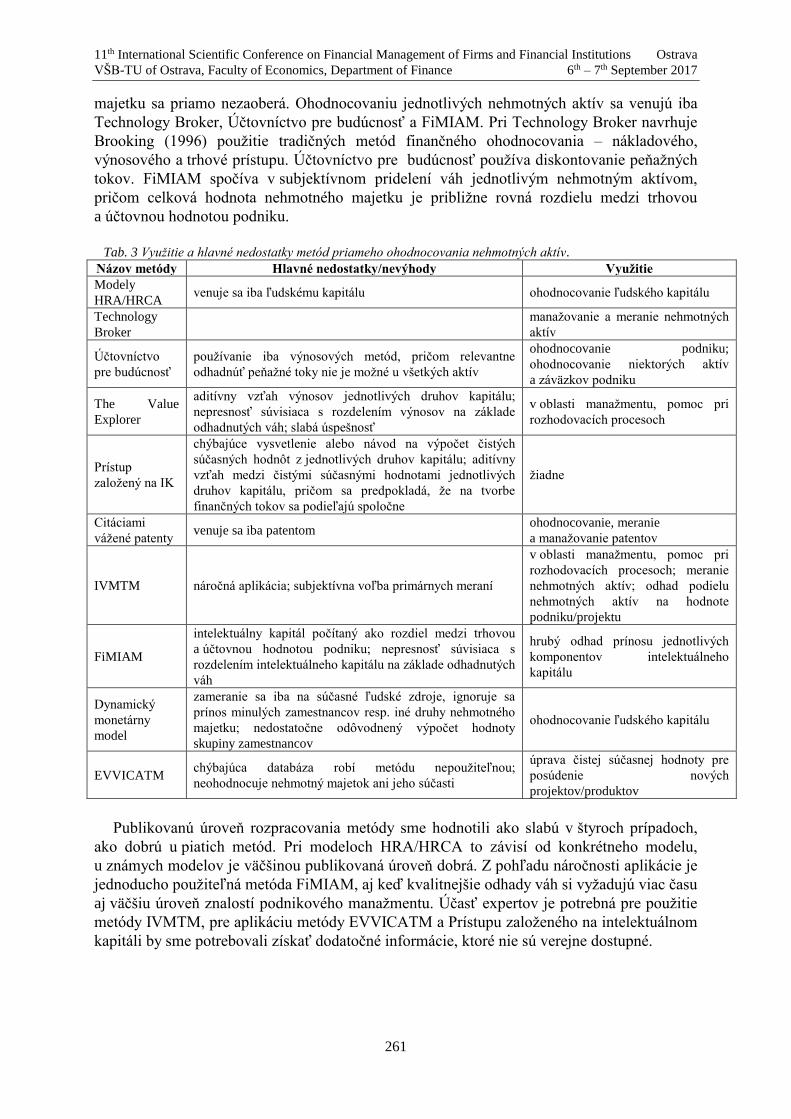
11th International Scientific Conference on Financial Management of Firms and Financial Institutions Ostrava
VŠB-TU of Ostrava, Faculty of Economics, Department of Finance 6th – 7th September 2017
261
majetku sa priamo nezaoberá. Ohodnocovaniu jednotlivých nehmotných aktív sa venujú iba
Technology Broker, Účtovníctvo pre budúcnosť a FiMIAM. Pri Technology Broker navrhuje
Brooking (1996) použitie tradičných metód finančného ohodnocovania – nákladového,
výnosového a trhové prístupu. Účtovníctvo pre budúcnosť používa diskontovanie peňažných
tokov. FiMIAM spočíva v subjektívnom pridelení váh jednotlivým nehmotným aktívom,
pričom celková hodnota nehmotného majetku je približne rovná rozdielu medzi trhovou
a účtovnou hodnotou podniku.
Tab. 3 Využitie a hlavné nedostatky metód priameho ohodnocovania nehmotných aktív.
Názov metódy Hlavné nedostatky/nevýhody Využitie
Modely
HRA/HRCA venuje sa iba ľudskému kapitálu ohodnocovanie ľudského kapitálu
Technology
Broker
manažovanie a meranie nehmotných
aktív
Účtovníctvo
pre budúcnosť
používanie iba výnosových metód, pričom relevantne
odhadnúť peňažné toky nie je možné u všetkých aktív
ohodnocovanie podniku;
ohodnocovanie niektorých aktív
a záväzkov podniku
The Value
Explorer
aditívny vzťah výnosov jednotlivých druhov kapitálu;
nepresnosť súvisiaca s rozdelením výnosov na základe
odhadnutých váh; slabá úspešnosť
v oblasti manažmentu, pomoc pri
rozhodovacích procesoch
Prístup
založený na IK
chýbajúce vysvetlenie alebo návod na výpočet čistých
súčasných hodnôt z jednotlivých druhov kapitálu; aditívny
vzťah medzi čistými súčasnými hodnotami jednotlivých
druhov kapitálu, pričom sa predpokladá, že na tvorbe
finančných tokov sa podieľajú spoločne
žiadne
Citáciami
vážené patenty venuje sa iba patentom
ohodnocovanie, meranie
a manažovanie patentov
IVMTM náročná aplikácia; subjektívna voľba primárnych meraní
v oblasti manažmentu, pomoc pri
rozhodovacích procesoch; meranie
nehmotných aktív; odhad podielu
nehmotných aktív na hodnote
podniku/projektu
FiMIAM
intelektuálny kapitál počítaný ako rozdiel medzi trhovou
a účtovnou hodnotou podniku; nepresnosť súvisiaca s
rozdelením intelektuálneho kapitálu na základe odhadnutých
váh
hrubý odhad prínosu jednotlivých
komponentov intelektuálneho
kapitálu
Dynamický
monetárny
model
zameranie sa iba na súčasné ľudské zdroje, ignoruje sa
prínos minulých zamestnancov resp. iné druhy nehmotného
majetku; nedostatočne odôvodnený výpočet hodnoty
skupiny zamestnancov
ohodnocovanie ľudského kapitálu
EVVICATM chýbajúca databáza robí metódu nepoužiteľnou;
neohodnocuje nehmotný majetok ani jeho súčasti
úprava čistej súčasnej hodnoty pre
posúdenie nových
projektov/produktov
Publikovanú úroveň rozpracovania metódy sme hodnotili ako slabú v štyroch prípadoch,
ako dobrú u piatich metód. Pri modeloch HRA/HRCA to závisí od konkrétneho modelu,
u známych modelov je väčšinou publikovaná úroveň dobrá. Z pohľadu náročnosti aplikácie je
jednoducho použiteľná metóda FiMIAM, aj keď kvalitnejšie odhady váh si vyžadujú viac času
aj väčšiu úroveň znalostí podnikového manažmentu. Účasť expertov je potrebná pre použitie
metódy IVMTM, pre aplikáciu metódy EVVICATM a Prístupu založeného na intelektuálnom
kapitáli by sme potrebovali získať dodatočné informácie, ktoré nie sú verejne dostupné.

11th International Scientific Conference on Financial Management of Firms and Financial Institutions Ostrava
VŠB-TU of Ostrava, Faculty of Economics, Department of Finance 6th – 7th September 2017
262
Acknowledgement
This research was supported by VEGA project No. 1/0311/17 on Measuring and Reporting
Intangible Assets
References
[1] Andriessen, D. and Tissen, R. (2000). Weightless Wealth: Finding your real value in a
future of intangible assets. New York: Pearson Education.
[2] Andriessen, D. (2005). Implementing the KPMG Value Explorer: Critical success factors
for applying IC measurement tools. Journal of Intellectual Capital, 6(4), 474 – 488.
[3] Bontis, N. (2001). Assessing knowledge assets: a review of the models used to measure
intellectual capital. International journal of management reviews, 3(1), 41-60.
[4] Brooking, A. (1996). Intellectual capital. Cengage Learning EMEA.
[5] Brummet, R. L. et al. (1968). Human Resource measurement: A challenge for
accountants. Accounting Review, 217-224.
[6] Gröjer, J. E., Johanson, U., Clancy, M. and Robertson, S. (1996). Human resource
costing and accounting. Joint Industrial Safety Council, Stockholm.
[7] IASB (2010). IAS 38: Intangible Assets. International Financial Reporting Standards.
[8] IASB (2013). IFRS 13: Fair Value Measurement. International Financial Reporting
Standards.
[9] IVSC. (2011). International Valuation Standards 2011. London: International Valuation
Standards Council. [online]. Available at: < iopcg.me/images/IVS_2011.pdf> [Accessed
21 June 2017].
[10] Johanson, U., Eklöv, G., Holmgren, M. and Mårtensson, M. (1998), Human Resource
Costing and Accounting versus the Balanced Scorecard, Report prepared for OECD,
School of Business, Stockholm University, Stockholm.
[11] Krabec, T. (2009). Oceňování podniku a standardy hodnoty. Praha: Grada Publishing.
[12] M’Pherson, P. K. and Pike, S. (2001). Accounting, empirical measurement and
intellectual capital. Journal of Intellectual Capital, 2(3):246–260.
[13] Mařík, M. et al. (2007). Metody oceňování podniku. 2. vyd. Praha: Ekopress.
[14] McCutcheon, G. A. (2008). EVVICA™, a valuation model for intellectual asset-rich
businesses. Measuring business excellence, 12(2), 79-96.
[15] Milost, F. (2007). A dynamic monetary model for evaluating employees. Journal of
Intellectual capital, 8(1):124–138.
Nash, H. (2003). Comments on FASB Proposal. Principles-Based Approach To U.S.
Standard Setting. [online] Available at:
<http://www.gasb.org/cs/BlobServer?blobkey=id&blobwhere=1175818116884&blobhea
der=application%2Fpdf&blobcol=urldata&blobtable=MungoBlobs> [Accessed 2 July
2017].
[16] Rodov, I. and Leliaert, P. (2002). FiMIAM: financial method of intangible assets
measurement. Journal of Intellectual capital, 3(3), 323-336.

11th International Scientific Conference on Financial Management of Firms and Financial Institutions Ostrava
VŠB-TU of Ostrava, Faculty of Economics, Department of Finance 6th – 7th September 2017
263
[17] Sullivan Jr., P. H. and Sullivan Sr., P. H. (2000). Valuing intangibles companies–an
intellectual capital approach. Journal of Intellectual capital, 1(4):328–340.
[18] Sveiby, K. E. (2010). Methods for Measuring Intangible Assets. [online] Available at:
<http://www.sveiby.com/articles/IntangibleMethods.htm> [Accessed 25 May 2017].
11th International Scientific Conference on Financial Management of Firms and Financial Institutions Ostrava
VŠB-TU of Ostrava, Faculty of Economics, Department of Finance 6th – 7th September 2017
264
Hedging portfolio risk management with VaR
Haochen Guo 1
Abstract
Hedging is the traditional approach to market risk management. It consists of taking positions that
lower the risk profile of the portfolio. Usually, hedging strategy eliminating the financial risk and
decrease low when operating the investment. It verified that application of chosen hedging
strategy leads to decreasing or reducing the financial risk in financial market. This paper presents
the hedging strategy f portfolio optimization based on Value at Risk (VaR) which considering
normal distribution returns. The objective of paper is verifying of minimal VaR hedging portfolio.
The method of verification that chosen hedging portfolio that estimating parameters of in-sample
period and evaluate out-of-sample period.
Key words
Hedging strategy, portfolio optimization, Value at Risk (VaR)
JEL Classification: D81, G11, G17, G19
1. Literature review: minimal VaR hedging portfolio
The traditional approach to market risk management is hedging. Hedging consists of taking
positions that lower the risk profile of the portfolio. The techniques for hedging have been
developed in the futures markets. The application of hedging consists of finding the optimal
position in a futures contract that minimizes the variance of the total, hedged position. The
objective function is the portfolio variance and hedging instruments are linear [3].
VaR states the risk level, which is defined as a minimal predictable loss on a given
probability level within a pre-specified time period [8].
Assumptions of VaR calculation are:
The VaR is stated for a portfolio of assets,
The increment in the value of an asset portfolio can be formulated by returns as
∆Π̃ = �̃�𝑇 − 𝑉𝑡 = 𝑉𝑡 ∙ �̃�𝑝 = ∑ 𝑥𝑖 ∙ �̃�𝑖𝑖 , (1)
where 𝑉𝑡(�̃�𝑇) is the initial portfolio value, �̃�𝑝 is a random portfolio return, 𝑥𝑖 is an absolute
amount of money put into the asset 𝑖, 𝑉𝑡 = ∑ 𝑥𝑖𝑖 , �̃�𝑖 is a random return of the asset 𝑖, Random returns of assets are normally distributed.
To determine the general formula for the analytical formulation of the VaR by following
equation
𝑉𝑎𝑅 = −Φ−1(𝛼) ∙ 𝜎(∆Π̃) − 𝐸(ΔΠ̃), (2)
where Φ−1(𝛼) is an inverse function of normal distribution function on a given significance
level 𝛼, ∆Π̃ is portfolio random profit, 𝜎(∆Π̃) is standard deviation of returns, and 𝐸(ΔΠ̃) is
mean value of returns
Suppose that the mean value of returns is zero, and then modify equation as follows
𝑉𝑎𝑅 = −Φ−1(𝛼) ∙ 𝜎(∆Π̃). (3)
1 Ing.Haochen Guo,Ph.D., VŠB-Technical University of Ostrava, Faculty of Economics, Department
of Finance, Sokolská třída 33, 70200 Ostrava, Czech Republic. [email protected]

11th International Scientific Conference on Financial Management of Firms and Financial Institutions Ostrava
VŠB-TU of Ostrava, Faculty of Economics, Department of Finance 6th – 7th September 2017
265
The general formulation of the VaR as stated above is applicable for non-symmetric
parametric probability distributions. However, if the case of change is of Normal distribution,
then by symmetry Φ−1(𝛼) = −Φ−1(1 − 𝛼), get following form
𝑉𝑎𝑅 = Φ−1(1 − 𝛼) ∙ 𝜎(∆Π̃) − 𝐸(∆Π̃), (4)
or the most frequent form of the VaR equation as following
𝑉𝑎𝑅 = Φ−1(1 − 𝛼) ∙ 𝜎(∆Π̃). (5)
VaR is an often-used acceptability functional. It is the standard in the Basel II accord. [6].
The VaR criterion, although having poor mathematical properties, is very relevant in many
decision models. [2][4][5][7]. Hence, the VaR minimization hedging strategy for financial
portfolio is by following problem.
Problem Minimal Value at Risk Hedging with Normal Distribution Returns
Objective Function min 𝑉𝑎𝑅 = −𝐸(𝑟𝑝) − Φ𝛼−1 ∙ 𝜎𝑝 (6)
Constraints 𝑓 = 𝑘 (7)
𝜇 ≥ 𝑧𝑖 ≥ −𝑙 (8)
where 𝐸(𝑟𝑝) and 𝜎𝑝 are the mean value and the standard deviation of the assets return, Φ𝛼−1
is an inverse function of normal distribution function on a given significance level 𝛼 and 𝑥𝑖 is
the amount of money invested into assets.
2. Application of minimal VaR hedging strategy
Suppose there are three financial assets portfolio (portfolio A, B and C) from China Stock
Exchange. Each portfolio includes 10 assets. To hedge the assets is against financial risk. The
historical prices by daily data of financial assets, the currency of determined in CNY (Chinese
Yuan). Expected retunes 𝐸(𝑟𝑝) and standard deviations of returns 𝜎(𝑟𝑝) are known. It is also
supposed that the returns are normal distribution. The task is to determine the optimal
composition of the portfolio significance by the VaR Minimization for 1% and 5% probability
level. Following Table 1 presents tests of input data returns normality.
Table 1: Expected return and standard deviation with returns normality tests
Portfolio Financial
Assets )( prE
)( pr
Kolmogorov-Smirnova Shapiro-Wilk
Statistic df Sig. Statistic df Sig.
Portfolio A
601857.ss -0.000183451 0.009359232 .129 120 .000 .913 120 .000
601398.ss -0.001111549 0.007948661 .169 120 .000 .894 120 .000
601939.ss -0.00071888 0.011998123 .152 120 .000 .817 120 .000
601288.ss -0.000203663 0.012340678 .210 120 .000 .653 120 .000
601988.ss -0.00050164 0.009964082 .166 120 .000 .841 120 .000
000918.sz -0.000835386 0.016087709 .087 120 .026 .944 120 .000
600028.ss 0.000667513 0.013197488 .112 120 .001 .964 120 .003
601628.ss 0.000708029 0.016790274 .113 120 .001 .880 120 .000
601318.ss 0.001941511 0.018261938 .090 120 .018 .961 120 .002
601088.ss -0.000879635 0.012114725 .092 120 .015 .941 120 .000
Portfolio B
601328.ss -0.000127429 0.015322959 .146 120 .000 .813 120 .000
600036.ss -0.00011857 0.016552557 .124 120 .000 .855 120 .000
000925.sz 0.000683696 0.016986638 .184 120 .000 .862 120 .000
600016.ss -0.00127081 0.017292519 .121 120 .000 .920 120 .000
601166.ss 0.000316712 0.020750604 .137 120 .000 .910 120 .000
600000.ss 0.001459839 0.022987089 .132 120 .000 .885 120 .000
601998.ss 0.000517948 0.017064673 .148 120 .000 .852 120 .000
601601.ss 0.000554494 0.01911728 .103 120 .003 .919 120 .000
600104.ss 0.000142552 0.019715068 .085 120 .032 .986 120 .247
600519.ss -0.001967482 0.018354373 .138 120 .000 .870 120 .000
Portfolio C
600030.ss 0.001182515 0.023277038 .148 120 .000 .881 120 .000
600018.ss 0.006682568 0.044648342 .146 120 .000 .926 120 .000
000001.sz 0.001628647 0.024342153 .120 120 .000 .950 120 .000
601633.ss -0.001041351 0.028427972 .080 120 .060 .967 120 .004
601808.ss 0.003749616 0.028124843 .091 120 .015 .979 120 .064
601006.ss 0.001667186 0.017045486 .094 120 .011 .943 120 .000
000895.sz 0.002182835 0.019387054 .114 120 .001 .945 120 .000
600837.ss 0.000138592 0.025085224 .112 120 .001 .933 120 .000
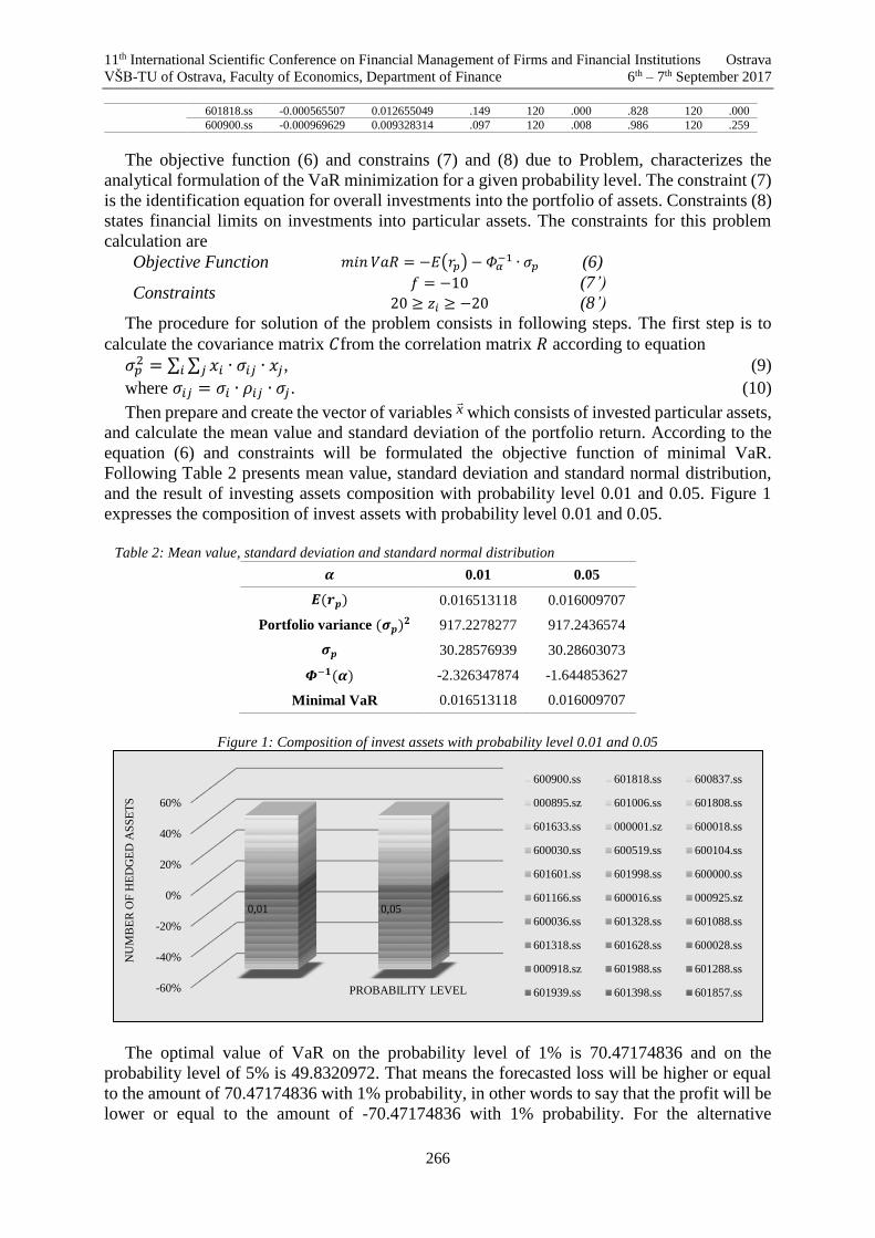
11th International Scientific Conference on Financial Management of Firms and Financial Institutions Ostrava
VŠB-TU of Ostrava, Faculty of Economics, Department of Finance 6th – 7th September 2017
266
601818.ss -0.000565507 0.012655049 .149 120 .000 .828 120 .000
600900.ss -0.000969629 0.009328314 .097 120 .008 .986 120 .259
The objective function (6) and constrains (7) and (8) due to Problem, characterizes the
analytical formulation of the VaR minimization for a given probability level. The constraint (7)
is the identification equation for overall investments into the portfolio of assets. Constraints (8)
states financial limits on investments into particular assets. The constraints for this problem
calculation are
Objective Function 𝑚𝑖𝑛 𝑉𝑎𝑅 = −𝐸(𝑟𝑝) − 𝛷𝛼−1 ∙ 𝜎𝑝 (6)
Constraints 𝑓 = −10 (7’)
20 ≥ 𝑧𝑖 ≥ −20 (8’)
The procedure for solution of the problem consists in following steps. The first step is to
calculate the covariance matrix 𝐶from the correlation matrix 𝑅 according to equation
𝜎𝑝2 = ∑ ∑ 𝑥𝑖 ∙ 𝜎𝑖𝑗 ∙ 𝑥𝑗𝑗𝑖 , (9)
where 𝜎𝑖𝑗 = 𝜎𝑖 ∙ 𝜌𝑖𝑗 ∙ 𝜎𝑗 . (10)
Then prepare and create the vector of variables x
which consists of invested particular assets,
and calculate the mean value and standard deviation of the portfolio return. According to the
equation (6) and constraints will be formulated the objective function of minimal VaR.
Following Table 2 presents mean value, standard deviation and standard normal distribution,
and the result of investing assets composition with probability level 0.01 and 0.05. Figure 1
expresses the composition of invest assets with probability level 0.01 and 0.05.
Table 2: Mean value, standard deviation and standard normal distribution
𝜶 0.01 0.05
𝑬(𝒓𝒑) 0.016513118 0.016009707
Portfolio variance (𝝈𝒑)𝟐 917.2278277 917.2436574
𝝈𝒑 30.28576939 30.28603073
𝜱−𝟏(𝜶) -2.326347874 -1.644853627
Minimal VaR 0.016513118 0.016009707
Figure 1: Composition of invest assets with probability level 0.01 and 0.05
The optimal value of VaR on the probability level of 1% is 70.47174836 and on the
probability level of 5% is 49.8320972. That means the forecasted loss will be higher or equal
to the amount of 70.47174836 with 1% probability, in other words to say that the profit will be
lower or equal to the amount of -70.47174836 with 1% probability. For the alternative
-60%
-40%
-20%
0%
20%
40%
60%
0,01 0,05
NU
MB
ER
OF
HE
DG
ED
AS
SE
TS
PROBABILITY LEVEL
600900.ss 601818.ss 600837.ss
000895.sz 601006.ss 601808.ss
601633.ss 000001.sz 600018.ss
600030.ss 600519.ss 600104.ss
601601.ss 601998.ss 600000.ss
601166.ss 600016.ss 000925.sz
600036.ss 601328.ss 601088.ss
601318.ss 601628.ss 600028.ss
000918.sz 601988.ss 601288.ss
601939.ss 601398.ss 601857.ss
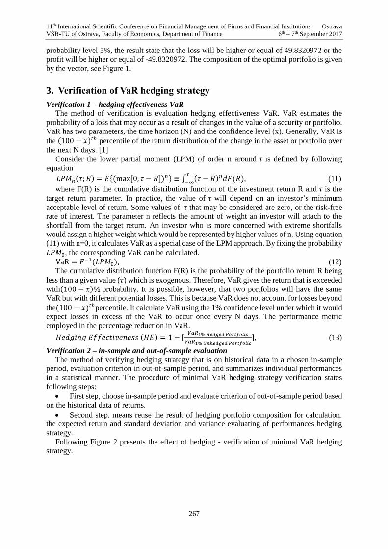
11th International Scientific Conference on Financial Management of Firms and Financial Institutions Ostrava
VŠB-TU of Ostrava, Faculty of Economics, Department of Finance 6th – 7th September 2017
267
probability level 5%, the result state that the loss will be higher or equal of 49.8320972 or the
profit will be higher or equal of -49.8320972. The composition of the optimal portfolio is given
by the vector, see Figure 1.
3. Verification of VaR hedging strategy
Verification 1 – hedging effectiveness VaR
The method of verification is evaluation hedging effectiveness VaR. VaR estimates the
probability of a loss that may occur as a result of changes in the value of a security or portfolio.
VaR has two parameters, the time horizon (N) and the confidence level (x). Generally, VaR is
the (100 − 𝑥)𝑡ℎ percentile of the return distribution of the change in the asset or portfolio over
the next N days. [1]
Consider the lower partial moment (LPM) of order n around 𝜏 is defined by following
equation
𝐿𝑃𝑀𝑛(𝜏; 𝑅) = 𝐸{(max [0, 𝜏 − 𝑅])𝑛} ≡ ∫ (𝜏 − 𝑅)𝑛𝑑𝐹(𝑅)𝜏
−∞, (11)
where F(R) is the cumulative distribution function of the investment return R and 𝜏 is the
target return parameter. In practice, the value of 𝜏 will depend on an investor’s minimum
acceptable level of return. Some values of 𝜏 that may be considered are zero, or the risk-free
rate of interest. The parameter n reflects the amount of weight an investor will attach to the
shortfall from the target return. An investor who is more concerned with extreme shortfalls
would assign a higher weight which would be represented by higher values of n. Using equation
(11) with n=0, it calculates VaR as a special case of the LPM approach. By fixing the probability
𝐿𝑃𝑀0, the corresponding VaR can be calculated.
VaR = 𝐹−1(𝐿𝑃𝑀0), (12)
The cumulative distribution function F(R) is the probability of the portfolio return R being
less than a given value (𝜏) which is exogenous. Therefore, VaR gives the return that is exceeded
with(100 − 𝑥)% probability. It is possible, however, that two portfolios will have the same
VaR but with different potential losses. This is because VaR does not account for losses beyond
the(100 − 𝑥)𝑡ℎpercentile. It calculate VaR using the 1% confidence level under which it would
expect losses in excess of the VaR to occur once every N days. The performance metric
employed in the percentage reduction in VaR.
𝐻𝑒𝑑𝑔𝑖𝑛𝑔 𝐸𝑓𝑓𝑒𝑐𝑡𝑖𝑣𝑒𝑛𝑒𝑠𝑠 (𝐻𝐸) = 1 − [𝑉𝑎𝑅1% 𝐻𝑒𝑑𝑔𝑒𝑑 𝑃𝑜𝑟𝑡𝑓𝑜𝑙𝑖𝑜
𝑉𝑎𝑅1% 𝑈𝑛ℎ𝑒𝑑𝑔𝑒𝑑 𝑃𝑜𝑟𝑡𝑓𝑜𝑙𝑖𝑜], (13)
Verification 2 – in-sample and out-of-sample evaluation
The method of verifying hedging strategy that is on historical data in a chosen in-sample
period, evaluation criterion in out-of-sample period, and summarizes individual performances
in a statistical manner. The procedure of minimal VaR hedging strategy verification states
following steps:
First step, choose in-sample period and evaluate criterion of out-of-sample period based
on the historical data of returns.
Second step, means reuse the result of hedging portfolio composition for calculation,
the expected return and standard deviation and variance evaluating of performances hedging
strategy.
Following Figure 2 presents the effect of hedging - verification of minimal VaR hedging
strategy.

11th International Scientific Conference on Financial Management of Firms and Financial Institutions Ostrava
VŠB-TU of Ostrava, Faculty of Economics, Department of Finance 6th – 7th September 2017
268
Figure 2: Verification of minimal VaR hedging strategy
Based on the verification results of minimal VaR hedging strategy, the results of hedged is
less than no hedge, which means this hedging strategy is successful to reduce risk.
4. Conclusion
Application of minimal VaR hedging strategy calculated by probability level of 1% and 5%.
The result of optimal value of VaR means the forecasted loss will be higher or equal to the
amount with probability level, in other words to say that the profit will be lower or equal to the
amount with probability level.
Verifications’ result for minimal VaR hedging strategy shows the hedged is less than no
hedge, which means the hedging strategy is successful to reduce risk in international financial
markets.
There were verified that applications of chosen hedging strategy lead to decreasing or
reducing the financial risk in financial markets. Hedging strategies are important in
international financial markets that means for eliminating the financial risk and decrease loss
when operating the investment.
References
[1] Cotter, J., Hanly, J. (2005). Re-evaluating hedging performance. UCD Geary Institute
Discussion Paper Series. Dublin.
[2] Duffie, D., and PAN, J. (1997). An overview of Value at Risk. The Journal of Derivatives.
4, p. 7-49.
[3] Elton, J, E., and Gruber, J, M. (1991). Modern portfolio theory and investment analysis.
John Wiley & Sons, Inc. ISBN 0-471-54194-X.
[4] Gourieroux, C., Laurent, J, P., Scaillet, O. (2000). Sensitivity analysis of VaR. Journal of
Empirical Finance. 7, p. 225-246.
[5] Manganelli,S., and Engle, F, R. (2001). Value at Risk models in finance. European Central
Bank Working Paper No.75.
[6] Pflug, Ch, G., and Römisch, W. (2007). Modeling, measuring and managing risk. World
Scientific. ISBN 9-789812-707406.
0,75 0,8 0,85 0,9 0,95 1 1,05
VARIANCE OF HEDGED
VARIANCE OF NO HEDGE
0.05 0.01

11th International Scientific Conference on Financial Management of Firms and Financial Institutions Ostrava
VŠB-TU of Ostrava, Faculty of Economics, Department of Finance 6th – 7th September 2017
269
[7] Silvapulle, P., Granger, W, J, C. (2001). Large returns, conditional correlation and
portfolio diversification: a Value at Risk approach. Journal of Quantitative finance. 1, p.
543-551.
[8] Zmeškal, Z., Dluhošová, D., and Tichý, T. (2004). Financial models. VŠB-Technická
Univerzita Ostrava, ISBN 80-248-0754-8.
11th International Scientific Conference on Financial Management of Firms and Financial Institutions Ostrava
VŠB-TU of Ostrava, Faculty of Economics, Department of Finance 6th – 7th September 2017
270
Estimation and analysis of value multipliers within processing industry in Czech Republic
Petr Gurný 12
Abstract
The paper is devoted to the analysis of the processing industry value in the Czech Republic. For
the analysis, parametric model (key value driver formula) of the market value estimation based
on the discounted cash flows will is used. By means of designed pyramidal decomposition and
the methods for the influences quantification, we analyse and quantify the differences in the
performance within processing industry in the Czech Republic. Goal of the paper is to estimate
value multipliers for processing industry in Czech Republic with respect to the different
combination of the rate of growth and return on capital.
Key words
Key value driver formula; value multipliers; pyramidal decomposition; processing industry.
JEL Classification: G12, G32
1. Úvod
V odborné literatuře existuje spousta studií, které se věnují makroekonomickému pohledu
na výkon ekonomiky rozvinutých a rozvíjejících se zemí. Tyto výzkumy analyzují výkon
ekonomiky především z perspektivy HDP. Tento příspěvek je naproti tomu zaměřen na odhad
tržní hodnoty konkrétního ekonomického odvětví v ČR postavený na budoucích očekáváních
ovlivňujících tržní hodnotu všech aktiv. Konkrétně pak bude analyzováno odvětví
zpracovatelského průmyslu. Nicméně, i v této oblasti existují výzkumy, které analyzují
ekonomickou výkonnost ve vztahu k jednotlivým odvětvím a vybraným ekonomickým
faktorům. Campos, Coricelli a Moretti (2014) odhadují, jak je HDP na obyvatele ovlivněno
produktivitou práce u vybraných zemí po jejich připojení k EU. Zde vysledovali pozitivní
korelace mezi oběma veličinami. Serrenho (2014) zkoumal produktivitu energetického
průmyslu v ekonomikách 15 zemí EU. Smith a kol. (2014) věnovali svůj výzkum
východoevropskému oděvnímu průmyslu, apod. Žádný z těchto výzkumů nebyl nicméně
zaměřen na odhad tržní hodnoty jednotlivých odvětví. Cílem tohoto příspěvku je odhadnout a
analyzovat hodnotový multiplikátor zpracovatelského průmyslu v ČR, a to pomocí
parametrického vzorce pro odhad hodnoty aktiv. V příspěvku budeme postupovat
následujícím způsobem. Nejprve bude představena metodika odhadu tržní hodnoty pomocí
parametrického vzorce, následně bude navržen pyramidový rozklad pro hlubší analýzu
vybraného multiplikátoru včetně kvantifikace odchylek. Nakonec pak bude provedena
dvoufaktorová citlivostní analýza vlivů vybraných relevantních parametrů na hodnotový
multiplikátor.
1 The paper is based on research activities sponsored through SGS Project No. SP2017/148 and
ESF Project No. CZ.1.07/2.3.00/20.0296. The support is greatly acknowledged. 2 Ing. Petr Gurný, Ph.D. (corresponding author): VŠB –Technická univerzita Ostrava, Ekonomická
fakulta, katedra financí, Sokolská 33, 701 21, Ostrava 1, e-mail: [email protected].

11th International Scientific Conference on Financial Management of Firms and Financial Institutions Ostrava
VŠB-TU of Ostrava, Faculty of Economics, Department of Finance 6th – 7th September 2017
271
2. Popis použité metodiky
Hodnota jakýchkoliv aktiv je primárně určena očekáváním budoucích užitků z těchto aktiv
plynoucích, které jsou následně převedeny na současnou hodnotu pomocí požadované míry
výnosnosti. Jelikož budoucí užitky jsou v případě finančních subjektů obvykle vyjadřovány
pomocí peněžních toků, můžeme zapsat základní formuli pro oceňování jako:
T
t
tWACC
FCFV
1 )1( (1)
kde FCF jsou očekávané peněžní toky, WACC průměrné náklady kapitálu (požadovaná míra
výnosnosti a T očekávaná životnost aktiva. Jestliže budeme očekávat nekonečnou životnost a
stabilní tempo růstu FCF, g, můžeme rovnici (1) přepsat na standardní současnou hodnotu
perpetuity jako:
gWACC
FCFV
. (2)
Jelikož INVtrEBITFCF 1 , kde EBIT je zisk před odečtením úroků a daní, tr je daňová
sazba and INV jsou celkové čisté investice (a to jak do dlouhodobých, tak krátkodobých
aktiv), IRtrEBITINV )1( , kde IR je investiční míra, která může být kalkulována jako
ROIC
gIR , kde ROIC je rentabilita investovaného kapitálu, můžeme rovnici (2) přepsat na
parametrický vzorec pro odhad hodnoty aktiv:
gWACC
ROIC
gtrEBIT
V
11
. (3)
Pro odhad hodnotového multiplikátoru pak lze využít relativní verzi rovnice (3):
gWACC
ROC
g
tEBIT
V
1
1 (4)
Rovnice (4), viz např. Koller (2015) pro další verze a variace tohoto vzorce, bude v tomto
příspěvku využita pro odhad hodnotového multiplikátoru zpracovatelského průmyslu v ČR,
přičemž pro odhad vstupních parametrů budou sloužit agregovaná data. Pro detailní analýzu
tohoto multiplikátoru byl následně navržen detailní pyramidový rozklad, který umožnuje určit
jednotlivé dílčí vlivy, které na výsledný multiplikátor působí. Výsledná podoba toho rozkladu
je pak zobrazena na Obr. 1.
Použité symboly: V – tržní hodnota, EBIT – zisk před úroky a daněmi, t – daňová sazba, g
– tempo růstu EBIT, ROIC – rentabilita investovaného kapitálu, WACC – průměrné vážené
náklady kapitálu, C – investovaný kapitál (aktiva), Exp – náklady, S – tržby, E – vlastní
kapitál, RE – náklady vlastního kapitálu, D – dluh, RD – náklady dluhu, IR – investiční míra,
FA – fixní aktiva, CA – oběžbá aktiva.

11th International Scientific Conference on Financial Management of Firms and Financial Institutions Ostrava
VŠB-TU of Ostrava, Faculty of Economics, Department of Finance 6th – 7th September 2017
272
Obr. 1: Navržený pyramidový rozklad hodnotového multiplikátoru V/EBIT(1-t)
Zdroj: vlastní zpracování
Na základě pyramidového rozklad na Obr. 1 budeme v analytické části příspěvku dále
analyzovat odchylky vrcholového multiplikátoru mezi hodnotou zpracovatelského průmyslu a
celkového průmyslu v ČR. Pro tuto hloubkovou analýzu vlivu dílčích ukazatelů se jeví jako
vhodné aplikovat analýzu odchylek, která umožnuje kvantifikovat vliv dílčích faktorů na
základní (vrcholový ukazatel).
Obecně, jakýkoliv vrcholový ukazatel x může být vyjádřen jako funkce dílčích ukazatelů
ai, i.e. n
aaafx ...,21
. Změna vrcholového ukazatele pak může určena jako suma vlivů dílčích
ukazatelů:
,i
ax ixy (5)
kde x vrcholový ukazatel, x
y je změna vrcholového ukazatele, ai je daný dílčí ukazatel, ia
x je
vliv daného dílčího ukazatele na vrcholový ukazatel.
Funkce n
aaafx ...,21
v rámci pyramidového rozkladu může být vyjádřena dvěma základními
vazbami: aditivní vazbou a multiplikativní vazbou. Kvantifikace vlivu pomocí aditivní vazby
vyjádřena jako podíl změn dílčích ukazatelů:
x
i
i
i
ay
a
ax
i
, (6)
kde 0,1, iii
aaa , 0,i
a je hodnota daného dílčího ukazatele na začátku analyzovaného období a
1,ia je hodnota daného dílčího ukazatele na konci daného období. Pro kvantifikaci
multiplikativních vazeb budeme v tomto příspěvku využívat funkcionální metoda. Obecný
vzorec pro kvantifikaci vlivů je pak následující (odvození viz Zmeskal (2004)):
x
ijjkik
kmim
aaa
ij ijjkik
aaaa
x
ayRRRRRRR
Rx
mkjkjjii
4
1
3
1
2
11
1, (7)
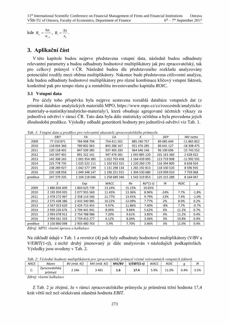
11th International Scientific Conference on Financial Management of Firms and Financial Institutions Ostrava
VŠB-TU of Ostrava, Faculty of Economics, Department of Finance 6th – 7th September 2017
273
kde 0,j
j
aa
aR
j
,
0x
xR
x
.
3. Aplikační část
V této kapitole budou nejprve představena vstupní data, následně budou odhadnuty
relevantní parametry a budou odhadnuty hodnotové multiplikátory jak pro zpracovatelský, tak
pro celkový průmysl v ČR. Následně budou dle představeného rozkladu analyzovány
potenciální rozdíly mezi oběma multiplikátory. Nakonec bude představena citlivostní analýza,
kde budou odhadnuty hodnotové multiplikátory pro různé kombinace klíčový vstupní faktorů,
konkrétně pak pro tempo růstu g a rentabilitu investovaného kapitálu ROIC.
3.1 Vstupní data
Pro účely toho příspěvku byla nejprve sestavena rozsáhlá databáze vstupních dat (z
primární databáze analytických materiálů MPO, https://www.mpo.cz/cz/rozcestnik/analyticke-
materialy-a-statistiky/analyticke-materialy/), která obsahuje agregované účetních výkazy za
jednotlivá odvětví v rámci ČR. Tato data byla dále statisticky očištěna a byla provedena jejich
dlouhodobá predikce. Výsledky odhadů generátorů hodnoty pro jednotlivá odvětví viz Tab. 1.
Tab. 1: Vstupní data a predikce pro relevantní ukazatele zpracovatelského průmyslu
EBIT FA CA E DEP INV netto
2009 77 210 871 784 908 794 754 411 501 885 240 757 89 085 649 -11 865 852
2010 118 004 366 789 802 963 843 286 167 921 476 285 89 641 127 -18 308 475
2011 120 158 401 847 509 385 937 405 293 964 646 146 96 190 696 -15 743 552
2012 142 097 401 891 322 141 947 476 381 1 043 885 120 101 163 360 2 628 022
2013 142 308 165 1 001 954 385 1 022 703 458 1 164 439 005 113 719 908 -11 992 591
2014 225 778 735 1 025 522 111 1 102 922 315 1 220 260 170 116 394 800 8 658 924
2015 238 289 927 1 042 577 199 1 131 298 134 1 265 192 813 118 330 520 8 596 935
2016 235 108 056 1 049 348 147 1 196 251 915 1 304 530 680 119 099 010 7 759 068
predikce 247 379 335 1 104 118 046 1 258 689 340 1 543 319 853 125 315 289 8 164 047
S Exp WACC Re Rd*(1-t) IR ROIC g
2009 1 880 836 609 1 803 625 739 13.24% 15.15% 10.65%
2010 2 195 959 935 2 077 955 569 11.45% 13.36% 8.96% -24% 7.7% -1.8%
2011 2 478 272 967 2 358 114 566 11.77% 13.45% 9.79% -13% 7.4% -1.0%
2012 2 575 438 386 2 433 340 985 10.22% 12.09% 7.77% 2% 8.0% 0.2%
2013 2 567 023 620 2 424 715 455 9.97% 11.86% 7.40% -8% 7.7% -0.7%
2014 2 930 220 676 2 704 441 941 8.04% 9.84% 5.62% 6% 11.2% 0.7%
2015 2 993 078 912 2 754 788 986 7.20% 9.61% 3.85% 4% 11.2% 0.4%
2016 2 994 561 333 2 759 453 277 6.12% 8.04% 3.46% 3% 10.8% 0.4%
predikce 3 150 860 098 2 903 480 763 5.9% 7.70% 3.46% 3% 11.0% 0.4%
Zdroj: MPO, vlastní úprava a kalkulace
Na základě údajů v Tab. 1 a rovnice (4) pak byly odhadnuty hodnotové multiplikátory (V/BV a
V/EBIT(1-t)), z nichž druhý jmenovaný je dále analyzován v následujích podkapitolách.
Výsledky jsou uvedeny v Tab. 2.
Tab. 2: Výsledné hodnoty multiplikátorů pro zpracovatelský průmysl včetně relevantních vstupních faktorů NACE Název BV (mld. Kč) MV (mld. Kč) MV/BV V/EBIT(1-t) WACC ROIC g IR
C: Zpracovatelský
průmysl 2 246 3 491 1.6 17.4 5.9% 11.0% 0.4% 3.5%
Zdroj: vlastní kalkulace
Z Tab. 2 je zřejmé, že v rámci zpracovatelského průmyslu je průměrná tržní hodnota 17,4
krát větší než než očekávaná zdaněná hodnota EBIT.
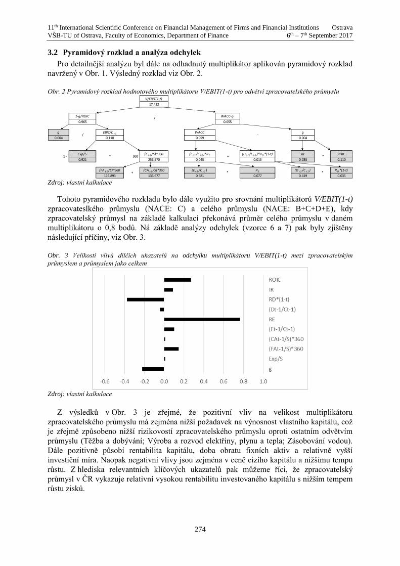
11th International Scientific Conference on Financial Management of Firms and Financial Institutions Ostrava
VŠB-TU of Ostrava, Faculty of Economics, Department of Finance 6th – 7th September 2017
274
3.2 Pyramidový rozklad a analýza odchylek
Pro detailnější analýzu byl dále na odhadnutý multiplikátor aplikován pyramidový rozklad
navržený v Obr. 1. Výsledný rozklad viz Obr. 2.
Obr. 2 Pyramidový rozklad hodnotového multiplikátoru V/EBIT(1-t) pro odvětví zpracovatelského průmyslu
V/EBIT(1-t)
17.422
1-g/ROIC WACC-g
0.965 0.055
g EBIT/C t-1 WACC g
0.004 0.110 0.059 0.004
Exp/S (C t-1 /S)*360 (E t-1 /C t-1 )*R E (D t-1 /C t-1 )*R D *(1-t) IR ROIC
0.921 256.570 0.045 0.015 0.035 0.110
(FA t-1 /S)*360 (CA t-1 /S)*360 (E t-1 /C t-1 ) R E (D t-1 /C t-1 ) R D *(1-t)
119.893 136.677 0.581 0.077 0.419 0.035 + *
1 - * 360 / + *
/
/ -
*
Zdroj: vlastní kalkulace
Tohoto pyramidového rozkladu bylo dále využito pro srovnání multiplikátorů V/EBIT(1-t)
zpracovateslkého průmyslu (NACE: C) a celého průmyslu (NACE: B+C+D+E), kdy
zpracovatelský průmysl na základě kalkulací překonává průměr celého průmyslu v daném
multiplikátoru o 0,8 bodů. Ná základě analýzy odchylek (vzorce 6 a 7) pak byly zjištěny
následující příčiny, viz Obr. 3.
Obr. 3 Velikostí vlivů dílčích ukazatelů na odchylku multiplikátoru V/EBIT(1-t) mezi zpracovatelským
průmyslem a průmyslem jako celkem
Zdroj: vlastní kalkulace
Z výsledků v Obr. 3 je zřejmé, že pozitivní vliv na velikost multiplikátoru
zpracovatelského průmyslu má zejména nižší požadavek na výnosnost vlastního kapitálu, což
je zřejmě způsobeno nižší rizikovostí zpracovatelského průmyslu oproti ostatním odvětvím
průmyslu (Těžba a dobývání; Výroba a rozvod elektřiny, plynu a tepla; Zásobování vodou).
Dále pozitivně působí rentabilita kapitálu, doba obratu fixních aktiv a relativně vyšší
investiční míra. Naopak negativní vlivy jsou zejména v ceně cizího kapitálu a nižšímu tempu
růstu. Z hlediska relevantních klíčových ukazatelů pak můžeme říci, že zpracovatelský
průmysl v ČR vykazuje relativní vysokou rentabilitu investovaného kapitálu s nižším tempem
růstu zisků.

11th International Scientific Conference on Financial Management of Firms and Financial Institutions Ostrava
VŠB-TU of Ostrava, Faculty of Economics, Department of Finance 6th – 7th September 2017
275
3.3 Citlivostní analýza
Vzhledem k faktu, že využití odhadnutých odvětvových multiplikátorů při oceňování
konkrétních firem nezávisí pouze na příslušnosti firmy k danému odvětví, ale také na velikosti
generátorů hodnot (tempa růstu a rentability kapitálu), je nutno při ocenění firmy zohlednit i
konkrétní kombinaci těchto generátorů. Z tohoto důvodu byla provedena citlivostní analýza na
tyto vybrané generátory hodnoty. Výsledkem je empirická matice daného hodnotového
multiplikátoru pro odvětví zpracovatelského průmyslu zohledňující rozdílné kombinace tempa
růstu a rentability kapitálu, viz Tab. 3.
Tab. 3: Hodnoty odvětvového multiplikátoru zpracovatelského průmyslu pro různé kombinace g a ROIC
g / ROC 8.0% 9.0% 10.0% 11.0% 12.0% 13.0% 14.0%
-2.6% 15.5 15.1 14.8 14.5 14.3 14.1 13.9
-1.6% 15.9 15.6 15.4 15.2 15.0 14.9 14.8
-0.6% 16.5 16.3 16.2 16.1 16.1 16.0 16.0
0.4% 17.2 17.3 17.4 17.4 17.5 17.5 17.6
1.4% 18.2 18.6 19.0 19.3 19.5 19.7 19.9
2.4% 19.8 20.8 21.5 22.1 22.6 23.1 23.4
3.4% 22.8 24.6 26.1 27.3 28.3 29.1 29.9 Zdroj: vlastní kalkulace
4. Závěr
V příspěvku byla diskutována a aplikována možnost odhadu odvětvového hodnotového
multiplikátoru pro využití oceňování firem v daném odvětví. Konkrétně byl pro analýzu
zvolen zpracovatelský průmysl v ČR. Cílem příspěvku bylo odhadnout a analyzovat
hodnotový multiplikátor zpracovatelského průmyslu v ČR, a to pomocí parametrického
vzorce pro odhad hodnoty aktiv. Pro účely detailní analýzy zvoleného multiplikátoru byl
rovněž navržen pyramidový rozklad. Na základě této analýzy bylo zjištěno, že zpracovatelský
průmysl v ČR vykazuje relativní vysokou rentabilitu investovaného kapitálu s nižším tempem
růstu zisků ve srovnání s průměrem v odvětví. Závěrem byla provedena dvoufaktorová
citlivostní analýza změny hodnotového multiplikátoru na změnu tempa růstu a rentability
investovaného kapitálu. Odhadnuté multiplikátory mají dle našeho názoru široké uplatnění v
praxi při odhadu hodnot firmy dle komparativních metod.
References
[1] Belkhir, M. et al. (2016). Institutions and corporate capital structure in the MENA region.
Emerging Markets Review 26: 99-129.
[2] Campos, N. F., Coricelli, F. and L. Moretti (2014). Economic Growth and Political
Integration: Estimating the Benefits from Membership in the European Union Using the
Synthetic Counterfactuals Method. IZA Discussion Paper No. 8162. Available at SSRN:
https://ssrn.com/abstract=2432446.
[3] Dong, F. (2014). The impact of economic openness on standard of living and income
inequality in eight countries. Emerging Markets Review 21: 234-264.
[4] Serrenho, A. C. et al. (2014). Decomposition of useful work intensity: The EU (European
Union)-15 countries from 1960 to 2009. Energy 76: 704-715.

11th International Scientific Conference on Financial Management of Firms and Financial Institutions Ostrava
VŠB-TU of Ostrava, Faculty of Economics, Department of Finance 6th – 7th September 2017
276
[5] Smith, A. et al. (2014). The political economy of global production networks: regional
industrial change and differential upgrading in the East European clothing industry.
Journal of Economic Geography 14(6): 1023-1051.
[6] Koller, T., Goedhart, M. and Wessels D. (2015). Valuation: Measuring and Managing
the Value of Companies. Wiley Finance.
[7] Zmeškal, Z. et al. (2013). Financial Models. Ekopress.
11th International Scientific Conference on Financial Management of Firms and Financial Institutions Ostrava
VŠB-TU of Ostrava, Faculty of Economics, Department of Finance 6th – 7th September 2017
277
Application of Sensitivity Analysis within Determination of Chosen Partial Effects on
Company's Value
Petr Gurný 12, Klára Slezáková
Abstract
The paper is focused on the analysis of key value driver parameters within the value creation.
Key value driver formula is used is used for the analysis, while influence of change in rate of
growth, costs and sales is researched. Goal of the paper is to generally derived formulas for
quantification of change in chosen value multipliers for change of these parameters. Derived
formulas are applied on the specific sector of Czech industry.
Key words
Assets valuation; key value driver formula; MV/EBIT multiplier; sensitivity analysis.
JEL Classification: G12, G32
1. Úvod
Hodnota jakýchkoliv aktiv je determinována výhradně jejich očekávanými užitky
diskontovanými na současnou hodnotu. Klasickým (a metodicky nejsprávnějším) vyjádřením
pro tyto očekávané užitky jsou (volné) peněžní toky, kdy je možné hodnotu aktiva vypočítat
jako 1 (1 )
Tt
tt
FCFFV
WACC
, kde tFCFF jsou volné peněžní toky v jednotlivých obdobích v
budoucnu, WACC je požadovaná míra výnosnosti a T je doba životnosti daného aktiva. Za
předpokladu nekonečné životnosti a stabilního tempa růstu peněžních toků g lze uvedenou
rovnici převést na současnou hodnotu perpetuity jako FCFF
VWACC g
(platí pro g WACC ,
což je nicméně ekonomicky nepřekročitelná podmínka). Přestože tato uvedená rovnice
naplňuje podstatu určování hodnoty, není z ní možno poznat, jakým způsobem se hodnota
vytváří (popřípadě ničí) a které klíčové faktory hodnotu ovlivňují a jaká je jejich vzájemná
kombinace. Z toho důvodu je možné současnou hodnotu perpetuity vyjádřit rovněž jako
kombinaci relevantních faktorů (pro odvození a podrobnější popis viz např. Koller (2015),
Hitchner (2011) nebo Mařík (2011):
1 1g
EBIT tROIC
VWACC g
, (1)
1 The paper is based on research activities sponsored through SGS Project No. SP2017/148 and
ESF Project No. CZ.1.07/2.3.00/20.0296. The support is greatly acknowledged. 2 Ing. Petr Gurný, Ph.D. (corresponding author): VŠB –Technická univerzita Ostrava, Ekonomická
fakulta, katedra financí, Sokolská 33, 701 21, Ostrava 1, e-mail: [email protected].
11th International Scientific Conference on Financial Management of Firms and Financial Institutions Ostrava
VŠB-TU of Ostrava, Faculty of Economics, Department of Finance 6th – 7th September 2017
278
kde EBIT je zisk před odečtením úroků a daní, ROIC je rentabilita investovaného kapitálu a
t je daňová sazba.
Pro tvorbu hodnoty je pak klíčová nejen samotná výše těchto parametrů, ale zejména jejich
vliv při změně těchto parametrů. Z tohoto důvodu je cílem tohoto příspěvku odvodit obecné
vztahy citlivosti vybraných veličin (hodnoty V a relativní hodnoty (hodnotového
multiplikátoru) 1
V
EBIT t
) na změny vybraných parametrů, konkrétně pak na změnu
rentability investovaného kapitálu a tempa růstu EBIT. Rovněž bude obecně odvozeno, jaký
mají tyto dva uvedené faktory konkrétní vliv při daných počátečních podmínkách.
V příspěvku budeme postupovat následujícím způsobem. Nejprve budou odvozeny obecné
vztahy pro vliv vybraných faktorů na zvolené veličiny. Následně budou tyto vztahy
aplikovány na vybrané odvětví ekonomiky ČR a nakonec bude řešeno, při jakých podmínkách
má daný faktor ( ROIC ) větší vliv na vybranou veličinu než druhý faktor (g).
2. Odvození vlivu vybraných faktorů na hodnotu aktiv
Citlivostní analýza je jednou z možností analýzy rizik a obecně zkoumá vliv změn
vstupních parametrů na výsledné hodnoty finančních veličin (blíže viz Dluhošová a kol.
(2014). V tomto případě se při analýze rizik nepracuje s rozdělením pravděpodobnosti
možných budoucích změn. Jestliže vyjádříme hodnotu aktiv (V) jako funkci dílčích ukazatelů
1, 2... nV f F F F , pak se citlivost souhrnného ukazatele dá vyjádřit jako přírůstek hodnoty
vlivem změny daného faktoru:
1 1
1 1 21 , ...F F
nV V V f F F F V , (2)
přičemž α charakterizuje odchylku3, která může být jak kladná, tak záporná.
V případě citlivostní analýzy hodnoty aktiv odhadnutých dle (1) a jejich relativní
multiplikátorové verze
1
1
gV ROIC
EBIT t WACC g
, budou zkoumanými faktory provozní
náklady (respektive jejich podíl na výnosech (tržbách) daného aktiva) a výnosy tržby (oba tyto
faktory ovlivňují výši rentability investovaného kapitálu ROIC a dále tempo růstu g.
Při odvozování budeme vycházet z následujících předpokladů:
1. provozní náklady (N) se vypočítají jako TkN N , kde T jsou tržby a T
Nk N obvyklé ,
2. nově vytvořený EBT (tedy EBTEBTEBT F 1
) vyvolaný změnou vybraného faktoru F o α
procent se v aktivech rozděluje mezi pohledávky a peněžní prostředky, a to v poměru POHk a
PPk , kde POHPP kk 1 a kde
T
POHk POH obvyklé (toto rozdělení nemá vliv na analytické
odvození citlivostní analýzy), přičemž od peněžních prostředků se dále vyplácejí očekávané
vyplacené podíly na zisku, viz bod 3,
3 V tomto případě relativní odchylku, v případě absolutní odchylky by byla změna daného parametru
určena analogicky jako F F .

11th International Scientific Conference on Financial Management of Firms and Financial Institutions Ostrava
VŠB-TU of Ostrava, Faculty of Economics, Department of Finance 6th – 7th September 2017
279
3. FEBT1
se do pasiv rozdělí mezi EAT a krátkodobé závazky ( daňkrtZÁVkrtZÁV F 1
),
přičemž nově vytvořený FEAT1
je částečně vyplacen ve formě peněžních dividend DIV, kde
IREATDIV F
11
a IR je investiční míra. Zisk vytvořený v daném období je tedy
v pasivech snížen o DIV, peněžní prostředky v aktivech jsou sníženy o IREAT 1 , kde
IREAT 1 jsou dodatečné DIV vyvolané změnou EAT oproti původní variantě,
4. nová pasiva ( FC1) se pak určí jako IREATEBITCC F
1
1 .4
Dále budeme při odvozování vycházet z následujících východisek:
NEBITkTTEBIT k
11
,
NEBTEBIT ,
1111
EBITTkTEBITT,
EBITEBTEBIT .
I. Analytické odvození ΔV na změnu vybraných faktorů
CCgEBITEBITgWACC
t
C
EBIT
EBITgEBIT
C
EBIT
EBITgEBIT
gWACC
t
ROC
gEBIT
ROC
gEBIT
gWACC
t
gWACC
ROC
gtEBIT
gWACC
ROC
gtEBIT
VVV
FF
F
F
F
F
F
F
F
F
FF
11
1
1
1
1
1
1
1
1
1
11
111
1111
a) pro NkF
CtIRNCgEBITNEBITCCgEBITEBIT kk
11111
a tedy
gWACC
tIRgNtV k
11111
. (3)
Pro neznámou α (při známém kV
)
tIRg
gWACC
Nt
V k
11111
. (4)
b) pro TF
CtIREBITCgEBITEBITEBITCCgEBITEBIT TT
11111
a tedy
4 Přičemž EBTEBIT pro předpoklad stejné výše nákladových úroků.
DÁLE SE ODVOZUJE

11th International Scientific Conference on Financial Management of Firms and Financial Institutions Ostrava
VŠB-TU of Ostrava, Faculty of Economics, Department of Finance 6th – 7th September 2017
280
gWACC
tIRgEBITtV T
11111
. (5)
Pro neznámou α (při známém TV
)
tIRg
gWACC
EBITt
V T
11111
. (6)
c) pro F g
gWACCgWACCROC
WACCROCgEBITtVVV gg
1
1
11
(7)
II. Analytické odvození ΔV/EBIT(1-t) na změnu vybraných faktorů
F
F
F
F
FFF
EBIT
C
EBIT
C
gWACC
g
C
EBIT
C
EBITgWACC
g
gWACC
ROC
g
gWACC
ROC
g
tEBIT
V
tEBIT
V
tEBIT
V
1
1
1
1
1
1
11
11
111
a) pro NkF
NEBIT
tIRNC
EBIT
C
EBIT
C
EBIT
Ck
k
111
1
1
a tedy
gWACC
tIREBITC
NEBITEBIT
gN
tEBIT
Vk
111
1
. (8)
Pro neznámou α (při známém ktEBITV
))1(/( )
tIREBITCggWACCEBIT
tEBIT
V
gWACCEBITtEBIT
V
N
EBITk
k
1111
1
. (9)
b) pro TF
1
111
1
1
EBIT
tIREBITC
EBIT
C
EBIT
C
EBIT
CT
T
a tedy
gWACC
tIREBITC
EBIT
g
tEBIT
VT
111
11
. (10)
Pro neznámou α (při známém TtEBITV
))1(/( )
DÁLE SE ODVOZUJE

11th International Scientific Conference on Financial Management of Firms and Financial Institutions Ostrava
VŠB-TU of Ostrava, Faculty of Economics, Department of Finance 6th – 7th September 2017
281
tIREBITCggWACCEBIT
tEBIT
V
gWACCEBITtEBIT
V
T
T
1111
1
. (11)
c) pro F g
gWACCgWACCROC
WACCROCg
tEBIT
V
tEBIT
V
tEBIT
Vgg
1
11111
. (12)
Výsledné vztahy odvozené v (3) až (12) jsou pak shrnuty v Tab. 1.
Tab. 1: Výsledné vztahy citlivosti ΔV a ΔV/EBIT(1-t) na vybrané parametry
ukazatel faktor vzorec
FV
Nk
gWACC
tIRgNt
11111
T
gWACC
tIRgEBITt
11111
g
gWACCgWACCROC
WACCROCgEBITt
1
1
1
F
tEBIT
V
1
Nk
gWACC
tIREBITC
NEBITEBIT
gN
111
T
gWACC
tIREBITC
EBIT
g
111
1
g
gWACCgWACCROC
WACCROCg
1
1
Zdroj: vlastní odvození
3. Aplikace citlivostní analýzy na změnu hodnoty zpracovatelského
průmyslu v ČR
Odvozená citlivostní analýza bude aplikována na odhad hodnoty zjištění vlivů uvedených
parametrů v rámci zpracovatelského průmyslu v ČR. Data pro tuto analýzu byla sesbírána a
upravena z primární databáze analytických materiálů MPO,
https://www.mpo.cz/cz/rozcestnik/analyticke-materialy-a-statistiky/analyticke-materialy/),
která obsahuje agregované účetních výkazy za jednotlivá odvětví v rámci ČR. Tato data byla
dále statisticky očištěna a byla provedena jejich dlouhodobá predikce. Výsledky odhadů
relevantních veličin pro zpracovatelský průmysl, včetně výsledného odhadu hodnoty (a
hodnotového multiplikátoru) jsou zpracovány v Tab. 2.

11th International Scientific Conference on Financial Management of Firms and Financial Institutions Ostrava
VŠB-TU of Ostrava, Faculty of Economics, Department of Finance 6th – 7th September 2017
282
Tab. 2: Predikce relevantních ukazatelů a hodnoty V a V/EBIT(1-t) pro zpracovatelský průmysl ČR Název BV (mld. Kč) EBIT (mld. Kč) WACC ROIC g V (mld. Kč) V/EBIT(1-t)
Zpracovatelský průmysl 2 246 247 5.9% 11.0% 0.4% 3 491 17.4
Zdroj: MPO, vlastní úprava a kalkulace
Grafické výsledky analýzy citlivosti ukazatelů V a V/EBIT(1-t) na změnu faktorů k(N), T a g
kalkulovaných na základě vztahů v Tab. 1 jsou zobrazeny na Obr. 1.
Obr. 1 Citlivostní analýza změny vybraných ukazatelů (V levý obrázek, V/EBIT(1-t) pravý obrázek) na změnu
vybraných ukazatelů
Zdroj: vlastní kalkulace
Z Obr. 1 je patrná značná citlivost změny hodnoty zpracovatelského průmyslu (aktiva) na
změnu koeficientu nákladů. Nicméně z hlediska využití tohoto postupu pro oceňování firem
pomocí komparativní metody je zajímavější pravý graf na Obr. 1 (z důvodu značné citlivosti a
pro lepší zobrazení je zde vynechán faktor koeficientu nákladů), kde je možné vidět vliv
vybraných faktorů na odvětvový multiplikátor. Je zde také možno pozorovat nejednoznačný
vliv vybraných faktorů, kdy se zřejmě pro rozdílnou výši α měni citlivost mezi jednotlivými
faktory navzájem. Z tohoto důvodu bylo také obecně analyzováno a odvozeno, při jakých
podmínkách a jakým způsobem tyto generátory hodnoty na výsledný multiplikátor (a tedy
zprostředkovaně na hodnotu firmy) působí. Tato analýza byla provedena pro faktor g a faktor
ROIC (jako komplexní faktor místo předešlých faktorů N(k) a T). Výsledné vztahy jsou pak
uvedeny v Tab. 3.
gROC
tEBIT
V
tEBIT
V
11
P1: gWACCgWACC 1
P2: gROCgROC 1
P3: 010 ROCROC
Z výše uvedených podmínek lze odvodit, že
1%100 g
WACCfD pro ROCWACC a
1%100 g
ROCfD pro ROCWACC
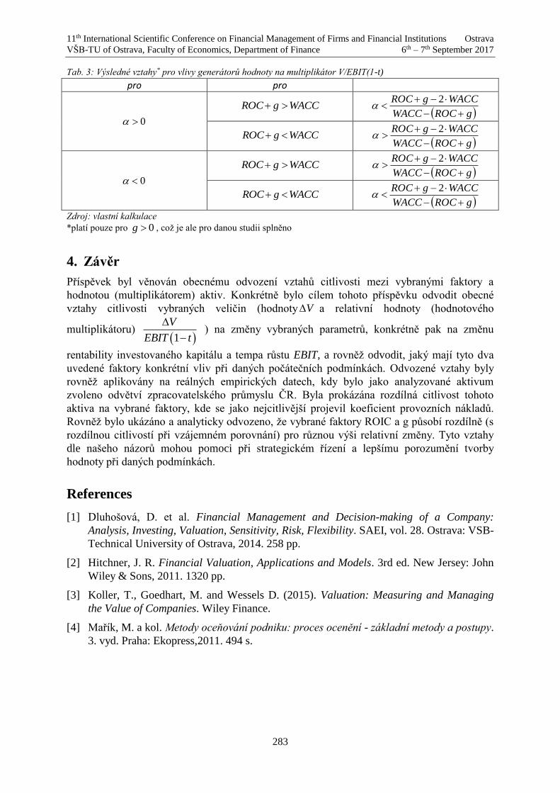
11th International Scientific Conference on Financial Management of Firms and Financial Institutions Ostrava
VŠB-TU of Ostrava, Faculty of Economics, Department of Finance 6th – 7th September 2017
283
Tab. 3: Výsledné vztahy* pro vlivy generátorů hodnoty na multiplikátor V/EBIT(1-t)
pro pro
0
WACCgROC gROCWACC
WACCgROC
2
WACCgROC gROCWACC
WACCgROC
2
0
WACCgROC gROCWACC
WACCgROC
2
WACCgROC gROCWACC
WACCgROC
2
Zdroj: vlastní kalkulace
*platí pouze pro 0g , což je ale pro danou studii splněno
4. Závěr
Příspěvek byl věnován obecnému odvození vztahů citlivosti mezi vybranými faktory a
hodnotou (multiplikátorem) aktiv. Konkrétně bylo cílem tohoto příspěvku odvodit obecné
vztahy citlivosti vybraných veličin (hodnoty V a relativní hodnoty (hodnotového
multiplikátoru) 1
V
EBIT t
) na změny vybraných parametrů, konkrétně pak na změnu
rentability investovaného kapitálu a tempa růstu EBIT, a rovněž odvodit, jaký mají tyto dva
uvedené faktory konkrétní vliv při daných počátečních podmínkách. Odvozené vztahy byly
rovněž aplikovány na reálných empirických datech, kdy bylo jako analyzované aktivum
zvoleno odvětví zpracovatelského průmyslu ČR. Byla prokázána rozdílná citlivost tohoto
aktiva na vybrané faktory, kde se jako nejcitlivější projevil koeficient provozních nákladů.
Rovněž bylo ukázáno a analyticky odvozeno, že vybrané faktory ROIC a g působí rozdílně (s
rozdílnou citlivostí při vzájemném porovnání) pro různou výši relativní změny. Tyto vztahy
dle našeho názorů mohou pomoci při strategickém řízení a lepšímu porozumění tvorby
hodnoty při daných podmínkách.
References
[1] Dluhošová, D. et al. Financial Management and Decision-making of a Company:
Analysis, Investing, Valuation, Sensitivity, Risk, Flexibility. SAEI, vol. 28. Ostrava: VSB-
Technical University of Ostrava, 2014. 258 pp.
[2] Hitchner, J. R. Financial Valuation, Applications and Models. 3rd ed. New Jersey: John
Wiley & Sons, 2011. 1320 pp.
[3] Koller, T., Goedhart, M. and Wessels D. (2015). Valuation: Measuring and Managing
the Value of Companies. Wiley Finance.
[4] Mařík, M. a kol. Metody oceňování podniku: proces ocenění - základní metody a postupy.
3. vyd. Praha: Ekopress,2011. 494 s.
11th International Scientific Conference on Financial Management of Firms and Financial Institutions Ostrava
VŠB-TU of Ostrava, Faculty of Economics, Department of Finance 6th – 7th September 2017
284
Business Strategy Management: The Importance of Employees During Implementation of Strategic
Changes
Jiří Havelka1
Abstract
Employees are the key element of each organization and the ultimate maker of any strategic
change. The presented article seeks to understand their role in strategic management, especially
at the implementation phase, and to identify the main aspects of their importance. The article is a
summary of the approaches of dozens of contemporary authors in the field of strategic
management on the background of the book Strategy: Process, Content, Context written by Bob
de Wit. The results confirmed that in most cases only revolutionary or evolutionary strategic
changes cannot be chosen. Strategic management must always be a combination that suits a given
firm’s size, structure and corporate culture. The contribution of the work is the confirmation of
the key importance of employees during strategy implementation and definition of the main
principles of of their importance in relation to the character of the company.
Key Words
Strategy; Business Strategy Management; Strategy Implementation; Employees; Revolutionary
Change; Evolutionary Change
JEL Classification L1
1. Úvod
Cílem této práce je zmapovat význam zaměstnanců při implementaci strategie na základě
stavu vědeckého poznání a přístupu současných autorů k tématu strategického řízení. Toto
shrnutí provedu na pozadí knihy Strategy: an international perspective od Boba de Wita [1],
která je odbornou veřejností považována za stěžejní literaturu v oblasti strategického řízení.
Nejdříve shrnu význam a úlohu zaměstnanců ve strategickém řízení obecně. Následně rozeberu
přístup k zaměstnancům při implementaci strategie. V předposledních dvou kapitolách ukáži
na pracích současných autorů nutnost kombinace revolučního a evolučního přístupu při
zavádění strategických změn. V závěru shrnu všechny získané poznatky a určím hlavní
zásady přístupu k zaměstnancům v návaznosti na charakter podniku.
2. Zaměstnanci a jejich význam pro strategické řízení
Zaměstnanci jsou základním stavebním kamenem každé organizace. Odvíjí se od nich
výrobní i inovační možnosti a schopnosti jakékoli firmy [2][3][4]. Obrázek níže přesně
charakterizuje jejich význam v rámci business modelu. Mezi pomyslnou špičkou firemní
struktury a řadovými zaměstnanci jsou tři základní pojítka – struktura organizace, vnitřní
procesy a firemní kultura. Tato tři pojítka musí být podporou jakékoli strategické změny,
1 Mgr. Jiří Havelka1, LLM, [email protected]

11th International Scientific Conference on Financial Management of Firms and Financial Institutions Ostrava
VŠB-TU of Ostrava, Faculty of Economics, Department of Finance 6th – 7th September 2017
285
přičemž strategická změna musí být (alespoň v pojetí De Wita) změnou celého business
modelu. Zařazení nového produktu do zákaznického portfolia není samo o sobě strategickou
změnou. Naopak orientace na nový tržní segment strategickou změnou je. Obdobné pojetí
nabízí Souček, pro kterého může být zařazení nového produktu jednou ze strategických operací,
které vedou k vyššímu komplexu [3].
Obrázek 1: Business model [1]
Strategické řízení je kontinuálním procesem, který lze rozdělit do několika navazujících
celků. Řada významných autorů nabízí své vlastní pojetí tohoto procesu. Většina z nich však
popisuje obdobné instrumenty rozdělené do určitého počtu kroků. Bob de Wit například
definuje základní tři části: formulace strategie; strategická změna (implementace); strategická
inovace. Prof. Souček používá jednoduší dvou etapový model prvotní formulace (která zahrnuje
podsoubor dalších operací) a následné implementace strategie. Robert Kaplan naopak nabízí
proces složený z pěti kroků: vytvoř strategii; přelož strategii; naplánuj činnosti; monitoruj a uč
se; testuj a adaptuj strategii [6].
Role řadových zaměstnanců je významná již při procesu formulace strategie, i když většinou
pouze v přeneseném duchu[1][5][6]. Strategie není výhradní záležitostí vrcholového
managementu nebo dokonce jen ředitele. Ve směru odshora dolů se dostává až k manažerům
první linie (vedoucí oddělení, apod.), kteří by měli representovat „hlas“ zaměstnanců. Je však
pouze na těchto manažerech a dané firemní kultuře, do jaké míry zaměstnance do aktivit v rámci
formulování strategie opravdu zapojí. Přitom toto zapojení není v praxi vůbec jednoduché [7].
Roger Martin navíc ve své studii zjistil, že dostat strategii k frontline-workers je jednou
z největších překážek i následné implementace strategie [8]. Přišel na to, že strategická
rozhodnutí přichází ve většině pouze zeshora a majorita zaměstnanců ani není schopna říci, jaká
je strategie jejich firmy. Zajímavé je také zjištění, že lidé zapojení do přípravy strategie mají o
úspěšnou implementaci výrazně vyšší zájem. To potvrzuje i studie provedená na 150 polských
firmách. Naši polští kolegové v ní doporučují vyšší zapojení zaměstnanců do strategického
managementu, což následně pozitivně ovlivní rozšíření zvolené strategie [9].
Zaměstnanci významně ovlivňují formulaci strategie (především její charakter) i když se do
ní přímo nezapojí. Aby vrcholový manažer docílil efektivního zavedení jím formulované
strategie, musí brát v potaz, jak zaměstnanci změnu přijmou. Tomu musí strategii i následnou
implementaci do značné míry přizpůsobit [1]. Prof. Souček přidává, že strategie má směřovat
k vytvoření takového podnikového klimatu, v němž jsou lidé šťastní a rádi zde pracují. To
odráží skutečnost, že úspěch stále více závisí na kreativitě lidí, která je závislá právě na štěstí a
spokojenosti lidí. Vliv spokojenosti a štěstí zaměstnanců na efektivitu a výkonnost firmy
11th International Scientific Conference on Financial Management of Firms and Financial Institutions Ostrava
VŠB-TU of Ostrava, Faculty of Economics, Department of Finance 6th – 7th September 2017
286
prokázali i další autoři [10][11][12]. V Součkově pojetí se zaměstnanci objevují při formulaci
strategie především v oblasti strategických cílů. Stratég musí definovat své strategické cíle
nejen k zákazníkům, majitelům, apod., ale také ke svým zaměstnancům. Strategické cíle potom
přímo ovlivňují charakter výsledné strategie.
3. Přístup k zaměstnancům při implementaci strategie
Aby mohla být strategická změna zavedena s dlouhotrvajícím účinkem, zaměstnanci
organizace potřebují čas, aby se naučili, adaptovali a vyrostli do nové organizační reality [13].
Každá změna má svůj rozsah, načasování a rychlost. Zároveň musí být dobře vyvážená (evoluce
x revoluce), aby ji zaměstnanci byli schopni vstřebat. Přitom zavedení strategické změny často
naráží na rigiditu ze strany zaměstnanců. V této souvislosti jsou v praxi časté:
psychologický odpor ke změně – čím více jsou lidé zaběhnuti v nějakém systému, tím
hůře změnu snášejí, chápou i implementují. Tyto změny pro ně nepředstavují
příležitosti ke zlepšení, ale nevítanou konfrontaci se systémem [14].
kulturní odpor ke změně – pokud je firemní kultura rigidní k jakýmkoli změnám, je
těžké úspěšně implementovat strategické změny [15]
politický odpor ke změně – jednotlivec nebo skupina, která strategickou změnu
považuje za oslabení své pozice nebo prohru, těmto změnám odporuje a je jejím
oponentem [16]
zamčené kompetence – firma dlouho běžící v jedněch kolejích už má natolik
zaběhnuté vnitřní kompetence, že změna skrz ně prakticky není možná [17]
uzavření v systému – pokud se firma jednou zaběhne v novém organizačním systému,
je velice těžké jej hned měnit. Zde jsou doporučovány změny typu zemětřesení [18].
etické problémy – zaměstnanec se soustředí primárně na své dobro a nesdílí
manažerský pohled na věc [19][20]
sdílení vědomostí - zaměstnanci často nemají chuť sdílet své schopnosti a vědomosti
[21]
Z výše uvedeného jasně vyplývají určité implikace, kterých si musí být stratég dobře vědom.
Čím méně je firemní kultura ztotožněná se změnami a jejich zaváděním, tím obtížněji se daná
strategická změna implementuje. Čím déle firma běží v neměnných kolejích, tím hůře si
zaměstnanci na změnu zvykají. Čím větší firma a více organizačních vrstev, tím složitější
implementace bývá. Čím větší změna, tím větší šok pro zaměstnance. Aby mohla být strategie
úspěšně implementovaná, je nezbytně nutné, aby daná firma disponovala firemní kulturou
nakloněnou k zavádění změn [22]. Každá strategická změna musí být vhodně (obsah,
načasování) komunikována směrem ke všem zaměstnancům. Při této komunikaci se stratég
snaží podat zaměstnancům změnu z pravidla tak, že zdůrazní jaké věci zůstávají stejné a jaké
se mění. Jednotliví zaměstnanci musí tuto informaci vstřebat takovým způsobem, aby byly
schopni na změnu efektivně odpovědět (implementovat) [23]. Opomenutí zaměstnanců a jejich
významu pro implementaci strategických změn je jednou z častých chyb stratégů. Někteří si
totiž neuvědomují, že úspěšná implementace strategie není možná, když není formulovaná
v souladu s firemními možnostmi (zaměstnanci, firemní kultura, leadership, atd.) [24][25][26].

11th International Scientific Conference on Financial Management of Firms and Financial Institutions Ostrava
VŠB-TU of Ostrava, Faculty of Economics, Department of Finance 6th – 7th September 2017
287
Je patrné, že strategie a její následná implementace musí odpovídat charakteru a velikosti
firmy s důrazem na kmenové zaměstnance. Změna nesmí být úplným zemětřesením, ale do
určité míry musí přijít kontinuálně, aby na ni zaměstnanci mohli vhodně reagovat. V tomto
ohledu se mezi autory objevují dva základní přístupy: perspektiva neplynulého zavádění
(revoluce) a perspektiva plynulého zavádění (evoluce).
4. Revoluce vs. Evoluce
První skupina autorů tvrdí, že obecně mají všichni lidé přirozený odpor ke změně. Po
zavedení změny nového systému směřují vždy k zajištění stability [27]. Především pokud je
firma úspěšná, je tato stabilita ještě hlubší. Dlouhodobá stabilita není nežádoucí, ale musí být
vyvážena úroveň, aby zaměstnanci nebyli ke změně rigidní. Tuto rigiditu poté nelze překonat
sériemi malých změn, ale zásadní změnou, která zároveň ovlivní zaběhnuté kognitivní mapy
zaměstnanců. Takováto změna musí proběhnout relativně rychle, protože zaměstnanci
nemohou dlouhodobě pracovat v nejistotě a musí se dostat do rovnováhy [12]. Důležitou roli
také hraje důvod změny – jestli se jedná o reakci na krizovou situaci nebo změnu pramenící
z přáni vedení firmy (proaktivní x reaktivní). V krizových situacích se zaměstnanci se změnou
dovedou lépe ztotožnit a implementace většinou probíhá plynuleji [1].
Druhá skupina autorů podporuje spíše plynulé zavádění menších změn [15][23]. Velké
změny vždy vyvolávají „hon“ za stabilitou. Velké změny revolučního charakteru navíc
z pravidla vyvolávají nutnost k další významné změně v budoucím období. Strategické řízení
vnímají tito autoři jako maratónský běh, který představuje kontinuální posun za jasně
definovaným cílem. Významným předpokladem v této souvislosti však je, že zaměstnanci
budou dostatečně motivovaní se učit – ve smyslu nových vědomostí i nové firemní kultury.
Tuto motivaci je nejúčinnější zajistit různými finančními nástroji [28]. Krizové situace
(reaktivní změny) mohou zaměstnance více motivovat ke změně, ale jiným směrem, než je
žádoucí. Zaměstnanci se pak soustředí na krátkodobé cíle a bojí se experimentovat – zkoušet
nové věci. Nejsou schopni se otevřít a ztotožnit se s dlouhodobými cíli firmy [15]. Mimo učení
musí být zaměstnanci motivovaní i k neustálé adaptaci na změny. Reálně přitom hrozí, že
budou z neustálých změn a inovací unaveni a přestanou spolupracovat [29]. Je proto úkolem
manažerů, aby vytvořili vhodné prostředí, které poskytne zaměstnancům dostatečnou kariérní
jistotu, která vyváží ostatní formy nejistoty.
Akademická obec ani odborníci z praxe se neshodují, jaký z těchto dvou přístupů zavádění
změn je vhodnější. Je proto vždy na strategickém manažerovi, aby volil styl strategického řízení
individuálně v návaznosti na charakter a potřeby dané firmy a jejich zaměstnanců. Zaměstnanci
nemusí být nutně ztotožněni s firemní kulturou, aby se dala strategie úspěšně implementovat.
Stratég ale musí vždy nalézt vhodné optimum, které bude dané firemní kultuře odpovídat [30].
De Wit ve své knize [1] popisuje dva hlavní póly přístupu k zaměstnancům při zavádění
strategických změn v návaznosti na charakter podniku. První skupinou jsou mechanistická
(autoritářských) uspořádání, kde se management snaží zbavit jakékoli závislosti na
zaměstnancích a jejich nenahraditelnosti. Zde je efektivnější zvolit revoluční změnu (neplynulé
zavádění). Tyto organizace jsou charakteristické organizačními schématy, jasně nastavenými
vnitřními procesy a kompetencemi všech zaměstnanců. Firemní kultura se mezi zaměstnanci
sdílí omezeně nebo vůbec a vztah s vedením funguje pouze na bázi příkazů. Zaměstnanci jsou
11th International Scientific Conference on Financial Management of Firms and Financial Institutions Ostrava
VŠB-TU of Ostrava, Faculty of Economics, Department of Finance 6th – 7th September 2017
288
zde trénovaní k úzce specifické činnosti a vyžadují pokročilou supervizi. Druhou skupinou
podniků jsou tzv. „clan-like cultures“ – podniky se silnou firemní kulturou a plošší strukturou.
Zde je naopak vhodnější zvolit plynule zavedenou strategickou změnu. Organizace s takto
propojenou firemní kulturou bývají navíc charakteristické kvalifikovanými zaměstnancemi
s pokročilými dovednostmi.
Obdobné rozdělení nabízí i další autoři. Mantere a Vaara například rozlišují organizace,
vzhledem k charakteru zavedeného strategického řízení, na ty s participačním a
neparticipačním přístupem zaměstnanců [31] [37]. Ve své analýze došli k závěru, že existují 3
zdroje, které jsou propojeny s neparticipačním přístupem – mystifikace, disciplinovanost a
technologizace. S participačním přístupem jsou naopak spojeny seberozvoj, dialogizace a
konkretizace.
Toto rozdělení do dvou pólů není mezi akademickou obcí ničím novým a prakticky odráží
obdobná zjištění i z jiných výzkumných oborů. Hlavním z nich je pochopitelně výzkum
lidských zdrojů, který se k obdobným závěrům dostal již před desítkami let, ale i politických
věd, managementu a další. V těchto oborech je zakořeněná především tzv. „stewardship“ teorie
[32] (zaměstnanci odkázaní sami na sebe se budou chovat jako zodpovědní stewardi zdrojů,
které kontrolují) a „agency“ teorie [33] (manažeři řídí podnik autoritativně ve svém vlastním
zájmu a na úkor shareholderů). Manažeři musí tyto dva přístupy vhodně vyvážit, aby docílili
efektivního fungování a prosperity firmy. Tato potřeba vyvážení je obdobná prakticky ve všech
firmách – velkých, malých, korporátních, rodinných, atd. [34][35].
5. Hledání rovnováhy
Je patrné, že v praxi musí stratégové najít vhodnou rovnováhu mezi revoluční a evoluční
změnou, aby docílili její úspěšné implementace. Určujícími prvky jsou především charakter
organizace: struktura, velikost, firemní kultura, povaha ekonomické činnosti, charakter
poskytované služby, apod. Jednoznačně v tom hrají roli i geografické rozdíly. Nelze aplikovat
stejný přístup v Japonsku nebo Indii, kde bývají zaměstnanci významně spjati s firemní
kulturou, jako například v Rusku nebo Číně [36][37].
Obecně lze říci, že čím vertikálně rozsáhlejší organizační struktura a méně kvalifikačně
náročná práce, tím víc by se měl stratég přiklánět k perspektivě neplynulého zavádění změn.
Zaměstnanci v těchto uspořádáních musí být jasně vedeni, významně kontrolováni a musí
dostávat pouze ty nejnutnější informace. I prof. Souček upozorňuje, že přílišné spoléhání na
autonomní aktivity pracovníků může vést k „akční ochablosti“. Na zaměstnance musí být
vyvíjen systematický, vlídný, ale neúprosný tlak. Strategie je pro všechny pracovníky firmy
závazná a je základní povinností všech pracovníků firmy [38]. Stejně jako de Wit nebo Mantere
netvrdí že se musí zaměstnanci se změnou nutně ztotožnit, aby mohla být úspěšně zavedena
(ačkoli je to silně preferováno).
Těmto přístupům odporuje řada autorů. Spee například souhlasí s tím, že je klíčové
komunikovat strategii a její důležitost napříč celou firmou, abychom dosáhli maximálních
výsledků. Tvrdí však, že se strategickými cíli firmy musí být ztotožněný každý zaměstnanec
[39]. Neilson, na základě své rozsáhlé studie přidává, že zaměstnanci, kteří přesně vědí za jaká
rozhodnutí a akce jsou zodpovědní, jsou nejvýznamnějším spojujícím prvkem společností,
které úspěšně implementují strategické změny [40]. Minimálně by měli umět odpovědět na
11th International Scientific Conference on Financial Management of Firms and Financial Institutions Ostrava
VŠB-TU of Ostrava, Faculty of Economics, Department of Finance 6th – 7th September 2017
289
otázky jako: Jaké zdroje mám, abych udělal svou práci? Jak se bude hodnotit má práce? S kým
se mohu setkat a ovlivnit, abych dosáhl svých cílů? Jakou podporu mohu očekávat, když budu
žádat o pomoc ostatní?[41]
Zároveň je nezbytně nutné, aby manažeři komunikovali i hlavní faktory úspěchu. Musí je
navíc podat tak, aby i „frontline-workers“ rozuměli přínosu jejich každodenní práce. Obdobnou
vizi sdílí i další autoři [6][42]. Martin například říká, že zaměstnance nelze brát jako bezduchou
prodlouženou ruku vedení firmy. Tento přístup nepřenáší úspěch a oddaluje zaměstnance.
Stratégové jsou tak odříznutí od implementačního těla.
V posledních letech se význam zaměstnanců při implementaci strategie v odborné literatuře
kontinuálně prohlubuje. To může souviset s několika aspekty. Hlavním důvodem je, že
vstupujeme do éry, v níž nehmotná aktiva, jako jsou odbornost, inteligence, rychlost, kreativita,
silné zaujetí, inovace a další stránky znalostí, jsou stále důležitější než hmotná aktiva [3].
Úspěch stále více závisí na motivaci a kreativitě lidí [43]. Roste počet znalostně intenzivních
oborů i subjektů v nich působících.
Někteří autoři dokonce tvrdí, že role zaměstnanců je natolik významná, že prostřednictvím
změny přístupu k nim lze implementovat i nedobře formulovanou strategii [44][45].
6. Závěr
Zaměstnanci jsou klíčovým prvkem strategického řízení naprosto každé firmy. Charakter
zaměstnanců a povaha firemní kultury je jedním z hlavních faktorů určujících rámec, jak by
měla být strategická změna pojata. Na každou takto významnou změnu musí zaměstnanec umět
vhodně zareagovat a zavést ji do svých každodenních procesů. Jedině tak lze zajistit i úspěšnou
implementaci strategické změny s potenciálně dlouhodobým účinkem.
V textech současných autorů se objevují dva hlavní protipóly v přístupu k zaměstnancům při
zavádění strategických změn: perspektiva neplynulého zavádění (revoluce) a perspektiva
plynulého zavádění (evoluce). Revoluční přístup bývá využíván především v organizacích
s autoritářským vedením, se složitou firemní strukturou a málo kvalifikačně náročnou prací.
Příkladem mohou být některé výrobní obory, zemědělské činnosti, apod. Vedení těchto firem
nechce být závislé na svých zaměstnancích, což se výrazně projevuje v jejich přístupu k nim.
Tyto organizace jsou proto charakteristické jasně nastavenými vnitřními procesy, velice
specificky vzdělanými zaměstnanci a jejich významnou supervizí. Do strategických rozhodnutí
těchto firem nejsou řadoví zaměstnanci nikdy zapojeni napřímo.
Opačným protipólem je evoluční způsob zavádění změn. Ten je charakteristický pro firmy
s plošší strukturou, kvalifikačně náročnou prací nebo například podnikající ve znalostně
intenzivním oboru. Příkladem mohou být firmy v oblasti poskytování služeb nebo různé IT
firmy. Vedení těchto společností si je dobře vědomo své závislosti na zaměstnancích a proto se
je ve zvýšené míře snaží zapojit už i do formulace strategie a vytvořit firemní kulturu vhodnou
pro implementaci změn. Tyto organizace jsou charakteristické vysoce kvalifikovanými
pracovníky s širokým záběrem vědomostí. Spíše než pokročilou supervizi tyto zaměstnanci
potřebují významnější autonomii, vzájemnou komunikaci a porozumění příčinám změn.
Je dobře patrné, že každý model má svá omezení a neexistuje univerzální verze, která by se
dala využít všude. Zvolit vhodnou kombinaci přístupů je proto stále klíčovou schopností
každého strategického manažera. V některých podnikatelských oborech s charakteristickým
11th International Scientific Conference on Financial Management of Firms and Financial Institutions Ostrava
VŠB-TU of Ostrava, Faculty of Economics, Department of Finance 6th – 7th September 2017
290
autoritářským řízením nám může být prakticky jedno, jak budou zaměstnanci na změnu
reagovat. V jiných oborech je reakce zaměstnanců hlavním určujícím aspektem úspěšné
implementace.
Oba póly sdílejí i společné charakteristiky. Zřejmě nejvýznamnější je, že všichni
zaměstnanci (a lidé obecně) směřují k vlastní stabilitě a při zavádění jakýchkoli změn musíme
překonávat jejich rigiditu. Všichni vyžadují zvláštní přístup. Sjednocujícím prvkem zde je
informovanost. Ve všech firemních uspořádáních musí být každý pracovní článek dobře
informovaný a dělat přesně to, co má. Rozdílnost přístupů poté spočívá především v tom, jestli
to zaměstnanci dělají prakticky samostatně nebo s pokročilým autoritářským vedením.
De Wit ani žádný jiný autor neříká do jaké míry zaměstnanci implementaci ovlivňují. Jen
hrstka autorů se snaží zjistit v jakých oblastech je vnímání strategie ze strany zaměstnanců a
top managementu odlišné. Tato témata si zaslouží samostatnou vědeckou studii, která by byla
významně prospěšná pro akademickou obec i praktiky.
Literatura
[1] De Wit, Bob a Meyer, Ron. (2014). Strategy: An International Perspective. Singapur:
Seng Lee Press.
[2] Lillis, Bob, Marek Szwejczewski, a Keith Goffin. (2015). The Development of
Innovation Capability in Services: Research Propositions and Management Implications.
Operations Management Research, 8(1–2), p. 48–68.
[3] Chang, S. C., N. P. Lin, C. L. Wea, a C. Sheu. (2002). Aligning Manufacturing
Capabilities with Business Strategy: An Empirical Study in High-Tech Industry.
International Journal of Technology Management, 24(1), p. 70–87.
[4] Mumford, M.D. (2000). Managing Creative People: Strategies and Tactics for
Innovation. Human Resource Management Review, 10(3), p. 313-351
[5] Souček, Zdeněk. (2015). Strategie úspěšného podniku: symbióza kreativity a disciplíny.
Vydání první. Praha: C.H. Beck.
[6] Kaplan, Robert S., a David P. Norton. (2008). Mastering the Management System.
Harvard Business Review, 86(1), p. 62–77.
[7] van Donk, D.-P., Esser, A. (1992). Strategic human resource management: A role of the
human resource manager in the process of strategy formation. Human Resource
Management Review, 2(4), p. 299–315.
[8] Martin, Roger L. (2010). How Hierarchy Can Hurt Strategy Execution. Harvard Business
Review, 88(7–8), p. 74–75.
[9] Kaleta, Andrzej, a Anna Witek-Crabb. (2015). Participation in the Strategic Management
Process and the Expansiveness. Argumenta Oeconomica, 34(1), p. 61–76.
[10] Koys, Daniel J. (2001). The Effects of Employee Satisfaction, Organizational Citizenship
Behavior, and Turnover on Organizational Effectiveness: A Unit-Level, Longitudinal
Study. Personnel Psycholog,y 54(1), p. 101–14.

11th International Scientific Conference on Financial Management of Firms and Financial Institutions Ostrava
VŠB-TU of Ostrava, Faculty of Economics, Department of Finance 6th – 7th September 2017
291
[11] Miller, Susan. (1997). Implementing Strategic Decisions: Four Key Success Factors.
Organization Studies (Walter de Gruyter GmbH & Co. KG.), 18(4), p. 577.
[12] Lee, Jangwoo, a Danny Miller. (1999). People Matter: Commitment to Employees,
Strategy and Performance in Korean Firms. Strategic Management Journal, 20(6), p.
579–93.
[13] Liu, Y., Perrewé, P.L. (2005). Another look at the role of emotion in the organizational
change: A process model. Human Resource Management Review, 15(4), p. 263–280.
[14] Hammer, M. (1990). Reeingeneering Work: Don’t Automate, Obliterate. Harward
Business Review, 68(4), p. 104-111
[15] Senge, P.M. (1990). The Leader’s New York: Building Learning Organizations. Sloan
Management Review, 31(1), p. 7-23
[16] Krüger, W. (1996). Implementation: The Core task of Change management. CEMS
Business Review, 1, p. 77-96
[17] Teece, D.J., Pisano, G. a Shuen, A. (1997). Dynamic Capabilities and Strategic
Management, Strategic Management Journal, 18(7), p. 509-533
[18] Arthur, W.B. (1996). Increasing Return and the New World of Business, Harward
Business Review, 74(4), p. 100-109
[19] Sonenshein, Scott. (2009). Emergence of Ethical Issues during Strategic Change
Implementation. Organization Science 20(1), p. 223–39.
[20] Lefkowitz, J. (2006). The constancy of ethics amidst the changing world of work. Human
Resource Management Review, The New World of Work and Organizations 16, p. 245–
268.
[21] Cater, Tomaz, a Danijel Pucko. (2010). Factors of Effective Strategy Implementation:
Empirical Evidence from Slovenian Business Practice. Journal for East European
Management Studies, 15(3), p. 207–236.
[22] Franken, Arnoud, Chris Edwards, a Rob Lambert. (2009). Executing Strategic Change:
Understanding the critical management elements that lead to success. California
Management Review, 51(3), p. 49–+.
[23] Sonenshein, Scott. (2010). We’re changing—or are we? Untangling the role of
progressive, regressive, and stability narratives during strategic change implementation.
The Academy of Management Journal, 53(3), p. 477–512.
[24] Slater, Stanley F., Eric M. Olson, a G. Tomas M. Hult. (2006). The Moderating Influence
of Strategic Orientation on the Strategy Formation Capability–performance Relationship.
Strategic Management Journal, 27(12), p. 1221–31.
[25] Mezger, Simon, a Maurice Violani. (2011). Seven Basic Strategic Missteps and How to
Avoid Them. Strategy & Leadership, 39(6), p. 19–26.
[26] Buller, P.F., McEvoy, G.M. (2012). Strategy, human resource management and
performance: Sharpening line of sight. Human Resource Management Review, 22, p. 43–
56.
[27] Mintzberg, H. (1991). The Effective Organization: Forces and Forms. Sloan Management
Review, 32(2), p. 54-67.

11th International Scientific Conference on Financial Management of Firms and Financial Institutions Ostrava
VŠB-TU of Ostrava, Faculty of Economics, Department of Finance 6th – 7th September 2017
292
[28] Kim, Hyondong, a Kang Sung-Choon. (2013). Strategic HR Functions and Firm
Performance: The Moderating Effects of High-Involvement Work Practices. Asia Pacific
Journal of Management 30(1), p. 91–113.
[29] Valackiene, Asta. (2011). Theoretical Substation of the Model for Crisis Management in
Organization. Inzinerine Ekonomika-Engineering Economics, 22(1), p. 78–90.
[30] Tushman, M.L., O’Reilly III, C.A. (1996). Ambidextrous Organizations: Managing
Evolutionary and Revolutionary Change. California Management Review, 38(4), p. 8-33.
[31] Mantere, Saku, a Eero Vaara. (2008). On the problem of participation in strategy: A
critical discursive perspective. Organization Science, 19(2), p. 341–358.
[32] Donaldson, L., a Davis, j.h. (1991). Stewardship theory or agency theory: CEO
governance and shareholder returns. Australian Journal of Management, 16, p. 49-64.
[33] Ross, Stephen A. (1973). The economic theory of agency: The principal's
problem. American Economic Review, 62(2): 134-139.
[34] Lee, Junghyun, a M. Susan Taylor. (2014). Dual roles in psychological contracts: When
managers take both agent and principal roles. Human Resource Management Review
24(1), p. 95–107.
[35] Eddleston, Kimberly A., Franz W. Kellermanns, a Roland E. Kidwell. (2017). Managing
Family Members: How Monitoring and Collaboration Affect Extra-Role Behavior in
Family Firms. Human Resource Management.
[36] Brown Johnson, N., Droege, S. (2004). Reflections on the generalization of agency
theory: Cross-cultural considerations. Human Resource Management Review, 14, p. 325–
335.
[37] Li, Xinjian, a Martin Putterill. (2007). Strategy Implications of Business Culture
Differences between Japan and China. Business Strategy Series 8(2), p. 148–54.
[38] Souček, Zdeněk. (2010). Firma 21. století (Předstihněme nejlepší!!!). Druhé vydání.
Professional Publishing.
[39] Spee, A. Paul, a Paula Jarzabkowski. (2011). Strategic Planning as Communicative
Process. Organization Studies, 32(9).
[40] Neilson, Gary L., Karla L. Martin, a Elizabeth Powers. (2008). The Secrets to Successful
Strategy Execution. Harvard Business Review, 86(6), p. 60–+.
[41] Simons, R. (2005). Designing High-Performance Jobs. Harvard Business Review, 83(7–
8), p. 54–+.
[42] Martin, Roger L. (2010). Drawing a Line between Strategy and Execution Almost
Guarantees Failure. Harvard Business Review, 88(7–8), p. 64–+.
[43] Foss, Nicolai J., a Siegwart Lindenberg. (2013). Microfoundations for Strategy: A Goal-
Framing Perspective on the Drivers of Value Creation. Academy of Management
Perspectives 27(2), p. 85–102.
[44] Lee, Eucman, a Phanish Puranam. (2016). The Implementation Imperative: Why One
Should Implement Even Imperfect Strategies Perfectly. Strategic Management Journal,
37(8), p. 1529–46.

11th International Scientific Conference on Financial Management of Firms and Financial Institutions Ostrava
VŠB-TU of Ostrava, Faculty of Economics, Department of Finance 6th – 7th September 2017
293
[45] Zeleny, Milan. (2008). Strategy and Strategic Action in the Global Era: Overcoming the
Knowing-Doing Gap. International Journal of Technology Management 43(1/2/3), p. 64.
11th International Scientific Conference on Financial Management of Firms and Financial Institutions Ostrava
VŠB-TU of Ostrava, Faculty of Economics, Department of Finance 6th – 7th September 2017
294
The use of Big Data in terms of overhead costs
Josef Horák, Jiřina Bokšová 1
Abstract
The submitted paper primarily deals with the big data which undeniably represent an essential
component of the Industry 4.0 itself. Nowadays, the companies are collecting the enormous
volume of data but on the other hand, they are facing the problems connected with the filtering
of relevant data ready for use in the area of the financial management, controlling, financial and
management accounting. The main aim of the paper is to analyse the influence of the big data
and their effective use from the view of savings in the overhead costs. These savings can
consequently increase the profit of the company and its financial performance. However, this
process is associated with the investments in new machines, technologies, devices that will be
able to effectively share the information, because the production process will be based on the
individual mass production.
Key words
big data, financial performance of the company, Industry 4.0, overhead costs
JEL Classification: M11, O31, O33
1. Úvod
Industry 4. 0 (v České republice je tento termín označován jako Průmysl 4.0), je pojem,
který se spojuje se vznikem 4. průmyslové revoluce. Tato revoluce je založena na
implementaci kyberneticko – fyzikálních systémů do tzv. „chytrých továren“. Jedná se o zcela
nový způsob v oblasti myšlení a chápání výrobního procesu, který s sebou přináší možnost
zvýšení „efektivity produkce“ v řádu desítek procent. Nejedná se primárně o zvýšení
produktivity (zvýšení objemu výroby), ale o zvýšení efektivity produkce (výroba
s minimálním počtem lidí, s minimální spotřebou energie apod.) V souvislosti s Industry 4.0
však musí ve firmě dojít k nastavení zcela nových modelů nejen ve výrobě, ale i v oblasti
finančního řízení, controllingu, manažerského účetnictví a v neposlední řadě i účetnictví
finančního.
Podnik bude v budoucnu konkurenceschopný pouze v takovém případě, že dokáže včas
pochopit a efektivně implementovat do podnikového prostředí nejen nové systémy
digitalizace, vzájemné propojení digitalizovaných výrobních a obslužných procesů, ale i nové
modely finančního řízení.
Uvedený proces digitalizace bude mít zcela zásadní dopad i na formy a metody finančního
řízení podniku. Finančního řízení „nové digitalizované generace“ bude čerpat informace
z cloudových uložišť, jejichž vznik je nezbytnou podmínkou realizace Industry 4.0. Změny
v oblasti finančního řízení budou mít bezpochyby dopad i na zaznamenávání a vykazování
hospodářských transakcí. Je více než zřejmé, že pouze takový podnik, který se připraví na
nadcházející změny, bude schopen udržet svoji konkurenceschopnost na trhu i v budoucnu.
Nové technologie nejenže produkují, ale jsou schopné i uchovávat enormní množství dat,
souhrnně označované pojmem Big Data. Tato data jsou či budou zachycena prostřednictvím 1 Ing. Josef Horák, Ph.D., ŠKODA AUTO UNIVERSITY, [email protected]
doc. Ing. Jiřina Bokšová, Ph.D., ŠKODA AUTO UNIVERSITY, [email protected]
11th International Scientific Conference on Financial Management of Firms and Financial Institutions Ostrava
VŠB-TU of Ostrava, Faculty of Economics, Department of Finance 6th – 7th September 2017
295
řady speciálních senzorů a čipů. [2] Je očekávatelné, že ve velmi blízké budoucnosti dojde k
exponenciálnímu růstu dat, která budou vytvořena a následně zpracována těmito
technologiemi. Spojení, prostřednictvím kterých budou vzájemně komunikovat výrobní
zařízení, obslužná zařízení, materiál, nedokončená výroba, polotovary či hotové výrobky,
dodavatelé, odběratelé se nazývá Internet věcí. [4] Je jasné, že bez značných investic v oblasti
informačních a produkčních technologií se proces digitalizace a vznik „chytrých továren“
neobejde.
V současné době již dochází v podnikových prostředích k shromažďovaní Big Data, avšak
řada podniků není schopna potenciál uložený v těchto datech optimálně strukturovat a
efektivně využít. Tuto skutečnost potvrzuje i studie, kterou uskutečnili McAfee a
Brynjolfsson. [6]
Pro finanční řízení „nové digitalizované generace“ je nezbytné, aby se vrcholní manažeři
naučili využívat nové technologie při strukturování Big Data v závislosti na konkrétních
potřebách podniku např. z pohledu dílčích cílů jednotlivých vnitropodnikových středisek,
z pohledu organizačních cílů podniku, z pohledu reportů příslušným uživatelům. [10, 11]
Implementace kyberneticko – fyzikálních systémů do podnikového prostředí bude zcela
zásadním způsobem ovlivňovat strukturu a celkovou hodnotu režijních nákladů. Hlavním
cílem předloženého článku není posouzení nákladovosti přeměny současných podniků na
„chytré továrny“, ale posouzení dopadu existence Big Data na oblast nákladů podniku
z pohledu finančního řízení, controllingu, manažerského a finančního účetnictví a otevřít
odbornou diskusi, zda využitím Big Data dojde k úsporám režijních nákladů podniku.
2. Metodologie výzkumu
Článek je založen na literární rešerši dostupných zdrojů z oblasti Industry 4.0, dále na
analýze účetních procesů a sběru dat ve vybraných společnostech působících v odvětví
automobilového průmyslu v České republice. Veškeré poznatky, které jsou prezentovány
v následujícím textu, jsou výsledkem unikátního primárního výzkumu, který bylo možné
realizovat ve spolupráci s těmito firmami. Zpracovaná analýza je založena zejména na metodě
brainstormingu, v rámci které byli osloveni vybraní zaměstnanci firem zapojených do
výzkumu. Prostřednictvím těchto sezení došlo k identifikaci vlivů, které s sebou přinese
probíhající digitalizace celého výrobního procesu se zaměřením na oblast zpracování Big Data
v podnikovém prostředí.
V současné době neexistují žádné dostupné databáze, ze kterých by bylo možné čerpat
sekundární data, firmy dosud nemají k dispozici reporty, které by mohly posloužit pro potřeby
výzkumu. Smyslem výzkumu je upozornit na další oblasti podnikového prostředí, které vedle
digitalizace výrobních procesů proces Industry 4.0 bezesporu zasáhne.
V následujícím textu bude nejprve charakterizována problematika Big Data, dále oblast
režijních nákladů a následně bude v další kapitole článku provedena diskuze nad tím, jakým
způsobem ovlivní Big Data režijní náklady jednotlivých účetních jednotek.
Sběr dat a jejich efektivní analýza pozitivně ovlivňuje konkurenceschopnost firmy na trhu.
Jedná se o velmi důležitý zdroj informací z pohledu celého výrobního procesu včetně
administrativních činností, které je nezbytné vykonávat, aby bylo možné zajistit celkový chod
podniku. Big Data mohou přinést firmě konkurenční výhodu pouze v případě, že je bude umět
správně filtrovat, analyzovat a využít v rámci rozhodovacích procesů či reportování
uživatelům.
Na základě relevantních dat bude možné zefektivnit výrobní proces tak, aby došlo k jeho
propojení s přáními a požadavky odběratelů. Nové produkty tak budou připraveny výlučně
v souladu s požadavky zákazníků, což současný výrobní proces zatím zcela neumožňuje. [1]
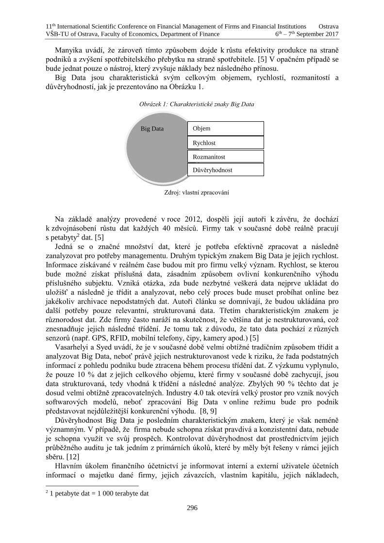
11th International Scientific Conference on Financial Management of Firms and Financial Institutions Ostrava
VŠB-TU of Ostrava, Faculty of Economics, Department of Finance 6th – 7th September 2017
296
Manyika uvádí, že zároveň tímto způsobem dojde k růstu efektivity produkce na straně
podniků a zvýšení spotřebitelského přebytku na straně spotřebitele. [5] V opačném případě se
bude jednat pouze o nástroj, který zvyšuje náklady bez následného přínosu.
Big Data jsou charakteristická svým celkovým objemem, rychlostí, rozmanitostí a
důvěryhodností, jak je prezentováno na Obrázku 1.
Obrázek 1: Charakteristické znaky Big Data
Zdroj: vlastní zpracování
Na základě analýzy provedené v roce 2012, dospěli její autoři k závěru, že dochází
k zdvojnásobení růstu dat každých 40 měsíců. Firmy tak v současné době reálně pracují
s petabyty2 dat. [5]
Jedná se o značné množství dat, které je potřeba efektivně zpracovat a následně
zanalyzovat pro potřeby managementu. Druhým typickým znakem Big Data je jejich rychlost.
Informace získávané v reálném čase budou mít pro firmu velký význam. Rychlost, se kterou
bude možné získat příslušná data, zásadním způsobem ovlivní konkurenčního výhodu
příslušného subjektu. Vzniká otázka, zda bude nezbytné veškerá data nejprve ukládat do
uložišť a následně je třídit a analyzovat, nebo celý proces bude muset probíhat online bez
jakékoliv archivace nepodstatných dat. Autoři článku se domnívají, že budou ukládána pro
další potřeby pouze relevantní, strukturovaná data. Třetím charakteristickým znakem je
různorodost dat. Zde firmy často naráží na skutečnost, že většina dat je nestrukturovaná, což
znesnadňuje jejich následné třídění. Je tomu tak z důvodu, že tato data pochází z různých
senzorů (např. GPS, RFID, mobilní telefony, čipy, kamery apod.) [5]
Vasarhelyi a Syed uvádí, že je v současné době velmi obtížné tradičním způsobem třídit a
analyzovat Big Data, neboť právě jejich nestrukturovanost vede k riziku, že řada podstatných
informací z pohledu podniku bude ztracena během procesu třídění dat. Z výzkumu vyplynulo,
že pouze 10 % dat z jejich celkového objemu, které firmy v současné době zachycují, jsou
data strukturovaná, tedy vhodná k třídění a následné analýze. Zbylých 90 % těchto dat je
dosud velmi obtížně zpracovatelných. Industry 4.0 tak otevírá velký prostor pro vznik nových
softwarových modelů, neboť zpracování Big Data v online režimu bude pro podnik
představovat nejdůležitější konkurenční výhodu. [8, 9]
Důvěryhodnost Big Data je posledním charakteristickým znakem, který je však neméně
významným. V případě, že firma nebude schopna získat pravdivá a konzistentní data, nebude
je schopna využít ve svůj prospěch. Kontrolovat důvěryhodnost dat prostřednictvím jejich
průběžného auditu je tak jedním z primárních úkolů, které by měly být řešeny v rámci jejich
sběru. [12]
Hlavním úkolem finančního účetnictví je informovat interní a externí uživatele účetních
informací o majetku dané firmy, jejich závazcích, vlastním kapitálu, jejich nákladech,
2 1 petabyte dat = 1 000 terabyte dat
Big Data Objem
Rychlost
Rozmanitost
Důvěryhodnost
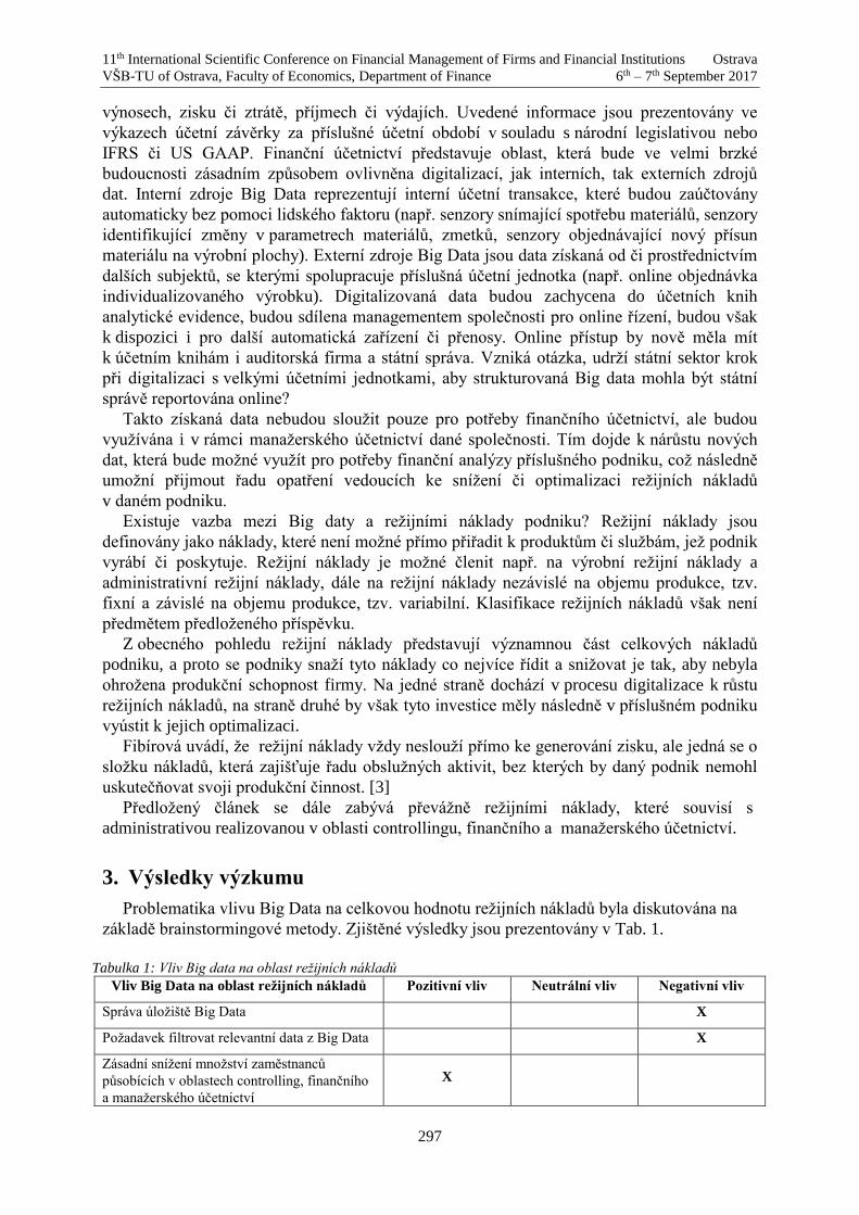
11th International Scientific Conference on Financial Management of Firms and Financial Institutions Ostrava
VŠB-TU of Ostrava, Faculty of Economics, Department of Finance 6th – 7th September 2017
297
výnosech, zisku či ztrátě, příjmech či výdajích. Uvedené informace jsou prezentovány ve
výkazech účetní závěrky za příslušné účetní období v souladu s národní legislativou nebo
IFRS či US GAAP. Finanční účetnictví představuje oblast, která bude ve velmi brzké
budoucnosti zásadním způsobem ovlivněna digitalizací, jak interních, tak externích zdrojů
dat. Interní zdroje Big Data reprezentují interní účetní transakce, které budou zaúčtovány
automaticky bez pomoci lidského faktoru (např. senzory snímající spotřebu materiálů, senzory
identifikující změny v parametrech materiálů, zmetků, senzory objednávající nový přísun
materiálu na výrobní plochy). Externí zdroje Big Data jsou data získaná od či prostřednictvím
dalších subjektů, se kterými spolupracuje příslušná účetní jednotka (např. online objednávka
individualizovaného výrobku). Digitalizovaná data budou zachycena do účetních knih
analytické evidence, budou sdílena managementem společnosti pro online řízení, budou však
k dispozici i pro další automatická zařízení či přenosy. Online přístup by nově měla mít
k účetním knihám i auditorská firma a státní správa. Vzniká otázka, udrží státní sektor krok
při digitalizaci s velkými účetními jednotkami, aby strukturovaná Big data mohla být státní
správě reportována online?
Takto získaná data nebudou sloužit pouze pro potřeby finančního účetnictví, ale budou
využívána i v rámci manažerského účetnictví dané společnosti. Tím dojde k nárůstu nových
dat, která bude možné využít pro potřeby finanční analýzy příslušného podniku, což následně
umožní přijmout řadu opatření vedoucích ke snížení či optimalizaci režijních nákladů
v daném podniku.
Existuje vazba mezi Big daty a režijními náklady podniku? Režijní náklady jsou
definovány jako náklady, které není možné přímo přiřadit k produktům či službám, jež podnik
vyrábí či poskytuje. Režijní náklady je možné členit např. na výrobní režijní náklady a
administrativní režijní náklady, dále na režijní náklady nezávislé na objemu produkce, tzv.
fixní a závislé na objemu produkce, tzv. variabilní. Klasifikace režijních nákladů však není
předmětem předloženého příspěvku.
Z obecného pohledu režijní náklady představují významnou část celkových nákladů
podniku, a proto se podniky snaží tyto náklady co nejvíce řídit a snižovat je tak, aby nebyla
ohrožena produkční schopnost firmy. Na jedné straně dochází v procesu digitalizace k růstu
režijních nákladů, na straně druhé by však tyto investice měly následně v příslušném podniku
vyústit k jejich optimalizaci.
Fibírová uvádí, že režijní náklady vždy neslouží přímo ke generování zisku, ale jedná se o
složku nákladů, která zajišťuje řadu obslužných aktivit, bez kterých by daný podnik nemohl
uskutečňovat svoji produkční činnost. [3]
Předložený článek se dále zabývá převážně režijními náklady, které souvisí s
administrativou realizovanou v oblasti controllingu, finančního a manažerského účetnictví.
3. Výsledky výzkumu
Problematika vlivu Big Data na celkovou hodnotu režijních nákladů byla diskutována na
základě brainstormingové metody. Zjištěné výsledky jsou prezentovány v Tab. 1.
Tabulka 1: Vliv Big data na oblast režijních nákladů
Vliv Big Data na oblast režijních nákladů Pozitivní vliv Neutrální vliv Negativní vliv
Správa úložiště Big Data X
Požadavek filtrovat relevantní data z Big Data X
Zásadní snížení množství zaměstnanců
působících v oblastech controlling, finančního
a manažerského účetnictví
X
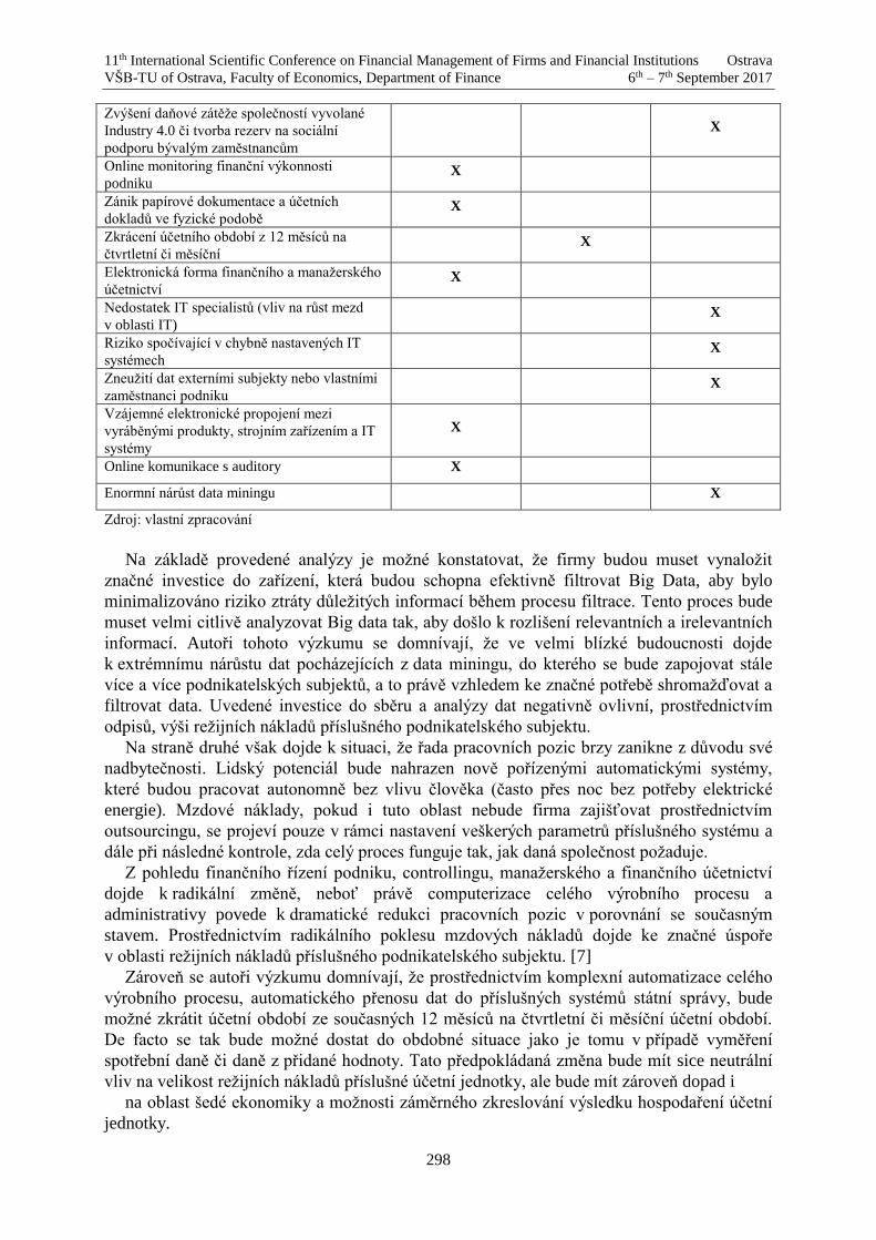
11th International Scientific Conference on Financial Management of Firms and Financial Institutions Ostrava
VŠB-TU of Ostrava, Faculty of Economics, Department of Finance 6th – 7th September 2017
298
Zvýšení daňové zátěže společností vyvolané
Industry 4.0 či tvorba rezerv na sociální
podporu bývalým zaměstnancům
X
Online monitoring finanční výkonnosti
podniku X
Zánik papírové dokumentace a účetních
dokladů ve fyzické podobě X
Zkrácení účetního období z 12 měsíců na
čtvrtletní či měsíční X
Elektronická forma finančního a manažerského
účetnictví X
Nedostatek IT specialistů (vliv na růst mezd
v oblasti IT) X
Riziko spočívající v chybně nastavených IT
systémech X
Zneužití dat externími subjekty nebo vlastními
zaměstnanci podniku X
Vzájemné elektronické propojení mezi
vyráběnými produkty, strojním zařízením a IT
systémy
X
Online komunikace s auditory X
Enormní nárůst data miningu X
Zdroj: vlastní zpracování
Na základě provedené analýzy je možné konstatovat, že firmy budou muset vynaložit
značné investice do zařízení, která budou schopna efektivně filtrovat Big Data, aby bylo
minimalizováno riziko ztráty důležitých informací během procesu filtrace. Tento proces bude
muset velmi citlivě analyzovat Big data tak, aby došlo k rozlišení relevantních a irelevantních
informací. Autoři tohoto výzkumu se domnívají, že ve velmi blízké budoucnosti dojde
k extrémnímu nárůstu dat pocházejících z data miningu, do kterého se bude zapojovat stále
více a více podnikatelských subjektů, a to právě vzhledem ke značné potřebě shromažďovat a
filtrovat data. Uvedené investice do sběru a analýzy dat negativně ovlivní, prostřednictvím
odpisů, výši režijních nákladů příslušného podnikatelského subjektu.
Na straně druhé však dojde k situaci, že řada pracovních pozic brzy zanikne z důvodu své
nadbytečnosti. Lidský potenciál bude nahrazen nově pořízenými automatickými systémy,
které budou pracovat autonomně bez vlivu člověka (často přes noc bez potřeby elektrické
energie). Mzdové náklady, pokud i tuto oblast nebude firma zajišťovat prostřednictvím
outsourcingu, se projeví pouze v rámci nastavení veškerých parametrů příslušného systému a
dále při následné kontrole, zda celý proces funguje tak, jak daná společnost požaduje.
Z pohledu finančního řízení podniku, controllingu, manažerského a finančního účetnictví
dojde k radikální změně, neboť právě computerizace celého výrobního procesu a
administrativy povede k dramatické redukci pracovních pozic v porovnání se současným
stavem. Prostřednictvím radikálního poklesu mzdových nákladů dojde ke značné úspoře
v oblasti režijních nákladů příslušného podnikatelského subjektu. [7]
Zároveň se autoři výzkumu domnívají, že prostřednictvím komplexní automatizace celého
výrobního procesu, automatického přenosu dat do příslušných systémů státní správy, bude
možné zkrátit účetní období ze současných 12 měsíců na čtvrtletní či měsíční účetní období.
De facto se tak bude možné dostat do obdobné situace jako je tomu v případě vyměření
spotřební daně či daně z přidané hodnoty. Tato předpokládaná změna bude mít sice neutrální
vliv na velikost režijních nákladů příslušné účetní jednotky, ale bude mít zároveň dopad i
na oblast šedé ekonomiky a možnosti záměrného zkreslování výsledku hospodaření účetní
jednotky.

11th International Scientific Conference on Financial Management of Firms and Financial Institutions Ostrava
VŠB-TU of Ostrava, Faculty of Economics, Department of Finance 6th – 7th September 2017
299
4. Závěr
Aby podnik mohl zůstat i nadále konkurenceschopným, musí přistoupit k analýze a
následnému využití Big Data takovým způsobem, aby zajistil optimální výrobní proces. Tento
výrobní proces bude realizovaný prostřednictvím využití kyberneticko – fyzikálních systémů,
na základě kterých vzájemně propojí jednotlivé vyráběné produkty se surovinami a dalšími
prostředky, které podnik využívá v rámci své produkční činnosti. Aby bylo možné efektivně
filtrovat relevantní data, bude z pohledu podniku nezbytné v blízké budoucnosti vynaložit
značné finanční prostředky ve formě investic do speciálních zařízení, softwarových produktů,
přípravy a školení zaměstnanců, celkové změny výrobního procesu takovým způsobem, aby
bylo možné vzájemně jednotlivé nové komponenty propojit v rámci dodavatelsko –
odběratelských řetězců.
Pouze firmy, které budou schopny společně komunikovat prostřednictvím IT systémů,
budou schopny vzájemně spolupracovat. Je možné konstatovat, že investice v oblasti
zachycení a zpracování Big Data povedou k nárůstu režijních nákladů, což zároveň negativně
ovlivní cash flow podniku a jeho výsledek hospodaření.
Na druhé straně dojde k úsporám režijních nákladů v oblasti nejen výroby, ale i
administrativy (např. úspory mzdových nákladů v oblasti controllingu, finančního a
manažerského účetnictví, úspory energií apod.). Společnosti budou zaměstnávat zejména
vysoce specializované a vyškolené zaměstnance, řada pracovních pozic v administrativě
zanikne v důsledku celkového přechodu na elektronickou formu, která nebude dále vyžadovat
účast lidského potenciálu. Převážná většina činností bude zajišťována prostřednictvím
elektronických zařízení, která umožní rychlejší, levnější a efektivnější zpracování relevantních
dat. Zároveň dojde k situaci, že uživatelé příslušných dat získají odpovídající informace včas,
v požadované kvalitě.
Uvedené úspory v oblasti režijních nákladů v oblasti administrativy pozitivně ovlivní
výsledek hospodaření příslušného podniku a jeho finanční výkonnost, což bude mít za
následek zvýšení konkurenceschopnosti na trhu.
References
[1] Čámská, D. (2014). Requirements for Models Predicting Corporate Financial Distress. 8th
International Days of Statistic and Economics, Slaný: Melandrium, 316-323.
[2] Alles, M. G. (2015). Drivers of the Use and Facilitators and Obstacles of the Evolution of
Big Data by the Audit Profession. Accounting Horizons, 29(2), 439-449.
[3] Fibírová, J. (2015). Manažerské účetnictví: nástroje a metody. Praha: Wolters Kluwer.
[4] Griffin, P. A., & Wright, A. M. (2015). Commentaries on Big Data's Importance for
Accounting and Auditing. Accounting Horizons, 29(2), 377-379.
[5] Manyika, J., Chui, M., Brown, B., Bughin, J., Dobbs, R., Roxburgh, C., & Byers, A. H.
(2011). Big Data: the next frontier for innovation, competition and productivity. New
York: McKinsey & Company.
[6] McAfee, A., & Brynjolfsson, E. (2015). Big Data: The Management Revolution. Harvard
business review, 90(10), 59-68.
[7] Pavelka, T., Skála, M., & Čadil, J. (2014). Selected issues of the minimum wage in the
Czech Republic. E+M Ekonomie a Management, 17(4), 30-45.

11th International Scientific Conference on Financial Management of Firms and Financial Institutions Ostrava
VŠB-TU of Ostrava, Faculty of Economics, Department of Finance 6th – 7th September 2017
300
[8] Syed, A. R., Gillela, K., & Venugopal, C. (2013). The future revolution on Big Data.
International Journal of Advanced Research in Computer and Communication
Engineering, 2(6), 2446-2451.
[9] Vasarhelyi, M. A., Kogan, A., & Tuttle, B. M. (2015). Big Data in Accounting: An
Overview. Accounting Horizons, 29(2), 381-396.
[10] Warren, J. D., Moffitt, K. C., & Byrnes, P. (2015). How Big Data Will Change
Accounting. Accounting Horizons, 29(2), 397-407.
[11] Yoon, K., Hoogduin, L., & Zhang, L. (2015). Big Data as Complementary Audit
Evidence. Accounting Horizons, 29(2), 431-438.
[12] Zhang, J., Yang, X., & Appelbaum, D. (2015). Toward Effective Big Data Analysis in
Continuous Auditing. Accounting Horizons, 29(2), 469-476.
11th International Scientific Conference on Financial Management of Firms and Financial Institutions Ostrava
VŠB-TU of Ostrava, Faculty of Economics, Department of Finance 6th – 7th September 2017
301
The nature and importance of dislosing information about interests in any subsidiaries, joint ventures
and associates according to IFRSs 1
Renáta Hornická 2
Abstract
The objective of accounting view of financial investments with interest in other entity is to
express an intense relationship between investor and investee. Based on the accounting
information, users evaluate the nature and effect of financial investment on financial position,
financial performance and cash flows of the investor and find out financial risk with interests in
the other entities. The paper deals with presentation and analysis requirements about disclosure
of information about consolidated subsidiaries and joint ventures and associates accounted by
equity method according to IFRSs.
Key words
disclosure of information, interests in other entities, subsidiary, joint venture, associate, IFRSs.
JEL Classification: M40, M41
1. Úvod
Účtovné zobrazenie finančných investícií3, prostredníctvom ktorých investor získava
podiel v iných účtovných jednotkách, patrí k náročným oblastiam účtovníctva. Pri výbere
účtovnej metódy sa postupuje v závislosti od klasifikácie finančnej investície v súlade
s uplatňovaným príslušným rámcom účtovného (finančného) vykazovania.
Používatelia informácií z účtovnej závierky požadujú relevantné účtovné informácie,
na základe ktorých môžu posúdiť charakter finančnej investície, zhodnotiť jej vplyv na
finančnú situáciu a finančnú výkonnosť investora a identifikovať prípadné možné finančné
riziká spojené s finančnou investíciou. V. Zelenka a M. Zelenková uvádzajú, že používatelia
informácií si často neuvedomujú, že čísla (údaje) prezentované v účtovných výkazoch sú len
výstupom modelu, ktorý sa rovnako ako každý iný model, zakladá na určitých predpokladoch
a viacerých obmedzeniach (Zelenka V.-Zelenková, M.,2013, s.7). Pre používateľov účtovných
informácií sú dôležité aj informácie zverejňované v poznámkach účtovnej závierky.
Od roku 2013 sú požiadavky týkajúce sa zverejňovania informácií o podieloch v iných
účtovných jednotkách predmetom samostatného štandardu IFRS 12 Zverejňovanie podielov
v iných účtovných jednotkách. Cieľom príspevku je prezentovať a analyzovať požiadavky
1 Príspevok bol spracovaný ako výstup výskumného projektu KEGA č. 026 EU-4/2016 Potreba
skvalitnenia účtovných informácií s využitím nadnárodných úprav, osobitne IFRS, v legislatívnych
podmienkach Slovenskej republiky. 2 Ing. Renáta Hornická, PhD., Fakulta hospodárskej informatiky, Katedra účtovníctva a audítorstva,
Ekonomická univerzita v Bratislave, Dolnozemská cesta 1, 852 35 Bratislava,
[email protected]. 3 Finančné investície môžu mať okrem investícií do podielov iných účtovných jednotiek aj inú formu,
napríklad investovanie do dlhových cenných papierov, poskytnuté dlhodobé pôžičky (Kovanicová,
D.,2005, s. 196-197). Týmto formám finančných investícií sa v príspevku nevenujeme.
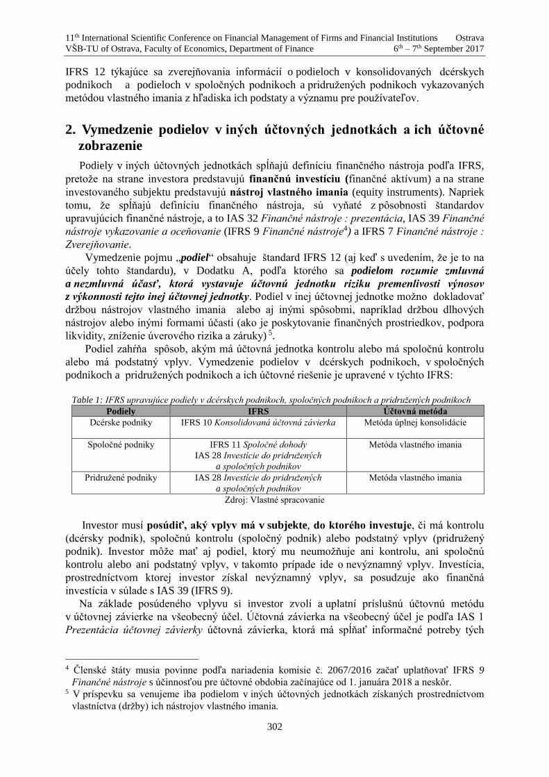
11th International Scientific Conference on Financial Management of Firms and Financial Institutions Ostrava
VŠB-TU of Ostrava, Faculty of Economics, Department of Finance 6th – 7th September 2017
302
IFRS 12 týkajúce sa zverejňovania informácií o podieloch v konsolidovaných dcérskych
podnikoch a podieloch v spoločných podnikoch a pridružených podnikoch vykazovaných
metódou vlastného imania z hľadiska ich podstaty a významu pre používateľov.
2. Vymedzenie podielov v iných účtovných jednotkách a ich účtovné
zobrazenie
Podiely v iných účtovných jednotkách spĺňajú definíciu finančného nástroja podľa IFRS,
pretože na strane investora predstavujú finančnú investíciu (finančné aktívum) a na strane
investovaného subjektu predstavujú nástroj vlastného imania (equity instruments). Napriek
tomu, že spĺňajú definíciu finančného nástroja, sú vyňaté z pôsobnosti štandardov
upravujúcich finančné nástroje, a to IAS 32 Finančné nástroje : prezentácia, IAS 39 Finančné
nástroje vykazovanie a oceňovanie (IFRS 9 Finančné nástroje4) a IFRS 7 Finančné nástroje :
Zverejňovanie.
Vymedzenie pojmu „podiel“ obsahuje štandard IFRS 12 (aj keď s uvedením, že je to na
účely tohto štandardu), v Dodatku A, podľa ktorého sa podielom rozumie zmluvná
a nezmluvná účasť, ktorá vystavuje účtovnú jednotku riziku premenlivosti výnosov
z výkonnosti tejto inej účtovnej jednotky. Podiel v inej účtovnej jednotke možno dokladovať
držbou nástrojov vlastného imania alebo aj inými spôsobmi, napríklad držbou dlhových
nástrojov alebo inými formami účasti (ako je poskytovanie finančných prostriedkov, podpora
likvidity, zníženie úverového rizika a záruky) 5.
Podiel zahŕňa spôsob, akým má účtovná jednotka kontrolu alebo má spoločnú kontrolu
alebo má podstatný vplyv. Vymedzenie podielov v dcérskych podnikoch, v spoločných
podnikoch a pridružených podnikoch a ich účtovné riešenie je upravené v týchto IFRS:
Table 1: IFRS upravujúce podiely v dcérskych podnikoch, spoločných podnikoch a pridružených podnikoch
Podiely IFRS Účtovná metóda
Dcérske podniky
IFRS 10 Konsolidovaná účtovná závierka Metóda úplnej konsolidácie
Spoločné podniky IFRS 11 Spoločné dohody
IAS 28 Investície do pridružených
a spoločných podnikov
Metóda vlastného imania
Pridružené podniky IAS 28 Investície do pridružených
a spoločných podnikov
Metóda vlastného imania
Zdroj: Vlastné spracovanie
Investor musí posúdiť, aký vplyv má v subjekte, do ktorého investuje, či má kontrolu
(dcérsky podnik), spoločnú kontrolu (spoločný podnik) alebo podstatný vplyv (pridružený
podnik). Investor môže mať aj podiel, ktorý mu neumožňuje ani kontrolu, ani spoločnú
kontrolu alebo ani podstatný vplyv, v takomto prípade ide o nevýznamný vplyv. Investícia,
prostredníctvom ktorej investor získal nevýznamný vplyv, sa posudzuje ako finančná
investícia v súlade s IAS 39 (IFRS 9).
Na základe posúdeného vplyvu si investor zvolí a uplatní príslušnú účtovnú metódu
v účtovnej závierke na všeobecný účel. Účtovná závierka na všeobecný účel je podľa IAS 1
Prezentácia účtovnej závierky účtovná závierka, ktorá má spĺňať informačné potreby tých
4 Členské štáty musia povinne podľa nariadenia komisie č. 2067/2016 začať uplatňovať IFRS 9
Finančné nástroje s účinnosťou pre účtovné obdobia začínajúce od 1. januára 2018 a neskôr. 5 V príspevku sa venujeme iba podielom v iných účtovných jednotkách získaných prostredníctvom
vlastníctva (držby) ich nástrojov vlastného imania.
11th International Scientific Conference on Financial Management of Firms and Financial Institutions Ostrava
VŠB-TU of Ostrava, Faculty of Economics, Department of Finance 6th – 7th September 2017
303
používateľov, ktorí od účtovnej jednotky nemôžu požadovať, aby im vypracovala správu
zohľadňujúcu ich špecifické informačné potreby (IAS 1.7).
V prípade investora, ktorý má podiely v dcérskom podniku je účtovnou závierkou na
všeobecný účel konsolidovaná účtovná závierka. V prípade investora, ktorý nemá podiely
v dcérskom podniku, ale má podiely v spoločnom podniku alebo v pridruženom podniku je
účtovnou závierkou na všeobecný účel účtovná závierka, v ktorej uplatňuje metódu vlastného
imania6. Zároveň treba uviesť, že IFRS stanovujú výnimku z konsolidácie podľa IFRS 10
(v prípade investora, ktorý je investičnou spoločnosťou7) a výnimku z uplatnenia metódy
vlastného imania podľa IAS 28 (ak je investor organizáciou rizikového kapitálu, podielovým
fondom alebo podobnou účtovnou jednotkou )8.
3. Zverejňovanie informácií o podieloch v iných účtovných jednotkách
Zverejňovanie informácií o podieloch v iných účtovných jednotkách rieši samostatný
štandard, IFRS 12 Zverejňovanie podielov v iných účtovných jednotkách. IFRS 12 bol
vydaný v máji 2011 a nadobudol účinnosť k 1. 1. 2013. Európska únia ho prevzala
nariadením komisie č. 1254/2012 spolu s ďalšími novými IFRS (IFRS 10 Konsolidovaná
účtovná závierka, IFRS 11 Spoločné dohody) a novelizovanými IAS (IAS 27 Individuálna
účtovná závierka, IAS 28 Investície do pridružených a spoločných podnikov), s tým že
umožnila členským štátom aplikáciu týchto nových IFRS a novelizovaných IAS najneskôr od
účtovného obdobia začínajúceho 1. 1. 2014. IFRS 12 nahradil požiadavky týkajúce sa
zverejňovania uvedené v dovtedy platných štandardoch ( IAS 27 Konsolidovaná
a individuálna účtovná závierka, IAS 31 Podiely na spoločnom podnikaní a IAS 28 Investície
do pridružených podnikov). Od svojho vydania bol IFRS 12 viackrát novelizovaný (v roku
2012, v roku 2014 a v roku 2016), v príspevku vychádzame z platného znenia k 1. 1. 2017.
IFRS 12 aplikuje účtovná jednotka, keď má podiel v dcérskom podniku, podiel na
spoločnej dohode (na spoločnom usporiadaní), podiel v pridruženom podniku
a v nekonsolidovaných štrukturovaných jednotkách9. Požiadavky IFRS 12 sa nevzťahujú na
individuálnu účtovnú závierku podľa IAS 27 (okrem stanovených výnimiek) a ďalšie
vymedzené oblasti (zamestnanecké požitky; podiel v inej účtovnej jednotke, prostredníctvom
ktorého investor nemá kontrolu, spoločnú kontrolu, ani podstatný vplyv; podiel v inej
účtovnej jednotke zaúčtovaný v súlade s IAS 39 (IFRS 9)).
6 Popri účtovnej závierke na všeobecný účel môže investor ako doplnok ku konsolidovanej účtovnej
závierke alebo v účtovnej závierke, v ktorej je uplatnená metóda vlastného imania, prezentovať aj
individuálnu (separátnu) účtovnú závierku podľa IAS 27 Individuálna účtovná závierka. V tejto
účtovnej závierke je predpísaný spôsob ocenenia finančných investícií v dcérskych podnikoch,
spoločných podnikoch a pridružených podnikoch, pričom zvolený spôsob oceňovania sa má
uplatňovať rovnako pri každej kategórii investícií (Mokošová, D., 2017, s. 61-62). Individuálnej
účtovnej závierke a požiadavkám na zverejnenie v tejto účtovnej závierke sa v príspevku
nevenujeme. 7 Investičná spoločnosť je podľa IFS 10 účtovná jednotka, ktorá získava finančné prostriedky od
jedného alebo viacerých investorov s cieľom poskytovať tomuto investorovi (investorom) služby
správy investícií len s cieľom výnosov z kapitálového zhodnotenia, investičného výnosu alebo
oboch. 8 Výnimkám z konsolidácie a výnimkám z uplatnenia metódy vlastného imania sa v príspevku
nevenujeme. 9 Štrukturované jednotky predstavujú subjekty (účtovné jednotky), v ktorých hlasovacie práva alebo
podobné práva nie sú rozhodujúcim faktorom pre posúdení, kto má kontrolu. V IFRS 12 sú rozlíšené
konsolidované a nekonsolidované štrukturované jednotky. Týmto subjektom sa v príspevku
nevenujeme.
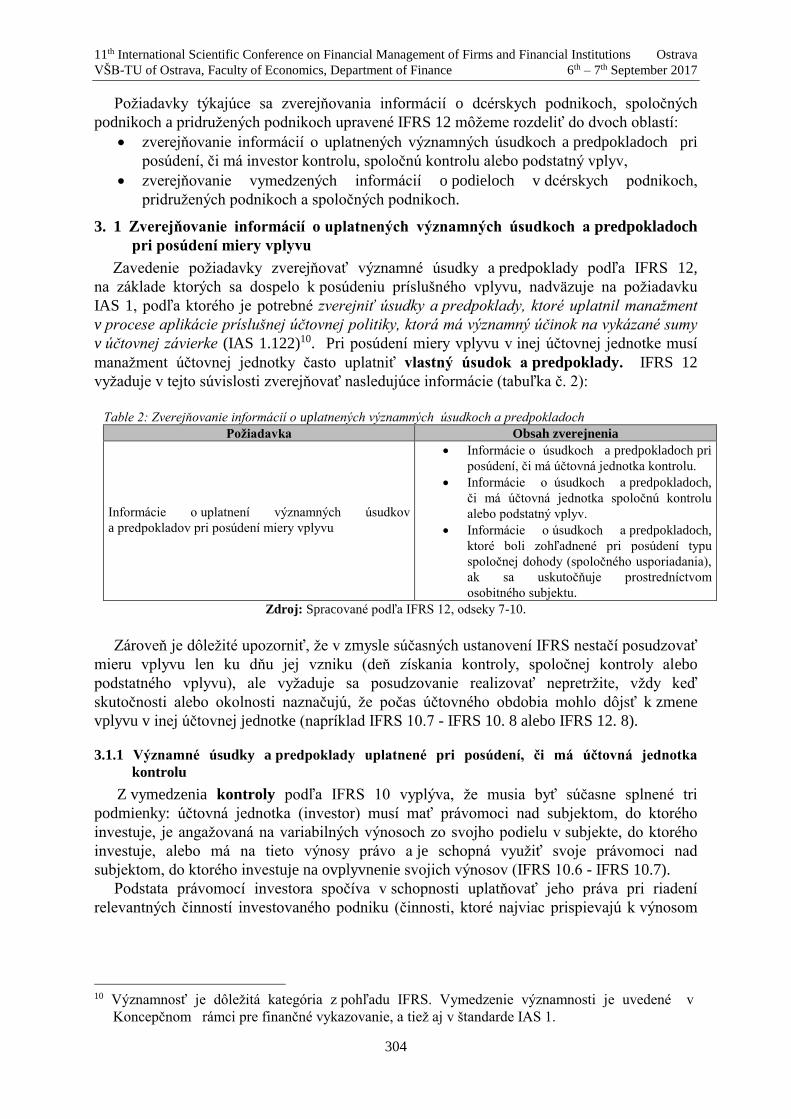
11th International Scientific Conference on Financial Management of Firms and Financial Institutions Ostrava
VŠB-TU of Ostrava, Faculty of Economics, Department of Finance 6th – 7th September 2017
304
Požiadavky týkajúce sa zverejňovania informácií o dcérskych podnikoch, spoločných
podnikoch a pridružených podnikoch upravené IFRS 12 môžeme rozdeliť do dvoch oblastí:
zverejňovanie informácií o uplatnených významných úsudkoch a predpokladoch pri
posúdení, či má investor kontrolu, spoločnú kontrolu alebo podstatný vplyv,
zverejňovanie vymedzených informácií o podieloch v dcérskych podnikoch,
pridružených podnikoch a spoločných podnikoch.
3. 1 Zverejňovanie informácií o uplatnených významných úsudkoch a predpokladoch
pri posúdení miery vplyvu
Zavedenie požiadavky zverejňovať významné úsudky a predpoklady podľa IFRS 12,
na základe ktorých sa dospelo k posúdeniu príslušného vplyvu, nadväzuje na požiadavku
IAS 1, podľa ktorého je potrebné zverejniť úsudky a predpoklady, ktoré uplatnil manažment
v procese aplikácie príslušnej účtovnej politiky, ktorá má významný účinok na vykázané sumy
v účtovnej závierke (IAS 1.122)10. Pri posúdení miery vplyvu v inej účtovnej jednotke musí
manažment účtovnej jednotky často uplatniť vlastný úsudok a predpoklady. IFRS 12
vyžaduje v tejto súvislosti zverejňovať nasledujúce informácie (tabuľka č. 2):
Table 2: Zverejňovanie informácií o uplatnených významných úsudkoch a predpokladoch
Požiadavka Obsah zverejnenia
Informácie o uplatnení významných úsudkov
a predpokladov pri posúdení miery vplyvu
Informácie o úsudkoch a predpokladoch pri
posúdení, či má účtovná jednotka kontrolu.
Informácie o úsudkoch a predpokladoch,
či má účtovná jednotka spoločnú kontrolu
alebo podstatný vplyv.
Informácie o úsudkoch a predpokladoch,
ktoré boli zohľadnené pri posúdení typu
spoločnej dohody (spoločného usporiadania),
ak sa uskutočňuje prostredníctvom
osobitného subjektu.
Zdroj: Spracované podľa IFRS 12, odseky 7-10.
Zároveň je dôležité upozorniť, že v zmysle súčasných ustanovení IFRS nestačí posudzovať
mieru vplyvu len ku dňu jej vzniku (deň získania kontroly, spoločnej kontroly alebo
podstatného vplyvu), ale vyžaduje sa posudzovanie realizovať nepretržite, vždy keď
skutočnosti alebo okolnosti naznačujú, že počas účtovného obdobia mohlo dôjsť k zmene
vplyvu v inej účtovnej jednotke (napríklad IFRS 10.7 - IFRS 10. 8 alebo IFRS 12. 8).
3.1.1 Významné úsudky a predpoklady uplatnené pri posúdení, či má účtovná jednotka
kontrolu
Z vymedzenia kontroly podľa IFRS 10 vyplýva, že musia byť súčasne splnené tri
podmienky: účtovná jednotka (investor) musí mať právomoci nad subjektom, do ktorého
investuje, je angažovaná na variabilných výnosoch zo svojho podielu v subjekte, do ktorého
investuje, alebo má na tieto výnosy právo a je schopná využiť svoje právomoci nad
subjektom, do ktorého investuje na ovplyvnenie svojich výnosov (IFRS 10.6 - IFRS 10.7).
Podstata právomocí investora spočíva v schopnosti uplatňovať jeho práva pri riadení
relevantných činností investovaného podniku (činnosti, ktoré najviac prispievajú k výnosom
10 Významnosť je dôležitá kategória z pohľadu IFRS. Vymedzenie významnosti je uvedené v
Koncepčnom rámci pre finančné vykazovanie, a tiež aj v štandarde IAS 1.
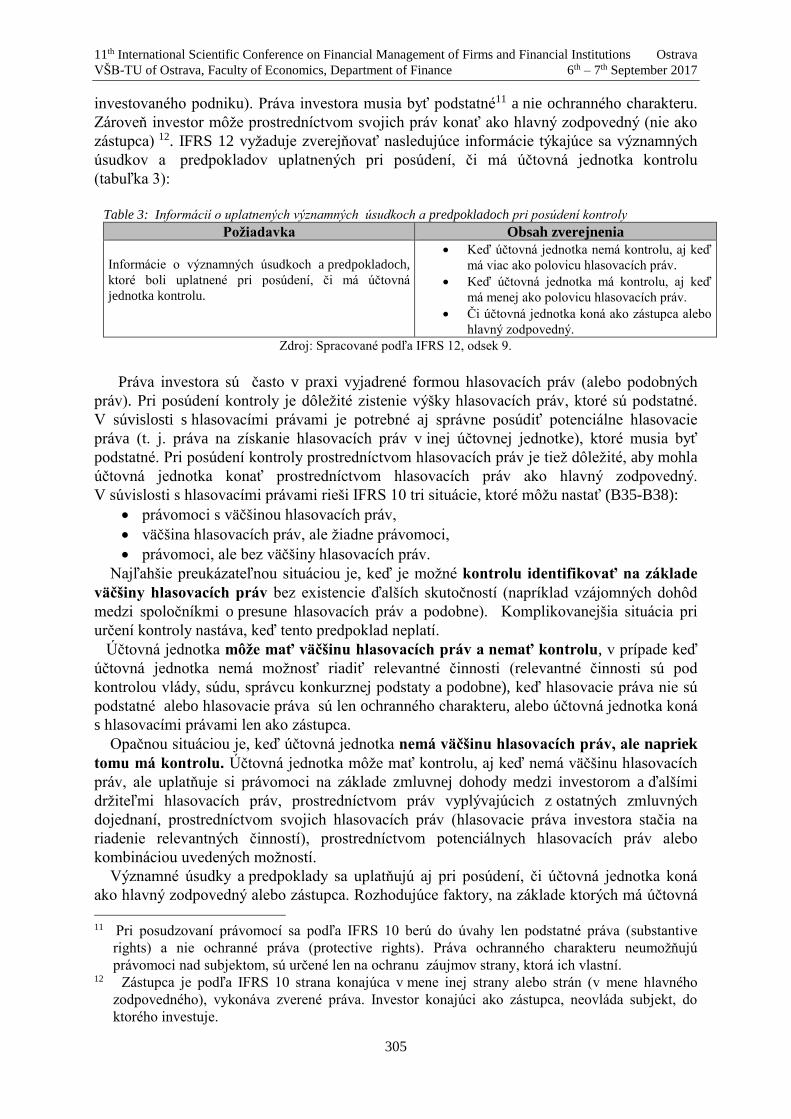
11th International Scientific Conference on Financial Management of Firms and Financial Institutions Ostrava
VŠB-TU of Ostrava, Faculty of Economics, Department of Finance 6th – 7th September 2017
305
investovaného podniku). Práva investora musia byť podstatné11 a nie ochranného charakteru.
Zároveň investor môže prostredníctvom svojich práv konať ako hlavný zodpovedný (nie ako
zástupca) 12. IFRS 12 vyžaduje zverejňovať nasledujúce informácie týkajúce sa významných
úsudkov a predpokladov uplatnených pri posúdení, či má účtovná jednotka kontrolu
(tabuľka 3):
Table 3: Informácií o uplatnených významných úsudkoch a predpokladoch pri posúdení kontroly
Požiadavka Obsah zverejnenia
Informácie o významných úsudkoch a predpokladoch,
ktoré boli uplatnené pri posúdení, či má účtovná
jednotka kontrolu.
Keď účtovná jednotka nemá kontrolu, aj keď
má viac ako polovicu hlasovacích práv.
Keď účtovná jednotka má kontrolu, aj keď
má menej ako polovicu hlasovacích práv.
Či účtovná jednotka koná ako zástupca alebo
hlavný zodpovedný.
Zdroj: Spracované podľa IFRS 12, odsek 9.
Práva investora sú často v praxi vyjadrené formou hlasovacích práv (alebo podobných
práv). Pri posúdení kontroly je dôležité zistenie výšky hlasovacích práv, ktoré sú podstatné.
V súvislosti s hlasovacími právami je potrebné aj správne posúdiť potenciálne hlasovacie
práva (t. j. práva na získanie hlasovacích práv v inej účtovnej jednotke), ktoré musia byť
podstatné. Pri posúdení kontroly prostredníctvom hlasovacích práv je tiež dôležité, aby mohla
účtovná jednotka konať prostredníctvom hlasovacích práv ako hlavný zodpovedný.
V súvislosti s hlasovacími právami rieši IFRS 10 tri situácie, ktoré môžu nastať (B35-B38):
právomoci s väčšinou hlasovacích práv,
väčšina hlasovacích práv, ale žiadne právomoci,
právomoci, ale bez väčšiny hlasovacích práv.
Najľahšie preukázateľnou situáciou je, keď je možné kontrolu identifikovať na základe
väčšiny hlasovacích práv bez existencie ďalších skutočností (napríklad vzájomných dohôd
medzi spoločníkmi o presune hlasovacích práv a podobne). Komplikovanejšia situácia pri
určení kontroly nastáva, keď tento predpoklad neplatí.
Účtovná jednotka môže mať väčšinu hlasovacích práv a nemať kontrolu, v prípade keď
účtovná jednotka nemá možnosť riadiť relevantné činnosti (relevantné činnosti sú pod
kontrolou vlády, súdu, správcu konkurznej podstaty a podobne), keď hlasovacie práva nie sú
podstatné alebo hlasovacie práva sú len ochranného charakteru, alebo účtovná jednotka koná
s hlasovacími právami len ako zástupca.
Opačnou situáciou je, keď účtovná jednotka nemá väčšinu hlasovacích práv, ale napriek
tomu má kontrolu. Účtovná jednotka môže mať kontrolu, aj keď nemá väčšinu hlasovacích
práv, ale uplatňuje si právomoci na základe zmluvnej dohody medzi investorom a ďalšími
držiteľmi hlasovacích práv, prostredníctvom práv vyplývajúcich z ostatných zmluvných
dojednaní, prostredníctvom svojich hlasovacích práv (hlasovacie práva investora stačia na
riadenie relevantných činností), prostredníctvom potenciálnych hlasovacích práv alebo
kombináciou uvedených možností.
Významné úsudky a predpoklady sa uplatňujú aj pri posúdení, či účtovná jednotka koná
ako hlavný zodpovedný alebo zástupca. Rozhodujúce faktory, na základe ktorých má účtovná
11 Pri posudzovaní právomocí sa podľa IFRS 10 berú do úvahy len podstatné práva (substantive
rights) a nie ochranné práva (protective rights). Práva ochranného charakteru neumožňujú
právomoci nad subjektom, sú určené len na ochranu záujmov strany, ktorá ich vlastní. 12 Zástupca je podľa IFRS 10 strana konajúca v mene inej strany alebo strán (v mene hlavného
zodpovedného), vykonáva zverené práva. Investor konajúci ako zástupca, neovláda subjekt, do
ktorého investuje.
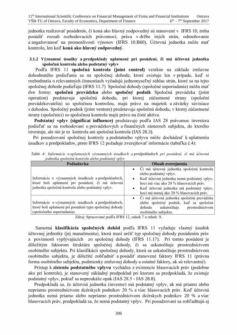
11th International Scientific Conference on Financial Management of Firms and Financial Institutions Ostrava
VŠB-TU of Ostrava, Faculty of Economics, Department of Finance 6th – 7th September 2017
306
jednotka realizovať posúdenie, či koná ako hlavný zodpovedný sú stanovené v IFRS 10, treba
posúdiť rozsah rozhodovacích právomocí, práva v držbe iných strán, odmeňovanie
a angažovanosť na premenlivosti výnosov (IFRS 10.B60). Účtovná jednotka môže mať
kontrolu, len keď koná ako hlavný zodpovedný.
3.1.2 Významné úsudky a predpoklady uplatnené pri posúdení, či má účtovná jednotka
spoločnú kontrolu alebo podstatný vplyv
Podľa IFRS 11 spoločná kontrola (joint control) vznikne na základe zmluvne
dohodnutého podieľania sa na spoločnej dohode, ktoré existuje len v prípade, keď si
rozhodnutia o relevantných činnostiach vyžadujú jednomyseľný súhlas strán, ktoré sa na tejto
spoločnej dohode podieľajú (IFRS 11.7) Spoločné dohody (spoločné usporiadania) môžu mať
dve formy: spoločnú prevádzku alebo spoločný podnik Spoločná prevádzka (joint
operation) predstavuje spoločnú dohodu, pri ktorej zúčastnené strany (spoloční
prevádzkovatelia) so spoločnou kontrolou, majú právo na majetok a záväzky súvisiace
s dohodou. Spoločný podnik (joint venture) predstavuje spoločnú dohodu, v ktorej zúčastnené
strany (spoločníci) so spoločnou kontrolu majú právo na čisté aktíva.
Podstatný vplyv (significat influence) predstavuje podľa IAS 28 právomoc investora
podieľať sa na rozhodovaní o prevádzkových a finančných zámeroch subjektu, do ktorého
investuje, ale nie je to kontrola ani spoločná kontrola (IAS 28.3).
Pri posudzovaní spoločnej kontroly a podstatného vplyvu môže dochádzať k uplatneniu
úsudkov a predpokladov, preto IFRS 12 požaduje zverejňovať informácie (tabuľka č.4):
Table 4: Informácie o uplatnených významných úsudkoch a predpokladoch pri posúdení, či má účtovná
jednotka spoločnú kontrolu alebo podstatný vplyv
Požiadavka Obsah zverejnenia
Informácie o významných úsudkoch a predpokladoch,
ktoré boli uplatnené pri posúdení, či má účtovná
jednotka spoločnú kontrolu alebo podstatný vplyv.
Či má účtovná jednotka spoločnú kontrolu
alebo podstatný vplyv.
Keď účtovná jednotka nemá podstatný vplyv,
hoci má viac ako 20 % hlasovacích práv.
Keď účtovná jednotka má podstatný vplyv,
hoci má menej ako 20 % hlasovacích práv.
Informácie o významných úsudkoch a predpokladoch,
ktoré boli uplatnené pri posúdení typu spoločnej dohody
(spoločného usporiadania).
Či má účtovná jednotka spoločnú prevádzku
alebo spoločný podnik, keď sa spoločná
dohoda uskutočňuje prostredníctvom
osobitného subjektu.
Zdroj: Spracované podľa IFRS 12, odsek 7 a odsek 9.
Samotná klasifikácia spoločných dohôd podľa IFRS 11 vyžaduje vlastný úsudok
účtovnej jednotky (jej manažmentu), ktorá musí určiť typ spoločnej dohody posúdením práv
a povinností vyplývajúcich zo spoločnej dohody (IFRS 11.17). Pri tomto posúdení je
dôležitým faktorom štruktúra spoločnej dohody, či sa uskutočňuje prostredníctvom
osobitného subjektu. Pri klasifikácii spoločnej dohody, ktorá sa uskutočňuje prostredníctvom
osobitného subjektu, je dôležité zohľadniť a posúdiť stanovené faktory IFRS 11 (právna
forma osobitného subjektu, podmienky zmluvnej dohody a ostatné faktory, ak sú relevantné).
Prístup k zisteniu podstatného vplyvu vychádza z existencie hlasovacích práv (podobne
ako pri kontrole), je stanovený základný predpoklad pri ktorom sa predpokladá, že existuje
podstatný vplyv, pokiaľ sa nepreukáže opak (IAS 28.5 - IAS 28.8).
Predpokladá sa, že účtovná jednotka (investor) má podstatný vplyv, ak má priamo alebo
nepriamo prostredníctvom dcérskych podnikov 20 % a viac hlasovacích práv. Keď účtovná
jednotka nemá priamo alebo nepriamo prostredníctvom dcérskych podnikov 20 % a viac
hlasovacích práv, predpokladá sa, že nemá podstatný vplyv. Pri posudzovaní sa zohľadňujú aj

11th International Scientific Conference on Financial Management of Firms and Financial Institutions Ostrava
VŠB-TU of Ostrava, Faculty of Economics, Department of Finance 6th – 7th September 2017
307
potenciálne hlasovacie práva, pri ktorých účtovná jednotka musí posúdiť, či potenciálne
hlasovacie práva prispievajú k podstatnému vplyvu.
Úsudky a predpoklady treba uplatniť predovšetkým v situácii, keď sa preukáže, že účtovná
jednotka, ktorá má priamo alebo nepriamo 20 % a viac hlasovacích práv nemá podstatný
vplyv. Opačná situácia nastáva, keď podstatný vplyv vznikne aj v situácii, keď účtovná
jednotka nemá priamo alebo nepriamo 20 % a viac hlasovacích práv, ale preukáže
existenciu podstatného vplyvu iným spôsobmi: zastúpením v predstavenstve alebo
v rovnocennom riadiacom orgáne podniku, do ktorého investuje, účasťou na rozhodovacích
procesoch vrátene účasti na rozhodnutiach o dividendách a iných rozdeleniach a ďalšími.
3. 2 Zverejňovanie informácií o podieloch v konsolidovaných dcérskych podnikoch,
spoločných podnikoch a pridružených podnikoch vykázaných metódou vlastného
imania
Účtovná jednotka, ktorá má kontrolu v inej účtovnej jednotke (dcérskej účtovnej jednotke)
je materskou účtovnou jednotkou. Materská účtovná jednotka prezentuje konsolidovanú
účtovnú závierku za skupinu podnikov ako účtovnú závierku jedinej účtovnej jednotky. Pri
konsolidácii dcérskeho podniku sa uplatňuje metóda úplnej konsolidácie. Účtovné riešenie
investícií do spoločného podniku a pridruženého podniku stanovuje IAS 28, ktorý predpisuje
v obidvoch prípadoch metódu vlastného imania.
3. 2. 1 Zverejňovanie informácií o podieloch v konsolidovaných dcérskych podnikoch
Po uplatnení metódy úplnej konsolidácie sú údaje v konsolidovaných výkazoch
kumulované za skupinu podnikov po eliminácii vnútroskupinových vzťahov. Zároveň sú
konsolidované výkazy doplnené o položky špecifické pre konsolidáciu, napríklad
nekontrolujúce podiely, goodwill vzniknutý pri konsolidácii. Podľa IFRS 12 sa v poznámkach
konsolidovanej účtovnej závierky zverejňujú tieto informácie (tabuľka 5):
Table 5: Zverejňovanie informácií o podieloch v konsolidovaných dcérskych podnikoch
Požiadavka Obsah zverejnenia
Zverejňovanie informácií o podieloch
v konsolidovaných dcérskych podnikoch
Zloženie skupiny a podiel nekontrolujúcich
spoločníkov a ich vplyv na činnosti
a peňažné toky skupiny.
Povaha a rozsah významných obmedzení
prístupu k aktívam skupiny a schopnosti
vyrovnávať záväzky skupiny.
Povaha a zmeny v rizík spojené s podielmi
v konsolidovaných štrukturovaných
jednotkách.13
Dôsledky zmien vlastníckych podielov
materskej účtovnej jednotky.
Ak je účtovná závierka dcérskeho podniku
zostavená k inému dňu, ako je deň,
ku ktorému sa zostavuje konsolidovaná
účtovná závierka.
Zdroj: Spracované podľa IFRS 12, odsek 10 a odsek 11.
Informácie o nekontrolujúcich podieloch sú dôležité z hľadiska zloženia skupiny
a vplyvu nekontrolujúcich spoločníkov na činnosti a peňažné toky skupiny. Medzi tieto
13 IFRS 12 upravuje tiež požiadavky týkajúce sa zverejňovania informácií o konsolidovaných štrukturovaných
jednotkách, ktorým sa v príspevku nevenujeme.

11th International Scientific Conference on Financial Management of Firms and Financial Institutions Ostrava
VŠB-TU of Ostrava, Faculty of Economics, Department of Finance 6th – 7th September 2017
308
informácie patrí predovšetkým: meno a sídlo dcérskeho podniku (identifikácia neúplne
vlastneného dcérskeho podniku), výška vlastníckeho podielu a hlasovacích práv
nekontrolujúcich spoločníkov, zisk alebo strata priradený nekontrolujúcim spoločníkom počas
účtovného obdobia, akumulovaný nekontrolujúci podiel na konci účtovného obdobia
a sumárne finančné informácie za dcérsky podnik pred vnútroskupinovými elimináciami
(vyplatené dividendy, neobežný majetok, obežný majetok, záväzky, náklady, výnosy,
komplexný výsledok).
Obmedzenia týkajúce sa prístupu k aktívam skupiny, ktoré môžu byť spôsobené
zákonnými, zmluvnými alebo inými regulačnými obmedzeniami majú vplyv na schopnosť
využívať tieto aktíva. Dôsledkom týchto obmedzení môže byť, že materská účtovná jednotka
alebo dcérska účtovná jednotka nemôžu prevádzať peňažné prostriedky alebo iné aktíva
v rámci skupiny. Obmedzenie schopnosti splácať záväzky v rámci skupiny môžu byť
spôsobené zárukami alebo inými požiadavkami, ktoré môžu obmedziť vyplácanie dividend
alebo splácanie úverov v rámci skupiny. Pre používateľov informácií sú dôležité informácie
týkajúce sa povahy a rozsahu týchto obmedzení spolu s uvedením konsolidovanej účtovnej
hodnoty aktív a záväzkov, ktorých sa tieto obmedzenia týkajú.
Zverejňovanie informácií o zmenách vlastníckych podielov materskej účtovnej jednotky
umožní používateľom pochopiť dôsledky účtovného spracovania týchto transakcií. Pri zmene
vlastníckeho podielu materskej spoločnosti bez straty kontroly má táto transakcia dopad
na vlastné imanie, preto sa požaduje zverejnenie zmien vlastného imania dcérskeho podniku,
ktoré je možné priradiť materskej spoločnosti. Pri zmene vlastníckeho podielu materskej
spoločnosti so stratou kontroly dochádza k procesu odkonsolidácie dcérskeho podniku,
cieľom ktorého je vyčísliť výsledok z vyradenia dcérskeho podniku. Na posúdenie účinku
odkonsolidácie požaduje IFRS 12 zverejniť: zisk alebo stratu z vyradenia dcérskeho podniku,
podiel zisku alebo straty zodpovedajúci reálnej hodnote ponechanej investície v bývalom
dcérskom podniku ocenenej ku dňu straty kontroly v reálnej hodnote a riadkovú položku vo
výkaze komplexného výsledku, kde je tento zisk alebo strata vykázaná (ak nie je výsledok
z vyradenia dcérskeho podniku prezentovaný samostatne).
Pri použití účtovnej závierky dcérskeho podniku zostavenej k inému dňu, ako je deň,
ku ktorému sa zostavuje konsolidovaná účtovná závierka, vyžaduje IFRS 12 zverejniť dátum
a koniec účtovného obdobia dcérskeho podniku spolu s uvedením dôvodu, prečo má dcérsky
podnik iný dátum vykazovania alebo má iné účtovné obdobie.
3. 2. 2 Zverejňovanie informácií o podieloch v spoločných podnikoch a pridružených
podnikoch vykázaných metódou vlastného imania
Metóda vlastného imania je podľa IAS 28 metóda účtovania a vykazovania investície,
pri ktorej sa investícia prvotne oceňuje v obstarávacej cene a následne sa upravuje o zmenu
podielu investora na čistých aktívach investovaného podniku po dátume nadobudnutia
investície. Prijaté rozdelenia (podiely na zisku) z pridruženého podniku alebo spoločného
podniku znižujú účtovnú hodnotu investície. Uplatnenie metódy vlastného imania zahŕňa aj
ďalšie špecifické oblasti, napríklad vykazovanie podielu investora na stratách spoločného
podniku alebo pridruženého podniku, riešenie vzájomných transakcií medzi spoločným
podnikom alebo pridruženým podnikom a investorom spojených s prevodmi majetku,
zníženie hodnoty investície a ďalšie.
Výsledkom uplatnenia metódy vlastného imania je vykázaná upravená účtovná hodnota
investície v súvahe investora a vo výkaze ziskov a strát a ostatných súčastiach komplexného
výsledku investora je vykázaný samostatne jeho podiel na výsledku hospodárenia a ostatných
súčastiach komplexného výsledku spoločného podniku alebo pridruženého podniku.
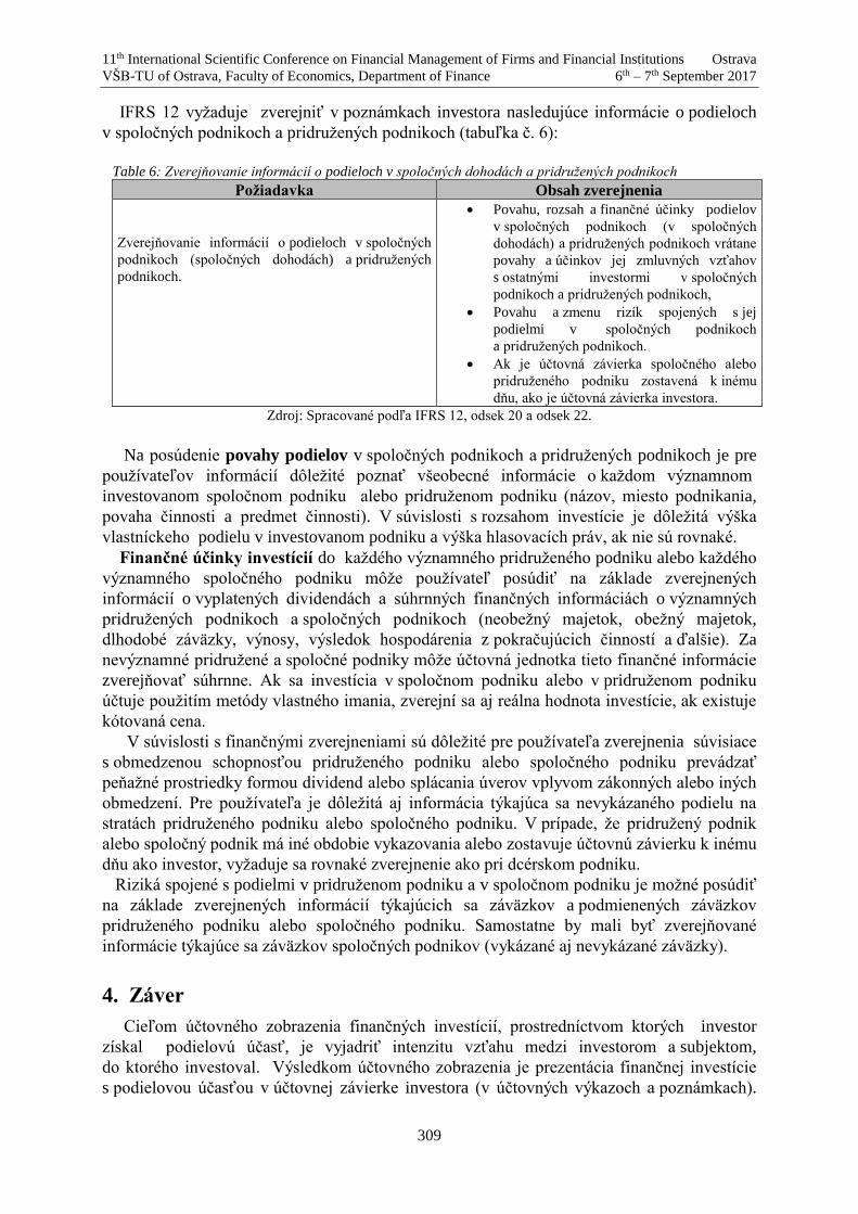
11th International Scientific Conference on Financial Management of Firms and Financial Institutions Ostrava
VŠB-TU of Ostrava, Faculty of Economics, Department of Finance 6th – 7th September 2017
309
IFRS 12 vyžaduje zverejniť v poznámkach investora nasledujúce informácie o podieloch
v spoločných podnikoch a pridružených podnikoch (tabuľka č. 6):
Table 6: Zverejňovanie informácií o podieloch v spoločných dohodách a pridružených podnikoch
Požiadavka Obsah zverejnenia
Zverejňovanie informácií o podieloch v spoločných
podnikoch (spoločných dohodách) a pridružených
podnikoch.
Povahu, rozsah a finančné účinky podielov
v spoločných podnikoch (v spoločných
dohodách) a pridružených podnikoch vrátane
povahy a účinkov jej zmluvných vzťahov
s ostatnými investormi v spoločných
podnikoch a pridružených podnikoch,
Povahu a zmenu rizík spojených s jej
podielmi v spoločných podnikoch
a pridružených podnikoch.
Ak je účtovná závierka spoločného alebo
pridruženého podniku zostavená k inému
dňu, ako je účtovná závierka investora.
Zdroj: Spracované podľa IFRS 12, odsek 20 a odsek 22.
Na posúdenie povahy podielov v spoločných podnikoch a pridružených podnikoch je pre
používateľov informácií dôležité poznať všeobecné informácie o každom významnom
investovanom spoločnom podniku alebo pridruženom podniku (názov, miesto podnikania,
povaha činnosti a predmet činnosti). V súvislosti s rozsahom investície je dôležitá výška
vlastníckeho podielu v investovanom podniku a výška hlasovacích práv, ak nie sú rovnaké.
Finančné účinky investícií do každého významného pridruženého podniku alebo každého
významného spoločného podniku môže používateľ posúdiť na základe zverejnených
informácií o vyplatených dividendách a súhrnných finančných informáciách o významných
pridružených podnikoch a spoločných podnikoch (neobežný majetok, obežný majetok,
dlhodobé záväzky, výnosy, výsledok hospodárenia z pokračujúcich činností a ďalšie). Za
nevýznamné pridružené a spoločné podniky môže účtovná jednotka tieto finančné informácie
zverejňovať súhrnne. Ak sa investícia v spoločnom podniku alebo v pridruženom podniku
účtuje použitím metódy vlastného imania, zverejní sa aj reálna hodnota investície, ak existuje
kótovaná cena.
V súvislosti s finančnými zverejneniami sú dôležité pre používateľa zverejnenia súvisiace
s obmedzenou schopnosťou pridruženého podniku alebo spoločného podniku prevádzať
peňažné prostriedky formou dividend alebo splácania úverov vplyvom zákonných alebo iných
obmedzení. Pre používateľa je dôležitá aj informácia týkajúca sa nevykázaného podielu na
stratách pridruženého podniku alebo spoločného podniku. V prípade, že pridružený podnik
alebo spoločný podnik má iné obdobie vykazovania alebo zostavuje účtovnú závierku k inému
dňu ako investor, vyžaduje sa rovnaké zverejnenie ako pri dcérskom podniku.
Riziká spojené s podielmi v pridruženom podniku a v spoločnom podniku je možné posúdiť
na základe zverejnených informácií týkajúcich sa záväzkov a podmienených záväzkov
pridruženého podniku alebo spoločného podniku. Samostatne by mali byť zverejňované
informácie týkajúce sa záväzkov spoločných podnikov (vykázané aj nevykázané záväzky).
4. Záver
Cieľom účtovného zobrazenia finančných investícií, prostredníctvom ktorých investor
získal podielovú účasť, je vyjadriť intenzitu vzťahu medzi investorom a subjektom,
do ktorého investoval. Výsledkom účtovného zobrazenia je prezentácia finančnej investície
s podielovou účasťou v účtovnej závierke investora (v účtovných výkazoch a poznámkach).
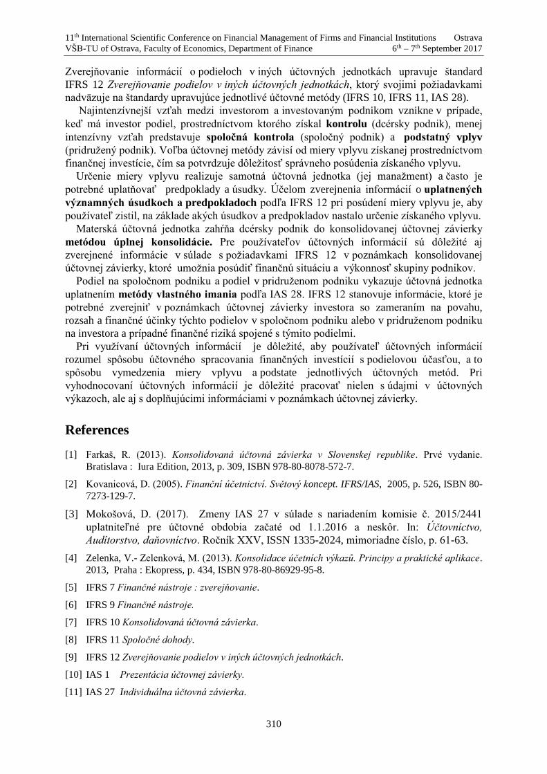
11th International Scientific Conference on Financial Management of Firms and Financial Institutions Ostrava
VŠB-TU of Ostrava, Faculty of Economics, Department of Finance 6th – 7th September 2017
310
Zverejňovanie informácií o podieloch v iných účtovných jednotkách upravuje štandard
IFRS 12 Zverejňovanie podielov v iných účtovných jednotkách, ktorý svojimi požiadavkami
nadväzuje na štandardy upravujúce jednotlivé účtovné metódy (IFRS 10, IFRS 11, IAS 28).
Najintenzívnejší vzťah medzi investorom a investovaným podnikom vznikne v prípade,
keď má investor podiel, prostredníctvom ktorého získal kontrolu (dcérsky podnik), menej
intenzívny vzťah predstavuje spoločná kontrola (spoločný podnik) a podstatný vplyv
(pridružený podnik). Voľba účtovnej metódy závisí od miery vplyvu získanej prostredníctvom
finančnej investície, čím sa potvrdzuje dôležitosť správneho posúdenia získaného vplyvu.
Určenie miery vplyvu realizuje samotná účtovná jednotka (jej manažment) a často je
potrebné uplatňovať predpoklady a úsudky. Účelom zverejnenia informácií o uplatnených
významných úsudkoch a predpokladoch podľa IFRS 12 pri posúdení miery vplyvu je, aby
používateľ zistil, na základe akých úsudkov a predpokladov nastalo určenie získaného vplyvu.
Materská účtovná jednotka zahŕňa dcérsky podnik do konsolidovanej účtovnej závierky
metódou úplnej konsolidácie. Pre používateľov účtovných informácií sú dôležité aj
zverejnené informácie v súlade s požiadavkami IFRS 12 v poznámkach konsolidovanej
účtovnej závierky, ktoré umožnia posúdiť finančnú situáciu a výkonnosť skupiny podnikov.
Podiel na spoločnom podniku a podiel v pridruženom podniku vykazuje účtovná jednotka
uplatnením metódy vlastného imania podľa IAS 28. IFRS 12 stanovuje informácie, ktoré je
potrebné zverejniť v poznámkach účtovnej závierky investora so zameraním na povahu,
rozsah a finančné účinky týchto podielov v spoločnom podniku alebo v pridruženom podniku
na investora a prípadné finančné riziká spojené s týmito podielmi.
Pri využívaní účtovných informácií je dôležité, aby používateľ účtovných informácií
rozumel spôsobu účtovného spracovania finančných investícií s podielovou účasťou, a to
spôsobu vymedzenia miery vplyvu a podstate jednotlivých účtovných metód. Pri
vyhodnocovaní účtovných informácií je dôležité pracovať nielen s údajmi v účtovných
výkazoch, ale aj s doplňujúcimi informáciami v poznámkach účtovnej závierky.
References
[1] Farkaš, R. (2013). Konsolidovaná účtovná závierka v Slovenskej republike. Prvé vydanie.
Bratislava : Iura Edition, 2013, p. 309, ISBN 978-80-8078-572-7.
[2] Kovanicová, D. (2005). Finanční účetnictví. Světový koncept. IFRS/IAS, 2005, p. 526, ISBN 80-
7273-129-7.
[3] Mokošová, D. (2017). Zmeny IAS 27 v súlade s nariadením komisie č. 2015/2441
uplatniteľné pre účtovné obdobia začaté od 1.1.2016 a neskôr. In: Účtovníctvo,
Audítorstvo, daňovníctvo. Ročník XXV, ISSN 1335-2024, mimoriadne číslo, p. 61-63.
[4] Zelenka, V.- Zelenková, M. (2013). Konsolidace účetních výkazů. Principy a praktické aplikace.
2013, Praha : Ekopress, p. 434, ISBN 978-80-86929-95-8.
[5] IFRS 7 Finančné nástroje : zverejňovanie.
[6] IFRS 9 Finančné nástroje.
[7] IFRS 10 Konsolidovaná účtovná závierka.
[8] IFRS 11 Spoločné dohody.
[9] IFRS 12 Zverejňovanie podielov v iných účtovných jednotkách.
[10] IAS 1 Prezentácia účtovnej závierky.
[11] IAS 27 Individuálna účtovná závierka.

11th International Scientific Conference on Financial Management of Firms and Financial Institutions Ostrava
VŠB-TU of Ostrava, Faculty of Economics, Department of Finance 6th – 7th September 2017
311
[12] IAS 28 Investície do pridružených a spoločných podnikov
[13] IAS 32 Finančné nástroje : prezentácia.
[14] IAS 39 Finančné nástroje : vykazovanie a oceňovanie.
11th International Scientific Conference on Financial Management of Firms and Financial Institutions Ostrava
VŠB-TU of Ostrava, Faculty of Economics, Department of Finance 6th – 7th September 2017
312
Indicating Insolvency in Firms
Jan Hospodka, Monika Randáková 1
Abstract
This paper seeks to assess whether it is possible for companies to predict that they are getting
closer to insolvency or financial distress. The research has focused on companies that filed for
bankruptcy in 2015 and their financial statements for periods 2012, 2013 and 2014. Through
standardized financial ratios, the aim was to look for a trend or a tendency that these indicators
might have signaled in advance to raise red flags and predict the forthcoming problems. The paper
also addresses the advantages and limitations of the particular financial ratios and discusses to
what extent these might be beneficial for the management in relation to providing them with
useful information.
Key words
Insolvency; financial ratios; bankruptcy; company; indication
JEL Classification: M41, G33
1. Introduction and literature review
Insolvency is a term that is widely covered by the media and is related to both individuals
and firms. The topic have also been covered by a number of research papers focusing both on
forms of bankruptcies of individuals (above all personal bankruptcy, in other words debt relief),
and on insolvency of companies. The research on individuals is primarily focused on
demographic characteristics of the people that apply for personal bankruptcy in terms of their
gender, age, origin. There has been a very thorough research on this topic done by researchers
from University of Economics in Prague (Randáková et al 2017) as well as other researchers.
Insolvency on company level requires, however, completely different approach, as the focus
is usually not on what sort of companies are headed towards insolvency, but the ability of
financial instruments to predict such scenario (or maybe in other words the inability of the
management to predict and prevent bankruptcy). This difference is rather self-explanatory and
results from the fact that (i) the reasons for individuals to become insolvent are usually different
to those of companies and (ii) is it very difficult to apply any financial instruments on financials
of individuals. There is also various literature covering insolvency of companies both in the
Czech Republic (i.e. Hrdý 2016) and abroad. It is vital for the management to be able to track
the financial situation in the firm in relation to its solvency and the ability of financial ratios to
help with that is therefore very important.
Papers trying to analyze the ability of financial ratios and other financial instruments to
predict nearing financial problems such as Altman (1968), Beawer (1966) or Mears (1966)
discuss in great detail the possible information that external readers can get from analyzing
financial statements and using financial ratios when trying to predict financial difficulties of
1 Ing. et Ing Jan Hospodka, University of Economics in Prague, Faculty of Finance and Accounting,
Department of Financial Accounting and Auditing, W. Churchill Sq. 4, 130 67 Prague 3, Czech
Republic; <[email protected]>.
Ing. Monika Randáková, Ph.D., University of Economics in Prague, Faculty of Finance and
Accounting, Department of Financial Accounting and Auditing, W. Churchill Sq. 4, 130 67 Prague 3,
Czech Republic; <[email protected]>.

11th International Scientific Conference on Financial Management of Firms and Financial Institutions Ostrava
VŠB-TU of Ostrava, Faculty of Economics, Department of Finance 6th – 7th September 2017
313
companies. In the Czech Republic, Mičudová (2013) researched how frequently companies use
the financial analysis, bankruptcy models and financial ratios to predict that they are nearing
insolvency (results of that paper are further discussed in the following chapter).
However, to authors’ knowledge, there hasn’t been a proper research conducted on
companies in the Czech Republic that declared insolvency, trying to follow their financials to
their history and search for clues that would retrospectively indicate nearing insolvency. As a
result of that, the Authors have decided to conduct exactly such research. This paper aims to
analyze financial statements of all companies that declared insolvency in 2015 for three years
prior to that year. It also analyses basic information about the age of the companies, their
location and their legal form. Beyond that, it also assesses whether the notion to declare
bankruptcy was brought by the companies themselves or the creditors.
Unfortunately, the limitations caused by using only annual statements and not having access
to actual, live, month to month managerial data of the company mean that the analysis cannot
be accurate enough from manager’s point of view. We, however, believe that it can bring to
managers’ attention different financial ratios that might be used and also give some idea about
which financial ratios to use in order to spot financial difficulties before they happen.
2. Introduction to financial analysis
Financial analysis is a process of assessing firms, projects, budgets or other financial bodies
in relation to their financial health. It can be done both internally by firm’s managers and
externally by anyone interested in the financial development of the company. Typically, this
financial analysis is used for evaluation of stability, solvency, liquidity and profitability of such
entity. Not only the financial analysis assesses the environment in which the business operates
and many other qualitative indicators, but primarily it also uses quantitative ratios. These help
managers to firstly understand the actual financial position in which the company is, but above
all they can see the trend that the financials of their company are following. From an investor
point of view, financial ratios allow to assess the overall risk of the firm. (CICA 1993 In: Faello
2015). It is also very common for banks to impose covenants that need to be met by the borrower
and because of that, the managers need to be even more cautious (Faello 2015). Because of all
these reasons, financial ratios are commonly used tools for financial analysis.
It is however important to bear in mind that financial indicators are considerably limited by
several facts. They comprise numerator and denominator both of which can be biased or wrong,
which could lead to the whole ratio giving invalid information. It is therefore vital for the
managers to have complete faith in the numbers that are being delivered to them by controlling
department. The reliability of the IT systems within the company that are involved in the
financial management is also very important. Mistakes can be both deliberate and by mistake.
It can also be the case that the management itself is remunerated based on financial performance
which is assessed by particular financial ratios. As a result, managers can incline to bias
financials that are important for their annual assessment (Beaver 1966). Another problem, often
related to financial ratios, is related to the fact that every financial statements could be based on
slightly different accounting principles and procedures. These can differ among companies and
sectors, leading to lower comparability between companies. This poses a problem especially
for external parties. Internal parties, e.g. CFOs, are however likely to understand these
differences and should therefore be able to analyze the financials of their company without
being misled. Furthermore, in case of managerial accounting, this is completely irrelevant.
As already stated in the previous chapter, Mičudová (2013), conducted a research on 58
companies in 2013, analyzing their regular usage of financial ratios and bankruptcy models by
financial management of the firm. It is very important to note that in the research, 775
companies were approached, out of which only 58 provided the author with answers to their
11th International Scientific Conference on Financial Management of Firms and Financial Institutions Ostrava
VŠB-TU of Ostrava, Faculty of Economics, Department of Finance 6th – 7th September 2017
314
questionnaire saying whether they use financial analysis or not. We can assume that companies
that use such ratios or bankruptcy models, were more likely to answer such questionnaire and
this could have led to biasing the results of the research. Out of the 58 firms, 17% periodically
use bankruptcy models to assess their financial health and 19% of the companies use financial
ratios. 67% of respondents have experienced a bank demanding to use bankruptcy model when
providing the company with a loan and 47% of the respondents have experienced their usage
in supplier-customer relationships.
This research seeks to analyze usage of financial ratios on annual accounts of companies that
have declared bankruptcy in 2015. It focuses on the period between 2012 and 2014 and tries to
link the deteriorating performance indicated by financial ratios to future bankruptcy of the
company. For this purpose, four different ratios were chosen:
Quick ratio
Cash conversion cycle
Net working capital/ Total assets
Earnings before interest and taxes (EBIT)/ Total assets.
3. Data and Methodology
Data analyzed in this paper are based primarily on data collection conducted by the authors
of this paper.
In the first phase of the research, the main source of data was the Insolvency Register of
Ministry of Justice of the Czech Republic (MSČR 2016a). Thanks to search engines of this
register, it was possible to find all the entities that declared insolvency in the year 2015. As the
register does not allow to download such information at once in some form of electronic
database, it was necessary to create a new list into which all such entities were inserted. Because
the search engine of the register does not make it possible to look up entries for a longer period
than 30 days, the authors had to search for all companies that declared insolvency in 13 different
periods (first one being 1st of January 2015 to 30th of January 2015, second one being 31st of
January 2015 to 28th of February 2015 etc.). In all these periods, every entity that declared
insolvency was recorded and added to the list. As this research aims to analyze only firms and
not individuals, only firms were recorded in the database. There were altogether 959 entities
which declared insolvency in 2015.
After the list of entities that declared insolvency in 2015 was finished, the second phase of
the research has started. In the phase, Commercial Register of Ministry of Justice of the Czech
Republic (MSČR 2016b) was used instead of Insolvency Register.
In this register, the authors searched for firms that have been identified as insolvent by
Insolvency Register. All 959 entities were consequently analyzed whether they have published
their annual accounts in years 2012, 2013 and 2014. Companies that have published their annual
accounts, were afterwards screened whether their financial statements were audited. Apart from
analysis of financial statements, also information about legal form and age of the firms were
collected. For the financial analysis, only those companies, which have published their audited
statements in all three periods, constitute the sample which was further analyzed. An overview
of the collected data is shown in the following table:
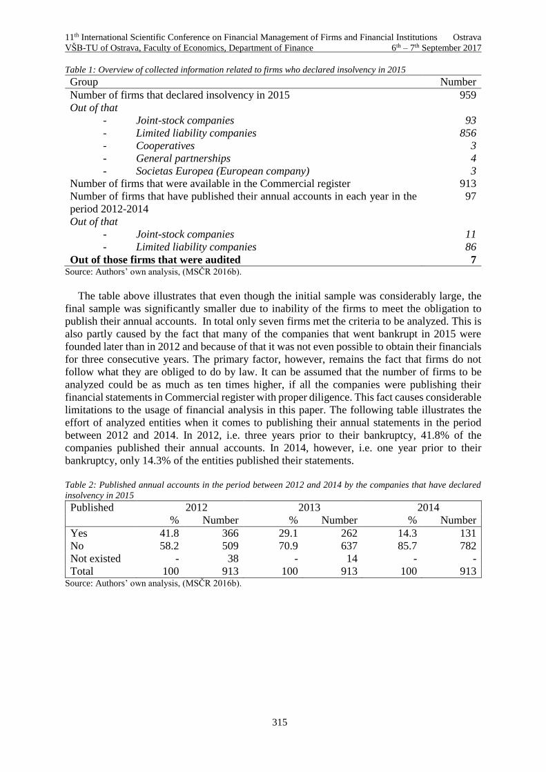
11th International Scientific Conference on Financial Management of Firms and Financial Institutions Ostrava
VŠB-TU of Ostrava, Faculty of Economics, Department of Finance 6th – 7th September 2017
315
Table 1: Overview of collected information related to firms who declared insolvency in 2015
Group Number
Number of firms that declared insolvency in 2015 959
Out of that
- Joint-stock companies 93
- Limited liability companies 856
- Cooperatives 3
- General partnerships 4
- Societas Europea (European company) 3
Number of firms that were available in the Commercial register 913
Number of firms that have published their annual accounts in each year in the
period 2012-2014
97
Out of that
- Joint-stock companies 11
- Limited liability companies 86
Out of those firms that were audited 7 Source: Authors’ own analysis, (MSČR 2016b).
The table above illustrates that even though the initial sample was considerably large, the
final sample was significantly smaller due to inability of the firms to meet the obligation to
publish their annual accounts. In total only seven firms met the criteria to be analyzed. This is
also partly caused by the fact that many of the companies that went bankrupt in 2015 were
founded later than in 2012 and because of that it was not even possible to obtain their financials
for three consecutive years. The primary factor, however, remains the fact that firms do not
follow what they are obliged to do by law. It can be assumed that the number of firms to be
analyzed could be as much as ten times higher, if all the companies were publishing their
financial statements in Commercial register with proper diligence. This fact causes considerable
limitations to the usage of financial analysis in this paper. The following table illustrates the
effort of analyzed entities when it comes to publishing their annual statements in the period
between 2012 and 2014. In 2012, i.e. three years prior to their bankruptcy, 41.8% of the
companies published their annual accounts. In 2014, however, i.e. one year prior to their
bankruptcy, only 14.3% of the entities published their statements.
Table 2: Published annual accounts in the period between 2012 and 2014 by the companies that have declared
insolvency in 2015
Published 2012 2013 2014
% Number % Number % Number
Yes 41.8 366 29.1 262 14.3 131
No 58.2 509 70.9 637 85.7 782
Not existed - 38 - 14 - -
Total 100 913 100 913 100 913 Source: Authors’ own analysis, (MSČR 2016b).

11th International Scientific Conference on Financial Management of Firms and Financial Institutions Ostrava
VŠB-TU of Ostrava, Faculty of Economics, Department of Finance 6th – 7th September 2017
316
4. Description of the sample
The analysis by regions shows that the highest number of firms that declared insolvency in
2015 is registered with the Commercial Register maintained by the Municipal Court in Prague.
When companies are founded, they are registered with the commercial register maintained by
one of the following seven regional courts in the Czech Republic:
- Municipal Court in Prague (Prague and Středočeský region)
- Regional Court in Pilsen (Plzeňský and Karlovarský regions)
- Regional Court in Ústí nad Labem (Ústecký and Liberecký regions)
- Regional Court in Hradec Králové (Královéhradecký and Pardubický regions)
- Regional Court in Brno (Jihomoravský and Zlínský regions, region Vysočina)
- Regional Court in Ostrava (Olomoucký and Moravskoslezský regions)
Because of the fact that some regions are maintained by the same regional court, it is not
possible to separate the firms directly by regions but only by the court with which they are
registered. Regional distribution of companies which declared bankruptcy in 2015 is illustrated
by the following graphics:
Graphics 1: Distribution of firms that declared insolvency in 2015 in the Czech Republic
Source: Authors’ own analysis, (MSČR 2016a).
Graphics above illustrate that the highest number of firms declaring insolvency is massively
dominated by Prague and Central Bohemian Region. Overall it can be said that the regions with
higher number of insolvencies are also the regions with the biggest and economically most
significant cities – Prague, Brno and Ostrava. This number needs to be compared with the
distribution of all companies within the Czech Republic, which is as follows:
Graphics 2: Actual distribution of firms in the Czech Republic as at 1st of January 2014
Source: Authors’ own analysis, IMPER CZ (2014).
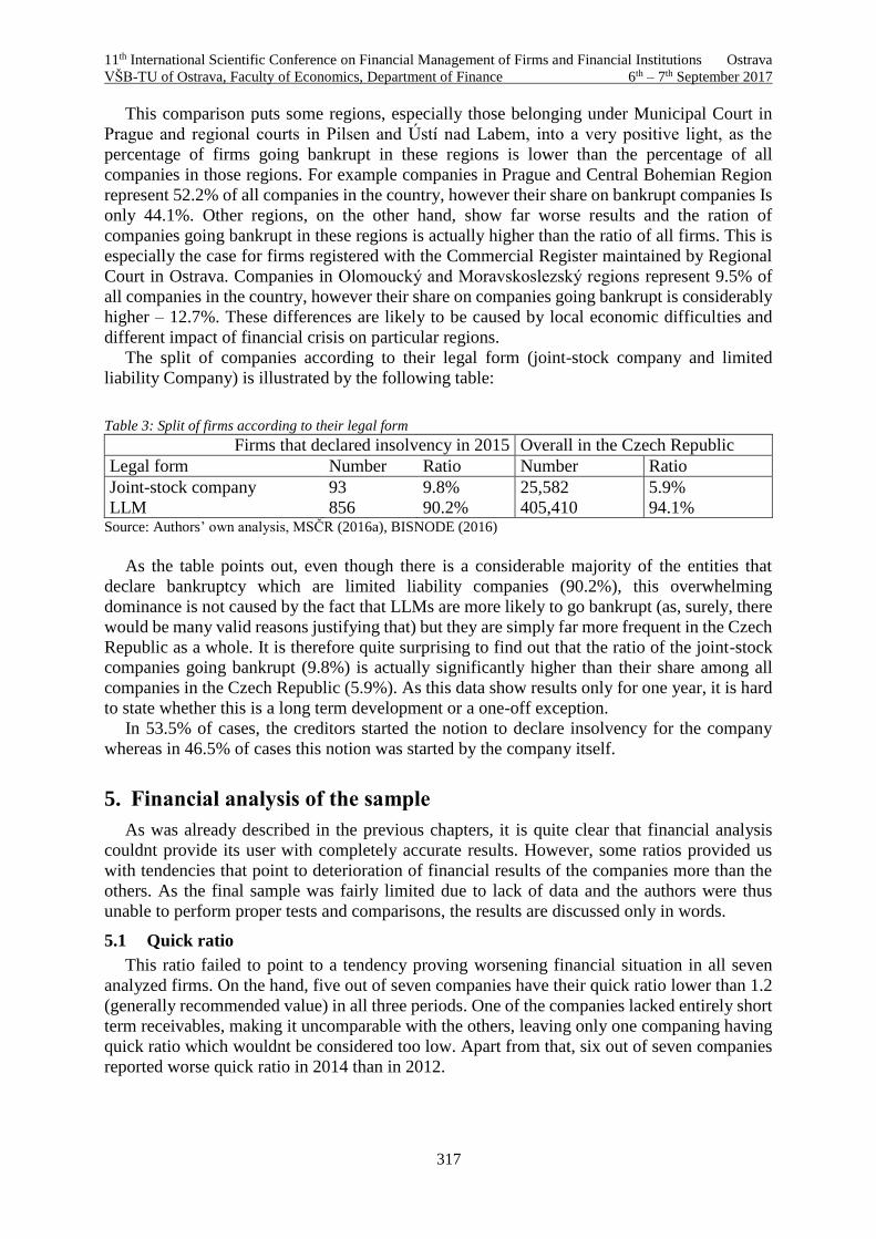
11th International Scientific Conference on Financial Management of Firms and Financial Institutions Ostrava
VŠB-TU of Ostrava, Faculty of Economics, Department of Finance 6th – 7th September 2017
317
This comparison puts some regions, especially those belonging under Municipal Court in
Prague and regional courts in Pilsen and Ústí nad Labem, into a very positive light, as the
percentage of firms going bankrupt in these regions is lower than the percentage of all
companies in those regions. For example companies in Prague and Central Bohemian Region
represent 52.2% of all companies in the country, however their share on bankrupt companies Is
only 44.1%. Other regions, on the other hand, show far worse results and the ration of
companies going bankrupt in these regions is actually higher than the ratio of all firms. This is
especially the case for firms registered with the Commercial Register maintained by Regional
Court in Ostrava. Companies in Olomoucký and Moravskoslezský regions represent 9.5% of
all companies in the country, however their share on companies going bankrupt is considerably
higher – 12.7%. These differences are likely to be caused by local economic difficulties and
different impact of financial crisis on particular regions.
The split of companies according to their legal form (joint-stock company and limited
liability Company) is illustrated by the following table:
Table 3: Split of firms according to their legal form
Firms that declared insolvency in 2015 Overall in the Czech Republic
Legal form Number Ratio Number Ratio
Joint-stock company 93 9.8% 25,582 5.9%
LLM 856 90.2% 405,410 94.1% Source: Authors’ own analysis, MSČR (2016a), BISNODE (2016)
As the table points out, even though there is a considerable majority of the entities that
declare bankruptcy which are limited liability companies (90.2%), this overwhelming
dominance is not caused by the fact that LLMs are more likely to go bankrupt (as, surely, there
would be many valid reasons justifying that) but they are simply far more frequent in the Czech
Republic as a whole. It is therefore quite surprising to find out that the ratio of the joint-stock
companies going bankrupt (9.8%) is actually significantly higher than their share among all
companies in the Czech Republic (5.9%). As this data show results only for one year, it is hard
to state whether this is a long term development or a one-off exception.
In 53.5% of cases, the creditors started the notion to declare insolvency for the company
whereas in 46.5% of cases this notion was started by the company itself.
5. Financial analysis of the sample
As was already described in the previous chapters, it is quite clear that financial analysis
couldnt provide its user with completely accurate results. However, some ratios provided us
with tendencies that point to deterioration of financial results of the companies more than the
others. As the final sample was fairly limited due to lack of data and the authors were thus
unable to perform proper tests and comparisons, the results are discussed only in words.
5.1 Quick ratio
This ratio failed to point to a tendency proving worsening financial situation in all seven
analyzed firms. On the hand, five out of seven companies have their quick ratio lower than 1.2
(generally recommended value) in all three periods. One of the companies lacked entirely short
term receivables, making it uncomparable with the others, leaving only one companing having
quick ratio which wouldnt be considered too low. Apart from that, six out of seven companies
reported worse quick ratio in 2014 than in 2012.
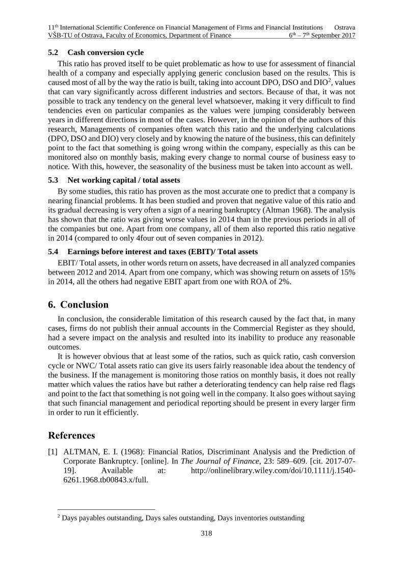
11th International Scientific Conference on Financial Management of Firms and Financial Institutions Ostrava
VŠB-TU of Ostrava, Faculty of Economics, Department of Finance 6th – 7th September 2017
318
5.2 Cash conversion cycle
This ratio has proved itself to be quiet problematic as how to use for assessment of financial
health of a company and especially applying generic conclusion based on the results. This is
caused most of all by the way the ratio is built, taking into account DPO, DSO and DIO2, values
that can vary significantly across different industries and sectors. Because of that, it was not
possible to track any tendency on the general level whatsoever, making it very difficult to find
tendencies even on particular companies as the values were jumping considerably between
years in different directions in most of the cases. However, in the opinion of the authors of this
research, Managements of companies often watch this ratio and the underlying calculations
(DPO, DSO and DIO) very closely and by knowing the nature of the business, this can definitely
point to the fact that something is going wrong within the company, especially as this can be
monitored also on monthly basis, making every change to normal course of business easy to
notice. With this, however, the seasonality of the business must be taken into account as well.
5.3 Net working capital / total assets
By some studies, this ratio has proven as the most accurate one to predict that a company is
nearing financial problems. It has been studied and proven that negative value of this ratio and
its gradual decreasing is very often a sign of a nearing bankruptcy (Altman 1968). The analysis
has shown that the ratio was giving worse values in 2014 than in the previous periods in all of
the companies but one. Apart from one company, all of them also reported this ratio negative
in 2014 (compared to only 4four out of seven companies in 2012).
5.4 Earnings before interest and taxes (EBIT)/ Total assets
EBIT/ Total assets, in other words return on assets, have decreased in all analyzed companies
between 2012 and 2014. Apart from one company, which was showing return on assets of 15%
in 2014, all the others had negative EBIT apart from one with ROA of 2%.
6. Conclusion
In conclusion, the considerable limitation of this research caused by the fact that, in many
cases, firms do not publish their annual accounts in the Commercial Register as they should,
had a severe impact on the analysis and resulted into its inability to produce any reasonable
outcomes.
It is however obvious that at least some of the ratios, such as quick ratio, cash conversion
cycle or NWC/ Total assets ratio can give its users fairly reasonable idea about the tendency of
the business. If the management is monitoring those ratios on monthly basis, it does not really
matter which values the ratios have but rather a deteriorating tendency can help raise red flags
and point to the fact that something is not going well in the company. It also goes without saying
that such financial management and periodical reporting should be present in every larger firm
in order to run it efficiently.
References
[1] ALTMAN, E. I. (1968): Financial Ratios, Discriminant Analysis and the Prediction of
Corporate Bankruptcy. [online]. In The Journal of Finance, 23: 589–609. [cit. 2017-07-
19]. Available at: http://onlinelibrary.wiley.com/doi/10.1111/j.1540-
6261.1968.tb00843.x/full.
2 Days payables outstanding, Days sales outstanding, Days inventories outstanding
11th International Scientific Conference on Financial Management of Firms and Financial Institutions Ostrava
VŠB-TU of Ostrava, Faculty of Economics, Department of Finance 6th – 7th September 2017
319
[2] BEAVER, W. H. (1966): Financial Ratios as Predictors of Failures. [online]. In Journal of
Accounting Research. [cit. 2016-07-19]. Vydání č. 4, Empirical Research in Accounting:
Selected Studies 1966. Wiley: University of Chicago. str. 71-111. Available at:
http://www.jstor.org/stable/2490171.
[3] BISNODE (2016): V ČR loni vzniklo 26 953 nových firem, nejvíce od roku 2007. [online].
In bisnode.cz.[cit. 2017-08-04]. Available at: http://www.bisnode.cz/tiskove-zpravy/v-cr-
loni-vzniklo-26953-novych-firem-nejvice-od-roku-2007/.
[4] FAELLO, J. (2015): Understanding the Limitations of Financial Ratios. [online]. In
Academy of Accounting and Financial Studies Journal. [cit. 2017-07-19]. Available at:
https://www.questia.com/read/1P3-3965157811/understanding-the-limitations-of-
financial-ratios.
[5] Hrdý, M. Vývoj zadluženosti českých podniků ve vybraných oborech. In Sborník
konference Nové Trendy – Nové Nápady, Znojmo, 2016
[6] IMPER CZ (2014): Kolik firem je v ČR v jednotlivých krajích?. [online]. In
http://onbusiness.cz/. [cit. 2017-08-03]. Available at: http://onbusiness.cz/kolik-firem-je-
v-cr-v-jednotlivych-krajich-835.
[7] MEARS, P. K. (1966): Discussion of Financial Ratios As Predictors of Failure. In Journal
of Accounting Research, vol. 4, 1966, pp. 119–122. JSTOR. Available at:
www.jstor.org/stable/2490173.
[8] MIČUDOVÁ, K. (2013): Úpadky podniků a využívání predikčních modelů pro jejich
včasné odhalení. In Trendy v podnikání – vědecký časopis Fakulty ekonomické ZČU
v Plzni. Available at: https://www.dfek.zcu.cz/tvp/doc/akt/tvp-3-2013-clanek-9.pdf
[9] MINISTERSTVO SPRAVEDLNOSTI ČESKÉ REPUBLIKY (2017a): Insolvenční
rejstřík. [online]. [cit. 2016-07-19]. Available at: http://www.justice.cz.
[10] MINISTERSTVO SPRAVEDLNOSTI ČESKÉ REPUBLIKY (2017b): Obchodní rejstřík.
[online]. [cit. 2016-07-19]. Available at: http://www.justice.cz.
[11] RANDÁKOVÁ, M., BOKŠOVÁ, J., HOSPODKA, J., BUBEN, O. (2017): Personal
Bankruptcy in the Czech Republic: Age and Gender of the Debtors and Structure of the
Creditors. In European Financial and Accounting Journal. 2017. v. 12, no. 1, p. 5--18.
ISSN 1802-2197. Available at: https://www.vse.cz/efaj/174

THE DEPARTMENT OF FINANCE IS SPONSORED BY