Final report Study on various aspects of earnings distribution ...
127
Final report Study on various aspects of earnings distribution using micro-data from the European Structure of Earnings Survey VC/2013/0019 Neil Foster-McGregor, Sandra Leitner, Sebastian Leitner, Johannes Pöschl, Robert Stehrer
-
Upload
khangminh22 -
Category
Documents
-
view
1 -
download
0
Transcript of Final report Study on various aspects of earnings distribution ...

Final report
Study on various aspects of earnings distribution u sing micro-data
from the European Structure of Earnings Survey
VC/2013/0019
Neil Foster-McGregor, Sandra Leitner, Sebastian Leitner,
Johannes Pöschl, Robert Stehrer


ACKNOWLEDGEMENT
This publication is commissioned by the European Union Programme for Employment and Social
Solidarity - PROGRESS (2007-2013).
This programme is implemented by the European Commission. It was established to financially
support the implementation of the objectives of the European Union in the employment, social affairs
and equal opportunities area, and thereby contribute to the achievement of the Europe 2020
Strategy goals in these fields.
The seven-year Programme targets all stakeholders who can help shape the development of
appropriate and effective employment and social legislation and policies, across the EU-27, EFTA-
EEA and EU candidate and pre-candidate countries.
For more information see: http://ec.europa.eu/progress
The information contained in this publication does not necessarily reflect the position or opinion of
the European Commission.


Contents
EXECUTIVE SUMMARIES IN ENGLISH, GERMAN AND FRENCH . ............................................. 1
1. INTRODUCTION ..................................................................................................................... 11
2. LITERATURE REVIEW ................................. .......................................................................... 12
3. DATA AND METHODS .................................. ......................................................................... 19
3.1 The Structure of Earnings Survey data ............................................................................. 19
3.2 A snapshot on methods used ........................................................................................... 22
4. DESCRIPTIVE RESULTS ON EARNINGS STRUCTURES AND INEQ UALITY ..................... 25
4.1 Mean and median earnings .............................................................................................. 25
4.2 Unconditional earning structures ...................................................................................... 26
4.3 Inequality in earnings ...................................................................................................... 29
4.4 Contributions to inequality ................................................................................................ 32
5. ANALYSIS OF EARNING STRUCTURES AND INEQUALITY ..... .......................................... 35
5.1 Personal characteristics ................................................................................................... 35
5.1.1 Gender..................................................................................................................... 35
5.1.2 Age .......................................................................................................................... 39
5.1.3 Education ................................................................................................................. 42
5.2 Job characteristics ........................................................................................................... 45
5.2.1 Length of service in enterprise (experience) .............................................................. 45
5.2.2 Contract type ............................................................................................................ 48
5.2.3 Full-time/part-time .................................................................................................... 50
5.2.4 Occupations ............................................................................................................. 55
5.3 Firm characteristics .......................................................................................................... 58
5.3.1 Firm size .................................................................................................................. 58
5.3.2 Public and private control ......................................................................................... 61
5.3.3 Collective pay agreements ....................................................................................... 64
5.3.4 Sectors .................................................................................................................... 66
6. SUMMARY AND CONCLUSIONS ........................... ............................................................... 70
7. LITERATURE ........................................ ................................................................................. 72
TECHNICAL APPENDIX................................. ............................................................................. 77
METHODOLOGICAL APPROACH AND DATA ISSUES ........... .................................................. 77
Mincer regressions .................................................................................................................... 77
Blinder-Oaxaca decomposition .................................................................................................. 78
Shapley value approach ............................................................................................................ 80
Data issues .............................................................................................................................. 82
TABLE APPENDIX .................................... .................................................................................. 86


Final Report Earnings structures and inequality in the EU
1
Executive Summaries in English, German and French
EXECUTIVE SUMMARY (EN)
According to the Europe 2020 strategy, high levels of employment, productivity and social cohesion
are highly ranked goals. Hence, to assist policy-makers in achieving smart, sustainable and inclusive
growth in the EU, a thorough understanding of earnings differences within a country but also across
countries and its evolution over time is necessary.
This study uses three different waves of the Structure of Earnings Survey (SES) – for 2002, 2006
and 2010 – and addresses issues related to recent wage developments in EU countries. Firstly, it
highlights determinants of earnings differences and their relative impact over time, and secondly, it
shows to which extent these determinants contribute to an overall measure of inequality, the Gini
index. Three broader categories of determinants are considered: (i) individual worker characteristics
(sex, age and education), (ii) job characteristics (experience, contract type, full-time/part-time work,
and occupations) and (iii) firm characteristics (size, industry, public versus private control, and
collective pay agreements).
Methodologically, so-called Mincer regressions are used to shed light on the contributions of
earnings differences to overall inequality. The most important results of these regressions can be
summarised as follows:
Individual characteristics : For gender, substantial conditional wage gaps emerge of between 5%
and 15%. However, over time, both unconditional and conditional gender wage gaps declined in the
majority of countries. Similarly, substantial age premia are found which are, however, lower in
CEECs than in the remaining EU Member States, irrespective of the age group considered.
Moreover, between 2002 and 2010, the contributions of age-related wage differences declined in the
majority of countries. Results also point to an interesting ranking of average returns to education
(relative to the group with only primary education) in the sample of EU countries in 2010, ranging
from 2% for lower secondary education, 9% for upper and post-secondary education, 19% for short
cycle tertiary education, 33% for Bachelor and Master (or equivalent) and, finally, to 51% for Doctoral
education. This ranking is replicated in the majority of countries. Moreover, between 2002 and 2010,
returns to education increased in the majority of countries, irrespective of the level of education
considered. These changes were stronger among higher levels of education and most pronounced
in the highest level of educational attainment.
Job characteristics : The analysis also finds non-negligible wage premia by length of service in the
enterprise. In particular, relative to employees who have been with the enterprise for less than a
year, employees with 1-4 years of employment in the same firm earn an average 6% wage
premium, which rises to 11% for employees with between 5 and 14 years with the enterprise and
reaches 18% for employees with more than 15 years with the enterprise. As for changes in
conditional premia over time, a rather heterogeneous picture emerges, however. Moreover, wage

Final Report Earnings structures and inequality in the EU
2
gaps also emerge by type of contract. As such, relative to employees with indefinite contract,
employees with a contract that is either temporary or has a fixed duration earn on average 4.7%
less, though non-negligible cross-country differences emerge. Non-negligible wage gaps are also
found for part-time employees. Relative to full-time employees, part-time employees tend to face
wage penalties of as much as 15%. These wage disadvantages tend to be most pronounced in the
Baltics, almost non-existent in Scandinavian countries and even (slightly) in favour of part-time
employees in a number of other countries. Moreover, earnings differences across occupations
contribute very strongly to the overall Gini index. Results for conditional average wage premia by
occupation (relative to elementary occupations) point to an interesting ordering, from as low as 3%
for skilled agricultural, forestry and fishery workers, to 11% for service and sales occupations, 12%
for plant and machine operators and assemblers, 15% for craft and related workers, 19% for clerical
support, 35% for technicians, 50% for professionals and as much as 73% for managers.
Firm characteristic : Moreover, with almost 10% on average, differences between NACE sectors
also contribute substantially to overall inequality, though some non-negligible differences exist
across countries, ranging between 5% and around 15%. In addition, results point to substantial size-
related wage gaps. Relative to small firms, large firms pay up to 42% higher wages while medium-
sized firms pay up to 35% higher wages. However, size-wage premia seem to be highest among
CEECs and lowest among the remaining EU countries. Over time, wage premia paid by medium-
sized firms increased in a large number of countries while those paid by large firms deteriorated in
the majority of countries. However, results also demonstrate that differences in firm size classes
contribute relatively little to inequality. Furthermore, a rather heterogeneous picture emerges in terms
of ownership-related wage differences. In particular, in countries such as Italy, Belgium, Croatia,
Poland or Portugal (among others) publicly controlled firms pay more than privately owned ones,
while in others such as Estonia, Finland, Bulgaria, Sweden or Slovakia (among others) publicly
owned firms pay less generously than privately owned firms. Between 2002 and 2010, the wage gap
between privately and publicly controlled enterprises declined in the majority of countries. Finally, the
conditional effects of collective wage agreement patterns are rather mixed. The contribution to
inequality of differences between the wages of employees covered by different types of collective
wage agreements is also very small.
Determinants of earnings inequality : Furthermore, the study addresses the extent to which these
characteristics explain overall earnings inequality as measured by the Gini index. Two major
conclusions can be drawn: Firstly, average earnings inequalities as measured by the Gini index
stayed roughly constant at around 0.3. However, in terms of levels, large differences emerge with
the Gini ranking from about 0.2 (in the Scandinavian countries) to more than 0.4 (e.g. in Romania
and Turkey). Moreover, despite cross-country differences in trends, there is no indication that the
crisis had any significant impact on changes in earnings inequalities. In this respect it is important to
note that this study looks at earnings, i.e. concerns incomes of people employed, and not overall
inequality (which is directly affected by changes in the number of unemployed persons) or
household incomes.

Final Report Earnings structures and inequality in the EU
3
Secondly, the contribution to inequality differs across the characteristics considered: individual
characteristics contribute about 20% to inequality, job characteristics about 35% and firm
characteristics about 15%, whereas about 30% of the Gini index cannot be explained by the
determinants investigated. This pattern remains relatively stable over time. With respect to particular
determinants, occupation and education are the two most important factors with about 25% and
12%, respectively, followed by industry (with about 10%), enterprise size (about 6%), job duration
(6%), age (5%) and gender (3.5%). The latter shows a tendency to become less important though.
Again non-negligible cross-country differences exist: Wage pay gaps driven by experience
contribute relatively strongly in the South European countries but also in Germany and Luxembourg;
the type of contract (i.e. whether permanent or fixed duration) contributes strongly in Germany,
Poland and the Netherlands; full-time versus part-time work contributes more strongly in Germany,
Latvia, Hungary, the Netherlands, Belgium, and Lithuania. Age is relatively important in explaining
earnings inequalities in the Netherlands, Norway, Belgium and Greece. Whether firms are public or
private controlled is very important in Cyprus, Italy, Spain, Finland and Sweden, whereas the
collective pay agreement coverage contributes more strongly in Cyprus, Portugal and Germany.

Final Report Earnings structures and inequality in the EU
4
EXECUTIVE SUMMARY (DE)
STUDIE ÜBER VERSCHIEDENE ASPEKTE DER LOHN- UND
EINKOMMENSVERTEILUNG BASIEREND AUF DATEN DER EUROPÄISCHEN
LOHNSTRUKTURERHEBUNG
ZUSAMMENFASSUNG
Gemäß der „Europa 2020“-Strategie sind ein hohes Niveau an Beschäftigung, Produktivität und
sozialer Kohäsion erstgereihte Ziele. Somit ist ein detailliertes Verständnis der Muster und Ursachen
von Lohn- und Einkommensdifferentialen innerhalb eines Landes, aber auch im Vergleich zu
anderen Ländern, und deren Entwicklung über die Zeit zur Unterstützung der politischen
Entscheidungsprozesse hinsichtlich der Erreichung eines intelligenten, nachhaltigen und
integrativen Wachstums notwendig.
Diese Studie beruht auf den drei Wellen der Verdienststrukturerhebung – für 2002, 2006 und 2010 –
und fokussiert auf aktuelle Entwicklungen der Lohn- und Einkommensstruktur in den EU-
Mitgliedstaaten. Die Studie beleuchtet, erstens, die Determinanten der Lohn- und
Einkommensdifferentiale und ihrer relativen Wichtigkeit über die Zeit hinweg. Zweitens zeigt sie, in
welchem Ausmaß diese zur Ungleichheit, gemessen durch den Gini-Index, beitragen. Drei breitere
Gruppen an Determinanten werden berücksichtigt: (i) individuelle Eigenschaften der Beschäftigten
(Geschlecht, Alter und Ausbildung), (ii) Merkmale des Arbeitsplatzes (Erfahrung, vertragliche
Bedingungen, Voll- und Teilzeit, Beruf), und (iii) Firmenmerkmale (Größe, Industrie, öffentlich versus
privat, Bezahlungs- und Lohnverhandlungssysteme).
Methodisch werden sogenannten Mincer-Regressionen angewendet, die es erlauben, die Beiträge
dieser Charakteristika zur Ungleichheit zu messen. Die wichtigsten Ergebnisse können wie folgt
zusammengefasst werden:
Individuelle Eigenschaften: Für die Ausprägung nach Geschlecht zeigen sich Lohndifferentiale
zwischen 5% und 15%. Diese Unterschiede sind jedoch über die Zeit in der Mehrzahl der Länder
geringer geworden. Ähnlich lassen sich auch substantielle Lohndifferential hinsichtlich des Alters
feststellen, die jedoch in den mittel- und osteuropäischen Ländern im Vergleich zu den anderen EU-
Mitgliedstaaten wesentlich geringer ausfallen. Außerdem sind diese altersbedingten Differentiale
und ihr Beitrag zur Ungleichheit zwischen 2002 und 2010 gesunken. Die Resultate zeigen auch ein
interessantes Muster der Bildungserträge (relativ zu der Gruppe der Personen mit primärer
Ausbildung) in den untersuchten EU-Mitgliedstaaten, die von 2% für Erwerbstätige mit unterer
Sekundarstufe und 9% für jene mit Oberstufe und post-sekundärer Bildung bis zu 19% für kürzere
tertiäre Ausbildungswege, 33% für Bachelor- und Masterabschlüsse und schließlich 51% für
Doktorats-Abschlüsse reichen. Dieses Ranking repliziert sich in der Mehrheit der Länder. Die
Lohnunterschiede aufgrund der Ausbildung sind in allen Ländern zwischen 2002 und 2010 größer
Final Report Earnings structures and inequality in the EU
5
geworden. Die Veränderungen waren dabei im Fall der Beschäftigten mi höheren
Bildungsabschlüssen stärker ausgeprägt.
Merkmale des Arbeitsplatzes: Die Ergebnisse zeigen auch nicht-vernachlässigbare Lohnprämien
gemäß der Dauer der Beschäftigung in einem Unternehmen. Relativ zu den Beschäftigten, die
weniger als ein Jahr Firmenzugehörigkeit aufweisen, verdienen Beschäftigte mit 1-4 Jahren
Beschäftigungsdauer 6% mehr; dieser Lohnunterschied steigt auf 11% für jene mit 5 bis 14 Jahren
Beschäftigungsdauer und erreicht 18% für jene mit mehr als 14 Jahren Beschäftigung in derselben
Firma. Im Ländervergleich zeigt sich jedoch eine stark unterschiedliche Entwicklung über die Zeit.
Lohnunterschiede entstehen auch durch die jeweiligen vertraglichen Bedingungen. Im Vergleich zu
Beschäftigten mit unbefristeten Verträgen verdienen Beschäftigte mit befristeten Verträgen im
Durchschnitt 4,7% weniger, wobei es allerdings nicht-vernachlässigbare Unterschiede zwischen den
Ländern gibt. Signifikante Unterschiede gibt es auch für Teilzeitbeschäftigte, die im Vergleich zu
Vollzeitbeschäftigten Lohneinbußen bis zu 15% hinnehmen müssen. Diese Einbußen sind am
stärksten in den baltischen Ländern ausgeprägt, so gut wie nicht existent in den skandinavischen
Ländern und tendieren in einigen Ländern sogar in die andere Richtung. Schließlich sind
Lohnunterschiede zwischen den Berufen für die allgemeine Ungleichheit von großer Bedeutung. Die
Ergebnisse für Lohndifferentiale nach Berufsgruppen (relativ zu Hilfsberufen) deuten auf eine
interessante Rangordnung hin: von 3% für Fachkräfte in Land- und Forstwirtschaft und Fischerei,
11% für Dienstleistungsberufe im Verkauf, 12% für Anlagen- und Maschinenbediener und Montierer,
15% für Handwerks- und verwandte Berufe, 19% für Büroarbeiten, 35% für Techniker, 50% für
Fachkräfte und sogar bis zu 73% für Managementberufe.
Firmenmerkmale: Weiters tragen Lohndifferentiale nach NACE-Sektoren mit 10% substantiell zur
Ungleichheit bei, obwohl auch hier große Unterschiede zwischen den Ländern bestehen, mit
Beiträgen zwischen 5% und 15%. Zusätzlich zeigen die Resultate erhebliche Lohndifferentiale
aufgrund der Firmengröße. Relativ zu kleinen Firmen zahlen große Unternehmen bis zu 42%
höhere Löhne und mittelgroße Firmen bis zu 35% höhere Löhne. Diese durch die Firmengröße
bestimmten Lohndifferentiale sind am größten in den mittel- und osteuropäischen Ländern und
relativ geringer in den übrigen EU-Mitgliedsländern. Über die Zeit hinweg gab es in der Mehrzahl der
Länder die Tendenz, dass dieses Lohndifferential für mittelgroße Firmen anstieg, jedoch für große
Firmen zurückging. Insgesamt tragen jedoch Lohndifferentiale aufgrund der Firmengröße relativ
wenig zur Erklärung der allgemeinen Ungleichheit bei. Ein eher heterogenes Bild zeigt sich, wenn
man die Eigentümerstruktur (öffentlich oder privat) betrachtet. Insbesondere zahlen in Ländern wie
Italien, Belgien, Kroatien, Polen und Portugal öffentliche Firmen mehr als private Firmen,
wohingegen beispielsweise in Estland, Finnland, Bulgarien, Schweden oder der Slowakei öffentliche
Firmen weniger generös bezahlen. Zwischen 2002 und 2010 ist jedoch der Lohnunterschied
aufgrund der Eigentümerstruktur in der Mehrzahl der Länder gesunken. Der bedingte Effekt von
Lohnverhandlungssystemen schließlich ist in den einzelnen Ländern sehr unterschiedlich. Der
Beitrag dieses Merkmals zur Ungleichheit ist ebenfalls eher gering.
Final Report Earnings structures and inequality in the EU
6
Bestimmungsfaktoren von Einkommensungleichheit: Ein zweiter wichtiger Punkt der Studie
untersucht das Ausmaß, in dem die einzelnen Charakteristika zur allgemeinen Ungleichheit –
gemessen am Gini-Index – beitragen. Zwei wichtige Schlussfolgerungen können gezogen werden:
Erstens, die durchschnittlichen Lohnungleichheiten gemessen am Gini-Index blieben über die Zeit
bei ca. 0,3 relativ konstant. Hier gibt es jedoch große Unterschiede zwischen den Ländern, wobei
der Gini-Index von 0,2 (in den skandinavischen Ländern) bis über 0,4 (z.B. in Rumänien und der
Türkei) reicht. Außerdem zeigt sich, dass es trotz dieser erheblichen Unterschiede im
Ländervergleich keinen signifikanten Effekt der Wirtschafts- und Finanzkrise auf Veränderungen in
der allgemeinen Einkommensungleichheit gibt. Hier ist jedoch darauf hinzuweisen, dass sich diese
Studie mit der Lohn- und Einkommenssituation der Beschäftigten befasst und nicht die allgemeine
Ungleichheitssituation (die z.B. durch die Zahl der arbeitslosen Personen beeinflusst wird) oder
Haushaltseinkommen betrachtet.
Zweitens, die Beiträge der einzelnen Faktoren zur Ungleichheit sind unterschiedlich. Individuelle
Eigenschaften tragen zu etwa 20% zur Ungleichheit bei, die Arbeitsplatzmerkmale zu etwa 35% und
Firmencharakteristika zu ungefähr 15%. Dieses Muster erweist sich auch als relativ stabil über die
Zeit. Hinsichtlich der einzelnen Determinanten sind der Beruf mit 25% und die Ausbildung mit 12%
die wichtigsten. Es folgt die NACE-Industrie mit 10%, Firmengröße (6%), Beschäftigungsdauer
(6%), Alter (5%) und Geschlecht (3,5%). Letzteres Merkmal zeigt eine Tendenz, immer weniger zum
Gini-Index beizutragen. Aber auch hier existieren signifikante Unterschiede zwischen den Ländern.
Lohndifferentiale aufgrund von Erfahrung tragen relativ stark in den südeuropäischen Ländern, aber
auch in Deutschland und Luxemburg bei. Der Vertrag (permanent oder temporär) trägt relativ stark
zur Ungleichheit in Deutschland, Polen und den Niederlanden bei. Für Deutschland, Lettland,
Ungarn, die Niederlande, Belgien, und Litauen weist die Dimension Voll- oder Teilzeit einen relativen
starken Beitrag zur allgemeinen Ungleichheit auf. Das Alter ist relativ wichtig in den Niederlanden,
Norwegen, Belgien und Griechenland. Schließlich leistet das Merkmal öffentlich versus privat einen
relativ starken Beitrag zur allgemeinen Ungleichheit in Zypern, Italien, Spanien, Finnland und
Schweden, wohingegen das Lohnverhandlungsschema in Zypern, Portugal und Spanien wichtiger
ist.
Final Report Earnings structures and inequality in the EU
7
EXECUTIVE SUMMARY (FR)
ETUDE DES DIFFÉRENTS ASPECTS DE LA RÉPARTITION DES REVENUS
BASÉE SUR LES MICRO-DONNÉES FOURNIES PAR
L’EUROPEAN STRUCTURE OF EARNING SURVEY
RÉSUMÉ ANALYTIQUE
En raison des hauts niveaux d’emploi en Europe prévus aux alentours de 2020, la productivité
et la cohésion sociale sont des thèmes de premier rang. C’est pourquoi, afin d’aider les
décideurs à atteindre une croissance lisible, durable et bénéfique pour tous en Europe, une
rigoureuse compréhension des différences de salaires dans les pays mais aussi entre les pays
et leurs évolutions dans le temps est nécessaire.
Cette étude se base sur trois volets de l’Enquête sur la Structure des Salaires (ESS) de 2002,
2006 et 2010 et traite des questions liées aux récents développements des salaires dans les
pays de l’UE. Premièrement, elle met en lumière les déterminants des différences de revenus et
leurs impacts relatifs dans le temps, et deuxièmement, elle montre que l'accroissement de ces
facteurs déterminants contribue à une mesure globale d’inégalité, le coefficient Gini. Trois
grandes catégories de facteurs déterminants sont abordées: (i) les caractéristiques individuelles
de travailleurs (sexe, âge et éducation), (ii) les caractéristiques de l’emploi (expérience, type de
contrat, plein/mi-temps, professions) et (iii) les caractéristiques de l’entreprise (taille, industrie,
contrôle privé ou public, conventions collectives et accords salariaux).
Méthodologiquement, les régressions de Mincer sont utilisées pour faire la lumière sur la
contribution des différences de revenus aux inégalités dans leur ensemble. Les résultats les
plus importants de ces régressions peuvent être résumés comme suit:
Caractéristiques individuelles: Par genre, on voit apparaître un écart substantiel compris
entre 5 et 15%. Toutefois, dans le temps, on constate que si le genre est pris en compte, les
écarts de revenus déclinent dans la majorité des pays. De la même manière, on observe aussi
que les avantages salariaux liés à l’ancienneté, sont toutefois, plus faibles dans les pays
d’Europe centrale et orientale que dans les autres pays de l’UE, sans considérations de groupe
d’âge. De plus entre 2002 et 2010, les contributions des différences de revenus liées à l’âge se
sont réduites dans la majorité des pays. Les résultats montrent aussi un classement intéressant
du taux moyen de retour à l’éducation (du groupe n’ayant qu’un niveau d’éducation primaire)
dans l’échantillon de pays de l’UE en 2010, variant de 2% pour l’enseignement secondaire, 9%
pour le post-secondaire, 19% pour de courts cycles de formation tertiaire, 33 % pour des
licences ou Masters (ou équivalent) et finalement jusqu’à 51% pour des doctorats. On retrouve
ce classement dans la majorité des pays. De plus, entre 2002 et 2010, le retour à l’éducation a
augmenté dans la majorité des pays, indépendamment du niveau d’éducation considéré. Ces

Final Report Earnings structures and inequality in the EU
8
changements étaient plus importants parmi les hauts niveaux d’éducation et plus prononcés,
plus le niveau des études réalisées était haut.
Caractéristiques de l’emploi : L’analyse montre aussi que les revenus sous forme de
d’avantages salariaux liés à l’ancienneté ne sont pas négligeables. En particulier, concernant
les employés ayant intégré l’entreprise il y a moins d’un an, les employés ayant de 1 à 4 ans
d’ancienneté gagne en moyenne 6% d’avantages salariaux en plus et cela monte à 11% pour
les employés entre 5 et 14 années d’ancienneté et atteint 18% pour les employés ayant plus de
15 ans de service dans l’entreprise.
Concernant les variations des avantages salariaux conditionnels dans le temps, un tableau
toutefois assez hétérogène apparait. De plus, des écarts de revenus apparaissent en fonction
du type de contrat. Ainsi, par rapport aux employés disposant d’un contrat indéterminé, ceux
disposant d’un contrat temporaire ou à durée déterminée gagnent en moyenne 4,7% de moins,
même si des différences non négligeables apparaissent entre les pays. Des écarts de revenus
non négligeables apparaissent aussi concernant les employés à mi-temps. Par rapport aux
employés à plein temps, les employés à mi-temps semble faire face à des pénalités de revenus
allant jusqu’à 15%. Ces différences de revenus semblent être les plus prononcées dans les
pays de la Baltique et quasi inexistantes dans les pays scandinaves et parfois (légèrement) en
faveur des employés à mi-temps dans un certain nombre d’autres pays. En outre, les
différences de revenus selon les emplois occupés contribuent très fortement au coefficient de
Gini dans son ensemble. Les résultats des avantages salariaux moyens par profession (par
rapport aux professions élémentaires) montrent un classement intéressant, allant de 3% pour
des travailleurs qualifiés dans les secteurs de l’agriculture, de la pêche et forestier, à 11% dans
les secteurs des services et de la vente, 12% pour les opérateurs d’usine ou de machine et les
monteurs, 15% pour les artisans et assimilés, 19% pour le soutien administratif, 35% pour les
techniciens, 50% pour les professionnels et jusqu’à 73% pour les manageurs.
Caractéristiques de l’entreprise : En outre, avec presque 10% de moyenne, les différences
entre les secteurs NACE (Nomenclature statistique des Activités économiques dans la
Communauté Européenne) contribuent aussi substantiellement aux inégalités dans leur
ensemble, même si des différences non-négligeables existent entre les pays, allant de 5% à
15%. De plus, les résultats montrent des écarts substantiels relatifs à la taille de l’entreprise.
Par rapport aux petites entreprises, les grandes entreprises payent des salaires allant jusqu’à
42% de plus, quand les moyennes entreprises payent, elles, des salaires jusqu’à 35%
supérieurs. Toutefois, les avantages salariaux en relation avec la taille semblent être
supérieures dans les pays d’Europe centrale et orientale et inférieures parmi les autres pays de
l’UE. Dans le temps, les avantages salariaux versés par les moyennes entreprises ont
augmenté dans un grand nombre de pays alors que ceux versés par les grandes entreprises se
sont réduits dans la majeure partie des pays. Toutefois, les résultats démontrent aussi que les
différences de taille des entreprises contribuent relativement peu aux inégalités. De plus, un
tableau assez hétérogène émerge en termes de différences de revenus liées à la propriété. En
Final Report Earnings structures and inequality in the EU
9
particulier, dans des pays comme, l’Italie, la Belgique, la Croatie, la Pologne ou le Portugal –
entre autres, les entreprises contrôlées par le secteur public payent plus que celles sous
contrôle privé, alors que dans d’autres pays comme l’Estonie, la Finlande, la Bulgarie, La
Suède ou la Slovaquie – entre autres, les entreprises sous contrôle public payent moins
généreusement que celles du secteur privé. Entre 2002 et 2010, les écarts de revenus entre les
entreprises publiques et privées ont déclinés dans la majeure partie des pays. Finalement, les
effets conditionnels des schémas de convention collective sont assez mélangés. La contribution
aux inégalités des différences entres les revenus des employés couverts par différents types de
conventions collectives est aussi assez faible.
Déterminants des inégalités de revenus : En outre, l’étude détermine dans quelle mesure ces
caractéristiques expliquent les inégalités de revenus globale comme celles mesurées par le
coefficient de Gini. Deux conclusions majeures peuvent être tirées: Premièrement, les inégalités
moyennes de revenu mesurées par le coefficient de Gini restent à peu près constantes autour
de 0.3. Toutefois, en termes de niveaux, de grandes différences apparaissent dans le
classement de Gini, de près de 0.2 (dans les pays scandinaves) à plus de 0.4 (en Roumanie et
en Turquie par exemple). De plus, malgré les différences de tendances entre les pays, il n’y a
pas d’indication que la crise ait eut un quelconque impact significatif sur des changements
concernant les inégalités de revenu. A cet égard, il est important de noter que cette étude se
focalise sur les revenus, c’est-à-dire les salaires des employés et non pas sur l’ensemble des
inégalités (qui sont directement affectées par les variations du taux de chômage) ou les revenus
des ménages.
Deuxièmement, la contribution aux inégalités diffère selon les caractéristiques considérées: les
caractéristiques individuelles contribuent environ à 20% aux inégalités, les caractéristiques de
l’emploi environ à 35% et les caractéristiques de l’entreprise environ à 15%, alors qu’environ
30% du coefficient de Gini ne peuvent être expliqués par les déterminants étudiés. Ce modèle
reste relativement stable dans le temps. Concernant des déterminants particuliers, le poste
occupé ou le niveau d’éducation sont les deux facteurs les plus importants avec environ
respectivement 25% et 12%, suivis par l’industrie (avec environ 10%), la taille de l’entreprise
(environ 6%), l’ancienneté (6%), l’âge (5%) et le sexe (3,5%). Ce dernier montre une tendance
devenant de moins en moins importante. D’autres différences non-négligeables entre les pays
existent: les écarts de revenus dus à l’expérience contribuent de manière relativement
importante dans les pays d’Europe du sud mais aussi en Allemagne et au Luxembourg, le type
de contrat (c’est-à-dire à durée indéterminée ou déterminée) y contribue fortement en
Allemagne, en Pologne et aux Pays-Bas, les contrats à plein temps vis-à-vis des contrats à mi-
temps y contribuent fortement en Allemagne, en Lettonie, en Hongrie, aux Pays-Bas, en
Belgique et en Lituanie. L’âge est relativement important pour expliquer les inégalités de
revenus aux Pays-Bas, en Norvège, en Belgique et en Grèce. Selon que l’entreprise
appartienne au secteur privé ou public, cela joue un rôle important à Chypre, en Italie, en

Final Report Earnings structures and inequality in the EU
10
Espagne, en Finlande et en Suède, tandis que la couverture des conventions collectives y
contribue largement à Chypre, au Portugal et en Allemagne.

Final Report Earnings structures and inequality in the EU
11
1. Introduction
An important feature of a labour market is the earnings people receive for doing their work. These
earnings reflect, on the one hand, labour demand decisions by firms and, on the other hand, labour
supply decisions of individuals. The investigation of the structure of earnings observable in an
economy and its evolution over time – with a particular view on the effects of the crisis – is therefore
important from both a social but also an economic point of view. High levels of employment,
productivity and social cohesion are highly ranked goals according to the Europe 2020 strategy. A
thorough understanding of earnings differences within a country but also across countries and its
evolution over time is therefore necessary to assist policy-makers in achieving these goals for the
EU to become a smart, sustainable and inclusive economy.
Differences in earnings across individuals arise for a large number of reasons related to the
education and experience levels of individuals, the occupations and industries in which they work,
the form and degree of collective bargaining, and firm-specific characteristics related to firm size and
ownership control for instance. Differences also arise due to differences that can be ascribed to
discrimination. Here we commonly observe differences in wages by gender, race and age that
remain after controlling for other differences in individuals. Such differences are also often found
when considering wages of part-time and full-time workers.
However, differences in earnings across individuals are far from static but tend to change over time,
for the better or worse. Changes may be attributable to successfully implemented policy initiatives
but may also be the result of changes in external circumstances. In particular, the recent global
financial crisis which hit Europe with full force towards the end of 2008, pushed all European
economies (but Poland) into partly deep recessions, destroyed millions of jobs and sent millions of
employees into unemployement. The crisis raised strong concerns among policy-makers and
economists alike that a non-negligible erosion of wages could ensue and that consequently, poverty
could soar. Arguably, alarmed by the sluggish demand situation they face and concerned about
quickly dwindling or slowly recovering profits, many entrepreneurs consider cost reduction their top
priority. Hence, as a consequence, employees could experience partly substantial losses in wages.
However, by contrast, since wages may be rigid downwards they do not necessary have to erode,
despite the crisis. Such wage rigidities result from either minimum wages, strong trade union which
secure high or higher wages for their members, or efficiency wages (i.e. above-equilibrium) which
are intended to lead to higher productivity levels. As a consequence of wage rigidities, however,
adjustments in labour markets manifest in terms of changes in hours worked and/or unemployment.
Hence, against this backdrop, the ensuing analysis will investigate prevailing earnings differences
across individuals. In particular, it will identify determinants of earnings differences and their
potentially changing relative importance over time. As such, it will shed light on the effects of the
crisis and how it manifested in terms of wage inequality and wage differences across individual
characteristics. Additionally, it will show to which extent these individual determinants contribute to
inequality, as measured by the Gini index, before as well as during the crisis.

Final Report Earnings structures and inequality in the EU
12
2. Literature review
A vast empirical literature exists considering the relationship between a wide variety of explanatory
variables and wages. The standard approach in the literature has been to run a so-called Mincer
regression (Mincer, 1974), regressing the log of wages on a set of individual characteristics (e.g.
age, experience, education, occupation, etc.) and possibly other characteristics (e.g. firm
characteristics, degree of collective wage bargaining, sector effects, etc.). An issue of particular
concern has been the extent to which certain sections of society are discriminated against. A
common observation is that wages tend to differ significantly by gender, race, marital status and so
on. A natural question that arises is the extent to which these differences reflect differences in
observable characteristics of the different groups and the extent to which the differences remain
unexplained and which can be assigned to discrimination. When addressing the extent of
discrimination, existing studies again use the Mincer regression approach, but often also look to
decompose wage differences into a component that can be explained and a component that
remains unexplained, with the Blinder-Oaxaca and Shapley decomposition being two popular
methods for doing this. These methods are described in more detail below. In this section we briefly
highlight some of the existing literature linking various individual and other characteristics to wages.
Numerous surveys of empirical research on wage determinants exist, including Willis (1986), Card
(1999), Kunze (2000), Harmon et al. (2003) amongst others.
Gender
Differences in earnings between males and females have been addressed in a number of
contributions, beginning with Becker (1957), with Cain (1986) and Altonji and Blank (1999) providing
surveys of this vast literature. Recent research (OECD, 2006) suggests that the unconditional pay
gap between males and females is 16%, with the gap being around 23% in the United States and
between 10% and 25% in EU countries. OECD (2006) further reports that the unconditional gender
wage gap has fallen by about a half since the 1960s, but that there has been little progress recently.
Studies of the conditional wage gap often proceed by including a gender dummy variable in a
Mincer-style wage regression and using the coefficient on the gender dummy as a measure of the
percentage difference in wages for males and females after holding other characteristics constant.
Following the contributions of Blinder (1973) and Oaxaca (1973) many studies also look to
decompose wage differences by gender into an explained and an unexplained effect, with the latter
being considered a measure of discrimination. Results from such studies tend to indicate large
differences in earnings between males and females, with observable characteristics only accounting
for a fraction of these differences. Rather than trying to summarise this large literature, a number of
authors (e.g. Stanley and Jarrell, 1998; Jarrell and Stanley, 2004; Weichselbaumer and Winter-
Ebmer, 2005, 2007) have conducted a meta-analysis of existing studies to shed light on the extent
and the determinants of gender wage differences. Weichselbaumer and Winter-Ebmer for example
consider results from 263 papers and 1535 different estimates of the gender wage gap from 63

Final Report Earnings structures and inequality in the EU
13
countries and find that the estimated gender wage gap declined from around 65% in the 1960s to
around 30% in the 1990s. This decline was almost entirely due to an equalisation of characteristics
however, with females becoming better educated and trained, meaning that the unexplained
component of the wage gap remained fairly constant. Despite this, results from the meta-analysis
indicate a slight tendency for the gender wage gap to diminish over time, with the results indicating
that the ratio of what women would earn absent of discrimination relative to their actual wages
decreased by around 0.17% annually. Kunze (2000), in her survey, also shows that there has been
a tendency for the uncorrected gender wage gap to decrease over time across many developed
countries. She also shows that the gender wage gap tends to be larger for married than for single
women, and for part-time as opposed to full-time workers. Kunze further indicates that the evidence
suggests that the wage gap exists from the start of a working career, and that this gap increases
over time. She further concludes that the available evidence indicates that the gender wage gap is
smaller for more educated individuals however. In a recent paper using data from the 2007
European Union Statistics on Income and Living Conditions (EU-SILC) for 24 EU Member States,
Christofides et al. (2010) find that gender wage gaps vary greatly across countries, with the gaps
being relatively low in Slovenia, Hungary, Belgium and Portugal, and relatively large in Cyprus,
Estonia, Czech Republic and Latvia. In most cases the majority of the wage gaps cannot be
explained by observables (similar results are found by Nicodemo, 2009). Using quantile regression,
the paper proceeds to examine wage differences at different points on the conditional wage
distribution. The results indicate that in most countries, wage gaps tend to be higher at higher
quantiles, from which the authors conclude that there exists a glass ceiling. In a smaller number of
cases, gender wage gaps are also relatively large at lower quantiles, which the authors term sticky
floors.
Education
In addition to its expected impact upon aggregate growth and innovation, human capital
accumulation is considered to be one of the most important determinants of an individual’s earnings.
A vast number of empirical studies have assessed the impact of an individual’s education on
earnings, with Cohn and Addison (1997), Psacharopoulos (1985, 1994) and Card (1999), amongst
others, providing surveys of this literature. A common approach to capture the effect of education on
earnings is to include a measure of the number of years of completed schooling of an individual in a
Mincer wage regression. Such an approach assumes that each additional year of education has the
same proportional impact on wages, with the estimated coefficient providing an estimate of the
returns to education. An alternative approach has been to include a separate variable indicating the
highest level of education achieved (e.g. no schooling, primary schooling completed, secondary
schooling completed, Bachelor’s degree, Master’s degree, higher degree), which relaxes the
assumption of a constant proportional impact. An additional econometric issue that has arisen in this
literature is the possibility of endogeneity of the education variable. Both earnings and education are
likely to be determined by an individual’s unobserved ability, which can lead to biased estimates of

Final Report Earnings structures and inequality in the EU
14
the returns to education. To get around this problem a number of studies have used additional
statistical methods (e.g. instrumental variables estimation) (see Angrist and Krueger, 1991; Card,
1995). Despite these methodological issues, results tend to suggest that the returns to education are
large. The estimated returns to education in the studies considered by Card (1999) in his survey
range from around 2.2% to 11.4% (with the majority of estimates lying between 4% and 9%),
implying that an additional year of schooling increases wages by 2.2% and 11.4% (holding all other
factors constant). Studies for Europe also suggest large returns to education in a European context.
In a sample of 15 European countries, Harmon et al. (2001) find that returns range from around 4%
in Sweden up to 14% for women in Ireland and 12% for women in the UK. The average effect
across countries tends to lie between 6% and 8%, depending on the specification of the model used.
Using data for Austria, Germany, Italy, Sweden and the UK from the EU-SILC database, Glocker
and Steiner (2011) use augmented Mincerian wage regressions to estimate the returns to education.
Returns to education are found to be highest for the UK (9%) and lowest for Sweden (4%).
Middendorf (2008) uses data from the European Community Household Panel on 12 countries to
examine the returns to education. Returns to education are found to vary significantly across
countries, being relatively large in Ireland and Portugal (10%) and relatively low in the UK, Italy and
Germany (4.8-5.5%).
Age and experience
One aspect of labour market dynamics that has been considered extensively is that on the returns to
experience and tenure. Early studies in the 1980s (e.g. Abraham and Farber, 1987; Altonji and
Shakotko, 1987; Marshall and Zarkin, 1987) suggested that there were large positive returns to
experience, but that the returns to tenure were much smaller. Such an outcome would suggest that
job-specific human capital as well as deferred compensation mechanisms were not important
empirically. More recent studies paint a different picture however. Topel (1991) uses data from the
US Panel Survey of Income Dynamics over the period 1968-1983 and finds that both the returns to
experience and the returns to tenure are large and positive. Topel estimates that over 10 years the
average returns to tenure are around 2.8%, while the returns to experience are estimated at around
7% per year on average. Altonji and Williams (1997) use a similar dataset but correct for a number
of problems with the Topel (1991) approach and find an average return to tenure of 1.1%, somewhat
lower than that found by Topel (1991).
In a European context, Dustmann and Meghir (2005) use data for Germany and find non-linear
returns to experience. For unskilled workers, the average returns to experience are 9% in the first
year, 7% in the second year, 1% in the third year, and insignificant thereafter. For skilled workers the
pattern is even closer to linear, with a return of 6% in the first two years and around 4% thereafter.
This further implies that there are substantially greater returns to experience for skilled workers in the
medium and long term relative to unskilled workers. The returns to tenure are again lower than those
for experience, with estimates of around 1% per year for unskilled and 2% per year for skilled

Final Report Earnings structures and inequality in the EU
15
workers. Using data for the UK over the period 1978-1997, Myck and Paull (2001) construct a
grouped panel dataset that allows them to estimate the returns to experience (both experience and
tenure) by group. Results indicate that for men the returns to overall experience are 16% in the first
two years of accumulating labour market experience, with the returns dropping to between 5% and
6% for the following four years, after which there is no significant impact. For females the returns are
lower in the first two years at 13% and 10%. Splitting the sample by education groups, the authors
find that the returns to labour market experience are largest among the least educated, with no
significant effect found for the highest skilled workers.
Related to experience is an individual’s age. A number of studies have shown that the age-earnings
profile tends to be concave (see e.g. Miller, 1955 and 1966 for early studies). Such studies also tend
to indicate that the age-earnings profile tends to fan out over time, an outcome that may be largely
due to differences in education. Miller (1955) for example plots the age-earnings profile for different
education groups and finds that the earnings of more educated workers tend to reach their peak
around 10 years later than in the case of less educated workers.
Full time/part time
A further important distinction is between the wages of part-time and full-time workers. As discussed
by the OECD (2010; Employment Outlook) part-time employment is increasingly important,
particularly as certain groups (e.g. mothers, youth workers and the elderly) take up work. The
evidence suggests that such workers suffer from a penalty in terms of their wages, though – as
discussed by the OECD (2010) – overall job satisfaction may not suffer due to more family-friendly
working hours and better access to health and safety. OECD (1999) conducted a comparison of the
wages of part-time and full-time workers in a sample of European countries as well as Australia,
Canada and the USA, and found that median hourly earnings of part-time workers were lower than
those of full-time workers. This difference was between 90% and 55% of full-time earnings,
depending on the country. While much of this difference reflects the fact that part-time workers tend
to have lower educational attainment and lower job tenure on average, evidence exists to suggest
that in some cases a wage differential remains. In the case of France, Kaukewitsch and Rouault
(1998) find that nearly all of the difference in hourly earnings between part-time and full-time workers
can be accounted for by differences in characteristics, while for Germany the figure is around 95%.
The wage gap is also found to be much smaller in occupations that employ the highest proportion of
part-time workers, with some evidence suggesting that wages are lower for part-time workers
working less than 20 hours per week than those working more than 20 hours (OECD, 1999).
Recently, Matteazzi et al. (2013) have addressed the question whether the overrepresentation of
women in part-time employment helps explain the gender wage gap in a sample of 12 European
countries, finding that the high prevalence of females in part-time employment explains only a small
share of gender wage differences.

Final Report Earnings structures and inequality in the EU
16
Enterprise control
An extensive literature looks to examine whether there are differences in earnings that are related to
the ownership control of the enterprise. Of particular interest in recent times has been the issue of
whether pay in the public sector is excessive relative to pay in the private sector, with Gregory and
Borland (1999) providing a survey of this literature. Results tend to indicate a pay gap that favours
public sector workers, with results for the UK (Rees and Shah, 1995), Italy (Comi et al., 2002),
Greece (Papapetrou, 2006), Ireland (Foley and O’Callaghan, 2009) and Portugal (Campos and
Pereira, 2009) all indicating that workers in the public sector are paid more than those in the private
sector. The wage premium for public sector workers is also often found to be higher for females than
for males (see Dustman and van Soest, 1997; Comi et al., 2002; Papapetrou, 2006; Campos and
Pereira, 2009; Foley and O’Callaghan, 2009; and Chatterji et al., 2011). In a multi-country setting,
Giordano et al. (2011) for example consider ten EU countries and find a pay gap favouring public
sector workers that is relatively large in Spain, Greece, Ireland, Portugal and Italy and relatively small
in Austria, Belgium, France, Germany and Slovenia. They further show that the gap is generally
higher for women at the low end of the wage distribution and that there tends to be some correlation
between a low public-private sector pay gap and more decentralised wage bargaining, though no
significant correlation is observed between the pay gap and union power. More recently Christofides
and Michael (2013) provide estimates of the public-private sector gap in 27 European countries
using data from the 2008 release of EU-SILC. They show that the unconditional wage gap ranges
from essentially zero in Belgium and Norway to 38% in Latvia, with gaps in excess of 30% found in
Greece, Luxembourg and Latvia. Based on Mincer regressions, Christofides and Michael further
show that the coefficient on the public sector variable is either above zero or insignificant for all
27 countries, with the highest coefficients observed for Hungary, Luxembourg and Bulgaria and the
lowest for Norway and Germany. The public sector wage gap ranges from around 12% for
Luxembourg to -3.8% for Norway, indicating substantial differences across countries. Using
decomposition methods however, the authors show that a substantial part of the conditional wage
gap can be explained by observables. Indeed, in the case of Belgium, Germany and Norway, the
personal and job characteristics of public sector employees would justify even higher pay (and
hence the unexplained components are negative). A recent study by de Castro et al. (2013) uses
data from the Structure of Earnings Survey to examine differences in wages between workers in the
public and private sector. The paper uses data from the 2006 and 2010 waves of the SES for all
EU-27 countries (except Sweden) and finds that public sector employees are paid more than
workers in the private sector. After controlling for standard wage determinants, the paper finds a
public sector wage premium of 3.6% averaged across countries. In the majority of countries, the
majority of this difference can be accounted for by differences in observable characteristics, with on
average less than a third of the difference remaining unexplained. The paper further finds, in
contrast to existing evidence, little evidence of a greater wage premium for females employed in the
public sector. The wage premium for public sector employees is also found to be largest for workers
Final Report Earnings structures and inequality in the EU
17
at lower job positions, with a negative public sector premium found for workers at the highest job
positions.
Collective pay agreements
In EU countries as well as the OECD more widely there has been a shift in the past few decades
towards greater decentralisation of wage bargaining, which may have important implications for
wage formation and wage dispersion. From a theoretical point of view, increased decentralisation
may lead to increased wage dispersion since firm- and individual-specific characteristics are more
likely to enter the wage contracts, while under centralised bargaining egalitarian union preferences
are easier to accomplish (Dahl et al., 2011). Further arguments suggest that decentralisation may
also impact upon wage levels, with firm-level bargaining leading to higher average wages (see
Blanchflower et al., 1996; Akerlof and Yellen, 1988; Fitzenberger and Franz, 1999; Calmfors, 1993).
Others suggest a potential hump-shaped relationship between the degree of centralisation and
wage levels. Calmfors and Drifill (1988) for example argue that unions are likely to internalise
externalities and moderate wage demands at the national level, while at the firm level they restrain
wage demands because higher wages lead to higher product prices, lower demand and ultimately
lower employment. Intermediate levels of centralisation would thus be expected to lead to the
highest levels of wages.
A number of cross-country studies (e.g. Rowthorn, 1992; Wallerstein, 1999; OECD, 2004) suggest
that centralised wage setting leads to less wage dispersion (see also Card et al., 2004 for a review
of the evidence on wages for union and non-unionised workers). Results at the micro-level are more
mixed however. Dell’Aringa and Lucifora (1994), using establishment level data for Italy, find that
wages are higher in firms where unions are associated with local bargaining as opposed to national
bargaining. Firm-level bargaining is found to raise wages more for white-collar than for blue-collar
workers. Card and de la Rica (2006) find similar results to Dell’Aringa and Lucifora using matched
worker-firm level data from the European Structure of Earnings Survey (ESES). Plasman et al.
(2007) also find for Belgium, Denmark and Spain that decentralised bargaining increases average
wages. Dahl et al. (2011) use longitudinal data and find for Denmark that wages are higher in the
case of firm-level bargaining and that the return to skills is higher under a more decentralised wage
bargaining system. A number of studies for Germany also tend to suggest that wages are higher
under firm-level as opposed to sector-level wage bargaining (see Fitzenberger et al., 2008). In the
case of the Netherlands, Hartog et al. (2002) find few differences in wage levels according to the
degree of centralisation of wage bargaining.
Contract type
Interest in the impact of contract type on wages, employment and working conditions has been
raised in recent years. In particular, it has been noted that the use of temporary contracts has been
Final Report Earnings structures and inequality in the EU
18
increasing, especially in continental Europe, a trend that has been attributed to the relatively strict
employment protection laws for workers on permanent contracts in these countries, which makes
the use of temporary contracts attractive (see e.g. Hasebe, 2011). Goux et al. (2001), for example,
using French data, find that it is less costly to adjust temporary workers as opposed to permanent
worker, with the costs of firing permanent workers also found to be higher than those associated with
hiring them.
A number of recent papers address issues related to the prevalence of temporary contracts
(examples including Blanchard and Landier, 2002; Dolado et al., 2002; Holmlund and Storrie, 2002).
A number of these studies concentrate on issues related to the relationship between contract type
and wages, with the general conclusion being that workers on permanent contracts are paid more
than those on temporary contracts. Booth et al. (2002), using data from the UK, show that workers
on temporary contracts are paid less than those on permanent contracts, with levels of job
satisfaction and work-related training also being lower for workers on temporary contracts. Hagen
(2002) reports data for Germany and finds a wage differential in favour of workers on permanent
contracts of between 6% and 10% if selection on observables is controlled for, but rises to more than
20% once selection on both observables and unobservables is controlled for. Brown and Sessions
(2003) use data from the 1997 British Social Attitudes Survey and find hourly wages of permanent
workers are around 13% higher than those of workers on temporary contracts. While some of this
difference can be attributed to differences in observable characteristics, around 70% of the
difference is unexplained and may be attributable to discrimination. Davia and Hernanz (2004)
however, using data for Spain, find that wage differences between workers on temporary and
permanent contracts can be largely explained by differences in job and individual characteristics, i.e.
by observables.
A related literature examines the effect of temporary contracts on wages throughout a person’s
career, examining whether experience with temporary contracts acts as a stepping stone to
improved long-term labour market performance or whether such experience leads to exclusion from
permanent positions. The paper of Booth et al. (2002), for example, finds that for women temporary
contracts can be a stepping stone to permanent work, with wages able to catch up with those who
start in permanent jobs.

Final Report Earnings structures and inequality in the EU
19
3. Data and methods
3.1 The Structure of Earnings Survey data
This study uses data from the Structure of Earnings Survey (SES) to highlight the importance of
some of the above mentioned factors on recent wage developments in EU countries. Using the
different waves of the SES for 2002, 2006 and 2010, the study also considers developments over
time in the strength of the relationships between those factors, wages and overall inequality. The
SES is conducted every four years in the Member States of the European Union and provides
comparable information on the relationship between the level of earnings, individual characteristics
of employees (gender, age, educational level), job characteristics (occupation, length of services in
the enterprise, employment contract type, etc.) and characteristics of their employer (economic
activity, size of the enterprise, existence and type of pay agreement, geographical location, etc.).
The SES data on earnings comprises for each employee in the sample average gross hourly
earnings, gross monthly earnings in the reference month and gross annual earnings in the reference
year, respectively. Moreover, detailed information on irregular payments (e.g. annual bonuses and
allowances, earnings related to overtime and special payments for shift work) and on working
periods (e.g. actual hours paid during the reference month, overtime hours paid in the reference
month, annual days of holiday leave, etc.) is provided. Currently, the SES is conducted in the 28
Member States of the European Union as well as the candidate countries and countries of the
European Free Trade Association (EFTA). Restricted access to CD-ROM version of the SES micro-
dataset is available for up to 24 countries for the 2002, 2006 and 2010 SES releases (BE, BG, CY,
CZ, DE (since 2006), EE, ES, FI, FR, EL, HR (since 2010), HU, IT, LT, LU, LV, NL, PL, PT, RO, SE,
SK, UK, NO). A much more detailed description of the data together with data issues is provided in
the Appendix.
To provide an overview of the sample and compositions, Tables 3.1.1 to 3.1.3 present the
(weighted) sample shares according to the respective characteristics considered in the study. In
doing so it differentiates between individual characteristics, job characteristics and firm
characteristics. Shares for the years 2002 and 2006 are reported in the Appendix.

Final Report Earnings distribution using the EU Structure of Earnings Survey
20
Table 3.1.1 – Sample shares (weighted), 2010, individual characteristics BE BG CY CZ DE EE ES FI FR EL HR HU IT LT LU LV NL NO PL PT RO SE SK UK
Gender Male 56.4 48.3 52.6 54.6 54.0 44.8 53.2 45.7 52.7 52.7 50.5 50.7 56.7 46.1 64.7 42.5 51.7 52.0 50.9 50.3 52.4 48.6 49.4 50.9
Female 43.6 51.7 47.4 45.4 46.0 55.2 46.8 54.3 47.3 47.3 49.5 49.3 43.3 53.9 35.3 57.5 48.3 48.0 49.1 49.7 47.6 51.4 50.6 49.1
Age 14-19 0.9 0.5 0.4 0.6 3.0 0.5 0.3 0.8 0.4 0.2 0.4 0.1 0.3 0.2 0.9 0.5 5.3 3.8 0.2 1.2 0.2 1.5 0.4 3.9 20-29 18.8 17.0 22.4 19.4 18.9 17.6 16.9 15.3 15.7 14.8 17.3 16.1 11.5 16.4 20.2 17.7 22.6 19.3 19.5 19.0 15.3 16.8 16.7 20.5
30-39 26.4 25.7 27.8 28.3 20.2 23.0 33.6 23.1 26.7 33.3 27.3 29.9 28.1 23.2 32.0 23.2 21.8 23.6 29.3 31.7 28.8 22.9 26.2 23.0 40-49 30.2 25.2 24.4 24.5 29.6 24.3 26.9 27.3 29.0 31.5 28.2 26.1 32.9 28.2 30.9 26.5 25.0 24.6 25.9 27.0 31.7 26.5 26.1 26.5 50-59 21.3 24.1 19.4 22.1 22.2 23.4 17.5 26.4 24.0 18.0 22.6 24.3 23.8 24.4 14.8 24.0 20.0 19.9 22.7 17.5 21.7 22.9 26.2 19.4
60+ 2.4 7.4 5.7 5.1 6.1 11.1 4.6 7.1 4.2 2.2 4.1 3.6 3.4 7.5 1.3 8.2 5.3 8.8 2.4 3.6 2.2 9.4 4.3 6.7
Education Primary 6.3 1.1 7.2 0.5 0.4 17.4 11.8 7.5 6.5 1.5 0.6 6.0 0.1 9.5 0.5 5.4 8.5 5.2 31.7 0.4 2.1 0.1
Lower secondary 18.7 6.2 6.5 8.0 19.2 6.7 27.5 12.5 9.8 9.9 13.7 33.2 3.6 15.1 5.6 21.6 18.6 0.1 22.5 6.3 7.9 6.9 11.4 Upper and post-secondary 41.5 60.5 51.4 72.7 66.6 56.7 21.5 43.1 43.8 41.8 58.3 61.2 44.4 45.9 47.0 53.9 43.7 40.8 60.5 20.9 63.9 42.6 67.9 40.2 Short cycle secondary 13.7 24.8 23.6 15.7 14.1 24.9 24.3 27.8 20.6 20.7 18.1 24.2 12.8 36.8 15.4 33.9 26.7 2.0 26.2 21.4 24.8 22.2 23.3 33.4
Bachelor and Master 19.4 6.6 10.6 1.7 10.0 8.7 15.7 14.7 15.3 10.8 0.3 2.3 13.0 12.0 5.4 1.9 29.3 6.8 2.6 3.8 10.9 1.1 13.5 Doctoral 0.4 0.7 0.7 1.4 1.2 0.5 1.6 1.0 5.9 1.4 1.4 0.7 0.9 0.7 0.6 0.8 1.2 0.8 0.9 14.3 0.8 1.4 Source: SES data; wiiw calculations.
Table 3.1.2 – Sample shares (weighted), 2010, job characteristics BE BG CY CZ DE EE ES FI FR EL HR HU IT LT LU LV NL NO PL PT RO SE SK UK
Experience 0-1 years 21.3 35.9 26.3 27.8 23.9 24.1 25.6 22.1 17.5 23.3 19.9 30.6 14.0 26.5 25.4 31.7 0.1 10.0 19.8 28.5 21.7 24.8 23.7 24.5 1-4 years 21.4 28.5 27.6 24.8 19.8 27.1 23.6 21.4 19.3 20.8 22.8 24.0 22.3 26.8 26.3 25.9 38.8 28.4 25.7 19.0 27.9 22.7 25.9 24.9
5-14 years 30.8 25.0 28.6 31.3 29.2 34.8 31.5 30.3 33.6 33.4 32.5 29.9 35.5 31.0 32.0 30.4 47.9 49.6 31.6 31.8 32.9 33.7 33.6 32.9 more than 14 years 26.5 10.6 17.5 16.1 27.1 14.1 19.3 26.3 29.6 22.5 24.8 15.5 28.3 15.8 16.4 12.0 13.2 11.9 22.8 20.7 17.4 18.7 16.7 17.7
Contract type Indefinite duration 92.3 90.7 97.2 81.4 87.0 93.9 77.5 87.4 90.2 88.6 87.1 94.7 90.7 94.0 90.6 94.5 88.9 95.4 71.7 76.3 97.3 84.0 91.7
Fixed term 7.5 9.3 2.8 18.6 7.7 6.1 22.5 12.5 7.9 11.2 12.6 5.3 8.0 6.0 8.6 5.5 10.2 4.0 28.3 23.7 2.7 16.0 7.2 Trainee 0.2 0.0 5.3 0.1 1.8 0.2 0.3 1.3 0.0 0.8 0.0 0.9 0.6 N/A 100.0 1.1
Full-time/Part-time Full-time 76.4 88.3 94.3 94.4 67.0 84.3 79.7 87.5 80.1 92.0 97.4 87.5 86.1 80.3 84.9 69.1 48.9 67.8 92.8 92.9 97.4 73.7 92.5 71.5 Part-time 23.6 11.7 5.7 5.6 33.0 15.7 20.3 12.5 19.9 8.0 2.6 12.5 13.9 19.7 15.1 30.9 51.1 32.2 7.2 7.1 2.6 26.3 7.5 28.5
Occupation Managers 4.1 5.8 3.1 5.0 3.3 9.0 2.4 4.2 8.2 3.8 2.5 8.3 1.5 10.9 5.7 15.5 5.8 7.8 7.8 3.6 5.8 5.6 5.4 10.1 Professionals 17.5 16.7 14.6 14.2 11.1 19.3 15.8 20.2 15.5 25.6 20.8 14.1 14.3 29.5 15.2 20.3 19.9 21.0 24.6 19.0 21.1 25.2 15.2 24.5 Technicians 13.6 9.9 12.9 20.3 21.7 17.9 15.1 22.4 19.8 11.3 11.1 18.8 15.3 10.5 15.4 13.7 16.9 15.7 11.2 9.8 10.2 15.1 22.1 13.2
Clerical support 16.6 9.3 17.2 8.3 16.6 6.2 12.6 8.9 15.8 15.8 13.4 8.6 23.4 4.4 13.8 6.4 11.6 8.9 9.3 12.2 7.4 8.0 7.0 12.1 Service and sales 12.7 21.3 18.7 13.6 11.8 15.8 21.4 20.1 15.3 18.0 20.9 12.5 11.8 12.4 12.1 14.8 20.7 24.2 10.9 18.5 13.4 22.6 13.1 19.2 Skilled agricultural 0.2 0.2 0.2 0.4 0.1 0.4 0.3 0.2 0.1 0.3 0.3 0.3 0.1 0.3 0.2 1.2 0.1 0.1 0.4 0.2 0.4 0.2 0.4
Craft and related trade workers 11.7 12.4 11.3 15.5 15.0 11.8 11.9 8.9 7.4 7.1 12.2 14.0 14.8 13.7 16.1 9.1 8.9 9.7 15.3 12.9 15.9 8.5 14.2 6.0 Plant and machine operators 11.1 12.3 5.6 15.6 8.2 10.6 8.5 8.0 8.3 8.2 7.4 8.3 10.0 9.4 10.2 9.0 4.6 7.2 11.8 10.4 13.9 7.9 15.4 4.7 Elementary occupations 12.8 12.2 16.5 7.1 11.9 9.2 12.1 6.9 9.6 10.3 11.3 12.5 8.7 9.0 11.3 10.9 9.9 5.3 9.0 13.2 12.1 6.7 7.5 9.8 Source: SES data; wiiw calculations.

Final Report Earnings distribution using the EU Structure of Earnings Survey
21
Table 3.1.3 – Sample shares (weighted), 2010, firm characteristics BE BG CY CZ DE EE ES FI FR EL HR HU IT LT LU LV NL NO PL PT RO SE SK UK
NACE 10_14 0.1 1.1 0.2 0.9 0.3 1.0 0.2 0.2 0.1 0.7 0.3 0.2 0.5 0.1 2.4 2.0 1.7 0.2 0.6 0.2
15_16 3.1 4.5 4.1 3.4 3.0 2.7 2.7 1.8 2.3 3.8 2.7 2.4 3.8 3.3 1.6 2.3 4.7 3.4 4.3 1.5 2.3 1.6 17_19 1.1 6.0 0.4 1.1 0.6 2.6 0.9 0.3 0.6 1.2 3.9 1.5 3.2 2.4 1.7 0.2 0.2 2.0 6.1 5.7 0.2 2.1 0.3 20_22 0.9 1.1 1.1 1.5 1.3 2.9 0.8 2.4 0.7 0.6 0.9 1.7 1.9 2.8 0.4 0.9 1.8 1.2 1.3 1.7 1.1 0.5
23_25 3.9 2.1 1.0 3.0 2.0 1.4 1.8 1.8 2.3 2.1 2.7 2.5 3.2 1.3 1.9 1.3 0.9 3.1 1.4 2.1 1.5 2.6 1.2 26 1.1 1.1 1.0 1.3 0.6 1.0 0.8 0.6 1.0 1.0 0.8 1.5 0.7 1.0 0.3 0.5 1.4 1.6 0.9 0.5 1.1 0.4 27_28 3.5 2.9 1.5 4.6 4.3 2.1 2.5 2.4 2.0 1.7 5.1 2.4 4.3 1.0 3.9 1.3 1.6 3.4 2.7 2.7 2.5 3.7 1.3
29 1.5 1.3 0.1 2.9 4.5 0.7 0.9 2.5 1.0 0.4 1.2 1.4 3.6 0.4 1.0 1.0 0.9 1.5 0.7 1.2 2.0 2.2 0.8 30_33 1.8 1.9 0.4 4.4 4.0 2.6 1.1 3.6 2.0 0.8 3.7 2.3 1.3 1.2 1.1 1.5 2.5 2.1 2.2 4.3 1.3 34_35 2.4 0.7 0.1 4.0 3.3 0.8 1.6 0.8 2.0 0.2 1.6 2.5 0.2 0.5 1.2 2.3 1.2 3.7 2.2 3.3 1.3
36_37 1.3 2.0 1.0 2.7 1.3 2.0 1.4 0.9 1.4 0.9 1.6 1.9 3.5 2.7 0.3 1.8 2.3 0.9 3.1 1.8 2.6 1.0 2.2 0.8 40_41 1.1 2.2 0.9 1.1 1.0 1.5 0.6 0.9 1.1 1.8 2.0 1.0 2.0 2.0 0.4 0.8 2.3 3.0 0.8 2.1 0.9 45 5.6 7.0 11.6 6.8 4.6 6.5 8.4 5.0 5.2 4.9 11.3 5.6 5.2 7.4 12.8 6.0 4.7 7.9 5.7 8.2 7.6 5.1 5.5 3.6
50_51 7.3 8.3 9.3 6.6 8.4 6.7 7.7 4.9 6.0 11.6 8.6 7.6 5.3 8.5 6.2 7.2 7.3 6.9 7.0 6.9 6.9 5.3 7.1 5.5 52 7.0 10.3 10.3 7.1 6.4 8.4 10.0 6.5 6.3 9.5 11.3 8.2 6.3 9.2 6.4 11.6 9.4 10.0 7.5 9.3 5.9 5.3 7.7 9.6 55 2.2 5.0 10.5 3.4 2.8 2.9 7.4 3.0 3.1 8.3 5.7 3.1 3.9 2.7 4.0 3.3 4.3 3.8 1.7 5.2 2.1 2.5 2.2 5.1
60_62 6.2 5.4 4.6 5.7 4.8 6.1 4.6 3.7 6.0 4.0 5.3 5.5 3.6 7.1 10.7 8.5 3.9 5.3 4.7 4.3 5.2 4.0 6.2 3.2 63_64 1.3 4.6 65_67 6.0 6.0 9.1 4.1 5.4 4.0 5.8 3.6 6.2 6.2 3.9 4.2 4.2 3.2 21.3 4.3 5.4 4.1 5.3 6.2 5.3 3.4 4.0 6.8
70_74 17.4 10.0 9.8 11.7 15.0 13.7 14.7 15.0 15.5 11.8 7.0 12.4 14.4 10.3 17.4 12.4 18.9 15.5 9.0 13.9 9.1 14.6 12.2 16.0 75 5.1 10.1 7.6 7.6 8.0 8.5 12.1 1.2 6.3 13.0 7.6 8.5 7.1 6.3 7.8 4.1 8.4 5.2 80 6.6 7.4 6.6 6.7 7.8 12.1 5.1 8.6 5.9 16.4 13.1 9.4 11.3 13.8 1.1 13.5 7.0 9.0 13.5 12.4 9.6 11.0 10.2 16.4
85 17.6 5.9 3.4 6.9 14.4 7.3 9.4 19.2 15.1 8.7 8.4 7.0 10.4 8.9 10.6 7.5 17.8 20.6 7.6 11.5 7.4 25.9 6.6 14.4 90_93 2.3 2.8 2.7 2.5 3.4 3.8 3.4 3.7 2.6 2.2 3.7 2.2 1.4 3.1 1.5 3.9 3.7 2.9 1.6 2.0 1.8 2.4 2.5 3.4
Size class 1-49 17.7 44.9 36.3 23.0 43.4 37.7 17.9 20.3 27.2 31.3 47.9 27.9 39.5 40.9 29.1 32.0 28.5 29.2 18.2 18.8 32.2 19.6
50-249 24.4 24.7 23.8 28.1 15.5 16.4 19.0 25.3 36.1 18.3 29.2 29.9 24.3 18.7 19.7 32.4 32.2 25.6 15.9 25.1 12.9 >250 57.3 27.9 39.9 48.9 32.0 65.7 60.7 47.5 32.7 33.8 42.7 30.7 34.8 52.1 48.3 39.1 38.6 56.2 65.3 42.7 67.3 N/A 0.6 2.5 100.0 56.6 14.8 0.2 100.0 0.3
Public/Private Public 10.2 24.9 20.9 24.6 15.1 30.6 18.2 39.4 31.2 27.5 40.7 35.3 24.3 36.4 38.7 32.7 31.8 37.4 19.2 34.5 41.7 29.9 28.5 Private 77.3 72.3 79.1 75.4 63.2 65.4 81.8 60.6 68.8 72.5 59.3 64.7 75.7 63.6 61.3 67.3 68.2 62.6 80.8 65.5 58.3 70.1 64.3
N/A 12.5 2.9 21.7 4.0 100.0 7.2
Pay agreement Enterprise 22.6 21.4 13.3 28.9 7.5 10.6 18.5 0.9 0.8 6.9 28.9 15.2 21.3 29.8 39.3 8.4 69.3 12.1 19.7 None 68.3 57.0 62.6 45.0 84.0 9.0 1.3 0.8 1.0 31.9 78.4 0.1 78.6 30.9 66.5 25.9 56.4 21.6 2.6 35.6 52.8
Individual 63.7 10.3 29.7 8.5 47.5 4.0 72.5 76.2 40.0 32.5 3.9 0.1 3.7 41.7 30.2 8.8 52.2 24.4 National 13.7 1.3 97.8 9.4 41.2 0.8 99.9 32.3 4.2 28.7 18.6 N/A 0.1 0.1 12.8 10.8 5.9 2.5 69.1 100.0 11.1 0.7 100.0 3.0 Source: SES data; wiiw calculations.

Final Report Earnings distribution using the EU Structure of Earnings Survey
22
Concerning individual characteristics, the share of males is in most cases slightly larger than 50%, with
notable exceptions being some of the Eastern European countries together with Finland and Sweden. With
respect to age groups, the most important groups are those aged 20-29, 30-39 and 40-49 which together
comprise about roughly 70% of the sample. Shares in the age group 50-59 range between around 20-25%
with some exceptions whereas those with age 60+ have generally lower shares ranging from 2% but up to
more than 10%. Workers aged 15-19 account for only very small shares of less than 1%. Workers with
secondary education comprise the largest shares with respect to educational attainment levels.
As for job characteristics the study differentiates between duration (experience), contract type, full-
time/part-time and occupations (ISCO-88 1-digit). Concerning the duration of stay in the firm the distribution
is rather balanced with about 20 (but up to 30% in some countries) being employed less than one year
(exceptions being Netherlands and Norway with much smaller shares). The share of workers staying 1-4
years is slightly higher on average (about 25%) though again shares vary between about 20 to 30% (a
higher value for Netherlands is observed with a share of almost 40%). Shares for workers staying between
5-14 years are again somewhat higher on average with about 30%, though again accounting for much
larger proportions in Netherlands and Norway with shares being almost up to 50%. Finally, the remaining
share of workers with experience more than 14 years makes about 15 to 20% in most countries. With
respect to contract type, the majority of workers report indefinite duration contracts which range from less
than 80% (e.g. Spain, Netherlands, Poland, Portugal) to about 95% (e.g. Hungary, Romania). Fixed-term
contracts are accordingly lower. The share of part-time workers shows quite a large range from more than
50% in the Netherlands (which however is quite outstanding) to less than 10%. Rather low shares are
reported for Croatia and Romania with around 2%.
Concerning firm characteristics, the study considers size class of firms, public versus private ownership and
pay agreement schemes (apart from the sectoral dimension). With respect to the first, the highest shares
on average are found for larger firms (more than 250 employees). However, there are quite important
country differences; this also applies for the other two size categories. Further, shares are also generally
higher for private-owned firms with shares ranging from around 60% (e.g. Poland, Lithuania, Croatia,
Sweden) up to around 80% (e.g. Portugal, Cyprus). Finally, concerning the characteristics with respect to
pay agreement, large differences across countries are observed.
3.2 A snapshot on methods used
To study the determinants of earnings inequalities, the next section shows some descriptive statistics
concerning mean and median income levels for the total sample and the respective subgroups. Further,
this section also shows some commonly used indicators of inequality (e.g. the Gini coefficient, percentile
ratios, etc.). That information reveals unconditional pay gaps. For analysing differences in the earnings
structure of a particular dimension conditional on all other dimensions, earnings regressions (commonly
referred to as Mincer regressions) need to be employed. These are then further used to calculate the

Final Report Earnings distribution using the EU Structure of Earnings Survey
23
contribution of each of the dimensions to the overall inequality as measured by the Gini coefficient. Here we
provide a non-technical discussion of these methods; technical details are discussed in the appendix.
Mincer regressions
The primary objective of this task is to determine the quantitative impact of the indicators (e.g. age, gender,
education, firm size, etc.) on the structure of earnings. Though a lot of information is provided by the
descriptive analysis, these econometric results shed further light on the relative strength and importance of
the various dimensions. Furthermore, the econometric analysis allows one to consider conditional
correlations between wages and the set of indicators, which is not possible in the descriptive analysis.
For each SES wave, regression models were estimated at the level of the Member State. The starting point
is the estimation of a so-called ‘Mincer equation’ (Mincer, 1958), which is the baseline specification in
estimating earnings. In the initial specification, the log of gross hourly earnings of a worker i at time t is
regressed on a number of indicators using OLS with robust standard errors. As in the descriptive analysis,
weights in the dataset have been used in order to make the sample representative for the whole working
population. The basic equation to be estimated is of the following form:
�� ��� � ���� �� �,��� � ���
where ��� denotes the log of gross hourly earnings (including bonuses) of a worker i at time t, ���� is a vector
of individual characteristics, and �� �,��� denotes firm-specific variables. � and � are parameters to be
estimated. Vector ���� contains information on the following individual characteristics: age (based on groups
defined above), education (based on ISCED), occupation (based on ISCO 1-digit), employment contract
type, gender, full-time/part-time and length of the service in the enterprise. The firm-specific variables used
in �� �,��� include firm size, industry affiliation, regional location, information on economic and financial
control and type of collective pay agreement covering at least 50% of the employees in the local unit. For
all variables, subgroups identical to the ones described above were generated for each indicator. These
subgroups are represented by dummies in the OLS estimation.
Blinder-Oaxaca decomposition
The Blinder-Oaxaca decomposition (Blinder, 1973; Oaxaca, 1973) has been extensively used in studies of
wages to consider differences in wages by different groups (usually by gender or race). The method
involves decomposing differences in mean log wages from wage regressions into an explained and an
unexplained component. The explained component can be accounted for by observable differences in
group characteristics, such as education and work experience, while the unexplained component cannot
be explained by such observable characteristics. In much of the literature, the unexplained component has
been used as a measure of discrimination, though this component also includes the effects of differences in
unobserved predictors of wages.

Final Report Earnings distribution using the EU Structure of Earnings Survey
24
Shapley value approach
Recently, the literature on inequality analysis has provided various decomposition methods which are
based on regression results like the Shapley value approach as introduced by Shorrocks (1999) but also
others (see Fields and Yoo, 2000; Morduch and Sicular, 2002; Fields, 2003; Wan, 2004; Gunatilaka and
Chotikapanich, 2006; Molini and Wan, 2008) for such applications; see also Cowell and Fiorio (2009) for a
critical review. The most important advantage of the Shapley value approach is that it takes the potential
correlation amongst regressors into account and that it allows assessing the importance of a multitude of
explanatories in shaping the situation of inequality. When having estimated a wage regression the average
contribution of each characteristics to the overall Gini coefficient is calculated by first calculating the
predicted values when including all combinations of one, two, etc. explanatory variables based on the
coefficients of the complete specification. The marginal contribution of each characteristic is then calculated
by building the sequence of differences of all combinations of elimination rounds. Shorrocks (1999) shows
that averaging these marginal contributions of each variable over all rounds results in the total marginal
effect of each variable which is then expressed relative to the Gini coefficient.
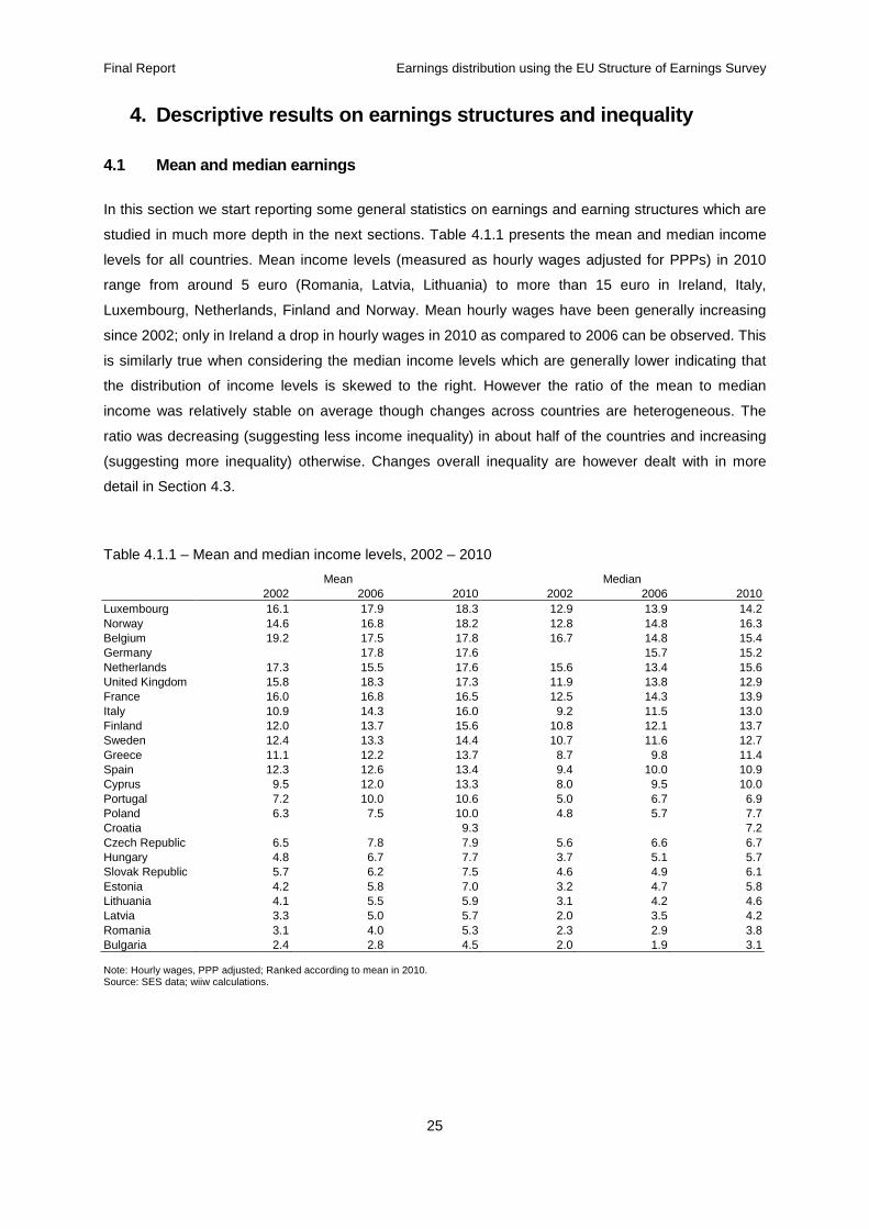
Final Report Earnings distribution using the EU Structure of Earnings Survey
25
4. Descriptive results on earnings structures and i nequality
4.1 Mean and median earnings
In this section we start reporting some general statistics on earnings and earning structures which are
studied in much more depth in the next sections. Table 4.1.1 presents the mean and median income
levels for all countries. Mean income levels (measured as hourly wages adjusted for PPPs) in 2010
range from around 5 euro (Romania, Latvia, Lithuania) to more than 15 euro in Ireland, Italy,
Luxembourg, Netherlands, Finland and Norway. Mean hourly wages have been generally increasing
since 2002; only in Ireland a drop in hourly wages in 2010 as compared to 2006 can be observed. This
is similarly true when considering the median income levels which are generally lower indicating that
the distribution of income levels is skewed to the right. However the ratio of the mean to median
income was relatively stable on average though changes across countries are heterogeneous. The
ratio was decreasing (suggesting less income inequality) in about half of the countries and increasing
(suggesting more inequality) otherwise. Changes overall inequality are however dealt with in more
detail in Section 4.3.
Table 4.1.1 – Mean and median income levels, 2002 – 2010
Mean Median 2002 2006 2010 2002 2006 2010 Luxembourg 16.1 17.9 18.3 12.9 13.9 14.2 Norway 14.6 16.8 18.2 12.8 14.8 16.3 Belgium 19.2 17.5 17.8 16.7 14.8 15.4 Germany 17.8 17.6 15.7 15.2 Netherlands 17.3 15.5 17.6 15.6 13.4 15.6 United Kingdom 15.8 18.3 17.3 11.9 13.8 12.9 France 16.0 16.8 16.5 12.5 14.3 13.9 Italy 10.9 14.3 16.0 9.2 11.5 13.0 Finland 12.0 13.7 15.6 10.8 12.1 13.7 Sweden 12.4 13.3 14.4 10.7 11.6 12.7 Greece 11.1 12.2 13.7 8.7 9.8 11.4 Spain 12.3 12.6 13.4 9.4 10.0 10.9 Cyprus 9.5 12.0 13.3 8.0 9.5 10.0 Portugal 7.2 10.0 10.6 5.0 6.7 6.9 Poland 6.3 7.5 10.0 4.8 5.7 7.7 Croatia 9.3 7.2 Czech Republic 6.5 7.8 7.9 5.6 6.6 6.7 Hungary 4.8 6.7 7.7 3.7 5.1 5.7 Slovak Republic 5.7 6.2 7.5 4.6 4.9 6.1 Estonia 4.2 5.8 7.0 3.2 4.7 5.8 Lithuania 4.1 5.5 5.9 3.1 4.2 4.6 Latvia 3.3 5.0 5.7 2.0 3.5 4.2 Romania 3.1 4.0 5.3 2.3 2.9 3.8 Bulgaria 2.4 2.8 4.5 2.0 1.9 3.1 Note: Hourly wages, PPP adjusted; Ranked according to mean in 2010. Source: SES data; wiiw calculations.

Final Report Earnings distribution using the EU Structure of Earnings Survey
26
4.2 Unconditional earning structures
Hidden behind these mean income levels there are significant differences of earnings across groups
of workers. As already done above, the data can be differentiated by several dimensions which are
distinguished between individual characteristics, job characteristics and firm characteristics. Tables
4.2.1 to 4.2.3 present the mean earnings per hour worked relative to a reference group (which is then
also used in the econometrics part reported in Section 5).1 It is important to note that in this exercise
the earnings present unconditional means, i.e. does not take into account that earnings might differ
across groups of the workforce, e.g. male-female, because differences in educational attainment
levels across these groups which is taken into account in the econometrics when estimating earnings
regressions. Nonetheless, such an unconditional consideration of wage gaps is informative as it
shows actual wage gaps e.g. taking into account that some persons do not get into particular jobs
(e.g. female with the same formal level of education are less likely to become managers).
Starting first with the individual characteristics as indicated in Table 4.2.1 one finds that on average
females earn about 10-20% less than male on average. In some countries the wage gaps are even
higher with e.g. 25% in Germany, Estonia and the UK. A relatively small gap is found for Croatia (with
basically no wage gap) and Poland. With respect to age one finds a clear wage ranking as such that
older workers earn higher wages with however relatively large cross-country differences observed with
respect to the overall magnitudes. For example, in some countries the ratio goes up to more than 3
(for workers aged 50-59) whereas in some countries it remains less than 2. This is similarly the case
with respect to educational attainment levels.
Second, there is a considerable wage gap between those having an indefinite duration contract as
compared to those with a fixed duration contract with the latter earning about 20-30% less though
again there exist considerable cross-country differences. Similarly, part-time workers earn on average
20-25% less per hour than full-time workers. Here again the range across countries is quite large; e.g.
the ratio is 0.66 in Bulgaria and the UK, 0.57 in Cyprus but around 1 or above in Hungary, Poland, and
Luxembourg with Croatia even reporting a ratio of above 1). There is also a pronounced wage
hierarchy with respect to occupations which tends to be relatively similar across countries though
wage differences are more pronounced for the Eastern European countries together with Italy and
Germany.
Finally, third, firm characteristics also play an important role for wage differences. Surprisingly, hourly
earnings in most industries are lower than in the reference group comprising the mining industries
which might can be explained by hard working conditions, job qualifications needed and unionization.
In some cases wages are higher in another energy related industry (NACE Rev. 1 40-41). Relatively
lower gaps are also observed for financial and business services sectors (NACE Rev. 1 65-67 and 70-
74). However, again countries are quite heterogeneous in that respect.
1 The unconditional gaps are reported only if the respective reference group is available. Underlying data on mean income levels
are reported in the Appendix Tables.

Final Report Earnings distribution using the EU Structure of Earnings Survey
27
Table 4.2.1 – Structure of earnings: Individual characteristics, reference group = 1, 2010 BE BG CY CZ DE EE ES FI FR EL HR HU IT LT LU LV NL NO PL PT RO SE SK UK
Gender Male 1.00 1.00 1.00 1.00 1.00 1.00 1.00 1.00 1.00 1.00 1.00 1.00 1.00 1.00 1.00 1.00 1.00 1.00 1.00 1.00 1.00 1.00 1.00 1.00 Female 0.89 0.87 0.83 0.80 0.75 0.76 0.84 0.79 0.83 0.84 1.01 0.88 0.92 0.90 0.91 0.88 0.82 0.82 0.94 0.86 0.92 0.83 0.80 0.73
Age 14-19 1.00 1.00 1.00 1.00 1.00 1.00 1.00 1.00 1.00 1.00 1.00 1.00 1.00 1.00 1.00 1.00 1.00 1.00 1.00 1.00 1.00 1.00 1.00 1.00 20-29 1.38 1.55 1.54 1.49 2.25 1.66 1.20 1.28 2.32 1.22 1.67 1.43 1.18 1.59 2.11 1.71 2.13 1.46 1.53 1.31 1.71 1.22 1.46 1.77
30-39 1.72 1.84 2.29 1.89 3.47 2.02 1.55 1.65 2.96 1.61 2.09 1.80 1.51 1.84 2.95 1.98 3.22 1.91 2.12 1.83 2.00 1.52 1.79 2.63 40-49 1.93 1.85 2.60 1.87 3.84 1.81 1.70 1.74 3.24 1.95 2.09 1.77 1.78 1.70 3.43 1.77 3.54 2.08 2.17 2.17 1.99 1.64 1.68 2.70 50-59 2.11 1.80 2.89 1.80 3.86 1.59 1.87 1.70 3.46 2.26 2.12 1.78 2.06 1.70 3.50 1.66 3.65 2.06 1.99 2.44 2.12 1.59 1.62 2.57
60+ 2.24 1.63 2.45 1.95 3.73 1.44 2.18 1.71 4.49 2.60 2.75 2.20 2.58 1.78 4.30 1.75 3.50 1.97 2.46 2.41 2.50 1.56 1.76 2.17
Education Primary 1.00 1.00 1.00 1.00 1.00 1.00 1.00 1.00 1.00 1.00 1.00 1.00 1.00 1.00 1.00 1.00 1.00 1.00 1.00 1.00 1.00 1.00 Lower secondary 1.06 1.07 1.03 1.02 1.20 1.03 1.11 0.98 1.04 0.98 1.05 1.26 1.05 0.86 1.07 0.94 0.88 1.16 1.05 1.05 1.31
Upper and post secondary 1.15 1.23 1.10 1.36 1.43 1.22 1.01 1.18 1.08 1.38 1.35 1.43 1.41 1.40 0.99 1.40 1.15 1.20 1.58 1.42 1.12 1.44 Short cycle secondary 2.25 2.59 2.30 2.53 2.46 1.84 1.49 1.85 1.66 2.78 2.80 2.20 2.77 2.59 1.82 2.18 1.70 2.54 3.01 3.18 1.45 2.17 Bachelor and Master 1.55 1.65 1.56 1.68 1.99 1.38 1.21 1.42 1.22 2.43 1.67 1.79 1.75 2.06 1.31 2.01 1.44 1.91 2.81 2.38 1.18 1.90
Doctoral 2.87 3.53 3.63 2.23 3.77 2.08 2.13 2.41 2.08 3.80 2.95 4.18 3.10 2.74 3.18 1.85 2.70 4.91 4.25 1.31 2.51 Source: SES data; wiiw calculations Table 4.2.2 – Structure of earnings: Job characteristics, reference group = 1, 2010 BE BG CY CZ DE EE ES FI FR EL HR HU IT LT LU LV NL NO PL PT RO SE SK UK
Job duration 0-1 year 1.00 1.00 1.00 1.00 1.00 1.00 1.00 1.00 1.00 1.00 1.00 1.00 1.00 1.00 1.00 1.00 1.00 1.00 1.00 1.00 1.00 1.00 1.00 1.00 1-4 years 1.12 1.25 1.16 1.21 1.27 1.10 1.17 1.15 1.10 1.09 1.32 1.31 1.11 1.17 1.28 1.21 3.65 1.10 1.13 1.14 1.17 1.12 1.16 1.19 5-14 years 1.28 1.44 1.65 1.36 1.61 1.22 1.33 1.26 1.21 1.31 1.39 1.41 1.24 1.34 1.50 1.34 5.72 1.11 1.40 1.32 1.33 1.18 1.28 1.38
more than 14 years 1.48 1.64 2.25 1.55 1.95 1.29 1.83 1.29 1.42 1.72 1.43 1.60 1.61 1.51 1.85 1.50 5.93 1.23 1.52 1.72 1.58 1.13 1.37 1.51
Contract type Indefinite duration 1.00 1.00 1.00 1.00 1.00 1.00 1.00 1.00 1.00 1.00 1.00 1.00 1.00 1.00 1.00 1.00 1.00 1.00 1.00 1.00 1.00 1.00 1.00
Fixed term 0.74 0.76 0.88 0.75 0.73 1.05 0.82 0.82 0.80 0.85 0.64 0.78 0.86 1.03 0.62 1.00 0.61 0.87 0.63 0.68 0.89 0.82 0.82 Trainee 0.45 0.56 0.24 0.62 0.48 0.44 0.74 0.57 0.24 0.46 0.13 0.70
Full-time/Part-time Full-time 1.00 1.00 1.00 1.00 1.00 1.00 1.00 1.00 1.00 1.00 1.00 1.00 1.00 1.00 1.00 1.00 1.00 1.00 1.00 1.00 1.00 1.00 1.00 1.00
Part-time 0.80 0.66 0.57 0.83 0.76 0.78 0.81 0.84 0.87 0.75 1.16 0.99 0.71 0.80 1.00 0.74 0.77 0.76 1.01 0.85 0.75 0.82 0.84 0.66
Occupation Managers 1.00 1.00 1.00 1.00 1.00 1.00 1.00 1.00 1.00 1.00 1.00 1.00 1.00 1.00 1.00 1.00 1.00 1.00 1.00 1.00 1.00 1.00 1.00 1.00
Professionals 0.69 0.67 0.57 0.63 0.65 0.81 0.67 0.65 0.72 0.71 0.65 0.79 0.62 0.79 0.58 0.96 0.81 0.74 0.74 0.61 0.55 0.66 0.58 0.81 Technicians 0.53 0.57 0.43 0.52 0.54 0.63 0.52 0.51 0.57 0.55 0.46 0.56 0.41 0.59 0.48 0.80 0.65 0.74 0.49 0.44 0.40 0.64 0.51 0.58 Clerical support 0.44 0.38 0.27 0.40 0.35 0.49 0.39 0.41 0.42 0.47 0.41 0.45 0.34 0.48 0.38 0.63 0.52 0.53 0.40 0.30 0.33 0.48 0.39 0.40
Service and sales 0.37 0.26 0.22 0.29 0.29 0.36 0.34 0.37 0.41 0.39 0.30 0.33 0.27 0.37 0.26 0.46 0.41 0.48 0.28 0.21 0.20 0.46 0.30 0.35 Skilled agricultural 0.25 0.22 0.29 0.28 0.45 0.35 0.34 0.34 0.37 0.28 0.30 0.25 0.34 0.25 0.49 0.39 0.48 0.28 0.18 0.19 0.43 0.26 0.35 Craft and related trade workers 0.40 0.39 0.28 0.37 0.38 0.52 0.39 0.46 0.44 0.52 0.29 0.39 0.27 0.47 0.27 0.58 0.50 0.57 0.36 0.22 0.31 0.53 0.37 0.46
Plant and machine operators 0.41 0.37 0.25 0.36 0.36 0.48 0.40 0.47 0.44 0.51 0.32 0.41 0.30 0.49 0.28 0.62 0.47 0.55 0.39 0.21 0.32 0.52 0.36 0.38 Elementary occupations 0.33 0.26 0.21 0.28 0.24 0.32 0.30 0.34 0.35 0.37 0.24 0.28 0.25 0.32 0.23 0.43 0.33 0.45 0.28 0.18 0.19 0.42 0.26 0.30
Source: SES data; wiiw calculations
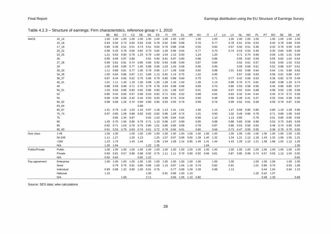
Final Report Earnings distribution using the EU Structure of Earnings Survey
28
Table 4.2.3 – Structure of earnings: Firm characteristics, reference group = 1, 2010 BE BG CY CZ DE EE ES FI FR EL HR HU IT LT LU LV NL NO PL PT RO SE SK UK
NACE 10_14 1.00 1.00 1.00 1.00 1.00 1.00 1.00 1.00 1.00 1.00 1.00 1.00 1.00 1.00 1.00 1.00 1.00 1.00 1.00 1.00 15_16 0.93 0.55 0.73 0.64 0.64 0.65 0.78 0.92 0.90 0.68 0.76 0.77 0.78 0.51 0.54 0.53 0.40 0.78 0.80 0.50
17_19 0.85 0.39 0.51 0.51 0.73 0.51 0.64 0.76 0.88 0.58 0.55 0.60 0.57 0.50 0.51 0.36 0.32 0.76 0.59 0.45 20_22 0.90 0.43 0.78 0.60 0.82 0.70 0.82 1.00 0.96 0.64 0.77 0.70 0.74 0.53 0.54 0.49 0.35 0.84 0.85 0.49 23_25 1.21 0.63 0.90 0.76 1.23 0.79 1.09 1.04 1.15 0.93 1.24 1.20 0.71 0.70 0.66 0.59 1.00 1.01 0.59
26 0.95 0.69 0.97 0.80 0.91 0.90 0.91 0.97 0.80 0.96 0.86 0.55 0.60 0.59 0.55 0.82 1.04 0.54 27_28 0.99 0.62 0.81 0.74 0.85 0.80 0.92 0.93 0.98 0.69 0.87 0.84 0.52 0.61 0.57 0.52 0.83 1.03 0.52 29 1.00 0.69 0.80 0.77 1.05 0.88 0.96 1.03 1.03 0.58 0.95 0.93 0.59 0.69 0.61 0.52 0.88 0.97 0.61
30_33 1.11 0.68 0.81 0.77 1.05 0.79 0.95 1.17 1.09 0.69 0.92 0.98 1.01 0.62 0.68 0.64 0.54 1.01 0.89 0.63 34_35 1.00 0.64 0.86 0.87 1.21 0.80 1.13 0.92 1.14 0.75 1.02 0.95 0.57 0.69 0.63 0.59 0.91 0.85 0.67 36_37 0.87 0.44 0.83 0.62 0.75 0.66 0.79 0.80 0.88 0.60 0.75 0.71 0.77 0.42 0.56 0.53 0.36 0.82 0.79 0.49
40_41 1.51 1.11 1.45 1.19 1.30 0.99 1.30 1.09 1.34 1.04 1.35 1.14 0.99 0.70 0.71 0.81 0.80 0.98 1.29 0.74 45 0.88 0.59 0.89 0.71 0.70 0.79 0.78 0.93 0.98 0.66 0.69 0.70 0.80 0.53 0.58 0.56 0.46 0.86 0.85 0.57 50_51 1.03 0.63 0.89 0.83 0.82 0.85 0.83 1.01 1.08 0.67 0.91 0.84 0.97 0.52 0.64 0.68 0.58 0.93 1.06 0.58
52 0.80 0.42 0.65 0.57 0.58 0.53 0.62 0.71 0.81 0.52 0.68 0.62 0.63 0.32 0.44 0.44 0.40 0.74 0.72 0.36 55 0.69 0.39 0.66 0.42 0.44 0.50 0.63 0.66 0.74 0.54 0.60 0.48 0.60 0.28 0.41 0.47 0.32 0.64 0.58 0.30 60_62 0.98 0.68 1.26 0.74 0.69 0.80 0.95 0.93 0.93 0.79 0.99 0.76 0.99 0.52 0.61 0.58 0.59 0.79 0.87 0.56
63_64 0.68 65_67 1.31 0.79 1.42 1.03 1.16 0.97 1.18 1.13 1.31 1.01 1.56 1.15 1.47 0.69 0.80 0.80 0.80 1.19 1.28 0.96 70_74 0.97 0.85 1.09 0.89 0.82 0.82 0.82 0.96 1.09 0.74 1.01 0.93 1.02 0.49 0.66 0.78 0.71 0.89 1.08 0.63
75 0.85 1.34 0.87 0.92 1.03 0.95 0.84 0.64 0.99 1.10 1.13 0.65 0.78 0.51 0.85 0.95 0.59 80 1.45 0.70 1.94 0.80 0.79 0.71 1.10 0.96 1.07 0.90 0.95 0.98 0.88 0.65 0.59 0.96 0.52 0.73 0.83 0.59 85 0.92 0.71 1.03 0.78 0.76 0.80 1.01 0.80 0.85 0.69 0.78 0.87 0.86 0.53 0.56 0.63 0.48 0.74 0.90 0.55
90_93 0.91 0.53 0.79 0.63 0.74 0.61 0.72 0.78 0.94 0.61 0.80 0.66 0.73 0.47 0.55 0.55 0.36 0.78 0.79 0.50
Size class 1-49 1.00 1.00 1.00 1.00 1.00 1.00 1.00 1.00 1.00 1.00 1.00 1.00 1.00 1.00 1.00 1.00 1.00 1.00 1.00 1.00 1.00 1.00
50-249 1.11 1.27 1.25 1.13 1.25 1.07 0.97 0.99 0.92 1.28 1.40 1.32 1.34 1.21 1.12 1.18 1.43 1.32 1.06 1.05 1.22 >250 1.23 1.75 1.43 1.44 1.39 1.04 1.09 1.14 0.95 1.49 1.41 1.44 1.43 1.29 1.10 1.21 1.58 1.68 1.02 1.12 1.26 N/A 1.30 1.64 1.22 1.35 1.04 1.30
Public/Private Public 1.00 1.00 1.00 1.00 1.00 1.00 1.00 1.00 1.00 1.00 1.00 1.00 1.00 1.00 1.00 1.00 1.00 1.00 1.00 1.00 1.00 1.00 1.00 Private 0.69 0.81 0.57 0.89 0.98 0.92 0.75 1.11 1.11 0.79 0.90 0.92 0.66 0.81 0.87 0.85 0.99 0.74 0.57 0.93 1.13 1.04 0.92 N/A 0.92 0.64 0.92 1.22 0.92
Pay agreement Enterprise 1.00 1.00 1.00 1.00 1.00 1.00 1.00 1.00 1.00 1.00 1.00 1.00 1.00 1.00 1.00 1.00 1.00 1.00 1.00 None 0.79 0.75 0.81 0.80 0.85 1.00 1.15 0.87 1.04 1.16 0.74 0.82 0.91 1.01 0.80 0.74 0.93 1.09
Individual 0.89 0.88 1.32 0.80 1.00 0.91 0.76 0.77 0.89 1.00 1.09 0.98 1.13 0.44 1.04 0.94 1.15 National 1.15 1.00 0.91 0.85 1.00 1.10 1.25 0.42 1.07 N/A 1.69 2.11 0.65 1.05 1.10 0.80 0.48 1.35 0.99 Source: SES data; wiiw calculations

Final Report Earnings distribution using the EU Structure of Earnings Survey
29
Results also indicate that larger firms pay higher wages on average with the wage of firms with more
than 250 employees as compared to those with less than 50 goes up to 50% and even higher in some
countries (e.g. Bulgaria and Romania). In other countries these gaps are relatively low as e.g. in
Finland, France and Norway. Public owned firms pay on average 20% hiegher wages than private
ones with again large differences across countries are being observed. For example, in Finland,
Sweden and France the latter pay about 10% higher wages. Finally, there are also significant wage
gaps with respect to pay agreement schemes with enterprise level bargaining resulting in relatively
highest wages.
As mentioned above, these unconditional means may hide substantial differences with respect to
other characteristics of the workers which are not considered along these single dimensions. The
conditional wage gaps are therefore studies in detail in Section 5.
4.3 Inequality in earnings
Based on the SES data, an initial analysis highlights similarities and differences in earnings structures
between and within Member States, as well as developments over time. For a first assessment of income
and earnings differences across the various dimensions, the following standard indicators have been
looked at for each country and country group: (i) mean and median, (ii) standard deviation, (iii) percentile
distributions (P90/P10, P90/50 and P50/P10), (iv) Gini coefficient, (v) Theil index and (vi) mean
logarithmic deviation. These indicators are reported in Table 4.3.1 whereas Figure 4.3.1 presents the
evolution of the Gini index by country.
The Gini inequality ranges from 0.2 in countries such as Finland, Sweden and Norway to about 0.4 in
Romania, Latvia, Croatia and Turkey. Trends across countries are heterogeneous: inequality is
decreasing, for example, in Latvia, Estonia, Lithuania, Spain and Greece whereas increasing in Italy,
Luxembourg, the Czech Republic and Cyprus. Thus neither can a common trend be observed across
countries, nor can a particular impact of the crisis on inequality in 2010 be detected.
Similar conclusions have to be drawn from the other indicators listed above and reported in the
following Tables 4.3.1 to 4.3.3. Though the levels of indicators are (by definition) different, the overall
trends are similar. This is also indicated by a high correlation and rank correlation of 0.9 and above
across these indicators. Again it holds, that, first, in countries with an increasing Gini one also finds
that the other inequality measures tend to increase and, second, that there has been no significant
impact of the crisis on these earnings inequalities.
The overall trends in inequality also hold when considering percentile income levels (Table 4.3.2) and
the respective ratios (Table 4.3.3). In the latter case the levels are interesting as e.g. the P90/P10
ratio, i.e. income of the 9th percentile relative to the 1st percentile, ranges from about 2 in Sweden (i.e.
income in the 9th percentile is two times larger as in the 1st) to almost 5 in Portugal and Romania.
Second, the P90/P50 ratio compared to the P50/P90 ratio is larger in almost all cases indicating again
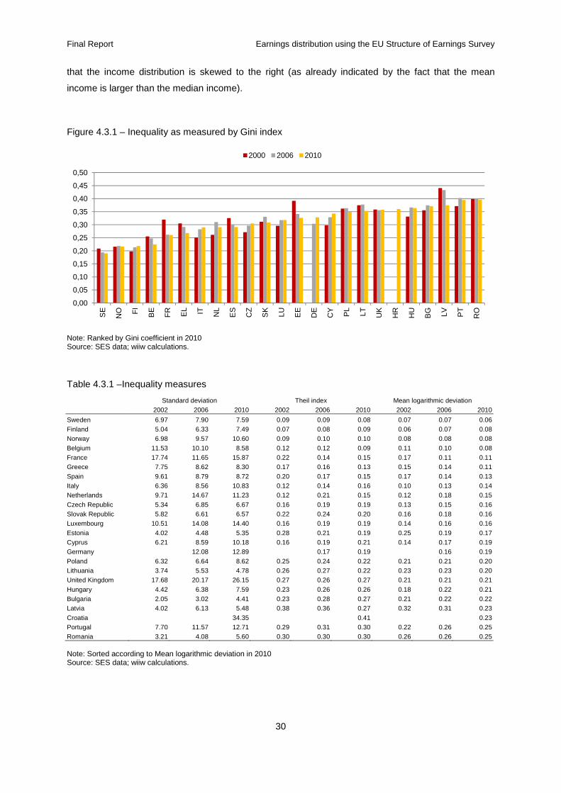
Final Report Earnings distribution using the EU Structure of Earnings Survey
30
that the income distribution is skewed to the right (as already indicated by the fact that the mean
income is larger than the median income).
Figure 4.3.1 – Inequality as measured by Gini index
Note: Ranked by Gini coefficient in 2010 Source: SES data; wiiw calculations.
Table 4.3.1 –Inequality measures
Standard deviation Theil index Mean logarithmic deviation 2002 2006 2010 2002 2006 2010 2002 2006 2010
Sweden 6.97 7.90 7.59 0.09 0.09 0.08 0.07 0.07 0.06 Finland 5.04 6.33 7.49 0.07 0.08 0.09 0.06 0.07 0.08 Norway 6.98 9.57 10.60 0.09 0.10 0.10 0.08 0.08 0.08
Belgium 11.53 10.10 8.58 0.12 0.12 0.09 0.11 0.10 0.08 France 17.74 11.65 15.87 0.22 0.14 0.15 0.17 0.11 0.11 Greece 7.75 8.62 8.30 0.17 0.16 0.13 0.15 0.14 0.11
Spain 9.61 8.79 8.72 0.20 0.17 0.15 0.17 0.14 0.13 Italy 6.36 8.56 10.83 0.12 0.14 0.16 0.10 0.13 0.14 Netherlands 9.71 14.67 11.23 0.12 0.21 0.15 0.12 0.18 0.15
Czech Republic 5.34 6.85 6.67 0.16 0.19 0.19 0.13 0.15 0.16 Slovak Republic 5.82 6.61 6.57 0.22 0.24 0.20 0.16 0.18 0.16 Luxembourg 10.51 14.08 14.40 0.16 0.19 0.19 0.14 0.16 0.16
Estonia 4.02 4.48 5.35 0.28 0.21 0.19 0.25 0.19 0.17 Cyprus 6.21 8.59 10.18 0.16 0.19 0.21 0.14 0.17 0.19 Germany 12.08 12.89 0.17 0.19 0.16 0.19
Poland 6.32 6.64 8.62 0.25 0.24 0.22 0.21 0.21 0.20 Lithuania 3.74 5.53 4.78 0.26 0.27 0.22 0.23 0.23 0.20 United Kingdom 17.68 20.17 26.15 0.27 0.26 0.27 0.21 0.21 0.21
Hungary 4.42 6.38 7.59 0.23 0.26 0.26 0.18 0.22 0.21 Bulgaria 2.05 3.02 4.41 0.23 0.28 0.27 0.21 0.22 0.22 Latvia 4.02 6.13 5.48 0.38 0.36 0.27 0.32 0.31 0.23
Croatia 34.35 0.41 0.23 Portugal 7.70 11.57 12.71 0.29 0.31 0.30 0.22 0.26 0.25 Romania 3.21 4.08 5.60 0.30 0.30 0.30 0.26 0.26 0.25 Note: Sorted according to Mean logarithmic deviation in 2010 Source: SES data; wiiw calculations.
0,00
0,05
0,10
0,15
0,20
0,25
0,30
0,35
0,40
0,45
0,50
SE
NO FI
BE
FR EL IT NL
ES
CZ
SK
LU EE
DE
CY PL
LT UK
HR
HU
BG LV PT
RO
2000 2006 2010

Final Report Earnings distribution using the EU Structure of Earnings Survey
31
Table 4.3.2 –Percentile income levels
p10 p50 p90 2002 2006 2010 2002 2006 2010 2002 2006 2010
Bulgaria 0.9 1.2 1.9 2.0 1.9 3.1 4.4 5.2 8.0
Romania 1.0 1.3 2.0 2.3 2.9 3.8 5.7 7.5 9.8 Latvia 1.2 1.4 2.3 2.0 3.5 4.2 6.5 9.6 10.4 Lithuania 1.5 1.9 2.3 3.1 4.2 4.6 7.4 9.9 10.7
Estonia 1.3 2.2 2.7 3.2 4.7 5.8 7.8 10.2 12.0 Slovak Republic 2.7 2.8 3.5 4.6 4.9 6.1 9.0 10.0 12.1 Czech Republic 3.3 3.7 3.5 5.6 6.6 6.7 9.8 12.2 12.6
Hungary 2.2 2.5 3.3 3.7 5.1 5.7 8.1 11.9 13.7 Croatia 3.8 7.2 14.4 Poland 2.4 2.7 3.9 4.8 5.7 7.7 12.0 14.3 18.7
Sweden 8.1 9.0 9.7 10.7 11.6 12.7 18.3 18.6 20.0 Portugal 3.1 3.7 4.2 5.0 6.7 6.9 13.0 20.4 21.1 Greece 5.5 6.2 7.3 8.7 9.8 11.4 19.4 20.5 21.8
Spain 5.7 6.2 6.6 9.4 10.0 10.9 21.4 21.7 23.1 Finland 7.7 8.6 9.6 10.8 12.1 13.7 17.6 20.7 23.4 Cyprus 4.4 5.1 5.7 8.0 9.5 10.0 16.2 22.4 25.5
France 7.9 9.1 9.2 12.5 14.3 13.9 26.2 25.9 25.5 Norway 9.2 10.4 11.2 12.8 14.8 16.3 21.9 24.6 26.4 Italy 6.2 7.4 8.3 9.2 11.5 13.0 17.0 24.9 27.1
Belgium 10.3 10.1 10.7 16.7 14.8 15.4 30.2 27.4 27.2 Netherlands 8.8 7.0 8.2 15.6 13.4 15.6 27.2 24.6 28.6 United Kingdom 6.5 7.6 7.2 11.9 13.8 12.9 27.3 31.6 29.6
Germany 7.5 6.8 15.7 15.2 29.5 30.5 Luxembourg 7.7 8.4 8.6 12.9 13.9 14.2 27.8 30.7 31.2 Note: Sorted according to p90 in 2010 Source: SES data; wiiw calculations.
Table 4.3.3 –Percentile ratios
p90/p10 p50/p10 p90/p50 2002 2006 2010 2002 2006 2010 2002 2006 2010
Sweden 2.26 2.08 2.06 1.32 1.30 1.31 1.71 1.60 1.58 Norway 2.39 2.36 2.36 1.39 1.42 1.45 1.72 1.66 1.63
Finland 2.29 2.41 2.43 1.41 1.41 1.42 1.63 1.71 1.72 Belgium 2.93 2.70 2.55 1.62 1.46 1.44 1.81 1.85 1.77 France 3.32 2.83 2.77 1.58 1.57 1.51 2.10 1.80 1.83
Netherlands 3.07 3.53 3.47 1.76 1.92 1.89 1.75 1.84 1.84 Czech Republic 2.94 3.29 3.60 1.69 1.78 1.91 1.74 1.85 1.88 Greece 3.51 3.29 2.97 1.58 1.57 1.55 2.22 2.09 1.92
Slovak Republic 3.38 3.60 3.49 1.73 1.76 1.78 1.96 2.05 1.96 Croatia 3.75 1.87 2.01 Germany 3.95 4.48 2.09 2.23 1.89 2.01
Estonia 5.91 4.74 4.37 2.43 2.19 2.11 2.43 2.16 2.07 Italy 2.74 3.37 3.26 1.48 1.55 1.57 1.84 2.17 2.07 Spain 3.75 3.47 3.48 1.65 1.61 1.64 2.27 2.16 2.12
Luxembourg 3.59 3.65 3.65 1.66 1.66 1.66 2.16 2.20 2.20 United Kingdom 4.18 4.13 4.12 1.81 1.80 1.79 2.30 2.29 2.30 Lithuania 5.00 5.16 4.59 2.08 2.15 1.95 2.41 2.40 2.36
Hungary 3.70 4.70 4.17 1.70 1.99 1.74 2.18 2.36 2.40 Poland 5.01 5.31 4.86 2.01 2.11 2.01 2.49 2.52 2.42 Latvia 5.58 6.71 4.50 1.73 2.44 1.81 3.23 2.75 2.49
Cyprus 3.66 4.39 4.49 1.80 1.86 1.77 2.03 2.36 2.53 Romania 5.96 5.99 5.00 2.39 2.33 1.94 2.49 2.57 2.57 Bulgaria 5.08 4.23 4.13 2.33 1.56 1.61 2.18 2.72 2.57
Portugal 4.21 5.51 4.98 1.62 1.80 1.62 2.61 3.06 3.06 Note: Sorted according to p90/p50 in 2010 Source: SES data; wiiw calculations.

Final Report Earnings distribution using the EU Structure of Earnings Survey
32
4.4 Contributions to inequality
We start to report results from the Shapley value decomposition which allows us to assess the relative
importance of the various characteristics for earning inequalities. As described above, the Shapley value
approach allows for the calculation of the contribution of each of the explanatory variables to a respective
inequality measure – in our case the Gini index. For individuals, predicted incomes are calculated for all
combinations of explanatory variables using the coefficients from the country-level regressions. Drawing on
those predicted incomes, Gini coefficients are calculated for all variable combinations. Thus we can detect
the effect of the individual variables on changes in the inequality measure.
We begin here with a description of the decomposition results based on the anonymised version of the
SES dataset for the years 2002, 2006 and 2010 for the average of all countries (see Figure 4.4.1). For this
we calculated the unweighted mean of the contributions of individual variables over all available countries
for all three years (excluding Germany and Croatia, where data are missing in 2002 for the former and
2002 and 2006 for the latter). The Shapley value decomposition explains on average 72% of the variation
of individual hourly wages including bonuses in all three years, with the remaining residual being
unexplained by the set of explanatory variables. As can be seen in Figure 4.4.1, we grouped the variables
according to individual characteristics (in shades of blue), job characteristics (in shades of red/yellow) and
enterprise/sector characteristics (in shades of green). It should be stated at the outset that a high or low
relative importance of an individual variable obviously does not mean that the characteristic is of more or
less policy relevance. Although the mean Gini index over all countries available in the anonymised dataset
remained stable over the years, the relative importance of individual factors driving inequality changed over
time. On average, individual characteristics accounted for 20.4% of the measured wage differences in the
three years. As expected, the educational attainment of employees is the most important individual
characteristic explaining conditional wage differences and is increasing over time from 10.8% in 2002 to
12.6% in 2010. Differences between age groups account for about 5% of the Gini index, while conditional
wage differences between males and females declined somewhat over the 8-year period on average. In
2002, 4.2% of the mean Gini index could be explained by gender differences, while in 2010 this dropped to
2.9%.
The most important characteristic in explaining wage inequality is occupation, which explains, on average,
about 24.9% of the Gini index. This result was expected as wage structures of firms are in general shaped
by differences between occupational categories. The second most important of the group of job
characteristics is the length of service of individual employees in the enterprise, which accounts for 5.9% of
the total Gini index. Differences between full- and part-time employed and between types of employment
contracts (indefinite duration, temporary/fixed duration or apprentice) both account for only about 1% of the
average observed inequality. However, the importance of differences between full- and part-time
employees, which had declined before the crisis, rose from 0.8% in 2006 to 1.2% in 2010.

Final Report Earnings distribution using the EU Structure of Earnings Survey
33
Figure 4.4.1 – Contribution of explanatory variables to Gini index
Note: Unweighted mean over available countries in individual years Source: SES; wiiw calculations.
Enterprise characteristics account for 20.3% on average of the Gini index in 2002 but their importance
declines to 17.4% in 2010. The second most important characteristic is the NACE sector of firms, which
accounts for 10.2% of the average Gini index in 2002. However, conditional wage differences between
industries fall to 8.2% in 2010. A similar development can be observed in the case of the size classes of
enterprises. In 2002 differences between larger and smaller enterprises explain 6.6% of overall wage
inequality, while in 2010 this falls to 6.1% on average. Conditional wage differences between public and
private companies and between enterprise units that are non-covered or covered by different types of
collective pay agreements both account for about 1.6% of total inequality on average in the period
analysed.
These general patterns also hold broadly across all countries considered as indicated in Figure 4.4.2
though there are also some distinct differences. For example, education has a much larger contribution to
inequality in Portugal and Croatia. Age contributes relatively strongly to inequality in the Netherlands,
Belgium and Greece. Job duration is relatively important as an explanatory factor in Cyprus, Germany,
Luxembourg, Spain and Greece. Also the size class of firms contributes differently across countries and is
relatively important in Latvia, Bulgaria, Lithuania and Hungary. The occupational categories however are in
all countries the most important factor to explain overall inequality levels though again the contributions
range from less than 20% (as in the case of Latvia and Hungary) to more than 30% (in Luxembourg,
France and Finland).
0,00
0,05
0,10
0,15
0,20
0,25
0,30
0,35
2002 2006 2010
Gender Age Education Job duration
Contract type Full-time/Part-time Occupation NACE
Size class Collective pay agreement Public Privat Residual

Final Report Earnings distribution using the EU Structure of Earnings Survey
34
Figure 4.4.2 – Contributions to Gini index (2010)
Source: SES; wiiw calculations.
In the next section the contributions of these factors to the overall inequality and their changes over time
are discussed in more detail alongside the results of the Mincer regressions.
0
0,05
0,1
0,15
0,2
0,25
0,3
0,35
0,4
0,45
RO PT LV BG HU HR UK LT PL CY DE EE LU SK CZ ES NL IT EL FR BE FI NO SE
Gender Age Education Job duration
Contract Full-time/Part-time Occupation NACE
Size class Collective pay agreement Public/Private Residual

Final Report
5. Analysis of earning structures and inequality
5.1 Personal characteristics
5.1.1 Gender
The issue of gender wage gaps
debate, the unadjusted gender wage gap based on gross monthly earnings is often reported, mostly due to
a lack of better data. This however provides an inaccurate picture
on average from men in terms of hours worked, choice of job, education level, etc.
effects as accurately as possible, the
gross hourly earnings, with a number of personal, job and firm characteristics as controls taken from the
SES dataset. Hence, the reported coefficient
between males and females for individuals with similar characteristics.
information on career breaks available in the dataset. Since women are more likely to take career breaks
which may negatively impact upon
of the wage gap slightly upwards.3
Figure 5.1.1 – Gender wage differences from Mincer regressions (2002
Note: The coefficients are taken from the full Mincer regressions estimated separately for each country A.1 to A.3. The reference category is male.
Source: SES; wiiw calculations.
2 This, however, does not address questions like why female workers are for example more o
working in different occupations with the same level of qualification. 3 The question is optional in the SES 2002 questionnaire, but hardly any countries provide information. It was dropped in the
subsequent SES waves.
Earnings distribution using the EU Structure of Earnings Survey
35
Analysis of earning structures and inequality
ersonal characteristics
is extensively discussed in the literature. In the media and the public
the unadjusted gender wage gap based on gross monthly earnings is often reported, mostly due to
however provides an inaccurate picture as women in the
from men in terms of hours worked, choice of job, education level, etc.
as possible, the regression results presented and discussed
a number of personal, job and firm characteristics as controls taken from the
reported coefficients should provide more accurate estimates of the wage gap
between males and females for individuals with similar characteristics.2 Unfortunately, there is no
information on career breaks available in the dataset. Since women are more likely to take career breaks
impact upon their wages, a failure to control for career breaks will bias the estimates 3 Results are presented in Figure 5.1.1.
Gender wage differences from Mincer regressions (2002-2010)
The coefficients are taken from the full Mincer regressions estimated separately for each country as reported in Countries are ranked according to gender wage gap in 2010.
This, however, does not address questions like why female workers are for example more often partworking in different occupations with the same level of qualification.
The question is optional in the SES 2002 questionnaire, but hardly any countries provide information. It was dropped in the
Earnings distribution using the EU Structure of Earnings Survey
n the media and the public
the unadjusted gender wage gap based on gross monthly earnings is often reported, mostly due to
workforce might differ
from men in terms of hours worked, choice of job, education level, etc. To control for these
and discussed below are based on
a number of personal, job and firm characteristics as controls taken from the
estimates of the wage gap
ortunately, there is no
information on career breaks available in the dataset. Since women are more likely to take career breaks,
for career breaks will bias the estimates
as reported in Appendix Tables
ften part-time employed or are
The question is optional in the SES 2002 questionnaire, but hardly any countries provide information. It was dropped in the
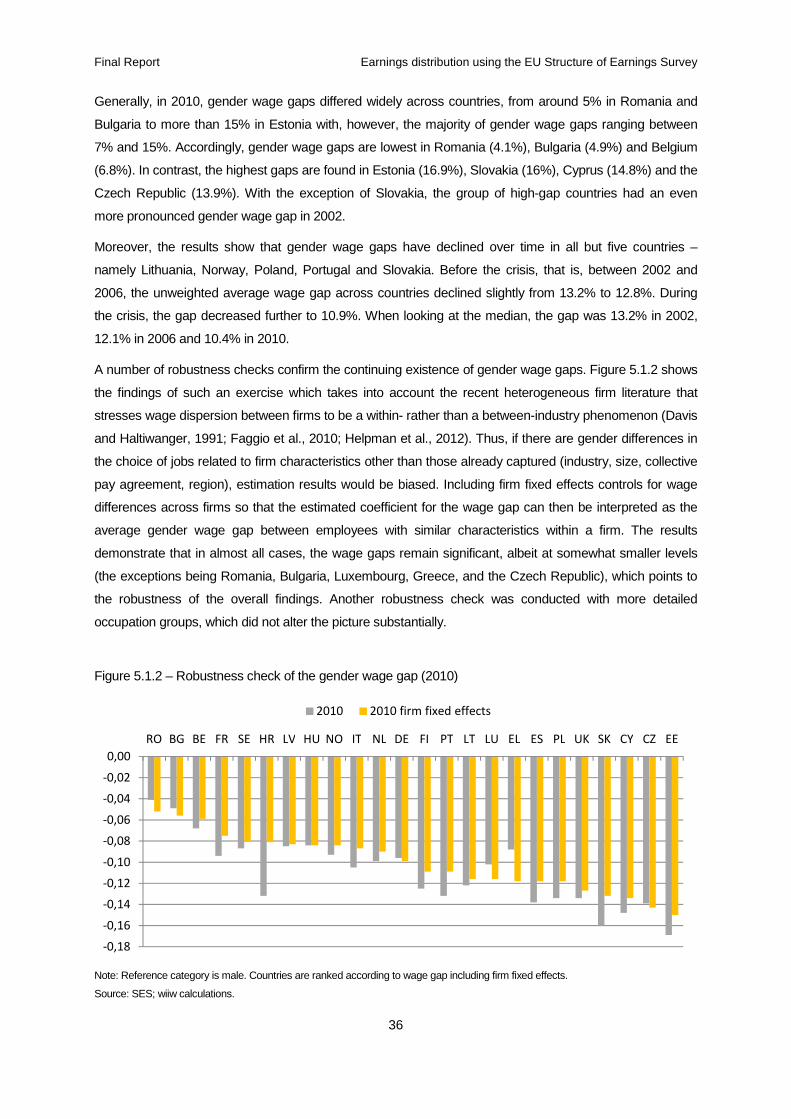
Final Report Earnings distribution using the EU Structure of Earnings Survey
36
Generally, in 2010, gender wage gaps differed widely across countries, from around 5% in Romania and
Bulgaria to more than 15% in Estonia with, however, the majority of gender wage gaps ranging between
7% and 15%. Accordingly, gender wage gaps are lowest in Romania (4.1%), Bulgaria (4.9%) and Belgium
(6.8%). In contrast, the highest gaps are found in Estonia (16.9%), Slovakia (16%), Cyprus (14.8%) and the
Czech Republic (13.9%). With the exception of Slovakia, the group of high-gap countries had an even
more pronounced gender wage gap in 2002.
Moreover, the results show that gender wage gaps have declined over time in all but five countries –
namely Lithuania, Norway, Poland, Portugal and Slovakia. Before the crisis, that is, between 2002 and
2006, the unweighted average wage gap across countries declined slightly from 13.2% to 12.8%. During
the crisis, the gap decreased further to 10.9%. When looking at the median, the gap was 13.2% in 2002,
12.1% in 2006 and 10.4% in 2010.
A number of robustness checks confirm the continuing existence of gender wage gaps. Figure 5.1.2 shows
the findings of such an exercise which takes into account the recent heterogeneous firm literature that
stresses wage dispersion between firms to be a within- rather than a between-industry phenomenon (Davis
and Haltiwanger, 1991; Faggio et al., 2010; Helpman et al., 2012). Thus, if there are gender differences in
the choice of jobs related to firm characteristics other than those already captured (industry, size, collective
pay agreement, region), estimation results would be biased. Including firm fixed effects controls for wage
differences across firms so that the estimated coefficient for the wage gap can then be interpreted as the
average gender wage gap between employees with similar characteristics within a firm. The results
demonstrate that in almost all cases, the wage gaps remain significant, albeit at somewhat smaller levels
(the exceptions being Romania, Bulgaria, Luxembourg, Greece, and the Czech Republic), which points to
the robustness of the overall findings. Another robustness check was conducted with more detailed
occupation groups, which did not alter the picture substantially.
Figure 5.1.2 – Robustness check of the gender wage gap (2010)
Note: Reference category is male. Countries are ranked according to wage gap including firm fixed effects.
Source: SES; wiiw calculations.
-0,18
-0,16
-0,14
-0,12
-0,10
-0,08
-0,06
-0,04
-0,02
0,00
RO BG BE FR SE HR LV HU NO IT NL DE FI PT LT LU EL ES PL UK SK CY CZ EE
2010 2010 firm fixed effects
Final Report Earnings distribution using the EU Structure of Earnings Survey
37
Table 5.1.1 decomposes the gender wage differences into explained and unexplained components using
the Blinder-Oaxaca decompositions. All countries report positive and significant wage gaps between males
and females in all years, with the exception of Hungary in 2010 where a wage gap in favour of females of
3.8% is found. Considering the results for 2002, we observe that the wage gaps are relatively large for
Cyprus and Slovakia, with gaps above 30%, as well as for the United Kingdom, Greece, Estonia, Belgium
and the Czech Republic, with wage gaps above 25%. Wage gaps are much smaller in Lithuania and
Poland, with wage gaps below 10%, as well as Bulgaria, Hungary, Luxembourg, Latvia, Romania and
Sweden, with wage gaps less than 15%. Considering changes across time, we observe that the wage gap
showed a tendency to decline between 2002 and 2010 in many countries. These declines have been
relatively large in a number of countries, including Belgium (25.3% to 7.6%), Cyprus (37% to 17%), Greece
(25.4% to 3.3%), Portugal (22.1% to 1.3%) and Hungary (12% to -3.8%). In a smaller number of countries,
slight increases in the wage gap were observed, with the wage gap rising from 13.5% to 15% in Sweden
and from 21.1% to 22.9% in Finland. A much larger rise was observed in Lithuania (6.5% to 15.8%), with a
large rise also recorded for Germany between 2006 and 2010 (from 13.9% to 24.2%).
Of more importance than the absolute value of the wage gaps is the extent to which these gaps can or
cannot be explained by differences in observable characteristics. The results for 2002 demonstrate that in
the majority of cases the greater part of the wage gap cannot be explained by observables. In particular, in
17 out of 22 countries the unexplained components account for more than 50% of the wage gap, with the
unexplained share reaching as much as 70% in 9 out of 22 countries, and even more than 100% in 3 out of
22 countries (Italy, Lithuania and Poland). The unexplained share of the wage gap is found to be relatively
low (i.e. below 50%) in Belgium, Greece, Hungary, the Netherlands, and Norway. Considering changes in
the share of the unexplained component of wage gaps over time mixed results emerge. In 10 out of 22
cases a decline in the unexplained share of wage gaps is observable between 2002 and 2010, while in 12
cases an increase is observed. Among the countries that showed an increase in the unexplained share
over time, four are countries for which the unexplained share was relatively low in 2002. These are Belgium
and Greece, which experienced relatively large increases, and the Netherlands and, Norway, for which the
change was much smaller. Eight of the 12 countries that experienced an increase in the unexplained share
of the wage gap show an increase of more than 20% in the unexplained share (Belgium, Cyprus, Greece,
Luxembourg, Latvia, Poland, Portugal and Slovakia), with two of these experiencing a more than 100%
increase (Greece and Poland). Of those countries experiencing a decline in the unexplained share of the
wage gap, Estonia and Sweden experienced a decline of more than 20 percentage points in the share of
the unexplained component, with Lithuania experiencing a decline of more than 100 percentage points. In
the case of Hungary, the share of the unexplained component of the wage gap dropped from 47% to
-140%.

Final Report Earnings distribution using the EU Structure of Earnings Survey
38
Table 5.1.1 - Blinder-Oaxaca male-female wage decomposition
2002 2006 2010
Difference Explained Unexplained Difference Explained Unexplained Difference Explained Unexplained
Belgium 0.253*** 0.173*** (68.38)
0.080*** (31.62)
0.065*** -0.005*** (-7.69)
0.070*** (107.69)
0.076*** 0.025*** (32.89)
0.051*** (67.11)
Bulgaria 0.123*** 0.027*** (21.95)
0.096*** (78.05)
0.068*** 0.023*** (33.82)
0.045*** (66.18)
0.082*** 0.033*** (40.24)
0.049*** (59.76)
Cyprus 0.373*** 0.177*** (47.45)
0.197*** (52.82)
0.197*** 0.007 (3.55)
0.190*** (96.45)
0.170*** 0.034*** (20.00)
0.136*** (80.00)
Czech Republic
0.265*** 0.076*** (28.68)
0.189*** (71.32)
0.244*** 0.075*** (30.74)
0.168*** (68.85)
0.221*** 0.083*** (37.56)
0.138*** (62.44)
Germany 0.139*** 0.044*** (31.65)
0.096*** (69.06)
0.242*** 0.146*** (60.33)
0.096*** (39.67)
Estonia 0.294*** 0.058*** (19.73)
0.237*** (80.61)
0.316*** 0.124*** (39.24)
0.192*** (60.76)
0.273*** 0.117*** (42.86)
0.156*** (57.14)
Spain 0.230*** 0.060*** (26.09)
0.170*** (73.91)
0.218*** 0.051*** (23.39)
0.167*** (76.61)
0.216*** 0.075*** (34.72)
0.142*** (65.74)
Finland 0.211*** 0.068*** (32.23)
0.144*** (68.25)
0.250*** 0.103*** (41.20)
0.148*** (59.20)
0.229*** 0.111*** (48.47)
0.118*** (51.53)
France 0.228*** 0.089*** (39.04)
0.138*** (60.53)
0.222*** 0.121*** (54.50)
0.101*** (45.50)
0.180*** 0.088*** (48.89)
0.092*** (51.11)
Croatia 0.145*** 0.068*** (46.90)
0.077*** (53.10)
Greece 0.254*** 0.130*** (51.18)
0.124*** (48.82)
0.167*** 0.071*** (42.51)
0.096*** (57.49)
0.033*** -0.072*** (-218.18)
0.104*** (315.15)
Hungary 0.120*** 0.064*** (53.33)
0.056*** (46.67)
0.111*** 0.026*** (23.42)
0.085*** (76.58)
-0.038*** -0.091*** (239.47)
0.053*** (-139.47)
Italy 0.165*** -0.003 (-1.82)
0.168*** (101.82)
0.093*** -0.033*** (-35.48)
0.127*** (136.56)
0.114*** 0.007*** (6.14)
0.107*** (93.86)
Lithuania 0.065*** -0.051*** (-78.46)
0.115*** (176.92)
0.123*** -0.003 (-2.44)
0.126*** (102.44)
0.158*** -0.004 (-2.53)
0.162*** (102.53)
Luxembourg 0.141*** 0.01
(7.09) 0.131*** (92.91)
0.087*** 0.024*** (27.59)
0.063*** (72.41)
0.047*** -0.025*** (-53.19)
0.072*** (153.19)
Latvia 0.130*** 0.013*** (10.00)
0.117*** (90.00)
0.044*** -0.047*** (-106.82)
0.092*** (209.09)
0.095*** -0.011*** (-11.58)
0.106*** (111.58)
Netherlands 0.229*** 0.155*** (67.69)
0.074*** (32.31)
0.192*** 0.068*** (35.42)
0.124*** (64.58)
0.177*** 0.098*** (55.37)
0.079*** (44.63)
Norway 0.215*** 0.144*** (66.98)
0.071*** (33.02)
0.164*** 0.083*** (50.61)
0.081*** (49.39)
0.152*** 0.093*** (61.18)
0.059*** (38.82)
Poland 0.057*** -0.024*** (-42.11)
0.081*** (142.11)
0.035*** -0.073*** (-208.57)
0.108*** (308.57)
0.025*** -0.071*** (-284.00)
0.096*** (384.00)
Portugal 0.221*** 0.093*** (42.08)
0.128*** (57.92)
0.027*** -0.107*** (-396.30)
0.134*** (496.30)
0.133*** 0.013*** (9.77)
0.121*** (90.98)
Romania 0.129*** 0.059*** (45.74)
0.070*** (54.26)
0.021*** -0.031*** (-147.62)
0.052*** (247.62)
0.065*** 0.019*** (29.23)
0.046*** (70.77)
Sweden 0.135*** 0.045*** (33.33)
0.090*** (66.67)
0.153*** 0.091*** (59.48)
0.061*** (39.87)
0.150*** 0.081*** (54.00)
0.069*** (46.00)
Slovakia 0.304*** 0.148*** (48.68)
0.155*** (50.99)
0.305*** 0.117*** (38.36)
0.187*** (61.31)
0.217*** 0.031*** (14.29)
0.186*** (85.71)
United Kingdom
0.263*** 0.130*** (49.43)
0.133*** (50.57)
0.233*** 0.108*** (46.35)
0.125*** (53.65)
0.196*** 0.066*** (33.67)
0.130*** (66.33)
Note: t-values in brackets; ***, **, * denotes significance at the 1, 5 and 10% level Source: SES; wiiw calculations.
We further report information on the extent to which gender contributes to overall wage inequality as
measured by the Gini index using the Shapley approach (Figure 5.1.3), which depicts the contribution of
gender wage differences to the overall Gini index in per cent. It demonstrates that, on average, differences
in gender contribute about 3% to overall inequality though important cross country differences are
apparent. For instance, in 2010 the contribution of differences between men and women to inequality
ranged from more than 6% in Finland and around 4% to 5% in Estonia, Slovakia, Sweden and Norway to

Final Report Earnings distribution using the EU Structure of Earnings Survey
39
less than 1% in Bulgaria and Romania. Moreover, in all countries analysed (except for Lithuania, Poland
and Portugal) the contribution of gender to inequality fell between 2002 and 2010. The declines were
particularly large in Cyprus (from initially around 9% in 2002 to only 3% in 2010) and the Czech Republic
(from initially 8% to 4% in 2010) where in 2002, the contribution of gender had been much above the
country average. An equally strong decline is observed for Italy (from 5% in 2002 to 2% in 2010).
Figure 5.1.3 – Contribution of wage differences between men and women to Gini index (in %)
Note: Countries are ranked according to contribution to Gini in 2010. Source: SES; wiiw calculations.
5.1.2 Age
The next dimension considered is age. Generally, due to accumulation of work experience or payment
schemes (among other factors), a positive impact of age on earnings is expected. Moreover, this effect is
expected to be stronger for younger age cohorts, becoming less pronounced for older cohorts (giving rise
to a concave shape of the age-earnings, or experience-earnings, relationship). Coefficients from the Mincer
regressions are provided in Figure 5.1.4 for the year 2010 for five different age cohorts with the age group
15 to 19 as reference group.
It turns out that the results for age groups differ considerably between Central and East European countries
(CEECs) and the other Member States. In particular, age premia for all age groups (relative to the age
group 15 to 19) are considerably lower in CEECs than in the remaining EU Member States. Moreover,
among other EU Member States there is a strong tendency of wage premia to increase by age group: for
the great majority of EU-15 countries, wage premia usually peak at the age of 60 and above, while in a few
countries (e.g. the Netherlands or Norway) wage premia peak at the age of 50 to 59, or in some cases
even earlier as in the UK and Germany where wage premia peak between 40 and 49. Among CEECs,
Croatia, Hungary, Romania, Cyprus and Bulgaria show a similar pattern of rising wage premia which peak
at the age of 60 and above. In contrast, in the Czech Republic, the Slovak Republic or the Baltics wage
premia peak earlier and are highest for employees aged 30 to 39 (or 40 to 49 in the case of Poland).
0
1
2
3
4
5
6
7
8
9
10
FI EE SK SE NO CZ UK ES CY DE FR NL EL BE PT HR IT PL LT LU HU LV BG RO
2002 2006 2010
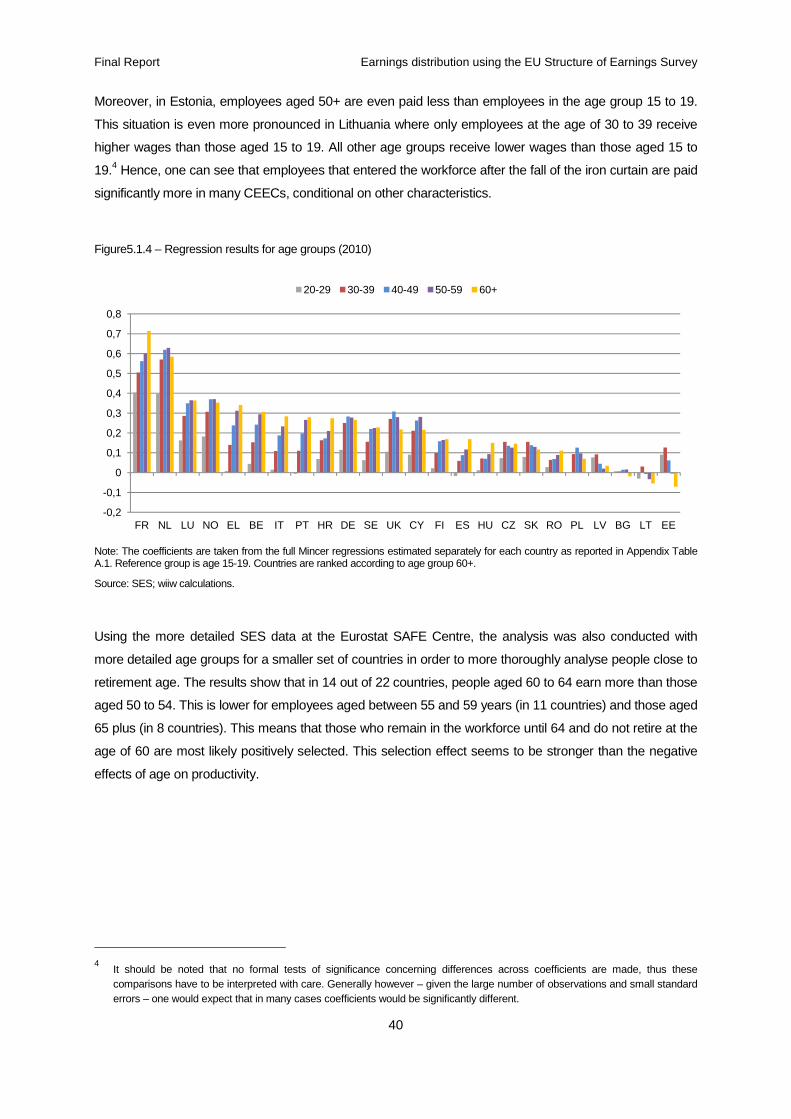
Final Report Earnings distribution using the EU Structure of Earnings Survey
40
Moreover, in Estonia, employees aged 50+ are even paid less than employees in the age group 15 to 19.
This situation is even more pronounced in Lithuania where only employees at the age of 30 to 39 receive
higher wages than those aged 15 to 19. All other age groups receive lower wages than those aged 15 to
19.4 Hence, one can see that employees that entered the workforce after the fall of the iron curtain are paid
significantly more in many CEECs, conditional on other characteristics.
Figure5.1.4 – Regression results for age groups (2010)
Note: The coefficients are taken from the full Mincer regressions estimated separately for each country as reported in Appendix Table A.1. Reference group is age 15-19. Countries are ranked according to age group 60+.
Source: SES; wiiw calculations.
Using the more detailed SES data at the Eurostat SAFE Centre, the analysis was also conducted with
more detailed age groups for a smaller set of countries in order to more thoroughly analyse people close to
retirement age. The results show that in 14 out of 22 countries, people aged 60 to 64 earn more than those
aged 50 to 54. This is lower for employees aged between 55 and 59 years (in 11 countries) and those aged
65 plus (in 8 countries). This means that those who remain in the workforce until 64 and do not retire at the
age of 60 are most likely positively selected. This selection effect seems to be stronger than the negative
effects of age on productivity.
4 It should be noted that no formal tests of significance concerning differences across coefficients are made, thus these
comparisons have to be interpreted with care. Generally however – given the large number of observations and small standard errors – one would expect that in many cases coefficients would be significantly different.
-0,2
-0,1
0
0,1
0,2
0,3
0,4
0,5
0,6
0,7
0,8
FR NL LU NO EL BE IT PT HR DE SE UK CY FI ES HU CZ SK RO PL LV BG LT EE
20-29 30-39 40-49 50-59 60+
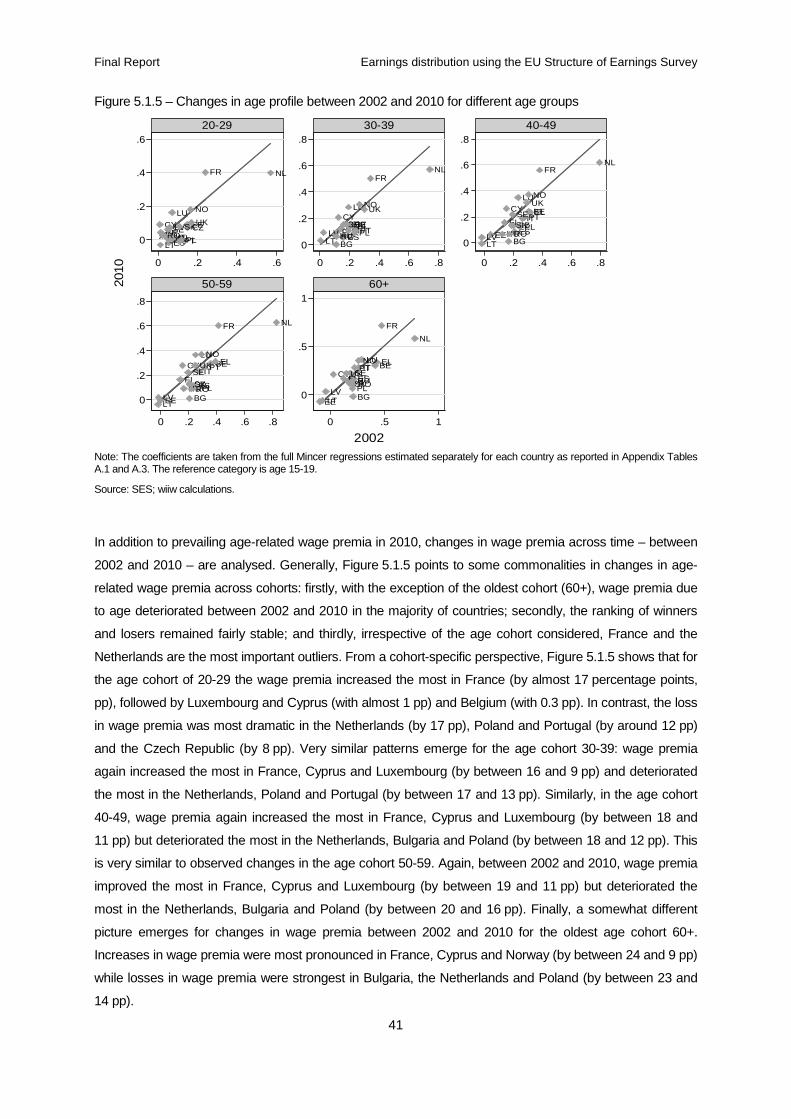
Final Report Earnings distribution using the EU Structure of Earnings Survey
41
Figure 5.1.5 – Changes in age profile between 2002 and 2010 for different age groups
Note: The coefficients are taken from the full Mincer regressions estimated separately for each country as reported in Appendix Tables A.1 and A.3. The reference category is age 15-19.
Source: SES; wiiw calculations.
In addition to prevailing age-related wage premia in 2010, changes in wage premia across time – between
2002 and 2010 – are analysed. Generally, Figure 5.1.5 points to some commonalities in changes in age-
related wage premia across cohorts: firstly, with the exception of the oldest cohort (60+), wage premia due
to age deteriorated between 2002 and 2010 in the majority of countries; secondly, the ranking of winners
and losers remained fairly stable; and thirdly, irrespective of the age cohort considered, France and the
Netherlands are the most important outliers. From a cohort-specific perspective, Figure 5.1.5 shows that for
the age cohort of 20-29 the wage premia increased the most in France (by almost 17 percentage points,
pp), followed by Luxembourg and Cyprus (with almost 1 pp) and Belgium (with 0.3 pp). In contrast, the loss
in wage premia was most dramatic in the Netherlands (by 17 pp), Poland and Portugal (by around 12 pp)
and the Czech Republic (by 8 pp). Very similar patterns emerge for the age cohort 30-39: wage premia
again increased the most in France, Cyprus and Luxembourg (by between 16 and 9 pp) and deteriorated
the most in the Netherlands, Poland and Portugal (by between 17 and 13 pp). Similarly, in the age cohort
40-49, wage premia again increased the most in France, Cyprus and Luxembourg (by between 18 and
11 pp) but deteriorated the most in the Netherlands, Bulgaria and Poland (by between 18 and 12 pp). This
is very similar to observed changes in the age cohort 50-59. Again, between 2002 and 2010, wage premia
improved the most in France, Cyprus and Luxembourg (by between 19 and 11 pp) but deteriorated the
most in the Netherlands, Bulgaria and Poland (by between 20 and 16 pp). Finally, a somewhat different
picture emerges for changes in wage premia between 2002 and 2010 for the oldest age cohort 60+.
Increases in wage premia were most pronounced in France, Cyprus and Norway (by between 24 and 9 pp)
while losses in wage premia were strongest in Bulgaria, the Netherlands and Poland (by between 23 and
14 pp).
BEBG
CY CZEE
ELESFI
FR
HUITLT
LU
LV
NL
NO
PLPTRO
SESKUK BE
BG
CYCZEEEL
ESFI
FR
HUIT
LT
LU
LV
NL
NO
PLPTRO
SESK
UK BE
BG
CY
CZEE
EL
ESFI
FR
HU
IT
LT
LU
LV
NL
NO
PLPT
RO
SESK
UK
BE
BG
CY
CZ
EE
EL
ESFI
FR
HU
IT
LT
LU
LV
NL
NO
PL
PT
RO
SE
SK
UK BE
BG
CYCZ
EE
EL
ESFI
FR
HU
IT
LT
LU
LV
NL
NO
PL
PT
ROSESK
UK
0
.2
.4
.6
0
.2
.4
.6
.8
0
.2
.4
.6
.8
0
.2
.4
.6
.8
0
.5
1
0 .2 .4 .6 0 .2 .4 .6 .8 0 .2 .4 .6 .8
0 .2 .4 .6 .8 0 .5 1
20-29 30-39 40-49
50-59 60+2010
2002

Final Report Earnings distribution using the EU Structure of Earnings Survey
42
Again the contribution of age-related wage differences to the overall wage inequality as measured by the
Gini index is considered.5 Figure 5.1.6 highlights that, in line with the results from the Mincer regressions,
the decomposition analysis again reveals that wage inequality due to age differences is well below average
in all CEECs. In 2010, the contribution of age to inequality was relatively high in the Netherlands (14%),
Norway (12%), Belgium (10%) and Greece (10%). In other countries, its contribution to inequality is around
5% on average with slightly higher values for Sweden, Italy and France and lower ones for Estonia and
Spain. Between 2002 and 2010, the contributions of wage differences due to age declined particularly in
the Netherlands, Belgium, Greece, Spain, Romania and Portugal and increased significantly in Norway and
France.
Figure 5.1.6 – Contribution of age differences to Gini index (in %)
Note: Countries are ranked according to contribution to Gini in 2010.
Source: SES; wiiw calculations.
5.1.3 Education
---In what follows, the education dimension is analysed, by discussing the returns to education. Generally,
the average returns to education (relative to the group with only primary education) in the sample of EU
countries in 2010, after controlling for other characteristics, are as follows – in ascending order: 2% for
lower secondary education, 9% for upper and post secondary education, 19% for short cycle tertiary
education, 33% for Bachelor and Master (or equivalent) and, finally, 51% for Doctoral (or equivalent).6
Figure 5.1.7 highlights that this ranking of returns to education is replicated in the majority of countries. The
only exceptions are Poland and the Czech Republic, where the returns to a Bachelor or Master’s degree
are higher than the returns to Doctoral degrees.
5 The Blinder-Oaxaca decomposition is not considered in this case because there are not two clear groups when considering the
age-wage premium. 6 These are unweighted averages across countries. Coefficients not statistically significant at the 5% level were set to zero.
0
2
4
6
8
10
12
14
16
18
20
NL NO BE EL SE IT FR UK LU PT CY FI DE EE ES HR PL CZ SK HU LV LT RO BG
2002 2006 2010

Final Report Earnings distribution using the EU Structure of Earnings Survey
43
The lowest returns to education are found in Anglo-Saxon and Scandinavian countries, where employees
with a Doctoral degree receive a premia of only around 20%. In contrast, wage premia for employees with
a Doctoral degree is highest in Portugal and Croatia where they earn, on average, almost twice as much as
employees with primary education only.
Figure 5.1.7 – Regression results for education groups (2010)
Note: The coefficients are taken from the full Mincer regressions estimated separately for each country as reported in Appendix Table A.1. The reference group is primary educated (ISCED 0-1). Countries are ranked according to educational group “Doctoral (or equivalent)”. For Germany different educational categories are reported (see Table 3.1.3).
Source: SES; wiiw calculations.
-0,2
0
0,2
0,4
0,6
0,8
1
1,2
PT HR RO LT LV EE BE CY NL SK LU FR FI EL IT BG NO PL CZ SE ES UK DE HU
Lower secondary Upper and post secondary Short cycle tertiary
Bachelor and Master (or equivalent) Doctoral (or equivalent)

Final Report Earnings distribution using the EU Structure of Earnings Survey
44
Figure 5.1.8 – Changes in returns to education between 2002 and 2010
Note: The coefficients are taken from the full Mincer regressions estimated separately for each country as reported in Appendix Tables A.1 and A.3. The reference group is primary education (ISCED 0-1).
Source: SES; wiiw calculations.
Changes in the returns to education between 2002 and 2010 are depicted in Figure 5.1.8. Generally, the
figure highlights that between 2002 and 2010, the returns to education increased in the majority of
countries, irrespective of the level of education considered. However, changes were stronger among higher
levels of education and most pronounced in the highest level of educational attainment. In addition, it
demonstrates that changes in the returns to education were most diverse and pronounced among CEECs.
Moreover, from the perspective of the individual level of education, different patterns emerge, both in terms
of ranking as well as the extent of change. Specifically, returns to lower secondary education increased the
most in Lithuania (by around 12 pp), followed by Bulgaria and Cyprus by around 10 and 6 pp, respectively,
In contrast, returns to lower secondary education deteriorated the most in Hungary (by 16 pp), followed by
the Czech Republic and Romania at around 8 pp. Returns to upper and post secondary education
increased the most in Lithuania (by 8 pp), followed by Bulgaria (by around 10 pp) and Belgium (by around
6 pp). In contrast, returns to upper and post secondary education dropped the most in Hungary and
Romania (by around 11 pp) and Poland (by around 6 pp). Returns to short-cycle tertiary education
improved the most in Portugal, Belgium and Slovakia (by between 17 and 10 pp) but deteriorated the most
in Romania, Hungary and the Netherlands (by between 26 and 6 pp). Between 2002 and 2010, returns to
Bachelors or Masters increased the most in Cyprus, Belgium and Lithuania (by between 17 and 12 pp) but
dropped the most in Romania, the Czech Republic and Hungary (by between 27 and 9 pp). Finally, returns
to the highest level of education, i.e. doctor’s degree, improved the most in the Baltics (Latvia and Lithuania
BE
BG
CY
CZ
EEELES
FR
HU
IT
LT
LULV
NL
NO
PLPT
ROSE
BE
BG
CY
CZ
EEELES
FI
FR
HU
ITLTLU
LV
NL
NO PL
PT
ROSE
SK
UKBE
BG
CY
CZEE EL
ESFI
FR HUITLTLULV
NL
NO
PT
ROSE
SK
UK
BE
BGCY
CZEE EL
ESFIFR
HU
IT
LT
LULV NL
NO
PL
PT
RO
SE
SK
UK
BE
BG
CY
CZ
EE
EL
ES
FI FRIT
LT
LU
LVNL
NO
PL
RO
SE
SK
UK
-.1
0
.1
.2
-.1
0
.1
.2
0
.2
.4
.6
0
.2
.4
.6
.2
.4
.6
.8
1
-.1 -.05 0 .05 .1 -.1 0 .1 .2 0 .2 .4
.2 .4 .6 .2 .4 .6 .8 1
Lower secondary Upper & post secondary Short cycle tertiary
Bachelor and Master Doctoral2010
2002
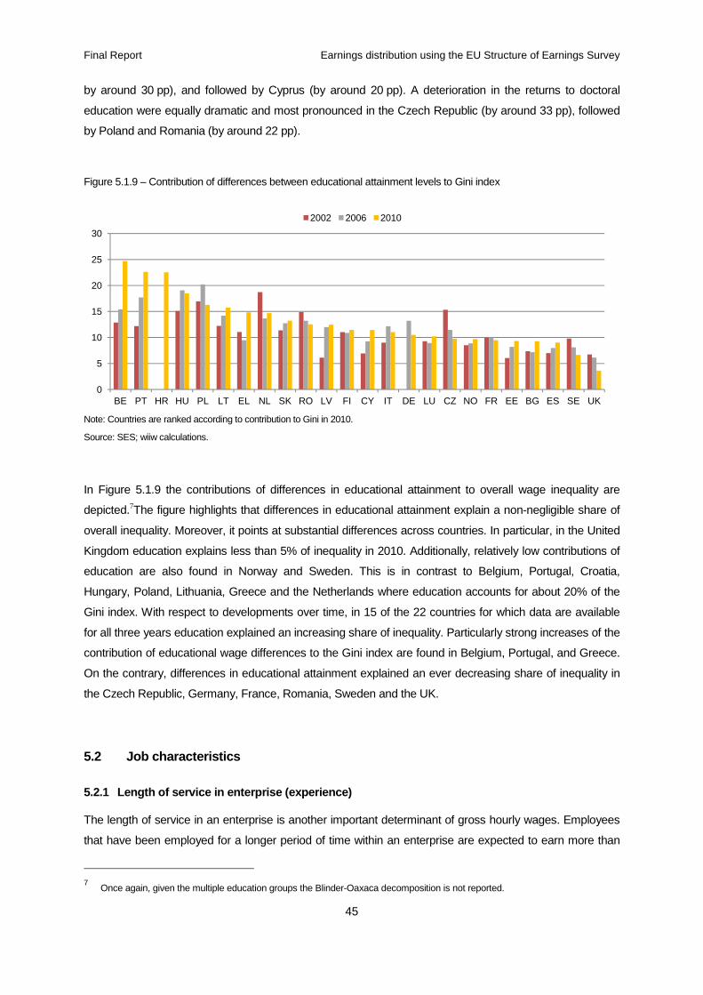
Final Report Earnings distribution using the EU Structure of Earnings Survey
45
by around 30 pp), and followed by Cyprus (by around 20 pp). A deterioration in the returns to doctoral
education were equally dramatic and most pronounced in the Czech Republic (by around 33 pp), followed
by Poland and Romania (by around 22 pp).
Figure 5.1.9 – Contribution of differences between educational attainment levels to Gini index
Note: Countries are ranked according to contribution to Gini in 2010.
Source: SES; wiiw calculations.
In Figure 5.1.9 the contributions of differences in educational attainment to overall wage inequality are
depicted.7The figure highlights that differences in educational attainment explain a non-negligible share of
overall inequality. Moreover, it points at substantial differences across countries. In particular, in the United
Kingdom education explains less than 5% of inequality in 2010. Additionally, relatively low contributions of
education are also found in Norway and Sweden. This is in contrast to Belgium, Portugal, Croatia,
Hungary, Poland, Lithuania, Greece and the Netherlands where education accounts for about 20% of the
Gini index. With respect to developments over time, in 15 of the 22 countries for which data are available
for all three years education explained an increasing share of inequality. Particularly strong increases of the
contribution of educational wage differences to the Gini index are found in Belgium, Portugal, and Greece.
On the contrary, differences in educational attainment explained an ever decreasing share of inequality in
the Czech Republic, Germany, France, Romania, Sweden and the UK.
5.2 Job characteristics
5.2.1 Length of service in enterprise (experience)
The length of service in an enterprise is another important determinant of gross hourly wages. Employees
that have been employed for a longer period of time within an enterprise are expected to earn more than
7 Once again, given the multiple education groups the Blinder-Oaxaca decomposition is not reported.
0
5
10
15
20
25
30
BE PT HR HU PL LT EL NL SK RO LV FI CY IT DE LU CZ NO FR EE BG ES SE UK
2002 2006 2010

Final Report Earnings distribution using the EU Structure of Earnings Survey
46
comparable employees in terms of age, education, etc. with less experience in the enterprise. One
advantage of experienced employees is that they have a great deal of firm specific knowledge – regarding
organisational processes, they know who to talk to in case of problems and they are experienced in
handling the daily challenges of their specific job in the enterprise. New employees still have to learn how
the land lies. In addition, employees acquire non-firm-specific knowledge in the fields they are working in.
This is especially true for higher skilled employees and research personnel, where tacit knowledge plays a
major role (Moen, 2005). Once they have acquired additional knowledge, they might be tempted to set up
or join a rival. In order to minimise knowledge outflows and possible knowledge transfers to competitors,
employers thus pay a wage premium in order to keep employees from leaving the enterprise. Again, this
wage premium is expected to be higher for higher skilled personnel.
Figure 5.2.1 – Wage premia depending on length of service in enterprise (2010)
Note: The coefficients are taken from the full Mincer regressions estimated separately for each country as reported in Appendix Table A.1. The reference group is the group of employees with less than a year of service with a firm. Countries are ranked according to group 15+.
Source: SES; wiiw calculations.
Figure 5.2.1 shows wage premia of employees by length of service in the enterprise (relative to those, who
have been with the enterprise for less than a year) in 2010. The median wage premium across countries
for 1-4 years of employment in the same firm is 6%. For 5-14 years, the median effect rises to 11% and for
more than 15 years it is 18%. However, there are a number of notable outliers. In particular, the premium at
less than 10% is much lower in Scandinavian countries. Moreover, Cyprus, Luxembourg, Germany, Spain
and Greece exhibit rather high premia where employees that have been employed for more than 15 years
in the same enterprise earn around 30% more than similar employees that have been with the enterprise
for less than a year. In the Netherlands, the premia seem to be very high for all three groups, but this is in
fact due to the small number of observations for employees with less than one year of service in the
enterprise.
Figure 5.2.2 depicts changes in service-time-related premia between 2002 and 2010 to shed light on how
premia have changed over time. Generally, it points to a pretty diverse and heterogeneous picture.
0
0,1
0,2
0,3
0,4
0,5
0,6
NL CY LU DE ES EL RO HU PT LT CZ HR BG LV PL IT SK FR UK BE FI EE SE NO
1-4 years 5-15 years 15 + years
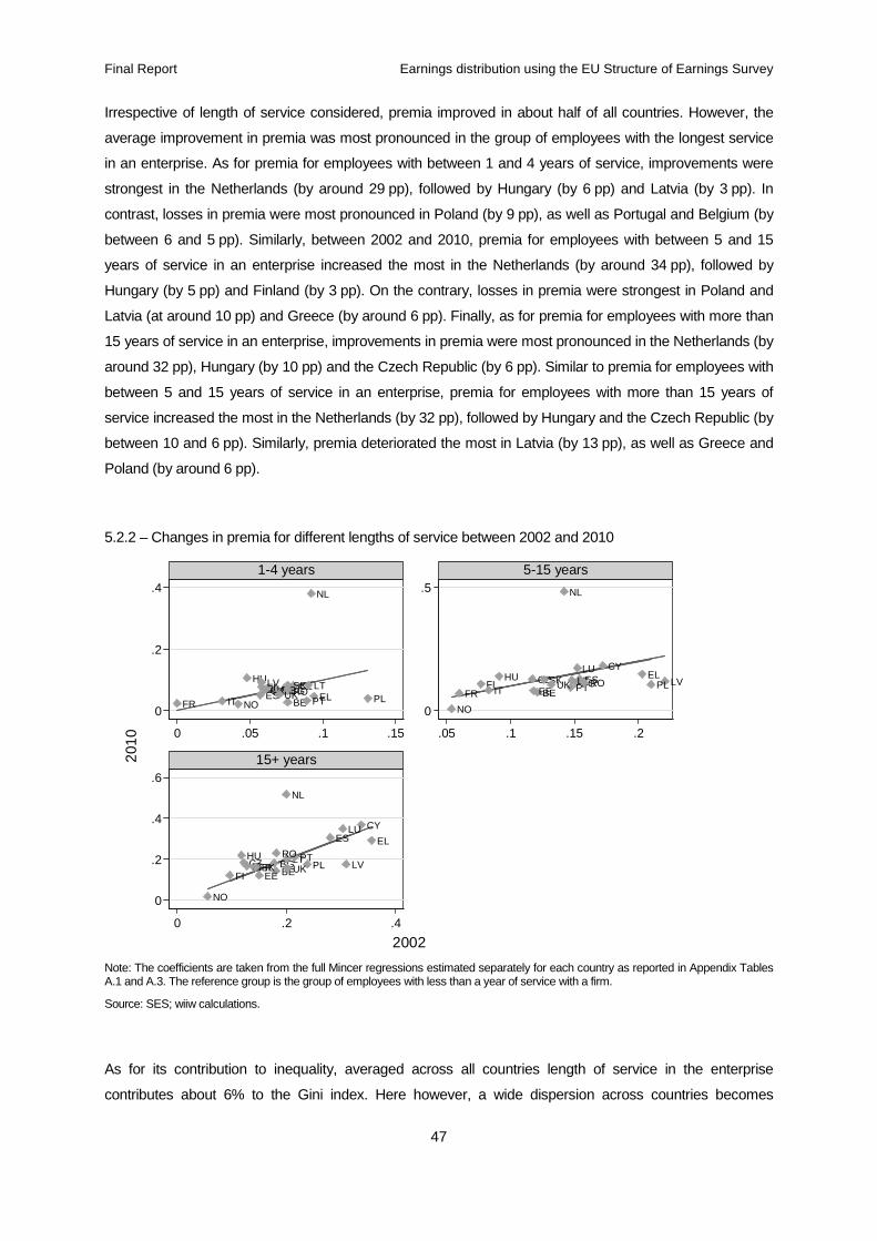
Final Report Earnings distribution using the EU Structure of Earnings Survey
47
Irrespective of length of service considered, premia improved in about half of all countries. However, the
average improvement in premia was most pronounced in the group of employees with the longest service
in an enterprise. As for premia for employees with between 1 and 4 years of service, improvements were
strongest in the Netherlands (by around 29 pp), followed by Hungary (by 6 pp) and Latvia (by 3 pp). In
contrast, losses in premia were most pronounced in Poland (by 9 pp), as well as Portugal and Belgium (by
between 6 and 5 pp). Similarly, between 2002 and 2010, premia for employees with between 5 and 15
years of service in an enterprise increased the most in the Netherlands (by around 34 pp), followed by
Hungary (by 5 pp) and Finland (by 3 pp). On the contrary, losses in premia were strongest in Poland and
Latvia (at around 10 pp) and Greece (by around 6 pp). Finally, as for premia for employees with more than
15 years of service in an enterprise, improvements in premia were most pronounced in the Netherlands (by
around 32 pp), Hungary (by 10 pp) and the Czech Republic (by 6 pp). Similar to premia for employees with
between 5 and 15 years of service in an enterprise, premia for employees with more than 15 years of
service increased the most in the Netherlands (by 32 pp), followed by Hungary and the Czech Republic (by
between 10 and 6 pp). Similarly, premia deteriorated the most in Latvia (by 13 pp), as well as Greece and
Poland (by around 6 pp).
5.2.2 – Changes in premia for different lengths of service between 2002 and 2010
Note: The coefficients are taken from the full Mincer regressions estimated separately for each country as reported in Appendix Tables A.1 and A.3. The reference group is the group of employees with less than a year of service with a firm.
Source: SES; wiiw calculations.
As for its contribution to inequality, averaged across all countries length of service in the enterprise
contributes about 6% to the Gini index. Here however, a wide dispersion across countries becomes
BEBGCY CZEE
ELESFI
FR
HU
IT
LTLULV
NL
NOPLPT
ROSK
UK BEBG
CYCZEE
ELESFIFR
HUIT
LTLU
LV
NL
NO
PLPT ROSKUK
BEBG
CY
CZEE
ELES
FIFR
HUIT
LT
LU
LV
NL
NO
PLPTRO
SK UK
0
.2
.4
0
.5
0
.2
.4
.6
0 .05 .1 .15 .05 .1 .15 .2
0 .2 .4
1-4 years 5-15 years
15+ years2010
2002

Final Report Earnings distribution using the EU Structure of Earnings Survey
48
apparent (see Figure 5.2.3). Especially in the Mediterranean countries (i.e. Cyprus, Spain and Greece)
wage differences are strongly influenced by this factor. Although there is a substantial fall in the premium of
job duration in Greece, the wage difference due to age and job duration combined still amount to 22% of
the Gini in 2010. Above average contributions of the characteristic length of service can be observed for
Germany and Luxembourg. Substantial below average contributions are found for the Scandinavian
countries, Norway and Sweden, and Estonia.
Figure 5.2.3 – Contribution of differences between lengths of service in enterprise to Gini index
Note: Countries are ranked according to contribution to Gini in 2010.
Source: SES; wiiw calculations.
5.2.2 Contract type
In this subsection the effect of contract type on wages is considered. Results from the Mincer regressions
(Figure 5.2.4) indicate that employees with a contract that is temporary or has a fixed duration earn on
average 4.7% less than those with a contract of indefinite duration. While this wage difference between the
two types of contract did not change during the crisis, the number of temporary contracts increased
significantly in most countries. In 2010, the biggest difference between contract types could be found in
Poland, Croatia, the Netherlands and the Czech Republic, where employees with temporary or fixed
contracts earned between 9 to 13% less than those with indefinite contracts. In contrast, people employed
with a temporary or fixed contract in the Baltics earn more than people employed with contracts of indefinite
duration. More specifically, while in Latvia, employees on fixed or temporary contracts earned around 7%
more than those on indefinite contracts, in Lithuania, they earned around 4% more.8
As for the change in the wage differential between 2002 and 2010 for contracts with fixed duration, Figure
5.2.5 points at a rather heterogeneous picture. It shows that wage differentials for fixed contracts improved
in 10 out of 19 cases. More specifically, wage differentials for fixed contracts increased the most in
8 The results for trainees are reported in the regression results in the Appendix tables.
0
2
4
6
8
10
12
14
16
18
EL CY ES LU DE BE IT FR CZ NL HU PT FI RO LT HR PL BG SK LV UK SE EE NO
2002 2006 2010
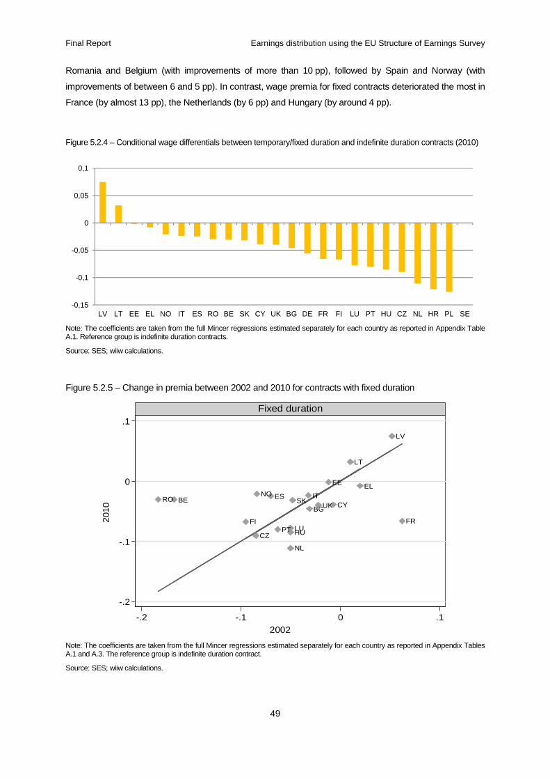
Final Report Earnings distribution using the EU Structure of Earnings Survey
49
Romania and Belgium (with improvements of more than 10 pp), followed by Spain and Norway (with
improvements of between 6 and 5 pp). In contrast, wage premia for fixed contracts deteriorated the most in
France (by almost 13 pp), the Netherlands (by 6 pp) and Hungary (by around 4 pp).
Figure 5.2.4 – Conditional wage differentials between temporary/fixed duration and indefinite duration contracts (2010)
Note: The coefficients are taken from the full Mincer regressions estimated separately for each country as reported in Appendix Table A.1. Reference group is indefinite duration contracts.
Source: SES; wiiw calculations.
Figure 5.2.5 – Change in premia between 2002 and 2010 for contracts with fixed duration
Note: The coefficients are taken from the full Mincer regressions estimated separately for each country as reported in Appendix Tables A.1 and A.3. The reference group is indefinite duration contract.
Source: SES; wiiw calculations.
-0,15
-0,1
-0,05
0
0,05
0,1
LV LT EE EL NO IT ES RO BE SK CY UK BG DE FR FI LU PT HU CZ NL HR PL SE
BEBG
CY
CZ
EE EL
ES
FI FR
HU
IT
LT
LU
LV
NL
NO
PT
RO SKUK
-.2
-.1
0
.1
-.2 -.1 0 .1
Fixed duration
2010
2002
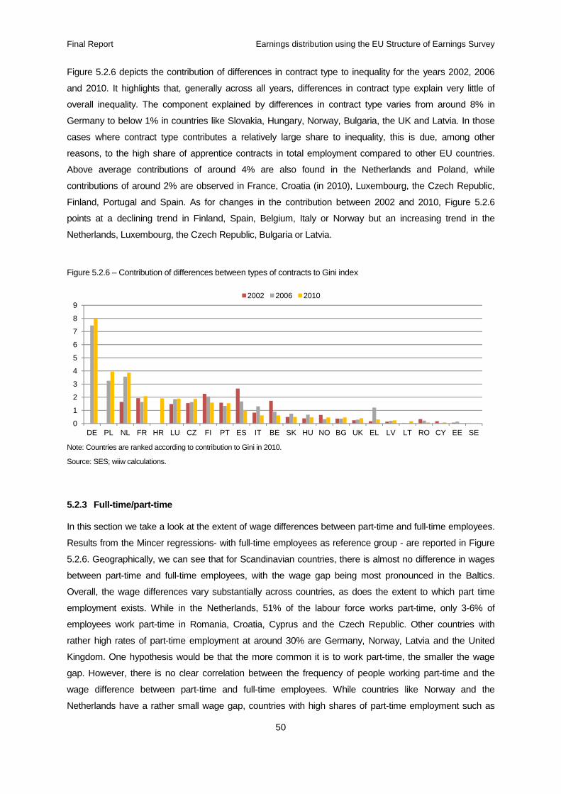
Final Report Earnings distribution using the EU Structure of Earnings Survey
50
Figure 5.2.6 depicts the contribution of differences in contract type to inequality for the years 2002, 2006
and 2010. It highlights that, generally across all years, differences in contract type explain very little of
overall inequality. The component explained by differences in contract type varies from around 8% in
Germany to below 1% in countries like Slovakia, Hungary, Norway, Bulgaria, the UK and Latvia. In those
cases where contract type contributes a relatively large share to inequality, this is due, among other
reasons, to the high share of apprentice contracts in total employment compared to other EU countries.
Above average contributions of around 4% are also found in the Netherlands and Poland, while
contributions of around 2% are observed in France, Croatia (in 2010), Luxembourg, the Czech Republic,
Finland, Portugal and Spain. As for changes in the contribution between 2002 and 2010, Figure 5.2.6
points at a declining trend in Finland, Spain, Belgium, Italy or Norway but an increasing trend in the
Netherlands, Luxembourg, the Czech Republic, Bulgaria or Latvia.
Figure 5.2.6 – Contribution of differences between types of contracts to Gini index
Note: Countries are ranked according to contribution to Gini in 2010.
Source: SES; wiiw calculations.
5.2.3 Full-time/part-time
In this section we take a look at the extent of wage differences between part-time and full-time employees.
Results from the Mincer regressions- with full-time employees as reference group - are reported in Figure
5.2.6. Geographically, we can see that for Scandinavian countries, there is almost no difference in wages
between part-time and full-time employees, with the wage gap being most pronounced in the Baltics.
Overall, the wage differences vary substantially across countries, as does the extent to which part time
employment exists. While in the Netherlands, 51% of the labour force works part-time, only 3-6% of
employees work part-time in Romania, Croatia, Cyprus and the Czech Republic. Other countries with
rather high rates of part-time employment at around 30% are Germany, Norway, Latvia and the United
Kingdom. One hypothesis would be that the more common it is to work part-time, the smaller the wage
gap. However, there is no clear correlation between the frequency of people working part-time and the
wage difference between part-time and full-time employees. While countries like Norway and the
Netherlands have a rather small wage gap, countries with high shares of part-time employment such as
0
1
2
3
4
5
6
7
8
9
DE PL NL FR HR LU CZ FI PT ES IT BE SK HU NO BG UK EL LV LT RO CY EE SE
2002 2006 2010
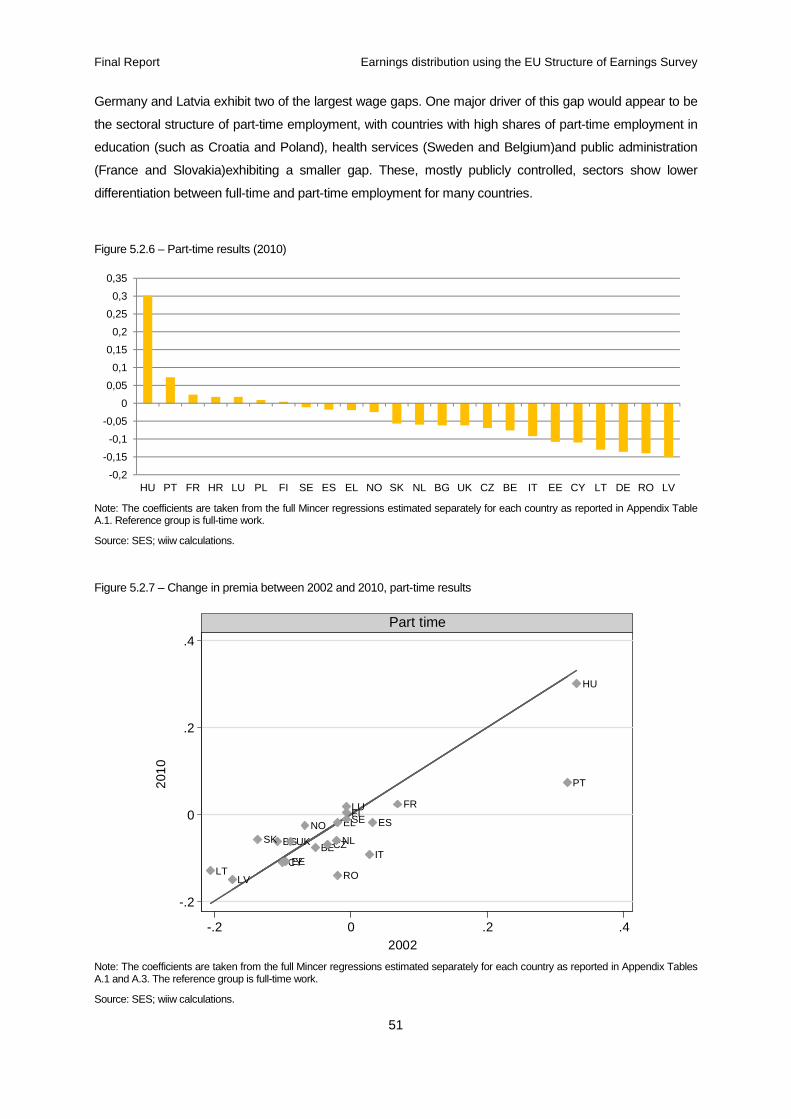
Final Report Earnings distribution using the EU Structure of Earnings Survey
51
Germany and Latvia exhibit two of the largest wage gaps. One major driver of this gap would appear to be
the sectoral structure of part-time employment, with countries with high shares of part-time employment in
education (such as Croatia and Poland), health services (Sweden and Belgium)and public administration
(France and Slovakia)exhibiting a smaller gap. These, mostly publicly controlled, sectors show lower
differentiation between full-time and part-time employment for many countries.
Figure 5.2.6 – Part-time results (2010)
Note: The coefficients are taken from the full Mincer regressions estimated separately for each country as reported in Appendix Table A.1. Reference group is full-time work.
Source: SES; wiiw calculations.
Figure 5.2.7 – Change in premia between 2002 and 2010, part-time results
Note: The coefficients are taken from the full Mincer regressions estimated separately for each country as reported in Appendix Tables A.1 and A.3. The reference group is full-time work.
Source: SES; wiiw calculations.
-0,2
-0,15
-0,1
-0,05
0
0,05
0,1
0,15
0,2
0,25
0,3
0,35
HU PT FR HR LU PL FI SE ES EL NO SK NL BG UK CZ BE IT EE CY LT DE RO LV
BEBG
CY
CZ
EE
EL ESFI
FR
HU
IT
LT
LU
LV
NL
NO
PT
RO
SE
SK UK
-.2
0
.2
.4
-.2 0 .2 .4
Part time
201
0
2002
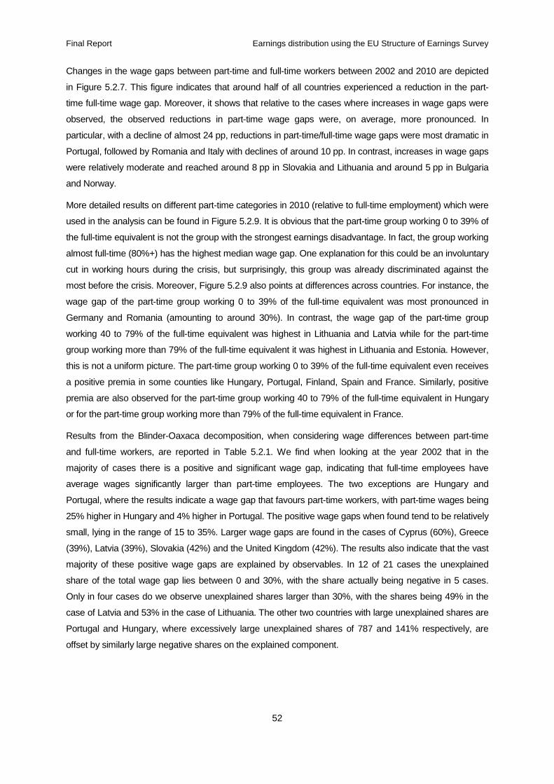
Final Report Earnings distribution using the EU Structure of Earnings Survey
52
Changes in the wage gaps between part-time and full-time workers between 2002 and 2010 are depicted
in Figure 5.2.7. This figure indicates that around half of all countries experienced a reduction in the part-
time full-time wage gap. Moreover, it shows that relative to the cases where increases in wage gaps were
observed, the observed reductions in part-time wage gaps were, on average, more pronounced. In
particular, with a decline of almost 24 pp, reductions in part-time/full-time wage gaps were most dramatic in
Portugal, followed by Romania and Italy with declines of around 10 pp. In contrast, increases in wage gaps
were relatively moderate and reached around 8 pp in Slovakia and Lithuania and around 5 pp in Bulgaria
and Norway.
More detailed results on different part-time categories in 2010 (relative to full-time employment) which were
used in the analysis can be found in Figure 5.2.9. It is obvious that the part-time group working 0 to 39% of
the full-time equivalent is not the group with the strongest earnings disadvantage. In fact, the group working
almost full-time (80%+) has the highest median wage gap. One explanation for this could be an involuntary
cut in working hours during the crisis, but surprisingly, this group was already discriminated against the
most before the crisis. Moreover, Figure 5.2.9 also points at differences across countries. For instance, the
wage gap of the part-time group working 0 to 39% of the full-time equivalent was most pronounced in
Germany and Romania (amounting to around 30%). In contrast, the wage gap of the part-time group
working 40 to 79% of the full-time equivalent was highest in Lithuania and Latvia while for the part-time
group working more than 79% of the full-time equivalent it was highest in Lithuania and Estonia. However,
this is not a uniform picture. The part-time group working 0 to 39% of the full-time equivalent even receives
a positive premia in some counties like Hungary, Portugal, Finland, Spain and France. Similarly, positive
premia are also observed for the part-time group working 40 to 79% of the full-time equivalent in Hungary
or for the part-time group working more than 79% of the full-time equivalent in France.
Results from the Blinder-Oaxaca decomposition, when considering wage differences between part-time
and full-time workers, are reported in Table 5.2.1. We find when looking at the year 2002 that in the
majority of cases there is a positive and significant wage gap, indicating that full-time employees have
average wages significantly larger than part-time employees. The two exceptions are Hungary and
Portugal, where the results indicate a wage gap that favours part-time workers, with part-time wages being
25% higher in Hungary and 4% higher in Portugal. The positive wage gaps when found tend to be relatively
small, lying in the range of 15 to 35%. Larger wage gaps are found in the cases of Cyprus (60%), Greece
(39%), Latvia (39%), Slovakia (42%) and the United Kingdom (42%). The results also indicate that the vast
majority of these positive wage gaps are explained by observables. In 12 of 21 cases the unexplained
share of the total wage gap lies between 0 and 30%, with the share actually being negative in 5 cases.
Only in four cases do we observe unexplained shares larger than 30%, with the shares being 49% in the
case of Latvia and 53% in the case of Lithuania. The other two countries with large unexplained shares are
Portugal and Hungary, where excessively large unexplained shares of 787 and 141% respectively, are
offset by similarly large negative shares on the explained component.

Final Report Earnings distribution using the EU Structure of Earnings Survey
53
Figure 5.2.9 – More detailed part-time results (2010)
Note: The coefficients are taken from the full Mincer regressions estimated separately for each country as reported in Appendix tables A.4. Reference group is full-time work. Coefficients not significant at a 5% level are set to 0.
Source: SES; wiiw calculations.
Considering the Blinder-Oaxaca results over time, we find mixed results when comparing the wage gaps
between part-time and full-time workers in 2002 and 2010. In ten cases we find that the wage gap
increased, while in 11 cases we observe that the wage gap declined. The changes in the wage gap tend to
be small in many cases. When considering those countries with an increase in the wage gap, we find
relatively large increases in Portugal (22 percentage points) and Italy (23 pp). The biggest declines in the
wage gap are found for Luxembourg and Slovakia (16 pp), with the wage gap in Luxembourg becoming
insignificant. Only in the case of Hungary (and Croatia, for which data are available in 2010) do we now find
a negative wage gap, with the wage gap in Portugal changing from -25% in 2002 to 7% in 2010. As with
2002 however, the vast majority of the wage gap can usually be explained by observables. Only in 3 out of
23 countries do we find that unexplained factors can explain more than 50% of the share of the observed
wage gap (Germany, Hungary and Latvia), with negative shares observed in 6 cases.
-0,30
-0,10
0,10
0,30
0,50
0,70
HU FR LU SE FI PT EL BE NO ES IT DE PL SK NL CZ BG RO CY EE LV LT
0-39% 40-79% 80%+
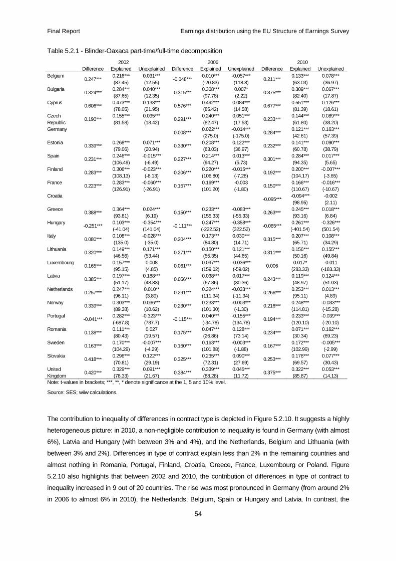
Final Report Earnings distribution using the EU Structure of Earnings Survey
54
Table 5.2.1 - Blinder-Oaxaca part-time/full-time decomposition
2002 2006 2010 Difference Explained Unexplained Difference Explained Unexplained Difference Explained Unexplained
Belgium 0.247***
0.216*** (87.45)
0.031*** (12.55)
-0.048*** 0.010*** (-20.83)
-0.057*** (118.8)
0.211*** 0.133*** (63.03)
0.078*** (36.97)
Bulgaria 0.324***
0.284*** (87.65)
0.040*** (12.35)
0.315*** 0.308*** (97.78)
0.007* (2.22)
0.375*** 0.309*** (82.40)
0.067*** (17.87)
Cyprus 0.606***
0.473*** (78.05)
0.133*** (21.95)
0.576*** 0.492*** (85.42)
0.084*** (14.58)
0.677*** 0.551*** (81.39)
0.126*** (18.61)
Czech Republic
0.190*** 0.155*** (81.58)
0.035*** (18.42)
0.291*** 0.240*** (82.47)
0.051*** (17.53)
0.233*** 0.144*** (61.80)
0.089*** (38.20)
Germany 0.008***
0.022*** (275.0)
-0.014*** (-175.0)
0.284*** 0.121*** (42.61)
0.163*** (57.39)
Estonia 0.339***
0.268*** (79.06)
0.071*** (20.94)
0.330*** 0.208*** (63.03)
0.122*** (36.97)
0.232*** 0.141*** (60.78)
0.090*** (38.79)
Spain 0.231***
0.246*** (106.49)
-0.015*** (-6.49)
0.227*** 0.214*** (94.27)
0.013*** (5.73)
0.301*** 0.284*** (94.35)
0.017*** (5.65)
Finland 0.283***
0.306*** (108.13)
-0.023*** (-8.13)
0.206*** 0.220*** (106.80)
-0.015*** (-7.28)
0.192*** 0.200*** (104.17)
-0.007*** (-3.65)
France 0.223***
0.283*** (126.91)
-0.060*** (-26.91)
0.167*** 0.169*** (101.20)
-0.003 (-1.80)
0.150*** 0.166*** (110.67)
-0.016*** (-10.67)
Croatia -0.095***
-0.094*** (98.95)
-0.002 (2.11)
Greece 0.388***
0.364*** (93.81)
0.024*** (6.19)
0.150*** 0.233*** (155.33)
-0.083*** (-55.33)
0.263*** 0.245*** (93.16)
0.018*** (6.84)
Hungary -0.251***
0.103*** (-41.04)
-0.354*** (141.04)
-0.111*** 0.247*** (-222.52)
-0.358*** (322.52)
-0.065*** 0.261*** (-401.54)
-0.326*** (501.54)
Italy 0.080***
0.108*** (135.0)
-0.028*** (-35.0)
0.204*** 0.173*** (84.80)
0.030*** (14.71)
0.315*** 0.207*** (65.71)
0.108*** (34.29)
Lithuania 0.320***
0.149*** (46.56)
0.171*** (53.44)
0.271*** 0.150*** (55.35)
0.121*** (44.65)
0.311*** 0.156*** (50.16)
0.155*** (49.84)
Luxembourg 0.165***
0.157*** (95.15)
0.008 (4.85)
0.061*** 0.097*** (159.02)
-0.036*** (-59.02)
0.006 0.017*
(283.33) -0.011
(-183.33) Latvia
0.385*** 0.197*** (51.17)
0.188*** (48.83)
0.056*** 0.038*** (67.86)
0.017*** (30.36)
0.243*** 0.119*** (48.97)
0.124*** (51.03)
Netherlands 0.257***
0.247*** (96.11)
0.010** (3.89)
0.291*** 0.324*** (111.34)
-0.033*** (-11.34)
0.266*** 0.253*** (95.11)
0.013*** (4.89)
Norway 0.339***
0.303*** (89.38)
0.036*** (10.62)
0.230*** 0.233*** (101.30)
-0.003*** (-1.30)
0.216*** 0.248*** (114.81)
-0.033*** (-15.28)
Portugal -0.041***
0.282*** (-687.8)
-0.323*** (787.7)
-0.115*** 0.040*** (-34.78)
-0.155*** (134.78)
0.194*** 0.233*** (120.10)
-0.039*** (-20.10)
Romania 0.138***
0.111*** (80.43)
0.027 (19.57)
0.175*** 0.047*** (26.86)
0.128*** (73.14)
0.234*** 0.071*** (30.34)
0.162*** (69.23)
Sweden 0.163***
0.170*** (104.29)
-0.007*** (-4.29)
0.160*** 0.163*** (101.88)
-0.003*** (-1.88)
0.167*** 0.172*** (102.99)
-0.005*** (-2.99)
Slovakia 0.418***
0.296*** (70.81)
0.122*** (29.19)
0.325*** 0.235*** (72.31)
0.090*** (27.69)
0.253*** 0.176*** (69.57)
0.077*** (30.43)
United Kingdom
0.420*** 0.329*** (78.33)
0.091*** (21.67)
0.384*** 0.339*** (88.28)
0.045*** (11.72)
0.375*** 0.322*** (85.87)
0.053*** (14.13)
Note: t-values in brackets; ***, **, * denote significance at the 1, 5 and 10% level.
Source: SES; wiiw calculations.
The contribution to inequality of differences in contract type is depicted in Figure 5.2.10. It suggests a highly
heterogeneous picture: in 2010, a non-negligible contribution to inequality is found in Germany (with almost
6%), Latvia and Hungary (with between 3% and 4%), and the Netherlands, Belgium and Lithuania (with
between 3% and 2%). Differences in type of contract explain less than 2% in the remaining countries and
almost nothing in Romania, Portugal, Finland, Croatia, Greece, France, Luxembourg or Poland. Figure
5.2.10 also highlights that between 2002 and 2010, the contribution of differences in type of contract to
inequality increased in 9 out of 20 countries. The rise was most pronounced in Germany (from around 2%
in 2006 to almost 6% in 2010), the Netherlands, Belgium, Spain or Hungary and Latvia. In contrast, the

Final Report Earnings distribution using the EU Structure of Earnings Survey
55
contribution of differences in type of contract to inequality decreased most substantially in Norway (from
initially 4% in 2002 to 1% in 2010), Lithuania and the UK.
Figure 5.2.10 – Contribution of differences between full- and part-time employees to Gini index (in %)
Note: Countries are ranked according to contribution to Gini index in 2010.
Source: SES; wiiw calculations.
5.2.4 Occupations
In the past several years, there has been much discussion regarding wages, and in particular the bonuses
of managers. In the regression analysis, occupations are captured according to the International Standard
Classification of Occupations (ISCO) at the one digit level. Conditional wage premia by occupation were
calculated relative to elementary occupations (e.g. cleaners, construction labourers, unskilled agricultural,
forestry and fishery workers, etc). In 2010, the ordering of average wage premia by occupation are as
follows – from lowest to highest: 3% for skilled agricultural, forestry and fishery workers, 11% for service
and sales, 12% for plant and machine operators and assemblers, 15% for craft and related workers, 19%
for clerical support, 35% for technicians, 50% for professionals (which include scientists, engineers, health
professionals, teachers and university professors as well as business, legal and IT professionals) and 73%
for managers.9
Apparently, the two occupations with the highest wage premia conditional on education, age and other
characteristics are managers and professionals. In particular, managers earn the highest premia in
Romania (102%), Cyprus (99%), Luxembourg (96%), Bulgaria (92%) and Portugal (92%), with relatively
low premia to managers found in Greece, the Netherlands, Norway (around 50%) and in Latvia (around
40%). The group of professionals earn the highest premia in the UK (69%), followed by Romania (66%),
Bulgaria (63%), Italy (61%) and Portugal (59%).
9 These are unweighted averages across countries.
0
1
2
3
4
5
6
7
DE LV HU NL BE LT IT UK EE ES NO BG CY SE SK CZ RO PT FI HR EL FR LU PL
2002 2006 2010
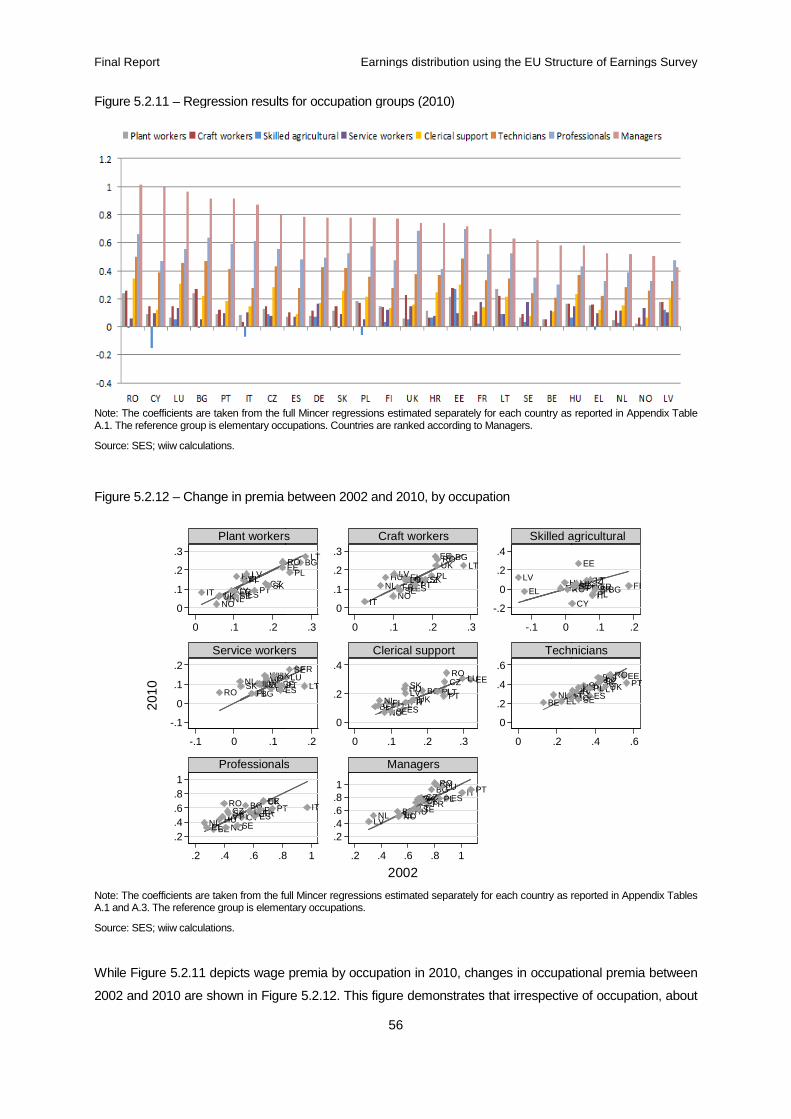
Final Report
Figure 5.2.11 – Regression results for occupation groups (2010)
Note: The coefficients are taken from the full Mincer regressions estimated separately for each country A.1. The reference group is elementary occupations. Countries are ranked according to Managers.
Source: SES; wiiw calculations.
Figure 5.2.12 – Change in premia between 2002 and 2010, by occupation
Note: The coefficients are taken from the full Mincer regressions estimated A.1 and A.3. The reference group is elementary occupations.
Source: SES; wiiw calculations.
While Figure 5.2.11 depicts wage premia by occupation in 2010, c
2002 and 2010 are shown in Figure 5.2.12.
CYCZEL
ES
FIFR
HU
IT LU
LV
NLNO
PTSE
SKUK
BGCYCZEEEL
ESFIHU
ITLVNL NO
PLPT
ROSK
UK
BE
BGCY
CZEE
ELESFI FR
HULTLU
LVNL NO
PL PTRO
SE
SKUK
0
.1
.2
.3
-.1
0
.1
.2
.2
.4
.6
.81
0 .1 .2
-.1 0 .1
.2 .4 .6 .8
Plant workers
Service workers
Professionals
2010
Earnings distribution using the EU Structure of Earnings Survey
56
Regression results for occupation groups (2010)
: The coefficients are taken from the full Mincer regressions estimated separately for each country as reported in Appendixelementary occupations. Countries are ranked according to Managers.
Change in premia between 2002 and 2010, by occupation
The coefficients are taken from the full Mincer regressions estimated separately for each country as reported in Appendix Tables A.1 and A.3. The reference group is elementary occupations.
While Figure 5.2.11 depicts wage premia by occupation in 2010, changes in occupational premia between
02 and 2010 are shown in Figure 5.2.12. This figure demonstrates that irrespective of occupation, about
BGEE
LT
PLRO
BG
CYCZ
EE
ELESFI
FRHU
IT
LT
LULV
NLNO
PLPT
RO
SESK
UK
EL ESHU
LVRO
CZEEES
FR
LTLU
PT
SEUK
BE
BG
CY
CZ EE
ELESFI FR
HU
ITLT
LU
LVNL
NO
PLPT
RO
SE
SK
UK BE ELNL
ITPT BE
BGCY
CZEE
EL
ESFI FRHU
IT
LT
LU
LVNL NO
PLPT
RO
SESKUK
0
.1
.2
.3
-.2
0
.2
.4
0
.2
.4
0
.2
.4
.6
.2
.4
.6
.81
.3 0 .1 .2 .3 -.1 0
.2 0 .1 .2 .3 0 .2
.8 1 .2 .4 .6 .8 1
Plant workers Craft workers Skilled agricultural
Service workers Clerical support Technicians
Professionals Managers
2002
Earnings distribution using the EU Structure of Earnings Survey
as reported in Appendix Table
separately for each country as reported in Appendix Tables
hanges in occupational premia between
demonstrates that irrespective of occupation, about
BG
CY
CZ
EE
ES FIFRHU
IT
LTNL NO
PLPTROSE SK
UK
BGCY CZ EE
ELESFIFRHU
ITLTLU
LVNO
PLPT
RO
SE
SKUK
.1 .2
.4 .6
Skilled agricultural
Technicians
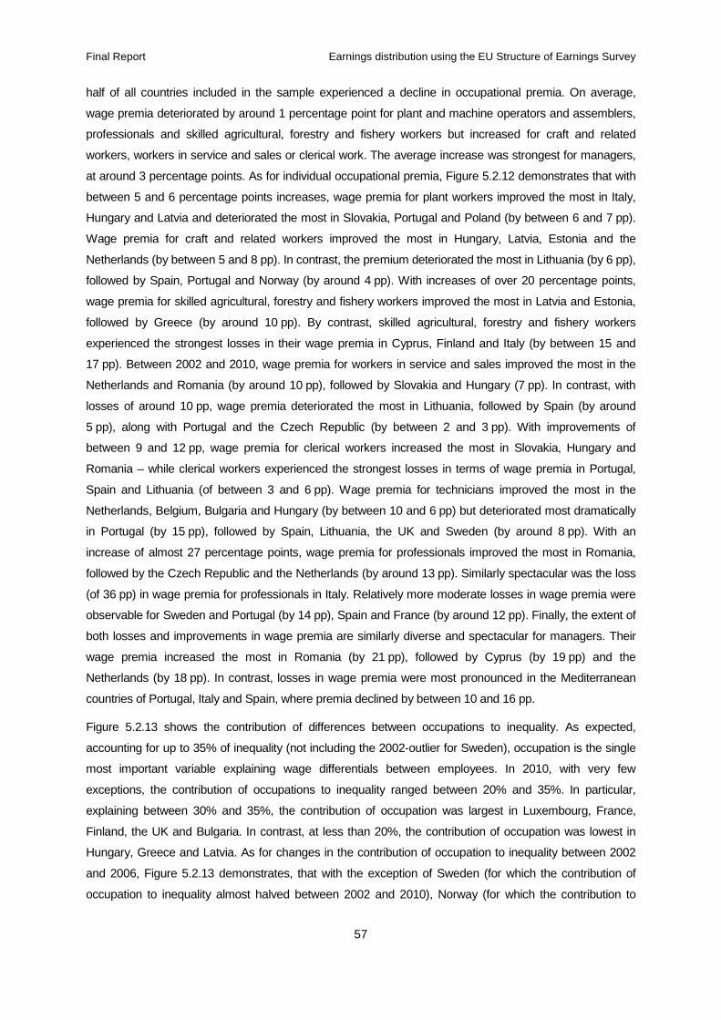
Final Report Earnings distribution using the EU Structure of Earnings Survey
57
half of all countries included in the sample experienced a decline in occupational premia. On average,
wage premia deteriorated by around 1 percentage point for plant and machine operators and assemblers,
professionals and skilled agricultural, forestry and fishery workers but increased for craft and related
workers, workers in service and sales or clerical work. The average increase was strongest for managers,
at around 3 percentage points. As for individual occupational premia, Figure 5.2.12 demonstrates that with
between 5 and 6 percentage points increases, wage premia for plant workers improved the most in Italy,
Hungary and Latvia and deteriorated the most in Slovakia, Portugal and Poland (by between 6 and 7 pp).
Wage premia for craft and related workers improved the most in Hungary, Latvia, Estonia and the
Netherlands (by between 5 and 8 pp). In contrast, the premium deteriorated the most in Lithuania (by 6 pp),
followed by Spain, Portugal and Norway (by around 4 pp). With increases of over 20 percentage points,
wage premia for skilled agricultural, forestry and fishery workers improved the most in Latvia and Estonia,
followed by Greece (by around 10 pp). By contrast, skilled agricultural, forestry and fishery workers
experienced the strongest losses in their wage premia in Cyprus, Finland and Italy (by between 15 and
17 pp). Between 2002 and 2010, wage premia for workers in service and sales improved the most in the
Netherlands and Romania (by around 10 pp), followed by Slovakia and Hungary (7 pp). In contrast, with
losses of around 10 pp, wage premia deteriorated the most in Lithuania, followed by Spain (by around
5 pp), along with Portugal and the Czech Republic (by between 2 and 3 pp). With improvements of
between 9 and 12 pp, wage premia for clerical workers increased the most in Slovakia, Hungary and
Romania – while clerical workers experienced the strongest losses in terms of wage premia in Portugal,
Spain and Lithuania (of between 3 and 6 pp). Wage premia for technicians improved the most in the
Netherlands, Belgium, Bulgaria and Hungary (by between 10 and 6 pp) but deteriorated most dramatically
in Portugal (by 15 pp), followed by Spain, Lithuania, the UK and Sweden (by around 8 pp). With an
increase of almost 27 percentage points, wage premia for professionals improved the most in Romania,
followed by the Czech Republic and the Netherlands (by around 13 pp). Similarly spectacular was the loss
(of 36 pp) in wage premia for professionals in Italy. Relatively more moderate losses in wage premia were
observable for Sweden and Portugal (by 14 pp), Spain and France (by around 12 pp). Finally, the extent of
both losses and improvements in wage premia are similarly diverse and spectacular for managers. Their
wage premia increased the most in Romania (by 21 pp), followed by Cyprus (by 19 pp) and the
Netherlands (by 18 pp). In contrast, losses in wage premia were most pronounced in the Mediterranean
countries of Portugal, Italy and Spain, where premia declined by between 10 and 16 pp.
Figure 5.2.13 shows the contribution of differences between occupations to inequality. As expected,
accounting for up to 35% of inequality (not including the 2002-outlier for Sweden), occupation is the single
most important variable explaining wage differentials between employees. In 2010, with very few
exceptions, the contribution of occupations to inequality ranged between 20% and 35%. In particular,
explaining between 30% and 35%, the contribution of occupation was largest in Luxembourg, France,
Finland, the UK and Bulgaria. In contrast, at less than 20%, the contribution of occupation was lowest in
Hungary, Greece and Latvia. As for changes in the contribution of occupation to inequality between 2002
and 2006, Figure 5.2.13 demonstrates, that with the exception of Sweden (for which the contribution of
occupation to inequality almost halved between 2002 and 2010), Norway (for which the contribution to

Final Report Earnings distribution using the EU Structure of Earnings Survey
58
inequality dropped slightly by around 7 pp) and Spain or Hungary (for which almost negligible reductions
are observable), the contribution of occupation to inequality increased between 2002 and 2010.
Specifically, the increase was most pronounced in Bulgaria, Italy, Romania, Estonia and Latvia but weakest
in the UK, Poland or Portugal.
Figure 5.2.13 – Contribution of differences between occupations to Gini index (in %)
Note: Countries are ranked according to contribution to Gini in 2010.
Source: SES; wiiw calculations.
5.3 Firm characteristics
5.3.1 Firm size
A vast literature using firm-level data indicates that a number of firm characteristics (such as size, trading
status, foreign ownership, etc.) are correlated with various indicators of firm performance (e.g. productivity,
profits, wages, employment). In this sub-section we discuss the relationship between firm size and wages.
Figure 5.3.1 reports estimates of wage differentials by firm size for 2010 from the Mincer regressions.
Relative to small firms (with less than 50 employees), large firms (with more than 250 employees) pay up to
42% higher wages while medium-sized firms (with between 50 and 249 employees) pay up to 35% higher
wages. The figure also indicates strongly diverging size-premia across countries. In particular, size-wage
premia appear to be highest among CEECs but lowest among the remaining EU-countries. For instance, at
42%, the size-wage premia paid by large firms are highest in Latvia and Bulgaria, followed by Romania and
Lithuania (with wage-size premia ranging between 35 and 40%), Hungary and the Czech Republic (with
size-wage premia slightly above 25%), Poland and Slovakia (with size-wage premia around 20%). Size-
wage premia of large firms are below 10% in the Netherlands, France, Norway, Finland and Belgium, and
are even below 5% in Sweden. Similarly, size-wage premia paid by medium-sized firms are again highest
in Latvia (at around 35%), followed by Lithuania, Romania, the Czech Republic, Hungary and Bulgaria
0
5
10
15
20
25
30
35
40
45
LU FR FI UK BG IT RO EE PL CZ PT SE CY SK ES BE NO DE LT NL HR HU EL LV
2002 2006 2010

Final Report Earnings distribution using the EU Structure of Earnings Survey
59
(ranging between 25% and 15%). With less than 10%, size-wage premia of medium-sized firms are lowest
in Belgium, Croatia, France and Sweden.
Figure 5.3.1 – Relative wage by firm size categories (2010)
Note: The coefficients are taken from the full Mincer regressions estimated separately for each country as reported in Appendix Table A.1. Reference group is size 1-45. Ranked according to coefficient for 250+.
Source: SES; wiiw calculations.
Figure 5.3.2 depicts changes in wage premia between 2002 and 2010. It shows that in around half of the
countries in the sample, the wage premium paid by medium-sized firms (with between 50 and 249
employees) increased between 2002 and 2010. In particular, at nearly 15 percentage points, it increased
the most in the Czech Republic, followed by Poland (with an increase of around 6 pp), Spain and Lithuania
(with increases of around 4 pp). In contrast, wage-premia paid by medium-sized firms deteriorated the most
in Portugal and Greece (by around 5 pp), Belgium (by around 3 pp), and Italy and France (with around
2 pp). The wage premium remained almost unchanged in Bulgaria, the Netherlands and Finland. Wage
premia paid by large firms deteriorated in the majority of countries. The loss in the wage premium was most
pronounced in Latvia (by 18 pp), followed by Portugal (by 10 pp), Romania (by 7 pp) and Greece (by 6 pp).
In contrast, no changes in the wage premia paid by large firms occurred in Norway while wage premia rose
the most in the Czech Republic (by around 15 pp), followed by more moderate increases in Poland (by
around 7 pp), Bulgaria (by 5 pp), and the Netherlands, Lithuania and the UK (by around 2 to 3 pp).
0
0,05
0,1
0,15
0,2
0,25
0,3
0,35
0,4
0,45
LV BG RO LT HU CZ PL SK ES DE UK EL IT PT HR NL FR NO FI BE SE
50-249 250+
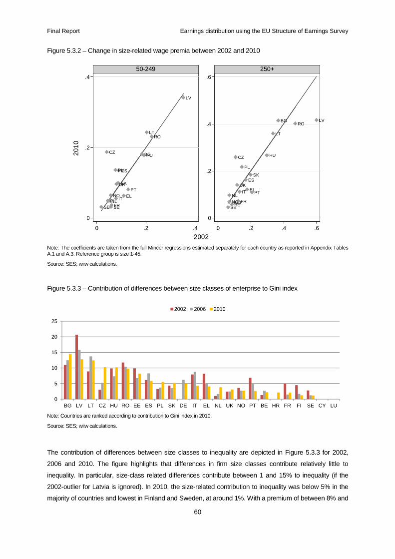
Final Report Earnings distribution using the EU Structure of Earnings Survey
60
Figure 5.3.2 – Change in size-related wage premia between 2002 and 2010
Note: The coefficients are taken from the full Mincer regressions estimated separately for each country as reported in Appendix Tables A.1 and A.3. Reference group is size 1-45.
Source: SES; wiiw calculations.
Figure 5.3.3 – Contribution of differences between size classes of enterprise to Gini index
Note: Countries are ranked according to contribution to Gini index in 2010.
Source: SES; wiiw calculations.
The contribution of differences between size classes to inequality are depicted in Figure 5.3.3 for 2002,
2006 and 2010. The figure highlights that differences in firm size classes contribute relatively little to
inequality. In particular, size-class related differences contribute between 1 and 15% to inequality (if the
2002-outlier for Latvia is ignored). In 2010, the size-related contribution to inequality was below 5% in the
majority of countries and lowest in Finland and Sweden, at around 1%. With a premium of between 8% and
BE
BGCZ
EL
ES
FIFR
HU
IT
LT
LV
NLNO
PL
PT
RO
SE
SKUK
BE
BG
CZ
EL
ES
FIFR
HU
IT
LT
LV
NL
NO
PL
PT
RO
SE
SK
UK
0
.2
.4
0
.2
.4
.6
0 .2 .4 0 .2 .4 .6
50-249 250+20
10
2002
0
5
10
15
20
25
BG LV LT CZ HU RO EE ES PL SK DE IT EL NL UK NO PT BE HR FR FI SE CY LU
2002 2006 2010

Final Report Earnings distribution using the EU Structure of Earnings Survey
61
15%, it was highest among a group of CEECs comprising Bulgaria, Latvia, Lithuania, the Czech Republic,
Hungary, Romania and Estonia. As for the change in the size-related contribution to inequality, Figure 5.3.3
emphasises that between 2002 and 2010 the contribution of wage differences between size classes
decreased in the majority of countries. The decrease was most pronounced in Latvia, Greece, France and
Finland and almost negligible in Spain and Norway. By comparison, increases were strongest in the Czech
Republic, Lithuania and Bulgaria.
5.3.2 Public and private control
Another interesting aspect to consider is the wage gap between enterprises that are either under public or
private economic and financial control. Figure 5.3.4 reports the estimated coefficients on a private sector
dummy from the Mincer regressions for 2010. Overall, a rather heterogeneous picture emerges.
Specifically, in about half of all countries, publicly controlled firms pay more than privately owned ones. In
particular, the wage advantage in publicly owned firms is most pronounced in Italy (with almost 15%),
followed by Belgium and Croatia (with around 6%) or Poland and Portugal (with almost 5%). Relative to
privately owned firms, publicly owned firms pay least generously in Estonia (giving rise to a premia of 10%),
followed by Finland, Bulgaria and Sweden.
Figure 5.3.4 – Wages of privately controlled employers relative to publicly controlled employers (2010)
Note: The coefficients are taken from the full Mincer regressions estimated separately for each country as reported in Appendix Table A.1. Reference group is public ownership.
Source: SES; wiiw calculations.
Figure 5.3.5 depicts changes between 2002 and 2010 in the wage gap between privately and publicly
controlled enterprises. It highlights that in 12 out of 21 cases, the wage gap declined between 2002 and
2010. The most pronounced reductions are observable for Belgium, where the wage gap dropped by
around 23 percentage points, followed by Hungary, Cyprus, Slovakia and Spain where wage gaps dropped
by between 12 and 15 pp. By comparison, ownership-related wage gaps increased the most in Bulgaria
(by almost 19 pp), followed by Latvia (by 12 pp), France (by around 10 pp), and Estonia and Finland (by
around 8 pp). Ownership-related wage premia remained fairly stable in a number of countries including
Greece, the Czech Republic, the Netherlands and Poland.
-0,15
-0,1
-0,05
0
0,05
0,1
0,15
EE FI BG SE SK LV DE FR NL EL LT NO CZ UK RO HU PT PL HR BE IT

Final Report Earnings distribution using the EU Structure of Earnings Survey
62
Figure 5.3.5 – Change in the ownership wage gap between 2002 and 2010
Note: The coefficients are taken from the full Mincer regressions estimated separately for each country as reported in Appendix Tables A.1 and A.3. Reference group is public ownership.
Source: SES; wiiw calculations.
Results from the Blinder-Oaxaca decomposition of wage differences between publicly and privately owned
enterprises are reported in Table 5.3.1. The results indicate that in 2002 the wage gap favoured public
sector employees in the majority of cases (i.e. 17 out of 21 cases). These positive wage gaps were found
to be relatively large for Greece (46%), Bulgaria (32%), Latvia (45%), Poland (31%), Portugal (74%) and
Romania (37%). In contrast, in very few cases (i.e. Finland, Hungary, Sweden and Slovakia) does a wage
gap in favour of the private sector emerge. The extent to which these wage gaps can be explained by
observable characteristics varies greatly across the sample of countries considered. For two countries only
(Sweden and the Czech Republic) observable characteristics explain more than 100% of the wage gap
between employees in publicly and privately owned enterprises, while for five countries (Belgium, France,
Lithuania, the Netherlands and Norway) unobservable factors explain more than 100% of this wage gap.
Unexplained factors also account for a relatively large share of the wage gap (i.e. above 50%) in Estonia,
Finland, Hungary, Latvia, Slovakia and the United Kingdom. In the majority of cases (13 out of 21) a decline in
the wage gap is observable between 2002 and 2010. These declines were relatively large in Latvia (by 39 pp),
Romania (by 32 pp), Greece (by 26 pp) and France (by 25 pp). In the remaining eight countries increases in the wage
gap between 2002 and 2010 are observable, which are highest for Belgium (by 28 pp). For Germany, a negative wage
gap for 2010 emerges, indicating that employees in privately owned enterprises earn more than those in publicly owned
enterprises, while for Croatia in 2010 a positive wage gap is observed. As for 2002 there is a great deal of heterogeneity
in the extent to which these wage gaps can be explained by observable characteristics. For France, Croatia, Hungary,
Lithuania, Romania and Slovakia the results indicate that observable characteristics explain more than 100% of the
wage gap, while for Germany, Estonia, Latvia and Norway unexplained factors account for more than 100% of the
wage gap. In another two countries (Bulgaria and Croatia) unexplained factors account for more than 50% of the
observed wage gap.
BE
BG
CY
CZ
EE
EL
ES
FI
FR
HU
IT
LT
LV
NLNO
PL PTRO
SE
SK
UK
-.2
0
.2
-.2 0 .2
Private
201
0
2002

Final Report Earnings distribution using the EU Structure of Earnings Survey
63
Table 5.3.1 - Blinder-Oaxaca enterprise control decomposition
2002 2006 2010 Difference Explained Unexplained Difference Explained Unexplained Difference Explained Unexplained
Belgium 0.040*** -0.328*** (-820.00)
0.369*** (922.50)
0.328*** 0.345*** (105.18)
-0.016 (-4.88)
0.329*** 0.231*** (70.21)
0.097** (29.48)
Bulgaria 0.323*** 0.250*** (77.40)
0.073*** (22.60)
0.303*** 0.181*** (59.74)
0.122*** (40.26)
0.193*** 0.096*** (49.74)
0.097*** (50.26)
Cyprus 0.266*** 0.157*** (59.02)
0.109*** (40.98)
0.388*** 0.593*** (152.84)
-0.205 (-52.84)
0.420*** 0.332*** (79.05)
0.088*** (20.95)
Czech Republic
0.078*** 0.088*** (112.82)
-0.010*** (-12.82)
0.038*** 0.012*** (31.58)
0.026*** (68.42)
0.059*** 0.021*** (35.59)
0.038*** (64.41)
Germany 0.193*** 0.210*** (108.81)
-0.017*** (-8.81)
-0.008*** 0.040*** (-500.00)
-0.047*** (587.50)
Estonia 0.174*** 0.003 (1.72)
0.171*** (98.28)
-0.015*** 0.075*** (-500.00)
-0.090*** (600.00)
0.062*** -0.038*** (-61.29)
0.100*** (161.29)
Spain 0.265*** 0.259*** (97.74)
0.007 (2.64)
0.324*** 0.276*** (85.19)
0.048*** (14.81)
0.279*** 0.201*** (72.04)
0.079*** (28.32)
Finland -0.036*** -0.016*** (44.44)
-0.019*** (52.78)
-0.133*** -0.070*** (52.63)
-0.064*** (48.12)
-0.112*** -0.064*** (57.14)
-0.048*** (42.86)
France 0.146*** -0.007 (-4.79)
0.154*** (105.48)
0.020*** -0.185*** (-925.00)
0.205*** (1025.00)
-0.112*** -0.159*** (141.96)
0.046*** (-41.07)
Greece 0.463*** 0.282*** (60.91)
0.181*** (39.09)
0.331*** 0.330*** (99.70)
0.002 (0.60)
0.204*** 0.123*** (60.29)
0.081*** (39.71)
Croatia 0.198*** 0.234*** (118.18)
-0.036*** (-18.18)
Hungary -0.080*** -0.007 (8.75)
-0.073*** (91.25)
0.336*** 0.171*** (50.89)
0.165*** (49.11)
-0.025*** -0.083*** (332.00)
0.058*** (-232.00)
Italy 0.195*** 0.189*** (96.92)
0.007 (3.59)
0.354*** 0.359*** (101.41)
-0.005 (-1.41)
0.343*** 0.285*** (83.09)
0.057*** (16.62)
Lithuania 0.236*** -0.033*** (-13.98)
0.269*** (113.98)
0.254*** 0.336*** (132.28)
-0.082* (-32.28)
0.175*** 0.184*** (105.14)
-0.01 (-5.71)
Latvia 0.451*** 0.217*** (48.12)
0.234*** (51.88)
0.190*** 0.181*** (95.26)
0.01 (5.26)
0.069*** -0.032 (-46.38)
0.101*** (146.38)
Netherlands 0.126*** -0.063*** (-50.00)
0.189*** (150.00)
0.178*** 0.166*** (93.26)
0.012 (6.74)
0.203*** 0.133 (65.52)
0.07 (34.48)
Norway 0.051*** -0.004 (-7.84)
0.055*** (107.84)
0.068*** 0.001 (1.47)
0.067*** (98.68)
0.037*** -0.045*** (-121.62)
0.081*** (218.92)
Poland 0.307*** 0.219*** (71.34)
0.088*** (28.66)
0.364*** 0.321*** (88.19)
0.042*** (11.54)
0.340*** 0.333*** (97.94)
0.007** (2.06)
Portugal 0.740*** 0.534*** (72.16)
0.207*** (27.97)
0.629*** 0.598*** (95.07)
0.031* (4.93)
0.555*** 0.532*** (95.86)
0.023 (4.14)
Romania 0.366*** 0.328*** (89.62)
0.039*** (10.66)
0.443*** 0.297*** (67.04)
0.146*** (32.96)
0.045*** 0.050*** (111.11)
-0.004 (-8.89)
Sweden -0.086*** -0.090*** (104.65)
0.005*** (-5.81)
-0.095*** -0.094*** (98.95)
-0.001 (1.05)
-0.095*** -0.056*** (58.95)
-0.040*** (42.11)
Slovakia -0.136*** -0.009* (6.62)
-0.127*** (93.38)
0.016*** 0.140*** (875.00)
-0.124*** (-775.00)
0.018*** 0.111*** (616.67)
-0.093*** (-516.67)
United Kingdom
0.087*** 0.031 (35.63)
0.055** (63.22)
0.109*** 0.072** (66.06)
0.037 (33.94)
0.176*** 0.170*** (96.59)
0.006 (3.41)
Note: t-values in brackets; ***, **, * denotes significance at the 1, 5 and 10% level.
Source: SES; wiiw calculations.
Figure 5.3.6 reports results of the Shapley decomposition for the public-private ownership distinction.
Differences between public and privately owned enterprises are found to be, in general, low conditional on
all other explanatory variables. In 2010, the contribution to inequality was above 2% in only five countries: it
was highest in Cyprus (with only 8%), followed by Italy, Spain, Sweden and Finland (with around 4%). For
the remaining countries, the contribution was below 2%. Moreover, in some countries the inclusion of the
variable in the decomposition analysis actually lowers the general wage differences, which leads to a
negative contribution of the characteristic, which is the case for Bulgaria in 2006, Greece in 2002, Latvia in
2002 and Portugal in 2002. The contribution of conditional wage differences to total inequality however
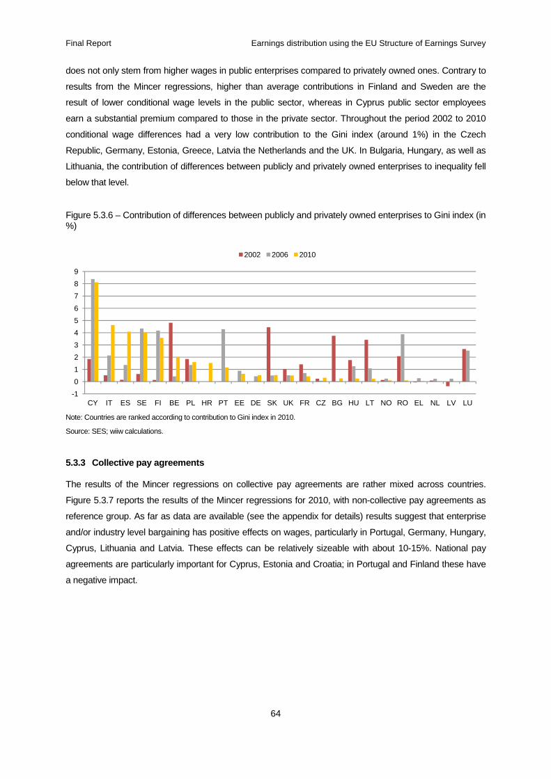
Final Report Earnings distribution using the EU Structure of Earnings Survey
64
does not only stem from higher wages in public enterprises compared to privately owned ones. Contrary to
results from the Mincer regressions, higher than average contributions in Finland and Sweden are the
result of lower conditional wage levels in the public sector, whereas in Cyprus public sector employees
earn a substantial premium compared to those in the private sector. Throughout the period 2002 to 2010
conditional wage differences had a very low contribution to the Gini index (around 1%) in the Czech
Republic, Germany, Estonia, Greece, Latvia the Netherlands and the UK. In Bulgaria, Hungary, as well as
Lithuania, the contribution of differences between publicly and privately owned enterprises to inequality fell
below that level.
Figure 5.3.6 – Contribution of differences between publicly and privately owned enterprises to Gini index (in %)
Note: Countries are ranked according to contribution to Gini index in 2010.
Source: SES; wiiw calculations.
5.3.3 Collective pay agreements
The results of the Mincer regressions on collective pay agreements are rather mixed across countries.
Figure 5.3.7 reports the results of the Mincer regressions for 2010, with non-collective pay agreements as
reference group. As far as data are available (see the appendix for details) results suggest that enterprise
and/or industry level bargaining has positive effects on wages, particularly in Portugal, Germany, Hungary,
Cyprus, Lithuania and Latvia. These effects can be relatively sizeable with about 10-15%. National pay
agreements are particularly important for Cyprus, Estonia and Croatia; in Portugal and Finland these have
a negative impact.
-1
0
1
2
3
4
5
6
7
8
9
CY IT ES SE FI BE PL HR PT EE DE SK UK FR CZ BG HU LT NO RO EL NL LV LU
2002 2006 2010

Final Report
Figure 5.3.7 – Wage effects of collective pay agreements (2010)
Note: The coefficients are taken from the full Mincer regressions estimated separately A.1. Reference group is non-collective pay agreements
Source: SES; wiiw calculations.
Figure 5.3.8 reports the contribution to inequality of differences between the wages of employees working
in enterprise units covered by collective agreements and those who are not covered by collective
agreements. The results indicate that such differences explain a
majority of countries. Explaining up to 12% (in 2002) and 9% (in 2010) it is, however, relatively high in
Cyprus, along with Portugal, Germany, Hungary and Spain. For Portugal, the regression results show that
contrary to expectations conditional wage levels are lower for employees covered by collective agreements
compared to employees who are not covered, which also resulted in
inequality. For Germany and Spain, due to higher remu
also above the average of all countries for all years considered. In Bulgaria this was only the case in 2002
and 2006. On the contrary, particularly low contributions to inequality
Italy (both after 2002), as well as Croatia, Estonia, Finland, Lithuania, Norway, Poland and Romania.
Earnings distribution using the EU Structure of Earnings Survey
65
Wage effects of collective pay agreements (2010)
The coefficients are taken from the full Mincer regressions estimated separately for each country as reported in Appendixcollective pay agreements. Countries are ranked according to Enterprise.
reports the contribution to inequality of differences between the wages of employees working
in enterprise units covered by collective agreements and those who are not covered by collective
agreements. The results indicate that such differences explain a relatively small share of inequality in the
majority of countries. Explaining up to 12% (in 2002) and 9% (in 2010) it is, however, relatively high in
Cyprus, along with Portugal, Germany, Hungary and Spain. For Portugal, the regression results show that
ntrary to expectations conditional wage levels are lower for employees covered by collective agreements
compared to employees who are not covered, which also resulted in its high contribution to overall
inequality. For Germany and Spain, due to higher remuneration in covered enterprises,
also above the average of all countries for all years considered. In Bulgaria this was only the case in 2002
and 2006. On the contrary, particularly low contributions to inequality of below 1% are found
Italy (both after 2002), as well as Croatia, Estonia, Finland, Lithuania, Norway, Poland and Romania.
Earnings distribution using the EU Structure of Earnings Survey
as reported in Appendix Table
reports the contribution to inequality of differences between the wages of employees working
in enterprise units covered by collective agreements and those who are not covered by collective
relatively small share of inequality in the
majority of countries. Explaining up to 12% (in 2002) and 9% (in 2010) it is, however, relatively high in
Cyprus, along with Portugal, Germany, Hungary and Spain. For Portugal, the regression results show that
ntrary to expectations conditional wage levels are lower for employees covered by collective agreements
its high contribution to overall
neration in covered enterprises, the contribution is
also above the average of all countries for all years considered. In Bulgaria this was only the case in 2002
of below 1% are found in Belgium and
Italy (both after 2002), as well as Croatia, Estonia, Finland, Lithuania, Norway, Poland and Romania.

Final Report Earnings distribution using the EU Structure of Earnings Survey
66
Figure 5.3.8 – Contribution of differences due to collective pay agreements to Gini index (in %)
Note: Countries are ranked according to contribution to Gini index in 2010. Source: SES; wiiw calculations.
5.3.4 Sectors
In the Mincer regression reported in the appendix sector dummies are included as well. As reported
above, unconditional means suggest that the mining sector (NACE Rev. 1 10-14) pays highest wages
on average. This also holds for the conditional results as presented in Table 5.3.2. In Figure 5.3.9
cross-country averages are reported due to wide cross-country differences. The wage gaps are lowest
with around with around10-15% in sectors like utilities (electrical energy, etc.), financial services and
coke, chemicals and rubber and plastics industry. Even in high-tech sectors, like electronics, these
gaps are substantial with around 20%. The largest conditional gaps are observed for personal and
public services, retail trade and hotel and restaurants.
0
2
4
6
8
10
12
14
CY PT DE HU ES CZ LV FR UK LU RO LT BE SK EE HR EL NO BG PL FI IT NL SE
2002 2006 2010

Final Report Earnings distribution using the EU Structure of Earnings Survey
67
Table 5.3.2 – Coefficients of industry dummies, 2010
Belgium Bulgaria Cyprus Czech
Republic Germany Estonia Spain Finland France Greece Croatia Hungary 15_16 -0.106*** -0.326*** -0.348*** -0.263*** -0.342*** -0.387*** -0.197*** -0.020 -0.088*** -0.242*** -0.256*** 17_19 -0.158*** -0.596*** -0.550*** -0.440*** -0.320*** -0.519*** -0.326*** -0.204*** -0.154*** -0.291*** -0.397*** 20_22 -0.099*** -0.537*** -0.266*** -0.280*** -0.211*** -0.310*** -0.191*** 0.020 -0.071*** -0.259*** -0.215*** 23_25 -0.014 -0.382*** -0.254*** -0.170*** -0.045*** -0.290*** -0.050*** 0.010 0.008 -0.111*** -0.003 -0.008 26 -0.058*** -0.184*** -0.179*** -0.137*** -0.174*** -0.097*** -0.064*** -0.055*** -0.146*** -0.204*** -0.106*** 27_28 -0.055*** -0.360*** -0.257*** -0.166*** -0.158*** -0.240*** -0.095*** -0.042*** -0.066*** -0.239*** 0.138*** -0.113*** 29 -0.088*** -0.343*** -0.284*** -0.207*** -0.117*** -0.160*** -0.103*** -0.043*** -0.090*** -0.286*** 0.122*** -0.086*** 30_33 -0.088*** -0.281*** -0.273*** -0.196*** -0.125*** -0.314*** -0.157*** -0.010 -0.070*** -0.237*** -0.198*** 34_35 -0.072*** -0.315*** -0.275*** -0.086*** -0.045*** -0.227*** -0.081*** -0.053*** -0.025 -0.138*** -0.088*** 36_37 -0.126*** -0.478*** -0.256*** -0.251*** -0.286*** -0.342*** -0.204*** -0.140*** -0.115*** -0.265*** 0.128*** -0.233*** 40_41 0.139*** -0.040*** -0.259*** 0.028*** -0.026** -0.176*** -0.033** 0.055*** 0.064*** -0.036 0.013 45 -0.043*** -0.257*** -0.241*** -0.222*** -0.213*** -0.290*** -0.124*** 0.008 -0.117*** -0.234*** 0.027* -0.239*** 50_51 -0.111*** -0.222*** -0.222*** -0.116*** -0.214*** -0.253*** -0.166*** -0.009 -0.109*** -0.252*** 0.156*** -0.183*** 52 -0.196*** -0.320*** -0.404*** -0.280*** -0.316*** -0.441*** -0.280*** -0.122*** -0.219*** -0.381*** 0.105*** -0.275*** 55 -0.221*** -0.344*** -0.361*** -0.436*** -0.435*** -0.384*** -0.186*** -0.158*** -0.178*** -0.280*** 0.125*** -0.271*** 60_62 -0.068*** -0.285*** -0.133*** -0.219*** -0.326*** -0.269*** -0.113*** 0.025** -0.096*** -0.130*** 0.103*** -0.156*** 65_67 -0.047*** -0.393*** -0.091*** -0.153*** -0.105*** -0.089*** 0.044*** -0.075*** -0.141*** 0.132*** 0.016 70_74 -0.112*** -0.271*** -0.268*** -0.159*** -0.283*** -0.309*** -0.265*** -0.097*** -0.139*** -0.245*** 0.165*** -0.232*** 75 -0.416*** -0.360*** -0.255*** -0.230*** -0.269*** -0.077*** -0.228*** -0.443*** 0.077*** -0.168*** 80 -0.101*** -0.316*** -0.206*** -0.284*** -0.537*** -0.438*** -0.275*** -0.193*** -0.448*** -0.270*** -0.060*** -0.328*** 85 -0.144*** -0.412*** -0.415*** -0.223*** -0.387*** -0.271*** -0.238*** -0.098*** -0.247*** -0.404*** 0.104*** -0.296*** 90_93 -0.144*** -0.488*** -0.380*** -0.323*** -0.381*** -0.429*** -0.333*** -0.202*** -0.213*** -0.329*** 0.077*** -0.269***

Final Report Earnings distribution using the EU Structure of Earnings Survey
68
Table 5.3.2 (contd.) – Coefficients of industry dummies, 2010
Italy Lithuania Luxembourg Latvia Netherlands Norway Poland Portugal Romania Sweden Slovak
Republic United
Kingdom 15_16 -0.254*** -0.415*** -0.356*** -0.375*** -0.488*** -0.554*** -0.230*** -0.229*** -0.433*** 17_19 -0.153*** -0.357*** -0.565*** -0.375*** -0.429*** -0.696*** -0.151*** -0.581*** -0.275*** -0.364*** -0.484*** 20_22 -0.101*** -0.257*** -0.376*** -0.332*** -0.401*** -0.527*** 0.087*** -0.524*** -0.175*** -0.188*** -0.413*** 23_25 -0.014 0.01 -0.262*** -0.251*** -0.410*** 0.151*** -0.297*** -0.141*** -0.056*** -0.364*** 26 -0.024** -0.191*** -0.096*** -0.334*** -0.312*** -0.442*** 0.070*** -0.362*** -0.218*** -0.052*** -0.353*** 27_28 -0.044*** -0.111** 0.015 -0.377*** -0.325*** -0.435*** 0.047*** -0.329*** -0.213*** -0.015* -0.392*** 29 -0.036*** -0.132*** -0.152*** -0.339*** -0.277*** -0.433*** 0.042*** -0.447*** -0.232*** -0.066*** -0.349*** 30_33 -0.088*** -0.090*** -0.276*** -0.334*** -0.282*** -0.417*** -0.337*** -0.185*** -0.141*** -0.379*** 34_35 -0.012 -0.109*** -0.368*** -0.273*** -0.376*** 0.118*** -0.255*** -0.219*** -0.151*** -0.264*** 36_37 -0.077*** -0.244*** 0.066 -0.358*** -0.482*** -0.392*** -0.470*** -0.052*** -0.499*** -0.235*** -0.185*** -0.445*** 40_41 0.013 -0.061** -0.250*** -0.263*** -0.303*** -0.322*** -0.156*** -0.162*** 0.035*** -0.274*** 45 0.045*** -0.316*** -0.193*** -0.380*** -0.306*** -0.297*** -0.462*** 0.085*** -0.455*** -0.151*** -0.195*** -0.367*** 50_51 -0.006 -0.220*** -0.116*** -0.285*** -0.398*** -0.342*** -0.382*** 0.142*** -0.364*** -0.196*** -0.063*** -0.423*** 52 -0.074*** -0.280*** -0.236*** -0.475*** -0.536*** -0.506*** -0.514*** 0.028** -0.478*** -0.277*** -0.232*** -0.623*** 55 -0.146*** -0.288*** -0.221*** -0.406*** -0.615*** -0.512*** -0.440*** 0.001 -0.513*** -0.307*** -0.290*** -0.671*** 60_62 -0.042*** -0.256*** -0.005 -0.284*** -0.353*** -0.313*** -0.492*** 0.192*** -0.325*** -0.209*** -0.176*** -0.344*** 65_67 0.287*** -0.150*** 0.086*** -0.140*** -0.300*** -0.287*** -0.497*** 0.288*** -0.457*** -0.105*** -0.072*** -0.219*** 70_74 -0.124*** -0.244*** -0.108*** -0.304*** -0.460*** -0.354*** -0.437*** 0.074*** -0.389*** -0.242*** -0.140*** -0.412*** 75 -0.206*** -0.340*** -0.364*** -0.504*** -0.717*** -0.330*** -0.163*** -0.408*** 80 -0.179*** -0.197*** 0.016 -0.587*** -0.406*** -0.529*** -0.320*** -0.006 -0.945*** -0.425*** -0.332*** -0.486*** 85 -0.184*** -0.290*** 0.143*** -0.470*** -0.367*** -0.445*** -0.599*** -0.116*** -0.688*** -0.381*** -0.244*** -0.496*** 90_93 -0.141*** -0.367*** -0.04 -0.409*** -0.468*** -0.474*** -0.578*** 0.047*** -0.791*** -0.320*** -0.292*** -0.550*** Note: The coefficients are taken from the full Mincer regressions estimated separately for each country as reported in Appendix Table A.1. Reference group is the mining sector. ***, **, * denote significance at the 1, 5 and 10% level.
Source: SES; wiiw calculations
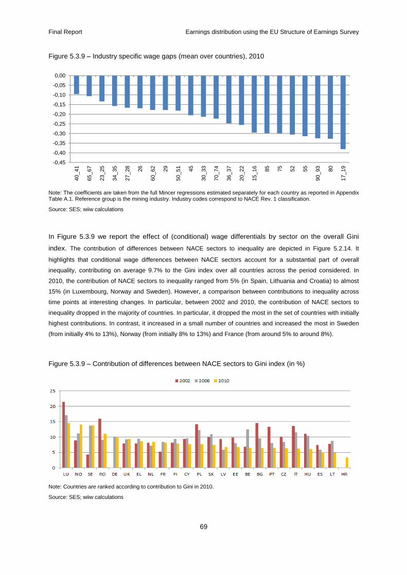
Final Report
Figure 5.3.9 – Industry specific wage gaps (mean over countries), 2010
Note: The coefficients are taken from the full Mincer regressions estimated separately for each country as reported in Appendix Table A.1. Reference group is the mining industry. Industry codes correspond to NACE Rev. 1 classification.
Source: SES; wiiw calculations
In Figure 5.3.9 we report the effect of (conditional) wage differentials by sector on the overall Gini
index. The contribution of differences between NACE sectors to inequality are depicted in Figure 5.2.14. It
highlights that conditional wage differences between NACE sectors account for a substantial part of overall
inequality, contributing on average 9.7%
2010, the contribution of NACE sectors to inequality ranged from 5% (in Spain, Lithuania and Croatia) to almost
15% (in Luxembourg, Norway and Sweden). However, a comparison between contributions to inequality across
time points at interesting changes. In particular, between 2002 and 2010, the contribution of NACE sectors to
inequality dropped in the majority of countries. In particular, it dropped the most in the set of countries with initially
highest contributions. In contrast, it increased in a small number of countries and increased the most in Sweden
(from initially 4% to 13%), Norway (from initially 8% to 13%) and France (from around 5% to around 8%).
Figure 5.3.9 – Contribution of differences between NACE sector
Note: Countries are ranked according to contribution to Gini in 2010.
Source: SES; wiiw calculations
-0,45
-0,40
-0,35
-0,30
-0,25
-0,20
-0,15
-0,10
-0,05
0,0040
_41
65_6
7
23_2
5
34_3
5
27_2
8 26
Earnings distribution using the EU Structure of Earnings Survey
69
Industry specific wage gaps (mean over countries), 2010
: The coefficients are taken from the full Mincer regressions estimated separately for each country as reported in Appendix group is the mining industry. Industry codes correspond to NACE Rev. 1 classification.
we report the effect of (conditional) wage differentials by sector on the overall Gini
ences between NACE sectors to inequality are depicted in Figure 5.2.14. It
onditional wage differences between NACE sectors account for a substantial part of overall
on average 9.7% to the Gini index over all countries across the period
2010, the contribution of NACE sectors to inequality ranged from 5% (in Spain, Lithuania and Croatia) to almost
15% (in Luxembourg, Norway and Sweden). However, a comparison between contributions to inequality across
ime points at interesting changes. In particular, between 2002 and 2010, the contribution of NACE sectors to
inequality dropped in the majority of countries. In particular, it dropped the most in the set of countries with initially
n contrast, it increased in a small number of countries and increased the most in Sweden
(from initially 4% to 13%), Norway (from initially 8% to 13%) and France (from around 5% to around 8%).
Contribution of differences between NACE sectors to Gini index (in %)
: Countries are ranked according to contribution to Gini in 2010.
60_6
2 29
50_5
1 45
30_3
3
70_7
4
36_3
7
20_2
2
15_1
6 85 75 52
Earnings distribution using the EU Structure of Earnings Survey
: The coefficients are taken from the full Mincer regressions estimated separately for each country as reported in Appendix group is the mining industry. Industry codes correspond to NACE Rev. 1 classification.
we report the effect of (conditional) wage differentials by sector on the overall Gini
ences between NACE sectors to inequality are depicted in Figure 5.2.14. It
onditional wage differences between NACE sectors account for a substantial part of overall
the period considered. In
2010, the contribution of NACE sectors to inequality ranged from 5% (in Spain, Lithuania and Croatia) to almost
15% (in Luxembourg, Norway and Sweden). However, a comparison between contributions to inequality across
ime points at interesting changes. In particular, between 2002 and 2010, the contribution of NACE sectors to
inequality dropped in the majority of countries. In particular, it dropped the most in the set of countries with initially
n contrast, it increased in a small number of countries and increased the most in Sweden
(from initially 4% to 13%), Norway (from initially 8% to 13%) and France (from around 5% to around 8%).
(in %)
52 55
90_9
3 80
17_1
9

Final Report Earnings distribution using the EU Structure of Earnings Survey
70
6. Summary and conclusions
This study provides a detailed view on earnings inequalities over the period 2002 to 2010 based on the
Structure of Earnings Survey. In doing so Mincer wage equations have been estimated to highlight patterns
and trends in earnings structures due to individual characteristics (sex, age, and education), job
characteristics (experience, contract type, full-time/part-time, occupations) and firm characteristics (firms
size, public and private control, collective pay agreements, sectors). Based on these results the
contributions of each of these characteristics to overall inequality as measured by the Gini index has been
calculated.
Particularly in the context of the Europe 2020 strategy which puts strong emphasis on goals like high levels
of employment, productivity and social cohesion highly, the study points at interesting findings. For
instance, results demonstrate that the crisis had no significant effect on the earnings distribution and did
not, as widely feared, lead to higher inequality among workers. In fact, inequality – as measured by the Gini
coefficient - remained fairly stable across time. This finding is indicative of a high degree of wage rigidity
across the EU which helped maintain averages wages for workers roughly at pre-crisis levels. This also
implies that labour market adjustments needed to accommodate the crisis were predominantly of
quantitative nature via adjustments in average hours worked and/or number of employees. Though overall
income inequality could be affected due to changes in employment and therefore household income, the
results do not point towards a significant due to changes in earnings of those which remain in employment.
Likewise, the contribution of individual worker, job and firm characteristics to inequality also hardly changed
as a result of the crisis. In particular, the analysis reveals that for all three years considered, on average
70% of observed inequality can be explained by individual worker, job and firm characteristics while 30%
remain unexplained. However, the contribution to inequality differs across characteristics considered:
individual characteristics contribute around 20% to inequality, job characteristics around 35% and firm
characteristics around 15%. In addition, as for the role of particular individual characteristics, occupation
and education turn out to be the two most important factors with about 25% and 12%, respectively,
followed by industry (with around 10%), enterprise size and job duration (with around 6% each), age (with
around 5%), gender (with only around 3.5%), type of ownership and type of collective pay agreements
(with around 2% each) and, finally, type of contract and full-time or part-time employment (with only around
1% each).
Moreover, findings point to interesting trends in wage differences between 2002 and 2010. For instance,
gender wage gaps clearly narrowed over time. In contrast, except for the oldest age cohort 60+, age-
related wage differences increased in the majority of countries. In addition, increases in education-related
wage differences observable in the majority of countries tended to be stronger for higher levels of education
and were most pronounced in the highest level of education. No clear trends emerge for the remaining job
and firm characteristics.
Thus, with respect to social cohesion one has to be aware of the changes in the dimensions driving
inequality in earnings. For example, whereas there is clear evidence that the gender wage declined in the
Final Report Earnings distribution using the EU Structure of Earnings Survey
71
period considered above in all countries, wage gaps increased with respect to other characteristics like age
cohorts and educational attainment levels. However, as results also indicate some of these trends can be
quite heterogeneous across countries and would therefore need a more in-depth cross-country analysis on
underlying institutional and labour market changes. This could be done focusing on the most important
aspects of earnings differences and contributions to inequality arising from the broad patterns and trends
outlined in this study. Another aspect which could deserve further attention is to explain potential
differences in the conditional and unconditional wage gaps which might arise due to the fact that some
groups in the labour market cannot enter specific jobs (e.g. occupations) for various reasons or the effect of
changes in employment patterns (e.g. in course of the crisis) on inequality dimensions.
Thus, the dataset – the Structure of Earnings Survey – is a highly valuable source for studying earnings
patterns and its determinants across countries and over time. In a next step a more in-depth analysis
concerning the question whether earnings differences across the many dimensions of a particular
characteristic are actually significantly different and whether changes over time are actually significant.
Furthermore, some analysis on interaction effects (e.g. part-time and female) was undertaken which
however could be extended to some other dimensions. Finally, in even allowing for a better assessment of
these issues concerning inequality and earnings differentials a solution to some technical problems (like
coding issues, classifications across countries, etc.) with the dataset (as outlined in the Appendix),
coherence of the CD-ROM and the Eurostat SAFE Centre dataset, etc. would be appreciated.
Furthermore, a slight extension of the survey, which would then capture more aspects of e.g. firm
characteristics (like exporter/non-exporter status, foreign owned, etc.), or are more accurate measure of
some characteristics (like experience) could allow for an even wider range of potential factors to be studied.
Final Report Earnings distribution using the EU Structure of Earnings Survey
72
7. Literature
Abraham, K.G. and H.S. Farber, 1987. Job duration, seniority, and earnings. American Economic Review, 77(3), 278-297.
Akerlof, G. and J. Yellen, 1988. Fairness and unemployment. American Economic Review, 78, 44-49.
Altonji, J.G. and R.M. Blank, 1999. Race and gender in the labor market. In O. Ashenfelter and D. Card (eds.), Handbook of Labor Economics, Vol. 3, pp. 3143-3259. Amsterdam: North Holland.
Altonji, J.G. and R.A. Shakotko, 1987. Do wages rise with job seniority.Review of Economic Studies, 54(3), 437-459.
Altonji, J.G. and N. Williams, 1997. Do wages rise with seniority? A reassessment. NBER Working Paper no. 6010, National Bureau of Economic Research.
Angrist, J.B. and A.B. Krueger, 1991. Does compulsory schooling attendance affect schooling and earnings? Quarterly Journal of Economics, 106, 976-1014.
Atkinson, A. B. (1975). The Economics of Inequality. Oxford: Clarendon Press.
Becker, G.S., 1957. The economics of discrimination. Chicago: University of Chicago Press.
Bernard,A. B., and J. B. Jensen (1999). Exceptional Exporter Performance: Cause, Effect, or Both? Journal of International Economics, 47, 1–25.
Blanchard, O. and A. Landier, 2002. The perverse effects of partial labour market reform: Fixed-term contracts in France. Economic Journal, 112, 214-244.
Blanchflower, D.G., Oswald, A.J. and P. Sanfey, 1996. “Wages, profits and rent sharing.” Quarterly Journal of Economics, 111, 227-251.
Blinder, A.S., 1973. Wage discrimination: Reduced forms and structural estimates. Journal of Human Resources, 8(4), 436-455.
Boockmann, B. and T. Hagen, 2008. Fixed-term contracts as sorting mechanisms: Evidence from job durations in West Germany. Labour Economics, 15, 984-1005.
Booth, A. L., Francesconi, M., and J. Frank, 2002. Temporary jobs: Stepping stones or dead ends? Economic Journal, 112, 189-213.
Brencic, V., 2009. Employers’ hiring practices, employment protection, and costly search: A vacancy-level analysis. Labour Economics, 16, 461-479.
Brown, S. and J. Sessions, 2003.Earnings, education, and fixed-term contracts. Scottish Journal of Political Economy, 50, 492-506.
Cain, G.G., 1986. The economic analysis of labor market discrimination: A survey. In O. Ashenfelter and R. Layard (eds.), Handbook of Labor Economics, Vol. 1, pp- 693-785. Amsterdam: Elsevier.
Calmfors, L. and J. Drifill, 1988.Bargaining structure, corporatism and macroeconomic performance. Economic Policy, 6, 13-61.
Calmfors, L. 1993. Centralization of wage bargaining and macroeconomic performance. OECD Economic Studies, 21, 161-191.
Campos, M.M. and M.C. Pereira, 2009.Wages and incentives in the Portuguese public sector. Economic Bulletin, Banco de Portugal, Summer, 57-77.
Card, D. and S. de la Rica, 2006. Firm-level contracting and the structure of wages. Industrial and Labor Relations Review, 59, 573-593.
Final Report Earnings distribution using the EU Structure of Earnings Survey
73
Card, D., Lemieux, T. and W.C. Riddell, 2004. Unions and wage inequality. Journal of Labor Research, 25, 519-562.
Card, D., 1995. Earnings, schooling and ability revisited. In S.W. Polachek (ed.), Research in Labor Economics, 14, pp. 23-48.JAI Press, Greenwich, Conn.
Card, D., 1999.The causal effect of education on earnings. In O.C. Ashenfelter and D. Card (eds.), Handbook of Labor Economics, vol. 3. North Holland, Amsterdam.
Chatterji, M., K. Mumford and N. Peter, 2011. The public-private sector gender wage differential: Evidence from matched employee-workplace data. Applied Economics, 43(26), 3819-3833.
Christofides, L.N. and M. Michael, 2013.Exploring the public-private sector wage gap in European countries.IZA Journal of European Labor Studies, 2-15.
Cohn, E. and J.T. Addison, 1997.The economic returns to lifelong learning.Working Paper no. 97-04, University of South Carolina.
Comi, S., P. Ghinetti and C. Lucifora, 2002. The distribution of wages in the public and private sectors: A disaggregated analysis. In C. Dell’Aringa and C. Lucifora (eds), Dinamica occupazionale salariale, Vita e Pensiero (in Italian).
Cotton, J. 1988. On the Decomposition of Wage Differentials. Review of Economics and Statistics, 70, 236–243.
Cowell, F. A. and C. V. Fiorio, 2009, Inequality decompositions. A reconciliation. ECINEQ Working Paper Series WP 2009-117.
Dahl, C.M., Le Maire, D. and J.R. Munch, 2011. Wage dispersion and decentralization of wage bargaining. IZA Working Paper no. 6176. Institute for the Study of Labour, Bonn.
Davia, M. and V. Hernanz, 2004. Temporary employment and segmentation in the Spanish labour market: An empirical analysis through the study of wage differentials. Spanish Economic Review, 6, 291-318.
Davis, S. J., and Haltiwanger, J. C., 1991. Wage Dispersion Between and Within U.S. Manufacturing Plants, 1963-86. Brookings Papers on Economic Activity: Microeconomics, 1991(1), 115–80.
DeCastro, F., Salto, M. and H. Steiner, 2013. The gap between public and private wages: New evidence for the EU. Economic Papers no. 508, DG-ECFIN, The European Commission.
Dell’Aringa, C. and C. Lucifora, 1994. Collective bargaining and relative earnings in Italy. European Journal of Political Economy, 10, 727-747.
Dolado, J., Garcia-Serrano, C., and J. Jimeno, 2002. Drawing lessons from the boom of temporary jobs in Spain. Economic Journal, 112, 270-295.
Dustmann, C. and C. Meghir, 2005. Wages, experience and seniority.Review of Economic Studies, 72(1), 77-108.
Dustman, C. and A.V. Soest, 1997. Wage structures in the private and public sectors in West Germany. Fiscal Studies, 18, 225-247.
Elia, L., 2010. Temporary/permanent workers’ wage gap: A brand-new form of wage inequality? Labour, 24, 178-200.
European Commission, 2010. Structure of Earnings Survey 2010 - Eurostat’s arrangements for implementing the Council Regulation 530/1999, the Commission Regulations 1916/2000 and 1738/2005.
Faggio, G., Salvanes, K. G., and Van Reenen, J., 2010. The Evolution of Inequality in Productivity and Wages: Panel Data Evidence. Industrial and Corporate Change 19 (6), 1919–1951.
Final Report Earnings distribution using the EU Structure of Earnings Survey
74
Fields, G. S., 2003, Accounting for income inequality and its change: a new method with application to distribution of earnings in the United States. Research in Labor Economics 22, 1-38.
Fields, G. S. and G. Yoo, 2000, Falling labor income inequality in Korea’s economic growth: patterns and underlying causes. Review of Income and Wealth 46, 139-159.
Fitzenberger, B. and W. Franz, 1999. Industry-level wage bargaining: A partial rehabilitation – The German experience. Scottish Journal of Political Economy, 46, 437-457.
Fitzenberger, B., Kohn, K. and A.C. Lembcke, 2008. Union density and varieties of coverage: The anatomy of union wage effects in Germany. IZA Discussion Paper no. 3356.
Foley, P. and F. O’Callaghan, 2009.Investigating the public-private wage gap in Ireland using data from the National Employment Survey 2007.Statistical and Social Inquiry Society.
Giordano, R., Depalo, D., Pereira, M.C., Eugene, B., Papapetrou, E., Perez, J., Reiss, L. and M. Roter, 2011. The public sector pay gap in a selection of euro area countries. European Central Bank Working Paper no. 1406. Frankfurt, European Central Bank.
Glocker, D. and V. Steiner, 2011. Returns to education across Europe: A comparative analysis for selected EU countries. Discussion Paper no. 2011/15, Free University Berlin.
Gregory, R.G. and J. Borland, 1999. Recent developments in public sector labour markets. In O. Ashenfelter and D. Card (eds.), Handbook of Labor Economics, Vol. 3C, pp. 3573-3630. Amsterdam: Elsevier.
Goux, D., Maurin, E., and M. Pauchet, 2001.Fixed-term contracts and the dynamics of labour demand.European Economic Review, 45, 533-552.
Gunatilaka, R. and Chotikapanich, D., 2006, Inequality Trends and Determinants in Sri Lanka 1980-2002: A Shapley Approach to Decomposition. Monash Econometrics and Business Statistics Working Papers 6/06. Monash University.Department of Econometrics and Business Statistics.
Harmon, C., Walker, I. and N. Westergaard-Nielsen, 2001. Education and earnings in Europe. Aldershot: Edward Elgar.
Harmon, C., Oosterbeck, H. and I. Walker, 2003. The returns to education: Microeconomics. Journal of Economic Surveys, 17(2), 115-155.
Hartog, J., Leuven, E. and C. Teulings, 2002. Wages and the bargaining regime in a corporatist setting: The Netherlands. European Journal of Political Economy, 18, 317-331.
Hasebe, T., 2011. The Type of Contract and Starting Wage and Wage Growth: The Evidence from New Graduates from Post-Secondary Schools in the Netherlands. Alma Laurea Working Papers no. 20.
Helpman, E., Itskhoki, O., Muendler, M.-A., Redding, S. J., 2012.Trade and Inequality: From Theory to Estimation. NBER Working Paper No. 17991, National Bureau of Economic Research.
Jann, B., 2008. The Blinder-Oaxaca Decomposition for Linear Regression Models. Stata Journal, 8(4), 453-479.
Jarrell, S.B. and T.D. Stanley, 2004. Declining bias and gender wage discrimination? A meta-regression analysis. Journal of Human Resources, 39(3), 828-838.
Kaukewitsch, P. And D. Rouault, 1998.Les structures des salaries en France et en Allegmagne en 1995: Une analyse statistique comparative des hierarchies salariales. Economiques et Statistique, 315, 3-27.
Kunze, A., 2000. The determination of wages and the gender wage gap: A survey. IZA Working Paper no. 193.
Marshall, R.C. and G.A. Zarkin, 1987. The effect of job tenure on wage offers. Journal of Labor Economics, 5(3), 301-324.

Final Report Earnings distribution using the EU Structure of Earnings Survey
75
Matteazzi, E., Pailhe, A. and A. Solaz, 2013. Does part-time employment widen the gender wage gap? Evidence from twelve European countries. Working Paper no. 293, Society for the Study of Economic Inequality.
Melitz, M. J., 2003. The Impact of Trade on Intra-Industry Reallocations and Aggregate Industry Productivity. Econometrica 71(6), 1695-1725.
Middendorf, T., 2008. Returns to education in Europe – Detailed results from a harmonized survey. Ruhr Economics Papers no. 65, Ruhr Universität Bochum
Miller, H.P., 1955. Income of the American people. Washington, DC: United States Government Printing Office.
Miller, H.P., 1966. Income distribution in the United States. Washington, DC: United States Government Printing Office.
Mincer, J., 1958.Investment in Human Capital and Personal Income Distribution. Journal of Political Economy 66(4), 281-302.
Mincer, J., 1974.Schooling, experience and earnings. New York: Columbia University.
Moen, J., 2005. Is Mobility of Technical Personnel a Source of R&D Spillovers? Journal of Labor Economics 23 (1), 81-114.
Molini, V. and G. Wan, 2008,Discovering sources of inequality in transition economies: a case study of rural Vietnam, Journal of Economic Change, 41, 75-96.
Morduch, J. and T. Sicular, 2002,Rethinking inequality decomposition, with evidence from rural China. The Economic Journal 112, 93–106.
Myck, M. and G. Paull, 2001.The role of employment experience in explaining the gender wage gap.Working Paper no. 01-18, Institute for Fiscal Studies.
Neumark, D. 1988. Employers’ Discriminatory Behavior and the Estimation of Wage Discrimination.Journal of Human Resources, 23, 279–295.
Oaxaca, R. 1973. Male-Female Wage Differentials in Urban Labor Markets. International Economic Review, 14, 693–709.
OECD, 1999.Economic Outlook, 1999. Paris, Organisation for Economic Cooperation and Development.
OECD, 2004.Economic Outlook, 2004. Paris, Organisation for Economic Cooperation and Development.
OECD, 2006.Women and men in OECD countries. Paris: Organisation for Economic Cooperation and Development.
OECD, 2010.Economic Outlook, 2010. Paris, Organisation for Economic Cooperation and Development.
Papapetrou, E., 2006. The public-private sector pay differential in Greece. Public Finance Review, 35(4), 450-473.
Plasman, R., Rusinek, M. and F. Rycx, 2007. How do company collective agreements affect wages? Evidence from four corporatist countries European, Journal of Industrial Relations, 13(2), 161-180.
Psacharopoulos, G., 1985. Returns to education: A further international update and implications. Journal of Human Resources, 20, 583-604.
Psacharopoulos, G., 1994. Returns to investment in education: A global update. World Development, 22, 1325-1343.
Rees, H. and A. Shah, 1995.Public-private sector wage differential in the UK. Manchester School, 63(1), 52-68.
Final Report Earnings distribution using the EU Structure of Earnings Survey
76
Reimers, C. W. 1983. Labor Market Discrimination Against Hispanic and Black Men. Review of Economics and Statistics, 65, 570–579.
Rowthorn, R.E., 1992. Centralisation, employment and wage dispersion. Economic Journal, 102, 506-523.
Sen, A. (1997). On Economic Inequality. Oxford, UK: Oxford University Press.
Shorrocks, A. F., 1999, Decomposition procedures for distributional analysis: A unified framework based on the Shapley value. Draft paper, University of Essex.
Song, J., Almeida, P. and Wu, G., 2003. Learning-by-Hiring: When Is Mobility More Likely to Facilitate Interfirm Knowledge Transfer? Management Science 49 (4), 351-365.
Stanley, T.D. and S.B. Jarrell, 1998.Gender wage discrimination bias? A meta-regression analysis. Journal of Human Resources, 33(4), 947-973.
Topel, R., 1991. Specific capital mobility, and wages: Wages rise with job seniority. Journal of Political Economy, 99(1), 145-176.
Wallerstein, M., 1999. Wage-setting institutions and pay inequality in advanced industrial societies. American Journal of Political Economy, 43, 649-680.
Wan, G., 2004, Accounting for income inequality in rural China: A regression-based approach. Journal of Comparative Economics 32, 348–363.
Wan, G., 2002, Regression-based Inequality Decomposition: Pitfalls and a Solution Procedure. UNU-WIDER, Discussion Paper No. 2002/101.
Weichselbaumer, D. and R. Winter-Ebmer, 2005. A meta-analysis of the international gender wage gap.Journal of Economic Surveys, 19(3), 479-511.
Weichselbaumer, D. and R. Winter-Ebmer, 2007. International gender wage gaps. Economic Policy, April, 237-287.
Willis, R.J., 1987. Wage determinants: A survey and reinterpretation of human capital earnings functions. In O. Ashenfelter and R. Layard (eds.), Handbook of Labor Economics, Vol 1, pp. 525-602. Amsterdam: Elsevier.

Final Report Earnings distribution using the EU Structure of Earnings Survey
77
Technical Appendix
Methodological approach and data issues
Mincer regressions
The primary objective of this task is to determine the quantitative impact of the indicators we have looked at
in the previous chapter (e.g. age, gender, education, firm size, ...) on the structure of earnings. Though a lot
of information is provided by the descriptive analysis, the econometric results shed further light on the
relative strength and importance of the various dimensions. Furthermore, the econometric analysis allows
one to consider conditional correlations between wages and the set of indicators, which is not possible in
the descriptive analysis.
For each SES wave, regression models were estimated at the level of the Member State. The starting point
is the estimation of a so-called ‘Mincer equation’ (Mincer, 1958), which is the baseline specification in
estimating earnings. In the initial specification, the log of gross hourly earnings of a worker i at time tis
regressed on a number of indicators using OLS with robust standard errors. As in the descriptive analysis,
weights in the dataset have been used in order to make the sample representative for the whole working
population. The basic equation to be estimated is of the following form:
�� ��� � ���� �� �,��� � ���
where ��� denotes the log of gross hourly earnings (including bonuses) of a worker i at time t, ���� is a
vector of individual characteristics, and �� �,��� denotes firm-specific variables. � and � are parameters to be
estimated. Vector ���� contains information on the following individual characteristics: age (based on groups
defined above), education (based on ISCED), occupation (based on ISCO 1-digit), employment contract
type, gender, full-time/part-time and length of the service in the enterprise. The firm-specific variables used
in �� �,��� include firm size, industry affiliation, regional location, information on economic and financial
control and type of collective pay agreement covering at least 50% of the employees in the local unit. For
all variables, subgroups identical to the ones described in Section 3.4 were generated for each indicator.
These subgroups are represented by dummies in the OLS estimation.
In the following two sections, the regression results are discussed in detail. The focus lies on the results of
SES 2010, while in some interesting cases, developments are shown over time. In order to be able to
present the findings, the results for each individual or firm characteristic are presented separately.
However, all results shown are always extracted from the full Mincer regressions accounting for all the firm
and personal characteristics.

Final Report Earnings distribution using the EU Structure of Earnings Survey
78
Blinder-Oaxaca decomposition
The Blinder-Oaxaca decomposition (Blinder, 1973; Oaxaca, 1973) has been extensively used in studies of
wages to consider differences in wages by groups (usually by gender or race). The method involves
decomposing differences in mean log wages from wage regressions into an explained and an unexplained
component. The explained component can be accounted for by observable differences in group
characteristics, such as education and work experience, while the unexplained component cannot be
explained by such observable characteristics. In much of the literature, the unexplained component has
been used as a measure of discrimination, though this component also includes the effects of differences in
unobserved predictors of wages.
The basic idea behind the decomposition is as follows. Consider two groups A and B (e.g. males and
females respectively), an outcome variable � (e.g. log wages) and a set of explanatory variables � (e.g.
education, work experience, …). We are interested in finding how much of the mean difference in
outcomes (i.e. � � � ��� � � ���) is accounted for by the explanatory variables. The difference in the
group specific means is obtained from a linear regression model of the form:
�� � ����� �� with � � ��, ! with � being the vector of explanatory variables, � being a set of parameters to be estimated and � being
an error term that has standard properties.10 The mean outcome difference can then be expressed as the
difference in the linear prediction at the group-specific means of the regressors, i.e.
� � � ��� � � ��� � � ��� ��"� � � ��� ��"�
Where a “^” indicates estimates from the linear regression model. This equation is then decomposed to
allow one to identify the contribution of group differences in the explanatory variables and a remaining
unexplained component. Note, that a further three-fold decomposition is also often used that includes an
interaction between the above two components, accounting for the fact that differences in endowments and
coefficients exist simultaneously between the two groups (see Jann, 2008 for further details). In our
analysis we concentrate on the two-fold decomposition. This is obtained by rearranging the above equation
to give:
� � #� ��� � � ���$��% #� ��� � �� � �%� � � ��� � �� � �%�$ where �% is a non-discriminatory vector of coefficients. Here the first term on the RHS captures the
difference that is explained by differences in the group explanatory variables, and the second term on the
RHS captures the unexplained component. This latter component is usually ascribed to discrimination, but
as mentioned above, it should be borne in mind that this will also capture differences in unobservables
across groups.
In order to implement this decomposition we need values for the non-discriminatory vector of coefficients,
�%. Here, we have to assume that discrimination is directed towards one of the two groups. Considering our
10
In our analysis we use unweighted regressions when calculating the Blinder-Oaxaca decomposition.
Final Report Earnings distribution using the EU Structure of Earnings Survey
79
example of gender groups, the male based decomposition assumes that males are paid their marginal
products and females are discriminated against. In this case, the non-discriminatory vector of coefficients is
that for males, i.e. ��, and the decomposition becomes:
� � #� ��� � � ���$��� #� ��� � �� � ��� � � ��� � �� � ���$ � � #� ��� � � ���$��� #� ��� � �� � ���$
The alternative is to assume that females are paid their marginal product and males are positively
discriminated against. In this case the decomposition is as follows:
� � #� ��� � � ���$��� #� ��� � �� � ��� � � ��� � �� � ���$ � � #� ��� � � ���$��� #� ��� � �� � ���$
Various methods have been suggested to combine these two decompositions, such as the use of
averages of the two sets of parameter estimates, weighting the parameter estimates by sample size or
using the parameters estimates from pooled regression (e.g. Reimers, 1983; Cotton, 1988; Neumark,
1988).11
Inequality measures
Measuring inequality based on survey data has a long tradition in the literature. Already in the 1970s a wide
range of inequality measures existed and their properties were described in detail e.g. in two essential
publications of that strand of research, Sen’s ’On Economic inequality’ (1973) (see Sen, 1997) and
Atkinson’s ’The Economics of Inequality’ (1975) (Atkinson, 1975). Inequality measurement is commonly
based on three different (classes of) measures, the first being simple percentile ratios &�/&( ; second the
well-known and most frequently used Gini index,
) � * 1* � 1 � 2
* * � 1�- . /�0�1
�23
Here * denotes the number of observations, 0� is the variable under consideration (e.g. wages of
individuals) and /� denotes the share of units with a specific wage in the total population.12 The third group
of indices considered is the generalized class of entropy measures defined as
45 � 16 6 � 1�
1* . 71 � 80�
- 95
:1
�23
for 6 ; 0,1. In the equation (and both measures described below) 0� denotes the wage of the individuals,
* is the number of units and µ is the unit’s average wage in the total population. In the formula of the
generalized class of entropy measures, the parameter 6 can be seen as an indicator of inequality aversion
and it also indicates the sensitivity to transfers at different parts of the distribution (for negative and low
11
There are few quantitative or qualitative differences when using these two approaches in our analysis. In this report, we report results based on the second assumption, assuming that females are paid their marginal product and males are discriminated against.
12 Note that the Gini index can be expressed in different ways.

Final Report Earnings distribution using the EU Structure of Earnings Survey
80
positive α the index is more sensitive to changes in the distribution that affect the lower tail); see Sen
(1997) for a discussion. This allows, e.g., to focus on changes in the lower part of the income distribution,
which might be more problematic with respect to social cohesion. For the limiting cases of 6 = 0 the
entropy measure becomes the Mean logarithmic deviation (also named Theil’s second measure)
4> � 1* . ��
1
�23 -0�
For 6 = 1 it becomes the well-known Theil measure (43)
43 � 1* . 0�
- ��1
�23 0�
-
The Gini index, the Mean logarithmic deviation and the Theil measure can all take values between 0 and 1,
where the former value denotes perfect equality and 1 perfect inequality, i.e. one individual would earn the
total payroll.
Shapley value approach
Recently, the literature on inequality analysis has provided various decomposition methods which are
based on regression results like the Shapley value approach as introduced by Shorrocks (1999) but also
others; see Fields and Yoo (2000), Morduch and Sicular (2002), Fields (2003), Wan (2004), Gunatilaka and
Chotikapanich (2006) or Molini and Wan (2008) for such applications; see also Cowell and Fiorio (2009) for
a critical review. The most important advantage of the Shapley value approach is that this takes the
potential correlation amongst regressors into account and that it allows assessing the importance of a
multitude of explanatories in shaping the situation of inequality.
The Shapley value approach can be illustrated by using a simple example with three explanatory variables.
We first regress individual income levels y on these explanatory variables xi (i = 1, 2, 3),
εββββ ++++= 3322110 xxxy ,
where ε denotes the error term. The predicted income level is then given by
.ˆˆˆˆˆ3322110123 xxxy ββββ +++=
This predicted value is then used to calculate the Gini coefficient when including all explanatory variables,
{ }( )0123G
, where subscripts denote the variables included. In the first round one then eliminates one variable
when calculating the predicted income level and calculates the predicted income levels { } { }1323ˆ,ˆ yy and { }12y ,
i.e. including explanatory variables 2 and 3, 1 and 3 and 1 and 2, respectively. The corresponding Gini
coefficients are then given by { }( )
{ }( )113
123
ˆ,ˆ GG and { }
( )112G
respectively. Analogously, in the second round one
eliminates two variables, thus calculating { } { }21ˆ,ˆ yy and { }3y . The resulting Gini coefficients are { }
( ){ }( )22
21
ˆ,ˆ GG

Final Report Earnings distribution using the EU Structure of Earnings Survey
81
and { }( )23G
. The final round would then be to include the constant only; the resulting Gini coefficient would
thus be { }( ) .0ˆ 3 =G
. It should be emphasised that in this procedure the Mincer regression is only estimated
once including all explanatory variables; the latter are sequentially excluded only when calculating the
predicted income levels.
The marginal contributions are then calculated using the Gini coefficients. The first round marginal
contributions for each variable are { } { })1(
23)0(
123
)1(
1ˆˆ GGC −=
, { } { })1(
13)0(
123
)1(
2ˆˆ GGC −=
and { } { })1(
12)0(
123
)1(
3ˆˆ GGC −=
. The
marginal contributions in the second round of the first variable are given by
{ } { })2(
2)1(
12
)1,2(
1ˆˆ GGC −=
and { } { })2(
3)1(
13
)2,2(
1ˆˆ GGC −=
The average of these contributions is the marginal contribution of the first variable in the second round, i.e.
( ) ( )( )2,21
1,21
)2(1 2
1CCC +=
. Similarly we calculate ( )22C and
( )23C
. The third round contribution is given by
{ } { } { })2(
1)3()2(
1
)3(
1ˆˆˆ GGGC =−=
as { } 0ˆ )3( =Gand analogously for { }
)2(2
)3(2 GC =
and { })2(
3)3(
3 GC =.
Finally, averaging the marginal contributions of each variable over all rounds results in the total marginal
effect of each variable 3,2,1=j i.e.
( ) ( ) ( )( )321
3
1jjjj CCCC ++⋅= .
The proportion of inequality not explained is then given by
{ })0(
123GGCR −= .
The approach can easily be extended to any number of explanatory factors and to other inequality or
poverty measures.
Wan (2002) points to the fact that the presence of a negative constant in the regression equation may lead
to negative predicted individual income levels. In that case the calculation of a Gini-coefficient and thus the
contributions of individual variables to overall inequality would be impossible. To overcome this pitfall he
shows in Wan (2004) that different model specifications can be used for the underlying estimated income
generating function, delivering moreover better log-likelihood values than the linear estimation model.
Following his approach, we choose for the analysis in this paper a semilog model:
εββββ ++++= 3322110ln xxxy ,
Since we are not interested in the decomposition of the log of income, but income we have to take the
antilog of the above model resulting in
( ) ( ) ( ) εββββ eeeeeexxxy ∗∗∗∗= 33221!0ln
, which is
( ) ( ) ( ) εββββ eeeeeyxxx ∗∗∗∗= 33221!0 .
Final Report Earnings distribution using the EU Structure of Earnings Survey
82
The simple advantage of this model is that the constant 0βe is now a positive scalar, which does not
influence the magnitude of the calculated Gini coefficient. The elimination procedure as described above
however remains unchanged.
Data issues
The underlying data for this study - the Structure of Earnings Survey (SES) - is conducted every four
years in the Member States of the European Union and provides comparable information at EU level
on relationships between the level of earnings, individual characteristics of employees (gender, age,
educational level), job characteristics (occupation, length of services in the enterprise, employment
contract type, etc.) and characteristics of their employer (economic activity, size of the enterprise,
existence and type of pay agreement, geographical location, etc.). Taken together, the different waves
of the survey allow one to observe earnings disparities for three years: 2002, 2006, and 2010.
Restricted access to CD-Rom version of the SES microdataset is available for up to 24 countries for
the 2002, 2006 and 2010 SES releases (BE, BG, CY, CZ, DE (since 2006), EE, ES, FI, FR, EL, HR
(since 2010), HU, IT, LT, LU, LV, NL, PL, PT, RO, SE, SK, UK, NO). Restricted access to more
detailed microdata for the 2002, 2006 and 2010 SES releases are available through the SAFE Centre
at the premises of Eurostat in Luxembourg. The 2002 and 2006 SES releases cover 21 EEA countries
(CY, CZ, EE, ES, FI, FR, EL, HU, IE, IT, LT, LU, LV, NL, PL, PT, RO, SE, SI, SK, NO). Two more
countries, namely HR and TR, have been added for the 2010 SES release.
With respect to the coverage of the SES survey, the following workers are excluded from the dataset
(European Commission, 2010):
• own-account workers (self-employed)
• sales representatives and other persons who are wholly remunerated by way of fees or
commission, are not on the payroll, or are self-employed
• owners, directors or managers whose remuneration wholly takes the form of a share in profits
• family workers who are not employees (as defined above) of the enterprise or local unit
• unpaid voluntary workers (e.g. those who typically work for non-profit institutions such as charities)
The focus of the report is on variables available in all SES versions. The SES 2002 version contains
some additional variables covering career breaks, days of sick leave, vocational training, as well as
more detailed information on bonuses paid. Information about these variables is, however, missing for
most countries and thus is not used.
Bonuses are included only in gross annual earnings. The word “bonuses” is hereby a bit too narrow as
bonuses include any “periodic, irregular, ad-hoc and exceptional bonuses and other payments that do
not feature every pay period” (European Commission, 2010). The regression results are based on
gross hourly earnings including bonuses. To that end, the share of bonuses in gross annual earnings
was calculated and added to the gross hourly earnings.
Final Report Earnings distribution using the EU Structure of Earnings Survey
83
The SES datasets includes gross hourly, monthly and annual earnings in national currency. In order to
make the data comparable across countries, data on purchasing power parities based on actual
individual consumption was used from Eurostat.
Three major issues have arisen with respect to the SES datasets. The first two issues are related to
coding differences across countries. In order to ensure confidentiality, and possibly also for other
reasons, rather different groupings were used across countries for some variables. These differences
across countries have, to some extent, shaped the groupings of our individual, job and firm
characteristics as can be seen from the list below. Second, the same information is not coded alike
across countries. Two examples of variables were these issues arise are sectors and firm size. An
example of a specific entry, which is coded differently: information, which is not available may be
coded “99999999”, “999999999999”, “999999999999999”, “OPT”, “UNK”, ".", "", "@" or "X" depending
on the country and SES version. Third, we stumbled upon a number of problems in the SAFE Centre
versions of the SES releases, mostly regarding separators.13
Concerning the identification of outliers, some manual research was done and outliers related to part
time identified. In particular, we dropped employees which worked less than 1% of the full time
equivalent and some instances with very high part time salaries (more than 400 PPP EUR per hour
worked).
The following individual, job and firm characteristics were used in the analysis:
Individual characteristics:
Concerning individual characteristics three dimensions are included.
• Sex (male/female)
• Age cohorts (15-19, 20-29, 30-39, 40-49, 50-59, 60+). In the SAFE Center version, the age of the
employee is available as a numeric variable, but the CD Rom version only contains information
according to the six groups mentioned above. At the SAFE Center, 5-year age groups were
formed to identify wage effects for certain groups (e.g. those aged 60 to 65).
• Educational attainment based on ISCED (0-1 Primary, 2, 3-4 Upper and post-secondary, 5B,
Short cycle tertiary, 5A Bachelor and Master and 6 Doctoral). ISCED 3 and 4 have been reported
separately in 2002, but together in 2006 and 2010. Therefore, these have been merged into one
group also in 2002.
13
Croatia 2010: Numeric values are sometimes, but not always formatted like this “200.120.140”. It seems like 1000 separators (commas) were replaced by points. As the decimal character is a point, it is unclear what numbers like "120.140" stand for.
- Netherlands 2006 Table B: The decimal character suddenly is a comma whereas it is a point in Table A and everywhere else.
- Finland 2002 Table B: The header is missing and values are separated by commas instead of semicolons (all other files are separated by semicolons).
- Estonia 2002 Table B: lots of commas are at the end of each line. As the separator is semicolon, the commas are then stored together with KEY_L, the variable identifying the enterprise. That makes it hard to merge employer and employee data.
- Greece 2010: Same point as above but with varying amount of spaces after KEY_L in both tables.

Final Report Earnings distribution using the EU Structure of Earnings Survey
84
Job characteristics
With respect to job characteristics four variables are considered.
• Job duration (or experience) with groupings into less than one year, 1-4 years, 5-14 years and 15+
years. For most countries, job duration is available as a continuous variable, but the data for the
Netherlands only allows for a grouping into these four categories.
• Employment contract type distinguished between indefinite duration (A), fixed/temporary duration
(B), apprenticeship (C). This distinction is however not reported in Sweden in all three years and
not for Poland in 2002. A group of other contract types (D), which is reported for a few countries in
2002 only, has been merged with the group for which the contract type was not available.
• Full-time/part-time – the grouping follows the classification in the dataset. Part-time workers were
then also subdivided into three groups: those that work up to 39%, 40 to 79% and above 80% of
the full-time equivalent in the respective country.
• Occupation according to ISCO-88 1-digit. In a few cases (e.g. NO 2002 and 2010; SI 2006) some
are coded as “Not applicable” or “Not available”. As the shares are rather small these have been
skipped them from the analysis.
Firm characteristics
Finally, four dimensions of firm characteristics could be included in the analysis.
• Firm size: 1-49, 50-249, 250+. These groups were most widely used by the member states. Two
notable deviations from this pattern are Estonia, which only reported 1-50 and 50+ and Italy, which
reported parallel to the above groups the size classes 50+, 1-250, 50-1000. Whenever these
groups did not fit the broad classification, they were dropped. In the case of Ital, this parallel
regime was not very widely used.
• Type of collective pay agreement covering at least 50% of the employees: national level or
interconfederal (A), industry (B+C), enterprise or local unit (D+E), any other type (F), and no
collective agreement (N)
• Firm’s economic and financial control: public (A) or private (B). Another type, covering balanced
public and private ownership (50/50 ‘shared control’), which existed as a separate group (C) in
SES 2002 was coded as under private control in later SES versions. Thus, it was put into group
private (B) for all SES versions in our analysis. The sector coverage, particularly related to public
administration differs quite significantly across countries.
• Industry is reported according to NACE Rev.1 in 2002 and 2006 and NACE Rev.2 in 2010. The
industry aggregation level used in our analysis is the same in the anonymized and the SAFE
Center version due to confidentiality problems in some countries (less than 10 observations).
Information on employment in agriculture was limited to a number of observations in few countries
in some SES waves, so this sector was dropped entirely. There were some issues related to the
German SES dataset, in which industries were coded very differently from the other countries. In
the SES 2010 dataset, the NACE Rev.2 data was converted to NACE Rev.1 to make the results
comparable to the earlier SES version.

Final Report Earnings distribution using the EU Structure of Earnings Survey
85
SAFE Centre experience
While the administrative part worked very well, a number of problems arose at the SAFE Centre with
respect to data processing. The problems are related to the dataset, as described above, as well as
the IT infrastructure. The IT infrastructure at the SAFE Centre limited our analysis to a large extent.
The first problem relates to the memory of the computer provided at the SAFE Centre. The computer
had 2 GB of RAM for the Operation System (Windows XP) and applications. The Stata file of each
SES version (2002, 2006, 2010) is around 2 GB when combining all countries. It was thus impossible
to run regressions across all countries. Secondly, the processor of the computer too slow to conduct
more sophisticated econometric analyses. Running e.g. quantile regressions for each country would
take more than a week to finish for all SES versions with the current setup. It would therefore be
desirable that the SAFE Centre is equipped better in terms of hardware as well as with a
multiprocessor version of the statistical program (in this case Stata).
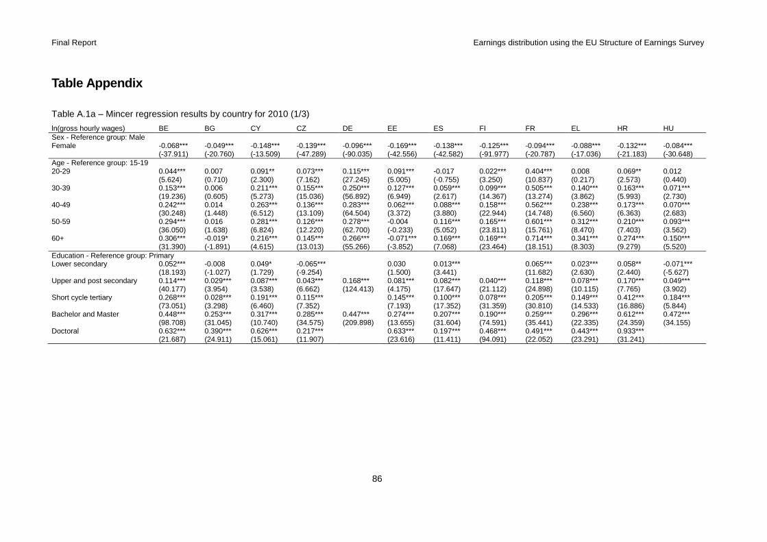
Final Report Earnings distribution using the EU Structure of Earnings Survey
86
Table Appendix
Table A.1a – Mincer regression results by country for 2010 (1/3)
ln(gross hourly wages) BE BG CY CZ DE EE ES FI FR EL HR HU Sex - Reference group: Male Female -0.068*** -0.049*** -0.148*** -0.139*** -0.096*** -0.169*** -0.138*** -0.125*** -0.094*** -0.088*** -0.132*** -0.084*** (-37.911) (-20.760) (-13.509) (-47.289) (-90.035) (-42.556) (-42.582) (-91.977) (-20.787) (-17.036) (-21.183) (-30.648) Age - Reference group: 15-19 20-29 0.044*** 0.007 0.091** 0.073*** 0.115*** 0.091*** -0.017 0.022*** 0.404*** 0.008 0.069** 0.012 (5.624) (0.710) (2.300) (7.162) (27.245) (5.005) (-0.755) (3.250) (10.837) (0.217) (2.573) (0.440) 30-39 0.153*** 0.006 0.211*** 0.155*** 0.250*** 0.127*** 0.059*** 0.099*** 0.505*** 0.140*** 0.163*** 0.071*** (19.236) (0.605) (5.273) (15.036) (56.892) (6.949) (2.617) (14.367) (13.274) (3.862) (5.993) (2.730) 40-49 0.242*** 0.014 0.263*** 0.136*** 0.283*** 0.062*** 0.088*** 0.158*** 0.562*** 0.238*** 0.173*** 0.070*** (30.248) (1.448) (6.512) (13.109) (64.504) (3.372) (3.880) (22.944) (14.748) (6.560) (6.363) (2.683) 50-59 0.294*** 0.016 0.281*** 0.126*** 0.278*** -0.004 0.116*** 0.165*** 0.601*** 0.312*** 0.210*** 0.093*** (36.050) (1.638) (6.824) (12.220) (62.700) (-0.233) (5.052) (23.811) (15.761) (8.470) (7.403) (3.562) 60+ 0.306*** -0.019* 0.216*** 0.145*** 0.266*** -0.071*** 0.169*** 0.169*** 0.714*** 0.341*** 0.274*** 0.150*** (31.390) (-1.891) (4.615) (13.013) (55.266) (-3.852) (7.068) (23.464) (18.151) (8.303) (9.279) (5.520) Education - Reference group: Primary Lower secondary 0.052*** -0.008 0.049* -0.065*** 0.030 0.013*** 0.065*** 0.023*** 0.058** -0.071*** (18.193) (-1.027) (1.729) (-9.254) (1.500) (3.441) (11.682) (2.630) (2.440) (-5.627) Upper and post secondary 0.114*** 0.029*** 0.087*** 0.043*** 0.168*** 0.081*** 0.082*** 0.040*** 0.118*** 0.078*** 0.170*** 0.049***
(40.177) (3.954) (3.538) (6.662) (124.413) (4.175) (17.647) (21.112) (24.898) (10.115) (7.765) (3.902) Short cycle tertiary 0.268*** 0.028*** 0.191*** 0.115*** 0.145*** 0.100*** 0.078*** 0.205*** 0.149*** 0.412*** 0.184***
(73.051) (3.298) (6.460) (7.352) (7.193) (17.352) (31.359) (30.810) (14.533) (16.886) (5.844) Bachelor and Master 0.448*** 0.253*** 0.317*** 0.285*** 0.447*** 0.274*** 0.207*** 0.190*** 0.259*** 0.296*** 0.612*** 0.472***
(98.708) (31.045) (10.740) (34.575) (209.898) (13.655) (31.604) (74.591) (35.441) (22.335) (24.359) (34.155) Doctoral 0.632*** 0.390*** 0.626*** 0.217*** 0.633*** 0.197*** 0.468*** 0.491*** 0.443*** 0.933*** (21.687) (24.911) (15.061) (11.907) (23.616) (11.411) (94.091) (22.052) (23.291) (31.241)
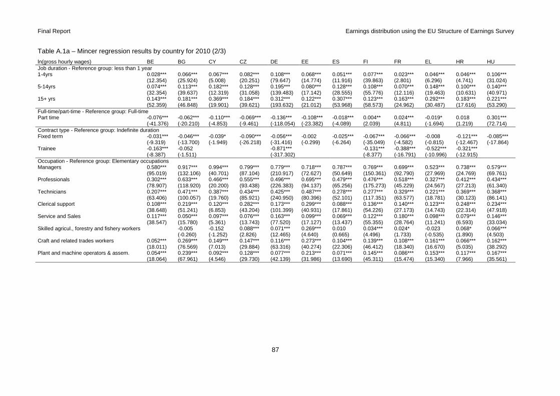
Final Report Earnings distribution using the EU Structure of Earnings Survey
87
Table A.1a – Mincer regression results by country for 2010 (2/3)
ln(gross hourly wages) BE BG CY CZ DE EE ES FI FR EL HR HU Job duration - Reference group: less than 1 year 1-4yrs 0.028*** 0.066*** 0.067*** 0.082*** 0.108*** 0.068*** 0.051*** 0.077*** 0.023*** 0.046*** 0.046*** 0.106*** (12.354) (25.924) (5.008) (20.251) (79.647) (14.774) (11.916) (39.863) (2.801) (6.296) (4.741) (31.024) 5-14yrs 0.074*** 0.113*** 0.182*** 0.128*** 0.195*** 0.080*** 0.128*** 0.108*** 0.070*** 0.148*** 0.100*** 0.140*** (32.354) (39.637) (12.319) (31.058) (139.483) (17.142) (28.555) (55.776) (12.116) (19.463) (10.631) (40.971) 15+ yrs 0.143*** 0.181*** 0.369*** 0.184*** 0.312*** 0.122*** 0.307*** 0.123*** 0.163*** 0.292*** 0.183*** 0.221*** (52.359) (46.848) (19.901) (39.621) (193.632) (21.012) (53.968) (58.573) (24.962) (30.487) (17.616) (53.290) Full-time/part-time - Reference group: Full-time Part time -0.076*** -0.062*** -0.110*** -0.069*** -0.136*** -0.108*** -0.018*** 0.004** 0.024*** -0.019* 0.018 0.301*** (-41.376) (-20.210) (-4.853) (-9.461) (-118.054) (-23.382) (-4.089) (2.039) (4.811) (-1.694) (1.219) (72.714) Contract type - Reference group: Indefinite duration Fixed term -0.031*** -0.046*** -0.039* -0.090*** -0.056*** -0.002 -0.025*** -0.067*** -0.066*** -0.008 -0.121*** -0.085*** (-9.319) (-13.700) (-1.949) (-26.218) (-31.416) (-0.299) (-6.264) (-35.049) (-4.582) (-0.815) (-12.467) (-17.864) Trainee -0.163*** -0.052 -0.871*** -0.131*** -0.388*** -0.522*** -0.321*** (-8.387) (-1.511) (-317.302) (-8.377) (-16.791) (-10.996) (-12.915) Occupation - Reference group: Elementary occupations Managers 0.580*** 0.917*** 0.994*** 0.799*** 0.779*** 0.718*** 0.787*** 0.769*** 0.699*** 0.523*** 0.738*** 0.579*** (95.019) (132.106) (40.701) (87.104) (210.917) (72.627) (50.649) (150.361) (92.790) (27.969) (24.769) (69.761) Professionals 0.302*** 0.633*** 0.466*** 0.555*** 0.496*** 0.695*** 0.479*** 0.476*** 0.518*** 0.327*** 0.412*** 0.434*** (78.907) (118.920) (20.200) (93.438) (226.383) (94.137) (65.256) (175.273) (45.229) (24.567) (27.213) (61.340) Technicians 0.207*** 0.471*** 0.387*** 0.434*** 0.425*** 0.487*** 0.278*** 0.277*** 0.329*** 0.221*** 0.369*** 0.368*** (63.406) (100.057) (19.760) (85.921) (240.950) (80.396) (52.101) (117.351) (63.577) (18.781) (30.123) (86.141) Clerical support 0.108*** 0.219*** 0.120*** 0.282*** 0.173*** 0.299*** 0.088*** 0.136*** 0.140*** 0.123*** 0.248*** 0.234*** (38.648) (51.241) (6.853) (43.204) (101.399) (40.931) (17.861) (54.226) (27.173) (14.743) (22.314) (47.918) Service and Sales 0.117*** 0.050*** 0.097*** 0.076*** 0.163*** 0.099*** 0.069*** 0.122*** 0.180*** 0.098*** 0.079*** 0.146***
(38.547) (15.780) (5.361) (13.743) (77.520) (17.127) (13.437) (55.355) (28.764) (11.241) (6.593) (33.034) Skilled agricul., forestry and fishery workers -0.005 -0.152 0.088*** 0.071*** 0.269*** 0.010 0.034*** 0.024* -0.023 0.068* 0.066***
(-0.260) (-1.252) (2.826) (12.465) (4.640) (0.665) (4.496) (1.733) (-0.535) (1.890) (4.503) Craft and related trades workers 0.052*** 0.269*** 0.149*** 0.147*** 0.116*** 0.273*** 0.104*** 0.139*** 0.108*** 0.161*** 0.066*** 0.162***
(18.011) (76.569) (7.013) (29.884) (63.316) (40.274) (22.306) (46.412) (18.340) (16.670) (5.035) (38.292) Plant and machine operators & assem. 0.054*** 0.239*** 0.092*** 0.128*** 0.077*** 0.213*** 0.071*** 0.145*** 0.086*** 0.153*** 0.117*** 0.167***
(18.064) (67.961) (4.546) (29.730) (42.139) (31.986) (13.690) (45.311) (15.474) (15.340) (7.966) (35.561)
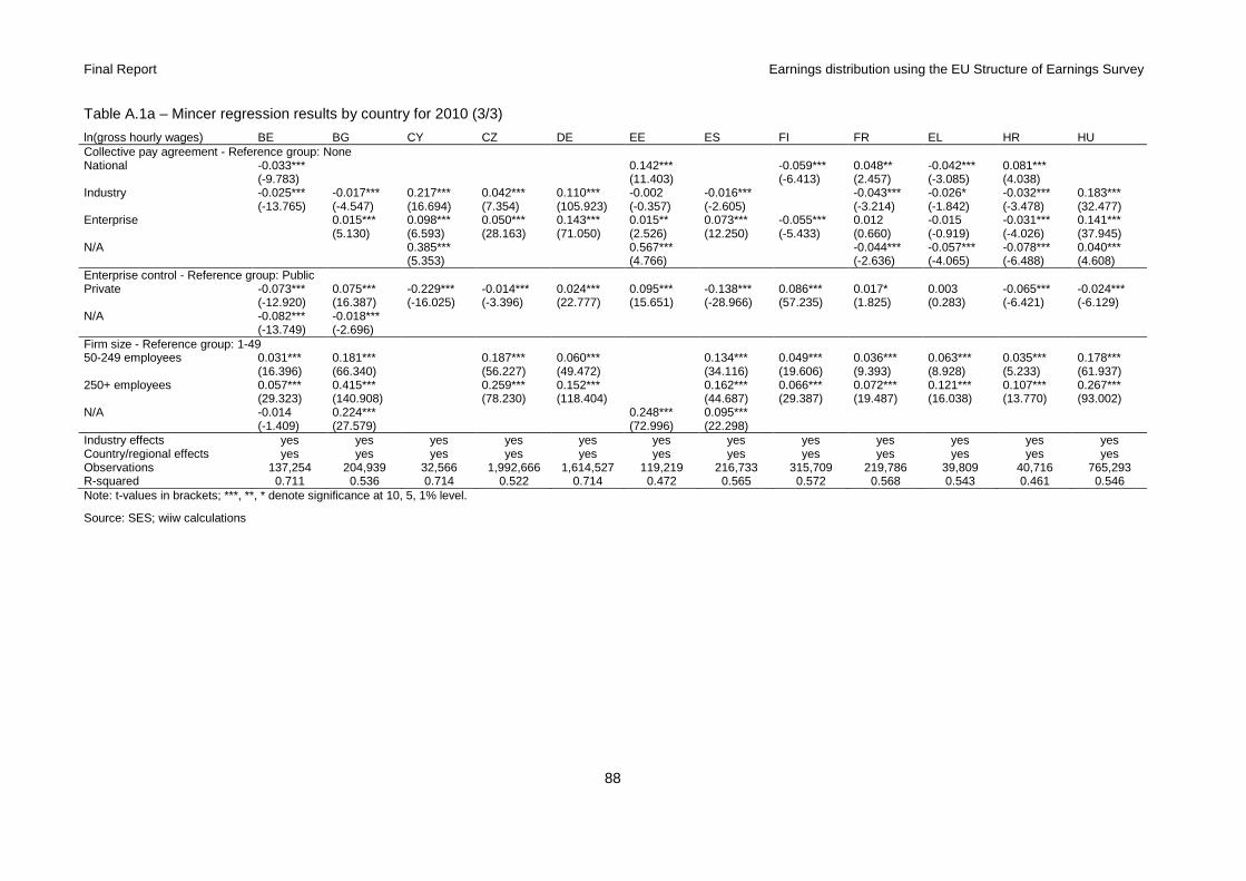
Final Report Earnings distribution using the EU Structure of Earnings Survey
88
Table A.1a – Mincer regression results by country for 2010 (3/3)
ln(gross hourly wages) BE BG CY CZ DE EE ES FI FR EL HR HU Collective pay agreement - Reference group: None National -0.033*** 0.142*** -0.059*** 0.048** -0.042*** 0.081*** (-9.783) (11.403) (-6.413) (2.457) (-3.085) (4.038) Industry -0.025*** -0.017*** 0.217*** 0.042*** 0.110*** -0.002 -0.016*** -0.043*** -0.026* -0.032*** 0.183*** (-13.765) (-4.547) (16.694) (7.354) (105.923) (-0.357) (-2.605) (-3.214) (-1.842) (-3.478) (32.477) Enterprise 0.015*** 0.098*** 0.050*** 0.143*** 0.015** 0.073*** -0.055*** 0.012 -0.015 -0.031*** 0.141***
(5.130) (6.593) (28.163) (71.050) (2.526) (12.250) (-5.433) (0.660) (-0.919) (-4.026) (37.945) N/A 0.385*** 0.567*** -0.044*** -0.057*** -0.078*** 0.040*** (5.353) (4.766) (-2.636) (-4.065) (-6.488) (4.608) Enterprise control - Reference group: Public Private -0.073*** 0.075*** -0.229*** -0.014*** 0.024*** 0.095*** -0.138*** 0.086*** 0.017* 0.003 -0.065*** -0.024*** (-12.920) (16.387) (-16.025) (-3.396) (22.777) (15.651) (-28.966) (57.235) (1.825) (0.283) (-6.421) (-6.129) N/A -0.082*** -0.018*** (-13.749) (-2.696) Firm size - Reference group: 1-49 50-249 employees 0.031*** 0.181*** 0.187*** 0.060*** 0.134*** 0.049*** 0.036*** 0.063*** 0.035*** 0.178*** (16.396) (66.340) (56.227) (49.472) (34.116) (19.606) (9.393) (8.928) (5.233) (61.937) 250+ employees 0.057*** 0.415*** 0.259*** 0.152*** 0.162*** 0.066*** 0.072*** 0.121*** 0.107*** 0.267*** (29.323) (140.908) (78.230) (118.404) (44.687) (29.387) (19.487) (16.038) (13.770) (93.002) N/A -0.014 0.224*** 0.248*** 0.095*** (-1.409) (27.579) (72.996) (22.298) Industry effects yes yes yes yes yes yes yes yes yes yes yes yes Country/regional effects yes yes yes yes yes yes yes yes yes yes yes yes Observations 137,254 204,939 32,566 1,992,666 1,614,527 119,219 216,733 315,709 219,786 39,809 40,716 765,293 R-squared 0.711 0.536 0.714 0.522 0.714 0.472 0.565 0.572 0.568 0.543 0.461 0.546 Note: t-values in brackets; ***, **, * denote significance at 10, 5, 1% level.
Source: SES; wiiw calculations
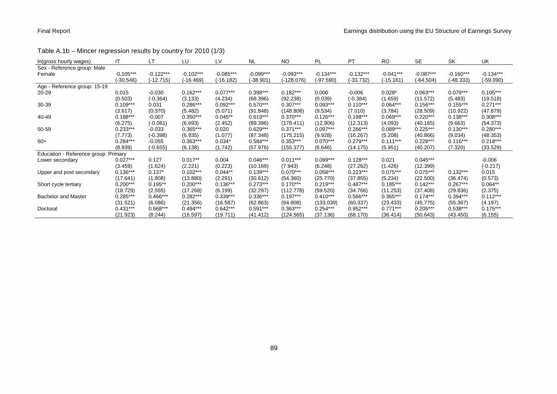
Final Report Earnings distribution using the EU Structure of Earnings Survey
89
Table A.1b – Mincer regression results by country for 2010 (1/3)
ln(gross hourly wages) IT LT LU LV NL NO PL PT RO SE SK UK Sex - Reference group: Male Female -0.105*** -0.122*** -0.102*** -0.085*** -0.099*** -0.093*** -0.134*** -0.132*** -0.041*** -0.087*** -0.160*** -0.134*** (-30.546) (-12.715) (-16.469) (-16.182) (-38.901) (-128.076) (-97.590) (-33.732) (-15.161) (-64.504) (-48.333) (-59.090) Age - Reference group: 15-19 20-29 0.015 -0.030 0.162*** 0.077*** 0.398*** 0.182*** 0.000 -0.006 0.028* 0.063*** 0.079*** 0.105*** (0.503) (-0.364) (3.133) (4.234) (68.396) (92.238) (0.039) (-0.384) (1.659) (11.572) (5.483) (19.518) 30-39 0.109*** 0.031 0.286*** 0.092*** 0.570*** 0.307*** 0.093*** 0.110*** 0.064*** 0.156*** 0.155*** 0.271*** (3.617) (0.370) (5.482) (5.071) (91.848) (148.808) (9.534) (7.010) (3.784) (28.509) (10.922) (47.879) 40-49 0.188*** -0.007 0.350*** 0.045** 0.619*** 0.370*** 0.126*** 0.198*** 0.069*** 0.220*** 0.138*** 0.308*** (6.275) (-0.081) (6.693) (2.452) (89.396) (178.411) (12.906) (12.313) (4.093) (40.165) (9.663) (54.373) 50-59 0.233*** -0.033 0.365*** 0.020 0.629*** 0.371*** 0.097*** 0.266*** 0.089*** 0.225*** 0.130*** 0.280*** (7.773) (-0.398) (6.935) (1.077) (87.348) (175.215) (9.928) (16.267) (5.208) (40.866) (9.034) (48.353) 60+ 0.284*** -0.055 0.363*** 0.034* 0.584*** 0.353*** 0.070*** 0.279*** 0.111*** 0.228*** 0.116*** 0.218*** (8.939) (-0.655) (6.138) (1.742) (57.976) (155.377) (6.646) (14.175) (5.951) (40.207) (7.320) (33.529) Education - Reference group: Primary Lower secondary 0.027*** 0.127 0.017** 0.004 0.046*** 0.011*** 0.099*** 0.128*** 0.021 0.045*** -0.006 (3.459) (1.624) (2.221) (0.223) (10.169) (7.943) (6.248) (27.262) (1.426) (12.399) (-0.217) Upper and post secondary 0.136*** 0.137* 0.102*** 0.044** 0.139*** 0.070*** 0.058*** 0.223*** 0.075*** 0.075*** 0.132*** 0.015
(17.641) (1.808) (13.880) (2.291) (30.612) (54.360) (25.770) (37.855) (5.234) (22.500) (36.474) (0.573) Short cycle tertiary 0.200*** 0.195** 0.200*** 0.136*** 0.273*** 0.170*** 0.219*** 0.487*** 0.185*** 0.142*** 0.267*** 0.064**
(18.729) (2.555) (17.268) (6.199) (32.297) (112.778) (59.520) (34.766) (11.253) (37.408) (29.836) (2.375) Bachelor and Master 0.285*** 0.466*** 0.282*** 0.339*** 0.336*** 0.197*** 0.410*** 0.566*** 0.365*** 0.174*** 0.394*** 0.112***
(31.521) (6.086) (21.356) (16.587) (62.863) (64.808) (133.039) (60.337) (23.433) (45.775) (55.367) (4.197) Doctoral 0.431*** 0.668*** 0.494*** 0.642*** 0.591*** 0.363*** 0.254*** 0.952*** 0.771*** 0.205*** 0.538*** 0.175*** (21.923) (8.244) (16.597) (19.711) (41.412) (124.565) (37.136) (68.170) (36.414) (50.643) (43.450) (6.155)
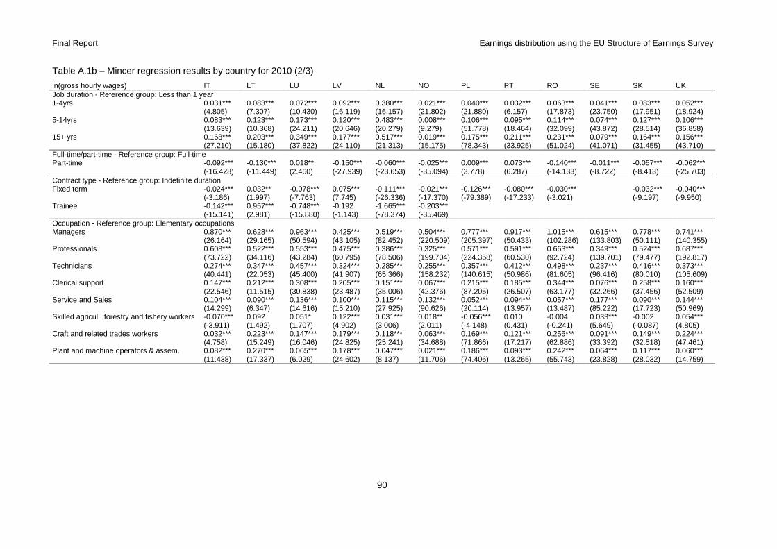
Final Report Earnings distribution using the EU Structure of Earnings Survey
90
Table A.1b – Mincer regression results by country for 2010 (2/3)
ln(gross hourly wages) IT LT LU LV NL NO PL PT RO SE SK UK Job duration - Reference group: Less than 1 year 1-4yrs 0.031*** 0.083*** 0.072*** 0.092*** 0.380*** 0.021*** 0.040*** 0.032*** 0.063*** 0.041*** 0.083*** 0.052*** (4.805) (7.307) (10.430) (16.119) (16.157) (21.802) (21.880) (6.157) (17.873) (23.750) (17.951) (18.924) 5-14yrs 0.083*** 0.123*** 0.173*** 0.120*** 0.483*** 0.008*** 0.106*** 0.095*** 0.114*** 0.074*** 0.127*** 0.106*** (13.639) (10.368) (24.211) (20.646) (20.279) (9.279) (51.778) (18.464) (32.099) (43.872) (28.514) (36.858) 15+ yrs 0.168*** 0.203*** 0.349*** 0.177*** 0.517*** 0.019*** 0.175*** 0.211*** 0.231*** 0.079*** 0.164*** 0.156*** (27.210) (15.180) (37.822) (24.110) (21.313) (15.175) (78.343) (33.925) (51.024) (41.071) (31.455) (43.710) Full-time/part-time - Reference group: Full-time Part-time -0.092*** -0.130*** 0.018** -0.150*** -0.060*** -0.025*** 0.009*** 0.073*** -0.140*** -0.011*** -0.057*** -0.062*** (-16.428) (-11.449) (2.460) (-27.939) (-23.653) (-35.094) (3.778) (6.287) (-14.133) (-8.722) (-8.413) (-25.703) Contract type - Reference group: Indefinite duration Fixed term -0.024*** 0.032** -0.078*** 0.075*** -0.111*** -0.021*** -0.126*** -0.080*** -0.030*** -0.032*** -0.040*** Trainee
(-3.186) (1.997) (-7.763) (7.745) (-26.336) (-17.370) (-79.389) (-17.233) (-3.021) (-9.197) (-9.950) -0.142*** 0.957*** -0.748*** -0.192 -1.665*** -0.203***
(-15.141) (2.981) (-15.880) (-1.143) (-78.374) (-35.469) Occupation - Reference group: Elementary occupations Managers 0.870*** 0.628*** 0.963*** 0.425*** 0.519*** 0.504*** 0.777*** 0.917*** 1.015*** 0.615*** 0.778*** 0.741*** (26.164) (29.165) (50.594) (43.105) (82.452) (220.509) (205.397) (50.433) (102.286) (133.803) (50.111) (140.355) Professionals 0.608*** 0.522*** 0.553*** 0.475*** 0.386*** 0.325*** 0.571*** 0.591*** 0.663*** 0.349*** 0.524*** 0.687*** (73.722) (34.116) (43.284) (60.795) (78.506) (199.704) (224.358) (60.530) (92.724) (139.701) (79.477) (192.817) Technicians 0.274*** 0.347*** 0.457*** 0.324*** 0.285*** 0.255*** 0.357*** 0.412*** 0.498*** 0.237*** 0.416*** 0.373*** (40.441) (22.053) (45.400) (41.907) (65.366) (158.232) (140.615) (50.986) (81.605) (96.416) (80.010) (105.609) Clerical support 0.147*** 0.212*** 0.308*** 0.205*** 0.151*** 0.067*** 0.215*** 0.185*** 0.344*** 0.076*** 0.258*** 0.160*** (22.546) (11.515) (30.838) (23.487) (35.006) (42.376) (87.205) (26.507) (63.177) (32.266) (37.456) (52.509) Service and Sales 0.104*** 0.090*** 0.136*** 0.100*** 0.115*** 0.132*** 0.052*** 0.094*** 0.057*** 0.177*** 0.090*** 0.144***
(14.299) (6.347) (14.616) (15.210) (27.925) (90.626) (20.114) (13.957) (13.487) (85.222) (17.723) (50.969) Skilled agricul., forestry and fishery workers -0.070*** 0.092 0.051* 0.122*** 0.031*** 0.018** -0.056*** 0.010 -0.004 0.033*** -0.002 0.054***
(-3.911) (1.492) (1.707) (4.902) (3.006) (2.011) (-4.148) (0.431) (-0.241) (5.649) (-0.087) (4.805) Craft and related trades workers 0.032*** 0.223*** 0.147*** 0.179*** 0.118*** 0.063*** 0.169*** 0.121*** 0.256*** 0.091*** 0.149*** 0.224***
(4.758) (15.249) (16.046) (24.825) (25.241) (34.688) (71.866) (17.217) (62.886) (33.392) (32.518) (47.461) Plant and machine operators & assem. 0.082*** 0.270*** 0.065*** 0.178*** 0.047*** 0.021*** 0.186*** 0.093*** 0.242*** 0.064*** 0.117*** 0.060***
(11.438) (17.337) (6.029) (24.602) (8.137) (11.706) (74.406) (13.265) (55.743) (23.828) (28.032) (14.759)
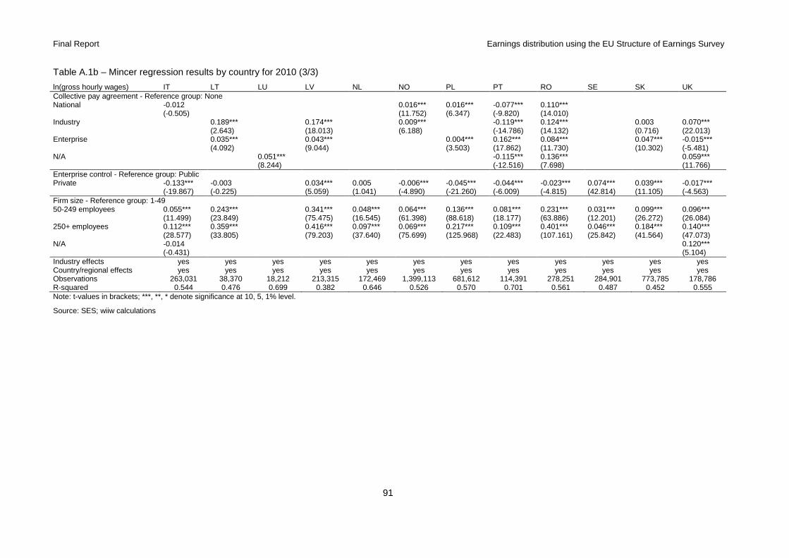
Final Report Earnings distribution using the EU Structure of Earnings Survey
91
Table A.1b – Mincer regression results by country for 2010 (3/3)
ln(gross hourly wages) IT LT LU LV NL NO PL PT RO SE SK UK Collective pay agreement - Reference group: None National -0.012 0.016*** 0.016*** -0.077*** 0.110*** (-0.505) (11.752) (6.347) (-9.820) (14.010) Industry 0.189*** 0.174*** 0.009*** -0.119*** 0.124*** 0.003 0.070*** Enterprise
(2.643) (18.013) (6.188) (-14.786) (14.132) (0.716) (22.013) 0.035*** 0.043*** 0.004*** 0.162*** 0.084*** 0.047*** -0.015***
(4.092) (9.044) (3.503) (17.862) (11.730) (10.302) (-5.481) N/A 0.051*** -0.115*** 0.136*** 0.059*** (8.244) (-12.516) (7.698) (11.766) Enterprise control - Reference group: Public Private -0.133*** -0.003 0.034*** 0.005 -0.006*** -0.045*** -0.044*** -0.023*** 0.074*** 0.039*** -0.017*** (-19.867) (-0.225) (5.059) (1.041) (-4.890) (-21.260) (-6.009) (-4.815) (42.814) (11.105) (-4.563) Firm size - Reference group: 1-49 50-249 employees 0.055*** 0.243*** 0.341*** 0.048*** 0.064*** 0.136*** 0.081*** 0.231*** 0.031*** 0.099*** 0.096*** (11.499) (23.849) (75.475) (16.545) (61.398) (88.618) (18.177) (63.886) (12.201) (26.272) (26.084) 250+ employees 0.112*** 0.359*** 0.416*** 0.097*** 0.069*** 0.217*** 0.109*** 0.401*** 0.046*** 0.184*** 0.140*** (28.577) (33.805) (79.203) (37.640) (75.699) (125.968) (22.483) (107.161) (25.842) (41.564) (47.073) N/A -0.014 0.120*** (-0.431) (5.104) Industry effects yes yes yes yes yes yes yes yes yes yes yes yes Country/regional effects yes yes yes yes yes yes yes yes yes yes yes yes Observations 263,031 38,370 18,212 213,315 172,469 1,399,113 681,612 114,391 278,251 284,901 773,785 178,786 R-squared 0.544 0.476 0.699 0.382 0.646 0.526 0.570 0.701 0.561 0.487 0.452 0.555 Note: t-values in brackets; ***, **, * denote significance at 10, 5, 1% level.
Source: SES; wiiw calculations
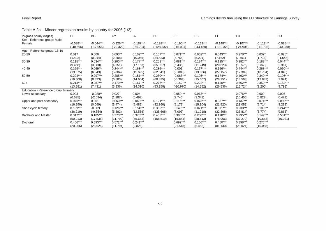
Final Report Earnings distribution using the EU Structure of Earnings Survey
92
Table A.2a – Mincer regression results by country for 2006 (1/3)
ln(gross hourly wages) BE BG CY CZ DE EE ES FI FR EL HU Sex - Reference group: Male Female -0.098*** -0.044*** -0.226*** -0.187*** -0.138*** -0.190*** -0.163*** -0.148*** -0.107*** -0.112*** -0.095*** (-40.596) (-17.056) (-22.322) (-65.794) (-128.832) (-45.031) (-44.450) (-110.328) (-24.906) (-12.708) (-43.378) Age - Reference group: 15-19 20-29 0.017 0.000 0.093** 0.102*** 0.107*** 0.071*** 0.062*** 0.043*** 0.278*** 0.037* -0.025* (1.402) (0.014) (2.208) (10.086) (24.823) (5.765) (5.201) (7.162) (7.761) (1.713) (-1.648) 30-39 0.115*** 0.034*** 0.200*** 0.177*** 0.251*** 0.081*** 0.134*** 0.125*** 0.382*** 0.183*** 0.044*** (9.458) (3.088) (4.651) (17.153) (55.027) (6.435) (11.249) (20.623) (10.575) (8.343) (2.967) 40-49 0.169*** 0.069*** 0.244*** 0.163*** 0.286*** -0.001 0.167*** 0.166*** 0.444*** 0.268*** 0.060*** (13.875) (6.343) (5.804) (15.695) (62.641) (-0.088) (13.886) (27.157) (12.309) (10.784) (4.045) 50-59 0.204*** 0.097*** 0.285*** 0.151*** 0.280*** -0.068*** 0.195*** 0.174*** 0.492*** 0.340*** 0.106*** (16.508) (8.833) (6.583) (14.604) (60.835) (-5.364) (15.607) (28.251) (13.598) (13.883) (7.074) 60+ 0.213*** 0.087*** 0.179*** 0.167*** 0.277*** -0.142*** 0.222*** 0.180*** 0.662*** 0.350*** 0.153*** (13.581) (7.431) (3.836) (14.310) (53.258) (-10.970) (14.552) (26.536) (15.724) (9.200) (9.798) Education - Reference group: Primary Lower secondary 0.003 -0.020** 0.027 0.004 0.052*** 0.013*** 0.076*** 0.009 0.005 (0.595) (-2.094) (1.287) (0.499) (2.746) (3.341) (10.455) (0.829) (0.479) Upper and post secondary 0.076*** 0.001 0.060*** 0.063*** 0.121*** 0.115*** 0.073*** 0.037*** 0.137*** 0.074*** 0.089***
(16.590) (0.099) (3.474) (9.485) (82.360) (6.175) (15.104) (21.520) (21.051) (6.714) (8.252) Short cycle tertiary 0.189*** -0.009 0.126*** 0.154*** 0.365*** 0.140*** 0.071*** 0.071*** 0.230*** 0.103*** 0.244***
(36.219) (-0.854) (5.882) (12.556) (135.668) (7.093) (11.218) (32.808) (28.814) (5.774) (9.863) Bachelor and Master 0.317*** 0.185*** 0.273*** 0.378*** 0.485*** 0.308*** 0.200*** 0.198*** 0.295*** 0.149*** 0.531***
(50.013) (17.535) (11.790) (45.652) (168.519) (15.844) (28.513) (78.966) (32.279) (10.558) (46.021) Doctoral 0.466*** 0.393*** 0.571*** 0.241*** 0.692*** 0.166*** 0.450*** 0.398*** 0.278*** (20.956) (23.625) (11.794) (9.826) (21.518) (5.452) (81.130) (23.021) (10.088)

Final Report Earnings distribution using the EU Structure of Earnings Survey
93
Table A.2a – Mincer regression results by country for 2006 (2/3)
ln(gross hourly wages) BE BG CY CZ DE EE ES FI FR EL HU Job duration - Reference group: Less than 1 year 1-4yrs 0.059*** 0.038*** 0.060*** 0.087*** 0.109*** 0.019*** 0.060*** 0.073*** 0.021*** 0.107*** 0.078*** (18.002) (13.426) (4.164) (22.749) (70.517) (4.092) (13.258) (38.037) (3.480) (8.371) (28.164) 5-14yrs 0.103*** 0.127*** 0.182*** 0.143*** 0.189*** 0.055*** 0.130*** 0.106*** 0.077*** 0.220*** 0.156*** (33.464) (38.763) (13.887) (39.541) (125.903) (11.790) (28.730) (56.234) (12.767) (15.659) (57.043) 15+ yrs 0.192*** 0.199*** 0.386*** 0.172*** 0.298*** 0.074*** 0.283*** 0.127*** 0.159*** 0.343*** 0.214*** (53.166) (50.643) (24.528) (42.559) (170.473) (11.645) (50.484) (64.345) (23.737) (17.645) (67.284) Full-time/part-time - Reference group: Full-time Part time 0.035*** -0.015*** 0.005 -0.046*** -0.069*** -0.154*** -0.020*** 0.008*** 0.004 0.148*** 0.275*** (14.051) (-3.740) (0.108) (-7.748) (-60.700) (-27.765) (-3.757) (3.797) (0.561) (7.653) (68.003) Contract type - Reference group: Indefinite duration Fixed term -0.055*** -0.019*** -0.005 -0.080*** -0.089*** 0.029*** -0.045*** -0.068*** -0.052*** 0.056*** -0.112*** (-15.048) (-5.449) (-0.256) (-25.566) (-47.916) (3.414) (-11.027) (-38.155) (-6.654) (6.716) (-30.677) Trainee -0.225*** -0.114*** -0.956*** -0.139*** -0.477*** -0.139** 0.298*** (-8.790) (-2.604) (-286.328) (-20.989) (-19.368) (-2.365) (4.480) Occupation - Reference group: Elementary occupations Managers 0.658*** 0.901*** 0.908*** 0.702*** 0.774*** 0.670*** 0.854*** 0.673*** 0.674*** 0.644*** 0.617*** (68.115) (106.972) (33.809) (75.111) (140.801) (74.583) (69.624) (140.309) (56.061) (23.492) (113.877) Professionals 0.414*** 0.654*** 0.598*** 0.562*** 0.465*** 0.715*** 0.490*** 0.420*** 0.559*** 0.347*** 0.420*** (71.666) (104.968) (26.123) (93.539) (171.569) (83.459) (54.337) (154.680) (53.439) (12.209) (77.548) Technicians 0.243*** 0.461*** 0.366*** 0.484*** 0.391*** 0.508*** 0.284*** 0.224*** 0.328*** 0.235*** 0.352*** (55.026) (84.253) (20.381) (109.082) (217.487) (77.529) (43.586) (99.586) (36.925) (17.727) (97.639) Clerical support 0.141*** 0.207*** 0.093*** 0.278*** 0.300*** 0.276*** 0.098*** 0.107*** 0.136*** 0.105*** 0.158*** (34.155) (47.649) (5.187) (50.819) (170.546) (35.243) (18.196) (45.276) (15.505) (9.603) (39.826) Service and Sales 0.104*** 0.021*** 0.128*** 0.124*** 0.163*** 0.125*** 0.049*** 0.096*** 0.135*** 0.116*** 0.115***
(24.825) (6.458) (6.555) (25.421) (75.205) (17.416) (8.570) (47.362) (13.821) (10.847) (28.359) Skilled agricul., forestry and fishery workers 0.073*** 0.137*** 0.264*** 0.029*** 0.260*** 0.079*** 0.025* 0.066 -0.004 -0.036***
(5.219) (4.306) (3.698) (3.901) (3.680) (3.818) (1.780) (1.406) (-0.104) (-2.779) raft and related trades workers 0.070*** 0.242*** 0.143*** 0.193*** 0.134*** 0.302*** 0.101*** 0.132*** 0.091*** 0.132*** 0.113***
(17.565) (68.345) (7.806) (44.730) (75.996) (44.462) (19.142) (44.297) (9.178) (12.979) (28.966) Plant and machine operators & assem. 0.096*** 0.244*** 0.103*** 0.187*** 0.069*** 0.290*** 0.078*** 0.134*** 0.104*** 0.137*** 0.140***
(22.497) (70.148) (5.581) (45.857) (35.202) (42.230) (15.253) (49.409) (12.271) (13.049) (35.198)
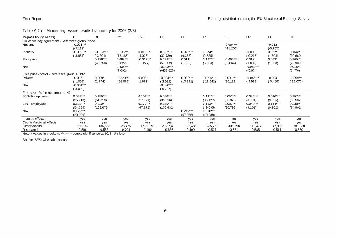
Final Report Earnings distribution using the EU Structure of Earnings Survey
94
Table A.2a – Mincer regression results by country for 2006 (3/3)
ln(gross hourly wages) BE BG CY CZ DE EE ES FI FR EL HU Collective pay agreement - Reference group: None National -0.021*** -0.094*** -0.012 (-5.119) (-11.203) (-0.765) Industry -0.009*** -0.013*** 0.136*** 0.019*** 0.037*** 0.075*** 0.074** -0.002 0.027* 0.164*** (-3.961) (-3.301) (13.465) (4.006) (37.739) (9.363) (2.535) (-0.295) (1.804) (30.660) Enterprise 0.136*** 0.093*** -0.013*** 0.084*** 0.011* 0.167*** -0.056*** 0.013 0.072* 0.105***
(42.253) (5.327) (-6.277) (57.052) (1.790) (5.654) (-5.864) (0.887) (1.958) (29.939) N/A 0.435*** -0.998*** -0.060*** 0.018** (7.692) (-437.825) (-5.674) (2.476) Enterprise control - Reference group: Public Private -0.006 0.008* -0.220*** 0.008* -0.004*** 0.092*** -0.096*** 0.091*** -0.045*** -0.004 -0.059*** (-1.097) (1.774) (-16.887) (1.663) (-2.952) (13.661) (-15.242) (59.161) (-4.996) (-0.499) (-17.077) N/A -0.054*** -0.020*** (-8.090) (-9.727) Firm size - Reference group: 1-49 50-249 employees 0.051*** 0.155*** 0.109*** 0.050*** 0.131*** 0.050*** 0.020*** 0.086*** 0.157*** (25.713) (51.819) (27.379) (35.616) (35.127) (20.978) (3.794) (9.925) (58.537) 250+ employees 0.123*** 0.329*** 0.179*** 0.155*** 0.183*** 0.080*** 0.049*** 0.144*** 0.238*** (54.685) (103.678) (47.872) (106.431) (49.595) (36.798) (9.201) (9.962) (84.901) N/A 0.129*** 0.249*** 0.098*** (20.900) (67.085) (10.288) Industry effects yes yes yes yes yes yes yes yes yes yes yes Country/regional effects yes yes yes yes yes yes yes yes yes yes yes Observations 165,182 186,663 26,475 1,970,091 2,587,433 126,485 235,261 305,598 113,472 47,905 781,830 R-squared 0.596 0.563 0.704 0.490 0.686 0.409 0.527 0.561 0.585 0.561 0.560 Note: t-values in brackets; ***, **, * denote significance at 10, 5, 1% level.
Source: SES; wiiw calculations
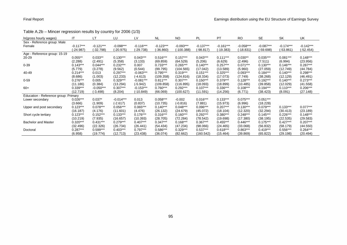
Final Report Earnings distribution using the EU Structure of Earnings Survey
95
Table A.2b – Mincer regression results by country for 2006 (1/3)
ln(gross hourly wages) IT LT LU LV NL NO PL PT RO SE SK UK Sex - Reference group: Male Female -0.117*** -0.121*** -0.098*** -0.116*** -0.123*** -0.093*** -0.137*** -0.161*** -0.058*** -0.087*** -0.174*** -0.142*** (-24.987) (-32.798) (-20.975) (-29.738) (-36.860) (-100.388) (-98.817) (-19.383) (-18.831) (-59.698) (-53.861) (-52.454) Age - Reference group: 15-19 20-29 0.055** 0.033** 0.130*** 0.043*** 0.516*** 0.157*** 0.043*** 0.111*** 0.030** 0.035*** 0.081*** 0.148*** (2.288) (2.491) (5.358) (3.133) (69.859) (64.529) (5.206) (6.629) (2.496) (7.511) (6.994) (23.956) 0-39 0.143*** 0.044*** 0.232*** 0.007 0.733*** 0.265*** 0.140*** 0.257*** 0.071*** 0.130*** 0.146*** 0.287*** (5.779) (3.278) (9.562) (0.544) (99.795) (104.565) (17.042) (13.589) (5.960) (27.059) (12.749) (44.784) 40-49 0.214*** 0.013 0.297*** -0.063*** 0.795*** 0.319*** 0.151*** 0.325*** 0.093*** 0.184*** 0.140*** 0.298*** (8.686) (1.003) (12.233) (-4.613) (109.358) (124.816) (18.334) (17.073) (7.749) (38.268) (12.129) (46.491) 0-59 0.276*** 0.005 0.329*** -0.081*** 0.811*** 0.307*** 0.150*** 0.379*** 0.128*** 0.192*** 0.140*** 0.273*** (11.186) (0.384) (13.294) (-5.942) (109.858) (116.895) (18.093) (18.899) (10.485) (39.858) (12.029) (41.558) 60+ 0.339*** -0.050*** 0.307*** -0.153*** 0.760*** 0.292*** 0.107*** 0.336*** 0.108*** 0.194*** 0.110*** 0.206*** (12.719) (-3.498) (8.204) (-10.849) (66.069) (100.627) (11.591) (14.256) (6.771) (38.423) (8.091) (27.148) Education - Reference group: Primary Lower secondary 0.026*** 0.037* -0.014*** 0.013 0.058*** -0.002 0.016*** 0.133*** 0.075*** 0.051*** (3.666) (1.909) (-2.617) (0.837) (10.735) (-0.816) (7.881) (15.973) (6.996) (18.228) Upper and post secondary 0.123*** 0.078*** 0.056*** 0.065*** 0.140*** 0.048*** 0.096*** 0.207*** 0.130*** 0.079*** 0.133*** 0.077***
(16.187) (4.176) (11.601) (4.476) (26.132) (24.679) (45.072) (18.104) (12.320) (32.294) (30.413) (23.189) Short cycle tertiary 0.123*** 0.152*** 0.133*** 0.176*** 0.316*** 0.160*** 0.292*** 0.380*** 0.248*** 0.145*** 0.226*** 0.148***
(10.219) (7.935) (16.657) (10.393) (28.705) (72.284) (78.542) (19.698) (17.380) (38.195) (22.535) (29.583) Bachelor and Master 0.320*** 0.431*** 0.279*** 0.407*** 0.347*** 0.168*** 0.367*** 0.455*** 0.446*** 0.175*** 0.427*** 0.207***
(32.496) (22.326) (26.734) (26.441) (54.434) (47.234) (98.066) (24.465) (33.068) (56.832) (58.179) (44.550) Doctoral 0.287*** 0.599*** 0.403*** 0.797*** 0.586*** 0.329*** 0.537*** 0.618*** 0.863*** 0.419*** 0.556*** 0.264*** (6.958) (19.774) (12.713) (23.438) (36.074) (82.662) (160.542) (15.464) (39.869) (65.822) (29.198) (20.494)

Final Report Earnings distribution using the EU Structure of Earnings Survey
96
Table A.2b – Mincer regression results by country for 2006 (2/3)
ln(gross hourly wages) IT LT LU LV NL NO PL PT RO SE SK UK Job duration - Reference group: Less than 1 year 1-4yrs 0.045*** 0.063*** 0.075*** 0.046*** 0.089*** 0.051*** 0.056*** 0.051*** 0.072*** 0.044*** 0.078*** 0.059*** (5.516) (14.721) (15.275) (10.584) (24.146) (44.409) (28.900) (3.601) (20.233) (22.778) (19.548) (19.792) 5-14yrs 0.082*** 0.122*** 0.164*** 0.120*** 0.111*** 0.071*** 0.138*** 0.113*** 0.151*** 0.065*** 0.132*** 0.118*** (10.053) (28.100) (34.265) (27.691) (28.626) (62.570) (66.042) (8.212) (39.778) (35.970) (33.674) (37.428) 15+ yrs 0.150*** 0.180*** 0.301*** 0.238*** 0.164*** 0.056*** 0.202*** 0.225*** 0.242*** 0.062*** 0.139*** 0.178*** (18.570) (34.483) (48.538) (39.505) (36.519) (40.446) (89.480) (14.549) (56.361) (32.857) (34.035) (44.885) Full-time/part-time - Reference group: Full-time Part-time -0.021*** -0.139*** 0.047*** -0.034*** 0.000 -0.031*** 0.000 0.228*** -0.064*** -0.009*** -0.078*** -0.039*** (-3.624) (-27.345) (8.123) (-6.090) (0.056) (-31.113) (0.128) (7.520) (-3.945) (-6.982) (-14.584) (-13.357) Contract type - Reference group: Indefinite duration Fixed term -0.085*** -0.013* -0.053*** 0.085*** -0.109*** -0.001 -0.113*** -0.068*** -0.133*** -0.064*** -0.038*** Trainee
(-10.248) (-1.796) (-5.824) (9.183) (-26.791) (-0.436) (-67.802) (-6.507) (-14.875) (-14.437) (-7.899) -0.262*** -0.294*** -0.752*** -0.167*** -0.165*** -0.317*** -0.300***
(-20.492) (-3.263) (-24.880) (-3.757) (-38.418) (-3.034) (-16.193) Occupation -Reference group: Elementary occupations Managers 0.896*** 0.610*** 1.018*** 0.521*** 0.427*** 0.508*** 0.779*** 0.975*** 0.990*** 0.601*** 0.779*** 0.723*** (55.762) (82.638) (68.111) (66.156) (62.781) (176.548) (191.126) (35.883) (86.595) (127.591) (69.953) (136.848) Professionals 0.500*** 0.497*** 0.634*** 0.558*** 0.357*** 0.370*** 0.534*** 0.702*** 0.589*** 0.371*** 0.487*** 0.698*** (50.316) (80.845) (61.584) (80.546) (60.413) (165.548) (196.329) (31.750) (59.151) (132.204) (70.949) (128.987) Technicians 0.330*** 0.321*** 0.536*** 0.386*** 0.258*** 0.251*** 0.366*** 0.506*** 0.493*** 0.234*** 0.395*** 0.435*** (34.163) (48.510) (67.489) (62.607) (51.685) (123.247) (145.422) (31.646) (84.988) (89.890) (78.807) (94.165) Clerical support 0.232*** 0.222*** 0.318*** 0.266*** 0.139*** 0.063*** 0.190*** 0.193*** 0.288*** 0.067*** 0.207*** 0.157*** (31.500) (29.605) (45.552) (37.623) (28.142) (32.515) (75.586) (16.032) (39.630) (26.563) (29.489) (45.311) Service and Sales 0.133*** 0.128*** 0.228*** 0.129*** 0.092*** 0.087*** 0.052*** 0.050*** -0.019*** 0.173*** 0.056*** 0.107***
(16.290) (22.735) (31.572) (23.328) (17.377) (44.601) (19.563) (3.015) (-3.794) (78.353) (8.771) (31.492) Skilled agricul., forestry and fishery workers -0.094* 0.036 0.141*** 0.046** -0.009 0.027 0.163*** -0.062*** -0.066*** -0.007 0.013 0.012
(-1.757) (1.119) (2.932) (2.178) (-0.702) (1.463) (7.644) (-2.661) (-3.653) (-1.006) (0.675) (0.886) Craft and related trades workers 0.105*** 0.272*** 0.199*** 0.236*** 0.112*** 0.075*** 0.180*** 0.110*** 0.212*** 0.068*** 0.145*** 0.217***
(13.550) (48.941) (27.712) (41.030) (18.979) (35.014) (81.799) (12.746) (44.528) (25.661) (29.276) (41.749) Plant and machine operators & assem. 0.116*** 0.267*** 0.161*** 0.224*** 0.081*** 0.039*** 0.204*** 0.125*** 0.204*** 0.063*** 0.143*** 0.092***
(11.174) (44.134) (21.569) (37.353) (12.044) (19.481) (90.319) (13.939) (43.401) (24.217) (29.426) (19.398)
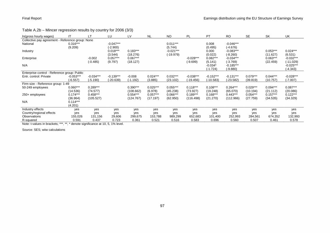
Final Report Earnings distribution using the EU Structure of Earnings Survey
97
Table A.2b – Mincer regression results by country for 2006 (3/3)
ln(gross hourly wages) IT LT LU LV NL NO PL PT RO SE SK UK Collective pay agreement - Reference group: None National 0.316*** -0.047*** 0.011*** 0.008 -0.046*** (9.209) (-2.900) (5.744) (0.495) (-4.676) Industry 0.018*** 0.183*** -0.021*** 0.000 -0.083*** 0.053*** 0.024*** Enterprise
(3.544) (18.276) (-19.979) (0.022) (-8.260) (11.627) (6.531) -0.002 0.057*** 0.067*** -0.028*** 0.082*** -0.034*** 0.063*** -0.032***
(-0.485) (9.797) (18.127) (-9.699) (5.141) (-3.769) (22.459) (-11.029) N/A -0.034* -0.185*** -0.025*** (-1.724) (-9.880) (-4.343) Enterprise control - Reference group: Public Entr. control: Private -0.053*** -0.034*** -0.139*** -0.008 0.024*** 0.032*** -0.038*** -0.152*** -0.131*** 0.079*** 0.044*** -0.028*** (-6.557) (-5.190) (-20.639) (-1.192) (3.885) (23.102) (-19.456) (-10.583) (-23.582) (39.819) (10.757) (-7.007) Firm size - Reference group: 1-49 50-249 employees 0.060*** 0.289*** 0.390*** 0.025*** 0.055*** 0.118*** 0.108*** 0.264*** 0.029*** 0.094*** 0.087*** (14.536) (74.577) (108.662) (6.978) (45.238) (73.927) (19.248) (65.070) (10.194) (21.112) (20.086) 250+ employees 0.174*** 0.458*** 0.554*** 0.057*** 0.066*** 0.189*** 0.168*** 0.443*** 0.054*** 0.157*** 0.122*** (36.964) (105.527) (124.767) (17.197) (62.950) (116.498) (21.270) (112.966) (27.759) (34.535) (34.329) N/A 0.114*** (4.201) Industry effects yes yes yes yes yes yes yes yes yes yes yes yes Country/regional effects yes yes yes yes yes yes yes yes yes yes yes yes Observations 155,026 131,156 29,606 299,675 153,788 989,299 652,683 101,400 252,993 284,561 674,352 132,993 R-squared 0.591 0.437 0.723 0.361 0.521 0.516 0.583 0.696 0.560 0.507 0.461 0.578 Note: t-values in brackets; ***, **, * denote significance at 10, 5, 1% level.
Source: SES; wiiw calculations

Final Report Earnings distribution using the EU Structure of Earnings Survey
98
Table A.3a – Mincer regression results by country for 2002 (1/3)
ln(gross hourly wages) BE BG CY CZ EE ES FI FR EL HU IT Sex - Reference group: Male Female -0.075*** -0.093*** -0.223*** -0.205*** -0.201*** -0.177*** -0.145*** -0.131*** -0.132*** -0.100*** -0.147*** (-19.404) (-30.244) (-16.454) (-92.103) (-32.042) (-52.629) (-67.401) (-27.613) (-29.372) (-42.437) (-32.209) Age - Reference group: 15-19 20-29 0.015 0.049*** 0.011 0.149*** 0.148*** 0.056*** 0.038*** 0.240*** 0.073*** 0.063*** 0.078*** (0.974) (2.894) (0.398) (12.276) (7.355) (5.952) (5.476) (9.529) (2.827) (5.920) (4.109) 0-39 0.204*** 0.108*** 0.125*** 0.204*** 0.143*** 0.157*** 0.118*** 0.342*** 0.224*** 0.102*** 0.193*** (12.981) (6.446) (4.224) (16.651) (6.991) (16.645) (16.599) (13.326) (8.714) (9.573) (9.901) 40-49 0.307*** 0.168*** 0.151*** 0.202*** 0.041** 0.205*** 0.139*** 0.381*** 0.316*** 0.122*** 0.261*** (18.962) (10.019) (4.844) (16.581) (2.032) (21.159) (19.343) (14.755) (12.146) (11.442) (13.413) 0-59 0.360*** 0.206*** 0.157*** 0.205*** -0.001 0.237*** 0.140*** 0.412*** 0.393*** 0.166*** 0.277*** (21.338) (12.260) (4.992) (16.833) (-0.055) (23.129) (18.939) (15.715) (14.996) (15.519) (13.825) 60+ 0.415*** 0.211*** 0.028 0.162*** -0.094*** 0.214*** 0.127*** 0.476*** 0.433*** 0.212*** 0.260*** (15.041) (11.217) (0.566) (12.621) (-4.350) (16.719) (13.683) (13.960) (12.923) (17.364) (9.433) Education - Reference group: Primary Lower secondary -0.006 -0.105*** -0.011 0.016** 0.033 0.001 -0.023 0.074*** 0.045*** 0.087*** 0.042*** (-0.501) (-8.607) (-0.521) (2.117) (1.628) (0.381) (-0.844) (9.771) (6.812) (8.212) (7.059) Upper and post secondary 0.054*** -0.043*** 0.042** 0.102*** 0.095*** 0.081*** 0.031*** 0.112*** 0.109*** 0.163*** 0.148***
(4.373) (-3.537) (2.166) (13.758) (4.830) (18.360) (12.912) (23.314) (18.414) (15.280) (22.006) Short cycle tertiary 0.154*** -0.005 0.228*** 0.152*** 0.053** 0.100*** 0.065*** 0.218*** 0.177*** 0.393*** 0.209***
(12.074) (-0.343) (8.156) (16.053) (2.359) (18.445) (18.514) (30.297) (14.571) (11.977) (8.241) Bachelor and Master 0.302*** 0.152*** 0.145*** 0.441*** 0.299*** 0.182*** 0.212*** 0.309*** 0.369*** 0.564*** 0.269***
(21.925) (11.456) (5.759) (46.843) (13.578) (26.130) (45.578) (28.731) (26.704) (46.598) (22.181) Doctoral 0.553*** 0.402*** 0.425*** 0.544*** 0.336*** 0.203*** 0.383*** 0.500*** 0.520*** 0.288*** (13.828) (24.335) (5.866) (34.726) (4.274) (7.413) (22.174) (10.276) (8.530) (12.357)
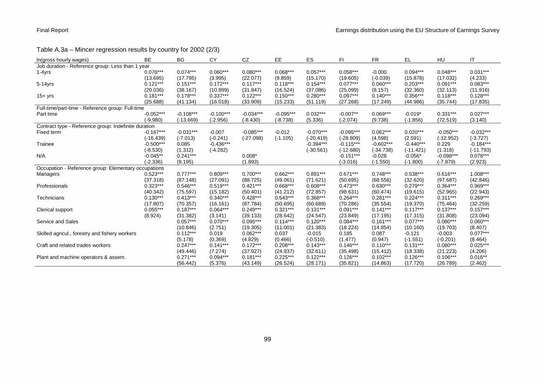
Final Report Earnings distribution using the EU Structure of Earnings Survey
99
Table A.3a – Mincer regression results by country for 2002 (2/3)
ln(gross hourly wages) BE BG CY CZ EE ES FI FR EL HU IT Job duration - Reference group: Less than 1 year 1-4yrs 0.076*** 0.074*** 0.060*** 0.080*** 0.068*** 0.057*** 0.058*** -0.000 0.094*** 0.048*** 0.031*** (13.695) (17.795) (3.995) (22.077) (9.859) (15.170) (19.605) (-0.039) (15.878) (17.032) (4.233) 5-14yrs 0.121*** 0.151*** 0.172*** 0.117*** 0.118*** 0.154*** 0.077*** 0.060*** 0.203*** 0.091*** 0.083*** (20.036) (38.167) (10.899) (31.847) (16.524) (37.086) (25.099) (8.157) (32.360) (32.113) (11.916) 15+ yrs 0.181*** 0.178*** 0.337*** 0.122*** 0.150*** 0.280*** 0.097*** 0.140*** 0.356*** 0.118*** 0.128*** (25.688) (41.134) (16.018) (33.909) (15.233) (51.119) (27.268) (17.249) (44.986) (35.744) (17.835) Full-time/part-time - Reference group: Full-time Part time -0.052*** -0.108*** -0.100*** -0.034*** -0.095*** 0.032*** -0.007** 0.069*** -0.019* 0.331*** 0.027*** (-9.980) (-13.669) (-2.956) (-8.430) (-8.738) (5.336) (-2.074) (9.738) (-1.856) (72.519) (3.140) Contract type - Reference group: Indefinite duration Fixed term -0.167*** -0.031*** -0.007 -0.085*** -0.012 -0.070*** -0.095*** 0.062*** 0.020*** -0.050*** -0.032*** (-16.439) (-7.013) (-0.241) (-27.098) (-1.105) (-20.419) (-28.809) (4.598) (2.591) (-12.952) (-3.727) Trainee -0.500*** 0.085 -0.436*** -0.394*** -0.115*** -0.602*** -0.440*** 0.229 -0.184*** (-8.530) (1.312) (-4.282) (-30.561) (-12.680) (-34.738) (-11.421) (1.318) (-11.793) N/A -0.045** 0.241*** 0.008* -0.151*** -0.028 -0.056* -0.098*** 0.078*** (-2.336) (9.195) (1.893) (-3.016) (-1.550) (-1.800) (-7.879) (2.923) Occupation - Reference group: Elementary occupations Managers 0.523*** 0.777*** 0.809*** 0.700*** 0.662*** 0.891*** 0.671*** 0.748*** 0.538*** 0.616*** 1.008*** (37.318) (87.148) (27.091) (88.725) (49.061) (71.621) (50.695) (68.556) (32.620) (97.687) (42.846) Professionals 0.323*** 0.546*** 0.519*** 0.421*** 0.668*** 0.608*** 0.473*** 0.630*** 0.279*** 0.364*** 0.969*** (40.342) (75.597) (15.182) (50.401) (41.212) (72.857) (98.631) (60.474) (19.615) (52.965) (22.943) Technicians 0.130*** 0.413*** 0.340*** 0.428*** 0.543*** 0.368*** 0.264*** 0.281*** 0.224*** 0.311*** 0.269*** (17.807) (70.357) (16.161) (87.784) (50.695) (60.689) (70.286) (35.554) (19.370) (75.464) (32.259) Clerical support 0.055*** 0.187*** 0.064*** 0.249*** 0.321*** 0.131*** 0.091*** 0.141*** 0.117*** 0.137*** 0.157*** (8.924) (31.382) (3.141) (39.133) (28.642) (24.547) (23.849) (17.195) (17.315) (31.808) (23.094) Service and Sales 0.057*** 0.070*** 0.095*** 0.114*** 0.120*** 0.084*** 0.161*** 0.077*** 0.080*** 0.060***
(10.846) (2.751) (19.305) (11.001) (21.383) (18.224) (14.854) (10.160) (19.703) (8.407) Skilled agricul., forestry and fishery workers 0.112*** 0.019 0.062*** 0.037 -0.015 0.185 0.087 -0.121 -0.003 0.077***
(5.178) (0.369) (4.829) (0.466) (-0.510) (1.477) (0.947) (-1.551) (-0.201) (8.464) Craft and related trades workers 0.247*** 0.141*** 0.172*** 0.208*** 0.143*** 0.146*** 0.110*** 0.131*** 0.080*** 0.025***
(49.446) (7.274) (37.927) (24.937) (32.611) (35.498) (15.412) (18.338) (21.223) (4.206) Plant and machine operators & assem. 0.271*** 0.094*** 0.181*** 0.225*** 0.122*** 0.126*** 0.102*** 0.126*** 0.106*** 0.016**
(56.442) (5.376) (43.149) (26.524) (28.171) (35.821) (14.863) (17.720) (26.789) (2.462)
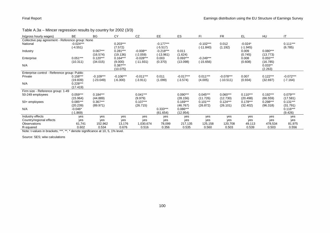
Final Report Earnings distribution using the EU Structure of Earnings Survey
100
Table A.3a – Mincer regression results by country for 2002 (3/3)
ln(gross hourly wages) BE BG CY CZ EE ES FI FR EL HU IT Collective pay agreement - Reference group: None National -0.024*** 0.203*** -0.177*** -0.102*** 0.012 -0.024* 0.111*** (-4.551) (7.572) (-5.517) (-11.840) (1.192) (-1.945) (6.785) Industry 0.067*** 0.281*** -0.008** -0.218*** 0.011 0.009 0.080*** (16.574) (19.136) (-2.059) (-13.961) (1.624) (0.745) (13.773) Enterprise 0.051*** 0.120*** 0.164*** -0.028*** 0.003 0.093*** -0.249*** 0.008 0.055***
(10.311) (34.015) (9.000) (-11.931) (0.370) (13.098) (-15.656) (0.608) (16.785) N/A 0.387*** 0.033** (10.075) (2.263) Enterprise control - Reference group: Public Private 0.158*** -0.109*** -0.106*** -0.011*** 0.011 -0.017*** 0.011*** -0.078*** 0.007 0.122*** -0.072*** (19.839) (-23.049) (-6.300) (-3.911) (1.099) (-3.574) (4.005) (-10.511) (0.934) (32.697) (-7.164) N/A 0.228*** (17.419) Firm size - Reference group: 1-49 50-249 employees 0.059*** 0.184*** 0.041*** 0.090*** 0.045*** 0.060*** 0.110*** 0.192*** 0.079*** (15.964) (44.889) (9.979) (28.156) (11.726) (12.730) (20.498) (66.559) (17.581) 50+ employees 0.085*** 0.367*** 0.107*** 0.169*** 0.101*** 0.124*** 0.178*** 0.298*** 0.131*** (20.239) (89.971) (26.715) (46.767) (26.872) (26.101) (32.402) (96.318) (31.791) N/A -0.046* 0.333*** 0.086*** 0.116*** (-1.869) (61.654) (12.954) (9.426) Industry effects yes yes yes yes yes yes yes yes yes yes yes Country/regional effects yes yes yes yes yes yes yes yes yes yes yes Observations 61,741 152,962 13,176 1,030,674 78,099 217,135 125,158 120,708 49,113 478,534 81,975 R-squared 0.602 0.534 0.676 0.516 0.356 0.535 0.560 0.503 0.539 0.503 0.556 Note: t-values in brackets; ***, **, * denote significance at 10, 5, 1% level.
Source: SES; wiiw calculations
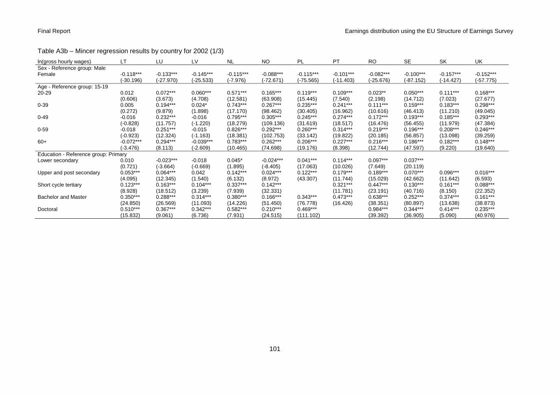
Final Report Earnings distribution using the EU Structure of Earnings Survey
101
Table A3b – Mincer regression results by country for 2002 (1/3)
ln(gross hourly wages) LT LU LV NL NO PL PT RO SE SK UK Sex - Reference group: Male Female -0.118*** -0.133*** -0.145*** -0.115*** -0.088*** -0.115*** -0.101*** -0.082*** -0.100*** -0.157*** -0.152*** (-30.196) (-27.970) (-25.533) (-7.976) (-72.671) (-75.565) (-11.403) (-25.676) (-87.152) (-14.427) (-57.775) Age - Reference group: 15-19 20-29 0.012 0.072*** 0.060*** 0.571*** 0.165*** 0.119*** 0.109*** 0.023** 0.050*** 0.111*** 0.168*** (0.606) (3.673) (4.708) (12.581) (63.908) (15.445) (7.540) (2.198) (14.712) (7.023) (27.677) 0-39 0.005 0.194*** 0.024* 0.743*** 0.267*** 0.235*** 0.241*** 0.111*** 0.159*** 0.183*** 0.298*** (0.272) (9.879) (1.898) (17.170) (98.462) (30.405) (16.962) (10.616) (46.413) (11.210) (49.045) 0-49 -0.016 0.232*** -0.016 0.795*** 0.305*** 0.245*** 0.274*** 0.172*** 0.193*** 0.185*** 0.293*** (-0.828) (11.757) (-1.220) (18.279) (109.136) (31.619) (18.517) (16.476) (56.455) (11.979) (47.384) 0-59 -0.018 0.251*** -0.015 0.826*** 0.292*** 0.260*** 0.314*** 0.219*** 0.196*** 0.208*** 0.246*** (-0.923) (12.324) (-1.163) (18.381) (102.753) (33.142) (19.822) (20.185) (56.857) (13.098) (39.259) 60+ -0.072*** 0.294*** -0.039*** 0.783*** 0.262*** 0.206*** 0.227*** 0.216*** 0.186*** 0.182*** 0.148*** (-3.476) (8.113) (-2.609) (10.465) (74.698) (19.176) (8.398) (12.744) (47.597) (9.220) (19.640) Education - Reference group: Primary Lower secondary 0.010 -0.023*** -0.018 0.045* -0.024*** 0.041*** 0.114*** 0.097*** 0.037*** (0.721) (-3.664) (-0.669) (1.895) (-8.405) (17.063) (10.026) (7.649) (20.119) Upper and post secondary 0.053*** 0.064*** 0.042 0.142*** 0.024*** 0.122*** 0.179*** 0.189*** 0.070*** 0.096*** 0.016***
(4.095) (12.345) (1.540) (6.132) (8.972) (43.307) (11.744) (15.029) (42.662) (11.642) (6.593) Short cycle tertiary 0.123*** 0.163*** 0.104*** 0.337*** 0.142*** 0.321*** 0.447*** 0.130*** 0.161*** 0.088***
(8.928) (18.512) (3.239) (7.939) (32.331) (11.781) (23.191) (40.716) (8.150) (22.352) Bachelor and Master 0.350*** 0.288*** 0.314*** 0.380*** 0.166*** 0.343*** 0.473*** 0.638*** 0.252*** 0.374*** 0.161***
(24.850) (26.569) (11.093) (14.226) (51.450) (76.778) (16.426) (38.351) (80.897) (13.638) (38.873) Doctoral 0.510*** 0.367*** 0.342*** 0.582*** 0.210*** 0.469*** 0.984*** 0.344*** 0.414*** 0.235*** (15.832) (9.061) (6.736) (7.931) (24.515) (111.102) (39.392) (36.905) (5.090) (40.976)
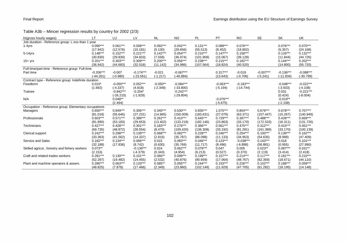
Final Report Earnings distribution using the EU Structure of Earnings Survey
102
Table A3b – Mincer regression results by country for 2002 (2/3)
ln(gross hourly wages) LT LU LV NL NO PL PT RO SE SK UK Job duration - Reference group: L ess than 1 year 1-4yrs 0.090*** 0.061*** 0.058*** 0.092*** 0.042*** 0.131*** 0.089*** 0.076*** 0.076*** 0.070*** (17.942) (12.576) (10.181) (5.130) (29.656) (55.513) (8.452) (18.802) (5.357) (24.168) 5-14yrs 0.148*** 0.152*** 0.221*** 0.142*** 0.054*** 0.210*** 0.147*** 0.158*** 0.126*** 0.132*** (30.830) (29.830) (34.603) (7.558) (36.974) (101.909) (15.067) (39.128) (11.844) (44.726) 15+ yrs 0.201*** 0.303*** 0.309*** 0.200*** 0.056*** 0.238*** 0.215*** 0.182*** 0.144*** 0.202*** (36.942) (44.683) (32.018) (11.142) (34.986) (107.564) (18.824) (40.520) (14.800) (55.720) Full-time/part-time - Reference group: Full-time Part time -0.206*** -0.007 -0.174*** -0.021 -0.067*** 0.317*** -0.019 -0.007*** -0.136*** -0.088*** (-44.261) (-0.980) (-23.561) (-1.217) (-40.884) (13.643) (-0.706) (-5.241) (-11.834) (-30.799) Contract type - Reference group: Indefinite duration Fixedterm 0.010* -0.050*** 0.052*** -0.050** -0.084*** -0.063*** -0.183*** -0.048*** -0.022*** (1.692) (-4.337) (4.818) (-2.349) (-33.800) (-5.194) (-14.744) (-3.503) (-4.108) Trainee -0.842*** -0.204* -0.242*** 0.031 -0.221*** (-26.210) (-1.929) (-29.804) (0.424) (-8.004) N/A 0.048** -0.076*** -0.019** (2.494) (-5.675) (-2.108) Occupation - Reference group: Elementary occupations Managers 0.650*** 0.849*** 0.306*** 0.340*** 0.530*** 0.835*** 1.075*** 0.804*** 0.679*** 0.678*** 0.707*** (81.018) (55.646) (27.231) (14.965) (150.009) (183.631) (27.079) (63.371) (157.447) (15.267) (140.949) Professionals 0.603*** 0.571*** 0.389*** 0.262*** 0.410*** 0.645*** 0.729*** 0.397*** 0.488*** 0.428*** 0.669*** (81.890) (53.183) (29.653) (13.402) (133.218) (182.146) (23.863) (33.170) (172.533) (16.311) (131.726) Technicians 0.427*** 0.428*** 0.301*** 0.183*** 0.276*** 0.366*** 0.561*** 0.475*** 0.312*** 0.415*** 0.451*** (69.735) (48.872) (28.554) (8.470) (109.420) (136.308) (33.192) (81.281) (161.389) (33.170) (100.139) Clerical support 0.242*** 0.298*** 0.139*** 0.068*** 0.082*** 0.228*** 0.246*** 0.254*** 0.100*** 0.139*** 0.162*** (33.363) (41.562) (14.337) (2.816) (35.787) (86.098) (11.133) (34.953) (54.635) (8.998) (47.409) Service and Sales 0.182*** 0.134*** 0.066*** 0.015 0.083*** 0.046*** 0.123*** -0.038*** 0.143*** 0.018 0.101***
(32.188) (17.836) (8.742) (0.630) (35.769) (11.717) (8.496) (-6.898) (56.881) (0.955) (27.990) Skilled agricul., forestry and fishery workers 0.073** -0.139*** 0.024 0.062*** 0.079*** 0.047 0.005 0.023** 0.087*** 0.031**
(2.153) (-4.379) (0.343) (4.954) (6.213) (0.527) (0.370) (2.119) (3.414) (2.418) Craft and related trades workers 0.281*** 0.130*** 0.101*** 0.066** 0.099*** 0.199*** 0.157*** 0.214*** 0.117*** 0.181*** 0.210***
(52.297) (19.482) (14.455) (2.532) (40.876) (90.659) (17.064) (48.767) (62.359) (18.671) (44.110) Plant and machine operators & assem. 0.285*** 0.063*** 0.133*** 0.085** 0.055*** 0.244*** 0.153*** 0.226*** 0.102*** 0.188*** 0.059***
(48.825) (7.878) (17.466) (2.349) (23.860) (102.149) (11.929) (47.705) (61.282) (18.195) (14.148)

Final Report Earnings distribution using the EU Structure of Earnings Survey
103
Table A3b – Mincer regression results by country for 2002 (3/3)
ln(gross hourly wages) LT LU LV NL NO PL PT RO SE SK UK Collective pay agreement - Reference group: None National -0.045*** -0.134*** -0.046*** (-8.292) (-5.619) (-2.899) Industry 0.118*** -0.164*** -0.082*** 0.018** -0.028*** Enterprise
(8.396) (-6.952) (-5.141) (2.428) (-6.755) 0.036*** 0.055*** 0.112*** -0.009 -0.087*** 0.011** -0.017***
(8.015) (8.692) (17.374) (-0.375) (-5.514) (2.045) (-6.283) N/A -0.169*** -0.031*** 0.000 (-7.019) (-4.517) (0.055) Enterprise control - Reference group: Public Private -0.121*** -0.218*** 0.069*** 0.007 0.029*** -0.049*** 0.000 -0.061*** 0.038*** 0.160*** -0.069*** (-17.932) (-24.183) (7.655) (0.246) (15.976) (-25.768) (0.021) (-14.061) (23.107) (26.916) (-18.908) Firm size - Reference group: 1-49 50-249 employees 0.203*** 0.352*** 0.050*** 0.057*** 0.077*** 0.128*** 0.223*** 0.019*** 0.088*** 0.080*** (48.269) (74.397) (2.695) (42.823) (49.584) (19.181) (48.038) (9.825) (9.693) (19.667) 250+ employees 0.335*** 0.600*** 0.070*** 0.069*** 0.146*** 0.207*** 0.471*** 0.061*** 0.199*** 0.117*** (56.792) (87.698) (4.275) (56.236) (80.373) (20.039) (104.656) (34.917) (21.944) (35.401) Industry effects yes yes yes yes yes yes yes yes yes yes yes Country/regional effects yes yes yes yes yes yes yes yes yes yes yes Observations 145,521 26,123 192,442 82,452 573,114 647,315 60,446 220,921 956,633 419,709 150,211 R-squared 0.423 0.746 0.387 0.570 0.558 0.561 0.624 0.554 0.527 0.434 0.562 Note: t-values in brackets; ***, **, * denote significance at 10, 5, 1% level.
Source: SES; wiiw calculations
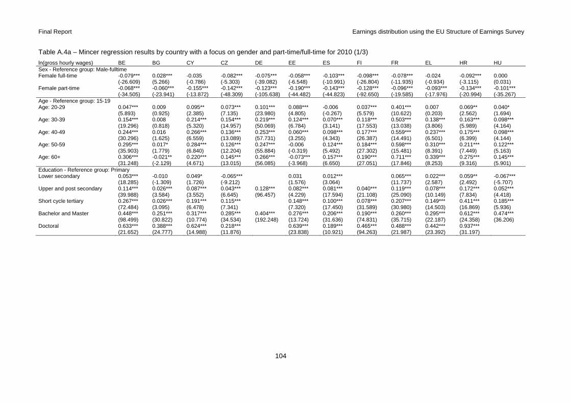
Final Report Earnings distribution using the EU Structure of Earnings Survey
104
Table A.4a – Mincer regression results by country with a focus on gender and part-time/full-time for 2010 (1/3)
ln(gross hourly wages) BE BG CY CZ DE EE ES FI FR EL HR HU Sex - Reference group: Male-fulltime Female full-time -0.079*** 0.028*** -0.035 -0.082*** -0.075*** -0.058*** -0.103*** -0.098*** -0.078*** -0.024 -0.092*** 0.000 (-26.609) (5.266) (-0.786) (-5.303) (-39.082) (-6.548) (-10.991) (-26.804) (-11.935) (-0.934) (-3.115) (0.031) Female part-time -0.068*** -0.060*** -0.155*** -0.142*** -0.123*** -0.190*** -0.143*** -0.128*** -0.096*** -0.093*** -0.134*** -0.101*** (-34.505) (-23.941) (-13.872) (-48.309) (-105.638) (-44.482) (-44.823) (-92.650) (-19.585) (-17.976) (-20.994) (-35.267) Age - Reference group: 15-19 Age: 20-29 0.047*** 0.009 0.095** 0.073*** 0.101*** 0.088*** -0.006 0.037*** 0.401*** 0.007 0.069** 0.040* (5.893) (0.925) (2.385) (7.135) (23.980) (4.805) (-0.267) (5.579) (10.622) (0.203) (2.562) (1.694) Age: 30-39 0.154*** 0.008 0.214*** 0.154*** 0.219*** 0.124*** 0.070*** 0.118*** 0.503*** 0.138*** 0.163*** 0.098*** (19.296) (0.818) (5.320) (14.957) (50.069) (6.784) (3.141) (17.553) (13.038) (3.806) (5.989) (4.164) Age: 40-49 0.244*** 0.016 0.266*** 0.136*** 0.253*** 0.060*** 0.098*** 0.177*** 0.559*** 0.237*** 0.175*** 0.098*** (30.296) (1.625) (6.559) (13.089) (57.731) (3.255) (4.343) (26.387) (14.491) (6.501) (6.399) (4.144) Age: 50-59 0.295*** 0.017* 0.284*** 0.126*** 0.247*** -0.006 0.124*** 0.184*** 0.598*** 0.310*** 0.211*** 0.122*** (35.903) (1.779) (6.840) (12.204) (55.884) (-0.319) (5.492) (27.302) (15.481) (8.391) (7.449) (5.163) Age: 60+ 0.306*** -0.021** 0.220*** 0.145*** 0.266*** -0.073*** 0.157*** 0.190*** 0.711*** 0.339*** 0.275*** 0.145*** (31.248) (-2.129) (4.671) (13.015) (56.085) (-3.968) (6.650) (27.051) (17.846) (8.253) (9.316) (5.901) Education - Reference group: Primary Lower secondary 0.053*** -0.010 0.049* -0.065*** 0.031 0.012*** 0.065*** 0.022*** 0.059** -0.067*** (18.285) (-1.309) (1.726) (-9.212) (1.576) (3.064) (11.737) (2.587) (2.492) (-5.707) Upper and post secondary 0.114*** 0.026*** 0.087*** 0.043*** 0.128*** 0.082*** 0.081*** 0.040*** 0.119*** 0.078*** 0.172*** 0.052***
(39.988) (3.584) (3.552) (6.645) (96.457) (4.229) (17.594) (21.108) (25.090) (10.149) (7.834) (4.418) Short cycle tertiary 0.267*** 0.026*** 0.191*** 0.115*** 0.148*** 0.100*** 0.078*** 0.207*** 0.149*** 0.411*** 0.185***
(72.484) (3.095) (6.478) (7.341) (7.320) (17.450) (31.589) (30.980) (14.503) (16.869) (5.936) Bachelor and Master 0.448*** 0.251*** 0.317*** 0.285*** 0.404*** 0.276*** 0.206*** 0.190*** 0.260*** 0.295*** 0.612*** 0.474***
(98.499) (30.822) (10.774) (34.534) (192.248) (13.724) (31.636) (74.831) (35.715) (22.187) (24.358) (36.206) Doctoral 0.633*** 0.388*** 0.624*** 0.218*** 0.639*** 0.189*** 0.465*** 0.488*** 0.442*** 0.937*** (21.652) (24.777) (14.988) (11.876) (23.838) (10.921) (94.263) (21.987) (23.392) (31.197)

Final Report Earnings distribution using the EU Structure of Earnings Survey
105
Table A.4a – Mincer regression results by country with a focus on gender and part-time/full-time for 2010 (2/3)
ln(gross hourly wages) BE BG CY CZ DE EE ES FI FR EL HR HU Job duration - Reference group: Less than 1 year 1-4yrs 0.027*** 0.066*** 0.065*** 0.082*** 0.096*** 0.068*** 0.050*** 0.078*** 0.022*** 0.045*** 0.045*** 0.112*** (12.087) (26.013) (4.878) (20.264) (72.427) (14.771) (11.755) (40.415) (2.721) (6.172) (4.733) (33.666) 5-14yrs 0.072*** 0.114*** 0.182*** 0.128*** 0.173*** 0.080*** 0.127*** 0.109*** 0.070*** 0.147*** 0.099*** 0.149*** (31.590) (39.768) (12.284) (31.078) (126.596) (17.011) (28.359) (56.472) (11.989) (19.405) (10.524) (44.751) 15+ yrs 0.142*** 0.182*** 0.368*** 0.185*** 0.275*** 0.122*** 0.304*** 0.124*** 0.163*** 0.291*** 0.181*** 0.231*** (51.814) (47.123) (19.846) (39.649) (172.677) (20.921) (53.767) (59.189) (24.707) (30.531) (17.436) (57.036) Full-time/part-time - Reference group: Full-time Part time 0-39% -0.055*** -0.043*** -0.209*** -0.073** -0.327*** -0.211*** 0.081*** 0.102*** 0.074*** -0.126*** -0.059* 0.631*** (-10.360) (-4.047) (-2.684) (-2.075) (-146.639) (-20.140) (6.211) (16.085) (4.955) (-3.467) (-1.788) (38.390) Part time 40-79% -0.076*** -0.119*** -0.191*** -0.115*** -0.082*** -0.198*** -0.081*** -0.040*** -0.015* -0.057** -0.060** 0.314*** (-24.312) (-28.016) (-5.244) (-6.991) (-39.759) (-21.266) (-9.042) (-10.378) (-1.852) (-2.473) (-2.107) (53.265) Part time 80%+ -0.055*** -0.152** -0.113*** -0.106*** -0.195*** -0.105*** -0.034*** 0.016** 0.423*** -0.110*** (-12.916) (-2.305) (-8.175) (-35.820) (-15.053) (-11.395) (-7.513) (1.965) (5.229) (-13.215) Contract type - Reference group: Indefinite duration Fixed term -0.032*** -0.050*** -0.037* -0.090*** -0.089*** 0.000 -0.034*** -0.068*** -0.067*** -0.005 -0.121*** -0.084*** (-9.456) (-14.762) (-1.898) (-25.920) (-49.660) (0.013) (-8.474) (-35.518) (-4.614) (-0.482) (-12.400) (-18.429) Trainee -0.165*** -0.050 -0.931*** -0.129*** -0.388*** -0.524*** -0.319*** (-8.539) (-1.390) (-337.825) (-8.238) (-16.805) (-11.094) (-12.808) Occupation - Reference group: Elementary occupations Managers 0.580*** 0.914*** 0.994*** 0.800*** 0.767*** 0.720*** 0.787*** 0.769*** 0.701*** 0.523*** 0.737*** 0.597*** (94.771) (131.785) (40.799) (87.414) (206.020) (72.866) (49.923) (150.659) (92.479) (27.963) (24.757) (73.532) Professionals 0.302*** 0.631*** 0.467*** 0.556*** 0.485*** 0.694*** 0.479*** 0.475*** 0.519*** 0.329*** 0.412*** 0.442*** (78.728) (118.675) (20.228) (93.733) (223.687) (93.938) (65.630) (175.652) (45.655) (24.601) (27.296) (63.761) Technicians 0.205*** 0.469*** 0.389*** 0.435*** 0.421*** 0.488*** 0.280*** 0.277*** 0.331*** 0.222*** 0.366*** 0.375*** (62.703) (99.697) (19.807) (86.310) (241.481) (80.708) (52.768) (117.953) (62.519) (18.867) (30.055) (91.323) Clerical support 0.106*** 0.218*** 0.121*** 0.283*** 0.181*** 0.302*** 0.094*** 0.136*** 0.143*** 0.124*** 0.247*** 0.242*** (37.617) (50.905) (6.959) (43.345) (108.518) (41.415) (19.185) (54.242) (26.734) (14.731) (22.209) (51.280) Service and Sales 0.116*** 0.048*** 0.097*** 0.077*** 0.154*** 0.102*** 0.071*** 0.122*** 0.183*** 0.097*** 0.079*** 0.148***
(38.076) (15.129) (5.397) (13.927) (74.844) (17.798) (13.909) (55.660) (28.622) (10.947) (6.549) (36.026) Skilled agricul., forestry and fishery workers -0.004 -0.155 0.090*** 0.070*** 0.271*** 0.013 0.036*** 0.028* -0.022 0.068* 0.074***
(-0.223) (-1.281) (2.874) (12.937) (4.598) (0.892) (4.745) (1.939) (-0.491) (1.877) (5.232) Craft and related trades workers 0.051*** 0.267*** 0.149*** 0.147*** 0.105*** 0.272*** 0.106*** 0.140*** 0.110*** 0.160*** 0.065*** 0.169***
(17.528) (75.991) (7.013) (30.005) (58.467) (40.191) (22.976) (47.039) (18.378) (16.594) (4.964) (41.523) Plant and machine operators & assem. 0.053*** 0.237*** 0.094*** 0.129*** 0.070*** 0.212*** 0.072*** 0.146*** 0.088*** 0.153*** 0.116*** 0.175***
(17.484) (67.447) (4.640) (29.924) (39.204) (31.881) (13.898) (45.886) (15.703) (15.470) (7.929) (38.663)

Final Report Earnings distribution using the EU Structure of Earnings Survey
106
Table A.4a – Mincer regression results by country with a focus on gender and part-time/full-time for 2010 (3/3)
ln(gross hourly wages) BE BG CY CZ DE EE ES FI FR EL HR HU Collective pay agreement - Reference group: None National -0.032*** 0.138*** -0.059*** 0.056*** -0.043*** 0.080*** (-9.592) (11.104) (-6.356) (2.863) (-3.111) (3.994) Industry -0.025*** -0.018*** 0.217*** 0.042*** 0.105*** -0.003 -0.017*** -0.038*** -0.026* -0.033*** 0.176*** (-13.648) (-4.599) (16.681) (7.318) (103.828) (-0.480) (-2.728) (-2.774) (-1.834) (-3.585) (31.850) Enterprise 0.015*** 0.097*** 0.050*** 0.138*** 0.016*** 0.073*** -0.054*** 0.019 -0.012 -0.031*** 0.139***
(5.185) (6.480) (27.979) (69.947) (2.680) (12.306) (-5.248) (1.032) (-0.745) (-4.064) (37.997) N/A 0.385*** 0.574*** -0.036** -0.058*** -0.078*** 0.039*** (5.368) (4.882) (-2.147) (-4.129) (-6.476) (4.518) Enterprise control - Reference group: Public Private -0.073*** 0.073*** -0.229*** -0.014*** 0.024*** 0.095*** -0.141*** 0.084*** 0.017* 0.003 -0.062*** -0.024*** (-12.694) (15.928) (-15.898) (-3.322) (23.235) (15.567) (-29.583) (56.274) (1.844) (0.299) (-6.141) (-6.447) N/A -0.082*** -0.020*** -0.197*** (-13.602) (-2.995) (-10.174) Firm size - Reference group: 1-49 50-249 employees 0.031*** 0.180*** 0.187*** 0.056*** 0.135*** 0.050*** 0.036*** 0.064*** 0.034*** 0.182*** (16.117) (66.355) (56.354) (46.946) (34.622) (19.921) (9.452) (9.145) (5.176) (64.301) 250+ employees 0.056*** 0.414*** 0.259*** 0.148*** 0.162*** 0.067*** 0.072*** 0.122*** 0.108*** 0.274*** (28.709) (140.611) (78.237) (117.263) (44.683) (29.686) (19.503) (16.414) (13.827) (96.259) N/A -0.016 0.222*** 0.247*** 0.095*** (-1.572) (27.281) (72.472) (22.447) Industry effects yes yes yes yes yes yes yes yes yes yes yes yes Country/regional effects yes yes yes yes yes yes yes yes yes yes yes yes Observations 137,254 204,939 32,566 1,992,666 1,614,527 119,219 216,733 315,709 219,786 39,809 40,716 765,293 R-squared 0.711 0.532 0.709 0.517 0.709 0.470 0.563 0.570 0.568 0.542 0.457 0.538 Note: t-values in brackets; ***, **, * denote significance at 10, 5, 1% level.
Source: SES; wiiw calculations
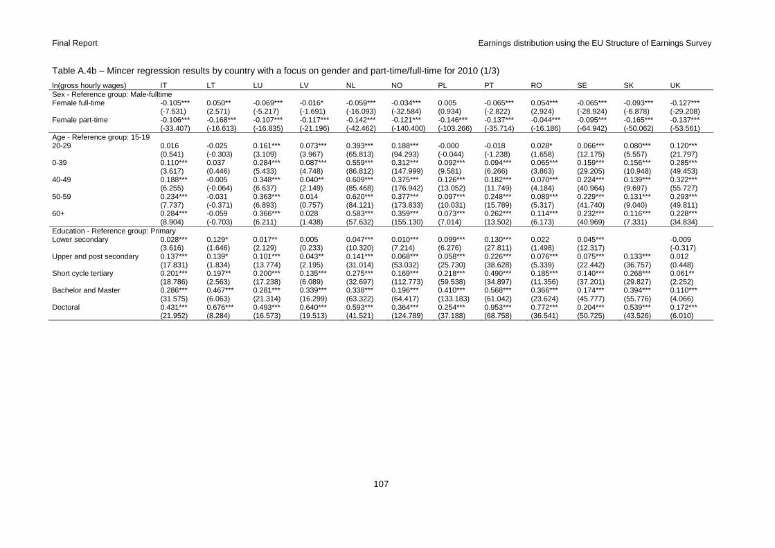
Final Report Earnings distribution using the EU Structure of Earnings Survey
107
Table A.4b – Mincer regression results by country with a focus on gender and part-time/full-time for 2010 (1/3)
ln(gross hourly wages) IT LT LU LV NL NO PL PT RO SE SK UK Sex - Reference group: Male-fulltime Female full-time -0.105*** 0.050** -0.069*** -0.016* -0.059*** -0.034*** 0.005 -0.065*** 0.054*** -0.065*** -0.093*** -0.127*** (-7.531) (2.571) (-5.217) (-1.691) (-16.093) (-32.584) (0.934) (-2.822) (2.924) (-28.924) (-6.878) (-29.208) Female part-time -0.106*** -0.168*** -0.107*** -0.117*** -0.142*** -0.121*** -0.146*** -0.137*** -0.044*** -0.095*** -0.165*** -0.137*** (-33.407) (-16.613) (-16.835) (-21.196) (-42.462) (-140.400) (-103.266) (-35.714) (-16.186) (-64.942) (-50.062) (-53.561) Age - Reference group: 15-19 20-29 0.016 -0.025 0.161*** 0.073*** 0.393*** 0.188*** -0.000 -0.018 0.028* 0.066*** 0.080*** 0.120*** (0.541) (-0.303) (3.109) (3.967) (65.813) (94.293) (-0.044) (-1.238) (1.658) (12.175) (5.557) (21.797) 0-39 0.110*** 0.037 0.284*** 0.087*** 0.559*** 0.312*** 0.092*** 0.094*** 0.065*** 0.159*** 0.156*** 0.285*** (3.617) (0.446) (5.433) (4.748) (86.812) (147.999) (9.581) (6.266) (3.863) (29.205) (10.948) (49.453) 40-49 0.188*** -0.005 0.348*** 0.040** 0.609*** 0.375*** 0.126*** 0.182*** 0.070*** 0.224*** 0.139*** 0.322*** (6.255) (-0.064) (6.637) (2.149) (85.468) (176.942) (13.052) (11.749) (4.184) (40.964) (9.697) (55.727) 50-59 0.234*** -0.031 0.363*** 0.014 0.620*** 0.377*** 0.097*** 0.248*** 0.089*** 0.229*** 0.131*** 0.293*** (7.737) (-0.371) (6.893) (0.757) (84.121) (173.833) (10.031) (15.789) (5.317) (41.740) (9.040) (49.811) 60+ 0.284*** -0.059 0.366*** 0.028 0.583*** 0.359*** 0.073*** 0.262*** 0.114*** 0.232*** 0.116*** 0.228*** (8.904) (-0.703) (6.211) (1.438) (57.632) (155.130) (7.014) (13.502) (6.173) (40.969) (7.331) (34.834) Education - Reference group: Primary Lower secondary 0.028*** 0.129* 0.017** 0.005 0.047*** 0.010*** 0.099*** 0.130*** 0.022 0.045*** -0.009 (3.616) (1.646) (2.129) (0.233) (10.320) (7.214) (6.276) (27.811) (1.498) (12.317) (-0.317) Upper and post secondary 0.137*** 0.139* 0.101*** 0.043** 0.141*** 0.068*** 0.058*** 0.226*** 0.076*** 0.075*** 0.133*** 0.012
(17.831) (1.834) (13.774) (2.195) (31.014) (53.032) (25.730) (38.628) (5.339) (22.442) (36.757) (0.448) Short cycle tertiary 0.201*** 0.197** 0.200*** 0.135*** 0.275*** 0.169*** 0.218*** 0.490*** 0.185*** 0.140*** 0.268*** 0.061**
(18.786) (2.563) (17.238) (6.089) (32.697) (112.773) (59.538) (34.897) (11.356) (37.201) (29.827) (2.252) Bachelor and Master 0.286*** 0.467*** 0.281*** 0.339*** 0.338*** 0.196*** 0.410*** 0.568*** 0.366*** 0.174*** 0.394*** 0.110***
(31.575) (6.063) (21.314) (16.299) (63.322) (64.417) (133.183) (61.042) (23.624) (45.777) (55.776) (4.066) Doctoral 0.431*** 0.676*** 0.493*** 0.640*** 0.593*** 0.364*** 0.254*** 0.953*** 0.772*** 0.204*** 0.539*** 0.172*** (21.952) (8.284) (16.573) (19.513) (41.521) (124.789) (37.188) (68.758) (36.541) (50.725) (43.526) (6.010)
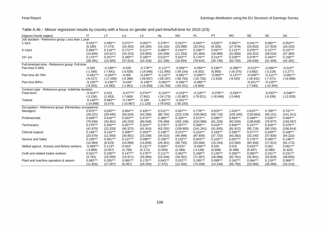
Final Report Earnings distribution using the EU Structure of Earnings Survey
108
Table A.4b – Mincer regression results by country with a focus on gender and part-time/full-time for 2010 (2/3)
ln(gross hourly wages) IT LT LU LV NL NO PL PT RO SE SK UK Job duration - Reference group: Less than 1 year 1-4yrs 0.032*** 0.085*** 0.072*** 0.092*** 0.379*** 0.022*** 0.040*** 0.033*** 0.062*** 0.041*** 0.082*** 0.053*** (5.180) (7.473) (10.450) (16.184) (16.152) (23.098) (22.041) (6.328) (17.676) (23.833) (17.910) (19.103) 5-14yrs 0.084*** 0.124*** 0.172*** 0.121*** 0.480*** 0.010*** 0.106*** 0.097*** 0.113*** 0.075*** 0.127*** 0.107*** (14.600) (10.517) (24.210) (20.904) (20.209) (11.333) (51.904) (18.968) (31.806) (43.322) (28.524) (37.365) 15+ yrs 0.170*** 0.207*** 0.349*** 0.180*** 0.512*** 0.022*** 0.176*** 0.214*** 0.229*** 0.079*** 0.164*** 0.158*** (28.491) (15.583) (37.814) (24.418) (21.169) (16.834) (78.642) (34.749) (50.750) (40.639) (31.406) (44.181) Full-time/part-time - Reference group: Full-time Part time 0-39% -0.045 -0.188*** -0.028 -0.178*** -0.112*** -0.056*** -0.059*** 0.196*** -0.288*** -0.013*** -0.066*** -0.013** (-1.556) (-7.841) (-0.929) (-14.048) (-21.900) (-39.154) (-8.352) (5.893) (-16.075) (-3.682) (-3.219) (-2.277) Part time 40-79% -0.081*** -0.284*** -0.005 -0.240*** -0.115*** -0.081*** -0.095*** -0.050*** -0.137*** -0.039*** -0.111*** -0.091*** (-6.417) (-17.000) (-0.389) (-26.947) (-28.197) (-68.763) (-20.726) (-2.818) (-9.429) (-16.441) (-7.471) (-19.858) Part time 80%+ -0.155*** -0.230*** -0.044* -0.148*** -0.063*** -0.096*** -0.085*** -0.021*** -0.125*** (-9.303) (-6.382) (-1.951) (-14.358) (-16.704) (-63.321) (-9.964) (-7.540) (-10.304) Contract type - Reference group: Indefinite duration Fixed term -0.024*** 0.023 -0.077*** 0.074*** -0.103*** -0.019*** -0.126*** -0.078*** -0.034*** -0.033*** -0.048*** (-3.236) (1.453) (-7.660) (7.661) (-24.173) (-15.887) (-79.521) (-16.949) (-3.484) (-9.336) (-12.029) Trainee -0.140*** 0.993*** -0.749*** -0.190 -1.667*** -0.201*** (-14.968) (3.074) (-15.867) (-1.120) (-78.042) (-35.163) Occupation - Reference group: Elementary occupations Managers 0.870*** 0.632*** 0.964*** 0.425*** 0.512*** 0.507*** 0.778*** 0.923*** 1.016*** 0.615*** 0.780*** 0.747*** (26.221) (29.445) (50.624) (43.280) (80.792) (222.129) (205.862) (50.718) (102.345) (133.863) (50.151) (141.311) Professionals 0.608*** 0.519*** 0.553*** 0.473*** 0.380*** 0.329*** 0.572*** 0.596*** 0.664*** 0.348*** 0.526*** 0.693*** (75.030) (34.361) (43.220) (60.548) (76.490) (202.106) (224.990) (61.228) (92.926) (138.838) (79.877) (193.557) Technicians 0.275*** 0.350*** 0.457*** 0.323*** 0.279*** 0.257*** 0.358*** 0.419*** 0.500*** 0.237*** 0.418*** 0.379*** (41.870) (22.333) (45.372) (41.915) (63.292) (159.893) (141.261) (51.835) (81.812) (95.719) (80.155) (106.814) Clerical support 0.148*** 0.215*** 0.308*** 0.203*** 0.148*** 0.072*** 0.216*** 0.193*** 0.345*** 0.077*** 0.259*** 0.168*** (23.570) (11.693) (30.801) (23.239) (34.013) (45.999) (87.650) (27.723) (63.362) (32.240) (37.830) (54.222) Service and Sales 0.105*** 0.091*** 0.137*** 0.098*** 0.109*** 0.132*** 0.053*** 0.103*** 0.057*** 0.176*** 0.090*** 0.148***
(14.904) (6.523) (14.690) (14.839) (26.461) (90.795) (20.666) (15.243) (13.560) (84.356) (17.912) (52.173) Skilled agricul., forestry and fishery workers -0.069*** 0.113** 0.052* 0.131*** 0.026** 0.023** -0.056*** 0.020 0.010 0.033*** 0.002 0.061***
(-3.889) (2.007) (1.756) (5.171) (2.503) (2.486) (-4.148) (0.848) (0.498) (5.587) (0.080) (5.424) Craft and related trades workers 0.031*** 0.226*** 0.147*** 0.179*** 0.111*** 0.062*** 0.168*** 0.126*** 0.256*** 0.090*** 0.151*** 0.231***
(4.781) (15.555) (15.971) (24.894) (23.434) (34.301) (71.467) (18.088) (62.761) (32.901) (32.829) (48.659) Plant and machine operators & assem. 0.082*** 0.265*** 0.065*** 0.175*** 0.043*** 0.022*** 0.185*** 0.099*** 0.242*** 0.064*** 0.119*** 0.066***
(11.816) (17.007) (6.067) (24.203) (7.472) (12.430) (74.169) (14.249) (55.756) (23.566) (28.369) (16.214)
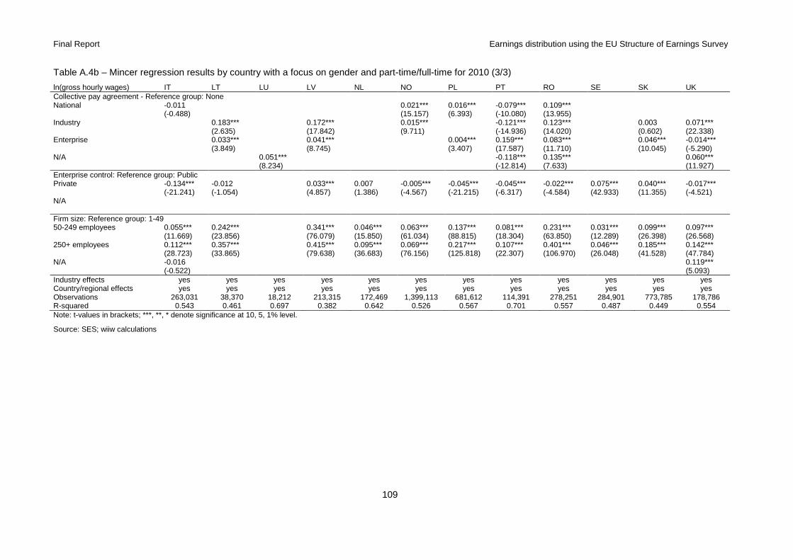
Final Report Earnings distribution using the EU Structure of Earnings Survey
109
Table A.4b – Mincer regression results by country with a focus on gender and part-time/full-time for 2010 (3/3)
ln(gross hourly wages) IT LT LU LV NL NO PL PT RO SE SK UK Collective pay agreement - Reference group: None National -0.011 0.021*** 0.016*** -0.079*** 0.109*** (-0.488) (15.157) (6.393) (-10.080) (13.955) Industry 0.183*** 0.172*** 0.015*** -0.121*** 0.123*** 0.003 0.071*** (2.635) (17.842) (9.711) (-14.936) (14.020) (0.602) (22.338) Enterprise 0.033*** 0.041*** 0.004*** 0.159*** 0.083*** 0.046*** -0.014***
(3.849) (8.745) (3.407) (17.587) (11.710) (10.045) (-5.290) N/A 0.051*** -0.118*** 0.135*** 0.060*** (8.234) (-12.814) (7.633) (11.927) Enterprise control: Reference group: Public Private -0.134*** -0.012 0.033*** 0.007 -0.005*** -0.045*** -0.045*** -0.022*** 0.075*** 0.040*** -0.017*** (-21.241) (-1.054) (4.857) (1.386) (-4.567) (-21.215) (-6.317) (-4.584) (42.933) (11.355) (-4.521) N/A Firm size: Reference group: 1-49 50-249 employees 0.055*** 0.242*** 0.341*** 0.046*** 0.063*** 0.137*** 0.081*** 0.231*** 0.031*** 0.099*** 0.097*** (11.669) (23.856) (76.079) (15.850) (61.034) (88.815) (18.304) (63.850) (12.289) (26.398) (26.568) 250+ employees 0.112*** 0.357*** 0.415*** 0.095*** 0.069*** 0.217*** 0.107*** 0.401*** 0.046*** 0.185*** 0.142*** (28.723) (33.865) (79.638) (36.683) (76.156) (125.818) (22.307) (106.970) (26.048) (41.528) (47.784) N/A -0.016 0.119*** (-0.522) (5.093) Industry effects yes yes yes yes yes yes yes yes yes yes yes yes Country/regional effects yes yes yes yes yes yes yes yes yes yes yes yes Observations 263,031 38,370 18,212 213,315 172,469 1,399,113 681,612 114,391 278,251 284,901 773,785 178,786 R-squared 0.543 0.461 0.697 0.382 0.642 0.526 0.567 0.701 0.557 0.487 0.449 0.554 Note: t-values in brackets; ***, **, * denote significance at 10, 5, 1% level.
Source: SES; wiiw calculations

Final Report Earnings distribution using the EU Structure of Earnings Survey
110
Appendix Table B.1 - Shares in % in 2002 BE BG CY CZ DE EE ES FI FR EL HR HU IT LT LU LV NL NO PL PT RO SE SK UK
Gender Male 60.9 48.9 58.4 55.0 54.0 63.0 62.7 64.6 61.5 51.3 67.5 47.2 66.7 53.0 55.6 65.2 52.1 59.8 52.6 65.5 48.8 50.6
Female 39.1 51.1 41.6 45.0 46.0 37.0 37.3 35.4 38.5 48.7 32.5 52.8 33.3 47.0 44.4 34.8 47.9 40.2 47.4 34.5 51.2 49.4
Age 14-19 0.4 0.6 1.7 0.6 1.1 1.4 2.0 1.3 0.7 0.3 0.6 0.6 1.2 1.5 6.0 4.3 0.3 2.7 0.8 2.2 0.6 5.4
20-29 21.8 17.0 24.4 19.8 20.2 26.7 19.7 21.8 25.5 21.8 18.9 18.5 24.6 21.4 21.1 21.1 20.3 28.6 19.3 21.5 21.3 19.0
30-39 32.3 25.3 28.4 22.9 24.6 31.4 26.9 29.7 32.2 24.5 35.0 27.4 37.3 25.3 28.2 28.1 27.4 30.0 31.2 28.4 26.0 26.5
40-49 27.6 30.6 24.8 26.5 26.9 23.7 27.5 27.3 26.5 29.5 28.2 29.5 25.7 27.3 24.6 23.3 33.3 22.5 32.8 22.4 30.4 25.2
50-59 17.0 23.9 16.3 26.4 18.9 14.5 22.0 18.9 14.1 21.2 16.2 18.8 10.7 18.6 18.0 18.5 17.1 13.6 14.8 21.0 20.1 19.4
60+ 0.9 2.5 4.4 3.7 8.2 2.3 1.9 1.1 1.1 2.7 1.1 5.2 0.6 5.9 2.0 4.8 1.6 2.6 1.1 4.4 1.7 4.5
Education Primary 2.4 1.1 18.0 0.4 1.0 25.6 23.4 20.6 15.3 0.7 7.3 0.7 12.9 0.4 9.7 4.7 9.8 55.0 1.0 6.4
Lower secondary 13.3 12.3 9.5 10.2 10.7 27.6 0.1 6.5 13.6 17.3 42.0 5.6 14.7 9.7 20.9 11.5 28.3 18.4 10.0 13.5 9.2 31.3
Upper and post secondary 36.0 57.2 49.0 71.2 64.2 17.7 45.5 48.4 51.5 62.8 42.0 52.2 52.5 67.3 45.6 65.4 38.6 17.9 70.1 63.7 67.9 36.7
Short cycle secondary 20.5 21.0 10.2 13.5 18.0 19.8 13.9 11.6 12.8 19.1 7.7 29.5 8.0 19.4 21.2 15.1 9.1 6.3 16.6 11.0 18.0 14.5
Bachelor and Master 27.1 7.5 13.1 3.9 5.8 9.0 16.9 12.2 6.5 0.1 0.5 11.5 11.4 2.8 2.2 3.0 2.4 1.8 4.8 4.2 11.1
Doctoral 0.7 0.8 0.1 0.8 0.2 0.3 0.3 0.6 0.2 0.5 0.5 0.4 0.3 0.4 0.3 14.1 0.5 0.5 0.7 6.5
Experience 0-1 years 21.1 32.6 29.2 21.3 29.3 36.3 23.6 12.7 32.7 29.0 16.7 31.8 29.6 38.4 19.6 33.9 17.2 30.4 23.4 21.2 29.7
1-4 years 22.4 21.2 21.7 19.9 29.5 21.2 20.8 26.3 22.1 22.6 20.6 21.1 25.6 31.3 39.9 24.5 23.0 22.7 22.4 22.2 24.6
5-14 years 25.3 28.0 31.6 36.8 32.0 23.7 27.1 30.4 25.6 29.7 32.9 31.8 30.4 24.3 24.5 29.6 35.1 29.7 29.8 35.1 29.1
more than 14 years 31.2 18.1 17.6 22.1 9.2 18.8 28.5 30.6 19.6 18.7 29.7 15.3 14.4 5.9 16.0 12.0 24.7 17.2 24.4 21.5 16.6
N/A 100.0
Contract type Indefinite duration 95.0 86.6 95.3 81.9 95.2 73.5 91.1 92.0 90.8 92.8 95.1 91.4 92.8 92.9 80.8 97.9 73.1 98.2 83.9 94.7
Fixed term 4.7 13.0 4.6 12.4 4.8 26.2 7.7 4.2 8.7 6.6 3.5 8.6 4.7 7.1 19.2 1.6 20.6 1.8 9.3 4.9
Trainee 0.1 0.0 0.2 0.3 1.1 1.8 0.1 0.0 1.2 0.7 0.0 0.4 0.0 0.4
N/A 0.3 0.4 5.8 0.1 2.0 0.4 0.5 0.3 1.8 100.0 6.3 100.0 6.7
Full-time/Part-time Full-time 84.7 97.2 96.2 90.6 90.2 89.2 91.2 84.4 94.5 94.6 87.6 84.3 88.6 83.4 56.8 78.4 100.0 96.6 99.2 84.0 93.5 73.9
Part-time 15.3 2.8 3.8 9.4 9.8 10.8 8.8 15.6 5.5 5.4 12.4 15.7 11.4 16.6 43.2 21.6 3.4 0.8 16.0 6.5 26.1
Occupation Managers 6.5 5.3 4.9 7.1 11.4 2.1 3.1 9.1 4.1 8.2 1.4 11.4 3.9 13.0 8.9 8.5 5.0 2.5 4.6 5.9 6.4 13.6
Professionals 23.4 13.7 4.3 11.8 7.2 12.0 9.7 8.2 9.0 12.1 0.5 20.6 8.9 9.2 15.9 6.5 18.6 3.8 13.3 11.2 12.6 12.5
Technicians 18.9 15.1 12.4 21.7 13.6 15.4 21.0 17.0 9.5 14.2 7.8 13.0 12.0 8.7 17.7 17.4 15.1 10.8 12.4 19.4 22.6 11.9
Clerical support 40.0 7.8 17.7 7.2 7.0 12.4 9.7 13.6 23.4 9.1 33.7 5.3 21.6 9.4 12.4 14.4 11.2 16.2 7.4 13.3 13.2 15.4
Service and sales 11.2 9.2 18.6 7.0 12.0 13.1 12.1 9.8 14.6 9.8 11.0 10.1 11.7 15.5 11.7 16.6 8.9 11.6 9.2 9.0 7.4 18.6
Skilled agricultural 0.2 0.2 0.2 0.1 0.2 0.0 0.1 0.2 0.3 3.3 0.1 0.3 0.8 0.1 0.1 0.0 0.4 0.1 0.1 0.4
Craft and related trade workers 16.7 15.8 20.0 22.0 16.1 16.8 13.8 12.5 21.3 22.6 15.1 17.5 20.7 9.0 15.3 19.2 25.8 26.5 13.8 16.3 7.9
Plant and machine operators 18.0 8.6 17.2 15.5 14.9 19.1 19.5 12.1 14.3 7.7 13.7 8.8 14.1 6.4 13.9 12.4 13.9 16.8 19.0 14.1 7.2
Elementary occupations 14.0 17.4 7.8 11.2 13.7 8.4 9.0 14.6 10.8 11.9 10.7 15.4 9.3 16.7 7.2 9.5 15.4 9.5 8.4 7.3 12.4

Final Report Earnings distribution using the EU Structure of Earnings Survey
111
Appendix Table B.1 (contd.) - Shares in % in 2002 BE BG CY CZ DE EE ES FI FR EL HR HU IT LT LU LV NL NO PL PT RO SE SK UK
NACE 10_14 0.1 2.0 0.3 1.4 1.7 0.5 0.3 0.2 1.4 0.4 0.4 0.3 0.4 0.1 2.2 2.5 4.1 0.4 1.0 0.2
15_16 2.8 5.4 6.0 3.7 5.1 3.3 4.1 3.5 6.4 5.4 3.4 4.6 6.7 2.0 4.8 5.6 4.4 3.8 3.4 3.3 1.8
17_19 1.0 10.7 2.1 3.7 6.6 2.5 1.2 1.6 4.8 4.9 7.0 5.6 4.8 0.3 0.5 3.4 12.5 11.4 0.5 4.6 0.7
20_22 2.2 1.9 2.3 1.7 5.7 2.6 9.4 4.4 4.1 2.4 3.2 3.3 7.5 1.8 4.1 2.7 3.7 2.6 5.9 2.3 2.1
23_25 8.9 3.0 2.0 3.0 2.2 2.9 4.4 4.9 4.1 3.5 5.1 1.5 2.8 1.4 1.6 1.9 2.9 2.3 2.6 3.6 2.1 2.2
26 0.9 1.2 1.4 2.7 1.0 1.8 2.0 1.0 1.8 1.3 2.3 0.8 1.4 0.8 0.5 0.8 1.6 2.9 1.8 0.8 1.5 0.6
27_28 3.2 3.0 1.6 4.6 2.6 3.7 5.2 5.3 3.2 3.3 7.0 1.1 2.9 2.0 1.7 3.5 3.1 3.8 3.8 5.0 4.8 1.8
29 2.0 4.1 0.5 4.6 1.3 1.6 5.8 2.9 1.5 2.6 6.5 1.0 1.3 1.4 1.3 1.6 2.4 2.0 4.0 4.4 3.1 1.5
30_33 3.4 1.8 0.4 4.9 2.8 1.8 7.2 4.3 1.3 4.8 4.4 1.7 0.8 1.1 1.3 1.5 2.1 2.2 2.0 5.4 3.0 1.7
34_35 2.9 0.8 0.3 3.2 1.1 2.7 2.3 3.2 1.4 2.2 3.5 0.9 1.3 0.8 3.1 1.9 1.9 3.1 5.1 1.7 2.0
36_37 0.5 1.0 1.6 1.6 3.7 1.3 1.1 1.3 1.6 1.1 2.5 1.6 2.2 2.1 1.1 1.9 2.0 2.3 1.2 0.8 0.7
40_41 2.7 3.6 1.6 2.5 2.7 0.9 1.2 3.3 3.0 3.2 1.7 3.0 3.2 0.4 1.2 3.2 4.1 1.2 1.8 0.6
45 2.7 5.5 13.1 5.9 8.7 12.0 7.9 7.5 5.3 5.4 6.0 6.9 13.2 8.5 5.8 8.9 5.5 13.9 7.6 7.3 5.0 3.9
50_51 9.1 5.6 12.1 4.9 11.9 8.3 8.4 8.7 13.3 6.3 6.8 7.7 8.4 11.3 8.1 13.0 7.0 11.4 5.0 10.1 8.4 6.0
52 7.8 2.6 10.0 4.4 11.7 8.0 8.5 8.9 10.4 6.2 5.5 6.2 8.0 16.4 9.2 10.5 4.9 8.0 3.7 8.9 4.4 9.3
55 1.7 2.0 17.6 1.3 3.6 5.1 2.8 5.5 10.7 2.5 3.9 1.6 4.9 3.2 3.8 6.4 1.2 6.2 1.4 3.6 1.1 4.0
60_62 4.5 4.1 3.5 8.7 6.6 3.5 4.9 6.9 4.8 6.3 5.4 4.6 7.5 8.1 3.4 8.1 3.8 4.0 5.0 5.1 4.5 2.4
63_64 9.7 5.0 6.8 2.7 5.6 2.7 6.6 4.7 6.4 4.3 6.4 2.8 3.7 6.0 3.1 6.7 3.4 3.5 2.8 6.1 15.6 3.8
65_67 16.1 1.6 9.2 2.9 2.0 4.3 4.2 5.5 6.5 2.5 5.9 1.8 17.5 3.3 3.7 3.9 3.0 4.4 1.5 4.4 1.4 5.1
70_74 18.0 5.1 7.4 7.6 13.3 13.5 12.6 16.3 8.0 6.6 13.0 5.2 27.6 10.4 15.8 16.1 8.8 10.9 4.5 17.5 5.9 13.2
75 6.2 7.8 7.7 7.6 5.8 5.8 5.1 5.9
80 12.2 6.0 4.6 0.0 12.7 16.3 6.7 10.7 9.6 7.5 15.4
85 7.4 6.0 8.1 0.0 9.0 9.6 14.9 10.4 5.9 7.6 11.5
90_93 4.2 4.3 4.2 0.0 3.0 4.1 4.0 2.3 1.6 3.6 3.8
Size class 1_49 6.2 19.6 19.4 49.4 33.8 23.4 24.7 32.3 32.0 34.1 29.0 44.3 31.5 42.0 26.1 41.0 14.7 25.3 25.3 19.9
50_249 15.5 36.8 31.3 23.2 21.7 20.3 26.4 24.6 23.4 35.5 25.2 18.4 22.9 32.8 27.7 21.5 23.0 22.8 12.1
>250 74.4 43.6 49.3 40.5 54.9 54.9 41.2 43.4 41.5 35.5 30.5 50.1 35.1 41.2 31.3 63.7 51.7 52.0 68.0
N/A 3.9 100.0 50.6 2.4 1.0 100.0
Public/Private Public 11.7 44.9 8.8 35.5 7.8 10.4 9.9 9.4 10.3 33.4 8.0 45.3 5.7 15.3 31.2 8.1 46.0 6.7 44.2 10.7 38.5 26.6
Private 72.8 55.1 91.2 64.5 92.2 89.6 90.1 90.6 89.7 66.6 92.0 54.7 94.3 84.7 68.8 91.9 54.0 93.3 55.8 89.3 61.5 73.4
N/A 15.4
Pay agreement Enterprise 35.2 31.8 4.4 62.3 14.8 19.3 0.1 12.7 27.2 18.9 14.5 21.2 8.4 73.7 49.1 37.3
None 46.6 41.9 29.9 82.2 2.4 4.9 0.0 68.3 7.2 81.1 43.4 75.8 2.9 0.7 34.2 42.5
Individual 35.7 21.6 49.1 7.7 2.9 76.8 55.0 4.0 3.0 35.9 16.1 11.5 18.7
National 29.1 3.4 0.1 97.5 95.1 29.8 92.8 42.1 35.2 9.5
N/A 1.2 3.9 2.4 0.5 100.0 100.0 100.0 17.7 100.0 5.3 1.5 Source: SES data; wiiw calculations

Final Report Earnings distribution using the EU Structure of Earnings Survey
112
Appendix Table B.2 - Shares in % in 2006
BE BG CY CZ DE EE ES FI FR EL HR HU IT LT LU LV NL NO PL PT RO SE SK UK
Gender Male 58.8 49.0 53.4 56.3 56.8 46.7 59.2 47.4 55.2 57.4 49.7 57.6 48.0 63.8 45.1 54.0 58.5 51.4 51.2 53.0 48.9 50.6 50.2
Female 41.2 51.0 46.6 43.7 43.2 53.3 40.8 52.6 44.8 42.6 50.3 42.4 52.0 36.2 54.9 46.0 41.5 48.6 48.8 47.0 51.1 49.4 49.8
Age 14-19 0.7 0.7 0.9 0.8 3.0 1.4 1.3 1.0 0.6 0.4 0.5 0.4 0.9 1.0 1.3 6.6 3.4 0.3 1.2 0.8 1.5 0.4 4.9
20-29 19.8 17.9 22.3 20.7 16.4 19.2 24.4 16.1 16.6 18.6 17.9 13.0 18.3 21.4 19.1 21.9 18.8 20.5 21.6 18.0 16.4 18.4 20.1
30-39 28.8 26.3 26.4 25.9 24.1 22.8 33.0 23.4 28.7 34.4 27.8 31.0 25.1 34.8 23.0 25.0 26.3 27.7 31.6 32.8 24.0 25.4 23.8
40-49 30.6 26.1 27.8 24.0 31.0 24.9 23.9 28.4 30.5 27.5 25.1 32.1 29.0 29.0 26.0 25.0 24.4 28.9 26.3 26.9 25.7 28.2 26.1
50-59 18.9 24.2 18.3 23.9 21.2 21.9 14.0 26.4 21.9 16.7 25.1 21.3 19.9 13.1 21.1 18.5 19.7 20.2 16.0 19.9 23.6 24.5 19.2
60+ 1.3 4.8 4.3 4.7 4.4 9.8 3.4 4.9 1.7 2.4 3.7 2.3 6.7 0.8 9.6 2.9 7.4 2.4 3.3 1.6 8.8 3.1 5.8
Education Primary 7.9 1.1 12.1 0.7 0.6 26.2 14.9 8.5 11.0 0.5 5.0 0.4 13.2 0.4 6.9 5.7 7.2 40.0 0.7 3.5
Lower secondary 17.0 9.7 10.3 9.3 17.1 8.5 26.0 12.8 11.6 14.7 34.7 5.6 13.2 7.0 22.2 19.6 26.3 18.7 11.4 8.6 7.9 8.0
Upper and post secondary 39.1 60.4 47.4 73.4 67.4 58.2 18.3 43.9 46.2 35.6 61.3 40.6 49.1 47.8 58.4 43.0 44.0 36.6 19.7 65.4 49.5 70.5 56.6
Short cycle secondary 13.7 22.1 19.5 12.8 8.3 25.3 20.4 22.0 15.8 14.0 23.3 13.2 31.2 10.9 28.7 25.7 2.8 8.9 17.5 20.0 31.0 19.7 24.1
Bachelor and Master 21.6 5.8 10.4 1.7 7.3 6.6 8.8 17.9 15.0 6.3 0.2 4.6 13.0 14.2 4.9 1.5 27.1 7.4 2.5 1.9 6.1 1.4 10.2
Doctoral 0.6 0.9 0.3 2.1 0.7 0.3 1.3 1.6 21.5 2.0 0.7 0.6 0.6 0.6 0.7 13.6 1.7 0.5 1.3 0.4 1.1
Experience 0-1 years 20.6 41.4 26.8 28.1 20.1 32.1 40.0 24.6 14.5 28.7 27.7 15.1 38.3 29.7 39.2 27.4 30.0 19.9 23.3 29.5 21.8 26.0 30.4
1-4 years 16.5 23.9 21.5 21.6 17.7 24.7 20.2 15.0 19.8 18.7 22.5 20.0 21.5 20.1 23.3 30.8 21.4 21.4 18.3 24.5 20.0 26.5 24.0
5-14 years 29.9 22.4 30.0 36.0 33.4 33.6 24.1 29.1 31.8 31.3 32.5 34.0 27.7 33.2 29.7 27.8 30.4 35.0 34.3 27.4 33.4 32.8 29.2
more than 14 years 33.0 12.3 21.6 14.3 28.7 9.6 15.7 31.3 33.9 21.4 17.3 30.9 12.5 16.9 7.9 14.0 18.2 23.7 24.2 18.6 24.9 14.6 16.4
Contract type Indefinite duration 89.5 87.2 95.6 82.4 89.1 94.1 71.6 85.5 93.3 68.9 93.7 92.7 95.1 92.5 94.7 76.9 94.4 71.1 75.6 98.0 88.1 93.9
Fixed term 10.4 12.8 4.4 17.6 6.5 5.9 28.4 13.6 5.4 31.0 6.3 6.1 4.9 6.4 5.3 23.1 4.7 28.9 24.4 2.0 11.9 6.1
Trainee 0.1 0.0 4.3 0.9 1.3 0.1 0.0 1.2 0.0 1.1 0.1 0.9 0.0 0.0
N/A 100.0
Full-time/Part-time Full-time 74.6 93.8 96.4 94.5 74.6 86.1 83.4 89.0 84.2 91.8 91.5 89.6 85.0 84.7 84.1 51.9 74.8 90.4 97.2 98.6 72.9 93.8 73.2
Part-time 25.4 6.2 3.6 5.5 25.4 13.9 16.6 11.0 15.8 8.2 8.5 10.4 15.0 15.3 15.9 48.1 25.2 9.6 2.8 1.4 27.1 6.2 26.8
Occupation Managers 3.0 4.8 3.1 7.8 1.8 11.1 2.3 3.9 7.2 2.5 10.4 1.4 13.0 5.5 13.8 6.5 8.8 6.7 3.2 4.7 5.4 5.8 14.6
Professionals 16.2 13.1 12.9 12.4 11.6 14.6 10.3 17.1 15.1 19.8 14.2 14.0 24.6 10.4 17.6 16.8 14.5 23.5 14.7 14.7 19.4 13.4 14.4
Technicians 15.2 10.6 16.0 22.8 19.5 17.4 14.7 22.3 20.7 11.5 16.9 13.3 9.7 18.3 14.1 16.9 19.3 12.7 11.7 12.3 19.5 22.3 13.0
Clerical support 18.0 10.4 13.3 6.9 19.3 6.2 13.8 9.7 13.8 20.4 9.6 22.0 4.7 16.3 7.4 12.5 11.2 9.5 14.2 7.0 9.5 7.1 14.9
Service and sales 9.3 15.7 18.9 8.3 9.6 12.5 14.9 17.0 11.6 14.0 10.4 11.8 10.0 10.7 13.8 13.0 17.9 8.6 13.2 11.2 20.9 9.3 18.0
Skilled agricultural 0.2 0.3 0.2 0.3 0.1 0.3 0.3 0.2 0.1 0.4 0.0 0.1 0.0 0.4 0.8 0.1 0.1 0.2 0.3 0.4 0.2 0.4
Craft and related trade workers 12.6 14.3 13.5 17.8 16.4 15.6 17.1 9.4 9.9 10.1 14.7 15.7 17.0 17.8 12.2 8.2 12.3 16.8 18.8 20.3 8.2 17.7 6.9
Plant and machine operators 13.6 14.9 6.5 16.2 8.3 12.1 11.3 10.5 13.6 9.4 12.4 13.7 10.5 10.1 9.5 5.9 9.5 12.2 10.1 16.9 10.4 15.7 6.4
Elementary occupations 12.0 16.1 15.5 7.5 13.3 10.5 15.3 9.1 7.9 12.1 11.0 8.2 10.4 10.9 11.2 18.8 6.4 9.8 13.8 12.6 6.3 8.6 11.5

Final Report Earnings distribution using the EU Structure of Earnings Survey
113
Appendix Table B.2 (contd.) - Shares in % in 2006
BE BG CY CZ DE EE ES FI FR EL HR HU IT LT LU LV NL NO PL PT RO SE SK UK
NACE 10_14 0.2 1.3 0.2 1.3 0.4 1.0 0.4 0.3 0.1 0.4 0.3 0.3 0.3 0.3 0.1 2.1 2.1 2.3 0.2 0.8 0.2
15_16 4.1 5.1 4.9 3.1 2.9 2.7 2.0 2.8 5.4 3.3 2.4 4.1 3.4 1.7 2.9 5.3 3.4 4.3 1.6 3.7 1.8
17_19 1.7 8.2 1.3 2.0 3.6 1.3 0.5 0.9 3.1 2.2 4.0 3.9 2.0 0.2 0.3 2.8 7.7 10.8 0.2 4.2 0.4
20_22 2.2 2.0 2.4 2.2 3.4 4.4 2.1 4.8 1.9 2.5 1.8 2.3 3.4 4.2 1.5 2.9 2.7 2.5 2.3 2.8 2.2 1.7
23_25 6.7 2.3 1.2 3.8 2.1 1.7 2.1 2.0 3.1 3.0 2.8 3.7 1.5 2.7 0.9 1.4 1.2 3.2 1.8 2.1 1.8 2.6 1.8
26 1.5 1.3 1.4 1.9 1.0 1.4 1.1 0.8 1.4 0.9 1.6 0.9 1.3 0.6 0.4 0.6 1.5 1.9 1.1 0.4 1.4 0.4
27_28 4.2 2.7 1.3 5.3 2.3 3.0 2.8 2.7 2.3 2.7 5.2 1.5 4.6 1.1 1.5 1.9 3.6 2.6 3.1 2.8 4.7 1.5
29 2.3 2.9 0.4 4.7 0.9 1.1 3.4 1.9 1.1 1.8 4.3 0.8 1.0 0.8 1.2 1.3 2.2 1.4 2.3 2.6 2.9 1.3
30_33 2.7 1.5 0.3 4.7 4.2 2.5 1.2 3.8 2.5 1.0 3.6 2.8 1.1 1.4 0.7 1.0 1.1 2.2 0.8 2.5 2.0 4.9 1.4
34_35 4.6 0.6 0.1 3.2 4.3 0.8 1.7 1.2 2.6 0.9 1.9 2.3 0.8 0.5 0.6 2.5 2.0 1.5 2.7 2.9 2.2 1.4
36_37 0.6 1.5 0.8 1.8 2.0 1.1 0.7 1.0 1.1 0.9 1.8 2.2 1.5 1.9 0.7 2.1 1.4 2.7 1.2 1.6 0.5
40_41 1.4 2.5 0.9 1.5 1.4 1.5 0.6 0.8 1.4 2.5 2.9 1.1 2.1 1.4 0.3 0.8 2.6 3.2 0.8 2.3 0.6
45 4.3 7.8 9.4 6.2 4.4 7.6 14.2 5.1 5.5 4.9 4.8 5.2 9.0 14.1 7.6 5.0 8.4 4.7 10.2 8.2 4.7 6.0 4.0
50_51 4.9 8.4 10.0 8.7 7.8 8.7 8.9 5.2 8.9 10.7 7.2 5.5 9.0 6.6 8.7 7.5 10.6 7.2 7.9 6.8 5.5 7.4 5.8
52 3.8 7.8 9.2 5.5 6.3 7.6 10.1 5.5 5.1 7.2 5.9 5.3 8.1 6.3 11.0 9.0 9.4 6.9 6.9 4.6 5.1 5.3 9.5
55 1.1 4.3 11.4 2.1 2.1 2.8 6.8 2.8 3.0 7.5 2.3 3.5 2.8 3.8 3.5 4.1 4.0 1.4 4.9 1.4 2.0 2.2 3.9
60_62 3.7 3.8 2.3 4.3 1.9 4.5 3.6 2.2 3.7 2.6 4.9 3.6 4.9 7.1 5.1 3.1 4.8 3.4 2.4 3.6 2.7 4.1 2.3
63_64 4.6 3.5 4.2 3.0 3.1 3.6 2.5 4.3 6.0 5.4 3.3 5.3 2.9 3.4 3.5 2.9 4.2 2.7 2.4 3.3 3.2 3.1 3.7
65_67 5.9 1.7 5.9 1.9 4.5 1.7 3.2 2.5 4.3 4.8 2.1 4.3 1.5 17.7 2.2 3.9 2.8 3.0 3.2 2.0 2.5 1.7 4.6
70_73 11.4 6.7 7.5 9.6 12.4 11.1 15.0 11.1 15.1 6.3 6.6 11.6 7.3 16.6 10.3 19.6 13.6 7.7 12.1 6.1 10.3 7.8 12.1
70_74 5.8 9.6 7.3 6.4 8.4 13.6 7.0 8.1 7.0 6.0 7.0 4.3 7.0 5.6
74 6.4 8.2 6.8 7.4 6.7 10.4 4.5 7.1 7.2 13.9 12.1 12.0 13.1 0.9 11.0 6.5 8.2 13.8 12.4 9.2 9.2 9.3 15.1
75 18.8 5.7 4.4 5.9 13.4 6.2 7.7 18.5 15.8 8.2 8.2 9.7 7.9 10.1 5.8 15.5 10.8 8.4 10.0 6.2 27.9 8.0 10.0
80 2.7 4.7 4.1 2.5 4.1 4.9 4.8 4.0 3.6 3.6 4.0 2.4 4.1 2.6 5.7 4.3 4.8 2.5 2.4 2.2 3.0 4.5 10.4
Size class 1_49 5.3 36.9 29.0 21.7 42.9 47.5 17.1 23.2 25.3 24.6 27.9 35.8 37.2 27.7 38.3 29.0 33.8 15.9 17.4 25.3 19.0
50_249 19.3 28.1 27.7 29.1 18.1 18.9 19.7 27.6 28.6 20.3 34.2 32.8 18.6 20.6 31.2 33.2 25.1 15.2 34.9 12.4
>250 72.5 35.0 43.3 49.2 32.5 63.9 57.1 47.1 46.9 51.6 30.0 30.0 53.7 41.1 39.8 33.0 59.0 67.4 39.8 68.6
N/A 3.0 100.0 57.1 2.0 0.1 100.0
Public/Private Public 13.5 29.2 23.4 26.3 7.7 27.2 7.3 39.3 9.4 26.8 42.7 24.6 35.0 11.8 35.6 30.1 21.2 40.9 17.4 33.1 44.1 29.9 26.9
Private 78.6 70.8 76.6 73.7 64.6 72.8 92.7 60.7 90.6 73.2 57.3 75.4 65.0 88.2 64.4 69.9 78.8 59.1 82.6 66.9 55.9 70.1 73.1
N/A 8.0 27.7
Pay agreement Enterprise 28.7 23.7 6.4 31.7 7.5 10.7 14.3 1.1 1.6 7.9 18.8 23.4 19.0 32.0 97.3 6.7 66.8 46.4 21.9
None 62.2 59.1 58.0 53.7 84.8 1.2 5.7 75.9 0.1 76.6 35.9 65.5 38.7 23.2 2.1 41.3 49.8
Individual 53.0 14.1 34.4 10.3 38.6 4.5 85.5 77.2 40.1 3.1 43.6 2.6 47.1 25.3 10.7 12.3 25.7
National 18.3 97.7 40.2 99.9 1.6 14.2 2.7 33.1 20.1
N/A 0.0 0.3 0.2 15.5 11.7 2.3 100.0 11.7 0.4 100.0 2.6
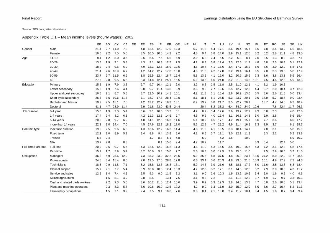
Final Report Earnings distribution using the EU Structure of Earnings Survey
114
Source: SES data; wiiw calculations.
Appendix Table C.1 – Mean income levels (hourly wages), 2002
BE BG CY CZ DE EE ES FI FR GR HR HU IT LT LU LV NL NO PL PT RO SE SK UK
Gender Male 21.4 2.7 11.0 7.3 4.8 13.4 12.9 17.0 12.3 5.2 11.6 4.4 17.1 3.6 19.4 15.7 6.5 7.8 3.4 13.2 6.6 18.5
Female 16.0 2.2 7.5 5.6 3.5 10.5 10.5 14.2 9.2 4.3 9.4 3.8 14.0 2.9 15.1 12.5 6.2 6.2 2.8 11.1 4.8 13.0
Age 14-19 8.4 1.2 5.0 3.6 2.6 6.6 7.6 6.5 5.9 3.0 6.2 2.4 6.5 2.2 5.8 8.1 2.6 3.5 1.3 8.3 3.3 7.1
20-29 13.5 1.9 7.1 5.8 4.3 9.1 10.3 12.5 7.5 4.2 8.3 3.8 12.4 3.3 12.6 11.9 4.8 5.8 2.3 10.3 5.1 12.9
30-39 18.9 2.4 9.5 6.9 4.9 12.3 12.5 15.9 10.5 4.8 10.4 4.1 16.6 3.4 17.7 15.2 6.6 7.6 3.0 12.9 5.8 17.6
40-49 21.4 2.6 10.9 6.7 4.2 14.2 12.7 17.0 13.0 4.8 11.8 4.2 17.8 3.2 19.4 16.4 6.5 7.8 3.3 13.6 5.8 17.9
50-59 23.7 2.7 11.5 6.6 3.8 15.5 12.4 18.7 15.4 5.3 13.2 4.1 19.0 3.2 20.9 15.9 7.3 8.6 3.8 13.3 5.9 16.4
60+ 27.6 2.8 9.5 6.5 3.3 14.8 12.1 25.1 16.5 5.9 13.6 4.0 24.0 3.2 21.3 14.5 10.1 7.5 4.6 12.3 5.9 13.3
Education Primary 15.8 1.9 7.9 3.8 2.7 9.7 10.4 12.1 9.0 3.2 8.8 2.5 11.8 2.5 11.0 12.1 4.1 5.2 1.9 10.3
Lower secondary 15.2 1.9 7.6 4.4 3.0 9.7 11.4 13.8 8.9 3.3 9.0 2.7 10.6 2.5 12.7 12.3 4.4 6.7 2.0 10.4 3.7 12.0
Upper and post secondary 16.5 2.1 8.7 5.8 3.7 12.5 10.9 14.1 10.1 4.2 11.8 3.1 15.4 2.8 16.2 13.6 5.5 8.6 2.6 11.8 5.0 13.4
Short cycle secondary 26.5 3.6 10.6 11.3 7.1 18.7 17.3 28.4 19.0 8.1 18.1 6.1 28.5 5.3 23.7 20.1 9.0 18.9 5.7 18.8 9.0 23.4
Bachelor and Master 19.2 2.5 15.1 7.0 4.2 13.2 12.7 18.3 13.1 6.2 13.7 3.8 21.7 3.5 22.7 20.1 13.7 4.7 14.0 6.2 18.4
Doctoral 41.1 4.7 23.9 11.4 7.9 21.8 23.0 43.5 24.4 20.4 8.2 35.3 6.4 34.2 24.9 12.6 7.6 22.4 11.7 26.3
Job duration 0-1 year 15.0 1.9 7.3 5.4 3.6 9.1 10.5 13.3 8.1 4.2 8.9 3.4 12.6 2.6 13.2 12.9 4.9 5.8 2.3 4.8 12.6
1-4 years 17.4 2.4 8.2 6.3 4.2 11.3 12.1 14.5 9.7 4.6 9.6 4.0 15.4 3.1 16.1 14.8 6.0 6.9 2.8 5.6 15.4
5-14 years 20.5 2.8 9.7 6.9 4.8 14.1 12.5 16.3 11.6 5.1 10.9 4.5 17.1 4.2 19.1 15.7 6.6 7.7 3.6 6.0 17.2
more than 14 years 22.3 3.0 14.4 7.0 4.5 17.6 12.7 18.2 17.0 5.6 12.9 4.7 22.2 4.9 21.4 16.1 7.3 8.9 3.7 6.1 19.7
Contract type Indefinite duration 19.6 2.5 9.6 6.6 4.3 13.6 12.2 16.3 11.4 4.8 11.0 4.1 16.5 3.3 18.4 14.7 7.8 3.1 5.8 15.9
Fixed term 12.1 2.0 8.9 5.2 3.4 8.8 9.4 13.8 8.6 4.2 8.6 3.7 11.1 3.0 12.1 11.3 5.3 2.2 5.2 13.8
Trainee 6.3 2.4 4.7 8.3 6.1 4.8 5.9 4.2 1.5 10.0 5.9 10.2
N/A 13.7 2.0 8.3 8.1 15.6 9.4 4.7 10.7 11.7 6.3 5.4 12.4 5.0
Full-time/Part-time Full-time 20.0 2.5 9.7 6.6 4.3 12.6 12.2 16.2 11.3 4.8 11.0 4.3 16.5 3.5 19.2 15.6 6.3 7.2 3.1 12.8 5.8 17.5
Part-time 15.2 1.7 5.9 5.4 3.2 10.0 9.3 15.0 7.7 5.0 10.3 3.0 12.9 2.0 15.0 11.0 7.5 2.9 10.5 3.7 11.0
Occupation Managers 36.2 4.9 23.6 12.9 7.3 33.2 23.0 32.2 23.5 9.9 35.6 6.8 37.5 4.8 26.0 23.7 13.5 27.2 8.0 22.9 11.7 28.5
Professionals 24.5 3.4 15.4 8.6 7.0 19.5 17.5 28.8 17.8 6.6 33.4 5.6 26.3 4.8 23.0 21.5 10.9 16.1 4.9 17.9 7.2 24.6
Technicians 18.5 2.9 11.8 7.1 5.2 15.8 13.3 16.3 13.1 5.2 14.3 3.9 21.6 4.5 18.1 17.2 6.0 11.6 3.5 13.8 6.3 18.4
Clerical support 15.7 2.1 7.7 5.4 3.9 10.8 10.3 12.4 10.3 4.2 12.3 3.2 17.1 3.1 14.6 12.5 5.2 7.9 3.0 10.0 4.3 11.7
Service and sales 12.6 1.4 7.4 4.3 2.5 9.3 9.0 11.5 8.2 3.1 9.0 2.6 10.3 1.9 13.2 10.6 3.4 5.0 1.6 9.9 4.0 9.6
Skilled agricultural 1.6 8.1 4.2 2.8 8.5 13.4 7.5 3.1 9.3 2.2 2.1 11.5 12.2 3.7 4.9 1.7 9.7 3.3 10.3
Craft and related trade workers 2.2 9.3 5.5 3.6 10.2 11.0 12.4 10.6 3.9 8.9 3.3 12.3 2.8 14.8 13.3 4.7 5.0 2.6 10.8 5.1 13.4
Plant and machine operators 2.3 8.3 5.5 3.6 10.6 10.9 12.5 10.2 4.2 9.0 3.3 11.9 3.0 15.0 12.9 5.0 5.6 2.7 10.4 5.2 11.3
Elementary occupations 1.5 7.1 3.9 2.4 7.5 9.1 10.6 7.6 3.0 8.4 2.1 10.0 2.4 11.2 10.4 3.4 4.5 1.6 8.7 3.4 9.4
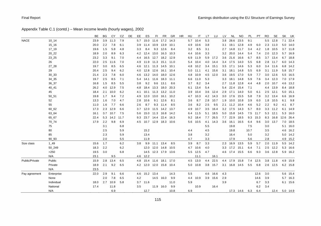
Final Report Earnings distribution using the EU Structure of Earnings Survey
115
Appendix Table C.1 (contd.) – Mean income levels (hourly wages), 2002
BE BG CY CZ DE EE ES FI FR GR HR HU IT LT LU LV NL NO PL PT RO SE SK UK
NACE 10_14 23.9 3.9 11.3 7.9 5.7 15.0 11.6 17.2 14.3 5.7 10.4 5.3 3.8 28.6 23.5 9.1 5.5 12.8 7.1 22.4
15_16 20.0 2.2 7.8 6.1 3.9 11.4 10.9 13.9 10.1 4.9 10.6 3.8 3.1 19.1 12.8 4.9 6.0 2.3 11.0 5.0 14.0
17_19 19.6 1.5 5.8 4.8 3.3 8.4 9.3 12.6 8.4 3.2 8.5 3.1 2.7 14.8 11.7 3.4 4.2 1.8 10.5 3.7 11.8
20_22 18.9 2.0 8.9 6.3 4.2 12.4 13.0 16.3 10.3 4.4 10.6 3.3 3.2 20.0 14.4 5.4 7.4 2.0 12.3 5.7 16.9
23_25 23.2 3.3 9.1 7.0 4.4 16.5 12.7 18.2 12.9 6.9 11.9 5.9 17.2 3.6 21.6 16.6 6.7 8.5 3.7 13.4 6.7 18.8
26 22.0 2.5 11.6 7.0 4.9 11.9 11.3 15.1 11.0 5.4 10.4 4.0 14.4 3.4 17.5 14.0 5.5 6.8 2.8 11.7 6.0 14.3
27_28 19.7 3.0 8.5 6.5 4.6 12.1 11.3 14.5 10.1 4.8 10.2 3.4 15.1 3.5 17.1 14.6 5.3 6.0 3.4 11.6 6.8 14.2
29 20.4 2.5 9.4 6.2 4.0 12.8 12.6 16.1 10.4 5.0 11.1 4.1 15.6 3.1 18.1 14.8 5.5 6.9 3.1 11.9 5.8 15.7
30_33 21.4 2.3 7.8 6.0 4.6 13.2 14.0 18.0 12.6 4.8 10.9 4.5 12.0 3.6 19.5 17.0 5.9 7.7 3.0 12.6 5.5 16.5
34_35 19.7 2.5 8.5 7.1 5.4 14.1 11.6 18.3 11.1 6.6 11.0 5.3 3.3 18.1 14.8 5.9 7.6 3.4 12.3 7.0 17.9
36_37 16.8 1.5 8.5 5.5 3.8 9.2 9.6 13.1 8.6 3.7 8.2 3.4 2.7 11.8 12.8 4.4 4.8 2.0 10.7 4.6 13.2
40_41 26.2 4.0 12.9 7.5 4.8 18.4 13.3 18.0 20.3 6.1 13.4 5.4 5.4 22.4 15.4 7.1 4.4 13.9 8.4 18.8
45 18.4 2.1 10.0 6.2 4.1 10.1 11.3 13.2 11.0 3.9 10.4 3.6 12.4 2.9 17.1 14.0 5.0 6.1 2.5 12.1 5.0 15.1
50_51 19.8 1.7 9.4 7.2 4.9 12.0 13.0 16.1 10.2 4.7 10.3 4.2 14.3 3.0 17.6 15.5 5.8 7.9 3.2 13.4 6.6 16.9
52 13.3 1.6 7.0 4.7 2.8 10.6 9.1 12.6 8.1 3.6 8.7 2.8 10.7 1.9 10.0 10.8 3.9 6.0 1.8 10.5 6.1 9.8
55 11.0 1.6 7.7 6.6 2.6 8.7 9.3 11.4 8.5 3.6 8.2 2.5 9.5 2.1 11.2 10.4 4.6 5.2 2.2 9.2 4.1 8.7
60_62 17.3 2.3 12.9 6.6 3.7 12.0 11.5 14.2 13.7 4.9 10.7 3.5 16.4 3.2 17.5 14.3 5.7 8.0 3.3 11.2 6.1 14.9
63_64 16.1 3.7 10.7 7.5 5.6 15.0 11.3 16.8 14.2 6.4 11.5 5.1 18.5 5.0 15.8 14.5 7.5 11.7 5.3 12.1 5.3 16.0
65_67 22.4 5.3 14.2 11.7 9.3 23.7 14.4 22.4 16.3 9.2 18.4 7.7 26.5 7.7 22.9 18.5 9.3 15.3 8.3 16.8 12.6 26.4
70_74 17.9 2.2 9.8 6.9 4.5 10.7 12.9 18.3 10.6 5.6 10.5 4.1 14.3 3.6 16.1 16.5 6.4 9.6 3.0 13.7 7.0 18.5
75 3.1 6.8 5.5 19.8 7.5 3.0 5.1 16.0
80 2.5 5.9 15.2 4.4 4.5 19.8 10.7 3.5 4.6 16.2
85 2.3 5.9 13.4 3.8 3.2 16.4 5.0 3.2 5.0 14.2
90_93 2.0 5.5 11.9 4.7 3.3 17.9 5.6 2.8 4.9 15.2
Size class 1_49 15.6 1.7 6.2 3.8 9.9 11.1 13.4 8.5 3.9 8.7 3.3 2.3 16.9 13.5 5.9 5.7 2.0 11.9 5.5 14.2
50_249 18.3 2.2 6.2 12.0 12.0 14.8 10.5 4.7 10.6 4.0 3.3 17.2 15.1 6.4 7.1 2.5 12.2 5.3 16.6
>250 19.5 3.0 6.8 14.5 12.3 17.9 13.6 5.5 12.5 4.7 4.6 17.4 15.5 6.6 9.3 3.6 12.8 5.9 16.2
N/A 23.1 9.5 4.6 12.2 11.1 16.1
Public/Private Public 15.9 2.8 13.4 6.5 4.8 15.4 11.6 18.1 17.0 4.5 13.0 4.4 22.5 4.4 17.9 15.8 7.4 12.5 3.8 11.8 4.9 15.9
Private 18.9 2.1 9.2 6.5 4.2 12.0 12.0 15.8 10.4 5.0 10.8 3.8 15.7 3.1 16.8 14.5 5.5 6.8 2.6 12.5 6.2 15.8
N/A 23.5
Pay agreement Enterprise 22.0 2.9 9.1 6.6 4.6 15.2 13.4 14.3 5.5 4.6 16.6 4.3 12.6 3.0 5.6 15.4
None 2.0 7.8 6.5 4.2 14.5 16.0 9.9 4.4 10.9 3.9 15.6 2.9 14.6 3.9 5.7 16.3
Individual 18.0 2.7 10.9 5.8 3.7 11.6 11.0 5.9 3.9 6.7 3.3 6.1 15.6
National 17.4 11.8 3.5 11.9 16.0 9.9 10.9 16.4 6.2 3.4
N/A 6.9 12.7 10.8 6.9 17.3 14.6 6.3 6.4 12.4 5.0 14.9

Final Report Earnings distribution using the EU Structure of Earnings Survey
116
Source: SES data; wiiw calculations.
Appendix Table C.2 – Mean income levels (hourly wages), 2006
BE BG CY CZ DE EE ES FI FR GR HR HU IT LT LU LV NL NO PL PT RO SE SK UK
Gender Male 18.4 3.0 13.5 8.7 19.8 6.7 13.7 15.6 18.5 13.3 7.2 14.8 6.0 18.7 5.4 17.2 18.1 7.7 10.5 4.1 14.6 7.1 21.2
Female 16.3 2.7 10.4 6.7 15.1 5.0 11.1 12.0 14.8 10.7 6.3 13.8 5.0 16.6 4.7 13.6 14.8 7.3 9.5 3.9 12.0 5.2 15.4
Age 14-19 10.2 1.6 5.7 4.4 4.8 3.9 7.6 8.6 6.1 6.8 3.7 7.1 3.3 6.4 3.1 5.0 9.1 3.3 4.3 1.9 9.0 3.8 8.0
20-29 13.6 2.3 8.2 6.7 12.2 6.0 9.6 11.1 12.3 8.3 5.4 9.6 5.2 12.9 5.0 11.3 13.1 5.5 6.9 3.2 10.8 5.4 14.2
30-39 16.9 2.9 11.6 8.4 18.3 6.7 12.4 14.0 15.7 11.3 6.8 12.4 5.8 18.0 5.5 16.7 17.2 7.8 9.7 3.9 13.4 6.5 20.4
40-49 18.6 3.0 13.3 8.3 19.6 5.9 14.0 14.4 17.6 13.9 6.8 14.8 5.5 20.0 5.0 18.1 18.7 7.9 11.3 4.1 14.2 6.3 21.0
50-59 20.7 3.1 15.5 7.9 20.1 5.2 15.2 14.3 19.2 15.8 7.2 18.1 5.5 21.7 4.8 18.8 18.3 8.1 12.7 4.8 14.0 6.2 19.4
60+ 24.4 3.0 12.9 8.3 21.2 4.6 16.9 15.0 28.4 17.7 8.8 22.2 5.5 27.4 4.5 18.2 17.6 10.2 12.2 5.8 13.6 6.6 16.2
Education Primary 13.1 2.1 9.1 4.7 3.6 10.2 11.9 11.6 10.0 4.4 10.6 3.2 12.4 3.7 10.0 14.0 4.7 6.1 2.0 11.1
Lower secondary 13.6 2.1 8.6 5.4 10.8 4.1 10.1 13.4 9.6 4.2 10.7 3.8 12.0 3.2 11.5 13.2 4.9 7.5 2.4 11.5 3.6 11.3
Upper and post secondary 14.9 2.3 10.1 7.0 17.2 5.0 12.4 12.0 14.8 10.8 5.4 13.8 4.1 16.1 3.8 14.6 16.0 6.1 9.7 3.1 12.0 5.3 15.0
Short cycle secondary 28.0 4.6 19.8 13.5 30.2 8.2 18.6 17.8 22.5 12.9 11.8 23.2 8.0 31.8 7.6 21.5 22.5 10.0 19.6 7.6 15.3 10.2 26.4
Bachelor and Master 19.9 3.0 12.2 8.4 25.7 5.9 12.8 13.9 17.1 10.7 6.9 19.2 5.0 23.3 5.3 21.4 20.2 10.0 15.6 4.6 15.3 6.1 21.9
Doctoral 36.3 7.0 33.3 12.6 12.3 19.8 24.2 24.9 19.5 25.7 11.3 38.3 13.4 29.0 25.3 14.6 26.5 11.5 21.3 11.4 30.6
Job duration 0-1 year 14.2 2.3 8.2 6.4 12.1 5.3 9.8 11.5 13.7 9.3 5.3 11.0 4.6 13.8 4.2 12.2 14.7 5.5 7.0 3.0 12.2 5.1 14.8
1-4 years 15.8 2.7 9.5 7.6 15.2 5.7 11.6 13.3 14.9 10.4 6.3 12.0 5.6 15.8 4.9 15.2 16.5 6.7 8.3 3.7 13.3 5.9 17.4
5-14 years 17.4 3.5 12.6 8.7 18.5 6.3 13.7 14.7 16.5 12.8 7.3 13.6 6.2 20.1 5.7 17.3 18.1 8.1 10.2 4.6 13.9 6.9 20.3
more than 14 years 20.5 3.9 18.5 8.9 22.5 6.1 18.4 14.8 19.0 17.1 8.4 18.0 6.4 23.6 6.6 19.3 18.3 8.9 13.8 5.2 13.3 6.8 22.5
Contract type Indefinite duration 17.7 2.9 12.1 8.2 18.8 5.8 13.6 14.2 17.1 11.5 6.8 14.6 5.4 18.4 4.9 16.9 16.9 8.3 10.8 4.0 6.3 18.5
Fixed term 16.0 2.3 10.0 6.3 13.5 6.3 10.2 11.3 14.3 14.2 5.2 11.5 6.3 13.3 6.1 11.1 14.4 5.4 7.4 3.3 5.0 15.1
Trainee 8.2 1.7 4.1 9.3 7.5 8.9 6.8 3.0 5.1 3.0 12.9 5.1
N/A 13.3
Full-time/Part-time Full-time 17.4 2.9 12.2 7.9 18.6 6.0 13.0 14.0 17.1 12.2 6.7 14.7 5.6 18.0 5.0 17.1 17.9 7.5 9.9 4.0 14.0 6.3 20.0
Part-time 17.8 2.0 8.5 6.3 15.5 4.4 10.7 11.5 15.2 12.2 6.7 11.4 4.7 17.6 4.9 13.8 13.5 7.2 12.6 3.5 11.4 4.6 13.6
Occupation Managers 36.4 6.8 31.9 15.0 9.3 33.2 26.2 28.9 26.9 13.2 36.2 9.1 45.2 7.7 24.5 26.5 15.4 31.2 11.1 23.2 14.6 32.5
Professionals 27.1 4.6 21.0 10.6 8.1 19.6 17.9 20.6 18.7 10.3 22.8 6.9 27.1 7.1 21.8 20.5 11.3 19.5 6.8 16.2 8.2 28.0
Technicians 17.8 3.7 14.1 8.7 6.2 15.6 13.9 16.5 13.4 7.1 15.8 5.3 23.1 5.5 17.4 18.8 7.4 13.5 4.4 14.2 6.6 20.3
Clerical support 16.0 2.5 8.7 6.4 4.7 11.0 11.6 12.6 11.0 5.4 14.2 4.4 15.8 4.3 13.8 14.1 5.6 8.6 3.7 11.0 5.0 13.0
Service and sales 13.0 1.7 8.3 4.9 3.7 9.3 10.0 11.2 9.2 4.1 10.6 3.3 11.2 2.9 11.5 12.4 3.8 5.9 2.2 10.6 3.8 10.6
Skilled agricultural 1.8 10.7 6.0 4.1 10.4 9.4 9.9 9.1 3.6 10.7 2.7 2.9 10.8 13.1 4.8 5.1 2.1 9.8 3.7 11.4
Craft and related trade workers 14.0 2.6 10.5 6.4 5.4 11.0 13.3 13.5 11.7 4.7 10.4 4.7 12.4 4.0 14.8 14.9 5.4 5.8 3.2 12.0 5.1 15.2
Plant and machine operators 15.0 2.5 9.8 6.3 5.0 11.2 13.3 13.0 11.2 5.0 11.4 4.4 13.0 3.9 14.8 14.8 5.6 6.7 3.1 11.9 5.3 12.8
Elementary occupations 11.9 1.7 8.1 4.4 3.1 8.6 10.0 10.4 8.5 3.7 9.4 3.0 10.1 2.8 9.8 12.1 4.0 5.6 2.0 9.6 3.5 10.4
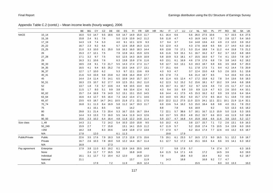
Final Report Earnings distribution using the EU Structure of Earnings Survey
117
Appendix Table C.2 (contd.) – Mean income levels (hourly wages), 2006
BE BG CY CZ DE EE ES FI FR GR HR HU IT LT LU LV NL NO PL PT RO SE SK UK
NACE 10_14 16.0 5.0 14.7 9.5 18.6 6.8 14.7 14.9 15.0 11.7 6.1 16.4 6.6 5.6 26.0 27.5 10.6 6.7 15.5 6.4 27.5
15_16 15.8 2.4 9.1 7.6 5.0 11.9 13.9 14.2 11.2 5.6 11.8 4.7 4.3 16.9 14.5 5.7 7.3 2.8 12.7 5.4 16.0
17_19 14.3 1.9 7.4 5.3 4.0 9.1 12.1 12.9 9.3 3.7 9.4 3.7 3.4 14.8 13.6 4.0 4.9 2.3 12.0 3.9 15.2
20_22 16.7 2.3 9.2 6.6 5.7 12.6 15.8 16.3 11.5 5.3 12.0 4.3 4.3 17.6 16.8 6.5 8.6 2.7 14.0 6.3 19.2
23_25 21.0 3.3 10.0 8.1 25.0 5.8 16.3 16.0 18.3 14.4 8.9 13.8 7.0 17.1 5.3 21.4 18.8 7.4 11.2 4.4 15.8 7.5 21.2
26 15.3 2.7 12.1 7.5 7.9 12.8 14.1 15.9 12.5 6.6 11.6 5.9 15.1 5.1 16.7 16.2 6.7 8.2 3.7 13.2 6.8 18.0
27_28 17.1 3.2 9.7 7.5 6.0 12.5 14.3 16.9 10.9 5.8 10.9 5.3 18.1 4.7 15.5 16.0 6.7 7.4 4.1 13.0 7.8 16.7
29 16.3 3.1 10.6 7.6 6.3 13.8 15.9 17.6 11.6 6.0 13.1 6.1 16.9 4.6 17.9 17.6 6.8 7.9 3.8 14.0 6.2 18.2
30_33 18.5 2.8 9.1 7.3 21.7 5.5 14.3 17.4 17.3 11.7 5.9 12.7 6.0 13.1 6.3 19.3 18.7 6.9 8.6 3.5 16.8 5.7 20.3
34_35 16.5 4.1 9.4 8.5 25.2 7.6 15.5 14.6 17.7 13.1 7.7 15.1 6.6 5.1 17.8 17.5 7.1 9.4 4.2 14.4 7.5 20.9
36_37 12.7 1.7 10.0 6.2 5.3 9.7 12.1 13.6 8.9 4.3 9.3 4.7 3.7 12.4 15.0 4.8 5.3 2.6 10.5 5.1 15.8
40_41 21.6 5.0 15.9 9.8 23.8 6.2 19.8 16.4 20.8 17.7 8.5 17.8 7.3 6.6 21.4 18.7 8.5 5.4 15.6 9.0 21.6
45 14.4 2.4 11.4 7.5 14.1 6.5 10.9 14.0 15.7 10.7 4.6 11.4 6.5 12.4 4.7 17.2 15.8 6.2 7.8 3.4 13.6 5.6 18.3
50_51 18.3 2.5 10.7 9.2 17.7 6.9 12.5 15.1 19.2 11.0 6.2 12.3 5.2 15.2 5.2 15.6 18.1 6.7 10.2 3.9 14.6 6.8 18.8
52 13.7 1.8 7.3 5.7 13.6 4.4 9.8 10.5 13.4 8.6 4.5 10.7 4.1 10.7 3.2 9.7 12.6 4.6 7.3 2.5 11.7 4.7 11.5
55 11.5 1.7 8.0 5.1 9.9 3.8 9.6 10.4 12.4 9.3 4.3 9.4 3.0 9.9 3.0 8.9 11.9 4.7 6.3 2.6 10.0 4.4 10.1
60_62 15.7 2.4 16.9 7.6 14.9 5.2 13.1 13.1 15.0 14.5 6.6 14.4 4.1 17.5 4.5 15.3 16.2 6.2 8.9 3.9 12.6 6.4 16.4
63_64 16.6 4.4 12.7 9.5 16.4 7.3 14.2 13.4 17.1 14.6 8.3 14.0 6.5 20.2 6.0 15.7 17.0 8.5 16.4 5.1 13.8 7.0 19.0
65_67 23.5 6.5 18.7 14.7 24.1 10.5 21.8 17.1 22.1 17.5 13.3 22.2 11.2 27.5 11.0 22.5 24.1 12.1 22.1 10.1 21.9 11.4 32.1
70_74 16.8 3.1 11.3 8.4 16.9 5.8 11.2 14.7 19.3 11.7 6.9 13.6 5.4 16.2 5.3 15.0 18.4 6.8 9.8 4.0 15.1 7.8 23.2
75 4.1 15.1 8.5 6.8 14.2 8.8 7.8 6.6 18.9 9.2 5.0 13.3 6.5 18.2
80 29.8 3.1 21.4 7.3 20.4 5.3 16.7 13.5 16.7 19.4 7.2 22.1 5.7 38.6 5.7 18.1 16.7 11.3 15.9 5.0 11.8 5.3 19.5
85 14.4 3.3 13.3 7.3 16.0 5.5 14.4 11.9 14.3 12.6 6.0 13.7 5.5 20.3 4.8 15.2 15.7 6.6 10.3 4.6 11.9 5.0 18.9
90_93 15.6 2.3 10.2 6.4 16.4 4.8 11.8 12.2 14.8 11.4 5.9 13.7 4.7 16.8 4.4 15.9 16.8 6.6 11.6 3.8 13.0 5.2 12.7
Size class 1_49 14.3 2.1 7.2 14.2 5.4 10.3 13.0 15.8 9.5 5.0 10.2 4.3 3.8 13.7 15.7 7.1 7.2 2.6 13.1 5.9 16.3
50_249 15.9 2.7 7.7 15.8 13.1 14.1 15.9 11.2 6.7 11.9 5.7 5.2 15.8 17.4 7.5 10.5 3.4 13.9 6.0 19.0
>250 18.2 3.8 8.3 20.6 14.9 13.8 17.3 13.8 7.7 17.0 6.7 6.2 16.4 17.4 7.7 12.6 4.6 13.2 6.5 18.7
N/A 17.8 12.0 6.1 11.3 19.8 17.9
Public/Private Public 22.6 3.5 17.6 7.9 18.3 5.8 17.3 12.8 17.5 15.6 7.5 19.1 6.1 23.3 5.7 16.5 17.3 9.0 16.5 5.1 12.2 5.9 18.7
Private 16.7 2.6 10.3 7.8 18.0 5.8 12.2 14.4 16.7 11.4 6.1 12.7 5.2 17.2 4.6 15.1 16.6 6.4 8.6 3.5 14.1 6.3 18.2
N/A 16.9 17.3
Pay agreement Enterprise 17.9 3.8 11.0 8.3 19.2 6.1 15.9 14.6 20.5 14.8 7.7 5.8 17.8 5.7 7.4 17.4 3.7 6.3 16.5
None 2.4 11.7 7.7 16.5 5.8 16.8 14.8 6.4 11.5 5.4 17.1 4.6 17.2 14.5 3.6 6.0 19.0
Individual 16.1 3.1 12.7 7.2 19.4 6.2 12.0 16.9 12.0 7.8 18.6 6.0 16.4 8.2 4.5 6.2 18.7
National 21.1 13.7 11.9 14.3 18.8 16.8 9.2 7.7 4.7
N/A 17.9 7.2 11.9 16.9 12.4 7.1 15.5 8.0 3.0 13.3 16.0
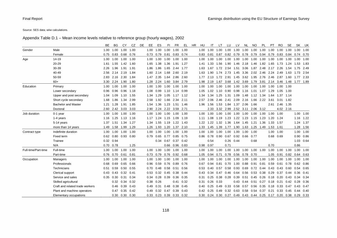
Final Report Earnings distribution using the EU Structure of Earnings Survey
118
Source: SES data; wiiw calculations.
Appendix Table D.1 – Mean income levels relative to reference group (hourly wages), 2002
BE BG CY CZ DE EE ES FI FR EL HR HU IT LT LU LV NL NO PL PT RO SE SK UK
Gender Male 1.00 1.00 1.00 1.00 1.00 1.00 1.00 1.00 1.00 1.00 1.00 1.00 1.00 1.00 1.00 1.00 1.00 1.00 1.00 1.00 1.00 1.00
Female 0.75 0.83 0.68 0.76 0.73 0.79 0.81 0.83 0.74 0.83 0.81 0.87 0.82 0.79 0.78 0.79 0.94 0.79 0.83 0.84 0.74 0.70
Age 14-19 1.00 1.00 1.00 1.00 1.00 1.00 1.00 1.00 1.00 1.00 1.00 1.00 1.00 1.00 1.00 1.00 1.00 1.00 1.00 1.00 1.00 1.00
20-29 1.61 1.55 1.42 1.60 1.65 1.38 1.36 1.91 1.27 1.41 1.33 1.56 1.90 1.46 2.18 1.46 1.82 1.65 1.73 1.24 1.53 1.83
30-39 2.26 1.96 1.91 1.91 1.86 1.86 1.65 2.44 1.77 1.63 1.67 1.72 2.54 1.51 3.06 1.87 2.48 2.17 2.26 1.54 1.75 2.49
40-49 2.56 2.14 2.19 1.84 1.60 2.14 1.68 2.60 2.19 1.63 1.90 1.74 2.73 1.45 3.36 2.02 2.46 2.24 2.49 1.63 1.73 2.54
50-59 2.83 2.16 2.30 1.84 1.47 2.35 1.64 2.86 2.60 1.77 2.13 1.72 2.91 1.45 3.62 1.95 2.76 2.46 2.87 1.60 1.77 2.33
60+ 3.30 2.24 1.90 1.80 1.28 2.24 1.60 3.84 2.79 1.98 2.19 1.67 3.68 1.42 3.69 1.79 3.81 2.14 3.46 1.48 1.77 1.89
Education Primary 1.00 1.00 1.00 1.00 1.00 1.00 1.00 1.00 1.00 1.00 1.00 1.00 1.00 1.00 1.00 1.00 1.00 1.00 1.00 1.00
Lower secondary 0.96 0.96 0.96 1.18 1.08 0.99 1.10 1.14 0.99 1.05 1.02 1.10 0.90 0.98 1.16 1.01 1.07 1.29 1.05 1.00
Upper and post secondary 1.04 1.09 1.10 1.55 1.34 1.29 1.05 1.17 1.12 1.34 1.34 1.25 1.31 1.09 1.48 1.12 1.34 1.64 1.37 1.14
Short cycle secondary 1.68 1.86 1.34 2.99 2.58 1.92 1.66 2.34 2.11 2.57 2.06 2.46 2.41 2.09 2.16 1.66 2.22 3.61 3.01 1.82
Bachelor and Master 1.21 1.28 1.91 1.85 1.54 1.36 1.23 1.51 1.46 1.96 1.56 1.53 1.84 1.37 2.06 1.66 2.61 2.46 1.35
Doctoral 2.60 2.42 3.03 3.03 2.90 2.24 2.22 3.59 2.71 2.33 3.32 2.99 2.52 3.11 2.06 3.12 4.02 2.16
Job duration 0-1 year 1.00 1.00 1.00 1.00 1.00 1.00 1.00 1.00 1.00 1.00 1.00 1.00 1.00 1.00 1.00 1.00 1.00 1.00 1.00 1.00 1.00
1-4 years 1.16 1.25 1.13 1.16 1.17 1.24 1.15 1.09 1.19 1.11 1.08 1.19 1.23 1.22 1.23 1.15 1.23 1.20 1.24 1.16 1.22
5-14 years 1.37 1.51 1.34 1.27 1.34 1.55 1.19 1.22 1.43 1.22 1.22 1.32 1.36 1.64 1.45 1.21 1.36 1.33 1.57 1.24 1.37
more than 14 years 1.49 1.58 1.99 1.29 1.26 1.93 1.20 1.37 2.10 1.33 1.45 1.39 1.77 1.90 1.63 1.25 1.49 1.53 1.61 1.28 1.56
Contract type Indefinite duration 1.00 1.00 1.00 1.00 1.00 1.00 1.00 1.00 1.00 1.00 1.00 1.00 1.00 1.00 1.00 1.00 1.00 1.00 1.00 1.00
Fixed term 0.62 0.80 0.93 0.80 0.79 0.65 0.77 0.85 0.75 0.86 0.78 0.90 0.67 0.92 0.66 0.77 0.68 0.69 0.90 0.86
Trainee 0.32 0.94 0.34 0.67 0.37 0.42 0.54 0.26 0.44 0.68 1.03 0.64
N/A 0.70 0.78 1.25 0.66 0.96 0.83 0.98 0.97 0.71 0.70 0.86
Full-time/Part-time Full-time 1.00 1.00 1.00 1.00 1.00 1.00 1.00 1.00 1.00 1.00 1.00 1.00 1.00 1.00 1.00 1.00 1.00 1.00 1.00 1.00 1.00 1.00
Part-time 0.76 0.70 0.61 0.81 0.73 0.79 0.76 0.92 0.68 1.05 0.94 0.71 0.78 0.56 0.78 0.70 1.05 0.91 0.82 0.64 0.63
Occupation Managers 1.00 1.00 1.00 1.00 1.00 1.00 1.00 1.00 1.00 1.00 1.00 1.00 1.00 1.00 1.00 1.00 1.00 1.00 1.00 1.00 1.00 1.00
Professionals 0.68 0.69 0.65 0.66 0.96 0.59 0.76 0.89 0.76 0.67 0.94 0.81 0.70 1.00 0.88 0.91 0.81 0.59 0.61 0.78 0.62 0.86
Technicians 0.51 0.59 0.50 0.55 0.70 0.48 0.58 0.51 0.56 0.53 0.40 0.57 0.58 0.93 0.69 0.72 0.44 0.43 0.43 0.60 0.54 0.65
Clerical support 0.43 0.43 0.32 0.41 0.53 0.32 0.45 0.38 0.44 0.43 0.34 0.47 0.46 0.64 0.56 0.53 0.38 0.29 0.37 0.44 0.36 0.41
Service and sales 0.35 0.30 0.31 0.34 0.34 0.28 0.39 0.36 0.35 0.31 0.25 0.38 0.28 0.39 0.51 0.45 0.26 0.18 0.20 0.43 0.34 0.34
Skilled agricultural 0.32 0.34 0.32 0.38 0.26 0.41 0.32 0.31 0.26 0.33 0.43 0.44 0.51 0.27 0.18 0.21 0.42 0.28 0.36
Craft and related trade workers 0.46 0.39 0.43 0.49 0.31 0.48 0.38 0.45 0.40 0.25 0.49 0.33 0.58 0.57 0.56 0.35 0.18 0.33 0.47 0.43 0.47
Plant and machine operators 0.47 0.35 0.42 0.49 0.32 0.47 0.39 0.43 0.42 0.25 0.49 0.32 0.63 0.58 0.54 0.37 0.21 0.33 0.45 0.44 0.40
Elementary occupations 0.30 0.30 0.30 0.33 0.23 0.39 0.33 0.32 0.30 0.24 0.30 0.27 0.49 0.43 0.44 0.25 0.17 0.20 0.38 0.29 0.33
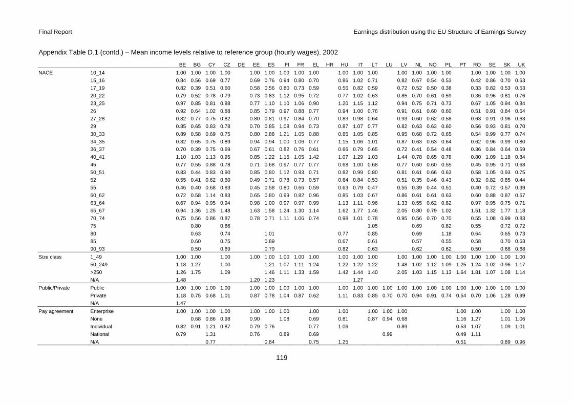
Final Report Earnings distribution using the EU Structure of Earnings Survey
119
Appendix Table D.1 (contd.) – Mean income levels relative to reference group (hourly wages), 2002
BE BG CY CZ DE EE ES FI FR EL HR HU IT LT LU LV NL NO PL PT RO SE SK UK
NACE 10_14 1.00 1.00 1.00 1.00 1.00 1.00 1.00 1.00 1.00 1.00 1.00 1.00 1.00 1.00 1.00 1.00 1.00 1.00 1.00 1.00
15_16 0.84 0.56 0.69 0.77 0.69 0.76 0.94 0.80 0.70 0.86 1.02 0.71 0.82 0.67 0.54 0.53 0.42 0.86 0.70 0.63
17_19 0.82 0.39 0.51 0.60 0.58 0.56 0.80 0.73 0.59 0.56 0.82 0.59 0.72 0.52 0.50 0.38 0.33 0.82 0.53 0.53
20_22 0.79 0.52 0.78 0.79 0.73 0.83 1.12 0.95 0.72 0.77 1.02 0.63 0.85 0.70 0.61 0.59 0.36 0.96 0.81 0.76
23_25 0.97 0.85 0.81 0.88 0.77 1.10 1.10 1.06 0.90 1.20 1.15 1.12 0.94 0.75 0.71 0.73 0.67 1.05 0.94 0.84
26 0.92 0.64 1.02 0.88 0.85 0.79 0.97 0.88 0.77 0.94 1.00 0.76 0.91 0.61 0.60 0.60 0.51 0.91 0.84 0.64
27_28 0.82 0.77 0.75 0.82 0.80 0.81 0.97 0.84 0.70 0.83 0.98 0.64 0.93 0.60 0.62 0.58 0.63 0.91 0.96 0.63
29 0.85 0.65 0.83 0.78 0.70 0.85 1.08 0.94 0.73 0.87 1.07 0.77 0.82 0.63 0.63 0.60 0.56 0.93 0.81 0.70
30_33 0.89 0.58 0.69 0.75 0.80 0.88 1.21 1.05 0.88 0.85 1.05 0.85 0.95 0.68 0.72 0.65 0.54 0.99 0.77 0.74
34_35 0.82 0.65 0.75 0.89 0.94 0.94 1.00 1.06 0.77 1.15 1.06 1.01 0.87 0.63 0.63 0.64 0.62 0.96 0.99 0.80
36_37 0.70 0.39 0.75 0.69 0.67 0.61 0.82 0.76 0.61 0.66 0.79 0.65 0.72 0.41 0.54 0.48 0.36 0.84 0.64 0.59
40_41 1.10 1.03 1.13 0.95 0.85 1.22 1.15 1.05 1.42 1.07 1.29 1.03 1.44 0.78 0.65 0.78 0.80 1.09 1.18 0.84
45 0.77 0.55 0.88 0.78 0.71 0.68 0.97 0.77 0.77 0.68 1.00 0.68 0.77 0.60 0.60 0.55 0.45 0.95 0.71 0.68
50_51 0.83 0.44 0.83 0.90 0.85 0.80 1.12 0.93 0.71 0.82 0.99 0.80 0.81 0.61 0.66 0.63 0.58 1.05 0.93 0.75
52 0.55 0.41 0.62 0.60 0.49 0.71 0.78 0.73 0.57 0.64 0.84 0.53 0.51 0.35 0.46 0.43 0.32 0.82 0.85 0.44
55 0.46 0.40 0.68 0.83 0.45 0.58 0.80 0.66 0.59 0.63 0.79 0.47 0.55 0.39 0.44 0.51 0.40 0.72 0.57 0.39
60_62 0.72 0.58 1.14 0.83 0.65 0.80 0.99 0.82 0.96 0.85 1.03 0.67 0.86 0.61 0.61 0.63 0.60 0.88 0.87 0.67
63_64 0.67 0.94 0.95 0.94 0.98 1.00 0.97 0.97 0.99 1.13 1.11 0.96 1.33 0.55 0.62 0.82 0.97 0.95 0.75 0.71
65_67 0.94 1.36 1.25 1.48 1.63 1.58 1.24 1.30 1.14 1.62 1.77 1.46 2.05 0.80 0.79 1.02 1.51 1.32 1.77 1.18
70_74 0.75 0.56 0.86 0.87 0.78 0.71 1.11 1.06 0.74 0.98 1.01 0.78 0.95 0.56 0.70 0.70 0.55 1.08 0.99 0.83
75 0.80 0.86 1.05 0.69 0.82 0.55 0.72 0.72
80 0.63 0.74 1.01 0.77 0.85 0.69 1.18 0.64 0.65 0.73
85 0.60 0.75 0.89 0.67 0.61 0.57 0.55 0.58 0.70 0.63
90_93 0.50 0.69 0.79 0.82 0.63 0.62 0.62 0.50 0.68 0.68
Size class 1_49 1.00 1.00 1.00 1.00 1.00 1.00 1.00 1.00 1.00 1.00 1.00 1.00 1.00 1.00 1.00 1.00 1.00 1.00 1.00 1.00
50_249 1.18 1.27 1.00 1.21 1.07 1.11 1.24 1.22 1.22 1.22 1.48 1.02 1.12 1.09 1.25 1.24 1.02 0.96 1.17
>250 1.26 1.75 1.09 1.46 1.11 1.33 1.59 1.42 1.44 1.40 2.05 1.03 1.15 1.13 1.64 1.81 1.07 1.08 1.14
N/A 1.48 1.20 1.23 1.27
Public/Private Public 1.00 1.00 1.00 1.00 1.00 1.00 1.00 1.00 1.00 1.00 1.00 1.00 1.00 1.00 1.00 1.00 1.00 1.00 1.00 1.00 1.00 1.00
Private 1.18 0.75 0.68 1.01 0.87 0.78 1.04 0.87 0.62 1.11 0.83 0.85 0.70 0.70 0.94 0.91 0.74 0.54 0.70 1.06 1.28 0.99
N/A 1.47
Pay agreement Enterprise 1.00 1.00 1.00 1.00 1.00 1.00 1.00 1.00 1.00 1.00 1.00 1.00 1.00 1.00 1.00 1.00
None 0.68 0.86 0.98 0.90 1.08 0.69 0.81 0.87 0.94 0.68 1.16 1.27 1.01 1.06
Individual 0.82 0.91 1.21 0.87 0.79 0.76 0.77 1.06 0.89 0.53 1.07 1.09 1.01
National 0.79 1.31 0.76 0.89 0.69 0.99 0.49 1.11
N/A 0.77 0.84 0.75 1.25 0.51 0.89 0.96

Final Report Earnings distribution using the EU Structure of Earnings Survey
120
Source: SES data; wiiw calculations.
Appendix Table D.2 – Mean income levels relative to reference group (hourly wages), 2006
BE BG CY CZ DE EE ES FI FR EL HR HU IT LT LU LV NL NO PL PT RO SE SK UK
Gender Male 1.00 1.00 1.00 1.00 1.00 1.00 1.00 1.00 1.00 1.00 1.00 1.00 1.00 1.00 1.00 1.00 1.00 1.00 1.00 1.00 1.00 1.00 1.00
Female 0.89 0.89 0.77 0.76 0.76 0.74 0.81 0.77 0.80 0.81 0.88 0.93 0.84 0.89 0.88 0.79 0.82 0.95 0.90 0.94 0.82 0.73 0.73
Age 14-19 1.00 1.00 1.00 1.00 1.00 1.00 1.00 1.00 1.00 1.00 1.00 1.00 1.00 1.00 1.00 1.00 1.00 1.00 1.00 1.00 1.00 1.00 1.00
20-29 1.33 1.44 1.44 1.51 2.52 1.52 1.27 1.29 2.02 1.22 1.45 1.36 1.57 2.03 1.60 2.26 1.44 1.68 1.62 1.65 1.21 1.43 1.78
30-39 1.66 1.80 2.04 1.89 3.80 1.71 1.63 1.62 2.57 1.66 1.82 1.75 1.74 2.84 1.76 3.33 1.88 2.39 2.29 2.02 1.49 1.72 2.56
40-49 1.83 1.92 2.33 1.87 4.06 1.50 1.84 1.67 2.87 2.04 1.83 2.09 1.66 3.14 1.59 3.62 2.05 2.42 2.65 2.14 1.59 1.66 2.63
50-59 2.03 1.94 2.72 1.78 4.17 1.33 2.00 1.65 3.14 2.33 1.93 2.56 1.67 3.42 1.52 3.75 2.01 2.46 2.99 2.49 1.56 1.65 2.43
60+ 2.39 1.90 2.26 1.89 4.40 1.16 2.22 1.74 4.64 2.60 2.36 3.14 1.66 4.31 1.43 3.64 1.93 3.10 2.87 3.02 1.52 1.73 2.03
Education Primary 1.00 1.00 1.00 1.00 1.00 1.00 1.00 1.00 1.00 1.00 1.00 1.00 1.00 1.00 1.00 1.00 1.00 1.00 1.00 1.00
Lower secondary 1.04 1.01 0.95 1.15 1.14 0.99 1.16 0.96 0.94 1.00 1.19 0.97 0.88 1.15 0.95 1.04 1.23 1.21 1.04
Upper and post secondary 1.14 1.09 1.11 1.49 1.38 1.22 1.01 1.28 1.08 1.22 1.30 1.31 1.30 1.04 1.45 1.15 1.29 1.60 1.58 1.08
Short cycle secondary 2.14 2.22 2.18 2.86 2.27 1.83 1.50 1.95 1.29 2.65 2.18 2.54 2.57 2.08 2.15 1.61 2.13 3.23 3.84 1.39
Bachelor and Master 1.51 1.44 1.34 1.79 1.65 1.26 1.17 1.48 1.08 1.56 1.80 1.59 1.89 1.45 2.14 1.45 2.13 2.57 2.33 1.38
Doctoral 2.77 3.35 3.67 2.68 3.41 1.95 2.04 2.15 1.96 2.41 3.57 3.09 3.65 2.89 1.81 3.09 4.36 5.84 1.93
Job duration 0-1 year 1.00 1.00 1.00 1.00 1.00 1.00 1.00 1.00 1.00 1.00 1.00 1.00 1.00 1.00 1.00 1.00 1.00 1.00 1.00 1.00 1.00 1.00 1.00
1-4 years 1.12 1.20 1.16 1.19 1.26 1.09 1.18 1.16 1.09 1.12 1.18 1.08 1.21 1.15 1.16 1.25 1.12 1.21 1.19 1.21 1.09 1.16 1.18
5-14 years 1.23 1.55 1.53 1.36 1.54 1.20 1.39 1.28 1.20 1.38 1.37 1.23 1.35 1.46 1.36 1.42 1.23 1.48 1.46 1.51 1.14 1.34 1.37
more than 14 years 1.45 1.74 2.26 1.40 1.86 1.15 1.87 1.29 1.38 1.83 1.57 1.63 1.39 1.71 1.56 1.59 1.25 1.62 1.98 1.72 1.09 1.31 1.52
Contract type Indefinite duration 1.00 1.00 1.00 1.00 1.00 1.00 1.00 1.00 1.00 1.00 1.00 1.00 1.00 1.00 1.00 1.00 1.00 1.00 1.00 1.00 1.00 1.00
Fixed term 0.90 0.80 0.82 0.77 0.72 1.09 0.75 0.80 0.84 1.23 0.76 0.79 1.16 0.72 1.24 0.66 0.85 0.66 0.69 0.82 0.79 0.81
Trainee 0.46 0.57 0.22 0.66 0.44 0.77 0.47 0.56 0.28 0.61 0.77 0.81
N/A
Full-time/Part-time Full-time 1.00 1.00 1.00 1.00 1.00 1.00 1.00 1.00 1.00 1.00 1.00 1.00 1.00 1.00 1.00 1.00 1.00 1.00 1.00 1.00 1.00 1.00 1.00
Part-time 1.02 0.69 0.70 0.80 0.84 0.73 0.82 0.82 0.89 1.00 0.99 0.78 0.84 0.98 0.97 0.81 0.75 0.96 1.27 0.88 0.82 0.73 0.68
Occupation Managers 1.00 1.00 1.00 1.00 1.00 1.00 1.00 1.00 1.00 1.00 1.00 1.00 1.00 1.00 1.00 1.00 1.00 1.00 1.00 1.00 1.00 1.00
Professionals 0.74 0.68 0.66 0.71 0.88 0.59 0.68 0.71 0.69 0.78 0.63 0.76 0.60 0.92 0.89 0.77 0.73 0.63 0.61 0.70 0.56 0.86
Technicians 0.49 0.54 0.44 0.58 0.67 0.47 0.53 0.57 0.50 0.54 0.44 0.58 0.51 0.72 0.71 0.71 0.48 0.43 0.40 0.61 0.45 0.62
Clerical support 0.44 0.36 0.27 0.43 0.51 0.33 0.44 0.43 0.41 0.41 0.39 0.49 0.35 0.56 0.56 0.53 0.37 0.27 0.33 0.47 0.35 0.40
Service and sales 0.36 0.24 0.26 0.33 0.40 0.28 0.38 0.39 0.34 0.31 0.29 0.36 0.25 0.38 0.47 0.47 0.25 0.19 0.19 0.46 0.26 0.33
Skilled agricultural 0.26 0.33 0.40 0.45 0.31 0.36 0.34 0.34 0.27 0.29 0.30 0.38 0.44 0.49 0.31 0.16 0.19 0.42 0.25 0.35
Craft and related trade workers 0.39 0.37 0.33 0.43 0.58 0.33 0.51 0.47 0.44 0.36 0.29 0.52 0.28 0.52 0.60 0.56 0.35 0.19 0.29 0.52 0.35 0.47
Plant and machine operators 0.41 0.37 0.31 0.42 0.54 0.34 0.51 0.45 0.42 0.38 0.31 0.49 0.29 0.51 0.60 0.56 0.36 0.22 0.28 0.51 0.36 0.39
Elementary occupations 0.33 0.24 0.25 0.30 0.33 0.26 0.38 0.36 0.31 0.28 0.26 0.33 0.22 0.37 0.40 0.46 0.26 0.18 0.18 0.41 0.24 0.32

Final Report Earnings distribution using the EU Structure of Earnings Survey
121
Appendix Table D.2 (contd.) – Mean income levels relative to reference group (hourly wages), 2006 BE BG CY CZ DE EE ES FI FR EL HR HU IT LT LU LV NL NO PL PT RO SE SK UK
NACE 10_14 1.00 1.00 1.00 1.00 1.00 1.00 1.00 1.00 1.00 1.00 1.00 1.00 1.00 1.00 1.00 1.00 1.00 1.00 1.00 1.00 1.00
15_16 0.99 0.48 0.62 0.80 0.73 0.81 0.93 0.95 0.96 0.92 0.72 0.71 0.77 0.65 0.53 0.53 0.41 0.82 0.85 0.58
17_19 0.89 0.37 0.50 0.56 0.58 0.62 0.81 0.86 0.79 0.60 0.58 0.55 0.60 0.57 0.50 0.38 0.34 0.77 0.61 0.55
20_22 1.05 0.47 0.63 0.69 0.84 0.86 1.06 1.09 0.98 0.87 0.73 0.66 0.76 0.68 0.61 0.62 0.40 0.90 0.99 0.70
23_25 1.31 0.65 0.68 0.85 1.34 0.85 1.11 1.07 1.22 1.22 1.47 0.84 1.07 0.95 0.82 0.69 0.70 0.66 1.02 1.19 0.77
26 0.96 0.53 0.83 0.79 1.16 0.87 0.95 1.06 1.06 1.09 0.71 0.89 0.91 0.64 0.59 0.63 0.55 0.85 1.07 0.65
27_28 1.07 0.64 0.66 0.78 0.88 0.85 0.96 1.13 0.93 0.95 0.67 0.79 0.84 0.60 0.58 0.63 0.62 0.84 1.23 0.61
29 1.02 0.62 0.72 0.80 0.92 0.93 1.06 1.17 0.99 0.98 0.80 0.93 0.82 0.69 0.64 0.65 0.57 0.90 0.98 0.66
30_33 1.16 0.56 0.62 0.77 1.17 0.80 0.97 1.17 1.15 1.00 0.97 0.78 0.90 1.13 0.74 0.68 0.65 0.52 1.08 0.89 0.74
34_35 1.03 0.81 0.64 0.89 1.36 1.11 1.05 0.98 1.18 1.12 1.26 0.92 0.99 0.90 0.69 0.64 0.67 0.63 0.93 1.18 0.76
36_37 0.79 0.34 0.68 0.65 0.77 0.66 0.81 0.91 0.76 0.71 0.57 0.72 0.66 0.48 0.54 0.45 0.38 0.68 0.80 0.57
40_41 1.35 0.99 1.08 1.03 1.28 0.91 1.35 1.10 1.39 1.51 1.40 1.09 1.11 1.18 0.82 0.68 0.81 0.81 1.01 1.41 0.79
45 0.90 0.48 0.77 0.79 0.76 0.96 0.74 0.94 1.05 0.91 0.76 0.70 0.99 0.83 0.66 0.58 0.59 0.50 0.88 0.88 0.67
50_51 1.15 0.50 0.73 0.97 0.95 1.02 0.85 1.01 1.28 0.94 1.01 0.75 0.79 0.92 0.60 0.66 0.63 0.58 0.94 1.08 0.68
52 0.86 0.37 0.50 0.60 0.73 0.65 0.67 0.70 0.90 0.73 0.74 0.65 0.62 0.58 0.37 0.46 0.44 0.38 0.76 0.74 0.42
55 0.72 0.33 0.54 0.54 0.53 0.56 0.65 0.70 0.83 0.79 0.70 0.57 0.45 0.54 0.34 0.43 0.45 0.39 0.65 0.70 0.37
60_62 0.98 0.48 1.15 0.80 0.80 0.77 0.89 0.88 1.00 1.24 1.08 0.88 0.62 0.81 0.59 0.59 0.59 0.58 0.81 1.01 0.60
63_64 1.04 0.87 0.86 1.00 0.88 1.06 0.96 0.90 1.14 1.24 1.36 0.86 0.99 1.07 0.60 0.62 0.80 0.76 0.89 1.11 0.69
65_67 1.47 1.31 1.27 1.55 1.30 1.54 1.48 1.14 1.48 1.49 2.20 1.36 1.69 1.97 0.87 0.88 1.14 1.50 1.41 1.79 1.17
70_74 1.05 0.63 0.77 0.88 0.91 0.86 0.76 0.99 1.28 1.00 1.14 0.83 0.81 0.95 0.58 0.67 0.65 0.60 0.97 1.23 0.84
75 0.82 1.03 0.90 0.81 1.00 0.95 1.44 1.18 1.17 0.73 0.87 0.75 0.86 1.02 0.66
80 1.86 0.63 1.46 0.77 1.09 0.78 1.14 0.91 1.12 1.65 1.18 1.35 0.86 1.02 0.70 0.61 1.07 0.75 0.76 0.83 0.71
85 0.90 0.65 0.90 0.77 0.86 0.80 0.98 0.80 0.96 1.07 0.98 0.83 0.83 0.86 0.58 0.57 0.62 0.68 0.77 0.80 0.69
90_93 0.98 0.46 0.70 0.67 0.88 0.71 0.80 0.82 0.99 0.97 0.97 0.83 0.70 0.79 0.61 0.61 0.62 0.56 0.84 0.82 0.46
Size class 1_49 1.00 1.00 1.00 1.00 1.00 1.00 1.00 1.00 1.00 1.00 1.00 1.00 1.00 1.00 1.00 1.00 1.00 1.00 1.00 1.00 1.00
50_249 1.11 1.28 1.08 1.12 1.27 1.08 1.01 1.18 1.32 1.17 1.33 1.38 1.16 1.11 1.07 1.46 1.30 1.06 1.01 1.16
>250 1.27 1.83 1.17 1.45 1.45 1.06 1.10 1.45 1.52 1.67 1.56 1.65 1.20 1.11 1.09 1.74 1.77 1.01 1.10 1.15
N/A 1.24 1.13 1.10 1.94
Public/Private Public 1.00 1.00 1.00 1.00 1.00 1.00 1.00 1.00 1.00 1.00 1.00 1.00 1.00 1.00 1.00 1.00 1.00 1.00 1.00 1.00 1.00 1.00 1.00
Private 0.74 0.74 0.59 0.99 0.98 1.00 0.71 1.12 0.95 0.73 0.82 0.66 0.84 0.74 0.80 0.91 0.96 0.71 0.52 0.68 1.16 1.08 0.97
N/A 0.75 0.94
Pay agreement Enterprise 1.00 1.00 1.00 1.00 1.00 1.00 1.00 1.00 1.00 1.00 1.00 1.00 1.00 1.00 1.00 1.00 1.00 1.00 1.00
None 0.63 1.07 0.93 0.86 0.94 1.15 0.72 0.84 0.92 0.96 0.82 0.83 0.96 0.94 1.15
Individual 0.90 0.82 1.16 0.87 1.01 1.01 0.76 0.82 0.81 1.02 1.04 1.05 0.47 1.22 0.98 1.13
National 1.18 0.94 0.80 1.05 1.24 0.44 1.26
N/A 1.63 0.38 0.75 0.83 0.84 0.92 0.46 0.82 0.97 Source: SES data; wiiw calculations.