DOE/GO-102006-2354 August 2006

Final Report on the Clean Energy/ Air Quality Integration Initiative Pilot Project of the U.S. Department of Energy’s Mid-Atlantic Regional Office D. Jacobson, George Washington University Law School P. O’Connor, Global Environment & Technology Foundation C. High, Resource Systems Group J. Brown, National Renewable Energy Laboratory

NOTICE

This report was prepared as an account of work sponsored by an agency of the United States government. Neither the United States government nor any agency thereof, nor any of their employees, makes any warranty, express or implied, or assumes any legal liability or responsibility for the accuracy, completeness, or usefulness of any information, apparatus, product, or process disclosed, or represents that its use would not infringe privately owned rights. Reference herein to any specific commercial product, process, or service by trade name, trademark, manufacturer, or otherwise does not necessarily constitute or imply its endorsement, recommendation, or favoring by the United States government or any agency thereof. The views and opinions of authors expressed herein do not necessarily state or reflect those of the United States government or any agency thereof.

Available electronically at http://www.osti.gov/bridge

Available for a processing fee to U.S. Department of Energy and its contractors, in paper, from:

U.S. Department of Energy Office of Scientific and Technical Information P.O. Box 62 Oak Ridge, TN 37831-0062 phone: 865.576.8401 fax: 865.576.5728 email: mailto:reports@adonis.osti.gov

Available for sale to the public, in paper, from: U.S. Department of Commerce National Technical Information Service 5285 Port Royal Road Springfield, VA 22161 phone: 800.553.6847 fax: 703.605.6900 email: orders@ntis.fedworld.gov online ordering: http://www.ntis.gov/ordering.htm

This publication is subject to government rights.

Printed on paper containing at least 50% wastepaper, including 20% postconsumer waste

Contents Preface ..................................................................................................................................................iii Acronyms .................................................................................................................................................. ivExecutive Summary ...................................................................................................................................... v 1.0 Background ............................................................................................................................... 1

1.1 EPA Guidance Documents that Affect Energy Efficiency and Renewable Energy.................. 1 1.2 Clean Energy/Air Quality Integration Initiative........................................................................ 2 1.3 New Jersey Clean Energy Program........................................................................................... 2

1.3.1 Residential Energy Efficiency ............................................................................................ 3 1.3.2 Commercial and Industrial Energy Efficiency.................................................................... 4 1.3.3 Renewable Energy .............................................................................................................. 4 1.3.4 New Jersey NOx Cap-and-Trade Program.......................................................................... 4

2.0 Energy Savings and Emissions Reduction Quantification Methodology.................................. 6 2.1 Energy Efficiency...................................................................................................................... 6

2.1.1 Annual Electricity Savings ................................................................................................. 6 2.1.2 Summer Season Electricity Savings ................................................................................... 7 2.1.3 Baselines ............................................................................................................................. 7 2.1.4 Avoided Emissions Rate and Tons NOx Avoided .............................................................. 9 2.1.5 Degradation Factor ............................................................................................................. 9

2.2 Renewable Energy..................................................................................................................... 9 2.2.1 Annual and Summer Season Renewable Energy Generation ........................................... 10 2.2.2 Avoided Emissions Rate and Tons NOx Avoided ............................................................ 11 2.2.3 Degradation Factor ........................................................................................................... 11

3.0 Analysis and Results ............................................................................................................... 12 3.1 Energy Efficiency.................................................................................................................... 12 3.2 Renewable Energy................................................................................................................... 12 3.3 Summary Analysis .................................................................................................................. 12 3.4 Preliminary Projection of NOx Emission Reductions from 2007 through 2012 ..................... 13

4.0 Policy Issues............................................................................................................................ 18 4.1 Interface between State Implementation Planning Process and State

Cap-and-Trade Regulations..................................................................................................... 18 4.2 Claims for New Jersey Incentive Allowances......................................................................... 19 4.3 Developing SIP Control Measures that Meet EPA Requirements .......................................... 20

4.3.1 Surplus Requirement......................................................................................................... 20 4.3.2 Quantifiable Requirement................................................................................................. 21 4.3.3 Enforceabity Requirement ................................................................................................ 21 4.3.4 Permanence Requirement ................................................................................................. 23

4.4 The Purpose and Uses of Allowances ..................................................................................... 23 5.0 Analytical Issues...................................................................................................................... 25

5.1 Energy Efficiency.................................................................................................................... 25 5.2 Degradation Factor .................................................................................................................. 27 5.3 Renewable Energy................................................................................................................... 27

6.0 Lessons Learned...................................................................................................................... 29

i

Appendixes Appendix 1: Methodology and Calculations for Avoided NOx Emissions

Appendix 2: Photovoltaic Systems Installed through CORE Program

Appendix 3: New Jersey Clean Energy Protocols

Appendix 4: Comparison of Alternative Methodologies to Calculate Avoided NOx Emissions

ii

Preface This final report and its underlying analysis were developed through a collaboration between Debra Jacobson, professorial lecturer in law, George Washington University Law School and president, DJ Consulting LLC; Peter O’Connor, project manager, Global Environment & Technology Foundation; Dr. Colin High, vice president, Resource Systems Group; and John Brown, project leader for State and Local Initiatives, National Renewable Energy Laboratory. Dr. High and Messrs. O’Connor and Brown were responsible for the technical analysis, and Ms. Jacobson took the lead in the policy and legal analysis. For purposes of this report, these four individuals are referred to as the “project team.” This work was conducted with the financial support of the U.S. Department of Energy (DOE). This report has been revised since hard copies were distributed. The project team wishes to thank all those who reviewed and commented on the report, including Ellen Lutz and James M. Ferguson of DOE’s Mid-Atlantic Regional Office, Jerry Kotas of DOE’s Central Regional Office, the Climate Protection Partnership Division of the U.S. Environmental Protection Agency’s (EPA) Office of Air and Radiation, EPA Regions II and III, Mike Winka, director of the Office of Clean Energy of the New Jersey Board of Public Utilities, Sandy Krietzman, Christine Schell, Melissa Evanago, and Tom McNevin of the New Jersey Department of Environmental Protection, Alden Hathaway of Environmental Resources Trust, Joe Romm of Global Environment & Technology Foundation, Arnold W. Reitze, Jr., chairman of the Environmental Law Department at the George Washington University Law School and J.B. and Maurice C. Shapiro, professors of Environmental Law, Jonathan Miles, professor at the Integrated Science and Technology Department at James Madison University, and Mike Ambrosio of Ambrosio Associates.

iii

Acronyms CAA Clean Air Act CAIR Clean Air Interstate Rule CEP Clean Energy Program CFL compact fluorescent light C&I commercial and industrial CHP combined heat and power CO2 carbon dioxide CORE New Jersey Customer On-Site Renewable Energy Program DOE U.S. Department of Energy EE Energy Efficiency EPA U.S. Environmental Protection Agency kWh kilowatt-hour HVAC heating, ventilation, and air conditioning MARO U.S. Department of Energy Mid-Atlantic Regional Office MWh megawatt-hour NOx nitrogen oxides NJ BPU New Jersey Board of Public Utilities NJ CEP New Jersey Clean Energy Program NJ DEP New Jersey Department of Environmental Protection NREL National Renewable Energy Laboratory OTC Ozone Transport Commission PV photovoltaic RE renewable energy REC Renewable Energy Credit RGGI Regional Greenhouse Gas Initiative SIP State Implementation Plan SREC Solar Renewable Energy Certificate STAC State Technologies Advancement Collaborative

iv

Executive Summary

DOE, in cooperation with EPA, in Fiscal Year 2005 initiated the Clean Energy/Air Quality Integration Initiative to facilitate state efforts to improve air quality and increase the use of renewable energy (RE) and energy efficiency (EE) technologies. The initiative also seeks to facilitate the development of new state policies to further these objectives. This report summarizes the results of one of the four pilot projects supported by the initiative in FY 2005—the Mid-Atlantic Regional Office (MARO) pilot project. The MARO pilot project represents the first effort in the country to seek to obtain credit under a Clean Air Act (CAA) State Implementation Plan (SIP) for nitrogen oxide (NOx) emission reductions. This project came about because of state-funded incentive programs and projects for RE and EE.1 Specifically, the pilot project focuses on the New Jersey (NJ) SIP and efforts to facilitate attainment of the new, 8-hour ozone standard under CAA by implementing selected categories of RE and EE programs and projects funded by the New Jersey Clean Energy Program (NJ CEP) of the New Jersey Board of Public Utilities (NJ BPU).2 The project is significant because of the broad scope of the RE and EE programs and projects considered, including: (1) EE projects in new construction and retrofits of commercial and industrial (C&I) and residential buildings and schools (36,000 projects); (2) Energy Star® air-conditioning (50,000 units) and lighting (3.5 million units); (3) high-efficiency central air-conditioning (50,000 units) and ground source heat pumps (1,000 units); and (4) solar photovoltaic projects (344 systems that total 2.5 MW). During the pilot project, the project team refined and expanded an analytical framework developed by NJ BPU and the New Jersey Department of Environmental Protection (NJ DEP) and conducted its own extensive analysis. The team’s analysis, which employed conservative assumptions, indicates that a subset of RE and EE measures implemented under the NJ CEP in 2002, 2003, and 2004 would result in the reduction of at least 240 tons of NOx emissions during the summer season of 2005 alone, based on summer electricity savings and RE generation of approximately 320,000 megawatt-hours (MWh).3 Based on the expected continuation and growth of the NJ CEP, NOx emission reductions that result from that program and from private investments will likely exceed the current incentive allowance cap of 410 tons annually by 2007. Preliminary estimates of potential NOx reductions during the summer ozone season of 2012 are 480−950 tons, depending on the specific assumptions that are used for program growth, duration

1 In May 2005, EPA approved the first-ever SIP credit for an RE measure in a SIP. This approval involved a wind purchase included in a revised SIP that was developed by the State of Maryland to meet the 1-hour ozone standard, 70 Fed. Reg. 24987 (May 12, 2005). Although this wind purchase was precedent setting, it involved only RE and did not include EE measures. It also did not involve state programs to provide financial incentives, such as rebates, to spur RE and EE use. 2 EPA is expected to require states to submit revised SIPs to meet the 8-hour ozone standard by June 2007, and New Jersey plans to identify its planned control measures by 2006. 3 This number includes savings from measures actually implemented through 2004. Other measures are “committed” to or under development.

v

of measures, and changes in the electricity grid.4 This analytical foundation also can be applied to estimate annual NOx emission reductions for the period 2008 to 2013 for the NJ SIP for fine particulate matter. It also can be applied to determine carbon dioxide (CO2) emission reductions for New Jersey’s participation in the Regional Greenhouse Gas Initiative (RGGI). The project expanded methodologies to evaluate: (1) the amount of electricity savings; (2) the summer component of the electricity savings; and (3) the NOx emission reductions.5 Also, approaches were developed to integrate various elements of the federal and state regulatory framework to ensure that RE and EE programs result in real emission reductions.6 Moreover, the analytical and policy framework developed during the pilot project provides many valuable lessons to other states, including Pennsylvania and New York—two states with direct involvement in MARO’s initial pilot project.7 During the course of the project, the project team resolved challenges in estimating reductions in emissions of NOx, a pollutant that is subject to emissions trading (cap and trade) regulations in New Jersey and most eastern states. Thus, the team needed to integrate elements of: (1) EPA’s requirements for crediting NOx emission reductions in SIPs; and (2) the implementation of New Jersey regulations that govern NOx emissions trading, including provisions to establish an RE and EE set-aside of NOx allowances for the summer ozone season. The work accomplished during the pilot project has already proven useful to other states in developing new NOx emissions trading programs that are required under EPA’s Clean Air Interstate Rule.8 Such work should help states achieve the full air quality benefits of their RE and EE programs.9 This report contains a detailed list of “lessons learned” that other states can replicate. The pilot project has facilitated the resolution of numerous analytical and policy issues, and provides direction for other states to follow.

4 See pp. 13−17 (infra). 5 The basic methodology for determining energy savings, the NJ Clean Energy Protocols, is attached as Appendix 3. Modifications and expansions are detailed on pp. 27−30 of this report. 6 See pp. 20−27 (infra). 7 Originally, the Mid-Atlantic pilot project was expected to include New Jersey, New York, and Pennsylvania and would parallel a separate State Technologies Advancement Collaborative (STAC) project that focused on regulatory barriers faced by distributed generation in the mid-Atlantic States. Following delays by outside parties in the issuance of the contract for the STAC project and the Request for Proposals associated with this project, MARO decided to revise the scope of the pilot project. 8 70 Fed. Reg. 25162 et seq. (May 12, 2005). 9 New Jersey has regulatory advantages that facilitated the integration of clean energy and air quality goals that some other states may not possess. For example, New Jersey is one of only seven states that have adopted an EERE set-aside in their NOx emission trading regulations, and New Jersey’s regulations contain a stipulated allocation rate that aided the conversion of energy savings into emission reductions. Lessons from the New Jersey experience that are relevant to other states are addressed in substantial detail in the final section of this report, titled “Lessons Learned.”

vi

1

1.0 Background 1.1 EPA Guidance Documents that Affect Energy Efficiency and

Renewable Energy In 2004, the U.S. Environmental Protection Agency (EPA) issued two important guidance documents to encourage innovative air pollution control measures, including renewable energy (RE) and energy efficiency (EE). EPA issued the first guidance document titled, Guidance on State Implementation Plan (SIP) Credits for Emission Reduction Measures from Electric-sector Energy Efficiency and Renewable Energy Measures in August 2004.10 The purpose of this guidance is to “promote the testing of promising new pollution reduction strategies, such as energy efficiency and renewable energy, within the air quality planning process.”11

10 U.S. Environmental Protection Agency, Guidance on State Implementation Plan (SIP) Credits for Emission Reduction Measures from Electric-sector Energy Efficiency and Renewable Energy Measures, August 2004 (hereinafter cited as EPA SIP Guidance). This document, the September 2004 voluntary measures guidance, and other documents are available at www.epa.gov/cleanenergy/stateandlocal/guidance.htm. 11 EPA SIP Guidance, p. 1.

Highlights: Findings, Issues, and Lessons Learned

• The U.S. Department of Energy (DOE) Mid-Atlantic Regional Office (MARO) pilot project represents the first effort in the country to seek to obtain credit under a Clean Air Act State Implementation Plan (CAA SIP) for nitrogen oxide (NOx) emission reductions that result from state-funded incentive programs and projects for renewable energy (RE) energy efficiency (EE).

• Preliminary estimates of NOx reductions during the 2009 summer ozone season in New Jersey that result from the New Jersey Clean Energy Program (NJ CEP) are 370−560 tons. By 2012, NOx reductions are expected to be 480−950 tons.

• A state with a NOx emissions trading program will not be able to claim NOx emission reduction credit in its SIP to meet the 8-hour ozone standard unless several criteria are met. In most cases, two of the key criteria include: (1) adopting regulations under the Clean Air Interstate Rule (CAIR) that allocate a percentage of NOx allowances to support RE/EE measures; and (2) retiring allowances to ensure that the emission reductions are surplus.

• Most of the procedures developed by New Jersey and the pilot project to convert RE generation and EE savings into emission reduction estimates will be replicable in other states. These procedures allow NOx emission reductions from RE/EE measures to be estimated with a relatively small investment.

EPA issued the second guidance document titled, Incorporating Voluntary and Emerging Measures in a State Implementation Plan (SIP), in September 2004. The purpose of this guidance is to facilitate efforts by state and local governments to include nontraditional control measures in their SIPs. The major purpose of the two guidance documents is to assist areas of the country that are facing challenges in meeting air quality standards. EPA has designated 474 counties or portions of counties as nonattainment areas for the 8-hour ozone standard and 225 counties or portions of counties as nonattainment areas for fine particulate matter.12

1.2 Clean Energy/Air Quality Integration Initiative

DOE established the Clean Energy/Air Quality Integration Initiative in late 2004 after the two EPA guidance documents were issued. This DOE initiative was undertaken in cooperation with EPA, several energy and environmental organizations,13 and the National Renewable Energy Laboratory (NREL). Its purpose was “to demonstrate how state energy and environmental officials can work together on energy efficiency and renewable energy technologies and policies that improve air quality while they address energy goals.”14 DOE designated four of its Regional Offices to develop pilot projects to pursue clean energy/air quality integration in the first phase of this initiative. This report summarizes the results of the pilot project in MARO. The MARO pilot project represents the first effort in the country to seek to obtain credit under a Clean Air Act (CAA) SIP for nitrogen oxide (NOx) emission reductions that result from state-funded incentive programs and projects for both RE and EE. Specifically, the pilot project focuses on the New Jersey (NJ) SIP and efforts to facilitate attainment of the new, 8-hour ozone standard under CAA through SIP credit for selected categories of RE and EE programs and projects funded by the Clean Energy Program (CEP) of the NJ Board of Public Utilities (BPU). The project is significant because of the broad scope of the RE and EE programs and projects considered, including: (1) EE projects in new construction and retrofits of commercial and industrial (C&I) and residential buildings and schools (36,000 projects); (2) Energy Star® air-conditioning (50,000 units) and lighting (3.5 million units); (3) high-efficiency central air-conditioning (50,000 units) and ground-source heat pumps (1,000 units); and (4) solar photovoltaic (PV) projects (344 systems that total 2.5 MW).15

1.3 New Jersey Clean Energy Program

The current NJ CEP began in 2001. It is funded by a “societal benefits charge” of more than $100 million annually,16 and includes a wide range of RE and EE programs and projects across

12 U.S. Environmental Protection Agency, Green Book for Nonattainment Areas. See http://www.epa.gov/oar/oaqps/greenbk/. Figures are from the October 5, 2005 update. 13 These organizations include the National Association of State Energy Officials, the Environmental Council of the States, and the Global Environment & Technology Foundation. 14 DOE fact sheet, “Integration Pilots: Improving Air Quality through Energy Efficiency and Renewable Energy Technologies,” 2004. 15 See infra. 16 Actual program expenditures were $100 million in 2002, $98 million in 2003, and $108 million in 2004. Funding increased to $140 million for 2004 and 2005 and is expected to increase to $235 million by 2008.

2

the state. New Jersey is one of nearly 20 states that fund energy incentive programs under a systems benefit charge. The New Jersey “societal benefits charge” is about 3 mills/kWh, of which NJ CEP receives about 1 mill/kWh.17 Growth in electricity savings18 has increased 70% from 2002 to 2003 and 14% from 2003 to 2004, to outpace growth in expenditures. Because these RE and EE improvements are long lasting, New Jersey will see a cumulative benefit, as measures implemented in previous years continue to save or generate energy. The project team focused on programs and projects completed under the NJ CEP in 2002, 2003, and 2004 in the following specific categories:

1.3.1 Residential Energy Efficiency

• Comfort Partners Low-Income Customers Program – This program improves EE in the homes of low-income customers and includes a pilot program, implemented in 2004, for weatherizing the homes of senior citizens. Projects can include a wide range of EE measures such as lighting, appliances, insulation, and duct sealing and repair. Program expenditures were $14.3 million in 2004. From 2002 through 2004, the program made improvements in more than 19,000 homes.

• NJ Energy Star Homes – This program works with residential builders to ensure that new homes are built to New Jersey Energy Star® standards, which exceed the standards of the national Energy Star program. Homes must use at least 30% less energy than homes built to the model national energy code and must be located in a “smart growth” area. Nearly 13,000 such homes were built between 2002 and 2004; in 2004, qualified homes represented 16% of all new homes in New Jersey. Program expenditures were $21.7 million in 2004.

• Cool Advantage and Warm Advantage – This program focuses on energy-efficient cooling and heating equipment. Program expenditures were $15.6 million in 2004. Between 2002 and 2004, the program led to the installation of more than 50,000 high-efficiency central air conditioners and more than 1,000 high-efficiency heat pumps.19

• New Jersey for Energy Star – This program promotes the use of Energy Star appliances and other products. The largest component of this program promotes compact fluorescent lights (CFLs) and other efficient residential lighting fixtures; more than 3.5 million units have been sold (commercial lighting is a separate program). Another element of this program provides rebates for high-efficiency room air conditioners; nearly 50,000 units were sold through 2004. In addition, New Jersey added a new component to this program in 2004 that promotes energy-efficient clothes washers. Lighting represented 97.8% of the electricity savings from 2004 projects in this category. In 2004, program expenditures totaled $8.4 million.

17 See Atlantic City Electric tariff, effective July 1, 2005. The benefits charge may vary from year to year, according to the NJ CEP funding levels set by the NJ BPU. 18 The program also implements several measures that can reduce natural gas demand and emissions. However, since our analysis focuses only on electricity savings, we have avoided use of the term energy savings to clarify that our analysis does not include natural gas savings. 19 The program also funds furnaces and water heaters. These programs provide natural gas savings rather than electricity savings and are not included in our analysis.

3

1.3.2 Commercial and Industrial Energy Efficiency

New Jersey SmartStart Buildings – This program includes all C&I EE programs, grouped into three categories: (1) C&I new construction ($3.9 million in 2004), (2) C&I retrofits ($22.7 million in 2004), and (3) new school construction and retrofits ($3.1 million in 2004). Measures may include lighting, motors, traffic signals, heat pumps, chillers, variable frequency drives, and other improvements. This program conducted more than 17,000 projects between 2002 and 2004.

1.3.3 Renewable Energy

Customer On-Site Renewable Energy (CORE) is the only RE program in New Jersey that has achieved energy generation to date. The project team’s analysis focused on the PV component of this program. Though other renewable technologies such as wind and biogas have been installed, available data are insufficient for the project team to determine the resulting generation or emission reductions. Three hundred forty-four PV systems were installed under the program from mid-2003 through 2004, with an aggregate capacity of 2.5 MW.20 This capacity represents five to six acres of PV panels.

1.3.4 New Jersey NOx Cap-and-Trade Program

Pursuant to the 1990 Amendments to CAA, EPA issued the NOx SIP Call, which required certain states to issue regulations that impose limits (a cap) on NOx emissions. The regulations also established a NOx emissions trading program to, among other things, reduce the cost of implementation to electric utilities. In response to the NOx SIP Call, New Jersey issued NOx budget regulations21 that included several components, such as an incentive reserve for RE and EE.22 The New Jersey Department of Environmental Protection (NJ DEP) has incorporated the total emissions cap under its NOx budget regulations into its attainment demonstration for the 1-hour ozone standard. The New Jersey incentive reserve set aside 410 NOx allowances that could be claimed by customers who saved electricity and owners and operators of RE projects. These incentive allowances can be traded or sold as an inducement to encourage RE and EE measures.23 A project owner or energy customer can also “retire” such allowances, which will reduce the total emissions cap and help the state attain the ozone standard.

20 See Appendix 2 for a complete list of CORE projects during this period. 21 NJAC 7:27-31 et seq. 22 NJAC 7:27-31.8. 23 Art Diem and Debra Jacobson, Options for New Jersey to Obtain and Retire Allowances in Order to Obtain SIP Credit for Energy Efficiency and Renewable Energy Measures, April 14, 2005, p. 4. Since its inception, the EERE incentive allowance pool has been undersubscribed in New Jersey, and the owners and operators of most of the projects subsidized through the NJ CEP have not yet applied for allowances under the Incentive Reserve. One of the major reasons for the limited use of the reserve appears to be that most small individual projects, such as small PV arrays and small EE projects, are not large enough to meet eligibility requirements for allowances on their own, and only one company has effectively pursued aggregation of projects to overcome this hurdle. Most projects involve emission reductions far below one ton, and allowances are only granted in one-ton increments. Discussion with Tom McNevin, NJ DEP, May 2005.

4

Under EPA’s Clean Air Interstate Rule (CAIR), issued in the spring of 2005, NJ DEP is required to issue new NOx cap-and-trade regulations to replace its NOx SIP Call regulations for electric generating units.24 NJ DEP has not yet developed these new regulations, which will govern NOx emission trading in New Jersey for the 2009 ozone season and thereafter. Therefore, the state has not yet announced its plans for allowance allocation under the new rules, including any decision on the continuation of its RE/EE incentive allowance.

24 70 Fed. Reg. 25290 (May 12, 2005).

5

2.0 Energy Savings and Emissions Reduction Quantification Methodology

2.1 Energy Efficiency

The project team refined and expanded methodologies that were developed by the NJ CEP to estimate NOx emission reductions during the summer ozone season that result from measures implemented under the NJ CEP. This methodology:

1. Calculates the annual electricity savings resulting from the energy efficiency measures. 2. Estimates the electricity savings during the summer ozone season. 3. Calculates the NOx emission reductions during the summer ozone season. 4. Estimates the current electricity savings and ozone season NOx emission reductions of

previously implemented projects. The project team relied on calculations that were conducted by the NJ CEP for step 1; step 2 involved applying a summer season “allocation factor” to the estimate of annual electricity savings, and step 3 required that a “conversion factor” be applied to convert summer electricity savings into summer emission reductions. During this process, we identified step 4, and we employed a “degradation factor” to determine this quantity. Details of the analysis follow.

2.1.1 Annual Electricity Savings

The first step—the calculation of annual electricity savings—was based on the official protocols developed by the NJ CEP.25 New Jersey has directed extensive effort into data tracking and estimating the electricity savings of various installed EE measures. For each type of technology, the protocols spell out the methodology used to estimate annual electricity savings. This approach is used in the program’s annual reports and in periodic cost-benefit analyses. Thus, under the New Jersey energy saving protocols, electricity savings are not measured directly for each piece of equipment, but are calculated based on the characteristics of the installed technology. This approach greatly simplifies the data tracking and measurement procedure. The protocols compare a piece of equipment, such as a CFL, an Energy Star air conditioner, or a highly efficient industrial motor, to the average new model of that type and size. The protocols also take into account the typical hours of operation of that type of equipment at a specified facility (school, C&I, or residential). The savings stipulated by the protocols are based on almost 10 years of direct measurement. For example, a CFL installed at a residential location is assumed to save 42 watts compared to a standard new light bulb,26 and to provide these savings for 2.5 hours/day. Thus, each CFL is

25 New Jersey Clean Energy Program, Protocols to Measure Resource Savings, September 2004. See Appendix 3 for a more detailed explanation. 26 This figure is based on a minimum electricity saving of 66% for Energy Star CFLs (as specified in the Energy Star labeling requirement), combined with NJ CEP assumptions about the typical wattage of incandescent bulbs replaced. The protocols indicate that this figure can be adjusted as the NJ CEP obtains better information.

6

assumed to save 38 kWh/year at the customer side, and 42 kWh of generation.27 For the Energy Star homes program, home energy rating software is used to evaluate energy savings for each building constructed.28

The value of the New Jersey protocols is that they eliminate the need for tracking electricity savings for each piece of equipment and greatly simplify the energy savings estimation process. Such an approach would be unnecessarily burdensome in most cases. However, individual tracking may be a valid approach where there are only a few instances of a technology, or where the energy generation or savings of individual units are particularly large.

2.1.2 Summer Season Electricity Savings

The second step—estimating summer ozone season electricity savings—is derived from “summer season allocation factors” specified by the protocols. In its annual reports, the NJ CEP uses the summer season allocation factors to determine the cost savings associated with various EE measures. This allocation is required because electricity tends to cost more in the summer. The summer season, as defined by the allocation factors, runs from May 1 through September 30, matching the ozone season. The project team used the allocation factors to identify NOx emission reductions during the summer ozone season when such factors were available. In some cases the New Jersey protocols do not provide allocation factors, and the project team used other resources to identify the fraction of electricity savings that occurs during the summer season. In particular, the team employed allocation factors provided in the Emission Reduction Workbook developed for the Ozone Transport Commission (OTC).29 Factors listed in the OTC Emission Reduction Workbook are well established and accepted by industry practitioners.

2.1.3 Baselines

A baseline must be determined to establish electricity savings from EE programs. New Jersey officials, as well as our own project team, measured the electricity savings of the New Jersey EE programs against a “business-as-usual” baseline case that assumes the program was not implemented. For example, these baseline methodologies quantify the electricity savings benefit of a new high-efficiency air-conditioning system by comparing this system to the average new system of that size that conforms to current applicable codes and standards. The New Jersey and pilot team methodologies are consistent with the standard methods for computing baselines for electricity savings. Such methods do not compare the new system to the previous system or to the average system, but rather to current standard technology. If, for example, a building consumes 4000 MWh/year less than before the energy-efficient equipment was installed, this amount is not used as the total savings. Improved technology and standards dictate that some degree of energy savings improvement must be used to determine the baseline. Models used by the Energy Information Administration

27 Assumed transmission and distribution losses are 11%, according to the protocols. 28 This approach will be required in other states, as it is required by the Energy Star homes program. 29 The OTC Emission Reduction Workbook 2.1, Synapse Energy Economics, 2001. The allocation factors used for the NJ CEP’s cost-benefit analysis could not be directly employed in certain cases. However, they did confirm the accuracy of other resources, such as the OTC Emission Reduction Workbook.

7

and other energy experts assume that old equipment will wear out and be replaced by newer and more efficient equipment. Under these models, the installation of a typical new system is considered business as usual and not surplus energy savings, even if the new system results in some savings from the previous levels of electricity consumption. Some degree of improvement is already incorporated into projections used to develop SIPs. A second component of the baseline determination involves identifying the impact of the electricity savings. If New Jersey did not implement its EE programs, additional electricity generation would be necessary to meet the increased load. Therefore, the type of technology that would have been used to meet this additional load needs to be projected. As recommended by EPA, the pilot team looked at the direct and immediate impact on fossil fuel plants.30

Modified Excerpts from New Jersey Clean Energy Program Protocols to Measure Resource Savings

Basic Methodology

Electric Demand Savings = ∆kW = kWbaseline - kWenergy efficient measureElectric Energy Savings = ∆kW × EFLH EFLH = Equivalent Full Load Hours of operation for the installed measure. Electric Peak Coincident Demand Savings = ∆kW × Coincidence Factor

Electric Loss Factor: The electric loss factor applied to savings at the customer meter is 1.11 for both energy and demand. The electric system loss factor was developed to be applicable to statewide programs. Therefore, New Jersey used average system losses at the margin, based on PJM grid data (referes to the PJM Interconnection region, which includes New Jersey, Pennsylvania, Maryland, and neighboring states). This approach reflects a mix of losses that occur relative to delivery at various voltage levels. The 1.11 factor used for both energy and capacity is a weighted average loss factor and was adopted by consensus.

Example: Central Air Conditioner

Energy Impact (kWh) = CAPY/1000 × (1/SEERb – (1/SEERq × (1-ESF)) × EFLH CAPY = Cooling capacity (output) of system SEERb = The Seasonal Energy Efficiency Ratio of the Baseline Unit (set at 10). SEERq = The Seasonal Energy Efficiency Ratio of the qualifying unit installed. These data are obtained from the application form based on the model number. ESF = The Energy Sizing Factor or the assumed saving that results from proper sizing and installation (set at 17%). EFLH = Equivalent Full Load Hours of operation for the installed measure (set at 600 hours for cooling).

Note: This text is based on the September 2004 New Jersey Protocol document and has been modified for illustrative purposes. A complete detailed list of the New Jersey energy-saving protocols may be found in Appendix 3 and at www.njcleanenergy.com/media/Protocols.pdf.

30 A large and lasting EE program might defer the need for new power plants. However, this consideration is beyond the scope of the analysis required by EPA.

8

2.1.4 Avoided Emissions Rate and Tons NOx Avoided

The third step in the energy savings and emission reduction quantification methodology is to determine the NOx emission reductions that are achieved for a given electricity saving. Under the New Jersey NOx emission trading regulations, this conversion factor is specified as 1.5 lb for each megawatt-hour of energy savings (1.5 lb/MWh). Under the regulations, this conversion factor is fixed even if the actual emission reductions are greater than this amount.31 Therefore, the actual avoided emissions need to meet or exceed the stipulated emission reductions.

2.1.5 Degradation Factor

When calculating the ongoing electricity savings from projects installed in previous years, the team decided that employing a degradation factor would be conservative and useful. The degradation factor accounts for some changes that may occur to an EE improvement: (1) equipment deteriorates over time, especially if maintenance is inadequate; (2) some equipment may be removed before the end of its useful life; and (3) a degradation factor can offer a substitute for estimating the lifetime effectiveness for specific types of efficiency measures. Our calculations include a degradation factor of 15%/year for EE measures. For example, energy savings from 2004 measures are credited fully in 2005, but at 85% of their previous value in each successive year. To be conservative, a high figure is used as a placeholder until more precise calculations are conducted. Though using a single overall factor to all measures simplifies the calculation process, using different factors for different types of measures may be more accurate.32

2.2 Renewable Energy

For RE generation,33 the methodology for calculating the annual and summer ozone season avoided NOx emissions consists of three steps:

1. Calculate the annual and summer ozone season electricity generation of the renewable source.

2. Estimate the annual and summer ozone season NOx emission reductions. 3. Estimate the electricity generation and NOx reductions of previously implemented

projects. Thus, the emission reductions that result from RE are easier to quantify than those that result from EE. The baseline is simply the case in which the project was not implemented. The business as usual scenario assumes a negligible amount of RE and does not include projects that are implemented as a result of the NJ CEP. Therefore, all RE generation that is implemented through the NJ CEP is surplus and not included in the baseline.

31 N.J.A.C. 7:27-31.7(e)3.i. 32 Examining varying degradation factors is beyond the scope of this initial pilot project. 33 The New Jersey regulations limit claims for incentive allowances to equipment that commenced operation in 1992 and thereafter and that generates electricity through one of the following “environmentally beneficial techniques”: (1) Generation through the burning of landfill gas or digester gas; (2) generation by a fuel cell; (3) generation using solar energy or wind power; or (4) generation through another environmentally beneficial technique approved by DEP. N.J.A.C. 7:27-31.8(c)

9

10

2.2.1 Annual and Summer Season Renewable Energy Generation

The first step is to calculate the annual and summer season electricity generation of the renewable source. The project team employed standard methodologies to estimate annual and summer season energy generation from PV projects based on the rated installed capacity. The annual and summer ozone season electricity generation for the 344 completed solar projects supported by the CORE program was calculated with the PVWATTS model (see Figure 1),34 which was developed by NREL. NREL developed this model to provide a calculator for estimating the monthly generation of specified PV units on a per-kilowatt basis of installed capacity. With this tool, annual and monthly generation are provided simultaneously, so identification of annual and summer season energy production can be considered in a single step. The calculation is based on measurements of incident solar radiation recorded at observation stations in all 50 states.

PV Watts

PVWATTS calculates electrical energy produced by a grid-connected photovoltaic (PV) system. Researchers at the National Renewable Energy Laboratory developed PVWATTS to permit non-experts to quickly obtain performance estimates for grid-connected PV systems within the United States and its territories. The grid cells indicate solar resource in kWh/m2/day.

Figure 1. PVWATTS model 34 PVWATTS program version 2, NREL. http://mapserve1.nrel.gov/website/PVWATTSLITE/viewer.htm.

Because New Jersey is relatively small on a geographic scale (compared to Florida or California), the project team used a representative factor based on examination of three areas across the state to apply the PVWATTS model to New Jersey. The PV systems were grouped into 21 categories according to orientation and inclination. For example, the largest group (by capacity) consisted of systems that are oriented generally southward (160°−220°) at a tilt of 30°−39°. This group was modeled as orientation of 180° (south) and an inclination of 35°. The second-largest group consisted of systems with an inclination less than 10°; these were modeled as flat-roof systems (which, in fact, most were).35

We calculated an average annual generation rate of 1,191 kWh/kW of installed capacity for the New Jersey solar PV projects.36 The generation rate for the five-month ozone season is 597 kWh/kW of installed capacity. The total annual generation from the solar electric capacity of 2,521 kW is 3,003 MWh and the ozone season generation is 1,505 MWh.

2.2.2 Avoided Emissions Rate and Tons NOx Avoided

A solar electric system produces no direct emissions. Moreover, solar electric displaces emissions from fossil fuel generating sources such as natural gas or coal-fired generation. As with EE measures, the New Jersey NOx regulations stipulate the allocation of incentive reserve allowances at a rate of 1.5 lb/MWh. This rate is applied to all nonemitting RE systems.

2.2.3 Degradation Factor

Similar to EE, when calculating the ongoing renewable generation from previous years, the team decided that a degradation factor should be applied. The actual deterioration of solar panels can be quite small: well-maintained systems may experience output declines of less than 1%/year. However, systems that are not well maintained may be shaded, soiled, or have inverter failures or other problems. For this analysis, we used a degradation factor of 5%/year for solar PV systems. As with EE, this is a conservative factor that accounts for deterioration and system failures, and obviates the need for a fixed system lifetime. A degradation factor of 5%/year implies that, by the end of 2012, the systems installed in 2004 will be, on average, at two-thirds of their original capacity. Some systems will have failed or been removed, but many will still be operating at almost their original capacity. NJ CEP conducts quality assurance tests through a random routine inspection of 10% of the larger (10 kW or greater) systems by comparing the estimated energy production with the inverter display. This sampling is conducted as part of the state’s Solar Renewable Energy Certificate (SREC) trading system. These data could be used in the future to more precisely estimate the actual degradation factor. These refined estimates might provide the basis for a lower degradation factor.

35 For variations and the uncertainties associated with the weather data and the model used to model the PV performance, future months and years may be encountered where the actual PV performance is less than or greater than the values shown in the table. The variations may be as much as 40% for individual months and up to 20% for individual years. Compared to long-term performance over many years, the values in the table are accurate to within 10%−12%. The model also assumes a standard combined default factor of 0.77 for inefficiencies in conversions from DC power to AC power. 36 The category with the highest annual generation included south-facing systems of 30°−39° inclination; these were deemed to have an annual generation of 1,263 kWh/DC kW.

11

3.0 Analysis and Results 3.1 Energy Efficiency

Our findings indicate that the efficiency measures installed pursuant to the NJ CEP in calendar years 2002, 2003, and 2004 should result in electricity savings for the summer of 2005 of approximately 320,000 MWh. Using the conversion factor specified in the New Jersey emissions trading regulations of 1.5 lb/MWh, this electricity saving translates into emission reductions of 240 tons of NOx.

3.2 Renewable Energy

Our analysis indicates that the solar electric projects installed under the CORE program in 2003 and 2004 generated 1,505 MWh during the summer ozone season of 2005. Based on the stipulated conversion factor in the New Jersey regulations, this generation accounted for emission reductions of approximately 1.13 tons of NOx during the 2005 summer ozone season.37

3.3 Summary Analysis

Table 1 illustrates the electricity savings, renewable generation, and avoided NOx emissions for the 2005 ozone season. It includes the savings from measures implemented in 2002 through 2004 with a 15% annual degradation factor for EE and a 5% annual degradation factor for RE. Table 1. Summary of 2005 Energy Savings, RE Generation, and Avoided NOx Emissions

2005 Summer MWh 2005 Summer NOx (tons) Residential HVAC

Central Air-Conditioning 38,457 28.84 Heat Pumps 407 0.31

Residential New Construction 4,715 3.54 Room Air-Conditioning 2,594 1.95 Lighting 63,464 47.60 Clothes Washers 276 0.21 Comfort Partners 6,733 5.05 C&I New Construction 62,794 47.10 C&I Retrofit 136,034 102.03 New School Construction and Retrofit 6,019 4.51 Combined Heat & Power N/A N/A Total Energy Efficiency 321,493 241 Renewable Energy Solar Electric 1,505 1.13 Wind TBD* TBD* Fuel Cells TBD* TBD* Landfill Gas TBD* TBD* Total Renewable Energy 1,505 1.13 TOTAL 322,998 242

* See discussion of analytical issues and data gaps on pages 27−31, infra.

37 If a power plant dispatch study were conducted, the actual displacement of NOx emissions might be calculated at a higher rate.

12

Although we have stated avoided emissions in tons per summer ozone season, SIP submissions to EPA to implement the ozone standard generally present NOx emissions avoided in tons/day. The 242 tons is equivalent to 1.6 tons/day.38

3.4 Preliminary Projection of NOx Emission Reductions from 2007 through 2012

If NJ DEP includes NOx emission reductions that result from the NJ CEP in its SIP for the 8-hour ozone standard, the agency will be required to project such reductions for the summer ozone season for the period 2007 through 2009 to demonstrate attainment of the ozone standard in 2010. The project team has not conducted a detailed analysis of the projected emission reductions for this period. However, we have developed preliminary projections based on the methodology and analysis conducted to date. We used the following assumptions to estimate NOx emission reductions for the summer ozone seasons from 2007 through 201239:

• The determination of the baseline for this analysis was limited only to the specific NJ CEP programs that were covered in our analysis of emission reductions for the 2005 ozone season.40

• Estimates provided by the NJ CEP for future years project a growth of 20%/year for EE programs and 40%/year for RE programs. These projections are based on a New Jersey goal of a 10% increase in energy savings per dollar invested and annual increases in funding of approximately 10% for EE and 30% for RE.41

• The fraction of summer electricity savings remains at 46.38% of annual savings, and the fraction of summer PV generation remains at 50.13% of annual PV generation.

• The actual avoided emissions rate is 1.85 lb/MWh in 2004 and is projected to be 1.65 lb/MWh in 2005 and 2006, 1.24 lb/MWh in 2007, and 0.97 lb/MWh in 2008. This rate is estimated to decrease by 5%/year after 2008; the credited value will be the lesser of the actual rate or the stipulated rate of 1.5 lb/MWh.42 The annual degradation factor is 15% for EE and 5% for RE, which reflects the relatively short lifetimes of many EE measures such as lighting, which accounts for a significant fraction of savings; and renovation or remodeling may also reduce EE measures.

To illustrate the sensitivity of our assumptions, four alternative scenarios are presented for comparison: Base Case Scenario: Table 2 summarizes avoided NOx emissions under the assumptions presented earlier:

38 Total emission reductions during the summer ozone season in tons can be converted into tons/day by dividing by 153 (the number of days in the summer season). 39 Although EPA is expected to require data for 2007 to 2009 only, the project team has provided projected scenarios through 2012 for informational purposes. 40 See pp. 2−3, supra. 41 The EE budget grows 43% over 2004 to 2008, and the RE budget grows 129% over that time. Program effectiveness per dollar has increased by more than 10% from 2002 to 2004. 42 Estimated rates for 2004 to 2008 were provided by NJ DEP. These emission rates represent the generation-weighted average emissions rate for all NOx budget units in New Jersey; that is, all fossil fuel units greater than 15 MW. An analysis for 2009 may be necessary for SIP crediting, and may need to account for the impacts of CAIR.

13

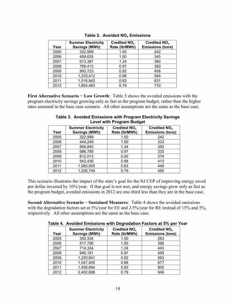
Table 2. Avoided NOx Emissions

Year Summer Electricity

Savings (MWh) Credited NOx Rate (lb/MWh)

Credited NOx Emissions (tons)

2005 322,999 1.50 242 2006 459,635 1.50 345 2007 613,387 1.24 380 2008 789,413 0.97 383 2009 993,723 0.92 458 2010 1,233,412 0.88 540 2011 1,516,942 0.83 631 2012 1,854,483 0.79 733

First Alternative Scenario − Low Growth: Table 3 shows the avoided emissions with the program electricity savings growing only as fast as the program budget, rather than the higher rates assumed in the base case scenario. All other assumptions are the same as the base case.

Table 3. Avoided Emissions with Program Electricity Savings Level with Program Budget

Year Summer Electricity

Savings (MWh) Credited NOx Rate (lb/MWh)

Credited NOx Emissions (tons)

2005 322,999 1.50 242 2006 444,249 1.50 333 2007 564,845 1.24 350 2008 686,788 0.97 333 2009 812,013 0.92 374 2010 942,436 0.88 413 2011 1,080,005 0.83 449 2012 1,226,749 0.79 485

This scenario illustrates the impact of the state’s goal for the NJ CEP of improving energy saved per dollar invested by 10%/year. If that goal is not met, and energy savings grow only as fast as the program budget, avoided emissions in 2012 are one-third less than they are in the base case. Second Alternative Scenario − Sustained Measures: Table 4 shows the avoided emissions with the degradation factors set at 5%/year for EE and 2.5%/year for RE instead of 15% and 5%, respectively. All other assumptions are the same as the base case.

Table 4. Avoided Emissions with Degradation Factors at 5% per Year

Year Summer Electricity

Savings (MWh) Credited NOx Rate (lb/MWh)

Credited NOx Emissions (tons)

2005 350,334 1.50 263 2006 517,790 1.50 388 2007 714,334 1.24 443 2008 946,181 0.97 459 2009 1,220,841 0.92 563 2010 1,547,405 0.88 677 2011 1,936,894 0.83 805 2012 2,402,698 0.79 949

14

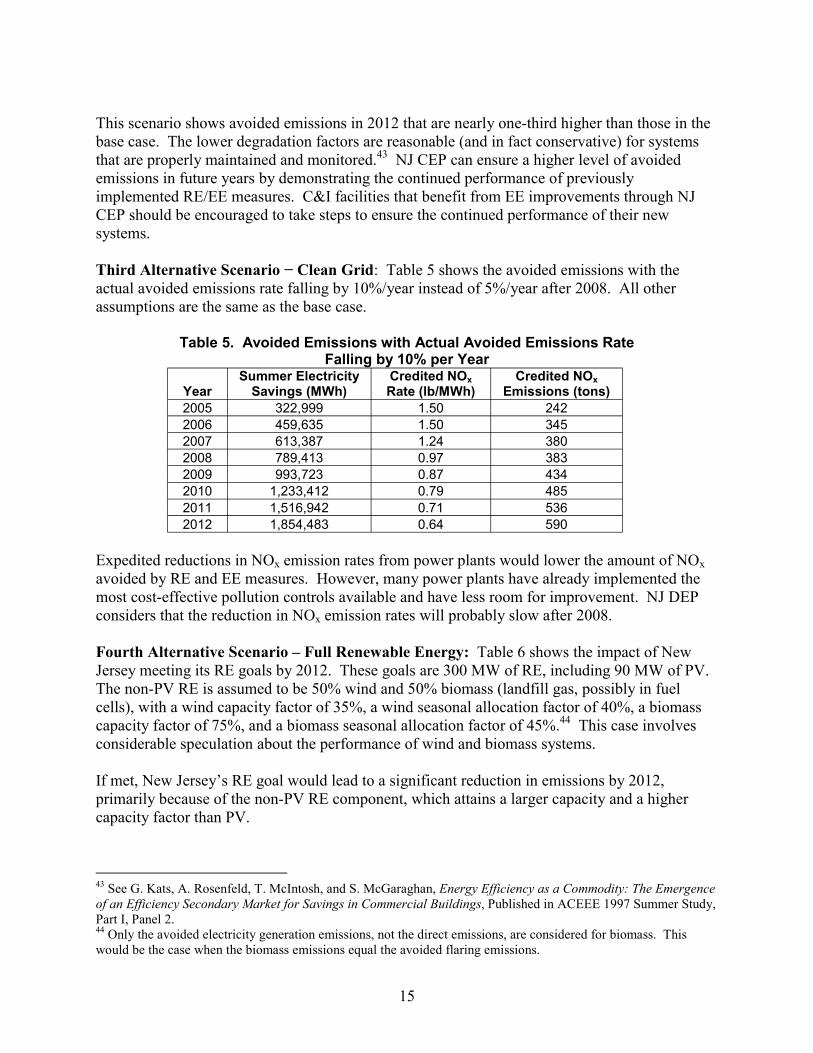
This scenario shows avoided emissions in 2012 that are nearly one-third higher than those in the base case. The lower degradation factors are reasonable (and in fact conservative) for systems that are properly maintained and monitored.43 NJ CEP can ensure a higher level of avoided emissions in future years by demonstrating the continued performance of previously implemented RE/EE measures. C&I facilities that benefit from EE improvements through NJ CEP should be encouraged to take steps to ensure the continued performance of their new systems. Third Alternative Scenario − Clean Grid: Table 5 shows the avoided emissions with the actual avoided emissions rate falling by 10%/year instead of 5%/year after 2008. All other assumptions are the same as the base case.

Table 5. Avoided Emissions with Actual Avoided Emissions Rate Falling by 10% per Year

Year Summer Electricity

Savings (MWh) Credited NOx Rate (lb/MWh)

Credited NOx Emissions (tons)

2005 322,999 1.50 242 2006 459,635 1.50 345 2007 613,387 1.24 380 2008 789,413 0.97 383 2009 993,723 0.87 434 2010 1,233,412 0.79 485 2011 1,516,942 0.71 536 2012 1,854,483 0.64 590

Expedited reductions in NOx emission rates from power plants would lower the amount of NOx avoided by RE and EE measures. However, many power plants have already implemented the most cost-effective pollution controls available and have less room for improvement. NJ DEP considers that the reduction in NOx emission rates will probably slow after 2008. Fourth Alternative Scenario – Full Renewable Energy: Table 6 shows the impact of New Jersey meeting its RE goals by 2012. These goals are 300 MW of RE, including 90 MW of PV. The non-PV RE is assumed to be 50% wind and 50% biomass (landfill gas, possibly in fuel cells), with a wind capacity factor of 35%, a wind seasonal allocation factor of 40%, a biomass capacity factor of 75%, and a biomass seasonal allocation factor of 45%.44 This case involves considerable speculation about the performance of wind and biomass systems. If met, New Jersey’s RE goal would lead to a significant reduction in emissions by 2012, primarily because of the non-PV RE component, which attains a larger capacity and a higher capacity factor than PV.

43 See G. Kats, A. Rosenfeld, T. McIntosh, and S. McGaraghan, Energy Efficiency as a Commodity: The Emergence of an Efficiency Secondary Market for Savings in Commercial Buildings, Published in ACEEE 1997 Summer Study, Part I, Panel 2. 44 Only the avoided electricity generation emissions, not the direct emissions, are considered for biomass. This would be the case when the biomass emissions equal the avoided flaring emissions.

15

Table 6. Impact of New Jersey Meeting Its Renewable Goals by 2012

Year Summer Electricity

Savings (MWh) Credited NOx Rate (lb/MWh)

Credited NOx Emissions (tons)

2005 322,999 1.50 242 2006 477,500 1.50 358 2007 655,576 1.24 406 2008 865,085 0.97 420 2009 1,115,850 0.92 514 2010 1,420,342 0.88 622 2011 1,794,610 0.83 746 2012 2,259,530 0.79 893

Figure 2 shows the NOx emission reductions achieved by each component of the NJ CEP: EE, PV systems, and other RE.

Credited NOx Reductions with 300 MW RE by 2012

0

100

200

300

400

500

600

700

800

900

1000

2003 2004 2005 2006 2007 2008 2009 2010 2011 2012Year

Tons

of N

Ox

EE Wind/Biomass PV

Figure 2. Credited NOx Reductions with 300 MW RE by 2012

Summary of Scenarios: Varying each of these assumptions leads to markedly different results. The projection of the avoided NOx emissions rate under each alternative assumption is particularly important. Because of these differences, NJ DEP should consider an analysis of the projected summer season NOx rate of dispatchable fossil fuel electric generation facilities. Also, demonstrating the sustained performance of previously implemented EERE measures and continued improvements in the cost effectiveness of the NJ CEP will be important. Figure 3 illustrates NOx credited to NJ CEP:

16

Figure 3. NOx Credited to NJ CEP

NOx Credited to NJ Clean Energy Program

0

100

200

300

400

500

600

700

800

900

1000

2005 2006 2007 2008 2009 2010 2011 2012Year

Tons

of N

Ox

Base Case Low Growth Sustained MeasuresIncentive Reserve Cap Full RE Clean Grid

A rapid decrease in the avoided NOx rate causes avoided emissions to level off or decline slightly from 2007 to 2008. In most scenarios, avoided emissions consistently approach or exceed 400 tons/year, and in some cases, they double that level. When non-BPU claimants to allowances are included,45 the current Incentive Allowance Reserve of 410 tons is likely to be oversubscribed in most years of the program.46 One possible option available to NJ DEP is to transfer unused allowances from the Growth/New Source Reserve to the Incentive Allowance Reserve.47 NJ DEP has indicated that the Growth/New Source Reserve is unlikely to be fully utilized.

45 The DEP issued 47 incentive allowances to private parties in 2004. 46 The limit of 410 tons per season is set forth in New Jersey Administrative Code, Title 7, Chapter 27, Subchapter 31.7, Part(d)ii. See www.state.nj.us/dep/aqm/Sub31v2004-04-05.htm. 47 The New Jersey NOx budget regulations allocate 820 allowances into this reserve from 2004 to 2008. NJAC 7:27-31.7(d)(1). New Jersey has not yet issued regulations to implement the EPA’s CAIR, and New Jersey’s CAIR rule will determine the size of any new source allocations for 2009 and thereafter.

17

4.0 Policy Issues 4.1 Interface between State Implementation Planning Process and State

Cap-and-Trade Regulations

One of the major challenges of this pilot project was to develop an approach to ensure that RE and EE programs result in real reductions in emissions of NOx, a pollutant that is subject to emissions trading (cap-and-trade) regulations in New Jersey and most eastern states. The SIP process under CAA Section 110 is the mechanism to account for emission reductions.48 Under EPA’s 2004 guidance, states can receive emission reduction credit in their SIPs for RE and EE measures that reduce NOx emissions and help achieve the 8-hour ozone health standard, under specified circumstances.49 Currently, states in the eastern United States have caps on NOx emissions from electric generating units (EGUs) through regulations that implement EPA’s NOx SIP Call. Beginning in 2009, these caps in 28 states and the District of Columbia will be governed by new regulations that are being developed by the states that implement EPA’s new CAIR.50 As a result, credit for RE and EE projects must be provided in a way that avoids double counting. According to EPA’s Guidance, the states will need to ensure that the emissions trading cap for NOx and the number of allowances allocated to fossil-fuel generators are reduced commensurate with the level of emission reductions that result from EERE projects and programs. This can be accomplished in one of two ways:

• Baseline Approach − Incorporates the estimated effect that the RE and EE programs have on emissions within the projected emissions inventory baseline and provides a corresponding decrease in the emissions cap. This decrease in the emissions cap to account for the RE and EE programs can be accomplished by issuing CAIR regulations that adjust the EPA-established state cap at the outset through an attainment reserve, public health reserve, or similar mechanism.

• Control Measures Approach − Incorporates emission reductions from individual

control measures such as a regional wind purchase or solar programs in schools (or as part of a voluntary bundle of control measures), and provides a corresponding decrease in the emissions cap. The decrease in the cap can be accomplished by retiring allowances that have been allocated to RE and EE projects through a set-aside or output-based regulations issued under the state’s NOx budget or CAIR regulations.

According to guidance issued by EPA in August 2004, both approaches are acceptable.51 Of course, under any approach, the state’s SIP will require approval by the relevant EPA Regional Office (Region II with respect to New Jersey).

48 42 U.S.C. 7410 (2005). 49 EPA SIP Guidance. 50 70 Fed. Reg. 25162 (May 12, 2005). 51 EPA SIP Guidance, pp. 13–14.

18

In other words, to achieve SIP credit under either approach, the state must either omit a certain fraction of allowances from distribution (thereby lowering the NOx emissions cap at the outset) or require the retirement of any such allowances allocated to EERE owners and operators. Otherwise, the emissions would be allowed within the trading program and could be double counted.52 The justification for EPA’s approach is that EERE activities are unlikely to result in emission reductions of a capped pollutant, particularly in the near term, unless the state lowers the cap directly or retires allowances (the authorization to emit a ton of NOx) to account for the reduction in demand from fossil fuel generators caused by the EERE measures. According to EPA, the cap-and-trade program allows the same emissions from fossil fuel-fired generation, no matter how much generation these sources are called upon to meet demand. EPA is concerned that fossil fuel generators are likely to take the allowances made available when coal, natural gas, or oil generation is displaced by RE and EE measures and either use such allowances or sell them to other generators. This results in the continued emissions of NOx at the capped amount and the failure to provide surplus emission reductions. As EPA states in its Guidance:

Cap and trade programs are enforced through the issuance of a limited number of allowances (authorizations to emit) that are equal to the emissions cap. Through trading and banking of these allowances, individual sources can vary their emissions as long as the aggregate emissions for all sources do not exceed the allowances issued. By limiting total mass emissions for the category of sources, cap and trade programs automatically account for any action that reduces emissions, including energy efficiency and renewable energy.53

Under the base case scenario for the NJ CEP, NJ DEP could lower the NOx emissions cap by 520 allowances on average for the summer ozone season from 2007 through 2012, which is equivalent to an average emission reduction of 3.4 tons of NOx per summer day. Because NJ CEP will increase the market for RE and EE and the integration pilot will raise the visibility of the Incentive Allowance Reserve, private parties will probably claim additional allowances.

4.2 Claims for New Jersey Incentive Allowances

Under its current emissions trading regulations, New Jersey has included a set-aside of NOx allowances for certain RE and EE activities.54 This is called the “incentive allowance” pool and

52 Id., p. 18. 53 Id. p. 9. 54 Under the incentive allowance regulations, the following two categories of entities are specifically listed as eligible to submit an annual claim for allowances: (1) New Jersey electricity consumers who reduce electricity consumption by implementing an EE measure initiated in 1992 or thereafter (subject to certain additional conditions); and (2) owners and operators of equipment that commenced operation after 1992 that generates electricity through certain environmentally beneficial techniques defined as generation by burning of landfill gas or digester gas, fuel cell, solar energy or wind power, or equipment that generates electricity by another environmentally beneficial technique approved by the DEP. N.J. 7:27-31.8.

19

is distributed at the rate of 1.5 lb/MWh with a current cap of 410 allowances.55 If the incentive allowance pool is oversubscribed, these allowances are distributed pro-rata.56 Under current NOx budget regulations, unused allowances can be transferred from the Growth/New Source Reserve, thereby increasing the number of incentive allowances distributed. However, the adequacy of the post-2008 allowances for RE and EE will depend on the specifics of the NJ CAIR regulations, which have not yet been issued.

The regulations do not directly authorize the issuance of allowances to an entity that aggregates allowances on behalf of energy-saving electric consumers or owners or operators of environmentally beneficial techniques. However, the regulatory history of the regulation, contained in the NOx Budget Rule Adoption Document (government response to comment 123), indicates that “the rules adopted herein do not preclude the submittal of a claim on behalf of the owner or operator of [a] project eligible for submitting a claim. Neither do the rules preclude aggregating several different projects into a single claim.” In addition, a precedent has been established for the award of allowances from the incentive reserve to an energy services company named SYCOM on behalf of its clients who contracted for EE projects.

4.3 Developing SIP Control Measures that Meet EPA Requirements

If a state proceeds with a SIP to seek approval of individual control measures for RE and EE, it will need to demonstrate to EPA that its emission reductions will be surplus, quantifiable, enforceable, and permanent.57

4.3.1 Surplus Requirement

EPA notes in its SIP Guidance that “the surplus requirement is especially important in areas subject to a cap and trade program.”58 However, the Guidance emphasizes that:

One acceptable way of achieving additional emission reductions from energy efficiency and renewable energy measures in the presence of a cap and trade program is through the retirement of allowances commensurate to the emissions expected to be reduced by the energy efficiency measures. The retirement of allowances provides some level of assurance that the energy efficiency measures will achieve emission reductions that are surplus to the emission reductions under the cap and trade program.59 (emphasis added)

As a result of this guidance, NJ BPU and DEP have worked together under this pilot project to plan an approach for retiring allowances that are obtained by BPU under the incentive allowance program. This should provide a key element to help meet the surplus requirement. In addition, if emission reductions from RE and other measures are included in individual control measures, they cannot be included in the baseline emissions inventory for a SIP to meet the 8-hour ozone standard. This element is crucial to ensure that emission reductions are not double counted and that they are surplus and have not been otherwise relied on to meet air quality attainment requirements.

55 N.J.A.C. 7:27–31.7(e).1. In 2004, applicants claimed 47 of the 410 incentive allowances (NJ DEP). 56 N.J.A.C. 7:27–31.7(e)3.iv. 57 EPA SIP Guidance, pp. 4–7. 58 Id., p. 5. 59 Id., p. 10.

20

4.3.2 Quantifiable Requirement

Another key component of EPA’s regulations and SIP Credit Guidance is a demonstration that the NOx emission reductions that result from the NJ CEP are quantifiable. During the course of the pilot project, EPA officials advised informally that this test might be simplified because of the stipulation of the New Jersey regulations that fossil fuel emissions are displaced by RE and EE at a rate of 1.5 lb/MWh. EPA officials have indicated that some basic analysis should be conducted to demonstrate that the avoided emissions associated with the displaced fossil fuel generation are no less than the presumed rate of 1.5 lb/MWh. The project team evaluated several methodologies to support the quantifiable requirement and to demonstrate that the avoided emissions were in fact greater than 1.5 lb/MWh. The team determined that the best methodology available for the purposes of the pilot project was to estimate the generation-weighted average NOx rate of New Jersey fossil fuel plants. This methodology would provide a reasonable approximation of the marginal emissions rate without the time and expense of a complete grid system dispatch analysis. The analysis included only facilities that were fossil fuel powered for their primary source of input energy, including those that burn coal, natural gas, and petroleum fuels. Under this generation-weighted approach, the estimated avoided emissions are driven by facilities that contribute the most generation to the system. Initially the primary data source for this methodology was EPA’s eGRID database 2002, which was last updated with emission rates from 2000.60 However, the mix of fossil fuel generating facilities in New Jersey has changed significantly since 2000. As a result, the project team used more recent estimates, provided by NJ DEP, of NOx emission rates for 2003 to 2008.61 These rates represent the generation-weighted average of NOx budget units in the state; they include all fossil fuel generating plants with a capacity greater than 15 MW. These and other methodologies are discussed in greater detail in Appendix 4. Under the New Jersey regulations, RE generation uses the same 1.5 lb/MWh rate for avoided NOx emissions as EE. This rate is fully applicable for zero-emission renewable sources such as solar electric generation.62

4.3.3 Enforceabity Requirement

If a state pursues SIP credit for RE and EE projects as individual control measures, it must also meet the enforceability test under EPA’s voluntary measures policy.63 RE and EE measures

60 The project team initially relied on data from the U.S. Energy Information Administration and EPA (the Emissions & Generation Integrated Database or eGRID). 61 Tom McNevin, Bureau Air Quality Planning, NJ DEP, personal communication, September 2005. 62 In comparison, certain RE sources such as landfill gas systems not only produce electricity but also produce some NOx emissions of their own and reduce emissions that would be produced by the alternative disposal of that landfill gas (typically flaring). In such cases, the net avoided emissions—the emissions produced by the landfill gas engine minus the sum of 1.5 lb/MWh (for the avoided generation of fossil fuel-fired electricity and the emissions that would be produced from flaring the landfill gas) must be calculated. 63 See EPA’s, “Incorporating Voluntary and Emerging Measures in a SIP,” September 2004 for the voluntary measures policy. Such EERE measures would need to meet all applicable requirements of the voluntary measures policy (hereinafter cited as Voluntary and Emerging Measures Policy). See www.epa.gov/ttn/oarpg/tl/pgm.html.

21

typically result in emission reductions at fossil fuel generating plants located some distance from the RE or EE activities. Although such measures are not enforceable against the direct emitting sources, they are enforceable against the entities such as state and local governments that undertake such activities.64 If a SIP revision is approved under the voluntary measures policy, a state is responsible to ensure that the reductions credited in the SIP are made. The state would need to make an enforceable SIP commitment to monitor, assess, and report on the emission reductions that result from the voluntary measure, and remedy any shortfalls from forecasted emission reductions in a timely manner. For voluntary and emerging measures that cover stationary sources, a presumptive limit of 6% of the total reductions is needed to meet any requirements related to attainment or maintenance of the air quality standards or reasonable further progress or rate of progress, as described in the policy.65 A separate limit of 3% applies to voluntary mobile source programs. Thus, there is a presumptive 9% limit on the inclusion of voluntary and emerging measures in a SIP, although a state may seek case-by-case EPA approval of a higher limit.66 Recently, EPA issued a new guidance document on incorporating bundled measures in a SIP,67 which should facilitate efforts by states to meet the enforceability requirement with voluntary SIP control measures. As stated in EPA’s transmittal memorandum to regional air directors:

The guidance supports the development of additional emissions reductions from innovative approaches by describing how States can identify individual voluntary and emerging measures and “bundle” them into a single SIP submission. The emissions reductions for each measure in the bundle would be quantified and, after applying an appropriate discount factor for uncertainty, the total reductions would be summed together in the SIP submission. After SIP approval, each individual measure would be implemented according to its schedule in the SIP. It is the performance of the entire bundle (the sum of emissions reductions from all the measures in the bundle) that is considered for SIP evaluation purposes, not the effectiveness of any individual measure.

In other words, by grouping a set of voluntary control measures into a bundle, the state minimizes the chance that it will experience a shortfall later when the effectiveness of the measures is evaluated. By averaging the contribution of multiple measures, overperformance of some measures will likely compensate for underperformance of others.

64 See EPA SIP Guidance, pp. 5–7. 65 Ibid. 66 EPA,Voluntary and Emerging Measures Policy, p. 9. 67 Memorandum from Stephen D. Page, director, Office of Air Quality Planning and Standards, EPA, and Margo Tsirigotis Oge, director, Office of Transportation and Air Quality, EPA, to Air Division Directors, “Guidance on Incorporating Bundled Measures in a State Implementation Plan,” August 16, 2005. See www.epa.gov/ttn/oarpg/t1pgm.html.

22

4.3.4 Permanence Requirement

EPA’s SIP Guidance requires that a control measure “should be permanent throughout the term for which the credit is granted unless it is replaced by another measure or the State demonstrates in a SIP revision that the emission reductions from the measure are no longer needed to meet applicable requirements.” The guidance emphasizes that the emission reductions will qualify as meeting the permanence test even if the emission reductions change over time or vary from season to season.68 Thus, NOx emission reductions that result from the BPU’s CEP will satisfy the permanence test even if the reductions from efficiency measures decline over time or the RE generation varies from one season to another. However, New Jersey will need to ensure that the estimated emission reductions are delivered. One way states have sought to address the fact that the impact of emission reductions from RE and EE measures is often variable during the term of the SIP is through the bundled measures approach addressed earlier. Maryland incorporated this creative approach in its SIP revision to meet the 1-hour ozone standard,69 and this example was showcased by EPA at its 2004 Air Innovations Conference.70

4.4 The Purpose and Uses of Allowances

The initial purpose of the New Jersey incentive allowance for EE and EE (and similar NOx allowance set-asides adopted by six other states)71 was to provide a financial incentive to entities that adopt such pollution prevention projects. Thus, issuance of such allowances to RE and EE developers was designed to offset the cost of installing such projects and spur increased use. In the past few years, state officials have recognized that the reduction of the NOx emissions cap (either through a direct reduction at the outset or by retiring NOx allowances) is a prerequisite to SIP credit in a state with a NOx cap-and-trade program. As stated previously,72 RE and EE activities are unlikely to result in emission reductions of a capped pollutant unless the state lowers the EPA-established cap directly or retires allowances to account for the reduction in demand from fossil fuel generators that results from the RE and EE measures. During the pilot project, participants discussed their interest in ensuring that two goals—spurring increased EERE development and achieving improved air quality—could be accomplished. For example, an approach that balances both goals might allow applicants for NOx allowances to either sell or retire such allowances.

68 EPA SIP Guidance, p. 7. 69 See 70 Fed. Reg. 24987 (May 12, 2005) for final EPA approval of the voluntary bundle and www.mwcog.org/committee/committee/archives.asp?COMMITTEE_ID=14 (February 19, 2004) for the detailed SIP revisions, Chapter 7, pp. 77−-81 and Appendix J, J-71-76. 70 www.epa.gov/ttnmain1/airinnovations/aiconf.2004.html Presentation by Brian Hug, Maryland Department of Environmental Protection. 71 These states are Maryland, New York, Massachusetts, Indiana, Ohio, and Missouri. 72 See p. 18, infra.

23

A recent presentation by Kevin Rackstraw of Clipper Wind Energy has underscored the monetary value in the Renewable Energy Credit (REC) market of NOx allowances awarded to RE generators under a well-structured allowance allocation program.73 According to Mr. Rackstraw, this monetary value accrues in the REC market with the retirement of NOx allowances, and can greatly enhance financing opportunities.74

73 It is important to recognize the difference between the RECs and emission trading markets that involve NOx allowances. In essence, RECs and allowances are two separate trading currencies. However, energy marketers have begun to recognize that the value of a REC can be increased if the REC is sold in conjunction with an allowance that can be retired because this REC will then ensure emission reduction of the capped pollutant. 74 See the Web site of the American Wind Energy Association for a copy of this presentation. www.awea.org/seminars/past_events.html.

24

5.0 Analytical Issues 5.1 Energy Efficiency

During this project, the team worked to resolve analytical challenges in a number of areas. These challenges included estimating the electricity savings, the summer season electricity savings, and the emission reductions. In many cases, the reporting mechanisms established by the NJ CEP resolved important issues. In other cases, experts from NJ BPU and NJ DEP were able to clarify key points. However, the project team sometimes had to refine and expand the methodologies. One of the major challenges was the estimation of summer season energy savings. This factor is essential because the current ozone regulations focus on NOx emissions during the summer ozone season.75

The seasonal allocation factors applied by the Clean Energy Protocols form a sound methodological tool and were applied by the project team, where available. The NJ CEP seasonal factors generally agree with the findings of other analyses, such as the OTC Emission Reduction Workbook. These allocation factors are particularly appropriate for consumer products and appliances such as light bulbs and clothes washers. However, NJ CEP could not provide data on seasonal load profiles for every category of energy-saving measure considered by the project team. For example, the Clean Energy Protocols include “custom measures” as a catch-all category that encompasses any type of measure not detailed elsewhere. In such cases, the Clean Energy Protocols allocate savings evenly across the year. This specific set of seasonal allocation factors is acceptable but not preferable.76 NJ CEP recognizes this limitation, noting that “[t]hese allocations may change [when] actual penetration numbers are available.”77

In addition, the annual and quarterly reports currently prepared by the NJ CEP do not provide sufficient detail on C&I EE improvements that are necessary to estimate summer season energy savings. The reports provide aggregated data on C&I electricity savings combined with information on the number, but not the size of electricity savings or of specific measures such as motors, chillers, or lighting controls. Unfortunately, many types of C&I measures have significantly different seasonal load profiles that have result in varying summer season electricity savings. In this situation, the project team employed the OTC Workbook seasonal allocation factors specified for “Commercial Comprehensive New Construction Design.” This approach was selected because this category includes a range of efficiency measures. Based on this factor, we

75 EPA’s new regulations under CAIR, issued in May 2005, focus on both summer season and annual NOx emissions. 70 Fed. Reg. 25162. 76 Because electricity use for most loads is either summer peaking (as for HVAC) or equal year-round (as for office computers), assuming equal year-round energy savings is unlikely to overstate summer energy savings. 77 Protocols to Measure Resource Savings, Appendix 3, p. 27.

25

assumed that 43% of C&I energy savings occurred during the summer season. For some types of commercial measures, such as the 364 high-efficiency electrical chillers and heating, ventilation, and air-conditioning (HVAC) systems installed in 2004, summer season savings are expected to be much higher. For other types of commercial measures, such as the 358 motors installed, summer season savings could be slightly lower (the OTC Workbook suggests that industrial motors achieve 39% of their savings in the summer season). NJ CEP has access to data on C&I energy savings by type of measure through the utilities. 78 In future years, the program will have the data readily available. NJ CEP could conduct an analysis to determine whether the project team’s estimated allocation factors are reasonable. A significant overrepresentation or underrepresentation of measures with high seasonal variability, such as HVAC systems, could lead to revisions of the projected emission reductions. Another area of uncertainty that the project team confronted was the definition of HVAC.” NJ CEP provided data on the number of units that were categorized as central air-conditioning or heat pumps, as well as the annual electricity savings that result from HVAC as a whole. However, NJ CEP did not provide the project team with information in its database on the relative size of these units, or on the summer season electricity savings for the heat pumps. These data are important because some heat pumps save electricity during the winter. In an effort to address these information gaps, the project team applied the following assumptions:

• Each measure saved the same amount of energy per unit, so the fraction of electricity savings attributable to central air conditioning was the same as the fraction of units that were central air conditioners.79

• Half the heat pumps were air-source and half were ground-source (affects peak versus off-peak calculations).

• Each heat pump achieved half of its annual electricity savings in the summer.

Our analysis is not significantly affected by these assumptions because the number of central air conditioners was 50 times greater than the number of heat pumps. Another analytical challenge arose because the New Jersey protocols did not specify how to allocate electricity savings by season for Energy Star homes in the Residential New Construction program. We applied the allocation factors specified under the Comfort Partners Low Income Customers program because that program also focuses on whole-home energy efficiency

78 In this and other instances, NJ CEP had access to more extensive data but could not provide the data to the project team because of confidentiality concerns. With appropriate confidentiality agreements, such information might be used in a future analysis. 79 In 2004, there were 16,986 CAC units and 339 heat pumps, saving 15,499 MWh of electricity. If electricity savings are proportional to the number of units, CAC savings are 15,196 MWh and heat pump savings are 303 MWh. Information on the capacity of units installed was not available; a directional bias, such as heat pumps tending to have larger capacity than CAC units, would produce slightly different results.

26

improvement.80 For Energy Star homes, employing energy modeling software to generate an estimate of summer and annual electricity savings would be preferable and not burdensome. New School Construction & Retrofit was another area of interest that lacked data. Some schools could be closed during most of the summer season and thus be a marginal source of summer season electricity savings. However, we were informed that many schools in New Jersey, particularly new schools or those that were renovated during the program, would continue to be used during the summer for a variety of programs. We therefore assessed schools according to the OTC Workbook factor for Commercial Comprehensive New Construction Design. The project team also identified analytical challenges that will need to be addressed with respect to combined heat and power (CHP) projects. At the time of our review, no CHP systems had been installed under the NJ CEP, but several had been approved for funding. When New Jersey officials begin to evaluate potential NOx emission reductions from CHP, they will need to address the following issues:

• CHP projects usually result in some additional emissions of NOx, which have to be measured or calculated, to determine the net emission reductions.

• The energy savings are variable, depending on season and the allocation of the energy savings between electricity and process heat.

We recommend that New Jersey officials develop a data collection and analysis protocol to facilitate analysis of the CHP technology.

5.2 Degradation Factor

The Clean Energy Protocols include assumed system lifetimes. In many cases, New Jersey officials have accounted for system degradation by shortening the estimated system lifetimes or adjusting the deemed energy savings. We recommend using an annual degradation factor rather than fixed lifetimes to better reflect degradation in the near term. An annual degradation factor also helps to account for the fact that some equipment is removed before the end of its useful life. Commercial buildings may be renovated, or new tenants may override the high-efficiency lighting or HVAC controls.

5.3 Renewable Energy

The RE analysis encountered numerous challenges, including limitations on available data and the need to supplement the New Jersey data with additional data sources. In analyzing solar electric generation, the project team supplemented the data provided by NJ CEP with a model developed by NREL to estimate electricity generation from the solar PV systems. Since no metered data were readily available to us for any of the solar generation funded under the CORE

80 This factor allocates the electricity savings as follows: summer/on-peak 21%; summer/off-peak 22%; winter/on-peak 28%; and winter/off-peak 29%. Because electricity consumption in New Jersey peaks during the summer season, and because the summer season (May−September) takes up 42% of the year, we consider it conservative to allocate 43% of the energy savings to the summer period.

27

program, the project team employed the PVWATTS Version 2 Tool to meet this need.81 The PVWATTS calculation was based on typical solar radiation from a location in south-central New Jersey. Other locations were examined as well: the highest resource location in the state showed summer generation as 4% higher; the lowest resource location showed summer generation as 4% lower. NJ CEP collects data through a sampling process of PV systems that are 10 kW or larger for SREC trading. The program is considering a more active remote-reading approach to encompass a broader range of systems. Comparing the projected summer production from our analysis with the observed summer production from the NJ CEP sampling would be advantageous. The team also employed the PVWATTS default factors to allow for power to be converted from DC to AC. This tool requires information about the direction of orientation and angle of tilt for the PV system considered. NJ CEP requires applicants to provide this information to receive a rebate, and tracks this information in a database. Because there were 344 systems, the project team grouped systems into categories of orientation and inclination to facilitate use of the PV WATTS tool. System orientation and inclination have a greater impact for year-round than for summer generation. NJ CEP data were insufficient to provide a reasonable estimate of electricity generation and NOx emission reductions during the summer ozone season in 2005 from a wind project and two biomass (landfill gas) projects funded by the agency. For the wind project, the location, height, and type of equipment are critical to estimating ozone season generation. Actual records of generation are preferred for making this determination, and were not available to us. The importance of these site-specific protocols will increase as additional wind projects come on line. Estimating the electric generation from landfill gas projects also requires site-specific data, which were not available to the project team. Actual generation is almost always metered, and those data could be made available in the program records. Landfill gas combustion emits significant direct NOx emissions, which must be compared to the emissions that are avoided when flaring is eliminated.82 This comparative analysis could not be performed because the emission rates from the specific combustion systems were not available to the project team. In projecting future emissions from landfill gas, the rate of decline in landfill gas releases from the specific landfills over time need to be forecast. The data available to the project team on the fuel cell projects funded by the NJ CEP were insufficient to estimate the 2005 generation and to determine whether such projects qualified as RE sources. The second problem has been resolved. NJ CEP has indicated that: “After a program modification in early 2004, only sustainably-fueled (landfill gas) fuel cells are eligible for rebates.”83 Generation records and technology-specific data also will be required to estimate generation and net avoided emissions of fuel cell projects.

81 See p. 10 (infra). 82 We understand that private companies have sought allowances for certain landfill gas projects. How they resolved these analytical issues is unclear. 83 New Jersey Clean Energy Programs Report, submitted to the New Jersey Board of Public Utilities, May 6, 2005, p. 30.

28

6.0 Lessons Learned The MARO pilot project provides numerous lessons learned about emissions trading programs that are applicable to other states. These lessons involve issues of regulatory policy as well as methodological approaches. First, the project underscores the importance of the state regulatory framework that governs NOx emissions trading. If state regulations limit the allocation of allowances to only fossil fuel-fired generating units, the state and local government agencies will be precluded, for all practical purposes, from obtaining SIP credit for RE or EE purchases or development. In other words, unless the state’s NOx trading regulations provide a pool of allowances to reward RE and EE development or purchases and provide a mechanism for lowering the total cap of allowances, an important market driver and revenue stream for RE and EE will be lost. State focus on NOx allocation regulations is particularly timely. EPA’s new CAIR requires most states in the ozone transport region to submit to EPA enforceable plans by September 2006 for complying with the CAIR requirements. The new CAIR requirements will replace the state regulations under the NOx SIP Call for electric generating units and will govern NOx allowance allocation in 2009 and thereafter for such units. The pilot project underscored several regulatory options that provide a pool of NOx allowances to encourage EERE measures. These options include:

• Allocate a percentage of NOx allowances into a so-called RE and EE set-aside to encourage RE and EE measures.

• Allocate a percentage of NOx allowance into a so-called attainment/public health reserve.

• Allocate allowances to all sources on an output basis (tons of emissions reduction per MWh) instead of a heat-input basis (used currently in most states and which covers only electric generators that burn fossil fuels).

• Allocate allowances to new sources on an output-basis.84 A recent document prepared by the State and Territorial Air Pollution Program Administrators (STAPPA) and the Association of Local Air Pollution Control Officials (ALAPCO) highlights these options.85 In addition, lessons learned from RE and EE set-aside regulations under the NOx SIP Call are helpful in crafting new CAIR rules for NOx trading. These lessons are highlighted in an EPA draft report titled State Set-Aside Programs for Energy Efficiency and Renewable Energy

84 This approach was adopted by the National Association of State Regulatory Commissioners in a resolution in the summer of 2004. This approach can encompass energy efficiency if a conversion factor is specified in the regulation. 85 “Alternative NOx Allowance Allocation Language for the Clean Air Interstate Rule,” August, 2005. See www.4cleanair.org/Bluestein-cairallocation-final.pdf.

29

Projects Under the NOx Budget Trading Program: A Review of Programs in Indiana, Maryland, Massachusetts, Missouri, New Jersey, New York, and Ohio.86 The pilot project and these two recent reports underscore several important provisions that states should consider including in new CAIR rules that provide allowances to spur EERE. These provisions include:

• Authority for a developer and the state to aggregate small projects in an application for allowance allocation. For example, small solar PV projects alone will not qualify for allowances since such projects result in emission reductions far lower than one ton (the minimum allocation in most states). If project aggregation authority is not provided in the state rules, the RE and EE set-aside will likely be underused.

• Authority for a state energy office that administers incentive programs to apply for

allowances relating to state-funded clean energy projects for owners and operators who have not applied on their own behalf. The state energy office could then retire these allowances to obtain SIP credit.

The pilot project highlights various methodological approaches that can facilitate the implementation of state regulations to reward RE and EE. Other states can benefit from employing some or all of the methodologies developed by the NJ CEP (and refined and expanded by the pilot project) to determine the emission reductions achieved by RE and EE measures. New Jersey’s clean energy protocols and incentive allowance regulations allow NOx emission reductions to be estimated with a relatively small investment.87 States may want to consider the following specific methodological approaches in their CAIR regulations to facilitate the integration of energy and air quality goals:

• Employ protocols with stipulated electricity savings to assess the benefits of specific EE measures and use the New Jersey clean energy protocols as a starting point. Some variables may need to be adjusted, depending on the specific state and region (e.g., the assumed equivalent full load hours of operation of an air-conditioning unit), but the equations included in the protocols appear to be sound and transferable.

86 EPA, Climate Protection Partnerships Division, Office of Atmospheric Programs, Office of Air and Radiation, EPA Document No. 430-R-03-005, September 2005, available at http://www.epa.gov/cleanenergy/pdf/eere_rpt.pdf. 87When using a simplified approach, such as that employed by the pilot project, be conservative in assumptions and default values. States may alternatively follow an approach developed by the Texas Energy Systems Laboratory (in partnership with EPA) that is more detailed and includes more in-depth analysis. This latter approach may result in a greater emission reductions credit but at a much higher cost. This methodology, which identifies county-level emissions impacts of RE/EE measures based on the county in which the measure was implemented, is both possible and necessary in a statewith regions that are not subject to NOx caps. (Emissions & Energy Calculator (eCalc), Energy Systems Laboratory, Texas A&M University. See http://ecalc.tamu.edu/.)

30

• Employ a stipulated avoided emissions rate (lb/MWh) for RE and EE measures that is based on the generation-weighted average NOx emissions rate of the relevant region’s variable dispatch fossil fuel plants.

o The CAIR regulations could require that the state update this stipulated allocation rate periodically to reflect changes in the composition of the fuel mix and control technologies. (This approach would significantly reduce the resources required to analyze specific facilities.)

o In addition, the state’s CAIR regulations could, if adequate evidence is presented, grant the state air agency authority to approve a higher allocation rate than the stipulated amount. (This approach allows parties who are responsible for developing large RE or EE projects to devote greater resources and claim higher actual emissions reductions.)

• Include seasonal allocation factors that define assumed electricity savings for specific

types of measures in state protocols.

• Seek to fulfill the requirements for Energy Star ratings for residential construction and renovation and employ Energy Star energy modeling for home EE improvements. This approach can ascertain the likely effect of a combination of efficiency measures and will help promote the Energy Star brand.

• Determine electricity savings for specific measures by comparison to a typical new

system for that load, and define the reference system in protocols. Determine electricity savings for comprehensive building improvements through energy modeling with an energy code as a reference.

• Examine the state’s emission inventory and SIP and identify any assumptions about RE

and EE that are already in the inventory. If the state intends to rely on RE/EE measures for SIP credit, it must ensure those measures are surplus to those included in the baseline.

31

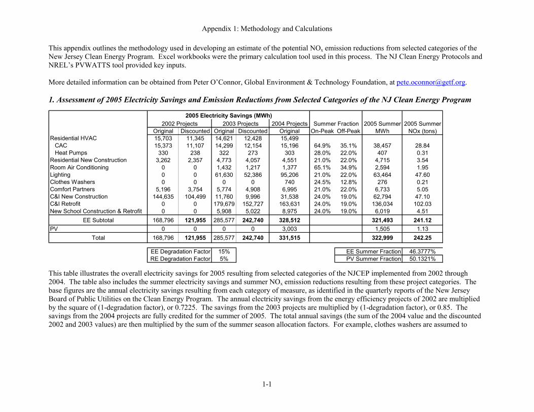
Appendix 1: Methodology and Calculations This appendix outlines the methodology used in developing an estimate of the potential NOx emission reductions from selected categories of the New Jersey Clean Energy Program. Excel workbooks were the primary calculation tool used in this process. The NJ Clean Energy Protocols and NREL’s PVWATTS tool provided key inputs. More detailed information can be obtained from Peter O’Connor, Global Environment & Technology Foundation, at pete.oconnor@getf.org. 1. Assessment of 2005 Electricity Savings and Emission Reductions from Selected Categories of the NJ Clean Energy Program

2004 ProjectsOriginal Discounted Original Discounted Original On-Peak Off-Peak

Residential HVAC 15,703 11,345 14,621 12,428 15,499CAC 15,373 11,107 14,299 12,154 15,196 64.9% 35.1% 38,457 28.84Heat Pumps 330 238 322 273 303 28.0% 22.0% 407 0.31

Residential New Construction 3,262 2,357 4,773 4,057 4,551 21.0% 22.0% 4,715 3.54Room Air Conditioning 0 0 1,432 1,217 1,377 65.1% 34.9% 2,594 1.95Lighting 0 0 61,630 52,386 95,206 21.0% 22.0% 63,464 47.60Clothes Washers 0 0 0 0 740 24.5% 12.8% 276 0.21Comfort Partners 5,196 3,754 5,774 4,908 6,995 21.0% 22.0% 6,733 5.05C&I New Construction 144,635 104,499 11,760 9,996 31,538 24.0% 19.0% 62,794 47.10C&I Retrofit 0 0 179,679 152,727 163,631 24.0% 19.0% 136,034 102.03New School Construction & Retrofit 0 0 5,908 5,022 8,975 24.0% 19.0% 6,019 4.51

EE Subtotal 168,796 121,955 285,577 242,740 328,512 321,493 241.12PV 0 0 0 0 3,003 1,505 1.13

Total 168,796 121,955 285,577 242,740 331,515 322,999 242.25

EE Degradation Factor 15% EE Summer Fraction 46.3777%RE Degradation Factor 5% PV Summer Fraction 50.1321%

2005 Electricity Savings (MWh)Summer Fraction 2005 Summer

MWh2005 Summer

NOx (tons)2002 Projects 2003 Projects

This table illustrates the overall electricity savings for 2005 resulting from selected categories of the NJCEP implemented from 2002 through 2004. The table also includes the summer electricity savings and summer NOx emission reductions resulting from these project categories. The base figures are the annual electricity savings resulting from each category of measure, as identified in the quarterly reports of the New Jersey Board of Public Utilities on the Clean Energy Program. The annual electricity savings from the energy efficiency projects of 2002 are multiplied by the square of (1-degradation factor), or 0.7225. The savings from the 2003 projects are multiplied by (1-degradation factor), or 0.85. The savings from the 2004 projects are fully credited for the summer of 2005. The total annual savings (the sum of the 2004 value and the discounted 2002 and 2003 values) are then multiplied by the sum of the summer season allocation factors. For example, clothes washers are assumed to

1-1

Appendix 1: Methodology and Calculations achieve 24.5%1 of their annual energy savings in the summer peak period and 12.8% of their annual energy savings in the summer off-peak period, for a total of 37.3% of their annual savings in the summer. For PV systems, the discount factors are not applied (all systems are assumed to have been installed in 2004), and the allocation factor is based on the input of specific system characteristics into NREL’s PVWATTS tool. This tool calculates the monthly output of systems based on size, location, and orientation. A flat-roof PV system will generate 56.1% of its annual electricity during the May to September period, whereas a south-facing system at 45° tilt will generate only 45.5% of its annual electricity in that time period (but about 15% more than the flat-roof system over the course of the year). Summer electricity savings were derived on a measure-specific basis, using the allocation factors from the NJ Clean Energy Protocols or using appropriate surrogates (such as the OTC Emission Reduction Workbook or PVWATTS). The combination of energy efficiency measures implemented in 2002 to 2004 have a weighted seasonal allocation factor of 46.38%. This factor is used for energy efficiency measures implemented in future years, as the exact combination of measures to be implemented is not known at this time. The PV systems installed have a weighted seasonal allocation factor of 50.13%, with generation of 1505.455 MWh per summer (May-September) and 3002.979 MWh per year. NOx emission reductions for 2005 are generated using the allowance allocation factor of 1.5 lbs/MWh. See Appendix 4 for our analysis establishing that 2005 emission reductions will likely exceed this value. 2. Projection of Future NOx Emission Reductions and Sensitivity Analysis Step 1: Defining the Scenarios

Base Case EE PVProgram Growth 20% 40%Degradation Factor 15% 5%Grid Improvement 5% 5%

Low Growth EE REProgram Growth 10% 30%Degradation Factor 15% 5%Grid Improvement 5% 5%

Continued Savings EE REProgram Growth 20% 40%Degradation Factor 5% 2.5%Grid Improvement 5% 5%

Full RE EE REProgram Growth 20% 41%Degradation Factor 15% 5%Grid Improvement 5% 5%

Clean Grid EE PVProgram Growth 20% 40%Degradation Factor 15% 5%Grid Improvement 10% 10%

These tables establish the variables for the analysis of future NOx emission reductions. The four scenarios other than the “Base Case” serve to illustrate the sensitivity of the analysis to the various assumptions. “Grid Improvement” refers to decreases in the avoided NOx rate after 2008; rates through 2008 were identified by NJ DEP.

1 We consider our results to be accurate to no more than two significant figures. However, in order to reduce rounding errors, we carry forward up to seven digits in our calculations, only rounding off the final result.

1-2

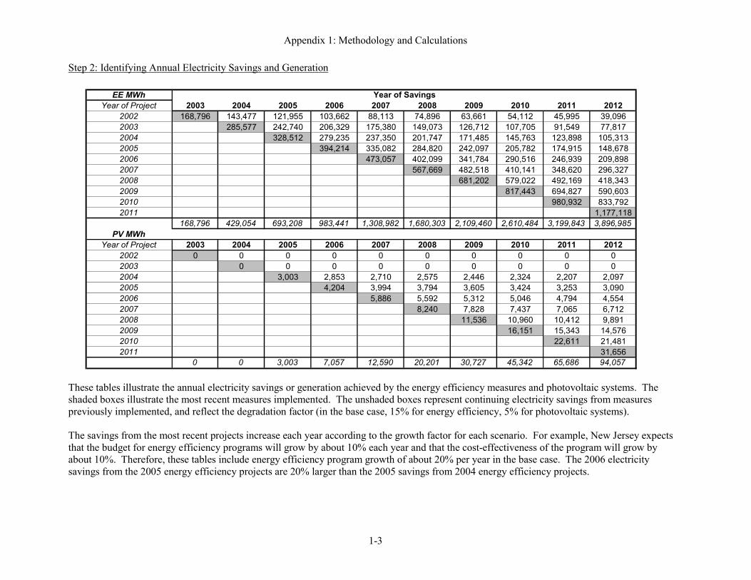
Appendix 1: Methodology and Calculations Step 2: Identifying Annual Electricity Savings and Generation

EE MWhYear of Project 2003 2004 2005 2006 2007 2008 2009 2010 2011 2012

2002 168,796 143,477 121,955 103,662 88,113 74,896 63,661 54,112 45,995 39,0962003 285,577 242,740 206,329 175,380 149,073 126,712 107,705 91,549 77,8172004 328,512 279,235 237,350 201,747 171,485 145,763 123,898 105,3132005 394,214 335,082 284,820 242,097 205,782 174,915 148,6782006 473,057 402,099 341,784 290,516 246,939 209,8982007 567,669 482,518 410,141 348,620 296,3272008 681,202 579,022 492,169 418,3432009 817,443 694,827 590,6032010 980,932 833,7922011 1,177,118

168,796 429,054 693,208 983,441 1,308,982 1,680,303 2,109,460 2,610,484 3,199,843 3,896,985PV MWh

Year of Project 2003 2004 2005 2006 2007 2008 2009 2010 2011 20122002 0 0 0 0 0 0 0 0 0 02003 0 0 0 0 0 0 0 0 02004 3,003 2,853 2,710 2,575 2,446 2,324 2,207 2,0972005 4,204 3,994 3,794 3,605 3,424 3,253 3,0902006 5,886 5,592 5,312 5,046 4,794 4,5542007 8,240 7,828 7,437 7,065 6,7122008 11,536 10,960 10,412 9,8912009 16,151 15,343 14,5762010 22,611 21,4812011 31,656

0 0 3,003 7,057 12,590 20,201 30,727 45,342 65,686 94,057

Year of Savings

These tables illustrate the annual electricity savings or generation achieved by the energy efficiency measures and photovoltaic systems. The shaded boxes illustrate the most recent measures implemented. The unshaded boxes represent continuing electricity savings from measures previously implemented, and reflect the degradation factor (in the base case, 15% for energy efficiency, 5% for photovoltaic systems). The savings from the most recent projects increase each year according to the growth factor for each scenario. For example, New Jersey expects that the budget for energy efficiency programs will grow by about 10% each year and that the cost-effectiveness of the program will grow by about 10%. Therefore, these tables include energy efficiency program growth of about 20% per year in the base case. The 2006 electricity savings from the 2005 energy efficiency projects are 20% larger than the 2005 savings from 2004 energy efficiency projects.

1-3

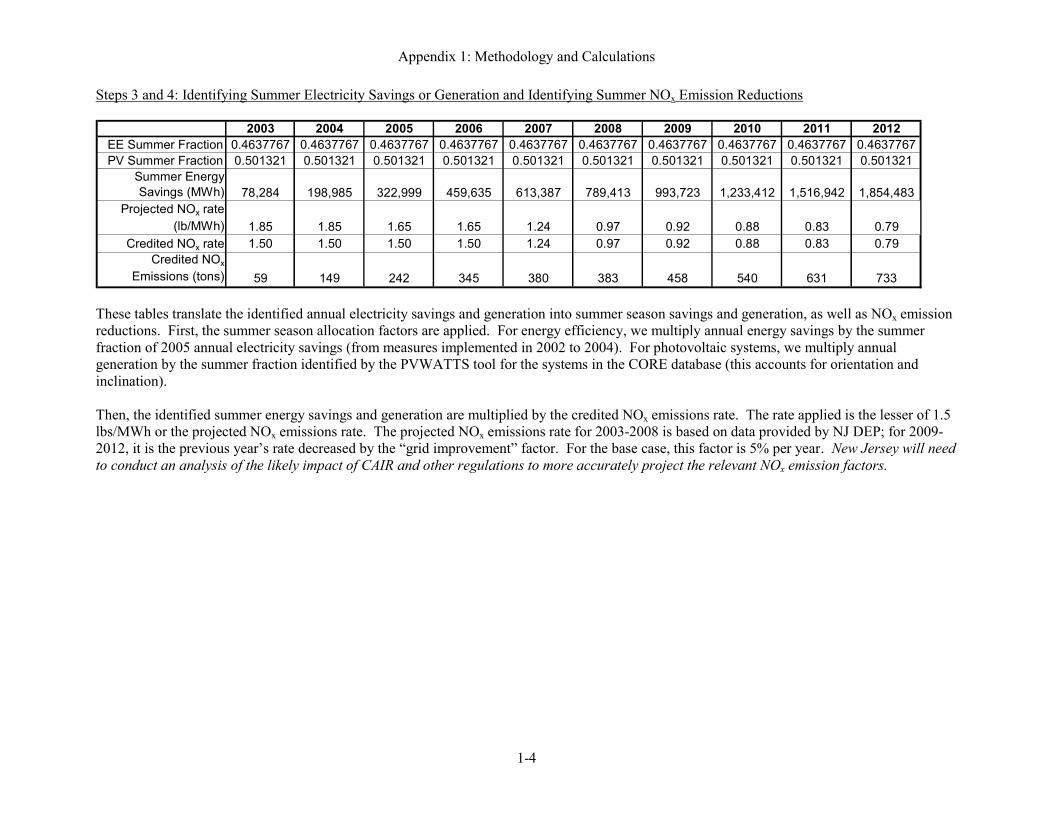
Appendix 1: Methodology and Calculations Steps 3 and 4: Identifying Summer Electricity Savings or Generation and Identifying Summer NOx Emission Reductions

2003 2004 2005 2006 2007 2008 2009 2010 2011 2012EE Summer Fraction 0.4637767 0.4637767 0.4637767 0.4637767 0.4637767 0.4637767 0.4637767 0.4637767 0.4637767 0.4637767PV Summer Fraction 0.501321 0.501321 0.501321 0.501321 0.501321 0.501321 0.501321 0.501321 0.501321 0.501321

Summer Energy Savings (MWh) 78,284 198,985 322,999 459,635 613,387 789,413 993,723 1,233,412 1,516,942 1,854,483

Projected NOx rate (lb/MWh) 1.85 1.85 1.65 1.65 1.24 0.97 0.92 0.88 0.83 0.79

Credited NOx rate 1.50 1.50 1.50 1.50 1.24 0.97 0.92 0.88 0.83 0.79Credited NOx

Emissions (tons) 59 149 242 345 380 383 458 540 631 733

Treductions. First, the summer season allocation factors are applied. For energy efficiency, we multiply annual energy savings by the summer fraction of 2005 annual electricity savings (from measures implemented in 2002 to 2004). For photovoltaic systems, we multiply annual generation by the summer fraction identified by the PVWATTS tool for the systems in the CORE database (this accounts for orientation and inclination). Then, the idenlbs/MWh or the projected NOx emissions rate. The projected NOx emissions rate for 2003-2008 is based on data provided by NJ DEP; for 2009-2012, it is the previous year’s rate decreased by the “grid improvement” factor. For the base case, this factor is 5% per year. New Jersey will need to conduct an analysis of the likely impact of CAIR and other regulations to more accurately project the relevant NOx emission factors.

hese tables translate the identified annual electricity savings and generation into summer season savings and generation, as well as NOx emission

tified summer energy savings and generation are multiplied by the credited NOx emissions rate. The rate applied is the lesser of 1.5

1-4

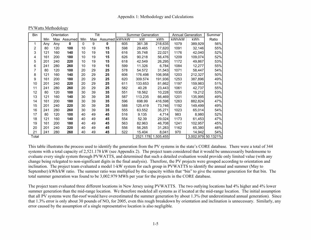
Appendix 1: Methodology and Calculations PVWatts Methodology

BinMin Max Assumed Min Max Assumed kWh/kW kW kWh kWh/kW kWh

1 Any Any 0 0 9 0 605 361.38 218,635 1079 389,929 56%2 80 120 100 10 19 15 598 29.465 17,620 1091 32,146 55%3 121 160 140 10 19 15 616 35.748 22,021 1176 42,040 52%4 161 200 180 10 19 15 626 90.218 56,476 1209 109,074 52%5 201 240 220 10 19 15 618 42.549 26,295 1172 49,867 53%6 241 280 260 10 19 15 599 11.326 6,784 1084 12,277 55%7 80 120 100 20 29 25 578 54.572 31,543 1071 58,447 54%8 121 160 140 20 29 25 606 176.498 106,958 1203 212,327 50%9 161 200 180 20 29 25 620 309.574 191,936 1253 387,896 49%10 201 240 220 20 29 25 611 133.653 81,662 1197 159,983 51%11 241 280 260 20 29 25 582 40.28 23,443 1061 42,737 55%12 80 120 100 30 39 35 551 18.562 10,228 1035 19,212 53%13 121 160 140 30 39 35 587 113.235 66,469 1201 135,995 49%14 161 200 180 30 39 35 596 698.99 416,598 1263 882,824 47%15 201 240 220 30 39 35 588 125.419 73,746 1192 149,499 49%16 241 280 260 30 39 35 555 63.552 35,271 1023 65,014 54%17 80 120 100 40 49 45 516 9.135 4,714 983 8,980 52%18 121 160 140 40 49 45 554 52.39 29,024 1173 61,453 47%19 161 200 180 40 49 45 563 82.963 46,708 1241 102,957 45%20 201 240 220 40 49 45 556 56.265 31,283 1162 65,380 48%21 241 280 260 40 49 45 522 15.404 8,041 970 14,942 54%

Total 2521.178 1,505,455 3,002,979 50.1321%

Summer Ratio

Annual GenerationOrientation Tilt Summer Generation

This table illustrates the process used to identify the generation from the PV systems in the state’s CORE database. There were a total of 344 systems with a total capacity of 2,521.178 kW (see Appendix 2). The project team considered that it would be unnecessarily burdensome to evaluate every single system through PVWATTS, and determined that such a detailed evaluation would provide only limited value (with any change being relegated to non-significant digits in the final analysis). Therefore, the PV projects were grouped according to orientation and inclination. The project team evaluated a model 1-kW system for each group in PVWATTS to identify the annual and summer (May to September) kWh/kW ratio. The summer ratio was multiplied by the capacity within that “bin” to give the summer generation for that bin. The total summer generation was found to be 3,002.979 MWh per year for the projects in the CORE database. The project team evaluated three different locations in New Jersey using PVWATTS. The two outlying locations had 4% higher and 4% lower summer generation than the mid-range location. We therefore modeled all systems as if located at the mid-range location. The initial assumption that all PV systems were flat-roof would have overestimated the summer generation by about 1.3% (but underestimated annual generation). Since that 1.3% error is only about 30 pounds of NOx for 2005, even this rough breakdown by orientation and inclination is unnecessary. Similarly, any error caused by the assumption of a single representative location is also negligible.

1-5

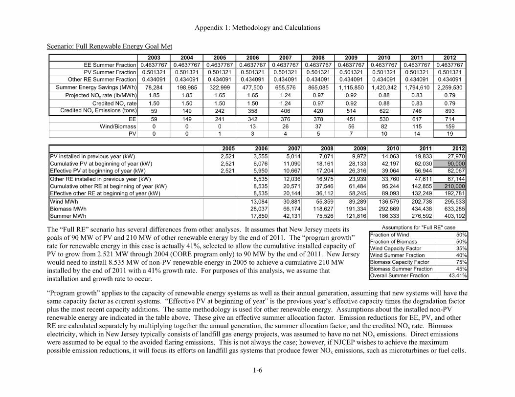
Appendix 1: Methodology and Calculations Scenario: Full Renewable Energy Goal Met

2003 2004 2005 2006 2007 2008 2009 2010 2011 2012EE Summer Fraction 0.4637767 0.4637767 0.4637767 0.4637767 0.4637767 0.4637767 0.4637767 0.4637767 0.4637767 0.4637767PV Summer Fraction 0.501321 0.501321 0.501321 0.501321 0.501321 0.501321 0.501321 0.501321 0.501321 0.501321

Other RE Summer Fraction 0.434091 0.434091 0.434091 0.434091 0.434091 0.434091 0.434091 0.434091 0.434091 0.434091Summer Energy Savings (MWh) 78,284 198,985 322,999 477,500 655,576 865,085 1,115,850 1,420,342 1,794,610 2,259,530

Projected NOx rate (lb/MWh) 1.85 1.85 1.65 1.65 1.24 0.97 0.92 0.88 0.83 0.79Credited NOx rate 1.50 1.50 1.50 1.50 1.24 0.97 0.92 0.88 0.83 0.79

Credited NOx Emissions (tons) 59 149 242 358 406 420 514 622 746 893EE 59 149 241 342 376 378 451 530 617 714

Wind/Biomass 0 0 0 13 26 37 56 82 115 159PV 0 0 1 3 4 5 7 10 14 19

2005 2006 2007 2008 2009 2010 2011 2012PV installed in previous year (kW) 2,521 3,555 5,014 7,071 9,972 14,063 19,833 27,970Cumulative PV at beginning of year (kW) 2,521 6,076 11,090 18,161 28,133 42,197 62,030 90,000Effective PV at beginning of year (kW) 2,521 5,950 10,667 17,204 26,316 39,064 56,944 82,067Other RE installed in previous year (kW) 8,535 12,036 16,975 23,939 33,760 47,611 67,144Cumulative other RE at beginning of year (kW) 8,535 20,571 37,546 61,484 95,244 142,855 210,000Effective other RE at beginning of year (kW) 8,535 20,144 36,112 58,245 89,093 132,249 192,781Wind MWh 13,084 30,881 55,359 89,289 136,579 202,738 295,533Biomass MWh 28,037 66,174 118,627 191,334 292,669 434,438 633,285Summer MWh 17,850 42,131 75,526 121,816 186,333 276,592 403,192

The “Full RE” scenario has several differences from other analyses. It assumes that New Jersey meets its goals of 90 MW of PV and 210 MW of other renewable energy by the end of 2011. The “program growth” rate for renewable energy in this case is actually 41%, selected to allow the cumulative installed capacity of PV to grow from 2.521 MW through 2004 (CORE program only) to 90 MW by the end of 2011. New Jersey would need to install 8.535 MW of non-PV renewable energy in 2005 to achieve a cumulative 210 MW installed by the end of 2011 with a 41% growth rate. For purposes of this analysis, we assume that installation and growth rate to occur.

Fraction of Wind 50%Fraction of Biomass 50%Wind Capacity Factor 35%Wind Summer Fraction 40%Biomass Capacity Factor 75%Biomass Summer Fraction 45%Overall Summer Fraction 43.41%

Assumptions for "Full RE" case

“Program growth” applies to the capacity of renewable energy systems as well as their annual generation, assuming that new systems will have the same capacity factor as current systems. “Effective PV at beginning of year” is the previous year’s effective capacity times the degradation factor plus the most recent capacity additions. The same methodology is used for other renewable energy. Assumptions about the installed non-PV renewable energy are indicated in the table above. These give an effective summer allocation factor. Emission reductions for EE, PV, and other RE are calculated separately by multiplying together the annual generation, the summer allocation factor, and the credited NOx rate. Biomass electricity, which in New Jersey typically consists of landfill gas energy projects, was assumed to have no net NOx emissions. Direct emissions were assumed to be equal to the avoided flaring emissions. This is not always the case; however, if NJCEP wishes to achieve the maximum possible emission reductions, it will focus its efforts on landfill gas systems that produce fewer NOx emissions, such as microturbines or fuel cells.

1-6

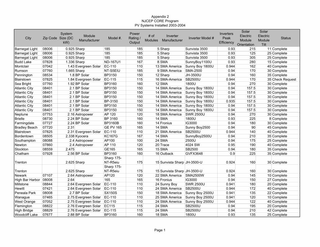
Appendix 2NJCEP CORE Program

PV Systems Installed 2003-2004

City Zip CodeSystem

Size (DC kW)

Module Manufacturer Model #.

Power Rating / Output

# of Modules

Inverter Manufacturer Inverter Model #

Inverters Peak

Efficiency

Solar Electric Module

Orientation

Solar Electric Module

Tilt

Status

Barnegat Light 08006 0.925 Sharp 185 185 5 Sharp Sunvista 3500 0.93 215 11 CompleteBarnegat Light 08006 0.925 Sharp 185 185 5 Sharp Sunvista 3500 0.93 125 25 CompleteBarnegat Light 08006 0.925 Sharp 185 185 5 Sharp Sunvista 3500 0.93 305 25 CompleteBudd Lake 07828 1.336 Sharp ND-167U1 167 8 SMA SunnyBoy1100U 0.93 280 15 CompleteMontclair 07042 1.43 Evergreen Solar EC-110 110 13 SMA America Sunny Boy 1800U 0.944 162 40 CompleteRumson 07760 1.665 Sharp NT-S5EIU 185 9 SMA America SMA-2500 0.94 170 30 CompletePennington 08534 1.8 BP Solar BP3150 150 12 Sharp JH-3500U 0.94 160 35 CompleteBlairstown 07825 1.84 Evergreen Solar EC-115 115 16 SMA-America SB2500U 0.944 170 35 Check RequestSea Bright 07760 1.92 BP Solar BP3160 160 12 SMA 1800U 0.94 270 30 CompleteAtlantic City 08401 2.1 BP Solar BP3150 150 14 SMA America Sunny Boy 1800U 0.94 157.5 30 CompleteAtlantic City 08401 2.1 BP Solar BP3150 150 14 SMA America Sunny Boy 1800U 0.94 157.5 30 CompleteAtlantic City 08401 2.1 BP Solar BP3150 150 14 SMA America Sunny Boy 1800U 0.94 157.5 30 CompleteAtlantic City 08401 2.1 BP Solar BP-3150 150 14 SMA America Sunny Boy 1800U 0.935 157.5 30 CompleteAtlantic City 08401 2.1 BP Solar BP3150 150 14 SMA America Sunny Boy 1800U 0.94 157.5 30 CompleteAtlantic City 08401 2.1 BP Solar BP3150 150 14 SMA America Sunny Boy 1800U 0.94 157.5 30 CompleteNeptune 07753 2.16 Astropower AP 120 120 18 SMA America SWR 2500U 0.94 270 30 CompleteBrielle 08730 2.24 BP Solar BP 3160 160 14 SMA 1800U 0.93 225 8 CompleteFarmingdale 07727 2.24 BP Solar BP3160B 160 14 Fronius IG3000 0.94 180 30 CompleteBradley Beach 07720 2.31 GE PV 165 165 14 SMA Sunny Boy2500 0.94 90 45 CompleteBlairstown 07825 2.31 Evergreen Solar EC-110 110 21 SMA America SB2500U 0.944 140 40 CompleteBordentown 08505 2.338 Kyocera KC167G 167 14 SMA SunnyBoy2500U 0.94 210 35 CompleteSouthampton 08088 2.4 Astropower AP100 100 24 SMA 2500U 0.94 175 25 CompleteNewton 07860 2.4 Astropower AP 110 120 20 Trace 4024 SW 0.95 190 40 CompleteStockton 08559 2.475 GE165 165 15 SMA SB2500 0.94 180 35 CompleteChatham 07928 2.56 BP Solar BP3160 160 16 Outback GVFX3648 0.9 225 35 Complete

Trenton 2.625 SharpSharp 175-NT-R5eiu 175 15 Sunvista Sharp JH-3500-U 0.924 160 30 Complete

Trenton 2.625 SharpSharp 175-NT-R5eiu 175 15 Sunvista Sharp JH-3500-U 0.924 160 30 Complete

Newark 07107 2.64 Astropower AP120 120 22 SMA America SMA2500W 0.94 145 10 CompleteHigh Bar Harbor 08008 2.64 165 165 16 Fronius IG3000 0.94 150 27 CompleteMillstone 08844 2.64 Evergreen Solar EC-110 110 24 Sunny Boy SWR 2500U 0.941 180 20 CompleteHewitt 07421 2.64 Evergreen Solar EC-110 110 24 SMA America SB2500U 0.944 172 40 CompletePeneala Park 08008 2.7 BP Solar SX150S 150 18 SMA America Sunny Boy 2500U 0.941 135 22 CompleteWanague 07465 2.75 Evergreen Solar EC-110 110 25 SMA America Sunny Boy 2500U 0.941 120 10 CompleteWest Orange 07052 2.75 Evergreen Solar EC-110 110 24 SMA America Sunny Boy 2500U 0.944 122 40 CompleteFlemington 08822 2.76 Evergreen Solar EC115 115 24 SMA SB2500U 0.94 195 20 CompleteHigh Bridge 08829 2.76 Evergreen Solar EC-115 115 24 SMA SB2500U 0.94 210 42 CompleteWoodcliff Lake 07677 2.88 BP Solar BP3160 160 18 SMA 1800U 0.93 135 25 Complete

Page 1

Appendix 2NJCEP CORE Program

PV Systems Installed 2003-2004

City Zip CodeSystem

Size (DC kW)

Module Manufacturer Model #.

Power Rating / Output

# of Modules

Inverter Manufacturer Inverter Model #

Inverters Peak

Efficiency

Solar Electric Module

Orientation

Solar Electric Module

Tilt

Status

Oakland 07436 2.88 Astropower AP120 120 24 SMA America 2500U 0.941 180 20 CompleteVineland 08360 2.88 Astropower AP120 120 24 Sunny Boy SMA2500W 0.941 200 25 CompleteEdgewater 07020 2.88 BP Solar BP3160 160 18 SMA 2500U 0.93 220 25 CompleteHillsborough 08844 2.88 Astropower AP 120 120 24 Trace SW 5548 W/GTI 0.96 180 35 CompletePennsville 08070 2.88 Astropower AP120 120 24 SMA America SMA 2500 0.941 180 30 InspectedCape May 08210 2.88 Astropower AP120 120 24 SMA America SWR2500U 0.941 250 30 CompleteBrigantine 08203 2.96 Sharp NT-185U 185 16 SMA 2500U 0.94 215 30 CompleteAtlantic City 08401 2.96 Sharp NT-185U1 185 16 SMA SWR-2500U 0.94 150 45 CompleteAtlantic City 08401 2.96 Sharp NT-185U1 185 16 SMA SWR-2500U 0.94 150 45 CompleteAtlantic City 08401 2.96 Sharp NT-185U1 185 16 SMA SWR-2500U 0.94 150 45 CompleteBarnegat Light 08006 2.97 Sharp 165 165 18 Sunny Boy SMA2500W 0.941 215 25 CompleteManville 08835 3 Shell SP150PC 150 20 SMA America 2500U 0.944 100 18 Complete

Avon by the Sea 07717 3 BP Solar BP3150 150 20 SMA Sunny Boy 2500U 0.94 200 15 CompleteBarnegat Light 08006 3 BP Solar BP SX 150 150 20 Sunny Boy SMA2500W 0.941 220 16 InspectedSouthampton 08088 3 BP Solar BP3150 150 20 Sunny Boy SMA 2500U 0.93 145 25 CompleteHowell 07731 3 BP Solar BP150 150 20 SMA SunnyBoy2500U 0.94 148 22 CompleteBarnegat Light 08006 3 BP Solar BP150 150 20 Sunny Boy SMA 2500 0.941 130 25 CompleteBeach Haven Terr. 08008 3 BP Solar SMA 2500 150 20 Sunny Boy SMA 2500 0.93 215 28 CompleteHigh Bar Harbor 08008 3 BP Solar 150 150 20 Sunny Boy 2500 0.93 230 23 CompleteHigh Bar Harbor 08008 3 BP Solar BP5X 150 20 Sunny Boy SMA 2500 0.941 230 23 Complete

Avon by the Sea 07717 3 BP Solar BP3150 150 20 SMA Sunny Boy 2500U 0.94 110 35 CompleteRoseland 07068 3 BP Solar BP3150 150 20 SMA SB 2500U 0.941 140 41 CompleteSurf City 08008 3 BP Solar BP5x150S 150 20 Sunny Boy SMA 2500 0.94 223 43 Complete

Lambertville 08530 3.09 Sharp/BPNEQ5E2U/BP3150 165 6 Trace SW 4048 0.95 250 23 Complete

North Beach Haven 08008 3.15 150 150 21 Fronius IG3000 0.94 216 22 CompleteOceanport 07757 3.162 Astropower AP120 120 28 SMA SB1800 0.941 190 25 CompleteMorristown 07960 3.2 BP Solar 3160 160 20 SMA America 2500U 0.93 130 20 Check RequestRed Bank 07701 3.2 BP Solar BP3160 160 20 SMA SB2500U 0.93 175 23 CompleteEdison 08837 3.2 BP Solar BP3160 160 20 SMA America SB 2500U 0.941 210 22 CompleteBradley Beach 07720 3.3 Evergreen Solar EC-110 110 30 SMA SB1800U 0.944 200 31 Complete

Manahawkin 08050 3.33 Sharp NE-Q5E2U 185 18 Sharp Sunvista JH3500-U 0.93 150 22.5 CompleteMarmora 08223 3.36 BP Solar BP3160 160 21 Fronius IG3000 0.94 230 11 CompleteHardwick 07825 3.45 Evergreen Solar EC-115 115 30 SMA SB1800U 0.94 200 32 Complete

Page 2

Appendix 2NJCEP CORE Program

PV Systems Installed 2003-2004

City Zip CodeSystem

Size (DC kW)

Module Manufacturer Model #.

Power Rating / Output

# of Modules

Inverter Manufacturer Inverter Model #

Inverters Peak

Efficiency

Solar Electric Module

Orientation

Solar Electric Module

Tilt

Status

West Orange 07052 3.45 Evergreen Solar EC-115 115 30 SMA SB1800U 0.944 200 45 CompleteLakewood 08701 3.6 BP Solar BP 3150 150 24 SMA SWR 1800 U SBD 0.94 235 20 CompleteEgg Harbor Township 08234 3.675 Sharp NT-175U1 175 21 Sharp Sunvista JH-3500U 0.94 175 43 CompleteHardwick 07825 3.68 Evergreen Solar EC-115 115 32 SMA SB1800U 0.944 150 35 CompleteNewton 07860 3.68 Evergreen Solar EC-115 115 32 SMA SB1800U 0.944 160 30 CompleteAsbury 08802 3.68 Evergreen Solar EC-115 115 32 SMA-America SB1800U 0.944 172 38 CompleteNorth Beach Long Island 07901 3.7 Sharp NT- 185U1 185 20 Sharp JH-3500U 0.94 135 25 CompleteHamilton 08610 3.7 Sharp NT-185U1 185 20 Sharp JH3500U 0.94 210 20 CompleteHope 07844 3.795 Evergreen Solar EC-115 115 33 SMA SB1800U 0.944 160 32 CompleteMarlboro 07751 3.84 BP Solar BP-3160 160 24 SMA SB1800U 0.93 102 15 CompleteEgg Harbor City 08215 3.84 Astropower AP-120 120 32 SMA 1800U 0.94 145 25 CompleteBrick 08723 3.84 BP Solar BP3160 160 24 SMA Sunny Boy 1800 0.941 130 22 CompletePennington 08534 3.885 Sharp NT-S5EIU 185 21 Sharp JH-3500U 0.93 90 16 CompleteAtlantic City 08401 3.885 Sharp NT-185U1 185 21 Sharp SunVista 3500 0.93 150 18 CompleteAtlantic City 08401 3.885 Sharp NT-185U1 185 21 Sharp SunVista 3500 0.93 150 18 InspectedHasbrouck Heights 07604 3.885 Sharp NT-5E1U 185 21 Sharp JH3500U 0.924 180 15 CompleteAllentown 08501 3.885 Sharp NT-S5E1U 185 21 Sharp JH-3500 0.93 170 35 CompletePalermo 08223 3.885 Sharp NT-185-U1 185 21 Sharp JH 3500 U 0.924 240 30 CompleteVillas 08251 3.885 Sharp NT-185U 185 21 Sharp Sunvista JH3500U 0.92 225 45 Check RequestClifton 07004 3.9 Sharp ND-NOECU 140 28 Sharp Sunvista JH3500u 0.92 180 30 Check RequestTitusville 08560 3.91 Evergreen Solar EC-115 115 34 SMA SB1800U 0.994 162 30 CompleteCherry Hill 08003 3.936 Sharp NT-123U1 123 32 SMA SWR1800U 0.94 270 30 CompleteBridgeton 08302 3.95 Sharp 10-185w 185 22 SMA SWR1800U 0.93 160 17 CompleteMt. Ephraim 08059 3.96 Sharp 165 165 24 SMA 2500U 0.935 170 30 CompleteMickleton 08056 3.96 Astropower AP 120 120 33 SMA Sunnyboy 1800U 0.935 180 30 CompleteMorristown 07960 3.96 Evergreen Solar EC-110 110 36 SMA America 1800U 0.941 180 30 CompleteMorristown 07960 3.96 Evergreen Solar EC-110 110 36 SMA America 1800U 0.941 180 30 CompleteMorristown 07960 3.96 Evergreen Solar EC-110 110 36 SMA America 1800U 0.941 180 30 CompleteRingoes 08551 4 Sharp ND167U1 167 24 Sharp JH 3500U 0.924 170 28 CompleteShort Hills 07078 4 BP Solar 3160 160 25 SMA SB2500 0.94 220 30 CompleteLambertville 08530 4.008 Sharp ND 16701 167 24 Sharp JH 3500U 0.93 155 17 CompleteTitusville 08560 4.008 Sharp ND-167U1 167 24 Sharp JH-3500U 0.93 140 22 CompleteSeaBright 07760 4.008 BP Solar 3160B 167 24 SMA 1800U 0.94 270 38 CompleteHowell 07731 4.05 BP Solar BP3150 150 27 SMA SB 2500 0.94 130 22 CompleteStone Harbor 08247 4.08 Astropower AP-120 120 36 Sunny Boy 1800U 0.942 135 30 CompleteCrosswicks 08515 4.2 Powerlight Powerguard 175 24 SMA America SWR 1800 0.94 220 0 Complete

Page 3

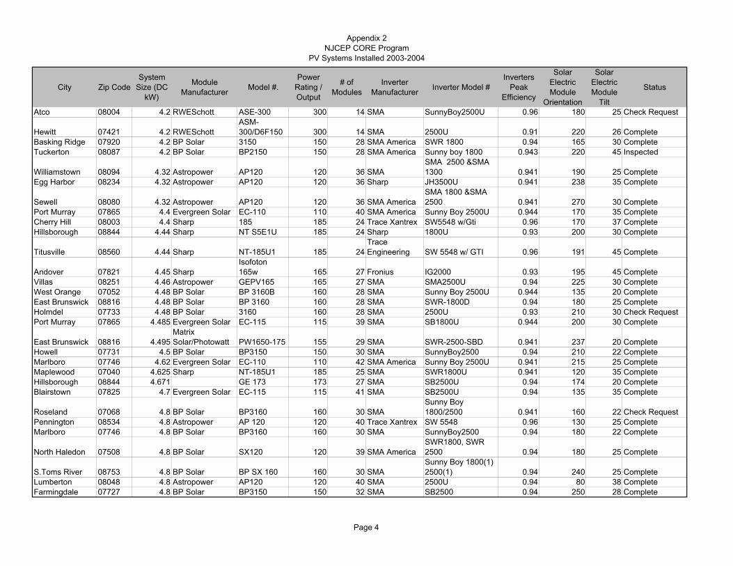
Appendix 2NJCEP CORE Program

PV Systems Installed 2003-2004

City Zip CodeSystem

Size (DC kW)

Module Manufacturer Model #.

Power Rating / Output

# of Modules

Inverter Manufacturer Inverter Model #

Inverters Peak

Efficiency

Solar Electric Module

Orientation

Solar Electric Module

Tilt

Status

Atco 08004 4.2 RWESchott ASE-300 300 14 SMA SunnyBoy2500U 0.96 180 25 Check Request

Hewitt 07421 4.2 RWESchottASM-300/D6F150 300 14 SMA 2500U 0.91 220 26 Complete

Basking Ridge 07920 4.2 BP Solar 3150 150 28 SMA America SWR 1800 0.94 165 30 CompleteTuckerton 08087 4.2 BP Solar BP2150 150 28 SMA America Sunny boy 1800 0.943 220 45 Inspected

Williamstown 08094 4.32 Astropower AP120 120 36 SMASMA 2500 &SMA 1300 0.941 190 25 Complete

Egg Harbor 08234 4.32 Astropower AP120 120 36 Sharp JH3500U 0.941 238 35 Complete

Sewell 08080 4.32 Astropower AP120 120 36 SMA AmericaSMA 1800 &SMA 2500 0.941 270 30 Complete

Port Murray 07865 4.4 Evergreen Solar EC-110 110 40 SMA America Sunny Boy 2500U 0.944 170 35 CompleteCherry Hill 08003 4.4 Sharp 185 185 24 Trace Xantrex SW5548 w/Gti 0.96 170 37 CompleteHillsborough 08844 4.44 Sharp NT S5E1U 185 24 Sharp 1800U 0.93 200 30 Complete

Titusville 08560 4.44 Sharp NT-185U1 185 24Trace Engineering SW 5548 w/ GTI 0.96 191 45 Complete

Andover 07821 4.45 SharpIsofoton 165w 165 27 Fronius IG2000 0.93 195 45 Complete

Villas 08251 4.46 Astropower GEPV165 165 27 SMA SMA2500U 0.94 225 30 CompleteWest Orange 07052 4.48 BP Solar BP 3160B 160 28 SMA Sunny Boy 2500U 0.944 135 20 CompleteEast Brunswick 08816 4.48 BP Solar BP 3160 160 28 SMA SWR-1800D 0.94 180 25 CompleteHolmdel 07733 4.48 BP Solar 3160 160 28 SMA 2500U 0.93 210 30 Check RequestPort Murray 07865 4.485 Evergreen Solar EC-115 115 39 SMA SB1800U 0.944 200 30 Complete

East Brunswick 08816 4.495Matrix Solar/Photowatt PW1650-175 155 29 SMA SWR-2500-SBD 0.941 237 20 Complete

Howell 07731 4.5 BP Solar BP3150 150 30 SMA SunnyBoy2500 0.94 210 22 CompleteMarlboro 07746 4.62 Evergreen Solar EC-110 110 42 SMA America Sunny Boy 2500U 0.941 215 25 CompleteMaplewood 07040 4.625 Sharp NT-185U1 185 25 SMA SWR1800U 0.941 120 35 CompleteHillsborough 08844 4.671 GE 173 173 27 SMA SB2500U 0.94 174 20 CompleteBlairstown 07825 4.7 Evergreen Solar EC-115 115 41 SMA SB2500U 0.94 135 35 Complete

Roseland 07068 4.8 BP Solar BP3160 160 30 SMASunny Boy 1800/2500 0.941 160 22 Check Request

Pennington 08534 4.8 Astropower AP 120 120 40 Trace Xantrex SW 5548 0.96 130 25 CompleteMarlboro 07746 4.8 BP Solar BP3160 160 30 SMA SunnyBoy2500 0.94 180 22 Complete

North Haledon 07508 4.8 BP Solar SX120 120 39 SMA AmericaSWR1800, SWR 2500 0.94 180 25 Complete

S.Toms River 08753 4.8 BP Solar BP SX 160 160 30 SMASunny Boy 1800(1) 2500(1) 0.94 240 25 Complete

Lumberton 08048 4.8 Astropower AP120 120 40 SMA 2500U 0.94 80 38 CompleteFarmingdale 07727 4.8 BP Solar BP3150 150 32 SMA SB2500 0.94 250 28 Complete

Page 4

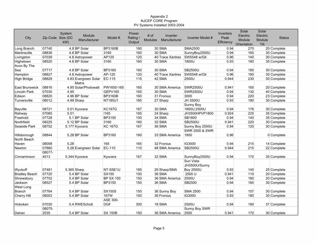
Appendix 2NJCEP CORE Program

PV Systems Installed 2003-2004

City Zip CodeSystem

Size (DC kW)

Module Manufacturer Model #.

Power Rating / Output

# of Modules

Inverter Manufacturer Inverter Model #

Inverters Peak

Efficiency

Solar Electric Module

Orientation

Solar Electric Module

Tilt

Status

Long Branch 07740 4.8 BP Solar BP3160B 160 30 SMA SMA2500 0.94 270 20 CompleteMartinsville 08836 4.8 BP Solar 3160 160 30 SMA SunnyBoy2500U 0.94 160 35 CompleteLivingston 07039 4.8 Astropower AP120 120 40 Trace Xantrex SW5548 w/Gti 0.96 140 30 CompleteHighstown 08520 4.8 BP Solar 3160 160 30 SMA 1800U 0.93 180 35 CompleteAvon By The Sea 07717 4.8 BP Solar BP3160 160 30 SMA SB2500U 0.94 180 30 CompleteHampton 08827 4.8 Astropower AP-120 120 40 Trace Xantrex SW5548 w/Gti 0.96 180 35 CompleteHigh Bridge 08829 4.83 Evergreen Solar EC-115 115 42 SMA 2500U 0.944 230 30 Complete

East Brunswick 08816 4.95Matrix Solar/Photowatt PW1650-165 165 30 SMA America SWR2500U 0.941 165 20 Complete

Lincoln Park 07035 4.95 GEPV165 165 30 SMA SWR2500U 0.94 130 40 CompleteEdison 08820 4.96 BP Solar BP3160B 160 31 Fronius 3000 0.94 220 23 CompleteTurnersville 08012 4.99 Sharp NT185U1 185 27 Sharp JH 3500U 0.93 180 30 Complete

Bayville 08721 5.01 Kyocera KC167G 167 30 SMASunny Boy 1800U;2500U 0.94 176 30 Complete

Rahway 07065 5.01 I165 165 24 Sharp JH3500HPVP1800 0.924 225 35 CompleteFreehold 07728 5.1 BP Solar BP3150 150 34 SMA SB1800 0.94 140 35 CompleteNorthfield 08225 5.12 BP Solar 3160 160 32 SMA SB2500U 0.941 220 30 CompleteSeaside Park 08752 5.177 Kyocera KC 167G 167 36 SMA Sunny Boy 2500U 0.94 120 30 Complete

Hillsborough 08844 5.28 BP Solar BP3160 160 33 SMA AmericaSWR 2500 & SWR 1800 0.96 0 Complete

North Beach Haven 08008 5.28 165 165 32 Fronius IG3000 0.94 215 14 CompleteNewton 07860 5.28 Evergreen Solar EC-110 110 48 SMA America SB2500U 0.944 215 22 Complete

Cinnaminson08077-4513 5.344 Kyocera Kyocera 167 32 SMA SunnyBoy2500U 0.94 170 35 Complete

Wyckoff 07481 5.365 Sharp NT-S5E1U 185 29 Sharp/SMA

Sun Vista JH3500U/Sunny Boy 2500U 0.93 140 25 Complete

Bradley Beach 07720 5.4 BP Solar SX150 150 36 SMA 2500 U 0.941 110 20 CompleteShrewsbury 07702 5.4 BP Solar BP SX 150 150 36 SMA America 2500U 0.94 180 20 CompleteJackson 08527 5.4 BP Solar BP3150 150 36 SMA SB2500 0.94 160 30 CompleteWest Long Branch 07764 5.4 BP Solar SX150S 150 36 Sunny Boy SMA 2500 0.94 157 30 CompleteCherry Hill 08003 5.4 BP Solar 167W 150 36 Fronius IG3000 0.93 180 30 Complete

Hoboken 07030 5.4 RWESchottASE 300-DGF 300 18 SMA 2500U 0.94 180 37 Complete

Delran08075-2035 5.4 BP Solar SX 150B 150 36 SMA America

Sunny Boy SWR 2500 0.941 170 30 Complete

Page 5

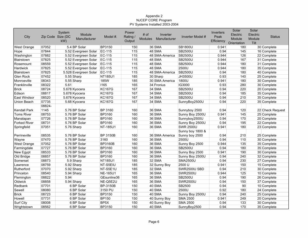
Appendix 2NJCEP CORE Program

PV Systems Installed 2003-2004

City Zip CodeSystem

Size (DC kW)

Module Manufacturer Model #.

Power Rating / Output

# of Modules

Inverter Manufacturer Inverter Model #

Inverters Peak

Efficiency

Solar Electric Module

Orientation

Solar Electric Module

Tilt

Status

West Orange 07052 5.4 BP Solar BP3150 150 36 SMA SB1800U 0.941 180 30 CompleteHope 07844 5.52 Evergreen Solar EC-115 115 48 SMA SB2500U 0.94 145 16 CompleteWashington 07882 5.52 Evergreen Solar EC-115 115 48 SMA-America SB2500U 0.944 126 22 CompleteBlairstown 07825 5.52 Evergreen Solar EC-115 115 48 SMA SB2500U 0.944 167 31 CompleteRosemount 08559 5.52 Evergreen Solar EC-115 115 48 SMA SB2500U 0.944 180 31 CompleteHardwick 07825 5.52 Evergreen Solar EC-115 115 48 SMA 2500U 0.944 180 35 CompleteBlairstown 07825 5.528 Evergreen Solar EC-115 115 48 SMA-America SB2500U 0.94 180 40 CompleteGlen Rock 07452 5.55 Sharp NT185U1 185 30 Sharp JH3500U 0.93 140 25 CompleteMonroeville 08343 5.55 Sharp 185W 185 30 SMA America 1800U 0.941 180 30 CompleteFranklinville 08322 5.61 I165 165 34 Fronius IG3000 0.93 280 30 CompleteBrick 08724 5.678 Kyocera KC167G 167 34 SMA SB2500U 0.94 220 20 CompleteEdison 08817 5.678 Kyocera KC167G 167 34 SMA SB2500U 0.94 185 35 CompleteEast Windsor 08520 5.678 Kyocera KC167G 167 34 SMA SB2500U 0.94 210 35 CompleteUnion Beach 07735 5.68 Kyocera KC167G 167 34 SMA SunnyBoy2500U 0.94 220 35 Complete

Kendall Park08824-1145 5.76 BP Solar BP 3160 160 36 SMA Sunnyboy 2500 0.94 120 22 Check Request

Toms River 08753 5.76 BP Solar BP3160 160 36 SMA Sunny Boy 2500U 0.941 145 25 CompleteManalapan 07726 5.76 BP Solar BP3160 160 36 SMA Sunnyboy2500U 0.94 170 20 CompleteForked River 08731 5.76 BP Solar BP3160 160 36 SMA Sunny Boy 2500U 0.94 195 22 CompleteSpringfeild 07051 5.76 Sharp NT-185U1 160 36 SMA SWR 2500U 0.941 180 23 Complete

Perrineville 08535 5.76 BP Solar BP 3150B 160 36 SMA AmericaSunny boy 1800 & Sunny boy 2500 0.94 210 25 Complete

Wayne 07470 5.76 BP Solar 3160 160 36 SMA 2500U 0.94 110 30 CompleteWest Orange 07052 5.76 BP Solar BP3160B 160 36 SMA Sunny Boy 2500 0.944 135 35 CompleteFarmingdale 07727 5.76 BP Solar BP3160 160 36 SMA SB2500U 0.94 180 35 CompleteNew Egypt 08533 5.76 BP Solar BP3160 160 36 SMA Sunny Boy 2500 0.941 190 30 CompleteOld Bridge 08857 5.76 BP Solar BP3160 160 36 SMA Sunny Boy 2500U 0.94 240 32 CompleteSomerset 08873 5.9 Sharp NT185U1 185 32 SMA SMA2500U 0.94 230 27 CompleteLawrence 08759 5.92 Sharp NT-S5EIU 185 32 Sunny Boy 2500 U 0.941 150 15 CompleteRutherford 07070 5.92 Sharp NT-S5E1U 185 32 SMA SWR2500U SBD 0.94 210 30 CompletePrinceton 08540 5.94 Sharp NE-165U1 165 36 SMA SWR2500U 0.944 125 10 CompleteFlemington 08822 5.94 GEsunline36 165 36 SMA SB2500U 0.94 190 26 CompleteOldwick 08858 5.94 Sharp NE-Q5E2U 165 36 SMA SWR2500U 0.94 150 37 CompleteRedbank 07701 6 BP Solar BP-3150B 150 40 SMA SB2500 0.94 90 10 CompleteSewell 08080 6 BP Solar 3150 PU 150 40 SMA 2500U 0.92 180 24 CompleteBrick 08723 6 BP Solar BP3150 150 40 SMA Sunny Boy 2500U 0.94 240 25 CompleteHowell 07731 6 BP Solar BP150 150 40 Sunny Boy SMA 2500 0.941 249 20 CompleteSurf City 08008 6 BP Solar BP5X 150 40 Sunny Boy SMA 2500 0.94 133 30 CompleteWrightstown 08562 6 BP Solar BP3150 150 40 SMA SunnyBoy2500 0.94 170 35 Complete

Page 6

Appendix 2NJCEP CORE Program

PV Systems Installed 2003-2004

City Zip CodeSystem

Size (DC kW)

Module Manufacturer Model #.

Power Rating / Output

# of Modules

Inverter Manufacturer Inverter Model #

Inverters Peak

Efficiency

Solar Electric Module

Orientation

Solar Electric Module

Tilt

Status

Wall 07719 6 BP Solar BP3150 150 40 SMA SB2500 0.94 200 30 CompleteBargenfield 07621 6.012 Sharp NT-167U1 167 36 SMA SMA2500U 0.94 120 22 Check Request

Bayville 08721 6.012 Kyocera KC-167G 167 36 SMA AmericaSunny Boy SWR 2500U 0.94 170 30 Complete

Montville 07045 6.012 Kyocera KC-167G 167 36 SMA America SMA 2500 UL-SBD 0.944 225 30 CompleteBrigantine 08203 6.105 Sharp NT-185-U1 185 33 Sharp JH 3500 U 0.924 240 25 CompleteSpringfield 07081 6.29 Sharp NT-185U1 185 34 SMA America Sunny Boy 2500U 0.941 220 18 Complete

Edison 08820 6.3Matrix Solar/Photowatt PW1650-165 175 36 SMA America SWR2500U 0.94 130 40 Complete

Kendall Park 08824 6.358 Kyocera KC187 187 34 SMA SB1800 0.94 170 35 Check RequestWall 07719 6.4 Uni-solar PVL-128 128 50 SMA PV10208 0.94 157 0 CompletePennington 08534 6.66 Sharp NT-185U1 185 36 Sharp JH 3500U 0.93 180 0 CompleteGlassboro 08028 6.66 ND 16701 165 24 Fronius IG3000 0.93 165 24 CompleteHillsborough 08844 6.66 Sharp NT-S5EIU 185 36 SMA SWR 1800U 0.94 200 25 CompleteHolmdel 07731 6.66 Sharp NT188U1 185 36 SMA America SWR2500U 0.941 220 20 CompleteCedar Grove 07009 6.68 Kyocera KC167G 167 40 SMA Sunnyboy 2500U 0.94 190 28 CompleteTuckerton 08087 6.72 BP Solar BP3160 160 42 SMA 2500U 0.94 220 16 Check Request

Allenhurst 07711 6.72 BP Solar BP3160 160 42 SMASunny Boy 1800/2500 0.941 270 45 Complete

Freehold 07728 6.8 BP Solar BP 5170 170 40 SMA 2500U 0.941 190 25 CompleteHamilton 08610 6.825 Sharp NT-S5E1U 175 39 Sharp JH3500 0.93 100 40 CompleteFranklinville 08322 6.89 Sharp 185W 185 21 Sharp JH-3500U 0.93 180 22 CompleteHackettstown 07840 6.9 Evergreen Solar EC-115 115 60 SMA SB2500U 0.944 160 31 Complete

Hamilton Square 08690 7 Sanyo HIP-J54BA2 180 40 Sharp JH-3500U 0.94 190 19 CompleteLebanon 7 Astropower AP 100 100 70 SMA America SWR2500U 0.96 190 35 CompleteBelle Mead/ Griggstown 08502 7.014 Sharp ND-167U1 167 42 Sharp JH-3500U 0.924 235 18 CompleteCorbin City 08270 7.175 Sharp NT-175U1 175 41 Sunvista JH3500 0.94 145 27 CompletePalmyra 08065 7.2 RWESchott ASE300 300 24 SMA Sunny Boy 2500 0.93 155 5 CompleteWhite house Station 08889 7.2 BP Solar SX150S 150 48 SMA America

Sunny Boy 1800 and 2500 0.94 170 25 Complete

Frenchtown 08825 7.2 Astropower AP-120 120 60 SMA America 2,500U SBD 0.94 180 30 Complete

Lebanon 7.2 Astropower AP 100 100 72 SMA AmericaSWR 1800, SWR 2500 0.96 190 30 Complete

Jackson 08527 7.2 Astropower AP120 120 60 SMA 2500U 0.94 160 40 CompleteIselin 08830 7.2 RWESchott 300ASE 300 24 SMA SunnyBoy2500 0.96 135 40 Complete

Page 7

Appendix 2NJCEP CORE Program

PV Systems Installed 2003-2004

City Zip CodeSystem

Size (DC kW)

Module Manufacturer Model #.

Power Rating / Output

# of Modules

Inverter Manufacturer Inverter Model #

Inverters Peak

Efficiency

Solar Electric Module

Orientation

Solar Electric Module

Tilt

Status

Long Valley 07853 7.35Matrix Solar/Photowatt

PW 1650-175 175 42 Xantrex SW 4080 0.94 140 30 Complete

West Milford 07840 7.36 Evergreen Solar EC-115 115 64 SMA SB2500U 0.94 220 30 CompleteWhitehouse Statiion 08889 7.4 GEPV 165 165 45 SMA America

Sunnyboy 2500-SBD(3) 0.94 200 35 Complete

Kendall Park 08824 7.425 GE165 165 45 SMA SB 2500 0.94 180 16 CompleteWest Atlantic City 08234 7.425 I165 165 45 Fronius IG2000 0.94 125 20 Check RequestBridgewater 08807 7.49 Sharp SH140 140 42 Xantrex SW5548 0.94 210 20 CompleteElm 08037 7.56 Sharp NE-Q5E2U 180 42 SMA America SWR2500U 0.94 180 49 Check RequestFlemington 08822 7.59 Evergreen Solar EC-115 115 66 SMA SB2500U 0.94 190 25 CompleteClarksburg 08510 7.63 Sunslates 14 545 Trace&Sharp Sw5548&JH3500 0.95 220 40 CompleteLittle Silver 07739 7.65 BP Solar SX150 150 51 Xantrex SW4048 0.96 220 45 CompleteOld Bridge 08857 7.68 BP Solar BP3160 160 48 SMA Sunny Boy 2500U 0.94 110 25 Complete

Hamilton Square 08690 7.68 BP Solar 3160 160 48 SMA 2500 0.94 180 20 Check Request

Chatsworth 08019 7.77 Sharp 185W 185 42 SharpSun Vista JH3500U/ Sunny Boy 2500U 0.93 190 20 Complete

Hampton 08827 7.77 Sharp NT-S5EIU 185 42 Sharp JH-3500U 0.92 205 23 CompleteGalloway 08205 7.77 Sharp NT-185U1 185 42 Sharp JH-3500U 0.924 190 35 Complete

Warren 07059 7.77 Sharp NT-185U1 185 42 SMA AmericaSunnyboy 2500 and 1800 0.944 190 47 Complete

Northfield 08225 7.8 BP Solar 3150B 150 52 SMA America Sunny Boy 2500 0.941 235 35 Complete

Little Egg Harbor 08087 7.84 BP Solar BP3160 160 49 SMASunny Boy 1800/2500 0.941 180 22 Check Request

Union 07083 7.84 Sharp

NDNU ECU&NDO70ERU 140 46 Sharp Sharp JH-3500U 0.924 140 30 Complete

Hopewell 08525 7.92 AP110 110 72 SMA SWR2500U 0.94 160 24 CompleteGlen Gardner 08828 7.92 Evergreen Solar EC-115 115 72 SMA-America SB2500U 0.944 240 22 CompleteBlairstown 07825 7.94 Evergreen Solar EC-115 115 61 SMA SB2500U 0.944 228 40 CompleteLawrence Township

08648-1431 8.016 Kyocera KC167G 167 48 SMA 2500U 0.94 220 35 Complete

Wall twp 07753 8.1 BP Solar SX150B 150 54 SMA America Sunny Boy 2500U 0.941 150 23 CompleteLong Valley 07853 8.28 Evergreen Solar EC-115 115 72 SMA SB2500U 0.944 193 31 CompleteMendham 07945 8.36 Evergreen Solar EC-110 110 76 SMA America SB2500U 0.944 153 30 Complete

Newton 07860 8.4 Sharp NT175U1 175 48 SMASunny Boy SWR 2500U 0.93 157 25 Complete

Page 8

Appendix 2NJCEP CORE Program

PV Systems Installed 2003-2004

City Zip CodeSystem

Size (DC kW)

Module Manufacturer Model #.

Power Rating / Output

# of Modules

Inverter Manufacturer Inverter Model #

Inverters Peak

Efficiency

Solar Electric Module

Orientation

Solar Electric Module

Tilt

Status

Monmouth Beach 07750 8.4 BP Solar BP3160 150 56 SMA SB2500U 0.94 135 22 CompleteLawrence Twp. 08648 8.4 Sharp NT175U1 175 48 SMA SWR2500U 0.94 180 22 CompleteFreehold 07728 8.64 BP Solar BP3160 160 54 SMA SB2500U 0.94 200 22 CompleteHolmdel 07733 8.64 BP Solar 3160 160 54 Outback GUFX7248 0.94 180 30 Check RequestFlemington 08822 8.64 Astropower AP120 120 72 Trace SW4048 0.96 191 40 CompleteMays Landing 08330 8.684 Sharp ND-167U1 167 52 Sharp Sunvista JH 3500U 0.92 265 40 Check RequestPitman 08071 8.695 Sharp NT-S5EIU 185 47 SMA America Sunny Boy 2500U 0.941 180 38 CompleteBlairstown 07825 8.8 Evergreen Solar EC-115 115 80 SMA America Sunny Boy 2500U 0.944 170 35 CompleteRingoes 08551 8.85 Sharp ND-167U1 167 53 Sharp JH-3500U 0.93 176 26 CompleteChester 07930 8.88 Sharp NE-S5E1U 185 48 SMA America SMA2500 UL-SBD 0.944 180 18 Complete

Califon 07830 8.888 Sharp NT-SSEIV 185 48 SMA AmericaSWR 1800 V w/display 0.94 180 15 Complete

Voorhees 08043 8.91 Sharp NE-Q5E2U 165 54 SMA America SMA 2500 0.94 150 25 CompleteHackettstown 07840 9.018 Kyocera KC167G 167 54 SMA SunnyBoy2500U 0.94 180 22 CompleteMarlboro 07746 9.018 Kyocera KC167G 167 54 SMA Sunny Boy 2500U 0.941 180 30 CompleteRandolph 07869 9.018 Kyocera KC167G 167 54 SMA SB2500U 0.94 260 30 CompleteAllentown 08514 9.24 GEPV-110 110 84 SMA Sunny Boy 2500U 0.94 170 45 CompleteMansfield 08022 9.28 BP Solar 3160 160 58 SMA 2500U 0.94 210 25 CompleteEdison 08820 9.45 Sharp NT175U1 175 54 Sharp JH-3500U 0.941 180 15 CompleteEdison 08820 9.45 Sharp NT185U1 175 54 Sharp JH3500U 0.941 180 15 CompletePennington 08534 9.45 Sharp NT-S5E1N 175 54 Sharp JH3500 0.93 180 23 CompleteBridgeton 08302 9.45 Sharp NT-175U1 175 54 Fronius IG3000 0.94 180 30 Complete

Neshanic Station 08853 9.45 I150S 150 63 SMA SB2500U 0.93 220 35 Check RequestAndover Township 07860 9.6 BP Solar 3160 160 60 Fronius IG2000 0.94 180 30 CompleteRed Bank 07701 9.6 BP Solar 3160 160 60 SMA 1800 0.94 180 35 CompleteBelle Meade 08502 9.72 Terra Solar TS 40 243 40 SMA America 2500U 0.94 180 15 CompleteBrick 08723 9.76 BP Solar BP3160 160 61 SMA Sunny Boy 2500 0.941 280 24 Check RequestManalapan 07726 9.76 BP Solar BP3160 160 61 SMA SB2500U 0.94 193 30 Complete

Lebanon 08833 9.795 RWESchottASE-300DGF150 32 SMA SWR2500U 0.96 180 34 Complete

Hopewell 08525 9.8 Sharp NT175U1 175 56 SMA JH3500U 0.93 180 30 CompleteHolmdel 07733 9.8 BP Solar SX140S 140 70 SMA America SMA-2500 0.94 180 30 CompleteHolmdel 07733 9.8 BP Solar SX140S 140 70 SMA America SMA-2500 0.94 180 30 Complete

Mahwah 07430 9.8 SanyoHIP-G751BA2 167 59 SMA America Sunny Boy 2500U 0.941 180 37 Complete

Page 9

Appendix 2NJCEP CORE Program

PV Systems Installed 2003-2004

City Zip CodeSystem

Size (DC kW)

Module Manufacturer Model #.

Power Rating / Output

# of Modules

Inverter Manufacturer Inverter Model #

Inverters Peak

Efficiency

Solar Electric Module

Orientation

Solar Electric Module

Tilt

Status

Ringoes 08551 9.8 Sharp NT-175U1 175 56Sharp Electronics J3500U 0.93 240 30 Complete

Morristown 07960 9.8 Sharp NT-175U1 175 56 Sharp JH3500 0.93 150 45 CompleteLong Branch 07740 9.805 Sharp NT-185U1 185 53 Sunny Boy 2500u 0.941 175 25 CompleteMorganville 07751 9.81 BP Solar BP3160 150 66 SMA SB2500 0.94 90 20 CompleteTitusville 08560 9.84 Astropower AP120 120 82 SMA America SWR2500U 0.94 235 23 CompletePrinceton 08540 9.853 Kyocera KC167G 167 59 SMA SB1100U 0.94 180 26 Complete

Glenwood07418-2015 9.853 Kyrocera KC161G 167 59 SMA

Sunny Boy 2500U(3)Sunny Boy 1800U (1) 0.94 165 35 Complete

Clifton 07013 9.9 Sharp NT-185U1 185 54 Sharp Sunvista 3500 0.924 130 22 Check RequestCedarbrook 08009 9.9 Sharp NT-185W 185 54 SMA 2500U 0.93 135 23 CompleteRingoes 08551 9.9 Sharp NT-185U1 185 54 Sharp JH-3500U 0.93 180 20 CompleteMilford 08848 9.9 GE-165 165 60 SMA SB2500U 0.94 180 20 CompleteElwood 08217 9.9 Sharp NE-165U1 165 60 SMA Sunny Boy 2500U 0.941 190 20 CompleteManalapan 07726 9.9 GEPV165 165 60 SMA SB2500 0.94 180 30 CompletePittstown 08867 9.9 GEPV165 165 60 SMA-America Sunny Boy 2500 0.94 270 30 CompleteManalapan 07726 9.9 GEPV165 165 60 SMA SB2500 0.94 270 30 CompleteSouthampton/Tabernacle 08088 9.9 Sharp NT-S5E1U 185 54 Sharp JH 3500U 0.924 260 30 CompletePennington 08534 9.9 Sharp NE-Q5E2U 165 60 SMA America SWR2500U 0.94 180 45 CompleteTrenton 08619 9.92 BP Solar 3160 160 62 SMA 2500 0.94 190 10 Check RequestEast Brunswick 08816 9.92 Sharp NT-185U1 160 62 SMA Sunny Boy 2500U 0.941 100 20 Check RequestBelmar 07719 9.96 Astropower AP120 120 83 SMA America 2500 U 0.94 0 0 CompleteBrick 08723 9.96 Astropower AP120 120 83 SMA America SW4048 1 210 19 CompleteLambertville 08530 9.96 Astropower AP120 120 83 SMA SWR2500U 0.94 180 25 CompleteWhitehouse Station 08889 9.967 GEPV 165 165 69 SMA America SunnyBoy 2500 0.94 180 30 CompleteAtco 08004 9.975 Sharp NE-175 175 57 Sharp JH3500u 0.93 180 23 CompleteWaterford 08089 9.98 Sharp NT-175U1 175 57 Sharp JH3500U 0.93 220 34 CompleteSouthampton 08088 9.99 Sharp NT-185U1 185 54 SMA 2500U 0.93 90 16 CompleteBrown's Mill 08015 9.99 Sharp NT-185U1 185 54 Sharp JH-3500U 0.92 270 18 Complete

Lebanon 07753 9.99 Sharp NT 185U1 185 54 SMASunny Boy SWR 2500U 0.941 100 20 Complete

Burlington 08016 9.99 Sharp NT S5E1U 185 54 Sharp Sunvista JH 3500U 0.93 150 25 Complete

Little Egg Harbor 08087 9.99 Sharp NT-185U1 185 54 Sharp JH-3500U 0.94 160 25 CompleteLong Valley 07853 9.99 Sharp NT-55EIU 185 54 Sharp Sunvista 0.92 180 20 CompleteWestampton 08060 9.99 Sharp NT185U1 185 54 Sharp JH3500U 0.93 180 37.5 Complete

Page 10

Appendix 2NJCEP CORE Program

PV Systems Installed 2003-2004

City Zip CodeSystem

Size (DC kW)

Module Manufacturer Model #.

Power Rating / Output

# of Modules

Inverter Manufacturer Inverter Model #

Inverters Peak

Efficiency

Solar Electric Module

Orientation

Solar Electric Module

Tilt

Status

Freehold 07728 10 BP Solar BP3150 160 63 SMA SB2500U 0.94 200 32 CompleteColts Neck 07722 10.02 Kyocera KC167G 167 60 SMA SB1100U 0.94 170 30 CompleteNeptune 07753 10.8 BP Solar BP-110 150 72 SMA America Sunny Boy 2500U 0.941 180 30 CompleteMagnolia 08049 11.04 Evergreen Solar EC-115 115 96 SMA-America Sunny Boy 2500U 0.944 200 5 CompleteCream Ridge 08514 11.04 Evergreen Solar EC-115 115 96 SMA America SB2500U 0.944 190 30 CompleteFarmingdale 07727 11.04 Evergreen Solar EC-115 115 96 SMA-America SB2500U 0.944 170 35 CompleteColts Neck 07722 11.1 Sharp NT-185U1 185 60 Sharp JH-3500U 0.924 180 24 CompleteAlloway 08001 11.84 Sharp NT-185U1 185 64 SMA America Sunny Boy 2500U 0.941 170 40 Complete

Somerset08873-2861 12.3 BP Solar SX150B 150 82 SMA

Sunny Boy 2500(2) 1800(3) 0.94 180 27 Complete

Gladstone 07934 12.6 Astropower AP75 75 168 SMA SB1800U 0.944 165 14 Complete

Springfiled 07081 14.4 RWESchottASE300 DGF50 300 48 SMA SU2500 0.94 150 5 Check Request

Lafayette 07848 16.56 Evergreen Solar EC-115 115 144 SMA SB2500U 0.94 180 35 CompleteNewton 07860 16.56 Evergreen Solar EC-115 115 144 SMA SB2500U 0.944 180 30 Check RequestRockleigh 07647 19.2 RWESchott ASE 300DG 300 64 SMA America SWR2500U 0.94 180 52 CompleteWall 07719 21.84 Astropower AP 130 130 168 Trace Xantrex PV 20 0.96 180 0 CompleteMandham 07945 22.08 Evergreen Solar EC-115 115 192 SMA-America Sunny Boy 2500U 0.944 180 35 Check RequestLong Valley 07853 22.08 Evergreen Solar EC-115 115 192 SMA SB2500U 0.944 193 30 CompleteCream Ridge 08514 38.64 Evergreen Solar EC-115 115 336 SMA America SB2500U 0.944 190 30 CompleteEast Windsor 08520 41.4 Evergreen Solar EC-115 115 360 SMA SB2500U 0.94 170 31 CompleteHowell 07731 50.4 BP Solar MSX 120 120 420 Trace Xantrex PV 45 0.96 180 0 CompleteHowell 07731 50.4 BP Solar MSX 120 120 420 Trace Xantrex PV 45 0.96 180 0 Complete

Newark 07102 50.4 RWESchottASE3005OV315W 315 160 PVPowered PVP2800 PVP1800 0.944 195 5 Complete

Sewell 08080 88.8 Sharp NT-S5EIU 185 480 SMA America Sunny Boy 2500U 0.941 170 30 CompleteEdgeWater 07020 120.96 BP Solar 3140 140 864 Xantrex PV100208 0.96 180 0 CompleteTotal 2521.178

Page 11

New Jersey Clean Energy Program

Protocols to Measure Resource Savings

New Jersey Clean Energy Protocols September 2004

DOE/GO-102006-2354 August 2006 Appendix 3

New Jersey Clean Energy Program Page i Protocols to Measure Resource Savings September 2004

Table of Contents Introduction...........................................................................................................1

Purpose.......................................................................................................................................1 Types of Protocols .....................................................................................................................2 Algorithms .................................................................................................................................4 Data and Input Values................................................................................................................4 Baseline Estimates .....................................................................................................................5 Resource Savings in Current and Future Program Years...........................................................5 Prospective Application of the Protocols...................................................................................6 Resource Savings .......................................................................................................................6

Electric...................................................................................................................................6 Natural Gas ...........................................................................................................................7 Other Resources.....................................................................................................................7

Post-Implementation Review .....................................................................................................7 Adjustments to Energy and Resource Savings...........................................................................8

Coincidence with Electric System Peak.................................................................................8 Measure Retention and Persistence of Savings .....................................................................8 Interaction of Energy Savings ...............................................................................................8

Calculation of the Value of Resource Savings...........................................................................8 Transmission and Distribution System Losses...........................................................................9

Electric Loss Factor ..............................................................................................................9 Gas Loss Factor.....................................................................................................................9

Calculation of Clean Air Impacts...............................................................................................9 Measure Lives ..........................................................................................................................10 Protocols for Program Measures..............................................................................................10

Residential Electric HVAC ................................................................................11 Protocols ..................................................................................................................................11

Central Air Conditioner (A/C) & Air Source Heat Pump (ASHP) ......................................11 Ground Source Heat Pumps (GSHP) ..................................................................................11 GSHP Desuperheater ..........................................................................................................12

Residential Gas HVAC.......................................................................................15 Protocols ..................................................................................................................................15

Space Heaters ......................................................................................................................15 Water Heaters ......................................................................................................................16

Residential Energy Star Windows.....................................................................17 Protocols ..................................................................................................................................17

ENERGY STAR Windows ....................................................................................................17 Residential Low Income Program.....................................................................21

Protocols ..................................................................................................................................21 Efficient Lighting .................................................................................................................21 Hot Water Conservation Measures......................................................................................21 Efficient Refrigerators .........................................................................................................22 Air Sealing ...........................................................................................................................22 Duct Sealing and Repair......................................................................................................23 Insulation Up-Grades ..........................................................................................................23 Thermostat Replacement .....................................................................................................23 Heating and Cooling Equipment Maintenance Repair/Replacement..................................24 Total Space Conditioning Savings.......................................................................................24

New Jersey Clean Energy Program Page ii Protocols to Measure Resource Savings September 2004

Other “Custom” Measures..................................................................................................24 Residential New Construction Program...........................................................28

Protocols ..................................................................................................................................28 Insulation Up-Grades, Efficient Windows, Air Sealing, Efficient HVAC Equipment, and Duct Sealing ........................................................................................................................28 Lighting and Appliances ......................................................................................................30 Ventilation Equipment .........................................................................................................30

Residential Retrofit Program.............................................................................35 Protocols ..................................................................................................................................35

Residential ENERGY STAR Lighting..............................................................36 Protocols ..................................................................................................................................36

Residential ENERGY STAR Appliances..........................................................37 Protocols ..................................................................................................................................37

ENERGY STAR Refrigerators..............................................................................................37 ENERGY STAR Clothes Washers ........................................................................................37 ENERGY STAR Dishwashers...............................................................................................37 ENERGY STAR Room Air Conditioners..............................................................................38

Commercial and Industrial Energy Efficient Construction ...........................41 C&I Electric Protocols .............................................................................................................41

Baselines and Code Changes...............................................................................................41 Lighting Equipment .............................................................................................................41 Prescriptive Lighting for Small Commercial Customers.....................................................45 Prescriptive Lighting Savings Table....................................................................................46 Lighting Controls.................................................................................................................47 Motors..................................................................................................................................48 HVAC Systems .....................................................................................................................49 Electric Chillers...................................................................................................................51 Variable Frequency Drives..................................................................................................54

C&I Construction Gas Protocols..............................................................................................55 Gas Chillers .........................................................................................................................55 Gas Fired Desiccants ..........................................................................................................58 Gas Booster Water Heaters .................................................................................................58 Water Heaters ......................................................................................................................59 Furnaces and Boilers...........................................................................................................60

Commercial and Industrial Building Operation & Maintenance Program .61 Protocols ..................................................................................................................................61

Electric Savings ...................................................................................................................61 Gas Savings .........................................................................................................................61

Compressed Air System Optimization..............................................................63 Protocols ..................................................................................................................................63

Compressed Air Systems......................................................................................................63 Residential Air Conditioning Cycling Load Control Program ......................64

Protocols ..................................................................................................................................64 School Energy Efficiency and Renewable Energy Education Program........65

Protocols ..................................................................................................................................65 Customer-Sited Generation ...............................................................................66

Protocols ..................................................................................................................................66 Photovoltaic Systems ...........................................................................................................66 Wind Systems .......................................................................................................................68

New Jersey Clean Energy Program Page iii Protocols to Measure Resource Savings September 2004

Fuel Cells.............................................................................................................................69 Sustainable Biomass ............................................................................................................69

Appendix A Measure Lives ..............................................................................70

New Jersey Clean Energy Program Page 1 Protocols to Measure Resource Savings September 2004

New Jersey Clean Energy Program Protocols to Measure Resource Savings

Introduction These protocols have been developed to measure resource savings, including energy, capacity, and other resource savings. Specific protocols for determination of the resource savings from each program are presented for each eligible measure and technology. These protocols use measured and customer data as input values in industry-accepted algorithms. The data and input values for the algorithms come from the program application forms or from standard values. The standard input values are based on the best available measured or industry data applicable for the New Jersey programs. The standard values for most commercial and industrial (C&I) measures are supported by end use metering for key parameters for a sample of facilities and circuits, based on the metered data from the JCP&L Shared Savings Program. These C&I standard values are based on five years of data for most measures and two years of data for lighting. Some electric and gas input values were derived from a review of literature from various industry organizations, equipment manufacturers, and suppliers.

Purpose These protocols were developed for the purpose of determining energy and resource savings for Clean Energy technologies and measures supported by the programs approved by Board Order dated March 9, 2001 and subsequently described in a Program Compliance Filing made on April 9, 2001 in the Comprehensive Resources Analysis (CRA) of Energy Programs proceeding, Docket Nos. EX99050347, EO99050348, EO99050349, EO99050350, EO99050351, GO99050352, GO99050353, and GO99050354. These protocols will be used consistently statewide to assess program impacts and calculate energy and resource savings to:

1. Report to the Board on program performance 2. Provide inputs for planning and cost-effectiveness calculations 3. Calculate lost margin revenue recovery 4. Provide information to regulators and program administrators for determining

eligibility for administrative performance incentives (to the extent that such incentives are approved by the BPU)

5. Assess the environmental benefits of program implementation Resource savings to be measured include electric energy (kWh) and capacity (kW) savings, natural gas savings (therms), and savings of other resources (oil, propane, water, and maintenance), where applicable. In turn, these resource savings will be used to determine avoided environmental emissions. The protocols in this document focus on the determination of the per unit savings for the energy efficiency measures included in the programs in the April 9, 2001 Program

New Jersey Clean Energy Program Page 2 Protocols to Measure Resource Savings September 2004

Compliance Filing. The number of adopted units to which these per unit savings apply are captured in the program tracking and reporting process, supported by market assessments for some programs. The unit count will reflect the direct participation and, through market assessments, the number of units due to market effects in comparison to a baseline level of adoptions. Free riders and free drivers will be captured implicitly on a net basis through this approach to counting adoption of units. Further, the net of free riders and free drivers are assumed to be zero in the counting of units from direct program participation. The following four attachments to Supplement 1 to the April 9, 2001 Program Compliance Filing present inter-related plans and analyses to support regulatory reporting, measure energy and resource savings, assess program cost effectiveness and environmental benefits, and track and evaluate program implementation:

• Attachment 1 - Energy and Economic Assessment of Energy Efficiency Programs (Cost Effectiveness)

• Attachment 2 - Protocols to Measure Resource Savings

• Attachment 3 - Program Evaluation Plan

• Attachment 4 - Regulatory Reporting

• Attachment 5 - Performance Incentives The protocols (Attachment 2) provide the methods to measure per unit savings for program tracking and reporting. The Evaluation Plan (Attachment 3) outlines the plans for assessing markets and program progress in transforming markets, and to update key assumptions used in the protocols to assess program energy savings. Reporting (Attachment 4) provides formats and definitions to be used to document program expenditures, participation rates, and program impacts, including energy and resource savings. The program tracking systems, that support program evaluation and reporting, will track and record the number of units adopted due to the program, and assist in documenting the resource savings using the per unit savings values in the protocols. The Energy and Economic Assessment of Energy Efficiency Programs (Cost Effectiveness) (Attachment 1) presents the projected impacts of programs, including market effects, and their relationship to costs in a multi-year analysis. The assumptions and methods used in these statewide analyses are consistent and integrated (e.g., the same per unit savings were used to project program savings, to assess program cost-effectiveness and environmental benefits, and to set savings goals for program performance incentives).

Types of Protocols In general, energy and demand savings will be measured using measured and customer data as input values in algorithms in the protocols, tracking systems, and information from the program application forms, worksheets, and field tools.

New Jersey Clean Energy Program Page 3 Protocols to Measure Resource Savings September 2004

The following table summarizes the spectrum of protocols and approaches to be used for measuring energy and resource savings. No one protocol approach will serve all programs and measures.

Summary of Protocols and Approaches

Type of Measure

Type of Protocol

General Approach Examples

1. Standard prescriptive measures

Standard formula and standard input values

Number of installed units times standard savings/unit

Residential lighting (number of units installed times standard savings/unit)

2. Measures with important variations in one or more input values (e.g., delta watts, efficiency level, capacity, load, etc.)

Standard formula with one or more site-specific input values

Standard formula in the protocols with one or more input values coming from the application form, worksheet, or field tool (e.g., delta watts, efficiency levels, unit capacity, site-specific load)

Some prescriptive lighting measures (delta watts on the application form times standard operating hours in the protocols) Residential Electric HVAC (change in efficiency level times site-specific capacity times standard operating hours) Field screening tools that use site-specific input values

3. Custom or site-specific measures, or measures in complex comprehensive jobs

Site-specific analysis

Greater degree of site-specific analysis, either in the number of site-specific input values, or in the use of special engineering algorithms

Custom Industrial process Complex comprehensive jobs

Three or four systems will work together to ensure accurate data on a given measure:

1. The application form that the customer or customer’s agent submits with basic information.

2. Application worksheets and field tools with more detailed site-specific data, input values, and calculations (for some programs).

New Jersey Clean Energy Program Page 4 Protocols to Measure Resource Savings September 2004

3. Program tracking systems that compile data and may do some calculations. 4. Protocols that contain algorithms and rely on standard or site-specific input values

based on measured data. Parts or all of the protocols may ultimately be implemented within the tracking system, the application forms and worksheets, and the field tools.

Algorithms The algorithms that have been developed to calculate the energy and or demand savings are driven by a change in efficiency level for the installed measure compared to a baseline level of efficiency. This change in efficiency is reflected in both demand and energy savings for electric measures and energy savings for gas. Following are the basic algorithms. Electric Demand Savings = ∆kW = kWbaseline - kWenergy efficient measure Electric Energy Savings = ∆kW X EFLH Electric Peak Coincident Demand Savings = ∆kW X Coincidence Factor Gas Energy Savings = ∆Btuh X EFLH Where:

EFLH = Equivalent Full Load Hours of operation for the installed measure. ∆Btuh = Btuhbaseline input – Btuhenergy efficient measure input

Other resource savings will be calculated as appropriate. Specific algorithms for each of the program measures may incorporate additional factors to reflect specific conditions associated with a program or measure. This may include factors to account for coincidence of multiple installations, or interaction between different measures.

Data and Input Values The input values and algorithms in the protocols and on the program application forms are based on the best available and applicable data for the New Jersey programs. The input values for the algorithms come from the program application forms or from standard values based on measured or industry data. Many input values, including site-specific data, come directly from the program application forms, worksheets, and field tools. Site-specific data on the application forms are used for measures with important variations in one or more input values (e.g., delta watts, efficiency level, capacity, etc.).

New Jersey Clean Energy Program Page 5 Protocols to Measure Resource Savings September 2004

Standard input values are based on the best available measured or industry data, including metered data, measured data from prior evaluations (applied prospectively), field data and program results, and standards from industry associations. The standard values for most commercial and industrial measures are supported by end use metering for key parameters for a sample of facilities and circuits. These standard values are based on five years of metered data for most measures1. Data that were metered over that time period are from measures that were installed over an eight-year period. Many input values are based on program evaluations of prior New Jersey programs or similar programs in other regions. For the standard input assumptions for which metered or measured data were not available, the input values (e.g., delta watts, delta efficiency, equipment capacity, operating hours, coincidence factors) were based on the best available industry data or standards. These input values were based on a review of literature from various industry organizations, equipment manufacturers, and suppliers. Program evaluation will be used to assess key data and input values to either confirm that current values should continue to be used or update the values going forward.

Baseline Estimates For most programs the ∆ kW and ∆ kWh values are based on the energy use of standard new products vs. the high efficiency products promoted through the programs. This baseline may be different than the baseline estimates used in previous programs such as the Standard Offer in which the baseline assumptions were based on either the existing equipment for retrofits or current code or practice for new construction. The approach used for the new programs encourages residential and business consumers to purchase and install high efficiency equipment vs. new standard efficiency equipment. The baseline estimates used in the protocols are documented in the baseline studies or other market information. Baselines will be updated to reflect changing codes, practices and market transformation effects.

Resource Savings in Current and Future Program Years The Protocols support tracking and reporting the following categories of energy and resource savings:

1. Savings from installations that were completed in the program year and prior program years due to the program’s direct participation and documented market effects.

2. Savings from program participant future adoptions due to program commitments. 3. Savings from future adoptions due to market effects.

1 Values for lighting, air conditioners, chillers, and motors are based on measured usage from a large sample of participants from 1995 through 1999. Values for heat pumps reflect metered usage from 1996 through 1998, and variable speed drives reflect metered usage from 1995 through 1998.

New Jersey Clean Energy Program Page 6 Protocols to Measure Resource Savings September 2004

Prospective Application of the Protocols The protocols will be applied prospectively. The input values are from the program application forms and standard input values (based on measured data including metered data and evaluation results). The protocols will be updated periodically based on evaluation results and available data, and then applied prospectively for future program years. The only exceptions to prospective application of the protocols are (1) utility review of tracking systems and any necessary adjustments after the end of the program year and prior to the completion of the annual report for that year, and (2) adjustments due to review and on-site verification of custom measures and large comprehensive jobs, also to be completed before the submission of the annual report for that year.

Resource Savings

Electric Protocols have been developed to determine the electric energy and coincident peak demand savings. Annual Electric energy savings are calculated and then allocated separately by season (summer and winter) and time of day (on-peak and off-peak). Summer coincident peak demand savings are calculated using a demand savings protocol for each measure that includes a coincidence factor. Application of this coincidence factor converts the demand savings of the measure, which may not occur at time of system peak, to demand savings that is expected to occur during the Summer On-Peak period. These periods for energy savings and coincident peak demand savings are defined as:

Energy Savings Coincident Peak Demand Savings

Summer May through September

June through August

Winter October through April

NA

On Peak (Monday - Friday)

8:00 a.m. to 8:00 p.m.

12:00 p.m. to 8:00 p.m.

Off Peak (Weekends and Holidays)

8:00 p.m. to 8:00 a.m.

NA

The time periods for energy savings and coincident peak demand savings were chosen to best fit the seasonal avoided cost patterns for electric energy and capacity that were used for the energy efficiency program cost effectiveness purposes. For energy, the summer period May through September was selected based on the pattern of avoided costs for energy at the PJM level. In order to keep the complexity of the process for calculating energy savings benefits to a reasonable level by using two time periods, the knee periods for spring and fall were split approximately evenly between the summer and winter

New Jersey Clean Energy Program Page 7 Protocols to Measure Resource Savings September 2004

periods. For capacity, the summer period June through August was selected to match the highest avoided costs time period for capacity. The experience in PJM and New Jersey has been that nearly all system peak events occur during these three months. The electric energy savings are tracked by rate schedules.

Natural Gas Protocols have been developed to determine the natural gas energy savings on a seasonal basis. The gas energy savings are tracked by rate schedule. The seasonal periods are defined as: Summer - April through September Winter - October through March The time periods for gas savings were chosen to best fit the seasonal avoided gas cost pattern that was used for calculating energy efficiency program benefits for cost effectiveness purposes. However, given the changing seasonal cost patterns for gas supply, different time periods may be more appropriate to reflect a current outlook for the seasonal pattern, if any, at the time that the avoided cost benefits are calculated. The seasonal factors used in the following protocols that correspond to the above time periods reflect either base load or heating load usage. In the case of base load, one twelfth of the annual use is allocated to each month. In the case of heating load, the usage is prorated to each month based on the number of normal degree-days in each month. This approach makes it relatively easy to calculate new seasonal factors to best match different avoided cost patterns.

Other Resources Some of the energy savings measures also result in environmental benefits and the saving of other resources. Environmental impacts are quantified based on statewide conversion factors supplied by the NJDEP for electric, gas and oil energy savings. Where identifiable and quantifiable these other key resource savings, such as water, will be estimated. Water, oil, propane and maintenance savings are the major resources that have been identified. If other resources are significantly impacted, they will be included in the resource savings estimates.

Post-Implementation Review Program administrators will review application forms and tracking systems for all measures and conduct field inspections on a sample of installations. For some programs and jobs (e.g., custom, large process, large and complex comprehensive design), post-installation review and on-site verification of a sample of application forms and installations will be used to ensure the reliability of site-specific savings estimates.

New Jersey Clean Energy Program Page 8 Protocols to Measure Resource Savings September 2004

Adjustments to Energy and Resource Savings

Coincidence with Electric System Peak Coincidence factors are used to reflect the portion of the connected load savings that is coincident with the electric system peak.

Measure Retention and Persistence of Savings The combined effect of measure retention and persistence is the ability of installed measures to maintain the initial level of energy savings over the measure life. Measure retention and persistence effects were accounted for in the metered data that were based on C&I installations over an eight-year period. As a result, some protocols incorporate retention and persistence effects in the other input values. For other measures, if the measure is subject to a reduction in savings over time, the reduction in retention or persistence is accounted for using factors in the calculation of resource savings (e.g., in-service rates for residential lighting measures).

Interaction of Energy Savings Interaction of energy savings is accounted for in certain programs as appropriate. For all other programs and measures, interaction of energy savings is zero. For the Residential New Construction program, the interaction of energy savings is accounted for in the home energy rating tool that compares the efficient building to the baseline or reference building and calculates savings. For the Commercial and Industrial Efficient Construction program, the energy savings for lighting is increased by an amount specified in the protocol to account for HVAC interaction. For commercial and industrial custom measures, interaction where relevant is accounted for in the site-specific analysis.

Calculation of the Value of Resource Savings The calculation of the value of the resources saved is not part of the protocols. The protocols are limited to the determination of the per unit resource savings in physical terms. In order to calculate the value of the energy savings for reporting and other purposes, the energy savings are determined at the customer level and then increased by the amount of the transmission and distribution losses to reflect the energy savings at the system level. The energy savings at the system level are then multiplied by the appropriate avoided costs to calculate the value of the benefits. System Savings = (Savings at Customer) X (T&D Loss Factor)

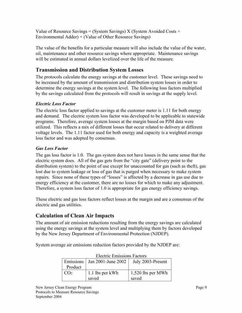
New Jersey Clean Energy Program Page 9 Protocols to Measure Resource Savings September 2004

Value of Resource Savings = (System Savings) X (System Avoided Costs + Environmental Adder) + (Value of Other Resource Savings) The value of the benefits for a particular measure will also include the value of the water, oil, maintenance and other resource savings where appropriate. Maintenance savings will be estimated in annual dollars levelized over the life of the measure.

Transmission and Distribution System Losses The protocols calculate the energy savings at the customer level. These savings need to be increased by the amount of transmission and distribution system losses in order to determine the energy savings at the system level. The following loss factors multiplied by the savings calculated from the protocols will result in savings at the supply level.

Electric Loss Factor The electric loss factor applied to savings at the customer meter is 1.11 for both energy and demand. The electric system loss factor was developed to be applicable to statewide programs. Therefore, average system losses at the margin based on PJM data were utilized. This reflects a mix of different losses that occur related to delivery at different voltage levels. The 1.11 factor used for both energy and capacity is a weighted average loss factor and was adopted by consensus.

Gas Loss Factor The gas loss factor is 1.0. The gas system does not have losses in the same sense that the electric system does. All of the gas gets from the “city gate” (delivery point to the distribution system) to the point of use except for unaccounted for gas (such as theft), gas lost due to system leakage or loss of gas that is purged when necessary to make system repairs. Since none of these types of “losses” is affected by a decrease in gas use due to energy efficiency at the customer, there are no losses for which to make any adjustment. Therefore, a system loss factor of 1.0 is appropriate for gas energy efficiency savings. These electric and gas loss factors reflect losses at the margin and are a consensus of the electric and gas utilities.

Calculation of Clean Air Impacts The amount of air emission reductions resulting from the energy savings are calculated using the energy savings at the system level and multiplying them by factors developed by the New Jersey Department of Environmental Protection (NJDEP). System average air emissions reduction factors provided by the NJDEP are:

Electric Emissions Factors Emissions Product

Jan 2001-June 2002 July 2003-Present

CO2 1.1 lbs per kWh saved

1,520 lbs per MWh saved

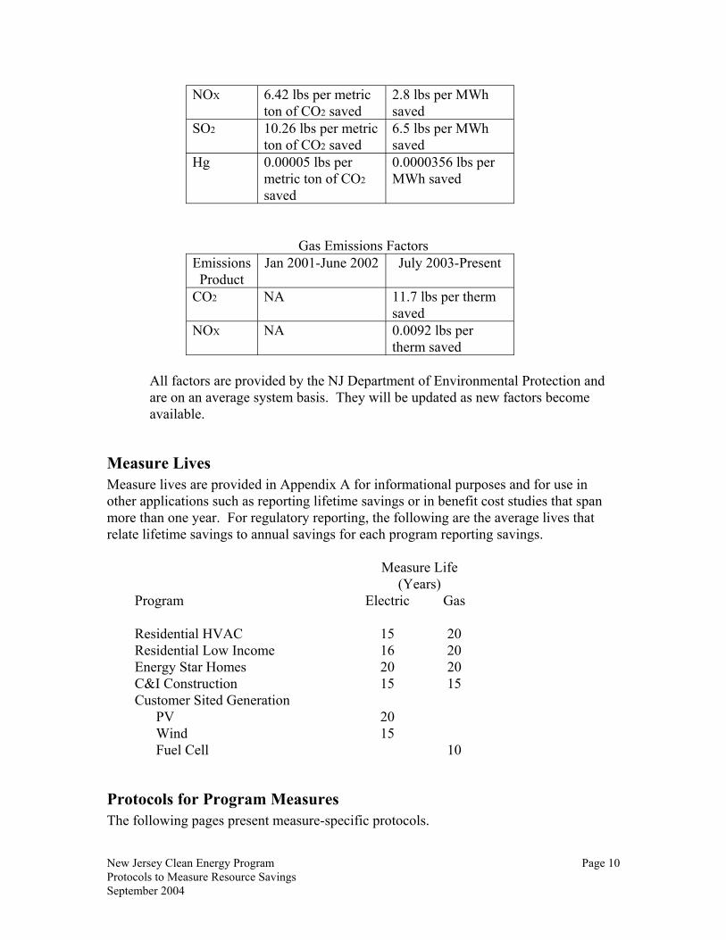
New Jersey Clean Energy Program Page 10 Protocols to Measure Resource Savings September 2004

NOX 6.42 lbs per metric ton of CO2 saved

2.8 lbs per MWh saved

SO2 10.26 lbs per metric ton of CO2 saved

6.5 lbs per MWh saved

Hg 0.00005 lbs per metric ton of CO2 saved

0.0000356 lbs per MWh saved

Gas Emissions Factors Emissions Product

Jan 2001-June 2002 July 2003-Present

CO2 NA 11.7 lbs per therm saved

NOX NA 0.0092 lbs per therm saved

All factors are provided by the NJ Department of Environmental Protection and are on an average system basis. They will be updated as new factors become available.

Measure Lives Measure lives are provided in Appendix A for informational purposes and for use in other applications such as reporting lifetime savings or in benefit cost studies that span more than one year. For regulatory reporting, the following are the average lives that relate lifetime savings to annual savings for each program reporting savings.

Measure Life (Years)

Program Electric Gas Residential HVAC 15 20 Residential Low Income 16 20 Energy Star Homes 20 20 C&I Construction 15 15 Customer Sited Generation PV Wind Fuel Cell

20 15

10

Protocols for Program Measures The following pages present measure-specific protocols.

New Jersey Clean Energy Program Page 11 Protocols to Measure Resource Savings September 2004

Residential Electric HVAC

Protocols The measurement plan for residential high efficiency cooling and heating equipment is based on algorithms that determine a central air conditioner’s or heat pump’s cooling/heating energy use and peak demand. Input data is based both on fixed assumptions and data supplied from the high efficiency equipment rebate application form. The algorithms also include the calculation of additional energy and demand savings due to the required proper sizing and installation of high efficiency units. The savings will be allocated to summer/winter and on-peak/off-peak time periods based on load shapes from measured data and industry sources. The allocation factors are documented below in the input value table. The protocols applicable for this program measure the energy savings directly related to the more efficient hardware installation. Estimates of energy savings due to the proper sizing of the equipment and improved installation practices are also included. The following is an explanation of the algorithms used and the nature and source of all required input data. Algorithms

Central Air Conditioner (A/C) & Air Source Heat Pump (ASHP) Cooling Energy Consumption and Peak Demand Savings – Central A/C & ASHP Energy Impact (kWh) = CAPY/1000 X (1/SEERb – (1/SEERq X (1-ESF))) X EFLH

Peak Demand Impact (kW) = CAPY/1000 X (1/EERb – (1/EERq X (1-DSF))) X CF

Heating Energy Savings – ASHP

Energy Impact (kWh) = CAPY/1000 X (1/HSPFb – (1/HSPFq X (1-ESF))) X EFLH

Ground Source Heat Pumps (GSHP) Cooling Energy (kWh) Savings = CAPY/1000 X (1/SEERb – (1/EERg X GSER)) X EFLH Heating Energy (kWh) Savings = CAPY/1000 X (1/HSPFb – (1/COPg X GSOP)) X EFLH

New Jersey Clean Energy Program Page 12 Protocols to Measure Resource Savings September 2004

Peak Demand Impact (kW) = CAPY/1000 X (1/EERb – (1/EERg X GSPK)) X CF

GSHP Desuperheater Energy (kWh) Savings = EDSH Peak Demand Impact (kW) = PDSH

Definition of Terms CAPY = The cooling capacity (output) of the central air conditioner or heat pump being installed. This data is obtained from the Application Form based on the model number. SEERb = The Seasonal Energy Efficiency Ratio of the Baseline Unit. SEERq = The Seasonal Energy Efficiency Ratio of the qualifying unit being installed. This data is obtained from the Application Form based on the model number. EERb = The Energy Efficiency Ratio of the Baseline Unit. EERq = The Energy Efficiency Ratio of the unit being installed. This data is obtained from the Application Form based on the model number. EERg = The EER of the ground source heat pump being installed. Note that EERs of GSHPs are measured differently than EERs of air source heat pumps (focusing on entering water temperatures rather than ambient air temperatures). The equivalent SEER of a GSHP can be estimated by multiplying EERg by 1.02. GSER = The factor to determine the SEER of a GSHP based on its EERg. EFLH = The Equivalent Full Load Hours of operation for the average unit. ESF = The Energy Sizing Factor or the assumed saving due to proper sizing and proper installation. CF = The coincidence factor which equates the installed unit’s connected load to its demand at time of system peak. DSF = The Demand Sizing Factor or the assumed peak demand capacity saved due to proper sizing and proper installation. HSPFb = The Heating Seasonal Performance Factor of the Baseline Unit. HSPFq = The Heating Seasonal Performance Factor of the unit being installed. This data is obtained from the Application Form. COPg = Coefficient of Performance. This is a measure of the efficiency of a heat pump.

New Jersey Clean Energy Program Page 13 Protocols to Measure Resource Savings September 2004

GSOP = The factor to determine the HSPF of a GSHP based on its COPg. GSPK = The factor to convert EERg to the equivalent EER of an air conditioner to enable comparisons to the baseline unit. EDSH = Assumed savings per desuperheater. PDSH = Assumed peak demand savings per desuperheater. The 1000 used in the denominator is used to convert watts to kilowatts. A summary of the input values and their data sources follows:

Residential Electric HVAC Component Type Value Sources CAPY Variable Rebate

Application SEERb Fixed Baseline = 10 1 SEERq Variable Rebate

Application EERb Fixed Baseline = 9.2 2 EERq Variable Rebate

Application EERg Variable Rebate

Application GSER Fixed 1.02 3 EFLH Fixed Cooling = 600 Hours

Heating = 2250 Hours 4

ESF Fixed 17% 5 CF Fixed 70% 6 DSF Fixed 7% 7 HSPFb Fixed Baseline = 6.8 8 HSPFq Variable Rebate

Application COPg Variable Rebate

Application GSOP Fixed 3.413 9 GSPK Fixed 0.8416 10 EDSH Fixed 1842 kWh 11 PDSH Fixed 0.34 kW 12

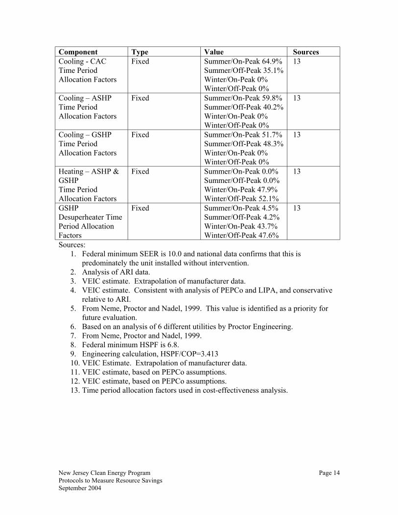
New Jersey Clean Energy Program Page 14 Protocols to Measure Resource Savings September 2004

Component Type Value Sources Cooling - CAC Time Period Allocation Factors

Fixed Summer/On-Peak 64.9% Summer/Off-Peak 35.1% Winter/On-Peak 0% Winter/Off-Peak 0%

13

Cooling – ASHP Time Period Allocation Factors

Fixed Summer/On-Peak 59.8% Summer/Off-Peak 40.2% Winter/On-Peak 0% Winter/Off-Peak 0%

13

Cooling – GSHP Time Period Allocation Factors

Fixed Summer/On-Peak 51.7% Summer/Off-Peak 48.3% Winter/On-Peak 0% Winter/Off-Peak 0%

13

Heating – ASHP & GSHP Time Period Allocation Factors

Fixed Summer/On-Peak 0.0% Summer/Off-Peak 0.0% Winter/On-Peak 47.9% Winter/Off-Peak 52.1%

13

GSHP Desuperheater Time Period Allocation Factors

Fixed Summer/On-Peak 4.5% Summer/Off-Peak 4.2% Winter/On-Peak 43.7% Winter/Off-Peak 47.6%

13

Sources: 1. Federal minimum SEER is 10.0 and national data confirms that this is

predominately the unit installed without intervention. 2. Analysis of ARI data. 3. VEIC estimate. Extrapolation of manufacturer data. 4. VEIC estimate. Consistent with analysis of PEPCo and LIPA, and conservative

relative to ARI. 5. From Neme, Proctor and Nadel, 1999. This value is identified as a priority for

future evaluation. 6. Based on an analysis of 6 different utilities by Proctor Engineering. 7. From Neme, Proctor and Nadel, 1999. 8. Federal minimum HSPF is 6.8. 9. Engineering calculation, HSPF/COP=3.413 10. VEIC Estimate. Extrapolation of manufacturer data. 11. VEIC estimate, based on PEPCo assumptions. 12. VEIC estimate, based on PEPCo assumptions. 13. Time period allocation factors used in cost-effectiveness analysis.

New Jersey Clean Energy Program Page 15 Protocols to Measure Resource Savings September 2004

Residential Gas HVAC

Protocols The following two algorithms detail savings for gas heating and water heating equipment. They are to be used to determine gas energy savings between baseline standard units and the high efficiency units promoted in the program. The input values are based on data on typical customers supplied by the gas utilities, an analysis by the Federal Energy Management Program (FEMP), and customer information on the application form, confirmed with manufacturer data. The energy values are in therms.

Space Heaters Algorithms Gas Savings = Capyq/Capyt X ((AFUEq – AFUEb)/AFUEq) X Baseline Heating Usage Definition of Variables Capyq = Actual output capacity of the qualifying heating system in Btus/hour Capyt = Output capacity of the typical heating unit output in Btus/hour AFUEq = Annual Fuel Utilization Efficiency of the qualifying energy efficient furnace or boiler AFUEb = Annual Fuel Utilization Efficiency of the baseline furnace or boiler Baseline Heating Usage = The weighted average annual heating usage (therms) of typical New Jersey heating customers

Space Heating

Component Type Value Source Capyq Variable Application Form,

confirmed with Manufacturer Data

Capyt Fixed 80,000 1 AFUEq Variable Application Form,

confirmed with Manufacturer Data

AFUEb Fixed Furnaces: 80% Boilers: 83%

2

Baseline Heating Usage

Fixed 965 therms 3

New Jersey Clean Energy Program Page 16 Protocols to Measure Resource Savings September 2004

Component Type Value Source Time Period

Allocation Factors Fixed Summer = 12%

Winter = 88%

4

Sources: 1. NJ utility analysis of heating customers, typical output capacity. 2. Based on the quantity of models available by efficiency ratings as listed in the

April 2003 Gamma Consumers Directory of Certified Efficiency Ratings. 3. NJ utility analysis of heating customers, annual gas heating usage. 4. Prorated based on 12% of the annual degree days falling in the summer period

and 88% of the annual degree days falling in the winter period.

Water Heaters Algorithms Gas Savings = ((EFq – EFb)/EFq) X Baseline Water Heater Usage Definition of Variables EFq = Energy factor of the qualifying energy efficient water heater. EFb = Energy factor of the baseline water heater. Baseline Water Heater Usage = Annual usage of the baseline water heater, in therms.

Water Heaters

Component Type Value Source Efq Variable Application Form,

confirmed with Manufacturer Data

Efb Fixed 0.544 1 Baseline Water Heater Usage

Fixed 277

2

Time Period Allocation Factors

Fixed Summer = 50% Winter = 50%

3

Sources: 1. Federal EPACT Standard for a 40 gallon gas water heater. Calculated as 0.62 –

(0.0019 X gallons of capacity). 2. DOE/FEMP website. http://www.eren.doe.gov/femp/pro 3. Prorated based on 6 months in the summer period and 6 months in the winter

period.

New Jersey Clean Energy Program Page 17 Protocols to Measure Resource Savings September 2004

Residential Energy Star Windows

Protocols The general form of the equation for the ENERGY STAR or other high efficiency windows energy savings algorithms is: Square Feet of Window Area X Savings per Square Foot To determine resource savings, the per square foot estimates in the protocols will be multiplied by the number of square feet of window area. The number of square feet of window area will be determined using market assessments and market tracking. Some of these market tracking mechanisms are under development. The per unit energy and demand savings estimates are based on prior building simulations of windows.

ENERGY STAR Windows Savings estimates for ENERGY STAR Windows are based on modeling a typical 2,500 square foot home using REM Rate, the home energy rating tool. Savings are per square foot of qualifying window area. Savings will vary based on heating and cooling system type and fuel. These fuel and HVAC system market shares will need to be estimated from prior market research efforts or from future program evaluation results. Heat Pump Electricity Impact (kWh) = ESavHP Demand Impact (kW) = DSavHP x CF Gas Heat/CAC Electricity Impact (kWh) = ESavGAS/CAC Demand Impact (kW) = DSavCAC x CF Gas Impact (therms) = GSavGAS Gas Heat/No CAC Electricity Impact (kWh) = ESavGAS/NOCAC Demand Impact (kW) = DSavNOCAC x CF Gas Impact (therms) = GSavGAS

New Jersey Clean Energy Program Page 18 Protocols to Measure Resource Savings September 2004

Oil Heat/CAC Electricity Impact (kWh) = ESavOIL/CAC Demand Impact (kW) = DSavCAC x CF Oil Impact (MMBtu) = OSavOIL Oil Heat/No CAC Electricity Impact (kWh) = ESavOIL/NOCAC Demand Impact (kW) = DSavNOCAC x CF Oil Impact (MMBtu) = OSavOIL Electric Heat/CAC Electricity Impact (kWh) = ESavRES/CAC Demand Impact (kW) = DSavCAC x CF Electric Heat/No CAC Electricity Impact (kWh) = ESavRES/NOCAC Demand Impact (kW) = DSavNOCAC x CF Definition of Terms ESavHP = Electricity savings (heating and cooling) with heat pump installed. ESavGAS/CAC = Electricity savings with gas heating and central AC installed. ESavGAS/NOCAC = Electricity savings with gas heating and no central AC installed. ESavOIL/CAC = Electricity savings with oil heating and central AC installed. ESavOIL/NOCAC = Electricity savings with oil heating and no central AC installed. ESavRES/CAC = Electricity savings with electric resistance heating and central AC installed. ESavRES/NOCAC = Electricity savings with electric resistance heating and no central AC installed.

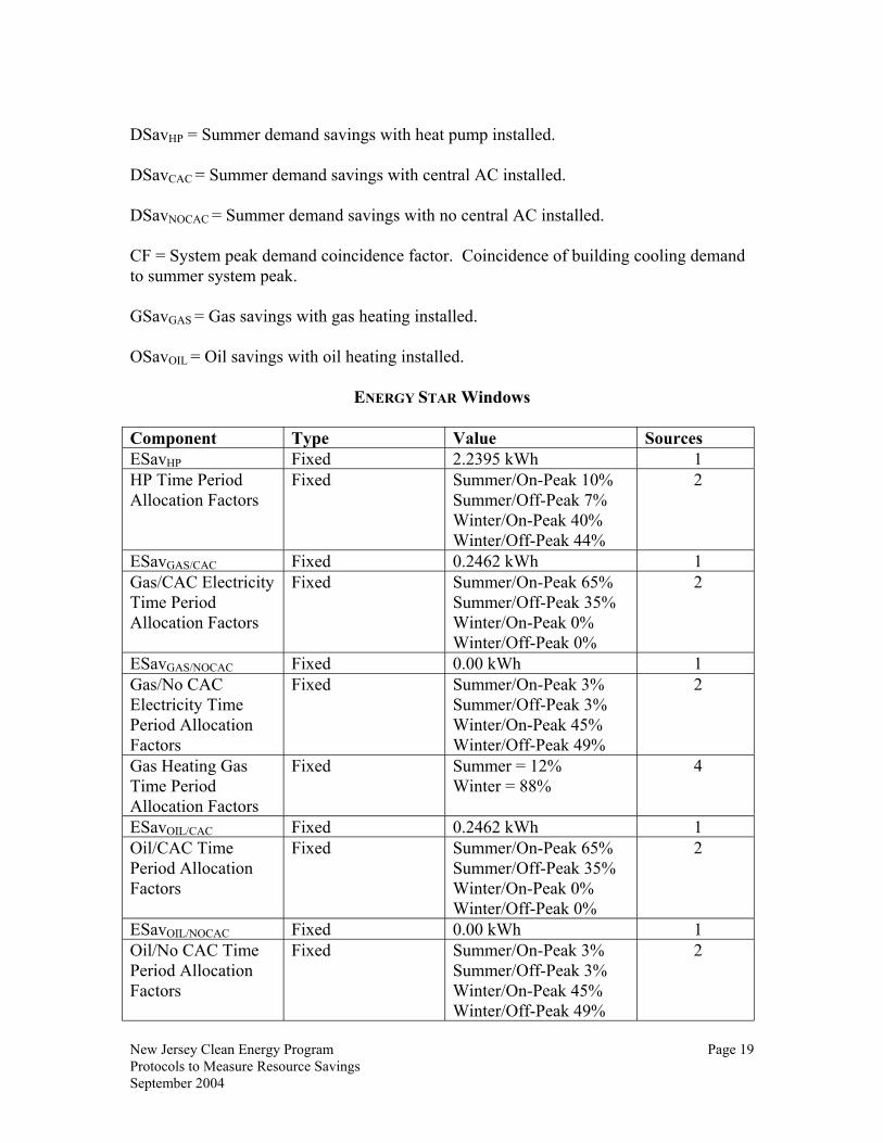
New Jersey Clean Energy Program Page 19 Protocols to Measure Resource Savings September 2004

DSavHP = Summer demand savings with heat pump installed. DSavCAC = Summer demand savings with central AC installed. DSavNOCAC = Summer demand savings with no central AC installed. CF = System peak demand coincidence factor. Coincidence of building cooling demand to summer system peak. GSavGAS = Gas savings with gas heating installed. OSavOIL = Oil savings with oil heating installed.

ENERGY STAR Windows Component Type Value Sources ESavHP Fixed 2.2395 kWh 1 HP Time Period Allocation Factors

Fixed Summer/On-Peak 10% Summer/Off-Peak 7% Winter/On-Peak 40% Winter/Off-Peak 44%

2

ESavGAS/CAC Fixed 0.2462 kWh 1 Gas/CAC Electricity Time Period Allocation Factors

Fixed Summer/On-Peak 65% Summer/Off-Peak 35% Winter/On-Peak 0% Winter/Off-Peak 0%

2

ESavGAS/NOCAC Fixed 0.00 kWh 1 Gas/No CAC Electricity Time Period Allocation Factors

Fixed Summer/On-Peak 3% Summer/Off-Peak 3% Winter/On-Peak 45% Winter/Off-Peak 49%

2

Gas Heating Gas Time Period Allocation Factors

Fixed Summer = 12% Winter = 88%

4

ESavOIL/CAC Fixed 0.2462 kWh 1 Oil/CAC Time Period Allocation Factors

Fixed Summer/On-Peak 65% Summer/Off-Peak 35% Winter/On-Peak 0% Winter/Off-Peak 0%

2

ESavOIL/NOCAC Fixed 0.00 kWh 1 Oil/No CAC Time Period Allocation Factors

Fixed Summer/On-Peak 3% Summer/Off-Peak 3% Winter/On-Peak 45% Winter/Off-Peak 49%

2

New Jersey Clean Energy Program Page 20 Protocols to Measure Resource Savings September 2004

Component Type Value Sources ESavRES/CAC Fixed 4.0 kWh 1 Res/CAC Time Period Allocation Factors

Fixed Summer/On-Peak 10% Summer/Off-Peak 7% Winter/On-Peak 40% Winter/Off-Peak 44%

2

ESavRES/NOCAC Fixed 3.97 kWh 1 Res/No CAC Time Period Allocation Factors

Fixed Summer/On-Peak 3% Summer/Off-Peak 3% Winter/On-Peak 45% Winter/Off-Peak 49%

2

DSavHP Fixed 0.000602 kW 1 DSavCAC Fixed 0.000602 kW 1 DSavNOCAC Fixed 0.00 kW 1 GSavGAS Fixed 0.169 therms 1 OSavOIL Fixed 0.0169 MMBtu 1 CF Fixed 0.75 3 Sources:

1. From REMRATE Modeling of a typical 2,500 sq. ft. NJ home. Savings expressed on a per sq. ft. of window area basis. New Brunswick climate data.

2. Time period allocation factors used in cost-effectiveness analysis. 3. Based on reduction in peak cooling load. 4. Prorated based on 12% of the annual degree days falling in the summer period

and 88% of the annual degree days falling in the winter period.

New Jersey Clean Energy Program Page 21 Protocols to Measure Resource Savings September 2004

Residential Low Income Program

Protocols The savings protocols for the low-income program are based upon estimated per unit installed savings. In some cases, such as lighting and refrigerators, the savings per unit estimate is based on direct observation or monitoring of the existing equipment being replaced. For other measures, for example air sealing and insulation, the protocols calculation is based on an average % savings of pre-treatment consumption. The protocols for space heating measures were established considering the non-additive nature of individual measures. Further, (for protocol reporting only) the cumulative savings from space conditioning measures is capped at 10% of pre-treatment electric space conditioning consumption and 15% of pre-treatment natural gas space conditioning consumption. Base Load Measures

Efficient Lighting Savings from installation of screw-in CFLs, high performance fixtures and fluorescent torchieres are based on a straightforward algorithm that calculates the difference between existing and new wattage, and the average daily hours of usage for the lighting unit being replaced. Algorithm

Compact Fluorescent Screw In Lamp

Electricity Impact (kWh) = ((CFLwatts) X (CFLhours X 365))/1000

Peak Demand Impact (kW) = (CFLwatts) X Light CF Efficient Fixtures

Electricity Impact (kWh) = ((Fixtwatts) X (Fixthours X 365))/1000

Peak Demand Impact (kW) = (Fixtwatts) X Light CF Efficient Torchieres

Electricity Impact (kWh) = ((Torchwatts) X (Torchhours X 365))/1000

Peak Demand Impact (kW) = (Torchwatts) X Light CF

Hot Water Conservation Measures The protocols savings estimates are based on an average package of domestic hot water measures typically installed by low-income programs.

New Jersey Clean Energy Program Page 22 Protocols to Measure Resource Savings September 2004

Algorithm

Electricity Impact (kWh) = HWeavg Gas Savings (MMBtu) = HWgavg Peak Demand Impact (kW) = HWwatts X HW CF Water Savings (gallons) = WS

Efficient Refrigerators The eligibility for refrigerator replacement is determined by comparing monitored consumption for the existing refrigerator with the rated consumption of the eligible replacement. Estimated savings are directly calculated based on the difference between these two values. Note that in the case where an under-utilized or unneeded refrigerator unit is removed, and no replacement is installed, the Refnew term of the equation will be zero. Algorithm

Electricity Impact (kWh) = Refold – Refnew

Peak Demand Impact (kW) = (Refold – Refnew) *(Ref DF)

Space Conditioning Measures Savings from individual space conditioning measures are affected by any other measures that also are being installed; i.e., such savings are not cumulative. Further, technical reasons dictate prioritizing certain measures over others. The savings algorithms for all space conditioning measures accommodate these considerations by presuming a fixed sequence of measure installation for the purpose of projecting savings and by limiting total estimated electric space conditioning savings to 10% of electric space conditioning pre-treatment usage. Fossil fuel heated houses typically have more substantial opportunities for space conditioning savings than electrically heated houses. Further, there are greater opportunities for interaction between measure types. For protocol reporting, these savings estimates will be capped at 15% of pre-treatment space heating consumption. When available, gas heat measure savings will be based on heating use. If only total gas use is known, heating use will be estimated as total use less 300 therms.

Air Sealing It is assumed that air sealing is the first priority among candidate space conditioning measures. Expected percentage savings is based on previous experiences with measured savings from similar programs. Note there are no summer coincident electric peak demand savings estimated at this time.

New Jersey Clean Energy Program Page 23 Protocols to Measure Resource Savings September 2004

Algorithm

Electricity Impact (kWh) = ESCpre X 0.05 MMBtu savings = (GHpre X 0.05)

Duct Sealing and Repair The second priority for homes with either Central Air Conditioning (CAC) or some other form of ducted distribution of electric space conditioning (electric furnace, gas furnace or heat pump) is ensuring integrity and effectiveness of the ducted distribution system. Algorithm With CAC

Electricity Impact (kWh) = (ECoolpre) X 0.10 Peak Demand Impact (kW) = (Ecoolpre X 0.10) / EFLH X AC CF MMBtu savings = (GHpre X 0.02)

No CAC Electricity Impact (kWh) = (ESCpre X 0.95) X 0.02 MMBtu savings = (GHpre X 0.02)

Insulation Up-Grades For savings calculations, it is assumed that any applicable air sealing and duct sealing/repair have been done, thereby reducing the space conditioning load, before consideration of upgrading insulation. Attic insulation savings are then projected on the basis of the “new” load. Gas savings are somewhat greater, as homes with gas heat generally have less insulation. Algorithm

Electricity Impact (kWh) = (ESCpre X 0.93) X 0.08 MMBtu savings = GHpre X 0.13

Thermostat Replacement Thermostats are eligible for consideration as an electric space conditioning measure only after the first three priority items. Savings projections are based on a conservative 3% of the “new” load after installation of any of the top three priority measures.

New Jersey Clean Energy Program Page 24 Protocols to Measure Resource Savings September 2004

Algorithm

Electricity Impact (kWh) = (ESCpre X 0.85) X 0.03 MMBtu savings = (GHpre X 0.03)

Heating and Cooling Equipment Maintenance Repair/Replacement Savings projections for heat pump charge and air flow correction. Protocol savings account for shell measures having been installed that reduce the pre-existing load. Algorithm

Electricity Impact (kWh) = (ESCpre X 0.93) X 0.17 Peak Demand Impact (kW) = (Capy/EER X 1000) X HP CF X DSF

Total Space Conditioning Savings As noted, for protocol reporting the total electric savings from all space conditioning measures are presumed to not exceed 10% of the pre-treatment consumption, and gas savings are presumed to not exceed 15% of pre-treatment space heating consumption. Algorithm

Maximum Electricity Impact (kWh) ≤ (ESCpre X 0.10) Maximum MMBtu savings = (GHpre X 0.15)

Other “Custom” Measures In addition to the typical measures for which savings algorithms have been developed, it is assumed that there will be niche opportunities that should be identified and addressed. The savings for these custom measures will be reported based on the individual calculations supplied with the reporting. As necessary the program working group will develop specific guidelines for frequent custom measures for use in reporting and contractor tracking. Definition of Terms CFLwatts = Average watts replaced for a CFL installation. CFLhours = Average daily burn time for CFL replacements. Fixtwatts = Average watts replaced for an efficient fixture installation.

New Jersey Clean Energy Program Page 25 Protocols to Measure Resource Savings September 2004

Fixthours = Average daily burn time for CFL replacements. Torchwatts = Average watts replaced for a Torchiere replacement. Torchhours = Average daily burn time for a Torchiere replacements. Light CF = Summer demand coincidence factor for all lighting measures. Currently fixed at 5%. HWeavg = Average electricity savings from typical electric hot water measure package. HWgavg = Average natural gas savings from typical electric hot water measure package. HWwatts = Connected load reduction for typical hot water efficiency measures HW CF = Summer demand coincidence factor for electric hot water measure package. Currently fixed at 75%. Refold = Annual energy consumption of existing refrigerator based on on-site monitoring. Refnew = Rated annual energy consumption of the new refrigerator. Ref DF = kW /kWh of savings. Refrigerator demand savings factor. Ref CF = Summer demand coincidence factor for refrigeration. Currently 100%, diversity accounted for in the Ref DF factor. ESCpre = Pre-treatment electric space conditioning consumption. ECoolpre = Pre-treatment electric cooling consumption.

EFLH = Equivalent full load hours of operation for the average unit. This value is

currently fixed at 650 hours. AC CF = Summer demand coincidence factor for air conditioning. Currently 85%. Capy = Capacity of Heat Pump in Btuh EER = Energy Efficiency Ratio of average heat pump receiving charge and air flow

service. Fixed at 9.2 HP CF = Summer demand coincidence factor for heat pump. Currently fixed at 70%. DSF = Demand savings factor for charge and air flow correction. Currently fixed at 7%. GCpre = Pre treatment gas consumption.

New Jersey Clean Energy Program Page 26 Protocols to Measure Resource Savings September 2004

GHpre = Pre treatment gas space heat consumption (=.GCpre less 300 therms if only total

gas use is known. WS = Water Savings associated with water conservation measures. Currently fixed at

3,640 gallons per year per home receiving low flow showerheads, plus 1,460 gallons saved per year per home receiving aerators.

Residential Low Income

Component Type Value Sources CFLWatts Fixed 42 Watts 1 CFLHours Fixed 2.5 hours 1 FixtWatts Fixed 90 Watts 1 FixtHours Fixed 3.5 hours 1 TorchWatts Fixed 245 Watts 1 TorchHours Fixed 3.5 hours 1 Light CF Fixed 5% 2 Elec. Water Heating Savings

Fixed 178 kWh 3

Gas Water Heating Savings

Fixed 1.01 MMBTU 3

WS Water Savings Fixed 3,640 gal/year per home receiving low flow shower heads, plus 1,460 gal/year per home receiving aerators.

12

HWwatts Fixed 0.022 kW 4 HW CF Fixed 75% 4 Refold Variable Contractor

Tracking Refnew Variable Contractor

Tracking and Manufacturer data

Ref DF Fixed 0.000139 kW/kWh savings

5

RefCF Fixed 100% 6 ESCpre Variable 7 Ecoolpre Variable 7 ELFH Fixed 650 hours 8 AC CF Fixed 85% 4 Capy Fixed 33,000 Btu/hr 1 EER Fixed 9.2 8 HP CF Fixed 70% 9

New Jersey Clean Energy Program Page 27 Protocols to Measure Resource Savings September 2004

Component Type Value Sources DSF Fixed 7% 10 GCpre Variable 7 GHpre Variable 7 Time Period Allocation Factors - Electric

Fixed Summer/On-Peak 21% Summer/Off-Peak 22% Winter/On-Peak 28% Winter/Off-Peak 29%

11

Time Period Allocation Factors - Gas

Fixed Heating: Summer 12% Winter 88% Non-Heating: Summer 50% Winter 50%

13

Sources/Notes: 1. Working group expected averages for product specific measures. 2. Efficiency Vermont Reference Manual – average for lighting products. 3. Experience with average hot water measure savings from low income and direct

install programs. 4. VEIC estimate. 5. UI Refrigerator Load Data profile, .16 kW (5pm July) and 1,147 kWh annual

consumption. 6. Diversity accounted for by Ref DF. 7. Billing histories and (for electricity) contractor calculations based on program

procedures for estimating space conditioning and cooling consumption. 8. Analysis of ARI data 9. Analysis of data from 6 utilities by Proctor Engineering 10. From Neme, Proctor and Nadel, 1999. 11. These allocations may change with actual penetration numbers are available. 12. VEIC estimate, assuming 1 GPM reduction for 14 five minute showers per week

for shower heads, and 4 gallons saved per day for aerators. 13. Heating: Prorated based on 12% of the annual degree days falling in the summer

period and 88% of the annual degree days falling in the winter period. Non-Heating: Prorated based on 6 months in the summer period and 6 months in the winter period.

New Jersey Clean Energy Program Page 28 Protocols to Measure Resource Savings September 2004

Residential New Construction Program

Protocols

Insulation Up-Grades, Efficient Windows, Air Sealing, Efficient HVAC Equipment, and Duct Sealing The energy savings due to the Residential New Construction Program will be a direct output of the home energy rating software. This software has a module that compares the energy characteristics of the energy efficient home to the baseline/reference home and calculates savings. The system peak electric demand savings will be calculated from the software output with the following algorithms then applied: Peak demand of the baseline home = (PLb X OFb) / (SEERb X BLEER X 1,000) Peak demand of the qualifying home = (PLq X OFq) / (EERq X 1,000)

Coincident system peak electric demand savings = (Peak demand of the baseline home – Peak demand of the qualifying home) X CF

Definition of Terms PLb = Peak load of the baseline home in Btuh. OFb = The oversizing factor for the HVAC unit in the baseline home. SEERb = The Seasonal Energy Efficiency Ratio of the baseline unit. BLEER = Factor to convert baseline SEERb to EERb. PLq = The actual predicted peak load for the program qualifying home constructed, in Btuh. OFq = The oversizing factor for the HVAC unit in the program qualifying home. EERq = The EER associated with the HVAC system in the qualifying home. CF = The coincidence factor which equates the installed HVAC system’s demand to its demand at time of system peak. In July 2002 energy code changes took place with the adoption of MEC 95. This code change affects baselines for variables used in the protocols. Therefore, to reflect these changes, tables and or values are identified as needed for installations completed during

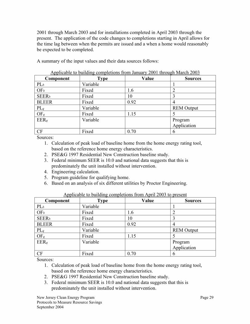
New Jersey Clean Energy Program Page 29 Protocols to Measure Resource Savings September 2004

2001 through March 2003 and for installations completed in April 2003 through the present. The application of the code changes to completions starting in April allows for the time lag between when the permits are issued and a when a home would reasonably be expected to be completed. A summary of the input values and their data sources follows:

Applicable to building completions from January 2001 through March 2003 Component Type Value Sources

PLb Variable 1 OFb Fixed 1.6 2 SEERb Fixed 10 3 BLEER Fixed 0.92 4 PLq Variable REM Output OFq Fixed 1.15 5 EERq Variable Program

Application CF Fixed 0.70 6 Sources:

1. Calculation of peak load of baseline home from the home energy rating tool, based on the reference home energy characteristics.

2. PSE&G 1997 Residential New Construction baseline study. 3. Federal minimum SEER is 10.0 and national data suggests that this is

predominately the unit installed without intervention. 4. Engineering calculation. 5. Program guideline for qualifying home. 6. Based on an analysis of six different utilities by Proctor Engineering.

Applicable to building completions from April 2003 to present

Component Type Value Sources PLb Variable 1 OFb Fixed 1.6 2 SEERb Fixed 10 3 BLEER Fixed 0.92 4 PLq Variable REM Output OFq Fixed 1.15 5 EERq Variable Program

Application CF Fixed 0.70 6 Sources:

1. Calculation of peak load of baseline home from the home energy rating tool, based on the reference home energy characteristics.

2. PSE&G 1997 Residential New Construction baseline study. 3. Federal minimum SEER is 10.0 and national data suggests that this is

predominately the unit installed without intervention.

New Jersey Clean Energy Program Page 30 Protocols to Measure Resource Savings September 2004

4. Engineering calculation. 5. Program guideline for qualifying home. 6. Based on an analysis of six different utilities by Proctor Engineering.

Lighting and Appliances Quantification of additional saving due to the addition of high efficiency light fixtures and clothes washers will be based on the algorithms presented for these appliances in the Energy Star Lighting Protocols and the Energy Star Appliances Protocols, respectively.

Ventilation Equipment Additional energy savings of 175 kWh and peak demand saving of 60 Watts will be added to the output of the home energy rating software to account for the installation of high efficiency ventilation equipment. These values are based on a baseline fan of 80 Watts and an efficient fan of 20 Watts running for 8 hours per day. The following table describes the characteristics of the three reference homes.

New Jersey Clean Energy Program Page 31 Protocols to Measure Resource Savings September 2004

New Jersey ENERGY STAR Homes REMRate User Defined Reference Homes -- Applicable to building completions from January 2001 through March 2003 Data Point Single Family Multiple Single Family Multifamily Active Solar None None None Ceiling Insulation R-30 R-30 R-30 Radiant Barrier None None None Rim/Band Joist R-13 R-13 R-13 Exterior Walls - Wood R-13 R-13 R-13 Exterior Walls - Steel R-7 effective R-7 effective R-7 effective Foundation Walls R-0 R-0 R-0 Doors R-2.6 R-2.6 R-2.6 Windows U=0.50, SHGC=0.60 U=0.50, SHGC=0.60 U=0.50, SHGC=0.60 Glass Doors U=0.50, SHGC=0.60 U=0.50, SHGC=0.60 U=0.50, SHGC=0.60 Skylights U=0.50, SHGC=0.60 U=0.50, SHGC=0.60 U=0.50, SHGC=0.60 Floor over Garage R-19 R-19 R-19 Floor over Unheated Basement R-0 R-0 R-0 Floor over Crawlspace R-19 R-19 R-19 Floor over Outdoor Air R-19 R-19 R-19 Unheated Slab on Grade R-0 edge/R-5 under R-0 edge/R-5 under R-0 edge/R-5 under Heated Slab on Grade R-0 edge/R-7 under R-0 edge/R-7 under R-0 edge/R-7 under Air Infiltration Rate 0.56 ACH winter/0.28 ACH summer 0.56 ACH winter/0.28 ACH summer 0.56 ACH winter/0.28 ACH summerDuct Leakage Observable Duct Leakage Observable Duct Leakage Observable Duct Leakage Mechanical Ventilation None None None Lights and Appliances Use Default Use Default Use Default Setback Thermostat Yes No No Heating Efficiency Furnace 80% AFUE 80% AFUE 80% AFUE Boiler 80% AFUE 80% AFUE 80% AFUE Combo Water Heater 76% AFUE (recovery efficiency) 76% AFUE (recovery efficiency) 76% AFUE (recovery efficiency) Air Source Heat Pump 5.4 HSPF 5.4 HSPF 5.4 HSPF Geothermal Heat Pump 2.8 COP open/3.0 COP closed 2.8 COP open/3.0 COP closed 2.8 COP open/3.0 COP closed

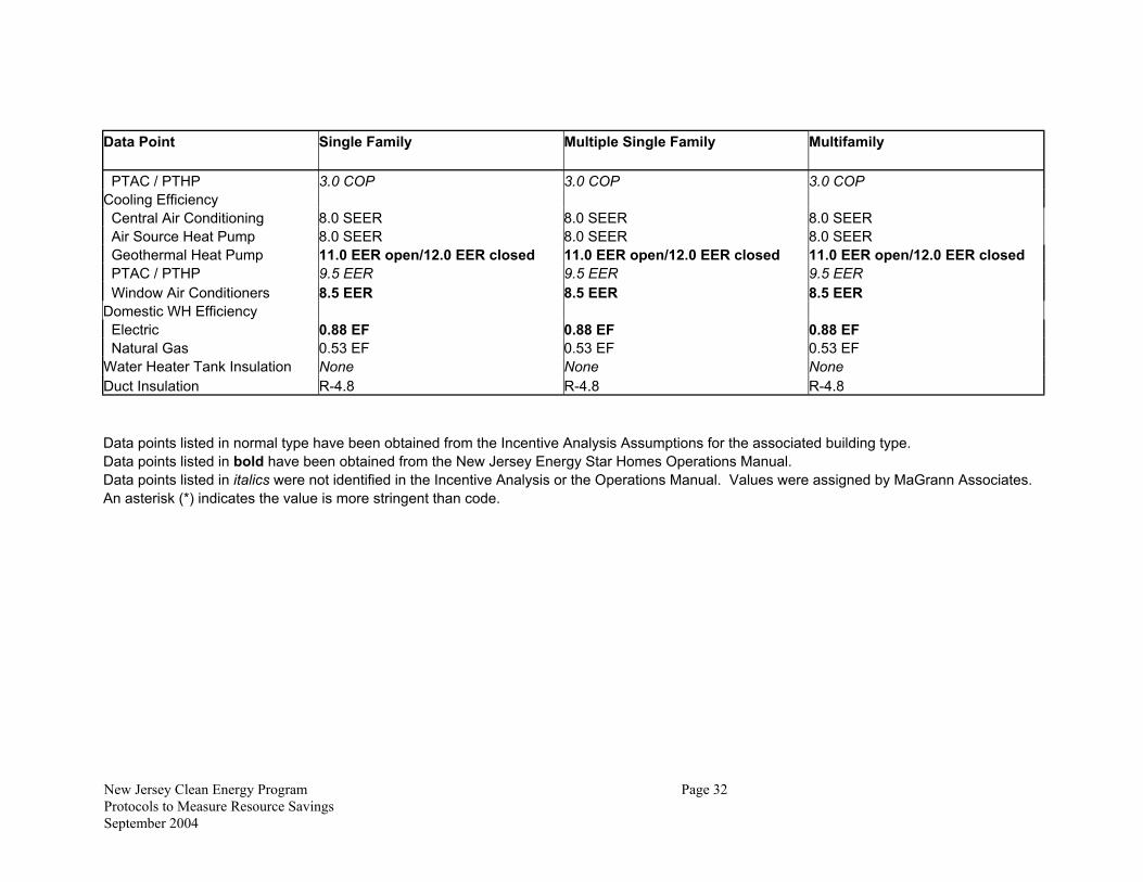
New Jersey Clean Energy Program Page 32 Protocols to Measure Resource Savings September 2004

Data Point Single Family Multiple Single Family Multifamily PTAC / PTHP 3.0 COP 3.0 COP 3.0 COP Cooling Efficiency Central Air Conditioning 8.0 SEER 8.0 SEER 8.0 SEER Air Source Heat Pump 8.0 SEER 8.0 SEER 8.0 SEER Geothermal Heat Pump 11.0 EER open/12.0 EER closed 11.0 EER open/12.0 EER closed 11.0 EER open/12.0 EER closed PTAC / PTHP 9.5 EER 9.5 EER 9.5 EER Window Air Conditioners 8.5 EER 8.5 EER 8.5 EER Domestic WH Efficiency Electric 0.88 EF 0.88 EF 0.88 EF Natural Gas 0.53 EF 0.53 EF 0.53 EF Water Heater Tank Insulation None None None Duct Insulation R-4.8 R-4.8 R-4.8 Data points listed in normal type have been obtained from the Incentive Analysis Assumptions for the associated building type. Data points listed in bold have been obtained from the New Jersey Energy Star Homes Operations Manual. Data points listed in italics were not identified in the Incentive Analysis or the Operations Manual. Values were assigned by MaGrann Associates. An asterisk (*) indicates the value is more stringent than code.

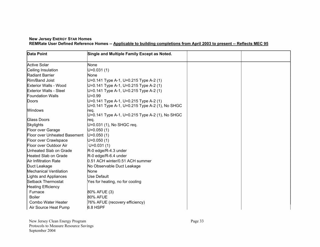
New Jersey Clean Energy Program Page 33 Protocols to Measure Resource Savings September 2004

New Jersey ENERGY STAR Homes REMRate User Defined Reference Homes -- Applicable to building completions from April 2003 to present -- Reflects MEC 95

Data Point Single and Multiple Family Except as Noted. Active Solar None Ceiling Insulation U=0.031 (1) Radiant Barrier None Rim/Band Joist U=0.141 Type A-1, U=0.215 Type A-2 (1) Exterior Walls - Wood U=0.141 Type A-1, U=0.215 Type A-2 (1) Exterior Walls - Steel U=0.141 Type A-1, U=0.215 Type A-2 (1) Foundation Walls U=0.99 Doors U=0.141 Type A-1, U=0.215 Type A-2 (1)

Windows U=0.141 Type A-1, U=0.215 Type A-2 (1), No SHGC req.

Glass Doors U=0.141 Type A-1, U=0.215 Type A-2 (1), No SHGC req.

Skylights U=0.031 (1), No SHGC req. Floor over Garage U=0.050 (1) Floor over Unheated Basement U=0.050 (1) Floor over Crawlspace U=0.050 (1) Floor over Outdoor Air U=0.031 (1) Unheated Slab on Grade R-0 edge/R-4.3 under Heated Slab on Grade R-0 edge/R-6.4 under Air Infiltration Rate 0.51 ACH winter/0.51 ACH summer Duct Leakage No Observable Duct Leakage Mechanical Ventilation None Lights and Appliances Use Default Setback Thermostat Yes for heating, no for cooling Heating Efficiency Furnace 80% AFUE (3) Boiler 80% AFUE Combo Water Heater 76% AFUE (recovery efficiency) Air Source Heat Pump 6.8 HSPF

New Jersey Clean Energy Program Page 34 Protocols to Measure Resource Savings September 2004

Data Point Single and Multiple Family Except as Noted. Geothermal Heat Pump Open not modeled, 3.0 COP closed PTAC / PTHP Not differentiated from air source HP Cooling Efficiency Central Air Conditioning 10.0 SEER Air Source Heat Pump 10.0 SEER Geothermal Heat Pump 3.4 COP (11.6 EER) PTAC / PTHP Not differentiated from central AC Window Air Conditioners Not differentiated from central AC Domestic WH Efficiency Electric 0.86 EF (4) Natural Gas 0.53 EF (4) Water Heater Tank Insulation None Duct Insulation N/A Notes: (1) Varies with heating degree-days (“HHD”). Above value reflects 5000 HDD average for New Jersey.

U values represent total wall system U value, including all components (i.e., clear wall, windows, doors). Type A-1 - Detached one and two family dwellings. Type A-2 - All other residential buildings, three stories in height or less.

(2) Closest approximation to MEC 95 requirements given the limitations of REM/Rate UDRH scripting language. (3) MEC 95 minimum requirement is 78 AFUE. However, 80 AFUE is adopted for New Jersey based on typical minimum availability and practice.(4) Size dependent. 50 gallon assumed.

New Jersey Clean Energy Program Page 35 Protocols to Measure Resource Savings September 2004

Residential Retrofit Program

Protocols No protocol was developed to measure energy savings for this program. The purpose of the program is to provide information and tools that residential customers can use to make decisions about what actions to take to improve energy efficiency in their homes. Many measure installations that are likely to produce significant energy savings are covered in other CRA programs. These savings are captured in the measured savings for those programs. The savings produced by this program that are not captured in other CRA programs would be difficult to isolate and relatively expensive to measure.

New Jersey Clean Energy Program Page 36 Protocols to Measure Resource Savings September 2004

Residential ENERGY STAR Lighting

Protocols See the protocols for efficient lighting savings under the Residential Low Income program. ENERGY STAR CFL Bulbs Same as Compact Flourescent Screw In Lamp. ENERGY STAR Torchieres Same as Efficient Torchieres ENERGY STAR Recessed Cans Same as Efficient Fixtures. ENERGY STAR Fixtures(Other) Same as Efficient Fixtures.

New Jersey Clean Energy Program Page 37 Protocols to Measure Resource Savings September 2004

Residential ENERGY STAR Appliances

Protocols The general form of the equation for the ENERGY STAR Appliance Program measure savings algorithms is: Number of Units X Savings per Unit To determine resource savings, the per unit estimates in the protocols will be multiplied by the number of appliance units. The number of units will be determined using market assessments and market tracking. Some of these market tracking mechanisms are under development. Per unit savings estimates are derived primarily from a 2000 Market Update Report by RLW for National Grid’s appliance program and from previous NEEP screening tool assumptions (clothes washers). Note that the pre-July 2001 refrigerator measure has been deleted given the timing of program implementation. As no field results are expected until July 2001, there was no need to quantify savings relative to the pre-July 2001 efficiency standards improvement for refrigerators.

ENERGY STAR Refrigerators Electricity Impact (kWh) = ESavREF Demand Impact (kW) = DSavREF x CFREF

ENERGY STAR Clothes Washers Electricity Impact (kWh) = ESavCW Demand Impact (kW) = DSavCW x CFCW Gas Impact (MMBtu) = EGSavCW Oil Impact (MMBtu) = OSavCW Water Impact (gallons) = WSavCW

ENERGY STAR Dishwashers Electricity Impact (kWh) = ESavDW Demand Impact (kW) = DSavREF x CFDW Gas Impact (MMBtu) = EGSavDW Oil Impact (MMBtu) = OsavDW

New Jersey Clean Energy Program Page 38 Protocols to Measure Resource Savings September 2004

Water Impact (gallons) = WSavDW

ENERGY STAR Room Air Conditioners Electricity Impact (kWh) = ESavRAC Demand Impact (kW) = DSavRAC x CFRAC Definition of Terms ESavREF = Electricity savings per purchased ENERGY STAR refrigerator. DSavREF = Summer demand savings per purchased ENERGY STAR refrigerator. ESavCW = Electricity savings per purchased ENERGY STAR clothes washer. DSavCW = Summer demand savings per purchased ENERGY STAR clothes washer. WSavCW = Water savings per purchased clothes washer. ESavDW = Electricity savings per purchased ENERGY STAR dishwasher. DSavDW = Summer demand savings per purchased ENERGY STAR dishwasher. WsavDW = Water savings per purchased dishwasher. ESavRAC = Electricity savings per purchased ENERGY STAR room AC. DSavRAC = Summer demand savings per purchased ENERGY STAR room AC. CFREF, CFCW, CFDW, CFRAC = Summer demand coincidence factor. The coincidence of average appliance demand to summer system peak equals 1 for demand impacts for all appliances reflecting embedded coincidence in the DSav factor except for room air conditioners where the CF is 58%.

ENERGY STAR Appliances Component Type Value Sources ESavREF Fixed 48 kWh 1 DSavREF Fixed 0.0066 kW 1 REF Time Period Allocation Factors

Fixed Summer/On-Peak 20.9% Summer/Off-Peak 21.7% Winter/On-Peak 28.0% Winter/Off-Peak 29.4%

2

ESavCW Fixed 201 kWh 3 GsavCW Fixed 10.6 therms 3

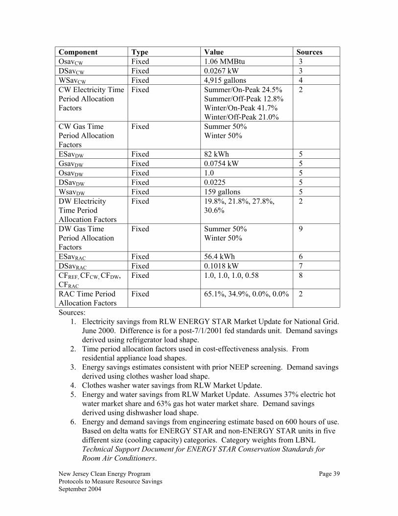
New Jersey Clean Energy Program Page 39 Protocols to Measure Resource Savings September 2004

Component Type Value Sources OsavCW Fixed 1.06 MMBtu 3 DSavCW Fixed 0.0267 kW 3 WSavCW Fixed 4,915 gallons 4 CW Electricity Time Period Allocation Factors

Fixed Summer/On-Peak 24.5% Summer/Off-Peak 12.8% Winter/On-Peak 41.7% Winter/Off-Peak 21.0%

2

CW Gas Time Period Allocation Factors

Fixed Summer 50% Winter 50%

ESavDW Fixed 82 kWh 5 GsavDW Fixed 0.0754 kW 5 OsavDW Fixed 1.0 5 DSavDW Fixed 0.0225 5 WsavDW Fixed 159 gallons 5 DW Electricity Time Period Allocation Factors

Fixed 19.8%, 21.8%, 27.8%, 30.6%

2

DW Gas Time Period Allocation Factors

Fixed Summer 50% Winter 50%

9

ESavRAC Fixed 56.4 kWh 6 DSavRAC Fixed 0.1018 kW 7 CFREF, CFCW, CFDW, CFRAC

Fixed 1.0, 1.0, 1.0, 0.58 8

RAC Time Period Allocation Factors

Fixed 65.1%, 34.9%, 0.0%, 0.0% 2

Sources: 1. Electricity savings from RLW ENERGY STAR Market Update for National Grid.

June 2000. Difference is for a post-7/1/2001 fed standards unit. Demand savings derived using refrigerator load shape.

2. Time period allocation factors used in cost-effectiveness analysis. From residential appliance load shapes.

3. Energy savings estimates consistent with prior NEEP screening. Demand savings derived using clothes washer load shape.

4. Clothes washer water savings from RLW Market Update. 5. Energy and water savings from RLW Market Update. Assumes 37% electric hot

water market share and 63% gas hot water market share. Demand savings derived using dishwasher load shape.

6. Energy and demand savings from engineering estimate based on 600 hours of use. Based on delta watts for ENERGY STAR and non-ENERGY STAR units in five different size (cooling capacity) categories. Category weights from LBNL Technical Support Document for ENERGY STAR Conservation Standards for Room Air Conditioners.

New Jersey Clean Energy Program Page 40 Protocols to Measure Resource Savings September 2004

7. Average demand savings based on engineering estimate. 8. Coincidence factors already embedded in summer peak demand reduction

estimates with the exception of RAC. RAC CF is based on data from PEPCO. 9. Prorated based on 6 months in the summer period and 6 months in the winter

period.

New Jersey Clean Energy Program Page 41 Protocols to Measure Resource Savings September 2004

Commercial and Industrial Energy Efficient Construction

C&I Electric Protocols

Baselines and Code Changes All baselines are designed to reflect an improvement over market practice defined by baselines, which are generally the higher of code or available equipment, that are updated periodically to reflect upgrades in code, or information from evaluation results. Baseline data reflect ASHRAE 90.1 1989 for program commitments made prior to July 16, 2002 and ASHRAE 90.1 1999 for commitments starting on July 16, 2002.

Lighting Equipment With the exception of small commercial lighting, savings are calculated using market-driven assumptions for new construction, renovation, remodeling, or equipment replacement that presume a decision to upgrade the lighting system. For small commercial lighting, the most efficient T-12 lamp and magnetic ballast fixture serves as the baseline. This approach is different from earlier protocols that referenced pre-existing lighting connected load. Lighting equipment includes fluorescent fixtures, ballasts, compact fluorescent fixtures, exit signs, and metal halide lamps. The measurement of energy savings is based on algorithms with measurement of key variables (i.e., Coincidence Factor and Operating Hours) through end-use metering data accumulated from a large sample of participating facilities from 1995 through 1999. Algorithms Demand Savings = ∆kW X CF X (1+IF) Energy Savings = ∆kW X EFLH X (1+IF) ∆kW is calculated from example worksheet below:

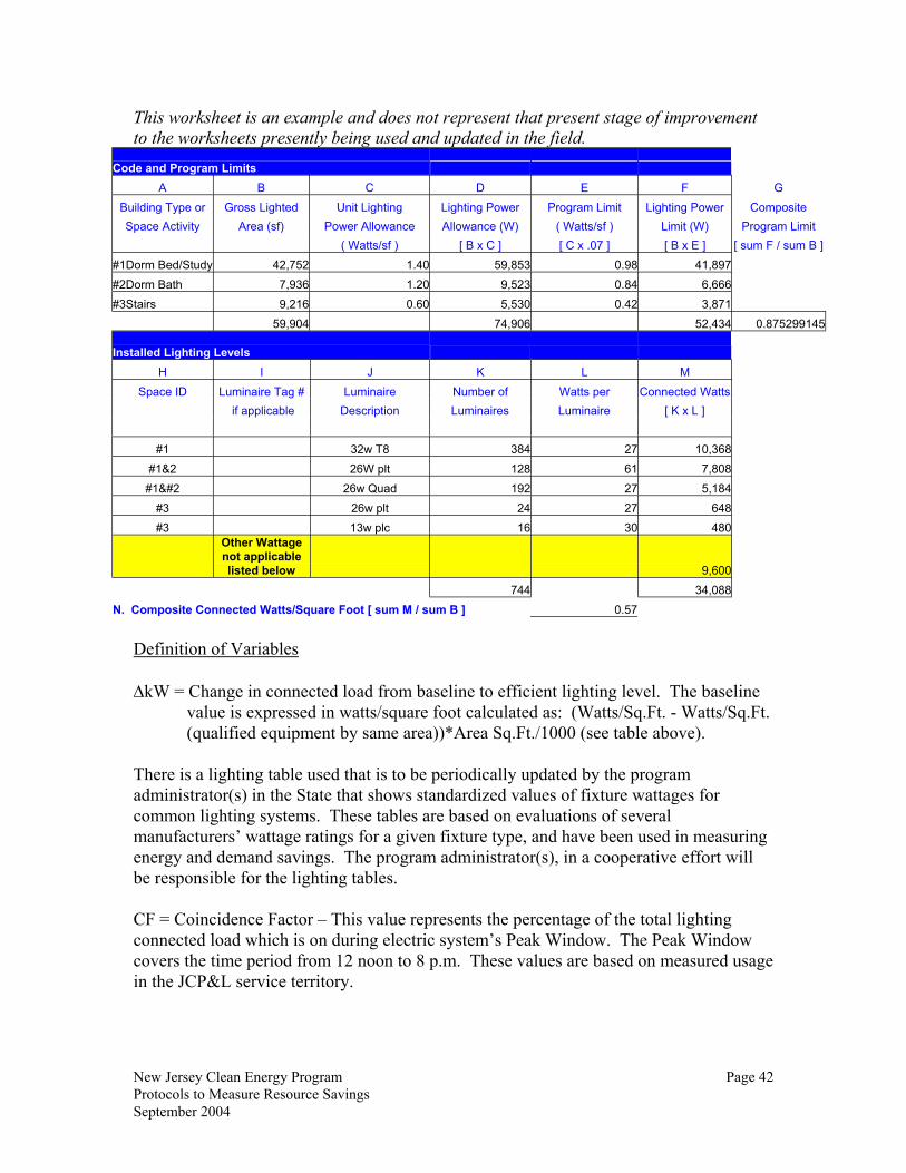
New Jersey Clean Energy Program Page 42 Protocols to Measure Resource Savings September 2004

This worksheet is an example and does not represent that present stage of improvement to the worksheets presently being used and updated in the field.

Code and Program Limits A B C D E F G

Building Type or Gross Lighted Unit Lighting Lighting Power Program Limit Lighting Power Composite Space Activity Area (sf) Power Allowance Allowance (W) ( Watts/sf ) Limit (W) Program Limit

( Watts/sf ) [ B x C ] [ C x .07 ] [ B x E ] [ sum F / sum B ]#1Dorm Bed/Study 42,752 1.40 59,853 0.98 41,897 #2Dorm Bath 7,936 1.20 9,523 0.84 6,666 #3Stairs 9,216 0.60 5,530 0.42 3,871 59,904 74,906 52,434 0.875299145 Installed Lighting Levels

H I J K L M Space ID Luminaire Tag # Luminaire Number of Watts per Connected Watts

if applicable Description Luminaires Luminaire [ K x L ]

#1 32w T8 384 27 10,368 #1&2 26W plt 128 61 7,808

#1&#2 26w Quad 192 27 5,184 #3 26w plt 24 27 648 #3 13w plc 16 30 480

Other Wattage not applicable listed below 9,600

744 34,088 N. Composite Connected Watts/Square Foot [ sum M / sum B ] 0.57

Definition of Variables ∆kW = Change in connected load from baseline to efficient lighting level. The baseline

value is expressed in watts/square foot calculated as: (Watts/Sq.Ft. - Watts/Sq.Ft. (qualified equipment by same area))*Area Sq.Ft./1000 (see table above).

There is a lighting table used that is to be periodically updated by the program administrator(s) in the State that shows standardized values of fixture wattages for common lighting systems. These tables are based on evaluations of several manufacturers’ wattage ratings for a given fixture type, and have been used in measuring energy and demand savings. The program administrator(s), in a cooperative effort will be responsible for the lighting tables. CF = Coincidence Factor – This value represents the percentage of the total lighting connected load which is on during electric system’s Peak Window. The Peak Window covers the time period from 12 noon to 8 p.m. These values are based on measured usage in the JCP&L service territory.

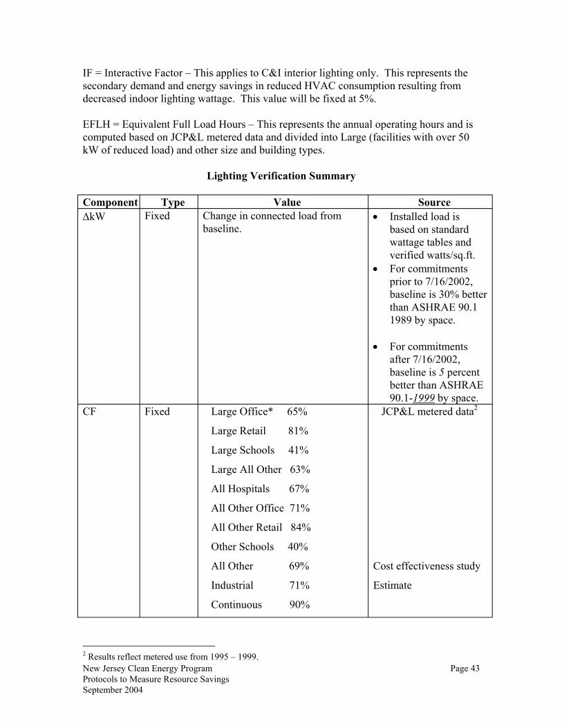
New Jersey Clean Energy Program Page 43 Protocols to Measure Resource Savings September 2004

IF = Interactive Factor – This applies to C&I interior lighting only. This represents the secondary demand and energy savings in reduced HVAC consumption resulting from decreased indoor lighting wattage. This value will be fixed at 5%. EFLH = Equivalent Full Load Hours – This represents the annual operating hours and is computed based on JCP&L metered data and divided into Large (facilities with over 50 kW of reduced load) and other size and building types.

Lighting Verification Summary

Component Type Value Source ∆kW Fixed Change in connected load from

baseline. • Installed load is

based on standard wattage tables and verified watts/sq.ft.

• For commitments prior to 7/16/2002, baseline is 30% better than ASHRAE 90.1 1989 by space.

• For commitments

after 7/16/2002, baseline is 5 percent better than ASHRAE 90.1-1999 by space.

CF Fixed Large Office* 65%

Large Retail 81%

Large Schools 41%

Large All Other 63%

All Hospitals 67%

All Other Office 71%

All Other Retail 84%

Other Schools 40%

All Other 69%

Industrial 71%

Continuous 90%

JCP&L metered data2

Cost effectiveness study

Estimate

2 Results reflect metered use from 1995 – 1999.

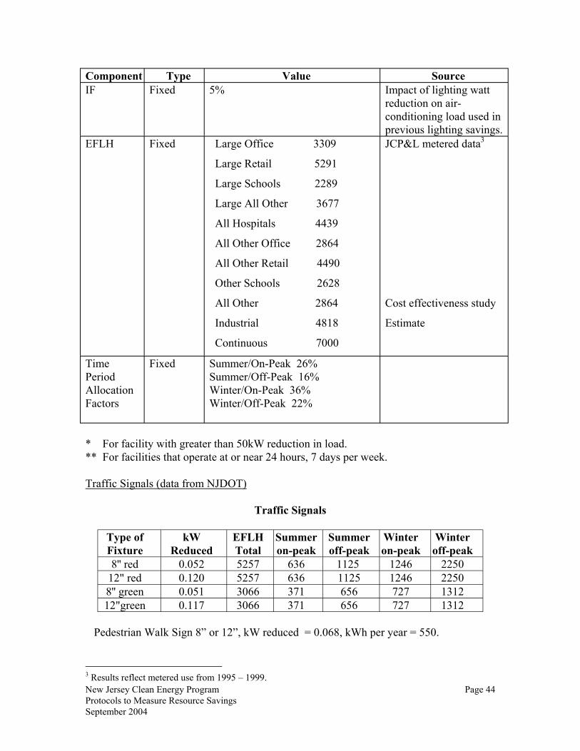
New Jersey Clean Energy Program Page 44 Protocols to Measure Resource Savings September 2004

Component Type Value Source IF Fixed 5% Impact of lighting watt

reduction on air-conditioning load used in previous lighting savings.

EFLH Fixed Large Office 3309

Large Retail 5291

Large Schools 2289

Large All Other 3677

All Hospitals 4439

All Other Office 2864

All Other Retail 4490

Other Schools 2628

All Other 2864

Industrial 4818

Continuous 7000

JCP&L metered data3

Cost effectiveness study

Estimate

Time Period Allocation Factors

Fixed Summer/On-Peak 26% Summer/Off-Peak 16% Winter/On-Peak 36% Winter/Off-Peak 22%

* For facility with greater than 50kW reduction in load. ** For facilities that operate at or near 24 hours, 7 days per week. Traffic Signals (data from NJDOT)

Traffic Signals

Type of Fixture

kW Reduced

EFLH Total

Summeron-peak

Summer off-peak

Winter on-peak

Winter off-peak

8'' red 0.052 5257 636 1125 1246 2250 12" red 0.120 5257 636 1125 1246 2250 8'' green 0.051 3066 371 656 727 1312 12"green 0.117 3066 371 656 727 1312

Pedestrian Walk Sign 8” or 12”, kW reduced = 0.068, kWh per year = 550.

3 Results reflect metered use from 1995 – 1999.

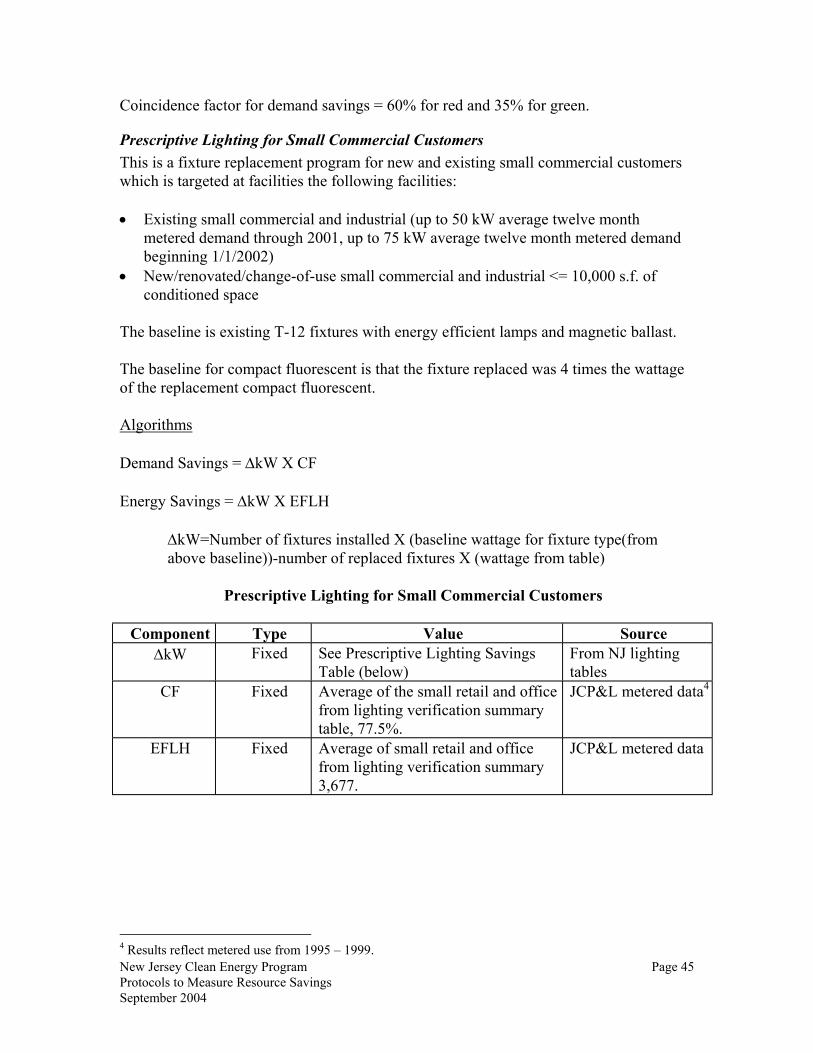
New Jersey Clean Energy Program Page 45 Protocols to Measure Resource Savings September 2004

Coincidence factor for demand savings = 60% for red and 35% for green.

Prescriptive Lighting for Small Commercial Customers This is a fixture replacement program for new and existing small commercial customers which is targeted at facilities the following facilities: • Existing small commercial and industrial (up to 50 kW average twelve month

metered demand through 2001, up to 75 kW average twelve month metered demand beginning 1/1/2002)

• New/renovated/change-of-use small commercial and industrial <= 10,000 s.f. of conditioned space

The baseline is existing T-12 fixtures with energy efficient lamps and magnetic ballast. The baseline for compact fluorescent is that the fixture replaced was 4 times the wattage of the replacement compact fluorescent. Algorithms Demand Savings = ∆kW X CF Energy Savings = ∆kW X EFLH

∆kW=Number of fixtures installed X (baseline wattage for fixture type(from above baseline))-number of replaced fixtures X (wattage from table)

Prescriptive Lighting for Small Commercial Customers

Component Type Value Source ∆kW Fixed See Prescriptive Lighting Savings

Table (below) From NJ lighting tables

CF Fixed Average of the small retail and office from lighting verification summary table, 77.5%.

JCP&L metered data4

EFLH Fixed Average of small retail and office from lighting verification summary 3,677.

JCP&L metered data

4 Results reflect metered use from 1995 – 1999.

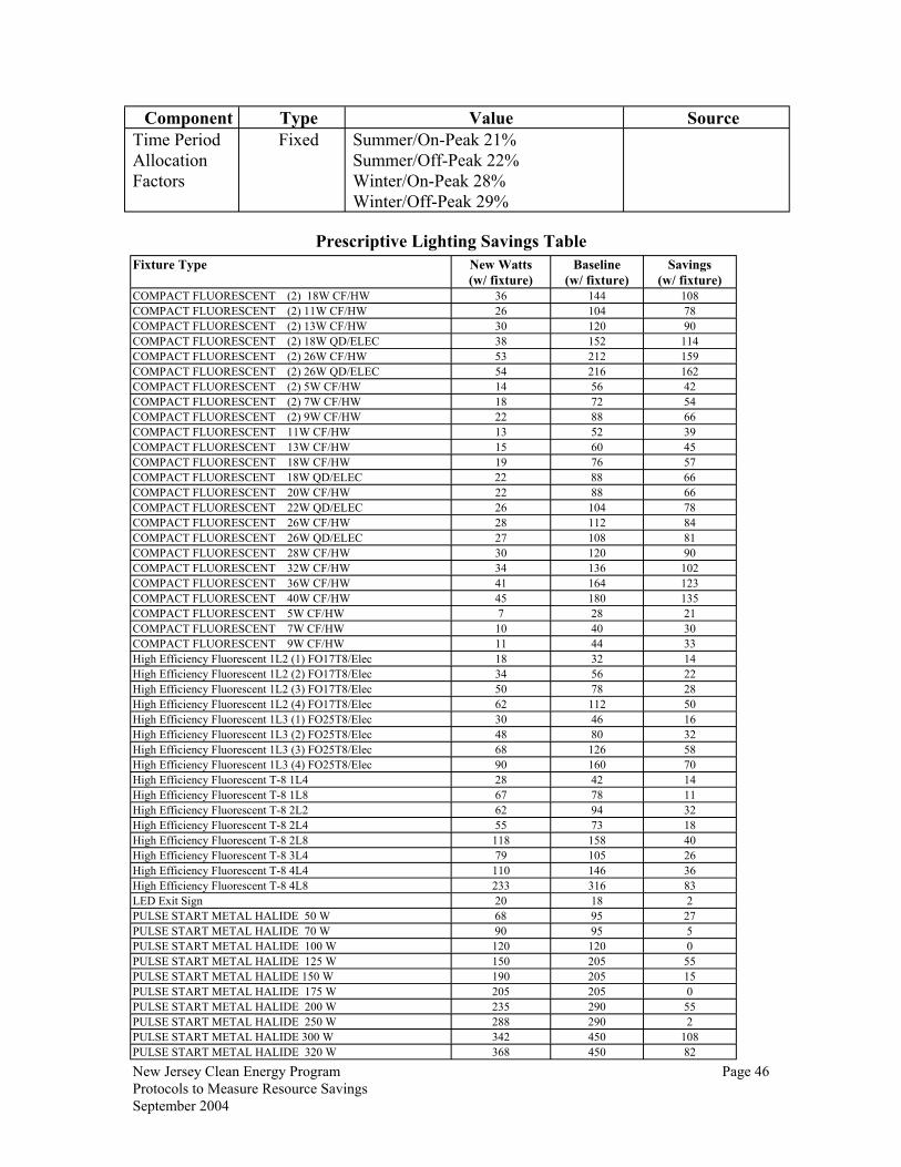
New Jersey Clean Energy Program Page 46 Protocols to Measure Resource Savings September 2004

Component Type Value Source Time Period Allocation Factors

Fixed Summer/On-Peak 21% Summer/Off-Peak 22% Winter/On-Peak 28% Winter/Off-Peak 29%

Prescriptive Lighting Savings Table Fixture Type New Watts

(w/ fixture) Baseline

(w/ fixture) Savings

(w/ fixture) COMPACT FLUORESCENT (2) 18W CF/HW 36 144 108 COMPACT FLUORESCENT (2) 11W CF/HW 26 104 78 COMPACT FLUORESCENT (2) 13W CF/HW 30 120 90 COMPACT FLUORESCENT (2) 18W QD/ELEC 38 152 114 COMPACT FLUORESCENT (2) 26W CF/HW 53 212 159 COMPACT FLUORESCENT (2) 26W QD/ELEC 54 216 162 COMPACT FLUORESCENT (2) 5W CF/HW 14 56 42 COMPACT FLUORESCENT (2) 7W CF/HW 18 72 54 COMPACT FLUORESCENT (2) 9W CF/HW 22 88 66 COMPACT FLUORESCENT 11W CF/HW 13 52 39 COMPACT FLUORESCENT 13W CF/HW 15 60 45 COMPACT FLUORESCENT 18W CF/HW 19 76 57 COMPACT FLUORESCENT 18W QD/ELEC 22 88 66 COMPACT FLUORESCENT 20W CF/HW 22 88 66 COMPACT FLUORESCENT 22W QD/ELEC 26 104 78 COMPACT FLUORESCENT 26W CF/HW 28 112 84 COMPACT FLUORESCENT 26W QD/ELEC 27 108 81 COMPACT FLUORESCENT 28W CF/HW 30 120 90 COMPACT FLUORESCENT 32W CF/HW 34 136 102 COMPACT FLUORESCENT 36W CF/HW 41 164 123 COMPACT FLUORESCENT 40W CF/HW 45 180 135 COMPACT FLUORESCENT 5W CF/HW 7 28 21 COMPACT FLUORESCENT 7W CF/HW 10 40 30 COMPACT FLUORESCENT 9W CF/HW 11 44 33 High Efficiency Fluorescent 1L2 (1) FO17T8/Elec 18 32 14 High Efficiency Fluorescent 1L2 (2) FO17T8/Elec 34 56 22 High Efficiency Fluorescent 1L2 (3) FO17T8/Elec 50 78 28 High Efficiency Fluorescent 1L2 (4) FO17T8/Elec 62 112 50 High Efficiency Fluorescent 1L3 (1) FO25T8/Elec 30 46 16 High Efficiency Fluorescent 1L3 (2) FO25T8/Elec 48 80 32 High Efficiency Fluorescent 1L3 (3) FO25T8/Elec 68 126 58 High Efficiency Fluorescent 1L3 (4) FO25T8/Elec 90 160 70 High Efficiency Fluorescent T-8 1L4 28 42 14 High Efficiency Fluorescent T-8 1L8 67 78 11 High Efficiency Fluorescent T-8 2L2 62 94 32 High Efficiency Fluorescent T-8 2L4 55 73 18 High Efficiency Fluorescent T-8 2L8 118 158 40 High Efficiency Fluorescent T-8 3L4 79 105 26 High Efficiency Fluorescent T-8 4L4 110 146 36 High Efficiency Fluorescent T-8 4L8 233 316 83 LED Exit Sign 20 18 2 PULSE START METAL HALIDE 50 W 68 95 27 PULSE START METAL HALIDE 70 W 90 95 5 PULSE START METAL HALIDE 100 W 120 120 0 PULSE START METAL HALIDE 125 W 150 205 55 PULSE START METAL HALIDE 150 W 190 205 15 PULSE START METAL HALIDE 175 W 205 205 0 PULSE START METAL HALIDE 200 W 235 290 55 PULSE START METAL HALIDE 250 W 288 290 2 PULSE START METAL HALIDE 300 W 342 450 108 PULSE START METAL HALIDE 320 W 368 450 82

New Jersey Clean Energy Program Page 47 Protocols to Measure Resource Savings September 2004

Fixture Type New Watts (w/ fixture)

Baseline (w/ fixture)

Savings (w/ fixture)

PULSE START METAL HALIDE 350 W 400 450 50 PULSE START METAL HALIDE 400 W 450 450 0 PULSE START METAL HALIDE 750 W 815 1075 260 PULSE START METAL HALIDE 875 W 940 1075 135 PULSE START METAL HALIDE 1000 W 1075 1075 0

Lighting Controls Lighting controls include occupancy sensors, daylight dimmer systems, and occupancy controlled hi-low controls for fluorescent, and HID controls. The measurement of energy savings is based on algorithms with key variables (i.e., coincidence factor, equivalent full load hours) provided through existing end-use metering of a sample of facilities or from other utility programs with experience with these measures (i.e., % of annual lighting energy saved by lighting control). For lighting controls, the baseline is a manual switch, based on the findings of the New Jersey Commercial Energy Efficient Construction Baseline Study. Algorithms Demand Savings = kWc X SVG X CF Energy Savings = kWc X SVG X EFLH X (1+IF) Definition of Variables

SVG = % of annual lighting energy saved by lighting control; refer to table by control type kWc = kW lighting load connected to control IF = Interactive Factor – This applies to C&I interior lighting only. This represents the secondary demand and energy savings in reduced HVAC consumption resulting from decreased indoor lighting wattage. This value will be fixed at 5%. CF = Coincidence Factor – This value represents the percentage of the total load which is on during electric system’s peak window. EFLH = Equivalent full load hours.

New Jersey Clean Energy Program Page 48 Protocols to Measure Resource Savings September 2004

Lighting Controls

Component Type Value Source kWc Variable Load connected to control Application SVG Fixed Occupancy Sensor, Controlled Hi-

Low Fluorescent Control and controlled HID = 30% Daylight Dimmer System=50%

See sources below

CF Fixed By building type and size see lighting verification summary table

Assumes same as JCP&L metered data

EFLH Fixed By building type and size see lightingverification summary table

JCP&L metered data

Time Period Allocation Factors

Fixed Summer/On-Peak 26% Summer/Off-Peak 16% Winter/On-Peak 36% Winter/Off-Peak 22%

Sources: • Northeast Utilities, Determination of Energy Savings Document, 1992 • Levine, M., Geller, H., Koomey, J., Nadel S., Price, L., "Electricity Energy Use

Efficiency: Experience with Technologies, Markets and Policies” ACEEE, 1992 • Lighting control savings fractions consistent with current programs offered by

National Grid, Northeast Utilities, Long Island Power Authority, NYSERDA, and Energy Efficient Vermont.

Motors Algorithms From application form calculate ∆kW where:

∆kW = HP*0.7456 X (1/EFFb – 1/ EFFq)

Demand Savings = (∆kW) X CF Energy Savings = (∆kW)*EFLH

Motors

Component Type Value Source Motor kW Variable Based on horsepower and

efficiency Application

EFLH Fixed Commercial 2,502 Industrial 4,599

JCP&L metered data5 and PSEG audit data for industrial

5 Results reflect metered use from 1995 – 1999.

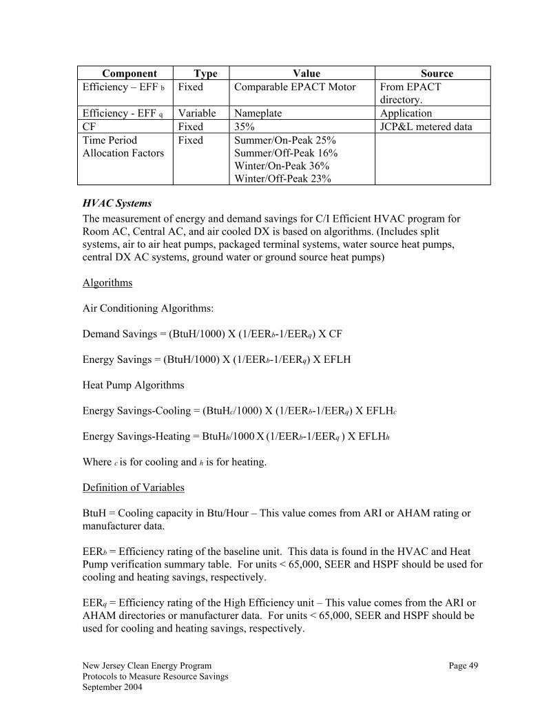
New Jersey Clean Energy Program Page 49 Protocols to Measure Resource Savings September 2004

Component Type Value Source Efficiency – EFF b Fixed Comparable EPACT Motor From EPACT

directory. Efficiency - EFF q Variable Nameplate Application CF Fixed 35% JCP&L metered data Time Period Allocation Factors

Fixed Summer/On-Peak 25% Summer/Off-Peak 16% Winter/On-Peak 36% Winter/Off-Peak 23%

HVAC Systems The measurement of energy and demand savings for C/I Efficient HVAC program for Room AC, Central AC, and air cooled DX is based on algorithms. (Includes split systems, air to air heat pumps, packaged terminal systems, water source heat pumps, central DX AC systems, ground water or ground source heat pumps) Algorithms Air Conditioning Algorithms: Demand Savings = (BtuH/1000) X (1/EERb-1/EERq) X CF Energy Savings = (BtuH/1000) X (1/EERb-1/EERq) X EFLH Heat Pump Algorithms Energy Savings-Cooling = (BtuHc/1000) X (1/EERb-1/EERq) X EFLHc

Energy Savings-Heating = BtuHh/1000 X (1/EERb-1/EERq ) X EFLHh Where c is for cooling and h is for heating. Definition of Variables BtuH = Cooling capacity in Btu/Hour – This value comes from ARI or AHAM rating or manufacturer data. EERb = Efficiency rating of the baseline unit. This data is found in the HVAC and Heat Pump verification summary table. For units < 65,000, SEER and HSPF should be used for cooling and heating savings, respectively. EERq = Efficiency rating of the High Efficiency unit – This value comes from the ARI or AHAM directories or manufacturer data. For units < 65,000, SEER and HSPF should be used for cooling and heating savings, respectively.

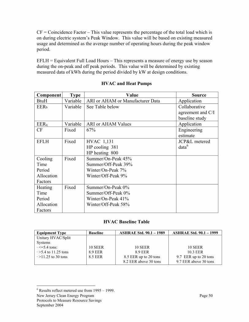
New Jersey Clean Energy Program Page 50 Protocols to Measure Resource Savings September 2004

CF = Coincidence Factor – This value represents the percentage of the total load which is on during electric system’s Peak Window. This value will be based on existing measured usage and determined as the average number of operating hours during the peak window period. EFLH = Equivalent Full Load Hours – This represents a measure of energy use by season during the on-peak and off peak periods. This value will be determined by existing measured data of kWh during the period divided by kW at design conditions.

HVAC and Heat Pumps Component Type Value Source BtuH Variable ARI or AHAM or Manufacturer Data Application EERb Variable See Table below Collaborative

agreement and C/I baseline study

EERq Variable ARI or AHAM Values Application CF Fixed 67% Engineering

estimate EFLH Fixed HVAC 1,131

HP cooling 381 HP heating 800

JCP&L metered data6

Cooling Time Period Allocation Factors

Fixed Summer/On-Peak 45% Summer/Off-Peak 39% Winter/On-Peak 7% Winter/Off-Peak 9%

Heating Time Period Allocation Factors

Fixed Summer/On-Peak 0% Summer/Off-Peak 0% Winter/On-Peak 41% Winter/Off-Peak 58%

HVAC Baseline Table

Equipment Type Baseline ASHRAE Std. 90.1 – 1989 ASHRAE Std. 90.1 – 1999 Unitary HVAC/Split Systems · <=5.4 tons: · >5.4 to 11.25 tons · >11.25 to 30 tons

10 SEER 8.9 EER 8.5 EER

10 SEER 8.9 EER

8.5 EER up to 20 tons 8.2 EER above 30 tons

10 SEER 10.3 EER

9.7 EER up to 20 tons 9.7 EER above 30 tons

6 Results reflect metered use from 1995 – 1999.

New Jersey Clean Energy Program Page 51 Protocols to Measure Resource Savings September 2004

Equipment Type Baseline ASHRAE Std. 90.1 – 1989 ASHRAE Std. 90.1 – 1999 Air-Air Heat Pump Systems · <=5.4 tons: · >5.4 to 11.25 tons · >11.25 to 30 tons

6.8 HSPF & 10.0 SEER 8.9 EER 8.5 EER

10 SEER

8.9 EER

8.5 EER up to 20 tons 8.2 EER above 30 tons

10 SEER

10.1 EER

9.3 EER up to 20 tons 9.0 EER above 30 tons

Package Terminal Systems 9 EER 10 – [0.91 * cap/1000] 10.9 – [0.213 * cap/1000] EER

Water Source Heat Pumps <=30 tons >30 tons

10.5 EER 10.5 EER

up to 5.4 tons– 9.3 EER >5.4 Tons 10.5

10.5 EER

up to 5.4 tons– 12.0 EER >5.4 Tons 12.0 EER

12.0 EER

Central DX AC Systems · >30 to 63 tons · > 63 tons

8.5 EER 8.5 EER

8.5 EER 8.2 EER

9.5 EER 9.5 EER

GWSHPs 11 EER 3.1 COP

Electric Chillers The measurement of energy and demand savings for C/I Chillers program is based on algorithms with key variables (i.e., kW/ton, Coincidence Factor, Equivalent Full Load Hours) measured through existing end-use metering of a sample of facilities. Algorithms Demand Savings = Tons X (kW/tonb – kW/tonq) X CF Energy Savings = Tons X (kW/tonb – kW/tonq) X EFLH Definition of Variables Tons = The capacity of the chiller (in tons) at site design conditions accepted by the program. kW/tonb = This data is the baseline and is found in the Chiller verification summary table. kW/tonq = This is the manufacturer data and equipment ratings in accordance with ARI Standard 550/590 latest edition. CF = Coincidence Factor – This value represents the percentage of the total load which is on during electric system’s Peak Window derived from JCP&L metered data. EFLH = Equivalent Full Load Hours – This represents a measure of chiller use by season determined by measured kWh during the period divided by kW at design conditions from JCP&L measurement data.

New Jersey Clean Energy Program Page 52 Protocols to Measure Resource Savings September 2004

Electric Chillers (Applicable to project commitments before 7/16/2002)

Component Type Value Source Tons Variable From Rebate Application kW/tonb Fixed Water Cooled Chillers (<70 tons)

Baseline:…………… 0.93 kW/Ton ASHRAE Std 90.1-1989…..0.93 kW/Ton

Water Cooled Chillers (70 to <150 tons) Baseline:…………… 0.86 kW/Ton ASHRAE Std 90.1-1989…..0.93 kW/Ton Water Cooled Chillers (150 to <300 tons) Baseline:…………… 0.72 kW/Ton ASHRAE Std 90.1-1989…..0.84 kW/Ton Water Cooled Chillers (=>300 tons)Baseline:…………… 0.64 kW/Ton ASHRAE Std 90.1-1989…..0.68 kW/Ton

Air Cooled Chillers (<150 tons) Baseline:…………… 1.30 kW/Ton ASHRAE Std 90.1-1989…..1.41 kW/Ton Air Cooled Chillers (+150 tons) Baseline:…………… 1.30 kW/Ton ASHRAE Std 90.1-1989…..1.41 kW/Ton

Collaborative agreement and C/I baseline study

kW/tonq Variable ARI Standards 550/590-Latest edition Application CF Fixed 67% Engineering estimate EFLH Fixed 1,360 JCP&L metered data7 Time Period Allocation Factors

Fixed Summer/On-Peak 45% Summer/Off-Peak 39% Winter/On-Peak 7% Winter/Off-Peak 9%

7 Results reflect metered use from 1995 – 1999.

New Jersey Clean Energy Program Page 53 Protocols to Measure Resource Savings September 2004

Electric Chillers

(Applicable to project commitments on or after 7/16/2002) Component Type Value Source Tons Variable From Rebate Application kW/tonb Fixed Water Cooled Chillers (<70 tons)

Baseline:…………… 0.79 kW/Ton ASHRAE Std 90.1-1999…..0.84 kW/Ton Water Cooled Chillers (70 to <150 tons) Baseline:…………… 0.79 kW/Ton ASHRAE Std 90.1-1999…..0.84 kW/Ton Water Cooled Chillers (150 to <300 tons) Baseline:…………… 0.718 kW/Ton ASHRAE Std 90.1-1999…..0.718 kW/Ton Water Cooled Chillers (=>300 tons)

Baseline:…………… 0.639 kW/Ton ASHRAE Std 90.1-1999…..0.639 kW/Ton Air Cooled Chillers (<150 tons) Baseline:…………… 1.256 kW/Ton ASHRAE Std 90.1-1999….1.256 kW/Ton

Air Cooled Chillers (+150 tons) Baseline:…………… 1.256 kW/Ton ASHRAE Std 90.1-1999…..1.256 kW/Ton

Collaborative agreement, C/I baseline study, E-Cube Inc. Study, May 2003

kW/tonq Variable ARI Standards 550/590-Latest edition Application CF Fixed 67% Engineering estimate EFLH Fixed 1,360 JCP&L metered data8 Time Period Allocation Factors

Fixed Summer/On-Peak 45% Summer/Off-Peak 39% Winter/On-Peak 7% Winter/Off-Peak 9%

For certain fixed components, studies and surveys developed by the utilities in the State or based on a review of manufacturer’s data, other utilities, regulatory commissions or consultant’s reports will be used to update the values for future filings. 8 Results reflect metered use from 1995 – 1999.

New Jersey Clean Energy Program Page 54 Protocols to Measure Resource Savings September 2004

Variable Frequency Drives The the measurement of energy and demand savings for C/I Variable Frequency Drive for VFD applications is for HVAC fans and water pumps only. VFD applications for other than this use should follow the custom path. Algorithms Energy Savings = Motor HP X kWh/motor HP There are no Demand Savings for VFD’s Definitions of Variables Motor HP – This value comes from the nameplate of the motor.

Variable Frequency Drives Component Type Value Source Motor HP Variable Nameplate Application kWh/motor HP Fixed 1,653 for VAV air handler

systems. 1,360 for chilled water pumps.

JCP&L metered data for VFD’s9 and chillers10.

Time Period Allocation Factors

Fixed Summer/On-Peak 22% Summer/Off-Peak 10% Winter/On-Peak 47% Winter/Off-Peak 21%

9 Results reflect metered use from 1995 – 1998. 10 Results reflect metered use from 1995 – 1999.

New Jersey Clean Energy Program Page 55 Protocols to Measure Resource Savings September 2004

C&I Construction Gas Protocols

Gas Chillers The the measurement of energy savings for C&I gas fired chillers and chiller heaters is based on algorithms with key variables (i.e., Equivalent Full Load Hours, Vacuum Boiler Efficiency, Input Rating, Coincidence Factor) provided by manufacturer data or measured through existing end-use metering of a sample of facilities. Algorithms Winter Gas Savings = (VBEq – BEb)/VBEq X IR X EFLH Electric Demand Savings = Tons X (kW/Tonb – kW/Tongc) X CF Electric Energy Savings = Tons X (kW/Tonb – kW/Tongc) X EFLH Summer Gas Usage (MMBtu) = MMBtu Output Capacity / COP X EFLH Net Energy Savings = Electric Energy Savings + Winter Gas Savings – Summer Gas Usage Definition of Terms VBEq = Vacuum Boiler Efficiency BEb = Efficiency of the baseline gas boiler IR = Input Rating = Therms/hour Tons = The capacity of the chiller (in tons) at site design conditions accepted by the program. kW/Tonb = The baseline efficiency for electric chillers, as shown in the Gas Chiller Verification Summary table below. kW/Tongc = Parasitic electrical requirement for gas chiller. COP = Efficiency of the gas chiller MMBtu Output Capacity = Cooling Capacity of gas chiller in MMBtu. CF = Coincidence Factor. This value represents the percentage of the total load that is on during electric system peak. EFLH = Equivalent Full Load Hours. This represents a measure of chiller use by season.

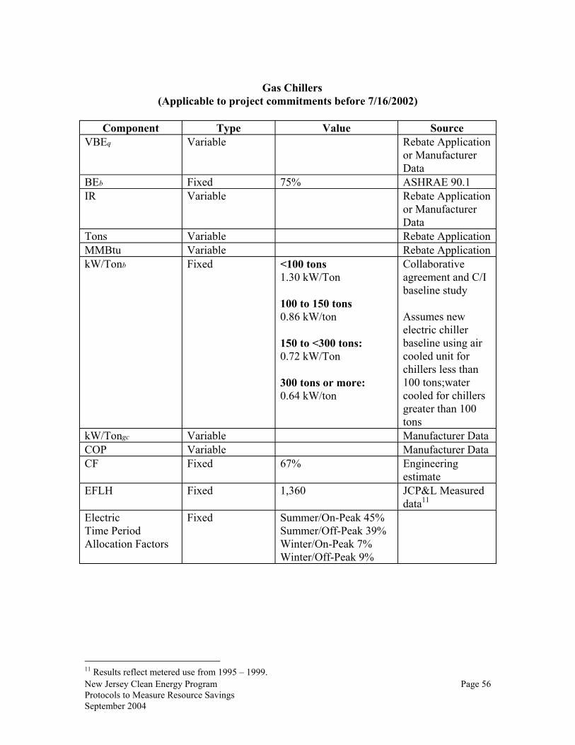
New Jersey Clean Energy Program Page 56 Protocols to Measure Resource Savings September 2004

Gas Chillers

(Applicable to project commitments before 7/16/2002)

Component Type Value Source VBEq Variable Rebate Application

or Manufacturer Data

BEb Fixed 75% ASHRAE 90.1 IR Variable Rebate Application

or Manufacturer Data

Tons Variable Rebate ApplicationMMBtu Variable Rebate ApplicationkW/Tonb Fixed <100 tons

1.30 kW/Ton 100 to 150 tons 0.86 kW/ton 150 to <300 tons: 0.72 kW/Ton 300 tons or more: 0.64 kW/ton

Collaborative agreement and C/I baseline study Assumes new electric chiller baseline using air cooled unit for chillers less than 100 tons;water cooled for chillers greater than 100 tons

kW/Tongc Variable Manufacturer Data COP Variable Manufacturer Data CF Fixed 67% Engineering

estimate EFLH Fixed 1,360 JCP&L Measured

data11 Electric Time Period Allocation Factors

Fixed Summer/On-Peak 45% Summer/Off-Peak 39% Winter/On-Peak 7% Winter/Off-Peak 9%

11 Results reflect metered use from 1995 – 1999.

New Jersey Clean Energy Program Page 57 Protocols to Measure Resource Savings September 2004

Gas Chillers (Applicable to project commitments on or after 7/16/2002)

Component Type Value Source

VBEq Variable Rebate Application or Manufacturer Data

BEb Fixed 75% ASHRAE 90.1 IR Variable Rebate Application

or Manufacturer Data

Tons Variable Rebate ApplicationMMBtu Variable Rebate ApplicationkW/Tonb Fixed <100 tons

0.79kW/Ton 100 to 150 tons 0.79 kW/ton 150 to <300 tons: 0.718 kW/Ton 300 tons or more: 0.639 kW/ton

Collaborative agreement and C/I baseline study. Assumes new electric chiller baseline using air cooled unit for chillers less than 100 tons; water cooled for chillers greater than 100 tons

kW/Tongc Variable Manufacturer Data COP Variable Manufacturer Data CF Fixed 67% Engineering

estimate EFLH Fixed 1,360 JCP&L Measured

data12 Electric Time Period Allocation Factors

Fixed Summer/On-Peak 45% Summer/Off-Peak 39% Winter/On-Peak 7% Winter/Off-Peak 9%

Variable data will be captured on the application form or from manufacturer’s data sheets and collaborative/utility studies. For certain fixed components, studies and surveys developed by the utilities in the State or based on a review of manufacturer’s data, other utilities, regulatory commissions or consultants’ reports will be used to update the values for future filings.

12 Results reflect metered use from 1995 – 1999.

New Jersey Clean Energy Program Page 58 Protocols to Measure Resource Savings September 2004

Gas Fired Desiccants Protocols to be developed.

Gas Booster Water Heaters C&I gas booster water heaters are substitutes for electric water heaters. The measurement of energy savings is based on engineering algorithms with key variables (i.e., Input Rating Coincidence Factor, Equivalent Full Load Hours) provided by manufacturer data or measured through existing end-use metering of a sample of facilities. Algorithms Demand Savings (kW) = IR X EFF/3412 X CF Energy Savings (kWh) = IR X EFF/3412 X EFLH Gas Usage Increase = IR X EFLH Net Energy Savings = Electric Energy Savings – Gas Usage Increase (Calculated in MMBtu) Definition of Variables IR = Input Rating in Btuh EFF = Efficiency CF = Coincidence Factor EFLH = Equivalent Full Load Hours The 3412 used in the denominator is used to convert Btus to kWh.

Gas Booster Water Heaters

Component Type Value Source IR Variable Application Form or

Manufacturer Data CF Fixed 50% PSE&G EFLH Fixed 1,000 PSE&G EF Variable Application Form or

Manufacturer Data

New Jersey Clean Energy Program Page 59 Protocols to Measure Resource Savings September 2004

Component Type Value Source Electric Time Period Allocation Factors

Fixed Requires additional research

Water Heaters This prescriptive measure targets solely the use of smaller-scale domestic water heaters (50 gallons or less per unit) in all commercial facilities. Larger gas water heaters are treated under the custom measure path. The measurement of energy savings for C&I gas water heaters is based on algorithms with key variables (i.e., energy factor) provided by manufacturer data. Algorithms Gas Savings = ((EFq – EFb)/EFq) X Baseline Usage Definition of Variables EFq = Energy factor of the qualifying energy efficient water heater.

EFb = Energy factor of the baseline water heater. Calculated as 0.62 – (0.0019 X gallons of capacity). Based on a 40 gallon water heater.

Baseline Usage = Annual usage of the baseline water heater, in therms.

Water Heaters

Component Type Value Source EFq Variable Application Form or

Manufacturer Data EFb Fixed 0.544 Federal EPACT

Standard Baseline Usage Fixed 277

DOE/FEMP website http://www.eren.doe.gov/femp/pro

Time Period Allocation Factors

Fixed Summer 50% Winter 50%

1

1. Prorated based on 6 months in the summer period and 6 months in the winter period.

New Jersey Clean Energy Program Page 60 Protocols to Measure Resource Savings September 2004

Furnaces and Boilers This prescriptive measure targets the use of smaller-scale boilers (less than or equal to 1500 MBH) and furnaces (no size limitation) in all commercial facilities. Larger sized boilers are treated under the custom measure path. The measurement of energy savings for C&I gas fired furnaces and boilers is based on algorithms with key variables (i.e. Annual Fuel Utilization Efficiency, capacity of the furnace, EFLH) provided by manufacturer data or utility data. Algorithms Gas Savings = ((AFUEq – AFUEb)/AFUEq) X CAPY X EFLH Definition of Variables AFUEq = Annual Fuel Utilization Efficiency of the qualifying energy efficient furnace or boiler AFUEb = Annual Fuel Utilization Efficiency of the baseline furnace or boiler CAPY = Capacity of the furnace or boiler in therms/hour EFLH = Equivalent full load heating hours

Furnaces and Boilers

Component Type Value Source AFUEq Variable Application Form or

Manufacturer Data AFUEb Fixed Furnaces: 78%

Boilers: 80% EPACT Standard for furnaces and boilers

CAPY Variable Application Form or Manufacturer Data

EFLH Fixed 900 PSE&G

Time Period Allocation Factors

Fixed Summer 12% Winter 88%

1

1. Prorated based on 12% of the annual degree days falling in the summer period and 88% of the annual degree days falling in the winter period.

New Jersey Clean Energy Program Page 61 Protocols to Measure Resource Savings September 2004

Commercial and Industrial Building Operation & Maintenance Program

Protocols The measurement of energy and demand savings for the building O&M program is based on saving a fixed percent of a building electric and gas load through the performance of various O&M improvement activities. It will be necessary to collect a facilities prior year electric and gas usage for input to the equations. The following is an explanation of the algorithms used and the nature and source of all required input data. Algorithms

Electric Savings Energy Impact (kWh) = PYEL X ESF Peak Demand Impact (kW) = (Energy Impact / EFLH) X CF

Gas Savings Energy Savings (Therms) = PYGL X GSF Definition of Variables PYEL = Participants previous years electric energy use. PYGL = Participants previous years gas energy use. EFLH = The equivalent full load hours of operation for the average commercial or industrial establishment in New Jersey. CF = The coincidence factor for the average commercial or industrial establishment in New Jersey. ESF = Electric savings factor as a % of facility load prior to program participation. GSF = Gas savings factor as a % of facility load prior to program participation. A summary of the data sources and fixed values follows:

New Jersey Clean Energy Program Page 62 Protocols to Measure Resource Savings September 2004

C&I Building O&M Component Type Value Sources PYEL Variable

Customer

Application PYGL Variable

Customer

Application EFLH Fixed 3900 1 CF Fixed 0.875 2 ESF Fixed 10% 3 GSF Fixed 7% 4 Source Notes:

1. EFLH: Equivalent Full Load Hours of 3900 is based on a typical NJ load profile from the NJ 2000 Forecast.

2. CF: Coincidence Factor of 0.875 is based on the average of 85% for commercial customers and 90% for industrial customers.

3. ESF: Electric Savings Factor of 10% of pre-participation facility load is based on a review of multiple O&M improvement programs.

4. GSF: Gas Savings Factor of 7% of pre-participation facility load is based on a review of multiple O&M improvement programs.

New Jersey Clean Energy Program Page 63 Protocols to Measure Resource Savings September 2004

Compressed Air System Optimization

Protocols

Compressed Air Systems The energy and peak demand savings due to Compressed Air Optimization measures will be based on an a site-specific engineering analysis completed for each participating site. The engineering analysis will determine what increase in efficiency will be realized through program participation. This will be compared to the current baseline condition to estimate savings.

New Jersey Clean Energy Program Page 64 Protocols to Measure Resource Savings September 2004

Residential Air Conditioning Cycling Load Control Program

Protocols Each company has individually assessed the peak reductions of this program utilizing methodologies acceptable for PJM contractual and reporting purposes. Those same impacts will be used to report the peak savings for this program.

New Jersey Clean Energy Program Page 65 Protocols to Measure Resource Savings September 2004

School Energy Efficiency and Renewable Energy Education Program

Protocols No protocol was developed to measure energy savings for this program, because the program purpose is to instill values and awareness as students that will inform their decisions about energy use as the next generation of consumers and buyers. A secondary purpose is to increase their families’ awareness through homework and family involvement in helping the children. Isolating the energy savings as a result of this program would require tracking behavior of these young participants ten or more years in the future. Actions that children’s parents take as a result of this program are likely to be reflected in measure installations or market effects that are covered in other CRA programs. These savings are captured in the measured savings for those programs. The savings produced by this program that are not captured in other CRA programs would be difficult to isolate and relatively expensive to measure.

New Jersey Clean Energy Program Page 66 Protocols to Measure Resource Savings September 2004

Customer-Sited Generation

Protocols The measurement of energy and demand impacts for customer sited generation systems is based on algorithms that estimate each systems annual energy production and coincident peak capacity production. Input data is based on fixed assumptions, engineering estimates and data supplied from the program’s technical worksheets and rebate application forms. An industry standard calculation tool (PVWATTS from the National Renewable Energy Laboratory) will be used for estimating PV system annual outputs. For wind installations estimated annual energy output is calculated using industry data table and inputs on average wind speed at hub height, rotor diameter and typical system efficiencies for wind speed/rotor diameter combinations. For fuel cell and sustainable biomass projects the protocols include recommended formats but the energy and peak capacity for each project will be estimated on a case by case basis. This level of flexibility allows for the use of more detailed case specific engineering data in the protocol reporting. All of the customer sited generation protocols report the gross energy production from the generation system. The protocols for fuel cell installations account for estimated natural gas consumption. Sustainable biomass projects account for estimated consumption of the applicable biomass fuel. In support of the protocol estimates, sub-metering must be installed to measure the gross output of the generating systems capable of recording at 15 minute intervals for a minimum of 12 months. Sub-Metering Samples Size by technology: • 50% of first 30 installations • 10% above 30 Installations • Not to exceed 100 The following is an explanation of the algorithms used and the nature and source of all required input data. Algorithms

Photovoltaic Systems PVWATTS will be used to estimate the energy generated by photovoltaic systems. PVWATTS was developed and is available through the Renewable Resource Data Center (RReDC). The RReDC is supported by the National Center for Photovoltaics (NCPV) and managed by the Department of Energy's Office of Energy Efficiency and Renewable

New Jersey Clean Energy Program Page 67 Protocols to Measure Resource Savings September 2004

Energy. The RReDC is maintained by the Distributed Energy Resources Center of the National Renewable Energy Laboratory. The subroutines used to calculate the energy generation are based on information developed by Sandia National Laboratories. PVWATTS is available through the RReDC website, http://rredc.nrel.gov/solar/codes_algs/PVWATTS/. The following input values are used by PVWATTS to estimate average annual energy production, and are collected for each PV project on the PV technical worksheet and rebate application. Annual Energy Production (kWh) calculated by PVWATTS is a function of:

• System Rated Output (AC output at Standard Rating Conditions) • Fixed, Single or Double Axis Tracking • Array Tilt angle (for fixed axis only) • Array Azimuth (for fixed axis only) • Weather data (based on City and State)

The Peak demand impact for photovoltaic systems is estimated separately from the annual energy output. Summer and winter peak impacts are based on research conducted by Richard Perez, of SUNY Albany, (http://www.nrel.gov/ncpv/documents/pv_util.html). The estimated summer effective load carrying capacity (ELCC) for New Jersey is 60% to 70%. A value of 65% is adopted for these protocols. Summer Peak Impact (kW) = System Rated Output * Summer Effective Load Carrying Capacity (ELCC). Winter Peak Impact (kW) = System Rated Output * Winter Effective Load Carrying Capacity (WELCC). A summary of the input values and their data sources follows:

Photovoltaic Systems Component Type Value Sources System Rated Output (SRO)

Variable Application Technical Worksheet

Fixed, Single, Double Axis tracking

Variable Application Technical Worksheet

Array Tilt Variable Application Technical Worksheet

Azimuth Angle Variable Application Technical Worksheet

Weather Data Variable City, State – four sites will be used

Application Technical Worksheet

New Jersey Clean Energy Program Page 68 Protocols to Measure Resource Savings September 2004

Component Type Value Sources (Wilkes Barre PA, Newark NJ, Philadelphia PA, and Atlantic City, NJ

ELCC Fixed 65% (http://www.nrel.gov/ncpv/documents/pv_util.html)

WELCC Fixed 8% Monitored system data from White Plains NY

Wind Systems Estimated annual energy output for wind systems will be based on an industry data table. Currently there is a lack of data on the peak impact of small wind systems in New Jersey and an estimate of 0% will be used. This value will be updated if supporting data are identified. Annual Energy Output (kWh) is a function of:

• Average annual wind speed at hub height • Rotor diameter • Total system efficiency

The Estimated Annual Energy Output data table is drawn from Gipe, Paul (1993), Wind Power for Home and Business, Chelsea Green Publishing Company. A spreadsheet with the values in this table is attached. Data summary of the input values and their data sources follows:

Wind Systems Component Type Value Sources Average annual wind speed at hub height (m/s) or (mph)

Variable Application Technical Worksheet

Rotor diameter in meters or feet

Variable Application Technical Worksheet

Typical System Efficiency

Fixed for each wind speed / rotor diameter combination

Ranges from 12% to 30%

Gipe, (1993). Appendix E-1 Table on Estimate Annual Energy Output. Efficiencies based on published data.

Summer Peak Impact

Fixed 0% Data on peak impact not available at this time

New Jersey Clean Energy Program Page 69 Protocols to Measure Resource Savings September 2004

Component Type Value Sources Winter Peak Impact Fixed 0% Data on peak impact not

available at this time

Fuel Cells Estimated annual energy output and peak impacts for fuel cell systems will be based on case specific engineering estimates and manufacturer data. Total Annual Energy = Average Electric Output + Average Thermal Energy Recovered Data collected for the protocol estimation for each fuel cell project will include the following.

Fuel Cells Component Type Value Sources Rated Continuous Peak Output (AC)

Variable Manufacturer Specifications – Application Technical Worksheet

Rated Fuel Input at Peak Output (MMBTU/hr)

Variable Manufacturer Specifications – Application Technical Worksheet

Average annual Electric Output

Variable Project specific based on estimated duty cycle

Average annual thermal energy recovery

Variable Project specific based on estimated duty cycle

Annual fuel consumption (MMBTU)

Variable Project specific based on estimated duty cycle

Average total system efficiency

Variable Project specific based on manufacturer specifications and estimated operating parameters.

Summer Peak Impact

Variable Project specific based on estimated duty cycle.

Winter Peak Impact Variable Project specific based on estimated duty cycle.

Sustainable Biomass Estimated annual energy output and peak impacts for sustainable biomass systems will be based on case specific engineering estimates and manufacturer data.

New Jersey Clean Energy Program Page 70 Protocols to Measure Resource Savings September 2004

Appendix A Measure Lives

NEW JERSEY STATEWIDE ENERGY-EFFICIENCY PROGRAMS Measure Lives Used in Cost-Effectiveness Screening

July 2001

PROGRAM/Measure Measure Life Residential Programs Energy Star Appliances ES Refrigerator post 2001 17 ES Refrigerator 2001 17 ES Dishwasher 13 ES Clotheswasher 20 ES RAC 10 Energy Star Lighting CFL 6.4 Recessed Can Fluourescent Fixture 20 torchiere residential 10 Fixtures Other 20 Energy Star Windows WIN-heat pump 20 WIN-gas heat/CAC 20 WIN-gas No CAC 20 Win-elec No AC 20 Win-elec AC 20 Residential New Construction SF gas w/CAC 20 SF gas w/o CAC 20 SF oil w/CAC 20 SF all electric 20 TH gas w/CAC 20 TH gas w/o CAC 20 TH oil w/CAC 20 TH all electric 20 MF gas w/AC 20 MF gas w/o AC 20 MF oil w/CAC 20 MF all electric 20 ES Clotheswasher 20 Recessed Can Fluor Fixture 20 Fixtures Other 20 Efficient Ventilation Fans w/Timer 10 Residential Electric HVAC CAC 13 15 CAC 14 15

New Jersey Clean Energy Program Page 71 Protocols to Measure Resource Savings September 2004

PROGRAM/Measure Measure Life ASHP 13 15 ASHP 14 15 CAC proper sizing/install 15 ASHP proper sizing/install 15 E-Star T-stat (CAC) 15 E-star T-stat (HP) 15 GSHP 30 CAC 15 15 ASHP 15 15 Residential Gas HVAC High Efficiency Furnace 20 High Efficiency Boiler 20 High Efficiency Gas DHW 10 E-Star T-stat 15 Low-Income Program Air sealing electric heat 17 Duct Leak Fossil Heat & CAC 15 typical fossil fuel heat 17 typical electric DHW pkg 10 typical fossil fuel DHW pkg 10 screw-in CFLs 6.4 high-performance fixtures 20 fluorescent torchieres 10 TF 14 20 TF 16 20 TF 18 20 SS 20 20 TF 21 20 SS 22 20 TF 25 20 audit fees 20 Attic Insulation- ESH 17 Duct Leak - ESH 15 T-Stat- ESH 5 HP charge air flow 8 electric arrears reduction 1 gas arrears reduction 1 Non-Residential Programs C&I Construction Commercial Lighting — New 15 Commercial Lighting — Remodel/Replacement 15 Commercial Custom — New 18 Commercial Chiller Optimization 18 Commercial Unitary HVAC — New - Tier 1 15 Commercial Unitary HVAC — Replacement - Tier 1 15 Commercial Unitary HVAC — New - Tier 2 15 Commercial Unitary HVAC — Replacement Tier 2 15

New Jersey Clean Energy Program Page 72 Protocols to Measure Resource Savings September 2004

PROGRAM/Measure Measure Life Commercial Chillers — New 25 Commercial Chillers — Replacement 25 Commercial Small Motors (1-10 HP) — New or Replacement 20 Commercial Medium Motors (11-75 HP) — New or Replacement 20 Commercial Large Motors (76-200 HP) — New or Replacement 20 Commercial VSDs — New 15 Commercial VSDs — Retrofit 15 Commercial Comprehensive New Construction Design 18 Commercial Custom — Replacement 18 Industrial Lighting — New 15 Industrial Lighting — Remodel/Replacement 15 Industrial Unitary HVAC — New - Tier 1 15 Industrial Unitary HVAC — Replacement - Tier 1 15 Industrial Unitary HVAC — New - Tier 2 15 Industrial Unitary HVAC — Replacement Tier 2 15 Industrial Chillers — New 25 Industrial Chillers — Replacement 25 Industrial Small Motors (1-10 HP) — New or Replacement 20 Industrial Medium Motors (11-75 HP) — New or Replacement 20 Industrial Large Motors (76-200 HP) — New or Replacement 20 Industrial VSDs — New 15 Industrial VSDs — Retrofit 15 Industrial Custom — Non-Process 18 Industrial Custom — Process 10 Small Commercial Gas Furnace — New or Replacement 20 Small Commercial Gas Boiler — New or Replacement 20 Small Commercial Gas DHW — New or Replacement 10 C&I Gas Absorption Chiller — New or Replacement 25 C&I Gas Custom — New or Replacement (Engine Driven Chiller) 25 C&I Gas Custom — New or Replacement (Gas Efficiency Measures) 18 Building O&M O&M savings 3 Compressed Air Compressed Air (GWh participant) 8

Appendix 4: Comparison of Alternative Methodologies to Calculate Avoided NOx Emissions The team completed an analysis of avoided emissions to determine if reductions from energy efficiency and renewable energy sources would offset at least 1.5 lbs/MWh of NOx emissions. The methodology used in our analysis focused on the generation-weighted average of the emissions of fossil fuel fired plants. This is the fourth methodology listed below. We present alternative methodologies for informational purposes. Several methods may be employed to model the avoided emissions resulting from energy efficiency or renewable energy measures. These include:

1) A complete grid-system dispatch analysis; 2) A system mix analysis; 3) A surrogate plant analysis; or 4) A generation-weighted average of the emissions of fossil fuel fired plants.

A complete grid-system dispatch analysis considers the dispatch order and scheduling of specific fossil fuel-fired units (coal, oil, or natural gas) at each facility on the regional grid, providing the most comprehensive estimate of the avoided emissions. An analysis of this type may be based on historical data and/or on a unit dispatch model. The principal unit dispatch models are proprietary.1 The dispatch analysis methodology allows the analyst to compare the EERE measures with the actual generation of variably dispatched fossil fuel units for specific time periods. This methodology is very time consuming and resource intensive and is hard to justify for validating an avoided emissions rate already stipulated in a State NOx trading regulation. However, the additional expense of this detailed approach can be justified to provide more precise estimates of displaced NOx emissions resulting from a large renewable energy project, such as a large wind farm.2 In such as case, a large premium obtained for Renewable Energy Certificates may justify the additional expense. The system mix analysis uses the generation weighted average of all the plants in the electric generating system. In other words, the universe of plants covered by this methodology is not limited to fossil fuel generating plants but also includes nuclear and hydroelectric plants. A major weakness of the system mix methodology is that it significantly underestimates the emission reductions resulting from EERE projects because it includes nuclear and

1 However, some utilities will enter into agreements to share such data for analysis purposes on a confidential basis. In addition, some of the new generation tracking systems may provide sufficient data to conduct this analysis. 2 See National Renewable Energy Laboratory, “Model State Implementation Plan (SIP) Documentation for Wind Energy Purchase in a State with Renewable Energy Set-Aside,” http://www.eere.energy.gov/windandhydro/windpoweringamerica/sips.asp

4-1

hydroelectric generating plants, which do not produce emissions, in calculating the average displaced emissions. In reality, EERE almost always displaces fossil fuel generation because EERE generally has zero or very low fuel and operating costs, whereas fossil fueled generation has relatively high operating costs. Fossil fueled units also have the ability to vary their output relatively quickly. In comparison, nuclear power and hydroelectric generation is almost never displaced by EERE measures. Nuclear plants cannot vary their output quickly and have relatively low marginal operating costs. Hydroelectric plants also have low marginal operating costs, and therefore, generation from other renewable energy rarely displaces that from hydroelectric power. In addition, hydroelectric plants have externally imposed storage limits and flow constraints that restrict the ability to meet unpredicted load changes. For these reasons, the generation at renewable energy plants and reductions in demand from energy efficiency programs will displace generation almost entirely at fossil fueled plants in the period from now through 2012. The surrogate plant analysis calculates the emissions of the next new plant or unit that is likely to be added to the electric grid as a basis for determining what emissions would be avoided if the demand were reduced by energy efficiency measures or displaced by renewable energy generation. In New Jersey, under prevailing fuel prices and air quality regulations, the most likely new plant would be a combined cycle natural gas plant with best available NOx control technology. With this approach, the calculated NOx reductions would be below the 1.5 lbs/MWh stipulated in the NJ NOx trading regulations. This approach is unrealistic in the short term because actual generation and energy efficiency displacement is spread across a wide range of fossil fueled generating units, some of which have relatively high NOx emission rates. The surrogate plant methodology may provide a reasonable estimate of the long-term avoided emissions if current trends continue. However, the actual mix of plants may be very different in the future depending on fuel prices and public policy. A fourth methodology – and the one relied upon by the project team – is an analysis based on the generation-weighted average of the emissions of fossil fuel fired plants. This methodology is a reasonable approximation of the marginal emission rate, without the time and cost of a complete grid-system dispatch analysis. Two independent analyses were conducted based on the generation-weighted average emissions of fossil fueled plants. Resource Systems Group, Inc. (RSG) performed the first analysis and relied on emissions and generation data from the EPA’s eGRID 2002 database.3 The emissions data in eGRID 2002 is based on emissions data collected in 2000. The list of facilities used for this assessment and their associated NOx emission rates, generation, and primary fuel are included in Table 1. The team included small facilities in the analysis even though such facilities do not influence the estimate significantly. In addition, it should be noted that although the

3 Emissions & Generation Resource Integrated Database (eGRID) 2002.

4-2

primary fuel is listed for each facility, many facilities operate subordinate units that burn other fuels, often contributing to varying emission rates among a fuel group. Based on the eGRID 2002 data, the team estimated the generation-weighted NOx emissions for both annual operation and ozone-season operations. The annual avoided NOx emission rates are 2.7 lbs/MWh, and the ozone season rates are 2.2 lbs/MWh. Both of these rates are well above the 1.5 lbs/MWh avoided emissions rate that is currently stipulated in the NJ NOx trading regulations. Even removing several of the largest and most inefficient coal burning facilities from the analysis is not enough to drop the estimate below 1.5 lbs/MWh. Therefore, the project team believes that 1.5 lbs/MWh is a reasonable (and probably conservative) value for avoided emissions credit in 2005. However, it should be noted that this emission rate is expected to decline in the future as older, dirtier generating plants are replaced by more efficient plants with superior NOx control technology. New Jersey DEP provided the second analysis,4 and the project team ultimately relied on this analysis for the calculations of emission reductions contained in the body of this report. The NJ DEP analysis was similar to the RSG analysis because both methodologies were based on the generation weighted average of emissions from fossil fueled plants in New Jersey. The two major differences were that the DEP analysis relied on: (1) plants operating in 2004 (compared to the 2000 data in the eGRID/RSG analysis); and (2) plants with a capacity of more than 15 MW (compared to all fossil fuel plants in the RSG analysis). The NJ DEP data provided an estimate of 1.85 lbs/MWh for the average avoided emissions rate in 2004. DEP also projected future average avoided ozone season NOx emission rates based on data about new plants completed, under construction, or expected to be retired. In addition, the NJ data included information projecting the installation of NOx control systems. Based on this information, DEP estimated the generation-weighted NOx emissions rates to be 1.65 lbs/MWh in 2005, 1.24lbs/MWh in 2007, and 0.97lbs/MWh in 2008. Both the RSG and DEP analyses validate the use of 1.5 lbs/MWh for 2005. The analysis team recommends the use of the DEP estimates beyond 2005 as they are based on more recent data and incorporate projected changes in control technology and the fossil fueled generation mix. These DEP estimates beyond 2005 have been incorporated into the projections for each of the four alternative scenarios in the report.

4 Tom McNevin, Bureau Air Quality Planning, NJ DEP, Personal Communication, September 2005.

4-3

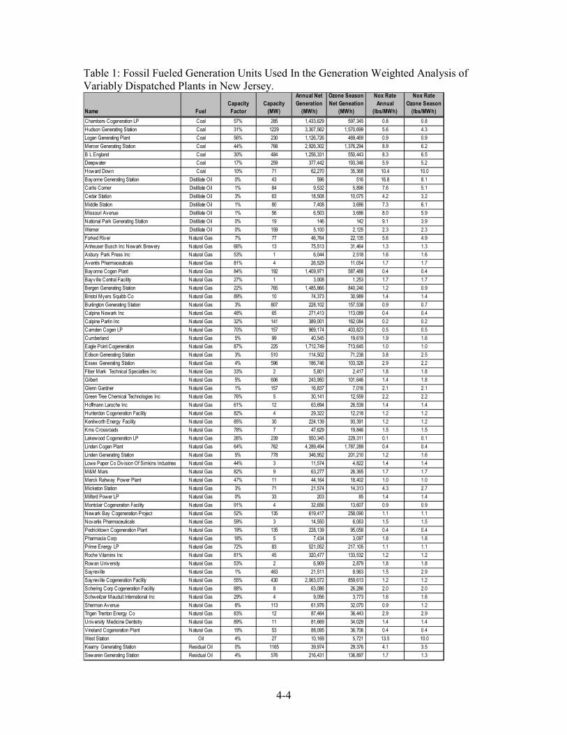
Table 1: Fossil Fueled Generation Units Used In the Generation Weighted Analysis of Variably Dispatched Plants in New Jersey.

Name FuelCapacity

FactorCapacity

(MW)

Annual Net Generation

(MWh)

Ozone Season Net Geneation

(MWh)

Nox Rate Annual

(lbs/MWh)

Nox Rate Ozone Season

(lbs/MWh)Chambers Cogeneration LP Coal 57% 285 1,433,629 597,345 0.8 0.8Hudson Generating Station Coal 31% 1229 3,307,562 1,570,699 5.6 4.3Logan Generating Plant Coal 56% 230 1,126,726 469,469 0.9 0.9Mercer Generating Station Coal 44% 768 2,926,302 1,376,294 8.9 6.2B L England Coal 30% 484 1,256,331 550,443 8.3 6.5Deepwater Coal 17% 259 377,442 193,346 5.9 5.2Howard Down Coal 10% 71 62,270 35,368 10.4 10.0Bayonne Generating Station Distillate Oil 0% 43 596 516 16.8 8.1Carlis Corner Distillate Oil 1% 84 9,532 5,896 7.6 5.1Cedar Station Distillate Oil 3% 63 18,508 10,075 4.2 3.2Middle Station Distillate Oil 1% 80 7,408 3,686 7.3 6.1Missouri Avenue Distillate Oil 1% 56 6,503 3,686 8.0 5.9National Park Generating Station Distillate Oil 0% 19 146 142 9.1 3.9Werner Distillate Oil 0% 159 5,100 2,125 2.3 2.3Forked River Natural Gas 7% 77 46,764 22,135 5.6 4.9Anheuser Busch Inc Newark Brewery Natural Gas 66% 13 75,513 31,464 1.3 1.3Asbury Park Press Inc Natural Gas 53% 1 6,044 2,518 1.6 1.6Aventis Pharmaceuticals Natural Gas 81% 4 26,529 11,054 1.7 1.7Bayonne Cogen Plant Natural Gas 84% 192 1,409,971 587,488 0.4 0.4Bayv ille Central Facility Natural Gas 27% 1 3,008 1,253 1.7 1.7Bergen Generating Station Natural Gas 22% 765 1,485,866 840,246 1.2 0.9Bristol Myers Squibb Co Natural Gas 89% 10 74,373 30,989 1.4 1.4Burlington Generating Station Natural Gas 3% 807 228,102 157,538 0.9 0.7Calpine Newark Inc Natural Gas 48% 65 271,413 113,089 0.4 0.4Calpine Parlin Inc Natural Gas 32% 141 389,001 162,084 0.2 0.2Camden Cogen LP Natural Gas 70% 157 969,174 403,823 0.5 0.5Cumberland Natural Gas 5% 99 40,545 19,619 1.9 1.6Eagle Point Cogeneration Natural Gas 87% 225 1,712,749 713,645 1.0 1.0Edison Generating Station Natural Gas 3% 510 114,502 71,238 3.8 2.5Essex Generating Station Natural Gas 4% 596 186,746 103,326 2.9 2.2Fiber Mark Technical Specialties Inc Natural Gas 33% 2 5,801 2,417 1.8 1.8Gilbert Natural Gas 5% 606 243,950 101,646 1.4 1.8Glenn Gardner Natural Gas 1% 157 16,837 7,016 2.1 2.1Green Tree Chemical Technologies Inc Natural Gas 76% 5 30,141 12,559 2.2 2.2Hoffmann Laroche Inc Natural Gas 61% 12 63,694 26,539 1.4 1.4Hunterdon Cogeneration Facility Natural Gas 82% 4 29,322 12,218 1.2 1.2Kenilworth Energy Facility Natural Gas 85% 30 224,139 93,391 1.2 1.2Kms Crossroads Natural Gas 78% 7 47,629 19,846 1.5 1.5Lakewood Cogeneration LP Natural Gas 26% 239 550,345 229,311 0.1 0.1Linden Cogen Plant Natural Gas 64% 762 4,289,494 1,787,289 0.4 0.4Linden Generating Station Natural Gas 5% 778 346,952 201,210 1.2 1.6Lowe Paper Co Div ision Of Simkins Industries Natural Gas 44% 3 11,574 4,822 1.4 1.4M&M Mars Natural Gas 82% 9 63,277 26,365 1.7 1.7Merck Rahway Power Plant Natural Gas 47% 11 44,164 18,402 1.0 1.0Micketon Station Natural Gas 3% 71 21,574 14,313 4.3 2.7Milford Power LP Natural Gas 0% 33 203 85 1.4 1.4Montclair Cogeneration Facility Natural Gas 91% 4 32,656 13,607 0.9 0.9Newark Bay Cogeneration Project Natural Gas 52% 135 619,417 258,090 1.1 1.1Novartis Pharmaceuticals Natural Gas 59% 3 14,550 6,063 1.5 1.5Pedricktown Cogeneration Plant Natural Gas 19% 135 228,139 95,058 0.4 0.4Pharmacia Corp Natural Gas 18% 5 7,434 3,097 1.8 1.8Prime Energy LP Natural Gas 72% 83 521,052 217,105 1.1 1.1Roche Vitamins Inc Natural Gas 81% 45 320,477 133,532 1.2 1.2Rowan University Natural Gas 53% 2 6,909 2,879 1.8 1.8Sayreville Natural Gas 1% 463 21,511 8,963 1.5 2.9Sayreville Cogeneration Facility Natural Gas 55% 430 2,063,072 859,613 1.2 1.2Schering Corp Cogeneration Facility Natural Gas 88% 8 63,086 26,286 2.0 2.0Schweitzer Mauduit International Inc Natural Gas 29% 4 9,056 3,773 1.6 1.6Sherman Avenue Natural Gas 6% 113 61,976 32,070 0.9 1.2Trigen Trenton Energy Co Natural Gas 83% 12 87,464 36,443 2.9 2.9University Medicine Dentistry Natural Gas 89% 11 81,669 34,029 1.4 1.4Vineland Cogeneration Plant Natural Gas 19% 53 88,095 36,706 0.4 0.4West Station Oil 4% 27 10,169 5,721 13.5 10.0Kearny Generating Station Residual Oil 0% 1165 39,974 29,376 4.1 3.5Sewaren Generating Station Residual Oil 4% 576 216,431 136,897 1.7 1.3

4-4

F1147-E(12/2004)

REPORT DOCUMENTATION PAGE Form Approved OMB No. 0704-0188

The public reporting burden for this collection of information is estimated to average 1 hour per response, including the time for reviewing instructions, searching existing data sources, gathering and maintaining the data needed, and completing and reviewing the collection of information. Send comments regarding this burden estimate or any other aspect of this collection of information, including suggestions for reducing the burden, to Department of Defense, Executive Services and Communications Directorate (0704-0188). Respondents should be aware that notwithstanding any other provision of law, no person shall be subject to any penalty for failing to comply with a collection of information if it does not display a currently valid OMB control number. PLEASE DO NOT RETURN YOUR FORM TO THE ABOVE ORGANIZATION. 1. REPORT DATE (DD-MM-YYYY)

August 2006 2. REPORT TYPE

Technical Report 3. DATES COVERED (From - To)

4. TITLE AND SUBTITLE

Final Report on the Clean Energy/Air Quality Integration Initiative Pilot Project of the U.S. Department of Energy’s Mid-Atlantic Regional Office

5a. CONTRACT NUMBER DE-AC36-99-GO10337

5b. GRANT NUMBER

5c. PROGRAM ELEMENT NUMBER

6. AUTHOR(S) D. Jacobson, George Washington University Law School P. O’Connor, Global Environment & Technology Foundation C. High, Resource Systems Group J. Brown, National Renewable Energy Laboratory

5d. PROJECT NUMBER NREL/TP-710-40477

5e. TASK NUMBER 60014204

5f. WORK UNIT NUMBER

7. PERFORMING ORGANIZATION NAME(S) AND ADDRESS(ES) National Renewable Energy Laboratory 1617 Cole Blvd. Golden, CO 80401-3393

8. PERFORMING ORGANIZATION REPORT NUMBER DOE/GO-102006-2354

9. SPONSORING/MONITORING AGENCY NAME(S) AND ADDRESS(ES)

10. SPONSOR/MONITOR'S ACRONYM(S) NREL

11. SPONSORING/MONITORING AGENCY REPORT NUMBER

12. DISTRIBUTION AVAILABILITY STATEMENT National Technical Information Service U.S. Department of Commerce 5285 Port Royal Road Springfield, VA 22161

13. SUPPLEMENTARY NOTES

14. ABSTRACT (Maximum 200 Words) The MARO pilot project represents the first effort in the country to seek to obtain credit under a Clean Air Act (CAA) State Implementation Plan (SIP) for nitrogen oxide (NOx) emission reductions. This project came about because of state-funded incentive programs and projects for RE and EE. Specifically, the pilot project focuses on the New Jersey (NJ) SIP and efforts to facilitate attainment of the new, 8-hour ozone standard under CAA by implementing selected categories of RE and EE programs and projects funded by the New Jersey Clean Energy Program (NJ CEP) of the New Jersey Board of Public Utilities (NJ BPU).

15. SUBJECT TERMS maro; mid-atlantic regional office; nitrogen oxide; nox; sip; ozone standard

16. SECURITY CLASSIFICATION OF: 17. LIMITATION OF ABSTRACT

UL

18. NUMBER OF PAGES

19a. NAME OF RESPONSIBLE PERSON a. REPORT

Unclassified b. ABSTRACT Unclassified

c. THIS PAGE Unclassified 19b. TELEPHONE NUMBER (Include area code)

Standard Form 298 (Rev. 8/98) Prescribed by ANSI Std. Z39.18

A Strong Energy Portfolio for a Strong America Energy efficiency and clean, renewable energy will mean a stronger economy, a cleaner environment, and greater energy independence for America. Working with a wide array of state, community, industry, and university partners, the U.S. Department of Energy's Office of Energy Efficiency and Renewable Energy invests in a diverse portfolio of energy technologies.

For more information contact: EERE Information Center 1-877-EERE-INF (1-877-337-3463) www.eere.energy.gov