final report - evaluation of superpave mixtures with and ... - NET

U.F. Project No: 49104504801-12

Contract No: BC-354 RPWO#: 36

EVALUATION OF SUPERPAVE MIXTURES WITH AND WITHOUT POLYMER MODIFICATION BY MEANS OF

ACCELERATED PAVEMENT TESTING

Mang Tia Reynaldo Roque

Okan Sirin Hong-Joong Kim

November 2002

Department of Civil & Coastal Engineering College of Engineering University of Florida Gainesville, Florida

FINAL REPORT

i

ACKNOWLEDGMENTS The Florida Department of Transportation (FDOT) is gratefully acknowledged for

providing the financial support for this study. The FDOT Materials Office provided the

additional testing equipment, materials and personnel needed for this investigation.

Sincere thanks go to the project manager, Dr. Bouzid Choubane for providing the

technical coordination and advices throughout the project. Sincere gratitudes are

extended to the FDOT Materials Office personnel, particularly to Messrs. Gale C. Page,

Tom Byron, Steve Ross, James Musselman, Patrick Upshaw, Greg Sholar, Howard

Moseley, Ron McNamara and Natasha Seavers. The help of Messrs. Booil Kim,

Sylvester Asiamah, Daniel D. Darku and Claude Villiers in the sampling of asphalt

mixtures and installation of thermocouples, and Mr. Rajarajan Subramanian in the

laboratory testing of the core samples are acknowledged. The technical inputs from Drs.

David Bloomquist and Byron E. Ruth of the University of Florida are duly

acknowledged.

ii

TABLE OF CONTENTS

ACKNOWLEDGMENTS ................................................................................................... i LIST OF TABLES............................................................................................................. iv LIST OF FIGURES ........................................................................................................... vi TECHNICAL SUMMARY ............................................................................................... ix CHAPTERS

1 INTRODUCTION ...................................................................................................1 1.1 Background .....................................................................................................1 1.2 Scope of Report...............................................................................................2

2 EXPERIMENTAL DESIGN AND INSTRUMENTATION ..................................4

2.1 Test Track Layout ...........................................................................................4 2.2 Testing Parameters and Sequence...................................................................4 2.3 Temperature Monitoring System ....................................................................6 2.4 Pavement Temperature Control System .........................................................9 2.5 Laser Profiler ................................................................................................14

3 MATERIALS.........................................................................................................16 4 CONSTRUCTION OF THE TEST TRACK.........................................................18

4.1 Construction of Control Strip........................................................................18 4.2 Placement of Thermocouples........................................................................18 4.3 Placement of the Asphalt Mixtures...............................................................20 4.4 Density of the Compacted Pavement............................................................22 4.5 Volumetric Properties and Binder Contents .................................................22 4.6 Additional Asphalt Mixture Samples............................................................26

5 TRIAL TESTS FOR DETERMINATION OF OPTIMUM HVS TEST CONFIGURATION .......................................................29

5.1 Testing Configurations..................................................................................29 5.2 Temperature Measurements..........................................................................30 5.3 Rut Measurement ..........................................................................................30 5.4 Comparison Between Bi-Directional and Uni-Directional Loading with No Wander ...................................................32 5.5 Comparison Between Bi-Directional and Uni-Directional Loading with 4-inch Wander..............................................37

iii

5.6 Comparison Between Uni-Directional Loading with 4-inch Wander in 2-inch Increments and Uni-Directional Loading with 4-inch Wander in 1-inch Increments ....................................................41 5.7 HVS Test Configuration Chosen ..................................................................49

6 PHASE I OF HVS FIELD TESTING PROGRAM...............................................50 6.1 Testing Configuration ...................................................................................50 6.2 Temperature Measurement ...........................................................................50 6.3 Rut Measurement ..........................................................................................50 6.4 Summary of Findings....................................................................................53

7 PHASE II OF HVS FIELD TESTING PROGRAM .............................................58 7.1 Testing Configuration ...................................................................................58 7.2 Temperature Measurement ...........................................................................58 7.3 Rut Measurement ..........................................................................................61 7.4 Summary of Findings....................................................................................68

8 LABORATORY TESTING PROGRAM ON PLANT-COLLECTED SAMPLES.......................................................................70 8.1 Tests on Plant-Collected Samples.................................................................70 8.2 Gyratory Testing Machine (GTM) Results...................................................70 8.3 Servopac Gyratory Compactor (SGC) Results .............................................73 8.4 Asphalt Pavement Analyzer (APA) Results .................................................81 8.5 Summary of Findings....................................................................................81

9 EVALUATION OF CORED SAMPLES FROM THE TEST SECTIONS.............................................................................83 9.1 Introduction...................................................................................................83 9.2 Thickness and Density Evaluation of Cores from the Test Sections ............83 9.3 Evaluation of Cores for Resilient Modulus and Indirect Tensile Strength .........................................................................................................88 9.4 Evaluation of Cores for Viscosity Test .........................................................92 9.5 Summary of Findings....................................................................................95

10 SUMMARY OF FINDINGS .................................................................................96

LIST OF REFERENCES...................................................................................................98 APPENDIX

A SUPERPAVE MIX DESIGN ...........................................................................101 B NUCLEAR DENSITY DATA .........................................................................105 C THICKNESS PROFILES OF CORES FROM TEST SECTIONS ..................113 D LITERATURE REVIEW ON ACCELERATED PAVEMENT TESTING AND FIELD RUT MEASUREMENT ...........................................119 E HEAVY VEHICLE SIMULATOR ..................................................................128

iv

LIST OF TABLES

Table Page

3.1 Properties of Aggregate Used in the Asphalt Mixture...........................................17

3.2 Volumetric Properties of the Asphalt Mixtures .....................................................17

4.1 Core and Nuclear Density Data for Lift 1..............................................................24

4.2 Core and Nuclear Density Data for Lift 2..............................................................25

4.3 Comparisons of Volumetric Properties of Asphalt Mixtures for Lift 1.................27

4.4 Comparisons of Volumetric Properties of Asphalt Mixtures for Lift 2.................28

5.1 Temperatures of Test Pavement in Trial Sections as Measured by Thermocouples Placed between the Two 2-inch Lifts of Asphalt Mixture ...........31

6.1 Temperatures of Test Pavement in Phase I as Measured by Thermocouples Placed Between the Two 2-inch Lifts of Asphalt Mixture ....................................51

7.1 Temperatures of Test Pavements in Section 3B and 5B as Measured by Thermocouples Placed at the Surface and at 2-inch Depth ...................................60

8.1 GSI values of the Four Mixtures Evaluated in the GTM.......................................71

8.2 Volumetric Properties of the Mixtures Compacted in the Servopac Gyratory Compactor Using 1.25 and 2.5° Gyratory Angles..................................76

8.3 Summary of Rut Depth Measurements in the APA Evaluation of the Four Mixtures ..............................................................................................82

9.1 Bulk Densities of Cores from Wheel Paths and Edges of Wheel Paths of the Test Sections................................................................................................85

9.2 Comparison of Air Voids of Cores before and after HVS Testing........................87

9.3 Resilient Modulus and Indirect Tensile Strength at 25° C of Cores from the Test Sections ...........................................................................................89

9.4 Resilient Modulus at 5° C of Cores from the Test Sections on Lane 7 .................92

9.5 Viscosity of Cores from the Test Sections.............................................................94

A.1 Summary of Aggregate Blending for Superpave Mix Design.............................102

A.2 Mix Design Data for the Unmodified Superpave Mix.........................................103

A.3 Mix Design Data for the SBS-Modified Superpave Mix.....................................104

B.1 Nuclear Density Data for Lane 1-Lift 1 ...............................................................106



v












vi

LIST OF FIGURES

Figure Page

2.1 APT Test Track Layout ...........................................................................................5

2.2 Testing Sequence .....................................................................................................7

2.3 Plan and Cross Section View of Thermocouples per Test Section..........................8

2.4 Photo of Sidewall-Paneled HVS............................................................................10

2.5 The Dimensions and Heat Flux Ranges of Radiant Heaters..................................10

2.6 Photo of RAYMAX Hairpin Radiant Heater Unit.................................................11

2.7 Locations of Thermocouples for Temperature Control .........................................12

2.8 The Installation of Thermo Probe at 2-inch Depth from the Surface ....................13

2.9 Photo of Pavement Inside of Insulating Area ........................................................13

2.10 Photo of Lasers Mounted onto Two Sides of the Test Carriage ............................14

2.11 The Paths of Laser Profiler in Measuring Pavement Surface Profile ....................15

4.1 Photo of K-Type Thermocouple Installed on the Limerock Base .........................19

4.2 Photo of the Thermocouples Installed on the First Lift of HMA ..........................20

4.3 Photo of Steel-Wheel Roller Used for Compaction...............................................21

4.4 Photo of Test Track................................................................................................21

4.5 Coring and Nuclear Density Testing Plan .............................................................23

5.1 Photo of Straight Edge Used for Measuring Rut Depth ........................................32

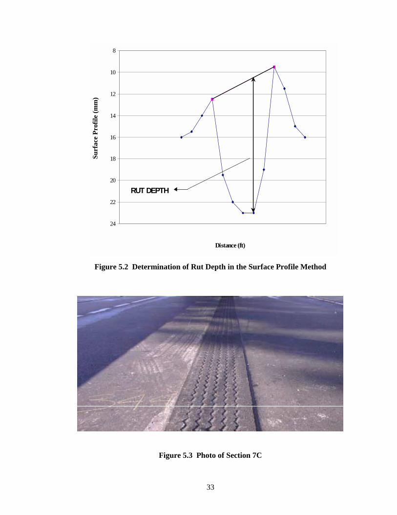
5.2 Determination of Rut Depth in the Surface Profile Method ..................................33

5.3 Photo of Section 7C ...............................................................................................33

5.4 Photo of Section 7B-W ..........................................................................................34

5.5 Comparison of Differential Surface Deformation versus Number of Passes between Bi-Directional and Uni-Directional Loading with No Wander ...............35

5.6 Comparison of Average Rut Depth as Measured by the Surface Profile Method versus Number of Passes Between Bi-Directional and Uni-Directional Loading with No Wander ............................................................36

5.7 Comparison of Differential Surface Deformation versus Time between Bi-Directional and Uni-Directional Loading .........................................................38

5.8 Comparison of Average Rut Depth as Measured by the Surface Profile Method versus Time Between Bi-Directional and Uni-Directional Loading with No Wander.......................................................................................39

vii

5.9 Photo of Section 7B-E ...........................................................................................40

5.10 Photo of Section 7A-E ...........................................................................................40

5.11 Comparison of Differential Surface Deformation versus Number of Passes Between Uni-Directional and Bi-Directional Loading with 4-inch Wander................................................................................................42

5.12 Comparison of Average Rut Depth by Profile Method versus Number of Passes Between Uni-Directional and Bi-Directional Loading with 4-inch Wander .................................................................................43

5.13 Comparison of Differential Surface Deformation versis Time Between Uni-Directional and Bi-Directional Loading with 4-inch Wander........................................................................................................44

5.14 Comparison of Average Rut Depth by the Profile Method versus Time Between Uni-Directional and Bi-Directional Loading with 4-inch Wander........................................................................................................45

5.15 Photo of Section 7A-W..........................................................................................46

5.16 Comparison of Differential Surface Deformation versus Number of Passes Between Uni-Directional Loading with 4-inch Wander in 1-inch Increments and 2-inch Increments..........................................................47

5.17 Comparison of Average Rut Depth by the Profile Method versus Number of Passes Between Uni-Directional Loading with 4-inch Wander in 1-inch Increments and 2-inch Increments ............................................48

6.1 Picture of Transverse Profiler ................................................................................52

6.2 Comparison of Differential Surface Deformation versus Number Passes for Test Sections in Phase I ........................................................................54

6.3 Comparison of Change in Rut Depth as Measured by the Surface Profile Method versus Number of Passes for Test Sections in Phase I .................55

6.4 Section 5C (Unmodified Mixture) after HVS Testing...........................................56

6.5 Section 2C (SBS-Modified Mixture) after HVS Testing.......................................56

7.1 Pavement Temperatures versus Time during Pre-Heating before Start of Test............................................................................................................59

7.2 Comparison of Rut Depth as Measured by the Differential Surface Profile Method versus Number of Passes ..............................................................62

7.3 Comparison of Change in Rut Depth as Measured by the Surface Profile Method versus Number of Passes ..............................................................63

7.4 Photo of Section 1B (SBS-Modified Mixture Tested at 50° C) ............................64

7.5 Photo of Section 2B (SBS-Modified Mixture Tested at 50° C) ............................64

viii

7.6 Photo of Section 3A (SBS-Modified Mixture over Unmodified Mixture Tested at 50° C) .......................................................................................65

7.7 Photo of Section 3B (SBS-Modified Mixture over Unmodified Mixture Tested at 50° C) .......................................................................................65

7.8 Photo of Section 4A (Unmodified Mixture Tested at 50° C) ................................66

7.9 Photo of Section 4B (Unmodified Mixture Tested at 50° C) ................................66

7.10 Photo of Section 5A (Unmodified Mixture Tested at 50° C) ................................67

7.11 Photo of Section 5B (Unmodified Mixture Tseted at 50° C) ................................67

7.12 Photo of Section 1A (SBS-Modified Mixture Tested at 65° C) ............................69

7.13 Photo of Section 2A (SBS-Modified Mixture Tested at 65° C) ............................69

8.1 Gyratory Shear Resistance of the Unmodified and Modified Asphalt Mixtures versus Number of Gyrations .....................................................72

8.2 Gyratory Shear Values versus Number of Gyrations Using 1.25° Gyratory Angle ......................................................................................................74

8.3 Gyratory Shear Values versus Number of Gyrations Using 2.5° Gyratory Angle .....................................................................................................75

8.4 Gyratory Shear Strength versus Log Cycles for Gyrations between Air Voids of 7% to 4% at 1.25° Gyratory Angle...................................................77

8.5 Gyratory Shear Strength versus Log Cycles for Gyrations between Air Voids of 7% to 4% at 2.5° Gyratory Angle.....................................................78

8.6 Gyratory Shear Strength versus Air Voids at 1.25° Gyratory Angle in the Servopac Gyratory Compactor ....................................................................79

8.7 Gyratory Shear Strength versus Air Voids at 2.5° Gyratory Angle in the Servopac Gyratory Compactor ....................................................................80

9.1 Picture Showing Locations of a Core Taken From the Middle of the Wheel Path and a Core Take From the Outside Edge of the Wheel Path..............84

C.1 Thickness Profiles of Cores from Section 7AE (Uni-Directional with 4″ Wander in 2″ Increments) ...............................................................................114

C.2 Thickness Profiles of Cores from Section 7AW (Uni-Directional with 4″ Wander in 2″ Increments) ...............................................................................115

C.3 Thickness Profiles of Cores from Section 7BE (Bi-Directional with 4″ Wander in 2″ Increments) ...............................................................................116

C.4 Thickness Profiles of Cores from Section 7BE (Uni-Directional without Wander)................................................................................................................117

C.5 Thickness Profiles of Cores from Section 7C (Bi-Directional without Wander)................................................................................................................118

ix

TECHNICAL SUMMARY Florida Department of Transportation (FDOT) started the use of Superpave

mixtures on its highway pavements in 1996. Modified binders have also been used in

some of the Superpave mixtures in an effort to increase the cracking and rutting

resistance of these mixtures. Due to the short history of these mixtures, it is still too early

to assess the long-term performance of these Superpave mixtures and the benefits from

the use of the modified binders. There is a need to evaluate the long-term performance of

these mixtures and the benefits obtained from the use of modified binders, so that the

Superpave technology and the selection of modified binders to be used could be

effectively applied.

The FDOT Materials Office has recently acquired a Heavy Vehicle Simulator

(HVS) and constructed an Accelerated Pavement Testing (APT) facility which uses this

Heavy Vehicle Simulator. The HVS can simulate 20 years of interstate traffic on a test

pavement within a short period of time. Thus, a research study was started to evaluate

the long-term performance of Superpave mixtures and modified Superpave mixtures

using the APT facility. The main objectives of this study are as follows:

(1 ) To evaluate the operational performance of the Heavy Vehicle Simulator, and to

determine its most effective test configurations for use in evaluating the rutting

performance of pavement materials and/or designs under typical Florida traffic

and climate conditions.

(2 ) To evaluate the rutting performance of a typical Superpave mixture used in

Florida and that of the same Superpave mixture modified with a SBS polymer.

x

(3 ) To evaluate the relationship between mixture properties and the rutting

performance.

(4 ) To evaluate the difference in rutting performance of a pavement using two lifts of

modified mixture versus a pavement using one lift of modified mixture on top of

one lift of unmodified mixture.

Five trial runs with the HVS were made using a super single tire with a load of

9,000 lbs (40 kN), tire pressure of 115 psi (792 kPa) and a wheel traveling speed of 8

mph (12.9 km/hr). These five trial runs used different combinations of wheel traveling

direction (uni-directional or bi-directional), total wheel wander and wander increments.

The uni-directional loading was found to be a more efficient mode for evaluation

of rutting performance using the HVS. As compared with the bi-directional loading

mode, the uni-directional mode produced substantially higher rut depths for the same

number of wheel passes and also for the same testing time duration. When the bi-

directional loading with no wander was used, imprints of the tire treads were observed on

the wheel track. It was found that using a loading mode with wander smoothened out the

imprints of the tire treads considerably. The uni-directional loading mode with 4-inch

(10.2-cm) wander using 1-inch (2.54-cm) increments was selected to be used in the main

field testing program for evaluation of rutting performance based on consideration of

testing efficiency and realistic rutting results.

Results from the HVS tests showed that the pavement sections with two lifts of

SBS-modified mixture clearly outperformed those with two lifts of unmodified mixture,

which had two to two and a half times the rut rate. The pavement sections with a lift of

SBS-modified mixture over a lift of unmodified mixture practically had about the same

xi

performance as the sections with two lifts of SBS-modified mixture, and had only about

20% higher rutting than those with two lifts of modified mixture when tested at 50° C.

The test section with two lifts of SBS-modified mixture and tested at 65° C still

outperformed the test sections with two lifts of unmodified mixture and tested at 50° C.

The mixtures with a higher rut depth in the APA also rutted more in the HVS tests.

The mixtures with a GSI of more than 1.0 as measured by the GTM rutted more than one

with a GSI close to 1.0. Rutting of the unmodified mixture was observed to be due to a

combination of densification and shoving, while that of the SBS-modified mixture was

due primarily to densification.

1

CHAPTER 1 INTRODUCTION

1.1 Background

Florida Department of Transportation (FDOT) started the use of Superpave

mixtures on its highway pavements in 1995. Modified binders have also been used in

some of the Superpave mixtures in an effort to increase the cracking and rutting

resistance of these mixtures. Due to the short history of these mixtures, it is still too early

to assess the long-term performance of these Superpave mixtures and the benefits from

the use of the modified binders. There is a need to evaluate the long-term performance

of these mixtures and the benefits obtained from the use of modified binders, so that the

Superpave technology and the selection of modified binders to be used could be

effectively applied.

The FDOT Materials Office recently acquired a Heavy Vehicle Simulator (HVS),

Mark IV Model, and constructed an Accelerated Pavement Testing (APT) facility, which

uses this Heavy Vehicle Simulator. The HVS can simulate 20 years of interstate traffic

on a test pavement within a short period of time. Thus, a research study was undertaken

to evaluate the long-term performance of Superpave mixtures and SBS-modified

Superpave mixtures with particular emphasis on the rutting resistance of these mixtures

using the FDOT APT facility. This research work was a cooperative effort between the

FDOT and the University of Florida. The main objectives of this study are as follows:

To evaluate the operational performance of the Heavy Vehicle Simulator, and to

determine its most effective test configurations for use in evaluating the long term

2

performance of pavement materials and/or designs under typical Florida traffic and

climate conditions.

To evaluate the rutting performance of a typical Superpave mixture used in

Florida and that of the same Superpave mixture modified with a SBS polymer.

To evaluate the relationship between mixture properties and the rutting performance.

To evaluate the difference in rutting performance of a pavement using two lifts of

modified mixture versus a pavement using one lift of SBS-modified mixture on top of

one lift of unmodified mixture.

1.2 Scope of Report

The description of the planning, design and construction of the test sections for

this study have previously been presented in an interim report entitled “Evaluation of

Superpave and Modified Superpave Mixtures by Means of Accelerated Pavement Testing

– Planning and Design Phase.” However, some changes were made to the experimental

design and instrumentation as the experiment progressed. Thus, in order to have an

updated description of the experimental design and instrumentation used in the study and

for ease of reference for the readers, this report describes this study in its entirety. The

main report includes descriptions of (1) the materials and mix designs used for the test

pavement sections, (2) the design of experiment, (3) the instrumentation and data

acquisition system, (4) the construction of the test sections, (5) the experimental program

for determination of the optimum HVS test configurations, (6) the main HVS testing

program, (7) the laboratory testing program, (8) test and analysis results, and (9) findings

from this study.

3

The following information are included in the appendices: (1) detailed mix

design data, (2) detailed nuclear density data obtained from the test sections, (3) thickness

profiles of cores obtained from the test sections, (4) literature review on full-scale

accelerated testing and methods for measurement of rutting, and (5) description of the

Heavy Vehicle Simulator, Mark IV Model.

4

CHAPTER 2 EXPERIMENTAL DESIGN AND INSTRUMENTATION

2.1 Test Track Layout

The layout of the test track, which was constructed at the FDOT APT facility for

this study, is shown in Figure 2.1. The test track consisted of seven test lanes. The

locations for these test lanes were selected such that they could fit around the two

existing concrete conduit boxes. Their widths varied from 12 to 13.5 feet. Each test lane

was divided into three test sections, which were identified as Sections A, B and C. Each

test section was to be 30 feet long, with 20 feet of test area and 5 feet at each end for

acceleration and deceleration of the test wheel. Adjacent to the test lanes was a 94 feet

long area, which was to be used for maneuvering of the HVS.

The test track had a 10.5-inch limerock base placed on top of a 12-inch limerock

stabilized subgrade. Lanes 1 and 2 were paved with two 2-inch lifts of the SBS-modified

Superpave mixture. Lane 3 had a 2-inch lift of the modified Superpave mix over a 2-inch

lift of unmodified Superpave mix. Lanes 4 through 7 were paved with two 2-inch lifts of

the unmodified Superpave mix. All Sections C in Lane 1 through 5 was named as Phase

I, and all Sections A and B in Lane 1 through 5 was named as Phase II.

2.2 Testing Parameters and Sequence

The main testing program was to be run on Test Lanes 1 through 5, which had a

total of 15 test sections. Test Lane 6 was set aside for additional testing deemed

necessary or desirable at the end of the main testing program. Test Lane 7 was to be

5

Figure 2.1 APT Test Track Layout

UnmodifiedMix (U)

ModifiedMix (M)

14.6’

44’

50’

Building Wall

N

HVS Maneuver Area

1 2 3 4 5 6 7

13’ 6’ 12’ 12’ 12’ 12’ 6’ 13.5’ 13.5’

30’

16’

30’

30’

A

B

20’ TestTrack Area

Initial CoringArea

5’ Acceleration andDeceleration Zones

ConcreteCurb

ConduitBox

1, 2, 3 etc. ! Lane No

A, B and C ! Test Sections

U+M

23’

30’

30’C

6

used for trial runs to evaluate the performance characteristics of the HVS and to

determine the most effective test configuration to be used in the testing program.

The testing parameters and sequence to be used for the main testing program are

shown in Figure 2.2. The testing program was divided into two phases. Phase I was

conducted at ambient condition on five test sections, 1C through 5C. Phase II was

conducted with temperature control on the other ten test sections. In Phase II, Lanes 1

and 2, which have two 2-inch lifts of SBS-modified Superpave mixture were tested at

controlled pavement temperatures of 50° C and 65° C. The rest of the test sections in

Phase II were tested at only one temperature, namely 50° C. The testing sequence was

arranged such that the effects of time on each lane could be averaged out. It was also

arranged such that the HVS vehicle would not have to drive over a test section, which has

not been tested in order to minimize damage to the test sections.

The wheel load to be used is a 9-kip super single tire. The type and amount of

wheel wander to be used were to be determined after all the trial tests on Lane 7 were

completed and evaluated.

2.3 Temperature Monitoring System

The temperature distributions in the test pavements were monitored by means of

Type K thermocouples installed at various depths and locations in the test pavements.

Type K thermocouple was selected to be used in consideration of its relatively high

sensitivity (40 µV/°C), high range of operation (-200 to 1250° C), reliability and low

cost. Figure 2.3 shows the plan and cross section views of the thermocouples for each

test section. A total of eight thermocouples were installed for each test section. For each

7

A B C

U +M

Figure 2.2 Testing Sequence

8 MB

9 MB

5 (U+M) A

7 UA

10 UA

6 MA

2 MA

3 (U+M) A

4 UA

1 UA

5 M

2 M

4 (U+M)

3 U

1 U

30 ‘

30’

30’

LANE 1 LANE 2 LANE 3 LANE 4 LANE 5

Modified Mix (M) Unmodified Mix (U)

U """" Unmodified Mix A """" Test Temperature of 50°C M """" Modified Mix B """" Test Temperature of 65°C U+M """"Unmodified +Modified Mix 1, 2, 3 …"""" Testing sequence number

N

Phase II

Phase I

8

Figure 2.3 Plan and Cross Section View of Thermocouples per Test Section

HVS Testing Beam

Thermocouple

2 in.

2 in.

Thermocouple

12’

30’

Cross-Section

Limerock Base

AC Layer

9

test section, three thermocouples were placed on top of the base course, three were placed

on top of the first lift of asphalt mixture, and two were placed on the surface. These

thermocouples were conducted to a PC data acquisition system. Temperature readings

were taken every 15 minutes and recorded in the PC during each test.

2.4 Pavement Temperature Control System

A temperature control system to control the temperature of the HVS test

pavements was installed at the end of Phase I and used in Phase II of the testing program.

It consisted mainly of (1) insulating panels to cover the pavement area to be tested, (2)

radiant heaters to heat the pavement surface, and (3) thermocouples to monitor the

pavement temperature and to control the heaters.

The insulating panels were made of 3-inch thick Styrofoam boards, which were

covered with 0.08-inch thick aluminum sheeting. The roof panels were installed directly

under the longitudinal beam of the HVS frame to cover the top of the test pavement area.

Each panel was approximately 12 feet wide and 7 feet long. A total of 6 roof panels were

used. Five sidewall panels were installed on each side of the HVS to cover the sides of

the enclosed test area. Figure 2.4 shows a picture of the HVS covered with the sidewall

panels. The total enclosed test area was approximately 3,675 cubic feet.

Three pairs of radiant heaters (Watlow’s Raymax 1525) were used to heat the test

pavement surface as needed. Figure 2.5 shows the locations and dimensions of a pair of

heaters, and the ranges of their heat flux inside the insulating area. Each heater was

supported by a 480-volt power and had a maximum capacity of 7500 watts. Figure 2.6

shows a picture of the Raymax radiant heater unit.

10

Figure 2.4 Photo of Sidewall-Paneled HVS Aluminum Panel 50” 11” 15” Asphalt Mixture 2”

Figure 2.5 The Dimensions and Heat Flux Ranges of Radiant Heaters

K-Type Thermocouple Thermo Probe Heat Flux Radiant Heater

Insulating Walls

11

Figure 2.6 Photo of RAYMAX Hairpin Radiant Heater Unit Each radiant heater was controlled by a pair of thermocouples. Figure 2.7 shows

the locations for these six pairs of thermocouples (K-type). At each location, one

thermocouple was glued on the surface by means of a high thermal conductivity paste

(Omegatherm 201). Another thermocouple was placed at a depth of 2 inches. This was

done by drilling a hole to a depth of 2 inches, placing the thermocouple inside a thermal

probe, and inserting the thermal probe into the drilled hole. A high thermal conductivity

paste (Omegatherm 201) was placed at the bottom of the drilled hole to ensure good

thermal contact between the tip of the thermal probe and the asphalt concrete at 2-inch

depth. Figure 2.8 shows the location of the thermo probe at a 2-inch depth. Figure 2.9

shows a picture of the pavement inside the insulating area.

12

Figure 2.7 Locations of Thermocouples for Temperature Control

TEST

WHEELPATH

HVS TOW END

HVS CABIN

Thermocouple at 2-inchDepth

Thermocouple at Surface

N

16”

324”

51.5”

2”

162”

2”

13

Figure 2.8 The Installation of Thermo Probe at 2-inch Depth from the Surface

Figure 2.9 Photo of Pavement Inside of Insulating Area

Thermo Probe

Surface of AC

2 in.

2 in.

AC Layer

OMEGATHERM 201,High Thermal Conductivity Paste

14

2.5 Laser Profiler

A laser profiler was installed on the HVS at the end of Phase I and used in Phase

II of the testing program in order to enable more frequent and consistent measurement of

the pavement profile during the HVS tests. The laser profiler used was a SLS 5000 TM

manufactured by LMI Selcom. It consisted of two lasers. The specified ambient

temperature surrounding the laser should be 0 to 50° C, while the temperature of objects

to be measured can be below 0° C and up to 1,600° C. Each of the two lasers was

mounted on each side of the test carriage as shown in Figure 2.10. The two lasers were

placed at a distance of 30 inches away from one another.

Figure 2.10 Photo of Lasers Mounted onto Two Sides of the Test Carriage Figure 2.11 shows the paths of the two lasers in making a profile measurement of

a tested pavement. In making a profile measurement of a tested pavement, the test

carriage holding the two lasers would travel (240 inches) longitudinally from one end to

15

another, and then move diagonally back to the other end with a lateral incremental shift

of 1 inch. In each pass, 58 data points would be collected, with each data point

representing the average reading from every 4-inch sweep. This process would be

repeated 30 ½ times (with a total of 61 sweeps) until that each laser would sweep over a

lateral distance of 30 inches. The last sweep of the right laser would overlap with the

first sweep of the left laser. The total lateral distance covered by the two lasers would be

60 inches.

Figure 2.11 The Paths of Laser Profiler in Measuring Pavement Surface Profile The longitudinal profiles as measured would be used to determine the lateral

profiles, which would in turn be used to determine the rut depth. The procedures for

determination of rut depths from lateral profiles are described in Chapter 7.

WHEEL

PATH

1” 1”

Left-Side Laser Right-Side Laser

Direction ofLaser Profiler

60”

240”

*Drawing Not Scaled

16

CHAPTER 3 MATERIALS

The two asphalt mixtures, which were placed in the test pavements, were (1) a

Superpave mixture using PG67-22 asphalt and (2) a Superpave mixture using PG67-22

asphalt modified with a SBS polymer, which had an equivalent grading of PG76-22.

Both mixtures were made with the same aggregate blend having the same gradation, and

had the same effective asphalt content. The types and gradation of the aggregate blend

used were similar to those of an actual Superpave mixture, which had recently been

placed down in Florida. These mixtures can be classified as 12.5 mm fine Superpave

mixes, with a nominal maximum aggregate size of 12.5 mm and the gradation plotted

above the restricted zone. The properties of the aggregates used are shown in Table 3.1.

Designs for these two mixtures were done by the personnel of the Bituminous

Section of the FDOT Materials Office. The optimum binder content was determined

according to the Superpave mix design procedure and criteria using a design traffic level

of 10 to 30 × 106 ESALs. The mix design data for these two mixtures are also given in

Tables A.1 through A.3 in the Appendix A. The binder contents and volumetric

properties for these two mixtures are shown in Table 3.2.

17

Table 3.1 Properties of Aggregate Used in the Asphalt Mixture

Type Material FDOT Code

Producer Pit No Date Sampled

1. S-1-A Stone 41 Rinker Mat. Corp TM-489 87-089 9/11/00

2. S-1-B Stone 51 Rinker Mat. Corp TM-489 87-089 9/11/00

3. Screenings 20 Anderson Mining Corp 29-361 9/11/00

4. Local Sand V.E.Whitehurst & Sons, Inc Starvation Hill 9/11/00

Percentage by Weight of Total Aggregate Passing Sieves

Blend 12% 25% 48% 15%

Number 1 2 3 4 JMF

Control Points

Restricted Zone

¾" 19.0mm 99 100 100 100 100 100

½" 12.5mm 45 100 100 100 93 90-100

3/8" 9.5mm 13 99 100 100 89 -90

No. 4 4.75mm 5 49 90 100 71

No. 8 2.36mm 4 10 72 100 53 28-58 39.1-39.1

No. 16 1.18mm 4 4 54 100 42 25.6-31.6

No. 30 600µm 4 3 41 96 35 19.1-23.1

No. 50 300µm 4 3 28 52 22

No. 100 150µm 3 2 14 10 9

S i e v e

S i z e

No. 200 75µm 2.7 1.9 5.9 2.2 4.5 2-10

Gsb 2.327 2.337 2.299 2.546 2.346

Table 3.2 Volumetric Properties of the Asphalt Mixtures

Mix Type Asphalt Binder

% Binder

Va @ Ndes

VMA VFA Pbe Gmm

Superpave Mix (Compacted at 300° F)

PG67-22 8.2 4.0 14.5 72 4.97 2.276

Modified Superpave Mix

(Compacted at 325° F) PG76-22 7.9 3.8 14.2 73 4.90 2.273

18

CHAPTER 4 CONSTRUCTION OF THE TEST TRACK

4.1 Construction of Control Strip

Before the Superpave and the SBS-modified Superpave mixtures were placed on

the test track, a control strip was constructed using the Superpave mixture. This was

done in order to determine the appropriate rolling pattern needed to achieve the desired

density and to calibrate the two nuclear density gauges to be used for checking the

density of the test pavements. The target density for the compacted mixture was 93±1%

of Gmm (maximum theoretical density). The density of the compacted mixture was

measured by means of the two nuclear density gauges using a reading time of one minute,

and cores taken from the compacted pavement. The density measurements from the

cores were used to calibrate the two nuclear density gauges.

The two rollers used by the paving contractor were 25,000-lb rollers, which could

be used in either a static mode or a vibratory mode. From the results of the test strip, it

was determined that the target density could be achieved by three passes of the vibratory

roller followed by three passes of the static roller. This rolling pattern was thus used in

the compaction of the asphalt mixtures in the test track.

4.2 Placement of Thermocouples

As described in Section 2.3, for each of the 21 test sections, three K-type

thermocouples were to be placed on top the limerock base course, three were to be placed

between the two lifts of asphalt layers, and two were to be placed on the surface of the

pavement. There were a total of 63 thermocouples to be placed on the limerock base.

19

This task was completed by October 16, 2000, one day before the placement of the

asphalt mixture on the test track. The end of each thermocouple wire was placed at its

designated location on the limerock base and secured by means of a U-shaped two-ended

nail, as shown in Figure 4.1. Each thermocouple wire was run from its designated

location to the nearest concrete conduit box. These thermocouple wires were secured to

the limerock by means of the U-shaped nails.

Figure 4.1 Photo of K-Type Thermocouple Installed on the Limerock Base There were a total of 63 thermocouples to be placed on top of the first lift of

asphalt mixture. This task was done in the afternoon of October 17, 2000 and in the

morning of October 18, 2000, between the time of the placement of the first lift and the

placement of the second lift. The thermocouples were secured to the asphalt layer by

mean of the U-shaped nails in a similar fashion as that for the limerock base. Figure 4.2

shows a picture of the thermocouples placed on top of the first lift of asphalt mixture.

20

Figure 4.2 Photo of the Thermocouples Installed on the First Lift of HMA 4.3 Placement of the Asphalt Mixtures

The placement of the asphalt mixtures on the test track was started on October 17,

2000 and completed on October 18, 2000. The first 2-inch lift of unmodified Superpave

mixture was placed on Lanes 3 through 7 on the first day. The second lift of unmodified

Superpave mixture was placed on Lanes 4 through 7 on the second day. The bottom lift

of SBS-modified Superpave mixture was placed on Lanes 1 and 2 in the morning of the

second day. The top lift of SBS-modified Superpave Mixture was placed in the afternoon

of the second day.

Each lift of asphalt mixture was compacted by three passes of the vibratory

followed by three passes of the static roller, as determined from the results of the test

strip. Figure 4.3 shows a picture of the 25,000-lb roller used. Additional passes of the

static rollers were made to smoothen the surface of the pavement as needed. Figure 4.4

shows the finished test pavement.

21

Figure 4.3 Photo of Steel-Wheel Roller Used for Compaction

Figure 4.4 Photo of Test Track

22

4.4 Density of the Compacted Pavement

The two calibrated nuclear density gauges were used to check the density of the

compacted mixtures after the completion of these six roller passes. After the nuclear

density measurements were taken, core samples were taken from the same locations.

The coring and nuclear density testing plan for the test track is shown in Figure 4.5. A

total of four cores and thirteen nuclear density measurements were taken per lift per lane

after each lift was completed. Coring and nuclear density readings were performed by

FDOT personnel. Core and nuclear density data taken at the same locations for lifts 1

and 2 are given in Tables 4.1 and 4.2, respectively. It can be seen that the density of each

lift was within the target range. Nuclear density at each location was the average of four

readings. The completed nuclear density data are presented in Tables B.1 through B.14

in Appendix B.

4.5 Volumetric Properties and Binder Contents

The Superpave and SBS-modified Superpave mixtures that were placed down on

the test track were sampled at the hot-mix plant and tested for their volumetric properties

and binder contents by FDOT personnel. One set of tests was run for every lift and every

lane. Thus, a total of 14 sets of samples were collected and 14 sets of tests were run.

The asphalt mixture samples were compacted in a Superpave gyratory compactor using

the same test parameters as used in the mix design procedure, and the volumetric

properties of the compacted mixtures were determined. Binder contents were determined

by means of the Ignition Oven test. Sieve analyses were performed on the recovered

aggregate after the ignition oven test.

23

Figure 4.5 Coring and Nuclear Density Testing Plan

12’

1 23

4

5

6 7

8

9

10

11 12

13

14

15

16 17

30’

30’

30’

Cores and Nuclear density to betaken at the following lane:

First Lift Coring

1, 7, 11 and 17

Second Lift Coring

2, 6, 12 and 16

Nuclear Density measurements

First Lift1, 3, 4, 5, 7, 8, 9, 10, 11, 13, 14, 15

and 17

Second Lift

2, 3, 4, 5, 6, 8, 9, 10, 12, 13, 14, 15and 16

AC/DC

20’ Test Area

Cores

1,2,3 etc.! Location

24

Table 4.1 Core and Nuclear Density Data for Lift 1

Core Data Nuclear Density Data

Lane Location Height

(in) Gmb Gmm % Gmm

Measured Density (lb/cf)

Density Avg. (lb/cf)

1 1 1.92 2.137 2.268 94.2% 133.4 130.6 1 7 1.96 2.138 2.268 94.3% 133.4 131.9 1 11 2.04 2.149 2.268 94.7% 134.1 133.4 1 17 1.88 2.102 2.268 92.7% 131.2 130.6 1 Average 1.95 2.132 94.0% 133.0 131.6 2 1 1.83 2.128 2.263 94.0% 132.8 130.7 2 7 2.04 2.072 2.263 91.6% 129.3 127.2 2 11 1.75 2.123 2.263 93.8% 132.5 130.7 2 17 1.83 2.077 2.263 91.8% 129.6 127.5 2 Average 1.86 2.100 92.8% 131.0 129.0 3 1 1.35 2.115 2.271 93.1% 132.0 128.1 3 7 1.71 2.080 2.271 91.6% 129.8 127.3 3 11 1.27 2.120 2.271 93.4% 132.3 132.4 3 17 1.38 2.081 2.271 91.7% 129.9 128.5 3 Average 1.43 2.099 92.4% 131.0 129.1 4 1 1.71 2.132 2.280 93.5% 133.1 133.3 4 7 1.46 2.089 2.280 91.6% 130.4 127.7 4 11 1.67 2.141 2.280 93.9% 133.6 130.3 4 17 1.63 2.086 2.280 91.5% 130.2 127.3 4 Average 1.62 2.112 92.6% 131.8 129.7 5 1 1.60 2.134 2.276 93.7% 133.1 131.2 5 7 1.71 2.125 2.276 93.4% 132.6 132.6 5 11 1.60 2.141 2.276 94.1% 133.6 134.3 5 17 1.92 2.108 2.276 92.6% 131.5 130.7 5 Average 1.71 2.127 93.4% 132.7 132.2 6 1 1.81 2.108 2.261 93.2% 131.5 130.2 6 7 1.77 2.138 2.261 94.6% 133.4 134.7 6 11 1.90 2.141 2.261 94.7% 133.6 132.5 6 17 1.54 2.127 2.261 94.1% 132.7 138.8 6 Average 1.75 2.129 94.1% 132.8 134.0 7 1 1.92 2.145 2.264 94.7% 133.9 134.6 7 7 1.75 2.168 2.264 95.8% 135.3 135.5 7 11 1.88 2.176 2.264 96.1% 135.8 137.0 7 17 1.67 2.134 2.264 94.3% 133.2 133.6 7 Average 1.80 2.156 95.2% 134.5 135.2

25

Table 4.2 Core and Nuclear Density Data for Lift 2

Core Data Nuclear Density Data

Lane Location Height

(in) Gmb Gmm % Gmm

Measured Density (lb/cf)

Density Avg. (lb/cf)

1 2 2.13 2.088 2.272 91.9% 130.3 131.1 1 6 1.92 2.129 2.272 93.7% 132.9 131.3 1 12 2.21 2.112 2.272 92.9% 131.8 131.4 1 16 1.75 2.113 2.272 93.0% 131.8 132.4 1 Average 2.00 2.110 92.9% 131.7 131.5 2 2 1.75 2.081 2.272 91.6% 129.9 130.2 2 6 1.42 2.120 2.272 93.3% 132.3 131.1 2 12 1.25 2.102 2.272 92.5% 131.2 129.8 2 16 1.83 2.122 2.272 93.4% 132.4 131.2 2 Average 1.56 2.106 92.7% 131.4 130.6 3 2 2.13 2.096 2.278 92.0% 130.8 128.6 3 6 1.92 2.124 2.278 93.3% 132.6 131.9 3 12 2.21 2.074 2.278 91.0% 129.4 132.0 3 16 1.75 2.120 2.278 93.0% 132.3 132.0 3 Average 2.00 2.104 92.3% 131.3 131.1 4 2 2.04 2.125 2.276 93.3% 132.6 131.0 4 6 1.88 2.139 2.276 94.0% 133.5 130.4 4 12 2.00 2.132 2.276 93.7% 133.0 130.2 4 16 1.58 2.133 2.276 93.7% 133.1 133.1 4 Average 1.87 2.132 93.7% 133.0 131.2 5 2 2.04 2.099 2.278 92.2% 131.0 129.1 5 6 1.88 2.117 2.278 92.9% 132.1 134.3 5 12 1.88 2.102 2.278 92.3% 131.2 134.0 5 16 1.92 2.116 2.278 92.9% 132.0 130.7 5 Average 1.93 2.108 92.6% 131.6 132.0 6 2 2.13 2.103 2.267 92.8% 131.2 128.8 6 6 2.38 2.133 2.267 94.1% 133.1 131.1 6 12 2.25 2.131 2.267 94.0% 133.0 130.4 6 16 2.00 2.123 2.267 93.6% 132.4 130.2 6 Average 2.19 2.122 93.6% 132.4 130.1 7 2 1.79 2.089 2.275 91.8% 130.4 130.1 7 6 1.50 2.129 2.275 93.6% 132.8 132.3 7 12 1.96 2.098 2.275 92.2% 130.9 128.4 7 16 1.63 2.121 2.275 93.2% 132.3 130.6 7 Average 1.72 2.109 92.7% 131.6 130.4

26

Tables 4.3 and 4.4 show the comparison of the aggregate gradations, volumetric

properties and binder contents of these sampled mixes with those of the job mix design

for lifts 1 and 2, respectively. It can be seen that the recovered aggregates from the

ignition oven tests were finer than the job mix formula. This difference might be caused

by the loss of aggregate materials due to the ignition process.

The binder contents for the mixtures in Lanes 1, 3, 4, and 5 of Lift 1 were very

close to the design binder content. However, the mixtures in Lanes 2, 6 and 7 of Lift 1

had higher binder contents than that of the design. Binder contents for all lanes of Lift 2

were close to the design value.

The air voids of all the compacted samples were lower than the design value of

4%. Particularly low air voids were observed for samples from Lanes 2, 6 and 7 of Lift

1. The low air voids for these mixtures can be explained by the high binder contents of

these mixtures.

4.6 Additional Asphalt Mixture Samples

Additional samples of asphalt mixtures were collected at the hot-mix plant by the

University of Florida investigators for additional laboratory testing. Four sets of samples

were obtained. One set of samples was obtained for each lift of the unmodified

Superpave mixture and each lift of the SBS-modified mixture.

A laboratory testing program was performed to characterize these mixtures to

evaluate potential performance of these mixes based on the laboratory results, and to

evaluate the correlation between the laboratory test results with the performance of the

test sections.

27

Table 4.3 Comparisons of Volumetric Properties of Asphalt Mixtures for Lift 1

PG 76-22 PG 67-22

Truck 1 Truck 3 Truck 7 Truck 6 Truck 4 Truck 3 Truck 1 Sieve Size

Design Job Mix Formula

Lane 1 Lane 2

Sieve Size


Lane 3 Lane 4 Lane 5 Lane 6 Lane 7

1" 100.0 100.0 1" 100.0 100.0 100.0 100.0 100.0

3/4" 100 100.0 100.0 3/4" 100 100.0 100.0 100.0 100.0 100.0

1/2" 93 97.8 97.4 1/2" 93 97.6 98.8 96.9 97.8 97.5

3/8" 89 95.8 95.7 3/8" 89 95.1 96.7 93.4 96.0 94.9

#4 71 77.8 75.4 #4 71 74.9 76.8 74.3 76.0 74.1

#8 53 54.6 51.9 #8 53 54.3 54.0 53.9 55.9 53.8

#16 42 44.6 42.4 #16 42 44.6 44.1 45.2 46.0 43.7

#30 35 39.2 36.4 #30 35 38.1 37.8 39.4 39.3 36.7

#50 22 24.5 23.6 #50 22 24.2 23.4 24.3 24.5 23.9

#100 9 8.8 9.4 #100 9 9.4 8.3 8.5 9.1 10.2

#200 4.5 4.0 4.3 #200 4.5 4.2 3.6 3.7 4.2 5.0

AC content

7.9 8.0 8.3 AC

content 8.2 8.0 8.2 8.0 8.4 8.7

Gmm 2.273 2.268 2.263 Gmm 2.276 2.271 2.280 2.276 2.261 2.264

Gmb @ Ndes

2.186 2.196 2.215 Gmb @

Ndes 2.185 2.200 2.196 2.197 2.204 2.220

Air Voids

3.8 3.2 2.1 Air

Voids 4 3.1 3.7 3.5 2.5 1.9

VMA 14.2 13.9 13.4 VMA 14.5 13.7 14.0 13.9 14.0 13.6

VFA 73 77.2 84.2 VFA 72.0 77.2 73.6 74.9 81.8 85.7

Pbe 4.9 5.1 5.3 Pbe 4.97 5.0 4.9 4.9 5.4 5.4

Dust Ratio

0.9 0.8 0.8 Dust Ratio

0.9 0.8 0.7 0.7 0.8 0.9

% Gmm @ Nini

89.1 90.6% 90.8% % Gmm @ Nini

88.8 90.2% 89.8% 90.5% 91.0% 90.8%

28

Table 4.4 Comparisons of Volumetric Properties of Asphalt Mixtures for Lift 2

PG 76-22 PG 67-22

Truck 3 Truck 2 Truck 1 Truck 1 Truck 3 Truck 4 Truck 6 Sieve Size


Lane 1 Lane 2 Lane 3

Sieve Size


Lane 4 Lane 5 Lane 6 Lane 7

1" 100.0 100.0 100.0 1" 100.0 100.0 100.0 100.0

3/4" 100 100.0 100.0 100.0 3/4" 100 100.0 100.0 100.0 100.0

1/2" 93 97.5 97.1 98.9 1/2" 93 98.0 97.9 97.4 97.2

3/8" 89 95.4 94.6 96.9 3/8" 89 96.3 96.1 95.7 95.7

#4 71 76.1 76.5 76.0 #4 71 76.7 76.0 76.3 76.6

#8 53 54.4 55.2 54.0 #8 53 54.6 53.9 54.2 54.7

#16 42 45.1 45.3 44.4 #16 42 44.4 44.2 44.1 44.4

#30 35 38.5 39.2 38.1 #30 35 37.5 37.9 37.8 37.7

#50 22 23.9 24.0 24.3 #50 22 24.0 23.6 23.7 24.3

#100 9 8.8 8.8 9.3 #100 9 9.7 8.8 8.9 10.2

#200 4.5 3.9 3.9 4.1 #200 4.5 4.6 3.9 4.2 4.9

AC content

7.9 8.0 7.9 7.8 AC

content 8.2 7.9 8.0 7.9 7.9

Gmm 2.273 2.272 2.272 2.278 Gmm 2.276 2.276 2.278 2.267 2.275

Gmb @ Ndes

2.186 2.201 2.202 2.200 Gmb @

Ndes 2.185 2.199 2.196 2.202 2.214

Air Voids

3.8 3.1 3.1 3.4 Air

Voids 4 3.4 3.6 2.9 2.7

VMA 14.2 13.7 13.6 13.5 VMA 14.5 13.7 13.9 13.6 13.1

VFA 73 77.0 77.3 74.7 VFA 72 75.1 73.9 78.9 79.3

Pbe 4.9 5.0 4.9 4.8 Pbe 4.97 4.8 4.8 5.0 4.8

Dust Ratio

0.9 0.8 0.8 0.9 Dust Ratio

0.9 1.0 0.8 0.8 1.0

% Gmm @ Nini

89.1 90.4% 90.5% 90.2% % Gmm @ Nini

88.8 89.7% 89.7% 90.4% 90.5%

The laboratory testing program for characterization of these mixtures and the

results from this testing program are presented in Chapter 8.

29

CHAPTER 5 TRIAL TESTS FOR DETERMINATION OF OPTIMUM HVS TEST CONFIGURATION

5.1 Testing Configurations

Five trial tests with the HVS were run on test Lane 7 in order to determine the

optimum HVS test configuration to be used in the main testing program. All five trial

runs with the HVS used a super single tire with a load of 9,000 lbs, tire pressure of 115

psi and a wheel traveling speed of 8 mph. These five trial runs used different

combinations of wheel traveling direction (uni-directional or bi-directional), total wheel

wander and wander increments as follows:

(1) Bi-directional travel with no wander

(2) Uni-directional travel with no wander

(3) Uni-directional travel with 4-inch wander in 2-inch increments

(4) Bi-directional travel with 4-inch wander in 2-inch increments

(5) Uni-directional travel with 4-inch wander in 1-inch increments

Trial Run 1 was run on Test Section 7C. Trial Runs 2 and 3 were run on the

western and the eastern sides, respectively, of Test Section 7B, and were designated as

7B-W and 7B-E. The edges of wheel tracks from these two tests were separated by a

distance of about 15 inches. Trial Runs 4 and 5 were run on the eastern and western

sides, respectively, of Test Section 7C, and were designated as 7A-E and 7A-W. The

edges of wheel tracks from these tests were separated by a distance of about 11 inches.

30

5.2 Temperature Measurement

Since the temperature control system was not ready yet at the time of these trial

runs, the temperature of the test pavements was not controlled. The temperature

distribution in each test pavement was monitored by eight thermocouples. For each test

section, three thermocouples (#1, 2 & 3) were placed on top of the base course, three (#4,

5 & 6) were placed between the two lifts of asphalt mixture, and two (#7 & 8) were

placed on the surface. During each of the trial runs, the temperature readings for the test

section were taken every 15 minutes and recorded by a PC data acquisition system.

Table 5.1 displays (1) the average of the daily minimum temperatures, (2) the average of

the daily maximum temperatures, (3) the overall minimum temperature, and (4) the

overall maximum temperature as recorded by the three thermocouples between the two

lifts of asphalt mixtures for each test. The averages of the values from the three

thermocouples are also given in the table.

5.3 Rut Measurement

For each test pavement, five transverse profiles were measured on a daily basis by

means of a straight edge placed across the pavement at five fixed locations evenly spaced

across the test section. A ruler was used to measure the relative elevation (or profile) of

the pavement surface with respect to the straight edge. Figure 5.1 shows how this

measurement was done.

Rut depths were determined by two different methods. In the first method, the

initial surface profile of the pavement before the test was subtracted from the measured

surface profile at specified times to give the “differential surface deformations.” This

method is termed the “Differential Surface Deformation Method” in this report.

31

Table 5.1 Temperatures of Test Pavement in Trial Sections as Measured by Thermocouples Placed between the Two 2-inch Lifts of Asphalt Mixture

Section 7C Bi-Directional Loading with No Wander Thermo.4 Thermo.5 Thermo.6 Average

Avg. Daily Min. Temp (oC) 20.6 20.4 20.3 20.4 Avg. Daily Max. Temp (oC) 31.3 31.6 33.3 32.1

Overall Min. Temp (oC) 18.9 20.1 18.0 18.0

Overall Max. Temp (oC) 34.2 33.7 37.5 37.5

Section 7BW Uni-Directional Loading with No Wander Thermo.4 Thermo.5 Thermo.6 Average Avg. Daily Min. Temp (oC) 19.2 18.9 19.0 19.0 Avg. Daily Max. Temp (oC) 33.1 28.4 27.7 29.7

Overall Min. Temp (oC) 13.3 12.7 13.1 12.7 Overall Max. Temp (oC) 36.7 31.9 32.4 36.7

Section 7BE Uni-Directional Loading with 4-inch Wander in 2-inch Increments

Thermo.4 Thermo.5 Thermo.6 Average Avg. Daily Min. Temp (oC) 14.5 15.3 14.1 14.6

Avg. Daily Max. Temp (oC) 16.3 23.0 22.9 20.7 Overall Min. Temp (oC) 7.4 8.8 7.0 7.0 Overall Max. Temp (oC) 32.2 28.6 28.9 32.2

Section 7AE Bi-Directional Loading with 4-inch Wander in 2-inch Increments Thermo.4 Thermo.5 Thermo.6 Average Avg. Daily Min. Temp (oC) 9.0 9.4 9.2 9.2 Avg. Daily Max. Temp (oC) 21.6 19.6 17.9 19.7


Section 7AW Uni-Directional Loading with 4-inch Wander in 1-inch Increments

Thermo.4 Thermo.5 Thermo.6 Average Avg. Daily Min. Temp (oC) 13.1 12.7 13.1 13.0 Avg. Daily Max. Temp (oC) 25.0 23.1 22.4 23.5


32

Figure 5.1 Photo of Straight Edge Used for Measuring Rut Depth In the second method, the measured profile was plotted, and a straight line was

drawn on the plot such that it touched the highest point on each side of the wheel track.

The maximum distance between the straight line and the measured profile was

determined as the rut depth. This procedure is similar to how rut depths are usually

determined in the field. Figure 5.2 illustrates how this was done. This method is termed

the “Surface Profile Method” in this report.

5.4 Comparison Between Bi-Directional and Uni-Directional Loading with No Wander

Trial Test No. 1 (bi-directional loading with no wander, Test Section 7C) was run

for 12 days with a total of 315,299 wheel passes. Figure 5.3 shows a picture of the rutted

pavement at the end of the test. With this mode of loading, the wheel appeared to travel

along the exact tire print as it moved back and forth without lifting itself off the ground.

As a result, imprints of the tire treads could be clearly seen on the wheel track. This is

not representative of pavement rutting in the field.

33

Figure 5.2 Determination of Rut Depth in the Surface Profile Method

Figure 5.3 Photo of Section 7C

8

10

12

14

16

18

20

22

24

Distance (ft)

Surf

ace

Pro

file

(m

m)

RUT DEPTH

34

Trial Test No. 2 (uni-directional loading with no wander, Test Section 7B-W) was

run for 8 days with a total of 101,414 passes. Figure 5.4 shows a picture of the rutted

pavement at the end of the test. It can be seen that the imprints of the tire treads were

smoothened out considerably in this loading mode. However, continuous ridges were

observed along the wheel track. Although the observed rutted pavement surface

represents an improvement over that observed in the bi-directional loading case, it is still

not representative of pavement rutting in the field.

Figure 5.4 Photo of Section 7B-W It was also observed that the loading wheel experienced more wear when run in

the uni-directional mode. Accumulation of rubber, which was rubbed off from the tire,

was observed on the surface of the wheel track, and mostly at the starting location.

Figure 5.5 shows the comparison of rut depths as measured by the differential surface

deformation method as a function of number of wheel passes between these two modes of

loading. Figure 5.6 shows similar comparison of rut depths as measured by the surface

35

Figure 5.5 Comparison of Differential Surface Deformation versus Number of Passes between Bi-Directional and Uni-Directional Loading with No Wander

0

1

2

3

4

5

6

7

8

9

10

0 50000 100000 150000 200000 250000 300000 350000

Number of Passes

Dif

fere

ntia

l Sur

face

Def

orm

atio

n (m

m)

7C (Bi-Directional No Wander) 7BW (Uni-Directional No Wander)

36

Figure 5.6 Comparison of Average Rut Depth as Measured by the Surface Profile Method versus Number of Passes Between Bi-Directional and Uni-Directional Loading with No Wander

0

2

4

6

8

10

12

14

16

0 50000 100000 150000 200000 250000 300000 350000

Num ber of Passes

Ave

rage

Rut

Dep

th (

mm

)

7C(Bi-directional No wander) 7B-W (Uni-directional No wander)

37

profile method. It can be seen from both figures that for the same number of wheel

passes, the uni-directional loading produced substantially higher rut depths than those by

the bi-directional loading.

Figures 5.7 and 5.8 show the comparisons of rut depths versus testing time

between these two modes of loading, using the differential surface deformation method

and surface profile method, respectively. Although the bi-directional mode can apply

almost twice the number of wheel passes per day as compared with the unidirectional

mode, the uni-directional mode of loading still produced slightly higher rut depths for the

same testing duration.

A comparison between the recorded pavement temperatures for these two tests

shows that both the average daily maximum temperature and the overall maximum

temperature during the bi-directional test were higher than those during the uni-

directional test. Although the pavement temperature was relatively lower during the uni-

directional test, rutting was still observed to be higher. Thus, it can be concluded that the

uni-directional loading is a more efficient mode for evaluation of rutting performance

using the HVS.

5.5 Comparison Between Bi-Directional and Uni-Directional Loading with 4-inch Wander

Trial Test No. 3 (uni-directional loading with 4-inch wander in 2-inch increments,

Test Section 7B-E) was run for 25 days with a total of 310,620 wheel passes. Figure 5.9

shows a picture of the rutted pavement at the end of the test. Trial Test No. 4 (bi-

directional loading with 4-inch wander in 2-inch increments, Test Section 7A-E) was run

for 33 days with a total of 843,151 passes. Figure 5.10 shows a picture of the rutted

38

Figure 5.7 Comparison of Differential Surface Deformation versus Time between Bi-Directional and Uni-Directional Loading

0

1

2

3

4

5

6

7

8

9

0.00 2.00 4.00 6.00 8.00 10.00 12.00

Time (days)

Dif

fere

ntia

l Sur

face

Def

orm

atio

n (m

m)

7C (Bi-Directional No Wander) 7BW (Uni-Directional No Wander)

39

Figure 5.8 Comparison of Average Rut Depth as Measured by the Surface Profile Method versus Time Between Bi-Directional and Uni-Directional Loading with No Wander

0

2

4

6

8

10

12

14

16

0.00 2.00 4.00 6.00 8.00 10.00 12.00

Time (days)

Ave

rage

Rut

Dep

th (

mm

)

7C(Bi-directional No wander) 7B-W(Uni-directional No wander)

40

Figure 5.9 Photo of Section 7B-E

Figure 5.10 Photo of Section 7A-E

41

pavement at the end of the test. In both cases, the rutted wheel tracks were observed to

be much smoother than those in Trial Tests 1 and 2 (with no wander). However,

continuous ridges were still observed along the wheel track. Accumulation of rubber on

the surface of the wheel track was also observed in Trial Test 3 (with uni-directional

loading).

Figure 5.11 shows the comparison of rut depths as measured by the differential

surface deformation method as a function of number of wheel passes between these two

modes of loading. Figure 5.12 shows similar comparison of rut depths as measured by

the surface profile method. It can be seen from both figures that for the same number of

wheel passes, the uni-directional loading produced substantially higher rut depths than

those by the bi-directional loading.

Figures 5.13 and 5.14 show the comparisons of rut depths versus testing time

between these two modes of loading, using the differential surface deformation method

and surface profile method, respectively. It can be seen that for the same testing time, the

uni-directional loading produced higher rut depths than those by the bi-directional

loading.

5.6 Comparison Between Uni-Directional Loading with 4-inch Wander in 2-inch Increments and Uni-Directional Loading with 4-inch Wander in 1-inch Increments

Trial Test No. 5 (uni-directional loading with 4-inch wander in 1-inch increments,

Test Section 7A-W) was run for 39 days with a total of 443,489 wheel passes. Figure

5.15 shows a picture of the rutted pavement at the end of the test. The rutted wheel track

42

0

1

2

3

4

5

6

7

8

0 100000 200000 300000 400000 500000 600000 700000 800000 900000

Number of Passes

Dif

fere

ntia

l Sur

face

Def

orm

atio

n (m

m)

7BE (Uni-Directional with 4-inch Wander) 7AE (Bi-Directional with 4-inch Wander)

Figure 5.11 Comparison of Differential Surface Deformation versus Number of Passes Between Uni-Directional and Bi-Directional Loading with 4-inch Wander

43

0

1

2

3

4

5

6

7

8

9

0 100000 200000 300000 400000 500000 600000 700000 800000 900000

Number of Passes

Ave

rage

Rut

Dep

th (

mm

)

7BE(Uni-Directional with 4-inch Wander) 7AE(Bi-Directional with 4-inch Wander)

Figure 5.12 Comparison of Average Rut Depth by Profile Method versus Number of Passes Between Uni-Directional and Bi-Directional Loading with 4-inch Wander

44

0

1

2

3

4

5

6

7

8

0 5 10 15 20 25 30 35

Time (days)

Dif

fere

ntia

l Sur

face

Def

orm

atio

n (m

m)

7BE (Uni-Directional with 4-inch Wander) 7AE (Bi-Directional with 4-inch Wander)

Figure 5.13 Comparison of Differential Surface Deformation versus Time Between Uni-Directional and Bi-Directional Loading with 4-inch Wander

45

0

1

2

3

4

5

6

7

8

9

0 5 10 15 20 25 30 35

Time(Days)

Ave

rage

Rut

Dep

th (

mm

)7BE(Uni-Directional with 4-inch Wander) 7AE(Bi-Directional with 4-inch Wander)

Figure 5.14 Comparison of Average Rut Depth by the Profile Method versus Time Between Uni-Directional and Bi-Directional Loading with 4-inch Wander

46

Figure 5.15 Photo of Section 7A-W was observed to be much smoother than those in Trial Tests 3 and 4 (with 4-inch wander

in 2-inch increments). Accumulation of rubber on the surface of the wheel track was also

observed in this test but was much less than that in the other tests using uni-directional

loading.

Figure 5.16 shows the comparison of rut depths as measured by the differential

surface deformation method as a function of number of wheel passes between uni-

directional loading with 4-inch wander in 2-inch increments and uni-directional loading

with 4-inch wander in 1-inch increments. It can be seen that for the same number of

wheel passes, the loading with wander in 2-inch increments gave slightly higher

differential deformations than those by the loading with wander in 1-inch increments.

Figure 5.17 shows similar comparison of rut depths as measured by the surface profile

method. In this comparison, the case using 1-inch increments appears to give slightly

47

0

1

2

3

4

5

6

7

8

0 50000 100000 150000 200000 250000 300000 350000 400000 450000

Number of Passes

Dif

fere

ntia

l Sur

face

Def

orm

atio

n (m

m)

7BE (Uni-Directional, 4-inch Wander with 2-inch Step)

7AW (Unii-Directional, 4-inch Wander with 1-inch Step)

Figure 5.16 Comparison of Differential Surface Deformation versus Number of Passes Between Uni-Directional Loading with 4-inch Wander in 1-inch Increments and 2-inch Increments

48

0

1

2

3

4

5

6

7

8

9

10

0 50000 100000 150000 200000 250000 300000 350000 400000 450000

Number of Passes

Ave

rage

Rut

Dep

th (

mm

)7BE (Uni-Directional, 4-inch Wander with 2-inch Step)

7AW (Unii-Directional, 4-inch Wander with 1-inch Step)

Figure 5.17 Comparison of Average Rut Depth by the Profile Method versus Number of Passes Between Uni-Directional Loading with 4-inch Wander in 1-inch Increments and 2-inch Increments

49

higher rut depths than those in the case using 2-inch increments. This may be explained

by the fact that the case using 1-inch increments produced more heaving at the edge of

the wheel track and thus resulted in higher rut depths as measured by the surface profile

method.

5.7 HVS Test Configuration Chosen

The test configuration of uni-directional loading with 4-inch wander in 1-inch

increments was chosen to be used in the main testing program. Using this test

configuration produced wheel track profiles, which did not have the wavy transverse

pattern due to tire treads, and which were more representative of observed rut profiles in

the field.

50

CHAPTER 6 PHASE I OF HVS FIELD TESTING PROGRAM

6.1 Testing Configuration

The main HVS testing program was run using a mode of uni-directional travel

with 4-inch wander in 1-inch increments, which was determined to be an effective testing

configuration from the trial tests. The applied load was a 9000-lb super single wheel

traveling at a speed of 6 mph. There was no temperature control on the test pavement in

Phase I of the main testing program. The testing sequence has been presented in Figure

2.2 in Chapter 2.


Table 6.1 presents the average pavement temperatures of all of the five test

sections in Phase I as measured by thermocouples placed between the two 2-inch lifts of

asphalt mixtures on the test sections. It can be seen that the average daily maximum

temperatures of Section 2C through 5C were very close to one another, while the average

daily maximum temperature of Section 1C was slightly lower than the rest.

6.3 Rut Measurement

Section 1C, which had two 2-inch lifts of SBS-modified Superpave mixture,

received 329,953 wheel passes over a 31-day period. Section 2C, which had the same

mixture as Section 1C, was tested for 28 days with a total of 295,950 wheel passes.

Section 3C, which had a 2-inch lift of SBS-modified Superpave mixture over a 2-inch lift

of unmodified Superpave mixture, was trafficked for 25 days with a total of 253,425

51

Table 6.1 Temperatures of Test Pavement in Phase I as Measured by Thermocouples Placed Between the Two 2-inch Lifts of Asphalt Mixture

Section 1C Uni-Directional Loading with 4-inch Wander in 1-inch

Increments

Thermocouple 4 Thermocouple 5 Thermocouple 6 Average

Avg. Daily Min. Temp (oC) 23.8 23.2 22.5 23.2

Avg. Daily Max. Temp (oC) 30.4 30.5 32.2 31.0




Increments







Increments







Increments







Increments






52

wheel passes. Section 4C, which had two 2-inch lifts of unmodified Superpave mixture,

was tested for 27 days with a total of 281,123 wheel passes. Finally, Section 5C, which

had the same mixture as Section 4C, was applied with a total of 164,525 wheel passes

over 14 test days.

For each test pavement, five transverse profiles were measured on a daily basis by

means of a transverse profiler placed across the pavement at five fixed locations evenly

spaced across the test section. Figure 6.1 shows the transverse profiler used for this

purpose. The transverse profiler plotted a transverse profile of the pavement as the

contact wheel of the transverse profiler was traveled transversely across the pavement.

Figure 6.1 Picture of Transverse Profiler

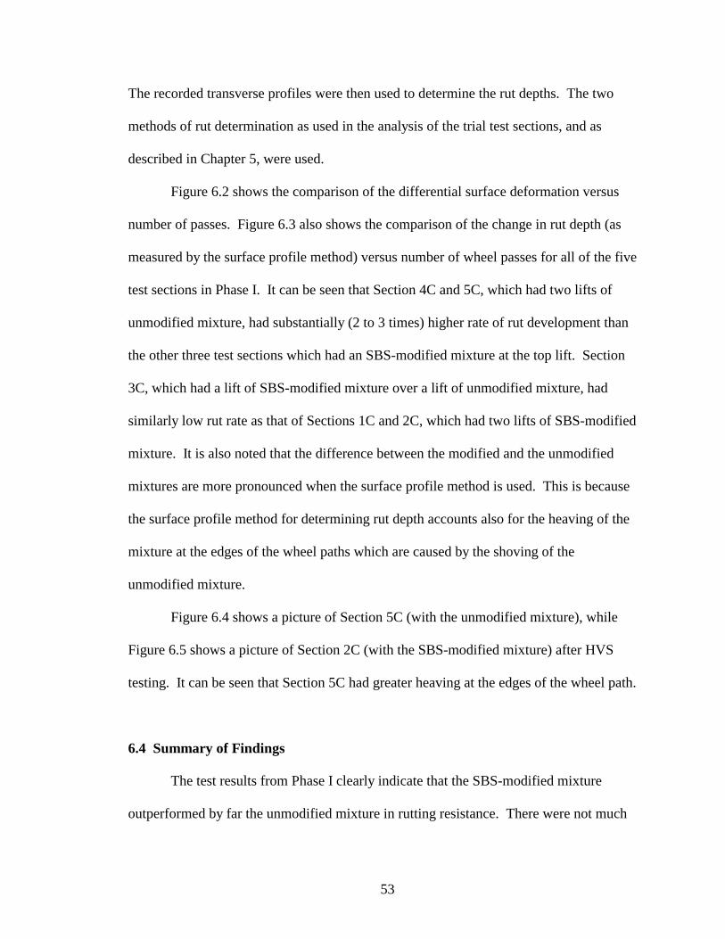
53

The recorded transverse profiles were then used to determine the rut depths. The two

methods of rut determination as used in the analysis of the trial test sections, and as

described in Chapter 5, were used.

Figure 6.2 shows the comparison of the differential surface deformation versus

number of passes. Figure 6.3 also shows the comparison of the change in rut depth (as

measured by the surface profile method) versus number of wheel passes for all of the five

test sections in Phase I. It can be seen that Section 4C and 5C, which had two lifts of

unmodified mixture, had substantially (2 to 3 times) higher rate of rut development than

the other three test sections which had an SBS-modified mixture at the top lift. Section

3C, which had a lift of SBS-modified mixture over a lift of unmodified mixture, had

similarly low rut rate as that of Sections 1C and 2C, which had two lifts of SBS-modified

mixture. It is also noted that the difference between the modified and the unmodified

mixtures are more pronounced when the surface profile method is used. This is because

the surface profile method for determining rut depth accounts also for the heaving of the

mixture at the edges of the wheel paths which are caused by the shoving of the

unmodified mixture.

Figure 6.4 shows a picture of Section 5C (with the unmodified mixture), while

Figure 6.5 shows a picture of Section 2C (with the SBS-modified mixture) after HVS

testing. It can be seen that Section 5C had greater heaving at the edges of the wheel path.

6.4 Summary of Findings

The test results from Phase I clearly indicate that the SBS-modified mixture

outperformed by far the unmodified mixture in rutting resistance. There were not much

54

0.0

1.0

2.0

3.0

4.0

5.0

6.0

7.0

8.0

0 50000 100000 150000 200000 250000 300000 350000

Number of Passes

Dif

fere

ntia

l Sur

face

Def

orm

atio

n (m

m)

1C(Modified Mix) 2C(Modified Mix)

3C(Modified + Unmodified Mix) 4C(Unmodified Mix)

5C(Unmodified Mix)

Figure 6.2 Comparison of Differential Surface Deformation versus Number of Passes for Test Sections in Phase I

55

0.0

2.0

4.0

6.0

8.0

10.0

12.0

14.0

0 50000 100000 150000 200000 250000 300000 350000

Number of Passes

Cha

nge

in R

ut D

epth

(m

m)

1C(Modified Mix) 3C(Modified + Unmodified Mix)4C(Unmodified Mix) 5C(Unmodified Mix)2C(Modified Mix)

Figure 6.3 Comparison of Change in Rut Depth as Measured by the Surface Profile Method versus Number of Passes for Test Sections in Phase I

56

Figure 6.4 Section 5C (Unmodified Mixture) after HVS Testing

Figure 6.5 Section 2C (SBS-Modified Mixture) after HVS Testing

57

observed difference in rutting performance between the pavement with a lift of SBS-

modified mixture over a lift of unmodified mixture and the pavement with two lifts of

SBS-modified mixture.

58

CHAPTER 7 PHASE II OF HVS FIELD TESTING PROGRAM

7.1 Testing Configurations

The HVS was run on the test sections using the same testing configurations as

used in Phase I. The applied load was a 9000-lb super single wheel traveling at a speed

of 6 mph, in a uni-directional mode with 4-inch wander in 1-inch increments. For each

test section, HVS loading was applied until the rut depth was judged to be more than 0.5

inch (12 mm). The testing sequence has been presented in Figure 2.2 in Chapter 2.


The temperature of each test section was monitored by six pairs of thermocouples

placed at six evenly spaced locations on the test pavement. At each location, a

thermocouple was placed on the surface and another thermocouple was placed at a depth

of 2 inches. Each pair of thermocouples was used to control a separate heater, which was

turned on and off depending on the readings from these two thermocouples. The target

pavement temperature measured at a depth of 2 inches was 50° C for eight test sections

and 65° C for the other two, as shown Figure 2.2.

Before each HVS testing, the pavement was pre-heated until the desired

temperature was reached. Figure 7.1 shows typical plots of the temperature versus time

during pre-heating of a test section before test. HVS testing was started when the

temperature at 2-inch depth reached the target temperature in a steady condition. Table

7.1 shows the minimum, maximum and average temperatures as measured by the six

pairs of thermocouples during the testing of Section 3B and 5B. It can be seen that the

59

25

30

35

40

45

50

55

0 5 10 15 20 25

Elapsed Time (hr)

Tem

pera

ture

(°C

)

1600 End Time1700 Start Time

Figure 7.1 Pavement Temperatures versus Time during Pre-Heating before Start of Test

60

Table 7.1 Temperatures of Test Pavements in Section 3B and 5B as Measured by

Thermocouples Placed at the Surface and at 2-inch Depth

Section 3B Uni-Directional loading, 4-inch wander with 1-inch Increment Surface Thermo.1 Thermo.2 Thermo.3 Thermo.4 Thermo.5 Thermo.6 Average

Avg. Daily Temp (o C) 51.7 52.1 52.2 51.1 52.0 51.9 51.8

Overall Min. Temp (o C) 50.0 51.0 51.0 50.0 51.0 51.0 50.7

Overall Max. Temp (o C) 53.0 53.0 53.0 53.0 54.0 54.0 53.3

2-inch below Thermo.1 Thermo.2 Thermo.3 Thermo.4 Thermo.5 Thermo.6 Average Avg. Daily Temp

(o C) 50.6 50.8 51.3 50.6 50.8 51.4 50.9 Overall Min. Temp

(o C) 49.0 50.0 50.0 49.0 50.0 50.0 49.7 Overall Max. Temp (o C) 53.0 52.0 52.0 51.0 52.0 53.0 52.2

Section 5B Uni-Directional loading, 4-inch wander with 1-inch Increment Surface Thermo.1 Thermo.2 Thermo.3 Thermo.4 Thermo.5 Thermo.6 Average

Avg. Daily Temp (o C) 51.9 51.8 51.9 50.6 51.1 51.8 51.5

Overall Min. Temp (o C) 47.0 50.0 49.0 47.0 50.0 51.0 49.0

Overall Max. Temp (o C) 55.0 54.0 54.0 53.0 53.0 54.0 53.8

2-inch below Thermo.1 Thermo.2 Thermo.3 Thermo.4 Thermo.5 Thermo.6 Average Avg. Daily Temp

(o C) 50.9 51.6 51.1 51.0 51.0 51.3 51.2 Overall Min. Temp

(o C) 48.0 49.0 49.0 49.0 47.0 50.0 48.7 Overall Max. Temp (o C) 53.0 54.0 53.0 53.0 54.0 53.0 53.3

range of temperature at 2-inch depth was within 48.0 to 54.0° C. The temperature ranges

were similar for the rest of test sections in Phase II.

61

7.3 Rut Measurement

A laser profiler was used to measure the pavement surface profiles of the test

pavements before, during and after the HVS testing. Analysis of the profiler data was

performed by Mr. Tom Byron of FDOT. Two different methods of analysis were used.

In the first method, the initial transverse surface profile (before test) was subtracted from

the transverse surface profile to obtain the “differential surface profile.” A straight line is

drawn over the “differential surface profile” and touching it at two highest points. The

greatest distance between this straight line and the “differential surface profile” is taken

to be the change in rut depth of the tested pavement relative to its initial condition.

Figure 7.2 shows the plots of change in rut depth as determined by this method.

In the second method, a straight line was drawn over the measured surface profile

and touching it at two highest points. The greatest distance between this straight line and

the surface profile was taken to be the rut depth of the test pavement. The rut depth of

the pavement at its initial condition (before testing) was also determined in the same

manner. The change in rut depth of the tested pavement relative to its initial condition

was determined by subtracting the initial rut depth from the determine rut depth at the

specified time. Figure 7.3 shows the plots of change in rut depth as determined by this

method.

Figures 7.4 and 7.5 show respectively the pictures of Sections 1B and 2B (with

two lifts of SBS-modified mixture) after HVS testing at 50° C. Figures 7.6 and 7.7 show

respectively the pictures of Sections 3A and 3B (with a lift of SBS-modified mixture over

an unmodified mixture) after HVS testing at 50° C. Figures 7.8 through 7.11 show

respectively the pictures of Sections 4A, 4B, 5A and 5B (with two lifts of unmodified

62

0

5

10

15

20

25

0 50000 100000 150000 200000 250000 300000

Number of Passes

Cha

nge

in R

ut D

epth

(m

m)

5B (Unmodified Mix)

4B (Unmodified Mix)

3B (Modified + Unmodified Mix)

2B (Modified Mix)

3A (Modified + Unmodified Mix)

1B (Modified Mix)

1A (Modified Mix) @ 65°C

4A (Unmodified Mix)


5A (Unmodified Mix)

Figure 7.2 Comparison of Rut Depth as Measured by the Differential Surface Profile Method versus Number of Passes

63

0

5

10

15

20

25

0 50000 100000 150000 200000 250000 300000

Number of Passes

Cha

nge

in R

ut D

epth

(m

m)

5B (Unmodified Mix)

4B (Unmodified Mix)

3B (Modified + Unmodified Mix)

2B (Modified Mix)1B (Modified Mix)

3A (Modified + Unmodified Mix)


4A (Unmodified Mix)


5A (Unmodified Mix)

Figure 7.3 Comparison of Change in Rut Depth as Measured by the Surface Profile Method versus Number of Passes

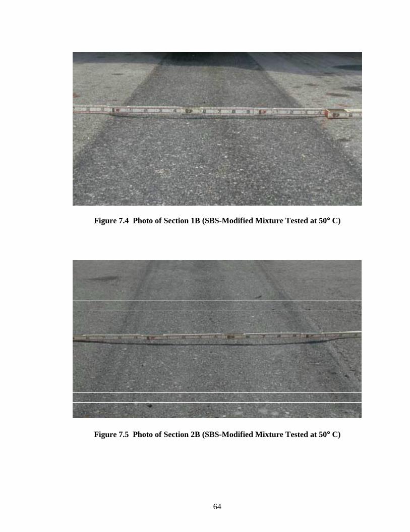
64

Figure 7.4 Photo of Section 1B (SBS-Modified Mixture Tested at 50°°°° C)

Figure 7.5 Photo of Section 2B (SBS-Modified Mixture Tested at 50°°°° C)

65

Figure 7.6 Photo of Section 3A (SBS-Modified Mixture over Unmodified Mixture Tested at 50°°°° C)

Figure 7.7 Photo of Section 3B (SBS-Modified Mixture over Unmodified Mixture Tested at 50°°°° C)

66

Figure 7.8 Photo of Section 4A (Unmodified Mixture Tested at 50°°°° C)

Figure 7.9 Photo of Section 4B (Unmodified Mixture Tested at 50°°°° C)

67

Figure 7.10 Photo of Section 5A (Unmodified Mixture Tested at 50°°°° C)

Figure 7.11 Photo of Section 5B (Unmodified Mixture Tested at 50°°°° C)

68

mixture) after HVS testing at 50° C. Figures 7.12 and 7.13 show respectively the

pictures of Sections 1A and 2A (with two lifts of SBS-modified mixture) after HVS

testing at 65° C.


The following observations can be made from the rutting results as plotted in

Figures 7.2 and 7.3:

1. Good repeatability of test results was generally observed between different test

sections with the same pavement design and test temperature. Lanes 4 and 5, which

had two lifts of unmodified mixture appeared to have relatively higher variability in

rut development than the other test sections.

2. The pavement sections with two lifts of SBS-modified mixture clearly outperformed

those with two lifts of unmodified mixture. Sections 4A , 4B, 5A and 5B (with two

lifts of unmodified mixture and tested at 50° C) had about two to two and a half times

the rut rate as compared with that of Sections 1B and 2B (with two lifts of modified

mixture and tested at the same temperature.

3. The pavement sections with a lift of SBS-modified mixture over a lift of unmodified

mixture (Sections 3A and 3B) had practically about the same rut rate as those with

two lifts of modified mixture (1B and 2B) when tested at 50° C.

4. Test Sections 1A and 2A, which had two lifts of SBS-modified mixture and tested at

65° C still had much lower rutting than the test sections with the unmodified mixture

and tested at 50° C (Sections 4A, 4B, 5A and 5B).

69

Figure 7.12 Photo of Section 1A (SBS-Modified Mixture Tested at 65°°°° C)

Figure 7.13 Photo of Section 2A (SBS-Modified Mixture Tested at 65°°°° C)

70

CHAPTER 8 LABORATORY TESTING PROGRAM ON

PLANT-COLLECTED SAMPLES 8.1 Tests on Plant-Collected Samples

The asphalt mixtures sampled from the hot-mix plant during the construction of

the test tracks were evaluated in the laboratory in order to determine the possible

relationship between mixture properties and field performance.

The following tests were run on the asphalt mixtures in the laboratory:

1. Compaction and evaluation in the Gyratory Testing Machine (GTM);

2. Compaction and evaluation in the Servopac Gyratory Compactor using 1.25 and 2.5°

gyratory angles; and

3. Evaluation in the Asphalt Pavement Analyzer (APA).

8.2 Gyratory Testing Machine (GTM) Results

Three samples from each lift of the unmodified and the SBS-modified mixtures

were compacted to ultimate density (when the change in density is equal to or less than

0.5 lb/ft3 per 50 revolutions) under a 120-psi vertical ram pressure in the Gyratory

Testing Machine (GTM). The unmodified mixture samples were compacted at 300° F,

whereas the SBS-modified asphalt mixtures were compacted at 325° F. These two

different compaction temperatures were used to simulate the actual placement

temperatures of these two mixtures at the test roads. The gyratory shear resistance (Sg) of

the mixture was determined at every 10 revolutions until 50 gyrations, and after that

every 25 revolutions until the ultimate density. The Gyratory Stability Index (the ratio of

71

the maximum gyratory angle to the minimum gyratory angle) was also determined at the

end of the test.

The average gyratory shear resistance of the unmodified and modified asphalt

mixtures versus number of gyrations was plotted in Figure 8.1. It can be seen that the

gyratory shear value of the unmodified mix-lift 2, modified mix-lift 1 and lift 2 were very

close to one another. The unmodified mix-lift 1 had slightly higher gyratory shear values

than those of the other three mixtures.

The Gyratory Stability Index (GSI) value of each specimen was calculated from

the gyrograph and displayed in Table 8.1. It can bee seen that the GSI values of the SBS-

modified mixtures were very close to 1.0. The unmodified mixtures had GSI values of

1.18 and 1.21 for lift 1 and lift 2, respectively. An increase in the GSI value beyond 1.0

usually indicates instability of the mixture under the applied ram pressure. Therefore,

this result could mean that the unmodified mixture (with a GSI of more than 1.0) was

relatively less stable than the SBS-modified mixture (with a GSI close to 1.0).

Table 8.1 GSI values of the Four Mixtures Evaluated in the GTM

Sample No Unmodified Mix Unmodified Mix Modified Mix Modified Mix

Lift 1 Lift 2 Lift 1 Lift 2

1 1.15 1.20 1.00 1.00

2 1.23 1.19 1.05 1.00

3 1.17 1.23 1.00 1.12

Average 1.18 1.21 1.02 1.04

72

Figure 8.1 Gyratory Shear Resistance of the Unmodified and Modified Asphalt Mixtures versus Number of Gyrations

200

250

300

350

400

450

0 50 100 150 200 250 300 350

Number of Gyrations

Gyr

ator

y Sh

ear

Stre

ngth

, Sg

(KP

a)

Unmodified mix-Lift 1 Unmodified mix-Lift 2

Modified mix-Lift 1 Modified mix-Lift 2

73

8.3 Servopac Gyratory Compactor (SGC) Results

Three asphalt specimens were compacted in the Servopac Gyratory Compactor

for each of the following materials and testing configurations:

1. Unmodified Mixture-Lift 1 using 1.25° gyratory angle

2. Unmodified Mixture-Lift 1 using 2.5° gyratory angle

3. SBS-modified Mixture-Lift 1 using 1.25° gyratory angle




One specimen was compacted to Ndesign (100) gyrations, and two specimens were

compacted to Nmax (160) gyrations. The unmodified mixtures were compacted at 300 °F

while the SBS-modified mixtures were compacted at 325 °F. The average gyratory shear

values versus number of gyrations using 1.25° and 2.5° gyratory angles were plotted in

Figure 8.2 and 8.3, respectively. It can be seen from these figures that the unmodified

mixture had higher gyratory shear values than those of the SBS-modified mixtures. This

could be due to the lower compaction temperature of the unmodified mixtures.

The volumetric properties of these mixtures compacted in the Servopac are given in

Table 8.2. In the case of 1.25° gyratory angle, the modified mixture from lift 1 had the

lowest air voids (2.05%) and VMA (13%) at Ndesign. The unmodified mixture from lift 1

had 2.35% air voids and 13.9% VMA at Ndesign. Similar trends were seen in the case of

2.5° gyratory angle. The modified mixture from lift 1 had the lowest air voids (0.22%)

and VMA (11.4%) at Ndesign. The unmodified mixture from lift 1 had an air voids value

(0.52%) between those of the two modified mixtures and higher VMA value (12.1%)

than those of the two modified mixtures.

74

Figure 8.2 Gyratory Shear Values versus Number of Gyrations Using 1.25°°°° Gyratory Angle

1.25 °

400

450

500

550

600

650

700

750

800

0 20 40 60 80 100 120 140 160 180

Number of Gyrations

Shea

r St

reng

th (

KP

a)

Unmodified Mix-Lift 1 Unmodified Mix-Lift 2Modified Mix-Lift 1 Modified Mix-Lift 2

75

Figure 8.3 Gyratory Shear Values versus Number of Gyrations Using 2.5°°°° Gyratory Angle

2.5 °

400

450

500

550

600

650

700

750

800

850

0 20 40 60 80 100 120 140 160 180

Number of Gyrations

Shea

r St

reng

th (

KP

a)


76

Table 8.2 Volumetric Properties of the Mixtures Compacted in the Servopac Gyratory Compactor Using 1.25 and 2.5° Gyratory Angles

Mix Type

% AC

% Air Voids

VMA

VFA

%Gmm (@Nini)

%Gmm (@Ndes)

%Gmm (@Nmax)

Dust Ratio

Unmod-Lift 1 (1.25°) 8.2 2.35 13.9 83.1 91.1 97.7 98.3 0.8

Unmod-Lift 2 (1.25°) 8.2 3.43 14.0 75.5 89.5 96.6 97.2 0.9

Mod-Lift 1 (1.25°) 7.9 2.05 13.0 84.2 90.6 97.9 98.5 0.9

Mod-Lift 2 (1.25°) 7.9 3.19 13.6 76.7 90.0 96.8 97.4 0.9

Unmod-Lift 1 (2.5°°°°) 8.2 0.52 12.1 95.7 92.5 99.5 100.0 0.8

Unmod-Lift 2 (2.5°°°°) 8.2 1.05 11.9 91.2 91.6 98.9 99.6 0.8

Mod-Lift 1 (2.5°°°°) 7.9 0.22 11.4 98.1 92.9 99.8 100.0 0.9

Mod-Lift 2 (2.5°°°°) 7.9 0.91 11.6 92.2 92.4 99.1 99.7 0.9

Figures 8.4 and 8.5 show the plots of gyratory shear versus log of number of

gyrations between air voids of 7% to 4% at 1.25° and 2.5° gyratory angles, respectively.

Some prior research results have indicated that the slope of the plot of gyratory shear

versus log of number of gyrations between air voids of 7% to 4% may be related to the

rutting resistance of the mixture. According to that hypothesis, a higher slope may

indicate higher resistance to rutting. However, the slopes of the plots of gyratory shear

versus log of number of gyrations as shown on Figures 8.4 and 8.5 do not support that

hypothesis. The slopes for the SBS-modified mixture did not show significantly higher

values than those for the unmodified mixtures.

Generally, the gyratory shear stress increases as air void decreases in compaction.

Figures 8.6 and 8.7 show the plots of gyratory shear stress versus air void of SBS-

modified and unmodified mixtures at 1.25 and 2.5° gyratory angles. It is clearly seen that

77

Figure 8.4 Gyratory Shear Strength versus Log Cycles for Gyrations between Air Voids of 7% to 4% at 1.25°°°° Gyratory Angle

1.25 °

y = 18.122Ln(x) + 687.32

R2 = 0.6114

y = 16.305Ln(x) + 515.37

R2 = 0.9974

y = 15.32Ln(x) + 496.18

R2 = 0.9963

y = 16.724Ln(x) + 457.07

R2 = 0.9957

450

500

550

600

650

700

750

800

1 10 100 1000Number of Gyrations

Shea

r St

ress

(K

Pa)


78

Figure 8.5 Gyratory Shear Strength versus Log Cycles for Gyrations between Air Voids of 7% to 4% at 2.5°°°° Gyratory Angle

2.5 °

y = 36.885Ln(x) + 646.58

R2 = 0.664

y = 18.57Ln(x) + 497.98

R2 = 0.9986

y = 16.605Ln(x) + 498.23

R2 = 0.9974

y = 19.98Ln(x) + 479.15

R2 = 0.9966

450

500

550

600

650

700

750

800

1 10 100

Number of Gyrations

Shea

r St

reng

th (

KP

a)


79

Figure 8.6 Gyratory Shear Strength versus Air Voids at 1.25°°°° Gyratory Angle in the Servopac Gyratory Compactor

1.25 °

400

450

500

550

600

650

700

750

800

0.0 2.0 4.0 6.0 8.0 10.0 12.0 14.0 16.0 18.0

Air Voids (%)

Shea

r St

reng

th (

KP

a)


80

Figure 8.7 Gyratory Shear Strength versus Air Voids at 2.5°°°° Gyratory Angle in the Servopac Gyratory Compactor

2.5 °

400

450

500

550

600

650

700

750

800

850

0.0 2.0 4.0 6.0 8.0 10.0 12.0 14.0 16.0 18.0

Air Voids (%)

Shea

r St

reng

th (

KP

a)

Unmodified Mix-Lift 1 Unmodified Mix-Lift 2

Modified Mix-Lift 1 Modified Mix-Lift 2

81

the SBS-modified showed lower gyratory shear than the unmodified mixture at the same

air void content.

8.4 Asphalt Pavement Analyzer (APA) Results

To evaluate the rutting performance of the asphalt mixtures in the laboratory,

cylindrical specimens were compacted to between 6.5 and 7.5% air voids with the

Superpave Gyratory Compactor. A 100-lb load was applied by a wheel to a hose placed

on top of the specimens in the APA. The rut depth was measured at two locations after

8000 wheel passes. Final rut depth was calculated by subtracting the rut depth after 8000

wheel passes by the rut depth after 25 wheel passes. A total of six specimens of the

unmodified mixture-lift 1 and four specimens of each of the other mixtures were

evaluated in the APA. From the summary of the rut measurements as shown in Table

8.3, it can be seen that the average rut depths for the unmodified asphalt mixtures (8.7

mm) were about 50% higher than those for the SBS-modified asphalt mixtures (5.75mm).


From the results of the laboratory testing program on the plant-collected mixtures,

it appears that the two laboratory test results which correlate with field rutting

performance are (1) the rut depth measurement from the APA, and (2) the GSI value as

measured in the GTM. A mixture with a higher rut depth in the APA will be likely to rut

more in the actual pavement. A mixture with a GSI of more than 1.0 as measured by the

GTM will be likely to rut more than one with a GSI close to 1.0.

82

Table 8.3 Summary of Rut Depth Measurements in the APA Evaluation of the Four Mixtures

Unmodified Mix-Lift 1 Unmodified Mix-Lift 2 Rut Measurement Rut Measurement Sample

No Measurement

No

25 Passes 8000

Passes Rut

Depth 25 Passes 8000

Passes Rut

Depth 1 20.2 11.8 8.4 19.8 12.6 7.2

1 2 20.6 11.1 9.5 20.3 11.9 8.4 1 20.8 10.8 10.0 20.6 12.6 8.0

2 2 20.6 11.3 9.3 20.1 13.1 7.0 1 20.5 9.4 11.1 20.3 13.0 7.3

3 2 20.7 9.6 11.1 20.4 12.6 7.8 1 20.8 10.4 10.4 20.4 13.4 7.0

4 2 20.0 11.0 9.0 18.5 14.5 4.0* 1 20.8 11.1 9.7

5 2 20.4 9.8 10.6 1 20.8 10.6 10.2

6 2 21.0 12.0 9.0

Overall Average (mm) 9.9 7.5

Modified Mix-Lift 1 Modified Mix-Lift 2 Rut Measurement Rut Measurement Sample

No Measurement

No

25 Passes 8000

Passes Rut

Depth 25 Passes 8000

Passes Rut

Depth 1 20.6 14.4 6.2 21.0 16.1 4.9

1 2 20.8 14.5 6.3 21.0 15.8 5.2 1 20.7 14.4 6.3 21.2 16.4 4.8

2 2 20.9 14.8 6.1 21.0 15.6 5.4 1 20.5 15.4 5.1 21.1 16.0 5.1

3 2 21.1 14.8 6.3 21.2 15.2 6.0 1 21.3 14.3 7.0 21.3 15.7 5.6

4 2 20.9 14.8 6.1 21.1 15.6 5.5

Overall Average (mm) 6.2 5.3 * Not considered in the overall average because the value is an outlier

83

CHAPTER 9 EVALUATION OF CORED SAMPLES

FROM THE TEST SECTIONS 9.1 Introduction

Cores were taken from the test sections after they had been tested by the HVS in

order to evaluate (1) the changes in properties of the pavement materials, and (2) the

possible relationship between the laboratory-measured mixture properties and the

observed rutting performance. For each of the test sections, two cores were taken from

the middle of the wheel path, and two cores were taken from the edge of the wheel path.

Figure 9.1 shows a picture of the locations of a core taken from the middle of the wheel

path and a core taken from the outside edge of the wheel path of a test section. All cores

were 6 inches in diameter and contained the two lifts of asphalt mixture, which were

bonded together.

These cores were evaluated to determine their (1) thickness, (2) density, (3)

resilient modulus at 5 and 25° C, (4) indirect tensile strength at 25° C, and (5) viscosity of

recovered binders at 60° C.

9.2 Thickness and Density Evaluation of Cores from the Test Sections

For each of the cores taken from the test sections, the thickness profile in the

direction perpendicular to the wheel path was determined. This was done by drawing a

line across the face and through the center of the core, in a direction judged to be

perpendicular to the wheel path. The thickness of the core along the marked line was then

measured with a caliper at a spacing of 0.5 inch.

84

Figure 9.1 Picture Showing Locations of a Core Taken From the Middle of the Wheel Path and a Core Taken From the Outside Edge of the Wheel Path

Plots of the thickness profiles of the cores tested are shown in Appendix C. The

average thickness of the cores from the wheel path and the cores from the outside edge of

the wheel path for each test section were calculated and shown in Table 9.1. The density

of all the cores were also measured and shown also in Table 9.1. The percents difference

in thickness and density between the cores from the wheel path and the cores from the

outside edge of the wheel path were also computed and shown in Table 9.1.

The data show that all the cores from the wheel paths are thinner and denser than

the cores from the edges of wheel paths. In comparing the percent difference in thickness

with the percent difference in density between these two groups of cores, it can be seen

85

Table 9.1 Bulk Densities of Cores from Wheel Paths and Edges of Wheel Paths of the Test Sections

that, except for Sections 2C and 2A (which had two layers of SBS-modified mixture), the

percent difference in thickness was much greater than the percent difference in density.

If the changes in density of the asphalt mixtures were due primarily to vertical

densification, the percent increase in density should be approximately equal to the

percent decrease in thickness. The greater difference in thickness as compared with the

No.1 No.2 Average % difference Average % differencewheelpath 2.140 2.152 2.146 81.33

edge of wheelpath 2.090 2.095 2.093 85.97wheelpath 2.141 2.113 2.127 76.96


















edge of wheelpath 2.101 2.101 2.101 103.32

3.37 10.10

10.35

4B 4.35 13.08

5B 4.02 18.06

2A

11.36

2.56

2.61

1.03

4.78

8.16

2.06

5.24

8.59

3.30

3.57

1.63

1.85

5.40

7.64

11.19

10.56

3C

7BW

4C

5C

7BE

7C

2C

SectionBulk Density

7AE

7AW

Thickness (mm)

2.49

1B 1.57 7.78

1A 3.47 6.98

2B 2.68 5.17

3B

5A 3.71 12.09

3.18 3.16

4A 4.72 12.67

3A 3.30

86

difference in density indicate that materials might be shoved from the wheel path to the

edge, giving the wheel-path cores a higher density which could not be accounted for by

their reduction in thickness.

The bulk densities and air voids of these cores (which were obtained after HVS

testing) were also compared with those of the cores obtained at the time of construction.

Table 9.2 shows the comparison of the air voids of the cores at the time of construction

with those of the cores after HVS testing. The change in percent air voids for each group

was also computed and shown in Table 9.2. For all of the test sections, the cores from

the wheel paths showed an increase in density (or a reduction in air voids). However,

two different trends can be observed on the changes of density of the cores from the edge

of wheel path. For the cores from the edges of wheel paths from the test sections with the

SBS-modified mixture (2C, 3C, 2B, 3B) with the exception of Section 3A, there was

generally a small increase in density (or a small reduction in air voids). Section 3A

showed a small decrease in density (or a small increase in air voids).

For the cores from the edges of wheel paths from the sections with two lifts of

unmodified mixture with the exception of Section 7C, there was generally decrease in

density (or an increase in air voids). Section 7C, which was a trial test section, showed a

slight increase in density (or slight decrease in air voids).

From the changes in thickness and density of the cores from these test sections, it

can be inferred that, for pavements with the unmodified mixture, rutting was caused by a

combination of densification and shoving. For the pavements with the SBS-modified

mixture, rutting was due primarily to densification of the mixture. This explains why the

SBS-modified mixture rutted less than the unmodified mixture though the SBS-modified

87

Table 9.2 Comparison of Air Voids of Cores before and after HVS Testing

Section Sample Gmb Gmm Average

Air Voids % Change in air

voids

Original 2.109 2.264 6.8 Tested (edge of wheelpath) 2.093 2.264 7.6 0.71 7AE

Tested (wheelpath) 2.146 2.264 5.2 -1.63 Original 2.109 2.264 6.8

Tested (edge of wheelpath) 2.055 2.264 9.2 2.39 7AW


Tested (edge of wheelpath) 2.091 2.264 7.6 1.02 7BE


Tested (edge of wheelpath) 2.088 2.264 7.8 1.15 7BW


Tested (edge of wheelpath) 2.116 2.264 6.5 -0.27 7C






Tested (edge of wheelpath) 2.032 2.280 10.9 3.95 4C


Tested (edge of wheelpath) 2.084 2.276 8.4 1.47 5C


Tested (edge of wheelpath) 2.128 2.263 6.0 -1.27 2B


Tested (edge of wheelpath) 2.105 2.271 7.3 -0.38 3B


Tested (edge of wheelpath) 2.091 2.280 8.3 1.57 4B


Tested (edge of wheelpath) 2.087 2.276 8.3 1.45 5B


Tested (edge of wheelpath) 2.097 2.271 7.7 0.43 3A

Tested (wheelpath) 2.169 2.271 4.5 -2.74

88

mixture was densified by the same amount or even greater amount than the unmodified

mixture.

9.3 Evaluation of Cores for Resilient Modulus and Indirect Tensile Strength

The cores obtained from the test sections contained two 2-inch layers of asphalt

mixture, which were bonded together. Each core was cut into two slices by a mechanical

saw at the interface between the two layers. In this report, the slice from the bottom layer

is referred to as “Lift 1” and the slice from the top layer is referred to as “Lift 2”. The

sliced specimens were tested for resilient modulus at 5 and 25° C and indirect tensile

strength at 25° C. The SHRP IDT test system as developed and improved by Roque et al.

(1997) was used to measure the resilient modulus and indirect tensile strength of the

specimens. The detailed description of specimen preparation, testing procedure and

analysis procedure can be found in the report by Roque et al. (1997). It is to be pointed

out that while the test system as recommended by Roque et al. called for at least three

replicate specimens to be tested, only two replicate specimens were available to be tested

in this laboratory study.

Table 9.3 shows the resilient modulus and indirect tensile strength at 25° C of the

cored specimens from the test sections. The resilient modulus of the SBS-modified

mixture appears to be not significantly different from that of the unmodified mixture.

However, the resilient modulus of the specimens from the wheel path appears to be

slightly higher than that of the specimens from the edge of the wheel path. For the

specimens from the wheel path and lift 2 (top layer), the resilient modulus of the

89

Table 9.3 Resilient Modulus and Indirect Tensile Strength at 25°°°° C of Cores from

the Test Sections

Resilient Modulus Tensile Strength Section Location

Gpa Psi (106) Mpa Psi Wheelpath 3.16 0.46 0.68 98.6

Lift 2 Edge 2.84 0.41 0.67 97.1

Wheelpath 3.40 0.49 0.75 108.7 7AW

Lift 1 Edge 4.13 0.60 0.85 123.2

Wheelpath 3.08 0.45 0.82 118.8 Lift 2

Edge 3.04 0.44 0.52 75.4 Wheelpath 3.75 0.54 0.72 104.3

7AE Lift 1

Edge 3.33 0.48 0.75 108.7 Wheelpath 2.47 0.36 0.62 89.9

Lift 2 Edge 2.34 0.34 0.52 75.4

Wheelpath 2.93 0.42 0.68 98.6 7BW

Lift 1 Edge 2.89 0.42 0.68 98.6

Wheelpath 2.91 0.42 0.60 87.0 Lift 2

Edge 1.97 0.29 0.53 76.8 Wheelpath 3.17 0.46 0.67 97.1

7BE Lift 1

Edge 2.88 0.42 0.68 98.6 Wheelpath 3.59 0.52 0.78 113.0

Lift 2 Edge 2.89 0.42 0.63 91.3

Wheelpath 4.11 0.60 0.91 131.9 7C

Lift 1 Edge 3.97 0.58 0.89 129.0

Wheelpath 4.27 0.62 0.91 131.9 Lift 2

Edge 2.05 0.30 0.60 87.0 Wheelpath 4.22 0.61 0.89 129.0

2C Lift 1

Edge 3.90 0.57 0.86 124.6 Wheelpath 3.12 0.45 0.57 82.6

Lift 2 Edge 2.38 0.34 0.70 101.4

Wheelpath 3.97 0.58 0.71 102.9 3C

Lift 1 Edge 3.81 0.55 0.72 104.3

Wheelpath 3.28 0.48 0.76 110.1 Lift 2

Edge 1.69 0.24 0.42 60.9 Wheelpath 3.33 0.48 0.76 110.1

4C Lift 1

Edge 2.34 0.34 0.64 92.8 Wheelpath 4.38 0.63 0.77 111.6

Lift 2 Edge 2.75 0.40 0.55 79.7

Wheelpath 3.63 0.53 0.82 118.8 5C

Lift 1 Edge 2.50 0.36 0.66 95.7

Wheelpath 4.92 0.71 0.93 134.8 Lift 2

Edge 2.76 0.40 0.73 105.8

Wheelpath 5.57 0.81 1.04 150.7 2B

Lift 1 Edge 3.58 0.52 1.00 144.9

90

Table 9.3 Resilient Modulus and Indirect Tensile Strength at 25°°°° C of Cores from the Test Sections (continued)

Resilient Modulus Tensile Strength

Section Location Gpa Psi (10^6) Mpa Psi

Wheelpath 4.88 0.71 0.91 131.9 Lift 2

Edge 2.85 0.41 0.78 113.0 Wheelpath 5.65 0.82 1.05 152.2

3B Lift 1

Edge 4.10 0.59 0.83 120.3 Wheelpath 4.97 0.72 0.92 133.3

Lift 2 Edge 2.59 0.38 0.66 95.7

Wheelpath 5.60 0.81 1.01 146.4 4B

Lift 1 Edge 3.59 0.52 0.77 111.6

Wheelpath 4.11 0.60 0.88 127.5 Lift 2

Edge 2.41 0.35 0.60 87.0 Wheelpath 5.55 0.80 1.01 146.4

5B Lift 1

Edge 4.02 0.58 0.91 131.9 Wheelpath 4.25 0.62 0.81 117.4

Lift 2 Edge 2.51 0.36 0.61 88.4

Wheelpath 4.91 0.71 0.87 126.1 3A

Lift 1 Edge 3.46 0.50 0.66 95.7

unmodified mixture varied from 0.36 to 0.72 × 106 psi with an average of 0.49 × 106 psi,

while that of the SBS-modified mixture varied from 0.45 to 0.71 × 106 psi with an

average of 0.62 × 106 psi. For the specimens from the edge of the wheel path and lift 2,

the resilient modulus of the unmodified mixture varied from 0.24 to 0.44 × 106 psi with

an average of 0.36 × 106 psi, while that of the SBS-modified mixture varied from 0.30 to

0.41 × 106 psi with an average of 0.36 × 106 psi.

The resilient modulus of the samples from lift 1 appears to be slightly higher than

that from lift 2. For the samples from the wheel path, the resilient modulus of the

samples from lift 2 varied from 0.36 to 0.72 × 106 psi with an average of 0.54 × 106 psi,

while that of the samples from lift 1 varied from 0.42 to 0.82 × 106 psi with an average of

0.62 × 106 psi.

91

The indirect tensile strength of the SBS-modified mixture appears to be slightly

higher than that of the unmodified mixture. The indirect tensile strength of the specimens

from the wheel path appears to be slightly higher than that of the specimens from the

edge of the wheel path. For the specimens from the wheel path and lift 2, the indirect

tensile strength of the unmodified mixture varied from 87 to 133.3 psi with an average of

110.5 psi, while that of the modified mixture varied from 82.6 to 134.8 psi with an

average of 119.7 psi.

For the specimens from the edge of the wheel path and lift 2, the indirect tensile

strength of the unmodified mixture varied from 60.9 to 97.1 psi with an average of 82.1

psi, while that of the modified mixture varied from 87.0 to 113 psi with an average of

95.4 psi.

The indirect tensile of the samples from lift 1 appears to be slightly higher than

that of the samples from lift 2. For the samples from the wheel path, the indirect tensile

strength of the samples from lift 2 varied from 82.6 to 134.8 psi with an average of 113.8

psi, while that of the samples from lift 1 varied from 97.1 to 152.2 psi with an average of

123.1 psi.

Resilient modulus test at 5° C was performed only on the cores from Lane 7. The

results are shown in Table 9.4. The resilient modulus of the specimens from the wheel

path appears to be slightly higher than that of the specimens from the edge of the wheel

path. The resilient modulus of the specimens from the wheel path and lift 2 (top layer)

varied from 1.27 to 1.73 × 106 psi with an average of 1.52 × 106 psi, while that of

specimens from the edge of wheel path varied from 1.35 to 1.54 × 106 psi with an

average of 1.42 × 106 psi.

92

Table 9.4 Resilient Modulus at 5°°°° C of Cores from the Test Sections on Lane 7

Resilient Modulus Section Location

Gpa Psi (10^6)

Wheelpath 8.76 1.27 Lift 2

Edge 9.62 1.39 Wheelpath 8.79 1.27

7AW Lift 1

Edge 11.15 1.62 Wheelpath 10.51 1.52

Lift 2 Edge 9.84 1.43

Wheelpath 10.59 1.53 7AE

Lift 1 Edge 10.22 1.48


Edge 10.61 1.54 Wheelpath 10.69 1.55

7BW Lift 1

Edge 9.73 1.41 Wheelpath 10.64 1.54

Lift 2 Edge 9.48 1.37

Wheelpath 12.55 1.82 7BE

Lift 1 Edge 11.25 1.63


Edge 9.34 1.35 Wheelpath 13.61 1.97

7C Lift 1

Edge 11.15 1.62

The resilient modulus of the samples from lift 1 appears to be slightly higher than

that from lift 2. For the samples from the wheel path, the resilient modulus of the

samples from lift 2 varied from 1.27 to 1.73 × 106 psi with an average of 1.47 × 106 psi,

while that of the samples from lift 1 varied from 1.27 to 1.97 × 106 psi with an average of

1.59 × 106 psi.

9.4 Evaluation of Cores for Viscosity Test

Asphalt binder was extracted and recovered from the mixtures to evaluate the

binder viscosity. The Reflux Asphalt Extraction procedure in accordance with ASTM D

2171-95 standard test method was used to extract the asphalt binder from the cores. The

93

asphalt binders were then recovered from the solvent using Trichloroethylene (TCE) in

accordance with ASTM D 5404-97 standard test method. The Brookfield viscosity test

was performed on the recovered binders at 60° C. The standard testing procedure for the

Brookfield viscosity test is described in ASTM D 4402-95. Three replicate tests were run

per sample.

Table 9.5 shows the viscosity of the recovered binders from the cored samples.

The viscosity of the recovered binders from the SBS-modified mixture are about two to

three times) higher than that from unmodified mixture. For the SBS-modified mixtures,

the viscosity of the recovered binders from the wheel path appears to be slightly higher

than that of the binders from the edge of the wheel path. The viscosity of the recovered

binders from the wheel path varied from 33,344 to 52,202 poises with an average of

40,589 poises, while that of the binders from the edge of wheel path varied from 25,514

to 45,510 poises with an average of 36,238 poises.

However, for the unmodified mixtures, the viscosity of the recovered binders

from the edge of the wheel path appears to be slightly higher than that of the binders from

the wheel path. The viscosity of the recovered binders from the wheel path varied from

12,547 to 17,955 poises with an average of 15,544 poises, while that of binders from the

edge of wheel path varied from 12,759 to 16,316 poises with an average of 14,577 poises.

For the unmodified mixture, the viscosity of the recovered binders from lift 2 (top

layer) appeared to be about the same as that from lift 1 (bottom layer). The average

viscosity of the unmodified binders from lift 1 was 15,016 poises, while the average

viscosity of the unmodified binders from lift 2 was 15,104 poises. For the modified

mixtures, the viscosity of the recovered binders from lift 2 was higher than that from

94

Table 9.5 Viscosity of Cores from the Test Sections

Viscosity

Section Location Poise

Wheelpath 33344 Lift 1

Edge 25514

Wheelpath 45468 2C

Lift 2 Edge 45510


Edge 14965

Wheelpath 34554 3C

Lift 2 Edge 39265


Edge 12759

Wheelpath 17282 4C

Lift 2 Edge 13761


Edge 14844

Wheelpath 17517 5C

Lift 2 Edge 16316


Edge 30897 Wheelpath 52202

2B Lift 2


Lift 1 Edge 13288

Wheelpath 34247 3B

Lift 2 Edge 29604

Wheelpath 12547 4B Lift 2


5B Lift 2 Edge 14690

lift 1. The average viscosity of the modified binders from lift 1 was 33,368 poises, while

that from lift 2 was 40,485 poises.

95


The following are the main findings from the results of evaluation of cored

samples from the test sections:

1. From the density and thickness of cores from the test sections, rutting of the

pavement sections with the unmodified asphalt mixture appeared to be due to a

combination of densification and shear movement, while rutting of the pavement

sections with the SBS-modified mixture appeared to be due primarily to densification.

2. The resilient modulus at 25° C of the SBS-modified mixture was not significantly

different from that of the unmodified mixture.

3. The average indirect tensile strength at 25° C of the SBS-modified mixture was

higher than that of the unmodified mixture by about 10%.

4. The viscosity at 60° C of the recovered binders from the SBS-modified mixture was

two to three times that of the recovered binders from the unmodified mixture.

96

CHAPTER 10 SUMMARY OF FINDINGS

A research study was conducted to evaluate the rutting performance of a

Superpave mixture and a SBS-modified Superpave mixture using a Heavy Vehicle

Simulator (HVS) at FDOT’s Accelerated Pavement Testing Facility. Before the main

field testing program was conducted, trial tests were performed to evaluate the operating

characteristics of the HVS and to determine an appropriate HVS testing configuration to

be used for the main testing program. A laboratory testing program was also conducted

on samples of asphalt mixtures collected from the plant during construction of the test

pavements, and cored samples from the test sections after HVS testing, in order to

determine the possible relationship between the mixture properties and their rutting

performance.

Results from the HVS tests showed that the pavement sections with two lifts of

SBS-modified mixture clearly outperformed those with two lifts of unmodified mixture,

which had two to two and a half times the rut rate. The pavement sections with a lift of

SBS-modified mixture over a lift of unmodified mixture had practically about the same

rut rate as those with two lifts of modified mixture when tested at 50° C. The test

sections with two lifts of SBS-modified mixture and tested at 65° C still outperformed the

pavement sections with two lifts of unmodified mixture and tested at 50° C.

Results from the laboratory testing program showed that a mixture with a higher

rut depth in the APA will be likely to rut more in the actual pavement. A mixture with a

GSI of more than 1.0 as measured by the GTM will be likely to rut more than one with a

GSI close to 1.0.

97

From the observation of the changes in thickness and density of the cores from

these test sections, it can be inferred that, for the pavements with the unmodified mixture,

rutting was caused by a combination of densification and shoving. For the pavements

with the SBS-modified mixture, rutting was due primarily to densification of the mixture.

The resilient modulus at 25° C of the SBS-modified mixture was not significantly

different from that of the unmodified mixture. The average indirect tensile strength at

25° C of the SBS-modified mixture was only slightly higher than that of the unmodified

mixture (by about 10%). The viscosity at 60° C of the recovered binders from the SBS-

modified mixture was two to three times that of the recovered binders from the

unmodified mixture. The higher viscosity of the SBS-modified binder was one of the

main reasons for the higher rutting resistance of the SBS-modified mixture.

98

LIST OF REFERENCES Asphalt Institute, Superpave Level 1 Mix Design, Superpave Series No.2 (SP-2),

Lexington, Kentucky, 1994.

Bonaquist, R., Sherwood, J., and Stuart, K., “Accelerated Pavement Testing at the Federal Highway Administration Pavement Testing Facility,” Journal of Association of Asphalt Pavement Technologists, Vol. 67, 1998.

Carpenter, S.H., “Permanent Deformation: Field Evaluation,” Transportation Research Record 1417, Transportation Research Board (TRB), National Research Council (NRC), Washington, D.C., 1993, pp 135-143.

Coetzee, N., Harvey, J.T., Nokes, W.A., Rust, F.C., Stolarski, P.J., “Establishing the California Department of Transportation Accelerated Pavement Testing Program,” Transportation Research Record 1540, TRB, NRC, Washington, D.C., 1996, pp 92-96.

Coetzee, N., Nokes, F., Monismith, W., Metcalf, J.B., Mahoney, J., “Full-Scale/ Accelerated Pavement Testing: Current Status and Future Directions,” Trans-portation in the New Millennium, TRB, NRC, Washington, D.C., 2000, pp. 4.

Coetzee, N., Harvey, J.T., Monismith, C.L., “(CAL/APT) Program Summary Report,” Institute of Transportation Studies, University of California, Berkeley, June 2000.

Dynatest International, Technical Specification for Heavy Vehicle Simulator (HVS Mark IV), HVS Technical Manual, South Africa.

Franklin Associates, Ltd., Hershey, R.L., “Markets for Scrap Tires,” Report EPA/530-SW-90-074A, Office of Solid Waste, Environmental Protection Agency, October 1991.

Gisi, A.J., Hossain, M., Wu, Z., “Performance of Superpave Mixtures Under Accelerated Load Testing,” Transportation Research Record 1325, TRB, NRC, Washington, D.C., 2000, pp 126-134.

Gramling, W.L., Hunt, J.E., Suzuki, G.S., “Rational Approach to Cross-Profile and Rut Depth Analysis,” Transportation Research Record 1311, TRB, NRC, Washington, D.C., 1991, pp 173-179.

Heitzman, M., “Design and Construction of Asphalt Paving Materials with Crumb Rubber Modifier,” Transportation Research Record 1339, TRB, NRC, Washington, D.C., 1992, pp 1-8.

Hoot, S., “Ohio State helps open nation's only indoor pavement test facility,” News in Engineering, The Ohio State College of Engineering, Vol. 69, No. 5, September 1997.

99

Huang, Y.H., Pavement Analysis and Design, Prentice-Hall, Eaglewood Cliffs, New Jersey, 1993.

Hugo, F., McCullough, F., van der Walt, B., “Full-Scale Accelerated Pavement Testing for Texas State Department of Highways and Public Transportation,” Transportation Research Record 1293, TRB, NRC, Washington, D.C., 1991, pp. 52-60.

Kluttz, Q., “SBS polymers affect mix characteristics,” Asphalt Contractor Magazine, Independence, Missouri, October 1999.

McNamara, W.M., Sebaaly, P.E., Epps, J.A., Weitzel, D., “Evaluation of Superpave Mixtures in Nevada,” Journal of Association of Asphalt Pavement Technologists, Vol. 69, 2000.

Metcalf, J.B., “The Development of Proposals for an Australian Full-Scale Accelerated Loading Pavement Testing Facility,” Institute fur Strassen-, Eissenbahn-und Felsbau an der Eidgenossischen Technischen Hochschule, Zurich, Switzerland, 1982, pp. 35-53.

Metcalf, J.B., “Application of Full-Scale Accelerated Pavement Testing,” NCHRP Synthesis of Highway Practice 235, TRB, NRC, Washington, D.C., 1996, pp. 116.

Metcalf, J.B., “Accelerated Pavement Testing, a Brief Review Directed Towards Asphalt Interests,” Journal of Association of Asphalt Pavement Technologists, Vol. 67, 1998.

Metcalf, J.B., Li, Y., Rasoulian, M., Romanoschi, S.A., “Assessment of Pavement Life at First Full-Scale Accelerated Pavement Test in Louisiana,” Transportation Research Record 1655, TRB, NRC, Washington, D.C., 1999, pp 219-226.

Musselman, J.A., Choubane. B, Page. G.C., Upshaw. P.B., “Superpave Field Implementation,” Transportation Research Record 1609, TRB, NRC, Washington, D.C., 1998, pp. 51-60.

Othman, A., Figueroa, L., Aglan, H., “Fatigue Behavior of Styrene-Butadiene-Styrene Modifier Asphaltic Mixtures Exposed to Low-Temperature Cyclic Aging,” Transportation Research Record 1492, TRB, NRC, Washington. D.C., 1995, pp. 129-134.

Pidwerbesky, B.D., “Accelerated Dynamic Loading of Flexible Pavements at the Canterbury Accelerated Pavement Testing Indoor Facility,” Transportation Research Record 1482, TRB, NRC, Washington, D.C., 1995, pp. 79-86.

Solaimanian, M., T.W. Kennedy, R. Tripathi, “Performance Characteristics of Asphalt Binders and Mixtures Modified by Waste Toner,” Transportation Research Record 1638, TRB, NRC, Washington, D.C., 1998, pp 120-128.

100

Terrel, R.L., “Asphalt Modifiers,” A User Manual for Additives and Modifiers in Hot Mix Asphalt, National Asphalt Pavement Association, Lanham, Maryland.

Texas Transportation Institute, AASHTO Innovative Highway Technologies, College Station, Texas, 1998.

White, T.D., Albers, J.M., Haddock, J.E., “Limiting Design Parameters for Accelerated Pavement Testing System,” Journal of Transportation Engineering, Vol. 118, 1992.

Witczak, M.W., Hafez, I., Qi, X., “Laboratory Characterization of Elvaloy®, Modified Asphalt Mixtures,” Technical Report, Vol. 1, University of Maryland, College Park, Maryland, June 1995.

101

APPENDIX A SUPERPAVE MIX DESIGN

102

Table A.1 Summary of Aggregate Blending for Superpave Mix Design

Blend 12% 25% 48% 15% Sieve Size S-1-A Stone S-1-B Stone Screenings Local Sand

Job Mix Formula

Control Points

Restricted Zone

3/4" 19.0 mm 99 100 100 100 100 100

1/2" 12.5mm 45 100 100 100 93 (90 - 100)

3/8" 9.5mm 13 99 100 100 89 -90

No. 4 4.75mm 5 49 90 100 71

No. 8 2.36mm 4 10 72 100 53 (28 - 58) 39.1 - 39.1

No. 16 1.18mm 4 4 54 100 42 25.6 - 31.6

No. 30 0.600mm 4 3 41 96 35 19.1 - 23.1

No. 50 0.300mm 4 3 28 52 22

No. 100 0.150mm 3 2 14 10 9

No. 200 0.075mm 2.7 1.9 5.9 2.2 4.5 (2 - 10)

Gsb 2.327 2.337 2.299 2.546 2.346

103

Table A.2 Mix Design Data for the Unmodified Superpave Mix

Pb Gmb @ Ndes Gmm Va VMA VFA Pbe P0.075 / Pbe %Gmm @ Nini % Gmm @ Ndesign %Gmm @ Nmax

7.2 2.159 2.306 6.4 14.6 56 3.94 1.1 86.7 93.6 94.7

7.7 2.168 2.281 5.0 14.7 66 4.66 1.0 88.1 95.0 96.3

8.2 2.185 2.276 4.0 14.5 72 4.97 0.9 88.8 96.0 97.0

8.7 2.193 2.232 1.7 14.7 88 6.09 0.7 91.0 98.3 99.5

Optimum Asphalt Content 8.20% FAA 47.00%

136.3 lbs/ft% %Gmm @ Ndes 96.00% Lab Density =2185 kg/m3 NCAT Oven Calibration Factor -0.07%

VMA 14.50% Mixing Temperature 300°F = 149°C

104

Table A.3 Mix Design Data for the SBS-Modified Superpave Mix

Pb Gmb @ Ndes Gmm Va VMA VFA Pbe P0.075 / Pbe %Gmm @ Nini %Gmm @ Ndesign %Gmm @ Nmax

7 2.163 2.300 6.0 14.3 58 3.97 1.1 87.1 94.0 94.7

7.5 2.177 2.285 4.7 14.2 67 4.48 1.0 88.1 95.3 95.8

7.9 2.186 2.273 3.8 14.2 73 4.90 0.9 89.1 96.2 96.7

8 2.185 2.268 3.7 14.3 74 5.04 0.9 89.3 96.3 96.8

8.5 2.195 2.253 2.6 14.4 82 5.56 0.8 90.4 97.4 98.2

Optimum Asphalt Content 7.90% FAA 47% 136.40% %Gmm @ Ndes 96.2%

Lab Density =2186 kg/m3 NCAT Oven Calibration Factor -6.00%

VMA 14.20% Mixing Temperature 340°F = 171°C

Compaction Temperature 325°F = 163°C

105

APPENDIX B NUCLEAR DENSITY DATA

106

Table B.1 Nuclear Density Data for Lane 1-Lift 1

Density (lb/cf) Location 1 2 3 4 Average

1 131.7 129.3 131.3 130.2 130.6 2 3 128.8 129.1 129.4 131.1 129.6 4 129.7 133.4 131.7 131.1 131.5 5 130.2 132.1 130.2 130.3 130.7 6 7 130.9 131.2 132.8 132.8 131.9 8 131.0 131.4 132.7 132.2 131.8 9 136.8 135.0 134.8 136.3 135.7

10 132.5 132.3 131.6 132.0 132.1 11 134.2 133.0 133.2 133.3 133.4 12 13 131.7 131.7 130.8 131.3 131.4 14 130.2 129.7 129.3 130.8 130.0 15 130.7 128.8 129.0 129.5 129.5 16 17 130.6 131.0 130.1 130.7 130.6



1 2 129.1 128.9 129.6 128.6 129.1 3 129.3 130.1 129.6 130.6 129.9 4 129.6 129.7 131.1 130.9 130.3 5 131.3 130.2 128.8 130.5 130.2 6 135.5 133.5 132.9 135.1 134.3 7 8 135.1 133.7 132.2 134.5 133.9 9 131.9 131.3 130.2 131.9 131.3

10 132.7 131.8 130.7 131.7 131.7 11 12 134.3 135.0 134.8 132.0 134.0 13 129.6 130.5 130.3 131.4 130.5 14 131.9 129.4 129.8 130.4 130.4 15 131.6 131.7 127.7 131.9 130.7 16 128.2 131.3 132.6 130.6 130.7

107

Table B.3 Nuclear Density Data for Lane 2-Lift1 Density (lb/cf)

Location 1 2 3 4 Average 1 130.1 128.8 131.2 132.8 130.7 2 3 130.2 131.2 132.4 132.2 131.5 4 129.2 128.5 130.8 131.4 130.0 5 132.5 129.7 132.6 133.2 132.0 6 7 126.7 126.7 126.4 129.0 127.2 8 132.9 134.5 132.2 129.5 132.3 9 129.8 129.8 130.4 127.9 129.5

10 132.3 132.4 133.0 130.9 132.2 11 129.9 129.8 131.4 131.5 130.7 12 13 135.3 132.2 134.4 133.2 133.8 14 133.8 134.2 135.2 133.7 134.2 15 132.6 131.5 132.2 132.9 132.3



1 128.6 128.2 128.4 130.0 128.8 2 132.1 131.9 132.9 131.2 132.0 3 131.1 132.0 133.2 132.4 132.2 4 132.3 132.1 133.4 132.4 132.6 5 131.8 130.5 130.5 131.5 131.1 6 7 130.1 130.8 130.7 131.0 130.7 8 130.7 132.6 130.8 130.2 131.1 9 133.8 132.9 132.6 133.1 133.1

10 11 130.0 129.7 130.4 131.4 130.4 12 132.0 130.7 132.1 130.6 131.4 13 132.6 131.0 132.0 130.3 131.5 14 132.1 130.8 133.1 131.5 131.9 15 130.2 130.7 130.0 129.8 130.2

108

Table B.5 Nuclear Density Data for Lane 3-Lift 1 Density (lb/cf)


10 130.8 132.2 132.0 133.8 132.2 11 133.2 132.7 132.4 131.3 132.4 12 13 130.3 130.9 132.6 132.1 131.5 14 129.5 130.7 130.4 131.6 130.6 15 130.5 129.8 130.8 131.8 130.7 16 17 129.0 129.6 127.6 127.8 128.5



1 2 129.2 129.6 131.0 130.7 130.1 3 129.5 130.8 130.4 131.2 130.5 4 132.0 130.1 130.2 131.5 131.0 5 132.4 131.3 129.9 130.0 130.9 6 132.5 132.4 132.0 132.3 132.3 7 8 133.6 133.1 131.2 132.2 132.5 9 131.3 131.1 131.3 132.2 131.5

10 133.1 132.2 129.5 134.4 132.3 11 12 128.5 128.6 127.7 128.7 128.4 13 131.9 129.4 128.9 129.6 130.0 14 131.6 131.1 129.9 130.7 130.8 15 136.7 136.2 135.7 136.6 136.3 16 130.1 130.3 131.5 130.5 130.6

109



10 132.6 130.7 130.0 132.8 131.5 11 129.9 130.8 130.3 130.2 130.3 12 13 132.3 133.3 132.2 131.8 132.4 14 129.1 129.1 129.0 130.8 129.5 15 130.0 130.7 131.3 131.3 130.8 16 17 127.0 125.9 127.2 129.1 127.3



1 2 131.5 130.6 131.3 130.9 131.1 3 132.1 133.3 130.9 132.3 132.2 4 131.4 133.3 132.7 131.9 132.3 5 130.4 131.5 131.4 132.0 131.3 6 131.5 131.2 131.0 131.5 131.3 7 8 131.2 130.4 132.1 131.9 131.4 9 131.8 131.7 133.1 132.6 132.3

10 130.8 132.0 132.9 132.8 132.1 11 12 130.7 132.0 130.8 132.0 131.4 13 131.1 132.9 132.3 131.3 131.9 14 131.5 130.6 131.8 132.3 131.6 15 132.0 131.0 131.0 131.8 131.5 16 133.4 132.2 131.8 132.3 132.4

110



10 132.3 131.8 130.6 132.4 131.8 11 134.2 134.2 133.8 135.0 134.3 12 13 132.0 130.7 131.8 131.5 131.5 14 134.7 134.5 133.3 135.1 134.4 15 132.4 132.0 132.3 132.0 132.2 16 17 131.0 131.0 130.1 130.6 130.7



1 2 130.3 130.0 130.4 130.0 130.2 3 131.6 132.0 132.4 132.1 132.0 4 132.5 132.6 131.8 132.7 132.4 5 131.0 130.5 133.3 132.0 131.7 6 131.0 130.9 131.5 130.9 131.1 7 8 129.3 131.5 131.9 131.4 131.0 9 132.2 131.8 131.5 130.9 131.6

10 132.6 132.4 131.0 132.0 132.0 11 12 130.5 129.2 130.0 129.5 129.8 13 129.8 130.0 130.5 128.9 129.8 14 130.9 131.5 131.5 131.4 131.3 15 131.3 130.5 130.1 132.4 131.1 16 129.0 131.1 132.3 132.4 131.2

111



10 133.0 132.6 132.1 133.0 132.7 11 133.2 131.6 132.6 132.5 132.5 12 13 132.7 134.8 134.8 132.6 133.7 14 134.0 134.6 136.8 134.0 134.9 15 133.6 133.9 133.5 132.9 133.5 16 17 135.3 137.0 141.9 141.0 138.8



1 2 128.6 127.9 128.9 129.1 128.6 3 131.3 128.7 128.8 130.1 129.7 4 132.0 132.8 131.7 131.3 132.0 5 132.8 132.2 133.6 133.9 133.1 6 132.0 132.0 131.6 132.1 131.9 7 8 132.8 132.6 132.2 131.7 132.3 9 129.7 130.0 130.2 129.3 129.8

10 131.7 130.8 132.6 132.2 131.8 11 12 131.2 133.4 130.8 132.4 132.0 13 131.9 131.7 130.9 132.8 131.8 14 130.9 132.2 131.9 131.7 131.7 15 129.8 131.0 129.5 131.7 130.5 16 131.1 132.6 132.5 131.6 132.0

112



10 134.2 134.3 134.3 133.9 134.2 11 137.0 136.3 136.5 138.0 137.0 12 13 135.6 136.5 134.5 136.1 135.7 14 136.6 134.3 133.0 135.3 134.8 15 132.3 134.7 133.6 133.3 133.5 16 17 134.7 133.8 131.9 134.0 133.6



1 2 131.7 130.8 131.1 130.3 131.0 3 128.3 128.6 128.6 128.7 128.6 4 130.2 128.1 128.2 129.2 128.9 5 131.0 130.0 131.3 129.9 130.6 6 130.0 129.6 131.2 130.8 130.4 7 8 131.5 131.7 131.8 131.5 131.6 9 129.4 129.4 131.4 131.0 130.3

10 130.8 130.6 130.5 130.7 130.7 11 12 131.5 130.2 129.1 130.1 130.2 13 127.8 128.5 130.7 130.3 129.3 14 131.3 129.7 128.4 131.4 130.2 15 131.5 130.8 130.9 130.5 130.9 16 133.9 132.7 133.8 131.9 133.1

113

APPENDIX C THICKNESS PROFILES OF CORES FROM TEST SECTIONS

114

Figure C.1 Thickness Profiles of Cores from Section 7AE (Uni-Directional with 4” Wander in 2” Increments)

78

80

82

84

86

88

90

0 1 2 3 4 5 6 7

Distance from edge of core (in)

Thi

ckne

ss (

mm

)

Wheelpath Edge of wheelpath Wheelpath Edge of wheelpath

Edge of wheelpath

Edge ofwheelpath

Wheelpath

Wheelpath

115

Figure C.2 Thickness Profiles of Cores from Section 7AW (Uni-Directional with 4” Wander in 1” Increments)

72

74

76

78

80

82

84

86

0 1 2 3 4 5 6 7


Thi

ckne

ss (

mm

)


Edge of wheelpath

Edge ofwheelpath

Wheelpath

Wheelpath

116

Figure C.3 Thickness Profiles of Cores from Section 7BE (Bi-Directional with 4” Wander in 2” Increments)

70

72

74

76

78

80

82

84

86

88

90

92

0 1 2 3 4 5 6 7Distance from edge of core (in)

Thi

ckne

ss (

mm

)


Edge ofwheelpath

Edge ofwheelpath

Wheelpath

Wheelpath

117

Figure C.4 Thickness Profiles of Cores from Section 7BE (Uni-Directional without Wander)

72

74

76

78

80

82

84

86

88

90

92

94

0 1 2 3 4 5 6 7


Thi

ckne

ss (

mm

)


Edge ofwheelpath

Edge ofwheelpath

Wheelpath

Wheelpath

118

Figure C.5 Thickness Profiles of Cores from Section 7C (Bi-Directional without Wander)

78

80

82

84

86

88

90

92

94

96

0 1 2 3 4 5 6 7


Thi

ckne

ss (

mm

)


Edge ofwheelpath

Edge ofwheelpath

Wheelpath

Wheelpath

119

APPENDIX D LITERATURE REVIEW ON ACCELERATED PAVEMENT

TESTING AND FIELD RUT MEASUREMENT

D.1 Full-Scale/Accelerated Pavement Testing

D.1.1 History of full-scale/accelerated pavement testing

Full-scale/accelerated pavement testing (FS/APT) had begun in 1909 with a test

track in Detroit, Michigan, as described by Metcalf in NCHRP Synthesis of Highway

Practice 235: Application of Full-Scale Accelerated Pavement Testing. Various

institutions and facilities have invented and developed their own full-scale accelerated

pavement testing equipment to pursue this activity. In NCHRP Synthesis of Highway

Practice 235, it was described as “the controlled application of a prototype wheel

loading, at or above the appropriated legal loading limit to a prototype or actual, layered

and structural pavement system to determine pavement response and performance under

a controlled, accelerated accumulation of damage in a compressed time of period”

[Metcalf 1996].

Since 1940, full-scale airfield pavements were experimented at the U.S. Army

Corps of Engineers (USACE) Waterways Experiment Station (WES). In the late 1950s,

the American Association of State Highway Officials (AASHTO) conducted the full-

scale AASHTO Road Test. During the 1970s and 1980s, FS/APT activities had also

started to take place in several European countries, Australia and South Africa. In the

United States, FS/APT research activities had been initiated and advanced significantly

through the efforts from the FHWA, USACE (at both WES and at the Cold Regions

120

Research and Engineering Laboratory (CRREL)), and the states of California, Louisiana,

Minnesota, Texas and others. The state of Florida and the National Center for Asphalt

Technology (NCAT) had also initiated FS/APT program with the collaboration of

Alabama Department of Transportation. In 2001, for the first time, Florida Department

of Transportation (FDOT) acquired a Heavy Vehicle Simulator (HVS), Mark IV model

and placed test tracks at the site of the State Materials Research Center in Gainesville,

Florida.

D.1.2 Benefits and functions of using FS/APT

Evaluation and validation of new pavement technologies and innovative concepts

require assessing their in-service long-term performance. In-service assessments require

the consideration of the interaction between traffic loading, material properties, and

environmental effects. The primary disadvantage of such an evaluation approach is the

extensive time period required before potentially meaningful results can be obtained. In

addition, it is difficult, impractical, and expensive to obtain all the data and information

required from in-service experimental test sites.

The need for faster and more practical evaluation methods under closely

simulated in-service conditions prompted various institutions to consider the adoption of

Full-Scale Accelerated Pavement Testing. Generally, APT is defined as a controlled

application of realistic wheel loading to a pavement system simulating long-term, in-

service loading conditions. However, FS/APT can simulate trafficking under more

realistic and severe pavement and environmental conditions than any other APTs.

FS/APT can produce early, reliable and beneficial results while improving pavement

technology and understanding/predicting pavement systems performance.

121

D.1.3 Various full-size accelerated pavement testing

Numerous accelerated pavement testing (APT) machines have been manufactured

and accepted by various state departments of transportation, institutions, and private

companies. In this section, several APT machines and facilities are described along with

the Heavy Vehicle Simulator.

D.1.4 Simulated Loading And Vehicle Emulator (SLAVE)

Canterbury Accelerated Pavement Testing Indoor Facility (CAPTIF) carried out

the SLAVE, managed by Transit New Zealand, the national highway authority with help

from the research staff of the University of Canterbury in 1986. The main feature of

CAPTIF is the Simulated Loading and Vehicle Emulator, which can apply a myriad of

loading conditions via an array of tire and load configurations at high rates of accelerated

loading [Pidwerbesky 1995]. This FS/APT can apply realistic dynamic loads at a high

rate (about 20,000 revolutions per 24 hours). The wheels mounted to a trapezoidal leaf,

can travel at a speed of 3.1 mph (5 km/h) to 31.1mph (50 km/h), and carry static loads

from 21 kN to 60 kN. The SLAVE is able to traffic over the test pavements with up to

1.45 m wander in 1 cm increments.

D.1.5 The Texas Mobile Load Simulator (TxMLS)

This TxMLS was developed by the Center for Transportation Research (CTR) at

the University of Texas at Austin in 1988. The development of the TxMLS took over 5

years and cost 3.4 million dollars. For safety and efficiency, the TxMLS is a closed-loop

design of six truck bogies linked by a chain-type mechanism. The TxMLS was designed

122

for 6,000-axle loading per hour, up to 10 in (25.4 cm) wander, and 12.5 mph (20 km/h)

[Hugo et al. 1991].

D.1.6 Accelerated Pavement Load Facility (APLF) tester

In 1996, the Ohio University and Ohio State University were awarded from the Ohio

Board of Regents for a 1.65 million-dollar project to develop and construct an enclosed

accelerated pavement load facility (APLF) at Ohio University’s Lancaster campus. The

4,100-square-foot APLF has the width capacity for two 12-foot wide adjacent lanes with

four 10-foot shoulders, and a 8-foot deep pit for construction of desired pavement

structures. The wheel travels at a speed of 5 mph (3.1 mph) with a lateral wheel wander

of up to 10 inches (25.4 cm). The APLF can apply reciprocating wheel loads of 9,000 lbs

to 30,000 lbs. The range of test air temperature is 10° F (-12° C) to 110 °F (43° C) [Hoot

1997].

D.1.7 INDOT/PURDUE accelerated pavement tester

In 1992, the Indiana Department of Transportation and the Purdue University

designed and constructed an approximately 2000-square feet environmentally controlled

building consisting of 20 by 20 feet wide and 6 feet deep test pit. A radiant heating

system was added to circulate the heat up to 50° C (122° F). This facility can apply test

loads up to 20,000 lbs in either static or dynamic mode with a speed of 10 mph (16 km/h)

[White et al. 1992].

D.1.8 Advanced Transportation Loading System (ATLaS)

Advanced Transportation Research Engineering Laboratory (ATREL) in former

Chanute Air Force Base was awarded a 2-million-dollar research project to build a full-

123

scale APT equipment by the Illinois Department of Transportation and the State of

Illinois in 2002. The ATLaS was manufactured by Applied Research Associate, Inc.

(ARA). It is approximately 124 ft. long, 12 ft. high, and 12 ft. wide. The length of test

area to be trafficked with constant velocity loading is approximately 65 feet. The

approximate weight of the machine is 156 kips. The ATLaS can transmit a load of up to

80,000 pounds to the test pavement through a hydraulic ram attached to a wheel carriage.

The ATLAS can apply up to 10,000 repetitions over the test pavements per day with bi-

directional mode. The machine's maximum speed is 10 miles per hour under all kinds of

daily environments [Mitchell 2002].

D.1.9 Accelerated Loading Facility (ALF) tester

The ALF is a transportable linear full-size accelerated pavement tester invested

and developed by the Department of Transportation and Development (DOTD) in

cooperation with the Federal Highway Administration (FHWA). The FHWA has been

conducting research associated with flexible pavement performance using ALF pavement

testing machine for over one decade [Bonaquist 1998]. The ALF was stationed at and

operated by the Louisiana Transportation Research Center (LTRC) Pavement Research

Facility in 1998, and Turner-Fairbank Highway Research Center (TFHRC) in Virginia.

The ALF simulates dual tires of a single truck axle and wheel loads of 10,000 lbs up to

21,000 lbs. The uni-directional trafficking tester operates 8,100 passes per day over 12

by 1.2-meter test pavements. The cost of the ALF was approximately 1.9-million dollars.

D.1.10 Kansas Accelerated Testing Laboratory (K-ATL) Tester

The Kansas Department of Transportation (KDOT) awarded a contract to Kansas

State University (KSU) and the Kansas Technology Enterprise Corporation to develop

124

the Kansas Accelerated Testing Laboratory (K-ATL) in 1996. This APT is equipped

with a tandem axle trafficking at 5 mph (8 km/h) and up to 40,000 lbs of loads on test

pavement 20 ft long and 20 ft wide in this facility. The test pit can be constructed in 6-

foot depth. Test temperatures can be controlled anywhere between –10° F (12° C) and

150° F (65.5° C).

D.1.11 Heavy Vehicle Simulator (HVS)

The Heavy Vehicle Simulator (HVS) is a mobile machine used to subject test

pavements to accelerated trafficking. The HVS is developed and marketed by the

Dynatest Company in South Africa. Currently, three HVS Mark IIIs are operational.

Two of them were purchased by the California Department of Transportation (Caltrans),

and the other is used in South Africa. Dynatest has upgraded the HVS Mark III to the

fully automated HVS Mark IV. Two HVS Mark IVs are owned and operated by the Cold

Regions Research & Engineering Laboratory (CRREL) of the U.S. Army Corps of

Engineers, and VTT in Finland and VTI in Sweden (joint project). The upgraded version

of the HVS Mark IV Plus has been purchased by CSIR, and Florida Department of

Transportation (FDOT). Dynatest has developed a super-heavy HVS, the HVS-A Mark

V used in the Waterways Experiment Station of U.S. Army Corps of Engineers. This

HVS-A is capable to simulate aircraft wheel loads up to 440 kN (100 kips).

The FDOT has employed the HVS machine due to its mobility, and high testing

ability. The benefits of using the HVS include cost-effective research, quick and highly

reliable test results that lead the FDOT and other institutions to fast implementation for

developing and validating lower-cost and better performing pavement technology. The

HVS, which costed approximately 1.9 million dollars, is capable of providing the service

125

either on indoor test pavements or in-service pavements. The HVS has the advantage of

being more mobile than any other APT machines. It can be transported between long-

distance test sites by means of towing with a trailer truck. It can be moved from one test

section to the other under its own power. The other advantage of choosing the HVS is its

numerous capabilities for accelerating pavement testing with temperature control. The

HVS was designed to provide wheel trafficking over a test pavement up to 20 ft (6 m)

long and 5 ft (1.5 m) wide. The HVS can apply wheel loads between 30 kN and 200 kN

(7 kips and 45 kips) at a speed of up to 8 mph (12 km/h) in either uni-directional or bi-

directional mode. Test temperatures can be set up by adding on the temperature control

chambers with the installation of radiant heaters [Coetzee 1996].

The detailed technical specifications of the HVS Mark IV Plus are described in

Appendix E of this report.

D.2 Field Measurements of Rutting

Testing of permanent deformation in the laboratory and measurement of rutting in

the field have been done by pavement engineers and researchers in order to understand

the rutting performance of pavements better. The measurement of transverse rut profile

and depth has been made by both static and dynamic methods. The static methods have

the problems of traffic control, safety of operators and slow work efficiency. They are

performed by means of tripod, string-lines, straight edges and dipstick. Unlike the static

methods, dynamic methods do not require much traffic control, and provide safer

environment, and better efficiency.

126

D.2.1 Tripod method

The three-legged device is used to measure only rut depth of wheel path in such a

manner as to straddle two legs with a width of 4 ft. on the observed location of maximum

rut depth. This method tends to be less effective and more erroneous due to its

dependence of the operator’s skill and judgment. This measurement is also extremely

hazardous and slow in on-going traffics [Gramling et al. 1991].

D.2.2 Stringline method

A piece of mason’s cord is stretched across the pavement, and the difference in

elevation between pavement surface and stringline is measured. The string can be held at

any level of pavement and measurements are normally taken at 1-ft intervals. However,

this procedure is also extremely slow and hazardous [Gramling et al. 1991].

D.2.3 Straight edge method

A straight wooded or metal beam is placed across the pavement and the elevation

difference between pavement surface and the beam is measured at regular intervals. The

length of beam should be higher than the width of pavement; therefore, this method can

be measured at only one level of pavement above the heaves. Although this method is

accepted, it requires extreme care and safety for the operator in all kinds of traffic

[Gramling et al. 1991].

D.2.4 Dipstick method

An electronic level and profiler instrument (dipstick) is used to measure the

transverse profile of a pavement. Two legs of the device are stretched in 2-in to 1-ft

increments. The sequential measurements are read and recorded, and data obtained from

127

the measurement can be plotted and calculated to determine transverse rut depths. There

is the possibility of missing maximum rut depth at large intervals of measurement

[Gramling et al. 1991].

D.2.5 Automatic laser sensor system

Either ultrasonic or laser sensors can be adapted to take transverse measurements

in this automated system. These sensors are commercially available with numerous

manufacturers. Unlike any static devices, these dynamic devices have the ability of

taking measurements of full width of lane and shoulder in transverse direction. In

addition, the capability of measuring from a moving vehicle with no traffic control is

another advantage of using this device. The recorded data can be transmitted to a

computer to evaluate the rut depths [Gramling et al. 1991].

D.2.6 Photography system

The Strategic Highway Research Program (SHRP) adopts this system to evaluate

and analyze long-term pavement performance. This system is referred as the “wire

method” of analysis. The system projects a line onto and across the pavement while the

35-mm film taking photographs of 15-ft. transverse profile from directly overhead. The

photographed data can be transmitted to a computer for analysis of the transverse ruts.

This system provides permanent records on the surveys conducted [Gramling et al. 1991].

128

APPENDIX E HEAVY VEHICLE SIMULATOR

E.1 General Description of HVS Mark IV

The Heavy Vehicle Simulator (HVS) Mark IV is a mobile Accelerated Pavement

Testing (APT) machine, which consists of following assemblies:

• Structure Assembly • Suspension Assembly • Hydraulic System Assembly • Electrical System Assembly • Generator Set

This section presents a description of these assemblies as given in the manual for

the HVS Mark IV [Dynatest].

E.2 Structure Assembly

E.2.1 Frame

The Frame consists of a double truss of rectangular tubing members. It serves as

the main chassis of the machine. The Main Power Pack, Diesel Power Pack and other

components are mounted onto the truss girder. The Frame is also connected to the

electrical devices and air brake.

129

E.2.2 Cabin

The Cabin accommodates the steering wheel, driver’s seat, controls and

instruments. Vehicle Computer Unit (VCU) is located behind the driver’s seat in the

Cabin. The steering is operated by means of a conventional power steering wheel. When

the HVS needs to be moved or transported to a towing trailer truck under its own power,

the controls located on the dashboard of driver seat can be used. The door for the access

to the inside of Cabin is located in the front of the Cabin of the HVS.

E.2.3 Test beam

A test wheel mounted in the Test Carriage operates trafficking. The test carriage

is also mounted in the Test Beam. The Test Beam is a longitudinal double-flanged steel

beam, which contains two sets of longitudinal metal chains at each side of the Test Beam.

The Test Beam can move laterally by means of hydraulic side shift cylinders, and the

Test Carriage is able to move in longitudinal direction by the action from the chains. The

Test Beam is supported by Vertical Shifts, which allow the Test Beam to be raised and

lowered vertically. The Vertical Shifts are locked after they are set to be in a certain

position. Three possible vertical locked positions are (1) the transport position, (2) the

upper load position, and (3) the lower load position.

E.2.4 Test carriage

The Test Carriage mounts either a super single tire or a dual truck tire. The load

on the tire is applied by the hydraulic cylinders mounted on the Test Carriage. The

Carriage Control Unit (CCU) controls all the operations of Test Carriage.

130

E.3 Suspension Assembly

E.3.1 Undercarriage cabin end

The four bogeys are connected to the Undercarriage Cabin End, and each bogey is

also fitted with two wheels. Two hydraulic cylinders and a system of cranks and links

operate the wheels. The vacuum air brake is mounted onto the bogey axles. These

bogeys are capable of being raised and lowered by means of the hydraulic system.

E.3.2 Undercarriage tow end

The Undercarriage Tow End is a welded structure fitted with an axle connecting

two wheels. The two wheels are moved by hydraulic motors and drive the HVS when

the machine is under its own power.

E.3.3 Steering

The Steering is connected to the bogeys at the Undercarriage Cabin End and

steers the HVS when the HVS needs to be carried to a transport truck or be moved by its

own power.

E.3.4 Brakes and Pneumatics

The operation of the brakes and the inflation of tires are operated by the Brakes

and Pneumatics System. The compressed air, which is supplied by the diesel engine’s

compressor, gives power to the air brakes. When the compressed air is switched on, the

parking brake of the HVS is released. The brakes lock automatically when pneumatic

power is lost.

131

E.4 Hydraulic System Assembly

E.4.1 Main pump

The Main Pump, powered by an 110-kW 480-V electric motor, drives the Test

Carriage. The pump is a variable displacement axial piston pump, which uses pilot

pressure to alter the angle of the swash plate. This boosts up the pump to supply

hydraulic fluid. Unlike the pump, the test carriage motors are fixed displacement and

radial type motors. They control the speed and direction of the test carriage.

E.4.2 Main reservoir unit

The Main Reservoir Unit (1) provides oil to the Main Pump and Carriage Drive,

(2) cools and filters hydraulic oils, and (3) interlocks the level of temperature and oil.

E.4.3 Carriage Hydraulic System

The Carriage Hydraulic System provides hydraulic power to apply the test load to

the test wheel. The variable displacement axial piston hydraulic pump powers the system

with component supports of a 30-kW electric motor, a fluid reservoir, a hydraulic load

cylinder, a manifold block, four accumulators and a hydraulic oil cooler.

E.4.4 Auxiliary hydraulics cabin end

The auxiliary pump from the Main Reservoir Unit supplies the hydraulic power to

allow the Auxiliary Hydraulics Cabin End to raise and lower the cabin end outriggers and

cabin end suspension bogeys.

132

E.4.5 Auxiliary Hydraulics Tow End

The Auxiliary Hydraulics Tow End is designed to adjust the height of the tow end

outtriggers, powered by the auxiliary pump from the Main Reservoir Unit.

E.5 Electrical System Assembly

E.5.1 Outside Computer Unit (OCU)

The functions of OCU are the followings:

• The automated operation of the HVS.

• Continuous reading and recording of test parameters during the test.

• Continuous reading and recording of fault operations of the HVS

• The recording of log file of all fault and operation conditions.

• Assistance to provide tools with operation and maintenance of the HVS.

E.5.2 Vehicle Computer Unit (VCU)

The VCU communicates directly with the OCU and allows the Carriage

Computer Unit (CCU) to operate the test. OCU sends the test parameters to VCU, and

the test parameters are downloaded to CCU.

The functions of VCU are the followings:

• Operation of Test Carriage along the Test Beam.

• Lateral movement of the Test Beam.

• Operation of the wheel drive motors.

133

E.5.3 Carriage Computer Unit (CCU)

The CCU located on the Test Carriage, receives the test parameters from the VCU

to enable the Test Carriage to operate the accelerated pavement testing.

The functions of CCU are the followings:

• Application of load on test wheels.

• Lift of the Test Carriage for uni-directional operation.

E.6 Generator Set

The 6-cylinder CAT diesel engine powers a 200kVA, 480 V AC generator. The

Generator Set generates the electric power.

final report - evaluation of superpave mixtures with and ... - NET

Documents

Transcript of final report - evaluation of superpave mixtures with and ... - NET