Feature preserving speckle filtering of the SAR images by wavelet transform

J. Indian Soc. Remote Sens. (March 2008) 36:51–60 51

Feature Preserving Speckle Filtering of the SAR Images by

Wavelet Transform

Karunesh K. Gupta . Rajiv Gupta

Received: 28 September 2006 / Accepted: 30 December 2007

Keywords Stationary wavelet transform · Multiresolution · Speckle models

Abstract Synthetic Aperture Radar (SAR) images

are corrupted by speckle noise due to random inter-

ference of electromagnetic waves. The speckle de-

grades the quality of the image and makes it diffi cult

to interpret, analyse and classify. This paper proposes

a method that reduces the speckle and preserves the

features by using scale-space correlation between the

scales. The results show that the proposed method

is better than the widely used fi lters based on the

spatial domain, such as Lee, Kuan, Frost, Ehfrost,

Median, Gamma fi lters in terms of feature preserva-

tion. Moreover the proposed method achieves a wide

range of balances between speckle reduction and

feature preservation, and thus is applicable in dif-

ferent applications such as road detection, detection/

identifi cation of bridge, and ribbon like structures.

Furthermore, the proposed method does not require

prior modeling of either the image or noise statistics.

It uses the variance of the detail wavelets coeffi cients

to estimate noise variance.

Introduction

Synthetic Aperture Radar (SAR) imagery has become

an important source of information about the Earth’s

surface and has been widely used in many fi elds,

such as ecology, hydrology, geology, oceanography

etc. (Fetter et al., 1994). However, SAR imagery

usually exhibits a speckled appearance due to coher-

ent imagery systems. Speckle degrades the quality

of SAR images, and it is usually desirable to reduce

speckle prior to image interpretation, analysis or

K. K. Gupta (�)1 . R. Gupta2

1Instrumentation Group

2Civil Group

B.I.T.S. Pilani - 333 031, India

e-mail: [email protected]

J. Indian Soc. Remote Sens. (March 2008) 36:51–60

RESEARCH ARTICLE

Photonirvachak

52 J. Indian Soc. Remote Sens. (March 2008) 36:51–60

classifi cation. The principles of speckle reduction

are classifi ed into fi ve categories: 1. control of spa-

tial coherence, 2. control of temporal coherence, 3.

spatial sampling, 4. spatial averaging, and 5. digital

image processing. Category 5 processes detected im-

ages by means of a digital technique in a computer

(Iwai and Asakura 1996). The present research in the

fi eld of speckle reduction conducted so far include

the above fi ve categories without exceptions. The

present paper deals with only digital signal process-

ing based techniques.

Many fi ltering algorithms have been developed to

reduce speckle on SAR imagery such as Lee (Lee,

1980), Enfrost, Kuan (Kuan et al., 1987), Median,

Gamma, Frost (Frost et al., 1982), Fukunda and

Hirosawa (Fukunda and Hirosawa 1998) etc. Never-

theless, speckle suppression and feature preservation

remain the two key issues in speckle fi ltering. Most

commonly used speckle fi lters have speckle-smooth-

ing capabilities. However, the resulting images are

subject to degradation of spatial resolution, which

can result in the loss of image features (Dong

et al., 2001). The amount of speckle reduction desired

must be balanced with the amount of detail required

for the spatial scale and the nature of the particular

application. For broad-scale interpretation or map-

ping, fi ne features can be ignored in many cases.

Thus, signifi cant speckle reduction and consequent

loss of image features may be acceptable. For

applications in which fi ne features and high resolu-

tion are required, the feature preserving performance

of a speckle fi lter is desired. The purpose of this

paper is to present a feature-preserving fi lter for

speckle suppression of SAR imagery. The method is

based on Multiresolution Analysis (MRA) in wavelet

domain.

Speckle-scene models

SAR is modeled as a two-dimensional (range,

azimuth) linear system. Fully developed speckle

is modeled as a white zero-mean complex Gauss-

ian process n(t) that modules the scene complex

refl ectivity r (t) at the 2-D spatial position t, to

form the input signal f (t) = r (t).n (t) to the linear

SAR system. The input signal f (t), is quadratically

phase modulated and amplitude weighted by the

prefi lter w, then compressed by the processor fi lter h,

gives the following complex voltage at the output:

g(t) = f(t) * q(t) + b(t) * h(t); where q is the system

impulse response (q = w * h, where * denoting con-

volution), and b is the receiver noise complex signal

(Touzi, 2002).

The multiplicative speckle model

In order to retrieve the “unspeckled” scene radar

backscatter from the observed image samples (pix-

els), a model that relates the two entities, at each pix-

el, as a function of speckle noise is used. The most

commonly used model is the multiplicative speckle

noise model that expresses the observed intensity as

the product of the scene signal intensity and speckle

noise intensity (Touzi, 2002).

The intensity of fully developed speckle noise is

considered as unit-mean gamma distributed. The ap-

proximate intensity expression is deduced from the

exact intensity expression of multiplicative model

in various ways, leading to various expressions for

the named “multiplicative speckle model” (Touzi,

2002). The models incorporate implicitly certain as-

sumptions on speckle, scene and observed signals.

Few of them assume that the multiplicative speckle

noise intensity is white noise. Others assume that

noise intensity is correlated noise.

The product model

Under the assumption that the multiplicative speckle

model is satisfi ed at each pixel position, the uncondi-

tional pdf of the observed intensity is given by:

The fully developed speckle is assumed to be non-

stationary in intensity mean, with spatially vary-

ing mean E [|n(t)|2] = S(t), and PS

is the spatial

distribution of the speckle mean S(t). The spatial

P I t P I t S t P S t dS tn t

s( ( )) ( ( ) | ( )) ( ( )) ( )

( )=

∞

∫ 2

0

(1)


averaging of the conditional speckle distribution leads

to the unconditional distribution of stationary mean

S = ‹E(I(t)|S(t)›S(t)

= ‹S(t)›t

. This supposes that the

limit S exists and that the speckle mean variation

process S(t) is ergodic and stationary such that its

spatial average converges to its ensemble average:

E(S(t)) = ‹S(t)›t

= S.

Explicit fi lter model assumptions on the stationary-

nonstationary nature of speckle and speckle noise

All (scalar) speckle fi lters of one channel polarization

SAR images assume that speckle noise is a multiplica-

tive unit-mean wide-sense stationary process. Such an

assumption signifi cantly simplifi es fi lter processing, as

speckle statistics that are constant on the whole scene

need to be estimated once. However, even though

random process, speckle might be considered as a

stationary or nonstationary process. Two categories

of speckle fi lters might be distinguished as a function

of the implicit model assumptions on stationarity-non-

stationarity nature of the speckle random process.

1. Multiplicative Stationary Speckle Model

(MSSM) Filters: MSSM fi lters assume that

the speckle random process is stationary

over the whole image. The most well-known

fi lters, such as the Lee and the Frost fi lters

belong to this category.

2. The Product Model (PM) Filters: PM fi lters

assume that speckle is not “locally” stationary

within the moving processing window. This is

for example the case of the fi lters based on the

product speckle scene model, such as the Kuan

fi lter and the Gamma fi lter which force the

speckle to be nonstationary in mean, with in-

tensity mean Gaussian or Gamma distributed.

Theses fi lters might also be named Multiplica-

tive Non-Stationary Speckle Model (MNSSM)

Filters. Both of the above categories assume

that the multiplicative speckle model is satis-

fi ed at each pixel. The various approximate

expressions of the “multiplicative speckle

model” are used and assessed with reference

to the exact expression of equation (1).

Wavelet theory (WT)

During the last decades the WT has become a popu-

lar and useful tool in the area of signal and image

processing. One of its main features is its ability to

perform multiresolution decomposition. The WT

does this by projecting a signal f(x) onto nested

subspaces Vj

of L2(R) that represent approximations

fj

(x) of the signal at different resolutions (Mallat,

1989). As a result the wavelet decomposition gives a

simultaneous spatial-frequency representation.

The wavelet transform of an image is found by

separable DWT. In the separable multiresolution

approximation, the two-dimensional (2D) scaling

function can be expressed by the product of two one-

dimensional (1D) scaling function:

Φ (x, y) = φ (x) φ (y) (2)

and the 2D wavelet basis function can be expressed

by separable products of functions φ and ψ as

ψ1 (x, y) = φ(x) ψ (y)

ψ2 (x, y) = ψ (x) ψ (y) (3)

ψ3 (x, y) = ψ (x) ψ (y)

The corresponding fi lter equations are:

hLL

(k,l) = h(k)h(l), hLH

(k,l) = h(k)g(l),

hHL

(k,l) = g(k)h(l), hHH

(k,l) = g(k)g(l), (4)

where, the fi rst and the second subscripts denote

the lowpass or highpass fi lter characteristics in the

horizontal and vertical directions, respectively.

The discrete WT (DWT) does not preserve transla-

tion invariance. This means that a translation of the

original signal does not necessarily imply a transla-

tion of the corresponding wavelet coeffi cients. DWT

has a very sparse sampling grid which is desirable for

coding and compression applications but often not

suitable for signal denoising application. Therefore,

the undecimated DWT is used in the present method.

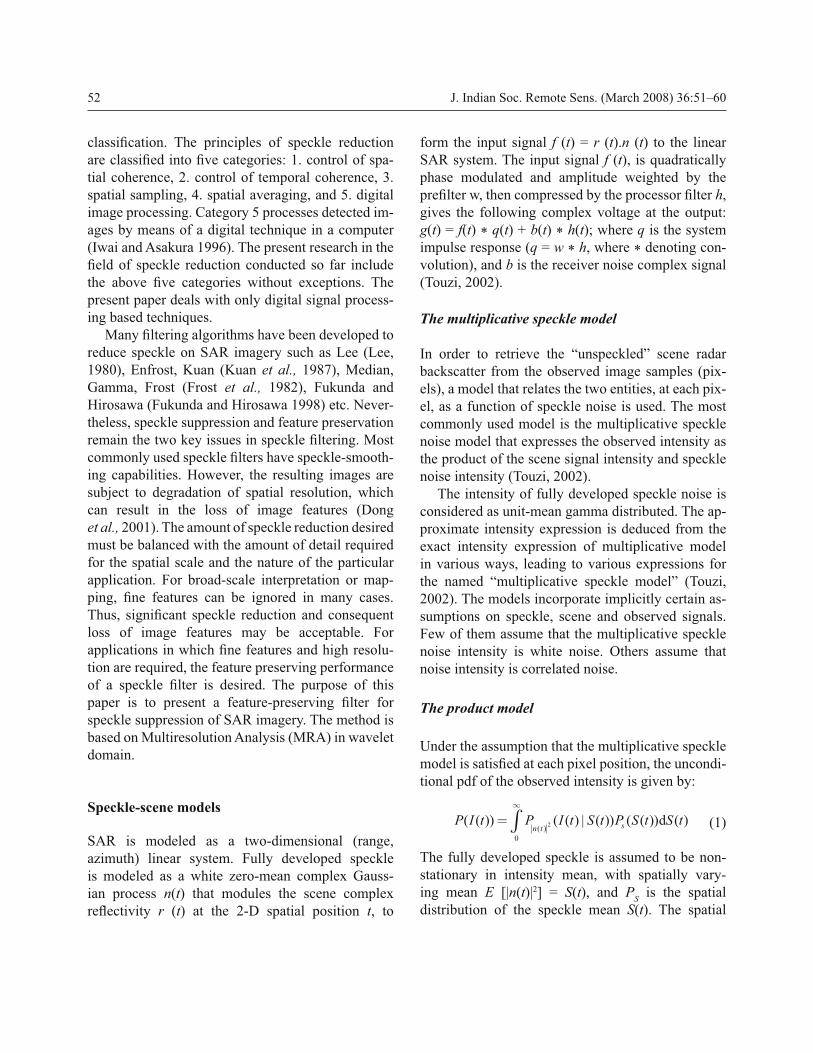
The undecimated DWT can be implemented using

an “algorithme a trous” as shown in Fig. 1 for one

dimensional signal (Cohen and Kovacevic 1996). It is

extended to two dimension signal. The wavelet trans-

form of an image, can be seen as a pair of two 1D-

wavelet transform along the horizontal and vertical


direction. Thus, image decomposition and reconstruc-

tion can be computed with separable fi ltering of the

signal along the horizontal and the vertical direction,

using the pyramid algorithm as in the 1D case.

The undecimated DWT is also called stationary

wavelet transform (SWT). SWT is a special version

of the DWT that has preserved translation invari-

ance. Instead of sub-sampling, the SWT utilizes

recursively dilated fi lters in order to halve the band-

width from one level to another. At scale 2j the fi lters

are dilated by inserting 2j–1 zeros between the fi lter

coeffi cients of the prototype fi lters.

For images, the following fi lter equations are used to

obtain wavelet coeffi cients dj+1

at level j+1 from scale

coeffi cients cj at level j (Cohen and Kovacevic 1996).

where, [m, n] are the pixel coordinates. The wave-

let coeffi cients d1

j+1,m,n

, d2

j+1,m,n

, d3

j+1,m,n

correspond to

image details with horizontal, vertical, and diagonal

orientations, respectively.

Proposed method

WT-based techniques have proved to be effective

due to its compressibility of information signal and

incompressibility of noise signal. The wavelet-based

speckle fi ltering is based on multiresolution analysis.

Speckle noise is suppressed by reducing the ampli-

tude of the pixels in the detail images with horizon-

tal, vertical and diagonal orientation. The proposed

method fl ow chart is given in Fig. 2. The SAR image

is decomposed into wavelet coeffi cients in fi ne to

coarse level and the speckle noise variance is esti-

mated by fi ne level of diagonal wavelet coeffi cients.

The variance is estimated by a robust estimating

technique (Donoho, 1995) as:

where Yi,j

and d3

1,m,n are pixel value and diagonal

wavelet coeffi cient respectively.

The wavelet coeffi cients are thresholded by uni-

versal thresholding rule proposed by Donoho, 1995

x

d1

d2

d3

d4

C1

G1(z)

H0(z) G1(z

2)

H0(z2) G1(z

4)

H0(z4) G1(z

8)

H0(z8)

Fig. 1 Implementation of the SWT by “algorithme a trous” for 1-dimension signal.

c H H cj m n j m n+ = ⊗

1, , , ,( )

= − −∑c h k m h l nj k l

k l

, ,

,

[ ] [ ]2 2

d H G cj m n j m n+ = ⊗

1

1

, , , ,( )

= − −∑c h k m g l nj k l

k l

, ,

,

[ ] [ ]2 2

d G H cj m n j m n+ = ⊗

1

2

, , , ,( )

= − −∑c g k m h l nj k l

k l

, ,

,

[ ] [ ]2 2

d G G cj m n j m n+ = ⊗

1

3

, , , ,( )

= − −∑c g k m g l nj k l

k l

, ,

,

[ ] [ ]2 2

(5)

σn

i j i j m nmedian Y Y d

=∈{ }( ) , , , ,

:

.

1

3

0 6745

(6)


as:

where, m × n is size of image.

The modifi ed wavelets coeffi cients are used in

reconstruction of denoised image. The performance

of the proposed fi lter was evaluated and compared

with several of the most widely used adaptive fi l-

ters based on the spatial domain, including the Lee,

Frost, Enfrost, Kuan, Median and Gamma fi lters.

The simulation parameters are given in Table 1.

The window size is 3 × 3 for standard fi lters. For

the Gamma fi lter, only the most commonly used

algorithm was used. A common way of estimat-

ing the speckle noise level in coherent imaging is

to calculate the mean-to-standard-deviation ratio

of the pixel intensity, often termed the Equivalent

Number of Looks (ENL), over a uniform image

area. Unfortunately, we found this measure is not

very robust mainly because of the diffi culty to iden-

tify a uniform area in a real image. For this reason,

we will use here only the mean square difference,

signal to noise ratio, peak signal to noise ratio. Mean

Square Error (MSE) indicates error of the pixels

throughout the image. A higher MSE indicates a

greater difference between the original and denoised

image. This means that there is a less speckle reduc-

tion. Nevertheless, it is necessary to be very careful

with the edges. Signal-to-Noise Ratio (SNR) and

Peak Signal-to-Noise Ratio (PSNR) are used as

quantitative comparison.

Result and discussion

The single band aerial image of Pilani area (512 ×

512 (pixels) × 255 (gray levels)) is taken as origi-

nal image. The image pixels value is normalized

and varies between 0 and 1. It is contaminated by

normal distributed multiplicative noise of variance

range 0.01 (standard deviation 0.1, 10% noise) to

0.05 (standard deviation 0.223, 22.3% noise). The

simulation fi lter parameters are given in Table 1.

The standard fi lters are tested by three window

sizes. It is observed that performance deteriorates

as the window size is increased. The results are

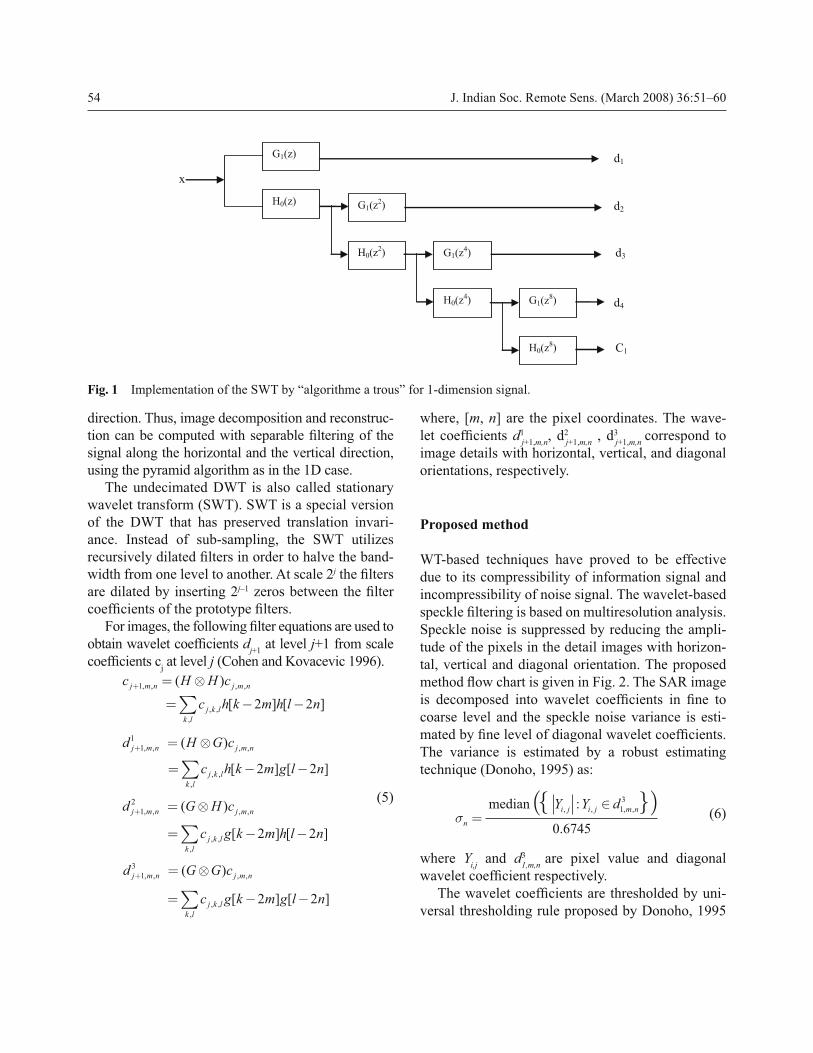
optimal for 3×3 window. The performance com-

parison results are given in Tables 2 and 3 for noise

variance of 0.01 and 0.05 respectively. The MSE,

SNR, PSNR are better for wavelet transform based

fi lters. To see the over all performance, results

are plotted in Fig. 3. The variance varies from

γ σ= ×2log( )m nn

(7)

Speckled

Image

Denoised Image

Wavelet Decomposition

Thresholding the WC Thresholding

estimation

Wavelet reconstruction

Fig. 2 Block diagram of the proposed algorithm

Table 1 Simulation fi lter parameters used in the paper.

Filters Parameters

Lee 3×3, 5×5, 7×7 window

Enfrost 3×3, 5×5, 7×7 window

Gamma 3×3, 5×5, 7×7 window

Kuan 3×3, 5×5, 7×7 window

Frost 3×3, 5×5, 7×7 window

Median 3×3, 5×5, 7×7 window

DWT(db2) Wavelet db2, level 3

DWT(sym4) Wavelet sym4, level 3

SWT(db2) Wavelet db2, level 3

SWT(sym4) Waveletsym4, level 3


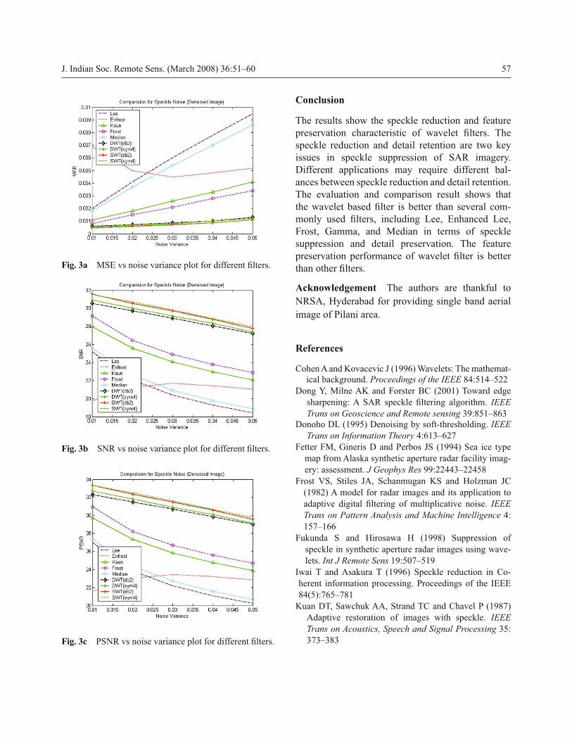
0.01 to 0.05. The wavelet fi lter performance is better

than others fi lters in whole span of speckle vari-

ance. The qualitative results are shown in Figs. 4

and 5 for noise variance of 0.01 and 0.05 respec-

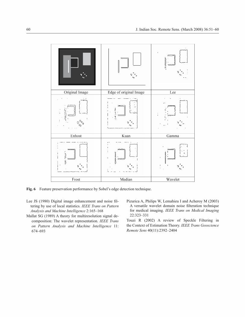
tively. The feature preservation performance is

tested by Sobel’s edge detection algorithm. The

fi lters are tested on synthetic image used by Pizu-

rica et al., 2003. The synthetic image is shown in

Fig. 6. The image has different types of objects with

different gray levels. The image is contaminated

by speckle of 0.05. The Sobel’s edge detection is

applied on despeckled image. The results are shown

in Fig. 6. The overall performance of wavelet fi lter

is better than other fi lters. All fi lters were imple-

mented in MATLAB® (Mathworks) on a PC with a

Pentium 4 (2.4 GHz) processor.

Table 2 Performance comparison for noise variance of 0.01 (standard deviation 0.1, 10%

noise).

Speckle noise reduction methodEvaluation Indices

MSE SNR PSNR

Noisy image 0.0066 20.0448 21.8259

Lee 0.0020 25.1851 26.9662

Enfrost 0.0069 19.7996 21.5808

Gamma 0.1645 6.0580 7.8391

Kuan 0.0011 27.9502 29.7313

Frost 8.0610e-004 29.1550 30.9361

Median 0.0018 25.5577 27.3389

DWT(db2) 5.8611e-004 30.5401 32.3202

DWT(sym4) 4.6436e-004 31.5514 33.3315

SWT(db2) 4.6710e-004 31.5259 33.3059

SWT(sym4) 4.6436e-004 31.5514 33.3315

Table 3. Preformance comparison for noise variance of 0.05 (standard deviation 0.223,

22.3% noise).

Speckle noise reduction methodEvaluation Indices

MSE SNR PSNR

Noisy image 0.0265 13.9823 15.7635

Lee 0.0095 18.4495 20.2307

Enfrost 0.0052 21.0691 22.8502

Gamma 0.3240 3.1137 4.8948

Kuan 0.0041 22.0676 23.8488

Frost 0.0034 22.9108 24.6920

Median 0.0086 18.8847 20.6658

DWT(db2) 0.0013 27.2350 29.0151

DWT(sym4) 0.0012 27.3790 29.1591

SWT(db2) 0.0011 27.7790 29.7693

SWT(sym4) 0.0011 27.7828 29.5628


Conclusion

The results show the speckle reduction and feature

preservation characteristic of wavelet fi lters. The

speckle reduction and detail retention are two key

issues in speckle suppression of SAR imagery.

Different applications may require different bal-

ances between speckle reduction and detail retention.

The evaluation and comparison result shows that

the wavelet based fi lter is better than several com-

monly used fi lters, including Lee, Enhanced Lee,

Frost, Gamma, and Median in terms of speckle

suppression and detail preservation. The feature

preservation performance of wavelet fi lter is better

than other fi lters.

Acknowledgement The authors are thankful to

NRSA, Hyderabad for providing single band aerial

image of Pilani area.

References

Co hen A and Kovacevic J (1996) Wavelets: The mathemat-

ical background. Proceedings of the IEEE 84:514–522

Do ng Y, Milne AK and Forster BC (2001) Toward edge

sharpening: A SAR speckle fi ltering algorithm. IEEE

Trans on Geoscience and Remote sensing 39:851–863

Do noho DL (1995) Denoising by soft-thresholding. IEEE

Trans on Information Theory 4:613–627

Fe tter FM, Gineris D and Perbos JS (1994) Sea ice type

map from Alaska synthetic aperture radar facility imag-

ery: assessment. J Geophys Res 99:22443–22458

Fr ost VS, Stiles JA, Schanmugan KS and Holzman JC

(1982) A model for radar images and its application to

adaptive digital fi ltering of multiplicative noise. IEEE

Trans on Pattern Analysis and Machine Intelligence 4:

157–166

Fu kunda S and Hirosawa H (1998) Suppression of

speckle in synthetic aperture radar images using wave-

lets. Int J Remote Sens 19:507–519

I wai T and Asakura T (1996) Speckle reduction in Co-

herent information processing. Proceedings of the IEEE

84(5):765–781

Ku an DT, Sawchuk AA, Strand TC and Chavel P (1987)

Adaptive restoration of images with speckle. IEEE

Trans on Acoustics, Speech and Signal Processing 35:

373–383

Fig. 3a MSE vs noise variance plot for different fi lters.

Fig. 3b SNR vs noise variance plot for different fi lters.

Fig. 3c PSNR vs noise variance plot for different fi lters.


b

e

h

k

c

f

i

l

a

d

g

j

Fig. 4 (a) original image (b) Noisy image with variance of 0.01 (c) Lee (d) Enfrost (e) Gamma (f) Kuan (g) Frost (h)

Median (i) DWT (db2) (j) DWT (sym4) (k) SWT (db2) (l) SWT (sym4).


b

e

h

k

c

f

i

l

a

d

g

j

Fig. 5 (a) original image (b) Noisy image with variance of 0.05 (c) Lee (d) Enfrost (e) Gamma (f) Kuan (g) Frost (h)

Median (i) DWT (db2) (j) DWT (sym4) (k) SWT (db2) (l) SWT (sym4).


Le e JS (1980) Digital image enhancement and noise fi l-

tering by use of local statistics. IEEE Trans on Pattern

Analysis and Machine Intelligence 2:165–168

Ma llat SG (1989) A theory for multiresolution signal de-

composition: The wavelet representation. IEEE Trans

on Pattern Analysis and Machine Intelligence 11:

674–693

Pi zurica A, Philips W, Lemahieu I and Acheroy M (2003)

A versatile wavelet domain noise fi lteration technique

for medical imaging. IEEE Trans on Medical Imaging

22:323–331

To uzi R (2002) A review of Speckle Filtering in

the Context of Estimation Theory. IEEE Trans Geoscience

Remote Sens 40(11):2392–2404

Fig. 6 Feature preservation performance by Sobel’s edge detection technique.

Feature preserving speckle filtering of the SAR images by wavelet transform

Documents

Transcript of Feature preserving speckle filtering of the SAR images by wavelet transform