1 2 3 4 5 6 7 8 9 1011121314151617181920212223242526272829303132333435363738394041424344454647484950515253545556575859606162636465

Feature Fusion for the Detection of Microsleep Events

Martin Golz1, David Sommer1, Mo Chen2, Udo Trutschel3, and Danilo Mandic2

1 Dptm. of Computer Science, University of Applied Sciences, 98574 Schmalkalden, Germany2 Dptm. of Electrical & Electronic Engineering, Imperial College, London, SW7 2BT, UK

3 Circadian Technologies, Inc., 2 Main Street, Stoneham, MA 02480, USA

AbstractA combination of linear and nonlinear methods for feature fusion is introduced and the performance of this methodology is illustrated on a real-world problem: the detection of sudden and non-anticipated lapses of attention in car drivers due to drowsiness. To achieve this, signals coming from heteroge-neous sources are processed, namely the brain electric activity, variation in the pupil size, and eye and eyelid movements. For all the signals considered, the features are extracted both in the spectral domain and in state space. Linear features are obtained by the modified periodogram , whereas the nonlinear features are based on the recently introduced method of Delay Vector Variance (DVV). The decision process based on such fused features is achieved by Support Vector Machines (SVM) and Learning Vector Quantization (LVQ) neural networks. For the latter also methods of metrics adaptation in the input space are applied. The parameters of all utilized algorithms are optimized empirically in order to gain maximal classification accuracy. It is also shown that metrics adaptation by weighting the input features can improve the classification accuracy, but only to a limited extent. Limited improvements are also obtained when fusing features of selected signals, but highest improvements are gained by fusion of features of all available signals. In this case test errors are reduced down to 9 % in the mean, which clearly illustrates the potential of our methodology to establish a reference standard of drowsiness and microsleep detection devices for future online driver monitoring.

1 IntroductionData fusion aims at improving performance and robustness in a variety of real-world prob-lems by processing complementary information coming from different sources. In fields such as recognition, identification, tracking, modality detection and decision making, multi-source and oftentimes non-commensurate signals are greatly benefiting from being processed within the framework of data fusion.When data fusion strategies are applied to biosignals (especially to electrophysiological time series) then the challenges arise from the necessity to process information about the mental state which is acquired from sensors recording a number of different underlying processes. In such cases fusion at the measurement or signal level, which is often called raw data fusion, is too impractical. Note that an appropriate model of signal generation in this field does not exist and that the observed signals contain large portion of irregularities. In case of brain electric signals, such as the electroencephalogram (EEG), the extent is not clear to which these irregu-larities are caused by the corresponding nonlinearities in the underlying signal generating sys-tem [1].Nevertheless, for relatively clear and abrupt changes of the system behaviour it should be pos-sible to detect and perhaps to predict the events of interest. This is the case with the detection of sudden and non-anticipated lapses of attention in subjects, due to drowsiness and monoto-ny, the so-called Microsleep Events (MSE). In case of car and train drivers such events are believed to be a major factor causing accidents. In recent years this topic has received broad attention from the government, public and also the research community. Recent developments in this field have shown that most promising approaches for this purpose are based on fusion of multiple electrophysiological signals coming from different sources together with SoftComputing methods [2-4].When modelling on the signal level is too complex then fusion on the second level, which is often called attribute or feature fusion, is preferred. Besides its advantage of a convenient

ManuscriptClick here to download Manuscript: IJVLSI-SP_12.doc

1 2 3 4 5 6 7 8 9 1011121314151617181920212223242526272829303132333435363738394041424344454647484950515253545556575859606162636465

multi-source integration this allows us to process data coming from so-called “transform domains”, e.g. of spectral, wavelet, state or some other space.Another way of data fusion is on the decision level [5]. Here, for each signal a classifier is trained and after optimizing all parameters of each pattern recognition step, the decisions are combined utilizing e.g. fuzzy logic based [4], statistical or voting methods. It is also possible to combine decisions coming from several experts. Here, decisions coming of single classi-fiers are not fused, but instead we based our analysis on subjective scores.Contrary to data fusion, methods of input feature selection and input feature weighting [6] aim to reduce the amount of information utilizing machine learning methods. It is assumed that processing of a large number of features leads to performance deteriorations because local classification approaches suffer from the so-called “curse of dimensionality”. Note that among high-dimensional input vectors the ratio of the distance between the nearest and the farthest distance converges to unity as the dimensionality approaches infinity [7]. In this res-pect, simple local algorithms such as the nearest-neighbour classifier are bound to suffer more than non-local learning algorithms such as SVMs.Apart from improving the classification accuracy, there is a further important advantage of feature weighting, namely the capability of Automatic Relevance Determination (ARD). In many applications, the usefulness of the extracted features is not known a priori. Here, relevance determination provides a way of knowledge extraction without explicitly stated assumptions. Feature selection is working in a discrete (binary) manner, that is, once un-selec-ted those features are no more relevant. Notice that feature weighting embodies the concept of feature relevance: low weighting is not as relevant as high weighting, since such features have lower impact on vector distance calculations which are fundamental to many classification algorithms, e.g. SVM and LVQ. The paper is organized as follows: In section 2 we give a short introduction to driving simula-tion experiments, measurements, observations of microsleep events during driving, and pre-processing of the resulting data. The methods of feature extraction are described in section 3. We also introduce our methodology utilized for data fusion on the feature level and providesome theoretical background. The presented methodology is generally applicable to other sto-chastic time series irrespective if they are originated by the same or by several distinct under-lying generating processes. The results in section 4 provide answer to the following important questions: (1) The extent to which it is possible to improve classification accuracy due to fusion of linear and non-linear features? (2) The extent to which it is possible to improve clas-sification accuracy due to fusion of feature vectors of different and non-commensurate biosig-nals? (3) The extent to which it is possible to improve classification accuracy due to feature weighting and ARD? (4) How large are the computational costs of different classification algorithms applied to the given data set?

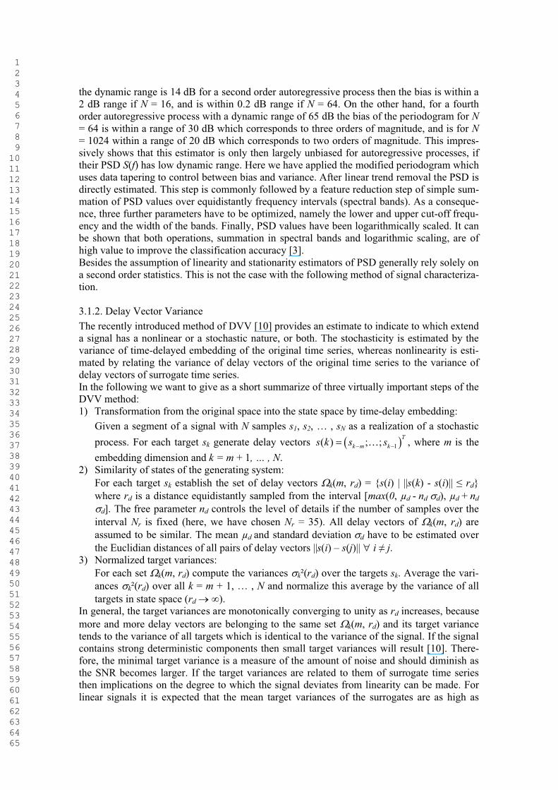
2 Experimental Study on Microsleep DetectionIn this section we provide short description of the recorded signals and microsleep experi-ments. For further insight into this topic the reader is referred to [2 - 4, 8] and references here-in.Twenty-three young adults started driving in our real car driving simulation lab (Fig. 1) at 1:00 a.m. after a day of normal activity and of at least 16 hours of incessant wakefulness. All in all, they had to complete seven driving sessions lasting 40 min, each followed by a 15 min long period of responding to sleepiness questionnaires and of vigilance tests and of a 5 min long break. Experiments ended at 8:00 am. Driving tasks were chosen intentionally monoto-nous to support drowsiness and occurrence of MSE. The latter are defined as short intrusions of sleep into wakefulness under demands of attention. They were detected by two experimen-ters who observed the subject utilizing three video camera streams: (i) of subjects left eye region, (ii) of her/his head and of upper part of the body, and (iii) of driving scene. Typical

1 2 3 4 5 6 7 8 9 1011121314151617181920212223242526272829303132333435363738394041424344454647484950515253545556575859606162636465

signs of MSE are e.g. prolonged eyelid closures, nodding-off, driving incidents and drift-out-of-lane accidents.

Fig. 1. Real car driving simulation lab

This step of online scoring is critical, because there are no unique signs of MSE, and their exact beginning is sometimes hardly to define. Therefore, all events were checked offline and were eventually corrected by an independent expert. Unclear MSE characterized by e.g. drifting of eye gaze, short phases with extremely small eyelid gap, inertia of eyelid opening movements or slow head down movements were excluded from further analysis. Non-MSE were selected at all times outside of clear and of unclear MSE. All in all we have found 3,573 MSE (per subject: mean number 162±91, range 11-399) and have picked out the same amount of non-MSE in order to have balanced data sets. Our intention was to design a detection system for clear MSE versus clear Non-MSE classi-fication, assuming that such a system can not only detect the MSE recognized by human experts, but would also offer a possibility to detect unclear MSE cases which are not recognizable by experts. Seven signals of EEG (C3, Cz, C4, O1, O2, A1, A2, common average reference) and two EOG channels (vertical, horizontal) were recorded by an electrophysiological polygraphy system at a sampling rate of 128 Hz. The electrode locations are typically used in sleep and vigilance research. The first three locations are related to electrical activity in somato-sensoric and motoric brain areas, whereas O1, O2 are related to electrical activity in the primary and secondary visual areas, and A1, A2 are assumed to be functionally less active and often serveas reference electrodes.Further six signals were recorded by an Eye Tracking System (ETS, binocular). This device samples at a rate of 250 Hz and is not strictly synchronized to the polygraphy system which is not problematic for later fusion on the feature level. For each eye of the subject three signalsare recorded, namely the pupil size and the two coordinates of eye gaze on the plane of pro-jection.All in all, 15 different signals were recorded. In subsequent pre-processing stages mainly three steps have to be performed: signal segmentation, artefact removal and missing data sub-stitution.Segmentation of all signals was done with respect to the observed temporal starting points of MSE / Non-MSE using two free parameters, the segment length and the temporal offset bet-ween first sample of segment and starting point of an event. The trade-off between temporal and spectral resolution is adjusted by the segment length and the location of the region-of-interest on the time axis is controlled by the temporal offset. Therefore, both parameters are of high importance and have to be optimized (section 4).

1 2 3 4 5 6 7 8 9 1011121314151617181920212223242526272829303132333435363738394041424344454647484950515253545556575859606162636465

Artefacts in the EEG are signal components which are presumably originated extracerebrally and often exhibit as transient, high-amplitude voltages. For their detection a sliding double data window is applied, in order to compare the power spectral densities in both windows. When the mean squared difference of them is higher than a thoroughly defined threshold value, then the condition of stationarity should be evidently violated and as a consequence this example of MSE or NMSE is excluded from further analysis. Missing data problem occurred in all six eyetracking signals during every eyelid closures. This is caused by the measuring principle. They are substituted by data generated by an auto-regressive model which is fitted to the signal immediately before the eyelid closure. This way,artificial data replace missing data under the assumption of stationarity. Nevertheless, this problem should be not important enough to give more insight. For instance, periods of mis-sing data are in the size of 150 msec which is small compared to the segment length of 8 sec (section 4).

3 MethodologyThis section introduces methods to process all 15 different signals coming out of the experi-ments with the objective to fuse them on a higher level. At first, characteristic features of each segment of the signals have to be extracted. Ideally, features which support sufficiently com-pact regions in the feature space are ideally sought. This can be achieved in the original time domain, or in the spectral or wavelet or some other transform domain. Here we propose to apply the frequently applied power estimation in the spectral domain and a new method in the state space, the recently introduced method of Delay Vector Variance estimation (DVV). Ob-viously, there are a lot of alternatives or of supplementary methods imaginable.Having extracted several features, then, secondly, they have to be fused. This can be done bymachine learning methods of classification. Here we compare several methods. In addition to some simple classificators we have applied modern methods without and with metrics adapta-tion in the feature space.

3.1. Feature ExtractionIrregularities in signals have at least two possible sources: stochasticity and nonlinearity of the underlying signal generating system [1]. In the following we will characterize a signal as linear when it is generated by a linear time-invariant system, driven by white Gaussian noise; otherwise it is considered as nonlinear. Mostly the definition of linearity is not strictly app-lied. Then, the distribution of the signal is allowed to deviate from the Gaussian form, to take into account that a linear signal may be measured by a static, monotonic, and possibly nonli-near observation function.A signal is characterized as deterministic or predictable, if it is possible to formulate a set of equations which precisely describe the signal; otherwise it is considered as stochastic. In general, a signal will be deterministic if all possible states of the generating system are located in a finite dimensional state space. Every transition from one state to another can then be formulated by a deterministic rule [1].

3.1.1. The PeriodogramThe periodogram has been widely used in quantitative biosignal analysis. When doing so, the signals are assumed to be outcomes of a linear, stochastic process which has to be stationary. The fact that the periodogram is an asymptotically unbiased estimator of the true power spect-ral density (PSD) S(f) does not mean that its bias is necessarily small for any particularly sam-ple size N. If S(f) is a smooth function then the estimation bias decreases at the rate of 1/N, but nothing is stated about the absolute magnitude of the bias. If we define the dynamic range of S(f) by 10 log10[max S(f) / min S(f)] then this value is zero for a white noise process and the periodogram is in this case an unbiased estimator. In [9] it is shown on two examples, that if

1 2 3 4 5 6 7 8 9 1011121314151617181920212223242526272829303132333435363738394041424344454647484950515253545556575859606162636465

the dynamic range is 14 dB for a second order autoregressive process then the bias is within a 2 dB range if N = 16, and is within 0.2 dB range if N = 64. On the other hand, for a fourth order autoregressive process with a dynamic range of 65 dB the bias of the periodogram for N= 64 is within a range of 30 dB which corresponds to three orders of magnitude, and is for N= 1024 within a range of 20 dB which corresponds to two orders of magnitude. This impres-sively shows that this estimator is only then largely unbiased for autoregressive processes, if their PSD S(f) has low dynamic range. Here we have applied the modified periodogram which uses data tapering to control between bias and variance. After linear trend removal the PSD is directly estimated. This step is commonly followed by a feature reduction step of simple sum-mation of PSD values over equidistantly frequency intervals (spectral bands). As a conseque-nce, three further parameters have to be optimized, namely the lower and upper cut-off frequ-ency and the width of the bands. Finally, PSD values have been logarithmically scaled. It can be shown that both operations, summation in spectral bands and logarithmic scaling, are of high value to improve the classification accuracy [3].Besides the assumption of linearity and stationarity estimators of PSD generally rely solely on a second order statistics. This is not the case with the following method of signal characteriza-tion.

3.1.2. Delay Vector VarianceThe recently introduced method of DVV [10] provides an estimate to indicate to which extend a signal has a nonlinear or a stochastic nature, or both. The stochasticity is estimated by the variance of time-delayed embedding of the original time series, whereas nonlinearity is esti-mated by relating the variance of delay vectors of the original time series to the variance of delay vectors of surrogate time series.In the following we want to give as a short summarize of three virtually important steps of the DVV method:1) Transformation from the original space into the state space by time-delay embedding:

Given a segment of a signal with N samples s1, s2, … , sN as a realization of a stochastic process. For each target sk generate delay vectors 1( ) ; ; T

k m ks k s s , where m is the embedding dimension and k = m + 1, … , N.

2) Similarity of states of the generating system:For each target sk establish the set of delay vectors k(m, rd) = {s(i) | ||s(k) - s(i)|| rd}where rd is a distance equidistantly sampled from the interval [max(0, μd - nd d), μd + nd

d]. The free parameter nd controls the level of details if the number of samples over the interval Nr is fixed (here, we have chosen Nr = 35). All delay vectors of k(m, rd) are assumed to be similar. The mean μd and standard deviation d have to be estimated over the Euclidian distances of all pairs of delay vectors ||s(i) – s(j)|| i j.

3) Normalized target variances:For each set k(m, rd) compute the variances k²(rd) over the targets sk. Average the vari-ances k²(rd) over all k = m + 1, … , N and normalize this average by the variance of all targets in state space (rd

In general, the target variances are monotonically converging to unity as rd increases, because more and more delay vectors are belonging to the same set k(m, rd) and its target variance tends to the variance of all targets which is identical to the variance of the signal. If the signal contains strong deterministic components then small target variances will result [10]. There-fore, the minimal target variance is a measure of the amount of noise and should diminish as the SNR becomes larger. If the target variances are related to them of surrogate time series then implications on the degree to which the signal deviates from linearity can be made. For linear signals it is expected that the mean target variances of the surrogates are as high as

1 2 3 4 5 6 7 8 9 1011121314151617181920212223242526272829303132333435363738394041424344454647484950515253545556575859606162636465

them of the original signal. Significant deviations from this equivalence indicate that nonline-ar components are present in the signal [10].For each segment of a signal, the DVV method results in Nr different values of target varian-ces. They constitute the components of feature vectors x which feed the input of the next pro-cessing stages and represent a quantification to which extend the segments of the measured signals has a nonlinear or a stochastic nature, or both.

3.2. Classification MethodsAfter having extracted a set of features, they are to be combined in order to obtain a suitable discrimination function. This feature fusion step can be performed in a weighted or unweigh-ted manner. Two methods of unweighted feature fusion are introduced in this section and two methods of weighted fusion are introduced in the next (section 3.3). We begin with Learning Vector Quantization because it is also the central part of the methods in section 3.3 and it is a useful method for relatively quick optimization of free parameters in the pre-processing and feature extraction stages. Support Vector Machines attract attention because of their good theoretical foundation and their coverage of complexity as demonstra-ted in different benchmark studies of several pattern recognition problems.

3.2.1. Learning Vector QuantizationOptimized Learning Vector Quantization (OLVQ1) is a robust, very adaptive and rapidly con-verging classification method [11]. Like the well-known k-Means algorithm it is based on adaptation of prototype vectors. But instead of utilizing the calculation of local centres of gra-vity LVQ is adapting iteratively based on Riccati-type of learning and aims to minimize the mean squared error between input and prototype vectors. Given a finite training set S of NS feature vectors T

1( , , )inx x x assigned to class labels y i:

S = , 1, , 1, ,i i nC Sx y N i N where NC is the number of different classes, and

given a set W of NW randomly initialized prototype vectors w j assigned to class labels c j:, 1, , 1, ,j j n

C WW w c N j N . In this paper superscripts on a vector always describe the number out of a data set, and subscripts on a vector describe vector components.The following equations define the OLVQ1 process [11]:For each data vector x i, randomly selected from S, find the closest prototype vector Cjw basedon a suitable vector norm in n :(1) arg min 1,...,i j

C Wjj x w j N .

Adapt Cjw due to the following update rule, whereby the positive sign has to be used if Cjw isassigned to the same class as x i, i.e. Cjiy c , otherwise the negative sign has to be used:(2) C C

C

j jijw x w .

The learning ratesCj

are computed by:

(3)( 1)

( )1 ( 1)

C

C

C

jj

j

tt

t,

whereby the positive sign in the denominator has to be used if Cjiy c and hence Cj

is decreasing with iteration time t. Otherwise it is increasing because the negative sign has to be used if Cjiy c . That is to say, whensoever a prototype vector is closest, then and only then,the vector and the assigned learning rate

Cjis updated following (2) and (3), respectively.

1 2 3 4 5 6 7 8 9 1011121314151617181920212223242526272829303132333435363738394041424344454647484950515253545556575859606162636465

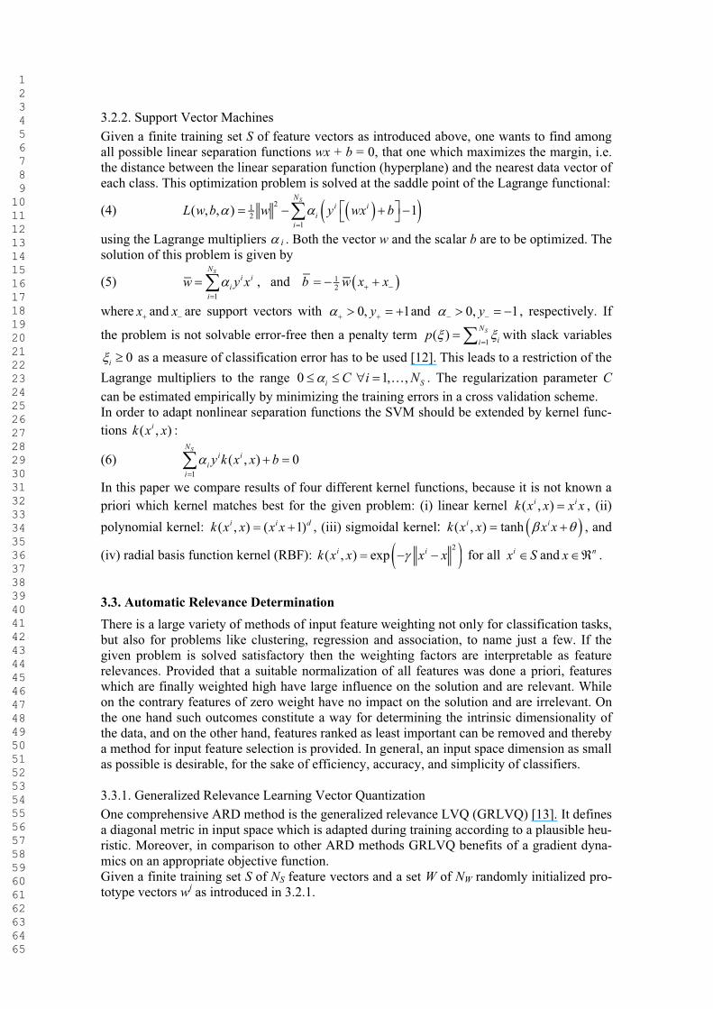
3.2.2. Support Vector MachinesGiven a finite training set S of feature vectors as introduced above, one wants to find among all possible linear separation functions wx + b = 0, that one which maximizes the margin, i.e. the distance between the linear separation function (hyperplane) and the nearest data vector of each class. This optimization problem is solved at the saddle point of the Lagrange functional:

(4) 212

1( , , ) 1

SNi i

ii

L w b w y wx b

using the Lagrange multipliers i . Both the vector w and the scalar b are to be optimized. The solution of this problem is given by

(5)1

SNi i

ii

w y x , and 12b w x x

where x and x are support vectors with 0, 1y and 0, 1y , respectively. If

the problem is not solvable error-free then a penalty term 1

( ) SNii

p with slack variables

0i as a measure of classification error has to be used [12]. This leads to a restriction of the Lagrange multipliers to the range 0 1, ,i SC i N . The regularization parameter Ccan be estimated empirically by minimizing the training errors in a cross validation scheme.In order to adapt nonlinear separation functions the SVM should be extended by kernel func-tions ( , )ik x x :

(6)1

( , ) 0SN

i ii

iy k x x b

In this paper we compare results of four different kernel functions, because it is not known a priori which kernel matches best for the given problem: (i) linear kernel ( , )i ik x x x x , (ii) polynomial kernel: ( , ) ( 1)i i dk x x x x , (iii) sigmoidal kernel: ( , ) tanhi ik x x x x , and

(iv) radial basis function kernel (RBF):2

( , ) expi ik x x x x for all ix S and nx .

3.3. Automatic Relevance DeterminationThere is a large variety of methods of input feature weighting not only for classification tasks, but also for problems like clustering, regression and association, to name just a few. If the given problem is solved satisfactory then the weighting factors are interpretable as feature relevances. Provided that a suitable normalization of all features was done a priori, features which are finally weighted high have large influence on the solution and are relevant. While on the contrary features of zero weight have no impact on the solution and are irrelevant. On the one hand such outcomes constitute a way for determining the intrinsic dimensionality of the data, and on the other hand, features ranked as least important can be removed and thereby a method for input feature selection is provided. In general, an input space dimension as small as possible is desirable, for the sake of efficiency, accuracy, and simplicity of classifiers.

3.3.1. Generalized Relevance Learning Vector QuantizationOne comprehensive ARD method is the generalized relevance LVQ (GRLVQ) [13]. It defines a diagonal metric in input space which is adapted during training according to a plausible heu-ristic. Moreover, in comparison to other ARD methods GRLVQ benefits of a gradient dyna-mics on an appropriate objective function. Given a finite training set S of NS feature vectors and a set W of NW randomly initialized pro-totype vectors wj as introduced in 3.2.1.

1 2 3 4 5 6 7 8 9 1011121314151617181920212223242526272829303132333435363738394041424344454647484950515253545556575859606162636465

The objective function to be minimized is given by:

(7)1

SNi

GRLVQi

E sgd x

with ( ) ( )( ) ( )

i ii

i i

d x d xxd x d x

and 1( )1 xsgd x

e; jd denotes the squared distance of ix

to the closest jw of the same class as ix , i.e. jiy c , and jd denotes the squared distance

of ix to the closest jw of a different class as ix , i.e. jiy c . The distances have to be calcu-lated according to the weighted Euclidian metric:

(8) 2 2

1

nk k kk

x w x w ,

where the weights k are the relevance values. The terms ix are negative if and only if ix isclassified correctly. Therefore, maximizing the number of correctly classified input vectors aims at minimizing the objective function.Taking the gradient of (7) yields the adaptation rule for the prototype vectors which is quali-tatively the same as of basic LVQ [11]:

(9a) j jiw x w for the closest correct prototype vector jw and

(9b) j jiw x w for the closest incorrect prototype vector jw ,

where is the learning rate which is equal for all prototype vectors and has to be monotoni-cally decreasing with increasing iteration time.

In (9a,b) the learning rate is modulated by two factors , which depend on jd , jd :

(10) 2 ' ( )( )

id sgd xd d

, 2 ' ( )( )

id sgd xd d

.

Next, the relevance values have to be adapted by

(11) 2 2( ) ( )j ji ik k k k kx w x w

utilizing another learning rate than in (9a) and (9b). Finally, tresholding and normalization should be executed in order to avoid negative relevance values: max ( ,0)k k k and to ob-tain || || = 1. The update (11) can be interpreted in a Hebbian way: those weighting factors are reinforced, which coefficients are closest to the input vector ix if classified correctly. And on the contrary, those weighting factors are faded, which coefficients are closest to the input vec-tor ix if classified incorrectly.

3.3.2. Combining Optimized Learning Vector Quantization with Genetic AlgorithmsIn the same line as GRLVQ, we have proposed an adaptive metric optimization approach [14]. Based on the fast converging and robust OLVQ1 algorithm [11] the same weight values

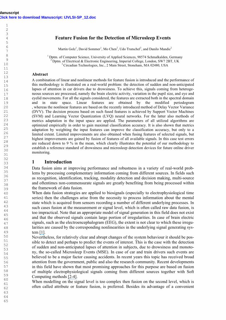
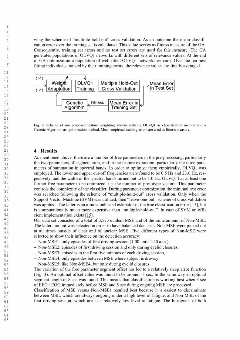
k as in (8) are adapted utilizing genetic algorithms (GA). In the following it is labelled as “OLVQ1 + GA”. As already mentioned, OLVQ1 is relatively fast converging. Therefore, this algorithm is suited to involve into a computationally intensive framework like the genetic algorithms (Fig. 2).Based on the given data set, several ten complete training runs of an OLVQ1 network were performed. For each run the data set is randomly partitioned in a training and a test set follo-

1 2 3 4 5 6 7 8 9 1011121314151617181920212223242526272829303132333435363738394041424344454647484950515253545556575859606162636465

wing the scheme of “multiple hold-out” cross validation. As an outcome the mean classifi-cation error over the training set is calculated. This value serves as fitness measure of the GA. Consequently, training set errors and no test set errors are used for this measure. The GA generates populations of OLVQ1 networks with different sets of relevance values. At the end of GA optimization a population of well fitted OLVQ1 networks remains. Over the ten best fitting individuals, ranked by their training errors, the relevance values are finally averaged.

Fig. 2. Scheme of our proposed feature weighting system utilizing OLVQ1 as classification method and a Genetic Algorithm as optimization method. Mean empirical training errors are used as fitness measure.

4 ResultsAs mentioned above, there are a number of free parameters in the pre-processing, particularly the two parameters of segmentation, and in the feature extraction, particularly the three para-meters of summation in spectral bands. In order to optimize them empirically, OLVQ1 was employed. The lower and upper cut-off frequencies were found to be 0.5 Hz and 23.0 Hz, res-pectively, and the width of the spectral bands turned out to be 1.0 Hz. OLVQ1 has at least one further free parameter to be optimized, i.e. the number of prototype vectors. This parameter controls the complexity of the classifier. During parameter optimization the minimal test error was searched following the scheme of “multiple-hold-out” cross validation. Only when the Support Vector Machine (SVM) was utilized, then “leave-one-out” scheme of cross validation was applied. The latter is an almost unbiased estimator of the true classification error [15], but is computationally much more expensive than “multiple-hold-out”. In case of SVM an effi-cient implementation exists [15].Our data set consisted of a total of 3,573 evident MSE and of the same amount of Non-MSE. The latter amount was selected in order to have balanced data sets. Non-MSE were picked out at all times outside of clear and of unclear MSE. Five different types of Non-MSE were selected to show their influence on the detection accuracy:

Non-MSE1: only episodes of first driving session (1:00 until 1:40 a.m.),Non-MSE2: episodes of first driving session and only during eyelid closures, Non-MSE3: episodes in the first five minutes of each driving session, Non-MSE4: only episodes between MSE where subject is drowsy, Non-MSE5: like Non-MSE4, but only during eyelid closures.

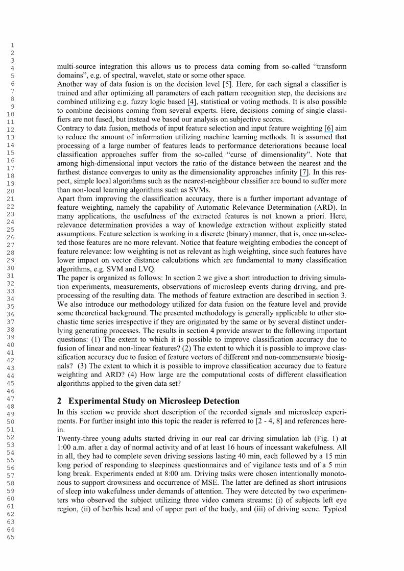
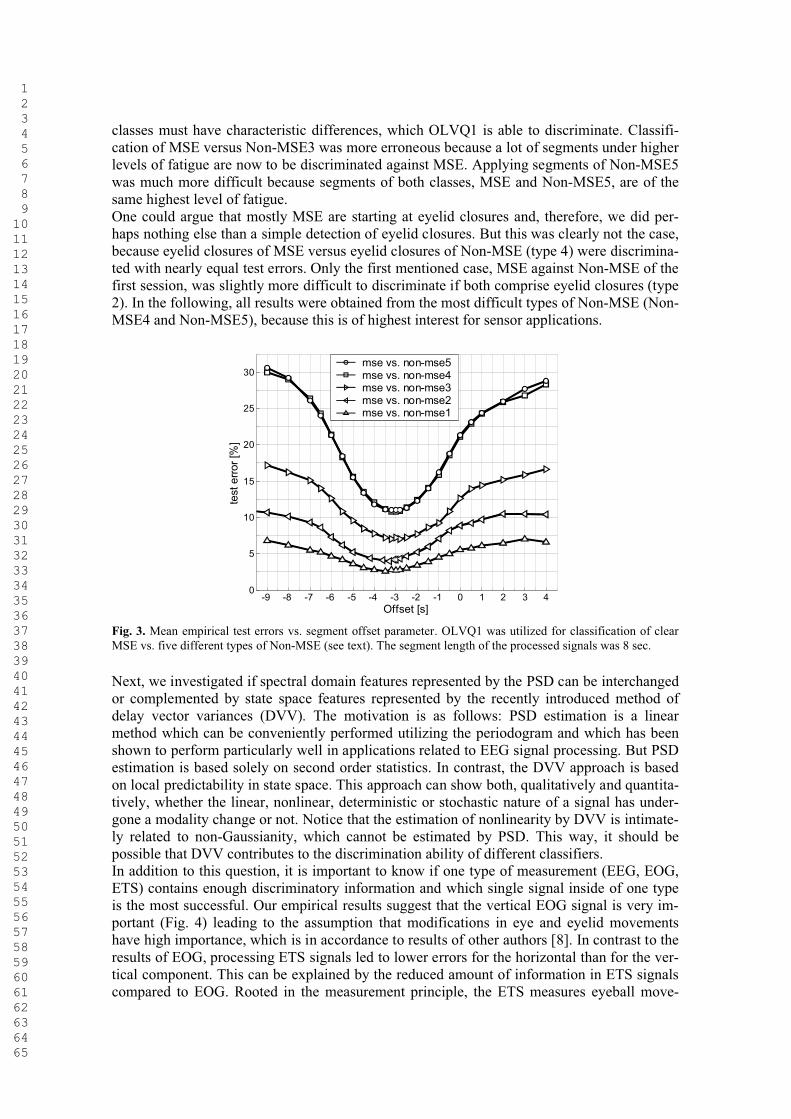
The variation of the free parameter segment offset has led to a relatively steep error function (Fig. 3). An optimal offset value was found to be around -3 sec. In the same way an optimal segment length of 8 sec was found. This means that classification is working best when 3 sec of EEG / EOG immediately before MSE and 5 sec during ongoing MSE are processed. Classification of MSE versus Non-MSE1 resulted best because it is easiest to discriminate between MSE, which are always ongoing under a high level of fatigue, and Non-MSE of the first driving session, which are at a relatively low level of fatigue. The biosignals of both

1 2 3 4 5 6 7 8 9 1011121314151617181920212223242526272829303132333435363738394041424344454647484950515253545556575859606162636465

classes must have characteristic differences, which OLVQ1 is able to discriminate. Classifi-cation of MSE versus Non-MSE3 was more erroneous because a lot of segments under higherlevels of fatigue are now to be discriminated against MSE. Applying segments of Non-MSE5 was much more difficult because segments of both classes, MSE and Non-MSE5, are of the same highest level of fatigue. One could argue that mostly MSE are starting at eyelid closures and, therefore, we did per-haps nothing else than a simple detection of eyelid closures. But this was clearly not the case, because eyelid closures of MSE versus eyelid closures of Non-MSE (type 4) were discrimina-ted with nearly equal test errors. Only the first mentioned case, MSE against Non-MSE of the first session, was slightly more difficult to discriminate if both comprise eyelid closures (type 2). In the following, all results were obtained from the most difficult types of Non-MSE (Non-MSE4 and Non-MSE5), because this is of highest interest for sensor applications.

-9 -8 -7 -6 -5 -4 -3 -2 -1 0 1 2 3 40

5

10

15

20

25

30

test

erro

r[%

]

Offset [s]

mse vs. non-mse5mse vs. non-mse4mse vs. non-mse3mse vs. non-mse2mse vs. non-mse1

Fig. 3. Mean empirical test errors vs. segment offset parameter. OLVQ1 was utilized for classification of clear MSE vs. five different types of Non-MSE (see text). The segment length of the processed signals was 8 sec.

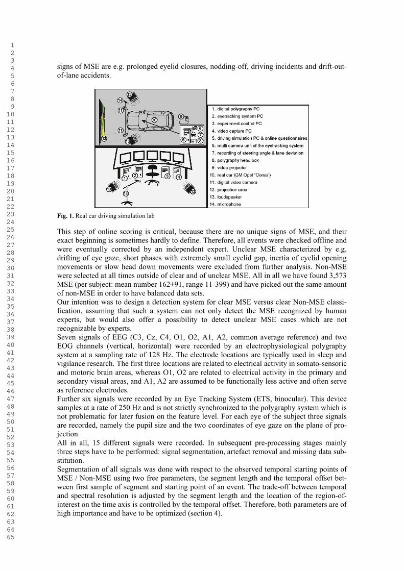
Next, we investigated if spectral domain features represented by the PSD can be interchanged or complemented by state space features represented by the recently introduced method of delay vector variances (DVV). The motivation is as follows: PSD estimation is a linear method which can be conveniently performed utilizing the periodogram and which has been shown to perform particularly well in applications related to EEG signal processing. But PSD estimation is based solely on second order statistics. In contrast, the DVV approach is based on local predictability in state space. This approach can show both, qualitatively and quantita-tively, whether the linear, nonlinear, deterministic or stochastic nature of a signal has under-gone a modality change or not. Notice that the estimation of nonlinearity by DVV is intimate-ly related to non-Gaussianity, which cannot be estimated by PSD. This way, it should be possible that DVV contributes to the discrimination ability of different classifiers.In addition to this question, it is important to know if one type of measurement (EEG, EOG, ETS) contains enough discriminatory information and which single signal inside of one type is the most successful. Our empirical results suggest that the vertical EOG signal is very im-portant (Fig. 4) leading to the assumption that modifications in eye and eyelid movements have high importance, which is in accordance to results of other authors [8]. In contrast to the results of EOG, processing ETS signals led to lower errors for the horizontal than for the ver-tical component. This can be explained by the reduced amount of information in ETS signals compared to EOG. Rooted in the measurement principle, the ETS measures eyeball move-

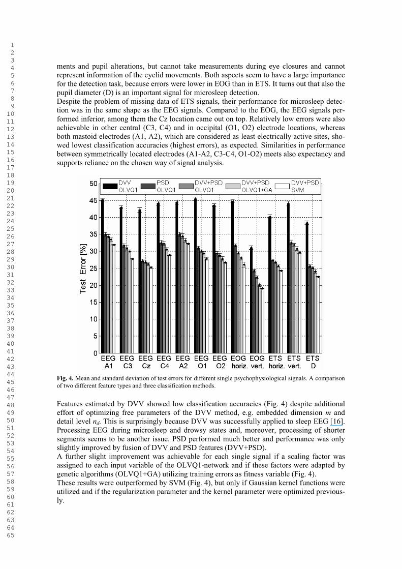
1 2 3 4 5 6 7 8 9 1011121314151617181920212223242526272829303132333435363738394041424344454647484950515253545556575859606162636465

ments and pupil alterations, but cannot take measurements during eye closures and cannot represent information of the eyelid movements. Both aspects seem to have a large importance for the detection task, because errors were lower in EOG than in ETS. It turns out that also the pupil diameter (D) is an important signal for microsleep detection.Despite the problem of missing data of ETS signals, their performance for microsleep detec-tion was in the same shape as the EEG signals. Compared to the EOG, the EEG signals per-formed inferior, among them the Cz location came out on top. Relatively low errors were also achievable in other central (C3, C4) and in occipital (O1, O2) electrode locations, whereas both mastoid electrodes (A1, A2), which are considered as least electrically active sites, sho-wed lowest classification accuracies (highest errors), as expected. Similarities in performance between symmetrically located electrodes (A1-A2, C3-C4, O1-O2) meets also expectancy and supports reliance on the chosen way of signal analysis.

Fig. 4. Mean and standard deviation of test errors for different single psychophysiological signals. A comparison of two different feature types and three classification methods.

Features estimated by DVV showed low classification accuracies (Fig. 4) despite additional effort of optimizing free parameters of the DVV method, e.g. embedded dimension m anddetail level nd. This is surprisingly because DVV was successfully applied to sleep EEG [16]. Processing EEG during microsleep and drowsy states and, moreover, processing of shorter segments seems to be another issue. PSD performed much better and performance was only slightly improved by fusion of DVV and PSD features (DVV+PSD). A further slight improvement was achievable for each single signal if a scaling factor was assigned to each input variable of the OLVQ1-network and if these factors were adapted by genetic algorithms (OLVQ1+GA) utilizing training errors as fitness variable (Fig. 4). These results were outperformed by SVM (Fig. 4), but only if Gaussian kernel functions were utilized and if the regularization parameter and the kernel parameter were optimized previous-ly.

1 2 3 4 5 6 7 8 9 1011121314151617181920212223242526272829303132333435363738394041424344454647484950515253545556575859606162636465

A pronounced improvement of the classification accuracies was achievable by feature fusion of more than one signal (Fig. 5). Compared to the best single signal of each signal type (3 left-most groups of bars in fig. 5), the feature fusion of vertical EOG and central EEG has led to a more accurate solution of the classification task, and has been also more successful than the fusion of features of both EOG or of all seven EEG signals. The feature fusion of 9 signals(all EOG + all EEG) and the feature fusion of all 15 signals (all EOG + all EEG + all ETS) re-sulted in slightly higher accuracies when OLVQ1 is applied as classification method. But, classification accuracies were considerably improved if OLVQ1 has been extended by feature weighting utilizing genetic algorithms (OLVQ1+GA) or if SVM has been applied.

Fig. 5. Mean and standard deviation of test errors for feature fusion of different signals. A comparison of two different feature types (PSD, DVV) and three classification methods (OLVQ1, GA+OLVQ1, SVM).

For the latter mentioned case best results were achieved; the fusion of features of both types (PSD + DVV) and of all 7 EEG, of both EOG, and of all 6 ETS signals utilizing SVM resul-ted in test errors lower than 10%. SVM clearly outperformed OLVQ1+GA.

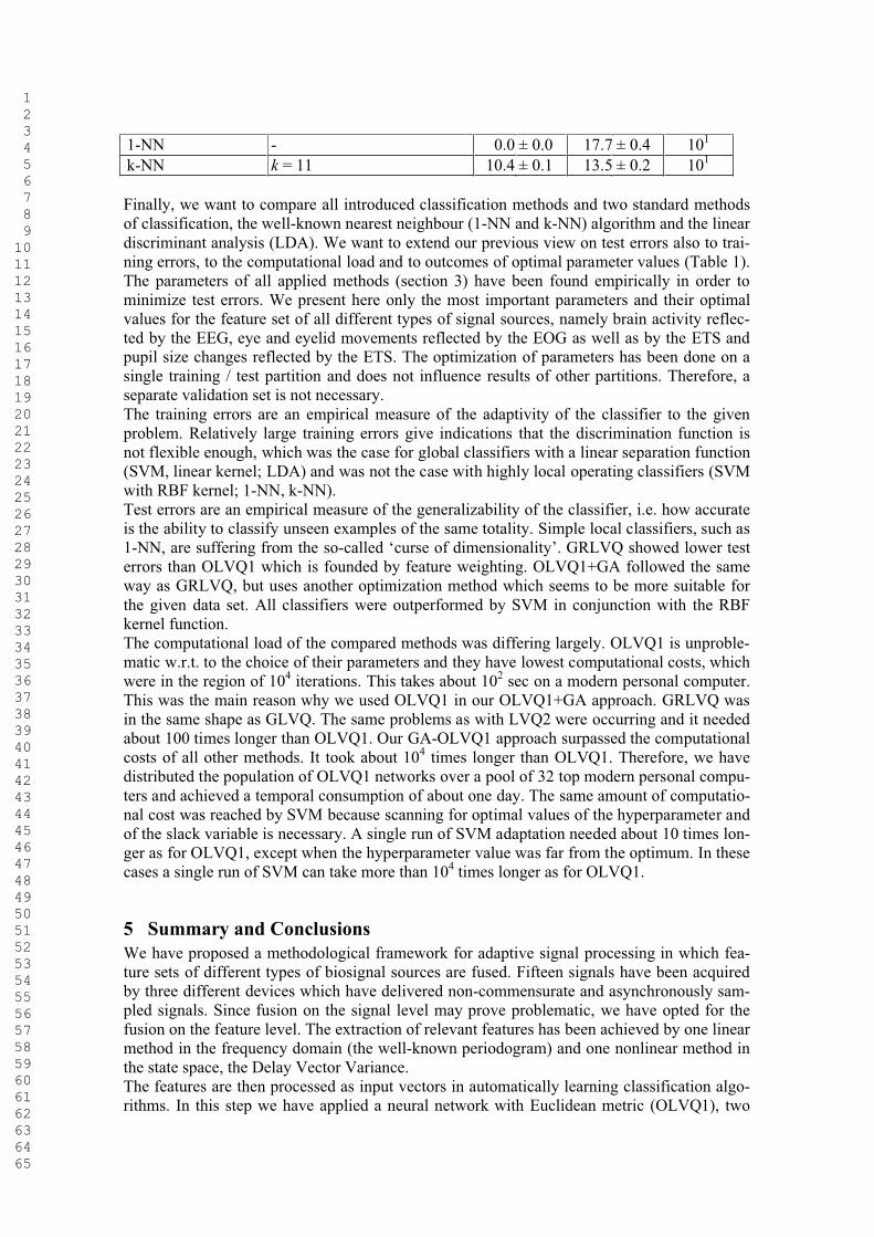
Table 1. Results of feature fusion of all 15 signals using different classification algorithms. Parameters were op-timized empirically. ETRAIN and ETEST contain mean and standard deviation of classification errors in the training and test set, respectively. FLOAD is a rough estimate of typical computational load normalized to that of OLVQ1.

Method Optimal parameter values ETRAIN [%] ETEST [%] FLOAD

OLVQ1 NW = 500 9.7 ± 0.2 15.1 ± 0.4 100

GRLVQ NW = 500; = 0.01 7.4 ± 0.2 14.4 ± 0.3 102

OLVQ1+GA #generat. = 200, #pop.=128 6.2 ± 0.2 12.3 ± 0.4 104

SVM, linear kernel C = 10-2.3 14.3 ± 0.1 15.4 ± 0.2 104

SVM, polynom. k. C = 10-2.2; d = 2 6.8 ± 0.1 13.4 ± 0.3 104

SVM, sigmoid k. C = 10+3.8; = 10-2.9; = -1.5 6.5 ± 0.1 11.5 ± 0.3 104

SVM, RBF k. C = 10+0.24; = 10-2.8 0.1 ± 0.0 9.1 ± 0.2 104

LDA - 13.5 ± 0.1 16.3 ± 0.2 100

1 2 3 4 5 6 7 8 9 1011121314151617181920212223242526272829303132333435363738394041424344454647484950515253545556575859606162636465

1-NN - 0.0 ± 0.0 17.7 ± 0.4 101

k-NN k = 11 10.4 ± 0.1 13.5 ± 0.2 101

Finally, we want to compare all introduced classification methods and two standard methods of classification, the well-known nearest neighbour (1-NN and k-NN) algorithm and the linear discriminant analysis (LDA). We want to extend our previous view on test errors also to trai-ning errors, to the computational load and to outcomes of optimal parameter values (Table 1). The parameters of all applied methods (section 3) have been found empirically in order to minimize test errors. We present here only the most important parameters and their optimal values for the feature set of all different types of signal sources, namely brain activity reflec-ted by the EEG, eye and eyelid movements reflected by the EOG as well as by the ETS and pupil size changes reflected by the ETS. The optimization of parameters has been done on a single training / test partition and does not influence results of other partitions. Therefore, a separate validation set is not necessary. The training errors are an empirical measure of the adaptivity of the classifier to the given problem. Relatively large training errors give indications that the discrimination function is not flexible enough, which was the case for global classifiers with a linear separation function (SVM, linear kernel; LDA) and was not the case with highly local operating classifiers (SVM with RBF kernel; 1-NN, k-NN).Test errors are an empirical measure of the generalizability of the classifier, i.e. how accurate is the ability to classify unseen examples of the same totality. Simple local classifiers, such as 1-NN, are suffering from the so-called ‘curse of dimensionality’. GRLVQ showed lower test errors than OLVQ1 which is founded by feature weighting. OLVQ1+GA followed the same way as GRLVQ, but uses another optimization method which seems to be more suitable for the given data set. All classifiers were outperformed by SVM in conjunction with the RBF kernel function.The computational load of the compared methods was differing largely. OLVQ1 is unproble-matic w.r.t. to the choice of their parameters and they have lowest computational costs, which were in the region of 104 iterations. This takes about 102 sec on a modern personal computer. This was the main reason why we used OLVQ1 in our OLVQ1+GA approach. GRLVQ was in the same shape as GLVQ. The same problems as with LVQ2 were occurring and it neededabout 100 times longer than OLVQ1. Our GA-OLVQ1 approach surpassed the computational costs of all other methods. It took about 104 times longer than OLVQ1. Therefore, we have distributed the population of OLVQ1 networks over a pool of 32 top modern personal compu-ters and achieved a temporal consumption of about one day. The same amount of computatio-nal cost was reached by SVM because scanning for optimal values of the hyperparameter and of the slack variable is necessary. A single run of SVM adaptation needed about 10 times lon-ger as for OLVQ1, except when the hyperparameter value was far from the optimum. In these cases a single run of SVM can take more than 104 times longer as for OLVQ1.

5 Summary and ConclusionsWe have proposed a methodological framework for adaptive signal processing in which fea-ture sets of different types of biosignal sources are fused. Fifteen signals have been acquired by three different devices which have delivered non-commensurate and asynchronously sam-pled signals. Since fusion on the signal level may prove problematic, we have opted for the fusion on the feature level. The extraction of relevant features has been achieved by one linear method in the frequency domain (the well-known periodogram) and one nonlinear method in the state space, the Delay Vector Variance.The features are then processed as input vectors in automatically learning classification algo-rithms. In this step we have applied a neural network with Euclidean metric (OLVQ1), two

1 2 3 4 5 6 7 8 9 1011121314151617181920212223242526272829303132333435363738394041424344454647484950515253545556575859606162636465

networks with adaptive weighted Euclidean metric (GRLVQ, OLVQ1+GA), and support vec-tor machines (SVM) with four different kernel functions. The performance of all stages of this framework is validated by the scheme of “multiple-hold-out” cross validation. It has been shown that all the signal sources had high importance when seeking for an optimal solution for the task of microsleep detection. Among the 7 recorded brain electrical signals the centrocentral (Cz) has found to be the most important. Between both of the electrooculogra-phical signals, the vertical component was found to be more important than the horizontal, and among six signals of the binocular eyetracking system the two signals representing pupil diameter of the left and of the right eye were slightly more important than both horizontal and both vertical eye gaze signals. Unfortunately, the pupil diameter is largely influenced by other processes like ambient light adaptation which may complicate the detection in real driving situations.Best classification accuracies have been obtained when not only the best performing single signals were fused. The fusion of all signals coming from all signal sources yielded highest accuracies. SVM utilizing Gaussian kernel function clearly outperforms the other classifica-tors with the corresponding test errors down to 9 %. The results have shown the periodogram (PSD) to be more effective as a feature extraction method than the DVV method. Complementing PSD by DVV features showed only small improvements, but there were some indications that DVV is beneficial when applied to the vertical channel of EOG which is largely influenced by large-amplitude components of eyelid movements.Future research should also be concerned about the large inter-individual differences in the characteristics of all types of biosignals which we have observed also in our previous studies. To date, the required amount of microsleep examples is not available to conduct such data analysis. To include a larger variety of features coming from different extraction methods is another issue of future research. This is likely to improve accuracy and robustness of MSE detection, an issue for establishing a reference standard of drowsiness and microsleep detec-tion devices for future online driver monitoring.

References[1] Kantz H, Schreiber T. Nonlinear Time Series Analysis. Second edn. Cambridge University Press, 2004.[2] Jung T-P, Stensmo M, Sejnowski T, Makeig S. Estimating Alertness from the EEG Power Spectrum. IEEE

Trans Biomed Engin 44, 60-69, 1997.[3] Golz M, Sommer D, Seyfarth A, Trutschel U, Moore-Ede M. Application of Vector-Based Neural Networks

for the Recognition of Beginning Microsleep Episodes with an Eyetracking System. In: Kuncheva LI (ed.) Comput Intell: Methods & Applic, 130-134, 2001.

[4] Trutschel U, Guttkuhn R, Ramsthaler C, Golz M, Moore-Ede M. Automatic Detection of Microsleep Events Using a Neuro-Fuzzy Hybrid System; Proc 6th Europ Congr Intellig Techn Soft Comput (EUFIT98), Vol 3, 1762-66, Aachen, Germany, 1998.

[5] Dasarathy BV. Decision Fusion. IEEE Computer Society Press, Los Alamitos, ISBN 0-8186-4452-4, 1994.[6] MacKay DJC. Probable Networks and Plausible Predictions - a Review of Practical Bayesian Methods for

Supervised Neural Networks. Network: Computation in Neural Systems, 6, 469-505, 1995.[7] Bengio Y, Delalleau O, Le Roux N. The Curse of Dimensionality for Local Kernel Machines. Techn. Rep.

1258, Université de Montréal, 2005.[8] Galley N, Andrés G, Reitter C. Driver Fatigue as Identified by Saccadic and Blink Indicators in Gale A (ed.)

Vision in Vehicles - VII; 49-59, Elsevier, Amsterdam, 1999. [9] Percival DB, Walden AT. Spectral Analysis for Physical Applications. University Press, Cambridge, 1993.[10] Gautama T, Mandic DP, Van Hulle MM. The Delay Vector Variance Method for Detecting Determinism

and Nonlinearity in Time Series. Physica D, 190, 167-176, 2004.[11] Kohonen T. Self-Organizing Maps, Springer, Berlin, 3rd ed., 2001.[12] Cortes C, Vapnik VN. Support Vector Networks. Machine Learning 20, 273-297, 1995.[13] Hammer B, Villmann T. Generalized Relevance Learning Vector Quantization. Neural Networks, 15 (8-9),

1059-1068, 2002.

1 2 3 4 5 6 7 8 9 1011121314151617181920212223242526272829303132333435363738394041424344454647484950515253545556575859606162636465

[14] Sommer D, Golz, M, Trutschel U, Mandic D. Fusion of State Space and Frequency-Domain Features for Improved Microsleep Detection; in Duch W et al. (eds.): Int Conf Artificial Neural Networks (ICANN 2005); LNCS3697, 753-759, Springer, Berlin, 2005.

[15] Joachims T. Learning to Classify Text Using Support Vector Machines. Kluwer, Boston, 2002.[16] Gautama T, Mandic DP, Van Hulle MM. A Novel Method for Determining the Nature of Time Series. IEEE

Trans Biomed Engin 51,728-736, 2004.