Montana Tech LibraryDigital Commons @ Montana Tech

Graduate Theses & Non-Theses Student Scholarship

Fall 2017

FEASIBILITY OF 802.11A-BASEDTRANSCEIVERS FOR VHF/UHFCOMMUNICATIONS IN REMOTEREGIONSAbhimanyu NathMontana Tech

Follow this and additional works at: http://digitalcommons.mtech.edu/grad_rsch

Part of the Other Electrical and Computer Engineering Commons, and the Signal ProcessingCommons

This Thesis is brought to you for free and open access by the Student Scholarship at Digital Commons @ Montana Tech. It has been accepted forinclusion in Graduate Theses & Non-Theses by an authorized administrator of Digital Commons @ Montana Tech. For more information, pleasecontact sjuskiewicz@mtech.edu.

Recommended CitationNath, Abhimanyu, "FEASIBILITY OF 802.11A-BASED TRANSCEIVERS FOR VHF/UHF COMMUNICATIONS IN REMOTEREGIONS" (2017). Graduate Theses & Non-Theses. 141.http://digitalcommons.mtech.edu/grad_rsch/141

FEASIBILITY OF 802.11A-BASED TRANSCEIVERS FOR VHF/UHF

COMMUNICATIONS IN REMOTE REGIONS

by

Abhimanyu Nath

A thesis submitted in partial fulfillment of the

requirements for the degree of

Master of Science in Electrical Engineering

Montana Tech

2017

ii

Abstract

The project focuses on adapting a traditional IEEE802.11a specification originally designed for indoors, to work across mountainous terrains such as areas of rural Montana in the UHF band. The goal of the project is to experiment with various CSMA/CA timing parameters to accommodate long propagation delays between mountain peaks. The simulation tool was built in C++. When links with various data rates and hidden nodes were introduced during worst case performance analysis, severe packet drops and queue latencies were found in the network statistics. A few timing optimizations were explored and alternatives were considered in the systems design. When stations attempt to deliver packets across the network, they benefit from adapting their timeout periods so as to accommodate long round-trip times while waiting for their response. Upon applying all optimizations in the source code, network performance greatly improved and thereafter, statistics were recorded to show the benefits of using Wi-Fi protocol within 50 km of coverage.

Keywords: 802.11, Wi-Fi, Long-range, Long-distance, Throughput, Latency, Dropped Packet

iii

Acknowledgements

I would like to thank my advisor, Dr. Kevin Negus for guiding me through the entire process and providing feedback on the way I was writing my simulator code. Since I am the sole author and programmer of the simulator, the best way to validate the features of my simulations were to show them to Kevin on Skype. In addition to the constructive criticism and suggestions that I have been receiving from him, I would like to thank him for his time. Kevin and I also discussed on how to improve the performance of the network in the long-distance propagation model while communicating with several of the distant nodes on the map. He provided the PER thresholds required to correctly build the PER curves for the lookup tables, which was one of the most difficult thing to do while maintaining a very high sampling rate. He also helped me understand the 802.11 IEEE specifications, and pointed out specific things and specific ways in which the document needs to be interpreted, since it is difficult to understand at first. In terms of Butte’s geographic data acquisition, I would like to thank my colleague, Erin Wiles for sharing her knowledge on using Splat! simulator who briefly introduced me to relevant simulations that I can run and experiment with on my own. I was able to create highly automated tasks using Python scripts after understanding the overall procedure involved in the pathloss and distance acquisitions using said third-party tool. Lastly, I would like to thank Dr. Stefan Mangold at ETH Zurich for giving me his time in explaining how his 802.11a Java-based “Jemula” simulator worked over Skype. I got some ideas last year about the data structure that were required before beginning to write my own C++ based 802.11a simulator.

iv

Table of Contents

ABSTRACT ................................................................................................................................................ II

ACKNOWLEDGEMENTS ........................................................................................................................... III

LIST OF TABLES ...................................................................................................................................... VII

LIST OF FIGURES ...................................................................................................................................... IX

LIST OF EQUATIONS ............................................................................................................................... XII

1. INTRODUCTION ................................................................................................................................. 1

2. PROPAGATION MODELLING ................................................................................................................. 2

2.1. Simulation parameters for SPLAT....................................................................................... 2

2.2. Site selection criteria for Butte ........................................................................................... 5

2.3. Station Placement Uncertainty .......................................................................................... 6

2.4. Antenna height validation .................................................................................................. 8

2.5. Using Google Earth’s KML File ........................................................................................... 9

2.6. Creating Node Matrix ....................................................................................................... 11

2.7. Corrections To Pathloss Table .......................................................................................... 12

3. SYSTEM ARCHITECTURE ..................................................................................................................... 14

3.1. Goals of the simulation .................................................................................................... 14

3.2. Introduction to Open Systems Interconnection, OSI model.............................................. 15

3.3. PCLP Protocol Data Unit (PPDU) and Frame Types .......................................................... 16

3.4. Frame Exchange Sequence Routine from DCF.................................................................. 18

3.5. Data Structures ................................................................................................................ 20

3.5.1. Queue/Transmit (TX) Buffer Data Structure ...................................................................................... 20

3.5.2. Output Buffer Data Structure ............................................................................................................ 22

3.5.3. Wireless Medium Data Structure ...................................................................................................... 23

3.5.4. Traffic Generator Structure / Event Scheduler .................................................................................. 25

v

3.6. Lookup Tables .................................................................................................................. 30

3.6.1. MCS Index vs. Modulation Scheme/Coding-rate ............................................................................... 30

3.6.2. Modulation Scheme/Coding-rate vs. Data bits per OFDM symbol .................................................... 31

3.6.3. Modulation Scheme/Coding-rate vs. PER Thresholds ....................................................................... 31

3.6.4. Modulation Scheme/Coding-rate vs. Data Rate ................................................................................ 32

3.6.5. Modulation Scheme/Coding-rate vs. PER Rate ................................................................................. 32

3.7. Using Channel State Information ..................................................................................... 36

3.8. Computing Energy Thresholds.......................................................................................... 40

3.8.1. SINR for Detection Threshold ............................................................................................................ 40

3.8.2. SINR for PLCP Preamble Locking and MSDU Decode Threshold ........................................................ 42

3.9. Station Timer Method ...................................................................................................... 43

3.9.1. Slot Time ............................................................................................................................................ 44

3.9.2. SIFS .................................................................................................................................................... 44

3.9.3. DIFS ................................................................................................................................................... 44

3.9.4. CTSTimeout Interval .......................................................................................................................... 45

3.9.5. ACKTimeout Interval ......................................................................................................................... 46

3.9.6. Backoff............................................................................................................................................... 47

3.9.7. NAV ................................................................................................................................................... 49

3.10. Transmit Procedure .......................................................................................................... 52

3.11. Receive Procedure ............................................................................................................ 53

3.12. Station Response to Received PPDU ................................................................................ 57

4. SIMULATION MODEL ........................................................................................................................ 59

4.1. Central Controller (Program Class)................................................................................... 59

4.2. Program setup .................................................................................................................. 61

4.2.1. Simulation Parameters ...................................................................................................................... 61

4.2.2. Object Initialization and Data Shortlisting ......................................................................................... 62

4.3. Station Object and Member Initializations ...................................................................... 63

4.4. Simulation Runtime .......................................................................................................... 64

vi

5. RESULTS AND ANALYSIS .................................................................................................................... 67

5.1. Procedure ......................................................................................................................... 67

5.2. Long-distance modifications ............................................................................................ 69

5.3. Data Analysis .................................................................................................................... 73

5.3.1. Case 1: Rocker and Big Butte (AP) ..................................................................................................... 75

5.3.2. Case 2: Small Butte, Small Butte Jr, Rocker and Big Butte ................................................................. 78

5.3.3. Case 3: Small Butte, Small Butte Jr, “Nice” Mountain and Big Butte ................................................. 83

5.3.4. Case 4: Mount Powell, Small Butte Jr, Sugarloaf Mountain and Big Butte ........................................ 90

5.4. Adaptive Timeout Interval at the Access Point ................................................................ 97

6. CONCLUSIONS ............................................................................................................................... 103

7. REFERENCES CITED ......................................................................................................................... 105

8. APPENDIX..................................................................................................................................... 108

8.1. Appendix A.1 .................................................................................................................. 108

8.2. Appendix A.2 .................................................................................................................. 114

8.3. Appendix B.1 .................................................................................................................. 115

8.4. Appendix B.2 .................................................................................................................. 117

8.5. Appendix B.3 .................................................................................................................. 118

8.6. Appendix C.1 .................................................................................................................. 119

8.7. Appendix C.2 .................................................................................................................. 120

8.8. Appendix C.3 .................................................................................................................. 121

8.9. Appendix D ..................................................................................................................... 123

8.10. Appendix E.1 ................................................................................................................... 124

8.11. Appendix E.2 ................................................................................................................... 126

8.12. Appendix E.3 ................................................................................................................... 134

8.13 Appendix E.4 ................................................................................................................... 135

vii

List of Tables

Table I: ITM parameters used by SPLAT [2] ......................................................................3

Table II: Derivation of Total PPDU size by the Traffic Generator ...................................28

Table III: Mapping of MCS Index to Modulation Parameters ..........................................30

Table IV: Modulation Scheme vs. ODFM data-bits per symbol .......................................31

Table V: Modulation Scheme vs. PER min thresholds......................................................31

Table VI: Modulation Scheme vs. PHY Data Rate ...........................................................32

Table VII: CW Window Size As Per OFDM PHY Characteristics...................................48

Table VIII: Simulation Parameter file for the startup of any simulation ...........................61

Table IX: System characteristics of various test cases ......................................................67

Table X: Distance and propagation delay to the AP ..........................................................69

Table XI: New timeout interval values calculated at AP ...................................................97

Table XII: Modulation Dependent Parameters found in IEEE802.11-2012 from Table 18-4

..............................................................................................................................120

Table XIII: OFDM PHY timing characteristics found in IEEE802.11-2012 from Table 18-17

..............................................................................................................................123

Table XIV : Theoretical vs. empirical throughput calculation with zero (1µs) delay .....124

Table XV: Theoretical vs. empirical throughput calculation with long (1µs) delay .......125

Table XVI: Performance Data for Case 1 ........................................................................126

Table XVII: Performance Data for Case 2 ......................................................................127

Table XVIII: Performance Data for Case 3 (Before Optimization) ................................128

Table XIX: Performance Data for Case 3 (After Optimization) ......................................129

Table XX: Performance Data for Case 4 (Before Optimization) ....................................130

viii

Table XXI: Performance Data for Case 4 (After Optimization) ......................................131

Table XXII: Performance Data for Case 4 (Before Optimization on Adaptation) ..........132

Table XXIII: Performance Data for Case 4 (After Optimization on Adaptation) ...........133

ix

List of Figures

Figure 1: An SRMT elevation data tile in Butte, MT, N46W112 .......................................5

Figure 2: SPLAT topographic elevation spatial resolution comparison, SRTM-3, left and SRTM-

1, right ......................................................................................................................8

Figure 3: Input and output data from SPLAT simulator ....................................................12

Figure 4: Side-view plot generator by SPLAT HD (left) and line of sight indicator (right)13

Figure 5: Input and Output data from the network simulator ............................................14

Figure 6: Transmit process of MAC Architecture, 802.11n HT [20] ................................17

Figure 7: CSMA/CA Frame Exchange found in IEEE802.11-2012 from Figure 9-4 .......20

Figure 8: Queue Structure ..................................................................................................21

Figure 9: Visual representation of wireless channel data structure ...................................23

Figure 10: Visual representation of wireless channel GUI data structure .........................24

Figure 11: Example of a wireless network in Infrastructure Mode ...................................27

Figure 12: PER vs. SINR Uncoded Curves .......................................................................33

Figure 13: PER vs. SINR after Convolutional Encoding ..................................................36

Figure 14: Antenna Pattern In Horizontal And Vertical Plane [17] ..................................37

Figure 15: Index mappings from the tables given in Appendix B.2/.3 ..............................38

Figure 16: Data re-organized to better visualize mappings for distance (left) and pathloss (right)

................................................................................................................................38

Figure 17: Various relationships between DFC timers as given in Figure 9-14 of IEEE spec.

................................................................................................................................43

Figure 18: Timing procedure with Backoff from IEEE802.11-2012, Figure 9-12 ............47

Figure 19: Exponential backoff windows from IEEE802.11-2012, Figure 9-10 ..............48

x

Figure 20: NAV setting on “Other” stations when listening, found in IEEE802.11-2012 from

Figure 9-4 ...............................................................................................................50

Figure 21: Propagation of the same PPDU in time ............................................................55

Figure 22: System diagram of major components .............................................................59

Figure 23: Position of all stations (Case 1) ........................................................................75

Figure 24: Throughput comparison (Case 1) .....................................................................76

Figure 25: Zero-propagation latency graph (Case 1) .........................................................77

Figure 26: Long-propagation latency graph (Case 1) ........................................................78

Figure 27: Position of all stations (Case 2) ........................................................................80

Figure 28: Throughput comparison (Case 2) .....................................................................81

Figure 29: Zero-propagation latency graph (Case 2) .........................................................82

Figure 30: Long-propagation latency graph (Case 2) ........................................................83

Figure 31: Position of all stations (Case 3) ........................................................................84

Figure 32: Throughput comparison without optimization (Case 3) ...................................85

Figure 33: Throughput comparison with optimization (Case 3) ........................................86

Figure 34: Zero-distance latency graph (Case 3) ...............................................................87

Figure 35: Long-distance latency graph (Case 3) ..............................................................88

Figure 36: Long-distance latency graph with Optimization (Case 3) ................................89

Figure 37: Position of all stations (Case 4) ........................................................................91

Figure 38: Throughput comparison without optimization (Case 4) ...................................92

Figure 39: Throughput comparison with optimization (Case 4) ........................................93

Figure 40: Zero-distance latency graph (Case 4) ...............................................................94

Figure 41: Long-distance latency graph (Case 4) ..............................................................95

xi

Figure 42: Long-distance latency graph with Optimization (Case 4) ................................96

Figure 43: Throughput comparison with and without adaptive timeout interval (Case 4) 98

Figure 44: Throughput comparison with adaptive timeout interval, and optimization (Case 4)

................................................................................................................................99

Figure 45: Plain long-distance latency graph (new sweep) (Case 4) ...............................100

Figure 46: Long-distance latency graph with adaptive mode (Case 4) ...........................101

Figure 47: Long-distance latency graph with adaptive mode and optimization (Case 4)102

Figure 48: MPDU Header Structure [20].........................................................................119

Figure 49: Transmit PLCP process found in IEEE802.11-2012 from Figure 18-17 .......119

Figure 50: Terrain plot at 1 arc-second between Small-Butte Jr (Left) and Nice Mountain (Right)

(hidden nodes) [1] ................................................................................................134

Figure 51: Terrain plot at 1 arc-second between Small-Butte (Left) and Sugarloaf Mountain

(Right) (hidden nodes) [1] ...................................................................................134

Figure 52: Terrain plot at 1 arc-second, between Big Butte (Left) and Mount Powell (Right)

[MCS5-7] [1] .......................................................................................................135

Figure 53: Terrain plot at 1 arc-second between Big Butte (Left) and Sugarloaf Mountain (Right)

[MCS0-3] [1] .......................................................................................................135

Figure 54: Simulation GUI for DATA Timeout Int. interruption ....................................135

xii

List of Equations

Equation (1) .........................................................................................................................7

Equation (2) .........................................................................................................................7

Equation (3) .......................................................................................................................28

Equation (4) .......................................................................................................................28

Equation (5) .......................................................................................................................28

Equation (6) .......................................................................................................................29

Equation (7) .......................................................................................................................29

Equation (8) .......................................................................................................................29

Equation (9) .......................................................................................................................34

Equation (10) .....................................................................................................................39

Equation (11) .....................................................................................................................39

Equation (12) .....................................................................................................................40

Equation (13) .....................................................................................................................41

Equation (14) .....................................................................................................................44

Equation (15) .....................................................................................................................44

Equation (16) .....................................................................................................................45

Equation (17) .....................................................................................................................46

Equation (18) .....................................................................................................................46

Equation (19) .....................................................................................................................51

Equation (20) .....................................................................................................................55

Equation (21) .....................................................................................................................55

Equation (22) .....................................................................................................................75

1

1. Introduction

In rural areas like Montana where people are scattered and distant from each other, it is

significantly harder to provide network connectivity and cellular coverage to all, compared to those

in densely populated areas. The issue is exacerbated by the mountainous terrain where fading effect

poses a major problem and line-of-sight (LOS) connection is not feasible due to handsets lying

behind a higher elevation. To solve this problem, one of the solutions is to use an unused spectrum

in the VHF/UHF part of the frequency domain so that longer signal propagation is possible, and it

is easier to reach non line-of-sight points with more diffractions and reflections. This thesis uses

IEEE 802.11-2012 specification or 802.11a Wi-Fi standard to model the behavior of modified

handsets communicating over long distances in and around Butte.

There are two parts to the thesis: first is building the 802.11a simulation model using a

compiled programming language such as C++, which is capable of simulating the Carrier Sense

Multiple Access - Collision Avoidance (CSMA/CA) behavior. And then using a third-party RF

tool to correctly acquire the distance and pathloss between stations. The simulator is fed the two

pieces of information for acquiring correct simulation results with a reasonable error margin and

results are validated as per a certain criteria. The second part of the process is to choose the

appropriate parameters so as to accommodate long-distance signal propagation outdoors instead

of using default design parameters.

2

2. Propagation Modelling

In order to add realistic characteristics in the simulation model, a third-party simulation

tool is used to get various RF characteristics of the channel based on certain inputs about the

terrain. This is an open-source tool called SPLAT! or "Signal Propagation, Loss, And Terrain"

for signal analysis in the electromagnetic spectrum between 20 MHz-20 GHz [1]. The output

from this simulator is imported into the 802.11 network simulator and tests are run based on the

new channel-related data. SPLAT requires input files that define the conditions in which

communication is to take place between a transmitter (source) and receiver (destination), thus

forming a link in a point-to-point analysis mode. Based on the input conditions and topographic

data or SRTM digital elevation models, SPLAT generates several readouts and results with

various characteristics about that link between the two stations with a certain margin of error. In

this project the two key pieces of information from the readouts are Great-Circle distance and

Longley-Rice (LR) pathloss number for the frequency and other user-defined simulation

parameters (for SPLAT) used for the transmitter (TX) and the receiver (RX). Using this data, the

network simulator can be programmed with a semi-realistic geographic and channel-related

scenario that can be used to run all long-distance related simulations and make conclusions with

a reasonable margin of error.

2.1. Simulation parameters for SPLAT

SPLAT uses three mandatory sets of files before each analysis. It uses one parameter file

with a QTH extension for the transmitter, another for the receiver, a file with an LRP extension,

and one or more SRTM Version 2 digital elevation model that are 1o by 1o raster tiles created

after Space Shuttle STS-99 Radar Topography Mission.

3

The QTH text file specifies 4 parameters each in its own line: station name, latitude,

longitude and antenna height in meters, in that order. This defines the location and antenna

height for analysis at those coordinates. An example is shown below:

AR01 46.06351707685676 112.6725228934488 2 m

Each station involved in the simulation, must have its own QTH parameters file. Next,

the LRP file is used in one or more simulations depending whether the input parameters change

for various simulations. In this project, since the geographic area and climate between stations

are constants, input parameters do not change and the input file is reused like SRTM data. The

experiments rely on the SPLAT Irregular Terrain Model (ITM) which is used in a wide variety of

engineering applications. The model takes into account electromagnetic theory and statistical

analysis of terrain data and radio measurements to predict the median attenuation of radio signals

as a function of distance and the variability of signal transmissions in time and space [2]. The

following are input parameters for ITM analysis:

Table I: ITM parameters used by SPLAT [2]

15.00 Earth Dielectric Constant (Relative permittivity) 0.005 Earth Conductivity (Siemens per meter)

301.00 Atmospheric Bending Constant (N-units) 530.00 Frequency in MHz

5 Radio Climate (5 = Continental Temperate) 1 Polarization (0 = Horizontal, 1 = Vertical)

0.50 Fraction of situations (50% of locations) 0.50 Fraction of time (50% of the time)

20.00 Effective Radiated Power (ERP) in Watts

Earth’s dielectric constant Since the average type of terrain in Butte consists of forests,

greenery and just plain ground, the value is set to 15.00

Earth’s conductivity The corresponding value that is used with the assumed terrain is 0.005

4

Atmospheric bending constant This value represents the atmospheric influence on the

electrometric energy. It is fixed for most places on Earth.

Frequency Is one of the UHF channel numbers translated to megahertz in which all stations

will be communicating at a given time.

Radio climate In the US, large land masses are in the temperate zone, therefore the value

corresponding to Continental Temperate is used.

Polarization Represents the polarization of antenna that would be used in a real scenario.

The Next Two Parameters are associated with the statistical analysis. The numbers imply

that SPLAT will return the maximum pathloss occurring in 50% of situations (7th param.),

50% of the time (8th param.)

ERP This power level is adjusted slightly to be higher than allowed by FCC in order to test

the capabilities of the system

Lastly, SRTM files need to be extracted in order to acquire the SDF (SPLAT Data Files)

that SPLAT will directly use. There are two types of SDF data: 3 arc-second files and 1 arc-

second files, the latter being higher resolution because of the smaller degree of uncertainty. At

the time of writing this document, Version 3.0 of SRTM-3 models were used and which were

last updated between 2013 and 2015 [3], whereas the Version 3.0 of SRTM-1 models that were

used, were last updated between 2014 and 2015 [4]. An example of a SRTM file of 3 arc-second

spatial resolution at N46W117 is shown in Figure 1:

5

2.2. Site selection criteria for Butte

Due to physical properties of the wireless medium, the further a point is, the more free-

space pathloss exists in the link. This is due to various absorption and scattering properties of the

medium as the electromagnetic signal energy propagates from a conductor (antenna). This is for

a simple line-of-sight scenario between an access-point (AP) and a client. For some test cases,

stations with similarly predictable pathloss and line-of-sight characteristics are required. Test

cases with more complex link terrain are also required, for e.g. having a peak or a lake in

between. Any type of waterbody will absorb higher than usual signal energy and therefore, the

signal after scattering will be weaker at the receiving station [5]. Stations that are closer to the

AP, as well as the Berkeley Pit can exhibit higher than expected LR pathloss. Points with these

characteristics are examples of how variations can be introduced in the simulation system.

Figure 1: An SRMT elevation data tile in Butte, MT, N46W112

6

Lastly, points that are slightly non-line-of-sight are also found and recorded for the purpose of

getting interesting behavior.

To achieve the said procedure, a map in Google Earth was used to pin the locations of

interest. These locations were selected based on certain criteria. In the project, the criteria for

choosing the location of the AP is fixed, which is on Big Butte Mountain. The highest point was

chosen based on the offered elevation resolution of within a meter (Google Earth) as displayed

with respect to sea level. Next, during the selection of the remote stations the procedure was also

bound by a few parameters. Points (clients) were selected to be on peaks and varied in distances

from the AP. Peaks are of particular interest because any point around it will cause scattering and

serve as obstructions from the rest of the terrain, thus leading to uncertainty. Moreover, due to

extreme fading and loss of signal it will provide sub-optimal pathloss numbers. As stated before,

this helps in acquiring a diverse set of points with different RF characteristics.

The closest peak selected was Rocker at 3.78 kilometers, and the furthest point selected

was Mount Powell at 49 kilometers. In other words if the peak of a mountain or a terrain is

visible after translating the camera on Big Butte and orienting it towards the said peak, then it is

assumed to be line-of-sight. Clients with various distances and terrain types from the AP were

chosen in an effort to have a variation in situations from excellent to one of the worst possible

cases. This will thoroughly profile the robustness of the long-distance network. Note, the peak

next to the suburb of Rocker is just called “Rocker”.

2.3. Station Placement Uncertainty

SPLAT has a terrain plotting tool switch that when enabled, plots the slice through the

topographic elevation file when simulating a signal between the stations as shown in Figure 2. In

7

order to ensure that the link receives the best signal level, the antenna height and coordinates have

to be empirically determined using trial-and-error. SPLAT has a certain degree of uncertainty in

its outputs that is caused by various limitations in its algorithm. In addition to that, uncertainty

based on accuracy of the SRTM files can also be found. SRTM-1 or 1 arc-second spatial resolution

is within 30.89 meters in longitude and 21.44 meters in latitude at Big Butte location [6]. Whereas

SRTM-3 or 3-arc second accuracy yields a spatial resolution with 3 times the error margin [2].

Errors can build up and cause slight fading if stations are not positioned exactly most optimally.

The error calculations can be derived using the following process: The coordinates system

divides Earth in 360o sections in latitude and longitude, and each degree is 60 arc-minutes, and

each arc-minute is 60 arc-second. Thus, when deriving what 1-arc second translates to:

longitudinal length per arc second = 𝑐𝑐𝑐𝑐𝑐𝑐𝑐𝑐𝑐𝑐𝑐𝑐𝑐𝑐𝑐𝑐𝑐𝑐𝑐𝑐𝑐𝑐𝑐𝑐𝑐𝑐 @ 𝑐𝑐𝑒𝑒𝑐𝑐𝑒𝑒𝑒𝑒𝑒𝑒𝑐𝑐

360o 𝑥𝑥 1o

60 𝑐𝑐𝑐𝑐𝑐𝑐 𝑥𝑥 1 𝑐𝑐𝑐𝑐𝑐𝑐60 𝑠𝑠𝑐𝑐𝑐𝑐 (1)

= 30.89 𝑐𝑐𝑐𝑐𝑒𝑒𝑐𝑐𝑐𝑐𝑠𝑠

where the circumference of Earth at the equator is 40,030,000 meters [7]. Since Earth bulges from

the equator due its oblate spheroid shape, the latitudinal length per arc-second is not uniformly

applicable across the planet. The following equation will help derive the necessary spatial

resolution in latitude:

latitudinal length per arc second = 𝑐𝑐𝑐𝑐𝑐𝑐𝑐𝑐𝑚𝑚𝑐𝑐𝑒𝑒𝑐𝑐𝑒𝑒𝑚𝑚 𝑐𝑐𝑐𝑐𝑐𝑐𝑐𝑐𝑐𝑐𝑐𝑐𝑐𝑐𝑐𝑐𝑐𝑐𝑐𝑐𝑐𝑐𝑐𝑐𝑐𝑐360o

𝑥𝑥 1o

60 𝑐𝑐𝑐𝑐𝑐𝑐 𝑥𝑥 1 𝑐𝑐𝑐𝑐𝑐𝑐60 𝑠𝑠𝑐𝑐𝑐𝑐 𝑥𝑥 𝑐𝑐𝑒𝑒𝑠𝑠 (𝜃𝜃) (2)

= 21.44 𝑐𝑐𝑐𝑐𝑒𝑒𝑐𝑐𝑐𝑐𝑠𝑠 @ 46o 𝑚𝑚𝑒𝑒𝑒𝑒𝑐𝑐𝑒𝑒𝑐𝑐𝑚𝑚𝑐𝑐

where the meridional circumference around the planet is from pole to pole. Therefore, a 3 arc-

second spatial resolution offers 3 times the derived numbers from above: 92.66 meters in

longitude and 64.33 meters @ 46o in latitude. As stated earlier, the closest station in the

experiments is Rocker at 3.78 km from the chosen Big Butte coordinates. When using 3 arc-

second files, there is a (92.66 / 3780) m error or 2.45% using longitude value. Using 1 arc-

8

second elevation files, there is a 0.82% error using longitude (larger) value. Being closest to the

AP, Rocker will have the highest uncertainty in distance and hence pathloss; location of more

distant stations being subject to the same degree of uncertainty will be less prone to error due to a

larger distance. The following terrain plots show a side-by-side comparison if SRMT1 or SRTM-

3 is used. In both versions, the receiver or Rocker site is on the left plot, and Big Butte (higher

elevation) is on the right. SRTM-1 plot is captioned as SPLAT! HD when simulations were re-

run.

2.4. Antenna height validation

As part of the station validation procedure, the antenna height had to be determined on

each site. Since higher signal strength across the medium leads to better link quality and

therefore higher chances of successful transmissions, minimum possible pathloss have to be

derived between a client station and an AP. A way to achieve that is to minimize the pathloss or

overall drop in signal quality. To derive that minimum, an experiment using very long antennas

on both sides of the link was conducted. Antenna heights on each site including the AP was set

to an arbitrary value of 200 meters and the mapping experiment was repeated with respect to Big

Butte. This ensured that for any site with an obstruction in the link or mountains that are slightly

Figure 2: SPLAT topographic elevation spatial resolution comparison, SRTM-3, left and SRTM-1, right

9

blocking the line-of-sight (LOS) communication are not a factor since the antennas are

unrealistically high. Antennas of such proportions should provide a picture of what the minimum

pathloss could have been if it was not for the obstruction between the client and AP. Upon

finishing the experiment, the pathloss numbers were recorded. Since a realistic minimum antenna

height is 2 meters and shorter antennas are always more cost effective (ignoring other factors),

antenna heights where the sites already had a direct line of sight to the AP were changed to the

minimum number. Tests were re-run to make sure that the pathlosses for those specific sites did

not change as a result of decreasing the antenna height. Furthermore, antenna heights for sites

with a more complicated terrain and one or more obstructions had to be adjusted down gradually

until the pathloss numbers rose up from the minimum value but it was still reasonable. Finally,

the height for the specific sites were recorded. The pathloss could not get better than what was

previously derived using 200-200 meter links from this experiment.

It was later decided that the maximum antenna height in this project will be 35 meters.

Anything above 20 meters for a traditional antenna implementation is difficult. However, another

15 meters were added to make the antenna height parameter borderline unrealistic before stress-

testing the system.

2.5. Using Google Earth’s KML File

After picking points on Google Earth, the program maintains and updates a KML file

(Keyhole Markup Language) in the background. Because a large number of points are involved in

the process, it is tedious to copy-paste the decimal coordinates on the map. Fortunately, the

program saves those coordinates in the KML file which can then be parsed using a script. The

KML file was copied into the Linux file system, and Python scripts were used to run SPLAT and

10

summarize data between links. The majority of the automation was performed by the first script

called, master.py, shown in Appendix A.1, which is the master file that reads the KML file and the

antenna heights file which has all the station names and their antenna heights. The script also takes

input parameters to define which one out of the N stations in the Earth file should be a transmitter,

whether to run the HD mode (1 arc-second) and whether it should perform SPLAT simulations

between the transmitter (AP) and all other N-1 stations or between the AP and a specific receiver

(client). These simulations are always point-to-point, and Big Butte is assumed to be the AP. An

example of a result file is in Appendix A.2 where Rocker is the client. In the example, the line that

reads,

Distance to Rocker: 3.78 kilometers

is the Great-Circle Distance as discussed in the previous section. Rocker is the name of the client

station that the simulation used in the link and 3.78 kilometers is the distance to it. In addition, the

line that reads,

Longley-Rice path loss: 98.14 dB

is the pathloss to the client, as the name suggests. This value is used in the computation of the

signal-to-noise ratio or SNR when a packet is received by the receiving station. If the SNR is too

low for the selected modulation scheme for that link, then the packet will be dropped and

transmission will be deemed as failure. The distance however, is translated to a time in

microseconds which represents how late a packet will arrive at that receiving station. Therefore,

both numbers from the simulation results file have to be accurate to a certain degree. More

details are presented in Section 3 and 4.

11

2.6. Creating Node Matrix

It must be noted that in section 2.5 the mapping performed is only with respect to the AP.

When calculating the interference between N client stations, the distance and pathloss also have to

be found for the said stations using similar procedure as described in section 2.5. The master

Python script has to be run an additional N times to create a list of list of mappings, i.e. table of

mappings. Upon completing validation of station placements and adjusting antenna heights,

another Python script called, post_master, shown in Appendix A.1 is used to create the table.

In the first stage, it imports the results-summary generated by the master script, creates an

internal data structure for the mappings, and uses the Big Butte station as a reference to shortlist

any client station that may not reachable. Since the operational bandwidth of the system is 20MHz,

the thermal noise floor is -101dBm [8]. In addition, with another 5 dB of effective system noise

figure (NF) [9], 12dBi antenna gain on the AP side, 2dBi of antenna gain on the client side, the

transmit power at the client is also required to be +30dBm. Using the stated numbers, the maximum

pathloss affordable can be solved by Friis transmission and signal-to-interference-noise ratio

(SINR) equations that will be explained in the next section and calculations will be presented for

the acceptable cut off number of 135.5 dB maximum pathloss. Therefore any station with more

than ~136 dB of Longley-Rice pathloss to AP theoretically cannot associate and must be removed

from the possible client list.

The post_master script gets a list of stations using the procedure described above and

removes any client station from the shortlist with more than ~136 dB separation with respect to

Big Butte station, aka. big_m. In the second stage of the post-processing, the script creates the

necessary mapping tables for the network simulator from its internally recorded data as follows:

12

Station-name mappings (“station_name.txt”)

Station great-circle distance mappings (“distance_table.txt”)

Station Longley–Rice pathloss mappings (“pathloss_table.txt”)

The tables described above in double-quotes are provided in Appendix B.1. The data from

the tables are used by the network simulator as the basis for the calculations of probability of

transmission success and failures. Figure 3 summarizes this entire section in one simplified

diagram.

2.7. Corrections to Pathloss Table

The Longley–Rice pathloss mappings were later found to have a flaw in their symmetry.

Because of the nature of the RF characteristic, any station X to Y or station Y to X must have the

same P dB of pathloss in either direction. Due to SPLAT’s limitation there were 2 different

numbers instead, Q and P where they would vary by 20-30 dB, depending on whether analyzing

link X-Y or Y-X respectively. Moreover it was later discovered that the 1-arc second also provided

drastically different numbers compared to the 3-arc second version point-to-point analysis. Also

this was often asymmetric in nature (P’ and Q’) in some of the cases. These results aka. Q, P, Q’,

Figure 3: Input and output data from SPLAT simulator

13

P’ were recorded and the smallest number among them was considered to be the acceptable

pathloss between the stations.

Upon checking the side view terrain plot between stations, it was discovered that SPLAT

would consider marginally LOS point-to-point analysis as non-LOS (still considered line-of-

sight), and report back an additional pathloss on top of the LOS pathloss. An example is shown in

Figure 4. Appendix B.2 shows the HD data acquired from 1-arc second point-to-point analysis

after a scripted run, and Appendix B.3 shows the corrections that were made for the stations in the

pathloss table as indicated in black. This correction was turned back into the format that the

pathloss file is meant to be in before feeding into the C++ simulator.

Figure 4: Side-view plot generator by SPLAT HD (left) and line of sight indicator (right)

14

3. System Architecture

3.1. Goals of the simulation

To continue the discussion about SPLAT results, the network simulator reads the tables

that were generated by Python. In addition to the topographic RF analysis, the simulation

software also imports the Block Error Rates vs. Signal-to-Noise ratio lookup tables. These tables

are pre-computed numbers derived in Matlab using the necessary equations. Lastly, the simulator

reads user-defined global configuration parameters as defined in the simulation parameter file,

which will allow it to run as per the requirements.

The network simulator simulates the overall flow of traffic from stations that are bound

by IEEE802.11 rules. It also benchmarks its performance with respect to two major aspects of

the simulations – queue size and frame latency. The queue grows during periods of congestion or

shrinks during lighter traffic loads. During periods of congestion, the frames may take longer to

leave the queue due to older events waiting for acknowledgement from the receiver or factors

like timeouts or virtual carrier-sensing as part of collision avoidance (CA). To generate a frame,

the simulator uses a discrete event scheduler framework which generates events or timestamps in

Figure 5: Input and Output data from the network simulator

15

each link and queues them in a given station. In the beginning of the simulation, the amount of

traffic load that the stations handle can be specified, among other things. Thus, some of the

major findings that the report will use as metric of performance of the system are: throughput vs.

offered load, latency vs. offered load and dropped packets vs. offered load.

To understand the full procedure on how the above results are generated, one of the best

approaches would be to explain some of the most sophisticated data structures in this section,

and then in Section 4.0 describe the general system and how everything fits in together.

3.2. Introduction to Open Systems Interconnection, OSI model

The 802.11 network simulator has several key aspects that are implemented from the

IEEE802.11a standard, revision 2012. Using OSI model as reference, the simulator in question is

comprised of Layer 1 or Physical Layer (PHY) and Layer 2 or Media Access Control Layer

(MAC). The physical layer deals with physical characteristics of wireless networks such as

antenna and its properties, types of conductors, signaling, voltage levels, radiation patterns,

antenna power, etc. [10].

The MAC layer comprises of the intelligence that helps to maximize the data transfer to

the destination stations. As found in traditional Wi-Fi systems, the simulated stations are half-

duplex, meaning that they can either transmit or receive, but not both simultaneously. The MAC

layer therefore, comprises a traffic-control mechanism known as CSMA/CA which is one type of

Distributed Coordinated Function, DCF that helps reduce chances of collisions with other

stations when a frame sequence between other stations are in progress [11]. This is in contrast to

CSMA/CD or Collision Detection found in the case of IEEE802.3 [12]. In wireless networks

interference detection from the transmitter is not feasible, therefore various countdown timers are

16

implemented in the MAC layer to minimize and avoid interfering with transmissions from other

stations altogether. The MAC provides virtual carrier sensing in addition to PHY’s channel clear

assessment or “physical carrier sensing” which is constantly checking for the state of the medium

for transmissions at the antenna. Virtual carrier sensing is a MAC-layer timer that is used to

predict the length of a frame exchange between stations. It aids in reducing interference when

hidden nodes are active. In the next section, the structure of the frame will be described with

respect to Layer 1 and Layer 2 of the OSI model.

3.3. PCLP Protocol Data Unit (PPDU) and Frame Types

In Figure 6, the transmitter side of the encapsulation process is shown. It is a simplified

802.11n high throughput (HT) MAC architecture. However this part of the encapsulation process

is the same as 802.11a which the report mainly deals with. After the packet arrives from Layer 3

– Network layer, it receives a MAC header and FCS (tail) fields. The size of the header is 30 bytes

as shown in Figure 48 in Appendix C.1, and the FCS field takes another 4 bytes. Layer 3 and

onwards from the OSI model is not part of the simulator. The simulation model is designed such

that the data is simply “created” on the source before MAC encapsulation, and simply “consumed”

at the destination after MAC decapsulation.

A frame or a MAC protocol data unit consists of a header, body and tail. The size of the

payload within a MAC service data unit (MSDU) ranges between 0-2304 bytes [11], however in

this project the size will be fixed at 1500 bytes. From Figure 6, the payload will be “attached” or

encapsulated with MAC information. Some of the vital parameters from the MAC header are,

source address, destination address, subvalue or type of frame, and duration ID as shown in

Appendix C.1. The duration ID is used to convey to other stations how long the DATA PPDU is

17

going to be [11]. Based on the information, stations perform different functions whether they are

a destination or a listening station (not source/destination). To clear up potential confusion

among readers, when describing the entire transmission unit, the PHY protocol data unit

(PPDU), and “frame” or MSDU will be used interchangeably depending on the context.

The PPDU is the result of the encapsulation when PSDU is found. PSDU is the same as

MSDU but is a PHY term. The PSDU also gets attached with a header, tail and some pad bits.

Eventually, the PPDU has three parts: PLPC Preamble, SIGNAL and DATA as given in Appendix

C.1. The DATA consists of the service field from the said header of the PSDU, the PSDU itself,

and tail and pad bits. This section of the PPDU is encoded by Modulation and Coding Scheme or

MCS index (later section) [11]. Depending on the type of 802.11 specification, MCS index (0-7)

is used to indicate the speed with which to transmit DATA PPDUs to other stations based on

channel conditions as seen from the station’s perspective. Synchronization packets are always

transmitted at MCS0 [11].

Figure 6: Transmit process of MAC Architecture, 802.11n HT [20]

18

The SIGNAL comprises of rest of the header information as shown in Appendix C.1.

This includes the rate information in order for the receiver to decode the DATA field. Even

though the SIGNAL field is always sent at BPSK-1/2 or MCS0, in this project the PREAMBLE

and SIGNAL fields of the DATA PPDU are all modulated at the same MCS as the DATA field

to simplify the RX state-machine. The SIGNAL also comprises of the LENGTH field which is

used by MAC-based timers, or Network Allocation Vector (NAV) [11].

Physical Layer Convergence Procedure (PLCP) is the sublayer that aids in converting a

frame to the PPDU. The PLCP Preamble “consists of 12 symbols and enables the receiver to

acquire an incoming OFDM signal” [11]. Note that in the simulator, the PREAMBLE, SIGNAL

and the PPDU components of the packet are treated the same in terms of the SINR required to

decode the frame or perform a preamble lock (in later section).

3.4. Frame Exchange Sequence Routine from DCF

As mentioned previously, the network simulator maintains a queue in order to buffer and

send frames to the destination station. As part of the IEEE802.11 standard, in a Distributed

Coordinated Function or CSMA/CA system, the station needs to ensure that the destination is

available to receive data at a given time before sending the DATA PPDU. This entails

transmitting RTS, CTS and ACK frames for synchronization along with the DATA. Even though

all frames other than the DATA frame is overhead and not useful to the destination, additional

exchange of these management frames need to be performed in order to respect the transmission

rules and avoid collisions.

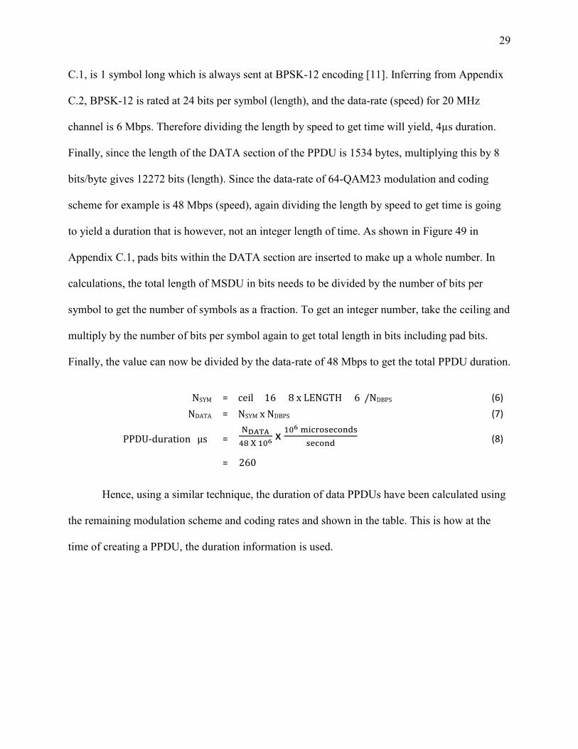
This is initiated by a handshake frame called RTS or request-to-send frame. The sending

station queues this type of frame until a form of acknowledgement is received. If a station that

19

this frame is meant for is available to receive data and the RTS frame is received by the

destination successfully, then it will transmit a response frame called CTS or clear-to-send to

respond to the source that the destination is ready to receive DATA. If the CTS successfully

makes it back to the source station, it will interpret the receipt of CTS as its signal to send its

DATA-α frame; where α is the sequence number to keep track of the DATA frame in question

(same for RTS/CTS). This completes the handshaking process. For ease of explanation, a suffix

number is used in conjunction to the type of frame, e.g. RTS-0, CTS-0 to express the frame type

and number. If and when this frame arrives at the station with matching destination address field,

the destination will decode the data and send it to the “upper layers” of the network stack, a.k.a.

L3, Network Layer (overhead ignored). In addition to that, the destination will respond back with

another acknowledgement or ACK-0 frame signaling that DATA-0 was decoded successfully

and it may receive the next frame data frame in the sequence, i.e. DATA-1. Finally, if the source

successfully decodes ACK-0, then it will count that sequence number towards “transmitted”.

Failure in any part of the exchange sequence causes the source to make another attempt until it

successfully decodes its ACK or run out of re-attempts [11]. On the access-point side, keeping

track of this sequence number is unique to each destination since the source would have most

likely transmitted different number of packets to each station due to randomness in the scheduler.

Figure 7 summarizes this entire sub-section. The timing information will be expanded later.

20

3.5. Data Structures

3.5.1. Queue/Transmit (TX) Buffer Data Structure

Stations need to maintain a buffer to store packets chronologically as per packet queue-

time. Since the scheduler is configurable at startup, the rate of generation of packets can be set

to be more than the rate at which they are deleted from the queue upon successful transmissions.

This mismatch is resolved by a transmit-buffer or queue. Depending on the network parameters,

a station can only transmit a limited number of packets before its queue starts growing towards

infinity and has to catch up to the packet scheduler. This catch process takes place only after the

last packet from the scheduler gets queued and the stations get as much time to empty the queue

as they require, in heavy loading. In under-loaded or some loaded conditions, stations could clear

the queue soon after packets show up there. In order to illustrate the implementation of the

transmit-buffer/queue, refer to the diagram Figure 8. Since the queue must maintain the order of

event-arrivals, a std::map from the C++ library is used to dynamically (automatically in runtime)

sort the frames in increasing order of arrival-time or queued-time (synthetic first-in first-out,

FIFO algorithm implementation). The map data structure has a key-value pair format where key

Figure 7: CSMA/CA Frame Exchange found in IEEE802.11-2012 from Figure 9-4

21

is the input used to lookup the map for its corresponding value (output). The key in this case is

the event-time/original release-time, the value is the frame that is associated in the MAC layer.

As described in the previous sub-section, unlike the RTS frame type, stations do not queue

DATA, CTS or ACK.

Note that as per the design of the simulator, apart from RTS none of the frames types

need to contend or check the medium before transmitting. CTS/DATA/ACK are transmitted

regardless of the state of the channel because they are response frames.

Figure 8 shows queued up pointers (PTR) to RTS frames at the AP. The STA# represents

destination (client) numbers. Each row can be interpreted as packets being queued in the system

or a new frame exchange. A station will create a new entry in the map each time the current

simulation time is equal to the next arrival time of a packet from the scheduler, meaning no

packet is queued in advance. While the station is waiting to make its first attempt or waiting for

a response back, the first entry at 9µs will remain in the queue. The entry will only be deleted

once its ACK is received or reattempts have exceeded, thus causing that packet to get dropped.

Once the first entry in the map is deleted, the second mapping is considered the first entry and

will be referred by the TX state-machine during next transmission. After the TX state-machine

decides that there are no more packets to send, the station becomes idle. Finally, when the

Figure 8: Queue Structure

22

controller sees that all stations are idle, then it will terminate the program and print network

statistics for the requested simulation duration.

A note on pointers – in this context it is a variable used to point to a special block of

memory containing the actual value. Each time this pointer is stored somewhere in the program,

it is stored by reference, not value [13]. Because properties of a frame is bound to change at

various subroutines of the program, the program needs to use the reference to a unique location

where the frame resides, instead of creating new frames which will cause software bugs.

3.5.2. Output Buffer Data Structure

The output buffer keeps track of a pointer to frame that will be transmitted, or is in

transit, or waiting to receive the ACK back from the destination after making an attempt. It is a

1-capacity frame pointer holder that consists of the same frame as the one in the first mapping of

the queue structure. When acknowledgement is received, the pointer is made to point to NULL

which is a C++ way of defining nothing. If there are one or more queued events, this process

continues until there are no more queued events left in the TX-buffer for the time being. The TX-

buffer can get filled with one or more packets at a later time as long as at least one packet is still

left to queue from the scheduler. When the station interacts with the wireless medium, it uses the

output buffer as its data structure to query whether it needs to send a frame or stay in receive

mode. Instead of working directly with the queue, this additional buffer is used to increase query

performance of the program due to its simplicity.

23

3.5.3. Wireless Medium Data Structure

The wireless channel data structure is simpler in implementation than the queue. The

wireless medium is a table of pointers to PSDUs that keeps track of when a frame is in transit to

another station from a source. In C++ terms it is a vector of vector from the std::vector library

and accepts objects of type: pointer to “frame”. A vector in C++ is a list or contiguous block of

memory that is specifically reserved for a sequence of data of the same type. The length of this

table (horizontal) depends on the duration of simulation. Since the program runs at a resolution

of microseconds, based on the input parameter specifying its end time the controller uses a loop

to iterate over the vector until the last microsecond. There are multiple instances of these vectors

in a vector and its count is decided by the number of stations. Figure 9 shows the visual

representation of the wireless data structure. As seen from the diagram, there are 4 stations

numbered from 0 to 3, and the horizontal direction shows the time-domain (1 box = 1µs) or

progress of the state-machine as stations transmit frames in the wireless medium (green). Initially

the table is initialized with values of NULL, meaning no release of packets at that instant (µs).

When the controller checks the output-buffer of each station and if buffer(s) are holding

a pointer to the frame, then it assigns the corresponding vector of that station with the said

pointer (PSDU) into as many bins as appropriate. Finally, it switches the station’s state of the

Figure 9: Visual representation of wireless channel data structure

24

PHY from RX to TX (receive to transmit). However, if the medium is busy, then the RTS

pointers in the time vector are assigned back a NULL value to negate the frame from the

channel, thus leaving that station to make a re-attempt.

When debugging the program, there is no graphical representation of the wireless

channel data structure but a separate GUI data structure is used to show the events of the

simulation. Instead of pointer to frames, the GUI-table is a vector of vector that accepts a type

of object called gcell. Each cell has a transmit mode and a receive mode. In a given time,

either/both modes can be activated. Regardless of whether a station is transmitting, it could

also receive from two or more stations simultaneously. Since the actual GUI is difficult to

visualize at first, refer to Figure 10. The diagram presents a simplified model of the graphical

layout of the timeline for each station.

Continuing from the previous figure - green means transmit, as well as red or blue

means receive depending on which station is transmitting, and grey means interference

between the two. In the real GUI output, receive is always red, but for the sake of explanation

the output is changed. When a station like STA0 transmits a PSDU, it takes time to propagate

Figure 10: Visual representation of wireless channel GUI data structure

25

to the other stations which is shown in the timelines of STA1, STA2 and STA3 by the color

red. This propagation delay was described in Section 2 with respect to distance between

stations. The amount of delay is directly proportional to the distance between any two stations.

Even though the traffic generator that schedules the events for the frame exchange is pseudo-

random, there is a chance that frames from two or more stations will be released at the same

time and interfere at the destination node. The destination however, like STA1, will check for

the signals coming from all station(s) and decide which one to consider as the useful signal,

and the rest as interference signal(s). At the end of the transmission from STA0 and STA3 for

example, despite the interference if STA1 derives the SNR to be at or higher than a certain

threshold, then it considers decoding that frame. Upon successful decode, it responds back with

a response frame after some time. While the signal source(s) decodes, accepts this response

and continues the frame exchange, all other senders that made an attempt to get a response will

contend for the medium using certain timers. The CTS/ACK response can only be meant for

one station.

3.5.4. Traffic Generator Structure / Event Scheduler

The traffic generator schedules the events (timestamps) that are pre-populated for each

link and each station. A real pseudo-random number uniform distribution generator like the

std::uniform_real_distribution from the C++ std library is used to generate a fraction between

0-1 with a uniform distribution pattern. It is used when traversing the number of slots from 0 -

(N-1) slots and with each iteration, comparing a random floating-point number with the

calculated average probability for traffic arrivals. This comparison is repeated until an array of

random arrival times have been created for the link.

26

Downlinks are traffic from AP to clients, and uplinks are vice-versa. When delivering

payloads to their destinations at random, because of several downlinks, one array of random

arrival times is generated for each link at the AP. These arrays are merged together in

chronological order to get a single scheduler for the station, as well as to create a uniform

random distribution of destinations, i.e. client station numbers, while removing duplicates. This

enables the AP to send requests to various stations in the network at random. Random integers

representing N station IDs have to be populated from 0 - (N-1) using

std::uniform_int_distribution. At the client side, just one array is created for the uplink that

will represent the client’s packet scheduler.

Neither distribution functions themselves consist of the random-number selection

algorithm. In an effort to create pseudo-random numbers that are as random as possible, in

addition to uniform real-distribution and int-distribution objects, std::mt19937_64 algorithm

and std::random_engine from the std library are used to populate the traffic in the vector as

integer multiples of 802.11a slot-time (9µs). The std::mt19937_64 object, or Mersenne Twister

(MT) algorithm is used to pick a pseudo-random number from within a range of numbers based

on a period that is known as Mersenne prime. The algorithm has a state size of 19937, hence a

long period of 219937 – 1 and 623-dimensional equidistribution with up to 64-bit accuracy [14].

It is fast, avoids complex arithmetic, uses caches, pipelines and makes efficient use of memory

[15]. The random_engine object on the other hand serves to be the seed for the MT random

number generator that will randomize the initial state of the generator and avoid same sequence

of numbers between simulations. A new seed is created by the object for each station and

recorded for debugging purposes when the same deterministic simulation is needed

27

afterwards. For the purpose of collecting data, a new seed is always created to maintain

statistical randomness in the system [16].

The said process described in this section so far applies to both uplink and downlink.

Figure 11 shows an example of a network that is used in Infrastructure Mode, where STA5 is the

AP and all other stations make up the clients in the downlink thus creating a star topology.

Downlink is in dark blue, uplink is in light blue.

The probability that a payload will arrive in the queue of the MAC layer from “upper

layers” depends on the random number generated using real-distribution, as well as the fraction

of time the traffic-generator calculates link to be busy. The following code aids in scheduling:

std::random_device rd; std::mt19937_64 generator(rd()); std::uniform_real_distribution<double> distribution(0.0, 1.0);

for (uint slot = 0; slot < slot_count; ++slot) { double prob = distribution(generator); if (prob <= busyf) payload_events.push_back(slot * dot11a_slot_time); }

Referring to the if-condition from the snippet above, the payload_events vector only

queues the timestamp of the times a payload arrives if the random number generated from the

Mersenne Twister algorithm is less than or equal to the busy-fraction or busy value of the

Figure 11: Example of a wireless network in Infrastructure Mode

28

medium (busyf). This value ranging between 0-1 is computed based on requested parameters

from the user during initialization, and the equations involved in the calculation are as follows:

offered_load = requested_traffic_load_mbps bytes_per_PPDU = payload_size

packets_per_second = 106 ∗ offered_load

8 ∗ bytes_per_PSDU (3)

slots_per_second = 106

dot11a_slot_time (4)

packets_per_slot = packets_per_second / slots_per_second (5)

In Eq.5 the packets_per_slot variable is the mean probability with which a payload may

arrive in a timeslot of the station queue in a given link, also called busyf. The value of busyf will

be different if the requested traffic load is unique for each link. With payload load size of 1500

bytes, the bytes_per_PPDU variable does not take into account the header/tail size. The

following table however, provides the total data PPDU size used to calculate the length of the

NAV timers, which will be described in a later section.

Table II: Derivation of Total PPDU size by the Traffic Generator

To calculate the total length of the PPDU in terms of time, the length is calculated using

the number of bits or symbols and the appropriate date-rate used to transmit the Preamble,

SIGNAL and DATA sections. The Preamble is 16µs and the SIGNAL as shown in Appendix

Modulation Scheme

Preamble (µs)

SIGNAL (µs)

DATA (µs)

PPDU duration (µs)

BPSK12 16 4 2052 2072 BPSK34 16 4 1368 1388 QPSK12 16 4 1028 1048 QPSK34 16 4 684 704

16-QAM12 16 4 516 536 16-QAM34 16 4 344 364 64-QAM23 16 4 260 280 64-QAM34 16 4 228 248

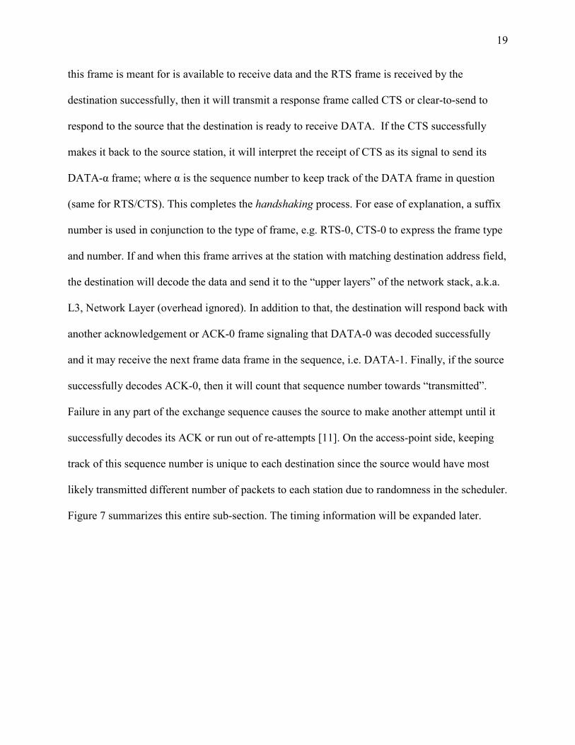
29

C.1, is 1 symbol long which is always sent at BPSK-12 encoding [11]. Inferring from Appendix

C.2, BPSK-12 is rated at 24 bits per symbol (length), and the data-rate (speed) for 20 MHz

channel is 6 Mbps. Therefore dividing the length by speed to get time will yield, 4µs duration.

Finally, since the length of the DATA section of the PPDU is 1534 bytes, multiplying this by 8

bits/byte gives 12272 bits (length). Since the data-rate of 64-QAM23 modulation and coding

scheme for example is 48 Mbps (speed), again dividing the length by speed to get time is going

to yield a duration that is however, not an integer length of time. As shown in Figure 49 in

Appendix C.1, pads bits within the DATA section are inserted to make up a whole number. In

calculations, the total length of MSDU in bits needs to be divided by the number of bits per

symbol to get the number of symbols as a fraction. To get an integer number, take the ceiling and

multiply by the number of bits per symbol again to get total length in bits including pad bits.

Finally, the value can now be divided by the data-rate of 48 Mbps to get the total PPDU duration.

NSYM = ceil ((16 + 8 x LENGTH + 6)/NDBPS) (6) NDATA = NSYM x NDBPS (7)

PPDU-duration (µs) = NDATA48 X 106

x 106 microseconds

second (8)

= 260

Hence, using a similar technique, the duration of data PPDUs have been calculated using

the remaining modulation scheme and coding rates and shown in the table. This is how at the

time of creating a PPDU, the duration information is used.

30

3.6. Lookup Tables

A few lookup tables are implemented in the simulator in the form of unordered-maps as

part of the C++ std library, aka std::unordered_map. The tables are the following:

i. MCS Index vs. name of modulation scheme + coding-rate ii. Modulation scheme + coding-rate vs. number of data bits/OFDM symbol iii. Modulation scheme + coding-rate vs. PER Thresholds iv. Modulation scheme + coding-rate vs. data rate v. Modulation scheme + coding-rate vs. PER rate

3.6.1. MCS Index vs. Modulation Scheme/Coding-rate

The MCS index is representative of the modulation scheme and coding rate – latter two

combined into one string, which is negotiated between the AP and a client before communication

starts. To bind the relationship between the MCS number and the string, a map is used in the

simulator as follows:

Table III: Mapping of MCS Index to Modulation Parameters

In software jargon, a map always has a key that is bound to its corresponding value. The

mapping above serves a simple task of providing the corresponding string value (right) for the

MCS key (left) which will be used to perform the lookup. After deriving the said string value,

the string in turn will be used as the key to look up data in the rest of the tables.

MCS INDEX (UINT)

MODULATION+CODING-RATE (STRING)

0 "BPSK12" 1 "BPSK34" 2 "QPSK12" 3 "QPSK34" 4 "16QAM12" 5 "16QAM34" 6 "64QAM23" 7 "64QAM34"

31

3.6.2. Modulation Scheme/Coding-rate vs. Data bits per OFDM symbol

The following lookup table helps the simulator with calculating the length of the PPDU

based on the number of data bits grouped in a symbol in an encoded bits stream for a given

digital modulation. It is taken from Table 18-4 of the IEEE802.11 document [11].

Table IV: Modulation Scheme vs. ODFM data-bits per symbol

3.6.3. Modulation Scheme/Coding-rate vs. PER Thresholds

The following lookup table shows the min SNR required threshold to get a packet-error-

rate of 1% or better. The thresholds are used in 3 instances during the simulations that will be

described in future sections. They are as follows:

MCS selection in MAC Layer [Section 3.6.5] PLCP preamble locking of PPDU [Section 3.8.2] MSDU decode and countdown timers [Section 3.8.2]

Table V: Modulation Scheme vs. PER min thresholds

MODULATION+CODING-RATE (STRING)

DATA-BITS/OFDM SYMBOL (UINT)

"BPSK12" 24 "BPSK34" 36 "QPSK12" 48 "QPSK34" 72

"16QAM12" 96 "16QAM34" 144 "64QAM23" 192 "64QAM34" 216

MODULATION+CODING-RATE (STRING)

1% PER min thresholds (dB) (FLOAT)

"BPSK12" 4.5 "BPSK34" 6.5 "QPSK12" 7.5 "QPSK34" 9.5

"16QAM12" 13 "16QAM34" 15 "64QAM23" 20 "64QAM34" 21

32

3.6.4. Modulation Scheme/Coding-rate vs. Data Rate

Appendix C.2 shows Table 18-4 of the IEEE802.11 document which has three OFDM

PHY data rates columns. This table has been adapted into a lookup table (unordered_map) by

making modulation-scheme/coding-rate as the key and making another unordered_map the

value. The reason for creating a nested map is that the data rate in megabits per second is

dependent on the bandwidth as well as the MCS. Depending on the MCS index, or in other

words, modulation scheme for the payload as well as the bandwidth configured at startup, an

appropriate row and column will be chosen from the table. Note - bandwidth will usually be 20

MHz.

Table VI: Modulation Scheme vs. PHY Data Rate

3.6.5. Modulation Scheme/Coding-rate vs. PER Rate

The modulation-scheme vs. PER or packet-error rate table is one of the most important

tables. It is similar in data structure since it is still a double-mapping with two other inputs. The

outer mapping being the modulation scheme to the nested unordered_map. And the nested map

is the mapping between SINR floating point type values to the packet-error-rate (PER) double-

precision floating point values. To clarify, by packet it refers to the PPDU. Similar to the

previous table described above, depending on the modulation scheme used for the link, the

probability of packet error can be looked up using the signal-to-interference-noise ratio that is

MODULATION+CODING-RATE (STRING)

Data Rate (Mbps) (FLOAT)

5 MHz 10 MHz 20 MHz "BPSK12" 1.5 3 6 "BPSK34" 2.25 4.5 9 "QPSK12" 3 6 12 "QPSK34" 4.5 9 18

"16QAM12" 6 12 24 "16QAM34" 9 18 36 "64QAM23" 12 24 48 "64QAM34" 13.5 27 54

33

calculated when decoding a fully received PPDU. The process of calculating the SINR will be

explained in more detail in Section 3.7. The ratio conveys the same idea as SNR but includes the

interference energy that may be received from other stations, while simultaneously receiving the

desired signal (Section 3.5.3).

To explain PER further, when a packet is in transition within the wireless medium, it is

prone to errors depending on the quality of signal, transmit power, pathloss and interference

while on its way to the receiver. In order to mathematically model and predict the likelihood of

bits arriving in error, modelling equations are used to derive a probability pattern that will

convey the chances of error in terms of numbers between 0-1 as shown in Figure 12.

Note that higher the PER error, the higher the chance of packet failing to get delivered. In

the figure above, the higher modulation schemes have higher probability of packet-error for the

same SINR value, which is intuitive in a sense that for higher modulation schemes and thus

higher throughput, the channel needs to be more favorable for the transmitter and receiver.

Figure 12: PER vs. SINR Uncoded Curves

34

Conversely, to maintain an error-rate of within 1% or 0.01, a chosen threshold value along the

dotted line will require the SINR to be higher than the cutoff value as shown in the x-axis (X =

10.6, 13.87, 20.76, 26.9 dB). For example SINR= 13.87dB allows the system to select BPSK or

QPSK as the modulation scheme. However, to be within the same 1% error, it is not good

enough for QAM-16 and QAM-64, since the error probability is almost 1.0, or 100% failure rate.

The modulation-scheme vs. PER rate table not just represents the type of digital

modulation that will be used by the encoder, but it also represents the coding rate for that

modulation scheme that is used for error-detection and recovery. Coding or encoding is the

process of conditioning of the digital signal/bit stream such that upon decoding the bit stream on

the receiver side there is a chance of error recovery. The formula used to represent coding rate is

as shown in Eq.9:

coding rate = k bits in

n bits out (9)

Where k-bits is the number of information bits of the payload, n-bits is the total number

of bits in the code word. The n-k bits are redundant bits based on the type of coding algorithm

used on both sides of the link. When the same mathematical model is applied on the encoded

bits, the PER curves become steeper and “shift” left, implying that for a range of SINR values

that were previously indicative of high error-rate now indicates smaller error-rate from the trend

getting closer to zero. This makes a difference when trying to set the highest MCS index for a

link (“MCS Selection”), as each modulation scheme has a minimum SINR requirement for the

maximum error threshold (10−2). After encoding the bits using an algorithm, it gets easier to

meet that SINR requirement because of the shift.

35

Usually the type of algorithm used in wireless applications is convolutional encoding and

the redundant bits are known as parity or checksum. From the IEEE document on page 1597,

“The DATA field, composed of SERVICE, PSDU, tail, and pad parts, shall be coded with a

convolutional encoder of coding rate R = 1/2, 2/3, or 3/4, corresponding to the desired data rate.

The convolutional encoder shall use the industry-standard generator polynomials, g0 = 1338 and

g1 = 1718, of rate R = 1/2” [11]. It performs data interleaving and subcarrier modulation

mapping which depending on the modulation scheme, the bit sequence is mapped to the

appropriate data subcarriers, which in turn goes through subcarrier frequency allocation. In order

to decode this bit sequence on the receiver side, the Viterbi algorithm is typically used [11]. If a

bit arrives at the receiver with the wrong value, because of said coding, there is a chance that the

correct value will be recovered. Figure 13 shows the advantage of coding. Appendix C.3

provides the code in a Matlab script for building theoretical PER vs. SINR curves for 1537 bytes

of data packet which includes the SERVICE and TAIL bits as well as the size of 1500-byte

payload MPDU.

The script takes thresholds from Table V such that the curves cross the 1% error rate at

the appropriate reference points, and curve-fitting and extrapolation is performed to ensure that

there is no discontinuity or breaks. A non-conditioned curve can cause potential problems when

the number returned is a noticeably different PER depending on whether the SINR was, for

instance, 0.01 dB above or below the point of artifact in the curve. The PER curves were heavily

sampled and each consists of thousands of points. Lastly, after carrying out an additional set of

corrections, they were imported into modulation-scheme vs. PER lookup table directly in the

source code. Data from the table is used on two occasions: for MCS selection during startup

36

using SNR, and each time a complete packet arrives at the receiver, it needs to decide whether

that packet has successfully arrived without an error using SINR.

3.7. Using Channel State Information

In order to assess the conditions of the medium before transmitting to another node in

question, internally any given station would compute the channel state information or channel

matrix. It is computed by replacing the pathloss component in the Friis Transmission equation

with SPLAT data, and using constants defined in the program such as client and AP transmit

power and antenna isotropic gains of the said stations. Isotropic antenna is an ideal and

theoretical antenna that radiates power uniformly in all directions [17]. Practically however, this

antenna radiates power uniformly in the azimuthal plane (considered 0 dBi directivity

horizontally) and it is shaped like a donut:

Figure 13: PER vs. SINR after Convolutional Encoding

37

The constants that are used in the upcoming equations for the project will be referring to

the given shape. In this project, a similar type of visualization as Figure 14 is expected, however

it is slightly flatter in azimuth because of added gain to the omnidirectional-antenna. Since the

azimuthal gain is uniform, the program does not need to store the angle vs. gain information in

the form of a lookup table; it is rather a reasonable constant value set for the AP (12 dB), and

another for all client stations (2 dB). In order to compute the channel matrix from the perspective

of a station, “h-values” to all destinations is computed regardless of whether a station is the

designated AP. In the case of the AP, the channel matrix will comprise of N-1 entries, whereas

clients will have one value to their destination which is for the AP. A WirelessChannel object

stores the h-values computed from three mappings described at the end of Section 2.0.

The station-name mappings are used as aliases for indices at which the desired data is

present in the other two map tables. For example if the 802.11 network simulator is specified

with a subset of stations, namely, Small Butte, Rocker and Fleecer with Big Butte as the AP,

then the tables generated will look like the following in the C++ data structure:

Figure 14: Antenna Pattern In Horizontal And Vertical Plane [17]

38

In Figure 15, the numbers in the bracket show mapping used internally by the simulator

to acquire the values on the right. Top-right shows distances to rest of the stations from Small-

Butte, same from Rocker and so on, in units of kilometers. The second mapping on the right

shows pathlosses to the stations in the same order, in units of dB. The data can be visually re-

organized into Figure 16. For a given node, distance or pathloss to itself is not applicable as

shown in “x”.

Figure 15: Index mappings from the tables given in Appendix B.2/.3

Small_Butte Rocker Fleecer big_m

Small_Butte x 5.33 25.67 6.21

Rocker 5.33 x 24.75 3.78

Fleecer 25.67 24.75 x 28.53

big_m 6.21 3.78 28.53 x

Small_Butte Rocker Fleecer big_m

Small_Butte x 101.28 115.07 102.6

Rocker 101.28 x 114.75 98.14

Fleecer 115.07 114.75 x 116

big_m 102.6 98.14 116 x

Figure 16: Data re-organized to better visualize mappings for distance (left) and pathloss (right)

39

As described in the previous section, the SINR value is used to lookup the failure rate of

the packet. This computation is performed to determine quality of the received signal from the

source while potentially receiving interference from other stations. In order to calculate the

SINR, the received signal power at the receiver of the transmission must be known. One of the

terms used to compute the power is the h-value, which can be calculated using pathloss matrix in

Figure 16:

hvalue |dB = GTX |dB + GRX |dB – PL[receiver-ID][source-ID] |dB (10)

Where GTX is the gain of the transmitter or the source station of the PPDU, GRX is the gain

of the receiver station which is the station in question, and finally PL is the 2D pathloss mapping

used to store the values by source and destination station IDs. Typically the GTX and GRX terms

are 2dB until the value is with respect to the AP, in which case one of them will be 12 dB. To get

the desired or interference signal power, the following is the received-power equation:

PRX |dBm = hvalue |dB + PTX[source-ID] |dBm (11)

Where PTX is the power of the transmitter that the signal came from (30 dBm for clients,

35 dBm for AP), and PRX is the power of the signal at the receiver. Eq.11 for received power is

used in both scenarios – computing the desired signal or computing the interference signal from

the station that happens to transmit in the same time as the source. Both Eq.10 and Eq.11

combined aids in obtaining the SINR value. The SINR when decoding a PPDU, is calculated by

subtracting the signal (in dBm) by the noise-interference term (in dBm) where the latter is

obtained by adding the two in RMS.

40

SINR |dB = PRX |dBm – (noise|Watts + interference|Watts) |dBm (12)

= PRX |dBm – W2dBm[dBm2W(system-noise) + W2dBm(interference)]

Where, system-noise is the addition of system noise figure (5 dB) and thermal noise

(Johnson–Nyquist) from the electronics at -101 dBm @ 20 MHz channel bandwidth [8]. The

unit, dBm is the absolute meansurement of power where 0 dBm is 1 mW. System-noise and

interference are converted to linear (Watts), added together and converted back to logarithmic

(dBm). Initializing links between stations during MCS selection does not entail the inteference

component and thus, stations only decide link speed a.k.a data rate based on the fulfillment of the

SNR requirment of the maximum modulation and encoded scheme used in DATA PPDU.

3.8. Computing Energy Thresholds

One of the challenges in a 802.11 network is the hidden node problem. This is caused when

2 or more stations do not receive signal energy from other node(s), decide to transmit their own

packet, and as a result causing collisions at the receiver. Collisions can be tolerated depending on

the severity of the SINR degradation while receiving a packet. To simulate this behaviour, an

energy threshold system is added in the source code, and acquire the hidden-node properties within

a network as follows:

SINR for detection threshold

SINR for PLCP preamble locking and MSDU decode threshold

3.8.1. SINR for Detection Threshold

The SINR for detection threshold is the quality of signal used to decide whether the

medium is busy, and switch to an appropriate state within the receiver state machine (the station

41

cannot react when medium becomes busy while already in the transmit state machine). A value

of 4.5 dB SNR from the convolutional PER curves at BPSK-1/2 in Table V is used in

distinguishing between a valid 802.11 OFDM PLCP preamble and spurious transmissions such

as microwave interference. As a side note, since there are no sources of interference other than

802.11 transmitters, the CCA busy threshold of -62 dBm@20 MHz is omitted from the simulator

[11].

Using BPSK-1/2 SNR threshold one can obtain the maximum pathloss cutoff from a

station to the AP that allows it to associate to the network. While ignoring interference, as would

be the case with MCS selection, and rearranging the terms in Eq.10-12, the maximum pathloss is

calculated to be 135.5 dB as follows:

SNR |dB = PRX |dBm – Noise |dBm (13)

4.5 dB = GTX |dB + GRX |dB – PL |dB + PTX |dBm – (Thermal + NF) |dB

PL (max pathloss to AP) = 4.5 + 12 + 2 + 30 – [-(101 + 5)] |dB

= 135.5 dB

The reason for using PTX of the client instead of the AP even though latter is higher is

because the channel and radio parameters must be good to enough to carry out communication in

both directions, therefore weaker of the two links is consdered. Any pathloss higher than 135.5

dB cannot associate to the AP, and hence not part of the network.

In order to consider an incoming signal as a valid detectable signal reaching the receiver,

the system-noise plus minimum BPSK-1/2 PER threshold gives -91.5 dBm as the minimum

detection threshold. The hidden node problem takes place when a client station is communicating

with the AP, but another client perhaps geographically on the other side of the AP, cannot detect

42

that signal at or over -91.5 dBm and therefore starts transmitting simultaneously. Stations cannot

transmit if already receiving sufficient signal energy because of half-duplex links.

Since a station can only preamble lock on to one incoming packet, the packet must meet a

certain SINR threshold for it to be decodable given channel conditions and interference(s) from

hidden node(s). If the interference is high enough, then the signal that an AP has premable lock

on, may be damaged to an extent that the SINR condition to decode that frame is no longer met.

3.8.2. SINR for PLCP Preamble Locking and MSDU Decode Threshold

Assuming that the signal strength at the antenna is above detection threshold, the SINR of

the signal is computed at the receiver using Eq.12 for each microsecond of the transmission. If it

is the first symbol of the PREAMBLE field of a PPDU and the SINR is equal or better than the

SNR required to decode the rest of the frame, then a preamble lock takes place. Locking implies

that no matter the source of transmission(s) that arrive at this station, newer preambles of an

interferring signal cannot make the station accept the frame as a desirable signal. The receiver

will continue to register the frame from the original source of the PPDU when the medium was

idle as desirable signal, for the duration of the PPDU. If however, 2 or more transmissions arrive

at the same time, the first symbol of the preamble with the highest signal strengh is considered

desirable, and the rest as interference. In both cases, the mean SINR is computed at the receipt of

the last symbol of the desirable PPDU and cyclic-redundancy-check, CRC is performed. The last

step is performed as part of decoding the MSDU if the CRC is a success, but if it is fails, then it

will re-initiate its DIFS and contend for the medium immediately if the medium becomes idle.

DIFS is DCF interframe spacing and it is used to evaluate if the medium is idle for a fixed

amount of time before taking control of it and transmitting a packet as part of CSMA/CA.

43

When preamble lock already takes place and the station starts receiving weak interfering

signals from two or more sources, then the locked PPDU may still be decodable upon receipt of

the last symbol. In general, it is more likely that the nearby stations with high signal power will

be unsusceptible to interference from distant stations, than distant stations with lower received

power being unsusceptible to orders of magnitude high power interference. If the overlap of

high power interference is not long enough, then it is still possible to decode the frame, i.e. as

long as average minimum SINR requirement is met for the duration of the PPDU. Events like

these can take place in a hidden node situation as well as in the long-distance model, and

throughput can negatively be affected as a consequence.

3.9. Station Timer Method

As part of the DFC, stations respect 802.11 waiting rules to minimize collisions while

trying to take control of the medium. Note that IFS is Interframe Frame Spacing, a generic

timing reference and implies spacing left between frames by the station in an effort to maintain

synchronization between nodes. The timer attributes are provided by PHY in Figure 17, and

description for applicable timers are provided as well.

Figure 17: Various relationships between DFC timers as given in Figure 9-14 of IEEE spec.

44

3.9.1. Slot Time

“Slot boundaries define when the transmitter shall be turned on by the MAC to meet the

different IFS timings on the medium, after subsequent detection of the CCA result of the

previous slot time [11].” The slot boundaries provide a relative sense of time for a station to

transmit or trigger certain actions based on the state of the medium. From 802.11a specification

and 20 MHz channel bandwidth, a slot time is 9µs.

3.9.2. SIFS

“The SIFS is the time from the end of the last symbol of the previous frame to the

beginning of the first symbol of the preamble of the subsequent frame as seen in the medium”

[11]. Hence, it is used upon receiving an RTS, a CTS and DATA frame. Since an

acknowledgement to a payload marks the end of a frame exchange, SIFS is not performed after

ACK. The formula to calculate SIFS is given in Eq.15, where the value of other timing constants

are given in Appendix D. From specifications and 20 MHz channel bandwidth, a SIFS is 16µs.

aSIFSTime |µs = aRxRFDelay + aRxPLCPDelay + aMACProcessingDelay + aRxTxTurnaroundTime (15)

3.9.3. DIFS

The DIFS time is the interval timer that is used to assess the state of the medium. It

always starts when the medium is free of transmissions and when there is at least one packet in

the queue. If the medium becomes busy during DIFS, then it restarts the next time medium is

idle and no other countdown timers are running. Once DIFS starts, it initiates its own frame

exchange after the channel evaluation period of 34µs, which is based on the equation:

aSlotTime |µs = aCCATime + aRxTxTurnaroundTime + aAirPropagationTime + aMACProcessingDelay (14)

45

DIFS |µs = aSIFSTime + 2 x aSlotTime (16)

The following are the situations that warrant entering DIFS state in the station’s state-machine:

i. In the beginning of a new frame exchange sequence before sending an RTS a station needs to

evaluate the state of the medium to ensure that the medium is idle and available for a DIFS

amount of time. The DIFS interval lasts 34µs, for 20MHz channel bandwidth.

ii. Stations must start DIFS after acknowledgement frame is received. As a station that is the

source of the payload and receiving an ACK, or as a third station that is witnessing an

exchange and receiving an ACK – both cases warrant a DIFS at the end of the last symbol of

the ACK frame. A source of the ACK also has to re-initiate DIFS after the last symbol of the

ACK is sent. This ensures that stations do not transmit out of turn. The DIFS timer is re-

initiated as soon as the medium become idle, and not necessarily right after receiving the last

symbol of the frame that had a preamble lock. This is due to overlapping transmissions.

iii. “If the medium is determined to be busy at any time during a backoff slot, then the backoff

procedure is suspended; that is, the backoff timer shall not decrement for that slot. The

medium shall be determined to be idle for the duration of a DIFS period” [11]. If the medium

becomes busy at any moment of the DIFS timer, then busy_difs flag will be set, and backoff

procedure will begin after the DIFS is over, or else a (re)transmit of the frame is warranted

immediately. The program maintains this flag if another station’s transmission is received in

an ongoing DIFS period.

3.9.4. CTSTimeout Interval

This timer is set after the last symbol of the PPDU of type RTS is transmitted from a

station and expires based on a formula given in Eq.17

46

CTS-timer |µs = aSIFSTime + aSlotTime + aPHY-RX-START-Delay (17)

The simulator is designed such that if the first symbol of any transmission does not reach

the sender of the RTS within the timeout period, then the backoff procedure will be initiated. If

the RXSTART.indication primitive is received, but upon RXEND.indication it does not consist of

the CTS frame that the RTS source is looking for, then the backoff is also warranted. If neither of

these cases occur, then the timer is reset, the release of RTS is considered a success and the

DATA frame in the queue is scheduled for release after a SIFS period.

3.9.5. ACKTimeout Interval

This timer is set after the last symbol of the PPDU of type ACK is transmitted from a station and

expires based on a formula given in Eq.18:

ACK-timer |µs = aSIFSTime + aSlotTime + aPHY-RX-START-Delay (18)

The simulator is designed such that if the first symbol of any transmission does not reach

the sender of the DATA within the timeout period, then the backoff procedure will be initiated. If

the RXSTART.indication primitive is received, but upon RXEND.indication it does not consist

of the ACK frame that the DATA source is looking for, then the backoff is also warranted. If

neither of these cases occur, then the timer is reset, the transmission of DATA is considered a

success and the next RTS frame in the queue (if present) is scheduled for release after a DIFS

period.

47

3.9.6. Backoff

A backoff timer is used after a DIFS when medium is determined to be busy and a packet

is in the queue. It is used when stations are contending for the medium and only one of them can

use it at a given time. This is done by using an exponential backoff algorithm where stations

draw random number of slot-times and countdown the timer until all slots are used up. In the

source code, within the Backoff_Manager class, the timer is also implemented in the units of µs

to maintain the microsecond-level simulation granularity. If the medium is detected to be busy at

any time of a given slot while the backoff timer is running, then that slot is marked as busy and

not counted towards expired time. Countdown ceases at that time. When the channel is idle

again, after a DIFS period, the station resumes the backoff timer as if that last slot time never

elapsed. This procedure is repeated for repeated periods of channel activity as perceived from

that station. The next time a station transmits a frame is going to be when the slot count reaches

0. See Figure 18 for the graphical representation of the timer.

The process of drawing a random number from an increasing window size is performed in

an effort to draw different slot numbers and hence, maximize the chances of waiting for unique

slot times between any 2 stations. Unique slot times will ensure that at least one station, i.e. with

Figure 18: Timing procedure with Backoff from IEEE802.11-2012, Figure 9-12

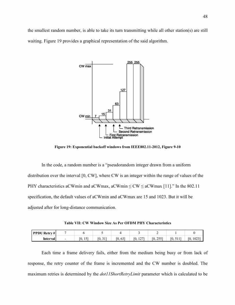
48

the smallest random number, is able to take its turn transmitting while all other station(s) are still

waiting. Figure 19 provides a graphical representation of the said algorithm.

In the code, a random number is a “pseudorandom integer drawn from a uniform

distribution over the interval [0, CW], where CW is an integer within the range of values of the

PHY characteristics aCWmin and aCWmax, aCWmin ≤ CW ≤ aCWmax [11].” In the 802.11

specification, the default values of aCWmin and aCWmax are 15 and 1023. But it will be

adjusted after for long-distance communication.

Each time a frame delivery fails, either from the medium being busy or from lack of

response, the retry counter of the frame is incremented and the CW number is doubled. The

maximum retries is determined by the dot11ShortRetryLimit parameter which is calculated to be

Figure 19: Exponential backoff windows from IEEE802.11-2012, Figure 9-10

Table VII: CW Window Size As Per OFDM PHY Characteristics

PPDU Retry # 7 6 5 4 3 2 1 0Interval - [0, 15] [0, 31] [0, 63] [0, 127] [0, 255] [0, 511] [0, 1023]

49

7 when aCWmin = 16 and aCWmax = 1024 using difference of power of 2. The first attempt being

“Try 7” is only performed after a DIFS and no backoff slots are drawn. If the medium either

becomes busy after a DIFS and the TX state-machine has to cancel (negate) the scheduled RTS or

if the RTS frame arrived in the queue at the time of serving another sequence number, then it is

considered a delivery failure.

If the CTS/ACK does not get decoded successfully or arrive at the source, the

transmission of RTS/DATA is considered a delivery failure. Following that event, the node

increases the window of distribution where the random slot-count will be drawn from, as given

in Table VII. If the RTS from the time when channel was not readily available is now being

served, then the first attempt will be considered “Retry 6”, but only after a DIFS as well as a

random backoff interval from [0, 15] slots. However, once a CTS or an ACK arrives at the

source, the CW window is reset to aCWmin. Upon failure to receive an ACK for the packet after

Retry 0, the packet with that sequence number is discarded from the queue and the CW window

is again reset to aCWmin.

3.9.7. NAV

Network Allocation Vector or NAV are timers in the MAC layer and they are maintained

by each station to keep track of the potential length of time it will take the frame exchange

between a source and destination to finish. Hidden nodes heavily rely on this feature to keep

their transmission synchronized. During NAV countdown, transmission in the medium is

deferred by the station regardless of whether the station’s clear channel assessment (CCA)

function at the PHY senses that the medium is busy (PHY_CCA.indication). The RTS-NAV

starts when the RTS frame is received by a witnessing station. Node(s) check for the SIGNAL

and MSDU header fields, which upon determining that the frame’s destination ID is not the same

50

its own station-ID, it defers access to the medium. It sets its NAV wait timer according to the

time it takes to complete the frame exchange after checking for length of the DATA PPDU in the

SIGNAL field. If the MPDU gets damaged or there was no preamble lock, then the next time

medium is found to be idle, the node will only DIFS. The CTS-NAV performs the same function

except that it starts after receiving the last symbol of the CTS frame as a witnessing station in a

frame exchange. Figure 20 shows this functionality in the timeline with only 3 stations. DATA-

NAV is ignored because it applies to multi-fragment DATA PPDUs that is not applicable for this

project.

When one or more stations are unable to get a response back from a destination, the

station(s) will continue trying to initiate the exchange by re-sending the same RTS frame with

the same sequence number. This phenomenon will cause the rest of the stations to keep updating

the RTS-NAV timer and renew the expiration time if that expiration time is larger (as in the case

of newer RTS/CTS). However, if there is no CTS response back, then instead of running the

entire length, it uses a timeout period for the RTS-NAV such that if there is no PHY-

RXSTART.indication event within that period, then the RTS times out or expires much sooner

Figure 20: NAV setting on “Other” stations when listening, found in IEEE802.11-2012 from Figure 9-4

51

which otherwise would have continued to run until the end of the calculated frame exchange

time (end of ACK). The timeout period is given as follows (note that the NAV timers do not take

into account propagation delays between stations and therefore it will potentially be a challenge

to predict when to transmit after the MAC timers have expired):

RTS-NAV-timeout |µs

= (2 x aSIFSTime) + CTS-dur + aPHY-RX-START-Delay + (2 x aSlotTime) (19)

Upon RXEND.indication if the frame is decoded to be CTS, it implies that the destination

station has responded and the RTS-NAV timer is updated to make the timeout value irrelevant if

still running. This allows the RTS-NAV timer to simultaneously run for the full length of the

frame exchange with the CTS-NAV until receipt of the last symbol of ACK PPDU.

Among two or more hidden nodes, when one of them sends an RTS, the nodes hidden

from the sender will not defer transmitting while the RTS is in transit and energizing other nodes

of the network. This is because the transmissions are below the detection threshold and hidden to

those nodes in particular. When the AP responds with CTS on the other hand, all nodes get

energized by the PPDU for its duration. In this case, with respect to the source, RTS-NAV and

CTS-NAV starts running at regular nodes, but only CTS-NAV at the other hidden nodes.

Conversely, if the RTS request was sent from the AP, all stations including hidden nodes will

initiate RTS-NAV, but their countdowns will expire after the timeout value, unless the PHY-

RXSTART event of the DATA PPDU is triggered from the AP before it expires. In this case, the

hidden nodes did not run the CTS-NAV because the destination which responded back to the AP

with a CTS was hidden. Situations like this as well as long-propagation delays make it

particularly challenging to keep the RTS-NAV running the full length of the frame exchange.

NAV timers do not take into account the delays into their timing calculations.

52

3.10. Transmit Procedure

The program checks at every microsecond for a potential RTS frame (genRTS) in each

station. Upon function call, the station responds by querying the event scheduler for a frame with

a timestamp equal to current_time (simulation time). If the condition is met, then the genRTS

function creates an RTS frame and adds it in the output queue as described in Section 3.5.1. If

the TX-buffer is empty, then the oldest frame from the output queue is copied over to the buffer

due to the FIFO nature of the queue. This process takes places regardless of all other

events/timers/states that a station is in, to ensure that the packets populate the queue in real-time;

and that the buffer has a reference to a packet when there are one or more packets in the queue. If

there are no packets in the queue, then the buffer stays empty as well. This is until the simulation

time reaches the next timestamp stored in the scheduler. This is very typical in lightly loaded

conditions. In the transmit-state machine, once a station decides an appropriate time to transmit a

frame, the program checks the transmit buffer at each station by calling the subroutine called

lookup_buffer().

Thereafter, given the right conditions the lookup-buffer call either starts the DIFS timer

or returns the pointer to the next frame in the TX-buffer. If the DIFS timer expires and the

medium has been idle, then an RTS frame is issued. If there are Backoff slots left over from a

previous (re)-try to transmit the frame, then the Backoff timer starts after a DIFS, and runs until

the timer has run for the duration of the remaining slots before another attempt is made.

If the response from the lookup function was a valid pointer to frame, then the header

information of the frame is extracted and appended in a new entry within the program’s top-level

propagation vector (controller). The vector, also called Over-The-Air or OTA-list, keeps track of

the source station-ID of the PPDU, its duration, and the exact time the first symbol of the PPDU

53

was released to the medium. There can be multiple entries for the same PPDU within the list, as

a consequence of the retry mechanism. Release time will be different between them.

Finally after having updated the OTA-list, the controller will call the transmit_frame()

function that will take the wireless channel object and pointer to the frame that is passed to it and

assign that pointer to as many bins of the channel object as the duration of the PPDU. And the

function will do so precisely at the times (µs) that the bins of the channel represents to keep track

of transmissions from the originating station. An oversimplified diagram to represent the

wireless channel object is provided in Figure 9, however in reality the length of the PPDU will

depend on the MCS index used for that link. The length of a PPDU in the case of 16-QAM1/2

will be 536µs, for example. Therefore, 536 bins will store the same pointer to the frame that is in

the output buffer of a station. There is no feature to distinguish between PREAMBLE, SIGNAL

and DATA of a PPDU.

3.11. Receive Procedure

To continue describing the CSMA procedure, when deciding the next state of other

stations, the program traverses through the OTA-list and decides whether in that instant, the

PPDU or the transmission is radiating out at other stations in the network. For the select stations

that do not see change in the medium in a given instant, they will not react to a channel event;

the channel is clear from their perspective. However if the signal is radiating at a station, then

from the perspective of the station in question, the wireless medium is busy; and also subject to

the detection threshold requirement. In 802.11 terms, PHY signals the MAC layer,

PHY_CCA.indication(busy) in order for CSMA to respond accordingly. If the channel is clear of

any transmissions, then the default primitive would be PHY_CCA.indication(idle) [11]. The

54

further a node is located from the rest of the network, the later it will react to change of state in

the medium, especially in long-distance.

Note that packets propagate towards other stations within an indoor wireless network

almost simultaneously due to relatively negligible physical separation between nodes of within

~50-100 meters, and due to speed of light, c.

Any station that infers the medium as busy will begin to keep track of the PPDUs that are

being received at the PHY layer. The clear-channel-assessment or CCA feature of the 802.11

senses whether a transmission is currently in progress by the approach explained as follows.

When the controller needs to decide if the channel for a station is busy, it calls the

PHY_CCA.indication() subroutine, which takes important parameters like “current time” and

destination ID of the station. The ID helps to identify the station that the signal is propagating

towards, and uses the current time as reference. Since the controller’s data structure maintains a

table of mappings of propagation delays between stations, the function uses the mappings and

current time to traverse along the last M number of transmissions in the medium, thus it is a

sliding window. M is a fixed parameter that is used to cut down the overhead involved with

traversing large vectors of size N. The value of M depends on the number of potential

simultaneous transmissions that can affect a station; mainly from adding more stations. While

traversing the OTA-list, the function evaluates a couple of conditions to check for transmissions

from station-X to station-Y, assuming P microseconds of propagation delay between the two,

and where ID X can be any source from the last M entries. It should not check for transmissions

from itself (X ≠ Y).

55

In Figure 21, the transmitter sends a PPDU at 7µs, assumes the degree of separation

between the transmitter and receiver of 9µs and duration of frame of 8µs. Based on this, the

receiver will consider the medium as busy at simulation times of 16-23µs inclusive. When the

simulation ticks to 24µs and after, the channel for that station is idle if there are no other,

simultaneous transmissions. The 3 conditions to evaluate if the medium is busy are the

following:

now >= Σ (time of release of PPDU first symbol, propagation delay) (20) now < Σ (time of release of PPDU first symbol, propagation delay, PPDU duration) (21)

uint a = frame.reltime + proptable[X][Y] + frame.dur(C); uint b = frame.reltime + proptable[X][Y];

if (now < a && now >= b)

return true; else

return false; If both conditions are true, then station Y is receiving transmission of potentially

sufficient signal strength to cause a response in the RX state-machine. To make sure that it is, the

last condition for the medium to be considered busy is if transmissions from more or more

station(s) are at or above the detection threshold. Conversely, if all transmissions are below the

detection threshold (hidden node problem), the station in question should not react to the

received signal.

Figure 21: Propagation of the same PPDU in time

56

The program calls the evaluate_channel() subroutine of a station that considers its

medium busy (all 3 conditions fulfilled) which calls the rx_state_machine() function that keeps

track of data-structure involved with the calculation of signal and interference levels. The state

machine subroutine looks for the preamble at the beginning of the PPDU to acquire a preamble

lock. The 2 conditions for a successful preamble lock are:

The SINR after calculation of signal-to-interference-noise ratio meets the minimum

signal quality required for the data rate indicated in the SIGNAL field of that PPDU.

The received frame in question at that time is the first symbol of the preamble or pointer

to a frame at the first microsecond (in simulation terms).

Only after the preamble lock the station may be able to decode the frame at the end of the

transmission and perform a CRC check. At the time of decode, mean SINR is calculated for the

duration of the PPDU and using PER threshold table, the appropriate success-rate probability

number is obtained. A number between 0-1 from the uniform number generator is used to

compare against the success-rate. If the number is equal or less than the rate, then CRC is a pass.

In the last step, if the station determines that the frame is the expected frame during exchange

sequence, then it responds to that event by calling the tx_response() subroutine.

Any type of frame other than RTS is “hard-coded” onto the wireless channel. By this it

means that only the RTS frame can be negated from being transmitted on the channel after a

DIFS, if by the time the DIFS interval expires, the medium is already busy. Frame negation is

highly common in lightly loaded conditions where the station immediately starts a DIFS upon a

packet arriving in the queue, so that it may transmit the RTS after. Stations disregard the state of

the medium after having hard-coded the beginning of the CTS/DATA/ACK frame and let the TX

state-machine take over the rest.

57

3.12. Station Response to Received PPDU

There are two ways in which the program retrieves a pointer to a frame before

transmitting to the medium. The first is by accessing the buffer of a station and de-queueing RTS

frames. And the second is when it checks the medium for transmission that needs to take place

and finds the first pointer to the frame stored in the wireless channel structure. See Section 3.5.1

and Section 3.5.2 regarding RTS transmission criteria.

The tx_response subroutine uses the MSDU to look up header information such as

source, destination, type of frame, and sequence number. Based on the sequence of exchange that

takes place in CSMA (See Section 3.4), the next frame created will be based on the type derived

from the subvalue field in the header, switched source and destination addresses, the same

sequence number and an MCS number. To respond to an RTS frame, the timestamp of the first

CTS pointer is calculated to be as follows:

Σ (time of last symbol that the RTS PPDU arrives, sifs-time, 1)

After creating a dynamic pointer to a CTS frame using the said parameters, the pointer is

directly written to the wireless channel data structure. CTS is transmitted at MCS0, the response

to which is a DATA. The first pointer is dynamically allocated based on the said parameters and

the original source and destination. To respond to a CTS frame, the timestamp of the first DATA

pointer is calculated to be as follows:

Σ (time of last symbol that the CTS PPDU arrives, sifs-time, 1)

After creating a dynamic pointer to a DATA frame using the said parameters, the pointer

is directly written to the wireless channel data structure. DATA is transmitted at the MCS

number selected during MCS selection, the response to which is an ACK. The procedure to

create the ACK is similar to creating the CTS frame, however the release time is calculated to be

as follows:

58

Σ (time of last symbol that the DATA PPDU arrives, sifs-time, 1)

After creating a dynamic pointer to an ACK frame using the said parameters, the pointer

is directly written to the wireless channel data structure. Upon receipt of an ACK, the number of

packets sent across that link is incremented, and at the AP side it is summed at the end of the

simulation to show the total. The corresponding RTS frame is dropped from the queue and buffer

and the next packet (RTS) with the next sequence number is scheduled to release using DIFS/BO

(Backoff) procedure. The Backoff slot window is reset to aCWmin.

59

4. Simulation Model

4.1. Central Controller (Program Class)

This section describes more about the 802.11 network simulator to make connections

between the various concepts covered so far about the system architecture. Like any C++

program, the simulator has a starting address that tells the program where the CPU should start

executing instructions from. This is called the "main" function in the context of C++. In the

project, main performs two primary things: perform the simulation based on the simulation-

parameters and then create a graphic that will show the timeline of the simulation for the length

of the simulation and for as many stations that are involved. The following is the simplified

system diagram of the simulation model:

Figure 22: System diagram of major components

60

A Window class (not shown) is the top-level graphics controller that renders elements on

the timeline (Section 3.5.3) such as the slot boundaries, timestamps, transmit (green) and receive

boxes (red) as well as various timers that get triggered in a station. The drawing library is

imported by including C++ based cross-platform Qt packages [18] for the GUI component of the

project. The GUI-table or timeline is the quickest way to visualize and debug glitches and bugs,

as well as in finding edge-cases which result in loss of synchronization between stations. In the

background, many essential aspects of the simulation results are logged and various log files are

written for data collection and analysis, hence the Logger component in Figure 22. The GUI is

developed to ease the debugging process.

Moreover, the Program class has a central controller that initiates all actions and

subroutines from stations. It creates Stations and that in turns triggers the initialization of various

components such as the MAC Layer (“MacLayer”), PHY Layer (“PhyAdapter”) objects, and so

on. Stations also have their timer objects such as tCTS, tDAT, tACK which are interval timers

for CTS, DATA and ACK. Data timeout interval will be covered in Section 5.0 as it was a long-

distance modification. The “McsManager” module performs MCS selection on each link to and

from the AP. The CSMA functions are performed in the PHY which also consists of preamble

locking and indication (signaling). The propagation and pathloss tables are stored in the

“WirelessChannel” object. “TrafficGenerator” uses the MCS data from the MCS-manager

module and checks for dead links. If either uplink or downlink has too weak of a signal, then the

station is completely removed from the network. Otherwise, the traffic generator or scheduler

spreads the packet arrivals across the simulation duration defined in the parameter file.

Before the simulation begins, the setup procedure assigns values to global variables and

defines the parameters of the simulation. Besides the three mapping files that were mentioned

61

before, the program checks for one additional file called the simulation_params.txt which was

briefly covered in Figure 5 of Section 3.1.

4.2. Program setup

4.2.1. Simulation Parameters

The simulation parameter file defines some of the most important configuration

parameters for the tests, which are as follows:

In Table VIII, some of the parameters that need more clarification is as follows:

traffi-load-mbps is a list of values that are assigned to each link. In a system of 6 links, the first

three comma-delimited values are for uplinks and the rest are for downlinks.

program-dur-ms value is the initial duration set for the program to keep iterating so to allow the

extra time to empty the queues from the station. It is usually larger than the next parameter. In

Table VIII: Simulation Parameter file for the startup of any simulation

Parameter Purposetraffi-load-mb Offered load for the configuration of TrafficGen object

program-dur-ms Duration provided to simulator to process all packets in the nodes, larger than sim-dursim-dur-ms Duration used by TrafficGen to schedule its arrival times for the queue(s)

databytes-b DATA PPDU's payload size in bytesbandwidth Channel bandwidth of the station transmission in Hertzsegments Number of segments that the DATA frame's payload will be segmented into

adaptive-tout Special mode for changing the length of the interval timeout at the APtxpower List of transmit powers for each station in dBm

stationsA subset of station names chosen from the KML Google Earth file that will be involved in the communication. The subset can contain all stations if required

pfactorA number between 0-1 indicating the % of the realistic propagation delay used between stations

channel-window The M value which is used to define the length of sliding window in OTA listseeds Values used to set the initial condition of the random number generator per station

aCWmax The largest backoff slot windowaCWmin The smallest backoff slot window

relimit Number of retries before a node decides to drop the frame

62

heavily loaded conditions this value is extended during runtime in increments of 1e6µs to allow

another second to finish the test.

sim-dur-ms value is the span of time across which the packets are spread out in the scheduler.

No further packets will arrive at the queue after the duration has expired. Stations will get

additional time to serve built up packets in the queue after simulation time has exceeded this

value.

adaptive-tout flag is used to perform an optimization in the long-distance model. It is a way of

extending timeouts and allowing the recipients to successfully receive acknowledgements. This

will be explained further in Section 5.0.

relimit is the dot11shortretrylimit parameter.

4.2.2. Object Initialization and Data Shortlisting

As stated in Section 3.7, based on a subset of stations, the shortlisting from the complete

mapping tables (Appendix B.1) is performed and the corresponding indices for distance and

pathloss are selected. This shortlisting procedure takes place in the setup function, where it

extracts the raw values from each index, and uses it to instantiate the Station objects. It initializes

and populates the connections between stations. The std::multimap feature of C++ is used to

allow the storage of multiple values for the same key. In the connection mapping however,

because of the multiple destinations that the AP has to send traffic to, there will be multiple

entries in the map with AP’s ID as the key, and rest of the IDs as values.

During initialization of the Station objects, a list of selected stations, a station mapping,

station-distances, and station-pathlosses are all passed to the constructor as parameters. In

addition, the setup procedure also initializes the wireless channel object called, channel by

63

reserving the memory for a 2D vector in the dimension: station-count by program-duration-µs.

Each entry in the table is initialized as a std::shared_pointer to NULL, because there are no

transmissions initially.

After Station initializations, a new table of propagation delays is constructed and the data

is taken from the WirelessChannel object of each station by the controller. It enables the Program

class to decide from the OTA list using Eq.20 and Eq.21 if the past transmissions in the medium

makes the channel busy for a given station.

4.3. Station Object and Member Initializations

Each station is represented by the Station class. The following events get triggered upon

calling the constructor:

It creates and initializes a MAC layer object which generates a MAC address, but for

simplicity a 1-digit ID is used in the program to refer to any station.

It creates and initializes a Physical layer object.

It creates and initializes the TrafficGenerator object as well as countdown and

interval timers.

Carry out MCS selection procedure for destination(s).

Within the PHY class, there exists an antenna object. The Antenna constructor initializes

and stores a WirelessChannel Object that will calculate propagation time and pathloss values as

described previously.

When a station’s MAC layer makes decisions during transmit and receive procedures, it

queries this internal wireless channel object for the channel matrix and the necessary h-values.

64

Moreover, functions of the traffic generator and timers take place at this time of the initialization

process within their respective constructors.

The Station constructor performs MCS selection by selecting the best modulation and

coding rate to the its destinations based on the 1% threshold as stated earlier. Most of the stations

select once, whereas the AP selects one per link. Based on this MCS value, the duration of the

DATA section of the PPDU will vary. Unlike in a real Wi-Fi system the MCS index will be

fixed at the beginning of the selection procedure, regardless of changing levels of interference at

a station at any given time. This is done in the interest of rapid prototyping and keeping the

architecture simple.

Besides the constructor, the station class also maintains the queue and output buffer as

defined in the header file. Both are custom objects implemented through the use of C++ struct

and various overloaded operators. The station maintains a handshaking station number to

sequence number vector mapping, where it keeps track of other station IDs and the sequence

number in the RTS that the receiving station should be expecting from the source address field.

This ensures that the receiver does not accidently accept DATA frames without having

performed the handshaking procedure for that sequence number from the source ID.

4.4. Simulation Runtime

The simulator's controller data structure can be summarized as a large for-loop of

millions of microseconds that a run method of the Program class iterates over. A nested for-loop

is also used based on the number of stations involved in the simulation, thus causing the runtime

to be O(N2). For every microsecond or simulation time-slot, the program iterates over a list of

stations and decides what each station should be doing at a given time. The controller method

will continue to perform this function until it reaches the last microsecond and the last station of

65

the double nested for-loops. When it is past that point, the channel object would be considered

“filled” in order for the GUI to take over and show the timeline. The Program class acts as the

central controller for initiating all actions during the simulations and collecting statistical data

from all nodes of the network.

In each iteration, the program begins with choosing the appropriate station, and looking

for the first pointer to PPDU in its channel. If PPDUs are not scheduled during the last

tx_response function in the Station class, the program calls tx_dequeue function to get the last

RTS in the queue. If the pointer returned is to an RTS, then the program checks if DIFS interval

taken place, in which case the first microsecond of the RTS pointer gets referenced into the

channel. If DIFS is not complete, then the DIFS starts from the beginning of an 802.11 slot

boundary (1 of 9µs) and the GUI’s timers are updated. If the pointer is NULL and the medium is

idle, then no action is taken for that station at that specific microsecond.

Since the simulation runs at a resolution of microseconds, the current time (µs) as one of

the input parameters can be found in numerous function calls and constructors. The

PHY_CCA_indication function is called by passing the current-time and station-ID to check for

transmissions in the medium that might have reached other stations, by utilizing the OTA list and

the controller’s propagation table.

If the channel is clear from a station’s view, then the program will check the state of

station’s mode of operation on whether it is transmitting or receiving. If in receiving mode, then

the program will check for the pointer to RTS it may have found from the queue or other types of

PPDUs that may be hard-coded, to evaluate if either can be sent at the current time. If there is a

packet to send, then the following procedure takes place:

66

i. The state of the station switches from RX to TX.

ii. transmit_frame function is called and the pointer is replicated as many times in

the channel as the duration of the PPDU in microseconds.

iii. The properties of the frame are updated in a new entry in the OTA-list.

iv. The GUI-table gets updated.

If the station is found to be in transmit state, then no action is taken except the GUI’s

timer functions are updated. If a particular cell in the channel is found to be NULL, then it

implies that the transmission has come to an end, this station needs to get out of the TX state, and

finally switch to the RX state again.

67

5. Results and Analysis

5.1. Procedure

The performance of the system is profiled by dividing the results into 4 types of

situations / test cases. Each situation a unique set of characteristics that are created to show the

effects on throughput, packet latency and queue size for each node in the network. They are as

follows:

Table IX: System characteristics of various test cases

Case# Nodes MCS Intended observation 1 2 7 Effect of communicating with one node in the network 2 4 7 Effect of adding 2 more nodes with the same speed 3 4 7 Effect of having hidden nodes 4 4 0-7 Effect of having hidden nodes and different transmit speeds

As mentioned in Section 2.0, several sites were pinned on Google Earth with various

degrees of RF characteristic and pathloss relative to each other. In each test case, specific test

sites were chosen to get the hidden node behavior and varying affordable transmit speed based

on the SNR AP. Most of the test cases were configured with 4 nodes since the main goal of the

simulations is to investigate the effects from long-distance propagation model while

simultaneously testing for robustness of the network despite conditions getting worse than the

previous. The focus is on providing reasonable throughput to the furthest stations while loading

all the links with equal traffic. Therefore, it is not crucial to check the effects of increasing node

count in the network. Increasing node count will increase the mean queue latency and increase

contention/interference, but that is beyond the scope of this research. Before describing the effect

on performance, the following is the definition of performance metrics used in this project:

68

Throughput The overall number of bits sent across the channel from all stations

(uplink/downlink). Calculated by checking for overall number of 1500 bytes DATA packets

exchanged in the network in one second (Mbps)

Mean packet latency The mean difference between the time when the packet was queued in

the system, and the time it was deleted from the queue as a result of successful transmission

and acknowledgement of the packet.

Mean queue size The mean size of the queue over time sampled when a packet is deleted

from the queue

In the next subsection, baseline results will be explained for individually profiled stations

and compared with the long distance model. Baseline is the zero-propagation delay model where

the delays have been set to 1µs to simulate a traditional indoor use case, i.e. ~0% of the real

propagation delay. Since the delays are virtually non-existent indoors, the latencies are expected

to be higher in the long-distance propagation model where 100% of the actual distances will be

tested. In essence, the only difference in RF characteristics between baseline and long-distance

model will be the percent of actual propagation delays between stations. The following table

shows distances to Big Butte and corresponding propagation delays:

69

Note that each simulation runs for 10 seconds to produce overall system throughput,

packet latency data for successfully transmitted packets and queue size at each station at each

link. When comparing the zero-propagation and long-distance propagation model, the same set

of seeds for the random number generator have been used for comparison reasons. These

seeds help set the initial state of the random number generator to one of the several million

available ones which help generate the same set of random numbers between two full

simulations. For instance, when comparing loading conditions of 24 Mbps for the two said

models, seeds are the same between two corresponding simulations; but not same for other

loading conditions to allow the effects of entropy or randomness.

5.2. Long-distance modifications

In the last two test cases, additional types of events and conditions had to be handled when

effects of very long distances were encountered. The IEEE specification does not specify how to

Table X: Distance and propagation delay to the AP

Test Case1 Site Distance (km) Prop Delay (µs)

Rocker 3.78 12.60

2 Small_Butte 6.21 20.70Small_Butte_Jr 4.11 13.70Rocker 3.78 12.60

3 Small_Butte 6.21 20.70Small_Butte_Jr 4.11 13.70NM 32.41 108.03

4 MP 49 163.33Small_Butte 6.21 20.70SM 30.68 102.27

70

handle frame exchanges upon arrival at their destination in the long-distance propagation model.

The modifications in the source code are the following:

a. Accepting CTS/ACK During DIFS As in the case with Small Butte, the response arrives

during the DIFS timer immediately after the CTS/ACK interval timer runs out. In order to

proceed with the frame exchange or packet deletion upon successful receipt of ACK, the

station needs to disregard the random backoff slot count selection. Since backoff slot

withdrawal takes place immediately after the interval timer expires, it must negate the slots

and reset the backoff timer after the response arrives during DIFS in order to behave like the

response arrived on time. This problem does not apply to Small Butte Jr due to its short

propagation time which behaves almost similar to zero-delay mode.

b. Accepting CTS/ACK During Backoff In a more extreme case such as in Nice Mountain,

Sugarloaf Mountain or Mount Powell, the distant nodes have to accept a response sometime

during the backoff timer which starts after the DIFS, and follow the same procedure as

above minus the backoff slots that had already expired without PHY-RXSTART of the

CTS/ACK PPDU. It is possible that the station will reject the response if the transmission of

the next attempt overlaps with the reception of the response frame back from the receiver

after a round trip time. In both of these modifications so far, if the source was at its last

attempt, a.k.a. “retry 0” and the PHY-RXSTART of the response is not received within the

timeout interval, then the frame is discarded. DIFS and Backoff will be restarted immediately

thereafter for the next frame in the queue, if there is a packet in the queue.

c. Adding DATA timeout interval In order to ensure that the stations keep checking for idle

medium when there is a packet in the queue, they have an additional interval timer that which

activated after transmitting the CTS PPDU, expires in a definite amount of time. In an event

71

that a station receives an RTS frame and responds with CTS, and for any reason the DATA

gets corrupted, there is no clause in the IEEE document about a failsafe timer, which upon

expiry will long-distance allow the station to exit the wait mode and perform a DIFS/BO

cycle.

When the DATA timeout interval expires, a node will perform DIFS/BO and transmit its

own packet (RTS) from the queue or it will terminate the timeout interval and respond

accordingly to a PHY-RXSTART signal; whichever is first. The length of the timeout is the

required amount of time when communicating with Mount Powell (37 time slots) + 1 time

slot + SIFS. It is used across long-distance all test cases and it is kept long enough to avoid

idling any station.

d. Dropped Frame Recovery In vast majority of the stations since responses arrive after the

timeout interval, if the CTS/ACK interval timer times-out after “retry 0”, as specified by

IEEE the frame is dropped. In an effort to increase tolerance towards late arrival of the

CTS/ACK frames i.e. during DIFS/BO, the source is designed to recover the sequence

number, X, of the most recently dropped packet from the TX-Buffer. The node will then

determine whether to proceed with the rest of the frame exchange. If the node has not yet

made its first attempt to transmit RTS-X+1, then it either accepts the late CTS-X and

proceeds to send DATA-X one last time and/or also accepts that late ACK+X. Accepting

ACK of the dropped packet results in subtracting 1 towards “dropped” packets and adding 1

towards “transmitted” packets. That is the recovery feature.

e. Making stations NAV interruptible It is possible for a station (witness) that is not involved

in the frame exchange to misinterpret the exchange of valid RTS/CTS between two other

stations. When a set of RTS/CTS get accepted at source/destination stations, then the

72

witnessing station(s) compute the length of the frame exchange and set their NAV timers.

While the NAV timers are active, the stations cannot respond to the RTS request from the

access-point when there is a packet in AP’s queue. This causes loss in throughput. The NAV

timers are made to be interruptible such that frame exchange can be initiated instead of

letting them continue their NAV countdown.

This is especially the case when more than one station sends the RTS/CTS frame and the

access-point accepts the more favorable one, but witnesses see the RTS/CTS which were

rejected by the access-point and potentially under/overestimate the length of the frame

exchange during NAV initialization. This can happen during a hidden node scenario or when

there is a collision between two requesting stations at the access-point and it rejects both

RTSs. If this NAV countdown continues based on one of the many requests, it will neither

try to send its own packets from the queue, nor will it accept an RTS request from the access-

point after the collision occurred; hence the change.

f. Relaxing the NAV timer update restriction In the IEEE specifications, the NAV timers can

only be updated if the update with a more recent RTS/CTS consists of a longer timeout

value. For the long-distance propagation model, this restriction was relaxed such that when

the CTS arrived, it would update the RTS with the correct length of the predicted frame

exchange, or when the most recent RTS frame arrived, the RTS NAV would update the

previously active CTS NAV with the correct length. This is crucial since the witnessing

stations must not waste time waiting for the NAV timer to expire after having overestimated

the length of the exchange. This is especially true when the sender has a long data packet at

MCS0 (~2 ms PPDU). It is possible to miscalculate the length of the exchange after relaxing

this restriction, but these miscalculations are fewer after the change.

73

g. Backoff Optimization In the simulations, distant stations have a tendency to make several

attempts to get a response back from the receiver of the packet before the round-trip time for

the first attempt has expired. This phenomenon leads to source stations simultaneously

retransmitting RTS/DATA while the response from the previous attempt shows up, thus

ignoring CTS/ACK at the sender after a round-trip delay. Due to the half-duplex nature of the

system, this kills throughput and causes frame drops. In order to make the stations wait

longer Backoffs, three 802.11a parameters, i.e. aCWmin, aCWmax and

dot11ShortRetryLimit are experimented with. First the aCWmax was fixed at 1024, and a

sweep of aCWmin was carried out between 16 and 256 to investigate the effects of a larger

lower bound for the backoff slot windows. From the simulation yielding the best throughput,

the corresponding aCWmin was selected and aCWmax was varied. In order to experiment

with the effects of changing the maximum number of attempts, best aCWmin and aCWmax

values were fixed and last of the said parameters was incremented by 1 for each simulation

after. With this optimization, it is more likely that on average the response will reach the

source before backoff slots have expired and the station tries to retransmit. This technique

was performed for only test case #3 and #4 due to much longer distances.

5.3. Data Analysis

Data has been analyzed in terms of throughput in megabits per second and latency of

packets in milliseconds. This section provides a comparison of overall numbers between the zero-

delay and long-distance models. The system load or the offered load of the network traffic is also

expressed in megabits per second which decide how quickly 1500-byte packets arrive in the queue.

Depending on the channel conditions, number of stations and successful receipt of the ACK, a

74

station will clear the beginning of the queue (oldest packet) and work on the next sequence number.

Based on maximum capacity of the channel, the system should reach a maximum throughput limit

with increasing offered load. Loading is done between 10-110% where 100% is the network

saturation point upon having reached the throughput wall. The throughput wall is the maximum

mean throughput observed after repeated experiments per test case.

Data on the approximate throughput wall for all 4 test cases and both simulation models

have been presented in Appendix E.1. Each row represents the speed characteristics between a

source and destination. The PPDU length is the total duration of the DATA PPDU, and link speed

has been calculated using the total length of the packet exchange including a DIFS time and

completely ideal conditions (no Backoffs, no retries, no hidden node problems, no interference or

NAV miscalculations, and arrival of packets in the queue occurs exactly when the ACK for the

previous packet is decoded at the source for ~1 million slot times). A link speed has been calculated

assuming the simulation consists of solely that link between a given source and a destination. By

calculating the data for the remaining links separately, the theoretical mean is presented as the

average expected throughput (includes 100% propagation delays in Table XV). Note, that the

propagation delay changes with source and destination, as well as the fact that uplink MCS is

always equal or lower than the downlink MCS because of the 5 dB higher transmit power at the

AP.

In each test, system throughput is calculated by counting the number of packets

successfully cleared (dequeue) each second from all stations combined and taking the mean in

Mbps. The value of the last dequeue time from Eq.22 will be 1e6µs. System throughput data will

be in upcoming graphs. In order to get the per-station throughput however, a node’s actual last

dequeue time must be used in Eq.22:

75

Throughput |Mbps = #packets 𝐱𝐱 1500 bytes 𝐱𝐱 8 bits/byte

last dequeue time (#µs) (22)

Appendix E.2 shows the per-station throughput including other network statistics. The

following test cases show comparisons between baseline (zero) and long-distance models. In

addition, note that in the following figures, “Z-Thru” means zero propagation (1µs delay), “L-

Thru” means long-distance, and “L-Fixed-Thru” means long distance mode with backoff

optimization. Finally in latency analysis, the latency in milliseconds is the delta between the time

when packet was queued and when it was dequeued. Latencies exceeding 200 ms are considered

as cut-off in this project, and indicate system overloading.

5.3.1. Case 1: Rocker and Big Butte (AP)

In this case, the site on the peak of Rocker (STA:0) and AP (STA:1) on Big Butte were

involved. Both uplinks and downlinks were set to MCS7 speed or 64-QPSK3/4. The following

map provides position info for this case:

Figure 23: Position of all stations (Case 1)

76

As offered load parameter was increased, the stations became busier and the throughput

for the zero mode also increased, as expected. The reasoning for same throughput numbers for

lower offered loads is because of the fact that on average, the nodes are able to transfer the same

number of packets with sufficient time between them. As the system becomes busier with higher

packet generation, the ability to transfer as many packets in the network per second diminishes

with increased propagation delays. In addition, stations go into Backoff more often due to the

lack of channel availability at the time of packet arrival in the queue. Transmission is deferred

until the backoff expires.

Moreover, delays are bigger the further the station(s) are, i.e. Rocker to AP is 3.78 km,

translating to 12.6µs propagation delay in the long distance model. Offered load in a test sweep

are assigned [2,2], [4,4], [6,6], [8,8], [10,10] and [11,11] Mbps, i.e. equal loading on uplink and

Figure 24: Throughput comparison (Case 1)

77

downlink, but Figure 24 shows total loading. No higher offered loads were considered after

establishing that the system hits a throughput wall at 19-20 Mbps for this test case, and it was

getting overloaded without further gain. Each test point in a sweep was 10 seconds of simulation

time like the rest of the test cases.

Figure 25 and Figure 26 provide data on zero-propagation and long-distance propagation

mean and max latencies respectively. The last station# in latency graphs is always the AP,

such as STA1. In this case, the plots for AP should look almost identical to STA0 (Rocker) due

to identical loading conditions unlike the rest of the test cases. Notice that in the long-distance

graph, the latencies are steeper and off the charts starting after 16 Mbps traffic load, caused by

system overloading. This explains the throughput wall of 17 Mbps in the throughput graph. The

tabulated data can be found in Appendix E.2.

Figure 25: Zero-propagation latency graph (Case 1)

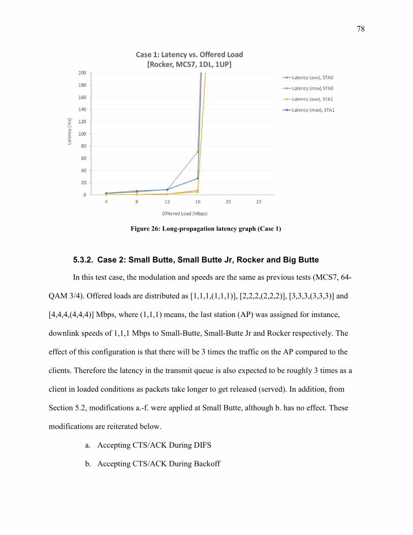
78

5.3.2. Case 2: Small Butte, Small Butte Jr, Rocker and Big Butte

In this test case, the modulation and speeds are the same as previous tests (MCS7, 64-

QAM 3/4). Offered loads are distributed as [1,1,1,(1,1,1)], [2,2,2,(2,2,2)], [3,3,3,(3,3,3)] and

[4,4,4,(4,4,4)] Mbps, where (1,1,1) means, the last station (AP) was assigned for instance,

downlink speeds of 1,1,1 Mbps to Small-Butte, Small-Butte Jr and Rocker respectively. The

effect of this configuration is that there will be 3 times the traffic on the AP compared to the

clients. Therefore the latency in the transmit queue is also expected to be roughly 3 times as a

client in loaded conditions as packets take longer to get released (served). In addition, from

Section 5.2, modifications a.-f. were applied at Small Butte, although b. has no effect. These

modifications are reiterated below.

a. Accepting CTS/ACK During DIFS

b. Accepting CTS/ACK During Backoff

Figure 26: Long-propagation latency graph (Case 1)

79

c. Adding DATA timeout interval

d. Dropped Frame Recovery

e. Making stations NAV interruptible

f. Relaxing the NAV timer update restriction

g. Backoff Optimization

Remaining stations in the network almost behaved like baseline. All tabulated data can be

found in Appendix E.2. The following list provides the binding between station names and

station numbers:

0. Small Butte, SB 1. Small Butte Jr, SBJr 2. Rocker, R 3. Big Butte, AP

80

In the Y-axis of Figure 28, the offered load is the combined total for the system. As

before, the throughputs are identical between baseline and long-distance at the lower end. Table

XVII from Appendix E.2, shows that contrary to the expected 3 times the mean latency, the AP

has little more than 2 times the latency in all stations combined at the last test point of

[4,4,4,(4,4,4)]. This is better than expected. Inferring from 18/24 Mbps loading, throughput stops

increasing for long-distance.

Figure 27: Position of all stations (Case 2)

81

The third test point starts showing signs of network overloading while inferring from the

AP data in Table XVII of Appendix E.2. The highest latency of all stations is ~450 ms. In the

last test point, Small Butte and AP are > 1 sec. This is due to the temporary hidden node issue

caused by 2 slot time delay. It would be a more reasonable to load AP at the lower-end of that

range. Similar to the previous case, latency data is presented in the next figures with upper cut-

off set at 200 ms, and any test point with higher loading such as STA3 (AP) is expected to be out

of bounds. It is normal for STA3’s mean and max to go out of bounds.

With 2 additional nodes as the previous test case, and with each of the 6 links having

equal loading, the throughput wall of 20 Mbps is hit much faster, as offered load increases.

Notice the jump from ~6-12 Mbps in the first two tests, and from ~12-17 Mbps in the 12/18

Mbps tests on the long-distance. STA3 had 3-12 Mbps of overall loading.

Figure 28: Throughput comparison (Case 2)

82

Comparing the network statistics in Figure 29 and Figure 30, as propagation delays get

bigger, the latencies get bigger faster. Baseline shows overloading after 18 Mbps, and long-

distance shows the same after 12 Mbps. As expected, STA3’s mean and max, both exceed 200

ms. And even though SB’s (STA0) mean latency is off the chart, it is still smaller than AP’s data.

Figure 29: Zero-propagation latency graph (Case 2)

83

5.3.3. Case 3: Small Butte, Small Butte Jr, “Nice” Mountain and Big Butte

In the next set of graphs after applying all modifications from Section 5.2, comparison

charts are provided between zero-distance and long-distance, as well as comparison between

long-distance and long-distance with backoff optimization, where the optimized version is the

final sweep for this test case. The terrain slice for the hidden nodes in Figure 50 is in Appendix

E.3. In addition, the following list presents the mapping between station numbers and station

names:

0. Small Butte, SB 1. Small Butte Jr, SBJr (hidden) 2. Nice Mountain, NM (hidden) 3. Big Butte, AP

Figure 30: Long-propagation latency graph (Case 2)

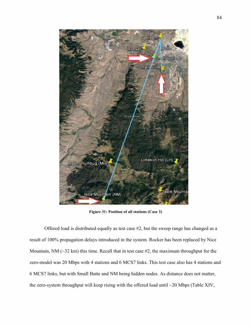
84

Offered load is distributed equally as test case #2, but the sweep range has changed as a

result of 100% propagation delays introduced in the system. Rocker has been replaced by Nice

Mountain, NM (~32 km) this time. Recall that in test case #2, the maximum throughput for the

zero-model was 20 Mbps with 4 stations and 6 MCS7 links. This test case also has 4 stations and

6 MCS7 links, but with Small Butte and NM being hidden nodes. As distance does not matter,

the zero-system throughput will keep rising with the offered load until ~20 Mbps (Table XIV,

Figure 31: Position of all stations (Case 3)

85

Appendix E.2). In Figure 32, while the zero-throughput keeps increasing, the long-distance

throughput gets saturated at ~10 Mbps during sweep. Hence the maximum offered load for the

system was set up to 15 Mbps only. The first throughput graph has default Backoff parameters.

The last sweep for this test case deviates from the zero and long distance parameters such

as, [0, 15], [0, 1023] and 7 as aCWmin, aCWmax and dot11ShortRetryLimit respectively, to the

following: [0, 31], [0, 4095] and 10. The delta in terms of 2’s power between the 32 and 4096 is

8 but reuses the last Backoff window 2 more times. In the code, a flag will override the dynamic

calculation of dot11ShortRetryLimit just based on the CWmin and CWmax. With additional

retries, the packet latency is expected to increase, but packets will more likely get transmitted in

an event of interference. Moreover, this leads to spending more time on a packet before dropping

Figure 32: Throughput comparison without optimization (Case 3)

86

it from the queue. In the next figure, “L-Fixed-Thru” is the optimized version and “L-Thru” is

based on the same values as the previous figure.

The optimization provides another 1 Mbps on the high end, and just ~3 Mbps shy of the

baseline number (Table XV of Appendix E.1). Being the furthest station from all stations

(~108ms), NM has demonstrated temporary hidden node properties for 10-12 slot times. In the

latency data analysis, three graphs depicting the three modes of operation are shown to

demonstrate how quickly latency goes up with default backoff parameters and with optimization.

The tabulated data is presented in Appendix E.2.

Figure 33: Throughput comparison with optimization (Case 3)

87

There is considerable difference in latency between baseline and long-distance model due

to the Nice Mountain being involved. This can be confirmed by comparing the average plots for

nearby stations, SB (STA0) and SBJr (STA1) with the rest of the plots in Figure 35. Only

average and max plots of NM (STA2) and AP (STA3) that make up half the data are off the

charts starting 8.4 Mbps.

SB/SBJr have the lowest drop rates, not just because of their DATA PPDU being 248µs

(shortest), but also due to the fact that signal level at the AP is the highest (SB,SNR:~37 dB and

SNR,SBJr:~40 dB). Recall that the MCS7 1% threshold is 21 dB and therefore the link with

SB/SBJr are highly robust when decoding frames at the receipt of last symbol of a PPDU. As per

preamble locking rules, the AP will lock on to the higher signal level while receiving preamble

of two or more PPDUs simultaneously. In this sense, the closer stations get to transmit more

often and clear the packet queue faster.

Figure 34: Zero-distance latency graph (Case 3)

88

The percentage of dropped frames can be explained using this comparison from Table

XVIII in Appendix E.2: while it ranges between 0-3% for STA0 and STA1 in the entire sweep,

STA2 and STA3 begin to encounter severe frame drops from 12-20% and 4-5% on high loading,

respectively. This disparity can be explained by recalling from Table XVII, that the max

throughput capacity demonstrated by SB and SBJr are ~3.5-4 Mbps in a 4-node network, hence

the range of loading in this test case is not pushing the limits of nearby stations at all.

In Table XVIII, Nice Mountain shows a sharp spike from ~950 ms to ~2000 ms packet

latency for loading 1.95 Mbps to 2.5 Mbps; whereas, the AP spikes from ~300 ms to ~2800 ms

for 3 times as much loading. While the AP is expected to have highest loading, it is important to

address the issues facing NM. Even though the length of the DATA PPDU is the same for all

links in this test case, the link still suffers from momentary hidden node properties. The SINR of

the DATA PDDU (NM, SNR:~23 dB) at the AP will get degraded in almost all cases if the

Figure 35: Long-distance latency graph (Case 3)

89

signal strength from a much closer station interferes, such as Small Butte Jr. As long as NM’s

SINR is closer to MCS7 threshold than that of SBJr., packets are more likely to get corrupted.

Lastly, SBJr is a permanent hidden node to NM. By definition, SBJr always sends out RTS out

of turn when NM is active, and vice-versa.

Notice the reduction of mean packet latency from STA0 and STA1 in Figure 36. Even

though half the latency data in the plots go off the chart, network performance data in Table XIX

from Appendix E.2 shows a substantial improvement in latency and dropped packets, as well as

a slight improvement in throughput. The greatest change is the frame drops from ~20% to ~1%

at 2.5 Mbps loading for STA2. While the throughput increases, the latency also increases which

is counter-intuitive from the previous comparisons. Technically, with additional retries the

latency is supposed to increase, but also decrease the chances of dropping packets. As a result of

more packets getting ACKed, the throughput increases. After optimization, STA2 has the worst

Figure 36: Long-distance latency graph with Optimization (Case 3)

90

mean latency in the sweep overall at ~5.4 sec and yet showed the greatest improvements in other

areas.

SB/SBJr have transmitted all packets in all test points and therefore had a flawless sweep

like the zero-model. Another area where there was a considerable improvement was at AP which

boosted throughput by over 1 Mbps at 7.5 Mbps loading, and reduced the mean latency by about

2 sec. A similar trend can be inferred from other loading conditions and aspect of max latency. In

summary, with the exception of higher loading packet latency at Nice Mountain, the stations

gained tremendously from Backoff optimization. Going over 15 Mbps offered load would not be

recommended.

5.3.4. Case 4: Mount Powell, Small Butte Jr, Sugarloaf Mountain and Big Butte

In this test case, similar to test case #3, throughput data is presented after applying all

modifications from Section 5.2 in comparisons between zero-distance and long-distance, as well

as one between long-distance and long-distance with backoff optimization are given. The terrain

slice for the hidden nodes is presented in Figure 51 in Appendix E.3, and in addition, the

following list shows mapping between station name and number:

0. Mount Powell, M1P 1. Small Butte, SB (hidden) 2. Sugarloaf Mountain, SM (hidden) 3. Big Butte, AP

91

Offered load is distributed equally as test case #2, but the range has changed again as a

result of 100% propagation delays introduced in the system. This time, Small-Butte-Jr and NM

have been replaced by MP (~49 km) and SM (~30 km). Recall that in test case #3, the maximum

throughput for the zero-model was 11 Mbps with 4 stations and 6 MCS7 links. This test case has

4 stations, 2-way MCS7 links to SB, MCS7 downlink to MP, MCS5 uplink from MP, MCS3

downlink to SM, MCS0 uplink to SM, where SB and SM are hidden nodes. The terrain between

Big Butte and SM is presented in Appendix E.3.

Figure 37: Position of all stations (Case 4)

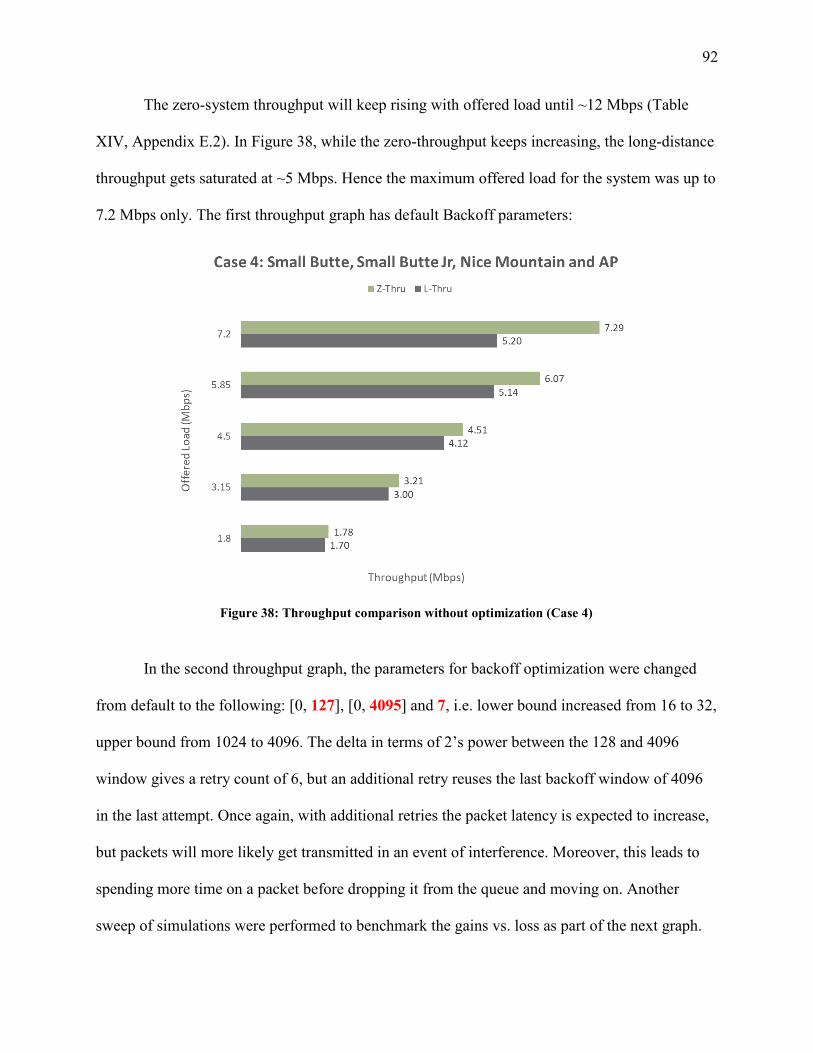
92

The zero-system throughput will keep rising with offered load until ~12 Mbps (Table

XIV, Appendix E.2). In Figure 38, while the zero-throughput keeps increasing, the long-distance

throughput gets saturated at ~5 Mbps. Hence the maximum offered load for the system was up to

7.2 Mbps only. The first throughput graph has default Backoff parameters:

In the second throughput graph, the parameters for backoff optimization were changed

from default to the following: [0, 127], [0, 4095] and 7, i.e. lower bound increased from 16 to 32,

upper bound from 1024 to 4096. The delta in terms of 2’s power between the 128 and 4096

window gives a retry count of 6, but an additional retry reuses the last backoff window of 4096

in the last attempt. Once again, with additional retries the packet latency is expected to increase,

but packets will more likely get transmitted in an event of interference. Moreover, this leads to

spending more time on a packet before dropping it from the queue and moving on. Another

sweep of simulations were performed to benchmark the gains vs. loss as part of the next graph.

Figure 38: Throughput comparison without optimization (Case 4)

93

It can be inferred from the figure that the optimization brought up the max throughput by

~1 Mbps, over 50% of the theoretical zero-distance maximum (Table XV of Appendix E.1). One

of the major reasons for the huge disparity between zero-distance and long-distance throughput

is because distant stations have temporary hidden node properties between each other, which

leads to greatly elevated chances of interference. When the state of the medium is yet to

propagate to other stations, being the furthest station from SB and AP, MP more often than SM

transmits when two other stations are in the middle of an exchange. Recall from Table X that the

MP-AP propagation time is ~163µs, which is 18 slot time delay, and SM-AP has 11 slot time

delay. And the loading on all uplinks is equal for unequal link capacity (See “Link Speed” from

Table XV). This issue is exacerbated by the long DATA PPDU length of 2072µs from SM that

has an uplink speed of MCS0, in addition to Small-Butte being the permanent hidden node to

SM. By definition, SB always sends out RTS out of turn when SB is active, and vice-versa.

Figure 39: Throughput comparison with optimization (Case 4)

94

Once again, there is a considerable difference in latency between baseline and long-

distance model due to the MP (STA0) and SM (STA2) being involved. This can be confirmed by

finding a large disparity between the average latency between SB (STA1) and the rest of the

stations as offered load reaches 7.2 Mbps in the long- model. In this test case only STA1 was

within 7 km radius from the AP. The average and max plots of all stations except STA1 average

are off the charts starting 4.5 Mbps. Surprisingly the next best latency curve is that of STA0

average, as seen in Figure 41.

Figure 40: Zero-distance latency graph (Case 4)

95

Referring to Table XX in Appendix E.2, the average latency on MP during higher loading

is only 5 times more than SB. SM has highest latency and drop rates of 20-30%, which can be

explained by the interference at the AP from other stations while receiving the DATA.

The furthest station, MP, having drop rates similar to that of AP suggests that propagation

delay was less of a contributing factor to packet failures than MCS#. Since both links were at

higher MCS# between MP and AP, than that between SM and AP, it suggests that the duration of

frame exchange and the SNIR at the receiver are primary deciding factor for dropped frames and

throughput. Furthermore, long frame exchanges with momentary and permanent hidden node

properties in the network are most susceptible to being interfered by other stations. The SINR of

the PDDU at the AP will get seriously degraded if the signal strength from a station communicating

at MCS0 (SM, SNR:~5 dB), is interfered by a station with the signal level that is much higher (e.g

Small-Butte). Recall that the SINR for MCS0 for 1% max error rate is 4.5 dB.

Figure 41: Long-distance latency graph (Case 4)

96

Due to reasoning stated above, SB has the lowest drop rate, not just because of its DATA

PPDU being 248µs (shortest), but also due to the fact that signal level at the AP is the highest

(SNR:~37 dB). Link with SB is highly robust in terms of decoding entire frames at the receipt of

the last symbol of a PPDU. As per preamble locking rules, the AP will lock on to the higher

signal level while receiving preamble of two or more PPDUs simultaneously. In this sense, SB

not just transmits the DATA relatively faster than all other clients, hence minimizes the chances

of interference, but also gets to transmit more often and clear the packet queue.

Referring to Figure 42, the latencies have greatly improved after the optimization. The

steeper curves now start from 5.85 Mbps of loading, and that too only for STA3 average and

max, the way it would normally be expected. One stark difference with STA2, which so far has

been performing the worst is that the average latency has been reduced to below the 200 ms

threshold. It is now one of the best latencies seen in the chart. Referring to Table XXI, MP is still

Figure 42: Long-distance latency graph with Optimization (Case 4)

97

struggling with clearing the packets from the queue but not as much as the AP in terms of mean

latency. While the drop rates are almost zero at all nodes and max latencies improved in general,

the mean latency at the AP has only gone up by 1 sec, and 400 ms on the max.

This optimization has yielded the highest reduction of dropped packet at 28% in the

entire research, and it can be deemed successful while maintaining loading at ~7.2 Mbps to avoid

increasing AP’s mean latency further.

5.4. Adaptive Timeout Interval at the Access Point

Having three times the loading on the access-point, packet latency goes up a lot faster

than the rest of the nodes during loading sweeps. To explore an alternative to the backoff

modification in test case #4 described in Section 5.3.4 the access point was allowed to

accommodate and wait for long propagation delays. This is done by extending the timeout

intervals by calculating the round trip propagation times to connected nodes in the network, and

adding 3 time slots to account for SIFS which is the spacing used before receiver sends a

response back. Because timeout intervals are usually rounded up to the next multiple of slot time

(i.e. 54µs), the following table shows lengths calculated similarly for the adaptive timeout

intervals associated to the access-point:

Table XI: New timeout interval values calculated at AP

Station Adapted Timeout Interval (µs) Small Butte 72

Sugarloaf Mountain 234 Mount Powell 360

Being a long interval timer as inferred from the table, it is easily interrupted by an RTS

request of length 72µs from station(s) not previously involved in the exchange. The access-point

is designed to respond regardless of whether it gets its own CTS/ACK response back for its

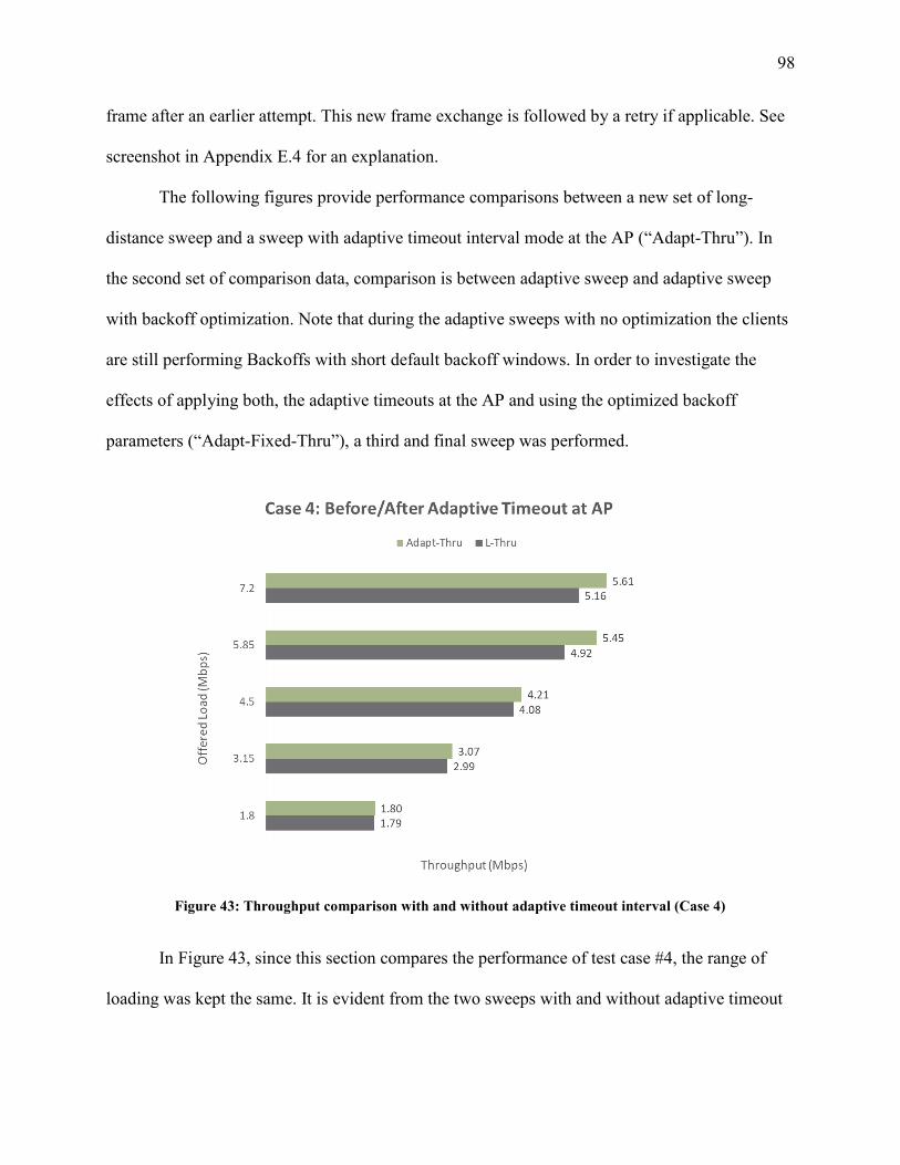
98

frame after an earlier attempt. This new frame exchange is followed by a retry if applicable. See

screenshot in Appendix E.4 for an explanation.

The following figures provide performance comparisons between a new set of long-

distance sweep and a sweep with adaptive timeout interval mode at the AP (“Adapt-Thru”). In

the second set of comparison data, comparison is between adaptive sweep and adaptive sweep

with backoff optimization. Note that during the adaptive sweeps with no optimization the clients

are still performing Backoffs with short default backoff windows. In order to investigate the

effects of applying both, the adaptive timeouts at the AP and using the optimized backoff

parameters (“Adapt-Fixed-Thru”), a third and final sweep was performed.

In Figure 43, since this section compares the performance of test case #4, the range of

loading was kept the same. It is evident from the two sweeps with and without adaptive timeout

Figure 43: Throughput comparison with and without adaptive timeout interval (Case 4)

99

interval length that as loading gets closer to the network capacity, the overall throughput is

slightly improved. Referring to Table XXII in Appendix E.2, AP has the largest delta.

In Figure 44, once again, there has been an improvement by applying the backoff window

optimization and choosing larger slot windows. The improvement between the plain long-

distance version and with all optimizations so far, is ~1 Mbps at higher loading. Because the AP

has a better predictive time window for the arrival of response for its packets, the simulations

should favor low latency of packets that are outbound from the AP.

Figure 44: Throughput comparison with adaptive timeout interval, and optimization (Case 4)

100

The latency plots in Figure 45 look very similar to the previous long-distance graph from

the previous section. The remaining two figures also look similar to the above, however the last

one shows the best visualization due to the combined optimizations. Table XXII and Table

XXIII show that without applying the numbers from the previous experiment, the latencies on

the clients has considerably reduced, but the throughputs have almost stayed the same. An

interesting phenomenon at SM is that the dropped frames have gone up but the latencies have

gone down. This implies that it was able to go through more packets from its queue because it

found the channel to be idle more often. This further implies that without the adaptive timeout at

the AP, stations found the channel to be busier from frequent retries - especially from the AP as

it has 3 times as much loading as any other station. Therefore, the adaptive experiments are a

success.

Figure 45: Plain long-distance latency graph (new sweep) (Case 4)

101

To further obtain the benefits from adaptive timeout interval, the previously found

optimum values for Backoff parameters were also applied for the last set of sweeps. From

Appendix E.2, the amount of dropped packet reduction this time compared to the last section is

26%, second to highest in the research. Mean and max latencies have been further reduced and

the boost in throughput is more than the previous comparison at the high end of the sweep.

Figure 46: Long-distance latency graph with adaptive mode (Case 4)

102

Figure 47: Long-distance latency graph with adaptive mode and optimization (Case 4)

103

6. Conclusions

From all 4 cases it can be concluded that the closer the stations are to the AP, the more

system throughput will match the theoretical value. This is expected when the network

conditions are favorable and stations can initiate both RTS and CTS NAVs when necessary,

instead of getting involved in between interference and using the Backoff timer. Entering

Backoff entails risks of drawing more number of slots than necessary and wasting the period of

time when channel has been idle. Conversely, since the larger backoff windows do not guarantee

a larger random number necessary to exceed the round trip time, stations can make multiple re-

attempts between the first time a packet was sent and the time of arrival of the response at the

source. This creates a huge scope for stations to receive the response while transmitting, and then

discarding that signal. Relying on the Backoff timer has its drawbacks.

The said issues create greater disparities in test case #3 and #4 between empirical and

theoretical data, where there were larger distances by an order of magnitude, hidden nodes, and

mismatching PPDU lengths. The uncertainty about the arrival of packets at the AP was much

higher. Due to this uncertainty and lack of predictability, there were far more collisions at any

given station compared to that of the first two test cases. The temporary hiddenness of the nodes

from long propagation delays with respect to each other made things worse.

One of the ways to reduce the chances of collisions and allowing stations to successfully

decode their response frames is by choosing a larger backoff slot window. However, while

every effort is made to avoid entering the Backoff period, an alternate optimization explored in

the research was to extend the timeout intervals where possible, i.e. at the access-point.

After applying all optimizations and depending on the test case, there was 50-90%

difference between theoretical and practical system throughput. The worst case network

104

throughput at full loading (4 nodes) was roughly 6.2 Mbps, 20% of which was at Mount Powell,

being furthest from the access-point. In this research the largest reduction of packet drops

achieved was 28%, and largest reduction in packet latency was shown to be at 93%.

105

7. References Cited

[1] J. Magliacane, "SPLAT! A Terrestrial RF Path Analysis Application For Linux/Unix,"

QSL.net, 2017. [Online]. Available: http://www.qsl.net/kd2bd/splat.html. [Accessed 19

November 2017].

[2] "NASA Shuttle Radar Topography Mission Global 3 arc second SRTMGL3S | The

Long Term Archive," USGS, January 2015. [Online]. Available:

https://lta.cr.usgs.gov/srtmgl3s.html. [Accessed 19 Novemebr 2017].

[3] US Government, NASA Earthdata, 2013. [Online]. Available:

https://e4ftl01.cr.usgs.gov/SRTM/SRTMGL3.003/2000.02.11/. [Accessed 19 November

2017].

[4] US Government, NASA Earthdata, 2015. [Online]. Available:

https://e4ftl01.cr.usgs.gov/SRTM/SRTMGL1.003/2000.02.11/. [Accessed 19 November

2017].

[5] M. Chaplin, "Water and microwaves," Water Structure and Science, 6 November 2017.

[Online]. Available: http://www1.lsbu.ac.uk/water/microwave_water.html. [Accessed

19 November 2017].

[6] "Shuttle Radar Topography Mission (SRTM) 1 Arc-Second Global | The Long Term

Archive," USGS, January 2015. [Online]. Available: https://lta.cr.usgs.gov/SRTM1Arc.

[Accessed 19 November 2017].

[7] J. M. P. N. Dr. Alan Smale, "The Earth," NASA, 24 August 2015. [Online]. Available:

https://imagine.gsfc.nasa.gov/features/cosmic/earth_info.html. [Accessed 19 November

2017].

106

[8] I. Poole, "Thermal Noise Calculator Formulae & Equations," Radio-Electronics,

[Online]. Available: http://www.radio-electronics.com/info/rf-technology-

design/noise/thermal-calculations.php. [Accessed 19 November 2017].

[9] I. Poole, "Radio receiver noise floor," Radio-Electronics, [Online]. Available:

http://www.radio-electronics.com/info/rf-technology-design/rf-noise-sensitivity/noise-

floor.php. [Accessed 4 December 2017].

[10] "The OSI Model's Seven Layers Defined and Functions Explained," Microsoft, 19 April

2017. [Online]. Available: https://support.microsoft.com/en-us/help/103884/the-osi-

model-s-seven-layers-defined-and-functions-explained. [Accessed 19 November 2017].

[11] Part 11: Wireless LAN Medium Access Control (MAC) and Physical Layer (PHY)

Specifications, IEEE, 2012.

[12] IEEE, "IEEE Std 802.3-2015 (Revision of IEEE Std 802.3-2012) - IEEE Standard for

Ethernet," IEEE, 2015. [Online]. Available:

https://standards.ieee.org/findstds/standard/802.3-2015.html. [Accessed 19 November

2017].

[13] "Pointers - C++ Tutorials," cplusplus, 2017. [Online]. Available:

http://www.cplusplus.com/doc/tutorial/pointers/. [Accessed 19 November 2017].

[14] "New random-number generator—64-bit Mersenne Twister," STATA, [Online].

Available: https://www.stata.com/stata14/random-number-generators/. [Accessed 19

November 2017].

107

[15] "The Mersenne Twister random number generator," VOSE, 2017. [Online]. Available:

https://www.vosesoftware.com/riskwiki/RandomnumbergenerationinModelRisk.php.

[Accessed 19 November 2017].

[16] "What is a seed in terms of generating a random number?," StackOverflow, 16 02 2013.

[Online]. Available: https://stackoverflow.com/questions/14914595/what-is-a-seed-in-

terms-of-generating-a-random-number. [Accessed 19 November 2017].

[17] "Antenna Theory - Isotropic Radiation," tutorialspoint, 2017. [Online]. Available:

https://www.tutorialspoint.com/antenna_theory/antenna_theory_isotropic_radiation.htm.

[Accessed 19 November 2017].

[18] "About Qt," QT, 14 February 2017. [Online]. Available: https://wiki.qt.io/About_Qt.

[Accessed 19 November 2017].

[19] J. T. Juha Heiskala, ODFM Wireless LANS: A Theoretical and Practical Guide, SAMS,

2001.

[20] "802.11 MAC Series – Basics of MAC Architecture – Part 1 of 3," CWNP, 8 January

2016. [Online]. Available: https://www.cwnp.com/802.11-mac-series-ndash-basics-

mac-architecture-ndash-part-1-3/. [Accessed 19 November 2017].

[21] A. G. L. a. W. A. K. George A Hufford, "A Guide to the Use of the ITS Irregular

Terrain Model in the Area Prediction Mode," National Telecommunication and

Information Administration, United States Department of Commerce, 01 April 1982.

[Online]. Available: https://www.ntia.doc.gov/report/1982/guide-use-its-irregular-

terrain-model-area-prediction-mode. [Accessed 19 Novemeber 2017].

108

8. Appendix

8.1. Appendix A.1

Script master.py

import os import sys from shutil import copy2 from subprocess import PIPE, STDOUT, Popen # station configuration parameters in Watts station_transmit_power = 20 station_transmit_freq = 530 inputs = str(sys.argv).split()[1:] inputs = [s[1:-2] for s in inputs] transmitter = inputs[0] bool_hd = "" receiver_station = "" rx_ant_height = "" topo = "" new = " -olditm " if len(inputs) > 4: bool_hd = '-hd' print "HD MODE ACTIVATED!" topo = 'topo' receiver_station = inputs[1] rx_ant_height = inputs[2] elif len(inputs) > 3: if 'hd' in inputs and 'topo' in inputs and 'new' in inputs: bool_hd = '-hd' print "HD MODE ACTIVATED!" topo = 'topo' new = " " else: receiver_station = inputs[1] if 'hd' in inputs and 'topo' in inputs: bool_hd = '-hd' print "HD MODE ACTIVATED!" topo = 'topo' elif 'hd' in inputs and 'new' in inputs: bool_hd = '-hd' print "HD MODE ACTIVATED!" new = " " elif 'topo' in inputs and 'new' in inputs: topo = 'topo' new = " " else: if 'hd' in inputs: bool_hd = '-hd' print "HD MODE ACTIVATED!" elif 'topo' in inputs: topo = 'topo' elif 'new' in inputs: new = " " rx_ant_height = inputs[2] elif len(inputs) > 2: if 'hd' in inputs and 'topo' in inputs: bool_hd = '-hd' print "HD MODE ACTIVATED!" topo = 'topo' elif 'hd' in inputs and 'new' in inputs: bool_hd = '-hd' print "HD MODE ACTIVATED!" new = " " elif 'topo' in inputs and 'new' in inputs:

109

topo = 'topo' new = " " else: receiver_station = inputs[1] if 'hd' in inputs: bool_hd = '-hd' print "HD MODE ACTIVATED!" elif 'topo' in inputs: topo = 'topo' elif 'new' in inputs: new = " " else: rx_ant_height = inputs[2] elif len(inputs) > 1: if 'hd' in inputs: bool_hd = '-hd' print "HD MODE ACTIVATED!" elif 'topo' in inputs: topo = 'topo' elif 'new' in inputs: new = " " else: receiver_station = inputs[1] google_earth_file = [f for f in os.listdir(os.getcwd()) if f.endswith('.kml')][0] with open(google_earth_file,'r') as f: lines = f.read().splitlines() # -------------------- parsing the Google Earth file -------------------- idx = [i for i, s in enumerate(lines) if '<name>Butte</name>' in s] lines = lines[idx[0]+3:] namesi = [i for i, s in enumerate(lines) if '<name>' in s] location = [s for i, s in enumerate(lines) if '<coordinates>' in s] names = [lines[i].split('>')[1].split('<')[0].replace(' ','_').replace('-','_') for i in namesi] idx = [i for i, s in enumerate(names) if s.find('(') != -1] for i in idx: names[i] = names[i].split('(')[1][:-1] longs = [s.split('>')[1].split('<')[0].split(',')[0][1:] for s in location] lats = [s.split('>')[1].split('<')[0].split(',')[1] for s in location] longitudes = {} latitudes = {} for idx, name in enumerate(names): longitudes[name] = longs[idx] latitudes[name] = lats[idx] antheight_file = 'antenna_heights.txt' with open(antheight_file,'r') as f: heights = f.read().splitlines() heights = [s.split(' ') for s in heights] antenna_heights = {} for h in heights: antenna_heights[h[0]] = h[1] print "\n------- Using " + transmitter + " as TX station -------" xloc_tx = 0 yloc_tx = 0 if receiver_station != "": names = [] names.append(transmitter) names.append(receiver_station) height_tx = antenna_heights[transmitter] height_rx = antenna_heights[receiver_station] antenna_heights = {} antenna_heights[transmitter] = height_tx print "height: " + rx_ant_height antenna_heights[receiver_station] = rx_ant_height if rx_ant_height != "" else height_rx for name in names: # build the LRP file if name == transmitter: rec_file = open(name + '.lrp', "w") rec_file.write("15.000"+"\n") rec_file.write("0.005"+"\n")

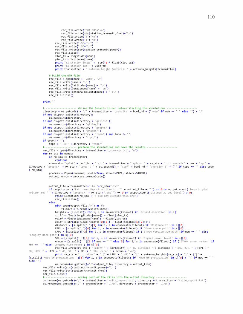
110

rec_file.write("301.00"+"\n") rec_file.write(str(station_transmit_freq)+"\n") rec_file.write("5"+"\n") rec_file.write("1"+"\n") rec_file.write(".5"+"\n") rec_file.write(".5"+"\n") rec_file.write(str(station_transmit_power)) rec_file.close() xloc_tx = longitudes[name] yloc_tx = latitudes[name] print "TX station long:" + str(-1 * float(xloc_tx)) print "TX station lat:" + yloc_tx print transmitter + " antenna height (meters): " + antenna_heights[transmitter] # build the QTH file rec_file = open(name + '.qth', "w") rec_file.write(name + '\n') rec_file.write(latitudes[name] + '\n') rec_file.write(longitudes[name] + '\n') rec_file.write(antenna_heights[name] + ' m\n') rec_file.close() print "" # -------------------- define the Results folder before starting the simulations -------------------- directory = os.getcwd() + '/' + transmitter + '_results' + bool_hd + ("-new" if new == " " else "") + '/' if not os.path.exists(directory): os.makedirs(directory) if not os.path.exists(directory + 'qfiles/'): os.makedirs(directory + 'qfiles/') if not os.path.exists(directory + 'graphs/'): os.makedirs(directory + 'graphs/') if not os.path.exists(directory + 'topo/') and topo != "": os.makedirs(directory + 'topo/') if topo != "": topo = " -o " + directory + "topo/" # -------------------- perform the simulations and move the results -------------------- rec_file = open(directory + transmitter + '_summary.txt', "w") for rx_sta in names: if rx_sta == transmitter: continue command = "splat" + bool_hd + " -t " + transmitter + ".qth -r " + rx_sta + ".qth -metric" + new + "-p " +

directory + 'graphs/' + rx_sta + ".png -d " + os.getcwd() + "/sdf" + bool_hd + "/version-3" + ("" if topo == "" else topo + rx_sta)

process = Popen(command, shell=True, stdout=PIPE, stderr=STDOUT) output, error = process.communicate() output_file = transmitter+"-to-"+rx_sta+".txt" if output.count('Path Loss Report written to: "' + output_file + '"') == 0 or output.count('Terrain plot

written to: "' + directory + 'graphs/' + rx_sta +'.png"') == 0 or output.count('assumed as sea-level') > 0: raise Exception(rx_sta + ': did not execute this one') rec_file.close() else: with open(output_file,'r') as f: fileout = f.read().splitlines() heights = [s.split() for i, s in enumerate(fileout) if 'Ground elevation' in s] xdiff = float(longitudes[name]) - float(xloc_tx) ydiff = float(latitudes[name]) - float(yloc_tx) zdiff = str(abs(float(heights[0][2]) - float(heights[1][2]))); distance = [s.split(' ')[3] for i, s in enumerate(fileout) if 'Distance to' in s][0] FSPL = [s.split(' ')[4] for i, s in enumerate(fileout) if 'Free space path' in s][0] LRPL = [s.split()[-2] for i, s in enumerate(fileout) if ('ITWOM Version 3.0 path' if new == " " else

"Longley-Rice path") in s][0] SPL = [s.split(' ')[5] for i, s in enumerate(fileout) if 'Signal power level' in s][0] ernum = [s.split(' ')[3 if new == " " else 3] for i, s in enumerate(fileout) if ('ITWOM error number' if

new == " " else 'Longley-Rice model') in s][0] rec_file.write(rx_sta + ":zdiff " + str(zdiff) + " m, distance " + distance + " km, FSPL " + FSPL + "

dB, LRPL " + LRPL + " dB, SPL " + SPL + " dBm, error " + ernum + "\n") print rx_sta + " ... done" + " [" + LRPL + " dB]" + "[" + antenna_heights[rx_sta] + "]" + ("[" +

[s.split('Mode of propagation: ')[1] for i, s in enumerate(fileout) if 'Mode of propagation' in s][0] + "]" if new == " " else "")

os.rename(os.getcwd()+'/'+output_file, directory + output_file) rec_file.write(str(station_transmit_power)+'\n') rec_file.write(str(station_transmit_freq)) rec_file.close() # -------------------- moving rest of the files into the output directory -------------------- os.rename(os.getcwd()+'/' + transmitter + '-site_report.txt', directory + transmitter + '-site_report.txt') os.rename(os.getcwd()+'/' + transmitter + '.lrp', directory + transmitter + '.lrp')

111

copy2(os.getcwd()+'/'+antheight_file, directory) qth_files = [f for f in os.listdir(os.getcwd()) if f.endswith('.qth')] for qfile in qth_files: os.rename(os.getcwd()+'/'+qfile, directory + 'qfiles/' + qfile) print "-------------------------------------------------\n" print "Scipt finished running\n"

112

Script post_master.py

import os import sys hd = "" txstation = str(sys.argv).split()[1:][0][1:-2] if (len(str(sys.argv).split()) > 2): hd = "-" + str(sys.argv).split()[1:][1][1:-2] print hd txpower = 0 frequency = 0 print '\n--------------------- Using ' + txstation + ' as TX station ---------------' stations = [f[:-(8 if hd == "" else 11)] for f in os.listdir(os.getcwd()) if f.endswith('_results' + hd)] #get

the list of stations # -------------------- shortlist stations based on the picked transmitter -------------------- viable_list = stations if len(viable_list) == 0: print "Station results not populated from master script!" print '\nGeographic coodinates found: ' + str(len(stations)) + '\n' for name in stations: directory = os.getcwd() + '/' + name + '_results' + hd + '/' with open(directory + name + '_summary.txt','r') as f: lines = f.read().splitlines() #go through each line in a file and look at individual numbers for i,sta in enumerate(lines): sta_name = sta.split()[0].split(':')[0] if name == txstation and i == len(lines)-2: txpower = sta_name #really this is a number (power in Watts) elif name == txstation and i == len(lines)-1: frequency = sta_name #just a number (frequency in Mega sHertz) elif name == txstation and float(sta.split()[10]) > 148.0: #pathloss is too damn high so ignore this one if sta_name in viable_list: print "Removing station: " + sta_name viable_list.remove(sta_name) else: print "Warning: " + sta_name + " station results not present" # -------------------- Now build the table -------------------- namtable = [] distable = [] pattable = [] print '\n---------------------------------------------------------------' print '\nNow building tables. Geographic coodinates count: ' + str(len(viable_list)) + '\n' for name in viable_list: directory = os.getcwd() + '/' + name + '_results' + hd + '/' with open(directory + name + '_summary.txt','r') as f: lines = f.read().splitlines() namtable_row = [] distable_row = [] pattable_row = [] namtable_row.append(name + ',') distable_row.append(name + ',') pattable_row.append(name + ',') for sta in lines: sta_name = sta.split()[0].split(':')[0] if sta_name in viable_list: namtable_row.append(sta_name + ',') distable_row.append(sta.split()[4] + ',') pattable_row.append(sta.split()[10] + ',') namtable.append(namtable_row) distable.append(distable_row) pattable.append(pattable_row) print name + " ... built" namtable[-1] = namtable[-1][:-1] distable[-1] = distable[-1][:-1]

113

pattable[-1] = pattable[-1][:-1] # -------------------- Write table to file -------------------- station_names = open('station_names.txt', "w") distance_file = open('distance_table.txt', "w") pathloss_file = open('pathloss_table.txt', "w") for idx, row in enumerate(distable): for idy, col in enumerate(distable[idx]): station_names.write(namtable[idx][idy]) distance_file.write(distable[idx][idy]) pathloss_file.write(pattable[idx][idy]) station_names.write('\n') distance_file.write('\n') pathloss_file.write('\n') station_names.write(str(txpower)+'\n') station_names.write(str(frequency)) station_names.close() distance_file.close() pathloss_file.close()

114

8.2. Appendix A.2

--==[ SPLAT! v1.4.2 Path Analysis ]==-- --------------------------------------------------------------------------- Transmitter site: big_m Site location: 46.0194 North / 112.5590 West (46° 1' 9" N / 112° 33' 32" W) Ground elevation: 1901.00 meters AMSL Antenna height: 20.00 meters AGL / 1921.00 meters AMSL Antenna height above average terrain: 61.59 meters Distance to Rocker: 3.78 kilometers Azimuth to Rocker: 222.94 degrees Depression angle to Rocker: -1.7745 degrees --------------------------------------------------------------------------- Receiver site: Rocker Site location: 45.9945 North / 112.5923 West (45° 59' 40" N / 112° 35' 32" W) Ground elevation: 1785.00 meters AMSL Antenna height: 20.00 meters AGL / 1805.00 meters AMSL Antenna height above average terrain: -36.56 meters Distance to big_m: 3.78 kilometers Azimuth to big_m: 42.91 degrees Elevation angle to big_m: +1.7405 degrees --------------------------------------------------------------------------- Longley-Rice Parameters Used In This Analysis: Earth's Dielectric Constant: 15.000 Earth's Conductivity: 0.005 Siemens/meter Atmospheric Bending Constant (N-units): 301.000 ppm Frequency: 530.000 MHz Radio Climate: 5 (Continental Temperate) Polarization: 1 (Vertical) Fraction of Situations: 50.0% Fraction of Time: 50.0% Transmitter ERP: 20 Watts (+43.01 dBm) Transmitter EIRP: 33 Watts (+45.15 dBm) --------------------------------------------------------------------------- Summary For The Link Between big_m and Rocker: Free space path loss: 98.51 dB Longley-Rice path loss: 98.14 dB Attenuation due to terrain shielding: -0.36 dB Field strength at Rocker: 78.75 dBuV/meter Signal power level at Rocker: -52.99 dBm Signal power density at Rocker: -67.03 dBW per square meter Voltage across a 50 ohm dipole at Rocker: 640.89 uV (56.14 dBuV) Voltage across a 75 ohm dipole at Rocker: 784.92 uV (57.90 dBuV) Mode of propagation: Line-Of-Sight Mode Longley-Rice model error number: 0 (No error) --------------------------------------------------------------------------- No obstructions to LOS path due to terrain were detected by SPLAT! The first Fresnel zone is clear. 60% of the first Fresnel zone is clear.

115

8.3. Appendix B.1

Mapping file station_names.txt

HM,SM,Rocker,TM01,TM02,MP,LM,Fleecer,AR02,AR01,AR03,Small_Butte,Small_Butte_Jr,Near_BerkeleyPit,NM,MH,TL02,TL01,TL03,big_m,LH, SM,HM,Rocker,TM01,TM02,MP,LM,Fleecer,AR02,AR01,AR03,Small_Butte,Small_Butte_Jr,Near_BerkeleyPit,NM,MH,TL02,TL01,TL03,big_m,LH, Rocker,HM,SM,TM01,TM02,MP,LM,Fleecer,AR02,AR01,AR03,Small_Butte,Small_Butte_Jr,Near_BerkeleyPit,NM,MH,TL02,TL01,TL03,big_m,LH, TM01,HM,SM,Rocker,TM02,MP,LM,Fleecer,AR02,AR01,AR03,Small_Butte,Small_Butte_Jr,Near_BerkeleyPit,NM,MH,TL02,TL01,TL03,big_m,LH, TM02,HM,SM,Rocker,TM01,MP,LM,Fleecer,AR02,AR01,AR03,Small_Butte,Small_Butte_Jr,Near_BerkeleyPit,NM,MH,TL02,TL01,TL03,big_m,LH, MP,HM,SM,Rocker,TM01,TM02,LM,Fleecer,AR02,AR01,AR03,Small_Butte,Small_Butte_Jr,Near_BerkeleyPit,NM,MH,TL02,TL01,TL03,big_m,LH, LM,HM,SM,Rocker,TM01,TM02,MP,Fleecer,AR02,AR01,AR03,Small_Butte,Small_Butte_Jr,Near_BerkeleyPit,NM,MH,TL02,TL01,TL03,big_m,LH, Fleecer,HM,SM,Rocker,TM01,TM02,MP,LM,AR02,AR01,AR03,Small_Butte,Small_Butte_Jr,Near_BerkeleyPit,NM,MH,TL02,TL01,TL03,big_m,LH, AR02,HM,SM,Rocker,TM01,TM02,MP,LM,Fleecer,AR01,AR03,Small_Butte,Small_Butte_Jr,Near_BerkeleyPit,NM,MH,TL02,TL01,TL03,big_m,LH, AR01,HM,SM,Rocker,TM01,TM02,MP,LM,Fleecer,AR02,AR03,Small_Butte,Small_Butte_Jr,Near_BerkeleyPit,NM,MH,TL02,TL01,TL03,big_m,LH, AR03,HM,SM,Rocker,TM01,TM02,MP,LM,Fleecer,AR02,AR01,Small_Butte,Small_Butte_Jr,Near_BerkeleyPit,NM,MH,TL02,TL01,TL03,big_m,LH, Small_Butte,HM,SM,Rocker,TM01,TM02,MP,LM,Fleecer,AR02,AR01,AR03,Small_Butte_Jr,Near_BerkeleyPit,NM,MH,TL02,TL01,TL03,big_m,LH, Small_Butte_Jr,HM,SM,Rocker,TM01,TM02,MP,LM,Fleecer,AR02,AR01,AR03,Small_Butte,Near_BerkeleyPit,NM,MH,TL02,TL01,TL03,big_m,LH, Near_BerkeleyPit,HM,SM,Rocker,TM01,TM02,MP,LM,Fleecer,AR02,AR01,AR03,Small_Butte,Small_Butte_Jr,NM,MH,TL02,TL01,TL03,big_m,LH, NM,HM,SM,Rocker,TM01,TM02,MP,LM,Fleecer,AR02,AR01,AR03,Small_Butte,Small_Butte_Jr,Near_BerkeleyPit,MH,TL02,TL01,TL03,big_m,LH, MH,HM,SM,Rocker,TM01,TM02,MP,LM,Fleecer,AR02,AR01,AR03,Small_Butte,Small_Butte_Jr,Near_BerkeleyPit,NM,TL02,TL01,TL03,big_m,LH, TL02,HM,SM,Rocker,TM01,TM02,MP,LM,Fleecer,AR02,AR01,AR03,Small_Butte,Small_Butte_Jr,Near_BerkeleyPit,NM,MH,TL01,TL03,big_m,LH, TL01,HM,SM,Rocker,TM01,TM02,MP,LM,Fleecer,AR02,AR01,AR03,Small_Butte,Small_Butte_Jr,Near_BerkeleyPit,NM,MH,TL02,TL03,big_m,LH, TL03,HM,SM,Rocker,TM01,TM02,MP,LM,Fleecer,AR02,AR01,AR03,Small_Butte,Small_Butte_Jr,Near_BerkeleyPit,NM,MH,TL02,TL01,big_m,LH, big_m,HM,SM,Rocker,TM01,TM02,MP,LM,Fleecer,AR02,AR01,AR03,Small_Butte,Small_Butte_Jr,Near_BerkeleyPit,NM,MH,TL02,TL01,TL03,LH, LH,HM,SM,Rocker,TM01,TM02,MP,LM,Fleecer,AR02,AR01,AR03,Small_Butte,Small_Butte_Jr,Near_BerkeleyPit,NM,MH,TL02,TL01,TL03,big_m,

Mapping file distrance_table.txt

HM,50.64,26.24,45.55,43.52,55.37,18.02,50.78,31.32,28.08,48.31,25.45,25.49,16.13,50.71,44.53,60.46,62.8,60.26,22.51,37.71 SM,50.64,28.18,48.68,45.94,37.45,39.53,23.97,19.36,22.59,10.82,32.79,30.46,37.38,41.43,36.18,33.25,34.73,34.38,30.68,44.3 Rocker,26.24,28.18,29.75,26.88,49.53,11.44,24.75,11.38,9.86,30.57,5.33,2.53,10.4,29.44,22.39,35.06,37.41,35.09,3.78,22.43 TM01,45.55,48.68,29.75,2.93,78.46,28.83,27.96,39.65,39.21,55.73,25.45,27.81,32.88,11.5,12.9,28.81,30.36,27.61,31.66,8.05 TM02,43.52,45.94,26.88,2.93,75.53,26.45,25.75,36.72,36.3,52.86,22.68,24.99,30.37,10.63,10.55,27.55,29.25,26.44,28.88,5.81 MP,55.37,37.45,49.53,78.46,75.53,56.55,59.81,38.83,39.67,26.69,54.67,51.89,52.16,74.64,68.08,70.18,71.85,71.17,49,71.74 LM,18.02,39.53,11.44,28.83,26.45,56.55,33.84,21.46,18.89,40.94,8.22,9.49,4.64,32.8,26.52,42.83,45.16,42.54,9.05,20.78 Fleecer,50.78,23.97,24.75,27.96,25.75,59.81,33.84,26.23,28.2,33.65,25.67,25.29,34.66,18.41,15.21,11.29,13.47,11.88,28.53,26.57 AR02,31.32,19.36,11.38,39.65,36.72,38.83,21.46,26.23,3.24,19.49,16.71,13.91,18.52,36.9,29.99,37.51,39.7,37.99,12.44,32.97 AR01,28.08,22.59,9.86,39.21,36.3,39.67,18.89,28.2,3.24,22.13,15.09,12.28,15.62,37.41,30.39,39.4,41.64,39.77,10.05,32.15 AR03,48.31,10.82,30.57,55.73,52.86,26.69,40.94,33.65,19.49,22.13,35.8,33.09,37.74,49.94,43.98,43.63,45.23,44.68,31.93,50.25 SB,25.45,32.79,5.33,25.45,22.68,54.67,8.22,25.67,16.71,15.09,35.8,2.82,9.48,26.78,19.98,35.01,37.35,34.81,6.21,17.77 SBJr,25.49,30.46,2.53,27.81,24.99,51.89,9.49,25.29,13.91,12.28,33.09,2.82,9.38,28.3,21.34,35.18,37.53,35.11,4.11,20.3 NB,16.13,37.38,10.4,32.88,30.37,52.16,4.64,34.66,18.52,15.62,37.74,9.48,9.38,35.87,29.25,44.39,46.74,44.24,6.94,24.84 NM,50.71,41.43,29.44,11.5,10.63,74.64,32.8,18.41,36.9,37.41,49.94,26.78,28.3,35.87,7.07,17.35,18.86,16.12,32.41,14.98 MH,44.53,36.18,22.39,12.9,10.55,68.08,26.52,15.21,29.99,30.39,43.98,19.98,21.34,29.25,7.07,18.66,20.72,17.86,25.44,12.03 TL02,60.46,33.25,35.06,28.81,27.55,70.18,42.83,11.29,37.51,39.4,43.63,35.01,35.18,44.39,17.35,18.66,2.35,1.49,38.79,30.54 TL01,62.8,34.73,37.41,30.36,29.25,71.85,45.16,13.47,39.7,41.64,45.23,37.35,37.53,46.74,18.86,20.72,2.35,2.87,41.13,32.49 TL03,60.26,34.38,35.09,27.61,26.44,71.17,42.54,11.88,37.99,39.77,44.68,34.81,35.11,44.24,16.12,17.86,1.49,2.87,38.78,29.62 big_m,22.51,30.68,3.78,31.66,28.88,49,9.05,28.53,12.44,10.05,31.93,6.21,4.11,6.94,32.41,25.44,38.79,41.13,38.78,23.97 LH,37.71,44.3,22.43,8.05,5.81,71.74,20.78,26.57,32.97,32.15,50.25,17.77,20.3,24.84,14.98,12.03,30.54,32.49,29.62,23.97

Mapping file pathloss_table.txt

HM,120.98,147.33,120.06,119.67,121.76,133.65,121.01,142.5,115.88,120.57,115.02,151.49,111.06,120.98,119.86,122.51,122.84,122.48,145.49,118.42, SM,120.98,146.37,120.64,120.14,118.38,118.84,114.5,112.64,113.99,166.62,144.99,144.57,118.36,145.52,152.71,161.89,165.58,161.7,134.9,119.81, Rocker,146.74,146.37,116.37,115.5,120.79,108.08,114.78,108.02,106.77,116.6,101.4,94.9,107.25,145.12,129.11,117.79,118.35,117.79,98.38,113.92, TM01,120.06,120.64,116.37,96.14,124.77,116.11,115.85,118.87,118.77,160.99,115.02,115.79,117.25,108.13,109.12,116.11,116.56,115.74,116.92,104.99, TM02,119.67,120.14,115.5,96.14,124.44,115.36,115.11,118.2,118.1,157.61,114.03,114.86,116.56,149.68,107.37,115.72,116.24,115.36,116.12,102.15, MP,121.76,118.38,120.79,124.77,124.44,121.94,122.43,118.69,118.88,115.44,121.64,121.19,121.24,124.33,123.54,123.79,124,123.91,120.7,123.99, LM,133.65,118.84,108.08,116.11,115.36,121.94,117.5,113.55,112.44,119.14,105.2,106.45,100.18,117.22,115.38,119.54,119.99,119.48,106.03,113.26, Fleecer,121.01,114.5,114.78,115.85,115.13,122.43,117.5,115.29,115.91,174.14,115.1,114.97,117.71,112.22,110.55,107.94,109.49,108.4,116.02,115.4, AR02,142.09,112.64,108.02,118.87,118.2,118.69,113.55,115.29,97.09,112.71,111.36,109.78,112.26,118.24,116.45,160.37,169.21,147.86,108.8,117.26, AR01,115.88,113.99,106.77,118.77,118.1,118.88,112.44,115.91,97.09,113.81,110.49,108.69,110.78,118.36,116.56,147.31,156.53,118.89,106.94,117.05, AR03,120.57,167.23,116.6,160.99,157.61,115.44,119.14,174.29,112.71,113.81,117.97,117.29,118.44,176.4,170.19,175.1,194.23,186.37,116.99,139.62, SB,115.02,144.99,101.4,115.02,114.03,121.64,105.2,115.1,111.36,110.49,117.97,95.78,106.43,115.45,112.91,141.29,146.94,142.57,102.72,111.9, SBJr,151.5,144.57,94.9,115.79,114.86,121.19,106.45,114.97,109.78,108.69,117.29,95.78,106.35,133.38,113.48,143.84,149.14,145.61,99.1,113.05, NB,111.06,118.36,107.25,117.25,116.56,121.24,100.18,117.71,112.26,110.78,118.44,106.43,106.35,117.99,116.23,119.84,120.29,119.82,103.71,114.81, NM,120.98,145.39,145.24,108.13,149.79,124.33,117.22,112.22,118.24,118.36,176.75,115.45,133.35,117.99,103.85,111.7,112.43,111.06,117.11,110.41, MH,119.86,152.52,128.6,109.12,107.37,123.54,115.38,110.55,116.45,116.56,170.19,112.91,113.48,116.23,103.85,112.33,113.24,111.95,115.01,108.51,

116

TL02,122.51,161.89,117.79,116.11,115.72,123.79,119.54,107.94,160.47,147.5,175.1,141.29,143.98,119.84,111.7,112.33,94.18,90.13,118.67,116.6, TL01,122.84,165.58,118.35,116.56,116.24,124,119.99,109.49,169.61,156.85,193.83,147.25,149.01,120.29,112.43,113.24,94.18,115.29,119.17,117.14, TL03,122.48,161.21,117.79,115.74,115.36,123.91,119.48,108.4,147.75,118.89,186.46,142.25,145.31,119.82,111.06,111.95,90.13,115.29,118.67,116.34, big_m,145.49,134.9,98.38,116.92,116.12,120.7,106.03,116.02,108.8,106.94,116.99,102.72,99.1,103.71,117.11,115.01,118.67,119.17,118.67,114.5, LH,118.42,119.81,113.92,104.99,102.15,123.99,113.26,115.4,117.26,117.05,139.62,111.9,113.05,114.81,110.41,108.51,116.6,117.14,116.34,114.5,

Mapping file antenna_heights.txt

Rocker 2 WC02 35 WC01 35 TM01 2 TM02 2 MP 2 LM 2 GM 35 Fleecer 3 AR02 2 AR01 2 AR03 35 AR04 35 SB 2 SBJr 2 NB 2 NM 2 MH 2 TL02 2 TL01 35 TL03 2 LH 2 SM 2 big_m 35

117

8.4. Appendix B.2

HM SM Rocker TM01 TM02 MP LM Fleecer AR02 AR01 AR03 Small_Buttemall_Butte_ar_Berkeley NM MH TL02 TL01 TL03 big_m LH

HM 120.98 147.33 120.06 119.67 121.76 133.65 121.01 142.5 115.88 120.57 115.02 151.49 111.06 120.98 119.86 122.51 122.84 122.48 146.73 118.42

SM 178.62 176.13 120.64 147.78 118.38 173.06 114.5 167.09 169.34 166.62 176.09 175.53 174.16 145.52 152.71 161.89 165.58 161.7 179.24 119.81

Rocker 146.74 146.37 116.37 115.5 120.79 108.08 114.78 108.02 106.77 116.6 101.4 94.9 107.25 145.12 129.11 117.79 118.35 117.79 98.38 113.92

TM01 120.06 120.64 116.37 96.14 124.77 116.11 115.85 118.87 118.77 160.99 115.02 115.79 117.25 108.13 109.12 116.11 116.56 115.74 116.92 130.34

TM02 119.67 120.14 115.5 96.14 124.44 115.36 138.22 118.2 118.1 160.83 114.03 114.86 116.56 149.68 144.84 144.05 148.32 144.21 116.12 102.15

MP 121.76 118.38 120.79 124.77 124.44 121.94 122.43 118.69 118.88 115.44 121.64 121.19 121.24 124.33 123.54 123.79 124 123.91 120.7 123.99

LM 160.99 118.84 108.08 116.11 115.36 121.94 117.5 113.55 112.44 119.14 105.2 106.45 100.18 117.22 115.38 119.54 119.99 119.48 106.03 113.26

Fleecer 121.01 114.5 114.78 115.85 115.13 122.43 117.5 115.29 115.91 174.14 115.1 114.97 117.71 112.22 110.55 107.94 109.49 108.4 116.02 115.4

AR02 142.09 112.64 108.02 118.87 118.2 118.69 113.55 115.29 97.09 112.71 111.36 109.78 112.26 118.24 116.45 160.37 169.21 147.86 108.8 117.26

AR01 115.88 113.99 106.77 118.77 118.1 118.88 112.44 115.91 116.43 113.81 110.49 108.69 110.78 118.36 116.56 147.31 156.53 118.89 106.94 117.05

AR03 120.57 167.23 116.6 162.79 157.61 115.44 119.14 174.29 112.71 113.81 117.97 117.29 118.44 176.4 170.19 185.9 194.23 186.37 116.99 145.08

Small_Butte 115.02 144.99 101.4 115.02 114.03 121.64 105.2 115.1 111.36 110.49 117.97 95.78 106.43 115.45 112.91 141.29 146.94 142.57 102.72 111.9

mall_Butte_ 151.5 144.57 94.9 115.79 114.86 121.19 106.45 114.97 109.78 108.69 117.29 95.78 106.35 133.38 113.48 143.84 149.14 145.61 99.1 113.05

ar_Berkele 137.59 118.36 107.25 117.25 116.56 121.24 100.18 117.71 112.26 110.78 118.44 106.43 106.35 117.99 116.23 119.84 120.29 119.82 103.71 114.81

NM 120.98 145.39 145.24 108.13 149.79 124.33 117.22 112.22 118.24 118.36 176.75 115.45 133.35 117.99 103.85 111.7 112.43 111.06 117.11 110.41

MH 119.86 152.52 128.6 109.12 107.37 123.54 115.38 110.55 116.45 116.56 171.22 112.91 113.48 116.23 103.85 112.33 113.24 111.95 115.01 108.51

TL02 122.51 164.19 117.79 116.11 115.72 123.79 119.54 107.94 160.47 147.5 175.1 142.12 143.98 119.84 111.7 112.33 94.18 90.13 118.67 132.84

TL01 122.84 167.59 118.35 116.56 116.24 124 119.99 109.49 169.61 156.85 193.83 147.25 149.01 120.29 112.43 113.24 94.18 115.29 119.17 117.14

TL03 122.48 161.21 117.79 115.74 115.36 123.91 119.48 108.4 147.75 118.89 186.46 142.25 145.31 119.82 111.06 111.95 90.13 118.81 118.67 116.34

big_m 145.49 134.9 98.38 116.92 116.12 120.7 106.03 116.02 108.8 106.94 116.99 102.72 99.1 103.71 117.11 115.01 118.67 119.17 118.67 114.5

LH 118.42 119.81 113.92 104.99 102.15 123.99 113.26 115.4 117.26 117.05 139.62 111.9 113.05 114.81 110.41 108.51 116.6 117.14 116.34 114.5

118

8.5. Appendix B.3

HM SM Rocker TM01 TM02 MP LM Fleecer AR02 AR01 AR03 Small_Buttemall_Butte_ar_Berkeley NM MH TL02 TL01 TL03 big_m LH

HM 120.98 147.33 120.06 119.67 121.76 133.65 121.01 142.5 115.88 120.57 115.02 151.49 111.06 120.98 119.86 122.51 122.84 122.48 145.49 118.42

SM 120.98 146.37 120.64 120.14 118.38 118.84 114.5 112.64 113.99 166.62 144.99 144.57 118.36 145.52 152.71 161.89 165.58 161.7 134.9 119.81

Rocker 146.74 146.37 116.37 115.5 120.79 108.08 114.78 108.02 106.77 116.6 101.4 94.9 107.25 145.12 129.11 117.79 118.35 117.79 98.38 113.92

TM01 120.06 120.64 116.37 96.14 124.77 116.11 115.85 118.87 118.77 160.99 115.02 115.79 117.25 108.13 109.12 116.11 116.56 115.74 116.92 104.99

TM02 119.67 120.14 115.5 96.14 124.44 115.36 115.11 118.2 118.1 157.61 114.03 114.86 116.56 149.68 107.37 115.72 116.24 115.36 116.12 102.15

MP 121.76 118.38 120.79 124.77 124.44 121.94 122.43 118.69 118.88 115.44 121.64 121.19 121.24 124.33 123.54 123.79 124 123.91 120.7 123.99

LM 133.65 118.84 108.08 116.11 115.36 121.94 117.5 113.55 112.44 119.14 105.2 106.45 100.18 117.22 115.38 119.54 119.99 119.48 106.03 113.26

Fleecer 121.01 114.5 114.78 115.85 115.13 122.43 117.5 115.29 115.91 174.14 115.1 114.97 117.71 112.22 110.55 107.94 109.49 108.4 116.02 115.4

AR02 142.09 112.64 108.02 118.87 118.2 118.69 113.55 115.29 97.09 112.71 111.36 109.78 112.26 118.24 116.45 160.37 169.21 147.86 108.8 117.26

AR01 115.88 113.99 106.77 118.77 118.1 118.88 112.44 115.91 97.09 113.81 110.49 108.69 110.78 118.36 116.56 147.31 156.53 118.89 106.94 117.05

AR03 120.57 167.23 116.6 160.99 157.61 115.44 119.14 174.29 112.71 113.81 117.97 117.29 118.44 176.4 170.19 175.1 194.23 186.37 116.99 139.62

Small_Butte 115.02 144.99 101.4 115.02 114.03 121.64 105.2 115.1 111.36 110.49 117.97 95.78 106.43 115.45 112.91 141.29 146.94 142.57 102.72 111.9

mall_Butte_ 151.5 144.57 94.9 115.79 114.86 121.19 106.45 114.97 109.78 108.69 117.29 95.78 106.35 133.38 113.48 143.84 149.14 145.61 99.1 113.05

ar_Berkele 111.06 118.36 107.25 117.25 116.56 121.24 100.18 117.71 112.26 110.78 118.44 106.43 106.35 117.99 116.23 119.84 120.29 119.82 103.71 114.81

NM 120.98 145.39 145.24 108.13 149.79 124.33 117.22 112.22 118.24 118.36 176.75 115.45 133.35 117.99 103.85 111.7 112.43 111.06 117.11 110.41

MH 119.86 152.52 128.6 109.12 107.37 123.54 115.38 110.55 116.45 116.56 170.19 112.91 113.48 116.23 103.85 112.33 113.24 111.95 115.01 108.51

TL02 122.51 161.89 117.79 116.11 115.72 123.79 119.54 107.94 160.47 147.5 175.1 141.29 143.98 119.84 111.7 112.33 94.18 90.13 118.67 116.6

TL01 122.84 165.58 118.35 116.56 116.24 124 119.99 109.49 169.61 156.85 193.83 147.25 149.01 120.29 112.43 113.24 94.18 115.29 119.17 117.14

TL03 122.48 161.21 117.79 115.74 115.36 123.91 119.48 108.4 147.75 118.89 186.46 142.25 145.31 119.82 111.06 111.95 90.13 115.29 118.67 116.34

big_m 145.49 134.9 98.38 116.92 116.12 120.7 106.03 116.02 108.8 106.94 116.99 102.72 99.1 103.71 117.11 115.01 118.67 119.17 118.67 114.5

LH 118.42 119.81 113.92 104.99 102.15 123.99 113.26 115.4 117.26 117.05 139.62 111.9 113.05 114.81 110.41 108.51 116.6 117.14 116.34 114.5

119

8.6. Appendix C.1

Figure 49: Transmit PLCP process found in IEEE802.11-2012 from Figure 18-17

Figure 48: MPDU Header Structure [20]

120

8.7. Appendix C.2

Table XII: Modulation Dependent Parameters found in IEEE802.11-2012 from Table 18-4

ModulationScheme

Coding Rate (R)

Coded bits per subcarrier

(NBPSC)

Coded bits per ODFM subcarrier

(NCBPS)

Data bits per ODFM symbol

(NDBPS)

Data rate (Mb/s)

(20 MHz)

Data rate (Mb/s)

(10 MHz)

Data rate (Mb/s)

(5 MHz)

BPSK 1/2 1 48 24 6 3 1.5BPSK 3/4 1 48 36 9 4.5 2.25QPSK 1/2 2 96 48 12 6 3QPSK 3/4 2 96 72 18 9 4.5

16-QAM 1/2 4 192 96 24 12 616-QAM 3/4 4 192 144 36 18 964-QAM 2/3 6 288 192 48 24 1264-QAM 3/4 6 288 216 54 27 13.5

121

8.8. Appendix C.3

Script curve_fitting_convo.m

cutoff = 1; % percent xaxis = -5:1/5:22; xlimit = [min(xaxis),max(xaxis)]; % 64-QUAM34 close all h = [ 13.75,1 15,8.5e-1 15.9,3.90e-1 17,7e-2 18,7.75e-3 19,1.4e-3]; x64 = h(:,1)' + 1; y64 = h(:,2)'; c = linspace(.3,1,5); semilogy([-5 x64],[1 y64],'Marker','.','Color',[0,c(1),0]); xlim(xlimit); grid on; hold on; semilogy([-5 (2*x64-6)/2],[1 y64],'Marker','.','Color',[0,c(2),0]); xlim(xlimit); grid on semilogy([-5 (x64-6)],[1 y64],'Marker','.','Color',[0,c(3),0]); xlim(xlimit); grid on semilogy([-5 (x64-12)],[1 y64],'Marker','.','Color',[0,c(4),0]); xlim(xlimit); grid on semilogy([-5 (x64-15)],[1 y64],'Marker','.','Color',[0,c(5),0]); xlim(xlimit); grid on f = [ -2,1 -.938,3.70e-1 0,5e-2 1.094,3.45e-3 2.05,2e-4]; x12 = f(:,1)' + 1; y12 = f(:,2)'; c2 = linspace(.3,1,3); semilogy([-5 x12],[1 y12],'Marker','.','Color',[0,0,c2(1)]); xlim(xlimit); grid on; hold on; semilogy([-5 (x12+3)],[1 y12],'Marker','.','Color',[0,0,c2(2)]); xlim(xlimit); grid on semilogy([-5 (x12+6)],[1 y12],'Marker','.','Color',[0,0,c2(3)]); xlim(xlimit); grid on plot(xaxis, (cutoff/100)*ones(numel(xaxis),1),'LineWidth',2,'LineStyle',':','Color',[0.5,0.5,0.5]) title('PER vs. SINR'); ylabel('PER') xlabel('SINR') %legend('64QAM34','64QAM23','16QAM34','QPSK34','BPSK34','BPSK12','QPSK12','16QAM12','Location','southwest') % curve-fitting xpoints = x64; xaxis_hd = xpoints(2):1/1000:xpoints(end-1); f = polyfit(xpoints,y64,6); qam64_34 = polyval(f,xaxis_hd); semilogy(xaxis_hd,qam64_34); xaxis_hd = xpoints(1):1/200:xpoints(2); f = polyfit(xpoints(1:2),y64(1:2),8); qam64_34_ = polyval(f,xaxis_hd); semilogy(xaxis_hd,qam64_34_); % xpoints = (2*x64 - 6)/2; xaxis_hd = xpoints(2):1/1000:xpoints(end-1); f = polyfit(xpoints,y64,6); qam64_23 = polyval(f,xaxis_hd); semilogy(xaxis_hd,qam64_23) xaxis_hd = xpoints(1):1/200:xpoints(2); f = polyfit(xpoints(1:2),y64(1:2),8); qam64_23_ = polyval(f,xaxis_hd); semilogy(xaxis_hd,qam64_23_); % xpoints = x64 - 6;

122

xaxis_hd = xpoints(2):1/1000:xpoints(end-1); f = polyfit(xpoints,y64,6); qam16_34 = polyval(f,xaxis_hd); semilogy(xaxis_hd,qam16_34) xaxis_hd = xpoints(1):1/200:xpoints(2); f = polyfit(xpoints(1:2),y64(1:2),6); qam16_34_ = polyval(f,xaxis_hd); semilogy(xaxis_hd,qam16_34_); % xpoints = x64 - 12; xaxis_hd = xpoints(2):1/1000:xpoints(end-1); f = polyfit(xpoints,y64,5); qpsk34 = polyval(f,xaxis_hd); semilogy(xaxis_hd,qpsk34) xaxis_hd = xpoints(1):1/200:xpoints(2); f = polyfit(xpoints(1:2),y64(1:2),3); qpsk34_ = polyval(f,xaxis_hd); semilogy(xaxis_hd,qpsk34_); % xpoints = x64 - 15; xaxis_hd = xpoints(2):1/1000:xpoints(end-1); f = polyfit(xpoints,y64,5); bpsk34 = polyval(f,xaxis_hd); semilogy(xaxis_hd,bpsk34) xaxis_hd = xpoints(1):1/200:xpoints(2); f = polyfit(xpoints(1:2),y64(1:2),10); bpsk34_ = polyval(f,xaxis_hd); semilogy(xaxis_hd,bpsk34_); % coding bpsk12 xpoints = x12; xaxis_hd = xpoints(2):1/1000:xpoints(end); semilogy(xaxis_hd(76:end),savey1) xaxis_hd_ = [ xpoints(1):1/200:xpoints(2) xaxis_hd(1:75)]; f = polyfit(xpoints(1:2),y12(1:2),1); bpsk12_ = polyval(f,xaxis_hd_); semilogy(xaxis_hd_,bpsk12_); % coding qpsk12 xpoints = x12 + 3; xaxis_hd = xpoints(2):1/1000:xpoints(end); semilogy(xaxis_hd(76:end),savey2) xaxis_hd_ = [ xpoints(1):1/200:xpoints(2) xaxis_hd(1:75)]; f = polyfit(xpoints(1:2),y12(1:2),1); qpsk12_ = polyval(f,xaxis_hd_); semilogy(xaxis_hd_,qpsk12_); % coding 16-qam12 xpoints = x12 + 6; xaxis_hd = xpoints(2):1/1000:xpoints(end); semilogy(xaxis_hd(76:end),savey3) xaxis_hd_ = [ xpoints(1):1/200:xpoints(2) xaxis_hd(1:75)]; f = polyfit(xpoints(1:2),y12(1:2),1); qam1612_ = polyval(f,xaxis_hd_); semilogy(xaxis_hd_,qam1612_); ylim([-10e-6,2]) legend('64QAM34','64QAM23','16QAM34','QPSK34','BPSK34','BPSK12','QPSK12','16QAM12','Location','southwest') p = [-1432 72 1412 814]; set(0, 'DefaultFigurePosition', p);

123

8.9. Appendix D

Table XIII: OFDM PHY timing characteristics found in IEEE802.11-2012 from Table 18-17

Characteristics 20 MHz channel spacing

10 MHz channel spacing

5 MHz channel spacing

aSlotTime 9 µs 13 µs 21 µs aSIFSTime 16 µs 32 µs 64 µs aCCATime < 4 µs < 8 µs < 16 µs

aPHY-RX-START-

25 µs 49 µs 97 µs

aRxTxTurnaroundTime < 2 µs < 2 µs < 2 µs

aTxPLCPDelay Implementation dependent as long as the requirements of aRxTxTurnaroundTime are met.

Implementation dependent as long as the requirements of aRxTxTurnaroundTime are met.

Implementation dependent as long as the requirements of aRxTxTurnaroundTime are met.

aRxPLCPDelay Implementation dependent as long as the requirements of aSIFSTime and aCCATime are met.

Implementation dependent as long as the requirements of aSIFSTime and aCCATime are met.

Implementation dependent as long as the requirements of aSIFSTime and aCCATime are met.

aRxTxSwitchTime << 1 µs << 1 µs << 1 µs

aTxRampOnTime Implementation dependent as long as the requirements of aRxTxTurnaroundTime are met.

Implementation dependent as long as the requirements of aRxTxTurnaroundTime are met.

Implementation dependent as long as the requirements of aRxTxTurnaroundTime are met.

aTxRampOffTime Implementation dependent as long as the requirements of aSIFSTime are met.

Implementation dependent as long as the requirements of aSIFSTime are met.

Implementation dependent as long as the requirements of aSIFSTime are met.

aTxRFDelay Implementation dependent as long as the requirements of aRxTxTurnaroundTime are met.

Implementation dependent as long as the requirements of aRxTxTurnaroundTime are met.

Implementation dependent as long as the requirements of aRxTxTurnaroundTime are met.

aRxRFDelay Implementation dependent as long as the requirements of aSIFSTime and aCCATime are met.

Implementation dependent as long as the requirements of aSIFSTime and aCCATime are met.

Implementation dependent as long as the requirements of aSIFSTime and aCCATime are met.

aAirPropagationTime << 1 µs << 1 µs << 1 µs aMACProcessingDelay < 2 µs < 2 µs < 2 µs

aPreambleLength 16 µs 32 µs 64 µs

aPLCPHeaderLength 4 µs 8 µs 16 µs

aMPDUMaxLength 4095 4095 4095

aCWmin 15 15 15

aCWmax 1023 1023 1023

124

8.10. Appendix E.1

Table XIV : Theoretical vs. empirical throughput calculation with zero (1µs) delay

Link (Src-Dst)

Prop-del (µs)

DATA Rate

PPDU length (µs)

Link Speed (Mbps)

Actual Speed (Mbps)

AP-R 1 MCS7 248 21.456R-AP 1 MCS7 248 21.456

21.456 20

AP-SB 1 MCS7 248 21.456SB-AP 1 MCS7 248 21.456

AP-SBJr 1 MCS7 248 21.456SBJr-AP 1 MCS7 248 21.456

AP-R 1 MCS7 248 21.456R-AP 1 MCS7 248 21.456

21.456 20

AP-SB 1 MCS7 248 21.456SB-AP 1 MCS7 248 21.456

AP-SBJr 1 MCS7 248 21.456SBJr-AP 1 MCS7 248 21.456AP-NM 1 MCS7 248 21.456NM-AP 1 MCS7 248 21.456

21.456 20

AP-SB 1 MCS7 248 21.456SB-AP 1 MCS7 248 21.456

AP-MP 1 MCS7 248 21.456MP-AP 1 MCS5 364 17.748AP-SM 1 MCS3 704 11.784SM-AP 1 MCS0 2072 5.028

16.488 15

125

Table XV: Theoretical vs. empirical throughput calculation with long (1µs) delay

Link (Src-Dst)

Prop-del (µs)

DATA Rate

PPDU length (µs)

Link Speed (Mbps)

Actual Speed (Mbps)

AP-R 12 MCS7 248 19.512R-AP 12 MCS7 248 19.512

19.512 17.2

AP-SB 20 MCS7 248 18.984SB-AP 20 MCS7 248 18.984

AP-SBJr 12 MCS7 248 19.512SBJr-AP 12 MCS7 248 19.512

AP-R 13 MCS7 248 19.476R-AP 13 MCS7 248 19.476

19.324 17.3

AP-SB 20 MCS7 248 18.984SB-AP 20 MCS7 248 18.984

AP-SBJr 12 MCS7 248 19.512SBJr-AP 12 MCS7 248 19.512AP-NM 108 MCS7 248 12.12NM-AP 108 MCS7 248 12.12

14.584 11.2

AP-SB 20 MCS7 248 18.984SB-AP 20 MCS7 248 18.984

AP-MP 163 MCS7 248 9.936MP-AP 163 MCS5 364 9.06AP-SM 102 MCS3 704 8.364SM-AP 102 MCS0 2072 4.272

11.6 6.2

126

8.11. Appendix E.2

Rocker STA0

Loading (Mbps) Packets Queued zero long zero long zero-ave long-ave zero-max long-max2 1645 1.97 1.97 0 0 0.63 0.71 2.16 3.134 3305 3.97 3.97 0 0 0.76 0.89 3.55 6.866 4881 5.86 5.86 0 0 1.07 1.33 8.69 8.198 6744 8.09 8.09 0 0 2.13 7.37 20.40 70.9210 8125 9.64 8.46 0 0 31.53 781.29 129.44 1540.3311 9211 9.83 8.59 0 0 648.55 1534.96 1243.74 2934.78

Big-M STA1 AP

Loading (Mbps) Packets Queued zero long zero long zero-ave long-ave zero-max long-max2 1646 1.98 1.98 0 0 0.65 0.73 2.24 2.624 3308 3.97 3.97 0 0 0.79 0.91 3.93 5.366 5076 6.09 6.09 0 0 1.10 1.42 11.12 8.808 6728 8.08 8.08 0 0 2.00 4.76 14.92 27.1210 8462 10.01 8.81 0 0 144.16 779.57 221.60 1522.8511 9297 9.85 8.70 0 0 725.75 1395.38 1373.04 2828.23

Latency (ms)Dropped %Throughput (Mbps)

Table XVI: Performance Data for Case 1

127

Table XVII: Performance Data for Case 2

Small-Butte STA0

Loading (Mbps) Packets Queued zero long zero long zero-ave long-ave zero-max long-max1 836 1.00 1.00 0 0 0.70 0.82 2.85 4.242 1657 1.99 1.99 0 0 1.03 1.62 11.05 16.353 2587 3.11 3.08 0 0.39 2.96 68.96 22.28 322.854 3366 4.03 3.45 0 0.30 48.09 1506.89 247.15 2300.74

Small-Butte-Jr STA1

Loading (Mbps) Packets Queued zero long zero long zero-ave long-ave zero-max long-max1 823 0.99 0.99 0 0 0.69 0.79 2.47 3.232 1653 1.99 1.99 0 0 0.99 1.21 5.88 12.363 2534 3.05 3.04 0 0 2.26 4.47 16.30 39.044 3378 4.05 4.05 0 0 11.05 8.82 71.51 82.15

Rocker STA2

Loading (Mbps) Packets Queued zero long zero long zero-ave long-ave zero-max long-max1 863 1.04 1.04 0 0 0.67 0.77 2.44 3.572 1716 2.06 2.06 0 0 1.00 1.32 5.79 12.553 2455 2.95 2.95 0 0 2.48 11.13 27.33 162.984 3332 4.00 4.00 0 0 9.79 25.39 75.52 173.36

Big-M STA3 AP

Loading (Mbps) Packets Queued zero long zero long zero-ave long-ave zero-max long-max3 2443 2.93 2.93 0 0 0.70 0.80 2.91 3.806 4935 5.92 5.92 0 0 1.05 1.45 7.17 16.759 7511 9.01 8.62 0 0 4.13 450.11 26.94 794.0312 9915 9.92 8.62 0 0.39 1923.95 3279.91 3254.95 4813.75

Latency (ms)Throughput (Mbps) Dropped %

128

Table XVIII: Performance Data for Case 3 (Before Optimization)

Small-Butte STA0

Loading (Mbps) ackets Queue zero long zero long zero-ave long-ave zero-max long-max0.3 263 0.32 0.32 0 0 0.57 0.82 1.14 4.840.85 722 0.87 0.87 0 0 0.66 1.25 2.89 13.111.4 1192 1.43 1.43 0 0.08 0.80 2.88 4.37 39.831.95 1564 1.88 1.87 0 0.45 1.00 15.22 8.00 171.512.5 2096 2.52 2.46 0 0.33 1.33 36.57 8.88 241.25

Small-Butte-Jr STA1

Loading (Mbps) ackets Queue zero long zero long zero-ave long-ave zero-max long-max0.3 239 0.29 0.29 0 0 0.58 0.73 1.19 3.770.85 688 0.83 0.83 0 0 0.68 1.28 2.14 16.871.4 1171 1.41 1.40 0 0.51 0.81 3.42 7.78 47.111.95 1550 1.86 1.83 0 1.29 1.03 10.85 9.26 99.362.5 2113 2.54 2.51 0 1.18 1.58 14.28 16.79 141.46

Nice Mountain STA2

Loading (Mbps) ackets Queue zero long zero long zero-ave long-ave zero-max long-max0.3 242 0.29 0.29 0 0.83 0.59 2.00 1.94 8.300.85 727 0.87 0.83 0 5.23 0.69 2.81 3.37 27.581.4 1180 1.42 1.24 0 12.63 0.88 7.53 12.29 60.021.95 1644 1.97 1.49 0 18.43 1.15 958.03 10.82 1970.572.5 2030 2.44 1.42 0 20.44 2.36 2012.73 23.58 3688.72

Big-M STA3 AP AP

Loading (Mbps) ackets Queue zero long zero long zero-ave long-ave zero-max long-max0.9 751 0.90 0.90 0 0.67 0.60 1.18 1.60 5.732.55 2153 2.58 2.52 0 2.55 0.67 1.80 3.06 14.224.2 3537 4.24 4.06 0 4.44 0.79 4.39 3.53 41.705.85 4873 5.85 5.26 0 5.38 0.99 313.94 6.23 668.337.5 6225 7.47 5.15 0 5.33 1.45 2810.09 8.84 4026.54

Throughput (Mbps) Dropped % Latency (ms)

129

Table XIX: Performance Data for Case 3 (After Optimization)

Small-Butte STA0

Loading (Mbps) Packets Queued long long-fixed long long-fixed long-ave fixed_ave long-max fixed-max0.3 263 0.32 0.32 0 0 0.82 0.72 4.84 3.970.85 722 0.87 0.87 0 0 1.25 1.10 13.11 8.411.4 1192 1.43 1.43 0.08 0 2.88 1.95 39.83 16.231.95 1564 1.87 1.88 0.45 0 15.22 3.22 171.51 46.852.5 2096 2.46 2.52 0.33 0 36.57 5.89 241.25 107.86

Small-Butte-Jr STA1

Loading (Mbps) Packets Queued long long-fixed long long-fixed long-ave fixed_ave long-max fixed-max0.3 239 0.29 0.29 0 0 0.73 0.73 3.77 6.250.85 688 0.83 0.83 0 0 1.28 1.05 16.87 12.021.4 1171 1.40 1.41 0.51 0 3.42 2.08 47.11 30.301.95 1550 1.83 1.86 1.29 0 10.85 5.13 99.36 106.442.5 2113 2.51 2.54 1.18 0 14.28 12.53 141.46 304.11

Nice Mountain STA2

Loading (Mbps) Packets Queued long long-fixed long long-fixed long-ave fixed_ave long-max fixed-max0.3 242 0.29 0.29 0.83 0 2.00 1.46 8.30 5.070.85 727 0.83 0.87 5.23 0.14 2.81 2.15 27.58 19.831.4 1180 1.24 1.41 12.63 0.25 7.53 6.94 60.02 73.961.95 1644 1.49 1.78 18.43 1.22 958.03 2245.42 1970.57 3969.212.5 2030 1.42 1.80 20.44 0.99 2012.73 5417.67 3688.72 8120.03

Big-M STA3 AP

Loading (Mbps) Packets Queued long long-fixed long long-fixed long-ave fixed_ave long-max fixed-max0.9 751 0.90 0.90 0.67 0 1.18 0.98 5.73 5.172.55 2153 2.52 2.58 2.55 0.05 1.80 1.51 14.22 12.714.2 3537 4.06 4.24 4.44 0.08 4.39 3.30 41.70 27.645.85 4873 5.26 5.82 5.38 0.33 313.94 25.40 668.33 168.247.5 6225 5.15 6.52 5.33 0.47 2810.09 1109.27 4026.54 1960.69

Throughput (Mbps) Dropped % Latency (ms)

130

Table XX: Performance Data for Case 4 (Before Optimization)

Mount Powell STA0

Loading (Mbps) Packets Queued zero long zero long zero-ave long-ave zero-max long-max0.3 259 0.31 0.31 0 0.41 0.81 2.71 3.26 24.99

0.525 484 0.58 0.57 0 5.41 0.96 5.51 5.09 65.960.75 584 0.70 0.66 0 5.31 1.18 17.68 9.64 134.240.975 878 1.05 0.96 0 8.66 1.30 190.36 8.70 786.201.2 1048 1.26 1.10 0 9.83 1.66 217.94 15.24 859.35

Small-Butte STA1

Loading (Mbps) Packets Queued zero long zero long zero-ave long-ave zero-max long-max0.3 266 0.32 0.32 0 0 0.68 1.33 3.30 16.54

0.525 427 0.51 0.51 0 2.26 0.85 3.87 10.71 49.550.75 642 0.77 0.75 0 2.18 1.17 9.41 22.09 147.470.975 816 0.98 0.92 0 5.27 1.34 37.70 14.06 333.601.2 1065 1.28 1.21 0 4.32 1.69 41.95 43.99 195.63

Sugarloaf Mt STA2

Loading (Mbps) Packets Queued zero long zero long zero-ave long-ave zero-max long-max0.3 250 0.30 0.26 0 7.35 2.55 6.22 8.06 27.73

0.525 449 0.54 0.42 0 38.80 2.68 8.38 11.11 43.560.75 648 0.78 0.59 0 23.92 2.95 17.17 12.00 84.930.975 772 0.93 0.63 0 28.24 3.14 166.94 10.13 800.591.2 994 1.19 0.67 0 28.77 3.67 1691.44 22.62 3114.43

Big-M STA3 AP

Loading (Mbps) Packets Queued zero long zero long zero-ave long-ave zero-max long-max0.9 726 0.87 0.84 0 2.19 0.82 2.34 3.64 20.58

1.575 1325 1.59 1.52 0 8.40 0.98 4.28 5.00 42.462.25 1879 2.26 2.12 0 5.85 1.17 9.02 9.82 127.492.925 2577 3.09 2.74 0 7.30 1.42 429.24 12.44 1086.353.6 2944 3.53 2.63 0 8.25 1.80 1781.35 18.03 2607.51

Throughput (Mbps) Dropped % Latency (ms)

131

Table XXI: Performance Data for Case 4 (After Optimization)

Mount Powell STA0

Loading (Mbps) Packets Queued long long-fixed long long-fixed long-ave fixed_ave long-max fixed-max0.3 259 0.31 0.31 0.41 0 2.71 1.89 24.99 9.23

0.525 484 0.57 0.58 5.41 0 5.51 3.13 65.96 25.930.75 584 0.66 0.70 5.31 0 17.68 5.29 134.24 89.080.975 878 0.96 1.05 8.66 0.11 190.36 27.13 786.20 197.161.2 1048 1.10 1.23 9.83 1.05 217.94 351.12 859.35 703.18

Small-Butte STA1

Loading (Mbps) Packets Queued long long-fixed long long-fixed long-ave fixed_ave long-max fixed-max0.3 266 0.32 0.32 0 0 1.33 0.98 16.54 11.87

0.525 427 0.51 0.51 2.26 0 3.87 1.58 49.55 15.560.75 642 0.75 0.77 2.18 0.16 9.41 3.86 147.47 90.980.975 816 0.92 0.98 5.27 0 37.70 11.47 333.60 175.911.2 1065 1.21 1.27 4.32 0.19 41.95 19.87 195.63 210.29

Sugarloaf Mt STA2

Loading (Mbps) Packets Queued long long-fixed long long-fixed long-ave fixed_ave long-max fixed-max0.3 250 0.26 0.30 7.35 0 6.22 3.58 27.73 14.16

0.525 449 0.42 0.54 38.80 0 8.38 4.35 43.56 22.930.75 648 0.59 0.78 23.92 0 17.17 8.54 84.93 105.730.975 772 0.63 0.92 28.24 0.78 166.94 18.77 800.59 140.381.2 994 0.67 1.18 28.77 0.60 1691.44 60.79 3114.43 235.21

Big-M STA3 AP

Loading (Mbps) Packets Queued long long-fixed long long-fixed long-ave fixed_ave long-max fixed-max0.9 726 0.84 0.87 2.19 0 2.34 1.67 20.58 10.53

1.575 1325 1.52 1.59 8.40 0 4.28 2.55 42.46 21.782.25 1879 2.12 2.25 5.85 0.05 9.02 5.29 127.49 41.452.925 2577 2.74 3.09 7.30 0.19 429.24 38.63 1086.35 145.443.6 2944 2.63 3.03 8.25 0.20 1781.35 1838.63 2607.51 3091.83

Latency (ms)Throughput (Mbps) Dropped %

132

Table XXII: Performance Data for Case 4 (Before Optimization on Adaptation)

Mount Powell STA0

Loading (Mbps) Packets Queued long adapted long adapted long-ave adap-ave long-max adap-max0.3 239 0.29 0.28 0.84 1.67 3.49 2.40 34.48 16.38

0.525 433 0.51 0.51 2.31 2.08 5.82 4.28 104.44 45.770.75 601 0.68 0.69 5.99 5.16 15.32 6.75 118.42 72.160.975 859 0.95 0.94 6.75 8.50 298.54 42.12 1012.99 209.791.2 995 0.93 1.05 10.15 10.55 1124.75 150.94 2160.23 548.04

Small-Butte STA1

Loading (Mbps) Packets Queued long adapted long adapted long-ave adap-ave long-max adap-max0.3 239 0.29 0.29 0 0.84 2.13 1.41 23.19 15.63

0.525 407 0.49 0.49 0.49 0.74 5.07 2.92 65.31 46.530.75 585 0.69 0.70 1.20 1.03 7.92 4.03 80.84 100.220.975 832 0.95 0.99 3.25 1.20 29.10 8.88 316.44 118.581.2 1009 1.17 1.18 3.47 2.97 53.11 19.63 399.18 166.82

Sugarloaf Mt STA2

Loading (Mbps) Packets Queued long adapted long adapted long-ave adap-ave long-max adap-max0.3 258 0.29 0.29 7.36 7.36 6.83 6.50 32.76 19.06

0.525 485 0.50 0.51 13.61 12.37 8.57 7.67 39.60 38.340.75 602 0.58 0.59 20.27 17.77 13.42 10.39 87.66 54.890.975 758 0.68 0.67 24.93 26.65 141.19 28.08 443.72 148.211.2 981 0.75 0.87 25.59 26.10 683.60 92.63 1798.04 384.64

Big-M STA3 AP

Loading (Mbps) Packets Queued long adapted long adapted long-ave adap-ave long-max adap-max0.9 782 0.93 0.94 1.41 0 2.56 1.90 25.02 17.86

1.575 1321 1.51 1.59 4.84 0 4.77 3.37 63.86 33.522.25 1875 2.14 2.24 4.91 0.27 7.83 6.48 53.60 71.382.925 2416 2.55 2.87 7.57 0.95 599.06 115.27 1293.63 533.503.6 2988 2.71 3.09 6.43 1.17 1918.56 2145.29 3307.80 4080.25

Throughput (Mbps) Dropped % Latency (ms)

133

Table XXIII: Performance Data for Case 4 (After Optimization on Adaptation)

Mount Powell STA0

Loading (Mbps) Packets Queued adapted adp-fixed adapted adp-fixed adap-ave fixed_ave adap-max fixed-max0.3 239 0.28 0.29 1.67 0 2.40 2.09 16.38 13.79

0.525 433 0.51 0.52 2.08 0 4.28 2.72 45.77 15.590.75 601 0.69 0.72 5.16 0 6.75 4.54 72.16 59.420.975 859 0.94 1.03 8.50 0.23 42.12 21.59 209.79 198.321.2 995 1.05 1.16 10.55 1.01 150.94 87.20 548.04 559.84

Small-Butte STA1

Loading (Mbps) Packets Queued adapted adp-fixed adapted adp-fixed adap-ave fixed_ave adap-max fixed-max0.3 239 0.29 0.29 0.84 0 1.41 1.15 15.63 9.72

0.525 407 0.49 0.49 0.74 0 2.92 1.79 46.53 14.770.75 585 0.70 0.70 1.03 0 4.03 2.29 100.22 19.910.975 832 0.99 1.00 1.20 0.12 8.88 4.57 118.58 73.891.2 1009 1.18 1.21 2.97 0 19.63 10.85 166.82 120.97

Sugarloaf Mt STA2

Loading (Mbps) Packets Queued adapted adp-fixed adapted adp-fixed adap-ave fixed_ave adap-max fixed-max0.3 258 0.29 0.31 7.36 0 6.50 3.55 19.06 12.47

0.525 485 0.51 0.58 12.37 0 7.67 4.37 38.34 25.100.75 602 0.59 0.72 17.77 0 10.39 5.95 54.89 29.190.975 758 0.67 0.91 26.65 0 28.08 15.21 148.21 122.601.2 981 0.87 1.16 26.10 0.20 92.63 60.62 384.64 404.26

Big-M STA3 AP

Loading (Mbps) Packets Queued adapted adp-fixed adapted adp-fixed adap-ave fixed_ave adap-max fixed-max0.9 782 0.94 0.94 0 0 1.90 1.59 17.86 9.09

1.575 1321 1.59 1.59 0 0 3.37 2.40 33.52 21.472.25 1875 2.24 2.25 0.27 0 6.48 4.00 71.38 29.512.925 2416 2.87 2.90 0.95 0.04 115.27 53.70 533.50 300.143.6 2988 3.09 3.10 1.17 0.10 2145.29 1611.99 4080.25 3051.22

Throughput (Mbps) Dropped % Latency (ms)

134

8.12. Appendix E.3

Figure 50: Terrain plot at 1 arc-second between Small-Butte Jr (Left) and Nice Mountain (Right) (hidden nodes) [1]

Figure 51: Terrain plot at 1 arc-second between Small-Butte (Left) and Sugarloaf Mountain (Right) (hidden nodes) [1]

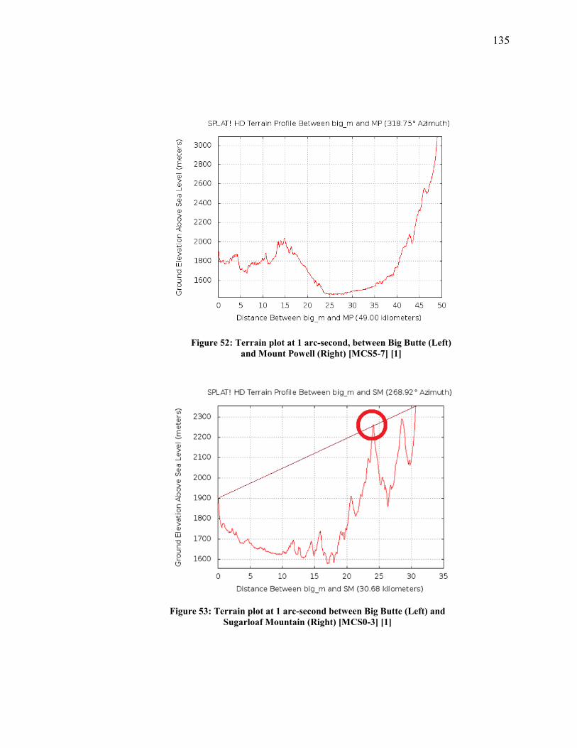
135

Figure 52: Terrain plot at 1 arc-second, between Big Butte (Left) and Mount Powell (Right) [MCS5-7] [1]

Figure 53: Terrain plot at 1 arc-second between Big Butte (Left) and Sugarloaf Mountain (Right) [MCS0-3] [1]

136

8.13

App

endi

x E.

4

Scre

ensh

ot is

take

n w

hile

stat

ions

wer

e in

the

mid

dle

of a

n ex

chan

ge. I

n th

is sim

ulat

ion,

aft

er e

xcha

ngin

g RT

S/CT

S, S

TA3

send

s the

DAT

A to

STA

2, w

hich

lead

s to

an A

CK b

ack

from

STA

2 to

STA

3. H

owev

er, s

ince

ther

e is

dela

y in

volv

ed, t

he A

CK

does

not

rea

ch S

TA3

befo

re a

noth

er r

eque

st (R

TS) c

omes

in a

t the

AP

from

STA

1. T

he A

P is

desig

ned

to te

rmin

ate

its

ACK

timeo

ut in

terv

al (o

rang

e) a

nd re

spon

d ba

ck w

ith a

CTS

to S

TA1.

STA

3 on

the

othe

r han

d w

ould

fini

sh tr

ansm

ittin

g th

e AC

K an

d in

itiat

e DI

FS/B

O c

ycle

bef

ore

atte

mpt

ing

to s

end

the

next

pac

ket i

n its

que

ue, w

hile

obl

ivio

us to

the

fact

th

at th

e AC

K on

the

rece

ivin

g en

d (A

P) h

as b

een

reje

cted

. The

AP

will

retr

y se

ndin

g RT

S/DA

TA w

ith th

e sa

me

sequ

ence

nu

mbe

r if t

his r

eatt

empt

is n

ot re

try#

0. If

it is

retr

y#0,

then

the

pack

et w

ith th

at se

quen

ce n

umbe

r will

be

drop

ped.

--- L

egen

d ---

Br

own

= pa

cket

reje

cted

whe

n re

ceiv

ed

Red

= pa

cket

acc

epte

d w

hen

rece

ived

Gr

een

= tr

ansm

ittin

g pa

cket

Pu

rple

= N

AV C

TS in

terv

al ti

mer

Bl

ue =

NAV

RTS

inte

rval

tim

er

Blui

sh-G

rey

= DI

FS

Blac

k =

Back

off

Ora

nge

= AC

K tim

eout

inte

rval

Br

own

= CT

S tim

eout

inte

rval

Do

tted

-line

= sl

ot b

ound

arie

s

Figure 54: Simulation GUI for DATA Timeout Int. interruption

STA0

STA1

STA2

STA3