Review of Income and WealthSeries 47, Number 2, June 2001

FAST DEVELOPMENT WITH A STABLE INCOME

DISTRIBUTION: TAIWAN, 1979–94

BY F. BOURGUIGNON

DELTA and World Bank, Paris

M. FOURNIER

CERDI (Uniûersite d’Auûergne) and CREST (INSEE, Paris)

AND

M. GURGAND

Centre d’etudes de l’emploi and CREST (INSEE), Paris

This paper studies the mechanisms underlying the apparent stability of the income distribution inTaiwan. An original decomposition method based on micro-simulation techniques is proposed.Applied to the distribution of income in Taiwan since 1979, it permits isolating the respective impactof changes in: (a) the earning structure; (b) labor-force participation behavior; and (c) the socio-demographic structure of the population. The stability of the distribution in Taiwan appears as theresult of various structural forces which happened to offset each other. The small drop observed inthe inequality of individual earnings resulted from the combination of unequalizing changes in thewage structure and the effects of changes in female labor-force participation as well as in the edu-cational structure of the population. However, the same offsetting forces, together with changes inthe composition of households, resulted in a small increase in the inequality of the distribution ofequivalized household income.

INTRODUCTION

A striking feature of Taiwan’s rapid development during the past twenty-fiveyears is that it occurred with very limited changes in the distribution of income.After a large drop in the 50s and 60s, initiated by a successful land reform andreinforced by a vigorous industrialization process,1 the Gini coefficient for indi-vidual earnings stabilized around 0.30.2 Yet structural changes in the economyand the society kept at a rapid pace. Among other things, the agricultural shareof the labor force went down from slightly less than 30 percent in 1979 to 10percent in 1995; the service sector largely overcame the industrial sector and nowemploys almost half the labor force; labor force participation increased signifi-cantly, family size fell, and the schooling level of the population went up in adramatic proportion. How such an evolution could occur without drastic changesin the distribution of income is the question we address in this paper.

Note: Part of a research project funded by the World Bank. We would like to thank the Director-ate-General of Budget Accounting and Statistics (DGBAS) in Taipei for their precious help.

1This is the process so eloquently described and analyzed by Ranis (1974), Fei, Ranis, and Kuo(1979), and Kuo, Ranis, and Fei (1981).

2This stabilization is observed for most inequality indices.

139

Possibly because the experience of Taiwan during the 50s and 60s has oftenbeen cited as one of the clearest cases of development with employment expansionand income equalization, a sizable literature has developed on income distributionin Taiwan. As pointed out by Chu (1997), however, a detailed study of the evol-ution of the distribution of income in Taiwan is still much needed for two reasons.First, the existing literature is at too much an aggregate level to permit under-standing the mechanisms through which income distribution may be affected byexogenous structural changes in the economy or in the socio-demographic struc-ture of the population. Second, it also tends to focus on a single aspect of theproblem—e.g. trade, strength of competition, education—while ignoring otheraspects and the way they interact to produce the observed change in the distri-bution of income.

Several authors have recently tried to overcome these difficulties, mostlythrough some kind of decomposition of income inequality, either by incomesource or by income groups at various points of time. Chu (1997) distinguishestwo periods in the recent history of Taiwan. By a decomposition analysis basedon standard wage regression he shows that the fall in wage inequality between1966 and 1977 is due for approximately one half to changes in both the edu-cational structure of the population and in the rate of return to schooling.Between 1981 and 1992, he finds with the same type of decomposition that thedistribution of household wage income remained relatively stable but theinequality of household income rose because of changes in participation behaviorand in family composition. Using another method based on Shorrocks’ (1982)decomposition of inequality by income sources, Fields and O’Hara (1996) foundthat various forces played a significant role in the observed evolution of earningsinequality. In particular, they show that a rise in the male–female wage differen-tial and in returns to education played an unequalizing role, whereas the drop inthe inequality of the distribution of human capital had an equalizing effect.

These results are in agreement with our conjecture that below the surfaceand behind the apparent stability of the distribution of income, powerful forceshave been at work in Taiwan which, taken in isolation, might have producedsignificant changes in the distribution of income but tended to offset each other.The objective of the present study is to shed light on these various forces by asystematic study of the changes in the micro-economic determinants of incomesand their effects on the distribution of income within the population. This is donethrough an original decomposition method based on an in-depth analysis of theevolution of not only the structure of individual earnings but also that of house-hold self-employment (farm and non-farm) incomes and of individual occu-pational choices within the household. A side product of this method is a measureof the distributional effects of changes in the socio-demographic structure of thepopulation.

The paper is organized as follows. Section 1 presents some basic quantitativefacts on the evolution of Taiwan’s economy over the past two decades, with someemphasis on income distribution. The methodological framework is presented insection 2. The results obtained from applying this method to household surveysover the period 1979–94 are analyzed in two separate sections. Section 3 discussesobserved changes in several types of micro-economic behavior likely to have had

140

substantial distribution effects.3 Section 4 presents the decomposition of thechange in the distribution of individual earnings and household income into thevarious effects mentioned above. Section 5 summarizes and concludes.

1. BASIC FACTS ABOUT ECONOMIC DEVELOPMENT AND INCOME

DISTRIBUTION IN TAIWAN SINCE 1979

Several features with potentially strong implications for the distribution ofincome are readily apparent in the evolution of the socio-demographic structureof Taiwan’s population over the past 20 years or so (see Table 1). The populationis becoming older, better educated, and more urbanized. At the same time, labor-force participation of women is increasing, whereas household composition ischanging.

TABLE 1

EVOLUTION OF THE STRUCTURE OF THE POPULATION AT WORKING AGE

1979 1983 1986 1989 1992 1994

Population (106) 11.0 12.1 12.8 13.4 14.0 14.4

Age structure (%)Less than 30 44.9 42.5 40.4 37.1 34.9 34.730 to 50 38.2 39.0 40.1 43.0 44.9 45.350 to 65 16.9 18.5 19.5 19.9 20.2 20

Education structure (%)Illiterate 12.9 10.9 9.7 8.4 7.2 6.2Primary 37.6 33.6 31.4 29.4 26.1 24.3Secondary 40.1 44.2 46.9 49.4 51.1 52.5University 9.4 11.2 11.9 12.9 15.5 17

Aûerage education by age groups (years)15–30 9.6 10.2 10.6 11.0 11.3 11.530–50 6.9 7.6 8.1 8.8 9.6 9.950–65 5.1 5.4 5.4 5.4 5.6 6

Indiûiduals in agriculturalhouseholds (%) 30.4 27.3 23.3 21.2 19.4 16.2

Aûerage participation rateAll individuals 63.9 62.8 63.0 64.0 64.0 63.3Women 46.1 45.4 47.5 48.8 49.5 50.2Men 81.5 80.3 78.4 78.9 78.4 76.3Agricultural households 57.1 58.2 59.2 59.9 60.3 60.7Non-agricultural households 79.6 75.0 75.7 79.3 79.3 76.5

Aûerage total size of householdsAgricultural households 5.7 5.4 5.1 4.6 4.5 4.4Non-agricultural households 4.6 4.5 4.4 4.2 4.0 3.9

Source: Household surveys, DGBAS, authors’ calculation. First row from Statistical Yearbook,DGBAS.

Most of this evolution is taking take place at a striking pace. Forty-fivepercent of the population at working age was below 30 in 1979. This figure isnow less than a third. Close to 20 percent of individuals at working age have now

3A more complete analysis of that evolution is provided in a companion paper (Bourguignon,Fournier, and Gurgand, 1998a).

141

gone beyond secondary school, a figure that nearly doubled between 1979 and1994. Conversely, the share of the population with no education or no more thanprimary education went down from 50 percent to 30 percent.

Equally impressive is the fast evolution of the urban�rural structure of thepopulation. Over the period studied, the number of individuals at working ageliving in households dedicated to some agricultural activity has approximatelyhalved. This process corresponded partly to a drop in the number of agriculturalhouseholds—which presumably means a change in the distribution of cultivatedland—and partly to a change in the composition of rural households, the size ofwhich diminished quite substantially—from 5.7 to 4.4 persons on average—overthe period under analysis.

This relative loss in the importance of agriculture is among the driving forcesbehind the evolution of other dimensions of the socio-demographic structure of thepopulation. It partly explains the drop in the average household size, although itmay be seen in Table 1 that family size fell significantly and continuously on boththe rural and the urban sides. It should also have had a positive impact on theoverall participation rate since participation is traditionally lower in agriculturalhouseholds. It turns out, however, that, on top of this, the participation rate ofmarried women increased, both in agricultural and non-agricultural households.

The evolution of the structure of GDP paralleled that of the population. Theextremely high growth of GDP recorded over the period under analysis—7.8 per-cent per annum on average—was accompanied by a dramatic change in its struc-ture, which corresponds itself to the superposition of two phenomena. First, theagricultural sector kept losing relative importance. Until 1984, the correspondingshare of GDP went to the manufacturing sector, a continuation of the processobserved since the take off of economic growth in the 60s. In the late 80s, how-ever, the industrialization process itself came to an end and the ‘‘tertiarization’’of the economy began. Between 1988 and 1995, the manufacturing sector lostground in the evolution of the sector structure of GDP in favor of services to thebusiness sector, and, to a lesser extent, commerce and personal services. Second,within the manufacturing sector itself, ‘‘traditional’’ activities like food, textile,wood and paper products lost relative importance in favor of more advancedsectors like chemical industry, metal industry, or electrical�electronic machinery.Overall, there is thus little doubt that, as with the evolution of the population,the period under study is one of intense structural changes in the economy andtherefore on the demand side of the labor market, clearly a constant feature ofTaiwan over the past 50 years or so.

Given the sizable changes that took place in the social and economic struc-ture of Taiwan in the past decade and the speed at which they occurred, onewould expect the distribution of income to have also undergone substantial altera-tions. Three different features are observed, depending on the definition that isadopted of income and income units—see Figure 1. First, the inequality of thedistribution of equiûalized disposable household income—that is, the distributionof individual income with every individual being given the disposable income,deflated by the number of adult equivalents,4 of the household he�she belongs

4The equivalence scale used here is such that the number of adult equivalents in a household isequal to the square root of the number of household members.

142

Figure 1. Evolution of Income Inequality: 1979–94 (Gini)

to—is approximately constant over time. Second, the Gini coefficient of the distri-bution of equivalized primary or market household income, that is, income beforetaxes and transfers, shows a slight ascending trend which tends to accelerate inthe early 90s. Finally, the inequality of individual earnings—non-wage workersexcluded—has been decreasing quite substantially since 1983.5

It seems to have become a stylized fact about the distribution of income inTaiwan that household income inequality made a ‘‘U-turn’’ around the beginningof the 80s—see in particular, Hung (1996) and also Chu (1997). Figure 1 doesnot really support such a view. Individual earnings inequality has substantiallydeclined, whereas the increase in the inequality of equivalized ‘‘primary’’ house-hold income is too moderate for referring to it as a U-turn, especially in view ofthe stability of the inequality of disposable household income. As noted by Fieldsand Leary (1997) and by Schultz (1997), the U-turn is in fact more apparent whenconsidering the distribution of total household income with the household as theincome unit. This suggests that the demographic composition of households haschanged during the period under analysis in a way that is non-neutral with respectto the distribution.

That inequality slightly increased or decreased depending on the definitionof income and of the income unit that is used, seems consistent with the idea ofseveral powerful forces affecting the distribution but offsetting each other. It isindeed natural that this offsetting process leads to different pictures of the evol-ution of the distribution when different perspectives are adopted. The rest of thispaper focuses on the identification of these forces and their compensating effects.

2. EXPLAINING THE EVOLUTION OF THE DISTRIBUTION OF HOUSEHOLD

INCOME: A MICRO-SIMULATION DECOMPOSITION METHOD

Generally speaking, changes in the distribution of individual earnings andequivalized household income over time may come from three sources. (a) People

5A similar evolution is shown for other inequality indices.

143

with given characteristics and the same occupation get a different income becauseprices on the labor and possibly output markets have been modified. We shallrefer to this as the ‘‘price effect.’’ (b) People with given characteristics do notmake the same occupational choices so that the population of earners is modified.This is the ‘‘participation’’ or ‘‘occupation effect.’’ (c) Finally the socio-demo-graphic characteristics of the population of households and individuals—e.g. edu-cation, age, household size—changes over time. We shall refer to this as the‘‘population effect.’’ The objective of the following decomposition method is toidentify these various effects and then to try to relate them to the general evol-ution of the economy.

2.1. Decomposition Principle

The income yit of household i observed at time t may be assumed to dependon four sets of arguments: its observable socio-demographic characteristics orthose of its members (x), unobservable characteristics summarized by ε, the setof prices and labor remuneration rates it faces (β), and a set of parametersdescribing the labor force participation and occupational choice behavior of itsmembers (λ ):

(1) yitGY (xit , ε it; β t; λ t).

The overall distribution of household income at time t, may be expressed as avector Dt of household incomes. Through (1) this vector is itself a function of thedistribution of observable and unobservable household characteristics at date t,the price vector, β t , and the vector of behavioral parameters, λ t. Let H( ) be thatfunction:

(2) DtGH({xit , ε it}, β t , λ t).

where { } refers to the distribution of the corresponding variable in thepopulation.

With such a definition, the various effects mentioned above to describe andexplain the evolution of the distribution between two dates t and t′ can be simplycomputed as follows:

(3) Price effect (a): Btt′GH({xit , ε it}, β t′ , λ t)AH({xit , ε it}, β t , λ t).

(4) Participation effect (b): Ltt′GH({xit , ε it}, βt , λt′)AH({xit, εit}, β t , λ t)

(5) Population effect (c): Ptt′GH({xit′, ε it′}, βt , λ t)AH({xit , ε it}, β t , λ t)

In other words, the population effect, P, is obtained by comparing the distri-bution at date t and the hypothetical distribution obtained by simulating on thepopulation observed at date t′ the remuneration structure and the behavioralparameters of period t. Likewise, the effect of the change in prices is obtained bycomparing the initial distribution and the hypothetical distribution obtained bysimulating on the population observed at date t the remuneration structureobserved at date t′, etc.

The preceding formulae may be seen as an extension of the well-knownBlinder–Oaxaca decomposition method. This method explains the mean income

144

difference between two groups of individuals on the one hand by different meancharacteristics of individuals in the two groups—i.e. our population effect—and,on the other hand, a different remuneration of these characteristics within eachgroup—i.e. our ‘‘price’’ effect. The difference with that method is first that thedecomposition is made here on the full distribution rather than on means and,second, that the income generating model—i.e. the function Y ( ) in (1) may bemore complicated than the linear regression model originally used by Blinder(1973) and Oaxaca (1973).6

A common problem with the Blinder–Oaxaca method is path dependence.For instance, the price effect and the participation effect are likely to depend onthe reference population that is used to evaluate them, unless population, pricestructure, and behavioral parameters are close to each other, which is unlikelyto be the case over the medium or long run in an economy subject to strongstructural changes. In the application that follows, this ambiguity will be takeninto account by considering simultaneously alternative definitions of the variouseffects.

It is also possible to decompose the population effect itself into what may bedue to unobservables and observables. This is easy once a model allowing for theidentification of the unobservable terms, ε it , is available. For instance, let usassume that yit refers to individual earnings. These are assumed to depend onobservables, xit , and unobservables, εit , according to:

(6) ln(yit)Gxitβ tCε it .

The econometric estimation of this earning function permits identifying the‘‘price’’ coefficients, β t , and the distribution of unobservables, {ε it}. Changingthe latter so as to make it identical to the distribution observed in year t′ can bedone using rank-preserving transformations:

(7) ε itGF−1t′ ° Ft (ε it),

where Ft( ) is the function giving the relative rank of its argument in year t’sdistribution. In a continuous framework Ft( ) would simply be the cumulativedistribution function of the unobservable term, ε it . We approximate here Ft( ) bya zero-mean normal distribution, so that the preceding transformation becomes:

(8) ε itGσ t′

σ t

ε it ,

where σ t is the standard deviation of the residual term ε it in year t.7

6A decomposition similar to the present one with a linear income generating function has beenproposed by Juhn, Murphy, and Pierce (1993).

7Note that the normality assumption is made here for simulation purposes, not for estimation.Note also that it is possible to assume some heteroscedasticity whereby the standard deviation of theeffect of unobservables may depend on observables. This makes the decomposition structure substan-tially more complicated. However, we could check that this would not modify the general conclusionsobtained under the assumption of heteroscedasticity. In particular, we checked that the change in thevariance of the residuals of the earning functions could not be imputed to changes in the observablecharacteristics of the population of wage earners.

145

2.2. Modeling Household Incomes

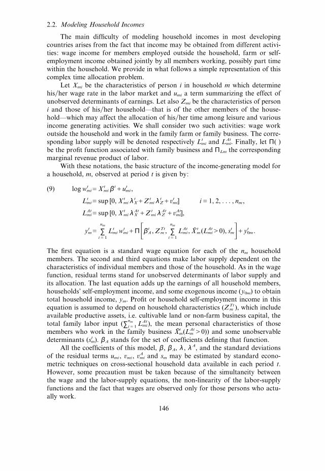
The main difficulty of modeling household incomes in most developingcountries arises from the fact that income may be obtained from different activi-ties: wage income for members employed outside the household, farm or self-employment income obtained jointly by all members working, possibly part timewithin the household. We provide in what follows a simple representation of thiscomplex time allocation problem.

Let Xmi be the characteristics of person i in household m which determinehis�her wage rate in the labor market and umi a term summarizing the effect ofunobserved determinants of earnings. Let also Zmi be the characteristics of personi and those of his�her household—that is of the other members of the house-hold—which may affect the allocation of his�her time among leisure and variousincome generating activities. We shall consider two such activities: wage workoutside the household and work in the family farm or family business. The corre-sponding labor supply will be denoted respectively Lt

mi and LAtmi. Finally, let Π( )

be the profit function associated with family business and ΠLm the correspondingmarginal revenue product of labor.

With these notations, the basic structure of the income-generating model fora household, m, observed at period t is given by:

(9) log wtmiGXt

mi β tCutmi ,

LtmiGsup [0, Xt

mi λ tXCZt

mi λ tZCût

mi] iG1, 2, . . . , nm ,

LAtmiGsup [0, Xt

mi λ AtX CZt

mi λ AtZ CûAt

mi],

ytmG ∑

nm

iG1

Ltmi w

tmiCΠ �β t

A , ZTtm , ∑

nm

iG1

LAtmi , Xr

tm (LAt

miH0), stm�Cyt

0m .

The first equation is a standard wage equation for each of the nm householdmembers. The second and third equations make labor supply dependent on thecharacteristics of individual members and those of the household. As in the wagefunction, residual terms stand for unobserved determinants of labor supply andits allocation. The last equation adds up the earnings of all household members,households’ self-employment income, and some exogenous income (y0m) to obtaintotal household income, ym. Profit or household self-employment income in thisequation is assumed to depend on household characteristics (ZTt

m ), which includeavailable productive assets, i.e. cultivable land or non-farm business capital, thetotal family labor input (∑nm

iG1 LAtmi ), the mean personal characteristics of those

members who work in the family business Xr tm(LAt

m H0)) and some unobservabledeterminants (st

m). βA stands for the set of coefficients defining that function.All the coefficients of this model, β, βA, λ , λ A, and the standard deviations

of the residual terms umi , ûmi , ûAmi and sm may be estimated by standard econo-

metric techniques on cross-sectional household data available in each period t.However, some precaution must be taken because of the simultaneity betweenthe wage and the labor-supply equations, the non-linearity of the labor-supplyfunctions and the fact that wages are observed only for those persons who actu-ally work.

146

Once parameters have been estimated at various points of time, the precedingmodel is used to answer the following questions. What would have been theincome of household m had it adopted at period t the labor supply behaviorobserved at period t′, or had earners been paid according to the wage equationobserved at period t′? To answer this question, it is sufficient to simulate in thepreceding model the effect on household income ym of replacing the set of coef-ficients (β t, β t

A , λt, λ tA) by the values estimated in period t′ while keeping all the

observed characteristics X tm and Zt

m constant. Concerning the residual terms, orthe unobserved household or individual characteristics behind them, it may beassumed that adopting the behavior of period t′ would not have modified theirabsolute value or that it would have maintained their relative values as in (8)above. The only difficulty in the preceding micro-simulation method is for personswho were inactive in period t. For them no value of the residual terms νt

mi andνAt

mi, nor of term utmi is observed. The solution consists of drawing randomly the

values of these three terms in a way consistent with the original model, that isconditionally on their labor-force status or labor supply in period t.8 Once thesethree terms are known, it is a simple matter to see whether the change in the wageequation—i.e. from β to β t—modifies the labor status of an inactive person ornot, and, if it does, how the income of the household is itself altered. The oppositecase of an active person becoming inactive is easier to handle because it is notnecessary to reconstitute the unobserved residual terms. The same technique isused for the residual term sm of the profit function.

The total income of a household appears, as initially postulated in (1), as aknown function of its characteristics, observable and non-observable, a set ofbehavioral parameters and a set of ‘‘prices.’’ What is interpreted as ‘‘prices’’ inthe present framework is the complete vector β as well as the coefficients βA

appearing in the profit function, Π( ). Changes in this vector over time show howmarket remuneration of individual and family attributes may have changed, thusaffecting potential personal wage and family self-employment income and poss-ibly participation or occupational decisions within the family.

The structure of the model is now complete. The full model (9) is what playsthe role of the income generating function (1) used above in the description of thedecomposition principles with the following set of equivalence between notations.Observable characteristics xit now correspond to the set of general characteristics ofa household and its members observed at period t, respectively Zt

m and Xtmi . Unob-

servables, ε it , are summarized by the set of residual terms (utmi , û

tmi , û

Atmi , s

tm) which

enter the individual earnings functions, individual labor supply equations and thehousehold profit function in case it engages in farm or independent business activi-ties. The price system includes the coefficients of the earnings and profit equations,β t and β t

A. Finally, the set of behavioral parameters λ t is the whole set of coefficientswhich enter the labor supply functions, that is (λ t, λ At ).

2.3. Econometric Specification

Estimating the complete income generation model (9) in its general formabove is practically impossible, or would be a formidable undertaking. There are

8For instance the value of νtmi in the wage labor supply function of (9) is bounded from above

by AXtmiλ t

XAZtmiλ t

Z for somebody not working as a wage worker.

147

several reasons for this. First, all the equations of the model must clearly beestimated simultaneously with non-linear estimation techniques due to the non-negativity constraint on labor supply and the very likely correlation betweenunobservables or the residual terms in the various equations. Although intricate,things might be manageable—under some simplifying assumptions—if there werea single individual in every household. But the obvious correlation between theearnings equations and labor supply equations of the various members of a house-hold at working age, whose number varies across households, makes things hope-lessly complicated. An additional risk would also be that the results of such acomplex model might not be very robust and show artificial time variability, thusjeopardizing the decomposition method shown above. The micro-economic esti-mation work undertaken for Taiwan relies on a simplified but at the same timemore robust specification based on the following principles.

• Individual earnings functions and household profit functions—if appli-cable—are estimated separately and consistently through the instrumen-tation of endogenous right-hand side variables and the correction ofselection biases. Residual terms of these functions are assumed to be inde-pendent across household members.

• Because of a lack of information on hours of work, labor-supply behavioris estimated in a discrete way. Household members are assumed to havethe choice between the following activities: (i) inactivity, (ii) wage work,(iii) work on family farm, (iv) work in family non-farm business, and(v) combinations of (ii) and (iii).9 This choice is specified as a multinomiallogit model.

• The simultaneity between household members’ labor-supply decisions istaken into account solely by considering sequentially the various membersof the household. This is in agreement with standard practice in the labor-supply literature. The labor-supply decision of the household head is esti-mated first with the preceding multinomial logit model and using both thegeneral exogenous characteristics of the household and those of all house-hold members as explanatory variables. Second, the labor-supply andoccupation decision of all other members is estimated conditionally on thedecision taken by the head, and possibly his�her income in case he�she isengaged in wage work. In addition, different models were estimateddepending on the position of a person in a family. Indeed, it seems naturalthat, other things being equal, the spouse of the head does not behave inthe same way with respect to labor-supply as his�her son�daughter. Thecategories for which distinct labor-supply models have been estimated arespouses, sons and daughters less than 25 years old, and ‘‘other’’ householdmembers.

• It would have been possible to use the results of the multinomial logitoccupational choice model to control for selection in the earnings and

9All sorts of combinations of these basic activities are encountered in the data. However, someof them are so infrequent that their incidence cannot be estimated econometrically. Individualsobserved with ruled-out combinations of activities were assigned to the activity in (i)–(v) yielding thehighest income.

148

profit functions. This was not done in order to keep the estimation pro-cedure simple. Instead, the usual Heckman two-step procedure wasimplemented with an intermediate Probit estimation of the probability thatan individual be a wage worker, whether full-time or in combination withself-employment, or that a household be engaged in self-employmentactivity.

• The lack of robustness of the estimates of some coefficients in the variousbehavioral equations of the model and their possibly non-significant varia-bility over time would clearly introduce some noise in the decompositiontechnique described above. To avoid this, all the original estimatesobtained in the various cross-sections have been submitted to the following‘‘time smoothing’’ treatment. For each series of estimates of a coefficientof the model, a simple regression was run on a time polynomial of order2. Only significant terms in this regression were kept and original estimateswere replaced by the corresponding predicted values. All behavioral equa-tions in the model were then rerun to adjust the intercept accordingly. Apossible consequence of this is to reduce the amplitude of price effects inthe decomposition method by taking away what is interpreted as tempor-ary changes in behavioral coefficients.

• In order to implement the micro-simulation procedure described above,three types of residuals have to be drawn. First, participation functionsresiduals are needed at the individual level. Once these are obtained in away consistent with observed occupational choices and the multinomiallogit model, the effect on activity of a change in estimated coefficients caneasily be simulated through the multinomial logit specification.10 Second,wage functions, residuals must be drawn for individuals observed out ofwage work in year t but predicted to be wage workers in the simulation.Third, profit function residuals are also needed at the household level forfamilies for which no independent activity is observed in the base year ofthe simulation.

3. CHANGES IN INCOME FUNCTIONS AND OCCUPATIONAL CHOICE BEHAVIOR

DURING THE 1976–94 PERIOD

The preceding method is now applied to a series of household surveys takenyearly from 1979 to 1994 by the Government of Taiwan (Directorate-General ofBudget Accounting and Statistics, DGBAS). Each sample comprises approxi-mately 16,000 households. Variables used in the present study are fully com-parable across all samples.

Discussing in detail the estimation results of the preceding model would havetaken too much space. We sketch here only those results that are important for

10The multilogit model relies on the following structural specification of choice among variousalternatives. Let pj be the probability that alternative j is chosen and let X be the explanatory variablesof the choice: pjGProb(XbjCûjHXbkCûk for all k≠ j), where the bi’s are vectors of coefficients. Themultilogit relies on the assumption that the effects of unobservables, ûi , are distributed as independentrandom variables with double exponential distributions. Simulation of occupational choices in thepresent method requires the drawing of these ûi terms conditionally on observed occupational choices.For the detail see Bourguignon, Fournier, and Gurgand (1998a).

149

the understanding of the decomposition analyzed in the next section. More detailon the estimation results is given in a companion paper (see Bourguignon, Four-nier, and Gurgand, 1998a).

Three changes in the structure of labor income and occupational choicebehavior are important for the understanding of the evolution of Taiwan’s incomedistribution since 1979. These are: (a) an increase in the rate of return to schoolingamong wage workers, (b) a drop in the variance of the residual term of the earn-ings equations, and (c) an increased autonomy of spouses’ labor supply and occu-pational choice, that is, lesser dependence on household heads’ income andgreater dependence on own education. We analyze briefly each issue in turn.

Table 2 reports the estimates of a standard Mincerian earning function esti-mated for various years during the period under analysis. The striking result inthat table is the increasing trend in the coefficient measuring the return to edu-cation for both men and women over the whole period under analysis.11 Roughlyspeaking the rate of return for an additional year of schooling increased from alittle more than 3 to 6 percent for men, and from 6 to 8 percent for women duringthe fifteen year period under analysis. Over time, the wage structure in Taiwan’slabor market thus tended to change in favor of better educated workers. Otherthings being equal, the earning differential between somebody with six years ofschooling (i.e. primary school) and somebody with twelve years (i.e. completedsecondary) increased by approximately 10 percent for both men and womenbetween the end of the 70s and the mid 90s.

Previous studies of the evolution of the wage structure in Taiwan are notin contradiction with this finding, although they point to a somewhat milderunequalizing trend. Using the Labor Force Survey of the Taiwan Area for 1978–91, Gindling, Goldfarb, and Chang (1995) found a slowly increasing trend in theearnings differential between upper and primary education until approximately1988 for men with a small drop afterwards, and a continuously increasing trenduntil 1991 for women. Using the same data source as Gindling et al. (1995), Fieldsand O’Hara (1996) also found that the coefficient of the number of years ofschooling in the typical log wage regression increased significantly from 0.050 to0.057 between 1980 and 1993 in a sample including both men and women.12

The evidence obtained from Household Surveys on the increase of the returnto education is thus more pronounced than with Labor Force Surveys. A possibleexplanation of this difference is the fact that the number of hours of work is notobserved in the household survey, whereas it is explicitly taken into account inthe studies just mentioned.13 These studies also make use of other variables notavailable in the household survey, like tenure in the current main job, job mobility

11All our results are robust to the introduction of education either as a quadratic form or througha set of dummy variables representing educational levels.

12Jiang (1992) found a ‘‘wage compression effect’’ across educational levels between 1978 and1986, although he also uses the Labor Force Surveys. However, it is possible that his conclusion isdue to the fact that he simultaneously controls for the sector of activity of wage earners and theiroccupations, both variables likely to be correlated with formal education.

13The part-time dummy variable appearing in the regressions shown in Table 2 actually corre-sponds to the case of workers reporting being involved in both wage work outside the household andself-employment.

150

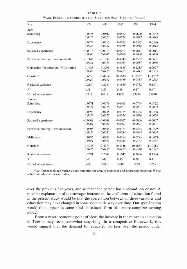
TABLE 2

WAGE FUNCTIONS CORRECTED FOR SELECTION BIAS (SELECTED YEARS)

Year 1979 1983 1987 1991 1994

MenSchooling 0.0325 0.0502 0.0562 0.0620 0.0582

0.0015 0.0016 0.0016 0.0017 0.0018

Experience 0.0674 0.0715 0.0705 0.0592 0.05860.0023 0.0021 0.0019 0.0018 0.0018

Squared experience −0.0013 −0.0013 −0.0013 −0.0011 −0.00110.0000 0.0000 0.0000 0.0000 0.0000

Part time dummy (instrumented) −0.1147 −0.1038 −0.0843 −0.0563 −0.06010.0034 0.0033 0.0034 0.0034 0.0036

Correction for selection (Mills ratio) 0.1488 0.3295 0.3635 0.2255 0.29770.0383 0.0412 0.0425 0.0445 0.0505

Constant 10.6350 10.4214 10.5639 11.0537 11.12320.0430 0.0442 0.0449 0.0487 0.0533

Residual variance 0.2180 0.2244 0.1850 0.1732 0.1801

R2 0.51 0.52 0.48 0.47 0.47

No. of observations 12711 14217 13428 13034 12990

WomenSchooling 0.0571 0.0679 0.0663 0.0794 0.0822

0.0024 0.0025 0.0023 0.0025 0.0024

Experience 0.0396 0.0435 0.0379 0.0384 0.03880.0032 0.0028 0.0026 0.0026 0.0024

Squared experience −0.0008 −0.0008 −0.0007 −0.0006 −0.00070.0001 0.0001 0.0001 0.0001 0.0001

Part time dummy (instrumented) −0.0605 −0.0548 −0.0371 −0.0282 −0.02290.0038 0.0035 0.0034 0.0034 0.0034

Mills ratio 0.0486 0.0283 0.0164 0.0785 0.04690.0391 0.0397 0.0368 0.0373 0.0355

Constant 10.4945 10.4774 10.8146 10.9684 11.05130.0475 0.0452 0.0473 0.0510 0.0541

Residual variance 0.2391 0.2348 0.1647 0.1666 0.1384

R2 0.45 0.42 0.36 0.39 0.41

No. of observations 5780 7403 7448 7729 7765

Note: Other included variables are dummies for area of residence and household position. Whiterobust standard errors in italics.

over the previous five years, and whether the person has a second job or not. Apossible explanation of the stronger increase in the coefficient of education foundin the present study would be that the correlation between all these variables andeducation may have changed in some systematic way over time. Our specificationwould thus appear as some kind of reduced form of a more complete earningmodel.

From a macroeconomic point of view, the increase in the return to educationin Taiwan may seem somewhat surprising. In a competitive framework, thiswould suggest that the demand for educated workers over the period under

151

analysis increased faster than the supply, which we have seen grew at an acceler-ated rate over the period. The growth of demand has obviously to do with theoverall growth rate but doubtlessly also with the change in the structure of theeconomy, which we have seen in section 1 has been quite dramatic.14

The second striking feature in Table 2 is the fall in the standard error of thedisturbance term of the earnings equation. Since the analysis of Juhn, Murphy,and Pierce (1993) for the USA it has become customary to interpret this term asrepresenting the dispersion of the remuneration of unobserved productive talents.In the case of Taiwan, the evidence would thus suggest that unobserved talentswere remunerated in a more homogeneous way in the 90s than in the late 70s. Itis not clear, however, that this would be the right interpretation. It must be keptin mind that we control very badly for hours of work in the earnings equations.We essentially do so through a dummy variable indicating that wage earnershave other self-employment activities and implicitly through the selection biascorrection factor, which in some sense may be interpreted as linked to laborsupply. Under these conditions, it is quite possible that the drop in the meansquared residual term of the earnings equations corresponds to more homogeneityin working hours among wage earners. To check whether this is actually the casewould require re-estimating earnings equations with another database that wouldinclude hours of work.

The last major change in the household income generation behavior is con-cerned with the occupational choices of married women. As mentioned above,this choice is modeled through a multinomial logit model. Reviewing all the esti-mated coefficients of this model would be cumbersome and of limited interest.The few significant changes in these coefficients are concerned with the incomeand price effect of married women’s occupational choice. Figure 2 shows theevolution of the estimated mean (quasi) elasticity of the probability that a marriedwoman takes up various occupations with respect to her husband’s earnings15—in case he is a wage worker—and with respect to her own education. It can beseen that inactivity and wage work are less and less dependent on husbands’income and more and more on education. It thus seems the case that the corre-lation between husbands’ and wives’ income tended to increase over time. Becauseof this husband income effect and the positive correlation between husbands’and wives’ education, it turns out that wives’ labor income increased over timerelatively more in households where heads were relatively well-off.

There are other noticeable features in the evolution of the coefficients ofearning equations, family farm and non-farm income functions, and occupationalchoice models over the period under analysis. They are quantitatively of lesserimportance than the points stressed above, however, and we prefer to leave themaside for the clarity of the argument.16

14It is interesting that the opposite evolution seems to have taken place in Korea in similarcircumstances. Kim and Topel (1995) insist on the fact that returns to education declined there becauseof the big increase in the average education of the labor force. Their paper refers to the 1970–90period, though. Things might be less clear cut for the more recent period.

15The quasi elasticity indicates by how many percentage points the probability of being inactiveor a wage worker changes when husbands’ earnings change by 1 percent.

16Some of them are handled in some detail in Bourguignon, Fournier, and Gurgand (1998a).

152

Figure 2. Quasi-Elasticity of Spouse Labor Supply With Respect to Head’s Wage and Education

4. DECOMPOSITION OF THE CHANGE IN THE DISTRIBUTION OF INCOME

OVER 1979–94

We are now in the position of applying the decomposition method presentedabove for identifying the distributional effects of changes in the structure of wagesand self-employment incomes, in occupational preferences, and in the structureof the population. To make the analysis clearer, we consider only the initial andterminal years of the period under analysis. However, as we have seen that thedecomposition method might be sensitive to the sample chosen as a referencefor computing the price and participation effects, we also used the second andpenultimate years. Actually, we consider in what follows results obtained with allcombinations of the two adjacent initial years, 1979–80, and the two terminalyears 1993–94, using alternatively the initial and the terminal year as the referencesample to compute price and participation effects. In view of the path dependenceproperty noted above, this leads to eight possible evaluations of price, partici-pation and population effects.17 In a very rough way, this permits identifying asort of ‘‘confidence interval’’ for these various effects or, alternatively, measuringthe extent to which they are sensitive to the population that is chosen as areference.

4.1. Decomposition of the Change in the Distribution of Indiûidual Earnings

We start with the distribution of individual wage earnings. The results of ourdecomposition method are summarized in Table 3(A) for changes in mean

17That is four different combinations of initial and terminal years, and for each combination twodecompositions depending on whether the initial or terminal population sample is used as a reference.

153

TABLE 3

DECOMPOSITION OF THE EVOLUTION OF INDIVIDUAL EARNINGS (79–80�93–94)

Mean Maximum MinimumChange (a) Change (a) Change (a)

A: Eûolution of the mean earnings ( percent change)Obserûed ûariation 129.8 137.7 122.0

Price and participation effect 118.2 131.5 108.3Price effect 118.4 128.9 110.8Participation effect −0.1 2.7 −2.6

Population effect 11.6 24.0 2.1

B: Eûolution of earnings inequality (change in Gini coefficient)Obserûed ûariation −0.024 −0.027 −0.021Price and participation effect 0.022 0.008 0.036

Price effect 0.028 0.016 0.040Participation effect −0.006 −0.010 −0.003

Change in earning equation’s residual variance −0.027 −0.036 −0.020

Population effect −0.018 −0.034 −0.001

Note: (a) Minimum and maximum values among all combinations of initial and terminal yearsand�or initial or terminal population samples for decomposition methodology. Mean changecomputed on all combinations.

income, in Table 3(B) for Gini coefficients, and in Figure 3 for the full distri-bution of individual earnings as approximated by conventional Kerneltechniques.18 For the various effects of interest, this figure depicts the change inthe density of the distribution after normalizing the mean income of thepopulation.19

Price Effect and the Unequalizing Influence of the Increase in Educational Returns

The first step in the decomposition consists of modifying the structure ofearnings while keeping the population of wage earners constant. This causes anincrease in the mean real earning of wage workers equal to 118 percent, of whichapproximately half is due to the change in the intercept of the wage functions inTable 2 and half is due to productivity gains associated with education or experi-ence. This impressive productivity gain represents 90 percent of the overallincrease in the mean earning of wage workers during the period under analysis.Interestingly enough, this implies that the change in the composition of the wagelabor force explained only a tiny fraction of the extremely fast expansion ofearnings.

Concerning the distribution of earnings, the dominant effect in the evolution isof course the observed increase in the return to education. This produces an un-ambiguous increase in the inequality of the distribution. Indeed, in this simulation,

18We use a Gaussian kernel with bandwidth hG0.9m�n1�5 where m is the minimum of the stan-dard error of the income distribution and the interquartile range divided by 1.349 and n is the numberof observations.

19A similar technique is used in a different framework by diNardo, Fortin, and Lemieux (1996).Note that, unlike Table 3(B), Figure 3 refers to a single pair of initial and terminal years. These are1979 and 1994. This may explain some discrepancy between the results appearing in Table 3(B) interms of mean changes in the Gini coefficient and Figure 3.

154

Figure 3. Decomposition of the 1979–94 Change in the Distribution of Individual Earnings (Change in Kernel estimates of density after normalizing earningsby the mean and taking logs)

155

earners in the bottom 10 centiles would have gained slightly less than 100 percentover the whole period, whereas people in the top 10 centiles would have gainedmore than 130 percent. Figure 3.1 shows that, after normalizing by the meanincome, the distribution resulting from the price effect corresponds to a mean-preserving spread of the initial distribution. The density of the distribution dimin-ishes in an interval slightly above the mean of the distribution and increases onboth sides of that interval. Depending on the population that is used to evaluatethis effect, it may be seen in Table 3(B) that the change in the Gini coefficientranges from 0.016 to 0.040 with a mean change equal to 0.028. There is nothingreally surprising in the magnitude of this range. It is indeed to be expected thatthe effect of a change in the return to education on the distribution of earningsdepends on the distribution of schooling in the population, which we have seenhas drastically changed over the period studied in Taiwan.

The Equalizing Effect of Changes in Participation and Occupational Choice

The effects of changes in participation and occupational choice behavior aremore subtle to analyze than the pure price effects above because they correspondto a modification in the population of individual earners. Figure 4 representsthese modifications by showing the simulated entries and exits from the 1979 wagelabor force which would have occurred had people adopted the participation and

Figure 4. Overall Participation Effect: Simulated Entries and Exits from the Wage Labor Force

occupational choice behavior observed in 1994. For all wage earners, Figure 4.1shows that there has been an equalizing effect resulting from net exits at the twoextremes of the distribution, thus leading to no significant change in mean earn-ings, as shown in Table 3(A). However, this general evolution results itself fromvarious phenomena and in particular from opposite tendencies among men and

156

women. The participation of men to the wage labor force fell over the periodunder analysis at approximately the same rate along the (men) wage scale, but alittle more at the bottom (Figure 4.2). For women, there were more entries thanexits, except in the bottom centiles of the (women) wage scale (Figure 4.4).Because there are more men than women at the top of the distribution of wageearners, the dominant effect there is the exit of workers, as may be seen in Figures4.1 and 4.3. Conversely, as women are located in the bottom and middle part ofthe overall distribution of wages, they contributed to a net entry of workers inthe middle part of the distribution, compensating there the net exit of men (seeFigures 4.5 and 4.1). Overall, the change in participation behavior, which essen-tially consisted of a drop in the wage labor force participation of men and anincrease in that of women, had an unambiguously equalizing effect on the overalldistribution of individual earnings. However, it may be seen in Figure 3.2 thatthis effect was very moderate. The change in participation behavior produceda mean preserving ‘‘squeeze’’ of the distribution that is almost negligible incomparison with the change actually observed between 1979 and 1994.

The Equalizing Effect of the Drop in Residual Earning Variance

Of course this change has by definition no effect on mean earnings. On thedistribution side, it also corresponds to a somewhat tautological step in thedecomposition method. We have seen that earnings heterogeneity as described bythe residual terms of earning equations fell substantially over time. This evolutionmay reflect an increase in the homogeneity of either the productivity of workerswith identical observed characteristics or of working hours. Table 3(B) showsthat this effect is responsible for a drop of 0.020 to 0.036 in the Gini coefficientof individual earnings. It may be seen in Figure 3.3 that this effect is responsiblefor a mean preserving squeeze of limited amplitude in terms of density. Howeverthis squeeze is taking place on a rather wide interval involving individuals at thetwo extremes of the distribution, which explains the relatively big change in theGini coefficient.

Population Effect

Taking the sum of the preceding effects out of the actual change in the distri-bution of individual earnings yields the population effect as a residual. As shownin Table 3(A), this evolution explains around 9 percent of the rise in the meanindividual earning, which is mostly due to the rise in the average education attain-ment within the working population. The resulting change in the distributionshown in Figure 3.4 as well as the change in the Gini coefficient shown in Table3(B) suggest that the change in the socio-demographic structure of the populationwas strongly equalizing. However, the estimation range appearing in Table 3(B)is rather wide, which means that this effect may be more path dependent thanthe preceding effects taken individually.

There is little doubt that the equalizing of the distribution of schooling withinthe wage labor force contributed to an equalizing of the distribution of earnings—see Fields and O’Hara (1996) as well as our own work (Bourguignon, Fournier,and Gurgand, 1998b). This is the phenomenon behind the mean preserving

157

squeeze shown in Figure 3.4. But the range estimated for the change in the Ginicoefficient in Table 3(B) shows that other forces have probably been at work.The effect of the change in the structure of schooling in the population is naturallymore pronounced when evaluated with 1993�1994 prices because the rate ofreturn to education was higher at that time. Schooling thus dominates otherchanges in the structure of the population which might have had an unequalizinginfluence. This is what is depicted by Figure 3.4 and the upper limit of the rangeof the Gini coefficient in Table 3(B). Using 1979�1980 prices to evaluate thepopulation effect yields less pronounced changes.

Overall, it thus appears that the fall in the inequality of individual earningsin Taiwan over the period 1979–94 results from several strong forces which havenot all pushed in the same direction. On the unequalizing side, a change occurredin the wage structure. More specifically a rise in the returns to education increasedearnings disparities. On the equalizing side, three phenomena of unequal import-ance permitted overcompensating the preceding evolution. They are: (a) the fallin the variance of the unobserved determinants of earnings; (b) changes in thesocio-demographic structure of the population of wage earners, most notablychanges linked to the structure of schooling; and finally (c) the change in partici-pation and occupational choice behavior which brought more women in the wagelabor force.

4.2. Decomposition of the Eûolution of the Distribution of Household Income

We may contrast the above results with the analysis of the distribution ofequivalized primary household income. We already know that this distributiontended to become more unequal during the period under analysis, whereas thatof individual earnings became more equal. This means that the forces that werejust identified for distributional changes in the case of individual earnings musthave had different intensities or must have been complemented by other ones. Inwhat follows we review the same issues as for individual earnings and try toidentify where the difference may lie. Results are summarized in Table 4 andFigures 5 and 6.

Price Effects

Over the period, the mean household income per adult equivalent rose fromNT$139,000 to 338,000. Table 4(A) shows that, as for individual income but toa lesser extent, most of that evolution is explained by pure productivity gains inearnings and self-employment incomes.

The unequalizing effect due to the evolution of the individual earning struc-ture should normally be transmitted to household incomes. It may be expectedto be smaller, however. Even though there is some correlation between the charac-teristics (e.g. education) of various household members this correlation is notperfect, which is an equalizing factor. Therefore, it comes as no surprise to see inTable 4(B) that the change in the Gini coefficient attributable to the pure priceeffect is smaller than the corresponding figure in Table 3(B). Although the meanvalue is still substantial (i.e. 0.021), the lower bound of the confidence interval isin fact rather low. In terms of the decomposition of the overall change in the

158

TABLE 4

DECOMPOSITION OF THE EVOLUTION OF EQUIVALIZED HOUSEHOLD INCOME (79–80�93–94)

Mean Maximum MinimumChange (a) Change (a) Change (a)

A: Eûolution of the mean earnings ( percent change)Obserûed ûariation 134.5 142.4 126.6Price and participation effect 109.2 126.4 95.4

Price effect 104.5 120.1 91.7Participation effect 4.7 6.3 3.6

Population effect 25.3 41.2 12.4

B: Eûolution of earnings inequality (change in Gini coefficient)Obserûed ûariation 0.021 0.015 0.027Price and participation effect 0.031 0.000 0.061

Price effect 0.021 0.003 0.036Participation effect 0.011 −0.003 0.025

Change in earning equation’s residual variance −0.017 −0.023 −0.010

Population effect 0.005 −0.028 0.037

Note: (a) Minimum and maximum values among all combinations of initial and terminal yearsand�or initial or terminal population samples for decomposition methodology. Mean changecomputed on all combinations.

distribution of household income, it may be seen in Figure 5 that, interestinglyenough, the price effect almost coincides with the actual mean preserving spreadactually observed between 1979 and 1994.

Participation Effects

The difference with individual earnings here is still more pronounced. First,as shown in Table 4(A), changes in participation behavior and occupationalchoice led to a rise in average household income. This effect was necessarily verylimited for individual earners since the mean income was evaluated, by definition,on the population of active individuals being employed as wage workers. Second,whereas this evolution was unambiguously equalizing in the case of individualearnings, it is not so any more. On average, it even is unequalizing when oneconsiders the change in the Gini coefficient (see Table 4(B)). In Figure 5 it clearlycontributes to a mean preserving spread at the middle of the distribution.

Two phenomena explain this difference. The first has been alluded to in thepreceding section and has been analyzed in some detail in Fournier (1997). It isthe drop in the (negative) effect of husbands’ income on married women laborforce participation. Because of this evolution, we expect that applying to thesample of 1979 households the participation and occupational choice behavior of1994 will lead to relatively more women entering—in net terms—the labor forceat the top of the distribution of household income. It may be seen that this isexactly what is observed in Figure 6.1. But there is another, more powerful expla-nation. It was seen above—Figure 4.4—that women who entered the (wage) laborforce between 1979 and 1994 were on average better educated than women whowere already active. This had an equalizing effect on the overall distribution ofindividual earnings because these women entered the middle of the distributionof wages. Things are different for household income, however, because better

159

Figure 5. Decomposition of the 1979–94 Change in the Distribution of Equivalized Household Market Income(Change in Kernel estimates of density after normalizing incomes by the mean and taking logs)

160

educated women tend to be in relatively richer households. Nothing of this typewas observed for men. It was seen above that they tended to exit the labor forcein a more or less neutral way with respect to the distribution of male individualearnings. Figure 6.2 suggests that neutrality also holds with respect to householdincome. It is therefore mostly the change in women labor force participation andits increased elasticity with respect to education that explains the unequalizingeffect of participation behavior on household income.

Figure 6. Overall Participation Effect on the Distribution of Household Income: Percentage ofIndividuals Entering or Exiting the Labor Force by Household Centiles

The Effect of Earnings’ Residual Variance

As for the price effects above, the fact that there are various wage earners ina household should reduce the distributional impact of the drop in the varianceof the unobserved determinants of individual earnings. This is what is observedin Table 4(B) and Figure 5. The drop in the Gini coefficient of equivalized house-hold income is only 0.017, whereas it was 0.028 for individual earnings.20

Population Effect

As for individuals, Table 4(A) shows that changes in the population structureled to an increase in average equivalized household income. The effect is greater,though, because the drop in household size comes on top of the rise in averageeducation. On the distribution side, an important difference with the decompo-sition of the change in the structure of individual earnings is that the populationeffect is now in the direction of more inequality. However, the confidence intervalappearing in Table 4(B) suggests this effect is ambiguous in the case of householdincome, whereas it was unambiguously equalizing in the case of individual earn-ings. The density difference shown in Figure 5.4 also suggests rather complexdistributional changes.

20Note, however, that no attempt has been made at simulating the effect of observed changes inthe variance of the residuals of farm and non-farm profit functions.

161

Because they are mostly determined as a residual effect, these changes areimpossible to identify directly. Since the population effect was strongly equalizingat the individual level, it is possible to say that unequalizing changes necessarilytook place in the matching of indiûiduals within households. For instance the corre-lation of potential earnings and schooling levels among household members mighthave increased. Likewise, changes in the composition of households, in particularthe drop in household size, may have been correlated with potential income. Thisis in agreement with the analysis of Fields and Leary (1997), who found thatchanges in the demographic structure of households and an increase in the corre-lation of spouses’ education had unequalizing effects on the level of inequality.The consequences of a change in this matching are also analyzed in Fournier(1999).21

5. CONCLUSION

Applying an original decomposition analysis of the change in income distri-bution to Taiwan during the 1979–94 period, this paper identified some explana-tory factors of the observed equalization of the distribution of individual earnersand of the unequalizing distribution of household income. These factors areclosely linked to the drastic transformation in the economy and in the socio-demographic structure of the population during that period.

Four phenomena were shown to be important in the evolution of the distri-bution of individual earnings. (a) Changes in the wage structure contributed toan increase in inequality. These can be imputed in a large part to an increase inthe return to schooling that took place despite a dramatic growth in the supplyof educated workers. However, this effect was more than offset by three othertendencies. (b) A drop in the variance of the effect of unobserved earnings deter-minants, the nature of which is still to be identified. (c) A change in participationand occupational choice behavior which contributed to an increase in the relativeweight of the middle earners. (d) Changes in the socio-demographic structure ofthe population. Altogether these four tendencies produced a significant drop inthe inequality of individual earnings.

The same phenomena affected the evolution of the distribution of equivalizedprimary household income but their overall effect was somewhat different. Otherforces were present too, so that the evolution went in the opposite direction andinequality unambiguously increased between 1979 and 1994. In comparison withthe evolution of the distribution of individual earnings, this was shown to bethe result of the participation effect which proved to be unequalizing at the house-hold level—the net entrants in the labor force belonging to the upper part of thedistribution—and changes in the socio-demographic structure of the householdpopulation, and more precisely in household composition.

REFERENCES

Blinder, A. S., Wage Discrimination: Reduced Form and Structural Estimates, Journal of HumanResources, 8, 436–55, Fall 1973.

21Following the method in Burtless (1998).

162

Bourguignon, F. and M. Martinez, La dynamique de la distribution des revenus: une analyse dedecomposition par micro-simulation, in D. Fougere and E. Malinvaud (eds), Emploi et Chomage,de Boek, forthcoming, 2001.

Bourguignon, F., M. Fournier, and M. Gurgand, Wage and Labor-force Participation Behavior inTaiwan: 1979–94, Mimeo, 1998a.

———, Distribution, Development and Education: Taiwan, 1979–94, Mimeo, 1998b.Burtless, G., Effects of Growing Wage Disparities and Changing Family Composition on the U.S.

Income Distribution, European Economic Reûiew; 43(4–6), 853–65, 1999.Chu, Y. P., Employment Expansion and Equitable Growth: Taiwan’s Postwar Experience, Mimeo,

1997.DiNardo, J., N. Fortin, and T. Lemieux, Labor Market Institutions and the Distribution of Wages,

1973-92: A Semiparametric Approach, Econometrica, 64(5), 1001–44, September 1996.Fei, J., G. Ranis, and S. Kuo, Growth and the Family Distribution of Income by Factor Component,

Quarterly Journal of Economics, 17–54, February 1978.———, Growth with Equity: The Taiwan Case, Oxford University Press, New York, 1979.Fields, G. and O’Hara, Changing Income Inequality in Taiwan: a Decomposition Analysis, Mimeo,

1996.Fields, G. and B. Leary, Economic and Demographic Aspects of Taiwan’s Rising Family Income

Inequality, Mimeo, 1997.Fournier, M., Inequality and Economic Development: A Microsimulation Study of the Taiwan

Experience (1976–92), Mimeo, 1997.———, Inequality Decomposition by Factor Component: A New Approach Illustrated on the Tai-

wanese Case, Etudes et documents du CERDI, 99–20, 1999.Gindling T., M. Goldfarb, and C. C. Chang, Changing Returns to Education in Taiwan: 1978–91,

World Deûelopment, 23, 343–56, 1995.Hung, R., The Great U-Turn in Taiwan: Economic Restructuring and a Surge in Inequality, Journal

of Contemporary Asia, 26, 151–63, 1996.Jiang, F. F., The Role of Educational Expansion in Taiwan’s Economic Development, Industry of

Free China, LXXVII, 37–68, April 1992.Juhn, C., K. Murphy, and B. Pierce, Wage Inequality and the Rise in Returns to Skill, Journal of

Political Economy, 101, 410–42, 1993.Kim, D.-I. and R. H. Topel, Labor Markets and Economic Growth: Lessons from Korea’s Indus-

trialization, 1970–90, in C. Freeman and L. Katz (eds), Differences and Changes in Wage Struc-tures, NBER, University of Chicago Press, 1995.

Kuo, S., G. Ranis, and J. Fei, The Taiwan Success Story, Westview Press, Boulder, Colorado, 1981.Lee, L. F., Generalized Econometric Models with Selectivity, Econometrica, 51, 507–12, March 1983.Oaxaca, R., Male–Female Wage Differentials in Urban Labor Markets, International Economic

Reûiew, 14, 693–709, October 1973.Ranis, G., Taiwan, in Chenery et al. (eds), Redistribution with Growth, Oxford University Press, 1974.Schultz, T. P., Income Inequality in Taiwan 1976–95: Changing Family Composition, Aging and

Female Labor-Force Participation, Economic Growth Center Discussion Paper, Yale University,no. 778, November 1997.

Shorrocks, A., Inequality Decomposition by Factor Components, Econometrica, 50, 193–211, 1982.

163