Fast depth from defocus from focal stacks - Graphics and ...

unco

rrec

ted

pro

of

Vis Comput

DOI 10.1007/s00371-014-1050-2

ORIGINAL ARTICLE

Fast depth from defocus from focal stacks

Stephen W. Bailey · Jose I. Echevarria ·

Bobby Bodenheimer · Diego Gutierrez

© Springer-Verlag Berlin Heidelberg 2014

Abstract We present a new depth from defocus method1 1

based on the assumption that a per pixel blur estimate (related2

with the circle of confusion), while ambiguous for a single3

image, behaves in a consistent way when applied over a focal4

stack of two or more images. This allows us to fit a simple2 5

analytical description of the circle of confusion to the differ-6

ent per pixel measures to obtain approximate depth values7

up to a scale. Our results are comparable to previous work8

while offering a faster and flexible pipeline.9

Keywords Depth from defocus · Shape from defocus10

1 Introduction11

Among single view depth cues, focus blur is one of the12

strongest, allowing a human observer to instantly under-13

stand the order in which objects are arranged along the14

z axis in a scene. Such cues have been extensively stud-15

ied to estimate depth from single viewpoint monocular16

systems [7]. The acquisition system is simple: from a17

fixed point of view, several images are taken, changing18

S. W. Bailey

University of California at Berkeley, Berkeley, USA

e-mail: [email protected]

J. I. Echevarria (B)

Universidad de Zaragoza, Zaragoza, Spain


B. Bodenheimer

Vanderbilt University, Nashville, USA


D. Gutierrez

Universidad de Zaragoza, Zaragoza, Spain


the focal distance consecutively for each shot. This set 19

of images is usually called a focal stack, and depend- 20

ing on the number of images in it, different approaches 21

to estimate depth can be taken. When the number of 22

images is high, a shape from focus [28] approach aims to 23

detect the focal distance with maximal sharpness for each 24

pixel, obtaining a robust first estimate that can be further 25

refined. 26

With a small number of images in the focal stack (as low as 27

two), that approach is not feasible. Shape from defocus [30] 28

techniques use the information contained in the blurred pixels 29

based on the idea of the circle of confusion, which relates the 30

focal position of the lens and the distance from a point to the 31

camera with the resulting size of the out-of-focus blur circle 32

in an image. 33

Estimating the degree of blur for a pixel in a single image 34

is difficult and prone to ambiguities. However, we propose 35

the hypothesis that those ambiguities are possible to disam- 36

biguate by applying and analyzing the evolution of the blur 37

estimates for each single pixel through the whole focal stack. 38

This process allows us to fit an analytical description of the 39

circle of confusion to the different estimates, obtaining actual 40

depth values up to a scale for each pixel. Our results demon- 41

strate that this hypothesis holds, providing reconstructions 42

comparable to those found in previous work, and making the 43

following contributions: 44

– We show that single image blur estimates can behave in 45

a robust way when applied over a focal stack, with the 46

potential to estimate accurate depth values up to a scale. 47

– A fast and flexible method, with components that can be 48

easily improved independently as respective state of the 49

art advances. 50

– A novel normalized convolution scheme with an edge- 51

preserving kernel to remove noise from the blur estimates. 52

123

Journal: 371 MS: 1050 TYPESET DISK LE CP Disp.:2014/11/17 Pages: 11 Layout: Large

Au

tho

r P

ro

of

unco

rrec

ted

pro

of

S. W. Bailey et al.

– A novel global error metric that allows the comparison of53

depth maps with similar global shapes but local misalign-54

ments of features.55

2 Related work56

There is a vast amount of literature on the topic of estimating57

depth and shape based on monocular focus cues; we comment58

on the main approaches and how they relate to ours. First, we59

discuss active methods that make use of additional hardware60

or setups to control the defocus blur. Next, we discuss passive61

methods that depend on whether the information comes from62

focused or defocused areas.63

Active methods Levin et al. [15] use coded apertures that64

modify the blur patterns captured by the sensor. Moreno-65

Noguer et al. [20] project a dotted pattern over the scene66

during capture. In the depth from diffusion approach [32], an67

optical diffuser is placed near the object being photographed.68

Lin et al. [17] combine a single-shot focal sweep and coded69

sensor readouts to recover full resolution depth and all-in-70

focus images. Our approach does not need any additional or71

specialized hardware, so it can be used with regular off-the-72

shelf cameras or mobile devices like smartphones and tablets.73

Passive methods: shape from focus These methods start com-74

puting a focus measure [24] for each pixel of each image in75

the focal stack. A rough depth map can then be easily built76

assigning to each of its pixels the position in the focal stack77

for which the focus measure of that pixel is maximal. As the78

resolution of the resulting depth map in the z axis depends79

critically on the number of images in the focal stack, this80

approach usually employs a large number of them (several81

tens). Improved results have been obtained when focus mea-82

sures are filtered [18,22,27] or smoother surfaces fitted to83

the previously estimated depth map [28]. Our method uses84

fewer images and the resolution in the z axis is independent85

of the number of them.86

Passive methods: shape from defocus In this approach, the87

goal is to estimate the blur radius for each pixel, which varies88

according to its distance from the camera and focus plane.89

Since the focus position during capture is usually known, a90

depth map can be recovered [23]. This approach significantly91

reduces the number of images needed for the focal stack,92

ranging from a single image to a few of them.93

Approaches using only a single image [1,3,4,21,33,34]94

make use of complex focus measures and filters to obtain95

good results in many scenarios. However, they are not able96

to disambiguate cases where the blur cannot be known to97

come from the object being in front of or behind the focus98

plane (see Fig. 2). Cao et al. [5] solves this ambiguity through99

user input.100

Using two or more images, Watanabe and Nayar [30] pro- 101

posed an efficient set of broadband rational operators, invari- 102

ant to texture, that produces accurate, dense depth maps. 103

However, those sets of filters are not easy to customize. 104

Favaro et al. [8] model defocus blur as a diffusion process 105

based on the heat equation, then they reconstruct the depth 106

map of the scene estimating the forward diffusion needed to 107

go from a focused pixel to its blurred version. Our algorithm 108

is not based on the heat diffusion model but on heuristics 109

that are faster to compute. Favaro [6] imposes constraints 110

for the reconstructed surfaces based on the similarity of their 111

colors. The results presented there show great details, but as 112

acknowledged by the author, color cannot be considered a 113

robust feature to determine surface boundaries. Li et al. [16] 114

use shading information to refine depth from defocus results 115

in an iterative method. 116

Hasinoff and Kutulakos [9] proposed a method that uses 117

variable aperture sizes along with focal distances for detailed 118

results. However, such an approach needs the aperture size 119

to be controllable and they use hundreds of images for each 120

depth map. 121

Our work follows a shape from defocus approach with 122

a reduced focal stack of at least two images. We use simple 123

but robust per-pixel blur estimates, coupled with high-quality 124

image filtering to remove noise and increase robustness. We 125

analyze the evolution of the blur at each pixel through the 126

focal stack by fitting it to an analytical model for the blur 127

size, which returns the distance of the object from the camera 128

up to a scale. 129

3 Background 130

The circle of confusion is the resulting blur circle captured 131

by the camera when light rays from a point source out of the 132

focal plane pass through a lens with a finite aperture [11]. 133

The diameter c of this circle depends on the aperture size 134

A, focal length f , the focal distance S1, and the distance S2 135

between the point source and the lens (see Fig. 1). Keeping 136

the aperture size, focal length, and distance between the lens 137

and the point source constant, the diameter of the circle of 138

confusion can be controlled by varying the focal position 139

using the following relation when the focal position S1 is 140

finite: 141

c = c(S1) = A|S2 − S1|

S2

f

S1 − f(1) 142

and when the focal position S1 is infinite 143

c =f A

S2. (2) 144

As shown in Fig. 2, the relation between the focal position 145

S1 and c is non-linear. The behavior of Eq. 1 is not symmetric 146

123


Au

tho

r P

ro

of

unco

rrec

ted

pro

of


Fig. 1 Diagram showing image formation on the sensor when points

are located on the focal plane (green), or out of it (red and pink)

Fig. 2 Circle of confusion (CoC) diameter vs. focus position of the

lens for points located at different distances from the camera S2 (axis

units in meters). Plots show how points become focused (smaller CoC)

as the focal distance gets closer to their actual positions. It can be seen

how different combinations of focal and object distances produce inter-

secting CoC plots, so a CoC measure from a single shot (orange dot) is

not enough to disambiguate the actual position of the object (potentially

at S2 = 0.5 or S2 = 0.75 for the depicted case). Blue dots show estima-

tions from additional focus positions that, even without being perfectly

accurate, have the potential to be fitted to the CoC function that returns

the actual object position S2 = 0.75 (shown by the green line) when its

output is zero

around the distance of the focal plane (S2), and approaches147

infinity for objects in front of the focal plane (making148

them disappear from the captured image) and asymptoti-149

cally approaches the value given by Eq. 2 for objects behind150

it.151

Our goal is to obtain the distance of each object S2 for each152

pixel in the image. But, as seen from Eq. 1 and Fig. 2, even153

knowing all parameters A, S1, c and f , there is ambiguity154

when recovering the position of S2 with respect to the focus155

position S1. So, instead of just using one estimate for c, the156

method described in this paper is based on the assumption that157

additional n ≥ 2 estimates of c, ci , 1 ≤ i ≤ n, for different158

known focal distances S1, Si1, will allow us to determine the159

single S2 value that makes Eq. 1 optimally approximate all160

the measures obtained.161

4 Algorithm 162

Our shape from defocus algorithm starts with a series of 163

images that capture the same stationary scene but vary the 164

focal position of the lens, a focal stack. For each image in the 165

focal stack, we compute an estimate of the amount of blur 166

using a two-step process. First, a focus measure is applied to 167

each pixel of each image in the stack. This procedure gen- 168

erates reliable blur estimates near edges. We next determine 169

which blur estimates are unreliable or invalid, and extrapo- 170

late them based on the existing irregularly sampled estimates 171

in each image. For this step, we propose a novel combina- 172

tion of normalized convolution [13] with an edge-preserving 173

filter for its kernel. 174

With blur estimates for each pixel in each image, we pro- 175

ceed to estimate per-pixel depth values fitting our blur esti- 176

mates to the analytical function for the circle of confusion. 177

We construct a least squares error minimization problem to 178

fit the estimates to that function. Minimizing this problem 179

gives the optimal depth for a point in the scene. 180

4.1 Focal stack 181

The input to our algorithm is a set of n images where n ≥ 2. 182

In our tests, we use 2 or 3 images. Each image captures the 183

same stationary scene from the same viewpoint. The only 184

difference between each image is the focal distance of the 185

lens when the image is captured. Thus, each point in the 186

object space will have varying circles of confusion in each 187

image of the focal stack. Additionally, the focal position Si1 188

of the lens when the image is captured is saved, where i is 189

the i th image in the focal stack. While this information can 190

be obtained easily from different sources (EXIF data, APIs 191

to access digital cameras or physical dials on the lenses), in 192

its absence a rough estimate of the focal distances based on 193

the location of the objects in focus may suffice (Fig. 9). 194

In this paper, we assume that the images are perfectly 195

registered to avoid misalignments due to the magnifica- 196

tion that occurs when the focal plane changes. This can be 197

achieved using telecentric optics [30] or image processing 198

algorithms [6,9,29]. 199

4.2 Local blur estimation 200

Our first step is to apply a focus measure that will give a rough 201

estimate of the defocus blur for each pixel and thus an esti- 202

mation of its circle of confusion. Several different measures 203

have been proposed previously [24]. In our case, Hu and De 204

Haan’s [12] provided enough robustness and consistency to 205

track the evolution of blur over the focal stack. 206

Given user defined parameters σa and σb, representing the 207

blur radii of two Gaussian functions with σa < σb, the local 208

blur estimation algorithm is applied to the focal stack. The 209

123


Au

tho

r P

ro

of

unco

rrec

ted

pro

of

S. W. Bailey et al.

algorithm estimates a radius of the Gaussian blur kernel σ210

for each signal in each image in the focal stack. Note that σa211

and σb are chosen a priori and for the algorithm to work well212

σa, σb ≫ σ . We empirically chose σa = 4 and σb = 7 for213

images of size 720 × 480. For the one-dimensional case, the214

radius of the Gaussian blur kernel, σ , is estimated as follows:215

σ(x) ≈σa · σb

(σb − σa) · rmax(x) + σb

(3)216

with217

rmax(x) =I (x) − Ia(x)

Ia(x) − Ib(x)(4)218

where x is the offset into the image, and I (x) is the input219

image; Ia(x) and Ib(x) are Ib(x) are blurred versions of220

I (x) using the blur kernels σa and σb, respectively. For 2-D221

images, isotropic 2D Gaussian kernels are used. We work222

with luminance values from the captured RGB images.223

Because this algorithm depends on the presence of edges224

(discontinuities in the luminance), regions of the image far225

from edges or significant changes in signal intensities need to226

be estimated by other means. Consider a region of the image227

that is sufficiently far from an edge; for example, around228

3σa from an edge, the intensities of the original image I (x)229

and the blurred images Ia(x) and Ib(x) will be close to each230

other because the intensities in a neighborhood around x in231

the original image I are similar. This similarity causes the232

difference ratio maximum rmax(x) from Eq. 4 to go to zero233

if the numerator approaches zero or to infinity if the denomi-234

nator approaches zero. If rmax(x) approaches zero, then from235

Eq. 3 the estimated blur radius approaches σa , and if rmax(x)236

approaches infinity, then the estimate approaches zero. Fig-237

ure 3 shows an example of the blur maps obtained with this238

method.239

It is important to note that similar to other single image blur240

measures, the method in [12] is not able to disambiguate an241

out-of-focus edge from a blurred texture. However, since we242

are using several images taken with different focus settings,243

our algorithm will seamlessly deal with their relative changes244

in blur during the optimization step (Sect. 4.4).245

4.3 Noise filtering and data interpolation246

Because of the assumption that σa, σb ≫ σ , the above algo-247

rithm does not perform well in regions of the image far from248

edges where σ → σa . Moreover, for constructing our depth249

map, we assume that discontinuities in depth correspond to250

discontinuities in the edge signals of an image, but the con-251

verse does not hold since they can come from discontinuities252

due to changes in texture, lighting, etc. The local blur esti-253

mation algorithm performs better over such discontinuities,254

but leaves uniform regions with less accurate estimations.255

Fig. 3 From top to bottom, the different steps of our algorithm: Input

focal stack consisting of three images (left to right) from a synthetic

dataset (more details in Sect. 5.1). Initial blur estimations. Confidence

maps from Eq. 6. Masked blur maps after Eq. 7. Refined blur maps after

the application of normalized convolution. It can be seen how we are

able to produce smooth and consistent blur maps to be used as the input

for our fitting step. Final reconstruction for this example is shown in

Sect. 5

Thus, we need a way of reducing noise by interpolating data 256

to those areas. A straightforward approach to filter noise is to 257

process pixels along with their neighbors over a small win- 258

dow. However, choosing the right window size is a problem 259

on its own [14,19] as large windows can remove detail in the 260

final results. So, we propose a novel combination of normal- 261

ized convolution [13] with an edge-preserving filter for its 262

kernel. 263

We use normalized convolution since this method is well 264

suited for interpolating irregularly sampled data. Normalized 265

convolution works by separating the data and the operator 266

into a signal part H(x) and a certainty part C(x). Missing 267

data is given a certainty value of 0, and trusted data a value 268

of 1. Using H(x) and C(x) along with filter kernel g(x) to 269

interpolate, normalized convolution is applied as follows: 270

H̄(x) =H(x) ∗ g(x)

C(x) ∗ g(x)(5) 271

where H̄(x) is the resulting data with interpolated values for 272

the missing data. 273

As the first step, we categorize good blur radius estimates 274

and poor ones, which we then mark as missing data. Poor 275

estimates will correspond to estimates for discrete signals 276

123


Au

tho

r P

ro

of

unco

rrec

ted

pro

of


in the input image that are sufficiently far from detectable277

edges, and can be identified by their values being close to278

σa . Thus, we define good estimates as any blur estimate σ279

contained in the interval [0, σa − δ) and invalid estimates are280

contained in the interval [σa − δ, σa] where δ > 0. In our281

experiments, we found that a value of 0.15σa worked well282

for δ. The confidence values for normalized convolution are283

then generated as follows:284

C(x) =

{

1 if σ(x) < σa − δ

0 otherwise(6)285

where σ(x) is from Eq. 3. Figure 3 shows the confidence286

maps for the sparse blur map generated from the prior stage287

of pipeline. Similarly, the discrete input signal for normalized288

convolution is generated as follows:289

H(x) =

{

σ(x) if σ(x) < σa − δ

0 otherwise.(7)290

With the resulting confidence values and input data, we only291

need to select a filter kernel g(x) to use with normalized292

convolution.293

Since we have estimates for discrete signals near edges294

in the image and need to interpolate signals far from edges,295

we want to use an edge-preserving filter. A filter with this296

property ensures that discontinuities between estimates that297

are caused by discontinuities in intensity in the original input298

signal are preserved, while spatially close regions with sim-299

ilar intensities will be interpolated based on valid nearby300

estimates that share similar intensities in the original image301

from the focal stack. There are several filters that have this302

property including the joint bilateral filter [25] and the guided303

image filter [10]. We use the guided image filter because of its304

efficiency and proven effectiveness [2]. In the absence of bet-305

ter guides, we use the original color images from the focal306

stack as the guides for the corresponding blur maps. With307

this filter as the kernel, we apply normalized convolution as308

described in Eq. 5. We use this technique to generate refined309

blur estimates for each image in the focal stack. The size of310

the spatial kernel for the guided image filter needs to be large311

enough to create an estimation of the Gaussian blur radius for312

every discrete signal in the image. Therefore, sparser maps313

require larger spatial kernels. The guided image filter has two314

parameters, the radius of the window and a value ǫ related to315

edge and detail preservation. Experimentally, we found that a316

window radius of between 15 and 30, and ǫ of 7.5e−3 works317

well for our focal stacks. The end result is a set of n maps,318

H̄i (x), that estimate the radius of the Gaussian blur kernel319

in image i of the focal stack. Since the circle of confusion320

can be modeled as a Gaussian blur, these maps can be used321

to estimate the diameter of the circle of confusion for each322

pixel in each image of the focal stack. Figure 3 shows the323

output of the normalized convolution for each image in the 324

focal stack. 325

4.4 Fit to the analytical circle of confusion function 326

Through the previous steps, each image Ii in the focal stack 327

of size n is accompanied by the focal distance of the shot 328

Si1. We can then estimate actual depth information. We first 329

show how to do this for one pixel and its n circle of confusion 330

estimations. 331

Given Eq. 1 for the circle of confusion, every variable is 332

currently known or estimated except for S2, the unknown 333

depth. Solving for S2 using only one estimate for the circle 334

of confusion is not possible because of the ambiguity shown 335

in Fig. 2; otherwise, there will be two possible values for S2, 336

as shown in the following equation: 337

S2 =S1

±c(S1− f )

A f− 1

. (8) 338

To find a unique S2, a system of non-linear equations is 339

constructed where we attempt to solve for S2 that satisfies 340

all of the equations. Each equation solves for depth given the 341

circle of confusion estimates ci for one image of the focal 342

stack: 343

S2 =Si

1

±ci (Si

1− f )

A f− 1

for all i = 1, .., n (9) 344

Since these equations are not, in almost all cases, satisfied 345

simultaneously, we use a least squares method to minimize 346

the error where we want to reduce the error in measured value 347

for the circle of confusion. Thus, we obtain the following 348

function to minimize: 349

n∑

i=1

(

ci − A|S2 − Si

1|

S2

f

S1 − f

)2

(10) 350

This equation leads to a single-variable non-linear func- 351

tion whose minimizer is the best depth estimation for the 352

given blur estimates. The resulting optimization problem is 353

tractable using a variety of methods [26]. In our implementa- 354

tion, we use quadratic interpolation with the number of itera- 355

tions fixed at four. This single-variable optimization problem 356

can then be extended to estimate depth for each discrete pixel 357

in the image. The result is a depth map that can be expressed 358

as: 359

D(x) = min

⎡

⎣

n∑

i=1

(

ci (x) − A|S2 − Si

1|

S2

f

S1 − f

)2⎤

⎦ for S2 360

To make our optimization run quickly, we assume bounds 361

on the range of values that S2 can have for each pixel. In 362

123


Au

tho

r P

ro

of

unco

rrec

ted

pro

of

S. W. Bailey et al.

particular, we assume that the depth of at every point in the363

scene lies between the nearest focal length and the farthest364

focal length of all the images in the focal stack [30]. Note365

that this assumption is only necessary for fast optimization;366

methods that have an unbounded range exist [26].367

However, because of this assumption every blur estimate368

needs to be scaled to ensure there are local minimizers of369

Eq. 10 that lie somewhere within the assumed range of depth.370

As shown in Appendix A, to ensure that there is a mini-371

mizer on the interval between the closest and farthest focal372

distances, an upper bound on the blur estimates ci must be373

imposed. This bound is given by374

A f

Sj1 − f

= r ≥ 2c. (11)375

Furthermore, we know that all blur estimates generated376

from normalized convolution are between 0 and σa . Thus,377

some positive scalar s can be defined as follows:378

s ≤A f

2σa(Sn1 − f )

(12)379

where Sn1 is the largest focal distance in the stack. Multiplying380

each blur estimate by s ensures that Eq. 11 is satisfied for all381

blur estimates, which implies that under normal conditions,382

there will be at least one local minimizer for Eq. 10 between383

the nearest and farthest focal distances. Figure 5 shows the384

final depth map for the focal stack from Fig. 3.385

5 Results386

In the following, we test our algorithm with synthetic scenes.387

Next, we run it over real scenes from previous work to allow388

visual comparisons between methods. Our algorithm can run389

in linear time. The C++ implementation of our algorithm390

takes less than 10s to generate the final depth map for 640 ×391

480 inputs on an Intel Core i7 2620M @ 2.7 GHz.392

5.1 Synthetic scenes393

To validate the accuracy of our algorithm, we generated syn-394

thetic focal stacks similar to those in prior work [8,18]. In395

particular, we used the slope, sinusoidal and wave objects as396

shown in Fig. 4.397

To create the synthetic focal stacks, we start from an in-398

focus image and its depth map. Using Eq. 1, we are able to399

estimate the amount of blur c to be applied to each pixel of400

the image. We assume that the depth map ranges between401

0.45 and 0.7 m, and the lens parameters are f = 30 mm and402

f -number N = 2.5. We then obtain three different images403

for each focal stack, with focal distances set to S11 = 0.4 m,404

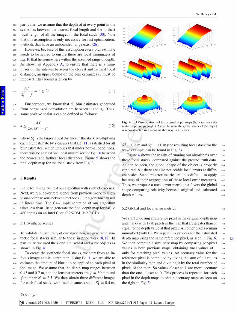
Fig. 4 3D Visualizations of the original depth maps (left) and our esti-

mated depth maps (right). As can be seen, the global shape of the object

is reconstructed in a recognizable way in all cases

S21 = 0.6 m and S3

1 = 1.0 m (the resulting focal stack for the 405

wave example can be found in Fig. 3). 406

Figure 4 shows the results of running our algorithms over 407

these focal stacks, compared against the ground truth data. 408

As can be seen, the global shape of the object is properly 409

captured, but there are also noticeable local errors at differ- 410

ent scales. Standard error metrics are thus difficult to apply 411

because of their aggregation of these local error measures. 412

Thus, we propose a novel error metric that favors the global 413

shape comparing relativity between original and estimated 414

depth values. 415

5.2 Global and local error metrics 416

We start choosing a reference pixel in the original depth map 417

and mark (with 1) all pixels in the map that are greater than or 418

equal to the depth value at that pixel. All other pixels remain 419

unmarked (with 0). We repeat this process for the estimated 420

depth map using the same reference pixel, as seen in Fig. 6. 3421

We then compute a similarity map by comparing per-pixel 422

values in both previous maps, obtaining final values of 1 423

only for matching pixel values. An accuracy value for the 424

reference pixel is computed by taking the sum of all values 425

in the similarity map and dividing it by the total number of 426

pixels of the map. So values closer to 1 are more accurate 427

than the ones closer to 0. This process is repeated for each 428

pixel in the depth maps to obtain accuracy maps as seen on 429

the right in Fig. 5. 430

123


Au

tho

r P

ro

of

unco

rrec

ted

pro

of


Fig. 5 Comparison of original depth maps (on the left) with our esti-

mations (middle left). Local error from the curve fitting step (middle

right) where the errors ranged between a magnitude of 10−9 and 10−8

(black and white, respectively, for better visualization), and our global

accuracy metric (right). In this last case, a value of one means a perfect

match. Our local and global accuracy metrics clearly show that while

local errors may occur, the reconstructed global shape of the object has

a good resemblance with the ground truth one, as appreciated also in

Fig. 4

In addition to our global accuracy metric, we can also431

obtain per-pixel error maps from the optimization step. Such432

maps show the squared error obtained when fitting Eq. 1 to433

the estimated blur values for one pixel through the focal stack434

to obtain its final depth value. Examples of these maps can435

be found in Fig. 5 (middle right).436

Looking at the blur estimates used for the optimization437

reveals that small blurs were over-estimated while large blurs438

were under-estimated. These inaccuracies caused the algo-439

rithm to compress the depth estimates such that the range440

of estimated depths is smaller than the actual range. How-441

ever, since blur estimate errors are consistent across the entire442

image, the depth estimates are still accurate relative to each443

other, and so the global shape captures the main features of444

the ground truth.445

5.3 Real scenes446

We also tested our algorithm with real scenes. We again used447

examples from prior work [6,8,30] to allow direct visual448

comparisons with our results. In these examples, the num-449

ber of images for each focal stack is two. As can be seen in450

Fig. 7, we obtain plausible reconstructions comparing favor-451

ably with both Watanabe and Nayar [30] and Favaro [8],452

even though our depth maps look blurrier due to the filter-453

ing explained in Sect. 4.3. Our work presents an interesting454

tradeoff between accuracy and speed, as it is significantly455

faster than the 10 min reported in [6]456

Fig. 6 Example of estimating the global accuracy of a pixel (marked

in red) for the wave object from Fig. 4. Pixels with depth values greater

or equal to it are marked in white, while the rest keep unmarked (black).

This is done for both the ground truth depth map (left) and the estimated

depth map (right). A similarity measure for that pixel is then computed

by marking with one all the pixels with matching values and dividing

that number by the total size of the map

Additional examples from real scenes can be found in 457

Fig. 8. The first two rows show plausible reconstructions for 458

different stuffed toys. The bottom row shows a difficult case 459

for our algorithm. Given the asymptotic behavior of the circle 460

of confusion function (Fig. 2), objects from a certain distance 461

show small differences in blur. Since our blur estimations are 462

not in real scale, this translates into either unrelated distant 463

points recovered into the same background plane, or inaccu- 464

rate and different depth values for neighboring pixels. This 465

happens usually in outdoor scenes, so our algorithm is better 466

suited for close-range scenes. 467

6 Conclusions 468

In this paper, we have presented an algorithm that estimates 469

depth from a focal stack of images. This algorithm uses 470

123


Au

tho

r P

ro

of

unco

rrec

ted

pro

of

S. W. Bailey et al.

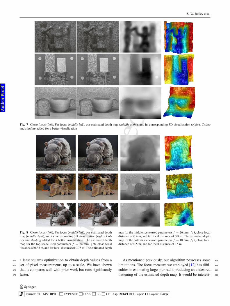
Fig. 7 Close focus (left), Far focus (middle left), our estimated depth map (middle right), and its corresponding 3D visualization (right). Colors

and shading added for a better visualization

Fig. 8 Close focus (left), Far focus (middle left), our estimated depth

map (middle right), and its corresponding 3D visualization (right). Col-

ors and shading added for a better visualization. The estimated depth

map for the top scene used parameters f = 24 mm, f/8, close focal

distance of 0.35 m, and far focal distance of 0.75 m. The estimated depth

map for the middle scene used parameters f = 26 mm, f/8, close focal

distance of 0.4 m, and far focal distance of 0.8 m. The estimated depth

map for the bottom scene used parameters f = 18 mm, f/8, close focal

distance of 0.5 m, and far focal distance of 15 m

a least squares optimization to obtain depth values from a471

set of pixel measurements up to a scale. We have shown472

that it compares well with prior work but runs significantly473

faster.474

As mentioned previously, our algorithm possesses some 475

limitations. The focus measure we employed [12] has diffi- 476

culties in estimating large blur radii, producing an undesired 477

flattening of the estimated depth map. It would be interest- 478

123


Au

tho

r P

ro

of

unco

rrec

ted

pro

of


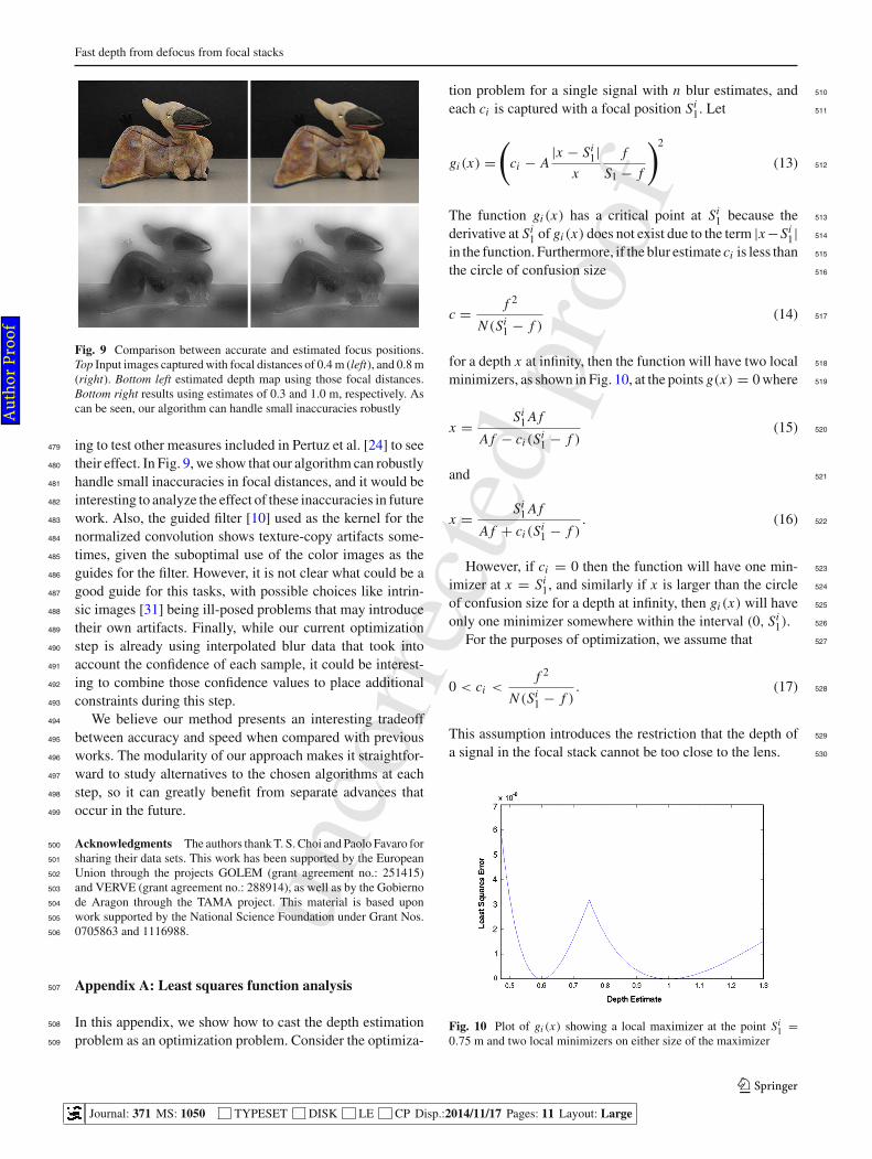
Fig. 9 Comparison between accurate and estimated focus positions.

Top Input images captured with focal distances of 0.4 m (left), and 0.8 m

(right). Bottom left estimated depth map using those focal distances.

Bottom right results using estimates of 0.3 and 1.0 m, respectively. As

can be seen, our algorithm can handle small inaccuracies robustly

ing to test other measures included in Pertuz et al. [24] to see479

their effect. In Fig. 9, we show that our algorithm can robustly480

handle small inaccuracies in focal distances, and it would be481

interesting to analyze the effect of these inaccuracies in future482

work. Also, the guided filter [10] used as the kernel for the483

normalized convolution shows texture-copy artifacts some-484

times, given the suboptimal use of the color images as the485

guides for the filter. However, it is not clear what could be a486

good guide for this tasks, with possible choices like intrin-487

sic images [31] being ill-posed problems that may introduce488

their own artifacts. Finally, while our current optimization489

step is already using interpolated blur data that took into490

account the confidence of each sample, it could be interest-491

ing to combine those confidence values to place additional492

constraints during this step.493

We believe our method presents an interesting tradeoff494

between accuracy and speed when compared with previous495

works. The modularity of our approach makes it straightfor-496

ward to study alternatives to the chosen algorithms at each497

step, so it can greatly benefit from separate advances that498

occur in the future.499

Acknowledgments The authors thank T. S. Choi and Paolo Favaro for500

sharing their data sets. This work has been supported by the European501

Union through the projects GOLEM (grant agreement no.: 251415)502

and VERVE (grant agreement no.: 288914), as well as by the Gobierno503

de Aragon through the TAMA project. This material is based upon504

work supported by the National Science Foundation under Grant Nos.505

0705863 and 1116988.506

Appendix A: Least squares function analysis507

In this appendix, we show how to cast the depth estimation508

problem as an optimization problem. Consider the optimiza-509

tion problem for a single signal with n blur estimates, and 510

each ci is captured with a focal position Si1. Let 511

gi (x) =

(

ci − A|x − Si

1|

x

f

S1 − f

)2

(13) 512

The function gi (x) has a critical point at Si1 because the 513

derivative at Si1 of gi (x) does not exist due to the term |x −Si

1| 514

in the function. Furthermore, if the blur estimate ci is less than 515

the circle of confusion size 516

c =f 2

N (Si1 − f )

(14) 517

for a depth x at infinity, then the function will have two local 518

minimizers, as shown in Fig. 10, at the points g(x) = 0 where 519

x =Si

1 A f

A f − ci (Si1 − f )

(15) 520

and 521

x =Si

1 A f

A f + ci (Si1 − f )

. (16) 522

However, if ci = 0 then the function will have one min- 523

imizer at x = Si1, and similarly if x is larger than the circle 524

of confusion size for a depth at infinity, then gi (x) will have 525

only one minimizer somewhere within the interval (0, Si1). 526

For the purposes of optimization, we assume that 527

0 < ci <f 2

N (Si1 − f )

. (17) 528

This assumption introduces the restriction that the depth of 529

a signal in the focal stack cannot be too close to the lens. 530

Fig. 10 Plot of gi (x) showing a local maximizer at the point Si1 =

0.75 m and two local minimizers on either size of the maximizer

123


Au

tho

r P

ro

of

unco

rrec

ted

pro

of

S. W. Bailey et al.

A further restriction for the depth x is that S11 < x < Sn

1531

where 0 < S11 < S2

1 < · · · < Sn1 . This restriction limits the532

depth of any point in the focal stack to be between the closest533

focal position of the lens and the farthest focal position.534

With these assumptions, we can now look at the least535

squares optimization equation536

z(x) =

n∑

i=1

gi (x). (18)537

Because each g′i (x) is undefined at x = Si

1 for all i =538

1, . . . , n, the function z(x) has critical points at S11 , . . . , Sn

1 .539

Furthermore, z(x) is continuous everywhere else for x > 0540

because the functions gi (x) are continuous where x > 0 and541

x = Si1. Because gi (x) has a local maximizer at Si

1, this point542

may be a local maximizer for z(x). This gives us n − 1 inter-543

vals on which z(x) is continuous for S11 < x < Sn

1 , and these544

intervals are (S11 , S2

1 ), (S21 , S3

1), . . . , (Sn−11 , Sn

1 ). These open545

intervals may or may not contain a local minimizer, and if546

an interval does contain a local minimizer, it might be the547

global minimizer of z(x) on the interval (S11 , Sn

1 ).548

Under certain conditions, z(x) is convex within the inter-549

val (S11 , Si+1

1 ) for all i = 1, . . . , n − 1. Note that g j (x) is550

convex within the open interval for all j = 1, . . . , n. To see551

this, assume that Eq. 11 holds and that the focus position of552

the lens is always greater than the focal length f of the lens553

so that r > 0. We also assume that554

Sn1 ≤

3r Sj1

2c j

. (19)555

If x < Sj1 then the absolute value term |x − S

j1 | in gi (x)556

becomes −x + Sj1 . From this, we know that557

r Sj1 ≥ 2c j x (20)558

from Relation 11 and because x and Sj1 are positive. Rear-559

ranging the relation, we get560

−2c j Sj1 + r S

j1 ≥ 0. (21)561

Since x < Sj1 , 2r x < 2r S

j1 and 2r S

j1 − 2r x > 0. Therefore,562

− 2c j x + 3r Sj1 − 2r x = −2c j x + r S

j1 + (2r S

j1 − 2r x)563

≥ 2r Sj1 − 2r x564

> 0 (22)565

Furthermore, since x > 0, r > 0, and Sj1 > 0, we know that566

2r Sj1

x4> 0. (23)567

Therefore, we know that 568

g′′j (x) =

2r Sj1 (−2c j x + 3r S

j1 − 2r x)

x4> 0 (24) 569

for 0 < x < Sj1 . 570

If x > Sj1 , then 571

x < Sn1 ≤

3r Sj1

2c j

(25) 572

from Eq. 19 and that x < Sn1 . Since c j > 0, we can multiply 573

the relation by 2c j to get 574

3r Sj1 > 2c j x . (26) 575

From relation (11), we can say that 576

2r − 2c j ≥ 4c j − 2c j = 2c j . (27) 577

Therefore, 578

3r Sj1 > x(2r − 2c j ) ≥ x(2c j ). (28) 579

Distributing x in the above relation, we get 580

3r Sj1 > 2r x − 2c j x (29) 581

Rearranging the terms, we get 582

2c j x + 3r Sj1 − 2r x > 0. (30) 583

Multiplying by the left-hand side of (23), we get 584

g′′j (x) =

2r Sj1 (2c j x + 3r S

j1 − 2r x)

x4> 0 (31) 585

for Sj1 < x < Sn

1 . 586

As shown above, the second derivative of g j (x) is always 587

positive on the interval (S11 , Sn

1 ) except at the point Sj1 for all 588

j = 1, . . . , n. Since z(x) is the summation of all g j (x), 589

z(x) is also convex on the interval except at the points 590

S11 , S2

1 , . . . , Sn1 . Therefore, z(x) is convex in the intervals 591

(Si1, Si+1

1 ) for all i = 1, 2, . . . , n−1. As a consequence, if Si1, 592

and Si+11 are local maximizers, then there is some local min- 593

imizer within the open interval (S11 , Sn

1 ). From this, a global 594

minimizer can be identified which gives the best depth esti- 595

mate for the given signal on the interval (S11 , Sn

1 ). Figure 11 596

shows an example of z(x) with the local maximizers and 597

minimizers. 598

123


Au

tho

r P

ro

of

unco

rrec

ted

pro

of


Fig. 11 Plot of z(x) shown in show dark blue with g1(x), g2(x), and

g3(x) shown in red, light blue, and green, respectively. This shows z(x)

with local maximizers at S11 = 0.75, S2

1 = 1, and S31 = 1.5 and local

minimizers in the intervals (S11 , S2

1 ) and (S21 , S3

1 )

References599

1. Bae, S., Durand, F.: Defocus magnification. Comput. Graph. Forum600

26(3), 571–579 (2007)601

2. Bauszat, P., Eisemann, M., Magnor, M.: Guided image filtering602

for interactive high-quality global illumination. Comput. Graph.603

Forum 30(4), 1361–1368 (2011)604

3. Calderero, F., Caselles, V.: Recovering relative depth from low-605

level features without explicit t-junction detection and interpreta-606

tion. Int. J. Comput. Vis. 1–31 (2013)4 607

4. Cao, Y., Fang, S., Wang, F.: Single image multi-focusing based on608

local blur estimation. In: Image and graphics (ICIG), 2011 Sixth609

International Conference on, pp. 168–175 (2011)610

5. Cao, Y., Fang, S., Wang, Z.: Digital multi-focusing from a single611

photograph taken with an uncalibrated conventional camera. Image612

Process. IEEE Trans. 22(9), 3703–3714 (2013). doi:10.1109/TIP.613

2013.2270086614

6. Favaro, P.: Recovering thin structures via nonlocal-means regu-615

larization with application to depth from defocus. In: Computer616

vision and pattern recognition (CVPR), 2010 IEEE Conference617

on, pp. 1133–1140 (2010)618

7. Favaro, P., Soatto, S.: 3-D Shape Estimation and Image Restoration:619

Exploiting Defocus and Motion-Blur. Springer-Verlag New York620

Inc, Secaucus (2006)621

8. Favaro, P., Soatto, S., Burger, M., Osher, S.J.: Shape from defocus622

via diffusion. Pattern Anal. Mach. Intel. IEEE Trans. 30(3), 518–623

531 (2008)624

9. Hasinoff, S.W., Kutulakos, K.N.: Confocal stereo. Int. J. Comput.625

Vis. 81(1), 82–104 (2009)626

10. He, K., Sun, J., Tang, X.: Guided image filtering. In: Proceed-627

ings of the 11th European conference on Computer vision: Part I.628

ECCV’10, pp. 1–14. Springer, Berlin, Heidelberg (2010)629

11. Hecht, E.: Optics, 3rd edn. Addison-Wesley (1997)5 630

12. Hu, H., De Haan, G.: Adaptive image restoration based on local631

robust blur estimation. In: Proceedings of the 9th international632

conference on Advanced concepts for intelligent vision systems.633

ACIVS’07, pp. 461–472. Springer, Berlin, Heidelberg (2007)634

13. Knutsson, H., Westin, C.F.: Normalized and differential convo-635

lution: Methods for interpolation and filtering of incomplete and636

uncertain data. In: Proceedings of Computer vision and pattern637

recognition (‘93), pp. 515–523. New York City, USA (1993)638

14. Lee, I.H., Shim, S.O., Choi, T.S.: Improving focus measurement639

via variable window shape on surface radiance distribution for 3d640

shape reconstruction. Optics Lasers Eng. 51(5), 520–526 (2013)641

15. Levin, A., Fergus, R., Durand, F., Freeman, W.: Image and depth 642

from a conventional camera with a coded aperture. ACM Trans- 643

actions on Graphics, SIGGRAPH 2007 Conference Proceedings, 644

San Diego, CA (2007) 645

16. Li, C., Su, S., Matsushita, Y., Zhou, K., Lin, S.: Bayesian depth- 646

from-defocus with shading constraints. In: Computer Vision and 647

Pattern Recognition (CVPR), 2013 IEEE Conference on, pp. 217– 648

224 (2013). doi:10.1109/CVPR.2013.35 649

17. Lin, X., Suo, J., Wetzstein, G., Dai, Q., Raskar, R.: Coded focal 650

stack photography. In: IEEE International Conference on Compu- 651

tational photography (2013) 652

18. Mahmood, M.T., Choi, T.S.: Nonlinear approach for enhancement 653

of image focus volume in shape from focus. Image Process. IEEE 654

Trans. 21(5), 2866–2873 (2012) 655

19. Malik, A.: Selection of window size for focus measure processing. 656

In: Imaging systems and techniques (IST), 2010 IEEE International 657

Conference on, pp. 431–435 (2010) 658

20. Moreno-Noguer, F., Belhumeur, P.N., Nayar, S.K.: Active refo- 659

cusing of images and videos. In: ACM SIGGRAPH 2007 papers, 660

SIGGRAPH ‘07. ACM, New York, NY, USA (2007) 661

21. Namboodiri, V., Chaudhuri, S.: Recovery of relative depth from 662

a single observation using an uncalibrated (real-aperture) camera. 663

In: Computer vision and pattern recognition, 2008. CVPR 2008. 664

IEEE Conference on, pp. 1–6 (2008) 665

22. Nayar, S., Nakagawa, Y.: Shape from focus. Pattern Anal. Mach. 666

Intel. IEEE Trans. 16(8), 824–831 (1994) 667

23. Pentland, A.P.: A new sense for depth of field. Pattern Anal. Mach. 668

Intel. IEEE Trans. PAMI 9(4), 523–531 (1987) 669

24. Pertuz, S., Puig, D., Garcia, M.A.: Analysis of focus measure oper- 670

ators for shape-from-focus. Pattern Recognit. 46(5), 1415–1432 671

(2013) 672

25. Petschnigg, G., Szeliski, R., Agrawala, M., Cohen, M., Hoppe, H., 673

Toyama, K.: Digital photography with flash and no-flash image 674

pairs. ACM SIGGRAPH 2004 Papers. SIGGRAPH ‘04, pp. 664– 675

672. ACM, New York, NY, USA (2004) 676

26. Press, W.H., Teukolsky, S.A., Vetterling, W.T., Flannery, B.P.: 677

Numerical Recipes: The Art of Scientific Computing, 3rd edn. 678

Cambridge University Press (2007) 6679

27. Shim, S.O., Choi, T.S.: A fast and robust depth estimation method 680

for 3d cameras. In: Consumer Electronics (ICCE), 2012 IEEE Inter- 681

national Conference on, pp. 321–322 (2012) 682

28. Subbarao, M., Choi, T.: Accurate recovery of three-dimensional 683

shape from image focus. Pattern Anal. Mach. Intel. IEEE Trans. 684

17(3), 266–274 (1995) 685

29. Vaquero, D., Gelfand, N., Tico, M., Pulli, K., Turk, M.: Generalized 686

autofocus. In: IEEE Workshop on Applications of Computer Vision 687

(WACV’11). Kona, Hawaii (2011) 688

30. Watanabe, M., Nayar, S.: Rational filters for passive depth from 689

defocus. Int. J. Comput. Vis. 27(3), 203–225 (1998) 690

31. Zhao, Q., Tan, P., Dai, Q., Shen, L., Wu, E., Lin, S.: A closed-form 691

solution to retinex with nonlocal texture constraints. Pattern Anal. 692

Mach. Intel. IEEE Trans. 34(7), 1437–1444 (2012) 693

32. Zhou, C., Cossairt, O., Nayar, S.: Depth from diffusion. In: IEEE 694

Conference on Computer vision and pattern recognition (CVPR) 695

(2010) 696

33. Zhuo, S., Sim, T.: On the recovery of depth from a single defo- 697

cused image. In: X. Jiang, N. Petkov (eds.) Computer Anal- 698

ysis of Images and Patterns, Lecture Notes in Computer Sci- 699

ence, vol. 5702, pp. 889–897. Springer, Berlin Heidelberg (2009). 700

doi:10.1007/978-3-642-03767-2_108. URL http://dx.doi.org/10. 701

1007/978-3-642-03767-2_108 702

34. Zhuo, S., Sim, T.: Defocus map estimation from a single image. 703

Pattern Recognit. 44(9), 1852–1858 (2011) 704

123


Au

tho

r P

ro

of

http://dx.doi.org/10.1109/TIP.2013.2270086

http://dx.doi.org/10.1109/TIP.2013.2270086

http://dx.doi.org/10.1109/CVPR.2013.35

http://dx.doi.org/10.1007/978-3-642-03767-2_108

http://dx.doi.org/10.1007/978-3-642-03767-2_108

http://dx.doi.org/10.1007/978-3-642-03767-2_108

Fast depth from defocus from focal stacks - Graphics and ...

Documents

Transcript of Fast depth from defocus from focal stacks - Graphics and ...