FASSWE SCRIPT FOR STRUCTURAL SIZING AND ...

1

FASSWE SCRIPT FOR STRUCTURAL SIZING AND OPTIMIZATION OF

AIRCRAFT UNDER EARLY DESIGN PHASES

EDGAR ARTURO GOMEZ MEISEL

FUNDACIÓN UNIVERSITARIA LOS LIBERTADORES ENGINEERING FACULTY

AERONAUTICAL ENGINEERING BOGOTÁ

JULY 2014

2

FASSWE SCRIPT FOR STRUCTURAL SIZING AND OPTIMIZATION OF

AIRCRAFT UNDER EARLY DESIGN PHASES

EDGAR ARTURO GOMEZ MEISEL

Degree work’s monograph to qualify for the title of Aeronautical Engineer

ADVISOR: Andreas Gravenhorst Aerospace Engineer

FUNDACIÓN UNIVERSITARIA LOS LIBERTADORES ENGINEERING FACULTY

AERONAUTICAL ENGINEERING BOGOTÁ

JULY 2014

3

Acceptance Note / Nota de Aceptación _________________________________ _________________________________ _________________________________ _________________________________ _________________________________ _________________________________ _________________________________

Jury’s president signature Firma presidente del jurado

_________________________________ Jury’s signature Firma del jurado

_________________________________ Jury’s signature Firma del jurado

Bogota DC, ______________________

4

Directors from Institucion Universitaria Los Libertadores, the jury and the staff are not responsible for the criteria and ideas submitted in this document. They correspond solely to the authors.

Las directivas de la Institucion Universitaria Los Libertadores, los jurados calificadores y el cuerpo docente no son responsables por los criterios e ideas expuestas en el presente documento. Estos corresponden unicamente a los autores

5

GIVEN TO THE LORD AND DEDICATED TO MY PARENTS …..

6

CONTENT

Page

1. INTRODUCTION 15 2. CONTEXTUAL FRAME 16 3. PROBLEM AND JUSTIFICATION 17 3.1 PROBLEM DEFINITION 17 3.2 JUSTIFICATION 17 3.2 .1 VALUE PROPOSITION 18 3.3 RESEARCH QUESTION 18 4. OBJECTIVES 21 4.1 GENERAL OBJECTIVE 21 4.2 SPECIFIC OBJECTIVES 21 5. METHODOLOGY 22 6. THEORITICAL FRAME 23 6.1 TYPE CERTIFICATION IN THE INDUSTRY 23 6.2 WING BOX STRUCTURE 25 6.3 WING BOX FAILURE MODES 30 6.4 WINGBOX METHODS OF ANALYSIS 35 6.4.1 Stress and deflection analysis 6.4.1.1 Modified beam theory (K method) 6.4.1.2 Castigliano’s Theorem, torsion in multiple cell sections 6.4.2 Instability analysis 6.4.2.1 Theory of instability of columns and thin sheets 6.4.2.2 NACA criteria for buckling of flat plates 6.4.2.3 NACA criteria for local buckling 6.4.2.4 NACA criteria for crippling strength 6.5 SUCCESIVE APROXIMATION 47 6.5.1 Mathematical method 6.5.2 Shear flow correction algorithm 6.6 OBJECT ORIENTED PROGRAMING 53 7. FASSWE OPERATIONAL REQUIREMENTS 57 7.1 SCRIPT OUTPUTS DETERMINATION 57 7.2 SCRIPT INPUTS DETERMINATION 58 8. PROCESSING SCHEME 61 9. DATA STRUCTURE 63

7

9.1 DATA STRUCTURE SUMARY 63 9.1.1 The class “Wingbox” 9.1.2 The class “Wing” 9.1.3 The classes “Stringer” and “Sheet” 9.1.4 The methods “obj.get_MS”, “obj.Stress_cr_calc” and “obj.get_factors” 9.1.5 The class “Spar” 9.1.6 The class “Completepanel” 9.1.7 The class “Material” 9.1.8 The classes “Point” and “Line” 9.1.9 The classes “Cell” and “Section” 9.1.9.1 The methods obj.Sigma_calc and obj.P_calc 9.1.9.2 The method obj.qs_calc 9.1.9.3 The methods obj.qcl_calc and obj.add_qcl 9.1.9.4 The methods “obj.SC_calc” and “obj.M_SC_calc” 9.1.9.5 The method “obj.qt_calc” 9.1.9.6 The method “obj.dtheta_dy_calc” 9.1.10 The “Routine” class 9.1.10.1 Routines’ stability calculation methods 9.1.10.2 The Routine’s visualization methods “obj.Vis_sigma” and “obj.Vis_tau” 9.1.10.3 The Routine’s visualization method “obj.Vis_twist” 9.1.10.3 The Routine’s visualization method “obj.Vis_MS_buck” 10 FUNCTIONS 89 10.1 USER BUILT FUNCTIONS 89 10.1.1 Functions for section properties calculation 10.1.2 Functions for shear flow calculation 10.2 MATLAB BUILT-IN FUNCTIONS 90

11 GRAFIC USER INTERFACE (GUI) 91 11.1 WINGBOX CREATION AND EDITION 91 11.2 ANALYSIS AND VISUALIZATION 95 12 SCRIPT VALIDATIONS 98 12.1 TEST 1 WEIGHT CALCULATION 98 12.2 TEST 2, AXIAL STREES IN TAPERED WINGBOX 99 12.3 TEST 3, STATIC SHEAR FLOW IN SINGLE AND MULTICELL 101 12.4 TEST 4 TOTAL SHEAR FLOW IN A 3 CELLS WINGBOX 103 12.5 TEST 5 TOTAL SHEAR FLOW IN A 10 CELLS WINGBOX 105 12.6 TEST 6 SHEAR CENTER IN A SINGLE CELL WINGBOX 107 12.7 TEST 7 TORSIONAL SHEAR FLOW IN A MULTICELL WINGBOX 107 12.8 TEST 8 SHEET BUCKLING CALCULATION TEST 108 12.9 VALIDATION IN OVERALL 109 13. PRACTICAL EXAMPLE 110

8

14. FUTURE DEVELOPMENT 116 15. CONCLUSIONS 117 16. REFERENCES 118 17. APPENDIX A LA-250 WINGLOADING CALCULATION 120

9

SPECIAL LISTS

LIST OF FIGURES Page

Figure 1 common wing box structure 25 Figure 2 aircraft aerodynamic forces 27 Figure 3 pylons transferring loads to the wingbox structure 29 Figure 4 internal reactions in a body 29 Figure 5 free body, v-x, and m-x diagrams for a beam 30 Figure 6 buckling of a cylindrical sheet 32 Figure 7 local buckling in a stringer 32 Figure 8 stringer stress pattern after local buckling 33 Figure 9 common rivet failure modes 34 Figure 10 z profile in bending around x and z axes 35 Figure 11 shear flow in a z section 37 Figure 12 torsional shear flow in a thin walled section 39 Figure 13 shear flow in a multiple cell section 40 Figure 14 simple supported column 41 Figure 15 rectangular thin sheet under compression stresses 42 Figure 16 coefficient k’s as a function of aspect ratio (a/b) 43 Figure 17 composite shapes as independent sheets 45 Figure 18 coefficients k as function of flange/web width 47 Figure 19 skin’s contribution to total effective area 47 Figure 20 static shear flow 49 Figure 21 first correction shear flow 50 Figure 22 successive correction shear flows 50 Figure 23 individual cell shear flow contribution 52 Figure 24 final shear flow 53 Figure 25 matlab class definition 54 Figure 26 matlab properties definition 55 Figure 27 matlab class initialization 55 Figure 28 matlab methods definition 56 Figure 29 processing scheme 62 Figure 30 wingbox properties and methods 64 Figure 31 wingswept and dihedral 65 Figure 32 airfoil twist rotation 66 Figure 33 wing properties and methods 67 Figure 34 stringer’s cross section 68 Figure 35 stringer’s properties and methods 68 Figure 36 sheet’s properties and methods 70 Figure 37 spar’s properties and methods 71 Figure 38 completepanel’s properties and methods 73 Figure 39 material’s properties and functions 73

10

Figure 40 point’s properties and methods 73 Figure 41 typical representation of point, lines and nodes 75 Figure 42 line’s properties and methods 77 Figure 43 typical cell representation 77 Figure 44 cell’s properties and methods 77 Figure 45 typical section representation 78 Figure 46 typical section representation with nodes 78 Figure 47 forces and moments equivalence 82 Figure 48 section’s properties and methods 83 Figure 49 routine’s properties and methods 85 Figure 50 axial stress visualization 86 Figure 51 shear stress visualization 87 Figure 52 twist angle visualization 87 Figure 53 skin’s sheets buckling ms visualization 88 Figure 54 wing design frame 91 Figure 55 wingbox creation frame 92 Figure 56 wingbox edition schematics 93 Figure 57 wingbox edition frame 93 Figure 58 complete panel edition frame 94 Figure 59 complete panel edition frame 94 Figure 60 wingbox analysis frame 95 Figure 61 wingbox visualization frame 96 Figure 62 stringer’s ms visualization frame 96 Figure 63 stringer and sheets in solid works and fasswe 98 Figure 64 spars in solid works and fasswe 98 Figure 65 example 21.2 scheme 100 Figure 66 lumped wingbox for test1 in fasswe 100 Figure 67 5 cells wingbox section in example A15.12 102 Figure 68 total shear flow due to shear load in z direction 103 Figure 69 10 cells wingbox section example a15.13 105 Figure 70 single cell wingbox example 8.6 106 Figure 71 shear center calculation output 106 Figure 72 4 cells wingbox example a16.15 (3) 107 Figure 73 LA-250 “renegade” 110 Figure 74 LA-250 wing design 112 Figure 75 LA-250 wingbox creation 112 Figure 76 LA-250 complete panels edition 113 Figure 77 LA-250 wingbox weight estimation 113 Figure 78 stress analysis results 114 Figure 79 LA-250 twist angle result 115 Figure 80 buckling analysis results 115

11

LIST OF TABLES

Page

Table 1 weight estimation comparison 99 Table 2 test 2 results comparison 100 Table 3 test 2 results comparison 101 Table 4 test 3 results comparison 101 Table 5 test 3 results comparison 102 Table 6 test 4 results comparison 103 Table 7 test 4 results comparison 104 Table 8 test 5 results comparison 105 Table 9 test 7 result comparison 108 Table 10 buckling parameters comparison 109 Table 11 LA-250 wing features 110 Table 12 Overall Results 110 Table 13 LA-250 spaces between ribs 113

12

GLOSARIO

ARGUMENT: input data required to compute a function or to initialize a class AXIAL STRESS: force per unit of area directed perpendicular to a chosen direction BUCKLING: structural instability phenomena that produces abrupt large deformations when supporting a critical load CLASS: computer data structure abstraction defined by specific data and functions CLOSING SHEAR FLOW: shear flow that compensates the effects of closed beam sections subjected to bending moments CRIPPLING: Structural failure of stringers’ corners under compression loads DEBUGGING: process of searching programing mistakes inside a script FAR: Federal aviation regulantions FUNCTION: programing abstraction that computes a set of arguments to return outputs GUI: graphic user interface LAR: Latin-american Aeronautical Regulations LSA: Light sport aircraft MATLAB: High level scientific and technical programming language developed by MathWorks METHOD: Function associated with a specific class MDO: multidisciplinary design optimization; aircraft design methodology that involves diverse aircraft design departments during early design phases. MS: Margin of safety, coefficient that determines how far is a structure to fail under current loads MVP: Minimum viable product; small version of a produc developed to make market research

13

OOP: Object Oriented programming; methodology to write code based in the use of classes. PROPERTY: Data belonging to a specific class that characterize it and its children classes RIBS: Structural frames of a wingbox located along the spanwise that distribute the wing loads and provide the aerodynamic shape of a wing. SHEAR STRESS: Force per unit of area directed tangencially to a choosen direction SHEAR FLOW: concept used in thin structures analysis and represent shear stress per unit of length STATIC SHEAR FLOW: Shear flow produced in a open section beam under bending moments SPAR: Wingbox structural component supporting most of the shear loads of the wing

STRINGER: Structural profile located in the upper and lower sides of a wingbox structure; they resist most of the axial loads produced in the wing. SKIN: Sheet that covers the wingbox structure and resist a huge part of shear stresses SCRIPT: Computation code TYPE CERTIFICATE: Certification issued by the aeronautical authority when an aircraft design accomplished the airworthiness requirements for a safe operation. TWIST SHEAR FLOW: Shear flow produced by torsion WINGBOX: Main aircraft’s wing structure WEB: Thin sheet that belongs to the spar.

14

SUMMARY

This monograph contains the development of a minimum viable version of FASSWE a computational script aimed to determine the viability of a wingbox design based on strength and weight criteria. FASSWE script user’s requirements are stated based in FAR 23 certification rule and they are related with well known structural mathematical models to create a processing scheme that is implemented in Matlab. Results provided by FASSWE on diverse stress analysis, deformations, and structural stability tests are compared with available literature in order to validate the feasability of the script. A practical example is also developed of the wingbox redesign for the Lanshe Lake LA-250 seaplane. At the final diverse discussions and future developments are proposed in order to improve the performance of the current script and to optimize it according to the user’s necesities.

15

1. INTRODUCTION FASSWE (fast analysis for structural strength and weight estimation) is a computational code developed under the programming language of MATLAB® that using thin walled structural analysis methods, Castigliano theorem, virtual work theory, and experimental NACA criteria for structural instability provides a fast tool in the early design phases allowing designers and another potential users to analyze basic structural parameters such as deflections, internal force patterns and arrangement weight in order to determine the structural viability of an specific model and to improve the aircraft performance reaching high strength, sizing, and weight goals. This application will be focused to support aircraft designers and aeronautical authorities to enforce structural certification requirements stated in the Federal Aviation Regulation (FAR) part 23, specially subchapter (23.305). The present work is aimed to the development of just a small version of the total code that is used to analyze the wing box structure (wing structure) of small to medium aircrafts, leaving the remainder aircraft structures for futures developments.

16

2. CONTEXTUAL FRAME Aircraft design is one of the most interdisciplinary works in the aerospace industry and therefore one of the most challenging one, especially since aircraft is a complex machine that involves a high interdependency of their parts. The early design phases such as the conceptual and preliminary phases are very important because in them are defined the main features of this machine in terms of its performance parameters. Empty weight is one of the most important aircraft parameters since it sub-defines other important aerodynamic and propulsive features; its high interdependency with other features makes that for example an increment in wing aspect ratio results in a increment in empty weight because more structural weight is needed to support the increment in wing bending moment. For this reason during early design phases rough estimations of the airplane weight must be done, a difficult task since in these stages there are a few available information, therefore the designer must do certain assumptions based in prior experience5. Structures are extremely important in weight determination, in fact structural weight is expressed as 20% to 40% of the aircraft gross weight and skin represents 50% to 70% of the total structural weight; it means that the arrangement of the different structural members has a great impact in the aircraft empty weight and subsequently in the aircraft performance 3 One common practice in early design phases is to estimate the weight through linear interpolation using old aircraft’s weights, and work with this estimate until a preliminary phase is reached and later apply very restrictive manufacturer’s methods for structural weight estimation 22

The problem with these “statistical” methods is that a few information about how the structural arrangement affects the aircraft empty weight is provided and structural-weight improvements in early phases are discarded, also those method are not useful when innovative aircraft concepts are studied because those methods requires the existence of previous designs 22. For those reasons important companies such as Bombardier under the concept of MDO (multidisciplinary design optimization) has created Structural design and weight estimations computational applications for the preliminary design phases, that using quick structural methods (such as successive approximation method) rather than complicated FEA methods evaluate innovative business jet concepts; a similar estimation method was developed at NASA Ames Research Center in which applying coarse FEA meshes the static buckling, stiffness requirements and

17

wing tip deflections are calculated in order to get the minimum structural needed material1 A joint work of Airbus and TU Braunschweig (technological University of Braunschweig) developed under the MDO strategy a complete application called FAME that under a standardized Matlab® platform joint a CFD software as Ansys-Fluent®, a structural FEM package such as Nastran® and a CAD/CAM software as Catia® to make a wing weight estimation code for optimization purposes in multidisciplinary way 15 Nowadays small Colombian aircraft producers such as Aeroandina, IBIS Aircraft, Aerodynos de Colombia, CIAC, Criquet aviation, Caldas aeronautica, and FIA are suitable potential users of MDO software since these are companies entering in the competitive light aircraft market. The implementation of these MDO methods focused in early design phases (where design changes are most cost-efficient) could be developed to satisfy their own necessities in the same way they were developed by Bombardier and Airbus some years ago. Latin American aircraft certification authorities under the legal frame of LAR (Latin-american aeronautical regulations) are committed to evaluate all structural proposals to emit a type certification; reason why as well as local aircraft designers they are potential users to implement quick analysis software in their processes. 2.2.3 Computational thinking as a tool Algorithms are step by step set of procedures to accomplish a task; and it have been used to solve different mathematical, science and engineering issues, and with the help of modern digital computers that compute several mathematical expressions per millisecond have become one of the most powerful tools that human have. A computational code or script is a set of syntax words and commands that are familiar for an inside computer interpreter, and basically states the desired computation that the user wants the computer develop. Computations that a computer can develop are built with 8 basic Boolean and Arithmetic operations that together with a good algorithm and criteria solve extremely complex models such as HIV virus grown in a body subjected to different treatments. When a computational application is developed is of paramount importance the code performance because high time and memory consumption are not allowed for

18

common application; this called “algorithmic complexity” can be mathematically evaluated to estimate how long the script could take in the worse scenario; the order of grown in which the number of computations made by the machine respect to the amount of inputs is defined as the “Big O”, this big O can be constant, linear, logarithmic, polynomic, or in fact exponential, the code developer always must try to make it in the lowest possible, but sometimes it is not an easy task. There are different ways to improve that performance, and all them are related of how the data will be processed, so common techniques as loop, divide and conquer, bisection search, recursion, merge sort and Artificial intelligence algorithms to name just a few can be used by the code developer to improve that performance13

19

3. PROBLEM DEFINITION AND JUSTIFICATION

3.1 PROBLEM DEFINITION FASSWE is aimed to solve the following problems for its two potential users: For aircraft designers working at small companies and evaluating structural arrangements:

Old statistical trends are poor for new aircraft configurations

Approximate handmade calculations are time expending and subjected to human errors

FEA methods are time consuming and do not provide to the desired insight during early design phases.

For Latin American aeronautical authorities evaluating the issue of a type certificate:

Lack the experience in structural analysis

Do not account with trained staff to use advanced FEA software

Sub contract these studies decentralizing their legal obligation to particulars.

3.2 JUSTIFICATION

Through its value proposition FASSWE provides the Latin American aircraft production industry as well as aeronautical authorities with a suitable tool to improve their processes and improve their products helping to the competitiveness of the local industry. 3.2.1 VALUE PROPOSITION

Quick analysis: Using the computer’s processing speed with rough and reliable structural analysis methods FASSWE allow users to analyze several wing-box configurations in just a matter of seconds; something impossible by hand calculations.

No handmade processing errors: Since the analysis is developed by a computer executing a MATLAB® script FASSWE is not subjected to human mistakes during the computation

Instinctive: FASSWE uses structural analysis methods taught in most of the bachelors in aerospace engineering; reason why it does not required specially trained staff for its manipulation.

20

Standardization: Since FASSWE uses feasible and widely used methods for structural analysis it can be taken as a main criteria when evaluating structural arrangements

Improvement in early designs: Due to its simplicity and high speed FASSWE provides the possibility to make structural optimization during initial design stages.

3.3 RESEARCH QUESTION Current methodologies in technological innovation suggest that bringing a successful product into the marketplace requires a prior user’s validation that helps designers to improve their product according to the customer’s real necessities According to Eric Rise in Ref 23 the most suitable way to scientifically obtain this user’s feedback is offering to them a small version of the whole product in order to analyze their behavior when using and purchasing the product. Bearing in mind this context the research question is: How to develop a small version of FASSWE that can be submitted to potential users to receive their feedback?

21

4. OBJECTIVES 4.1 GENERAL OBJECTIVE

To develop a script in MATLAB® that performs structural strength and weight estimations of wing-box structures of aircraft under 5700Kg of weight

4.2 SPECIFIC OBJECTIVES

To develop a detailed statement of the user’s requirements and structural analysis methods

To develop the FASSWE processing scheme

To develop the step by step procedure (Algorithm)

To translate the algorithm into the computer language of MATLAB®

Make the program validation

4.3 SCOPE The present work is bounded to the development of a computational script dealing just with structural analysis and weight estimation of metallic wingbox structures under steady state. Composite materials, external loads and structural dynamics are not treated here and they are expected to be developed in future works. Special structural cases such as failure in stiffened panels, riveting and ribs are not covered here since it is just a MVP of the entire FASSWE application.

22

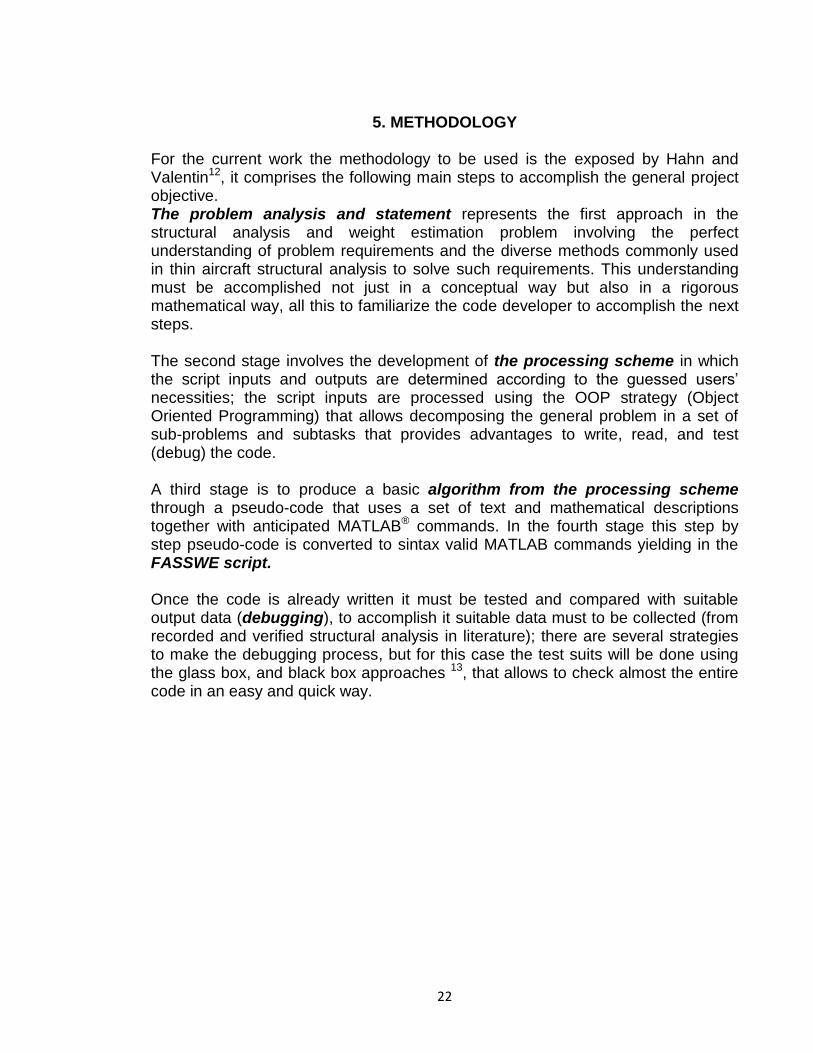
5. METHODOLOGY For the current work the methodology to be used is the exposed by Hahn and Valentin12, it comprises the following main steps to accomplish the general project objective. The problem analysis and statement represents the first approach in the structural analysis and weight estimation problem involving the perfect understanding of problem requirements and the diverse methods commonly used in thin aircraft structural analysis to solve such requirements. This understanding must be accomplished not just in a conceptual way but also in a rigorous mathematical way, all this to familiarize the code developer to accomplish the next steps. The second stage involves the development of the processing scheme in which the script inputs and outputs are determined according to the guessed users’ necessities; the script inputs are processed using the OOP strategy (Object Oriented Programming) that allows decomposing the general problem in a set of sub-problems and subtasks that provides advantages to write, read, and test (debug) the code. A third stage is to produce a basic algorithm from the processing scheme through a pseudo-code that uses a set of text and mathematical descriptions together with anticipated MATLAB® commands. In the fourth stage this step by step pseudo-code is converted to sintax valid MATLAB commands yielding in the FASSWE script. Once the code is already written it must be tested and compared with suitable output data (debugging), to accomplish it suitable data must to be collected (from recorded and verified structural analysis in literature); there are several strategies to make the debugging process, but for this case the test suits will be done using the glass box, and black box approaches 13, that allows to check almost the entire code in an easy and quick way.

23

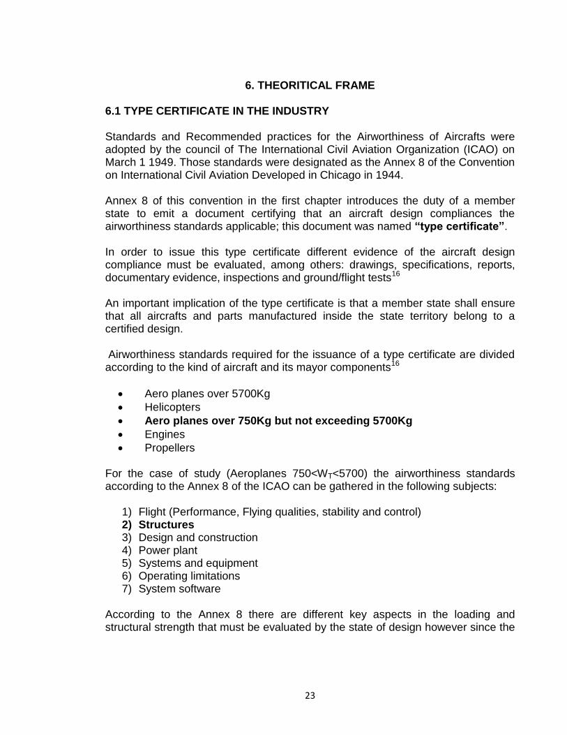
6. THEORITICAL FRAME 6.1 TYPE CERTIFICATE IN THE INDUSTRY Standards and Recommended practices for the Airworthiness of Aircrafts were adopted by the council of The International Civil Aviation Organization (ICAO) on March 1 1949. Those standards were designated as the Annex 8 of the Convention on International Civil Aviation Developed in Chicago in 1944. Annex 8 of this convention in the first chapter introduces the duty of a member state to emit a document certifying that an aircraft design compliances the airworthiness standards applicable; this document was named “type certificate”. In order to issue this type certificate different evidence of the aircraft design compliance must be evaluated, among others: drawings, specifications, reports, documentary evidence, inspections and ground/flight tests16 An important implication of the type certificate is that a member state shall ensure that all aircrafts and parts manufactured inside the state territory belong to a certified design. Airworthiness standards required for the issuance of a type certificate are divided according to the kind of aircraft and its mayor components16

Aero planes over 5700Kg

Helicopters

Aero planes over 750Kg but not exceeding 5700Kg

Engines

Propellers For the case of study (Aeroplanes 750<WT<5700) the airworthiness standards according to the Annex 8 of the ICAO can be gathered in the following subjects:

1) Flight (Performance, Flying qualities, stability and control) 2) Structures 3) Design and construction 4) Power plant 5) Systems and equipment 6) Operating limitations 7) System software

According to the Annex 8 there are different key aspects in the loading and structural strength that must be evaluated by the state of design however since the

24

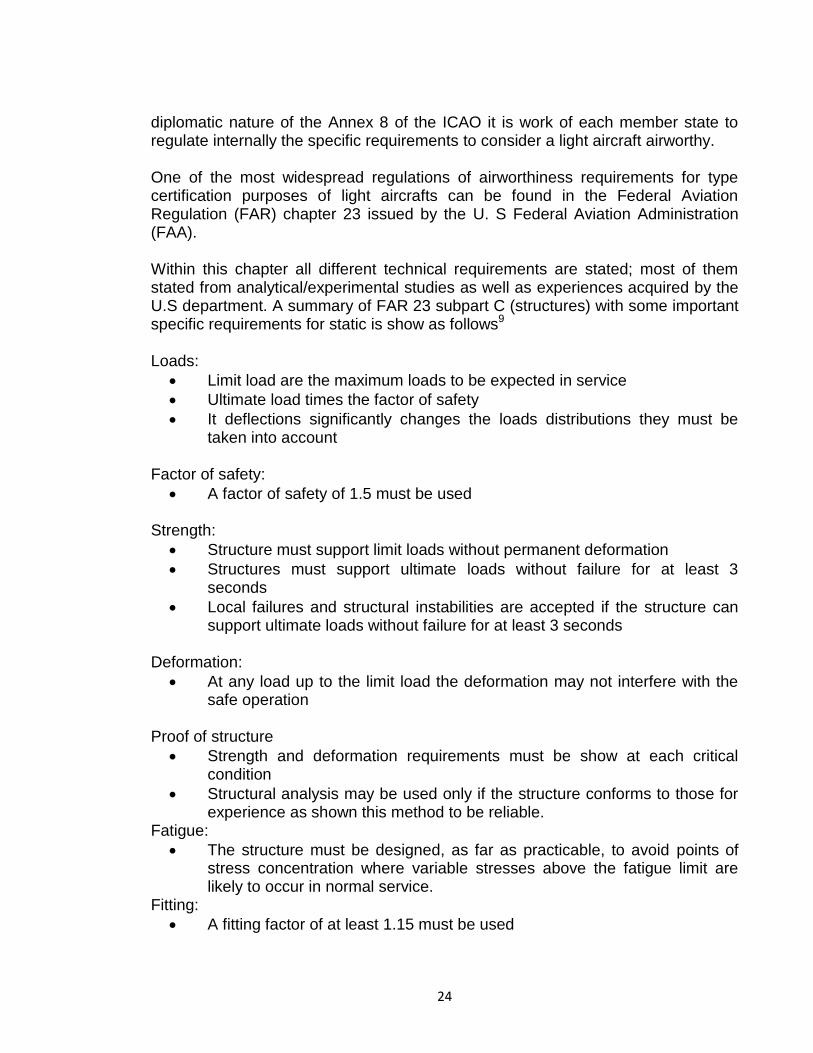
diplomatic nature of the Annex 8 of the ICAO it is work of each member state to regulate internally the specific requirements to consider a light aircraft airworthy. One of the most widespread regulations of airworthiness requirements for type certification purposes of light aircrafts can be found in the Federal Aviation Regulation (FAR) chapter 23 issued by the U. S Federal Aviation Administration (FAA). Within this chapter all different technical requirements are stated; most of them stated from analytical/experimental studies as well as experiences acquired by the U.S department. A summary of FAR 23 subpart C (structures) with some important specific requirements for static is show as follows9 Loads:

Limit load are the maximum loads to be expected in service

Ultimate load times the factor of safety

It deflections significantly changes the loads distributions they must be taken into account

Factor of safety:

A factor of safety of 1.5 must be used Strength:

Structure must support limit loads without permanent deformation

Structures must support ultimate loads without failure for at least 3 seconds

Local failures and structural instabilities are accepted if the structure can support ultimate loads without failure for at least 3 seconds

Deformation:

At any load up to the limit load the deformation may not interfere with the safe operation

Proof of structure

Strength and deformation requirements must be show at each critical condition

Structural analysis may be used only if the structure conforms to those for experience as shown this method to be reliable.

Fatigue:

The structure must be designed, as far as practicable, to avoid points of stress concentration where variable stresses above the fatigue limit are likely to occur in normal service.

Fitting:

A fitting factor of at least 1.15 must be used

25

As named before an aircraft type certificate is a requirement to get a manufacturer certificate and additionally in almost all countries around the world (including Colombia) is also a requirement for the issue of a certificate of operation. The worldwide importance of FAR 23 requirements is based in the high acceptance that it has around the world. Beginning from the fact that the U.S is the largest aircraft market around the world and the airworthiness requirements in FAR 23 are also validated by authorities such as the JAA (Joint Aviation Authorities) of Europe. In the case of Latin-America these FAR 23 requirements are not only used to validate type certificates issued in the U.S but also have been textually quoted in the LAR (Latin American aviation regulation) chapter 23 as technical requirements to get type certificate issued by Latin American authorities. 6.2 WINGBOX STRUCTURE As one of the aircraft’s main components the wing has a complex shape usually defined by aerodynamic criteria; additionally since the wing is subjected to different loads that vary in magnitude and sense it is also required a strong but light structure. Since the early 1930’s the structural concept of wing box has dominated the wing structural design due to its high strength and light weight. This wing box structure is a closed “box” where different structural components are arranged to overcome specific structural tasks in the most weight efficient manner.

Figure 1 Common wing box structure

Source: www.muelaner.com, 2014

http://www.muelaner.com/

26

A basic wing box structure comprises the following structural component:

Spars: Vertical beams composed by a thin web and two structural profiles (stringers) clamped in the upper and lower edges; its main function it to resists vertical shear loads, although it is also useful overcoming part of the torsional moment.

Stringers: Structural profiles allocated in the upper and lower side of the wing box, its main function is to resist axial loads produced by the wing bending.

Skin: Thin sheet allocated in the upper and lower wing box’s covers, its main function is to resist the shear stresses produced by the wing’s torsional moment; additionally to transmit the aerodynamics forces over the wing to the others wing box components.

Ribs: Structural components located along the span wise axis that prevents the wing box skin, stringers and spar’s webs to fail due to structural instability. Additionally ribs also ensures the aerodynamic shape for each wing section and become in a good mechanism for force transmission of external punctual loads such as engines or fuel tanks weight.

Stiffeners: Structural profiles usually clamped over the wing box’s webs in order to avoid structural instability failure.

6.2.1 Loads over the wing The determination of loads supported by the aircraft wing is a complex work usually developed with the aircraft loads department; a detailed analysis is carried out in advanced design phases due to the necessity of high amounts of data; however it is paramount for the design engineer point of view to realize what are main sources of those loads. Greater part of the forces that the aircraft wing must support comes from the following sources:

27

6.2.1.1 Aerodynamic forces One of the most important parts in a light aero plane is the wing; its main function is to produce one of the forces required to keep the aircraft in a desired flight condition. To produce this force often called “Lift” the wing surface interacts with the relative airstream changing the trajectory of the air particles, downstream yielding in a local pressure distribution change that considered over the entire surface creates a net force. When the air passes along the entire aircraft surface in the microscopic world atoms are striking each other and also with the surface; since this surface is irregular in nature during those collisions some air particles lose part of its momentum and certain energy in what is called “viscous dissipation”. This viscous dissipation effect is the main source of what we know as “profile drag” that in common words is the force that opposes the aircraft movement produced by each independent 2D aircraft section 8 In order to generate Lift the Potential flow theory introduces the concept of airflow circulation; this circulation in a finite wing creates the well-known “wingtip vortices” that in addition to the circulation along the wing induce a tilt in the Lift vector generating a negative work over the aircraft; the force producing this effect is called “Induced Drag” 7 For aircraft loads analysis the total Drag produced the aircraft can be packed in a single force parallel to the airstream this force is simply called “Drag”

Figure 2 Aircraft aerodynamic forces

Source: Ref 7 (Image of public domain)

28

6.2.1.2 Weight distribution force The airplane wing is one of the heaviest components in an aircraft despite it is built of light materials; therefore its inclusion in the load estimation analysis in highly important. Although in cruise phase this weight does not represent special threats due to the upward aerodynamics forces when static on the ground or during taxiing/parking procedures its weight and distribution is of mayor concern. 6.2.1.3 Inertial Forces An aircraft during the different flight phases is constantly accelerating or decelerating; these changes in velocity induce inertial forces produced by the aircraft mass and its distribution. Common maneuvers that introduce risks for the airframe are 3:

Air gust: Loads produced by changes in the free stream produced by the weather

Normal pull up: Upward circular path maneuver

Inverted pull up: Downward circular path maneuver

Level landing: Load produced by the landing impact

Level landing with side load: Load produced by the landing impact together with side airstream loads

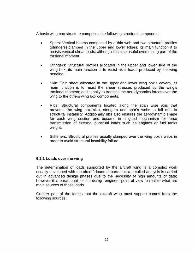
Arresting (Carriers): Loads produced by external vehicles moving the aircraft 6.2.1.4 Transferred forces It is a generic way to gather all forces produced by individual aircraft components that are structurally clamped to the Wing; in this description one can easily highlight the following cases:

Structural pylons transferring engines’ weight and thrust forces to the wingbox

Structural pylons transferring the weight of external fuel tanks to the wingbox

Structural fittings transferring different equipment weight and forces (e.g servos, pulleys, wiring, pipelines, weapons)

29

Figure 3 Examples of pylons transferring loads to the wingbox structure

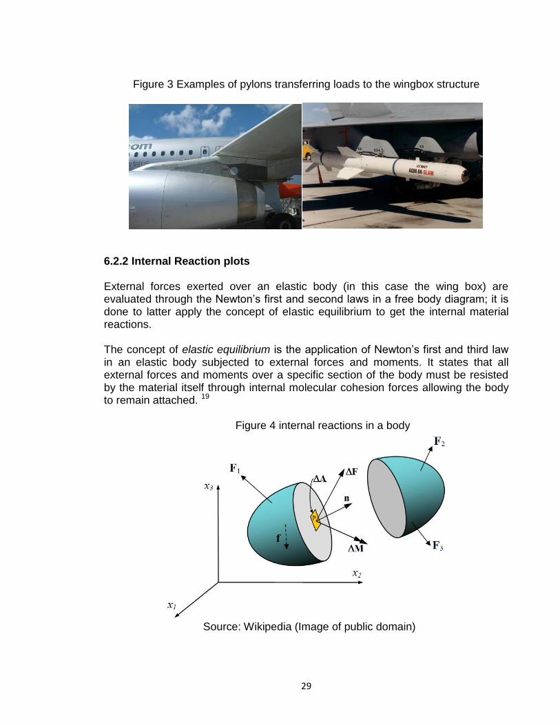
6.2.2 Internal Reaction plots External forces exerted over an elastic body (in this case the wing box) are evaluated through the Newton’s first and second laws in a free body diagram; it is done to latter apply the concept of elastic equilibrium to get the internal material reactions. The concept of elastic equilibrium is the application of Newton’s first and third law in an elastic body subjected to external forces and moments. It states that all external forces and moments over a specific section of the body must be resisted by the material itself through internal molecular cohesion forces allowing the body to remain attached. 19

Figure 4 internal reactions in a body

Source: Wikipedia (Image of public domain)

30

These internal reactions are usually defined with their resultant at different sections of the body and they are divided usually in 4 basic types:

Normal force: Resultant internal force that tends to compact or expand the body along an axis

Shear forces: Resultant internal forces tending to shear the body and to create an angular deformation

Bending moments: Resultant internal moments tending to bend or flex the body.

Torsional moment: Resultant internal moment tending twist the body along an axis.

As will be seen in the following sections the values of these internal reactions have a significant impact in the structural behavior of the wingbox, therefore it is a common practice to draw a plot of its value at each respective body location.

Figure 5 free body, V-x, and M-x diagrams for a beam


6.3 WINGBOX FAILURE MODES For aircraft design and type certification purposes to know how a wing box can fail is an important task, especially since there is a large variety of failure modes of each component. For a typical wing box under steady loads (non-fatigue) the failure modes can be divided in the following 6 groups:

1. Stringers under tension loads 2. Spar’s webs under shear loads

31

3. Skin and web buckling 4. Stringers local buckling 5. Stringers crippling 6. Riveting failure

6.3.1 Stringers under tension loads

As stated before the main purpose of a stringer is to resist the axial loads produced by a bending moment; the portion of the wing box experiencing tension have the tendency to enter in the plastic region yielding in permanent deformations that according to FAR 23 requirements are not allowed under aircraft limit loads.

6.3.2 Spar’s webs under shear loads Spar’s webs are the wing box components experiencing the highest levels of shear loads; although they can fail in different modes the plastic deformation is one of the highest concerns since they are prohibit under limit loads by FAR 23.

6.3.3 Skin and web buckling Sheets used to cover the wing box are usually subjected to combined axial and shear internal forces; according to the elastic instability theory little loads over thin sheets can result in large deflections respect the sheet plane. The same theory of instability states that there is a limit load pattern by which this deflection respect to the sheet plane tends theoretically to infinity and will not return to its unperturbed state; this condition is called “buckling” (for more details of structural instability theory refer to Ref [1] chapter A18). In a real wing box structure this theoretical buckling condition result in large deflections of the sheet, weakening the entire panel since the sheet is not allowed to keep supporting loads. Furthermore this large deflection causes perturbations in the aerodynamics shape of the wing. For these two reasons buckling analysis is of high importance in order to enforce the requirements stated in FAR 23 regarding to failure analysis and deformations that causes large aerodynamic perturbations.

32

Figure 6 buckling of a cylindrical sheet

Source: www.NASA.com (Image of public domain)

6.3.4 Stringers local buckling Wing box’s stringers are usually thin sheets folded to create a composite shape; the stringers regions between corners are called flanges and when subjected to compression loads they behave as a common thin sheets buckling in a similar way of a skin or a web. It must be clear that the buckling of a single flange does not represent the buckling of all remaining flanges in a specific stringer; therefore each stringer’s flange buckles independently.

Figure 7 local buckling in a stringer

Source: NASA Marshall Space Flight Center (Image of public domain)

33

6.3.5 Stringers’ crippling After a stringer has locally bucked, it has still the possibility to keep carrying loads. After local bucking the stress distribution changes abruptly comparing to the non-buckling state showing a rise in the local stress of the stringer’s corners and almost no stress at the flanges. This behavior states that the axial loads are supported almost entirely by the stringer’s corners3 Crippling is reached if the local stress at any of the corners reaches a sufficiently high value to cause a deformation that result in the material failure.

Figure 8 Stringer stress pattern after local buckling


6.3.6 Riveting failure

Rivets are very often used to clamp most of the wing box components; its basic function is to resists the shear stresses that tend to separate the parts. Since they are one of the most common sources of failure in an aircraft structure its failure analysis is very important in initial-intermediate structural design phases. In this subpart will be briefly defined the 4 most common failure modes associated with rivets

1) Tension failure: The sheet’s material fails due to axial stress concentration produced by the rivet hole.

2) Shear out failure: The sheet’s material fails due to shear stress concentration produced by the rivet hole.

34

3) Bearing failure: The sheet’s material in direct contact with the rivet flattens due to the high stress concentration in this point.

4) Fastener shear off: The rivet’s material fails due to the shear stress that it is

supporting

Figure 9 Common rivet failure modes


6.4 WING BOX’S METHODS OF ANALYSIS In the present section are depicted the basic mathematical equations used in the development of the FASSWE script; since they are models widely used and referenced in the aircraft industry during the last 60 years his derivation is omitted in this work; however the reader is encouraged to consult Ref three and two for further explanation. 6.4.1 Stress and deflection analysis 6.4.1.1 Modified beam theory (K method) In the early 1910’s the necessity to understand the behavior in bending of indeterminate light structures such as wing-boxes resulted in the development of a theory that modifies the well know Thimoshenko’s beam theory. This modified beam theory considers the following assumptions:

Wing box behaving in the elastic range

35

Steady shear forces and bending moments

Shear Forces along X and Z axes

Shear forces do not produce torsional moment

Deflections are small enough to consider cross sections tilt negligible

Figure 10 Z profile in bending around X and Z axes


As is shown later the modified theory provides a useful mechanism to calculate stresses produced in bending; these stresses are highly dependent of well-known inertial properties which are depicted as follows:

Equations 1.1, 1.2, 1.3 Moments and product of inertia of area

Where:

Ix Moment of inertia around the x axis Iz Moment of inertia around the z axis Ixz Product of inertia around the neutral point

x distance along the x axis from the neutral point (section’s

center of area) to the analyzed location z distance along the x axis from the neutral point (section’s

center of area) and the analyzed location dA Infinitesimal section area

36

At each location the axial stress in the y direction produced to counteract the bending moments is given by [1]:

Equation 2 axial stress

Where:

σyy axial stress in the y axis direction Mz bending moment around the z axis Mx bending moment around the x axis

k1, k2, k3 Inertia k constants:

At each location of the wing-box section the shear flow (shear stress x thickness) that opposes to the external shear forces is given by:

Equation 3 shear flow

Where: qy shear flow in the y direction τxy shear stress in the y direction Vx shear force in the x direction Vz shear force in the z direction Ai Discretized small area

Due to the summation in equation 3 it is clear that the shear flow value at each location depends not only in the position but also in the accumulated value of shear flow of adjacent locations.

37

Figure 11 Shear flow in a Z section


6.4.1.4 Torsion in thin walled sections The wing-box structure is usually composed by closed thin walled sections of one or more cells; these cells have the primary function to support the torsional moment through shear flows exerted at each wall location; to know the value of these shear flows and stresses is an important structural calculation.

Figure 12 torsional shear flow in a thin walled section


The following equation shows the torsional moment as the integral around the entire section of all infinitesimal shear forces exerted at each wall location:

Equation 4 Torsional moment

Where:

38

T torsional moment q shear flow dA infinitesimal wall area 6.4.1.2 Castigliano’s Theorem and torsion in multiple cell sections In order to determine the twist angle of a cross section the Castigliano’s theorem relates the concept of elastic strain energy with the internal shear flow reactions along the entire thin walled section.

Equation 5 Twist angle per unit span in a thin walled section

Where: θ twist angle A cross section area G Modulus of rigidity of the material ds Infinitesimal wall length

t local wall thickness For a wingbox of variable cross section along the span the twist angle in the nth station is given by:

Equation 6 Twist angle at an specific yn location

For a constant dθ/dy along the span this 2 equation can be written in its simplified form for a tube:

Equation 7 Twist angles in a tube

39

When dealing with sections of multiple cells the points where more than 2 sheets joint (junction points) creates indetermination conditions that need additional equations to be solved. These additional equations arise from the equilibrium of forces at each junction points and the elastic continuity required at each cell to twist the same angle than adjacent cells:

Figure 13 Shear flow in a multiple cell section


Equation 8 shear flows in a junction point

Equation 9 twist angle elastic continuity

Where: q1 junction’s point left sheet shear flow q2 junction’s point right sheet shear flow q3 junction’s point central sheet shear flow θn twist angle in the n cell 6.4.2 INSTABILITY ANALYSIS 6.4.2.1 Theory of instability of columns and thin sheets When slender structural components are subjected to compression the theory of elasticity states that even without transverse (shear) loads a column will deflect to the infinite (buckling) if the compression load reaches a critical value.

40

Figure 14 simple supported column


For the case of a column simply supported in one end and hinged to the other this critical load is called “Euler’s critical load” and is given by the following equation:

Equation 10 Euler’s critical load

Where: Pcr critical buckling load E Young’s modulus I Minimum inertial moment l column length Thin sheets used as skin and webs in the wing-box structure are also subjected to the instability phenomena in a similar way than a column. The derivation of its behavior is very similar than the column instability derivation with the main difference that transverse deflections lies in the sheets’ plane rather than in a line.

41

Figure 15 Rectangular thin sheet under compression stresses


The sheet’s buckling theory considers diverse additional variables to determine the critical load e.g (support restrictions, types of stresses involved, shape, and so on) however the simplest and very useful result is a simple supported rectangular sheet under one directional compression. For this case the critical stress is given by:

Equation 11 critical compression buckling stress of a rectangular sheet

Where: σcr buckling compression stress

k buckling coefficient dependent of edge boundary conditions and sheet aspect ratio (a/b)

υ elastic Poisson’s ratio b loaded edge length

6.4.2.2 NACA criteria for buckling of flat plates For structural design purposes Gerard and Becker at National Advisory Committee for Aeronautics in Ref 11 published practical trends of flat plate buckling. Their work was based on typical buckling theory of thin sheets (described above) and several experimental studies carried out at NACA facilities. In summary the result of this work is an experimental – analytical model to predict the buckling of thin sheets subjected to different edge conditions and types of loads.

42

All these new variables impose new boundary conditions to the differential equation which domains the thin sheet buckling, therefore this new structural behavior was mathematically gathered in two buckling coefficient (kc) for compression and (ks) for shear which are included in the simplest equation for sheet buckling stress (shown in the previous section). Using this new coefficient the critical compression and shear stresses of a rectangular sheet are given by: Equation 12 critical compression stress for a sheet according to the NACA criteria

for buckling

Equation 13 critical shear stress for a sheet according to the NACA criteria for buckling

Figure 16, Coefficient k’s as a function of aspect ratio (a/b)


43

Where: kc Compression buckling stress coefficient ks Shear buckling stress coefficient A Lateral edges clamped B One edge clamped and the other simply supported C Lateral edges simply supported If a rectangular sheet is subjected to combined compression and shear stresses (as in the case of most wing-box structures) the buckling is present under the following criteria:

Equation 14 buckling criteria for combined compression and shear

Where:

6.4.2.3 NACA criteria for local buckling Composite shapes either formed by folded sheets or extruded material are used in stringers and stiffeners in common wing-boxes. In order to determine their strength they can be analyzed as independent set of sheets (flanges and webs) that are jointed with elastic simple supports at the corners.

Figure 17 Composite shape as independent sheets


44

Each flange or web can be considered as a thin sheet that has the tendency to buckle in the same manner than explained in the previous section; therefore a common practice in wing-box structural analysis is to determine the critical stress of each flange and web and determine which of them is more likely to buckle first. The mathematical expression used for each independent sheet is the same that equation 12 highlighting that the restrain conditions must be either:

One lateral edge free and the other simply supported (for flanges), or

All lateral edges simply supported (for webs) For common structural shapes such as, Z, channels, and I there is already computed plots to directly determine the minimum stress in which the profile is going to buckle first.

Figure 18 coefficients k as function of flange/web width (Image extracted from Ref 2)

6.4.2.4 NACA criteria for crippling strength Usually after a section has buckled it still has the possibility to keep carrying the loads that are redistributed almost entirely to the profile’s corners. To determine the critical value that makes the corners fail (crippling strength) requires a semi-empirical method based on numerous observations developed by Gerard [1].

45

The Gerard’s method divides the entire profile in single corners and determines experimentally the average stress for the entire section in which any of the corners will fail. This average crippling stress for the entire unit is calculated using the following equations:

Equation 15 Gerard’s crippling stress for angles, tubes, V groove plates, multi corner sections and stiffened panels

Equation 16 Gerard’s crippling stress for T, cruciform, and H sections

Equation 17 Gerard’s crippling stress for Z, J, channel sections

Where: g number of flanges + number of cuts t stringer’s flange thickness

A total unit effective area Fcy stringer’s material yield stress in compression These equations work within a 10% limits and hold just below the following maximum Fcs :

Table 1 Validity ranges

Type of section Max Fcs

Angles 0.7 Fcy

V Groove plates Fcy

Multi corner sections 0.8 Fcy

Stiffened panels Fcy

Tee, cruciform, H sections 0.8 Fcy

Zee, J, Channels 0.9 Fcy

46

Since Fcs is an average stress in the entire effective unit, it is important to determine the effective area that is resisting the compression load. This effective are is no more than the profile’s area and the contribution of the portion of skin panels clamped in the rivet line.

Figure 19 skin’s contribution to total effective area

For a rivet line located in a one end free stringer the total effective sheet width is given by:

Equation 18 total effective skin width in an end free riveted stringer

Where: w1 effective edge width w/2 effective internal width t sheet thickness Fst stringer’s crippling stress 6.5 SUCCESIVE APROXIMATIONS 6.1 MATHEMATICAL METHOD The successive approximations or trial and error method is a mathematical iterative method for solving real ordinary equations that are hard to solve using analytical techniques. This method considers that any equation can be written as function of itself in the following manner:

47

Its fundamental theorem states that if an initial assumed solution for this equation (xn) lays in certain range the difference between xn and the exact solution X is given by the following formula10:

Equation 19 difference between successive approximations

Where: xn guessed solution in the nth iteration

X exact solution f'(ξ) = f’(x) for the one variable case

xn-1 guessed solution in the n-1th iteration It is important to note that if f’(x) is negative, the denominator 1-f’(x) is greater than 1 and therefore the iterative method do not converge. For these reasons two key aspects when using the successive approximations method are:

To select a nearby initial guess to the exact solution value

To ensure f’(x) is positive For further detail in the successive approximations method the reader is encouraged to consult Ref 10 6.5.2 Shear flow correction algorithm This algorithm is a practical application of the successive approximations method, used to calculate the total shear flow of a wing-box section subjected to combined bending and twist. Let’s decompose the total shear flow in a point using the contributions of bending and torsion separately.

Equation 20 total shear flow

Where: qtotal Total shear flow

qB Shear flow produced by bending qT Shear flow produced by torsion

48

Each component can be calculated in the following manner: 6.5.2.1 Bending for multiple cells The first step is to make the structure statically determined assuming no shear flow at all but one webs in order to calculate the corresponding shear flow (static shear flow qs)

Figure 20 Static shear flow


This static shear flow produces a net twist angle and therefore an additional (closing) shear flow must be added to enforce the condition that pure bending does not produce twist angle. There are many ways to calculate this shear flow; most of them solve systems of equations for all cells; however these methods are not suitable for multi cell wing-boxes since they are hard to write computationally. An alternative and more general case is to use the successive approximations method to determine this closing shear flow (q). First consider each cell acting separately; the static shear flow (qs) will cause net twist at each cell therefore a shear flow q’ is added to make this twist zero.

49

Figure 21 first correction shear flow


Once this q1’ is added in cell 1 it also affects the neighbor cells (cell 2) inducing an additional shear flow; to enforce the no twist condition a q’ shear flow is added on cell 2 as consequence this q’2 will perturb this first cell yielding in the necessity to add an additional q1’’.

Figure 22 successive correction shear flows


Knowing the value of these correction shear flow q’, q’’, q’’’… the closing shear flow for cell 2 is given by:

Equation 21 closing shear flow successive corrections

50

Where: q2 closing shear flow q2’, q2’’, q2’’’ successive correction shear flows C1-2, C3-2 Carry over influence factors Equation 21 has the same form that the successive approximation equation therefore under the appropriated conditions it will converge when the number of iterations tend to infinity. Carry over factors C’s can be explained has non dimensional coefficients that relates the influence of a shear flow in neighbor cells over the analyzed cell; these carry over factors are given as follows:

Equation 22 Carry over factors for cell 2

Where: C1-2 Carry over factor of cell 1 over cell 2

C3-2 Carry over factor of cell 3 over cell 2 L sheet length

t sheet thickness As a suitable initial guess of closing shear flow is:

Where: q’2 Initial guess for closing shear flow qs static shear flow

Finally the shear flow produced just by bending is:

51

Equation 23 shear flow in a wing-box section subjected to pure bending

6.5.2.2 Torsion for multiple cells The bending shear flow allows calculating the shear center just by determining the centroid of this pattern. With the shear center external shear forces respect to this point can be added computed with torsional moments in order to determine the absolute torsional moment. Successive approximation provides a suitable method to determine the shear flow produced by pure torsion, its algorithm is similar than explained in the bending case but more simplified. First consider a multi cell wing-box subjected to pure torsion, as in the bending case considers each cell acting separately; a usual initial guess for the shear flow is:

Equation 24 Twist condition for the initial guess

Later assume the cells acting together joined by a common web; since the shear flow of each cell is added in the common web, the real twist of each cell will be different. A correction shear flow is required to correct the influence of the neighbor cell through the common web.

Equation 25 Successive approximation shear flow

Figure 23 Individual cell shear flow contribution

52

Once the difference between successive corrections shear flows is negligible the torsion produced by this shear flow is compared with the real torsion and iterated shear flows are corrected multiplying them by a factor proportional to the ratio between real torsion and torsion produced by Gθ=1.

Figure 24 Final shear flow


Equation 26 Final correction factor for successive approximations in torsion

Where: T torsional moment A wing-box section area q cell’s shear flow K correction factor 6.6 OBJECT ORIENTED PROGRAMING The necessity of writing program in a more direct and easy way has yielded in the concept of object oriented programming. Object oriented programing (OOP) is a programming methodology that allows gathering data and functions in such a manner that a computational program can be organized in modules and data abstractions. Programming is based on data and what can be done with this data; therefore gathering them in packets that shares similar features is suitable not just to write code but also to make changes and debug. 6.6.1 Objects and Classes OOP is based in the concept of objects. An object can be considered as a packet where different data (properties) and functions (methods) are stored; these objects,

53

their properties and methods can be called during a line of code to compute them for different purposes suppressing undesirable details that are not needed when writing. Objects in Matlab are implemented and individualized in classes; these classes have properties and methods that characterize it and objects that depend of it. Properties and methods belonging to a class are usually are called in the workspace in the following manner: class.property class.method(argument1,argument2,argument3,….) Imagine “Student1” an instance of the class “Student” this object is initialized with the following properties: Name: Arturo Age: 23 Grades: [4.5, 4.2, 3.8] The correct ways to call the properties of “Student1” in Matlab are Student1.name = “Arturo” Student1.age = 24 Student1.grade = [4.5, 4.2, 3.8] The class “Student” has the possibility to compute the method “calc_aver_grade” to calculate the average grade; if this method is called in a line of code Matlab returns Student1.calc_aver_grade= 4.16 6.6.2 Creating a class In the environment of Matlab there are 4 basic steps that are done when creating a new class:

1) Class definition and inheritance: It is the first line to create a class in Matlab. It is required the statement “classdef” followed by the class name and the inheritance information (see inheritance in the next sub section)

Figure 25 Matlab class definition

54

2) Class properties: In this step the variable’s names of all data that characterizes a class are written below the statement “properties”

Figure 26 Matlab properties definition

3) Initializing the class: This step defines which data is required to create the class and what are the first computations that are developed during its creation.

This class is initialized using a function of the form “obj=classname(argument1, argument2,….)” that is written as the first line below the “methods” statement; later the properties defined above must be set using the form “obj.property”

Figure 27 Matlab class initialization

55

4) Defining the class methods: Class methods are defined in the same manner that normal functions; they can take as arguments class properties and external arguments.

Figure 28 Matlab methods definition

6.6.3 Inheritance Inheritance deals with classes that are specific cases of a more general class; they can be defined as children of its parent; for example “University_student” class can be a special case of “Student” since it shares most of the properties of its parent e.g (name, age) but it contains special properties that differentiate it from his parent e.g (university, major, etc..).

56

When defining a class (step 1) the sign “<” in the left hand side of the class name determines the parent of the class that is being created.

57

7. FASSWE OPERATIONAL REQUIREMENTS Script operational requirements came from 4 sources:

1) Required information needed to validate wing box strength and certify it under FAR 23 certification norm.

2) Suitable information for script user to keep track the calculation procedure and comprise the physical behavior on it.

3) Useful information to develop wing box sizing and weight estimation

4) A comfortable user interface and data visualization

7.1 SCRIPT OUTPUTS DETERMINATION Primary script outputs were determined through the required information needed in the structures aircraft certification under FAR 23. The following paragraphs were used to infer this required data: Sec 23.305, a) “The structure must be able to support limit loads without detrimental, permanent deformation, at any load up to limit loads, the deformation may not interfere with safe operation”; this part states that is needed a mean to determine whether or not a wing box structure develops permanent deformation under certain load condition. Sec 23.305, b) states: “The structures must be able to support ultimate loads without failure for at least 3 seconds, except local failure or structural instabilities between limit and ultimate load are acceptable only if the structure can sustain the required ultimate load factor for at least 3 seconds”, it infers structural script must determine failure loads, including local failure and structural instabilities. Sec 23.307, a) “Compliance with the strength and deformation requirements of sec 23.305 must be shown for each critical load condition. Structural analysis may be used only if the structure conforms to those for which experience has shown this method to be reliable”, what this section states is that deformation analysis must be available in the script for all different critical conditions, in order to validate it through experimental tests. Sec 23.611, “for each part that requires maintenance, inspection, or other servicing, appropriate means must be incorporated to allow such servicing to be accomplished”, statement that requires cutoff, access holes and lighting holes must be analyzed.

58

This information can be gathered and main requirements can be more specifically determined as follows:

Possibility to analyze different load conditions

Stringers tension yield stress

Skin shear yield stress

Web shear yield stress

Stringers tension failure stress

Stringers local buckling stress

Composite shape stringers crippling stress

Skin and web flat sheet buckling stress

Cut-offs and access holes failure stresses Wing box sizing and weight estimation requires geometry will be known therefore the following data must be part of the script outputs

Wing box weight

Wing box center of gravity

Cross section geometry

Cross section inertia properties (first, second moment of area)

Aerodynamic airfoil and wing box interferences Output data is displayed using data visualization techniques, similar to those used in softwares like Ansys® or Algor®, that provide user the capability to easily evaluate points of high stress and deflection through color images indicating internal reactions of the wing box structure 7.2 SCRIPT INPUTS DETERMINATION Wing box shape inputs From the main goal of the FASSWE script to provide a quick tool to make structural wing box analyses during early design phases, some data defined by aircraft designer during conceptual design can be used in order to provide a first set of data that is useful for structural computations. This first set of data can be can be defined as “conceptual design inputs” and are basically stated by reference wing design which is described by Raymer in [8], such as first set input variables are:

Wing span

Wing swept angle

Wing root chord, aerodynamic airfoil and twist angle

59

Wing tip chord, aerodynamic airfoil and twist angle

Wing dihedral angle It is important to note that those wing features are set due to aerodynamic, aircraft stability performance and design criteria that are beyond the scope of a structural analysis; therefore they are introduced in the script when it is initialized and it is not possible to change it later. The other set of input variables that the script needs to make the structural computations are called “general structural arrangement inputs”, those variables basically allows to determine the general shape of the wing box within the reference wing that is defined by conceptual design reference wing. In this set can be found the following variables:

Wing box root location in terms of wing half span

Wing box tip location in terms of wing half span

Number of wing box spars

Spars location in terms of wing root and tip chord

Number of cut outs location in terms of wing box length

Cut outs location in terms of wing box length

Cut outs size

Number of non-cut out wing ribs

Non-cut out wing ribs location in terms of wing box length

Is important to note that wing box stations where cut off are located must be stiffened by wing ribs, therefore further ribs are added in the final arrangement. The last set of input variables are known as “specific component inputs”, as its name indicates they state the specific features of each one of the different sub components coming from the other inputs defined before, such a kind of input variables are the following:

Number of stringers per panel

Location of panel’s stringers in terms of root and tip chord

Stringers cross section shape

Stringers materials

Web and skin sheet thicknesses

Web and skin sheet materials

Web lightning hole dimensions

60

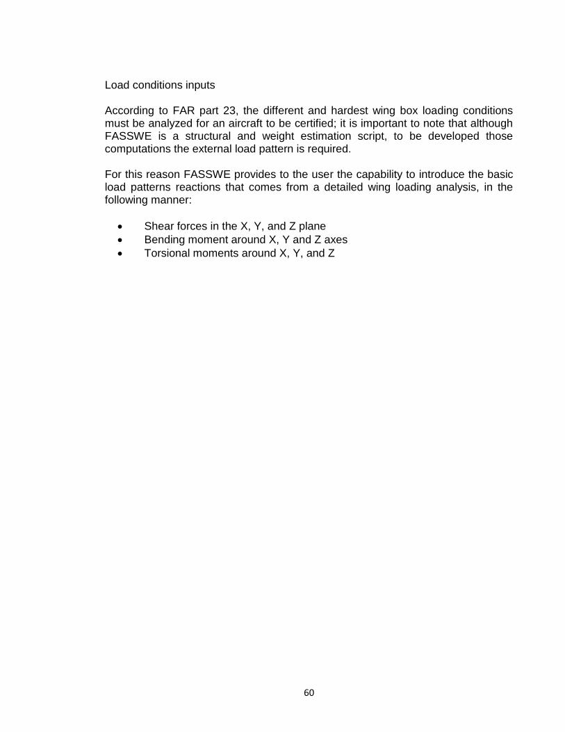
Load conditions inputs According to FAR part 23, the different and hardest wing box loading conditions must be analyzed for an aircraft to be certified; it is important to note that although FASSWE is a structural and weight estimation script, to be developed those computations the external load pattern is required. For this reason FASSWE provides to the user the capability to introduce the basic load patterns reactions that comes from a detailed wing loading analysis, in the following manner:

Shear forces in the X, Y, and Z plane

Bending moment around X, Y and Z axes

Torsional moments around X, Y, and Z

61

8. PROCESSING SCHEME In order to accomplish the desired tasks an order of processing must be defined; it basically indicates the main tasks that must be developed, the method that is used in each one and furthermore the inputs and outputs for each task. Within the processing scheme the encapsulation methodology to develop the script is chosen, therefore all tasks are defined through individual functions, and all data is called and stored using data abstractions, specially the OOP (Object Oriented programing). The main processing scheme is show as follows:

Figure 29 Basic processing scheme

62

Figure 29 Processing scheme

63

9. DATA STRUCTURE

9.1 DATA STRUCTURE SUMARY In this section is shown a rough approach of FASSWE data structure’s properties and methods, additionally a small portion of the code is displayed in order to give the reader an insight of the FASSWE data structure and data handling design. 9.1.1 The Class “Wingbox” The core of the entire FASSWE script; as its name indicates this data abstraction contains all data and sub-classes that are required to define an aircraft wingbox. The geometry of this wingbox data abstraction is first defined by a platform wing through the property and class “Wing”; later it is required to determine how the wingbox lies in the entire wing span; it is done through 2 spanwise boundaries, one at the wingbox root and the other at the wingbox tip, for this job the properties “obj.R_location” and “obj.T_location” as implemented. The wingbox characteristics such as number of ribs and number of spars are stored in the properties “N_ribs” and “N_Spars” respectively. In order to be initialized the wingbox class requires as input all data mentioned above; once this data is provided by the user directly or through a graphical user interface unit (GUI) the wingbox class creates 2 basic properties “obj.” With all this data mentioned above entered by the user this Class is initialized creating two properties “obj.Spars” and “obj.Completepanels” which are arrays of “Spar” and “Completepanel” objects that stores and allow the data handling of lower level subclasses as will be explained in the following subsections. The Class “Wingbox” have diverse methods used for FASSWE being highlighted three special kinds:

Edition methods such as “obj.edit_spar”, “obj.move_rib”,”update_spars” etc… allow the user to vary main features of the wingbox once it was created.

“obj.weight_calculation” determines the total wingbox’s weight ans stores it in the property “obj.Weight”. This method calls internal weight calculation methods of each wingbox component (e.g Spar, Complete panels).

64

Wingbox visualization methods such as “obj.plot_wingbox”, “obj.plot_ribs”, etc… allow the user to visualize in 3D the entire wingbox and its components.

Figure 30 Wingbox properties and methods

9.1.2 The Class “Wing” This is a basic class used in the script especially because it defines the geometric shape of the wing and the subsequent wing box structure.

65

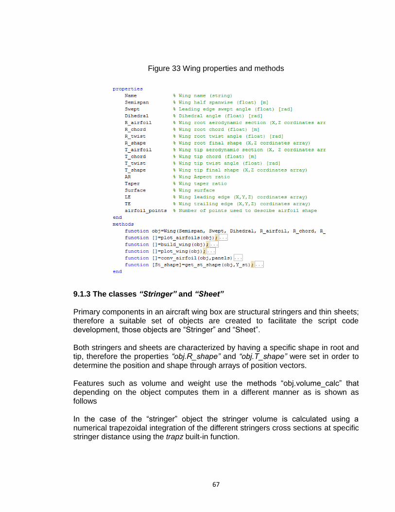
This class is based on a corresponding reference wing developed under aircraft conceptual design and it is initialized with basic data such as wing-half span, swept angle, dihedral angle, airfoil sections, chord, and twist angles. The airfoils are X, Z position vector arrays that constitutes a closed curve defining the airfoil shape; this closed curve is given in term of unitary chord, beginning from the trailing edge passing through leading edge and finishing again in TE. Later than entering an airfoil array of general length of position vectors, airfoil shape is updated through the method obj.conv_airfoil in order to define the airfoil shape with a a constant number of points. The method obj.conv_airfoil uses the built-in function interp1 that interpolates for a desired set of points there location based in the array entered by the user. During initialization other important parameters such as Aspect ratio, wing surface and Taper ratio are computed; in addition to the execution of obj.build_wing method. This method states the final shape and location of root and tip wing cross sections in the corresponding properties called “obj.R_shape” and “obj.T_shape”; these shapes and locations are determined through the wing features entered by the user for example: Swept and Dihedral angles produce a movement of tip reference frame over X and Z axis as is shown as follows:

Figure 31 Wingswept and dihedral

66

The twist angle at root and tip produces a change in the reference frame that can be seen in the next image as a movement and a rotation:

Figure 32 Airfoil twist rotation

The movement vector Δr0 can be determined trigonometrically, and the rotation through a rotation matrix using the twist angle, and the non-twisted airfoil shape (position vectors of each point in the airfoil); the rotation matrix used to determine the new airfoil position with respect the origin, is show as follows:

The object Wing has also a method useful to calculate the cross section shape in wherever part of the wing; this method is called obj.get_st_shape; as in the method obj.conv_airfoil, this method uses the built-in function interp1 to interpolate the position vectors at the desired wing span location. The method get_st_shape takes as an input the span location where is desired the cross section shape, and deploy as an output an array of position vectors defining the cross section shape at this specific spanwise location.

67

Figure 33 Wing properties and methods

9.1.3 The classes “Stringer” and “Sheet” Primary components in an aircraft wing box are structural stringers and thin sheets; therefore a suitable set of objects are created to facilitate the script code development, those objects are “Stringer” and “Sheet”. Both stringers and sheets are characterized by having a specific shape in root and tip, therefore the properties “obj.R_shape” and “obj.T_shape” were set in order to determine the position and shape through arrays of position vectors. Features such as volume and weight use the methods “obj.volume_calc” that depending on the object computes them in a different manner as is shown as follows In the case of the “stringer” object the stringer volume is calculated using a numerical trapezoidal integration of the different stringers cross sections at specific stringer distance using the trapz built-in function.

68

Figure 34 Stringer’s cross section

For the volume integration the required cross sections through the stringer length is calculated using the linear interpolation built-in function interp1 that using the root and tip shape provides the stringer cross section shape at the desired stringer distance. Stringers’ crippling stress used for structural stability purposes is computed in the method “obj.get_MS” applying equations 15, 16, 17 and diverse stringers properties (e.g thickness, cross area, material properties). This stringer’s crippling stress is stored in the property “obj.F_cs”

Figure 35 Stringer’s properties and methods

69

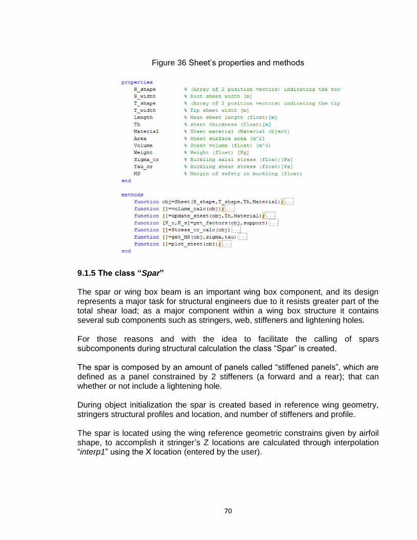
For the case of the “Sheet” object, volume is computed through the method “volume_calc” using the equation for a trapezoid area and its thickness.

Where a,b,c,d represent the sheet side lengths that are computed using the position vector at each vertex. 9.1.4 The methods “obj.get_MS”, “obj.Stress_cr_calc” and “obj.get_factors” The buckling strength calculation of each skin’s sheet is developed using a method implemented inside the “Sheet”. The three mentioned methods are complementary since they compute independently diverse variables required to get the sheet’s margin of safety. For example the method “obj.get_factors” determines the buckling factors Kc and Ks according to the curves exposed in section 6.4.2.2; these curves were stored point by point in the file “Buckling_factors.xls” and it is called each time a buckling factor is required for a special sheets’ width/length ratio. Based in these factors the method “obj.Stress_cr_calc” calculates the critical buckling stresses using equations 12, 13; this value is later compared with the actual stresses over the sheet in order to determine the margin of safety (MS); this last procedure is done in the method “obj.get_MS”.

70

Figure 36 Sheet’s properties and methods

9.1.5 The class “Spar” The spar or wing box beam is an important wing box component, and its design represents a major task for structural engineers due to it resists greater part of the total shear load; as a major component within a wing box structure it contains several sub components such as stringers, web, stiffeners and lightening holes. For those reasons and with the idea to facilitate the calling of spars subcomponents during structural calculation the class “Spar” is created. The spar is composed by an amount of panels called “stiffened panels”, which are defined as a panel constrained by 2 stiffeners (a forward and a rear); that can whether or not include a lightening hole. During object initialization the spar is created based in reference wing geometry, stringers structural profiles and location, and number of stiffeners and profile. The spar is located using the wing reference geometric constrains given by airfoil shape, to accomplish it stringer’s Z locations are calculated through interpolation “interp1” using the X location (entered by the user).

71

During object initialization the spar is created with the desired number of stiffeners located at the same distance from each other, later than object initialization is completed, this distance can be re-adjusted by calling the method “move_stiffener” that allows the user relocate an already created stiffener in the desired span location. In the same manner spar is firstly created without lightening hole, but they can be added in the spar calling the method “add_hole” that just requires the hole diameter and the panel number where is desired to add the referenced hole. Other important method for the “Spar” class is the method “weight_calculation”, as its name indicates it performs the task to calculate the total Spar weight, to accomplish so each one of the subcomponents weights is estimated within their own methods and added together as is displayed as follows:

Figure 37 Spar’s properties and methods

72

9.1.6 The class “Completepanel” A complete panel represents a kind of panel located in the upper or bottom surface between 2 spars; this wingbox sub-structure contains all stringers located between the two spars gathering them in a property called “obj.Stringers”. Additionally this object contains the property called “obj.Singlepanels” that is an array of “Singlepanel”; this object represents a single and little skin bounded by two stringers contained in the “obj.Stringers” property and 2 wingbox ribs. Each “Singlepanel” object has its own sub-class called “Skin” that is a kind of “Sheet” where basic information such as thickness and material can be easily called. The class “Completepanel” is initialized with default values of stringer location, thickness, profile, and material all this through the method “obj.update_completepanel”. The object “Completepanel” contains 2 methods that allows the user to change features in already created “Stringer” and “Singlepanel” objects. The method “obj.edit_stringer” gives the possibility to redefine stringer location, structural profiles, and material; additionally the method “obj.edit_singlepanel” allows changing singlepanel thickness and material. In order to determine the “Completepanel” weight the “obj.weight_calc” method calls the “obj.weight_calc” method of each stringer and singlepanel that is contained in “Completepanel” and adds them. It is important to recall that spar and their corresponding stringers weights are not computed here, rather than they are computed in the “Spar” method “obj.weight_calc”.

73

Figure 38 Completepanel’s properties and methods

9.1.7 The class “Material” Structural computations require certain materials properties of each component; this data is stored and handled through the class “Material”. The class “Material” stores diverse mechanical properties (e.g density, yield stress, Young modulus)

Figure 39 Material’s properties and functions

9.1.8 The classes “Point” and “Line” “Point” and “Line” objects constitute the most basic elements within a specific “Cell” object.

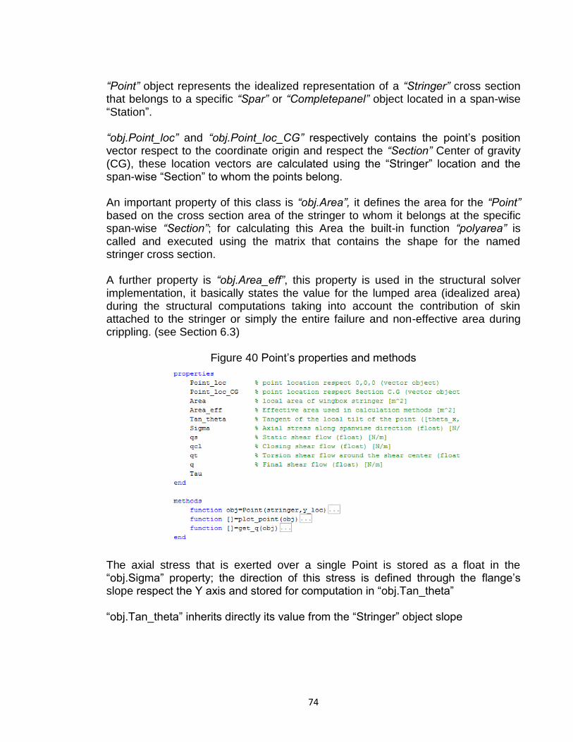
74

“Point” object represents the idealized representation of a “Stringer” cross section that belongs to a specific “Spar” or “Completepanel” object located in a span-wise “Station”. “obj.Point_loc” and “obj.Point_loc_CG” respectively contains the point’s position vector respect to the coordinate origin and respect the “Section” Center of gravity (CG), these location vectors are calculated using the “Stringer” location and the span-wise “Section” to whom the points belong. An important property of this class is “obj.Area”, it defines the area for the “Point” based on the cross section area of the stringer to whom it belongs at the specific span-wise “Section”; for calculating this Area the built-in function “polyarea” is called and executed using the matrix that contains the shape for the named stringer cross section. A further property is “obj.Area_eff”, this property is used in the structural solver implementation, it basically states the value for the lumped area (idealized area) during the structural computations taking into account the contribution of skin attached to the stringer or simply the entire failure and non-effective area during crippling. (see Section 6.3)

Figure 40 Point’s properties and methods

The axial stress that is exerted over a single Point is stored as a float in the “obj.Sigma” property; the direction of this stress is defined through the flange’s slope respect the Y axis and stored for computation in “obj.Tan_theta” “obj.Tan_theta” inherits directly its value from the “Stringer” object slope

75

“Line” object as “Point” is an idealized representation but in this case of the “Panel” cross section located in a span-wise “Section”; the “Line” object connects two “Point” objects representing two neighbor stringers connected by a single sheet. “Line” object inherits the thickness property “obj.Th” from the “Panel” object located in the specific span-wise “Section” “obj.Length” property contains the distance between points and it is used in addition to “obj.Th” to get “obj.L_t” that represents the Length/Thickness ratio useful for structural calculations. The effective thickness property or “obj.Th_eff” is used during structural computation and allows the script to know whether or not the sheet is effective resisting the loads (see Section 6.3) A special method in the “Line” class is the method “obj.get_nodes” this method generates a set of “Node” objects located along the “Line”. Those “Node” objects are operational points to be used during the structural analysis; they contain similar properties than the “Point” object in order to store certain results from the structural computation such as axial stresses in “obj.sigma”

Figure 41 Typical representation of Point, Lines and Nodes

Figure 42 Line’s properties and methods

76

9.1.9 The classes “Cell” and “Section” “Cell” and “Section” objects represent two of the most important objects in the FASSWE script; they define the lumped cross sectional shape, contain key methods for structural analysis and store some results. The class “Cell” is a data abstraction representing a set of “Point” and “Line” objects arranged in a close shape that belongs to a specific span-wise “Section”. “obj.Left_points” and “obj.Left_line” properties contains a set of 2 “Point” objects and a “Line” object that bound the data structure in the Left side; in the same manner “obj.Right_points” and “obj.Right_line” contains a set of 2 “Point” objects and a “Line” that works in the same manner but in the Right side. Properties “obj.Up_points”, “obj.Low_points”, “obj.Up_lines”, and “obj.Low_lines” do the same job in the upward and downward “Cell” location, being the idealized representation of a “Singlepanel” object and its “Stringers” in an specific span-wise “Section” Three important properties used during the structural computational method are “obj.Sum_L_t”, “obj.Sum_qs_L_t” and “obj.Sum_q_L_t”. For each line within a common “Cell” are computed the respective summations of length/ thickness ratio, static shear flow times length/ thickness ratio and final shear flow times length/ thickness ratio.

77

Figure 43 Typical Cell representation

Figure 44 Cell’s properties and methods

The class “Section” contains the entire number of “Cell” objects which belong to it and gathers them in the property “obj.Cells”; this “Section” is the main object used in the structural computation procedure because it represents the idealized (lumped) cross section of a wingbox in a specific span-wise “Station” In order to be useful for the structural computational method, the different moments of area are calculated and stored; it is accomplished using the “Point” and “Line” areas and locations through the following methods

78

“obj.CG_calc” method calculates the center of gravity for the entire “Section” respect the origin (0,0,0) and stores it in the property “obj.CG_loc”

“obj.Ixx_calc” method calculates the moment of inertia around the X-X axis that passes through the CG for the entire “Section” and stores it in the property “obj.Ixx”

“obj.Izz_calc” method calculates the moment of inertia around the Z-Z axis that passes through the CG for the entire “Section” and stores it in the property “obj.Izz”

“obj.Ixz_calc” method calculates the product of inertia around the CG for the entire “Section” and stores it in the property “obj.Ixz”

Based in the calculated moments of area, the inertia constants K1, K2 and K3 are estimated (see “K method” section 6.4.1.1) and stored in the properties “obj.K1”, “obj.K2”, “obj.K3” respectively.

Figure 45 Typical section representation

An important method that is called in higher level data abstractions is “obj.get_nodes”; this method provides the entire set of operational points (Nodes) in a section, it is done sub calling the method “Line.get_nodes” for each line belonging to this “Section” object.

Figure 46 Typical section representation with nodes

Two additional properties that store the results yielding from the stress analysis are:

79

“obj.P”, property that stores the resultant shear forces produced by flanges tilt

“obj.e”, property that stores the distance from the section CG to the shear center

9.1.9.1 The methods obj.Sigma_calc and obj.P_calc The axial stress is calculated using the “K method” approach for all “Point” and “Node” objects in a single “Section”, this is done by calling the method “obj.Sigma_calc”. The method “obj.Sigma_calc” takes as input the Mxx and Mzz bending moments and evaluates Point to Point and Node to Node every “Cell” in “obj.Cells”, storing the value of axial stress at each “Point” or “Node” property “obj.Sigma”. Once all the axial stresses are calculated and stored, the total shear forces contributions due to flanges tilt are calculated using “obj.P_calc” and stored in the “obj.P_calc” property. “obj.P_calc” method takes the stress and effective area of each “Point” in order to get the Force in the Y direction. With this value and with the flanges slope (property “Point.Tan_theta”) the corresponding magnitude in the X and Z direction are determined; the algebraic summation of those forces at each direction yields the result stored in “obj.P” 9.1.9.2 The method obj.qs_calc The method “obj.qs_calc” using the local shear forces (Vx, Vz) evaluates and stores the static shear flow value for each “Point” and “Node” in the “Section”. To accomplish so, this method uses the “K method approach”, and the corresponding initial condition (qs=0) or “cut” at certain section’s places (see section 6.5.2) The static shear flow is evaluated “Cell” by “Cell” in the entire “Section” and in order to evaluate them efficiently the following 4 user’s functions are used “qs_left”, “qs_ul”, “qs_r_nc”, “qs_right”. Although those functions will be described later in a more exhaustive manner they basically evaluates the “K method” summations based on whether or not there is a “cut” in a “Line”. The method “obj.qs_calc” has a conditional statement that determines the difference in the calculation procedure according to the “Cell” that is evaluated; for example if “Section” just contains a single “Cell” there is just one “cut” condition;

80

however if there are n number of “Cell” objects there are also n number of “cut” conditions. Once the method is ran all values of shear flow are stored in the property “qs” of each “Point” and “Node” objects. 9.1.9.3 The methods obj.qcl_calc and obj.add_qcl Both methods are used together in order to calculate and store the closing shear flow in a Section object. The method obj.qcl_calc uses the successive approximations method (see section 6.5.2) in order to calculate the closing shear flow pattern for a Section considering that no twist is generated. This method starts drawing back different summations of properties for each cell and stores them in simple arrays in order to be handled ease. With this data collected the Carry over factors and the first approximation for the shear flows are determined to begin the convergence. The successive approximation algorithm is evaluated Cell by Cell in order to refine the closed shear flow until the convergence is achieved. The shear flow converges when the percentage difference reaches a value lower than 0.5%, this is done through an operator “while”, however if the number of iterations is greater than 50 the script breaks the loop and returns the last value of closing shear flow that was calculated. Once the obj.qcl_calc method finishes the last values of closing shear flow per each Cell is returned using a simple array of values. With the corresponding closing shear flow per Cell, they must be stored in each one of the nodes and points that belongs to the Section; it is accomplished through the method obj.add_qcl. In a rough description this method computes and stores those values in such a manner that the shear flow directions adds appropriately (see). 9.1.9.4 The methods “obj.SC_calc” and “obj.M_SC_calc” As mentioned in the theoretical frame the shear center location is an important point in order to determine the net Torsional moment that the wingbox is carrying.

81

Once the non-twist condition shear flows are calculated (static + closing shear flows) the net torsional moment is calculated in FASSWE. For accomplishing so the method “obj.SC_calc” first determines the Shear center location; it is done evaluating the total torsional moment produced by the non-twist shear flows respect the center of gravity and calculating the point where the net shear force at this section cancels out (ΣM=0) (see section 6.4.1.4) For the implementation of the method “obj.SC_calc” it is important to highly the especial data treatment that was done in order to get the correct direction of the shear flows torsion contributions. According to the theory the infinitesimal contribution in Torsional moment is given by the following vector equation:

Or in the scalar form as:

The scalar from is useful for hands-made calculations but a little hard to implement computationally due to the absence of direction; however it can be taken as the magnitude of the torsional contribution and the infinitesimally area is ease determined using the built-in function “polyarea” In order to determine the final direction of this moment contribution around the CG the built-in function “cross” is used to evaluate the cross product between the “lever” vector and the “force” vector produced by shear flow (h x ds). Once this cross product is determined the shear flow sign (clockwise or anti-clockwise) is computed to determine the final direction. At this moment the only which remains yet in order to determine the total torsional moment (torsional moment respect the SC) is to translate the entire pattern of forces and moment from the origin [0,0,0] where input data is taken to the SC location. The last is done through the method “obj.M_SC_calc”; this method basically evaluates the torsion produced for each of the shear forces (Vx, Vz input) applied at the origin and adds to the torsional moment at origin (Myy input).

82

Figure 47 Forces and moments equivalence

9.1.9.5 The method “obj.qt_calc” With the torsional moment around the SC already known, the last step in order to calculate the final shear flow is to determine the shear flow produced just by torsion. This step is carried out through the method “obj.qt_calc” which using the successive approximation approach (see section 6.5.2.2) iterates over a first approximation of shear flow until it converges. Like the “obj.qcl_calc” method it also initiates calculating certain summations and factor needed for the numerical process (sum_L_t, L_t, Carry over factor etc ...) The shear flow converges when the percentage difference reaches a value lower than 0.5%, this is done through an operator “while”, however if the number of iterations is greater than 50 the script breaks the loop and returns the last value of torsional shear flow that was calculated. With these values of torsional shear flow they must be scaled according to the torsional moment around SC; this is done basically determining a scale factor between the torsion produced by the shear flow drawn from iteration with the desired torsional moment. Once those escalation factors are estimated they are applied to the shear flows in order to get the real torsional shear show (qt) at each cell. 9.1.9.6 The method “obj.dtheta_dy_calc” This method allows computing the derivative (dθ/dy) or “twist angle per unit of span” at each section; the final shear flow is calculated before this method can be called since it requires the final shear flow pattern and other arguments such as sheet thicknesses and material rigidity constant.

83

Figure 48 Section’s properties and methods

9.1.10 The “Routine” class The routine class is a data abstraction that stores and operates all that is needed within a single structural analysis; its basic function is to create a single workspace to analyze a “Wingbox” object subjected to a specific load pattern. When this class is initialized a copy of the “obj.Wingbox.Rib_stations” is created and stored in the “obj.Results” property this allows updating the “Section” objects without affecting the original Rib_stations.

84

“obj.Results” as mentioned above is a suitable set of “Section” objects that stores all results generated by the structural analysis methods. A “Routine” object is initialized with an internal reactions load pattern that is left ready for calling through the following properties:

“obj.M”, is a 4xn matrix that contains the internal moments reactions. The first column indicates the span-wise location and the last 3 columns their respective values for moments around X, Y, and Z.

The method “obj.Mesh” creates the operational points (nodes) used for the analysis, it is done sub calling the method “Section.get_nodes” at each section within the property “obj.Results”. The “obj.axial_strees_calc” calculates the axial stress pattern at every “Section” which belongs to a specific “obj.Results” The bending moments (Mxx and Mzz) are determined from the “obj.M” property through linear interpolation at each “Section”. They are used as inputs when the method “Section.Sigma_calc” is sub called at each Section within the “obj.Results” The method “obj.shear_stress_calc” calculates the final shear stress pattern at every “Section” which belong to “obj.Results”, it is accomplished by calling the following methods at each “Section” “obj.qs_calc” calculates static shear flow “obj.qcl_calc” calculates the closing shear flow “obj.SC_calc” calculates the shear center “obj.M_SC_calc” calculates the net torsional moment “obj.qt_calc” calculates the torsional shear flow “obj.update” adds all shear flows and calculates shear stresses based on

line thickness. Twist angle at each section is calculated as explained in section 6.4.1.5; the method “obj.twist_calc” estimates numerically the twist angle using the small disturbance approach. This method is based on local twist per unit of span (dθ/dy) and the net distance between stations. As initial condition there is considered zero twist in the wingbox root 9.1.10.1 Routines’ stability calculation methods FASSWE estimates three basic structural stability failure modes through three methods:

85

The method “skin_buck_calc” determines the MS in buckling of all skin “singlepanels” subjected to compression stresses; this method calls the local stability methods “obj.Stress_cr_calc” and “obj.get_MS” of each “Sheet” object. The method “str_crip_calc” calculates the crippling margin of safety (MS) of all wingbox’s stringers subjected to compression; as all the other stability methods its function is to call local methods of each “Stringer” class that calculates and stores crippling stresses of each one and compares it with the actual stresses which were evaluated through the method “obj.axial_stress_calc”. Another feature is that this method uses diverse conditionals to determine whether or not a stringers’ section is subjected to compression

Figure 49 Routine’s properties and methods

86

9.1.10.2 The Routine’s visualization methods “obj.Vis_sigma” and “obj.Vis_tau” In order to improve the comfortability of the user when checking out the calculation methods results, they are displayed in a 3D image of the idealized wingbox. The respective stress value at an especific location are showed using a set of colors that indicates a numerical value in N/m2 This visulization technique can be implemented through the Matlab built-in function “patch” (see built-in functions); this function requires a set of vertices in order to create faces that all together states a complete patch. Once this patch is already created it can be modified in order to set the desired color at the respective vertex. The method “obj.get_layers” creates all layers that are in the entire wingbox and stores all data needed in order to create the patch; this information is drawn back from the different nodes and strored at each property on “layer” objects. Once all the information needed for visualization is stored at their respective “layer” object, the stresses are visualized through the methods “obj.Vis_sigma” and “obj.Vis_Tau”, those methos basically execute the patch built in function and set the desire color within a certain range (min-max value of stress). Common visualization results can be seen as follows:

Figure 50 Axial stress visualization

87

Figure 51 Shear stress visualization

9.1.10.2 The Routine’s visualization method “obj.Vis_twist” The twist angle produced by a torsional moments around the shear center are visualized in FASSWE using the method “obj.Vis_twist”. In almost the same way as “obj.Vis_Sigma” and “obj.Vis_Tau” this method uses the matlab built-in function patch to plot the local twist angle using a set of color varying from the minimum to the maximum angle. This method also requires the Vis_layers data sarray that is contained in the routine in order to compute the visualization. Although the twist angle is handled through the entire script in units of radians, once it is plotted the visualization is done in terms of [°] degrees.

Figure 52 Twist angle visualization

88

9.1.10.3 The Routine’s visualization method “obj.Vis_MS_buck If the user is interested to know which skin’s panel has buckled it can use the routine’s method “obj.Vis_MS_buck”; this method visualize the upper and lower parts of the complete panel and indicates the margin of safety (MS)in buckling of all them through a color-bar that ranges from the maximum MS of the wingbox to the minimum MS. Panels that are not subjected to compression are showed in “black” color indicating that its MS tends to infinity.

Figure 53 Skin’s sheets Buckling MS visualization

89

10. FUNCTIONS

10.1 USER BUILT FUNCTIONS In order to encapsulate certain procedures that are developed many times through the FASSWE code were developed a set of user functions, the next is a brief summary of them: 10.1.1 Functions for section properties calculation

Sum_A_ulr(cell) adds the individual contributions of each “Point” belonging to the upper, lower and right “Lines” (summations) in order to calculate the final first moments of area

sum_A_left(cell) adds the individual contributions of each “Point” belonging to the left “Line” (summation) in order to calculate the final first moments of area

sum_I_ulr(cell) adds the individual contributions of each “Point” belonging to the upper, lower and right “Lines” (summations) in order to calculate the final second moments of area

sum_I_left(cell) adds the contributions of each “Point” belonging to the left “Line” in order to calculate the final seconds moments of area; this function is called mainly to estimate the contribution of the first wingbox cell

10.1.2 Functions for shear flow calculation

qs_left (cell, CG_loc, cte1,cte2) calculates the static shear flow summation produced by the Left_line and Left_points of a cell.

qs in the middle node is zero (cut condition)

qs_ul (cell, CG_loc, cte1, cte2) calculates the static shear flow summation produced by Upper and Lower Lines and Points of a cell.

qs in the middle node of each line is zero (cut condition)

qs_right (cell, CG_loc, cte1, cte2) calculates the static shear flow summation produced by the Right_line and Right_points of a cell.

qs in the middle node is zero (cut condition)

qs_r_nc (cell, CG_loc, cte1, cte2) calculates the static shear flow summation produced in the Right_line and Right_points of a cell.

90

It is just used for the Right_line in the last Cell where there is “non-cut” condition

10.2 MATLAB BUILT-IN FUNCTIONS

Matlab provides certain by default functions that are used during the development of the code, some of the more useful are the following:

linspace (a,b,n) generates a row of n number of elements equally spaced between a and b

plot (X,Y) displays a 2D plot based in X and Y location vectors

plot3 (X,Y,Z) displays a 2D plot based in X and Y location vectors

interp1(X,Y,x2) returns the linear interpolation value corresponding to the function given by X and Y location vector for a x2 value. For more information visit: http://www.mathworks.com/help/matlab/ref/interp1.html

polyarea(X,Y) returns the internal area of a closed polygon that is given by the position coordinates through the vectors X and Y . For more information visit http://www.mathworks.com/help/matlab/ref/polyarea.html

trapz(X,Y) returns the numerical trapezoidal integration of a curve given by the position coordinates through the vectors X and Y. For more information visit http://www.mathworks.com/help/matlab/ref/trapz.html

surf(X,Y,Z) creates and plots a surface given by vertices such as their locations are given by location vector X,Y,Z. For more information visit http://www.mathworks.com/help/matlab/ref/cylinder.html

classname.empty(n,m) creates and nxm empty array of either kind of object (classname). For more information visit: http://www.mathworks.com/help/matlab/matlab_oop/creating-object-arrays.html?s_tid=doc_12b

patch (X,Y,Z,C) creates a set of polygons using all vertex given by the location vectors X,Y,Z; additionally polygons color can be customized through the C vector according to the chosen color data option. For more information visit: http://www.mathworks.com/help/matlab/ref/patch.html

91

11. GRAFIC USER INTERFACE (GUI)

In order to facilitate the user to handle FASSWE a graphic user interface (GUI) is developed in Matlab using the built in function GUIDE. GUIDE is a function in Matlab that assists the GUIs code developer through a graphic environment avoiding most of the writing code regarded to graphic design and allowing the programmer to focus just in the data handling computations. 11.1 WINGBOX CREATION AND EDITION Creating and editing the wingbox are major tasks developed by FASSWE. There are 3 main frames that are used for this purpose:

a) Wing Design frame Platform wing creation frame (or wing design frame for simplicity) allows the user to create a platform wing that could be used to define the geometrical boundaries of the wingbox structure The wing design frame initializes and stores a “Wing” object within the main frame (MF); this “Wing” is initialized with basic wing design inputs entered by the user such as dihedral and twist angles, semi spanwise, chords, etc… Wing’s airfoils can be entered by the user uploading a .txt file with the airfoils X, and Z coordinates.

Figure 54 Wing design frame

92

b) Wingbox creation frame

Once the platform wing was created, FASSWE is ready to allow the user to create the wingbox object over which all structural analysis will be developed. The frame “Wingbox creation” initializes a wingbox object using inputs that define the basic configuration of a wingbox structures (e.g numer of ribs, number of spars, and wingbox location along the wing platform)

Figure 55 Wingbox creation frame

c) Wingbox edition With the exception of number of ribs and number of spars all remained wingbox features can be modified by the user; it includes specific features of Spars and horizontal complete panels and shifting the location of wingbox ribs.

93

Figure 56 Wingbox edition schematics

The wingbox edition frame deploys two independent frames for the edition of selected spars and complete panels. Main features that can be modified are stringers profiles and materials, sheets and webs thicknesses, and their respective locations. Default list of materials and structural profiles used in FASSWE are imported from “Profile_tables.xls” and “Material_tables.xls”; these lists can be customized by the user by simply updating them in Office Excel.

Figure 57, Wingbox edition frame

94

Figure 58 complete panel edition frame

Sets of skin’s single panels can be updated at the same time by using the row and column white box; each time a space is selected and features such as thickness and sheet material are changed they are updated automatically.

Figure 59 complete panel edition frame

95

* When is desired to change the number of spars and number of Ribs, the code automatically creates a new wing box, losing all data of previous wing boxes. Nevertheless for all other kinds of changes within the wingbox structure all data is stored by the application.

11.2 ANALYSIS AND VISUALIZATION Once a wingbox is created and modified the user is ready to develop the structural computations over the selected wingbox. The wingbox analysis frame creates a “Routine” object with the desired pattern of internal forces and moments; this pattern can be uploaded by the user through a .txt file stored in the PC memory.

a) Wingbox Analysis

Figure 60 Wingbox analysis frame

b) Wingbox visualization A wingbox can be visualized clicking the first button in the tools bar located in the upper left hand side. This button displays the wingbox visualization frame seen as follows:

96

Figure 61 Wingbox visualization frame

c) Results visualization Results that are produced by running a “Routine” in the Analysis frame can be displayed in the Results visualization frame; it allows the user to choose the specific output variable among all possible (e.g axial stress, shear stress, twist angle, stability MS) As explained in the data structure chapter these results are visualized through a color bar ranging from minimum to maximum values over the entire wingbox.

Figure # Results visualization frame

97

Although in the same frame Margin of safety (MS) for crippling is visualized in a slightly different manner than remained results; each independent stringer located either in a spar or in a completepanel is selected by the user through popupmenus and the corresponding MS for each spanwise station is automatically updated in a 2D plot.

Figure 62 Stringer’s MS visualization frame

98

12. SCRIPT VALIDATION 12.1 TEST 1 WEIGHT CALCULATION The validation of weight estimation methods implemented in FASSWE is developed using the CAD software Solid Works and specifically its tool “physical properties”; this tool estimates diverse physical properties of the selected design, in this case the weight and volume. Three independent cases were evaluated: 1) A single Z stringer with the same dimensions and material was designed in

Solid Works and also in FASSWE.

2) A single tapered web sheet with the same dimensions and material was designed in Solid Works and also in FASSWE.

3) Three complete spars with same dimensions and materials were designed in Solid Works and FASSWE and analyzed together.

Figure 63 Z stringer and sheets designed in Solid Works and FASSWE

Figure 64 Spars in Solid Works and FASSWE

99

The comparison between the volume and weight estimations returned by FASSWE and Solid Works are shown in the following table; it is clear that the results provided by FASSWE agree within a perceptual error no greater than 2.8%

Table 1 Weight estimation comparison

Cases

FASSWE Solid Works error [%] Volume

[m^3] Weight

[Kg] Volume [m^3]

Weight [Kg]

Z stringer 4.5 x10-5 0.35 4,3x10-5 0.34 2.8

Sheet 8.3x10-5 0.65 8.3x10-5 0.65 0

Spar (x3) N/A 3.19 N/A 3.23 1.2

Wing-box

12.2 TEST 2, AXIAL STREES IN TAPERED WINGBOX The validation Test 2 was carried out in order to determine the correct calculation of axial stresses and forces, and its subsequent contributions to total internal shear loads; for doing this the example 21.2 of ref [2] was chosen and simulated in a routine of FASSWE. In the book’s example a shear load of 100KN is exerted over a tapered wingbox and the corresponding axial stresses and Forces are calculated in the middle section in addition to the shear contributions.

100

Figure 65. Example 21.2 scheme

Source Ref 18, example 21.2

In order to simulate the example an equal lumped wingbox is created and evaluated under the same load path using the test_routine.stress_calc

Figure 66. Lumped wingbox for Test1 in FASSWE

Table 2 shows the comparison between the results obtained in the FASSWE analysis and the results stated in the text book showing that the maximum perceptual error in the axial loads calculation is near 2.5%, error produced by the rough numerical approximation in the boom area calculation.

Table 2. Test 2 results comparison

Boom Area

(mm2)

Book FASSWE

dx/dz dy/dz Py

(KN) dx/dz dy/dz

σ (Mpa)

Py (KN)

1 900 0,1 -0,05 -100 0,1 -0,05 -115 -101

2 1200 0 -0,05 -133 0 -0,05 -114 -137

3 900 -0,1 -0,05 -100 -0,1 -0,05 -115 -101

101

4 900 -0,1 0,05 100 -0,1 0,05 115,1 100

5 1200 0 0,50 133 0 0,05 143,2 137

6 900 0,1 0,50 100 0,1 0,05 114,6 101

To validate the shear force contribution in the 2nd section (middle) due to flanges tilt the property test_routine.Results(2).P is called and compared to the book’s result, as in the previous comparison the perceptual error in near 2.5%


Book FASSWE

ΣPx (KN) 0 0

ΣPy (KN) 0 0

ΣPz (KN) 33,4 34,2

12.3 TEST 3, STATIC SHEAR FLOW IN SINGLE AND MULTICELL WINGBOXES Test $ is a validation suit developed to check the correct operation of the static shear flow calculation method, to validate this one 2 different book’s examples were chosen. In the first example the simple tapered “Wingbox” used in Test 1 is evaluated with FASSWE in the middle section under a local shear force Vz=66.6 KN and compared with the results found in example 21.2 ref 18.


Booms Book FASSWE

qs(KN/m) qs(KN/m)

1 -2 -33,2 33,7

2 -3 -77,5 78,6

3 – 4 -110,7 112,5

4 – 5 -77,5 78,6

5 – 6 -33,2 33,7

When compared the opposite signs between both results come from the fact that the book’s example takes as positive the clockwise direction rather than FASSWE that always takes as positive the anti-clockwise. Despite of that the final shear flow

102

in both results is anti-clockwise agreeing with the fact that net force between booms 3 and 4 must be in the upward direction because the shear load is positive. The second example is drawn from ref 3, example A15.12 and its main goal is to validate the same static shear flow calculation but now in a multiple-cell wingbox. Example A15.12 set up a 5 Cells wingbox subjected to an external load of 1000lb=4.45KN, the static shear flow is found just considering the flanges areas effective in bending and doing the “cut” conditions in the first 5 vertical lines from left hand side.

Figure 67 5 Cells wingbox section in example A15.12

Flange areas are as follows: Flanges a, a’ = 2 in2 = 1.29x10-3 m2 Flanges b, b’, f, f’ = 1 in2 = 0.65x10-3 m2 Flanges c, c’, d, d’, e, e’ = 0.5 in2 = 0.32x10-3 m2

The table displayed as follows gathers the constant shear flows between the different flanges at this station, comparison shows a good agreement between data collected from the text book and the FASSWE evaluation. For both cases the single and the multicell wingbox the shear flow percentage difference is lower than the 2%, error that has was told before depends on the numerical approximation techniques that FASSWE uses in different computations.


Booms Book FASSWE

qs (lb/in) qs(KN/m) qs(KN/m)

a’ – b’ -36,4 -6,4 -6,3

b’ – c’ -54,6 -9,6 -9,5

c’ – d’ -63,6 -11,1 -11,1

d’ – e’ -72,7 -12,7 -12,7

e’ – f’ -81,8 -14,3 -14,3

f’ – f -100,0 -17,5 -17,6

103

f – e -81,8 -14,3 -14,4

e – d -72,7 -12,7 -12,7

d – c -63,6 -11,1 -11,1

c – b -54,6 -9,6 -9,5

b – a -36,4 -6,4 -6,3

12.4 TEST 4 TOTAL SHEAR FLOW IN A 3 CELLS WINGBOX The closing shear flow calculation is validated for a multicell wingbox using the static stress analysis provided in Ref 24. The mentioned analysis states a 3 cell wingbox all material effective that is subjected to shear loads in the X and Z directions. In the mentioned paper the internal shear flow pattern is determined independently for each load alone. In the first suit case the internal reaction for a shear load of -1173 lb = -5220 N in the Z direction is estimated in FASSWE, the comparison in the results obtained is shown as follows.

Figure 68. Total shear flow due to shear load in Z direction

Figure extracted from Ref [12]

Test 6. Results comparison

Points

Paper FASSWE

q total (lb/in)

q total (KN/m)

q total (KN/m)

10 -50 -8,76 8,67

1 -10 -1,75 1,65

20 -70 -12,26 12,19

70 30 5,25 -5,36

90 -40 -7,00 6,62

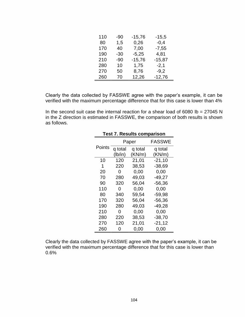
104

110 -90 -15,76 -15,5

80 1,5 0,26 -0,4

170 40 7,00 -7,55

190 -30 -5,25 4,81

210 -90 -15,76 -15,87

280 10 1,75 -2,1

270 50 8,76 -9,2

260 70 12,26 -12,76

Clearly the data collected by FASSWE agree with the paper’s example, it can be verified with the maximum percentage difference that for this case is lower than 4% In the second suit case the internal reaction for a shear load of 6080 lb = 27045 N in the Z direction is estimated in FASSWE, the comparison of both results is shown as follows.

Test 7. Results comparison

Points

Paper FASSWE

q total (lb/in)

q total (KN/m)

q total (KN/m)

10 120 21,01 -21,10

1 220 38,53 -38,69

20 0 0,00 0,00

70 280 49,03 -49,27

90 320 56,04 -56,36

110 0 0,00 0,00

80 340 59,54 -59,98

170 320 56,04 -56,36

190 280 49,03 -49,28

210 0 0,00 0,00

280 220 38,53 -38,70

270 120 21,01 -21,12

260 0 0,00 0,00

Clearly the data collected by FASSWE agree with the paper’s example, it can be verified with the maximum percentage difference that for this case is lower than 0.6%

105

12.5 TEST 5 TOTAL SHEAR FLOW IN A 10 CELLS WINGBOX In order to bring the script to an extreme case; especially the shear flow calculation method, the Ref 3 example A15.13 is chosen. In this method a supersonic airplane wingbox structure composed by 10 cells is subjected to a shear load of -1000lb = -38921N, all material is considered effective and there are not flanges.

Figure 69 10 cells wingbox section example A15.13

Table 8. Test 5 Results comparison

Web (Line)

Book FASSWE

q total (lb/in)

q total (KN/m)

q total (KN/m)

1 -109,3 -19,1 18,9

2 177,7 31,1 -29,8

3 183,2 32,1 -31,5

4 185,2 32,4 -31,8

5 187,1 32,8 -32,2

6 191,6 33,6 -33,0

7 176,5 30,9 -30,2

8 182,1 31,9 -31,8

9 167,9 29,4 -29,5

10 161,4 28,3 -28,8

11 120,6 21,1 -22,9

Clearly the data collected by FASSWE agree with the paper’s example, it can be verified with the maximum percentage difference that for this case is 1%

106

12.6 TEST 6 SHEAR CENTER IN A SINGLE CELL WINGBOX

The shear center calculation method is validated through the example 8.6 of Ref 20, in this example a single cell wingbox is subjected to a shear load of 400lb = 1779.2 N in the downward direction, the following figure shows its shape using the FASSWE plotting capability.

Figure 70 Single cell wingbox example 8.6

According to the mentioned example the shear center is located 9.42 in = 0.239 m to the left from right hand side spar. Later than the static and closing shear flows are calculated the method “obj.Section.SC_calc” is called in order to determine the shear center location respect the origin ([0,0,0]); the method output is showed as follows.

Figure 71 shear center calculation output

According to the last line in this code output, the shear center location is 0.2987 m from [0,0,0] point; as the right spar is located 21 in = 0.533 m from the origin is

107

means that the shear location according to FASSWE is 0.235 m from the right spar. Clearly one can see the good agreement between book’s example and FASSWE output; in fact the percentage difference is 1.6% 12.7 TEST 7 TORSIONAL SHEAR FLOW IN A MULTICELL WINGBOX The final shear flow calculation method that is validated is the “obj.qt_calc”; as explained before it is in charge of torsional shear flow contribution, in order to validate this one the example 3 of section A6.15 in Ref 3 is used. In this example a 4 cell wingbox is subjected to a torsional moment of 100.000 lb.in = 11298 N/m without not any shear load that produce an additional torsion.

Figure 72 4 Cells wingbox example A16.15 (3)

The wingbox shape and features where created in FASSWE and the method for torsional shear flow was called for the section showed before through the following statement: test_routine.Results(1).qt_calc(11298); “test_routine” is the routine created for the wingbox analysis

108

As output FASSWE determines the following values that are compared with the results that can be check out in Ref 3.

Table 9 Test 7 result comparison

Cell

Book FASSWE

q torsion (lb/in)

q torsion (KN/m)

q torsion (KN/m)

1 47,1 8,25 8,17

2 65,3 11,44 11,72

3 49,9 8,74 8,99

4 29,41 5,15 5,30

12.8 TEST 8 SHEET BUCKLING CALCULATION TEST

In order to validate the implementation of the sheet’s buckling strength calculation, the example C5.13 of Ref 3 is used. In this example the critical axial and shear stresses are calculated and compared to the actual stresses produced by combined shear and compression in order to get the margin of safety (MS) The example is recreated in FASSWE through calling the following methods of the “Sheet” object: “test_sheet=Sheet(R_shape,T_shape,Th,material);” This method creates a sheet with the same geometric característics and materials than sheets in example C5.13 “test_sheet.Stress_cr_calc;” calculates the critical stresses for the sheet buckling “test_sheet.get_MS(5.64e6,5.8e6)” estimates the margin of safety of the sheet subjected to an axial stress of 819psi (5.64 Mpa) and a shear stress of 854 psi (5.8 Mpa) The data returned by FASSWE is compared with the book’s results in the following table:

109

Table 10. Buckling parameters comparison

FASSWE Book

KC 4 4

KS 5.8 5.8

σcr (Mpa)

13.2 13.1

(1.9 Kpsi)

τcr (Mpa)

19.1 19

(2.7 Kpsi)

M.S 0.71 0.69

12.9 VALIDATION IN OVERALL

Table 11 Overall Results

Test Item evaluated max error

(%)

1 Components weight 2,8

2 Tapered WB axial load 2,3

3 Static shear flow 1,6

4 Total shear flow (5c) 0,5

5 Total shear fow (10 c) 8,1

6 Shear center calc 1,6

7 Torsional shear flow 2,4

8 Sheet buckling 2,8

110

13. PRACTICAL EXAMPLE

In this section is presented a complete user’s example of the redesign of a wingbox structure using FASSWE. For this case the wingbox of a LANSHE LAKE LA-250 sea-plane is analyzed when subjected to external forces during a steady level flight.

Figure 73 LA-250 “Renegade”


Wing features required to create the wingbox structure are depicted as follows:

Table 11 LA-250 Wing features

Wing span (m) 11.68

mac (m) 1.35

Root airfoil NACA 4415

Root chord (m) 1.7

Tip airfoil NACA 4409

Tip chord (m) 1

AR 8.6

Dihedral (°) 5

# Spars 3

Hinge line (% chord) 75

111

Figure 74 LA-250 Wing Design

The wingbox is created from the platform wing shape using 3 Spars and 25 Ribs; the wingbox root is slightly sideward in order to provide space for the carry-through structure and the wingbox tip is also slightly inward to provide space for the tip fairing.

Figure 75 LA-250 Wingbox creation

By design trend spaces between ribs are established in such manner that they are closed to each other in the wingbox root and more separated at the tip; the spaces distribution is shown in the following table

112

Table 13 LA-250 Spaces

between ribs

Ribs Space (m)

1-12 0,1

12-20 0,2

20-25 0,5

Since upper panels are dominated by compression stresses, instability phenomena is more likely to occur in this region therefore 2 inter spar Z stringers (1.2”x1.2”) are located to reduce this tendency; in the bottom side is located just 1 stringers. The entire upper panel is covered by a 1.5 mm skin, while the bottom panel has a thickness of 1mm; both using aluminum 2024-T6

Figure 76 Complete panels edition

According to FASSWE the estimated weight for the entire wingbox without include the ribs is 63.5 Kg.

113

Figure 77 LA-250 wingbox weight estimation

The wingbox analysis is carried out based in the external loads estimated in appendix A

Figure 78 stress analysis results

Maximum axial stresses ranges from -63MPa to 45 MPa Maximum shear stresses ranges from -16MPa to 12 MPa

114

Aluminum 2024-T6 used for both panels has yield stresses σy=324 MPa and τy=162 MPa therefore upper and bottom panels as well as lower stringers are safe from failure.

Figure 79 LA-250 Twist angle result

Maximum twist angles ranges from -0.08° to 0.65°

Figure 80 Buckling analysis results

From skin stability analysis clearly can be observed that the root of the upper panel is slightly subjected to buckling since their M.S lies in the threshold (M.S=0);

115

additionally panels at the tip have large MS as expected due to low axial and shear stresses. Black regions in the bottom panel indicated that the root is not subjected to buckling since tension is dominant in this region.

116

14. FUTURE DEVELOPMENTS

This version of FASSWE is a minimum viable product (MVP) aimed to be submitted to potential customers to receive feedback from them in order to keep improving the application according to their necessities. Main developments and changes over the current application will be stated by this future market research; however based in the experience acquired in the development of the present product there are some improvements that the author suggest for a future α (Alpha) version:

To implement a more accurate numerical method to estimate the stringer’s volume. Although the current maximum error is around 2.8% (see section 12.9) this value could be considerable during critical designs.

To avoid updating the wingbox weight each time a component is edited; it would reduce considerably the overall execution time.

To develop a more efficient wingbox visualization method that just updates the visualization of components which were edited rather than plot again the entire wingbox.

To make changes in the spar edition method implementation “Wingbox.edit_spar” allowing it to work quicker. As a hint this method is taking too long because it is creating new adjacent complete panels from scratch each time this method is called.

To make further software validation comparing results in FASSWE with widely used structural software such as Ansys and NASTRAN.

To make further software validation comparing results in FASSWE with experimental data collected from structural tests.

To develop a further debugging of GUI

To create alerts to the user to communicate when a wingbox is not yet ready for analysis

117

15. CONCLUSIONS According to the software validation this Minimum Viable Product (MVP) of FASSWE is a reliable application ready to be submitted in the marketplace for market research and customer’s feedback. FASSWE development required a big effort in the data structure implementation reason why its detailed planning prior than writing the code saved a lot of time in redefining objects through the procedure. For complex data structures such as used in FASSWE to debug codes a long time later than finishing the implementation creates many troubles for the programmer since knowledge associated with the code behavior sometimes is no longer.

118

16. REFERENCES 1. ARDEMA Mark D., CHAMBERS Mark C., PATRON Anthony P., HAHN Andrew S., MIURA Hirokazu, and MOORE Mark D. , Analytical Fuselage and Wing Weight Estimation of Transport Aircraft, National Aeronautics and Space Administration NASA, Ames Research Center, California, May 1996 2. BECKER Herbert; buckling of composite elements NACA Technical note 3782, Washington, July 1957 3. BRUHN E.F., Analysis and Design of Flight Vehicles Structures, 1st edition, Jacobs Publishing Inc., Carmel, Indiana, U.S.A, June 1973 4. BUDYNAS, NISBET, ,Shynglie’s Mechanical Engineering design, 8th edition, Mc Graw Hill, 2006 5. CHUN YUNG Niu Michael, Airframe stress analysis and sizing, 2nd edition, Conmilit Press Ltd., Hong Kong, January 1999 6. CHUN YUNG Niu, Airframe structural design, 1st edition, Conmilit Press Ltd., Wanchai, Hong Kong, January 1995 7. DARMOFAL David, Drela Mark and Uranga Alejandra, Lecture notes 16.101x Introduction to aerodynamics, Massachusetts Institute of Technology (MIT), Cambridge Massachusetts, 2003 8. DRELA Mark, Flight Vehicles Aerodynamics, Massachusetts Institute of Technology (MIT), 1st edition, The MIT Press, London, England 9. Federal aviation Organization, Federal Aviation Regulation Part 23, May 2002 10. FORD L.R., The solution of equations by the method of successive approximations, The American Mathematical Monthly, 1925 11. GERARD, BECKER; buckling of flat plates NACA Technical note 3781, Washington, July 1957 12. GILAT Amos, Matlab® An introduction with applications, John Wiley & Sons Inc., Danvers, Massachusetts, United States, 2004 13. GUTTAG John V., Introduction to Computation and Programming in Python,1st

edition, MIT series, Fall 2012 14. HAHN Brian, VALENTIN Daniel T., Essential Matlab® for Engineers and Scientists, 3rd edition, Elsevier Ltd., Jordan Hill, Oxford, Great Britain, 2007

119

15. HÜRLIMANN F., KELM R., DUGAS M., OLTMANN K., Kress G., Mass estimation of transport aircraft wingbox structures with a CAD/CAE-based multidisciplinary process, Elsevier Ltd., Aerospace science and technology, 2011 16. INTERNATIONAL CIVIL AVIATION ORGANIZATION (ICAO), Annex 8 Airworthiness of aircraft, 10th edition, April 2005 17. Jane’s all the world aircrafts 2004-2005, Jane’s Information Group, Virginia 2004 18. MEGSON T.H.G., Aircraft structures for engineering students, 4th edition, Elsevier Ltd, Jordan Hill, Oxford, Great Britain, 2007 19. ORTIZ BERROCAL Luis, Elasticidad, 3rd edition, Mc Graw Hill, 1998 20. PEERY David J, Azar J. J., Aircraft structures, 2nd edition, McGraw Hill, 1982 21. PIPERNI P., ABDO M., and KAFYEKE F., The Application of Multi-Disciplinary Optimization Technologies to the Design of a Business Jet, 10th AIAA/ISSMO Multidisciplinary Analysis and Optimization Conference, New York, 2004 22. RAYMER Daniel P., Aircraft Design a conceptual approach, 2nd edition, AIAA Education Series, American Institute of Aeronautics and Astronautics Inc., Washington D.C, 1992 23. RIES Eric, The lean Start Up, Crow business, New York, 2011 24. RONALD D Kriz, Static stress analysis of a sailplane wing constructed of composite materials, California Polytechnic State University San Luis Obispo, December 1973.

120

17. APPENDIX A LANSHE LAKE LA-250 STEADY LEVEL FLIGHT WINGLOADING

CALCULATION

In this appendix is presented a rough wing loading estimation of the LANSHE LAKE LA-250 in level flight at mean sea level location. The only external forces considered are Aerodynamic wing forces (Lift and Drag) and fuel weight. In order to facilitate the calculations the following assumptions are considered.

Lift produced by fuselage and tail is negligible compared with wing

Elliptic wing loading distribution

Profile drag is negligible compared to induced drag 17.1 Wing lift distribution The aerodynamic circulation in the wing is given by:

Equation A.1 Elliptical circulation distribution

Where: Γ Circulation Γ0 Circulation constant y Span location b Spanwise Since the aircraft is in level flight the aircraft gross weight is supported by the wing lift and it can be expressed in term of circulation distributions as:

Equation A.2 Circulation as function of weight

Where: WTO Gross take-off weight ρ Air density at MS

121

Evaluating the integral:

Replacing terms and solving for Γ0

The lift distribution of lift per unit of span is given by:

Equation A.3 Elliptic lift distribution

Replacing terms

In the range

17.2 Wing drag distribution Since induced angles are usually small the Induced Drag (or Drag due to lift) per unit of span can be approximated as:

Equation A.4 Section induced Drag

Where

122

Since the wing is subjected to an elliptical lift distribution the induced angle is constant along the wing span 18 and is given by:

Equation A.5 Induced angle for an elliptic lift distribution

Where: V Flight speed

Replacing terms the induced drag per unit of span is:

Since

17.3 Wing pitching moment The pitching moment is assumed to be constant along the wing span since the airfoils curvatures are the same in the root as well as in the tip; a simulation in Xfoil is carried out at a Reynolds number of 6x106 (Cruise Reynolds number) Since the induced angle is constant and there is not wing twist the required local lift coefficient at each span section is cl=0.35, yielding in an angle of attack α=-1°; according to Xfoil at this angle the pitching moment is equal cm=-0.0103 Therefore the pitching moment per unit of span at y=c/4 is:

Equation A.6 Pitching moment per unit of span

Where:

123

C mean aerodynamic cord Cmc/4 pitching moment coefficient at 25% of mean chord The pitching moment per unit of span around the LE or origin is:

Equation A.7 Leading edge pitching moment per unit of span

Where: M’LE Pitching moment at Leading edge per unit of span M’c/4 Pitching moment at 25% of mean chord per unit of span

17.4 Fuel tanks contribution Since tanks dimensions are not available, a good estimate can be achieved using the airfoil height and fuel weight to determine a approximated weight distribution

The fuel tank volume is known from Ref 17, the fuel tank length can be estimated as follows:

Solving l=0.296m LA-250 aircraft uses AV-GAS as fuel with a density of 0.72 Kg/lt; therefore fuel tank weight is:

124

The fuel weight load distribution is therefore:

In the region

17.5 Shear Forces Shear forces in the Z direction are given as: Lift contribution

Equation A.8 Lift shear force

Where: V’z Shear force in Z direction Fuel tank contribution

Equation A.9 Fuel tank shear force

The entire shear force distribution can be compute adding both segmented functions in the corresponding ranges The shear Force in the X direction is:

125

Equation A.10 Drag shear force

Where: Vx Shear force in the X direction

17.6 Moments Bending moments or reaction moments about X and Z axes are mainly produced by aerodynamic shear forces

Equation A.11 Bending moment around X-X axis

Where: Mxx Bending moment around XX axis

Equation A.12 Bending moment around Z-Z axis

Where: Mzz Bending moment around Z-Z axis

126

Torsional moment or reaction moment about Y axis is given by the pitching moment around the leading edge:

Equation A.13 Torsional moment around Y-Y axis

Where: Myy Torsional moment around Y-Y axis

FASSWE SCRIPT FOR STRUCTURAL SIZING AND ...

Documents

Transcript of FASSWE SCRIPT FOR STRUCTURAL SIZING AND ...