Farklı Seviyelerde Korozyona Uğramış Bir Köprünün Hasar ...

Farklı Seviyelerde Korozyona Uğramış Bir Köprünün Hasar Görebilirlik Analizi

Gökhan Barış SAKCALI1*, İsa YÜKSEL1

1Bursa Teknik Üniversitesi, İnşaat Mühendisliği Bölümü, Bursa * Sorumlu yazar, [email protected]

ÖzetBetonarme yapılarda “sessiz deprem” diye nitelendirilen donatı korozyonu, donatı çubuğunda enkesit kaybına, donatı çubuğunun mekanik özelliklerinde bozulmalara (akma dayanımı, kopma dayanımı, elastisite modülü ve kopma birim şekil değiştirmesinde azalmalar), betonda çatlamalar ve aderans kaybına neden olmaktadır. Bunun taşıyıcı sisteme yansıması ise zamana yayılı olarak önemli performans kayıpları olarak ortaya çıkmaktadır. Bu çalışmada Harşit Nehri üzerinde yer alan bir betonarme köprünün farklı donatı korozyonu senaryoları için kırılganlık eğrileri oluşturulmuş ve EC-8 ile uyumlu yapısal performans değerlendirmesi sunulmaktadır. İlk olarak, köprünün SAP2000 yazılımı ile yapısal modeli oluşturulmuştur. Referans (korozyonsuz durum) dahil olmak üzere köprü için dört farklı korozyon senaryosu öngörülmüştür. Korozyon senaryoları köprü ayağında kullanılan en büyük çaplı donatı çubuğu olan 26 mm çaplı donatının %0 (referans), %5, %10 ve %15 kütle kaybına denk gelecek şekilde seçilmiştir. Kütle kaybının belirlenmesinde literatürde bulunan mevcut bağıntılar kullanılmıştır. Kütle kaybına göre donatı çubuğunun mekanik özelliklerinde meydana gelen değişimleri belirlemede, literatürde bulunan uniform korozyon için önerilen denklemler kullanılmıştır. Her bir senaryo için betonarme köprünün artımsal dinamik analizi yapılmıştır. Artımsal dinamik analizde ayakların göçmesine neden olabilecek bir dizi yer hareketi seti belirlenmiştir. Her bir yer hareketi setine karşılık gelen göçme olasılığı hesaplanmıştır. Artımsal dinamik analiz için yedi farklı deprem kaydı seçilmiştir. Bu deprem kayıtları, farklı yer hareketi özelliklerine sahip olup, EC-8’e uygun şekilde ölçeklendirilmiştir. Her senaryo için seçilen deprem kayıtları artımsal dinamik analizde kullanılmıştır. Analizler sonucunda tepe yerdeğiştirmesi, taban kesme kuvveti ve kırılganlık eğrileri elde edilip değerlendirilmiştir. Kesit analizleri köprü ayaklarının eksenel yük taşıma gücünün ve moment kapasitesinin korozyon düzeyine bağlı olarak azaldığını göstermektedir. Bu sonuca parelel olarak, korozyon düzeyi yükseldikçe köprü ayaklarının rijitliği azalmakta, köprü ayağının tepe yerdeğiştirmesi artmaktadır. Korozyonsuz ve korozyonlu senaryolarda PGA değerinin artmasıyla köprünün kenar ve orta ayaklarında meydana gelen tepe yerdeğiştirmesi artış eğilimi göstermektedir. Diğer taraftan, korozyon düzeyinin taban kesme kuvveti üzerine çok büyük etkisi olmadığı ve ayaklarda meydana gelen taban kesme kuvvetinin PGA seviyesine bağlı olarak doğruya yakın bir değişim gösterdiği belirlenmiştir. Yapısal performans açısından değerlendirildiğinde; maksimum yer ivmesi değerleri arttıkça korozyonlu köprü ayaklarında önemli yapısal hasarlar meydana gelmektedir. Korozyon seviyesi arttıkça köprü ayaklarındaki mafsallaşma olasılığının arttığı görülmektedir. Korozyon seviyesinin artmasına ek olarak, zemin yer hareket düzeyine bağlı olarak sistemin göçme olasılığı artmaktadır. Bu çalışmada elde edilen sonuçlar gösteriyor ki, betonarme taşıyıcı elemanlarda donatı korozyonu yapısal performansı son derece olumsuz etkilemektedir. Köprünün hasar alma olasılığı korozyon düzeyine bağlı olarak artmaktadır. Köprü ve viyadük gibi önemli yapılarda korozyona neden olabilecek yıpratıcı çevresel etkenlerin de varlığı dikkate alınarak, bu yapıların belirli zamanlarda performans kontrolüne tabi tutulmaları sürdürülebilirlik açısından gereklidir.

Anahtar Kelime: Artımsal dinamik analiz, betonarme, korozyon, köprü.

Giriş

Donatı korozyonu donatı çubuğunda enkesit kaybına, donatının mekanik özelliklerinde bozulmalara ve aderans kaybına sebep olur. Bu durum betonarme elemanların taşıma gücünü azaltmaktadır. Bu azalma

720

ile birlikte maksimum yer ivmesindeki değişime bağlı olarak sismik performans düşmektedir. Bu çalışmada, örnek vaka için seçilen gerçek bir betonarme köprünün ayaklarına farklı düzeylerde hayali donatı korozyonları uygulanmıştır. Bu senaryolar altında köprünün artımsal dinamik analizler yapılmıştır. Bunun sonucunda, maksimum yer ivmesi ve korozyon düzeyindeki değişimlerin köprü ayakları hasar yüzdelerindeki değişimler incelenmiştir.

Materyal ve Metod

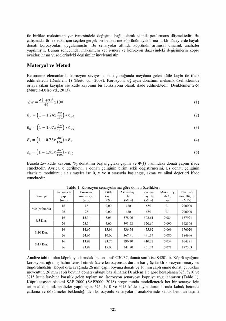
Betonarme elemanlarda, korozyon seviyesi donatı çubuğunda meydana gelen kütle kaybı ile ifade edilmektedir (Denklem 1) (Berto vd., 2008). Korozyona uğrayan donatının mekanik özelliklerinde ortaya çıkan kayıplar ise kütle kaybının bir fonksiyonu olarak ifade edilmektedir (Denklemler 2-5) (Murcia-Delso vd., 2013).

𝛥𝑤 𝑥100 (1)

б 1 1.24𝑥 ∗ б (2)

б 1 1.07𝑥 ∗ б (3)

𝐸 1 0.75𝑥 ∗ 𝐸 (4)

𝜀 1 1.95𝑥 ∗ 𝜀 (5)

Burada Δw kütle kaybını, Φ donatının başlangıçtaki çapını ve Φ t t anındaki donatı çapını ifade etmektedir. Ayrıca, б gerilmeyi, ε donatı çeliğinin birim şekil değiştirmesini, Es donatı çeliğinin elastisite modülünü; alt simgeler ise 0, y ve u sırasıyla başlangıç, akma ve nihai değerleri ifade etmektedir.

Tablo 1. Korozyon senaryolarına göre donatı özellikleri

Senaryo Başlangıçta

çap (mm)

Korozyon sonrası çap

(mm)

Kütle kaybı (%)

Akma day., fy

(MPa)

Kopma day., fu (MPa)

Maks. b. ş. değ., εsu

Elastisite modülü, Es

(MPa)

%0 (referans) 16 16 0,00 420 550 0.1 200000

26 26 0,00 420 550 0.1 200000

%5 Kor. 16 15.34 8.05 378.06 502.61 0.084 187921

26 25.34 5.00 393.98 520.60 0.090 192506

%10 Kor. 16 14.67 15.99 336.74 455.92 0.069 176020

26 24.67 10.00 367.91 491.14 0.080 184996

%15 Kor. 16 13.97 23.75 296.30 410.22 0.054 164371

26 23.97 15.00 341.90 461.74 0.071 177503

Analize tabi tutulan köprü ayaklarındaki beton sınıfı C30/37, donatı sınıfı ise S420’dir. Köprü ayağının korozyona uğramış halini temsil etmek üzere korozyonsuz durum hariç üç farklı korozyon senaryosu öngörülmüştür. Köprü orta ayağında 26 mm çaplı boyuna donatı ve 16 mm çaplı enine donatı çubukları mevcuttur. 26 mm çaplı boyuna donatı çubuğu baz alınarak Denklem 1’e göre hesaplanan %5, %10 ve %15 kütle kaybına karşılık gelen toplam üç korozyon senaryosu köprüye uygulanmıştır (Tablo 1). Köprü taşıyıcı sistemi SAP 2000 (SAP2000, 2018) programında modellenerek her bir senaryo için artımsal dinamik analizler yapılmıştır. %5, %10 ve %15 kütle kaybı durumlarında kabuk betonda çatlama ve dökülmeler beklendiğinden korozyonlu senaryoların analizlerinde kabuk betonun taşıma

721

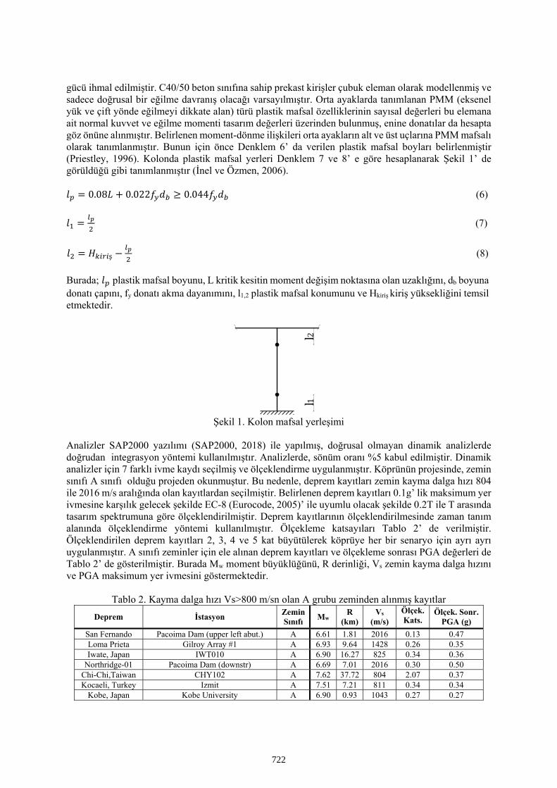
gücü ihmal edilmiştir. C40/50 beton sınıfına sahip prekast kirişler çubuk eleman olarak modellenmiş ve sadece doğrusal bir eğilme davranış olacağı varsayılmıştır. Orta ayaklarda tanımlanan PMM (eksenel yük ve çift yönde eğilmeyi dikkate alan) türü plastik mafsal özelliklerinin sayısal değerleri bu elemana ait normal kuvvet ve eğilme momenti tasarım değerleri üzerinden bulunmuş, enine donatılar da hesapta göz önüne alınmıştır. Belirlenen moment-dönme ilişkileri orta ayakların alt ve üst uçlarına PMM mafsalı olarak tanımlanmıştır. Bunun için önce Denklem 6’ da verilen plastik mafsal boyları belirlenmiştir (Priestley, 1996). Kolonda plastik mafsal yerleri Denklem 7 ve 8’ e göre hesaplanarak Şekil 1’ de görüldüğü gibi tanımlanmıştır (İnel ve Özmen, 2006).

𝑙 0.08𝐿 0.022𝑓 𝑑 0.044𝑓 𝑑 (6)

𝑙 (7)

𝑙 𝐻 ş (8)

Burada; 𝑙 plastik mafsal boyunu, L kritik kesitin moment değişim noktasına olan uzaklığını, db boyuna donatı çapını, fy donatı akma dayanımını, l1,2 plastik mafsal konumunu ve Hkiriş kiriş yüksekliğini temsil etmektedir.

Şekil 1. Kolon mafsal yerleşimi

Analizler SAP2000 yazılımı (SAP2000, 2018) ile yapılmış, doğrusal olmayan dinamik analizlerde doğrudan integrasyon yöntemi kullanılmıştır. Analizlerde, sönüm oranı %5 kabul edilmiştir. Dinamik analizler için 7 farklı ivme kaydı seçilmiş ve ölçeklendirme uygulanmıştır. Köprünün projesinde, zemin sınıfı A sınıfı olduğu projeden okunmuştur. Bu nedenle, deprem kayıtları zemin kayma dalga hızı 804 ile 2016 m/s aralığında olan kayıtlardan seçilmiştir. Belirlenen deprem kayıtları 0.1g’ lik maksimum yer ivmesine karşılık gelecek şekilde EC-8 (Eurocode, 2005)’ ile uyumlu olacak şekilde 0.2T ile T arasında tasarım spektrumuna göre ölçeklendirilmiştir. Deprem kayıtlarının ölçeklendirilmesinde zaman tanım alanında ölçeklendirme yöntemi kullanılmıştır. Ölçekleme katsayıları Tablo 2’ de verilmiştir. Ölçeklendirilen deprem kayıtları 2, 3, 4 ve 5 kat büyütülerek köprüye her bir senaryo için ayrı ayrı uygulanmıştır. A sınıfı zeminler için ele alınan deprem kayıtları ve ölçekleme sonrası PGA değerleri de Tablo 2’ de gösterilmiştir. Burada Mw moment büyüklüğünü, R derinliği, Vs zemin kayma dalga hızını ve PGA maksimum yer ivmesini göstermektedir.

Tablo 2. Kayma dalga hızı Vs>800 m/sn olan A grubu zeminden alınmış kayıtlar Deprem İstasyon

Zemin Sınıfı

Mw R

(km) Vs

(m/s) Ölçek. Kats.

Ölçek. Sonr. PGA (g)

San Fernando Pacoima Dam (upper left abut.) A 6.61 1.81 2016 0.13 0.47 Loma Prieta Gilroy Array #1 A 6.93 9.64 1428 0.26 0.35 Iwate, Japan IWT010 A 6.90 16.27 825 0.34 0.36

Northridge-01 Pacoima Dam (downstr) A 6.69 7.01 2016 0.30 0.50 Chi-Chi,Taiwan CHY102 A 7.62 37.72 804 2.07 0.37 Kocaeli, Turkey Izmit A 7.51 7.21 811 0.34 0.34

Kobe, Japan Kobe University A 6.90 0.93 1043 0.27 0.27

722

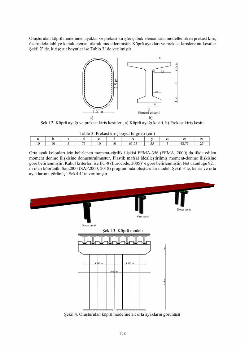
Oluşturulan köprü modelinde, ayaklar ve prekast kirişler çubuk elemanlarla modellenirken prekast kiriş üzerindeki tabliye kabuk eleman olarak modellenmiştir. Köprü ayakları ve prekast kirişlere ait kesitler Şekil 2’ de, kirişe ait boyutlar ise Tablo 3’ de verilmiştir.

a) b) Şekil 2. Köprü ayağı ve prekast kiriş kesitleri, a) Köprü ayağı kesiti, b) Prekast kiriş kesiti

Tablo 3. Prekast kiriş boyut bilgileri (cm) a b c d e f x y z1 z2 z3 10 10 5 75 10 10 63.75 35 5 48.75 25

Orta ayak kolonları için belirlenen moment-eğrilik ilişkisi FEMA-356 (FEMA, 2000) da ifade edilen moment dönme ilişkisine dönüştürülmüştür. Plastik mafsal idealleştirilmiş moment-dönme ilişkisine göre belirlenmiştir. Kabul kriterleri ise EC-8 (Eurocode, 2005)’ e göre belirlenmiştir. Net uzunluğu 92.1 m olan köprünün Sap2000 (SAP2000, 2018) programında oluşturulan modeli Şekil 3’te, kenar ve orta ayaklarının görünüşü Şekil 4’ te verilmiştir.

Şekil 3. Köprü modeli

Şekil 4. Oluşturulan köprü modeline ait orta ayakların görünüşü

723

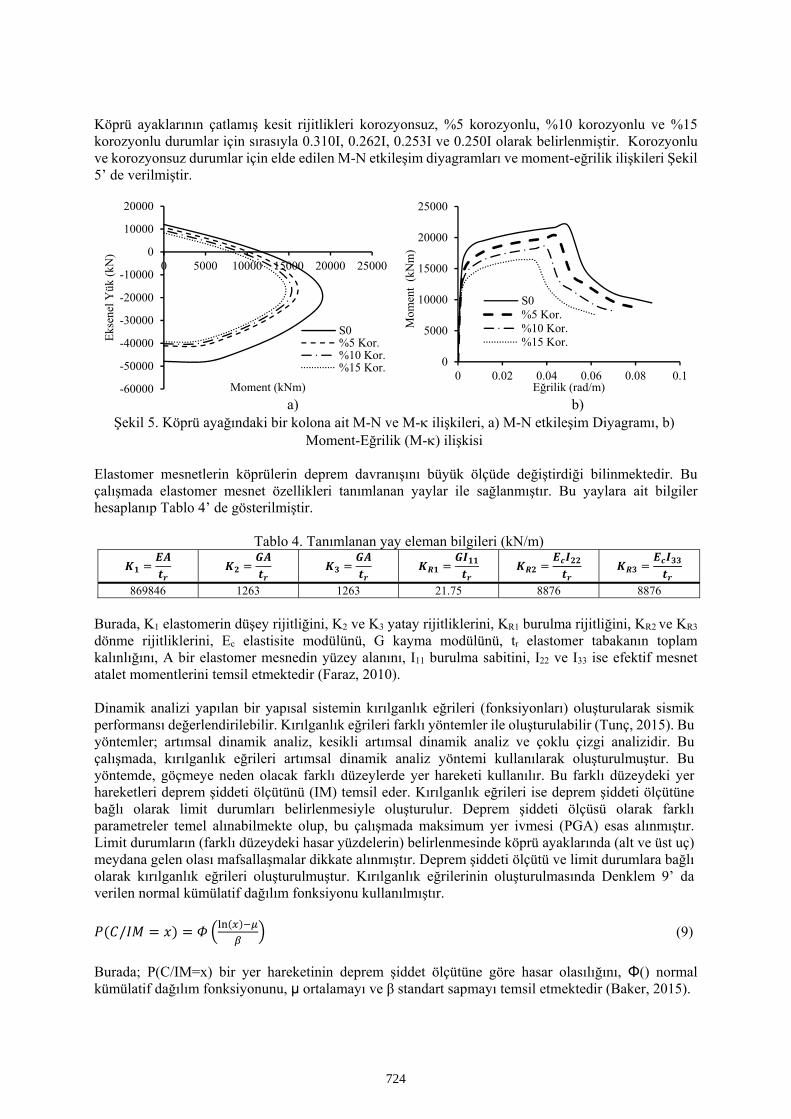
Köprü ayaklarının çatlamış kesit rijitlikleri korozyonsuz, %5 korozyonlu, %10 korozyonlu ve %15 korozyonlu durumlar için sırasıyla 0.310I, 0.262I, 0.253I ve 0.250I olarak belirlenmiştir. Korozyonlu ve korozyonsuz durumlar için elde edilen M-N etkileşim diyagramları ve moment-eğrilik ilişkileri Şekil 5’ de verilmiştir.

a) b) Şekil 5. Köprü ayağındaki bir kolona ait M-N ve M- ilişkileri, a) M-N etkileşim Diyagramı, b)

Moment-Eğrilik (M-) ilişkisi

Elastomer mesnetlerin köprülerin deprem davranışını büyük ölçüde değiştirdiği bilinmektedir. Bu çalışmada elastomer mesnet özellikleri tanımlanan yaylar ile sağlanmıştır. Bu yaylara ait bilgiler hesaplanıp Tablo 4’ de gösterilmiştir.

Tablo 4. Tanımlanan yay eleman bilgileri (kN/m) 𝑲𝟏

𝑬𝑨𝒕𝒓

𝑲𝟐𝑮𝑨𝒕𝒓

𝑲𝟑𝑮𝑨𝒕𝒓

𝑲𝑹𝟏𝑮𝑰𝟏𝟏

𝒕𝒓𝑲𝑹𝟐

𝑬𝒄𝑰𝟐𝟐

𝒕𝒓𝑲𝑹𝟑

𝑬𝒄𝑰𝟑𝟑

𝒕𝒓

869846 1263 1263 21.75 8876 8876

Burada, K1 elastomerin düşey rijitliğini, K2 ve K3 yatay rijitliklerini, KR1 burulma rijitliğini, KR2 ve KR3

dönme rijitliklerini, Ec elastisite modülünü, G kayma modülünü, tr elastomer tabakanın toplam kalınlığını, A bir elastomer mesnedin yüzey alanını, I11 burulma sabitini, I22 ve I33 ise efektif mesnet atalet momentlerini temsil etmektedir (Faraz, 2010).

Dinamik analizi yapılan bir yapısal sistemin kırılganlık eğrileri (fonksiyonları) oluşturularak sismik performansı değerlendirilebilir. Kırılganlık eğrileri farklı yöntemler ile oluşturulabilir (Tunç, 2015). Bu yöntemler; artımsal dinamik analiz, kesikli artımsal dinamik analiz ve çoklu çizgi analizidir. Bu çalışmada, kırılganlık eğrileri artımsal dinamik analiz yöntemi kullanılarak oluşturulmuştur. Bu yöntemde, göçmeye neden olacak farklı düzeylerde yer hareketi kullanılır. Bu farklı düzeydeki yer hareketleri deprem şiddeti ölçütünü (IM) temsil eder. Kırılganlık eğrileri ise deprem şiddeti ölçütüne bağlı olarak limit durumları belirlenmesiyle oluşturulur. Deprem şiddeti ölçüsü olarak farklı parametreler temel alınabilmekte olup, bu çalışmada maksimum yer ivmesi (PGA) esas alınmıştır. Limit durumların (farklı düzeydeki hasar yüzdelerin) belirlenmesinde köprü ayaklarında (alt ve üst uç) meydana gelen olası mafsallaşmalar dikkate alınmıştır. Deprem şiddeti ölçütü ve limit durumlara bağlı olarak kırılganlık eğrileri oluşturulmuştur. Kırılganlık eğrilerinin oluşturulmasında Denklem 9’ da verilen normal kümülatif dağılım fonksiyonu kullanılmıştır.

𝑃 𝐶/𝐼𝑀 𝑥 𝛷 (9)

Burada; P(C/IM=x) bir yer hareketinin deprem şiddet ölçütüne göre hasar olasılığını, Φ() normal kümülatif dağılım fonksiyonunu, μ ortalamayı ve β standart sapmayı temsil etmektedir (Baker, 2015).

-60000

-50000

-40000

-30000

-20000

-10000

0

10000

20000

0 5000 10000 15000 20000 25000

Ekse

nel Y

ük (k

N)

Moment (kNm)

S0%5 Kor.%10 Kor.%15 Kor. 0

5000

10000

15000

20000

25000

0 0.02 0.04 0.06 0.08 0.1

Mom

ent

(kN

m)

Eğrilik (rad/m)

S0%5 Kor.%10 Kor.%15 Kor.

724

Bulgular ve Tartışma

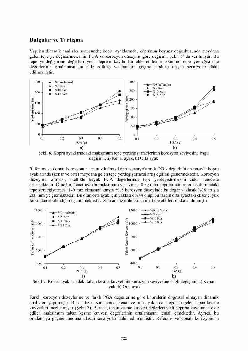
Yapılan dinamik analizler sonucunda; köprü ayaklarında, köprünün boyuna doğrultusunda meydana gelen tepe yerdeğiştirmelerinin PGA ve korozyon düzeyine göre değişimi Şekil 6’ da verilmiştir. Bu tepe yerdeğiştirme değerleri yedi deprem kaydından elde edilen maksimum tepe yerdeğiştirme değerlerinin ortalamasından elde edilmiş ve bunlara göçme moduna ulaşan senaryolar dâhil edilmemiştir.

a) b) Şekil 6. Köprü ayaklarındaki maksimum tepe yerdeğiştirmelerinin korozyon seviyesine bağlı

değişimi, a) Kenar ayak, b) Orta ayak

Referans ve donatı korozyonuna maruz kalmış köprü senaryolarında PGA değerinin artmasıyla köprü ayaklarında (kenar ve orta) meydana gelen tepe yerdeğiştirmesi artış eğilimi göstermektedir. Korozyon düzeyinin artması, özellikle büyük PGA değerlerinde tepe yerdeğiştirmesini ciddi derecede artırmaktadır. Örneğin, kenar ayakta maksimum yer ivmesi 0.5g olan deprem için referans durumdaki tepe yerdeğiştirmesi 149 mm olmasına karşın %15 korozyon düzeyinde bu değer yaklaşık %38 artışla 206 mm’ye çıkmaktadır. Bu oran orta ayak için yaklaşık %44 olup, bu farkın orta ayaktaki eksenel yük farkından etkilendiği düşünülmektedir. Zira analizlerde ikinci mertebe etkileri dikkate alınmıştır.

a) b) Şekil 7. Köprü ayaklarındaki taban kesme kuvvetinin korozyon seviyesine bağlı değişimi, a) Kenar

ayak, b) Orta ayak

Farklı korozyon düzeylerine ve farklı PGA değerlerine göre köprülerin doğrusal olmayan dinamik analizleri yapılmıştır. Bu analizler sonucunda; kenar ve orta ayaklarda meydana gelen taban kesme kuvvetleri incelenmiştir (Şekil 7). Burada, taban kesme kuvveti değerleri yedi deprem kaydından elde edilen maksimum taban kesme kuvveti değerlerinin ortalamasını temsil etmektedir. Ayrıca, bu ortalamaya göçme moduna ulaşan senaryolar dahil edilmemiştir. Referans ve donatı korozyonuna

0

50

100

150

200

250

0.1 0.2 0.3 0.4 0.5

Yer

deği

ştirm

e (m

m)

PGA (g)

%0 (referans)%5 Kor.%10 Kor.%15 Kor.

0

50

100

150

200

250

300

0.1 0.2 0.3 0.4 0.5

Yer

deği

ştirm

e (m

m)

PGA (g)


4000

6000

8000

10000

12000

0.1 0.2 0.3 0.4 0.5

Taba

n K

esm

e K

uvve

ti (k

N)

PGA (g)


4000

6000

8000

10000

12000

0.1 0.2 0.3 0.4 0.5

Taba

n K

esm

e K

uvve

ti (k

N)

PGA (g)


725

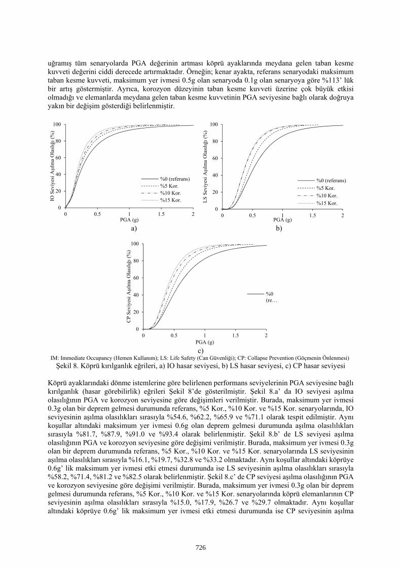
uğramış tüm senaryolarda PGA değerinin artması köprü ayaklarında meydana gelen taban kesme kuvveti değerini ciddi derecede artırmaktadır. Örneğin; kenar ayakta, referans senaryodaki maksimum taban kesme kuvveti, maksimum yer ivmesi 0.5g olan senaryoda 0.1g olan senaryoya göre %113’ lük bir artış göstermiştir. Ayrıca, korozyon düzeyinin taban kesme kuvveti üzerine çok büyük etkisi olmadığı ve elemanlarda meydana gelen taban kesme kuvvetinin PGA seviyesine bağlı olarak doğruya yakın bir değişim gösterdiği belirlenmiştir.

a) b)

c) IM: Immediate Occupancy (Hemen Kullanım); LS: Life Safety (Can Güvenliği); CP: Collapse Prevention (Göçmenin Önlenmesi)

Şekil 8. Köprü kırılganlık eğrileri, a) IO hasar seviyesi, b) LS hasar seviyesi, c) CP hasar seviyesi

Köprü ayaklarındaki dönme istemlerine göre belirlenen performans seviyelerinin PGA seviyesine bağlı kırılganlık (hasar görebilirlik) eğrileri Şekil 8’de gösterilmiştir. Şekil 8.a’ da IO seviyesi aşılma olasılığının PGA ve korozyon seviyesine göre değişimleri verilmiştir. Burada, maksimum yer ivmesi 0.3g olan bir deprem gelmesi durumunda referans, %5 Kor., %10 Kor. ve %15 Kor. senaryolarında, IO seviyesinin aşılma olasılıkları sırasıyla %54.6, %62.2, %65.9 ve %71.1 olarak tespit edilmiştir. Aynı koşullar altındaki maksimum yer ivmesi 0.6g olan deprem gelmesi durumunda aşılma olasılılıkları sırasıyla %81.7, %87.9, %91.0 ve %93.4 olarak belirlenmiştir. Şekil 8.b’ de LS seviyesi aşılma olasılığının PGA ve korozyon seviyesine göre değişimi verilmiştir. Burada, maksimum yer ivmesi 0.3g olan bir deprem durumunda referans, %5 Kor., %10 Kor. ve %15 Kor. senaryolarında LS seviyesinin aşılma olasılıkları sırasıyla %16.1, %19.7, %32.8 ve %33.2 olmaktadır. Aynı koşullar altındaki köprüye 0.6g’ lik maksimum yer ivmesi etki etmesi durumunda ise LS seviyesinin aşılma olasılıkları sırasıyla %58.2, %71.4, %81.2 ve %82.5 olarak belirlenmiştir. Şekil 8.c’ de CP seviyesi aşılma olasılığının PGA ve korozyon seviyesine göre değişimi verilmiştir. Burada, maksimum yer ivmesi 0.3g olan bir deprem gelmesi durumunda referans, %5 Kor., %10 Kor. ve %15 Kor. senaryolarında köprü elemanlarının CP seviyesinin aşılma olasılıkları sırasıyla %15.0, %17.9, %26.7 ve %29.7 olmaktadır. Aynı koşullar altındaki köprüye 0.6g’ lik maksimum yer ivmesi etki etmesi durumunda ise CP seviyesinin aşılma

0

20

40

60

80

100

0 0.5 1 1.5 2

IO S

eviy

esi A

şılm

a O

lasl

ığı (

%)

PGA (g)


0

20

40

60

80

100

0 0.5 1 1.5 2

LS S

eviy

esi A

şılm

a O

lası

lığı (

%)

PGA (g)


0

20

40

60

80

100

0 0.5 1 1.5 2

CP

Sevi

yesi

Aşı

lma

Ola

sılığ

ı (%

)

PGA (g)

%0(re…

726

olasılıkları sırasıyla %53.9, %65.9, %74.6 ve %79.3 olarak belirlenmiştir. Korozyon seviyesi arttıkça köprü ayaklarındaki mafsallaşma olasılığının arttığı görülmektedir. Korozyon seviyesinin artmasına ek olarak zemin yer hareket düzeyine bağlı olarak sistemin göçme olasılığı artmaktadır. İki durum süperpoze edildiğinde korozyon düzeyindeki artış elemanların hasar düzeylerindeki değişimi hızlandırdığı sonucuna varılabilir.

Sonuçlar

Bu bildiride, betonarme bir köprünün ayaklarında referans (korozyonsuz) durum ve üç farklı korozyon senaryosu altında artımsal dinamik analizler yapılmak suretiyle kırılganlık eğrileri oluşturulmuş ve performans değişimi incelenmiştir. Betonarme elemanların donatı korozyonuna maruz kalmasıyla donatı çubuğunda enkesit kaybı, donatı-beton arasında aderans kaybı ve donatı çubuğu mekanik özelliklerinde kayıplar meydana gelmektedir. Bu nedenle elemanın eksenel yük ve moment kapasitesi düşmektedir. Analizler sonucunda, korozyonsuz ve korozyonlu köprü senaryolarında PGA değerinin artmasıyla köprü ayaklarında meydana gelen maksimum tepe yerdeğiştirmesi ve taban kesme kuvveti artış eğilimi göstermektedir. Korozyon düzeyindeki artış eleman ve sistem rijitliğini düşürdüğünden, maksimum tepe yerdeğiştirmeleri artmakta, fakat maksimum taban kesme kuvvetinde ise çok büyük bir etki ortaya çıkarmamaktadır. Ayrıca, PGA seviyesinde ve korozyon düzeyindeki artışların, elemanların hasar görme olasılıklarını ciddi derecede artırabileceği sonucuna varılmıştır.

Referanslar

Baker JW (2015) “Efficient analytical fragility function fitting using dynamic structural analysis”, Earthquake Spectra, 31(1):579-599.

Berto L, Seatta A, Simioni P, Vitaliani R (2008) “Nonlinear static analyses of RC frame structures: influence of corrosion on seismic response”, Proceedings of the 8th. World Congress on Computational Mechanics (WCCM8) and 5th. European Congress on Computational Methods in Applied Sciences and Engineering (ECCOMAS 2008), Venice, Italy, 30 June-4 July.

CSI. SAP2000 V-20 (2018) “Integrated finite element analysis and design of structures basic analysis reference manual” Berkeley (CA, USA): Computers and Structures Inc.

Faraz S (2010) Betonarme köprü modellenmesi üzerine bir çalışma, Yüksek Lisans Tezi, Gazi Üniversitesi, Türkiye.

Federal Emergency Management Agency (FEMA-356) (2000) Prestandard and commentary for seismic rehabilitation of buildings, Washington (DC).

Inel M, Ozmen HB (2006) “Effects of plastic hinge properties in nonlinear analysis of reinforced concrete buildings” Engineering structures, 28(11):1494-1502.

Murcia-Delso J, Stavridis A, Shing PB (2013) “Bond Strength and Cyclic Bond Deterioration of Large-Diameter Bars” ACI Structural Journal, 110(4):659-670.

Priestley MJN, Seible F, Calvi GMS (1996) Seismic design and retrofit of bridges, 1st Ed., John Wiley & Sons, New York.

Standard B (2005) Eurocode 8: Design of structures for earthquake resistance. Part, 1, 1998-1. Tunç Ç (2015) Yarı rijit mesnetlenmiş perdeler ile güçlendirilen bir okul binasının kırılganlık eğrileri,

Doktora Tezi, İstanbul Teknik Üniversitesi, Türkiye.

727

Recent Studies on Application of Structural Fuse Concept in Seismic Design

of Steel Structures

Borislav Belev1*, Angel Ashikov

2, Georgi Bonchev

2

1 Professor, Dept. of Steel and Timber Structures, UACEG, Sofia, Bulgaria

2 PhD candidate, Dept. of Steel and Timber Structures, UACEG, Sofia, Bulgaria

*Corresponding author, [email protected]

AbstractThe paper overviews two recent research projects developed at the University of Architecture, Civil

Engineering and Geodesy (UACEG), Sofia, Bulgaria. These projects implement the structural fuse

concept in the field of seismic design and retrofit of steel structures. The lessons learnt from recent

strong quakes around the world imply that the modern seismic-force-resisting systems should be easily

repairable if damaged. The first of the reported studies was focused on developing and testing a new

type of replaceable seismic link element for eccentrically braced frames (EBFs). A new detailing

option was proposed by the second author in which bolted flange- and web splicing was used to

connect the link to the adjacent collector beam or column. This new link prototype was investigated

both experimentally and numerically. The results confirmed that the behaviour of the specimens

resembled that of the conventional EBFs and showed stable energy dissipation.

The second reported research project developed a seismic retrofit technique for existing steel moment

frames with limited ductility. For the existing steel frames designed to Bulgarian codes of 1970-1990

vintage a retrofitting technique based on added set of Linked Columns (LCs) was proposed. In order to

avoid any damage and subsequent replacement of the conventional short steel links connecting the LC

piers, they were substituted by rotational friction dampers (RFDs). Two sets of representative MRFs

designed according to Bulgarian design codes of year 1987 were analyzed using the SAP2000

software. The seismic performance of the representative MRFs and their retrofitted counterparts was

assessed using the capacity spectrum method based on two-dimensional static nonlinear pushover

analyses. The results illustrate the viability and applicability of the proposed concept for seismic

retrofit of steel frames. The friction dampers act as structural fuses and dissipate a major part of the

seismic input energy and protect the original MRFs from significant damage.

Keywords: seismic link, friction damper, seismic design, steel structures.

Introduction

The Structural Fuse Concept (SFC) is a relatively new approach in seismic engineering which can be

considered as a further development of the capacity design philosophy. It is best illustrated by

implementation of specialized devices called passive energy dissipaters or dampers which if inserted at

pre-selected locations within the primary structure can protect it from seismic damage. A

comprehensive analytical study on the key parameters of the structures incorporating metallic dampers

is reported in Vargas and Bruneau (2006).

The primary role of the seismic fuses is to dissipate the seismic input energy in a stable and reliable

way, thus providing a predictable dynamic response of the primary framing preferably within the

elastic range. In addition, similarly to their counterparts in electrical systems, the structural fuses

should be easily replaceable if damaged during extreme loading, and non-expensive.

The steel eccentrically braced frames (EBFs), Hjelmstad and Popov (1984), can be considered one of

the first practical applications of the SFC in conventional seismic-resistant structures without dampers.

The so-called buckling-restraint braces (BRB) used in seismic design over the last two decades and

other more advanced passive energy dissipation systems also employ the SFC as a guiding principle.

728

Newly-developed replaceable seismic link for use in EBFs

The EBFs are a hybrid lateral load-resisting system which combines the high elastic stiffness typical

of the concentrically braced frames (CBFs) and the excellent global ductility and energy dissipation

capacity of moment resisting frames (MRFs). By applying capacity design procedures the seismic

energy dissipation is purposely directed towards beam segments called seismic links or active links,

which are designed and detailed for sustaining large inelastic deformations under severe cyclic loading

without degradation. The seismic links should act as ductile fuses, limiting the forces transmitted to

and protecting the primary structure. In the conventional EBFs the seismic links are continuous with

the collector beams and support the floor slab. Recent strong seismic events in New Zealand proved

the reliable performance of the EBFs in office buildings and car parks (Clifton et al., 2012) but

revealed that the repair and replacement of the damaged links were costly and disruptive. This

drawback can be mitigated by designing EBFs with replaceable seismic links. The replaceable link

concept allows for quick inspection and replacement of damaged links following a major earthquake,

significantly minimising time to reoccupy the building. A bolted replaceable active link provides more

flexibility to the designer because the cross sections of the seismic links can be chosen to meet

precisely the required resistance and fabricated from a lower steel grade, if needed. A new design

guide was published which incorporates updated procedures and worked example for design of EBFs

with replaceable links, (HERA, 2013).

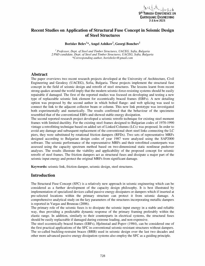
Most replaceable seismic links tend to use bolted end-plate connections at their ends. However, in a

recent PhD study an alternative detailing option proposed by the second author was investigated both

experimentally and numerically. This new concept is presented in Fig. 1. Both the seismic link and

collector beam have built-up I-cross-sections. Bolted flange- and web splicing is used to connect the

link to the adjacent collector beam or column.

Figure 1. Proposed configuration and detailing of replaceable seismic link

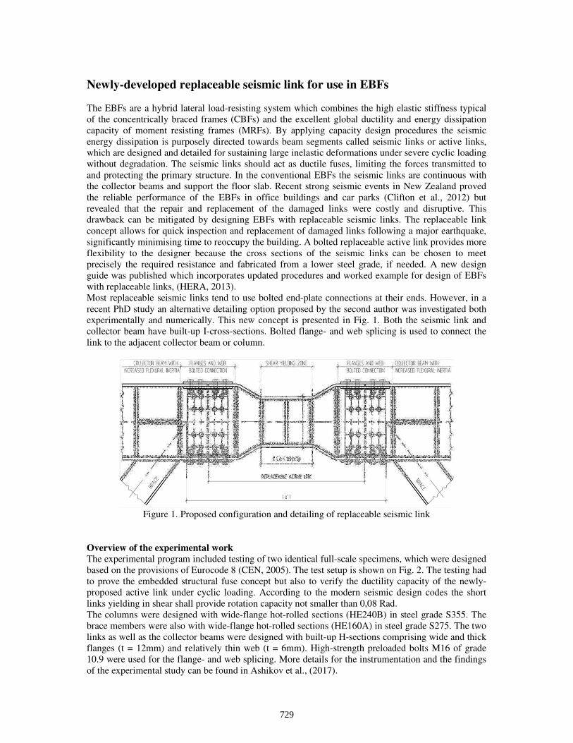
Overview of the experimental work

The experimental program included testing of two identical full-scale specimens, which were designed

based on the provisions of Eurocode 8 (CEN, 2005). The test setup is shown on Fig. 2. The testing had

to prove the embedded structural fuse concept but also to verify the ductility capacity of the newly-

proposed active link under cyclic loading. According to the modern seismic design codes the short

links yielding in shear shall provide rotation capacity not smaller than 0,08 Rad.

The columns were designed with wide-flange hot-rolled sections (HE240B) in steel grade S355. The

brace members were also with wide-flange hot-rolled sections (HE160A) in steel grade S275. The two

links as well as the collector beams were designed with built-up H-sections comprising wide and thick

flanges (t = 12mm) and relatively thin web (t = 6mm). High-strength preloaded bolts M16 of grade

10.9 were used for the flange- and web splicing. More details for the instrumentation and the findings

of the experimental study can be found in Ashikov et al., (2017).

729

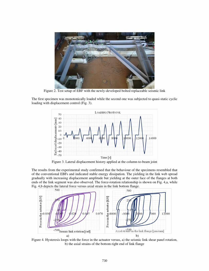
Figure 2. Test setup of EBF with the newly-developed bolted replaceable seismic link

The first specimen was monotonically loaded while the second one was subjected to quasi-static cyclic

loading with displacement control (Fig. 3).

Figure 3. Lateral displacement history applied at the column-to-beam joint

The results from the experimental study confirmed that the behaviour of the specimens resembled that

of the conventional EBFs and indicated stable energy dissipation. The yielding in the link web spread

gradually with increasing displacement amplitude but yielding at the outer face of the flanges at both

ends of the link segment was also observed. The force-rotation relationship is shown on Fig. 4,a, while

Fig. 4,b depicts the lateral force versus axial strain in the link bottom flange.

a) b)

Figure 4. Hysteresis loops with the force in the actuator versus, a) the seismic link shear panel rotation,

b) the axial strains of the bottom right end of link flange

730

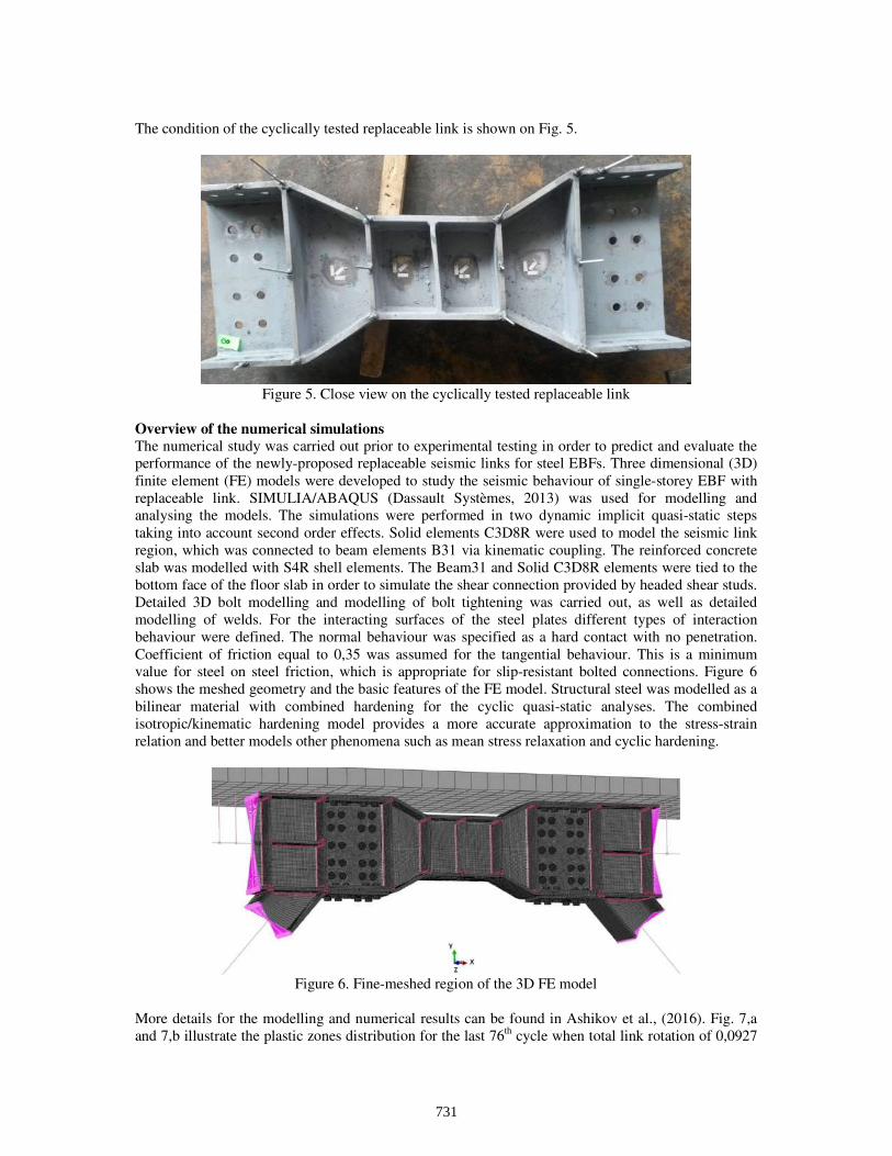
The condition of the cyclically tested replaceable link is shown on Fig. 5.

Figure 5. Close view on the cyclically tested replaceable link

Overview of the numerical simulations

The numerical study was carried out prior to experimental testing in order to predict and evaluate the

performance of the newly-proposed replaceable seismic links for steel EBFs. Three dimensional (3D)

finite element (FE) models were developed to study the seismic behaviour of single-storey EBF with

replaceable link. SIMULIA/ABAQUS (Dassault Systèmes, 2013) was used for modelling and

analysing the models. The simulations were performed in two dynamic implicit quasi-static steps

taking into account second order effects. Solid elements C3D8R were used to model the seismic link

region, which was connected to beam elements B31 via kinematic coupling. The reinforced concrete

slab was modelled with S4R shell elements. The Beam31 and Solid C3D8R elements were tied to the

bottom face of the floor slab in order to simulate the shear connection provided by headed shear studs.

Detailed 3D bolt modelling and modelling of bolt tightening was carried out, as well as detailed

modelling of welds. For the interacting surfaces of the steel plates different types of interaction

behaviour were defined. The normal behaviour was specified as a hard contact with no penetration.

Coefficient of friction equal to 0,35 was assumed for the tangential behaviour. This is a minimum

value for steel on steel friction, which is appropriate for slip-resistant bolted connections. Figure 6

shows the meshed geometry and the basic features of the FE model. Structural steel was modelled as a

bilinear material with combined hardening for the cyclic quasi-static analyses. The combined

isotropic/kinematic hardening model provides a more accurate approximation to the stress-strain

relation and better models other phenomena such as mean stress relaxation and cyclic hardening.

Figure 6. Fine-meshed region of the 3D FE model

More details for the modelling and numerical results can be found in Ashikov et al., (2016). Fig. 7,a

and 7,b illustrate the plastic zones distribution for the last 76th cycle when total link rotation of 0,0927

731

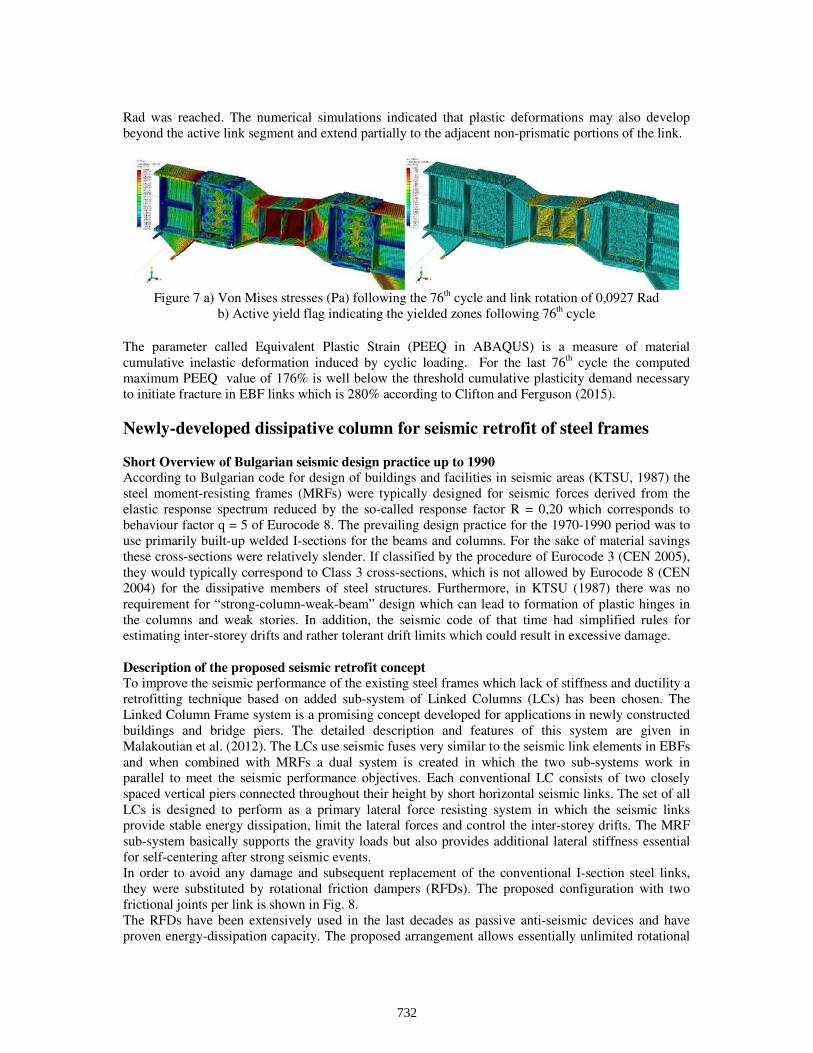
Rad was reached. The numerical simulations indicated that plastic deformations may also develop

beyond the active link segment and extend partially to the adjacent non-prismatic portions of the link.

Figure 7 a) Von Mises stresses (Pa) following the 76th cycle and link rotation of 0,0927 Rad

b) Active yield flag indicating the yielded zones following 76th cycle

The parameter called Equivalent Plastic Strain (PEEQ in ABAQUS) is a measure of material

cumulative inelastic deformation induced by cyclic loading. For the last 76th cycle the computed

maximum PEEQ value of 176% is well below the threshold cumulative plasticity demand necessary

to initiate fracture in EBF links which is 280% according to Clifton and Ferguson (2015).

Newly-developed dissipative column for seismic retrofit of steel frames

Short Overview of Bulgarian seismic design practice up to 1990 According to Bulgarian code for design of buildings and facilities in seismic areas (KTSU, 1987) the

steel moment-resisting frames (MRFs) were typically designed for seismic forces derived from the

elastic response spectrum reduced by the so-called response factor R = 0,20 which corresponds to

behaviour factor q = 5 of Eurocode 8. The prevailing design practice for the 1970-1990 period was to

use primarily built-up welded I-sections for the beams and columns. For the sake of material savings

these cross-sections were relatively slender. If classified by the procedure of Eurocode 3 (CEN 2005),

they would typically correspond to Class 3 cross-sections, which is not allowed by Eurocode 8 (CEN

2004) for the dissipative members of steel structures. Furthermore, in KTSU (1987) there was no

requirement for “strong-column-weak-beam” design which can lead to formation of plastic hinges in

the columns and weak stories. In addition, the seismic code of that time had simplified rules for

estimating inter-storey drifts and rather tolerant drift limits which could result in excessive damage.

Description of the proposed seismic retrofit concept To improve the seismic performance of the existing steel frames which lack of stiffness and ductility a

retrofitting technique based on added sub-system of Linked Columns (LCs) has been chosen. The

Linked Column Frame system is a promising concept developed for applications in newly constructed

buildings and bridge piers. The detailed description and features of this system are given in

Malakoutian et al. (2012). The LCs use seismic fuses very similar to the seismic link elements in EBFs

and when combined with MRFs a dual system is created in which the two sub-systems work in

parallel to meet the seismic performance objectives. Each conventional LC consists of two closely

spaced vertical piers connected throughout their height by short horizontal seismic links. The set of all

LCs is designed to perform as a primary lateral force resisting system in which the seismic links

provide stable energy dissipation, limit the lateral forces and control the inter-storey drifts. The MRF

sub-system basically supports the gravity loads but also provides additional lateral stiffness essential

for self-centering after strong seismic events.

In order to avoid any damage and subsequent replacement of the conventional I-section steel links,

they were substituted by rotational friction dampers (RFDs). The proposed configuration with two

frictional joints per link is shown in Fig. 8.

The RFDs have been extensively used in the last decades as passive anti-seismic devices and have

proven energy-dissipation capacity. The proposed arrangement allows essentially unlimited rotational

732

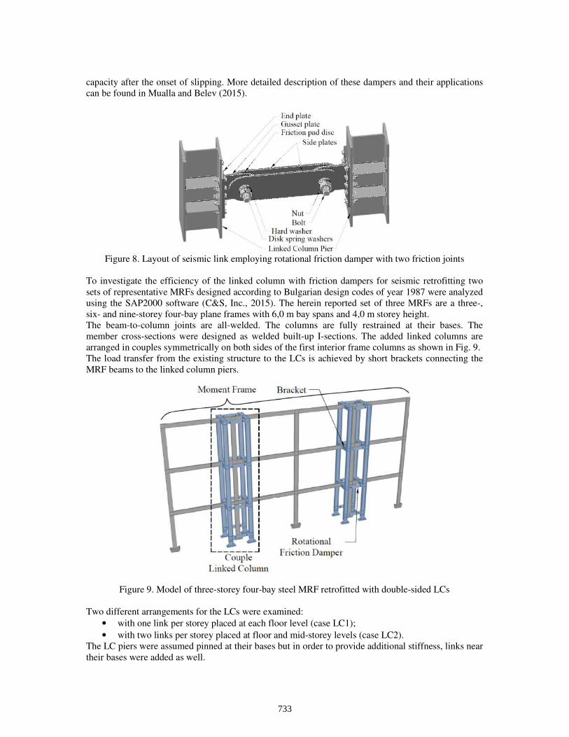
capacity after the onset of slipping. More detailed description of these dampers and their applications

can be found in Mualla and Belev (2015).

Figure 8. Layout of seismic link employing rotational friction damper with two friction joints

To investigate the efficiency of the linked column with friction dampers for seismic retrofitting two

sets of representative MRFs designed according to Bulgarian design codes of year 1987 were analyzed

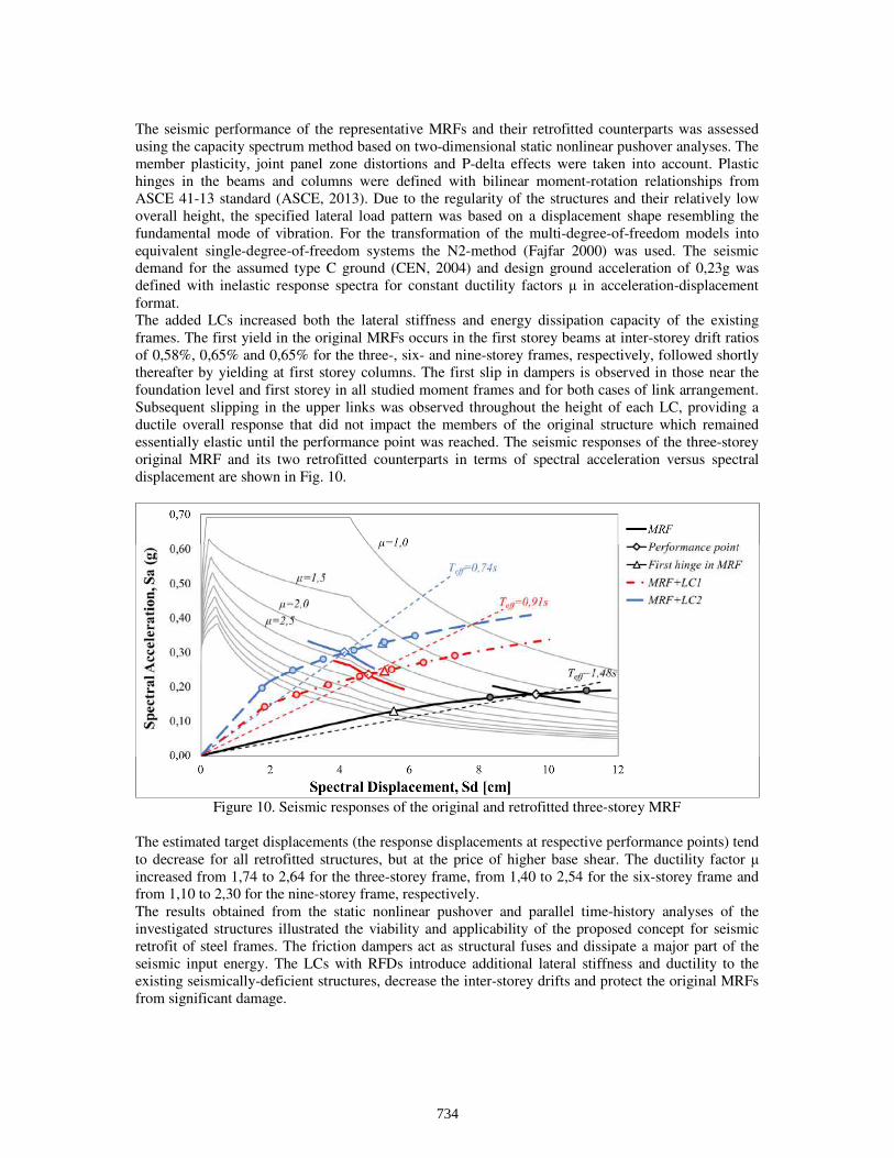
using the SAP2000 software (C&S, Inc., 2015). The herein reported set of three MRFs are a three-,

six- and nine-storey four-bay plane frames with 6,0 m bay spans and 4,0 m storey height.

The beam-to-column joints are all-welded. The columns are fully restrained at their bases. The

member cross-sections were designed as welded built-up I-sections. The added linked columns are

arranged in couples symmetrically on both sides of the first interior frame columns as shown in Fig. 9.

The load transfer from the existing structure to the LCs is achieved by short brackets connecting the

MRF beams to the linked column piers.

Figure 9. Model of three-storey four-bay steel MRF retrofitted with double-sided LCs

Two different arrangements for the LCs were examined:

• with one link per storey placed at each floor level (case LC1);

• with two links per storey placed at floor and mid-storey levels (case LC2).

The LC piers were assumed pinned at their bases but in order to provide additional stiffness, links near

their bases were added as well.

733

The seismic performance of the representative MRFs and their retrofitted counterparts was assessed

using the capacity spectrum method based on two-dimensional static nonlinear pushover analyses. The

member plasticity, joint panel zone distortions and P-delta effects were taken into account. Plastic

hinges in the beams and columns were defined with bilinear moment-rotation relationships from

ASCE 41-13 standard (ASCE, 2013). Due to the regularity of the structures and their relatively low

overall height, the specified lateral load pattern was based on a displacement shape resembling the

fundamental mode of vibration. For the transformation of the multi-degree-of-freedom models into

equivalent single-degree-of-freedom systems the N2-method (Fajfar 2000) was used. The seismic

demand for the assumed type C ground (CEN, 2004) and design ground acceleration of 0,23g was

defined with inelastic response spectra for constant ductility factors µ in acceleration-displacement

format.

The added LCs increased both the lateral stiffness and energy dissipation capacity of the existing

frames. The first yield in the original MRFs occurs in the first storey beams at inter-storey drift ratios

of 0,58%, 0,65% and 0,65% for the three-, six- and nine-storey frames, respectively, followed shortly

thereafter by yielding at first storey columns. The first slip in dampers is observed in those near the

foundation level and first storey in all studied moment frames and for both cases of link arrangement.

Subsequent slipping in the upper links was observed throughout the height of each LC, providing a

ductile overall response that did not impact the members of the original structure which remained

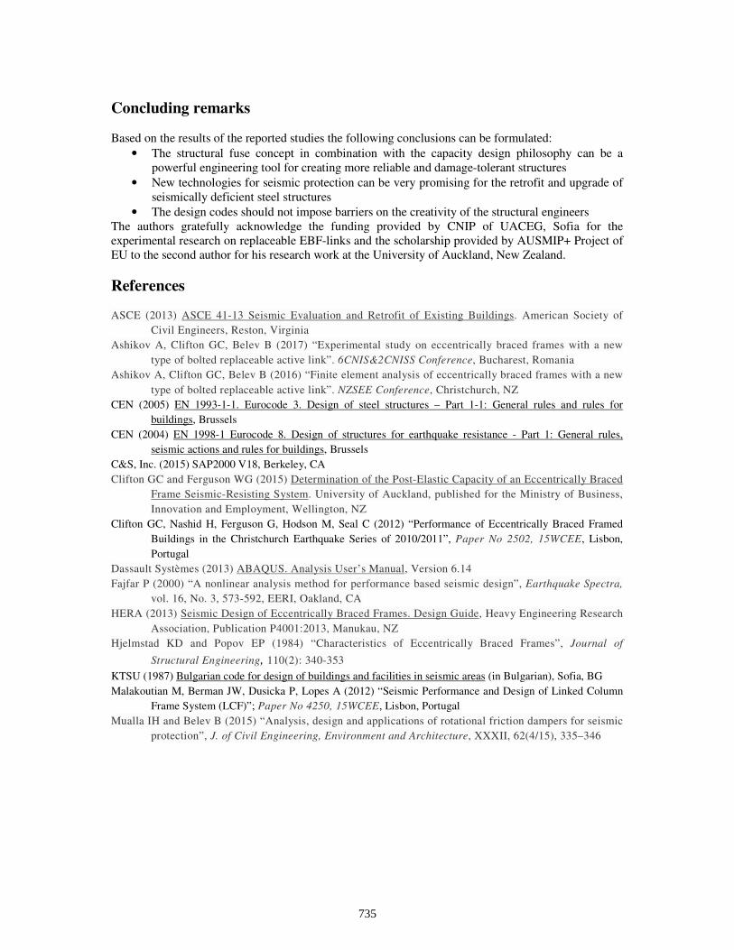
essentially elastic until the performance point was reached. The seismic responses of the three-storey

original MRF and its two retrofitted counterparts in terms of spectral acceleration versus spectral

displacement are shown in Fig. 10.

Figure 10. Seismic responses of the original and retrofitted three-storey MRF

The estimated target displacements (the response displacements at respective performance points) tend

to decrease for all retrofitted structures, but at the price of higher base shear. The ductility factor µ

increased from 1,74 to 2,64 for the three-storey frame, from 1,40 to 2,54 for the six-storey frame and

from 1,10 to 2,30 for the nine-storey frame, respectively.

The results obtained from the static nonlinear pushover and parallel time-history analyses of the

investigated structures illustrated the viability and applicability of the proposed concept for seismic

retrofit of steel frames. The friction dampers act as structural fuses and dissipate a major part of the

seismic input energy. The LCs with RFDs introduce additional lateral stiffness and ductility to the

existing seismically-deficient structures, decrease the inter-storey drifts and protect the original MRFs

from significant damage.

734

Concluding remarks

Based on the results of the reported studies the following conclusions can be formulated:

• The structural fuse concept in combination with the capacity design philosophy can be a

powerful engineering tool for creating more reliable and damage-tolerant structures

• New technologies for seismic protection can be very promising for the retrofit and upgrade of

seismically deficient steel structures

• The design codes should not impose barriers on the creativity of the structural engineers

The authors gratefully acknowledge the funding provided by CNIP of UACEG, Sofia for the

experimental research on replaceable EBF-links and the scholarship provided by AUSMIP+ Project of

EU to the second author for his research work at the University of Auckland, New Zealand.

References

ASCE (2013) ASCE 41-13 Seismic Evaluation and Retrofit of Existing Buildings. American Society of

Civil Engineers, Reston, Virginia

Ashikov A, Clifton GC, Belev B (2017) “Experimental study on eccentrically braced frames with a new

type of bolted replaceable active link”. 6CNIS&2CNISS Conference, Bucharest, Romania

Ashikov A, Clifton GC, Belev B (2016) “Finite element analysis of eccentrically braced frames with a new

type of bolted replaceable active link”. NZSEE Conference, Christchurch, NZ

CEN (2005) EN 1993-1-1. Eurocode 3. Design of steel structures – Part 1-1: General rules and rules for

buildings, Brussels

CEN (2004) EN 1998-1 Eurocode 8. Design of structures for earthquake resistance - Part 1: General rules,

seismic actions and rules for buildings, Brussels

C&S, Inc. (2015) SAP2000 V18, Berkeley, CA

Clifton GC and Ferguson WG (2015) Determination of the Post-Elastic Capacity of an Eccentrically Braced

Frame Seismic-Resisting System. University of Auckland, published for the Ministry of Business,

Innovation and Employment, Wellington, NZ

Clifton GC, Nashid H, Ferguson G, Hodson M, Seal C (2012) “Performance of Eccentrically Braced Framed

Buildings in the Christchurch Earthquake Series of 2010/2011”, Paper No 2502, 15WCEE, Lisbon,

Portugal

Dassault Systèmes (2013) ABAQUS. Analysis User’s Manual, Version 6.14

Fajfar P (2000) “A nonlinear analysis method for performance based seismic design”, Earthquake Spectra,

vol. 16, No. 3, 573-592, EERI, Oakland, CA

HERA (2013) Seismic Design of Eccentrically Braced Frames. Design Guide, Heavy Engineering Research

Association, Publication P4001:2013, Manukau, NZ

Hjelmstad KD and Popov EP (1984) “Characteristics of Eccentrically Braced Frames”, Journal of

Structural Engineering, 110(2): 340-353

KTSU (1987) Bulgarian code for design of buildings and facilities in seismic areas (in Bulgarian), Sofia, BG

Malakoutian M, Berman JW, Dusicka P, Lopes A (2012) “Seismic Performance and Design of Linked Column

Frame System (LCF)”; Paper No 4250, 15WCEE, Lisbon, Portugal

Mualla IH and Belev B (2015) “Analysis, design and applications of rotational friction dampers for seismic

protection”, J. of Civil Engineering, Environment and Architecture, XXXII, 62(4/15), 335–346

735

Effects of Seismic and Aerodynamic Loads on a 5 MW Scale Steel Wind

TurbineElif Altunsu

1*, Onur Güneş

2, Shokrullah Sorosh

2, Ali Sarı

3

1 Research Asistant, Department of CiviEng., Istanbul University-Cerrahpasa, Istanbul 2 Graduated Student, Department of CiviEng., Istanbul Technical University, Istanbul

3Assoc.Prof. Dr., Department of CiviEng., Istanbul Technical University, Istanbul

* [email protected]

Abstract

Renewable energy sources continue to be the most popular energy sources nowadays. The negative

effects of fossil energy resources on the environment have made such energy resources even more

important. Wind energy, which is the most widely used of these, is discussed in this study. Important

developments are taking place in the wind energy industry all over the world. Numerous studies have been addressed in this regard, but seismic effects have recently been studied. Although the analysis of

wind turbines under wind loads are required, if these structures are built in high seismic regions, the

analysis of these structures under strong ground motion is also needed. The effects of these two important dynamic loading on the complex dynamic structure of the turbine were investigated by

examining two different situations. These situations are; The situation in which the earthquake load did

not affect while the turbine was in operation and the situation where both dynamic loads were affected while the turbine was in operation. Turbulent wind is used as wind load. Seismic effects were

investigated by considering 3 different strong ground motion. The full system model of the turbine was

developed in the FAST finite element program, a special code for wind turbines, developed by the

National Renewable Energy Laboratory (NREL). As a result of all these analyzes, it was observed that while applying the wind loads only, the wind load had great effects in low modes. In the analysis, in

which both seismic and wind loads are applied at the same time, it was understood that aerodynamic

loads caused a certain damping in the system as a result the internal forces due to earthquake loads are increased.

Keywords: Wind turbine, Wind, Seismic, Finite element analysis, Aerodynamic damping

Introduction

In recent years, the trend towards renewable energy sources has been increasing rapidly. While fossil energy sources continue to be the dominant energy source all over the world, rapid development of

technology and significant growth in population growth have created great energy needs. This need is

expected to increase further in the coming years. While this is a factor in the transformation of energy

policies to renewable energy sources, the other important factor is the irreversible damage caused by fossil energy sources to the nature. All over the world, the wind energy industry production capacity has

significant increase year to year. According to the report published by the 2019 Turkey Wind Energy

Association statistics, 7.615 GW which corresponds to 7.40 percent of Turkey’s energy needs are provided by wind energy. These positive developments in wind energy in Turkey has brought important

goals. Today, while the offshore wind turbines are at the top of these targets, another target is planned

to be 17 GW in the next 10 years with an increase of 1 GW installation power every year. Turkey has a high potential for wind energy field. The fact that it is surrounded by the sea on three sides is an

inevitable field for offshore structures.

In terms of early studies on wind turbines, Europe has a comprehensive literature survey. Since Europe

does not have a seismically active geography, seismic effects are not included in its literature. Towards the end of the 20th century, seismic effects were started to be taken into consideration with the use of

wind technology in regions with high seismic activity such as China, America and Japan. While studies

736

in this sense are still insufficient, studies are ongoing. Turkey is also experiencing a strong earthquake.

Investigation of seismic effects on turbines is required for the geography we live in.

As the rotor diameter and tower height of the wind turbines increase, it has more power generation.

Although it is provided to use lighter materials for the blades in the studies carried out, the structure

mass is large. The increase in the building mass causes high seismic demand and base moment. The

high seismic activity of the regions with high wind potential has also revealed a negative situation.

The IEC (2005), DNV (2001) and GL (2003) standards have made some recommendations for the

consideration of seismic effects. These codes propose to model the tower as a single degree of freedom

system and to collect the rotor and tower mass at the top of the tower as lumped mass. This simple approach makes the solution easy. Since full system models include the complex effects of rotor

dynamics, exact observation of seismic effects may not be possible. By focusing on the single degree of

freedom system tower, the effects of ground motion can be easily resolved. The disadvantage of this

method is that in the first tower flexural mode, ignoring the effect of higher modes may not give accurate

results.

To mention the studies for modelling wind turbines under strong ground motions, the research began in

the early 2000s by Prowell and Veers (2009). They gathered a large review of the current literature on the subject. In the pioneering researches of Bazeos et al. (2002) and Lavassas et al. (2003), they assumed

the rotor and nacelle system as a lumped mass at the top of the tower and used a detailed finite element

method to model the tower. Later, more realistic models that consider the dynamics of the rotor and the

flexibility of the rotor and tower are also considered.

Otoniel Díaz and Luis E. Suárez (2014) studied the behaviour and load capacity of the structure of a

three-bladed horizontal axis wind turbine based on three components of static and strong earthquake

ground motions with the help of simplified models proposed by finite elements and presented a formulation. They conducted an investigation assuming that the turbine was exposed to a normal wind

and strong earthquake at the same time. Triantafyllos K. Makarios et al. (2015) studied the torsional-

displacement behaviour of the wind turbine tower prototype that may occur as a result of a strong ground motion effect. According to this study, the use of additional diaphragms at higher diaphragms

contributes to a safer design against the torsional collapse of the tower.

Raffaele De Risi et al. (2018) aimed at understanding the fragility of the turbine and developing design procedures under high seismic effects. In modelling, important issues such as different soil structure

interaction modelling approaches, different material behaviours and the effect of the door opening on

the tower base were examined.

In this study, the wind turbine full system model is modelled in the FAST code (Fatigue, Aerodynamics, Structures, and Turbulence). Wind effects were taken into account with the full system model. It is

modeled on the top of the rotor mass in an accumulation. The aim of the study is to observe the behaviour

of wind turbine under two different loading cases; to examine the case in which the earthquake load does not affect while the turbine is in operation and the situations in which both wind and earthquake

dynamic loads are applied while the turbine is in operation.

Turbine Model

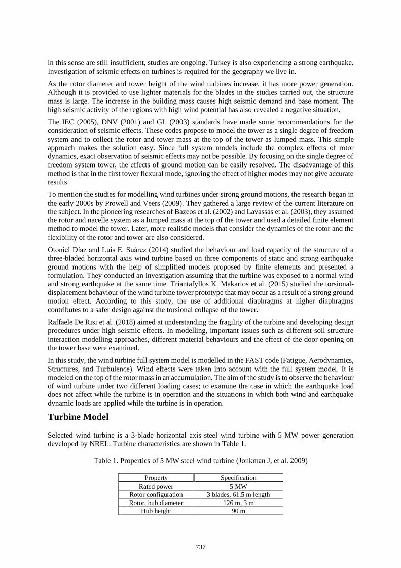
Selected wind turbine is a 3-blade horizontal axis steel wind turbine with 5 MW power generation developed by NREL. Turbine characteristics are shown in Table 1.

Table 1. Properties of 5 MW steel wind turbine (Jonkman J, et al. 2009)

Property Specification

Rated power 5 MW

Rotor configuration 3 blades, 61.5 m length

Rotor, hub diameter 126 m, 3 m

Hub height 90 m

737

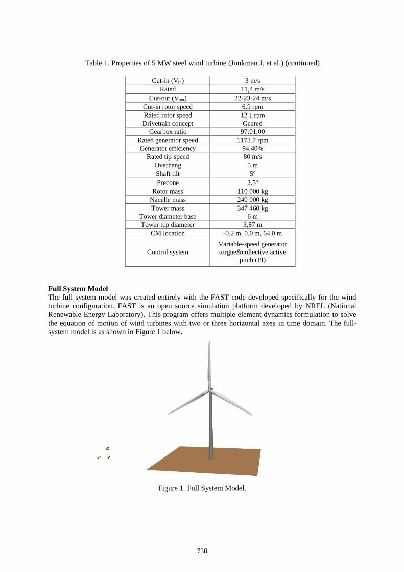
Table 1. Properties of 5 MW steel wind turbine (Jonkman J, et al.) (continued)

Cut-in (Vin) 3 m/s

Rated 11,4 m/s

Cut-out (Vout) 22-23-24 m/s

Cut-in rotor speed 6.9 rpm

Rated rotor speed 12.1 rpm

Drivetrain concept Geared

Gearbox ratio 97:01:00

Rated generator speed 1173.7 rpm

Generator efficiency 94.40%

Rated tip-speed 80 m/s

Overhang 5 m

Shaft tilt 5o

Precone 2.5o

Rotor mass 110 000 kg

Nacelle mass 240 000 kg

Tower mass 347 460 kg

Tower diameter base 6 m

Tower top diameter 3,87 m

CM location -0.2 m, 0.0 m, 64.0 m

Control system

Variable-speed generator

torgue&collective active

pitch (PI)

Full System Model

The full system model was created entirely with the FAST code developed specifically for the wind

turbine configuration. FAST is an open source simulation platform developed by NREL (National

Renewable Energy Laboratory). This program offers multiple element dynamics formulation to solve the equation of motion of wind turbines with two or three horizontal axes in time domain. The full-

system model is as shown in Figure 1 below.

Figure 1. Full System Model.

738

Analysis

The analyses were carried out in two steps. First of all, the system was analysed under normal operational

conditions under only wind loads. In the second case, different strong ground motions were also applied

on the system after a certain second. All these cases are examined with the FAST code.

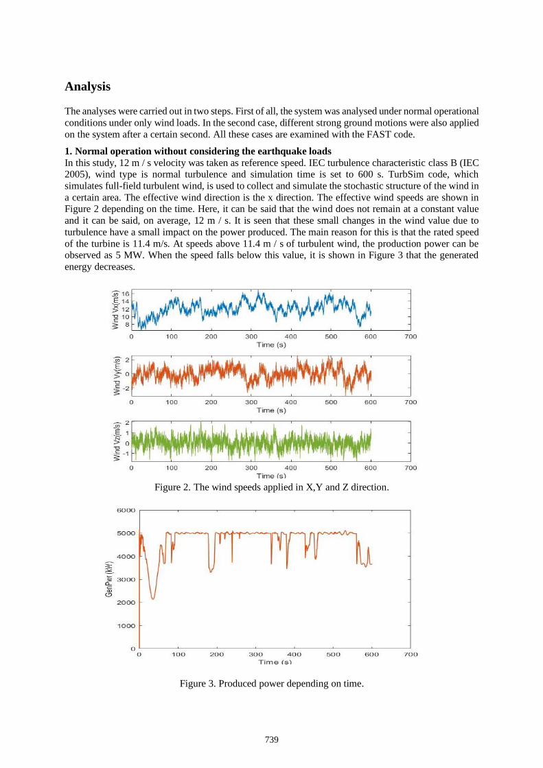
1. Normal operation without considering the earthquake loads

In this study, 12 m / s velocity was taken as reference speed. IEC turbulence characteristic class B (IEC2005), wind type is normal turbulence and simulation time is set to 600 s. TurbSim code, which

simulates full-field turbulent wind, is used to collect and simulate the stochastic structure of the wind in

a certain area. The effective wind direction is the x direction. The effective wind speeds are shown inFigure 2 depending on the time. Here, it can be said that the wind does not remain at a constant value

and it can be said, on average, 12 m / s. It is seen that these small changes in the wind value due to

turbulence have a small impact on the power produced. The main reason for this is that the rated speed

of the turbine is 11.4 m/s. At speeds above 11.4 m / s of turbulent wind, the production power can beobserved as 5 MW. When the speed falls below this value, it is shown in Figure 3 that the generated

energy decreases.

Figure 2. The wind speeds applied in X,Y and Z direction.

Figure 3. Produced power depending on time.

739

At variable wind speeds, the turbine needs to reach the cut-in wind speed to actively switch to the

electricity generation zone. They cannot produce electrical energy at speeds lower than this. When the turbine speed reaches the cut-out wind speed, the control systems stop the turbine power generation due

to the high wind load. The system becomes idle. Here, it is considered that the blade yaw angle has

reached 90o. In other words, electricity production remains within a certain region. While the speed limit

to initiate the energy production is 3 m / s, the wind speed at which the turbine becomes idle is 22-23-24 m / s. As described above, the turbine must reach the rated speed in order to reach the expected

production power. As seen in Figure 3 below, system power generation has decreased from time to time

due to turbulent wind.

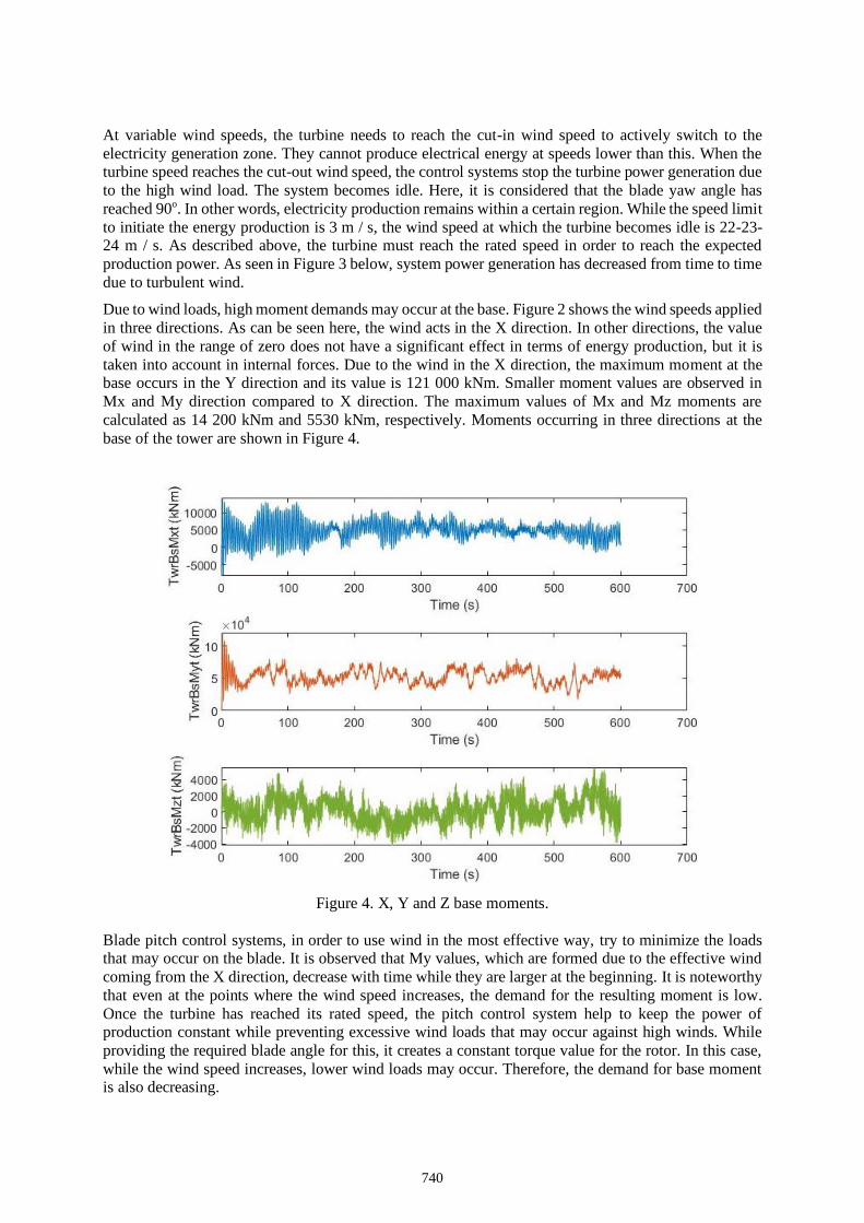
Due to wind loads, high moment demands may occur at the base. Figure 2 shows the wind speeds applied

in three directions. As can be seen here, the wind acts in the X direction. In other directions, the value

of wind in the range of zero does not have a significant effect in terms of energy production, but it is

taken into account in internal forces. Due to the wind in the X direction, the maximum moment at the base occurs in the Y direction and its value is 121 000 kNm. Smaller moment values are observed in

Mx and My direction compared to X direction. The maximum values of Mx and Mz moments are

calculated as 14 200 kNm and 5530 kNm, respectively. Moments occurring in three directions at the

base of the tower are shown in Figure 4.

Figure 4. X, Y and Z base moments.

Blade pitch control systems, in order to use wind in the most effective way, try to minimize the loads that may occur on the blade. It is observed that My values, which are formed due to the effective wind

coming from the X direction, decrease with time while they are larger at the beginning. It is noteworthy

that even at the points where the wind speed increases, the demand for the resulting moment is low.

Once the turbine has reached its rated speed, the pitch control system help to keep the power of production constant while preventing excessive wind loads that may occur against high winds. While

providing the required blade angle for this, it creates a constant torque value for the rotor. In this case,

while the wind speed increases, lower wind loads may occur. Therefore, the demand for base moment is also decreasing.

740

2. Normal operation with considering the earthquake loads

Selection of ground motions

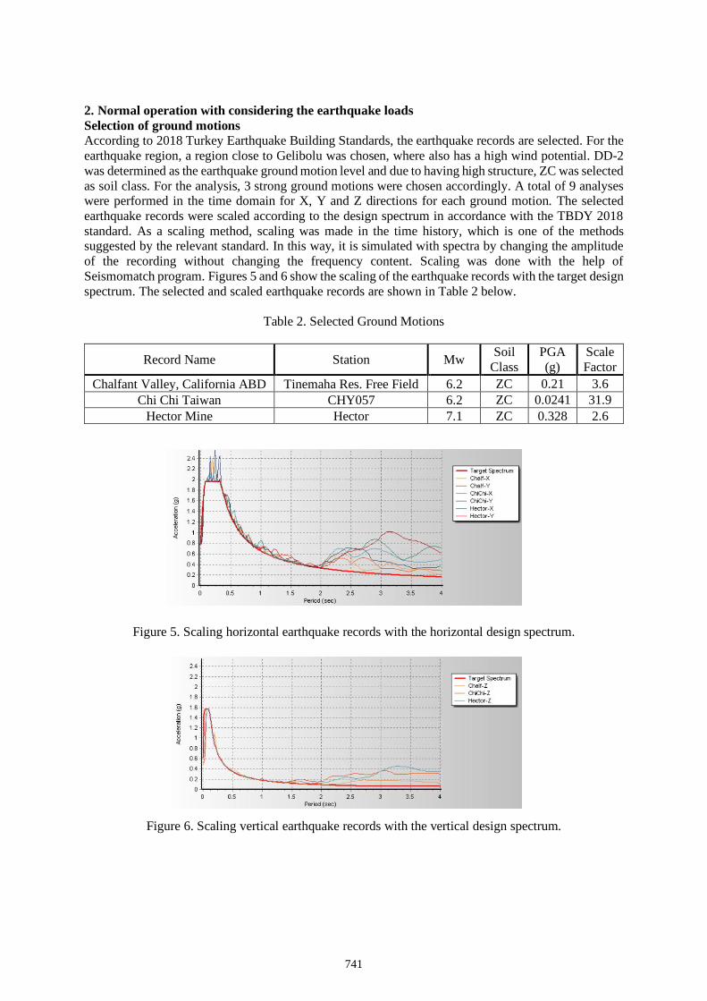
According to 2018 Turkey Earthquake Building Standards, the earthquake records are selected. For the

earthquake region, a region close to Gelibolu was chosen, where also has a high wind potential. DD-2

was determined as the earthquake ground motion level and due to having high structure, ZC was selected

as soil class. For the analysis, 3 strong ground motions were chosen accordingly. A total of 9 analyseswere performed in the time domain for X, Y and Z directions for each ground motion. The selected

earthquake records were scaled according to the design spectrum in accordance with the TBDY 2018

standard. As a scaling method, scaling was made in the time history, which is one of the methodssuggested by the relevant standard. In this way, it is simulated with spectra by changing the amplitude

of the recording without changing the frequency content. Scaling was done with the help of

Seismomatch program. Figures 5 and 6 show the scaling of the earthquake records with the target design

spectrum. The selected and scaled earthquake records are shown in Table 2 below.

Table 2. Selected Ground Motions

Record Name Station Mw Soil

Class

PGA

(g)

Scale

Factor

Chalfant Valley, California ABD Tinemaha Res. Free Field 6.2 ZC 0.21 3.6

Chi Chi Taiwan CHY057 6.2 ZC 0.0241 31.9

Hector Mine Hector 7.1 ZC 0.328 2.6

Figure 5. Scaling horizontal earthquake records with the horizontal design spectrum.

Figure 6. Scaling vertical earthquake records with the vertical design spectrum.

741

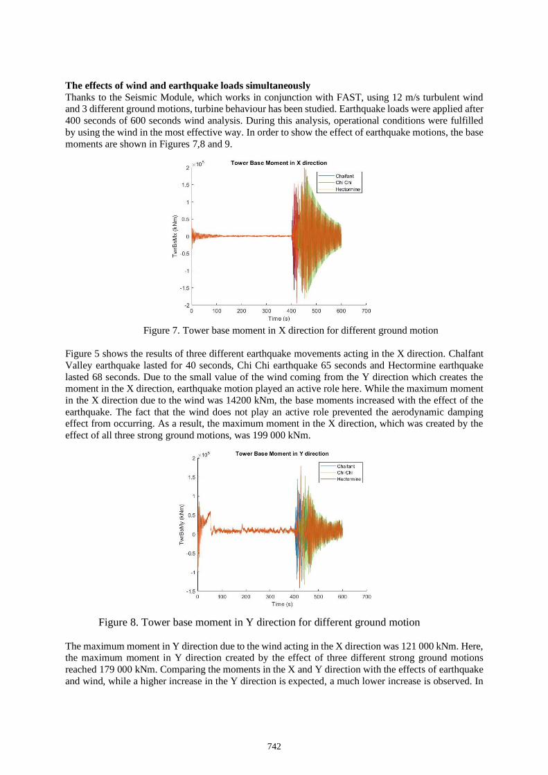
The effects of wind and earthquake loads simultaneously

Thanks to the Seismic Module, which works in conjunction with FAST, using 12 m/s turbulent wind and 3 different ground motions, turbine behaviour has been studied. Earthquake loads were applied after

400 seconds of 600 seconds wind analysis. During this analysis, operational conditions were fulfilled

by using the wind in the most effective way. In order to show the effect of earthquake motions, the base

moments are shown in Figures 7,8 and 9.

Figure 7. Tower base moment in X direction for different ground motion

Figure 5 shows the results of three different earthquake movements acting in the X direction. Chalfant

Valley earthquake lasted for 40 seconds, Chi Chi earthquake 65 seconds and Hectormine earthquake

lasted 68 seconds. Due to the small value of the wind coming from the Y direction which creates the moment in the X direction, earthquake motion played an active role here. While the maximum moment

in the X direction due to the wind was 14200 kNm, the base moments increased with the effect of the

earthquake. The fact that the wind does not play an active role prevented the aerodynamic damping effect from occurring. As a result, the maximum moment in the X direction, which was created by the

effect of all three strong ground motions, was 199 000 kNm.

Figure 8. Tower base moment in Y direction for different ground motion

The maximum moment in Y direction due to the wind acting in the X direction was 121 000 kNm. Here, the maximum moment in Y direction created by the effect of three different strong ground motions

reached 179 000 kNm. Comparing the moments in the X and Y direction with the effects of earthquake

and wind, while a higher increase in the Y direction is expected, a much lower increase is observed. In

742

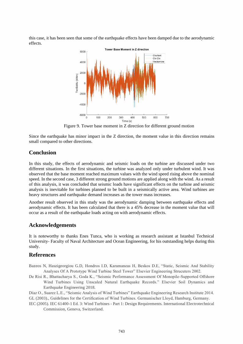
this case, it has been seen that some of the earthquake effects have been damped due to the aerodynamic

effects.

Figure 9. Tower base moment in Z direction for different ground motion

Since the earthquake has minor impact in the Z direction, the moment value in this direction remains

small compared to other directions.

Conclusion

In this study, the effects of aerodynamic and seismic loads on the turbine are discussed under two

different situations. In the first situations, the turbine was analyzed only under turbulent wind. It was

observed that the base moment reached maximum values with the wind speed rising above the nominal speed. In the second case, 3 different strong ground motions are applied along with the wind. As a result

of this analysis, it was concluded that seismic loads have significant effects on the turbine and seismic

analysis is inevitable for turbines planned to be built in a seismically active area. Wind turbines are

heavy structures and earthquake demand increases as the tower mass increases.

Another result observed in this study was the aerodynamic damping between earthquake effects and

aerodynamic effects. It has been calculated that there is a 45% decrease in the moment value that will

occur as a result of the earthquake loads acting on with aerodynamic effects.

Acknowledgements

It is noteworthy to thanks Enes Tunca, who is working as research assistant at Istanbul Technical

University- Faculty of Naval Architecture and Ocean Engineering, for his outstanding helps during this

study.

References

Bazeos N, Haszigeorgiou G.D, Hondros I.D, Karamaneas H, Beskos D.E, “Static, Seismic And Stability

Analyses Of A Prototype Wind Turbine Steel Tower” Elsevier Engineering Strucuters 2002.

De Risi R., Bhattacharya S., Goda K., “Seismic Performance Assessment Of Monopile-Supported Offshore

Wind Turbines Using Unscaled Natural Earthquake Records.” Elsevier Soil Dynamics and

Earthquake Engineering 2018.

Díaz O., Suarez L.E., “Seismic Analysis of Wind Turbines” Earthquake Engineering Research Institute 2014.

GL (2003)., Guidelines for the Certification of Wind Turbines. Germanischer Lloyd, Hamburg, Germany.

IEC (2005). IEC 61400-1 Ed. 3: Wind Turbines - Part 1: Design Requirements. International Electrotechnical

Commission, Geneva, Switzerland.

743

Jonkman J, Butterfield S., Musial W., Scott G., “Definition of a 5 MW Reference Wind Turbine for Offshore

System Development”, February 2009.

Laino, D. J.; Hansen, A.C. User’s Guide to the Wind Turbine Dynamics Aerodynamics Computer Software

AeroDyn. Salt Lake City, UT: Windward Engineering, LC, December 2002.

Makarios T.K., Efthymiou E., Baniotopoulos C.C, “On the Torsional–Translational Response of Wind

Turbine Structures” King Fahd University of Petroleum & Minerals 2015.

Prowell, I., Veers P.,“ Assessment of Wind Turbine Seismic Risk: Existing Literature and Simple Study of

Tower Moment Demand”, SANDIA REPORT 2009.

Risø (2001). Guidelines for Design of Wind Turbines. Wind Energy Department of Risø National Laboratory

and Det Norske Veritas, Copenhagen, Denmark.

Santangelo F., Failla G., Santini A., Arena F., “Time-Domain Uncoupled Analyses For Seismic Assessment

Of Land-Based Wind Turbines” Elsevier Engineering Strucuters 2016.

Türkiye Rüzgar Enerjisi İstatistik Raporu Temmuz 2019.

744

Yüksek Yapı Davranışında Yakın ve Uzak Alan Kaynaklı Depremlerin

Etkisi

Kemal Beyen

Dr. Deprem Müh. İnşaat Mühendisliği Bölümü, Kocaeli Üniversitesi, Umuttepe, Kocaeli, Türkiye

Email: [email protected]

Özet Yakın ve uzak alan kaynaklı depremlerin yapısal davranış ve ürettikleri tepkiler üzerine etkilerinin

yürütüldüğü çalışmalar gündemin sıcak konularıdır. Benzer şekilde yakın ve uzak kaynaklı deprem

şartlarında yüksek yapı davranışının kayıtlarla araştırılması bir başka önemli konudur. Yakın alan

kaynaklı yer hareketinin deprem merkezi civarında yüksek yapılara kıyasla az katlı olan konvansiyonel

alışkanlıklarla inşaa edilmiş konutlarda hasarların ağır hasardan göçmeye kadar giden bir yayılım içinde

dağılım gösterdiği bilinmektedir. Genellikle yakın alan depremler kararlı yer deplasmanı ve yüksek

freakans içeriğiyle kısa süreli itkilerle depremin başında yapıya yüksek enerji girişi verirler. Dahası, açık

alan yer hareketinin yapı temel seviyesinde büyük oranda değişimi ise yapı-zemin etkileşimini

tartışmaya açabilmektedir. Aslında, her yakın-alan kaynaklı deprem kaydı kendine özgün frekans ve

dalga yayılım farklılıkları içermektedir. Yerel şartlarda oluşan değişik alan kaynaklı depremler

birbirlerinden farklı olup deprem oluşum mekanizmalarının, kaynaklanma, yırtılma, yönelme ve yayılım

özellikleri açısından her biri taşıdıkları kendi özgün karekteristiklerini sergilerler. Bu açıdan, sunulacak

çalışma yakın ve uzak alan kaynaklı depremler altında yüksek yapının davranışını incelemeyi

amaçlamaktadır. Yakın ve uzak alan kaynaklı depremlerin karekteristik özelliklerinin çalışma

bölgesinde gösterilmesi, sunduğu yer hareketi açısından farklılıkları ve yüksek yapı tepkisinde gözlenen

temel farklılıkları bu çalışmada etraflıca tartışılmaktadır. Bu çalışmada yapı sağlığı izleme programı

içinde bulunan bir yüksek yapı ağından temin edilen veriler kullanılmıştır. Bir dizi sinyal işleme ve yapı

tanı algoritmaları uygulanarak önemli tepkisel karekteristikler ve ilgili yapısal davranışı açıklayan

deplasman, hız ve ivme zaman grafikleri her iki tür depremler için elde edilmiştir. Değişik seviyedeki

katlar ile temel ve giriş katları arasında elde edilen transfer fonksiyonları yakın ve uzak alan kaynağa

sahip depremler altında yapıda ürettiği tepkisel davranışlar kinematik değişimler içinde sunulmuştur.

Bunların yanı sıra, yerel zemin tepki davranışları ve çalışılan yüksek yapının global davranışı yakın ve

uzak alan depremler altında gösterdiği benzerlikler ve farklılıklar sonuçlarıyla beraber tablo ve grafikler

eşliğinde tartışılmıştır. İncelenen yakın alan kaynaklı depremlerde maksimum deplasman yön dağılımı

fay normali ve fay dik yönleri ile bir tutarlılık göstermediği izlenmiştir. İncelenen yapılar gibi lineer

elastik davranış sergileyen mühendislik yapılarında maksimum yerdeğiştirmeler hakim hız itki

frekanslarıyla yapı hakim frekanslarının yakın olduğu durumlarda izlenmiştir. Rezonans potansiyeline

yakın şartlarda geometrik veya eleman kapasite aşımından kaynaklı doğrusal olmayan davranışın

periyotları büyüterek senkronizasyonu bozması ve rezonans çanağına düşmesi beklenebilir. Yapı

yüksekliklerinin kilometreye ulaştığı günümüz mühendislik dünyasında, yapıdan istenen sismik talepler

açısından ilk modlarda yakın alan kaynaklı depremlerin gökdelenlerde artan periyotla beraber hız

taleplerini ve deplasman taleplerini yükseltiği, buna mukabil uzak alan kaynaklı depremlerin düşük

genlik altında dahi kararlı salınımlarla yapı titreşimini saate ulaşacak sürelere uzattığı izlenmiştir.

Uzayan transient davranış özellikle düşük sönüm özelliği olan yüksek yapıların, yerel zemin hakim

periyotlarının büyük olduğu veya yapı periyot bandında kaldığı koşullarda gerçekleşmektedir.

Anahtar Kelimeler: Yakın-alan Deprem, Uzak-alan Deprem, Veri İşleme, Yapı Tanılama, Göreceli

Davranış, Yüksek Yapı.

1. Giriş

Farklı özellikler sergileyen yakın alan kaynaklı depremlere mühendislik yapılarının sergilediği tepkiler

uzak alan kaynaklı depremlerin ürettiği tepkilerle mukayese edildiğinde önemli çarpıcı farklılıkların öne

745

çıktığı gözlenmektedir (M. Davoodi, M. Sadjadi, 2015). Genel olarak deprem kaynağını oluşturan fay

düzlemine parallel ve normal yönlerde ortama yayılan yer hareketi sismik kaynağın kırılma-üretme

özelliklerinden, kaynaktan çalışılan sahaya dalga yayılma ortamının etkilerinden ve yerel şartlar olarak

nitelendirilen alt katman ve üst topoğrafik düzensizlikleriyle yerel zemin özelliklerinden etkilenerek yer

hareketini şekillendirir (Beyen, K. ve Tanırcan, G., 2015, Beyen, K., 2019). Dalga yayılımının seyahati

boyunca aldığı bu etkilerden dolayı kaynağa yakın çevredeki yer hareketi özellikleri uzak alanlara

seyahat ederken değişir ve hasar potansiyeli bazı yapılar için yükselirken bazı yapılar için tehlike

olmaktan çıkar. Deprem kaynağına yakın alanlarda yer hareketi yüksek genlik ve büyük periyot ivme

ve hız itkileriyle (pulse) fay normalinde oluşur. Yönelim-yayılım etkisi, kalıcı yer değiştirme ve parçalı

kopma etkisinde (fling step effect) yüksek frekans zenginliğiyle kayıtlarda görünür (Beyen, K. ve

Tanırcan, G., 2015, Beyen, K., 2019). Fay kırılma mekaniği incelenecek olursa yırtılma/kırılma

enerjisinin ürettiği dalga yayılımı (Vkırılma) ortamın kayma dalga yayılım hızı (Vs)’e yaklaştıkça (örneğin,

Vkırılma ~ 0.8Vs) super kayma (super shear, Vkırılma ≈ Vs) hızına yaklaştıkça önündeki yakın sahaya fay

enerjisinin büyük bir miktarını kısa sürede büyük genlik ile transfer eder. Bu parallel fay davranışı fay

normalinde deprem hız kayıtlarında başlangıçta görülür. Uzak alan kaynaklı deprem yer hareketi ise

kayıtlarda mutedil zaman uzunluklarında büyük periyotlu salınımlar içinde görünür. Fay-kırılmasının

ürettiği dalgaların yüksek frekans bileşenleri ince, kalın veya mercek yer katman ortamı içinde yayılır

ve katman sınırlarında yansıma ve kırılma şartlarında süzülür ve uzak alanlara büyük periyot ve uzun

süreli salınım genlikleri ulaşır.

2. Yakın ve uzak alan kaynaklı depremlerin yapısal davranışa etkisi

Yapılar için hala çözülemeyen bir mühendislik tasarım problemi olarak yakın-alan büyük periyotlu

darbe (pulse) benzeri yüksek yer hızı ve yayılım-yönelim etkisi ciddi saha kayıtlarıyla desteklenmek

zorundadır. Benzer şekilde yatay yer düzlemindeki yer hareketinin bizati kaydedilmiş fay-normali ve

fay-dik yönlerdeki dalga yayılımlarının veya döndürülmüş fay-normal ve fay-dik bileşenlerinin yüksek

yapı tasarımında her zaman en büyük kritik sismik talebi veremeyeceği veya maksimum yer hareketini

veren istikametteki hakim tepe genlikleri ve tepe frekanslarıyla yüksek yapının temel karekteristik

frekansları yapıda kritik yapısal yer değiştirmelerin tahmininde tutarlılık düzeylerinin sorgulanması

problemin çözümünde faydalı olacaktır (Archila, M., Ventura, C. E. vd., 2014). Gerçekte yönelim

etkisinin yüksek yapılarda doğuracağı kritik yerdeğiştirme tepkilerini önden kestirmenin hale hazırda

uygulanan bir yöntemi de yoktur. Klasik yaklaşım içinde ciddi vakit harcanan bir yöntem olarak; yapının

plandaki eksenlerine göre belirli açı artımıyla sistematik olarak döndürülen yer hareketinin her bir

bileşeninin yapıda üreteceği maksimum deplasman tepkilerinin zarfından üretilen deplasman spektrumu

kullanılarak tasarım için nümerik analiz yürütülmektedir (Manuel Archila, 2014). Tartışılan kritik

sismik talep ve yönelim yönüyle ilgili karar verme güçlüğüne bir çözüm olarak bu çalışmada

cihazlandırılan mecvut bir yüksek yapının son bir kaç yılda maruz kaldığı yakın ve uzak alan kaynaklı

depremler incelenerek yapı davranışını etkileyen yön ve değerleri tartışılmıştır. Bu tartışmaya ışık

tutması açısından farklı alan kaynaklı farklı yayılım şartlarında etkiyen depremlere örneğin yapının ana

eksenleri üstünden izlenen ivme ölçerlerle kaydedilen tepki kayıtları kullanılarak 3 boyut için

tartışılmıştır.

Reyes ve Kalkan (2012)’ ın bir çalışmasında yapı tepkilerinin hesaplanmasında yer hareketinin özellikle

yakın alan deprem etkisinde (aktif faya 5Km ile 60 Km mesafelere kadar) faya parallel ve fay normal

bileşenleriyle veya maksimum yönde (CBSC, 2010) mühendislik parametrelerinin sismik talebinin

hesaplanmasının avantajları tartışılmıştır. Yakın alan deprem etkilerinin izlendiği mesafeler ise

gözlemlere bağlı olarak tartışma konusu olup tam bir mutabakat yoktur. Örneğin California Yapı

Yönetmeliği-Bölüm 1615A.1.25 (CBSC, 2010) 5Km’yi sınır olarak verirken bir diğer saha çalışması

60Km’lere kadar etkilerin izlendiğini paylaşmaktadır (Stewart v.d., 2001). Fay normal ve fay parallel

bileşenlerinin veya maksimum yönde etkiyen yer hareketinin doğrusal olmayan analizlerde beklendiği

gibi mühendislik parametrelerinde kritik sınır değerlere ulaşılmadığı sonucu çıkarsanmış ve yeni tasarım

için güvenli tarafta kalacak bir klasik yaklaşım olarak tasarım tutarlılığının sınanması amacına uygun

olabileceği Reyes ve Kalkan (2012) tarafından ifade edilmiştir. Zaman tanım alanında davranış çalışılan

çok serbestlik dereceli doğrusal elastik simetrik ve asimetrik plana sahip yapıya uygulanan bir seri

döndürülmüş açılar altındaki girdi bileşenleri örneğin yapı simetri eksenleri boyunca uygulanan yük

746

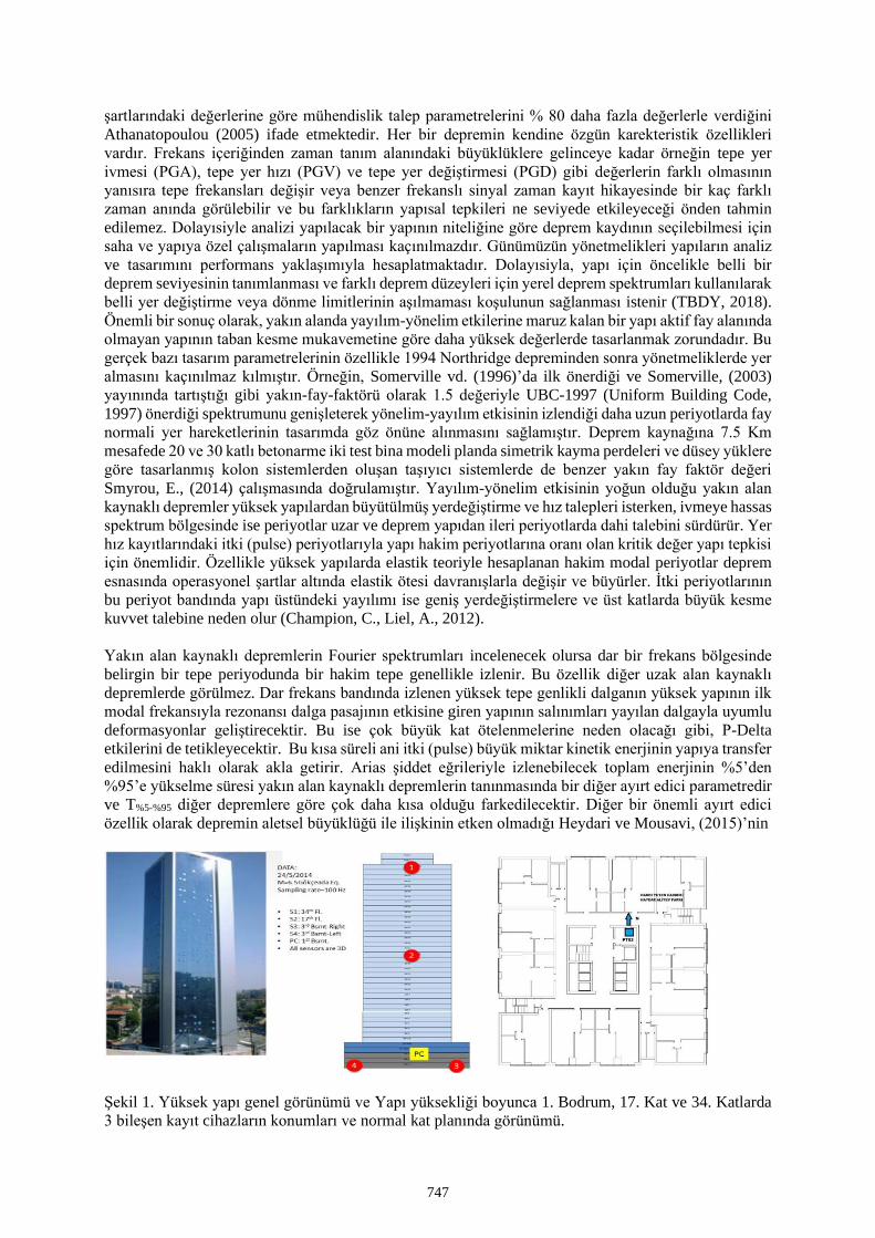
şartlarındaki değerlerine göre mühendislik talep parametrelerini % 80 daha fazla değerlerle verdiğini

Athanatopoulou (2005) ifade etmektedir. Her bir depremin kendine özgün karekteristik özellikleri

vardır. Frekans içeriğinden zaman tanım alanındaki büyüklüklere gelinceye kadar örneğin tepe yer

ivmesi (PGA), tepe yer hızı (PGV) ve tepe yer değiştirmesi (PGD) gibi değerlerin farklı olmasının

yanısıra tepe frekansları değişir veya benzer frekanslı sinyal zaman kayıt hikayesinde bir kaç farklı

zaman anında görülebilir ve bu farklıkların yapısal tepkileri ne seviyede etkileyeceği önden tahmin

edilemez. Dolayısiyle analizi yapılacak bir yapının niteliğine göre deprem kaydının seçilebilmesi için

saha ve yapıya özel çalışmaların yapılması kaçınılmazdır. Günümüzün yönetmelikleri yapıların analiz

ve tasarımını performans yaklaşımıyla hesaplatmaktadır. Dolayısiyla, yapı için öncelikle belli bir

deprem seviyesinin tanımlanması ve farklı deprem düzeyleri için yerel deprem spektrumları kullanılarak

belli yer değiştirme veya dönme limitlerinin aşılmaması koşulunun sağlanması istenir (TBDY, 2018).

Önemli bir sonuç olarak, yakın alanda yayılım-yönelim etkilerine maruz kalan bir yapı aktif fay alanında

olmayan yapının taban kesme mukavemetine göre daha yüksek değerlerde tasarlanmak zorundadır. Bu

gerçek bazı tasarım parametrelerinin özellikle 1994 Northridge depreminden sonra yönetmeliklerde yer

almasını kaçınılmaz kılmıştır. Örneğin, Somerville vd. (1996)’da ilk önerdiği ve Somerville, (2003)

yayınında tartıştığı gibi yakın-fay-faktörü olarak 1.5 değeriyle UBC-1997 (Uniform Building Code,

1997) önerdiği spektrumunu genişleterek yönelim-yayılım etkisinin izlendiği daha uzun periyotlarda fay

normali yer hareketlerinin tasarımda göz önüne alınmasını sağlamıştır. Deprem kaynağına 7.5 Km

mesafede 20 ve 30 katlı betonarme iki test bina modeli planda simetrik kayma perdeleri ve düsey yüklere

göre tasarlanmış kolon sistemlerden oluşan taşıyıcı sistemlerde de benzer yakın fay faktör değeri

Smyrou, E., (2014) çalışmasında doğrulamıştır. Yayılım-yönelim etkisinin yoğun olduğu yakın alan

kaynaklı depremler yüksek yapılardan büyütülmüş yerdeğiştirme ve hız talepleri isterken, ivmeye hassas

spektrum bölgesinde ise periyotlar uzar ve deprem yapıdan ileri periyotlarda dahi talebini sürdürür. Yer

hız kayıtlarındaki itki (pulse) periyotlarıyla yapı hakim periyotlarına oranı olan kritik değer yapı tepkisi

için önemlidir. Özellikle yüksek yapılarda elastik teoriyle hesaplanan hakim modal periyotlar deprem

esnasında operasyonel şartlar altında elastik ötesi davranışlarla değişir ve büyürler. İtki periyotlarının

bu periyot bandında yapı üstündeki yayılımı ise geniş yerdeğiştirmelere ve üst katlarda büyük kesme

kuvvet talebine neden olur (Champion, C., Liel, A., 2012).

Yakın alan kaynaklı depremlerin Fourier spektrumları incelenecek olursa dar bir frekans bölgesinde

belirgin bir tepe periyodunda bir hakim tepe genellikle izlenir. Bu özellik diğer uzak alan kaynaklı

depremlerde görülmez. Dar frekans bandında izlenen yüksek tepe genlikli dalganın yüksek yapının ilk

modal frekansıyla rezonansı dalga pasajının etkisine giren yapının salınımları yayılan dalgayla uyumlu

deformasyonlar geliştirecektir. Bu ise çok büyük kat ötelenmelerine neden olacağı gibi, P-Delta

etkilerini de tetikleyecektir. Bu kısa süreli ani itki (pulse) büyük miktar kinetik enerjinin yapıya transfer

edilmesini haklı olarak akla getirir. Arias şiddet eğrileriyle izlenebilecek toplam enerjinin %5’den

%95’e yükselme süresi yakın alan kaynaklı depremlerin tanınmasında bir diğer ayırt edici parametredir

ve T%5-%95 diğer depremlere göre çok daha kısa olduğu farkedilecektir. Diğer bir önemli ayırt edici

özellik olarak depremin aletsel büyüklüğü ile ilişkinin etken olmadığı Heydari ve Mousavi, (2015)’nin

Şekil 1. Yüksek yapı genel görünümü ve Yapı yüksekliği boyunca 1. Bodrum, 17. Kat ve 34. Katlarda

3 bileşen kayıt cihazların konumları ve normal kat planında görünümü.

747

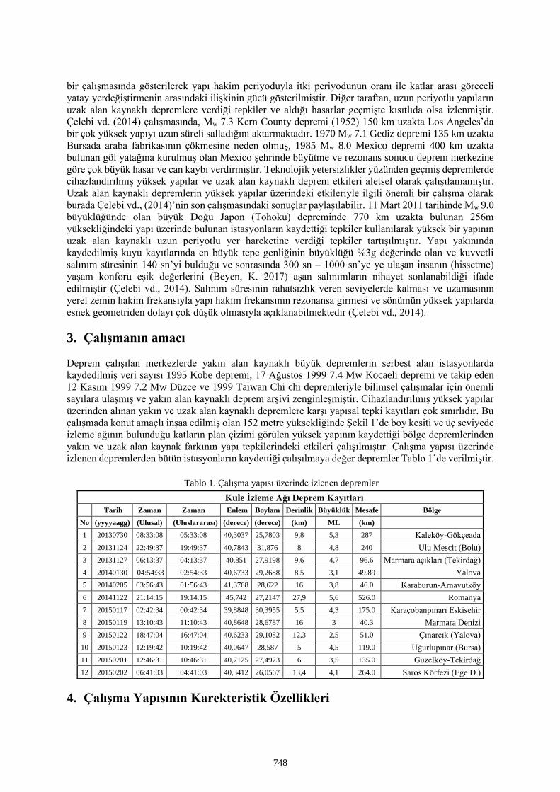
bir çalışmasında gösterilerek yapı hakim periyoduyla itki periyodunun oranı ile katlar arası göreceli

yatay yerdeğiştirmenin arasındaki ilişkinin gücü gösterilmiştir. Diğer taraftan, uzun periyotlu yapıların

uzak alan kaynaklı depremlere verdiği tepkiler ve aldığı hasarlar geçmişte kısıtlıda olsa izlenmiştir.

Çelebi vd. (2014) çalışmasında, Mw 7.3 Kern County depremi (1952) 150 km uzakta Los Angeles’da

bir çok yüksek yapıyı uzun süreli salladığını aktarmaktadır. 1970 Mw 7.1 Gediz depremi 135 km uzakta

Bursada araba fabrikasının çökmesine neden olmuş, 1985 Mw 8.0 Mexico depremi 400 km uzakta

bulunan göl yatağına kurulmuş olan Mexico şehrinde büyütme ve rezonans sonucu deprem merkezine

göre çok büyük hasar ve can kaybı verdirmiştir. Teknolojik yetersizlikler yüzünden geçmiş depremlerde

cihazlandırılmış yüksek yapılar ve uzak alan kaynaklı deprem etkileri aletsel olarak çalışılamamıştır.

Uzak alan kaynaklı depremlerin yüksek yapılar üzerindeki etkileriyle ilgili önemli bir çalışma olarak

burada Çelebi vd., (2014)’nin son çalışmasındaki sonuçlar paylaşılabilir. 11 Mart 2011 tarihinde Mw 9.0

büyüklüğünde olan büyük Doğu Japon (Tohoku) depreminde 770 km uzakta bulunan 256m

yüksekliğindeki yapı üzerinde bulunan istasyonların kaydettiği tepkiler kullanılarak yüksek bir yapının

uzak alan kaynaklı uzun periyotlu yer hareketine verdiği tepkiler tartışılmıştır. Yapı yakınında

kaydedilmiş kuyu kayıtlarında en büyük tepe genliğinin büyüklüğü %3g değerinde olan ve kuvvetli

salınım süresinin 140 sn’yi bulduğu ve sonrasında 300 sn – 1000 sn’ye ye ulaşan insanın (hissetme)

yaşam konforu eşik değerlerini (Beyen, K. 2017) aşan salınımların nihayet sonlanabildiği ifade

edilmiştir (Çelebi vd., 2014). Salınım süresinin rahatsızlık veren seviyelerde kalması ve uzamasının

yerel zemin hakim frekansıyla yapı hakim frekansının rezonansa girmesi ve sönümün yüksek yapılarda

esnek geometriden dolayı çok düşük olmasıyla açıklanabilmektedir (Çelebi vd., 2014).

3. Çalışmanın amacı

Deprem çalışılan merkezlerde yakın alan kaynaklı büyük depremlerin serbest alan istasyonlarda

kaydedilmiş veri sayısı 1995 Kobe depremi, 17 Ağustos 1999 7.4 Mw Kocaeli depremi ve takip eden

12 Kasım 1999 7.2 Mw Düzce ve 1999 Taiwan Chi chi depremleriyle bilimsel çalışmalar için önemli

sayılara ulaşmış ve yakın alan kaynaklı deprem arşivi zenginleşmiştir. Cihazlandırılmış yüksek yapılar

üzerinden alınan yakın ve uzak alan kaynaklı depremlere karşı yapısal tepki kayıtları çok sınırlıdır. Bu

çalışmada konut amaçlı inşaa edilmiş olan 152 metre yüksekliğinde Şekil 1’de boy kesiti ve üç seviyede

izleme ağının bulunduğu katların plan çizimi görülen yüksek yapının kaydettiği bölge depremlerinden

yakın ve uzak alan kaynak farkının yapı tepkilerindeki etkileri çalışılmıştır. Çalışma yapısı üzerinde

izlenen depremlerden bütün istasyonların kaydettiği çalışılmaya değer depremler Tablo 1’de verilmiştir.

Tablo 1. Çalışma yapısı üzerinde izlenen depremler

4. Çalışma Yapısının Karekteristik Özellikleri

Kule İzleme Ağı Deprem Kayıtları

Tarih Zaman Zaman Enlem Boylam Derinlik Büyüklük Mesafe Bölge

No (yyyyaagg) (Ulusal) (Uluslararası) (derece) (derece) (km) ML (km)

1 20130730 08:33:08 05:33:08 40,3037 25,7803 9,8 5,3 287 Kaleköy-Gökçeada

2 20131124 22:49:37 19:49:37 40,7843 31,876 8 4,8 240 Ulu Mescit (Bolu)

3 20131127 06:13:37 04:13:37 40,851 27,9198 9,6 4,7 96.6 Marmara açıkları (Tekirdağ)

4 20140130 04:54:33 02:54:33 40,6733 29,2688 8,5 3,1 49.89 Yalova

5 20140205 03:56:43 01:56:43 41,3768 28,622 16 3,8 46.0 Karaburun-Arnavutköy

6 20141122 21:14:15 19:14:15 45,742 27,2147 27,9 5,6 526.0 Romanya

7 20150117 02:42:34 00:42:34 39,8848 30,3955 5,5 4,3 175.0 Karaçobanpınarı Eskisehir

8 20150119 13:10:43 11:10:43 40,8648 28,6787 16 3 40.3 Marmara Denizi

9 20150122 18:47:04 16:47:04 40,6233 29,1082 12,3 2,5 51.0 Çınarcık (Yalova)

10 20150123 12:19:42 10:19:42 40,0647 28,587 5 4,5 119.0 Uğurlupınar (Bursa)

11 20150201 12:46:31 10:46:31 40,7125 27,4973 6 3,5 135.0 Güzelköy-Tekirdağ

12 20150202 06:41:03 04:41:03 40,3412 26,0567 13,4 4,1 264.0 Saros Körfezi (Ege D.)

748

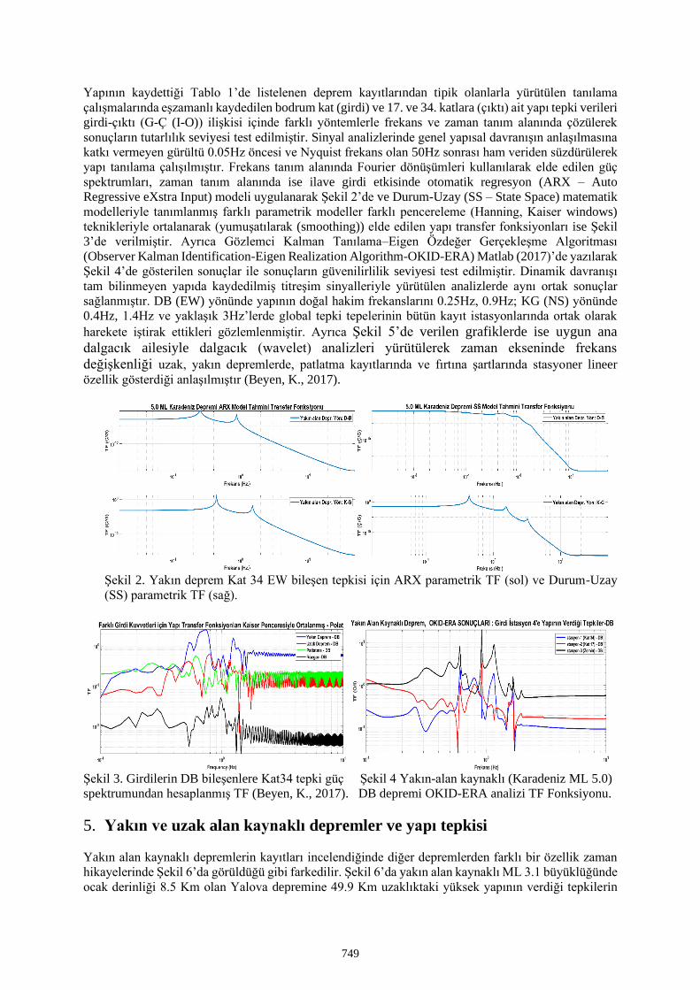
Yapının kaydettiği Tablo 1’de listelenen deprem kayıtlarından tipik olanlarla yürütülen tanılama

çalışmalarında eşzamanlı kaydedilen bodrum kat (girdi) ve 17. ve 34. katlara (çıktı) ait yapı tepki verileri

girdi-çıktı (G-Ç (I-O)) ilişkisi içinde farklı yöntemlerle frekans ve zaman tanım alanında çözülerek

sonuçların tutarlılık seviyesi test edilmiştir. Sinyal analizlerinde genel yapısal davranışın anlaşılmasına

katkı vermeyen gürültü 0.05Hz öncesi ve Nyquist frekans olan 50Hz sonrası ham veriden süzdürülerek

yapı tanılama çalışılmıştır. Frekans tanım alanında Fourier dönüşümleri kullanılarak elde edilen güç

spektrumları, zaman tanım alanında ise ilave girdi etkisinde otomatik regresyon (ARX – Auto

Regressive eXstra Input) modeli uygulanarak Şekil 2’de ve Durum-Uzay (SS – State Space) matematik

modelleriyle tanımlanmış farklı parametrik modeller farklı pencereleme (Hanning, Kaiser windows)

teknikleriyle ortalanarak (yumuşatılarak (smoothing)) elde edilen yapı transfer fonksiyonları ise Şekil

3’de verilmiştir. Ayrıca Gözlemci Kalman Tanılama–Eigen Özdeğer Gerçekleşme Algoritması

(Observer Kalman Identification-Eigen Realization Algorithm-OKID-ERA) Matlab (2017)’de yazılarak

Şekil 4’de gösterilen sonuçlar ile sonuçların güvenilirlilik seviyesi test edilmiştir. Dinamik davranışı

tam bilinmeyen yapıda kaydedilmiş titreşim sinyalleriyle yürütülen analizlerde aynı ortak sonuçlar

sağlanmıştır. DB (EW) yönünde yapının doğal hakim frekanslarını 0.25Hz, 0.9Hz; KG (NS) yönünde

0.4Hz, 1.4Hz ve yaklaşık 3Hz’lerde global tepki tepelerinin bütün kayıt istasyonlarında ortak olarak

harekete iştirak ettikleri gözlemlenmiştir. Ayrıca Şekil 5’de verilen grafiklerde ise uygun ana

dalgacık ailesiyle dalgacık (wavelet) analizleri yürütülerek zaman ekseninde frekans

değişkenliği uzak, yakın depremlerde, patlatma kayıtlarında ve fırtına şartlarında stasyoner lineer

özellik gösterdiği anlaşılmıştır (Beyen, K., 2017).

Şekil 2. Yakın deprem Kat 34 EW bileşen tepkisi için ARX parametrik TF (sol) ve Durum-Uzay

(SS) parametrik TF (sağ).

Şekil 3. Girdilerin DB bileşenlere Kat34 tepki güç Şekil 4 Yakın-alan kaynaklı (Karadeniz ML 5.0)

spektrumundan hesaplanmış TF (Beyen, K., 2017). DB depremi OKID-ERA analizi TF Fonksiyonu.

5. Yakın ve uzak alan kaynaklı depremler ve yapı tepkisi

Yakın alan kaynaklı depremlerin kayıtları incelendiğinde diğer depremlerden farklı bir özellik zaman

hikayelerinde Şekil 6’da görüldüğü gibi farkedilir. Şekil 6’da yakın alan kaynaklı ML 3.1 büyüklüğünde

ocak derinliği 8.5 Km olan Yalova depremine 49.9 Km uzaklıktaki yüksek yapının verdiği tepkilerin

749

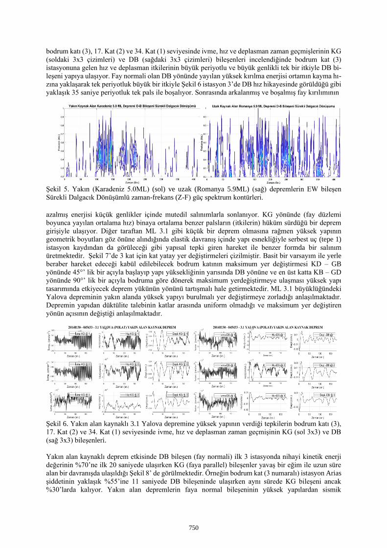
bodrum katı (3), 17. Kat (2) ve 34. Kat (1) seviyesinde ivme, hız ve deplasman zaman geçmişlerinin KG

(soldaki 3x3 çizimleri) ve DB (sağdaki 3x3 çizimleri) bileşenleri incelendiğinde bodrum kat (3)

istasyonuna gelen hız ve deplasman itkilerinin büyük periyotlu ve büyük genlikli tek bir itkiyle DB bi-

leşeni yapıya ulaşıyor. Fay normali olan DB yönünde yayılan yüksek kırılma enerjisi ortamın kayma hı-

zına yaklaşarak tek periyotluk büyük bir itkiyle Şekil 6 istasyon 3’de DB hız hikayesinde görüldüğü gibi

yaklaşık 35 saniye periyotluk tek pals ile boşalıyor. Sonrasında arkalanmış ve boşalmış fay kırılımının

Şekil 5. Yakın (Karadeniz 5.0ML) (sol) ve uzak (Romanya 5.9ML) (sağ) depremlerin EW bileşen

Sürekli Dalgacık Dönüşümlü zaman-frekans (Z-F) güç spektrum kontürleri.

azalmış enerjisi küçük genlikler içinde mutedil salınımlarla sonlanıyor. KG yönünde (fay düzlemi

boyunca yayılan ortalama hız) binaya ortalama benzer palsların (itkilerin) hüküm sürdüğü bir deprem

girişiyle ulaşıyor. Diğer taraftan ML 3.1 gibi küçük bir deprem olmasına rağmen yüksek yapının

geometrik boyutları göz önüne alındığında elastik davranış içinde yapı esnekliğiyle serbest uç (tepe 1)

istasyon kaydından da görüleceği gibi yapısal tepki giren hareket ile benzer formda bir salınım

üretmektedir. Şekil 7’de 3 kat için kat yatay yer değiştirmeleri çizilmiştir. Basit bir varsayım ile yerle

beraber hareket edeceği kabül edilebilecek bodrum katının maksimum yer değiştirmesi KD – GB

yönünde 45°’ lik bir açıyla başlayıp yapı yüksekliğinin yarısında DB yönüne ve en üst katta KB – GD

yönünde 90°’ lik bir açıyla bodruma göre dönerek maksimum yerdeğiştirmeye ulaşması yüksek yapı

tasarımında etkiyecek deprem yükünün yönünü tartışmalı hale getirmektedir. ML 3.1 büyüklüğündeki

Yalova depreminin yakın alanda yüksek yapıyı burulmalı yer değiştirmeye zorladığı anlaşılmaktadır.

Depremin yapıdan düktülite talebinin katlar arasında uniform olmadığı ve maksimum yer değiştiren

yönün açısının değiştiği anlaşılmaktadır.

Şekil 6. Yakın alan kaynaklı 3.1 Yalova depremine yüksek yapının verdiği tepkilerin bodrum katı (3),

17. Kat (2) ve 34. Kat (1) seviyesinde ivme, hız ve deplasman zaman geçmişinin KG (sol 3x3) ve DB

(sağ 3x3) bileşenleri.

Yakın alan kaynaklı deprem etkisinde DB bileşen (fay normali) ilk 3 istasyonda nihayi kinetik enerji

değerinin %70’ne ilk 20 saniyede ulaşırken KG (faya parallel) bileşenler yavaş bir eğim ile uzun süre

alan bir davranışda ulaşıldığı Şekil 8’ de görülmektedir. Örneğin bodrum kat (3 numaralı) istasyon Arias

şiddetinin yaklaşık %55’ine 11 saniyede DB bileşeninde ulaşırken aynı sürede KG bileşeni ancak

%30’larda kalıyor. Yakın alan depremlerin faya normal bileşeninin yüksek yapılardan sismik

750

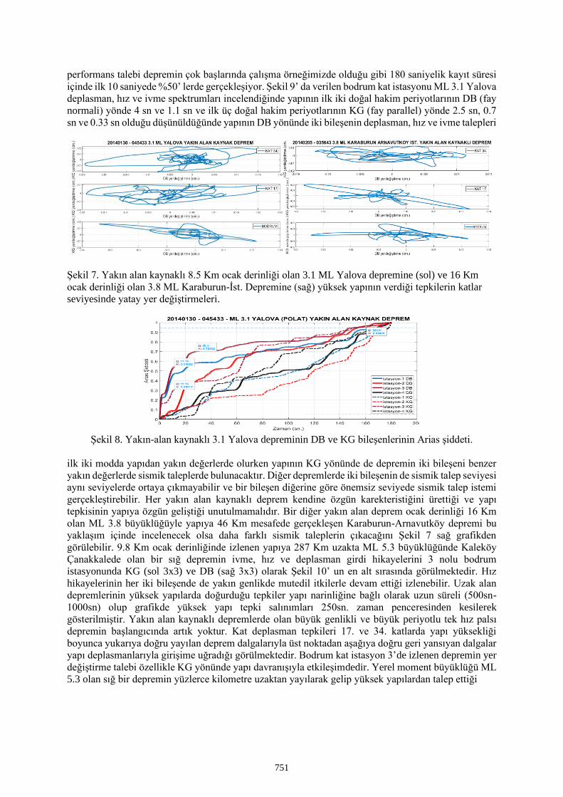
performans talebi depremin çok başlarında çalışma örneğimizde olduğu gibi 180 saniyelik kayıt süresi

içinde ilk 10 saniyede %50’ lerde gerçekleşiyor. Şekil 9’ da verilen bodrum kat istasyonu ML 3.1 Yalova

deplasman, hız ve ivme spektrumları incelendiğinde yapının ilk iki doğal hakim periyotlarının DB (fay

normali) yönde 4 sn ve 1.1 sn ve ilk üç doğal hakim periyotlarının KG (fay parallel) yönde 2.5 sn, 0.7

sn ve 0.33 sn olduğu düşünüldüğünde yapının DB yönünde iki bileşenin deplasman, hız ve ivme talepleri

Şekil 7. Yakın alan kaynaklı 8.5 Km ocak derinliği olan 3.1 ML Yalova depremine (sol) ve 16 Km

ocak derinliği olan 3.8 ML Karaburun-İst. Depremine (sağ) yüksek yapının verdiği tepkilerin katlar

seviyesinde yatay yer değiştirmeleri.

Şekil 8. Yakın-alan kaynaklı 3.1 Yalova depreminin DB ve KG bileşenlerinin Arias şiddeti.

ilk iki modda yapıdan yakın değerlerde olurken yapının KG yönünde de depremin iki bileşeni benzer

yakın değerlerde sismik taleplerde bulunacaktır. Diğer depremlerde iki bileşenin de sismik talep seviyesi

aynı seviyelerde ortaya çıkmayabilir ve bir bileşen diğerine göre önemsiz seviyede sismik talep istemi

gerçekleştirebilir. Her yakın alan kaynaklı deprem kendine özgün karekteristiğini ürettiği ve yapı

tepkisinin yapıya özgün geliştiği unutulmamalıdır. Bir diğer yakın alan deprem ocak derinliği 16 Km

olan ML 3.8 büyüklüğüyle yapıya 46 Km mesafede gerçekleşen Karaburun-Arnavutköy depremi bu

yaklaşım içinde incelenecek olsa daha farklı sismik taleplerin çıkacağını Şekil 7 sağ grafikden

görülebilir. 9.8 Km ocak derinliğinde izlenen yapıya 287 Km uzakta ML 5.3 büyüklüğünde Kaleköy

Çanakkalede olan bir sığ depremin ivme, hız ve deplasman girdi hikayelerini 3 nolu bodrum

istasyonunda KG (sol 3x3) ve DB (sağ 3x3) olarak Şekil 10’ un en alt sırasında görülmektedir. Hız

hikayelerinin her iki bileşende de yakın genlikde mutedil itkilerle devam ettiği izlenebilir. Uzak alan

depremlerinin yüksek yapılarda doğurduğu tepkiler yapı narinliğine bağlı olarak uzun süreli (500sn-

1000sn) olup grafikde yüksek yapı tepki salınımları 250sn. zaman penceresinden kesilerek

gösterilmiştir. Yakın alan kaynaklı depremlerde olan büyük genlikli ve büyük periyotlu tek hız palsı

depremin başlangıcında artık yoktur. Kat deplasman tepkileri 17. ve 34. katlarda yapı yüksekliği

boyunca yukarıya doğru yayılan deprem dalgalarıyla üst noktadan aşağıya doğru geri yansıyan dalgalar

yapı deplasmanlarıyla girişime uğradığı görülmektedir. Bodrum kat istasyon 3’de izlenen depremin yer

değiştirme talebi özellikle KG yönünde yapı davranışıyla etkileşimdedir. Yerel moment büyüklüğü ML

5.3 olan sığ bir depremin yüzlerce kilometre uzaktan yayılarak gelip yüksek yapılardan talep ettiği

751

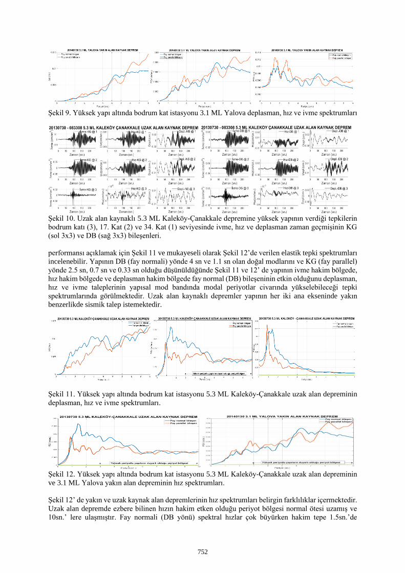
Şekil 9. Yüksek yapı altında bodrum kat istasyonu 3.1 ML Yalova deplasman, hız ve ivme spektrumları

Şekil 10. Uzak alan kaynaklı 5.3 ML Kaleköy-Çanakkale depremine yüksek yapının verdiği tepkilerin

bodrum katı (3), 17. Kat (2) ve 34. Kat (1) seviyesinde ivme, hız ve deplasman zaman geçmişinin KG

(sol 3x3) ve DB (sağ 3x3) bileşenleri.

performansı açıklamak için Şekil 11 ve mukayeseli olarak Şekil 12’de verilen elastik tepki spektrumları

incelenebilir. Yapının DB (fay normali) yönde 4 sn ve 1.1 sn olan doğal modlarını ve KG (fay parallel)

yönde 2.5 sn, 0.7 sn ve 0.33 sn olduğu düşünüldüğünde Şekil 11 ve 12’ de yapının ivme hakim bölgede,

hız hakim bölgede ve deplasman hakim bölgede fay normal (DB) bileşeninin etkin olduğunu deplasman,

hız ve ivme taleplerinin yapısal mod bandında modal periyotlar civarında yükselebileceği tepki

spektrumlarında görülmektedir. Uzak alan kaynaklı depremler yapının her iki ana ekseninde yakın

benzerlikde sismik talep istemektedir.

Şekil 11. Yüksek yapı altında bodrum kat istasyonu 5.3 ML Kaleköy-Çanakkale uzak alan depreminin

deplasman, hız ve ivme spektrumları.

Şekil 12. Yüksek yapı altında bodrum kat istasyonu 5.3 ML Kaleköy-Çanakkale uzak alan depreminin

ve 3.1 ML Yalova yakın alan depreminin hız spektrumları.

Şekil 12’ de yakın ve uzak kaynak alan depremlerinin hız spektrumları belirgin farklılıklar içermektedir.

Uzak alan depremde ezbere bilinen hızın hakim etken olduğu periyot bölgesi normal ötesi uzamış ve

10sn.’ lere ulaşmıştır. Fay normali (DB yönü) spektral hızlar çok büyürken hakim tepe 1.5sn.’de

752

oluşmuş ve göreceli olarak azalmış 6sn ve sonrası kararlı salınımlara girmiştir. Parallel bileşen 1sn.

civarında yarı genliğe yakın tepe vererek, sonrasında kararlı gittiği görülmektedir. Yapının hakim

modları uzak alan depremin her iki bileşeninin (normali parallelin 2 katı) etkisi altındadır. Yakın alan

kaynaklı deprem spektrumu büyüyen periyotla beraber birbirini yakın izleyerek artan hız talebini

göstermektedir. Parallel bileşen büyüyen periyot ile genelde grafiğin maksimumlarını oluşturacak

şekilde büyümektedir. Çalışma yapısının ilk iki periyodu DB yönünde 4sn ve 1.1sn ve KG yönünde ilk

üç doğal hakim periyotları 2.5sn, 0.7sn ve 0.33saniyedir. Yapı yüksekliklerinin yüzlerce metrelerden

kilometreye yükseldiği düşünüldüğünde, yapıdan istenen sismik talepler açısından ilk modlarda yakın

alan kaynaklı depremlerin gökdelenlerde artan periyotla beraber hız taleplerini ve deplasman taleplerini

yükseltiği uzak alan kaynaklı depremlerin ise kararlı salınımlarla yapı titreşimini saatlere ulaşacak

sürelere uzattığı Şekil 12’den anlaşılmaktadır.

6. Sonuçlar

Bu çalışmada; incelenen yakın alan kaynaklı depremlerde maksimum deplasman yönlerin dağılımı fay

normali ve fay dik yönler ile bir tutarlılık göstermeyen bir dağılım sergiliyor. İncelenen yapılar gibi

lineer elastik davranış sergileyen mühendislik yapılarında maksimum yerdeğiştirmeler hakim hız itki

frekanslarıyla yapı hakim frekanslarının yakın olduğu durumlarda izlenmiştir. Rezonans potansiyeline

yakın şartlarda (geometrik ve/veya kesit/kapasite aşımıyla) nonlinear davranışın periyotları büyüterek

senkronizasyonu bozması beklenir. Çalışmaya tipik örnekleri konulan iki yakın kaynaklı depremde

gözlenen maksimum yön değişimi incelenen yapıya mahsus özel bir maksimum yönün (örneğin zayıf

rijidlik yönü) mühendislik parametrelerini maksimuma ulaştıracağı kanaatini garantilememektedir.

Yapı yüksekliklerinin yüzlerce metrelerden kilometreye yükseldiği günümüz mühendislik dünyasında,

yapıdan istenen sismik talepler açısından ilk modlarda yakın alan kaynaklı depremlerin gökdelenlerde

artan periyotla beraber hız taleplerini ve deplasman taleplerini yükseltiği uzak alan kaynaklı depremlerin

ise kararlı salınımlarla yapı titreşim süresini uzattığı gerçek yüksek yapı kayıtlarından tespit edilmiştir.

7. Teşekkür

Çalışmada kulanılan yapı sağlığı izleme kayıtları Boğaziçi Üniversitesi, Kandilli Rasathanesi ve

Deprem Araştırma Enstitüsü, Deprem Mühendisliği Bölümü hocalarımız sayın Prof. Dr. Erdal Şafak ve

sayın Prof. Dr. Eser Çaktı tarafından verilmiştir. Müteşekkirim. Destekleri için teşekkür ediyorum.

Kaynaklar

Archila, M., Ventura, C. E. ve Finn, L. W.D. (2014) ‘New Insights on effects of directionality and duration of near

fault ground motions on seismic response of tall buildings’, Advances in Structural Design for Seismic

Regions. Los Angeles Tall Buildings Structural Design Council

Archila, Manuel (2014) ‘Directionality Effects of Pulse-Like Near Field Ground Motions on Seismic Response of

Tall Buildings’, Doktora Tezi, British Columbia Üniversitesi

Athanatopoulou, A.M. (2004) ‘Critical Orientation of Three Correlated Seismic Components’, Engineering

Structures, v.27, p. 301–312

Beyen, K. ve Tanırcan, G. (2015) ‘Strong Ground Motion Characteristics of The Van Earthquake of Turkey:

Implications of Seismological Aspects on Engineering Parameters’, Earthquakes and Structures, V:8, N:6

Beyen, K. (2019) ‘HangingWall and Footwall Effects in the Largest Reverse-Slip Earthquake of Turkey, October

23, 2011, MW 7.2 Van Earthquake’, Arabian Journal for Science and Engineering, 44:4757–4781;

https://doi.org/10.1007/s13369-018-3547-x

Beyen, K. (2017) ‘Deprem ve Çevrel Titreşimler Etkisinde Yüksek Binalarda İnsanın Algısı ve Komfor Kalitesinin

Değerlendirilmesi’, 4. Uluslararası Deprem Mühendisliği ve Sismoloji Konferansı (4. UDMSK), 11-13

Ekim, Anadolu Üniversitesi, Eskişehir

California Building Code, California Code of regulations, title 24, Part1 & 2, California Building Standards

Commission (CBSC)

753

https://doi.org/10.1007/s13369-018-3547-x

Champion, C., Liel, A. (2012) ‘The effect of Near‐Fault Directivity on Building Seismic Collapse Risk’,

Earthquake Engineering Structural Dynamics, 41(10):1391‐1409

Çelebi, M., Okawa, I., Kashima, T., Koyama, S. and Iiba, M. (2014) ‘Response of a Tall Building Far From the

Epicenter of the 11 March 2011 M 9.0 Great East Japan Earthquake and Aftershocks’, Structural Design

of Tall and Special Buildings, 23, 427-441

Heydari, M. ve Mousavi, M (2015) ‘The Comparison of Seismic Effects of Near-field and Far-field Earthquakes

on Relative Displacement of Seven-store Concrete Building with Shear Wall’, Current World

Environment, Vol. 10 (Special Issue 1.07), 40-46

MATLAB 2019a: The MathWorks Inc., Natick, MA (2019)

M. Davoodi, M. Sadjadi (2015) ‘Assessment of near-field and far-field strong ground motion effects on soil-

structure SDOF system’, International Journal of Civil Engineering, Vol. 13, Nos. 3&4B, Transaction B:

Geotechnical Engineering, September & December 2015

Reyes, Juan C. and Kalkan, E. (2012) ‘Should Ground Motion Records be Rotated to Fault-Normal/Parallel or

Maximum Direction for Response History Analysis of Buildings?’, Open-File report 2012, U.S.

Geological Survey, Reston, Virginia

Stewart J P, Chiou S J, Bray J D, et al. (2001) ‘Ground Motion Evaluation Procedures for Performance-Based

Design’, California: Pacific Earthquake Engineering Research Center, University of California, Berkeley,

Report No. 01-09, 63-67

Smyrou, Eleni (2014) ‘Near-Field Effects on Tall Structures’, Second European Conference on Earthquake

Engineering and Seismology, İstanbul, August 25-29

Somerville, P.G., Smith, N.F., Graves, R.W., Abrahamson, N.A. (1997) ‘Modification of Empirical Strong Ground

Motion Attenuation Relations to Include the Amplitude and Duration Effects of Rupture Directivity’,

Seismoligical Res. Lett., 68(1), 199‐222

Somerville, P.G. (2003) ‘Magnitude Scaling of the Near Fault Rupture Directivity Pulse’, Physics of the Earth and

Planetary Interiors, 137, 201-212

Türkiye Bina Deprem Yönetmeliği (2018) Afet ve Acil Durum Yönetimi Başkanlığı, Ankara.

Uniform Building Code (UBC) (1997) International Conference of Building Officials, 5360 Workman Mill

Roadwhittier, California, 90601-2298(800) 284-4406 S(562) 699-0541, 6th PrintingPublication, April

1997; ISSN 0896-9655.

754

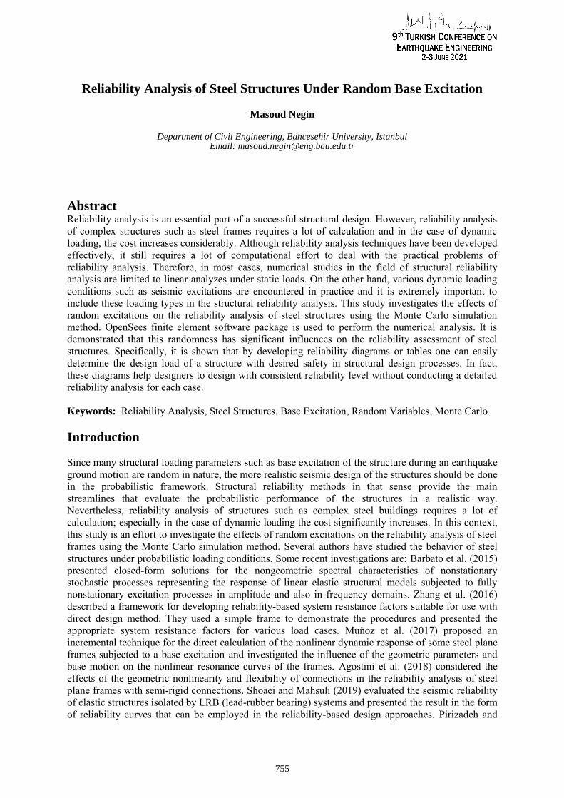
Reliability Analysis of Steel Structures Under Random Base Excitation

Masoud Negin

Department of Civil Engineering, Bahcesehir University, Istanbul Email: [email protected]

AbstractReliability analysis is an essential part of a successful structural design. However, reliability analysis of complex structures such as steel frames requires a lot of calculation and in the case of dynamic loading, the cost increases considerably. Although reliability analysis techniques have been developed effectively, it still requires a lot of computational effort to deal with the practical problems of reliability analysis. Therefore, in most cases, numerical studies in the field of structural reliability analysis are limited to linear analyzes under static loads. On the other hand, various dynamic loading conditions such as seismic excitations are encountered in practice and it is extremely important to include these loading types in the structural reliability analysis. This study investigates the effects of random excitations on the reliability analysis of steel structures using the Monte Carlo simulation method. OpenSees finite element software package is used to perform the numerical analysis. It is demonstrated that this randomness has significant influences on the reliability assessment of steel structures. Specifically, it is shown that by developing reliability diagrams or tables one can easily determine the design load of a structure with desired safety in structural design processes. In fact, these diagrams help designers to design with consistent reliability level without conducting a detailed reliability analysis for each case.

Keywords: Reliability Analysis, Steel Structures, Base Excitation, Random Variables, Monte Carlo.

Introduction

Since many structural loading parameters such as base excitation of the structure during an earthquake ground motion are random in nature, the more realistic seismic design of the structures should be done in the probabilistic framework. Structural reliability methods in that sense provide the main streamlines that evaluate the probabilistic performance of the structures in a realistic way. Nevertheless, reliability analysis of structures such as complex steel buildings requires a lot of calculation; especially in the case of dynamic loading the cost significantly increases. In this context, this study is an effort to investigate the effects of random excitations on the reliability analysis of steel frames using the Monte Carlo simulation method. Several authors have studied the behavior of steel structures under probabilistic loading conditions. Some recent investigations are; Barbato et al. (2015) presented closed-form solutions for the nongeometric spectral characteristics of nonstationary stochastic processes representing the response of linear elastic structural models subjected to fully nonstationary excitation processes in amplitude and also in frequency domains. Zhang et al. (2016) described a framework for developing reliability-based system resistance factors suitable for use with direct design method. They used a simple frame to demonstrate the procedures and presented the appropriate system resistance factors for various load cases. Muñoz et al. (2017) proposed an incremental technique for the direct calculation of the nonlinear dynamic response of some steel plane frames subjected to a base excitation and investigated the influence of the geometric parameters and base motion on the nonlinear resonance curves of the frames. Agostini et al. (2018) considered the effects of the geometric nonlinearity and flexibility of connections in the reliability analysis of steel plane frames with semi-rigid connections. Shoaei and Mahsuli (2019) evaluated the seismic reliability of elastic structures isolated by LRB (lead-rubber bearing) systems and presented the result in the form of reliability curves that can be employed in the reliability-based design approaches. Pirizadeh and

755

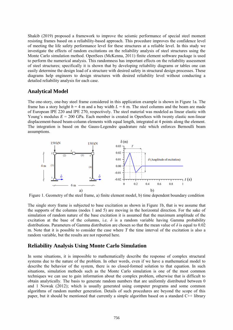
Shakib (2019) proposed a framework to improve the seismic performance of special steel moment resisting frames based on a reliability-based approach. This procedure improves the confidence level of meeting the life safety performance level for these structures at a reliable level. In this study we investigate the effects of random excitations on the reliability analysis of steel structures using the Monte Carlo simulation method. OpenSees (McKenna, 2011) finite element software package is used to perform the numerical analysis. This randomness has important effects on the reliability assessment of steel structures; specifically it is shown that by developing reliability diagrams or tables one can easily determine the design load of a structure with desired safety in structural design processes. These diagrams help engineers to design structures with desired reliability level without conducting a detailed reliability analysis for each case.

Analytical Model

The one-story, one-bay steel frame considered in this application example is shown in Figure 1a. The frame has a story height h = 4 m and a bay width L = 6 m. The steel columns and the beam are made of European IPE 220 and IPE 270, respectively. The steel material was modeled as linear elastic with Young’s modulus E = 200 GPa. Each member is created in OpenSees with twenty elastic non-linear displacement-based beam-column elements with equal length, integrated at 4 points along the element. The integration is based on the Gauss-Legendre quadrature rule which enforces Bernoulli beam assumptions.

a) b) Figure 1. Geometry of the steel frame, a) finite element model, b) time dependent boundary condition

The single story frame is subjected to base excitation as shown in Figure 1b, that is we assume that the supports of the columns (nodes 1 and 5) are moving in the horizontal direction. For the sake of simulation of random nature of the base excitation it is assumed that the maximum amplitude of the excitation at the base of the columns, i.e. δ is a random variable having Gamma probability distributions. Parameters of Gamma distribution are chosen so that the mean value of δ is equal to 0.02 m. Note that it is possible to consider the case where T the time interval of the excitation is also arandom variable, but the results are not reported here.

Reliability Analysis Using Monte Carlo Simulation

In some situations, it is impossible to mathematically describe the response of complex structural systems due to the nature of the problem. In other words, even if we have a mathematical model to describe the behavior of the system, there is no closed-formed solution to that equation. In such situations, simulation methods such as the Monte Carlo simulation is one of the most common techniques we can use to gain information about the complex problem, otherwise that is difficult to obtain analytically. The basis to generate random numbers that are uniformly distributed between 0 and 1 Nowak (2012); which is usually generated using computer programs and some common algorithms of random number generation. Details of such procedures are beyond the scope of this paper, but it should be mentioned that currently a simple algorithm based on a standard C++ library

756

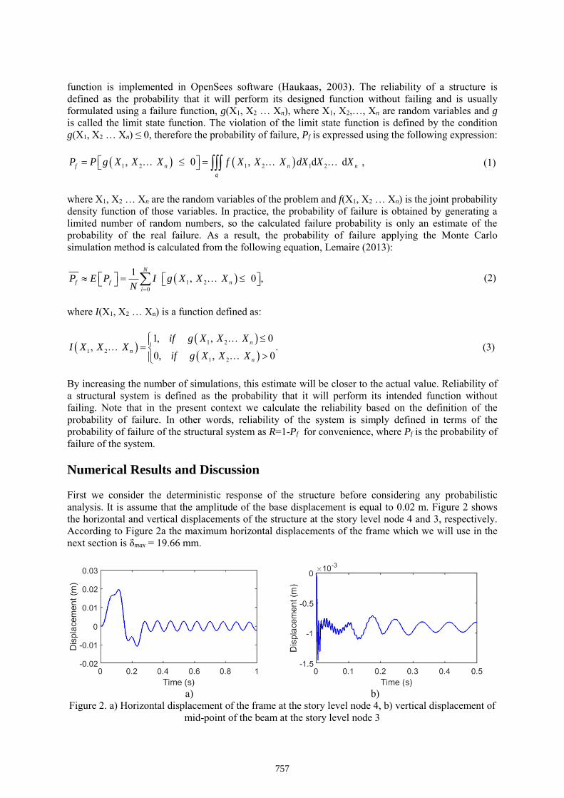
function is implemented in OpenSees software (Haukaas, 2003). The reliability of a structure is defined as the probability that it will perform its designed function without failing and is usually formulated using a failure function, g(X1, X2 … Xn), where X1, X2,…, Xn are random variables and g is called the limit state function. The violation of the limit state function is defined by the condition g(X1, X2 … Xn) ≤ 0, therefore the probability of failure, Pf is expressed using the following expression:

1 2 1 2 1 2, 0 , d d ,f n n n

g

P P g X X X f X X X X X Xd (1)

where X1, X2 … Xn are the random variables of the problem and f(X1, X2 … Xn) is the joint probability density function of those variables. In practice, the probability of failure is obtained by generating a limited number of random numbers, so the calculated failure probability is only an estimate of the probability of the real failure. As a result, the probability of failure applying the Monte Carlo simulation method is calculated from the following equation, Lemaire (2013):

1 20

1 , 0 ,N

f f n

i

P E P I g X X XN

(2)

where I(X1, X2 … Xn) is a function defined as:

1 21 2

1 2

1, , 0, .

0, , 0n

n

n

if g X X XI X X X

if g X X X

(3)

By increasing the number of simulations, this estimate will be closer to the actual value. Reliability of a structural system is defined as the probability that it will perform its intended function without failing. Note that in the present context we calculate the reliability based on the definition of the probability of failure. In other words, reliability of the system is simply defined in terms of the probability of failure of the structural system as R=1-Pf for convenience, where Pf is the probability of failure of the system. Numerical Results and Discussion First we consider the deterministic response of the structure before considering any probabilistic analysis. It is assume that the amplitude of the base displacement is equal to 0.02 m. Figure 2 shows the horizontal and vertical displacements of the structure at the story level node 4 and 3, respectively. According to Figure 2a the maximum horizontal displacements of the frame which we will use in the next section is δmax = 19.66 mm.

a) b)

Figure 2. a) Horizontal displacement of the frame at the story level node 4, b) vertical displacement of mid-point of the beam at the story level node 3

757

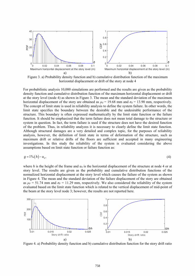
a) b) Figure 3. a) Probability density function and b) cumulative distribution function of the maximum

horizontal displacement or drift of the story at node 4

For probabilistic analysis 10,000 simulations are performed and the results are given as the probability density function and cumulative distribution function of the maximum horizontal displacement or drift at the story level (node 4) as shown in Figure 3. The mean and the standard deviation of the maximum horizontal displacement of the story are obtained as μd = 19.68 mm and σd = 13.90 mm, respectively. The concept of limit state is used in reliability analysis to define the system failure. In other words, the limit state specifies the boundary between the desirable and the undesirable performance of the structure. This boundary is often expressed mathematically by the limit state function or the failure function. It should be emphasized that the term failure does not mean total damage to the structure or system in question. In fact, the term failure is used if the structure does not have the desired function of the problem. Thus, in reliability analyzes it is necessary to clearly define the limit state function. Although structural damages are a very detailed and complex topic, for the purposes of reliability analysis, however, the definition of limit state in terms of deformation of the structure, such as maximum drift or relative drifts of the floors are sufficient and accepted in many engineering investigations. In this study the reliability of the system is evaluated considering the above assumptions based on limit state function or failure function as:

41% ,g h u (4)

where h is the height of the frame and u4 is the horizontal displacement of the structure at node 4 or at story level. The results are given as the probability and cumulative distribution functions of the normalized horizontal displacement at the story level which causes the failure of the system as shown in Figure 4. The mean and the standard deviation of the failure displacement of the story are obtained as μF = 51.74 mm and σF = 11.29 mm, respectively. We also considered the reliability of the system evaluated based on the limit state function which is related to the vertical displacement of mid-point of the beam at the story level node 3; however, the results are not reported here.

a) b) Figure 4. a) Probability density function and b) cumulative distribution function for the story drift ratio

758

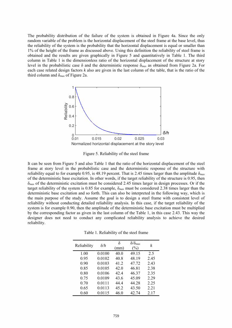
The probability distribution of the failure of the system is obtained in Figure 4a. Since the only random variable of the problem is the horizontal displacement of the steel frame at the base level, thus the reliability of the system is the probability that the horizontal displacement is equal or smaller than 1% of the height of the frame as discussed above. Using this definition the reliability of steel frame is obtained and the results are given graphically in Figure 5 and quantitatively in Table 1. The third column in Table 1 is the dimensionless ratio of the horizontal displacement of the structure at story level in the probabilistic case δ and the deterministic response δmax as obtained from Figure 2a. For each case related design factors k also are given in the last column of the table, that is the ratio of the third column and δmax of Figure 2a.

Figure 5. Reliability of the steel frame It can be seen from Figure 5 and also Table 1 that the ratio of the horizontal displacement of the steel frame at story level in the probabilistic case and the deterministic response of the structure with reliability equal to for example 0.95, is 48.19 percent. That is 2.45 times larger than the amplitude δmax of the deterministic base excitation. In other words, if the target reliability of the structure is 0.95, then δmax of the deterministic excitation must be considered 2.45 times larger in design processes. Or if the target reliability of the system is 0.85 for example, δmax must be considered 2.38 times larger than the deterministic base excitation and so forth. This can also be interpreted in the following way, which is the main purpose of the study. Assume the goal is to design a steel frame with consistent level of reliability without conducting detailed reliability analysis. In this case, if the target reliability of the system is for example 0.90, then the amplitude of the deterministic base excitation must be multiplied by the corresponding factor as given in the last column of the Table 1, in this case 2.43. This way the designer does not need to conduct any complicated reliability analysis to achieve the desired reliability.

Table 1. Reliability of the steel frame

Reliability δ/h δ (mm)

δ/δmax (%) k

1.00 0.0100 40.0 49.15 2.5 0.95 0.0102 40.8 48.19 2.45 0.90 0.0103 41.2 47.72 2.43 0.85 0.0105 42.0 46.81 2.38 0.80 0.0106 42.4 46.37 2.35 0.75 0.0109 43.6 45.09 2.29 0.70 0.0111 44.4 44.28 2.25 0.65 0.0113 45.2 43.50 2.21 0.60 0.0115 46.0 42.74 2.17

759

Conclusion

Reliability analysis of complex structures such as steel frames requires a lot of calculations. Especially in the case of dynamic loadings it will be time consuming and computationally expensive. That is why in most studies structural reliability analyzes are limited to linear static cases. On the other hand, it is extremely important to consider seismic excitations which are random in nature in structural reliability analysis. This study investigates the effects of special types of random excitations on the reliability analysis of steel structures using the Monte Carlo simulation method. It is shown that by developing reliability diagrams or tables as demonstrated here (Figure 5 or Table 1) one can easily design structures with desired safety or reliability levels. In fact, preparing diagrams like these will help designers to design structures with consistent reliability levels without conducting any detailed reliability analysis for each case.

References

Agostini, B.M., Freitas, M.S.D.R., Silveira, R.A.D.M. and Silva, A.R.D.D. (2018) “Structural reliability analysis of steel plane frames with semi-rigid connections” REM-International Engineering

Journal, 71(3), pp.333-339. Barbato, M. and Conte, J.P., (2015). “Time-variant reliability analysis of linear elastic systems subjected to

fully nonstationary stochastic excitations”, Journal of Engineering Mechanics, 141(6), p.040141731-10.

Haukaas, T. (2003) Finite element reliability and sensitivity methods for performance-based engineering, Ph.D. Thesis, University of California, Berkeley.

Lemaire, M. (2013) Structural reliability. John Wiley & Sons. McKenna, F. (2011) “OpenSees: a framework for earthquake engineering simulation” Computing in

Science & Engineering, 13(4), 58-66. Muñoz, P., Fernando, L., Gonçalves, P.B., Silveira, R.A. and Silva, A., (2017) “Nonlinear Resonance

Analysis of Slender Portal Frames under Base Excitation”, Shock and Vibration. Nowak, Andrzej S., and Kevin R. Collins (2012) Reliability of structures, CRC Press. Pirizadeh, M. and Shakib, H., (2019) “On a reliability-based method to improve the seismic performance of

midrise steel moment resisting frame setback buildings” International Journal of Steel Structures, 19(1), pp.58-70.

Shoaei, P. and Mahsuli, M., (2019) “Reliability-based design of steel moment frame structures isolated by lead-rubber bearing systems”, In Structures, Vol. 20, pp. 765-778.

Zhang, H., Shayan, S., Rasmussen, K.J. and Ellingwood, B.R. (2016) “System-based design of planar steel frames, I: Reliability framework” Journal of constructional steel research, 123, pp.135-143.

760

A Novel Approach for Post-Earthquake Collapse Risk Assessment of

Damaged RC Buildings Subjected to Aftershock Hazard

Ziya Muderrisoglu1, Ufuk Yazgan2*

1Asst. Prof. Dr., Department of Civil Engineering, Beykent University 2Assoc. Prof. Dr., Earthquake Engineering and Disaster Management Institute, Istanbul Technical University


AbstractPost-earthquake collapse risk assessment of damaged structures is crucial in recovery processes. Rapid

evaluation of post-earthquake risks strongly affects the crisis management and meeting the needs of

disaster victims. Accordingly, identification of the safety level of a damaged structure becomes a major

challenge. Several post-earthquake safety assessment methodologies have been proposed in the past.

Increase in the vulnerability due to cumulative damages caused by mainshock-aftershock sequences and

systematic calibrations based on engineering analyses have not been taken into account explicitly in

these approaches. Thus, the accuracy of safety based decisions is still an issue of concern. Based on this

premise, a novel post-earthquake safety assessment approach that takes into account the collapse

probability estimated by combining post-mainshock fragility and aftershock hazard, is proposed in this

proceeding.

Collapse fragility characteristics of a structure and the seismic hazard at a site form the basis of

collapse probability of a structure. In this proceeding, these fundamental properties are utilized to

develop a practical assessment methodology. For this purpose, nonlinear time history analyses are

performed to estimate the fragility characteristics of structures subjected to a set of mainshock-

aftershock ground motion pairs. In order to obtained improved collapse capacity evaluations, major

sources of uncertainties (i.e. material uncertainty, record-to-record variability) are considered.

Aftershock hazard is explicitly considered by using the observable indicators (instrumental or

macroseismic) related to the mainshock demand at the site. Specifically, a novel aftershock hazard

assessment approach that has been proposed by the authors is utilized to provide a consistent risk

evaluation methodology. This approach enables the engineers to make use of the mainshock ground

motion indicators observed at the site in the assessment of aftershock hazard.

A numerical example is performed for a set of damaged structures to illustrate the framework

of the proposed assessment approach. Sensitivity of resulting risk evaluations are investigated by using

a set of critical parameters related to structural and site properties. Results of sensitivity analyses are

considered to discuss and evaluate the limitations and effectiveness of the proposed methodology.

Results presented in this proceeding are expected to provide estimates of collapse probabilities for the

reinforced concrete structures having different levels of damage.

Keywords: post-earthquake collapse risk assessment, aftershock hazard assessment, collapse fragility,

uncertainties.

761

Introduction

Assessing the collapse probability of a damaged building following a strong earthquake is crucial in

successful management of the recovery process and in achieving seismic resilience. Accurate

quantification of the post-earthquake risk of damaged buildings give opportunity to make reliable

decisions related to safety of the investigated buildings. However, this assessment becomes more

complicated due to uncertainties related to the collapse probability of damaged buildings at the site

subjected to potential aftershock excitations.

Considerable efforts have been undertaken for developing reliable post-earthquake safety assessment

methods for damaged buildings.

The majority of existing guidelines are based on post-earthquake field inspections. One of the

most widely-known post-earthquake safety guidelines, ATC-20 (ATC-20; ATC-20-2) aims at

categorization of the damage (i.e. green tag-safe to occupy, yellow tag-restricted to use/limited for post-

earthquake use, red tag-unsafe to occupy). The tagging decision is extensively based on the visual

inspection by the experts. The post-earthquake safety assessment and rapid evaluation sheet, AeDES

was proposed by Baggio et al. (2007) for the assessment of damaged buildings within European Union.

The damaged buildings are qualitatively evaluated based on the potential collapse probability of

investigated building by taking into account the critical indicators (i.e. damage level in structural/non-

structural members, adjacent building conditions). Furthermore, evaluation procedures (Taskin et al.,

2012; Nakano et al., 2004) have been developed for the post-earthquake safety evaluation of damaged

buildings in accordance with the specific requirements and conditions of different countries and regions.

A comprehensive methodology based on the quantification post-earthquake performance of a

damaged building subjected to an aftershock hazard exhibited at a site was proposed by Yeo and Cornell

(2005). Aftershock tagging criteria based on discretizing the damage states by taking into account the

life-safety risks in aftershock environment was explicitly utilized. Raghunandan et al. (2015) developed

a probabilistic methodology to evaluate the aftershock collapse vulnerability of reinforced concrete

frame type structures. Physical damage indicators (i.e. plastic hinging occurrences, roof drifts, structural

member deformations) were considered to identify the damage limit states of buildings subjected to

mainshock-aftershock sequences. A fragility-based framework based on investigating the effects of

damage accumulation on the aftershock vulnerability was developed by Jeon et al. (2015). Visual

observations were considered to define the damage limit states. Burton and Deierlein (2018) proposed

a methodology to assess the post-earthquake safety of structures by integrating the visual component

damage simulation, virtual inspection and the collapse performance of investigated structure. Several

threshold damage state ratios were proposed to model the increment in collapse vulnerability level of a

building. Jalayer and Ebrahimian (2017) proposed a procedure to determine the exceedance probability

of a specific limit state by taking into consideration the time-dependent mainshock-aftershock risk and

the cumulative damages (i.e. referred as best-estimate procedure). Cloud analyses methodology was

identified to be more sensitive in record selection phase. Moreover, a recent study including the

discussions and suggestions on the current trends in fragility and vulnerability analyses was published

by Silva et al. (2019). A comprehensive set of recommendations were detailed by taking into account

the valuable opinions of experts on fragility and vulnerability topics.

In this proceeding, a post-earthquake assessment methodology that explicitly takes into account

the collapse probability of buildings is proposed. Two main factors are considered to estimate the

collapse probability characteristics of the buildings such as: (1) aftershock collapse probability of a

mainshock-aftershock sequence induced building, and (2) aftershock hazard exhibited at the site.

Nonlinear time history analyses are performed for simulating the responses of buildings subjected to

mainshock-aftershock sequences. Major uncertainty sources (e.g. material, system, model, and record-

to-record variability) are taken into account in the estimation of aftershock collapse fragility. An

aftershock hazard assessment approach (Muderrisoglu and Yazgan, 2018) that takes into account the

mainshock ground motion intensity indicators observed at the site, is utilized. A numerical example is

performed for a set of low-rise reinforced concrete frame type buildings that are assumed to be located

in Turkey and subjected to a scenario mainshock. Moreover, sensitivity analyses are performed to

investigate the effects of critical parameters (i.e. mainshock intensity level, site properties) on the results.

762

Methodology

The proposed approach is based on the collapse probability of buildings subjected to mainshock-

aftershock sequences. This is achieved by taking into account two fundamental components: (1) the

collapse probability of damaged building subjected to aftershocks, (2) the aftershock hazard exhibited

at the site. The collapse probability of a building with a damage level, RDM=d, subjected to an

aftershock hazard, ( )as is evaluated as follows:

0

( )( | ) ( | , ). a

a a

d sP C RDM d P C RDM d S s ds

ds

(1)

where RDM is the ratio of mainshock induced damaged members and ( )as is the mean annual rate of

exceedance of the aftershock ground motion intensity, sa. Here, the terms P(C|RDM=d,Sa=sa) and

( ) /ad s ds represent the aftershock fragility curve of a building with a damage level of RDM=d and

the aftershock hazard exhibited at the site, respectively.

The collapse probability-based approach enables to take into account both the accumulated

damages induced by successive excitations and the possible aftershock hazard that may exhibit at the

site. In this proceeding, RDM levels that are assumed as the initial conditions for aftershock sequences

are evaluated by using the damages recorded after each mainshock event. Aftershock collapse capacity

of a building is evaluated via fragility analyses. Major uncertainties (e.g. material, system, model, and

record-to-record variability) are explicitly taken into account in fragility analyses. Furthermore, the

aftershock hazard exhibited at the site is assessed based on the mainshock demand indicators. A general

overview of the proposed safety evaluation approach is presented in Figure 1.

Figure 1. A general overview of the proposed collapse probability-based safety evaluation approach

Case 1: Aftershock Hazard Assessment

Higher levels of aftershock hazard significantly affects the vulnerability of damaged structures subjected

to consecutive aftershock sequences. Nonetheless, the assessment process becomes more complex

depending on the variety of uncertainty conditions. In this paper, this is achieved by using the recently

proposed aftershock hazard assessment framework (Muderrisoglu and Yazgan, 2018). The proposed

approach is based on reducing the uncertainties related to estimated aftershock hazard by utilizing the

level of correlation between mainshock and aftershock ground motion intensities.. Accordingly, the

mean number, of aftershock ground motion intensity Y exceeding a given threshold level y at the site

is evaluated for a duration of T days that starts t days after the mainshock as follows:

* * *

| |( , , ; , , ) ( , ; ) ( | ) ( ; ) 1 ( | , , )m

a

l

m

m m m R M M m E I m m

R m

y t T m i r t T m f r m f m m F i m r dmdr (2)

Here, mm denotes the mainshock magnitude, i* is the observed mainshock intensity, MMI (i.e. the

Modified Mercalli Intensity level) at the site, rm is the distance between the mainshock rupture plane and

Identify

Collapse

Fragility

Characteristics

Identify Hazard

Characteristics

Aftershock Hazard

Curve

(Eq. 2)

Evaluate

Ratio of

Damaged

Members,

RDM (Eq. 3)

RDM-based Aftershock

Collapse

Fragility Curves (Eq. 4)Evaluate

Collapse

Probability

(Eq. 1)

763

the site. Moreover, FEa|I(.) in Eq. 2 represents the conditional probability distribution of aftershock

epsilon, Ea given the observed mainshock macroseismic intensity. The conditional mean, μEa|I and the

standard deviation, σEa|I of aftershock epsilon, Ea are evaluated as | , . 'a a mE I E E E and

2 2

| , ,( . ' ) (1 )a a m a mE I E E E E E , respectively. Here, ρEa,Em is the correlation between the mainshock

and aftershock epsilons, 'E and 'E are the expected value and the standard deviation of the standard

deviation of the mainshock epsilon given the observed mainshock intensity, respectively. Details of the

proposed approach are provided by Muderrisoglu and Yazgan, 2018.

Case 2: Aftershock Collapse Fragility Analysis

Estimation of the collapse capacity of a mainshock damaged building is a challenging issue in

earthquake engineering. Typically, it is estimated by taking into account the quantitative and/or

qualitative parameters and observations. The qualitative parameters mainly depend on the visual damage

indicators (e.g. cracks). Additionally, measurable parameters (e.g. modal properties and residual

deformations) are utilized as quantitative indicators. In this proceeding, the severity of damage is

quantified in terms of the ratio of damaged members, RDM that is defined as follows:

1 2

1 2

.

.T T

n a nRDM

n a n

(3)

where n1 and n2 represent the numbers of moderately and heavily damaged beams and columns observed

in the most-damaged story, nT1 and nT2 are the total numbers of beams and columns in related story.

Here, the parameter a reflects the participation of beams’ damage severity to the RDM (i.e., considered

as 0.7 for this study). The unitless RDM parameter varies between 0 and 1 and explicitly depends on the

damage level of structural members subjected to successive ground motion excitations. The collapse

fragility curve of a mainshock damaged building that is subjected to an aftershock with a spectral

acceleration of sa is identified for the given mainshock damage level, RDM as follows:

ln ( )( | , )

( )

aa a

s dP C RDM d S s

d

(4)

Fundamental difference between the collapse fragility analyses of damaged and undamaged buildings

is based on taking into account the impact of mainshock damage on the increasing level of vulnerability.

Each building model is subjected to a set of consecutive earthquake excitations in aftershock collapse

fragility analyses. Here, the first motion reflects the effects of mainshock that causes a damage severity

with RDM=d. Moreover, the second excitation represents the aftershock event. The collapse capacity of

a building is evaluated via Incremental Dynamic Analysis-IDA (Vamvatsikos and Cornell, 2002) by

increasing the intensity of aftershock excitation until the system reaches its collapse capacity.

Numerical Application

Scenario event and the site properties

This section includes an example application to illustrate the proposed post-earthquake safety evaluation

approach. Two different reference models (i.e. one-story and three-story frame type models) are taken

into consideration. These models are assumed to be located in Istanbul, Turkey. Researchers indicate a

slip deficit accumulation in Princes’ Island Fault (PIF) Segment of the North Anatolian Fault (e.g.

Ergintav et al., 2014). An event with the moment magnitude of Mw>7.1 is expected to be generated by

the PIF segment. A possible rupture (represented as a dashed line in Figure 2a) along this segment is

considered as a scenario event for this application. Furthermore, the moment magnitude of assumed

764

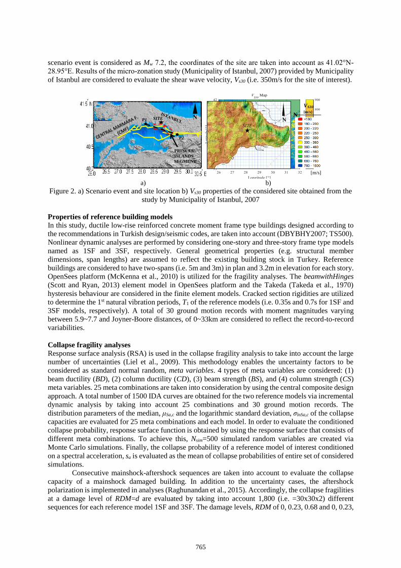
scenario event is considered as Mw 7.2, the coordinates of the site are taken into account as 41.02°N-

28.95°E. Results of the micro-zonation study (Municipality of Istanbul, 2007) provided by Municipality

of Istanbul are considered to evaluate the shear wave velocity, Vs30 (i.e. 350m/s for the site of interest).

a) b)

Figure 2. a) Scenario event and site location b) Vs30 properties of the considered site obtained from the

study by Municipality of Istanbul, 2007

Properties of reference building models

In this study, ductile low-rise reinforced concrete moment frame type buildings designed according to

the recommendations in Turkish design/seismic codes, are taken into account (DBYBHY2007; TS500).

Nonlinear dynamic analyses are performed by considering one-story and three-story frame type models

named as 1SF and 3SF, respectively. General geometrical properties (e.g. structural member

dimensions, span lengths) are assumed to reflect the existing building stock in Turkey. Reference

buildings are considered to have two-spans (i.e. 5m and 3m) in plan and 3.2m in elevation for each story.

OpenSees platform (McKenna et al., 2010) is utilized for the fragility analyses. The beamwithHinges

(Scott and Ryan, 2013) element model in OpenSees platform and the Takeda (Takeda et al., 1970)

hysteresis behaviour are considered in the finite element models. Cracked section rigidities are utilized

to determine the 1st natural vibration periods, T1 of the reference models (i.e. 0.35s and 0.7s for 1SF and

3SF models, respectively). A total of 30 ground motion records with moment magnitudes varying

between 5.9~7.7 and Joyner-Boore distances, of 0~33km are considered to reflect the record-to-record

variabilities.

Collapse fragility analyses

Response surface analysis (RSA) is used in the collapse fragility analysis to take into account the large

number of uncertainties (Liel et al., 2009). This methodology enables the uncertainty factors to be

considered as standard normal random, meta variables. 4 types of meta variables are considered: (1)

beam ductility (BD), (2) column ductility (CD), (3) beam strength (BS), and (4) column strength (CS)

meta variables. 25 meta combinations are taken into consideration by using the central composite design

approach. A total number of 1500 IDA curves are obtained for the two reference models via incremental

dynamic analysis by taking into account 25 combinations and 30 ground motion records. The

distribution parameters of the median, μSa,c and the logarithmic standard deviation, σlnSa,c of the collapse

capacities are evaluated for 25 meta combinations and each model. In order to evaluate the conditioned

collapse probability, response surface function is obtained by using the response surface that consists of

different meta combinations. To achieve this, Nsim=500 simulated random variables are created via

Monte Carlo simulations. Finally, the collapse probability of a reference model of interest conditioned

on a spectral acceleration, sa is evaluated as the mean of collapse probabilities of entire set of considered

simulations.

Consecutive mainshock-aftershock sequences are taken into account to evaluate the collapse

capacity of a mainshock damaged building. In addition to the uncertainty cases, the aftershock

polarization is implemented in analyses (Raghunandan et al., 2015). Accordingly, the collapse fragilities

at a damage level of RDM=d are evaluated by taking into account 1,800 (i.e. =30x30x2) different

sequences for each reference model 1SF and 3SF. The damage levels, RDM of 0, 0.23, 0.68 and 0, 0.23,

PRINCES’

ISLANDS

SEGMENT

SITEP1

P2

N N

[m/s]

(a) (b)

SITE

VS30

[m/s]

(b)

N

765

0.84 are considered for 1SF and 3SF reference models, respectively. Finally, 180,000 IDA analyses are

performed to evaluate the collapse capacity of damaged reference models. Parallel processing

capabilities of the computer cluster in Istanbul Technical University-National Center for High

Performance Computing (UHEM) is utilized to reduce the time and computational effort.

Results

Numerical analyses are performed to evaluate the collapse probability of the reference buildings. A time

interval of T=1year starting t=7days after the mainshock is considered in analyses. The collapse fragility

curves of the reference buildings are evaluated for the selected RDM values (Figure 3). Results show

that the median collapse capacities of each building decreases as the damage level, RDM increases. This

case is mainly based on the increment in aftershock collapse fragility of a building related to the

increasing mainshock damage levels.

a) b)

Figure 3. Aftershock collapse fragility curves a) 1SF b) 3SF

The aftershock hazard curves estimated using the proposed (Muderrisoglu and Yazgan, 2018) and the

conventional approach (i.e. represented as dotted line) are presented in Figure 4a. Results indicated that,

the aftershock hazard estimated at the site increases with increasing values of mainshock intensities,

MMI. The collapse probabilities of reference buildings are evaluated by taking into account different

levels of mainshock intensities and the damage levels (Figure 4b). It is observed that, the collapse

probability evaluated for 3SF reference model with a damage level, RDM=0.84 and mainshock intensity

IX is considerably higher (i.e. 7.6%) compared to that probability obtained for 1SF model. The collapse

probability is observed to be reduced to 0.6% as the intensity, MMI decreases to IV. This can be

attributed to the fact that the change in predicted aftershock hazard is significantly affected by the MMI

observations exhibited at the site. Moreover, the collapse probability of the reference building is

estimated as 1.8 times greater in case of RDM=0.84 damage level is considered compared to undamaged

condition (i.e. RDM=0)

a) b)

Figure 4. a) The aftershock hazard curves for different MMI values b) collapse probabilities

µEa|I=0.24; σEa|I=0.98

µEa|I=0.07; σEa|I=0.98

µEa|I=-0.10; σEa|I=0.98

µEa|I=-0.28; σEa|I=0.98

µEa|I=-0.45; σEa|I=0.98

µEa|I=-0.62; σEa|I=0.98

µEa=0.; σEa=1

1SF Model 3SF Model

766

Conclusions

This proceeding presents a post-earthquake safety assessment framework that is based on the aftershock

induced collapse probability of mainshock damaged buildings. Following conclusions are drawn based

on the evaluations:

The proposed framework enables the aftershock hazard to be assessed by taking into account

the mainshock intensity observed at the site. Furthermore, the level of uncertainty in aftershock

hazard is significantly reduced by implementing the correlation between mainshock and

aftershock shaking levels exhibited at the site.

The proposed methodology is applied to evaluate the collapse probabilities of a set of reference

buildings. Results indicate that, the collapse probabilities increase with increasing levels of

mainshock intensities exhibited at the site. This can be attributed to the fact that, higher

aftershock hazard levels are estimated for higher levels of mainshock macroseismic intensities.

Results show that, the three-story reference model is estimated to have higher rate of aftershock

collapse than one-story reference model. This case is mainly based on the aftershock hazard

exhibited at the site.

The collapse probabilities of the reference building are found to increase with the increasing

level of structural damage due to mainshock, as expected.

Finally, it should be stated that these results are specifically related to the considered type of reference

buildings (i.e. low-rise reinforced concrete frame type building models) and the aftershock hazard

parameters calibrated for the considered site. Site and building-type based analyses should be performed

for further investigations.

Acknowledgments

This study was supported and funded by the Scientific and Technological Research Council of Turkey

(TUBITAK) for the project Risk of Collapse Based Rating of Damaged Low Rise Reinforced Concrete

Frame Buildings Subjected to Aftershock Hazard with the project number 213M454. Moreover, the

support by the Istanbul Technical University- National Center for High Performance Computing

(UHEM) is acknowledged.

References

ATC, ATC-20-2 (1995) Addendum to ATC-20, Procedures for postearthquake safety evaluation of buildings,

Applied Technology Council, Redwood City, California

Baggio C, Bernardini A, Colozza R, Corazza L, Della Bella M, Di Pasquale G, Dolce M, Goretti A, Martinelli

A, Orsini G, Papa F and Zuccaro G (2007) Field Manual for Post-Earthquake Damage and Safety

Assessment and Short Term Countermeasures (AeDES), EUR 22868 EN-2007, Joint Research

Center Ispra, Italy

Burton HV and Deierlein GG (2018) “Integrating visual damage simulation, virtual inspection, and collapse

capacity to evaluate post-earthquake structural safety of buildings,” Earthq. Engng. Struct. Dyn.,

47:294-310

Ergintav S, Reilinger R, Cakmak R et al. (2014) “Istanbul’s earthquake hot spots: geodetic constraints on

strain accumulation along faults in the Marmara seismic gap ,” Geophysical Research Letters,

41(16):5783-5788

Jalayer F and Ebrahimian H (2017) “Seismic risk assessment considering cumulative damage due to

aftershocks,” Earthq. Engng. Struct. Dyn., 46:369-389

767

Jeon JS, DesRoches R, Lowes LN and Brilakis I (2015) “Framework of aftershock fragility assessment-case

studies: older California reinforced concrete building frames ,” Earthq. Engng. Struct. Dyn.,

44(15):2617-2636

Liel AB, Haselton C, Deierlein G and Baker J (2009) “Incorporating modelling uncertainties in the

assessment of seismic collapse risk of buildings,” Structural Safety, 31(2):197-211

McKenna F, Scott MH and Fenves GL (2010) “Nonlinear finite-element analysis software architecture using

object composition,” Journal of Computing in Civil Engineering, 24(1):95-107

Muderrisoglu Z and Yazgan U (2018) “Aftershock hazard assessment based on utilization of observed

mainshock demand,” Earthquake Spectra, 34(2):569-586

Municipality of Istanbul (2007) Microzonation report and maps for the Southern of the European part project,

Istanbul, Turkey

Nakano Y, Maeda M, Kuramoto H and Murakami M (2004) “Guideline for Post-Earthquake Damage

Evaluation and Rehabilitation of RC Buildings in Japan,” 13th World Conference on Earthquake

Engineering, Vancouver B.C., Canada

Raghunandan M, Liel A and Luco N (2015) “Aftershock collapse vulnerability assessment of reinforced

concrete frame type structures,” Earthq. Engng. Struct. Dyn., 44(3):419-439

Scott MH and Ryan K (2013) “Moment-rotation behavior of force-based plastic hinged elements,” Journal

of Structural Engineering, 597-607

Silva V, Akkar S, Baker J, Bazzuro P, Castro JM, Crowley H, Dolsek M, Galasso C, Lagomarsino S, Monteiro

R and Perrona D (2019) “Current challenges and future trends in analytical fragility and vulnerability

modeling,” Earthquake Spectra, 35(4):1927-1952

Takeda T, Sözen M and Nielsen N (1970) “Reinforced concrete response to simulated earthquakes ,” Journal

of the Structural Division, 2557-2573

Taşkın B, Güler K, Tuğsal MU, Gençoğlu M, Çelik M, Hasgür Z, Aydoğan M and Saygun A (2012) “A Novel

Post-Earthquake Damage Survey Sheet: Part I-RC Buildings,” 15th World Conference on Earthquake

Engineering, Lisbon

TEC (2007) Specification for buildings to be built in seismic zones, Ministry of Public Works and Settlement

Government of Republic of Turkey

TS500 (2000) Requirements for design and construction of reinforced concrete structures, TSE, Ankara,

Turkey

Vamvatsikos D and Cornell C (2002) “Incremental dynamic analysis,” Earthq. Engng. Struct. Dyn.,

31(3):491-514

Yeo GL and Cornell CA (2005) Stochastic Characterization and Decision Bases Under Time-Dependent

Aftershock Risk in Performance-Based Earthquake Engineering, Technical Report PEER 2005/13,

Pasific Earthquake Engineering Research Center, Berkeley, CA

768

Atmosferik Depolama Tankları için Ampirik Sismik Kırılganlık Eğrileri

Sezer Öztürk1*, Fırat Bezir2, Ali Sarı3

1Araş. Gör. Sezer Öztürk, İnşaat Mühendisliği, Fatih Sultan Mehmet Vakıf Üniversitesi, İstanbul, Türkiye 2Araş. Gör. Fırat Bezir, İnşaat Mühendisliği, Gebze Teknik Üniversitesi, Kocaeli, Türkiye

3Doç. Dr. Ali Sarı, İnşaat Mühendisliği, İstanbul Teknik Üniversitesi, İstanbul, Türkiye *[email protected]

ÖzetSilindirik sıvı depolama tankları petrol rafinerileri ve petrokimyasal tesisler gibi endüstriyel tesislerin

önemli yapılarıdır. Muhtemel deprem olaylarında bir depolama tankı tesisinde meydana gelebilecek,

domino etkisi olarak isimlendirilen olaylar büyük kaza ve felaketlere yol açıp bütün tesisin zarar

görmesine veya servis dışı duruma gelmesine sebep olabilir. Depremlerde tanklardan dışarı tehlikeli

madde sızması ile büyük patlama ve yangınlar ortaya çıkabilir. Geçmiş depremlerdeki performansları

incelendiğinde bu tür yapıların sismik açıdan kırılganlık gösterdikleri ortaya çıkmıştır. Bu sebeple sıvı

depolama tanklarının sismik kırılganlıklarının değerlendirilmesi, deprem riski yüksek olan bölgelerde

önemli bir durum teşkil etmektedir. Kırılganlık eğrileri, yapıların deprem etkisindeki hassasiyetlerinin

değerlendirilmesinde önemli araçlardır. Bu eğriler deprem risk seviyesi bakımından herhangi bir hasar

durumuna ulaşılma veya bu hasar durumunun aşılma olasılığını ifade etmektedir. Bu çalışma

kapsamında, geçmiş yıllarda meydana gelmiş depremlerde depolama tanklarının hasar durumları için

incelenen geniş veri tabanı göz önüne alınarak gözleme dayalı (ampirik) kırılganlık eğrileri

oluşturulmaya çalışılmıştır. Elde edilen eğriler yer hareketi yoğunluk ölçüsü parametresi (PGA) ile

ilişkili olarak yorumlanmıştır. Ayrıca sıvı sızmasının oluşturabileceği kaza olaylarının etkileri

düşünüldüğünde, sızabilecek sıvı miktarı yırtık boyutlarıyla ilişkili olduğundan zaman tanım alanında

doğrusal olmayan analizlerin gerçekleştirilmesiyle depremlerde tank duvarlarında meydana gelen

yırtık boyutlarının hasar sınıflarıyla olan ilişkisi yorumlanmıştır.

Anahtar Kelimeler: Kırılganlık eğrisi, sismik risk değerlendirilmesi, hasar sınıfı, domino etkisi,

depolama tankları.

Abstract The cylindrical liquid storage tanks are important structures for industrial facilities such as oil

refineries and petrochemical plants. In a storage tank facility, events called domino effects that may

occur in possible earthquake events may cause major accidents and disasters and cause the entire

facility to be damaged or out of service. Large explosions and fires can occur with the leakage of

dangerous substances from tanks during earthquakes. From their performance in past earthquakes, it

has been revealed that such structures have seismic vulnerability. For this reason, the evaluation of the

seismic vulnerabilities of liquid storage tanks constitutes an important situation in high earthquake

risky regions. Fragility curves are important tools for assessing the vulnerability of structures to

earthquake effects. These curves indicate the probability of reaching or exceeding any damage state in

terms of earthquake risk level. Within the scope of this study, observational (empirical) fragility

curves were tried to be created by taking into consideration the large database examined for the

damage cases of storage tanks in earthquakes that occurred in past years. The curves obtained were

interpreted in relation to ground motion intensity measure parameter (PGA). In addition, considering

the effects of accident events due to content release, the relationship between rupture dimensions and

damage states on the tank walls during earthquakes was interpreted by performing nonlinear time

history analyzes.

Keywords: Fragility curves, seismic risk assessment, damage state, domino effect, storage tanks.

769

Giriş

Depolama tankları, sıvı maddelerin depolanması için tasarlanıp imal edilen tanklardır. Genellikle

petrol endüstrisinde kullanılsa da gıda sanayisi, gübre sanayisi gibi farklı sektörlerde de

kullanılmaktadır. Petrol üretimi, petrol arıtımı, petrokimyasal ve kimyasal üretim gibi işlemlerde

kullanılır. Depolanan ürünler, genellikle petrol türevleri maddeler veya petrol endüstrisinde kullanılan

kimyasallardır. Yapıların genelinde olduğu gibi depolama tanklarında da en önemli doğal tehditlerin

başında depremler gelmektedir. Muhtemel bir deprem sırasında veya sonrasında bir depolama tankı

tesisinde ortaya çıkabilecek, domino etkisi olarak adlandırılan kaza olayları daha büyük felaketlere

neden olup tüm tesisin zarar görmesine veya kullanılamaz duruma gelmesine yol açabilir. Depremlerin

tanklarda oluşturduğu hasarlardan dolayı, tanklardan yanıcı ve patlayıcı sıvıların sızması ile İzmit

TÜPRAŞ Rafinerisi’nde, 1999 Kocaeli depreminde olduğu gibi büyük ve söndürülmesi güç yangınlar,

hatta patlamalar ve toksik gaz yayılımı meydana gelebilir. Bu sebeple deprem risk analizinin önemi

büyüktür. Sismik tehlikelerin değerlendirilme işlemi deterministik veya olasılıksal yöntemler

kullanılarak gerçekleştirilir. Hasar tespitinde daha güvenilir sonuçlar elde etmek için deprem tehlikesi

değerlendirilmesi sürecinin olasılıksal yöntemlerle yapılması önerilmektedir. Bu doğrultuda yapıların

olasılıksal deprem davranışını ifade eden kırılganlık eğrileri oluşturulmaya çalışılır. Bu çalışmada da

atmosferik depolama tankları için geçmiş depremlerden elde edilen hasar bilgileri toplanmış, önceki

yıllarda gerçekleştirilmiş kırılganlık analizleri çalışmaları incelenmiş ve takip edilen istatistiksel

işlemlerin açık bir anlatımı yapılarak ampirik (gözleme dayalı) kırılganlık eğrileri oluşturulmaya

çalışılmıştır. Ayrıca analitik çalışmalar ile elde edilmiş olan, depremlerde tank gövdesinde meydana

gelen yırtık boyutlarının, kırılganlık eğrilerinin oluşturulmasında kullanılan hasar sınıfları ile ilişkisi

incelenmiştir.

Atmosferik Depolama Tankları ve Kırılganlık Eğrileri

Depolama tanklarının günümüz endüstrisinde yeri çok önemlidir. Kimyasal maddeler, petrol, doğal

gaz, su ve her türlü yakıt çeşidi, uygun biçimde güvenlik ve verimliliğin sağlanması için yüksek

performanslı depolama tanklarına taşınır ve bu tanklarda depolanır. Zemin üstü depolama tankları, yer

seviyesinin üzerinde güvenli bir depolamanın gerçekleştirilmesi için özel olarak üretilirler ve

endüstriyel işlemler ile depolama amacıyla oldukça yaygın kullanıma sahiptirler. Bu tanklar genellikle

tehlikeli, yanıcı veya zehirli maddelerin muhafaza edilmesi için kullanılmaktadır. Dünya genelinde yapıların yıkıldığı veya ağır hasarlar etkisinde kaldığı birçok deprem olayından

bahsetmek mümkündür. Endüstriyel depolama tankları da doğal olarak etkilenen yapılara dahildir.

1933 Long Beach, 1952 Kern Country, 1960 Şili, 1964 Niigata, 1971 San Fernando, 1978 Miyagi-Oki,

1979 Imperial Valley, 1983 Coalinga, 1989 Loma Prieta, 1992 Landers, 1994 Northridge gibi

depremlerde, depolama tankları ve buna bağlı olarak çevre ortamında da önemli hasarlar meydana

gelmiştir (Sarı, (2019), O’Rourke ve So (2000)). Ülkemiz göz önüne alındığında ise 1999 Kocaeli

depreminde TÜPRAŞ rafinerisinde meydana gelen hasarların ekonomi üzerindeki etkisi büyük

olmuştur. Yerli ve yabancı uzmanlar ile birlikte TÜPRAŞ’tan uzmanların gerçekleştirdiği ön hasar

tespit çalışmaları sonunda, hasar tutarı yaklaşık 115 milyon dolar olarak belirlenmiştir.

Gelecek depremlerde bu felaketin tekrarlanmaması için önlemlerin alınması şarttır. Bu bilgilerin

ışığında tüm yapılarda olduğu gibi depolama tankları için de olası deprem senaryoları için hasar

analizlerinin kapsamlı, gerçekçi bir şekilde gerçekleştirilmesi gerekmektedir. Bunun için

gerçekleştirilecek sismik risk değerlendirilmesinde tank performans düzeyleri sınır durumlar adı

verilen hasar eşikleriyle tanımlanabilir. Atmosferik silindirik depolama tankları için tank duvarı

burkulması (fil ayağı, elmas veya diz burkulması), çeliğin çekme gerilmeleri sebebiyle kaynak

dikişlerinin kopması, sıvı çalkalanması etkisiyle tank duvarının üst kısmının burkulması, kaynak–

cıvata bağlantılarının kopması, tank-temel bağlantısının kopması, boruların zarar görmesi gibi hasar

durumları tank performansının belirlenmesinde göz önünde bulundurulmaktadır.

Kırılganlık eğrileri göz önüne alınan yapılarda çok sayıda yer hareketi şiddetleri için daha önceden

saptanmış bir hasar seviyesine ulaşılma veya bu hasar seviyesinin aşılma olasılığını ifade etmektedir.

Kırılganlık analizleri bu yapıların muhtemel depremler karşısında taşıdığı genel riskin hesaplanması

770

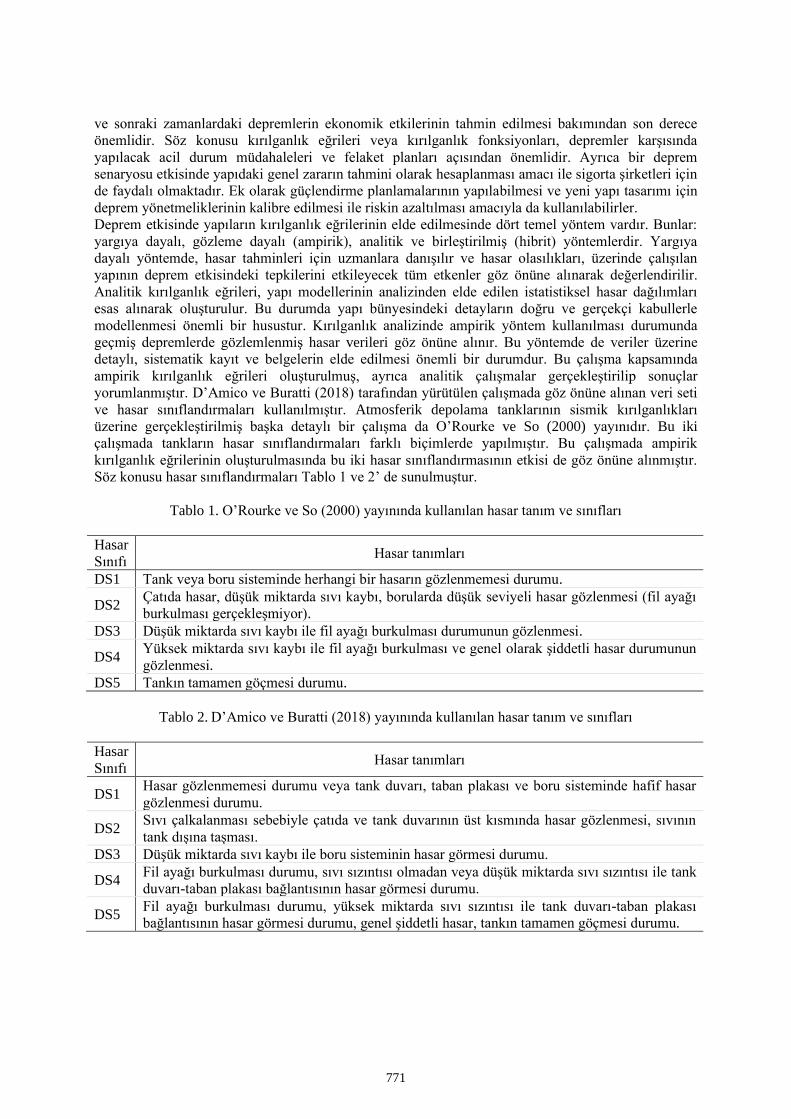
ve sonraki zamanlardaki depremlerin ekonomik etkilerinin tahmin edilmesi bakımından son derece

önemlidir. Söz konusu kırılganlık eğrileri veya kırılganlık fonksiyonları, depremler karşısında

yapılacak acil durum müdahaleleri ve felaket planları açısından önemlidir. Ayrıca bir deprem

senaryosu etkisinde yapıdaki genel zararın tahmini olarak hesaplanması amacı ile sigorta şirketleri için

de faydalı olmaktadır. Ek olarak güçlendirme planlamalarının yapılabilmesi ve yeni yapı tasarımı için

deprem yönetmeliklerinin kalibre edilmesi ile riskin azaltılması amacıyla da kullanılabilirler.

Deprem etkisinde yapıların kırılganlık eğrilerinin elde edilmesinde dört temel yöntem vardır. Bunlar:

yargıya dayalı, gözleme dayalı (ampirik), analitik ve birleştirilmiş (hibrit) yöntemlerdir. Yargıya

dayalı yöntemde, hasar tahminleri için uzmanlara danışılır ve hasar olasılıkları, üzerinde çalışılan

yapının deprem etkisindeki tepkilerini etkileyecek tüm etkenler göz önüne alınarak değerlendirilir.

Analitik kırılganlık eğrileri, yapı modellerinin analizinden elde edilen istatistiksel hasar dağılımları

esas alınarak oluşturulur. Bu durumda yapı bünyesindeki detayların doğru ve gerçekçi kabullerle

modellenmesi önemli bir husustur. Kırılganlık analizinde ampirik yöntem kullanılması durumunda

geçmiş depremlerde gözlemlenmiş hasar verileri göz önüne alınır. Bu yöntemde de veriler üzerine

detaylı, sistematik kayıt ve belgelerin elde edilmesi önemli bir durumdur. Bu çalışma kapsamında

ampirik kırılganlık eğrileri oluşturulmuş, ayrıca analitik çalışmalar gerçekleştirilip sonuçlar

yorumlanmıştır. D’Amico ve Buratti (2018) tarafından yürütülen çalışmada göz önüne alınan veri seti

ve hasar sınıflandırmaları kullanılmıştır. Atmosferik depolama tanklarının sismik kırılganlıkları

üzerine gerçekleştirilmiş başka detaylı bir çalışma da O’Rourke ve So (2000) yayınıdır. Bu iki

çalışmada tankların hasar sınıflandırmaları farklı biçimlerde yapılmıştır. Bu çalışmada ampirik

kırılganlık eğrilerinin oluşturulmasında bu iki hasar sınıflandırmasının etkisi de göz önüne alınmıştır.

Söz konusu hasar sınıflandırmaları Tablo 1 ve 2’ de sunulmuştur.

Tablo 1. O’Rourke ve So (2000) yayınında kullanılan hasar tanım ve sınıfları

Hasar

Sınıfı Hasar tanımları

DS1 Tank veya boru sisteminde herhangi bir hasarın gözlenmemesi durumu.

DS2 Çatıda hasar, düşük miktarda sıvı kaybı, borularda düşük seviyeli hasar gözlenmesi (fil ayağı

burkulması gerçekleşmiyor).

DS3 Düşük miktarda sıvı kaybı ile fil ayağı burkulması durumunun gözlenmesi.

DS4 Yüksek miktarda sıvı kaybı ile fil ayağı burkulması ve genel olarak şiddetli hasar durumunun

gözlenmesi.

DS5 Tankın tamamen göçmesi durumu.

Tablo 2. D’Amico ve Buratti (2018) yayınında kullanılan hasar tanım ve sınıfları

Hasar

Sınıfı Hasar tanımları

DS1 Hasar gözlenmemesi durumu veya tank duvarı, taban plakası ve boru sisteminde hafif hasar

gözlenmesi durumu.

DS2 Sıvı çalkalanması sebebiyle çatıda ve tank duvarının üst kısmında hasar gözlenmesi, sıvının

tank dışına taşması.

DS3 Düşük miktarda sıvı kaybı ile boru sisteminin hasar görmesi durumu.

DS4 Fil ayağı burkulması durumu, sıvı sızıntısı olmadan veya düşük miktarda sıvı sızıntısı ile tank

duvarı-taban plakası bağlantısının hasar görmesi durumu.

DS5 Fil ayağı burkulması durumu, yüksek miktarda sıvı sızıntısı ile tank duvarı-taban plakası

bağlantısının hasar görmesi durumu, genel şiddetli hasar, tankın tamamen göçmesi durumu.

771

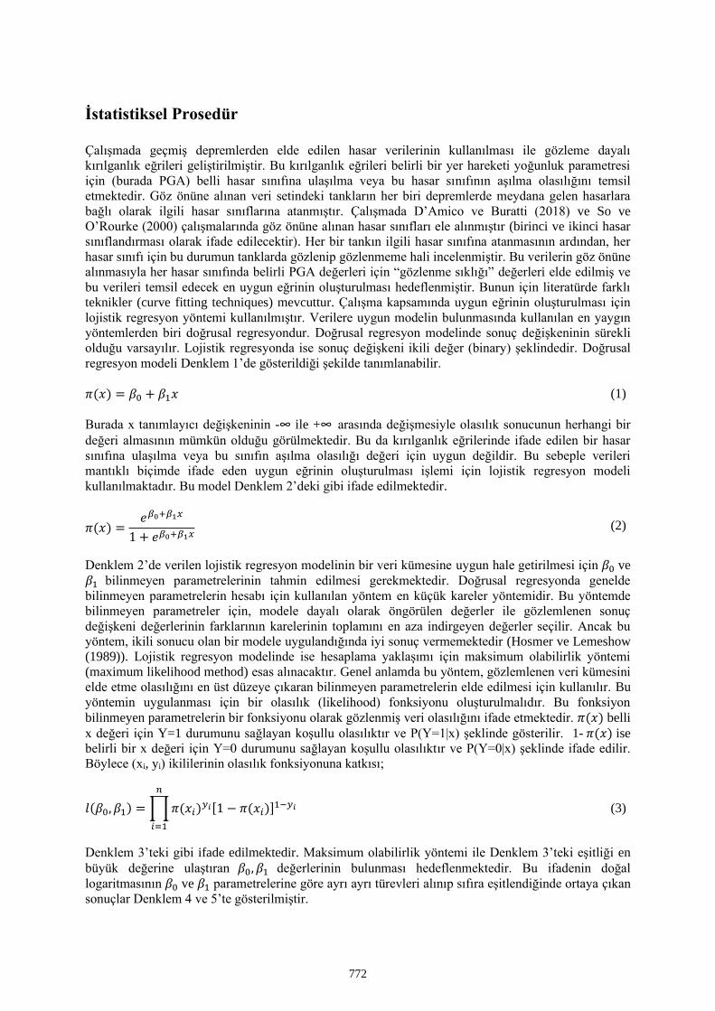
İstatistiksel Prosedür

Çalışmada geçmiş depremlerden elde edilen hasar verilerinin kullanılması ile gözleme dayalı

kırılganlık eğrileri geliştirilmiştir. Bu kırılganlık eğrileri belirli bir yer hareketi yoğunluk parametresi

için (burada PGA) belli hasar sınıfına ulaşılma veya bu hasar sınıfının aşılma olasılığını temsil

etmektedir. Göz önüne alınan veri setindeki tankların her biri depremlerde meydana gelen hasarlara

bağlı olarak ilgili hasar sınıflarına atanmıştır. Çalışmada D’Amico ve Buratti (2018) ve So ve

O’Rourke (2000) çalışmalarında göz önüne alınan hasar sınıfları ele alınmıştır (birinci ve ikinci hasar

sınıflandırması olarak ifade edilecektir). Her bir tankın ilgili hasar sınıfına atanmasının ardından, her

hasar sınıfı için bu durumun tanklarda gözlenip gözlenmeme hali incelenmiştir. Bu verilerin göz önüne

alınmasıyla her hasar sınıfında belirli PGA değerleri için “gözlenme sıklığı” değerleri elde edilmiş ve

bu verileri temsil edecek en uygun eğrinin oluşturulması hedeflenmiştir. Bunun için literatürde farklı

teknikler (curve fitting techniques) mevcuttur. Çalışma kapsamında uygun eğrinin oluşturulması için

lojistik regresyon yöntemi kullanılmıştır. Verilere uygun modelin bulunmasında kullanılan en yaygın

yöntemlerden biri doğrusal regresyondur. Doğrusal regresyon modelinde sonuç değişkeninin sürekli

olduğu varsayılır. Lojistik regresyonda ise sonuç değişkeni ikili değer (binary) şeklindedir. Doğrusal

regresyon modeli Denklem 1’de gösterildiği şekilde tanımlanabilir.

𝜋(𝑥) = 𝛽0 + 𝛽1𝑥 (1)

Burada x tanımlayıcı değişkeninin -∞ ile +∞ arasında değişmesiyle olasılık sonucunun herhangi bir

değeri almasının mümkün olduğu görülmektedir. Bu da kırılganlık eğrilerinde ifade edilen bir hasar

sınıfına ulaşılma veya bu sınıfın aşılma olasılığı değeri için uygun değildir. Bu sebeple verileri

mantıklı biçimde ifade eden uygun eğrinin oluşturulması işlemi için lojistik regresyon modeli

kullanılmaktadır. Bu model Denklem 2’deki gibi ifade edilmektedir.

𝜋(𝑥) =𝑒𝛽0+𝛽1𝑥

1 + 𝑒𝛽0+𝛽1𝑥 (2)

Denklem 2’de verilen lojistik regresyon modelinin bir veri kümesine uygun hale getirilmesi için 𝛽0 ve

𝛽1 bilinmeyen parametrelerinin tahmin edilmesi gerekmektedir. Doğrusal regresyonda genelde

bilinmeyen parametrelerin hesabı için kullanılan yöntem en küçük kareler yöntemidir. Bu yöntemde

bilinmeyen parametreler için, modele dayalı olarak öngörülen değerler ile gözlemlenen sonuç

değişkeni değerlerinin farklarının karelerinin toplamını en aza indirgeyen değerler seçilir. Ancak bu

yöntem, ikili sonucu olan bir modele uygulandığında iyi sonuç vermemektedir (Hosmer ve Lemeshow

(1989)). Lojistik regresyon modelinde ise hesaplama yaklaşımı için maksimum olabilirlik yöntemi

(maximum likelihood method) esas alınacaktır. Genel anlamda bu yöntem, gözlemlenen veri kümesini

elde etme olasılığını en üst düzeye çıkaran bilinmeyen parametrelerin elde edilmesi için kullanılır. Bu

yöntemin uygulanması için bir olasılık (likelihood) fonksiyonu oluşturulmalıdır. Bu fonksiyon

bilinmeyen parametrelerin bir fonksiyonu olarak gözlenmiş veri olasılığını ifade etmektedir. 𝜋(𝑥) belli

x değeri için Y=1 durumunu sağlayan koşullu olasılıktır ve P(Y=1|x) şeklinde gösterilir. 1- 𝜋(𝑥) ise

belirli bir x değeri için Y=0 durumunu sağlayan koşullu olasılıktır ve P(Y=0|x) şeklinde ifade edilir.

Böylece (xi, yi) ikililerinin olasılık fonksiyonuna katkısı;

𝑙(𝛽0, 𝛽1) = ∏ 𝜋(𝑥𝑖)𝑦𝑖[1 − 𝜋(𝑥𝑖)]1−𝑦𝑖

𝑛

𝑖=1

(3)

Denklem 3’teki gibi ifade edilmektedir. Maksimum olabilirlik yöntemi ile Denklem 3’teki eşitliği en

büyük değerine ulaştıran 𝛽0, 𝛽1 değerlerinin bulunması hedeflenmektedir. Bu ifadenin doğal

logaritmasının 𝛽0 ve 𝛽1 parametrelerine göre ayrı ayrı türevleri alınıp sıfıra eşitlendiğinde ortaya çıkan

sonuçlar Denklem 4 ve 5’te gösterilmiştir.

772

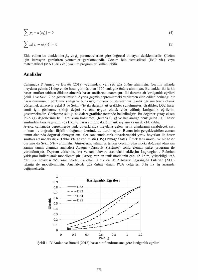
∑[𝑦𝑖 − 𝜋(𝑥𝑖)] = 0 (4)

∑ 𝑥𝑖[𝑦𝑖 − 𝜋(𝑥𝑖)] = 0 (5)

Elde edilen bu denklemler 𝛽0 ve 𝛽1 parametrelerine göre doğrusal olmayan denklemlerdir. Çözüm

için iterasyon gerektiren yöntemler gerekmektedir. Çözüm için istatistiksel (JMP vb.) veya

matematiksel (MATLAB vb.) yazılım programları kullanılabilir.

Analizler

Çalışmada D’Amico ve Buratti (2018) yayınındaki veri seti göz önüne alınmıştır. Geçmiş yıllarda

meydana gelmiş 21 depremde hasar görmüş olan 1356 tank göz önüne alınmıştır. Bu tanklar iki farklı

hasar sınıfları tablosu dikkate alınarak hasar sınıflarına atanmıştır. İki duruma ait kırılganlık eğrileri

Şekil 1 ve Şekil 2’de gösterilmiştir. Ayrıca geçmiş depremlerdeki verilerden elde edilen herhangi bir

hasar durumunun gözlenme sıklığı ve buna uygun olarak oluşturulan kırılganlık eğrisini örnek olarak

göstermek amacıyla Şekil 3 ve Şekil 4’te iki duruma ait grafikler sunulmuştur. Grafikler, DS2 hasar

sınıfı için gözlenme sıklığı değeri ve ona uygun olarak elde edilmiş kırılganlık eğrilerini

göstermektedir. Gözlenme sıklığı noktaları grafikler üzerinde belirtilmiştir. Bu değerler yatay eksen

PGA (g) değerlerinin belli aralıklara bölünmesi (burada 0,1g) ve her aralığa denk gelen ilgili hasar

sınıfındaki tank sayısının, söz konusu hasar sınıfındaki tüm tank sayısına oranı ile elde edilir.

Ayrıca çalışmada depremlerde tank duvarlarında meydana gelen yırtık alanlarının sızabilecek sıvı

miktarı ile doğrudan ilişkili olduğunun üzerinde de durulmuştur. Bunun için gerçekleştirilen zaman

tanım alanında doğrusal olmayan analizler sonucunda tank duvarlarındaki yırtık boyutları ile hasar

sınıfları arasındaki ilişki Tablo 3’te gösterilmiştir (DS; Damage State). Örnek tank modeli ve bir hasar

durumu da Şekil 5’te verilmiştir. Atmosferik, silindirik tankın deprem etkisindeki doğrusal olmayan

zaman tanım alanında analizleri Abaqus (Dassault Systémes) sonlu eleman paket programı ile

yürütülmüştür. Deprem etkisinde, sıvı ve tank duvarı arasındaki etkileşim Lagrangian / Eulerian

yaklaşımı kullanılarak modellenmiştir. Örneği verilen tank modelinin çapı 45,72 m, yüksekliği 19,8

‘dir. Sıvı seviyesi %50 oranındadır. Çalkalanma etkileri de Arbitrary Lagrangian Eulerian (ALE)

tekniği ile modellenmiştir. Analizlerde göz önüne alınan PGA değerleri 0,1g ila 1g arasında

değişmektedir.

Şekil 1. D’Amico ve Buratti (2018) hasar sınıflandırmasına göre kırılganlık eğrileri

0

0.1

0.2

0.3

0.4

0.5

0.6

0.7

0.8

0.9

1

0 0.2 0.4 0.6 0.8 1 1.2

Ola

sılı

k

PGA, g

Kırılganlık Eğrileri

DS2

DS3

DS4

DS5

773

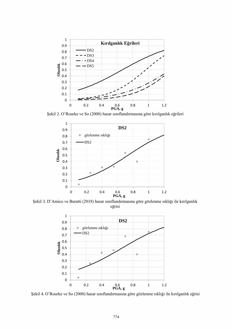
Şekil 2. O’Rourke ve So (2000) hasar sınıflandırmasına göre kırılganlık eğrileri

Şekil 3. D’Amico ve Buratti (2018) hasar sınıflandırmasına göre gözlenme sıklığı ile kırılganlık

eğrisi

Şekil 4. O’Rourke ve So (2000) hasar sınıflandırmasına göre gözlenme sıklığı ile kırılganlık eğrisi

0

0.1

0.2

0.3

0.4

0.5

0.6

0.7

0.8

0.9

1

0 0.2 0.4 0.6 0.8 1 1.2

Ola

sılı

k

PGA, g

Kırılganlık Eğrileri

DS2

DS3

DS4

DS5

0

0.1

0.2

0.3

0.4

0.5

0.6

0.7

0.8

0.9

1

0 0.2 0.4 0.6 0.8 1 1.2

Ola

sılı

k

PGA, g

DS2

gözlenme sıklığı

DS2

0

0.1

0.2

0.3

0.4

0.5

0.6

0.7

0.8

0.9

1

0 0.2 0.4 0.6 0.8 1 1.2

Ola

sılı

k

PGA, g

DS2

gözlenme sıklığı

DS2

774

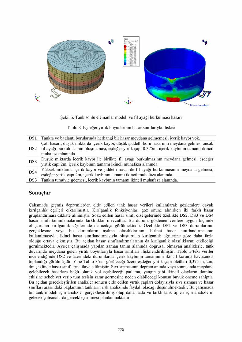
Şekil 5. Tank sonlu elemanlar modeli ve fil ayağı burkulması hasarı

Tablo 3. Eşdeğer yırtık boyutlarının hasar sınıflarıyla ilişkisi

DS1 Tankta ve bağlantı borularında herhangi bir hasar meydana gelmemesi, içerik kaybı yok.

DS2

Çatı hasarı, düşük miktarda içerik kaybı, düşük şiddetli boru hasarının meydana gelmesi ancak

fil ayağı burkulmasının oluşmaması, eşdeğer yırtık çapı 0.375m, içerik kaybının tamamı ikincil

muhafaza alanında.

DS3 Düşük miktarda içerik kaybı ile birlikte fil ayağı burkulmasının meydana gelmesi, eşdeğer

yırtık çapı 2m, içerik kaybının tamamı ikincil muhafaza alanında.

DS4 Yüksek miktarda içerik kaybı ve şiddetli hasar ile fil ayağı burkulmasının meydana gelmesi,

eşdeğer yırtık çapı 4m, içerik kaybının tamamı ikincil muhafaza alanında.

DS5 Tankın tümüyle göçmesi, içerik kaybının tamamı ikincil muhafaza alanında.

Sonuçlar

Çalışmada geçmiş depremlerden elde edilen tank hasar verileri kullanılarak gözlemlere dayalı

kırılganlık eğrileri çıkarılmıştır. Kırılganlık fonksiyonları göz önüne alınırken iki farklı hasar

gruplandırması dikkate alınmıştır. Sözü edilen hasar sınıfı çizelgelerinde özellikle DS2, DS3 ve DS4

hasar sınıfı tanımlamalarında farklılıklar mevcuttur. Bu durum, gözlenen verilere uygun biçimde

oluşturulan kırılganlık eğrilerinde de açıkça görülmektedir. Özellikle DS2 ve DS3 durumlarının

gerçekleşme veya bu durumların aşılma olasılıklarının, birinci hasar sınıflandırmasının

kullanılmasıyla, ikinci hasar sınıflandırmasıyla oluşturulan kırılganlık eğrilerine göre daha fazla

olduğu ortaya çıkmıştır. Bu açıdan hasar sınıflandırmalarının da kırılganlık olasılıklarını etkilediği

görülmektedir. Ayrıca çalışmada yapılan zaman tanım alanında doğrusal olmayan analizlerle, tank

duvarında meydana gelen yırtık boyutlarıyla hasar sınıfları ilişkilendirilmiştir. Tablo 3’teki veriler

incelendiğinde DS2 ve üzerindeki durumlarda içerik kaybının tamamının ikincil koruma havuzunda

toplandığı görülmüştür. Yine Tablo 3’ten görüleceği üzere eşdeğer yırtık çapı ölçüleri 0,375 m, 2m,

4m şeklinde hasar sınıflarına ilave edilmiştir. Sıvı sızmasının deprem anında veya sonrasında meydana

gelebilecek hasarlara bağlı olarak yol açabileceği patlama, yangın gibi ikincil olayların domino

etkisine sebebiyet verip tüm tesisin zarar görmesine neden olabileceği konusu büyük öneme sahiptir.

Bu açıdan gerçekleştirilen analizler sonucu elde edilen yırtık çapları dolayısıyla sıvı sızması ve hasar

sınıfları arasındaki bağlantının tankların risk analizinde faydalı olacağı düşünülmektedir. Bu çalışmada

bir tank modeli için analizler gerçekleştirilmiş olup daha fazla ve farklı tank tipleri için analizlerin

gelecek çalışmalarda gerçekleştirilmesi planlanmaktadır.

775

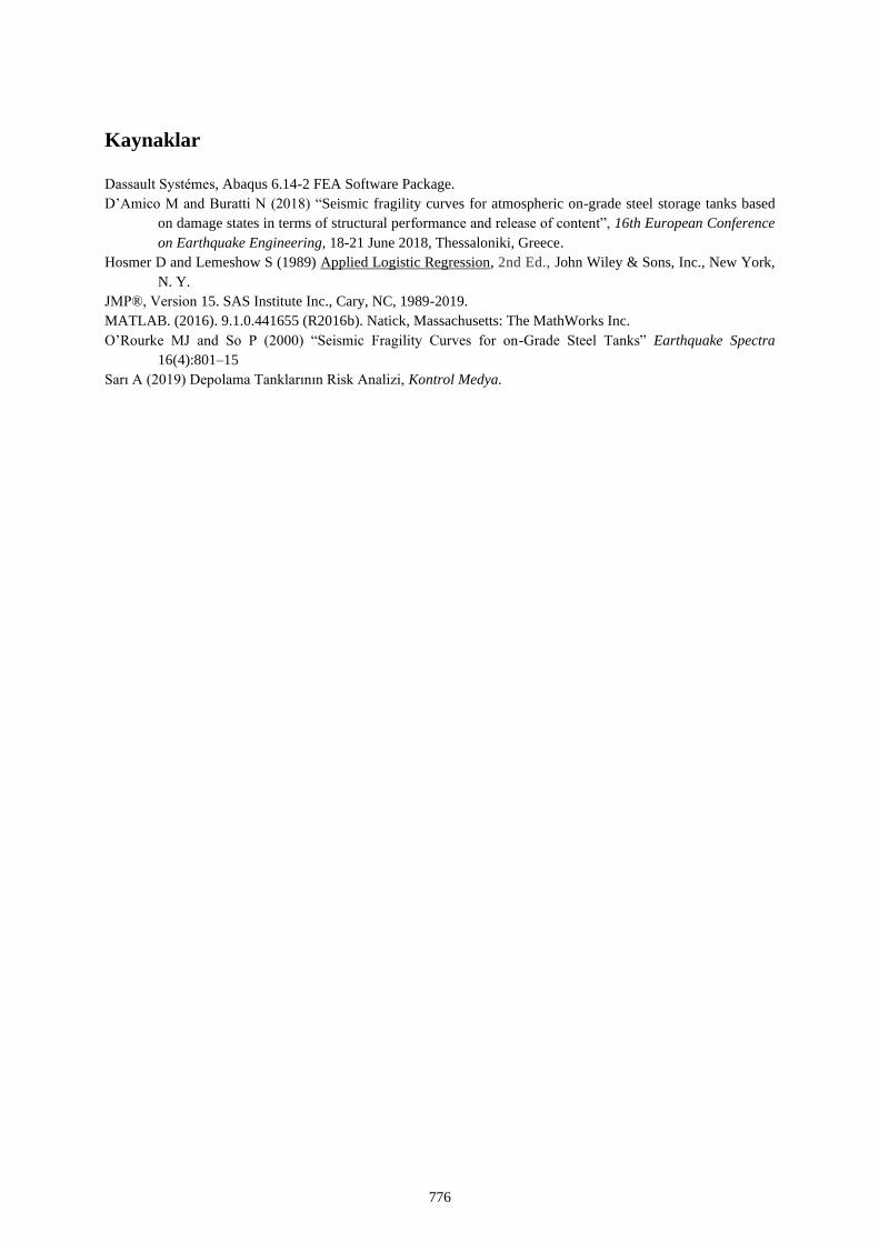
Kaynaklar

Dassault Systémes, Abaqus 6.14-2 FEA Software Package.

D’Amico M and Buratti N (2018) “Seismic fragility curves for atmospheric on-grade steel storage tanks based

on damage states in terms of structural performance and release of content”, 16th European Conference

on Earthquake Engineering, 18-21 June 2018, Thessaloniki, Greece.

Hosmer D and Lemeshow S (1989) Applied Logistic Regression, 2nd Ed., John Wiley & Sons, Inc., New York,

N. Y.

JMP®, Version 15. SAS Institute Inc., Cary, NC, 1989-2019.

MATLAB. (2016). 9.1.0.441655 (R2016b). Natick, Massachusetts: The MathWorks Inc.

O’Rourke MJ and So P (2000) “Seismic Fragility Curves for on-Grade Steel Tanks” Earthquake Spectra

16(4):801–15

Sarı A (2019) Depolama Tanklarının Risk Analizi, Kontrol Medya.

776

On the Residual Displacement Demands of SDOF Systems using Code

Compatible Record Sets

M. Palanci1, A. Demir2* and A.H. Kayhan3

1Assoc. Prof. Dr., Civil Eng. Department, Istanbul Arel University, Istanbul 2Res. Assist. Dr., Civil Eng. Department, Bolu Abant İzzet Baysal University, Bolu

3Prof. Dr., Civil Eng. Department, Pamukkale University, Denizli *[email protected]

AbstractResidual displacement can be considered as an important engineering demand parameter since it is effectively used in post-earthquake assessment of structures. Although this parameter is not directly used in code applications, application of this parameter for the rehabilitation of structures is addressed. Residual displacements of single degree of freedom (SDOF) systems are evaluated using Turkish Building Earthquake Code compatible ground motion record sets in this study. In order to evaluate the variation of residual displacements, effect of different soil types, structural topologies and hysteresis models with different post yield stiffness ratios (r) are considered. Different natural vibration periods (T) and lateral strength capacity ratios (Fy/W) are used to cover range of structural topologies. ZB, ZCand ZD soil classes which reflect the different target spectral shapes are used. Seven different groundmotion record sets compatible with corresponding target spectrum and SDOF system are utilized toinclude possible divergence of code compliant record selection. According to above considerations,nonlinear dynamic analyses were performed for each SDOF systems and residual displacements wereobtained. Then, residual displacements are assessed according to mean of the residual displacements ofthe record sets. Results showed that different residual displacements can be obtained for different groundmotion record sets although they are compatible with same target spectrum. Post-yield stiffness andFy/W have significantly effect on the residual displacements. It is also observed that dispersion of theresidual displacements around the mean is remarkably high regardless of T, Fy/W and r. In addition tothis, ZB has the highest mCoV(res) values than ZC and ZD for both r values.

Keywords: SDOF systems, residual displacement, nonlinear dynamic analysis, ground motion selection.

Introduction

Performance-based design procedures intend to control earthquake induced damage to structural and nonstructural elements by limiting deformation demands (ATC-40, 1996; FEMA-440, 2005). Peak displacement and drift demands are generally considered for evaluating structural performance. Residual or permanent displacement and drift demands are additional important parameters for seismic performance evaluation of structures (FEMA-356, 2000). These parameters can be used to evaluate the technical and economic feasibility of repairing and retrofitting structures that have been damaged due to earthquake excitations (FEMA-P58, 2018). Thus, it is important to estimate residual structural displacements for the evaluation and rehabilitation of structures (Ji et al., 2018; Aydemir and Aydemir, 2019). In order to estimate the response of structures to seismic excitation, nonlinear time history analysis of three-dimensional structural models is the most comprehensive and accurate method. However, it can be said that nonlinear time history analysis of three-dimensional structural models are complex and difficult. For this reason, many research efforts have focused on simpler approaches. Using equivalent single degree of freedom (SDOF) system is one of the simpler approaches (ATC-40, 1996). SDOF

777

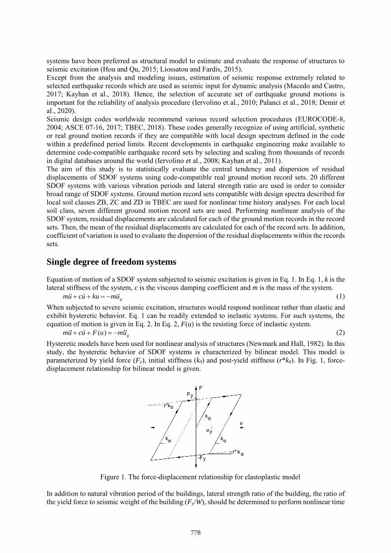
systems have been preferred as structural model to estimate and evaluate the response of structures to seismic excitation (Hou and Qu, 2015; Liossatou and Fardis, 2015). Except from the analysis and modeling issues, estimation of seismic response extremely related to selected earthquake records which are used as seismic input for dynamic analysis (Macedo and Castro, 2017; Kayhan et al., 2018). Hence, the selection of accurate set of earthquake ground motions is important for the reliability of analysis procedure (Iervolino et al., 2010; Palanci et al., 2018; Demir et al., 2020). Seismic design codes worldwide recommend various record selection procedures (EUROCODE-8, 2004; ASCE 07-16, 2017; TBEC, 2018). These codes generally recognize of using artificial, synthetic or real ground motion records if they are compatible with local design spectrum defined in the code within a predefined period limits. Recent developments in earthquake engineering make available to determine code-compatible earthquake record sets by selecting and scaling from thousands of records in digital databases around the world (Iervolino et al., 2008; Kayhan et al., 2011). The aim of this study is to statistically evaluate the central tendency and dispersion of residual displacements of SDOF systems using code-compatible real ground motion record sets. 20 different SDOF systems with various vibration periods and lateral strength ratio are used in order to consider broad range of SDOF systems. Ground motion record sets compatible with design spectra described for local soil classes ZB, ZC and ZD in TBEC are used for nonlinear time history analyses. For each local soil class, seven different ground motion record sets are used. Performing nonlinear analysis of the SDOF system, residual displacements are calculated for each of the ground motion records in the record sets. Then, the mean of the residual displacements are calculated for each of the record sets. In addition, coefficient of variation is used to evaluate the dispersion of the residual displacements within the records sets.

Single degree of freedom systems

Equation of motion of a SDOF system subjected to seismic excitation is given in Eq. 1. In Eq. 1, k is the lateral stiffness of the system, c is the viscous damping coefficient and m is the mass of the system.

gmu cu ku mu (1) When subjected to severe seismic excitation, structures would respond nonlinear rather than elastic and exhibit hysteretic behavior. Eq. 1 can be readily extended to inelastic systems. For such systems, the equation of motion is given in Eq. 2. In Eq. 2, F(u) is the resisting force of inelastic system.

( ) gmu cu F u mu (2) Hysteretic models have been used for nonlinear analysis of structures (Newmark and Hall, 1982). In this study, the hysteretic behavior of SDOF systems is characterized by bilinear model. This model is parameterized by yield force (Fy), initial stiffness (k0) and post-yield stiffness (r*k0). In Fig. 1, force-displacement relationship for bilinear model is given.

Figure 1. The force-displacement relationship for elastoplastic model

In addition to natural vibration period of the buildings, lateral strength ratio of the building, the ratio of the yield force to seismic weight of the building (Fy/W), should be determined to perform nonlinear time

778

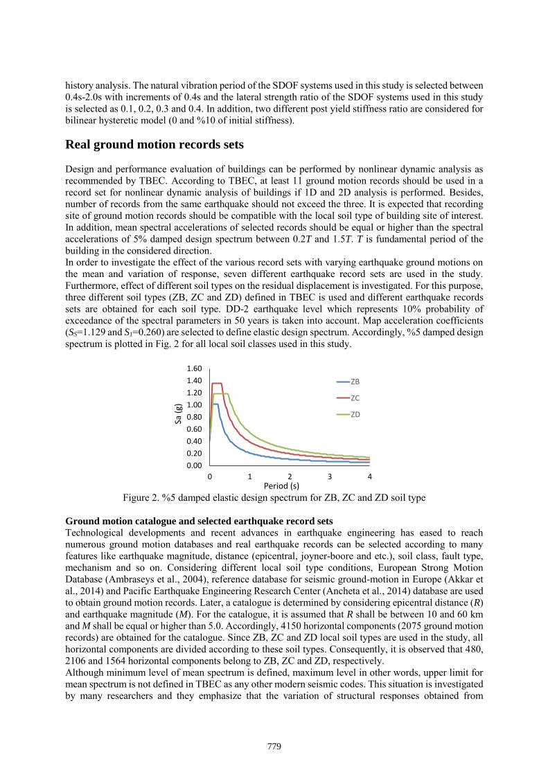
history analysis. The natural vibration period of the SDOF systems used in this study is selected between 0.4s-2.0s with increments of 0.4s and the lateral strength ratio of the SDOF systems used in this study is selected as 0.1, 0.2, 0.3 and 0.4. In addition, two different post yield stiffness ratio are considered for bilinear hysteretic model (0 and %10 of initial stiffness).

Real ground motion records sets

Design and performance evaluation of buildings can be performed by nonlinear dynamic analysis as recommended by TBEC. According to TBEC, at least 11 ground motion records should be used in a record set for nonlinear dynamic analysis of buildings if 1D and 2D analysis is performed. Besides, number of records from the same earthquake should not exceed the three. It is expected that recording site of ground motion records should be compatible with the local soil type of building site of interest. In addition, mean spectral accelerations of selected records should be equal or higher than the spectral accelerations of 5% damped design spectrum between 0.2T and 1.5T. T is fundamental period of the building in the considered direction. In order to investigate the effect of the various record sets with varying earthquake ground motions on the mean and variation of response, seven different earthquake record sets are used in the study. Furthermore, effect of different soil types on the residual displacement is investigated. For this purpose, three different soil types (ZB, ZC and ZD) defined in TBEC is used and different earthquake records sets are obtained for each soil type. DD-2 earthquake level which represents 10% probability of exceedance of the spectral parameters in 50 years is taken into account. Map acceleration coefficients (SS=1.129 and S1=0.260) are selected to define elastic design spectrum. Accordingly, %5 damped design spectrum is plotted in Fig. 2 for all local soil classes used in this study.

Figure 2. %5 damped elastic design spectrum for ZB, ZC and ZD soil type

Ground motion catalogue and selected earthquake record sets

Technological developments and recent advances in earthquake engineering has eased to reach numerous ground motion databases and real earthquake records can be selected according to many features like earthquake magnitude, distance (epicentral, joyner-boore and etc.), soil class, fault type, mechanism and so on. Considering different local soil type conditions, European Strong Motion Database (Ambraseys et al., 2004), reference database for seismic ground-motion in Europe (Akkar et al., 2014) and Pacific Earthquake Engineering Research Center (Ancheta et al., 2014) database are used to obtain ground motion records. Later, a catalogue is determined by considering epicentral distance (R) and earthquake magnitude (M). For the catalogue, it is assumed that R shall be between 10 and 60 km and M shall be equal or higher than 5.0. Accordingly, 4150 horizontal components (2075 ground motion records) are obtained for the catalogue. Since ZB, ZC and ZD local soil types are used in the study, all horizontal components are divided according to these soil types. Consequently, it is observed that 480, 2106 and 1564 horizontal components belong to ZB, ZC and ZD, respectively. Although minimum level of mean spectrum is defined, maximum level in other words, upper limit for mean spectrum is not defined in TBEC as any other modern seismic codes. This situation is investigated by many researchers and they emphasize that the variation of structural responses obtained from

0.00

0.20

0.40

0.60

0.80

1.00

1.20

1.40

1.60

0 1 2 3 4

ZB

ZC

ZD

Period (s)

Sa (

g)

779

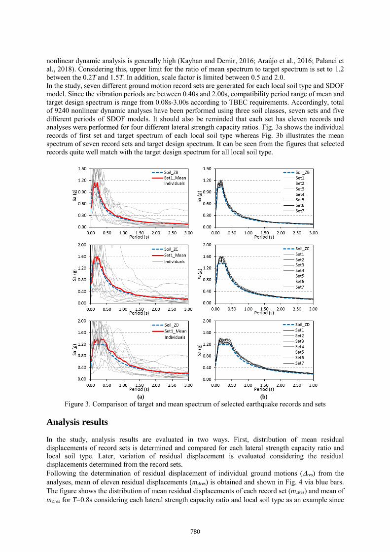
nonlinear dynamic analysis is generally high (Kayhan and Demir, 2016; Araújo et al., 2016; Palanci et al., 2018). Considering this, upper limit for the ratio of mean spectrum to target spectrum is set to 1.2 between the 0.2T and 1.5T. In addition, scale factor is limited between 0.5 and 2.0. In the study, seven different ground motion record sets are generated for each local soil type and SDOF model. Since the vibration periods are between 0.40s and 2.00s, compatibility period range of mean and target design spectrum is range from 0.08s-3.00s according to TBEC requirements. Accordingly, total of 9240 nonlinear dynamic analyses have been performed using three soil classes, seven sets and five different periods of SDOF models. It should also be reminded that each set has eleven records and analyses were performed for four different lateral strength capacity ratios. Fig. 3a shows the individual records of first set and target spectrum of each local soil type whereas Fig. 3b illustrates the mean spectrum of seven record sets and target design spectrum. It can be seen from the figures that selected records quite well match with the target design spectrum for all local soil type.

(a) (b)

Figure 3. Comparison of target and mean spectrum of selected earthquake records and sets

Analysis results In the study, analysis results are evaluated in two ways. First, distribution of mean residual displacements of record sets is determined and compared for each lateral strength capacity ratio and local soil type. Later, variation of residual displacement is evaluated considering the residual displacements determined from the record sets. Following the determination of residual displacement of individual ground motions (res) from the analyses, mean of eleven residual displacements (mres) is obtained and shown in Fig. 4 via blue bars. The figure shows the distribution of mean residual displacements of each record set (mres) and mean of mres for T=0.8s considering each lateral strength capacity ratio and local soil type as an example since

780

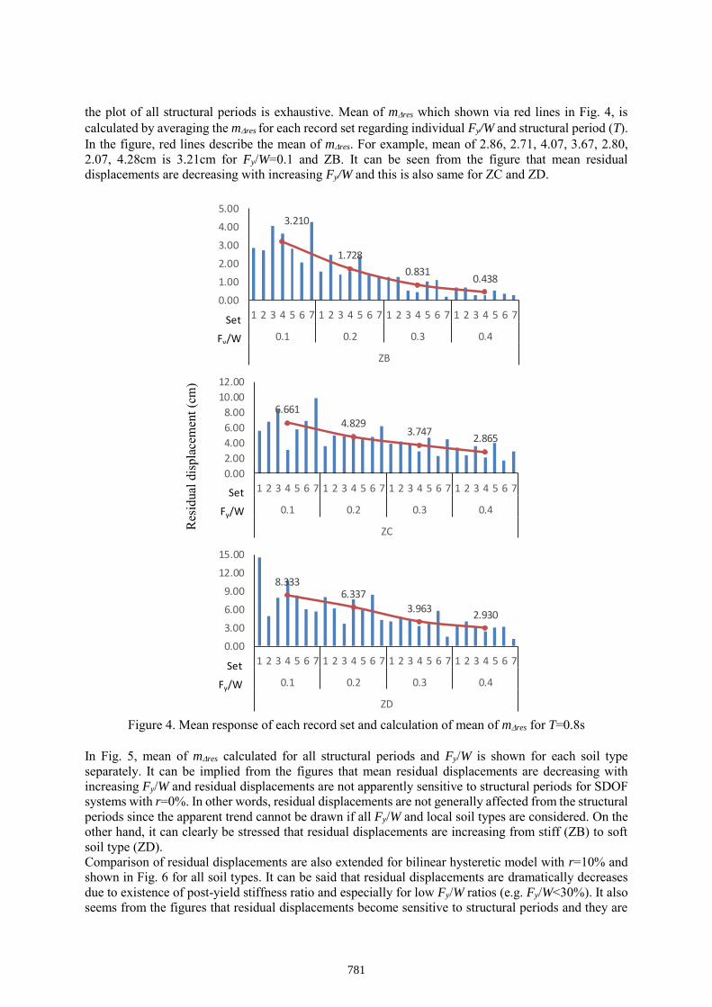
the plot of all structural periods is exhaustive. Mean of mres which shown via red lines in Fig. 4, is calculated by averaging the mres for each record set regarding individual Fy/W and structural period (T). In the figure, red lines describe the mean of mres. For example, mean of 2.86, 2.71, 4.07, 3.67, 2.80, 2.07, 4.28cm is 3.21cm for Fy/W=0.1 and ZB. It can be seen from the figure that mean residual displacements are decreasing with increasing Fy/W and this is also same for ZC and ZD.

Res

idua

l dis

plac

emen

t (cm

)

Figure 4. Mean response of each record set and calculation of mean of mres for T=0.8s

In Fig. 5, mean of mres calculated for all structural periods and Fy/W is shown for each soil type separately. It can be implied from the figures that mean residual displacements are decreasing with increasing Fy/W and residual displacements are not apparently sensitive to structural periods for SDOF systems with r=0%. In other words, residual displacements are not generally affected from the structural periods since the apparent trend cannot be drawn if all Fy/W and local soil types are considered. On the other hand, it can clearly be stressed that residual displacements are increasing from stiff (ZB) to soft soil type (ZD). Comparison of residual displacements are also extended for bilinear hysteretic model with r=10% and shown in Fig. 6 for all soil types. It can be said that residual displacements are dramatically decreases due to existence of post-yield stiffness ratio and especially for low Fy/W ratios (e.g. Fy/W<30%). It also seems from the figures that residual displacements become sensitive to structural periods and they are

3.210

1.728

0.8310.438

0.00

1.00

2.00

3.00

4.00

5.00

1 2 3 4 5 6 7 1 2 3 4 5 6 7 1 2 3 4 5 6 7 1 2 3 4 5 6 7

0.1 0.2 0.3 0.4

ZB

Set

Fy/W

6.6614.829

3.7472.865

0.00

2.00

4.00

6.00

8.00

10.00

12.00

1 2 3 4 5 6 7 1 2 3 4 5 6 7 1 2 3 4 5 6 7 1 2 3 4 5 6 7

0.1 0.2 0.3 0.4

ZC

Set

Fy/W

8.3336.337

3.9632.930

0.00

3.00

6.00

9.00

12.00

15.00

1 2 3 4 5 6 7 1 2 3 4 5 6 7 1 2 3 4 5 6 7 1 2 3 4 5 6 7

0.1 0.2 0.3 0.4

ZD

Set

Fy/W

781

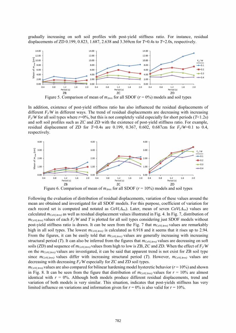
gradually increasing on soft soil profiles with post-yield stiffness ratio. For instance, residual displacements of ZD 0.199, 0.823, 1.687, 2.638 and 3.369cm for T=0.4s to T=2.0s, respectively.

Figure 5. Comparison of mean of mres for all SDOF (r = 0%) models and soil types

In addition, existence of post-yield stiffness ratio has also influenced the residual displacements of different Fy/W in different ways. The trend of residual displacements are decreasing with increasing Fy/W for all soil types where r=0%, but this is not completely valid especially for short periods (T<1.2s) and soft soil profiles such as ZC and ZD with the existence of post-yield stiffness ratio. For example, residual displacement of ZD for T=0.4s are 0.199, 0.367, 0.602, 0.687cm for Fy/W=0.1 to 0.4, respectively.

Figure 6. Comparison of mean of mres for all SDOF (r = 10%) models and soil types

Following the evaluation of distribution of residual displacements, variation of these values around the mean are obtained and investigated for all SDOF models. For this purpose, coefficient of variation for each record set is computed and notated as CoV(res). Later, mean of seven CoV(res) values are calculated mCoV(res) as well as residual displacement values illustrated in Fig. 4. In Fig. 7, distribution of mCoV(res) values of each Fy/W and T is plotted for all soil types considering just SDOF models without post-yield stiffness ratio is drawn. It can be seen from the Fig. 7 that mCoV(res) values are remarkably high in all soil types. The lowest mCoV(res) is calculated as 0.918 and it seems that it rises up to 2.94. From the figures, it can be easily told that mCoV(res) values are generally increasing with increasing structural period (T). It can also be inferred from the figures that mCoV(res) values are decreasing on soft soils (ZD) and sequence of mCoV(res) values from high to low is ZB, ZC and ZD. When the effect of Fy/W on the mCoV(res) values are investigated, it can be said that apparent trend is not exist for ZB soil type since mCoV(res) values differ with increasing structural period (T). However, mCoV(res) values are decreasing with decreasing Fy/W especially for ZC and ZD soil types. mCoV(res) values are also compared for bilinear hardening model hysteretic behavior (r = 10%) and shown in Fig. 8. It can be seen from the figure that distribution of mCoV(res) values for r = 10% are almost identical with r = 0%. Although both models produce different residual displacements, trend and variation of both models is very similar. This situation, indicates that post-yields stiffness has very limited influence on variations and information given for r = 0% is also valid for r = 10%.

782

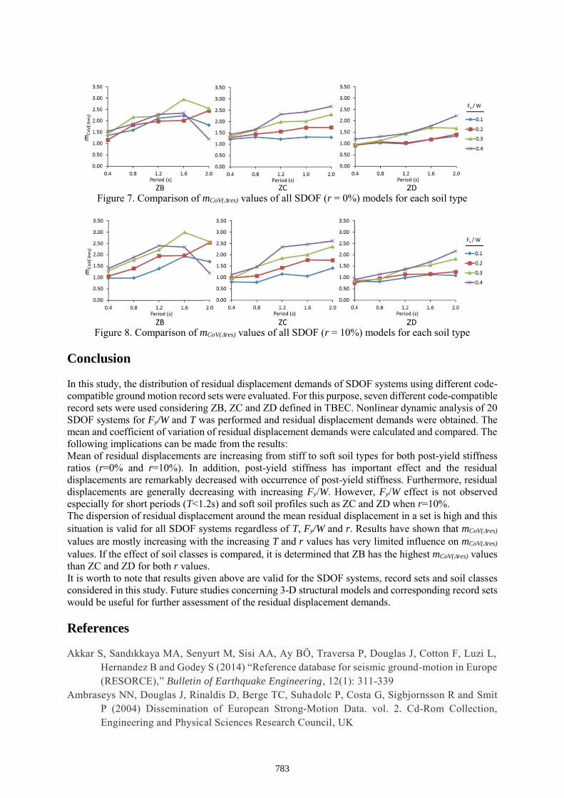
Figure 7. Comparison of mCoV(res) values of all SDOF (r = 0%) models for each soil type

Figure 8. Comparison of mCoV(res) values of all SDOF (r = 10%) models for each soil type

Conclusion

In this study, the distribution of residual displacement demands of SDOF systems using different code-compatible ground motion record sets were evaluated. For this purpose, seven different code-compatible record sets were used considering ZB, ZC and ZD defined in TBEC. Nonlinear dynamic analysis of 20 SDOF systems for Fy/W and T was performed and residual displacement demands were obtained. The mean and coefficient of variation of residual displacement demands were calculated and compared. The following implications can be made from the results: Mean of residual displacements are increasing from stiff to soft soil types for both post-yield stiffness ratios (r=0% and r=10%). In addition, post-yield stiffness has important effect and the residual displacements are remarkably decreased with occurrence of post-yield stiffness. Furthermore, residual displacements are generally decreasing with increasing Fy/W. However, Fy/W effect is not observed especially for short periods (T<1.2s) and soft soil profiles such as ZC and ZD when r=10%. The dispersion of residual displacement around the mean residual displacement in a set is high and this situation is valid for all SDOF systems regardless of T, Fy/W and r. Results have shown that mCoV(res) values are mostly increasing with the increasing T and r values has very limited influence on mCoV(res) values. If the effect of soil classes is compared, it is determined that ZB has the highest mCoV(res) values than ZC and ZD for both r values. It is worth to note that results given above are valid for the SDOF systems, record sets and soil classes considered in this study. Future studies concerning 3-D structural models and corresponding record sets would be useful for further assessment of the residual displacement demands.

References

Akkar S, Sandıkkaya MA, Senyurt M, Sisi AA, Ay BÖ, Traversa P, Douglas J, Cotton F, Luzi L, Hernandez B and Godey S (2014) “Reference database for seismic ground-motion in Europe (RESORCE),” Bulletin of Earthquake Engineering, 12(1): 311-339

Ambraseys NN, Douglas J, Rinaldis D, Berge TC, Suhadolc P, Costa G, Sigbjornsson R and Smit P (2004) Dissemination of European Strong-Motion Data. vol. 2. Cd-Rom Collection, Engineering and Physical Sciences Research Council, UK

783

Ancheta TD, Darragh RB, Stewart JP, Seyhan E, Silva WJ, Chiou BSJ, Wooddell KE, Graves RB, Kottke AR, Boore DM, Kishida T and Donahue JL (2014) “NGA-West2 Database,” Earthquake Spectra, 30(3): 989-1005

ASCE 07–16 (2017) Minimum Design Loads for Buildings and Other Structures. American Society of Civil Engineers, Reston, Virginia

ATC-40 (1996) Seismic Evaluation and Retrofit of Concrete Buildings. Applied Technology Council, California

Aydemir ME and Aydemir C (2019) “Residual displacement demand evaluation from spectral displacement,” Teknik Dergi, Paper 528, 8913-8935

Demir A, Palanci M and Kayhan AH (2020) “Evaluation of supplementary constraints on dispersion of EDPs using real ground motion record sets,” Arabian Journal for Science and

Engineering, 45: 8379-8401 EUROCODE-8 (2004) Design Provisions for Earthquake Resistance of Structures, Part 1: General

rules, Seismic Actions and Rules for Buildings. European Committee for Standardization, Brussels

FEMA-356 (2000) Prestandard and Commentary for the Seismic Rehabilitation of Buildings. Federal Emergency Management Agency, Washington

FEMA-440 (2005) Improvement of Nonlinear Static Seismic Analysis Procedures. Federal Emergency Management Agency, Washington

FEMA-P58 (2012) Seismic Performance Assessment of Buildings, Volume 1 - Methodology. Federal Emergency Management Agency, Washington

Hou H and Qu B (2015) “Duration effect of spectrally matched ground motions on seismic demands of elastic perfectly plastic SDOFs,” Engineering Structures, 90: 48–60

Iervolino I, Maddaloni G and Cosenza E (2008) “Eurocode 8 compliant real record sets for seismic analysis of structures,” Journal of Earthquake Engineering, 12(1): 54–90

Iervolino I, Galasso C and Cosenza E (2010) “REXEL: computer aided record selection for code-based seismic structural analysis,” Bulletin of Earthquake Engineering, 8(2): 339–362

Ji D, Wen W, Zhai C and Katsanos EI (2018) “Residual displacement ratios of SDOF systems subjected to ground motions recorded on soft soils,” Soil Dynamics and Earthquake

Engineering, 115: 331–335 Kayhan AH, Korkmaz KA and Irfanoglu A (2011) “Selecting and scaling real ground motion

records using harmony search algorithm,” Soil Dynamics and Earthquake Engineering, 31(7): 941–953

Kayhan AH, Demir A and Palanci M (2018) “Statistical evaluation of maximum displacement demands of SDOF systems by code-compatible nonlinear time history analysis,” Soil

Dynamics and Earthquake Engineering, 115: 513-530 Liossatou E and Fardis MN (2015) “Residual displacements of RC structures as SDOF systems,”

Earthquake Engineering and Structural Dynamics, 44(5): 713–734 Macedo L and Castro JM (2017) “SelEQ: an advanced ground motion record selection and scaling

framework,” Advances in Engineering Software, 114: 32-42 Newmark NM and Hall WJ (1982) Earthquake Spectra and Design. EERI Monograph Series,

Earthquake Engineering Research Institute, Oakland, CA Palanci M, Kayhan AH and Demir A (2018) “A statistical assessment on global drift ratio demands

of mid-rise RC buildings using code-compatible real ground motion records,” Bulletin of

Earthquake Engineering, 16(11): 5453-5488 TBEC (2018) Turkish Building Earthquake Code. Ministry of Public Works and Settlement, Ankara

784

PGV Based No-Code Mid-Rise Reinforced Concrete Frame-Type Building

Fragilities in Istanbul

İbrahim Duran1*, Sinan Akkar2

1Civ. Eng. MSc., Department of Earthquake Engineering, Boğaziçi University, İstanbul, Turkey 2Prof. Dr., Department of Earthquake Engineering, Boğaziçi University, İstanbul, Turkey

*İbrahim Duran, [email protected]

Abstract

16 building models representing a building stock in the Zeytinburnu District in Istanbul that includes

approximately 800 mid-rise reinforced concrete (RC) frame buildings are used to develop PGV based

fragility models that could partially represent the no-code building vulnerability in Turkey. The 3-D

analytical models of the subject frames are modeled with distributed plasticity using the Open System

for Earthquake Engineering Simulation (OpenSees) software. The damage states of the fragilities are

determined by use of the performance limits of structural members from 2018 version of the Turkish

Building Earthquake Code and 2005 version of the Eurocode 8. Peak ground velocity (PGV) is preferred

as seismic intensity measure since it has a better correlation with deformation demands. 25 real ground

motion pairs are selected using disaggregation results of three different PGV hazard curves determined

from three ground motion predictive models that are used in the development of the most recent national

seismic hazard maps. Response statistics are kept through incremental dynamic analysis (IDA) to

develop fragilities for each model. The fragilities computed from above comprehensive nonlinear

response history analyses advocate that consideration of variabilities in (a) structural models, (b) ground

motion records and (c) limit states makes a huge impact in the exceedance probabilities of damage states.

Therefore, a backbone fragility model, which covers the above uncertainties by up and down scaling of

a central model is a must in proper loss assessment of building stocks.

Keywords: reinforced concrete mid-rise no-code frame building stock in İstanbul, fragility functions,

nonlinear response history analysis, incremental dynamic analysis, earthquake loss in Turkey

Introduction

Turkey is one of the most quake-prone countries in the world since it has active fault zones and due to

the high population density around fault zones, the country has suffered significant loss of life as well

as economic losses with the actions of earthquakes during last decades. It is quite clear that these losses

are due to the structural damage to the buildings during ground shaking. In recent years, in the course

of rapid urbanization of the cities, buildings have been constructed with traditional techniques. This

condition implies inadequate or no seismic design that ends up with structural damage under quake

loads. Besides, since workmanship quality is inadequate, controlling mechanism is poor and unlicensed

construction is popular around the country, earthquake loss, which can be defined as the decrease in the

value of asset as a result of earthquake damage, is inevitable in this country. With the cheapness and

availability of the construction material and the simplicity of the application of the construction, RC

becomes the most preferred construction technique across the world. In Turkey, mid-rise RC MRF

buildings occupied as commercial or residential purposes are widely used. The ones constructed during

fast urbanization of the cities after the 1960s do not meet with seismic design codes and so, do not have

adequate lateral load-carrying capacity. Therefore, for this country, the abovesaid building type is

considered as one of the most vulnerable ones under seismic actions.

This study focuses on generating fragility functions for no-code mid-rise reinforced concrete frame-type

buildings in İstanbul. For this purpose, an inventory study from the Zeytinburnu District in Istanbul that

includes 16 building models representing approximately 800 existing mid-rise RC MRF buildings are

785

used. Subject buildings are constructed before 1980. They are not designed according to a seismic design

code and supervision in the construction period is inadequate. So, they can be classified as no-code. 5-

story building models are created considering structural model variability of the subject building type.

The frame buildings are classified as Type-1 and Type-2 according to the existence of confinement

mechanism in the structural members and satisfiability of minimum reinforcement detailing of the

structural members with the TEC (1975). 3-D analytical building models are created using 3.0 version

of the OpenSees (UC Berkeley, 2019) software. IDA (Vamvatsikos and Cornell, 2002) is applied to

those buildings by use of 25 real ground motion pairs. Ground motion pairs are selected from the PEER

Strong Motion database (http://peer.berkeley.edu) based on disaggregation results of 3 different site-

specific seismic hazard curves developed for İstanbul. The performance limits are determined using

strain limits from the TBEC (2018) and chord rotation limits from the Eurocode 8 (2005). At the end,

fragility curves in the form of lognormal distribution functions with two parameters (logarithmic mean

and logarithmic standard deviation) are generated for the target building stock considering structural

model variability, limit state uncertainty and ground motion variability.

Structural Systems and Ground Motion Selection

Description of Building Models

Outcomes of a detailed inventory study published by Dolağan (2019) is used in order to generate fragility

functions for no-code mid-rise RC MRF buildings in İstanbul. The blueprints of 800 existing RC

residential buildings that are constructed before 1980 in the Zeytinburnu distinct in İstanbul are

examined. The variations in key parameters like plan geometry, story height, cross-section dimensions

of structural components, their material properties, column end conditions, as well as presence of

mezzanine or pent floor are considered to develop 16 representative building models to partially

encompass the model variation of the investigated building type. 95% of the buildings are MRF-type

and 69% of them have 5-story. Therefore, only 5-story MRF buildings are created. Rectangular story

plans are generated considering a set of parameters like observed span number and dimensions,

asymmetrical configuration of columns and unconstrained columns. Most observed values of story

heights, plan dimensions and beam-column dimensions from the building inventory are used to create

representative buildings. Story height is taken as 2.75 m for typical floors, 3.25 m for ground floors

without mezzanine floor and 5.5 m for ground floors with mezzanine floor. 3x2 or 3x3 frame grid

systems and span dimensions between 2-6 m are considered. 45/35 cm column dimensions and 20/50

cm beam dimensions are used for the generation of representative buildings. The mean value of the

concrete compressive strength of existing buildings (11 MPa) is used for generic models and

reinforcement yield strength is taken as 220 MPa since it is the same for all 800 buildings. There is no

information about the reinforcement detailing of the building stock. For half of the models, minimum

conditions of the TEC (1975) are used for the detailing of structural members and, confined concrete

properties are used in nonlinear modeling. They are named as Type-1 buildings. For the other half, the

buildings are named as Type-2 buildings and unconfined concrete properties are considered. The amount

of longitudinal reinforcement is assumed as less than the minimum conditions of the TEC (1975) for

Type-2 buildings.

Nonlinear Modelling

3-D finite element building models are created by use of 3.0 version of OpenSees (UC Berkeley, 2019)

software. Columns and beams are modeled using the “nonlinearBeamColumn” element of the software.

This command considers distributed plasticity along with the line elements. Five integration points are

assigned to the columns and beams, and element deformations are calculated by integrating section

internal forces at each integration point using the Gauss-Radau rule (Jamei et al., 2005) within the

software. The cross-sections of the structural components are divided into several numbers of fibers

(20x20 fibers for core concrete, 10x10 fibers for cover concrete, 1 fiber for each longitudinal

reinforcement). The “Concrete04” material of the software which is identical to the concrete model

proposed by Mander et al. (1988) is used to define compressive stress and strain relationships of core

and cover concrete. The tensile strength of concrete is taken as 0. For reinforcement model definition,

786

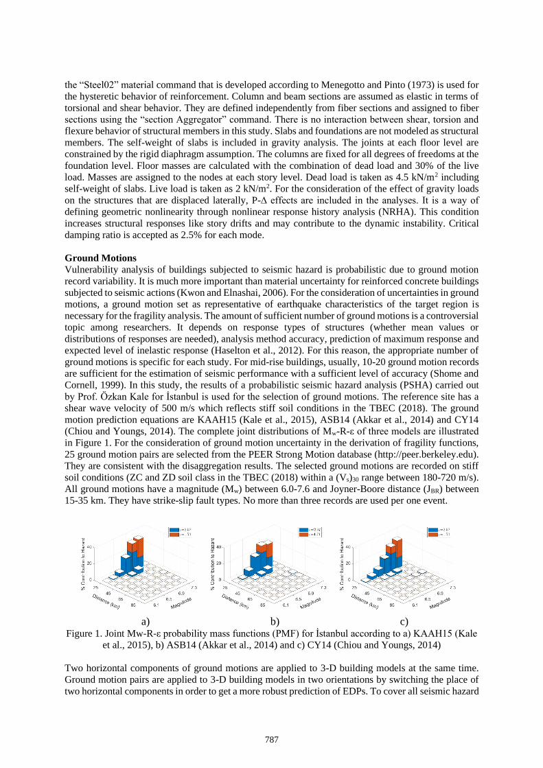
the “Steel02” material command that is developed according to Menegotto and Pinto (1973) is used for

the hysteretic behavior of reinforcement. Column and beam sections are assumed as elastic in terms of

torsional and shear behavior. They are defined independently from fiber sections and assigned to fiber

sections using the “section Aggregator” command. There is no interaction between shear, torsion and

flexure behavior of structural members in this study. Slabs and foundations are not modeled as structural

members. The self-weight of slabs is included in gravity analysis. The joints at each floor level are

constrained by the rigid diaphragm assumption. The columns are fixed for all degrees of freedoms at the

foundation level. Floor masses are calculated with the combination of dead load and 30% of the live

load. Masses are assigned to the nodes at each story level. Dead load is taken as 4.5 kN/m2 including

self-weight of slabs. Live load is taken as 2 kN/m2. For the consideration of the effect of gravity loads

on the structures that are displaced laterally, P-∆ effects are included in the analyses. It is a way of

defining geometric nonlinearity through nonlinear response history analysis (NRHA). This condition

increases structural responses like story drifts and may contribute to the dynamic instability. Critical

damping ratio is accepted as 2.5% for each mode.

Ground Motions

Vulnerability analysis of buildings subjected to seismic hazard is probabilistic due to ground motion

record variability. It is much more important than material uncertainty for reinforced concrete buildings

subjected to seismic actions (Kwon and Elnashai, 2006). For the consideration of uncertainties in ground

motions, a ground motion set as representative of earthquake characteristics of the target region is

necessary for the fragility analysis. The amount of sufficient number of ground motions is a controversial

topic among researchers. It depends on response types of structures (whether mean values or

distributions of responses are needed), analysis method accuracy, prediction of maximum response and

expected level of inelastic response (Haselton et al., 2012). For this reason, the appropriate number of

ground motions is specific for each study. For mid-rise buildings, usually, 10-20 ground motion records

are sufficient for the estimation of seismic performance with a sufficient level of accuracy (Shome and

Cornell, 1999). In this study, the results of a probabilistic seismic hazard analysis (PSHA) carried out

by Prof. Özkan Kale for İstanbul is used for the selection of ground motions. The reference site has a

shear wave velocity of 500 m/s which reflects stiff soil conditions in the TBEC (2018). The ground

motion prediction equations are KAAH15 (Kale et al., 2015), ASB14 (Akkar et al., 2014) and CY14

(Chiou and Youngs, 2014). The complete joint distributions of Mw-R-ε of three models are illustrated

in Figure 1. For the consideration of ground motion uncertainty in the derivation of fragility functions,

25 ground motion pairs are selected from the PEER Strong Motion database (http://peer.berkeley.edu).

They are consistent with the disaggregation results. The selected ground motions are recorded on stiff

soil conditions (ZC and ZD soil class in the TBEC (2018) within a (Vs)30 range between 180-720 m/s).

All ground motions have a magnitude (Mw) between 6.0-7.6 and Joyner-Boore distance (JBR) between

15-35 km. They have strike-slip fault types. No more than three records are used per one event.

a) b) c)

Figure 1. Joint Mw-R-ε probability mass functions (PMF) for İstanbul according to a) KAAH15 (Kale

et al., 2015), b) ASB14 (Akkar et al., 2014) and c) CY14 (Chiou and Youngs, 2014)

Two horizontal components of ground motions are applied to 3-D building models at the same time.

Ground motion pairs are applied to 3-D building models in two orientations by switching the place of

two horizontal components in order to get a more robust prediction of EDPs. To cover all seismic hazard

787

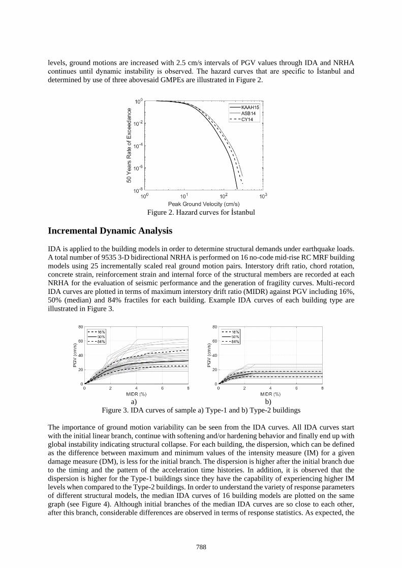
levels, ground motions are increased with 2.5 cm/s intervals of PGV values through IDA and NRHA

continues until dynamic instability is observed. The hazard curves that are specific to İstanbul and

determined by use of three abovesaid GMPEs are illustrated in Figure 2.

Figure 2. Hazard curves for İstanbul

Incremental Dynamic Analysis

IDA is applied to the building models in order to determine structural demands under earthquake loads.

A total number of 9535 3-D bidirectional NRHA is performed on 16 no-code mid-rise RC MRF building

models using 25 incrementally scaled real ground motion pairs. Interstory drift ratio, chord rotation,

concrete strain, reinforcement strain and internal force of the structural members are recorded at each

NRHA for the evaluation of seismic performance and the generation of fragility curves. Multi-record

IDA curves are plotted in terms of maximum interstory drift ratio (MIDR) against PGV including 16%,

50% (median) and 84% fractiles for each building. Example IDA curves of each building type are

illustrated in Figure 3.

a) b)

Figure 3. IDA curves of sample a) Type-1 and b) Type-2 buildings

The importance of ground motion variability can be seen from the IDA curves. All IDA curves start

with the initial linear branch, continue with softening and/or hardening behavior and finally end up with

global instability indicating structural collapse. For each building, the dispersion, which can be defined

as the difference between maximum and minimum values of the intensity measure (IM) for a given

damage measure (DM), is less for the initial branch. The dispersion is higher after the initial branch due

to the timing and the pattern of the acceleration time histories. In addition, it is observed that the

dispersion is higher for the Type-1 buildings since they have the capability of experiencing higher IM

levels when compared to the Type-2 buildings. In order to understand the variety of response parameters

of different structural models, the median IDA curves of 16 building models are plotted on the same

graph (see Figure 4). Although initial branches of the median IDA curves are so close to each other,

after this branch, considerable differences are observed in terms of response statistics. As expected, the

788

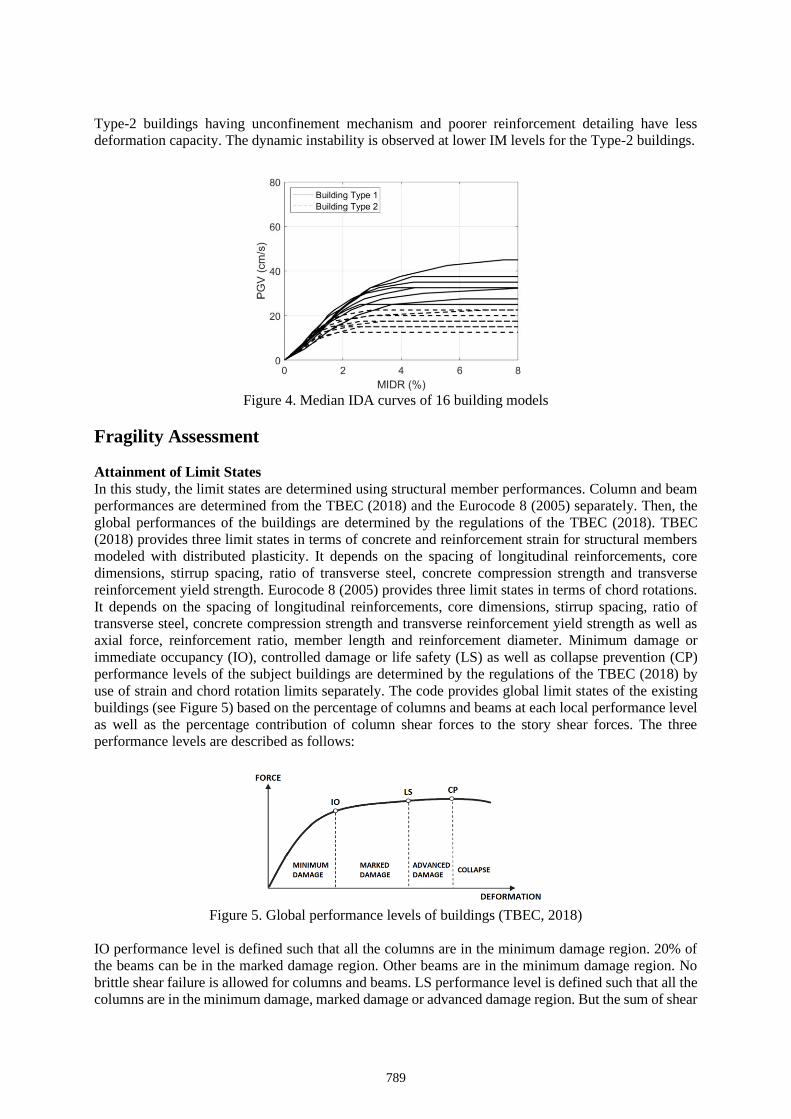
Type-2 buildings having unconfinement mechanism and poorer reinforcement detailing have less

deformation capacity. The dynamic instability is observed at lower IM levels for the Type-2 buildings.

Figure 4. Median IDA curves of 16 building models

Fragility Assessment

Attainment of Limit States

In this study, the limit states are determined using structural member performances. Column and beam

performances are determined from the TBEC (2018) and the Eurocode 8 (2005) separately. Then, the

global performances of the buildings are determined by the regulations of the TBEC (2018). TBEC

(2018) provides three limit states in terms of concrete and reinforcement strain for structural members

modeled with distributed plasticity. It depends on the spacing of longitudinal reinforcements, core

dimensions, stirrup spacing, ratio of transverse steel, concrete compression strength and transverse

reinforcement yield strength. Eurocode 8 (2005) provides three limit states in terms of chord rotations.

It depends on the spacing of longitudinal reinforcements, core dimensions, stirrup spacing, ratio of

transverse steel, concrete compression strength and transverse reinforcement yield strength as well as

axial force, reinforcement ratio, member length and reinforcement diameter. Minimum damage or

immediate occupancy (IO), controlled damage or life safety (LS) as well as collapse prevention (CP)

performance levels of the subject buildings are determined by the regulations of the TBEC (2018) by

use of strain and chord rotation limits separately. The code provides global limit states of the existing

buildings (see Figure 5) based on the percentage of columns and beams at each local performance level

as well as the percentage contribution of column shear forces to the story shear forces. The three

performance levels are described as follows:

Figure 5. Global performance levels of buildings (TBEC, 2018)

IO performance level is defined such that all the columns are in the minimum damage region. 20% of

the beams can be in the marked damage region. Other beams are in the minimum damage region. No

brittle shear failure is allowed for columns and beams. LS performance level is defined such that all the

columns are in the minimum damage, marked damage or advanced damage region. But the sum of shear

789

forces of the columns in the advanced damage region is less than 20% of the story shear force. In

addition, the sum of shear forces of the columns whose top and bottom regions are in the marked damage

or advance damage region is less than 30% of the story shear force. 35% of the beams can be in the

advanced damage region. Other beams are in the minimum damage or marked damage region. No brittle

shear failure is allowed for columns and beams. CP performance level is defined such that all the

columns are in the minimum damage, marked damage or advanced damage region. But the sum of shear

forces of the columns whose top and bottom regions are in the marked damage or advance damage

region is less than 30% of the story shear force. 20% of the beams can be in the collapse region. Other

beams are in the minimum damage, marked damage or advanced damage regions. Brittle shear failure

can only be observed at the beams in the collapse region.

Evaluation of Analytical Fragility Curves

The probability of exceeding a damage state (DS) at a given PGV level is calculated with the fraction

of ground motion records for each building model separately considering two limit state definitions. A

lognormal cumulative distribution function is assumed for the continuous estimation of the exceedance

probability of each DS as a function of PGV. The fragility curves that show the probability of

exceedance of the IO, LS, and CP are illustrated separately and the buildings having the same typology

are included in the same figure (see Figure 6, Figure 7 and Figure 8).

a) b)

Figure 6. IO fragility curves of a) Type-1 and b) Type-2 buildings

a) b)

Figure 7. LS fragility curves of a) Type-1 and b) Type-2 buildings

a) b)

Figure 8. CP fragility curves of a) Type-1 and b) Type-2 buildings

790

Although both building types reach collapse state at low PGV values, the Type-2 buildings seem more

vulnerable since their structural members have unconfined concrete and less amount of reinforcement.

It is observed that there is considerable variability between fragility curves of the buildings that are in

the same typology. Therefore, consideration of variabilities in structural models makes a huge impact

on the exceedance probabilities of damage states. According to the results of NRHA, in almost all cases,

the exceedance of the IO limit of the buildings is due to the beams. That is, although columns do not

reach the IO limit yet, the buildings exceed the IO limit since 20% of the beams exceeds the IO limit.

For the exceedance of the LS limit of the buildings, both columns and beams are effective. But the

performance of columns mostly determines whether the building exceed the CP limit or not. In general,

failure is observed in the first story. Among two limit state definitions, in all cases, strain limits

calculated according to the TBEC (2018) give more conservative fragility curves when compared to the

chord rotation limits calculated according to the Eurocode 8 (2005). This is mainly due to the difference

between formulation of limit state definitions of abovesaid codes. In general, LS fragility curves are

close to the CP fragility curves. The main reason is the way for the determination of the global

performance of the buildings used in this study. When only columns are considered, the only difference

between the DS of LS and CP is that the LS performance level does not allow the sum of shear forces

of the columns in the advanced damage region to be more than 20% of the story shear force at each

story. When columns are dominant for buildings to reach the DS of the LS and CP, the resultant LS

fragility curves are close to the CP fragility curves. Another reason for this situation is that the LS limits

of structural members are close to the CP limit rather than the IO limit, especially for the Type-1

buildings.

In addition, fragility curves of two building types are generated with 95% confidence intervals and

illustrated in Figure 9. Two limit state definitions and all the building models that are in the same

typology are included in the same fraction for the generation of fragilities for subject building stock.

a) b)

Figure 9. Fragility curves of a) Type-1 and b) Type-2 buildings with 95% confidence levels

It can be seen from fragility curves that subject buildings are collapsed at very low IM levels and they

are explicitly vulnerable under future earthquakes. The TBEC (2018) states that the target performance

level for existing residential RC buildings is LS under earthquakes with DD-2 level (earthquakes having

10% exceedance probability in 50 years). According to the hazard curves illustrated in Figure 2, the

PGV values of earthquakes having 10% exceedance probability in 50 years is 25 cm/s in KAAH15 (Kale

et al., 2015), 31 cm/s in ASB14 (Akkar et al., 2014) and 29 cm/s in CY14 (Chiou and Youngs, 2014).

The above fragility curves show that all no-code mid-rise RC buildings in İstanbul reach collapse under

the earthquakes having the 475-year return period.

Conclusion

This study has been carried out to provide analytical fragility functions for no-code mid-rise reinforced

concrete frame-type buildings for İstanbul that partially encompass the no-code building vulnerability

in Turkey. The resulting fragility curves strongly depend on the variation of structural models within

the same building typology. Therefore, consideration of different types of structural plan is essential for

a proper fragility assessment of building stocks. It is a well-known fact that in order to observe full

791

inelastic response ranges of buildings under seismic actions, a large suite of suitable earthquake records

with different time and pattern characteristics should be applied to the building models. In addition,

change in the definition of limit states highly imprints the results of analytical fragility analysis. To

illustrate, for subject building models, consideration of strain limits of the structural components gives

conservative fragility curves when compared to the ones developed using chord rotation limits. As a

result, consideration of uncertainties in (a) structural models, (b) earthquake records and (c) limit state

definitions makes an enormous effect on the loss assessment of building stocks. To this respect, a

backbone fragility curve by up and down scaling of a central model is an obligation for the estimation

of exceedance probability of damage states of building stocks.

Among analysis types, IDA (Vamvatsikos and Cornell, 2002) gives ideal and practical solutions for the

estimation of inelastic response of buildings under an increasing intensity level of earthquakes. NRHA

results of 16 building models reflecting about 800 existing no-code mid-rise RC MRF buildings in the

Zeytinburnu distinct in Istanbul show that subject building stock is highly vulnerable under future

earthquakes. The existing buildings are constructed before 1980 with traditional techniques and poor

controlling mechanism, i.e., structural detailing of them do not satisfy an earthquake design code.

Therefore, subject buildings are named as no-code buildings. Poor detailing of structural members of

no-code buildings results reaching collapse state at earlier stages of IDA. That is, the buildings exceed

the CP performance level at low IM levels. All building models reach collapse state under earthquakes

having 475-year return period.

References

Dolağan, İ. (2019), “Development of Peak Ground Acceleration (PGA) Based Pre-Code Reinforced Concrete

Frame Building Fragilities for İstanbul”, M.Sc. Thesis, Departmen t of Earthquake Engineering,

Boğazici University, Istanbul, Turkey

Duran, H.İ. (2020), “PGV Based No-Code Mid-Rise Reinforced Concrete Frame-Type Building Fragilities

in Istanbul”, M.Sc. Thesis, Department of Earthquake Engineering, Boğazici University, Istanbul,

Turkey

European Committee for Standardization (2005), “Eurocode 8: Design of Structures for Earthquake

Resistance, Part 3: Strengthening and Repair of Buildings”, Eurocode 8, Brussels

Haselton, C. B., Whittaker, A. S., Hortacsu, A., Baker, J. W., Bray, J., & Grant, D. N. (2012), “Selecting and

Scaling Earthquake Ground Motions for Performing Response-History Analyses”, In Proceedings of

the 15th World Conference on Earthquake Engineering 4207-4217, Earthquake Engineering

Research Institute

Kwon, O. S., & Elnashai, A. (2006), “The Effect of Material and Ground Motion Uncertainty on the Seismic

Vulnerability Curves of RC Structure”, Engineering Structures, 28(2), 289 -303

Mander, J. B., Priestley, M.J.N., and Park, R. (1988), “Theoretical Stress‐Strain Model for Confined

Concrete”, Structural Engineering, Vol. 114, Issue 8

Masjed-Jamei, Mohammad, M. R. Eslahchi, and Mehdi Dehghan (2005), “On Numerical Improvement of

Gauss–Radau Quadrature Rules”, Applied Mathematics and Computation, 168.1, 51 -64

Menegotto, M., & Pinto, P. (1973), “Method of Analysis for Cyclically Loaded Reinforced Concrete Plane

Frames Including Changes in Geometryand Non-elastic Behavior of Elements Under Combined

Normal Force and Bending. Proceedings”, IABSE Sympoium on Resistance and Ultimate

Deformability of Structures Acted on by Well-Defined Repeated Loads

Shome, N. and Cornell, C. A. (1999), “Probabilistic Seismic Demand Analysis of Nonlinear Structures”,

Report No. RMS-35, RMS Program, Stanford University, Stanford, CA

Turkish Building Earthquake Code (2018), “Specification for Design of Buildings in Disaster Areas”,

Disaster and Emergency Management Presidency, Government of Republic of Turkey

Turkish Earthquake Code (1975), “Specification for Structures to be Built in Disaster Areas”, Ministry of

Public Works and Settlement, Government of Republic of Turkey

Vamvatsikos, D., and Cornell, C.A. (2002), “Incremental Dynamic Analysis”, Earthquake Engineering and

Structural Dynamics, 31:491–514

792

Development of PGA-Based Pre-Code Reinforced Concrete Frame Building Fragilities for Istanbul

İpek Dolağan1, Sinan Akkar2

1Department of Earthquake Engineering, Boğaziçi University, Istanbul, Turkey 2Prof. Dr., Department of Earthquake Engineering, Boğaziçi University, Istanbul, Turkey

*İpek Dolağan, [email protected]

AbstractAn important portion of the pre-code building stock in Istanbul runs a significant earthquake risk. Given a building class, the uncontrolled construction of pre-code buildings in the past leads to considerable model variability and complicates the prediction of losses for future earthquakes in Istanbul. However, the social and economic loss estimations are necessary for this megapol to have planned actions to improve earthquake resilience. At this point, fragility curves that describe the exceedance probability of a particular damage state are one of the most critical components of seismic resilience-based performance assessment of building inventories in large metropolitan areas. This study aims to provide fragility curves for pre-code reinforced concrete frame residential buildings in Istanbul. For this purpose, 800 mid-rise frame buildings located in the Zeytinburnu district in Istanbul are compiled, and 16 representative building models are developed to account for the model variability of the same building class. The fragilities are based on Peak Ground Acceleration because such practical ground-motion intensity measures are being popularly used in the loss assessment of large building stocks. Nonlinear building responses are derived from three-dimensional nonlinear response history analyses that are carried out by using OpenSees Software (Open System for Earthquake Simulation). Incremental Dynamic Analysis is performed to determine the statistical distribution of the response parameters. A set of real ground motions, which are consistent with the disaggregation results of a probabilistic seismic hazard assessment for Istanbul, are considered in the analyses. Together with the chosen ground-motion dataset, the IDA results represent the variability in building models of the same building class as well as the record-to-record variability that is reflected on to developed fragilities. The fragility model is represented as a backbone cure with upper and lower bounds covering the model and ground-motion variabilities for mid-rise pre-code RC frame buildings in the investigated building stock.

Keywords: Mid-rise reinforced concrete frame buildings in Turkey, Fragility function modeling, Incremental Dynamic Analysis, Earthquake risk in Istanbul.

Introduction

The rapid urbanization in 1970’s and 1980’s resulted in large residential building stocks with low quality in the metropolitan cities in Turkey. A large portion of these buildings are poorly engineered against seismic action since the first national earthquake code is enforced in Turkey in 1975. This is because the design engineers were not fully aware of the fundamentals of earthquake resistant design. Besides the lack of control during the construction period further increased the vulnerability of these buildings against earthquakes. This led to enormous economic losses and casualties in 1999, the Marmara Earthquakes, the first urban earthquakes in Turkey. The lessons learned from the Marmara earthquakes motivated the Turkish state to replace the poor quality building stock in metropolitan areas, in particular large earthquake prone cities such as Istanbul, Bursa and Izmir. This national policy triggered many earthquake engineering studies both in academia and professional environment having objectives of rapid seismic performance assessment (e.g., Erdik et al., 2003).

793

Currently, seismic performance assessment is risk-oriented and follow probabilistic approaches due to inherent uncertainties in ground motions, building models and building response due to complicated interaction between earthquakes and buildings. Probabilistic methods in risk-oriented seismic performance assessment make use of occurrence probability of ground motion amplitudes given a specific time interval and occurrence probability of different damage states under this excitation (Moehle and Deierlein, 2004). Regardless of the complications in probabilistic risk-oriented performance assessment methods, one of the corner stones in these approaches is fragility functions that are used to estimate the exceedance probabilities of damage states given a ground motion demand. Development of building-based fragility functions for no code buildings in Istanbul is the main topic of investigation in this study that can be used in probabilistic risk-oriented performance assessment.

Evaluation of Fragility Functions Fragility curves represent the probability of reaching or exceeding a specific damage state for a given Engineering Demand Parameter (EDP) of the structure. Components of the fragility curves are the intensity measure and the damage state definition. Intensity measure (e.g., PGA, PSa, MMI) correlates the earthquake parameter to the building damage. The damage state definitions are related to the evaluated performance metrics. There are various damage state definitions such as Immediate Occupancy, Life safety, and Collapse Prevention in the guidelines and in the literature. These definitions indicate the likely damage state of the structure due to an earthquake. Traditionally, fragility curves are expressed by lognormal distribution. The lognormal distribution defines the conditional probability of the damage state of interest at various intensity levels. For a regional earthquake risk assessment, fragility curves are derived for a class of building group such as mid-rise reinforced concrete moment resisting frame buildings are used. The fragility functions should be compatible with the local construction practice and adopting the fragilities specifically derived for other countries may lead to erroneous structural performance estimations.

Building Inventory

The blueprints of 800 residential buildings in Zeytinburnu District that are built before 1980 (pre-1980 buildings) are examined to develop subject fragility functions. The construction practice of the residential buildings compiled from Zetyinburnu is similar to most of the existing pre-1980 residential buildings in Istanbul. Thus, it is believed that the compiled building inventory is representative of pre-1980 residentail buildings in Istanbul. Given a building in the inventory, more than 50 parameters that characterize material properties and geometrical characteristics (e.g., plan dimensions, element cross-sections, story height, etc.) are extracted from the blueprints. The statistics of these parameters are combined to establish representative building models for nonlinear response history analysis. Since 95% of these buildings are RC-MRF, only this building typology is included within the scope of this study. The compiled building inventory is limited in terms of story numbers to consider modelling of different height-based building classes. Hence, the models established from the database is representative of mid-rise RC-MRF pre-1980 buildings in Turkish building construction.

Definitions of the Building Characteristics The inventory survey reveals that the subject building stock has poor geometrical configuration and low material quality, which are the general characteristics of pre-1975 construction practice in Istanbul. The most notable geometrical layout characteristics are the unsymmetrical plan configuration, discontinuities in columns and beams along a frame axis, the existence of added floor and mezzanine floor. It is believed that neither of these geometrical characteristics are considered during the design stage at that time. The existence of added floor and mezzanine floor, and the discontinuities along a frame axis are explicitly modelled in the representative buildings. The statistics of the rest of the parameters are directly used while establishing the representative models.

794

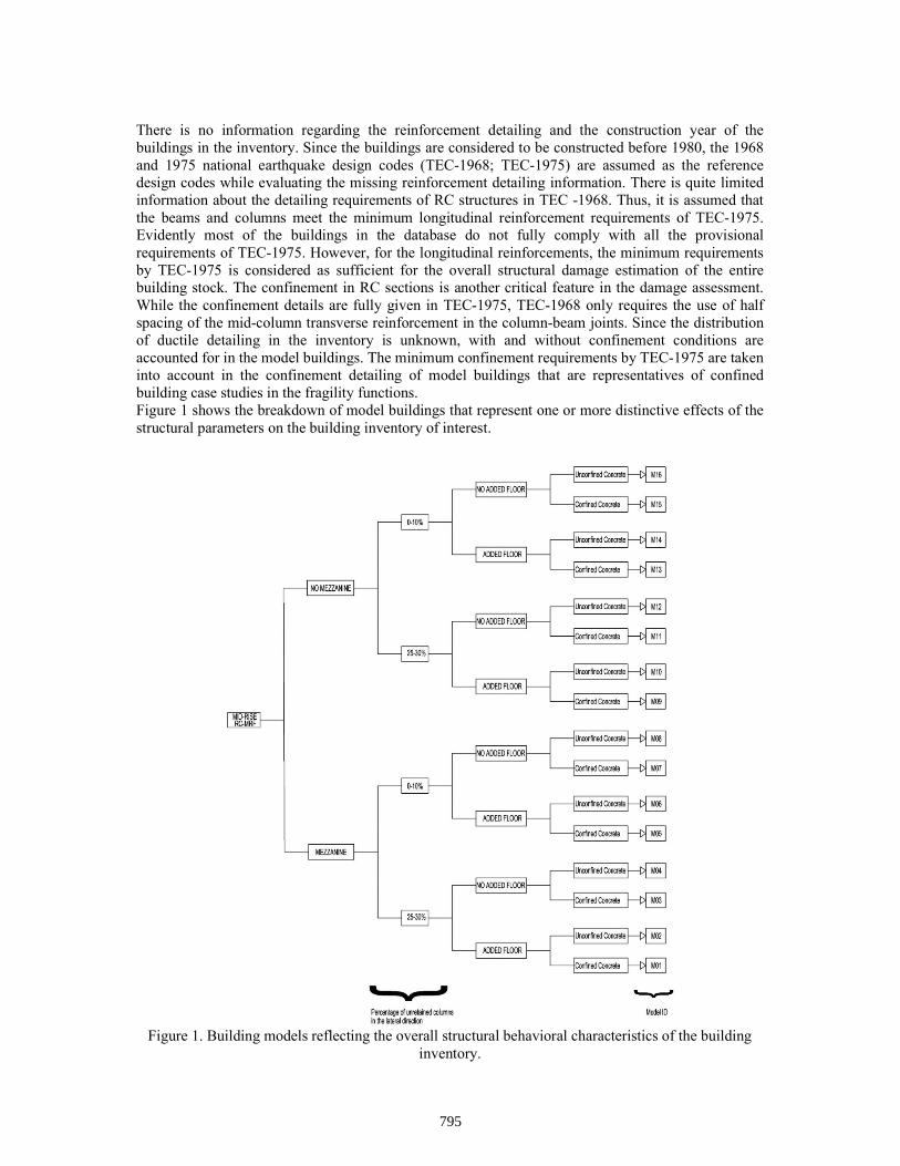
There is no information regarding the reinforcement detailing and the construction year of the buildings in the inventory. Since the buildings are considered to be constructed before 1980, the 1968 and 1975 national earthquake design codes (TEC-1968; TEC-1975) are assumed as the reference design codes while evaluating the missing reinforcement detailing information. There is quite limited information about the detailing requirements of RC structures in TEC -1968. Thus, it is assumed that the beams and columns meet the minimum longitudinal reinforcement requirements of TEC-1975. Evidently most of the buildings in the database do not fully comply with all the provisional requirements of TEC-1975. However, for the longitudinal reinforcements, the minimum requirements by TEC-1975 is considered as sufficient for the overall structural damage estimation of the entire building stock. The confinement in RC sections is another critical feature in the damage assessment. While the confinement details are fully given in TEC-1975, TEC-1968 only requires the use of half spacing of the mid-column transverse reinforcement in the column-beam joints. Since the distribution of ductile detailing in the inventory is unknown, with and without confinement conditions are accounted for in the model buildings. The minimum confinement requirements by TEC-1975 are taken into account in the confinement detailing of model buildings that are representatives of confined building case studies in the fragility functions. Figure 1 shows the breakdown of model buildings that represent one or more distinctive effects of the structural parameters on the building inventory of interest.

Figure 1. Building models reflecting the overall structural behavioral characteristics of the building inventory.

795

Analytical Modelling

OpenSees Software (Open System for Earthquake Simulation; UC Berkeley, 2019) is used to generate the 3D numerical models of the model buildings. Beam and column elements are modeled with force-based ‘nonlinearBeamColumn’ command in OpenSees, which considers the spread plasticity along the element. Gauss-Lobatto Integration (Neuenhofer and Filippou, 1997) is utilized by using five integration points within the element. P-Δ effects are considered along the columns in all buildings. The columns are fixed at the base floor. The elements are modeled with fiber sections, in which the cover and the core concrete are divided into 10 x 10 and 20 x 20 subsections, respectively and the reinforcing bars are defined by straight layers. Confined concrete model is implemented in accordance with the model proposed by Mander et al. (1984). The coupled axial and biaxial-bending behavior is directly modeled in fiber sections. Shear behavior is introduced linearly (uncoupled axial/flexural-shear behavior) to the models. For columns, brittle shear failure is taken into account (i.e., analysis stops when the column experiences shear failure) by considering the member shear capacity formulation defined in Turkish Standards for Design and Construction of RC Structures, TS-500 (Turkish Standards Institute, 2000). Shear failure is not explicitly included in the analytic models for beams because it is not desired to stop the analysis due to brittle failure of one (or few) beams. However, the occurrence of shear failure in beams is post-processed. No other deterioration modes such as bond-slip, local buckling, and fracture of reinforcing steel are considered because the utilized fiber model is not capable of capturing such effects. Consideration of such nonlinear failure modes increases the complexity in the analytical models and may lead to convergence problems. It should be noted that neglecting these failure modes would affect the response of no-code (or low-code) building models that are of interest in this study. Therefore, resulting fragility functions that are presented in the following sections should be evaluated within this limitation imposed to the analytical models. The story masses are obtained according to the dead and 30% of the live loads and are assigned to the beam-column joints. Modal damping of 2.5% is assumed for the building models. The record dataset is compiled from the Pacific Earthquake Engineering Research (PEER) Center Strong Motion database (https://ngawest2.berkeley.edu/) and represents the site-specific Probabilistic Seismic Hazard Assessment (PSHA) at a site in Istanbul. In essence, the compiled ground-motion dataset consists of 25 ground-motion records of strike-slip faulting, within a moment magnitude range of 6.0 ≤ Mw ≤ 7.6 and Joyner-Boore distance of 15 km ≤ RJB ≤ 35 km. The records are from sites pertaining to site classes ZC and ZD (TEC-2019) having average shear wave velocities at the top 30 m soil layer 360 m/s ≤ VS30 ≤ 760 m/s and 180 m/s ≤ VS30 ≤ 360 m/s, respectively. Pulse-dominant waveforms are not included in the ground motion record set.

Incremental Dynamic Analysis

The present study conducts Incremental Dynamic Analysis (IDA) (Vamvatsikos and Cornell, 2002). Since this study aims to provide fragility functions to assess the probabilistic risk of broad classes of building inventories, PGA, which is one of the structural period independent IMs is selected as the ground motion IM. PGA is also one of the most frequent IMs computed in Probabilistic Seismic Hazard Assessment (PSHA). Therefore, the fragility relations defined in terms of PGA can easily be implemented for seismic risk analysis along with available PSHA studies. Response parameters, including interstory drift ratios in both direction, strains, chord rotations, and plastic rotations, are recorded during the NRHA. The geometrical mean (geomean) PGA of selected ground-motion records are scaled from 0.025 g to the PGA value, which causes dynamic instability in the model for IDA runs. The increment used for geomen PGA scaling is 0.025 g. Dynamic instability (collapse) is defined when a significant increase is observed in the EDP (e.g., interstory drift ratio) for small increments of the mean PGA. Dynamic instability is also assessed and when numeric instability is observed in the nonlinear response history

796

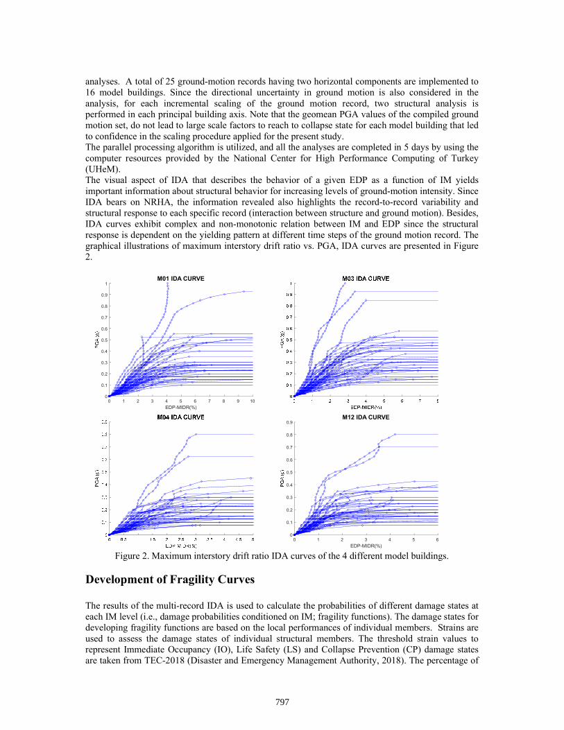
analyses. A total of 25 ground-motion records having two horizontal components are implemented to 16 model buildings. Since the directional uncertainty in ground motion is also considered in the analysis, for each incremental scaling of the ground motion record, two structural analysis is performed in each principal building axis. Note that the geomean PGA values of the compiled ground motion set, do not lead to large scale factors to reach to collapse state for each model building that led to confidence in the scaling procedure applied for the present study. The parallel processing algorithm is utilized, and all the analyses are completed in 5 days by using the computer resources provided by the National Center for High Performance Computing of Turkey (UHeM). The visual aspect of IDA that describes the behavior of a given EDP as a function of IM yields important information about structural behavior for increasing levels of ground-motion intensity. Since IDA bears on NRHA, the information revealed also highlights the record-to-record variability and structural response to each specific record (interaction between structure and ground motion). Besides, IDA curves exhibit complex and non-monotonic relation between IM and EDP since the structural response is dependent on the yielding pattern at different time steps of the ground motion record. The graphical illustrations of maximum interstory drift ratio vs. PGA, IDA curves are presented in Figure 2.

Figure 2. Maximum interstory drift ratio IDA curves of the 4 different model buildings.

Development of Fragility Curves

The results of the multi-record IDA is used to calculate the probabilities of different damage states at each IM level (i.e., damage probabilities conditioned on IM; fragility functions). The damage states for developing fragility functions are based on the local performances of individual members. Strains are used to assess the damage states of individual structural members. The threshold strain values to represent Immediate Occupancy (IO), Life Safety (LS) and Collapse Prevention (CP) damage states are taken from TEC-2018 (Disaster and Emergency Management Authority, 2018). The percentage of

0 1 2 3 4 5 6 7 8 9 10

EDP-MIDR(%)

0

0.1

0.2

0.3

0.4

0.5

0.6

0.7

0.8

0.9

1M01 IDA CURVE

0 1 2 3 4 5 6

EDP-MIDR(%)

0

0.1

0.2

0.3

0.4

0.5

0.6

0.7

0.8

0.9M12 IDA CURVE

797

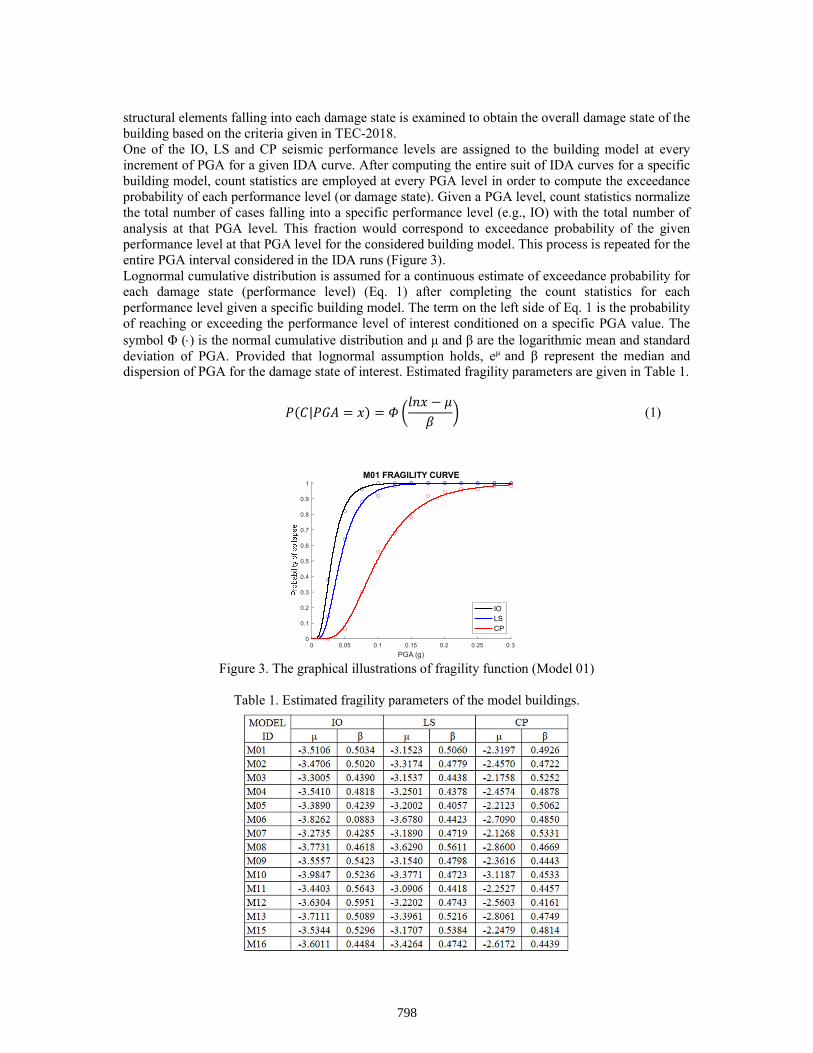
structural elements falling into each damage state is examined to obtain the overall damage state of the building based on the criteria given in TEC-2018. One of the IO, LS and CP seismic performance levels are assigned to the building model at every increment of PGA for a given IDA curve. After computing the entire suit of IDA curves for a specific building model, count statistics are employed at every PGA level in order to compute the exceedance probability of each performance level (or damage state). Given a PGA level, count statistics normalize the total number of cases falling into a specific performance level (e.g., IO) with the total number of analysis at that PGA level. This fraction would correspond to exceedance probability of the given performance level at that PGA level for the considered building model. This process is repeated for the entire PGA interval considered in the IDA runs (Figure 3). Lognormal cumulative distribution is assumed for a continuous estimate of exceedance probability for each damage state (performance level) (Eq. 1) after completing the count statistics for each performance level given a specific building model. The term on the left side of Eq. 1 is the probability of reaching or exceeding the performance level of interest conditioned on a specific PGA value. The symbol Φ () is the normal cumulative distribution and μ and β are the logarithmic mean and standard deviation of PGA. Provided that lognormal assumption holds, eμ and β represent the median and dispersion of PGA for the damage state of interest. Estimated fragility parameters are given in Table 1.

Figure 3. The graphical illustrations of fragility function (Model 01)

Table 1. Estimated fragility parameters of the model buildings.

0 0.05 0.1 0.15 0.2 0.25 0.3

PGA (g)

0

0.1

0.2

0.3

0.4

0.5

0.6

0.7

0.8

0.9

1M01 FRAGILITY CURVE

IOLSCP

𝑃(𝐶|𝑃𝐺𝐴 = 𝑥) = 𝛷𝑙𝑛𝑥 − 𝜇

𝛽 (1)

798

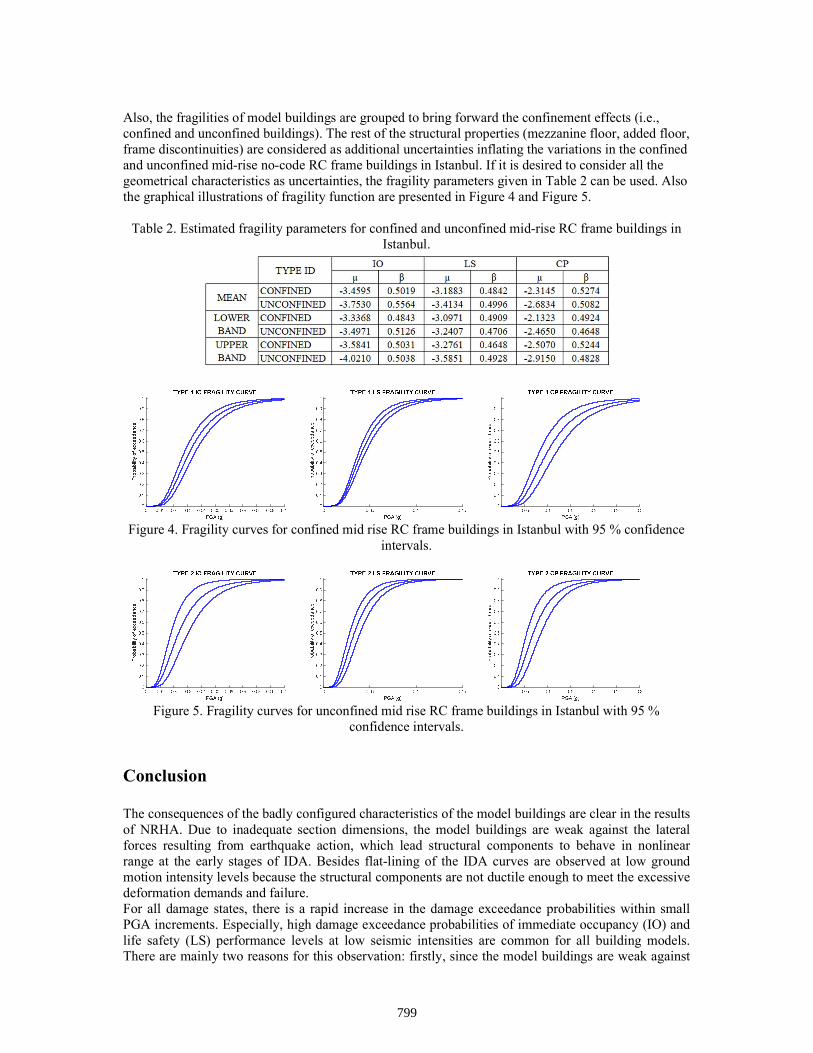
Also, the fragilities of model buildings are grouped to bring forward the confinement effects (i.e., confined and unconfined buildings). The rest of the structural properties (mezzanine floor, added floor, frame discontinuities) are considered as additional uncertainties inflating the variations in the confined and unconfined mid-rise no-code RC frame buildings in Istanbul. If it is desired to consider all the geometrical characteristics as uncertainties, the fragility parameters given in Table 2 can be used. Also the graphical illustrations of fragility function are presented in Figure 4 and Figure 5.

Table 2. Estimated fragility parameters for confined and unconfined mid-rise RC frame buildings in Istanbul.

Figure 4. Fragility curves for confined mid rise RC frame buildings in Istanbul with 95 % confidence intervals.

Figure 5. Fragility curves for unconfined mid rise RC frame buildings in Istanbul with 95 % confidence intervals.

Conclusion

The consequences of the badly configured characteristics of the model buildings are clear in the results of NRHA. Due to inadequate section dimensions, the model buildings are weak against the lateral forces resulting from earthquake action, which lead structural components to behave in nonlinear range at the early stages of IDA. Besides flat-lining of the IDA curves are observed at low ground motion intensity levels because the structural components are not ductile enough to meet the excessive deformation demands and failure. For all damage states, there is a rapid increase in the damage exceedance probabilities within small PGA increments. Especially, high damage exceedance probabilities of immediate occupancy (IO) and life safety (LS) performance levels at low seismic intensities are common for all building models. There are mainly two reasons for this observation: firstly, since the model buildings are weak against

799

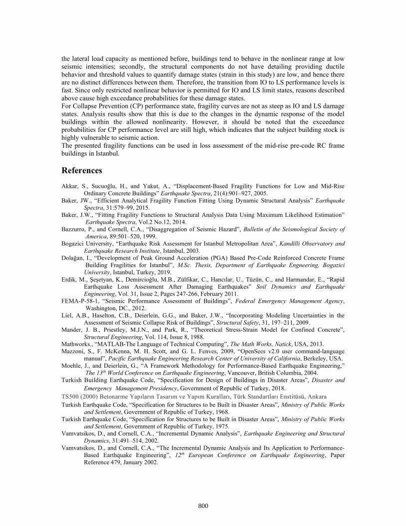
the lateral load capacity as mentioned before, buildings tend to behave in the nonlinear range at low seismic intensities; secondly, the structural components do not have detailing providing ductile behavior and threshold values to quantify damage states (strain in this study) are low, and hence there are no distinct differences between them. Therefore, the transition from IO to LS performance levels is fast. Since only restricted nonlinear behavior is permitted for IO and LS limit states, reasons described above cause high exceedance probabilities for these damage states. For Collapse Prevention (CP) performance state, fragility curves are not as steep as IO and LS damage states. Analysis results show that this is due to the changes in the dynamic response of the model buildings within the allowed nonlinearity. However, it should be noted that the exceedance probabilities for CP performance level are still high, which indicates that the subject building stock is highly vulnerable to seismic action. The presented fragility functions can be used in loss assessment of the mid-rise pre-code RC frame buildings in Istanbul.

References

Akkar, S., Sucuoğlu, H., and Yakut, A., “Displacement-Based Fragility Functions for Low and Mid-Rise Ordinary Concrete Buildings” Earthquake Spectra, 21(4):901–927, 2005.

Baker, JW., “Efficient Analytical Fragility Function Fitting Using Dynamic Structural Analysis” Earthquake Spectra, 31:579–99, 2015.

Baker, J.W., “Fitting Fragility Functions to Structural Analysis Data Using Maximum Likelihood Estimation” Earthquake Spectra, Vol.2 No.12, 2014.

Bazzurro, P., and Cornell, C.A., “Disaggregation of Seismic Hazard”, Bulletin of the Seismological Society of America, 89:501–520, 1999.

Bogazici University, “Earthquake Risk Assessment for Istanbul Metropolitan Area”, Kandilli Observatory and Earthquake Research Institute, Istanbul, 2003.

Dolağan, I., “Development of Peak Ground Acceleration (PGA) Based Pre-Code Reinforced Concrete Frame Building Fragilities for Istanbul”, M.Sc. Thesis, Department of Earthquake Engneering, BogaziciUniversity, Istanbul, Turkey, 2019.

Erdik, M., Şeşetyan, K., Demircioğlu, M.B., Zülfikar, C., Hancılar, U., Tüzün, C., and Harmandar, E., “Rapid Earthquake Loss Assessment After Damaging Earthquakes” Soil Dynamics and Earthquake Engineering, Vol. 31, Issue 2, Pages 247-266, February 2011.

FEMA-P-58-1, “Seismic Performance Assessment of Buildings”, Federal Emergency Management Agency, Washington, DC., 2012.

Liel, A.B., Haselton, C.B., Deierlein, G.G., and Baker, J.W., “Incorporating Modeling Uncertainties in the Assessment of Seismic Collapse Risk of Buildings”, Structural Safety, 31, 197–211, 2009.

Mander, J. B., Priestley, M.J.N., and Park, R., “Theoretical Stress‐Strain Model for Confined Concrete”, Structural Engineering, Vol. 114, Issue 8, 1988.

Mathworks., “MATLAB-The Language of Technical Computing”, The Math Works, Natick, USA, 2013. Mazzoni, S., F. McKenna, M. H. Scott, and G. L. Fenves, 2009, “OpenSees v2.0 user command-language

manual”, Pacific Earthquake Engineering Research Center of University of California, Berkeley, USA. Moehle, J., and Deierlein, G., “A Framework Methodology for Performance-Based Earthquake Engineering,”

The 13th World Conference on Earthquake Engineering, Vancouver, British Columbia, 2004. Turkish Building Earthquake Code, “Specification for Design of Buildings in Disaster Areas”, Disaster and

Emergency Management Presidency, Government of Republic of Turkey, 2018. TS500 (2000) Betonarme Yapıların Tasarım ve Yapım Kuralları, Türk Standartları Enstitüsü, Ankara Turkish Earthquake Code, “Specification for Structures to be Built in Disaster Areas”, Ministry of Public Works

and Settlement, Government of Republic of Turkey, 1968. Turkish Earthquake Code, “Specification for Structures to be Built in Disaster Areas”, Ministry of Public Works

and Settlement, Government of Republic of Turkey, 1975. Vamvatsikos, D., and Cornell, C.A., “Incremental Dynamic Analysis”, Earthquake Engineering and Structural

Dynamics, 31:491–514, 2002. Vamvatsikos, D., and Cornell, C.A., “The Incremental Dynamic Analysis and Its Application to Performance-

Based Earthquake Engineering”, 12th European Conference on Earthquake Engineering, Paper Reference 479, January 2002.

800

Comparison of an RC Flat-Slab and a Frame Building’s Dynamic Behavior Utilizing Ambient Vibration Measurements

Canberk Bolat1*, Hasan Celil Yelken1, Onur Kaplan2

1 Civil Engineering Department, Eskisehir Technical University, Turkey 2 Earth and Space Sciences Institute, Eskisehir Technical University, Turkey


Abstract

Flat-slab is a reinforced concrete slab supported directly by columns without beams. Since there are no beams in the system, the load transfer between the vertical structural system components is only possible with the reinforced concrete slab. Therefore, earthquake behavior of flat-slab buildings is not so good and are considered risky to be applied in earthquake-prone regions. In this study, a reinforced concrete flat-slab building's dynamic characteristics were determined through ambient vibration measurements using seismometers. Additionally, the flat-slab building’s lateral stiffness was compared to a reinforced concrete frame building, in which the mass of the building is close to the flat-slab building's mass, utilizing fundamental periods of the buildings. Results showed that, although the total stiffness of the vertical members of the flat-slab building is about five times greater than the frame building’s, the fundamental period of the flat-slab building was observed to be 37% longer than the frame building’s fundamental period.

Keywords: Flat-slab, ambient vibration, frame building, fundamental period.

Introduction

The flat slab is a two-way reinforced concrete slab that usually does not have beams and girders, and the loads are transferred directly to the supporting concrete columns (Hassoun and Manaseer, 2012). Flat-slab systems are preferred due to its advantages compare to moment-resisting frame counterparts such as obtaining a flat ceiling without beams, lower floor height, ease of formwork and reinforcement work, and practicality of applying mechanical and electrical equipment. Even though, flat-slab systems are preferred due to their various advantages they are considered as risky to be applied in earthquake-prone regions. Since there are no beams in the system, the load transfer between the vertical structural system components is only possible with the reinforced concrete slab. Therefore, earthquake behavior of flat-slab buildings is not so good that is why it was recommended that in regions with high seismic hazard, flat-slab construction should only be used as the vertical load carrying system in structures braced by frames or shear walls responsible for the lateral capacity of the structure, earthquake loads should be resisted by structural walls in such systems (ACI, 1988). Generally in mediterranean region, contrary to the above code provision the flat-slab systems are often adopted as the primary lateral load-resisting system. In these cases, the design of the flat-slab buildings is typically carried out in a manner similar to ordinary frames (Erberik and Elnashai, 2004). Where this practice is followed, the response under moderate earthquakes indicates extensive damage to non-structural elements even when the code provisions for drift limitation are satisfied (Chow and Selna, 1995). Erberik and Elnashai (2004) investigated the vulnerability of the flat-slab sructures and developed fragility curves for flat-slab structures. Another disadvantage of the flat-slab systems is the punching effect around the columns and the flat-slab buildings are more significantly flexible than moment-resisting frame buildings because of the absence of deep beams. In other words the lateral stiffness of a flat-slab building is generally less than a similar frame building. Fundamental period of a building is a good indicator of buildings’ lateral stiffness. Ambient vibration measurements provide us the opportunity to determine the fundamental

801

period of an existing building. Carder (1937) first introduced the concept of ambient vibration method when measuring buildings in California and Montana (Salameh et al. 2016). This method has been developed over the years and has been used worldwide because it is easy, fast, cheap, reliable, and based on the use of low excitation generated by ambient sources like wind or anthropic activity such as traffic, machinery, etc. and applicable on buildings (Trifunac 1972; Farsi and Bard 2004; Mikael et al. 2013). In this study, a reinforced concrete flat-slab building's dynamic characteristics were determined through ambient vibration measurements using four broadband force-balanced seismometers. Additionally, the flat slab building’s lateral stiffness was compared to a reinforced concrete frame building, in which the mass of the building is quite close to the flat-slab building's mass, utilizing fundamental periods of the buildings.

Material and methods

To compare the lateral stiffness difference between a frame building and a flat slab building, ambient vibration measurements were conducted in two reinforced concrete residential buildings that are located in Eskisehir, Turkey. The flat-slab building type is a very rare practice in Eskisehir building stock. Then it was a good opportunity to find such a building to compare with a frame building counterpart in terms of lateral stiffness. Structural properties of these two buildings are shown in Table 1. Both buildings have five stories. The floor areas and the height of the buildings are very close to each other. Exterior photos, schematic views of the structural systems and formwork plans of the frame and the flat-slab buildings are shown in Figure 1.

Table 1. Structural properties of the frame and the flat-slab buildings

The Flat-Slab Building The Frame Building Number of floors 5 5 Typical floor area (m2) 234 244 Building height (m) 15 14 Total area of vertical members in x-direction (m2) 2.70 1.85 Total area of vertical members in y-direction (m2) 2.16 1.55 Total moment of inertia of vertical members in x-direction (m4) 0.53 0.10 Total moment of inertia of vertical members in y-direction (m4) 0.52 0.18 Total moment of inertia of infill walls in x-direction (m4) 27.11 30.16 Total moment of inertia of infill walls in y-direction (m4) 39.14 42.32 Estimated building mass (kg) 1191000 1031000 28-day cylinder compressive strength of the concrete (MPa) 30 30

802

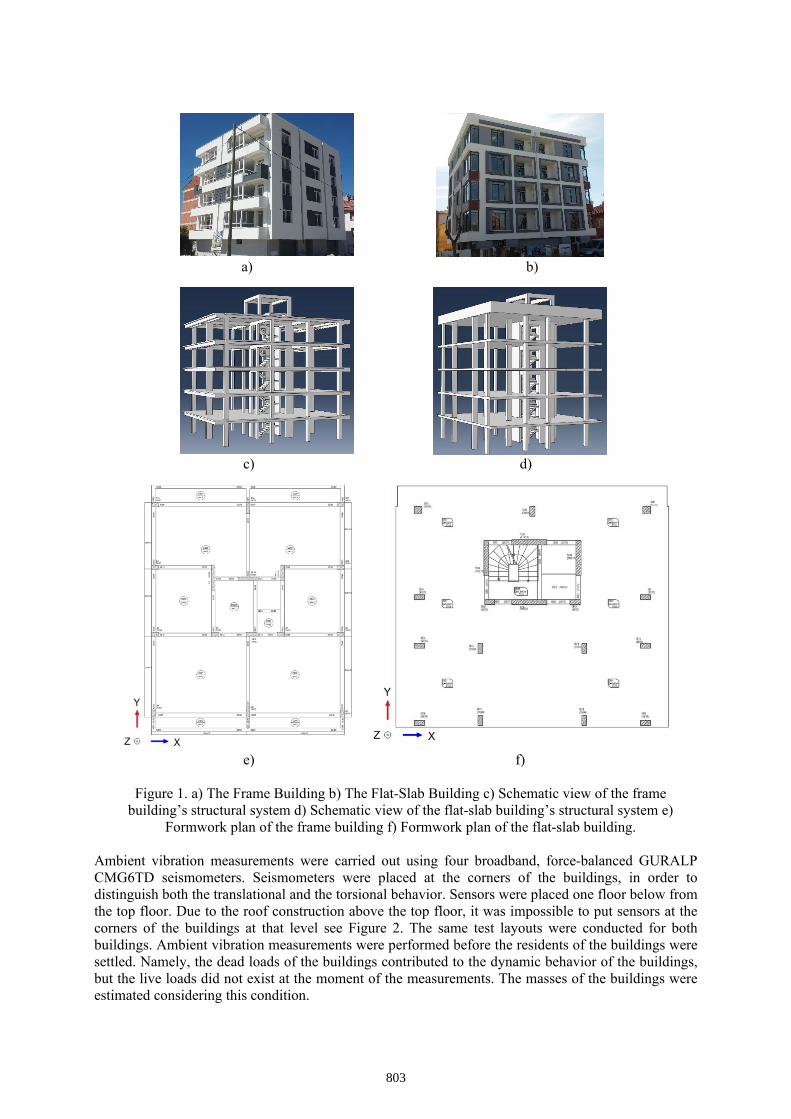
a) b)

c) d)

e) f)

Figure 1. a) The Frame Building b) The Flat-Slab Building c) Schematic view of the frame building’s structural system d) Schematic view of the flat-slab building’s structural system e)

Formwork plan of the frame building f) Formwork plan of the flat-slab building.

Ambient vibration measurements were carried out using four broadband, force-balanced GURALP CMG6TD seismometers. Seismometers were placed at the corners of the buildings, in order to distinguish both the translational and the torsional behavior. Sensors were placed one floor below from the top floor. Due to the roof construction above the top floor, it was impossible to put sensors at the corners of the buildings at that level see Figure 2. The same test layouts were conducted for both buildings. Ambient vibration measurements were performed before the residents of the buildings were settled. Namely, the dead loads of the buildings contributed to the dynamic behavior of the buildings, but the live loads did not exist at the moment of the measurements. The masses of the buildings were estimated considering this condition.

803

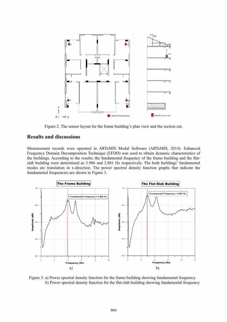
Figure 2. The sensor layout for the frame building’s plan view and the section cut.

Results and discussions

Measurement records were operated in ARTeMIS Modal Software (ARTeMIS, 2014). Enhanced Frequency Domain Decomposition Technique (EFDD) was used to obtain dynamic characteristics of the buildings. According to the results; the fundamental frequency of the frame building and the flat-slab building were determined as 3.906 and 2.881 Hz respectively. The both buildings’ fundamental modes are translation in x-direction. The power spectral density function graphs that indicate the fundamental frequencies are shown in Figure 3.

a) b)

Figure 3. a) Power spectral density function for the frame building showing fundamental frequency b) Power spectral density function for the flat-slab building showing fundamental frequency

804

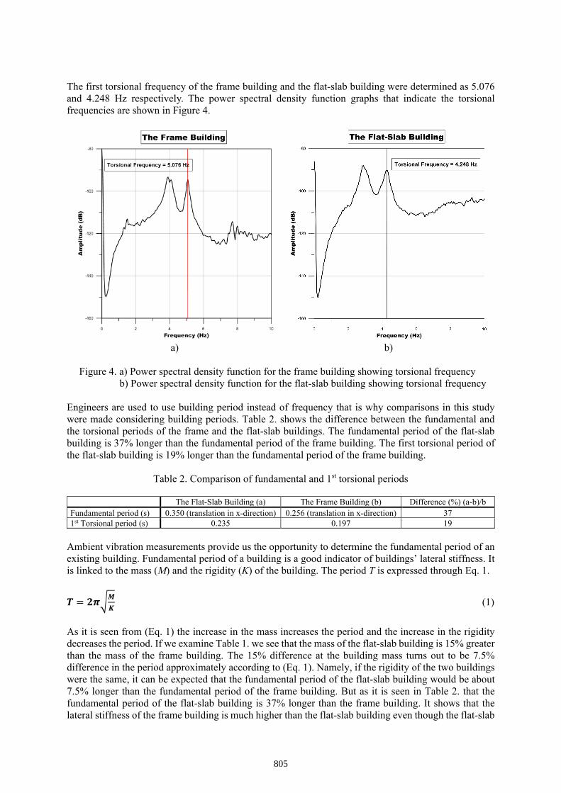
The first torsional frequency of the frame building and the flat-slab building were determined as 5.076 and 4.248 Hz respectively. The power spectral density function graphs that indicate the torsional frequencies are shown in Figure 4.

a) b)

Figure 4. a) Power spectral density function for the frame building showing torsional frequency b) Power spectral density function for the flat-slab building showing torsional frequency

Engineers are used to use building period instead of frequency that is why comparisons in this study were made considering building periods. Table 2. shows the difference between the fundamental and the torsional periods of the frame and the flat-slab buildings. The fundamental period of the flat-slab building is 37% longer than the fundamental period of the frame building. The first torsional period of the flat-slab building is 19% longer than the fundamental period of the frame building.

Table 2. Comparison of fundamental and 1st torsional periods

The Flat-Slab Building (a) The Frame Building (b) Difference (%) (a-b)/b Fundamental period (s) 0.350 (translation in x-direction) 0.256 (translation in x-direction) 37 1st Torsional period (s) 0.235 0.197 19

Ambient vibration measurements provide us the opportunity to determine the fundamental period of an existing building. Fundamental period of a building is a good indicator of buildings’ lateral stiffness. It is linked to the mass (M) and the rigidity (K) of the building. The period T is expressed through Eq. 1.

𝑻𝑻 = 𝟐𝟐𝟐𝟐�𝑴𝑴𝑲𝑲

(1)

As it is seen from (Eq. 1) the increase in the mass increases the period and the increase in the rigidity decreases the period. If we examine Table 1. we see that the mass of the flat-slab building is 15% greater than the mass of the frame building. The 15% difference at the building mass turns out to be 7.5% difference in the period approximately according to (Eq. 1). Namely, if the rigidity of the two buildings were the same, it can be expected that the fundamental period of the flat-slab building would be about 7.5% longer than the fundamental period of the frame building. But as it is seen in Table 2. that the fundamental period of the flat-slab building is 37% longer than the frame building. It shows that the lateral stiffness of the frame building is much higher than the flat-slab building even though the flat-slab

805

building’s total moment of inertia of vertical members in x-direction is nearly five times greater than the frame building’s and total moment of inertia of vertical members in y-direction is about three times greater than the frame building’s. Concrete classes of the two buildings are the same as C30/37 (TS-EN 206-2014) then the modulus of elasticities of the buildings are assumed as same. The lengths of thevertical members are also very close to each other so it does not cause a remarkable difference in thestiffness of the vertical members. Lastly, considering the contribution of the infill walls to the lateralstiffness, it can be said that there is no significant difference between two buildings in terms of the totalmoment of inertia of infill walls in both directions see Table 1.

Conclusions

A reinforced concrete flat-slab building’s lateral stiffness was compared to a reinforced concrete frame building, in which the mass of the building is quite close to the flat-slab building's mass, utilizing fundamental periods of the buildings. In addition, three-dimensional computer models of both buildings were also generated using the finite element software ABAQUS (ABAQUS, 2017) to compare the seismic performance of the buildings numerically for future studies. The vibration modes of the buildings and the frequencies of these modes that determined by the ambient vibration measurements were used in the calibration of the three-dimensional computer models of the buildings.

Results showed that, although the total stiffness of the vertical members of the flat-slab building is approximately five times greater than the frame building’s, the fundamental period of the flat-slab building was observed to be 37% longer than the frame building’s fundamental period. The rigidity of the frame building comes from the frame behavior, thanks to the deep beams that connect vertical members in the structural system.

The study showed the significant difference in flexibility between these two structural systems. This flexibility in flat-slab systems causes extensive damages to non-structural elements even under moderate intensity earthquakes. The authors offer that the non-structural elements of the flat-slab buildings especially the infill walls should be isolated from the structural system to prevent undesirable damages even under moderate earthquakes. Also it is obligatory according to Turkey Building Earthquake Code 2018 (TBEC, 2018) that the earthquake forces should be resisted by structural walls in flat-slab buildings.

Acknowledgements

The authors would like to thank Furkan Guney and Reyhan Gozoglu for their contribution to ambient vibration measurements. The authors also would like to thank Ömer Murat Cabbar, Osman Murat Erkan and Semih Sirin for their support for getting permission for measurements in the buildings.

References

ABAQUS (2017) Dassault Systèmes. ABAQUS CAE 2017, Providence, RI

ACI-ASCE Committee 352. Recommendations for design of slab–column connections in monolithic reinforced concrete structures. ACI Structural Journal 1988;85(6):675–96.

ARTeMIS Modal 3.6.0.3., (2014) Structural Vibration Solutions A/S. http://www.svibs.com

Carder, D. S. (1937) Observed vibrations of bridges. Bulletin of the Seismological Society of America, 27(4), 267-303.

806

Chow H L and Selna L G (1995) Seismic response of nonductile flat-plate buildings. Journal of Structural Engineering, 121(1), 115-123.

Erberik M A and Elnashai A S (2004) Fragility analysis of flat-slab structures. Engineering Structures, 26(7), 937-948.

Farsi, M.N. ve Bard, P.Y. (2004) Estimation des periodes propres de batiments et vulnerabilite du bati existant dans l’agglomeration de Grenoble. Revue Francaise de Genie Civil 8(2–3):149–179

Hassoun M N and Al-Manaseer A (2012) Structural Concrete: Theory and Design. John Wiley & Sons.

Mikael A Gueguen P Bard P Y Roux P and Langlais M (2013) The analysis of long‐term frequency and damping wandering in buildings using the Random Decrement Technique. Bulletin of the Seismological Society of America, 103(1), 236-246.

Trifunac, M. D. (1972). Comparisons between ambient and forced vibration experiments. Earthquake Engineering & Structural Dynamics, 1(2), 133-150.

TBEC (2018). Turkey Building Earthquake Code, Republic of Turkey Ministry of Interior Disaster and Emergency Management Authority, Ankara, Turkey.

807

Ön Değerlendirme Yöntemlerinin Betonarme Binaların Deprem

Performanslarını Tahmin Etmedeki Başarıları

Barış Erdil1*, Harun Ceylan2

1 Van Yüzüncü Yıl Üniversitesi, İnşaat Mühendisliği Bölümü, Van, Türkiye 2 Van Yüzüncü Yıl Üniversitesi, Van Meslek Yüksekokulu, Van, Türkiye


Özet

Her deprem sonrası mevcut betonarme binalar önemli hasarlar görmekte ve bu hasarların bir kısmı can

kayıpları ile sonuçlanmaktadır. Maddi kayıpların bir kısmı telafi edilebilir fakat can kayıpları hiçbir

zaman kabul edilemez. Bu sebeple mevcut betonarme binaların hızlı bir şekilde değerlendirilerek

deprem performanslarının ortaya konması, problemli binaların tespit edilerek güçlendirme veya yıkım

çalışmalarının erken başlaması olası bir depremde ortaya çıkacak can kayıplarının azaltılmasını

sağlayacaktır. Bu kapsamda geliştirilmiş ve literatürde kendine yer bulmuş hızlı değerlendirme

yöntemleri ikiye ayrılmaktadır: sokak taraması ve ön değerlendirme yöntemleri. Sokak taraması

yöntemleri tekil bir bina yerine belirli bir bina stoku içindeki problemli olanları tespit etmekte fakat

binanın taşıyıcı sistem elemanları ile malzeme kalitesini dikkate almadıklarından çeşitli hatalara sebep

olmaktadır. Aksine ön değerlendirme yöntemleri taşıyıcı sistem elemanlarının boyutsal özellikleri,

malzeme kalitesi vs. daha detaylı bilgiler ile değerlendirme yapmayı esas aldığından nispeten daha

sağlıklı sonuçlar vermektedir ve bu yöntemler tekil binanın deprem performanslarının belirlenmesi için

de kullanılabilmektedir. Bu çalışmada Türkiye verileri dikkate alınarak ve etki/kapasite oranı tabanlı

olarak geliştirilen 8 adet (Sucuoglu ve Yazgan, 2003; Yakut, 2004; Boduroğlu vd. 2004; Temur

(DURTES), 2006; Tezcan vd. (P25), 2011; Sucuoğlu vd. 2015; Kaplan vd. 2018; Erdil ve Ceylan

(MVP), 2019) ön değerlendirme yönteminin Van depremlerinden etkilenen 146 binanın deprem

performansını ne derece doğru tahmin ettiği belirlenmeye çalışılmıştır. İnceleme konusu binaların 69

adedi deprem sonrası onarım ve güçlendirme ile tekrar kullanılabilecek binalar (düşük riskli binalar,

DRB) olmasına karşın 77 bina ya ağır hasar görmüş ya da yıkılmış olduğundan (yüksek riskli binalar,

YRB) deprem sonrası kullanımı mümkün olmayan binalardır. Karşılaştırmalar hem DRB hem de YRB

için ayrı ayrı yapıldıktan sonra nihai doğru tahmin oranları belirlenmiştir. Nihai doğru tahmin oranları

sonucunda bu çalışmada göz önüne alınan binalar için MVP yönteminin toplamda %93.8, Yakut (2004)

yönteminin %87, Sucuoğlu ve Yazgan (2003) yönteminin %84.9, Boduroğlu vd. (2004)’ün %82.2 ve

P25 yönteminin %80.1 oranında iyi tahminler yaptığı belirlenmiştir. Genel olarak yöntemlerin doğru

tahmin yüzdelerinin %80 ve üzerinde olduğu, nispeten düşük tahmin yüzdesine sahip yöntemlerde ise

yöntemde kullanılan sınır değerlerin revize edilmesi ile doğru tahmin yüzdesinin arttığı görülmüştür.

Mevcut yöntemler farklı sayıda bina verisine ihtiyaç duymaktadır. En az veriyi Sucuoğlu vd. (2015) 11

veri ile kullanmakta, en fazla veriye ise (22 ile) P25 yöntemi ihtiyaç duymaktadır.

Anahtar Kelimeler: Ön Değerlendirme Yöntemleri, Deprem Performansı, Betonarme Bina.

Giriş

Türkiye’de 1903’ten bu yana VI şiddetinde 24, VII şiddetinde 19, VIII şiddetinde 47, IX-X şiddetinde

2, X şiddetinde 4 ve X-XI şiddetinde 1 olmak üzere toplam 119 adet deprem kaydedilmiştir. Yaşanan

bu depremlerde 83.088 vatandaşımız hayatını kaybetmiş, yüzbinlerce vatandaşımız yaralanmış ve

587.302 bina hasar almıştır (KRDAE, 2018).

Sadece 1980-2014 yılları arasında meydana gelen depremlerde 24.534.800$ ekonomik kayıp oluşmuştur

(Şahin ve Kılınç, 2016). Ancak bu depremlerde meydana gelen ekonomik zararlar bununla sınırlı

808

kalmamakta deprem sonrası acil kurtarma, rehabilitasyon, insani yardım malzemeleri ve yeniden

yapılanma harcamaları vs. gibi durumlardan ötürü 1980-2012 yılları arasında meydana gelen

depremlerin ülke ekonomisine yüklediği maliyet 13 milyar dolar civarındadır (Akar, 2013).

Ülkemizdeki yapı stoku dikkate alındığında, mevcut binaları TBDY2018’de verilen hesap ilkelerine

göre incelemenin zaman, bu işi yapacak nitelikli personel sayısı ve maliyet açısından ilk aşamada uygun

olmayacağı görülmektedir. Bu sebeplerden dolayı binaların deprem güvenliğinin hızlı şekilde tahmin

edilmesini sağlayabilecek bazı hızlı ve pratik yöntemlerin kullanılması gerekmektedir.

Mevcut betonarme binaların hızlı bir şekilde değerlendirilerek deprem performanslarının ortaya

konması, problemli binaların tespit edilerek güçlendirme veya yıkım çalışmalarının erken başlaması

olası bir depremde ortaya çıkacak can kayıplarının azaltılmasını sağlayacaktır. Bu kapsamda

geliştirilmiş ve literatürde kendine yer bulmuş hızlı değerlendirme yöntemleri ikiye ayrılmaktadır: sokak

taraması ve ön değerlendirme yöntemleri. Sokak taraması yöntemleri tekil bir bina yerine belirli bir bina

stoku içindeki problemli olanları tespit eder fakat binanın taşıyıcı sistem elemanları ile malzeme

kalitesini dikkate almadıklarından çeşitli hatalara sebep olmaktadır. Aksine ön değerlendirme

yöntemleri taşıyıcı sistem elemanlarının boyutsal özellikleri, malzeme kalitesi vs. daha detaylı bilgiler

ile değerlendirme yapmayı esas aldığından nispeten daha sağlıklı sonuçlar vermektedir ve bu yöntemler

tekil binanın deprem performanslarının belirlenmesi için de kullanılabilmektedir. Bu çalışmada Türkiye

verileri dikkate alınarak ve etki/kapasite oranı tabanlı olarak geliştirilen 8 adet (Sucuoglu ve Yazgan,

2003; Yakut, 2004; Boduroğlu vd. 2004; Temur (DURTES), 2006; Tezcan vd. (P25), 2011; Sucuoğlu

vd. 2015; Kaplan vd. 2018; Erdil ve Ceylan (MVP), 2019) ön değerlendirme yönteminin Van

depremlerinde incelenen 146 binanın deprem performansını ne derece doğru tahmin ettiği belirlenmeye

çalışılmıştır.

Ön değerlendirme yöntemleri

Kapasite ve istem ilişkisi kullanan yöntemlerin tamamında kritik katın kolon, perde duvar ve kat alanı

gibi verileri kullanılarak kesme kapasitesi hesaplanmakta, daha sonra bu kapasite, mimari özellikleri

içerecek şekilde revize edilmekte ve istatistiksel olarak önceden belirlenmiş bir sınır değer ile

karşılaştırılarak binanın nihai performansına karar verilmektedir. Bu kapsamda yöntemini oluşturan

Yakut (2004) (kısaca Y) Türkiye’nin dört farklı ilinden toplamda 220 bina inceleyerek yaptığı çalışmada

binanın kritik katının kesme kapasitesini dolgu duvarı ve mimari özellikleri içerecek şekilde hesaplayıp,

kesme kapasitesini binaya etkiyebilecek deprem yükü ile ilişkilendirerek binanın deprem performansını

anlamaya çalışmıştır. Sucuoğlu vd. (2015) (kısaca SVD), Yakut (2004) yönteminde kullanılan mimari

özellikleri iptal edip kesme kapasitesi hesabına donatıları katarak revize bir yöntem geliştirmiştir.

Boduroğlu vd. (2004) (kısaca BVD) Japan Building Disaster Prevention Association (JBDPA, 2001)

tarafından geliştirilmiş olan Japon Sismik İndeks Yöntemi’ni Türkiye’deki binalara uyarlamıştır. Temur

(2006) DURTES adlı bir yöntem geliştirerek, betonarme bir binanın kesme kapasitesini yapısal ve

mimari özellikleri kullanarak hesaplamakta ve daha sonra kapasiteleri taban kesme kuvveti ile

kıyaslamaktadır. DURTES yöntemi daha sonra Kaplan vd. (2018) (kısaca KVD) tarafından revize

edilmiştir. Erdil ve Ceylan (2019) moment (M), kesme kuvveti (V) ve eksenel yük (P) kapasitelerini

istemlerle kıyaslayarak MVP adında bir yöntem önermişlerdir. Bu yöntemde kapasiteler ve istemler

basit formlasyonlarla ifade edilmiş, mimari özelliklerin etkilediği her kapasite revize edilmiş, moment-

kesme kuvveti-eksenel yük bağıntıları arasında etkileşim oluşturulmuş, son olarak her kapasite/istem

oranı bu etkileşimler dikkate alınarak toplanmış ve nihai performans puanı elde edilmeye çalışılmıştır.

Nihai performans puanı daha sonra önceden belirlenmiş bir puan ile kıyaslanarak binanın hasar

görebilirliği hakkında yorum yapılmaktadır.

Doğrudan kapasite ve istemlerin kullanıldığı yöntemlerden farklı olarak bazı yöntemler istatistiksel

tabana oturtulmuşlardır. Bu yöntemlerde de kapasiteler ve istemler hesaplanmakta fakat doğrudan

kullanılmamaktadır. Özcebe vd. (2003) depremlerde hasar gören bina bilgilerini diskriminant analiz

yöntemi ile değerlendirmiş ve istatistiki bir yöntem önermiştir. Bu yöntemde kapasite ve istemler

hesaplanmasına rağmen dolaylı olarak kullanılmaktadır. Sucuoğlu ve Yazgan (2003) (kısaca SY) sokak

809

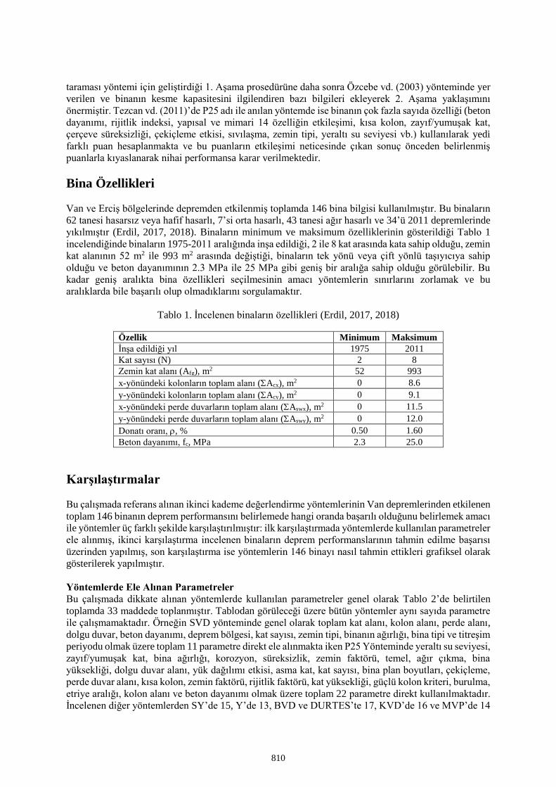
taraması yöntemi için geliştirdiği 1. Aşama prosedürüne daha sonra Özcebe vd. (2003) yönteminde yer

verilen ve binanın kesme kapasitesini ilgilendiren bazı bilgileri ekleyerek 2. Aşama yaklaşımını

önermiştir. Tezcan vd. (2011)’de P25 adı ile anılan yöntemde ise binanın çok fazla sayıda özelliği (beton

dayanımı, rijitlik indeksi, yapısal ve mimari 14 özelliğin etkileşimi, kısa kolon, zayıf/yumuşak kat,

çerçeve süreksizliği, çekiçleme etkisi, sıvılaşma, zemin tipi, yeraltı su seviyesi vb.) kullanılarak yedi

farklı puan hesaplanmakta ve bu puanların etkileşimi neticesinde çıkan sonuç önceden belirlenmiş

puanlarla kıyaslanarak nihai performansa karar verilmektedir.

Bina Özellikleri

Van ve Erciş bölgelerinde depremden etkilenmiş toplamda 146 bina bilgisi kullanılmıştır. Bu binaların

62 tanesi hasarsız veya hafif hasarlı, 7’si orta hasarlı, 43 tanesi ağır hasarlı ve 34’ü 2011 depremlerinde

yıkılmıştır (Erdil, 2017, 2018). Binaların minimum ve maksimum özelliklerinin gösterildiği Tablo 1

incelendiğinde binaların 1975-2011 aralığında inşa edildiği, 2 ile 8 kat arasında kata sahip olduğu, zemin

kat alanının 52 m2 ile 993 m2 arasında değiştiği, binaların tek yönü veya çift yönlü taşıyıcıya sahip

olduğu ve beton dayanımının 2.3 MPa ile 25 MPa gibi geniş bir aralığa sahip olduğu görülebilir. Bu

kadar geniş aralıkta bina özellikleri seçilmesinin amacı yöntemlerin sınırlarını zorlamak ve bu

aralıklarda bile başarılı olup olmadıklarını sorgulamaktır.

Tablo 1. İncelenen binaların özellikleri (Erdil, 2017, 2018)

Özellik Minimum Maksimum

İnşa edildiği yıl 1975 2011

Kat sayısı (N) 2 8

Zemin kat alanı (Afg), m2 52 993

x-yönündeki kolonların toplam alanı (Acx), m2 0 8.6

y-yönündeki kolonların toplam alanı (Acy), m2 0 9.1

x-yönündeki perde duvarların toplam alanı (Aswx), m2 0 11.5

y-yönündeki perde duvarların toplam alanı (Aswy), m2 0 12.0

Donatı oranı, , % 0.50 1.60

Beton dayanımı, fc, MPa 2.3 25.0

Karşılaştırmalar

Bu çalışmada referans alınan ikinci kademe değerlendirme yöntemlerinin Van depremlerinden etkilenen

toplam 146 binanın deprem performansını belirlemede hangi oranda başarılı olduğunu belirlemek amacı

ile yöntemler üç farklı şekilde karşılaştırılmıştır: ilk karşılaştırmada yöntemlerde kullanılan parametreler

ele alınmış, ikinci karşılaştırma incelenen binaların deprem performanslarının tahmin edilme başarısı

üzerinden yapılmış, son karşılaştırma ise yöntemlerin 146 binayı nasıl tahmin ettikleri grafiksel olarak

gösterilerek yapılmıştır.

Yöntemlerde Ele Alınan Parametreler

Bu çalışmada dikkate alınan yöntemlerde kullanılan parametreler genel olarak Tablo 2’de belirtilen

toplamda 33 maddede toplanmıştır. Tablodan görüleceği üzere bütün yöntemler aynı sayıda parametre

ile çalışmamaktadır. Örneğin SVD yönteminde genel olarak toplam kat alanı, kolon alanı, perde alanı,

dolgu duvar, beton dayanımı, deprem bölgesi, kat sayısı, zemin tipi, binanın ağırlığı, bina tipi ve titreşim

periyodu olmak üzere toplam 11 parametre direkt ele alınmakta iken P25 Yönteminde yeraltı su seviyesi,

zayıf/yumuşak kat, bina ağırlığı, korozyon, süreksizlik, zemin faktörü, temel, ağır çıkma, bina

yüksekliği, dolgu duvar alanı, yük dağılımı etkisi, asma kat, kat sayısı, bina plan boyutları, çekiçleme,

perde duvar alanı, kısa kolon, zemin faktörü, rijitlik faktörü, kat yüksekliği, güçlü kolon kriteri, burulma,

etriye aralığı, kolon alanı ve beton dayanımı olmak üzere toplam 22 parametre direkt kullanılmaktadır.

İncelenen diğer yöntemlerden SY’de 15, Y’de 13, BVD ve DURTES’te 17, KVD’de 16 ve MVP’de 14

810

parametre kullanılmıştır. Genel olarak bütün yöntemlerin kolon alanı, perde duvar alanı, beton dayanımı

ve deprem bölgesi ifadelerini içerdiği belirlenmiştir. Zamana bağlı deformasyon, topoğrafya, korozyon,

yeraltı su seviyesi, yük dağılım etkisi, asma kat varlığı, güçlü kolon ilkesi, süneklik, zemin kat alanı ve

rijitlik faktörünün sadece bir yöntem tarafından (çoğunlukla P25 yöntemi) kullanıldığı tespit edilmiştir.

Ön değerlendirme yöntemleri detaylı yöntemlere nazaran daha hızlı yöntemler olduklarından az

parametre ve az hesap yükü ile daha doğru tahmin yapan yöntemlerin başarılı oldukları düşünülecektir.

Tablo 2. Yöntemlerde kullanılan parametreler

Parametreler SY Y BVD DURTES P25 SVD KVD MVP

1 Kolon alanı (Ac) X X X X X X X X

2 Perde duvar alanı (Asw) X X X X X X X X

3 Yumuşak/Zayıf kat X X X X X X X

4 Toplam kat alanı X X X X X X X

5 Beton dayanımı (fc) X X X X X X X X

6 Kat sayısı X X X X X X X

7 Deprem bölgesi X X X X X X X X

8 Dolgu duvar alanı (Aiw) X X X X X X

9 Çerçeve süreksizliği X X X X

10 Kısa kolon X X X X X X X

11 Zemin tipi X X X X X

12 Binanın ağırlığı X X X X X X

13 Bina tipi X X X X

14 Burulma X X X X X

15 Yapım yılı X X X X

16 Ağır çıkma X X X X

17 Binanın titreşim periyodu X X X

18 Rijitlik faktörü X

19 Bodrum kat varlığı X X

20 Temel tipi X X X

21 İnşaat kalitesi X X

22 Kat yüksekliği X X

23 Plan boyutları X X X

24 Süneklik X

25 Zemin kat alanı (Agf) X

26 Çekiçleme etkisi X X

27 Zamana bağlı deformasyon

X

28 Topoğrafya X

29 Korozyon X

30 Yeraltı su seviyesi X

31 Yük dağılım etkisi X

32 Asma kat varlığı X

33 Güçlü kolon ilkesi X

Toplam 15 13 17 17 22 11 16 14

Yöntemlerin Başarı Yüzdeleri

Tablo 3 bu çalışmada dikkate alınan yöntemlerin 146 binanın hasarını tahmin etme başarısını

göstermektedir. İncelenen 146 binanın 69’u en fazla orta hasar gördüğü için ve bu binalar onarılıp veya

güçlendirilip tekrar kullanılabilecek binalar olduklarından “Düşük Riskli Binalar (DRB)”, diğer 77 bina

ise ağır hasar görmüş veya yıkılmış olduğundan tekrar kullanılamayacakları için “Yüksek Riskli Binalar

(YRB)” olarak değerlendirilmiştir.

Tablodan görüleceği üzere MVP yöntemi DRB’nin %97.1’i, YRB’nin ise %90.9’u olmak üzere toplam

binaların %93.8’inin hasarını doğru tahmin edebilmiştir. Bu yöntemi takiben Y yöntemi (bu yöntemde

811

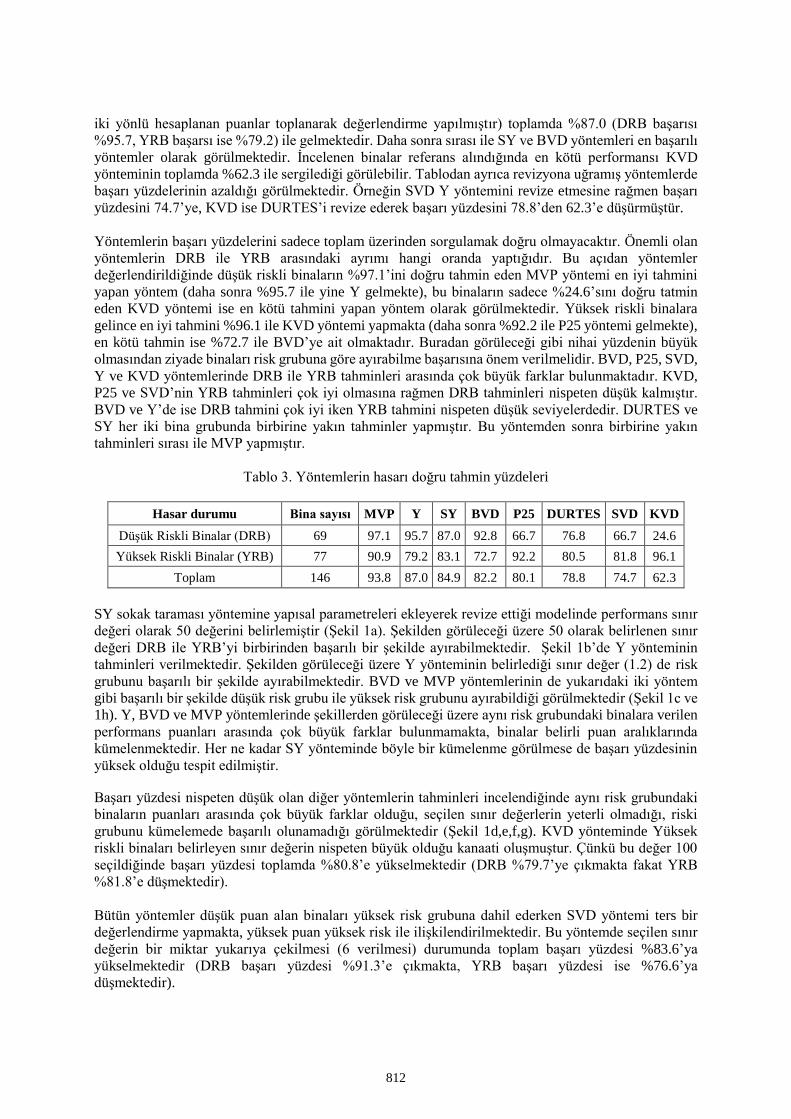
iki yönlü hesaplanan puanlar toplanarak değerlendirme yapılmıştır) toplamda %87.0 (DRB başarısı

%95.7, YRB başarsı ise %79.2) ile gelmektedir. Daha sonra sırası ile SY ve BVD yöntemleri en başarılı

yöntemler olarak görülmektedir. İncelenen binalar referans alındığında en kötü performansı KVD

yönteminin toplamda %62.3 ile sergilediği görülebilir. Tablodan ayrıca revizyona uğramış yöntemlerde

başarı yüzdelerinin azaldığı görülmektedir. Örneğin SVD Y yöntemini revize etmesine rağmen başarı

yüzdesini 74.7’ye, KVD ise DURTES’i revize ederek başarı yüzdesini 78.8’den 62.3’e düşürmüştür.

Yöntemlerin başarı yüzdelerini sadece toplam üzerinden sorgulamak doğru olmayacaktır. Önemli olan

yöntemlerin DRB ile YRB arasındaki ayrımı hangi oranda yaptığıdır. Bu açıdan yöntemler

değerlendirildiğinde düşük riskli binaların %97.1’ini doğru tahmin eden MVP yöntemi en iyi tahmini

yapan yöntem (daha sonra %95.7 ile yine Y gelmekte), bu binaların sadece %24.6’sını doğru tatmin

eden KVD yöntemi ise en kötü tahmini yapan yöntem olarak görülmektedir. Yüksek riskli binalara

gelince en iyi tahmini %96.1 ile KVD yöntemi yapmakta (daha sonra %92.2 ile P25 yöntemi gelmekte),

en kötü tahmin ise %72.7 ile BVD’ye ait olmaktadır. Buradan görüleceği gibi nihai yüzdenin büyük

olmasından ziyade binaları risk grubuna göre ayırabilme başarısına önem verilmelidir. BVD, P25, SVD,

Y ve KVD yöntemlerinde DRB ile YRB tahminleri arasında çok büyük farklar bulunmaktadır. KVD,

P25 ve SVD’nin YRB tahminleri çok iyi olmasına rağmen DRB tahminleri nispeten düşük kalmıştır.

BVD ve Y’de ise DRB tahmini çok iyi iken YRB tahmini nispeten düşük seviyelerdedir. DURTES ve

SY her iki bina grubunda birbirine yakın tahminler yapmıştır. Bu yöntemden sonra birbirine yakın

tahminleri sırası ile MVP yapmıştır.

Tablo 3. Yöntemlerin hasarı doğru tahmin yüzdeleri

Hasar durumu Bina sayısı MVP Y SY BVD P25 DURTES SVD KVD

Düşük Riskli Binalar (DRB) 69 97.1 95.7 87.0 92.8 66.7 76.8 66.7 24.6

Yüksek Riskli Binalar (YRB) 77 90.9 79.2 83.1 72.7 92.2 80.5 81.8 96.1

Toplam 146 93.8 87.0 84.9 82.2 80.1 78.8 74.7 62.3

SY sokak taraması yöntemine yapısal parametreleri ekleyerek revize ettiği modelinde performans sınır

değeri olarak 50 değerini belirlemiştir (Şekil 1a). Şekilden görüleceği üzere 50 olarak belirlenen sınır

değeri DRB ile YRB’yi birbirinden başarılı bir şekilde ayırabilmektedir. Şekil 1b’de Y yönteminin

tahminleri verilmektedir. Şekilden görüleceği üzere Y yönteminin belirlediği sınır değer (1.2) de risk

grubunu başarılı bir şekilde ayırabilmektedir. BVD ve MVP yöntemlerinin de yukarıdaki iki yöntem

gibi başarılı bir şekilde düşük risk grubu ile yüksek risk grubunu ayırabildiği görülmektedir (Şekil 1c ve

1h). Y, BVD ve MVP yöntemlerinde şekillerden görüleceği üzere aynı risk grubundaki binalara verilen

performans puanları arasında çok büyük farklar bulunmamakta, binalar belirli puan aralıklarında

kümelenmektedir. Her ne kadar SY yönteminde böyle bir kümelenme görülmese de başarı yüzdesinin

yüksek olduğu tespit edilmiştir.

Başarı yüzdesi nispeten düşük olan diğer yöntemlerin tahminleri incelendiğinde aynı risk grubundaki

binaların puanları arasında çok büyük farklar olduğu, seçilen sınır değerlerin yeterli olmadığı, riski

grubunu kümelemede başarılı olunamadığı görülmektedir (Şekil 1d,e,f,g). KVD yönteminde Yüksek

riskli binaları belirleyen sınır değerin nispeten büyük olduğu kanaati oluşmuştur. Çünkü bu değer 100

seçildiğinde başarı yüzdesi toplamda %80.8’e yükselmektedir (DRB %79.7’ye çıkmakta fakat YRB

%81.8’e düşmektedir).

Bütün yöntemler düşük puan alan binaları yüksek risk grubuna dahil ederken SVD yöntemi ters bir

değerlendirme yapmakta, yüksek puan yüksek risk ile ilişkilendirilmektedir. Bu yöntemde seçilen sınır

değerin bir miktar yukarıya çekilmesi (6 verilmesi) durumunda toplam başarı yüzdesi %83.6’ya

yükselmektedir (DRB başarı yüzdesi %91.3’e çıkmakta, YRB başarı yüzdesi ise %76.6’ya

düşmektedir).

812

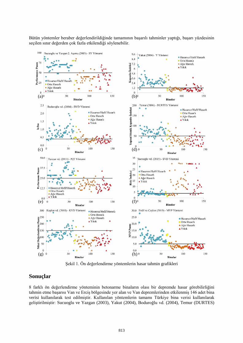
Bütün yöntemler beraber değerlendirildiğinde tamamının başarılı tahminler yaptığı, başarı yüzdesinin

seçilen sınır değerden çok fazla etkilendiği söylenebilir.

Şekil 1. Ön değerlendirme yöntemlerin hasar tahmin grafikleri

Sonuçlar

8 farklı ön değerlendirme yönteminin betonarme binaların olası bir depremde hasar görebilirliğini

tahmin etme başarısı Van ve Erciş bölgesinde yer alan ve Van depremlerinden etkilenmiş 146 adet bina

verisi kullanılarak test edilmiştir. Kullanılan yöntemlerin tamamı Türkiye bina verisi kullanılarak

geliştirilmiştir: Sucuoglu ve Yazgan (2003), Yakut (2004), Boduroğlu vd. (2004), Temur (DURTES)

(a) (b)

(c) (d)

(e) (f)

(g) (h)

813

(2006), Tezcan vd. (P25) (2011), Sucuoğlu vd. (2015), Kaplan vd. (2018), Erdil ve Ceylan (MVP)

(2019).

İncelenen 8 yöntemin de farklı sayıda parametreye ihtiyaç duyduğu görülmüştür. Örneğin SVD 11 veri

talep ederken, P25 yöntemi 22 veri ile çalışmaktadır. Genel olarak bütün yöntemlerin kolon alanı, perde

duvar alanı, beton dayanımı ve deprem bölgesi ifadelerini içerdiği belirlenmiştir. Zamana bağlı

deformasyon, topoğrafya, korozyon, yeraltı su seviyesi, yük dağılım etkisi, asma kat varlığı, güçlü kolon

ilkesi, süneklik, zemin kat alanı ve rijitlik faktörünün sadece bir yöntem tarafından (çoğunlukla P25

yöntemi) kullanıldığı tespit edilmiştir.

Yöntemlerin betonarme binaların olası bir depremdeki performansları başarılı bir şekilde tahmin

edebildikleri görülmüştür. En başarılı yöntemin MVP (%93.8) ve Y (%87.0) olduğu belirlenmiştir.

Genel olarak yöntemlerin %80 ve üzerinde bir doğrulukla tahmin yaptıkları, nispeten düşük tahmin

oranına sahip yöntemlerdeki sınır değerlerin değiştirilmesi ile tahmin yüzdelerin arttığı belirlenmiştir.

Sonuç olarak Türkiye veri tabanını kullanarak geliştirilen yöntemlerin betonarme binaların riskli olup

olmadıkların belirlemede yeterli bir başarı oranı sahip oldukları, başarı oranının veri sayısı arttıkça ve

değerlendirmeye esas sınır değerler revize edildikçe artacağı düşünülmektedir.

Kaynaklar

Akar S (2013) “Doğal afetlerin kamu maliyesine ve makro ekonomiye etkileri: Türkiye değerlendirmesi”, Yönetim

ve Ekonomi Araştırmaları Dergisi, 11 (21):185-206.

Boduroglu H, Ozdemir P, Ilki A, Sirin S, Demir C, Baysan F (2004) “Towards a modified rapid screening method

for existing medium rise RC buildings in Turkey”, Proceedings of 13th World Conference on Earthquake

Engineering, Vol. 13.

Erdil B (2017) “Why RC buildings failed in the 2011 Van, Turkey, Earthquakes: Construction versus design

practices”, Journal of Performance of Constructed Facilities, 31(3):04016110.

Erdil B (2018) “2011 Van Earthquakes: Design vs Construction”, Disaster Science and Engineering, 4 (1):1-11.

Erdil B, Ceylan H (2019) “MVP interaction based seismic vulnerability assessment of RC buildings”, Građevinar,

71 (06): 489-503

JBDPA (2001) “Standard for seismic evaluation of existing reinforced concrete buildings (Version 2001)”, The

Japan Building Disaster Prevention Association, Tokyo, Japan.

Kaplan O, Guney Y, Topcu A, Ozcelikors Y (2018) “A rapid seismic safety assessment method for mid-rise

reinforced concrete buildings”, Bulletin of Earthquake Engineering, 16(2): 889-915.

KRDAE (2018) Boğaziçi Üniversitesi Kandilli Rasathanesi ve Deprem Araştırma Enstitüsü.

http://www.koeri.boun.edu.tr/sismo/2/deprem-bilgileri/buyuk-depremler/. Erişim tarihi: 08.02.2018.

Ozcebe G, Yucemen MS, Aydogan V, Yakut A (2003) “Preliminary seismic vulnerability assessment of existing

reinforced concrete buildings in Turkey”, In: Wasti S.T., Ozcebe G. (eds) Seismic Assessment and

Rehabilitation of Existing Buildings. NATO Science Series (Series IV: Earth and Environmental Sciences),

vol 29. Springer, Dordrecht.

Sucuoglu H, Yazgan U (2003) “Simple survey procedures for seismic risk assessment in urban building stocks”,

In: Wasti ST, Özcebe G, editors. Seismic assessment and rehabilitation of existing buildings, earth and

environmental sciences, Vol. 29. London: Kluwer Academic Publishers; 97–118.

Sucuoğlu H, Yakut A, Özmen A, Kubin J (2015) “Seismic Risk Prioritization and Retrofit Cost Evaluation of

Code-Deficient RC Public Buildings in Turkey”, Earthquake Spectra, 31(1):601-614.

Şahin İ, Kılınç T (2016) “Türkiye’de 1980-2014 yılları arasında görülen depremlerin ekonomik etkileri”, Siirt

Üniversitesi İktisadi ve İdari Bilimler Fakültesi İktisadi Yenilik Dergisi, 4 (1):33-42.

Temur R (2006) “Hızlı Durum Tespit (DURTES) yöntemi ve bilgisayar programının geliştirilmesi”, Yüksek Lisans

Tezi, İstanbul Üniversitesi, İstanbul

Tezcan SS, Bal IE, Gulay FG (2011) “P25 scoring method for the collapse vulnerability assessment of RC

buildings”, Journal of The Chinese Institute of Engineers, 34(6):769-781.

Yakut A (2004) “Preliminary seismic assessment procedure for existing RC buildings”, Engineering Structures,

26(10):1447-1461.

814

Residual displacement based damage index for SDOF systems

Müberra Eser Aydemir*, Cem Aydemir, Eylem Eyyüpoğlu

Department of Civil Engineering, Istanbul Aydin University *Corresponding author, [email protected]

AbstractSeismic design procedures aim at controlling earthquake damage to structural elements and many types

of nonstructural elements by limiting lateral deformations on structures. Structural performance is

usually estimated using peak deformation demands. However, the past earthquakes have shown that the

excessive permanent lateral deformations at the end of the earthquake motion (i.e. residual

displacement) of a system -in addition to peak demands- is one of the major parameters to determine

whether the structural system can continue its function or the system should be strengthened/repaired or

the system should be rebuilt. In this study a new damage index is proposed based on residual

displacement, spectral displacement and structural period. To this purpose SDOF systems with period

range between 0.1s and 3.0s are analyzed for far field ground motions.

Keywords: Damage index, residual displacement, and spectral displacement.

Introduction

Although the elastic design -in other words no inelastic behavior / damage- of a structure for the case of

severe earthquake motions is preferable, current earthquake – resistant design provisions allow the

nonlinear response of structures because of economic factors. The main goal of seismic design

procedures is to control the structural and nonstructural earthquake damage by limiting lateral

deformations on structures. Global performance is usually evaluated using peak deformation demands

of the structure. However, the past earthquakes have revealed that the permanent deformation of a

system -in addition to peak demands- is one of the key parameters to determine whether the structural

system can continue its function or the system should be strengthened or rebuilt. Besides, the necessity

to consider the residual displacements and residual drifts in seismic performance assessment is

addressed in Vision 2000 (1995) and FEMA356 (2000) guidelines. As the level of structural damage is

important to decide whether the building is suitable for use or not, measurable damage definitions are

needed. Thus, damage indexes (DI), are used to quantify degradation in structures and provide a measure

of structural damage. DI can be defined as a mathematical model that varies between 0 and 1, where it

is equal to zero when the structure remains elastic and equal to one, when there is potential for collapse.

A damage index (DI) is based on a set of structural response parameters such as force, deformation, and

dissipation of energy. There are numerous DIs available (Park and Ang 1985; Powell and Allahabadi

1988; Fajfar 1992; Cosenza et al. 1993; Williams and Sexsmith 1995; Ghobarah et al. 1999; Rodriguez

and Aristizabal 1999; Mehanny and Deierlein 2000; Bozorgnia and Bertero 2003). These models

represent structural damage defined locally for an individual element, or globally a whole structure.

Even the definition of structural damage and damage index is different, classification of damage level

is quite similar for many of the existing damage indexes.

• None - no damage

• Minor - minor cracks

• Moderate - significant damage, localized spalling

• Severe - crushing of concrete and bar buckling

• Collapse - failure

815

mailto:[email protected]

A general overview for the most commonly used damage indices is explained briefly. Park and Ang

(1985) proposed a combined damage index model based on both deformation and hysteretic energy due

to an earthquake as follows:

𝐷𝐼 =∆𝑚

∆𝑢+ 𝛽

𝐸ℎ

𝐹𝑦∆𝑢 (1)

where, ∆m is the maximum displacement of a SDOF system subjected to earthquake, ∆u is the ultimate

displacement under monotonic loading, Eh is the hysteretic energy dissipated by the SDOF system, Fy

is the yield force and β is the parameter to include the effect of hysteretic loading. This is the most

commonly used DI, due to its general applicability and the clear definition of different damage states

such as DI < 0.1 refers to no damage or localized minor cracking, 0.1 ≤ DI < 0.25 is minor damage, 0.25

≤ DI < 0.40 is moderate damage: severe cracking, localized spalling, 0.4 ≤ DI < 1.00 is severe damage:

concrete crushing, reinforcement buckling and finally DI ≥ 1.00 refers to collapse. Bozorgnia and

Bertero (2003) later modified the Park and Ang’s DI as follows:

𝐷𝐼1 = [(1 − 𝛼1)(𝜇 − 𝜇𝑒)/(𝜇𝑚𝑜𝑛 − 1)] + 𝛼1(𝐸𝐻/𝐸𝐻𝑚𝑜𝑛)𝐷𝐼2 = [(1 − 𝛼2)(𝜇 − 𝜇𝑒)/(𝜇𝑚𝑜𝑛 − 1)] + 𝛼2(𝐸𝐻/𝐸𝐻𝑚𝑜𝑛)

1/2 (2)

where,

μ = umax / uy = displacement ductility

μe = uelastic / uy = maximum elastic portion of deformation / uy (equals to 1 for inelastic behavior and μ

for elastic response)

μmon is monotonic displacement ductility, EH is hysteretic energy demanded by earthquake motion, EHmon

is hysteretic energy capacity under monotonically increasing lateral deformation and α1 and α2 are

constant coefficients between 0 and 1.

In this study, a parametric analysis is carried out to obtain a possible relationship between damage and

residual displacement for SDOF systems considering various structural parameters such as structural

period (T), lateral strength (R) and post-yield stiffness ratio (α). The selected values of considered

parameters are, SDOF systems with period range of 0.1s-3.0s and five levels of known lateral strength

R = 2 – 6, post-yield stiffness ratio of α = 0, 5% and 10% , 30 far field ground motions and elastoplastic

behavior.

Seismic Input

Seismic excitation consists of real far-field earthquakes. A set of 30 far-field acceleration time-histories

are used in this study. The selection of ground motions are based on the earthquakes given in ATC

document (1996). Details of selected ground motions are listed in Table 1. The soil categorization is

based on classification system presented in NEHRP provisions which corresponds to shear wave

velocity higher than 1500 m/s for Soil Class A, between 760-1500 m/s for Soil Class B, 360-760 m/s

for Soil Class C, 180-360 m/s for Soil Class D and lower than 180 m/s for Soil Class E. These

accelerograms are downloaded from the strong motion database of the Pacific Earthquake Engineering

Research Center (Last access 2019). A total of 13500 analyses have been conducted for SDOF

structures with period range of 0.1s-3.0s, five levels of lateral strength (R = 2, 3, 4, 5, 6), 30

ground motions and three strain hardening ratios (α = 0, 5%, 10%).

816

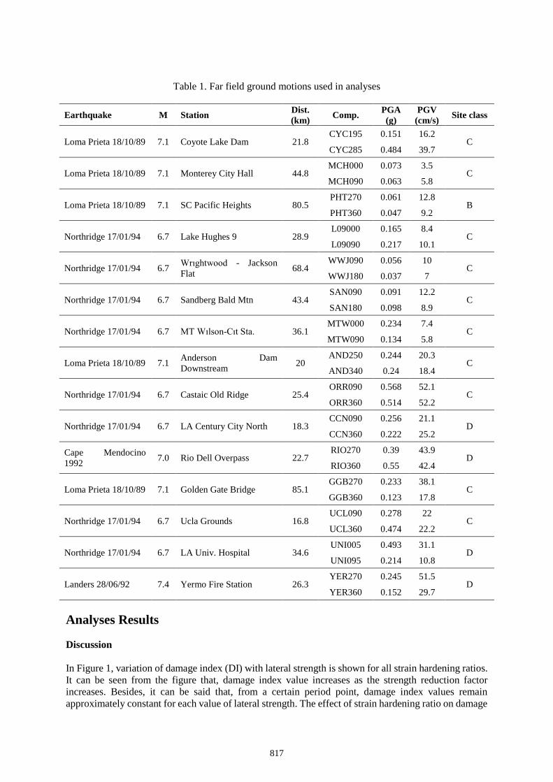
Table 1. Far field ground motions used in analyses

Earthquake M Station Dist.

(km) Comp.

PGA

(g)

PGV

(cm/s) Site class

Loma Prieta 18/10/89 7.1 Coyote Lake Dam 21.8 CYC195 0.151 16.2

C CYC285 0.484 39.7

Loma Prieta 18/10/89 7.1 Monterey City Hall 44.8 MCH000 0.073 3.5

C MCH090 0.063 5.8

Loma Prieta 18/10/89 7.1 SC Pacific Heights 80.5 PHT270 0.061 12.8

B PHT360 0.047 9.2

Northridge 17/01/94 6.7 Lake Hughes 9 28.9 L09000 0.165 8.4

C L09090 0.217 10.1

Northridge 17/01/94 6.7 Wrıghtwood - Jackson

Flat 68.4

WWJ090 0.056 10 C

WWJ180 0.037 7

Northridge 17/01/94 6.7 Sandberg Bald Mtn 43.4 SAN090 0.091 12.2

C SAN180 0.098 8.9

Northridge 17/01/94 6.7 MT Wılson-Cıt Sta. 36.1 MTW000 0.234 7.4

C MTW090 0.134 5.8

Loma Prieta 18/10/89 7.1 Anderson Dam

Downstream 20

AND250 0.244 20.3 C

AND340 0.24 18.4

Northridge 17/01/94 6.7 Castaic Old Ridge 25.4 ORR090 0.568 52.1

C ORR360 0.514 52.2

Northridge 17/01/94 6.7 LA Century City North 18.3 CCN090 0.256 21.1

D CCN360 0.222 25.2

Cape Mendocino

1992 7.0 Rio Dell Overpass 22.7

RIO270 0.39 43.9 D

RIO360 0.55 42.4

Loma Prieta 18/10/89 7.1 Golden Gate Bridge 85.1 GGB270 0.233 38.1

C GGB360 0.123 17.8

Northridge 17/01/94 6.7 Ucla Grounds 16.8 UCL090 0.278 22

C UCL360 0.474 22.2

Northridge 17/01/94 6.7 LA Univ. Hospital 34.6 UNI005 0.493 31.1

D UNI095 0.214 10.8

Landers 28/06/92 7.4 Yermo Fire Station 26.3 YER270 0.245 51.5

D YER360 0.152 29.7

Analyses Results

Discussion

In Figure 1, variation of damage index (DI) with lateral strength is shown for all strain hardening ratios.

It can be seen from the figure that, damage index value increases as the strength reduction factor

increases. Besides, it can be said that, from a certain period point, damage index values remain

approximately constant for each value of lateral strength. The effect of strain hardening ratio on damage

817

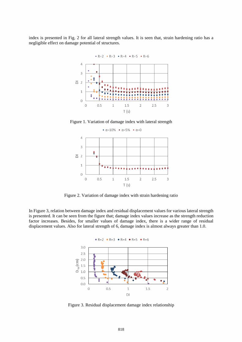
index is presented in Fig. 2 for all lateral strength values. It is seen that, strain hardening ratio has a

negligible effect on damage potential of structures.

Figure 1. Variation of damage index with lateral strength

Figure 2. Variation of damage index with strain hardening ratio

In Figure 3, relation between damage index and residual displacement values for various lateral strength

is presented. It can be seen from the figure that; damage index values increase as the strength reduction

factor increases. Besides, for smaller values of damage index, there is a wider range of residual

displacement values. Also for lateral strength of 6, damage index is almost always greater than 1.0.

Figure 3. Residual displacement damage index relationship

818

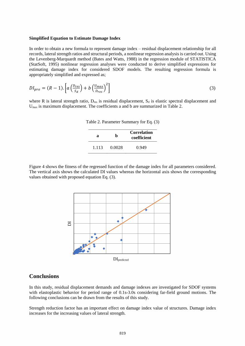
Simplified Equation to Estimate Damage Index

In order to obtain a new formula to represent damage index – residual displacement relationship for all

records, lateral strength ratios and structural periods, a nonlinear regression analysis is carried out. Using

the Levenberg-Marquardt method (Bates and Watts, 1988) in the regression module of STATISTICA

(StatSoft, 1995) nonlinear regression analyses were conducted to derive simplified expressions for

estimating damage index for considered SDOF models. The resulting regression formula is

appropriately simplified and expressed as;

𝐷𝐼𝑝𝑟𝑒 = (𝑅 − 1). [𝑎 (𝐷𝑟𝑒𝑠

𝑆𝑑) + 𝑏 (

𝑈𝑚𝑎𝑥

𝐷𝑟𝑒𝑠)2

] (3)

where R is lateral strength ratio, Dres is residual displacement, Sd is elastic spectral displacement and

Umax is maximum displacement. The coefficients a and b are summarized in Table 2.

Table 2. Parameter Summary for Eq. (3)

a b Correlation

coefficient

1.113 0.0028 0.949

Figure 4 shows the fitness of the regressed function of the damage index for all parameters considered.

The vertical axis shows the calculated DI values whereas the horizontal axis shows the corresponding

values obtained with proposed equation Eq. (3).

Conclusions

In this study, residual displacement demands and damage indexes are investigated for SDOF systems

with elastoplastic behavior for period range of 0.1s-3.0s considering far-field ground motions. The

following conclusions can be drawn from the results of this study.

Strength reduction factor has an important effect on damage index value of structures. Damage index

increases for the increasing values of lateral strength.

DIpredicted

DI

819

The effect of strain hardening ratio on damage index is negligible for all lateral strength values. For

lateral strength value of 6, damage index is almost always greater than unity.

A new equation is proposed to express damage index based on lateral strength, residual displacement,

elastic spectral displacement and maximum displacement.

References

Vision 2000 (1995) Performance Based Seismic Engineering of Buildings, SEAOC.

FEMA 356 (2000) Prestandard and Commentary for The Seismic Rehabilitation of Buildings

Park, Y.-J., & Ang, A.H.-S. (1985). Mechanistic seismic damage model for reinforced concrete. ASCE Journal

of Structural Engineering, 111(4), 722-739.

Powell, G.H., & Allahabadi, R. (1988). Seismic damage prediction by deterministic methods: Concepts and

procedures. Earthquake Engineering & Structural Dynamics, 16(5), 719- 734.

Fajfar, P. (1992). Equivalent ductility factors, taking into account low-cycle fatigue. Earthquake Engineering &

Structural Dynamics, 21(10), 837-848.

Cosenza, E., Manfredi, G., & Ramasco, R. (1993). The use of damage functionals in earthquake engineering: A

comparison between different methods. Earthquake Engineering &

Structural Dynamics, 22(10), 855-868.

Williams, M.S., Sexsmith, R.G. (1995). Seismic Damage Indices for Concrete Structures: A State-of-the-Art

Review, Earthquake Spectra, https://doi.org/10.1193/1.1585817

Ghobarah, A., Abou-Elfath, H., & Biddah, A. (1999). Response based damage assessment of structures.

Earthquake Engineering & Structural Dynamics, 28(1), 79-104.

Rodriguez, M.E., Aristizabal, J.C. (1999). Evaluation of a seismic damage parameter. Earthquake Engineering

& Structural Dynamics 28(5):463-477.

Mehanny, S.F., Deierlein, G.G. (2001). Seismic Damage and Collapse Assessment of Composite Moment

Frames, Journal of Structural Engineering 127(9).

Bozorgnia, Y., Bertero V.V. (2003). Damage Spectra: Characteristics and Applications to Seismic Risk

Reduction. Journal of Structural Engineering 129(10).

Applied Technology Council (ATC-1996). ATC 40: The Seismic Evaluation and Retrofit of Concrete Buildings.

2 volumes. Redwood City, California.

Pacific Earthquake Engineering Research Center. PEER Strong motion database. http://peer.berkeley.edu/smcat.

Last access: 2019.

Bates DM, Watts DG (1988). Nonlinear regression analysis and its applications. Wiley: New York.

StatSoft Inc (1995). STATISTICA V.12.0 for Windows. Tulsa, OK, USA.

820

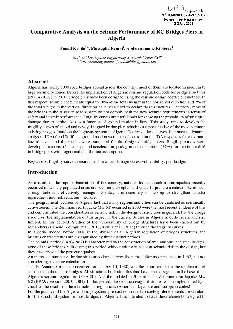
Comparative Analysis on the Seismic Performance of RC Bridges Piers in Algeria

Fouad Kehila1*, Mustapha Remki1, Abderrahmane Kibboua1

1National Earthquake Engineering Research Center CGS *Corresponding author, [email protected]

AbstractAlgeria has nearly 6000 road bridges spread across the country; most of them are located in medium to high seismicity zones. Before the implantation of Algerian seismic regulation code for bridge structures (RPOA-2008) in 2010, bridge piers have been designed using the seismic design coefficient method. In this respect, seismic coefficients equal to 10% of the total weight in the horizontal direction and 7% of the total weight in the vertical direction have been used to design these structures. Therefore, most of the bridges in the Algerian road system do not comply with the new seismic requirements in terms of safety and seismic performance. Fragility curves are useful tools for showing the probability of structural damage due to earthquakes as a function of ground motion indices. This study aims to develop the fragility curves of an old and newly designed bridge pier, which is a representative of the most common existing bridges found on the highway system in Algeria. To derive these curves. Incremental dynamic analyses (IDA) for (15) fifteen ground motion were carried out to plot the IDA responses for maximum hazard level, and the results were compared for the designed bridge piers. Fragility curves were developed in terms of elastic spectral acceleration, peak ground acceleration (PGA) for maximum drift in bridge piers with lognormal distribution assumption.

Keywords: fragility curves; seismic performance; damage states; vulnerability; pier bridge.

Introduction

As a result of the rapid urbanization of the country, natural disasters such as earthquakes recently occurred in densely populated areas are becoming complex and vital. To prepare a catastrophe of such a magnitude and effectively manage the risks, it is necessary to step up to strengthen disaster reparedness and risk reduction measures. The geographical location of Algeria fact that many regions and cities can be qualified as seismically active zones. The Zemmouri earthquake Mw 6.8 occurred in 2003 were the most recent evidence of this and demonstrated the consideration of seismic risk in the design of structures in general. For the bridge structures, the implementation of this aspect in the current studies in Algeria is quite recent and still limited. In this context, Studies of the vulnerability of bridge structures have been carried out by researchers (Hamaidi Zourgui et al., 2017; Kehila et al. ,2018) through the fragility curves. In Algeria, Indeed, before 2008, in the absence of an Algerian regulation of bridges structures, the bridge's characteristics are distinguished by three distinct periods. The colonial period (1830-1962) is characterized by the construction of arch masonry and steel bridges, none of these bridges built during this period without taking in account seismic risk in the design, but they have resisted the past earthquakes. An increased number of bridge structures characterizes the period after independence in 1962, but not considering a seismic calculation. The El Asnam earthquake occurred on October 10, 1980, was the main reason for the application of seismic calculations for bridges. All structures built after this date have been designed on the base of the Algerian seismic regulations (RPA 80). And the updated in 2003 after the Zemmouri earthquake Mw 6.8 (RPA99 version 2003, 2003). In this period, the seismic design of studies was complemented by a check of the results on the international regulations (American, Japanese and European codes). For the practice of the Algerian bridge system, pre-cast reinforced concrete girder elements are standard for the structural system in most bridges in Algeria. It is intended to have these elements designed to

821

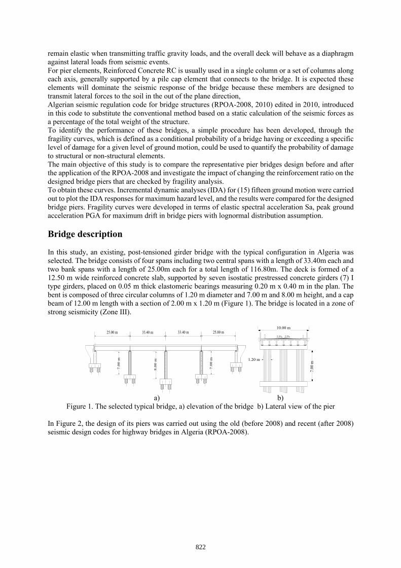
remain elastic when transmitting traffic gravity loads, and the overall deck will behave as a diaphragm against lateral loads from seismic events. For pier elements, Reinforced Concrete RC is usually used in a single column or a set of columns along each axis, generally supported by a pile cap element that connects to the bridge. It is expected these elements will dominate the seismic response of the bridge because these members are designed to transmit lateral forces to the soil in the out of the plane direction, Algerian seismic regulation code for bridge structures (RPOA-2008, 2010) edited in 2010, introduced in this code to substitute the conventional method based on a static calculation of the seismic forces as a percentage of the total weight of the structure. To identify the performance of these bridges, a simple procedure has been developed, through the fragility curves, which is defined as a conditional probability of a bridge having or exceeding a specific level of damage for a given level of ground motion, could be used to quantify the probability of damage to structural or non-structural elements. The main objective of this study is to compare the representative pier bridges design before and after the application of the RPOA-2008 and investigate the impact of changing the reinforcement ratio on the designed bridge piers that are checked by fragility analysis. To obtain these curves. Incremental dynamic analyses (IDA) for (15) fifteen ground motion were carried out to plot the IDA responses for maximum hazard level, and the results were compared for the designed bridge piers. Fragility curves were developed in terms of elastic spectral acceleration Sa, peak ground acceleration PGA for maximum drift in bridge piers with lognormal distribution assumption.

Bridge description

In this study, an existing, post-tensioned girder bridge with the typical configuration in Algeria was selected. The bridge consists of four spans including two central spans with a length of 33.40m each and two bank spans with a length of 25.00m each for a total length of 116.80m. The deck is formed of a 12.50 m wide reinforced concrete slab, supported by seven isostatic prestressed concrete girders (7) I type girders, placed on 0.05 m thick elastomeric bearings measuring 0.20 m x 0.40 m in the plan. The bent is composed of three circular columns of 1.20 m diameter and 7.00 m and 8.00 m height, and a cap beam of 12.00 m length with a section of 2.00 m x 1.20 m (Figure 1). The bridge is located in a zone of strong seismicity (Zone III).

a) b) Figure 1. The selected typical bridge, a) elevation of the bridge b) Lateral view of the pier

In Figure 2, the design of its piers was carried out using the old (before 2008) and recent (after 2008) seismic design codes for highway bridges in Algeria (RPOA-2008).

7.00

m

8.00

m

25.00 m 33.40 m 33.40 m 25.00 m

7.00

m

7.00

m

1.20 m

2.5% 2.5%

10.00 m

822

Figure 2. Cross-section of pier designed before and after the RPOA-2008

Numerical model

A three-dimensional analytical model of a bridge was generated in SeismoStruct (SeismoSoft 2018) to perform incremental dynamic analysis IDA. the circular cross-section of the pier was modelled with a fiber element, each fiber has a stress-strain relationship, which can be specified to represent unconfined concrete, confined concrete and longitudinal steel reinforcement. Mander et al. (1988) model was used to simulate the behaviour of confined and unconfined concrete, for the steel model, a model of Menegotto-Pinto (1973) coupled with isotropic hardening rules proposed by Filippou et al. (1983). Elastic frame element has been used for modelling the deck and girders. The model of elastomeric bearing as defined in the longitudinal and transverse direction using the symmetric bilinear zero-length link element. A 3D numerical analytical model of the chosen bridge, which represents a typical bridge structure in Algeria, is shown in Figure 3.

Figure 3. The numerical model of the selected bridge

Ground motions selection

A set of 15 strong ground motion records are selected from the Pacific Earthquake Engineering Research Center (PEER 2016) Strong Motion Database and listed in Table 1. This suite of records covers a wide range of magnitudes between 5.2 and 7.36 and epicentral distance up to around 39 km, as illustrated by the scatter diagram in Figure 4a. Figure 4b shown the associated spectral shapes for the suite of ground motions. According to the region of the selected bridge, The ground motion records have a spectral acceleration value close to the spectral acceleration values in seismic zone III of the RPOA-2008 code and site class S3 (soft soil type).

24T25

Hoops T16@15cm

1.20m

24T32

Hoops T16@10cm

1.20m

After RPOA2008Before RPOA2008

15 cm 10 cm

Plan

Elevation

d

b

h

Steel plate

Internal rubber layers

hs

Rubber cover

Bear

ing

Pier

823

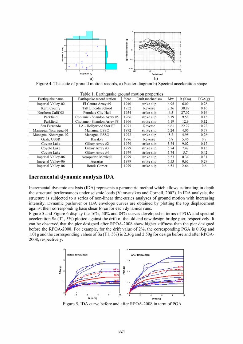
a) b) Figure 4. The suite of ground motion records, a) Scatter diagram b) Spectral acceleration shape

Table 1. Earthquake ground motion properties Earthquake name Earthquake record station Year Fault mechanism Mw R (Km) PGA(g)

Imperial Valley-02 El Centro Array #9 1940 strike slip 6.95 6.09 0.28 Kern County Taft Lincoln School 1952 Reverse 7.36 38.89 0.16

Northern Calif-03 Ferndale City Hall 1954 strike-slip 6.5 27.02 0.16 Parkfield Cholame - Shandon Array #5 1966 strike slip 6.19 9.58 0.15 Parkfield Cholame - Shandon Array #8 1966 strike slip 6.19 12.9 0.12

San Fernando LA - Hollywood Stor FF 1971 Reverse 6.61 22.77 0.22 Managua, Nicaragua-01 Managua, ESSO 1972 strike slip 6.24 4.06 0.37 Managua, Nicaragua-02 Managua, ESSO 1972 strike slip 5.2 4.98 0.26

Gazli, USSR Karakyr 1976 Reverse 6.8 5.46 0.7 Coyote Lake Gilroy Array #2 1979 strike-slip 5.74 9.02 0.17 Coyote Lake Gilroy Array #3 1979 strike slip 5.74 7.42 0.15 Coyote Lake Gilroy Array #4 1979 strike-slip 5.74 5.7 0.42

Imperial Valley-06 Aeropuerto Mexicali 1979 strike slip 6.53 0.34 0.31 Imperial Valley-06 Agrarias 1979 strike slip 6.53 0.65 0.29 Imperial Valley-06 Bonds Corner 1979 strike-slip 6.53 2.66 0.6

Incremental dynamic analysis IDA

Incremental dynamic analysis (IDA) represents a parametric method which allows estimating in depth the structural performances under seismic loads (Vamvatsikos and Cornell, 2002). In IDA analysis, the structure is subjected to a series of non-linear time-series analyses of ground motion with increasing intensity. Dynamic pushover or IDA envelope curves are obtained by plotting the top displacement against their corresponding base shear force for each dynamics runs. Figure 5 and Figure 6 display the 16%, 50% and 84% curves developed in terms of PGA and spectral acceleration Sa (T1, 5%) plotted against the drift of the old and new design bridge pier, respectively. It can be observed that the pier designed after RPOA-2008 show higher stiffness than the pier designed before the RPOA-2008. For example, for the drift value of 2%, the corresponding PGA is 0.93g and 1.01g and the corresponding values of Sa (T1, 5%) is 2.36g and 2.50g for design before and after RPOA-2008, respectively.

Figure 5. IDA curve before and after RPOA-2008 in term of PGA

5 6 7 80

10

20

30

40

50

Dis

tanc

e R

(kM

)

Magnitude Mw

0.01 0.1 1 100.001

0.01

0.1

1

10

Spec

tral

acc

eler

atio

n (g

)

Period (sec)

0 2 4 6 8 100

1

2

3

4

PGA

(g)

Drift (%)

84 %

50 %

16 %

Before RPOA-2008

0 2 4 6 8 100

1

2

3

4

After RPOA-2008

PGA

(g)

Drift (%)

84 %

50 %

16 %

824

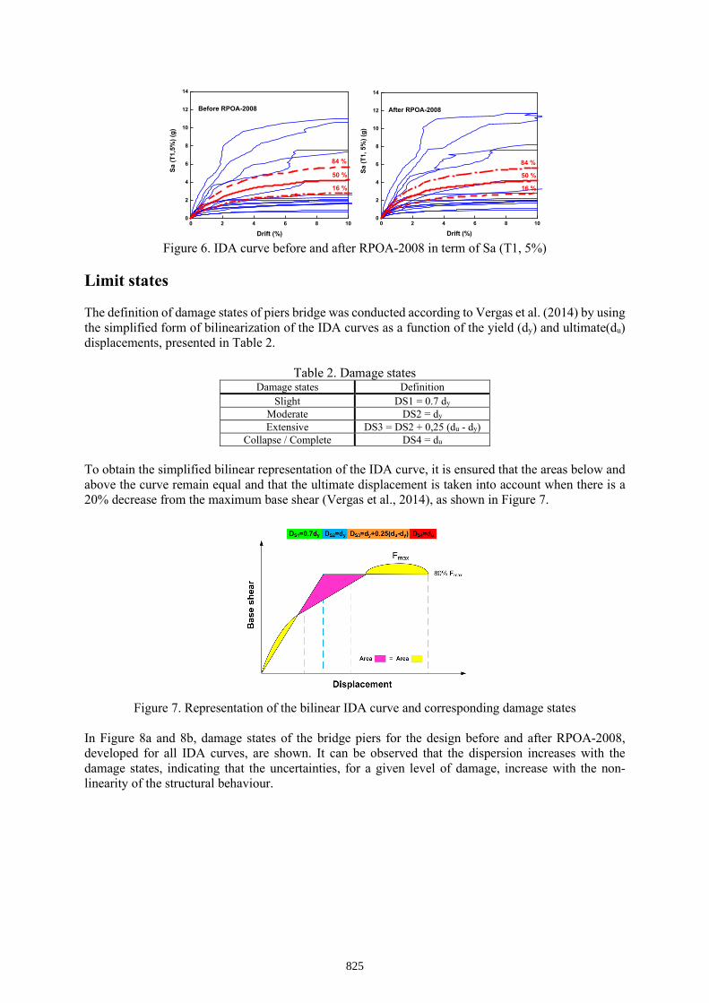
Figure 6. IDA curve before and after RPOA-2008 in term of Sa (T1, 5%)

Limit states

The definition of damage states of piers bridge was conducted according to Vergas et al. (2014) by using the simplified form of bilinearization of the IDA curves as a function of the yield (dy) and ultimate(du) displacements, presented in Table 2.

Table 2. Damage states Damage states Definition

Slight DS1 = 0.7 dy Moderate DS2 = dy Extensive DS3 = DS2 + 0,25 (du - dy)

Collapse / Complete DS4 = du

To obtain the simplified bilinear representation of the IDA curve, it is ensured that the areas below and above the curve remain equal and that the ultimate displacement is taken into account when there is a 20% decrease from the maximum base shear (Vergas et al., 2014), as shown in Figure 7.

Figure 7. Representation of the bilinear IDA curve and corresponding damage states

In Figure 8a and 8b, damage states of the bridge piers for the design before and after RPOA-2008, developed for all IDA curves, are shown. It can be observed that the dispersion increases with the damage states, indicating that the uncertainties, for a given level of damage, increase with the non-linearity of the structural behaviour.

0 2 4 6 8 100

2

4

6

8

10

12

14

Before RPOA-2008

16 %

50 %

84 %Sa

(T1,

5%) (

g)

Drift (%)0 2 4 6 8 10

0

2

4

6

8

10

12

14

After RPOA-2008

16 %

50 %Sa (T

1, 5

%) (

g)

Drift (%)

84 %

825

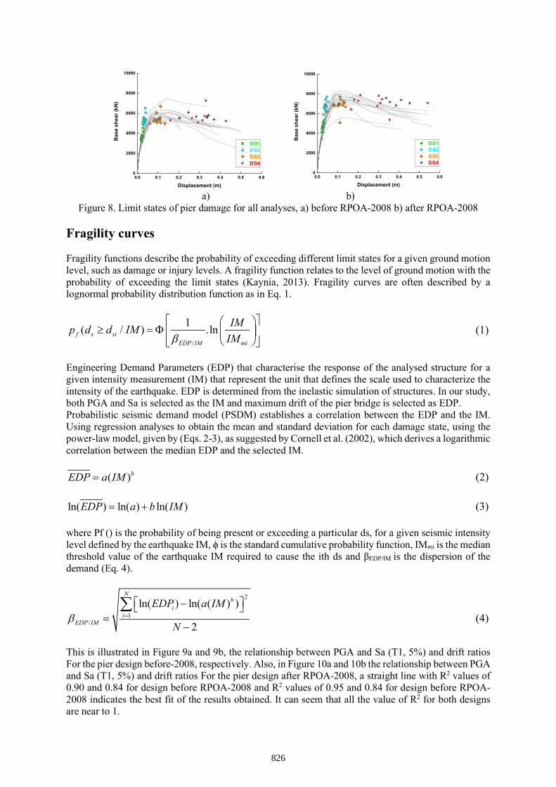
a) b) Figure 8. Limit states of pier damage for all analyses, a) before RPOA-2008 b) after RPOA-2008

Fragility curves

Fragility functions describe the probability of exceeding different limit states for a given ground motion level, such as damage or injury levels. A fragility function relates to the level of ground motion with the probability of exceeding the limit states (Kaynia, 2013). Fragility curves are often described by a lognormal probability distribution function as in Eq. 1.

/

1( / ) .lnf s siEDP IM mi

IMp d d IMIMβ

≥ = Φ

(1)

Engineering Demand Parameters (EDP) that characterise the response of the analysed structure for a given intensity measurement (IM) that represent the unit that defines the scale used to characterize the intensity of the earthquake. EDP is determined from the inelastic simulation of structures. In our study, both PGA and Sa is selected as the IM and maximum drift of the pier bridge is selected as EDP. Probabilistic seismic demand model (PSDM) establishes a correlation between the EDP and the IM. Using regression analyses to obtain the mean and standard deviation for each damage state, using the power-law model, given by (Eqs. 2-3), as suggested by Cornell et al. (2002), which derives a logarithmic correlation between the median EDP and the selected IM.

( )bEDP a IM= (2)

ln( ) ln( ) ln( )EDP a b IM= + (3)

where Pf () is the probability of being present or exceeding a particular ds, for a given seismic intensity level defined by the earthquake IM, ϕ is the standard cumulative probability function, IMmi is the median threshold value of the earthquake IM required to cause the ith ds and βEDP/IM is the dispersion of the demand (Eq. 4).

2

1/

ln( ) ln( ( ) )

2

Nb

ii

EDP IM

EDP a IM

Nβ =

− =

−

∑ (4)

This is illustrated in Figure 9a and 9b, the relationship between PGA and Sa (T1, 5%) and drift ratios For the pier design before-2008, respectively. Also, in Figure 10a and 10b the relationship between PGA and Sa (T1, 5%) and drift ratios For the pier design after RPOA-2008, a straight line with R2 values of 0.90 and 0.84 for design before RPOA-2008 and R2 values of 0.95 and 0.84 for design before RPOA-2008 indicates the best fit of the results obtained. It can seem that all the value of R2 for both designs are near to 1.

0.0 0.1 0.2 0.3 0.4 0.5 0.60

2000

4000

6000

8000

10000

Bas

e sh

ear (

kN)

Displacement (m)

DS1 DS2 DS3 DS4

0.0 0.1 0.2 0.3 0.4 0.5 0.60

2000

4000

6000

8000

10000

Bas

e sh

ear (

kN)

Displacement (m)

DS1 DS2 DS3 DS4

826

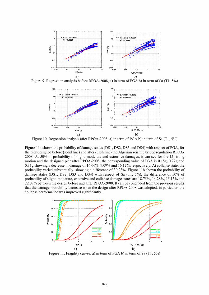
a) b) Figure 9. Regression analysis before RPOA-2008, a) in term of PGA b) in term of Sa (T1, 5%)

a) b) Figure 10. Regression analysis after RPOA-2008, a) in term of PGA b) in term of Sa (T1, 5%)

Figure 11a shown the probability of damage states (DS1, DS2, DS3 and DS4) with respect of PGA, for the pier designed before (solid line) and after (dash line) the Algerian seismic bridge regulation RPOA-2008. At 50% of probability of slight, moderate and extensive damages, it can see for the 15 strong motion and the designed pier after RPOA-2008, the corresponding value of PGA is 0.18g, 0.22g and 0.31g showing a decrease in damage of 16.66%, 9.09% and 16.12%, respectively. At collapse state, the probability varied substantially, showing a difference of 30.23%. Figure 11b shown the probability of damage states (DS1, DS2, DS3 and DS4) with respect of Sa (T1, 5%), the difference of 50% of probability of slight, moderate, extensive and collapse damage states are 18.75%, 14.28%, 15.15% and 22.07% between the design before and after RPOA-2008. It can be concluded from the previous results that the damage probability decrease when the design after RPOA-2008 was adopted, in particular, the collapse performance was improved significantly.

a) b) Figure 11. Fragility curves, a) in term of PGA b) in term of Sa (T1, 5%)

0.001 0.01 0.1 1 100.001

0.01

0.1

1

10

100

Drif

t (%

)

PGA (g)

Y = 0.7307X - 0.4827 R2 = 0.9021

0.001 0.01 0.1 1 100.001

0.01

0.1

1

10

100

Y = 0.74427X - 0.19981 R2 = 0.8386

Drif

t (%

)

Sa (T1,5%) (g)

0.001 0.01 0.1 1 100.001

0.01

0.1

1

10

100

Y = 0.74284X - 0.16536 R2 = 0.95382

Drif

t (%

)

PGA (g)0.001 0.01 0.1 1 10

0.001

0.01

0.1

1

10

100

Y = 0.74944X + 0.1872 R2 = 0.84004

Drif

t (%

)

Sa (T1,5%) (g)

0 0.5 1 1.5 20

0.2

0.4

0.6

0.8

1

Prob

abili

ty

PGA (g)

DS1 DS2 DS3 DS4

0 1 2 3 40

0.2

0.4

0.6

0.8

1

Prob

abili

ty

Sa(T1, 5%) (g)

DS1 DS2 DS3 DS4

827

Conclusion

In this study, the fragility curves are established for drift thresholds and different types of the ground motion intensity measure, namely the peak ground acceleration PGA, and the structure-specific spectral acceleration Sa (T1, 5%) for bridge pier designed with both the old seismic design code before RPOA-2008 and the Algerian seismic code for bridges in Algeria (after RPOA-2008). To generate the fragility curves, dynamic pushover obtains from IDA analysis were used to define the limit states. The results show for the pier designed after RPOA-2008 a best seismic performance while compared to the same bridge pier designed by the old seismic code (RPOA-2008). The designed pier after RPOA-2008 decreases the damage probability to 16.66%, 9.09%, 16.12% and 30.23% for slight, moderate, extensive and collapse in term of PGA and 18.75%, 14.28%, 15.15% and 22.07% in term of Sa (T1, 5%) at 50% of damage probability.

References

Cornell AC, Jalayer F and Hamburger RO (2002) “Probabilistic basis for 2000 SAC federal emergency management agency steel moment frame guidelines,” Journal of Structural Engineering, 128(4): 526–532

Filippou FC, Popov EP and Bertero VV (1983) Effects of bond deterioration on hysteretic behavior of reinforced concrete joints, Report EERC 83-19, Earthquake Engineering Research Center, University of California, Berkeley.

Hemaidi Zourgui N, Kibboua A and Taki M (2018) “Using full bridge model to develop analytical fragility curves for typical concrete bridge piers,” GRAĐEVINAR, 70 (6): 519-530

Kaynia AM (2013) Guidelines for Deriving Seismic Fragility Functions of Elements at Risk: Buildings, Lifelines, Transportation Networks and Critical Facilities. SYNER-G Reference Report 4, Publications Office of the European Union, Luxembourg

Kehila F, Kibboua A, Bechtoula H and Remki M (2018) “Seismic performance assessment of R.C. bridge piers designed with the Algerian seismic bridges regulation,” Earthquakes and Structures, 15(6): 701–713

Mander JB, Priestley MJN and Park R (1988) “Theoretical stress-strain model for confined concrete,” Journal of Structural Engineering, 114(8): 1804-1826

Menegotto M, Pinto PE (1973) “Method of analysis for cyclically loaded R.C. plane frames including changes in geometry and nonelastic behaviour of elements under combined normal force and bending”. Symposium on the Resistance and Ultimate Deformability of Structures Acted on By Well-Defined Repeated Loads, International Association for Bridge and Structural Engineering, Zurich, Switzerland, 15–22

PEER (Pacific Earthquake Engineering Research Center) (2016) Online Strong Motion Database. PEER, University of California, Berkeley, CA, USA. See http://ngawest2.berkeley.edu/.

RPA99 version 2003 (2003), Algerian Seismic Code, Ministry of Housing and Urban Planning, DTR-BC 2.48, Algeria

RPOA 2008 (2008) Algerian seismic regulation code for bridge structures, Document Technique Règlementaire, Ministère des Travaux Publics, Algeria

Seismosoft (2018) SeismoStruct: A Computer Program for Static and Dynamic Analysis for Framed Structures, Seismosoft, Pavia, Italy. See http://www.seismosoft.com.

Vamvatsikos D and Cornell CA (2002) “Incremental dynamic analysis,” Earthquake Engineering & Structural Dynamics, 31(3): 491–514

Vargas YF, Barbat AH, Pujades LG and Hurtado JE (2014) “Probabilistic seismic risk evaluation of reinforced concrete buildings,” Proceedings of the Institution of Civil Engineers - Structures and Buildings, 167(6): 327–336

828

A Sensitivity Study for Seismic Response Assessment of Highway Bridges

with Uncertain Modeling, Scour and Deterioration Parameters

Züleyha Kanpara Cıvaş 1, Onur Cem Aygın 1, Taner Yılmaz 2*

1 M.Sc. Student, Department of Civil Engineering, Ozyegin University, Istanbul, Turkey; 2 Assistant Professor, Department of Civil Engineering, Ozyegin University, Istanbul, Turkey;


AbstractSeismic performance assessment of bridges subject to flood-induced scour is essential to achieve better

design procedures and reduced risk of failure for highway bridges on rivers. However, bridge seismic

response computed through nonlinear analysis can vary considerably due to the uncertainties existing in

modeling parameters, estimated scour depth at pier foundations and parameters defining structural

deterioration which can downgrade the time-varying structural performance. Uncertainty quantification

of seismic performance of bridges in the form of fragility functions can be computationally expensive

in the case of performing nonlinear time-history analysis of bridge models which contain a large set of

uncertain parameters. To address this problem, this study presents a sensitivity analysis conducted to

identify the most significant uncertain parameters to which bridge structural response is sensitive under

several earthquake ground motions. Tornado diagrams are generated based on the results of nonlinear

time-history analyses of the finite element models of a typical highway bridge. The outcomes of this

study yield valuable insight that can be employed in the succeeding studies for generation of seismic

fragility curves of highway bridges.

Keywords: Bridges, Sensitivity, Seismic, Scour, Deterioration.

Introduction

Bridges are generally regarded to have a vital importance for highway transportation networks. In case

of an earthquake disaster, it is desired to prevent bridge failures and accordingly the disruption of the

transportation (of people or necessary equipment or aids) between communities. Therefore, assessment

of seismic risk of bridges is essential for the reduced risk and enhanced resilience of bridge networks.

A reliable assessment of bridge seismic risk relies on a rigorous performance evaluation in which the

uncertainties in the parameters affecting the seismic response are well propagated. Considering the

uncertainties in all input parameters within the seismic analysis of bridges can be time-consuming and

may lead to inadequacy of computing resources. For this reason, determining the uncertain parameters

which are the most effective on the structural response of bridges under an earthquake excitation is

needed for an efficient procedure of generating analytical fragility curves of bridges.

Seismic fragility assessment of the bridges under the effect of flood-induced scour has been investigated

by many researchers (e.g. Wang et al., 2014; Yilmaz et al., 2016; Yilmaz and Banerjee, 2018). In most

of these studies, seismic fragility curves of bridges were developed under various levels of scour depth

or flood events. On the other hand, time-varying seismic fragility curves of deteriorating bridges under

the influence of chloride-induced corrosion at reinforced concrete (RC) piers were developed in a couple

of studies (e.g. Ghosh and Padgett, 2010; Yilmaz and Aygin, 2019). Billah and Allam (2015) reviewed

past studies on seismic fragility assessment of highway bridges and presented a list of uncertain

parameters that influence the development of seismic fragility curves. This list includes the uncertainties

in modeling, scour depth estimation formula, soil and aging parameters that were considered in various

studies. Yilmaz et al. (2018) performed a detailed uncertainty analysis to obtain the variations of seismic

fragility curves of a bridge for several flood conditions with varied frequencies and found out that

uncertain input parameters should not be ignored in seismic risk assessment of bridges under the

presence of flood-induced scour.

829

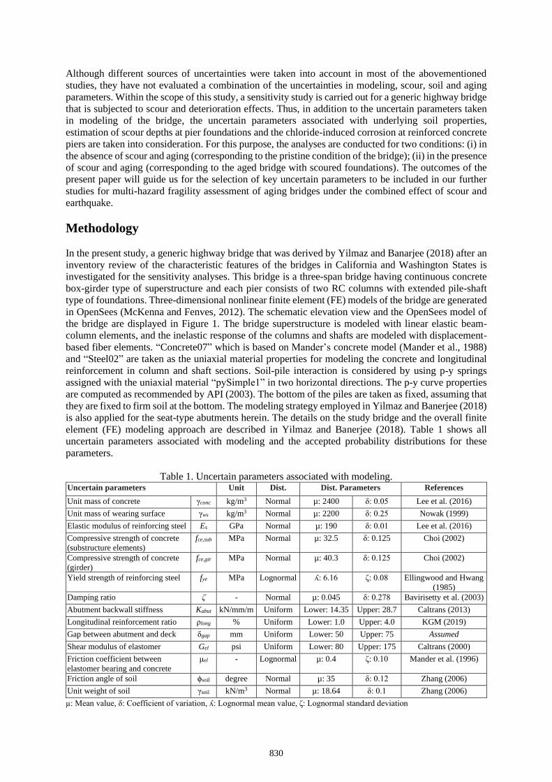
Although different sources of uncertainties were taken into account in most of the abovementioned

studies, they have not evaluated a combination of the uncertainties in modeling, scour, soil and aging

parameters. Within the scope of this study, a sensitivity study is carried out for a generic highway bridge

that is subjected to scour and deterioration effects. Thus, in addition to the uncertain parameters taken

in modeling of the bridge, the uncertain parameters associated with underlying soil properties,

estimation of scour depths at pier foundations and the chloride-induced corrosion at reinforced concrete

piers are taken into consideration. For this purpose, the analyses are conducted for two conditions: (i) in

the absence of scour and aging (corresponding to the pristine condition of the bridge); (ii) in the presence

of scour and aging (corresponding to the aged bridge with scoured foundations). The outcomes of the

present paper will guide us for the selection of key uncertain parameters to be included in our further

studies for multi-hazard fragility assessment of aging bridges under the combined effect of scour and

earthquake.

Methodology

In the present study, a generic highway bridge that was derived by Yilmaz and Banarjee (2018) after an

inventory review of the characteristic features of the bridges in California and Washington States is

investigated for the sensitivity analyses. This bridge is a three-span bridge having continuous concrete

box-girder type of superstructure and each pier consists of two RC columns with extended pile-shaft

type of foundations. Three-dimensional nonlinear finite element (FE) models of the bridge are generated

in OpenSees (McKenna and Fenves, 2012). The schematic elevation view and the OpenSees model of

the bridge are displayed in Figure 1. The bridge superstructure is modeled with linear elastic beam-

column elements, and the inelastic response of the columns and shafts are modeled with displacement-

based fiber elements. “Concrete07” which is based on Mander’s concrete model (Mander et al., 1988)

and “Steel02” are taken as the uniaxial material properties for modeling the concrete and longitudinal

reinforcement in column and shaft sections. Soil-pile interaction is considered by using p-y springs

assigned with the uniaxial material “pySimple1” in two horizontal directions. The p-y curve properties

are computed as recommended by API (2003). The bottom of the piles are taken as fixed, assuming that

they are fixed to firm soil at the bottom. The modeling strategy employed in Yilmaz and Banerjee (2018)

is also applied for the seat-type abutments herein. The details on the study bridge and the overall finite

element (FE) modeling approach are described in Yilmaz and Banerjee (2018). Table 1 shows all

uncertain parameters associated with modeling and the accepted probability distributions for these

parameters.

Table 1. Uncertain parameters associated with modeling. Uncertain parameters Unit Dist. Dist. Parameters References

Unit mass of concrete γconc kg/m3 Normal µ: 2400 δ: 0.05 Lee et al. (2016)

Unit mass of wearing surface γws kg/m3 Normal µ: 2200 δ: 0.25 Nowak (1999)

Elastic modulus of reinforcing steel Es GPa Normal µ: 190 δ: 0.01 Lee et al. (2016)

Compressive strength of concrete

(substructure elements)

fce,sub MPa Normal µ: 32.5 δ: 0.125 Choi (2002)

Compressive strength of concrete

(girder)

fce,gir MPa Normal µ: 40.3 δ: 0.125 Choi (2002)

Yield strength of reinforcing steel fye MPa Lognormal ʎ: 6.16 ζ: 0.08 Ellingwood and Hwang

(1985)

Damping ratio ζ - Normal µ: 0.045 δ: 0.278 Bavirisetty et al. (2003)

Abutment backwall stiffness Kabut kN/mm/m Uniform Lower: 14.35 Upper: 28.7 Caltrans (2013)

Longitudinal reinforcement ratio ρlong % Uniform Lower: 1.0 Upper: 4.0 KGM (2019)

Gap between abutment and deck δgap mm Uniform Lower: 50 Upper: 75 Assumed

Shear modulus of elastomer Gel psi Uniform Lower: 80 Upper: 175 Caltrans (2000)

Friction coefficient between

elastomer bearing and concrete

μel - Lognormal µ: 0.4 ζ: 0.10 Mander et al. (1996)

Friction angle of soil ϕsoil degree Normal µ: 35 δ: 0.12 Zhang (2006)

Unit weight of soil γsoil kN/m3 Normal µ: 18.64 δ: 0.1 Zhang (2006)

µ: Mean value, δ: Coefficient of variation, ʎ: Lognormal mean value, ζ: Lognormal standard deviation

830

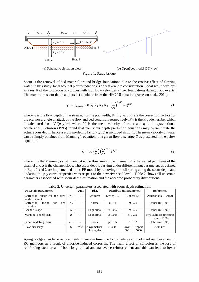
(a) Schematic elevation view (b) OpenSees model (3D view)

Figure 1. Study bridge.

Scour is the removal of bed material around bridge foundations due to the erosive effect of flowing

water. In this study, local scour at pier foundations is only taken into consideration. Local scour develops

as a result of the formation of vortices with high flow velocities at pier foundations during flood events.

The maximum scour depth at piers is calculated from the HEC-18 equation (Arneson et al., 2012):

𝑦𝑠 = f𝑠𝑐𝑜𝑢𝑟 2.0 𝑦1 K1 K2 K3 (𝑎

𝑦1)

0.65𝐹𝑟1

0.43 (1)

where y1 is the flow depth of the stream, a is the pier width; K1, K2, and K3 are the correction factors for

the pier nose, angle of attack of the flow and bed condition, respectively. Fr1 is the Froude number which

is calculated from V1/(g y1)1/2, where V1 is the mean velocity of water and g is the gravitational

acceleration. Johnson (1995) found that pier scour depth prediction equations may overestimate the

actual scour depth, hence a scour modeling factor (fscour) is included in Eq. 1. The mean velocity of water

can be simply obtained from Manning’s equation for a given flow discharge Q as presented in the below

equation:

𝑄 = 𝐴 (1

𝑛) (

𝐴

𝑃)

2/3𝑆1/2 (2)

where n is the Manning’s coefficient, A is the flow area of the channel, P is the wetted perimeter of the

channel and S is the channel slope. The scour depths varying under different input parameters as defined

in Eq.’s 1 and 2 are implemented in the FE model by removing the soil spring along the scour depth and

updating the p-y curve properties with respect to the new river bed level. Table 2 shows all uncertain

parameters associated with scour depth estimation and the accepted probability distributions.

Table 2. Uncertain parameters associated with scour depth estimation. Uncertain parameters Unit Dist. Distribution Parameters References

Correction factor for the flow

angle of attack

K2 - Uniform Lower: 1.0 Upper: 1.5 Arneson et al. (2012)

Correction factor for bed

condition

K3 - Normal µ: 1.1 δ: 0.05 Johnson (1995)

Channel slope S - Lognormal µ: 0.002 δ: 0.25 Johnson (1996)

Manning’s coefficient n - Lognormal µ: 0.025 δ: 0.275 Hydraulic Engineering

Center (1986)

Scour modeling factor fscour - Normal µ: 0.55 δ: 0.52 Johnson (1995)

Flow discharge Q m3/s Asymmetrical

Triangular

µ: 3500 Lower:

300

Upper:

5000

Assumed

Aging bridges can have reduced performance in time due to the deterioration of steel reinforcement in

RC members as a result of chloride-induced corrosion. The main effect of corrosion is the loss of

reinforcing steel areas of both longitudinal and transverse reinforcement and this can lead to lower

Hc = 7 m

Hs = 14 m

Abut. 1

Bent 2 Bent 3

45 m 35 m 35 m

Abut. 4

D = 1.52 m

831

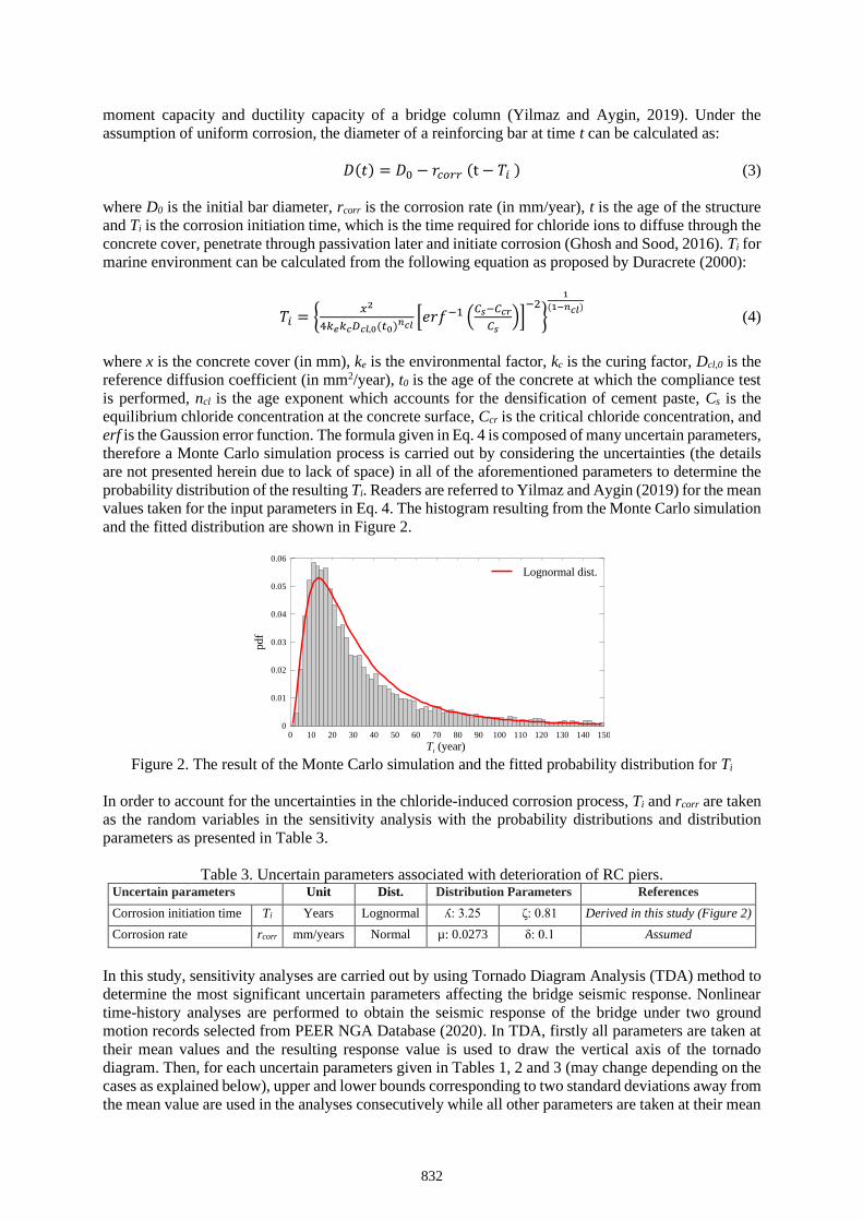
moment capacity and ductility capacity of a bridge column (Yilmaz and Aygin, 2019). Under the

assumption of uniform corrosion, the diameter of a reinforcing bar at time t can be calculated as:

𝐷(𝑡) = 𝐷0 − 𝑟𝑐𝑜𝑟𝑟 (t − 𝑇𝑖 ) (3)

where D0 is the initial bar diameter, rcorr is the corrosion rate (in mm/year), t is the age of the structure

and Ti is the corrosion initiation time, which is the time required for chloride ions to diffuse through the

concrete cover, penetrate through passivation later and initiate corrosion (Ghosh and Sood, 2016). Ti for

marine environment can be calculated from the following equation as proposed by Duracrete (2000):

𝑇𝑖 = {𝑥2

4𝑘𝑒𝑘𝑐𝐷𝑐𝑙,0(𝑡0)𝑛𝑐𝑙[𝑒𝑟𝑓−1 (

𝐶𝑠−𝐶𝑐𝑟

𝐶𝑠)]

−2}

1

(1−𝑛𝑐𝑙)

(4)

where x is the concrete cover (in mm), ke is the environmental factor, kc is the curing factor, Dcl,0 is the

reference diffusion coefficient (in mm2/year), t0 is the age of the concrete at which the compliance test

is performed, ncl is the age exponent which accounts for the densification of cement paste, Cs is the

equilibrium chloride concentration at the concrete surface, Ccr is the critical chloride concentration, and

erf is the Gaussion error function. The formula given in Eq. 4 is composed of many uncertain parameters,

therefore a Monte Carlo simulation process is carried out by considering the uncertainties (the details

are not presented herein due to lack of space) in all of the aforementioned parameters to determine the

probability distribution of the resulting Ti. Readers are referred to Yilmaz and Aygin (2019) for the mean

values taken for the input parameters in Eq. 4. The histogram resulting from the Monte Carlo simulation

and the fitted distribution are shown in Figure 2.

Figure 2. The result of the Monte Carlo simulation and the fitted probability distribution for Ti

In order to account for the uncertainties in the chloride-induced corrosion process, Ti and rcorr are taken

as the random variables in the sensitivity analysis with the probability distributions and distribution

parameters as presented in Table 3.

Table 3. Uncertain parameters associated with deterioration of RC piers. Uncertain parameters Unit Dist. Distribution Parameters References

Corrosion initiation time Ti Years Lognormal ʎ: 3.25 ζ: 0.81 Derived in this study (Figure 2)

Corrosion rate rcorr mm/years Normal µ: 0.0273 δ: 0.1 Assumed

In this study, sensitivity analyses are carried out by using Tornado Diagram Analysis (TDA) method to

determine the most significant uncertain parameters affecting the bridge seismic response. Nonlinear

time-history analyses are performed to obtain the seismic response of the bridge under two ground

motion records selected from PEER NGA Database (2020). In TDA, firstly all parameters are taken at

their mean values and the resulting response value is used to draw the vertical axis of the tornado

diagram. Then, for each uncertain parameters given in Tables 1, 2 and 3 (may change depending on the

cases as explained below), upper and lower bounds corresponding to two standard deviations away from

the mean value are used in the analyses consecutively while all other parameters are taken at their mean

0 10 20 30 40 50 60 70 80 90 100 110 120 130 140 150

Ti (year)

0

0.01

0.02

0.03

0.04

0.05

0.06

pdf

Lognormal dist.

832

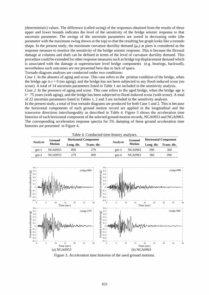
(deterministic) values. The difference (called swing) of the responses obtained from the results of these

upper and lower bounds indicates the level of the sensitivity of the bridge seismic response to that

uncertain parameter. The swings of the uncertain parameters are sorted in decreasing order (the

parameter with the maximum swing shown at the top) so that the resulting bar graph looks like a tornado

shape. In the present study, the maximum curvature ductility demand (μ) at piers is considered as the

response measure to monitor the sensitivity of the bridge seismic response. This is because the flexural

damage at columns and shaft can be defined in terms of the level of curvature ductility demand. This

procedure could be extended for other response measures such as bridge top displacement demand which

is associated with the damage at superstructure level bridge components (e.g. bearings, backwall),

nevertheless such outcomes are not presented here due to lack of space.

Tornado diagram analyses are conducted under two conditions:

Case 1. In the absence of aging and scour. This case refers to the pristine condition of the bridge, when

the bridge age is t = 0 (no aging), and the bridge has not been subjected to any flood-induced scour (no

scour). A total of 14 uncertain parameters listed in Table 1 are included in the sensitivity analysis.

Case 2. In the presence of aging and scour. This case refers to the aged bridge, when the bridge age is

t= 75 years (with aging), and the bridge has been subjected to flood-induced scour (with scour). A total

of 22 uncertain parameters listed in Tables 1, 2 and 3 are included in the sensitivity analysis.

In the present study, a total of four tornado diagrams are produced for both Case 1 and 2. This is because

the horizontal components of each ground motion record are applied in the longitudinal and the

transverse directions interchangeably as described in Table 4. Figure 3 shows the acceleration time

histories of each horizontal component of the selected ground motion records, NGA0953 and NGA0963.

The corresponding acceleration response spectra for 5% damping of these ground acceleration time

histories are presented in Figure 4.

Table 4. Conducted time-history analyses.

Analysis Ground

Motion

Horizontal Component Analysis

Ground

Motion

Horizontal Component

Long. dir. Trans. dir. Long. dir. Trans. dir.

gm-1 NGA0953 009 279 gm-3 NGA0963 090 360

gm-2 NGA0953 279 009 gm-4 NGA0963 360 090

(a) NGA0953 (b) NGA0963

Figure 3. Acceleration time histories of the used ground motions.

0 5 10 15 20 25 30

Time (sec)

-0.4

-0.3

-0.2

-0.1

0

0.1

0.2

0.3

0.4

0.5

0.6

Gro

und a

ccel

erat

ion (

g) comp-009

0 5 10 15 20 25 30 35 40

Time (sec)

-0.4

-0.3

-0.2

-0.1

0

0.1

0.2

0.3

0.4

0.5

0.6

Gro

un

d a

ccel

erat

ion

(g) comp-090

0 5 10 15 20 25 30

Time (sec)

-0.5

-0.4

-0.3

-0.2

-0.1

0

0.1

0.2

0.3

0.4

0.5

0.6

Gro

und a

ccel

erat

ion (

g) comp-279

0 5 10 15 20 25 30 35 40

Time (sec)

-0.5

-0.4

-0.3

-0.2

-0.1

0

0.1

0.2

0.3

0.4

0.5

0.6

Gro

un

d a

ccel

erat

ion

(g) comp-360

833

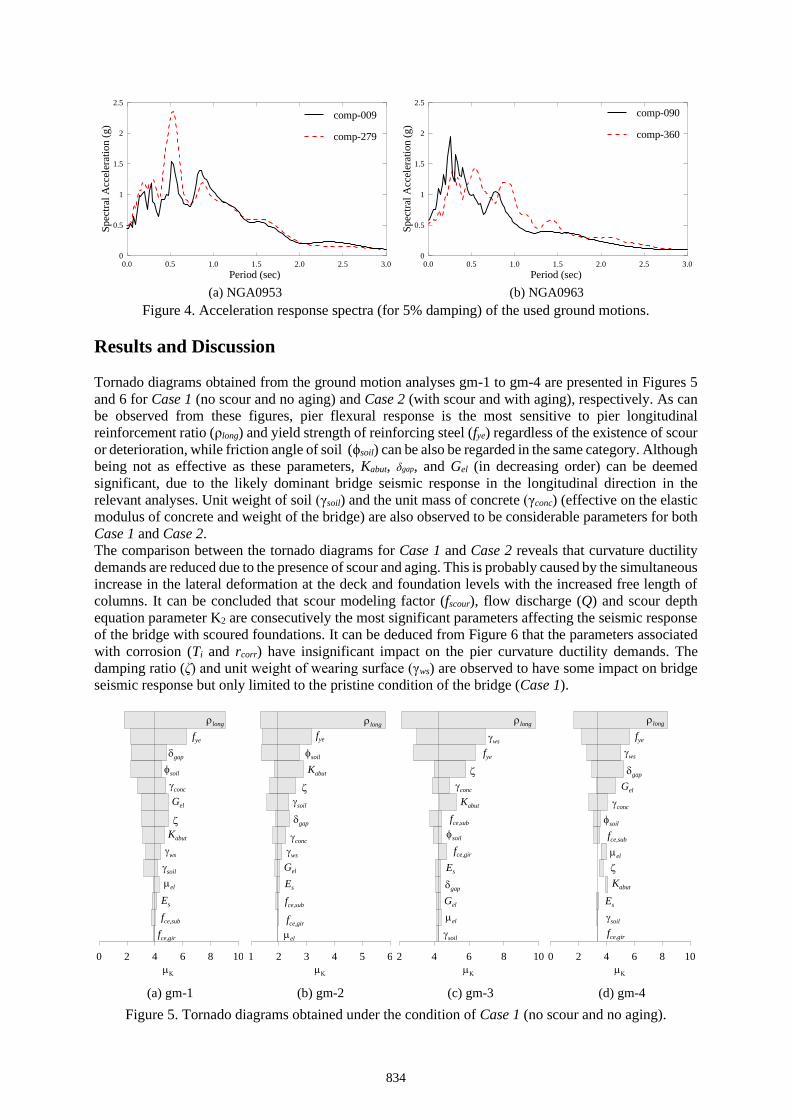
(a) NGA0953 (b) NGA0963

Figure 4. Acceleration response spectra (for 5% damping) of the used ground motions.

Results and Discussion

Tornado diagrams obtained from the ground motion analyses gm-1 to gm-4 are presented in Figures 5

and 6 for Case 1 (no scour and no aging) and Case 2 (with scour and with aging), respectively. As can

be observed from these figures, pier flexural response is the most sensitive to pier longitudinal

reinforcement ratio (ρlong) and yield strength of reinforcing steel (fye) regardless of the existence of scour

or deterioration, while friction angle of soil (ϕsoil) can be also be regarded in the same category. Although

being not as effective as these parameters, Kabut, δgap, and Gel (in decreasing order) can be deemed

significant, due to the likely dominant bridge seismic response in the longitudinal direction in the

relevant analyses. Unit weight of soil (γsoil) and the unit mass of concrete (γconc) (effective on the elastic

modulus of concrete and weight of the bridge) are also observed to be considerable parameters for both

Case 1 and Case 2.

The comparison between the tornado diagrams for Case 1 and Case 2 reveals that curvature ductility

demands are reduced due to the presence of scour and aging. This is probably caused by the simultaneous

increase in the lateral deformation at the deck and foundation levels with the increased free length of

columns. It can be concluded that scour modeling factor (fscour), flow discharge (Q) and scour depth

equation parameter K2 are consecutively the most significant parameters affecting the seismic response

of the bridge with scoured foundations. It can be deduced from Figure 6 that the parameters associated

with corrosion (Ti and rcorr) have insignificant impact on the pier curvature ductility demands. The

damping ratio (ζ) and unit weight of wearing surface (γws) are observed to have some impact on bridge

seismic response but only limited to the pristine condition of the bridge (Case 1).

(a) gm-1 (b) gm-2 (c) gm-3 (d) gm-4

Figure 5. Tornado diagrams obtained under the condition of Case 1 (no scour and no aging).

0.0 0.5 1.0 1.5 2.0 2.5 3.0

Period (sec)

0

0.5

1

1.5

2

2.5S

pec

tral

Acc

eler

atio

n (

g)

comp-009

comp-279

0.0 0.5 1.0 1.5 2.0 2.5 3.0

Period (sec)

0

0.5

1

1.5

2

2.5

Spec

tral

Acc

eler

atio

n (

g)

comp-090

comp-360

0 2 4 6 8 10

ws

fce,sub

soil

Gel

fye

conc

long

fce,gir

Es

gap

Kabut

soil

el

1 2 3 4 5 6

ws

fce,sub

soil

Gel

fye

conc

long

fce,gir

Es

gap

Kabut

soil

el

2 4 6 8 10

ws

fce,sub

soil

Gel

fye

conc

long

fce,gir

Es

gap

Kabut

soil

el

0 2 4 6 8 10

ws

fce,sub

soil

Gel

fye

conc

long

fce,gir

Es

gap

Kabut

soil

el

834

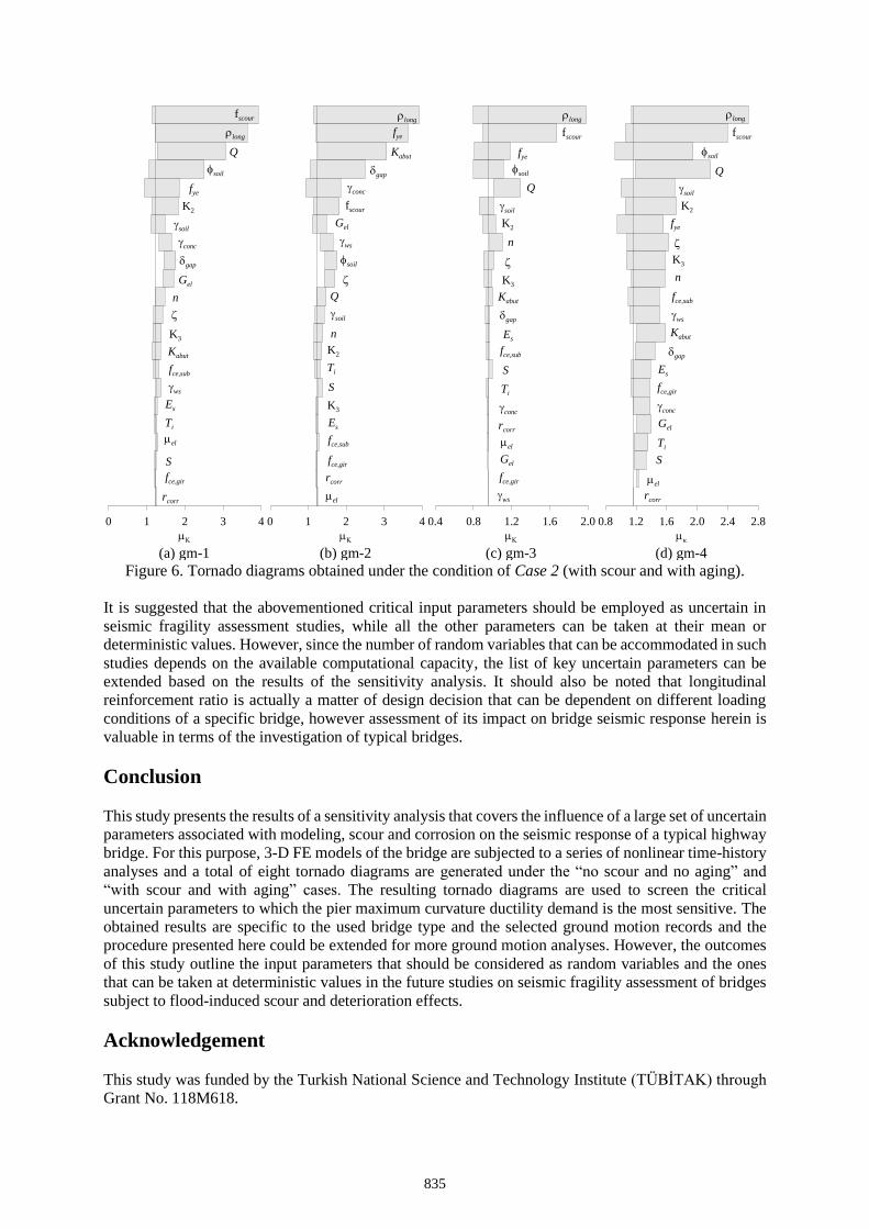
(a) gm-1 (b) gm-2 (c) gm-3 (d) gm-4

Figure 6. Tornado diagrams obtained under the condition of Case 2 (with scour and with aging).

It is suggested that the abovementioned critical input parameters should be employed as uncertain in

seismic fragility assessment studies, while all the other parameters can be taken at their mean or

deterministic values. However, since the number of random variables that can be accommodated in such

studies depends on the available computational capacity, the list of key uncertain parameters can be

extended based on the results of the sensitivity analysis. It should also be noted that longitudinal

reinforcement ratio is actually a matter of design decision that can be dependent on different loading

conditions of a specific bridge, however assessment of its impact on bridge seismic response herein is

valuable in terms of the investigation of typical bridges.

Conclusion

This study presents the results of a sensitivity analysis that covers the influence of a large set of uncertain

parameters associated with modeling, scour and corrosion on the seismic response of a typical highway

bridge. For this purpose, 3-D FE models of the bridge are subjected to a series of nonlinear time-history

analyses and a total of eight tornado diagrams are generated under the “no scour and no aging” and

“with scour and with aging” cases. The resulting tornado diagrams are used to screen the critical

uncertain parameters to which the pier maximum curvature ductility demand is the most sensitive. The

obtained results are specific to the used bridge type and the selected ground motion records and the

procedure presented here could be extended for more ground motion analyses. However, the outcomes

of this study outline the input parameters that should be considered as random variables and the ones

that can be taken at deterministic values in the future studies on seismic fragility assessment of bridges

subject to flood-induced scour and deterioration effects.

Acknowledgement

This study was funded by the Turkish National Science and Technology Institute (TÜBİTAK) through

Grant No. 118M618.

0 1 2 3 4

ws

fce,sub

soil

Gel

fye

conc

long

fce,gir

Es

gap

Kabut

soil

el

fscour

Q

K2

n

K3

Ti

S

rcorr

0 1 2 3 4

ws

fce,sub

soil

Gel

fye

conc

long

fce,gir

Es

gap

Kabut

soil

el

fscour

Q

K2

n

K3

Ti

S

rcorr

0.4 0.8 1.2 1.6 2.0

ws

fce,sub

soil

Gel

fye

conc

long

fce,gir

Es

gap

Kabut

soil

el

fscour

Q

K2

n

K3

Ti

S

rcorr

0.8 1.2 1.6 2.0 2.4 2.8

ws

fce,sub

soil

Gel

fye

conc

long

fce,gir

Es

gap

Kabut

soil

el

fscour

Q

K2

n

K3

Ti

S

rcorr

835

References

American Petroleum Institute (API) (2003). “Recommended Practice for Planning, Designing and Constructing

Fixed Offshore Platform-Working Stress Design”. Washington, D.C.

Arneson LAM, Zevenbergen LW, Lagasse PF, Clopper PE (2012). “Evaluating scour at bridges.” Hydraulic

Engineering Circular (HEC) No.18, Publication No. FHWA-HIF-12-003.

Billah AHMM, Alam MS (2014). “Seismic fragility assessment of highway bridges: a state-of-the-art review.”

Structure and infrastructure engineering, 11:6, 804-832, DOI: 10.1080/15732479.2014.912243.

Bavirisetty R, Vinayagamoorthy M, Duan L (2000). “Dynamic Analysis”, Bridge Engineering Handbook, Edited

by Chen W-F and Duan L, CRS Press.

Caltrans (2000). “Bridge Design Specification.” California Department of Transportation. Sacramento, CA.

Caltrans (2013). “Seismic design criteria, version 1.7”, California Department of Transportation, Sacramento, CA.

Choi E (2002). “Seismic analysis and retrofit of Mid-America bridges.” Ph.D. Dissertation, Georgia Institute of

Technology, GA.

Duracrete (2000). “Probabilistic Performance-Based Durability Design of Concrete Structures: Final Technical

Report”, The European Union – Brite EuRam III.

Ellingwood BR and Hwang H (1985). “Probabilistic descriptions of resistance of safety-related structures in

nuclear plants.” Nuclear Engineering and Design, 88(2):169-178.

Johnson PA (1995). “Comparison of pier-scour equations using field data.” Journal of Hydraulic Engineering,

121:626-629.

Johnson PA (1996). “Uncertainty of hydraulic parameters.” Journal of Hydraulic Engineering, 122(2):112-114.

Hydraulic Engineering Center (1986). “Accuracy of Computed Water Surface Profiles.” U.S. Army Corps of

Engineers, Davis, CA.

Ghosh J and Padgett JE (2010). “Aging considerations in the Development of Time-Dependent Seismic Fragility

Curves.” Journal of Structural Engineering, 136(12): 1497-1511.

Ghosh J and Sood P (2016). “Consideration of time-evolving capacity distributions and improved degradation

models for seismic fragility assessment of aging highway bridges.” Reliability Engineering and System Safety,

154: 197-218.

Karayolları Genel Müdürlüğü (KGM) (2019). “Karayolu ve Demiryolu Köprü ve Viyadükleri.” Nihai Rapora

Esas Taslak Rapor (Ara Rapor-3), Ankara, Turkey (in Turkish).

Lee J, Lee Y-J, Kim H, Sim S, Kim J-M (2016). “A new methodology development for flood fragility curve

derivation considering structural deterioration for bridges.” Smart Structures and Systems, 17(1): 149-165.

Mander JB, Kim D-K, Chen SS, Premus GJ (1996). “Response of Steel Bridge Bearings to Reversed Cyclic

Loading.” Report No. NCEER 96-0014, NCEER.

Mander JB, Priestley MJN, Park R (1988). “Theoretical stress-strain model for confined concrete.” Journal of

Structural Engineering, 114(8): 1804–1826.

McKenna F, Fenves GL (2012). “Open System for Earthquake Engineering Simulation, Version 2.4.0.”, Pacific

Earthquake Engineering Research Center, Berkeley, CA.

Nowak AS (1999). “Calibration of LRFD Bridge Design Code.” NCHRP Report 368, TRB.

PEER (2020). “NGA Database”, Pacific Earthquake Engineering Research Center, available from:

https://ngawest2.berkeley.edu/ (last access: 28.03.2020).

Wang Z, Duenas-Osorio L, Padgett JE (2014). “Influence of scour effects on the seismic response of reinforced

concrete bridges.” Engineering Structures, 76:202-214.

Yilmaz T, Banerjee S, Johnson PA (2016) “Performance of two real-life California bridges under regional natural

hazards.” Journal of Bridge Engineering, ASCE, 21(3), doi: 10.1061/(ASCE)BE.1943-5592.0000827,

04015063.

Yilmaz T, Banerjee S, Johnson PA (2018). “Uncertainty in risk of highway bridges assessed for integrated seismic

and flood hazards”, Structure and Infrastructure Engineering, 14(9), 1182-1196, doi:

10.1080/15732479.2017.1402065.

Yilmaz T and Banerjee S (2018) “Impact spectrum of flood hazard on seismic vulnerability of bridges”, Structural

Engineering and Mechanics, 66(4): 515-529. doi: 10.12989/sem.2018.66.4.515.

Yilmaz T and Aygin OC (2019). “Time-dependent seismic risk of regular highway bridges under the effect of

structural deterioration”. SECED 2019 Conference, Greenwich, London, UK.

Zhang Y (2006). “Probabilistic structural seismic performance assessment methodology and application to an

actual bridge-foundation-ground system.” Ph.D. Dissertation, University of California, San Diego, CA.

836

Comparison of Two Approaches for Developing Analytical Seismic

Fragility Curves of Highway Bridges

Onur Cem Aygın 1, Taner Yılmaz 2*

1 M.Sc. Student, Department of Civil Engineering, Ozyegin University, Istanbul, Turkey; 2 Assistant Professor, Department of Civil Engineering, Ozyegin University, Istanbul, Turkey;


Abstract

Fragility curves are the fundamental tools in the probabilistic risk assessment framework of structures

under earthquake hazards. Over the past years, researchers have applied various approaches to develop

seismic fragility curves of bridges. This study aims to evaluate the effect of employing different

methodologies on analytical seismic fragility curves of highway bridges. For this purpose, a typical

bridge pier is investigated by considering two different structural reliability approaches. In the first

approach, fragility curve parameters are obtained from the application of method of maximum likelihood

after damage states of the pier are assessed under a large number of seismic analyses. In the second

approach, fragility curve parameters are obtained through the use of statistically defined capacity model

and the probabilistic seismic demand model which is based on the correlation between the seismic

demand and the ground motion intensity. Seismic demands are obtained from the nonlinear time-history

analyses of the finite element model of the bridge pier. The impact of the investigated approaches are

evaluated based on the comparison of the resulting fragility curves and how the uncertainties in input

parameters are managed in these approaches.

Keywords: Bridges, seismic fragility, method of maximum likelihood, probabilistic seismic demand

model.

Introduction

Bridges can be considered as the most susceptible elements to earthquake damage in highway

transportation systems. Social and economic losses arising from bridge failures and the consequential

disruptions in the service of transportation systems makes it critical to assess the seismic vulnerability

and associating risks of highway bridges. In recent years, fragility curves have evolved as a competent

tool to assess the seismic vulnerability for bridges within risk assessment frameworks. There are several

ways of developing fragility curves including the use of expert opinion, empirical damage data or the

results of computer analyses. Investigating the seismic response of bridges on full scale experimental

setups can be cumbersome and impractical, while the damage data acquired after the earthquake

occurrences can be limited as well. For these reasons, researchers have focused on developing

methodologies for fragility assessment analytically by employing computer analyses so that large

numbers of earthquake scenarios and damage record can be simulated (Mackie and Nielson, 2009).

There are various reliability-based approaches to estimate the fragility curve parameters (also referred

to as “fragility parameters”), and to the best of authors’ knowledge, there is no such study to compare

their distinctive features. So far in literature, Monteiro et al. (2014) compared the static and dynamic

analysis procedures employed in analytical fragility curve development, and Mackie and Nielson (2009)

studied uncertainty quantification aspect in their fragility curve methodology and compared different

techniques having different ways of uncertainty propagation. Both of the abovementioned studies

applied the same methodology to estimate the fragility parameters.

The present study aims to evaluate two different reliability-based approaches that are used to estimate

the analytical seismic fragility curve parameters for bridge piers. In the first approach (Approach 1), the

structural model of the bridge pier is generated for a single set of input parameters at their deterministic

values, then nonlinear time-history analyses are conducted under a large ground motion dataset. The

837

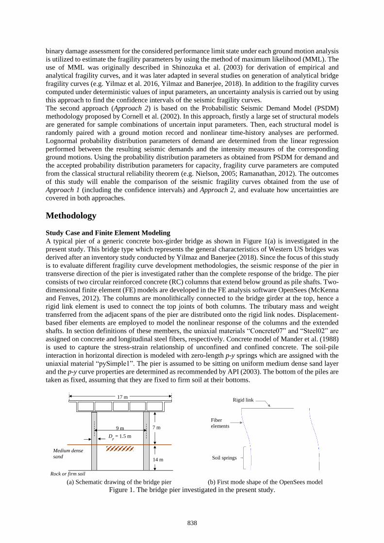
binary damage assessment for the considered performance limit state under each ground motion analysis

is utilized to estimate the fragility parameters by using the method of maximum likelihood (MML). The

use of MML was originally described in Shinozuka et al. (2003) for derivation of empirical and

analytical fragility curves, and it was later adapted in several studies on generation of analytical bridge

fragility curves (e.g. Yilmaz et al. 2016, Yilmaz and Banerjee, 2018). In addition to the fragility curves

computed under deterministic values of input parameters, an uncertainty analysis is carried out by using

this approach to find the confidence intervals of the seismic fragility curves.

The second approach (Approach 2) is based on the Probabilistic Seismic Demand Model (PSDM)

methodology proposed by Cornell et al. (2002). In this approach, firstly a large set of structural models

are generated for sample combinations of uncertain input parameters. Then, each structural model is

randomly paired with a ground motion record and nonlinear time-history analyses are performed.

Lognormal probability distribution parameters of demand are determined from the linear regression

performed between the resulting seismic demands and the intensity measures of the corresponding

ground motions. Using the probability distribution parameters as obtained from PSDM for demand and

the accepted probability distribution parameters for capacity, fragility curve parameters are computed

from the classical structural reliability theorem (e.g. Nielson, 2005; Ramanathan, 2012). The outcomes

of this study will enable the comparison of the seismic fragility curves obtained from the use of

Approach 1 (including the confidence intervals) and Approach 2, and evaluate how uncertainties are

covered in both approaches.

Methodology

Study Case and Finite Element Modeling

A typical pier of a generic concrete box-girder bridge as shown in Figure 1(a) is investigated in the

present study. This bridge type which represents the general characteristics of Western US bridges was

derived after an inventory study conducted by Yilmaz and Banerjee (2018). Since the focus of this study

is to evaluate different fragility curve development methodologies, the seismic response of the pier in

transverse direction of the pier is investigated rather than the complete response of the bridge. The pier

consists of two circular reinforced concrete (RC) columns that extend below ground as pile shafts. Two-

dimensional finite element (FE) models are developed in the FE analysis software OpenSees (McKenna

and Fenves, 2012). The columns are monolithically connected to the bridge girder at the top, hence a

rigid link element is used to connect the top joints of both columns. The tributary mass and weight

transferred from the adjacent spans of the pier are distributed onto the rigid link nodes. Displacement-

based fiber elements are employed to model the nonlinear response of the columns and the extended

shafts. In section definitions of these members, the uniaxial materials “Concrete07” and “Steel02” are

assigned on concrete and longitudinal steel fibers, respectively. Concrete model of Mander et al. (1988)

is used to capture the stress-strain relationship of unconfined and confined concrete. The soil-pile

interaction in horizontal direction is modeled with zero-length p-y springs which are assigned with the

uniaxial material “pySimple1”. The pier is assumed to be sitting on uniform medium dense sand layer

and the p-y curve properties are determined as recommended by API (2003). The bottom of the piles are

taken as fixed, assuming that they are fixed to firm soil at their bottoms.

(a) Schematic drawing of the bridge pier (b) First mode shape of the OpenSees model

Figure 1. The bridge pier investigated in the present study.

7 m 9 m

14 m

Dp = 1.5 m

Rock or firm soil

Medium dense

sand

17 m

Fiber

elements

Rigid link

Soil springs

838

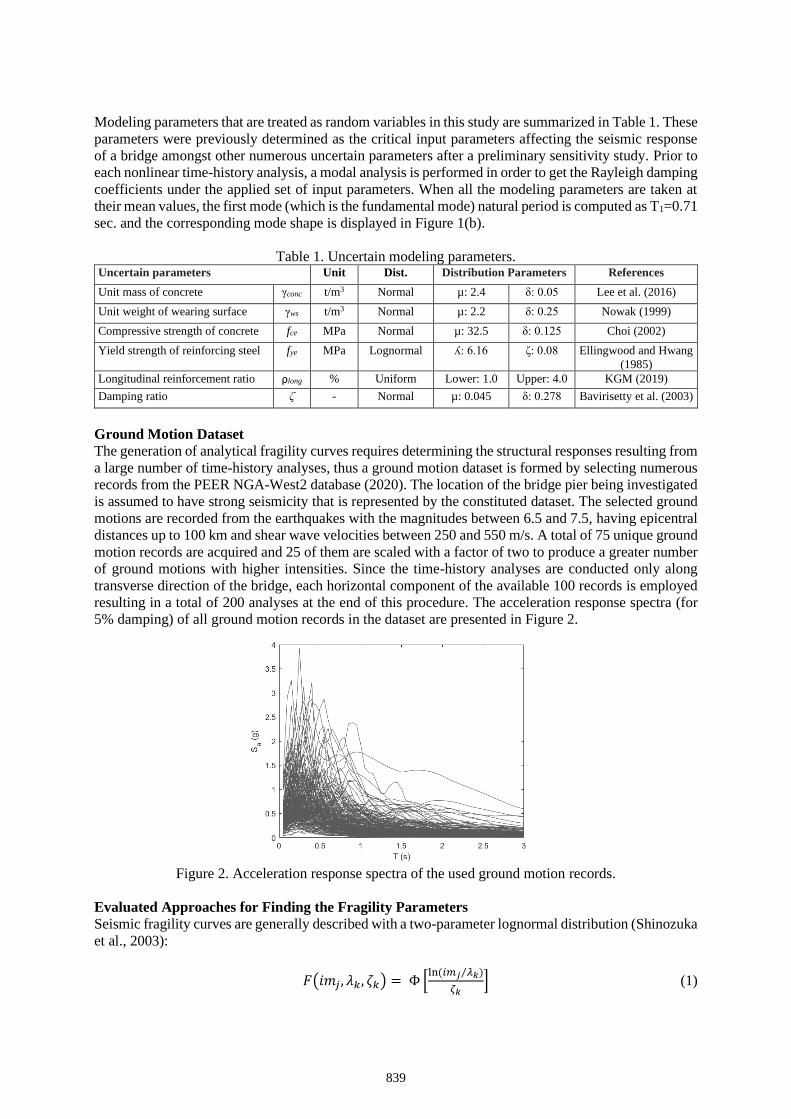
Modeling parameters that are treated as random variables in this study are summarized in Table 1. These

parameters were previously determined as the critical input parameters affecting the seismic response

of a bridge amongst other numerous uncertain parameters after a preliminary sensitivity study. Prior to

each nonlinear time-history analysis, a modal analysis is performed in order to get the Rayleigh damping

coefficients under the applied set of input parameters. When all the modeling parameters are taken at

their mean values, the first mode (which is the fundamental mode) natural period is computed as T1=0.71

sec. and the corresponding mode shape is displayed in Figure 1(b).

Table 1. Uncertain modeling parameters. Uncertain parameters Unit Dist. Distribution Parameters References

Unit mass of concrete γconc t/m3 Normal µ: 2.4 δ: 0.05 Lee et al. (2016)

Unit weight of wearing surface γws t/m3 Normal µ: 2.2 δ: 0.25 Nowak (1999)

Compressive strength of concrete fce MPa Normal µ: 32.5 δ: 0.125 Choi (2002)

Yield strength of reinforcing steel fye MPa Lognormal ʎ: 6.16 ζ: 0.08 Ellingwood and Hwang

(1985)

Longitudinal reinforcement ratio ρlong % Uniform Lower: 1.0 Upper: 4.0 KGM (2019)

Damping ratio ζ - Normal µ: 0.045 δ: 0.278 Bavirisetty et al. (2003)

Ground Motion Dataset

The generation of analytical fragility curves requires determining the structural responses resulting from

a large number of time-history analyses, thus a ground motion dataset is formed by selecting numerous

records from the PEER NGA-West2 database (2020). The location of the bridge pier being investigated

is assumed to have strong seismicity that is represented by the constituted dataset. The selected ground

motions are recorded from the earthquakes with the magnitudes between 6.5 and 7.5, having epicentral

distances up to 100 km and shear wave velocities between 250 and 550 m/s. A total of 75 unique ground

motion records are acquired and 25 of them are scaled with a factor of two to produce a greater number

of ground motions with higher intensities. Since the time-history analyses are conducted only along

transverse direction of the bridge, each horizontal component of the available 100 records is employed

resulting in a total of 200 analyses at the end of this procedure. The acceleration response spectra (for

5% damping) of all ground motion records in the dataset are presented in Figure 2.

Figure 2. Acceleration response spectra of the used ground motion records.

Evaluated Approaches for Finding the Fragility Parameters

Seismic fragility curves are generally described with a two-parameter lognormal distribution (Shinozuka

et al., 2003):

𝐹(𝑖𝑚𝑗, 𝜆𝑘, 𝜁𝑘) = Φ [ln(𝑖𝑚𝑗 𝜆𝑘)⁄

𝜁𝑘] (1)

839

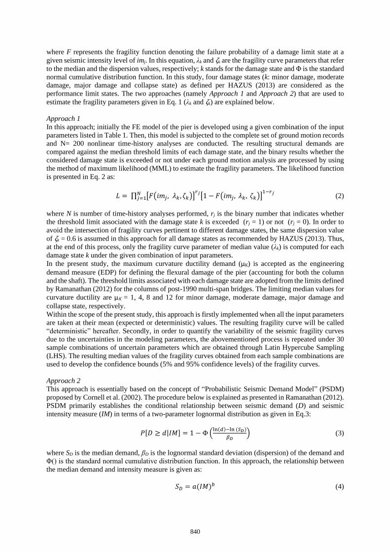
where F represents the fragility function denoting the failure probability of a damage limit state at a

given seismic intensity level of imj. In this equation, λk and ζk are the fragility curve parameters that refer

to the median and the dispersion values, respectively; k stands for the damage state and Φ is the standard

normal cumulative distribution function. In this study, four damage states (k: minor damage, moderate

damage, major damage and collapse state) as defined per HAZUS (2013) are considered as the

performance limit states. The two approaches (namely Approach 1 and Approach 2) that are used to

estimate the fragility parameters given in Eq. 1 (λk and ζk) are explained below.

Approach 1

In this approach; initially the FE model of the pier is developed using a given combination of the input

parameters listed in Table 1. Then, this model is subjected to the complete set of ground motion records

and N= 200 nonlinear time-history analyses are conducted. The resulting structural demands are

compared against the median threshold limits of each damage state, and the binary results whether the

considered damage state is exceeded or not under each ground motion analysis are processed by using

the method of maximum likelihood (MML) to estimate the fragility parameters. The likelihood function

is presented in Eq. 2 as:

𝐿 = ∏ [𝐹(𝑖𝑚𝑗, 𝜆𝑘 , 𝜁𝑘)]𝑟𝑗

[1 − 𝐹(𝑖𝑚𝑗, 𝜆𝑘 , 𝜁𝑘)]1−𝑟𝑗𝑁

𝑗=1 (2)

where N is number of time-history analyses performed, rj is the binary number that indicates whether

the threshold limit associated with the damage state k is exceeded (rj = 1) or not (rj = 0). In order to

avoid the intersection of fragility curves pertinent to different damage states, the same dispersion value

of ζk = 0.6 is assumed in this approach for all damage states as recommended by HAZUS (2013). Thus,

at the end of this process, only the fragility curve parameter of median value (λk) is computed for each

damage state k under the given combination of input parameters.

In the present study, the maximum curvature ductility demand (μK) is accepted as the engineering

demand measure (EDP) for defining the flexural damage of the pier (accounting for both the column

and the shaft). The threshold limits associated with each damage state are adopted from the limits defined

by Ramanathan (2012) for the columns of post-1990 multi-span bridges. The limiting median values for

curvature ductility are μK = 1, 4, 8 and 12 for minor damage, moderate damage, major damage and

collapse state, respectively.

Within the scope of the present study, this approach is firstly implemented when all the input parameters

are taken at their mean (expected or deterministic) values. The resulting fragility curve will be called

“deterministic” hereafter. Secondly, in order to quantify the variability of the seismic fragility curves

due to the uncertainties in the modeling parameters, the abovementioned process is repeated under 30

sample combinations of uncertain parameters which are obtained through Latin Hypercube Sampling

(LHS). The resulting median values of the fragility curves obtained from each sample combinations are

used to develop the confidence bounds (5% and 95% confidence levels) of the fragility curves.

Approach 2

This approach is essentially based on the concept of “Probabilistic Seismic Demand Model” (PSDM)

proposed by Cornell et al. (2002). The procedure below is explained as presented in Ramanathan (2012).

PSDM primarily establishes the conditional relationship between seismic demand (D) and seismic

intensity measure (IM) in terms of a two-parameter lognormal distribution as given in Eq.3:

𝑃[𝐷 ≥ 𝑑|𝐼𝑀] = 1 − Φ (ln(𝑑)−ln (𝑆𝐷)

𝛽𝐷) (3)

where SD is the median demand, βD is the lognormal standard deviation (dispersion) of the demand and

Φ() is the standard normal cumulative distribution function. In this approach, the relationship between

the median demand and intensity measure is given as:

𝑆𝐷 = 𝑎(𝐼𝑀)𝑏 (4)

840

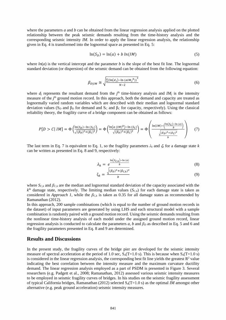
where the parameters a and b can be obtained from the linear regression analysis applied on the plotted

relationship between the peak seismic demands resulting from the time-history analysis and the

corresponding seismic intensity IM. In order to apply the linear regression analysis, the relationship

given in Eq. 4 is transformed into the lognormal space as presented in Eq. 5:

ln(𝑆𝐷) = ln(𝑎) + 𝑏 𝑙𝑛(𝐼𝑀) (5)

where ln(a) is the vertical intercept and the parameter b is the slope of the best fit line. The lognormal

standard deviation (or dispersion) of the seismic demand can be obtained from the following equation:

𝛽𝐷|𝐼𝑀 ≅ √∑(ln(𝑑𝑗)−ln (𝑎𝐼𝑀𝑗𝑏))

2

𝑁−2(6)

where dj represents the resultant demand from the jth time-history analysis and IMj is the intensity

measure of the jth ground motion record. In this approach, both the demand and capacity are treated as

lognormally varied random variables which are described with their median and lognormal standard

deviation values (SD and βD for demand and SC and βC for capacity, respectively). Using the classical

reliability theory, the fragility curve of a bridge component can be obtained as follows:

𝑃[𝐷 > 𝐶| 𝐼𝑀] = Φ (ln(𝑆𝐷)−ln (𝑆𝐶)

√(𝛽𝐷)2+(𝛽𝐶)2) = Φ (

ln(𝑎 (𝐼𝑀)𝑏)−ln (𝑆𝐶)

√(𝛽𝐷)2+(𝛽𝐶)2) = Φ (

ln(𝐼𝑀)−(ln(𝑆𝐶)−ln (𝑎)

𝑏)

√(𝛽𝐷)2+(𝛽𝐶)2

𝑏

) (7)

The last term in Eq. 7 is equivalent to Eq. 1, so the fragility parameters λk and ζk for a damage state k

can be written as presented in Eq. 8 and 9, respectively:

𝜆𝑘 = 𝑒ln(𝑆𝐶,𝑘)−ln (𝑎)

𝑏 (8)

ζ𝑘 = √(𝛽𝐷)2+(𝛽𝐶,𝑘)2

𝑏(9)

where SC,k and βC,k are the median and lognormal standard deviation of the capacity associated with the

kth damage state, respectively. The limiting median values (SC,k) for each damage state is taken as

considered in Approach 1, while the βC,k is taken as 0.35 for all damage states as recommended by

Ramanathan (2012).

In this approach, 200 sample combinations (which is equal to the number of ground motion records in

the dataset) of input parameters are generated by using LHS and each structural model with a sample

combination is randomly paired with a ground motion record. Using the seismic demands resulting from

the nonlinear time-history analysis of each model under the assigned ground motion record, linear

regression analysis is conducted to calculate the parameters a, b and βD as described in Eq. 5 and 6 and

the fragility parameters presented in Eq. 8 and 9 are determined.

Results and Discussions

In the present study, the fragility curves of the bridge pier are developed for the seismic intensity

measure of spectral acceleration at the period of 1.0 sec, Sa(T=1.0 s). This is because when Sa(T=1.0 s)

is considered in the linear regression analysis, the corresponding best fit line yields the greatest R2 value

indicating the best correlation between the intensity measure and the maximum curvature ductility

demand. The linear regression analysis employed as a part of PSDM is presented in Figure 3. Several

researchers (e.g. Padgett et al., 2008; Ramanathan, 2012) assessed various seismic intensity measures

to be employed in seismic fragility curves of bridges. In his studies on the seismic fragility assessment

of typical California bridges, Ramanathan (2012) selected Sa(T=1.0 s) as the optimal IM amongst other

alternative (e.g. peak ground acceleration) seismic intensity measures.

841

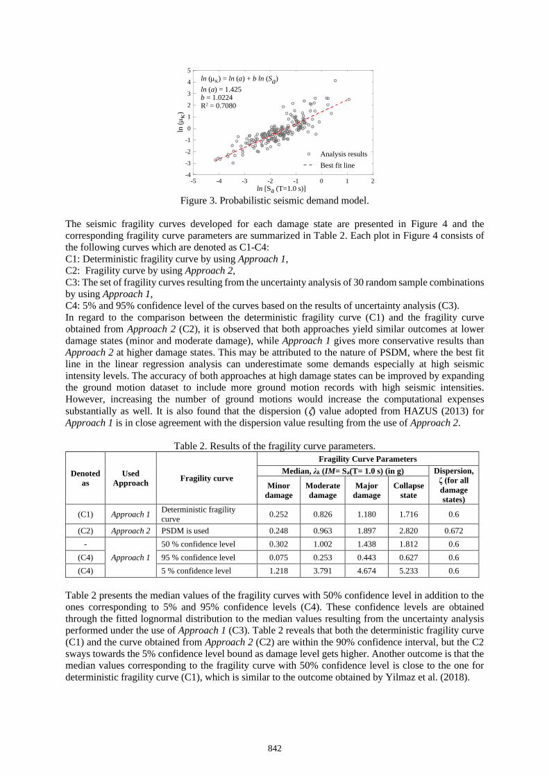
Figure 3. Probabilistic seismic demand model.

The seismic fragility curves developed for each damage state are presented in Figure 4 and the

corresponding fragility curve parameters are summarized in Table 2. Each plot in Figure 4 consists of

the following curves which are denoted as C1-C4:

C1: Deterministic fragility curve by using Approach 1,

C2: Fragility curve by using Approach 2,

C3: The set of fragility curves resulting from the uncertainty analysis of 30 random sample combinations

by using Approach 1,

C4: 5% and 95% confidence level of the curves based on the results of uncertainty analysis (C3).

In regard to the comparison between the deterministic fragility curve (C1) and the fragility curve

obtained from Approach 2 (C2), it is observed that both approaches yield similar outcomes at lower

damage states (minor and moderate damage), while Approach 1 gives more conservative results than

Approach 2 at higher damage states. This may be attributed to the nature of PSDM, where the best fit

line in the linear regression analysis can underestimate some demands especially at high seismic

intensity levels. The accuracy of both approaches at high damage states can be improved by expanding

the ground motion dataset to include more ground motion records with high seismic intensities.

However, increasing the number of ground motions would increase the computational expenses

substantially as well. It is also found that the dispersion (ζ) value adopted from HAZUS (2013) for

Approach 1 is in close agreement with the dispersion value resulting from the use of Approach 2.

Table 2. Results of the fragility curve parameters.

Denoted

as

Used

Approach Fragility curve

Fragility Curve Parameters

Median, λk (IM= Sa(T= 1.0 s) (in g) Dispersion,

ζ (for all

damage

states)

Minor

damage

Moderate

damage

Major

damage

Collapse

state

(C1) Approach 1 Deterministic fragility

curve 0.252 0.826 1.180 1.716 0.6

(C2) Approach 2 PSDM is used 0.248 0.963 1.897 2.820 0.672

-

Approach 1

50 % confidence level 0.302 1.002 1.438 1.812 0.6

(C4) 95 % confidence level 0.075 0.253 0.443 0.627 0.6

(C4) 5 % confidence level 1.218 3.791 4.674 5.233 0.6

Table 2 presents the median values of the fragility curves with 50% confidence level in addition to the

ones corresponding to 5% and 95% confidence levels (C4). These confidence levels are obtained

through the fitted lognormal distribution to the median values resulting from the uncertainty analysis

performed under the use of Approach 1 (C3). Table 2 reveals that both the deterministic fragility curve

(C1) and the curve obtained from Approach 2 (C2) are within the 90% confidence interval, but the C2

sways towards the 5% confidence level bound as damage level gets higher. Another outcome is that the

median values corresponding to the fragility curve with 50% confidence level is close to the one for

deterministic fragility curve (C1), which is similar to the outcome obtained by Yilmaz et al. (2018).

-5 -4 -3 -2 -1 0 1 2

ln [Sa (T=1.0 s)]

-4

-3

-2

-1

0

1

2

3

4

5

ln (

)

Analysis results

Best fit line

ln () = ln (a) + b ln (Sa)

ln (a) = 1.425b = 1.0224R2 = 0.7080

842

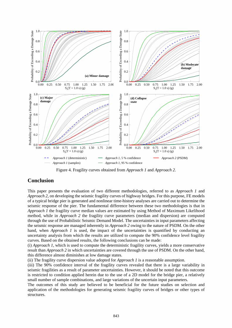
Figure 4. Fragility curves obtained from Approach 1 and Approach 2.

Conclusion

This paper presents the evaluation of two different methodologies, referred to as Approach 1 and

Approach 2, on developing the seismic fragility curves of highway bridges. For this purpose, FE models

of a typical bridge pier is generated and nonlinear time-history analyses are carried out to determine the

seismic response of the pier. The fundamental difference between these two methodologies is that in

Approach 1 the fragility curve median values are estimated by using Method of Maximum Likelihood

method, while in Approach 2 the fragility curve parameters (median and dispersion) are computed

through the use of Probabilistic Seismic Demand Model. The uncertainties in input parameters affecting

the seismic response are managed inherently in Approach 2 owing to the nature of PSDM. On the other

hand, when Approach 1 is used, the impact of the uncertainties is quantified by conducting an

uncertainty analysis from which the results are utilized to compute the 90% confidence level fragility

curves. Based on the obtained results, the following conclusions can be made:

(i) Approach 1, which is used to compute the deterministic fragility curves, yields a more conservative

result than Approach 2 in which uncertainties are covered through the use of PSDM. On the other hand,

this difference almost diminishes at low damage states.

(ii) The fragility curve dispersion value adopted for Approach 1 is a reasonable assumption.

(iii) The 90% confidence interval of the fragility curves revealed that there is a large variability in

seismic fragilities as a result of parameter uncertainties. However, it should be noted that this outcome

is restricted to condition applied herein due to the use of a 2D model for the bridge pier, a relatively

small number of sample combinations, and large variations of the uncertain input parameters.

The outcomes of this study are believed to be beneficial for the future studies on selection and

application of the methodologies for generating seismic fragility curves of bridges or other types of

structures.

0.0

0.2

0.4

0.6

0.8

1.0P

robab

ilit

y o

f E

xce

edin

g a

Dam

age

Sta

te

0.00 0.25 0.50 0.75 1.00 1.25 1.50 1.75 2.00Sa(T = 1.0 s) (g)

(a) Minor damage

0.0

0.2

0.4

0.6

0.8

1.0

Pro

bab

ilit

y o

f E

xce

edin

g a

Dam

age

Sta

te

0.00 0.25 0.50 0.75 1.00 1.25 1.50 1.75 2.00Sa(T = 1.0 s) (g)

(b) Moderate

damage

0.0

0.2

0.4

0.6

0.8

1.0

Pro

bab

ilit

y o

f E

xce

edin

g a

Dam

age

Sta

te

0.00 0.25 0.50 0.75 1.00 1.25 1.50 1.75 2.00Sa(T = 1.0 s) (g)

(c) Major

damage

0.0

0.2

0.4

0.6

0.8

1.0

Pro

bab

ilit

y o

f E

xce

edin

g a

Dam

age

Sta

te

0.00 0.25 0.50 0.75 1.00 1.25 1.50 1.75 2.00Sa(T = 1.0 s) (g)

(d) Collapse

state

Approach 1, 5 % confidence

Approach 1, 95 % confidence

Approach 2 (PSDM)Approach 1 (deterministic)

Approach 1 (samples)

843

Acknowledgement

This study was funded by the Turkish National Science and Technology Institute (TÜBİTAK) through

Grant No. 118M618.

References

American Petroleum Institute (API) (2003). “Recommended Practice for Planning, Designing and Constructing

Fixed Offshore Platform-Working Stress Design”. Washington, D.C.

Choi E (2002). “Seismic analysis and retrofit of Mid-America bridges.” Ph.D. Dissertation, Georgia Institute of

Technology, GA.

Cornell AC, Javaler F, Hamburger RO and Foutch AD (2002) “Probabilistic basis for 2000 SAC Federal

Management Agency steel moment frame guidelines”, Journal of Structural Engineering, 128(4): 526-533.

HAZUS (2013) MR4 Multi-hazard loss estimation methodology, Earthquake Model (Technical manual), FEMA

Mitigation Division, Department of Homeland Security, Washington, DC

Karayolları Genel Müdürlüğü (KGM) (2019). “Karayolu ve Demiryolu Köprü ve Viyadükleri.” Nihai Rapora

Esas Taslak Rapor (Ara Rapor-3), Ankara, Turkey (in Turkish).

Lee J, Lee Y-J, Kim H, Sim S, Kim J-M (2016). “A new methodology development for flood fragility curve

derivation considering structural deterioration for bridges.” Smart Structures and Systems, 17(1): 149-165.

Mackie KR and Nielson BG (2009) “Uncertainty quantification in analytical bridge fragility curves”, Lifeline

Earthquake Engineering in a Multihazard Environment, 88-99, Oakland, CA.

Mander JB, Priestley MJN, Park R (1988). “Theoretical stress-strain model for confined concrete.” Journal of

Structural Engineering, 114(8): 1804–1826.

McKenna F, Fenves GL (2012). “Open System for Earthquake Engineering Simulation, Version 2.4.0.”, Pacific

Earthquake Engineering Research Center, Berkeley, CA.

Monteiro R, Zhang X and Pinho R (2014) “Different approaches to derive analytical fragility functions of bridges.”

Proceedings of the Second European Conf. on Earthquake Engineering and Seismology, Istanbul, Turkey.

Nielson BG (2005). “Analytical fragility curves for highway bridges in moderate seismic zones.” Ph.D.

Dissertation, Georgia Institute of Technology, GA.

Nowak AS (1999). “Calibration of LRFD Bridge Design Code.” NCHRP Report 368, TRB.

Padgett JE, Nielson BG, DesRoches R (2008). “Selection of optimal intensity measures in probabilistic seismic

demand models of highway bridge portfolios.” Earthquake Engineering and Structural Dynamics, 37: 711-

725, doi:10.1002/eqe.782.

PEER (2020). “NGA Database”, Pacific Earthquake Engineering Research Center, available from:

https://ngawest2.berkeley.edu/ (last access: 28.03.2020).

Ramanathan KN (2012). “Next generation seismic fragility curves for California bridge incorporating the

evolution in seismic design philosophy.” Ph.D. Dissertation, Georgia Institute of Technology, GA.

Shinozuka M, Feng MQ, Kim H, Uzawa T and Ueda T (2003). “Statistical analysis of fragility curves.” Report

MCEER-03-0002, Multidisciplinary Center for Earthquake Engineering Research, State University of New

York, Buffalo, NY.

Yilmaz T, Banerjee S, Johnson PA (2016) “Performance of two real-life California bridges under regional natural

hazards.” Journal of Bridge Engineering, ASCE, 21(3), doi: 10.1061/(ASCE)BE.1943-5592.0000827,

04015063.

Yilmaz T, Banerjee S, Johnson PA (2018). “Uncertainty in risk of highway bridges assessed for integrated seismic

and flood hazards”, Structure and Infrastructure Engineering, 14(9), 1182-1196,

doi:10.1080/15732479.2017.1402065.

Yilmaz T and Banerjee S (2018) “Impact spectrum of flood hazard on seismic vulnerability of bridges”, Structural

Engineering and Mechanics, 66(4): 515-529. doi: 10.12989/sem.2018.66.4.515.

Zhang Y (2006). “Probabilistic structural seismic performance assessment methodology and application to an

actual bridge-foundation-ground system.” Ph.D. Dissertation, University of California, San Diego, CA.

844

Fragility Curves of Simply Supported Prestressed Girders Bridge with Two-Column Bent

Abderrahmane Kibboua1*, Nadjib Hemaidi-Zourgui2, Fouad Kehila3, Mustapha Remki4

1,3,4 National Earthquake Engineering Center (CGS) 2National School of Built and Ground Works Engineering (ENSTP)


Abstract It is known that the seismic performance of transportation systems plays key rolls for the post-earthquake emergency management. It needs to be evaluated from both physical and functional viewpoints. This paper deals with the fragility curves to assess the seismic vulnerability of a bridge with two columns bent that can be used for post-earthquake management of transportation systems. The fragility curves are used to represent the probabilities that structural damage under various level of seismic excitations exceed specified damage states. A sample of two span, two-lane railway over bridge, situated in a high seismic region in Algiers is considered for the development of fragility curves considering piers, abutments and elastomeric bearings. Capacity of the bridge columns bent has been determined by a static non-linear analysis (pushover). The damage parameters of the bridge were obtained by performing nonlinear time history analysis for different ground motion histories recorded in the past earthquakes. The seismic fragility curves are developed for collapsed, major damage, moderate damage, and minor damage situation. They have been constructed assuming a log-normal distribution. The fragility curves resulting from this study are used for estimating seismic losses due to earthquakes. Such loss estimations are essential for the important purposes of disaster planning and formulation risk reduction policies.

Keywords: Seismic vulnerability, Fragility curves, Damage levels, Log-normal distribution.

Introduction

Seismic vulnerability assessment and development of fragility curves for existing bridges are a matter of great concern among the researchers in the recent years (Padgett and DesRoches, 2008; Moschonas et al., 2009; Kibboua et al., 2011). Fragility curve is a useful tool for seismic vulnerability assessment of infrastructures (Kibboua et al., 2014). Many researchers developed fragility curves for structures not only based on empirical methods but also analytical procedures. Developing fragility functions from empirical observations sometimes encounter challenges due to the lack of sufficient damage data caused by past earthquakes. In an alternative way, fragility curves can be constructed by applying some analytical procedures such as elastic spectral analysis, nonlinear static analysis, and nonlinear time-history analysis methods (Billah et al., 2015; Kibboua et al., 2008). Among these analytical methods, nonlinear time history analysis is the most widely used and the most reliable method for deriving fragility curves of structures (Abbasi et al., 2016; Kibboua et al., 2017; Kehila et al., 2018). The main objective of this study is to derive analytical fragility curves for a typical Algerian reinforced concrete bridges based on numerical approach taking into account the member elements (piers, abutments and elastomeric bearings). By using worldwide and local strong motion records, the damage indices as defined by (Park et al, 1985) for piers and the others proposed in terms of the displacement ratio (FEMA, 1999 and FEMA, 2003) for abutments and elastomeric bearings. Four damage states, namely slight, moderate, extensive, and complete (collapse) are defined based on the proposed damage indices. The finite element framework Seismostruct (Seismostruct, 2016) is utilized to perform nonlinear time history analyses. From the observation of damage levels, fragility curves for the bridge are obtained using the maximum likelihood estimation.

845

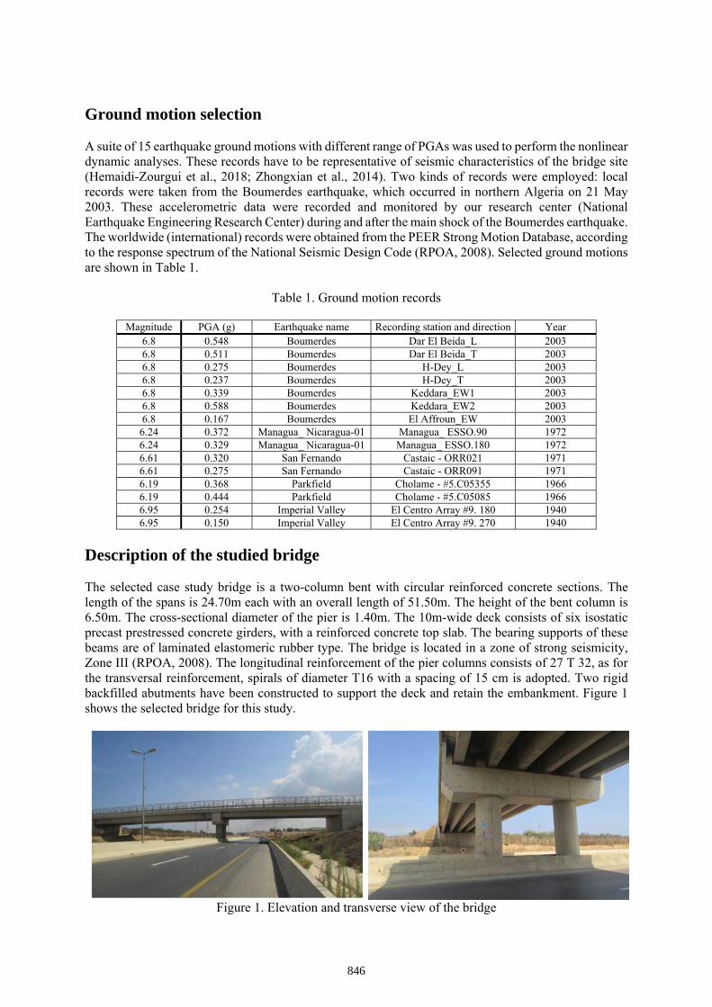
Ground motion selection

A suite of 15 earthquake ground motions with different range of PGAs was used to perform the nonlinear dynamic analyses. These records have to be representative of seismic characteristics of the bridge site (Hemaidi-Zourgui et al., 2018; Zhongxian et al., 2014). Two kinds of records were employed: local records were taken from the Boumerdes earthquake, which occurred in northern Algeria on 21 May 2003. These accelerometric data were recorded and monitored by our research center (National Earthquake Engineering Research Center) during and after the main shock of the Boumerdes earthquake. The worldwide (international) records were obtained from the PEER Strong Motion Database, according to the response spectrum of the National Seismic Design Code (RPOA, 2008). Selected ground motions are shown in Table 1.

Table 1. Ground motion records

Magnitude PGA (g) Earthquake name Recording station and direction Year 6.8 0.548 Boumerdes Dar El Beida_L 2003 6.8 0.511 Boumerdes Dar El Beida_T 2003 6.8 0.275 Boumerdes H-Dey_L 20036.8 0.237 Boumerdes H-Dey_T 20036.8 0.339 Boumerdes Keddara_EW1 20036.8 0.588 Boumerdes Keddara_EW2 20036.8 0.167 Boumerdes El Affroun_EW 20036.24 0.372 Managua_ Nicaragua-01 Managua_ ESSO.90 1972 6.24 0.329 Managua_ Nicaragua-01 Managua_ ESSO.180 1972 6.61 0.320 San Fernando Castaic - ORR021 1971 6.61 0.275 San Fernando Castaic - ORR091 1971 6.19 0.368 Parkfield Cholame - #5.C05355 1966 6.19 0.444 Parkfield Cholame - #5.C05085 1966 6.95 0.254 Imperial Valley El Centro Array #9. 180 1940 6.95 0.150 Imperial Valley El Centro Array #9. 270 1940

Description of the studied bridge

The selected case study bridge is a two-column bent with circular reinforced concrete sections. The length of the spans is 24.70m each with an overall length of 51.50m. The height of the bent column is 6.50m. The cross-sectional diameter of the pier is 1.40m. The 10m-wide deck consists of six isostatic precast prestressed concrete girders, with a reinforced concrete top slab. The bearing supports of these beams are of laminated elastomeric rubber type. The bridge is located in a zone of strong seismicity, Zone III (RPOA, 2008). The longitudinal reinforcement of the pier columns consists of 27 T 32, as for the transversal reinforcement, spirals of diameter T16 with a spacing of 15 cm is adopted. Two rigid backfilled abutments have been constructed to support the deck and retain the embankment. Figure 1 shows the selected bridge for this study.

Figure 1. Elevation and transverse view of the bridge

846

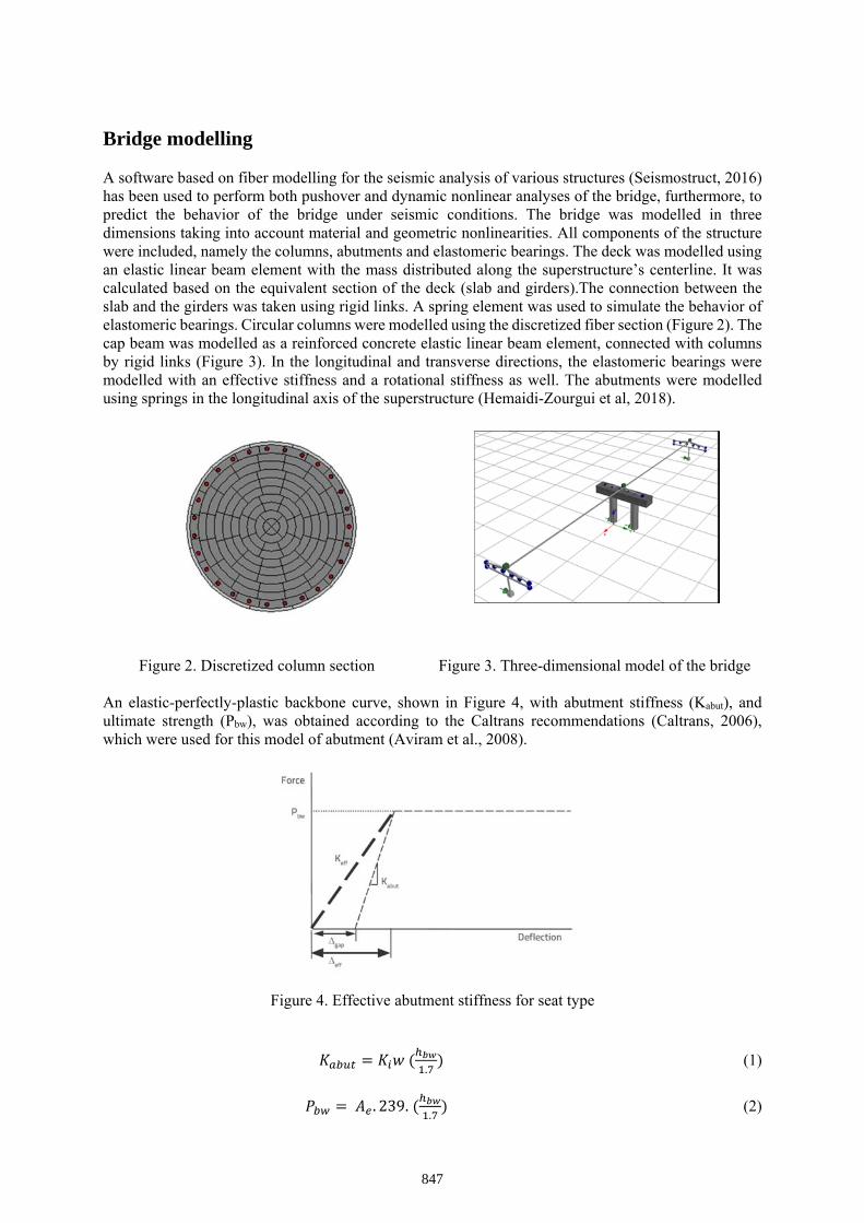
Bridge modelling

A software based on fiber modelling for the seismic analysis of various structures (Seismostruct, 2016) has been used to perform both pushover and dynamic nonlinear analyses of the bridge, furthermore, to predict the behavior of the bridge under seismic conditions. The bridge was modelled in three dimensions taking into account material and geometric nonlinearities. All components of the structure were included, namely the columns, abutments and elastomeric bearings. The deck was modelled using an elastic linear beam element with the mass distributed along the superstructure’s centerline. It was calculated based on the equivalent section of the deck (slab and girders).The connection between the slab and the girders was taken using rigid links. A spring element was used to simulate the behavior of elastomeric bearings. Circular columns were modelled using the discretized fiber section (Figure 2). The cap beam was modelled as a reinforced concrete elastic linear beam element, connected with columns by rigid links (Figure 3). In the longitudinal and transverse directions, the elastomeric bearings were modelled with an effective stiffness and a rotational stiffness as well. The abutments were modelled using springs in the longitudinal axis of the superstructure (Hemaidi-Zourgui et al, 2018).

Figure 2. Discretized column section Figure 3. Three-dimensional model of the bridge

An elastic-perfectly-plastic backbone curve, shown in Figure 4, with abutment stiffness (Kabut), and ultimate strength (Pbw), was obtained according to the Caltrans recommendations (Caltrans, 2006), which were used for this model of abutment (Aviram et al., 2008).

Figure 4. Effective abutment stiffness for seat type

.

(1)

. 239. .

(2)

847

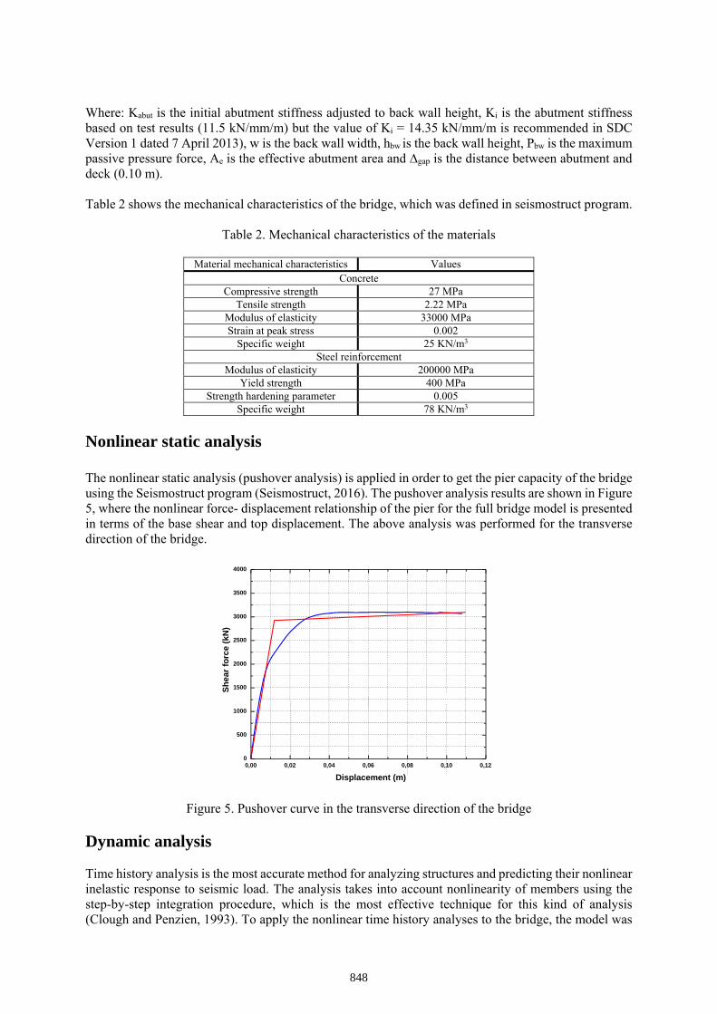
Where: Kabut is the initial abutment stiffness adjusted to back wall height, Ki is the abutment stiffness based on test results (11.5 kN/mm/m) but the value of Ki = 14.35 kN/mm/m is recommended in SDC Version 1 dated 7 April 2013), w is the back wall width, hbw is the back wall height, Pbw is the maximum passive pressure force, Ae is the effective abutment area and ∆gap is the distance between abutment and deck (0.10 m).

Table 2 shows the mechanical characteristics of the bridge, which was defined in seismostruct program.

Table 2. Mechanical characteristics of the materials

Material mechanical characteristics Values Concrete

Compressive strength 27 MPa Tensile strength 2.22 MPa

Modulus of elasticity 33000 MPa Strain at peak stress 0.002

Specific weight 25 KN/m3 Steel reinforcement

Modulus of elasticity 200000 MPa Yield strength 400 MPa

Strength hardening parameter 0.005 Specific weight 78 KN/m3

Nonlinear static analysis

The nonlinear static analysis (pushover analysis) is applied in order to get the pier capacity of the bridge using the Seismostruct program (Seismostruct, 2016). The pushover analysis results are shown in Figure 5, where the nonlinear force- displacement relationship of the pier for the full bridge model is presented in terms of the base shear and top displacement. The above analysis was performed for the transverse direction of the bridge.

Figure 5. Pushover curve in the transverse direction of the bridge

Dynamic analysis

Time history analysis is the most accurate method for analyzing structures and predicting their nonlinear inelastic response to seismic load. The analysis takes into account nonlinearity of members using the step-by-step integration procedure, which is the most effective technique for this kind of analysis (Clough and Penzien, 1993). To apply the nonlinear time history analyses to the bridge, the model was

0,00 0,02 0,04 0,06 0,08 0,10 0,120

500

1000

1500

2000

2500

3000

3500

4000

Sh

ear

forc

e (

kN

)

Displacement (m)

848

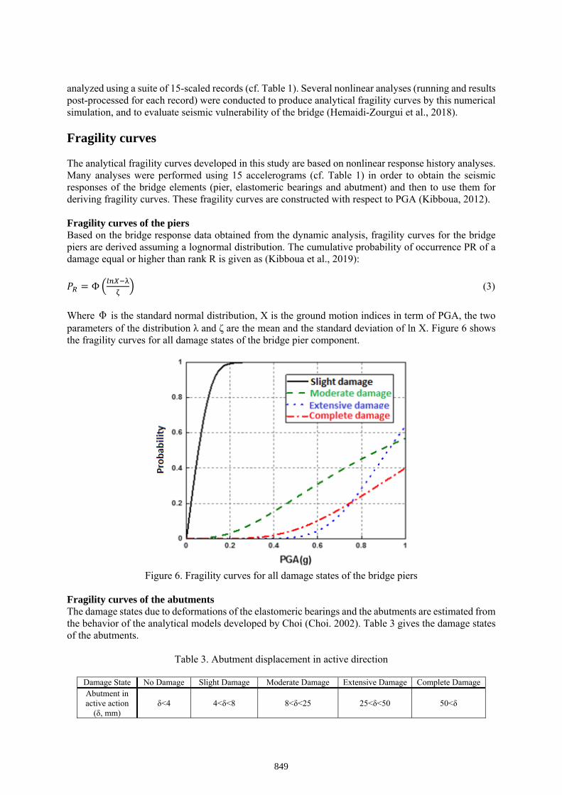
analyzed using a suite of 15-scaled records (cf. Table 1). Several nonlinear analyses (running and results post-processed for each record) were conducted to produce analytical fragility curves by this numerical simulation, and to evaluate seismic vulnerability of the bridge (Hemaidi-Zourgui et al., 2018).

Fragility curves

The analytical fragility curves developed in this study are based on nonlinear response history analyses. Many analyses were performed using 15 accelerograms (cf. Table 1) in order to obtain the seismic responses of the bridge elements (pier, elastomeric bearings and abutment) and then to use them for deriving fragility curves. These fragility curves are constructed with respect to PGA (Kibboua, 2012).

Fragility curves of the piers Based on the bridge response data obtained from the dynamic analysis, fragility curves for the bridge piers are derived assuming a lognormal distribution. The cumulative probability of occurrence PR of a damage equal or higher than rank R is given as (Kibboua et al., 2019):

Φ (3)

Where Φ is the standard normal distribution, X is the ground motion indices in term of PGA, the two parameters of the distribution λ and ζ are the mean and the standard deviation of ln X. Figure 6 shows the fragility curves for all damage states of the bridge pier component.

Figure 6. Fragility curves for all damage states of the bridge piers

Fragility curves of the abutments The damage states due to deformations of the elastomeric bearings and the abutments are estimated from the behavior of the analytical models developed by Choi (Choi. 2002). Table 3 gives the damage states of the abutments.

Table 3. Abutment displacement in active direction

Damage State No Damage Slight Damage Moderate Damage Extensive Damage Complete Damage Abutment in active action

(δ, mm) δ<4 4<δ<8 8<δ<25 25<δ<50 50<δ

849

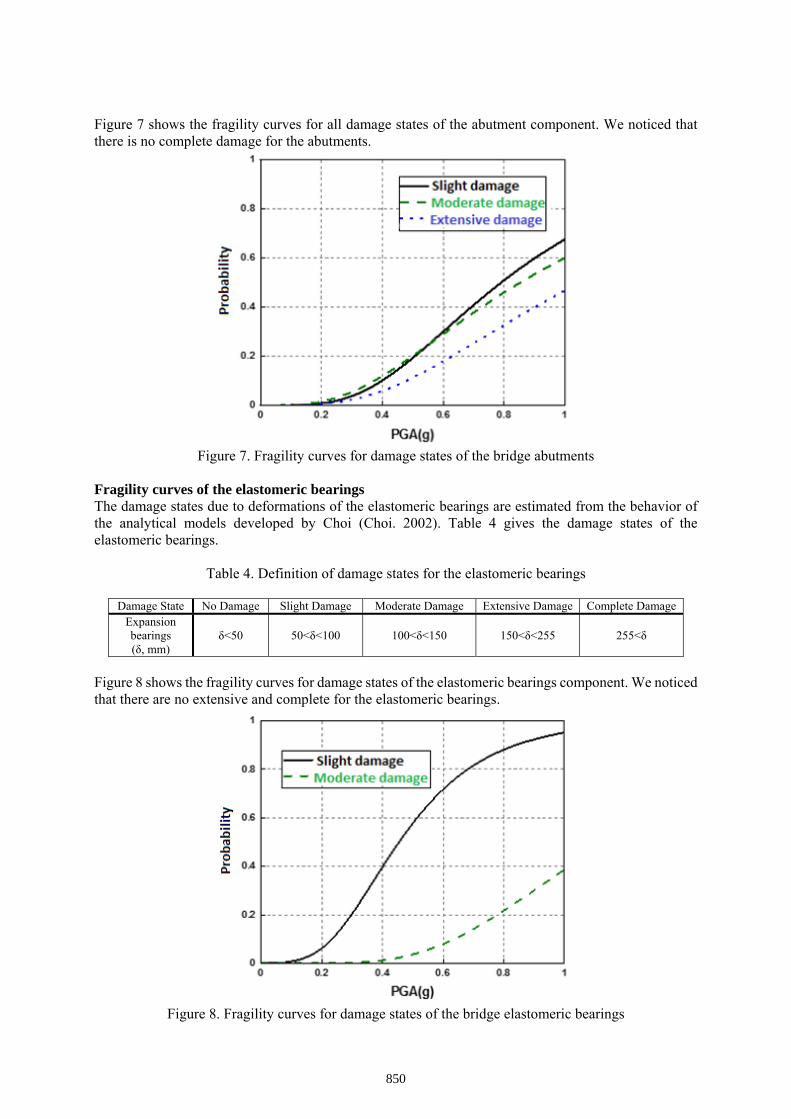
Figure 7 shows the fragility curves for all damage states of the abutment component. We noticed that there is no complete damage for the abutments.

Figure 7. Fragility curves for damage states of the bridge abutments

Fragility curves of the elastomeric bearings The damage states due to deformations of the elastomeric bearings are estimated from the behavior of the analytical models developed by Choi (Choi. 2002). Table 4 gives the damage states of the elastomeric bearings.

Table 4. Definition of damage states for the elastomeric bearings

Damage State No Damage Slight Damage Moderate Damage Extensive Damage Complete Damage Expansion bearings (δ, mm)

δ<50 50<δ<100 100<δ<150 150<δ<255 255<δ

Figure 8 shows the fragility curves for damage states of the elastomeric bearings component. We noticed that there are no extensive and complete for the elastomeric bearings.

Figure 8. Fragility curves for damage states of the bridge elastomeric bearings

850

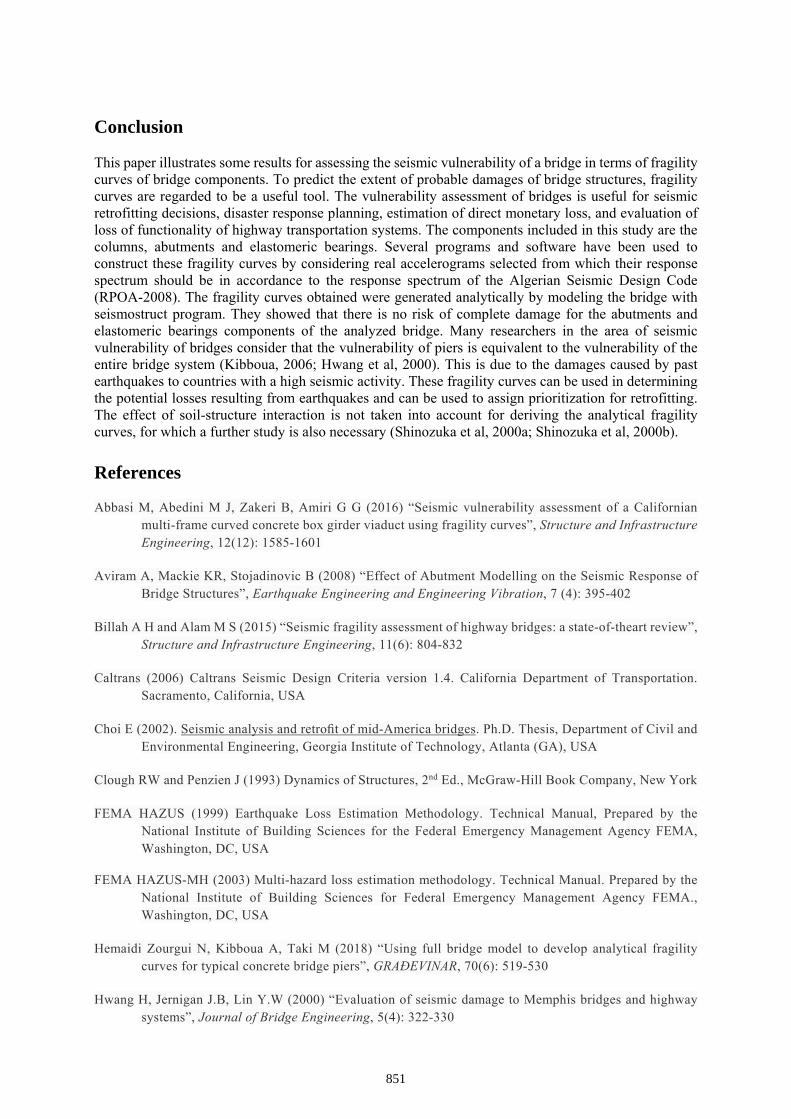
Conclusion

This paper illustrates some results for assessing the seismic vulnerability of a bridge in terms of fragility curves of bridge components. To predict the extent of probable damages of bridge structures, fragility curves are regarded to be a useful tool. The vulnerability assessment of bridges is useful for seismic retrofitting decisions, disaster response planning, estimation of direct monetary loss, and evaluation of loss of functionality of highway transportation systems. The components included in this study are the columns, abutments and elastomeric bearings. Several programs and software have been used to construct these fragility curves by considering real accelerograms selected from which their response spectrum should be in accordance to the response spectrum of the Algerian Seismic Design Code (RPOA-2008). The fragility curves obtained were generated analytically by modeling the bridge with seismostruct program. They showed that there is no risk of complete damage for the abutments and elastomeric bearings components of the analyzed bridge. Many researchers in the area of seismic vulnerability of bridges consider that the vulnerability of piers is equivalent to the vulnerability of the entire bridge system (Kibboua, 2006; Hwang et al, 2000). This is due to the damages caused by past earthquakes to countries with a high seismic activity. These fragility curves can be used in determining the potential losses resulting from earthquakes and can be used to assign prioritization for retrofitting. The effect of soil-structure interaction is not taken into account for deriving the analytical fragility curves, for which a further study is also necessary (Shinozuka et al, 2000a; Shinozuka et al, 2000b).

References

Abbasi M, Abedini M J, Zakeri B, Amiri G G (2016) “Seismic vulnerability assessment of a Californian multi-frame curved concrete box girder viaduct using fragility curves”, Structure and Infrastructure Engineering, 12(12): 1585-1601

Aviram A, Mackie KR, Stojadinovic B (2008) “Effect of Abutment Modelling on the Seismic Response of Bridge Structures”, Earthquake Engineering and Engineering Vibration, 7 (4): 395-402

Billah A H and Alam M S (2015) “Seismic fragility assessment of highway bridges: a state-of-theart review”, Structure and Infrastructure Engineering, 11(6): 804-832

Caltrans (2006) Caltrans Seismic Design Criteria version 1.4. California Department of Transportation. Sacramento, California, USA

Choi E (2002). Seismic analysis and retrofit of mid-America bridges. Ph.D. Thesis, Department of Civil and Environmental Engineering, Georgia Institute of Technology, Atlanta (GA), USA

Clough RW and Penzien J (1993) Dynamics of Structures, 2nd Ed., McGraw-Hill Book Company, New York

FEMA HAZUS (1999) Earthquake Loss Estimation Methodology. Technical Manual, Prepared by the National Institute of Building Sciences for the Federal Emergency Management Agency FEMA, Washington, DC, USA

FEMA HAZUS-MH (2003) Multi-hazard loss estimation methodology. Technical Manual. Prepared by the National Institute of Building Sciences for Federal Emergency Management Agency FEMA., Washington, DC, USA

Hemaidi Zourgui N, Kibboua A, Taki M (2018) “Using full bridge model to develop analytical fragility curves for typical concrete bridge piers”, GRAĐEVINAR, 70(6): 519-530

Hwang H, Jernigan J.B, Lin Y.W (2000) “Evaluation of seismic damage to Memphis bridges and highway systems”, Journal of Bridge Engineering, 5(4): 322-330

851

Kibboua A, Naili M, Benouar D, Kehila F (2011) “Analytical fragility curves for typical Algerian reinforced concrete bridge piers”, Structural Engineering and Mechanics, 39(3): 411-425

Kibboua A, Bechtoula H, Mehani Y, Naili M (2014) “Vulnerability assessment of reinforced concrete bridge structures in Algiers using scenario earthquakes”, Bulletin of earthquake engineering, 12(2): 807-827

Kibboua A, Farsi M-N, Chatelain J-L, Guillier B, Bechtoula H, Mehani Y (2008) “Modal analysis and ambient vibration measurements on Mila-Algeria cable stayed bridge”, Structural Engineering and Mechanics, 29(2): 171-186

Kibboua A, Kehila F, Hemaidi-Zourgui N, Remki M (2017) “Comparison between fragility curves of RC bridge piers designed by old and recent Algerian codes”, Eurasian Journal of Engineering Sciences and Technology, 1(2): 56–67

Kibboua A (2012) Développement d’une méthodologie d’analyse pour la vulnérabilité sismique des piles

de ponts algériens, Ph.D. Thesis, Laboratoire de recherche du Bâti dans l’Environnement, University of Science and Technology Houari Boumediene, Bab Ezzouar, Algiers, Algeria

Kibboua A (2006) Analyse dynamique sous vibrations ambiantes d’un pont à haubans sur l’Oued Dib à Mila, Magister Thesis, Ecole Nationale des Travaux Publics, Kouba, Algiers, Algeria

Kibboua A, Kehila F, Hemaidi-Zourgui N, Remki M (2019) “Fragility curves for bridge piers using recorded ground motions”, 5th International Conference on Earthquake Engineering and Seismology (5ICEES), Metu, Ankara, Turkey, 8-11 October, 1-10

Kehila F, Kibboua A, Bechtoula H, Remki M (2018) “Seismic performance assessment of R.C. bridge piers designed with the Algerian seismic bridges regulation”, Earthquakes and Structures, 15(6): 701-713

Moschonas IF, Kappos AJ, Panetsos P, Papadopoulos V, Makarios T, Thanopoulos P (2009) “Seismic fragility curves for Greek bridges: methodology and case studies”, Bulletin of Earthquake Engineering, 7 (2): 439-468

Padgett JE and DesRoches R (2008) “Methodology for the development of analytical curves for retrofitted bridges”, Earthquake Engineering & Structural Dynamics, 37 (8): 1157-1174

Park YJ, Ang AHS, Wen YK (1985) “Seismic damage analysis of reinforced concrete buildings”, Journal of Structural Engineering, 111(4): 740 –757

RPOA (2008) Règles Parasismiques Applicables au Domaine des Ouvrages d’ Art. Document Technique Réglementaire. Ministère des Travaux Publics, Algiers, Alegria

Seismostruct (2016) A Computer Program for Static and Dynamic Nonlinear Analysis of Framed Structures. Available from http://www.seismosoft.com

Shinozuka M, Feng M.Q, Lee J, Naganuma T (2000a) “Statistical analysis of fragility curves”, Journal of Engineering Mechanics, 126(12): 1224-1231

Shinozuka M, Feng M.Q, Kim H-K, Kim S-H (2000b) “Nonlinear static procedure for fragility curve development”, Journal of Engineering Mechanics, 126(12): 1287-1296

Zhongxian L, Yang L, Ning L (2014) “Vector-Intensity Measure Based Seismic Vulnerability Analysis of Bridge Structures”, Earthquake Engineering and Engineering Vibration, 13 (4): 695-7

852

Influence of High Strength Rubberized Concrete on the Energy Dissipation

and Seismic Demand of Jacketed RC Structures

Ahed Habib1*, Umut Yıldırım1, Özgür Eren1

1Department. of Civil Engineering, Eastern Mediterranean University, Famagusta, North Cyprus, via Mersin 10, Turkey


AbstractNowadays, many researches are focused on investigating the behavior of rubberized concrete as a

structural material due to its enhanced properties such as ductility, energy dissipation and damping ratio

and its role in the sustainability development by recycling non-biodegradable wastes and reducing the

amount of natural aggregates in concrete mixture. Currently, the performance of this material in

retrofitting applications such as reinforced concrete jacketing is still unclear and need to be addressed

in order to be implemented in the construction activities. Thus, the main aim of this research is to

investigate the seismic performance of reinforced concrete buildings strengthened using rubberized

concrete jackets under severe earthquake excitations. As a part of this study, laboratory tests will be

conducted to evaluate the properties of high-strength rubberized concrete mixture against the control

one. Furthermore, finite element models of reinforced concrete moment-resisting frame retrofitted with

reinforced concrete jacket will be analyzed using nonlinear response history analysis to examine its

performance in comparison to the control models. In general, the results of this study have shown that

using rubberized concrete rather than normal one provides a better source of damping energy under

severe ground motion actions.

Keywords: Rubberized concrete, reinforced concrete jacketing, damping, structural material, energy

dissipation.

List of Nomenclature

Symbol Description

RC Reinforced concrete

RBC Rubberized concrete

25RBC Concrete with 25% rubber replacement ratio

ZRBC Control concrete with zero rubber

BS Bare structure (without retrofitting)

SMS The MCER, 5% damped, spectral response acceleration

parameter at short periods

SM1 The MCER, 5% damped, spectral response acceleration

parameter at a period of 1s

MCER Risk-targeted

Tp Pulse period

Ip Pulse indicator

PGA Peak ground acceleration

Introduction

Seismic retrofitting of reinforced concrete (RC) structures is a very common topic in the literature. On

this matter, several solutions were proposed and many investigations were published in the literature.

Currently, control systems can be considered as effective approaches for mitigating RC structures (De

Domenico et al., 2019; Symans and Constantinou, 1999). However, such methods are expensive and

853

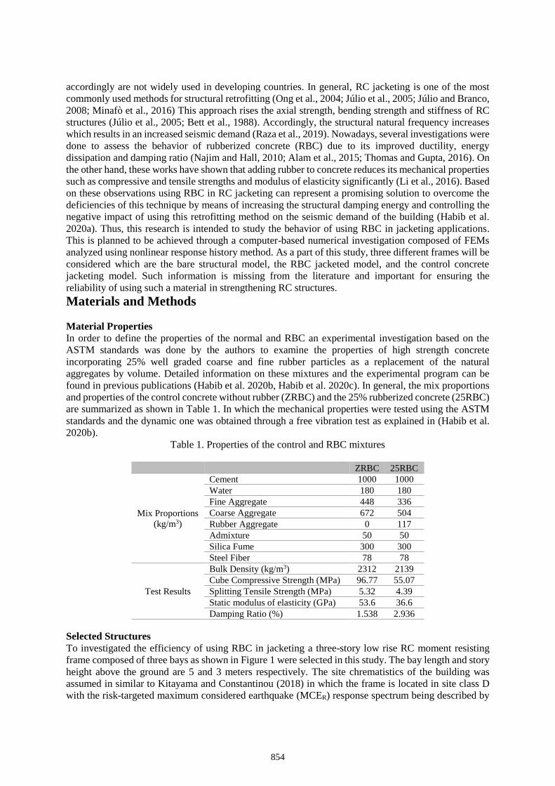
accordingly are not widely used in developing countries. In general, RC jacketing is one of the most

commonly used methods for structural retrofitting (Ong et al., 2004; Júlio et al., 2005; Júlio and Branco,

2008; Minafò et al., 2016) This approach rises the axial strength, bending strength and stiffness of RC

structures (Júlio et al., 2005; Bett et al., 1988). Accordingly, the structural natural frequency increases

which results in an increased seismic demand (Raza et al., 2019). Nowadays, several investigations were

done to assess the behavior of rubberized concrete (RBC) due to its improved ductility, energy

dissipation and damping ratio (Najim and Hall, 2010; Alam et al., 2015; Thomas and Gupta, 2016). On

the other hand, these works have shown that adding rubber to concrete reduces its mechanical properties

such as compressive and tensile strengths and modulus of elasticity significantly (Li et al., 2016). Based

on these observations using RBC in RC jacketing can represent a promising solution to overcome the

deficiencies of this technique by means of increasing the structural damping energy and controlling the

negative impact of using this retrofitting method on the seismic demand of the building (Habib et al.

2020a). Thus, this research is intended to study the behavior of using RBC in jacketing applications.

This is planned to be achieved through a computer-based numerical investigation composed of FEMs

analyzed using nonlinear response history method. As a part of this study, three different frames will be

considered which are the bare structural model, the RBC jacketed model, and the control concrete

jacketing model. Such information is missing from the literature and important for ensuring the

reliability of using such a material in strengthening RC structures.

Materials and Methods

Material Properties

In order to define the properties of the normal and RBC an experimental investigation based on the

ASTM standards was done by the authors to examine the properties of high strength concrete

incorporating 25% well graded coarse and fine rubber particles as a replacement of the natural

aggregates by volume. Detailed information on these mixtures and the experimental program can be

found in previous publications (Habib et al. 2020b, Habib et al. 2020c). In general, the mix proportions

and properties of the control concrete without rubber (ZRBC) and the 25% rubberized concrete (25RBC)

are summarized as shown in Table 1. In which the mechanical properties were tested using the ASTM

standards and the dynamic one was obtained through a free vibration test as explained in (Habib et al.

2020b).

Table 1. Properties of the control and RBC mixtures

ZRBC 25RBC

Mix Proportions

(kg/m3)

Cement 1000 1000

Water 180 180

Fine Aggregate 448 336

Coarse Aggregate 672 504

Rubber Aggregate 0 117

Admixture 50 50

Silica Fume 300 300

Steel Fiber 78 78

Test Results

Bulk Density (kg/m3) 2312 2139

Cube Compressive Strength (MPa) 96.77 55.07

Splitting Tensile Strength (MPa) 5.32 4.39

Static modulus of elasticity (GPa) 53.6 36.6

Damping Ratio (%) 1.538 2.936

Selected Structures

To investigated the efficiency of using RBC in jacketing a three-story low rise RC moment resisting

frame composed of three bays as shown in Figure 1 were selected in this study. The bay length and story

height above the ground are 5 and 3 meters respectively. The site chrematistics of the building was

assumed in similar to Kitayama and Constantinou (2018) in which the frame is located in site class D

with the risk-targeted maximum considered earthquake (MCER) response spectrum being described by

854

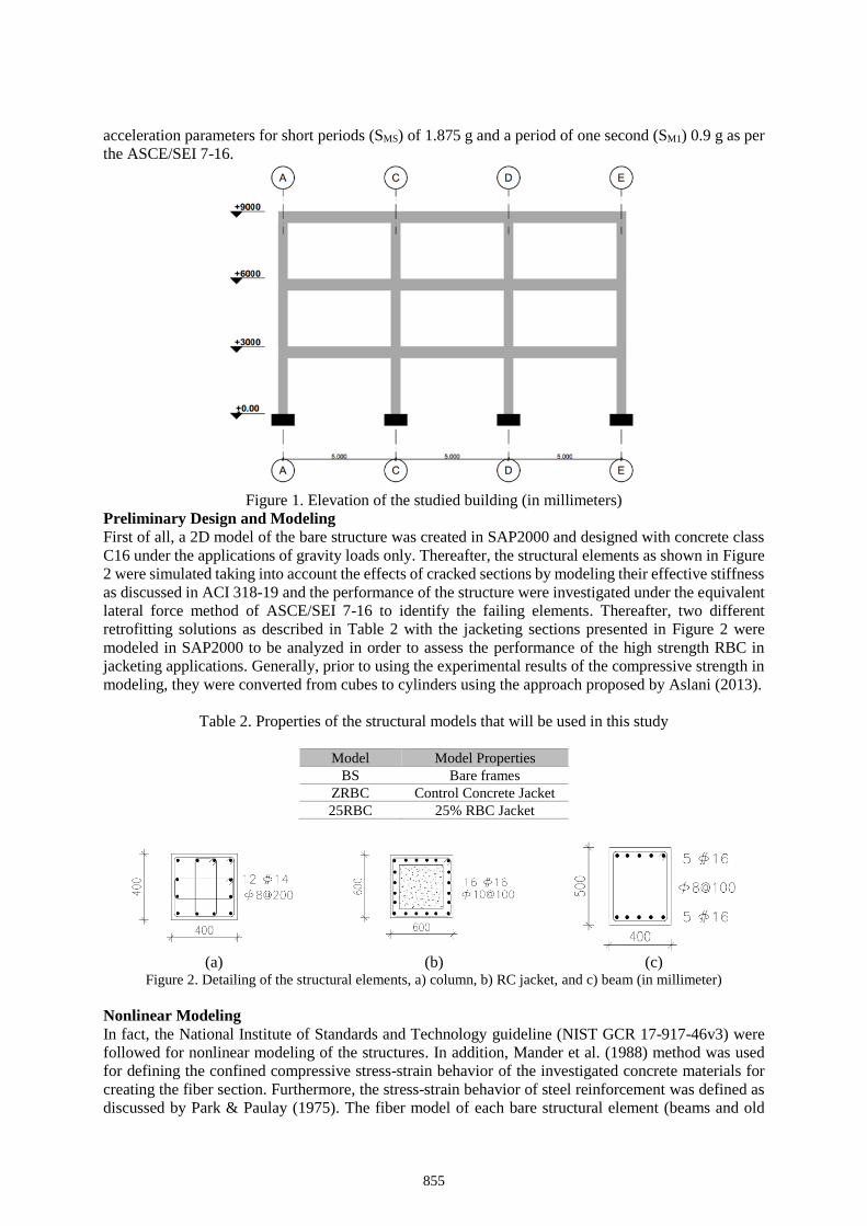
acceleration parameters for short periods (SMS) of 1.875 g and a period of one second (SM1) 0.9 g as per

the ASCE/SEI 7-16.

Figure 1. Elevation of the studied building (in millimeters)

Preliminary Design and Modeling

First of all, a 2D model of the bare structure was created in SAP2000 and designed with concrete class

C16 under the applications of gravity loads only. Thereafter, the structural elements as shown in Figure

2 were simulated taking into account the effects of cracked sections by modeling their effective stiffness

as discussed in ACI 318-19 and the performance of the structure were investigated under the equivalent

lateral force method of ASCE/SEI 7-16 to identify the failing elements. Thereafter, two different

retrofitting solutions as described in Table 2 with the jacketing sections presented in Figure 2 were

modeled in SAP2000 to be analyzed in order to assess the performance of the high strength RBC in

jacketing applications. Generally, prior to using the experimental results of the compressive strength in

modeling, they were converted from cubes to cylinders using the approach proposed by Aslani (2013).

Table 2. Properties of the structural models that will be used in this study

Model Model Properties

BS Bare frames

ZRBC Control Concrete Jacket

25RBC 25% RBC Jacket

(a) (b) (c) Figure 2. Detailing of the structural elements, a) column, b) RC jacket, and c) beam (in millimeter)

Nonlinear Modeling

In fact, the National Institute of Standards and Technology guideline (NIST GCR 17-917-46v3) were

followed for nonlinear modeling of the structures. In addition, Mander et al. (1988) method was used

for defining the confined compressive stress-strain behavior of the investigated concrete materials for

creating the fiber section. Furthermore, the stress-strain behavior of steel reinforcement was defined as

discussed by Park & Paulay (1975). The fiber model of each bare structural element (beams and old

855

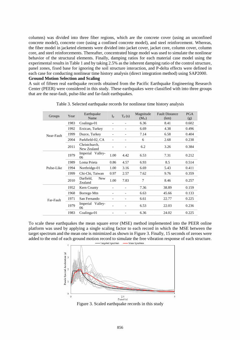
columns) was divided into three fiber regions, which are the concrete cover (using an unconfined

concrete model), concrete core (using a confined concrete model), and steel reinforcement. Whereas,

the fiber model in jacketed elements were divided into jacket cover, jacket core, column cover, column

core, and steel reinforcements. Thereafter, concentrated hinge model was used to simulate the nonlinear

behavior of the structural elements. Finally, damping ratios for each material case model using the

experimental results in Table 1 and by taking 2.5% as the inherent damping ratio of the control structure,

panel zones, fixed base for ignoring the soil structure interaction, and P-delta effects were defined in

each case for conducting nonlinear time history analysis (direct integration method) using SAP2000.

Ground Motion Selection and Scaling

A suit of fifteen real earthquake records obtained from the Pacific Earthquake Engineering Research

Center (PEER) were considered in this study. These earthquakes were classified with into three groups

that are the near-fault, pulse-like and far-fault earthquakes.

Table 3. Selected earthquake records for nonlinear time history analysis

Groups Year Earthquake

Name Ip Tp (s)

Magnitude

(Mw)

Fault Distance

(km)

PGA

(g)

Near-Fault

1983 Coalinga-01 - - 6.36 8.41 0.602

1992 Erzican, Turkey - - 6.69 4.38 0.496

1999 Duzce, Turkey - - 7.14 6.58 0.404

2004 Parkfield-02, CA - - 6 2.68 0.238

2011 Christchurch,

New Zealand - - 6.2 3.26 0.384

Pulse-Like

1979 Imperial Valley-

06 1.00 4.42 6.53 7.31 0.212

1989 Loma Prieta 0.86 4.57 6.93 8.5 0.514

1994 Northridge-01 1.00 3.16 6.69 5.43 0.411

1999 Chi-Chi, Taiwan 0.97 2.57 7.62 9.76 0.359

2010 Darfield, New

Zealand 1.00 7.83 7 8.46 0.257

Far-Fault

1952 Kern County - - 7.36 38.89 0.159

1968 Borrego Mtn - - 6.63 45.66 0.133

1971 San Fernando - - 6.61 22.77 0.225

1979 Imperial Valley-

06 - - 6.53 22.03 0.236

1983 Coalinga-01 - - 6.36 24.02 0.225

To scale these earthquakes the mean square error (MSE) method implemented into the PEER online

platform was used by applying a single scaling factor to each record in which the MSE between the

target spectrum and the mean one is minimized as shown in Figure 3. Finally, 15 seconds of zeroes were

added to the end of each ground motion record to simulate the free vibration response of each structure.

Figure 3. Scaled earthquake records in this study

856

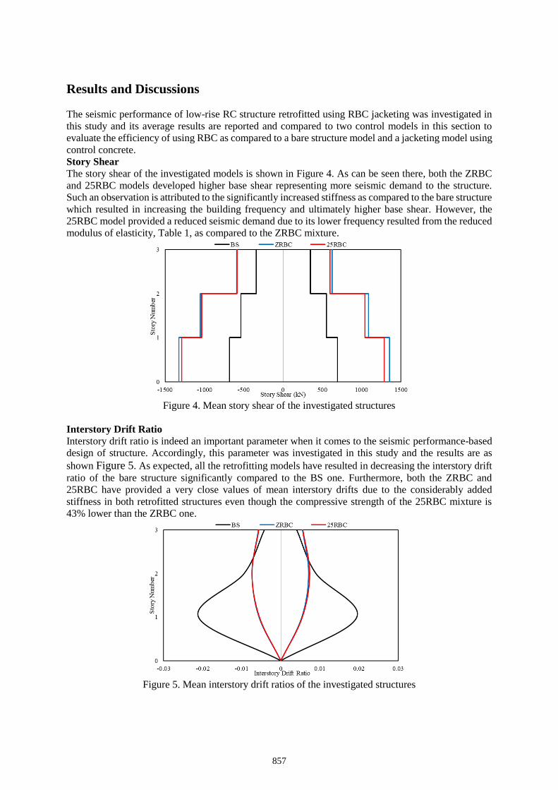
Results and Discussions

The seismic performance of low-rise RC structure retrofitted using RBC jacketing was investigated in

this study and its average results are reported and compared to two control models in this section to

evaluate the efficiency of using RBC as compared to a bare structure model and a jacketing model using

control concrete.

Story Shear

The story shear of the investigated models is shown in Figure 4. As can be seen there, both the ZRBC

and 25RBC models developed higher base shear representing more seismic demand to the structure.

Such an observation is attributed to the significantly increased stiffness as compared to the bare structure

which resulted in increasing the building frequency and ultimately higher base shear. However, the

25RBC model provided a reduced seismic demand due to its lower frequency resulted from the reduced

modulus of elasticity, Table 1, as compared to the ZRBC mixture.

Figure 4. Mean story shear of the investigated structures

Interstory Drift Ratio

Interstory drift ratio is indeed an important parameter when it comes to the seismic performance-based

design of structure. Accordingly, this parameter was investigated in this study and the results are as

shown Figure 5. As expected, all the retrofitting models have resulted in decreasing the interstory drift

ratio of the bare structure significantly compared to the BS one. Furthermore, both the ZRBC and

25RBC have provided a very close values of mean interstory drifts due to the considerably added

stiffness in both retrofitted structures even though the compressive strength of the 25RBC mixture is

43% lower than the ZRBC one.

Figure 5. Mean interstory drift ratios of the investigated structures

857

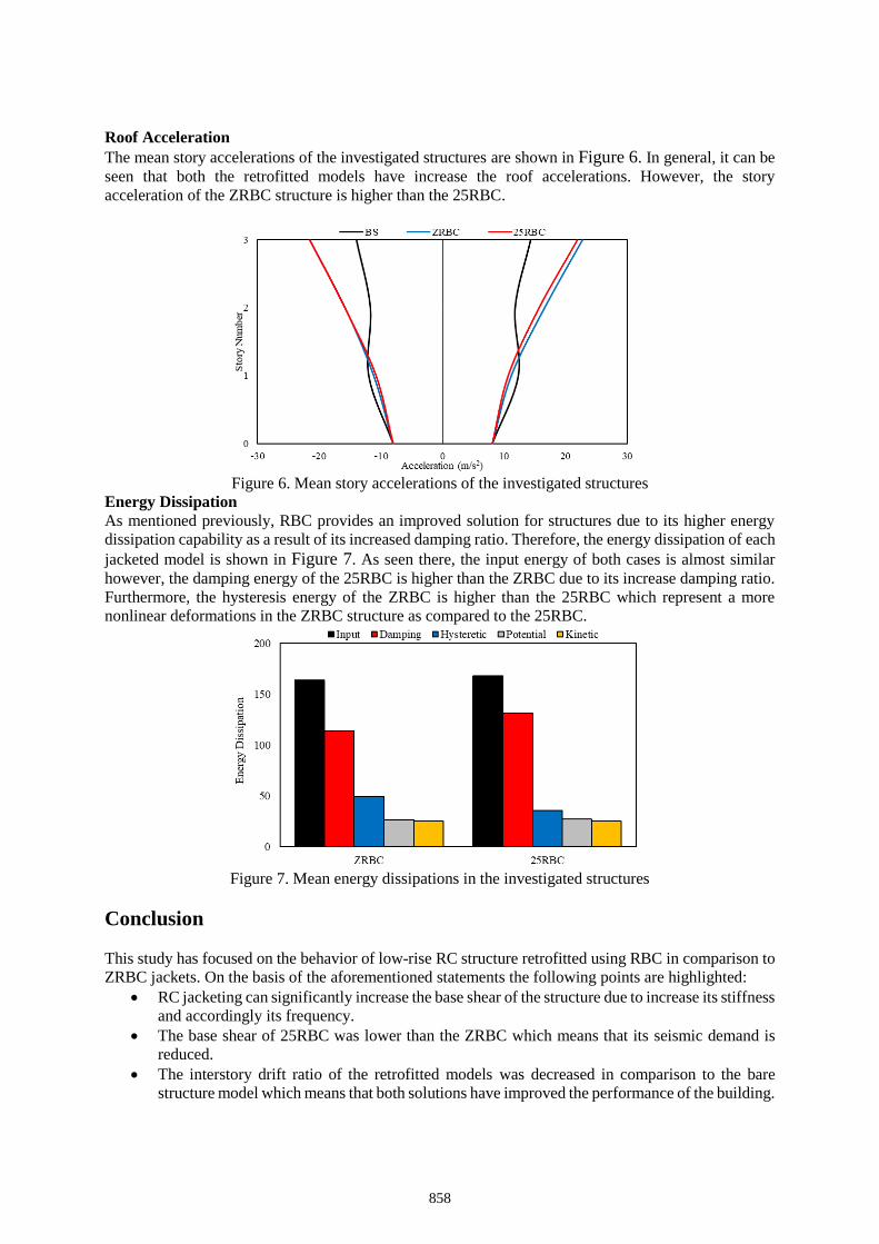
Roof Acceleration

The mean story accelerations of the investigated structures are shown in Figure 6. In general, it can be

seen that both the retrofitted models have increase the roof accelerations. However, the story

acceleration of the ZRBC structure is higher than the 25RBC.

Figure 6. Mean story accelerations of the investigated structures

Energy Dissipation

As mentioned previously, RBC provides an improved solution for structures due to its higher energy

dissipation capability as a result of its increased damping ratio. Therefore, the energy dissipation of each

jacketed model is shown in Figure 7. As seen there, the input energy of both cases is almost similar

however, the damping energy of the 25RBC is higher than the ZRBC due to its increase damping ratio.

Furthermore, the hysteresis energy of the ZRBC is higher than the 25RBC which represent a more

nonlinear deformations in the ZRBC structure as compared to the 25RBC.

Figure 7. Mean energy dissipations in the investigated structures

Conclusion

This study has focused on the behavior of low-rise RC structure retrofitted using RBC in comparison to

ZRBC jackets. On the basis of the aforementioned statements the following points are highlighted:

• RC jacketing can significantly increase the base shear of the structure due to increase its stiffness

and accordingly its frequency.

• The base shear of 25RBC was lower than the ZRBC which means that its seismic demand is

reduced.

• The interstory drift ratio of the retrofitted models was decreased in comparison to the bare

structure model which means that both solutions have improved the performance of the building.

858

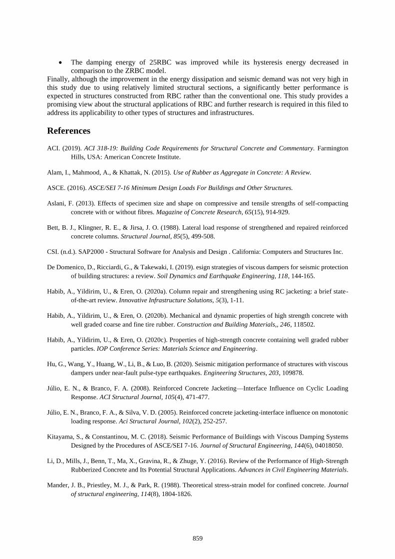
• The damping energy of 25RBC was improved while its hysteresis energy decreased in

comparison to the ZRBC model.

Finally, although the improvement in the energy dissipation and seismic demand was not very high in

this study due to using relatively limited structural sections, a significantly better performance is

expected in structures constructed from RBC rather than the conventional one. This study provides a

promising view about the structural applications of RBC and further research is required in this filed to

address its applicability to other types of structures and infrastructures.

References

ACI. (2019). ACI 318-19: Building Code Requirements for Structural Concrete and Commentary. Farmington

Hills, USA: American Concrete Institute.

Alam, I., Mahmood, A., & Khattak, N. (2015). Use of Rubber as Aggregate in Concrete: A Review.

ASCE. (2016). ASCE/SEI 7-16 Minimum Design Loads For Buildings and Other Structures.

Aslani, F. (2013). Effects of specimen size and shape on compressive and tensile strengths of self-compacting

concrete with or without fibres. Magazine of Concrete Research, 65(15), 914-929.

Bett, B. J., Klingner, R. E., & Jirsa, J. O. (1988). Lateral load response of strengthened and repaired reinforced

concrete columns. Structural Journal, 85(5), 499-508.

CSI. (n.d.). SAP2000 - Structural Software for Analysis and Design . California: Computers and Structures Inc.

De Domenico, D., Ricciardi, G., & Takewaki, I. (2019). esign strategies of viscous dampers for seismic protection

of building structures: a review. Soil Dynamics and Earthquake Engineering, 118, 144-165.

Habib, A., Yildirim, U., & Eren, O. (2020a). Column repair and strengthening using RC jacketing: a brief state-

of-the-art review. Innovative Infrastructure Solutions, 5(3), 1-11.

Habib, A., Yildirim, U., & Eren, O. (2020b). Mechanical and dynamic properties of high strength concrete with

well graded coarse and fine tire rubber. Construction and Building Materials,, 246, 118502.

Habib, A., Yildirim, U., & Eren, O. (2020c). Properties of high-strength concrete containing well graded rubber

particles. IOP Conference Series: Materials Science and Engineering.

Hu, G., Wang, Y., Huang, W., Li, B., & Luo, B. (2020). Seismic mitigation performance of structures with viscous

dampers under near-fault pulse-type earthquakes. Engineering Structures, 203, 109878.

Júlio, E. N., & Branco, F. A. (2008). Reinforced Concrete Jacketing—Interface Influence on Cyclic Loading

Response. ACI Structural Journal, 105(4), 471-477.

Júlio, E. N., Branco, F. A., & Silva, V. D. (2005). Reinforced concrete jacketing-interface influence on monotonic

loading response. Aci Structural Journal, 102(2), 252-257.

Kitayama, S., & Constantinou, M. C. (2018). Seismic Performance of Buildings with Viscous Damping Systems

Designed by the Procedures of ASCE/SEI 7-16. Journal of Structural Engineering, 144(6), 04018050.

Li, D., Mills, J., Benn, T., Ma, X., Gravina, R., & Zhuge, Y. (2016). Review of the Performance of High-Strength

Rubberized Concrete and Its Potential Structural Applications. Advances in Civil Engineering Materials.

Mander, J. B., Priestley, M. J., & Park, R. (1988). Theoretical stress-strain model for confined concrete. Journal

of structural engineering, 114(8), 1804-1826.

859

Minafò, G., Di Trapani, F., & Amato, G. (2016). Strength and ductility of RC jacketed columns: A simplified

analytical method. Engineering Structures, 122, 184-195.

Najim, K., & Hall, M. (2010). A review of the fresh/hardened properties and applications for plain- (PRC) and

self-compacting rubberised concrete (SCRC). Construction and Building Materials.

NIST. (2017). Guidelines for Nonlinear Structural Analysis for Design of Buildings Part IIb – Reinforced Concrete

Moment Frames. National Institute of Standards and Technology. doi:10.6028/NIST.GCR.17-917-46v3

Ong, K. C., Kog, Y., Yu, C. H., & Sreekanth, A. P. (2004). Jacketing of reinforced concrete columns subjected to

axial load. Magazine of Concrete Research, 56(2), 89-98.

Park, R., & Paulay, T. (1975). Reinforced Concrete Structures. Wiley .

Raza, S., Khan, M. K., Menegon, S. J., Tsang, H. H., & Wilson, J. L. (2019). Strengthening and Repair of

Reinforced Concrete Columns by Jacketing: State-of-the-Art Review. Sustainability, 11(11), 3208.

Symans, M. D., & Constantinou, M. C. (1999). Semi-active control systems for seismic protection of structures: a

state-of-the-art review. Engineering structures, 21(6), 469-487.

Thomas, B., & Gupta, R. (2016). A comprehensive review on the applications of waste tire rubber in cement

concrete. Renewable and Sustainable Energy Reviews.

860

© 2021, İstanbul Teknik Üniversitesi

ISBN No / ISBN Number: 978-975-561-519-6

İstanbul Teknik Üniversitesi Yayınları. Yayın No / ITU Publications, Publication No: 2021.2KNF/2TDV Yayın No / TDV Publication Number: 21/01İMO Yayın No / İMO Publication Number: E/21/01Yayın Tarihi / Date of Publication: 1 Haziran / June 2021

Farklı Seviyelerde Korozyona Uğramış Bir Köprünün Hasar ...

Documents

Transcript of Farklı Seviyelerde Korozyona Uğramış Bir Köprünün Hasar ...