Family structure and child health - CORE

1

Family structure and child health

Lidia Panico

Thesis submitted for the degree of Doctor of Philosophy

University College London

January 2012

2

Declaration

I, Lidia Panico, confirm that the work presented in this thesis is my own. Where

information has been derived from other sources, I confirm that this has been indicated in

the thesis.

This work has been funded by an Economic and Social Research Council/Medical

Research Council Interdisciplinary Studentship.

3

Abstract

This inter-disciplinary project investigates the relationship between family structure and early

child health. The two main aims are: (1) to determine whether family structure and changes

in family structure are associated with children‘s physical health in the Millennium Cohort

Study; (2) to explore potential pathways through which these associations operate.

In spite of much public debate around families, marriage, and child outcomes, UK literature

on this topic remains incomplete. This thesis aims to fill two gaps: first, testing whether there

is a link with children‘s physical health, rather than more commonly reported outcomes such

as cognitive function or education achievements. Physical health outcomes included are

respiratory health, childhood growth, and unintentional injuries. Second, few studies use

prospective, longitudinal data and methods. Cross sectional studies cannot examine the

direction of the relationship, nor capture the dynamics of changes in family structure. Here,

longitudinal techniques test a complex model made up of variables ordered a priori.

In unadjusted analyses, family structure presented a consistent gradient in child health: cross-

sectionally, children living with married parents had better health than those living with

cohabiting parents, while those living with lone parents had the worst health. Longitudinally,

those who experienced changes in family structure fared worse than those living with

continuously married parents, with some important exceptions, such as those living with

cohabiting parents who subsequently married. Socio-economic factors were important

predictors of family structure and child health. Proximal pathways through which socio-

economic characteristics and family structure affected child health varied according to health

outcome. Maternal mental health appeared to be important across outcomes.

Concluding, this work shows the importance of using nuanced definitions of family,

particularly when it comes to capturing its fluidity over time. Children who experienced

changes in family structure were a heterogeneous group with diverse backgrounds and

outcomes. Socio-economic factors emerged as important antecedents to both family structure

and child health.

4

Acknowledgments

This thesis would have not been possible without the guidance, encouragement, and

support of my supervisors, Professor Mel Bartley, Professor Yvonne Kelly, Dr Anne

McMunn, and Professor Amanda Sacker. Their support has been invaluable since I

arrived at UCL, and this work, as well as my overall experience at UCL, would have not

been the same without them.

I am also grateful for the support of many other colleagues at UCL, especially Paola

Zaninotto and Dr Mai Stafford for statistical support, and at the International Centre for

Life Course Studies. My upgrade examiner, Professor Heather Joshi, helped give

direction to this work. I would also like to thank my viva examiners, Professors Ann

Berrington and Richard Watt, for invaluable feedback.

Thanks must go to the Millennium Cohort Study families for their time and co-

operation, as well as the Millennium Cohort Study team at the Institute of Education for

their advice and support.

I am grateful to Drs John, Silvia, Conor, Beth, Ed, Libby, Laia and Paola for their

support, innumerable cups of coffee, and for understanding it all. I would like to thank

my parents, Aurora and Enzo, for their unconditional love, support, and free childcare,

without which none of this would have been done. And finally, to Velia, who has given

me a whole new perspective, and to John, for his constant support and endless

encouragement when it was most needed.

5

Table of Contents

Declaration ............................................................................................................................. 2

Abstract .................................................................................................................................. 3

Acknowledgments .................................................................................................................. 4

List of Figures ........................................................................................................................ 9

List of Tables........................................................................................................................ 10

Chapter 1 Introduction ......................................................................................................... 12

1.1 Thesis structure .......................................................................................................... 14

Chapter 2 Literature review ................................................................................................. 16

2.1 Conceptualizing family ............................................................................................ 16

2.1.1 The changing demographic context of family and parenthood ........................... 16

2.1.2 The family in contemporary Britain: salient new features .................................. 18

2.1.3 What is happening to the family? Literature from sociology and family studies 21

2.1.4 Tools to define and describe family .................................................................... 25

2.1.5 Family structure in epidemiology ....................................................................... 28

2.2 Family structures and health ...................................................................................... 29

2.2.1 Marriage and adult health.................................................................................... 29

2.2.2 Family structure and child health ........................................................................ 30

2.2.3 Explanations ........................................................................................................ 34

2.2.4 Diversity in families and child health ................................................................. 48

2.3 The Policy Context ..................................................................................................... 50

2.3.1 Child health and well being................................................................................. 50

2.3.2 Family policy ...................................................................................................... 51

2.4 Key gaps in the literature and justification for this work ........................................... 55

2.5 Summary .................................................................................................................... 57

Chapter 3 Hypothesised pathways and conceptual model ............................................. 58

3.1 Study Aims and Hypothesis ....................................................................................... 58

3.2 Conceptual Model ...................................................................................................... 59

Chapter 4 Data and variable description .............................................................................. 64

4.1 The Dataset: Millennium Cohort Study (MCS) ......................................................... 64

4.2 Exposure and outcome variables ................................................................................ 66

4.2.1 Family structure .................................................................................................. 67

4.2.2 Child health outcomes ......................................................................................... 69

4.3 Explanatory variables ................................................................................................. 70

6

4.3.1 Socio-economic antecedents ............................................................................... 70

4.3.2 The emotional environment of the child ............................................................. 73

4.3.3 The physical environment ................................................................................... 76

4.3.4 Health behaviours................................................................................................ 78

4.4 Summary .................................................................................................................... 80

Chapter 5 Methods ............................................................................................................... 81

5.1 Cross sectional analyses ............................................................................................. 81

5.2 Longitudinal modelling .............................................................................................. 81

5.2.1 Model building .................................................................................................... 84

5.3 Regression analyses ................................................................................................... 86

5.4 Missing data ............................................................................................................... 88

Figures for Chapter 5 ....................................................................................................... 90

Chapter 6 Initial results and the development of a working model ..................................... 92

6.1 Family structure: cross sectional description ............................................................. 92

5.1.2 Family characteristics: describing family structure cross-sectionally ................ 92

6.2 Longitudinal family change ....................................................................................... 99

6.2.1 Family characteristics by typologies of family change ..................................... 100

6.3 From a theoretical model to an empirical model ..................................................... 104

6.4 Longitudinal Model .................................................................................................. 106

6.5 Summary and conclusions ....................................................................................... 108

Tables for Chapter 6 ....................................................................................................... 111

Chapter 7 Childhood respiratory illnesses ......................................................................... 133

7.1 Family structure and respiratory health: a review of the evidence .......................... 135

7.1.1 Socio-economic factors ..................................................................................... 135

7.1.2 Stress ................................................................................................................. 136

7.1.3 Family stress ..................................................................................................... 137

7.1.4 Hygiene hypothesis ........................................................................................... 138

7.1.5 Behavioural and environmental pathways ........................................................ 139

Breastfeeding.............................................................................................................. 140

7.1.6 Environmental pathways ................................................................................... 141

7.2 Conceptual model..................................................................................................... 142

7.3 Cross-sectional results .............................................................................................. 142

7.4 Longitudinal modelling ............................................................................................ 145

7.5 Conclusions .............................................................................................................. 148


Chapter 8 Childhood growth .............................................................................................. 168

7

8.1 Drivers of growth ..................................................................................................... 168

8.2 The influence of socio-economic disadvantage ....................................................... 169

8.3 The influence of psychosocial stress ........................................................................ 170

8.4 The influence of behavioural and lifestyle factors ................................................... 171

8.4.1 Nutrition and physical activity .......................................................................... 171

8.4.2 Exposure to smoke ............................................................................................ 172

8.5 Chronic disease ........................................................................................................ 173


8.7 Methods .................................................................................................................... 173

8.7.1 Measures of growth ........................................................................................... 174

8.7.2 Standardization methodologies ......................................................................... 175

8.8 Cross sectional results .............................................................................................. 176

8.8.1 Height ................................................................................................................ 176

8.8.2 Waist circumference.......................................................................................... 178

8.8.3 Body Mass Index .............................................................................................. 178

8.9 Longitudinal modelling ............................................................................................ 182

8.10 Conclusions ............................................................................................................ 184


Chapter 9 Unintentional injuries ........................................................................................ 200

9.1 Family structure and unintentional injury ................................................................ 200

9.1.2 Socio-economic factors ..................................................................................... 201

9.1.3 Psychosocial factors .......................................................................................... 202

9.1.4 Supervision ........................................................................................................ 203

9.1.5 Housing ............................................................................................................. 203

9.1.6 Childcare ........................................................................................................... 204

9.1.7 Area level explanations ..................................................................................... 204


9.3 Methods .................................................................................................................... 205

9.3.1 Measures of injury............................................................................................. 205

9.4 Cross sectional results .............................................................................................. 206

9.5 Longitudinal model .................................................................................................. 210

9.6 Conclusion ............................................................................................................... 212


Chapter 10 Discussion and conclusions ............................................................................. 224

10.1 Summary of results ................................................................................................ 224

10.2 Strengths of the study ............................................................................................. 229

8

10.3 Limitations ............................................................................................................. 230

10.4 Adapting the family stress model ........................................................................... 236

10.5 Explaining differences in child health by family structure .................................... 237

10.6 Recognising heterogeneity within families ............................................................ 241

10.7 Policy implications ................................................................................................. 242

10.8 Recommendation for future research ..................................................................... 244

10.9 Final conclusions .................................................................................................... 247

Bibliography ....................................................................................................................... 250

Annex I Household Characteristics by presence in sweeps 1 and 2 .................................. 273

Annex II ISAAC Core Questionnaire for Wheezing and Asthma ..................................... 274

9

List of Figures

Figure 2.1: Number of marriages and divorces in England ................................................. 17 Figure 2.2: Parenting styles .................................................................................................. 38 Figure 2.3: Conger et al (1992)‘s family stress model. ........................................................ 45

Figure 2.4: Linver et al. (2002)‘s family stress model adapted for younger children.......... 46

Figure 3.1: Initial conceptual model .................................................................................... 60 Figure 5.1: An acrylic graph ................................................................................................ 82 Figure 5.2: A cyclic graph .................................................................................................... 82 Figure 5.3: A graphical chain model .................................................................................... 83

Figure 5.4: Missing data in a cross sectional model,: asthma at sweep 3 ............................ 90 Figure 5.5: Missing data in a longitudinal model: asthma by sweep 3 ................................ 91 Figure 6.1: Final conceptual model .................................................................................... 105

10

List of Tables

Table 5.1: Summary of the models used in the longitudinal model..................................... 88

Table 6.1: Distribution of family structures at different ages, % ....................................... 111

Table 6.2: Family characteristics by family structure, sweep 1, % ................................... 112

Table 6.3: Mean number of years living with child‘s father by time of birth, by family

structure .............................................................................................................................. 113

Table 6.4: Family activities by family structure, sweep 2, % ............................................ 114

Table 6.5: Involvement with non-resident father if lone parent at sweep 1 ....................... 116

Table 6.6: Grandparents in the household, by family structure, sweep 1, % ..................... 117

Table 6.7: Distance from grandparents, by family structure, sweep 3, % ......................... 117

Table 6.8: Financial help from parents by family structure, sweep 1, % ........................... 117

Table 6.9: Maternal grandfather NS-SEC5 by family structure at birth, % ....................... 118

Table 6.10: Paternal grandfather NS-SEC5 by family structure at birth, % ...................... 118

Table 6.11: Psychosocial variables by family structure at the same sweep, % ................. 119

Table 6.12: Health behaviours by family structure at the same sweep .............................. 120

Table 6.13: Environmental variables by family structure at the same sweep .................... 121

Table 6.14: Main source of childcare main respondent at work/school by family structure,

sweeps 1, 2 & 3, % ............................................................................................................. 122

Table 6.15: Average hours of childcare per week by family structure, sweeps 1, 2 and 3 123

Table 6.16: Change and stability in family structures over time, compositional change .. 124

Table 6.17: Households who experience a change in parents or parental figure, by family

structure at birth ................................................................................................................. 125

Table 6.18: Typologies of changes in family structure, birth to sweep 3 .......................... 126

Table 6.19: Household characteristics at sweep 3, by typology of family change ............ 127

Table 6.20: Child and parental well-being, sweep 1, by typology of family change......... 129

Table 6.21: Logit parameter estimates for multinomial regression model of typology of

family change on block 1 variables .................................................................................... 130

Table 6.22: Logit parameter estimates for linear regression models of block 3 variables on

block 1 and 2 variables ....................................................................................................... 131

Table 6.23: Logit parameter estimates for linear regression model of block 4 variables on


Table 7.1: Ever asthma and wheeze in the last 12 months, by relationship status at the same

sweep of measurement, % .................................................................................................. 151

Table 7.2: Explanatory factors by ever asthma and recent wheeze, sweep 2 .................... 152

Table 7.3: Explanatory factors by ever asthma and recent wheeze, sweep 3 .................... 156

Table 7.4: Cross-sectional logistic models, Odds Ratios of ever asthma by sweep 2 ....... 160

Table 7.5: Cross-sectional logistic models, Odds Ratios for wheeze in the last year, sweep 2

............................................................................................................................................ 161

Table 7.6: Cross-sectional logistic models, Odds Ratios for ever asthma, sweep 3 .......... 162


............................................................................................................................................ 163

Table 7.8: Interactions: cross sectional analysis of wheeze in the last year, sweep .......... 164

Table 7.9: Interactions: cross sectional analysis of ever asthma, sweep 3 ......................... 164

Table 7.10: Interactions: cross sectional analysis of wheeze in the last year, sweep 3 .. 164

Table 7.11: Probit parameter estimates for regression model of block 5 and 6 variables on


11

Table 7.12: Probit parameter estimates for binary probit regression model of all blocks on

ever asthma at sweep 3 ....................................................................................................... 166


wheeze in the last year at sweep 3 ..................................................................................... 167

Table 8.1: Mean age and sex standardized height scores at age 5, by family structure .... 188

Table 8.2: Waist circumference at age 5, by relationship status ........................................ 189

Table 8.3: Body Mass Index (BMI) at age 5, by relationship status .................................. 190

Table 8.5: Cross-sectional logistic models, Odds Ratios of Body Mass Index, sweep 3 .. 195

Table 8.6: Interactions: cross sectional analysis of BMI, sweep ...................................... 196

Table 8.7: Proportion of children underweight, overweight and obese at age 5, by typology

of family change from birth to age 5, ................................................................................ 197

Table 8.8: Probit parameter estimates for binary probit regression model of block 5

variables on block 1 and 2 variables .................................................................................. 198


being overweight/obese at sweep 3 .................................................................................... 199

Table 9.1: Children who had at least one injury that required any type of medical attention

or at least one accident that required a hospital visit, by family structure, % .................... 215

Table 9.2: Explanatory factors by risk of sustaining an injury which required medical

attention, sweeps 2 and 3 ................................................................................................... 216

Table 9.3: Cross-sectional logistic models, Odds Ratios of the risk of sustaining an injury

which required medical attention, sweep 3 ........................................................................ 220

Table 9.4: Proportion of children who had at least one injury as collected at sweep 3, by

typology of family change from birth to age 5 .................................................................. 221

Table 9.5: Probit parameter estimates for binary probit regression model of block 4 and 5

variables on block 1 and 2 variables .................................................................................. 222


injury requiring a medical visit, sweep 3 ........................................................................... 223

12

Chapter 1 Introduction

The environment in which British children are born and raised has changed significantly in

the last 5 decades. In the 1960s, about 6% of children were born to unmarried parents; by

2004 the proportion of children born to unmarried parents stood at 46% (Office for

National Statistics, 2006). Unmarried parenthood is largely driven by three phenomena:

increases in lone parent households, in cohabiting households, and in divorce rates.

Unmarried parenthood, and particularly lone parenthood, is often seen in a negative manner

in current UK public policy debates. Government policy mostly engages with the financial

problems associated with lone parenthood, although recent political and policy debate has

moved into a more general arena, questioning whether certain family types lead to social

problems for the child and the community.

A number of studies, particularly in the US, have shown that children growing up with two

continuously married parents do better on a range of cognitive, emotional and

developmental outcomes, both in childhood and adulthood (reviews of the literature include

Amato, 2005, Amato, 2001, Cherlin et al., 1998, Aquilino, 1996, Amato and Keith, 1991).

While these effects appear to be modest, they have persisted over time, even as

unconventional family structures have become more common (Amato 2005, Sigle-Rushton

et al., 2005).

While most of the literature focuses on lone parenthood, showing that children from two-

parent households consistently outperform those living with lone parents in cognitive,

educational and emotional outcomes, a smaller but growing body of research also shows

that children living with two cohabiting parents appear to report worse outcomes than

children living with married parents. For example, they are more likely to experience

behavioural and emotional problems and have lower school engagement (Brown, 2004). It

is important to note that variation in outcomes also occurs within each family type,

particularly for children born to unmarried parents, partly because they are likely to

experience a variety of family structures throughout their childhood (Joshi et al., 1999,

Aquilino, 1996).

13

Potential and demonstrated pathways through which family structures influence child well-

being include poorer social and economic backgrounds (Amato, 2005, McMunn et al.,

2001). The use of socio-economic resources might be more efficient in two parent families

(McLanahan and Sandefur, 1994). The family stress model hypothesises that financial

stresses affect child health through exposure to poor parental mental health and parenting

skills (Conger et al., 1992). Differing parenting styles may affect the emotional support and

the disciplining received by the child, as well as exposure to stressful environments and

events, such as divorce (Amato, 2005, Aquilino, 1996). Area characteristics, such as crime,

poor local schools and services, may also have an effect (Amato, 2005), as different family

types may live in different neighbourhoods.

Most of the literature on family structure and child wellbeing concentrates on cognitive and

emotional outcomes, and is often generated by studies based in the US. Research on a link

between family structure and physical health is sparser. A community-level study of

families in Avon, England (the Avon Longitudinal Study of Parents and Children,

ALSPAC) described differences by family type in early life accidents and access to health

care services for physical illnesses (O'Connor et al., 2000b). At the national level,

preliminary analysis of the nationally-representative Millennium Cohort Study (MCS)

showed that children of non-married parents were significantly lighter at birth than children

of married parents (Panico and Kelly, 2006). Kiernan and Pickett (2006) also found

differences in the prevalence of smoking during pregnancy and breastfeeding between

married, cohabiting and one-parent mothers. Furthermore, studies tend to be restricted to a

particular event (parental divorce) and its effects on specific groups (school-aged children

and/or adults). We know less about younger children, especially pre-schoolers, and we

know especially little about cohabitees and their children.

The diversity, instability and inequalities of different family settings have been widely

debated in the public discourse, while academic literature often focuses on cross-sectional

data which cannot fully capture the intrinsically dynamic quality of family life. The

underlying assumption of many studies is that children‘s family environments are fairly

static over their childhood, perhaps allowing for one event such as parental divorce.

However, many children experience a variety of family structures before adulthood, and

some of the changes might be quite subtle (for example, brief periods of unmarried

14

cohabitations). Therefore, longitudinal data is potentially very important in understanding

the relationships between family structure and outcomes for family members.

This PhD project seeks to address two main questions: are family structure and changes in

family structure associated with children‘s health and, if so, what are the pathways through

which these effects operate. In this thesis, ―family structure‖ is intended to describe

whether children reside with two married parents, two cohabiting parents, or a lone parent;

any changes to these arrangements over the study period are also explored. The analyses

cannot separate out children living within a stepfamily, because of the small numbers of

children living with a step-parent at very young ages. A recent, longitudinal and nationally

representative cohort study, the Millennium Cohort Study, which follows the lives of

children born in the UK in a period between 2000 and 2001, is used. Sweeps of data used

relate to when the cohort members were aged on average 9 months, 3 and 5 years.

1.1 Thesis structure

This thesis is organized in nine chapters. Chapter 2 sets the scene by describing the

evolution of the family in the UK, as well as presenting the surrounding sociological

literature on family studies. It goes on to detail the literature on family structure and child

well being and the policy settings within which these issues are couched. Based on this

literature, Chapter 3 sets out the potential pathways through which family structure may

affect child health by describing a conceptual model that will guide analyses. The chapter

defines the aims and hypotheses for this work.

Chapter 4 describes the dataset used and Chapter 5 the analytical methods employed

throughout the thesis. Chapter 6 describes family structure according to the socio-

economic, psychosocial, behavioural and environmental variables that define the

conceptual model, and introduces a typology of family change used in the longitudinal

work. Chapters 7, 8 and 9 report the main findings according to the three sets of health

outcome considered (respiratory health, childhood growth and unintentional injuries). Each

result chapter begins with a cross sectional analysis before employing longitudinal

techniques to explore the associations between family structure and the relevant health

15

outcome. Chapter 10 closes the thesis by discussing the results, drawing the final

conclusions and setting these results within the wider policy context.

16

Chapter 2 Literature review

Chapter 2 introduces the setting for this work, by describing the relevant demographic,

sociological and economic literature on families in the UK, as well as describing the

academic literature and the policy context regarding family structure and child health. The

chapter is split into three main sections. The first section conceptualizes ―family‖, first by

describing how family structure has been changing in the UK, before moving to a summary

of the theories surrounding the ―family‖ in both the sociological and family studies

literature. The second section provides an overview of studies of family structure and child

wellbeing, both in the UK and the USA, where more literature is available, including a

summary of the main explanations advanced to explain differences in child health across

different family structures. The third section summarizes the main current and past policy

discourses in the UK regarding child health and families. Finally, the main gaps in the

literature are summarized and the justifications for this work are given.

2.1 Conceptualizing family

2.1.1 The changing demographic context of family and parenthood

The change in the demographic structure of households and families in the last few decades

has drawn much attention, especially since the 1970s. Attention has been paid to the

increasing diversity of family living arrangements, especially those forms that are not

captured by the concept of the ―nuclear family‖. The focus on recent changes, and

comparisons with the 1950s and the 1960s, ignores a pattern of change in household and

family organization that has arguably started much earlier. In fact, as Morgan (2003) writes,

family life appears to have become more varied recently partly because previously

commentators have not been able or willing to detect the heterogeneity of family forms.

The demographic transition, which describes the transition from high birth and death rates

to low birth and death rates, started in France as early as the late 18th

century, and spread to

most of Europe by the mid-19th

century. It was argued to be a response to wider economic

17

changes. It is claimed that the nuclear family is a product of these changes. Extended,

patriarchal families were dramatically changed by the Industrial Revolution, possibly

because a smaller nuclear family, with breadwinner and caretaker roles, better met the new

economic order (Hernandez, 1993). Furthermore, as children became a cost rather than an

economic benefit, smaller families became more efficient (Livi Bacci, 1997). Other

changes, such as the disappearance of the high proportion of servants, also dramatically

changed the structure of households (Livi Bacci, 1997).

Divorce statistics have been collected since 1860, when divorce laws were introduced

(figure 2.1). A marked increase is seen around World War II and again from the 1960s. The

number of divorces in Great Britain doubled between 1961 and 1969. By 1972, the number

of divorces in the United Kingdom had doubled again. This latter increase was partly a

result of the Divorce Reform Act 1969 in England and Wales, which came into effect in

1971, and was consolidated by the 1973 Matrimonial Causes Act. The Act introduced a

single ground for divorce - irretrievable breakdown - which could be established by proving

one or more certain facts: adultery; desertion; separation either with or without consent; or

unreasonable behaviour. Since 1985 divorce rates have remained relatively stable (Wilson

and Smallwood 2008).

0

50,000

100,000

150,000

200,000

250,000

300,000

350,000

400,000

450,000

500,000

1860 1870 1880 1890 1900 1910 1920 1930 1940 1950 1960 1970 1980 1990 2000

Number of marriages

and divorces

0

10

20

30

40

50

60

70

Number of divorces

per 100 marriages

number of marriages

number of divorces

number of divorces per 100 marriages

Source: Office for National Statistics

Figure 2.1: Number of marriages and divorces in England

18

Policy and public debate on family change often draw comparisons with the 1950s. The

1950s in the US, and slightly later in 1960s in the UK because of the aftermath of the war,

were in fact unusual decades for family life. This was the only period in the last two

centuries in which the total fertility rate in developed countries increased rapidly (Cherlin

and Furstenberg Jr, 1988). The 1960s in the UK had unusually high levels of early and near

universal marriage, the culmination of a long-term, gradual trend over the first half of the

twentieth century (Kiernan and Eldridge, 1987). Even the ―golden age‖ of the nuclear

family of the fifties and sixties was preceded by high levels of post-war family breakdown

as divorce rates increased dramatically (Thornton and Rodgers, 1987), especially among

war veterans who had experienced combat (Pavalko and Elder, 1990). Yet these

phenomena are hardly mentioned by sociological commentators of the 1950s and 1960s.

Furthermore, while marriage has long been the normative setting for childbearing, there is

evidence in England of illegitimate births as far as records are available, albeit in smaller

proportions of about 5% of all births (Laslett, 1980).

2.1.2 The family in contemporary Britain: salient new features

Approximately 7 in 10 British households contained a married couple in 2006. Between

1996 and 2006 the number of married couples fell by over 4%, while the number of

cohabiting couples increased by over 60%, and the number of households headed by a lone

mother increased by over 11%. In 2006 nearly nine out of ten lone parents were lone

mothers. These trends are a continuation of those recorded in the late 1980s and 1990s

(McConnell and Wilson, 2007, Haskey, 1996). Therefore, while the nuclear family, made

up of two married adults, is still the norm (Haskey, 2001, Ermish and Francesconi, 2000),

children have increasingly experienced various family living arrangements over their

lifecourse, even if born to married parents (Haskey, 1997).

In Britain, it is estimated that in the early 1990s 41% of marriages would end in divorce

(Haskey, 1996), resulting in 28% of children born to married parents who will experience

their divorce by the age of 16 (Haskey, 1997). In the US, the risk of experiencing parental

19

divorce by age 16 for children born to married parents was 45% (Bumpass, 1984). These

estimates still hold true as divorce rates in the US have levelled off at 1980s rates

(Goldstein, 1999). Conversely, Aquilino found that only 1 in 5 of children born to a lone

mother spends their entire childhood in a lone-parent household (Aquilino, 1996).

In the UK, an important new social trend has been the increase in cohabitation.

Cohabitation has increased over time across all ages and all socio-economic groups. Since

about the 1970s, the cross-sectional prevalence of cohabiting couples has increased steadily

in the US (Seltzer, 2004), and this is matched by longitudinal data in both US and UK

(Bumpass and Lu, 2000, Ermisch and Francesconi, 2000). Cohabitation before marriage

has become the norm: over half of US first-time marriages were preceded by cohabitation

(Bumpass and Lu, 2000); in the UK over two thirds of couples cohabit before their first

marriage (Haskey, 2001). The prevalence of cohabiting women has increased at all ages

(Seltzer, 2004), for all educational levels (Bumpass and Lu, 2000), and, at least in the US,

across all ethnic groups (Casper and Bianchi, 2002).

However, while cohabitation is becoming more widespread, it is still more prevalent in

certain socio-economic groups: for example, in the US women with lower educational

qualifications are more likely to have ever cohabited than their more educated peers

(Bumpass and Lu, 2000). In Britain, socio-economic characteristics initially don‘t appear to

be as closely linked to cohabitation, as cohabitation is now so common. In fact, highly

educated British women are more likely to cohabit before marriage rather than directly

marry than their less educated peers (Kiernan, 1999). However, in Britain socio-economic

characteristics such as unemployment, being in unskilled occupations and, for women,

having a father with an unskilled occupation, increase the risk of women having their first

child within a cohabiting union and decrease the chance that cohabitees will marry

(Ermisch and Francesconi, 2000). Therefore, it appears that in Britain cohabitation is a

popular but temporary ―trial‖ period among those with advantaged socio-economic

characteristics, while it is a more permanent structure, an alternative to marriage, among

poorer groups.

Cohabitants generally do not reject the idea of marriage. In fact, research shows that for

cohabitees marriage is still a highly valued state (Thornton and Young-de Marco, 2001,

20

Barlow et al., 2001). Maybe because it is so highly valued, cohabitees have high

expectations about the conditions necessary to marry, such as financial security and high

expectations of their relationship (Seltzer, 2004, Reed and Edin, 2005). Therefore, less

advantaged cohabitants might find it harder to achieve the circumstances that they deem

necessary for marriage (Seltzer, 2004; Reed and Edin, 2005). While they may not lack the

material resources to set up a common household (as they have already live together), they

cannot purchase the lifestyle (home ownership, savings, a wedding reception) deemed

necessary to marry (Reed and Edin, 2005). Research from the US shows that most lone

mothers did not believe that a poor but happy marriage would survive (Edin, 2000). Low

relationship quality, exacerbated by more stressful lives, might also be a barrier to marriage

among poorer households (Reed and Edin, 2005). In the UK, richer cohabitees convert their

unions into marriage, while those with lower household incomes were more likely to

dissolve their cohabiting unions altogether, increasing their risk of become lone parents

(Ermisch and Francesconi, 2000).

Recent demographic British research (Haskey, 1996, Allan and Crow, 2001) suggests that

the proportion of stepfamilies has increased. Reliable data on the prevalence of stepfamilies

over time is sparse because of the small sample sizes involved and because the 2001

Census was the first census to identify stepfamilies. In the 2001 Census, about 700,000

stepfamilies were identified; they made up about 5% of all families and just under 10% of

all families with dependent children (Office for National Statistics, 2007). However, just

under 40% of cohabiting couples with dependent children include stepfamilies, while

stepfamilies only make up 8% of all married households with dependent children (Office

for National Statistics, 2007). The proportion of children living in a stepfamily also varies

by the age of the child: the proportion of pre-schoolers living in a stepfamily is rarer than at

older ages. For example, in the Millennium Cohort Study, less than 1% of 9-month old

babies lived within a stepfamily; by age 5 4% of the sample lived in a stepfamily, which

usually included a step-father (Calderwood, 2008).

Another important change for families has been the increased availability of extended kin.

Increased longevity means that families are changing from ―pyramids to beanpoles‖, with

an increased availability of extended intergenerational kin and ―shared years of life‖ across

generations (Bengtson, 2001). This may be important in understanding experiences of

21

parenthood, especially for lone teenage mothers (Chase-Lansdale et al., 1992). Lone parent

households often contain a grandparent: a quarter of US children born to unmarried

mothers had lived in a three-generation or extended household by the age of 15 (Aquilino,

1996).

2.1.3 What is happening to the family? Literature from sociology and family

studies

The start of family sociology

The study of the family by sociologists has its roots in the changing demographic context of

the post-war years, characterised by near universal marriage, gender-specific roles and a co-

residential family with two married parents. Perhaps because of the socio-demographic

context in the 1950s and 1960s, the nuclear family was seen as the sole, universal,

normative type of family living (Winch, 1963), a basic unit which played an important role

in society through its efficient and gendered division of labour (Murdock, 1968), an

unchanging and ideal family type (Mount, 1982). The nuclear family was supported by

strict and authoritarian external forces including social norms, institutional influences, and

legal controls (Burgess and Locke, 1945).

Much of the literature of that time focused on the ideal operation of the nuclear family as an

economic and reproductive unit. Murdock (1949) first defined the nuclear family as:

―a social group characterized by common residence, economic co-operation,

and reproduction. It includes adults of both sexes, at least 2 of whom

maintain a socially approved sexual relationship, and one or more children,

own or adopted, of the sexually cohabiting adults (p.1)‖

This nuclear family became the definition of the family, the benchmark against which

alternative forms of family life were judged. The terminology used to identify other forms

of family life was negative: broken families, out-of-wedlock childbearing, father-absence

etc. (Emery and Lloyd, 2001).

22

Burgess (Burgess, 1926, Burgess and Locke, 1945), one of the first sociologists to describe

a shift in family structures, saw the family as becoming smaller and freer from wider kin

and societal control. The ―modern nuclear family‖ was based on individuals‘ desires to

form and maintain relationships, as well as a sense of mutual affection and comradeship.

His thesis was that the family was changing from ―an institution to a companionship‖

(Burgess and Locke, 1945).

Burgess and other theorists such as Parsons (1956) saw the shift as a positive adaptation of

the family to wider societal changes. The family was in transition but would stabilize to a

new state more appropriate to the macro-social context. Burgess did not expect that the

shift would produce a diversity of family types: his ―new‖ nuclear family was still

described as White, middle class, and made up of two generations (Bengtson, 2001).

From fifties ideology to current thinking in family sociology

There are two major reasons why there has been a shift in the thinking around families.

Firstly, the feminist critique which started in the 1970s questioned the post-war

assumptions of the nuclear family as a basic, universal and homogenous concept. These

authors argued that there was nothing natural or inevitable about the ―nuclear family‖

(Gillies, 2003). Feminist insights include recognition of the gendered roles in families,

which separated women from the public sphere (Rosaldo and Lamphere, 1974). Second, the

―family‖ did not stop changing after the inter-war period as predicted by Burgess. The

demographic changes since the 1960s produced diverse family structures (Levin, 1993).

Burgess‘s idea of a shift in focus from institutional to individual needs has been picked up

by many writers. Modern sociologists like Foucault (1978) argue that modern relationships

are shifting focus from a deployment of alliances towards a deployment of sexuality.

According to Foucault, this would undermine the family as sexual encounters are not

confined to marriage. Similarly, Giddens describes ―a global revolution in how we think of

ourselves and how we form ties and connections with others‖ (Giddens, 1999). This

revolution in our emotional lives has reduced marriage to a ―shell institution‖, while

23

couples and ―coupledom‖ are the rising social units, with love, sexual attraction and

emotional communication as the basis of these ties. These ―pure relationships‖ are

sustained only as long as each partner derives sufficient satisfaction from the relationship

(Giddens, 1991). People can put love and intimacy at the heart of their family life as

traditional roles and constraints of social ties have decreased and have less importance

(Beck and Beck-Gernsheim, 2002). Therefore, family is seen as a set of personal

relationships rather than an institution. The paradox though is that as love and intimacy are

increasingly important, they become more difficult to secure and maintain if institutional

and social norms no longer support relationships (Beck and Beck-Gernsheim, 2002).

Some authors argue that, rather than being the site of reproduction and economic

production, families today support, socialize and shape the development of its members

(Cheal, 1993). However, if relationships are entered into in their own right, then the quality

of these relationships becomes the central focus of the family, rather than its social

function.

Differently from Burgess, who saw change in family types as a positive adaptation to wider

societal shifts, current public debate usually depicts change in family structure negatively.

The traditional ―nuclear family‖ is a powerful image (Bernardes, 1993), while other forms

of family living are usually problematised. For example, Murray and colleagues (1994)

defines the increase in ―illegitimacy‖ as the ―collapse of the family‖, which he in turn

blames for the creation of a ―new underclass‖ of criminal, promiscuous young people failed

by their families. He advocates that governments should re-enforce marriage and the

concept of family responsibility (Murray et al., 1994). Fevre (2000) similarly argues that

values of love and responsibility are not easily reconciled in a culture of choice and

personal freedom, resulting in ―social breakdown‖.

Giddens (1999) disagrees and points out that these romanticised images of the ―traditional‖

family forget the diminished rights and inequalities in the day-to-day life of women and

children. As relationships are less institutionalized, there is more scope for negotiating

more equal relationships (Gillies, 2003).

24

The individualism often cited as the reason for the ―break down‖ of the family may be

exaggerated. Bengtson‘s (2001) found that inter-generational bonds may have increased in

importance as generations share longer years of life. He argues that these bonds may not be

evident as they are not very active in everyday life, perhaps because of geographical

distance. However, these relationships are often relied upon in crises (Bengtson 2001). A

study showed that most adults engage in an ―exchange relationship‖ with their elderly

parents, and the exchange is usually downward, contrary to images of elderly parents being

―burdens‖ to their children (Grundy, 2005). In fact, as relationships become more

democratic, ties between family members might become stronger (Gillies, 2003).

Family economics

Almost in parallel to the sociological literature, economists have long been trying to explain

and quantify entry and exits into relationships, and how families operate, make decisions

and allocate resources. Gary Becker (1981) emphasized the importance of division of

labour and specialization of family members into specific roles. Based on his 1965 paper,

"A Theory of the Allocation of Time", Becker postulates that household production

functions describe the possibilities for producing "household commodities". Household

commodities are nonmarket goods that are the outputs of production processes that use

market goods and the labour time of household members as inputs. According to Becker,

central to families is the reproduction and rearing of their own children.

The concept of a production function applied to families has been popular and has inspired

a large body of literature, subjecting individuals' decisions about relationships, marriage,

childbearing, and childrearing to rational choice analysis (for overviews of the literature,

see, for instance, Ermisch, 2003, Weiss, 1997, Bergstrom, 1997). Becker‘s approach to

families has attempted to explain changes in family structures. For example, fertility

decline has been explained it terms of the decreasing economic value of children, therefore

parents have fewer children but invested more in each child, a ―quantity–quality‖ trade-off.

Greenwood and Guner (2004) identified technological progress and declining prices of

household appliances as a source of reduced returns to living in the same residence. In her

25

analysis of the changing economic role of women, Goldin (2006) also emphasizes changes

in technology: the diffusion of the electrical consumer goods, and contraceptive innovation.

Despite the ability of family economics to explain broader patterns of family change, the

complexity and heterogeneity of current family arrangements has resulted in the need for

increasingly complex models. Micro models have attracted critique, in particular the

principle of rational-choice theory that underpins such models (for example, see Sen, 1977)

and the assumption of a unitary family, ignoring the importance of individuality within the

family (Seltzer et al., 2005). Intra-household interaction, or bargaining theory, has also

attracted criticism. According to this theory, household members cooperate with each other

as long as they are better off than by not cooperating. However, different cooperating

activities will be more favourable to some members than others. Whether they are carried

out or not depends on the relative bargaining power of different household members. The

theory focuses on the partners and ignores other possible actors, such as children and wider

social networks (Seltzer et al, 2005).

2.1.4 Tools to define and describe family

What is the family? Definitions

While there are a variety of discourses and images surrounding ―family‖, most tend to

emphasize boundaries around the family and are concerned with who belongs and who

does not belong in a family. Inclusions are largely rooted in marriage and biology, although

trends in cohabitation and divorce are challenging this.

Levin and Trost‘s (1992) research showed individual variation in defining family. While

most people recognize the classic nuclear family structure as ―family‖, 97% of their

Swedish sample thought a non-married cohabiting couple with a young child was a family,

while, if the cohabiting couple did not have children, 30% thought of them as family. 23%

thought non-resident grandparents were ―family‖ and 8% thought two divorced partners

were still ―family‖ (Levin and Trost, 1992). Allan and Crow (2001) argue that the

26

―boundaries of inclusions‖ into the family have changed. While the main criterion was

kinship, increases in cohabitation, re-marriage, divorce etc. are changing that. It is also

recognized that we can no longer equate households with families (Allan and Crow, 2001,

Levin, 1993), as co-residence is an important, but no longer necessary characteristic of the

family. Similarly, we cannot restrict our analysis of the family to kin (Allan and Crow,

2001).

A monolithic concept of the family that only includes the nuclear family is no longer

widely accepted. Levin (1993) says that defining the family in a closed and non-

problematised way makes other forms of family life invisible or ―deviant‖. Furthermore,

models and definitions have to be constantly updated because of continuous change in the

composition of families. In fact, some commentators argue that the new ―equilibrium‖ is a

state of constant change. As a result of these observations, Bernardes (1993) argue that you

cannot define the family, as any definition would exclude certain forms of family living and

would never capture an individual‘s own definition and experience of the family, missing

important spheres of ―real‖ family life.

Doing and displaying family: family defined as processes

As definitions become harder to formulate, researchers are turning to different tools to

describe the family. David Morgan (1996) moved the concept of family away from the

family as a structure to which individuals belong, towards the idea that the family is a set of

active processes or practices that, in a given context or time, are associated with family.

These are, for example, actions that occur within marriage, partnering, parenting and

interacting with other generations. This concept of ―doing family‖ is rooted in the everyday

interactions, and the individuals doing these actions are active social actors. As Morgan

(2003) writes ―we are talking about the active presentation of family in everyday life‖ (p.2).

By looking at what happens within the family, family takes a more active meaning, rather

than being a ―thing‖, and researchers being concerned about what it ―looks like‖ from the

outside. In doing so, Morgan addresses feminist critique which argues that most family

studies ignore what goes on within the ―private sphere‖ of the family, ignoring the unfair

27

distribution of resources, oppression and even violence. In fact, Morgan‘s concept only

addresses what goes on internally in the family and largely ignores what these processes

may mean or what they look like to external audiences, or how they relate to the public

sphere.

Building on Morgan‘s idea and perhaps addressing this last point, Janet Finch suggested

that the concept of ‗display‘ might be a useful addition ‗to the sociological tool kit‘ for

sociologists facing the question of what the family is and how it might be understood

(Finch, 2007). She proposes that the day-to-day activities that ―make up‖ family need to be

―displayed‖ as family, that is, the actions of ―doing family‖ need to be conveyed and

understood as family by the individual‘s audience. Display happens because individuals

want recognition from others as a family, as well as feedback from others about their

performance as a family (as well as their own performance within the family). Display may

become a more salient concept as the ―family‖ is increasingly defined by its qualitative

characteristics (there is, for example, a great emphasis on marital happiness), rather than by

its membership (Finch, 2007).

Finch drew on Morgan‘s work, particularly his suggestion that ‗a sense of fluidity and flux

in family studies reflects not only the problem of a sociological definition, but also the fact

that people themselves using ‗family‘ to describe increasingly diverse sets of relationships,

activities and living arrangements (Beck-Gernsheim, 2002, Silva and Smart, 1999). Finch

argued, ‗display‘ could be seen as a family activity, a set of daily practices that families

‗do‘ through which they construe their family life on and by which families ‗convey to each

other and to relevant audiences that certain of their actions constitute ―doing family

things‖‘ (Finch, 2007: 67). Family display is therefore not a private activity and is rooted in

the social and cultural contexts families operate in.

The importance of display may vary during the life-course: individuals may feel necessary

to display more in some circumstances or at certain times (for example, during divorce or

when a child moves to a different country). Finch postulates that displaying actions tend to

happen more in public settings, through face-to-face interaction, but also by keeping and

cherishing certain objects (such as heirlooms) to which they attach sentimental importance.

Other examples of display used (qualitatively) by other scholars include eating (especially

28

sharing Sunday meals and other special occasions such as Christmas dinner), and the

display of photographs and other family-related items around the home. Finch (2007) has

argued that display may become especially important to families that are most different

from the idea of what a ―proper‖ family should look like. As a result, there is a growing

literature on display within same-sex couples, particularly same-sex parents. Becoming a

parent within a same sex couple adds further layers of ‗outness‘ to be negotiated. In an

investigation of the negotiations involved for lesbian parents within their children‘s school

settings, Lindsay et al. (2006) identified coming out as a process in which family members

must decide ‗to display or not to display … and in each case to whom, how, when and

where‘. Same sex parents feel they have to negotiate the stigma in new child-related

settings where they are faced with new decisions about coming out (Almack, 2007).

The ideas of ―doing‖ and ―displaying‖ family add to the concept of the family no longer

being defined as an institution, but as a fluid network of personal relationships and

practices, which views families in a nuanced and qualitative manner (Finch and Mason,

1993, Smart et al., 2001, Morgan, 1996). Family ―doing‖ and ―display‖ support the idea

that while the form an structure of families may vary, they still retain an important

(although possibly not pre-determined or fixed) meaning to the individuals involved.

Because family is normally understood as a concept per se, family structures are still an

important way of looking at the family as it is meaningful to people. However, adding tools

that pick up on the day-to-day activities that make up family life might be an important

addition to provide a more holistic approach to the concept of ―family‖.

2.1.5 Family structure in epidemiology

Few epidemiological papers problematise ―the family‖, and often use a simplistic variable

to describe family types and structures, often focusing on co-residence and/or only

considering the parents and their children. This is similar to definitions used in official

statistics such the UK 2001 Census. Family is described as ―a married or cohabiting couple

with or without child(ren) or a lone parent with child(ren). Child(ren) may be dependent or

non-dependent‖. Households are defined separately as: ―a person living alone or a group of

29

people living at the same address who either share one main meal a day or share the living

accommodation (or both)‖ (McConnell and Wilson, 2007).

2.2 Family structures and health

2.2.1 Marriage and adult health

Since William Farr observed in 1858 that ―marriage is a healthy estate‖, one of the most

consistent finding in social demography is that married people have lower mortality than

their single, divorced and widowed peers. Farr‘s study of 19th

century France showed

significantly lower mortality for married women over the age of 30 and for married men

over the age of 20. Younger married women did not benefit from a protective effect

probably due to high mortality risk of childbirth (Farr, 1858).

The positive effect of marriage on adult health persists when controlling for age, health

behaviours, material resources, and other socioeconomic and health status factors. It has

been found in studies using a range of health indicators, including mortality, work

disability, hospital admissions, length of hospital stay, and limiting conditions (Lillard and

Waite, 1995, Amato, 2000)

A variety of explanations have been put forwards to explain these differences, varying by

gender. Men generally appear to benefit more from marriage, particularly through increased

healthier behaviours and increased social and emotional support. Married men for example

have lower rates of drinking, drunk-driving and smoking than divorced men (Umberson,

1987). By providing a system of ‗meaning, obligation, [and] constraint‘, family

relationships reduce the likelihood of unhealthy practices, as marriage and parenthood exert

a ‗deterrent effect on health compromising behaviours‘ (Umberson, 1987). The social

support provided by marriage may also mediate stress and helping coping with stressful

events (McEwen and Stellar, 1993).

30

Results from British elderly population suggest that these effects may also apply to other

partnerships such as cohabitation (Grundy et al., 1999), although this is debated. Waite

(1995) argues that cohabitation is different from marriage because partners bring lower

levels of commitment to the relationship; making relationships more uncertain, which may

be why cohabitants are less likely to share their resources (Waite, 1995).

Wealth appears to be the main pathway through which married women have better health

than unmarried women, especially following divorce, as divorce tends to be associated with

a fall in income for women (Waite and Gallagher, 2000, Zick and Smith, 1991, Wickrama

et al., 2006).

2.2.2 Family structure and child health

In the following section the literature on family structure and child health is summarized,

for the US and the UK. A subsequent section reviews the main explanations advanced to

explain differences in child health by family structure. A final part looks at the concept on

intra-group differences and resilience among children, recognizing the heterogeneity of

families and subsequent outcomes for children.

American studies

Research on family structure and child health has focused on children who experience

parental divorce compared to children who grow up with two continuously married

biological parents. Most of the research focuses on child ―well-being‖, which includes

mental health, school related performance and behavioural problems. Behavioural problems

are the most consistently associated with family structure (Hofferth, 2006), possibly

because most research is conducted among teenagers. While a review of the literature

(Amato, 1993) found that the timing of divorce had no consistent effects on later life

outcomes for children, most of the literature refers to teenage and adult outcomes and little

is known about outcomes at younger ages. Most studies come from the US. The American

literature is reviewed separately from UK work as there are important differences in the

prevalence of different family structure and the contexts in which families operate.

31

Parental divorce has been associated with poor emotional, psychosocial and educational

outcomes for teenagers. Those in intact two-parent families tend to have the best outcomes

(Cherlin et al., 1998, Amato et al., 1995). Poor outcomes appear to persist into adulthood

(McLanahan et al., 1997). A meta-analysis by Amato and Keith (1991) showed that

parental divorce affected negatively school performance, conduct, mental well-being and

the ability to create bonds with peers and their kin. The authors noted that the effects were

modest, probably because children who experience parental divorce are not a homogenous

group. Amato (2005) calculated that if all US children lived with continuously married

parents, the improvement in school problems, delinquency, violence and behaviours such as

smoking would only be marginal; for example, the proportion of children repeating a grade

would fall from 24% to 23%.

While the effects appear to be modest, they do appear to be persistent over time.

Replicating the same meta-analysis a decade later, Amato (2001) found that the negative

effects of divorce persisted a decade on, even as divorce became more common and less

stigmatised. This is supported by other studies such as (Biblarz and Raftery, 1999) in the

USA, and (Ely et al., 1999, Sigle-Rushton et al., 2005) in the UK.

The second group of children that have been followed in the literature are those born and

raised by lone parents. Children of unmarried lone parents appear to have the same long-

term risks as those of divorced parents such as low educational attainment, having an early

pregnancy or experiencing divorce themselves (McLanahan and Sandefur, 1994, Amato,

2001).

Less is known about children who grow up with two cohabiting parents. Cohabiting parents

are more likely than married parents to have poor relationship quality and have fewer

educational qualifications and lower incomes (Seltzer, 2000, Brown, 2000, Brown and

Booth, 1996), therefore Amato (2005) speculates that their children may also be worse off.

Brown (2004) found teenage children of cohabiting parents to have more behavioural and

emotional problems than those living with married parents. Some of the differential was

explained by the parents‘ socio-economic profile and psychological and emotional status,

some remained unexplained. Cohabitation in American appears to be relatively rare (in the

32

1999 National Survey of American Families used by (Brown, 2004), unmarried cohabiting

parents were only 1.5% of the sample) and fragile (in the Fragile Families Study, a quarter

of cohabiting parents were no longer living together a year after the child‘s birth). This

picture of cohabitation as a rare phenomenon does not match the UK‘s reality. A quarter of

British children born in 2000-2001 were born to unmarried cohabiting couples (Kiernan

and Smith, 2003), although cohabiting parents do appear to be more likely to separate than

married parents in the UK as well (Kiernan, 2001, Kiernan, 2004)

Some US studies have shown a link between family structure and the child‘s physical

health, however this research is limited. Angel and Worobey (1988) concluded that ‗single

mothers report poorer overall physical health for their children‘. The authors concluded this

was due to the lower incomes and younger maternal ages of lone mothers. Bird et al (2000)

also found differences in low birthweight between married, cohabiting and lone parents,

particularly among Hispanic women without a cohabiting partner. These differences were

confounded by maternal factors such as age, education and socio-economic position, and

relationship characteristics such as duration of the relationship and intendedness of the

pregnancy (Bird et al., 2000).

UK studies

In the UK, studies are more limited but have shown similar trends to those presented above.

In general, it seems that among children living with lone parents, behavioural and

psychological problems appear to be worse; while educational outcomes appear to only be

modestly affected by family structure, if at all.

In the National Child Development Study (NCDS), Wiggins and Wale (1996) found no

significant difference between children aged 5 to 17 of lone versus two-parent families in

cognitive skills such as numeracy and literacy once household and parental characteristics

were controlled for (Wiggins and Wale, 1996). Joshi et al. (1999), also using the 1958

NCDS, did find some difference between ―intact‖ and ―unconventional‖(which included

lone- and step-parent households) families in terms of educational achievement, with more

marked differences for behavioural outcomes. The children most at risk were those in lone

33

parent households both at birth and at interview, however in all groups the risks were

modest (Joshi et al., 1999). McMunn et al. (2001) found that psychosocial morbidity of

children aged 4 to 15 years of age was worse among children of lone parents, although this

disadvantage was rendered insignificant when taking account of benefits receipts, home-

ownership and maternal education (McMunn et al., 2001). Similarly, Dunn et al (1998)

found that differences by family structure in young children‘s adjustment and pro-social

behaviour largely disappeared when a range of socio-economic and parental psychosomatic

characteristics were accounted for in a community sample in Avon. Early work on the

Millennium Cohort Study by Kiernan and Mensah (Kiernan and Mensah 2010) identified

differences across a number of family trajectories, which tract family structure

longitudinally, in children‘s emotional well-being at 5 years of age. They showed that

children who had experienced different family trajectories varied in the extent to which

they displayed emotional and behaviour problems. In unadjusted analyses, children who

had not lived with continuously married parents over their first five years of life were more

likely to be exhibiting behavioural problems at age 5. This relationship was attenuated but

not eliminated after controls were entered in the models. After adjustment, children of

cohabiting parents who had separated, and those who were born to lone mothers who went

on to re-partner, still exhibited higher levels of behaviour problems than those who lived

with continuously married parents. The authors concluded that family instability and

change appears to be important in explaining differences in early childhood behavioural

problems.

Looking at adult outcomes, Kiernan (1992) found that childhood family structure affected

early school leaving and early parenthood by age 23 in the NCDS. By age 33, parental

divorce still predicted poorer outcomes in education and economic attainment, as well as

forming and maintaining relationships. These associations were attenuated by childhood

socio-economic characteristics (Kiernan, 1992).

Less is known about the effects of family structure on child physical health in Britain.

Official birth registration statistics show that, compared with children registered to married

couples, infant mortality rates are 20% higher for births registered by cohabiting couples,

and 60% higher still for births registered by couples not at same address or with no father

recorded (Office for National Statistics, 2006). Data from 1991 to 1994 British General

34

Household Survey found that children of lone parents reported more ill-health only if their

parent was unemployed, while children in lone parent households where the parent was

employed had a comparable self-reported health status with those living with two parents

where the household head is employed (Cooper et al., 1998).

2.2.3 Explanations

The next section summarizes the main explanations advanced to explain differences in

child health by family structure. Some of the studies reviewed explicitly explored the

potential reasons for differences across various family structures in child outcomes

(although often referring to emotional, educational and cognitive outcomes, rather than

child health). However, as the research is somewhat limited, potential explanations are also

explored. More proximal factors specific to certain health outcome will be considered in the

relevant results chapters.

Socio economic factors

Socio-economic characteristics vary widely by family structure. In the UK, women from

disadvantaged backgrounds are less likely to marry (Kiernan, 2002), lone mothers

households are among the poorest in Britain (Department of Social Security, 1999) and

cohabiting households are more likely to have fathers who are unemployed or in a lower

occupational class than married couples (Ermisch, 2001). A longstanding line of research

has shown that divorce means a drop in income if the main bread winner leaves the

household (Cherlin and Furstenberg Jr, 1988, McLanahan and Sandefur, 1994). Research

has also repeatedly highlighted the socio-economic disadvantage of lone parent households

(McLanahan and Sandefur, 1994). In particularly, research based on the Millennium Cohort

Study has shown a cross sectional economic disadvantaged for children born to lone

mothers (Kiernan and Smith, 2003), as well as a smaller disadvantage to those born to

cohabiting parents (Panico et al., 2010). Changes in income after a transition in family

structure were also reported (Panico et al., 2010), while the concurrent experience of

poverty at age 5 was linked to previous changes in family structure (Kiernan and Mensah,

2010).

35

McLanahan and Sandefur (1994) calculated that 50% of the effects of family structure on

the child‘s educational attainment can be accounted for by the changing socio-economic

characteristics of the family after a transition. Children of lone parents do better in school

and have fewer behavioural problems if their non-resident father pays child support

(McLanahan et al., 1996). Furthermore, economists argue that two-parent households can

use their incomes more efficiently as they can share bills, goods and services (Waite, 1995).

Studies do show that socio-economic circumstances attenuate the association between

family structure and child well being. Cooksey (1997) found that once income and maternal

education are taken into account, there were no significant differences in children‘s math

scores according to their family structure. Hofferth (2006) also found a strong attenuating

effect of socio-economic circumstances when studying differences in education and

behavioural outcomes between children living in one- versus two-parent households. Smith

et al (1997) and Brown (2004) found that income played a stronger role when considering

younger children rather than teenagers. Some studies found little or no confounding of

family structure by socio-economic variables, however, they tended to use indicators of

socio-economic status such as welfare receipt (Aquilino, 1996) rather than household

income. In British studies, the relationship between family structure and child well-being

also appears to be mediated by income and socio-economic characteristics (Kiernan, 1992,

McMunn et al., 2001, Wiggins and Wale, 1996). Persistent poverty in particular appears to

be associated with family structure: in the Millennium Cohort Study, Kiernan and Mensah

(2009) show that over half of lone parents were poor at both sweeps of data collection by

the time the child was aged 3 years, compared to 7% of married parents and 20% of

cohabiting parents.

When considering the American and British literature on this subject it is however

important to note the different contexts within which that literature is couched: Joshi et al.

(1999) found that maternal education and income were more important explanatory

variables in the US than in the UK, possibly because of the large economic inequalities

present between different family structures in the US.

36

Parental time

A different type of investment that a parent can give a child is his or her time, which

Coleman (1988) sees as a form of social capital, which enables the transmission of human

capital. Family structure could affect the amount of time that can be spent on a child, for

example, a new relationship may mean that a parent has less time to spend on a child

(Hofferth, 2006). There is little research on the effect of parental time, although one study

suggests the effects may be modest and of smaller magnitude than the effects of the socio-

economic characteristics (Hofferth, 2006). While a study in the US found that non-resident

fathers appear to have little engagement with their children (Amato and Sobolewski, 2001),

data from the UK appears to be more encouraging, with about 40% of non-resident fathers

visiting their children at least once a week in the Millennium Cohort Study sample when

the children were aged about 9 months (Kiernan and Smith, 2003).

Quality of parental relationships

Analysis of the Millennium Cohort Study revealed links between the marital status of the

parents‘ and the mother‘s mental health, smoking, and drinking habits during pregnancy,

even after adjusting for socio-demographic factors (Kiernan and Pickett, 2006). Kiernan

and Pickett (2006) suggest that ―the degree of bonding between parents has important

implications for maternal health and health-related behaviours‖. In fact, lone mothers who

reported being closely involved with the father at the time of the child‘s birth reported

better outcomes than those who reported no involvement. Cohabitation per se did not

improve maternal outcomes, on average cohabiting mothers reported worse outcomes than

married mothers.

Unmarried cohabiting couples appear to be less happy (Ferri and Smith, 1996), more likely

to have relationship problems (Amato and Booth, 1997) and be less committed to each

other (Brown and Booth, 1996) than married couples. This may suggest a ―hierarchy of

parental bonding‖, where married parents have the strongest bonds while lone parents the

weakest (Kieran and Pickett 2006). This may be linked to negative role models that lone

and cohabiting parents may have had from their own parents, which may influence certain

37

health behaviours (Kiernan and Pickett 2006), as well as their ability to form and maintain

emotional bonds.

Parent-child Relationships

In the early 1900s, Dr Frederic Truby King advocated babies should not be cuddled or

comforted, even when in distress (King, 1913). A more child-centred approach came into

prominence as a result of increased interest in the psychological and social development of

children. This interest evolved from experiments by Harlow and colleagues on maternal

deprivation and social isolation in Rhesus monkeys that demonstrated the importance of

care-giving and companionship in the early stages of primate development (Harlow et al.,

1965). Following on from this, Bowlby‘s work on attachment theory had a profound

influence on the way that parent-child relationships are viewed (Bowlby, 1982). He

recognised the importance of parental affection and the role of parents in fostering a secure

and loving relationship with their child early in life. He identified a sensitive period in the

first five years of life when children were most dependent on parents for physical and

emotional nurturance and protection.

While there is not much research looking at the child-parent relationship and child health, a

link may be possible through increased levels of stress for the child, a relationship that is

further explored in a later section.

Parenting styles and quality

Parenting – and what constitutes good parenting – has been at the centre of a longstanding

debate. Concepts of parenting have varied in accordance with prevailing cultural standards.

One of the dominant theories in development research on parenting evolves from

Baumrind‘s (1966, 1967, 1971) work. She based her framework of parenting styles on two

axes, warmth/responsiveness and control/demandingness. Warmth relates to the ability of

parents to foster individuality, self-regulations and self-assertion in their children. Parents

do so by being supportive and attentive to the children‘s needs and demands.

Control/demandingness describes how parents supervise and discipline their children and

38

their ability to bring their child into family life and help their child recognize their place

beyond their own needs/demands. Baumrind asserted that the most successful parenting

type was one which combined high attachment with clear, consistently enforced rules. This

is known as ―authoritative parenting‖. Controlling but dis-engaged parenting is termed

authoritarian parenting. Maccoby and Martin (1983) revised Baumrind's framework to

distinguish between two types of permissive parenting: those that are indulgent (warm but

non-demanding) and those that are neglectful (non-demanding, non-controlling, and

uninvolved). Figure 2.2 summarizes these profiles.

Current development research varies widely in the measures used, but most seem to draw

on measures of attachment, as discussed in the previous section, and measures to assess the

parents‘ engagement with and control (characterized by firmness, maturity demands,

explanations, and flexibility) over their children‘s lives. The quality of parenting is a

difficult dimension to capture quantitatively, and many studies struggle to capture parenting

in its full complexity (Amato and Gilbreth, 1999). Most studies measure specific

behaviours such as listening to children‘s problems, giving advice, monitoring school

Controlling

Warm

Permissive

AUTHORITATIVE

AUTHORITARIAN NEGLETFUL

INDULGENT

Figure 2.2: Parenting styles

39

performance, helping with homework, and using non-coercive discipline (Amato and

Gilbreth, 1999).

While not much is known about parenting very young children, and associations with child

health, parenting styles are associated with a range of cognitive, behavioural and mental

health outcomes for school-aged children, as well as being associated with socio-economic

and health outcomes in adulthood. Usually ―authoritative‖ parents report better child

outcomes than ―authoritarian‖ parents (Glasgow et al., 1997, Aunola et al., 2000, Rhee et

al., 2006). In the Millennium Cohort Study, Kiernan and Mensah (2011) report that

children who experienced ―positive parenting‖ were more likely to be doing well in school

by the time the child was aged 5. Differences were marked: 70% of children who

experienced high quality parenting had a good level of achievement, compared to 51% of

children with the mid-level parenting scores and 31% of children with low parenting scores.

―Processes‖ research into how parental conflict and marital dissolution affect children has

highlighted parenting styles and the quality of parenting as a potential mediator (Davies and

Cummings, 1994, Katz and Gottman, 1995, Katz and Gottman, 1997). It is important to

note that parenting, and its effect on child developmental and cognitive outcomes, varies

according to the child‘s age. For example, for two parenting measures, Gutman and

Feinstein (2010) report that mother–child interactions increased from infancy to early

childhood but engagement in outside activities decreased during the toddling years as

mothers of toddlers tend to be more concerned with their child‘s safety. Furthermore, while

outside activities were related to both contemporaneous and later outcomes, mother–child

interactions did not have significant associations with concurrent children‘s outcomes but

were related to the development of fine and gross motor skills 12 months later, suggesting

that this form of parenting manifests itself over time (Gutman and Feinstein 2010). A

longitudinal approach might therefore be important when thinking about the effects of

parenting on child outcomes.

Socioeconomic factors have been shown to have a direct influence on parenting behaviour,

both in disciplinary practices and the ways that the intellectual development of the child is

fostered. There is also evidence that poverty, income loss and unemployment variously

reduce the degree of responsiveness, warmth, and nurturance of parents towards their

children while increasing inconsistent disciplinary practices and the use of harsh

40

punishment (Elder, et al., 1985; Herrnstein & Murray, 1994; Lempers, et al., 1989; McLeod

& Shanahan, 1993; Hoff et al, 2002). Parental education may also influence the social

distribution of parenting practices. In the British 1946 birth cohort, Wadsworth (1986)

found that better educated mothers reported themselves to be less punitive, more

affectionate, more stimulating and more imaginative in terms of coping with boredom in

their children. However, both an analysis of the Avon Longitudinal Study of Parents and

Children data by Gutman and Feinstein (2010) and work on the Millennium Cohort Study

by Kiernan and Mensah (2011) showed that ―good‖ parenting had a positive effect on

cognitive, social and developmental outcomes irrespective of socioeconomic

circumstances.

The literature also hints at differences in parenting according to family structure. For

example, a study found that lone parent households were less likely to provide consistent

discipline and supervision (Hetherington and Clingempeel, 1992). Lone mothers are more

likely to experience depression, which is related to effective parenting (McLanahan and

Sandefur, 1994), a finding also replicated more recently in the UK (Kiernan and Pickett,

2006). Using data from the Youth Panel of the British Household Panel Survey, (Koo and

Chan, 2007) found that parenting style (authoritarian, authoritative and permissive) varied

according to family structure for children aged 15, as well as by social class and parental

education. The importance of parenting has been found to be independent of family socio-

economic status (Sandefur et al., 1992).

The quality (not just the quantity) of parenting received from the non-resident parent

appears also to be important, decreasing emotional and behavioural problems (Amato and

Gilbreth, 1999), particularly when the parents have a co-operative approach to parenting

such as agreeing on rules and discipline (Amato, 2005). Parenting for non-resident parents

may be more ambiguous and non-resident parents in particular may have fewer role models

of what ―good parenting‖ constitutes.

Parental mental health

41

Parental mental health may have important repercussion of children‘s well-being. Using

the Millennium Cohort Study, Mensah and Kiernan (2010) found poorer outcomes for a

range of cognitive, social and emotional development outcomes among children whose

parents reported psychological distress compared to children whose parents did not report

distress. The parents‘ socioeconomic resources did mediate the effects of parents‘

psychological distress on child outcomes, however an independent effect of mother‘s

mental health was retained (Mensah and Kiernan 2010). Persistent maternal depression was

particularly shown to increase the risk of behavioural problems among 3 year olds in the

Millennium Cohort (Kiernan and Mensah 2009). Parental mental health may act through

the quality of the parenting the parent can provide to the child. In a meta-analysis of 46

observational studies of maternal depression and parenting behaviour, Lovejoy and

colleagues (2000) concluded that depressed mothers of infants and young children were

more hostile and irritable, more disengaged from their children and registered lower rates of

play and other positive social interactions. In another analysis of postnatal depression,

which specifically looked at maternal depressive illness following childbirth, mothers with

depressive symptoms were less likely to play with and talk to their infants (McLearn et al.,

2006a). Overall, these effects were moderated by the timing of depression with current

depression associated with the greatest effects (Lovejoy et al., 2000, McLearn et al.,

2006b).

Stressful events and circumstances

Children living with lone parents or who experience parental divorce may be more exposed

to stressful events and circumstances, such as poverty, poor parenting, loss of contact with

a parent and moving to a different neighbourhood or town. For example, (Feijten and Van

Ham, 2007) showed that divorced parents were more likely to move than other parents.

Transitions in particular appear to be linked to behavioural and emotional problems in

adolescents, as stressors may exceed the child‘s coping resources (Thoits, 1995, Pearlin et

al., 1981). Therefore, Wu and Martinson (1993) and Aquilino (1996) argue that stability in

living arrangements is preferable, even if this means remaining in a lone-parent household,

except if the transition is from a lone parent to a two parent household with both biological

42

parents. These social stressors appear to be more important for older children (Smith et al,

1997).

Stress is also linked to physical health. There is a consistent finding based on studies that

children with increased psychosocial stress are significantly more likely to be ill and need

hospital treatment, as well as use health services more frequently than other children (Grey,

1993, Haavet and Grünfeld, 1997). The role of stress in viral infections has been the focus

of research involving both adults and children. Well controlled, prospective, and

experimental studies have shown that adverse life events and other stresses significantly

increase a person's susceptibility to acute and recurring upper respiratory tract infections

(Cobb and Steptoe, 1996, Cobb and Steptoe, 1998, Cohen et al., 1998, Drummond and

Hewson-Bower, 1997). One likely explanation for this association lies in stress

compromising the body's immunological responses (Drummond and Hewson-Bower, 1997,

Cohen et al., 1998).

Parental conflict can also be a source of stress for children (Tschann et al., 1999,

Vandewater and Lansford, 1998), and can affect children‘s feelings of emotional security

with their own parents (Davies and Cummings, 1994). The effects of family stress can also

be shown in ―intact‖ married families. When parents exhibit constant and overt conflict,

children have similar behavioural and emotional problems as children of divorced parents

(Mechanic and Hansell, 1989, Peterson and Zill, 1986). For divorce, the effects on children

can be seen before divorce takes place as stressful events and situations emerge (Cherlin et

al., 1991, Elliott and Richards, 1991), suggesting that divorce is not just an event, but a

process that started long before the actual event (Joshi et al., 1999). Studies have shown

that children in high-conflict married families do better in the long run if the parents split

up (Morrison and Coiro, 1999, Amato et al., 1995). However, children in low-conflict

families that experience parental divorce are particularly at risk, as divorce is a more

unexpected and unwelcome event for the children (Amato and Booth, 1997). Amato (2005)

speculates that if we focused on children growing up with two happily married parents, the

differences seen across family types would be more pronounced.

43

Childcare

Two different perspectives have guided much of the research examining the effects of early

child care. On one hand, nursery schools and preschools have been viewed as a means to

promote social and academic skills prior to entering formal schooling (Lamb and Ahnert,

2006). In contrast, others, influenced in part by attachment theory, have theorized that

extensive non-maternal care, especially in early in life, could disrupt attachment bonds and

result in problem behaviours (Belsky and Rovine, 1988, Egeland and Hiester, 1995).

Furthermore, the co-residence with or childcare provided by grandparents seems to be

linked to better educational outcomes for both lone mothers (Unger and Cooley, 1992) and

their children (Aquilino, 1996), as well as improved parenting of children of young mothers

(Stevens Jr and Duffield, 1986).

Experimental studies of high-quality early intervention programs have demonstrated that

these programs can enhance social, cognitive, and academic development of economically

disadvantaged children (Campbell et al., 2001, Reynolds, 2000). Evidence of social benefits

of child care has been more mixed. Researchers reported adverse consequences of long

hours of care (Bates et al., 1994, Belsky, 2001, Loeb et al., 2007, Nomaguchi, 2006). Time

in centre-type settings has been related to negative social behavioural outcomes but positive

academic outcomes (Huston et al., 2001, Loeb et al., 2007, Magnuson et al., 2007). In order

to explain these contrasting findings, differentiating between quality, quantity, and type of

care as distinct pathways may be important (Vandell et al., 2010).

The potential effect of childcare on physical health could work through increased stress at

separation from the main caregivers. Following Bowlby‘s attachment theory, Belsky (1988)

theorized that separation from the mother figure would lead to more insecure attachment

styles between mother and child. Through a meta-analysis of four studies that used the

―Strange Situation‖ approach (Ainsworth and Wall, 1978) to measure attachment styles, he

concluded that long hours in childcare in the first year of life was detrimental (Belsky,

1988). This has however been debated in the literature, particularly whether the ―Strange

Situation‖ test, which was originally designed for home-reared children, could be used to

measure attachment in children attending day-care, as they are more used to separation and

hence less stressed by it (Clarke-Stewart, 1988).

44

Since then, the National Institute of Child Health & Human Development Study of Early

Child Care (NICHD) study, which followed 1,300 children from 10 sites in the US,

reported no direct or main effect of the amount, quality or type of day care on attachment

security. However, the combination of poor quality care paired with either more than 10

hours of day care per week, or more than one childcare arrangement, was associated with

an increased risk of insecure attachment (NICHD Early Child Care Research Network,

1997).

The number of hours spent in childcare as well as the type of care might also be important:

in the Avon Longitudinal Survey of Parents and Children (ALSPAC) unadjusted analyses

showed that long hours of care by unpaid carers were associated with worse behaviour

when the child was aged 2, while children looked after by a nanny or childminder reported

the best outcomes (Burgess et al., 2006). By age 7, the use of informal childcare in the early

years (up to age 2) had persistently adverse effects on school attainment. All other early

care arrangements appeared to have no significant impact on a number of outcomes at age 7

(Burgess et al., 2006).

Family Stress Model

The family stress model, developed by Conger et al in 1992, amalgamates the two main

themes emerging above, socioeconomic disadvantage and stressful situations or

relationships. The authors argue that chronic and acute household financial strains affect

the parents‘ mental health and their relationship, which in turns influence their parenting

style and therefore adolescent outcomes (see figure 2.3).

45

Figure 2.3: Conger et al (1992)’s family stress model. Source: Conger et al (1992)

The authors tested this model on 205 White, middle class families with two parents and an

adolescent boy in 7th

grade (aged about 12 years old) in the Midwest of the United States.

Using structural equation models, they found that economic pressure was best described by

income level and the ratio of household debts to assets (Conger et al., 1992). Economic

pressure had a strong effect on parental depressed mood, and maternal mood especially

predicted parental conflict. Both parents‘ mood and conflict levels had a direct impact on

their parenting, and both parents‘ parenting styles were important predictors of adolescent

boys‘ adjustments, as determined by depression and hostility measurements. These results

were replicated among adolescent girls (Conger et al., 1993) and African American families

with two resident carers (Conger et al., 2002).

Similar models had been previously tested, for example by Elder and Caspi (1988). Using

two US longitudinal child studies of children who lived during through Great Depression,

the study identified two models of how economic stress affects child development. First, a

family's relationships change when its economy shifts from capital to labour intensive

operations, thus placing more responsibility on mothers and children and causing some

children to assume adult work roles and to leave school sooner than expected. This pathway

46

may be specific to the historic context of the sampled children. Second, and echoing

Conger‘s work, economic stress causes family disorganization, marital tension, and

inconsistent parenting. Children reflected their parents‘ inconsistent parenting through

difficult behaviour and temper tantrums. The study points out those children with strong

and affectionate parents fared better than did those whose parents were unable to cope.

Family stress models have been adapted and validated for young children (Linver et al.,

2002). Linver et al. (2002) tested the model on 493 White and African-American families

with premature and low birthweight infants who were followed from birth until age 5. They

found that family income was associated with cognitive ability and behaviour problems at

age 3 and 5. The provision of stimulating experiences in the home mediated the relationship

between income and cognitive outcomes; while emotional distress and parenting styles

mediated the relationship between income and children‘s behaviour problems (see figure

2.4). A similar model was employed by Schoon et al. (2010) to assess the different

mediating processes that affect children‘s development, including school readiness and

behavioural problems, at age 3 in the Millennium Cohort Study. Their findings suggest that

persistent family hardship was associated with child developmental outcomes. The impact

of hardship on child outcomes was partially mediated by maternal distress, which affected

the quality of parent-child interactions and the provision of a stimulating home environment

(Schoon et al., 2010).

Figure 2.4: Linver et al. (2002)’s family stress model adapted for younger children. Source: Linver et al., 2002

47

Selection

An alternative explanation to why family structure appears to be associated with child

health may that poorly adjusted individuals are selected out of marriage or into divorce.

These parents may then transmit these problematic characteristics to their own children.

However, studies are highly inconclusive, with very different results (Amato, 2005). A

study found links between parental divorce and their adoptive children‘s well-being,

potentially ruling our genetic selection (O'Connor et al., 2000a), although not ruling out

behaviour or psychosocial characteristic transmission. Sigle-Rushton et al (2005) points out

that if the selection hypothesis was true, the effects of divorce should diminish as divorce

becomes more prevalent as on average, children who experience parental divorce will have

less troubled parents, but this is not the case.

Residual effects

While it is unusual for differences in child outcomes to be completely explained away by

them, most studies report significant effects of the factors outlined above on the association

between family structure and child health. Care is required before assuming causation

between family structure and child outcomes, as we are not comparing groups of children

with identical characteristics (Murphy, 2007). Furthermore, even if results show an

association between child health and family structure, this does not imply that family

structure is the cause (Murphy, 2007). Ni Bhrolchain (2001) in fact concludes that there is

not enough evidence to claim causality between parental divorce and long-term adverse

effects for the children who experience it. This is partly due to the very nature of the

subject: it would involve selecting background variables that, when controlled for, could

make the studied families so similar that they could have been assigned randomly to

―separated‖ or ―intact‖ groups. Even if this could be achieved, these pre-existing

differences may be contributing to later child outcomes, regardless of family‘s divorce

status. Furthermore, reported measures of child outcomes (whether reported by the parent

or a teacher) may be coloured by the divorce itself, biasing the data (Ni Bhrolcháin 2001).

48

It should also be recognized that all studies will contain imperfect measurements of

confounders and mediators, which may explain why most studies report some residual,

unexplained difference in child outcomes across family structures, even after all factors are

accounted for. For example, the adequacy of socio-economic and cultural measures is often

questioned. Further, researchers often cannot always study features of the areas in which

people live that are linked to deprivation, such as availability of health services and

transport links, as well as the structural exclusion experienced by some groups, which

might play an important role in health inequalities.

2.2.4 Diversity in families and child health

The negative effects outlined above appear to be largely statistically modest. This may

partly be due to the fact that, while on average children who experience divorce or live with

lone parents do worse than those who grow up with two continuously married parents,

many of these children do report positive outcomes. Drexler‘s (2005) qualitative work of 60

lone mother families followed over a 10 year period showed that lone parents developed

―collected families‖ of grandparents, godparents, relatives, and friends who provide support

and role models to their children, and ultimately it was the lack of money, rather than the

lack of a partner, that caused problems for their children. In fact, financially-secure lone

parent households did not struggle much (Drexler, 2005).

Recognizing the heterogeneity of families, and the contribution of extended kin such as

grandparents, may be an important feature of resilience for some families: for example,

studies have found that the childcare provided by grandparents helps young mothers return

to education (Unger and Cooley, 1992), while co-resident grandparents helped compensate

for young mothers‘ lack of parenting skills (Stevens Jr and Duffield, 1986). Aquilino

(1996) found that living in an extended living arrangement was associated with higher

educational attainment for the children, possibly because children benefited from extra

supervision. However, while short periods of co-residence were positive, longer co-

residence had negative effects (Furstenberg et al., 1987), possibly through a drop in quality

of parenting and the diffusion of responsibility between two authority figures (Aquilino

1996) or a self-selection of the sample drawn from the poorest households.

49

Joshi et al. (1999) suggests that not all lone parent households lack resources, and that

living in an ―unconventional family form‖ should not be a ―necessary nor sufficient

condition for children to fail, particularly as they become sufficiently common to be

tolerated rather than stigmatized‖. For example, while children living in lone parent

households are more likely to be poor, they may have more social capital available to them

than children in step-families (Joshi et al., 1999). The insignificant or modest effects that

the authors found were partly accounted by economic disadvantage, leading the authors to

suggest that children appeared to be relatively resilient and reflects children‘s diverse

reactions to diverse family histories.

A few studies have also found that after a ―crisis period‖ following a stressful event such as

parental divorce, which typically lasts two years, outcomes such as behavioural and

emotional problems improve (Hetherington et al., 1982, Chase-Lansdale and Hetherington,

1990), probably because children and their families adapt to their new circumstances.

Hence, taking a lifecourse perspective shows that negative outcomes for children observed

cross-sectionally may not be permanent.

Recognizing diversity in the meanings and contexts of different family structures across

ethnic groups may also be significant. For example, while there is not much research to

reach firm conclusions about ethnic differences in the effect of family structure on child‘s

well being, some initial studies suggest that living with a lone parent affects the educational

attainment of US African American children less negatively than their White peers

(McLanahan and Sandefur 1994). For example, analysis by Bird et al (2000) found that

even after adjusting for maternal and relationship factors, Hispanic women in non-

cohabiting relationships still reported that their babies were lighter at birth than their

married or cohabiting peers, while within other ethnic groups maternal and relationship

factors accounted for most of the differences in birthweight across family structures. This

may be because of the lower social and economic support and the increased stress

associated with births outside a relationship within the Hispanic group. This suggests either

a potential difference in interpersonal dynamics within family groups across different

ethnic groups, or differences in the cultural contexts in which families live, and the stigma

attached to certain family structures in different groups.

50

2.3 The Policy Context

2.3.1 Child health and well being

Concerns about health inequalities have a long tradition in the UK, going back to Edwin

Chadwick‘s 1842 report on the living conditions of the working classes that lead to the

1848 Public Health Act, which focused on improving refuse collections, water supplies and

sewage systems. The introduction of universal, state funded health care did not appear until

a century later, when National Health Service was introduced in 1948. Subsequently, the

health inequality discourse was largely non-existent for nearly 3 decades, possibly because

it was assumed that the NHS would resolve any health inequalities (Oliver, 2008). The

Black Report, released in 1980, showed widening occupational gradients in poor health at

all ages. The Report emphasized that health care played a small role in causing or resolving

health inequalities (Black et al., 1980). The serving government of the time did not act on

the policy recommendations contained in the Report, concluding that it would not be able

to meet the cost of implementation.

The Report did however put the idea of health inequalities back in the policy debate, and at

the 1997 general elections the Labour party won on a manifesto that included a new

independent inquiry on health inequalities. Carried out by Sir Donald Acheson and

published the following year in 1998, this Report included descriptions of inequalities

according to various markers of socio economic position, including education, gender and

ethnicity. It emphasized childhood as having a profound impact on health outcomes

throughout the lifecourse and championed the reduction of income inequalities as a mean to

tackle health inequalities (Acheson et al., 1998). In fact, not only did the government take

up much of the suggested public health recommendations, it couched them within a wider

program of social reforms. These included the minimum wage, the New Deal to assist

young people and the long term unemployed back into work, and Sure Start to provide

early learning provision to poor areas. However, there has been much controversy about

whether these initiatives have done anything to tackle health inequalities. In fact, while

infant mortality overall is at an all times low, the gap between manual and routine groups

51

and the whole population has actually slightly widened from 1995-97 to 2004-06

(Department of Health, 2007).

The latest Public Health White Paper, Healthy Lives, Healthy People, draws extensively on

the Marmot Review, focusing on health inequalities and the wider determinants of health.

However, this appears to be at odds with its actual recommendations, which focus on

personal responsibility, the promotion of health behaviours and adapting the environment

to make healthy choices (Department of Health, 2010). With regards to children, the Report

acknowledges that children rely on adults to ―help make decisions‖ but do not, in its

recommendations, recognize the effect of the social, economic and neighbourhood

constraints within which those decisions are made.

While public health funding is ring-fenced under the new government, universal Early

Years provisions such as Sure Start centres will be subject to funding restrictions. In the

White Paper, Early Years provision focuses on groups with complex needs, such as young

mothers, and on behaviour, particularly through parenting programmes. The National

Children‘s Bureau argues that, if such interventions are to be effective, they need to be

universal to avoid stigmatizing services, making them less attractive to potential users

(National Children‘s Bureau, 2011). The Early Years period has also been the subject of a

parliamentary report. The report highlights the importance of early years both for individual

health, educational and employment outcomes, but also in terms of reducing costs to the

state over the lifecourse (Allen, 2011). The report focuses on parenting, claiming it is a

bigger influence on children‘s futures than ―wealth, class, education or any other common

social factor‖ (p.xiv), and recommends programs to improve the parenting styles of at-risk

teenage mothers.

2.3.2 Family policy

The arena of family and family forms have always been a challenging area for

policymakers, as the term evokes strong responses from a variety of audiences with often

little common ground (Kyle, 2001). Perhaps because of this, the UK does not have an

explicit, coherent family policy like other European countries. In the UK, the post war

52

welfare regime was based on a traditional family structure with a breadwinner husband and

a full time carer wife. As a result, family and especially the provision of care within the

family have often been seen as a private matter that the state should not interfere in.

Government policy tend to neutral stance around issues of family formation (Ford and

Millar, 1998), however the rhetoric and some policies have sometime supported a

problematisation of non-traditional family types (McMunn et al., 2001). This tension

between family as a private sphere and state involvement in encouraging or enforcing

certain family decisions (for example, the allocation of resources post separation) has been

particularly tested by the trend in changing family structures (Millar, 1994). This trend per

se may not have given rise to policy concerns if it was not for the parallel increase in lone

parent unemployment and receipt of state benefits.

The 1974 Finer Report described the disadvantaged conditions of lone parents and

concluded that government policy could no longer influence diverse family formation

behaviours (Finer, 1974). Its recommendations were not implemented and by the 1980s,

lone parents came under scrutiny by policy makers. As control of public expenditure

became a growing concern, the ‗culture of dependency‘ became a prime example of

abdication of personal responsibility. Ideological factors probably also played a part and

negative terms were increasingly used, both by politicians and in the media, to describe

lone parents and their ―choice‖ to depend on the state (Millar, 1994). This culminated in the

1991 Child Support Act, which aimed to enforce parental responsibility, particularly the

non-resident father‘s financial responsibility, by instituting the Child Support Agency and

taking away the courts‘ discretion in setting and enforcing payments for children, which

often allowed non-resident parents to concentrate resources on a second family while

leaving the first family to the support of the state. A ―package‖ of three means of support

for lone parents, made up of personal earnings, child support and family credit, was meant

to encourage more private as opposed to public funding of lone parents, as if either of the

first two components of the package increased, family credit would be reduced accordingly.

The Child Support Agency became controversial as it was compulsory for any benefit

recipient (and therefore it was compulsory for them to name the child‘s father and continue

a financial dependency on him) but not for other lone mothers (Clarke et al., 1994). Millar

(1994) concluded that the Act attempted to recreate traditional family and gender roles after

couples separated (or, indeed, even if parents were never together) by forcing men into the

53

traditional role of financial provider and women as carers (the Act did not contain improved

provision or subsidizing of childcare for lone parents to return to work). In fact, the Act did

not encourage any involvement from the father other than a financial one (Finch, 2004).

The Act was controversial as it is argued that it was intended more as a tool to shift the cost

of lone parent households away from state funding, rather than alleviate child poverty

(Finch, 2004). Few lone parent households found themselves better off as a result of the

Act (Craig et al., 1996).

Therefore, while government policy never actively promoted certain family structures, it

certainly highlighted financial problems with non-traditional family forms, and in particular

lone parenthood.

While the New Labour government of the late 1990s and 2000s had not entirely departed

from previous policy, it attempted to introduce an explicit approach to family policy

through its Green Paper ―Supporting Families‖ (Home Office 1998). The Green Paper

flagged up various measures relevant to family life with a particular focus on children, and

expressed a particular philosophy of the governmental role in relation to family

relationships, including ambivalence towards the nature of the parents‘ relationship.

Overall, the new government tried to move from a ―familistic‖ regime towards a more

individualistic one. This involved a promotion of employment for all, including lone

mothers, and along with it an increase in the provision of services that enable women to

return to work after having children. The childcare strategy included increasing the number

of available childcare places; making childcare more affordable and raising quality of

childcare (Knight et al., 2001). These were new ideas in British legislation: no previous

government had taken some responsibility for the provision of childcare. The Adoption and

Children Act of 2002 also included legislation to improve maternity (but not paternity)

leave and introduce the right for parents of children under 6 to request flexible working

patterns. The Act made it easier for an unmarried father to obtain parental responsibility,

thus allowing them more than just a financial role.

The current coalition government has hinted to a return to a focus on marriage and personal

responsibility, with a pledge to be ‗the most family-friendly government in history‘

supporting ―strong and stable families of all kinds‖. However this is still not entirely

54

defined in its policy terms: the Government is currently consulting on reforms to the child

maintenance system. In the election campaign, the Conservative Party made statements

about the importance of marriage, including a pledge to recognize marriage in the tax

system. Both the Liberal Democratic and Conservative manifestos pledged to further

improve maternity and paternity leave. The new government has in fact proposed to

―encourage shared parenting from the earliest stages of pregnancy – including the

promotion of a system of flexible parental leave‖, focusing on shared leave between both

parents (HM Government, 2010:20).

The more controversial Conservative pledge to recognize marriage in the tax system has

still not been debated. The coalition agreement allows Liberal Democrat MPs to abstain on

transferable tax allowances for married couples (HM Government, 2010). However,

generally, the agreement, and subsequent speeches from the Prime Minister, implies an

ongoing support for marriage. For example, at his first Prime Ministers‘ Questions, David

Cameron responded to a question from Harriet Harman on the Conservatives‘ marriage

policy:

‘I am an unashamed supporter of families and marriage, and I simply do not understand

why, when so many other European countries…recognise marriage in the tax system, we do

not. I believe that we should bring forward proposals to recognise marriage in the tax

system… If we are going to get control of public spending in the long term in this country,

we should target the causes of higher spending, one of which is family breakdown

(Cameron, 2010).’

The Green Paper published at beginning of the current consultation period, Strengthening

Families, Promoting Responsibility, focuses on the involvement of both parents in

children‘s lives, and ―taking responsibility‖, both in reaching agreements on both financial

and childcare arrangements privately if separating, and in paying child maintenance if a

parent no longer lives with the child (Department for Work and Pensions, 2011). The

Government hopes to make the Child Support Agency not the default option for separated

parents seeking maintenance, and proposes introducing a charge for parents who do use the

Agency‘s services (Department for Work and Pensions, 2011).

55

2.4 Key gaps in the literature and justification for this work

The review of the literature on family structure and child wellbeing highlights a number of

gaps which merit further research. Research on this field tends to concentrate on cognitive,

behavioural, and emotional outcomes; less is known on family structure and physical health

outcomes. A community-level study of families in Avon, England (the Avon Longitudinal

Study of Parents and Children, ALSPAC) described differences by family type in early life

accidents and access to health care services for physical illnesses (O'Connor et al., 2000b).

At the national level, preliminary analysis from the nationally-representative Millennium

Cohort Study (MCS) showed that children of non-married parents were lighter at birth than

children of married parents (Panico and Kelly, 2006). Kiernan and Pickett (2006) also

found differences in the prevalence of smoking during pregnancy and breastfeeding

between married, cohabiting and one-parent mothers. Furthermore, studies tend to be

restricted to a particular event (parental divorce) and its effects on specific groups (school-

aged children and/or adults). A link between family structure and child physical health is

therefore probable, and worthy of further research. This is the main focus of this work.

Partly because of the data available, research in this field tends to focus on outcomes for

teenagers or adults. Less is known about younger children, especially pre-schoolers, and

this is problematic as the association between family structure and child outcomes, as well

as the pathways linking family structure to child health, could be different from those

reported in the literature for older children and adults. The use of the Millennium Cohort

Study, which tracked the lives of British children from 9 months of age, allows this work to

make a direct contribution to the literature on family structure and child well-being among

pre-schoolers.

There is also less research available on outcomes for children who live with two cohabiting,

unmarried parents. Within US research, this may partly be due to the relatively smaller

proportions of children living with cohabiting parents. Differences in the socio-economic

background of cohabiting parents compared to their married peers have however been

reported, both in the US (Seltzer, 2000, Brown, 2000, Brown and Booth, 1996), and the UK

56

(Kiernan and Mensah, 2009; Panico et al., 2010). This suggests that there may be

differences in child outcomes for children living with cohabiting parents compared to

married parents. In this study, thanks to the sampling strategy of the Millennium Cohort

Study, large enough sample sizes of married, cohabiting and lone parent households are

available for consideration.

Few studies use detailed ethnic classifications when looking at family structure and child

well being. This may be problematic because ethnic minority groups in the UK are very

diverse in terms of their socio-economic profile, migration, and acculturation status and

health behaviours (Modood, 2003, Office for National Statistics, 2003, Jones, 1996).

Further, there are well-known ethnic differences in the distribution of family types. For

instance, unmarried parenthood is more common in Black African and Caribbean groups

and is very low in South Asian groups in the Millennium Cohort Study (Panico and Kelly,

2006). Exploring the relationship between ethnicity, family structure and child health is

therefore important. However, for the purposes of this work, adding an ethnicity focus to

these analyses would reduce the power of the study to test a complex model as set out in

Chapter 3. Future analyses that will include ethnicity are detailed in chapter 10. In this

work, the entire population, including both majority and minority ethnic groups, are

included in the sample.

Finally, as academic literature often has to rely on cross-sectional, the instability of family

life has not been fully explored. As a result, while public discourse recognizes the

instability of family environments, researchers often have to assume a static state of family

structure over a child‘s lifecourse. However, a longitudinal approach to family structure is

important in understanding the relationships between family structure and child outcomes.

This work expands on the recent longitudinal research on trajectories and typologies of

family change in the Millennium Cohort Study by Kiernan and Mensah (2009) and Panico

et al. (2010) by testing whether typologies of family change are significantly different from

each other in terms of their socio-economic background and whether there are differences

in child health outcomes across these typologies.

By using a recent, longitudinal and nationally representative cohort study, the Millennium

Cohort Study, which follows the lives of children born in the UK in a period between 2000

57

and 2001, this PhD project seeks to begin to address some of the gaps in the literature

highlighted above. The Millennium Cohort Study allows looking in detail at family

structure in a longitudinal manner. Large enough sample sizes of married, cohabiting and

lone parents are available to examine the three groups individually. Alongside the more

commonly reported cognitive outcomes, the Study also collects information on a number of

physical health outcomes. As the children were on average 9 months, 3 years and 5 years

when data was collected, this project can look at pre-schoolers, an age range often missing

from the literature.

2.5 Summary

This chapter described the setting for this work. Firstly, the relevant demographic,

sociological and economic debates on families were summarized. To do so, the literature

conceptualizing ―family‖ was analysed, describing how family structure has been changing

in the UK, and giving a summary of the theories surrounding the ―family‖ in both the

sociological and family studies literature. The second section provided an overview of

studies of family structure and child outcomes, including a summary of the main

explanations advanced to explain differences in child health across different family

structures. The third section looked at the and past policy discourses in the UK regarding

child health and families. To conclude, the main gaps in the literature were summarized and

the justifications for this work given. In the next chapter, this literature is used to formulate

the aims and hypothesises of this work, as well as to advance a conceptual model where

variables are ordered in a hierarchical manner according to the theoretical notions set out in

this chapter.

58

Chapter 3 Hypothesised pathways and conceptual model

3.1 Study Aims and Hypothesis

This PhD project has two primary aims: (1) to determine whether family structure and

changes in family structure are associated with children‘s health in the Millennium Cohort

Study, a nationally representative British study, focusing on physical health as less is

known about this aspect of child well-being; and (2) to explore potential pathways through

which these effects may operate.

More specific objectives are:

a) To test whether these effects vary depending on household characteristics (including

income, parental occupational class and education);

b) To consider the mediating pathways through which family structure, household

characteristics, and social networks act on child health;

c) To explore why the children of cohabitees have consistently poorer outcomes than

children of married couples.

Based on the literature review, initial hypotheses for this work are:

(i) The physical health of children living with two parents will be better than those

living with one parent.

(ii) Children living with two married parents will be better off than children living

with two un-married cohabiting parents.

(iii) Children who experience a change in family structure will have worse health

than peers who do not experience a change.

59

(iv) Markers of the socioeconomic circumstances of the child‘s household and, in

the longitudinal models, changes in income after a change in family structure,

will explain much of the effects between family structure and child health.

Socio-economic circumstances and family structure are theorized to be more

distal factors that will work through more proximal variables (such as family

processes) or other latent constructs.

(v) Social networks (grandparents, non-resident parents, and friends) will modify

the basic relationship between family structure and child health.

3.2 Conceptual Model

Based on the literature explored in the previous chapter, an initial conceptual model

describes family more widely by including extended family and social networks, as well as

the activities carried out in order to ―do‖ and ―display‖ family. The model therefore

conceptualizes that the household characteristics, the social networks and family processes

and behaviours describe ―family‖. This conceptual model takes an inclusive approach to

―family‖ by including the qualities associated with family rather than just thinking of

family structure as an isolated, discrete concept (see figure 3.1).

60

Figure 3.1: Initial conceptual model

The conceptual model attempts to depict a process through pathways interlinking variables

at different levels. The broad process identified combines both the ideas suggested by the

family stress model with theoretical models focusing on parental income and investment.

Briefly, this process hypothesises that socio-economic characteristics are the antecedents

that shape the family structure children live in and, both directly and through family

structure, affect the everyday, more proximal family processes experienced by the child.

The model is organized into five ―levels‖ which represent the causal ordering of the

variables. This allows a conceptual differentiation between proximal and distal variables

(Bronfenbrenner, 1979). Therefore, the first levels represent more distal processes, while

later levels indicate more proximal processes. The last level only includes the child health

outcome of interest. The model assumes that variables in distal levels, such as socio-

Level 2

Level 3

Level 4

Level 5

Level 1

61

economic precursors, impact on children‘s outcomes through more proximal processes

experienced directly by the children, such as the emotional environment. Direct links

between variables in distal levels and child outcomes are also explored.

Variables are primarily ordered in a theoretically and conceptually driven manner, rather

than a strictly temporal way. Some temporal ordering is applied: the child health outcome is

measured at sweep 3, when the child is aged 5, while previous levels are largely measured

at sweeps 1 and 2, unless data on for a specific variable was only collected at sweep 3. The

sweep in which each model variable was measured is listed in Chapter 4, as well as

summarized in Table 5.1. While some longitudinal data are available, at the time of starting

analyses only 3 sweeps of data were available, providing at most 3 data points for any one

variable, although often variables are only available at one or two sweeps. This made it

difficult to operationalise a truly longitudinal model. Particularly, treating health outcome

variables in a longitudinal manner in very young children was problematic. Looking, for

example, at changes in a health outcome over time assumes that variable retains the same

meaning across the life course. This is problematic in young children. For example, wheeze

at 9 months may be due to small airways and be a temporary symptom, while by 5 years

atopy may become increasingly important and chronic wheezing patterns have set in.

Similarly, accidental injuries at 9 months, when many babies do not yet or are just starting

to crawl, are likely to be different from the type (and quantity) of injuries that a more

mobile toddler may sustain. By age 5, when a child can understand and act upon rules and

directions, their risk of accidental injury may again be changing. Treating child health

outcomes in a longitudinal manner among very young children therefore may not always be

appropriate, as it would mean that the outcome is conceptualized to have the same

meanings at all the ages considered. As such, the latest available set of outcomes, collected

at sweep 3 when the child was aged 5 years, is used as the end of the longitudinal model.

In the conceptual model, variables are grouped into conceptual blocks, whereby variables in

each block describe a common construct. Causal relationships are theorised between

blocks, while the association between variables within blocks is theorised to be non-causal.

This is a simplified model which does not include relationships between blocks of variables

within the same level, although it is recognized that such relationships may exist. For

example, health behaviour variables may be influenced by the parent‘s mental health.

62

On level one, the socio-economic background of the grandparents, a proxy for the parents‘

childhood socio-economic background, forms the first part of the model. This in turn leads

to the parents‘ own socio-demographic profile on level 2, which includes both socio-

economic variables as well as parental demographic characteristics such as their age. Due

to the nature of the data (a cohort of children), these ―antecedents‖ to the child‘s birth were

in reality measured when the child is 9 months old, therefore both relationship formation

and the birth of the child might have had an effect on the socio-economic characteristics

measured.

Family structure is on level three and is the focal part of the model. A simple measure of

―family‖ as measured by family structure was complemented by the type and quality of

interactions with kin and other social networks, as well as the activities of ―doing‖ and

―displaying‖ family carried out by the household. A hypothesized causal relationship

between family structure and the wider social network recognizes that the type of family

structure may have an effect on the interactions necessary with other family members and

friends. For example, a lone parent may be more likely to access these networks for

emotional and economic support or help with childcare or other household duties than two

parent households. A relationship between family structure and family activities was drawn

to test whether different family structures have different approaches to doing and displaying

family.

The fourth level deals with family processes and the immediate environment of the child

and is split into several blocks. The model theorized that the initial ―family characteristics‖

discussed (socio economic antecedents and family structure) can either act indirectly on

child health through other latent variables not accounted for in the conceptual model (for

example, certain area level variables) or through family processes. Following the family

stress model (Conger et al, 1992), family characteristics work through processes bound up

with the emotional environment (such as parental depression, parental relationship quality

and the quality of the relationship with the child) and the health behaviours experienced by

the child (this will vary according to the health outcome examined, but may include, for

example, markers of dietary habits).

63

The family stress model was only tested on two-carer households, and as Patterson (1991)

points out, stressors such as low income may affect parenting directly in lone parent

households as there isn‘t the buffer of a second carer in the household. Furthermore, as lone

parent households tend to be more stressed and vulnerable than two-parent households,

their threshold to economic stressors might be lower. Therefore, a direct link between

household socio-economic characteristics and parenting styles and behaviours might be an

important pathway and is included in the conceptual model.

A further block is made up by variables describing the child‘s physical environment; these

will vary depending on the outcome studied. For example, for respiratory illnesses it might

include variables measuring the child‘s exposure to smoke and damp. The last potential

pathway on level 4 is made up of measures of the household‘s changing socio-economic

environment. This group of variables is included to measure changes from the baseline

indicators of socio-economic disadvantage. For example, income as measured at sweep 2

allows modelling gains and losses in income compared to sweep 1.

The conceptual model doesn‘t include potential moderators, such as ethnicity, which will

be returned to in the conclusions. Different components of this model may have differential

effects on child outcomes. Therefore, this model is a starting point; an adapted model will

be presented and considered for each set of child health outcomes. As mentioned above,

this will particularly apply to the behavioural and environmental, but also more generally

when the relative importance of the various pathways through which family structure

affects child health is assessed.

The process of model reduction and the emergence of a final, working model are described

in detail in Chapter 5.

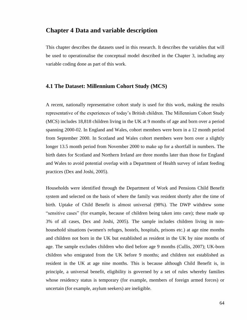
64

Chapter 4 Data and variable description

This chapter describes the datasets used in this research. It describes the variables that will

be used to operationalise the conceptual model described in the Chapter 3, including any

variable coding done as part of this work.

4.1 The Dataset: Millennium Cohort Study (MCS)

A recent, nationally representative cohort study is used for this work, making the results

representative of the experiences of today‘s British children. The Millennium Cohort Study

(MCS) includes 18,818 children living in the UK at 9 months of age and born over a period

spanning 2000-02. In England and Wales, cohort members were born in a 12 month period

from September 2000. In Scotland and Wales cohort members were born over a slightly

longer 13.5 month period from November 2000 to make up for a shortfall in numbers. The

birth dates for Scotland and Northern Ireland are three months later than those for England

and Wales to avoid potential overlap with a Department of Health survey of infant feeding

practices (Dex and Joshi, 2005).

Households were identified through the Department of Work and Pensions Child Benefit

system and selected on the basis of where the family was resident shortly after the time of

birth. Uptake of Child Benefit is almost universal (98%). The DWP withdrew some

―sensitive cases‖ (for example, because of children being taken into care); these made up

3% of all cases, Dex and Joshi, 2005). The sample includes children living in non-

household situations (women's refuges, hostels, hospitals, prisons etc.) at age nine months

and children not born in the UK but established as resident in the UK by nine months of

age. The sample excludes children who died before age 9 months (Cullis, 2007); UK-born

children who emigrated from the UK before 9 months; and children not established as

resident in the UK at age nine months. This is because although Child Benefit is, in

principle, a universal benefit, eligibility is governed by a set of rules whereby families

whose residency status is temporary (for example, members of foreign armed forces) or

uncertain (for example, asylum seekers) are ineligible.

65

The sample has a probability design and is clustered at the electoral ward level. The survey

design is based on the principle that the MCS should provide usable data for sub-groups of

children, especially those living in disadvantaged circumstances, children of ethnic

minorities, and children living in Scotland, Wales and Northern Ireland. As a result, the

sampled wards over-represent areas with high ethnic density, areas of high child poverty,

and the three smaller UK countries. Therefore, the sample is stratified by country of

residence. In England, disadvantaged residential areas and areas with a high proportion of

ethnic minority population were over sampled. In Scotland, Northern Ireland and Wales

only disadvantage wards were over sampled. A ward was considered as a high proportion

of ethnic minority population if at the 1991 UK Census over 30% of the population was

classed as Black or Asian. A ward was considered disadvantaged if it was not classed as a

ward with a high proportion of ethnic minority population and was in the poorest 25%

wards based on the Child Poverty Index (Dex and Joshi, 2005).

To date, four sweeps of data collection have been archived, when cohort members were

aged about 9 months, 3, 5 and 7 years. The first three data sweeps are used here as the

fourth sweep was not archived in time to be included in this work. The overall response rate

for sweep 1 was 68%. The response rate was highest in ―advantaged‖ wards and lowest in

the ―ethnic‖ wards. Response rate was 78% for sweep 2. The non-response rate includes

167 households (0.9%) who became ineligible because of the death of the cohort member

(n=14) or because of migration out of the sampled ward (n=153). 1390 households

identified as eligible for the study at sweep 1 but not interviewed were re-contacted at

sweep 2, response rate in this group was 50%. Response rate at sweep 3 was 79%. 300

households were ineligible due to death of the cohort member (n=18) or permanent

emigration (n=282). 1,444 households that were not interviewed at sweep 2 were recovered

at sweep 3 (Hansen, 2008). Final sample sizes were: 18,818 cohort children in 18,552

households at sweep 1 (with 256 sets of twins or triplets); 15,808 cohort members in 15,590

households at sweep 2; and 15,459 cohort children in 15,246 households at sweep 3

(Hansen, 2008).

As for all cohort studies, there were some losses to follow-up. This can be a source of bias

as the households lost over the sweeps are likely to be systematically different from those

66

retained in the sample. For example, the households lost to follow up between sweeps 1 and

2 were more likely to come from a disadvantaged occupational class, to be lone parents and

slightly more likely to not speak English than those retained in sweep 2 (see Annex 1). As

mentioned previously, the MCS does try to recover households lost in one sweep for the

next sweep, boosting the sample sizes. Unit non-response (missing answers to certain

questions) may also be a source of bias. For example, information on income was more

likely to be missing for non-White ethnic groups (nearly a third of Bangladeshi households

did not report their income compared to 6% in the White group). Survey weights have been

calculated both to correct for cohort members having unequal probabilities of selection in

the study due to the stratified and clustered sample design as well as to take account of

attrition between sweeps and unit non-response. Weights are available both for single

country analysis and for the whole of the UK (Plewis, 2007).

The study mainly consisted of interviews with the main carer. This was the mother in 98%

of cases; in sweep 1 28 fathers were the main respondent, 18 of whom were lone fathers.

The number of male main respondents increased markedly at sweep 2, with 394 natural

fathers completing the main interview, 72 of whom were lone fathers. By sweep 3 185

main respondents were the fathers. Information about the main respondent‘s resident

partner was also collected in a separate interview with them. A proxy interview with the

main respondent was conducted if the resident partner could not be interviewed directly.

When the main carer could not understand or speak English, the resident partner was asked

to be the main respondent. If neither of the resident parents could undertake the interview in

English, another household member above the age of 16 was asked to translate; otherwise a

translator was used. Questions included detailed health measures for children, such as

birthweight, immunisations, and respiratory problems. A number of measurements were

taken by the interviewer at sweep 3, which included the child‘s height, weight, and waist

circumference. Respondents were also asked about a number of dimensions representing

family circumstances, and the socioeconomic, health and health behaviour characteristics of

cohort member‘s households.

4.2 Exposure and outcome variables

67

This section describes the variables identified for inclusion in the models. First, the

measures used to describe ―family‖, and in particular the main measure of family structure,

are discussed. An initial, brief look at the outcome variables follows. These variables will

be described in more detail in the relevant results section.

4.2.1 Family structure

The MCS collects information on the number of parents or carers in the household, their

relationship, and any changes to that over the study period. It also collects information on

other residents in the household, including the number of siblings, and any grandparents

living with the cohort member.

To measure family structure, two sets of variables - four cross sectional variables and a

longitudinal variable - were created. Their coding is described below, and descriptive cross

tabulations are presented in the Chapter 5. Cross sectional variables of family structure

describe whether the resident partners are married, cohabiting, or whether only one parent

is resident in the household. These variables are created for each sweep, as well as at the

time of the child‘s birth. To code these variables, two archived derived variables were used

as a starting point. These indicated if there was more than one parent or partner in the

household, and the relationship status between the partners. A retrospective question on

relationship status at birth was also used. To check for any errors in the archived variables,

the household grid was used. In particular, households for which the relationship between

two resident parents or carers was classed as ―neither‖ married nor cohabiting, or their

relationship type was classed as ―not known‖, were checked. This applied to 93 households

at sweep 1, 186 at sweep 2 and 61 at sweep 3. All households classed as ―neither‖ married

nor cohabiting contained two partners eligible for interview who were the natural parents of

the child. A high proportion of partners in this group (76%) were classed as ―part-time

residents‖. They tended to be slightly more likely to not have been interviewed than other

resident partners (19.3% were not interviewed compared to 11.5% of married partners and

14.9% of cohabiting partners), although the vast majority were interviewed. Most were

single and never married (78%). Sensitivity analyses showed that this group was similar to

the cohabiting group in terms of their socio-economic profiles, and were re-coded as such.

68

To take into account of possible changes in family structure over the study period, a

longitudinal family structure variable was created indicating whether cohort members had

always lived with two married parents, two cohabiting parents, one lone parent, or whether

they experienced one or more changes in family structure. This variable was based on the

cross sectional variables described above and represents a typology of family structure

according to the number and type of changes in family structure experienced. Initially, the

creation of this typology of family change was attempted using empirical approaches such

as cluster analysis and categorical factor analysis. However, these methods did not produce

credible categories. A theoretically-driven variable was therefore produced, with a check

that sample sizes were large enough for analysis. Because of sample sizes, the last category

(households that experienced more than one change) was not split into further subgroups.

This category is therefore made up of a heterogeneous group which is difficult to analyze.

On the other hand, households experiencing one change in family structure over the study

periods were further categorised into the following sub groups: cohabitees who marry,

married households who become lone parent households, cohabitees who become lone

parents, lone parents who move to a cohabiting relationship, and lone parents who marry.

Family activities and wider networks

The previous chapter showed that few epidemiological papers problematise ―the family‖,

and often use a simplistic approach to describe family types. Yet sociological theories about

what ―the family‖ means and how it could be defined suggest a number of more nuanced

tools to describe families. These tools have not been applied empirically, especially in the

secondary analysis of a large data set. Here, an attempt to identify variables that might

operationalise the concepts of ―doing‖ and ―displaying‖ family was made, as well as

variables that allow describing families in terms of their wider networks of kin, rather than

just as nuclear, co-resident households.

To describe the activities that families carry out in order to ―do‖ and ―display‖ family, a

number of variables were investigated. Most of the variables relate to sweep 2, when the

child was about 3 years old, when more questions about family activities were included.

69

Questions were asked on regular bedtimes, the number of hours spent watching TV

(perhaps a ―non-doing‖ family activity), how often the child is read to, if anyone is teaching

the child the alphabet and to count, and whether the child draws at home or sing songs with

a parent. These activities may represent ―doing‖ family. To try and identify activities of

family ―display‖, questions on whether the child is taken to the library, whether the family

did something special for the child‘s birthday, whether they visit friends with young

children, were identified.

To explore the wider kin networks connected to the child‘s households, two sets of

questions were identified. One concerns contact and interactions with grandparents,

including how often they saw them, how far away they lived, whether they live in the

child‘s household, whether they provided financial help or childcare. The second relates to

the non-resident father. Questions were asked at all sweeps, but the most detailed set comes

from sweep 1, when carers were asked about their relationship with the non-resident father,

how often the non-resident father saw the child, and whether the non-resident father

provided financial support.

4.2.2 Child health outcomes

Three groups of child health outcomes are examined: respiratory health, childhood growth

and unintentional injury. Detailed information on how health information was collected and

coded follows in the relevant results chapter. Below is a brief summary.

Questions on asthma and wheezing were available at all sweeps as part of the interview

with the main carer. The questions were taken from the ISAAC (International Study of

Asthma and Allergies in Childhood) core questionnaire (see Annex 2), a widely used and

validated instrument (ISAAC Steering Committee, 2000). It includes questions on the

occurrence of asthma and wheezing, as well as a variety of severity indicators, such as if

the wheeze is severe enough to affect the child‘s ability to talk. Report of ever asthma and

wheeze in the last year for both sweep 2 and 3 will be examined. Anthropometric

measurements were taken by the interviewer at sweep 3 and include the cohort members‘

height, weight, and waist circumference. Parental height was also measured, as well as

asked during interviews if it could not be measured. The main carer was asked about any

70

accidents that required contact with health services or a hospital visit (either to visit

Accident and Emergencies, or due to a referral to a hospital ward). Questions on accidents

were asked at all sweeps.

4.3 Explanatory variables

Below is a description of the variables identified in the Millennium Cohort Study which are

used as indicators for various portions of the conceptual model, as well as variables used

for descriptive analyses.

4.3.1 Socio-economic antecedents

Grandparents’ occupational class

The grandparents‘ socio-economic circumstances were explored as a possible a proxy for

parental childhood socio-economic position. Looking at the parents‘ childhood socio-

economic status would also allow to test whether certain individuals are more likely to be

selected into married, cohabiting or lone parenthood. Both partners were asked about both

their parents‘ last occupation. These were coded into a National Statistics Socio-Economic

Classification (NS SEC), which is described later on.

Parental income

The income earned by the resident partners was reported by the main respondent at all

sweeps using a banded show card. The show card listed income in weekly, monthly and

annual amounts. Separate show cards were available for two- and one-parent households.

For example, at sweep 3, 18 different categories were included, ranging from less than

£1,050 a year to over £52,000 a year for one-parent households and from less than £1,600 a

year to over £80,000 a year for two-parent households. It is important to note that this

relates to the resident partners‘ income, not the overall household income, as other earners

71

in the household were not included. It does however include any regular payments made by

a non-resident parent to the resident carer.

A variety of formats is used to describe the economic environment of the study households.

The variable used for modelling purposes is a continuous, log-transformed measure of

parental income. A continuous variable is used to decrease the number of degrees of

freedom, and it is logged because of its skewed distribution. A categorical variable is also

included for descriptive purposes. Categories vary according to the sweep the data was

collected in. A category on missing income is included.

An income variable was chosen over a poverty indicator in the modelling as the majority of

lone parent households fell into the ―poor‖ category; therefore, this variable did not

describe this group effectively. A poverty indicator was however included in the descriptive

analyses. Households were classed as poor if their equivalised income was 60% below the

mean income for that sweep. Equivalised income is also reported in descriptive analyses.

Equivalised income is calculated using McClements equivalence scale. This measure does

not take account of the detailed child weights in the McClements scale. Instead, all

dependent children in the household are assigned the average of the child weights of 0.23.

Equivalised income is not used in the models for two reasons. First, income data was only

collected for the partners and not other adults in the household, while equivalised income

takes into account of all household members, including any other adults living in the

household, who may or may not be earners themselves. This may disproportionally affect

some groups, such as lone parent households, who are more likely to live with adults other

than a partner. Second, the formula used to equivalise income may not be appropriate for

female-headed households: the McClements scale assigns a value of ―1‖ to the usually male

household head, who may be more ―expensive‖ than a female household head. Perhaps as a

result of these two reasons, equivalised income was not as predictive of child outcomes as

raw income for the lone parent groups.

A persistent poverty indicator was also created, classifying households as: never poor, poor

at one sweep, poor at two sweeps, always poor. This was used for descriptive purposes but

not in cross sectional or longitudinal modelling. While this indicator of persistent poverty

did predict child outcomes, it was less predictive of child health outcomes than other

72

measures of income. A categorical outcome would also have reduced the degrees of

freedom of the models. Therefore, a continuous, concurrent measure of income was chosen

for the modelling work. Persistent poverty indicators have however been successfully used

to predict child outcomes: Kiernan and Mensah (2009) show that the experience of

persistent poverty predicts intellectual and behavioural problems in 3 years old in the

Millennium Cohort Study.

Education

Questions on the educational qualifications achieved by the resident parents were asked

individually to both respondents. Here, the highest educational qualification held by either

resident partner in the household is reported. The variable is classed according to the

National Vocational Qualification (NVQ) classification. Categories for analyses are: no

qualifications, overseas qualifications only, NVQ 1, NVQ 2, NVQ 3, NVQ 4, and NVQ 5.

Roughly, an NVQ5 is equivalent to a graduate degree; an NVQ3 is equivalent to two A-

levels. If only overseas qualifications are held in the household, this is classed in a separate

category. If a partner holds an overseas qualification while the other partner holds a British

qualification, the latter is used as the ―highest‖ qualification. This is because no detailed

information on overseas qualification was collected.

Occupational Class

Detailed information on the parent‘s occupation is collected via questions asked

individually to both resident partners. Parental occupations are classed according to the

National Statistics Socio-Economic Classification (NS SEC). These socio-economic

classifications are based on occupation, in combination with employment status and in

some circumstances size of workplace. A 5 category variable is presented. This collapse is

one of those officially recommended by the Office for National Statistics (Rose et al.,

2001). Households are classed as: managerial and professional, intermediate occupations,

small & self employers, lower supervisory & technical occupations, semi routine and

routine occupations. An additional category is added to describe those for whom

occupational class is missing. This may include those who have never had a job.

73

The peak occupational class in the household is reported. Occupational class is only

presented in descriptive analyses as, given the other socio-economic variables, it was not

adding any extra predicting power to this block of variables to both cross sectional and

longitudinal models. This is discussed in more detail in Chapter 6.

Car ownership

Questions of the number of cars and vans owned by the household are included as a marker

of access to the material resources required to own and maintain a vehicle. Questions on the

number of cars or vans were included in the main interview with the main carer at sweep 2,

and specify that either partner has access to the vehicle as a passenger or driver.

Financial stress

Variables that measured material deprivation (such as, being able to afford a warm coat or

properly fitted shoes) were not explored as they were not significantly associated with child

health outcomes. However, markers of financial stress appeared to predict a range of child

outcomes. Three questions are available to measure financial stress, which were asked at

each sweep to the main respondent: being able to afford an annual holiday (in sweeps 1 and

2, it asks about being able to afford a holiday away from home, in sweep 3 it specifies a

holiday not staying at relatives), being up to date with bills, and how the household is

managing financially. The first two variables are binary, yes-no answers; the third is on a 5

point scale ranging from ―managing comfortably‖ to ―not making ends meet‖.

4.3.2 The emotional environment of the child

Parental depressive symptoms

74

The Malaise Inventory was used to measure maternal psychological symptoms at sweep 1.

It is a shortened version of the original 24-item scale that was developed from the Cornell

Medical Index Questionnaire (Rutter et al., 1970). The Malaise Inventory is a commonly

used self-completion scale for assessing psychiatric morbidity and was included in the self-

completion questionnaire at sweep 1 for the main carer. There is some evidence that it may

represent two separate psychological and somatic sub-scales rather than a single underlying

factor of distress. Factor analysis of all 24 items identified a first main general factor and a

second more purely psychological factor (Rodgers et al., 1999). This self-completion

measure has been used widely in general population studies (Rodgers et al., 1999, Rutter et

al., 1976). In the MCS, 9 of the original 24 items from both sub-scales of the Malaise

Inventory were used.

At sweeps two and three, psychological distress was assessed using the six item (K6)

Kessler Psychological Distress Scale (Kessler et al., 2002, Kessler and Mroczek, 1992,

Kessler and Mroczek, 1994), using a computer assisted self completion form. Each parent

was asked how often in the past 30 days they had felt: ‗so depressed that nothing could

cheer you up ‗, ‗hopeless ‗, ‗restless or fidgety ‗, ‗that everything you did was an effort‘,

‗worthless‘, ‗nervous.‘ Individuals scored four points for responding ‗all of the time‘; three

points for ‗most of the time‘; two points for ‗some of the time‘; one point for ‗a little of the

time‘ and no points for ‗none of the time‘. A continuous score was used in analyses. Both

the Kessler and Maternal Malaise scale have good reliability and validity (Rodger, 1999;

Kessler et al., 2002, Kessler et al., 2004), and correlate with previously diagnosed

depression and currently treated depression. In the Millennium Cohort Study, the Maternal

Malaise scale was shown to correlate strongly with depression constructs, including being

ever clinically diagnosed with depression (Kiernan and Huerta, 2008).

Marital Satisfaction

The Golombok Rust Inventory of Marital State is a 28-item questionnaire designed to

assess the quality of the relationship between a married or cohabiting couple. It produces an

overall score of relationship quality for the male and female partner separately (Rust and

Golombok, 1986). Six questions were included in sweep 1, and four in sweeps 2 and 3.

75

They were asked during the self completion part of the survey. They are used as continuous

scores in the modelling.

Parent-child relationships

A well-tested proxy for warmth/hostility is the child‘s attachment to the main care giver. In

the MCS, attachment is measured by 6 questions at sweep 1 using the Condon Maternal

Attachment Questionnaire (Condon and Corkindale, 1998). Mother's attachment to her

infant is assessed by 6 Likert items that were selected from the original 19-item self-

reported questionnaire, with two questions picked from each of the 3 factors observed

(tolerance and acceptance; pleasure in proximity; and competence as a parent). A total

score was created using these variables, so the higher the score, the stronger the attachment.

At sweep 2, the Pianta scale (Pianta, 1992) is available. The Pianta scale is designed to

assess the parent‘s perception of the quality of the relationship with their child. The 15-item

scale measures closeness, dependency, and conflict in the child‘s relationship with his/her

parent or primary caregiver. It is self-administered by the respondent, with responses on a 5

point Likert scale scored from 0 to 4. Items were derived from attachment theory and the

attachment Q-set (Waters and Deane, 1985) as well as a review of the literature on mother-

child interactions. The Pianta scale is not an age-dependent scale. It generates a total scale

score reflecting an overall positive relationship. Lower scores reflect warmer relationships.

In the MCS, questions were included in the second sweep only.

Parenting styles

As discussed in the previous chapter, parenting styles as described by Baumrind (1966;

1971), are based on two axes, warmth/responsiveness and control/demandingness, to

produce four parenting styles: authoritative, authoritarian, indulgent and neglectful.

Authoritative parenting appears to produce the best results for children.

While the Pianta scale was explicitly devised to measure parental warmth, there is no

explicit scale for ―control‖ or ―structured parenting‖ in the MCS. Items on harsh

76

disciplining, which assess the frequency of use of harsh disciplining practices such as

shouting, bribing and ignoring the child, were not included as they did not capture the

concept of ‗control‘ and ‗structure‘ which is highlighted in the literature on parenting.

However, at sweep 2 questions on whether rules were applied consistently, whether the

child had regular bedtimes and mealtimes, were included. Research found that while the

number of rules had little impact on cognitive and mental health outcomes, but the

enforcement of rules was an important factor (Lexmond and Reeves, 2009). Considering

the three questions mentioned, there is evidence of only one factor, which loaded positively

on all responses (the factor loadings are 0.48, 0.69, and 0.70, respectively). Therefore, a

measure of ‗control‘ draws on these three questions; higher values on this factor can be

interpreted as ‗more structured‘ parenting. Merging this measure with the Pianta scale, four

parenting profiles can be described at sweep 2: authoritative, authoritarian, indulgent and

neglectful. As shown in figure 2.2, authoritative parenting combines a warm relationship

with structured parenting; authoritarian parents present a disengaged relationship with their

child but high ‗control‘ scores; indulgent parents combine a warm relationship with low

levels on control; while neglectful parenting is defined by low warmth and control. Both

the control and the Pianta scales are split into binary variables based on the median value to

take into account of the skewness of the data. While measures of both control and warmth

are not available in sweep 1 and 3, it is thought that parenting styles are a fairly stable

measure across the lifecourse. This categorical measure is however only used for

descriptive purposes, while for modelling work the continuous scores are used to avoid

reducing the degrees of freedom in the model.

4.3.3 The physical environment

Measures of childcare

Two variables are used to examine the effect of childcare on early life outcomes: the

number of hours spent in a formal or informal childcare arrangement, and the main type of

care experienced by the child. Variables distinguish between care provided by the main

carer or a partner (in sweep 3, only care provided by a non-resident partner was coded), a

77

grandparent, another informal arrangement (including other relatives and friends), a nanny

or an au pair, a childminder, formal group care (which includes attendance to a nursery,

crèche, or play group) or another arrangement. Differently from Hansen and Hawkes

(2009), these variables distinguish between childminders and nannies/au pairs as the setting

differs: in the former, the child is looked after in the childminder‘s home, while nannies and

au pairs will normally look after a child in the child‘s home. This may have implication in

terms of the environment the child is exposed to, and in particular the lack of information

on the childminder‘s home (for example, the presence of damp or pets might be significant

for respiratory outcomes).

According to the literature presented in Chapter 2, quality of care appears to be a central

issue when thinking of the effects of childcare. Unfortunately, while in the Millennium

Cohort Study we can gauge the time spent in childcare at all three sweeps of data, as well

as the type of care, there is little to indicate the quality of the childcare received.

Overcrowding

Overcrowding provides an indication of the family living conditions and was defined as

having more than one individual per room, excluding the bathroom and kitchen. The

household grid was used to calculate the number of full time residents in the household at

each sweep, while questions in the interview to the main carer include the number of rooms

available in the house.

Damp

Standards of living conditions were also assessed by measuring the presence of damp in the

child‘s home, as reported by the main carer. This variable can contribute to establish the

living conditions which may have an effect on health, especially when respiratory illnesses

are analysed. Damp in the home is measured on a five point scale ranging from no

problems with damp to severe damp problems.

Home environment

78

A series of questions asked to the main respondent aim to tap into the atmosphere in the

home. The main respondent was asked whether they thought the following statements

applied to their home: ―the atmosphere in your home is calm‖, ―it‘s really disorganised in

your home‖ and ―you can‘t hear yourself think in your home‖. Answers are on a five point

scale and range from ―strongly agree‖ to ―strongly disagree‖. Furthermore, at sweep 2,

when the child was aged 3, the interviewer was asked to assess whether the home

environment was safe. Answers were on a three-point scale ranging from ―safe‖ to ―unsafe‖.

Very few responses (n=355) fell in the first or last category, with most of the interviewers

picking the middle, neutral answer.

Local area safety

To describe area-level variables, a question which asks the main respondent to describe

how safe they feel in the area they live in is reported. Respondents are asked to choose they

answer from a five point scale and range from ―very safe‖ to ―very unsafe‖.

4.3.4 Health behaviours

Smoking

Exposure to tobacco smoke was defined as whether either resident partner smokes. This

information was collected at all sweeps. These variables were preferred to other available

variables which asked whether anyone smoked in the same room as the child, as they were

more predictive of health outcomes, particularly respiratory outcomes. This may be due to

bias in answering questions about socially unaccepted behaviours. Any smoking during

pregnancy by the mother was also collected and is reported here.

Breastfeeding

The main carer was asked if the child was ever breastfeed and the age at which the child

was last fed breast milk. In 2004, the UK Department of Health breastfeeding guidelines

advocate the exclusive feeding of infants on breast milk for the six months following birth

79

(Department of Health, 2004) in line with the World Health Organisation‘s global strategy

on infant feeding practice (World Health Organization, 2003), although this

recommendation was made after the birth of the Millennium Cohort Study children. The

recommended duration of exclusive breastfeeding at the time of the cohort children‘s birth

was 4 month. However, while in the Millennium Cohort 71% of children had had any

breast milk, the proportion of children exclusively breastfed drops sharply thereafter: by 1

month of age only 33% of children were exclusive breastfed, 3% were exclusively

breastfed by 4 months and just 0.3% by 6 months (Kelly and Watt, 2005). Using exclusive

breastfeeding for 4 or 6 months was therefore an unsuitable target for identifying

inter‐group differences. Consequently, breastfeeding initiation, irrespective of duration, was

used. As shown in the following chapters, breastfeeding initiation on its own remains

highly predictive of child outcomes.

Diet

Questions asked to the main respondent in sweep 3 tap into four parts of the child‘s dietary

behaviours and habits: the type of snacks the child mostly eats in between meals, whether

the child eats at regular times, the portions of fruit eaten per day and whether the child has

breakfast every day.

A diet score was created from these measures of diet. A point was given for every

unfavourable diet behaviour (does not mostly eat fruit and vegetables in between meals,

mostly eats crisps and sweets between meals, does not have regular meal times, eats less

than 2 portions of fruit per day, does not have breakfast every day). A score of 0 is the

healthiest diet score, while a score of 5 is the worst diet score. The overall mean (weighted)

score was 1.46 with a 95% confidence interval of 1.42 to 1.50. This suggests relatively

good reported dietary habits.

Exercise

Sweep 3 includes some limited measure of exercise through questions asked to the main

respondent. These variables are summed to produce a composite score. The score includes

80

measures of both activity and inactivity: how often the parent takes the child to the

playground, whether the child mostly walks or cycle to school, how often the child plays

sports, the daily number of hours spent watching TV, and the daily number of hours spent

playing videogames. As these variables were categorical, to construct the binary variables

needed to produce a composite score, the bottom 20% in each variable were classed as

―poor‖ exercisers. The score ranges from 0 to 5, where 0 is the healthiest score. The overall

(weighted) mean score was 3.70, with a 95% confidence interval of 3.66 to 3.73.

4.4 Summary

In this chapter the dataset used in these analyses, the Millennium Cohort Study, was

introduced and described. The variables used to operationalise the conceptual model were

also defined. The next chapter will look at the methodology to be employed to test the

model, both in a cross sectional and a longitudinal manner, and will describe how missing

data are considered.

81

Chapter 5 Methods

This chapter sets out the methodology employed in this thesis. The methods used for cross

sectional analyses are first described, followed by the analytical plan for the longitudinal

work. Finally, the regression methods used across both cross sectional and longitudinal

models are described in more detail in the last section.

5.1 Cross sectional analyses

Initial cross sectional analyses were carried out in Stata 11 (Stata Corp, 2009) and used

appropriate survey (svy) commands with the MCS weights to take into account of the

survey design. Initial analyses are primarily descriptive, and include simple cross

tabulations of key variables. First, the distribution of health outcomes and explanatory

variables by family structure was characterized using bivariate analysis. Second, cross

sectional multivariate regression models were estimated, informed by earlier work. These

allow the examination of the relationships between health outcomes and possible

determinants and correlates in a multivariate context. These simple cross-sectional

regression models look at the relationship between family structure (whether the child is

living with a married, cohabiting or lone parent) and child health outcomes at the same age,

and whether the household‘s socio-economic characteristics, the emotional environment,

the physical environment or certain relevant health behaviours measured at the same age

appear to mediate differences across different family groups. As all health outcomes are

binary, logistic regression is used, and results are presented as odds ratios. Cross sectional

analyses for the last sweep of data are presented, when the child was aged about 5, although

these analyses were also repeated for the second sweep of data, where data were available,

with similar substantive conclusions.

5.2 Longitudinal modelling

The next stage tests hypotheses regarding the key relationships using regression techniques

to model aspects of child health using longitudinal data. As explained in Chapter 3, where

82

the conceptual model was set out, variables are ordered a priori, following theoretically

derived hypothesised pathways. The model represents the associations running from

background variables to the outcome. Subsets of variables are divided into blocks and

blocks are linked by arrows. Blocks are split into levels; blocks in the first level are

potential causes for blocks in the next level, and so on. To break down the model into parts

that are more easily modelled, and to allow the inclusion of variables with different

measurement properties, the relationships between each variable in a block to the variables

in the previous block are tested individually. This allows for different types of regressions

to be used, depending on the measurement property of the dependant variable.

The approach used in this thesis borrows the organizing principles of graph theory and

graphical chain methods. Some of the main relevant notions of graph theory are set out

here, more detail can be found in, for example, West (2001) and Wilson (1996). A graph is

a pair of sets made up of a set of nodes and a set of edges. Two nodes connected by an edge

are called adjacent. Edges can be undirected or directed. Directed edges are depicted by an

arrow. A path is a sequence of adjacent edges. If a no directed edges are included in the

sequence, it is known as an acyclic graph (see Figure 5.1). A cyclic graph instead includes

at least one directed edge, as shown in the Figure 5.2.

Figure 5.1: An acrylic graph

a b

c

d

Figure 5.2 A cyclic graph

a b

c

d

83

In graphical chain models, nodes represent variables and undirected edges the association

between two variables. When one variable is thought to precede or cause another variable,

this is represented through a directed edge (arrow). A hypothetical model is shown in

Figure 5.3. The modelling approach employed in this work differs from a graphical chain

model in that the concept of conditional independence is not applied; that is, there is no test

to check whether two variables within the same block are independent of each once other

variables in the same block are taken into account. This is returned to in the final chapter.

Figure 5.3: A graphical chain model

Household income Parental education

Parental occupational class

Housing quality

To accommodate situations with possible causal relationships, variables are split into sub-

sets called blocks. Variables in different blocks are joined by directed arrows, while nodes

within a block are joined by undirected edges, excluding graphs with cycles. For simplicity,

when all variables in a block have edges with all variables in the following block, a single

arrow from one block to the next is drawn, as shown in Figure 5.3. Blocks are ordered to

form a chain. Variables in the first block are thought to be potential causes for variables in

the next block, and so on. Associations between variables within a block are assumed to be

non-causal. Figure 5.3 above shows a simple 2 block chain graph.

The use of arrows and boxes gives an important substantive meaning to these models. The

use of boxes allows the specification of variables as explanatory, response or intermediate

84

variables. The use of arrows allows the specification of the direction of the relationships

between processes. Variables are ordered in advance, according to theory which suggests

associations. The presence of an edge or arrow can then be empirically tested.

This approach is time intensive, and differently from modelling approaches such as

Structural Equations Models, there is no direct global likelihood test to determine model

mis-specification. However, SEM estimation of complex models can be problematic, as the

potential sources of model mis-specification grow as the number of variables in the model

grows, leading to problems of non-convergence (Kline, 2005, Kaplan, 2000). Most

importantly, SEM does not easily allow the simultaneous modelling of variables with

different measurement properties.

5.2.1 Model building

While borrowing from the graphical chain approach, as described above the analyses do not

represent a test of a full graphical chain model. The model is built in steps, as set out below:

o A model is set up, based on a priori conceptual and temporal ordering, as outlined in

Chapter 3.

o Correlations within blocks are estimated to establish convergent validity. This type

of test of construct validity confirms whether measures which should be related to

each other are in reality related. This allows a check of whether a set of variables, as

represented by a block, represent a coherent concept.

o Regression models are estimated for each variable in each block with the each of the

child health outcome variables and with the family structure variables. The type of

regression model varies according to the measurement property of each variable, for

example, for continuous outcome variables linear regression models were applied.

A full description of the types of regression models used is given in section 5.3, and

summarized in table 5.1.

o Building on the previous step, forward and backwards selection methods are applied

to simplify the initial conceptual model. This step involved exploring whether all

variables in the model were predictors of the main exposure (family structure) or the

85

dependent (child health) variables. Variables not predicting the main exposure

and/or dependent variables were not retained in the model. Further, an assessment

of which of the retained variables might be removed from the model without loss of

power was carried out. This is further discussed in the following chapter, where the

final, working model is presented.

o Regression models are estimated for each variable in each block with all variables

in blocks in the previous levels included as independent variables. The type of

regression model varies according to the measurement property of each variable

(see table 5.1).

The longitudinal modelling was carried out using the statistical program Mplus Version 6

(Muthén and Muthén, 2010), which allows for more sophisticated analyses and complex

data handling. All analyses include the appropriate weights. Here, because of the mix of

categorical and continuous outcomes, two estimators were used. For ordered categorical

and binary outcomes, Weighted Least Square was employed using a diagonal weight matrix

for the standard errors (to take account of uncorrelated errors) and a full weight matrix for

the test statistics. This estimator was chosen as it fits well the categorical and continuous

variables that make up the model, as well as being able to estimate the model using survey

weights and taking account of the clustered nature of the data. This estimator produces

probit estimates. Bootstrap standard errors are presented. The number of bootstraps draws

used in the computation of the errors was 500.

For continuous outcomes, models using Maximum Likelihood with robust errors (MLR)

are estimated, which also allow for complex survey settings and is robust to deviations

from normality. For the multinomial regression when the typology of family change is the

outcome, an MLR model is estimated. This estimator produces logit estimates. In an MLR

model, all independent variables have to be treated as continuous linear variables. A first

model was estimated with all independent variables treated as continuous variables. This

may be problematic as some independent variables are ordered categorical. Therefore, to

keep categorical variables from being treated as continuous, a second model was run with

an extra statement added in which all variables were regressed on the child‘s gender,

making all variables dependent variables and therefore allowing the identification of

categorical variables. Nonetheless, the first model without this extra statement fit the data

86

significantly better (by having smaller AIC and BIC values – which test for model fit and

complexity) than the second MLR model.

5.3 Regression analyses

The modelling approach used means that the overall model is split into several sub-models,

with each dependent variable can be modelled independently. Therefore, depending on the

dependent variable of interest, different regression models are used. They are briefly

described here. Linear regression models the relationship between two variables by fitting a

linear equation to observed data using the simple equation

Y = a + βx (1)

where x is the explanatory variable, Y the dependent variable, β the regression coefficient,

and a the intercept when x = 0.

Logistic regression models are non-linear regression models where the outcome variable is

binary or categorical. A logistic regression can be defined as:

(2)

The variable z is usually defined as

(3)

where β0 is the intercept and βk are the regression coefficients of xk.

In the cross sectional models, the results of the logistic regression are odds ratios. In the

longitudinal models, logit estimates are presented when continuous outcomes are presented,

while probit estimates are used for binary and continuous variables.

The inverse relation of equation (2) is

http://en.wikipedia.org/wiki/Y-intercept

http://en.wikipedia.org/wiki/Regression_coefficient

87

(4)

this is the natural logarithm of the odds ratio, known as the logit. A logit model assumes

that there is a linear relationship between the predictors in the model and the logit of the

outcome. It is based on a binomial distribution.

In a probit regression model, the probit function used is the inverse of the cumulative

distribution of the normal distribution. Probit and logit models can both be used to predict

the probability of an event happening and in practice tend to produces similar estimates.

This model can be presented as:

(3)

where p is the proportion and Φ−1 is the inverse of the cumulative distribution function of

the standard normal distribution.

Interpretation of probit coefficients is not as straightforward as in linear or logit regressions,

as the increase in probability attributed to a one-unit increase in a predictor is dependent

both on the values of the other predictors in the model and the starting value of the given

predictors. However, probit and logit models tend to produce similar results in that while

parameter estimates in a logistic regression tend to be higher than in a probit model, the

substantive results are generally the same (Long, 1997).

For the longitudinal model, table 5.1 summarises the estimate and regressions used

according to the outcome variable.

88

Table 5.1: Summary of the models used in the longitudinal model

Dependent variable Sweep used

in models Measurement

property Regression Estimator Estimate

Family structure 1, 2 and 3 Nominal categorical Multinomial MLR Logit Malaise 1 Continuous Linear MLR Logit Mother‘s Kessler 2 Continuous Linear MLR Logit Father‘s Kessler 2 Continuous Linear MLR Logit Relationship score 1 and 2 Continuous Linear MLR Logit Attachment score 1 Continuous Linear MLR Logit Warmth scale 2 Continuous Linear MLR Logit Control scale 2 Continuous Linear MLR Logit Any parent smokes 1 and 2 Binary Probit WLSMV Probit Smoke in pregnancy 1 Binary Probit WLSMV Probit Breastfeeding initiation 1 Binary Probit WLSMV Probit Damp in the home 1 and 2 Ordered categorical Probit WLSMV Probit Other siblings in the home 1 and 2 Continuous Linear MLR Logit Use of car as passenger 2 Continuous Linear MLR Logit Overcrowding 2 Continuous Linear MLR Logit Area safety 2 Continuous Linear MLR Logit Older siblings in the hh 1 Continuous Linear MLR Logit Eating at regular times 2 Binary Probit WLSMV Probit Over 3 hours of TV use 2 Binary Probit WLSMV Probit Over 3 hours computer use 2 Binary Probit WLSMV Probit Income 2` Continuous Linear MLR Logit Education 2 Continuous Linear MLR Logit Asthma 3 Binary Probit WLSMV Logit Wheeze 3 Binary Probit WLSMV Logit BMI 3 Binary Probit WLSMV Logit Injury 3 Binary Probit WLSMV Logit

5.4 Missing data

Figures 5.4 and 5.5 show the distribution of missing data in cross sectional and longitudinal

models. The asthma models are used as an example, similar results were observed when

looking at other outcomes. The two figures show that, when restricting the sample to cases

with complete information for all model variables (i.e. complete cases analysis), the sample

size drops from 15,246 to 6,769 for a cross sectional model of asthma at sweep 3, and from

19,244 to 5,812 for a longitudinal model of asthma by sweep 3. Therefore, to avoid such

large drops in sample sizes, analyses are not restricted to complete cases. However, a

number of strategies have been deployed to ensure that the analyses made and the

conclusions drawn from them were valid.

89

In the longitudinal models, the available sample is used at each level of the chain, so that

the effect of sample size reduction is only felt further down to the later blocks of the model.

A feature of Mplus is the use of the Full Information Maximum Likelihood (FIML) as a

default option, which allows dealing with missing data by estimating the model under

missing data theory using information for all available cases. FIML estimation does not

impute or fill in missing data, but computes parameter estimates on the basis of all available

data, including incomplete cases, and tends to be less biased than either listwise or pairwise

deletion methods when missing data are missing at random (MAR) data (Arbuckle, 1996,

Enders and Bandalos, 2001, Wothke, 2000). FIML and Multiple Imputation methods

produce similar findings if the data are missing at random (MAR). As many of the variables

included in the models predict missingness (for example, parental income), the data should

conform well to MAR. When using the estimator employed in the analyses of categorical

outcomes (WLSMV), missingness is allowed to be a function of the observed covariates,

but not of the outcomes. The sample size is therefore smaller than the total sample and is

indicated for each model. When estimating models with MLR for continuous outcomes, the

full sample is used.

Furthermore, sensitivity analyses were carried out to describe cases with missing data.

These are described in more detail in each chapter. Briefly, they entailed comparing models

with sample sizes restricted to complete cases with models that did not restrict sample

sizes. This exercise showed that there were no substantive differences between these two

types of models, suggesting that the missing data mechanism could be missing at random.

90

Figures for Chapter 5

All present in sweep 3

N= 15246

All single births N= 15042

With family structure data

N= 15038 9,274 married

2,774 cohabiting 2,990 lone parent

parents

With asthma data N= 14918

With all model variables N= 6769

5,249 married 1,519 cohabiting

1,681** lone parents

Parents income N = 11514

Golombok Rust N = 11028

Father’s Kessler N = 9765

*Variables not individually shown have missing data for

less than 10% cases ** Excluding “couple” variables

With data on each individual model variable *

Figure 5.4: Missing data in a cross sectional model,: asthma at sweep 3

91

All cohort members

N= 19244

Present at all sweeps

N= 13234

With family structure data

N= 12873

With asthma, sweep 3

N= 12741

With all model variables *

N= 5812

Parents income, sweep 2 N = 10964

Golombok Rust, sweep 2 N = 9459

Mother’s Kessler N = 11532

Father’s Kessler N = 8559

Pianta scale N = 10648

All single births N= 13054

*Variables not individually shown have

missing data for less than 10% cases

Golombok Rust, sweep 2 N = 9459

With data on each individual model variable *

Figure 5.5: Missing data in a longitudinal model: asthma by sweep 3

92

Chapter 6 Initial results and the development of a working

model

In this chapter the relationship between family structure and the variables highlighted in

Chapter 4 which operationalise the initial conceptual model presented in Chapter 3 is

considered. These initial, descriptive results are cross sectional. The chapter goes on to

present a longitudinal typology of family change which summarises the experience of

family structure over the first five years of the children‘s lives. This variable is described by

simple cross tabulations with measures of social, economic and well being markers. Based

on these analyses, as well as further selection methods, a final, working conceptual model

is presented. The initial part of the longitudinal model, which will remain constant for the

three groups of health outcomes to be considered, is tested in the final part of this chapter.

6.1 Family structure: cross sectional description

Table 6.1 presents consecutive cross-sectional snapshots of family structure at 9 months, 3

years and 5 years. In the Millennium Cohort Study, at sweep 1, when the children were

aged approximately 9 months, nearly 60% lived with two married parents, 23% with two

cohabiting parents and 17% with one parent. Retrospective questions were also asked about

the parents‘ relationship at the birth of the child. Table 6.1 shows that there is little

difference between family structure at birth and 9 months. These results are similar to birth

registration data: about 60% of all live births registered in England and Wales in 2000 were

registered to married parents, 20% to unmarried parents living together and 20% to a sole

parent (ONS, 2001).

5.1.2 Family characteristics: describing family structure cross-sectionally

To describe the different family structure groups, they are cross tabulated against the

variables that make up the conceptual model. For most variables, analyses from sweep 1 are

presented as results from sweep 2 and 3 were similar. For some variables, such as parenting

practices, there is only information for certain sweeps; this is noted where relevant. Some

93

variables, notably childcare, vary across the three sweeps, and therefore data for all sweeps

is presented.

Socio-economic characteristics

Table 6.2 shows that, at sweep 1, married parents were more likely to be in managerial or

professional occupations, to hold more educational qualification, to have higher incomes,

and less likely to receive benefits than lone parents. Cohabitees appeared to do better than

lone parents across these measures but worse than married parents. Nearly 80% of lone

parent households had annual incomes below the poverty line of £10,400 when the cohort

member was 9 months old, compared to 10% of married households and 23% of cohabiting

households. Lone parents‘ average income was just over a quarter of the average income of

married parents. Looking at it longitudinally, when comparing annual household income

for sweep 1 and 2, only 11% of lone parents had not experienced poverty at either sweep,

compared to 76% of married and 62% of cohabiting parents.

Part of this may be due to parental age: married mothers were on average over 5 years older

than lone mothers and about 4 years older than cohabiting mothers. Therefore lone parents

may be less likely to have achieved their highest occupational class or highest income than

married parents. Having two sources of income probably also plays a part: while cohabiting

households appear to have a higher proportion of households in routine and semi-routine

occupations than lone parent households (60% versus 52%, respectively), their annual

income is higher than lone parent households.

Married couples had on average lived together longer by the time of cohort member‘s birth

than cohabiting or lone parents (table 6.3). The largest difference was between married and

non-married parents, while the difference between cohabiting and lone parents was

relatively small, although still statistically significant.

Family activities

94

To describe activities carried out by the family in order to ―do‖ and ―display‖ family, a

number of variables were explored. Table 6.4 appears to indicate that, regarding the day-to-

day family activities (e.g. ―doing‖ family), there is a mixed picture by family structure. The

familiar gradient of married households doing best, followed by cohabitants and finally

lone parent households, is not always present. For example, when considering whether the

child has a regular bedtime, it is cohabiting parents who are most likely to report that the

child never or only sometimes has a regular bedtime. Cohabiting and lone parents are both

as likely to report that the child watches TV for more than 3 hours a day. However, when it

comes to interactions with the child (how often the child is read to, whether anyone teaches

the child the alphabet), the gradient described above is evident, with married parents most

likely to report these activities, and lone parents least likely to do so. Whether the child

paints or draws at home does present this gradient, but the number of children who do not

draw or paint at home are very small across all family structures.

The next part of table 6.4 explores whether these interaction have an element of ―display‖.

Here the gradients across family structures are consistent, with married parents reporting

more such activities and lone parents the least, however, except for taking the child to the

library, there are few households who report not taking part in these activities across all

family structures.

Wider networks

A number of variables relating to the wider network of the household, including measures

of the involvement of non-resident fathers and grandparents, are described below.

The non-resident father

Data on the involvement of the non-resident father was collected at sweep 1. Over 60% of

lone mothers (N=3203) reported that they were still in touch with the baby‘s father,

potentially making the role of the non-resident father important in the child‘s life. Table 6.5

provides an initial look at the level of involvement of these fathers in the child‘s early life.

95

Of the 62% of mothers still in touch with the baby‘s father at sweep 1, only 8% rate their

relationship with him as unfriendly, and only 10% report a lack of interest in the baby from

the non-resident father. Nearly 60% of non-resident fathers see the baby over 4 times a

week and a further 23% saw the baby at least weekly.

Grandparents

Grandparents were an important part of lone parent households: 21% of lone parent

households included a grandparent when the baby was about 9 months old. These

proportions were much lower in married and cohabiting households, 5% and 4%

respectively. As table 6.6 shows, as the child became older, fewer households included

grandparents. The drop was largest for lone parent households, particularly between sweep

1 and 2, when the proportion of households with a grandparent dropped from 21% to 9%.

By sweep 3, lone parent households were only slightly more likely to include a grandparent

(7%) than married (4%) or cohabiting households (2.5%).

However, potential help from grandparents may go beyond co-residence. As shown in table

6.7, the majority of grandparents lived within 30 min of the cohort member. Distances were

smallest for cohabiting and lone parents and largest for married households.

Financial help was also important (table 6.8). Over 70% of grandparents contributed

financially at sweep 1. For cohabiting and lone parents, over 70% of grandparents bought

household essentials. The provision of household basics was also important in the married

group, but slightly less so (61%). The section on childcare below shows that grandparents

are also an important source of care for some groups.

Grandparents’ socio-economic class

Table 6.9 shows that family structure at birth is associated with the maternal grandfather‘s

occupational class. Children born to two married parents were more likely to have a

grandparent in an advantaged occupational class than those born to cohabiting or lone

96

parents. A similar but slightly weaker relationship is also present when looking at paternal

grandparents (see table 6.10).

The psychosocial environment

Table 6.11 shows the distribution of a number of psychosocial variables that make up the

―emotional environment‖ block of the conceptual model. The quality of the relationship

between the parents and the child is captured by the parenting styles as described by

Baumrind (1971). The differences by family structure at sweep 2 are significant (p<0.001):

married parents are more likely to be authoritative parents compared to unmarried parents,

although there were no differences between cohabiting and lone parents. Married parents

also appear to be less likely to be classed as ‗neglectful‘ compared to unmarried parents,

and again there were no differences between cohabiting and lone parents.

The quality of the relationship between the parents is summarized by the Golombok Rust

score. As this a slightly skewed distribution, both the mean and the median by family

structure at sweep 1 are presented. Both measures show that cohabiting parents had slightly

but statistically significant worse relationships than married parents (a higher score

signifies a better relationship).

Measures of parental mental health include the Maternal Malaise and the Kessler score, the

latter is presented for both mothers and fathers. The mean and median are presented to take

account of the skewed nature of the data. Across these three measures, a gradient can be

seen across family structures, with better mental health for married parents, followed by

cohabiting parents and worst for lone parents. While differences can be observed for both

mothers‘ and fathers‘ Kessler scores according to their marital status, the difference

between married and cohabiting fathers‘ scores is smaller than between married and

cohabiting mothers.

Health behaviours

97

To explore the dietary and exercise habits of children at age 5 two composite scores were

created. These measures are described in detail in Chapter 8. Briefly, children living with

married parents at age five appear to have better dietary habits than those living with two

cohabiting parents, while those living with a lone parent do worst (table 6.12). Their

exercise habits do not show marked differences, although children living with a lone parent

appear to have slightly worse exercise habits. For descriptive purposes, two of the questions

that make up the diet and exercise score are further analysed. Children living with two

married parents were least likely to skip breakfast, while those living with a lone parent

were most likely to. While children living with married and cohabiting parents did not

report differences in TV use, children living with lone parents were more likely to watch 3

hours or more of TV daily.

Breastfeeding initiation also shows a gradient across family structures: over three quarters

of married parents ever breastfed their child, compared to 64% of cohabiting parents and

half of lone parents. Exposure to smoke as described by whether either parent smokes

showed a different picture, with cohabiting households being most likely to contain at least

one parent who smoked and married parents the least likely to do so.

Environmental variables

This block aims to describe the physical environment the child is exposed to in the home,

neighbourhood, and place of childcare. Two measures of the quality of housing, whether

the home is overcrowded or damp, do not show the familiar gradient in family structure

(table 6.13). While married households are least likely to inhabit an overcrowded or damp

house, cohabitees were most likely to experience overcrowding. The differences in

overcrowding between married and lone parents were minimal, as were the differences in

damp housing between cohabiting and lone parents. Questions on whether the home felt

calm showed that married respondents were least likely to disagree with the statement,

while lone parents were most likely to disagree that their home felt ―calm‖.

98

Area safety, as reported by the main respondent, showed large differences by family

structure: only 3% of married respondents answered that their local area felt unsafe or very

unsafe, compared to 9% of cohabiting parents and 11% of lone parents.

Childcare

As childcare practices may change over the first five years of life, childcare variables are

described separately for all sweeps. Table 6.14 shows that married parents are more likely

to use some form of childcare, particularly when the child is young, than cohabiting or lone

parents. Lone parents tend to use the least amount of childcare, although such differences

diminish as the child ages. When the child is aged 9 months, lone parents predominantly

use grandparents as a source of childcare, while married and cohabiting parents show a

slightly wider range of options. Married parents are more likely to use formal group care

when the child is 9 months old. Lone parents are least likely to use such arrangements,

although the trend reverses by the time the child is aged 3. By the time the child is aged

about five (sweep 3) and attending school, informal arrangements are much more popular

across all groups, with grandparents and other informal arrangements (such as friends and

relatives) being predominant.

The average number of hours spent in childcare reflects some of the trends outlined above

(table 6.15). At 9 months, children living with married and cohabiting parents spent the

most time in childcare (about 10 hours a week), compared to about 8 hours for children

living with lone parents. By the time the children are aged 3, the gaps are reducing slightly,

and children living with lone parents spend slightly less time in childcare that those living

with married parents. These smaller differences in hours at age 3, and the increased use in

formal group care arrangements by lone parents at this age, may be due to the government‘s

scheme whereby all three and four year olds are offered up to 15 hours of free nursery

education for 38 weeks of the year. In fact, by age 5 the gaps are significant again, although

it is now children living with cohabiting parents that spend the least time in childcare.

99

6.2 Longitudinal family change

Table 6.16 begins looking at the data longitudinally. The shaded rows of table 5.16 show

the proportion of families who did not experience changes in family structure over the first

five years of the child‘s life. Children born to married parents had the highest chance of still

being in the same family structure at age 5 (91% compared to 54% of those born to

cohabiting parents and 57% of those born to lone parents). There are similar proportions of

children born to cohabitees and to lone parents who experienced a change in family

structure by age 5. At 9 months the differences between those who were cohabiting when

the child was born and those who were lone parents when the child was born are still

observable (nearly 86% of cohabitees were still in the same family structure 9 months after

birth, compared with 75% of lone parents). By age 3 these differences have diminished and

by age 5, about 46% of children born to cohabiting parents and 43% of children born to

lone parents had experienced a change in family structure.

Just looking at changes in family structure may misrepresent the picture for cohabiting

parents. In fact, as shown in table 6.16, over half of those who were no longer cohabiting

by age 5 had married; all had married their cohabiting partner except for 12 couples.

Therefore, the rate of partnership dissolution is much lower at 19%.

Table 6.16 also shows that the majority of married couples who separated before their

child‘s fifth birthday became lone parents. Lone parent who had not partnered by age 5

tended to be cohabiting rather than married.

The MCS collects information on all the resident members of the households in a

―household grid‖, providing information on the year in which each household member

entered and left, if applicable. To some extent, this allows us to explore family structure

during the periods of time in between sweeps. Table 6.17 shows the proportion of children

who experience a change in parent or parental figure (for example, a new partner moving in

or out of the household). This includes both households who gained a new parent or

parental figure and those who lost one. The information on table 6.17 is useful as it helps

100

fill the gaps on what happens between sweeps and provides information on partner change

which is not necessarily captured by family structure.

Table 6.17 confirms that children living with cohabiting or lone parents were most likely to

experience a change in parents or parental figures. Encouragingly, the figures that emerge

from using the household grid are not very different than from those presented above. Until

3 years of age, children born into cohabiting households were most likely to see a change in

parents or parental figures, with 17% having experienced such a change by age 3. By age 5,

children born to lone parents were slightly more likely than those born into cohabiting

households to experience a change in parents or parental figures (24% versus 21%). By

contrast, married couple households had lower rates of change throughout, reaching just

under 7% by age 5.

To summarise the different experiences of family change and to be able to describe groups

according to their family structure and their experience of changes in family structure, a

typology of changes in family structure over the first 5 years of the children‘s life was

created (see table 6.18). The first three groups (‗always married‘, ‗always cohabiting‘ and

‗always lone parents‘) are stable groups who did not experience changes in family structure

from birth and across the three sweeps of data. They make up nearly 73% of the sample. A

further 20% of the sample is made up of families who experienced one change, for

examples, couples who separate. The largest group within this part of the sample was

cohabitees who married; they made up about 6% of the sample and, except for 12 couples,

involved the same two cohabiting parents. Two groups of couples (married and cohabitees)

who became lone parents constituted 8% of the sample. Lone parents who married or

moved in with a partner made up 6% of the sample. The remainder of the sample was

composed of households who experienced more than one change in family structure. This

group could not be further stratified because of small sample sizes. Because of their

heterogeneity, it is difficult to comment on this group. As a result, they will not be

discussed at length in this chapter.

6.2.1 Family characteristics by typologies of family change

101

Do these different typologies of family change over the first five years of life matter? To

describe these groups, the next tables look at a number of social, economic, demographic

and wellbeing indicators. To begin, table 6.19 describes the groups outlined above in terms

of their socio-economic characteristics. These analyses confirm that, when limited to a

sample of parents with young children, some familiar patterns are observed: continuously

married parents were the highest earners, while continuously lone parents had the lowest

incomes. Equivalised income allows us to compare across different households as they take

into account the number of adults and children and their ages, with the caveat, as explained

in Chapter 4, that only parental income was available, and not household income. At sweep

1, when the cohort children were on average 9 months old, equivalised parental income for

households who stayed married throughout the 5 years was £436 per week. Parents who

remained in a cohabiting relationship earned £340. Those who remained lone parents

earned £141. Therefore, even after taking into account of different sizes and structures of

households, there was a nearly £300 difference in equivalised weekly incomes between

those who remained married and those who remained lone parents.

The ‗always lone parent‘ group also had lower incomes than those groups who experienced

family changes. Cohabitees who married earned slightly more than those who stayed in an

unmarried cohabiting relationship (£371 versus £340 per week), although this difference

was not statistically significant. At 9 months, coupled parents who became lone parents

earned about £100 per week less than their continuously partnered peers. Therefore, those

whose relationship breaks up appear to be already poorer before the actual separation

occurs. In a similar vein, lone parents who would go on to partner already earned more than

those who remained lone parents, although their earnings are still much less than the

continuously partnered groups.

The proportion of households where the highest parental occupation was a routine or semi-

routine job shows a similar pattern. Among the stable groups, the married group was least

likely to be in a less advantaged occupation when the child was aged 9 months, followed by

cohabitees and lone parents. Across the groups who experienced one transition, the

cohabitees who married were least likely to be in routine occupations (and do slightly better

in this respect than the cohabitees who do not marry); the coupled groups who became lone

parents were more likely to be in routine occupations than their consistently coupled

102

counterparts; and the lone parents who married tended to be in more advantaged

occupations than the ‗always lone parent‘ although still showing disadvantage compared

with the always partnered groups. In contrast to the income data, when the child was aged 9

months lone parents who went on to cohabit were just as likely to be in routine or semi-

routine occupations as lone parents who did not partner, although within these broad

occupational groups their income was somewhat higher.

The following column in table 6.19 shows the proportion of households where no parent

had any educational qualifications when the child was 9 months old. This pattern is similar

to those outlined above, with a marked disadvantage for lone parent households. This could

be partially due to their younger age profile (see below).

The next column of table 6.19 shows average maternal ages at birth of the child.

Households who remained married throughout the study contained older mothers than other

groups (31 years at the birth of the child). Among the stable groups, the cohabitees were

younger than married parents (28 years) and both groups were older than the lone parents

(25.5 years). Cohabitees who married were of the same age as the always cohabiting

mothers, while married and cohabiting mothers who became lone parents were younger

than their constantly coupled peers. Lone parents who went on to cohabit were on average a

year younger than lone parents who did not partner, while lone parents who married were

on average nearly 2 years older than their ‗always lone parents‘ counterparts.

The second half of table 6.19 looks at changes in economic circumstances over the first five

years of life according to the typologies of family change. To look at the longitudinal

experience of poverty a persistent poverty score flags up whether mean equivalised parental

income was below 60% of the median at each sweep. Describing the sample in this manner

broadly confirms the pattern depicted above, while emphasizing the persistent poverty of

some groups as well as the dynamic household circumstances of others. While about 20%

of ‗always married‘ households experienced poverty at least at one sweep, poverty was

likely to be a transient state (only 4% were ‗always poor‘). In contrast, 60% of the ‗always

lone parent‘ group was poor at every sweep. 10% of this group had never experienced

poverty, compared to 81% of married and 65% of cohabiting households. The ‗always

cohabiting‘ group appeared to be slightly worse off than the ―always married‖ (35% of

103

cohabiting households experienced poverty at some stage). However, only 8.5% of ‗always

cohabiting‘ households were poor at every sweep. Therefore, having two partners in the

household does appear to provide a safety net against persistent income poverty.

Among the groups that had experienced at least one change, cohabitees who married did

particularly well, with 72% of them never experiencing poverty. This is better than the

‗always cohabiting‘ group but still not as high as the ‗always married‘ group. Of the

separating couples, over 50% of married parents who became lone parents and 75% of

cohabitees who separate experienced poverty at least once. This is much higher than their

stable-partnered counterparts. Lone parents who went on to marry or cohabit had smaller

chances of experiencing poverty than their ‗always lone parent‘ counterparts (70% and 80%

respectively experienced poverty, compared to the 90% of ‗always lone parents‘), but these

proportions are still much higher than their always coupled peers.

The final column of table 6.19 shows the difference in mean equivalised weekly income

between 9 months and 5 years. Those who gained the most income were lone parents who

married, followed by lone parents who went on to cohabit. These groups gained £135 and

£110 per week respectively. It is important to note that their initial incomes at 9 months

were some of the lowest across all groups and, in spite of their increased income, these two

groups did not catch up with the incomes of those who were continuously partnered. Those

who lost the most income were married parents who became lone parents. On average this

group suffered a decrease in income of £74 per week. Cohabitees who became lone parents

experienced a smaller loss of income of about £26 per week. After 5 years, households with

continuously lone parents still had the lowest income of all groups. These figures are

equivalised for the number of people in the household, therefore changes in the number and

composition of household members are accounted for.

To continue the description of families who experience changes in family structure, two

indicators of parental wellbeing (table 6.20) are briefly cross tabulated against the typology

of family change. Maternal mental health is examined by looking at maternal depression

measured using the Malaise Inventory (Rutter et al., 1970) when the child was aged 9

months. Maternal depression was especially high in lone parents and lone parents who

married. Cohabitees who married had slightly lower depression rates than continuously

104

cohabiting parents. Coupled parents who separated had over twice the rates of depression of

their continuously coupled peers, even when the child was aged 9 months. Finally, parental

smoking is defined as whether either of the child‘s resident parents smoked when the child

was aged 9 months. Smoking rates were much lower in the continuously married group

than all other groups (29.6%). Cohabitees who became lone parents and lone parents who

went on to cohabit had the highest rates of parental smoking (65.8% and 64.5%

respectively).

6.3 From a theoretical model to an empirical model

The literature- and hypotheses-driven initial conceptual model described in Chapter 3 did

not rule out any association between the selected variables. However, having a

parsimonious model consistent with the observed data is important both for statistical

analyses and the interpretation of results. Therefore, a simpler working model was

identified. To do so, two steps were carried out: first, variables were checked to be

correlated with family structure (the exposure variable) and a number of child health

outcomes. Second, forward and backward selection methods within each block were used

to eliminate variables that were not adding any extra predictive power to the model.

The main changes from the initial, saturated model to the final working model are

described here. While the interplay between family structure, wider social networks, and

family activities was explored, wider social networks are excluded from the final

conceptual model as these variables were not consistently associated with each other,

suggesting they weren‘t a single construct, and were not predictive of child outcomes. The

possible reasons for a lack of correlation with child health are returned to in the final

chapter. Interaction terms were also checked (for example, if family structure interacted

with the presence of a grandparent in the household when predicting child health). However

these did not result in any statistically significant association.. As well as not being

predictive of child health, this set of variables was also not consistently associated with

family structure. While this means the model loses its holistic treatment of ―family‖, from

an interpretative point of view, using family structure as the ―exposure‖ in the model makes

it easier to set up statistical models and interpret findings. From a relevance point of view,

105

current academic, policy and public debates focus heavily on marriage and lone

parenthood. Setting up the statistical models with family structure as the exposure makes it

possible to make a direct contribution to such debates. The wider approach to describing

family is however considered when giving full interpretation of the results, and returned to

in the conclusions. Furthermore, the grandparent‘s socio-economic characteristics are not

present in the final working model as these were not consistently associated with other

markers of parental socio-economic background; while occupational class was excluded

from the socio-economic antecedents block as it was not adding extra predictive power to

the model.

Figure 6.1 illustrates the final working model linking family structures to child health.

Variables within a block are correlated to each other, while inter-block edges are always

directed. For simplicity, blocks are connected when all variables in one block have edges

with all variables in a second block. The arrows from one block to the other represent a

number of directed edges originating from all variables in one block to all variables in

subsequent blocks.

Level 1

Level 2

Level 3

Level 4

Figure 6.1: Final conceptual model

106

6.4 Longitudinal Model

While the conceptual model will be adapted in each chapter according to the health

outcome analyzed, the initial part of the model (levels 1 and 2); as well as blocks 3 and 4 on

level 3 (the emotional and the economic environments) remain the same and are

empirically tested here.

The conceptual model, as described above, is divided into seven blocks on four levels.

Level one includes the socio-economic pre-cursors block. Level two depicts the

longitudinal typology of changes in family structure. Level 3 describes a variety of features

of the child‘s environment: the physical environment, the emotional environment, the

behavioural environment and the changing economic environment over the child‘s life.

In the final longitudinal model, all variables within each block correlated (all p-values are

smaller than 0.0001, except for the correlation between maternal attachment to the child at

9 months and the father‘s mental health score at sweep 2, where p=0.013). The next stage

involved setting up regression models for each variables in block 2 (in this case, the only

variable in block 2 is the typology of changes in family structure) against all the variables

in the previous block (i.e. the socio-economic pre-cursors). Details of the type of model

used for each regression are listed in table 5.1. All groups were significantly different from

the ―always married‖ group (which remains the baseline comparison group throughout

these analyses) for each of the socio-economic pre-cursors variables, even as other

variables in the block are taken into account (table 6.21). For example, even after taking

account of the household education, parental income, and car ownership, all groups were

significantly younger at the birth of the child than the ―always married‖ group. Unmarried

households and households who experience changes in family structure appeared to be

younger, poorer and hold fewer educational qualifications that those who were married

throughout the child‘s first five years.

107

Next each of the variables in level 3 was regressed against all the variables on levels 1 and

2 (socio-economic pre-cursors and family change, table 6.22). Starting with the emotional

environment (block 3), maternal depression at 9 months as measured by the maternal

malaise score was associated with not owning a car and lower parental incomes, but not

with parental education or age, after other socio-economic antecedents were accounted in

the model. It was not associated with the various typologies of family change except for

weak associations for married mothers who separate and for those who experienced more

than one transition compared to the always married group. The patterns were similar for

mother‘s mental health (although the association with the group of married couples who

separate is stronger) and father‘s depression (although this was not associated with

income). The parents‘ relationship scores (both when assessed when the child was aged 9

months and 3 years) were associated with maternal age (younger mothers had worse

relationship scores), car ownership (car owners had better relationship scores). All the

typologies of family change had significantly worse scores than the ―always married‖

group, except for the lone parents who married (who did not have significantly different

scores) and the cohabitees who married, who had significantly better scores than the always

married. Turning to the parent-child interaction variables, the mother‘s attachment to the

child at 9 months were correlated with maternal age and parental income (younger and

poorer mother were less attached). Cohabitees who married had higher levels of attachment

than the always married, while married mothers who separated were more disengaged. All

other groups were not significantly different from the ―always married‖. Warmth and

control, or ‗structured‘ parenting, the two variables used to determine parenting styles, were

complicated to interpret. When other socio-economic factors were accounted for, older

mothers had a warmer relationship with their child, and exhibited more structured

parenting. Holding higher educational qualifications and higher incomes were related to

more structured parenting and warmer relationships. Car ownership was related to warmth

but not structured parenting. Warmth and control did not vary much by family structure

once socio-economic antecedents were taken in account, except for cohabitees who

married, lone parents who later cohabited and groups who experienced more than one

transition, who were slightly less likely than the always married group to have a warm

relationship with their child or to exhibit structured parenting.

108

The changing socio-economic environment (block 4) allows to model whether families

experienced changes in income or educational qualifications from the baseline

measurements taken at 9 modelled at level 1. Income and educational qualifications at

sweep 2 were included in this block. Once the socio-economic antecedents were accounted

for, there was no further association between educational qualifications at sweep 2 and

family structure (see table 6.23). Income at age 3 was still significantly associated with

family structure, and this is consistent with resulted presented earlier in this chapter which

showed that groups gained and lost income as they changed family structure.

Analyses of blocks 5 and 6 are presented in each results chapter, as the variables included

in each block vary depending on the outcome analysed. The final models, where all the

blocks regressed against the health outcome, are presented separately in each results

chapter.

6.5 Summary and conclusions

This chapter sought to describe the household characteristics of the study sample. The

majority of children in the Millennium Cohort Study were born and raised by two married

parents. Households with two married parents were the most stable, reporting fewer

changes in family structure across the first five years of life. Just under half of cohabiting

and lone parents had changed their relationship status by sweep 3, when the child was 5

years old; although a quarter of those who were cohabiting at birth of the child had gone on

to marry each other by the child‘s fifth birthday.

In cross-sectional analyses, married households were on average richer, less likely to

experience poverty, more educated and in more advantaged occupations than cohabiting

and lone parent households. Lone parent households fared the worst economically. The age

of the parents may partly account for these differences. A double income may be another

important reason as to why two-parent households do much better than lone parents. Issues

around gender differences in income and affordable childcare may also be important.

109

Longitudinal analyses showed evidence of a complex and dynamic pattern to the family

structures that some children live in. A typology of changes in family structure over the

first 5 years of life was presented. About 20% of the sample was made up of groups who

experienced one change in family structure; while 7.5% of children experienced more than

one change in family structure in their first 5 years of life. Children born to lone parents

were most likely to experience a change in family structure by age 5, with just under half of

these children experiencing at least one change. These findings show that the experience of

family life of today‘s children is becoming more complex than those of earlier generations.

For example, around 90% of British Cohort Study children born in 1970 were still living

with their parents by the time they turned 5 (Kiernan, 2004), compared with just under 75

per cent for the children in the MCS.

While these patterns highlight growing diversity and complexity in the living arrangements

of today‘s young children compared with previous generations, these data also show that

there is continued stability in certain groups. Three-quarters of all children did not

experience any changes at all over the first 5 years of life. Over 90% of children born to

married parents and over 80 per cent of those born to cohabiting parents were still living

with two parents by age 5. In fact, during the first five years of their child‘s life, cohabitees

were more likely to marry each other than to separate.

In longitudinal analyses, continuously married families were the most advantaged

households. They had the highest incomes, were least likely to be in a routine occupation or

not hold any educational qualifications. They were also least likely to experience maternal

depression or to include a parent who smokes. The most disadvantaged group across these

domains was families who remained lone parents throughout the 5 years. A longitudinal

indicator of poverty shows how persistent their economic disadvantage was: nearly 60% of

lone parent households were classed as poor across the three sweeps of data, and an

additional 30% had experienced poverty at least once. This confirms work done in older

children. Clarke and Joshi (2003) used data from the ONS Longitudinal Study to show that

experiencing family instability was associated with subsequent economic disadvantage

among children aged 5-17.

110

These analyses also highlight diversity across the groups who experienced family changes.

Across groups who experienced at least one change in family structure, cohabitees who

later married appear to be the most economically advantaged, doing better than

continuously cohabiting parents across a range of indicators although not quite as well as

the continuously married group. These analyses confirm that cohabitants appear to be more

economically disadvantaged than married couples (Kiernan and Estaugh, 1993). Married

and cohabiting parents who separated during the 5 years were already showing signs of

economic disadvantage at 9 months compared with their continuously partnered peers.

These two groups also lost the most income over the 5 years studied. Lone parents who

later partnered had higher incomes than their continuously lone parent counterparts;

however, in spite of gaining the most income over the 5-year study period, they were still

much more disadvantaged than the continuously partnered groups.

These patterns were repeated across other socio-economic factors, such as occupational

class and educational qualifications, as well as markers of parental health such as maternal

depression. Mothers who were continuously partnered had lower rates of depression nine

months after birth than those who were continuously lone parents or who experienced

periods of lone parenthood.

A longitudinal model allowed us to explore the longitudinal relationship between family

structure and respiratory health in a hierarchical manner. All typologies of family change

were significantly different from the ―always married‖ group in terms of their socio-

economic antecedents, being largely younger, poorer and holding less educational

qualifications than the continuously married. The cohabitants who married appeared to be

the exception. Building on this, each chapter will show the significance of more proximal

determinants on different health outcomes across various family structures.

111

Tables for Chapter 6

Table 6.1: Distribution of family structures at different ages, %

At birth 9 months 3 yrs 5 yrs

Married 57.2 58.9 61.8 61.6

Cohabiting 23.5 23.4 17.1 18.2

Lone parent 18.8 17.5 20.1 19.9

Unweighted sample

size

18,552 18,552 15,590 15,246

112

Table 6.2: Family characteristics by family structure, sweep 1, % unless otherwise

indicated

Married Cohabiting Lone parent

Maternal age at birth of 13 to 19 1.6 13.6 25.1

cohort member 20 to 29 42.2 55.0 51.4

30 to 39 53.5 29.9 22.2

40 plus 2.6 1.5 1.3

N 10,928 4,337 3,194

Maternal age at birth of

cohort member

Mean age 30.2 26.4 24.7

Highest NSSEC5 in hh Managerial & professional 24.7 10.8 7.9

Intermediate 12.4 8.7 11.7

Small & self employers 10.0 6.7 1.6

Low support & tech 10.4 10.7 6.2

Semi routine & routine 38.9 60.0 51.9

Missing 3.6 3.2 20.6

N 10,928 4,337 3,194

Highest qualifications None 7.0 7.7 30.2

Overseas only 2.4 1.6 2.5

NVQ 1 3.7 7.4 13.9

NVQ 2 20.8 33.2 31.5

NVQ 3 15.7 20.8 12.3

NVQ 4 41.0 26.5 9.0

NVQ 5 9.3 2.8 0.6

N 10,916 4,327 3,186

Household income Missing/ unknown/ refused 9.7 7.5 6.6

0-£10400 10.2 23.1 79.1

£10400-20800 31.7 40.2 12.7

£20800-31200 23.1 17.2 1.2

£31200-52000 18.2 9.6 0.2

£52000+ 6.9 2.4 0.1

Mean income £26669 £19072 £7832

N 10,928 4,337 3,194

Persistent poverty Poor at both sweeps 2.4 8.1 34.3

score, sweep 1 and 2 Never poor 75.6 62.0 11.4

113

N 10,928 4,337 3,194

Benefits Receive benefits 26.8 47.9 89.4

Unweighted sample

size

10,928 4,337 3,194

Table 6.3: Mean number of years living with child’s father by time of birth, by family

structure

Relationship status at birth Mean number yrs living together

Married 6.7 (6.6 to 6.8)

Cohabiting 3.4 (3.3 to 3.5)

Lone parent 2.8 (2.6 to 3.0)

Unweighted sample size 11 527

114

Table 6.4: Family activities by family structure, sweep 2, %


Doing family

Child has regular bedtime Never 5.5 9.7 9.0

Sometimes 10.6 16.0 15.9

Usually 39.2 38.2 34.9

Always 44.7 36.0 40.1

N 9,642 2,657 3,105

Daily TV hours None 1.2 0.8 1.8

Up to 1 hour 24.5 18.7 20.3

1 to 3 hours 60.9 58.5 56.0

More than 3 hours 13.5 21.9 21.8

N 9,642 2,657 3,105

How often the child is read to Every day 65.5 56.4 50.8

Several times a week 18.2 19.8 20.1

Once/twice a week 11.4 16.3 18.5

Once/twice a month 1.9 3.6 3.3

Less often 1.2 1.9 2.9

Not at all 1.8 1.9 4.2

N 9,642 2,657 3,105

Teach alphabet at home Yes 80.7 83.0 82.3

No 19.2 17.0 17.5

N 9,642 2,657 3,105

Paints or draw at home Yes 98.4 97.9 97.0

No 1.6 2.0 2.8

N 9,642 2,657 3,105

Displaying family

Take child to library Yes 48.4 36.6 32.2

No 51.6 63.3 67.6

N 9,642 2,657 3,105

Child eaten with family in last Yes 98.7 98.1 97.9

week No 1.2 1.9 2.0

115

N 9,642 2,657 3,105

Something special for child‘s Yes 97.3 97.4 95.5

birthday No 2.6 2.5 4.3

N 9,642 2,657 3,105

Visit other friends with young Yes 93.3 90.6 90.8

children No 6.6 9.3 9.1

N 9,642 2,657 3,105

116

Table 6.5: Involvement with non-resident father if lone parent at sweep 1

%

Whether lone parent is still in touch with baby‘s father

Yes 61.7

No 38.3

Unweighted sample size (cases

with complete longitudinal data)

3 203

Relationship with non-resident father

Married but separated 10.4

Divorced 1.3

Lived together then separated 29.7

Never lived together 58.5

N 3 189

Quality of relationship with non-resident father

Friendly 74.5

Neither friendly nor unfriendly 17.5

Unfriendly 8.0

N 1 968

How interested is the non-resident father in the baby

Very 69.2

somewhat 19.6

not very 8.4

not at all 2.8

N 2 339

How often non-resident father sees baby

More than 4 times a week 57.6

Once or twice a week 23.2

Less often 16.3

Never 2.9

N 2 340

117

Table 6.6: Grandparents in the household, by family structure, sweep 1, %


Sweep 1 5.4 3.9 21.2

Sweep 2 4.1 2.7 9.4

Sweep 3 4.1 2.5 7.0

Table 6.7: Distance from grandparents, by family structure, sweep 3, %


Not applicable 13.1 11.3 17.6

Less than 15 minutes 39.2 47.7 43.8

15 minutes to less than 30 min 13.4 15.8 14.0

30 minutes to less than 1 hour 7.6 8.7 7.9

1 hour or more away 16.7 13.2 10.8

Outside the UK 9.9 3.1 5.5

Unweighted sample size 9 390 2 774 3 021

Table 6.8: Financial help from parents by family structure, sweep 1, %


No help 23.0 20.2 20.7

Any help 73.9 77.5 76.2

Whether received any financial help for:

Essentials for baby/household 60.6 72.2 72.9

Gifts 76.0 78.7 75.6

Capital 2.8 4.2 2.4

Unweighted sample size 10 928 4 337 3 194

118

Table 6.9: Maternal grandfather NS-SEC5 by family structure at birth, %

Maternal grandfather NS-SEC5

Family structure at birth

Managerial &

professional Intermediate

Self & small

employer Supervisory

Routine &

semi-routine

Married 32.3 10.4 17.9 13.9 25.6

Cohabiting 21.1 11.1 20 16.3 31.6

Lone parent 17.8 8.0 18.2 16.3 39.8

p-value <0001

Table 6.10: Paternal grandfather NS-SEC5 by family structure at birth, %

Paternal grandfather NS-SEC5

Family structure at birth

Managerial &

professional Intermediate

Self & small

employer Supervisory

Routine &

semi-routine

Married 30.8 10.8 15.7 13.9 38.9

Cohabiting 20.5 9.5 17.5 16.8 35.7

Lone parent 14.7 7.0 21.5 17.2 39.7

p-value <0001

119

Table 6.11: Psychosocial variables by family structure at the same sweep, % unless indicated


Parenting styles sweep 2, % Authoritative 36.7 27.3 28.5 Indulgent 15.7 16.6 15.6 Authoritarian 29.8 29.3 31.9 Neglectful 17.0 26.7 24.0

N 8,071 2,304 2,387

Golombok Rust score sweep 1 Mean (95% c.i.) 24.2 (24.1-24.3) 23.1 (22.9-23.3) -- Median 25 24 --

N 9999 3795 --

Maternal malaise sweep 1 Mean 16.5 (16.5- 16.6) 16.3 (16.2-16.3) 16.0 (15.9-16.1) Median 17 17 16

N 10405 4255 3055

Maternal Kessler score sweep 2 Mean (95% c.i.) 2.96 (2.87-3.05) 3.79 (3.61-3.98) 4.60 (4.39-4.80) Median 2 3 3

N 8391 2518 2679

Paternal Kessler score sweep 2 Mean (95% c.i.) 2.94 (2.86-3.02) 3.40 (3.20-3.59) -- Median 2 2 --

N 7758 2150 --

120

Table 6.12: Health behaviours by family structure at the same sweep


Diet score sweep 3 Mean (95% c.i.) 1.33 (1.29-1.38) 1.59 (1.51-1.66) 1.81 (1.73-1.88) Median 1 2 2

N 8055 2362 2505

Exercise score sweep 3 Mean (95% c.i.) 3.73 (3.70-3.77) 3.73 (3.68-3.79) 3.53 (3.47-3.58) Median 4 4 4

N 9256 2735 2976

Do not have breakfast daily,

sweep 3 % 5.4 8.5 12.1

p-value <0.0001

N 9371 2776 3013

Watch 3 hours or more of TV,

sweep 3 % 12.4 12.4 16.7

p-value <0.0001

N 1238 501 574

Ever breastfed, sweep 1 % 79.0 63.9 50.6

p-value <0.0001

N 8215 2590 1540

Either parent smokes, sweep 1 % 32.1 60.6 56.3

p-value <0.0001

N 3636 2690 1763

121

Table 6.13: Environmental variables by family structure at the same sweep


Overcrowded housing, sweep 2 % 6.7 11.2 6.6 p-value <0.001

N 1009 326 273

Damp or condensation, sweep 1 % 10.3 17.5 17.8

p-value <0.0001

N 1211 758 550

Area feels unsafe, sweep 2 % 3.4 9.2 11.3

p-value <0.0001

N 431 282 377

Atmosphere at home does not

feel calm, sweep 3 % 12.5 14.3 15.6

p-value <0.0001

N 1168 416 465

122

Table 6.14: Main source of childcare main respondent at work/school by family structure,

sweeps 1, 2 & 3, %

Married Cohabiting Lone parent Unweighted sample size

Sweep 1

None 49.4 53.4 76.8 10692 Partner/self 14.5 16.6 1.9 2182 Grandparent 15.0 15.6 10.1 2715 Other informal 2.8 3.5 3.1 611 Nanny/au pair 1.5 1.0 0.1 150 Childminder 6.4 4.3 3.7 911 Formal group care 10.0 5.1 3.9 1224 Other 0.4 0.5 0.3 67

Sweep 2

None 33.3 38.6 27.0 5108 Partner/self 17.8 7.2 16.6 2166 Grandparent 20.9 20.1 19.9 3229 Other informal 3.8 4.8 3.0 587 Nanny/au pair 2.2 2.4 2.3 327 Childminder 6.9 6.9 8.9 1114 Formal group care 14.6 18.9 21.7 2761 Other 0.6 1.1 0.7 110

Sweep 3

None 61.5 61.0 55.9 9062 Grandparent 22.3 21.1 18.7 3343 Other informal 9.7 11.9 14.7 1713 Nanny/au pair 1.9 0.7 0.8 157 Childminder 3.9 3.0 2.7 522 Formal group care 0.3 0.4 0.5 64 Other 0.4 0.6 0.6 62 Non resident partner 0.1 1.3 6.2 206

123

Table 6.15: Average hours of childcare per week by family

structure, sweeps 1, 2 and 3

Hours 95% confidence interval

Sweep 1

Married 10.3 9.72819 10.8101

Cohabiting 9.3 8.77719 9.88113

Lone parent 7.9 7.28517 8.49328

Sweep 2

Married 14.8 14.26758 15.41792

Cohabiting 13.6 12.83374 14.34551

Lone parent 12.7 11.94268 13.38814

Sweep 3

Married 13.3 12.51703 14.10365

Cohabiting 4.3 4.088897 4.54056

Lone parent 6.8 6.267127 7.332242

124

Table 6.16: Change and stability in family structures over time, compositional change, %

(Shaded rows represent groups who did not experience a change in family structure.)

Relationship status at…

9 months 3 yrs 5 yrs

…if married at birth

Married (no change) 98.5 93.4 90.8

Cohabiting 0.2 0.8 1.7

Lone parent 1.2 4.8 7.2

… if cohabiting at birth

Married 7.1 27.9 27.1

Cohabiting (no change) 85.7 56.1 53.7


… if not living with father at birth

Married 5.6 13.1 14.7


Lone parent (no change) 75.3 60.0 57.5

Unweighted sample 13,234

125

Table 6.17: Households who experience a change in parents or parental figure,

by family structure at birth

% households with a change in parents by…

Relationship status at birth 9 months 3 yrs 5 yrs

Married 1.0 4.5 6.7



Unweighted sample 644 1,683 2,097

126

Table 6.18: Typologies of changes in family structure, birth to sweep 3

% Unweighted sample size

No changes

Always married 55.0 7,148

Always cohabiting 10.8 1,398

Always lone parent 7.0 908

Total 72.8 9,454

One transition

Cohabiting to married 6.1 788

Married to lone parent 4.3 556

Cohabiting to lone parent 3.6 474

Lone parent to cohabiting 3.9 506

Lone parent to married 1.9 240

Total 19.7 2,564

More than one transition 7.5 990

Unweighted sample 100.0 13,008

127

Table 6.19: Household characteristics at sweep 3, by typology of family change

Mean weekly

equivalised

parental income, £

(confidence

interval)

Households in

semi- & routine

occupations, %

Households with

no educational

qualifications, %

Mean maternal

age at birth of

cohort member

Always married 436 (414-459) 29.9 2.8 31.1

Always cohabiting 340 (319-360) 49.3 3.9 28.3

Always lone parent 141 (135-148) 52.6 26.0 25.5

Cohabiting to married 371 (351-392) 47.5 2.9 28.0

Married to lone parent 345 (320-371) 47.4 5.2 29.5

Cohabiting to lone parent 250 (228-271) 59.1 9.4 25.8

Lone parent to cohabiting 162 (150-178) 58.7 19.8 24.2

Lone parent to married 209 (169-250) 49.7 22.4 27.3

More than one transition 242 (227-257) 58.1 10.5 26.3

p-value <0.001 <0.001 <0.001

Unweighted sample 11,999 5,713 1,140 13,008

128

Table 6.19 con’t: Longitudinal economic characteristics between sweeps 1 and 3, by typology of family

change

Persistent poverty status, % Change in parental income

between 9 months and 5

years, £ Never

poor

Poor at

one sweep

Poor at

two

sweeps

Always

poor

Always married 80.6 10.8 4.5 4.1 +51

Always cohabiting 64.9 17.3 9.4 8.5 +49

Always lone parent 9.7 8.4 22.8 59.1 +44

Cohabiting to married 72.2 17.1 6.3 4.4 +51

Married to lone parent 46.7 22.6 15.6 15.2 -74

Cohabiting to lone parent 24.5 21.0 27.0 27.5 -26

Lone parent to cohabiting 20.1 21.6 25.1 33.2 +110

Lone parent to married 29.4 27.2 23.1 20.4 +135

More than one transition 32.9 23.0 19.0 25.2 +53

p-value <0.001 <0.001

Unweighted sample 5,652 1,418 1,089 1,523 10,932

129

Table 6.20: Child and parental well-being, sweep 1, by

typology of family change

Either parent

smokes, %

Mother

depressed, %

Always married 29.6 1.7

Always cohabiting 57.6 2.6

Always lone parent 59.1 7.7

Cohabiting to married 51.6 2.3

Married to lone parent 46.8 4.7

Cohabiting to lone parent 65.8 5.8

Lone parent to cohabiting 64.5 4.6

Lone parent to married 37.1 7.7

More than one transition 60.2 6.5

p-value <0.001 0.001

Unweighted sample size 5,546 398

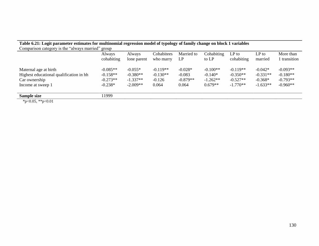
130

*p<0.05, **p<0.01

Table 6.21: Logit parameter estimates for multinomial regression model of typology of family change on block 1 variables Comparison category is the ―always married‖ group

Always

cohabiting Always

lone parent Cohabitees

who marry Married to

LP Cohabiting

to LP LP to

cohabiting LP to

married More than

1 transition Maternal age at birth -0.085** -0.055* -0.119** -0.028* -0.100** -0.119** -0.042* -0.093** Highest educational qualification in hh -0.158** -0.380** -0.130** -0.083 -0.140* -0.350** -0.331** -0.180** Car ownership -0.273** -1.337** -0.126 -0.879** -1.262** -0.527** -0.368* -0.793** Income at sweep 1 -0.238* -2.009** 0.064 0.064 0.679** -1.770** -1.633** -0.960**

Sample size 11999

131

Table 6.22: Logit parameter estimates for linear regression models of block 3 variables on block 1 and 2 variables Comparison category is ―always married‖

Emotional environment

Maternal

malaise at

sweep 1

Maternal

Kessler

sweep 2

Paternal

Kessler

score

sweep 2

Relation

ship

score at

sweep 1

Relations

hip score

at sweep

2

Attachment

at sweep 1 Warmth

at sweep

2

Control at

sweep 2

Block 1

Maternal age at birth -0.002 0.004 0.007 -0.042** -0.033** -0.039** -0.094** -0.025**

Highest educational qualifications in household 0.043** -0.206** 0.003 0.101* 0.108** -0.164** -0.167* 0.199**

Car ownership 0.217** -0.648** -0.647** 0.312* 0.191* 0.018 -0.701** 0.059

Income at sweep 1 0.175** -0.435** -0.258** 0.542** 0.271** -0.122* -0.385* 0.243**

Block 2

Always cohabiting -0.073 0.255 0.103 -1.132** -1.026** -0.029 0.536* -0.323**

Always lone parent 0.038 0.308 -- -- -- -0.130 0.169 0.120

Cohabiting to married 0.028 -0.181 0.207 0.508* 0.111 0.476** -0.057 -0.099

Married to LP -0.316** 0.776** 0.717* -2.414** -2.710** -0.143 -0.378 0.097

Cohabiting to LP -0.252* 0.590* 0.691 -3.066** -2.781** -0.072 -0.286 -0.036

LP to cohabiting 0.014 0.025 0.088 -0.925 -0.552* -0.304 1.424* -0.234*

LP to married -0.052 0.332 0.249 -0.045 -0.168 0.242 -0.556 -0.138

More than 1 transition -0.293** 0.910** 1.070** -1.383** -1.495** -0.004 0.797* -0.221*

Sample size 19244 19244 15420 19244 19244 19244 19244 19244 *p<0.05, **p<0.01

132

Table 6.23: Logit parameter estimates for linear regression model of

block 4 variables on block 1 and 2 variables Comparison category is ―always married‖

Economic environment

Income at sweep 2 Education at sweep 2

Block 1

Maternal age at birth 0.011** -0.002**

Highest educational

qualifications in household

0.087** 0.975**

Car ownership 0.204** 0.027**

Income at sweep 1 0.453 -0.002

Block 2

Always cohabiting 0.012 0.004

Always lone parent -0.325** 0.002

Cohabiting to married 0.059* 0.002

Married to LP -0.253** -0.009

Cohabiting to LP -0.426** -0.032

LP to cohabiting -0.039 0.042

LP to married 0.039 0.079

More than 1 transition -0.212** 0.011

Sample size 19244 19244

*p<0.05, **p<0.01

133

Chapter 7 Childhood respiratory illnesses

This chapter will focus on two markers of childhood respiratory health: parent-reported

asthma and wheeze. Asthma is a long-term chronic inflammatory disorder of the airways,

which may have different triggers and present different symptoms across individuals.

Wheeze is a symptom resulting from the narrowing of the small airways and is normally

described as a high-pitched whistling sound in the chest. Asthma and wheezing are

common illnesses during childhood: about 1 in 5 British children have doctor diagnosed

asthma (Fuller, 2006, Kaur et al., 1998) and nearly half of all children wheeze in early

childhood (Wright, 2002). In the second sweep of the Millennium Cohort Study, when

children were on average 3 years old, 12% had ever had asthma and 20% had wheezed in

the last year (Panico et al., 2007). Lower respiratory tract illnesses have a high health care

burden: they are one of the most common reasons for seeking healthcare in the first year of

life (Wright, 2002).

The epidemiology of childhood respiratory health is influenced by the child‘s age. Most

childhood asthma begins in infancy, with about 80% of asthmatic children experiencing

their first symptoms (usually wheeze) before their third birthday (Martinez et al., 1995).

Adverse events in early life, possible allergen exposure, infant feeding practices, and viral

infections seem important precipitating factors in infancy and toddlerhood (Wright and

Taussig, 1998), while airway inflammation associated with allergy seems to be the most

important underlying cause of later asthma (Wright, 2002). Wheezing presents separate

phenotypes at different ages, with changing characteristics, risk factors and prognoses

(Midodzi et al., 2008, Wright et al., 2002b). Wheezing that is limited to the early years does

not appear to be associated with reduced lung function, while persistent wheezers have

poorer lung function and are more likely to develop asthma (Sears et al., 2003, Lau et al.,

2003). Wheeze in early life is linked to mechanical (because of small airways) and

infectious causes (Martinez et al., 1995; Wright, 2002), while allergy plays an increasingly

important role among older children (Halonen et al., 1992). Accordingly, risk factors vary

by age. Early wheezing appears to be increased by exposure to smoke and contact with

other children, and decreased by breastfeeding (Wright et al., 1989; Midodzi et al. 2003).

134

On the other hand, certain factors, such as exposure to other children, appear to be

protective against later allergic wheeze (Wright, 2002).

Increasingly, for many people asthma has become the synonymous with wheeze and vice

versa (Peat et al., 2001). However, while children who develop asthma are more likely to

have wheezed in early life, and recurrent wheeze is one of the most common symptoms of

asthma, the majority of young children who experience wheeze will not go on to develop

asthma (Wright, 2002). Early wheeze is in fact not necessarily an indicator of later-life

respiratory health: 60% of children who experienced wheezing illnesses in the first three

year of life were ―transient wheezers‖ who did not wheeze by age 6 (Martinez et al., 1995).

Asthma has stronger links to adult health: of children who developed asthma before age 7,

nearly a third had had a recent attack at age 33 (Strachan et al., 1996), and the earlier the

age of onset, the higher the risk of relapse by early adulthood (Sears et al., 2003).

As the measures of asthma and wheeze in the Millennium Cohort Study are reported by the

parent, it is important to note that both outcomes are difficult concepts to describe and

interpret. A study of parents of wheezy children found that some thought that wheeze was a

sound such as whistling, squeaking, or gasping, whereas others defined it as a different rate,

style, or timbre of breathing, and some thought it was the same as coughing (Cane et al.,

2000). Therefore, parent-reported wheeze might not be wheeze after all while parents of

children who do wheeze may not interpret it (and report it) as such. Similarly, for asthma, a

study found that while a questionnaire completed by the parents provided an acceptable

estimation of the prevalence of asthma in children aged 2 to 6, only half of parent-reported

cases of asthma matched those identified clinically (Hederos et al., 2007). This is

complicated by the fact that the diagnosis of asthma in children under the age of 5 is

problematic and not always consistent. Diagnosis is hampered by the difficulty in obtaining

objective lung function measures at this age. As a result of the difficulty in diagnosing

asthma, there is a lack of consensus across countries as to the appropriate diagnostic

approaches at young ages. In the UK, the British Thoracic Society (2008) suggests that

there is often insufficient evidence to reach a firm diagnosis of asthma for children under

the age of 5 and suggests watchful waiting for all but the most severe cases. In the US, the

National Institutes of Health guidelines suggest using the essential elements of adult

135

diagnostics for under-4s and the introduction of stepwise therapy from the outset of

diagnosis (National Heart Lung and Blood Institute, 2007).

7.1 Family structure and respiratory health: a review of the evidence

Few studies have specifically looked at the patterning of respiratory health by family

structure, beyond adding variables for unmarried and/or lone parenthood into models as

possible confounders. Furthermore, studies tend to focus on lone parenthood, with little

known about cohabitation. Fleming and Charlton (1998) reported higher rates of GP

consultations among lone parent families for asthma and acute respiratory illnesses. Cross

sectional analysis of children aged 0-2 showed a 3 fold increase in longstanding respiratory

problems (including asthma and bronchitis) for children living with a lone parent,

attenuated by measures of material deprivation and maternal smoking (Spencer, 2005). The

association of lone parenthood with longstanding respiratory problems was not significant

for the older 3-11 age group (Spencer, 2005). In spite of sparse evidence, a link between

family structure and childhood respiratory health seems likely, as a number of studies have

reported associations between variables that are linked to both family structure and

respiratory health, such as socio-economic disadvantage and exposure to stress. These

variables, and the possible pathways linking family structure to respiratory health, are

reviewed in the next sections.

7.1.1 Socio-economic factors

The association between respiratory health and socio-economic factors is complex and may

change across time and countries. For example, a Swedish study showed a reversal of the

association between socio-economic disadvantage and asthma prevalence over the last few

decades; more disadvantaged military conscripts had the lowest prevalence of asthma until

three decades ago, when the trend reversed (Bråbäck et al., 2005). When looking across

countries, the lifetime prevalence of symptoms usually appears to be higher in more

affluent societies (Poyser et al., 2002, Asher et al., 2006). However, when looking within

countries, literature from the US and Britain reports strong socio-economic gradients for

136

childhood asthma and wheeze with higher prevalence of illness in more disadvantaged

groups (Gold and Wright, 2005, Mielck et al., 1996, Strachan et al., 1994). Lifetime

experience of poverty may be particularly important: an Australian study found that chronic

exposure to a low-income environment from birth was associated with the development of

persistent asthma by age 14. There was also a protective effect against asthma among

children whose families had moved out of poverty (Kozyrskyj et al., 2010). Previous

studies also highlighted the importance of socio-economic disadvantage as a possible

explanation for inequalities in childhood asthma, such as inequalities across ethnic groups

(Rona et al., 1997), including in the Millennium Cohort Study (Panico et al., 2007).

Access to quality health care (Finkelstein et al., 1995) and asthma management (Celano,

1998) have been put forward as explanations for social gradients in asthma. However, the

effect on overall rates of asthma is probably modest. Housing quality is another potential

pathway and is further discussed later on.

Physical characteristics of the neighbourhood children live in may also be responsible for

the socio-economic gradients highlighted above. A review by Evans (Evans, 2004) found

that poor children are more likely to be exposed to polluted air and water; to reside in

noisier,

lower-quality, and more crowded homes; to live in more dangerous

neighbourhoods, with poorer services; and to attend lower quality schools and nurseries.

However, studies found that area-level characteristics do not explain the social distribution

of respiratory illnesses well, and place importance on the stresses associated with poverty

(Wright and Fisher, 2003, Sandel and Wright, 2006), which is discussed next.

7.1.2 Stress

A growing appreciation of the behavioural, neural, endocrine and immune processes also

links psychosocial stressor to the start of asthma. As reviewed by Wright et al (1998), there

is an emerging understanding of asthma as an inflammatory process regulated by complex

immune and neural phenomena, providing plausible biological pathways through which

stress influences asthma expression.

Chapter 2 highlighted the importance of psychosocial stress as a pathway through which

family structure may affect child health; stress may be an important pathway also in the

137

mediation between socio-economic characteristics and child health. Stress may be

particularly relevant for respiratory health, as it influences the development and expression

of inflammatory diseases and the risk of somatic diseases, particularly those that result from

the weakening of the body's natural defence mechanisms. This is relevant as asthma is

increasingly seen as a chronic inflammatory disorder (Wright et al., 1998). Asthma is also

linked to childhood infections, and adverse life events and other stresses significantly

increase a person's susceptibility to acute and recurring upper respiratory tract infections in

both adults and children (Cobb and Steptoe, 1998, Cobb and Steptoe, 1996, Cohen et al.,

1999, Drummond and Hewson-Bower, 1997). Stress may also play an important role in

how asthma is perceived and managed, management being an important pathway through

which many risk factors impact asthma outcomes (Wright et al., 1998).

Stress may affect also the severity of asthma, rather than just its genesis. For example,

Sandberg and colleagues (2000) found that negative life events increased the risk of asthma

attacks among children aged 6-11 who attended an asthma clinic, particularly when

multiple chronic stressors were present. Chronic stressors included poverty, family discord,

and poor housing, with family problems being particularly important. Acute stressful events

(mostly due to loss – parental separation, death of a grandparent etc.) without other

background chronic stress did have an effect on asthma attacks, but it was not immediate

(Sandberg et al., 2000).

Different types of stress may be experienced by children, particularly relevant here may be

the stress experienced within the family interactions. The next section reviews the literature

specifically on family stress and respiratory health.

7.1.3 Family stress

A number of studies have found that the stress experienced within the every-day family

interactions may be important in asthma expression. Two of the most important

psychosocial factors linked to childhood respiratory health include parental mental health

and depression. For example, the National Cooperative Inner-City Asthma Study found that

the child‘s main carer‘s mental health was the strongest predictor of asthma hospitalizations

138

among 4 to 9 years old (Wade et al., 1997). Studies further suggest that maternal depressive

symptoms prospectively predict asthma morbidity (Bartlett et al., 2004, Klinnert et al.,

2001). These family stresses may be a pathway through which socio-economic

disadvantage affects respiratory health. For example, Chen et al (2006) report that chronic

stress and threat perception were statistically significant pathways between SES and

immune processes among older children with clinically diagnosed asthma. A biological link

between parental distress and children‘s asthma appears plausible: Wolf et al (2008) found

that parental stress and depression at baseline predicted increases in children‘s

inflammatory profiles over a six month period.

Furthermore, more structured parenting style may have an impact on asthma management

in terms of adhering to a drugs regime. Studies with young children have shown that family

functioning is linked to regime adherence for various health conditions such as diabetes

(Davis et al., 2000, Jacobson et al., 1994). Studies also found that family conflict was

associated with regime adherence (Miller-Johnson et al., 1994, Hauser et al., 1990,

Jacobson et al., 1994). Similarly, formal childcare arrangements which are more structured

and involved trained personnel may be a better context within which to manage a child‘s

asthma than informal care arrangements.

7.1.4 Hygiene hypothesis

While stress due to socio-economic and/or family stressors form a large part of the current

literature on childhood respiratory health, a second, slightly older set of studies focus on the

so-called ―hygiene hypothesis‖. Strachan (1989) first proposed the idea that infections and

unhygienic contact might confer protection against the development of allergic illnesses.

Examples of studies supporting this theory include Illi et al (2001), which found that in a

longitudinal study of 1314 German children born in 1990, those exposed to repeated viral

infections (with the exception of lower respiratory tract infections) in the first few years of

life were less likely to develop asthma at age 7. Suggested proxies for this hypothesis have

included day-care attendance, number of siblings in the households, and living on a farm

(von Mutius, 2002, Rona et al., 1997, Karmaus and Botezan, 2002). However, it has also

been suggested that while the hygiene hypothesis may find support among school-aged

139

children, it may work in the opposite direction among younger children as wheezing at

young ages is more likely to be attributed to infectious pathways (Midodzi et al, 2008).

Furthermore, its relevance to family structure is more tenuous than the stress literature:

there may be some differentials by family structures in childcare arrangements, as

suggested by Chapter 5, but there is no evidence in the literature of variation in the number

of siblings across family structures.

7.1.5 Behavioural and environmental pathways

Finally, the literature on a number of more proximal, potential mediators between family

structure and childhood respiratory health is presented, including a number of behavioural

(parental smoking, breastfeeding initiation) and environmental variables (exposure to damp

and the presence of pets).

Smoking

A systematic review of the effect of passive smoking on respiratory health in early

childhood (Strachan and Cook, 1997) concluded that parental smoking, particularly

maternal smoking, has an effect on asthma, wheeze, cough and other respiratory conditions

independent of confounding factors. The effects were particularly large in infancy and early

childhood. Studies have also linked maternal smoking during pregnancy to childhood

wheeze and asthma, independently of post-natal exposure to smoke and foetal growth (Lux

et al., 2000, Gilliland et al., 2001, Jaakkola and Gissler, 2004). Parental smoking may be

important for this study as family structure can be a determinant of children‘s exposure to

smoke: for example, Jaakkola et al (1994) found that lone parenthood was an important

predictor of exposure to smoke among Finnish children aged 1-6. Maternal smoking is also

closely linked with socio-economic indicators such as education and socio-economic status

(Graham and Blackburn, 1998), which in turn predict family structure. Qualitative studies

have reported that smoking among low-income women is a coping mechanism to deal with

the daily hassle and stresses and is embedded in their lives (Graham, 1987, Greaves, 1996).

140

Breastfeeding

Breastfeeding provides balanced nutrition and the chance for the mother and child to bond,

as well as a number of health benefits. These include reduced incidence of infections,

reduced incidence of diabetes and obesity, and improved cognitive development (Quigley

et al., 2009, Quigley et al., 2007, Kramer et al., 2008, Sacker et al., 2006, Scholtens et al.,

2007). However, while for decades the received wisdom was that breast milk was

protective for asthma and other allergic diseases, the subject is now more controversial, and

a recent BMJ editorial argued that ‗…the claim that breastfeeding reduces the risk of

allergy and asthma is not supported by evidence‘ (Gahagan, 2007).

Empirical studies are contradictory. Some studies have shown that breastfeeding is

protective for respiratory outcomes (Oddy et al., 1999, Kull et al., 2004, Wright et al.,

2001), while others suggest it is a risk factor for asthma in later childhood and adulthood

(Sears et al., 2002), particularly for older children with atopy and a maternal history of

asthma (Wright et al., 2001). Cross-sectional studies performed among school-aged

children from 20 countries as part of the ISAAC Phase Two reported better lung function

for children who had had any breast milk, and lower non-atopic wheeze, but no effects

were seen on atopic (allergic) wheeze (Nagel et al., 2009). A meta-analysis of prospective

studies by Gdalevich et al. (2001), subsequently updated Ip et al (2007), has suggested that

breastfeeding does reduce the risk of asthma. Looking specifically at younger children, in

the Millennium Cohort Study breastfeeding initiation had a strong unadjusted relationship

with both asthma and wheeze at age 3 (Panico et al., 2007), and a prospective New Zealand

study found a significant protective effect of breastfeeding on wheezing among 15 month

old infants (Silvers et al, 2009).

The mixed literature on breastfeeding and respiratory health may be due to the presence of

two separate processes: for young children, as breastfeeding is protective of infection, the

decrease in wheeze and other respiratory illnesses may be due to a protection against

respiratory tract infections. For older children, the lack of data on the duration of

breastfeeding may be making the results for older children and atopy difficult to interpret,

as studies suggest the possibility that short term breastfeeding may increase the risks of

http://onlinelibrary.wiley.com/doi/10.1111/j.1740-8709.2008.00169.x/full#b21



141

atopy and asthma, while a reduction is seen with prolonged, exclusive breastfeeding (Oddy

et al., 2004, Sears et al., 2002).

Breastfeeding may be an important variable to consider when studying the link between

family structure and respiratory health. In the Millennium Cohort Study, Kelly and Watt

(2005) showed social class differences in breast-feeding initiation and exclusivity for the

first 4 months of the child‘s life, with more advantaged groups reporting higher rates of

breastfeeding initiation and continuation. Similarly, an educational gradient was found in a

Dutch cohort study (van Rossem et al., 2009), and an education and social class gradient

was evident in the Growing up in Scotland cohort study (Skafida, 2009), all of which point

to potential differences in breastfeeding by the family structure groups under consideration.

7.1.6 Environmental pathways

Exposure to damp

Fungal exposure is hypothesized to contribute to asthma development and to trigger

symptoms. While mechanisms are not fully understood, the epidemiological evidence

seems to suggest a link between asthma and exposure to mould and damp. A meta-analysis

concluded that building damp and mould was associated with a 30-50% increase in a

variety of respiratory outcomes in the general population (Fisk et al., 2007). Looking

specifically at children does however support the same conclusion. Living in damp housing

was associated with wheeze in the first year of life in a Dutch study (Visser et al., 2010).

The ISAAC Phase Two cross sectional surveys for 17 countries showed exposure to damp

spots and moulds, both in the first year of life and co-currently, were significantly

associated with wheeze in the past year among school-age children (Weinmayr et al.,

2009).

Pets

The evidence on pet ownership is mixed. Early studies showed that animal danders,

particularly dogs‘ and cats‘, were associated with the development of asthma. Recent data

142

however suggest that dog and cat exposure in early life may actually protect against the

development of asthma (National Heart, Lung and Blood Institute, 2007).

7.2 Conceptual model

The model in this chapter will follow the working model described in Chapter 6, with the

following adaptations. Guided by the literature reviewed above, the health behaviours

included in block 5 are parental smoking (both current smoking status and maternal

pregnancy smoking) and breastfeeding initiation. The physical environment variables in

block 6 will assess the mediating effects of the number of siblings present in the household,

and the type and numbers of hours spent in childcare to test the hygiene hypothesis; as well

as the presence of damp in the household. Pets were not found to be associated with family

structure and, given the mixed literature, were not included. Separate questions on the

presence of furry pets also did not detect variation by family structure

7.3 Cross-sectional results

Cross-sectionally, children living with a lone parent were most likely to have reported ever

having asthma by age 3 (see table 7.1). 16% of children living with a lone parent had ever

had asthma by age 3, compared to 10% for children living with married parents. Children

living with cohabiting parents were slightly more likely to have ever had asthma (13.7%)

than those of married parents but slightly less likely than those living with lone parents.

Ever asthma went up slightly between ages 3 and 5, but the trends by family structure

remain similar. About 20% of children had wheezed in the previous year by age 3.

Similarly to asthma trends, this was lower among children living with two married parents

(17%) and higher among children living with a lone parent (24%), while children living

with two cohabiting parents were somewhat in between (22%). The prevalence of recent

wheeze decreased between ages 3 and 5 (overall 15.8% of children had wheeze in the past

year at age 5), although trends by family structure remain the same. Differences across

family structures for both asthma and wheeze were all statistically significant (all p-values

< 0.0001).

143

Next, cross tabulations between asthma and potential model variables are described for age

3 (table 7.2) and age 5 (table 7.3). Asthma and wheeze were significantly associated

(p<0.0001) with maternal age (the older the mother, the lower the prevalence of asthma and

wheeze, except for a slight increase in wheeze at both age 3 and 5 for children born to

mothers over 40); parental income (the higher the income the lower the risk of asthma or

wheeze); occupational class (more advantaged, professional occupations had a lower risk of

asthma and wheeze than less advantaged, routine occupations); being financially

overstretched (children whose parents were ―living comfortably‖ had lower reported rates

of asthma and wheeze than children whose parents were ―finding it difficult‖ to manage

financially); parental education (children whose parents held higher educational

qualifications had a lower risk of asthma and wheeze); the parents‘ relationship score (the

better the parents‘ relationship, the lower the risk of asthma and wheeze); maternal mental

health (the worse the maternal mental health score, the higher the risk of asthma and

wheeze); parental smoking (children living with parents who smoked were more likely to

report asthma and wheeze); and damp in the home (the more severe the damp, the higher

the risk of asthma and wheeze).

There were also significant (but with p-values higher than 0.001) associations with

breastfeeding initiation (any breast milk was protective of asthma and wheeze, however the

relationship was slightly weaker for wheeze at age 5); car ownership (the more cars owned

by the household, the lower the risk of asthma and wheeze, although there was a weaker

association at age 3 for asthma); parenting styles (authoritative parents had the lowest risk

of asthma and wheeze, and authoritarian the highest, for both outcomes and ages).

Overcrowding and paternal depression was only predictive of asthma at age 3. Owning

furry pets was not significantly related to either asthma or wheeze.

Tables 7.4 to 7.7 show cross sectional logistic regression models for asthma and wheeze,

for ages 3 and 5. The models show the relationship between the respiratory outcome and

the variables described in the previous tables. Variables were entered individually, so each

column represents a separate model which estimates the relationship between family

structure and the outcome, controlled for the individual variable considered. Odds ratios are

presented, and the married group is always the reference category.

144

Socio-economic variables such as maternal age, parental education, income and car

ownership were the most powerful predictors across both outcomes and ages. For example,

at age 3 parental income alone reduces the odds ratio of asthma for children living with

cohabiting compared to married parents from 1.43 to 1.34, explaining about 20% of the

difference between these two groups. The explanatory power of income was even larger

when considering the difference between the married and lone parent groups. Using the

sample example, the odds ratio in this case was reduced from 1.74 to 1.43, explaining just

over 40% of the difference between the married and lone parent groups. Measures of

financial stress such as being up-to-date on bills also showed a modest but statistically

significant effect.

Variables that captured the emotional environment had a mixed effect depending on age,

outcome and family structure. Starting with the variables that concern the parents, at age 3,

the quality of the relationship between the parents (the Golombok Rust scale) and the

mother‘s mental health (as measured by the Kessler score) were as strong as the socio-

economic factors in reducing differences in asthma for children living with cohabiting

versus married parents. For wheeze at age 3, they were in fact more powerful predictors of

asthma than socio-economic characteristics. On the other hand, the mother‘s mental health

did not attenuate differences between the married and lone parents group in asthma at age

3. At age 5, the parents‘ relationship and the mother‘s mental health were strong predictors

of wheeze (similar or better than the socio-economic characteristics) for both the cohabiting

and lone parents groups, while for asthma their effect was more modest. The father‘s

mental health had little impact across ages and outcomes. There was little effect between

the measure of relationship warmth between mother and child at age 3 on either outcomes.

In fact, by age 5 this variable actually slightly increased the differences between the

married and unmarried groups.

Both breastfeeding initiation and exposure to smoke appeared to have an effect for both

outcomes and ages under consideration, except for breastfeeding initiation and asthma at

age 3. Relevant markers of the physical environment, including the number of siblings and

the degree of damp in the home, had modest effects across the ages and outcomes. The

experience of childcare had little effect on either outcome.

145

While the individual cross sectional models do explain some of the differences across

family structures, no single variable renders the odds ratios statistically non-significant.

However, when all the variables described above are entered into the model, most

differences are reduced to non-significance except for wheeze at age 3, which remains

statistically significant although odds ratios are reduced. At age 3, the fully adjusted odds

ratio for the cohabiting compared to married group is 1.08 for asthma (p-value=0.444) and

1.21 for wheeze (0.011); while for lone parents compared to married parents the odds ratios

are 1.14 for asthma (0.182) and 1.21 for wheeze (0.008). At age 5 the odds ratio for the

cohabiting compared to married group is 0.93 for asthma (p-value=0.452) and 0.95 for

wheeze (0.521); while for lone parents compared to married parents the odds ratios are 1.00

for asthma (0.990) and 1.04 (0.680) for wheeze.

A few interactions (described in tables 7.8 to 7.10) were observed, largely driven by the

lone parent group. The maternal mental health was not related to wheeze at age 3 or asthma

at age 5 in the lone parent group, in contrast to the married and cohabiting groups.

Breastfeeding initiation was not related to the child‘s reported asthma or wheeze status at

age 5 in the lone parent group, though it was significant in the married and cohabiting

groups. Parental income at age 5 was not related to wheeze status in the married and lone

parent groups, while these differences were significant in the cohabiting group.


The next part of these analyses builds a longitudinal model depicting the relationship

between a longitudinal typology of changes in family structure and respiratory outcomes by

age 5. The initial part of the model is common to the three longitudinal models developed

in this thesis, and was described in Chapter 6 and in tables 6.21 and 6.22. Briefly, all

typologies of family change were significantly different from the ―always married‖ group

(which remains the baseline throughout these analyses) for each of the socio-economic

antecedents in block 1, even as other variables in the block are accounted. Unmarried

households and households who experienced changes in family structure appeared to be

younger, poorer and held fewer educational qualifications that those who were continuously

married (see table 6.21).

146

Next, all variables on levels 1 and 2 (socio-economic antecedents and the typology of

family change) were regressed against each variable on level 3, which includes four blocks

depicting the emotional, physical, behavioural factors and the changing economic

environment (see table 6.22). Details of the type of model used for each regression are

listed in table 5.1. The pattern by variables that make up the emotional environment (block

3) was complex. Maternal malaise in infancy was associated with not owning a car and

lower parental incomes, but not with parental education or age. Maternal malaise was not

associated with the various typologies of family change except for a weak association for

married mothers who separated and for those who experienced more than one transition.

The patterns were similar for mothers‘ and fathers‘ mental health as measured at sweep 2.

The parents‘ relationship scores were associated with maternal age (younger mothers had

worse relationship scores), and car ownership (car owners had better relationship scores).

All typologies of family change had significantly worse parental relationship scores than

the always married group, except for the lone parents who marry, who did not have

significantly different scores, and the cohabitees who marry, who had significantly better

scores than the always married group. Turning to the parent-child interaction variables, the

mother‘s attachment to the child at 9 months was correlated with maternal age and parental

income (younger and poorer mothers were less attached). Cohabitees who married had

higher levels of attachment than the always married, while married mothers who separated

had lower levels. None of the other groups were significantly different from the ―always

married‖ group. Warmth and control, the two variables used to determine parenting styles,

were correlated with mothers‘ age. When other socio-economic factors were accounted,

older mothers had a warmer relationship with their child, and exhibited more structured

parenting. Holding higher educational qualifications and higher incomes was related to

more structured parenting and warmer relationships. Car ownership was related to warmth

but not structured parenting. Once other factors were accounted for, cohabitees who

married, lone parents who later cohabited and groups who experienced more than one

transition, who were slightly less likely than the always married group to have a warm

relationship with their child or to exhibit structured parenting.

The two behavioural variables in this model, parental smoking and breastfeeding initiation

were modelled against variables on levels 1 and 2 (see table 7.11). Maternal age, car

147

ownership and parental income were linked to smoking at both sweeps of data (younger age

at birth increased the risk of parental smoking, car owners were less likely to smoke and

lower parental incomes predicted parental smoking) and with education at sweep 2 (higher

parental educational qualifications decrease the risk of parental smoking) but not at sweep

1. All groups were more likely to smoke compared to the continuously married group.

Exceptions include the ―always lone parents‖ group, and the lone parents who married.

These groups were not significantly different from the married group at the sweeps 1 and 2,

respectively. Breastfeeding initiation was strongly associated with socio-economic

antecedents. Older mothers, who held more educational qualifications and had higher

parental incomes, and car owners, were more likely to initiate breastfeeding. There were

some differences in breastfeeding initiation compared to the always married group: the

―always cohabiting‖ group, the cohabitees who separate and the lone parents who go on to

cohabit were less likely to initiated breastfeeding compared to the always married group,

after adjustments.

The two final tables present parameter estimates for all the blocks regressed against ever

asthma by age 5 and recent wheeze at age 5, respectively. Table 7.12 shows that most of the

initial differences in asthma status by typology of family change are attenuated by the

model variables, with the exception of cohabitees who separate. This group is still more

likely to report ever asthma by age 5, even after all variables are entered in the model. The

more distal mediators in the model (i.e. socio-economic antecedents) are no longer

statistically significant, indicating that the more proximal blocks mediate the relationship

between these variables and asthma fairly well. In fact, when all blocks are entered in this

final model, breastfeeding, damp and maternal malaise are still moderately related to

asthma. Table 6.13 shows that parameter estimates for the wheeze model are similar to

those seen in table 6.12 for asthma. After all variables are entered in the model, all

typologies of family change are no longer significantly different from the ―always married‖

group in terms of reported recent wheeze. However, the final proximal variables that

remain significant are slightly different for wheeze than asthma. Malaise, maternal mental

health and parenting ―control‖ appear to moderate the relationship between distal variables

and wheeze outcome at age 5.

148

7.5 Conclusions

Respiratory illnesses, measured by parental reports of ever asthma and recent wheeze,

appeared to have a high prevalence in this British sample of pre-school age children. In line

with other studies, about 1 in 5 children had ever had asthma by age 5, and similarly

wheeze peaked at age 3 when about 20% of children experienced recent wheeze. Recent

wheeze decreased between age 3 and 5, supporting evidence that wheeze is most common

in the first 3 years of life. Asthma rates do not decrease but this is to be expected as the

question asks about ever asthma. In unadjusted analyses, respiratory health was shown to

be associated with family structure both cross-sectionally and longitudinally. In cross

sectional analyses, children living with two married parents reported the lowest rates of

illness, those living with a lone parent the highest, while those living with two cohabiting

parents were in between. A typology of family change showed that children always living

with two continuously married parents reported the best respiratory outcomes. Those who

experienced a change were a heterogeneous group with diverse outcomes.

Reported rates of asthma and wheeze at ages 3 and 5 presented strong socio-economic

gradients: poorer households, households in more disadvantaged occupations, households

with fewer educational qualifications and households were the mother was younger were

more likely to report asthma and wheeze at ages 3 and 5. Measures of financial stress were

also linked to both outcomes. The household environment during the first five years of life

appeared to be important and there were strong associations between asthma and the

parents‘ relationship, the mother‘s mental health, damp in the home, parental smoking and

breastfeeding initiation. Associations with the type of childcare, as well as the number of

hours spent in childcare, were not significantly associated with respiratory outcomes.

Therefore, like Midodzi et al (2008), this would suggest that in this sample of young

children a hygiene hypothesis for this age group is not supported. The association with the

number of siblings in the household was J-shaped: children with no siblings, as well as

those with 3 or more siblings reported higher rates of asthma and wheeze than those with

one or two siblings. This therefore provides mixed evidence for the hygiene hypothesis: on

the one hand, not having any siblings is associated with a small but significant increase in

the rates of asthma and wheeze, but having a large number of siblings appeared to be even

149

more detrimental. This J-shaped relationship between respiratory health and the number of

co-resident siblings may, for young children, be reflecting other characteristics of the

household: over crowding, in the case of large sib-ships (over crowding was significantly

associated with asthma but not wheeze), and, in the case first-born children, a differential in

reporting respiratory symptoms by first-time parents compared to parents of more than one

child (as a reminder, the measures available for asthma and wheeze are parent-reports,

rather than doctor-reported, and, as described in the introductory section of this chapter,

parental reports of asthma and wheeze do not always correspond to clinical cases of asthma

and wheeze, possibly due to the difficulty in identifying these conditions).

Simple cross sectional regression models showed that socio-economic variables such as

maternal age, parental education, income, and car ownership were powerful predictors of

asthma and wheeze at both age 3 and 5. Striking gradients in asthma and wheeze could be

seen by parental income (the lower the income, the higher the rates of asthma and wheeze)

and parental education (the more qualifications held, the lower the risk of asthma and

wheeze). Similarly to other studies, the main carer‘s mental health appears to be an

important predictor of childhood respiratory health, and, in longitudinal models, maternal

mental health appears to mediate between socioeconomic antecedents, family structure, and

respiratory outcomes, particularly recent wheeze. Interestingly, in cross sectional models,

the mother‘s mental health attenuated the relationship between lone parents and respiratory

health at age 5 but not at age 3. This may be due to the fact that material disadvantage is

more important than psychosocial factors at younger ages, or that older children had been

exposed for longer to their mothers‘ poor mental health. Exposure to damp also seems to be

an important mediator for asthma. In fact, a dose-response relationship between degrees of

damp in the home and asthma could be seen, with children living in more damp homes

reporting higher rates of asthma and wheeze than those in less damp homes. When all

variables were entered into the cross sectional models, most differences in respiratory

health across family structures were reduced to insignificance. Some interactions were

noted, and were mostly driven by the lone parent group, which suggest a lack of variation

within this group in terms of their incomes, breastfeeding initiation rates and mental health.

A longitudinal model allowed exploring the longitudinal relationship between family

structure and respiratory health in a hierarchical manner. Building on the first part of the

150

longitudinal model presented in Chapter 5, results indicated that more proximal

determinants of childhood asthma such as damp, breastfeeding initiation and maternal

mental health and structured parenting, are heterogeneous across various typologies of

changes in family structures. Maternal mental health seems a consistent mediator in both

the asthma and wheeze models. After all variables were included in the model, maternal

malaise at 9 months post-birth remained significantly associated with both asthma and

wheeze, though in these adjusted analyses the effect was not large. Maternal depression at 3

years of age was associated with wheeze but not asthma, and while the effect remained

significant after adjustments for all other model variables, it was not large. Asthma also

appears to be mediated through variables linked to the physical and nutritional environment

the child experiences, such as damp housing and breastfeeding initiation, both of which,

after adjustment for all model variables, retained a significant predictive effect on asthma.

For wheeze, the emotional and parenting environment appeared to be more important:

maternal mental health, both at 9 months and 3 years, and the experience of structured

parenting, appear to be important mediators. After all variables were included in the model,

the experience of structured parenting at 2 years remained significantly associated with

recent wheeze, though, similarly to maternal mental health, in these adjusted analyses the

effect was not large. The difference in the importance of proximal variables is a reminder to

note that while asthma and wheeze are often used interchangeably in the literature, and did

present a similar socio-economic patterning, they are two distinct concepts. The final model

shows that the variables tested absorbed most of the differential across the typologies of

family change, suggesting the model specified satisfactorily identified proximal mediating

pathways.

151


Table 7.1: Ever asthma and wheeze in the last 12 months, by relationship status at the same sweep of measurement, %

Sweep 2 Sweep 3

Unweighted

sample size Ever

asthma

Unweighted

sample size Wheeze in

the last

year

Unweighted

sample size Ever

asthma

Unweighted

sample size Wheeze in

the last year

Married 9650 10.0% 9796 17.4% 9503 12.5% 9529 14.2% Cohabiting 2628 13.7% 2675 22.1% 2787 16.1% 2800 17.2% Lone parents 3084 16.2% 3136 24.0% 3038 19.8% 3049 20.2%

Total 15362 11.7% 15607 19.4% 15328 14.4% 15378 15.8%

152

Table 7.2: Explanatory factors by ever asthma and recent wheeze, sweep 2

Unweighted

sample size Asthma Unweighted

sample size Wheeze in the last year

% (unless otherwise indicated)


Maternal age at birth of cohort

child

13-19 1102 17.8 1118 23.2 20-29 6568 13.7 6668 20.8 30-39 6532 9.2 6643 17.3 40 and over 327 7.6 337 23.3 p-value <0.001 <0.001

Mean maternal age at birth of

cohort child

No asthma 29.5 (29.2-29.7) 29.4 (29.2-29.6)

Asthma 27.7 (27.3-28.1) 28.7 (28.4-29.0)

Parental income 0 – £11000 3023 15.8 3072 22.2 £1000 - 22000 3815 14.1 3884 22.5 £22000 - 33000 2830 10.7 2884 19.1 £33000 - 55000 2380 8.5 2410 16.4 £55000 and over 861 6.8 872 13.5 Missing, don‘t know, refused 1160 11.7 1200 17.7 p-value <0.001 <0.001

Mean weekly equivalised parental

income

No asthma £398 (£382-415) £398 (£381-415)

Asthma £332 (£312-351) £354 (£336-372)

Highest NS-SEC5 in household Managerial & professional 3450 8.3 3510 16.1 Intermediate 1471 9.5 1493 19.3 Small & self employers 1625 10.5 1656 18.0 Low supervisory & technical 1272 11.9 1295 19.7 Semi routine & routine 4155 13.9 4129 20.9 Missing 3219 15.8 3264 23.0 p-value <0.001 <0.001

How managing financially Living comfortably 3758 9.3 3821 16.5

Doing alright 5909 11.1 5989 18.4

Just about getting by 4036 14.1 4116 22.0

Finding it quite difficult 1100 13.8 1115 24.0

Finding it very difficult 386 16.7 393 25.7

153

p-value <0.001 <0.001

Highest educational qualifications

in the household

None 1297 16.6 1316 21.9 Overseas qualifications 250 15.7 252 20.3 NVQ1 871 16.4 885 23.1 NVQ2 3462 13.4 3535 21.4 NVQ3 2416 11.5 2454 19.7 NVQ4 4673 9.9 4744 17.6 NVQ5 1559 8.5 1579 16.7 p-value <0.001 <0.001

Poverty indicator: parental income

below 60% median

Missing 2388 11.6 2422 18.5 Above 60% median 8753 10.5 8897 18.6 Below 60% median 4051 15.3 4118 22.0 p-value <0.001 0.0002

Car ownership No car 2410 17.6 2448 23.3 1 car 6365 12.5 6468 20.0 2+ cars 6417 9.9 6521 17.9 p-value <0.001 0.0021

Up-to-date on bills No 2280 16.2 2315 24.5 Yes 12909 10.1 13119 18.6 p-value <0.001 <0.001

Can afford holidays away from

home once a year

Yes 9506 10.5 9660 18.2 No 5683 14.2 5774 21.8 p-value <0.001 <0.001

Parenting styles Authoritative 1,296 8.8 1315 14.8 Indulgent 485 10.9 491 17.4 Authoritarian 813 15.0 825 23.5 Neglectful 867 13.0 878 20.9 Average 8,963 11.5 9111 19.8 p-value 0.0066 0.0002

Mean Golombok-Rust score

(relationship score)

No asthma/ No wheeze 16.3 (16.2-16.4) 16.3 (16.2-16.4)

Asthma/ Wheeze 15.9 (15.6-16.1) 16.0 (15.8-16.1)

Mean maternal Kessler score

154

(maternal depression) No asthma/ No wheeze 3.30 (3.21-3.40) 3.21 (3.13-3.30)

Asthma/ Wheeze 4.04 (3.82-4.27) 4.10 (3.92-4.27)

Mean paternal Kessler score

(paternal depression)


Asthma/ Wheeze 3.20 (3.00-3.42) 3.31 (3.13-3.49)

Furry pets kept at home Yes 5654 12.1 5761 19.1 No 9538 11.4 9676 19.6 p-value 0.2961 0.5096

Either parent smokes Yes 6175 14.5 6287 22.0 No 9017 9.91 9150 17.7 p-value <0.0001 <0.0001

Ever tried to breastfeed Yes 10061 10.2 10221 18.1 No 4450 15.4 4527 22.5 p-value <0.001 <0.001

Damp/condensation in the home No damp 13012 11.2 13220 18.5 Not much of a problem 1100 12.7 1113 21.2 Some problems 771 17.2 788 28.2 Great problems 308 19.5 315 30.7 p-value <0.0001 <0.0001

Overcrowding No 13602 11.4 13821 19.3 Yes 1589 14.9 1615 20.1 p-value 0.0019 0.5835

Number of siblings in household 0 5966 12.6 3888 22.4 1 5046 11.1 6901 19.0 2 2211 10.8 2981 17.8 3 and over 1638 14.1 1667 18.5 p-value 0.0211 0.001

Childcare type None 5041 12.5 5117 18.9 Partner/self 2142 10.1 2171 19.7 Grandparent 3189 11.9 3236 21.0 Other informal 578 13.3 586 18.0 Nanny/au pair 317 11.8 327 17.3 Childminder 1098 13.2 1117 20.8 Formal group care 2716 10.6 2770 18.2

155

Other 109 10.8 111 18.6 p-value 0.0799 0.2488

Childcare hours No asthma/ No wheeze 14.3 (13.7-14.7) 14.2 (13.8-14.7)

Asthma/ Wheeze 14.0 (13.0-15.0) 14.2 (13.4-15.1)

156

Table 7.3: Explanatory factors by ever asthma and recent wheeze, sweep 3

Unweighted

sample size Asthma Unweighted

sample size Wheeze in the last year




child

13-19 1124 20.9 1118 18.7 20-29 6628 16.1 6668 16.6 30-39 6473 12.1 6643 14.5 40 and over 324 10.1 337 19.3 p-value <0.001 0.001


cohort child

No asthma 29.4 (29.2-29.6) 29.3 (29.0-29.5)

Asthma 28.0 (27.7-28.4) 28.8 (28.5-29.1)

Parental income 0 – £11000 2597 18.6 2605 19.8 £1000 - 22000 3408 16.9 3419 17.6 £22000 - 33000 2624 13.3 2635 14.2 £33000 - 55000 2239 10.5 2246 13.0 £55000 and over 793 8.6 795 11.5 Missing, don‘t know, refused 3450 15.4 3467 16.8 p-value <0.001 <0.001


income

No asthma £412 (£396-427) £408 (£393-423)

Asthma £340 (£325-357) £365 (£348-384)


How managing financially Living comfortably 3491 12.2 3821 16.5

Doing alright 5738 14.6 5989 18.4




p-value 0.007 <0.001

157


in the household

None 1297 16.6 1316 21.9 Overseas qualifications 250 15.7 252 20.3 NVQ1 871 16.4 885 23.1 NVQ2 3462 13.4 3535 21.4 NVQ3 2416 11.5 2454 19.7 NVQ4 4673 9.9 4744 17.6 NVQ5 1559 8.5 1579 16.7 p-value <0.001 <0.001


below 60% median

Missing 1547 13.5 2422 18.5 Above 60% median 9027 12.8 8897 18.6 Below 60% median 4544 19.2 4118 22.0 p-value <0.001 0.0002

Car ownership No car 2111 19.4 2119 19.9 1 car 5637 15.7 5656 16.9 2+ cars 5949 11.7 5968 13.6 p-value <0.001 0.0021



home once a year

Yes 9408 12.6 9437 14.3 No 5694 18.3 5714 18.8 p-value <0.001 <0.001





Asthma/ Wheeze 15.7 (15.5-15.9) 15.7 (16.6-15.9)


(maternal depression)

158


Asthma/ Wheeze 3.86 (3.64-4.07) 3.90 (3.70-4.10)




Asthma/ Wheeze 3.27 (3.05-3.50) 3.18 (1.96-3.37)

Furry pets kept at home Yes 6070 15.2 6095 15.9 No 9048 13.9 9072 15.6 p-value 0.0391 0.6501

Either parent smokes Yes 5951 17.1 5981 17.8 No 9161 12.9 9180 14.6 p-value <0.0001 <0.0001

Ever tried to breastfeed Yes 10048 13.1 10077 15.1 No 4478 17.9 4495 17.9 p-value <0.001 0.0012

Damp/condensation in the home No damp 13133 14.0 13169 15.2 Not much of a problem 842 14.6 848 16.0 Some problems 815 19.7 820 20.8 Great problems 310 19.5 312 25.4 p-value <0.0001 <0.0001


Number of siblings in household 0 2546 16.2 2552 20.4 1 7000 14.1 7027 15.0 2 3584 14.0 3594 14.5 3 and over 1988 14.6 1994 14.9 p-value 0.0924 0.001

Childcare type None 8958 14.5 8985 15.3 Non-resident partner 206 22.3 206 27.3 Grandparent 3330 13.9 3343 15.9 Other informal 1709 15.2 1712 17.5 Nanny/au pair 156 10.6 157 12.9 Childminder 520 13.2 522 13.6 Formal group care 63 18.2 64 13.1 Other 61 9.6 62 16.6

159

p-value 0.1233 0.0045

Childcare hours No asthma/ No wheeze 6.3 (6.00-6.51) 6.2 (5.96-6.46)

Asthma/ Wheeze 7.1 (6.49-7.81) 7.3 (6.70-7.88)

160

Table 7.4: Cross-sectional logistic models, Odds Ratios of ever asthma by sweep 2

Unadjusted Adjusted for: Socio-economic environment

Managing

financially

Up-to-date

on bills

Can afford

annual holiday

Parental

education

Parental

income

Car

ownership

Married 1 1 1 1 1 1 1

Cohabiting 1.43** 1.38** 1.38** 1.39** 1.34** 1.34** 1.32**

Lone parent 1.74** 1.62** 1.66** 1.64** 1.47** 1.43** 1.43**

Sample size 15151 15151 15148 15148 14488 12871 15151

Unadjusted Adjusted for: Emotional environment

Golombok

Rust scale

Maternal

Kessler

score

Paternal

Kessler

score

Warmth

towards

child

Parental

control

Childcare

hours

Childcare

type

Married 1 1 1 1 1 1 1 1

Cohabiting 1.43** 1.34** 1.36** 1.48** 1.38** 1.42** 1.43** 1.42**

Lone parent 1.74** -- 1.73** -- 1.76** 1.77** 1.77** 1.75**

Sample size 15362 10701 13359 9750 12396 15151 15151 15149

Unadjusted Adjusted for: Behavioural environment Physical environment

Breastfeeding initiation Parental smoking Number siblings Damp

Married 1 1 1 1 1

Cohabiting 1.43** 1.42** 1.29* 1.39** 1.39**

Lone parent 1.74** 1.75** 1.65** 1.73** 1.73**

Sample size 15393 15362 15151 15151 15151 *p<0.05, **p<0.01

161



Managing

financially

Up-to-date

on bills

Can afford

annual

holiday

Parental

education

Parental

income

Car

ownership

Maternal age

at birth of

child

Married 1 1 1 1 1 1 1 1

Cohabiting 1.35** 1.30** 1.31** 1.32** 1.30** 1.33** 1.32** 1.29**

Lone parent 1.52** 1.39** 1.44** 1.45** 1.39** 1.38** 1.45** 1.39**

Sample size 15393 15393 15390 15390 14724 13081 15393 14734


Golombok

Rust scale

Maternal

Kessler

score

Paternal

Kessler

score

Warmth

towards

child

Parental

control

Childcare

hours

Childcare

type

Married 1 1 1 1 1 1 1 1

Cohabiting 1.35** 1.28** 1.27** 1.34** 1.34** 1.33** 1.35** 1.35**

Lone parent 1.52* -- 1.40** -- 1.46** 1.50** 1.52** 1.54**

Sample size 15393 10870 13578 9902 12590 15393 15393 15391



Married 1 1 1 1 1

Cohabiting 1.35** 1.27** 1.32** 1.30** 1.30**

Lone parent 1.52* 1.46** 1.47** 1.47** 1.47**

Sample size 15393 15362 15393 15393 15118 *p<0.05, **p<0.01

162

Table 7.6: Cross-sectional logistic models, Odds Ratios for ever asthma, sweep 3


Up-to-date

on bills

Can afford

annual holiday

Parental

education

Parental

income

Maternal

age at birth

Married 1 1 1 1 1 1

Cohabiting 1.34** 1.31** 1.26* 1.18* 1.22* 1.18*

Lone parent 1.75** 1.68** 1.55** 1.37** 1.30** 1.47**

Sample size 15118 13551 15102 14642 13571 14556


Golombok

Rust scale

Maternal

Kessler

score

Paternal

Kessler

score

Closeness

to child

Parental

competence

Childcare

hours

Childcare

type

Married 1 1 1 1 1 1 1 1

Cohabiting 1.34** 1.32** 1.31** 1.34** 1.35** 1.34** 1.34** 1.35**

Lone parent 1.75** -- 1.66** -- 1.80** 1.80** 1.74** 1.74**

Sample size 15118 11185 14304 9909 14268 14198 15116 15003



Married 1 1 1 1 1

Cohabiting 1.34** 1.27* 1.25* 1.34** 1.31**

Lone parent 1.75** 1.60** 1.66** 1.74** 1.72**

Sample size 15118 15362 15112 15118 15118 *p<0.05, **p<0.01

163



Up-to-date

on bills

Can afford

annual holiday

Parental

education

Parental

income

Maternal

age at birth

Married 1 1 1 1 1 1

Cohabiting 1.26** 1.22* 1.21* 1.22* 1.19* 1.24*

Lone parent 1.56** 1.47** 1.43** 1.38** 1.37** 1.49**

Sample size 15167 13595 15151 14688 13612 14602


Golombok

Rust scale

Maternal

Kessler

score

Paternal

Kessler

score

Closeness

to child

Parental

competence

Childcare

hours

Childcare

type

Married 1 1 1 1 1 1 1 1

Cohabiting 1.26** 1.21* 1.21* 1.23* 1.35** 1.25* 1.25** 1.25**

Lone parent 1.56** -- 1.42** -- 1.80** 1.57** 1.55** 1.51**

Sample size 15167 11221 14304 9909 14268 14316 14247 15165



Married 1 1 1 1 1

Cohabiting 1.26** 1.23* 1.20* 1.22* 1.23**

Lone parent 1.56** 1.48** 1.50** 1.45** 1.51**

Sample size 15167 14602 15167 15118 15167 *p<0.05, **p<0.01

164

Table 7.8: Interactions: cross sectional analysis of wheeze in the last year, sweep 2

Mean maternal Kessler score by wheeze status at

sweep 2 (95% confidence intervals)

Married

households

Cohabiting

households

Lone parent

households

Wheeze status

No wheeze 2.83 (2.73-2.93) 3.57 (3.38-3.76) 4.44 (4.22-4.66)

Wheeze 3.57 (3.37-3.78) 4.56 (4.15-4.96) 5.08 (4.63-5.20)

Table 7.9: Interactions: cross sectional analysis of ever asthma, sweep 3

% asthma within each family structure group (N) and

mean maternal Kessler score by asthma status at sweep

3 (95% confidence interval)

Married

households

Cohabiting

households

Lone parent

households

Breastfeeding initiation

Yes 11.4 (850) 14.1 (221) 20.0 (299)

No 16.7 (366) 19.1 (222) 18.9 (249)

Total 12.5 16.0 19.5

p-value >0.0001 0.0133 0.7816


No asthma 2.62 (2.52-2.72) 3.28 (3.10-3.46) 4.52 (4.27-4.75)

Ever asthma 3.24 (3.00-3.49) 4.30 (3.76-4.84) 4.84 (4.36-5.31)

Table 7.10: Interactions: cross sectional analysis of wheeze in the last year, sweep 3

% wheeze within each family structure group (N) and mean maternal

Kessler score by wheeze status at sweep 3 (95% confidence interval)

Married households Cohabiting

households

Lone parent

households

Breastfeeding initiation

Yes 13.5 (971) 16.7 (255) 20.8 (316)

No 16.9 (372) 18.2 (223) 19.1 (260)

Total 14.2 17.3 20.1

p-value 0.0002 0.6823 0.7346

Mean parental income

No wheeze 36631 (35013-38249) 26897 (25772-28021) 11927 (11459-12394)

Wheeze 34774 (32961-36586) 23318 (21629-25006) 11219 (10472-11966)

165

Table 7.11: Probit parameter estimates for regression model of block 5 and 6 variables on block 1 and 2 variables

Comparison category is ―always married‖

Behavioural environment Physical environment

Parental

smoking

at sweep 1

Parental

smoking

at sweep

2

Breastfeeding

initiation

Damp at

sweep 1

Damp at

sweep 2

Number of

siblings

Block 1

Maternal age at birth 0.019** 0.017** -0.019** 0.010** -0.003 0.057**

Highest educational qualifications in household 0.062 0.140** -0.146** 0.001 -0.061 -0.101**

Car ownership 0.187** 0.161** -0.066* 0.203** -0.234** -0.075**

Income at sweep 1 0.003* 0.005** -0.006** 0.006** -0.003 0.000

Block 2

Always cohabiting -0.502** -0.521** 0.158** -0.199** 0.131* -0.172**

Always lone parent -0.060 -0.141* 0.070 0.052 -0.026 -0.455**

Cohabiting to married -0.380** -0.361** 0.075 -0.107 0.019 -0.005

Married to LP -0.207** -0.206** -0.076 -0.086 -0.064 -0.431**

Cohabiting to LP -0.428* -0.441* 0.208* -0.197* -0.008 -0.227**

LP to cohabiting -0.313** -0.476** 0.0224** -0.037 0.113 0.024

LP to married 0.323* 0.126 -0.089 -0.115 0.101 -0.024

More than 1 transition -0.386** -0.361** 0.034 -0.217** 0.132* -0.237**

Sample size 13689 13628 13672 13689 13689 19244 *p<0.05, **p<0.01

166

*p<0.05, **p<0.01


ever asthma at sweep 3. Comparison category is ―always married‖

Parameter estimate

Block 6 Damp at sweep 1 0.000

Damp at sweep 2 0.097*

Siblings -0.024

Block 5 Parental smoking at sweep 1 0.073

Parental smoking at sweep 2 -0.050

Breastfeeding initiation 0.180*

Block 4 Income at sweep 2 0.023

Block 3 Malaise at sweep 1 -0.036*

Maternal Kessler at sweep 2 0.002

Paternal Kessler at sweep 2 -0.006

Relationship at sweep 1 -0.009


Attachment at sweep 1 0.009

Control at sweep 2 -0.000

Warmth at sweep 2 0.005

Block 2 Always cohabiting 0.054

Always lone parent 0.150

Cohabiting to married 0.058

Married to LP 0.207

Cohabiting to LP 0.123*

LP to cohabiting 0.017

LP to married -0.179

More than 1 transition 0.011

Block 1 Maternal age at birth -0.008*

Highest education qualification in household -0.091*

Car ownership -0.024

Income at sweep 1 -0.085

Sample size 8880

167

*p<0.05, **p<0.01


wheeze in the last year at sweep 3. Comparison category is ―always married‖

Parameter estimate

Block 6 Damp at sweep 1 0.000

Damp at sweep 2 0.054

Siblings -0.006

Block 5 Parental smoking at sweep 1 0.064


Breastfeeding initiation 0.093



Maternal Kessler at sweep 2 0.026**




Attachment at sweep 1 0.010

Control at sweep 2 -0.030*




Cohabiting to married -0.062

Married to LP 0.051

Cohabiting to LP 0.266

LP to cohabiting -0.445

LP to married 0.160


Block 1 Maternal age at birth -0.002

Highest education qualification in household 0.037



Sample size 8883

168

Chapter 8 Childhood growth

Growth is an important marker of both childhood and adult health status and well being.

Infancy and childhood are sensitive periods in human growth, and restrictions during this

period can have life-long repercussions (Lejarraga, 2002). For example, overweight in

childhood is an important marker of obesity risk in adulthood (Dunger et al, 2007). This

chapter will consider a series of anthropometric measures that relate to childhood growth

and describe how they relate to family structure. The measures explored are height, Body

Mass Index and waist circumference at about age five.

8.1 Drivers of growth

There is a wide individual variation in growth among children at any age and in the velocity

of growth over time (Tanner, 1990). Childhood growth is normally seen as being split in

four phases: a foetal stage; infancy, which lasts roughly until 18 months during which

children grow rapidly, normally in short bursts; an extended period of slower but steady

childhood growth, interceded by a short burst of growth in weight and body fat around ages

6 to 8; and the adolescent growth spurt. The infant stage is largely driven by nutrition,

while childhood growth is increasingly driven by hormones. The adolescent growth spurt

comprises a similar contribution from both growth hormones and sex steroids (Hindmarsh,

2002, Lejarraga, 2002). Most skeletal and muscular development happens at approximately

the same rate, with some notable exceptions. Subcutaneous fat peaks at 9 months of age

and decreases until age 6 to 8, when it begins to rise again with diverging curves for boys

and girls (Tanner, 1990). Weight also has a similar small mid-growth spurt around 6 to 8

years (Cole, 1990), while height does not.

This variation is partly driven by the two basic principles to childhood growth: canalization

and catch-up. First described by Waddington in 1957, canalization implies that the process

of growth is self-stabilising, that is, growth has a tendency to return to its normal path if

circumstances temporarily force a change. The rapid growth following a period of growth

restriction is called catch-up growth. Catch up growth, however, is not always complete.

169

Completion appears to depend on the timing, severity and duration of the insult (Cameron,

2002) and catch up growth appears to have negative health consequences. For example,

Finnish boys who were thin at birth but whose weight had caught up by age 7 had an

increased risk of coronary heart disease in adulthood (Eriksson et al., 1999).

Growth is a product of complex interactions between hereditary and environmental factors.

Its regulation is not entirely understood, and is likely to include both prenatal and postnatal

factors. While a large number of factors can affect growth, post-natally most operate

through growth hormones as the final, common pathway. In most cases, removal of the

underlying problem results in the growth hormones returning to normal levels (Hindmarsh,

2002). The following sections review the evidence of possible pathways linking family

structure and childhood growth. The review begins by looking at distal factors such as

socio-economic characteristics, before moving to more proximal pathways such as stress

and behavioural factors.

8.2 The influence of socio-economic disadvantage

Socio-economic position appears to be an important factor, affecting both magnitude and

tempo of growth. As unmarried households come from more disadvantaged backgrounds,

this may be important in explaining any associations between growth and family structure.

The child‘s socio-economic environment begins to affect growth already during pregnancy;

the effect on birthweight is well documented (Kramer, 1987, Finch, 2003). The inverse

association between socio-economic position and obesity is also consistently reported

(Morgenstern et al., 2009).

Looking at childhood height, most of the literature comes from developing countries, where

nutritional status and disease are the most important explanations (Johnston, 2002). In the

UK, the effect of socio-economic factors can be seen in the British National Child

Development Survey (NCDS) of children born in 1958, where differences in height were

observed as early as age 1 and through to adolescence (Goldstein, 1971). However, there is

a suggestion that in developed societies, the relative importance of socio-economic factors

170

on childhood height is diminishing across cohorts (Li and Power, 2004, Silventoinen et al.,

2000).

As discussed in Chapter 6, socio-economic status may act through a number of proximal

pathways. Potential pathways mediating the relationship between socio-economic status,

family structure and childhood growth are now reviewed.

8.3 The influence of psychosocial stress

As discusses in Chapters 5 and 6, stress appears to have a key influence on childhood

health. Stress can be an important reason for failure to thrive, as it can inhibit secretions of

the growth hormone through stimulation of the pituitary gland. When stress is removed,

secretions resume, and in clinical cases catch-up growth occurs similarly to what is

observed following the administration of growth hormones to a child with permanent

deficits (Tanner, 1990). Stress also stimulates the adrenal medulla, which produces

epinephrine and norepinephrine and has an effect on growth and sexual maturation (Schell

and Knutsen, 2002). In a famous study of orphaned children in post-war Germany, Emily

Widdowson (Widdowson, 1951) showed that under identical food rations, children who

lived in an orphanage under the control of the stern and unfriendly Fraulein Schwarz

weighed less and grew more slowly than the children living at a different orphanage headed

by the warmer and affectionate Fraulein Grun. By chance, Schwarz replaced Grun halfway

through the study and the growth rates also reversed, in spite of increased food rations at

Fraulein Schwarz‘s orphanage.

Because of the central importance for young children of the family environment and the

interactions with parents, exposure to parental stress may be particularly important for their

growth. Parental stress could have an effect on children‘s growth both through an increase

in the child‘s stress levels, as well as through parenting styles (Östberg, 1998), which may

change during stressful periods. Aspects of parenting itself may also be a source of stress:

non-secure attachment styles could reflect more stressful interactions between parent and

child. Parental stress may also influence the parents‘ lifestyle and dietary choices

(O‘Connor et al, 2008), which may affect young children‘s growth. Exposure to parental

171

stress, and especially maternal stress, has been associated with children‘s overweight and

underweight in cross sectional and longitudinal studies (Stenhammar et al., 2010, Moens et

al., 2009, Koch et al., 2008). Non-secure attachment styles in mothers has been associated

with children‘s overweight (Trombini et al., 2003), although Stenhammar and colleagues

(2010) found that this association was attenuated by maternal stress.

8.4 The influence of behavioural and lifestyle factors

Behavioural and lifestyle factors are important determinants of body composition and

growth. In this section, the effects of nutrition, exercise and exposure to smoke on

childhood growth are considered; as well as their association with family structure.

8.4.1 Nutrition and physical activity

Nutrition and quality of diet are theorized to have an impact on growth and, particularly in

developed societies where malnutrition is rare, on obesity and excess adiposity. However,

concrete evidence in children, especially young children, is lacking, because of the

difficulties in conducting long-term studies where physical activity, energy intake and

health status are comparable across groups (Zemel, 2002). There is evidence that the

lifestyle of British children is increasingly sedentary. A cohort study of 75 Scottish children

(Montgomery et al., 2004) which objectively measured the total energy expenditures

(TEE), physical activity and sedentary behaviours in 3 year olds, found that children spent

on average 80% of daytime, monitored hours in sedentary activities and only spent about

20 to 25 minutes per day engaging in moderate to vigorous activity. Current

recommendations are for 60 minutes a day spent in moderate to vigorous activities.

Physical activity, particularly weight bearing activity, is important for growth and can

influence body composition (Zemel, 2002). This can be illustrated by looking at the

extremes of physical activity: children with quadriplegic cerebral palsy have reduced

growth of the lower limbs and reduced muscle and fat stores (Zemel, 2002). Milder

limitations of physical activity, instead, can promote increased fatness. There is not much

172

evidence available on an association between family structure and exercise among pre-

schoolers, and this will be tested in this chapter.

There is evidence that infant feeding practices in infancy do have an effect on childhood

growth: breastfed babies appear to grown more slowly through infancy than bottled-fed

babies in the Avon Longitudinal Study of Parents and Children (ALSPAC) which followed

children born in the early nineties (Ong et al., 2002). Differences in weight and height

according to breastfeeding status were still significant at 3 years but no longer by 5 years

(Ong et al., 2002). A cohort study of 32,000 Scottish children showed a reduced risk of

obesity in breastfed children aged 3 to 4 years, even after adjustment for socio-economic

status, birthweight and sex (Armstrong and Reilly, 2002). Less evidence is available on

nutrition after weaning. This may be because capture the quantity and quality of food

consumed by young children is difficult. This is returned to in the closing section of this

chapter.

8.4.2 Exposure to smoke

Chapter 5 showed that cigarette smoking during pregnancy and post-natally is associated

with family structure. Maternal smoking strongly affects foetal growth and is the single

greatest influence after gestational age on birthweight in developed countries (Kramer,

1987), especially in the first trimester (Toschke et al., 2002). Smoking exposure after the

first trimester of gestation is probably increasingly confounded by the socio-economic

characteristics of smokers (Toshke et al., 2008). However, the longitudinal study ALSPAC

found that while smoking during pregnancy was associated with birthweight, infants

exposed to smoke prenatally had caught up in both height and weight over the first year of

life (Ong et al., 2002). Smoking during pregnancy appears to be associated with the

offspring‘s increased risk of type-2 diabetes and non-diabetic adiposity in adulthood in the

1958 British cohort study NCDS (Montgomery and Ekbom, 2002).

Postnatal effects of exposure to cigarette smoke appear to reduce height slightly. Results

from the NCDS show a reduction of about 1 cm in children‘s height at 7 and 11 years

associated with maternal smoking (Butler and Goldstein, 1973). Rona et al. (1981) found

173

that children‘s height was associated with the number of smokers in the household, after

correcting for birthweight to take account of exposures during pregnancy.

8.5 Chronic disease

Chronic disease may also have an impact on growth. The most common chronic diseases

that can affect growth include severe asthma, malabsorption, chronic anaemia, and chronic

infections such as AIDS and tuberculosis (Lejarraga, 2002). This may have a smaller

impact in developed societies where such diseases are relatively rare, although they may

have a socio-economic patterning in which case children from unmarried households may

be disproportionally affected.


The model in this chapter will follow the conceptual model described in Chapter 6, with the

following adaptations. Guided by the literature reviewed above, the behaviours included in

the model are parental smoking, smoking during pregnancy and breastfeeding initiation.

Markers of diet and activity are also included in this block, through the use of a diet and

activity score. The physical environment block assesses the effects of the type and numbers

of hours spent in childcare, as the child will be exposed to different feeding habits and

physical activities from what is reported by their parents at home.

8.7 Methods

This section starts with a description of the three anthropometric measures used to describe

growth: height, weight and waist circumference. It includes how measurements were taken

as well as why these variables were chosen and how they relate to growth. It goes on to

explain that standardization techniques used to take account of the slightly different ages,

and gender, of the Millennium Cohort children.

174

8.7.1 Measures of growth

Height mainly indicates length of the long bones of the lower limb and the bones of the

vertebral column, although it is also an indirect indicator of growth of the total lean body

mass. For children, height was measured by the interviewer at age 5. Height was taken

using a Leicester stadiometer, which consists of a base-plate, measuring rod, and a head-

plate.

Because mature height varies widely across individuals, height per se does not represent

developmental age or physiological maturity, but rather represents how far an individual

has progressed along his or her own trajectory to full maturity. The percentage of the

individual‘s mature height at any given age is a better measure but only available

retrospectively (Tanner, 1990). In this chapter, the ratio of the child‘s height to the mid-

parental height is also included as an estimate of the child‘s progress towards his or hers

achievable height. Parental height was measured at sweep 3. If that was not available, self-

reported height, which was asked at every sweep, was used. For parents whose height was

not available, information was imputed using the mean Health Survey for England height

according to age and sex. Parental height was standardised using the mean (women 164.1

cm; men 178.4 cm) and standard deviation (women 6.91 cm; men 7.25 cm) within the full

MCS sample.

The child‘s weight was measured by the interviewer using Tanita scales. Weight includes

both lean and fat body mass. Weight is a sensitive measurement that can change from day

to day, such as in response to a common cold. A weight to height ratio can indirectly

evaluate body fat. A measure such as the Body Mass Index (BMI, which is equal to

weight/height²) identifies overweight and obesity as well as thinness, making it a useful

tool to screen both for excess adiposity and underweight. Because of its ease of data

collection and calculation, BMI is widely used and international standards have been

developed (Cole et al., 1998, Cole et al., 2007). Although there is debate about the use of

BMI as a measure for assessing adiposity in individual children, it is widely acknowledged

to be a reliable population measure of obesity risk. At an individual level, BMI cannot

differentiate between lean body mass, normal adiposity and excess adiposity. To define

thinness, the international cut-off points for BMI according to the child‘s age as defined by

175

Cole et al (2007) are used and cut off points proposed by Cole et al (1998) for overweight

and obesity.

A centralised fat distribution (one that has a greater proportion fat on the trunk) is

associated with metabolic abnormalities and is a particular risk for health complications

(Zemel, 2002). To explore this measure of childhood growth and anthropometry, a measure

of waist circumference, as taken by the interviewer at age 5, is included. Waist

circumference was measured in duplicate to the nearest completed millimetre on bare skin

or over light clothing, using a non-elasticated tape positioned midway between the costal

margin and the iliac crest. A third measure was performed if the first two measures differed

by more than 2 cm. Measures taken over clothing were corrected by subtracting 2 cm. The

average of the two closest measures was used for analysis.

8.7.2 Standardization methodologies

While children in the Millennium Cohort Study are on average about the same age at each

sweep, there is almost a 2 year difference between the oldest and youngest cohort member.

These differences may be especially significant when considering measures of childhood

growth. Therefore, all measurements in this chapter were standardized for age and sex. To

do so, the World Health Organization standards (WHO Multicentre Growth Reference

Study Group, 2006) were used. These standards describe the growth of children living in a

well-supported health environment in six different countries: Brazil, Ghana, India, Norway,

Oman and USA. Children were exclusively or predominantly breastfed for at least four

months (Onis et al., 2009). It is argued that the data describe ―how children should grow‖

and represent a standard, rather than a reference describing ―how children are growing‖, as

the breastfed infants exhibit a desirable pattern of growth, which is associated with

healthier outcomes (Singhal and Lucas, 2004). A growing body of evidence suggests that a

higher plane of growth during infancy is associated with an increase in the risk of obesity in

childhood (Baird et al., 2005, Ong and Loos, 2006).

The UK1990 growth reference charts (Wright et al., 2002a) have been adopted widely both

for monitoring growth in a clinical setting and for cross-sectional assessments of population

176

samples. The WHO standards were preferred over the UK1990 charts as the latter do not

describe well the ideal growth of exclusively breastfed infants, particularly with respect to

weight, since the sample also included mixed and formula-fed infants. The main differences

between the UK1990 and WHO charts are observed in the first 2 years and particularly the

first 2 months of life, as the WHO Growth Standards depict slower weight gain. In this

context, the growth curves described by the WHO Growth Standards represent better

health. Generally, the WHO standards tend to class fewer children as underweight and

more as overweight than the UK1990 standards, although these differences start converging

around 2 years and are observable but small by 5 years (Joint Scientific Advisory

Committee on Nutrition/Royal College of Paediatricians and Child Health Expert Group on

Growth Standards, 2007). The differences for length are non-significant (Joint Scientific

Advisory Committee on Nutrition/Royal College of Paediatrics and Child Health Expert

Group on Growth Standards, 2007)

WHO Child Growth Standards are created using the Least Mean Squares (LMS) method.

The LMS method summarises the changing distribution by three curves representing the

median (M), coefficient of variation (S) and skewness (L) (for details of the LMS method,

see Cole and Green, 1992). For height and BMI, these standards are used to create standard

deviation score or z-score computed using LMSgrowth, a Microsoft Excel add-in (Pan and

Cole, 2010). The SDS or z-score of a child's measurement (shown as ―y‖ in the formula

below) is calculated from the L, M and S curves, using values appropriate for the child's

age and sex. Two formulas are relevant depending on the value of L:

8.8 Cross sectional results

8.8.1 Height

177

In the Millennium Cohort Study, after accounting for the sampling strategy and the

clustered nature of the data, children were on average shorter at age 5 than the WHO Child

Growth Standards would have predicted according to their age and gender (table 8.1), as

shown by the negative z-scores for the whole sample. While children living with two

married parents at age 5 appear to be shorter than those living with cohabiting or lone

parents, these differences were not statistically significant (table 8.1). Cross tabulating

height by family structure at sweep 1 and 2 (ages 9 months and 3 years) or by the typology

of changes in family structure from birth to age 5 produced similar results (results not

shown): children not living with two continuously married parents appear to be slightly

taller but those differences were not statistically significant.

A possible explanation for the lack of significant results might be catch-up growth, that is,

while children living with non-married parents are about as tall as the children living with

married parents by age 5, they were smaller at birth and therefore grew faster in the

intervening period. In the literature reviewed above, this pattern of growth was associated

with poor outcomes. To test this hypothesis, a linear regression model adjusting for

birthweight was estimated. Using a continuous measure of birthweight (as reported by the

main carer at 9 months) did increase the coefficients and reduced p-values, but not to a

statistically significant level. Using a binary measure of low birthweight (with a cut-off

point of 2500 grams) produced similar results.

Next, it was checked whether results were driven by different parental heights. To do so, a

ratio of the child‘s height to the mid-parental height was used. Mid-parental height was

constructed by taking an average of the two natural parents‘ heights, plus or minus 5 cm

according to the child‘s sex. This was obviously only possible for two-parent households,

although reported parental height from sweeps 1 or 2 was also available, therefore for a

household with a newly separated parent, the natural non-resident parent‘s height was, if

available, extracted from a previous sweep. Comparing the child‘s height to their mid-

parental height allowed measuring how much of their target height the child had achieved

by age 5. Linear regression models also adjusted for the child‘s sex and age. While the

coefficient were slightly lower for cohabiting and lone parent groups compared to the

married group, the differences were again not statistically significant, even in a second

178

model which also adjusted for birthweight. Using the typology of family change also did

not produce significant results.

Finally, linear regression models adjusted for birthweight and the child‘s ethnic group. In

the Millennium Cohort Study, Black children are taller than White children at age 5 (Sacker

and Kelly, 2010). We also know that Black children are more likely than White children to

live with cohabiting or lone parents. Again, results were not significant, both when using

standardized height scores and achieved height, except for a slight difference in achieved

height by age 5 between the always married group and those who experienced more than

one change in family structure by age 5 (coefficient -0.00324, p-value 0.042). However,

because of the heterogeneity of this group, it is not possible to explore this finding in more

detail.

8.8.2 Waist circumference

Waist circumference did not appear to be significantly associated with family structure

(table 8.2). A continuous z-score variable adjusted for age and sex was tested, as a well as

two binary variables testing whether the proportion of children in the top 20% or in the top

10% of waist measurements varied across family structures. In spite of marked variation in

the z-scored across family structures, no statistically significant differences were detected

across family structure, probably due to the wide, overlapping confidence intervals.

8.8.3 Body Mass Index

Compared to the WHO Child Growth standards by age and sex, the children of the

Millennium Cohort Study had on average higher Body Mass Indexes (BMI). This is in line

with previous research (Joint Scientific Advisory Committee on Nutrition/Royal College of

Paediatricians and Child Health, 2007).

When compared to children living with two married parents at age 5, children living with

cohabiting or lone parents did not have significantly different mean BMI when standardized

by age and sex. However, when looking at the proportion of children classed as overweight

179

or obese (cut off points vary by age and sex, see Cole et al., 2000), children living with

cohabiting and lone parents did appear to have a significantly higher risk of overweight and

obesity than those living with married parents at age 5. Particularly, children living with

lone parents were at an increased risk of being classed as obese compared to the two other

groups (table 8.3). It is difficult to comment on the proportion of children who were

underweight because of small numbers in all groups. To increase sample sizes, taking the

bottom 5% of the age and sex standardized BMI does produce differences between the

married and the two unmarried groups at age 5 (although no differences were evident

between the cohabiting and lone parent groups), with children living with married parents

more likely to be in the bottom 5% of the BMI distribution than children living with

cohabiting or lone parents. However, those differences were not statistically significant.

The risk of a child being classed as overweight or obese at age 5, once age and sex were

accounted for, was associated with markers of socio-economic disadvantage such as low

parental income, holding fewer educational qualifications and being in a less advantaged

occupational class (see table 8.4). However, it was not associated with maternal age. Mean

equivalised parental income was higher in households without an obese or overweight child

but this association was not significant. Using a cut-off point of 60% of the median income

as a marker of poverty and using non-equivalised income produced significant results.

BMI was also significantly associated with markers of economic difficulty as measured by

questions on whether the household was managing comfortably financially, as well as more

specific questions on whether the household could afford annual holidays and whether the

household was up-to-date with bills. Being financially overstretched, not being to afford

annual holidays and not being able up-to-date on bills were strongly associated with an

increased risk of being overweight or obese.

In terms of psychosocial and emotional variables, the quality of the parents‘ relationship

was not associated with the risk of overweight or obesity. The father‘s mental health was

also not significantly associated, while poorer maternal mental health increased the risk of

overweight or obesity.

180

Measures of the child‘s environment, such as current parental smoking, smoking during

pregnancy and breastfeeding initiation, were all strongly associated with the risk of a child

being overweight or obese. While the number of hours spent in childcare was not

significantly associated with BMI, the type of childcare used was. In particular, being

looked after by a grandparent or other informal arrangements at age 5 increased the risk of

overweight/obesity compared to those who did not use any childcare. Using a nanny or

childminder decreased the risk compared to those who received no non-parental care.

Questions about the child‘s diet and exercise behaviours were summed into scores. As these

scores were not associated with the risk of obesity or overweight, individual questions that

made up these scores were looked at. Portions of fruit per day, the type of snacks eaten

between meals, whether the child walks to school and how often they visited a playground

or played sports were not associated with BMI. However, markers of regular eating

patterns, such as having breakfast every day, were protective against overweight and

obesity. For the exercise score, markers of inactivity (such as spending over 3 hours

watching TV or playing on the computer) predicted an increased risk of overweight or

obesity. Other variables that made up the exercise score, such as playing sports monthly,

resulted in cell sizes too small to produce significant results when cross tabulated against

obesity/overweight.

A multinomial logistic regression model did not detect any significant differences between

cohabiting and married groups when considering the risk of being underweight, overweight

and obese separately. There were significant differences between the lone parent and the

married groups when modelling overweight and obesity separately. As obesity and

overweight appeared to behave in a similar manner, the following cross sectional models

use the risk of overweight/obesity versus underweight/normal BMI.

In cross sectional unadjusted logistic models, where each model variable is individually

regressed against overweight/obesity, living in a lone parent household significantly

increased the risk of being overweight or obese by 22% compared to the married group (see

table 8.5). The differences between children living with cohabiting versus married parents

were not significant. When measures of socio-economic position (parental income,

education and occupational class) were individually entered in the model, they strongly

181

decreased the odds ratio between the married and the lone parent groups to non-

significance. Measures of financial difficulty also decreased the odds ratios by about a

third, particularly the more general question on whether the household was managing

comfortably financially, which reduced the OR to non-significance.

Measures of the emotional environment such as the mother‘s mental health, parental

competence and closeness to the child did not diminish the association between family

structure and overweight or obesity. Parental smoking, both current and during pregnancy,

and breastfeeding initiation slightly reduced the odds ratios but did not render them non-

significant. Regularly having breakfast and markers of inactivity similarly reduced the odds

ratios but also did not render them non-significant.

When the odds ratios were adjusted for all the variables mentioned, the odds ratio for lone

parents compared to married parents was 0.99, and was no longer statistically significant.

There was only one significant interaction (see table 8.6): regularly having breakfast was

not associated with overweight and obesity in the lone parent group, while it significantly

predicted overweight and obesity in the married and cohabiting group. Sensitivity analyses

were carried out to check that allowing the sample to vary in each regression did not bias

estimates. Two exercises were carried out. First, the same models were run on a sample

restricted to complete cases and compared to the models run on the available-cases sample

presented in table 8.5. In this analysis all lone parent households were lost as they did not

report on any variables relating to the partner or the parents‘ relationships. The comparison

between children living with married versus cohabiting parents did not change: the

unadjusted odds ratio was slightly higher at 1.20 (compared to 1.10) but remained

statistically non-significant. To check that the comparisons between the lone parent and

married groups were not biased by the differences in sample across models, a second

sample was identified, restricted to cases with complete information on all variables except

for those relating to partner and relationship questions. This allowed the inclusion of lone

parent households. In this exercise, both the unadjusted and the fully adjusted odds ratio for

children living with lone parents compared to those living with married parents remained

the same. Results across the various individual regressions did not change appreciably.

182


As BMI is the only growth variable analyzed here which appears to be associated with

family structure in this sample, height and waist circumference are not considered for

longitudinal modelling. About 22% of children are either overweight or obese at age 5 in

the Millennium Cohort Study. This measure is used to carry out longitudinal analyses.

Compared to the always married group, all typologies of changes in family structure from

birth to age 5 have higher frequencies of children being overweight or obese (see table 8.7).

The exception is households where two married parents who separated. This group has a

smaller proportion of children who were overweight or obese at age 5. Among the other

groups, cohabiting parents who became lone parents have the highest proportion of children

who are overweight or obese, although those who are lone parents throughout the five years

have the highest proportion of obese children.

The initial part of the longitudinal model has been presented in detail in Chapter 6, where

the relationships between the typology of family change (block 2) and the socio-economic

antecedents (block 1) are described. Relationships between the emotional (block 3) and the

changing economic environments (block 4) against blocks 1 and 2 are estimated and

described in detail in Chapter 6. Details of the type of model used for each regression are

listed in table 5.1. To summarize: compared to the ―always married‖ group, all other groups

in the typology of family change tended to have lower incomes, held fewer educational

qualifications and had younger maternal ages. An important exception is cohabiting parents

who married. While this group was younger and held fewer educational qualifications than

the continuously married group, they did not have significantly different incomes once

maternal age and education were accounted.

Once their socio-economic antecedents were taken in account, typologies of family change

varied by markers of the emotional environment the child experienced. Coupled parents

who had separated presented worse outcomes than their continuously partnered

counterparts: for example, married parents who had become lone parents had worse

parental mental health and parental relationship quality than the ―always married‖, although

the relationship with the child did not appear to be affected. Cohabitees who later married

had higher levels of attachment to the child at 9 months than continuously married parents.

183

Across all variables in this block, the group presenting the poorest outcomes was

households that experienced more than one change of family structure in five years.

Some of the variables examined in block 5 (health behaviours) are similar to the respiratory

health model presented in Chapter 7. Except for the ―always lone parents‖, all groups were

more likely to include a smoker in the household than the continuously married group at

both 9 months and 3 years. Maternal smoking during pregnancy was even more strongly

associated with family structure than postnatal smoking, even after socio-economic

antecedents were adjusted for. Included in this model are markers of regular eating patterns,

such as having breakfast every morning and having meals at regular times, and of physical

inactivity, such as numbers of hours watching TV or playing computer games. These

variables were not associated with family structure once socio-economic antecedents were

accounted for. Eating meals at regular times was only associated with being in the ―always

lone parent‖ groups versus being in the ―always married‖ group, with the former group

being less likely to report regular meal times than the latter. Eating breakfast daily was

more strongly associated with family structure. The ―always cohabiting‖ group and the two

coupled groups who separated were less likely to have breakfast regularly than the always

married group. There are no variables regressed from block 6 (physical environment) as

childcare was found not to be associated with BMI in cross sectional models.

The final model regresses all the blocks described above on the risk of overweight or

obesity. Once all blocks are taken in account, some typologies of family change are still

associated with an increased risk of overweight or obesity at age 5. Being in a continuously

lone parent household or living with cohabiting parents who became lone parents was still

associated with a higher risk of being overweight or obese at age 5. Once variables are

accounted for, living with a married parent that became a lone parent decreased the risk of

being overweight or obese compared to those living with continuously married parents.

Of the more proximal variables, once all blocks are adjusted for, smoking during

pregnancy, smoking post-natally, breastfeeding initiation, attachment between the main

carer and the cohort member at 9 months, the degree of parental control and the quality of

the parents‘ relationship at age 3 are still associated with the risk of overweight or obesity

184

at age 5. Interestingly, markers used to identify diet and physical activity were no longer

associated with the risk of overweight or obesity once all blocks were adjusted for.

While in the respiratory model only proximal factors remained significant in the final

model, in this model parental income, education and car ownership were still significantly

associated with the risk of overweight or obesity at age 5. This suggests that this model is

identifying some but not all proximal pathways through which socio-economic

disadvantage and family structure act on childhood overweight or obesity.

8.10 Conclusions

In this chapter the cross sectional and longitudinal relationships between family structure

and childhood growth are explored. At five years of age, height and waist circumference do

not appear to be associated with family structure cross-sectionally. The possibility of catch-

up growth, that is, children who were born small catch up in height by age 5, is explored.

This type of growth is associated with a number of poor outcomes in adulthood. While

adjusting for birthweight did decrease the p-values assessing the relationship between

height and family structure, these were still not statistically significant. The possibility that

ethnicity was confounding the relationship between height and family structure was also

tested, particularly because Black children are both taller at age 5 (Sacker and Kelly, 2011)

and are over-represented in the unmarried groups (Panico et al., 2007). However, adjusting

for ethnicity still did not produce a significant association between height and family

structure. Comparing the child‘s height against the mid-parental height also did not produce

significant differences by family structure; however, there were a large number of excluded

cases where the non-resident parent‘s height was not known. This might have introduced

bias in this analysis as missing data on one of the parents‘ height is obviously higher in the

lone parent group, and in fact any household that was always a lone parent household

throughout the study period could not be included in this analysis. The lack of significant

differences in height across family structures may also simply be because, as reported in

recent studies, the relative importance in socio-economic status in driving height

differentials is decreasing across cohorts (Li and Power, 2004; Silventoinen et al., 2000).

185

No statistically significant differences were detected for waist circumference by family

structure. Literature on childhood growth points out that subcutaneous fat peaks at 9

months of age and then decreases until age 6 to 8, when it starts to increase again (Tanner,

1990). Furthermore, body fat is laid down both subcutaneously and intra-abdominally

during childhood (Brambilla et al., 1994). The distribution of fat between the subcutaneous

and intra-abdominal sites is likely to vary as a result of excessive body fat accumulation,

but also age (Fox et al., 1993). Therefore, to detect significant differences in waist

circumference, analyses need to be carried out at older ages. Age 7 or 8 might be

appropriate as by then most children will have entered their pre-pubescent growth spurt,

while at age 5 most children are naturally decreasing in body fat. This data is now available

in the fourth sweep of Millennium Cohort data. Measurement errors, particularly as some

measurements were taken over clothing, may also a part in the lack of significant results.

Confidence intervals for mean waist circumference z-scores were very wide, indicating a

large range of measurements even when standardized by age and sex.

Body Mass Index at age 5, and particularly the risk of being classed as overweight or obese,

was associated with family structure in unadjusted analyses. In cross sectional analyses, the

married group was least likely to have a child that was obese or overweight, and the lone

parent group the most likely. This was confirmed when using a longitudinal typology of

family change by age 5. Compared to the always married group, all groups were more

likely to have a child that was overweight or obese (cohabiting couples who separate were

the most likely), except for children living with a married couple who separated, who had a

slightly lower risk of overweight or obesity than the always married group. Overweight and

obesity were associated with a variety of socio-economic variables: poorer households,

households with lower occupational qualifications, households with fewer educational

qualifications and households where the mother was younger were more likely to include a

child that was overweight or obese. Measures of financial stress were also linked to

overweight and obesity. Of the variables describing the households‘ emotional

environment, only the mother‘s depression score and the degree of control in the

relationship with the child were associated with the risk of overweight or obesity. Smoking,

both during and after pregnancy, was strongly associated with the risk of overweight or

obesity, as was breastfeeding initiation. Markers of diet and exercise at age 5 presented a

mixed picture. The variables that appeared to be significantly associated with the risk of

186

overweight or obesity tapped into particular constructs of eating and exercising. For diet,

having breakfast daily and eating meals at regular times appeared to be important, while the

type of food reportedly consumed was not. For exercise, inactivity (as measured by hours

spent watching TV or using a computer) was significantly associated with the risk of

overweight or obesity while measures of activity (such as playing sports) were not.

One interaction was found in the cross sectional analyses: at age 5, in the lone parent group

having breakfast everyday was not associated with BMI, while it was for the married and

cohabiting groups. This may be due to the quality of breakfast served in the lone parent

group, or perhaps indicates that, in two-parent households, those who don‘t have breakfast

daily are significantly different from those who do, while in the lone parent group daily

breakfast may not be picking up on much diversity.


maternal age, parental education, income and car ownership were powerful predictors of

overweight and obesity when individually regressed against overweight and obesity. When

all variables were entered into the model, most differences across family structure were

reduced to non-significance.

A longitudinal model allowed exploring the longitudinal relationship between changes in

family structure and BMI in a hierarchical manner. As shown before, all typologies of

family change were significantly different from the ―always married‖ group in terms of

their socio-economic antecedents, being largely younger, poorer and holding fewer

educational qualifications than the continuously married group. The cohabitants who marry

appear to be the exception. Differently from the previous model for respiratory health, the

final model here does not fully explain the differences in overweight and obesity across the

typologies of family change, especially when considering the poorer outcomes for children

living with always lone parents and those living with cohabitees who become lone parents.

It also does not eliminate the relationship between more distal variables such as socio-

economic antecedents and BMI. In particular, the size of the effect between income and

BMI in the final model is relatively large. This suggests that, unlike the respiratory health

model, this model did not fully identify the proximal variables through which more distal

antecedents act to affect childhood overweight and obesity. This indicates that either there

187

were pathways that were not recognized by the conceptual model, or that some of the

variables available did not fully capture the concepts they were supposed to explore. This

could be the case for the variables that make up the diet and exercise scores. Objective

measures of exercise and diet in young children are notoriously difficult to assess,

especially when using questionnaires (Ness et al., 2007). For many aspects of diet and

exercise, only a single question was available, which may not fully represent that facet of

diet or exercise. Furthermore, Basterfield and colleagues (2008) found that parents

overestimated the amount of physical activity done by their 6–7-year-old children when

that information was collected to a questionnaire compared to activity measured through

accelerometry. Therefore, since these variables were based on parental report, there may be

a reporting bias towards the more desirable behaviour.

188


Table 8.1: Mean age and sex standardized height scores at age 5, by family structure

Unweighted

sample size Mean z score

(95% confidence intervals)

Married 6274 -0.0457 (-0.0751 to -0.0164)

Cohabiting 1917 -0.0073 ( -0.0613-0.0466) Lone parents 1967 0.0034 (-0.0474 to 0.0543)

Total 10158 -0.0299 (-0.0528 to -0071)

189

Table 8.2: Waist circumference at age 5, by relationship status

Unweighted



% in top

20%

% in the

top 10%

Married 8946 -0.106 (-1.489 to 1.276) 19.9 9.5 Cohabiting 2621 -0.242 (-2.235 to 1.750) 18.8 9.6 Lone parents 2765 0.622 (1.926 to 3.171) 19.1 9.7 Total 14332 -0.006 (-1.243 to 1.231) 19.6 9.5

p value 0.4953 0.9591

190

Table 8.3: Body Mass Index (BMI) at age 5, by relationship status

Unweighted



%

underweight

%

overweight

%

obese

Married 6271 0.620 (0.588 to 0.651) 0.5 14.6 7.1 Cohabiting 1915 0.661 (0.614 to 0.709) 0.4 15.3 8.0 Lone parents 1965 0.618 (0.560 to 0.676) 0.4 15.4 9.9 Total 10151 0.627 (0.604 to 0.651) 0.5 14.8 7.7

p value 0.031

191

Table 8.4: Explanatory factors by proportion of children overweight or obese at age 5

Unweighted

sample size Proportion overweight or

obese



child

13-19 1135 24.6

20-29 6698 22.6

30-39 6519 22.3

40 and over 328 25.1

p-value 0.3981


cohort child

Overweight/obese 29.1 (28.8-29.4)

Normal weight 29.2 (29.0-29.5)

Parental income 0 – £12000 3103 24.3 £12000 – 22000 2903 24.2 £22000 – 29000 3001 21.7 £29000 – 40000 1818 23.4 £40000 and over 2297 19.0 p-value 0.0004


income

Overweight/obese £385 (£369-400)

Normal weight £410 (£395-425)

Highest NS-SEC5 in household Managerial & professional 5594 20.6

Intermediate 1504 22.5

Small & self employers 1296 22.5

Low supervisory & technical 933 23.4

Semi routine & routine 2158 24.5

p-value 0.0197

How managing financially Living comfortably 3409 19.6

Doing alright 5573 22.1

Just about getting by 4068 24.8

Finding it quite difficult 1143 24.2

Finding it very difficult 396 29.5

p-value <0.001

192


in the household

None 1468 26.1

Overseas qualifications 336 26.6

NVQ1 866 28.1

NVQ2 3637 24.4

NVQ3 2305 22.0

NVQ4 4614 21.2

NVQ5 1433 18.5

p-value <0.001


below 60% median

Missing 1556 24.8

Above 60% median 8804 21.8

Below 60% median 4318 24.0

p-value 0.0196

Up-to-date on bills No 2003 26.1

Yes 11034 21.8

p-value 0.002

Can afford yearly holidays not

staying with relatives

Yes 9188 21.3

No 5405 25.0

p-value <0.001

Parenting competence Overweight/Obese 1.12 (1.09-1.14) Normal 1.13 (1.10-1.16)

Close to child Overweight/Obese 0.309 (0.286-0.332) Normal 0.333 (0.318-0.348)



Overweight/Obese 16.0 (15.9-16.2)

Normal 16.1 (16.0-16.2)




Normal 3.08 (2.99-3.17)




193

Normal 2.94 (2.85-3.02)

Either parent smokes Yes 5753 24.7

No 8871 21.3

p-value 0.0002

Maternal smoke during pregnancy Yes 2532 25.9

No 11125 21.6

p-value 0.0001

Ever tried to breastfeed Yes 10127 21.7

No 4528 25.1

p-value 0.001

Diet score Normal diet 9957 22.1

Poor diet 2506 23.2

p-value 0.2928

Exercise score Normal 11320 23.0

Poor 3088 21.1

p-value 0.0582

Regularly has breakfast Not every day 1228 32.0

Daily 13367 21.8

p-value <0.0001

Regular mealtimes Never/rarely 1123 25.3

Usually/most days 13484 22.3

p-value 0.0684

Hours of TV watching 3 or more a day 2213 25.7

Less than 3 a day 12391 22.0

p-value 0.0008

Hours playing with a computer More than 1 hour a day 3470 24.6

Less than 1 hour 11135 22.0

p-value 0.0049

Childcare type None 8670 21.8

194

Grandparent 3268 24.7

Other informal 1652 25.0

Nanny/au pair 147 12.9

Childminder 509 20.5

Formal group care 63 23.4

Other 60 27.9

Non-resident partner 199 18.6

p-value 0.0015

Childcare hours Overweight/Obese 6.69 (6.23-7.15)

Normal 6.23 (5.96-6.50)

195

Table 8.5: Cross-sectional logistic models, Odds Ratios of Body Mass Index (normal vs. overweight/obese), sweep 3


Managing

financially

Up-to-date

on bills

Can afford

annual holiday

Parental

education

Parental

income

Occupational

class

Married 1 1 1 1 1 1 1

Cohabiting 1.10 1.08 1.08 1.07 1.04 1.08 1.10

Lone parent 1.22** 1.13 1.17* 1.14* 1.09 1.08 1.07

Sample size 15151 14589 14593 13037 14655 13122 11485

Unadjusted Adjusted for: Emotional

environment

Adjusted for: Health behaviours

Maternal

Kessler

score

Parental

closeness and

competence

Smoking

during

pregnancy

Current parental

smoking

Breastfeeding

initiation

Regular

breakfast

Hours of screen

use

Married 1 1 1 1 1 1 1 1

Cohabiting 1.10 1.11 1.12 1.05 1.06 1.07 1.09 1.09

Lone parent 1.22** 1.20* 1.24** 1.15* 1.17* 1.19* 1.18* 1.20**

Sample size 15151 13861 13725 14540 14624 14643 14595 14601 *p<0.05, **p<0.01

196

Table 8.6: Interactions: cross sectional analysis of BMI, sweep 3

Reported % overweight/obese within each family structure group (N)

Married households Cohabiting households Lone parent households

Regular breakfast

Rarely/never 32.4 (186) 36.3 (90) 27.9 (106) Everyday 20.9 (1871) 22.1 (561) 24.9 (639) Total 21.5 23.4 25.2

p-value <0.0001 0.0001 0.3271

197

Table 8.7: Proportion of children underweight, overweight and obese at age 5, by typology of family

change from birth to age 5, %

Unweighted

sample size Underweight Normal Overweight Obese Overweight

or obese

Always married 7148 0.6 78.1 14.9 6.4 21.3 Always cohabiting 1398 0.6 76.1 16.0 7.3 23.3 Always lone parent 908 0.7 71.0 16.9 11.5 28.3 Cohabiting to married 788 0.2 76.7 15.0 8.1 23.1 Married to LP 556 0.4 81.1 13.5 5.0 18.6 Cohabiting to LP 474 0.2 70.2 18.5 11.0 29.5 LP to cohabiting 506 0.3 73.3 17.1 9.2 26.4 LP to married 240 0.7 76.5 13.6 9.2 22.8 More than 1 transition 990 0.2 77.5 13.5 8.7 22.2 Total 13008 0.5 77.1 15.1 7.3 22.4 p-value 0.002

198

Table 8.8: Probit parameter estimates for binary probit regression model of block 5 variables on block 1 and 2

variables. Comparison category is ―always married‖

Behaviours

Smoking

during

pregnancy

Parental

smoking

at sweep

1

Parental

smoking at

sweep 2

Breastfee

ding

initiation

Meals at

regular

times

Has

breakfast

regularly

Over 3 hours TV

and/or

videogames a day

Block 1

Maternal age at birth 0.010** 0.019** 0.018** -0.020** -0.004 0.015** 0.004

Highest ed qual in hh 0.161** 0.128** 0.150** -0.219** 0.125** 0.099** 0.090**

Car ownership 0.204** 0.190** 0.152** -0.090* 0.210** 0.062** 0.075*

Income at sweep 1 0.138** 0.110** 0.142** -0.094* 0.119** 0.179** 0.156**

Block 2

Always cohabiting -0.472** -0.526** -0.537** 0.168** -0.049 -0.155* -0.053

Always lone parent -0.389** -0.067 -0.114 0.063 0.162* -0.098 0.044

Cohabiting to married -0.250** -0.407** -0.369** 0.065 0.041 -0.037 -0.032

Married to LP -0.085 -0.266** -0.213** -0.068 0.052 -0.299** 0.038

Cohabiting to LP -0.566** -0.483* -0.466* 0.194* 0.163 -0.302** 0.025

LP to cohabiting -0.599** -0.312** -0.454** 0.234** -0.089 -0.190 -0.107

LP to married 0.086 0.317* 0.115 -0.074 0.010 0.075 0.032

More than 1 transition -0.386** -0.376** -0.333** 0.027 -0.040 -0.097 0.027

Sample size 13560 13689 13628 13672 13689 12139 12145

199

Table 8.9: Probit parameter estimates for binary probit regression model of all blocks on being

overweight/obese at sweep 3. Comparison category is ―always married‖

Parameter

estimate

Block 5 Smoking during pregnancy 0.159*

Parental smoking at sweep 1 0.208*


Breastfeeding initiation 0.068**

Eat meals at regular times -0.028


Block 3 Malaise at sweep 1 -0.011


Paternal Kessler at sweep 2 0.004


Relationship at sweep 2 -0.013*

Attachment at sweep 1 0.018*

Control at sweep 2 -0.022*



Always lone parent 0.086*


Married to LP -0.067*

Cohabiting to LP 0.098*


LP to married 0.002

More than 1 transition -0.004


Highest education qualification in household -0.047*

Car ownership -0.044*

Income at sweep 1 -0.095*

Sample size 8552 *p<0.05, **p<0.01

200

Chapter 9 Unintentional injuries

Globally, unintentional injury is a top 15 cause of death across all age groups of children,

with road traffic injuries, drowning, fire-related burns and falls being the most common

injuries (Peden et al., 2008, Dowswell and Towner, 2002, Audit Commission and

Healthcare Commission, 2007). Data from the UK show that, between 2000 and 2002,

nearly three-quarters of a million children aged 0–15 years presented at hospital with

injuries sustained inside the home (Home and Leisure Accident Surveillance System,

2003). Unintentional injury in young children is more common among poorer families and

in deprived areas but little is known about how these factors interact. Perhaps as a result of

this, some literature points to an increased risk of unintentional injuries among children

living with cohabiting or lone parents. As reported below, the explanations for described

inequalities in childhood unintentional injuries across family structures appear to be located

in the psychosocial and economic contexts children live in.

Reviewed below are results from studies that look specifically at family structure (or, more

commonly, comparing between two and one parent families) and unintentional injury.

Further on, the literature identifying potential explanatory variables between family

structure and unintentional injuries is summarised. Unintentional injury is only referred to

as injury hereafter.

9.1 Family structure and unintentional injury

In the 1970 Birth Cohort Study (BCS70), Wadsworth and colleagues (1983) found that 5

year old children from ―atypical‖ households (lone and step parent households) were at

higher risk of scalding and burns. They speculated that two major reasons for this increased

risk were lower levels of supervision and a more dangerous environment. This may have

been due to the increased financial and family stressors that these households faced

(Wadsworth et al., 1983).

201

In the Avon Longitudinal Study of Parents and Children (ALSPAC), O‘Connor et al

(2000b) found that psychosocial risks, such as teenage motherhood and early home leaving,

explained the higher injury risk of 2 year old children living in lone parent households

versus children living in two-parent households better than financial status or social class.

Therefore they speculated that either certain psychosomatic aspects of the parents are

passed on to the child, or that the parent is more likely to provide a high risk environment

through poorer supervision (O'Connor et al., 2000b). The authors also found that higher

education increased the risk of having 2 or more injuries; the authors speculated this may

be due to differential recall and reflecting more accurate reporting in households with

higher educational qualifications.

9.1.2 Socio-economic factors

The strong association between injury and poverty is the most consistent finding in the

literature of childhood injury. In Britain, the association is present at all age groups, and

applies to all types of injury. The social class gradient for deaths due to injury is steeper

than for any other cause of death in childhood (Roberts et al., 1998b). The magnitude of the

social class gradients in injury death rates varies widely depending on the mechanism of

injury. Children in the lowest social class are 10 times more likely than those in the highest

social class to die as a result of a fall at home (Roberts and Pless, 1995), while the risk of

fire related death for a child in the lowest social class is 16 times that of children in the

highest social class (Roberts et al., 1998a). The corresponding figure for pedestrian death is

a fivefold elevation in risk. Gradients are lowest for motor vehicle occupant injuries,

probably because children in the most disadvantaged social groups do not have access to a

car (Roberts et al., 1998a). Similarly, injuries due to sports do not present a strong gradient,

possibly because children from disadvantaged areas are less likely to participate in such

activities (Faelker et al., 2000).

Possible pathways through which socioeconomic disadvantage might affect childhood

injury rates include the availability of safety equipment in the home. Those living in rented

accommodation or with extended family may be unable to modify their environment by

fitting safety equipment and childproofing their home (Hendrickson, 2008, Bennett

202

Murphy, 2001). Socio-economic disadvantage may also be a barrier to being able to afford

or know how to operate equipment such as socket plugs and smoke detectors (Brussoni et

al., 2006).

Furthermore, studies found that younger, less educated parents did not anticipate the child's

rate of development in terms of ability to climb, open containers, and light fires. Parents

tend to overestimate children's ability to remember instructions and underestimate rapid

developmental changes (Gibbs et al., 2005, Bennett Murphy, 2001).

While British studies consistently find associations between markers of socio-economic

status and injury, a study of 15 Swedish National Registers for children aged 0 to 4 did not

find an association between household socio-economic status and injury in this age group,

although a gradient was evident for teenagers (Engström et al., 2002). The authors

speculate this may be due to social policies which aim to make ―high quality living‖

accessible to all families, combined with efforts to combat structural determinants of

childhood injury risks —for example, through various housing and safety regulations

(Engström et al., 2002). Similarly, a study of over 170,000 Danish children looking at how

socio-demographic factors affect the incidence of home injuries in Danish children did not

find an association between living in a one- versus two-parent household once socio-

economic characteristics were accounted (Laursen and Nielsen, 2008). This reinforces the

idea that results presented here are context-specific, and cannot necessarily be extrapolated

to different policy settings.

9.1.3 Psychosocial factors

Parental mental health, and particularly maternal mental health, appears to be associated

with the risk of injury. For example, depressive symptoms in a cohort of young mothers of

children aged 6 years and under were significantly associated with an increased risk of

subsequent medically attended injury (Phelan et al., 2007). High and persistent levels of

depression were particularly linked with a greater risk of injury (Phelan et al., 2007). A

study of 1364 American children found that severe maternal depression increased the risk

of injury for children aged 0 to 3, even after controlling for family socio-economic status,

parenting strategies and externalizing behaviours (Schwebel and Brezausek, 2008).

203

However, less severe symptoms of depression were not associated with infant and toddler

injury (Schwebel and Brezausek, 2008). Similarly, a link between maternal anxiety and

child injury is also reported (Bradbury et al., 1999). Mechanisms that may explain the

effect of poorer maternal mental health on childhood injury include maternal supervisory

behaviour (Morrongiello et al., 2006b, Morrongiello et al., 2006a), ability to maintain the

safety of the home environment (Mott, 1999, Lyons et al., 2006), and perceptions of child

behaviour and injury risk (Morrongiello and Dawber, 1998).

Furthermore, maternal depression increased the child‘s externalizing behaviours (Phelan et

al., 2007; Kahn et al., 2004). This may be a possible pathway as findings from the 1997

Health Survey for England (HSE) show that, for children aged 4 to 15, hyperactivity and

other behavioural problems were linked with an increased risk of head injury (Lalloo et al.,

2003).

9.1.4 Supervision

A potential proximal mechanism for childhood injury suggested by the literature is the

amount and type of supervision received by the child. Studies suggest that lapses in

supervision are a potential contributing factor to childhood injury (see Morrongiello, 2005,

for a review of the literature). For example, a prospective study of children‘s home injuries

over a 12-week period revealed that as the supervision levels provided to toddlers

decreased there was an increase in the frequency of children‘s injuries (Morrongiello et al.,

2004a, 2004b). Family structure could be linked to supervision. For example, lone parents

may have more demands on their time and may therefore be less able to provide constant

supervision. However, neither quantitative nor observational studies on this were found.

9.1.5 Housing

A second proximal pathway for childhood injury may be the type of and safety of the house

the child lives in, as most deaths and serious injuries to preschool children occur in the

home (Towner et al., 1993). The injury rates for children in temporarily housed homeless




204

families are especially high (Constantinides, 1988). The risk of death in a house fire is

higher in older houses, rented accommodation, mobile homes, and homes without

telephones or smoke detectors (Runyan et al., 1992). Cohabiting and lone parent

households may be overrepresented in these types of accommodation compared to married

households. Lone parents also may share accommodation with friends or relatives and

move often.

The type of housing is bound up with the socioeconomic status of these households and

some potential mechanisms through which poor housing act on injuries (such being unable

to afford safety equipment or to modify their homes) were discussed in the socioeconomic

section above.

9.1.6 Childcare

Formal childcare might decrease the risk of injury compared to informal childcare through

providing safer environments and potentially removing them from the hazards of poor

housing (Roberts and Pless, 1995). Results from the Millennium Cohort Study show that, at

age 3, informal childcare was associated with an increased risk of injury within more

disadvantaged groups (Pearce et al., 2010). Formal childcare was not associated with injury

at age 3, however at 9 months babies from higher socio-economic groups were less likely to

be injured if they were cared for in formal childcare (compared to being cared for only by a

parent), whereas those from lower socio-economic groups were more likely to be injured

(Pearce et al., 2010). This suggests that the quality of childcare is important may be an

important dimension of childcare to consider.

9.1.7 Area level explanations

Children living with cohabiting or lone parents could have higher rates of injury than those

living with married parents because they live in less safe, urban neighbourhoods. This

proposition would mean that individual level variance is not as important in explaining

inequalities in injury across family structure as area level variables. Hospital admission

rates for serious injury to children aged 0–15 years in England between 1999 and 2004

205

showed steep inequalities, particularly for pedestrians, according to area level deprivation

measures (Edwards et al., 2008).

However, using data from a population based study of preschool accident and emergency

attendances in Norwich, Reading et al (1999) found that while unintentional injury rates

were higher in deprived urban areas, multilevel analyses showed that the variation in rates

was mostly accounted for by factors at the individual level (such as maternal age, number

of elder siblings and distance from hospital). The effect of area deprivation was stronger

however when the sample was restricted to severe injuries.


The model in this chapter will follow the working model described in Chapter 6, with the

following adaptations. Guided by the literature reviewed, the behaviours (block 5) included

in the model are modes of transport to school (available at sweep 3) and whether the child

is regularly a passenger in a car (sweep 2). ―Parental control‖ as measured in sweep 2 is

considered as a proxy measure of parental supervision behaviour. The physical

environment (block 6) is assessed by the availability of safety devices such as stair gates

(sweep 1), overcrowding (all sweeps), the presence of older siblings in the household (all

sweeps), whether the main carer felt the neighbourhood was safe (all sweeps), whether the

main carer describes the home atmosphere as ―calm‖, ―organized‖, and ―can‘t hear yourself

think‖ (sweeps 2 and 3). Childcare type and the number of hours spent in childcare are also

analyzed, to explore another physical environment the child is exposed to. However, the

quality of childcare is a dimension that cannot be directly explored in the MCS.

9.3 Methods

9.3.1 Measures of injury

Two measures of childhood injury are used. The first measure classifies children according

to whether they required medical attention for an injury. This was reported by the main

206

carer (normally the mother) and applies if the parent reported the child being taken to a

general practitioner (GP), health centre, or a hospital as the result of an injury. The

variables relate to three time periods: between birth and 9 months (as collected in sweep 1),

between 9 months and 3 years of age (sweep 2), and between 3 and 5 years of age (sweep

3). The second measure describes more serious injury by looking at children who were

taken to hospital (either to Accident and Emergencies, or who were admitted to a ward) as a

result of an injury. This was reported by the main carer and refers to the same three periods:

between birth and 9 months, between 9 months and 3 years of age, and between 3 and 5

years of age. For simplicity, the sweep the data was collected in, rather than the time period

it refers to, is usually referred to in the text.

Sensitivity analyses show that the results presented here for injury requiring medical

attention were very similar to those for injury requiring hospitalizations. Therefore, to avoid

repetition, only results for injury that required medical attention are shown here, other than

a brief description of injury that required a hospital visit in the following section. This does

not affect the substantive conclusions reached. Results from sweep 1 are only briefly

described, as small sample sizes did not permit more detailed analysis.

9.4 Cross sectional results

In the Millennium Cohort Study, 7.8% of carers reported at least one injury that required

medical attention by 9 months. At sweep 2 this rose to 35% and then decreased slightly to

28% at sweep 3. When restricting to injuries that required a hospital visit (either to A&E or

admitted to a ward), figures are only slightly lower and follow the same trend. Therefore,

5.7% of children visited a hospital because of an injury sustained between birth and 9

months, 31.2% between 9 months and 3 years, and 24.8% between 3 and 5 years. Table 9.1

shows the unadjusted cross sectional relationship between family structure and injury, both

at sweep 2 and 3 and for both measures of injury. Children living with married parents are

less likely to sustain an injury than those living with unmarried parents. Children living

with cohabitees are more likely to sustain an injury than those living with married parents

but less likely than those living with a lone parent. The relationships were all statistically

significant (all p-values<0.0001).

207

Because of the small number of reported injuries between birth and 9 months, this chapter

concentrates on the older age groups. Briefly, at sweep 1, the most common type of injury

was a bang on the head or another type of knock or fall. Children living with unmarried

parents were more likely to report having an injury which required medical attention (the

difference between cohabiting and lone parents was small). There was a slight socio-

economic pattern to having had an injury, with more disadvantaged groups reporting

slightly higher rates of injury. Interestingly, ethnic minorities were less likely to report

injuries that required medical attention.

At older ages, the association between injury and socio-economic factors was stronger.

Table 9.2 shows strong associations at sweeps 2 and 3 with parental income, occupational

class and parental education. Children from poorer homes, whose parents held fewer

educational qualifications and held routine jobs, were more likely to report an injury than

those from more advantaged backgrounds. The association of maternal age with injury at

sweep 2 was interesting: children of teenage mothers had the highest rates of injury that

required medical attention, and those born to mothers aged 20 to 29 had the lowest rates.

Children born to mothers in their 30s or 40s had higher rates of injury that those born to

mothers in their 20s. At sweep 3, the pattern of injury by maternal age was more

straightforward, and the rates of injury decreased with increasing maternal age. Measures of

financial stress showed a similar picture to the socio-economic indicators: more financially

stressed households were more likely to report an injury that required medical attention at

both ages, although the relationships were stronger at sweep 3 than sweep 2.

Moving onto the emotional and parenting variables, parenting styles were associated with

injury. Authoritative parents reported lower rates of injury; the highest rates were reported

by ―neglectful‖ parents at sweep 2 and authoritarian parents at sweep 3. The quality of the

parents‘ relationship was only weakly associated with injury, with children of parents

reporting better relationships having lower rates of injury at both sweeps. The parents‘

mental health (and in particular the mother‘s) had stronger association with injury at both

ages (the poorer the reported mental health, the higher the risk of injury).

208

A number of variables covering the child‘s physical environment were tested. While there

was a gradient in the rates of injury according to the interviewer‘s safety assessment (table

9.2), it was not statistically significant, probably because of small numbers in the first and

last categories. The main carer was asked at both sweeps whether they thought their

neighbourhood was safe, and responses were significantly associated with injury at both

sweeps, with those reporting higher safety levels less likely to report an injury.

Respondents were also asked at both sweeps a series of questions about the atmosphere in

the home: whether the atmosphere was calm, whether the home felt disorganized, and

whether ―you can‘t hear yourself think‖. All these variables were significantly associated

with injury at both ages. Children of parents reporting calmer, less disorganized homes and

less likely to agree with the statement ―you can‘t hear yourself think‖ had a lower risk of

injury at both ages.

At sweep 1, the main carer was asked if they owned any appliances from of a list of seven

safety appliances such as a smoke detector, stair gate, and socket plugs. They are

categorized as whether the household reported having none, some or all those appliances.

When cross tabulated with the risk of injury, there was a significant relationship at sweep 2

but not at sweep 3. The association between owning safety appliances and injury is

interesting. Households who reported not having any safety appliances from the list

appeared to have a lower risk of injury requiring a hospital visit than those who had some

or all appliances on the list. However, further investigation showed that households with no

safety appliances had a higher proportion of missing data on reported injuries. Over 30% of

this group did not have data on accidents at sweep 2, probably because of drop out between

sweeps (questions on safety appliances were only asked at sweep 1), while for households

with some or all appliances the rate of missingness is about 11%.

Other measures of the child‘s physical environment included the presence of older siblings

in the household, which was only associated with injury at sweep 3 (those who did not have

an older sibling reported higher rates of an injury than those who did not co-reside with

older siblings). Overcrowding was associated with injury at sweep 2 but not sweep 3

(children living in overcrowded homes were more likely to report an injury than those

living in non crowded homes). The type of childcare used and the number of hours spent in

childcare was not associated with injury at either age.

209

Cross sectional regression models investigated the relationship between family structure

and injury when controlling for each of the variables described above, entered individually

in the model. Living in a lone parent household increased the risk of injury by about 37%

compared to the married group and by 33% for children living with a cohabiting compared

to a married couple. Measures of socio-economic position (parental income, education and

occupational class) individually entered in the model decreased the odds ratios of injury

across family structures, although they remained statistically significant. Maternal age at

birth of the child reduced the odds ratios the most (to 1.21 for the lone parent group and

1.25 for the cohabiting group, compared to the married group), although they remained

significant. Measures of financial difficulty decreased the odds ratios slightly, except for

the question on being able to afford annual holidays, which did not change the odds ratios.

Measures of the emotional environment such as the parents‘ mental health, the quality of

the parents‘ relationship, and parental competence and closeness to the child slightly

diminished the differences by family structure in the risk of injury. Of the variables

measuring the emotional environment, the mother‘s mental health had the strongest impact

in reducing odd ratios for both lone parent and cohabiting groups, compared to the married

group.

When the odds ratios were adjusted for all variables mentioned, the odds ratio for lone

parents compared to married parents was 1.21 and for cohabiting compared to married

parents 0.95. These differences were no longer statistically significant. No significant

interactions were found.

As each column in table 9.3 is a separate model, the sample sizes for each model differ and

this could make comparisons across the models biased. To address this point, sensitivity

analyses were carried out. Initially, the same models were run restricting the sample to

cases with complete data. This decreased the sample size to 6096 and eliminated all lone

parent households from the sample. For cohabiting parents, restricting the sample did not

alter the relationships found in the available-case analyses presented in table 8.3. To

include lone parents, the sample was then restricted to cases with information on parental

income at sweep 3. This reduced the sample size to 13267 cases and allowed the retention

210

enough lone parent households to include them in the modelling. Running analyses on this

restricted sample produced similar results to table 9.3 and did not change the substantive

conclusions drawn above.

9.5 Longitudinal model

Compared to the always married group, all typologies of family change from birth to age 5

had a higher risk of sustaining an injury (see table 9.4). Lone parents who went on to

cohabit had the highest proportion of children who sustained an injury that required

medical attention, followed closely by those who were always lone parents. The always

married group had the lowest rates of injury, followed by married parents who become lone

parents.

Next, the longitudinal relationship between the typology of family change and injury as

measured at sweep 3 is analyzed using longitudinal techniques. The initial parts of the

model correspond to those presented in Chapter 6. To summarize, a longitudinal typology

of changes in family structure showed heterogeneity in terms of their socio-economic

antecedents: compared to the ―always married‖ group, all other groups tended to have

lower incomes, held fewer educational qualifications and had younger maternal ages. An

important exception to this is cohabiting parents who went on to marry. While this group

was younger and held fewer educational qualifications than the continuously married

group, they did not have significantly different incomes once their age and education were

accounted for. The emotional block, which included markers of parental mental health,

relationship quality and parenting styles, was modelled against the typology of family

change, taking account of their socio-economic antecedents. Results were discussed in

detail Chapter 6 and presented in table 6.22.

Blocks 5 (health behaviours) and 6 (physical environment) are different from models

presented in the previous chapters. In block 5, whether the child had use of a car as a

passenger was associated with socio-economic antecedents (children whose parents held

fewer educational qualifications and held jobs from more disadvantaged occupational

classes were less likely to have a car to use as a passenger) except for income which, once

other antecedents were entered, was not associated with car use (table 9.5). The association

211

with family structure, after socio-economic antecedents were adjusted for, was mixed.

Compared to the always married group, children living with always cohabiting parents and

cohabiting parents who married were slightly more likely to have use of a car as

passengers, while those living with always cohabiting parents, cohabitees who become lone

parents or those who experience more than one transition were less likely to have the use of

a car.

Block 6 included a number of markers of the child‘s physical environment. The first

column looks at whether the child co-resided with an older sibling. Once socio-economic

antecedents are controlled, all typologies of family change were less likely to include older

siblings than the always married group, except for the cohabitees who married and lone

parents who married, where there were no significant differences, and married parents who

separated, who were more likely to have an older sibling than the always married group.

Overcrowding was less common in three groups (always lone parent, married parents who

become lone parents, and cohabitees who become lone parents) and slightly more common

in the cohabiting parents who married group compared to the always married group, once

economic antecedents are controlled for. Neighbourhood safely was strongly associated

with socio-economic factors, and once they were accounted, only the always cohabiting

group remained significantly different from the married group and was more likely to

report not living in a safe neighbourhood. The variable depicting the atmosphere at home

(whether the main carer agrees with the statement ―you can‘t hear yourself think‖) was

chosen based on its strong association with injury (see above) and included in the model.

Once socio-economic antecedents are controlled, the always cohabiting group and those

experiencing more than one transition were more likely to agree with the statement than the

continuously married group. Including other financial stress variables did not change

coefficients and were therefore not added to the model.

The final model regressed all blocks on the risk of sustaining an injury that required

medical attention between ages 3 and 5 (table 9.6). Once all blocks were taken in account,

there was no association between typologies of family change and injury between ages 3

and 5. Once all blocks were controlled for, the socio-economic antecedents were no longer

associated with injury. Of the more proximal variables, the presence older siblings in the

home, agreeing with the statement ―you can‘t hear yourself think‖, increased maternal

212

malaise at 9 months and relationship quality at 9 months were still associated with an

increased risk of injury at age 5, suggesting that these variables may be mediating the

relationship between socio-economic antecedents and family structure with childhood

injury.

9.6 Conclusion

In this chapter the cross sectional and longitudinal relationships between family structure

and childhood unintentional injury were explored. About 8% of children had an injury that

required medical attention by 9 months. Between 9 months and 3 years, over a third a

children reported such an injury; while between the ages of 3 and 5 28% of children

reported an injury. The peak in injuries between 9 months and 3 years coincides with the

increasing mobility of children around that stage: most children learn to crawl or shuffle

around 8 months, and to walk (after a period of ―cruising‖ holding on to furniture) between

10 and 18 months. Reporting an injury that required medical attention or a hospital visit

was associated with family structure cross-sectionally at all ages considered. Children

living with cohabiting or lone parent were more likely to sustain such an injury than those

living with married parents.

An issue to consider is that only injuries which the main carer reported as having received

medical attention were recorded. No information on injuries that did not result in a visit to a

medical professional was available. These results may therefore be confounded by differing

healthcare seeking behaviour of parents and how these may be patterned by their socio-

economic background. There is evidence in the UK that low-income individuals and ethnic

minorities have lower use of secondary and tertiary care, but higher use of primary care

(Goddard and Smith, 2001, Morris et al., 2005) and emergency care (Adamson et al.,

2003). As data reported here refer to primary and emergency care, results may be at least

partially affected by the higher service use more disadvantaged group, which include

unmarried parents, make. These studies however do not account for medical status and

therefore cannot say whether higher use of these groups is due to poorer health status or

differential health care seeking behaviours. Wadsworth et al (1983) also suggested that

children from more deprived backgrounds might be more likely to be admitted to a ward

213

because medical staff might be following a more cautious approach with them. There is

some evidence in the literature that elderly people from more deprived areas are more likely

to be admitted after a fall (West et al., 2004), adults more likely to be admitted due to heart

problems (Blatchford et al., 1999), and unintentional poisoning among children aged 0-4

was more likely to lead in hospitalization if they came from more deprived wards (Groom

et al., 2006). However, this could be due to severity rather than a different approach to

admissions.

Similarly to the literature described in the introductory part of this chapter, in the

Millennium Cohort Study childhood injury was associated with a number of socio-

economic variables: poorer households, households in more disadvantaged occupations,

and who held fewer educational qualifications were more likely to include a child that

sustained an injury. In cross sectional analyses, measures of financial stress were also

linked to injury. The variables describing the households‘ emotional environment were

associated with injury, in particular the mother‘s mental health. Markers of the child‘s

physical environment presented a mixed picture, possibly due to the type of question asked

and that some questions were not asked at all sweeps. Questions around the atmosphere at

home (whether the atmosphere at home is calm, disorganized or you ―can‘t hear yourself

think‖) appeared to consistently predict injury at both sweeps. These variables may have

been tapping into how chaotic the home environment is. There appeared to be some

variation by age in what variables more strongly explained childhood injury: for example,

socio-economic gradients were slight at 9 months, while they were much more pronounced

for the two next sweeps of data at ages 3 and 5. Financial stressors and variables describing

the home environment (for example, if the main carer thinks the home is disorganized)

were more strongly associated with injury at sweep 3 than sweep 2. ―Neglectful‖ parents

reported the highest rates of injury at sweep 2, while ―authoritarian‖ parents reported the

worst rates at sweep 3. This may have to do with the mechanisms of injury: supervision

may be more important at age 3 than 5 (hence why ―neglectful‖ parents, who exhibit less

structured parenting, report worst outcomes at sweep 2) while by age 5, when children are

able to remember rules and act accordingly. By this age, supervision is less important while

the home environment and family stress increasingly predict injury.

214

The Millennium Cohort Study does not directly include questions on the quality and

quantity of supervision a child receives, and this may indeed be difficult to measure in a

quantitative study. Variables on childcare were included, as potentially children in formal

childcare arrangement may receive more consistent supervision for at least part of the day,

however, no association between childcare and injury was found. Variables tapping into the

degree of ―control‖ the main carer had in their relationship with the child might also

describe the level of supervision. While there was an association between parenting styles

and injury at the cross sectional level, there was no association between parental control

and injury in the longitudinal model once other variables were controlled for.


maternal age, parental education, income and car ownership explained some, but not all, the

relationship between family structure and child health. Variables such as the mother‘s

mental health and overcrowding in the household also attenuated some of the relationship.

A longitudinal model explored the relationship between changes in family structure and

injury in a hierarchical manner. As shown before, typologies of family change were

significantly different from the ―always married‖ group in terms of their socio-economic

antecedents. Cohabitants who married appear to be the exception. Building on this, the

longitudinal model presented in this chapter demonstrated the significance of more

proximal determinants across various family structures. The final model showed no

significant association between the typologies of family change and injury, once all

variables were entered in the model. The relationships between more distal variables such

as parental income and education and injury were also no longer significant. Proximal

variables that were still significant included maternal malaise, the presence of older siblings

and the atmosphere in the home. While these effects were statistically significant, they were

all of relatively small magnitude once the model was adjusted for all variables. The size of

the relationship between maternal malaise and injury at age 5 was similar to that produced

in the asthma and BMI models. These variables may be mediating between socio-economic

antecedents and family structure and the risk of childhood injury.

215


Table 9.1: Children who had at least one injury that required any type of medical

attention or at least one accident that required a hospital visit, by family structure, %

Sweep 2 Sweep 3

Unweighted

sample size Injury that

required

medical

attention

Injury that

required a

hospital

visit

Unweighted

sample size Injury that

required

medical

attention

Injury that

required a

hospital

visit

Married 9637 33.4 29.3 9370 25.8 22.8 Cohabiting 2654 38.4 34.6 2776 31.6 27.0 Lone parents 3102 39.8 35.2 3013 32.2 28.5

Total 15393 35.4 31.2 15159 28.0 24.8

216

Table 9.2: Explanatory factors by risk of sustaining an injury which required medical

attention, sweeps 2 and 3

Unweighted

sample size Sweep 2 Unweighted

sample size Sweep 3




child

13-19 1118 40.1 1127 28.8 20-29 6667 22.5 6644 26.6 30-39 6644 27.7 6490 22.4 40 and over 337 31.3 324 21.9 p-value <0.001 <0.001


cohort child

No hospital 29.6 (29.3-29.8) 29.4 (29.2-29.6)

Hospital visit 28.5 (28.3-28.8) 28.7 (28.4-29.0)

Parental income 0 – £11000 3072 36.1 3072 22.2 £1000 - 22000 3884 32.2 3884 22.5 £22000 - 33000 2884 32.1 2884 19.1 £33000 - 55000 2409 28.9 2410 16.4 £55000 and over 873 27.3 872 13.5 p-value <0.001 <0.001


income

No hospital £398 (£380-416) £398 (£381-415)

Hospital visit £371 (£355-388) £354 (£336-372)


How managing financially Living comfortably 3822 29.8 3821 16.5 Doing alright 5989 30.2 5989 18.4




p-value 0.0050 <0.001

217


in the household

None 1316 31.0 1316 21.9 Overseas qualifications 252 30.1 252 20.3 NVQ1 885 30.2 885 23.1 NVQ2 3535 33.9 3535 21.4 NVQ3 2454 31.4 2454 19.7 NVQ4 4743 29.9 4744 17.6 NVQ5 1580 28.9 1579 16.7 p-value 0.0218 <0.001


below 60% median

Missing 2422 28.3 2422 18.5 Above 60% median 8897 30.8 8897 18.6 Below 60% median 4118 34.3 4118 22.0 p-value 0.0006 0.0002

Car ownership No car 2448 33.3 2448 23.3 1 car 6468 31.9 6468 20.0 2+ cars 6521 30.2 6521 17.9 p-value 0.0433 0.0021



home once a year

Yes 9660 30.5 9660 18.2 No 5774 32.8 5774 21.8 p-value 0.0109 <0.001




No hospital 16.3 (16.2-16.4) 16.3 (16.2-16.4)

Hospital visit 16.1 (16.0-16.2) 16.0 (15.8-16.1)



No hospital 3.30 (3.21-3.39) 3.21 (3.13-3.30)

218

Hospital visit 3.59 (3.45-3.72) 4.10 (3.92-4.27)



No hospital 2.98 (2.90-3.07) 2.97 (2.89-3.04)

Hospital visit 3.15 (3.00-3.29) 3.31 (3.13-3.49)

Interviewer’s assessment of the in-

home play environment safety at

sweep 2

Unsafe 251 39.7 204 27.2 Neither 14027 31.3 12480 23.8 Safe 103 30.7 84 22.2 p-value 0.0670 0.7894

Safety appliances in the home at

sweep 1

None 454 20.4 454 20.3 Some 12925 31.5 12768 24.6 All 1372 28.9 1342 25.6 p-value 0.0002 0.2574

How safe feels in the area Very safe 5648 29.6 5183 22.7 Fairly safe 7652 31.2 7795 25.7 Neither 1045 37.3 1259 26.4 Fairly unsafe 784 35.7 687 26.9 Very unsafe 307 37.0 212 32.0 p-value 0.0001 0.0004

Atmosphere at home is calm Strongly agree 1634 32.0 1541 28.2 Agree 8459 34.5 7560 26.4 Neither 3563 37.8 3974 28.9 Disagree 1623 36.7 1844 30.9 Strongly disagree 156 49.7 203 41.8 p-value 0.0003 <0.0001

Can’t hear yourself think in home Strongly agree 381 40.6 506 37.7 Agree 2370 40.6 2289 30.2 Neither 2938 37.4 3086 28.9 Disagree 7612 33.7 7339 27.4 Strongly disagree 2134 32.5 1894 23.9 p-value <0.00001 <0.0001

Atmosphere at home is really

disorganized

Strongly agree 337 43.7 678 34.5 Agree 1668 38.4 1799 29.0 Neither 2005 37.4 2420 29.5

219

Disagree 8333 35.0 7481 27.8 Strongly disagree 3092 32.9 2741 25.0 p-value 0.0012 <0.0001

Number of siblings in the

household

0 3888 32.6 3888 22.4 1 6901 31.4 6901 19.0 2 2981 29.9 2981 17.8 3 and over 1667 29.2 1667 18.5 p-value 0.1195 0.001


Childcare type None 5117 30.2 5117 18.9 Partner/self 2171 30.7 2171 19.7 Grandparent 3135 31.0 3236 21.0 Other informal 587 36.5 586 18.0 Nanny/au pair 327 33.2 327 17.3 Childminder 1117 32.7 1117 20.8 Formal group care 2770 31.6 2770 18.2 Other 111 34.8 111 18.6 p-value 0.2564 0.2488

Childcare hours No asthma 14.3 (13.8-14.9) 14.2 (13.8-14.7)

Asthma 14.0 (13.4-14.6) 14.2 (13.4-15.1)

220

Table 9.3: Cross-sectional logistic models, Odds Ratios of the risk of sustaining an injury which required medical attention, sweep 3


Managing

financially

Up-to-date

on bills

Can afford

annual holiday

Parental

education

Mother‘s

age at birth

Parental

income

Car

ownership

Married 1 1 1 1 1 1 1 1

Cohabiting 1.33** 1.32** 1.29** 1.33** 1.30** 1.21* 1.28** 1.23*

Lone parent 1.37** 1.33** 1.31** 1.37** 1.33** 1.25** 1.31** 1.24*

Sample size 15159 15142 13588 15144 14680 14594 13605 13736


Golombo

k Rust

scale

Maternal

Kessler

Paternal

Kessler

Close to

child

Parental

competence

Married 1 1 1 1 1 1

Cohabiting 1.33** 1.30** 1.28** 1.30** 1.31** 1.29**

Lone parent 1.37** -- 1.32** -- 1.39** 1.38**

Sample size 15159 11217 14345 9944 14308 14239

Unadjusted Adjusted for:

Behaviours

Physical environment

How travels to

school

Childcare

hours

Childcare

type

Safety

appliances

Over

crowding

Neighbourhoo

d safety

Atmosphere at home

(can‘t hear yourself think)

Married 1 1 1 1 1 1 1 1

Cohabiting 1.33** 1.33** 1.33** 1.31** 1.31** 1.26** 1.31** 1.30**

Lone parent 1.37** 1.37** 1.38** 1.32** 1.38** 1.30** 1.33** 1.34**

Sample size 15159 15159 15157 15043 14590 13642 15159 15114 *p<0.05, **p<0.01

221

Table 9.4: Proportion of children who had at least one injury as

collected at sweep 3, by typology of family change from birth to age 5

Unweighted

sample size %

Always married 7120 24.7

Always cohabiting 1389 28.1

Always lone parent 905 32.1

Cohabiting to married 783 26.8

Married to LP 555 25.4

Cohabiting to LP 474 27.1

LP to cohabiting 505 32.3

LP to married 239 25.6

More than 1 transition 981 32.6

Total 12951 26.6

p-value <0.0001

222

Table 9.5: Probit parameter estimates for binary probit regression model of block 4 and 5 variables on block 1

and 2 variables. Comparison category is ―always married‖

Behaviours Physical environment

Use of car as passenger Older

siblings in

the home

Over

crowding Neighbourhood

safety† Atmosphere at

home (can‘t hear

yourself think)†

Block 1

Maternal age at birth -0.002** 0.069** 0.003** -0.006** -0.010**

Highest ed qual in hh -0.008** -0.177** -0.029** -0.040** 0.100**

Car ownership -0.321** -0.106** -0.035** -0.187** 0.068**

Income at sweep 1 -0.001 -0.035* -0.030** -0.086** 0.075**

Block 2

Always cohabiting -0.020* -0.089* 0.009 0.109** -0.135**

Always lone parent 0.097** -0.175** -0.092** 0.011 0.083

Cohabiting to married -0.025* -0.030 0.021* -0.035 -0.071

Married to LP -0.017 0.180* -0.024* 0.037 0.076

Cohabiting to LP 0.039* -0.137* -0.069** -0.005 0.036

LP to cohabiting 0.018 -0.157** -0.019 0.021 -0.064

LP to married -0.022 0.012 0.020 0.082 0.163

More than 1 transition 0.033* 0.090* 0.017 0.015 -0.149*

Sample size 13580 13689 13580 13580 13579 *p<0.05, **p<0.01

† ordinal categorical probit

Table 9.6: Probit parameter estimates for binary probit regression model of all blocks on injury

requiring a medical visit, sweep 3. Comparison category is ―always married‖

Parameter

estimate

Block 6 Older siblings in the household 0.059*

Overcrowding -0.026

Safety of neighbourhood 0.0001

Atmosphere in home -0.072*

Block 5 Use car as passenger 0.189





Relationship at sweep 1 0.014*


Attachment at sweep 1 -0.009

Control at sweep 2 -0.009

223

Warmth at sweep 2 -0.003




Married to LP -0.053

Cohabiting to LP -0.268


LP to married -0.532



Highest education qualification in household -0.014



Sample size 8872 *p<0.05, **p<0.01

224

Chapter 10 Discussion and conclusions

10.1 Summary of results

This thesis sought to describe and explain differences in childhood health according to

family structure, in both a cross sectional and a longitudinal manner. Childhood physical

health was chosen as the main focus of these analyses in order to address a gap in the

literature on family structure and child outcomes. Health outcomes included measures of

the child‘s respiratory health, growth and unintentional injuries. A large, representative

cohort study of British children born in 2000-2002, the Millennium Cohort Study, allowed

for both cross sectional and longitudinal analyses to be carried out. In unadjusted cross

sectional analyses, there was a striking and consistent gradient in childhood health by

family structure, with married parents reporting better child outcomes than those living

with cohabiting parents, while lone parent reported the worst outcomes. All measures of

childhood health explored exhibited this gradient, except for two measures of childhood

growth (height and waist circumference) which were not significantly associated with

family structure. This gradient is consistent with literature presented in Chapter 2, which

highlighted differences in cognitive, behavioural, educational, and, to a limited extent,

health outcomes among children living with one versus two parent families, or in married

versus unmarried households. This work confirms that such findings apply to a wide range

of child health outcomes, and is one of the first studies to differentiate between children

living with married, cohabiting and lone parents, rather than be limited to a dichotomous

measure of family structure. These results support the conclusion that using binary

variables to describe family structure (for example, comparing one- versus two-parent

households, or married versus unmarried parents) disguises important differences between

groups.

Relatively few studies explore differences in child outcomes in the early years according to

socio-economic characteristics, even though there are suggestions that, for example,

material hardship has its strongest effects on child outcomes in the early years (Plewis and

Kallis, 2008). Those that do look at inequalities at young ages do tend to focus on cognitive

and behavioural development (Schoon et al., 2010; Kiernan and Huerta, 2008; Kiernan and

225

Mensah, 2009; Linver et al., 2002). This study highlighted that substantial and consistent

inequalities in physical health outcomes were already present in a very young age group (in

this case, in the first five years of life) stressing the need to include such age groups in

inequality research when possible to understand the determinants that forge health

inequalities across the life course. Variation in both outcomes and predictors of ill health

could be seen even within this young age group, suggesting that distinguishing age groups

within the wider ―pre-school‖ age group is also advisable, when possible.

Longitudinal analyses have been able to take account the fact that families change over

time. The experiences of the children in the Millennium Cohort show that, even in early

life, there is evidence of a complex and dynamic pattern of family change affecting some

children. About 27% of this sample experienced at least one change in family structure in

the first five years of life. A typology of changes in family structure from birth to age 5 was

created, describing family structure also in terms of its fluidity over time. While

continuously married parents continued to report the best child health outcomes by age 5,

this typology of family change highlighted the heterogeneity within groups. For example,

adding a longitudinal perspective made it possible to distinguish between parents who are

cohabiting at birth of the child and remain in a cohabiting union throughout the five years,

versus parents who are cohabiting at birth but married by the time the child is five. This

distinction is important, as the latter group reported child outcomes often more similar to

those reported by the continuously married group than the always cohabiting group. In

unadjusted analyses, the experience of parental separation does appear to have a negative

impact on children‘s health, particularly if the parents were married. And while lone

parents who re-partner do report better child outcomes than their continuously lone parent

counterparts, these groups still tend to be at a disadvantage compared to their always

coupled peers. Adding a longitudinal perspective to family structure therefore provided an

important dimension to the representations of family structure in identifying different

groups with differing outcomes.

After describing differences in child health across family structures, the second main aim of

this work was to suggest possible pathways through which family structure affects child

health, paying particular attention to why children living with two cohabiting parents

should report worse outcomes than those living with two married parents. To do so, a

226

conceptual model was established. The model brought together the two main frameworks

used in the literature to explain differences in childhood outcomes by family structure:

socio-economic disadvantage and family stress. The conceptual model was split into four

levels, from distal variables to more proximal determinants of childhood health. This

allowed for a hierarchical analysis of the model variables. While models were adapted for

each health outcome, the more distal parts of the model remain the same across all

outcomes. On level 1, the socio-economic antecedents of the parents are conceptualized to

play a part in influencing the family structure that people will be in when they become

parents. Family structure is on the following level, and affects child health through four

proximal blocks of variables on level 3. These four blocks depict the everyday behaviours

and interactions experienced by the child: their emotional environment (which included

variables such as the parents‘ mental health and parenting styles), the behavioural

environment (which varied according to the health outcome studied; for example, it

included diet for growth), and the physical environment (depending on the health outcome,

variables included, for example, damp housing for respiratory health, and safety appliances

for injury). Level 3 also includes a block which, in longitudinal modelling, represents the

changing household socio-economic environment, compared to the baseline measures

introduced at level 1. This is particularly important for households who experience a

change in family structure, as such transitions are often accompanied by changing socio-

economic circumstances. Finally, level 4 represents the child health outcome explored.

Initially, simple unadjusted cross sectional cross tabulations characterised family structure

by a range of economic, psychosocial, behavioural and environmental factors. These factors

were chosen as possible potential pathways between family structure and child health as

highlighted in the relevant literature. The gradient in family structure mentioned above for

child health was also evident in these cross tabulations. In cross-sectional analyses, married

parents had higher incomes, held more educational qualifications, and were on average

older at the birth of the child when compared to lone parents. Cohabiting parents fell

somewhere in between married and lone parents in a striking gradient consistent with the

child health outcome gradients described above. Income differences were large: when the

child was aged 9 months, married parents earned on average £7,000 per year more than

cohabiting parents, and nearly £20,000 per year more than lone parents, although, as it will

be discussed below, these are parental incomes, not household income. Married parents

227

also reported better parental mental health than cohabiting and lone parents, with lone

parents reporting worst outcomes. Married parents also reported better relationship scores

than cohabiting parents. Married parents were most likely, and lone parents least likely, to

report a calm and organized home, to say that their neighbourhood felt safe, to initiate

breastfeeding, and to provide healthier diets for their children, with cohabiting parents in

between. Although this gradient in family structure in cross sectional, unadjusted analyses

was fairly consistent; some important exceptions were noted. These usually concerned the

difference between the two unmarried groups rather than the overall advantage of the

married group. For example, married parents were less likely to report a damp home than

unmarried parents, but no differences could be detected between cohabiting and lone

parents‘ report of damp. Parental smoking was low in the married group (about a third of

married households included a least one parent that smoked), while similar higher rates

were reported for the cohabiting (61%) and the lone parent groups (56%).

Simple regression analyses estimated the cross sectional differences in each of the health

outcomes across the three family structures. These models showed the same gradient in

family structure described above. Each of the variables approximated the economic,

psychosocial, environmental and behavioural settings experienced by the child was entered

individually in the model. For all health outcomes, variables representing the socio-

economic environment, and particularly parental income, produced the largest reduction in

the odds ratio between the married group (the comparison group) and each of the unmarried

groups for all health outcomes. The importance of the other variables varied according to

health outcome and by family structure; they were generally not as powerful as socio-

economic variables in reducing the odds ratios.

Finally, the longitudinal modelling, in which the typology of family change was the central

family structure variable to be tested, made it possible to explore possible pathways from

family structure to child health in a hierarchical manner and to distinguish between distal

and proximal variables. A longitudinal methodology allowed to test the data in a

hierarchical manner, and allowed for a mix of types of variables to be tested at the same

time. These analyses showed that all typologies of family change were significantly

different from the ―always married‖ group for each of the socio-economic antecedents

considered, even after taking account of the other variables in the block. For example, even

228

after taking account of parental education and age, all groups had significantly lower

incomes than the always married group. Compared to the always married group, all other

groups in the typology of family change tended to have lower incomes, held fewer

educational qualifications and had younger maternal ages. An important exception was

cohabiting parents who married. While this group was younger and held fewer educational

qualifications than the continuously married group, they did not have significantly different

incomes once age and education were accounted. Once their socio-economic antecedents

were taken in account, typologies of family change varied by markers of the emotional

environment the child experienced. Coupled parents who had separated presented worse

outcomes than their continuously partnered counterparts: for example, married parents who

had become lone parents had worse parental mental health and parental relationship quality

than the ―always married‖ group, although the relationship with the child did not appear to

be affected. Cohabitees who later married had higher levels of attachment to the child at 9

months than continuously married parents. Across all variables in this block, the group

presenting the poorest outcomes was households that experienced more than one change of

family structure. Specific proximal variables that were relevant to certain health outcomes

were explored in a similar manner, and these are discussed further below. Like in the cross

sectional models, once all variables were entered, few significant differences across the

typologies of changes in family structure remained. Socio-economic factors also became

non-significantly associated with child health, suggesting that models were largely

successful in identifying proximal pathways, with the exception perhaps of the BMI model.

While differences in child outcomes between two and one parent families are better

documented, there is little in the literature on differences within two parent families.

Therefore, looking at cohabitation was one of the specific aims of this thesis. In this work,

cohabitants had different socio-economic antecedents to married parents. Therefore, they

may have been ―selected‖ into cohabitation by their more disadvantaged background.

Furthermore, important differences were observed when distinguishing between

cohabitants who married before the child was aged five, those who continuously cohabited,

and cohabitants who separated before the child was five. The first group often presented a

socio-economic profile, and child health outcomes, similar or only slightly less advantaged

than their continuously married counterparts. The main difference was the younger age

profile of the cohabitants who married compared to the always married group. On the other

229

hand, cohabitants who separated before the child reached their fifth birthday appeared to be

one of the most disadvantaged groups across all typologies of family change identified. It is

also important to note that the group that experienced more than one family transition

included many parents who experienced short periods of cohabitations. This group

appeared to present a disadvantaged background and poor child outcomes, but, given their

heterogeneity, it was not analysed and discussed in detail. Taking a longitudinal approach

to family structure therefore showed that cohabiting parents are a very diverse group, with

different experiences and to whom cohabitation probably has different meaning. For some,

cohabitation was a prelude to marriage; while for others cohabiting relationships were

transient ones; and, for others still, cohabitation was a more permanent state. Treating

cohabitation in a static manner is therefore problematic and ignores the very heterogeneous

nature of this group.

10.2 Strengths of the study

This study is one of the first studies to explore the link between family structure and the

child‘s physical health, as opposed to more commonly reported outcomes such as cognitive

and emotional development or behavioural problems. It largely confirms the gradient in

child outcomes according to family structure, with children living with married parents

reporting better outcomes than those living with unmarried parents, and children living with

lone parents reporting the worst outcomes. The study was able to confirm results across

three different types of health outcomes (respiratory health, BMI and accidental injury).

A large, prospective, nationally representative cohort study, the Millennium Cohort Study,

was used for these analyses. The sampling strategy of the study, which over-sampled poor

wards and wards with a high proportion of ethnic minority populations, meant that sample

sizes were large enough to look at married, cohabiting and lone parent groups individually,

and, in longitudinal analyses, to be able to divide the sample in a number of typologies of

family change. Therefore, this study had the power to distinguish between a number of

family structure groups, and to provide meaningful commentaries about them. Particularly,

it allowed separating out unmarried, cohabiting parents, a group that researchers are often

unable to look at in detail. Furthermore, the use of the Millennium Cohort Study allowed

230

looking at an age range, the early pre-school years that is often missing from the

inequalities literature.

The survey data used allowed the application of longitudinal methods using prospective

data, allowing looking at change in family structures over the first five years of the child‘s

life. This is an important addition to the current literature, as academic research often has to

rely on cross-sectional data. Longitudinal data allowed capturing the dynamic nature of

family life, and therefore this study can contribute to the on-going public discourse on

family instability and its consequences.

The interdisciplinary nature of the study allowed creating a holistic conceptual model that

attempted to explain the relationship between socio-economic disadvantage and family

structure and child outcomes by including a number of spheres of a child‘s life. These

included psycho-social variables such as parental mental health; environmental variables

such as housing quality; and health behaviours such as markers of nutritional status and

exercise. The use of longitudinal models that ordered variables in a theoretical manner

allowed distinguishing between distal and proximal variables, thus allowing theorizing the

direction of relationships in the conceptual model.

10.3 Limitations

As in any quantitative study based on secondary analysis of a large dataset, there are some

considerations to keep in mind when interpreting results. Even though the Millennium

Cohort Study is based on a representative sample of British children born at the beginning

of the last decade, initial response rates and subsequent attrition of participating households

from the sample tend to result in a wealthier sample made up of less mobile households.

The results may underestimate the gap between different family structures, as the ―lost‖

households are more likely to come from unmarried groups and groups who experienced

transitions in family structure, especially as changes in family structures often result in a

change in residence and location. Weights did try to account for sample attrition, and were

applied in all analyses.

231

The second concern with regard to missing data is that not all households answered all

questions posed to them, resulting in cases with incomplete data. Many researchers

approach this problem by restricting their analyses to complete cases. However, in this case

restricting the sample to complete cases would have meant a significant drop in sample

size, as shown in figures 4.1 and 4.2, as well as being problematic in terms of including

households for whom questions such as relationship quality did not apply. Therefore,

analyses were carried out for available cases, including those with some missing data. The

longitudinal methodology used allowed this, as the sample is allowed to vary at each step.

In longitudinal analyses, the Full Information Maximum Likelihood default option in Plus

deals with missing data by estimating the model under missing data theory using

information for all available cases. FIML estimation does not impute or fill in missing data;

therefore sensitivity analyses comparing models using complete and available samples were

carried out. This showed that there were no substantive differences between models using

complete cases and available cases. FIML is therefore sufficiently robust for the scope of

these analyses. For future work, auxiliary variables might be added to help the MAR

assumption in the FIML model. The most recent version of Plus allows for rapid

imputations to be carried out, an option which will also be considered in future analyses.

The health measures explored in this work may have also introduced some bias into these

analyses. Two possible sources of bias should be considered: bias relating to self-report,

and bias due to measurement errors. Two sets of outcomes, the respiratory health and injury

outcomes, were reported by main respondent, usually the mother. As mentioned in Chapter

6, asthma and wheeze are difficult concepts to fully understand, and diagnosis of asthma

among very young children is complicated by the inability to take accurate lung function

measures, as well as the difficulty in distinguishing between early wheeze that will resolve

itself and chronic asthma. Parent reports of asthma and wheeze are therefore unlikely to

always be accurate. This may have an effect on the results by widening confidence intervals

and therefore decreasing the power of the study to observe certain differences reliably.

However, this does not appear to be an important problem for the results presented in

Chapter 6, as differences were strongly significant.

Reporting bias for the injury outcomes is likely to have worked in a different way. The

question carers were asked refers to injuries that resulted in a visit to health services

232

(examples listed in the questionnaire included a GP, health centre or Accident and

Emergencies), as well as a more specific question on injuries that resulted in a visit to a

hospital, either through A&E, an outpatients clinic or admission to a ward. Information on

injuries that did not receive medical attention was not collected. Results may have therefore

been confounded by differential healthcare seeking behaviour, although, as discussed in the

Chapter 8, there is no evidence to suggest differences in the rates of primary and emergency

care use by socio-economic background. As most children with an injury would at least

initially require access to primary or emergency care services, these results should only be

minimally affected by this type of bias.

The set of outcomes relating to childhood growth are based on measurements taken by the

interviewer when the child was aged 5 years. The interviewer was asked to measure the

child‘s height and waist circumference, and take the child‘s weight using scales. While

height and weight use simple equipment (stadiometers and scales) which should give

accurate measurements, waist circumference was more complex to measure. In the

technical report for the third sweep of fieldwork, it is reported that the interviewers found

following the protocol for measuring waist circumference difficult (Chaplin Gray et al.,

2009). The protocol states that the interviewer had to ask the child to lift their vest or t-shirt

to their ribs, feel the child‘s lower ribs and hip bones, locate the mid-point between the two,

marking it with a sticker or pen, and then pass a tape around the child‘s waist (Chaplin

Gray et al., 2009). This involved process may have made parents or children, or indeed

interviewers, uncomfortable. If the parent or child requested it, the measurement was taken

over the child‘s clothing and 2cm were deducted from such a measurement, irrespective of

the type of clothing worn. The association between waist circumference and family

structure was not significant, probably because of the extremely wide confidence intervals,

which may have been partly due to inaccurate measurements.

A number of variables outside of the main health outcomes may also have been subjected

to reporting biases, or, due to the question asked, may not accurately measure the concept

they were intended to approximate in the model. Without the use of more time-intensive

tools such as actigraphs and food diaries, diet and exercise are difficult concepts to

operationalise in quantitative, self-reported studies. In the Millennium Cohort Study,

questions on the child‘s diet were designed to tap into specific dimensions of diet,

233

particularly healthy eating patterns and eating at regular times. Of those questions, only the

questions on eating regularly (such as having breakfast every day or having specific meal

times) appeared to predict BMI, while questions on the type of food eaten were not

predictive. This suggests two possibilities: first, that asking charged questions on whether

children eat ―mostly sugary foods in between meals‖ may lead parents to give the more

socially acceptable answer, and second, that such questions do not capture the real

nutritional value of children‘s diets. Similarly, questions on exercise attempted to captures

two dimensions: active and inactive behaviour. While questions on inactive behaviour (time

spent watching TV or playing videogames) did predict BMI, questions on active behaviour

(how often the child plays a sport, whether the child walks to school etc.) are harder to

formulate and here they were not predictive of BMI. However, without implementing

expensive and time consuming methods of measurements, such as use of actigraphs and

food diaries, improving on these types of questions within the context of a large,

quantitative survey is difficult. Lacking accurate measures of energy intake and expenditure

may be a reason why models did not fully identify all the proximal pathways through which

socio-economic disadvantage and family structure influence childhood BMI. Reverse

causation may also be an issue here: parents of overweight or obese children may over-

report physical activity, and under-report unhealthy dietary habits, than parents of children

with normal BMIs. Parents of overweight or obese children may also be attempting to

increase their child‘s activity levels, and improve their dietary habits.

In the injury models, socio-economic antecedents were no longer associated with childhood

injury once all proximal variables were included. However, the variables that were still

significant – such as maternal malaise and relationship quality – still hint that not all

proximal mechanisms were fully identified. This may be because questions on possible

path variables were either not included (in the case of parental supervision) or did not

appear to be associated with outcomes in the expected manner (in the case of safety

appliances). The concept of parental supervision is difficult to operationalise in this type of

surveys. Most previous work on supervision has involved observational fieldwork,

assessing the quantity and quality of supervision received (Morrongiello et al., 2005). A

similar method would be difficult to implement in a survey like the Millennium Cohort

Study. A question on safety appliances was included, but was asked in the first sweep of

data collection, when children were about 9 months and probably not yet very mobile.

234

Therefore, equipment such as stair gates may not have been yet acquired. Furthermore, the

answer was coded as whether the household had all, some or none of the safety equipment

listed. Therefore households that for example that did not require a stair gate would have

been classed as having ―some‖ equipment even though they would have had ―all‖ the

necessary equipment they required, given their needs. The question on safety appliances did

not attenuate the relationship between family structure and injury, and in fact, when cross

tabulated against the risk of injury between 9 months and 3 years, those reporting no safety

equipment had a much lower risk of injury than those reporting owning some or all

equipment. As explained in Chapter 8, this may be due to the high proportion of missing

data on reported injury for households with no safety appliances.

Lastly, the manner in which income is measured in the Millennium Cohort Study should be

taken into account when interpreting results. Questions on income ask about the income of

the main respondent and their partner. It therefore excludes income from any other

members of the households. Income as measured in the MCS is therefore parental income,

rather than the more commonly reported household income. This may be a problem in

groups were parents, especially younger parents, have access to other household members‘

incomes, for example if they co-reside with a grandparent or other family members, or

where an older child contributes to the household income. This may explain the very low

income of lone parent households, especially at sweep 1: nearly a quarter of this group co-

resided with a grandparent at sweep 1, yet the income of the grandparents could not be

included in models.

One of the main limitations of this study has been the inability to fully operationalise the

original conceptual model as based on the theoretical frameworks advanced in the

sociological literature. The initial conceptual model took an inclusive approach to ―family‖

by including the qualities associated with family rather than just thinking of family

structure as an isolated, discrete concept. To do so meant operationalising sociological

theories of the family within the constraints of the secondary data analysis of a quantitative

dataset. To operationalise all parts of the model, such as including the wider networks the

family was part of, and taking into account the activities of daily living the family carried

out in order to represent itself as a family, questions within the MCS that approximated the

relevant concepts were identified and analysed. However, these variables were excluded

235

from the final working model as they were not predicting child outcomes, and, in the case

of family activities, were also not correlated with family structure. This may be due to a

number of possible explanations. For the daily activities of family life, the MCS did not

specifically set out to study concepts such as ―doing and displaying‖ family, and therefore

the questions chosen to approximate them in models may not fully capture the relevant

concepts. Furthermore, these concepts are fairly abstract, and may simply not translate well

into quantitative data collection. While the literature does suggest that inter-generational

relationships (Bengtson, 2001; Grundy, 2005) and the involvement of non-resident partners

(Kiernan and Smith, 2003) are a significant part of family life, the association of these

variables with child health may be more complicated than allowed by the models presented

in this work, and may benefit from further research. For example, while a young lone

mother and her child may benefit from living with her own mother, co-residence with a

grandparent may also be an indicator of other socio-economic characteristics of the

household, and therefore simple analyses may not pick up on the positive effects of living

with a grandparent. For some, co-residing with a grandparent may be a sign of financial

difficulty, while in certain ethnic groups residence with a grandparent may be a marker of

cultural tradition. Such complex interactions may explain why no straightforward

associations between markers of the wider social network and child health were found.

Furthermore, the model starts off with parental socio-economic pre-cursors, that is, the

socio-economic variables that characterised parents before entry into a certain family

structure. However, as this is a cohort of children in which data collection began when the

child was 9 months old, no true ―antecedent‖ to family structure could be identified, and the

socio-economic characteristics of the parents when the child was 9 months old were used as

a proxy. Initially, the grandparents‘ occupational class was examined as a measure of

parental childhood socio-economic position. This was conceptualized as an indicator of

each parent‘s socio-economic position before entering the relationship with the child‘s

other parent. However, as grandparents‘ social class did not correlate well with the child

health outcomes, it was not included in the longitudinal models. This surprising finding

may be due to the high level of missing data for this variable, as well as the difficult in

recalling, recording and coding such information accurately and in a format that is

comparable over time.

236

Finally, although the longitudinal modelling strategy borrowed from graphical chain

methods, it does not implement this technique fully, notably conditional independence

between variables within the same block was not checked for. Conditional independence

stipulates that two variables, A & B, are independent of each other once a third variable, Y,

is taken in account. Because conditional independence was not checked for, the analyses

presented in this thesis cannot describe direct and indirect effects in the model, that is, it

cannot be said whether the relationship between two variables could be in fact mediated by

a third variable within the same block as the variable on a higher (more proximal) level.

This is returned to in the further research section below.

10.4 Adapting the family stress model

The main part of the conceptual model was based on Conger‘s family stress model (Conger

et al., 1992). This thesis shows that the family stress model can be successfully applied to

explain health outcomes for young children, as well as its more classical use in behavioural

and cognitive outcomes among adolescents. The family stress model has previously been

applied to samples of young children (Linver et al., 2002; Schoon et al., 2010) but not in

relation to physical health outcomes, either for older or younger children. The family stress

model was adapted to fit the research question under consideration in this work, and in

particular to have a more nuanced approached to the socio-economic background of the

household. To do so, the socio-economic characteristics were expanded to include

measures such as education and maternal age, rather than just Conger‘s ―financial stress‖,

to better identify differences between family structures. Similarly to Schoon et al. (2010), a

variety of measures of socio-economic background were included in the model in order to

give a more rounded picture of a household‘s socio-economic background, rather than only

relying on a single measure of income or poverty, as is often done (Blanden and Gregg

2004; Blanden and Machin 2010; Waldfogel and Washbrook 2010). Family structure was

inserted between socio-economic factors and the family processes. To adapt the model to

physical health outcomes, other proximal variables were inserted alongside Conger‘s

psychosocial variables (termed here the ―emotional environment‖). Such proximal variables

depended on the health outcome studied, but broadly included health behaviours and

measures of the physical environment. Lastly, to operationalise the model in a longitudinal

237

manner, two measures of socio-economic characteristics at age 3 were included to model

the changing socio-economic environment the child experienced. As in Conger‘s work, the

―emotional‖ block was very important in mediating the impact of socio-economic pre-

cursors and family structure on child health, often more so than health behaviours and

measures of the physical environment. Similarly to Conger, maternal mental health

appeared to be particularly important, much more so than the father‘s mental health.

10.5 Explaining differences in child health by family structure

Similarly to a large body of literature, this work has demonstrated the social and economic

disadvantage experienced by unmarried households compared to their married counterparts,

especially when the lone parent group is considered. Nearly 80% of lone parents had

income that were below the poverty line of £10,400 when their child was aged 9 months,

compared to only 10% of married parents and 23% of cohabiting parents. Compared to

married parents, unmarried parents held fewer educational qualifications and were more

likely to hold routine jobs. In cross sectional analyses, there was a consistent gradient in

socio-economic variables by which married parents reported the most advantaged socio-

economic profiles, cohabiting parents followed, and lone parents reported the most

disadvantaged. In line with previous work on the Millennium Cohort Study (Panico et al.,

2010; Kiernan and Mensah, 2010), this was confirmed in longitudinal analyses: parents

who were married throughout the study period reported the most advantaged socio-

economic profile, while those who were lone parents throughout reported the least

advantaged profiles. Adding to Panico et al. (2010) and Kiernan and Mensah (2010), t

longitudinal modelling confirmed that these results applied even after controlling for other

variables within the socio-economic antecedent block, that is, the always married group had

higher incomes than other groups even after taking account of its more advantaged

educational profile and older ages. Those who reported changes in family structures over

the study period were a mixed group: cohabitees who married tended to report the most

advantaged profile, usually better than the always cohabiting group although never quite as

good as the always married group, even after their slightly younger age was accounted for.

Lone parents who partnered in the first five years of the child‘s life gained the most

income, especially if they married, but were still not as advantaged as the always married

238

group. The couples who separated before the child‘s fifth birthday reported the sharpest

drops in income over the study periods, especially if they were married before splitting up.

Research from the Millennium Cohort Study has shown the predictive power of

socioeconomic characteristics when considering early childhood outcomes such as

educational attainment, child development and behavioural outcomes (Schoon et al., 2010;

Kiernan and Mensah, 2011; Kiernan and Mensah, 2009). Here, results shown that such

finding can be extended to physical health outcomes. Like other research (Kiernan and

Mensah, 2009, McMunn et al., 2001), controlling for socio-economic characteristics

accounted for large portion of the health differences across family structures, often

rendering them statistically not significant. There was a strong dose-response relationship

between child health and various measures of socio-economic position and financial stress,

such as income, education and whether the household was ‗managing comfortably‘

financially, with increasing parental income and education both resulting in a reduction in

health risks for children, suggesting possible causal relationships. However, in contrast

with other literature, rather than seeing socio-economic position as a mediator between

family structure and child outcomes, here socio-economic characteristic are conceptualized

as an antecedent to family structure, that is, family structure is partly a result of the parents‘

prior socio-economic background. The longitudinal methodology applied allowed the

selected variables to be arranged in a hierarchical manner. Placing socio-economic

background upstream of family structure conceptualizes socio-economic position as the

genesis of child outcomes, rather than family structure per se.

Once all variables were accounted for, the relationships of socio-economic antecedents and

family structure to child health outcomes were often, although not always entirely,

explained. This suggests that, while socio-economic position and family structure play an

important distal role in determining child health outcomes, proximal variables were

identified that acted as pathways between distal background variables and child health. The

association between mother‘s mental health and cognitive and behavioural outcomes has

been consistently described (reviews include Davies and Cummings, 1994; and Shonkoff

and Phillips, 2000). More recently, this relationship has been described in samples of young

children from the Millennium Cohort Study (Mensah and Kiernan, 2010; Kiernan and

Mensah, 2009). Associations between maternal mental health and physical health outcomes

239

have been reported by fewer studies, and tend to relate to respiratory health (Bartlett et al.,

2004; Wade et al., 1997). In this work, maternal mental health, particularly when the child

was 9 months old, emerged as an important pathway for all health outcomes, including

BMI and injury, along with the quality of the parents‘ relationship. This resonates with

Conger‘s family stress model, which puts maternal emotional distress at the heart of the

mediating pathway between financial stress and child developmental outcomes (Conger et

al, 1992). Similarly to other work from the Millennium Cohort Study (Mensah and

Kiernan, 2010), we find that the father‘s mental health does not maintain an independent

effect on child health outcomes after adjustment for socio-economic and family structure

background characteristics.

More specific variables proved important mediators to individual health outcomes: damp

and breastfeeding initiation were important mediators for asthma; breastfeeding initiation,

parental smoking (both during pregnancy and when the child was 9 months old) and

measures of structured parenting for BMI; whether the main respondent felt the home

atmosphere to be calm, and the presence of older siblings for injury.

However, differently from other work, measures of parenting styles did not appear to have

strong relationships with family structure, once socio-economic characteristics were

accounted for, nor with child health outcomes, once socio-economic characteristics and

family structure was taken in account. Exceptions to this are higher attachment scores

between the mother and the child at 9 months for cohabitees who later married compared to

the always married parents; although warmth at age 3 was not significantly different

between these two groups. At age 3, there were some weak differences in parental warmth

between the always married group and the always cohabiting group, the lone parents who

later cohabit and those who experienced more than one transition, with the last 3 groups

having slightly lower warmth scores than the always married group. Using the Millennium

Cohort Study, research had found a mediating effect of parenting between markers of

socio-economic disadvantage and behavioural problems at age 3 (Kiernan and Huerta 2008;

Schoon et al. 2010) and socio-emotional difficulties (Kelly et al., 2011). Here, parenting

style was only a significant mediating factor when considering structured parenting for

BMI. Once all model variables were accounted for, it did not have a relationship with other

child outcomes.

240

There was no evidence that childcare arrangements mediated the relationship between

socio-economic antecedents, family structure and child health, although measures on the

quality of the childcare were not available.

This study tested the relationship between family structure and child health by using three

diverse sets of physical health outcomes: respiratory health, growth and accidental injury.

Across the three sets of variables, a similar gradient in health by family structure could be

observed: in unadjusted analyses, children living with two married parents reported better

health outcomes than those living with a lone parent, with children living with two

cohabiting parents somewhere in between these two groups. Similarly, in longitudinal

unadjusted analysis, children always living with two married parents during the study

period reported the best outcomes. The worst health outcomes were usually reported by

children always living with a lone parent. While the distal relationships between socio-

economic antecedents, family structure and child health were largely similar across the

three sets of outcomes, the more proximal variables that potentially mediated between

socio-economic background and family structure to child health sometimes differed. For

example, while the atmosphere in the home and the presence of older siblings were

important for unintentional injury, this was not the case for BMI or respiratory health.

Smoking and breastfeeding were recognized as important proximal variables in the

relationship between socio-economic antecedents, family structure and the risk of being

over-weight or obese, while these factors did not seem important for injury or respiratory

health, once other variables were controlled for. Maternal mental health did however appear

to be an important mediator across all three sets of health outcomes. However, even for

maternal mental health there was some variation across outcomes, for example, maternal

malaise at 9 months had a significant but small effect on injury at 5 years, while, after all

variables were adjusted for, maternal mental health at 3 years was no longer significantly

associated with injury. On the other hand, both maternal malaise at 9 months and maternal

mental health at 3 years were significantly associated with wheeze at 5 years, after controls,

while only maternal malaise was significant for asthma. The variation in the proximal

mediating factors across health outcomes is important as it lends biological plausibility to

the pathways tested. A variation in the proximal mediating variables across different sets of

child outcomes (although not specifically physical health outcomes) has been reported by

241

other studies: for example, in the Millennium Cohort Study, Schoon et al. (2010) found that

the provision of stimulating experiences in the home was an important mediator between

family hardship and cognitive development at age 3, while maternal distress and parenting

styles was more important for behavioural adjustment. Kelly et al (2011) found that

psychosocial environmental factors were more important in mediating socio-economic

differences in socio-emotional difficulties at age 5 than markers of home learning and

family routines; while they had an only relatively conservative effects for cognitive test

scores as measured at the same age.

10.6 Recognising heterogeneity within families

An important insight of this work has been the ability to distinguish within the fairly crude,

often dichotomous, classifications of family structures commonly used in the literature.

Applying a longitudinal perspective recognizes that family life is not static, and that some

children experience changes in family structures, which can influence their health

outcomes, at young ages. These results show that distinguishing, for example, cohabitants

according to their future family structure is important as children living with cohabitants

who separated reported worse health outcomes, and children who lived with cohabitants

who married reported better outcomes, than children whose parents remained in a

cohabiting relationship. Recognizing heterogeneity, in this case according to longitudinal

family change, is therefore important in predicting outcomes for children.

An important caveat to the heterogeneity narrative is the homogeneity of the always lone

parent group: most of the interactions found in this work were driven by the lone parent

households, for example, interactions were reported with parental income, maternal mental

health, and breastfeeding initiation. This suggests that, at least across these variables, there

was little variation within the always lone parent group.

An attempt was also made to differentiate families according to their wider networks (for

example, by co-residence with a grandparent, or by the involvement of a non-resident

parent). It was however not possible to model such variables in this dataset, although a

description of these variables by families structure is reported in Chapter 5.

242

10.7 Policy implications

A reduction in health inequalities among children has long been a policy concern in the

UK, and has been championed, to various extents, by all major political parties. This thesis

highlights systematic inequalities in health outcomes among young British children

according to their background as determined by their socio-economic status and family

structure and therefore supports the need for further investment in this area. The presence

of strong health inequalities at such young ages underlines the importance of the early

years. However, at odds with the Public Health White Paper, Healthy Lives, Healthy People

(Department of Health, 2010), this thesis does not recognise health behaviours that would

fall under a ―personal responsibility‖ header to be the main cause of such inequalities, but

instead underscores the importance of socio-economic background as a pre-cursor to both

family structure and child health outcomes. The ―causes of causes‖, as highlighted by the

Marmot Review (Marmot, 2010), were discussed widely in the White Paper, but these

constructs were not then reflected in its recommendations.

Parenting styles, emphasised strongly by both the White Paper and the parliamentary report

on Early Intervention (Allen, 2011), did not appear to be an important pathway mediating

the relationship between the child‘s background and his or her health, with the exception

perhaps of the risk of overweight or obesity, where structured parenting, but not warmth,

mediated some the relationship between socio-economic background, family structure and

the risk of overweight/obesity. Previous research, including work from the Millennium

Cohort on young children, has found an important mediating effect of positive parenting

between financial hardship and a range of educational and behavioural outcomes for

children (see for example, Kiernan and Mensah, 2011; Schoon et al., 2010). Results from

this work however highlight that parenting may not be important across all aspect of well-

being, and that not all aspect of parenting affect child outcomes in the same way. Policy

literature does not currently differentiate between different dimensions of parenting: the

academic literature distinguishes attachment between the parent and the child or ―warmth‖

from structured parenting, or the level of ―control‖ the parent exerts in the child‘s life. This

work supports the view that these two dimensions of parenting should be considered

243

separately for two reasons: first, while measures of structured parenting varied across

family structure, measures of parental warmth were more uniform. Furthermore, there is

little evidence of deficits in parental warmth among certain types of family structure once

their background is taken in account, as suggested by the public health white paper or the

Allen review. Furthermore, in sharp contrast to the Allen parliamentary review on early

years (Allen, 2011), which concludes that parenting ―is a bigger influence on [children‘s]

future than wealth, class, education or any other common social factor‖ (Allen, 2011:xiv),

strong variations in parenting styles were found according to measures of income,

education and maternal age. This is in line with previous work on the Millennium Cohort

Study which shows gradients of positive parenting scores according to a number of

measures of family resources and poverty, leading Kiernan and Mensah (2011) to state that

socio-economic disadvantage and poor parenting are ―two aspects of disadvantage that

often co-occur‖ (p.323).

In these results, maternal mental health and depression, which are not usually addressed by

policy documents on child health and inequality, was an important mediator across all child

health outcomes,. Maternal depression contributes an important burden of mental illness to

the parents of young children. In the Millennium Cohort Study, just under 20% of all

mother reported they were depressed when their child was 9 months old, and maternal

distress was found to be associated with contextual risk factors measuring socio-economic

disadvantage, suggesting the importance of detecting and screening for maternal depression

among mothers of young children, especially among disadvantaged groups. Treating

depression among the mothers of children has been shown to have a positive effect on both

mothers and their children in a clinical trial study (Weissman et al., 2006). Overall, the

introduction of measures to ensure parental responsibility for children, focusing on

parenting ―above and beyond socio-economic background‖, are not supported by this work.

With regards to policy on encouraging marriage, while no specific policy details are

available at present, two considerations can be made based on this work. First, while

marriage did appear to be more stable than cohabitation over the first five years of a child‘s

life, the picture for most children is one of stability: over 80% of children born to

cohabiting parents were still living with the same two parents by age 5 (compared to 91%

of children born to married parents). Second, the conceptual model presented here depicts

244

the socio-economic background upstream from family structure, to represent the

importance of socio-economic background in influencing and constraining behaviours

relating to family formation. The conceptual model therefore recognizes that family

structure cannot be considered without the wider background within which it is embedded.

While children living with married parents, and particularly parents who remained married

throughout their first five years of life, did report the best health outcomes, when

controlling for other socio-economic factors that advantage largely disappeared. Models in

this thesis presented potential proximal mediators through which these relationships might

work. While there did appear to be an economic benefit to marriage, and lone parents who

married showed the most gain in income over the study period, lone parents who partnered

still had much lower incomes than the always coupled parents. Marriage is therefore not a

magic bullet, and other characteristics of unmarried households, particularly their socio-

economic background, must be considered when developing policies to reduce inequalities

in childhood outcomes.

10.8 Recommendation for future research

This research highlighted the importance of early years in the emergence of health

inequalities, and therefore encourages future research to include these age groups in

inequalities research when possible. There are several more specific recommendations for

future research suggested to improve and extend the literature on understanding of the link

between family structure and child health.

Extending the model to other child outcomes

To take a holistic approach to child well being, future research could be extended to

consider a wider range of child outcomes. In the Millennium Cohort Study, measures such

as cognitive, motor and psychosocial development are available. This would provide a

more complete picture of the child‘s well-being, as well as allow more direct comparisons

with the available literature which tends to focus on cognitive, behavioural and education

outcomes.

245

In the MCS, two cognitive tests were administered to cohort members at sweeps 2, 3 and 4.

In sweep 2, the full Bracken School Readiness Assessment was administered. This tests the

child‘s ability to identify colours, shapes and make comparisons. The British Abilities Test

is designed to test the cognitive abilities and educational achievements of children and was

administered at sweeps 3 and 4. Furthermore, teacher reports are available at sweep 4,

which include assessments of the child‘s educational and behavioural outcomes compared

to their peers. At sweep 1, three areas of motor and psychosocial development were

assessed through questions to the main carer on gross motor coordination, fine motor

coordination, and communicative gestures. Socio-emotional well-being was assessed at

sweeps 2 through 4 through parental reports, as well as through teachers‘ reports at sweep

4.

Furthermore, data from actigraphs is available for sweep 4, when children were aged on

average 7 years. This may provide useful data in assessing the contribution of physical

activity to differences in BMI across family structure.

Ethnicity

Few studies use detailed ethnic classifications when looking at family structure and child

well being. This may be problematic because ethnic minority groups in the UK are very

diverse in terms of their socio-economic profile, migration, and acculturation status and

health behaviours (Modood, 2003; Office for National Statistics; 2003, Jones, 1996).

Further, there are well known ethnic differences in the distribution of family types. For

instance, unmarried parenthood is more common in Black African and Caribbean groups

and is very low in South Asian groups.

Recognizing diversity in the meanings and contexts of different family structures across

different groups may be significant. For example, while there is not much research to reach

firm conclusions about ethnic differences in the effects of family structures on child well

being, a study suggests that living with a lone parents affects the educational attainment of

US African American children less negatively than their White peers (McLanahan and

Sandefur, 1994). Analyses by Bird et al (2000) found that even after adjusting for maternal

246

characteristics and relationship variables, significant differences remained for one group:

Hispanic women in non-cohabiting relationships. This may be because of lower social and

economic support and the increased stress associated with births outside a relationship in

this group. Therefore these studies suggest either a potential difference in interpersonal

dynamics within family groups across different ethnic groups, or differences in the cultural

contexts in which families live, and in the stigma attached to certain family structures in

different groups. It is therefore hypothesised that ethnic groups where cohabitation and lone

parenthood are more prevalent, such as the Black Caribbean group, will show smaller

negative effects of not living with two married parents.

The Millennium Cohort Study would be a suitable data set to look at whether the

associations discussed in this thesis differ by ethnic group. Because of the sampling

structure, ethnically-dense wards were over-sampled (see Chapter 4), thus providing fairly

large number of cohort members in non-White groups. For example, at sweep 1, the

following groups had large enough sample sizes for analysis: White (n = 12 209), Indian (n

= 409), Pakistani (n = 710), Bangladeshi (n = 265), Black Caribbean (n = 342), Black

African (n = 315) and Other Ethnicities (n = 357).

Comparative analyses

Comparing the experiences of different countries would make it possible to explore

whether the link between family structure and child health is weaker in communities where

this unmarried parenthood is more prevalent and stronger in those where it is more atypical.

The US and UK would make a good comparison, as they have different distributions of

family structures. In the US cohabitation is rarer and more temporary than in the UK, and

divorce rates are slightly higher than in the UK. Comparative analyses of these two

countries would allow an examination of the differential pathways through which early

social, economic and behavioural exposures at the individual, neighbourhood and national

level influence the outcomes of children born in different family structures in the UK and

the US. To this end, a grant application is being developed which proposes the analysis of

the Millennium Cohort Study and the US Fragile Family Study. The Fragile Family Study

is a cohort study of 5,000 children drawn from 20 US cities designed to look at children

247

living with unmarried parents, along with a sample of children living with married parents

for comparison purposes.

Methodology: Graphical Chain Models and Missing data

Two methodological strategies will be implemented when expanding work presented in this

thesis. First, a full graphical chain approach will be used, and checks for conditional

independence will be carried out. As mentioned above, this will allow to check for direct

and indirect effects in the model and to test whether any of the relationships identified in

this work are mediated by other variables contained within the same blocks. Second, due to

time constraints, multiple imputations were not carried out on this dataset. Mplus‘s Full

Information Maximum Likelihood option was used instead. Given that sensitivity analyses

did not report significantly different results between the complete-case and the available-

case samples, FIML was judged to be appropriate in this context of this research. However,

the newest version of Mplus does allow for quick imputation of missing data and this

option will also be taken into consideration when planning future research.

10.9 Final conclusions

This study explored the link between family structure and three sets of child health

outcomes, and examined pathways through which family structure operates to influence

child health. Inequalities in child health outcomes by socio-economic status and family

structure were already evident in this young sample of children followed over their first five

years of life. Results showed a clear and consistent gradient in child health across three

family structure groups: children living with married parents had the best health outcomes,

children living with lone parents the worst, and those living with cohabiting parents were

somewhat in between. A typology of changes in family structure across the first five years

of life showed that just under a third of this sample of British children had experienced a

change in family structure in the first five years of life.

The longitudinal methodology used allowed a hierarchical exploration of socio-economic

antecedents, family structure, the daily interactions and environments experienced by

248

children and their effects on child health outcomes. These models showed the importance

of socio-economic background in predicting family structure and changes in family

structure. Proximal variables through which the more distal variables of socio-economic

background and family structure acted were identified. These varied in expected ways by

health outcome, but maternal mental health did come across as an important pathway across

all health outcomes. With few exceptions, once all model variables were accounted for,

there were no significant differences between different family structures in child health

outcomes, in both cross sectional and longitudinal analyses.

Issues around marriage and child rearing have become highly politicised and are sensitive

areas of debate. Current policy discourse suggests that marriage should be promoted, for

example through the tax system, and that there should be a focus parenting, particularly

among younger parents, in order to improve child outcomes. The results of this study

suggest that marriage itself does not in itself improve child outcomes in any simple way,

but that there are a number of social and economic characteristics that appear to select

parents into certain family structures, and therefore the background within which parents

operate should always be taken into consideration when formulating policy. Parenting

styles did not appear to be an important pathway through which socio-economic

background and family structure influenced child outcomes. Along with a number of

outcome-specific proximal variables, maternal mental health appears to be far more

significant rather than parenting, and therefore this work suggests that this should be

focused on in order to reduce inequalities in child outcomes.

250

Bibliography

ACHESON, D. 1998. Independent Inquiry into Inequalities in Health, London, The

Stationary Office.

ADAMSON, J., BEN-SHLOMO, Y., CHATURVEDI, N. & DONOVAN, J. 2003.

Ethnicity, socio-economic position and gender: do they affect reported health-care

seeking behaviour? Social Science & Medicine, 57, 895-904.

AINSWORTH, M. D. S. & WALL, S. 1978. Patterns of attachment: A psychological study

of the strange situation, Hillsdale, NJ, Lawrence Erlbaum Associates.

ALLAN, G. & CROW, G. 2001. Families, households, and society, New York, Palgrave.

ALLEN, G. 2011. Early Intervention: The next steps. An Independent Report to Her

Majesty's Government. London, The Early Intervention Review Team.

ALMACK, K. 2007. Out and About: Negotiating the Layers of Being Out in the Process of

Disclosure of Lesbian Parenthood. Sociological Research Online, 12, 1.

AMATO, P. R. 1993. Children. Journal of Marriage and Family, 55, 23-38.

AMATO, P. R. 2000. The Consequences of Divorce for Adults and Children. Journal of

Marriage and Family, 62, 1269-1287.

AMATO, P. R. 2001. Children of divorce in the 1990s: An update of the Amato and Keith

(1991) meta-analysis. Journal of Family Psychology, 15, 355-370.

AMATO, P. R. 2005. The Impact of Family Formation Change on the Cognitive, Social,

and Emotional Well-Being of the Next Generation. The Future of Children, 15, 75-

92.

AMATO, P. R. & BOOTH, A. 1997. A Generation at Risk: Growing Up in an Era of

Family Upheaval, Cambridge, MA, Harvard University Press.

AMATO, P. R. & GILBRETH, J. G. 1999. Nonresident fathers and children's well-being:

A meta-analysis. Journal of Marriage and Family, 61, 557-573.

AMATO, P. R. & KEITH, B. 1991. Parental divorce and adult well-being: A meta-

analysis. Journal of Marriage and Family, 53, 43-58.

AMATO, P. R., LOOMIS, L. S. & BOOTH, A. 1995. Parental Divorce, Martial Conflict,

and Offspring Well-Being During Early Adulthood. Social Forces, 73, 895-915.

AMATO, P. R. & SOBOLEWSKI, J. M. 2001. The effects of divorce and marital discord

on adult children's psychological well-being. American Sociological Review, 66,

900-921.

ANGEL, R. & WOROBEY, J. L. 1988. Single motherhood and children's health. Journal

of Health and Social Behavior, 29, 38-52.

AQUILINO, W. S. 1996. The life course of children born to unmarried mothers: Childhood

living arrangements and young adult outcomes. Journal of Marriage and the

Family, 58, 7.

ARBUCKLE, J. L. 1996. Full information estimation in the presence of incomplete data.

Advanced structural equation modeling: Issues and techniques, 243–277.

ARMSTRONG, J. & REILLY, J. J. 2002. Breastfeeding and lowering the risk of childhood

obesity. The Lancet, 359, 2003-2004.

ASHER, M. I., MONTEFORT, S., BJÖRKSTÉN, B., LAI, C. K. W., STRACHAN, D. P.,

WEILAND, S. K. & WILLIAMS, H. 2006. Worldwide time trends in the

prevalence of symptoms of asthma, allergic rhinoconjunctivitis, and eczema in

childhood: ISAAC Phases One and Three repeat multicountry cross-sectional

surveys. The Lancet, 368, 733-743.

251

AUDIT COMMISSION AND HEALTHCARE COMMISSION 2007. Better Safe than

Sorry: Preventing unintentional injury to children. London, The Audit Commission.

AUNOLA, K., STATTIN, H. & NURMI, J. E. 2000. Parenting styles and adolescents'

achievement strategies. Journal of Adolescence, 23, 205-222.

BAIRD, J., FISHER, D., LUCAS, P., KLEIJNEN, J., ROBERTS, H. & LAW, C. 2005.

Being big or growing fast: systematic review of size and growth in infancy and later

obesity. British Medical Journal, 331, 929.

BARLOW, A., DUNCAN, S., JAMES, G. & PARK, A. 2001. Just a piece of paper?

Marriage and cohabitation. British Social Attitudes, 18, 29-58.

BARTLETT, S. J., KRISHNAN, J. A., RIEKERT, K. A., BUTZ, A. M., MALVEAUX, F.

J. & RAND, C. S. 2004. Maternal depressive symptoms and adherence to therapy in

inner-city children with asthma. Pediatrics, 113, 229.

BASTERFIELD, L., ADAMSON, A. J., PARKINSON, K. N., MAUTE, U., LI, P. X. &

REILLY, J. J. 2008. Surveillance of physical activity in the UK is flawed:

validation of the Health Survey for England Physical Activity Questionnaire.

Archives of disease in childhood, 93, 1054.

BATES, J. E., MARVINNEY, D., KELLY, T., DODGE, K. A., BENNETT, D. S. &

PETTIT, G. S. 1994. Child care history and kindergarten adjustment.

Developmental Psychology, 30, 690.

BAUMRIND, D. 1966. Effects of authoritative parental control on child behavior. Child

Development, 37, 887-907.

BAUMRIND, D. 1967. Child care practices anteceding three patterns of preschool

behavior. Genetic Psychology Monographs, 75, 43-88.

BAUMRIND, D. 1971. Current patterns of parental authority. Developmental Psychology,

4, 1-103.

BECK-GERNSHEIM, E. 2002. Reinventing the family: In search of new lifestyles,

Cambridge, Polity Press.

BECK, U. & BECK-GERNSHEIM, E. 2002. Individualization: Institutionalized

individualism and its social and political consequences. London, Sage Publications.

BECKER, G. S. 1965. A Theory of the Allocation of Time. The Economic Journal, 75,

493-517.

BECKER, G. S. 1981. Altruism in the Family and Selfishness in the Market Place.

Economica, 48, 1-15.

BELSKY, J. 1988. The" effects" of infant day care reconsidered. Early Childhood

Research Quarterly, 3, 235-272.

BELSKY, J. 2001. Emanuel Miller Lecture: Developmental risks (still) associated with

early child care. Journal of Child Psychology and Psychiatry, 42, 845-859.

BELSKY, J. & ROVINE, M. J. 1988. Nonmaternal care in the first year of life and the

security of infant-parent attachment. Child Development, 59, 157-167.

BENGTSON, V. L. 2001. Beyond the nuclear family: The increasing importance of

multigenerational bonds. Journal of Marriage and the Family, 63, 16.

BENNETT MURPHY, L. 2001. Adolescent mothers' beliefs about parenting and injury

prevention: results of a focus group. Journal of Pediatric Health Care, 15, 194-199.

BERGSTROM, T. C. 1997. A Survey of theories of the family. In: ROSENZWEIG, M. &

STARK, O. (eds.) Handbook of Population and Family Economics. Amsterdam,

Elsevier.

BERNARDES, J. 1993. Responsibilities in Studying Postmodern Families. Journal of

Family Issues, 14, 14.

252

BERRINGTON, A., HU, Y., SMITH, P. W. F. & STURGIS, P. 2008. A graphical chain

model for reciprocal relationships between women's gender role attitudes and labour

force participation. Journal of the Royal Statistical Society: Series A (Statistics in

Society), 171, 89-108.

BIBLARZ, T. J. & RAFTERY, A. E. 1999. Family Structure, Educational Attainment, and

Socioeconomic Success: Rethinking the" Pathology of Matriarchy". American

Journal of Sociology, 105, 321-365.

BIRD, S. T., CHANDRA, A., BENNETT, T. & HARVEY, S. M. 2000. Beyond Marital

Status: Relationship Type and Duration And the Risk of Low Birth Weight. Family

Planning Perspectives, 32, 281-287.

BLACK, D., MORRIS, J., SMITH, C. & TOWNSEND, P. 1980. Inequalities in Health:

Report of a Research Working Group. London, Department of Health and Social

Security.

BLANDEN, J. & GREGG, P. 2004. Family income and educational attainment: a review of

approaches and evidence for Britain. Oxford Review of Economic Policy, 20, 245-

267.

BLANDEN, J. & MACHIN, S. 2010. Intergenerational inequality in early years

assessments. In: HANSEN, K., JOSHI, H. & DEX, SH. (eds.) Children of the 21st

Century–The First Five Years. Bristol, The Policy Press, 153-168.

BLATCHFORD, O., CAPEWELL, S., MURRAY, S. & BLATCHFORD, M. 1999.

Emergency medical admissions in Glasgow: general practices vary despite

adjustment for age, sex, and deprivation. The British Journal of General Practice,

49, 551.

BOWLBY, J. 1982. Attachment and loss: Retrospect and prospect. American Journal of

Orthopsychiatry, 52, 664-678.

BRÅBÄCK, L., HJERN, A. & RASMUSSEN, F. 2005. Social class in asthma and allergic

rhinitis: a national cohort study over three decades. European Respiratory Journal,

26, 1064.

BRADBURY, K., JANICKE, D. M., RILEY, A. W. & FINNEY, J. W. 1999. Predictors of

unintentional injuries to school-age children seen in pediatric primary care. Journal

of Pediatric Psychology, 24, 423.

BRAMBILLA, P., MANZONI, P., SIRONI, S., SIMONE, P., DEL MASCHIO, A., DI

NATALE, B. & CHIUMELLO, G. 1994. Peripheral and abdominal adiposity in

childhood obesity. International Journal of Obesity, 18, 795-800.

BRITISH THORACIC SOCIETY 2008. British Guidelines on the Management of Asthma.

London, British Thoracic Society.

BRONFENBRENNER, U. 1979. Contexts of Child Rearing: Problems and Prospects.

American Psychologist, 34, 844-850.

BROWN, S. L. 2000. The Effect of Union Type on Psychological Well-Being: Depression

among Cohabitors versus Marrieds. Journal of Health and Social Behavior, 41, 14.

BROWN, S. L. 2004. Family Structure and Child Well-Being: The Significance of Parental

Cohabitation. Journal of Marriage and Family, 66, 351-367.

BROWN, S. L. & BOOTH, A. 1996. Cohabitation versus Marriage: A Comparison of

Relationship Quality. Journal of Marriage and the Family, 58, 10.

BRUSSONI, M., TOWNER, E. & HAYES, M. 2006. Evidence into practice: combining

the art and science of injury prevention. Injury prevention, 12, 373.

BUMPASS, L. & LU, H. 2000. Cohabitation: How the families of US children are

changing. Focus, 21, 5-8.

253

BUMPASS, L. L. 1984. Children and marital disruption: A replication and update.

Demography, 21, 71-82.

BURGESS, E. W. 1926. The Family as a Unity of Interacting Personalities. The Family, 7,

3-9.

BURGESS, E. W. & LOCKE, H. J. 1945. The family : from institution to companionship,

New York, The American Book Company.

BURGESS, S., GREGG, P., HALL, E., MEADOWS, S., PROPPER, C., PROUD, S. &

WASHBROOK, E. 2006. Up to age 7: family background and child development

up to age 7 in the Avon Longitudinal Survey of Parents and Children (ALSPAC).

Research Report 808, Department for Education and Skills.

BUTLER, N. & GOLDSTEIN, H. 1973. Smoking in pregnancy and subsequent child

development. British Medical Journal, 4, 573.

CALDERWOOD, L. 2008. Family Demographics. In: HANSEN, K. & JOSHI, H. (eds.)

Millennium Cohort Study third survey: A user’s guide to initial findings. London:

Centre for Longitudinal Studies, Institute of Education, University of London.

CAMERON, D. 2010. Prime Minister's Questions, Wednesday 2 June 2010.

CAMERON, N. 2002. Human growth and development, San Diego, CA, Elsevier Science.

CAMPBELL, F. A., PUNGELLO, E. P., MILLER-JOHNSON, S., BURCHINAL, M. &

RAMEY, C. T. 2001. The development of cognitive and academic abilities: Growth

curves from an early childhood educational experiment. Developmental Psychology,

37, 231.

CANE, R., RANGANATHAN, S. & MCKENZIE, S. 2000. What do parents of wheezy

children understand by ―wheeze‖? Archives of disease in childhood, 82, 327.

CASPER, L. & BIANCHI, S. 2002. Change and Continuity in the American Family.

Thousand Oaks, CA: Sage Publications.

CELANO, M. 1998. Treatment adherence among low-income children with asthma.

Journal of Pediatric Psychology, 23, 345.

CHAPLIN GRAY, J., GATENBY, R. & SIMMONDS, N. 2009. Millennium Cohort Study:

Sweep 3. London: Centre for Longitudinal Studies, Institute of Education.

CHASE-LANSDALE, P. L., BROOKS-GUNN, J. & PAIKOFF, R. L. 1992. Research and

programs for adolescent mothers: Missing links and future promises. American

Behavioral Scientist, 35, 290-313.

CHASE-LANSDALE, P. L. & HETHERINGTON, E. M. 1990. The impact of divorce on

life-span development: short and long-term effects. In: BALTES, P.,

FEATHERMAN, D.L. & LERNER, M. (eds.) Lifespan Development and

Behaviour, Vol. 10. Hillsdale, NJ, Lawrence Erlbaum.

CHEAL, D. 1993. Unity and Difference in Postmodern Families. Journal of Family Issues,

14, 14.

CHEN, E., HANSON, M. D., PATERSON, L. Q., GRIFFIN, M. J., WALKER, H. A. &

MILLER, G. E. 2006. Socioeconomic status and inflammatory processes in

childhood asthma: the role of psychological stress. Journal of allergy and clinical

immunology, 117, 1014-1020.

CHERLIN, A. & FURSTENBERG JR, F. F. 1988. The Changing European Family:

Lessons for the American Reader. Journal of Family Issues, 9, 291-97.

CHERLIN, A. J., CHASE-LANSDALE, P. L. & MCRAE, C. 1998. Effects of parental

divorce on mental health throughout the life course. American Sociological Review,

63, 239-249.

CHERLIN, A. J., FURSTENBERG, F. F., CHASE-LANSDALE, L., KIERNAN, K. E.,

ROBINS, P. K., MORRISON, D. R. & TEITLER, J. O. 1991. Longitudinal studies

254

of effects of divorce on children in Great Britain and the United States. Science,

252, 1386-1389.

CLARKE-STEWART, K. A. 1988. Parents' effects on children's development: A decade of

progress? Journal of Applied Developmental Psychology, 9, 41-84.

CLARKE, K., GLENDINNING, C. & CRAIG, G. 1994. Losing Support: Children and the

Child Support Act. London, The Children's Society.

CLARKE, L. & JOSHI, H. 2003. Children‘s changing families and family resources. In:

JENSEN, A.M. & MCKEE, L. (eds.) Children and the Changing Family: between

transformation and negotiation. London: Routledge-Falmer.

COBB, J. M. & STEPTOE, A. 1996. Psychosocial stress and susceptibility to upper

respiratory tract illness in an adult population sample. Psychosomatic medicine, 58,

404.

COBB, J. M. T. & STEPTOE, A. 1998. Psychosocial influences on upper respiratory

infectious illness in children. Journal of psychosomatic research, 45, 319-330.

COHEN, S., DOYLE, W. J. & SKONER, D. P. 1999. Psychological stress, cytokine

production, and severity of upper respiratory illness. Psychosomatic Medicine, 61,

175.

COHEN, S., FRANK, E., DOYLE, W. J., SKONER, D. P., RABIN, B. S. & GWALTNEY,

J. M. 1998. Types of stressors that increase susceptibility to the common cold in

healthy adults. Health Psychology, 17, 214-223.

COLE, T. J. 1990. The LMS method for constructing normalized growth standards.

European Journal of Clinical Nutrition, 44, 45.

COLE, T. J., BELLIZZI, M. C., FLEGAL, K. M. & DIETZ, W. H. 2000. Establishing a

standard definition for child overweight and obesity worldwide: international

survey. British Medical Journal, 320, 1240.

COLE, T. J., FLEGAL, K. M., NICHOLLS, D. & JACKSON, A. A. 2007. Body mass

index cut offs to define thinness in children and adolescents: international survey.

British Medical Journal, 335, 194.

COLE, T. J., FREEMAN, J. V. & PREECE, M. A. 1998. British 1990 growth reference

centiles for weight, height, body mass index and head circumference fitted by

maximum penalized likelihood. Statistics in Medicine, 17, 407-429.

COLE, T.J. & GREEN, P.J. 1992. Smoothing Reference Percentile: The LMS method and

penalized likelihood. Statistics in Medicine, 11, 1305.

CONDON, J. T. & CORKINDALE, C. J. 1998. The assessment of parent-to-infant

attachment: Development of a self-report questionnaire instrument. Journal of

Reproductive and Infant Psychology, 16, 57-76.

CONGER, R. D., CONGER, K. J., ELDER, G. H., LORENZ, F. O., SIMONS, R. L. &

WHITBECK, L. B. 1992. A family process model of economic hardship and

adjustment of early adolescent boys. Child Development, 63, 526-541.

CONGER, R. D., CONGER, K. J., ELDER, G. H., LORENZ, F. O., SIMONS, R. L. &

WHITBECK, L. B. 1993. Family economic stress and adjustment of early

adolescent girls. Developmental Psychology, 29, 206.

CONGER, R. D., WALLACE, L. E., SUN, Y., SIMONS, R. L., MCLOYD, V. C. &

BRODY, G. H. 2002. Economic pressure in African American families: A

replication and extension of the family stress model. Developmental Psychology,

38, 179.

CONSTANTINIDES, P. 1988. Safe at home? Children's accidents and inequality. Radical

Community Medicine, 31-4.

255

COOKSEY, E. C. 1997. Consequences of young mothers' marital histories for children's

cognitive development. Journal of Marriage and Family, 59, 245-261.

COOPER, H., ARBER, S. & SMAJE, C. 1998. Social class or deprivation? Structural

factors and children‘s limiting longstanding illness in the 1990s. Sociology of

Health & Illness, 20, 289-311.

CRAIG, G., CLARKE, K. & GLENDINNING, C. 1996. Policy on the Hoof: The Child

Support Act in Practice. Social Policy Review, 106-124.

CULLIS, A. 2007. Infant Mortality in the Millennium Cohort Study (MCS) Sample Areas:

A technical report. London, Centre for Longitudinal Studies, Institute of Education.

DAVIES, P. T. & CUMMINGS, E. M. 1994. Marital Conflict and Child Adjustment: An

Emotional Security Hypothesis. Psychological Bulletin, 116, 387-387.

DAVIS, R. M., WAGNER, E. G. & GROVES, T. 2000. Advances in managing chronic

disease. British Medical Journal, 320, 525.

DEPARTMENT FOR WORK AND PENSIONS 2011. Strengthening Families, Promoting

Responsibility: The future of child maintenance. London, TSO.

DEPARTMENT OF HEALTH 2004. Breastfeeding. London, Department of Health.

DEPARTMENT OF HEALTH 2007. Tacking Inequalities: 2007 Status Report on the

Programme for Action. London, The Stationary Office.

DEPARTMENT OF HEALTH 2010. Healthy Lives, Healthy People: Public Health White

Paper, London, The Stationary Office.

DEPARTMENT OF SOCIAL SECURITY 1999. Opportunity for All: Tackling poverty and

social exclusion. London, The Stationary Office.

DEX, S. & JOSHI, H. (eds.) 2005. Children of the 21st century: from birth to nine months,

Bristol, Policy Press.

DOWSWELL, T. & TOWNER, E. 2002. Social deprivation and the prevention of

unintentional injury in childhood: a systematic review. Health Education Research,

17, 221.

DREXLER, P. 2005. Raising Boys Without Men, Emmaus, PA, Rodale Books.

DRUMMOND, P. D. & HEWSON-BOWER, B. 1997. Increased psychosocial stress and

decreased mucosal immunity in children with recurrent upper respiratory tract

infections. Journal of psychosomatic research, 43, 271-278.

DUNN, J., DEATER-DECKARD, K., PICKERING, K., O‘CONNOR, T. & GOLDING, J.

1998. Children's Adjustment and Pro-Social Behaviour in Step, Single parent, and

Non stepfamily Settings: Findings from a Community Study. Journal of Child

Psychology and Psychiatry, 39, 1083-1095.

EDIN, K. 2000. What do low-income single mothers say about marriage? Social Problems,

47, 112-133.

EDWARDS, P., GREEN, J., LACHOWYCZ, K., GRUNDY, C. & ROBERTS, I. 2008.

Serious injuries in children: variation by area deprivation and settlement type.


EGELAND, B. & HIESTER, M. 1995. The Long Term Consequences of Infant Day Care

and Mother Infant Attachment. Child Development, 66, 474-485.

ELDER, G. H. & CASPI, A. 1988. Economic stress in lives: Developmental perspectives.

Journal of Social Issues, 44, 25-45.

ELLIOTT, B. J. & RICHARDS, M. P. M. 1991. Children and Divorce: Educational

Performance and Bevaviour Before and After Parental Separation. International

Journal of Law, Policy and the Family, 5, 258-276.

ELY, M., RICHARDS, M. P. M., WADSWORTH, M. E. J. & ELLIOTT, B. J. 1999.

Secular Changes in the Association of Parental Divorce and Children's Educational

256

Attainment–Evidence from Three British Birth Cohorts. Journal of Social Policy,

28, 437-455.

EMERY, B. C. & LLOYD, S. A. 2001. The evolution of family studies research. Family

and Consumer Sciences Research Journal, 30, 197-222.

ENDERS, C. K. & BANDALOS, D. L. 2001. The relative performance of full information

maximum likelihood estimation for missing data in structural equation models.

Structural Equation Modeling: A Multidisciplinary Journal, 8, 430-457.

ENGSTRÖM, K., DIDERICHSEN, F. & LAFLAMME, L. 2002. Socioeconomic

differences in injury risks in childhood and adolescence: a nation-wide study of

intentional and unintentional injuries in Sweden. Injury prevention, 8, 137.

ERIKSSON, J., FORSEN, T., TUOMILEHTO, J., WINTER, P., OSMOND, C. &

BARKER, D. 1999. Catch-up growth in childhood and death from coronary heart

disease: longitudinal study. British Medical Journal, 318, 427.

ERMISCH, J. 2001. Cohabitation and childbearing outside marriage in Britain. In: WU, L.

& WOLFE, B. (eds.) Out of wedlock: Causes and consequences of nonmarital

fertility. New York, Russel Sage Foundation.

ERMISCH, J. 2003. An economic analysis of the family, Princeton, NJ, Princeton

University Press.

ERMISCH, J. & FRANCESCONI, M. 2000. Cohabitation in Great Britain: not for long,

but here to stay. Journal of the Royal Statistical Society: Series A (Statistics in

Society), 163, 153-171.

EVANS, G. W. 2004. The environment of childhood poverty. American psychologist, 59,

77-92.

FAELKER, T., PICKETT, W. & BRISON, R. J. 2000. Socioeconomic differences in

childhood injury: a population based epidemiologic study in Ontario, Canada.

Injury prevention, 6, 203.

FARR, W. 1858. The influence of marriage on the mortality of the French people,

Metuchen, New Jersey, Scarecrow Press.

FEIJTEN, P. & VAN HAM, M. 2007. Residential Mobility and Migration of the Separated.

Demographic Research, 17, 21.

FERRI, E. & SMITH, K. 1996. Parenting in the 1990s. London: Family Policy Studies

Centre.

FEVRE, R. 2000. The demoralization of Western culture : social theory and the dilemmas

of modern living, New York, N.Y., Continuum.

FINCH, B. K. 2003. Socioeconomic Gradients and Low Birth Weight: Empirical and

Policy Considerations. Health Services Research, 38, 1819-1842.

FINCH, J. 2007. Displaying families. Sociology, 41, 65.

FINCH, J. & MASON, J. 1993. Negotiating family responsibilities, London, Routledge.

FINCH, N. 2004. Family Policy in the UK. Third Report for the project: Welfare Policy

and Employment in the Context of Family Change. York, Social Policy Unit,

University of York.

FINER, M. 1974. Report of the Committee on One-parent Families. London, The

Stationery Office.

FINKELSTEIN, J. A., BROWN, R. W., SCHNEIDER, L. C., WEISS, S. T., QUINTANA,

J. M., GOLDMANN, D. A. & HOMER, C. J. 1995. Quality of care for preschool

children with asthma: the role of social factors and practice setting. Pediatrics, 95,

389.

257

FISK, W. J., LEI GOMEZ, Q. & MENDELL, M. J. 2007. Meta analyses of the associations

of respiratory health effects with dampness and mold in homes. Indoor Air, 17, 284-

296.

FLEMING, D. M. & CHARLTON, J. R. H. 1998. Morbidity and healthcare utilisation of

children in households with one adult: comparative observational study. British

Medical Journal, 316, 1572.

FORD, R. & MILLAR, J. 1998. Private lives and public responses: lone parenthood and

future policy, London, Policy Studies Institute.

FOUCAULT, M. 1978. The history of sexuality: An introduction. New York, Vintage.

FOX, K., PETERS, D., ARMSTRONG, N., SHARPE, P. & BELL, M. 1993. Abdominal

fat deposition in 11-year-old children. International journal of obesity and related

metabolic disorders, 17, 11.

FULLER, E. 2006. Children's Health. Health Survey for England 2004: The Health of

Minority Ethnic Groups. Leeds, The Information Centre.

FURSTENBERG, F. F., BROOKS-GUNN, J. & MORGAN, S. P. 1987. Adolescent

mothers and their children in later life. Family Planning Perspectives, 19, 142-151.

GAHAGAN, S. 2007. Breast feeding and the risk of allergy and asthma. British Medical

Journal, 335, 782.

GDALEVICH, M., MIMOUNI, D. & MIMOUNI, M. 2001. Breast-feeding and the risk of

bronchial asthma in childhood: a systematic review with meta-analysis of

prospective studies. The Journal of Pediatrics, 139, 261-266.

GIBBS, L., WATERS, E., SHERRARD, J., OZANNE-SMITH, J., ROBINSON, J.,

YOUNG, S. & HUTCHINSON, A. 2005. Understanding parental motivators and

barriers to uptake of child poison safety strategies: a qualitative study. Injury

prevention, 11, 373.

GIDDENS, A. 1991. Modernity and self identity : self and society in the late modern age,

Cambridge, Polity Press in association with Basil Blackwell.

GIDDENS, A. 1999. The Family. The BBC Reith Lectures: Runaway World. Washington,

D.C.

GILLIES, V. 2003. Family and Intimate Relationships: A review of the sociological

research. Families and Social Capital ESRC Research Group Working Paper.

London, South Bank University.

GILLILAND, F. D., LI, Y. F. & PETERS, J. M. 2001. Effects of maternal smoking during

pregnancy and environmental tobacco smoke on asthma and wheezing in children.

American journal of respiratory and critical care medicine, 163, 429.

GLASGOW, K. L., DORNBUSCH, S. M., TROYER, L., STEINBERG, L. & RITTER, P.

L. 1997. Parenting styles, adolescents' attributions, and educational outcomes in

nine heterogeneous high schools. Child Development, 68, 507-529.

GODDARD, M. & SMITH, P. 2001. Equity of access to health care services: Theory and

evidence from the UK. Social Science & Medicine, 53, 1149-1162.

GOLD, D. R. & WRIGHT, R. 2005. Population disparities in asthma. Annual Review of

Public Health, 26, 89-113.

GOLDIN, C. 2006. The quiet revolution that transformed women's employment, education,

and family. National Bureau of Economic Research Working Paper No. 11953.

Cambridge, MA, National Bureau of Economic Research.

GOLDSTEIN, H. 1971. Factors influencing the height of seven year old children--results

from the National Child Development Study. Human Biology, 43, 92.

GOLDSTEIN, J. R. 1999. The Leveling of Divorce in the United States. Demography, 36,

409-414.

258

GRAHAM, H. 1987. Women's smoking and family health. Social Science & Medicine, 25,

47-56.

GRAHAM, H. & BLACKBURN, C. 1998. The Socio economic Patterning of Health and

Smoking Behaviour among Mothers with Young Children on Income Support.

Sociology of Health & Illness, 20, 215-240.

GREAVES, L. 1996. Smoke screen: women's smoking and social control, Halifax, Canada,

and London, England, Fernwood Publishers.

GREENWOOD, J. & GUNER, N. 2004. Marriage and divorce since World War II:

analyzing the role of technological progress on the formation of households.

National Bureau of Economic Research Working Paper No. 10772. Cambridge,

MA, National Bureau of Economic Research.

GREY, M. 1993. Stressors and children's health. Journal of pediatric nursing, 8, 85.

GROOM, L., KENDRICK, D., COUPLAND, C., PATEL, B. & HIPPISLEY-COX, J.

2006. Inequalities in hospital admission rates for unintentional poisoning in young

children. Injury prevention, 12, 166.

GUTMAN, L. M. & FEINSTEIN, L. 2010. Parenting Behaviours and Children. Early

Child Development and Care, 180, 22.

GRUNDY, E. 2005. Reciprocity in relationships: socio-economic and health influences on

intergenerational exchanges between Third Age parents and their adult children in

Great Britain. British Journal of Sociology, 56, 233-255.

GRUNDY, E., MURPHY, M. & SHELTON, N. 1999. Looking beyond the household:

intergenerational perspectives on living kin and contacts with kin in Great Britain.

Population Trends, 97, 19-26.

HAAVET, O. & GRÜNFELD, B. 1997. Are life experiences of children significant for the

development of somatic disease? A literature review. Tidsskrift for den Norske

lægeforening: tidsskrift for praktisk medicin, 117, 3644.

HALONEN, M., STERN, D., TAUSSIG, L., WRIGHT, A., RAY, C. G. & MARTINEZ, F.

1992. The predictive relationship between serum IgE levels at birth and subsequent

incidences of lower respiratory illnesses and eczema in infants. The American

Review of Respiratory Disease, 146, 866.

HANSEN, K. (ed.) 2008. The Millennium Cohort Study: A Guide to the Datasets, 3rd

Edition, London: Centre for Longitudinal Studies, Institute of Education.

HANSEN, K. & HAWKES, D. 2009. Early childcare and child development. Journal of

Social Policy, 38, 211-239.

HARLOW, H. F., DODSWORTH, R. O. & HARLOW, M. K. 1965. Total social isolation

in monkeys. Proceedings of the National Academy of Sciences of the United States

of America, 54, 90.

HASKEY, J. 1996. Population review: Families and households in Great Britain.

Population Trends, 85, 7-24.

HASKEY, J. 1997. Children who experience divorce in their family. Population Trends,

87, 5-10.

HASKEY, J. 2001. Cohabitation in Great Britain: past, present and future trends and

attitudes. Population Trends, 4, 25.

HAUSER, S. T., JACOBSON, A. M., LAVORI, P., WOLFSDORF, J. I., HERSKOWITZ,

R. D., MILLEY, J. E., BLISS, R., WERTLIEB, D. & STEIN, J. 1990. Adherence

among children and adolescents with insulin-dependent diabetes mellitus over a

four-year longitudinal follow-up: II. Immediate and long-term linkages with the

family milieu. Journal of Pediatric Psychology, 15, 527.

259

HEDEROS, C. A., HASSELGREN, M., HEDLIN, G. & BORNEHAG, C. G. 2007.

Comparison of clinically diagnosed asthma with parental assessment of children's

asthma in a questionnaire. Pediatric Allergy and Immunology, 18, 135-141.

HENDRICKSON, S. G. 2008. Maternal worries, home safety behaviors, and perceived

difficulties. Journal of Nursing Scholarship, 40, 137-143.

HERNANDEZ, D. 1993. The historical transformation of childhood, children's statistics,

and social policy. Childhood, 1, 187.

HERRNSTEIN, RJ & MURRAY, C. 1994. The Bell Curve: The reshaping of American life

by differences in intelligence, New York, Free.

HETHERINGTON, E. M. & CLINGEMPEEL, W. G. 1992. Coping with marital

transitions: A family systems perspective. Monographs of the Society for Research

in Child Development, 57, 2-3.

HETHERINGTON, E. M., COX, M. & COX, R. 1982. Effects of divorce on parents and

children. In: LAMB, M. (ed.) Non-traditional families: Parenting and Child

Development. Hillsdale, NJ, Erlbaum.

HINDMARSH, PC. 2002. Endocrinology of Growth. In: CAMERON, N. 2002. Human

growth and development, San Diego, CA, Elsevier Science.

H.M. GOVERNMENT 2010. The coalition: our programme for government. London: The

Cabinet Office.

HOFF, E., LAURSEN, B. & TARDIF, T. 2002. Socioeconomic status and parenting. In:

BORNSTEIN, MH. (ed.) Handbook of parenting: Vol. 2: Biology and ecology of

parenting, Mahwah, NJ, Lawrence Erlbaum Associates Publishers.

HOFFERTH, S. L. 2006. Residential Father Family Type and Child Well-being.

Demography, 43, 53-77.

HOME AND LEISURE ACCIDENT SURVEILLANCE SYSTEM 2003. Annual Report.

London, Department for Trade and Industry.

HOME OFFICE 1998. Supporting Families: A Consultation Document. London, Home

Office.

HUSTON, A. C., DUNCAN, G. J., GRANGER, R., BOS, J., MCLOYD, V., MISTRY, R.,

CROSBY, D., GIBSON, C., MAGNUSON, K. & ROMICH, J. 2001. Work-based

antipoverty programs for parents can enhance the school performance and social

behavior of children. Child Development, 72, 318-336.

ILLI, S., MUTIUS, E., LAU, S., BERGMANN, R., NIGGEMANN, B., SOMMERFELD,

C. & WAHN, U. 2001. Early childhood infectious diseases and the development of

asthma up to school age: a birth cohort study. British Medical Journal, 322, 390.

IP, S., CHUNG, M., RAMAN, G., CHEW, P., MAGULA, N., DEVINE, D.,

TRIKALINOS, T. & LAU, J. 2007. Breastfeeding and maternal and infant health

outcomes in developed countries. Evidence report/technology assessment. Report

153. Rockville, USA: Agency for Healthcare Research and Quality, 2007. ISAAC STEERING COMMITTEE 2000. ISAAC Phase Three Manual. Auckland:

International Study of Asthma and Allergies in Childhood.

JAAKKOLA, J. J. K. & GISSLER, M. 2004. Maternal smoking in pregnancy, fetal

development, and childhood asthma. American Journal of Public Health, 94, 136.

JACOBSON, A. M., HAUSER, S. T., LAVORI, P., WILLETT, J. B., COLE, C. F.,

WOLFSDORF, J. I., DUMONT, R. H. & WERTLIEB, D. 1994. Family

environment and glycemic control: a four-year prospective study of children and

adolescents with insulin-dependent diabetes mellitus. Psychosomatic Medicine, 56,

401.

260

JOHNSTON, F. E. 2002. Social and economic influences on growth and secular trends. In:

CAMERON, N. (ed.) Human growth and development. San Diego, CA, Academic

Press.

JOINT SCIENTIFIC ADVISORY COMMITTEE ON NUTRITION/ROYAL COLLEGE

OF PAEDIATRICS AND CHILD HEALTH EXPERT GROUP ON GROWTH

STANDARDS 2007. Application of the WHO Growth Standards in the UK.

Norwich, The Stationary Office.

JONES, T. 1996. Britain's ethnic minorities. London, Policy Studies Institute.

JOSHI, H., COOKSEY, E. C., WIGGINS, R. D., MCCULLOCH, A., VERROPOULOU,

G. & CLARKE, L. 1999. Diverse family living situations and child development: a

multi-level analysis comparing longitudinal evidence from Britain and The United

States. International Journal of Law, Policy and the Family, 13, 18.

KAPLAN, D. 2000. Structural Equation Models: Foundation and extension, Thousand

Oaks, CA, Sage.

KARMAUS, W. & BOTEZAN, C. 2002. Does a higher number of siblings protect against

the development of allergy and asthma? A review. Journal of Epidemiology and

Community Health, 56, 209.

KATZ, L. F. & GOTTMAN, J. M. 1995. Marital interaction and child outcomes: A

longitudinal study of mediating and moderating processes. In: CICHETTI, D &

TOTH, SL. (eds.) Emotion, Cognition, and Representation. Rochester symposium

on developmental psychopathology. Rochester, NY: University of Rochester Press.

KATZ, L. F. & GOTTMAN, J. M. 1997. Buffering children from marital conflict and

dissolution. Journal of Clinical Child Psychology, 26, 156-171.

KAUR, B., ANDERSON, H. R., AUSTIN, J., BURR, M., HARKINS, L. S., STRACHAN,

D. P. & WARNER, J. O. 1998. Prevalence of asthma symptoms, diagnosis, and

treatment in 12-14 year old children across Great Britain (International Study of

Asthma and Allergies in Childhood, ISAAC UK). British Medical Journal, 316,

118-24.

KELLY, Y. & WATT, R. 2005. Breast-feeding initiation and exclusive duration at 6

months by social class–results from the Millennium Cohort Study. Public health

nutrition, 8, 417-421.

KELLY, Y., SACKER, A., DEL BONO, E., FRANCESCONI, M. & MARMOT, M. 2011.

What role for the home learning environment and parenting in reducing the

socioeconomic gradient in child development? Findings from the Millennium

Cohort Study. Archives of disease in childhood.

KESSLER, R. & MROCZEK, D. 1992. An update of the development of mental health

screening scales for the us national health interview study [memo dated 12/22/92].

Ann Arbor, MI, Survey Research Center of the Institute for Social Research,

University of Michigan.

KESSLER, R. & MROCZEK, D. 1994. Final versions of our non-specific psychological

distress scale. A written communication-memo. Ann Harbour: Michigan University.

KESSLER, R. C., ANDREWS, G., COLPE, L. J., HIRIPI, E., MROCZEK, D. K.,

NORMAND, S. L., WALTERS, E. E. & ZASLAVSKY, A. M. 2002. Short

screening scales to monitor population prevalences and trends in non-specific

psychological distress. Psychological Medicine, 32, 959-76.

KESSLER, R. C. & USTÜN, T. B. 2004. The World Mental Health (WMH) Survey

Initiative Version of the World Health Organization (WHO) Composite

International Diagnostic Interview (CIDI). International Journal of Methods in

Psychiatric Research, 13, 93.

261

KIERNAN, K. 1999. Childbearing outside marriage in western Europe. Population Trends,

98, 11-20.

KIERNAN, K. 2001. ―Non-marital childbearing: a European Perspective. ‖ In: WU, L. &

WOLFE, B. (eds.) Out of Wedlock: Causes and Consequences of Nonmarital

fertility. New York, Russell Sage Foundation.

KIERNAN, K. 2002. The state of European unions: an analysis of partnership formation

and dissolution. In: MACURA, M. & BEETS, G. (eds.) Dynamics of fertility and

partnership in Europe. Insights and lessons from comparative research.Volume I.

New York, United Nations.

KIERNAN, K. 2004. Cohabitation and Divorce across Nations and Generations. In:

CHASE-LANSDALE, P. L., KIERNAN, K. & FRIEDMAN, R. (eds.) Human

Development Across Lives and Generations. Cambridge: Cambridge University

Press.

KIERNAN, K. & MENSAH, F.K. 2010. Partnership trajectories, parent and child well-

being. In: HANSEN, K., JOSHI, H. & DEX, SH. (eds.) Children of the 21st

Century–The First Five Years. Bristol: The Policy Press.

KIERNAN, K. E. & HUERTA, M.C. 2008. Economic deprivation, maternal depression,

parenting and children's cognitive and emotional development in early childhood.

The British journal of sociology, 59, 783-806.

KIERNAN, K. E. & MENSAH, F.K. 2009. Poverty, maternal depression, family status and

children's cognitive and behavioural development in early childhood: A longitudinal

study. Journal of Social Policy, 38, 569-588.

KIERNAN, K. E. & MENSAH, F.K. 2011. Poverty, family resources and children‘s early

educational attainment: the mediating role of parenting. British Educational

Research Journal, 37, 317-336.

KIERNAN, K. & PICKETT, K. E. 2006. Marital status disparities in maternal smoking

during pregnancy, breastfeeding and maternal depression. Social Science and

Medicine, 63, 335-346.

KIERNAN, K. & SMITH, K. 2003. Unmarried parenthood: new insights from the

Millennium Cohort Study. Population Trends, 114, 26-33.

KIERNAN, K. E. 1992. The Impact of Family Disruption in Childhood on Transitions

Made in Young Adult Life. Population Studies, 46, 213-234.

KIERNAN, K. E. & ELDRIDGE, S. M. 1987. Age at marriage: inter and intra cohort

variation. British Journal of Sociology, 38, 44-65.

KIERNAN, K. E. & ESTAUGH, V. 1993. Cohabitation Extra-marital childbearing and

social policy. London: Family Policy Studies Centre.

KING, FT. 1913. Feeding and Care of Baby, London, Society for the Health of Women

and Children.

KLINE, RB. 2005. Principles and practice of structural equation models, New York,

Guildford.

KLINNERT, M. D., NELSON, H. S., PRICE, M. R., ADINOFF, A. D., LEUNG, D. Y. M.

& MRAZEK, D. A. 2001. Onset and persistence of childhood asthma: predictors

from infancy. Pediatrics, 108, e69.

KNIGHT, A., MOONEY, A., MOSS, P. & OWEN, C. 2001. Who Cares? Childminding in

the 1990’s. Family Policy Studies Centre for The Policy Press in association with

Joseph Rowntree Foundation.

KOCH, F. S., SEPA, A. & LUDVIGSSON, J. 2008. Psychological stress and obesity. The

Journal of Pediatrics, 153, 839-844.

262

KOO, A. & CHAN, T. W. 2007. Parenting style in Britain. British Houshould Panel Study

Conference. University of Essex, Colchester.

KOZYRSKYJ, A. L., KENDALL, G. E., JACOBY, P., SLY, P. D. & ZUBRICK, S. R.

2010. Association between socioeconomic status and the development of asthma:

analyses of income trajectories. American journal of public health, 100, 540.

KRAMER, M. S. 1987. Determinants of low birth weight: methodological assessment and

meta-analysis. Bulletin of the World Health Organization, 65, 663.

KRAMER, M. S., ABOUD, F., MIRONOVA, E., VANILOVICH, I., PLATT, R. W.,

MATUSH, L., IGUMNOV, S., FOMBONNE, E., BOGDANOVICH, N. &

DUCRUET, T. 2008. Breastfeeding and child cognitive development. Archives of

General Psychiatry, 65, 578-584.

KULL, I., ALMQVIST, C., LILJA, G., PERSHAGEN, G. & WICKMAN, M. 2004.

Breast-feeding reduces the risk of asthma during the first 4 years of life. Journal of

allergy and clinical immunology, 114, 755-760.

KYLE, K. 2001. The use and ―abuse‖ of family in policy matters. Sociological Practice: A

Journal of Clinical and Applied Sociology, 3, 205-219.

LALLOO, R., SHEIHAM, A. & NAZROO, J. 2003. Behavioural characteristics and

accidents: findings from the Health Survey for England, 1997. Accident Analysis &

Prevention, 35, 661-667.

LAMB, M. E. & AHNERT, L. 2006. Nonparental child care: Context, concepts, correlates,

and consequences. In: RENNINGER, A. (ed.) Handbook of child psychology.

Hoboken, NJ, Wiley.

LASLETT, P. 1980. Introduction: Comparing illegitimacy over time and between cultures.

In: LASLETT, P. (ed.) Bastardy and its Comparative History. Cambridge, MA,

USA: Harvard University Press.

LAU, S., ILLI, S., SOMMERFELD, C., NIGGEMANN, B., VÖLKEL, K., MADLOCH,

C., GRÜBER, C., NICKEL, R., FORSTER, J. & WAHN, U. 2003. Transient early

wheeze is not associated with impaired lung function in 7 yr-old children. European

Respiratory Journal, 21, 834.

LAURSEN, B. & NIELSEN, J. W. 2008. Influence of sociodemographic factors on the risk

of unintentional childhood home injuries. The European Journal of Public Health,

18, 366.

LEJARRAGA, H. 2002. Growth in infancy and childhood: A pediatric approach. In:

CAMERON, N. 2002. Human growth and development, San Diego, CA, Elsevier

Science.

LEMPERS, JD., CLARK-LEMPERS, D. & SIMONS, RL. 1989. Economic Hardship,

Parenting, and Distress in Adolescence. Child Development, 60, 25-39.

LEVIN, I. 1993. Family as Mapped Realities. Journal of Family Issues, 14, 9.

LEVIN, I. & TROST, J. 1992. Understanding the Concept of Family. Family Relations, 41,

348-351.

LEXMOND, J. & REEVES, R. 2009. Building character. London, Demos.

LI, L. & POWER, C. 2004. Influences on childhood height: comparing two generations in

the 1958 British birth cohort. International Journal of Epidemiology, 33, 1320.

LILLARD, L. A. & WAITE, L. J. 1995. 'Til Death Do Us Part: Marital Disruption and

Mortality. American Journal of Sociology, 100, 1131.

LINVER, M. R., BROOKS-GUNN, J. & KOHEN, D. E. 2002. Family processes as

pathways from income to young children's development. Developmental

Psychology, 38, 719-734.

263

LINDSAY, J, PERLESZ, A, BROWN, R, MCNAIR, R, de VAUS, D & PITTS, M. (2006)

Stigma or Respect: Lesbian-parented families negotiating the school

setting. Sociology, 40, 1059-1077.

LIVI BACCI, M. 1997. A concise history of world population, Cambridge, MA, Blackwell.

LOEB, S., BRIDGES, M., BASSOK, D., FULLER, B. & RUMBERGER, R. W. 2007.

How much is too much? The influence of preschool centers on children's social and

cognitive development. Economics of Education Review, 26, 52-66.

LONG, J. S. 1997. Regression models for categorical and limited dependent variables,

Thousand Oaks, CA, Sage Publications.

LOVEJOY, M. C., GRACZYK, P. A., O'HARE, E. & NEUMAN, G. 2000. Maternal

depression and parenting behavior: A meta-analytic review. Clinical Psychology

Review.

LUX, A., HENDERSON, A. & POCOCK, S. 2000. Wheeze associated with prenatal

tobacco smoke exposure: a prospective, longitudinal study. Archives of disease in

childhood, 83, 307.

LYONS, R. A., SANDER, L., WEIGHTMAN, A., PATTERSON, J., JONES, S. &

LANNON, S. 2006. Modification of the home environment for the reduction of

injuries. Cochrane Database of Systematic Reviews, Issue 4.

MACCOBY, E. E. & MARTIN, J. A. 1983. Socialization in the context of the family:

Parent-child interaction. Handbook of child psychology, 4, 1-101.

MAGADI, M., DIAMOND, I., MADISE, N. & SMITH, P. 2004. Pathways of the

determinants of unfavourable birth outcomes in Kenya. Journal of biosocial

science, 36, 153-176.

MAGNUSON, K. A., RUHM, C. & WALDFOGEL, J. 2007. Does prekindergarten

improve school preparation and performance? Economics of Education Review, 26,

33-51.

MARMOT, M. 2010. Fair Society, Healthy Lives. A strategic review of health inequalities

in England post 2010. London, The Marmot Review, University College London.

MARTINEZ, F. D., WRIGHT, A. L., TAUSSIG, L. M., HOLBERG, C. J., HALONEN, M.

& MORGAN, W. J. 1995. Asthma and wheezing in the first six years of life. The

Group Health Medical Associates. The New England journal of medicine, 332, 133.

MCCONNELL, H. & WILSON, B. 2007. Families. In: OFFICE FOR NATIONAL

STATISTICS Focus on: Families. Basingstoke, Palgrave Macmillan.

MCEWEN, B. S. & STELLAR, E. 1993. Stress and the individual. Mechanisms leading to

disease. Archives of Internal Medicine, 153, 2093-2101.

MCLANAHAN, S. & SANDEFUR, G. D. 1994. Growing Up With a Single Parent: What

Hurts, What Helps, Boston: Harvard University Press.

MCLEARN, K. T., MINKOVITZ, C. S., STROBINO, D. M., MARKS, E. & HOU, W.

2006a. Maternal depressive symptoms at 2 to 4 months post partum and early

parenting practices. Archives of Pediatrics and Adolescent Medicine, 160, 279-284.

MCLEARN, K. T., MINKOVITZ, C. S., STROBINO, D. M., MARKS, E. & HOU, W.

2006b. The timing of maternal depressive symptoms and mothers' parenting

practices with young children: implications for pediatric practice. Pediatrics, 118,

e174.

MCLEOD, JD & SHANAHAN, MJ. 1993. Poverty, Parenting, and Children's Mental

Health. American Sociological Review, 58, 351-366.

MCMUNN, A. M., NAZROO, J. Y., MARMOT, M. G., BOREHAM, R. & GOODMAN,

R. 2001. Children's emotional and behavioural well-being and the family

264

environment: findings from the Health Survey for England. Social Science and

Medicine, 53, 423-440.

MECHANIC, D. & HANSELL, S. 1989. Divorce, family conflict, and adolescents' well-

being. Journal of Health and Social Behavior, 30, 105-116.

MENSAH, F. K. & KIERNAN, K.E. 2010. Parents‘ mental health and children‘s cognitive

and social development. Social Psychiatry and Psychiatric Epidemiology, 45, 1023.

MIDODZI, W. K., ROWE, B. H., MAJAESIC, C. M., SAUNDERS, L. D. &

SENTHILSELVAN, A. 2008. Predictors for wheezing phenotypes in the first

decade of life. Respirology, 13, 537-545.

MIELCK, A., REITMEIR, P. & WJST, M. 1996. Severity of childhood asthma by

socioeconomic status. International journal of epidemiology, 25, 388.

MILLAR, J. 1994. State, family and personal responsibility: The changing balance for lone

mothers in the United Kingdom. Feminist Review, 48, 24-39.

MILLER-JOHNSON, S., EMERY, R. E., MARVIN, R. S., CLARKE, W., LOVINGER, R.

& MARTIN, M. 1994. Parent-chld relationships and the management of insulin-

dependent diabetes mellitus. Journal of Consulting and Clinical Psychology, 62,

603.

MODOOD, T. 2003. Ethnic differentials in educational performance. Explaining Ethnic

Differences. London: Policy Press.

MOENS, E., BRAET, C., BOSMANS, G. & ROSSEEL, Y. 2009. Unfavourable family

characteristics and their associations with childhood obesity: A cross sectional

study. European Eating Disorders Review, 17, 315-323.

MOHAMED, W. N., DIAMOND, I. & SMITH, P. 1998. The determinants of infant

mortality in Malaysia: a graphical chain modelling approach. Journal of the Royal

Statistical Society. Series A (Statistics in Society), 161, 349-366.

MONTGOMERY, C., REILLY, J. J., JACKSON, D. M., KELLY, L. A., SLATER, C.,

PATON, J. Y. & GRANT, S. 2004. Relation between physical activity and energy

expenditure in a representative sample of young children. The American journal of

clinical nutrition, 80, 591.

MONTGOMERY, S. M. & EKBOM, A. 2002. Smoking during pregnancy and diabetes

mellitus in a British longitudinal birth cohort. British Medical Journal, 324, 26.

MORGAN, D. 2003. Everyday life and family practices. In: SILVA, E.S. & BENNETT,

T. (eds.) Contemporary culture and everyday life. Durham, NC: Sociologypress.

MORGAN, D. H. J. 1996. Family Theory and Research in Great Britain. Marriage &

Family Review, 23, 457-486.

MORGENSTERN, M., SARGENT, J. D. & HANEWINKEL, R. 2009. Relation Between

Socioeconomic Status and Body Mass Index. Arch Pediatr Adolesc Med, 163, 731-

738.

MORRIS, S., SUTTON, M. & GRAVELLE, H. 2005. Inequity and inequality in the use of

health care in England: an empirical investigation. Social Science & Medicine, 60,

1251-1266.

MORRISON, D. R. & COIRO, M. J. 1999. Parental conflict and marital disruption: Do

children benefit when high-conflict marriages are dissolved? Journal of Marriage

and Family, 61, 626-637.

MORRONGIELLO, B. A. 2005. The role of supervision in child injury risk: Assumptions,

issues, findings, and future directions. Journal of Pediatric Psychology, 30, S36

MORRONGIELLO, B. A., CORBETT, M., MCCOURT, M. & JOHNSTON, N. 2006a.

Understanding unintentional injury-risk in young children I. The nature and scope

265

of caregiver supervision of children at home. Journal of Pediatric Psychology, 31,

529.

MORRONGIELLO, B. A., CORBETT, M., MCCOURT, M. & JOHNSTON, N. 2006b.

Understanding unintentional injury risk in young children II. The contribution of

caregiver supervision, child attributes, and parent attributes. Journal of Pediatric

Psychology, 31, 540.

MORRONGIELLO, B.A., ONDEJKO, L. & LITTLEJOHN, A. 2004a. Understanding

Toddlers‘ In-Home Injuries: I. Context, Correlates, and Determinants. Journal of

Pediatic. Psychology, 29, 415-431.

MORRONGIELLO, B.A., ONDEJKO, L. & LITTLEJOHN, A. 2004b. Understanding

Toddlers‘ In-Home Injuries: II. Examining Parental Strategies, and Their Efficacy,

for Managing Child Injury Risk. Journal of Pediatic. Psychology, 29, 433-446.

MORRONGIELLO, B. A. & DAWBER, T. 1998. Toddlers' and mothers' behaviors in an

injury-risk situation: Implications for sex differences in childhood injuries. Journal

of Applied Developmental Psychology, 19, 625-639.

MOTT, J. A. 1999. Personal and family predictors of children's medically attended injuries

that occurred in the home. Injury prevention, 5, 189.

MOUNT, F. 1982. The subversive family: An alternative history of love and marriage.

London, Springer.

MURDOCK, G. P. 1949. Social structure. Oxford, Macmillan Press.

MURDOCK, G. P. 1968. The Universality of the Nuclear Family. In: BELL, N. & VOGEL,

L. (eds.) A Modern Introduction to the Family. New York, Free Press.

MURPHY, M. 2007. Family living arrangements and health. In: Office for National

Statistics (ed.) Focus on: Families. Basingstoke, Palgrave Macmillan.

MURRAY, C. A., ALCOCK, P. & INSTITUTE OF ECONOMIC AFFAIRS. HEALTH

AND WELFARE UNIT. 1994. Underclass : the crisis deepens, London, IEA

Health and Welfare Unit.

MUTHÉN, L. K. & MUTHÉN, B. O. 2010. Mplus Version 6. Los Angeles, CA, Muthén &

Muthén.

NAGEL, G., BÜCHELE, G., WEINMAYR, G., BJÖRKSTÉN, B., CHEN, Y., WANG, H.,

NYSTAD, W., SARACLAR, Y., BRÅBÄCK, L. & BATLLES-GARRIDO, J.

2009. Effect of breastfeeding on asthma, lung function and bronchial

hyperreactivity in ISAAC Phase II. European Respiratory Journal, 33, 993.

NATIONAL HEART LUNG AND BLOOD INSTITUTE 2007. Guidelines for the

Diagnosis and Management of Asthma. Washington, D.C., National Institutes of

Health, US Department of Health and Human Services.

NESS, A. R., LEARY, S. D., MATTOCKS, C., BLAIR, S. N., REILLY, J. J., WELLS, J.,

INGLE, S., TILLING, K., SMITH, G. D. & RIDDOCH, C. 2007. Objectively

measured physical activity and fat mass in a large cohort of children. PLoS

Medicine, 4, e97.

NI BHROLCHÁIN, M. 2001. Divorce Effects‘ and Causality in the Social Sciences.

European Sociological Review, 17, 33.

NICHD EARLY CHILD CARE RESEARCH NETWORK 1997. Familial factors

associated with the characteristics of nonmaternal care for infants. Journal of

Marriage and the Family, 389-408.

NOMAGUCHI, K. M. 2006. Maternal Employment, Nonparental Care, Mother Child

Interactions, and Child Outcomes During Preschool Years. Journal of Marriage and

Family, 68, 1341-1369.

266

O'CONNOR, T. G., CASPI, A., DEFRIES, J. C. & PLOMIN, R. 2000a. Are Associations

Between Parental Divorce and Children's Adjustment Genetically Mediated? An

Adoption Study. Developmental Psychology, 36, 429-437.

O'CONNOR, T. G., DAVIES, L., DUNN, J. & GOLDING, J. 2000b. Distribution of

Accidents, Injuries, and Illnesses by Family Type. Pediatrics, 106, e68.

ODDY, W., HOLT, P., SLY, P., READ, A., LANDAU, L., STANLEY, F., KENDALL, G.

& BURTON, P. 1999. Association between breast feeding and asthma in 6 year old

children: findings of a prospective birth cohort study. British Medical Journal, 319,

815.

ODDY, W. H., SHERRIFF, J. L., DE KLERK, N. H., KENDALL, G. E., SLY, P. D.,

BEILIN, L. J., BLAKE, K. B., LANDAU, L. I. & STANLEY, F. J. 2004. The

relation of breastfeeding and body mass index to asthma and atopy in children: a

prospective cohort study to age 6 years. American journal of public health, 94,

1531.

OFFICE FOR NATIONAL STATISTICS 2003. Census 2001: National Report for

England and Wales, London, The Stationary Office.

OFFICE FOR NATIONAL STATISTICS 2006. Infant and Perinatal Mortality by Social

and Biological Factors, 2005. Health Statistics Quartely, 32, 4.

OLIVER, A. 2008. Reflections on the development of health inequalities policy in the

United Kingdom. LSE Health working papers, 14/2009. London, LSE Health,

London School of Economics and Political Science.

ONG, K. K. & LOOS, R. J. F. 2006. Rapid infancy weight gain and subsequent obesity:

systematic reviews and hopeful suggestions. Acta Paediatrica, 95, 904-908.

ONG, K. K. L., PREECE, M. A., EMMETT, P. M., AHMED, M. L. & DUNGER, D. B.

2002. Size at birth and early childhood growth in relation to maternal smoking,

parity and infant breast-feeding: longitudinal birth cohort study and analysis.

Pediatric Research, 52, 863.

ONIS, M., GARZA, C., ONYANGO, A. & ROLLAND-CACHERA, M. 2009. WHO

growth standards for infants and young children. Archives de Pédiatrie, 16, 47-53.

ÖSTBERG, M. 1998. Parental stress, psychosocial problems and responsiveness in help-

seeking parents with small (2-45 months old) children. Acta paediatrica, 87, 69-76.

PAN, H. & COLE, T. J. 2010. LMSgrowth, a Microsoft Excel add-in to access growth

references based on the LMS method. Version 2. www.healthforallchildren.co.uk.

PANICO, L., BARTLEY, M., KELLY, Y., MCMUNN, A. & SACKER, A. 2010. Changes

in family structure in early childhood in the Millennium Cohort Study. Population

Trends, 142, 78-92.

PANICO, L., BARTLEY, M., MARMOT, M., NAZROO, J. Y., SACKER, A. & KELLY,

Y. J. 2007. Ethnic variation in childhood asthma and wheezing illnesses: findings

from the Millennium Cohort Study. International Journal of Epidemiology, 36,

1093-1102.

PANICO, L. & KELLY, Y. 2006. Family Structure and Child Health. British Society for

Population Studies Annual Conference, Southampton.

PARSONS, T. 1956. Family: Socialisation and Interaction Process, London, Routledge.

PAVALKO, E. K. & ELDER, G. H. 1990. World War II and divorce: A life-course

perspective. The American Journal of Sociology, 95, 1213-1234.

PEARCE, A., LI, L., ABBAS, J., FERGUSON, B., GRAHAM, H. & LAW, C. 2010. Does

childcare influence socioeconomic inequalities in unintentional injury? Findings

from the UK Millennium Cohort Study. Journal of epidemiology and community

health, 64, 161.

267

PEARLIN, L. I., LIEBERMAN, M. A., MENAGHAN, E. G. & MULLAN, J. T. 1981. The

stress process. Journal of Health and Social Behavior, 22, 337-56.

PEAT, J., TOELLE, B., MARKS, G. & MELLIS, C. 2001. Continuing the debate about

measuring asthma in population studies. Thorax, 56, 406.

PEDEN, M., OYEBITE, K. & OZANNE-SMITH, J. 2008. World Report on Child Injury

Prevention, Geneva, World Health Organization.

PETERSON, J. L. & ZILL, N. 1986. Marital Disruption, Parent-Child Relationships, and

Behavior Problems in Children. Journal of Marriage and Family, 48, 295-307.

PHELAN, K., KHOURY, J., ATHERTON, H. & KAHN, R. S. 2007. Maternal depression,

child behavior, and injury. Injury Prevention, 13, 403.

PIANTA, R. C. 1992. Parent-child relationship scale. Richmond, VA, University of

Virginia.

PLEWIS, I. (ed.) 2007. The Millennium Cohort Study: Technical Report on Sampling, 4th

edition. London, Centre for Longitudinal Studies, Institute of Education.

PLEWIS, I. & KALLIS, C. 2008. Changing economic circumstances in childhood and their

effects on subsequent educational and other outcomes. Working Paper No 49,

London, Department for Work and Pensions. POYSER, M., NELSON, H., EHRLICH, R., BATEMAN, E., PARNELL, S.,

PUTERMAN, A. & WEINBERG, E. 2002. Socioeconomic deprivation and asthma

prevalence and severity in young adolescents. European Respiratory Journal, 19,

892.

QUIGLEY, M., HOCKLEY, C., CARSON, C., KELLY, Y., RENFREW, M. & SACKER,

A. 2009. Breastfeeding is associated with improved child cognitive development:

evidence from the UK Millennium Cohort Study. Journal of epidemiology and

community health, 63, 8.

QUIGLEY, M. A., KELLY, Y. J. & SACKER, A. 2007. Breastfeeding and hospitalization

for diarrheal and respiratory infection in the United Kingdom Millennium Cohort

Study. Pediatrics, 119, e837.

READING, R., LANGFORD, I. H., HAYNES, R. & LOVETT, A. 1999. Accidents to

preschool children: comparing family and neighbourhood risk factors. Social

Science & Medicine, 48, 321-329.

REED, J. M. & EDIN, K. 2005. Why don't they just get married? Barriers to marriage

among the disadvantaged. The Future of Children, 15, 117-137.

REYNOLDS, A. J. 2000. Success in Early Intervention: the Chicago child parent centers.

Chicago, University of Nebraska Press.

RHEE, K. E., LUMENG, J. C., APPUGLIESE, D. P., KACIROTI, N. & BRADLEY, R. H.

2006. Parenting styles and overweight status in first grade. Pediatrics, 117, 2047.

ROBERTS, I., DIGUISEPPI, C. & WARD, H. 1998a. Childhood injuries: extent of the

problem, epidemiological trends, and costs. Injury Prevention, 4, S10.

ROBERTS, I., LI, L. & BARKER, M. 1998b. Trends in intentional injury deaths in

children and teenagers (1980–1995). Journal of Public Health, 20, 463.

ROBERTS, I. & PLESS, B. 1995. For Debate: Social policy as a cause of childhood

accidents: the children of lone mothers. British Medical Journal, 311, 925.

RODGERS, B., PICKLES, A., POWER, C., COLLISHAW, S. & MAUGHAN, B. 1999.

Validity of the Malaise Inventory in general population samples. Social Psychiatry

and Psychiatric Epidemiology, 34, 333-341.

RONA, R. J. 1981. Genetic and environmental factors in the control of growth in

childhood. British Medical Bulletin, 37, 265.

268

RONA, R. J., DURAN-TAULERIA, E. & CHINN, S. 1997. Family size, atopic disorders

in parents, asthma in children, and ethnicity. Journal of allergy and clinical

immunology, 99, 454-460.

ROSALDO, M. Z. & LAMPHERE, L. 1974. Woman, culture and society. Stanford, CA,

Stanford University Press.

ROSE, D., PEVALIN, D. & O'REILLY, K. 2001. The national statistics socio-economic

classification: Genesis and overview. London, Office of National Statistics.

RUNYAN, C. W., BANGDIWALA, S. I., LINZER, M. A., SACKS, J. J. & BUTTS, J.

1992. Risk factors for fatal residential fires. The New England journal of medicine,

327, 859.

RUST, J. & GOLOMBOK, S. 1986. The GRISS: A psychometric instrument for the

assessment of sexual dysfunction. Archives of Sexual Behavior, 15, 157-165.

RUTTER, M., TIZARD, J. & WHITMORE, K. 1970. Education, health and behaviour.

London, Longman Publishing Group.

RUTTER, M., TIZARD, J., YULE, W., GRAHAM, P. & WHITMORE, K. 1976. Isle of

Wight studies. Psychological Medicine, 6, 313-332.

SACKER, A. & CABLE, N. 2010. Transitions to adulthood and psychological distress in

young adults born 12 years apart: constraints on and resources for development.

Psychological Medicine, 40, 301-313.

SACKER, A. & KELLY, Y. J. 2011. Ethnic differences in growth in early childhood: an

investigation of two potential mechanisms. The European Journal of Public Health.

SACKER, A., QUIGLEY, M. A. & KELLY, Y. J. 2006. Breastfeeding and developmental

delay: findings from the millennium cohort study. Pediatrics, 118, e682.

SANDBERG, S., PATON, J. Y., AHOLA, S., MCCANN, D. C., MCGUINNESS, D.,

HILLARY, C. R. & OJA, H. 2000. The role of acute and chronic stress in asthma

attacks in children. Lancet, 356, 982-987.

SANDEFUR, G. D., MCLANAHAN, S. & WOJTKIEWICZ, R. A. 1992. Effects of

Parental Marital Status during Adolescence on High School Graduation. Social

Forces, 71, 103-121.

SANDEL, M. & WRIGHT, R. 2006. When home is where the stress is: expanding the

dimensions of housing that influence asthma morbidity. Archives of Disease in

Childhood, 91, 942.

SCHELL, L. & KNUTSEN, K. 2002. Environmental effects on growth. In: CAMERON,

N. (ed.) Human Growth and Development. San Diego, CA, Academic Press.

SCHOLTENS, S., GEHRING, U., BRUNEKREEF, B., SMIT, H. A., DE JONGSTE, J. C.,

KERKHOF, M., GERRITSEN, J. & WIJGA, A. H. 2007. Breastfeeding, weight

gain in infancy, and overweight at seven years of age. American Journal of

Epidemiology, 165, 919.

SCHOON, I., HOPE, S., ROSS, A. & DUCKWORTH, K. 2010. Family hardship and

children's development: the early years. Longitudinal and Life Course Studies, 1,

209.

SCHWEBEL, D. C. & BREZAUSEK, C. M. 2008. Chronic maternal depression and

children's injury risk. Journal of Pediatric Psychology, 33, 1108.

SEARS, M. R., GREENE, J. M., WILLAN, A. R., TAYLOR, D. R., FLANNERY, E. M.,

COWAN, J. O., HERBISON, G. P. & POULTON, R. 2002. Long-term relation

between breastfeeding and development of atopy and asthma in children and young

adults: a longitudinal study. The Lancet, 360, 901-907.

SEARS, M. R., GREENE, J. M., WILLAN, A. R., WIECEK, E. M., TAYLOR, D. R.,

FLANNERY, E. M., COWAN, J. O., HERBISON, G. P., SILVA, P. A. &

269

POULTON, R. 2003. A longitudinal, population-based, cohort study of childhood

asthma followed to adulthood. New England Journal of Medicine, 349, 1414-1422.

SELTZER, J. A. 2000. Families formed outside of Marriage. Journal of Marriage and

Family, 62, 21.

SELTZER, J. A. 2004. Cohabitation in the United States and Britain: Demography,

kinship, and the future. Journal of Marriage and Family, 66, 921-928.

SELTZER, J. A., BACHRACH, C. A., BIANCHI, S. M., BLEDSOE, C. H., CASPER, L.

M., CHASE LANSDALE, P. L., DIPRETE, T. A., HOTZ, V. J., MORGAN, S. P.

& SANDERS, S. G. 2005. Explaining family change and variation: Challenges for

family demographers. Journal of Marriage and Family, 67, 908-925.

SEN, A. K. 1977. Rational fools: A critique of the behavioral foundations of economic

theory. Philosophy and public affairs, 6, 317-344.

SIGLE-RUSHTON, W., HOBCRAFT, J. & KIERNAN, K. 2005. Parental Divorce and

Subsequent Disadvantage. Demography, 42, 19.

SILVA, E. B. & SMART, C. 1999. The new family? London, Sage Publications Ltd.

SILVENTOINEN, K., KAPRIO, J., LAHELMA, E. & KOSKENVUO, M. 2000. Relative

effect of genetic and environmental factors on body height: differences across birth

cohorts among Finnish men and women. American journal of public health, 90,

627.

SINGHAL, A. & LUCAS, A. 2004. Early origins of cardiovascular disease: is there a

unifying hypothesis? The Lancet, 363, 1642-1645.

SHONKOFF, J.P. & PHILLIPS, D. 2000. From Neurons to Neighborhoods: The science of

early child development, Washington, D.C., National Academy Press.

SKAFIDA, V. 2009. The relative importance of social class and maternal education for

breast-feeding initiation. Public health nutrition, 12, 2285-2292.

SMART, C., NEALE, B. & WADE, A. 2001. The changing experience of childhood:

Families and divorce, Cambridge, Polity Press.

SPENCER, N. 2005. Maternal education, lone parenthood, material hardship, maternal

smoking, and longstanding respiratory problems in childhood: testing a hierarchical

conceptual framework. Journal of Epidemiology and Community Health, 59, 842.

STATA CORP 2009. STATA Software Release 11. College Station, TX, StataCorp LP.

STENHAMMAR, C., OLSSON, G. M., BAHMANYAR, S. & HULTING, A. 2010.

Family stress and BMI in young children. Acta Pædiatrica, 99, 1205-1212.

STEVENS JR, J. H. & DUFFIELD, B. N. 1986. Age and Parenting Skill Among Black

Women in Poverty. Early childhood research quarterly, 1, 221-35.

STRACHAN, D. P. 1989. Hay fever, hygiene, and household size. British Medical Journal,

299, 1259.

STRACHAN, D. P., ANDERSON, H. R., LIMB, E. S., O'NEILL, A. & WELLS, N. 1994.

A national survey of asthma prevalence, severity, and treatment in Great Britain.


STRACHAN, D. P., BUTLAND, B. K. & ANDERSON, H. R. 1996. Incidence and

prognosis of asthma and wheezing illness from early childhood to age 33 in a

national British cohort. British Medical Journal, 312, 1195.

STRACHAN, D. P. & COOK, D. G. 1997. Health effects of passive smoking. 1. Parental

smoking and lower respiratory illness in infancy and early childhood. Thorax, 52,

905.

TANNER, J. M. 1990. Foetus into Man: Physical growth from conception to maturity,

Boston, MA, Harvard University Press.

270

THOITS, P. A. 1995. Stress, coping, and social support processes: where are we? What

next? Journal of Health and Social Behavior, 53-79.

THORNTON, A. & RODGERS, W. L. 1987. The influence of individual and historical

time on marital dissolution. Demography, 24, 1-22.

THORNTON, A. & YOUNG-DE MARCO, L. 2001. Trends in Family Attitudes. Journal

of Marriage and Family, 63, 1009-1025.

TOSCHKE, A., KOLETZKO, B., SLIKKER, W., HERMANN, M. & VON KRIES, R.

2002. Childhood obesity is associated with maternal smoking in pregnancy.

European journal of pediatrics, 161, 445-448.

TOWNER, E., DOWSWELL, T. & JARVIS, S. 1993. The effectiveness of health

promotion interventions in the prevention of unintentional childhood injury: a

review of the literature. HEA policy review. London, Health Education Authority.

TROMBINI, E., BALDARO, B., BERTACCINI, R., MATTEI, C., MONTEBAROCCI, O.

& ROSSI, N. 2003. Maternal attitudes and attachment styles in mothers of obese

children. Perceptual and Motor Skills, 97, 613-620.

TSCHANN, J. M., FLORES, E., PASCH, L. A. & VANOSSMARIN, B. 1999. Assessing

interparental conflict: Reports of parents and adolescents in European american and

Mexican american families. Journal of Marriage and Family, 61, 269-283.

UMBERSON, D. 1987. Family status and health behaviors: Social control as a dimension

of social integration. Journal of Health and Social Behavior, 28, 306-319.

UNGER, D. G. & COOLEY, M. 1992. Partner and grandmother contact in black and white

teen parent families. Journal of Adolescent Health, 13, 546-552.

VAN ROSSEM, L., OENEMA, A., STEEGERS, E. A. P., MOLL, H. A., JADDOE, V. W.

V., HOFMAN, A., MACKENBACH, J. P. & RAAT, H. 2009. Are starting and

continuing breastfeeding related to educational background? The generation R

study. Pediatrics, 123, e1017.

VANDELL, D. L., BELSKY, J., BURCHINAL, M., STEINBERG, L. & VANDERGRIFT,

N. 2010. Do effects of early child care extend to age 15 years? Results from the

NICHD study of early child care and youth development. Child Development, 81,

737-756.

VANDEWATER, E. A. & LANSFORD, J. E. 1998. Influences of family structure and

parental conflict on children‘s well-being. Family Relations, 47, 323-330.

VISSER, C. A. N., GARCIA MARCOS, L., EGGINK, J. & BRAND, P. L. P. 2010.

Prevalence and risk factors of wheeze in Dutch infants in their first year of life.

Pediatric pulmonology, 45, 149-156.

VON MUTIUS, E. 2002. Environmental factors influencing the development and

progression of pediatric asthma. Journal of Allergy Clinical Immunology, 109,

s525-532.

WADDINGTON, C. H. & KACSER, H. 1957. The Strategy of the Genes, London, Allen

and Unwin.

WADE, S., WEIL, C., HOLDEN, G., MITCHELL, H., EVANS III, R., KRUSZON

MORAN, D., BAUMAN, L., CRAIN, E., EGGLESTON, P. & KATTAN, M. 1997.

Psychosocial characteristics of inner city children with asthma: a description of the

NCICAS psychosocial protocol. Pediatric pulmonology, 24, 263-276.

WADSWORTH, J., BURNELL, I., TAYLOR, B. & BUTLER, N. 1983. Family type and

accidents in preschool children. Journal of Epidemiology and Community Health,

37, 100.

271

WADSWORTH, J. 1986. Effects of parenting style and preschool experience on children's

verbal attainment: results of a British longitudinal study. Early Childhood Research

Quarterly, 1, 237-248.

WALDFOGEL, J. & WASHBROOK, E. 2010. Low income and early cognitive

development in the UK. London, The Sutton Trust.

WAITE, L. J. 1995. Does marriage matter? Demography, 32, 483-507.

WAITE, L. J. & GALLAGHER, M. 2000. The case for marriage: why married people are

happier, healthier, and better off financially, New York, Doubleday.

WATERS, E. & DEANE, K. E. 1985. Defining and assessing individual differences in

attachment relationships: Q-methodology and the organization of behavior in

infancy and early childhood. Monographs of the Society for Research in Child

Development, 50, 41-65.

WEINMAYR, G., BÜCHELE, G., GENUNEIT, J., CRANE, J., FLOHR, C., STRACHAN,

D. & WONG, G. 2009. Dampness and Moulds in Relation to Asthma Symptoms in

Children: Results from Phase Two of the International Study of Asthma and

Allergies in Childhood (Isaac Phase Two). Epidemiology, 20, S41.

WEISS, Y. 1997. The formation and dissolution of families: Why marry? Who marries

whom? And what happens upon divorce. In: ROSENZWEIG, M. & STARK, O.

(eds.) Handbook of population and family economics. Amsterdam: Elsevier.

WEST, J., HIPPISLEY-COX, J., COUPLAND, C., PRICE, G., GROOM, L., KENDRICK,

D. & WEBBER, E. 2004. Do rates of hospital admission for falls and hip fracture in

elderly people vary by socio-economic status? Public Health, 118, 576-581.

WEST, DB. 2001. Introduction to Graph Theory, Upper Saddle River, NJ, Prentice-Hall.

WHITTAKER, J. 1990. Graphical Models in Applied Multivariate Statistics, Chichester,

Wiley.

WHO MULTICENTRE GROWTH REFERENCE STUDY GROUP 2006. WHO Child

Growth Standards based on length/height, weight and age. Acta Paediatrica, 450,

76-85.

WICKRAMA, K. A. S., LORENZ, F. O., CONGER, R. D., ELDER, G. H., TODD

ABRAHAM, W. & FANG, S. A. 2006. Changes in family financial circumstances

and the physical health of married and recently divorced mothers. Social Science

and Medicine, 63, 123-136.

WIDDOWSON, E. M. 1951. Mental contentment and physical growth. Lancet, 1, 1316.

WIGGINS, R.D. & WALE, C.J. 1996. Modelling intergenerational transmission in

longitudinal birth cohorts using multilevel methods. Bulletin de Methologie

Sociologique, 27-41.

WILSON, B. & SMALLWOOD, S. 2008. The proportion of marriages ending in divorce.

Population Trends, 131, 28.

WILSON, RJ. 1996. An introduction to graph theory, Harlow, Longman.

WINCH, R. F. 1963. The Modern Family, New York, Holt, Rinehart and Winston.

WOLF, J. M., MILLER, G. E. & CHEN, E. 2008. Parent psychological states predict

changes in inflammatory markers in children with asthma and healthy children.

Brain, Behavior, and Immunity, 22, 433-441.

WORLD HEALTH ORGANIZATION 2003. Global strategy for infant and young child

feeding. Geneva, World Health Organization.

WOTHKE, W. 2000. Longitudinal and multigroup modeling with missing data. In:

LITTLE, T., SCHNABEL, K. & BAUMERT, J. (eds.) Modeling longitudinal and

multilevel data: Practical issues, applied approaches, and specific examples.

Mahwah, NJ: Lawrence Erlbaum Associates Publishers.

272

WRIGHT, A., HOLBERG, C., TAUSSIG, L. & MARTINEZ, F. 2001. Factors influencing

the relation of infant feeding to asthma and recurrent wheeze in childhood. Thorax,

56, 192.

WRIGHT, A. L. 2002. Epidemiology of asthma and recurrent wheeze in childhood.

Clinical Reviews in Allergy and Immunology, 22, 33-44.

WRIGHT, A. L. & TAUSSIG, L. M. 1998. Lessons from long-term cohort studies.

Childhood asthma. The European Respiratory Journal, 27, 17s.

WRIGHT, C., BOOTH, I., BUCKLER, J., CAMERON, N., COLE, T., HEALY, M.,

HULSE, J., PREECE, M., REILLY, J. & WILLIAMS, A. 2002a. Growth reference

charts for use in the United Kingdom. Archives of Disease in Childhood, 86, 11.

WRIGHT, R., RODRIGUEZ, M. & COHEN, S. 1998. Review of psychosocial stress and

asthma: an integrated biopsychosocial approach. Thorax, 53, 1066-1074.

WRIGHT, R. J., COHEN, S., CAREY, V., WEISS, S. T. & GOLD, D. R. 2002b. Parental

Stress as a Predictor of Wheezing in Infancy A Prospective Birth-Cohort Study.

American Journal of Respiratory and Critical Care Medicine, 165, 358-365.

WRIGHT, R. J. & FISHER, E. B. 2003. Putting asthma into context: community influences

on risk, behavior, and intervention. Neighborhoods and Health, 233–264.

WU, L. L. & MARTINSON, B. C. 1993. Family Structure and the Risk of a Premarital

Birth. American Sociological Review, 58, 210-32.

ZEMEL, B. 2002. Body composition during growth and development. In: CAMERON, N.

(ed.) Human growth and development. San Diego, CA.

ZICK, C. D. & SMITH, K. R. 1991. Marital Transitions, Poverty, and Gender Differences

in Mortality. Journal of Marriage and Family, 53, 32.

273

Annex I Household Characteristics by presence in sweeps 1 and 2

Selected household characteristics by household presence in Millennium Cohort Study sweeps 1 and 2, %

Whether household present in sweep 1 and 2

Sweep 1 only Sweeps 1 and 2

Occupational class Managerial & professional 30.5 49.0

Intermediate 13.4 12.9

Small & self employers 7.3 6.4

Low supervisory & technical 9.1 8.3

Semi routine & routine 31.2 19.8

Missing 8.5 3.6

Lone parenthood Lone parent household 23.2 11.9

Household income 0 – £10400 31.6 17.6

£10400 – 20800 30.2 28.9

£20800 – 31200 14.1 21.9

£31200 – 52000 9.4 17.6

£52000 and over 4.3 7.1

Unknown, refused, or missing 10.4 6.8

Maternal age at entry into motherhood 19 years and under 26.6 15.9

20 to 24 years old 31.1 23.8

25 to 29 years old 24.6 31.1

30 to 34 years old 13.5 22.6

35 and over 4.2 6.6

Household language English only 85.6 91.0

English and other 10.7 7.0

Other only 3.8 2.0

274

Annex II ISAAC Core Questionnaire for Wheezing and Asthma

1) Has your child ever had wheezing or whistling in the chest at any time in the past?

2) Has your child had wheezing or whistling in the chest in the last 12 months?

3) How many attacks of wheezing has your child had in the last 12 months?

4) In the last 12 months, how often, on average, has your child's sleep been disturbed due to

wheezing?

5) In the last 12 months, has wheezing ever been severe enough to limit your child's speech

to only one or two words at a time between breaths?

6) Has your child ever had asthma?

7) In the last 12 months, has your child's chest sounded wheezy during or after exercise?

8) In the last 12 months, has your child had a dry cough at night, apart from a cough

associated with a cold or chest infection?

Family structure and child health - CORE

Documents

Transcript of Family structure and child health - CORE