
Fair Load Shedding Solutions for Developing Countries
134
UNIVERSITY OF SOUTHAMPTON Fair Load Shedding Solutions for Developing Countries by Olabambo Ifeoluwa Oluwasuji A thesis submitted in partial fulfillment for the degree of Doctor of Philosophy in the Faculty of Engineering and Physical Sciences School of Electronics and Computer Science June 2019
-
Upload
khangminh22 -
Category
Documents
-
view
1 -
download
0
Transcript of Fair Load Shedding Solutions for Developing Countries

UNIVERSITY OF SOUTHAMPTON
Fair Load Shedding Solutions for
Developing Countries
by
Olabambo Ifeoluwa Oluwasuji
A thesis submitted in partial fulfillment for the
degree of Doctor of Philosophy
in the
Faculty of Engineering and Physical Sciences
School of Electronics and Computer Science
June 2019

UNIVERSITY OF SOUTHAMPTON
ABSTRACT
FACULTY OF ENGINEERING AND PHYSICAL SCIENCES
SCHOOL OF ELECTRONICS AND COMPUTER SCIENCE
Doctor of Philosophy
FAIR LOAD SHEDDING SOLUTIONS FOR DEVELOPING COUNTRIES
by Olabambo Ifeoluwa Oluwasuji
In order to remain in operation by maintaining a balance between demand and supply,
grid operators in many developing countries often resort to disconnecting the load on
parts of the grid from supply. This measure, known as load shedding, is often neces-
sitated by shortages in their supply capacity. A consequence of load shedding is that
households in disconnected parts are left without supply. In addition, existing load shed-
ding schemes do not take fairness into consideration at the household level, meaning that
some homes bear the brunt of load shedding. Against this background, we present a
number of fair household-level load shedding solutions in this thesis. We first simulate a
representative dataset for formulating and evaluating our solutions from a Pecan Street
Inc. dataset. Thereafter, we model homes as agents and, in so doing, create a vector
of values (i.e., the comfort vector) to embody their electricity needs. Thereupon, we
develop a first set of solutions which result in homes being connected to electricity for
even durations. Following this, we develop a second set of solutions which make up for
the limitations of the first, in that they factor the comfort values of agents into consid-
eration. In developing the second set of solutions, we establish agent utilities in terms of
the number of hours they are connected to supply, the comfort they derive from supply,
and the level at which their demand is satisfied. Then, we model the solutions as Mixed
Integer Programming (MIP) problems, with objectives and constraints that maximize
the groupwise and individual utilities of agents and minimize the pairwise differences
between their utilities. Using a number of experiments, we show how the MIP solutions
outperform the heuristics, by producing results which outperform and Pareto dominate
those of the heuristics in terms of all utilities. When taken together, this thesis es-
tablishes a set of benchmarks for fair load shedding schemes. In addition, it provides
insights for designing fair allocation solutions for other scarce resources.


Contents
Declaratory xiii
Acknowledgements xv
List of Acronyms xix
1 Introduction 1
1.1 Requirements . . . . . . . . . . . . . . . . . . . . . . . . . . . . . . . . . . 5
1.2 Research Challenges . . . . . . . . . . . . . . . . . . . . . . . . . . . . . . 6
1.3 Research Contributions . . . . . . . . . . . . . . . . . . . . . . . . . . . . 7
1.4 Report Outline . . . . . . . . . . . . . . . . . . . . . . . . . . . . . . . . . 10
2 Background 13
2.1 Managing the Load on Electricity Grids . . . . . . . . . . . . . . . . . . . 13
2.1.1 Demand Side Management . . . . . . . . . . . . . . . . . . . . . . 14
2.1.1.1 Time-of-Use Tariffs . . . . . . . . . . . . . . . . . . . . . 14
2.1.1.2 Real Time Pricing . . . . . . . . . . . . . . . . . . . . . . 15
2.1.2 Network-level Load Shedding Techniques . . . . . . . . . . . . . . 16
2.1.2.1 Conventional Techniques . . . . . . . . . . . . . . . . . . 16
2.1.2.2 Adaptive Techniques . . . . . . . . . . . . . . . . . . . . . 17
2.1.2.3 Algorithmic Load Shedding Techniques . . . . . . . . . . 18
2.1.3 Appliance-level Load Shedding Techniques . . . . . . . . . . . . . . 19
2.1.3.1 Direct Load Control . . . . . . . . . . . . . . . . . . . . . 19
2.1.3.2 Dynamic Demand Control . . . . . . . . . . . . . . . . . 19
2.2 Load Management on Grids in Developing Countries . . . . . . . . . . . . 20
2.2.1 DSM . . . . . . . . . . . . . . . . . . . . . . . . . . . . . . . . . . . 21
2.2.2 Network-level Load Shedding . . . . . . . . . . . . . . . . . . . . . 21
2.2.3 Appliance-level Load Shedding . . . . . . . . . . . . . . . . . . . . 23
2.3 The Role of Electric Meters in Balancing Demand and Supply . . . . . . . 24
2.4 Solving the FLSP as a Fair Resource Allocation Problem . . . . . . . . . 26
2.4.1 Using Multiagent Systems for Resource Allocation on Electric Grids 26
2.4.2 Capturing the Preferences of Consumers . . . . . . . . . . . . . . . 27
2.4.2.1 Eliciting Preferences (or Household Consumption) fromHouseholds . . . . . . . . . . . . . . . . . . . . . . . . . . 28
2.4.2.2 Forecasting Household Electricity Demand . . . . . . . . 29
2.4.2.3 Simulating Household Electricity Demand . . . . . . . . . 30
2.4.3 Fairness and Efficiency in Resource Allocation . . . . . . . . . . . 31
2.4.3.1 The Egalitarian (and Elitist) Criteria . . . . . . . . . . . 32
v

vi CONTENTS
2.4.3.2 The Envy-freeness Criterion . . . . . . . . . . . . . . . . 33
2.4.3.3 The Shapley Value and the Core . . . . . . . . . . . . . . 33
2.4.3.4 Pareto Efficiency . . . . . . . . . . . . . . . . . . . . . . . 34
2.4.3.5 The Proportionality Criterion . . . . . . . . . . . . . . . 35
2.4.3.6 The Utilitarian Criterion . . . . . . . . . . . . . . . . . . 36
2.4.3.7 The Nash product criterion . . . . . . . . . . . . . . . . . 36
2.4.4 Fairness and Efficiency over Multiple Allocations: the Multi-KnapsackApproach . . . . . . . . . . . . . . . . . . . . . . . . . . . . . . . . 37
2.5 Summary . . . . . . . . . . . . . . . . . . . . . . . . . . . . . . . . . . . . 39
3 Modelling Fair Load Shedding for Developing Countries 41
3.1 Simulating Developing Country Energy Consumption Data . . . . . . . . 41
3.1.1 Appliance Usage . . . . . . . . . . . . . . . . . . . . . . . . . . . . 43
3.1.2 Temperature . . . . . . . . . . . . . . . . . . . . . . . . . . . . . . 44
3.1.3 Consumption Patterns . . . . . . . . . . . . . . . . . . . . . . . . . 45
3.2 Modelling Households as Agents . . . . . . . . . . . . . . . . . . . . . . . 46
3.3 The Fair Load Shedding Problem (FLSP) . . . . . . . . . . . . . . . . . . 49
3.4 Key Assumptions . . . . . . . . . . . . . . . . . . . . . . . . . . . . . . . . 50
3.5 Summary . . . . . . . . . . . . . . . . . . . . . . . . . . . . . . . . . . . . 52
4 Developing Household-level Load Shedding Heuristics 55
4.1 Heuristic for Minimizing Pairwise Differences in Connection Duration . . 55
4.1.1 Grouper Algorithm (GA) . . . . . . . . . . . . . . . . . . . . . . . . 56
4.1.2 Consumption-Sorter Algorithm (CSA1) . . . . . . . . . . . . . . . . 57
4.1.3 Random-Selector Algorithm (RSA) . . . . . . . . . . . . . . . . . . 59
4.1.4 Cost-Sorter Algorithm (CSA2) . . . . . . . . . . . . . . . . . . . . . 60
4.2 Assessing the Performance of Heuristics in terms of Connection . . . . . . 61
4.3 Key Observations from Results . . . . . . . . . . . . . . . . . . . . . . . . 63
4.4 Summary . . . . . . . . . . . . . . . . . . . . . . . . . . . . . . . . . . . . 64
5 Optimizing Fair Load Shedding 67
5.1 The Knapsack MIP Formulation . . . . . . . . . . . . . . . . . . . . . . . 67
5.2 MKP Formulation of the FLSP . . . . . . . . . . . . . . . . . . . . . . . . 68
5.2.1 Fairness Based on Number of Hours of Connection . . . . . . . . . 69
5.2.1.1 Egalitarianism for Hours of Connection . . . . . . . . . . 70
5.2.1.2 Envy-freeness for Hours of Connection . . . . . . . . . . . 70
5.2.2 Fairness Based on Comfort . . . . . . . . . . . . . . . . . . . . . . 71
5.2.3 Fairness Based on Electricity Supplied . . . . . . . . . . . . . . . . 72
5.3 Maximizing Supply . . . . . . . . . . . . . . . . . . . . . . . . . . . . . . . 74
5.4 Summary . . . . . . . . . . . . . . . . . . . . . . . . . . . . . . . . . . . . 75
6 Evaluating the Load Shedding Solutions 77
6.1 Experimental Setting . . . . . . . . . . . . . . . . . . . . . . . . . . . . . . 78
6.2 Experiment 1: Fairness and Efficiency in terms of Connections . . . . . . 79
6.3 Experiment 2: Fairness and Efficiency in terms of Comfort . . . . . . . . . 81
6.4 Experiment 3: Fairness and Efficiency in terms of Supply . . . . . . . . . 84
6.5 Experiment 4: Efficiency of Solutions with respect to Excess Load Shed . 88
6.6 Experiment 5: Average Comfort and Supply . . . . . . . . . . . . . . . . . 89
CONTENTS vii
6.6.1 Average Comfort per Agent . . . . . . . . . . . . . . . . . . . . . . 89
6.6.2 Average Supply per Agent . . . . . . . . . . . . . . . . . . . . . . . 91
6.7 Implementation with Different Levels of Uncertainty . . . . . . . . . . . . 92
6.7.1 Connections to Supply under Different Levels of Uncertainty . . . 93
6.7.2 Comfort Delivered under Different Levels of Uncertainty . . . . . . 93
6.7.3 Electricity Supplied under Different Levels of Uncertainty . . . . . 94
6.8 Implementation with other Datasets . . . . . . . . . . . . . . . . . . . . . 95
6.8.1 Dataset of USA Homes . . . . . . . . . . . . . . . . . . . . . . . . 96
6.8.2 Dataset of Multiple Homes in Developing Countries . . . . . . . . 96
6.9 On the Time Complexity of Solutions . . . . . . . . . . . . . . . . . . . . 96
6.10 Summary . . . . . . . . . . . . . . . . . . . . . . . . . . . . . . . . . . . . 99
7 Conclusions 101
7.1 Summary . . . . . . . . . . . . . . . . . . . . . . . . . . . . . . . . . . . . 101
7.2 Future Work . . . . . . . . . . . . . . . . . . . . . . . . . . . . . . . . . . 103
Bibliography 105


List of Figures
1.1 Load shedding as implemented by the city of Johannesburg (copied from(City Power Johannesburg, 2014)). . . . . . . . . . . . . . . . . . . . . . . 3
2.1 Classification of load shedding techniques (Laghari et al., 2013). . . . . . . 17
3.1 Number of appliance occurrences in households on Dataport (reproducedfrom (Parson et al., 2015)). . . . . . . . . . . . . . . . . . . . . . . . . . . 44
3.2 Average monthly temperature in Lagos and Texas. . . . . . . . . . . . . . 45
3.3 The average load profile computed from our representative dataset. Itshows that consumption reduces overnight, increases through the day andpeaks in the evening. . . . . . . . . . . . . . . . . . . . . . . . . . . . . . . 46
3.4 Weekly consumption data of four prior weeks (A), hourly averages anderrors of four-week data (B), and comfort (C). . . . . . . . . . . . . . . . 47
6.1 The connection status of the set of agents, H during each hour of day, D . 82
6.2 Comfort delivered to the set of agents, H during each hour of day, D . . . 85
6.3 Electricity supplied to the set of agents, H during each hour of day, D . . 88
6.4 Excess load shed during each of a group of 20 shedding events. . . . . . . 90
6.5 Average number of connections to supply under different levels of uncer-tainty . . . . . . . . . . . . . . . . . . . . . . . . . . . . . . . . . . . . . . 93
6.6 Average comfort delivered under different levels of uncertainty . . . . . . 94
6.7 Average electricity supplied under different levels of uncertainty . . . . . . 95
6.8 The average runtimes of all load shedding solutions after nine executions. 98
ix


List of Tables
2.1 Summary of capabilities of a smart retrofitted meter (Keelson et al., 2014) 25
3.1 Publicly available household electricity consumption datasets of 20 ormore households (Murray et al., 2015; The NILM wiki, 2014) . . . . . . . 42
4.1 Utilitarian, egalitarian and envy-freeness results in terms of the numberof hours agents are connected to supply . . . . . . . . . . . . . . . . . . . 62
6.1 Results of MIP models and heuristics in terms of hours of connection tosupply on the average, along with their standard deviations (SD) withinparenthesis . . . . . . . . . . . . . . . . . . . . . . . . . . . . . . . . . . . 80
6.2 Results of MIP models and heuristics in terms of comfort delivered onthe average, along with their standard deviations (SD) within parenthesis 83
6.3 Results of MIP models and heuristics in terms of electricity supplied onthe average, along with their standard deviations (SD) within parenthesis 86
6.4 Comfort delivered to each agent connected to supply on the average, alongwith their standard deviations (SD) within parenthesis . . . . . . . . . . . 91
6.5 Electricity supplied to each agent connected to supply on the average,along with their standard deviations (SD) within parenthesis . . . . . . . 91
6.6 MIP constraint factors under different levels of uncertainty in predictionof consumption, and constant supply capacity . . . . . . . . . . . . . . . . 92
6.7 Results of MIP models and heuristics in terms of the average number ofhours of connection to supply, average comfort delivered and average elec-tricity supplied (following a number of implementations with the datasetof USA homes), along with their standard deviations (SD) within paren-thesis . . . . . . . . . . . . . . . . . . . . . . . . . . . . . . . . . . . . . . 97
6.8 Results of MIP models and heuristics in terms of the average number ofhours of connection to supply, average comfort delivered and average elec-tricity supplied (following a number of implementations with the datasetof 1000 homes in developing countries), along with their standard devia-tions (SD) within parenthesis . . . . . . . . . . . . . . . . . . . . . . . . . 97
6.9 MIP constraint factors under different settings (i.e., different populationof agents) . . . . . . . . . . . . . . . . . . . . . . . . . . . . . . . . . . . . 99
xi


Declaration of Authorship
I, Olabambo I. Oluwasuji declare that the thesis titled “Fair Load Shedding Solutions
for Developing Countries”, and the work presented in the thesis are both my own, and
have been generated by me as the result of my own original research. I confirm that:
• This work was done wholly while in candidature for a research degree at the
University
• Where any part of this thesis has previously been submitted for a degree or any
other qualification at this University or any institution, this has been clearly stated
• Where I have quoted from the work of others, the source is always given
• Where the thesis is based on work done by myself jointly with others, I have
identified what was done by others and what I contributed myself
• Parts of this work have been published in the following venues:
– Oluwasuji et al., Algorithms for Fair Load Shedding in Developing Countries,
in Proceedings of the 27th International Joint Conference on Artificial Intel-
ligence (IJCAI), 2018
– Oluwasuji et al., Algorithms to Manage Load Shedding Events in Develop-
ing Countries, in Proceedings of the 17th International Conference on Au-
tonomous Agents and Multi-Agent Systems (AAMAS), 2018.
Signed: ........................................................................................................................
Date: ........................................................................................................................
xiii


Acknowledgements
I begin by thanking my supervisor, Professor Sarvapali (Gopal) Ramchurn, who single-
handedly guided me along the paths to this PhD all through its entirety. Professor Gopal
supported me in more ways than one, for which I will be eternally grateful. I also thank
Dr. Jie Zhang, whose expertise and knowledge were of great benefit to me at some stages.
I thank my co-author, Dr. Obaid Malik, for his invaluable contributions to parts of this
thesis and for his all-round support. I am grateful to my examiners, Dr. Samir Aknine,
Dr. Long Tran-Tranh and Professor PAB James, for all the stimulating conversations,
constructive criticisms and advice. My thanks also go to Dr. Md. Mosaddek Khan
(Sajeeb) for his inputs and encouragement all through. I thank my colleagues, Nhat
Truong and Jorge Palominos, who helped lay foundations to parts of this work. I am
grateful to Professor Dele Olowokudejo for being a father-figure indeed, and to Professor
Toyin Ogundipe (the former Head of the Academic Planning Unit and present Vice
Chancellor of the University of Lagos) for the opportunity granted me to pursue this
course of study. I owe to my colleagues in the Department of Systems Engineering,
University of Lagos, immense gratitude for bearing my workload during my absence.
I appreciate many friends in Southampton and abroad, who have contributed in one way
or the other to a rich and less stressful life in the UK. With their shoulders, the burden
was greatly reduced. In this respect, I thank Eliud Kibuchi, Belfrit Batlajery, Nhat
Truong, Kolade Olanipekun, Dr. Chris Adetunji, Dr. Abiodun Komolafe, the Awonusis
(both in the UK and Nigeria), the Olapegbas, the Ajileyes, and the Olawuyis. I also
thank the members of Winners Chapel International Southampton for their prayers and
encouragement.
Lastly, but by no means least, I thank my entire family for their all-round support all
through my study. I reserve special thanks to my partner, Adesuwa, for being a pillar
of hope and great help all through, and for playing more than her part in raising our
beautiful daughter, Beata. I am grateful to Beata for always reinvigorating me with her
pleasantness and exuberance. I thank my parents, Mr and Mrs Johnson and Ebunoluwa
Oluwasuji; siblings, Oluwatosin, Oluwadunsin, Boluwatife, Oluwakorede; and my very
special aunt, Mrs Jumoke Adamolekun; all for their belief in me, prayers, moral support,
timely advice, encouragement and love.
xv


To my life partner, Adesuwa, and my daughter, Beata
xvii


List of Acronyms
FLSP Fair Load Shedding Problem
GSM Global System for Mobile communications
MKP Multiple Knapsack Problem
MIP Mixed Integer Programming
MAS Multiagent Systems
DSM Demand Side Management
TOU Time-of-use
RTP Real Time Pricing
UFLS Under-Frequency Load Shedding
UVLS Under-Voltage Load Shedding
ROCOF Rate of Change of Frequency
ANN Artificial Neural Networks
FLC Fuzzy Logic Control
ANFIS Adaptive Neuro-Fuzzy Inference System
GA Genetic Algorithms
PSO Particle Swarm Optimization
DLC Direct Load Control
DDC Dynamic Demand Control
MG Micro-Grid
EV Electric Vehicle
CDA Continuous Double Auction
POU Prediction-of-Use
SVM Support Vector Machines
GA Grouper Algorithm
CSA1 Consumption-Sorter Algorithm
RSA Random-Selector Algorithm
CSA2 Cost-Sorter Algorithm
COM Comfort Optimization Model
SOM Supply Optimization Model
ACS Agent Comfort Share
ASS Agent Supply Share
xix


Chapter 1
Introduction
Energy is the key driver for growth in developing countries. However, many such coun-
tries face significant challenges in providing enough energy to power their industries
and communities (Kaygusuz, 2012). To put this into perspective, the United Kingdom
generates over 30 GW of electricity (Stolworthy, 2018) for a population of around 65
million people. Comparatively, Nigeria, a developing country, generates under 8 MW for
a population of over 170 million people (Oyedepo, 2012). Furthermore, the demand for
electricity is steadily growing in developing countries, due to an increase in population,
the modernization of poorer areas and an increase in the number of digital appliances
and devices using electricity within these countries. In addition, on the one hand, while
many of these countries do not have the means to channel the required investment into
developing their energy sectors, it is also generally cumbersome and time consuming to
increase the generation capacity of electric grids. On the other hand, existing generation
capacities of grids in some developing countries are declining due to mismanagement and
lack of adequate maintenance.1 As a result of these, the energy challenges in developing
countries are likely to remain significant for the near and medium term.
Although there is a wide gap between the demand on the grid and its supply capacity (or
generation) in many developing countries, there is also the need to constantly maintain
the alternating current frequency of the power system at its operational value (50 Hz
or 60 Hz). In order to maintain this operational frequency, the electric load on the
system has to constantly match its supply capacity. If the load on the system outweighs
its supply capacity, the grid’s operational frequency decreases. In the event that the
frequency reduces beyond certain thresholds, the system may succumb to a brownout
or even a blackout.2 While the effects of brownouts are more temporary, blackouts may
occur when grid frequency reduces further as a result of cascading failures, faults or
1Such is the case in South Africa, where Eskom, an electricity utility which generates about 95% ofthe electricity used in the country, blames a recent decline in its generation capacity on the collapse ofseven of its vital generating units (Daniel, 2019).
2A brownout occurs when the voltage on the grid reduces. However, a blackouts is a result of thecomplete failure of the electric grid.
1

2 Chapter 1 Introduction
contingencies (such as brownouts) that are not quickly mitigated. They are more severe
and may leave longer lasting effects on the grid. For example, on the 31st of July, 2012,
a blackout was triggered by overloaded transmission lines which first led to a brownout
in India (Laghari et al., 2013). It occurred in 22 states in the country, affected 670
million people and hundreds of thousands of households, disrupted hundreds of train
services, and lasted for 15 hours. India also suffered a smaller scale blackout which was
caused by a transmission line fault on the 2nd of January, 2001. It affected 226 million
people, lasted for 12 hours and led to an economic loss of $4 million (Laghari et al.,
2013). It is said that, due to the recent strain on its power system, South Africa may
soon experience a major blackout (Daniel, 2019).
To maintain a balance between demand and supply on the grid (and hence mitigate
against brownouts or blackouts), demand response and load shedding measures may
be taken when demand outweighs supply. In demand response programs (also known
as demand side management), consumers are provided with monetary incentives which
motivate them to shift their demands from peak periods (i.e., periods when aggregate
demand is higher) to off-peak periods (i.e., periods when aggregate demand is lower)
(Ramchurn et al., 2011). The monetary incentives are designed such that the price of
electricity is directly proportional to its demand. The implication of this is that demand
response programs may result in electricity becoming too expensive for the poor to afford,
given the wide divide between demand and generation capacity in many developing
countries.3 In addition, the technology infrastructure (such as smart metering) upon
which demand response programs thrive are yet to be common in developing countries.
Conversely, in load shedding, grid operators systematically and deliberately cut off the
supply to parts of the power network, so that the demand on the grid matches its supply
capacity, and the strain on the electric grid is reduced. Load shedding is executed as
a more common reactive measure, as a planned measure, or as a combination of both.
As a reactive measure, load shedding generally entails the disconnection of parts of the
power system in response to contingencies such as faults, overloads or voltage dips. In
contrast, typical planned load shedding measures often use computational intelligence-
based techniques (see more details in Chapter 2.1) to estimate the values of demand
and supply. In this regard, simulations are used to determine the amounts of load and
parts of the system to be disconnected from supply ahead (Laghari et al., 2013). A
combination of both measures will become necessary when planned load shedding does
not result in the desired effect.
Load shedding tends to be more rampant in developing countries, due to the substantial
difference between supply capacity and demand (as depicted by the example of Nigeria in
3To put this into perspective, while the African Development Bank claims that over half of theNigerian populace live on less than $2 a day (Amaefule, 2018), the minimum cost of electricity in thecountry is approximately $0.06 (at ₦365.99 to the dollar) per kWh in the country (The Nairametricsresearch team, 2018). As such, increasing the price of electricity will reduce the purchasing power ofover half of the Nigerian populace.

Chapter 1 Introduction 3
Figure 1.1: Load shedding as implemented by the city of Johannesburg (copied from(City Power Johannesburg, 2014)).
the first paragraph of this report). The effect of this is that large parts of the power grids
(or large quantities of load) in developing countries are constantly disconnected from
supply. For example, there are five stages of load shedding in the Johannesburg, South
Africa (City Power Johannesburg, 2014), the last of which leads to the disconnection
of up to 90% of grid load from supply within the city (see Figure 1.1). In effect, many
households which constitute the load on disconnected parts of the grid are left without
electricity.4 Furthermore, as far as load shedding ensures the stability of the network,
due consideration is not given to what parts of the system are disconnected, in terms of
when or how often they are disconnected. The consequence of this is that some parts
of the system may be constantly disconnected from supply, while some others remain
online. As such, the homes within these constantly disconnected parts may remain in
darkness for days or weeks and will end up bearing the brunt of the effects of load
shedding.
Against this background, it is necessary to develop techniques to reduce the unfairness
resulting from load shedding. Such techniques will improve the availability of electricity
to homes, increase the welfare of individuals, increase the rate of development, and
provide a better platform for combating poverty (Alam et al., 2013).
It is noteworthy that some attempts at developing fair load shedding techniques have
been made. An example is the work of Pahwa et al. (2013), where load shedding was
fairly executed at the electric bus level, such the same percentage of load was reduced
on all buses of the power system in the event of an overload. They also developed
another bus-level solution that reduced the affected areas of the power network. In so
doing, they localize load shedding to overloaded buses and their neighbours during load
shedding. Another example is the work of Shi and Liu (2015), which rightly considered
4Such will be the case in Nigeria, where the residential sector constitutes 51.3% of the demand onthe grid (Nwachukwu et al., 2014).

4 Chapter 1 Introduction
the electricity needs of buses, represented as intelligent agents,5 when executing load
shedding. In addition, Wong and Lau (1991) designed an algorithm for fairly selecting
substations to be disconnected from the grid.6
Nonetheless, these network-level solutions all fail to consider the heterogeneous (i.e., dif-
ferent) needs of households that make up these buses or substations on power networks.
Instead, they result in all households within the affected distribution area being dis-
connected from electricity at a go, such that their heterogeneous needs have no bearing
on their allocations. To mitigate this, a solution to the Fair Load Shedding Problem
(FLSP) should consider the unique needs of these individual consumers (which depend
on the number of occupants in the homes, the occupancy profiles of the homes, and the
appliances used within the homes etc.). It should take insights from economic theory,
where fair division frameworks for maximizing social welfare when allocating resources
within environments of entities with heterogeneous needs have been developed. This has
led to researchers proposing solutions which fairly allocate resources among beneficia-
ries. For example, Freeman and Conitzer (2017) propose resource allocation solutions7
which are designed to satisfy the needs of different autonomous agents at different times,
so that all agents receive fair allocations after a period. Moreover, Caragiannis et al.
(2016) suggest that both divisible and indivisible goods can be fairly allocated. These
establish the foundations upon which fair load shedding solutions can be modelled as
resource allocation problems. In this manner, a fair load shedding solution will fairly
distribute electricity to households while considering their electricity needs.
On account of this, a fair load shedding solution should be implemented at the household
level, instead of at the network level. This is possible because the supply to individual
consumers can be remotely controlled using smart meters (Zheng et al., 2013).8 Although
smart meters are too expensive for general deployment in many developing countries,
household-level control can still be implemented therein because of smart meter retrofits
which have specifically been developed for their use (Azasoo and Boateng, 2015; Keelson
et al., 2014). These retrofits use Global System for Mobile Communications (GSM)
technology to connect individual meters and utilities, such that the benefits of smart
metering is acquired. We discuss this in more detail in the Chapter 2.3.
5An intelligent agent is a hardware or software program that acts on behalf of a user and has thecapacity to act autonomously and intelligently, towards achieving its purpose.
6These fair, distribution-level (or network-level) solutions are discussed in detail in Chapter 2.2.2.7A resource allocation problem is a fair division problem whose solution involves finding an allocation
of limited resources between a number of interested entities, subject to the availability of the resourceand how interested the entities are in the resource (Diago et al., 2016).
8A smart meter is a new-generation electricity meter which provides real-time, two-way communica-tion between individual consumers and suppliers, together with other capabilities which we discuss inmore detail in Chapter 2.3.

Chapter 1 Introduction 5
In this thesis, we focus on developing only planned9 household-level load shedding solu-
tions because they are simpler,10 and because they form a basis for future work. This
is useful because the residential sector contributes to a large share of the demand on
electric grids (as shown by the example of Nigeria above). In addition, an effective
household-level load shedding solutions will be beneficial to a country’s electric grid and
energy situation. Household-level load shedding solutions need to fulfill a number of
requirements. We list all these requirements in the section that follows.
1.1 Requirements
It is desirable that the solution to a FLSP will fulfill the following requirements:
1. Household-level Shedding: it is required that load shedding is implemented
at the household-level, such that homes are disconnected from (and reconnected
to) supply individually. In so doing, the individual electricity needs of homes can
be taken into account when designing fair load shedding solutions. Such solutions
should result in households been fairly supplied electricity based on their needs.
This is impossible with current load shedding practices, where buses or substa-
tions (made up of a number of households) within an electric network are wholly
disconnected from supply.
2. Temporal Fairness: it is required that a fair load shedding solution fairly dis-
tributes electricity over load shedding events, as there will be different instances
when load shedding will be necessary (i.e., when demand outstrips supply on the
grid). In each of these instances, some households will be disconnected from sup-
ply while others will be left online. As such, it is necessary to design solutions
that consider fairness over different load shedding instances, as opposed to a re-
source allocation solution that fairly distributes a resource among entities in a
single instance (as in fairly dividing a piece of land among a number of entities).
3. Utility Maximization: it is required that a fair load shedding solution should
maximize the utility each household derives from electricity and, as such, maximize
social welfare. Such a solution should be designed as a resource allocation problem
which connects households to electricity when they need it more. In so doing,
the electricity need of each household should be a mapping from the household’s
9Our solution will determine the households to be disconnected from supply during hours of overloadsin the day ahead.
10To be relevant to developing countries, complexities of solutions to the FLSP should be low, asare atypical of solutions which deal with issues around consumer-determined (or consumer-dependent)preferences, incentives and the possibility of non-compliance or non-adoption by consumers (as in (Shiand Liu, 2015)). This is because preferences may vary over time significantly, models of incentives arenot always linear utility functions and consumers may not always behave rationally, thus increasing thecomplexity of such solutions (as in Shi and Liu (2015)).

6 Chapter 1 Introduction
electricity consumption, so that it represents the utility the household derives form
the electricity supplied to the household. However, it should be interpersonally
comparable, such that a fair load shedding solution can supply a similar level
of needs of all households, even if the amount of electricity they consumer is
dissimilar.
4. Efficiency: it is required that a fair load shedding solution should be efficient
in terms of allocating as much electricity as is available to consumers. This is
especially important within resource-constrained environments. In fulfilling this
requirement, while maintaining grid stability through a demand-supply balance,
such a solution will maximize the turnover of generators and utility providers,
maximize the access to electricity, and minimize the social cost of load shedding.
A number of challenges stand in the way of designing solutions that fulfill these require-
ments. We highlight these challenges in the section that follows.
1.2 Research Challenges
The following challenges need to be addressed in order to design fair load shedding
solutions:
C1: Household Energy Consumption Modelling: in order to develop, implement
and evaluate planned load shedding solutions for homes in developing countries,
we require household consumption data. This data may also be used to deduce
the individual electricity needs of households, if the FLSP is to be modelled as a
resource allocation problem. Therefore, our fair load shedding solutions must be
designed using a dataset of multiple households in developing countries. However,
there is no such dataset publicly available. For this reason, it is necessary to first
simulate a dataset that can be suitably representative of the consumption data of
households in developing countries. The suitable dataset should be in time-series,
for multiple households, and should span over long periods. In simulating the
dataset, the factors that affect the consumption of electricity in households within
developing countries should be considered.
C2: User Preference Modelling: it is not straightforward to model or derive the
electricity needs of households from their consumption, which is necessary in our
problem.11 Nonetheless, the preferences (or needs) of households should be a
mapping from either their historical consumption, or their consumption estimates.
Whichever these individual preferences are modelled from, they should be different
11We say this because it is unrealistic to elicit such preferences from households in developing countriesdue to cost and complexity implications. We discuss this in more detail in Section 2.4.2.1.

Chapter 1 Introduction 7
(i.e., heterogeneous) because households consume different amounts of electricity at
different times. Furthermore, they should be interpersonally comparable, as they
will be used to distribute the same resource (i.e., electricity) among households.
In addition to these, they should be realistic for developing countries, where it is
generally uncommon to have sensors which collect information that can be used to
model the preference of homes for electricity using more sophisticated models.12
C3: Achieving Fairness over Time and Across Homes: the solutions to fair
division problems sometimes deal with fairly dividing a resource like land estates,
inheritances and divorce settlements among entities in one round of allocation.
However, in our case, electricity is to be fairly distributed among households in
multiple rounds of allocation, while considering their needs (or preferences) over
these allocations. In so doing, the fairness considerations made during individual
allocations have to be tailored to result in fairness over time (or over multiple
rounds of allocation).
C4: Accounting for Multiple Objectives: solutions to many resource allocation
problems (one of which is our FLSP) are aimed at maximizing social welfare
(Chevaleyre et al., 2006), while also maximizing revenue.13 However, these two
objectives may be sometimes conflicting or difficult to achieve.14 This makes it
less challenging to design some solutions that maximize either of these objectives.
Nonetheless, in a resource allocation problem like ours, it is necessary to ensure our
allocations are fair, while we also distribute all the electricity on the grid in order
to improve efficiency, ensure a demand-supply balance and maximize revenue.
The fair load shedding solutions presented in this work fully address all of these chal-
lenges. In meeting the requirements and overcoming the challenges above, we discuss
the contributions we make to the state-of-art in the next section.
1.3 Research Contributions
In solving the FLSP, we make the following contributions.
1. By combining multiple sources of data, we create a dataset relevant to Nigeria (a
representative developing country) from publicly available disaggregated electricity
consumption data. In doing this, we consider all publicly available datasets of
household consumption. We end up with Pecan Street Incs Dataport from the
12Some of these are appliance-level consumption, internal and external weather conditions, and con-sumer activities.
13Maximizing revenue is important to utility providers.14For example, it may be easier to fairly allocate resources while reserving some of the resources being
allocated.

8 Chapter 1 Introduction
USA as our resource, because it contains time-series data that spans over a long
period. Being also at the appliance-level, it allows us to consider the similarities
between the typical consumption of households in Nigeria and in the USA. Using
insights about these similarities gained from multiple research, we develop the
appliance-level data into household consumption data for households in Nigeria.
Our technique for developing this dataset can serve as a benchmark, and the
dataset is available for use by the academic community.15 We elaborate on this
contribution in Chapter 3.
2. We model households as agents, each with its preference (or need) for consuming
electricity. In so doing, we create a notion of comfort that results in the computa-
tion of the electricity needs of each household for each hour of the week. As such,
we are able to uniquely quantify the preferences (or needs) of household agents for
electricity and, consequently, design the utilities they receive from the electricity
they are supplied. Our formulation also allows these utilities to be comparable
between households, in spite of their heterogeneous demand. We elaborate on this
contribution in Chapter 3.
3. We develop four heuristic algorithms with the objective of connecting agents to
supply as evenly as possible, in terms of number of hours. Our heuristics select
households to be disconnected from supply, based on this objective. Using the
utilitarian, egalitarian and envy-freeness social welfare metrics, we present the
results achieved by our heuristics against the objective. We show how three of
the four heuristics result in the highest pairwise difference of a single hour in the
number of hours all households are connected to supply. We elaborate on this
contribution in Chapter 4.
4. We model the fair load shedding as a Multiple Knapsack Problem (MKP), with the
objectives and constraints formulated using the utilitarian, egalitarian and envy-
freeness social welfare metrics. Using the utilitarian metric, we developed two
MKPs, one with the objective to maximize the overall comfort of agents (i.e., the
Comfort Model) and the other with the objective to maximize the overall supply to
agents (i.e., the Supply Model). Using the egalitarian and envy-freeness metrics,
we develop a number of constraints that ensure the number of hours agents are
connected to supply, as well as the comfort and electricity delivered to individual
agents, are as high and as equal as possible. We also include another constraint
that limits the load on the grid to the supply capacity when load shedding becomes
necessary. In doing these, our models maximize both social welfare and revenue,
and result in agents being connected to supply when they need electricity more.
We elaborate on this contribution in Chapter 5.
15It is deposited on the Open Science Framework repository (Oluwasuji, 2018).

Chapter 1 Introduction 9
When taken together, this work establishes a novel approach to designing fair load
shedding solutions. It also establishes fairness benchmarks for such solutions. The work
begins by proposing and implementing the novel idea of executing load shedding at the
household level, because it presents a platform upon which the heterogeneous needs of
homes can be considered. In addition, executing load shedding at the household level
also provides a means by which waste can be reduced and revenue can be increased. It
does this by mitigating against overshedding that may occur when load is disconnected
at the bus or substation level, as is being done by conventional load shedding approaches.
Furthermore, we create solutions that consider the length of time individual households
are connected to electricity, with the aim of keeping these households connected to supply
as equally as possible (i.e., the heuristics). However, we highlight that the heuristics have
the shortcoming of not considering agents’ preference (or needs) for electricity using their
comfort values. To address this shortcoming, we use the consumption and comfort values
of homes to model the fair load shedding (resource allocation) problem as a knapsack
problem. Thereafter, because fairness considerations can only be made over different
allocations in the load shedding problem, we extend the model to a MKP. We also
develop constraints which ensure that homes are connected to electricity, delivered their
comfort and supplied their demand as much and as evenly as possible. Following this,
we compare the performance of our constrained optimization solutions with those of the
heuristics, in terms of fairness and efficiency. Our solutions are implemented using the
dataset we develop from publicly available data.
It is noteworthy that our approach to solving the FLSP in developing countries is based
on the assumptions that there are estimates of household-level consumption, that electric
grids have emergency power which can be used when estimates are lower than actual
demand, that there is household-level load control, and that agents neither envisage load
shedding nor immediately react to being reconnected to supply. We expand on these
assumptions in Chapter 3.4.
Parts of this work have been published in the following venues:
• “Algorithms to Manage Load Shedding Events in Developing Countries” at the
17th International Conference on Autonomous Agents and Multiagent Systems
(AAMAS 2018) (Oluwasuji et al. (2018a)). This is a short paper that introduced
the novel idea of executing load shedding at the household level. In this paper, we
introduced four heuristic algorithms for selecting households to be disconnected
from supply during load shedding. We also briefly evaluated the performance of
the heuristics in the publication. The paper is detailed within chapters 4 and 6 of
this report.
• “Algorithms for Fair Load Shedding in Developing Countries” at the 27th Inter-
national Joint Conference on Artificial Intelligence (IJCAI 2018) (Oluwasuji et al.

10 Chapter 1 Introduction
(2018b)). This publication contains a better analysis and evaluation of the load
shedding heuristics. Also in the paper, we briefly described our approach to the
simulation of household electricity consumption data relevant to homes in devel-
oping countries and showed how we modelled households into agents. The paper
is detailed within chapters 3, 4 and 6 of this report.
In addition, parts of this work have been:
• accepted as an extended abstract at the 18th International Conference on Au-
tonomous Agents and Multiagent Systems (AAMAS 2019). Titled “A Constrained
Optimization Solution to the Fair Load Shedding Problem in Developing Coun-
tries”, we introduced one of the constrained optimization solutions to the FLSP,
compared the performance of the solution against those of the four heuristic algo-
rithms and highlighted its improvements thereof in the submission. The contents
of the paper are expanded within chapters 4, 5 and 6.16
• accepted with minor corrections into the Special Issue on Agents and Multiagent
Systems for Social Good in the Journal of Autonomous Agents and Multiagent
Systems (JAAMAS). This was based on a request to submit an extended version
of our IJCAI publication (i.e., “Algorithms for Fair Load Shedding in Developing
Countries”, IJCAI 2018, (Oluwasuji et al., 2018a)). In this submission, we suc-
cinctly described our approach to the simulation of household electricity consump-
tion data relevant to homes in developing countries and showed how we modelled
households as agents. We also presented two constrained optimization solutions
and all heuristic solutions to the FLSP. Finally, we compared the results of all
solutions and discussed their computational complexities within the submission.
The submission is detailed within chapters 3, 4, 5 and 6.
This report follows the structure itemized and briefly introduced in the next section.
1.4 Report Outline
The remainder of this report is structured as follows:
In Chapter 2, we explore the bodies of work related to ours. The chapter explains the
approaches to managing demand on an electric grid, with emphasis on load shedding.
It also discusses fairness in load shedding. Then, it considers how electric meters can
be used to implement load shedding at the household level, thereby laying a foundation
upon which the load shedding problem can be modelled as a resource allocation problem.
16Note that we have now resubmitted this paper to the 10th IEEE International Conference on Com-munications, Control, and Computing Technologies for Smart Grids (SmartGridComm 2019).
Chapter 1 Introduction 11
Thereafter, it discusses bodies of work in the area of fair resource allocation in which
individual preferences are considered. It then explores the approaches to develop these
individual preferences, and to establish fairness over many allocations.
Chapter 3 details how we create a relevant dataset from existing, appliance-level con-
sumption data. In the chapter, we discuss how we do so using information gathered from
multiple sources of research. We also develop the notion of comfort which represents
the electricity needs of individual consumers in the chapter. With this notion, each
household is considered as an agent with associated comfort values at different times.
Finally, we express the load shedding problem and discuss the assumptions we make in
this chapter. The chapter specifically addresses the challenges, C1 and C2.
In Chapter 4, we present and evaluate four heuristic household load shedding algorithms
against some social welfare metrics, namely the utilitarian, egalitarian and envy-freeness
metrics. The heuristics are presented with the objective to connect agents to electricity
as equally as possible in terms of number of hours. Following this, we assess the perfor-
mance of the heuristics using the social welfare metrics. We conclude by identifying the
limitations of our heuristics. The chapter addresses parts of the challenge, C3.
To address the shortcomings of the approach in Chapter 4, we model the FLSP into
a constrained optimization in Chapter 5. The chapter begins by modelling the load
shedding problem into a Mixed Integer Programming (MIP) problem based on a basic
knapsack packing problem formulation. The MIP model maximizes the utilitarian social
welfare metric based on a constraint that ensures the electricity supplied to households is
limited to the supply capacity. Thereafter, we extend the MIP into a MKP formulation
and introduce other constraints that are modelled using the egalitarian and envy-freeness
metrics. We also define an additional MIP in the chapter. The chapter specifically
addresses the challenges, C3 and C4.
In Chapter 6, we evaluate and compare the results of all our solutions with the help
of the same social welfare metrics (used in Chapter 4). In the chapter, we assess the
performance of all solutions based on the number of hours agents are connected to supply,
the comfort they deliver to agents, and the electricity they supply to agents (which we
all model as their utilities). We also show how our solutions react to uncertainties in
estimates of supply, and how they perform in a number of other settings. The chapter
concludes with an analysis of the computational complexities involved in executing our
load shedding solutions.
Chapter 7 summarizes the accomplishment of this research. We also outline how this
research can be improved upon in the future within the chapter.


Chapter 2
Background
We present some background to our research in this chapter. In Section 2.1, we review
how the load on electric grids can be managed, being the main crux of our work. Within
the section, we discuss demand side management, distribution-level (or network-level)
load shedding and appliance-level load shedding. Thereafter, we examine how these
approaches can be used on electric grids in developing countries in Section 2.2, especially
when considering fair load shedding solutions that take into account the electricity needs
of household. We then go into electric meters in Section 2.3, because they provide a
means to which load shedding solutions that consider household electricity needs and
provide household level control can be designed. In Section 2.4, we survey the approaches
based on Multiagent Systems (MAS) to solve the fair load shedding problem (FLSP).
We also examine how household electricity needs can be elicited, forecast or modelled.
Thereafter, we discuss fairness and efficiency in resource allocation. Following this, we
explore the suitability of the multi-knapsack approach for solving the FLSP at the end
of the section. We conclude the chapter with a summary of our key findings.
It should be noted that the review of literature is not limited to this chapter alone, as
some relevant literature are discussed within some other chapters.
2.1 Managing the Load on Electricity Grids
The balance between demand (or load) and supply on an electric grid is critical to its
stability. When electricity available for supply is equal to consumption, the frequency of
alternating current on the grid remains constant (Kirschen and Strbac, 2004). However,
this grid frequency fluctuates in response to the load on the grid. As such, when the
load on a grid increases while generation remains the same (or does not increase in the
same measure), the frequency on the grid reduces and brownouts may occur. A further
increase in load can cause, in the worst case, cascading blackouts across the grid. To
13

14 Chapter 2 Background
forestall this, for example in traditional grids, fossil fuel-powered generators are quickly
turned on (or up) to catch up with demand (i.e., the power system’s spinning reserve
is deployed). Together with this (or as a sole solution), some of the electric load on the
grid may be taken off supply in order to maintain a demand-supply balance.
Now, because many grids in developing countries are unable to produce enough elec-
tricity to cater for grid demand (see Chapter 1), we consider approaches that can be
taken to disconnect some electric load from supply (i.e., control the load on the grid).
We categorize these approaches based on who implements the control action, as it can
be implemented by either consumers (from the demand side) or grid operators (from
the supply side). The consumer-dependent, demand-side techniques often entail the
provision of incentives (often financial) to consumers, such that they are encouraged to
modify their consumption and, in effect, control the load on the grid when necessary.
These techniques are known as Demand Side Management (DSM) (or demand response)
techniques. Under the operator-based, supply-side techniques, electric load is primarily
disconnected by grid operators (or grid operation), either at the network level or at
the consumer level, in order to maintain a demand-supply balance on the grid when
necessary. We refer to this class of techniques as network-level and appliance-level load
shedding techniques, and discuss these later in sections 2.1.2 and 2.1.3. We begin by
discussing DSM techniques in the section that follows.
2.1.1 Demand Side Management
Demand Side Management (DSM) (or demand response) is a method for controlling the
load on the electric grid through the provision of incentives for consumers to modify
their demand. This class of techniques has the potential to increase the utilization and
efficiency of power plants and flatten the demand curve on the grid through shifting
electric load from periods of high demand (i.e., peak periods) to periods of low demand
(i.e., off-peak periods) (Strbac, 2008; Ramchurn et al., 2011; Akasiadis and Chalkiadakis,
2013). As such, the need to boost generation capacity during peak periods is reduced.
DSM also creates a platform on which cost effective plants (or fuels) and renewable
energy sources can be incorporated into existing electric grids.1 Some examples of com-
mon DSM measures, which include time-of-use tariffs and real time pricing, are hereby
discussed.
2.1.1.1 Time-of-Use Tariffs
Time-of-Use (TOU) tariffs are a measure to provide financial incentives for consumers
to use less electricity during peak periods, and more during off-peak periods (Ramchurn
1In so doing, consumers are motivated to consume more when electricity is being generated byintermittent renewable sources.
Chapter 2 Background 15
et al., 2011; Torriti, 2012). TOU tariffs are designed to charge cheaper electricity rates
when demand is at its lowest, and higher rates when demand is high. An example
is Green Energy plc (UK)’s2 “Tide” tariff, which offers a TOU price scheme where
consumers save over 20 pence per kWh, by paying 4.99 pence per kWh of electricity
consumed between the 11pm to 6am off-peak period daily.3 As such, TOU tariffs have
the potential to control the demand on the grid and reduce the cost of electricity to
consumers.
TOU tariffs generally rely on smart meters within homes to relay real-time information
on the cost and usage of electricity to consumers, and to report these to the energy
provider. Unfortunately, it is presently unrealistic for smart meters to become common
in homes within developing countries.4 On the other hand, TOU tariffs can in themselves
lead to peaks during off-peak periods due to consumers shifting their activities to off-
peak periods (Ramchurn et al., 2011). This is shown in the work of Torriti (2012), where
TOU tariffs were found to have increased consumption (by 13.69%) and resulted in a
number of peaks (as 75.6% of substations experienced increases in demand during peak
periods) in Northern Italy. Consequently, in order to acquire the desired effects of TOU
tariffs, it will be necessary for consumers to make some behavioural changes.
2.1.1.2 Real Time Pricing
Real Time Pricing (RTP) schemes are equally a measure to provide financial incentives
for consumers to modify their demand in order to balance demand and supply on the
grid. In so doing, RTP schemes offer the real-time price of electricity to consumer for
the period (usually half-hourly) ahead (Ramchurn et al., 2011), based on price changes
in the electricity spot market (Calliere et al., 2016).5 RTP schemes have the potential
to be better than TOU tariffs because they encourage consumers to dynamically modify
their demand with respect to the dynamic price of electricity. As such, they are more
suited to mitigating peaks in demand (Ramchurn et al., 2011). They are also more
accurate, as they reflect the real cost of electricity within short periods. For this reason,
RTP schemes result in an increase in the social welfare of consumers because they pay
for electricity at its actual marginal (production) cost (Sioshansi and Short, 2009).
However, RTP schemes can also potentially create peaks in demand if customers all
react to low price alerts by switching on their appliances at periods when prices are to
fall. This is evident in the work of Ramchurn et al. (2011), where the RTP scheme shifts
the demand of consumers to different times within the day, such that peaks occur at
2Green Energy (UK) plc is a major sustainable energy company that produces 100% green andrenewable energy and supplies such to consumers in the UK.
3See https://www.thegreenage.co.uk/tech/time-of-use-tariffs/.4We discuss more in Section 2.3.5An electricity spot market is one where electricity is traded as a commodity between utilities and
consumers by taking into account its real-time generation, transmission, distribution costs and demand(Schweppe et al., 1989).

16 Chapter 2 Background
these times. As such, like TOU tariffs, RTP schemes are unable to completely control
the demand on the grid without consumers making the appropriate adjustments to their
consumption. For example, an RTP scheme was found not to shift the demand of
consumers to off-peak periods in (Allcott, 2011). RTP schemes also depend on smart
metering infrastructure to relay pricing to consumers and provide consumption data to
utilities. In addition, the demand of electricity, which is used to determine the real-
time price of electricity, is largely unpredictable. Furthermore, as renewable sources of
electricity are increasingly incorporated into the grid, it will also become more difficult
to predict supply (also used to determine the real-time price of electricity).
2.1.2 Network-level Load Shedding Techniques
With load shedding measures, utilities are left with the onus of taking the action that
maintains grid stability, either at the network level or appliance level. In this section,
we discuss a number of techniques which operators can use to take this action at the
network-level.
As described in Chapter 1, load shedding (at the network level) becomes necessary to
prevent the total collapse of the grid, if the frequency keeps reducing as a result of an
increase in load (or decrease in supply), especially when generation cannot be made
to catch up with grid demand. A practical example is depicted by Figure 1.1, where
different stages of network-level load shedding are executed following different levels of
increase in grid load. In (Laghari et al., 2013), network-level load shedding techniques
are classified under three main categories, namely conventional load shedding techniques,
adaptive load shedding techniques and algorithmic load shedding techniques (see Figure
2.1.2). We discuss each of these approaches in turn in what follows.
2.1.2.1 Conventional Techniques
Conventional load shedding techniques are categorized as either Under-Frequency Load
Shedding techniques (UFLS) or Under-Voltage Load Shedding techniques (UVLS).6
With UFLS techniques, different frequencies are set as thresholds. When grid frequency
descends to these thresholds, different amounts of the load on the grid are taken off sup-
ply until a balance between demand and supply is reached. As such, UFLS approaches
maintain the overall stability of power systems by keeping the AC frequency on the
system close to its operational value (Concordia et al., 1995) (see more in Chapter 1).
On the other hand, UVLS measures protect the power system from voltage collapse.
This is because a voltage collapse can occur when cascading events which follow a fall in
operational voltage levels lead to a brownout or blackout (Kundur et al., 2004). Voltage
6Under-voltage occurs when the voltage on the buses of the power system falling below the acceptablelevel after being subjected to a disturbance (Kundur et al., 2004).

Chapter 2 Background 17
Load shedding techniques
Conventionaltechniques
Adaptive techniquesAlgorithmic load
shedding techniques
Under frequency loadshedding techniques
Under voltage load shed-ding techniques
Artificial neural net-works
Fuzzy logic control
Adaptive neuro fuzzyinference system
Genetic algorithm
Particle swarm optimiza-tion
Figure 2.1: Classification of load shedding techniques (Laghari et al., 2013).
instabilities also arise when the load on the power system outweighs its supply capacity.
The implementation of load shedding can help resolve voltage instability issues.
However, both UFLS and UVLS approaches often do not always result in efficient load
shedding by disconnecting the exact amount of load that results in a demand-supply
balance on the grid. Instead, they either result in too much or not enough load being
disconnected from supply, both of which can lead to cascading problems on the grid.
2.1.2.2 Adaptive Techniques
Adaptive load shedding techniques calculate the power imbalance on the system before
deciding on the amount of load to disconnect from the power system. An estimate of
the power imbalance on the grid is computed using the Rate of Change of Frequency
(ROCOF i.e., ∂f/∂t) (Laghari et al., 2013). Whenever the power system is subjected to
a disturbance which distorts the demand-supply balance, the frequency on the system
begins to change. By considering this ROCOF together with the system frequency
and the inertia constant of the generator,7 the power imbalance on the system can be
estimated. From this, the amount of load which returns the grid to a stable condition
can be likewise estimated (Abedini et al., 2014). In addition to using the ROCOF to
7The inertia constant of a power system generator can be used to analyze the dynamic behavior ofthe system frequency when subjected to a disturbance (Inoue et al., 1997).

18 Chapter 2 Background
estimate power imbalance, the rate of change of voltage can also be used in the same
manner (Laghari et al., 2013).
Although adaptive techniques are an improvement on conventional techniques, they
also do not always result in efficient load shedding. This is because the rates of change
of frequency (or voltage) are not always estimated accurately (Laghari et al., 2013).
Consequently, as in the case of conventional techniques, there is the possibility that
adaptive techniques can lead to cascading problems on the grid.
2.1.2.3 Algorithmic Load Shedding Techniques
Algorithmic approaches to load shedding use simulations to determine the impact of
shedding events on the stability of the grid. Some algorithmic load shedding techniques
that have been used include Artificial Neural Networks (ANN), Fuzzy Logic Control
(FLC), Adaptive Neuro-Fuzzy Inference System (ANFIS), Genetic Algorithms (GA),
and Particle Swarm Optimization (PSO). In the ANN-based UFLS measure, the total
generation capacity, the total load on the power system, the available emergency power
generation capacity and the frequency reduction rate were used as the inputs for train-
ing the ANN (Hooshmand and Moazzami, 2012). With the FLC-based load shedding,
a UFLS scheme which used the frequency on the system, the rate of change of this
frequency and the prioritization of loads on the grid to optimally disconnect loads from
supply was developed. In particular, loads were prioritized with regard to their active
power values, so that loads with higher active power were given higher priority (Mokhlis
et al., 2012). Being a combination of both ANN and FLC, ANFIS was proposed as a
fast and accurate load shedding solution. In so doing, ANN was used to predict the
occurrence of an overload, while FLC was used to determine the amount of load to be
disconnected from supply when the overload occurs (Haidar et al., 2009). In addition,
GA was used to determine the amount of load to be taken off supply at each stage of
load shedding, based on grid frequency, with an objective to minimize this load, as well
as to reduce the impact of load shedding on grid frequency (Hong and Chen, 2012). On
the other hand, PSO was used to solve the UVLS problem. In this regard, an optimal
load shedding PSO algorithm which determines how the system can be optimally loaded
without collapsing was developed (Sadati et al., 2009).
Algorithmic approaches to load shedding often result in efficient load shedding (i.e., by
minimizing the amount of load disconnected from supply, yet maintaining grid stability).
However, these techniques result in electric load being disconnected at the network
(or grid) level without giving due consideration to individual consumers that make up
the demand on the grid. In so doing, these techniques may, time and again, unfairly
disconnect the same loads from the grid (by disconnecting the same buses made up of
lines, and lines made up of different consumers from supply). In the next section, we
consider the load shedding techniques that are carried out by operators at the appliance

Chapter 2 Background 19
level, at which point the electricity needs of consumers may be individually considered
(such that fairness can be improved).
2.1.3 Appliance-level Load Shedding Techniques
We have identified a number of network-level load shedding techniques, but argued that
they may unfairly target some groups of consumers within the power network. In this
section, we identify and discuss a number of appliance-level load shedding techniques,
which include direct load control and dynamic demand, that may be used to implement
load shedding.
2.1.3.1 Direct Load Control
With Direct Load Control (DLC), consumers give operators, utilities or third parties the
permission to remotely control some of their shiftable loads (or appliances)8 (Stenner
et al., 2017). The operation of these appliances are then controlled (by switching them
on or off via remotely controllable devices connected to them) by the grid operator
whenever fluctuations in grid frequency occur. The operators control these appliances
in an attempt to reduce the demand on the grid and maintain its frequency.
Note that because consumers neither trust operators to act in their best interest nor
want to loose control of their appliances, DLC schemes have not been widely accepted
and adopted (Xu et al., 2018; Stenner et al., 2017). As such, they may need to be
combined with other load shedding approaches so as to achieve the desired impact. In
addition, they need to be implemented quickly, strategically and optimally to stabilize
grid frequency.
2.1.3.2 Dynamic Demand Control
Dynamic Demand Control (DDC) is a technique for adjusting the load on an electric
grid by controlling the operation of domestic and industrial shiftable appliances during
periods of instability (Short et al., 2007).9 Connected to these appliances are devices
which are able to control their operation and monitor grid frequency. The devices then
advance or delay the operation of the appliances when necessary, in order to maintain a
balance between grid demand and available supply, and ensure such appliances operate
as normally as possible.
8We refer to shiftable appliances as those whose operating cycles can be delayed or brought forwardfor short periods (i.e., seconds) without seriously affecting their operations. Some examples of these arerefrigerators, freezers, air conditioners, water heaters, ovens, heating systems and pumps.
9See more at http://www.dynamicdemand.co.uk/index.htm.

20 Chapter 2 Background
In investigating the effect of DDC on grid stability, Short et al. (2007) developed a
simplified model of an electric grid, within which they had a large number of DDC devices
connected to domestic refrigerators. They simulated the response of the grid, without
the refrigerators, to increases in demand (from 30 GW to 31 GW) and stable supply, then
to load shedding and an increase in supply. From this, they found that the frequency of
the grid declined when demand increased. The frequency then steadily recovered as they
executed load shedding and increased supply. Thereafter, they introduced a number of
these refrigerators, whose aggregated electric load constituted a demand of 1320 MW
on the system. In their simulation, the DDC devices would switch off any refrigerators
with internal temperatures below different set points and switch on others with internal
temperatures above different set points, based on the different grid frequencies. They
modelled these on-off operations in a way that the DDC devices mimicked the operation
of the thermostats of the refrigerators. In addition, the DDC devices would switch off
the coolest appliances first (during load shedding) and switch on the warmest appliances
first (during load recovery). Thereafter, they simulated contingencies on the system with
the DDC refrigerators. They found their DDC scheme to significantly delay and reduce
the severity of frequency declines, and to reduce the dependence on backup generation
(or spinning reserve).
Note that it will be necessary to deploy DDC devices on as many appliances as can
contribute to frequency stability on the grid. This is as depicted in the example above,
where the load on the DDC-connected refrigerators is over 3% of the load on the grid. In
addition, DDC devices may negatively affect the operation of appliances. For example,
Short et al. (2007) found that the DDC scheme resulted in the increase in temperatures
of refrigerators, which may reduce the quality of food and the life span of the appliance.
In addition, DDC measures may lead to the synchronization of the temperature cycling
of appliances, such that the diversity of such appliances may reduce (Short et al., 2007).
In this event, the operation of the power system may be negatively impacted during load
recovery. In addition, they opine that DDC measures may fail to control the frequency
on the grid if a number of successive major disturbances occur.
In the next section (i.e., in sections 2.1.1, 2.1.2 and 2.1.3), we explore the use of the
approaches presented so far with regards to fairly managing the load on electric grids
within developing countries.
2.2 Load Management on Grids in Developing Countries
We have hitherto discussed demand side management and load shedding (at the grid level
and consumer level) approaches to manage the load on electric grids. We have described
these approaches and highlighted their shortcomings. In this section, we specifically

Chapter 2 Background 21
consider the use of these approaches with regards to fairly managing the load on electric
grids within developing countries.
2.2.1 DSM
Generally (i.e., within both developing and developed countries), demand is heavily de-
pendent on time of the day and season, and is more diversified within households because
of the usage of different kinds of appliances (Strbac, 2008). This diversity reduces when
TOU tariffs and RTP schemes lead to consumers shifting their demand to periods when
electricity becomes cheaper. When the diversity in the operation of appliances decreases,
the power system can be subjected to strain during load recovery (Strbac, 2008; Torriti,
2012). Other general challenges include the lack of understanding of the benefits of
DSM solutions, lack of competitiveness of DSM-based solutions, increase in complexity
of system operation as a result of DSM-based solutions, inappropriate market structures
and lack of adequate incentives.
In experimental studies particular to developing countries, DSM measures have been
shown to have the potential to flatten peaks out (Natarajan and Closepet, 2012; Thakur
and Chakraborty, 2016). However, as in the general case, they may also create other
peaks. There is also a need to restructure electricity markets and increase participation
in the wholesale market for DSM measures to thrive in developing countries (Thakur and
Chakraborty, 2016). In addition, consumers may encounter challenges in appropriately
adjusting their demand, as smart metering technologies and intelligent appliances are
yet to be common in these countries (Natarajan and Closepet, 2012). Furthermore, the
generation capacities of many of their grids are often inadequate to meet the demand
for electricity, even within off-peak periods. For example, as discussed in Chapter 1,
the generation capacity of the electric grid in Nigeria 8 MW, while the demand from
the homes of over 170 million people far exceeds this amount. In such cases, imple-
menting DSM measures that are often price-based may render the poorer to be without
electricity altogether.10 For these reasons, it is necessary to consider load shedding tech-
niques, where operators have the onus to maintain a demand-supply balance through
the disconnection of load from the grid.
2.2.2 Network-level Load Shedding
Network-level load shedding is more applicable to developing countries because grid
operators can always disconnect the amount of load which maintains grid stability from
the grid. However, the work we have presented so far (in Section 2.1.2) do not address
our requirements in terms of fairness (as drawn up in Chapter 1). In this section, we
10This is possible especially because it is common to find wide gaps between the rich and the poor indeveloping countries.

22 Chapter 2 Background
survey the specific literature around fair load shedding solutions that can be implemented
within developing countries.
Pahwa et al. (2013) proposed a number of fair network-level load shedding techniques.
The first was a simple technique that focused on reducing the same percentage of load
on all buses of a power system (i.e., parts of a power system that are each made up of
multiple households) at the event of an overload. As such, when there is a grid deficit,
say dg ∈ R≥0,11 their solution will ensure the following:
sg = lg − dg,
where: dg =∑
b∈B
k(lb)(2.1)
In Equation 2.1, sg ∈ R>0 is the supply capacity of the grid, lg ∈ R>0 is the aggregated
load on the grid, b is each bus within the set of buses on the grid, B, lb is the load on
each bus on the grid (i.e., lb =∑n
i=1 li, where li ∈ R>0 is the load of each individual
consumer among all n consumers on lines within the bus b) and k is a constant between
0 and 1. Their solution is, to some extent, fair because it executes load shedding by
disconnecting equal amounts of load from all buses of the system in a simple and fast
manner. However, it also results in too much electric load being disconnected from the
grid. They saw the need to develop another fair technique in order to avoid the ill-effects
of shedding too much electric load, namely the loss of revenue and the possibility for
unbalancing the power system. In their more efficient technique, they disconnect the
same percentage of load on only a subset of buses on the grid. This is in the same
manner as depicted in Equation 2.1, howbeit with dg =∑
b∈Z k(lb), where Z ⊆ B.12
The set of affected buses includes all buses within a tree whose root is the bus of the
initially failed line, and leaf is a generator, a peripheral bus or a sink bus. In comparison
with their first approach, this results in more efficient load shedding, but reduces the
size of the system being affected by the measure. We argue that this is unfair for these
reasons:
i. Only the buses on which there are overloads, together with some others around it
will always be affected by load shedding. As such, areas where overloading occurs
suffer the consequences. However, because all or most of the loads within or around
these overloaded areas are disconnected from supply, some with very small loads
(or demands) within the areas are also affected.
ii. We consider it unfair for load to be disconnected from areas on the grid at periods
when they need electricity the most, as opposed to times when they may not
be running critical activities. For example, the occupant of home A (within a
11The deficit on the grid is its difference between the supply capacity and the aggregated load on it.12As such, each bus is equally made up of the load of individual consumers on lines within it.
Chapter 2 Background 23
disconnected bus) may run night shifts on her job away from home, while the
occupant of home B (also within a disconnected bus) runs day shifts on his job
away from home. A fairer load shedding solution should often disconnect A from
supply at night, and B from supply in the day (i.e.,when the occupants do not need
electricity as much in their homes). It should also endeavour to often connect A to
supply during the day, and B to supply during the night (i.e.,when the occupants
are likely to run critical activities).
As such, it becomes important to consider electricity needs when developing load shed-
ding solutions. To this end, Shi and Liu (2015) considers the electricity needs (or pref-
erences) of buses on the power system. In so doing, they designed a solution where load
shedding depends on interactions between intelligent agents, each representing a bus
on the system. They assume that these agents have computational capabilities. The
agents update their profiles by communicating with their neighbours and working out
how much they can contribute to the load shedding exercise, based on their electricity
needs. They also determine the associated compensations for their contribution towards
load shedding, based on the proportional fairness criterion.13 In their solution, they
minimize both the amount of load disconnected from supply and the aggregate costs of
load shedding to the nodes that participate in load shedding. Additionally, their solution
relies on agents being able to reconnect the disconnected load in a way that preserves
the stability of the system during load recovery. As such, load shedding is decentralized
and not dependent on a central operator.
Note that their solution is applicable to electric grids where power buses are able to com-
municate and interact with each other, as is the case in a smart grid. More importantly,
each bus on the network is made up of lines, while each line is made up of multiple indi-
vidual consumers (as in (Pahwa et al., 2013) above). As such, each bus is representative
of a collection of individual consumers which all have heterogeneous electricity needs. A
fair load shedding solution should take these heterogeneous needs into account in fairly
distributing the effect of load shedding. We discuss appliance-level load shedding in the
next section, as it provides a platform upon which individual heterogeneous needs can
be considered.
2.2.3 Appliance-level Load Shedding
Although network-level load shedding is more applicable to developing countries be-
cause they can be implemented by grid operators, current network-level solutions do
not consider the heterogeneous needs of individual consumers. Instead, executing load
shedding at the appliance level can allow each consumer to be treated individually, after
considering its unique electricity needs.
13We discuss the proportional fairness criterion in Section 2.4.3.

24 Chapter 2 Background
The appliance-level load shedding techniques we have discussed so far (i.e., DLC and
DDC) require that peripheral devices be connected to appliances within homes (see
Section 2.1.3). However, there are issues with adopting these as fair household-level
solutions in developing countries. First, fair load shedding solutions (that consider the
allocations to individual consumers based on their needs) cannot be implemented for all
consumers except they all have similar DDC-controlled appliances in their homes. Sec-
ond, the electricity needs of consumers are often beyond those required by the shiftable
appliances which DLC and DDC measures control. Third, DLC and DDC measures
have to be executed on a massive scale14 before they can considerably contribute to the
maintenance of grid stability within developing countries. As such, DLC and DDC de-
vices will have to be installed on multiple electricity-consuming appliances within each
of a multitude of homes before the overall needs of households can be taken into account
when designing fair load shedding solutions. However, the cost of implementing these
measures in this manner is too high for many developing countries.
In turn, a single electric meter, which enables load control at the household level, can
be deployed in place of DLC and DDC devices to implement fair consumer-level load
shedding. We therefore review the role of electric meters in how they can be used to
solve the FLSP at the household level in developing countries.
2.3 The Role of Electric Meters in Balancing Demand and
Supply
Electricity meters are devices used in quantifying the amount of electricity consumed by
households, buildings or devices powered by electricity (EEI, 2014). These meters are
typically calibrated in kilowatt hour (kWh), and are primarily used to bill customers for
the electricity they consume. However, new generation electric meters, known as smart
meters, can now interact with the grid in order to reduce peaks in demand (Ramchurn
et al., 2011). These new generation meters are regarded as a fundamental bedrock for
the evolution of smart grids (Rogers et al., 2012; Ramchurn et al., 2012), because they
provide real-time data that can be used for efficient power system control and monitoring
at the grid level (Bhor et al., 2016). Smart meters are also able to automatically detect
anomalies in input signals and execute energy cost allocation, especially within smaller
parts of the grid (Depuru et al., 2011). More importantly (to this work), smart meters
can be used to remotely control the supply to consumers (Zheng et al., 2013). One other
key benefit of smart metering is its application in demand response, where consumers
can control their consumption based on the flexible price of electricity under RTP and
TOU schemes.
14As in the example in Section 2.1.3.2, where the load of DDC-controlled refrigerators was over 3% ofthe load on the power system.

Chapter 2 Background 25
Table 2.1: Summary of capabilities of a smart retrofitted meter (Keelson et al., 2014)
Capabilities
1 Two-way communication via GSM2 Secure transmission of energy consumption data3 Display of usage statistics4 Remote connection and disconnection5 Tamper proof mechanism6 Power quality measurements (such as voltage and phase angle)7 Setting of thresholds8 Outage notifications and tariff updates
While smart meters provide the capabilities above, they are costly to install. The plan
to roll out smart meters across the UK by 2020 has stalled for this reason (Ramchurn
et al., 2011).15 In addition, they are yet to be common even in the European Union, as
the estimated cost of installing smart meters in the region is approximated to be £44
billion.
As a consequence of this, a different approach is being considered in some developing
countries. In Ghana, a group of researchers have designed smart meter retrofits that
are better suited to developing countries, especially in terms of cost and compatibility
with existing meters (Keelson et al., 2014; Azasoo and Boateng, 2015). These retrofits
provide many of the applications of smart meters especially because they employ GSM
technology to connect homes wirelessly to utility providers. Thus, households can be
remotely disconnected from and reconnected to supply, and the consumption history
of households can be used to analyze the needs of individual households, as well as
to plan for contingencies that may occur on the grid (Table 2.1 displays a summary
of capabilities of the designed retrofits). This presents a background upon which fair
consumer-level (or household-level) load shedding solutions can be designed for use in
developing countries. In so doing, the heterogeneous electricity needs of consumers (or
households) can be independently considered when fairly allocating electricity to them
during load shedding periods.
On account of this, the household-level FLSP can be mapped to a fair resource allocation
problem16 where the resource that needs to be divided among entities (i.e., households)
is the amount of electricity generated by the grid. To this end, we now proceed to discuss
the background upon which the FLSP can be solved as a resource allocation problem in
the next section.
15In addition, it is reported that consumers will pay £500 million more than is expected for this cause(Vaughan, 2018).
16A fair resource allocation problem is one in which a set of resources is divided among a group ofentities, such that each entity receives a fair share, based on its demand (or need) for the resource(Chevaleyre et al., 2006).

26 Chapter 2 Background
2.4 Solving the FLSP as a Fair Resource Allocation Prob-
lem
In taking into account the heterogeneous needs of households (or agents) when allocating
electricity on the grid during periods of overload, we consider the FLSP as a resource
allocation problem. Resource allocation is the process of efficiently and feasibly assigning
divisible or indivisible resources among a number of entities (or agents) who have the
ability to influence the allocation process (Chevaleyre et al., 2006). In our domain, we
describe resource allocation as the distribution of available supply (which is divisible)
among several households whose electricity needs are considered within the allocation
process. Some allocation problems on electric grids have been solved using resource
allocation in the past. We discuss these in the next section.
2.4.1 Using Multiagent Systems for Resource Allocation on Electric
Grids
Different resource allocation problems have been solved on electric grids. One of them
was by Chao and Hsiung (2016), where they focused on solving the problem encountered
when trading electricity within the smart grid. In their work, they simulated the smart
grid as being made up of n Micro-Grids (MGs), with each MG consisting of distributed
energy resources (i.e., power generators and energy storage units) and loads. Then,
they solved the problem of trading electricity among these MGs (or between MGs and
utility) to meet energy needs within the smart grid. They showed that their Multiagent
System17 (MAS) approach to solve the resource allocation problem on the grid produces
better results (in terms of fairness and cost) than other traditional (non-MAS-based)
resource allocation methods.18 This suggests the suitability of MAS for solving resource
allocation problems within systems that include the involvement of different players
interacting in different ways (as in a power grid).
For this reason, a number of allocation problems have been solved on electric grids using
MAS. An example is presented in (Gerding et al., 2011), within which an allocation
problem, where charging slots were allocated to Electric Vehicles (EVs) based on re-
ports19 submitted by agents representing owners of EVs, is solved. It became necessary
to solve this resource allocation problem in order to coordinate the charging of a rising
number of electric vehicles. In so doing, the electric network is prevented from being
17A multiagent system can be described as a computerized system made up of multiple interactingintelligent agents within an environment.
18These are the priority-based trading process, where MGs are given priority based on their demandand the number of times they trade, and the round-robin trading process, where all MGs have the samepriority and energy is allocated to them one after the other.
19These reports indicate the periods within which the EVs will be available for charging. As such,they represent user preferences.

Chapter 2 Background 27
overloaded, especially at peak times. Stein et al. (2012) extended the problem by con-
sidering EVs which have preferences that the system commits to fulfilling to an extent.
Additionally, Miller et al. (2012) used agent-based coordination algorithms to solve the
optimal dispatch problem of allocating power outputs of intermittent power generators,
such that the electricity generated by these renewable sources is optimally utilized. In
addition to these, Robu et al. (2011), Robu et al. (2013) and Gerding et al. (2013) have
solved such resource allocation problems (of coordinating the charging of electric vehi-
cles) on electric grids using MAS. Vytelingum et al. (2010a) also solved the resource
allocation problem involved with trading electricity between homes and micro-grids as
demand and supply fluctuate. These studies show that MAS are suited to efficient re-
source allocation. Note that there is a necessity for self-interested participants to behave
rationally and truthfully in all of the studies. In addition, a fair allocation will consider
the heterogeneous interests in (or preferences for), and valuations of resources within
the multiagent resource allocation settings presented in the studies.
A number of challenges arise when designing MAS-based solutions to resource allocation
problems (on electric grids and otherwise). These challenges, according to Chevaleyre
et al. (2006), are concerned with capturing the preferences of receivers and providers.20
They also include receivers expressing constraints on allocations from providers based
on their preferences (i.e., items required and attributes of these items) and buyers ex-
pressing constraints on offers made by receivers. Others challenges include choosing
automated negotiation strategies, designing negotiation mechanisms, designing algo-
rithms which identify the optimal set of offers in settings where there are multiple items
and attributes, and structuring negotiations for items or auctioning items individually
or as a combination. In our setting, we mainly face the challenges of capturing the
preferences of receivers (i.e., household agents), and designing algorithms that produce
optimal results.21 We discuss these challenges in the sections that follow.
2.4.2 Capturing the Preferences of Consumers
The preferences of the agents, among which resources will be distributed, are critical
to resource allocation problems. It is the norm that these agents communicate their
preferences through reports (often within a centralized allocation procedure) or bids (of-
ten within a distributed allocation procedure) (Chevaleyre et al., 2006). As examples,
in (Vytelingum et al., 2010a), agents representing homes and micro-grids submit bids
using a Continuous Double Auction (CDA) mechanism,22 which controls the trading
20An example is presented in (Gerding et al., 2011), where EVs have time slots in which they areavailable for charging and service providers have different levels of supply during these time slots.
21We do not face the other challenges in solving the resource allocation problem on electric grids indeveloping countries because household agents do not communicate or negotiate with themselves or theoperator.
22In a CDA mechanism, potential buyers and sellers simultaneously submit their bids and ask prices(respectively). The mechanism then selects prices that are below the buyers’ bids and sellers’ ask pricesin order to clear the market.

28 Chapter 2 Background
of electricity between these agents in order to maintain a demand-supply balance. In
(Gerding et al., 2011), agents representing owners of EVs submit reports of times when
the EVs are available for charging, and bid for slots on behalf of these owners. Like-
wise, in (Robu et al., 2011), agents representing EV owners report their valuations for
electricity, the arrival and departure times of the EVs and their charging rates. Also in
(Gerding et al., 2013), the agents which represent EV owners report their preferences for
time slots and charging locations while those which represent charging stations report
their availability and costs. Allocations are made based on these “preference” reports in
all of these examples. As such, it is important to consider the mechanisms for eliciting
these preference reports correctly (or truthfully).
2.4.2.1 Eliciting Preferences (or Household Consumption) from Households
Stein et al. (2012) designed a mechanism which provides incentives for agents represent-
ing EV owners to truthfully report the availability periods of EVs, by pre-committing to
allocate charging slots to the EVs based on their availability reports. In addition, Robu
et al. (2011) designed an online mechanism in which agents representing EV owners
receive price-based incentives for truthfully reporting their valuations, availability and
charging speeds.
Additionally, for general electricity consumers, a mechanism for eliciting information
about the electricity needs of agents is used within Prediction-of-Use (POU) tariffs
(Vinyals et al., 2014). In a POU tariff, agents are asked to submit predictions of their
demand (or preference for electricity) ahead of time. These agents are then charged
based on their actual consumption and how it deviates from their submitted predictions.
As such, agents receive payments for submitting accurate estimates of their electricity
needs, and for keeping to these estimates.
Another mechanism for eliciting information about the electricity needs of agents ahead
of times is a scoring rule-based mechanism (Robu et al., 2012; Rose et al., 2012). In
this regard, agents receive incentives to produce and report accurate estimates of their
consumption to the operator. Agents also receive payments based on the savings the
operator makes by using their information over its prior information. As such, agents
are encouraged to compute estimates that are more accurate than those of the operator,
and to truthfully report these estimates to the operator.
In truthfully and completely eliciting the preferences of agents, there may be the need
for interactions between agents and decision makers (e.g., through questioning). Users
may become increasingly bothered or intruded upon because of these interactions.23 The
23The techniques for reducing the bother costs to users within preference elicitation programs is anarea of interest to researchers (Truong et al., 2016; Le et al., 2018). In (Le et al., 2018), for example, apreference elicitation solution where the bother cost to users does not exceed a user-defined budget isdeveloped.

Chapter 2 Background 29
interactions are also likely to increase the monetary costs (incurred through interactions)
and complexity (of computing preferences from information collected after interactions)
of such solutions. Furthermore (and more seriously), the electric grids in developing
countries lack the infrastructure with which these preference elicitation mechanisms can
function.
Therefore, we consider other approaches that may serve to elicit the preference of agents
within our domain. We consider these as centralized approaches, in which a central
agent (for example, one representing an operator) computes the preferences of agents
on their behalf. Although these preferences may not be as accurate as those which
are produced by the agents themselves, such approaches will result in minimal bother
and monetary costs, and lower complexity (especially when information collected from
multiple consumer agents will be processed in order to generate their preferences).
2.4.2.2 Forecasting Household Electricity Demand
A bother-free, more tractable, cheaper preference elicitation approach may be based on
forecasting the demand of individual household agents. Zhao and Magouls (2012) re-
view a number of techniques for doing so. They classify these techniques as engineering
techniques, statistical techniques or artificial intelligence techniques. The engineering
techniques calculate the consumption of households using information about the building
(such as construction type and appliances) and the environment (such as temperature).
The statistical techniques generally use regression analysis to find correlations between
energy consumption and influencing variables from historical data. These influencing
variables include ambient weather conditions, building structure and characteristics, ap-
pliance usage, occupancy and the behaviour of occupants, the disposable income of the
household and the price of electricity (Bentzen and Engsted, 2001; Zhao and Magouls,
2012). ANN is a widely used artificial intelligence technique for predicting electricity
consumption at the household level, especially because they are suitable for solving non-
linear problems (Zhao and Magouls, 2012).24 Another common artificial intelligence
techniques is Support Vector Machines (SVM), also suitable for solving non-linear prob-
lems.25 Other artificial intelligence techniques, such as fuzzy logic, GA and PSO, have
also been used to produce estimates of demand at the household level (Suganthi and
Samuel, 2012).
It is noteworthy that there have been attempts to also predict the energy usage of specific
appliances within households. For instance, in (Truong et al., 2013b), a prediction algo-
rithm that forecasts the usage of multiple appliances within households was developed,
with the aim of notifying consumers to delay or reduce their consumption when imple-
menting demand side management measures. Nonetheless, forecasting building energy
24See (Zhao and Magouls, 2012) for multiple examples of where ANN is used.25Likewise, see (Zhao and Magouls, 2012) for multiple examples of where SVM is used.

30 Chapter 2 Background
depends on the adequate availability of their historical consumption data, especially in
the case of statistical techniques. This is as shown in the work of Cho et al. (2004),
where prediction errors of 100%, 30% and 6% occur after using a regression model to
predict energy consumption from 1-day, 1-week and 3-month long datasets. It is also
of importance that the right variables serve as tools26 to run any predictive models.
However, the variables which influence the consumption of electricity (listed above) are
themselves challenging to acquire, model or estimate. As such, there are challenges
with predicting household electricity usage (Zhao and Magouls, 2012). In the next sec-
tion, we consider another approach that can be used centrally to model the preference
of agents in a bother-free, cheaper, more tractable (than the approaches presented in
Section 2.4.2.1) way.
2.4.2.3 Simulating Household Electricity Demand
Household electricity demand (or consumption profiles) can also be simulated in order
to gather information of household consumption and create their preference models in a
less bothersome, cheaper, more tractable way. The approaches to simulate these profiles
are categorized as:
i. The top-down approach: With this approach, the residential sector is treated as a
unit, and no consideration is given to individual end-users (Muratori et al., 2013).
ii. The bottom-up approach: With this approach, realistic consumption profiles are
first generated for individual appliances within the household, and then aggregated
(Paatero and Lund, 2006).
Top-down approaches do not provide an explicit representation of end-users (i.e., house-
holds). As a consequence, they are irrelevant in our domain. With bottom-up ap-
proaches, a level of stochasticity is introduced into realistic models of household con-
sumption profiles. This is because a major determinant of household electricity con-
sumption is the diversified usage of appliances within homes (Strbac, 2008). As a result,
appliance usage within a home is often modelled using random probability distributions
to factor in the randomness in the behaviour of occupants of households. For this reason,
different distributions have been used to generate usage profiles of household appliances
(Bella et al., 2013; Ramchurn et al., 2011; Vytelingum et al., 2010b). In creating a
UK electricity market suitable for analysis, Vytelingum et al. (2010b) set up individual
consumers with typical UK load profiles by using Poisson distribution for selecting the
timing of events (usage of appliances withing households), and uniform distribution for
selecting the households for these events. In generating data for some empirical evalu-
ation, Ramchurn et al. (2011) used UK’s average load profile to generate a probability
26For instance, the determinants of household electricity consumption in Ghanaian homes were estab-lished in (Sakah et al., 2018). These determinants can be used to predict consumption is such homes.

Chapter 2 Background 31
density function that detailed the probabilities with which household appliances would
be switched on by the users, then used a Poisson distribution to determine the number of
times these appliances will be switched on daily. They went on to model two appliances
that could have their operations delayed. In creating energy demand aggregators for
residential consumers, Bella et al. (2013) considered only appliances that can be flexibly
used by householders. The activation of these appliances was modelled using Poisson
distribution, but with an assumption that the appliances had the same working inter-
val. Although creating household consumption profiles presents a basis upon which the
consumption of electricity within households can be analyzed, the approach does not
produce the estimates of each individual household within a power system.
When taken together, the techniques for eliciting, forecasting or creating household con-
sumption profiles (which we have discussed within this section) provide estimates of, or
information about household electricity consumption. These should then be appropri-
ately formulated into the preference profiles (or utilities) of agents.
In designing solutions which produce optimal results within solutions to the resource
allocation problem, being one of the challenges mentioned above, we consider notions and
criteria that are used to fairly and efficiently allocate divisible homogeneous resources,
or increase the overall social welfare.27 These include the egalitarian (and elitist), envy-
freeness, Shapley and the core, Pareto efficiency, proportionality, utilitarian and Nash
product criteria. We discuss them in the following section.
2.4.3 Fairness and Efficiency in Resource Allocation
Notions and criteria that result in fair and efficient allocations are commonly used within
resource allocation problems. We discuss these herein. We begin by defining a general
setting that will be used within this section.
Let e ∈ R>0 be the quantity of divisible, homogeneous resources to be shared among a
number of entities. Let n be the number of entities (represented as agents) in a set I,
among which the e resources are to be divided. Let pi ∈ R≥0 be the share (or number
of resources) allocated to agent i after an allocation P . Let u be the utility that agent
i receives from the share allocated to it (i.e., ui(P ) ∈ R≥0).28 As such, allocation P
produces a utility vector U = (u1(P ), . . . , un(P )). Some criteria that are often used in
arriving at fair allocations are hereby discussed.
27Fairness and efficiency when allocating electricity during load shedding are some of the requirementsof our fair load shedding solutions, as we discussed in Section 1.1.
28We normalize all utilities to zero, such that no agent ends up with a negative utility.

32 Chapter 2 Background
2.4.3.1 The Egalitarian (and Elitist) Criteria
The egalitarian criterion is a social welfare criterion that represents the utility of the
agent which derives the lowest utility from allocation P (Chevaleyre et al., 2006; Leite
et al., 2009). It is mathematically defined as:
me(P ) = min{ui(P ) | i ∈ I} (2.2)
whereme(P ) ∈ R≥0 is the allocation to the agent that is currently worst off. In achieving
fairness within a resource allocation solution, it is often the case that this egalitarian
criterion is maximized (i.e., max{min{ui(P ) | i ∈ I}}) (Moulin, 2003). In maximizing
this criterion, every agent receives the highest possible utilities such that the allocation
becomes fairer.
The egalitarian criterion is used within the work of Moreno-Ternero and Roemer (2012)
to model a resource allocation problem in which an amount of wealth is distributed
among individual agents which possess different capabilities to transform the wealth
into different outcomes (i.e., interpersonally comparable values which the wealth can be
transformed into). They show that this criterion can be used to guarantee that agents
which have poor capabilities to transform the wealth allocated to them receive at least
as much wealth as agents with better capabilities. Such agents (i.e., with poor wealth-
transformation capabilities) are also never allocated as much wealth as would result in
their outcomes exceeding those with better capabilities. In addition, they show that the
criterion can guarantee allocations where changes in the amount of wealth to be allocated
to agents and the population of agents among which the wealth is to be distributed will
equally affect all incumbent agents. They also showed that the egalitarian criterion can
result in the same allocations even if the resource to be allocated is initially wrongly
estimated.
We also highlight the elitist criterion, being the opposite of the egalitarian criterion.
Equally a social welfare criterion, it represents the utility of the agent which derives
the highest utility from allocation P (Chevaleyre et al., 2006; Leite et al., 2009). It is
mathematically defined as:
m(P ) = max{ui(P ) | i ∈ I} (2.3)
where m(P ) ∈ R>0 is the allocation to the agent that is currently best off. It is not
seen as a a fair measure for social welfare, but it can be useful when the utility of a
single agent is of value in a resource allocation problem (Chevaleyre et al., 2006).

Chapter 2 Background 33
2.4.3.2 The Envy-freeness Criterion
This is a fairness criterion that results in allocations in which no agent envies another
(Chevaleyre et al., 2006). It is mathematically defined as:
i /∈ I : ui(pj) > ui(pi) (2.4)
As such, there is no agent i in set I (i.e., i /∈ I) that finds the utility it receives from an
allocation P (i.e., ui(pi)) less than the utility it would have received, if the allocation
to another agent j within P is assigned to it instead (i.e., ui(pj)). In other words, for
i to envy j, j must have a strictly higher share of the resource that i wants (Ghodsi
et al., 2011). In this regard, every agent has an allocation that is at least as much as
the allocation of every other agent, so that allocations are regarded as fair.
The envy-freeness criterion was used within the work of Ghodsi et al. (2011) as a property
of an allocation policy which they term as “dominant resource fairness”. They show
that, when scheduling tasks in a data centre, the envy-freeness criterion contributes to a
fairer allocation and better utilization of resources than existing solutions which allocate
identical resource slices (i.e., slots) to all tasks.
It is important to note that an envy-free allocation does not always exist if all items are
to be allocated, while there are allocation problems which cannot both be Pareto optimal
(which we discuss later) and envy-free at the same time (Chevaleyre et al., 2006). As
such, the “degree of envy” should be minimized in such allocations by minimizing the
number of envious agents, or minimizing the difference between the most envied agent
and all envious agents (i.e., min{maxi,j(|ui(pi)− uj(pj)|)}).
2.4.3.3 The Shapley Value and the Core
Being the most prominent way of dividing resources within a coalition of self-interested
agents, the Shapley value is used to assign a fair share of a resource (or a payoff)
generated as a result of agents cooperating with themselves (Alam et al., 2013). It is
mathematically defined for an agent as:
msv(I, v) =∑
S⊆I\(i)
|S|!(|I| − |S| − 1)!
I![v(S ∪ i)− v(S)] (2.5)

34 Chapter 2 Background
where msv ∈ R≥0 is the Shapley value of agent i, v is the characteristic function,29
S is the subset (formed by cooperating agents) of the set of all agents (i.e., I) and
[v(S∪ i)−v(S)] is the marginal contribution of agent i to the coalition S. In this regard,
every agent receives a share of its pay off based on its marginal contribution to the
coalition.
The Shapley value was used in the work of Alam et al. (2013) to compute the battery
charging each agent contributes on average to the total battery charging requirements of
a community, and the energy saving that the agent contributes on average to the total
energy saving of the community. These were then used to fairly distribute the surpluses
that accrue because of the reduction in overall battery usage and in energy losses.
It is noteworthy that, although the Shapley value can be used to fairly divide the payoff
generated as a result of a coalition to agents which make up a coalition, the agents,
in reality, may receive higher payoffs if they form smaller coalitions within the grand
(or large) coalition, S. However, they will only form a grand coalition if the payment
vector (i.e., an assignment of a certain amount of utility to each of the different agents
of a coalition) is drawn from a set called the core (Arnold and Schwalbe, 2002). This
payment vector, x, is within the core if:
∀S ⊆ I,∑
i∈I
xi = v(I),
∑
i∈S
xi ≥ v(S)(2.6)
where xi ∈ R≥0 is the payoff (or utility) i gets from the payoff vector of a grand coalition
of agents in I or another coalition of a fewer number of agents in S. As such, the sum
of the utilities that a payoff vector allocates to agents is at least the amount of the
utility which agents that form any possible subsets (i.e., smaller coalitions) in the grand
coalitions will get. In this manner, the Shapley value also guarantees the stability of
coalitions, as agents have no incentives to break away from a grand coalition. This is
shown in (Maleki, 2015), where the Shapley value was used to distribute profit between
distributed energy resources within a virtual power plant.
2.4.3.4 Pareto Efficiency
A Pareto efficient allocation is one where resources cannot be reallocated such that an
agent becomes better off without leading to another agent becoming worse off (Caillou
et al., 2002). An allocation P is pareto efficient if:
29The characteristic function, v, says that if S is a coalition of agents, v(S) is the worth of thecoalition (i.e., the expected sum of payoffs) which the expected members of S can obtain as a result oftheir cooperation.

Chapter 2 Background 35
∀i ∈ I, ui(P ) ≥ ui(P′),
j ∈ I : uj(P ) > uj(P′)
(2.7)
As such, every agent i receives a utility from allocation P that is at least as much as
the utility it will receive from any other allocation, P ′. Also, there is an agent j that
is strictly better off (i.e., receives a higher utility) within allocation P than it does in
allocation P ′. In this case, allocation P Pareto dominates allocation P ′, and is therefore
Pareto efficient.
An algorithm based on the pareto efficiency property was used in (Injeti, 2018) to deter-
mine the size and location of distributed generators within a power distribution system
in order to minimize power losses and operating cost. In (Ghodsi et al., 2011), it was
combined with the envy-freeness criterion to develop a dominant resource fairness al-
location policy for scheduling tasks in a data centre. They show that it contributes
to a fairer allocation and better utilization of resources than solutions which allocate
identical resource slots to all tasks in the data centre. However, in combining it with
the envy-freeness criterion, they show that it cannot deliver fair allocations in itself. In
summary, while it implies efficiency in resource allocation, it fails to imply fairness in
resource allocation.
2.4.3.5 The Proportionality Criterion
Allocation P satisfies the proportionality criterion if every agent perceives that it receives
a utility that is at least 1/n of the total utilities within the entire quantity of resources
e (Steinhaus, 1948). We mathematically define it as:
∀i ∈ I, ui(P ) ≥1
n
∑
i∈I
ui(P ) (2.8)
As such, the allocation is proportional if each agent receives a utility from allocation
P that it perceives to be, at least, as high as 1/n of the utility it assigns to the total
resources. This definition only holds if the utilities are monotonic, so that the utility
i assigns to P is higher than that which it assigns to an allocation of resources less
than those of P (i.e.,∑
i∈I ui(P ) >∑
i∈I ui(G), where G is an allocation of d ∈ R>0
resources, with d less than e).
In (Shi and Liu, 2015), the proportionality criterion is used within a fair load shedding
solution to fairly distribute the costs of load shedding to the intelligent agents which
represent the buses that participate in load shedding. Note that while the proportionality
criterion implies fairness, proportionally fair allocations do not always exist (Nguyen
36 Chapter 2 Background
et al., 2017). A reason for this is if the quantity of resources (i.e., e) is less than the
number of agents (i.e., n), such that some agents will end up with no allocations.
2.4.3.6 The Utilitarian Criterion
The utilitarian criterion is a social welfare metric that is defined as the sum of the
individual utilities of all agents in a resource allocation problem (Chevaleyre et al.,
2006; Leite et al., 2009). It focuses on maximizing the sum of these utilities within the
problem. Mathematically, it is defined as:
mu =∑
i∈I
ui(P ) (2.9)
where mu ∈ R>0 is the sum of the utilities all agents receive from allocation P . In
optimizing the result of an allocation problem, it is often the case that the utilitarian
criterion is maximized (i.e., max{∑
i∈I ui(P )}). As such, the sum of all the shares of
resources allocated to agents is as high as possible. However, this may lead to the
differences between the utilities agents receive from an allocation being high. To this
effect, the criterion fails to imply fairness.
This social welfare criterion was used in the work of Nongaillard et al. (2008) to design
a mechanism which enables a MAS resource allocation process to produce results which
converge to a global optimum or close to it.
2.4.3.7 The Nash product criterion
The Nash product is a social welfare criterion that is defined as the product of the
individual utilities of all agents in a resource allocation problem (Leite et al., 2009). It
focuses on maximizing the product of these utilities within the problem. Mathematically,
it is defined as:
mnp =∏
i∈I
ui(P ) (2.10)
where mnp ∈ R>0 is the product of the utilities all agents receive from allocation P . As
such, it favours more even distribution of utilities, while also resulting in higher utilities
for the agents, as far as all agents’ utilities are positive and non-zero (Chevaleyre et al.,
2006). In so doing, it looks at the cardinal 30 utilities agents will receive from allocations
when distributing the resource. For example, with the Nash product social welfare
30With this, the ordering of agents’ utilities (i.e., ordinal), as well as the values of these utilities aretaken into account.

Chapter 2 Background 37
criterion being utilized when distributing resources among three agents respectively, a
distribution that produces a utility vector (4, 3, 2) (wherein the product of utilities is
higher) will prevail over one that produces the utility vector (9, 2, 1) (wherein the sum
of utilities is higher, as in the utilitarian case). It is shown to be an important welfare
criterion which combines efficiency and fairness considerations in the work of Ramezani
and Endriss (2010).
To sum up in this section, when considered within the context of the requirements we
have outlined for our problem domain (in Section 1.1), a number of these fairness and
efficiency criteria become indispensable. These include the egalitarian, envy-freeness and
utilitarian criteria. Consequently, the elitist criterion does not suit our requirements, as
we desire results that are fair all-round. The Shapley value and the Core are beyond the
scope of our work, as they are useful when self-interested agents are able to cooperate
and form coalitions. They are also computationally intractable. In addition, we focus on
also fairly distributing electricity overtime on the electric grid, instead of only obtaining
Pareto efficient solutions. On the other hand, the proportionality criterion considers the
utility an agent receives with respect to the entire utility bundle. However, agents are
unaware of the amount of electricity available for supply, hence have no knowledge of
the entire utility bundle. Finally, we do not consider the Nash product criterion because
the egalitarian and utilitarian social welfare criteria can together provide its benefits.
In the next section, we consider another concept that can be used to fulfill our require-
ments of fairly and efficiently allocating electricity over time.
2.4.4 Fairness and Efficiency over Multiple Allocations: the Multi-
Knapsack Approach
A Knapsack Packing problem is one where a fixed-capacity knapsack is to be fitted with
a set of items, each with its weight and value, in such a way that the knapsack holds
the items with the highest values within its capacity (Pisinger and Toth, 1998).
In formally describing this, we define a set of n items, where each item i has a weight
wi and a value vi. We also define a knapsack with a capacity A. A “0− 1”31 knapsack
problem which selects a number of items from the set with the objective to maximize
the value in the knapsack, howbeit without exceeding its capacity, is mathematically
defined as:
31A “0− 1” knapsack is referred so, being that an item left out of the knapsack takes the value 0, and1 otherwise.

38 Chapter 2 Background
max f(x) =n∑
i=1
vizi,
s.t.:n∑
i=1
wizi ≤ A,
zi = 0 or 1
(2.11)
In the above, the variable zi represents the decision made about the choice of item i
(i.e., the decision variable). Using this expression, the value of items packed into the
knapsack (i.e., when zi = 1) is maximized (i.e., max∑n
i=1 vizi), while ensuring that the
capacity of the knapsack is not exceeded (i.e.,∑n
i=1wizi ≤ A).
A knapsack problem is often modelled as an optimization problem and solved using
linear programming, where a combination of items are selected to maximize the value
of items packed into the knapsack, subject to the knapsack’s capacity constraints. In
this regard, the electric grid is analogous to a knapsack with a fixed supply capacity at
a given time or period. In addition, households (represented as agents) are analogous
of the items in the knapsack problem, and can either be disconnected (or connected)
to supply during the period. Finally, the weights of each item represent the demand of
each agent within the period, while the value may be designed to maximize the social
welfare of agents.32 However, a single knapsack problem does not capture the entirety
of the load shedding problem, as there are different times when load shedding becomes
necessary. As such, it cannot be used to satisfy our requirement of fairly distributing
electricity over time (as discussed in Section 1.1). For this reason, we consider another
variant of the knapsack problem, namely the Multiple Knapsack Problem (MKP).
A MKP differs from the classic knapsack problem in that it has m bins or knapsacks
(where m > 1) (Martello and Toth, 1980). A “0−1” MKP is one where objects are either
inserted (i.e., 1) into or omitted (i.e., 0) from the knapsacks, in which the objective is to
maximize the total value within all knapsacks, howbeit without exceeding the capacity
of any knapsack. Together with the parameters used in the knapsack setting, a MKP is
mathematically defined as:
max f(x) =
n∑
i=1
m∑
j=1
vizi,j ,
s.t.:
n∑
i=1
wizi,j ≤ Aj ,
m∑
j=1
zi,j ≤ 1,
zi,j = 0 or 1
(2.12)
32We do this in Chapter 3.
Chapter 2 Background 39
In Equation 2.12, the value of items packed into each knapsack (i.e., m, when zi,j =
1) is maximized (i.e., max∑n
i=1
∑mj=1 vizi,j), while ensuring that the capacity of each
knapsack is not exceeded (i.e.,∑n
i=1wizi,j ≤ Aj) and no item is packed into any knapsack
more than once (i.e.,∑m
j=1 zi,j ≤ 1).
We consider the MKP to be a better representation of the FLSP because the number
of periods during which overloads occur can be taken as the number of knapsacks in
the MKP. In this regard, each time period represents a knapsack within the MKP. By
establishing the right fairness and efficiency considerations, our FLSP can be formulated
as a MKP to meet all the requirements described in Section 1.1.
2.5 Summary
We surveyed the bodies of work which establish the key concepts that form the back-
ground to our research in this chapter. Specifically, in Section 2.1, we discussed the
approaches used to control the load on electric grids. These include DSM techniques,
network-level load shedding techniques and appliance-level load shedding techniques.
Thereafter, we deliberated on how these approaches can be used to manage the load
on electric grids in developing countries (Section 2.2). In summary, we discussed how
DSM measures may lead to electricity becoming too expensive for the poor to afford
in developing countries. We also highlighted how network-level load shedding results in
unfair distribution of electricity among individual household consumers. In addition, we
argued that in using appliance-level load shedding measures to fairly manage the load
on electric grids in developing countries, it will be necessary for devices which alter the
operation of appliances to be generally deployed. We considered this to be unrealistic,
given the cost and complexity of deploying such devices.
For this reason, we explored how smart meters can be used to control electric load at
the consumer (or household) level instead in Section 2.3. Thereafter, we discussed how
smart meter retrofits which provide the functionalities of conventional smart meters for
a fraction of the cost have been specifically developed for use in developing countries.
Then, we established how the technology provides a background upon which the FLSP
can be modelled as a resource allocation problem in a centralized manner, within which
the electricity needs of households (represented as agents) are taken into account. It is
upon this background that we provide fair household-level load shedding solutions later
in this thesis.
In Section 2.4, we identified the challenges that are particular to general MAS resource
allocation problems, then went on to focus on a couple which are specific to our set-
ting. In so doing, we surveyed the approaches which can be used to model or elicit
the preferences of individual households for electricity (the first specific challenge), and

40 Chapter 2 Background
to generate fair allocations over time (the second specific challenge). In the first case,
we submit that a suitable preference elicitation (or modelling) approach for our setting
should be tractable, bother-free and cheap. It is based on this that we proffer the solu-
tion in Chapter 3. In discussing the second challenge, we considered the criteria which
can be used to achieve efficiency and fairness in resource allocation (also in Section 2.4).
From these, we established a number of criteria which we will use to develop a set of
solutions in Chapter 5, and to evaluate all our fair load shedding solutions in Chapter
6 in terms of efficiency and fairness. To conclude the section, we established how our
FLSP can be modelled into a MKP, such that fair and efficient allocations can be made
over time. It is based on this that we model the FLSP into a MKP in Chapter 5.
A first step to solving the FLSP is to simulate a dataset representative of developing
countries from a publicly available dataset. This is necessary because there is no publicly
available dataset of household electricity consumption in developing countries. We do
this in the next chapter. We also model households into agents, and thus address the
preference modelling challenge in the chapter. In addition, we express the load shedding
problem and discuss the related assumptions we make therein.

Chapter 3
Modelling Fair Load Shedding for
Developing Countries
In Section 1.2, we highlighted the challenges in solving the FLSP in developing countries.
One of these challenges is the unavailability of a suitable dataset (i.e., challenge C1).
We address this challenge by simulating a household electricity consumption data that is
representative of households in developing countries herein (Section 3.1). In Section 3.2,
we create agent models of households from our representative data and formulate the
user preferences (i.e., utilities) for each household from their consumption. In so doing,
we address another challenge, C2. Thereafter, we formally express the FLSP in Section
3.3. Also within the section, we generically express how the criteria we identified in
Section 2.4.3 will be used to maximize efficiency and fairness later in this thesis. Finally,
we discuss the assumptions that justify our use of household-level consumption estimates
for developing our household-level fair load shedding solutions in Section 3.4. Section
3.5 summarizes the key contributions of this chapter.
3.1 Simulating Developing Country Energy Consumption
Data
As discussed in Chapter 1, we focus on developing load shedding solutions for households.
We do this because the residential sector constitutes a large percentage of the demand
on the grid. An example is in Nigeria,1 where the residential sector accounts for 51.3% of
grid demand (Nwachukwu et al., 2014). As such, effective household-level load shedding
solutions will improve grid conditions and energy situations.
Our solutions need to be simulated, implemented and evaluated using a relevant real-
world household-level electricity consumption dataset of households in a developing
1We take Nigeria to be our representative developing country in this thesis.
41

42 Chapter 3 Modelling Fair Load Shedding for Developing Countries
Table 3.1: Publicly available household electricity consumption datasets of 20 or morehouseholds (Murray et al., 2015; The NILM wiki, 2014)
Dataset Number Data Point Location Data Lengthof Houses
1 Dataport Over 1200 Appliance USA Over 4 years2 HES 251 Submeter United Kingdom 12 months (26 houses) &
1 month (225 houses)3 Tracebase 158 Appliance Germany 1 day4 RBSA 101 Submeter USA 27 months5 PLAID 55 Appliance USA 5 seconds6 OCTES 33 Submeter Finland, 4 to 13 months
Iceland &Scotland
7 EEU data 23 Submeter Canada 27 months8 REFIT 20 Submeter United Kingdom 24 months
country. However, to the best of our knowledge, no such dataset exists.2 Now, in-
stead of creating or simulating an entirely artificial dataset, we consider collecting verifi-
able, authenticated, readily available household consumption data of homes in developed
countries, then adapting the data to one representative of a developing country.3 This is
because an adapted real-word dataset will preserve some of the consumption signatures
and features typical to households.
A number of real-world household-level consumption datasets from developed countries
exist. However, we consider those collected from a multiple of households. As such, in
Table 3.1, we present a few of the datasets collected from over 20 households (Murray
et al., 2015; The NILM wiki, 2014).
In addressing the challenge, C3 (see Section 1.2), our fair load shedding solutions should
result in fair allocations over time. Therefore, a suitable dataset for implementing and
evaluating our fair load shedding solutions should cover long periods. For this reason,
the Tracebase (The NILM wiki, 2014; Murray et al., 2015) and PLAID (Gao et al., 2014)
datasets are inadequate. Consequently, we are left with other datasets which cover a
2There is the iAWE dataset from India (The NILM wiki, 2014). However, the dataset is collected fromonly one house. Only a dataset collected from multiple households is useful for simulating, implementingand evaluating our fair load shedding solutions.
3Before this, we considered running a field trial to gather data of household consumption in Lagos,Nigeria. We had two options in mind. The first option was to deploy the retrofit smart meters discussedin Section 2.3 within a network made up of a data collection centre and multiple households. Our datacollection centre will then receive data from these households using a GSM receiver module, and storethe data on a memory. The second option was to connect data collection kits to electric meters inmultiple homes. These kits would collect the electricity consumption data for such households usingnon-invasive AC current sensors, and store these on micro-SD cards. It would have also been necessaryto monitor activities in homes and collect internal and external temperature data. In running this fieldtrial, we would have had to procure the retrofits and data collection kits, set up a data collection centre,recruit a number of households, deploy the retrofits and kits, monitor the data collection process andtravel between the UK and Nigeria for these implementations. However, we decided against the fieldtrial majorly due to cost and time restrictions.

Chapter 3 Modelling Fair Load Shedding for Developing Countries 43
month and over. In further examining the suitability of the remaining datasets, we
consider a number of factors which affect the consumption of electricity in households.
These include appliance usage, temperature and consumption habits. We discuss how
these factors are used to determine our source of data and simulation approach in the
sections that follow.
3.1.1 Appliance Usage
Homes in developing countries do not have as many appliances as those in developed
countries. To illustrate this, in 2010, the average consumption of an electrified household
in Nigeria was 570 kWh (World Energy Council, 2010). In contrast, 11, 698 kWh of
electricity was consumed by an electrified home in the USA in the same year (World
Energy Council, 2010). A reason for this is that, on average, homes in Nigeria are poorer
than those in the USA, which directly impacts on the appliances used within a typical
home in Nigeria.
For this reason, any dataset adapted to the developing country context should be one
from which the consumption data of appliances commonly used in Nigeria can be ex-
tracted. Consequently, the HES (Department for Environment, Food and Rural Affairs,
2011), RBSA (The NILM wiki, 2014), OCTES (Murray et al., 2015; The NILM wiki,
2014), EEU (known as the Electrical-end-use data) (Johnson and Beausoleil-Morrison,
2017) and REFIT (Murray and Stankovic, 2015) datasets are inadequate as they were
collected at the submeter level. This leaves us with the dataset from Pecan Street Inc’s
Dataport (Pecan Street Inc., 2018). Thankfully, Dataport is the largest provider of dis-
aggregated (i.e., appliance-level) customer energy data (Parson et al., 2015), as seen from
Table 3.1. In Figure 3.1, we show the number of occurrences of individual appliances
on Dataport (Parson et al., 2015). Therefore, we collect the time-series appliance-level
data from Dataport for the period of a year. We point out that the dataset on Dataport
is collected from households in the USA.
Thereafter, we discover from multiple studies that the appliances typically available in
a home in Nigeria include lighting, televisions, electric fans, DVD players, washing ma-
chines, electric irons, air conditioners, refrigerators, sewing machine and water pumps
(Oji et al., 2012; Salmon and Tanguy, 2016; Emodi et al., 2017; Monyei et al., 2018;
Oluwadamilola et al., 2015). Hence, we extract the consumption data from the appli-
ances which are common to both countries from our Dataport dataset. These include
the consumption data of air conditioners, washing machines, lighting and refrigerators.
In the next section, we discuss how we consider temperature in simulating our represen-
tative dataset.

44 Chapter 3 Modelling Fair Load Shedding for Developing Countries
sockets
air c
onditio
ners
elec
tric furnace
fridg
edish washe
rspin dryer
washing machine
micr
owav
elig
htwa
ste disposal unit
stov
eov
enwa
ter h
eater
elec
tric ve
hicle
applianc
ewa
sher dryer
pool hea
ter
hot tub
hea
ter
unkn
own
freezer
secu
rity alarm
space he
ater
0
400
800
1200
1600
Numbe
r of a
pplia
nces
Figure 3.1: Number of appliance occurrences in households on Dataport (reproducedfrom (Parson et al., 2015)).
3.1.2 Temperature
In simulating our representative dataset, in this section, we consider the effect which
temperature has on the electricity consumed within a household. This consideration is
one of the reasons for the wide contrast between the electricity consumed in the USA
and in Nigeria (as stated above). Now, the location of a household determines the ex-
ternal temperature the household becomes subjected to, while the external temperature
influences the electricity consumed in the home. Consequently, the temperature in the
USA is such that a typical home in the country spends energy on heating. For instance,
in 2010, 41.5% of the average electricity consumed within a home in the USA was spent
on heating, while 17.7% was spent on water heating. In turn, about 16% of the average
electricity consumed within homes in Nigeria is spent on cooling (Yohanna et al., 2013).
To factor this in, we consider the similarities between the monthly temperature of Texas,
USA and Lagos, Nigeria. We do this because many of the households whose appliance
usage data is collected from Dataport are situated in Texas, while Lagos is the largest
city in Nigeria (and one of the largest in sub-Saharan Africa). Figure 3.2 shows how the
average monthly temperature of Lagos and Texas (Holiday Weather, 2018a,b) are simi-
lar during summer in Texas. On this ground, from our Dataport dataset, we extract the
data from appliances used within households in Texas during the 13 weeks of summer.
By so doing, it is reasonable to assume that the consumption of appliances extracted
from our Dataport dataset will resemble those typical of Lagos homes (particularly the
air conditioning).

Chapter 3 Modelling Fair Load Shedding for Developing Countries 45
Jan Feb Mar Apr May Jun Jul Aug Sep Oct Nov DecMonth
0
5
10
15
20
25
30
35
40
Temperature (C
entig
rade)
Lagos, NigeriaTexas, USA
Figure 3.2: Average monthly temperature in Lagos and Texas.
3.1.3 Consumption Patterns
Furthermore, we consider the consumption patterns within typical households in both
countries by examining their typical load profiles. To derive the typical load profile of a
home in the USA, we aggregate the data originally collected from Dataport and compute
the average hourly consumption of a household. We derive the typical load profile of a
home in Nigeria from (Prinsloo et al., 2016). Thereafter, we compute the load profile of
our representative dataset (i.e., the Dataport dataset adapted so far) and present it in
Figure 3.3. Following these, we discover that the average load profiles for the USA and
Nigeria are similar to that in Figure 3.3 during summer. This depicts that occupants
of households in both countries tend to consume less during hours of the night (i.e.,
from 12AM to 6AM). It also suggests an increase in activities that require electricity
in the mornings (i.e., from 7AM onward). In addition, it suggests that consumption
peaks between 6PM and 8PM in both countries. Given this similarity, we aggregate
the appliance consumption data of our representative dataset for each household. This
makes up the overall household electricity consumption of the households. In so doing,
we end up with a dataset that is representative of the household consumption of 367
typical Nigerian homes. Note that our approach to the development of this dataset
is similar to that in (Fabini et al., 2014), where demographic data was used for data
re-representation. Having described how we created a representative home consumption
dataset for Nigeria, we will use it to formally model individual homes as agents, and
to express a generic model of the FLSP. First, we formally model individual homes as
agents in the next section.

46 Chapter 3 Modelling Fair Load Shedding for Developing Countries
4 8 12 16 20 24Hours
0.0
0.5
1.0
1.5
2.0
Consum
ption (kWh)
Figure 3.3: The average load profile computed from our representative dataset. Itshows that consumption reduces overnight, increases through the day and peaks in the
evening.
3.2 Modelling Households as Agents
In this section, we model each household as an agent using the household consumption
data developed above. We take the following steps in doing this. First, we collect
the actual hourly consumption data for each household for up to four previous weeks,
if the data is available. In this regard, we end up with a vector of 168 (i.e., from
24 hours × 7 days) values for each week’s worth of data. We define this vector as
Cwi = (ct=1
i , . . . , ct=168i ), where ci ∈ R>0 is the consumption of household i at the hour (t)
during the week (w). Although no vector is available during the first week, C1i becomes
available after the first week (i.e., on the second week). In the same manner, (C1i , C
2i ),
(C1i , C
2i , C
3i ) and (C1
i , C2i , C
3i , C
4i ) become available on the third, fourth and fifth weeks
respectively. From this point on, four vectors will provide a moving window over four
weeks of data for each household. For example, the vectors (C4i , C
5i , C
6i , C
7i ) will make up
the consumption data over four weeks on the eight week. Note that we consider weekly
periods based on the assumption that the correlation between the electricity consumed
on the same day of a week over weeks (e.g., between Sundays) is likely to be higher
than those between different days of the week (e.g., between Sundays and Mondays). As
such, the consumption patterns of a typical household will likely differ on different days
of the week (Truong et al., 2013a; Do et al., 2016), as their activities may differ and be
particular to these days. Consequently, when computing the consumption profile of a
household, it becomes necessary to consider its typical consumption pattern during each
day of the week (Truong et al., 2013a). Figure 3.4(A) shows an example of the data
collected for a household over all 168 hours on the fifth week.

Chapter 3 Modelling Fair Load Shedding for Developing Countries 47
1.0
2.0
Wee
kly
con
sum
ptio
n k
Wh
AWeek 1 Week 2 Week 3 Week 4
0
2
Aver
age
con
sum
ptio
n k
Wh
B
24 48 72 96 120 144 168Hours in a week
0.0
0.5
1.0
Com
fort
C
Figure 3.4: Weekly consumption data of four prior weeks (A), hourly averages anderrors of four-week data (B), and comfort (C).
Second, we model each household’s consumption profile using the electricity it consumes
in each hour of the week. We do this by computing the average hourly consumption
and the standard deviation from this average over all 168 data points in the available
vectors. Then, for each household i, the consumption profile is modelled as a vector,
ζi, of values drawn from the normal distribution of the mean and variance as shown in
Equation 3.1.4
ζi =(
N (µt=1i , σt=1
i ), . . . ,N (µt=168i , σt=168
i ))
(3.1)
where ζi is the vector of the hourly consumption of i over the week, with the consumption
for each hour drawn from a normal distribution of mean µti (i.e., µ
ti =
∑4w=1 c
w,ti ) and
variance σti (i.e., σ
ti =
(∑4
w=1(cw,ti − µt
i)2)
/4). We show the consumption profile of our
example household in Figure 3.4(B). Note that, as a result of replacing the oldest vector
used in calculating the 168 hourly averages with the newest (when available), we are
able to capture any changes in the consumption patterns of a household. In other words,
our vector of averages take into account the effects of changes in season, appliance usage
or habits.
Finally, we normalize the vector ζi, so that the consumption profiles of all households
fall within the range (ǫ, 1), where ǫ ∈ R>0 is a very small number. With this, we create a
vector of comfort for each household, and finalize the modelling of households as agents.
We define this comfort vector, ∆i, for an agent i, as:
4By drawing from this normal distribution of our hourly consumption values over weekly periods, wemay end up with a negative value of consumption. To avoid this (as it is unrealistic to have a negativeconsumption), we take an absolute value of any negative consumption value that is drawn from thedistribution.
48 Chapter 3 Modelling Fair Load Shedding for Developing Countries
∆i =ζi
maxt
{ζi}=
(
δt=1i , . . . , δt=168
i
)
(3.2)
where ∆i is a vector of values δti ∈ R>0. Consequently, ∆i represents the preference
agent i has for electricity during all hours in a week. A value close to 1 within the vector
represents an hour during which an agent has a high need for electricity in the week.
On the other hand, a value close to ǫ reflects the agent’s low need for electricity at that
hour of the week. The comfort profile of our example agent is shown in Figure 3.4(C).
Our formulation provides two benefits. (i) It represents the vector of utilities5 of each
agent in terms of the electricity needs of agents. This vector is formulated in such a
way that the utility of an agent is the highest during the hour it needs electricity the
most, and the lowest during the hour it needs electricity the least. As such, an agent
receives higher utilities if it is connected to electricity at hours it needs more electricity.
(ii) With this formulation, the electricity needs of agents can be uniquely quantified and
interpersonally compared6 at the same time, without considering how much electricity
the agents consume with respect to others. For example, values of 1 within the comfort
vectors of two different agents represent the hours in a week that both agents need the
most electricity. It is worthy of mention that we use the term “comfort” to qualify this
vector because, the more an agent is connected to supply during hours with higher δt
values, the more it benefits (or derives comfort) from electricity.
Note that our comfort formulation: (i) is an independent, linear utility function for each
agent, (ii) is one that is relevant to developing countries where, in reality, there is limited
information (such as appliance-level consumption, internal and external temperature
data, occupancy information from sensors e.t.c.) that can be used to formulate comfort
with more sophisticated approaches, and (iii) can be used to design our fair load shedding
solutions to provide results similar to those of incentive compatible mechanisms.7 In
making our solutions incentive compatible, agents can receive their highest utilities by
consuming electricity in their usual manner.8 We express the FLSP in the next section.
5The utility of an agent is a numerical value that is used to represent the preference of the agentfor the resource, such that agent i receives a utility of ui(P ) from an allocation P (Chevaleyre et al.,2006). This utility is a mapping from the consumption of agents, so that it addresses challenge, C2, asdiscussed in Section 1.2.
6Comparison between agents is possible because all agents’ comfort values are on the same scale of ǫto 1, not minding how much the electricity they demand (or consume) differ.
7Incentive compatible mechanisms are known to reward agents which act according to their prefer-ences with the best outcomes for such actions (Rose et al., 2012).
8We design our fair load shedding solutions in this manner in Chapter 5.

Chapter 3 Modelling Fair Load Shedding for Developing Countries 49
3.3 The Fair Load Shedding Problem (FLSP)
Herein, we formally define the load shedding problem, based on the data and comfort
model above. Our definition will be applicable to the rest of this thesis.
We define I as a set of n agents, where each agent is denoted as i. Also, we derive
the hourly estimated consumption (or demand) of each agent, cti, at hour (t) from
the representative data, as would be necessary when planning load shedding ahead.
We do so by drawing from the normal distribution cti ∼ N (cti, σ).9 The aggregated
hourly estimated demand of the set of agents represents the hourly load on the system.
We denote this hourly load as lt ∈ R>0, where lt =∑n
i=1 cti. Similarly, the hourly
estimated supply capacity available for meeting the demand of agents in I is represented
as gt ∈ R>0.10
Now, in a developing country, it is often the case that lt is greater than gt. In this event,
there is a deficit, dt (i.e., dt = lt−gt), on the system and the demand of all agents cannot
be met. System operators then have to resort to load shedding in order to maintain a
balance between demand (lt) and supply (gt) and keep the system in operation (as
discussed in Chapter 1). In executing load shedding, we define a piece-wise variable Λti,
which takes the value 1 if i is connected to electricity at t, and 0 otherwise. As such, an
agent is either connected to supply or not.11 Consequently, the stability of the system
can be established by ensuring that the following holds:
gt ≥n∑
i=1
Λtic
ti (3.3)
As such, the supply capacity can match the demand on the power system. Our aim is
to do this while also ensuring fairness on the system. Furthermore, we define a variable,
Ni ∈ N≥0, which represents the total number of times each agent has been connected to
supply within an accumulated number of q ∈ N>0 hours (i.e., Ni =∑q
t=1 Λti).
The load shedding problem is essentially a resource allocation problem where a cen-
tralized allocation procedure is used in selecting agents to be disconnected from supply
whenever there is a deficit in supply or a surge in demand. In a centralized alloca-
tion procedure, a single entity (in our case, the operator) decides on the resources to
be allocated to agents while considering their preferences. This is what we highlighted
9We state later in Section 3.4 that we use accurate predictions of household consumption to solve theFLSP. For this reason, we specifically take σ as 0.05 to produce consumption estimates that are close tothe actual consumption of homes. However, we evaluate our solutions under higher levels of uncertaintyin Section 6.7.
10For our purposes, we take the value of gt for each day ahead as the average of the sum of hourlyhousehold consumption estimates for that day (i.e., gt = (
∑24
t=1
∑n
i=1cti)/24).
11Note that this approach is different to the appliance-level load shedding approaches discussed inSection 2.2.3, which are presently not suitable for developing countries because of communication andtechnological limitations (see Section 2.2.3 for more details).
50 Chapter 3 Modelling Fair Load Shedding for Developing Countries
as one of the requirements of a fair load shedding solution (see Section 1.1). As such,
agents are selected for disconnection from supply, based on their electricity needs and
some objectives. These objectives are primarily to maximize efficiency and to maximize
fairness in load shedding, so that some of the requirements highlighted in Section 1.1
are fulfilled.
In light of this, the FLSP is expressed as:
max{mu(δ),mu(c)},
s.t.: lt ≤ gt(3.4)
where mu(δ) ∈ R>0 and mu(c) ∈ R>0 are representations of the utilitarian criterion (see
Section 2.4.3) in terms of comfort and consumption respectively. Also, in maximizing
fairness, the FLSP is further expressed as:
max{me(N),me(c),me(δ)},
min{mef (N),mef (c),mef (δ)}(3.5)
where the me(N) ∈ N>0, me(c) ∈ R>0 and me(δ) ∈ R>0 are the egalitarian criteria
(see Section 2.4.3) expressed in terms of the number of hours agents are connected
to supply, the comfort they enjoy and the electricity they are supplied respectively,
while mef (N) ∈ N>0, mef (c) ∈ R>0 and mef (δ) ∈ R>0 are the envy-freeness criteria
(see Section 2.4.3) expressed in terms of the number of hours agents are connected to
supply, the comfort they enjoy and the electricity they are supplied respectively. These
expressions will be expounded and specialized upon later in this thesis.12
It is necessary that we make a number of assumptions in solving the FLSP. We discuss
these assumptions in the next section.
3.4 Key Assumptions
In solving the FLSP, we use day-ahead hourly estimates of demand and supply to plan
for load shedding a day ahead. Our solutions result in the selection of households to be
disconnected from supply in a way that ensures fairness and grid stability. As such, we
classify our solutions as planned, day-ahead, household-level load shedding options. We
make the following assumptions in solving our problem in this manner:
12Note that we first formulate and evaluate fairness in terms of connections in Chapter 4. Thereafter,we formulate fairness also in terms of comfort and consumption in Chapter 5. Finally, we assess our fairload shedding solutions in terms of connections, comfort and consumption in 6.

Chapter 3 Modelling Fair Load Shedding for Developing Countries 51
1. Household-level load control: we assume that the retrofits which provide the
means for household-level load control are generally available in homes within dis-
tribution networks in developing countries. This is necessary because our solutions
warrant the execution of load shedding at the household level. We can make this
assumption because household-level load control is possible with the smart meter
retrofits discussed in Section 2.3.
2. Household consumption estimates: we assume that we receive (or compute)
near-accurate estimates from homes (hence the level of uncertainty introduced into
cti to derive cti). This is necessary because we use hourly estimates of demand within
our solutions, but do not focus on computing these estimates ourselves. Instead, we
take these estimates, cti, as values drawn from a normal distribution with values
of our representative hourly household electricity consumption data (i.e., cti) as
the mean. However, we can make this assumption because it is possible to receive
(or estimate) near-accurate household consumption estimates using approaches
such as POU games (see Section 2.4.2.1), and with the tools and techniques for
estimating household demand (see some of these in Section 2.4.2.2).
3. Spinning reserve: we assume that the sum of available supply and emergency
power will always suffice for any uncertainties in demand estimates. We can make
this assumption because generators ensure that they have a spinning reserve avail-
able, as they are unable to always predict consumption. An example is in South
Africa, another developing country, as depicted by the “reserve margin” shown
in Figure 1.1. In addition, while some households may consume more than their
estimates, others may consume less than their estimates. Such estimation errors
may cancel themselves out. Furthermore, we assume that the spinning reserve will
cater for any power flow concerns (e.g., transmission losses).
4. Comfort vector: we assume that comfort is independent of load shedding events.
Although we design solutions which are able to factor in the effect of load shedding
on consumption after supply is restored (i.e., the rebound effect)13 in Section 5.2.2
and Section 5.2.3, it is necessary to assume that consumers may not know in
advance when load shedding events will happen and so do not preemptively run
some activities. As such, our comfort formulation in this thesis embodies the
preference of agents for electricity, even when they may be arbitrarily subjected
to load shedding.
As will be seen majorly in Chapter 5, we endeavour to connect agents to supply on an
hourly basis and do this when they are known to consume (or need) more electricity.
In so doing, agents have less cause to change their consumption patterns. If their
13The rebound effect, illustrated in the work of Ramchurn et al. (2011) (and described as the “paybackeffect” in (Holyhead et al., 2015)) is the reaction of consumers to load management measures by shiftingtheir consumption to periods when electricity is more available.

52 Chapter 3 Modelling Fair Load Shedding for Developing Countries
consumption patterns are maintained, the uncertainties contained within the estimates
of their demand (used in solving the FLSP herein and for planning load shedding ahead)
should decrease. In addition, our solutions will be designed to ensure fair allocations to
agents in terms of the hours they are connected to supply, the comfort they achieve and
the electricity they are supplied.
On this account, in Chapter 4, we first develop a number of heuristics for selecting
households to be disconnected from supply during each load shedding exercise in the day
ahead. Our heuristics are designed with the objective to connect agents to supply for a
similar number of times, while ensuring that demand is close to, but never exceeds supply
(as specified in Section 3.3). However, because our heuristics do not consider the needs
of agents, we develop other solutions which are modelled as knapsack packing problems.
These constrained optimization models are designed using the criteria introduced in
Section 3.3 in such a way that fairness and efficiency are achieved in terms of comfort,
hours of connection and supply. This we detail in Chapter 5.
3.5 Summary
In this chapter, we simulated household electricity consumption data representative of
households in developing countries, modelled houses as agents, expressed the FLSP and
discussed some assumptions we make in solving the FLSP in this thesis.
Specifically, in Section 3.1, we simulated household electricity consumption data that
is representative of households in developing countries from a readily available, verifi-
able and authenticated household consumption dataset of homes in developed countries.
This dataset was sourced from Pecan Street Inc’s Dataport, because of its size (in terms
of number of households) and length, and because it is at the appliance level. In sim-
ulating the representative dataset, we collected the hourly appliance-level consumption
data and extracted the data of appliances commonly used in typical Nigerian homes
within a period of typical Nigerian temperatures. We finalized our simulation process
by aggregating the extracted data. We use the simulated data to model, implement and
evaluate our solutions in this thesis.
Using this dataset, we then modelled each household as an agent in Section 3.2. We
did this by computing a consumption profile for each household from its historical con-
sumption data and, in turn, computing their comfort vectors from their consumption
profiles. To this end, each value in an agent’s comfort vector represents the utility of
the agent (or its preference or need for electricity). Our formulation sets the basis upon
which the load shedding problem is solved as a resource allocation problem (specifically
in Chapter 5).

Chapter 3 Modelling Fair Load Shedding for Developing Countries 53
Thereafter, we formally expressed the FLSP in Section 3.3. In doing this, we stated
that the electricity available for supply is not always adequate for meeting the estimated
demand of all agents in a developing country setting, so that load shedding becomes
necessary. We utilized estimates of consumption in planning load shedding ahead, then
defined the necessary variables (including one that determines if an agent is connected
to supply or not). This formulation provides a basis for the solutions we present in
Chapter 4 and Chapter 5. In Section 3.3 also, we generically expressed the criteria that
will be used to maximize efficiency and fairness in Chapter 5 and evaluate our solutions
in Chapter 6.
Finally, in Section 3.4, we discussed the assumptions that justify the manner in which
we develop our household-level fair load shedding solutions. In the next chapter, we
develop some heuristic algorithms which select agents to be disconnected from supply.
We also assess the performance of these heuristics using the utilitarian, egalitarian and
envy-freeness social welfare metrics therein.


Chapter 4
Developing Household-level Load
Shedding Heuristics
As discussed in Section 1.1, one of the key requirements of a fair load shedding solution is
to execute load shedding at the household level, which is possible due to the capabilities
of the retrofits discussed in Section 2.3. In Section 1.2, we also highlighted the challenge
of ensuring load shedding is fair over multiple shedding events (i.e., challenge C3). In
this chapter, we aim to fulfill this requirement and address this challenge. To this end,
in Section 4.1, we design four heuristics that execute load shedding at the household
level, and minimize the pairwise differences between the number of hours household
agents are connected to supply. We implement these heuristics using the representative
household-level consumption dataset developed in Chapter 3. Thereafter, in Section
4.2, we assess their performances in terms of the number of hours agents are connect
to supply over all shedding events. We carry out this evaluation using the utilitarian,
egalitarian and envy-freeness criterion. In Section 4.3, we highlight the shortcomings of
these load shedding solutions. Section 4.4 concludes the chapter with a summary.
4.1 Heuristic for Minimizing Pairwise Differences in Con-
nection Duration
In this section, we focus on the single objective to minimize the maximum difference in
the number of hours agents are connected to supply (i.e., to minimize envy in terms of
connections as specified in Section 3.3). We formulate this objective as:
min{maxi,j(|Ni −Nj |)} (4.1)
55

56 Chapter 4 Developing Household-level Load Shedding Heuristics
where Ni and Nj are the total number of hours agents i and j are connected to supply
in q hours. We develop heuristic algorithms which disconnect agents from supply during
load shedding in a way that satisfies the objective in Equation 4.1. In solving the load
shedding problem a day-ahead, we make use of estimates of overall demand and available
supply. Also, we let St ⊂ I represent the set of m agents to be disconnected at hour t,
and ltS ∈ R>0 represent the hourly consumption of agents in St, such that ltS =∑m
i=1 cti.
In addition, we let NS ∈ N>0 be the sum of the aggregated number of times all agents in
St have been connected to supply (i.e., NS =∑
i∈St Ni). We now present and describe
our fair load shedding heuristics as follows.
4.1.1 Grouper Algorithm (GA)
When load shedding becomes necessary, human operators disconnect a group of subsys-
tems (i.e., a number of buses) whose consumption is enough to offset the deficit from
supply as quickly as possible. Over time, these operators tend to develop a level of bias
when disconnecting buses from supply, as they may not wish to constantly disconnect
the same set of buses from supply. This heuristic algorithm (i.e., GA) is designed to
mimic this sort of response to load shedding, albeit at the household level.
As such, when there is a deficit (i.e., when dt > 0), GA creates a few sets (say S)
of agents, such that each set’s total consumption is enough to offset the deficit (i.e.,
ltS ≥ dt). Thereafter, the algorithm selects the set of agents that have been connected to
supply the most, then disconnects all agents in this set from supply (using Ns defined
above). The disconnected set becomes the shedding set defined above (i.e., St). The
heuristic algorithm is described in Algorithm 1.
In Algorithm 1, in line 1-2, a load shedding exercise is initiated every hour there is
an expected deficit (i.e., when dt > 0) within the day ahead. A set of agents whose
consumption is enough to offset the deficit will be selected and disconnected from supply
at these hours. To start with, in line 3-5, we initialize: (i) an empty shedding set, S
(line 3 ), (ii) an empty master set to contain different candidate sets, P (line 4 ), and (iii)
a variable that updates the demand of agents selected into a shedding set, ltS (line 5 ).
In line 6-12, agents are selected into a number of candidate shedding sets determined
by the parameter, ρ.1 In more detail, the agents are selected randomly from I (line 7 ),
then added to S (line 8 ). The total consumption of agents in S (i.e., ltS) is updated
whenever an agent is added to S (line 9 ). The set (i.e., S) is added to the master set
as soon as its ltS is greater than the deficit (lines 10 and 11 ). Thereafter, all agents in
the set are removed (line 12 ) and the selection process begins again. This process is
1Note that ρ is a parameter that limits the number of candidate sets we have to create. For imple-mentation and evaluation purposes in this thesis, we will always have 10 of these sets (i.e., ρ = 10). Welimit the number of sets to 10 to mimic the action of an operator who aims to disconnect a set of entitiesfrom supply during load shedding, without overly targeting particular entities. The operator does thisas quickly as possible, such that only a few combinations of entities can be considered.

Chapter 4 Developing Household-level Load Shedding Heuristics 57
Algorithm 1: Grouping, then selecting a group of agents for disconnection (i.e.,Grouper Algorithm).
Data: A set of all agents, I; the estimated hourly consumption of each agent, cti; theestimated hourly load on the system, lt (where lt =
∑ni=1 c
ti); the hourly supply
capacity of the system, gt; the hourly deficit on the system, dt = lt − gt; aparameter, ρ.
1 for each hour t ∈ {1, 2, . . . , 24} do // to check for hours with deficits
2 if dt > 0 then // to initialize load shedding if there is a deficit
3 S = {} // create an empty Shedding Set (SS)
4 P = {} // create an empty Master Set (MS)
5 ltS = 0 // initialize variable for updating load in SS
6 while |P | < ρ do // to terminate after a number of SS in MS
7 I.RandomSample(i) // randomly select an agent from I8 S.Add(i) // add selected agent to SS
9 ltS = ltS + cti // update load of agents in SS
10 if ltS > dt then // to add created set to master set
11 P.Add(S) // add SS to MS
12 S = {} // remove all agents from SS
13 compute(NS ∀ S ∈ P ) // number of aggregated total connections
14 disconnect(St.max(NS)) // disconnect SS with maximum
repeated until there are 10 candidate sets in the master set, P . Following the completion
of the selection process initiated in line 6, the total number of hours the agents in each
candidate set within the master set have been connected to supply is aggregated (line
13 ). The shedding exercise concludes by taking the most connected candidate set of
agents in P off supply (line 14 ). We regard the set of disconnected agents as St.
We adopt this algorithm as the baseline, being that this uniform random, overlapping
selection (and disconnection) process mimics that of a human grid operator. As such, we
take it to be a conventional load shedding technique.2 It is also the simplest approach to
maintaining some level of equality between agents in terms of the number of hours they
are connected to supply. The next set of algorithms aims to attain fairer solutions by
further minimizing the pairwise differences in the number of hours agents are connected
to supply.
4.1.2 Consumption-Sorter Algorithm (CSA1)
This heuristic utilizes a round-robin scheme in disconnecting agents from supply during
load shedding. As such, once an agent is disconnected from supply, it is not disconnected
again until all other agents have been disconnected from supply in the same round.
2Nonetheless, note that conventional techniques operate at the network level by disconnecting busesor substations whose demand offsets the deficit.

58 Chapter 4 Developing Household-level Load Shedding Heuristics
Algorithm 2: Selecting agents for disconnection based on their consumption, while min-imizing the difference in the number of hours all agents are connected (i.e., Consumption-Sorter Algorithm).
Data: A set of all agents, I; the estimated hourly consumption of each agent, cti; theestimated hourly load on the system, lt (where lt =
∑ni=1 c
ti); the hourly supply
capacity of the system, gt; the hourly deficit on the system, dt = lt − gt.
1 C = I // initialize set of Agents Available for Selection (AAS)
2 for each hour t ∈ {1, 2, . . . , 24} do // to check for hours with deficits
3 if dt > 0 then // to initialize load shedding if there is a deficit
4 St = {} // create an empty Shedding Set (SS)
5 ltS = 0 // initialize variable for updating load in SS
6 C.DescendSort(cti) // sort agents in AAS in order of consumption
7 while ltS < dt do // to select agents until no more deficit
8 C.SelectFirst(i) // select first agent in AAS
9 C.Remove(i) // remove selected agent from AAS
10 St.Add(i) // add selected agent to SS
11 ltS = ltS + cti // update load of agents in SS
12 if C = {} then // to ensure agents are available for selection
13 C = I − St // add agents not selected in hour to AAS
14 disconnect(St) // disconnect agents in SS
Notably, a round of selection of agents for disconnection may extend over a number of
hourly shedding exercises and will only be completed after all agents have each been
selected once. As such, the length of a round of selection will ultimately depend on
the deficit being offset and may either terminate within the hour it begins or span over
multiple hours.
In each round of selection, the CSA1 first sorts agents available for selection in a descend-
ing order of their consumption. It then selects agents in this order, until the sum of the
consumption of selected agents is enough to offset the deficit. All selected agents are
then disconnected from supply. In this way, the minimum number of agents is discon-
nected from supply while also utilizing the round-robin selection scheme. Algorithm 2
describes this process.
Line 1 ensures that all agents are made available for selection only at the first shedding
event. Thereafter, the algorithm checks through each hour in a day and initiates a load
shedding exercise whenever there is a deficit (line 2-3 ). An empty set that stores agents
to be disconnected from supply (i.e., the shedding set St) is initialized at the beginning
of each shedding exercise (line 4 ). A variable for updating the sum of the estimated
consumption of agents in the set (i.e., ltS) is also initialized in line 5. The selection
process aims to pick agents in a decreasing order of their consumption. On this account,
agents are sorted in this order in line 6. Consequently, agents are added one after the
other into St, until the sum of consumption of agents in the set is enough to offset the

Chapter 4 Developing Household-level Load Shedding Heuristics 59
Algorithm 3: Randomly selecting agents for disconnection while minimizing the differ-ence in the number of hours all agents are connected (i.e., Random-Selector Algorithm).
Data: A set of all agents, I; the estimated hourly consumption of each agent, cti; theestimated hourly load on the system, lt (where lt =
∑ni=1 c
ti); the hourly supply
capacity of the system, gt; the hourly deficit on the system, dt = lt − gt.
1 C = I // initialize set of Agents Available for Selection (AAS)
2 for each hour t ∈ {1, 2, . . . , 24} do // to check for hours with deficits
3 if dt > 0 then // to initialize load shedding if there is a deficit
4 St = {} // create an empty Shedding Set (SS)
5 ltS = 0 // initialize variable for updating load in SS
6 while ls < dt do // to select agents until no more deficit
7 C.RandomSample(i) // select first agent in AAS
8 C.Remove(i) // remove selected agent from AAS
9 St.Add(i) // add selected agent to SS
10 ltS = ltS + cti // update load of agents in SS
11 if C = {} then // to ensure agents are available for selection
12 C = I − St // add agents not selected in hour to AAS
13 disconnect(St) // disconnect agents in SS
deficit (line 7-13 ). This follows a process where agents are selected in order from the
set of available agents, C (line 8 ), removed from this set (line 10 ), then added into the
set of agents to be disconnected, St (line 10 ). In line 11, the total estimated demand of
agents (i.e., ltS) in St is updated with each agent included in the set. The set of available
agents (C) is repopulated with those that have not already been selected within the
hour if C becomes empty in the middle of a selection process (line 12-13 ). The agents
in the shedding set are then disconnected from supply (line 14 ).
As seen, the CSA1 attempts to maintain the similarity between the number of times
all households are connected to supply. However, the selection order is determined by
the consumption of the agents. The next algorithm is designed to be agnostic to the
consumption of agents.
4.1.3 Random-Selector Algorithm (RSA)
The RSA differs from the CSA1 in that it does not sort agents based on their consumption.
Instead, in an attempt to avoid a bias based on consumption, it randomly selects agents
for disconnection during shedding events. However, it still maintains the round-robin
scheme used by CSA1. The algorithm is presented in Algorithm 3.
The description of the algorithm is similar to that of Algorithm 2. However, as afore-
mentioned, this algorithm does not sort agents in any order. Instead, agents are selected
randomly from the set of available agents (line7 in Algorithm 3).

60 Chapter 4 Developing Household-level Load Shedding Heuristics
Algorithm 4: Selecting agents for disconnection based on their comfort, while mini-mizing the difference in the number of hours all agents are connected (i.e., Cost-SorterAlgorithm).
Data: A set of all agents, I; the estimated hourly consumption of each agent, cti; theestimated hourly load on the system, lt (where lt =
∑ni=1 c
ti); the hourly supply
capacity of the system, gt; the hourly deficit on the system, dt = lt − gt; thehourly comfort values of each agent, δti .
1 C = I // initialize set of Agents Available for Selection (AAS)
2 for each hour t ∈ {1, 2, . . . , 24} do // to check for hours with deficits
3 if dt > 0 then // to initialize load shedding if there is a deficit
4 St = {} // create an empty Shedding Set (SS)
5 ltS = 0 // initialize variable for updating load in SS
6 C.AscendSort(δti) // sort agents in AAS in order of comfort
7 while ls < dt do // to select agents until no more deficit
8 C.SelectFirst(i) // select first agent in AAS
9 C.Remove(i) // remove selected agent from AAS
10 St.Add(i) // add selected agent to SS
11 ltS = ltS + cti // update load of agents in SS
12 if C = {} then // to ensure agents are available for selection
13 C = I − St // add agents not selected in hour to AAS
14 disconnect(St) // disconnect agents in SS
Inasmuch as the GA, CSA1 and RSA heuristics have, to some extent, been fair when
selecting agents, they have not directly considered the possibility of connecting agents
to electricity based on their need (or preference) for electricity. To factor this in, we use
the comfort values or utilities of agents (defined in Section 3.2) to determine the order
of selection of agents within the round-robin selection process. Thus, the sum of utilities
of agents is maximized while still utilizing the round-robin process. We do this using
the Cost-Sorter algorithm described next.
4.1.4 Cost-Sorter Algorithm (CSA2)
The CSA2 uses the comfort values of agents (i.e., δti , defined in Section 3.2) to decide on
the order in which agents will be disconnected from supply. It aims to connect the agents
that need electricity the most to supply, while still utilizing the round-robin selection
process employed by the CSA1 and RSA heuristics. Note that an agent is caused some
discomfort during each hour it is disconnected from supply. As such, we say that the
agent bears a discomfort “cost” at the hour it is off supply. For this reason, we describe
the algorithm as the Cost-Sorter Algorithm. We present it in Algorithm 4.
The CSA2 algorithm works to reduce the discomfort cost to agents and, in effect, increase
the utilities of agents, while still utilizing the round-robin selection process. In contrast

Chapter 4 Developing Household-level Load Shedding Heuristics 61
to CSA1, CSA2 sorts agents in ascending order of their comfort (line 6 ). Then, it selects
agents in this order, such that the agents that need electricity the most among those
available for selection are connected to supply during the load shedding event (line 8 ).
Otherwise, the description of the algorithm is similar to that of the CSA1.
In summary, the GA randomly selects households into different groups until the aggre-
gated consumption of the households in each group is just enough to offset the deficit.
It then disconnects the agents in the group that has been connected to supply the most.
In turn, CSA1, RSA and CSA2 keep the number of hours all agents are connected to supply
as close as possible using a round-robin selection process. With this selection process,
agents that have been selected within a round are exempted from further selection in
that round. On the one hand, while the CSA1 creates an order of selection within rounds
using the consumption of agents, the CSA2 does the same using the comfort values of
agents. On the other hand, RSA randomly selects agents in no particular order.
In the next section, we use the utilitarian, egalitarian and envy-freeness metrics to assess
the performance of these heuristics against their objective.
4.2 Assessing the Performance of Heuristics in terms of
Connection
In this section, we assess the performance of our heuristics in terms of Ni (i.e., the
number of hours for which they connect agents to supply). We have defined Λti and Ni
in Section 3.3. We point out that q is 2184 hours, because the representative dataset is
for a period of 13 weeks. For the purpose of our assessment in this section, we take Ni to
be the utility of each agent. Using this utility, we adapt the utilitarian, egalitarian and
envy-freeness metrics, which we have defined in Section 2.4.3 and generically expressed
in Section 3.3, to our use case.
In so doing, we adopt the utilitarian objective as the total number of hours all n agents
are connected to electricity within q hours (i.e.,∑n
i=1Ni).3 Furthermore, in our do-
main, we adopt the egalitarian criterion as the number of hours the agent connected
to supply the least within q hours was connected for (i.e., mini{Ni}).4 With regard to
the envy-freeness criterion, our fair load shedding problem (FLSP) is an example of a
resource allocation problem where no envy-free allocation exists (as we highlighted in
Section 2.4.3). A reason for this is that our domain is one where no agent has the total
information about how much (or when) electricity is supplied to others. We say this
because households lit up in the night may either be connected to supply or alternative
3As we adopt this definition in terms of the number of hours all agents are connected to supply herein,it will also be adapted to other utilities (expressed in Section 3.3) later in this report.
4We also establish a number of other “egalitarian” agent utility metrics later in this report using thegeneral definition expressed in Section 3.3.

62 Chapter 4 Developing Household-level Load Shedding Heuristics
Table 4.1: Utilitarian, egalitarian and envy-freeness results in terms of the number ofhours agents are connected to supply
Heuristic Utilitarian Egalitarian Envy-freeness
GA 631498 1607 697CSA1 646971 1766 1RSA 640233 1758 1CSA2 640651 1745 1
power sources (e.g., inverters or generating sets). In addition, a household will neither
have the knowledge of the duration for which all others are connected to supply nor have
the knowledge of the electricity needs of all others. This is why we set the objective to
reduce the degree of envy in our allocation (in Section 4.1) by minimizing the difference
between the most envied agent and all envious agents. As such, we define envy-freeness
in terms of the maximum difference between the allocations to every pair of agents, such
that the sum of envies will be minimal if the all agents were aware of the allocations
to others. In this case, the envy-freeness criterion is defined as maxi,j{|Ni −Nj |}, rep-
resenting the maximum difference between the number of hours all pairs of agents are
connected to supply for within q hours.5 We solve the load shedding problem with our
heuristics and present the results based on these metrics in Table 4.1.6
Table 4.1 shows the results obtained by our four heuristics under the objective of main-
taining a parity between the number of hours all agents are connected to supply. The
four heuristics achieve a somewhat similar performance in terms of the number of hours
for which they connect the total population of agents to supply over q hours, as seen
in the Utilitarian column. In this regard, CSA1 performs best, while the results of GA,
RSA and CSA2 are 2.45%, 1.05% and 0.99% worse than that of CSA1 respectively. As
shown in the Egalitarian column, CSA1 connects the least connected agent to electricity
the highest number of times (i.e., 1766 hours of all 2184 hours). It’s performance in
this regard is 0.46% better than that of the RSA (i.e., 1758), 1.20% better than that
of the CSA2 (i.e., 1745) and 9.89% better than that of the GA (i.e., 1607). GA performs
so because it fails to evenly target household agents during load shedding, due to the
limited number of sets it considers during load shedding, and to the fact that an agent
may be within more than one of these sets (see Section 4.1.1).
Furthermore, in the Envy-freeness column,7 CSA1, RSA and CSA2 heuristics all achieve
a difference of one hour of connection between the agents they connect to supply the
most and the least. This is so because of the round-robin scheme they use in selecting
agents to be disconnected from supply. In turn, GA uses the groupwise utilities of agents
5Likewise, the general definition in Section 3.3 will be adapted to suit some other “envy-freeness”agent utility metrics later in this report.
6Note that the results presented in Table 4.1 are gotten from solving the fair load shedding problemonce.
7Note that the smaller the number is, the better the result in this column.
Chapter 4 Developing Household-level Load Shedding Heuristics 63
to select a group of agents which it disconnects from supply. This is why the difference
between the number of hours it connects the most connected and least connected agents
to supply is huge (i.e., 697).
4.3 Key Observations from Results
Although our algorithms achieve the desired objective to different extents, the following
questions arise:
× What if agent i is mostly connected to supply when the occupants are home (and,
as such, need electricity the more) but agent j is mostly connected to supply when
they are away (and, as such, need electricity the less)?
× Would an agent prefer to be connected to supply when it needs electricity the
most, even if it ends up being connected to supply for a fewer hours?
These questions arise because we observe that some agents may end up being connected
to supply when they do not need energy, while others may be disconnected when they
need energy more. To address these questions, it becomes necessary to model the FLSP
into a resource allocation problem. With this approach, the electricity needs of agents
are taken into account when solving the FLSP as generically modelled in Section 3.3.
In Section 3.2, the preference of each household for electricity is represented by their
comfort vector. Then, in Section 3.3, we generically express how this vector can be
included within objectives formulated using the utilitarian, egalitarian and envy-freeness
criteria. From this, we can define the “utilitarian comfort” as the sum of the comfort
delivered to all agents within a period. We can also define the “egalitarian comfort” as
the comfort share8 of the agent with the lowest comfort share in the same period. Also
in terms of comfort, the maximum difference between the comfort shares of all pairs of
agents in the period can be taken as the “envy-freeness comfort”.
We can do the same in terms of the electricity supplied to agents. In this case, the
“utilitarian supply” can be defined as the sum of electricity supplied to all agents within
a period. The “egalitarian supply” can also be defined as the supply share9 of the agent
with the lowest supply share in the period under consideration. Finally, we can define
the “envy-freeness supply” as the highest difference between the supply share of all pairs
of agents in that period.
8The sum of the daily comfort of all agents will be different. As such, it becomes important toconsider the total comfort each agent is delivered daily, with respect to its total daily comfort. This, weregard as the “comfort share” of each agent.
9In addition, the sum of the daily demand of all agents will be different. As such, it becomes importantto consider the total electricity each agent is supplied daily, with respect to its total daily demand. This,we regard as the “supply share” of each agent.

64 Chapter 4 Developing Household-level Load Shedding Heuristics
Using these fairness and efficiency metrics and those defined in terms of connection (i.e.,
the utilitarian, egalitarian and envy-freeness connection metrics defined in Section 4.2),
we are now able to model the FLSP into a resource allocation problem. In doing so,
in the next chapter, we model the problem into MKPs that maximize the comfort and
supply of all agents (thus maximizing the utilitarian metric). We then subject these to
constraints that result in fairness in terms of comfort, supply and number of connections
(by maximizing the egalitarian metric and minimizing the envy-freeness metric). An
additional constraint is also included to ensure that there is a balance between demand
and supply (thus implementing load shedding).
4.4 Summary
In this chapter, we developed four heuristic algorithms that select agents to be discon-
nected from supply during each load shedding event, such that the differences between
the hours all pairs of agents are connected to supply are minimized. We expressed this
singular objective in Section 4.1 and presented the four algorithms therein. The first
algorithm (i.e., GA) tries to mimic the response of an operator to load shedding. It does
so by creating a few groups of agents, such that the sum of the estimated demand of the
agents in each group is enough to offset the deficit. Thereafter, it sums up the number
of hours all agents in each group have been connected to supply, then disconnects the
group of agents that have been connected to supply the most.
The other heuristic algorithms (i.e., the CSA1, RSA and CSA2) use a round-robin scheme
to select agents in rounds over all load shedding events. In this manner, when an agent
is disconnected from supply, it will not be disconnected again until all agents have been
disconnected in that round.10 The CSA1 disconnects agents in each round based on their
consumption, the CSA2 disconnects agents in each round based on their comfort, and
the RSA is designed to be agnostic of the consumption or comfort of agents, so that it
randomly disconnects agents in each round.
The algorithms were implemented and, in Section 4.2, their performances were evaluated
in terms of the number of hours agents are connected to supply over all shedding events.
The heuristics were evaluated using the utilitarian, egalitarian and envy-freeness metrics.
The CSA1 was found to connect the entire population of agents the highest (with respect
to the utilitarian metric). In addition, it connected the least connected agent to supply
for the highest number of hours (with respect to the egalitarian metric). Finally, because
of the round-robin scheme employed by the CSA1, RSA and CSA2 heuristics, all three
heuristics resulted in the maximum pairwise difference of an hour of supply (with respect
to the envy-freeness metric).
10A round is completed when each agent has been disconnected once. Depending on the deficits, around may either span over different load shedding implementations or terminate within the implemen-tation it begins.

Chapter 4 Developing Household-level Load Shedding Heuristics 65
Nonetheless, in Section 4.3, we highlighted that these heuristics all failed to consider the
preferences (or needs) of agents for electricity, as is done in a typical resource allocation
solution (as discussed in Section 2.4), and as is necessary to fulfill the requirements
of our fair load shedding solutions (as discussed in Section 1.1). We identified that
this may lead to many agents being connected to supply when they need electricity
the least, while many other agents may be disconnected from supply when they need
electricity the most. To address this, in the next chapter, we formulate some fair load
shedding solutions as MKPs whose objectives and constraints are designed to fulfill our
requirements.


Chapter 5
Optimizing Fair Load Shedding
In Chapter 4, we developed a number of heuristic algorithms that resulted in agents
being connected to supply for an almost equal number of hours. However, they failed
to particularly consider the preference (or needs) of agents for electricity, as is required
of the solution to a FLSP (see Section 1.1). As such, it was likely that some agents
connected to supply had little use of electricity at the time, while other agents which
greatly needed electricity at these instances may have been disconnected from supply.
Against this background, in this chapter, we use the consumption and comfort values of
agents to solve the FLSP as a MIP1 problem. First, in Section 5.1, we model the MIP op-
timization problem as a knapsack packing problem which maximizes the comfort utility
of agents. In order to fulfill the requirements of the FLSP, in Section 5.2, we develop our
model into a MKP which maximizes the comfort of agents subject to some constraints
that ensure fair allocations over time. In Section 5.3, we develop a second solution to
the FLSP which maximizes the supply to agents subject to the constraints that ensure
fair allocations over time. With our FLSP solutions, we address also challenges C3 and
C4 (see Section 1.2). In Section 5.4, we conclude the chapter with a summary.
5.1 The Knapsack MIP Formulation
Here we model the load shedding problem as a knapsack packing problem. To recap
(from Section 2.4.4 and Section 3.3), we take the values of the items in a knapsack
problem as the comfort values (or utilities) of the agents. In turn, we take the weights
of these items as the consumption (or demand) of each agent. As such, the capacity of
the knapsack is taken as the supply capacity of the grid.
1Our FLSP is modelled as a “0− 1” knapsack packing problem (as in Section 2.4.4). It is essentiallya mathematical optimization problem within which, among other non-integer variables, the variable, Λt
i
(introduced in Section 3.3), is restricted to being either 0 or 1, i.e., a MIP problem.
67

68 Chapter 5 Optimizing Fair Load Shedding
Now, we expand on the objectives we introduced in Section 3.3. In so doing, we formulate
an MIP that maximizes the comfort delivered to all agents (or the utilities of all agents)
in a single hour, t, as:
maxn∑
i=1
δtiΛti,
s.t.:n∑
i=1
ctiΛti ≤ gt,
Λti = 0 or 1
(5.1)
where δti is the comfort of agent i at time t, cti is the estimated demand of i at t, gt is
the supply capacity at t, and Λti is the decision variable which either disconnects i from
supply at t (i.e., Λti = 0) or connects i to supply at t (i.e., Λt
i = 1).
The objective in Equation 5.1 is an implementation of the utilitarian social welfare
metric in terms of comfort, in that the summed utility of all agents is maximized (see
Section 2.4.3). With this objective, we are able to give priority to the agents that need
electricity the most at t. We subject the objective to a constraint that limits the total
electricity supplied to the supply capacity. As such, the constraint ensures load shedding
is executed when the total estimated demand of agents exceeds supply capacity.
However, this formulation of the fair load shedding problem does not fulfill our temporal
fairness requirement in Section 1.1. As pointed out therein, fairness considerations can
only be incorporated into this problem when it is solved over a number of hours or, in
this case, a number of knapsacks. Hence, we next reformulate the problem over multiple
time steps as an MKP.
5.2 MKP Formulation of the FLSP
The optimization of fair load shedding over the course of multiple hours can be formu-
lated as a MKP. This is also solved using MIP techniques. The objective and associated
constraints are provided as follows:

Chapter 5 Optimizing Fair Load Shedding 69
max
p∑
t=1
n∑
i=1
δtiΛti (O1),
s.t.:n∑
i=1
ctiΛti ≤ gt ∀ t ∈ {1, . . . , p} (C1),
β2 ≥
p∑
t=1
Λti ≥ β1 ∀ i ∈ I (C2),
p∑
t=1
δtiΛti ≥ β3 ∀ i ∈ I (C3),
p∑
t=1
ctiΛti ≥ β4 ∀ i ∈ I (C4),
Λti = 0 or 1
(5.2)
where δti is the comfort of agent i at time t, cti is the estimated demand of i at t, gt is the
supply capacity at t, β1, β2, β3 and β4 are constraint parameters (which we will soon
discuss further), and Λti is the decision variable which either disconnects i from supply
at t (i.e., Λti = 0) or connects i to supply at t (i.e., Λt
i = 1).
As such, the sum of the comfort utilities of all agents is maximized within p hours
(where p = 24),2 such that agents with greater electricity needs are generally prioritized
for connection to supply over these hours. The objective is also an implementation of
the utilitarian criterion over these hours. The objective is subjected to a number of
constraints, C1 to C4. The first constraint (i.e., C1) ensures that the supply to agents
does not exceed the capacity within any hour of the day ahead, so that load shedding is
executed whenever the total estimated demand of agents exceeds supply capacity. The
other constraints (i.e., C2 to C4) are used to ensure that electricity is fairly distributed
to agents in the day ahead based on some fairness criteria. We succinctly discuss these
criteria and constraints in the sections that follow.
5.2.1 Fairness Based on Number of Hours of Connection
We begin by discussing a fairness criterion based on the number of hours individual
agents are connected to supply (one of the utilities of agents), as was the focus of our
heuristics in Section 4.1. This criteria is formulated as a constraint, C2. The constraint
is constructed using the egalitarian and envy-freeness metrics. In so doing, we specialize
on the expressions we introduced in Section 3.3 for use as constraints within the FLSP.
2Note that, because we look to plan for load shedding a day ahead, we take p to be equal to 24hours. As such, the FLSP objective above ensures that the comfort of agents is maximized daily. Ineffect, every daily solution to the load shedding problem results in the hourly needs of the agents beingconsidered within the day.

70 Chapter 5 Optimizing Fair Load Shedding
Algorithm 5: Deriving an upper bound and a lower bound for the number of hours allagents should be connected to supply the day ahead
Data: The number of agents in I, n; the hourly consumption of each agent, cti; theestimated hourly load on the system, lt (where lt =
∑ni=1 c
ti); the hourly supply
capacity of the system, gt; the hourly deficit on the system, dt = lt − gt
1 F ⊆ t ∈ {1, . . . , 24} ∀ dt > 0 // Set of hours to shed load, F
2 cfµ =(
∑ni=1 c
fi
)
/n // Average hourly demand of agents during f ∈ F
3 πf = gt/cfµ // Estimated number of households connected in F
4 Π =∑
f∈F πf // Total estimated households connected hourly in F
5 N iµ = Π/n // Estimated average connections per agent in F
6 β1 =⌊
N iµ
⌋
+ 24− |F | // Round down average day ahead connections per agent
7 β2 =⌈
N iµ
⌉
+ 24− |F | // Round up average day ahead connections per agent
5.2.1.1 Egalitarianism for Hours of Connection
The egalitarian metric is described as the number of hours which the agent least con-
nected to supply is connected for. Accordingly, higher numbers (of hours) within our
solutions will amount to better results because it means all agents are connected to sup-
ply for longer periods. As such, we constrain our FLSP to ensure that there is a lower
bound, β1 ∈ {0, . . . , 24}, to the number of hours every agent will be connected to supply
within 24 hours. The egalitarian criterion can be satisfied in terms of connections in
that a high value for β1 will ensure all agents are connected to supply for a minimum
number of hours within the day ahead.
5.2.1.2 Envy-freeness for Hours of Connection
In order to satisfy the envy-freeness criterion, we specify an upper bound, β2 ∈ {0, . . . , 24},
on the number of hours every agent will be connected to supply within 24 hours. There-
upon, we are able to limit the differences between the number of hours all pairs of agents
are connected to supply within 24 hours. Furthermore, we use the hourly supply ca-
pacity (gt) and the estimated demand of all agents (∑n
i=1 cti) for each hour within the
day-ahead to derive the values for parameters β1 and β2. We do this using the set of
computations shown in Algorithm 5.
Algorithm 5 first finds the hours within the day ahead in which load shedding is necessary
(Line 1 ). For each of these hours, it then computes the average hourly estimated demand
of agents (Line 2 ). Thereafter, it divides the hourly supply capacity by the average
hourly estimated demand of agents during load shedding hours. This provides what we
say is an estimate of the total number of agents which can be connected to electricity
in these hours (Line 3 ). Next, it sums up these hourly estimates (Line 4 ). Thereafter,
it divides this total number of connections by the total number of agents, to obtain an

Chapter 5 Optimizing Fair Load Shedding 71
average number of hours each agent can be connected to supply during load shedding
hours (Line 5 ). To compute an exact number of whole hours agents can be connected to
supply in the day ahead, it rounds down (Line 6 ) and up (Line 7 ) the number computed
in Line 5 plus the number of hours no load shedding is necessary.
These bounds are used in C2 to determine the number of hours which agents will be con-
nected to supply the day ahead. It should be noted that the values of these parameters
are absolutely dependent on the data used in solving the FLSP (i.e., the consumption
of agents and the supply capacity from the representative dataset developed in Chapter
3). However, the above steps have generated parameters that result in feasible solutions
in this case and can be used in different scenarios (i.e., for different datasets or system
characteristics) as will be shown in Section 6.9. C2 only considers the hours for which
agents are connected to supply, with respect to the egalitarian and envy-freeness metrics.
We discuss C3 and its associated fairness criterion in the next section.
5.2.2 Fairness Based on Comfort
Next, we consider the comfort of each agent over each day’s period, being one of the
utilities of agents. We use this consideration in formulating another constraint, C3,
based on the egalitarian and envy-freeness metrics. However, we do not have a comfort
capacity herein for computing bounds (as we did in Section 5.2.1, where bounds which
determine the number of hours that agents will be connected to supply daily are derived
from supply capacity). In addition, we do not have a single yardstick that we can equally
base the comfort of all agents on (as we did in Section 5.2.1, where all agents had the
same 24 hours in which they can be connected to supply). Furthermore, the comfort of
each agent for each hour is a function of their consumption over 168 hours of a week.
By this, we mean that the comfort enjoyed by two agents which consume the same
amount of electricity in a day is unlikely to be the same because we derive their comfort
from their weekly historical consumption data (as described in a Section 3.2). For this
reason, we do not have the adequate information to analytically determine lower and
upper bounds for implementing the egalitarian and envy-freeness metrics in terms of
comfort.
To remedy this, we define a factor (or parameter), β3 ∈ R≥0, which represents the
percentage of the summed comfort of each agent within a day as:
β3 = α3
p∑
t=1
δti ∀ i ∈ I (5.3)
where α3 ∈ R≥0 is a parameter which determines the value of β3.3 We set β3 as a lower
bound of the comfort that must be delivered to every agent daily. We do not select
3This is the comfort share we had defined in Section 4.3.

72 Chapter 5 Optimizing Fair Load Shedding
an upper bound because constraint C2 already ensures the solution to the MIP does
not result in any agent being connected to supply all hours of the day. As such, there
is no day an agent enjoys all of its summed comfort.4 To this end, our MIP produces
solutions that satisfy the egalitarian and envy-freeness metrics as a result of the lower
bound. With respect to the egalitarian metric, the lower bound ensures all agents are
delivered a minimum level of their comfort daily. Whereas, the envy-freeness metric is
satisfied with respect to the value of parameter α3 which limits the difference between
the comfort enjoyed by all agents.
In arriving at a value for α3, we provide a grid of values in the range 0 < α3 < 1
to our solver.5 Using a binary search algorithm, we then find values which result in
feasible solutions within the range. From these values, we then select a value, α3, which
maximizes the solution to the MIP. As defined above (see Equation 5.3), α3 determines
the value of β3. Note that α3 depends on the supply capacity and demand of agents
and, as such, will change when these differ. On this ground, our FLSP is subjected to
the constraint C3 in Equation 5.2. As such, a minimum level of comfort will be delivered
to each agent daily and the differences between the comfort shares of all agents will be
reduced.
In addition, we attempt to factor in the rebound effect (described in Section 3.4) herein.
It is necessary to do so because if i is disconnected from supply at t, it is likely to need
electricity more (than it would have if it was not disconnected) in the next hour, t+ 1.
This is because some activities which consumers may have been deprived of at t are likely
to become more important at t + 1. In this regard, we take δt+1i as a value randomly
selected between the computed comfort value for that hour and the maximum comfort
value of the week (i.e., δt+1i = {δt+1
i , 1}). We discuss an additional fairness criterion,
which is modelled as constraint C4, in the section that follows.
5.2.3 Fairness Based on Electricity Supplied
We begin by pointing out that if an agent is delivered a certain level of its summed
comfort over a particular day, there is no guarantee that the agent will be supplied the
same level of its total demand that day. This is because comfort is derived from historical
consumption while demand is estimated. In addition, as stated in Section 5.2.2, comfort
is derived from weekly consumption. Therefore, it is necessary to also formulate another
constraint, C4, that delivers a minimum percentage of (i.e., a lower bound on) each
agent’s daily demand (the third of the utilities of agents). We formulate this lower
4Although this is dependent on data, our representative dataset (in Section 3.1) and problem formu-lation (in Section 3.3) are such that load shedding will be necessary during a number of hours daily andno agent is connected to supply all hours of the day. We will discuss this further in Chapter 6.
5We use CPLEX® to solve this constrained optimization problem. CPLEX® is a flexible, high-performance optimization software package for solving constrained programming problems such as linearprogramming.

Chapter 5 Optimizing Fair Load Shedding 73
bound as a percentage because all agents have different demands over different hours
such that no single amount of electricity supply will equally satisfy them. In addition,
as in Section 5.2.2, we do not have enough information from which we can analytically
determine this lower bound. Likewise, we do not compute an upper bound because our
constraint in Section 5.2.1 already ensures that no agent is connected to supply all 24
hours of a day as an effect of load shedding.
As in the Section 5.2.2, a lower bound presents a basis for which our MIP formulation
can conform to the egalitarian and envy-freeness metrics. With respect to the egalitarian
metric, the lower bound ensures all agents are supplied a minimum level of their demand
daily. It also determines the maximum difference between the pairwise percentages of
the daily total demand that is supplied to the agents, such that the envy-freeness metric
is satisfied to a degree determined by the lower bound. We define this lower bound as:
β4 = α4
p∑
t=1
cti ∀ i ∈ I (5.4)
where α4 ∈ R≥0 is a parameter which determines the value of β4.6 On this ground, our
FLSP is subjected to the constraint C4 in Equation 5.2. As such, a minimum level of
demand is supplied to each agent daily and the differences between the supply shares of
all agents is reduced.
Similar to parameter α3, our solver arrives at a value for parameter α4 within the range,
0 < α4 < 1, such that the solution to the MIP is maximized. Also, α4 determines the
value of β4 (see Equation 5.4), and depends on the demand and supply capacity of the
system.
In addition, we also attempt to factor in the rebound effect (described in Section 3.4)
herein. It is necessary to do so because if i is disconnected from supply at t, it is
likely to consume electricity more (than it would have if it was not disconnected) in the
next hour, t + 1. This is because appliances like refrigerators will cycle on (and may
remain on for longer than usual), and home occupants may run activities they were
deprived of at t. In this regard, we take ct+1i as a value randomly selected between the
computed consumption value for that hour and the maximum consumption value in its
consumption profile (i.e., ct+1i = {ct+1
i ,maxt
{ζi}}).
When taken together, the solution of the FLSP MIP selects the agents to be connected
to supply at each hour within a day, such that comfort is maximized over the day. It
ensures that the electricity supplied to agents (being a function of comfort) is as high as
possible without exceeding the hourly supply capacity. It also ensures that the number
of hours each agent is connected to supply within the day, the percentage of the daily
6We previously defined this as the supply share of agents in Section 4.3.

74 Chapter 5 Optimizing Fair Load Shedding
total comfort of each agent and the percentage of the daily total consumption of each
agent all satisfy the egalitarian and envy-freeness metrics.
5.3 Maximizing Supply
Next, we consider the FLSP in the context of revenue maximization (instead of comfort
maximization as in Section 5.2), being an objective that will be desirable to suppliers.
Hence, we formulate another solution to the FLSP below:
max
p∑
t=1
n∑
i=1
ctiΛti (O2),
s.t.:n∑
i=1
ctiΛti ≤ gt ∀ t ∈ {1, . . . , p} (C1),
β2 ≥
p∑
t=1
Λti ≥ β1 ∀ i ∈ I (C2),
p∑
t=1
δtiΛti ≥ β3 ∀ i ∈ I (C3),
p∑
t=1
ctiΛti ≥ β4 ∀ i ∈ I (C4),
Λti = 0 or 1
(5.5)
Note that the objective in Equation 5.5 is subjected to the constraints C1 to C4, which
we have previously discussed. While this objective maximizes revenues, it also increases
the efficiency of load shedding schemes and, in effect, increases the utilization of the
available supply and reduces waste. In addition, subject to its constraints, this solution
can also connect agents to supply when they need electricity the most. It is noteworthy
that, for constraints C3 and C4, we also use a binary search algorithm to determine the
parameters α3 and α4 within the ranges (0 < α3 < 1) and (0 < α4 < 1) respectively.
Consequently, we proffer a pair of solutions to the FLSP. These solutions present options
that can be utilized in different conditions and environments, depending on the desired
objectives or requirements. In highlighting these objectives or requirements, we describe
these solutions as:
1. The Comfort Optimization Model (COM): We present Equation 5.2 as the COM,
being a solution that maximizes the comfort objective. In so doing, we think of an
environment which places a premium on supplying electricity to households based
on their needs. The key objective within this environment would be to maximize
comfort. A consideration may be that, if a household has access to electricity when
Chapter 5 Optimizing Fair Load Shedding 75
it needs it more, the household is likely to maintain its consumption patterns. As
a consequence, the feasibility of day-ahead fair load shedding schemes is increased.
2. The Supply Optimization Model (SOM): Likewise, we present Equation 5.5 as
the SOM, being a solution that maximizes the supply objective. In so doing, we
think of an environment that places a premium on maximizing revenue. The
objective within the environment would be to maximize the access of households
to electricity. A consideration may be that a scheme such as this will result in the
least waste and the highest revenue, as we highlighted above.
We highlight that since both comfort (as in COM) and demand (as in SOM) are related,
each of the models above maximizes the objective of the other to an extent. This is the
sort of compromise that exists when solving multi-objective problems. In addition, while
both of the models are individually less complex than a multi-objective model, they may
produce results which Pareto dominated those of their multi-objective counterpart.
Finally, we believe our models in this chapter present frameworks upon which other
fairness problems involving constrained utility maximization (or resource allocation)
can be generalized. Specifically, our approach dissects the general fairness problem in
terms of modelling user utilities, preferences or comfort levels, and using these utilities
within a constraint optimization solution that maximizes the utilities allocated to users
(independently and collectively) and minimizes the differences between their individual
allocations.
5.4 Summary
In this chapter, we formulated the FLSP into two MKPs. First, in Section 5.1, we
expressed the fair load shedding problem as a knapsack problem whose capacity is taken
as the supply capacity of the grid. We formulated the objective of the knapsack to
maximize the comfort of all agents, subject to the constraint that executes load shedding.
However, our knapsack model only solves the load shedding problem in an hour by
prioritizing the supply of electricity to those that need it more in that hour. This
knapsack model is ill-suited to fulfill our requirement of fairly distributing electricity
over time.
For this reason, in Section 5.2, we extended the knapsack model into a MKP and, in
so doing, presented a MIP solution to the FLSP. Therein, we formulated the MIP’s
objective to maximize comfort (with regards to the utilitarian criterion). In meeting
the requirements we specified in Section 1.1, we used the egalitarian and envy-freeness
criteria to formulate the constraints of the MIP, such that its solution can result in fair
allocations to agents in terms of the hours they are connected to supply, the comfort
they are delivered and the electricity they are supplied over time.

76 Chapter 5 Optimizing Fair Load Shedding
In Section 5.3, we formulated an additional MIP solution which maximizes supply (with
regards to the utilitarian criterion). We subjected this solution to the same constraints
of the MIP solution in Section 5.2. The first MIP solution (i.e., the COM) maximizes
comfort daily, as an environment which prioritizes the satisfaction of the electricity
needs of households would do. The second MIP solution (i.e., the SOM) maximizes the
electricity supplied to agents, as an environment which prioritizes the maximization of
revenue (or minimization of waste) would do.
In the next chapter, we will evaluate the results produced by these MIPs, and compare
their performance to those of the heuristics in Chapter 4. We will also consider the time
complexities of implementing all of our solutions (i.e., our heuristics and MIPs) therein.

Chapter 6
Evaluating the Load Shedding
Solutions
We developed four heuristics (i.e., the Grouper Algorithm (GA), Consumption-Sorter
Algorithm (CSA1), Random-Selector Algorithm (RSA) and Cost-Sorter Algorithm (CSA2))
in Chapter 4. These heuristic algorithms focused on achieving pairwise fairness in terms
of the number of hours agents are connected to supply. To recap, during each load
shedding hour, GA disconnects the group of agents that have suffered the least number
of disconnections over time (among a few number of pre-constituted groups), while CSA1
uses a round-robin technique to disconnect individual agents from supply based on their
consumption. In turn, RSA uses a round-robin technique to disconnect agents from
supply without considering their consumption, while CSA2 uses the same round-robin
technique to disconnect individual agents from supply based on their comfort.1
In Chapter 5, we developed two models of the fair load shedding problem (FLSP) (i.e.,
COM and SOM). These FLSP models are designed to result in fair allocations in terms of
number of hours agents are connected to supply, the comfort delivered to agents with
respect to their total daily comfort and the electricity supplied to agents with respect
to their total daily demand. To recap, the COM represents a case where comfort is
maximized daily, so that agents which have high preferences (or needs) for electricity
are prioritized for connection to supply. This is done while we ensure hourly allocations
satisfy some predefined constraints which maintain some level of fairness. In turn, the
SOM represents a case where supply is maximized daily, towards maximizing revenue and
reducing waste. We also do this while we ensure that hourly allocations are fair, subject
to the same constraints used within the COM.
In this chapter, we compare the results of all six solutions (four heuristics and two
FLSP models). First, in Section 6.1, we discuss the setting in which we experiment
1The comfort formulation of each agent is used as a measure of the electricity needs of agents (seeSection 3.2).
77
78 Chapter 6 Evaluating the Load Shedding Solutions
these solutions. In Section 6.2, we then consider how our solutions perform with respect
to the utilitarian, egalitarian and envy-freeness metric in terms of the number of hours
for which agents are connected to supply. We do the same in terms of comfort (in Section
6.3) and supply to agents (in Section 6.4). In Section 6.5, we evaluate them in terms
of the amount of load they disconnect from supply during load shedding. In Section
6.6, we consider the amount of comfort they deliver to each agent connected to supply
(Section 6.6.1) and the amount of electricity they supply to each agent connected to
supply (Section 6.6.2). In Section 6.7, we evaluate the performance of our solutions with
different levels of uncertainty in consumption estimates. Thereafter, in Section 6.8, we
present the results obtained from running our models on the original dataset of homes
in USA (Section 6.8.1), and a simulated dataset of 1000 homes in developing countries
(Section 6.8.2). Following this, in Section 6.9, we discuss the computation complexities
of our solutions. We conclude our evaluation with a summary of our key findings.
6.1 Experimental Setting
In Section 3.1, we developed a 13-week long dataset of hourly household consumption,
then used the dataset to model households into agents in Section 3.2. Then, in Section
3.3, we derived the hourly estimated consumption (or demand) of each agent, cti, from
the representative dataset. Similarly, we defined the hourly supply capacity as gt. To
carry out our experiments, we took the value of gt for each day as the average of the sum
of hourly household consumption estimates for the day (i.e., gt = (∑24
t=1
∑ni=1 c
ti)/24).
As a result, the supply capacity is inadequate to meet the demand of all agents for a
number of hours in a day, as is obtainable in many developing countries. To execute
load shedding during these hours, we defined a piece-wise variable Λti, which takes the
value 1 if agent i is connected to supply at t, and 0 otherwise.
With regards to our FLSP solutions, we defined parameters β1 and β2 (in Sections 5.2.1)
as bounds that determine the number of hours all agents are connected to supply the
day ahead. Using the computational steps shown in Algorithm 5, we find that β1 = 21
hours and β2 = 22 hours. In turn, we defined a parameter β3 (in Section 5.2.2) as a
lower bound to the comfort to be delivered to every agent (where β3 is determined by
α3). We used a binary search algorithm to find that α3 = 0.78 for COM and α3 = 0.8
for SOM. Additionally, we defined a parameter β4 (in Section 5.2.3) as a lower bound to
the demand to be supplied to every agent (where β4 is determined by α4). Likewise,
we used a binary search algorithm to find that α4 = 0.75 for COM and α4 = 0.8 for SOM.
As such, COM aims to supply 78% of each agent’s daily comfort and 75% of each agent’s
daily demand to the agent daily. Meanwhile, SOM is designed to supply 80% of each
agent’s daily comfort and 80% of each agent’s daily demand to the agent daily. Note
that the values of these parameters are specific to our representative dataset.

Chapter 6 Evaluating the Load Shedding Solutions 79
In experiments presented in the sections that follow, we will evaluate the performance
of our load shedding solutions in terms of (i) the number of hours they connect agents
to supply individually (with respect to the egalitarian criterion) and collectively (with
respect to the utilitarian criterion), and the pairwise differences between the number
of hours they connect individual agents to supply (with respect to the envy-freeness
criterion), (ii) the comfort they deliver to agents individually (with respect to the egal-
itarian criterion) and collectively (with respect to the utilitarian criterion), and the
pairwise differences between the comfort of individual agents (with respect to the envy-
freeness criterion), (iii) the electricity they supply to agents individually (with respect
to the egalitarian criterion) and collectively (with respect to the utilitarian criterion),
and the pairwise differences between the supply of individual agents (with respect to the
envy-freeness criterion), (iv) the efficiency of solutions with respect to how much they
minimize the excess load disconnected from the grid, and (v) the comfort and electricity
they distribute to each agent connected to supply. Our evaluations are based on how the
solutions perform over all q2 hours in the dataset. Note that using different experiments,
we run multiple independent simulations of our models to consider how they perform
on the average. We present these average results through the sections that follow.
6.2 Experiment 1: Fairness and Efficiency in terms of Con-
nections
In Section 4.2, we analyzed the performance of our heuristic algorithms based on the
number of hours for which agents are connected to supply. We assessed how fair and
efficient their allocations were, using the utilitarian, egalitarian and envy-freeness social
welfare metrics. The results showed that GA outperformed the three others under the
utilitarian metric, while GA performed best and joint best (alongside RSA and CSA2)
under the egalitarian and envy-freeness metrics respectively. However, for the sake
of completeness, we evaluate the performance of all our load shedding solutions with
respect to the number of hours they connect agents to supply individually (i.e., the
egalitarian and envy-freeness social welfare metrics) and collectively (i.e., the utilitarian
social welfare metric) on the average herein. We present the average results obtained by
each solution after a number of independent implementations, along with their standard
deviations (in parenthesis) in Table 6.1.
Within the Utilitarian column in Table 6.1, we show the average number of hours all
agents are connected to electricity within q hours. Therein, we see that COM connects
the entire population of agents to supply more hours than the other solutions on the
average. Intuitively, this is because COM connects more agents to supply as it maximizes
the comfort objective, being that many comfort values are minute (i.e., close to 0). In
2We reiterate that there are 2184 hours within the 13-week long dataset, and we take this as q.

80 Chapter 6 Evaluating the Load Shedding Solutions
Table 6.1: Results of MIP models and heuristics in terms of hours of connection tosupply on the average, along with their standard deviations (SD) within parenthesis
Solution Utilitarian (SD) Egalitarian (SD) Envy-freeness (SD)
COM 717031 (3950) 1920 (3.24) 123 (2.09)SOM 709676 (3878) 1922 (3.41) 71 (2.04)GA 629534 (4178) 1609 (4.69) 695 (3.28)CSA1 647439 (3063) 1764 (2.27) 1 (0.00)RSA 643504 (4094) 1753 (4.33) 1 (0.00)CSA2 641002 (3154) 1746 (2.38) 1 (0.00)
addition, the round-robin heuristic algorithms (i.e., CSA1, RSA and CSA2) all connect
agents to supply in rounds during load shedding events, resulting in fewer connections
for all agents in total. Meanwhile, the GA connects agents to supply in groups (as a result
of disconnecting a group of agents from supply) during each load shedding events, which
also results in fewer connections for all agents in total. Having highlighted these, note
that SOM connects agents to electric supply for a number of hours that are only 1.04%
less than COM on the average. Meanwhile, the heuristic algorithms perform considerably
worse. In more detail, the best performing heuristic under this consideration (i.e., CSA1)
connects agents to electric supply 10.75% less than COM on the average. Whereas, RSA,
CSA2 and GA obtain results that are 11.43%, 11.86% and 13.90% worse than that of COM
respectively.
As seen in the Egalitarian column, COM and SOM result in every individual agent being
connected to supply for longer periods. This is depicted by the fact that they connect
the worst off agents (in terms of connection) for more hours than the heuristic algorithms
on the average. It is so because of constraint, C2 (see Section 5.2.1), which ensures every
agent is connected to supply for at least 21 hours daily by both FLSP solutions. SOM
connects the worst off agent to supply for 1920 hours, 2 hours more than COM manages
(so that COM performs only 0.10% worse). However, GA, CSA1, RSA and CSA2 connect
the worst off agents to supply for 1609, 1764, 1753 and 1746 hours respectively on the
average. These results are 19.45% (for GA), 8.96% (for CSA1), 9.64% (for RSA) and 10.08%
(for CSA2) worse than that of the best performing SOM.3
Furthermore, because of the round-robin scheme utilized by CSA1, RSA and CSA2, they
connect agents to supply with pairwise differences that are lower than those of COM and
SOM, as shown within the Envy-freeness column. As such, the round-robin heuristics
result in the highest pairwise difference of 1 hour of connection on the average. However,
the effect of this is that CSA1, RSA and CSA2 connect the agents most connected to supply
for 1765, 1754 and 1747 hours respectively (i.e., the egalitarian value added to the envy-
freeness value). These are all much lower than the number of hours which the MIP
models connect the worst off agents to supply (1920 for COM and 1922 for SOM). On
3See Section 4.2 for more on the results of the benchmark heuristics.

Chapter 6 Evaluating the Load Shedding Solutions 81
account of this, although the MIP models result in the difference between the utilities
(in terms of hours of connection) obtained by agents being higher, they also result in
all agents obtaining higher utilities all round (i.e., they Pareto dominate the heuristics
under this consideration). In addition, as we discussed in Section 4.2, agents may more
likely prefer to be connected to supply when they need it more, as opposed to them only
being connected to supply an equal number of hours as others (which is our motivation
for developing the MIP models).
To conclude in this section, in Figure 6.1, we show how the Pareto dominant day-ahead
FLSP MIP solutions connect a set of five different home agents, H,4 to supply during
each hour of a day, D. From this, we see that these agents are disconnected from supply
after the 13th hour of the day, depicting when demand outweighs supply. Our MIPs also
disconnect the same agents from supply at different hours of load shedding, but ensure
that they are connected to supply either 21 or 22 hours of the day. They also sometimes
result in agents being disconnected from supply for a number of successive hours (e.g.,
COM for Home 2), or disconnected, reconnected then disconnected again (e.g., COM for
Home 4). In the next section, we show how their performances compare to those of the
heuristics in terms of providing electricity to agents based on their comfort.
6.3 Experiment 2: Fairness and Efficiency in terms of Com-
fort
We developed the notion of comfort in order to consider the preference (or electricity
needs) of agents when allocating electricity. Now, we evaluate the results obtained by
our solutions using the utilitarian, egalitarian and envy-freeness social welfare metrics.
On the one hand, the results obtained by our solutions under the utilitarian metric can
be directly presented in this evaluation, being an addition of the comfort delivered to all
agents during q hours. On the other hand, their results under the egalitarian and envy-
freeness metrics are dependent on the comfort delivered to individual agents in q hours.
These results should not be presented without first developing a unifying scale for all
agents, since the total comfort values of agents within q hours are different.5 It was why,
for our MIPs, we defined β3 as a lower bound of percentages of each agent’s summed
comfort to be delivered to the agent within a period in Section 5.2.2, as opposed to
specifying a single value of comfort to be delivered to all agents. Therefore, we provide
a unifying scale for assessing the results of our solutions. In so doing, we define the
Agent Comfort Share (ACS), δ∗i , as the total comfort enjoyed by each agent in q hours,
divided by its total comfort over q hours, as shown in the equation below:
4In this regard, H = {Home 1,Home 2,Home 3,Home 4,Home 5}.5As such, any solution that delivers an equal amount of comfort to all agents does not necessarily
distribute comfort evenly.

82 Chapter 6 Evaluating the Load Shedding Solutions
1
Home 1
COM SOM
1
Home 2
1
Conn
ectio
n Status Home 3
1
Home 4
1 2 3 4 5 6 7 8 9 10 11 12 13 14 15 16 17 18 19 20 21 22 23 24Hours
1
Home 5
Figure 6.1: The connection status of the set of agents, H during each hour of day, D
δ∗i =
∑qt=1 δ
tiΛ
ti
∑qt=1 δ
ti
(6.1)
where δti ∈ R≥0 is the comfort of agent i at time t and Λti is the decision variable that
determines if i is connected to supply at t (i.e., Λti = 1). Note that we had defined this
as the “comfort share” of an agent in Section 4.3. To this end, we present the results
obtained by each solution after a number of independent implementations, along with
their standard deviations (in parenthesis) in Table 6.2.
In Table 6.2, the Utilitarian column shows the total comfort enjoyed by all agents withing
q hours. Of all load shedding solutions, COM delivers the maximum comfort to all agents
on the average under this metric. This is as expected, with the objective of the model
being to maximize comfort. The next best performing solution in this category is SOM,
which performs 3.79% worse than COM on the average. The performance of CSA1 is close
to SOM’s as it obtains a result that is 3.87% worse than that of COM. The column also
shows how close the result obtained by GA is to those of SOM and CSA1 on the average.
However, the results of RSA and CSA2 are off, as they are 12.90% and 12.19% worse

Chapter 6 Evaluating the Load Shedding Solutions 83
Table 6.2: Results of MIP models and heuristics in terms of comfort delivered on theaverage, along with their standard deviations (SD) within parenthesis
Solution Utilitarian (SD) Egalitarian (SD) Envy-freeness (SD)
COM 303217 (3447) 0.81 (0.01) 0.13 (0.02)SOM 292135 (3802) 0.83 (0.01) 0.09 (0.02)GA 291021 (5198) 0.38 (0.04) 0.56 (0.03)CSA1 291909 (3201) 0.67 (0.02) 0.25 (0.02)RSA 268564 (5106) 0.65 (0.04) 0.28 (0.03)CSA2 270262 (3112) 0.64 (0.02) 0.28 (0.02)
than that of COM respectively. Their results are connected to those they achieve in the
experiment shown in Section 6.2, where thy both performed worse than other solutions
on the average.
It is under the egalitarian and envy-freeness metrics that our MIP solutions are expected
to obtain results which are in line with their purpose. We begin with the egalitarian
metric, where the Egalitarian column displays the ACSs of the agents with the minimum
ACSs on the average. Table 6.2 shows how SOM delivers the highest ACS to the worst off
agent on the average after all load shedding periods. This is because it is constrained to
deliver the highest level of the ACS of agents daily. The results of CSA1 are 23.88% worse
than those of SOM on the average in this regard. CSA1 performs best of the heuristics
because it connects individual agents to supply the most, as shown in the Egalitarian
column of Table 6.1 (in Section 6.2). The results of other heuristic solutions, i.e., RSA,
CSA2 and GA, are 27.69%, 29.69% and 118.42% worse than that of SOM respectively. They
are worse because they neither consider the individual comfort of agents nor connect
agents to supply as much as any of the other solutions (as shown in Table 6.1).6 In turn,
the result obtained by COM is only 2.47% worse than that of SOM. It is worse because
its comfort constraint factor (i.e., α3) is lower than that of SOM (α3 is 0.78% for COM
and 0.80% for SOM, as specified in Section 6.1). Nonetheless, it is seen that COM and SOM
deliver 81% and 83% of the ACSs of the agents with the minimum, so that they both
satisfy the constraints which ensure that 78% and 80% of the sum of the comfort of
individual agents is delivered to them respectively. In turn, CSA1 only delivers 67% of
its ACS to the worst off agent, while the next best heuristic (i.e., RSA) delivers 65% of
the same. The result obtained by CSA2 is also close (at 64%) but the worst performing
GA only delivers 38% of its ACS to the worst off agent on the average. These results
show that our MIP solutions both consider and satisfy the individual electricity needs
of agents by supplying electricity to them when they need it the most.
Next, we assess the results of the load shedding solutions under the envy-freeness metric
in terms of comfort. Within the Envy-freeness column, we show the maximum difference
between the ACS of all pairs of agents (i.e., the difference between the ACS of the agent
6Note that the performance of GA is particularly poor because its selection process (see Section 4.1.1)results in some agents being targeted a lot more often than others.

84 Chapter 6 Evaluating the Load Shedding Solutions
with the highest comfort share and that with the lowest comfort share) on the average.
It is worthy of note that though CSA1, RSA, and CSA2 connect agents to electric supply
an even number of hours, they still fail to distribute comfort as evenly as either of the
MIP models. This fact is reinforced by results shown in the Envy-freeness column of
Table 6.2, where the highest differences between the ACS of all pairs of agents over q
hours are higher for all heuristics. In this regard, SOM evenly distributes comfort the
best, with the maximum difference between the ACS delivered to all agents only 0.09 on
the average. The next best performing solution, COM, obtains a 0.13 difference between
the ACSs delivered to the agent with the most and the least ACS on the average. SOM
performs better than COM because, as described above, its comfort constraint factor is
higher than COM’s. As such, SOM increases the ACSs of all agents and results in the ACSs
of the agents being more evenly delivered. Meanwhile, the best performing heuristic
(i.e., CSA1) obtains a result that is 177.78% worse than SOM’s, with a difference of 0.25
between the ACSs delivered to the agents with the most and least ACS. Furthermore,
the results obtained by RSA and CSA2 are both 211.11% worse than that of SOM (with the
difference of 0.28 in both cases between the ACSs delivered to the agents with the most
and least ACS), while the worst performing heuristic (i.e., GA) obtains a result that is
522.22% worse (with a difference of 0.56 between the ACSs delivered to the agents with
the most and least ACS) on the average. GA performs this poorly because its selection
process results in some agents being omitted from load shedding a lot more often than
others. These heuristics all perform in the order they did above (i.e., with respect to
the egalitarian metric), and for the reasons we discussed therein.
To summarize, COM and SOM both outperform the four heuristics under the utilitarian
metric. In addition, they both fulfill their purpose by delivering more comfort to all
agents than any of the heuristics, with respect to the egalitarian metric. They also
distribute comfort more evenly than any of the heuristics, with respect to the envy-
freeness metric. To conclude in this section, in Figure 6.2, we show the comfort which
the MIP solutions deliver to the set of agents, H. We display these for each hour of the
day, D. From the figure, it is suggested that in maximizing comfort, COM particularly
disconnects agents from supply when their comfort is relatively low (e.g., for Home 2
and Home 5). In the next section, we discuss how the MIPs compare to our heuristics
when considering the amount of electricity supplied to individual agents.
6.4 Experiment 3: Fairness and Efficiency in terms of Sup-
ply
We assess the performance of all load shedding solutions based on the amount of electric-
ity supplied by our solutions on the average in this section, based on the utilitarian, egal-
itarian and envy-freeness metrics. Note that as with the egalitarian and envy-freeness

Chapter 6 Evaluating the Load Shedding Solutions 85
1Home 1
COM SOM
1Home 2
1
Comfort
Home 3
1Home 4
1 2 3 4 5 6 7 8 9 10 11 12 13 14 15 16 17 18 19 20 21 22 23 24
Hours
1Home 5
Figure 6.2: Comfort delivered to the set of agents, H during each hour of day, D
results presented in Section 6.3, there needs to be a basis upon which the electricity sup-
plied to meet the heterogeneous demand of each agent can be compared. This is because
the total electricity demanded by (or supplied to) agents within q hours is different. As
such, it will be erroneous to evaluate our solutions solely based on the quantity of elec-
tricity they supply to individual agents. It was also because of this that, for our MIPs,
we defined β4 as a lower bound on the percentages of each agent’s total demand which
must be supplied daily (see Section 5.2.3), instead of specifying a single value of elec-
tricity to be supplied to each agent. In light of this, we equally develop a unifying scale
for all agents to adequately compare with respect to the egalitarian and envy-freeness
metrics. The scale is provided by the Agent Supply Share (ASS), c∗i , which is defined
as the summed electricity supplied to each agent in q hours, divided by its actual total
demand (or consumption) over q hours, as shown in the equation below:
c∗i =
∑qt=1 c
tiΛ
ti
∑qt=1 c
ti
(6.2)
where cti ∈ R≥0 is the electricity supplied to i at t, cti ∈ R≥0 is the demand of i at t and

86 Chapter 6 Evaluating the Load Shedding Solutions
Table 6.3: Results of MIP models and heuristics in terms of electricity supplied onthe average, along with their standard deviations (SD) within parenthesis
Solution Utilitarian (SD) Egalitarian (SD) Envy-freeness (SD)
COM 1340015 (8299) 0.78 (0.01) 0.17 (0.02)SOM 1347801 (8304) 0.83 (0.01) 0.11 (0.02)GA 1297020 (11264) 0.35 (0.04) 0.58 (0.03)CSA1 1296939 (7564) 0.66 (0.02) 0.28 (0.02)RSA 1344945 (11284) 0.68 (0.03) 0.25 (0.03)CSA2 1345537 (7388) 0.63 (0.03) 0.30 (0.02)
Λti is the decision variable that determines if i is connected to supply at t (i.e., Λt
i = 1).
Note that we had also defined this as the “supply share” of an agent in Section 4.3. To
this end, we present the average results obtained by each solution following a number of
independent simulations, along with their standard deviations (in parenthesis) in Table
6.3.
The Utilitarian column in Table 6.3 shows the total electricity supplied to all agents
within q hours. Of all load shedding solutions, SOM supplies the most electricity to all
agents on the average under this criterion. This is expected, as the objective of the model
is to maximize the supply of electricity. COM performs the second best, with its result
only 0.58% worse than that of SOM on the average. Meanwhile, the results obtained by
GA, CSA1, RSA and CSA2 are 3.91%, 3.92%, 3.68% and 3.63% worse than that of the best
performing SOM on the average respectively. These “utilitarian supply” results show that
our solutions are reasonably efficient, in terms of the collective supply of electricity.
We next explore the performance of our solutions under the egalitarian and envy-freeness
metrics. It is under these metrics that our MIP solutions are expected to obtain results
which are in line with their purpose. We begin with the egalitarian metric, where the
Egalitarian column displays the average ASSs of the worst off agents (in terms of their
ASSs). The column shows how SOM delivers the most ASS of all worst off agents, due
to its higher supply constraint factor (i.e., α4). The best performing heuristic (i.e., RSA)
performs 22.01% worse than the best performing SOM. RSA’s performance in comparison
to other heuristics is so as it supplies the most electricity to all agents on the average
(under the utilitarian criterion). The results of other heuristic solutions, i.e., CSA1,
CSA2 and GA, are 25.76%, 31.75% and 137.14% worse than that of SOM on the average
respectively.7 In turn, the result obtained by COM is only 6.41% worse than that of SOM.
COM performs this worse because its supply constraint factor is much lower than that of
SOM (α4 is 0.75% for COM and 0.80% for SOM, as specified in Section 6.1). Nonetheless,
it is seen that COM and SOM deliver 78% and 83% of the ASSs of the worst off agents
on the average, so that they both satisfy the constraints which ensure that they supply
75% and 80% of the sum of the demand of individual agents to them respectively. In
7Note that the performance of GA is particularly poor because its selection process results in someagents being targeted a lot more often than others.

Chapter 6 Evaluating the Load Shedding Solutions 87
turn, RSA only delivers 68% ASS to the worst off agent, while the next best heuristic
(i.e., CSA1) delivers 66% of the same on the average. The result obtained by CSA2 is
also not afar (at 63%) but the worst performing GA only manages to deliver 35% ASS
to the worst off agent on the average. These results show that our MIP solutions both
consider and satisfy the individual demand of agents by supplying electricity to them
based on their demand.
Next, we assess the results of the load shedding solutions under the envy-freeness metric
in terms of supply. Within the Envy-freeness column, we show the maximum average
difference between the ASS of the agent with the maximum and that of the agent with
the minimum. It is worthy of note that though CSA1, RSA, and CSA2 connect agents
to supply for an even number of hours, they still fail to meet the demand of agents as
evenly as either of the MIP models. This fact is reinforced by results shown in the Envy-
freeness column of Table 6.3, where the highest differences between the ASS delivered to
agents over q hours is higher for all heuristics on the average. In this regard, SOM evenly
meets the demand of all agents the best, with the maximum difference between the ASS
delivered to all agents only 0.11. The next best performing solution, COM, obtains a 0.17
difference between the ASSs delivered to the agent with the most and the least ASS
on the average. SOM performs better than COM because, as described above, its supply
constraint factor is higher than COM’s. As such, SOM increases the ASSs of all agents
and results in the ASSs of the agents being more evenly supplied. Meanwhile, the best
performing heuristic under this consideration (i.e., RSA) obtains a result that is 127.27%
worse than SOM’s, with a difference of 0.25 between the ASSs delivered to the agents
with the most and least ASS on the average. Furthermore, the results obtained by CSA1
and CSA2 are 154.55% and 172.73% worse than that of SOM respectively (with differences
of 0.28 and 0.30 respectively between the ASSs delivered to the agents with the highest
and lowest ASS on the average), while the worst performing heuristic (i.e., GA) obtains
a result that is 427.27% worse (with a difference of 0.58 between the ASSs delivered to
the agents with the highest and lowest ASS on the average). GA performs this poorly
because its selection process results in some agents being omitted from load shedding a
lot more often than others. In all, the heuristics all perform in the order they did above
(i.e., with respect to the egalitarian metric), and for the reasons we discussed above.
To summarize, COM and SOM outperform the four heuristics under the utilitarian metric,
where the worst performing solution (i.e., CSA1) obtains a result that is only 3.92%
worse than that of the best performing SOM. Furthermore, both MIP models fulfill their
purpose by meeting the demand of all agents better than any of the heuristics, with
respect to the egalitarian metric (with SOM also recording the best performance). They
also meet the demand of all agents more evenly than any of the heuristics, with respect
to the envy-freness metric (with SOM again performing best under this consideration).
To conclude in this section, in Figure 6.3, we show the electricity which the MIP solutions
supply to the set of agents, H. We display these for each hour of day, D. From the figure,

88 Chapter 6 Evaluating the Load Shedding Solutions
1
Home 1
COM SOM
1
Home 2
1
Electricit
y Su
pply Home 3
1
Home 4
1 2 3 4 5 6 7 8 9 10 11 12 13 14 15 16 17 18 19 20 21 22 23 24Hours
1
Home 5
Figure 6.3: Electricity supplied to the set of agents, H during each hour of day, D
it is suggested that in maximizing supply, SOM particularly connects agents to supply
when their demand is high (e.g., for Home 2 and Home 4). In experiments within the
sections that follow, we consider the performances of our load shedding solutions against
a number of other qualities.
6.5 Experiment 4: Efficiency of Solutions with respect to
Excess Load Shed
Our four heuristics work by selecting (and disconnecting) agents one after the other,
until the sum of consumption of the selected (and disconnected) agents is enough to
offset the deficit. Whereas, our MIP solutions connect agents to electricity in a way
that maximizes supply and comfort. Being implemented at the household level, all six
solutions are designed to result in efficient solutions with respect to the balance between
demand and supply. To evaluate their performances in this regard, we visualize the
difference between the electricity disconnected by these solutions and the associated

Chapter 6 Evaluating the Load Shedding Solutions 89
deficits during the first 1208 shedding events within q hours (within which there are
1002 shedding events altogether) in Figure 6.4.9
Figure 6.4 shows how SOM is the most efficient of the solutions, as it is on the base of all
six subplots. The figure also shows how COM looks to be almost as efficient, albeit slightly
disconnecting more load from supply, as during the 2nd shedding event in Subplot 4.
This is because it focuses on maximizing comfort. In turn, GA turns out to be the
most inefficient solution, notably disconnecting over 7 kWh during the 11th shedding
event in Subplot 3 and about 8 kWh during the 2nd shedding event in Subplot 5. It
does so because its grouping scheme sometimes creates groups of agents whose total
demand is much higher than the deficit, but whose total number of disconnections is
the minimum (see description of GA in Section 4.1.1). The round-robin heuristics are all
inconsistent, in that they sometimes disconnect too much load from supply. Specifically,
CSA1 sometimes disconnects an agent whose demand is much higher than what is left
of the deficit because it disconnects agents in a descending order of their demand, as
during the the 9th and 16th shedding events in the 5th subplot (see description of CSA1
in Section 4.1.2). In turn, the demand of the last agent RSA randomly disconnects from
supply in order to completely nullify the deficit is sometimes much higher than what is
left of the deficit, as during the 16th and 4th shedding events in the 1st and 4th subplots
respectively (see description of RSA in Section 4.1.3). Furthermore, although CSA2 looks
to be the most consistent of all heuristic algorithms (as it disconnects agents in order of
comfort), it can still excessively disconnect load from supply, as during the 7th shedding
event in Subplot 2 (see description of CSA2 in Section 4.1.4). We consider other qualities
in the experiment within the next section.
6.6 Experiment 5: Average Comfort and Supply
In this section, we consider how much comfort (in Section 6.6.1) and supply (in Section
6.6.2) all solutions manage to deliver for each agent that is connected to supply on the
average.
6.6.1 Average Comfort per Agent
We begin by considering how much comfort all solutions manage to deliver for each
agent that is connected to supply. This consideration is a result of dividing the average
number of hours all agents are connected to supply by the average comfort delivered to
all solutions in q hours (i.e., utilitarian connections divided by utilitarian comfort). The
results are displayed in Table 6.4.
8These 120 shedding events are presented in 6 subplots, each of 20 shedding events.9In so doing, we zero in (by considering 120 of 1002 shedding events) on the differences between all
deficits and loads disconnected from the grid in order to visualize these differences better.

90Chapter6EvaluatingtheLoadSheddingSolutions
0
2
4
6
81
SOMCOMGACSA1RSACSA2
2 3
5 10 15 200
2
4
6
84
5 10 15 20
5
5 10 15 20
6
Individual Shedding Events
Excess Load Disconnected (k
Wh)
Figure 6.4: Excess load shed during each of a group of 20 shedding events.

Chapter 6 Evaluating the Load Shedding Solutions 91
Table 6.4: Comfort delivered to each agent connected to supply on the average, alongwith their standard deviations (SD) within parenthesis
Solution Comfort per agent (SD)
COM 2.36 (0.04)SOM 2.43 (0.04)GA 2.16 (0.05)CSA1 2.22 (0.03)RSA 2.40 (0.04)CSA2 2.37 (0.03)
Table 6.5: Electricity supplied to each agent connected to supply on the average,along with their standard deviations (SD) within parenthesis
Solution Supply per agent (SD)
COM 0.54 (0.004)SOM 0.53 (0.003)GA 0.49 (0.006)CSA1 0.50 (0.003)RSA 0.50 (0.005)CSA2 0.49 (0.003)
The table shows how SOM delivers the most comfort per agent. RSA performs next
best in this regard, followed by CSA1. These heuristics perform better than COM, only10
because COM delivers the highest total comfort, as a result of maximizing its objective. In
turn, GA performs worst of all solutions under this consideration, with its result 12.30%
worse than that of the best performing SOM. In the next section, we consider how much
electricity all solutions manage to deliver for each agent connected to supply.
6.6.2 Average Supply per Agent
Next, we consider how much electricity all solutions manage to deliver for each agent
that is connected to supply. This consideration is a result of dividing the total number
of agents connected to supply by the total electricity supplied by all solutions in q hours
(i.e., utilitarian connections divided by utilitarian supply). The results are displayed in
Table 6.5.
The table shows how COM supplies the most electricity per agent on the average, per-
forming slightly better than SOM. This occurs because SOM supplies the highest total
electricity, as a result of maximizing its objective, and because COM connects agents to
supply the most. CSA1 and RSA perform joint best among the heuristics under this con-
sideration, owing to the fact that they connect the most number of agents to supply
among them. Their results are 8% worse than that of COM. In turn, CSA2 and CSA2
10This is because COM also connects agents to supply the most.
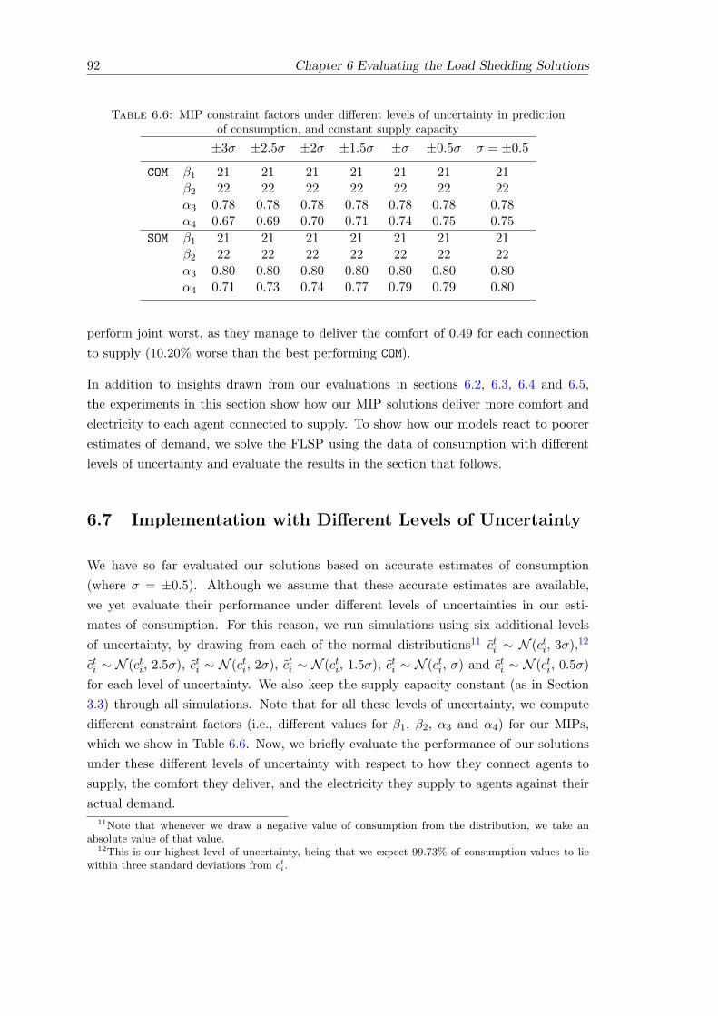
92 Chapter 6 Evaluating the Load Shedding Solutions
Table 6.6: MIP constraint factors under different levels of uncertainty in predictionof consumption, and constant supply capacity
±3σ ±2.5σ ±2σ ±1.5σ ±σ ±0.5σ σ = ±0.5
COM β1 21 21 21 21 21 21 21β2 22 22 22 22 22 22 22α3 0.78 0.78 0.78 0.78 0.78 0.78 0.78α4 0.67 0.69 0.70 0.71 0.74 0.75 0.75
SOM β1 21 21 21 21 21 21 21β2 22 22 22 22 22 22 22α3 0.80 0.80 0.80 0.80 0.80 0.80 0.80α4 0.71 0.73 0.74 0.77 0.79 0.79 0.80
perform joint worst, as they manage to deliver the comfort of 0.49 for each connection
to supply (10.20% worse than the best performing COM).
In addition to insights drawn from our evaluations in sections 6.2, 6.3, 6.4 and 6.5,
the experiments in this section show how our MIP solutions deliver more comfort and
electricity to each agent connected to supply. To show how our models react to poorer
estimates of demand, we solve the FLSP using the data of consumption with different
levels of uncertainty and evaluate the results in the section that follows.
6.7 Implementation with Different Levels of Uncertainty
We have so far evaluated our solutions based on accurate estimates of consumption
(where σ = ±0.5). Although we assume that these accurate estimates are available,
we yet evaluate their performance under different levels of uncertainties in our esti-
mates of consumption. For this reason, we run simulations using six additional levels
of uncertainty, by drawing from each of the normal distributions11 cti ∼ N (cti, 3σ),12
cti ∼ N (cti, 2.5σ), cti ∼ N (cti, 2σ), c
ti ∼ N (cti, 1.5σ), c
ti ∼ N (cti, σ) and cti ∼ N (cti, 0.5σ)
for each level of uncertainty. We also keep the supply capacity constant (as in Section
3.3) through all simulations. Note that for all these levels of uncertainty, we compute
different constraint factors (i.e., different values for β1, β2, α3 and α4) for our MIPs,
which we show in Table 6.6. Now, we briefly evaluate the performance of our solutions
under these different levels of uncertainty with respect to how they connect agents to
supply, the comfort they deliver, and the electricity they supply to agents against their
actual demand.
11Note that whenever we draw a negative value of consumption from the distribution, we take anabsolute value of that value.
12This is our highest level of uncertainty, being that we expect 99.73% of consumption values to liewithin three standard deviations from cti.

Chapter 6 Evaluating the Load Shedding Solutions 93
±3σ
±2.5
σ
±2σ
±1.5
σ ±σ
±0.5
σ
σ=±0
.5
6000
0062
5000
6500
0067
5000
7000
0072
5000
Conn
ectio
n (h
ours
)
Utilitarian
COMSOMGA
CSA1RSACSA2
±3σ
±2.5
σ
±2σ
±1.5
σ ±σ
±0.5
σ
σ=±0
.5
Uncertainties in prediction of consumption
1600
1650
1700
1750
1800
1850
1900
1950 Egalitarian
±3σ
±2.5σ
±2σ
±1.5σ ±σ
±0.5σ
σ=±0
.5
010
020
030
040
050
060
070
0
Envy-freeness
Figure 6.5: Average number of connections to supply under different levels of uncer-tainty
6.7.1 Connections to Supply under Different Levels of Uncertainty
We display the average number of hours our solutions connect agents to supply individ-
ually (with respect to the egalitarian and envy-freeness metrics) and collectively (with
respect to the utilitarian metric) under different levels of uncertainty in Figure 6.5.
Figure 6.5 shows how our solutions produce results that are increasingly inconsistent
as more uncertainties are introduced into consumption. However, the number of agents
they connect to supply does not show any consistent pattern. This is because the errors
in consumption (predicted during our simulations) seem to cancel themselves out, such
that the average number of agents our solutions connect to supply do not change in any
pattern over all levels of uncertainty. These hold under the utilitarian, egalitarian and
envy-freeness considerations.
6.7.2 Comfort Delivered under Different Levels of Uncertainty
We display the average comfort our solutions deliver to agents individually (with re-
spect to the egalitarian and envy-freeness metrics) and collectively (with respect to the
utilitarian metric) under different levels of uncertainty in Figure 6.6.
As in Section 6.7.1, Figure 6.6 shows how our solutions produce results that are in-
creasingly inconsistent as more uncertainties are introduced into consumption, due to
more varied consumption data being generated under higher levels of uncertainty. This

94 Chapter 6 Evaluating the Load Shedding Solutions
±3σ
±2.5σ
±2σ
±1.5σ ±σ
±0.5σ
σ=±0
.5
2450
0025
7500
2700
0028
2500
2955
0030
7500
Comfort
Utilitarian
COMSOMGA
CSA1RSACSA2
±3σ
±2.5σ
±2σ
±1.5σ ±σ
±0.5σ
σ=±0
.5Uncertainties in prediction of consumption
0.3
0.4
0.5
0.6
0.7
0.8
Egalitarian
±3σ
±2.5σ
±2σ
±1.5σ ±σ
±0.5σ
σ=±0
.5
0.1
0.2
0.3
0.4
0.5
0.6
Envy-freeness
Figure 6.6: Average comfort delivered under different levels of uncertainty
holds under the utilitarian, egalitarian and envy-freeness considerations. Furthermore,
the comfort our solutions deliver to agents collectively (under the utilitarian consider-
ations) does not show any particular trend. This is due to comfort being formulated
from historical (actual) consumption and not predicted consumption. However, our MIP
models deliver slightly higher levels of comfort to the worst of agents as uncertainties
reduce. This is so because the supply constraint factors they compute (see Table 6.6)
are lower under higher levels of uncertainty, such that they impact on their egalitarian-
comfort results. Contrariwise, our heuristics do not show any particular pattern under
the egalitarian consideration. While the differences between the comfort delivered to
the worst and best off agents by our MIP solutions slightly reduce with uncertainties
(under the envy-freeness consideration), the results produced by our heuristics show no
such patterns.
6.7.3 Electricity Supplied under Different Levels of Uncertainty
We display the average amount of electricity our solutions supply to agents individually
(with respect to the egalitarian and envy-freeness metrics) and collectively (with respect
to the utilitarian metric) under different levels of uncertainty in Figure 6.7.
Herein also, Figure 6.7 shows how our solutions produce results that are increasingly
inconsistent as more uncertainties are introduced into consumption, due to more varied
consumption data being generated under higher levels of uncertainty. This holds under
the utilitarian, egalitarian and envy-freeness considerations. Furthermore, the electricity

Chapter 6 Evaluating the Load Shedding Solutions 95
±3σ
±2.5σ
.2σ
.1.5σ .σ
.0.5σ
σ=.0
.5
1220
000
1255
000
1290
000
1325
000
1360
000
Elec
tricit
y Su
pply (k
Wh)
Utilita(ian
COMSOMGA
CSA1RSACSA2
±3σ
±2.5σ
.2σ
.1.5σ .σ
.0.5σ
σ=.0
.5
Uncertainties in prediction of consumption
0.2
0.3
0.4
0.5
0.6
0.7
0.8
Egalitarian
±3σ
±2.5σ
.2σ
.1.5σ .σ
.0.5σ
σ=.0
.5
0.1
0.2
0.3
0.4
0.5
0.6
0.7
Envy-freeness
Figure 6.7: Average electricity supplied under different levels of uncertainty
our solutions supply to agents collectively (under the utilitarian considerations) does not
show any particular trend. This is due to the errors in predicted consumption which seem
to cancel themselves out, such that the average sum of electricity supplied to agents fail
to display any particular pattern over all levels of uncertainty. However, our MIP models
supply higher amounts of electricity to the worst of agents as uncertainties reduce. This
is mainly due to the supply constraint factors they compute as in Table 6.6. Contrariwise,
our heuristics do not show any particular pattern under the egalitarian consideration.
While the differences between the electricity supplied to the worst and best off agents
by our MIP solutions consistently reduce with uncertainties (under the envy-freeness
consideration), the results produced by our heuristics show no such patterns. To show
that our models can be used within different settings, we show the results obtained by
solving the FLSP on other datasets in the next section.
6.8 Implementation with other Datasets
To show that our solutions generalize, we now show results of solving the FLSP with
two other datasets: (i) the original dataset of homes in the USA (see Section 3.1) in
Section 6.8.1, and (ii) a simulated dataset of 1000 homes based on the dataset of homes
in Nigeria (see Section 3.1) in Section 6.8.2.

96 Chapter 6 Evaluating the Load Shedding Solutions
6.8.1 Dataset of USA Homes
In this section, we show the results of solving the FLSP with the original dataset of
household consumption of homes in the USA (from which we simulated the dataset
in Section 3.1). This Pecan Street dataset is for 414 homes over 13 weeks (i.e., Q
hours). We model all homes as agents by formulating their comfort profiles as we did
in Section 3.2. Thereafter, we find parameters β1, β2, α3 and α4 to be 21, 22, 0.78 and
0.72 respectively for COM. We also find parameters β1, β2, α3 and α4 to be 21, 22, 0.79
and 0.78 respectively for SOM. We solve the FLSP and show the results in Table 6.7.
Table 6.7 shows how our solutions perform in line with our evaluations in Section 6.2,
Section 6.3, Section 6.4, Section 6.5 and Section 6.6, albeit under a different setting.
This suggests that our solutions are applicable within other applicable settings with
unique characteristics.
6.8.2 Dataset of Multiple Homes in Developing Countries
In this section, we show the results of solving the FLSP with the dataset of 1000 homes
in developing countries. In Section 3.1, we generated the hourly consumption data of
367 homes in developing countries over three months. In order to see how our solutions
scale and generalize, we generate the data of 1000 homes from the dataset for the same
duration.13 Thereafter, we model all homes as agents by formulating their comfort
profiles as we did in Section 3.2. Then, we find parameters β1, β2, α3 and α4 to be 21,
22, 0.80 and 0.76 respectively for COM. We also find parameters β1, β2, α3 and α4 to be
21, 22, 0.82 and 0.82 respectively for SOM. We solve the FLSP and show the results in
Table 6.8.
As in Section 6.8.1, Table 6.8 also shows how our solutions perform in line with our
evaluations in Section 6.2, Section 6.3, Section 6.4, Section 6.5 and Section 6.6 under a
different setting. This suggests that our solutions are applicable within other applicable
settings with unique characteristics. We conclude this chapter by discussing the time
complexities of all load shedding solutions in the next section.
6.9 On the Time Complexity of Solutions
Our heuristics are polynomial time algorithms that mainly depend on the number of
agents (i.e., O(n) for GA, O(n logn) for CSA1, O(n) for RSA and O(n logn) for CSA2, where
n is the number of agents). In turn, our MIP solutions are built upon a MKP formulation
which has a non-polynomial time complexity (polynomial time complexity, if bounded).
13We do this by drawing from a normal distribution with the consumption of homes in the dataset ofSection 3.1 as the mean.

Chapter
6Evaluatin
gtheLoadSheddingSolutio
ns
97
Table 6.7: Results of MIP models and heuristics in terms of the average number of hours of connection to supply, average comfort delivered andaverage electricity supplied (following a number of implementations with the dataset of USA homes), along with their standard deviations (SD)
within parenthesis
COM (SD) textttSOM (SD) GA (SD) CSA1 (SD) RSA (SD) CSA2 (SD)
Connections Utilitarian 810355 (4112) 801094 (4006) 712859 (4400) 725414 (2979) 722264 (4428) 719683 (3319)Egalitarian 1923 (3.27) 1926 (3.44) 1603 (4.60) 1752 (2.30) 1744 (4.26) 1738 (2.30)Envy-freeness 145 (2.37) 97 (2.85) 723 (3.34) 1 (0) 1 (0) 1 (0)
Comfort Utilitarian 339622 (3987) 326125 (4036) 325999 (4993) 326961 (3084) 300856 (4986) 302704 (3492)Egalitarian 0.81 (0.01) 0.82 (0.01) 0.40 (0.05) 0.68 (0.03) 0.67 (0.05) 0.65 (0.02)Envy-freeness 0.12 (0.02) 0.10 (0.03) 0.57 (0.03) 0.27 (0.03) 0.30 (0.04) 0.31 (0.03)
Supply Utilitarian 3353701 (16447) 3370189 (16722) 3261206 (20587) 3260997 (14197) 3268866 (20547) 3270249 (14228)Egalitarian 0.75 (0.01) 0.81 (0.02) 0.42 (0.04) 0.67 (0.01) 0.69 (0.03) 0.65 (0.03)Envy-freeness 0.17 (0.02) 0.11 (0.03) 0.55 (0.04) 0.28 (0.02) 0.28 (0.02) 0.30 (0.03)
Comfort (per agent) 2.39 (0.03) 2.46 (0.03) 2.19 (0.04) 2.22 (0.02) 2.40 (0.04) 2.38 (0.02)Supply (per agent) 0.24 (0.002) 0.24 (0.002) 0.22 (0.002) 0.22 (0.001) 0.22 (0.002) 0.22 (0.001)
Table 6.8: Results of MIP models and heuristics in terms of the average number of hours of connection to supply, average comfort deliveredand average electricity supplied (following a number of implementations with the dataset of 1000 homes in developing countries), along with their
standard deviations (SD) within parenthesis
COM (SD) SOM (SD) GA (SD) CSA1 (SD) RSA (SD) CSA2 (SD)
Connections Utilitarian 1953676 (7318) 1933673 (7330) 1735451 (8344) 1766103 (6483) 1755480 (8296) 1746608 (6609)Egalitarian 1922 (3.31) 3.31 (3.46) 1610 (4.68) 1766 (2.19) 1755 (4.42) 1746 (2.36)Envy-freeness 108 (1.86) 57 (1.54) 681 (3.11) 1 (0) 1 (0) 1 (0)
Comfort Utilitarian 826212 (7769) 798271 (7837) 793047 (10949) 795427 (7487) 731820 (10895) 736455 (7025)Egalitarian 0.83 (0.01) 0.85 (0.02) 0.41 (0.05) 0.69 (0.02) 0.67 (0.03) 0.67 (0.02)Envy-freeness 0.11 (0.02) 0.8 (0.02) 0.53 (0.02) 0.24 (0.02) 0.27 (0.03) 0.26 (0.02)
Supply Utilitarian 3656510 (17952) 3671976 (18076) 3557644 (23799) 3555753 (16368) 3563821 (24252) 3567188 (15477)Egalitarian 0.79 (0.02) 0.85 (0.01) 0.42 (0.04) 0.67 (0.02) 0.70 (0.02) 0.66 (0.03)Envy-freeness 0.14 (0.02) 0.09 (0.03) 0.52 (0.04) 0.25 (0.02) 0.23 (0.02) 0.27 (0.03)
Comfort (per agent) 2.36 (0.02) 2.42 (0.02) 2.19 (0.03) 2.22 (0.02) 2.40 (0.04) 2.37 (0.02)Supply (per agent) 0.53 (0.003) 0.53 (0.003) 0.49 (0.004) 0.50 (0.003) 0.49 (0.004) 0.49 (0.002)

98 Chapter 6 Evaluating the Load Shedding Solutions
30 60 90 120
150
180
210
240
270
300
330
367
414
1000
Number of Agents
0
2000
4000
6000
8000
10000
12000
14000
16000
Solutio
n Time (s)
SOM COM GA CSA1 RSA CSA2
Figure 6.8: The average runtimes of all load shedding solutions after nine executions.
However, we solve our MIP using the IBM® ILOG® CPLEX® optimization package
(version 12.7.1) within the Python environment (version 2.7). CPLEX® uses branch
and cut to solve integer programming problems. It begins with the MIP relaxation at
the root node, where certain cuts that tighten the bounds may be deduced or certain
heuristics that arrive at integer-feasible solutions may be utilized, depending on the
CPLEX® parameters used (IBM, 2015). These CPLEX® parameters also determine
the algorithms for executing MIP relaxations at other nodes, if these further relaxations
becomes necessary.14 It is the case that solutions obtained from the relaxations of
an MIP are more computationally efficient in terms of complexity (Balas and Martin,
1980). We illustrate this by solving the FLSP for different populations of agents drawn
from our main evaluation dataset,15 and with other test datasets (i.e., datasets used
in Section 6.8.1 and Section 6.8.2). We show the time taken to arrive at all solutions.
It should be noted that, for all these datasets, our solver arrives at different factors
(i.e., different values for β1, β2, α3 and α4) for our MIPs. It further suggests that
our constrained optimization approach is applicable within different settings, each with
different system characteristics.16 We implement all load shedding solutions with these
datasets and show their average execution times in Figure 6.8.
As can be seen in Figure 6.8, the execution time of the MIPs appears to grow polyno-
mially, and does not entirely depend on the population of agents. This is depicted by
results which show that some MIPs with higher agent population are solved in less time
than others (e.g., the COM with 240 and 367 agents that have lower runtimes than the
14Refer to the IBM® ILOG® CPLEX® Optimization Studio User’s Manual (IBM, 2015).15These populations (or datasets) are taken from the original developing country dataset simulated in
Section 3.1.16By this we mean that, for each dataset, we take the steps in Section 3.3 to compute the hourly
supply capacities and estimates of agent demands. As such, we develop a number of applicable settings,each with its unique characteristics.
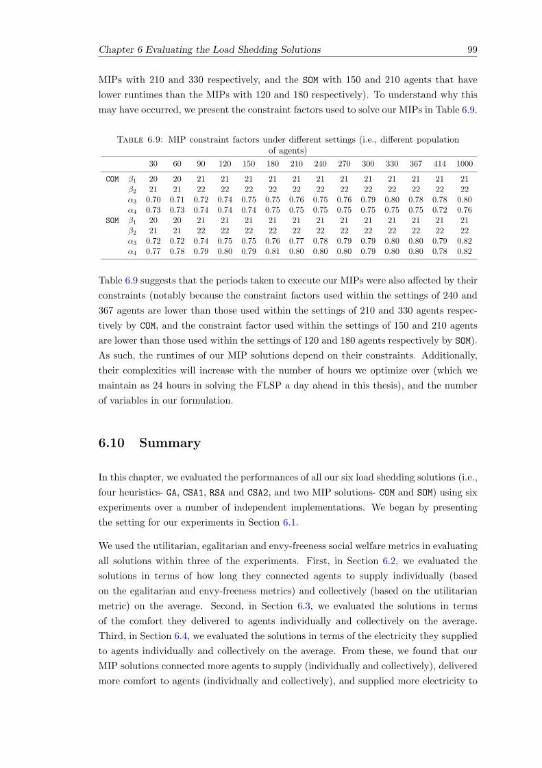
Chapter 6 Evaluating the Load Shedding Solutions 99
MIPs with 210 and 330 respectively, and the SOM with 150 and 210 agents that have
lower runtimes than the MIPs with 120 and 180 respectively). To understand why this
may have occurred, we present the constraint factors used to solve our MIPs in Table 6.9.
Table 6.9: MIP constraint factors under different settings (i.e., different populationof agents)
30 60 90 120 150 180 210 240 270 300 330 367 414 1000
COM β1 20 20 21 21 21 21 21 21 21 21 21 21 21 21β2 21 21 22 22 22 22 22 22 22 22 22 22 22 22α3 0.70 0.71 0.72 0.74 0.75 0.75 0.76 0.75 0.76 0.79 0.80 0.78 0.78 0.80α4 0.73 0.73 0.74 0.74 0.74 0.75 0.75 0.75 0.75 0.75 0.75 0.75 0.72 0.76
SOM β1 20 20 21 21 21 21 21 21 21 21 21 21 21 21β2 21 21 22 22 22 22 22 22 22 22 22 22 22 22α3 0.72 0.72 0.74 0.75 0.75 0.76 0.77 0.78 0.79 0.79 0.80 0.80 0.79 0.82α4 0.77 0.78 0.79 0.80 0.79 0.81 0.80 0.80 0.80 0.79 0.80 0.80 0.78 0.82
Table 6.9 suggests that the periods taken to execute our MIPs were also affected by their
constraints (notably because the constraint factors used within the settings of 240 and
367 agents are lower than those used within the settings of 210 and 330 agents respec-
tively by COM, and the constraint factor used within the settings of 150 and 210 agents
are lower than those used within the settings of 120 and 180 agents respectively by SOM).
As such, the runtimes of our MIP solutions depend on their constraints. Additionally,
their complexities will increase with the number of hours we optimize over (which we
maintain as 24 hours in solving the FLSP a day ahead in this thesis), and the number
of variables in our formulation.
6.10 Summary
In this chapter, we evaluated the performances of all our six load shedding solutions (i.e.,
four heuristics- GA, CSA1, RSA and CSA2, and two MIP solutions- COM and SOM) using six
experiments over a number of independent implementations. We began by presenting
the setting for our experiments in Section 6.1.
We used the utilitarian, egalitarian and envy-freeness social welfare metrics in evaluating
all solutions within three of the experiments. First, in Section 6.2, we evaluated the
solutions in terms of how long they connected agents to supply individually (based
on the egalitarian and envy-freeness metrics) and collectively (based on the utilitarian
metric) on the average. Second, in Section 6.3, we evaluated the solutions in terms
of the comfort they delivered to agents individually and collectively on the average.
Third, in Section 6.4, we evaluated the solutions in terms of the electricity they supplied
to agents individually and collectively on the average. From these, we found that our
MIP solutions connected more agents to supply (individually and collectively), delivered
more comfort to agents (individually and collectively), and supplied more electricity to

100 Chapter 6 Evaluating the Load Shedding Solutions
agents (individually and collectively) on the average. SOM performed better than all
other solutions in most of these experiments.
In Section 6.5, we evaluated all six solutions in terms of the excess load they disconnected
from supply during load shedding. The MIP solutions were found to be more efficient in
this regard, as they disconnected less excess load than the heuristics. Furthermore, in
Section 6.6, we considered how much comfort (in Section 6.6.1) and supply (in Section
6.6.2) they delivered for each agent that was connected to supply on the average. The
MIP solutions were found to deliver more of these to every agent connected to supply
in most cases.
In order to see how our solutions perform when estimates of demand are poor, we evalu-
ated them under different levels of uncertainty in Section 6.7. We found that though they
performed erratically when estimates of demand become poorer, their average results
did not change much. To show that they generalize within similar settings (where load
shedding is necessary), we used them to solve FLSPs with other datasets in Section 6.8.
Specifically, in Section 6.8.1, we solved the FLSP using the original dataset of 414 homes
in the USA. In turn, in Section 6.8.2, we solved the FLSP using the simulated dataset
of 1000 homes in developing countries. The results presented in both sections showed
how our solutions performed in line with prior evaluations.
In concluding the chapter, we briefly considered the time complexities of all our solutions
in Section 6.9, within which our heuristics and MIP solutions appeared to solve in
exponential and linear time respectively with respect to the population of agents. When
taken together, we show that our solutions result in allocations that are fair (in terms of
duration of connections to supply, comfort and supply) and efficient. We conclude this
report and outline our future work in the next chapter.

Chapter 7
Conclusions
In this chapter, we summarize our solution to the FLSP and discuss the open challenges
that still exist. Specifically, in Section 7.1, we summarize the main body and results of
this thesis while, in Section 7.2, we discuss the future lines of work that can advance our
solutions.
7.1 Summary
In this thesis, we proposed to solve the FLSP by considering the heterogeneous needs (or
preferences) of homes for electricity, as in a resource allocation problem. Our proposal
necessitated the execution of load shedding at the household level, at which point elec-
tricity can be individually distributed among households based on their preferences for
electricity. In this manner, a balance between the demand on the grid and its available
supply can be sustained in order to maintain its operation. Executing load shedding at
the household level in developing countries is now possible owing to recent technological
solutions that allow for smart meter retrofits for use in these countries (Azasoo and
Boateng, 2015; Keelson et al., 2014). The retrofits are such that homes can be remotely
reconnected and disconnected from supply, while the electricity consumed by homes can
be securely collected by the operators for billing and analyses (e.g., for prediction and
preference modelling).
To design, implement and evaluate our proposal, we first simulated data that was rep-
resentative of households in Nigeria from a publicly available dataset in Chapter 3. We
did this because no dataset for electricity consumption within homes in any developing
country is currently publicly available. We also elected to simulate our representative
dataset from one that is verifiable, authenticated and readily available, as opposed to
creating an entirely artificial dataset. We considered many publicly available datasets
but settled for those available on Pecan Street’s Dataport, for the reason that the re-
source contains the consumption data of multiple households, at the appliance level,
101

102 Chapter 7 Conclusions
and for long periods. Thereafter, based on findings on appliances common to homes
in Nigeria and the USA1 (Oji et al., 2012; Salmon and Tanguy, 2016; Emodi et al.,
2017; Monyei et al., 2018; Oluwadamilola et al., 2015), the temperature in cities of both
countries (Holiday Weather, 2018a,b) and their load profiles (Prinsloo et al., 2016), we
developed the appliance-level data into household consumption data for households in a
developing country. Then, we modelled households into agents, each with its preference
for electricity. In so doing, we created a notion of comfort that resulted in some com-
puted values which embody the electricity needs of households. We also expressed the
FLSP and discussed our key assumptions within the chapter.
Following this, in Chapter 4, we developed four heuristic algorithms which disconnect
agents from supply based on the objective to connect them to supply as evenly as
possible, in terms of number of hours. Using the utilitarian, egalitarian and envy-
freeness social welfare criteria, we demonstrated that these heuristics allow for a fairer
distribution of energy compared to the randomly-selective, utility maximizing approach
usually taken in this domain. However, we highlighted that the heuristics had the
shortcoming of not considering the agents’ preference (or needs) for electricity.
On this ground, in Chapter 5, we modelled the fair load shedding problem as MIP prob-
lems built upon a multiple knapsack problem formulation. We formulated the objectives
and constraints of two MIPs using the utilitarian, egalitarian and envy-freeness criteria.
One MIP had the objective to maximize the overall comfort of agents and the other had
the objective to maximize the overall supply to agents (both with respect to the utili-
tarian metric). Using the egalitarian and envy-freeness metrics, we developed a number
of constraints which ensure that the number of hours individual agents are connected
to supply, and the comfort delivered and electricity supplied to these individual agents
are as high and as equal as possible for both MIPs. We also included another constraint
that executed load shedding when necessary, thus limiting demand to available supply.
Thereafter, in Chapter 6, we evaluated the performance of all six fair load shedding solu-
tions (i.e., the four heuristics and two MIPs) under six experiments run within a number
of implementations. We performed the evaluations with respect to the number of hours
agents were connected to supply individually and collectively, the comfort delivered to
agents individually and collectively, and the electricity supplied to agents individually
and collectively. We also evaluated our solutions with respect to the amount of excess
load they disconnect from supply, and the comfort and electricity they deliver to every
agent connected to supply. We also considered the effect of poor estimates of consump-
tion on the performances of our solutions. Furthermore, to show that they generalize,
we also experimented on the FLSP with other datasets, and presented the results in
the chapter. We found that the MIP solutions outperformed the heuristics under our
experiments. In addition, we discussed the computation complexities of our solutions
1The datasets on Pecan Street Inc’s Dataport are collected from homes in the USA.

Chapter 7 Conclusions 103
and found that our solver (i.e., CPLEX®) executed our MIPs in an efficient manner in
the chapter.
When taken together, we have presented a data-simulation approach and simulated
data which will be useful for future studies that address energy management issues in
developing countries. We have also designed a number of fair and efficient load shedding
solutions which can be adapted to suit different objectives. In addition, our solutions
can serve as benchmarks for designing future household-level fair load shedding schemes.
They can also serve as benchmarks for designing schemes which allocate other scarce
resources to consumers (e.g., the water allocation problem addressed by Read et al.
(2014)). In all, our approach presents a framework upon which other fairness problems
involving constrained utility maximization (or resource allocation) can be generalized.
We briefly describe how our work can be improved upon in the next section.
7.2 Future Work
We made some assumptions in developing our household-level fair load shedding solu-
tions. One of these is that we receive near-accurate estimates from homes, based on
which we took the estimates of household consumption as values drawn from a normal
distribution of the electricity they actually consume. However, it will be useful to de-
sign solutions which incorporate the computation of these estimates in the future. Such
solutions may utilize some of the tools and techniques discussed in Section 2.4.2.2, or
incorporate elicitation methods such as POU games (discussed in Section 2.4.2.1).
Furthermore, approaches like “soft load shedding” (see (Aslam and Arshad, 2018)) are
being developed to mitigate against the rebound effect (described in Section 3.4), and
may be incorporated into our solutions in the future. In addition, it is important to
consider that households which are arbitrarily subjected to load shedding may advance
their consumption to periods when electricity is available. As such, future fair load shed-
ding solutions should also consider the effect load shedding has on prior consumption.
Although made the attempt to consider the rebound effect in this thesis, our comfort
formulation may be further improved to ensure it still embodies the preference of agents
for electricity, even after load shedding influences their consumption.
In addition to this, the accuracy of the comfort of homes may be improved upon con-
sidering the needs of individual consumers in homes. For instance, some homes may
have occupants which need electricity all the time to run some important activities. An
example is an occupant who needs an electric respiratory aid in the home for manag-
ing and treating sleep apnea. An approach to this may be to elicit some information
(maybe through text messages) from homes in a bother-free manner (as has been studied
in (Truong et al., 2016; Le et al., 2018)). In this case, it is necessary to appropriately
incentivize the true reporting of the information with suitable elicitation techniques. To

104 Chapter 7 Conclusions
surmise, the individual needs of occupants within the home will generate more varied
user profiles, which can be used to develop more accurate models of comfort, and to
supply electricity to homes based on these needs (i.e., comfort).
We produced hourly solutions which are applicable because electricity billing is on an
hourly basis (i.e., in kWh). Additionally, many energy, resource allocation and schedul-
ing problems are solved in hourly or half-hourly time slots (e.g., in (Alam et al., 2015)).
Likewise, RTPs are hourly (or half-hourly) pricing schemes that contribute to grid sta-
bility. However, in the future, our solution can be implemented using per minute data.
This will be more computationally intensive, as shown in Section 6.9, where we suggested
that the computation time of our MIPs will increase with the number of knapsacks in our
MKP formulation. Nonetheless, to ensure the computational cost of using per minute
data remains tractable, future solutions may solve the FLSP incrementally (e.g., one
hour at a time), and employ approximation and relaxation techniques. Note that the
computation complexity of such FLSP solutions is not a deterring factor, as they are not
designed to be implemented at real-time. Furthermore, solutions that use per minute
data should produce more accurate results (from using more accurate comfort values
and estimates of consumption).
To make our solutions more scalable across the network (especially when many homes
need to be disconnected to offset the deficit or when load shedding cannot be imple-
mented at the household level), an agent that sits at the network level may coordinate
the disconnection and re-connection of home agents to supply. This network agent may
coordinate load shedding within a region on the electricity network (e.g., within a bus
or line). The network agent will consider the individual needs and electricity demand of
each home agent and aggregate these (i.e., develop a utility function that is an aggrega-
tion of the utility functions of the individual agents). It may then use the information
to source for electricity from the grid, and to distribute electricity to home agents fairly
and efficiently.
Finally, our work can be designed to fit alongside other reactive load shedding measures,
and load management measures such as DSM (discussed in Section 2.1.1). In the case
of DSM, it is necessary to design incentives that encourage consumers to manage their
consumption appropriately, and to have an understanding of how they will react to such
incentives. In addition, with the right coordination mechanisms, our work can cope with
the introduction of distributed renewable sources and storage on the grid (Chalkiadakis
et al., 2011). However, it will be necessary to accurately predict demand (and supply,
especially in the case of distributed renewable sources and storage) before our solutions
can be effective when incorporated with these smart grid technologies (Ramchurn et al.,
2012).

Bibliography
Moein Abedini, Majid Sanaye-Pasand, and Sadegh Azizi. Adaptive load shedding scheme
to preserve the power system stability following large disturbances. IET Generation,
Transmission and Distribution, 8(12):2124 – 2133, 2014. ISSN 1751-8695.
Charilaos Akasiadis and Georgios Chalkiadakis. Agent cooperatives for effective power
consumption shifting. In Proceedings of the Twenty-Seventh AAAI Conference on
Artificial Intelligence, July 14-18, 2013, Bellevue, Washington, USA., 2013.
Muddasser Alam, Enrico H. Gerding, Alex Rogers, and Sarvapali D. Ramchurn. A
scalable, decentralised multi-issue negotiation protocol for energy exchange. In Inter-
national Joint Conference on Artificial Intelligence (IJCAI), April 2015.
Muddasser Alam, Sarvapali D Ramchurn, and Alex Rogers. Cooperative Energy Ex-
change for the Efficient Use of Energy and Resources in Remote Communities. Pro-
ceedings of the 12th International Conference on Autonomous Agents in Multiagent
Systems (AAMAS 2013), pages 731–738, 2013.
Hunt Allcott. Rethinking real-time electricity pricing. Resource and Energy Economics,
33(4):820–842, 2011.
E. Amaefule. 152 million Nigerians live on less than $2 per day: AfDB, 2018.
https://goo.gl/EtNqgT.
Tone Arnold and Ulrich Schwalbe. Dynamic coalition formation and the core. Journal
of Economic Behavior & Organization, 49(3):363 – 380, 2002. ISSN 0167-2681.
Tayyab Aslam and Naveed Arshad. Soft load shedding: An efficient approach to manage
electricity demand in a renewable rich distribution system. pages 101–107, 01 2018.
J.Q. Azasoo and K.O. Boateng. A retrofit design science methodology for smart metering
design in developing countries. In 15th International Conference on Computational
Science and Its Applications, 2015.
Egon Balas and Clarence H. Martin. Pivot and complementa heuristic for 0-1 program-
ming. Management Science, 26(1):86–96, 1980.
105

106 BIBLIOGRAPHY
G. Di Bella, L. Giarre, M. Ippolito, A. Jean-Marie, G. Neglia, and I. Tinnirello. Modeling
energy demand aggregators for residential consumers. Decision and Control (CDC),
2013 IEEE 52nd Annual Conference on, pages 232–237, 2013. ISSN 0191-2216.
Jan Bentzen and Tom Engsted. A revival of the autoregressive distributed lag model in
estimating energy demand relationships. Energy, 26(1):45 – 55, 2001. ISSN 0360-5442.
Dhananjay Bhor, Kavinkadhirselvan Angappan, and Krishna M. Sivalingam. Network
and power-grid co-simulation framework for smart grid wide-area monitoring net-
works. Journal of Network and Computer Applications, 59:274 – 284, 2016. ISSN
1084-8045.
Philippe Caillou, Samir Aknine, and Suzanne Pinson. A multi-agent method for forming
and dynamic restructuring of pareto optimal coalitions. In Proceedings of the First
International Joint Conference on Autonomous Agents and Multiagent Systems: Part
3, AAMAS ’02, pages 1074–1081, New York, NY, USA, 2002. ACM. ISBN 1-58113-
480-0.
Romain Calliere, Samir Aknine, Antoine Nongaillard, and Sarvapali Ramchurn. Man-
aging energy markets in future smart grids using bilateral contracts. In European
Conference on Artificial Intelligence (ECAI), The Hague, Netherlands, 2016.
I. Caragiannis, D Kurokawa, H. Moulin, A.D. Procaccia, N. Shah, and J. Wang. The
unreasonable fairness of maximum nash welfare. In Proceedings of the 2016 ACM
Conference on Economics and Computation, 2016.
Georgios Chalkiadakis, Valentin Robu, Ramachandra Kota, Alex Rogers, and
Nicholas R. Jennings. Cooperatives of Distributed Energy Resources for Efficient
Virtual Power Plants. Proc. of 10th Int. Conf. on Autonomous Agents and Mul-
tiagent Systems Innovative Applications Track (AAMAS 2011), pages 787–794, 2011.
Hung-Lin Chao and Pao-Ann Hsiung. A fair energy resource allocation strategy for
micro grid. Microprocessors and Microsystems, 42:235–244, 2016. ISSN 01419331.
Yann Chevaleyre, Paul E. Dunne, Ulle Endriss, Jerome Lang, Michel Lemaitre, Nicolas
Maudet, Julian Padget, Steven Phelps, Juan Antonio Rodrguez-Aguilar, and Paulo
Sousa. Issues in multiagent resource allocation. Applied Soft Computing, 2006.
Sung-Hwan Cho, Won-Tae Kim, Choon-Soeb Tae, and M Zaheeruddin. Effect of length
of measurement period on accuracy of predicted annual heating energy consumption
of buildings. Energy Conversion and Management, 45(18):2867 – 2878, 2004. ISSN
0196-8904.
City Power Johannesburg. The Five Stages of Load Shedding, 2014.
https://www.citypower.co.za/customers/Pages/Infographic.aspx.

BIBLIOGRAPHY 107
Charles Concordia, Lester H Fink, Boza Avramovic, and George Poullikkas. Load Shed-
ding on an Isolated System. System, 10(3):1467–1472, 1995.
Luke Daniel. Load shedding: Here’s what happens to South Africa at Stage 8, 2019.
https://www.thesouthafrican.com/what-is-eskom-load-shedding-stage-8/.
Department for Environment, Food and Rural Affairs. Household Electricity Study,
2011. http://randd.defra.gov.uk/.
Soma Shekara Sreenadh Reddy Depuru, Lingfeng Wang, and Vijay Devabhaktuni. Smart
meters for power grid: Challenges, issues, advantages and status. Renewable and
Sustainable Energy Reviews, 15(6):2736 – 2742, 2011. ISSN 1364-0321.
N. A. Diago, S. Aknine, O. Shehory, S. Arib, R. Cailliere, and M. Sene. Decentralized
and fair multilateral negotiation. In 2016 IEEE 28th International Conference on
Tools with Artificial Intelligence (ICTAI), pages 149–156, Nov 2016.
L.P.C. Do, Kuan-Heng Lin, and P. Molnar. Electricity consumption modelling: A case
of germany. In Economic Modelling, 2016.
EEI. Handbook for Electricity Metering, 11th Edition. Edison Electric Institute, 2014.
ISBN 10-0931032598.
N.V. Emodi, C.C. Emodi, G.P. Murthy, A.D. Procaccia, and A.S.A. Emodi. Energy
policy for low carbon development in nigeria: A leap model application. In Renewable
and Sustainable Energy Reviews, 2017.
Douglas Henry Fabini, Diego Ponce de Leon Barido, Akomeno Omu, and Jay Taneja.
Mapping induced residential demand for electricity in kenya. In Proceedings of the
Fifth ACM Symposium on Computing for Development, ACM DEV-5 ’14, pages 43–
52, New York, NY, USA, 2014. ACM. ISBN 978-1-4503-2936-1.
Zahedi S.M. Freeman, R. and V. Conitzer. Fair and efficient social choice in dynamic
settings. 2017.
Jingkun Gao, Suman Giri, Emre Can Kara, and Mario Berges. The Plug Load Appli-
ance Identification Dataset (PLAID), a Public Dataset of High Resolution for Load
Identification Research, 2014. http://plaidplug.com.
Enrico Gerding, Sebastian Stein, Valentin Robu, D Zhao, and N. R. Jennings. Two-sided
online markets for electric vehicle charging. pages 989–996, 2013.
Enrico H. Gerding, Valentin Robu, Sebastian Stein, David C. Parkes, Alex Roggers, and
Nicholas R. Jennings. Online mechanism design for electric vehicle charging. 10th
Int. Conf. on Autonomous Agents and Multiagent Systems (AAMAS 2011), pages
811–818, 2011.

108 BIBLIOGRAPHY
Ali Ghodsi, Matei Zaharia, Benjamin Hindman, Andy Konwinski, Scott Shenker, and
Ion Stoica. Dominant resource fairness: Fair allocation of multiple resource types. In
Proceedings of the 8th USENIX Conference on Networked Systems Design and Imple-
mentation, NSDI’11, pages 323–336, Berkeley, CA, USA, 2011. USENIX Association.
Ahmed M. A. Haidar, Azah Mohamed, Majid Al-Dabbagh, Aini Hussain, and Mo-
hammad Masoum. An intelligent load shedding scheme using neural networks and
neuro-fuzzy. International Journal of Neural Systems, 19(06):473–479, 2009. PMID:
20039470.
Holiday Weather. Austin: Annual Weather Averages, 2018a.
https://www.holiday-weather.com/austin/averages/.
Holiday Weather. Lagos: Annual Weather Averages, 2018b.
https://www.holiday-weather.com/lagos/averages/.
James C Holyhead, Sarvapali D. Ramchurn, and Alex Rogers. Consumer targeting in
residential demand response programmes. In Proceedings of the ACM International
Conference on Future Energy Systems, 2015.
Y. Hong and P. Chen. Genetic-based underfrequency load shedding in a stand-alone
power system considering fuzzy loads. IEEE Transactions on Power Delivery, 27(1):
87–95, Jan 2012. ISSN 0885-8977.
R. Hooshmand and M. Moazzami. Optimal design of adaptive under frequency load shed-
ding using artificial neural networks in isolated power system. International Journal
of Electrical Power and Energy Systems, 42(1):220 – 228, 2012. ISSN 0142-0615.
IBM. IBM ILOG CPLEX Optimization Studio CPLEX User’s Manual, Version 12
Release 6, 2015. https://goo.gl/1ZWRJM.
Satish Kumar Injeti. A pareto optimal approach for allocation of distributed generators
in radial distribution systems using improved differential search algorithm. Journal of
Electrical Systems and Information Technology, 5(3):908 – 927, 2018. ISSN 2314-7172.
T. Inoue, H. Taniguchi, Y. Ikeguchi, and K. Yoshida. Estimation of power system
inertia constant and capacity of spinning-reserve support generators using measured
frequency transients. IEEE Transactions on Power Systems, 12(1):136–143, Feb 1997.
ISSN 0885-8950.
Geoffrey Johnson and Ian Beausoleil-Morrison. Electrical-end-use data from 23 houses
sampled each minute for simulating micro-generation systems. Applied Thermal En-
gineering, 114:1449 – 1456, 2017. ISSN 1359-4311.
Kamil Kaygusuz. Energy for sustainable development: A case of developing countries.
Renewable and Sustainable Energy Reviews, 16(2):1116 – 1126, 2012. ISSN 1364-0321.
BIBLIOGRAPHY 109
E. Keelson, K. Boateng, and I. Ghansah. A smart retrofitted meter for developing
countries. In International Journal of Computer Applications, 2014.
D Kirschen and G Strbac. Fundamentals of Power System Economics. Wiley, 2004.
P. Kundur, J. Paserba, V. Ajjarapu, G. Andersson, A. Bose, C. Canizares, N. Hatziar-
gyriou, D. Hill, A. Stankovic, C. Taylor, T. Van Cutsem, and V. Vittal. Definition and
classification of power system stability ieee/cigre joint task force on stability terms
and definitions. IEEE Transactions on Power Systems, 19(3):1387–1401, Aug 2004.
ISSN 0885-8950.
J.A. Laghari, H. Mokhlis, A.H.A. Bakar, and Hasmaini Mohamad. Application of com-
putational intelligence techniques for load shedding in power systems: A review. En-
ergy Conversion and Management, 75:130 – 140, 2013. ISSN 0196-8904.
Tiep Le, Atena M. Tabakhi, Long Tran-Thanh, William Yeoh, and Tran Cao Son. Prefer-
ence elicitation with interdependency and user bother cost. In Proceedings of the 17th
International Conference on Autonomous Agents and MultiAgent Systems, AAMAS
’18, pages 1459–1467, Richland, SC, 2018. International Foundation for Autonomous
Agents and Multiagent Systems.
J. Leite, J. Alferes, and B. Mito. Resource allocation with answer-set programming. In
Proceedings of The 8th International Conference on Autonomous Agents and Multia-
gent Systems, 2009.
Sasan Maleki. Addressing the computational issues of the shapley value with applications
in the smart grid. August 2015.
Silvano Martello and Paolo Toth. Solution of the zero-one multiple knapsack problem.
European Journal of Operational Research, 4(4):276 – 283, 1980. ISSN 0377-2217.
Combinational Optimization.
Sam Miller, Sarvapali D Ramchurn, and Alex Rogers. Optimal decentralised dispatch
of embedded generation in the smart grid. In AAMAS 12 International Conference
on Autonomous Agents and Multiagent Systems. ACM, June 2012.
Hazlie Mokhlis, J.A. Laghari, Ab Halim Abu Bakar, and Mazaher Karimi. A fuzzy based
under-frequency load shedding scheme for islanded distribution network connected
with dg. International Review of Electrical Engineering-Iree, 7:4992–5000, 07 2012.
C.G. Monyei, A.O. Adewumi, M.O. Obolo, and S. Sajou. Nigeria’s energy poverty:
Insights and implications for smart policies and framework towards a smart nigeria
electricity network. In Renewable and Sustainable Energy Reviews, 2018.
Juan D. Moreno-Ternero and John E. Roemer. A common ground for resource and
welfare egalitarianism. Games and Economic Behavior, 75(2):832 – 841, 2012. ISSN
0899-8256.

110 BIBLIOGRAPHY
H. Moulin. Fair Division and Collective Welfare. The MIT Press, 2003.
Matteo Muratori, Matthew C. Roberts, Ramteen Sioshansi, Vincenzo Marano, and Gior-
gio Rizzoni. A highly resolved modeling technique to simulate residential power de-
mand. Applied Energy, 107:465 – 473, 2013. ISSN 0306-2619.
David Murray, Jing Liao, Lina Stankovic, Vladimir Stankovic, Richard Hauxwell-
Baldwin, Charlie Wilson, Michael Coleman, Tom Kane, and Steven Firth. A data
management platform for personalised real-time energy feedback. In Procededings of
the 8th International Conference on Energy Efficiency in Domestic Appliances and
Lighting. IET, August 2015.
David Murray and Lina Stankovic. REFIT: Electrical Load Measurements, 2015.
https://goo.gl/DxHNXD.
V. Natarajan and A. S. Closepet. Demand-side approaches to manage electricity outages
in developing countries. In 2012 IEEE International Energy Conference and Exhibition
(ENERGYCON), pages 829–835, Sep. 2012.
Nhan-Tam Nguyen, Trung Thanh Nguyen, and Jorg Rothe. Approximate solutions to
max-min fair and proportionally fair allocations of indivisible goods. In Proceedings
of the 16th Conference on Autonomous Agents and MultiAgent Systems, AAMAS ’17,
pages 262–271, Richland, SC, 2017. International Foundation for Autonomous Agents
and Multiagent Systems.
Antoine Nongaillard, Philippe Mathieu, and Brigitte Jaumard. A multi-agent resource
negotiation for the utilitarian welfare. volume 5485, pages 208–226, 09 2008.
M.U. Nwachukwu, N.F. Ezedinma, and U. Jiburum. Comparative analysis of electric-
ity consumption among residential, commercial and industrial sectors of the nigerias
economy. In Journal of Energy Technologies and Policy, 2014.
J.O. Oji, N. Idusuyi, T.O. Aliu, M.O. Petinrin, O.A. Odejobi, and A.R. Adetunji. Uti-
lization of solar energy for power generation in nigeria. In International Journal of
Energy Engineering, 2012.
O. Oluwadamilola, G. Harrison, and H. Weijde. Modelling electricity and cooling load
profiles for domestic customers in Nigeria, 2015. https://goo.gl/nwk9KR.
O.I. Oluwasuji, M. Obaid, J. Zhang, and S.D. Ramchurn. Algorithms for fair load shed-
ding in developing countries. In Proceedings of the 27th International Joint Conference
on Artificial Intelligence, 2018a.
O.I. Oluwasuji, M. Obaid, J. Zhang, and S.D. Ramchurn. Algorithms to manage load
shedding events in developing countries. In Proceedings of the 17th International
Conference on Autonomous Agents and Multiagent Systems (AAMAS 2018), 2018b.

BIBLIOGRAPHY 111
Olabambo I. Oluwasuji. Dataset for Fair Load Shedding Problem., 2018. osf.io/bxmkr.
S.O. Oyedepo. Energy and sustainable development in nigeria: the way forward. 2012.
J.V. Paatero and P.D. Lund. A model for generating household electricity load profiles.
International Journal of Energy Research, 30(5):273–290, 2006. cited By 226.
S. Pahwa, C. Scoglio, S. Das, and N. Schulz. Load-shedding strategies for preventing
cascading failures in power grid. Electric Power Components and Systems, 41(9):
879–895, 2013.
O. Parson, G. Fisher, A. Hersey, N Batra, J. Kelly, A. Singh, W. Knottenbelt, and
A. Rogers. Dataport and nilmtk: A building data set designed for non-intrusive
load monitoring. In IEEE Global Conference on Signal and Information Processing
(GlobalSIP), 2015.
Pecan Street Inc. Dataport: More than the Largest Source of Energy Data and Water
Data, 2018. https://dataport.cloud.
David Pisinger and Paolo Toth. Knapsack problems. Du DZ., Pardalos P.M. (eds)
Handbook of Combinatorial Optimization, pages 299–428, 1998.
Gerro Prinsloo, Robert Dobson, and Alan Brent. Scoping exercise to determine load
profile archetype reference shapes for solar co-generation models in isolated off-grid
rural african villages. 28, 08 2016.
Sarvapali D. Ramchurn, Perukrishnen Vytelingum, Alex Rogers, and Nicholas R. Jen-
nings. Putting the ‘smarts’ into the smart grid: A grand challenge for artificial intel-
ligence. Commun. ACM, 55(4):86–97, April 2012. ISSN 0001-0782.
Sarvapali D. Ramchurn, Perukrishnen Vytelingum, Alex Rogers, and Nick Jennings.
Agent-based control for decentralised demand side management in the smart grid. In
The 10th International Conference on Autonomous Agents and Multiagent Systems -
Volume 1, AAMAS ’11, pages 5–12, Richland, SC, 2011. International Foundation for
Autonomous Agents and Multiagent Systems. ISBN 0-9826571-5-3, 978-0-9826571-5-
7.
Sara Ramezani and Ulle Endriss. Nash social welfare in multiagent resource alloca-
tion. In Esther David, Enrico Gerding, David Sarne, and Onn Shehory, editors,
Agent-Mediated Electronic Commerce. Designing Trading Strategies and Mechanisms
for Electronic Markets, pages 117–131, Berlin, Heidelberg, 2010. Springer Berlin Hei-
delberg. ISBN 978-3-642-15117-0.
L. Read, K. Madani, and B. Inanloo. Optimality versus stability in water resource
allocation. In Journal of Environmental Management, 2014.

112 BIBLIOGRAPHY
Valentin Robu, Enrico H. Gerding, Sebastian Stein, David C. Parkes, Alex Rogers, and
Nicholas R. Jennings. An online mechanism for multi-unit demand and its application
to plug-in hybrid electric vehicle charging. Journal of Artificial Intelligence Research,
48:175–230, 10 2013. ISSN 1076-9757.
Valentin Robu, Ramachandra Kota, Georgios Chalkiadakis, Alex Rogers, and
Nicholas R. Jennings. Cooperative virtual power plant formation using scoring rules.
In Proceedings of the 11th International Conference on Autonomous Agents and Mul-
tiagent Systems - Volume 3, AAMAS ’12, pages 1165–1166, Richland, SC, 2012. In-
ternational Foundation for Autonomous Agents and Multiagent Systems. ISBN 0-
9817381-3-3, 978-0-9817381-3-0.
Valentin Robu, Sebastian Stein, Enrico H. Gerding, David C. Parkes, Alex Rogers, and
Nicholas R. Jennings. An online mechanism for multi-speed electric vehicle charging.
In Proceedings of the Second Conference on Auctions, Market Mechanisms and Their
Applications (AMMA), pages 100–112, 2011.
Alex Rogers, Sarvapali Ramchurn, and Nicholas R Jennings. Delivering the smart grid:
Challenges for autonomous agents and multi-agent systems research. Proceedings of
the 26th AAAI Conference on Artificial Intelligence, pages 2166–2172, 2012.
Harry Rose, Alex Rogers, and Enrico H. Gerding. A scoring rule-based mechanism for
aggregate demand prediction in the smart grid. AMMAS Proceedings of the 11th
International Conference on Autonomous Agents and Multiagent Systems, pages 661–
668, 2012.
N. Sadati, T. Amraee, and A.M. Ranjbar. A global particle swarm-based-simulated
annealing optimization technique for under-voltage load shedding problem. Applied
Soft Computing, 9(2):652 – 657, 2009. ISSN 1568-4946.
Marriette Sakah, Stephane de la Rue du Can, Felix Amankwah Diawuo, Morkpork-
por Delight Sedzro, and Christoph Kuhn. A study of appliance ownership and elec-
tricity consumption determinants in urban ghanaian households. Sustainable Cities
and Society, 2018. ISSN 2210-6707.
C. Salmon and J. Tanguy. Rural electrification and household labor supply: Evidence
from nigeria. In World Development, 2016.
F. C. Schweppe, B. Daryanian, and R. D. Tabors. Algorithms for a spot price responding
residential load controller. IEEE Transactions on Power Systems, 4(2):507–516, May
1989. ISSN 0885-8950.
B. Shi and J. Liu. Decentralized control and fair load-shedding compensations to prevent
cascading failures in a smart grid. In International Journal of Electrical Power and
Energy Systems, 2015.

BIBLIOGRAPHY 113
J. A. Short, D. G. Infield, and L. L. Freris. Stabilization of grid frequency through
dynamic demand control. IEEE Transactions on Power Systems, 22(3):1284–1293,
Aug 2007. ISSN 0885-8950.
R. Sioshansi and W. Short. Evaluating the impacts of real-time pricing on the usage
of wind generation. IEEE Transactions on Power Systems, 24(2):516–524, May 2009.
ISSN 0885-8950.
Sebastian Stein, Enrico Gerding, Valentin Robu, and Nick Jennings. A model-based on-
line mechanism with pre-commitment and its application to electric vehicle charging.
Online, (June):4–8, 2012.
H. Steinhaus. The problem of fair division. Econometrica, 1948.
Karen Stenner, Elisha R. Frederiks, Elizabeth V. Hobman, and Stephanie Cook. Will-
ingness to participate in direct load control: The role of consumer distrust. Applied
Energy, 189:76 – 88, 2017. ISSN 0306-2619.
M. Stolworthy. UK Electricity National Grid Demand and Output per Production Type,
2018. http://gridwatch.co.uk.
Goran Strbac. Demand side management: Benefits and challenges. Energy Policy, 36
(12):4419–4426, 2008. ISSN 03014215.
L. Suganthi and Anand A. Samuel. Energy models for demand forecastinga review.
Renewable and Sustainable Energy Reviews, 16(2):1223 – 1240, 2012. ISSN 1364-0321.
Jagruti Thakur and Basab Chakraborty. Demand side management in developing na-
tions: A mitigating tool for energy imbalance and peak load management. Energy,
114:895 – 912, 2016. ISSN 0360-5442.
The Nairametrics research team. Here is How Much You Pay as Electricity bill in Your
State, 2018. https://goo.gl/N5xkrw.
The NILM wiki. NILM datasets, 2014. http://wiki.nilm.eu/datasets.html.
Jacopo Torriti. Price-based demand side management: Assessing the impacts of
time-of-use tariffs on residential electricity demand and peak shifting in northern
italy. Energy, 44(1):576 – 583, 2012. ISSN 0360-5442. Integration and Energy System
Engineering, European Symposium on Computer-Aided Process Engineering 2011.
N.C. Truong, L. Tran-Thanh, E. Costanza, and S.D. Ramchurn. Towards appliance
usage prediction for home energy management. In Proceedings of the Fourth Interna-
tional Conference on Future Energy Systems, 2013a.
Ngoc Cuong Truong, Tim Baarslag, Gopal Ramchurn, and Long Tran-Thanh. Interac-
tive scheduling of appliance usage in the home. July 2016.

114 BIBLIOGRAPHY
Ngoc Cuong Truong, James McInerney, Long Tran-Thanh, Enrico Costanza, and Sar-
vapali Ramchurn. Forecasting multi-appliance usage for smart home energy manage-
ment. pages 2908–2914, 08 2013b.
Adam Vaughan. Smart meters rollout labelled a ‘fiasco’ as consumers face extra £500m
bill, 2018. https://goo.gl/jP31S9.
Meritxell Vinyals, Valentin Robu, Alex Rogers, and Nicholas R. Jennings. Predic-
tion-of-use games: A cooperative game theory approach to sustainable energy tar-
iffs. In Proceedings of the 2014 International Conference on Autonomous Agents and
Multi-agent Systems, AAMAS ’14, pages 829–836, Richland, SC, 2014. International
Foundation for Autonomous Agents and Multiagent Systems. ISBN 978-1-4503-2738-
1.
Perukrishnen Vytelingum, Sarvapali D. Ramchurn, Thomas D. Voice, Alex Rogers, and
Nicholas R. Jennings. Trading agents for the smart electricity grid. In The Ninth
International Conference on Autonomous Agents and Multiagent Systems (AAMAS
2010), pages 897–904, 2010a. Event Dates: May 10-14, 2010.
Perukrishnen Vytelingum, Thomas D. Voice, Sarvapali D. Ramchurn, Alex Rogers, and
Nicholas R. Jennings. Agent-based micro-storage management for the smart grid. In
Proceedings of the 9th International Conference on Autonomous Agents and Multia-
gent Systems: Volume 1 - Volume 1, AAMAS ’10, pages 39–46, Richland, SC, 2010b.
International Foundation for Autonomous Agents and Multiagent Systems. ISBN
978-0-9826571-1-9.
K.P. Wong and B.S. Lau. An algorithm for load shedding and restoration during re-
duced generation periods. In International Conference on Advances in Power System
Control, Operation and Management (APSCOM-91), 1991.
World Energy Council. Average household electricity use around the world, 2010.
https://goo.gl/DRQLXG.
Xiaojing Xu, Chien fei Chen, Xiaojuan Zhu, and Qinran Hu. Promoting acceptance of
direct load control programs in the united states: Financial incentive versus control
option. Energy, 147:1278 – 1287, 2018. ISSN 0360-5442.
I. Yohanna, H. Iortyer, and A. Ierve. Assessment of energy use pattern in residential
buildings of kano and kaduna northern nigeria. In American Journal of Engineering
Research, 2013.
Hai-Xiang Zhao and Frdric Magouls. A review on the prediction of building energy
consumption. Renewable and Sustainable Energy Reviews, 16(6):3586 – 3592, 2012.
ISSN 1364-0321.
J. Zheng, D. W. Gao, and L. Lin. Smart meters in smart grid: An overview. In 2013
IEEE Green Technologies Conference (GreenTech), pages 57–64, April 2013.