Retrospective Theses and Dissertations Iowa State University Capstones, Theses andDissertations

1960

Factors affecting the incidence of reaction tissue inPopulus deltoides BartrGraeme Pierce BerlynIowa State University

Follow this and additional works at: https://lib.dr.iastate.edu/rtd

Part of the Agriculture Commons, Animal Sciences Commons, Natural Resources andConservation Commons, and the Natural Resources Management and Policy Commons

This Dissertation is brought to you for free and open access by the Iowa State University Capstones, Theses and Dissertations at Iowa State UniversityDigital Repository. It has been accepted for inclusion in Retrospective Theses and Dissertations by an authorized administrator of Iowa State UniversityDigital Repository. For more information, please contact digirep@iastate.edu.

Recommended CitationBerlyn, Graeme Pierce, "Factors affecting the incidence of reaction tissue in Populus deltoides Bartr " (1960). Retrospective Theses andDissertations. 2754.https://lib.dr.iastate.edu/rtd/2754

This dissertation has been microfilmed

exactly as received

Mic 60-4889

B£RLYM, Graeme Pierce. FACTORS AFFECTING THE ÏNC1DMCE OF REACTION TISSUE IN POPULUS DEL­TOÏDES BAiiTR.

Iowa State University of science and Technology i?h. û., 1960 Agriculture, forestry and v/ildlife

University Microfilms, Inc., Ann Arbor, Michigan

FACTORS AFFECTING THE INCIDENCE OF REACTION

TISSUE IN POPULUS DELTOÏDES BARTR.

by

Greene Pierce Berlyn

A Dissertation Submitted to the

Graduate Faculty in Partial Fulfillment of

The Requirements for the Degree of

DOCTOR OF PHILOSOPHY

Major Subjects: Wood Technology Plant Morphology

Approved:

In Charge of Major Work

)ean on Graduate Colle

Iowa State University Of Science and Technology

Ames, Iowa

i960

Signature was redacted for privacy.

Signature was redacted for privacy.

Signature was redacted for privacy.

ii

TABLE OF CONTENTS

Page

INTRODUCTION 1

REVIEW OF LITERATURE . 3

Incidence and Distribution of Tension Wood 3 Morphology and Chemistry of the Tension Wood Fiber .... 11 Physical Properties 22

METHOD OF INVESTIGATION 28

Objectives 28 Preliminary Considerations 28 Field Plot Investigation 31 Laboratory Investigation 37

EXPERIMENTAL OBSERVATIONS U5

Field Observations Histological Observations U5 Regression Analyses 98

DISCUSSION IU5

SUMMARY I50

LITERATURE CITED 152

ACKNOWLEDGMENTS ?.6l

1

INTRODUCTION

Although extensive technological research work has been done on the

reaction tissues of angiosperms and gymnosperms, no comprehensive account

of the functional relationships between reaction tissue and environmental

and genetic factors is to be found in the literature. The association be­

tween stimulated cells and the leaning of the tree is well known, but more

precise information is needed concerning the nature of reaction tissue and

its association with such factors as radial growth rate, height and volume

growth, and edaphic factors.

Biologically, reaction tissue seems to be involved in maintaining

morphogenetic patterns by specialized cellular differentiation. Know­

ledge of the reaction tissue situation may lead to a better understanding

of some fundamental problems of form and function.

For this study Populus deltoïdes Bartr., eastern cottonwood, was used

as the experimental material. This plant is currently of high techno­

logical interest in many states, including Iowa. It can be grown on sub-

marginal agricultural lands, produces a large volume of merchantable

timber in a short period of time, and has a wide ecological and geographical

range. Serious limitations to the commercial importance of cottonwood arise

from the presence of reaction tissue (tension wood) in this species. The

presence of tension wood in lumber is associated with extremely high

longitudinal shrinkage, twisting, and warping. A thorough knowledge of

the botanical nature of tension wood is, then, of more than academic

interest.

2

This investigation was undertaken to provide information on the

effect of various intrinsic and environmental factors on the incidence

of tension wood in cottonwood.

3

REVIEW OF LITERATURE

Incidence and Distribution of Tension Wood

The term reaction tissue is a general term used to refer to tissues

found in leaning or otherwise stimulated plant organs. In angiosperms the

reaction tissue forms on the upper side of leaning stems and is termed ten­

sion wood, whereas in gymnosperms the reaction wood forms on the lower side

of the leaning stem and is called compression wood. The tissues in these

regions are physically, chemically, and anatomically different from the

surrounding tissues. The disposition of reaction tissue in branches is

more complex than in stems because in reality the phenomenon is morpho-

genetic in nature, i.e. the physical location of the reaction tissue is

more directly related to morphogenetic pattern than to adazial or abaxial

position (Wardrop, 1956).

The reaction tissue of angiosperms has been referred to in the litera­

ture as tension wood, bois de tension, "ate", Zugholz, Weissholz, and white

wood (Rendle, 1937) Marra, 1942; Dadswell and Wardrop, 1949; Onaka, 1949).

The latter three names are unfortunate because they have also been used by

many workers to describe wood on the side of the stem opposite to compres­

sion wood (Bartlg, 1901; Dadswell and Wardrop, 1949).

Because of its fundamental relationship to growth and morphogenesis,

reaction tissue has been the subject of much basic biological inquiry (viz.

Newccmbe, I895). Several good reviews of the literature are available

(Marra, 1942; Onaka, 1949; Sinnott, 1951, 1952; Spurr and HyvSrinen, 1954a;

Wahlgren, 1956).

k

Anatomically the stimulated cells of tension wood tissue are char­

acterized by the presence of a layer of gelatinous appearing material in

the secondary cell wall. These cells are commonly called gelatinous

fibers (Rendle, 1937) or tension wood fibers (Dadswell and Wardrop,

I9U9). According to Onaka (19U9) these gelatinous fibers were first ob­

served by Th. Hartig. Sanio called them "Knorpelig-gelatinose Vertarkung".

However, Onaka further states that it was not until I9O8 that Metzger

associated the presence of gelatinous fibers (Zugfaser) with reaction

tissue. Dadswell and Wardrop (194-9) suggest that since it has been estab­

lished that the presence of gelatinous fibers is indicative of tension

wood, it is preferable to refer to them as tension wood fibers.

Tension wood fibers are of widespread occurrence in woody plants.

In fact it would probably be rash to imply that they are completely lacking

in any woody angiosperms (Wahlgren, 1956). However, Onaka (I9U9) after ob­

serving hundreds of species says that tension wood seems to be character­

istic of broad leaved trees in the early stages of evolutionary develop­

ment, and it is absent in groups such as Ilex, Euonymus, and Rhododendron.

Gelatinous fibers may occur in both xylem and phloem and they may occur

in stems, branches, and petioles. Although tension wood is characteristi­

cally found on the upper side of leaning stems, its occurrence in other

positions has been recorded. Dadswell (I9U5) describes the presence of

tension wood in straight stems of trees in the rain forests of New Guinea.

Brown et al. (1949, p« 215) describe the seemingly sporadic occurrence of

occasional gelatinous fibers in straight stems of several species. Several

workers have found that in Populus deltoides Bartr. the gelatinous fibers

5

are heavily concentrated on the upper side of the leaning stem at breast

height, but that in the higher parts of the stem the distribution spreads

around the entire bole (Kaeiser, 1955) Kaeiser and Pillow, 1955) Wahl-

gren, 1956). Kaeiser and Pillow (1955) also found that the amount of

tension wood increases with increasing lean of the tree. These data are

in general agreement with those found in English elm (Ulmus campestris L.)

and English oak (Quercus robur L.) by Rendle (1937) and in those found in

English oeech (Fagus sylvatlea L.) by Clarke (1937a)• Clarke also reported

that in Fagus sylvatica L. tension wood usually occupied about one-third

or more of the circumference.

Bole of tension wood in morphogenesis

The nature of the various internal and external environmental factors

which influence the formation of reaction wood have been studied inten­

sively (Hartmann, 1942; Jaccard, 1938, 194-0; Onaka, 1949; Wardrop, 1949).

The first theory on tension wood was that it was a morphological response

to tensile stress. This view appeared to be consistent with information

on vines, tendrils and petioles (Haberlandt, 1914; Wardlaw, 1952; Btisgen

and Mttnch, 1929). However, the inadequacies of this concept became appar­

ent when stems were bent into vertical hoops, in which case the tension

wood developed on the upper side with respect to gravity regardless of

whether the tissue was under tension or compression (Ewart and Mason-Jones,

1906; Jaccard, 1938, 1940). When the same experiment was applied to

coniferous species the compression wood always formed on the lower side re­

gardless of stress (Hartig, 1901; White, 1908; Burns, 1920; Sinnott, I95I,

6

1952). These series of experiments led to the conclusion that reaction

wood was primarily geomorphic in nature, i.e. a morphogenetic response

to gravitational stimulus. This theory was also supported by centri-

fugation experiments (jaccard, 194-0). Jaccard (194-0) also noted that

irrespective of the initial stress condition tension wood was inti­

mately associated with forces leading to the contraction of the stem.

He felt that tension wood was regulatory in nature and tended to main­

tain stems and branches in an equilibrium position with respect to

gravity. Analogous conclusions were reached in regard to compression

wood.

Hartmann (1932, 1942) reported the results of 20 years of research

on reaction wood. His investigations included the study of reaction wood

in naturally and artificially bent stems and branches of many species in­

cluding Finus sylvestris L., Acer pseudo-platànus, Acer negundo L., Fraxi-

nus excelsior L., Picea excelsa Link., Ulmus campestris L. He postulated

that a shoot has an "Innerewachsrichtung", an intrinsic growth direction.

When an organ deviates from its "Innerewachsrichtungreaction tissue forms

in such a way that it restores or tends to restore the intrinsic growth

direction. The reaction tissue of angiosperms, he said, forms in such a

way that it tends to pull (contractive force) the organ back into its fore­

ordained position, while in gymnosperms the reaction tends to push (ex­

pansive force) the organ back into its intrinsic growth direction. Re­

gardless of the teleological and vitalistic implications, Hartmann's con­

cept does correctly locate reaction wood under all conditions. In support

of this Wardrop (1956) bent a branch upward from its original position.

Tension wood formed on the lower side where it exerted a measurable "pull­

7

ing" force in the downward direction. When a branch was bent downward

tension wood formed on the upper side. Sinnott (I95I, 195^), using Pinus

strobus L., duplicated Hartmann1s experiments and reached the same con­

clusions.

Hartmann further stated that the particular stimulus which induces

tension wood proceeds from the shoot apex and is transmitted downward in

the phloem, i.e. it is a basipetally directed morphogenetic influence.

Several studies have been conducted to measure the amount of force

actually exerted by tension wood (Jacobs, 1939a, 1939b, 19^5) Wardrop,

1956). The results showed that the formation of tension wood produces

strong contractile forces of sufficient magnitude to cause orientation

movements in stems and branches. The contractive force is thought to arise

during differentiation of the fiber cell wall. Since growth movements are

also associated with other phenomena such as phototropism, geotropism,

plag iotr op ism, epinasty, etc., the situation becomes quite complex.

Eccentric growth and tension wood formation

Quite often the development of tension wood is associated with eccen­

tric growth. However, this is not always the case (Jaccard, 1938: Wahlgren,

1956; Lassen, 1958; Wardrop, 1956). Where they do occur together they are

presumably covariates associated with at least some common causalities. It

is well known that fiber length is inversely related to radial growth rate

(Spurr and Hyvârinen, 1954b); hence eccentric growth is also obviously re­

lated to fiber length. However, studies on the length of stimulated and

nonstimulated cells have revealed that tension wood fibers may be longer,

8

equal to, or shorter than those of non-tension wood (Wardrop, 1$$6;

Dadswell and Wardrop, 1949; Kaeiser and Stewart, 1955) Kaeiser, 1956)

Jayme, I95I; Messeri, 1954; Chow, 1946). Wardrop (1956) concludes that

if eccentricity is associated with tension wood, it results from one

of two causes:

1. a differential time of growth of the cambium

2. a differential rate of cambial activity.

When (l) occurs the fibers may be of the same length or longer than those

of corresponding unstimulated cells, but when (2) occurs the stimulated

cells would be shorter than corresponding unstimulated cells. It is also

important to realize that factors other than radial growth rate (e.g.,

age, position in the tree, nutrition, and hormonal gradients) greatly in­

fluence fiber length. The fibers first laid down in the life cycle are

short; with increasing age and corresponding increase in size of cambial

initials, longer fibers are laid down until a maximum fiber length is

attained. Subsequently cell length varies slightly around this maximum

length until, late in the life cycle, cell length decreases (Cf. Spurr and

%v#rinen, 195**) « In addition to this general pattern fiber length in­

creases acropetally in the stem. Also fiber length varies within each

annual increment, being greatest in the late wood (Amos, Bisset, and Dads­

well, 195O; Kuziel, 1953). This three-ordered variation perhaps explains

some of the confusion in the literature. However, a number of studies

have shown that there is no significant difference in length between

stimulated and non-stimulated cells which may indicate that fiber length

is established before development of the gelatinous layer (Jayme, I95I;

Kaeiser, 1956; Wardrop and Dadswell, 1949; Dadswell and wardrop, 1955).

9

Mechanism of tension wood, formation

Spurr and %rv#rinen (1954a) state that anyone familiar with the be­

havior of plant hormones cannot fail to see a close similarity between

reaction wood formation and auxin activity. They feel that auxin is the

regulator which sets off an intracellular reaction which results in reac­

tion wood formation. Several workers have successfully induced compres­

sion wood with application of indole-3-acetic acid (Wershing and Bailey,

1942; Onaka, 1949; Fraser, 1952). Onaka was also able to evoke com­

pression wood with naphthalene acetic acid. Bioassays of auxin have

shown that in leaning coniferous stems the auxin concentration is

highest on the lower side of the lean (Sinnott, 1952). Onaka (1949)

found no increase in auxin on the lover side, but a decided decrease

in auxin concentration on the upper side of coniferous stems. Appar­

ently no information is available on the hormonal relationships assoc­

iated with tension wood (Onaka, 1949). However, it is well known that

gravity influences the translocation of auxin and further that the con­

centration is usually greatest on the lower side of inclined organs

(Gordon, 1953). However, auxin synthesis and activity are directly in­

fluenced by light. In addition various tropistic phenomena such as

geotropism and phototropism are intimately associated with plant hormonal

system.

One of the primary effects of gravity may be its influence on auxin

source (Dadswell and Wardrop, 1949). In angiosperms development of buds,

the main sites of auxin synthesis, is primarily on the upper side of lean­

ing stems, while in gymnosperms bud development is greatest on the lower

10

side (Priestly and Tong, 1927). Auxin is translocated basipetally even

against concentration gradients (Gordon, 1953) Schrank, l95°) Went and

Thimann, 1937). A number of interesting experiments have been conducted

on the electrical potentials in plants (Rosene and Lund, 1953)• The

apices of plants are negative while the basal ends are positive, thus

establishing a gradient consistent with auxin transport. Displacement

of an organ does alter the bioelectric field, but precise relationships

have not been established.

Wardrop (1956), working with young stems of Eucalyptus sp., found

that no tension wood developed if stems were bent in horizontal position

after rénovai of the apices. However, removal of the apices after the

stems were bent and tension wood formation was initiated did not stop

further tension wood development. In explanation of this latter result

Wardrop states that the development of epicormic shoots along the upper

side of the stem was greatly enhanced. Wardrop also states that in the

primitive dicotyledon Dring-s aromatica F. Muell. the xylem is composed

entirely of tracheids and the reaction tissue is said to be homologous

with that of gymnosperms except that it forms on the upper side of the

leaning stems (Dadswell and Wardrop, 194-9).

The actual mechanisms by which auxins influence plant metabolism are

imperfectly known. It is well known that auxin causes an increase in the

plasticity of the cell walls of plants (Bonner and Galston, 1952, p.

362; Heyn, 1940). The genetic basis of auxin synthesis and effects on

the primary cell wall have been examined in maize (van Overbeek, 1938).

In one strain of maize the auxin distribution is indifferently related to

gravity and the plants lie flat or bend downwards. In cotton, there have

11

been many investigations of the genetic factors that determine the orien­

tation of the cellulose micelles in the cell vail (see Swanson, 1957,

p. 21). Westing (1959) concludes that geotropic stimulation produces

differential sensitivity to auxin on the upper and lower sides, but that

increased auxin levels are not involved.

Onaka (I9U9) states flatly that the formation of reaction wood in

stems is due to gravity acting in the transverse direction. He also says

that in angiosperms the formation of reaction tissue may decrease with

time even in stems not restored to the vertical position. He noted that

reaction tissue activity increases with increasing deviation from the

vertical, up to 90 degrees. Since the sine of the angle of inclination

has similar behavior, he postulates that the formation of reaction tissue

follows the sine law. There is some interesting classical growth mathe­

matics in this paper.

It must be admitted that after nearly 100 years of research the

problem of reaction wood remains an enigma. For the present it can only

be said that reaction tissue is apparently an auxin mediated anatomical

manifestation of various metabolic activities associated with morpho­

genesis.

Morphology and Chemistry of the Tension Wood Fiber

Macroscopic appearance

Tension wood is not as visually conspicuous as the compression wood of

gymnosperms and perhaps for this reason has not received as much attention.

12

One of the most obvious features of tension wood is the presence of pro­

jecting fibers on sawn boards (Dadswell and Wardrop, 1949; Terrell, 1952,

Pillow, 1950). The bands of projecting fibers may be quite dense, even

to the point of imparting a thick woolly appearance to the board. Veneer

made of wood containing tension wood also exhibits this fuzzy quality

which seriously detracts from its usability (Akins and Baudendistel,

1946; Jayme, 1951)*

Many workers have reported color differences between tension wood and

the surrounding tissue (Jacobs, 1945; Dadswell and Wardrop, 1949; Pillow,

1953). In many Australian species and in West African mahogany (Khaya sp.)

bands of tension wood are darker in color than the rest of the tissue

(Wardrop and Dadswell, 1949; Pillow, 1950). Tension wood is evidenced

by a silvery sheen in sugar maple (Acer saccharum Marsh.), English beech

(Fagus sylvatica L.), and wane (Ocotea rubra Mez.), (Brown, et al., 1949,

p. 293; Clarke, 1937si Jutte, 1956; Marra, 1942). According to Clarke

(1937a) the color difference in English beech may be accentuated by brush­

ing the surface of the wood with a solution of phloroglucino.l in hydro­

chloric acid. Under this treatment tension wood is supposed to stain

silvery pink in contrast to the deep red background of the unstimulated

tissue. This test was not successful with a number of Australian species

(Dadswell and Wardrop, 1949)•

Microscopic appearance

The so-called gelatinous fiber or tension wood fiber is characterized

by the presence of a gelatinous layer in the secondary cell wall. Gener­

13

ally this gelatinous layer is adjacent to the cell lumen, i.e. it forms

an inner layer. However, Wahlgren (1957) describes a central gelatinous

layer in overcup oak (Quercus lyrata Walt.). In the general case the

inner gelatinous layer is quite thick and crinkled in appearance. It may

completely occlude the cell lumen as a dense jelly-like mass, hence the

name gelatinous fiber (Dadswell and Wardrop, 194-9).

At the present there are at least three known different cell wall

organizations in tension wood fibers (Jutte, 1956; Wardrop and Dadswell,

1955; Onaka, 1949). If we consider the secondary cell wall of a normal

unstimulated tracheid, fiber tracheid, or libriform fiber as consisting

of three layers, we may identify these layers sequentially as Sj_, 82, and

S3. The thin outer enveloping layer is designated as the Sj_, the thick

middle layer the 82, and the thin inner layer the S3 (Wardrop and Dads­

well, 1948, 1955) Dadswell and Wardrop, 1955). The gelatinous layer, when

it occurs, can be designated as G. Using this notation, the three main

types of cell wall organization are:

a. Si, 82, S3, G

b. 8^, 82, G

c. Sj_, G

(After Wardrop and Dadswell, 1948, 1955) Dadswell and Wardrop, 1955)

Onaka, 1949). The previously mentioned situation in overcup oak has not

been examined closely enough to determine the exact layers involved. Var­

iations from the general types apparently occur. Jutte (1956) lists

three general types of tension wood fibers. His classification includes

the above types and adds two more: (1) secondary wall layers followed by

a gelatinous layer and then an inner lignified layer and (2) secondary

14

wall layers followed by a gelatinous layer, then a lignin ring, and

finally an inner gelatinous layer.

Different types may occur in the same annual increment (Wardrop and

Dadswell, 1955), and certain types may be characteristic of particular

species (Onaka, 1949). There is now evidence that the cell wall layers

accompanying the gelatinous layers differ from so-called normal cell wall

layers. Indeed, some workers state that varying degrees of stimulation

occur, and thus, in fact, a distribution of cell wall organizations exists

(Dadswell and Wardrop, 1955)•

The thickness of the gelatinous layer varies considerably, ranging

from a thin layer bordering a well-defined cell lumen to the complete

occlusion of the lumen by a dense mass of gelatinous-appearing material.

It is thought that this variation can be traced to the time and duration

of the causal stimulus and the stage of cell wall differentiation at induc­

tion (Wardrop and Dadswell, 1955)• Apparently the entire cambial mechanism

is altered during induction and initiation. In some observations the

vessels appeared to be reduced both in size and number in wood containing

tension wood (Chow, 1946; Dadswell and Wardrop, 1949; Dadswell, 1945).

Marra (1942) reported that the vessels were reduced in size, but were more

numerous in tension wood of silver maple (Acer saccarinum L. ).

Chemical composition

The chemistry and structure of the cell walls of higher plants have

been reviewed by Northecote (1958) and Eoelofsen (1959).

It has been established through optical, x-ray, electron microscopic,

15

and chemical evidence that the gelatinous layer of tension wood fibers

consists primarily of very pure, axially oriented, highly crystalline

cellulose (Wardrop and Dadswell, 1948, 1955) Jayme and Harders-Stein-

hauser, 1950; Lange, 1954). The gelatinous layer itself is virtually

unlignified, but the extent of lignification prior to the initiation

of the gelatinous layer is variable. The condition of the accompanying

cell wall layers ranges from fully lignified to unlignified (Wardrop and

Dadswell, 1955; Dadswell and Wardrop, 1955). The lignin itself appar­

ently contains significantly more oxidized (aldehyde) side chains than

normal wood (Bland, 1958). The yield of cellulose is generally high in

tension wood. Jayme and Harders-Steinhauser (I95O) reported that in

Populus canadensis tension wood contained 20 to 23 percent more cellu­

lose than normal wood.

There is seme conflicting evidence in the literature on the relative

amounts of pentosan in tension wood and normal wood. Brown et al. (1949,

p. 295) report that tension wood has higher pentosan content than un­

stimulated tissue. However, other workers have found the reverse to be

the case (Chow, 1946; Dadswell and Wardrop, 1949; Jayme, 1951) Jayme and

Harders-Steinhauser, I95O; Schwerin, 1958). Jayme and Harders-Steinhauser

(I95O) found tension wood fibers to have a slightly higher content of the

strongly adhering pentosan, but less total pentosan. Xylan, one of the

two major pentosans in the cell walls of woody tissue was very low in

Eucalyptus regnans F.v.M. (Wardrop and Dadswell, 1948). Araban, the

other major cell wall pentosan, is often associated with pcctic compounds

in the plant cell wall (Meyer and Anderson, 1952, p. 374). Fresh tension

wood fibers stain strongly with ruthenium red, a pectin stain, but the

16

reaction is evanescent and the significance of it is not as yet ascer­

tained because the test is not exact. Chow (19 6) further reported that

tension wood of English beech bad higher ash content, higher solubility

in water, and lower solubility in 1 percent NaOH. Onaka1s data (19 9)

showed tension wood to be low in mannan content.

Schwerin (1958) found that tension wood of Eucalyptus goniocalyx and

compression wood of Pinus radiata both contained about five times more

galactose than corresponding normal wood. This is consistent with re­

sults from a study on Pices exceisa by H&gglund (1951). Schwerin (19$8)

also noted that tension wood contained more non-cellulosic polysaccharides

than normal wood. Furthermore, non-resistant polysaccharides dissociated

much more readily in tension wood samples under methanol extraction.

Microchemical reactions

Although the gelatinous layer can be observed in unstained transverse

sections using ordinary light, polarized light, or phase contrast, certain

stains greatly accentuate the layer. Because of its cellulosic nature

the gelatinous layer reacts with the so-called cellulose stains such as

fast green, light green, aniline blue, and erythrosin (Bendle, 1937)

Wahlgren, 1956). The rest of the secondary wall takes (variably) the

lignin stains, e.g. safranin and crystal violet. Double staining with

safranin and fast green is perhaps the most widely used permanent stain.

With this technique the gelatinous layer takes a bright green stain and

buckles away from the rest of the secondary wall, folding into the cell

lumen. The rest of the secondary wall stains red depending on the degree

17

of lignification. Safranin and. picroaniline blue supposedly stain the

gelatinous layer blue, the rest of the secondary wall yellow and the

middle lamella red (Akins and Baudendistel, 1946).

Chloriodide of zinc is a very widely used temporary stain for differ­

entiating gelatinous fibers and it is also a qualitative test for cellu­

lose. The gelatinous layer stains blue and frequently swells into the

cell lumen in response to this reagent. Dignified cell wall material

stains yellow. Another temporary stain used for differentiating the

gelatinous layer is phloroglucin in hydrochloric acid. With this stain

lignified tissues stain red (Chow, 1946; Wardrop and Dadswell, 1949; Wahl-

gren, 1956). The method of Coppick and Fowler (1939) may also be used to

show the unlignified nature of the gelatinous layer. This method is re­

putedly a modified Tollen's reaction in which silver is deposited in ligni­

fied areas (Wardrop and Dadswell, 1948).

Clarke (1936) reported that the gelatinous layer of beech tension wood

did not take gentian violet whereas the rest of the cell did. Jutte and

Isings (1955) claim that it is not possible to demonstrate tension wood in

ash (Fraxinus sp.) by:

1. chloriodide of zinc method

2. phloroglucin-hydrochloric acid method

3. safranin-fast green method

It was, they report, possible to determine the presence of tension wood with

the phase-contrast microscope. The ruthenium red reaction has been pre­

viously described. Pillow (I95O) working with mahogany was successful in

using the dye Calco Condensation Bed BX in conjunction with ultra violet

light. Normal fibers showed yellow fluorescence in contrast to the blue

18

fluorescence of the gelatinous layer. The dye is apparently strongly ad­

sorbed by the unstimulated cell wall. Onaka (194-9) states that the gela­

tinous fibers will not undergo the Màule reaction which is actually

specific for syringaldehyde and Populus sp. have a large amount of this

group in their lignin (Gibbs, 1958, p. 308). Onaka (194-9) also reports

the positive reaction of the gelatinous layer with the iodine-sulphuric

acid test, a cellulose reagent (Cf. Sass, 1958, p. 97).

Submicroscopic organization

The submicroscopic structure of plant cell walls was a tempting but

almost unapproachable problem to the early biologist. In 1864 NSgeli pro­

posed his classic micellar theory. Bailey (1939) remarked that much of

the controversy and discrepancy in the literature might have been avoided

if the investigators had appreciated the significance of the numerous

biological variables in the materials under investigation. Fortunately,

in the case of tracheids, fiber-tracheids, and libriform fibers, the three

layer concept of the unstimulated cell wall is not too far from reality in

most cases (Bailey and Kerr, 1935; Frey-Wyssling, 1935; Wardrop and Dads­

well, 1955)' The divergence of the stimulated cell from this condition

has been previously considered. The highly crystalline cellulosic nature

of the gelatinous layer has been established from the following lines of

evidence :

1. low equilibrium moisture content of tension wood

2. higher density of the cell wall substance (1.47 as opposed to

1.43 in the normal, using benzene at 29°C.)

19

3. sharpness of the x-ray diffraction patterns

4. resistance to hydrolysis

5. chemical analysis-

6. microchemical reactions

(After Wardrop and Dadswell, 1948, 1949, 1955)•

Electron microscope information plus a large amount of optical evi­

dence suggest that the cellulose molecules of a cell wall are aggregated

into micelles or crystallites. These micelles in turn compose supermi-

cellar structures termed microfibrils (Frey-Wyssling, 195^> 1957) Frey-

Wyssling and Mtihlethaler, 1946; Preston and Wardrop, 1949). The micelles

or crystallites are purported to be embedded in a paracrystalline matrix.

This paracrystalline phase consists of cellulose molecules parallel with

those in the micelles, but lacking order in the two transverse directions.

The non-cellulosic materials are believed to be deposited here (Bonner

and Galston, 1952, p. 209) Wardrop and Dadswell, 1955)• Indeed the struc­

tural individuality of the micelle is questioned (Bailey, 1940; Wardrop

and Dadswell, 1955)• A single cellulose chain may participate in several

micelles, and therefore the micelles can no longer be considered as dis­

crete particles. The paracrystalline cellulose is believed responsible

for the aggregation of the micelles into microfibrils. The aggregation

is greater in the 101 plane because it is more hydrophilic. The diameter

of the micelle according to Frey-Wyssling (1957) is 70 A. to 90 A., while

the diameter of the microfibril is 250 A. The density of crystalline cellu­

lose is I.59 gn/cm3, while that of pure fiber cellulose is 1.55 gm/cm3.

The 0.04 difference is due to unorderly crystallized (paracrystalline)

cellulose (Frey-Wyssling, 1954, 1957).

20

Wardrop and Dadswell (1955) present evidence that the high degree of

crystallinity in tension wood is derived from greater micelle size and

not from difference in amount of paracrystalline cellulose. Frey-Wyssling

(I95U), on the other hand, expresses the view that differences in crystal-

Unity are due to differences in amount of paracrystalline cellulose. He

further states that the micelles are of relatively uniform size and

possess structural individuality within the microfibril. He showed a

diagram of a microfibril composed of four micelles embedded in a para­

crystalline cortex.

The micelles consist of overlapping chains of cellulose in a crystal

lattice. Cellulose itself is, of course, composed of glucose molecules

linked by y8 oxygen linkages between carbon atoms 1 and 4 (Bonner and

Galston, 1952, p. 209)- The micelle is a term used now to designate areas

where the cellulose chains are parallel. The chains fray out into non-

oriented regions and then perhaps re-align with other chains to form another

crystalline region. In this way a single cellulose chain may participate

in several crystalline regions (Bonner and Galston, 1952, p. 210). The long

axis of the micelle is parallel to the long axis of the microfibril which

is in turn parallel to the cell surface (Wardrop and Dadswell, 1955). The

OH groups of the cellulose swell in the transverse direction upon the ad­

sorption of water (Preston, 1942). In view of this fact the alignment of

the cellulose chains in the cell wall is an important determinant of the

physical behavior of wood. The alignment of the microfibrils differs be­

tween stimulated and nonstimulated cells. The microfibrils in the outer

layer (S3.) and inner layer (S3) of the secondary wall of an unstimulated

cell are aligned at a large angle relative to the longitudinal axis of the

21

cell. In the thicker Sg layer the microfibrillar angle is smaller rela­

tive to the vertical (Bailey and Vestal, 1937) Kerr and Bailey, 193^i

Wardrop and Dadswell, 1948, 1955). In the gelatinous layer of a stimu­

lated cell, hctrever, the microfibrillar angle is very axial, averaging

about 5 degrees (Ollinmaa, 1956; Preston and Ranganathan, 1947; Wardrop

and Dadswell, 1948, 1955). Since, as mentioned previously, the cell wall

organization of tension wood fibers varies in regard to layers present,

etc., no all-encompassing statements can be made. Generally the gela­

tinous layer comprises the bulk of the cell wall material present in a

stimulated cell; hence it would be logical to expect the physical be­

havior of the cell wall to be primarily determined by the gelatinous

layer. In regard to shrinking and swelling this is apparently not the

case (Wardrop and Dadswell, 1955).

The above discussion of the structure of the cell wall includes a

brief survey of the modern concepts. This presentation is often loosely

termed the fringe micellar theory or hypothesis (Jane, 1956; Pentoney,

1953). This theory, however, is not a discrete entity and has changed

as knowledge of the subject has increased. For example, workers in the

field formerly spoke of definite crystalline and amorphous regions.

Little was known about the amorphous regions and intermicellar areas be­

cause x-ray microscopy reveals little about them. Later work with the

electron microscope coupled with chemical and mathematical information

indicates that the socalled amorphous and intermicellar regions consist

of poorly oriented cellulose (paracrystalline, intercrystalline), water,

lignine, and other various compounds.

22

Physical Properties

Very serious difficulty is encountered in the utilization of tension

wood. Since the occurrence of tension wood is quite widespread it becomes

of high technological interest as well as of interest for its role in

morphogenesis and anatomy.

Seasoning

The wealth of literature on this topic in conjunction with tension

wood has been reviewed by Wahlgren (1956). Most of the trouble in season­

ing tension wood is due to its excessive longitudinal shrinkage and latent

stresses (Akins and Pillow, I95O; Clarke, 1937®J Dadswell and Wardrop,

19U9; Wahlgren, 1956). Wood generally exhibits greatest shrinkage in the

tangential plane, somewhat less radially and very little longitudinally.

In boards containing tension wood the difference in the percent of longi­

tudinal shrinkage between the two types of tissue results in bowing, crook­

ing, and twisting (Chow, 1946; Pillow, 1950, I95I, 1953)• As shown in the

literature, variation in shrinkage in the tangential and radial planes

occurs with respect to normal wood and tension wood. In English beech

Bendle (1937) and Clarke (1937a) found tension wood shrank more in the

tangential direction than normal wood. The reverse was the case with hard

maple according to Marra (1942). In the latter case normal wood had a

tangential shrinkage of 10.65 percent as opposed to only 7 percent or 8

percent for tension wood. Total volumetric shrinkage was also greater in

normal wood. Ollinmaa (1956) working with white birch (Betula papyrifera

Marsh.) found radial, tangential, and volumetric shrinkage to be greater

23

in tension wood.

The cause of the excessive longitudinal shrinkage in tension wood is

still open to question despite a great deal of research in this area

(Dadswell and Wardrop, 1955). Compression wood of conifers exhibits

even more extreme longitudinal shrinkage than tension wood (Koehler,

1954). In compression wood the effect may be attributed to the large

angle of the microfibrils in the middle layer (S2) of the secondary wall

(Dadswell and Wardrop, 1955J Wahlgren, 1956). It has been suggested that

although the micellar angle of the gelatinous layer of a stimulated cell

is axial, a direction which would resist longitudinal shrinkage, the

layer is not in intimate contact with the rest of the secondary wall;

hence it offers little impediment (Wahlgren, 1956). Some authors believe

factors other than micellar angle are involved in the shrinkage of wood

(Dadswell and Wardrop, I9U9; Cockrell, 1946). The chemical composition

of the wall material may be the cardinal factor.

Another hypothesis is that the absence of lignin, a substance less

hydrophilic than cellulose, in the gelatinous layer may facilitate inter-

micellar movement (Preston, 19^2). This viewpoint is consistent with the

behavior of low lignin-containing textile fibers such as ramie. In this

case the crystallites actually do move closer together in the longitudinal

direction (Dadswell and Wardrop, 1955). Chow (1946) attributed the high

longitudinal shrinkage to minute markings on the fiber walls which he

described as tension failures. This conclusion has been directly disputed

in several papers (Preston and Banganathan, 19Vf; Wardrop and Dadswell,

1948, I9U9)• Preston and Banganathan examined Chow's material (English

beech samples) and concluded that the markings were actually on the primary

24

vail and could not Influence shrinkage. Wardrop and Dadswell contend that

the markings are incipient slip planes and compression failures and did not

influence longitudinal shrinkage.

Collapse

This defect is often associated with tension wood (Kaeiser and Pillow,

1955; Wahlgren, 1956; Wardrop and Dadswell, 194-9, 1955» Akins and Baudendis-

tel, 1946). The collapse associated with tension wood is often of an ir­

reversible nature (Dadswell and Wardrop, 1955)» Pressures created as a

result of the removal of free water are of sufficient magnitude to collapse

the cells. This is generally associated with highly saturated conditions

and few air bubbles in the cell lumina. Recent evidence on tension wood

suggests that the hydroxyl-rich 101 planes of the cellulose lattice are

parallel to the wall surface and that upon drying, the planes of successive

lamellae are brought close enough together so that hydrogen bonding occurs

--an irreversible process. In an unstimulated cell the lamellae of the Sg

layer are separated partially by lignin (Dadswell and Wardrop, 1955).

Machining characteristics

Another serious technological problem encountered in the utilization

of tension wood is its extremely poor machining characteristics. A major

problem is associated with the masses of projecting fibers associated with

this anomaly (Davis, 194-7; Kaeiser and Pillow, 1955). Tension wood is

difficult to work with tools and the fibers clog the saw causing overheat­

ing, jamming, and equipment breakage (Dadswell, 1945; Dadswell and Wardrop,

1955, Clark, 1956, Lassen, 1958). Marra (1942) noted, that during saving

tension vood boards "vormed and squirmed" as latent stresses vere released.

It is also difficult to cut veneer from logs containing tension vood

(U. S. Forest Products Lab., I95O). Due to unequal longitudinal shrink­

age in veneer containing tension vood, having, tvisting, crooking, buck­

ling and even cross breaks may develop. The fuzzy nature of the veneer

has also been reported to interfere vith gluing characteristics (Harrar,

1954, p. 30). Tearing results vhen tension vood is planed against the

grain, and planing vith the grain tends to result in raised grain (Pillow,

1953; Clark, 1956).

Strength properties

The strength of a heterogeneous anisotropic material such as vood

depends on the chemical and the physical nature of its component parts.

It has been pointed out that tension vood has higher specific gravity,

lover equilibrium moisture content, and different, if variable, cell vail

organization from corresponding normal vood.

Specific gravity depends primarily on the amount of cell vail sub­

stance present per unit volume of vood. It is a function of cell type,

cell size, and cell vail organization and thickness. The specific gravity

figures for tension vood are interesting because not only is there often

more cell vail material present, but the specific gravity of the gelatin­

ous layer is higher than that of the so-called normal lignif led cell vail

material. Using benzene at 29°C., Wardrop and Dadsvell (1948, 1955) found

the specific gravity of the gelatinous layer to be 1.47 as opposed to I.43

26

for corresponding normal wood. A calculation from their data reveals that

the hysteresis effect is less in the gelatinous layer although equili­

brium moisture content is also lower. Specific gravity is supposed to be

directly related to strength. However, as Clarke (1937a) points out

specific gravity actually tells how much cell wall substance is present

and little about the physico-chemical nature of the material. Numerous

studies have shown that tension wood is weaker than normal wood under

compression parallel to tha grain regardless of specific gravity (Clarke,

1937^; Dadswell and Wardrop, 1949; Lassen, 1958; Pillow, 1951). According

to Clarke (1935> 1937&) strength under compression parallel to the grain

(endwise compression) is primarily related to the secondary wall while

toughness is more dependent on the middle lamella and primary wall. This

is consistent with the evidence that tension wood is higher in toughness,

the capacity of wood to absorb energy or resist shock (Lassen, 1958). Also

lignification is supposed to increase strength under compression, but de­

crease toughness.

Haskell's data (1956) showed tension wood to be stronger in shear

than normal wood of Populus deltoïdes but weaker in tension perpendicular

to the grain. Clarke (1937a) on the other hand found that at constant

specific gravity the tensile strength of beech and ash tension wood was

greater than normal wood. Dadswell and Wardrop (1955) report little

difference in the wet tensile strength of tension and normal wood, but

cite the data of Hunger and Klauditz (1953) as having shown that tension

wood is weaker in this respett. Air dry tension wood was found to be

stronger in tensile strength by Klauditz and Stolley (1955). They say

the reason for this difference is that in the air-dry condition the gelatin-

27

eus layer is more tightly adhered to the rest of the secondary vail and

is broken with the other layers. Marra (1942) found tension vood to be

veaker in modulus of rupture, vork to proportional limit, and vork to

maximum load. The hardness of tension vood in relation to corresponding

normal vood apparently varies. Gllinmaa (1956) working vith white birch

and Marra (j.942) using hard maple round tension vood to be lower in hard­

ness. The reverse is true in a number of Australian species (Dadswell

and Wardrop, 1949).

28

METHOD OF INVESTIGATION

Objectives

The objective of this investigation was to study the effects of some

intrinsic and environmental factors on the occurrence of reaction tissue

in the xylem of Populus deItoides Bartr. This general objective may be

subdivided into two parts : (1) the relationships between the various en­

vironmental factors and the occurrence and distribution of reaction

tissue, and (2) the variations in anatomy and physiology associated with

the presence of this tissue.

Preliminary Considerations

The problem area

Fourteen plots along the Missouri River in western Iowa were selected

for use in this study. These plots were located on previously established

experimental areas in Monona and Harrison Counties.* They supported

bottomland cottonwood timber in the early stages of maturity, which is

about 40 years for this species. The plots had been previously selected

on the basis of complete crown closure and were of relatively uniform

density. Each plot occurred on a single soil type. The soils are all

alluvial and range in texture from coarse sands to clay. All of these

soils are subject to frequent overflow and flooding; however, seme are

* Soils information and site indices were recorded in a previous study by R. H. Brendemuhl (195T)*

29

only flooded at Intervals of 5 to 10 years. A unique feature of the area

is the presence of oxbows and other remnants of old streams beds. The

flatness of the flood plain is also sporadically interrupted by shallow

swales which impart an undulating pattern to portions of the landscape =

Some important soils of these Missouri bottomlands are the Salix

(Brunizems), Luton (Wiesenbodens), Albaton, Onawa, Sarpy, Haynie, Kenne­

bec, Zook, and Colo.

The 14 plots selected supported pure, even-aged stands. The criterion

for the latter specification was that there could be no more than 5 years

difference in age between dominant and codominant trees in the stand.

Table 1 is composed of selected extracts from Brendemuhl1s thesis which

contain soil-site information on the plots used in this study. Preliminary

investigations by Brendemuhl showed that the pH of the soils varies from

6.6 to 8.2 with over 90 percent of the values in the range of pH 7.0 to

8.0. Calcium was not considered limiting and phosphorous is readily

available to plants in this pH range. Exchangeable potassium on 10 differ­

ent areas was found to be greater than 400 pounds per acre. This amount

is quite adequate for plant growth and no further investigations on this

element were made. However, in his conclusions Brendemuhl did state that

potassium may have been responsible for some of the unexplained variation.

The element may be present in excessive amounts.

Site evaluation

Tree growth and development are functions of the associated environ­

mental and heritable factors involved. Plants obtain moisture and nutrients

30

Table 1. Soil-site information on some Missouri bottomlands.

NO3 - N Plot No. Site Available Average silt Foliar after Available

index moisture plus clay nitrogen 2 week Phosphorus

* * * incubation lbs./acre

* * * lbs./acre lbs./acre 0-48" 0-48"

9 87 10.1 74.5 2.051 31.1 2.0

12 88 6.8 44.4 1.466 6.8 1.5

10 89 4.6 39.1 1.492 35-0 2.0

2 89 13-6 96.5 1.739 20.6 14.0

20 93 9-9 67.5 1.936 49.0 1-5

1 95 15.4 96.2 2.020 3-8 48.0

5 97 11.2 90.7 1.472 4.1 1-5

22 100 12.0 67.1 1.860 78.8 4.5

18 101 9.8 57.O I.5I5 23.3 3-5

13 103 I6.3 97-8 1.986 83.9 6.5

14 112 13.6 90.1 2.330 100.6 13.5

3 113 18.0 95-5 2.148 40.9 34.5

16 120 12.1 87.6 2.170 83.8 10.5

23 120 15.5 93.3 2.360 44.9 9.0

from the soil, and in a given area with a somewhat constant supply of

atmospheric materials the soil becomes of major importance in discrim­

inating variations in growth processes. Site is an inclusive term designed

to represent the entire biotic, climatic, and edaphic complex operating

on a given locus. Foresters classically have used a numerical value

31

called site index as a measure of site quality. Site index is defined as

the average height attained by the dominant trees of a stand at a speci­

fied age. This specified age is commonly 50 years and was so in this

study. Hartig (1901) claims to have been the first to observe that the

best measure of the quality of a site is the height growth it supports.

Height growth is presumably the least contaminated by density and other

extrinsic factors. The utility of site index is that it defines yield

without harvesting at any time and is not confounded with age. Good

correlation also exists between stand volume and the height attained by

the best trees. Brendemuhl calculated site indices for these 14 plots

by standard methods which may be found in any text on forest mensuration.

On the plot areas of interest, low site index generally stems from

either of two extremities. Either the site has an excessive clay con­

tent and is too wet, or the soil contains an overabundance of sand and is

too dry. Actually pure clays and sands exist in these bottomland areas.

However, productivity is a result of the entire attendant complex includ­

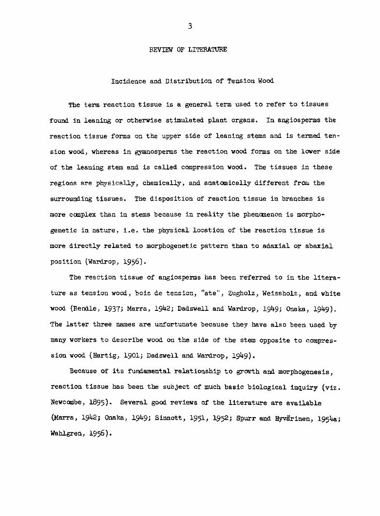
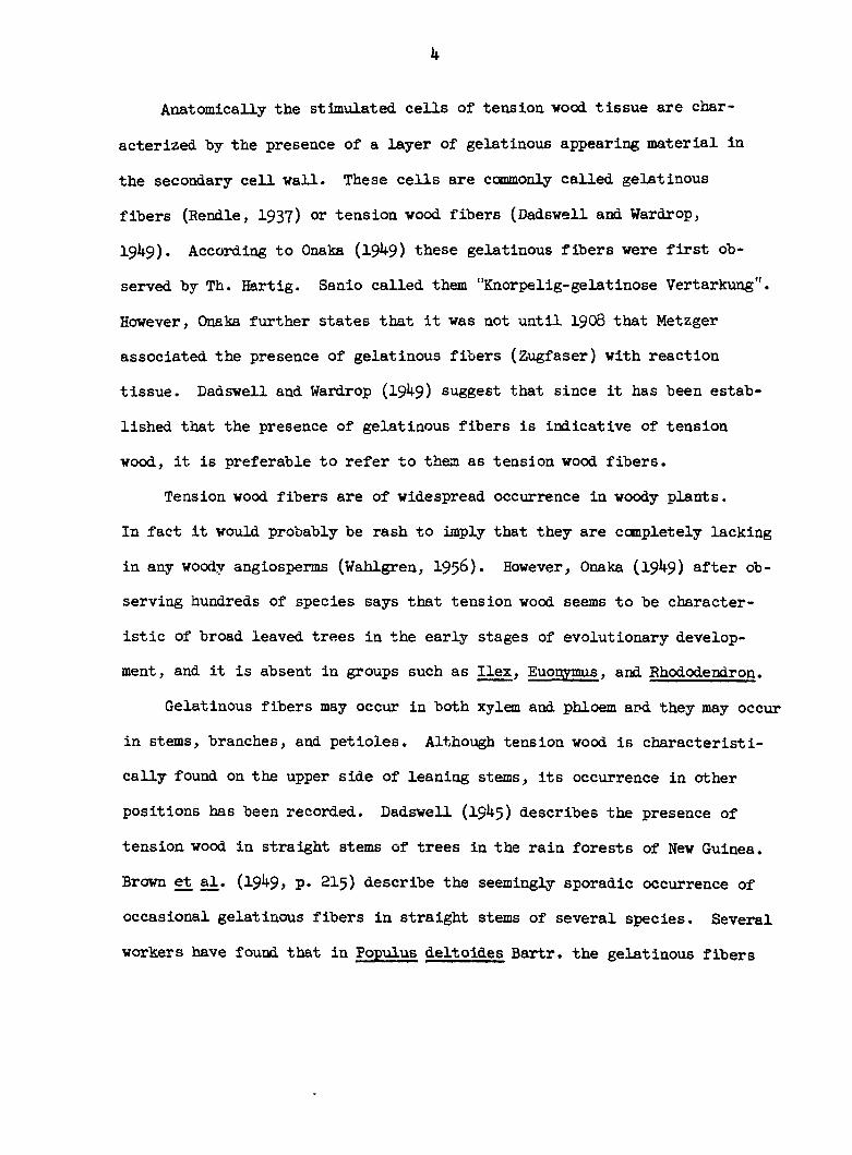
ing gradations from the extremes. Figures 1 and 2 show some typical

bottomland cottonvood stands. The striking uniformity of height growth

of this intolerant species evidences uniformity of the site conditions.

Fluctuations in growth conditions are revealed by abrupt height variation.

Field Plot Investigation

Trees on each of the 14 plots were individually measured, sampled, and

described. Leaning trees were limited in number and on the average about

six suitable trees were available on a given site area. Data recorded in

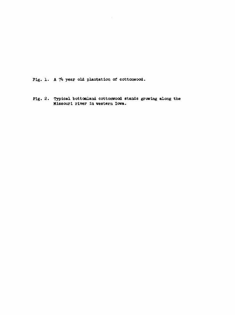
Pig. 1. A 74 year old plantation of cottonwood.

Fig. 2. Typical bottomland cottonwood stands growing along the Missouri river in western Iowa.

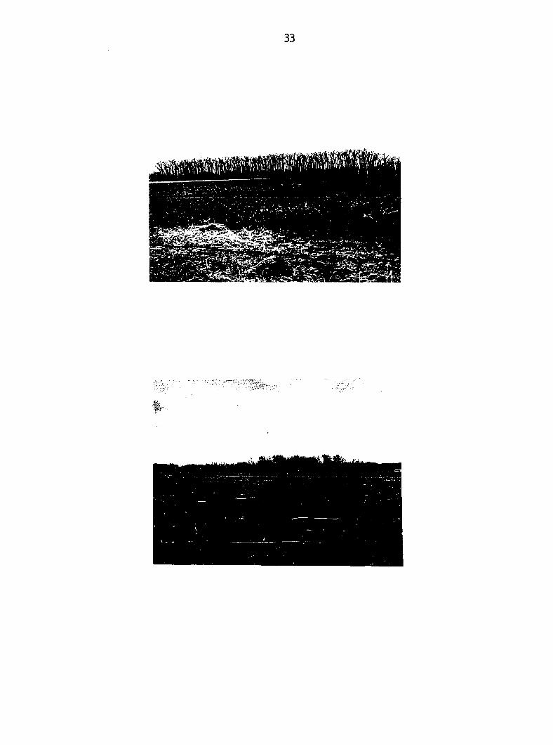
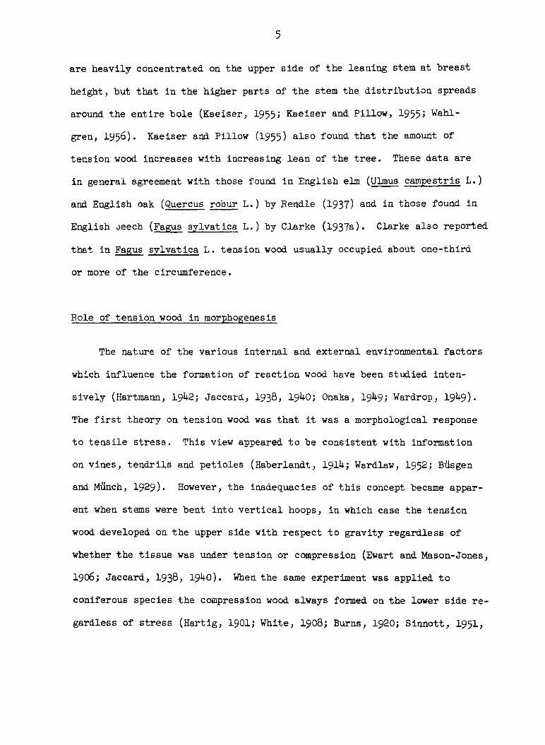
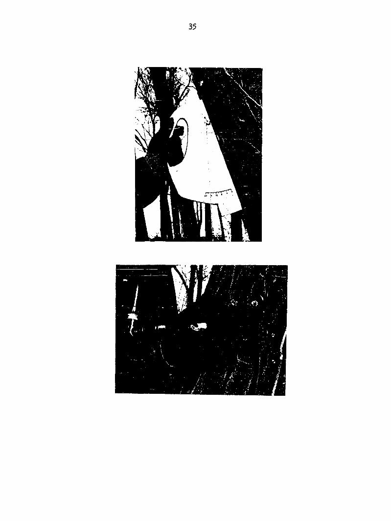
Fig. 3* Measuring a leaning tree with the inclinometer.

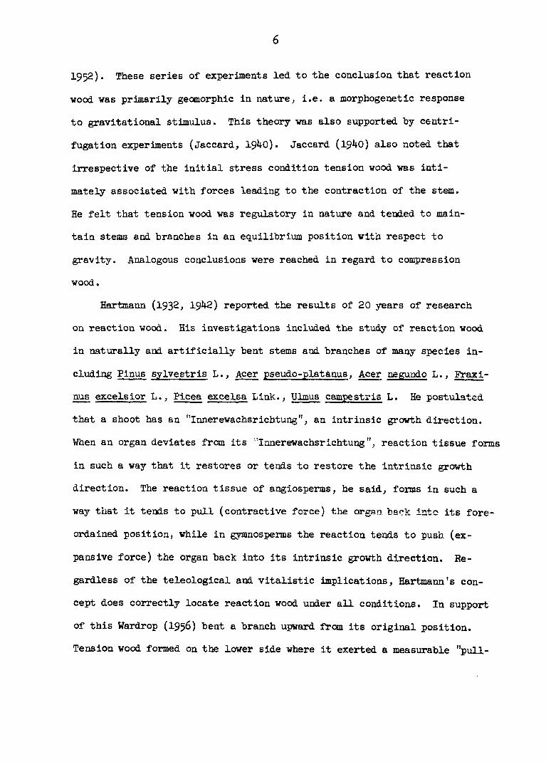
Fig. k. An extracted sample core.

36

the field included the following:

1. Plot and tree numbers

2. Date of sampling and age of timber

3. Diameter at breast height in inches (d.b.h.)

4. Two orthogonal crown diameters in feet

5. Crown length, symmetry, and position in canopy

6. Total stem height in feet

7. Lean at breast height (b.h.) in degrees and direction of lean

In addition a sketch of each tree was made on the field sheet. Height

measurements were made with a Haga altimeter and diameters were measured

by tape. Lean was measured with an inclinometer as shown in Figure 3*

Sampling for the histological studies consisted of extracting three

large cores of tissue containing xylem, cambium, and phloem. These cores

were taken at a point feet from the ground and on the upper side of the

leaning stem. This vertical elevation is termed breast height (b.h.) in

the forestry literature, and here the sampling points were also loci of

reaction tissue. The three cores were taken in such a way that the upper

one-third of the circumference was sampled. A center plug was taken frcm

the upper side and in the plane of maximum lean. The other two cores were

taken at points along the circumference (at b.h.) so that the one-third

coverage was effected. The following example illustrates the procedure.

Tree A had a diameter at breast height (d.b.h.) of 20

inches. Its circumference was 62.8 inches, one-third

of this being 20.9 inches. Therefore the two side cores

were taken at points which were I0A5 circumferential

inches on either side of the center plug.

37

The plugs were numbered 1, 2, and 3 from left to right with the designa­

tion made as the investigator faced the direction of lean. Upon extrac­

tion the three cores were individually labelled and then placed in a

labelled sample bottle of ?0 percent ethyl alcohol. The bottles were

identified by plot and tree and were then stored for subsequent use.

A one-half inch plug cutter was used for the core extraction. The

cutter was used in an ordinary brace and bit and Figure k shows the cutter

and an extracted core. Generally, the cores were about two inches in

length which was sufficient to insure the presence of three annual incre­

ments of xylem.

The field sheet information was tabulated and organized for mens tara-

tional computations. This phase of the study is discussed in a subsequent

section.

Laboratory Investigation

Microtechnique

The cores were removed from the 70 percent ethyl alcohol and trimmed

before sectioning. This process consisted of shaping a block of tissue

which contained the cambium and three annual increments of xylem. Sections

were cut unembedded at approximately 13 microns. A Spencer sliding micro­

tome was employed for this procedure. The specimens were oriented so that

the cambium and the three increments of xylem appeared in cross section.

For the bulk of the histological work the sections were immersed in a drop

of chloroiodide of zinc placed directly on the glass slide, and cover

38

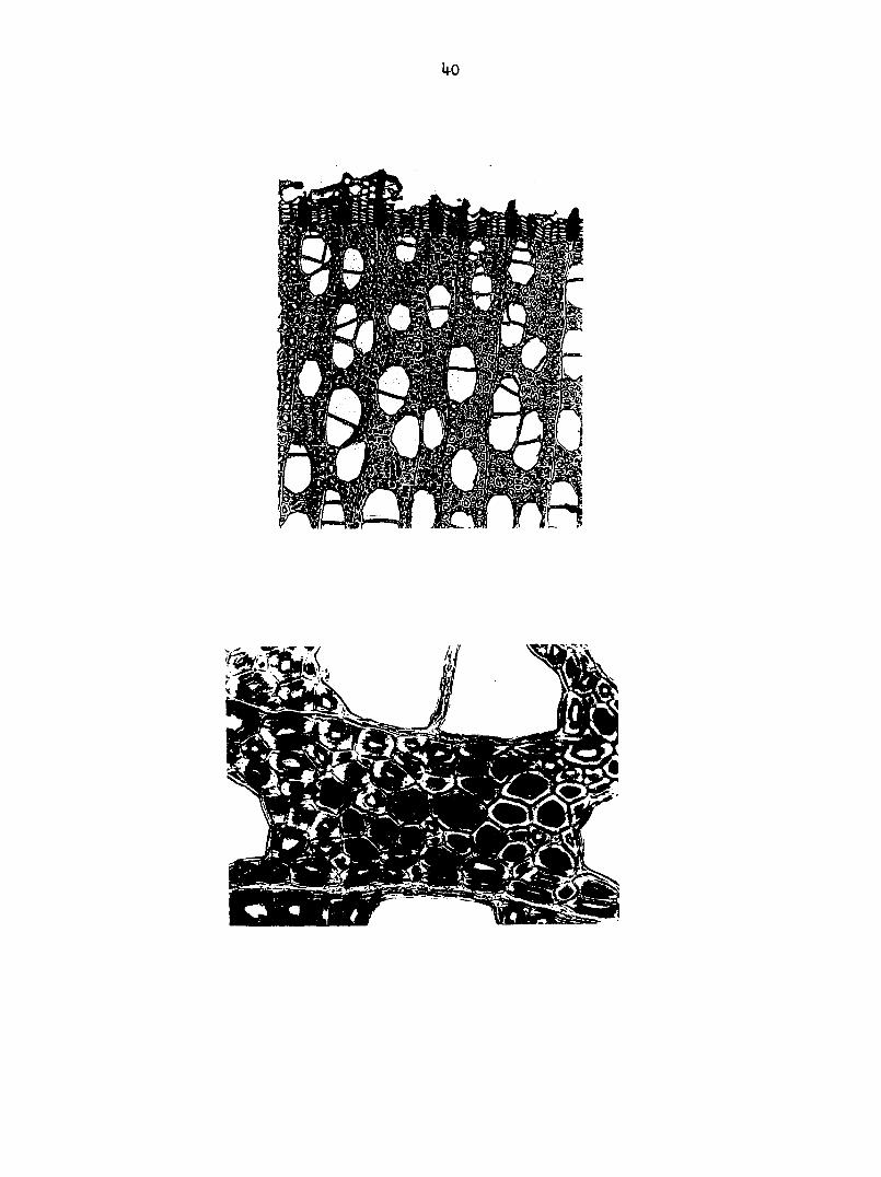
glasses were sealed with wax. This temporary stain is specific for the

cellulosic material of the so-called gelatinous layer of the cell wall

of tension wood fibers. The gelatinous layer of the stimulated cells

stains dark blue, and in eastern cottonwood frequently swells into the

cell lumen in response to this stain. The zinc chloride swells the cellu-

losic material, and in this condition the material becomes stainable in the

presence of potassium, tri-iodide. (See Fig. 5 and Fig. 6). The unstimu­

lated cells do not exhibit this reaction sequence. On the basis of starch

chemistry the deep blue indicates long chain molecules.

Some permanent slides were made with a safranin-fast green staining

combination. The gelatinous layers took up fast green and frequently

swelled into the cell lumens. The non-stimulated cells stained with

safranin only.

Quantitative histological analysis

The following procedures were employed for the main part of the

study. Variations of this analytical method were used for certain special

purposes and these will be described subsequently. The essentials of the

principal histological analysis were published previously. (See Berlyn,

1959). The center cores on 13 plots were analyzed by the following method,

but on plot 2 all three cores were analyzed. The temporary slides were

projected vertically at magnification I39X with a microprojector using a

ribbon filament lamp. The heat supplied by carbon arc lamps limits their

use for these temporary mounts. The image of the tissue with its three

included annual increments was projected on a paper grid system which was

Fig. 5. Transverse section of the cambium and subjacent tissue which has been stained in chloriodide of zinc. 10QX

Fig. 6. Transverse section showing gelatinous fibers stained with chloriodide of zinc. 40QX

kl

taped to a desk surface. Observations for each microscopic field were re­

corded on separate grid sheets. These sheets serve as a permanent record.

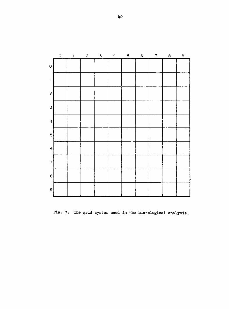
The mult Hit hed 10 x 10 grid pictured in Figure 7 measures 12.5 cm* by

12.5 cm. Each grid square is I.25 cm square. At 139X the entire grid

system covers an area of tissue 0.9 mm. by 0.9 mm. or 810,000 square mi­

crons. Each of the 100 individual grid squares then encloses 0.09 mm.

by 0.09 mn. of tissue or 8100 square microns. Three grid systems were

analyzed for each of three annual increments, making a total of 9 grid

systems per slide. The grid systems within each annual increment were

located systematically for maximum coverage. Within a grid system 8 grid

squares were selected at random for observation. This was conveniently

done with the aid of a random numbers table (Snedecor, 195&, pp. 10-13).

Each square in the 10 x 10 grid system can be identified by its respective

coordinates. A pair of coordinates like 3,6 identifies the grid square

at the juncture of column 3 and row 6.

In each of the individual grid squares selected for observation actual

counts were made of stimulated and nonstimulated cells. The data were re­

corded directly in the individual grid squares. In the binomial system

used, the first number in a particular grid square refers to the number of

cells with a gelatinous layer and the second number refera to the number

of nonstimulated cells. Since 8 grid squares were analyzed per grid sys­

tem, data were recorded for 72 grid squares per slide. On the average about

15 cells were tabulated in each square and hence, about 1100 cells were

tabulated per slide. Proportion of gelatinous fibers as used here means

the number of stimulated cells divided by the total number of cells (G/N).

This index was calculated on a per ring and a per tree basis.

k2

0 I 2 3 4 5 6 7 8 9

0

1

2

3

4 !

5

6

7

8

9

Fig. 7. The grid system used in the histological analysis.

%3

In the correlogram analysis, which will be fully elucidated later,

a variation of the basic procedure was employed. Sections from five

trees of varying lean were prepared in the usual way. On each of the

five slides a single annual ring was selected for analysis. The Image

of this annual ring was projected on the paper grid system as usual.

The objectives, however, were to obtain information on the variance

of data taken by this technique and also to examine the mathematical

structure of the sampling system in relation to the specific phenomenon

of interest (reaction tissue). This involves replication which builds up

frequency data. Five grid squares were selected which were at different

grid square distances from each other. Figure 11 shows the fixed samples

that were used on each of the grid systems. The sets of coordinates were;

(1) 0,0; (2) 1,0; (3) 3,0, (4) 6,3; and (5) 9>9« Distances between squares

were computed from Pythagorean relationships. These distances were re­

corded and used for plotting purposes. This was a fixed sampling scheme

and each grid system was identically marked. On each ring 2k grid systems

were analyzed, three at a time. The positioning of each set of three grid

systems was identical to positioning of the three grid systems per ring in

the main study. This involved 2 grid systems near the edges of the section

and one in the center. The grid systems were twirled so that a random

placement was effected. Since the grid squares were the same fixed dis­

tances from each other it was possible to calculate correlation coeffi­

cients between the squares. Also the variance of the percent gelatinous

fiber figures was calculated. The results aad discussion of this study are

taken up in a following section.

Another variation of the main analysis was developed in order to study

44

the relative efficiency of weighted as compared to unweighted means. This

consisted of running a 100 percent sample on a grid system.

45

EXPERIMENTAL OBSERVATIONS

Field. Observations

The concentration of foliage on the upper side of the stems of lean­

ing Cottonwood trees is shown in Figure 8. In general this was found to

be the case. This supports the observations of Strassburger in 1891 and

will be referred to in this report as the Strassburger effect. Figure 9

illustrates an inverse effect. This tree was growing along the edge of

a cottonwood grove, and light reactivated dormant buds on the lower side

of the stem. Figures 8, 9, and 10 also illustrate the phototropic nature

of the species. Any opening in the canopy is a source of lean and there­

fore reaction tissue.

Histological Observations

Correlogram studies

Quantitative histological data in the form of precise numerical at­

tributes have not been used extensively; therefore, it was necessary to

develop specialized statistical techniques and to investigate the assump­

tions Implicit in each proposed mathematical model.

The first investigation was the study of the correlograms. The

specific histological technique for this study has been previously

described. This approach was designed to elucidate the geometrical con­

figuration of gelatinous fiber initiation. Specifically, the relationship

of percentage figures, Pi, in various squares of the grid system was re-

Fig. 8. Strassburger effect showing foliage on the upper side of a leaning stem.

Fig. 9« Inverse Strassburger effect showing reactivated buds.

Fig. 10. Phototropic response of a cottcnwood stand..

1*9

50

vealed. The squares were at fixed distances apart and by computing corre­

lation coefficients it was possible to see whether certain squares tended

to be more like each other than like other squares. For example, squares

that were close together could resemble each other, particularly if the

gelatinous fibers were laid down by the cambium in rather large groups.

Tables 2 and 3 represent the experimental evidence on this phase of the

study.

The 5 fixed squares were labelled A, B, C, D, and E. The straight

line distances between the squares from center to center are given in

Table 4. Figure 11 shows a paper grid with the 5 fixed squares.

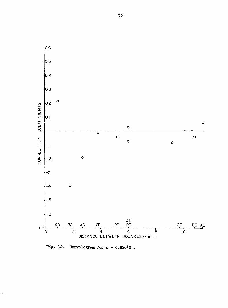
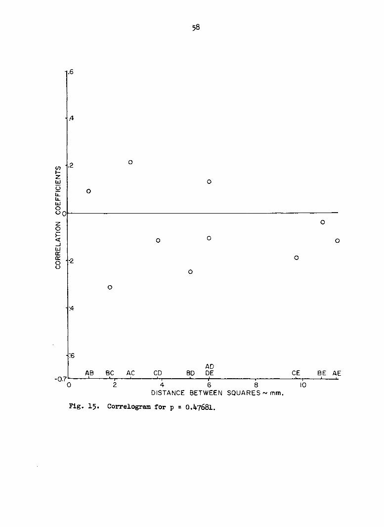
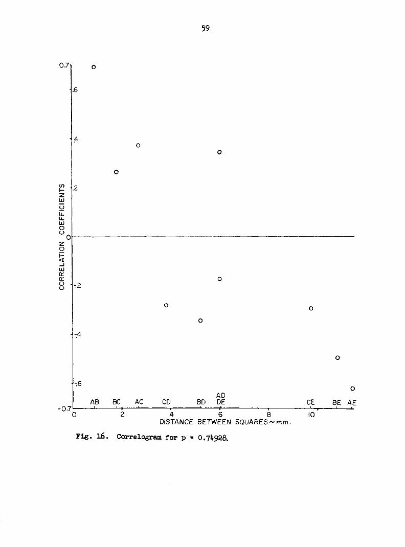
Figures 12 through 16 are plots of the mean correlation coefficients

between the five squares against the actual distances between squares.

Figure 17 is the summary graph of all 5 annual increments. The magnitude

of the correlation coefficients is low. There is apparently no strong

relationship between distance and correlation.

The question of interest was whether grid squares situated in close

proximity on the grid system tend to have more similar pi than distantly

located squares. Since the correlation coefficients, which are a measure

of linear association, hover around zero, it appears that most of the grid

squares are independent. Evidence and potential application, however, in­

volve only the concept of pairwise correlation. As a rough illustration

of the meaning of pairwise correlation, we give the following definition

of the stronger but similar property of pairwise independence:

fPa< Pi,A<: PbJ " *r (Pa < Pi,A<Pb I P e < Pi,D<Pf J = Pr (Pa<Pi,A<Pb I Pc<Pi,C^Pd j »

51

0 1 2 3 4 5 6 7 8 9

A B C

D

E

Fig. 11. Grid system showing fixed sample.

52

Table 2. Correlation coefficients between grid, squares.

Proportion gelat inous Square s fibers

Correlation coefficients B C D E

0.22642

Average

0.28426

Average

A B C D E A B C D E A B C D E A B C D E

A B C D E A B C D E A B C D E A B C D E

0.114663 0.341405 -0.497193

0.411063 -0.425887 -0.167167

0.125686 -0.490708 -0.522062

0.217137 -0.191730 -0.395470

-0.319907 -0.528800 0.723160

0.061586 0.271266 -0.305051

•0.736837 -0.333490 0.730381

-0.330519 -0.197008 0.382830

-0.069505 0.029034 0.139501 -0.418778 -0.488705 -0.108394-

-0.146198

0.080973 -0.144727 0.549283 -0.127508 0.151280 0.368862

0.336279

0.058718 0.288784 •0.819285 0.409461 0.303748 -0.736709

-0.425748

0.023395 0,0*7607 -0.043500 -0.043606 -0.011226 -O.O86477

-0.078555

-0.152745 0.404753 -0.050556 0.565549 0.029260 0.470467

-0.044340

0.598657 -0.118428 -0.567583 -0.395826 0.525746 0.339969

0.097121

-0.520509 0.045363 0.420526 -0.213706 0.616736 -0.453504

0.252878

-0.024866 0.110563 -0.065871 -0.014661 *0.390580 0.118977

0.077190

53

Table 2. Continued

Proportion Correlation coefficients gelatinous Squares A B C D E fibers

O.45099 L A 0.117692 -0.673413 0»55697b 0.164973 B -0.179976 -0.240773 0.827149 c -0.689636 -0.304113 D -0.I52074 E

C A 0.482756 O.395292 0.291030 -O.47983I B 0.358752 0.802452 -O.587833 C 0.369434 -0.644290 D -O.I74129 E

R A 0.756405 O.5988IO 0.270372 -0.337444 B 0.499835 0.605423 -O.54OO73 c 0.253156 -0.749578 D -O.478O38 E

Average A 0.452284 0.106896 0.393460 -O.2i74.34 B 0.226203 0.389034 -0.100252 C -0.022348 -O.565993 D -O.268O8O E

0.47681 L A 0.753450 -0.124003 O.O896I5 -O.O3I798 B -0.401045 "0.340518 -0.076684 c 0.106721 0.015320 D 0.461536 E

C A -0.018457 0.627988 -0.121839 0.026020 B -O.5I2465 -O.O5477I 0.170520 c -0.314040 -0.183461 D -0.374015 E

R A -0.451329 0.152881 0.433915 -0.344972 B -0.020288 -O.336879 -0.201393 c -O.I23962 -O.4OI234 D -0.401035 E

Average A 0.094554 0.218955 0.133897 -O.II6916 B -O.3II266 -0.244056 -O.O35852 c -0.110427 -O.I8979I D -0.104504

Table 2. Continued.

5%

Proportion gelâtinous Squares fibers

Correlation coefficients B C D

0.74928

Average

A B C D E A B C D E A B C D E A B C D E

0.841441 0.802306 0.893685

0.596110 0.116331 -0.048993

0.633612 0.201048 -0.048838

0.690387 0.373228 0.265284

-0.792379 -0.730012 -0.609828 -0.656052 -0.537215 -0.566290

0.738126

-0.351318 -0.669344 -0.364269 -0.348515 -0.287283 0.113216

0.131420

0.614275 -0.452507 -0.050956 -0.474814 -0.022739 -0.437437

0.175930

-0.176474 -0.617287 -0.341684 -0.493127 -0.282412 -0.296837

0.348494

Table 3- Grand average of correlation coefficients between grid squares.

Squares Correlation coefficients A B C D E

A 0.224769 0.062068 0.069882 -0,156675 B 0.033516 -0.061215 -O.I375OO C -O.OO7I67 -0.204024 D -O.OO5O9I E

Table 4. Distances between squares in mm.

Squares A B C D E

A 0 0.90 2.70 6.04 11.46" B 1.80 5.25 10.84 C 3.82 9.74 D 6.04 E

55

i0.6

05

•0.4

0.3

co "|0.2 l— z UJ

y 4o.i

LU

Boh

UJ cc g 4-2 u

-.3

o o

o

-.4

-.5

AD AB BC AC CD BD DE CE BE AE

-0.71 ' H ' h 1 •—i— 0 2 4 6 8 10

DISTANCE BETWEEN SQUARES ~ mm.

_L_

Fig. 12. Correlogram for p • 0.22642 .

56

.6

.4

.2

-.2

-.4

O o

AD AB BC AC CD BD DE CE BE AE

1 1 1 1— 4 6 8 10

DISTANCE BETWEEN SQUARES~mm.

Fig. 13. Correlogram for p • 0.28426,

57

.4

.2

- 2

-.4

O

AD AB B C AC CD BD DE CE BE AE _i L-, i *—i ' 1< 1 i * •

2 4 6 8 10 DISTANCE BETWEEN SQUARES*, mm.

Fig. 14. Correlogram for p • 0.4-5099.

58

.6

.2

-2

:4

AD AB BC AC CD BD DE CE BE AE

4 6 8 10 DISTANCE BETWEEN SQUARES ~ mm.

Fig. 15. Correlogram for p = O.4768I.

59

0.71

.6

V) i-z UJ

u u_ u. UJ O °0h

UJ cr cc IB 1^2

-.4

O AD

AB BC AC CD BD DE CE BE AE -0.7' ' _1_

0 2 4 6 8 10 DISTANCE BETWEEN SQUARES ~ mm,

T"

Fig. 16. Correlogram for p - 0.74928.

6o

.6

.4

P z UJ

u LL U. O

O ° o (jj e o~

z o

UJ cr

o 1-2 u

-.4

1-6

AD AB BC AC CD BD DE CE BE AE

- 0.7 ' '-i ' H ' i 1 •—i ' «• 0 2 4 6 8 10

DISTANCE BETWEEN SQUARES ~ mm.

Fig. 17. Grand average correlogram.

61

i.e., the probability that the proportion pijA in square A lies between

pa and pfc when the proportion pi>D in square D lies between Pe and pf

is equal to the probability that the proportion pijA lies between Pa and

pb when the proportion p^g in square C lies between pc and p^.

The question of correlation of p^ is of course based upon only a

finite number of sampling repetitions, hence is subject to the usual

sampling variation. It should be further noted that each annual incre­

ment selected for this study constitutes a separate population sampled

from, each with its particular "true" population correlation coefficient.

Hence, any empirical correlation coefficient obtained by averaging over

empirical ring correlations is in effect an estimate of the average of the

true population correlation coefficients.

The correlagram analysis reveals some aspects of the cambial response.

For example, if the stimulated cells were laid down in sufficiently large

clumps, correlation between proximate squares would be expected to be higher

than correlation between more distant squares. If the ruction was more

diffuse, the previously described independence would be expected. It should

be noted that there is a suggestion of positive correlation between adjacent

squares and negatave correlation between distant squares (see Figure 17).

This suggests that clumping may extend somewhat beyond the confines of a

single grid square. With sufficient mathematical sophistication it should

be possible to derive effective clumping radii. It may be noted that nega­

tive correlation between distant squares might indeed be expected to occur

under "clumping", since, if a certain clump of stimulated cells occurs, say

in grid square A, it is automatically excluded from grid square E.

62

It must also be recognized that marked histological population

differences can occur, for example when there are abrupt variations in

the reaction response of a given increment. The stimulated cells may-

stop or start abruptly. This, however, is presumably due to discon­

tinuity in the stimulus rather than particulate distribution. This

may also be a factor in the void of stimulated cells which often appears

at the annual terminus.

It may be of interest to close this section with two technical com­

ments alluded to in the above discussions.

1. Significance of the correlation coefficients in Figure 1%:

z * l/2 £ln(l * r) - ln(l-r)J dz/dr = l/2 f 1 • 1 1 : 1 ,

1 4 r 1-r J l-r^

where z = the normal transformation of r r = sample correlation coefficient

= population correlation coefficient

Var(r) = (var z) ( -^"|p )2 (Volk, 1958, p. l4l)

Var(r) = (l/(n~3)) (l-r^|p , where we estimate by r.

SD (r) = l-r^ , where SD(r) = standard deviation of r -/ n~3 n : number of units in a sample

(i.e., 8)

SD(ric) = l-r^ , where (r) is an average of 15 numbers. yi5(n-3)

2 SD(r)i^ defines an approximate 95 percent confidence interval

around the zero line. In the case of Figure 17 the confidence limit is

0.2188. The magnitude of the adjacent and most distant correlation coef­

ficients is about O.23. They are significantly different from zero.

2. Potential usefulness of the negative correlation between distant

grid squares.

63

Var(X*Y) = Var(X) * Var(Y) •» 2Cov(X,Y) (Snedecor, 1956, p. 168)

where Cov(X,Y) =/) xy V Var(x) Var(Y)

In this case p xy is negative, and hence the variance of X-*Y is

reduced.

These comments indicate that random sampling might be Improved upon,

since the addition of negatively correlated quantities actually leads to

low variance. This could be accomplished by developing a sampling

system which utilizes the negative correlation between distant squares.

An appealing procedure is to randomly place a large fixed geometrical con­

figuration (e.g., an equilateral triangle) on the grid system to be

sampled, selecting squares to be tabulated by the vertices of the con­

figuration.

Efficiency of weighted means

In this phase of the study a single grid system was analyzed in its

entirety, i.e., data were recorded in each of the 100 grid squares. Tree

33 from plot 5 was used in this study, and the data are recorded in

Table 5.

Table 5» Complete grid system analysis of tree 33» Weighted Weighted Unweighted Unweighted Sample v ariance Popula-popula- sample population population estimate of sample tion

Lean tion mean mean variance of means binomial mean population variance

variance

12 0.8820 0.8533 0.8306 0.0493 0.02152 0.002475 O.OO763

6h

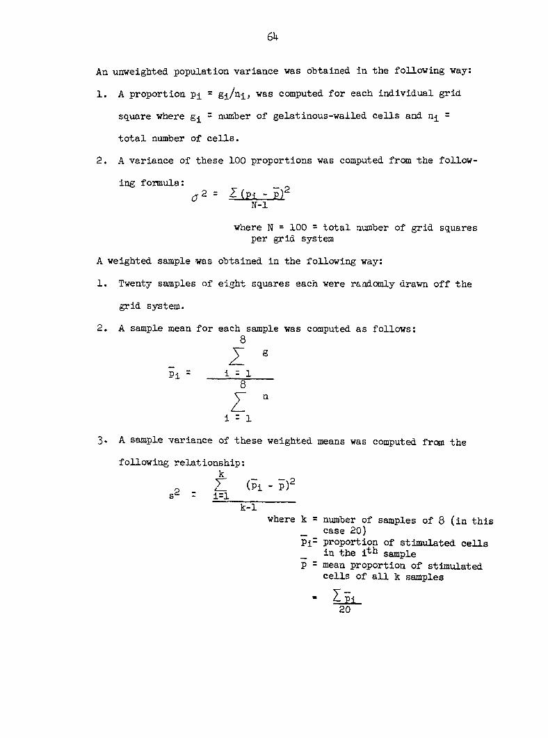
An unweighted population variance was obtained in the following way:

1. A proportion Pi = g±/n±, was computed for each individual grid

square where g^ - number of gelatinous-walled cells and n^ =

total number of cells.

2. A variance of these 100 proportions was computed from the follow­

ing formula : _ 6 2 = ^(Pi - P?

N-l

where N = 100 = total number of grid squares per grid system

A weighted sample was obtained in the following way:

1. Twenty samples of eight squares each were randomly drawn off the

grid system.

2. A sample mean for each sample was computed as follows : 8

Z 8 Pi = i = 1

8

z * 1 = 1

3. A sample variance of these weighted means was computed from the

following relationship:

2 H (Pi " P)2

s : 1=1 k-1

where k = number of samples of 8 (in this _ case 20) Pi= proportion of stimulated cells _ in the 1th sample P = mean proportion of stimulated

cells of all k samples

• Lii_ 20

65

4. From the above sample mean variance it is possible to obtain an

estimate of the population variance from the following formula:

A2v = s2 Nn (Cochran, 1953, P- 10) 0

where N = total number of squares in the population = 100

n - number of grid squares per sample = 8

A binomial variance may also be computed since P and % are known:

V = PQ , where V = binomial variance n P = the population proportion of

gelatinous fibers Q = (1 - P) n - average number of cells per

grid square

This binomial variance is actually of pseudobincmlal character because of

the random denominator.

For tree 33, s2 = 0.002475, q\ = 0.02152, <j2 = 0.0493, and

V = 0.00763* A 95 percent confidence interval can be computed from the

following well-known relationship:

L - * / A 2 / x 2 (Snedecor, 1956, _ 2 ^ 2 P* 59) X 0.025 0.975

For our situation this becomes:

s2 ( irr)(19) p s2 (_m_)(i9)

2 < û v ^ N-n

"X. O.025 _^2 0.975

This yields:

.2 0.01245<rj% 0.04589

66

The interval does not include the unweighted population variance. Effi­

ciency is gained by using weighted sample means.

R. E. = a2 = 0.0493 = 2.291 0.02152

f w

This represents a gain in efficiency of 129 percent. A confidence interval

may be placed around the efficiency.

0.0493 > Ef > 0.0493 0.01245 0.04589

3.96O 2: Ef S 1.074

Weighted means of samples were used throughout this entire study. It is also

obvious that sampling variance was not binomial here. The next section will

attempt to further clarify this.

Investigating the advisability of a transformation

When dealing with proportions, especially with proportions subject to

substantial variation, it is often advantageous to transform the data to

some more stable scale of measurement. However, a transformation offers

certain dangers to the exactitude of inferences. This is especially rele­

vant when the denominator of the proportion varies. The data in this study

are of the form gi/ni • p^ , where g^ is the number of anomalous cells and

n^ is the total number of cells for thfct unit. The ni's vary slightly and

the Pi's vary from zero to one. In this situation a useful transformation

should meet the following stipulations:

1. The situation should be such that the variance is a function of

P, (V(P)), where P is the population mean.

67

2. The variance should be stabilized, i.e. VT(P) ~ VT , where

is the variance of the transformation.

3. Inference on PT should be "similar" to inference on AP,

i.e., the differences in the population means should be similar

for the transformed and untransformed case. This stipulation

suggests the employment of a single monotone transformation

applied to all p^'s.

4. In view of Stipulation #2, VVt(P) ^ -/Vt and not much Prp Ftp

greater than Vv(P) . This stipulation requires that the P

transformation be such that it does not inflate the variance at

the expense of sharpness of inference on P.

Weighting transformed values by/ni , the square root of the total

number of cells in a sample, poses a danger to the validity of inference

as outlined in Stipulation #3*

A study of the nature of the variances was designed in order to deter­

mine the advisability of a transformation. The question to be resolved was

whether to use the untransformed p^, /pj , or sin™1 VpÏ • The arcsine is

a commonly used transformation for proportions. This transformation

weights more heavily the small percentages which have small variance if

the distribution is of the binomial form.

Figure 18 was derived from the five rings used in the correlogram

study. The data are presented in Table 6. The variances of p^, Jp±, and

sin"1 VpI"were computed for each of the five rings. In addition a pseudo-

binomial variance was computed for each ring from the well known formula

V = pq/n , where p - proportion gelatinous fibers, q = (i-p), n = average number of cells per replication (15 squares).

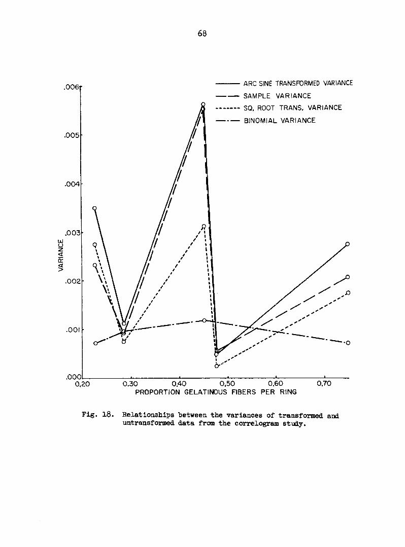
68

ARC SINE TRANSFORMED VARIANCE

SAMPLE VARIANCE

SO, ROOT TRANS. VARIANCE

BINOMIAL VARIANCE

.0001— 0.20 0.30 0.40 0.50 0.60

PROPORTION GELATINOUS FIBERS PER RING 0.70

Fig. 18. Relationships "between the variances of transformed and untransformed data from the correlogram study.

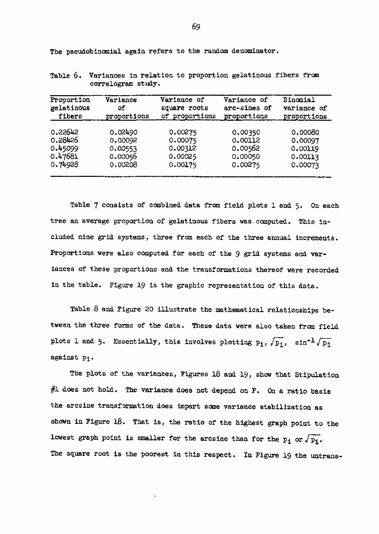
69

The pseudobinomial again refers to the random denominator.

Table 6. Variances in relation to proportion gelatinous fibers from correlogram study.

Proportion gelatinous

fibers

Variance of

proportions

Variance of square roots of proportions

Variance of arc-sines of proportions

Binomial variance of proportions

0.22642 0.28426 0.45099 O.4768I 0.74928

0.02490 0.00092 O.OO553 O.OOO56 0.00208

0.00275 O.OOO75 0.00312 0.00025 O.OOI75

O.OO35O 0.00112 O.OO562 0.00050 O.OO275

0.00080 0.00097 0.00119 0.00113 0.00073

Table 7 consists of combined data from field plots 1 and 5. On each

tree an average proportion of gelatinous fibers was computed. This in­

cluded nine grid systems, three from each of the three annual increments.

Proportions were also computed for each of the 9 grid systems and var­

iances of these proportions and the transformations thereof vere recorded

in the table. Figure 19 is the graphic representation of this data.

Table 8 and Figure 20 illustrate the mathematical relationships be­

tween the three forms of the data. These data were also taken from field

plots 1 and 5. Essentially, this involves plotting p^, /p^, sin"1 V™Pi

against pj_.

The plots of the variances, Figures 18 and 19, show that Stipulation

#1 does not hold. The variance does not depend on P. On a ratio basis

the arcsine transformation does impart some variance stabilization as

shown in Figure 18. That is, the ratio of the highest graph point to the

lowest graph point is smaller for the arcsine than for the p^ or /p^~.

The square root is the poorest in this respect. In Figure 19 the untrans-

70

Table 7. Variance computations on individual tree basis for Plots 1

and 5.

Average Proportion j-— , / Plot, tree, lean gelatinous fibers V(g/n) Vyg/n V(sin" Vg/n

1 - 6 - 2 0.02987 0.000501 O.OO8O3 0.00817

5 - 31 - 3 0.0000 0.0000 0.0000 0.0000

1 - 3 - 4 0.4221 0.0331 0.0170 0.0397

5 - 30 - 5 0.0000 0.0000 0.0000 0.0000 1 - 13 - 6 0.5803 0.0975 0.0580 0.1231

5 - 34 - 6 0.09478 0.00710 0.01882 0.02105 1 - 12 - 8 0.7890 0.0176 O.OO58 0.032

5 - 29 - 9 0.3283 0.0254 0.0215 0.0316 1 - 5 - 10 0.9188 0.0050 0.0014 0.0144 1 - 4 - 12 0.8121 0.0128 0.0043 0.0272

5 - 33 - 12 0.7960 0.0244 0.0082 0.0459 1 - 8 - 14 0.9364 0.0176 0.0056 0.04.74

5 - 32 - 1 5 0.8230 0.0310 0.0107 0.0715 1 - 11 - 16 0.9281 0.0033 0.0009 0.0111 1 - 7 - 1 7 0.9107 0.0061 0.0017 0.0256

Table 8. Mean values with transformations taken from plots 1 and 5.

gi/%i V6i/ni sin"1ygi/ni

0.0128 O.H32 0.II3 0.1222 0.3496 0.357 0.2237 0.4730 0.493 0.2459 0.4959 O.5I9 O.3267 O.57I6 0.608 0.4054 O.6367 O.69O 0.5289 0.7273 0.814 0.6667 O.8165 0.955 0.8298 0.9109 1.146 0.9009 0.9492 1.251 0.9767 O.9883 1.418 1.0000 1.0000 1.571

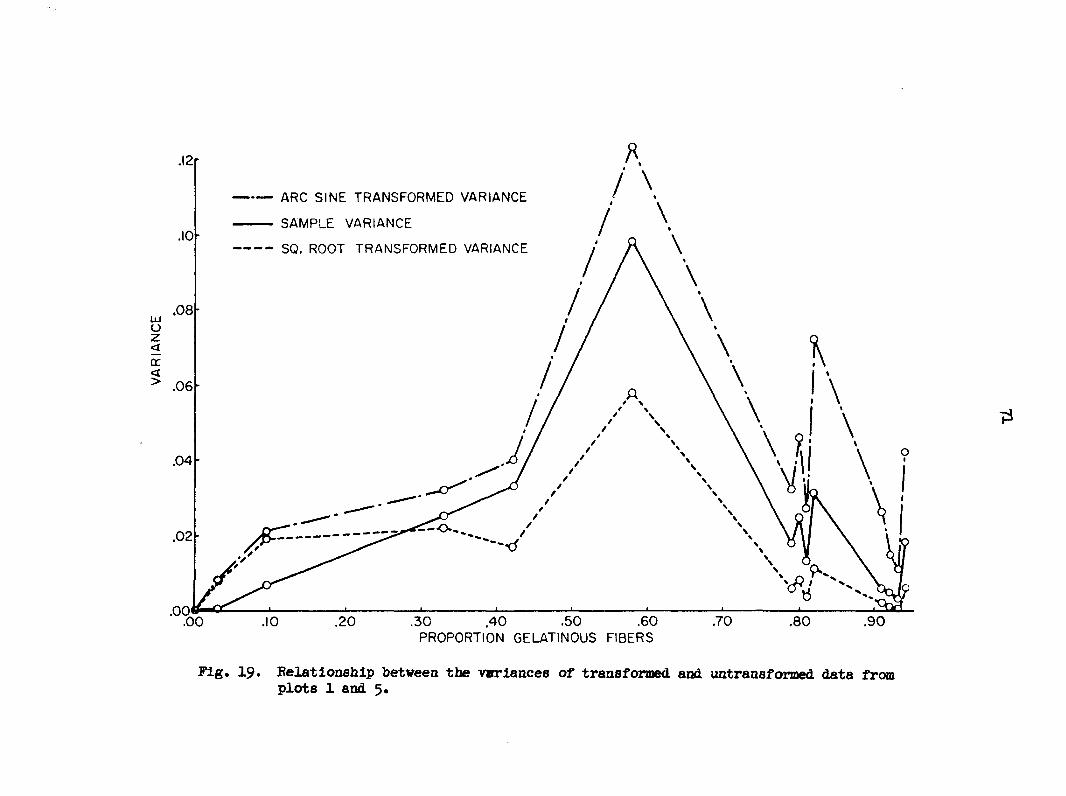
ARC SINE TRANSFORMED VARIANCE

SAMPLE VARIANCE .10

SO. ROOT TRANSFORMED VARIANCE

.06

.04

O-.02

.00' .50 .60 .70 .80 .90 .20 .30 .40 .00 .10

PROPORTION GELATINOUS FIBERS

Fig. 19. Relationship between the variances of transformed and untransformed data from plots 1 and 5.

72

0.8

0.6

0,4

0.2

0.0

Pi

Fig. 20. Mathematical relationships between transformed and untransformed data from plots 1 ancL 5.

73

formed variance is about as stable as the arcsine vhile the square root is

again considerably less stable. The square root transformation deflates

the standard deviation J Vip(P) , i.e.VvfV^Ï) However, it also deflates AP^,

the differences in means. This is shown in Figure 20. The differences are

deflated for three-fourths of the abscissa values. This can be shown as

follows:

y • xl/2

cLy/d* = 1/2 x ~ly/2

when l/2 x"1/2 = 1, x = l/4

This shows that the maximum point of the square root curve above the

straight line p^ curve occurs at one-fourth of the x range. Hence, for

three-fourths of the x range the differences of the means are deflated.

The arcsine does accentuate the zlPrp.

Variances are notoriously variable. This of course is evident in

Figures 18 and 19* For Figure 18 an approximate 95 percent confidence

interval has half length approximately equal to:

±2 J 2 (X « j2 ^8/8 = J"2 (Snedecor, 1956, p. 73) 1 n

This should be considered when studying this graph. The half length of

the confidence interval is equal to the ordinate magnitude.

It is apparent that transformations are not desirable in this case.

Transformations may validate the use of a specific statistical technique,

but may do so at the expense of a considerable amount of information. Con­

clusions drawn from such transformed data may have little biological

validity.

74

Cytohistological observations

During the histological analysis, the width of each annual increment

and the number of cells observed in each experimental unit were recorded

for 29U annual increments from 84 different trees. After the geometric

and analytical study of the quantitative histological methods and of the

distributional form of the data, statistical examination of the micro­

scopic data was conducted for cell number, ring width, and proportion of

gelatinous fibers.

The term "ring width" refers to the radial tissue growth of the xylem

in millimeters, which occurred during a specific year of interest. With

the previously mentioned exception (plot 2), information was recorded on

three annual increments per tree. Ring width is an additive measure of

growth including cambial division plus cellular enlargement. The "cell

number" designation refers to a more relative consideration, the number of

cells contained in the 2k grid squares analyzed per tree (eight grids per

annual increment). The relativity of the ensuing inferences arises from

the presence of both tracheae and fiber tracheids in the xylem. With this

measurement it is not possible to ascribe variations to fibers or vessels

individually; nevertheless, it is a general measure of transverse cellular

dimensions.

Microscopic observations indicate that small annual increments contain

fewer stimulated cells, and that below some threshold, no gelatinous mater­

ial is synthesized, regardless of the magnitude of stimulation. This trend

is illustrated by Figures 21 and 22. Figure 21 shows the cambium and the

last deposited annual increment of xylem. Note that the population of

Fig. 21. Transverse section showing the cambium and most recent annual increment of xylem. h6x

Fig. 22. Transverse section from same slide as Fig. 21 showing the second and third annual increments. 46%

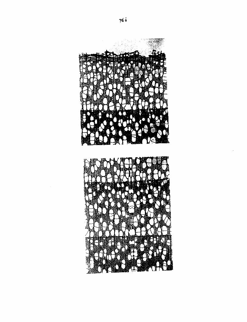
j6o

77

gelatinous fibers is somewhat sparse. Figure 22 is a picture of the same

slide as Figure 21. The population of stimulated cells increases in ring

2, which is somewhat larger than ring 1, and becomes greater in the much

larger ring 3. Note the apparent depression of vessel size in ring 3.

A sequence of 2 or more borderline years often occurs before depression

of reaction takes place. Time can thus substitute for ring width in the

depression of reaction.

Figures 23 and 2k show that the initiation of the gelatinous layer

occurs immediately subjacent to the cambial zone. Presumably, induction

occurs even earlier. The cytological features of the stimulated cell wall

are further depicted in Figures 25 and 26. Figure 26 was taken with polar­

ized light. The opaque appearance of the gelatinous material is due to the

axial orientation of the cellulose micelles in the layer. The wound paren­

chyma and associated stimulation illustrated in Figure 27 represent a par­

tially antagonistic sequence of development. Only partial lignification

is present and tremendous cell enlargement has occurred. Cell division

was also stimulated.

Analyzing triplets

Individual regressions for ring width and for cell number were com­

puted for each tree. Since three annual rings were analyzed per tree, a

series of triplets arose. For ring width there were only 3 significant

F-statistics from 93 triplets (see Table 9). Since 5 percent significant

"F'"s or "t"'s would be expected by chance alone, no obvious relationship

between ring width and proportion of gelatinous fibers was revealed by

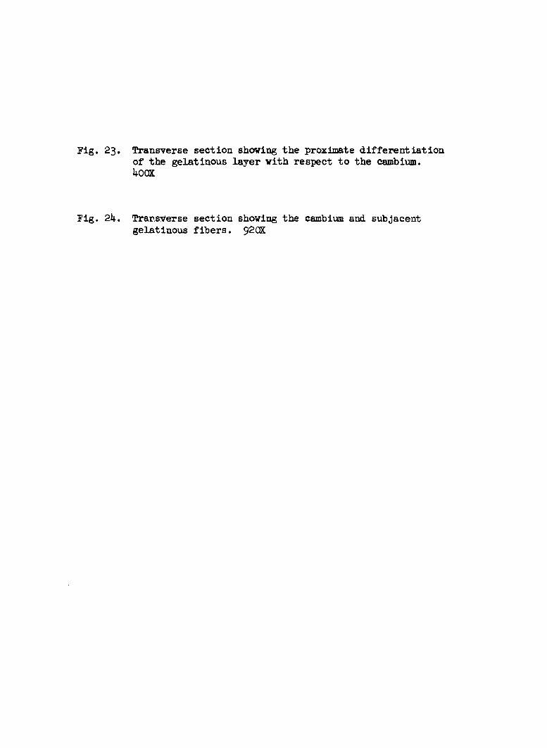
Fig. 23. Transverse section showing the proximate differentiation of the gelatinous layer vith respect to the cambium. UOCK

Fig. 2k. Transverse section showing the cambium and subjacent gelatinous fibers. 92CK

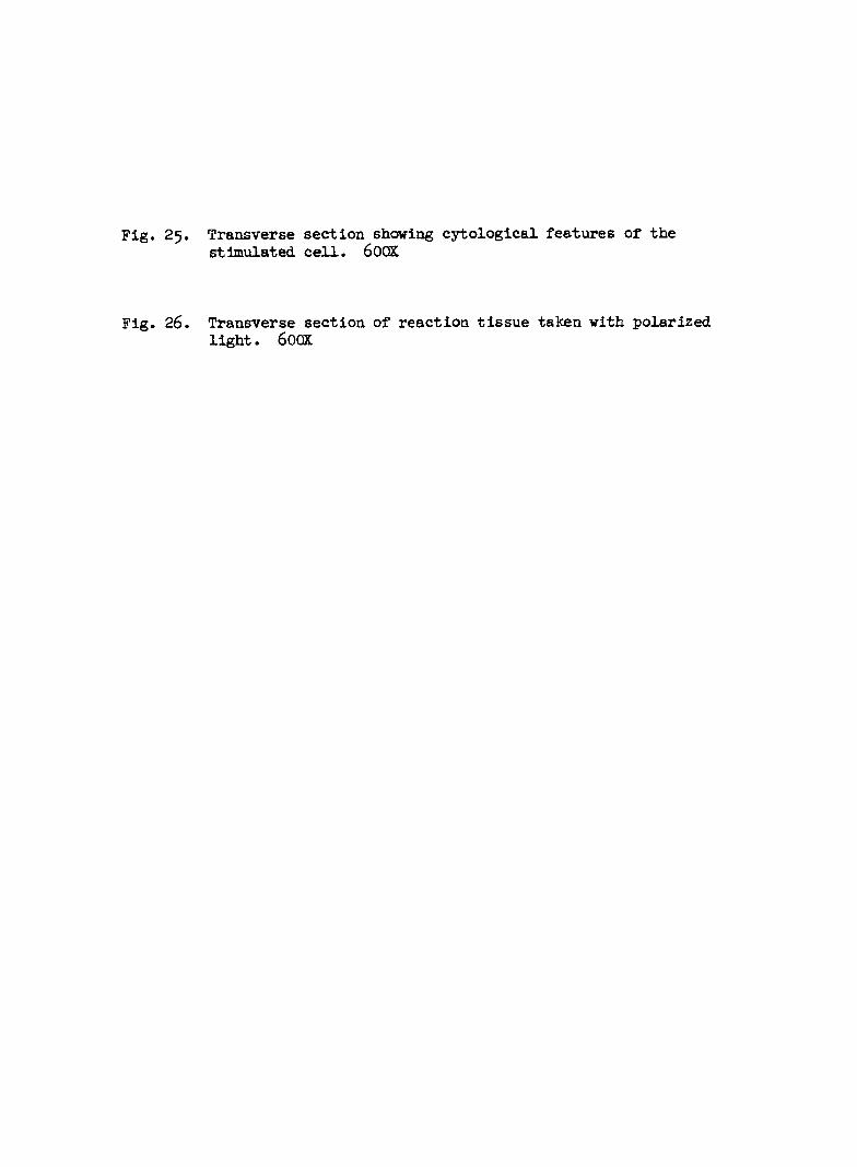
Fig. 25. Transverse section showing cytological features of the stimulated cell. 600X

Fig. 26. Transverse section of reaction tissue taken with polarized light. 60CX

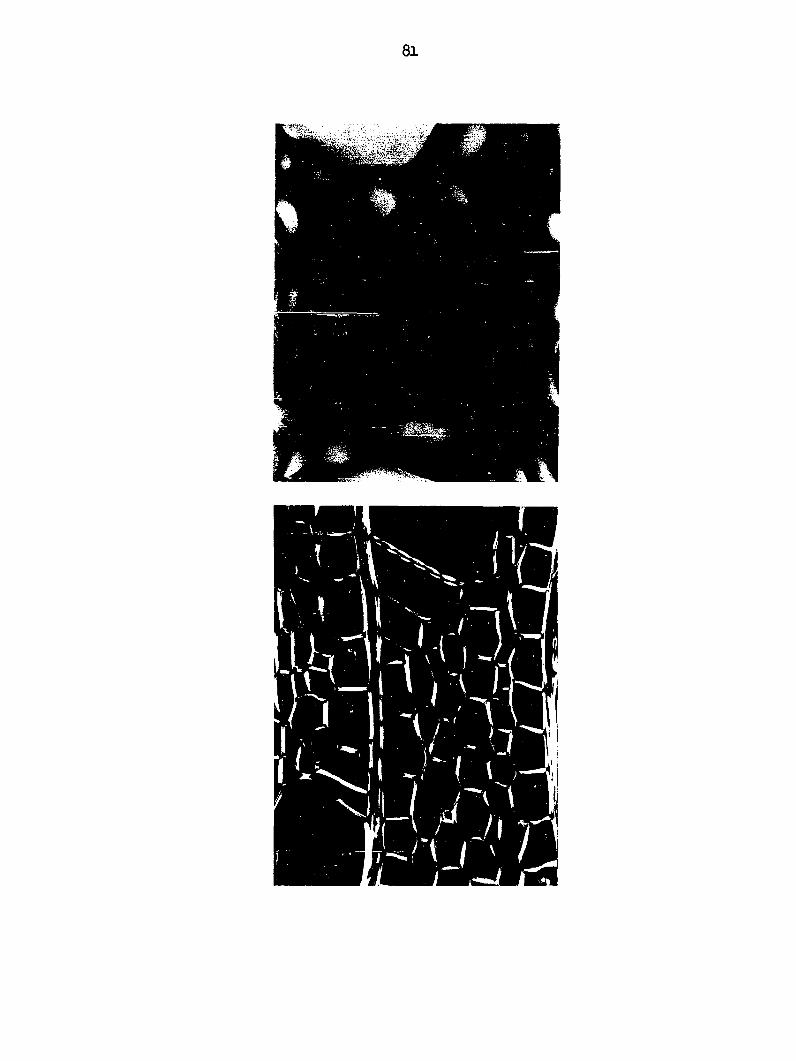
Fig. 27. Transverse section showing reaction tissue and wound parenchyma. 20QX

83

84

Table 9» Regression coefficients, t, and F values for ring width.

Plot, tree, core Regression coefficient

F values t

1 - 3 ~ 2 -0.008948 4.176 -2,0435 1 - 4 - 2 -0.000041 0.004 -0.0632 1 - 5 - 2 0.000861 3.180 1.7832 1 - 6 - 2 0 - -

1 - 7 - 2 0.000605 1.187 1.0895 1 - 8 2 -O.OOO396I O.2759 -0.5253 1 - 11 - 2 0.000334 0.362 0.6017 1 - 12 - 2 0,000565 O.O36 0.1897 l - 13 - 2 0.000494 0.0018 0.0424

2 - 55 - 1 O.OOO836 O.7274 0.8529 2 - 55 - 2 0.005418 9.320 3.0529 2 - 55 - 3 O.OO34.56 3.6582 1.9126 2 - 56 - 1 0.000974 O.2256 0.4750 2 - 56 - 2 -O.OO736O 0.369 -0.6075 2 - 56 - 3 0.000574 17.8674 4.2770 2 - 57 - 1 0.000382 00** 00** 2 - 57 - 2 0.002157 0.652 0.8075 2 - 57 - 3 -O.OOI766 1.9296 -1.3891 2 - 58 1 0.001176 0.7872 0.8873 2 - 58 2 0.000757 0.700 0.8367 2 - 58 - 3 0.002928 0.3617 0.6014 2 - 59 - 1 0.000181 0.0997 0.3158 2 - 59 - 2 0.000025 0.032 0.1789 2 - 59 - 3 0.000099 1.5349 1.2389 2 - 60 1 -O.OOOO72 0 0 2 - 60 - 2 -0.001941 0.500 -0.7071 2 - 60 - 3 -O.OOOI98 5.8000 -2.4083 2 - 6l 1 -0.000108 4.4909 -2.1190 2 - 6l - 2 0.000270 0.1287 0.3587 2 - 61 - 3 -O.OOO765 9.5541 -3.0910 3 -22 - 2 0.001466 1.935 0.4399 3 " 23 - 2 0.00l6l6 0.2645 0.5143 3 - 24 2 0.017301 0.813 0.9017 3 - 25 - 2 0.000901 0.931 0.9649 3 -25 - 2 -O.OOO995 2.961 -1.7208 3 - 27 - 2 O.OOI658 0.649 0.8056 3 - 28 - 2 0.000848 0.502 0.7085

5 - 29 - 2 0.002654 20.753 4.5555 5 - 30 - 2 - -

5 - 31 - 2 - -

5 - 32 - 2 -0.0002650 0.323 -0.5683 5 - 33 - 2 0.003573 11.603 3.4063 5 - 34 - 2 0.002142 2.025 1.4230

85

Table 9* Continued

Regression F Plot, tree, core coefficient values t

9 - 50 — 2 — — -9 - 5 1 - 2 0 . 0 0 0 2 8 8 3 5 . 5 5 8 I 5 . 9 6 5 O 9 - 5 2 - 2 - 0 . 0 0 0 2 8 9 0 . 6 2 6 4 - 0 . 7 9 7 7 9 - 5 3 - 2 - 0 . 0 0 1 9 2 1 4 5 . 0 5 6 9 - 6 . 7 1 2 4 9 - 5 4 - 2 - 0 . 0 0 0 0 0 1 0 0

10 - 105 - 2 0.000436 3.8534 I.963O 1 0 - 1 0 6 - 2 0.003899 8.0504 2.8373 10 - 107 - 2 O.OOO597 0.0253 O.I59I 1 0 - 1 0 8 - 2

1 2 - 1 0 9 - 2 - O . O O 3 3 I O 2 . 3 0 0 7 - I . 5 I 6 8 12 - 110 - 2 0.001440 62.533 7.907 1 2 - 1 1 1 - 2 O . O O 5 I I 8 4 0 . 8 2 6 2 6 . 3 8 9 5 1 2 - 1 1 2 - 2 0 . 0 0 2 0 8 5 I . 3 3 6 O 1 . 1 5 5 9 1 2 - 1 1 3 - 2 0 . 0 0 3 3 0 7 O . 7 6 6 O O . 8 7 5 2

1 3 - 6 2 - 2 O . O O O 8 O 5 0 . 0 7 2 0 . 2 6 8 3 13-63-2 0.003044 O.754 0.8683 13-64-2 -0.000142 O.O545 -O.2334 13-66-2 -O.OOO547 0.107 -O.327I 13-68-2 -0.000456 0.666 -0.8161 13-69-2 -0.000062 0.372 -0.6099 1 3 - 6 7 - 2 0 . 0 0 2 7 4 7 7 . 4 7 7 2 . 7 3 4 4

14 - 75 - v 0.000062 1.589 1.2606 14- 7 6 - 2 0.002442 241.833* I5.55IO* 14-77-2 -0.000048 0.320 -O.5657 14-78-2 O.OOOO55 0.0920 O.3033 14-79-2 0.001717 12.505 3.5362 14-80-2 0.003866 9.744 3.1215

1 6 - 9 3 - 2 0 . 0 0 3 0 3 0 1 9 . 5 5 8 4 . 4 2 2 4 1 6 - 9 4 - 2 - 0 . 0 0 8 0 8 7 3 2 . 3 9 2 - 5 . 6 9 1 4 I 6 - 9 5 - 2 0 . 0 0 4 1 2 2 0 . 0 6 4 O . 2 5 3 O I6- 9 6 - 2 - 0 . 0 2 0 8 8 8 1.043 -I.O213 1 6 - 9 7 - 2 - 0 . 0 0 0 0 0 5 0 . 1 0 0 - 0 . 3 1 6 2 36 - 98 - 2 0.001525 4.737 2.1765

1 8 - 8 1 - 2 0 . 0 0 5 1 7 9 69.693 8.3482 1 8 - 8 2 - 2 0 . 0 0 1 3 8 3 0 . 2 2 5 0 . 4 7 4 3 1 8 - 8 3 - 2 0 . 0 0 0 0 2 3 3 . 6 4 5 1 . 9 0 9 2 1 8 - 8 4 - 2 0 . 0 0 1 1 4 0 0 . 1 1 0 0 . 3 3 1 7 1 8 - 8 5 - 2 0 . 0 0 2 9 6 0 0 . 8 3 1 0 . 9 1 1 6 1 8 - 8 6 - 2 - 0 . 0 0 1 3 8 6 0 . 0 6 1 - 0 . 2 4 7 0

86

Table 9* Continued

Plot, tree, core Eegression coefficient

F values t

20 - 87 • - 2 0.000147 4.026 2.006 20 - 88 • - 2 0.002116 114.460 10.6986 20 - 89 • - 2 0.004022 14.669 3.8300 20 - 90 • - 2 0.002638 314.706* 17.7400* 20 - 91 • - 2 -O.OOOO59 O.O52 -0.2280 20 - 92 . - 2 0.002217 11.294 3.3607

22 - 99 -- 2 0.003263 52.183 7.2238 22 - 100 • - 2 0.000686 0.990 0.9950 22 - 101 • - 2 0.007182 21.448 4.6312 22 - 102 -- 2 0.002822 3.407 1.8458 22 - 103 • - 2 -0=005910 0.958 -0.9788 22 - io4 • - 2 -0.007606 0.464 -0.6812

23 - 70 . - 2 0.000281 18.9333 4.3512 23 - 72 ' - 2 O.OOOO83 16.3000 4.0373 23 - 73 - 2 0.007994 104.3256 10.2140 23 - 74 - 2 -0.000014 0.0230 -0.15166

F .05 • l6l F .01 = 4,052

87

standard regression methods. The situation was similar for cell number.

As shown in Table 10 there were only 4 significant "F" 's out of 90

triplets.

However, despite the low magnitude of the F- and t- statistics,

the signs of the regression coefficients for both ring width and cell

number are decidedly positive. Specifically, there are 64 positive and

29 negative regression coefficients for ring width, and 66 positive and

24 negative regression coefficients for cell number. This split of the

distributions was subjected to a sign test (cf. Vfallis and Roberts, 1956,

p. 598). The discrepancies between the number of plus and minus signs for

both ring width and cell number were significant beyond the 1 percent level.

The development of a series of "t" values from the triplets permits

the observation of the complete cumulative distribution functions (CDF) for

"t" and comparison of this empirical distribution with the null distribution

of "t" via the Kolmogoroff-Smirnoff test. These graphic and tabular ob­

servations are found in Tables 11, 12 and 13 and Figures 28 and 29. The

following formula gives the approximate critical values of the maximum

vertical deviation between the empirical and null distributions at the

specified level (Birribaum, 1952; Birnbaum and Tingey, 1951):

For ring width the maximum observed discrepancy was 0.21, and this can be

compared to the 0.1 per cent level of O.I93 for Kolmogoroff's statistic.

For cell number the observed figure is O.23 as compared to the mill o.l

where oc is the level of the test and n is the sample size

88

Table 10. Regression coefficients, t, and F values for cell number.

Plot, tree, core Regression coefficient

F values t

1 - 3 -- 2 0.003039 1 - 4 -• 2 0.000118 1 - 5 -• 2 -0.004829 1 - 6 -• 2 -0.000275 1 - 7 • - 2 0.000930 1 - 8 -. 2 o.ooo446 1 - 11 • - 2 0.000212 1 - 12 -• 2 0.002496 1 - 13 • - 2 0.016352

2 - 55 -• 1 0.006049 2 - 55 • - 2 0.006080 2 - 55 -• 3 0.000259 2 - 56 • - 1 0.003810 2 - 56 • - 2 -0.028678 2 - 56 -• 3 -0.000699 2 - 57 -• 1 -o.o4i6oi 2 - 57 • • 2 0.002204 2 - 57 • • 3 -0.003872 2 - 58 -• 1 0.002013 2 - 58 -• 2 0.003125 2 - 58 -• 3 0.004235 2 - 59 • • 1 0.003198 2 - 59 • - 2 0.00027944 2 - 59 -• 3 -0.00269 2 - 60 -• 1 0.000959 2 - 60 • - 2 -0.00169106 2 - 60 . • 3 -0.000121 2 - 61 -• 1 0.000145 2 - 61 -- 2 0.000596 2 - 61 -• 3 -0.002305

3 - 22 • • 2 O.OO39663 3 -23 -• 2 O.OIOOO6I5 3 - 24 -• 2 0.0095537 3 " 25 -- 2 0.ooo4o84i 3 - 26 -• 2 -0.00114499 3 - 27 • • 2 0.0009229 3 - 28 . • 2 0.00028618

5 - 29 -• 2 0.001888 5 - 30 -- 2 -

5 - 31 -• 2 -

5 - 32 -- 2 -0.00007820 5 - 33 -- 2 0.00351462 5 - 34 -• 2 0.00183416

0.444 0.009 0.232 0.1743

6800.00** 0.1013 0.103

58.844 64.14

16.0878 23.993 0.0107 0.22 0.554 91.12

0.14 0.365 0.71 0.52

61.982 14.74 0.30 0.419 1.52 0.54 53.941 0.15 8.44 0.84 3.12

45.123 2-559 1.740 1.251 0.885 2.173 0.007

945.25*

0.0143 9.6544 0.965

0.6663 0.094868 -0.4816638 -0.4175 82.46211** 0.317645 0.3209 7.7051 8.00866

4,0094 4.8983 0.1034 0.4690 -0.7443 -9,5457 -0.3742 0.6042

-0.8426 0.7211 7.8729 3.8393 5A772 0.6473 -1.2329 0.7348

-7.3445 -0.3873 2.9052 0.9165 -1.7664

6.7174 1.5997 1.3191 I.II85 -0.9407 1.4741 0.08367

30.7449*

-0.1196 3.1072 0.9823

89

Table 10. Continued

Regression F Plot, tree, core coefficient values

9 - 50 - 2

9 - 51 - 2

9 - 52 - 2

9 - 53 - 2

9 - 54 - 2

10 - 105 - 2 10 - 106 - 2 10 - 107 - 2 10 - 108 - 2

12 - 109 - 2 12 - 110 - 2 12 - 111 - 2 12 - 112 - 2 12 - 113 - 2

13 - 62 - 2 13 - 63 - 2 13 - 64 - 2 13 - 66 - 2 13 - 67 - 2 13 - 68 - 2 13 - 69 - 2

14 - 75 - 2 l4 - 76 - 2 14 - 77 - 2 14 - 78 - 2 14 - 79 - 2 14 - 80 - 2

16 - 93 - 2 16 - 94 - 2 16 - 95 - 2 16 - 96 - 2 16 - 97 - 2 16 - 98 - 2

18 - 81 - 2 18 - 82 - 2 18 - 83 - 2 18 - 84 - 2 18 - 85 - 2 18 - 86 - 2

0.000422 6.98 2.6420 -0.000424 4.62 -2.1494 -0.000224 0.002 -0.04472 0.000133 O.563 O.75O3

0.000639 1.92 I.3856 0.002276 0.103 0.3209 0.006339 51.738 7.1930

0.4000 3.0724 4.2131 21.3775* 1.9849

-0.6992 -2.1503 -2.0420 8.2639 1.1410 0.5376 3.7081

5-9904 1.0291 -0.6986 I.5231 3.0095 8.2793

2.8966 0.5000 0.1703 2.1171 -2.1213 1.5621

1.8706 -0.6205 0.5477 0.3962 13.0354* 1.8828

0.002485 0.16 0.002212 9.44 0.013801 17.75 0.008821 456.98* 0.013022 3.94

-O.OO3987 0.489 -0.048018 4.624 -O.OOO2557 4.17 0.0011815 68.292 0.0029061 1.302 0.00050078 0.289 0.00033704 13.750

0.00010181 35.885 0.0044186 1.059 -0.00004024 0.488 0.00041748 2.320 0.0025512 9.057 0.0066757 68.547

0.003776 8.390 0.0008196 0.250 0.003532 0.029 0.005994 4.482 -0.0003158 4.500 0.002837 2.440

0.004534 3-499 -0.0025797 0.385 0.00004333 0.300 0.00307010 O.I57 0.00241199 169.921* 0.00400271 3.545

90

Table 10. Continued

Plot, tree, core Regression coefficient

F values t

20 - 3? • - 2 0.00013621 0.471 0.6863 20 - 88 • - 2 0.00126927 0.030 0.1732 20 - 89 • - 2 0.00539335 3.509 I.8732 20 - 90 . - 2 0.00485051 50.222 7.0867 20 - 91 • - 2 -O.OOOO65 0.012 -O.IO95 20 - 92 • - 2 0.00011941 0.023 O.I516

22 - 99 • - 2 0.00829010 11.712 3.4223 22 - 100 • - 2 -O.OOO2585I 0.082 -0.2864 22 - 101 • - 2 0.01374355 24.568 4.9566 22 - 102 • - 2 0.00460761 1.434 1.1975 22 - 103 • - 2 -0.0028318 O.678 -0.8234 22 - 104 • - 2 -O.OOI3459 0.099 -0.3146

91

Table 11. Values for the null distribution of t for one degree of freedom.a

t P(t V=l) (1-P) t P(t V=l)

0.0 0.5000 3.1 0.90067 0.1 O .53173 3-2 0.90359 0.2 O .56283 3.3 0.90634 0-3 0.59277 3.4 0.90895 0.4 0.62112 3-5 0.91141 0.5 0.64758 0.35242 3.6 0.91376 0.6 0.67202 3-7 0.91598 0.7 0.69440 3.8 0.91809 0.8 0.71478 3.9 0.92010 0.9 0.73326 4.0 0.92202 1.0 O.75OO 0.2500 4.2 0.92560 1.1 O.765I5 4.4 0.92887 1.2 O.77GP6 4.6 0.93186 1.3 O.79129 4.8 0.93462 1.4 0.80257 5.0 0.93717 1-5 0.81283 0.18717 5.2 0.93952 1.6 0.82219 5.4 0.94171 1-7 0.83075 5.6 0.94375 1.8 O .83859 5.8 0.94565 1.9 0.84579 6.0 0.94753 2.0 0.85242 0.14758 6.2 0.94910 2.1 0.85854 6.4 0.95066 2.2 0.86420 6 .6 0.95214 2.3 0.86945 6.8 0.95352 2.4 0.87433 7.0 0.95483 2-5 0.87888 7.2 0.95607 2.6 0.88313 7.4 0.95724 2.7 0.88709 7.6 0.95836 2.8 0.89081 7-8 0.95941 2.9 0.89430 8.0 0.96042 3.0 0.89758 0.10242 12.706

25.452 63.657

0.97500 0.98750 0.99500 1.00000

(1-P)

O.O7798

O.O6283

0.05247

0.04517

O.O3958

Values as tabulated by Pearson and Hartley (1954, p. 132).

1 2 3 4

I 7 8 9 10 11 12 13 14

3 17 18 19 20 21 22 23 24 25 26 27 28 29 30 31 32 33 34

36 37 38 39 40 41 42 43 44 45

92

Cumulative distribution of t values for cell number.

t value CDF Index t value CDF

-9.5457 0.01111 46 0.7503 0.51111 -7.3445 0.0?.???. 47 0.9165 0.52222 -2.1503 0.03333 43 0.9823 0.53333 -2.1494 0.04444 49 1.0291 O.54444 -2.1213 0.05555 50 I.II85 0.55555 -2.0420 0.06667 51 1.1410 O.56667 -I.7664 0.07778 52 1.1975 0.57778 -I.2329 0.08889 53 1.3191 O.58889 -0.9407 0.10000 54 1.3856 0.60000 -0.8426 0.11111 55 1.4741 0.61111 -O.8234 0.12222 56 I.523I 0.62222 -O.7443 0.13333 57 1.5621 0.63333 -O.6992 0.14444 58 1.5997 0.64444 -O.6986 O.I5555 59 1.8706 0.65555 -O.62O5 0.16667 60 1.8732 0.66667 -0.48166 0.17778 61 1.8828 0.67778 -0.4175 O.I8889 62 1.9849 0.68889 -0.3873 0.20000 63 2.1171 0.70000 -0.3742 0.21111 64 2.6420 0.71m -0.3146 0.22222 65 2,8966 O.72222 -0.2864 0.23333 66 2.9052 0.73333 -0.1196 0.24444 67 3.0095 0.74444 -0.1095 0.25555 68 3.0724 0.75555 -0.04472 0.26667 69 3.1072 0.76667 0.08367 0.27778 70 3.4223 0.77778 0.094868 0.28889 71 3.7081 0.78889 0.1034 0.30000 72 3.8393 0.80000 0.1516 0.31111 73 4.0094 0.8111,1 O.1703 0.32222 74 4.2131 0.82222 0.1732 0.33333 75 4.8983 0.83333 0.317645 0.34444 76 4.9566 0.84444 0.3209 0.35555 77 5.4772 0.85555 0.3209 0.36667 78 5.9904 0.86667 0.3962 0.37778 79 6.7174 0.87778 0.40000 0.38889 80 7.O867 0.88889 0.4690 0.40000 81 7.1930 0.90000 0.50000 0.41111 82 7.7051 0.91111 0.5376 0.42222 83 7.8729 0.92222 0.5477 0.43333 84 8.00865 0.93333 0.6042 0.44444 85 8.2639 0.94444 0.6473 0.45555 86 8.2793 0.95555 0.6663 0.46667 87 13.0354 0.96667 0.6863 0.47778 88 21.3775 0.97778 0.7211 0.48889 89 30.7449 0.98889 0.7348 0.50000 90 82.46211 1.00000

adt

1 2

3 4

I 7 8 9 10 11 12 13 14 15 16 17 18 19 20 21 22 23 24 25 26 27 28 29 30 31 32 33 34 35 36 37 38 39 40 41 42 43 44 45 46

93

Cumulative distribution of t values for ring width.

t value CDF Index t value CDF

-6.7124 0.01075 47 0.8056 0.50537 -5.6914 0.02150 48 0.8075 0.51612

-3.0910 0.03225 49 0.8367 0.52688 -2.4083 0.04301 50 0.8529 0.53763 -2.1190 0.05376 51 0.8683 0.54838 -2.0435 0.06451 52 0.8752 O.55913 -1.7208 0.07526 53 0.8873 0.56989 -1.5168 0.08602 54 0.9017 0.58064 -1.3891 0.09677 55 0.9116 O.59139 -I.0213 0.10752 56 0.9649 0.60215 -0.9788 0.11827 57 0.9950 0.61290 -O.8161 0.12903 58 1.0895 0.62365 -O.7977 0.13978 59 1.1559 0.63440 -0.7071 0.15053 60 1.2389 0.64516 -0.6812 0.16129 61 1.2606 0.65591 -0.6099 0.17204 62 1.4230 0.66667 -0.6075 0.18279 63 1.7832 0.67741 -0.5683 0.19354 64 1.8458 0.68817 -0.5657 0.20430 65 1.9092 0.69892 -O.5253 0.21505 66 1.9126 0.70967 -0.3271 0.22580 67 1.9630 0.72043 -0.3162 0.23655 68 2.0060 0.73118 -0.2470 0.24731 69 2.1765 0.74193 -0.2334 0.25806 70 2.7344 0.75268 -0.2280 0.26881 71 2.8373 0.76344 -o.15166 0.27956 72 3.0529 0.77419 -O.O632 0.29032 73 3.1215 0.78494

0 0.30107 74 3.3607 0.79569 0 0.31182 75 3.4063 0.80645

0.0424 0.32258 76 3.5362 0.81720 0.1591 0.33333 77 3.8300 0.82795 0.1789 0.34408 78 4.0375 0.83870 0.1897 0.35483 79 4.2770 0.84946 0.2530 0.36559 80 4.3512 0.86021 0.2683 0.37634 81 4.4224 0.87096 0.3033 0.38709 82 4.5555 0.88172 0.3158 0.39784 83 4.6312 0.89247 0.9317 0.40860 84 5.9650 0.90322 0.3587 0.41935 85 6.3895 0.91397 0.4399 0.43010 86 7.2238 0.92473 0.4743 0.44086 87 7.9070 0.93548 9.4750 0.45161 88 8.3482 0.94623 0.5143 0.46236 89 10.2140 0.95698 0.6014 0.47311 90 10.6986 0.96774 0.6017 0.48387 91 15.5510 0.97849 0.7085 0.49462 92 17.7400 0.98924

91 1.00000

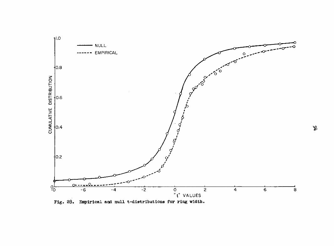
NULL •cr

-o-EMPIRICAL

0.8

cy

.'O

0.6 en

LU

0.4

0.2

-o

- 6 -4 " t " V A L U E S

Fig. 28. Empirical and null t-distributions for ring width.

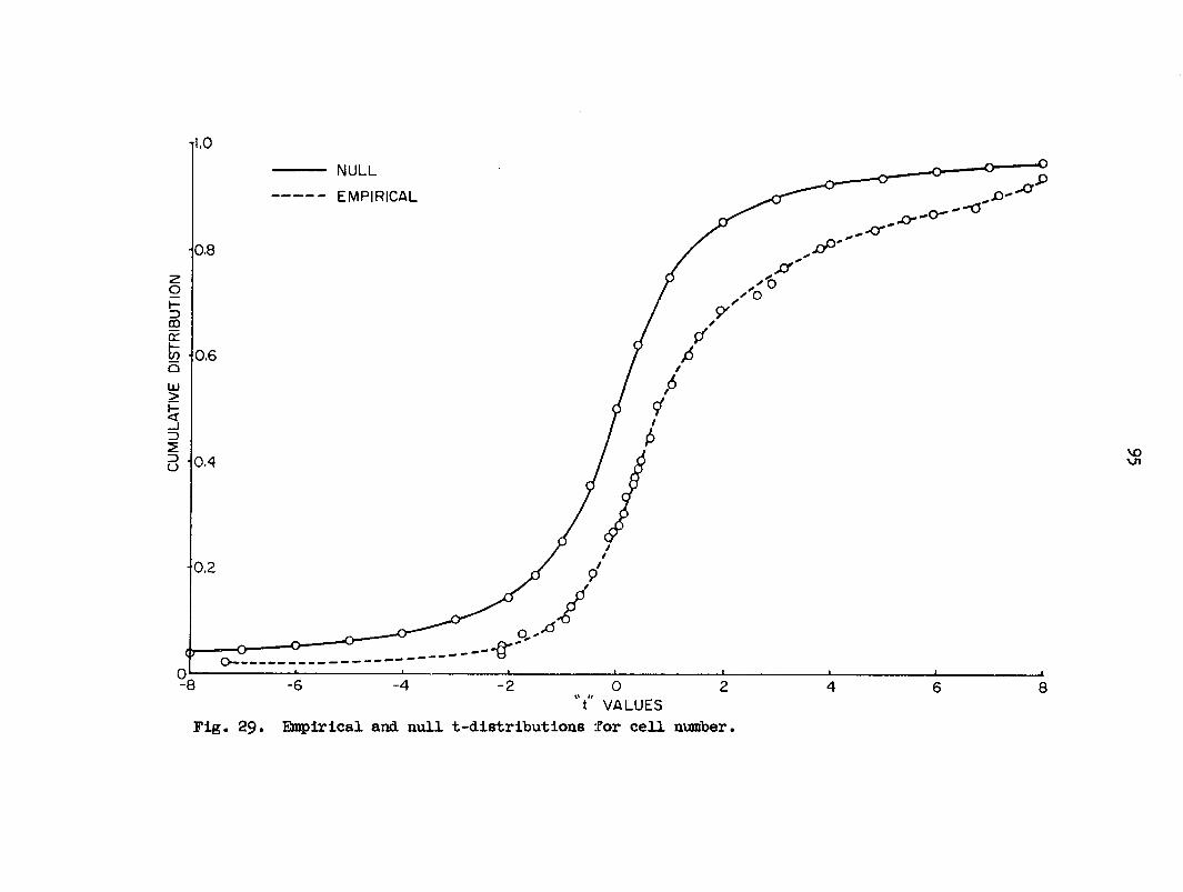
NULL JO EMPIRICAL

-cr •0.8

0.6

UJ

0.4

0.2

O-

-4 - 2

t VALUES Fig. 29. Empirical and null t-dlstrlbutlons for cell number.

96

percent levd. of O.I95. For cell number the shift to the right is

accentuated somewhat, relative to ring width. These results Imply that

high proportion of gelatinous fibers is associated vith larger number

of smaller cells and larger ring width.

This effect does not materialize in the standard tests of hypo­

theses because under these circumstances only the tails of the empirical

"t"-distribution are examined. Here the shift in the distribution occurred

in the central portion of the distribution.

Bing width and cell number have a positive association with proportion

of gelatinous fibers. The relationships were not revealed by traditional

methods. The Kolmogoroff-Smirnoff technique revealed these effects because

it scrutinizes all the percentiles of the empirical distribution in con­

trast to the corresponding percentiles of the theoretical distribution.

It is a multiple comparison procedure for all percentiles and presents the

full distributional picture.

A further elucidation of the nature of the ring width-reaction tissue

association can be obtained via Youden's D/cL outlier criterion (Youden,

1953)• The special case for triplets is relevant. With the statistic,

D/cL, almost no alternative to homogeneity is Immune from detection. This

statistic consists of the largest sequential difference between size-

ordered triplets (D) divided by the smallest sequential difference between

size ordered triplets (d). The D/d's were computed for ring width anâ the

corresponding analogous statistic, G/g, was computed for the proportion of

gelatinous fibers. The G/g data were then divided into two approximately

equal groups on the basis of the magnitude of tfc* ring width criterion

(D/d). One group consisted of G/g's from triplets where D/d > 3,- and was

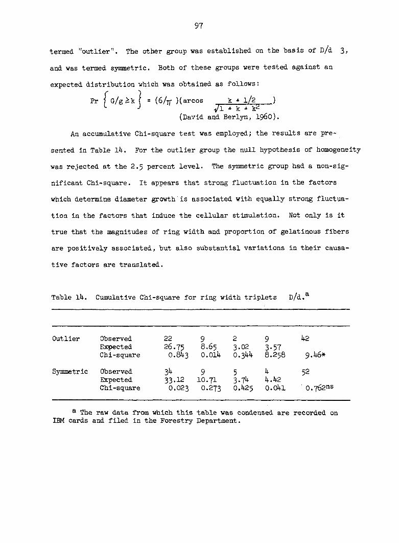
97

termed "outlier". The other group was established on the basis of D/d 3>

and was termed symmetric. Both of these groups were tested against an

expected distribution which was obtained as follows:

Pr j G / g è - k I = (6/77- )( arcos k * l/2 ) L J Vl * k * k*

(David and Berlyn, i960).

An accumulative Chi-square test was employed; the results are pre­

sented in Table 14. For the outlier group the null hypothesis of homogeneity

was rejected at the 2.5 percent level. The symmetric group had a non-sig­

nificant Chi-square. It appears that strong fluctuation in the factors

which determine diameter growth is associated with equally strong fluctua­

tion in the factors that induce the cellular stimulation. Not only is it

true that the magnitudes of ring width and proportion of gelatinous fibers

are positively associated, but also substantial variations in their causa­

tive factors are translated.

Table 14. Cumulative Chi-square for ring width triplets D/d.a

Outlier Observed 22 9 2 9 42 Expected 26.75 8.65 3.02 3-57 Chi-square 0.843 0.014 0.344 8.258 9.46*

Symmetric Observed 34 9 5 4 52 Expected 33.12 10.71 3.74 4.42 Chi-square 0.023 0.273 0.425 0.041 ' 0.762ns

a The raw data from which this table was condensed are recorded on IBM cards and filed in the Forestry Department.

98

Regression Analysis

Standard multiple linear regression methods were employed to assess

the relationships among the numerous variables tabulated in this study.

Average "proportion of gelatinous fibers" per tree vas designated as the

dependent variable for most of these analyses. The multiple linear re­

gressions were of two types: composite regressions over 14 plots, and

individual plot regressions.

Mensurational considerations

The independent variables consist of both Individual tree factors and

soil factors. The soils data were compiled by Brendemuhl (cf. Table 1).

There are six soil factors (including site index) contained in this study.

There are 11 individual tree factors, which were directly tabulated for

the study. The tree variables are further dichotomized into external

and internal morphological characters. The 17 factor array with the nota­

tion used throughout the study is as follows:

Xi Linear lean - degrees

%2 Stem basal area - square feet

X3 Total height - feet

XI4. Crown percent

Xcj Crown volume - cubic feet

X6 Crown surface area - square feet

Xy Stem volume - total cubic feet

Xg Proportion gelatinous fibers

X9 Orthogonal quadratic lean (orthogonal to linear lean)

99

X10 Site index

X]2 Average silt plus clay content

Available water - percent

Foliar nitrogen - percent

X^ Nitrifiable nitrogen - pounds per acre - 0-48"

Xi5 Available phosphorous - pounds per acre - 0-46"

Xjj5 Ring vidth - millimeters

X3.7 Cell number

All but three of the factors were compiled by standard methods. Stem vol­

ume, crown volume, and crown surface area contain sane specialized aspects€

Total cubic foot volume was obtained as follows :

V = B.A. X h , 2.37

Where B.A. = basal area at breast height h = total height

2.37 • a form factor

This equation was taken from a regional volume table for Cottonwood (Gevor-

kiantz and Olsen, 1955 ). The total volume calculated in this manner agreed

within 1 percent with the regional table. This method has the advantage

that extra sensitivity is derived from using total height to the nearest

foot and diameter to the nearest tenth of an inch, whereas the regional

table contained heights to the nearest 10 feet and diameters to the nearest

inch. There was little fluctuation in the form factor in the regional

table itself.

Crown volume was computed by the paraboloid formula. The form assump­

tion, however, was based on empirical evaluation. The general correlation

tables (Tables 15 and 16) show that crown volume is highly correlated with

other tree growth factors such as stem volume, crown surface area, and stem

100

basal area. This suggests the assumption was not grossly aberrant. The

linear functionality of crown volume with the other tree attributes offers

possibilities for mensurational and photogrammetric studies.

Crown surface area was computed from the following equation for the

surface of a paraboloid:*

This attribute represents the photosynthetic area of the tree. Again the

form assumption was empirical. This measurement is also associated with

other tree and soil variables.

Composite multiple linear regressions

The composite regressions were computed over the 14 plots. Four of

these composite analyses were computed: a ly-factor analysis, a 15-factor

analysis, a 7-factor analysis, and a 5-factor analysis. Fundamentally the

approach was to compute a 15-factor and a 5-factor analysis and then re­

compute , adding in average ring width and average cell number. This served

as a computational check and sharpened the analysis. The results of the

composite analyses are presented in Tables 15 through 24.

With only 14 plots the number of soil factors included was limited to

6 in order to obviate unrealistic inflation of R, the multiple correlation

^Greenwood, J. A. Ames, Iowa. Equation for the surface of a para­boloid. Private communication. 1958.

CSA

where Z = crown length R = geometric mean radius of

the base of the crown

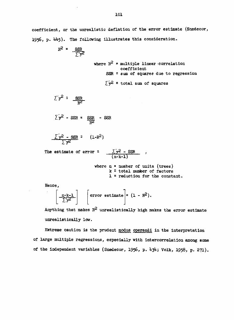
101

coefficient, or the unrealistic deflation of the error estimate (Snedecor,

1956, p. 445). The following illustrates this consideration.

R2 = SSR

Ty2

where R2 » multiple linear correlation coefficient

SSR = sum of squares due to regression

ly2 = total sum of squares

l'y2 = SSR R*

l'y2 - SSR = SSR - SSR -RZ

I t2 - SSR I'y%

(1-B2)

The estimate of error = Z'y2 - SSR (n-k-1)

where n * number of units (trees) k = total number of factors 1 = reduction for the constant.

Hence ,

n-k-1

.

error estimate = (1 - R2).

Anything that makes R2 unrealistically high makes the error estimate

unrealistically low.

Extreme caution is the prudent modus operandi in the interpretation

of large multiple regressions, especially with intercorrelation among seme

of the independent variables (Snedecor, 1956, p. 4g4; Volk, 1958, p. 271).

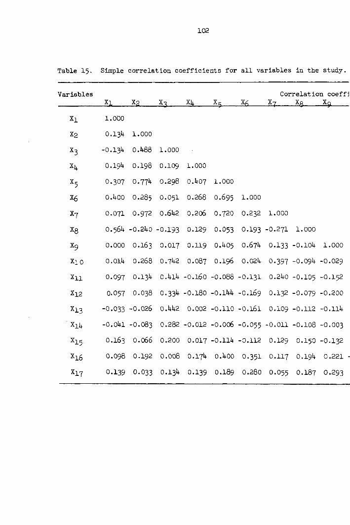
102

Table 15- Simple correlation coefficients for ail variables in the study.

Variables Correlation coeffj Il *2 Xj Q ^ X£ X^ Xg Xç

XI 1.000

X2 0.134 1.000

X3 -0.134 0.488 1.000

X4 0.194 0.198 0.109 1.000

X5 0.307 0.774 0.298 0.1)07 1.000

X6 0.400 0.285 0.051 0.268 0.695 1.000

Xy 0.071 0.972 0.642 0.206 0.720 0.232 1.000

Xq 0.564 -0.240 -0.193 0.129 0.053 0.193 -0.271 1.000

X9 0.000 0.163 0.017 0.119 0.405 0.674 0.133 -0.104 1.000

X10 0.014 0.268 0.742 0.087 0.196 0.024 0.397 -0.094 -0.029

XII 0.097 0.134 0.414 -0.160 -0.088 -0.131 0.240 -0.105 -0.152

X12 0.057 0.038 0.334 -0.180 -0.144 -0.169 0.132 -0.079 -0.200

X13 -O.O33 -0.026 0.442 0.002 -0.110 -O.16I 0.109 -0.112 -0.114

Xi4 -0.041 -O.O83 0.282 -0.012 -0.006 -0.055 -0.011 -0.108 -0.003

X15. O.I63 0.066 0.200 0.017 -0.114 -0.112 0.129 0.150 -O.I32

X16 0.098 0.192 0.008 0.174 0.400 O.35I 0.117 0.194 0.221

X17 O.I39 O.O33 0.134 0.139 0.189 0.280 O.O55 0.187 0.293

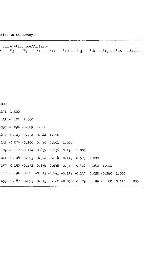
ibles in the study.

Correlation coefficients x« x9 Xm Xn X1P Xj_3 X-,%. X^ Xj_^

000

271 1.000

133 -0.104 1.000

397 -0.094 -0.029 1.000

240 -0.105 -0.152 0.522 1.000

132 -0.079 -0.200 0.419 0.891 1.000

109 -0.112 -0.114 0.659 0.656 0.592 1.000

Oil -0.108 -0.003 0.592 0.214 0.143 0.575 1.000

129 0.150 -0.132 0.156 0.648 0.543 0.402 -0.260 1.000

117 0.194 0.221 -0.013 -0.241 -0.132 -0.137 0.082 -0.260 1.000

055 0.187 0.293 0.213 -0.088 -0.058 0.179 0,199 -0.180 0.510 1.000

103

Table 16. Simple correlation coefficients greater than O.5OO.

Variables Correlated factors r

xl> Xg lean, proportion gelatinous fibers O.564

X2, X7 stem basal area, stem volume 0.972

X2 ; X5 stem basal area, crown volume 0.774

x3, X7 stem height, stem volume 0.642

X5, X5 crown volume, crown area O.695

%5,%7 crown volume, stem volume O.721

X6, X9 crown surface area, quadratic lean 0.674

xl6> x17 ring width, cell number 0.510

X10, X3 site Index, stem height 0.742

x10> X11 site index, average silt plus clay 0.522

x10; x13 site index, foliar nitrogen 0.659

x10> Xl4 site index, nitrifiable nitrogen 0.593

%11, %12 average silt plus clay, available water 0.891

xll, x13 average silt plus clay, foliar nitrogen O.657

xll> Xl5 average silt plus clay, available P 0.648

x12, X13 available water, foliar N 0.594

Xl2, X15 available water, available P 0.543

x13' xlk foliar N, nitrifiable N 0.575

104

Table 17. Summary of composite 17-factor regression analysis.

Variables Means Partial

regression coefficients

"t"

7.929 0.03525 4.92** 1.590 -O.35713 1.36 91.964 0.004637 0.92 53-741 -0.002919 1.15

14414.516 O.OOOOI595 2.94** 3411.387 -O.OOOOO795 1.28 63.712 -0.0002796 0.05 0.000488 -0.001446 1.31

100.464 0.001363 0.29 12.5048 -0.01599 0.71 80.696 -0.0007894 0.24 1.904 -0.27540 1.54 42.842 0.0001313 0.09 12.958 0.008825 2.84** 5-764 0.013103 1.01

949.964 0.0003036 1.34

X1 X2 x3 X4

xi x7

x9 x10 X11 x12 xl3 xl4 xl5 xl6 x17

B2 = 0.614793 H = 0.784087**

Table 18. Analysis of variance for the 17-factor composite regression analysis.

Source of variation Degrees of freedom

Sum of squares

Mean squares

Due to regression 16 5.4686 0.34179

Deviations about regression 67 3.4204 0.05114

Total 83 8.8950

F = 6,683** F .01 = 2.29

105

Table 19. Summary of composite 15-factor regression analysis.

Variables Partial

Means regression coefficients

"•fc "

7.929 O.O3729 5.25** 1.590 -0.27798 1.11 91.964 0.006177 1.23 53.741 -0.00270 1.03

IW14.516 0.000017 S.#** 3411.387 -O.OOOOO7 1.21 63.712 -O.OO232 0.42 0.000488 -O.OOIO3 0.94

100.464 O.OOI95 0.39 12.505 -0.02630 1.15 80.696 0.000453 0.14 1.904 -0.18121 1.02 42.842 -O.OOOI89 0.13 12.958 0.00763 2.43**

*2

5 S x7

*10 Xll X12 x13 xl4 Ï15

0.4-13419

B2 = 0.57984 B = O.76147** Constant * 0.414880

Table 20. Analysis of variance for the 15-factor composite multiple linear regression.

Source of variation Degrees of freedom

Sums of squares

Mean squares

Due to regression 14 5.157716 0.368408

Deviations about regression 69 3.737310 0.054163

Total 83 8.895026

F - 6.815** F .01 = 2.35

B2= O.58O B = O.76I**

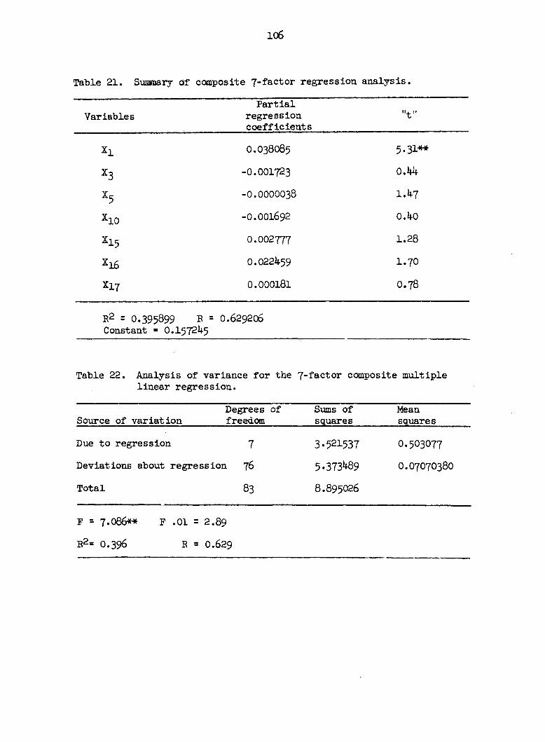
106

Table 21. Summary of composite 7-factor regression analysis.

Variables Partial

regression coefficients

"t"

X1 O.O38O85 5.31**

x3 -O.OOI723 0.44

X5 -O.OOOOO38 1.47

X10 -O.OOI692 0.40

xl5 0.002777 1.28

xl6 0.022459 1.70

x17 0.000181 0.78

R2 = 0.395899 B = Constant » O.I572U5

0.629206

Table 22. Analysis of variance for the 7-factor composite multiple linear regression.

Source of variation Degrees of freedom

Sums of squares

Mean squares

Due to regression 7 3.521537 0.503077

Deviations about regression 76 5-373489 O.O7O7O38O

Total 83 8.895026

F = 7.086** F .01 = 2.89

R2» O.396 E = 0.629

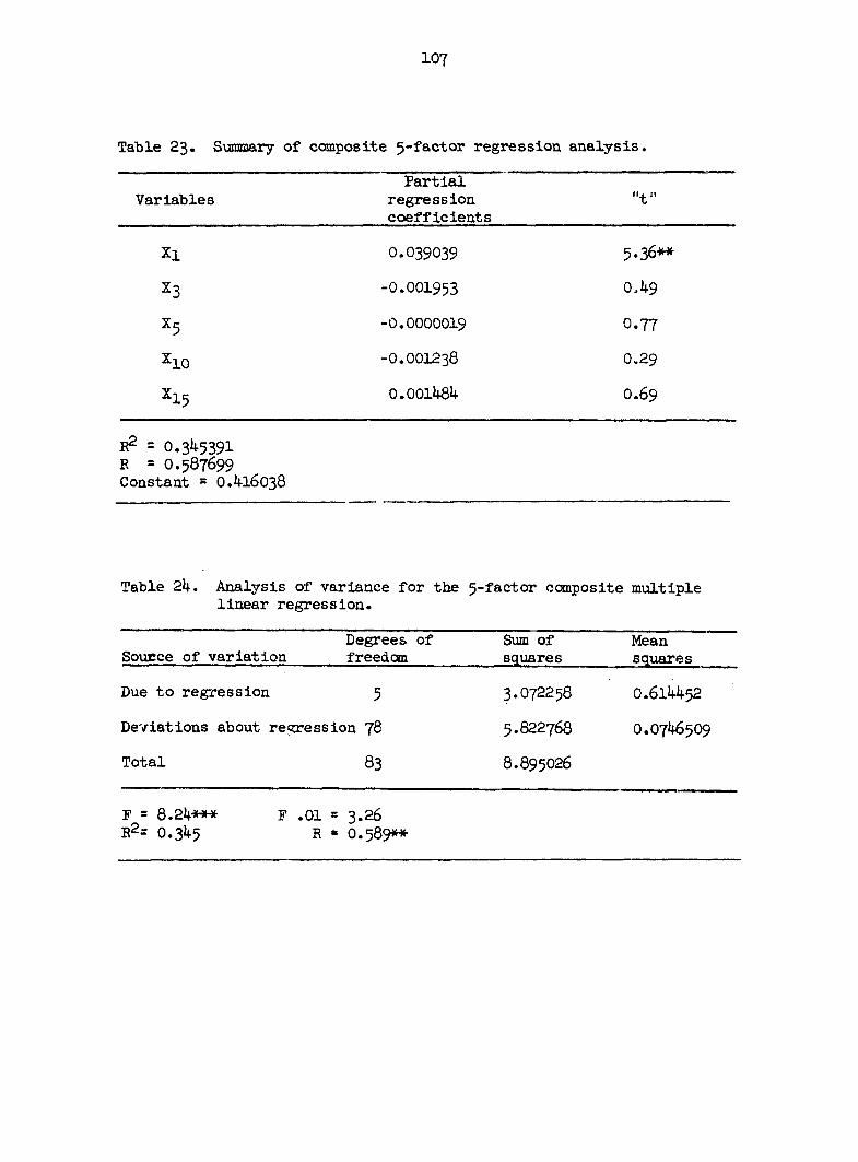
107

Table 23. Summary of composite 5-factor regression analysis.

Variables Partial

regression coefficients

"t"

%1 O.O39039 5.36**

x3 -0.001953 0,49

x5 -û.0000019 0.77

X10 -O.OOI238 0.29

X15 0.001484 0.69

R2 = 0.345391 R = O.587699 Constant = 0A16038

Table 24. Analysis of variance for the 5-factor composite multiple linear regression.

Source of variation Degrees of freedom

Sum of squares

Mean squares

Due to regression 5

Deviations about regression 78

Total 83

3.072258

5.822768

8.895026

0.614452

0.0746509

F = 8.24*** F .01 = 3.26 R2- 0.345 R • O.589**

108

As measured by the magnitude of the t-statistic, lean is clearly the

factor most strongly related to the proportion of gelatinous fibers.

Graphically the overall relationship is presented in Figures 30, 31 and

32. Figure 30 is a functional plot of all the data. In cottonwood there

are no gelatinous fibers in vertical boles, hence no realistic line

would intereect the ordinate above zero. For this reason the least

square lines are stopped at the last data points (2 degrees lean). There

are two least squares lines on Figure 30* One is the regression line for

lean alone; the other line has the partial slope, all other factors being

evaluated at their respective means. Figure 31 is a grouping of the least

linear plots, and Figure 32 is a similar grouping of the most linear plots.

Orthogonal quadratic lean was not related to proportion of gelatinous

fibers in these analyses. However, it is apparent that the linear func­

tionality of proportion gelatinous fibers with lean certainly is not

applicable over the entire range of lean values.

Crown volume has a highly significant "t" value in the 15- and 17-

factor analyses, but has a non-significant "t" in the 5- and 7-factor

analyses. The simple linear correlation coefficient between crown volume

and proportion of gelatinous fibers is only O.O53. The linear regression

coefficient is quite low in absolute value and changes sign from positive

in the two larger analyses to negative in the two smaller analyses. One

reason for the shift is probably the exclusion of intercorrelated negative

quantities in the smaller analyses. The low magnitude of the coefficients

is also due to individual plot variation. In some cases crown volume is

positively correlated with good growth conditions and in other cases with

senescence and the life-cyclic decrease in diameter growth. Table 25

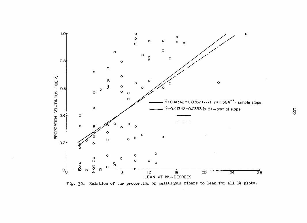
I.Or

0.8

v) ce lu cd

0.6 v) 3 o

o

§

2 o cr C L

0.4

0.2

0

Y - 0.41342 + 0.0387 (x-x) r = 0.564 ~simple slope

Yr0.41342 +0-0353 (x-x) ~ partial slope

o

 .

o o

Ji 8

O

o

o

0 8 12 16 LEAN AT b.h.~ DEGREES

20 24 28

Fig. 30. Reletion of the proportion of gelatinous fibers to lean for all 14 plots.

1.0

o

o o o

o

o o

° o °

-Q 2—û-

o

8

o

o o

o o

o

o

o 8 12 16 20 24 28

LEAN AT b.h.~DEGREES

Fig. 31. Relation of the proportion of gelatinous fibers to lean for plots 2 19 12, 13, 20, 23.

1.0

0.8 v) ce UJ cd u-

v)

I 0J6 p

lu o

o H 0.4

2 g CL

0.2

0

O O

O

o 0 -e—o—<-

o

6

: . O

8 O

o 0

o o

o

° o o o o o o

o

0 4 8 12 16 20 24 28 LEAN AT b.h.~ DEGREES

Fig. 32- Relation of the proportion of gelatinous fibers to lean for plots 1, 5, 10, 14, 16, 18 and 22.

112

shows the age split of the positively and negatively correlated plots.

These plots were selected for constant age, and hence the variation in age

is slight. However, the two youngest plots showed positive relationships

between crown volume and proportion gelatinous fibers, while the two

oldest showed negative relationships.

The t-statistic for available phosphorous was also highly significant

in the larger analysis and non-significant in the two smaller analyses.

The linear regression coefficient is positive in all four analyses, and

the simple linear correlation coefficient is O.I5O. The pH range of

these soils vas 7-8 and this is precisely the range in which phosphorous

is most available to plants. The observation is the more striking in view

of the fact that Brendemuhl did not consider phosphorous to be severely

limiting on any of these soils.

No other variables appear to be highly related to the proportion of

gelatinous fibers in the xylem of Populus deltoïdes. The two-step addition

of average ring width and average cell number did sharpen the analyses.

In going from 15 to 17 factors, B2 increased from O.58O to O.615. This

represents an additional explanation of 3.5 percent of the variation in the

sums of squares. In going from 5 to 7 factors, B2 went from O.345 to O.396,

which represents a 5.1 percent increase in information. It is also obvious

that information was actually lost by excluding variables. With the addi­

tion of 12 factors there was a 27.0 percent increase in the explanation of

the variation. The multiple linear correlation coefficient, R, went from

O.588 to 0.784.

It may be of interest to compare these percentages vith the expected

percentage increase in R2 due to the addition of random factors, assuming,

113

Table 25. Associated means and plot variables.

Plot no.

Site index

Age %/%l

Average crown volume cubic feet

lbs./A. available phosphorus

0-48"

rX8-Xi bX8-Xi

9 87 41 0.0579 8,444 2.0 0.376 0.058

12 88 34 0.0597 19,386 1-5 0.712 0.032

10 89 38 0.0832 16,155 2.0 0.997 0.1235

2 89 44 0.0439 6,499 14.0 0.039 0.0034

20 93 56 0.0459 12,893 1-5 0.227 0.0162

1 95 46 0.0720 63,338 48.0 0.864 0.0500

5 97 53 0.0415 17,736 1-5 0.961 0.082

22 100 38 0.0392 6,4O4 4.5 0.763 0.0234

18 101 46 0.0647 28,615 3-5 0.810 0.0258

13 103 34 0.0524 13,255 6.5 0.399 0.0316

14 112 37 0.0466 12,097 13.5 0.966 0.0671

3 113 74* 0.0188 22,186 34.5 -0.781 -0.0280

16 120 35 0.0756 21,612 10.5 0.801 0.0622

23 120 47 0.0341 15,066 9.0 0.787 O.O898

X 100.5 44.5 0.0523

Ilk

say, that lean is the only systematic factor in the regression.

Consider:

B2 = SSR L2 4 ka2 rw

Zy2 L2 ( a - l ) C J 2

= L2 *02 * (k-1) (T2

L2 +<?2 * (n-2)

' k-1

t2L * n-2

t2L -1 ' L

t2^' n-2 t,2^ -* n-2

where n = total number of units (trees) in the analysis

k = total number of factors in the analysis

L2 : ( £x-2±) = systematic contribution of lean to the numerator of B2.

t2L = I2 * 02 = value of the square of the t-statistic for lean.

Û2

It is seen that the expected percentage increase per additional random

factor is approximated by

1 100 ,

twL s n-2

which equals about 1 in the present study.

A number of site and tree growth variables were negatively correlated

with proportion of gelatinous fibers. These relationships are contingent

115

upon the size and life cycle stage of the individual tree; timber in vary­

ing stages of maturity was used in this study. Average ring width (on

the basis of the last 3 years) is also negatively correlated with many

of these same variables. Again diametric growth conditions are influenced

by the same factors influencing tension wood.

It appears that there is a single standard partial regression coeffi­

cient for proportion of gelatinous fibers and lean unless extreme environ­

mental or life cyclic fluctuations occur. The average standard partial

regression coefficient of proportion of gelatinous fibers and lean is

O.O374, and a small variance is associated with this figure (see Tables

15 through 24). The composite non-partial regression coefficient of pro­

portion of gelatinous fibers on lean alone is 0.0387. Table 52 also shows

that the average proportion of gelatinous fibers per degree lean is fairly

constant (O.O523). The only really divergent figure is derived from plot

3 which is almost twice the age of the other plots. Seventy-four years

approaches senescence for Fopulus deltoïdes. The regression coefficient is

also negative on this plot. The rate and capacity for reaction apparently

are depressed with the onset of maturity and the levelling off of diameter

growth.

Individual plot multiple linear regressions

Individual 4-factor multiple regressions were computed on 12 of the 14

plots. On plots 10 and 23 there were not enough trees per plot for a 4-

factor regression, therefore, a single linear regression of proportion of

gelatinous fibers on lean was computed. Average proportion of gelatinous

116

fibers per tree was again designated as the dependent variable. In addi­

tion linear regressions of proportion of gelatinous fibers on lean and

orthogonal quadratic lean were calculated on an individual ring basis

for plots 1 and 5. The data are presented in Tables 26 through 52, and

graphs of proportion of gelatinous fibers and lean are presented in

Figures 33 through 48. Scatter diagrams of proportion of gelatinous fibers

and site index are presented in Figures 49 through 56. These diagrams con­

sist of lean classes and are projected over all plots.

On the individual plot graphs only the least squares line for lean

alone has been plotted. The partial slopes have excessive fluctuation.

This arises because there are only 1 or 2 degrees of freed on for error in

the individual plot multiple linear regressions. The confidence interval

is enormous. This is illustrated in the following examples :

1. Plot 20

Y = O.35I7 - 0.00335 Ul - xx) 4 O.O5I (X3-Z3) - 0.000053(X5-x5)

The confidence interval around the partial slope for lean is

-0.00335 i 8^.05(2) = -O.OO335 i 0.0607

2. Plot 9

Y : 0.2897 - 0.0236(X1-xi) * 0.0310(X3-xJ - 0.000027l(X -x )

The confidence interval around the partial slope for lean is

-0.0236 * sbt.05(i) = -0.0236 t 3.5

Again the lines of best fit were not drawn past the data points. While

the data points appear restricted to a linear range, the overall curve form

could well be curvilinear. This curvilinearity must arise at some point, if

only because the limits of the ordinate are 0 and 1. There also appears to

be an inflection point between 0 and 2 degrees lean, at least on sane plots.

117

On plots 3, 5, 10 and I k the least squares line crosses the abscissa

to the right of the origin, and hence a single straight line obtains. On

plot 9 the line of best fit passes through the origin and a single straight

line obtains. No line is drawn for plot 2; instead, a scatter diagram is

plotted for all three cores. The lack of functionality with lean was

translated circumferentially. Plot 3 is the only plot with a negative

slope. As previously mentioned, this plot was senescent. Duration of lean

has a negative relationship with reaction (Onaka, I9U9), and on plot 3 the

heavily leaning trees may have been locked in position for a long time

while the smaller leans may be of more recent origin. Plots 20 and 23

had been cut over prior to sampling, and borne change of orientation had

undoubtedly occurred due to the additional canopy space. The released

trees still had small crowns (see Tables 4-7, 4S and 51), but there was in­

creased physiological activity present.

Only lean stands out as a constant factor, although it is apparently

not operative on some plots. On plot 20, for example, the "t" for lean

is not significant, but the "t"'s for crown volume and total height are

highly significant. The small number of degrees of freedom pushes the re­

quired significance levels quite high. Also with the few degrees of free­

dom the variance of the "t" values is much greater, and unusual values of

"t" may be due to chance. With the large number of "t" values there is high

probability that sane will be significant due to chance and some will be

non-significant due to chance. The occurrence of Type 2 error is possible.

However, despite these perversities, the regression coefficient for the

proportion of gelatinous fibers and lean alone remains essentially constant.

118

Table 26. Individual regressions for plot 1, SI 95-Partial

Variables Means regression "t" coefficients

Xl

§ Y

9.8889 88.444

63338.4144 0.71244

0.053174 O.OO5523

-O.OOOOOI955

4.03** 0.63 0.12

R^ = E = Y =

0.77345 C = -O.28951 0.8795 0.71244 4 0.0500 (XI-X^R = 0.864**

Table 27. Analysis of variance for plot 1.

Source of Degrees of

variation freedom Sums of squares

Mean squares

Reduction Residual Total

3 5 8

0.58173 0.17039 0.75212

0.19391 0.03408

F = ; j.69*

Table 28. Individual regressions for plot 2, SI 89.

Variables Means Partial

regression coefficients

"t"

%1 %3

?

7.7143 81.0000

6499.5329 0.3387

-O.OI575 -O.OI8O93 -O.OOOOI7OI5

0.26 0.30 0.5I

R'd. = R = Y =

0.14808 C = 2.036731 0-3848 O.3387 1 0.0034(X1-X1) r • = 0.039

Table 29. Analysis variance for plot 2.

Source of Degrees of

var iation freedom Sums of sqnArPR

Mean RmiAVPfi

Reduction Residual Total

3 3 6

0.09659 O.5557O 0.65229

0.03220 0.18523

F = 0.174AS

119

Table 30. Individual regressions for plot 3, SI 113 .

Variables Means Partial

regression coefficients

"t"

%1

P 9.0000

109.2857 22186.5630

0.1691

-0.23096 -O.OOI7II -0.00000084

0.89 O.32 0.22

b2 = B = Y =

0.62266 c = 0.20858 0.7891* 0.1691 - 0.028(Xi-Xi)r = -•O.78I*

Table 31. Analysis of variance for Plot 3.

Source of Degrees of

var iat ion freedom Sums of squares

Mean squares

Reduction Residual Total

3 3 6

O.O5595 O.O339I 0.08986

O.OI865 0.011302

F = 1.6500s

Table 32. Individual regressions for plot 5» SI 97. Partial

Variables Means regression "t!!

coefficients

%1 8.3333 0.09360 7.04**

%3 96.0000 -O.O325 1-59 x5 17736.0420 -O.OOOOO76 0.70 Y O.3458

RZ - 0.96745 c = 2.82452 R : 0.9836** Y = O.3458 * 0.082(X1-Xi) r = O.961**

Table 33. Analysis of variance for plot 5. Degrees of Sums of Mean

Source of variation freedom squares squares

Reduction 3 0.72314 0.24104 Residual 2 0.02433 0.01216 Total 5 0.74746

F = 19.822*

Table 34. Individual regressions for plot 9> SI 87.

Variables Means Partial

regression coefficients

:'t "

xx 5.0000 X3 76.8OOO X5 8444.3920 Y 0.2897

-0.02376 O.O3O99

-O.OOOO27

0.08 0.42 0.43

= 0.37710 c = -1.7429 R = o.6l4l Y = 0.2897 * 0.058(Xi-XI) r = O.376

Table 35» Analysis of variance for plot 9.

Degrees Source of variation freedom

of Sums of squares

Mean squares

Reduct ion 3 Residual 1 Total 4

0.21272 O.35I38 0.56410

0.07091 0.35138

F = 0.202ns

Table 36. Mean values for plot 10 , si 89.

Variables Means

Xl

P 6.0000

87.OOOO I6155.448O

0.4993

(Y-Y)2 = O.61378 Y = O.I235 4 Q.1235(XI-X1) R = O.997**

121

Table 37. Individual regressions for plot 12, SI 88 • Partial

Variables Means regression V coefficients

%1 7.6000 0.051904 1.45 x3 75.4000 0.02125 1.17 x5 19386.1860 -O.OOOOO29 O.29 Y O.4538

R^ = 0.79463 C - -1.48782 R - 0.8914* Y = 0.4538 •» 0.032(X1-Xi) r - 0.712

Table 38. Analysis of variance. Degrees of Sums of Mean

Source of variation freedom squares squares

Reduction 3 0.18226 O.O6O75 Residual 1 0.04710 0.047106 Total 4 0.22937

F = 1.290

Table 39• Individual regressions for plot 13, SI 103. Pattial

Variables Means regression " t ' ' coefficients

%1 7.571k -O.OII92 0.37 x3 88.2857 -0.04328 2.32 x5 13254.6040 0.000002606 0.18 Y O.3968 -

R^ = 0.6985 c = 4.2731 R = 0.8357 Y = 0.3968 •» 0.0316 (Xi-Xj r = O.399

Table 40. Analysis of variance. Degrees of Sums of Mean

Source of variat ion freedom squares squares

Reduction 3 0.44592 0.14864 Residual 3 O.I9258 0.06419 Total 6 O.6385O

F = 2.316

122

Table 41. Individual regressions for plot 14, SI 112.

Variables Means Partial

regression coefficient

"t "

Xl 23 x5 •V

8.5OOO IOO.5OOO

12097.3620 0.3959

O.O6945 -O.OOO676

O.OOOOO65

6.20** 0.003 0.74

R* = B = Y =

0.95217 c = -0.20512 O.9758** 0.3959 •» 0.067l(Xi-XL) r = O.966**

Table 1+2. Analysis of variance for plot 14.

Source of Degrees of

variation freedom Sums of squares

Mean squares

Reduction Residual Total

3 2 5

0.62265 0.03128 0.65393

0,207.55 0.015640

F = 13.27ns

Table 43. Individual regressions for plot 16, SI 120.

Variables Means Partial

regression coefficient

"trr

X1 x3

ï5

7.333 102.6667

21612.8000 O.55I+I

O.O5886 -O.OO557 0.00001459

3.73* 0.70 2.71*

R* -B = Y =

0.92800 c = 0.37931 O.9634** 0.5541 * 0.0622(Xi-X1) r • 0.8011*

Table 44. Analysis of variance for plot 16.

Source of Degrees of

variation freedom Sums of squares

Mean squares

Reduction Residual Total

3 2 5

O.52178 0.04043 0.56220

0.17393 0.02021

F = 1 S.606ns

123

Table 45• Individual regressions for plot 18, SI 101.

Variables Means Partial

regression coefficients

"t"

%1

P 9.3333

93.3333 28615.I38O

o.6o4i

O.O2953 -O.OO657 -O.OOOOOI6

0.70 0.09 0.10

R* = R = Y =

0.66309 c = 0.97138 0.8143* o.6o4l ' 0.0258(x1-x1) r = 0.810*

Table 46• Analysis of variance for plot 18.

Source of Degrees of

variation freedom Sums of squares

Mean squares

Reduct ion Residual Total

3 2 5

0.25147 O.12777 0.37924

0.08382 0.06388

F - 1.312*

Table 47. Individual regressions for plot 20, SI 93.

Variables Means Partial

regression coefficients

"t"

%1 %3

?

7.6667 89.1667

12893.4820 0.3517

-O.OO335 O.O5O77 O.OOOO53

0.24 4.12**

5.35**

R2 -R = Y =

0.94279 c = -3.4705 0.9710** O.35I7 i 0.0162 (X1-X1) r = 0.227

Table 48. Analysis of variance.

Source of Degrees of

variation freedom Sums of squares

Mean squares

Reduction Residual Total

3 2 5

O.4523I 0.02745 0.47976

0.I5077 O.OI372

F - : IO.9890S

124.

*r ' -LUU"'-J-L'

Variables Means Partial

regression coefficients

If

*1

P 8.8333 88.3333

6403.7567 0.3459

-O.OOI65 -0.0268

O.OOOOI75

*

VQ H OO

A CO

O

O (M

H

C - 2 B = O.96IS** T - 0.3459 * 0.0234(X1-XI) r = O.763*

Table 50. Analysis of variance for plot 22.

Source of variation Degrees of freedom

Sums of squares

Mean squares

Reduction Residual Total

3 2

5

0.22321 0.01822 0.24142

11 0 0

F = 8.167ns

Table 51. Mean values for plot 23, SI 120. Variables Means

%1

P 5.OOOO

112.5000 I5O65.658O

0.1704 Y « 0.1704 * 0.0898(Xi-Xi) r - 0.787"

Table 52. Sign and age comparison for crown volume and proportion gelatin-ous fibers.

plot, age plot, age plot, age plot, age

5 - 53 1 - 46 5 - 53 1 - 46 12 - 34 2 - 44 9 - 41 2 - 44 13 - 34 3 - 74 12 - 34 3 - 74 16 - 35 9 - 4l 13 - 34 14 - 37 1 8 - 4 6 14 - 37 18 - 46 16 - 35

20 - 56 20 - 56 22 - 38 22 - 38 23 " 47 23 - 47

Average 40.4 10 - 38 10 - 38

Average 40.4 46.8 41.6 46.1

l.Or

Y=0.7I24 +0-050 (x-x) r = 0.864

lu vn

8 12 16 20 LEAN AT b.h. ~ DEGREES

24 28

Fig. 33- Belation of the proportion of gelatinous fibers to lean for plot 1 and site index 95*

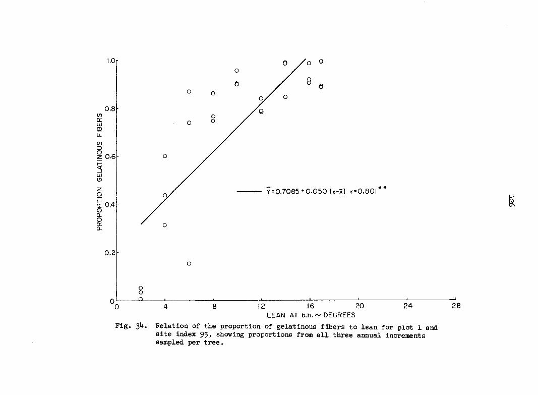
l.Or

0.8

0.6-

V) cr LU m

cn Z) o

lu O

b: 0.4 O CL O CE CL

O

6

Y = 0.7085 + 0.050 (x-x) r = 0.80l

0.2 o

_o_

28 0

Fig. 34.

8 12 16 20 LEAN AT b.h. ~ DEGREES

24

Relation of the proportion of gelatinous fibers to lean for plot 1 and site index 95, showing proportions from all three annual increments sampled per tree.

l.Or

O

A

A # O

1

• CORE 2

O CORE 3

A CORE I

0 4 8 12 16 20 24 28 LEAN AT b.h. ~ DEGREES

Fig. 35. Relation of the proportion of gelatinous f i bers to lean for plot 2 and site index 89.

0,8

li­en

Y = 0.1691-0.0284 (x-x) r = 0.7!8

0.4

0.2

20 24 28 LEAN AT b.h.~ DEGREES

Fig. 36. Relation of the proportion of gelatinous fibers to lean for plot 3 and. site index 113.

CO 0-8

u.

bO-6

Y=0.3458 +0.082 (x-x) r=0-96l** £0.4

0.2

20 24 28 LEAN AT b.h. "DEGREES

Fig. 37. Relation of the proportion of gelatinous fibers to lean for plot 5 and site index 97.

0.8

lu

z 0.6

- 9 = 0.3429*0.0811 (x-x) r=0.946**

• INDICATES 3 POINTS

% 0.4

0.2

20 28 24 LEAN AT b.h. ~ DEGREES

Fig. 38. Relation of the proportion of gelatinous fibers to lean for plot 5 and. site index 97 showing proportions from all three annual increments sampled per tree.

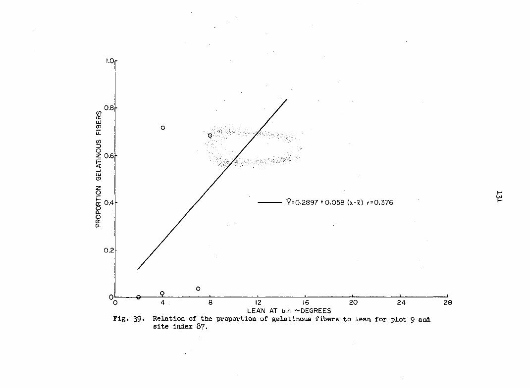
l.Or

O )l e ° ' 1 ' ' ' O 4 8 12 16 20 24 28

LEAN AT b.h. "DEGREES Fig. 39. Relation of the proportion of gelatinous fibers to lean for plot 9 and

site index 87.

uj

co

'93 + 0.124 (x-x) r =0.997** = 0.6

0.4

0.2

20 28 24 LEAN AT b.h. ~ DEGREES

Fig. 40. Relation of the proportion of gelatinous fibers to lean for plot 10 and site index 89.

l.Or

Yr0.4538 + 0.032 (x-x) r = 0.7l2

0 8 20 24 12 16 LEAN AT b.h. ~ DEGREES

Fig. 41. Eelation of the proportion of gelatinous fibers to lean for plot 12 and site index 88.

28

l.Or

0.8

(z) CH. y

3 0.6h O

lu O

| 0,4 CL

2 o tr ÛL

Y = 0.3968 +0-0316 (x-x) r = 0.399

0.2

0

Fig. 42.

8 20 24 12 16 LEAN AT b.h. ~ DEGREES

Relation of the proportion of gelatinous fibers to lean for plot 13 and site index 103.

28

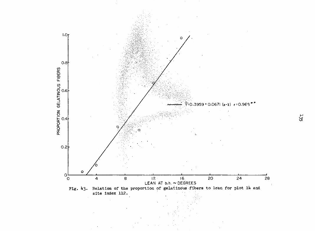
1.0

0.8

O 0.6

: Y=0.3959 +0.0671 (x-x) r=0.965*** lu

b 0.4

0.2

0 28 20 24 0

LEAN AT b.h, ~ DEGREES Fig. 4-3. Relation of the proportion of gelatinous fibers to lean for plot 14 and

site index 112.

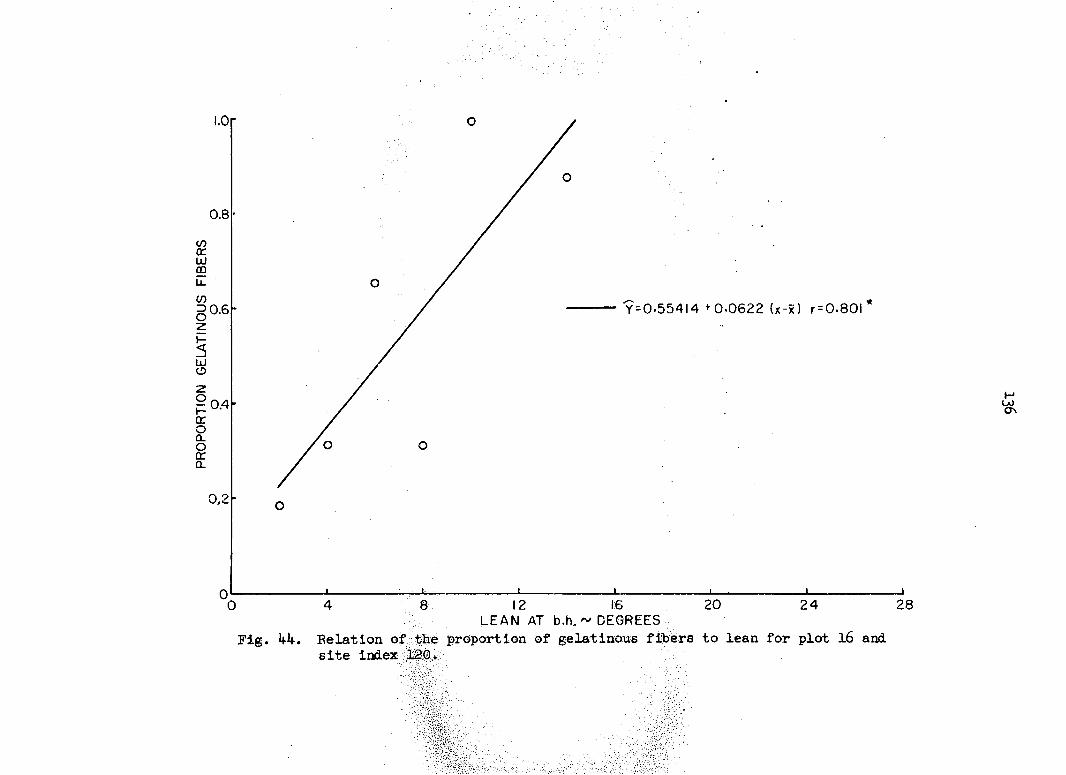
Y = 0-554I4 +0-0622 (x-x) r = 0.80l

L E A N A T b . h , ~ D E G R E E S

Fig. 44. Relation of the proportion of gelatinous fibers to lean for plot 16 and site index 12:0.

l.Or o

Y =0.6.041 + 0.0258 (x-x) r = 0.8l0

8 20 24

Fig. 45.

1:2 1(6 . LE AW m b-.,hi'. ~ DEGREES

Eelation of the proportion -o;ïF ;g >M*9iniQ,u6 fibers to lean for plot 18 and site index 101. < - ~4,

28

l.Or

Y = 0.35I7+O.OI62 (xrx) r = 0.227

•o, i o

Fig. h6.

& 20 24 12 It© • • LEAN AT bh.~DE@WEES

Relation of the pj?o;pprt-iq,n ©f géiat inou's f StW,s t<o lean for plot 20 and site index 93»

28

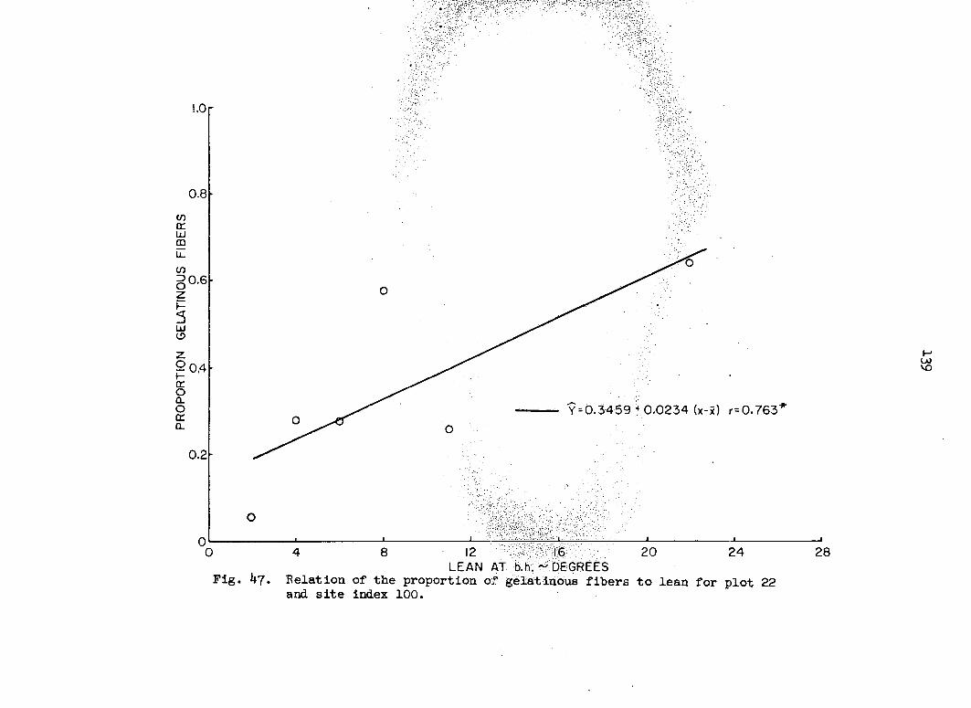
l.Or

Y = 0.3459 + 0.0234 (x-x) r= 0.763'

0 8

Fig. 47.

20 24 12 16 LEAN AT b.h. ~ DEGREES

Relation of the proportion of gelatinous fibers to lean for plot 22 and site index 100.

28

0.8

UL

O 0.6

Y = G.I704 +0.0898 (x-x) r = 0.787 lu

2 0.4

0.2

20 24 28 LEAN AT b.h. ~ DEGREES

Fig. 48. Eelation of the proportion of gelatinous fibers to lean for plot 23 and. site index 120.

1.0

•8

.6

.2

O LEAN 2°

# LEAN 3e

e

o

o'—e—©-»—o—»—#—• • 1

85 90 95 100 105 110 115 120 SITE INDEX

Fig. 49. Relation of proportion of gelatinous fibers to site index for lean 2 and 3 degrees.

il.O

00 tr UJ 00

CO 3 O z

LU (5

O -I— tt O

è cc CL

• .6

•8

%

O LEAN 4C

• LEAN 5C

O

O

O

90 95 no 115 120 100 105 SITE INDEX

Fig. 50. Relation of proportion of gelatinous fibers to site index for lean 4 and 5 degrees.

V) CE LU CD

«J O

3 LU <5

Z O h-OC

O g

1.0

O LEAN 6

• LEAN

mam

.8

.6

•O

0 85 90 95 120 100 105 ; 110 115

site index Fig. 51. Relation of proportion of gelatinous

fibers to site index for lean 6 and 7 degrees.

£ LU CD

CO 3 O z

LU (5

Z o H-0C O CL O CE CL

o lean 8°

• lean 9°

.6

.4 £

.2

0 85 90 95 110 115 120

Fig. 52.

100 105 site index , . . .

Relation of proportion of gelatinous fibers to site index for lean 8 and 9 degrees.

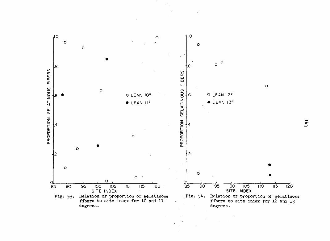
1.0

o

g t- 1 CL O CL O tr o.

.8

O LEAN 10°

• L E A N I I 6

.4

O 0 85 90 95 I00 105 IIO II5 I20

SITE INDEX Fig. 53. Relation of proportion of gelatinous

fibers to site index for 10 and 11 degrees.

nl.O

.8

.2

O °

o LEAN 12°

• LEAN I3C

H

<5"

85 90 . 95 100 105 110 115 120 SITE INDEX

Fig. 54. Relation of proportion of gelatinous fibers to site index for 12 and 13 degrees.

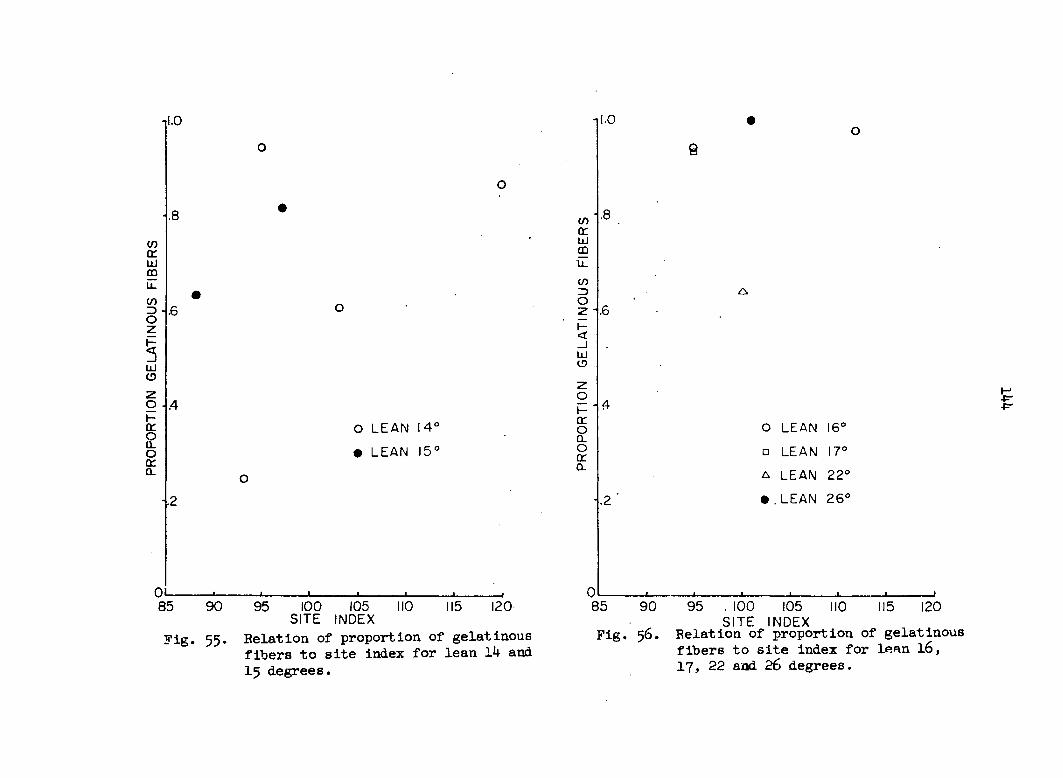
O LEAN 14°

• LEAN 15°

.2

i 1 , i i i i • )5 90 95 100 105 110 115 120

SITE INDEX Fig. 55. Relation of proportion of gelatinous

fibers to site index for lean 14 and 15 degrees.

il.O

.8

• .6

8

4 I

O LEAN 16°

• LEAN 17°

a LEAN 22°

.2 " • , LEAN 26°

85 90 95 . 100 105 110 115 120 SITE INDEX

Fig. 56. Relation of proportion of gelatinous fibers to site index for lean 16, 17, 22 and 26 degrees.

145

DISCUSSION

The chemical and. physical properties of xylem are determined by the

lignin-cellulose ratio in the cell walls. The walls of stimulated cells

become swollen and stained purple by chloriodide of zinc, indicating the

presence of long-chain molecules, whereas the walls of unstimulated cells

in situ are not appreciably swollen or stained. Extracted cellulose from

unstimulated tissues is iodine-stainable after swelling by zinc chloride

(Bonner, 195O, p. 362; Schorger, 1926, p. 214). The gelatinous layer and

extracted cellulose are essentially devoid of lignin. The blue color

complex apparently cannot form when lignin bonding and/or structural

interpénétration are present. The lack of structural rigidity and

lamellar unification, plus possible intermicellar movement, are sources of

dimensional instability. The greater amount of hydrophilic material may

also be a source of instability in tension wood.

The orientation of the cellulose micelles in the gelatinous layer has

been shown by both chemical and microscopic evidence to be axial with re­

spect to the vertical axis of the cell. It is also known that the gelatin­

ous layer has greater density than lignified cell wall substance. Since

according to Frey-wyssling (1957, p. 17) there is no "mass deficit" between

tension wood and "normal wood", the question remains whether the space

vacancy created by the absence of lignin is actually occupied by more cellu­

lose micelles of usual size fluctuation, larger micelles, smaller micelles,

or some combination. Controversy in the literature concerning this point

arises because there is a distribution of micelle size and degree of

crystalliuity associated vith cellulose biosynthesis. The population means

146

and. medians require examination. Frey-Wyssling states that the presence of

non-eellulosic constituents limits and causes defective cellulose crystal­

lization, but this is not a factor in substances like polyethylene glycol,

which also have micellar structure. The role of phosphorus in cellulose

synthesis may be important in answering these questions. It is now be­

lieved that, cellulose synthesis proceeds through uridine triphosphate (UTP)

carrier molecules (Whelan, 1959)* Glucose and UTP combine to form uridine

diphosphate glucose units (UDPG) which add to primer chains. The accelera­

tion of cellulose synthesis in tension wood may account for the increased

phosphorus demand revealed in this study. This should be checked at more

critical levels of phosphorus. The apparent phosphorus demand may also

involve nucleoprotein levels since the current literature indicates that

nucleoprotein metabolism is functionally related to the occurrence of plant

tumors.

Compression wood occurs on the lower side of leaning coniferous stems

and in contrast to tension wood exhibits extremely high lignification, which

indicates accelerated lignin synthesis. Westing (1959) found shifts in

peroxidase levels and also a Salkowski positive substance to be associated

with the initiation of compression wood. Peroxidase is stated to be essen­

tial for lignin biosynthesis in conifers. There is analogy between tension

wood and compression wood, but they are not homologous. Considerable insight

might be gained by studying some of the analogies through the medium of

vesselless dicotyledons such as Drimys aromatica F. Muell. In this angiosperm

the reaction tissue appears to be homologous with that of gymnosperms except

that it forms on the upper side of the stem.

The sequence of bud development observed in this study may be related

147

to reaction tissue initiation. Buds are loci of auxin biosynthesis, and

auxin is normally basipetally transported with little lateral transloca­

tion. Auxin is a stimulant of cell division, and hence the observations

appear consistent with the sometimes observed eccentricity of the upper

side of angiosperm stems and of the lower side of gymnosperm stems. It

is also known that sub-epidermal application of IAA-lanolin pastes effects

the formation of compression wood. However, it is questionable that auxin

that is formed in the tops of large trees exerts a translocated effect

at breast height. Such long distance translocation is questionable be­

cause of auxin inactivation and destruction by photooxidation, conjugation,

and by action of the IAA oxidase system. Diffusion of IAA to the lower

side of inclined organs has been demonstrated, however, the results of

bioassays on this point are conflicting. Reaction tissue in cottonwood

is concentrated on the upper side of the leaning stem at breast height,

but spreads around the bole in the upper expanses of the tree. Westing's

conclusions that ".ovels of auxin are unimportant and that differential

sensitivity to auxin is the important factor may have some merit.

Studies involving anti-metabolites may provide important information

about tension wood. The shifting levels of metabolites are probably due

to negative feedback mechanisms similar to those currently being found to

be fundamental in other regulatory functions. The absolute nature of the

cytological response and the distributional nature of the histological

response are evidence of cyclical phenomena. The distributional form of

the histological response arises from: (l) the cambial production of small

groups of stimulated cells, and (2) the abrupt cambial fluctuation result­

ing from interruptions, possibly at various points in the metabolic cycle.

146

Regardless of the source of the inducting complex, the induction cones

very early in the ontogeny of the cell.

Reaction tissue tends to develop where it opposes a deforming force

and where it maintains or restores a specific morphogenetic pattern. In

angiosperms the locus of reaction tissue is so disposed that the contrac­

tive force which develops in the presence of the reaction tissue will tend

to restore the morphogenetic pattern. The response of the plant is ulti­

mately controlled by its genetic constitution and the evolution of the

phenomenon was therefore due to natural selection acting on genetic varia­

tion.

Mechanical tissue in general has regulatory functions. This can be

observed in climbing vines, petioles, and suitably stimulated herbaceous

stems, as well as in the stems and branches of woody plants. The reac­

tion of tissues is a normal physiological and anatomical phenomenon. It

is not abnormal, in the sense that plant vigor is not depressed.

The most immediate measures of environmental conditions in this study

were "ring width" (radial growth) and cell number" (cambial division).

Both of these quantities were significantly and positively correlated with

the proportion of gelatinous fibers. Furthermore, the same factors that

cause fluctuation in reaction tissue cause equally strong fluctuation in

radial growth. The cytological observations also indicate that below a

certain metabolic threshold (as revealed by radial growth) no reaction

tissue is produced irrespective of the amount of stimulation. There is

also a maximum expression of a given amount of stimulation, and beyond this

point no additional increase in metabolism, as revealed by radial growth,

will cause an increase in reaction. Thus for a given amount of stimulation

149

the reaction is limited to certain metabolic intervals as expressed by-

radial growth.

However, the results presented in this report are only one random­

ization of a general age class. Capacity to react is a function of age

as well as stimulation. Perhaps younger plants would have been more

suitable experimental material, as suggested by the varying effects of

the permanent site factors. With younger experimental plants more posi­

tive relationships with the gross growth factors may be demonstrable.

150

SUMMARY

1. A biométrie technique was developed for the study of reaction

tissue. Images of cross sections including the cambium and 3 annual

increments taken from the upper side of leaning cottonwood stems were

projected on paper grid systems. Counts of stimulated and non-stimulated

cells in randomly selected grids were recorded. This procedure provides

a means of subjecting to statistical analysis the data on the gelatinous

cells of tension wood and other cytohistological features.

2. The induction of the gelatinous layer occurs early in cellular

ontogeny. The cambium produces stimulated cells in small groups, but

abrupt variations occur, possibly from blockage at various points in the

metabolic pathway.

3. Higher proportions of gelatinous fibers are associated with larger

ring width and larger numbers of smaller cells.

4. There is a suppression of vessel size associated with the presence

of reaction tissue.

5. Strong fluctuation in the factors which determine radial growth

is associated with equally strong fluctuation in the factors that induce

reaction tissue. The association of reaction tissue and the factors con­

trolling radial growth occur in certain metabolic intervals.

6. Significant but small positive correlation exists between adjacent

grid squares, and significant but small negative correlation exists between

distant grid squares.

7. A gain in efficiency of 129 percent was obtained by using the

weighted mean of samples of eight grid squares instead of the unweighted

151

means of individual squares.

8. The variance associated with the proportion of gelatinous fibers

as recorded on the grid systems is significantly greater than simple bi­

nomial variance.

9. Lean is the strongest correlate with the proportion of gelatinous

fibers in Populus deltoïdes.

10. For the age group and ecological situations of the trees examined

in this study, there is one overall regression coefficient for proportion

of gelatinous fibers regressed on lean.

11. In two large multiple linear regressions crown volume was highly

significantly correlated with the proportion of gelatinous fibers. How­

ever, its effect varies depending on the age and condition of the trees.

Crown volume is an excellent correlate of many soil and tree attributes.

12. The rate and capacity for reaction tissue production in woody

plants are depressed with the onset of senescence, the duration of stimulus,

and the levelling off of diameter growth.

13. In two large multiple linear regressions, available phosphorus

was found to be highly significantly and positively related to the pro­

portion of gelatinous fibers. This result may be related to the increased

cellulose synthesis which is associated with tension wood. This result

should be checked at more critical levels of phosphorus.

14. It appears that tension wood involves a lack of lignin synthesis

whereas compression wood is associated with the stimulation of lignin

synthesis in the xylem.

152

LITERATURE CITED

Aklute, Virginia and Baudendi- tel, M. E. 1 $46. High longitudinal shrinkage and gelatinous fibers in an eccentric cottonwood log. Jour. Forestry

44: IO53-IO57.

and Pillow, Maxon Y. I95O. Occurrence of gelatinous fibers and their effect upon properties of hardwood species. For. Prod. Res. Soc. Ann. Proc. 4: 254-264.

Amos, G. L., Bisset, I. J. ¥., and Dadswell, H. E. I95O. Wood structure in relation to growth in Eucalyptus gigantea Hook. F. Australian Jour. Scientific Res., Series B, Biological Sciences 1: 3-16.

Bailey, I. W. 1939« The microfibrillar and microcapillary structure of the cell wall. Bull. Torrey Bot. Club 66: 201-213.

. 1940. The walls of plant cells. American Association for the Advancement of Science Publ. 14: 31-43•

and Kerr, Thomas. 1935* The visible structure of the secondary wall and its significance in physical and chemical investigations of tracheary cells and fibers. Jour. Arnold Arboretum 16: 273-3OO.

and . -1-937• The structural variability of the secondary wall as revealed by lignin residues. Jour. Arnold Arboretum 18: 261-272.

and Vestal, Mary R. 1937* The orientât ion of cellulose in the secondary cell walls of tracheary cells. Jour. Arnold Arboretum 18: I85-I95..

Berlyn, Graeme P. 1959* A biométrie technique for reaction tissue research. Proc. Iowa Academy of Science 66: 98-102.

Birnbaum, Z. W. 1952. Numerical tabulation of the distribution of Kolmo-goroff's statistic for finite sample size. Jour. American Statistical Association 47: 425-441.

&nd Tingey, F. H. 1951• One-sided confidence contours for probability distribution functions. Annals of Mathematical Statistics 22: 592-596.

Bland, David E. 1958- The chemistry of reaction wood. Part I. The lig-nins of Eucalyptus goniocalyx and Pinus radiata. Holzforschune 12: 36-42.

Bonner, James, I95O. Plant biochemistry. Academic Press, Inc., New York, N. Y.

153

and Galston, Arthur W. 1952. Principles of plant physi­ology. W. H. Freeman and Company, San Francisco, Calif.

Braun, A. C. 1954. The physiology of plant tumors. Ann. Rev. Plant Phys.

5: I33-I63-

Brendemuehl, R. H. 1957- Growth yield and site requirements of eastern cottonwood. Unpublished Ph. D. Thesis. Library, Iowa State University of Science and Technology, Ames, Iowa.

Brown, H. P., Panshin, A. J., and Forsaith, C. C. I9^9« Textbook of wood technology. Vol. 1. McGraw-Hill Book Company, Inc., New York, N.Y.

Burns, George P. 1920. Eccentric growth and the formation of redwood in the main stem of conifers. Vermont Agricultural Exp. Sta. Bull. 219.

Btisgen, M. and Mûnch, E. I929. The structure and life of forest trees. John Wiley and Sons, Inc., New York, N. Y.

Chow, K. Y. 1946. A comparative study of the structure and chemical com­position of tension wood and normal wood in beech (Fagus sylvatica L.). Forestry 20: 62-77.

Clark, Wendell P. 1956. The effect of tension wood on the seasoning and machining properties of eastern cottonwood. Unpublished M. 8. Thesis. Library, Iowa State University of Science and Technology, Ames, Iowa.

Clarke, S. H. 1930- Home grown timbers: their anatomical structure and its relation to physical properties: elm. Great Britain Dept. of Science and Ind. Res. For. Prod. Bull. No. 7. 1930.

1931* The tertiary wall of wood fibers. Nature (London) 128: IO78.

1933* 0& estimating the mechanical strength of the wood of ash. Forestry 7: 26-31.

1935a• Application of microchemical tests in assessing the quality of ash timber. Nature (London) 135: 910.

1935b. Recent work on the relation between anatomical struc­ture and mechanical strength in ash. Forestry 9: 132-138.

„ 1936. The influence of cell-wall composition on the physical properties of beech wood. Forestry 10: 143-148.

1937a• A comparison of certain properties of temperate and tropical timbers. Tropical Woods 52: 1-11.

1937b. The distribution, structure, and properties of tension wood in beech (Fagus sylvatica L.). Forestry 11: 85-91.

154

Cochran, W. G. 1953. Sampling techniques. John Wiley and Sons, Inc., New York, N. Y.

Cockrell, R. A. 1946. Influence of fibril angle on the longitudinal shrink­age of ponderosa pine wood. Jour. Forestry 44: 876-878.

Coppick, B., and Fowler, W. F. 1939. The location of potential reducing substances in woody tissues. Paper Trade Jour. 109: l35~l^O.

Dadswell, H. E. 1945. Timbers of the New Guinea region. Tropical Woods 83: 1-14.

and Wardrop, A. B. 1949. What is reaction wood? Australian Forestry 13: 22-33*

and 1955. The structure and properties of tension wood. Holzforschung 9: 97-104.

David, H. T. and Berlyn, G. P. i960. Analyzing triplets (Dittoed). Statistical Laboratory, Iowa State University of Science and Tech­nology, Ames, Iowa

Davis, E. M. 1947. Machining and related properties of aspen. Lake States For. Exp. Sta. Rept. No. 8.

Ewart, A. J. and Mason-Jones, A. J. 1906. The formation of redwood in conifers. Annals of Bot. 20: 201.

Frazer, Donald A. 1952• Initiation of cambial activity in some forest trees in Ontario. Ecology 33: 259-273.

Frey-Wyssling, A. 1935• Die St offaus sche idung der Htiheren Pflanzen. Julius Springer, Berlin.

195^" The fine structure of cellulose microfibrils. Science 119: 80-81.

1957» Macromolecules in cell structure. Harvard Univer­sity Press, Cambridge, Massachusetts.

and Mtihlethaler, K. 1946. Submicroscopic structure of cellulose gels. Jour. Polymer Science 1: 172-174.

Gevorkiantz, S. R. and Olsen, L. P. 1955. Composite volume tables for timber and their application in the Lake States. U. S. Dept. Agr. Forest Service Tech. Bull. No. 1104.

Gibbs, R. Darnley. 1958. The M&ule reaction, lignins, and the relationship between woody plants. In Thimann, K. V., ed. The physiology of forest trees, pp. 269-312. The Ronald Press Company, New York, N. Y.

155

Gordon, Solon A. I953. Physiology of hormone action. In W. E. Loomis, ed. Growth and differentiation in plants, pp. 253-281. The Iowa State College Press, Ames, Iowa.

Haberlandt, G. 1914. Physiological plant anatomy. 4th ed. Macmillan and Company, Ltd., St. Martin's Street, London.

HSgglund, E. 1951. Chemistry of wood. Academic Press, Inc., New York, N. Y.

Harlow, William M. 1928a. Contributions to the chemistry of the plant cell wall. II. Lignification in the secondary and tertiary layers of the cell walls of wood. New York State College of Forestry Tech. Publ. No. 24.

1928b. Contributions to the chemistry of the plant cell wall. III. The reliability of staining reagents in microchemical studies of the plant cell walls. New York State College of Forestry Tech. Publ. No. 24.

1941. Contributions to the plant cell wall XI. Paper Trade Jour. 112: 31.

Harrar, E. 8. 1954. Defects in hardwood veneer logs; their frequency and importance. Southeastern For. Exp. Sta. Paper No. 39«

Hartig, Robert. 1901. Holzuntersuchungen Altes und Neues. Verlag von Julius Springer, Berlin.

Hartmann, F. 1932. Untersuchungen tiber Ursachen und Gesetzméissigkeit exzentrischem Dickenwachstums bei Nadel- und Laubbéiumen. Fcrstwissen-schaftliches Centralblatt 54: 497-517, 541-566, 58I-59O, 622-634.

1942. Das statische Wucsgesetz bei Nadel- und LaubbSumen. neue Erkenntnis iiber Ursache, Gesetzméissigkeit und Sinn des Reaktion-holzes. Springer-Verlag, Wien.

Haskell, Henry H. 195b. Gluing properties of tension wood in eastern cottonwood using cross-lap and block shear test specimens. Unpub­lished M, S. Thesis. Library, Iowa State University of Science and Technology, Ames, Iowa.

Heyn, A. N. J. 1940. The physiology of cell elongation. Bot. Rev. 6: 515-532.

Jaccard, P. 1938. Exzentrisches Dickenwachstum und anatomischhistologische Differenzierung des Holzes. Berichte der Schweizerischen botanischen Gesellschaft 48: 491-502.

1$6

ig40. Tropisme et bois de reaction provoques par la force centrifuge ches des feuillus. Berichte der Schweizerischen botan-ischen Gesellschaft $0: 279-284.

Jacobs, M. R. 1939a. Further studies on fiber tension. Australia Common­wealth Forestry Bur. Bull. No. 24.

1939b. A stud?- of the effect of sway on trees. Australia Commonwealth Forestry Bur. Bull. No. 26.

I9U5. The growth stresses of woody stems. Australia Commonwealth Forestry Bur. Bull. No. 28.

Jane, F. W. 1956. The structure of wood. The Macmillan Company, New York, N. Y.

Jayme, G. 19$1. tîber die Bedeutung des Zugholzanteils in Pappelh&Lzern. Holz Roh-u Werkstoff 9: 173-175» (Original not available; abstracted in Forestry Abstracts 13: 1526. I95I).

and Harders-Steinhàuser, M. 1950. Ûber die chemische Zusammensetzung des Zugholzes in einem Pappelholz. Papier, Darm­stadt 4: 104-113. (Original not available; abstracted in Forestry Abstracts 14: 2613. 1953).

Jutte, S. M. 1956. Tension wood in wane (Ocotea rubra Mez.). Holzforschung 10: 32-35.

and Isings, J. 1955* The determination of tension wood in ash with the aid of the phase-contrast microscope. Experentia 11: 386-387.

Kaeiser, Margaret. 1955* Frequency and distribution'of gelatinous fibers in eastern cottonwood. American Jour. Bot. 42: 331-334.

1956. Variations in fiber length of eastern cottonwood. U. S. For. Prod. Lab, Rept. No. 2047.

and Pillow, Maxon Y. 1955* Tension wood in eastern cottonwood. Central States For. Exp. Sta. Tech. Paper No. 149.

and Stewart, Kenneth D. 1955. Fiber size in Populus deltoides Marsh, in relation to lean of trunk and position in trunk. Bull. Torrey Bot. Club 82: 57-61.

Kerr, Thomas and Bailey, I. W. 1934. The cambium and its derivative tissues, X. Structure, optical properties and chemical composition of the so-called middle lamella. Jour. Arnold Arboretum 15: 327-349.

157

Klauditz,, W. and Stolley, I. 1955- tTber die biologisch mechanischen und technischen Eigenschaften des Zugholzes. Holzforschung 9: 5~10. (Original not available; abstracted in Forestry Abstracts If: 3204.

1956).

Koehler, Arthur. 1954. Longitudinal shrinkage of wood. U. S. For. Prod. Lab. Bept. No. 1093*

Kuziel, S. 1953- Recherches sur la longueur de fibres du bois. Bull, de la Soc. des Sciences et des Lettres de Lodz, Classe III de Sciences mathématiques et naturelles 4: 13. (Original not available; ab­stracted in Forestry Abstracts 16: 2153. 1955).

Lange, P. W. 1954. The distribution of lignin in the cell wall of normal and reaction wood from spruce and a few hardwoods. Svensk Papp. Tidn. 57: 525-535. (Original not available; abstracted in Forestry Ab­stracts 16: 866. 1955).

Lassen, L. E. 1958. Effect of tension wood on density, toughness, and end­wise compression of cottonwood. Unpublished M. S. Thesis. Library, Iowa State University of Science and Technology, Ames, Iowa.

Marra, Alan A. 1942. Characteristics of tension wood in hard maple, Acer saccharum Marsh. Unpublished M. S. Thesis. Library, New York State College of Forestry, Syracuse, N. Y.

Messeri, A. 1954. Caratteri dimensional! e strutturali delle fibre di tensione di un campione di pioppo. Cellulosa e Carta, Roma 5: 8-10. (Original not available; abstracted in Forestry Abstracts 16: 2154. 1955)-

Meyer, B. S. and Anderson, D. B. 1952. Plant physiology. D. Van Nostrand Company, Inc., New York, N. Y.

Newconbe, Frederick C. 1895» The regulatory formation of mechanical tissue. Bot. Gaz. 20: 441-448.

Northcote, D. 1958. The cell walls of higher plants, their composition, structure, and growth. Biol. Rev. 33: 53-102.

Ollinmaa, Paavo J. 1956. Vetopuupitoisuuden merkityksestS punta eri tarkeituksiin k&ytett&essë. (On the anatomic structure and prop­erties of the tension wood in birch. In Finnish, English transla­tion). Acta Forestalia Fennica 64: 144-263.

Onaka, F. 1949. Studies on compression and tension wood. Wood. Res., Kyoto No. 1. (Original not available; abstracted in Forestry Ab­stracts 11: 28I5. 1950).

Pearson, E. S. and Hartley, H. 0. 1954. Biometrika tables for stati­sticians. Volume I. Cambridge University Press, London.

158

Pentoney, Richard E. 1953. Mechanisms affecting tangential v$. radial shrinkage. Jour. For. Prod. Res. Soc. Ill: 27-32.

Pillow, Maxon Y. I95O. Presence of tension wood in mahogany in relation to longitudinal shrinkage. U. S. For. Prod. Lab. Rept. No. DI763•

I95I. What is compression wood and tension wood; and what is their practical significance? Southern Lumberman 182: 52.

1953. Effects of tension wood in hardwood lumber and veneer. U. S. For. Prod. Lab. Rept. No. RI9U3.

Preston, R. D. 1941. The fine structure of phloem fibers. II. Un­treated and swollen jute. Proc. Roy. Soc. B. 130: IO3.

1942. Anisotropic contraction of wood and its constituent cells. Forestry 16: 32-48.

and Ranganathan, V. 1947- The fine structure of the fibers of normal and tension wood in beech (Fagus sylvatica L.) as revealed by x-rays. Forestry 21: 92-98.

and Wardrop, A. B. 1949. The submicroscopic organization of the walls of conifer cambium. Biochim. et Biophys. Acta 3: 549.

Priestly, J. H. and Tong, Dorothy. 1927. The effects of gravity upon cambial activity in trees. Proc. Leeds Phil. Soc. 1: 199-208.

Rendle, B. J. 1937• Gelatinous wood fibers. Tropical Woods 52: H-19.

195S. Tension wood. A natural defect of hardwoods. Wood 20: 348-351-

Roelofsen, P. A. 1959- The plant cell wall. Gebrtider Borntraeger, Berlin-Nikola s see.

Rosene, H. F. and Lund, E. J. I953. Bioelectric fields and correlation in plants. In W. E. Loomis, ed. Growth and differentiation in plants, pp. 219-252. The Iowa State College Press, Ames, Iowa.

Runger, H. G. and Klauditz, W. 1953- Ober Beziehungen zwischen der chemischen Zusammensetzung und den Festigkeitseigenschaften des Stammholzes von Poppeln. Holzforschung 7: 43.

Sass, J. E. 1958. Botanical microtechnique. 3rd ed. The Iowa State College Press, Ames, Iowa.

Schorger, A. W. 1926. The chemistry of cellulose and wood. McGraw-Hill Book Company, Inc., New York, N. Y.

159

Schrank, A. H. 1950. Plant trorisms. Ann. Rev. Plant Phys. 1: 59~7 -

Scnwerin, Gerda. 1958. The chemistry of reaction wood. Part II. The polysaccharides of Eucalyptus goniocalyx and Pinus radiate. Holz­forschung 12: 43-48.

Sinnott, E. W. I55I. The morphogenetic significance of reaction wood. Science 114: 478-488.

1952. Reaction wood and regulation of tree form. American Jour. Bot. 39: 69-78.

Snedecor, George W. 1956. Statistical methods. 5th ea The Iowa State College Press, Ames, Iowa.

Spurr, Stephen H. and Hyvârinen, Matti J. 1954a. Compression wood in conifers as a morphogenetic phenomenon. Bot. Rev. 20: 55l"560.

and 1954b. Wood fiber length as related to position in tree and growth. Bot. Rev. 20: 561-575»

Swanson, Carl P. 1957» Cytology and cytogenetics. Prentice-Hall, Inc., Englewood Cliffs, N. J.

Terrell, Bessie Z. 1952• Distribution of tension wood and its relation to longitudinal shrinkage in aspen. U. S. For. Prod. Lab. Sept. No. R 1917.

U. S. Forest Products Laboratory. 1950» Veneer cutting and drying properties : cottonwood. U. S. For. Prod. Lab. Rept. No. DI766-3.

van Overbeek, J. 1938. "Laziness" in maize due to abnormal distribution of growth hormone. Jour. Heredity ?9: 339-341.

Volk, William. 1958. Applied statistics for engineers. McGraw-Hill Book Company, Inc., New York, N. Y.

Wahlgren, H. E. 1956• Effect of tension wood on the longitudinal shrink­age and specific gravity of eastern cottonwood. Unpublished M. S. Thesis, Library, Iowa State University of Science and Technology, Amçs, Iowa.

1957. Tension wood in overcup oak. U. S. For. Prod. Lab. Rept. No. 2089.

Wallis, W. A. and Roberts, H. V. 1956. Statistics. The Free Press, Glencoe, 111inois.

Wardlaw, C. W. I952. Phylogeny and morphogenesis. Macmillan and Company, Ltd., St. Martin's Street, London.

i6o

Wardrop, A. B. I9U9. Micellar organisation in primary cell walls. Nature 164: 366.

1956. The nature of reaction wood. V. The distribution and formation of tension wood in sane species of Eucalyptus. Australian Jour. Bot. 4: I52-I56.

and Dadswell, H. E. 1948. The nature of reaction wood. I. The structure and properties of tension wood fibers. Australian Jour. Scientific Res., Series B, Biological Sciences 1: 3"l6.

and 1955* The nature of reaction wood. IV. Variation in cell wall organization of tension wood fibers. Australian Jour. Bot. 3: 177-189»

Went, F. W. and Thimann, K. V. 1937* Phytohormones. The Macmillan Company, New York, N. Y.

Wershing, Henry F. and Bailey, I. W. 1942. Seedlings as experimental material in the study of "Redwood" in conifers. Jour. Forestry 40: 411-414.

Westing, A. H. 1959* Studies on the physiology of compression wood forma­tion. Unpublished Ph. D. Thesis. Library, Yale University School of Forestry, New Haven, Conn.

Whelan, W. J. 1959* The enzymic synthesis and degradation of cellulose and starch. In Honeyman, J., ed. Recent advances in the chemistry of cellulose and starch, pp. 307-336. Inter science Publishers, Inc.", New York, N. Y.

White, J. 1908. The formation of redwood in conifers. Proc. Roy. Soc. Victoria 20: 107-124.

Youden, W. J. 1953* Sets of three measurements. Scientific Monthly 77: 143-147.

l6l

ACKN CWLEDGMENTS

The author wishes to express his appreciation to Dr. Dwight W.

Bensend. for suggesting the problem and for his sustained encouragement,

and to Dr. John E. Sass for invaluable guidance in anatomy, microtech­

nique, and photomicrography. It is a pleasure for the writer to

acknowledge the very considerable assistance of Dr. Herbert T. David

in the statistical phases of this study.

Appreciation is also due to the Iowa Agricultural and Home Econ­

omics Experiment Station, the Central States Forest Experiment Station,

and to Dr. Maxon Y. Pillow and the Forest Products Laboratory for their

interest and financial support.

Lastly, the author wishes to acknowledge the editorial and typo­

graphical contributions of his wife.