Copyright � 2009 by the Genetics Society of AmericaDOI: 10.1534/genetics.108.098277

Factors Affecting Accuracy From Genomic Selection in PopulationsDerived From Multiple Inbred Lines: A Barley Case Study

Shengqiang Zhong,* Jack C. M. Dekkers,† Rohan L. Fernando† and Jean-Luc Jannink‡,1

*Department of Agronomy, Iowa State University, Ames, Iowa 50011, †Department of Animal Science and Center for IntegratedAnimal Genomics, Iowa State University, Ames, Iowa 50011 and ‡U. S. Department of Agriculture–Agricultural Research Service,

Robert W. Holley Center for Agriculture and Health, Ithaca, New York 14583

Manuscript received November 3, 2008Accepted for publication March 1, 2009

ABSTRACT

We compared the accuracies of four genomic-selection prediction methods as affected by markerdensity, level of linkage disequilibrium (LD), quantitative trait locus (QTL) number, sample size, and levelof replication in populations generated from multiple inbred lines. Marker data on 42 two-row springbarley inbred lines were used to simulate high and low LD populations from multiple inbred line crosses:the first included many small full-sib families and the second was derived from five generations of randommating. True breeding values (TBV) were simulated on the basis of 20 or 80 additive QTL. Methods usedto derive genomic estimated breeding values (GEBV) were random regression best linear unbiasedprediction (RR–BLUP), Bayes-B, a Bayesian shrinkage regression method, and BLUP from a mixed modelanalysis using a relationship matrix calculated from marker data. Using the best methods, accuracies ofGEBV were comparable to accuracies from phenotype for predicting TBV without requiring the time andexpense of field evaluation. We identified a trade-off between a method’s ability to capture marker-QTLLD vs. marker-based relatedness of individuals. The Bayesian shrinkage regression method primarilycaptured LD, the BLUP methods captured relationships, while Bayes-B captured both. Under most of thestudy scenarios, mixed-model analysis using a marker-derived relationship matrix (BLUP) was moreaccurate than methods that directly estimated marker effects, suggesting that relationship informationwas more valuable than LD information. When markers were in strong LD with large-effect QTL, or whenpredictions were made on individuals several generations removed from the training data set, however,the ranking of method performance was reversed and BLUP had the lowest accuracy.

WITH the advent of cheap and high-density array-based DNA marker technologies, genomewide

dense molecular markers are becoming available forlivestock and crop species. As examples, cattle geneti-cists have genotyping systems that provide .50,000single nucleotide polymorphisms (SNP; VanRaden et al.2009); the U. S. Department of Agriculture-sponsoredBarley Coordinated Agricultural Project (CAP) is de-veloping 3000 informative SNP to be scored on 3840elite U. S. breeding lines. Meuwissen et al. (2001)developed a method called ‘‘genomic selection’’ topredict breeding values using precisely this kind ofgenomewide dense marker data. Marker effects are firstestimated on a training data set with marker genotypesand trait phenotypes. Breeding value can then bepredicted for any genotyped individual in the popula-tion using the marker-effect estimates. Simulationstudies have shown that genomic selection can lead tohigh correlations between predicted and true breeding

value over several generations without repeated pheno-typing (Meuwissen et al. 2001; Habier et al. 2007).Therefore, genomic selection can result in lower costsand increased rates of genetic gain.

Several statistical methods have been proposed foranalysis of the training data for genomic selection.Meuwissen et al. (2001) and Habier et al. (2007)compared least squares, random-regression best linearunbiased prediction (RR–BLUP) and Bayesian methods(Bayes-A and Bayes-B). Xu (2003) proposed a Bayesianshrinkage approach for quantitative trait locus (QTL)detection on the basis of the genomic-selection idea(Meuwissen et al. 2001). ter Braak et al. (2005)provided modifications to the Xu (2003) model to ensureproper posterior distributions-of-effect estimates and tobetter estimate QTL locations. We can regard theseBayesian shrinkage regression methods as another formof genomic selection when using them to predict breed-ing values. In previous work, these genomic-selectionprediction methods have predominantly been com-pared under a specific simulation scenario such thattheir relative strengths under different conditions oflinkage disequilibrium (LD), marker density, trainingdata set size, and distribution of QTL effects are not

Supporting information is available online at http://www.genetics.org/cgi/content/full/genetics.108.098277/DC1.

1Corresponding author: USDA-ARS, Robert W. Holley Center for Agricul-ture and Health, Ithaca, NY 14853-2901.E-mail: jean-luc.jannink@ars.usda.gov

Genetics 182: 355–364 (May 2009)

known. Furthermore, genomic selection was pioneeredin animal breeding systems and few studies haveconsidered plant breeding systems. Indeed, genomicselection in plants has been studied only for populationsderived from crosses of biparental lines (Bernardo andYu 2007; Piyasatian et al. 2007; Zhong and Jannink

2007). The extent and nature of LD in such popula-tions, however, will be quite different from populationswith many founders in mutation-drift-recombinationequilibrium.

Plant breeding populations have special characteristicsrelative to animal breeding populations. In particular,plant breeders often work with full-sib families createdfrom crosses of inbred parents that vary in size, whereashalf-sib families from non-inbred parents are moretypical in animal breeding. Extensive LD will arise withineach family but, given differing linkage phases acrossfamilies, LD across a large set of families should representthe underlying population-wide LD. In typical plant-breeding practice, enough lines from a germplasm poolwill have been sampled such that associations with adense marker set should be consistent population-wide,which would be particularly useful for association map-ping or marker-assisted selection (MAS) (Yu et al. 2008).Another characteristic of plant breeding is that the use ofinbred lines is common and breeders usually have theability to replicate individual genotypes over space andtime and, by averaging across replicates, can thus obtainvery accurate phenotypic measurements for a quantita-tive trait. Given a fixed amount of resources, breedershave the option to evaluate more individuals with loweraccuracy or fewer individuals with higher accuracy.These characteristics might affect how genomic selectionshould be carried out in crops relative to livestock.

Barley offers an excellent public-sector model forcrops because the Barley CAP and its partners havegenerated .4500 SNP from expressed sequence tags.These SNP have been scored on the ‘‘Barley CAP core,’’ aset of 102 inbred barley lines primarily of U. S. origin. Weused this data set as a starting point to test genomicselection for levels and structures of LD that are realisticfor a self-pollinating crop. Here, we report on the relativeperformance of alternate genomic-selection predictionmethods under different conditions of marker density,QTL effect distribution, and training data set size usingmating schemes that affected the extent of LD. We alsoassessed the adequacy of the marker density that iscurrently available for barley for genomic selection,contrasting the accuracies of genomic estimated breed-ing values (GEBV) with those that might be obtainedfrom phenotypic information.

MATERIALS AND METHODS

Overview: An ideal evaluation of genomic-selection estima-tion methods would require large data sets of individuals with

known breeding values scored at high marker density. In theabsence of such data sets, we simulated them realistically onthe basis of actual barley marker data. These data encapsulateactual LD structure upon which we can impose a geneticmodel to obtain phenotypes and true breeding values.Simulated mating designs allow generation of samples ofdifferent sizes and levels of LD, enabling us to explore a broadrange of scenarios. In the following, we describe the originalBarley CAP core data set, the assumed genetic model, themating designs used to generate samples, and, finally, thegenomic-selection prediction models that were evaluated.

Germplasm and genetic map: To avoid excessive popula-tion structure due to the historical separation between six- andtwo-row barley, we worked only with data from 42 two-rowspring barley lines (see supporting information, Table S1).The 1933-locus, 1279-cM map constructed by Peter Szucs andPatrick Hayes on the Oregon Wolfe Barley (OWB) population(http://www.barleycap.org/) was used as the reference map.This map contains Diversity Array Technology (DArT) markers,SNP, and classical markers (e.g., simple sequence repeat andrestriction enzyme fragment polymorphism markers). TheSNP genotypes were obtained from two Illumina GoldenGateassays. One assay was described in Rostoks et al. (2006) and theother was developed by similar methods (T. J. Close, personalcommunication). Map positions of SNP and classical markersbased on other mapping populations (T. J. Close, personalcommunication) were obtained from HarvEST: Barley 1.64(http://harvest.ucr.edu/). A consensus map of DArT andclassical markers was obtained from Wenzl et al. (2006). Thefollowing expedient approach was used to merge these maps.First, common markers between the OWB and each of theother two maps were identified. Per chromosome, there wereon average 77 (range: 65–97) and 69 (range: 32–94) markers incommon between the OWB and the SNP and DArT maps,respectively. The OWB map positions were then regressed onSNP map positions and on DArT map positions to project theSNP and DArT maps onto OWB-predicted positions. A mark-er’s final linkage map position was estimated as the mean of allavailable OWB or OWB-predicted positions. Only markers thathad a minor allele frequency .0.1 across the 42 two-row springbarley lines were used. This criterion resulted in the selectionof 1605 markers. Markers were then chosen so that they were atleast 0.2 or 0.75 cM apart, resulting in dense and sparse settingsof 1040 and 575 markers, respectively. In both settings, therewere 19 marker gaps .5 cM. All markers were biallelic. Giventhe low rate of missing marker data (1.7%), missing markergenotypes were randomly assigned according to their popula-tion allele frequency.

Genetic model: All loci were biallelic with inbred genotypescoded as 0 or 1. The number of segregating QTL affecting thetrait was set at either 20 or 80. QTL were simulated byrandomly drawing positions on the genetic map and assigningthe closest marker among the 1040 and 575 to be a QTL. Onemarker allele was randomly chosen to have a positive effectand the other to have a negative effect on the simulated trait.QTL effect sizes were scaled according to the allele frequen-cies to obtain variances that followed a geometric series(Lande and Thompson 1990). The breeding value of a linewas the sum of the effects of the QTL alleles that it carried. Toobtain the phenotype, we added a normal error deviate withvariance calculated to achieve the desired heritability.

Mating designs: Using the 42 lines as a founder pool, wesimulated four mating designs by pairing inbred lines,generating gametes according to Mendelian inheritanceassuming no crossover interference, and then by doublingthe gametes to create doubled haploid (DH) lines. Thesemating designs, which are described in detail in the followingand are summarized in Table 1, produced the training data

356 S. Zhong et al.

sets that were analyzed by genomic-selection methods topredict breeding values of individuals in testing data sets.Regardless of the mating design used to generate the trainingdata set, the testing data set was produced by one or fourgenerations of 500 random crosses between the DH lines ofthe training data, each with one progeny.

Design 1: Training data sets of 42 families of 12 DHs (504DHs in total) were generated using a single round-robindesign (Verhoeven et al. 2006); i.e., the lines were firstrandomly ordered and then crossed as follows: line 1 3 line2, line 2 3 line 3, . . ., line 42 3 line 1. To evaluate the effect ofincreasing the training data set size, we also generated design1–1000 data sets in which each family contained 24 DHs,resulting in 1008 lines.

Design 2: Training data sets of 500 double haploids withlower long-range LD than in design 1 were derived afterrandomly mating the original 42 lines for five generations. Thepopulation size during random mating was 200 individuals,and 500 DHs were derived at random from the last generation.Design 2–1000 data sets that contained 1000 DHs were alsocreated. The environmental variance for these designs was setsuch that the heritability was 0.4 for the original 42 lines.

Designs 3 and 4: Designs 3 and 4 were similar to designs 1and 2, respectively, but had one-third as many DHs. Assuminga fixed number of plots to grow plants, this would allow forincreased replication. A heritability of 0.67 was used tosimulate phenotypes for each DH, given that we had one-third the number of DH lines and therefore could afford threetimes more replicates relative to designs 1 and 2.

Linkage disequilibrium measures: Markers with minorallele frequency .0.2 in the Barley CAP core were used toestimate the extent of LD between all pairs of markers within100 cM in all chromosomes. The LD was computed as thesquared correlation between alleles at two markers: r̂ ¼D2

ij=ðpið1� piÞpjð1� pjÞ (Hill and Robertson 1968), whereDij ¼ pij � pipj and pij, pi, and pj are the frequencies ofhaplotype ij and allele i at one locus and allele j at the otherlocus.

Statistical models: Four genomic-selection predictionmethods were used for analysis of each training data set. Twowere as described by Meuwissen et al. (2001): RR–BLUP andBayes-B. RR–BLUP assumed that each marker had varianceequal to VG/M, where VG is the genetic variance and M is thenumber of markers. In the Bayes-B approach, the prior for theproportion of markers associated with zero phenotypic vari-ance, p, was assumed known. We evaluated two values, p ¼(M � 80)/M (denoted Bayes-B1) and p ¼ (M � 150)/M(denoted Bayes-B2). Other prior hyperparameters for markervariance components were the same between Bayes-B1 andBayes-B2 and were as given in Meuwissen et al. (2001). Thethird statistical method was based on ter Braak et al.’s (2005)improvements to the Bayesian shrinkage regression methoddeveloped by Xu (2003), which shrinks small effects toward zero(denoted ‘‘Xu2003’’). In the fourth method, markers were used

only to estimate the relationship between lines. First, a marker-based relationship matrix, A ¼ XX 9=

Pk pkð1� pkÞ, was calcu-

lated, where X is the DH line by marker matrix of marker scores,the summation is over all markers, and pk is the allele frequencyat marker k in the training data set (Habier et al. 2007;VanRaden and Tooker 2007). To ensure a positive definitematrix, A* ¼ A 1 10�6I was used in calculations (I is theidentity matrix). The heritability used to solve the mixed modelequations was set at the simulated heritability. To obtainbreeding value estimates for the testing data set, A wascalculated across the DH lines from both training and testingsets. Because this method uses an estimate of the realized Amatrix, we called it the RA–BLUP method.

In some cases, although the QTL were not identified, theirgenotypes were included along with all other markers in theanalysis. We contrast these ‘‘observed’’ QTL cases to moretypical ‘‘unobserved’’ QTL cases. For each mating design andmarker density scenario, 30–50 replicates were simulated andanalyzed using the four methods. After each analysis, thepredicted breeding values of the testing data set sample werecorrelated with their known true breeding values. This pre-diction accuracy was used as the performance criterion for themethods.

RESULTS

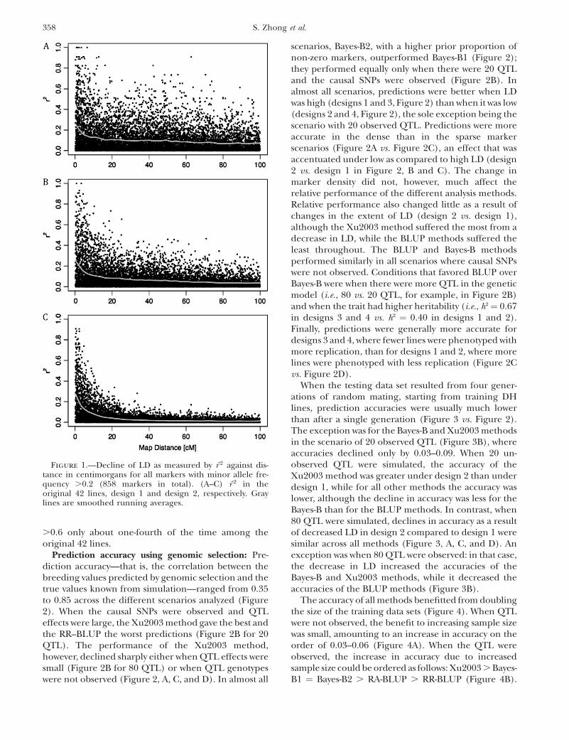
Extent of LD in two-row barley founders: Despiteavoiding structure due to the division between two- andsix-row barley, many instances of long-range LD re-mained among the 42 founders (Figure 1A), in agree-ment with previous studies in barley (Kraakman et al.2004; Rostoks et al. 2006). Even though high long-range LD occurred, LD at short range was low, averagingabout r̂ 2 ¼ 0.25 for markers ,0.25 cM apart. The singleround-robin mating of design 1 removed high LD (r̂ 2 .

0.4) at distances .30 cM (Figure 1B), although moder-ate LD (r̂ 2 . 0.2) still occasionally extended to 100 cM.After the five rounds of random mating as in design 2,moderate LD occurred only up to distances of �15 cM(Figure 1C). Design 2 also eliminated long-distance LDgreater than an r̂ 2 of 0.1. Thus, as expected, recombi-nation in designs 1 and 2 greatly reduced long-distanceLD but had little effect on LD at distances ,2 cM(Figure 1). If we assume that LD between marker pairsapproximates LD between markers and QTL, themarker density of �1/cM available for this study wouldoften lead QTL to be only in low LD with any marker: forexample, for QTL within 0.5 cM of a marker, the r̂ 2 was

TABLE 1

Mating designs used to simulate training data sets from 42 inbred founders

Design 1 Design 2 Design 3 Design 4 Design 1–1000 Design 2–1000

Generations of mating 1 5 1 5 1 5Mating structure Round Random Round Random Round RandomNo. of families 42 500 42 168 42 1000No. of DH per family 12 1 4 1 12 1No. of lines 504 500 168 168 1008 1000Heritability 0.4 0.4 0.67 0.67 0.4 0.4

Genomic Selection in Barley 357

.0.6 only about one-fourth of the time among theoriginal 42 lines.

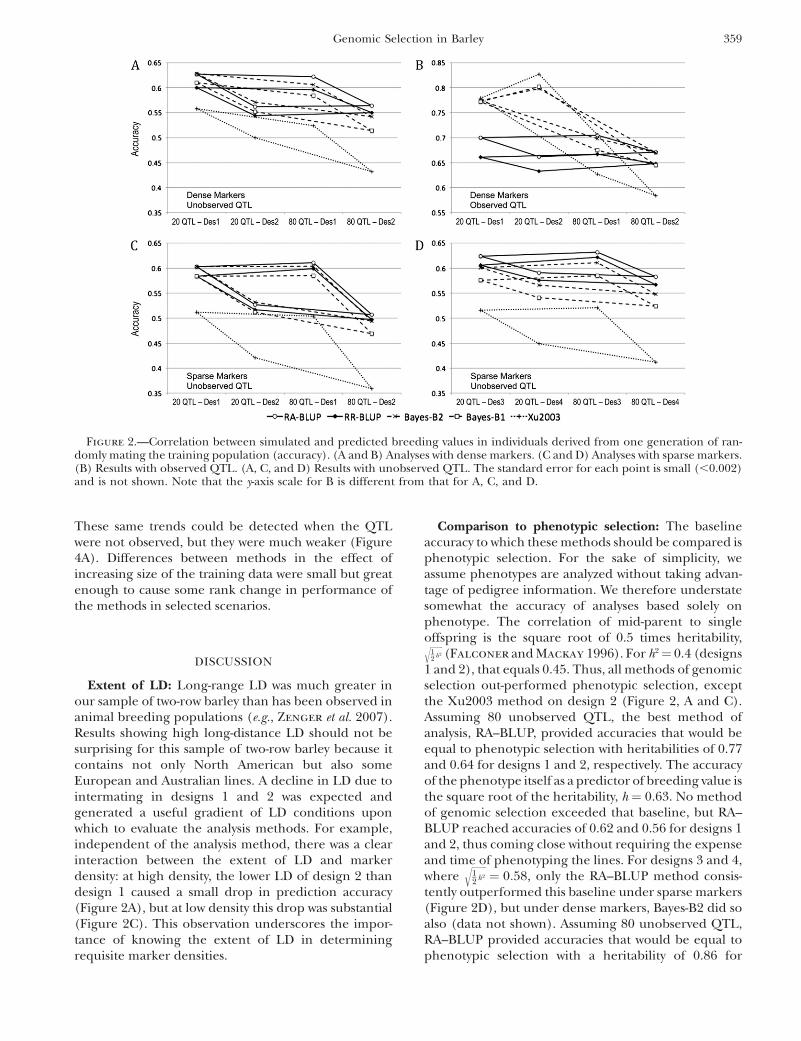
Prediction accuracy using genomic selection: Pre-diction accuracy—that is, the correlation between thebreeding values predicted by genomic selection and thetrue values known from simulation—ranged from 0.35to 0.85 across the different scenarios analyzed (Figure2). When the causal SNPs were observed and QTLeffects were large, the Xu2003 method gave the best andthe RR–BLUP the worst predictions (Figure 2B for 20QTL). The performance of the Xu2003 method,however, declined sharply either when QTL effects weresmall (Figure 2B for 80 QTL) or when QTL genotypeswere not observed (Figure 2, A, C, and D). In almost all

scenarios, Bayes-B2, with a higher prior proportion ofnon-zero markers, outperformed Bayes-B1 (Figure 2);they performed equally only when there were 20 QTLand the causal SNPs were observed (Figure 2B). Inalmost all scenarios, predictions were better when LDwas high (designs 1 and 3, Figure 2) than when it was low(designs 2 and 4, Figure 2), the sole exception being thescenario with 20 observed QTL. Predictions were moreaccurate in the dense than in the sparse markerscenarios (Figure 2A vs. Figure 2C), an effect that wasaccentuated under low as compared to high LD (design2 vs. design 1 in Figure 2, B and C). The change inmarker density did not, however, much affect therelative performance of the different analysis methods.Relative performance also changed little as a result ofchanges in the extent of LD (design 2 vs. design 1),although the Xu2003 method suffered the most from adecrease in LD, while the BLUP methods suffered theleast throughout. The BLUP and Bayes-B methodsperformed similarly in all scenarios where causal SNPswere not observed. Conditions that favored BLUP overBayes-B were when there were more QTL in the geneticmodel (i.e., 80 vs. 20 QTL, for example, in Figure 2B)and when the trait had higher heritability (i.e., h2¼ 0.67in designs 3 and 4 vs. h2 ¼ 0.40 in designs 1 and 2).Finally, predictions were generally more accurate fordesigns 3 and 4, where fewer lines were phenotyped withmore replication, than for designs 1 and 2, where morelines were phenotyped with less replication (Figure 2Cvs. Figure 2D).

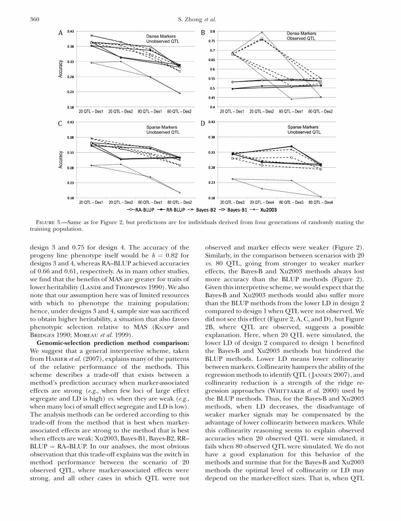
When the testing data set resulted from four gener-ations of random mating, starting from training DHlines, prediction accuracies were usually much lowerthan after a single generation (Figure 3 vs. Figure 2).The exception was for the Bayes-B and Xu2003 methodsin the scenario of 20 observed QTL (Figure 3B), whereaccuracies declined only by 0.03–0.09. When 20 un-observed QTL were simulated, the accuracy of theXu2003 method was greater under design 2 than underdesign 1, while for all other methods the accuracy waslower, although the decline in accuracy was less for theBayes-B than for the BLUP methods. In contrast, when80 QTL were simulated, declines in accuracy as a resultof decreased LD in design 2 compared to design 1 weresimilar across all methods (Figure 3, A, C, and D). Anexception was when 80 QTL were observed: in that case,the decrease in LD increased the accuracies of theBayes-B and Xu2003 methods, while it decreased theaccuracies of the BLUP methods (Figure 3B).

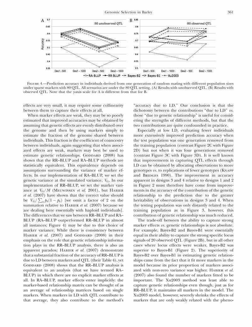
The accuracy of all methods benefitted from doublingthe size of the training data sets (Figure 4). When QTLwere not observed, the benefit to increasing sample sizewas small, amounting to an increase in accuracy on theorder of 0.03–0.06 (Figure 4A). When the QTL wereobserved, the increase in accuracy due to increasedsample size could be ordered as follows: Xu2003 . Bayes-B1 ¼ Bayes-B2 . RA-BLUP . RR-BLUP (Figure 4B).

Figure 1.—Decline of LD as measured by r̂ 2 against dis-tance in centimorgans for all markers with minor allele fre-quency .0.2 (858 markers in total). (A–C) r̂ 2 in theoriginal 42 lines, design 1 and design 2, respectively. Graylines are smoothed running averages.

358 S. Zhong et al.

These same trends could be detected when the QTLwere not observed, but they were much weaker (Figure4A). Differences between methods in the effect ofincreasing size of the training data were small but greatenough to cause some rank change in performance ofthe methods in selected scenarios.

DISCUSSION

Extent of LD: Long-range LD was much greater inour sample of two-row barley than has been observed inanimal breeding populations (e.g., Zenger et al. 2007).Results showing high long-distance LD should not besurprising for this sample of two-row barley because itcontains not only North American but also someEuropean and Australian lines. A decline in LD due tointermating in designs 1 and 2 was expected andgenerated a useful gradient of LD conditions uponwhich to evaluate the analysis methods. For example,independent of the analysis method, there was a clearinteraction between the extent of LD and markerdensity: at high density, the lower LD of design 2 thandesign 1 caused a small drop in prediction accuracy(Figure 2A), but at low density this drop was substantial(Figure 2C). This observation underscores the impor-tance of knowing the extent of LD in determiningrequisite marker densities.

Comparison to phenotypic selection: The baselineaccuracy to which these methods should be compared isphenotypic selection. For the sake of simplicity, weassume phenotypes are analyzed without taking advan-tage of pedigree information. We therefore understatesomewhat the accuracy of analyses based solely onphenotype. The correlation of mid-parent to singleoffspring is the square root of 0.5 times heritability,ffiffiffiffiffiffiffiffiffi

12 h2

r(Falconer and Mackay 1996). For h2¼ 0.4 (designs

1 and 2), that equals 0.45. Thus, all methods of genomicselection out-performed phenotypic selection, exceptthe Xu2003 method on design 2 (Figure 2, A and C).Assuming 80 unobserved QTL, the best method ofanalysis, RA–BLUP, provided accuracies that would beequal to phenotypic selection with heritabilities of 0.77and 0.64 for designs 1 and 2, respectively. The accuracyof the phenotype itself as a predictor of breeding value isthe square root of the heritability, h ¼ 0.63. No methodof genomic selection exceeded that baseline, but RA–BLUP reached accuracies of 0.62 and 0.56 for designs 1and 2, thus coming close without requiring the expenseand time of phenotyping the lines. For designs 3 and 4,where

ffiffiffiffiffiffiffiffiffi12 h2

r¼ 0:58, only the RA–BLUP method consis-

tently outperformed this baseline under sparse markers(Figure 2D), but under dense markers, Bayes-B2 did soalso (data not shown). Assuming 80 unobserved QTL,RA–BLUP provided accuracies that would be equal tophenotypic selection with a heritability of 0.86 for

Figure 2.—Correlation between simulated and predicted breeding values in individuals derived from one generation of ran-domly mating the training population (accuracy). (A and B) Analyses with dense markers. (C and D) Analyses with sparse markers.(B) Results with observed QTL. (A, C, and D) Results with unobserved QTL. The standard error for each point is small (,0.002)and is not shown. Note that the y-axis scale for B is different from that for A, C, and D.

Genomic Selection in Barley 359

design 3 and 0.75 for design 4. The accuracy of theprogeny line phenotype itself would be h ¼ 0.82 fordesigns 3 and 4, whereas RA–BLUP achieved accuraciesof 0.66 and 0.61, respectively. As in many other studies,we find that the benefits of MAS are greater for traits oflower heritability (Lande and Thompson 1990). We alsonote that our assumption here was of limited resourceswith which to phenotype the training population;hence, under designs 3 and 4, sample size was sacrificedto obtain higher heritability, a situation that also favorsphenotypic selection relative to MAS (Knapp andBridges 1990; Moreau et al. 1999).

Genomic-selection prediction method comparison:We suggest that a general interpretive scheme, takenfrom Habier et al. (2007), explains many of the patternsof the relative performance of the methods. Thisscheme describes a trade-off that exists between amethod’s prediction accuracy when marker-associatedeffects are strong (e.g., when few loci of large effectsegregate and LD is high) vs. when they are weak (e.g.,when many loci of small effect segregate and LD is low).The analysis methods can be ordered according to thistrade-off from the method that is best when marker-associated effects are strong to the method that is bestwhen effects are weak: Xu2003, Bayes-B1, Bayes-B2, RR–BLUP ¼ RA–BLUP. In our analyses, the most obviousobservation that this trade-off explains was the switch inmethod performance between the scenario of 20observed QTL, where marker-associated effects werestrong, and all other cases in which QTL were not

observed and marker effects were weaker (Figure 2).Similarly, in the comparison between scenarios with 20vs. 80 QTL, going from stronger to weaker markereffects, the Bayes-B and Xu2003 methods always lostmore accuracy than the BLUP methods (Figure 2).Given this interpretive scheme, we would expect that theBayes-B and Xu2003 methods would also suffer morethan the BLUP methods from the lower LD in design 2compared to design 1 when QTL were not observed. Wedid not see this effect (Figure 2, A, C, and D), but Figure2B, where QTL are observed, suggests a possibleexplanation. Here, when 20 QTL were simulated, thelower LD of design 2 compared to design 1 benefitedthe Bayes-B and Xu2003 methods but hindered theBLUP methods. Lower LD means lower collinearitybetween markers. Collinearity hampers the ability of theregression methods to identify QTL ( Jansen 2007), andcollinearity reduction is a strength of the ridge re-gression approaches (Whittaker et al. 2000) used bythe BLUP methods. Thus, for the Bayes-B and Xu2003methods, when LD decreases, the disadvantage ofweaker marker signals may be compensated by theadvantage of lower collinearity between markers. Whilethis collinearity reasoning seems to explain observedaccuracies when 20 observed QTL were simulated, itfails when 80 observed QTL were simulated. We do nothave a good explanation for this behavior of themethods and surmise that for the Bayes-B and Xu2003methods the optimal level of collinearity or LD maydepend on the marker-effect sizes. That is, when QTL

Figure 3.—Same as for Figure 2, but predictions are for individuals derived from four generations of randomly mating thetraining population.

360 S. Zhong et al.

effects are very small, it may require some collinearitybetween them to capture their effects at all.

When marker effects are weak, they may be so poorlyestimated that improved accuracies may be obtained byassuming that genetic effects are evenly distributed overthe genome and then by using markers simply toestimate the fraction of the genome shared betweenindividuals. This fraction is the coefficient of coancestrybetween individuals, again suggesting that when associ-ated effects are weak, markers may best be used toestimate genetic relationships. Goddard (2008) hasshown that the RR–BLUP and RA–BLUP methods arestatistically equivalent. This equivalence depends onassumptions surrounding the variance of marker ef-fects. In our implementation of RA–BLUP, we set thegenetic variance at the simulated variance, VG. In ourimplementation of RR–BLUP, we set the marker vari-ance at VG/M (Meuwissen et al. 2001), but Habier

et al. (2007) have shown that the correct value shouldbe VG=

Pk pkð1� pkÞ [we omit a factor of 2 on the

summation relative to Habier et al. (2007) because weare dealing here essentially with haploid individuals].The differences that we saw between RR–BLUP and RA–BLUP (RA–BLUP outperformed RR–BLUP in almostall instances; Figure 4) may be due to this choice ofmarker variance. While there is consistency betweenHabier et al. (2007) and Goddard (2008) in theiremphasis on the role that genetic relationship informa-tion plays in the RR–BLUP analysis, there is also anapparent paradox: Habier et al. (2007) demonstratethat a substantial fraction of the accuracy of RR–BLUP isdue to LD between markers and QTL (their Table 4), yetGoddard (2008) shows that the RR–BLUP analysis isequivalent to an analysis (that we have termed RA–BLUP) in which there are no explicit marker effects atall. In RA–BLUP, marker effects enter implicitly: themarker-based relationship matrix can be thought of asan average of relationship matrices based on singlemarkers. When markers in LD with QTL contribute tothat average, they also contribute to the method’s

‘‘accuracy due to LD.’’ Our conclusion is that thedichotomy between the contributions ‘‘due to LD’’ vs.those ‘‘due to genetic relationship’’ is useful for consid-ering the strengths of different methods, but that thetwo contributions are quite confounded in practice.

Especially at low LD, evaluating fewer individualsmore extensively improved prediction accuracy whenthe test population was one generation removed fromthe training population (contrast Figure 2C with Figure2D) but not when it was four generations removed(contrast Figure 3C with Figure 3D). It is well knownthat improvements in capturing QTL effects throughLD can be obtained by allocating observations to moregenotypes vs. to replications of fewer genotypes (Knapp

and Bridges 1990). The improvement in accuracyapparent in designs 3 and 4 relative to designs 1 and 2in Figure 2 must therefore have come from improve-ments in the accuracy of the contribution of the geneticrelationship to the prediction due to the greaterheritability of observations in designs 3 and 4. Whenthe testing population was only distantly related to thetraining population as in Figure 3, however, thiscontribution of genetic relationship was much reduced.

The trade-off between the ability to capture strongmarker effects vs. genetic relationships is not absolute.For example, Bayes-B2 and Bayes-B1 were essentiallyequal in their ability to capture the strong specific locussignals of 20 observed QTL (Figure 2B), but in all othercases where locus effects were weaker, Bayes-B2 wassuperior to Bayes-B1 (Figure 2). The superiority ofBayes-B2 over Bayes-B1 in estimating genetic relation-ships came from the fact that it fit more markers in themodel because its prior proportion of markers associ-ated with non-zero variance was higher. Habier et al.(2007) also found the number of markers fitted to beimportant. The Xu2003 method was least able tocapture genetic relationships even though, just as forRR–BLUP, it maintains all markers in the model. TheXu2003 model, however, severely shrinks the effects ofmarkers that are only weakly related with the pheno-

Figure 4.—Prediction accuracy in individuals derived from one generation of random mating with different population sizesunder sparse markers with 80 QTL. All scenarios are under the 80 QTL setting. (A) Results with unobserved QTL. (B) Results withobserved QTL. Note that the y-axis scale for A is different from that for B.

Genomic Selection in Barley 361

types, such that their weight in estimating geneticrelationships is practically null. It may be possible toimplement a model intermediate between the severeshrinkage of Xu2003 and the uniform shrinkage of RR–or RA–BLUP, for example, by adding a polygenic effectto the Xu2003 model. We purposely suggest thecombination of the two models that appear mostdifferent according to our simulations because other-wise there will be confounding between model compo-nents. For example, adding a polygenic effect to amodel that resembled the Bayes-B described here hardlyaffected prediction accuracy (Calus and Veerkamp

2007). This lack of improvement from the polygeniceffect may have been because the Bayes-B method usedby Calus and Veerkamp (2007) fit a sufficient numberof markers to adequately capitalize on genetic relation-ships in the absence of a polygenic term.

Prediction accuracy after random mating and withlarge training data sets: Our hypotheses concerning theinterplay between the ability to capture large markereffects, collinearity between markers, and the ability toestimate relatedness among individuals were furtherexplored by assessing model accuracy after four gen-erations of random mating (Figure 3). First, we wouldpredict that methods that capture strong marker-associated effects would maintain greater accuracy,despite generations of random mating between thetraining and testing data sets (Habier et al. 2007). Thisprediction is most obviously borne out by the scenario inwhich 20 observed QTL were simulated. Here the Bayes-B and Xu2003 methods retained accuracies almost ashigh after four (Figure 3B) as after one round ofrandom mating (Figure 2B). The effect of capturingspecific marker effects is also visible, although to a muchlesser extent, from the scenario with 20 unobservedQTL. In that scenario, after four generations of randommating, Bayes-B2 out-performed RA–BLUP for allmating designs and for dense or sparse markers (Figure3), although it underperformed RA–BLUP after onegeneration of mating (Figure 2). In the scenario of 80unobserved QTL, the BLUP methods retained theirslight superiority over the Bayes-B methods, even afterrandom mating. We assume here that with 80 QTL,effect sizes were small enough that they were poorlyestimated and prediction accuracy was due primarily tothe use of information on genetic relatedness. In thiscase, a further indication that genetic relatedness in-formation contributed more than strong marker-associatedeffects to accuracy for all methods is that all methodsresponded similarly to the decrease in LD in designs2 and 4 relative to designs 1 and 3 (Figure 3, A, C, andD). It may be puzzling that a genomic-selection pre-diction method such as RA–BLUP that relies strictly ongenetic relatedness information should decline inaccuracy with decreasing LD. After all, whether LD ishigh or low, the same number of markers are used toestimate coancestry. But when LD is high, each marker

in some sense represents a larger segment of thegenome and therefore contains a greater amount ofthe required information.

A final illustration of the idea that the BLUP methodsrelied on genetic relatedness information in themarkers, while the Bayes-B and Xu2003 methods reliedon capturing QTL effects associated with markers,comes from simulations in which sample sizes weredoubled from 500 to 1000 (Figure 4). We predict thatthe Bayes-B and Xu2003 methods would benefit morefrom expanded sample size than the BLUP methodsbecause greater size would improve estimates of specificmarker effects. In contrast, as a pedigree extends,average genetic relatedness diminishes and increasesin homogeneity so that the informativeness of knowinga relationship decreases. This prediction is particularlywell supported by results for design 2 under observedQTL, and to a lesser extent from results across allscenarios (Figure 4). Small sample size was also a likelycause of the superiority of the BLUP methods in designs3 and 4, where the training data set contained only 168observations (Figure 2D). In contrast to our results,Meuwissen et al. (2001) found that accuracy increasedmore rapidly with training data set size for RR–BLUPthan for Bayes-B. In their study, however, Bayes-Baccuracy was already quite high at the lowest data-setsize so the extent to which it could increase was limited.

We hypothesize that the difference in the effect ofsample size between the BLUP vs. the Bayes-B and Xu2003methods would have been stronger, were it not for thefact that our founder population consisted of only 42individuals. For design 1, the testing sample was just twogenerations removed from the founders, and increasedsample size allowed the breeding values of those foundersto be estimated more accurately; the small foundernumber prevented relationship information from dissi-pating over a large pedigree. In all scenarios, we foundthat the divergence in the effect of sample size on theBLUP vs. the Bayes-B and Xu2003 methods was greaterunder design 2 than under design 1. This observation isconsistent with the notion that large sample size will bemore important for Bayes-B and Xu2003 relative to BLUPonly when the effective population size is also large.

In terms of assessing the relative performance of thedifferent methods, the frequent occurrence of highlong-range LD in crops may be a hindrance to the Bayes-B and Xu2003 methods more so than in livestock andalso more so than to the BLUP methods. Finally, thedistinction between LD and relationship sources ofaccuracy (Habier et al. 2007) and the recognition ofthe equivalence of RR– and RA–BLUP methods arepowerful guides for predicting what circumstances mayfavor the different genomic-selection prediction meth-ods currently available.

Implications for genomic selection in the publicsector: Even at the relatively low marker densitiesinvestigated here, accuracies from the best genomic-

362 S. Zhong et al.

selection methods were comparable to accuracies fromphenotypic selection. Nevertheless, at these low densi-ties, predictions relied primarily on marker informationto model genetic relationships between the training andtesting data sets, rather than on markers capturing QTLeffects by association. The relatively low mean r2

between markers at the average marker interval (aver-age r2 � 0.25) suggests that an important fraction ofQTL will not be in strong LD with a marker. The generalsuperiority of the BLUP methods in our simulationsfurther supports this conclusion.

We have used a simple additive model and thus didnot address questions of QTL interactions with envi-ronment (G 3 E) or with genetic background (G 3 G).Such interactions should hamper accurate estimation ofmarker effects and therefore decrease GEBV accuracies,but they should also decrease the accuracy of thephenotype as an indicator of breeding value. In fact,genomic selection may have advantages in the presenceof interactions. With regard to G 3 E, allele effects canbe assayed over years and locations more easily than lineeffects and thus should have effect estimates closer totheir expectations in the target population of environ-ments (Heffner et al. 2009). In the presence of G 3 G,genomic selection should estimate the additive compo-nent of an allele’s effect as an average weighted by thefrequencies of genetic backgrounds. The GEBV couldtherefore be a better indicator of breeding value thaneven a well-replicated line phenotype that deviates frombreeding value because of gene interactions.

We have performed these simulations on the basis oftwo-row spring barley combined from several breedingprograms. Separate analyses should be performed forother barley populations and other crops. To guideintuition on how these results might relate to prospectsin specific barley breeding programs, we note that highLD increases the accuracy of genomic selection (e.g., thecontrast between designs 1 and 2). In the Barley CAPgermplasm, LD is generally higher in six- than in two-row spring barley, and LD is also higher within singlebreeding programs than in populations combiningprograms (M. T. Hamblin, unpublished results). TheseLD patterns suggest that genomic selection should alsoperform well in six-row barley and within breedingprograms. Nevertheless, in the next couple of years, aspublic sector programs experiment with genomic selec-tion empirically, it seems likely that marker densities willbe low relative to the extent of linkage disequilibrium(as for the conditions simulated in this study), andsample sizes will be restricted by genotyping costs. Thisstudy shows that these conditions favor genomic-selectionmethods that effectively use genetic relationship in-formation in markers, in particular the BLUP methods.Conversely, we predict that, as genotyping costs dropand marker densities rise, it will become increasinglypossible to genotype many experimental lines that havebeen phenotyped with only low levels of replication.

Under those conditions, marker-QTL LD will become amore important component of genomic-selection accu-racy, and large sample sizes will compensate for higherror variation in phenotypic evaluations.

Patrick Hayes and Peter Szucs mapped DArT and SNP markers onthe OWB mapping population used in this research. Timothy J. Close,Stefano Lonardi, and Yonghui Wu developed the SNP map. We thanktwo anonymous reviewers for their constructive comments. Thisresearch was supported by U. S. Department of Agriculture-Cooper-ative State Research, Education, and Extension Service-NationalResearch Initiative grant no. 2006-55606-16722, ‘‘Barley CoordinatedAgricultural Project: Leveraging Genomics, Genetics, and Breedingfor Gene Discovery and Barley Improvement.’’

LITERATURE CITED

Bernardo, R., and J. Yu, 2007 Prospects for genome-wide selectionfor quantitative traits in maize. Crop Sci. 47: 1082–1090.

Calus, M. P. L., and R. F. Veerkamp, 2007 Accuracy of breeding val-ues when using and ignoring the polygenic effect in genomicbreeding value estimation with a marker density of one SNPper cM. J. Anim. Breed. Genet. 124: 362–368.

Falconer, D. S., and T. F. C. Mackay, 1996 Introduction to Quantita-tive Genetics. Longman, New York.

Goddard, M. E., 2008 Genomic selection: prediction of accuracyand maximisation of long term response. Genetica (in press).

Habier, D., R. L. Fernando and J. C. M. Dekkers, 2007 The impactof genetic relationship information on genome-assisted breedingvalues. Genetics 177: 2389–2397.

Heffner, E. L., M. E. Sorrells and J.-L. Jannink, 2009 Genomicselection for crop improvement. Crop Sci. 49: 1–12.

Hill, W. G., and A. Robertson, 1968 Linkage disequilibrium infinite populations. Theor. Appl. Genet. 38: 226–231.

Jansen, R. C., 2007 Quantitative trait loci in inbred lines, pp. 589–622 in Handbook of Statistical Genetics, edited by D. Balding, M.Bishop and C. Cannings. John Wiley & Sons, New York.

Knapp, S. J., and W. C. Bridges, 1990 Using molecular markers toestimate quantitative trait locus parameters: power and geneticvariances for unreplicated and replicated progeny. Genetics126: 769–777.

Kraakman, A. T., R. E. Niks, P. M. M. M. Van den Berg, P. Stam andF. A. Van Eeuwijk, 2004 Linkage disequilibrium mapping ofyield and yield stability in modern spring barley cultivars.Genetics 168: 435–446.

Lande, R., and R. Thompson, 1990 Efficiency of marker-assisted selec-tion in the improvement of quantitative traits. Genetics 124: 743–756.

Meuwissen, T. H., B. J. Hayes and M. E. Goddard, 2001 Predictionof total genetic value using genome-wide dense marker maps.Genetics 157: 1819–1829.

Moreau, L., H. Monod, A. Charcosset and A. Gallais,1999 Marker-assisted selection with spatial analysis of unrepli-cated field trials. Theor. Appl. Genet. 98: 234–242.

Piyasatian, N., R. L. Fernando and J. C. M. Dekkers,2007 Genomic selection for marker-assisted improvement inline crosses. Theor. Appl. Genet. 115: 665–674.

Rostoks, N., L. Ramsay, K. Mackenzie, L. Cardle, P. R. Bhat et al.,2006 Recent history of artificial outcrossing facilitates whole-genome association mapping in elite inbred crop varieties. Proc.Natl. Acad. Sci. USA 103: 18656–18661.

ter Braak, C. J. F., M. P. Boer and M. Bink, 2005 Extending Xu’sBayesian model for estimating polygenic effects using markers ofthe entire genome. Genetics 170: 1435–1438.

VanRaden, P. M., and M. E. Tooker, 2007 Methods to explain ge-nomic estimates of breeding value. J. Dairy Sci. 90(Suppl. 1):374(abstr. 413).

VanRaden, P. M., C. P. Van Tassell, G. R. Wiggans, T. S. Sonstegard, R.D.Schnabel etal.,2009 Invitedreview:reliabilityofgenomicpredic-tions for North American Holstein bulls. J. Dairy Sci. 92: 16–24.

Verhoeven, K. J. F., J.-L. Jannink and L. M. McIntyre, 2006 Usingmating designs to uncover QTL and the genetic architecture ofcomplex traits. Heredity 96: 139–149.

Genomic Selection in Barley 363

Wenzl, P., H. Li, J. Carling, M. Zhou, H. Raman et al., 2006 A high-density consensus map of barley linking DArT markers to SSR,RFLP and STS loci and agricultural traits. BMC Genomics 7: 206.

Whittaker, J. C., R. Thompson and M. C. Denham, 2000 Marker-assisted selection using ridge regression. Genet. Res. 75: 249–252.

Xu, S., 2003 Estimating polygenic effects using markers of the entiregenome. Genetics 163: 789–801.

Yu, J., J. B. Holland, M. D. McMullen and E. S. Buckler,2008 Genetic design and statistical power of nested associationmapping in maize. Genetics 178: 539–551.

Zenger, K. R., M. S. Khatkar, J. A. Cavanagh, R. J. Hawken andH. W. Raadsma, 2007 Genome-wide genetic diversity of Hol-

stein Friesian cattle reveals new insights into Australian globalpopulation variability, including impact of selection. Anim.Genet. 38: 7–14.

Zhong, S., and J.-L. Jannink, 2007 Using QTL results to discrimi-nate among crosses based on their progeny mean and variance.Genetics 177: 567–576.

Communicating editor: B. Beavis

364 S. Zhong et al.

Supporting Information http://www.genetics.org/cgi/content/full/genetics.108.098277/DC1

Factors Affecting Accuracy From Genomic Selection in Populations Derived From Multiple Inbred Lines: A Barley Case Study

 

Shengqiang Zhong, Jack C. M. Dekkers, Rohan L. Fernando and Jean-Luc Jannink

Copyright © 2009 by the Genetics Society of America 10.1534/genetics.108.098277

S. Zhong et al. 2 SI

TABLE S1

Two-row spring barley lines used in this study

No. Name No. Name No. Name No. Name

1 B1202 12 CDC Copeland 23 Flagship 34 Newdale

2 2B96-5038 13 CDC Kendall 24 Franklin 35 Orca

3 2B98-5312 14 CDC Stratus 25 Garnett 36 Pasadena

4 AC Metcalfe 15 CIho 4196 26 Geraldine 37 Radiant

5 Arapiles 16 Collins 27 Harrington

6 B1215 17 Conlon 28 Haxby

38 Rawson (ND19119-2)

7 Baronesse 18 Conrad 29 Hays 39 Scarlett

8 BCD47 19 Craft 30 Hockett 40 Shenmai 3

9 Bowman 20 Crest 31 Klages 41 Sublette

10 C-14 21 Eslick 32 Merit 42 TR306

11 Canela 22 Farmington 33 ND21863