External control in Markovian genetic regulatory networks: the imperfect information case

Machine Learning, 52, 169–191, 2003c© 2003 Kluwer Academic Publishers. Manufactured in The Netherlands.

External Control in Markovian GeneticRegulatory Networks

ANIRUDDHA DATTA [email protected] CHOUDHARY [email protected] of Electrical Engineering, Texas A&M University, College Station, TX 77843-3128, USA

MICHAEL L. BITTNER [email protected] Human Genome Research Institute, National Institutes of Health, Bethesda, MD 20892-4470, USA

EDWARD R. DOUGHERTY [email protected] of Electrical Engineering, Texas A&M University, College Station, TX 77843-3128, USA;Department of Pathology, University of Texas M.D. Anderson Cancer Center, 1515 Holcombe Blvd.,Houston, TX 77030, USA

Editors: Paola Sebastiani, Isaac S. Kohane and Marco F. Ramoni

Abstract. Probabilistic Boolean Networks (PBN’s) have been recently introduced as a rule-based paradigmfor modeling gene regulatory networks. Such networks, which form a subclass of Markovian Genetic Regula-tory Networks, provide a convenient tool for studying interactions between different genes while allowing foruncertainty in the knowledge of these relationships. This paper deals with the issue of control in probabilisticBoolean networks. More precisely, given a general Markovian Genetic Regulatory Network whose state transitionprobabilities depend on an external (control) variable, the paper develops a procedure by which one can choosethe sequence of control actions that minimize a given performance index over a finite number of steps. The pro-cedure is based on the theory of controlled Markov chains and makes use of the classical technique of DynamicProgramming. The choice of the finite horizon performance index is motivated by cancer treatment applicationswhere one would ideally like to intervene only over a finite time horizon, then suspend treatment and observethe effects over some additional time before deciding if further intervention is necessary. The undiscounted finitehorizon cost minimization problem considered here is the simplest one to formulate and solve, and is selectedmainly for clarity of exposition, although more complicated costs could be used, provided appropriate technicalconditions are satisfied.

Keywords: gene regulatory network, Markov chain, optimal control, dynamic programming

1. Introduction

Probabilistic Boolean Networks (PBN’s) have been recently proposed as a paradigm forstudying gene regulatory networks (Shmulevich et al., 2002a). These networks which allowthe incorporation of uncertainty into the inter-gene relationships, are essentially probabilisticgeneralizations of the standard Boolean networks introduced by Kauffman (1969, 1993)and Kauffman and Levin (1987). Given a probabilistic Boolean network, the transition fromone state to the next takes place in accordance with certain transition probabilities. Indeed,as shown in Shmulevich et al. (2002a), and as will be briefly reviewed in the next section,

170 A. DATTA ET AL.

the states of a PBN form a homogeneous Markov chain with finite state space. Thus thePBN’s form a subclass of the general class of Markovian Genetic Regulatory Networks.

The probabilistic Boolean networks considered thus far in the literature can be describedby Markov chains with fixed transition probabilities. Consequently, for such a network, givenan initial state, the subsequent states evolve according to apriori determined probabilities.This set up provides a model for dynamically tracking the gene activity profile while allowingfor uncertainty in the relationship between the different genes. However, it does not provideany effective knobs that could be used to externally guide the time evolution of the PBN,hopefully towards more desirable states.

Intervention has been considered in the context of probabilistic Boolean networks fromother perspectives. By exploiting concepts from Markov Chain theory, it has been shown howat a given state, one could toggle the expression status of a particular gene from ON to OFFor vice-versa to facilitate transition to some other desirable state or set of states (Shmulevich,Dougherty, & Zhang, 2002b). Specifically, using the concept of the mean first passage time,it has been shown how the particular gene, whose transcription status is to be momentarilyaltered to initiate the state transition, can be chosen to “minimize” in a probabilistic sense thetime required to achieve the desired state transitions. These results come under the categoryof “transient” intervention which essentially amounts to letting the original network evolveafter re-initializing the state to a different value. A second approach has aimed at changing thesteady-state (long-run) behavior of the network by minimally altering its rule-based structure(Shmulevich, Dougherty, & Zhang, 2002c). This too constitutes transient intervention, butis more permanent in that it involves structural intervention.

In this paper, we consider probabilistic Boolean networks where the transition probabil-ities between the various states can be altered by the choice of some auxiliary variables.These variables, which we will refer to as control inputs, could then be chosen to increasethe likelihood that the network will transition from an undesirable state to a desirable one.Such a situation is likely to arise in the treatment of diseases such as cancer where theauxiliary variables could represent the current status of therapeutic interventions such asradiation, chemo-therapy, etc. To be consistent with the binary nature of the state spaceassociated with PBNs, these auxiliary control inputs will be allowed to be in one of twostates: an ON state indicating that a particular intervention is being actively applied at thatpoint in time and an OFF state indicating that the application of that particular interventionhas ceased. The control objective here would be to “optimally” apply one or more treat-ments so that an appropriate cost function is minimized over a finite number of steps, whichwe will refer to as the treatment horizon. The choice of the cost function, as well as thelength of the treatment window are two important aspects where the expert knowledge frombiologists/clinicians could play a crucial role.

Once the cost function and the treatment window have been selected, the control problemis essentially reduced to that of controlling a Markov Chain over a finite horizon. Controlproblems of this type have been extensively studied in the controls literature for overfour decades. Among the different solution methods available, the most popular one isthe technique of Dynamic Programming, pioneered by Bellman in the 1960’s (Bellman,1957; Bertsekas, 1976). In this paper, we will formulate the optimal control problem for aprobabilistic Boolean network and arrive at a solution based on the dynamic programming

EXTERNAL CONTROL IN MARKOVIAN GENETIC REGULATORY NETWORKS 171

approach. A preliminary version of the ideas in this paper were first presented in the talk“Control Theory and PBNs,” at the First Workshop on Probabilistic Boolean Networksin Genomic Signal Processing, National Human Genome Research Institute, Bethesda,February 2002.

The paper is organized as follows. In Section 2, we provide a brief review of probabilisticBoolean networks as introduced in Shmulevich et al. (2002a). In Section 3, we formulate thecontrol problem for PBNs. The solution to this problem using the Dynamic Programmingtechnique is presented in Section 4. Section 5 contains two examples while Section 6contains some concluding remarks.

2. Review of probabilistic Boolean networks

In this section, we provide a brief review of probabilistic Boolean networks. We will onlyfocus on those aspects that are critical to the development in this paper. For a detailed andcomplete exposition, the reader is referred to Shmulevich et al. (2002a) and Shmulevich,Dougherty, and Zhang (2002b).

A probabilistic Boolean network is a formalism that has been developed for modelingthe behaviour of gene regulatory networks. In such a network, each gene can take on one oftwo binary values, zero or one. A zero value for a gene corresponds to the case when thatparticular gene is not expressed and a one value indicates that the corresponding gene hasbeen turned ON. The functional dependency of a given gene value on all the genes in thenetwork is given in terms of a single Boolean function or a family of Boolean functions.The case of a single Boolean function for each gene arises when the functional relationshipsbetween the different genes in the network are exactly known. Such a situation is not verylikely to occur in practice. Nevertheless, networks of this type, referred to as standardBoolean networks (Kauffman, 1993) have been extensively studied in the literature.

To account for uncertainty in our knowledge of the functional dependencies between thedifferent genes, one could postulate that the expression level of a particular gene in thenetwork is described by a family of Boolean functions with finite cardinality. Furthermore,each member of this family is assumed to describe the functional relationship with a certainprobability. This leads to a probabilistic Boolean network, as introduced in Shmulevichet al. (2002a).

Our discussion so far has only concentrated on the static relationships between the differ-ent genes in the network. To introduce dynamics, we assume that in each time step, the valueof each gene is updated using the Boolean functions evaluated at the previous time step. ForPBNs, the expression level of each gene will be updated in accordance with the probabilitiescorresponding to the different Boolean functions associated with that particular gene.

To concretize matters, let us assume that we are attempting to model the relationshipbetween ‘n’ genes. Suppose that the activity level of gene ‘i’ at time step ‘k’ is denotedby xi (k). Thus xi (k) = 0 would indicate that at the kth time step, the i th gene is notexpressed while xi (k) = 1 would indicate that the corresponding gene is expressed. Theoverall expression levels of all the genes in the network at time step k is given by the rowvector x(k) = [x1(k), x2(k), . . . , xn(k)]. This vector is sometimes referred to as the geneactivity profile (GAP) of the network at time k.

172 A. DATTA ET AL.

Now suppose that for each gene i , there are l(i) possible Boolean functions

f (i)1 , f (i)

2 , f (i)3 , . . . , f (i)

l(i)

that can be used to describe the dependency of xi on x1, x2, . . . , xn . Furthermore, supposethat f (i)

j is selected with a probability c(i)j so that

l(i)∑j=1

c(i)j = 1.

Then the expression level of the i th gene transitions according to the equation:

xi (k + 1) = f (i)j (x(k)) with probability c(i)

j . (2.1)

Let us consider the evolution of the entire state vector x(k). Corresponding to a proba-bilistic Boolean network with n genes, there are at most N = ∏n

i=1 l(i) distinct Booleannetworks, each of which could capture the inter-gene functional relationships with a certainprobability. Let P1, P2, . . . , PN be the probabilities associated with the selection of each ofthese networks. Suppose the kth network is obtained by selecting the functional relation-ship f (i)

ikfor gene i , i = 1, 2, . . . , n, 1 ≤ ik ≤ l(i). Then, if the choice of the functional

relationship for each gene is assumed to be independent of that for other genes, we have

Pk =n∏

i=1

c(i)ik

. (2.2)

As discussed in Shmulevich et al. (2002a), even when there are dependencies between thechoice of the functional relationships for different genes, one can calculate the Pi ’s by usingconditional probabilities instead of the unconditional ones c(i)

j .The evolution of the states of the PBN can be described by a finite Markov chain model.

To do so, we first focus on standard Boolean networks. Then the state vector x(k) at anytime step k is essentially an n-digit binary number whose decimal equivalent is given by

y(k) =n∑

j=1

2n− j x j (k). (2.3)

As x(k) ranges from 000 . . . 0 to 111 . . . 1, y(k) takes on all values from 0 to 2n − 1. Nowto be completely consistent with the development in Shmulevich et al. (2002a), define

z(k) = 1 + y(k). (2.4)

Then as x(k) ranges from 00 · · · 0 to 11 · · · 1, z(k) will take on all values from 1 to 2n .Clearly, the map from x(k) to z(k) is one-to-one, onto and hence invertible. Thus insteadof the binary representation x(k) for the state vector, one could equivalently work with


the decimal representation z(k). Furthermore, each z(k) could be uniquely represented bya basis vector w(k) ∈ R2n

where w(k) = ez(k), e.g. if z(k) = 1, then w(k) = [1, 0, . . .].Then, as discussed in Shmulevich et al. (2002a), the evolution of the vector w(k) proceedsaccording to the following difference equation

w(k + 1) = w(k)A (2.5)

where A is a 2n × 2n matrix having only one non-zero entry (equal to one) in each row.Equation (2.5) is reminiscent of the state transition equation in Markov Chain theory. Theonly difference here is that for a given initial state, the transition is completely deterministic.However, Eq. (2.5) can also be easily interpreted within a stochastic framework. For instance,the vector w(k) does represent the probability distribution over the entire state space at timestep k. Indeed, because of the deterministic nature of the evolution, at each time stepk, the entire probability mass is concentrated on only one out of the 2n possible states,thereby accounting for the 2n dimensional vectors w(k) with only one non-zero entry ofone corresponding to the location where the probability mass is concentrated. The matrix Aalso qualifies as a bonafide stochastic matrix with the sole non-zero entry in each row beingequal to one. Thus, given an initial state, the transition to the next state is deterministic andtakes place with probability one.

The stochastic interpretation of (2.5) given above allows us to readily extend (2.5) toaccomodate state transitions in probabilistic Boolean networks. Towards this end, let a andb be any two basis vectors in R2n

. Then, using the total probability theorem, it follows thatthe transition probability Pr{w(k + 1) = a | w(k) = b} is given by

Pr{w(k + 1) = a | w(k) = b}

=N∑

i=1

Pr{w(k + 1) = a | w(k) = b, Network i is selected}.Pi

=∑i∈I

Pi (2.6)

where

I = {i : Pr{w(k + 1) = a | w(k) = b, Network i is selected} = 1}.

By letting the vectors a and b range over all possible basis vectors in R2n, we can determine

the 2n × 2n entries of the transition probability matrix A.Now let w(k) denote the probability distribution vector at time k, i.e. wi (k) = Pr{z(k) =

i}. It is straightforward to show that w(k) evolves according to the equation

w(k + 1) = w(k)A (2.7)

where the entries of the A matrix have been determined using (2.6). This completes our dis-cussion of PBNs. For a more rigorous derivation of (2.7), the reader is referred to Shmulevichet al. (2002a).

174 A. DATTA ET AL.

3. Control in probabilistic Boolean networks: Problem formulation

Probabilistic Boolean networks can be used for studying the dynamic behaviour of generegulatory networks. However, once a probability distribution vector has been specified forthe initial state, the subsequent probability distribution vectors evolve according to Eq. (2.7)and there is no mechanism for “controlling” this evolution. Thus the PBNs considered thusfar in the literature are “descriptive” in nature in the sense that they can be used to describethe evolution of the probability distribution vector, starting from any initial distribution. Fortreatment or intervention purposes, we are interested in working with “prescriptive” proba-bilistic Boolean networks where the transition probabilities of the associated Markov chaindepend on certain auxiliary variables, whose values can be chosen to make the probabilitydistribution vector evolve in some desirable fashion.

The use of such auxiliary variables makes sense from a biological perspective. For in-stance, in the case of diseases like cancer, auxilary treatment inputs such as radiation,chemo-therapy, etc. may be employed to move the state probability distribution vectoraway from one which is associated with uncontrolled cell proliferation or markedly re-duced apoptosis. The auxilary variables could also include genes which serve as externalmaster-regulators for all the genes in the network. To be consistent with the binary natureof the expression status of individual genes in the PBN, we will assume that the auxiliaryvariables (control inputs) can take on only the binary values zero or one. The values of theindividual control inputs can be changed from one time step to the other in an effort to makethe network behave in a desirable fashion.

Suppose that a probabilistic Boolean network with n genes has m control inputs u1,u2, . . . , um . Then at any given time step k, the row vector u(k)

�= [u1(k), u2(k), . . . , um(k)]describes the complete status of all the control inputs. Clearly, u(k) can take on all bi-nary values from [0, 0, . . . , 0] to [1, 1, . . . , 1]. As in the case of the state vector, one canequivalently represent the control input status using the decimal number

v(k) = 1 +m∑

i=1

2m−i ui (k). (3.8)

Clearly, as u(k) takes on binary values from [0, 0 . . . , 0] to [1, 1, . . . , 1], the variable v(k)ranges from 1 to 2m . We can equivalently use v(k) as an indicator of the complete controlinput status of the probabilistic Boolean network at time step k.

We now proceed to derive the counterpart of Eq. (2.7) for a probabilistic Boolean networksubject to auxiliary controls. Let v∗ be any integer between 1 and 2m and suppose thatv(k) = v∗. Then, it is clear that the procedure outlined in the last section can be used tocompute the corresponding A matrix which will now depend on v∗ and can be denoted byA(v∗). Furthermore, the evolution of the probability distribution vector at time k will takeplace according to the following equation:

w(k + 1) = w(k)A(v∗). (3.9)

Since the choice of v∗ is arbitrary, the one-step evolution of the probability distributionvector in the case of a PBN with control inputs takes place according to the equation:

w(k + 1) = w(k)A(v(k)). (3.10)


Note that the transition probability matrix here is a function of all the control inputsu1(k), u2(k), . . . , um(k). Consequently, the evolution of the probability distribution vectorof the PBN with control now depends not only on the initial distribution vector but also onthe values of the control inputs at different time steps. Furthermore, intuitively it appearsthat it may be possible to make the states of the network evolve in a desirable fashion byappropriately choosing the control input at each time step. We next proceed to formalizethese ideas.

Equation (3.10) is referred to in the control literature as a Controlled Markov Chain(Bertsekas, 1976). Markov chains of this type occur in many real life applications, themost notable example being the control of queues. Given such a controlled Markov chain,the objective is to come up with a sequence of control inputs, usually referred to as acontrol strategy, such that an appropriate cost function is minimized over the entire classof allowable control strategies. To arrive at a meaningful solution, the cost function mustcapture the costs and the benefits of using any control. The actual design of a “good” costfunction is application dependent and is likely to require considerable expert knowledge.We next outline a procedure that we believe would enable us to arrive at a reasonable costfunction for determining the course of therapeutic intervention using PBNs.

In the case of diseases like cancer, treatment is typically applied over a finite time horizon.For instance, in the case of radiation treatment, the patient may be treated with radiationover a fixed interval of time following which the treatment is suspended for some time asthe effects are evaluated. After that, the treatment may be applied again but the importantpoint to note is that the treatment window at each stage is usually finite. Thus we will beinterested in a finite horizon problem where the control is applied only over a finite numberof steps.

Suppose that the number of steps over which the control input is to be applied has beenapriori determined to be M and we are interested in controlling the behaviour of the PBNover the interval k = 0, 1, 2, . . . , M−1. Suppose at time step k, the state1 of the probabilisticBoolean network is given by z(k) and the corresponding control input is v(k). Then we candefine a cost Ck(z(k), v(k)) as being the cost of applying the control input v(k) when thestate is z(k). With this definition, the expected cost of control over the entire treatmenthorizon becomes

E

[M−1∑k=0

Ck(z(k), v(k)) | z(0)

]. (3.11)

Note that even if the network starts from a given (deterministic) initial state z(0), thesubsequent states will be random because of the stochastic nature of the evolution in (3.10).Consequently, the cost in (3.11) had to be defined using an expectation. Equation (3.11)does give us one component of the finite horizon cost, namely the cost of control. We nowproceed to introduce the second component.

The net result of the control actions v(0), v(1), . . . , v(M − 1) is that the state of thePBN will transition according to (3.10) and will end up in some state z(M). Because ofthe probabilistic nature of the evolution, the terminal state z(M) is a random variable thatcould possibly take on any of the values 1, 2, . . . , 2n . Depending on the particular PBN and

176 A. DATTA ET AL.

the control inputs used at each step, it is possible that some of these states may never bereached because of non-communicating states in the resulting Markov chains, etc. However,since the control strategy itself has not yet been determined, it would be difficult, if notimpossible, to identify and exclude such states from further consideration. Instead, weassume that all the 2n terminal states are reachable and assign a penalty or terminal costCM (z(M)) associated with each one of them. Indeed, in the case of PBNs with perturbation,all states communicate and the Markov chain is ergodic (Shmulevich, Dougherty, & Zhang,2002b). We next consider penalty assignment.

First, consider the PBN with all controls set to zero i.e. v(k) ≡ 1 for all k. Then dividethe states into different categories depending on how desirable or undesirable they are andassign higher terminal costs to the undesirable states. For instance, a state associated withrapid cell proliferation leading to cancer should be associated with a high terminal penaltywhile a state associated with normal behaviour should be assigned a low terminal penalty.For the purposes of this paper, we will assume that the assignment of terminal penaltieshas been carried out and we have at our disposal a terminal penalty CM (z(M)) which is afunction of the terminal state. Thus we have arrived at the second component of our costfunction. Once again, note that the quantity CM (z(M)) is a random variable and so we musttake its expectation while defining the cost function to be minimized. In view of (3.11), thefinite horizon cost to be minimized is given by

E

[M−1∑k=0

Ck((z(k), v(k)) + CM (z(M)) | z(0)

]. (3.12)

To proceed further, let us assume that at time k, the control input v(k) is a function of thecurrent state z(k) i.e.

v(k) = µk(z(k)) (3.13)

where µk : {1, 2, . . . , 2n} → {1, 2, . . . , 2m}. The optimal control problem can now bestated as follows: Given an initial state z(0), find a control law π = {µ0, µ1, . . . , µM−1}that minimizes the cost functional

Jπ (z(0)) = E

[M−1∑k=0

Ck(z(k), µk(z(k))) + CM (z(M))

](3.14)

subject to the constraint

Pr{z(k + 1) = j | z(k) = i} = ai j (v(k)) (3.15)

where ai j (v(k)) is the i th row, j th column entry of the matrix A(v(k)).

4. Solution using dynamic programming

Optimal control problems of the type described by (3.14), (3.15) can be solved by using thetechnique of Dynamic Programming. This technique, pioneered by Bellman in the 1960’s


is based on the so-called Principle of Optimality. This principle is a simple but powerfulconcept and can be explained as follows.

Suppose that we have an optimization problem where we are interested in optimizing aperformance index over a finite number of steps, say M . At each step, a decision is madeand the objective is to come up with a strategy or sequence of M decisions which is optimalin the sense that the cumulative performance index over all the M steps is optimized. Ingeneral, such an optimal strategy may not exist. However, when such an optimal strategydoes exist, the principle of optimality asserts the following: if one searches for an optimalstrategy over a subset of the original number of steps, then this new optimal strategy willbe given by the overall optimal strategy, restricted to the steps being considered. Althoughintuitively obvious, the principle of optimality can have far reaching consequences. Forinstance, it can be used to obtain the following proposition proven in Bertsekas (1976)(Ch. 2, p. 50).

Proposition 1. Let J ∗(z(0)) be the optimal value of the cost functional (3.14). Then

J ∗(z(0)) = J0(z(0)),

where the function J0 is given by the last step of the following dynamic programmingalgorithm which proceeds backward in time from time step M − 1 to time step 0:

JM (z(M)) = CM (z(M)) (4.16)

Jk(z(k)) = minv(k)∈{1,2,...,2m }

E{Ck(z(k), v(k)) + Jk+1[z(k + 1)]}k = 0, 1, 2, . . . , M − 1 (4.17)

Furthermore, if v∗(k) = µ∗k (z(k)) minimizes the right hand side of (4.17) for each z(k) and

k, the control law π∗ = {µ∗0, µ

∗1, . . . , µ

∗N−1} is optimal.

Note that the expectation on the right hand side of (4.17) is conditioned on z(k) and v(k).Hence, in view of (3.15), it follows that

E[Jk+1(z(k + 1)) | z(k), v(k)] =2n∑

j=1

az(k), j (v(k)).Jk+1( j).

Thus the dynamic programming solution to (3.14), (3.15) is given by

JM (z(M)) = CM (z(M)) (4.18)

Jk(z(k)) = minv(k)∈{1,2,...,2m }

[Ck(z(k), v(k)) +

2n∑j=1

az(k), j (v(k)).Jk+1( j)

]

k = 0, 1, 2, . . . , M − 1 (4.19)

178 A. DATTA ET AL.

5. Examples

In this section, we present two examples to show optimal control design using the dynamicprogramming approach. The first example is a simple contrived one for illustrative purposesonly while the second one is a realistic example based on actual gene expression data.

5.1. A simple illustrative example

In this subsection, we present an example of a PBN with control and work through thedetails to show how (4.18), (4.19) can be used in arriving at an optimal control strategy. Theexample we consider is adapted from Example 1 in Shmulevich et al. (2002a). That exampleinvolves a PBN with three genes, x1, x2, x3. There are two functions f (1)

1 , f (1)2 associated

with x1, one function f (2)1 associated with x2, and two functions f (3)

1 , f (3)2 associated with

x3. These functions are given by the truth table shown in Table 1. The above truth tablecorresponds to an uncontrolled PBN. To introduce control, let us assume that x1 is nowgoing to be a control input whose value can be externally switched between 0 and 1 andthe states of the new PBN are x2 and x3. To be consistent with the notation introduced inSection 3, the variables x1, x2 and x3 will be renamed; the variable x1 now becomes u1

while the variables x2 and x3 become x1 and x2 respectively. With this change, we havethe truth table shown in Table 2 which also contains the values of the variables v and zcorresponding to u1 and [x1 x2] respectively. The values of c(i)

j in the table dictate that thereare two possible networks, the first corresponding to the choice of functions ( f (1)

1 , f (2)1 ) and

the second corresponding to the choice of functions ( f (1)1 , f (2)

2 ). The probabilities P1 andP2 associated with each of these networks is given by P1 = P2 = 0.5. We next proceed tocompute the matrices A(1) and A(2) corresponding to the two possible values for v.

From Table 2, it is clear that when v = 1, the following transitions are associated withthe network N1 and occur with probability P1:

z = 1 → z = 1, z = 2 → z = 3, z = 3 → z = 3, z = 4 → z = 2. (5.20)

Table 1. Truth table for Example 1 in Shmulevich et al. (2002a).

x1x2x3 f (1)1 f (1)

2 f (2)1 f (3)

1 f (3)2

000 0 0 0 0 0

001 1 1 1 0 0

010 1 1 1 0 0

011 1 0 0 1 0

100 0 0 1 0 0

101 1 1 1 1 0

110 1 1 0 1 0

111 1 1 1 1 1

c(i)j 0.6 0.4 1 0.5 0.5


Table 2. Truth table for the example of this section.

u1 v x1 x2 z f (1)1 f (2)

1 f (2)2

0 1 0 0 1 0 0 0

0 1 0 1 2 1 0 0

0 1 1 0 3 1 0 0

0 1 1 1 4 0 1 0

1 2 0 0 1 1 0 0

1 2 0 1 2 1 1 0

1 2 1 0 3 0 1 0

1 2 1 1 4 1 1 1

c(i)j 1 0.5 0.5

The corresponding transitions associated with network N2 that occur with probability P2

are given by:

z = 1 → z = 1, z = 2 → z = 3, z = 3 → z = 3, z = 4 → z = 1. (5.21)

In view of (5.20) and (5.21), the matrix A(1) is given by

A(1) =

1 0 0 0

0 0 1 0

0 0 1 0

P2 P1 0 0

. (5.22)

Similarly, we can arrive at the following A(2) matrix:

A(2) =

0 0 1 0

0 0 P2 P1

P2 P1 0 0

0 0 0 1

. (5.23)

In this example, n = 2 so that the variable z can take on any one of the four values1, 2, 3, 4. Also since m = 1, the control variable v can take on any one of the two values1, 2. Suppose that the control action is to be carried out over 5 steps so that M = 5.Moreover, assume that the terminal penalties are given by

C5(1) = 0, C5(2) = 1, C5(3) = 2, C5(4) = 3. (5.24)

Note that the above choices of M and the values of the terminal penalties are completelyarbitrary; in a real-world example, this information would be obtained from biologists. The

180 A. DATTA ET AL.

current choice of terminal penalties indicates that the most desirable terminal state is 1 whilethe least desirable terminal state is 4. To set up the optimization problem (3.14), (3.15), weneed to define the function Ck(z(k), v(k)). For the sake of simplicity, let us define

Ck(z(k), v(k)) =m∑

i=1

ui (k) = u1(k) (5.25)

where v(k) and ui (k), i = 1, 2, . . . , m are related by (3.8). Clearly, the cost Ck(z(k), v(k))captures the cost of applying the input u1(k) at the kth step. The optimization problem(3.14), (3.15) can now be posed using the quantities defined in (5.22), (5.23), (5.24), (5.25).The dynamic programming algorithm resulting from (4.18), (4.19) becomes:

J5(z(5)) = C5(z(5)) (5.26)

Jk(z(k)) = minv(k)∈{1,2}

[u1(k) +

4∑j=1

az(k), j (v(k)).Jk+1( j)

], k = 0, 1, 2, 3, 4. (5.27)

We proceed backwards step by step from k = 4 to obtain a solution to (5.26), (5.27). Thedetails are given in the Appendix.

The optimal control strategy for this finite horizon problem is:

µ∗0(z(0)) = µ∗

1(z(1)) = µ∗2(z(2)) = µ∗

3(z(3)) = 1 for all z(0), z(1), z(2), z(3)(5.28)

µ∗4(z(4)) =

{2 if z(4) = 3

1 otherwise.(5.29)

Thus the control input is applied only in the last time step provided the state z of the systemat that time step is equal to 3; otherwise, the optimal control strategy is to not apply anycontrol at all. Let us now consider a few different initial states z(0) and see whether theoptimal control strategy determined above makes sense.

Case 1. z(0) = 1: According to (5.28), (5.29), (5.22), the optimal control strategy in this caseis no control. Note from (5.24) that the evolution of the probabilistic Boolean networkis starting from the most desirable terminal state. Furthermore, from (5.22), it is clearthat in the absence of any control, the state of the network remains at this position.Hence, the control strategy arrived at is, indeed, optimal and the value of the optimalcost is 0.

Case 2. z(0) = 4: In this case, from (5.24), it is clear that the evolution of the probabilisticBoolean network is starting from the most undesirable terminal state. Moreover, from(5.23) note that if the control input was kept turned ON over the entire control horizon,then the state would continue to remain in this most undesirable position during theentire control duration. Such a control strategy cannot be optimal since not only does thenetwork end up in the most undesirable terminal state but also the maximum possiblecontrol cost is incurred over the entire time horizon.


To get a more concrete feel for the optimal control strategy, let us focus on the caseswhere the probabilistic Boolean network degenerates into a standard (deterministic) Booleannetwork. There are two cases to consider:

(i) P2 = 1, P1 = 0: In this case, from (5.22) we have

A(1) =

1 0 0 0

0 0 1 0

0 0 1 0

1 0 0 0

. (5.30)

Clearly, if no control is employed then, starting from z(0) = 4, the network will reach thestate z(1) = 1 in one step and stay there forever, after. Thus this no-control strategy is,indeed, optimal and the optimal cost is 0 which does agree with the value determined from(7.10) with P1 = 0.

(ii) P2 = 0, P1 = 1: In this case, from (5.22), (5.23) we have

A(1) =

1 0 0 0

0 0 1 0

0 0 1 0

0 1 0 0

, A(2) =

0 0 1 0

0 0 0 1

0 1 0 0

0 0 0 1

(5.31)

Note from (5.28) that the optimal control strategy is no control over the first four time steps.From (5.31) it follows that with z(0) = 4, we will have z(1) = 2, z(2) = 3, z(3) = 3 andz(4) = 3. Then at the last time step, the control input is turned ON and from (5.31), theresulting state is z(5) = 2. The optimal cost is given by 2 (the sum of the terminal cost andthe cost of control) and this value agrees with that determined from (7.10) with P1 = 1.

5.2. A real world example based on gene expression data

In this subsection, we apply the methodology of this paper to derive an optimal interventionstrategy for a particular gene regulatory network. The network chosen as an example ofhow control might be applied is one developed from data collected in a study of metastaticmelanoma (Bittner et al., 2000). In this expression profiling study, the abundance of messen-ger RNA for the gene WNT5A was found to be a highly discriminating difference betweencells with properties typically associated with high metastatic competence versus thosewith low metastatic competence. These findings were validated and expanded in a secondstudy (Weeraratna et al., 2002). In this study, experimentally increasing the levels of theWnt5a protein secreted by a melanoma cell line via genetic engineering methods directlyaltered the metastatic competence of that cell as measured by the standard in vitro assaysfor metastasis. A further finding of interest in the current study was that an intervention thatblocked the Wnt5a protein from activating its receptor, the use of an antibody that bindsWnt5a protein, could substantially reduce Wnt5a’s ability to induce a metastatic phenotype.This of course suggests a study of control based on interventions that alter the contributionof the WNT5A gene’s action to biological regulation, since the available data suggests

182 A. DATTA ET AL.

that disruption of this influence could reduce the chance of a melanoma metastasizing, adesirable outcome.

The methods for choosing the genes involved in a small local network that includesthe activity of the WNT5A gene and the rules of interaction have been described in Kimet al. (2002). As discussed in that paper, the WNT5A network was obtained by studyingthe predictive relationship between 587 genes. The expression status of each gene wasquantized to one of three possible levels: −1 (down-regulated), 0 (unchanged) and 1 (up-regulated). Thus in this case, the gene activity profile at any time step is not a binary numberbut a ternary one. However, the PBN formulation and the associated control strategy can bedeveloped exactly as described in Sections 2, 3 and 4 with the only difference that now foran n-gene network, we will have 3n states instead of the 2n states encountered earlier. In thiscontext, it is appropriate to point out that to apply the control algorithm of this paper, it is notnecessary to actually construct a PBN; all that is required are the transition probabilitiesbetween the different states under the different controls.

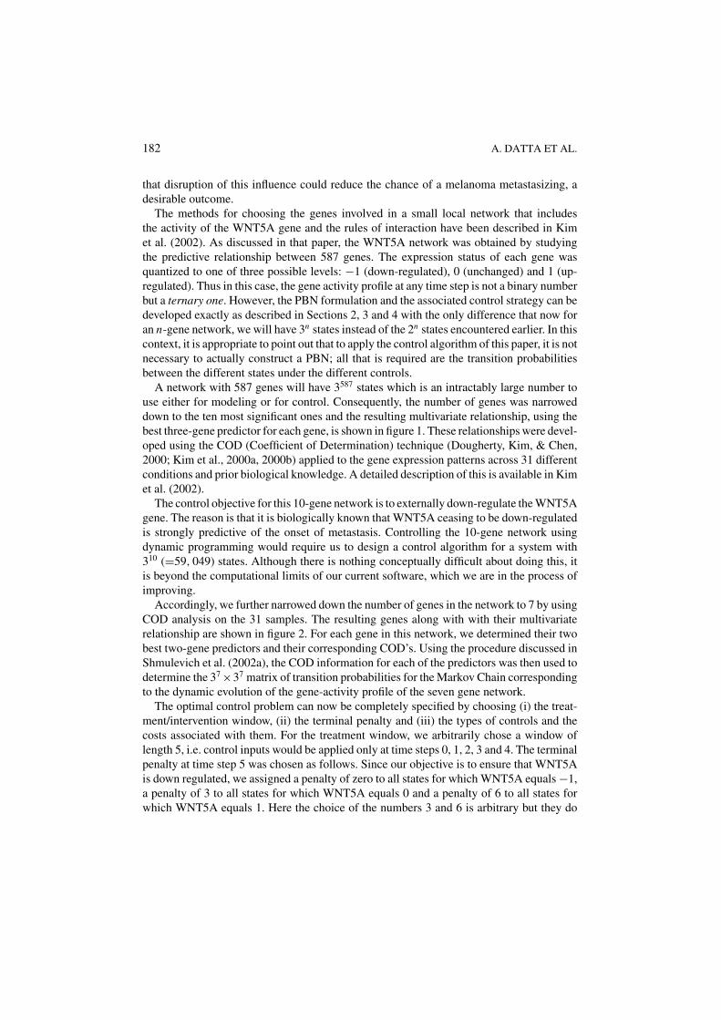
A network with 587 genes will have 3587 states which is an intractably large number touse either for modeling or for control. Consequently, the number of genes was narroweddown to the ten most significant ones and the resulting multivariate relationship, using thebest three-gene predictor for each gene, is shown in figure 1. These relationships were devel-oped using the COD (Coefficient of Determination) technique (Dougherty, Kim, & Chen,2000; Kim et al., 2000a, 2000b) applied to the gene expression patterns across 31 differentconditions and prior biological knowledge. A detailed description of this is available in Kimet al. (2002).

The control objective for this 10-gene network is to externally down-regulate the WNT5Agene. The reason is that it is biologically known that WNT5A ceasing to be down-regulatedis strongly predictive of the onset of metastasis. Controlling the 10-gene network usingdynamic programming would require us to design a control algorithm for a system with310 (=59, 049) states. Although there is nothing conceptually difficult about doing this, itis beyond the computational limits of our current software, which we are in the process ofimproving.

Accordingly, we further narrowed down the number of genes in the network to 7 by usingCOD analysis on the 31 samples. The resulting genes along with with their multivariaterelationship are shown in figure 2. For each gene in this network, we determined their twobest two-gene predictors and their corresponding COD’s. Using the procedure discussed inShmulevich et al. (2002a), the COD information for each of the predictors was then used todetermine the 37 ×37 matrix of transition probabilities for the Markov Chain correspondingto the dynamic evolution of the gene-activity profile of the seven gene network.

The optimal control problem can now be completely specified by choosing (i) the treat-ment/intervention window, (ii) the terminal penalty and (iii) the types of controls and thecosts associated with them. For the treatment window, we arbitrarily chose a window oflength 5, i.e. control inputs would be applied only at time steps 0, 1, 2, 3 and 4. The terminalpenalty at time step 5 was chosen as follows. Since our objective is to ensure that WNT5Ais down regulated, we assigned a penalty of zero to all states for which WNT5A equals −1,a penalty of 3 to all states for which WNT5A equals 0 and a penalty of 6 to all states forwhich WNT5A equals 1. Here the choice of the numbers 3 and 6 is arbitrary but they do


Figure 1. Multivariate relationship between the genes of the 10-gene WNT5A network (Kim et al., 2002).

Figure 2. Multivariate relationship between the genes of the 7-gene WNT5A network.

184 A. DATTA ET AL.

reflect our attempt to capture the intuitive notion that states where WNT5A equals 1 areless desirable than those where WNT5A equals 0. Two types of possible controls were usedand next we discuss the two cases separately.

Case 1. WNT5A Controlled Directly: In this case, the control action at any given time stepis to force WNT5A equal to −1, if necessary, and let the network evolve from there.Biologically such a control could be implemented by using a WNT5A inhibitory protein.In this case, the control variable is binary with 0 indicating that the expression status ofWNT5A has not been forcibly altered while 1 indicates that such a forcible alterationhas taken place. Of course, whether at a given time step, such intervention takes placeor not is decided by the solution to the resulting dynamic programming algorithm andthe actual state of the network immediately prior to the intervention. With this kind ofintervention strategy, it seems reasonable to incur a control cost at a given time step ifand only if the expression status of WNT5A has to be forcibly changed at that time step.Once again, we arbitrarily assigned a cost of 1 to each such forcible change and solvedfor the optimal control using dynamic programming.

The net result was a set of optimal control inputs for each of the 2187 (=37) states ateach of the five time points. Using these control inputs, we studied the evolution of the stateprobability distribution vectors with and without control. For every possible initial state,our simulations indicated that at every time step from 1 to 5, the probability of WNT5Abeing equal to −1 was higher with control than that without control. Furthermore, withcontrol, WNT5A always reached −1 at the final time point (k = 5). Thus, we concludethat the optimal control strategy of Sections 3 and 4 was, indeed, successful in achievingthe desired control objective. In this context, it is significant to point out that if thenetwork starts from the initial state STC2 = −1, HADHB = 0, MART-1 = 0, RET-1 = 0, S100P = −1, pirin = 1, WNT5A = 1 and if no control is used, then it quicklytransitions to a bad absorbing state (absorbing state with WNT5A = 1). With optimalcontrol, however, this does not happen.

Case 2. WNT5A Controlled Through pirin: In this case, the control objective is the sameas in Case 1, namely to keep WNT5A down-regulated. The only difference is that thistime, we use another gene, pirin to achieve this control. The treatment window and theterminal penalties are kept exactly the same as before. The control action consists of eitherforcing pirin to −1 (corresponding to a control input of 1) or letting it remain whereverit is (corresponding to a control input of 0). As before, at any step, a control cost of 1is incurred if and only if pirin has to be forcibly reset to −1 at that time step. Havingchosen these design parameters, we implemented the dynamic programming algorithmwith pirin as the control.

Using the resulting optimal controls, we studied the evolution of the state probabilitydistribution vectors with and without control. For every possible initial state, our simulationsindicated that, at the final state, the probability of WNT5A being equal to −1 was higher withcontrol than that without control. In this case, there was, however, no definite ordering ofprobabilities between the controlled and uncontrolled cases at the intermediate time points.Moreover, the probability of WNT5A being equal to −1 at the final time point was not, ingeneral, equal to 1. This is not surprising given that, in this case, we are trying to control


the expression status of WNT5A using another gene and the control horizon of length 5simply may not be adequate for achieving the desired objective with such a high probability.Nevertheless, even in this case, if the network starts from the state corresponding to STC2 =−1, HADHB = 0, MART-1 = 0, RET-1 = 0, S100P = −1, pirin = 1, WNT5A = 1 andevolves under optimal control, then the probability of WNT5A = −1 at the final time pointequals 0.673521. This is quite good in view of the fact that the same probability would havebeen equal to zero in the absence of any control action.

6. Concluding Remarks

In this paper, we have introduced probabilistic Boolean networks with one or more controlinputs. In contrast to the PBNs introduced in Shmulevich et al. (2002a), the evolution ofthe state of the networks considered here depends on the status of these control inputs. Inthe case of diseases like cancer, these control inputs can potentially be used to model theeffects of treatments such as radiation, chemo-therapy, etc. on the holistic behaviour of thegenes. Furthermore, the control inputs can themselves be chosen so that the genes evolvein a more “desirable fashion.” Thus the PBNs with control can be used as a modeling toolto facilitate effective strategies for therapeutic intervention.

In Shmulevich et al. (2002a), it was shown how the state evolution of a PBN can bemodeled as a standard Markov Chain. In this paper, we have shown how control can beintroduced into a PBN leading to a controlled Markov Chain. Furthermore, we also showedhow the control inputs can be optimally chosen using the Dynamic Programming technique.

The optimal control results presented in this paper assume known transition probabilitiesand pertain to a finite horizon problem of known length. Their extension to the situationwhere the transition probabilities and the horizon length are unknown is a topic for furtherinvestigation.

Appendix

The appendix gives a step-by-step solution of (5.26), (5.27).

Step 4. We compute J4(z(4)) for each of the four possible states. Here k = 4 so that k+1 = 5;also from (5.24), (5.26), we have

J5(1) = 0, J5(2) = 1, J5(3) = 2, J5(4) = 3. (7.1)

From (5.27), setting k = 4, we obtain

J4(z(4)) = minv(4)∈{1,2}

[u1(4) +

4∑j=1

az(4), j (v(4)).J5( j)

].

Now z(4) can take on any of the four values 1, 2, 3, 4. Thus, we will have to compute J4(1),J4(2), J4(3) and J4(4).

Now J4(1) = minv(4)∈{1,2}

[u1(4) + a12(v(4)).1 + a13(v(4)).2 + a14(v(4)).3]

(using (7.1))

186 A. DATTA ET AL.

= min{a12(1) + a13(1).2 + a14(1).3, 1 + a12(2).1 + a13(2).2 + a14(2).3}(using (3.8))

= min{0, 1 + 2} = 0

and µ∗4(1) = 1. Similarly,

J4(2) = minv(4)∈{1,2}

[u1(4) + a22(v(4)).1 + a23(v(4)).2 + a24(v(4)).3]

= min{a22(1) + a23(1).2 + a24(1).3, 1 + a22(2).1 + a23(2).2 + a24(2).3}= min{2, 1 + 2P2 + 3P1}= 2 (since P1 + P2 = 1)

and µ∗4(2) = 1. Again,

J4(3) = minv(4)∈{1,2}

[u1(4) + a32(v(4)).1 + a33(v(4)).2 + a34(v(4)).3]

= min{a32(1) + a33(1).2 + a34(1).3, 1 + a32(2).1 + a33(2).2 + a34(2).3}= min{2, 1 + P1}= 1 + P1 (since P1 < 1)

and µ∗4(3) = 2. Finally,

J4(4) = minv(4)∈{1,2}

[u1(4) + a42(v(4)).1 + a43(v(4)).2 + a44(v(4)).3]

= min{a42(1) + a43(1).2 + a44(1).3, 1 + a42(2).1 + a43(2).2 + a44(2).3}= min{P1, 1 + 3}= P1 (since P1 < 1)

and µ∗4(4) = 1. Thus the net result is

J4(1) = 0, J4(2) = 2, J4(3) = 1 + P1, J4(4) = P1 (7.2)

and

µ∗4(1) = 1, µ∗

4(2) = 1, µ∗4(3) = 2, µ∗

4(4) = 1. (7.3)

Step 3. Again we compute J3(z(3)) for each of the four possible states z(3) = 1, 2, 3, 4using the values J4(1), J4(2), J4(3), J4(4) obtained in the previous stage:

Now J3(1) = minv(3)∈{1,2}

[u1(3) + a12(v(3)).J4(2) + a13(v(3)).J4(3) + a14(v(3)).J4(4)]

= min{a12(1).2 + a13(1).(1 + P1) + a14(1).P1, 1 + a12(2).2

+ a 13(2).(1 + P1) + a14(2).P1}= min{0, 1 + (1 + P1)}= 0


and µ∗3(1) = 1.

J3(2) = minv(3)∈{1,2}

[u1(3) + a22(v(3)).J4(2) + a23(v(3)).J4(3) + a24(v(3)).J4(4)]

= min{a22(1).2 + a23(1).(1 + P1) + a24(1).P1, 1 + a22(2).2

+ a23(2).(1 + P1) + a24(2).P1}= min

{(1 + P1), 1 + P2(1 + P1) + P2

1

}= (1 + P1)

and µ∗3(2) = 1.

J3(3) = minv(3)∈{1,2}

[u1(3) + a32(v(3)).J4(2) + a33(v(3)).J4(3) + a34(v(3)).J4(4)]

= min{a32(1).2 + a33(1).(1 + P1) + a34(1).P1, 1 + a32(2).2

+ a33(2).(1 + P1) + a34(2).P1}= min{(1 + P1), (1 + 2P1)}= 1 + P1

and µ∗3(3) = 1.

J3(4) = minv(3)∈{1,2}

[u1(3) + a42(v(3)).J4(2) + a43(v(3)).J4(3) + a44(v(3)).J4(4)]

= min{a42(1).2 + a43(1).(1 + P1) + a44(1).P1, 1 + a42(2).2

+ a43(2).(1 + P1) + a44(2).P1}= min{2P1, 1 + P1}= 2P1

and µ∗3(4) = 1. Thus

J3(1) = 0, J3(2) = 1 + P1, J3(3) = 1 + P1, J3(4) = 2P1 (7.4)

and

µ∗3(1) = 1, µ∗

3(2) = 1, µ∗3(3) = 1, µ∗

3(4) = 1. (7.5)

Step 2. Computation of J2(z(2)) for each of the four possible states z(2) = 1, 2, 3, 4 usingthe values J3(1), J3(2), J3(3), J3(4) obtained in the previous stage.

J2(1) = minv(2)∈{1,2}

[u1(2) + a12(v(2)).J3(2) + a13(v(2)).J3(3) + a14(v(2)).J3(4)]

= min{a12(1).(1 + P1) + a13(1).(1 + P1) + a14(1).2P1, 1

+ a12(2).(1 + P1) + a13(2).(1 + P1) + a14(2).2P1}= min{0, 1 + (1 + P1)}= 0

188 A. DATTA ET AL.

and µ∗2(1) = 1.

J2(2) = minv(2)∈{1,2}

[u1(2) + a22(v(2)).J3(2) + a23(v(2)).J3(3) + a24(v(2)).J3(4)]

= min{a22(1).(1 + P1) + a23(1).(1 + P1) + a24(1).2P1, 1 + a22(2).(1 + P1)

+ a23(2).(1 + P1) + a24(2).2P1}= min

{1 + P1, 1 + P2(1 + P1) + 2P2

1

}= 1 + P1

and µ∗2(2) = 1.

J2(3) = minv(2)∈{1,2}

[u1(2) + a32(v(2)).J3(2) + a33(v(2)).J3(3) + a34(v(2)).J3(4)]

= min{a32(1).(1 + P1) + a33(1).(1 + P1) + a34(1).2P1, 1 + a32(2).(1 + P1)

+ a33(2).(1 + P1) + a34(2).2P1}= min{1 + P1, 1 + P1(1 + P1)}= 1 + P1

and µ∗2(3) = 1.

J2(4) = minv(2)∈{1,2}

[u1(2) + a42(v(2)).J3(2) + a43(v(2)).J3(3) + a44(v(2)).J3(4)]

= min{a42(1).(1 + P1) + a43(1).(1 + P1) + a44(1).2P1, 1 + a42(2).(1 + P1)

+ a43(2).(1 + P1) + a44(2).2P1}= min{P1(1 + P1), 1 + 2P1}= P1(1 + P1)


J2(1) = 0, J2(2) = 1 + P1, J2(3) = 1 + P1, J2(4) = P1(1 + P1) (7.6)

and

µ∗2(1) = 1, µ∗

2(2) = 1, µ∗2(3) = 1, µ∗

2(4) = 1. (7.7)


J1(1) = minv(1)∈{1,2}

[u1(1) + a12(v(1)).J2(2) + a13(v(1)).J2(3) + a14(v(1)).J2(4)]

= min{a12(1).(1 + P1) + a13(1).(1 + P1) + a14(1).P1(1 + P1), 1

+ a12(2).(1 + P1) + a13(2).(1 + P1) + a14(2).P1(1 + P1)}= min{0, 1 + 1 + P1}= 0


and µ∗1(1) = 1.

J1(2) = minv(1)∈{1,2}

[u1(1) + a22(v(1)).J2(2) + a23(v(1)).J2(3) + a24(v(1)).J2(4)]

= min{a22(1).(1 + P1) + a23(1).(1 + P1) + a24(1).P1(1 + P1), 1

+ a22(2).(1 + P1) + a23(2).(1 + P1) + a24(2).P1(1 + P1)}= min

{(1 + P1), 1 + P2(1 + P1) + P2

1 (1 + P1)}

= 1 + P1

and µ∗1(2) = 1.

J1(3) = minv(1)∈{1,2}

[u1(1) + a32(v(1)).J2(2) + a33(v(1)).J2(3) + a34(v(1)).J2(4)]

= min{a32(1).(1 + P1) + a33(1).(1 + P1) + a34(1).P1(1 + P1), 1

+ a32(2).(1 + P1) + a33(2).(1 + P1) + a34(2).P1(1 + P1)}= min{1 + P1, 1 + P1(1 + P1)}= 1 + P1

and µ∗1(3) = 1.

J1(4) = minv(1)∈{1,2}

[u1(1) + a42(v(1)).J2(2) + a43(v(1)).J2(3) + a44(v(1)).J2(4)]

= min{a42(1).(1 + P1) + a43(1).(1 + P1) + a44(1).P1(1 + P1), 1

+ a42(2).(1 + P1) + a43(2).(1 + P1) + a44(2).P1(1 + P1)}= min{P1(1 + P1), 1 + P1(1 + P1)}= P1(1 + P1)


J1(1) = 0, J1(2) = 1 + P1, J1(3) = 1 + P1, J1(4) = P1(1 + P1) (7.8)

and

µ∗1(1) = 1, µ∗

1(2) = 1, µ∗1(3) = 1, µ∗

1(4) = 1. (7.9)


J0(1) = minv(0)∈{1,2}

[u1(0) + a12(v(0)).J1(2) + a13(v(0)).J1(3) + a14(v(0)).J1(4)]

= min{a12(1).(1 + P1) + a13(1).(1 + P1) + a14(1).P1(1 + P1), 1

+ a12(2).(1 + P1) + a13(2).(1 + P1) + a14(2).P1(1 + P1)}= min{0, 1 + (1 + P1)}= 0

190 A. DATTA ET AL.

and µ∗0(1) = 1.

J0(2) = minv(0)∈{1,2}

[u1(0) + a22(v(0)).J1(2) + a23(v(0)).J1(3) + a24(v(0)).J1(4)]

= min{a22(1).(1 + P1) + a23(1).(1 + P1) + a24(1).P1(1 + P1), 1

+ a22(2).(1 + P1) + a23(2).(1 + P1) + a24(2).P1(1 + P1)}= min

{(1 + P1), 1 + P2(1 + P1) + P2

1 (1 + P1)}

= 1 + P1

and µ∗0(2) = 1.

J0(3) = minv(0)∈{1,2}

[u1(0) + a32(v(0)).J1(2) + a33(v(0)).J1(3) + a34(v(0)).J1(4)]

= min{a32(1).(1 + P1) + a33(1).(1 + P1) + a34(1).P1(1 + P1), 1

+ a32(2).(1 + P1) + a33(2).(1 + P1) + a34(2).P1(1 + P1)}= min{(1 + P1), 1 + P1(1 + P1)}= 1 + P1

and µ∗0(3) = 1.

J0(4) = minv(0)∈{1,2}

[u1(0) + a42(v(0)).J1(2) + a43(v(0)).J1(3) + a44(v(0)).J1(4)]

= min{a42(1).(1 + P1) + a43(1).(1 + P1) + a44(1).P1(1 + P1), 1

+ a42(2).(1 + P1) + a43(2).(1 + P1) + a44(2).P1(1 + P1)}= min{P1(1 + P1), 1 + P1(1 + P1)}= P1(1 + P1)


J0(1) = 0, J0(2) = 1 + P1, J0(3) = 1 + P1, J0(4) = P1(1 + P1) (7.10)

and

µ∗0(1) = 1, µ∗

0(2) = 1, µ∗0(3) = 1, µ∗

0(4) = 1. (7.11)

In view of (7.3), (7.5), (7.7), (7.9), (7.11), the optimal control strategy for this finite horizonproblem is given by (5.28), (5.29).

Acknowledgments

This work was supported in part by the National Cancer Institute under Grant CA90301,by the National Human Genome Research Institute, by the National Science Foundationunder Grant ECS-9903488 and by the Texas Advanced Technology Program under GrantNo. 000512-0099-1999.


Note

1. In the rest of this paper, we will be referring to z(k) as the state of the probabilistic Boolean network since, asdiscussed in Section 2, z(k) is equivalent to the actual state x(k).

References

Bellman, R. (1957). Dynamic Programming. Princeton, NJ: Princeton University Press.Bertsekas, D. P. (1976). Dynamic Programming and Stochastic Control. Academic Press.Bittner, M., Meltzer, P., Chen, Y., Jiang, Y., Seftor, E., Hendrix, M., Radmacher, M., Simon, R., Yakhini, Z., Ben-

Dor, A., Sampas, N., Dougherty, E., Wang, E., Marincola, F., Gooden, C., Lueders, J., Glatfelter, A., Pollock,P., Carpten, J., Gillanders, E., Leja, D., Dietrich, K., Beaudry, C., Berens, M., Alberts, D., & Sondak, V. (2000).Molecular classification of cutaneous malignant melanoma by gene expression profiling. Nature, 406:6795,536–540.

Dougherty, E. R., Kim, S., & Chen, Y. (2000). Coefficient of determination in nonlinear signal processing. SignalProcessing, 80:(10), 2219–2235.

Kauffman, S. A. (1969). Metabolic stability and epigenesis in randomly constructed genetic nets. TheoreticalBiology, 22, 437–467.

Kauffman, S. A. (1993). The Origins of Order: Self-Organization and Selection in Evolution. New York: OxfordUniversity Press.

Kauffman, S. A. & Levin, S. (1987). Towards a general theory of adaptive walks on rugged landscapes. TheoreticalBiology, 128, 11–45.

Kim, S., Dougherty, E. R., Bittner, M. L., Chen, Y., Sivakumar, K., Meltzer, P., & Trent, J. M. (2000a). A generaldramework for the analysis of multivariate gene interaction via expression arrays. Biomedical Optics, 4:(4),411–424.

Kim, S., Dougherty, E. R., Chen, Y., Sivakumar, K., Meltzer, P., Trent, J. M., & Bittner, M. (2000b). Multivariatemeasurement of gene-expression relationships. Genomics, 67, 201–209.

Kim, S., Li, H., Dougherty, E. R., Cao, N., Chen, Y., Bittner, M., & Suh, E. (2002). Can Markov chain modelsmimic biological regulation? Journal of Biological Systems, 10, 447–458.

Shmulevich, I., Dougherty, E. R., Kim, S., & Zhang, W. (2002a). Probabilistic Boolean networks: A rule-baseduncertainty model for gene regulatory networks. Bioinformatics, 18, 261–274.

Shmulevich, I., Dougherty, E. R., & Zhang, W. (2002b). Gene perturbation and intervention in probabilisticBoolean networks. Bioinformatics, 18, 1319–1331.

Shmulevich, I., Dougherty, E. R., & Zhang, W. (2002c). Control of stationary behavior in probabilistic Booleannetworks by means of structural intervention. Biological Systems, 10, 431–446.

Weeraratna, A. T., Jiang, Y., Hostetter, G., Rosenblatt, K., Duray, P., Bittner, M., & Trent, J. M. (2002). Wnt5asignalling directly affects cell motility and invasion of metastatic melanoma. Cancer Cell, 1, 279–288.

Received June 18, 2002Revised December 23, 2002Accepted December 23, 2002Final manuscript January 14, 2003

External control in Markovian genetic regulatory networks: the imperfect information case

Documents

Transcript of External control in Markovian genetic regulatory networks: the imperfect information case