Exposure analysis modeling system (EXAMS) - EPA
205
EPA/600/R!00/081 September, 2000 Revision A Exposure Analysis Modeling System (EXAMS): User Manual and System Documentation By Lawrence A. Burns, Ph.D. Ecologist, Ecosystems Research Division U.S. Environmental Protection Agency 960 College Station Road Athens, Georgia 30605-2700 National Exposure Research Laboratory Office of Research and Development U.S. Environmental Protection Agency Research Triangle Park, NC 27711
-
Upload
khangminh22 -
Category
Documents
-
view
0 -
download
0
Transcript of Exposure analysis modeling system (EXAMS) - EPA

EPA/600/R!00/081 September, 2000
Revision A
Exposure Analysis Modeling System(EXAMS): User Manual and
System Documentation
By
Lawrence A. Burns, Ph.D. Ecologist, Ecosystems Research Division
U.S. Environmental Protection Agency 960 College Station Road
Athens, Georgia 30605-2700
National Exposure Research Laboratory Office of Research and Development
U.S. Environmental Protection Agency Research Triangle Park, NC 27711

Notice
The U.S. Environmental Protection Agency through its Office of Research and Development funded and managed the research described here under GPRA Goal 4, Preventing Pollution and Reducing Risk in Communities, Homes, Workplaces and Ecosystems, Objective 4.3, Safe Handling and Use of Commercial Chemicals and Microorganisms, Subobjective 4.3.4, Human Health and Ecosystems, Task 6519, Advanced Pesticide Risk Assessment Technology. It has been subjected to the Agency’s peer and administrative review and approved for publication as an EPA document. Mention of trade names or commercial products does not constitute endorsement or recommendation for use.
ii

Foreword
Environmental protection efforts are increasingly directed toward preventing adverse health and ecological effects associated with specific chemical compounds of natural or human origin. As part of the Ecosystems Research Division’s research on the occurrence, movement, transformation, impact, and control of environmental contaminants, the Ecosystems Assessment Branch studies complexes of environmental processes that control the transport, transformation, degradation, fate, and impact of pollutants or other materials in soil and water and develops models for assessing the risks associated with exposures to chemical contaminants.
Concern about environmental exposure to synthetic organic chemicals has increased the need for techniques to predict the behavior of chemicals entering the environment as a result of the manufacture, use, and disposal of commercial products. The Exposure Analysis Modeling System (EXAMS), which has been undergoing continual development, evaluation, and revision at this Division since 1978, provides a convenient tool to aid in judging the environmental consequences should a specific chemical contaminant enter a natural aquatic system. Because EXAMS requires no chemical monitoring data, it can be used for new chemicals not yet introduced into commerce as well as for those whose pattern and volume of use are known. EXAMS and other exposure assessment models should contribute significantly to efforts to anticipate potential problems associated with environmental pollutants.
Rosemarie C. Russo Director Ecosystems Research Division Athens, Georgia
iii

Abstract
The Exposure Analysis Modeling System, first published in 1982 (EPA-600/3-82-023), provides interactive computer software for formulating aquatic ecosystem models and rapidly evaluating the fate, transport, and exposure concentrations of synthetic organic chemicals – pesticides, industrial materials, and leachates from disposal sites. EXAMS contains an integrated Database Management System (DBMS) specifically designed for storage and management of project databases required by the software. User interaction is provided by a full-featured Command Line Interface (CLI), context-sensitive help menus, an on-line data dictionary and CLI users’ guide, and plotting capabilities for review of output data. EXAMS provides 20 output tables that document the input datasets and provide integrated results summaries for aid in ecological risk assessments.
EXAMS’ core is a set of process modules that link fundamental chemical properties to the limnological parameters that control the kinetics of fate and transport in aquatic systems. The chemical properties are measurable by conventional laboratory methods; most are required under various regulatory authority. When run under the EPA’s GEMS or pcGEMS systems, EXAMS accepts direct output from QSAR software. EXAMS
limnological data are composed of elements historically of interest to aquatic scientists world-wide, so generation of suitable environmental datasets can generally be accomplished with minimal project-specific field investigations.
EXAMS provides facilities for long-term (steady-state) analysis of chronic chemical discharges, initial-value approaches for study of short-term chemical releases, and full kinetic simulations that allow for monthly variation in mean climatological parameters and alteration of chemical loadings on daily time scales. EXAMS
has been written in generalized (N-dimensional) form in its implementation of algorithms for representing spatial detail and chemical degradation pathways. This DOS implementation allows for study of five simultaneous chemical compounds and 100 environmental segments; other configurations can be created through special arrangement with the author. EXAMS provides analyses of
Exposure: the expected (96-hour acute, 21-day and long-term chronic) environmental concentrations of synthetic chemicals and their transformation products,
Fate: the spatial distribution of chemicals in the aquatic ecosystem, and the relative importance of each transformation and transport process (important in establishing the acceptable uncertainty in chemical laboratory data), and
Persistence: the time required for natural purification of the ecosystem (via export and degradation processes) once chemical releases end.
EXAMS includes file-transfer interfaces to the PRZM3 terrestrial model and the FGETS and BASS bio-accumulation models; it is a complete implementation of EXAMS in Fortran 90.
This report covers a period from December 1, 1999 to September 15, 2000 and work was completed as of September 17, 2000. This version of the Manual reflects continuous maintenance and upgrade of EXAMS.
iv

Contents
Foreword . . . . . . . . . . . . . . . . . . . . . . . . . . . . . . . . . . . . . . . . . . . . . . . . . . . . . . . . . . . . . . . . . . . . . . . . . . . . . . . . . . . . . . . . . . . . . iiiAbstract . . . . . . . . . . . . . . . . . . . . . . . . . . . . . . . . . . . . . . . . . . . . . . . . . . . . . . . . . . . . . . . . . . . . . . . . . . . . . . . . . . . . . . . . . . . . . . iv
1.0 Introduction to the Exposure Analysis Modeling System (EXAMS) . . . . . . . . . . . . . . . . . . . . . . . . . . . . . . . . . . . . . . . . . . . . . . . . . . 1 1.1 Background . . . . . . . . . . . . . . . . . . . . . . . . . . . . . . . . . . . . . . . . . . . . . . . . . . . . . . . . . . . . . . . . . . . . . . . . . . . . . . . . . . . . . . . . . 1 1.2 Exposure Analysis in Aquatic Systems . . . . . . . . . . . . . . . . . . . . . . . . . . . . . . . . . . . . . . . . . . . . . . . . . . . . . . . . . . . . . . . . . . . . 1
1.2.1 Exposure . . . . . . . . . . . . . . . . . . . . . . . . . . . . . . . . . . . . . . . . . . . . . . . . . . . . . . . . . . . . . . . . . . . . . . . . . . . . . . . . . . . . . . 1 1.2.2 Persistence . . . . . . . . . . . . . . . . . . . . . . . . . . . . . . . . . . . . . . . . . . . . . . . . . . . . . . . . . . . . . . . . . . . . . . . . . . . . . . . . . . . . 1 1.2.3 Fate . . . . . . . . . . . . . . . . . . . . . . . . . . . . . . . . . . . . . . . . . . . . . . . . . . . . . . . . . . . . . . . . . . . . . . . . . . . . . . . . . . . . . . . . . . 1
1.3 The EXAMS program . . . . . . . . . . . . . . . . . . . . . . . . . . . . . . . . . . . . . . . . . . . . . . . . . . . . . . . . . . . . . . . . . . . . . . . . . . . . . . . . . . 2 1.4 Sensitivity Analysis and Error Evaluation . . . . . . . . . . . . . . . . . . . . . . . . . . . . . . . . . . . . . . . . . . . . . . . . . . . . . . . . . . . . . . . . . 2 1.5 EXAMS Process Models . . . . . . . . . . . . . . . . . . . . . . . . . . . . . . . . . . . . . . . . . . . . . . . . . . . . . . . . . . . . . . . . . . . . . . . . . . . . . . . . 3
1.5.1 Ionization and Sorption . . . . . . . . . . . . . . . . . . . . . . . . . . . . . . . . . . . . . . . . . . . . . . . . . . . . . . . . . . . . . . . . . . . . . . . . . . . 3 1.5.2 Transformation Processes . . . . . . . . . . . . . . . . . . . . . . . . . . . . . . . . . . . . . . . . . . . . . . . . . . . . . . . . . . . . . . . . . . . . . . . . . 4 1.5.3 Transport Processes . . . . . . . . . . . . . . . . . . . . . . . . . . . . . . . . . . . . . . . . . . . . . . . . . . . . . . . . . . . . . . . . . . . . . . . . . . . . . 5 1.5.4 Chemical Loadings . . . . . . . . . . . . . . . . . . . . . . . . . . . . . . . . . . . . . . . . . . . . . . . . . . . . . . . . . . . . . . . . . . . . . . . . . . . . . . 5
1.6 Ecosystems Analysis and Mathematical Systems Models . . . . . . . . . . . . . . . . . . . . . . . . . . . . . . . . . . . . . . . . . . . . . . . . . . . . . 5 1.6.1 EXAMS Design Strategy . . . . . . . . . . . . . . . . . . . . . . . . . . . . . . . . . . . . . . . . . . . . . . . . . . . . . . . . . . . . . . . . . . . . . . . . . . . 5 1.6.2 Temporal and Spatial Resolution . . . . . . . . . . . . . . . . . . . . . . . . . . . . . . . . . . . . . . . . . . . . . . . . . . . . . . . . . . . . . . . . . . . 6 1.6.3 Assumptions . . . . . . . . . . . . . . . . . . . . . . . . . . . . . . . . . . . . . . . . . . . . . . . . . . . . . . . . . . . . . . . . . . . . . . . . . . . . . . . . . . . 7
1.7 Further Reading . . . . . . . . . . . . . . . . . . . . . . . . . . . . . . . . . . . . . . . . . . . . . . . . . . . . . . . . . . . . . . . . . . . . . . . . . . . . . . . . . . . . . 8
2.0 Fundamental Theory . . . . . . . . . . . . . . . . . . . . . . . . . . . . . . . . . . . . . . . . . . . . . . . . . . . . . . . . . . . . . . . . . . . . . . . . . . . . . . . . . . . . 102.1 Compartment Models and Conservation of Mass . . . . . . . . . . . . . . . . . . . . . . . . . . . . . . . . . . . . . . . . . . . . . . . . . . . . . . . . . . . 102.2 Equilibrium Processes . . . . . . . . . . . . . . . . . . . . . . . . . . . . . . . . . . . . . . . . . . . . . . . . . . . . . . . . . . . . . . . . . . . . . . . . . . . . . . . . 11
2.2.1 Ionization Reactions . . . . . . . . . . . . . . . . . . . . . . . . . . . . . . . . . . . . . . . . . . . . . . . . . . . . . . . . . . . . . . . . . . . . . . . . . . . . 112.2.2 Sediment Sorption . . . . . . . . . . . . . . . . . . . . . . . . . . . . . . . . . . . . . . . . . . . . . . . . . . . . . . . . . . . . . . . . . . . . . . . . . . . . . . 132.2.3 Biosorption . . . . . . . . . . . . . . . . . . . . . . . . . . . . . . . . . . . . . . . . . . . . . . . . . . . . . . . . . . . . . . . . . . . . . . . . . . . . . . . . . . . 152.2.4 Complexation with DOC . . . . . . . . . . . . . . . . . . . . . . . . . . . . . . . . . . . . . . . . . . . . . . . . . . . . . . . . . . . . . . . . . . . . . . . . . 162.2.5 Computation of Equilibrium Distribution Coefficients . . . . . . . . . . . . . . . . . . . . . . . . . . . . . . . . . . . . . . . . . . . . . . . . . 16
2.3 Kinetic Processes . . . . . . . . . . . . . . . . . . . . . . . . . . . . . . . . . . . . . . . . . . . . . . . . . . . . . . . . . . . . . . . . . . . . . . . . . . . . . . . . . . . 192.3.1 Transport . . . . . . . . . . . . . . . . . . . . . . . . . . . . . . . . . . . . . . . . . . . . . . . . . . . . . . . . . . . . . . . . . . . . . . . . . . . . . . . . . . . . . 19
2.3.1.1 Hydrology and advection . . . . . . . . . . . . . . . . . . . . . . . . . . . . . . . . . . . . . . . . . . . . . . . . . . . . . . . . . . . . . . . . . . . 212.3.1.2 Advected water flows . . . . . . . . . . . . . . . . . . . . . . . . . . . . . . . . . . . . . . . . . . . . . . . . . . . . . . . . . . . . . . . . . . . . . . 222.3.1.3 Advective sediment transport . . . . . . . . . . . . . . . . . . . . . . . . . . . . . . . . . . . . . . . . . . . . . . . . . . . . . . . . . . . . . . . . 242.3.1.4 Dispersive transport . . . . . . . . . . . . . . . . . . . . . . . . . . . . . . . . . . . . . . . . . . . . . . . . . . . . . . . . . . . . . . . . . . . . . . . 26
2.3.1.4.1 Dispersion within the water column (27) 2.3.1.4.2 Dispersion within the bottom sediments (28) 2.3.1.4.3 Exchanges between bed sediments and overlying waters (28)
2.3.1.5 Transport of synthetic organic chemicals . . . . . . . . . . . . . . . . . . . . . . . . . . . . . . . . . . . . . . . . . . . . . . . . . . . . . . . 312.3.2 Volatilization . . . . . . . . . . . . . . . . . . . . . . . . . . . . . . . . . . . . . . . . . . . . . . . . . . . . . . . . . . . . . . . . . . . . . . . . . . . . . . . . . 32
2.3.2.1 Chemical Data Entry . . . . . . . . . . . . . . . . . . . . . . . . . . . . . . . . . . . . . . . . . . . . . . . . . . . . . . . . . . . . . . . . . . . . . . . 352.3.2.2 Exchange Constants for Water Vapor . . . . . . . . . . . . . . . . . . . . . . . . . . . . . . . . . . . . . . . . . . . . . . . . . . . . . . . . . 35
v

2.3.2.3 Exchange Constants for Molecular Oxygen . . . . . . . . . . . . . . . . . . . . . . . . . . . . . . . . . . . . . . . . . . . . . . . . . . . . . 362.3.2.4 Validation and Uncertainty Studies . . . . . . . . . . . . . . . . . . . . . . . . . . . . . . . . . . . . . . . . . . . . . . . . . . . . . . . . . . . 36
2.3.2.4.1 Radon in small lakes in the Canadian Shield (37) 2.3.2.4.2 1,4-Dichlorobenzene in Lake Zurich (38)
2.3.3 Direct Photolysis . . . . . . . . . . . . . . . . . . . . . . . . . . . . . . . . . . . . . . . . . . . . . . . . . . . . . . . . . . . . . . . . . . . . . . . . . . . . . . . 422.3.3.1 Direct photolysis in aquatic systems . . . . . . . . . . . . . . . . . . . . . . . . . . . . . . . . . . . . . . . . . . . . . . . . . . . . . . . . . . . 422.3.3.2 Light attenuation in natural waters . . . . . . . . . . . . . . . . . . . . . . . . . . . . . . . . . . . . . . . . . . . . . . . . . . . . . . . . . . . . 45
2.3.3.2.1 Distribution functions (D) in natural waters (45) 2.3.3.2.2 Absorption coefficients (a) in natural waters (46)
2.3.3.3 Reaction quantum yields (M; Qyield) . . . . . . . . . . . . . . . . . . . . . . . . . . . . . . . . . . . . . . . . . . . . . . . . . . . . . . . . . . 472.3.3.4 Absorption spectra (ABSORG) . . . . . . . . . . . . . . . . . . . . . . . . . . . . . . . . . . . . . . . . . . . . . . . . . . . . . . . . . . . . . . . . 482.3.3.5 Effects of sorption on photolysis rates . . . . . . . . . . . . . . . . . . . . . . . . . . . . . . . . . . . . . . . . . . . . . . . . . . . . . . . . . 49
2.3.3.5.1 Sensitivity analysis of sorption effects on direct photolysis (50) 2.3.3.6 Near-surface solar beam and sky irradiance . . . . . . . . . . . . . . . . . . . . . . . . . . . . . . . . . . . . . . . . . . . . . . . . . . . . . 522.3.3.7 Input data and computational mechanics – Summary . . . . . . . . . . . . . . . . . . . . . . . . . . . . . . . . . . . . . . . . . . . . . . 53
2.3.4 Specific Acid, Specific Base, and Neutral Hydrolysis . . . . . . . . . . . . . . . . . . . . . . . . . . . . . . . . . . . . . . . . . . . . . . . . . . 552.3.4.1 Temperature effects . . . . . . . . . . . . . . . . . . . . . . . . . . . . . . . . . . . . . . . . . . . . . . . . . . . . . . . . . . . . . . . . . . . . . . . 572.3.4.2 Ionization effects . . . . . . . . . . . . . . . . . . . . . . . . . . . . . . . . . . . . . . . . . . . . . . . . . . . . . . . . . . . . . . . . . . . . . . . . . 582.3.4.3 Sorption effects . . . . . . . . . . . . . . . . . . . . . . . . . . . . . . . . . . . . . . . . . . . . . . . . . . . . . . . . . . . . . . . . . . . . . . . . . . . 58
2.3.5 Indirect Photochemistry, Oxidation and Reduction . . . . . . . . . . . . . . . . . . . . . . . . . . . . . . . . . . . . . . . . . . . . . . . . . . . . 602.3.5.1 Oxidation . . . . . . . . . . . . . . . . . . . . . . . . . . . . . . . . . . . . . . . . . . . . . . . . . . . . . . . . . . . . . . . . . . . . . . . . . . . . . . . 612.3.5.2 Singlet Oxygen . . . . . . . . . . . . . . . . . . . . . . . . . . . . . . . . . . . . . . . . . . . . . . . . . . . . . . . . . . . . . . . . . . . . . . . . . . . 622.3.5.3 Reduction . . . . . . . . . . . . . . . . . . . . . . . . . . . . . . . . . . . . . . . . . . . . . . . . . . . . . . . . . . . . . . . . . . . . . . . . . . . . . . . 63
2.3.6 Microbial Transformations . . . . . . . . . . . . . . . . . . . . . . . . . . . . . . . . . . . . . . . . . . . . . . . . . . . . . . . . . . . . . . . . . . . . . . . 642.4 Input Pollutant Loadings . . . . . . . . . . . . . . . . . . . . . . . . . . . . . . . . . . . . . . . . . . . . . . . . . . . . . . . . . . . . . . . . . . . . . . . . . . . . . . 68
2.4.1 Product Chemistry . . . . . . . . . . . . . . . . . . . . . . . . . . . . . . . . . . . . . . . . . . . . . . . . . . . . . . . . . . . . . . . . . . . . . . . . . . . . . 702.5 Data Assembly and Solution of Equations . . . . . . . . . . . . . . . . . . . . . . . . . . . . . . . . . . . . . . . . . . . . . . . . . . . . . . . . . . . . . . . . 71
2.5.1 Exposure . . . . . . . . . . . . . . . . . . . . . . . . . . . . . . . . . . . . . . . . . . . . . . . . . . . . . . . . . . . . . . . . . . . . . . . . . . . . . . . . . . . . . 712.5.2 Fate . . . . . . . . . . . . . . . . . . . . . . . . . . . . . . . . . . . . . . . . . . . . . . . . . . . . . . . . . . . . . . . . . . . . . . . . . . . . . . . . . . . . . . . . . 732.5.3 Persistence . . . . . . . . . . . . . . . . . . . . . . . . . . . . . . . . . . . . . . . . . . . . . . . . . . . . . . . . . . . . . . . . . . . . . . . . . . . . . . . . . . . 73
3.0 Tutorials and Case Studies . . . . . . . . . . . . . . . . . . . . . . . . . . . . . . . . . . . . . . . . . . . . . . . . . . . . . . . . . . . . . . . . . . . . . . . . . . . . . . . 773.1 Tutorial 1: Introduction to Exposure Analysis with EXAMS – Laboratory 1 . . . . . . . . . . . . . . . . . . . . . . . . . . . . . . . . . . . . . . . 773.2 Tutorial 1: Introduction to Exposure Analysis with EXAMS – Laboratory 2 . . . . . . . . . . . . . . . . . . . . . . . . . . . . . . . . . . . . . . . 813.3 Command Sequences for Tutorial 1, Lab. 1 . . . . . . . . . . . . . . . . . . . . . . . . . . . . . . . . . . . . . . . . . . . . . . . . . . . . . . . . . . . . . . . 85
3.3.1 Lab. 1, Exercise 1: Steady-State Analysis (Mode 1) . . . . . . . . . . . . . . . . . . . . . . . . . . . . . . . . . . . . . . . . . . . . . . . . . . . 853.3.2 Lab. 1, Exercise 2: Mode 2 Analysis of Initial Value Problems – Sixty Day RUn Time . . . . . . . . . . . . . . . . . . . . . . . . 863.3.3 Lab. 1, Exercise 3: Time-varying seasonal analysis using Mode 3 . . . . . . . . . . . . . . . . . . . . . . . . . . . . . . . . . . . . . . . . 88
3.4 Introduction to EXAMS – Lab. 1 Exercises with Complete EXAMS Responses . . . . . . . . . . . . . . . . . . . . . . . . . . . . . . . . . . . . . 903.4.1 Lab. 1, Exercise 1: Steady-State Analysis (Mode 1) . . . . . . . . . . . . . . . . . . . . . . . . . . . . . . . . . . . . . . . . . . . . . . . . . . . 903.4.2 Lab. 1, Exercise 2: EXAMS in Mode 2 . . . . . . . . . . . . . . . . . . . . . . . . . . . . . . . . . . . . . . . . . . . . . . . . . . . . . . . . . . . . . . . 993.4.3 Lab. 1, Exercise 3: EXAMS in Mode 3 . . . . . . . . . . . . . . . . . . . . . . . . . . . . . . . . . . . . . . . . . . . . . . . . . . . . . . . . . . . . . . 106
3.5 Tutorial 2: Chemical & Environmental Data Entry . . . . . . . . . . . . . . . . . . . . . . . . . . . . . . . . . . . . . . . . . . . . . . . . . . . . . . . . 1133.5.1 Exercise 4: p-DCB in Lake Zurich . . . . . . . . . . . . . . . . . . . . . . . . . . . . . . . . . . . . . . . . . . . . . . . . . . . . . . . . . . . . . . . . 1133.5.2 Exercise 4 (Lake Zurich) with Complete EXAMS Responses . . . . . . . . . . . . . . . . . . . . . . . . . . . . . . . . . . . . . . . . . . . . 116
4.0 EXAMS Command Language Interface (CLI) User’s Guide . . . . . . . . . . . . . . . . . . . . . . . . . . . . . . . . . . . . . . . . . . . . . . . . . . . . . . 1254.1 Conventions Used in this Chapter . . . . . . . . . . . . . . . . . . . . . . . . . . . . . . . . . . . . . . . . . . . . . . . . . . . . . . . . . . . . . . . . . . . . . . 1254.2 Overview . . . . . . . . . . . . . . . . . . . . . . . . . . . . . . . . . . . . . . . . . . . . . . . . . . . . . . . . . . . . . . . . . . . . . . . . . . . . . . . . . . . . . . . . . 1254.3 Entering Commands . . . . . . . . . . . . . . . . . . . . . . . . . . . . . . . . . . . . . . . . . . . . . . . . . . . . . . . . . . . . . . . . . . . . . . . . . . . . . . . . 1254.4 Command Prompting . . . . . . . . . . . . . . . . . . . . . . . . . . . . . . . . . . . . . . . . . . . . . . . . . . . . . . . . . . . . . . . . . . . . . . . . . . . . . . . 1264.5 EXAMS Messages . . . . . . . . . . . . . . . . . . . . . . . . . . . . . . . . . . . . . . . . . . . . . . . . . . . . . . . . . . . . . . . . . . . . . . . . . . . . . . . . . . . 1274.6 The HELP Command . . . . . . . . . . . . . . . . . . . . . . . . . . . . . . . . . . . . . . . . . . . . . . . . . . . . . . . . . . . . . . . . . . . . . . . . . . . . . . . . 1274.7 Command Procedures . . . . . . . . . . . . . . . . . . . . . . . . . . . . . . . . . . . . . . . . . . . . . . . . . . . . . . . . . . . . . . . . . . . . . . . . . . . . . . . 127
vi

4.8 Wild Card Characters . . . . . . . . . . . . . . . . . . . . . . . . . . . . . . . . . . . . . . . . . . . . . . . . . . . . . . . . . . . . . . . . . . . . . . . . . . . . . . . 1274.9 Truncating Command Names and Keywords . . . . . . . . . . . . . . . . . . . . . . . . . . . . . . . . . . . . . . . . . . . . . . . . . . . . . . . . . . . . . 1284.10 Summary Description of EXAMS’ System Commands . . . . . . . . . . . . . . . . . . . . . . . . . . . . . . . . . . . . . . . . . . . . . . . . . . . . . 128
5.0 System Command Descriptions . . . . . . . . . . . . . . . . . . . . . . . . . . . . . . . . . . . . . . . . . . . . . . . . . . . . . . . . . . . . . . . . . . . . . . . . . . . 129AUDIT . . . . . . . . . . . . . . . . . . . . . . . . . . . . . . . . . . . . . . . . . . . . . . . . . . . . . . . . . . . . . . . . . . . . . . . . . . . . . . . . . . . . . . . . . . . . . . . 129CATALOG . . . . . . . . . . . . . . . . . . . . . . . . . . . . . . . . . . . . . . . . . . . . . . . . . . . . . . . . . . . . . . . . . . . . . . . . . . . . . . . . . . . . . . . . . . . . 131CHANGE . . . . . . . . . . . . . . . . . . . . . . . . . . . . . . . . . . . . . . . . . . . . . . . . . . . . . . . . . . . . . . . . . . . . . . . . . . . . . . . . . . . . . . . . . . . . . 133CONTINUE . . . . . . . . . . . . . . . . . . . . . . . . . . . . . . . . . . . . . . . . . . . . . . . . . . . . . . . . . . . . . . . . . . . . . . . . . . . . . . . . . . . . . . . . . . . 135DESCRIBE . . . . . . . . . . . . . . . . . . . . . . . . . . . . . . . . . . . . . . . . . . . . . . . . . . . . . . . . . . . . . . . . . . . . . . . . . . . . . . . . . . . . . . . . . . . . 139DO . . . . . . . . . . . . . . . . . . . . . . . . . . . . . . . . . . . . . . . . . . . . . . . . . . . . . . . . . . . . . . . . . . . . . . . . . . . . . . . . . . . . . . . . . . . . . . . . . 141ERASE . . . . . . . . . . . . . . . . . . . . . . . . . . . . . . . . . . . . . . . . . . . . . . . . . . . . . . . . . . . . . . . . . . . . . . . . . . . . . . . . . . . . . . . . . . . . . . 144EXIT . . . . . . . . . . . . . . . . . . . . . . . . . . . . . . . . . . . . . . . . . . . . . . . . . . . . . . . . . . . . . . . . . . . . . . . . . . . . . . . . . . . . . . . . . . . . . . . . 146HELP . . . . . . . . . . . . . . . . . . . . . . . . . . . . . . . . . . . . . . . . . . . . . . . . . . . . . . . . . . . . . . . . . . . . . . . . . . . . . . . . . . . . . . . . . . . . . . . . 147LIST . . . . . . . . . . . . . . . . . . . . . . . . . . . . . . . . . . . . . . . . . . . . . . . . . . . . . . . . . . . . . . . . . . . . . . . . . . . . . . . . . . . . . . . . . . . . . . . . 149NAME . . . . . . . . . . . . . . . . . . . . . . . . . . . . . . . . . . . . . . . . . . . . . . . . . . . . . . . . . . . . . . . . . . . . . . . . . . . . . . . . . . . . . . . . . . . . . . . 152PLOT . . . . . . . . . . . . . . . . . . . . . . . . . . . . . . . . . . . . . . . . . . . . . . . . . . . . . . . . . . . . . . . . . . . . . . . . . . . . . . . . . . . . . . . . . . . . . . . . 153PRINT . . . . . . . . . . . . . . . . . . . . . . . . . . . . . . . . . . . . . . . . . . . . . . . . . . . . . . . . . . . . . . . . . . . . . . . . . . . . . . . . . . . . . . . . . . . . . . . 158QUIT . . . . . . . . . . . . . . . . . . . . . . . . . . . . . . . . . . . . . . . . . . . . . . . . . . . . . . . . . . . . . . . . . . . . . . . . . . . . . . . . . . . . . . . . . . . . . . . . 159READ . . . . . . . . . . . . . . . . . . . . . . . . . . . . . . . . . . . . . . . . . . . . . . . . . . . . . . . . . . . . . . . . . . . . . . . . . . . . . . . . . . . . . . . . . . . . . . . 160RECALL . . . . . . . . . . . . . . . . . . . . . . . . . . . . . . . . . . . . . . . . . . . . . . . . . . . . . . . . . . . . . . . . . . . . . . . . . . . . . . . . . . . . . . . . . . . . . 162RUN . . . . . . . . . . . . . . . . . . . . . . . . . . . . . . . . . . . . . . . . . . . . . . . . . . . . . . . . . . . . . . . . . . . . . . . . . . . . . . . . . . . . . . . . . . . . . . . . 164SET . . . . . . . . . . . . . . . . . . . . . . . . . . . . . . . . . . . . . . . . . . . . . . . . . . . . . . . . . . . . . . . . . . . . . . . . . . . . . . . . . . . . . . . . . . . . . . . . . 165SHOW . . . . . . . . . . . . . . . . . . . . . . . . . . . . . . . . . . . . . . . . . . . . . . . . . . . . . . . . . . . . . . . . . . . . . . . . . . . . . . . . . . . . . . . . . . . . . . . 167STORE . . . . . . . . . . . . . . . . . . . . . . . . . . . . . . . . . . . . . . . . . . . . . . . . . . . . . . . . . . . . . . . . . . . . . . . . . . . . . . . . . . . . . . . . . . . . . . 170WRITE . . . . . . . . . . . . . . . . . . . . . . . . . . . . . . . . . . . . . . . . . . . . . . . . . . . . . . . . . . . . . . . . . . . . . . . . . . . . . . . . . . . . . . . . . . . . . . 172ZERO . . . . . . . . . . . . . . . . . . . . . . . . . . . . . . . . . . . . . . . . . . . . . . . . . . . . . . . . . . . . . . . . . . . . . . . . . . . . . . . . . . . . . . . . . . . . . . . 173
Appendices . . . . . . . . . . . . . . . . . . . . . . . . . . . . . . . . . . . . . . . . . . . . . . . . . . . . . . . . . . . . . . . . . . . . . . . . . . . . . . . . . . . . . . . . . . . . . . 191Appendix A
Appendix B
Appendix C
Partitioning to Natural Organic Colloids . . . . . . . . . . . . . . . . . . . . . . . . . . . . . . . . . . . . . . . . . . . . . . . . . . . . . . . . . . . . . . . . 191
EXAMS data entry template for chemical molar absorption spectra (ABSOR) . . . . . . . . . . . . . . . . . . . . . . . . . . . . . . . . . . . . 195
Implementing the microcomputer runtime EXAMS . . . . . . . . . . . . . . . . . . . . . . . . . . . . . . . . . . . . . . . . . . . . . . . . . . . . . . . . . 196
Data Dictionary . . . . . . . . . . . . . . . . . . . . . . . . . . . . . . . . . . . . . . . . . . . . . . . . . . . . . . . . . . . . . . . . . . . . . . . . . . . . . . . . . 175 EXAMS6.0
vii

viii

1.0 Introduction to the Exposure Analysis Modeling System (EXAMS)
1.1 Background Industrial production of agricultural chemicals, plastics, and pharmaceuticals has increased steadily over the past five decades. More recently, growth of the chemical industry has been accompanied by increasing concern over the effects of synthetic chemicals on the environment. The suspicion has arisen that, in some cases, the benefits gained by using a chemical may not offset the cost of incidental damage to man’s natural life-support system – the biosphere. The toxicity of a chemical does not of itself indicate that the environmental risks associated with its use are unacceptable, however, as it is the dose that makes the poison. A rational evaluation of the risk posed by the use and disposal of synthetic chemicals must begin from a knowledge of the persistence and mobility of chemicals in the environment, which in turn establish the conditions of exposure leading to absorption of toxicological dose.
The Exposure Analysis Modeling System (EXAMS), developed at the U.S. Environmental Protection Agency’s research laboratory in Athens, Georgia, is an interactive computer program intended to give decision-makers in industry and government access to a responsive, general, and controllable tool for readily deriving and evaluating the behavior of synthetic chemicals in the environment. The research and development effort has focused on the creation of the interactive command language and user aids that are the core of EXAMS, and on the genesis of reliable EXAMS mathematical models. EXAMS was designed primarily for the rapid screening and identification of synthetic organic chemicals likely to adversely impact aquatic systems. This report is intended to acquaint potential users with the underlying theory, capabilities, and use of the system.
1.2 Exposure Analysis in Aquatic Systems EXAMS was conceived as an aid to those who must execute hazard evaluations solely from laboratory descriptions of the chemistry of a newly synthesized toxic compound. EXAMS
estimates exposure, fate, and persistence following release of an organic chemical into an aquatic ecosystem. Each of these terms was given a formal operational definition during the initial design of the system.
1.2.1 Exposure When a pollutant is released into an aquatic ecosystem, it is entrained in the transport field of the system and begins to spread to locations beyond the original point of release. During the course of these movements, chemical and biological processes transform the parent compound into daughter products. In the face of continuing emissions, the receiving system evolves toward a “steady-state” condition. At steady state, the pollutant concentrations are in a dynamic equilibrium
in which the loadings are balanced by the transport and transformation processes. Residual concentrations can be compared to those posing a danger to living organisms. The comparison is one indication of the risk entailed by the presence of a chemical in natural systems or in drinking-water supplies. These “expected environmental concentrations” (EECs), or exposure levels, in receiving water bodies are one component of a hazard evaluation.
1.2.2 PersistenceToxicological and ecological “effects” studies are of two kinds: investigations of short-term “acute” exposures, as opposed to longer-term “chronic” experiments. Acute studies are often used to determine the concentration of a chemical resulting in 50% mortality of a test population over a period of hours. Chronic studies examine sub-lethal effects on populations exposed to lower concentrations over extended periods. Thus, for example, an EEC that is 10 times less than the acute level does not affirm that aquatic ecosystems will not be affected, because the probability of a “chronic” impact increases with exposure duration. A computed EEC thus must be supplemented with an estimate of “persistence” in the environment. (A compound immune to all transformation processes is by definition “persistent” in a global sense, but even in this case transport processes will eventually reduce the pollutant to negligible levels should the input loadings cease.) The notion of “persistence” can be given an explicit definition in the context of a particular contaminated ecosystem: should the pollutant loadings cease, what time span would be required for dissipation of most of the residual contamination? (For example, given the half-life of a chemical in a “first-order” system, the time required to reduce the chemical concentration to any specified fraction of its initial value can be easily computed.) With this information in hand, the appropriate duration and pollutant levels for chronic studies can be more readily decided. More detailed dynamic simulation studies can elicit the probable magnitude and duration of acute events as well.
1.2.3 FateThe toxicologist also needs to know which populations in the system are “at risk.” Populations at risk can be deduced to some extent from the distribution or “fate” of the compound, that is, by an estimate of EECs in different habitats of single ecosystems. EXAMS reports a separate EEC for each compartment, and thus each local population, used to define the system.
The concept of the “fate” of a chemical in an aquatic system has an additional, equally significant meaning. Each transport or transformation process accounts for only part of the total behavior of the pollutant. The relative importance of each process can be determined from the percentage of the total
1

system loadings consumed by the process. The relative importance of the transformations indicate which process is dominant in the system, and thus in greatest need of accuracy and precision in its kinetic parameters. Overall dominance by transport processes may imply a contamination of downstream systems, loss of significant amounts of the pollutant to the atmosphere, or pollution of ground-water aquifers.
1.3 The EXAMS program The need to predict chemical exposures from limited data has stimulated a variety of recent advances in environmental modeling. These advances fall into three general categories:
! Process models giving a quantitative, often theoretical, basis for predicting the rate of transport and transformation processes as a function of environmental variables.
! Procedures for estimating the chemical parameters required by process models. Examples include linear free energy relationships, and correlations summarizing large bodies of experimental chemical data.
! Systems models that combine unit process models with descriptions of the environmental forces determining the strength and speed of these processes in real ecosystems.
The vocabulary used to describe environmental models includes many terms, most of which reflect the underlying intentions of the modelers. Models may be predictive, stochastic, empirical, mechanistic, theoretical, deterministic, explanatory, conceptual, causal, descriptive, etc. The EXAMS program is a deterministic, predictive systems model, based on a core of mechanistic process equations derived from fundamental theoretical concepts. The EXAMS computer code also includes descriptive empirical correlations that ease the user’s burden of parameter calculations, and an interactive command language that facilitates the application of the system to specific problems.
EXAMS “predicts” in a somewhat limited sense of the term. Many of the predictive water-quality models currently in use include site-specific parameters that can only be found via field calibrations. After “validation” of the model by comparison of its calibrated outputs with additional field measurements, these models are often used to explore the merits of alternative management plans. EXAMS, however, deals with an entirely different class of problem. Because newly synthesized chemicals must be evaluated, little or no field data may exist. Furthermore, EECs at any particular site are of little direct interest. In this case, the goal, at least in principle, is to predict EECs for a wide range of ecosystems under a variety of geographic, morphometric, and ecological conditions. EXAMS includes no direct calibration parameters, and its input environmental data can be developed from a variety of sources. For example, input data can be
synthesized from an analysis of the outputs of hydrodynamic models, from prior field investigations conducted without reference to toxic chemicals, or from the appropriate limnological literature. The EECs generated by EXAMS are thus “evaluative” (Lassiter et al. 1979) predictions designed to reflect typical or average conditions. EXAMS’ environmental database can be used to describe specific locales, or as a generalized description of the properties of aquatic systems in broad geographic regions.
EXAMS relies on mechanistic, rather than empirical, constructs for its core process equations wherever possible. Mechanistic (physically determinate) models are more robust predictors than are purely empirical models, which cannot safely be extended beyond the range of prior observations. EXAMS contains a few empirical correlations among chemical parameters, but these are not invoked unless the user approves. For example, the partition coefficient of the compound on the sediment phases of the system, as a function of the organic carbon content of its sediments, can be estimated from the compound’s octanol-water partition coefficient. A direct load of the partition coefficient (KOC, see the EXAMS Data Dictionary beginning on page 175) overrides the empirical default estimate, however. (Because EXAMS is an interactive program in which the user has direct access to the input database, much of this documentation has been written using the computer variables (e.g., KOC above) as identifiers and as quantities in the process equations. Although this approach poses some difficulties for the casual reader, it allows the potential user of the program to see the connections between program variables and the underlying process theory. The EXAMS data dictionary in this document (beginning on page 175) includes an alphabetical listing and definitions of EXAMS’ input variables.)
EXAMS is a deterministic, rather than a stochastic, model in the sense that a given set of inputs will always produce the same output. Uncontrolled variation is present both in ecosystems and in chemical laboratories, and experimental results from either milieu are often reported as mean values and their associated variances. Probabilistic modeling techniques (e.g., Monte Carlo simulations) can account, in principle, for this variation and attach an error bound or confidence interval to each important output variable. Monte Carlo simulation is, however, very time-consuming (i.e., expensive), and the statistical distributions of chemical and environmental parameters are not often known in the requisite detail. The objective of this kind of modeling, in the case of hazard evaluations, would in any case be to estimate the effect of parameter errors on the overall conclusions to be drawn from the model. This goal can be met less expensively and more efficiently by some form of sensitivity analysis.
1.4 Sensitivity Analysis and Error EvaluationEXAMS does not provide a formal sensitivity analysis among its options: the number of sub-simulations needed to fully account
2

for interactions among chemical and environmental variables is prohibitively large (Behrens 1979). When, for example, the second-order rate constant for alkaline hydrolysis of a compound is described to EXAMS via an Arrhenius function, the rate constant computed for each compartment in the ecosystem depends on at least six parameters. These include the frequency factor and activation energy of the reaction, the partition coefficient of the compound (KOC), the organic carbon content of the sediment phase, the temperature, and the concentration of hydroxide ion. The overall rate estimate is thus as dependent upon the accuracy of the system definition as it is upon the skill of the laboratory chemist; in this example, the rate could vary six orders of magnitude as a function of differences among ecosystems. In order to fully map the parameter interactions affecting a process, all combinations of parameter changes would have to be simulated. Even this (simplified) example would require 63 simulations (2n-1, where n is the number (6) of parameters) merely to determine sensitivities of a single component process in a single ecosystem compartment.
Sensitivity analysis remains an attractive technique for answering a crucial question that arises during hazard evaluation. This question can be simply stated: “Are the chemical data accurate enough, and precise enough, to support an analysis of the risk entailed by releases of the chemical into the environment?” Like many simple questions, this question does not have a simple, definitive answer. It can be broken down, however, into a series of explicit, more tractable questions whose answers sum to a reasonably complete evaluation of the significance that should be attached to a reported error bound or confidence interval on any input datum. Using the output tables and command language utilities provided by EXAMS, these questions can be posed, and answered, in the following order.
! Which geographic areas, and which ecosystems, develop the largest chemical residuals? EXAMS allows a user to load the data for any environment contained in his files, specify a loading, and run a simulation, through a simple series of one-line English commands.
! Which process is dominant in the most sensitive ecosystem(s)? The dominant process, i.e., the process most responsible for the decomposition of the compound in the system, is the process requiring the greatest accuracy and precision in its chemical parameters. EXAMS produces two output tables that indicate the relative importance of each process. The first is a “kinetic profile” (or frequency scaling), which gives a compartment-by-compartment listing with all processes reduced to equivalent (hour-1) terms. The second is a tabulation of the overall steady-state fate of the compound, giving a listing of the percentage of the load consumed by each of the transport and transformation processes at steady state.
Given the dominant process, the input data affecting this process can be varied over the reported error bounds, and a simulation can be executed for each value of the parameters. The effect of parameter errors on the EECs and persistence of the compound can then be documented by compiling the results of these simulations.
This sequence of operations is, in effect, a sensitivity analysis, but the extent of the analysis is controlled and directed by the user. In some cases, for example, one process will always account for most of the decomposition of the compound. When the database for this dominant process is inadequate, the obvious answer to the original question is that the data do not yet support a risk analysis. Conversely, if the dominant process is well defined, and the error limits do not substantially affect the estimates of exposure and persistence, the data may be judged to be adequate for the exposure analysis portion of a hazard evaluation.
1.5 EXAMS Process Models In EXAMS, the loadings, transport, and transformations of a compound are combined into differential equations by using the mass conservation law as an accounting principle. This law accounts for all the compound entering and leaving a system as the algebraic sum of (1) external loadings, (2) transport processes exporting the compound out of the system, and (3) transformation processes within the system that degrade the compound to its daughter products. The fundamental equations of the model describe the rate of change in chemical concentrations as a balance between increases due to loadings, and decreases due to the transport and transformation processes removing the chemical from the system.
The set of unit process models used to compute the kinetics of a compound is the central core of EXAMS. These unit models are all “second-order” or “system-independent”models: each process equation includes a direct statement of the interactions between the chemistry of a compound and the environmental forces that shape its behavior in aquatic systems. Thus, each realization of the process equations implemented by the user in a specific EXAMS simulation is tailored to the unique characteristics of that ecosystem. Most of the process equations are based on standard theoretical constructs or accepted empirical relationships. For example, light intensity in the water column of the system is computed using the Beer-Lambert law, and temperature corrections for rate constants are computed using Arrhenius functions. Detailed explanations of the process models incorporated in EXAMS, and of the mechanics of the computations, are presented in Chapter 2.
1.5.1 Ionization and SorptionIonization of organic acids and bases, complexation with dissolved organic carbon (DOC), and sorption of the compound with sediments and biota, are treated as thermodynamic
3

properties or (local) equilibria that alter the operation of kinetic processes. For example, an organic base in the water column may occur in a number of molecular species (as dissolved ions, sorbed with sediments, etc.), but only the uncharged, dissolved species can be volatilized across the air-water interface. EXAMS
allows for the simultaneous treatment of up to 28 molecular species of a chemical. These include the parent uncharged molecule, and singly, doubly, or triply charged cations and anions, each of which can occur in a dissolved, sediment-sorbed, DOC-complexed, or biosorbed form. The program computes the fraction of the total concentration of compound that is present in each of the 28 molecular structures (the “distribution coefficients,” ").
These (") values enter the kinetic equations as multipliers on the rate constants. In this way, the program accounts for differences in reactivity that depend on the molecular form of the chemical, as a function of the spatial distribution of environmental parameters controlling molecular speciation. For example, the lability of a particular molecule to hydrolytic decomposition may depend on whether it is dissolved or is sorbed with the sediment phase of the system. EXAMS makes no intrinsic assumptions about the relative transformation reactivities of the 28 molecular species, with the single exception that biosorbed species are unavailable to inorganic reactions. These assumptions are controlled through the structure of the input data describing the species-specific chemistry of the compound.
1.5.2 Transformation ProcessesEXAMS computes the kinetics of transformations attributable to direct photolysis, hydrolysis, biolysis, and oxidation reactions. The input chemical data for hydrolytic, biolytic, and oxidative reactions can be entered either as single-valued second-order rate constants, or as a pair of values defining the rate constant as a function of environmental temperatures. For example, the input data for alkaline hydrolysis of the compound consists of two computer variables: KBH, and EBH. When EBH is zero, the program interprets KBH as the second-order rate constant. When EBH is non-zero, EBH is interpreted as the activation energy of the reaction, and KBH is re-interpreted as the pre-exponential (frequency) factor in an Arrhenius equation giving the second-order rate constant as a function of the environmental temperature (TCEL) in each system compartment. (KBH and EBH
are both actually matrices with 21 elements; each element of the matrix corresponds to one of the 21 possible molecular species of the compound, i.e., the 7 ionic species occurring in dissolved, DOC-complexed, or sediment-sorbed form--as noted above, biosorbed forms do not participate in extra-cellular reactions.)
EXAMS includes two algorithms for computing the rate of photolytic transformation of a synthetic organic chemical. These algorithms accommodate the two more common kinds of laboratory data and chemical parameters used to describe photolysis reactions. The simpler algorithm requires only an
average pseudo-first-order rate constant (KDP) applicable to near-surface waters under cloudless conditions at a specified reference latitude (RFLAT). To control reactivity assumptions, KDP is coupled to nominal (normally unit-valued) reaction quantum yields (QYIELD) for each molecular species of the compound. This approach makes possible a first approximation of photochemical reactivity, but neglects the very important effects of changes in the spectral quality of sunlight with increasing depth in a body of water. The more complex photochemical algorithm computes photolysis rates directly from the absorption spectra (molar extinction coefficients) of the compound and its ions, measured values of the reaction quantum yields, and the environmental concentrations of competing light absorbers (chlorophylls, suspended sediments, DOC, and water itself). When using a KDP, please be aware that data from laboratory photoreactors usually are obtained at intensities as much as one thousand times larger than that of normal sunlight.
The total rate of hydrolytic transformation of a chemical is computed by EXAMS as the sum of three contributing processes. Each of these processes can be entered via simple rate constants, or as Arrhenius functions of temperature. The rate of specific-acid-catalyzed reactions is computed from the pH of each sector of the ecosystem, and specific-base catalysis is computed from the environmental pOH data. The rate data for neutral hydrolysis of the compound are entered as a set of pseudo-first-order rate coefficients (or Arrhenius functions) for reaction of the 28 (potential) molecular species with the water molecule.
EXAMS computes biotransformation of the chemical in the water column and in the bottom sediments of the system as entirely separate functions. Both functions are second-order equations that relate the rate of biotransformation to the size of the bacterial population actively degrading the compound (Paris et al. 1982). This approach is of demonstrated validity for at least some biolysis processes, and provides the user with a minimal semi-empirical means of distinguishing between eutrophic and oligotrophic ecosystems. The second-order rate constants (KBACW for the water column, KBACS for benthic sediments) can be entered either as single-valued constants or as functions of temperature. When a non-zero value is entered for the Q10 of a biotransformation (parameters QTBAW and QTBAS, respectively), KBAC is interpreted as the rate constant at 25 degrees Celsius, and the biolysis rate in each sector of the ecosystem is adjusted for the local temperature (TCEL).
Oxidation reactions are computed from the chemical input data and the total environmental concentrations of reactive oxidizing species (alkylperoxy and alkoxyl radicals, etc.), corrected for ultra-violet light extinction in the water column. The chemical data can again be entered either as simple second-order rate constants or as Arrhenius functions. Oxidations due to singlet oxygen are computed from chemical reactivity data and singlet
4

oxygen concentrations; singlet oxygen is estimated as a function of the concentration of DOC, oxygen tension, and light intensity. Reduction is included in the program as a simple second-order reaction process driven by the user entries for concentrations of reductants in the system. As with biolysis, this provides the user with a minimal empirical means of assembling a simulation model that includes specific knowledge of the reductants important to a particular chemical safety evaluation.
1.5.3 Transport ProcessesInternal transport and export of a chemical occur in EXAMS via advective and dispersive movement of dissolved, sediment-sorbed, and biosorbed materials and by volatilization losses at the air-water interface. EXAMS provides a set of vectors (JFRAD, etc.) that specify the location and strength of both advective and dispersive transport pathways. Advection of water through the system is then computed from the water balance, using hydrologic data (rainfall, evaporation rates, stream flows, groundwater seepages, etc.) supplied to EXAMS as part of the definition of each environment.
Dispersive interchanges within the system, and across system boundaries, are computed from the usual geochemical specification of the characteristic length (CHARL), cross-sectional area (XSTUR), and dispersion coefficient (DSP) for each active exchange pathway. EXAMS can compute transport of synthetic chemicals via whole-sediment bed loads, suspended sediment wash-loads, exchanges with fixed-volume sediment beds, ground-water infiltration, transport through the thermocline of a lake, losses in effluent streams, etc. Volatilization losses are computed using a two-resistance model. This computation treats the total resistance to transport across the air-water interface as the sum of resistances in the liquid and vapor phases immediately adjacent to the interface.
1.5.4 Chemical LoadingsExternal loadings of a toxicant can enter the ecosystem via point sources (STRLD), non-point sources (NPSLD), dry fallout or aerial drift (DRFLD), atmospheric wash-out (PCPLD), and ground-water seepage (SEELD) entering the system. Any type of load can be entered for any system compartment, but the program will not implement a loading that is inconsistent with the system definition. For example, the program will automatically cancel a rainfall loading (PCPLD) entered for the hypolimnion or benthic sediments of a lake ecosystem. When this type of corrective action is executed, the change is reported to the user via an error message.
1.6 Ecosystems Analysis and Mathematical Systems Models The EXAMS program was constructed from a systems analysis perspective. Systems analysis begins by defining a system’s goals, inputs, environment, resources, and the nature of the system’s components and their interconnections. The system
goals describe the outputs produced by the system as a result of operating on its input stream. The system environment comprises those factors affecting system outputs over which the system has little or no control. These factors are often called “forcing functions” or “external driving variables.” Examples for an aquatic ecosystem include runoff and sediment erosion from its watershed, insolation, and rainfall. System resources are defined as those factors affecting performance over which the system exercises some control. Resources of an aquatic ecosystem include, for example, the pH throughout the system, light intensity in the water column, and dissolved oxygen concentrations. The levels of these internal driving variables are determined, at least in part, by the state of the system itself. In other words, these factors are not necessarily single-valued functions of the system environment. Each of the components or “state variables” of a system can be described in terms of its local input/output behaviors and its causal connections with other elements of the system. The systems approach lends itself to the formulation of mathematical systems models, which are simply tools for encoding knowledge of transport and transformation processes and deriving the implications of this knowledge in a logical and repeatable way.
A systems model, when built around relevant state variables (measurable properties of system components) and causal process models, provides a method for extrapolating future states of systems from knowledge gained in the past. In order for such a model to be generally useful, however, most of its parameters must possess an intrinsic interest transcending their role in any particular computer program. For this reason, EXAMS was designed to use chemical descriptors (Arrhenius functions, pKa, vapor pressure, etc.) and water quality variables (pH, chlorophyll, biomass, etc.) that are independently measured for many chemicals and ecosystems.
1.6.1 EXAMS Design Strategy The conceptual view adopted for EXAMS begins by defining aquatic ecosystems as a series of distinct subsystems, interconnected by physical transport processes that move synthetic chemicals into, through, and out of the system. These subsystems include the epilimnion and hypolimnion of lakes, littoral zones, benthic sediments, etc. The basic architecture of a computer model also depends, however, on its intended uses. EXAMS was designed for use by toxicologists and deci-sion-makers who must evaluate the risk posed by use of a new chemical, based on a forecast from the model. The EXAMS
program is itself part of a “hazard evaluation system,” and the structure of the program was necessarily strongly influenced by the niche perceived for it in this “system.”
Many intermediate technical issues arise during the development of a systems model. Usually these issues can be resolved in several ways; the modeling “style” or design strategy used to build the model guides the choices taken among the available
5

alternatives. The strategy used to formulate EXAMS begins from a primary focus on the needs of the intended user and, other things being equal, resolves most technical issues in favor of the more efficient computation. For example, all transport and transformation processes are driven by internal resource factors (pH, temperature, water movements, sediment deposition and scour, etc.) in the system, and each deserves separate treatment in the model as an individual state variable or function of several state variables. The strategy of model development used for EXAMS suggests, however, that the only state variable of any transcendent interest to the user is the concentration of the chemical itself in the system compartments. EXAMS thus treats all environmental state variables as coefficients describing the state of the ecosystem, and only computes the implications of that state, as residual concentrations of chemicals in the system.
Although this approach vastly simplifies the mathematical model, with corresponding gains in efficiency and speed, the system definition is now somewhat improper. System resources (factors affecting performance that are subject to feedback control) have been redefined as part of the system environment. In fact, the “system” represented by the model is no longer an aquatic ecosystem, but merely a chemical pollutant. Possible failure modes of the model are immediately apparent. For example, introduction of a chemical subject to alkaline hydrolysis and toxic to plant life into a productive lake would retard primary productivity. The decrease in primary productivity would lead to a decrease in the pH of the system and, consequently, a decrease in the rate of hydrolysis and an increase in the residual concentration of the toxicant. This sequence of events would repeat itself indefinitely, and constitutes a positive feedback loop that could in reality badly damage an ecosystem. Given the chemical buffering and functional redundancy present in most real ecosystems, this example is inherently improbable, or at least self-limiting. More importantly, given the initial EEC, the environmental toxicologist could anticipate the potential hazard.
There is a more telling advantage, moreover, to the use of environmental descriptors in preference to dynamic environmental state variables. Predictive ecosystem models that include all the factors of potential importance to the kinetics of toxic pollutants are only now being developed, and will require validation before any extensive use. Furthermore, although extremely fine-resolution (temporal and spatial) models are often considered an ultimate ideal, their utility as components of a fate model for synthetic chemicals remains suspect. Ecosystems are driven by meteorological events, and are themselves subject to internal stochastic processes. Detailed weather forecasts are limited to about nine days, because at the end of this period all possible states of the system are equally probable. Detailed ecosystem forecasts are subject to similar constraints (Platt et al. 1977). For these reasons, EXAMS was designed primarily to forecast the prevailing climate of chemical exposures, rather than
to give detailed local forecasts of EECs in specific locations.
1.6.2 Temporal and Spatial ResolutionWhen a synthetic organic chemical is released into an aquatic ecosystem, the entire array of transport and transformation processes begins at once to act on the chemical. The most efficient way to accommodate this parallel action of the processes is to combine them into a mathematical description of their total effect on the rate of change of chemical concentration in the system. Systems that include transport processes lead to partial differential equations, which usually must be solved by numerical integration. The numerical techniques in one way or another break up the system, which is continuously varying in space and time, into a set of discrete elements. Spatial discrete elements are often referred to as “grid points” or “nodes”, or, as in EXAMS, as “compartments.” Continuous time is often represented by fixing the system driving functions for a short interval, integrating over the interval, and then “updating” the forcing functions before evaluating the next time-step. At any given moment, the behavior of the chemical is a complicated function of both present and past inputs of the compound and states of the system.
EXAMS is oriented toward efficient screening of a multitude of newly invented industrial chemicals and pesticides. Ideally, a full evaluation of the possible risks posed by manufacture and use of a new chemical would begin from a detailed time-series describing the expected releases of the compound into aquatic systems over the entire projected history of its manufacture. Given an equivalently detailed time-series for environmental variables, machine integration would yield a detailed picture of EECs in the receiving water body over the entire period of concern. The great cost of this approach, however, militates against its use as a screening tool. Fine resolution evaluation of synthetic chemicals can probably be used only for compounds that are singularly deleterious and of exceptional economic significance.
The simplest situation is that in which the chemical loadings to systems are known only as single estimates pertaining over indefinite periods. This situation is the more likely for the vast majority of new chemicals, and was chosen for development of EXAMS. It has an additional advantage. The ultimate fate and exposure of chemicals often encompasses many decades, making detailed time traces of EECs feasible only for short-term evaluations. In EXAMS, the environment is represented via long-term average values of the forcing functions that control the behavior of chemicals. By combining the chemistry of the compound with average properties of the ecosystem, EXAMS
reduces the screening problem to manageable proportions. These simplified “first-order” equations are solved algebraically in EXAMS’s steady-state Mode 1 to give the ultimate (i.e., steady-state) EECs that will eventually result from the input loadings. In addition, EXAMS provides a capability to study initial
6

value problems (“pulse loads” in Mode 2), and seasonal dynamics in which environmental driving forces are updated on a monthly basis (Mode 3). Mode 3 is particularly valuable for coupling to the output of the PRZM model, which can provide a lengthy time-series of contamination events due to runoff and erosion of sediments from agricultural lands.
Transport of a chemical from a loading point into the bulk of the system takes place by advected flows and by turbulent dispersion. The simultaneous transformations presently result in a continuously varying distribution of the compound over the physical space of the system. This continuous distribution of the compound can be described via partial differential equations. In solving the equations, the physical space of the system must be broken down into discrete elements. EXAMS is a compartmental or “box” model. The physical space of the system is broken down into a series of physically homogeneous elements (compartments) connected by advective and dispersive fluxes. Each compartment is a particular volume element of the system, containing water, sediments, biota, dissolved and sorbed chemicals, etc. Loadings and exports are represented as mass fluxes across the boundaries of the volume elements; reactive properties are treated as point processes within each compartment.
In characterizing aquatic systems for use with EXAMS, particular attention must be given the grid-size of the spatial net used to represent the system. In effect, the compartments must not be so large that internal gradients have a major effect on the estimated transformation rate of the compound. In other words, the compartments are assumed to be “well-mixed,” that is, the reaction processes are not slowed by delays in transporting the compound from less reactive to more reactive zones in the volume element. Physical boundaries that can be used to delimit system compartments include the air-water interface, the thermocline, the benthic interface, and perhaps the depth of bioturbation of sediments. Some processes, however, are driven by environmental factors that occur as gradients in the system, or are most active at interfaces. For example, irradiance is distributed exponentially throughout the water column, and volatilization occurs only at the air-water interface. The rate of these transformations may be overestimated in, for example, quiescent lakes in which the rate of supply of chemical to a reactive zone via vertical turbulence controls the overall rate of transformation, unless a relatively fine-scale segmentation is used to describe the system. Because compartment models of strongly advected water masses (rivers) introduce some numerical dispersion into the calculations, a relatively fine-scale segmentation is often advisable for highly resolved evaluations of fluvial systems. In many cases the error induced by highly reactive compounds will be of little moment to the probable fate of the chemical in that system, however. For example, it makes little difference whether the photolytic half-life of a chemical is 4 or 40 minutes; in either case it will not long survive exposure
to sunlight.
1.6.3 Assumptions EXAMS has been designed to evaluate the consequences of longer-term, primarily time-averaged chemical loadings that ultimately result in trace-level contamination of aquatic systems. EXAMS generates a steady-state, average flow field (long-term or monthly) for the ecosystem. The program thus cannot fully evaluate the transient, concentrated EECs that arise, for example, from chemical spills. This limitation derives from two factors. First, a steady flow field is not always appropriate for evaluating the spread and decay of a major pulse (spill) input. Second, an assumption of trace-level EECs, which can be violated by spills, has been used to design the process equations used in EXAMS. The following assumptions were used to build the program.
! A useful evaluation can be executed independently of the chemical’s actual effects on the system. In other words, the chemical is assumed not to itself radically change the environmental variables that drive its transformations. Thus, for example, an organic acid or base is assumed not to change the pH of the system; the compound is assumed not to itself absorb a significant fraction of the light entering the system; bacterial populations do not significantly increase (or decline) in response to the presence of the chemical.
! EXAMS uses linear sorption isotherms, and second-order (rather than Michaelis-Menten-Monod) expressions for biotransformation kinetics. This approach is known to be valid for the low concentrations of typical of environmental contaminants; its validity at high concentrations is less certain. EXAMS controls its computational range to ensure that the assumption of trace-level concentrations is not grossly violated. This control is keyed to aqueous-phase (dissolved) residual concentrations of the compound: EXAMS aborts any analysis generating EECs in which any dissolved species exceeds 50% of its aqueous solubility (see Chapter 2.2.2 for additional detail). This restraint incidentally allows the program to ignore precipitation of the compound from solution and precludes inputs of solid particles of the chemical. Although solid precipitates have occasionally been treated as a separate, non-reactive phase in continuous equilibrium with dissolved forms, the efficacy of this formulation has never been adequately evaluated, and the effect of saturated concentrations on the linearity of sorption isotherms would introduce several problematic complexities to the simulations.
! Sorption is treated as a thermodynamic or constitutive property of each segment of the system, that is, sorption/desorption kinetics are assumed to be rapid compared to other processes. The adequacy of this assumption is partially controlled by properties of the chemical and system being evaluated. Extensively sorbed
7

chemicals tend to be sorbed and desorbed more slowly than weakly sorbed compounds; desorption half-lives may approach 40 days for the most extensively bound compounds. Experience with the program has indicated, however, that strongly sorbed chemicals tend to be captured by benthic sediments, where their release to the water column is controlled by their availability to benthic exchange processes. This phenomenon overwhelms any accentuation of the speed of processes in the water column that may be caused by the assumption of local equilibrium.
1.7 Further Reading Baughman, G. L., and L. A. Burns. 1980. Transport and
transformation of chemicals: a perspective. pp. 1-17 In: O. Hutzinger (Ed.). The Handbook of Environmental Chemistry, vol.2, part A. Springer-Verlag, Berlin, Federal Republic of Germany.
Burns, L. A. 1989. Method 209--Exposure Analysis Modeling System (EXAMS--Version 2.92). pp. 108-115 In: OECD
Environment Monographs No. 27: Compendium of Environmental Exposure Assessment Methods for Chemicals. Environment Directorate, Organization for Economic Co-Operation and Development, Paris, France.
Burns, L. A. 1986. Validation methods for chemical exposure and hazard assessment models. pp. 148-172 In: Gesellschaft für Strahlen- und Umwelt forschung mbH München, Projektgruppe “Umwelt gefahrdungspotentiale von Chemikalien” (Eds.) Environmental Modelling for Priority Setting among Existing Chemicals. Ecomed, München-Landsberg-/Lech, Federal Republic of Germany.
Burns, L. A. 1985. Models for predicting the fate of synthetic chemicals in aquatic systems. pp. 176-190 In: T.P. Boyle (Ed.) Validation and Predictability of Laboratory Methods for Assessing the Fate and Effects of Contaminants in Aquatic Ecosystems. ASTM STP 865, American Society for Testing and Materials, Philadelphia, Pennsylvania.
Burns, L. A. 1983a. Fate of chemicals in aquatic systems: process models and computer codes. pp. 25-40 In: R.L. Swann and A. Eschenroeder (Eds.) Fate of Chemicals in the Environment: Compartmental and Multimedia Models for Predictions. Symposium Series 225, American Chemical Society, Washington, D.C.
Burns, L. A. 1983b. Validation of exposure models: the role of conceptual verification, sensitivity analysis, and alternative hypotheses. pp. 255-281 In: W.E. Bishop, R.D. Cardwell, and B.B. Heidolph (Eds.) Aquatic Toxicology and Hazard Assessment. ASTM STP 802, American Society for Testing and Materials, Philadelphia,, Pennsylvania.
Burns, L. A. 1982. Identification and evaluation of fundamental transport and transformation process models. pp. 101-126 In: K.L. Dickson, A.W. Maki, and J. Cairns, Jr. (Eds.). Modeling the Fate of Chemicals in the Aquatic Environment. Ann Arbor Science Publ., Ann Arbor,
Michigan. Burns, L. A., and G. L. Baughman. 1985. Fate modeling. pp.
558-584 In: G.M. Rand and S.R. Petrocelli (Eds.) Fundamentals of Aquatic Toxicology: Methods and Applications. Hemisphere Publ. Co., New York, NY.
Games, L. M. 1982. Field validation of Exposure Analysis Modeling System (EXAMS) in a flowing stream. pp. 325-346 In: K. L. Dickson, A. W. Maki, and J. Cairns, Jr. (Eds.) Modeling the Fate of Chemicals in the Aquatic Environment. Ann Arbor Science Publ., Ann Arbor, Michigan.
Games, L. M. 1983. Practical applications and comparisons of environmentalexposure assessment models. pp. 282-299 In: W. E. Bishop, R. D. Cardwell, and B. B. Heidolph (Eds.) Aquatic Toxicology and Hazard Assessment, ASTM STP 802. American Society for Testing and Materials, Philadelphia, Pennsylvania.
Kolset, K., B. F Aschjem, N. Christopherson, A. Heiberg, and B. Vigerust. 1988. Evaluation of some chemical fate and transport models. A case study on the pollution of the Norrsundet Bay (Sweden). pp. 372-386 In: G. Angeletti and A. Bjørseth (Eds.) Organic Micropollutants in the Aquatic Environment (Proceedings of the Fifth European Symposium, held in Rome, Italy October 20-22, 1987). Kluwer Academic Publishers, Dordrecht.
Lassiter, R. R. 1982. Testing models of the fate of chemicals in aquatic environments. pp. 287-301 In: K. L. Dickson, A. W. Maki, and J. Cairns, Jr. (Eds.) Modeling the Fate of Chemicals in the Aquatic Environment. Ann Arbor Science Publ., Ann Arbor, Michigan.
Lassiter, R. R., R. S. Parrish, and L. A. Burns. 1986. Decomposition by planktonic and attached microorganisms improves chemical fate models. Environmental Toxicology and Chemistry 5:29-39.
Mulkey, L. A., R. B. Ambrose, and T. O. Barnwell. 1986. Aquatic fate and transport modeling techniques for predicting environmental exposure to organic pesticides and other toxicants--a comparative study. In: Urban Runoff Pollution. Springer-Verlag, New York.
Paris, D. F., W. C. Steen, and L. A. Burns. 1982. Microbial transformation kinetics of organic compounds. pp. 73-81 In: O. Hutzinger (Ed.). The Handbook of Environmental Chemistry, v.2, pt. B. Springer-Verlag, Berlin, Germany.
Plane, J. M. C., R. G. Zika, R. G. Zepp, and L.A. Burns. 1987. Photochemical modeling applied to natural waters. pp. 250267 In: R. G. Zika and W. J. Cooper (Eds.) Photochemistry of Environmental Aquatic Systems. ACS Symposium Series 327, American Chemical Society, Washington, D.C.
Pollard, J. E., and S. C. Hern. 1985. A field test of the EXAMS
model in the Monongahela River. Environmental Toxicology and Chemistry 4:362-369.
Platt, T., K. L. Denman, and A.D. Jassby. 1977. Modeling the productivity of phytoplankton. pp. 807-856 In: E.D. Goldberg, I. N. McCave, J. J. O’Brian, and J. H. Steele,
8

Eds. Marine Modeling: The Sea, Vol. 6. Wiley-Interscience: New York.
Reinert, K. H., P. M. Rocchio, and J. H. Rodgers, Jr. 1987. Parameterization of predictive fate models: a case study. Environmental Toxicology and Chemistry 6:99-104.
Reinert, K.H., and J. H. Rodgers, Jr. 1986. Validation trial of predictive fate models using an aquatic herbicide (Endothall). Environmental Toxicology and Chemistry 5:449-461.
Ritter, A.M., J.L. Shaw, W.M. Williams, and K.Z. Travis. 2000. Characterizing aquatic ecological risks from pesticides using a diquat bromide case study. I. Probabilistic exposure estimates. Environmental Toxicology and Chemistry 19:749-759.
Sanders, P. F., and J. N. Seiber. 1984. Organophosphorus pesticide volatilization: Model soil pits and evaporation ponds. pp. 279-295 In: R. F. Kreuger and J. N. Seiber (Eds.) Treatment and Disposal of Pesticide Wastes. ACS
Symposium Series 259, American Chemical Society, Washington, D.C.
Schnoor, J. L., C. Sato, D. McKetchnie, and D. Sahoo. 1987. Processes, Coefficients, and Models for Simulating Toxic Organics and Heavy Metals in Surface Waters. EPA/600/3-87/015, U.S. EPA, Athens, Georgia.
Sato, C., and J. L. Schnoor. 1991. Applications of three completely mixed compartment models to the long-term fate of dieldrin in a reservoir. Water Research 25:621-631.
Schramm, K.-W., M. Hirsch, R. Twele, and O. Hutzinger. 1988. Measured and modeled fate of Disperse Yellow 42 in an outdoor pond. Chemosphere 17:587-595.
Slimak, M. W., and C. Delos. 1982. Predictive fate models: their role in the U.S. Environmental Protection Agency’s water program. pp. 59-71 In: K. L. Dickson, A. W. Maki, and J. Cairns, Jr. (Eds.) Modeling the Fate of Chemicals in the Aquatic Environment. Ann Arbor Science Publ., Ann
Arbor, Michigan. Staples, C.A., K. L. Dickson, F. Y. Saleh, and J. H. Rodgers, Jr.
1983. A microcosm study of Lindane and Naphthalene for model validation. pp. 26-41 In: W. E. Bishop, R. D. Cardwell, and B.B. Heidolph (Eds.) Aquatic Toxicology and Hazard Assessment: Sixth Symposium, ASTM STP 802, American Society for Testing and Materials, Philadelphia, Pennsylvania.
Wolfe, N. L., L. A. Burns, and W. C. Steen. 1980. Use of linear free energy relationships and an evaluative model to assess the fate and transport of phthalate esters in the aquatic environment. Chemosphere 9:393-402.
Wolfe, N. L., R. G. Zepp, P. Schlotzhauer, and M. Sink. 1982. Transformation pathways of hexachlorocylcopentadiene in the aquatic environment. Chemosphere 11:91-101.
References for Chapter 1.
Behrens, J. C. 1979. An exemplified semi-analytical approach to the transient sensitivity of non-linear systems. Applied Mathematical Modelling 3:105-115.
Lassiter, R. R., G. L. Baughman, and L. A. Burns. 1979. Fate of toxic organic substances in the aquatic environment. Pages 219-246 in S. E. Jorgensen, editor. State-of-the-Art in Ecological Modelling. Proceedings of the Conference on Ecological Modelling, Copenhagen, Denmark 28 August 2 September 1978. International Society for Ecological Modelling, Copenhagen.
Paris, D. F., W. C. Steen, and L. A. Burns. 1982. Microbial transformation kinetics of organic compounds. Pages 73-81 in O. Hutzinger, editor. The Handbook of Environmental Chemistry, Volume 2/Part B. Springer-Verlag, Berlin.
Platt, T., K. L. Denman, and A. D. Jassby. 1977. Modeling the productivity of phytoplankton. Pages 807-856 in E. D. Goldberg, I. N. McCave, J. J. O'Brien, and J. H. Steele, editors. Marine Modeling. Wiley-Interscience, New York.
9

2.0 Fundamental Theory
Many excellent books, review articles, and journal reports have been written on the subject of the fate and transport of chemicals in the environment. This report is not intended as an exhaustive summary of the ideas and factual information available from the literature. EXAMS is a distillation of that literature, encoded in a computer program. This chapter (2) summarizes the fundamental ideas that were used to construct the EXAMS program. The references cited represent only the key findings or papers that directly influenced the EXAMS code. Additional detail and background information can be found in the works listed in the bibliography for this report.
2.1 Compartment Models and Conservation of Mass EXAMS’ environmental data are contained in a file (the “canonical environments file”) that includes a series of concise descriptions of the aquatic systems of interest to a user. (The term “canonical” simply means that the data in the file includes only those quantities bearing directly on the fate and transport of synthetic organic chemicals.) Each water-body is represented via a set of N compartments or distinct zones in the system. The program is based on a series of mass balances, which give rise to a single differential equation for each compartment. Working from the transport and transformation process equations, EXAMS
compiles an equation for the net rate of change of chemical concentration in each compartment. The resulting system of N differential equations describes a mass balance for the entire ecosystem. These equations have the general form of Equation (2-1):
(2-1)
where:V is the volume of water in the compartment (liters),[C] is the total chemical concentration as mg/liter of V, Le is the total external loading on the compartment (mg/h), Li is the total internal loading on the compartment (mg/h)
resulting from contaminated flows among system compartments, and
K is an overall pseudo-first-order (/h) loss constant that expresses the combined effect of transport and transformation processes that decrease chemical concentration.
The “canonical environments file” currently supplied with the EXAMS computer program is intended primaruily as a series of test values to establish that the program is operating correctly. Although the data supplied in this file are within the range of observed values, this file is not intended for production runs of the program. EXAMS has been designed to accept standard water-quality parameters and system characteristics that are commonly measured by limnologists throughout the world. EXAMS also includes a descriptor language (parameters JFRAD, JTURB, etc.) that simplifies the specification of system geometry and connectedness. The procedure for defining an EXAMS environment is illustrated in Chapter 3. The EXAMS code has been written in a general (N-compartment) form; the program can be modified and recompiled to handle up to 999 compartments. The program is available in 10-, 50-, and 100compartment versions.
The chemical data base supplied with the program includes 11 compounds investigated by Smith and coworkers (1978). As with EXAMS’ nominal environmental data base, these data should not be regarded as immutably fixed. In many instances the data of Smith et al. (1978) were augmented in order to illustrate EXAMS’ data entry capabilities, and the assumptions used to fill gaps in the chemical data base are open to revision as additional experimental data become available.
References for Chapter 2.1. Smith, J. H., W. R. Mabey, N. Bohonos, B. R. Holt, S. S. Lee,
T.-W. Chou, D. C. Bomberger, and T. Mill. 1978. Environmental Pathways of Selected Chemicals in Freshwater Systems: Part II. Laboratory Studies. EPA-600/7-78-074, U.S. Environmental Protection Agency, Athens, Georgia.
10

2.2 Equilibrium ProcessesThe kinetic properties of organic chemicals are often strongly influenced by the molecular state of the compound. Consider, for example, a compound that can both ionize and sorb to suspended sediments. In this case, the compound will be present in the water column in ionized, unionized, and sorbed states. In inland waters, where aerosol formation can be neglected, only the unionized, unsorbed molecule will volatilize across the air-water interface. An accurate evaluation of the tendency of the compound to volatilize thus cannot be obtained until ionization and sorption are incorporated in the estimation method. Ionization and sorption also affect the reactivity of chemicals to transformation processes, although the magnitude of the changes cannot be as readily predicted.
Laboratory determinations of kinetic rate constants are often limited to homogeneous phase (clean water) investigations. Modeling the behavior of a compound in real systems requires some knowledge, or some assumptions, about the effects of sorption and ionization on a chemical’s behavior in the environment. EXAMS does not contain “hard-wired” assumptions that sorption either “protects” the compound, enhances its reactivity, or has no effect. Instead, the input chemical data include separate rate constants for each molecular form of the compound. This data array allows a user to include unique rate constants for ions and sorbed molecules when these are known. When heterogeneous phase (or pH dependent) chemical data are not available, the necessary assumptions are left to the user’s discretion.
Ionization and sorption of synthetic chemicals are treated as thermodynamic or constitutive properties of each computational element in EXAMS. EXAMS treats these processes as local (within-compartment) reversible equilibria, rather than calculating a global (system-wide) equilibrium partitioning of the compound among its possible molecular species. The inclusion of partitioning to colloidal “dissolved” organic carbon precludes any need to explicitly account for “particle concentration” effects or desorption hysteresis (Gschwend and Wu 1985), (Morel and Gschwend 1987).
Ionization equilibria are usually achieved within a very short time, compared to the time-scale of transport and transformation processes, so a (local) equilibrium assumption is usually justified in natural systems. Desorption of neutral molecules bound to sediments, however, may be relatively slow for compounds that are extensively bound (large partition coefficients). EXAMS’ evaluations do not explicitly include the effects of sorption/desorption kinetics on transport or transformation processes. The program does, however, compute the major transport effect of slow desorption, as an implicit function of interactions between benthic sediments and the overlying water column.
Extensively sorbed compounds are usually predominantly captured by the bottom sediments (benthic compartments) in an aquatic system. Release of the compound to the water column is then limited by the turnover rate of the bottom sediments themselves. The turnover times of benthic sediments, except during storm erosion, are longer than the desorption half-lives of organic chemicals. Consequently, the intrinsic kinetic limitations imposed by residence in bottom sediments generally exceed those attributable to desorption kinetics as such.
EXAMS allows for the existence of six ionized species, in addition to the parent unionized molecule. Each of these can complex with “dissolved” organic matter (EXAMS variable DOC), and sorb with the sediment phase and the biota in an ecosystem compartment (computational element). The program computes the fraction of the total chemical concentration present in each molecular structure. These distribution coefficients (") are used as multipliers on the user-specified transformation rate coefficients for each decomposition process.
2.2.1 Ionization Reactions According to the Brönsted-Lowry concept of ionization reactions, acids and bases react with solvent (water) to form a conjugate acid-base pair (Stumm and Morgan 1970). The EXAMS
program regards any synthetic organic as potentially capable of acting as an ampholyte, forming both singly, doubly, and triply charged cations and anions in the aqueous medium. The unionized molecule is taken as the parent compound, and is denoted in the program documentation as “RH3.” The potential acid-base reactions are then:
(1) Basic reactions:
(2-2)
(2-3)
(2-4)
(2) Acidic reactions:
(2-5)
(2-6)
(2-7)
This set of chemical reactions describes the simultaneous existence of seven chemical species of the compound:
! the unionized parent molecule ,
! a singly charged cation ,
! a doubly charged cation ,
! a triply charged cation ,
11

! a singly charged anion ,
! a doubly charged anion , and
! a triply charged anion .
(Again, because EXAMS is an interactive program in which the user has direct access to the input data base, much of this documentation has been written using the input data variables as identifiers and as quantities in the process equations. Although this approach poses some difficulties for the casual reader, it allows the potential user of the program to see the connections between program variables and the underlying process theory. The Data Dictionary chapter of this document (beginning on page 175) contains an alphabetical listing and definitions of EXAMS’ input variables. Input data are named with a terminal “G” (“Global”), and variables internal to the EXAMS program itself are named with a terminal “L” (“Local”). For example, “KPSG” can be specified by the user; “KPSL” is its internal equivalent.)
Most compounds do not exhibit the full range of behaviors given in Eq. (2-2)–(2-7). EXAMS’ chemical input data stream carries, for each chemical, a vector (SPFLG) of 7 flags that tells the program which of the ionization reactions are appropriate for that compound. (A “flag” in this usage means a signal used to control execution of the program.) Setting an element of the SPFLG vector to “1" indicates that the corresponding chemical species in fact exists; setting an element of SPFLG to “0" (zero) indicates the chemical species does not exist. SPFLG(1) should usually be set to indicate the existence of the parent molecule. When, for example, the remaining flags (SPFLG(2...7)) are all zero, EXAMS treats the chemical as a neutral (unionizable) organic compound. When SPFLG(2) is set (=1), and SPFLG(3...7) are 0, the compound is taken to be an organic base forming only a singly charged cation (RH4
+).
The equilibrium constants for the ionization reactions provide a measure of the strength of the organic acid/base relative to water. The basicity constants corresponding to Eq. (2-2), (2-3), and (2-4) are:
(2-8)
(2-9)
(2-10)
The acidity constants corresponding to Eq. (2-5), (2-6), and (2-7) are:
(2-11)
(2-12)
(2-13)
These ionization constants are “mixed” constants (Stumm and Morgan 1970:82), which take pH = -log{H3O
+} ({H3O+} or {H+}
is hydrogen ion activity, IUPAC convention), and the compound is expressed in concentration units. (Salt effects on pK values, and changes in pKw with temperature, are currently neglected in EXAMS.)
In dilute aqueous solutions (unit water activity, {H2O}=1), the water terms in the equilibrium constants can be neglected. In benthic sediments, however, much of the compartment volume is occupied by solids, and the decreased activity of water must be considered. In EXAMS, this problem is overcome by referring all concentrations to the aqueous phase of the compartment (note dimensions of variables in Eq. (2-1)).
Basicity and acidity constants are entered to EXAMS as the negative of their Briggsian logarithms, that is, as pK values. The computer variables are PKB(1), PKB(2), and PKB(3) for the
+first, second and third basicity constants (generating RH4 , 2+ 3+RH5 , RH6 and respectively) and PKA(1), PKA(2), and
PKA(3) for the first, second and third acidity constants (generating RH2
! , RH2! , and R3! respectively). The equilibrium constants can be entered either as single (tempera-ture-independent) pK values or as functions of temperature. Temperature dependencies of the equilibrium constants are computed from an integrated form of the Gibbs-Helmholtz equation (Castellan 1964:215-217). Each computer input datum (PKB, PKA) has a corresponding enthalpy variable (EPK, EPK).
When the enthalpy term (EPK) is Table 1. Ka2 of Phenol-Sulfonic Acid zero, the PK datum is taken as a
temperature-independent pK. When T(°C) Ka2(×1010) the EPK term is non-zero, the PK
datum is interpreted as the constant 0 4.45
in the equation describing the
5 5.20 equilibrium constant as a function of temperature. For example: The
10 6.03 Handbook of Chemistry and Physics, Ed. 51 p. D122 (Weast 1971), gives
15 6.92 the second acidity constant (Ka2) of phenol-sulfonic acid for 0° to 50°C
20 7.85 (Table 1).
25 8.85
30 9.89 EXAMS could be loaded with a typical value drawn from this data
35 10.9 set, for example, at 25°C, Ka2 = 8.85×10! 10 and PKA(2) = 9.05 (also
40 12.0 load EPK(2) = 0.0). The pKa will
45 13.1 then be taken as 9.05 regardless of the water temperature of the
50 14.2 compartment.
12

Alternatively, the visible dependence of the acidity constant on temperature could be described to EXAMS via PKA(2) and a non-zero value of EPK(2). Statistical regression of these data on the model Ka = A exp(-B/RT), where R is the gas constant (1.9872 cal/deg mol) and T is absolute temperature, yields the parameters A = 8.2724×10! 7 and (B/R) = 2.0466×10³ and accounts for 99.7% of the variation in Ka. EXAMS requires the logarithm of A, and B in kcal/mol, as input data. Therefore, the dependence of Ka2 on temperature would be described to EXAMS
via
PKA(2) = log A = !6.082 and
EPK(2) = (B/R)×R×0.001(kcal/cal) = 4.067 kcal/mol
EXAMS will then compute a local value of Ka2 as a function of the water temperature (TCEL) in each system compartment, using the equation:
log(Ka)=PKA(2)-[1000×EPK(2)/{2.303×R×(TCEL+273.15)}]
2.2.2 Sediment SorptionEXAMS computes a (local) equilibrium value for the partitioning of each chemical species (RH3, RH4
+, etc.) to sediment phases in the system. The chemical input data includes a vector of partition coefficients (KPSG) whose elements apply to each of the corresponding chemical species. That is, KPSG(1) is the partition coefficient for neutral organics or the unionized molecule (RH3), KPSG(2) applies to the RH4
+ molecule, etc.
EXAMS uses linear isotherms for all sorption computations, rather than the non-linear Freundlich or Langmuir formulations. (A linear isotherm is equivalent to a partition coefficient.) Linear isotherms are usually an adequate descriptor of the capture of neutral organics by sediments, at least up to 50% of their water solubility (Karickhoff 1999 (pers. comm.)) residual in the aqueous phase. For compounds whose melting point (EXAMS
input parameter MP) is greater than the ambient temperature a crystal energy term is added (compare Eq. 12 in (Karickhoff 1984)):
C
in which X is mole fraction solubility, )Sf is the solute entropy of fusion, Tm is the melting point in K, T is absolute temperature, and R is the gas constant. )Sf is between 12 and 15 eu (entropy units, cal/mol K), so, for compounds that are solids at the ambient temperature EXAMScomputes the limiting concentration
l as
in which SOL, MP, and TCEL are EXAMS input parameters; the factor 6.5 results from )Sf/R. (For liquids, this correction is ignored.)
EXAMS restricts its operating range to ensure that the assumption of isotherm linearity is not violated. These restrictions are imposed by evaluating the external loadings to ensure that the inputs to the system are not excessive, and by a pre-output evaluation of the computed EECs in all compartments. Loadings via rainfall and groundwater seepage may not exceed solubility of the neutral species, evaluated using the pH and temperature of the receiving segment. Stream-borne and NPS loads, as with calculated EECs, may not exceed Cl in the dissolved neutral molecule. Upon detecting errors in loadings or in final EECs, EXAMS reports the problem and returns control to the user for corrections.
The uptake of neutral organic chemicals by soils and aquatic sediments apparently involves dissolution of the compound into the organic matrix of the soil/sediment, rather than a pure physical (surface) adsorption (see, for example, Chiou et al. 1979). Sorption of this class of chemical probably takes place by a hydrophobic mechanism, in which the compound (or more generally the RH3 molecule of acids and bases) is driven from the water phase of the system by a large fugacity. This process is conceptually similar to the extraction and recovery of an organic pollutant from water using an organic solvent.
The partition coefficient (KPS) for a particular compound can be normalized to the organic content of soils (Chiou et al. 1979) or, equivalently, to the organic carbon content of aquatic sediments (Karickhoff et al. 1979). The resulting parameter (KOC) is a relatively stable, system-independent measure of an intrinsic property of organic compounds. KOC can be used to compute a local partition coefficient (KPSL) for sediment phases of an aquatic system, as a function of the organic carbon content (FROC, organic carbon as fraction of dry weight) of the sediment phase of each compartment.
KOC is strongly correlated with the octanol-water partition coefficient (KOW) (Karickhoff et al. 1979). For whole sediments, as used in EXAMS, KOC can be estimated (within a factor of 2.5) as 35% of KOW (Seth et al. 1999). The preferred approach is to include at least a measured Kow and Koc measured on aquatic sediment, as sediment Koc tends to be about twice that of soil Koc (Chiou et al. 1998).
EXAMS computes the RH3 partition coefficient (KPSL(1)) for each system compartment via an hierarchical evaluation of these input data (KPSG(1), KOCG, KOWG). KOCG is the preferred datum, and if it is non-zero, a local (compartment-specific) KPSL(1) is computed from KOCG and the organic carbon content (FROC) of the sediment phase of each compartment. When KOCG is zero, but the KOWG entry is non-zero, KPSL(1) is computed as
13

0.35×KOWG×FROC. The KPSG datum is used as a system-wide partition coefficient only when both KOCG and KOWG are zero entries. Thus when a single KPS is preferred for a specific simulation, both KOCG and KOWG must be omitted from the input data (that is, set to zero) because, otherwise, the preferred computations will override the user’s intentions. Setting KOW
and KOC to zero will, however, also disable EXAMS' estimates of KPB (see Chapter 2.2.3) and KPDOC (Chapter 2.2.4) so bioconcentration factors and DOC complexation constants must be entered explicitly, either as measured values or as estimates developed using the methods described in Chapters 2.2.3 and 2.2.4.
Organic ions can exchange with the normal soil ions, to an extent probably governed by the ion exchange capacity of a sediment. The particle size distribution of the sediment, however, apparently also governs the ability of the sediment to take up organic ions (Karickhoff and Brown 1978). The complexity of this process has hindered the development of robust, system- independent analogs of KOC for organic ions.
EXAMS includes a series of “system- independent” measures of ion sorption that can be invoked at the user’s option. These parameters relate the (internal) KPSL for the organic ions to the ion exchange capacities of sediment phases in each system compartment. The computer variables are:
(1) for sorption ofKIEC – KPSL(2) computed from CEC
KIEC(2) for sorption of – KPSL(3) computed from CEC
KIEC(3) for sorption of – KPSL(4) computed from CEC
KIEC(4) for sorption of – KPSL(5) computed from AEC
KIEC(5) for sorption of – KPSL(6) computed from AEC
KIEC(6) for sorption of – KPSL(7) computed from AEC
The units of KIEC are ((mg/kg)/(mg/L))/(meq/100 g dry weight); the cation (CEC) and anion (AEC) exchange capacities of system sediments are entered as milliequivalents (meq) per 100 grams dry weight of the sediment. When a single partition coefficient is preferred for all sediments in the system, it must be loaded via the appropriate element of the KPSG vector and the corresponding element in KIEC or KIEC must be set to zero.
EXAMS uses the internal value of the partition coefficient (KPSL) for each chemical species, however computed, to calculate the equilibrium sediment sorption of each species on each particulate sediment phase (P) throughout the system. The chemical equations and equilibrium expressions are similar for each chemical species:
(2-14)
(2-15)
(2-16)
(2-17)
(2-18)
(2-19)
(2-20)
Sediment partition coefficients are usually reported as a ratio of the concentration of sorbed chemical (mg compound/g dry weight of sediment) to the residual aqueous phase concentration (mg/liter), in “dimensionless” units ((mg/kg)/(mg/L)). The sorption equilibrium constants are equivalent to conventional partition coefficients only so long as the concentration of particulate matter [P] is expressed as a “sediment:water ratio” D (kg dry weight/liter of water), and the chemical concentrations (e.g., [RH3P] and [RH3]) are referred to the aqueous phase of the system and expressed as (mg compound/liter of water). EXAMS
strictly adheres to this convention for its internal computations. EXAMS’ output tables, however, are converted to conventional reporting units. For example, concentrations of sediment-sorbed chemicals are reported to the user as mg/kg dry weight of sediment, but are carried internally as (sorbed mg)/(liter of water).
The need for strict adherence to this convention arises from the very large sediment/water ratios of benthic sediments. Water column compartments can be assumed to have a water volume essentially the same as their environmental volume (VOL). For these compartments, EXAMS’ internal variable (SEDCOL, the sediment/water ratio (D, kg/L)) is simply computed as 10! 6
(kg/mg) times the input datum (SUSED, suspended sediments in mg/L).
Because the solid phase occupies a significant fraction of the total environmental volume of bed sediments, D (SEDCOL) is computed quite differently for benthic (TYPE “B”) compartments. For benthic compartments, the input datum BULKD is the bulk density of the sediment (g/cc environmental volume). The sediment:water ratio is computed from the bulk density and water content (PCTWA, 100 × the fresh weight/dry weight ratio) of the sediment, and the total environmental volume (VOL, cubic meters) of the compartment. (The
14

computation takes Dw, the density of water, as 1 g/cm3.) The equations (using the internal code variables) are:
(2-21)
where
TOTMAS = BUKLD×VOL×1000. SEDMSL = TOTMAS/(PCTWA/100.), and WATVOL = (TOTMAS - SEDMSL)×Dw
Here TOTMAS is the total compartment mass (kg), SEDMSL is the mass of sediment in the compartment (kg), and WATVOL is the volume of water contained in the compartment (liters).
The sediment/water ratio can also be computed directly from the water content of the sediment (Eq. (2-22)):
(2-22)
Eq. (2-21) is the more efficient computation for EXAMS, however, because the results of the intermediate computations (WATVOL, SEDMSL) are used elsewhere in the program.
2.2.3 BiosorptionThe uptake of chemicals by living organisms is represented in EXAMS via seven simple bioconcentration factors or biomass partition coefficients (KPBG). KPBG is a vector of 7 elements, each of which applies to the corresponding chemical species (RH3, RH4
+, etc.). The chemical equations and equilibrium expressions are analogous to those for sediment sorption:
(2-23)
(2-24)
(2-25)
(2-26)
(2-27)
(2-28)
(2-29)
Bioconcentration factors (BCF, EXAMS input variable KPBG) should be entered to EXAMS on a dry weight basis. The expected units of KPBG are (µg/g(dry))/ (mg/L), or the numerically equivalent unit (mg/kg(dry))/(mg/L). EXAMS estimates KPB from KOW if the input data is not present. The estimation equation (Baughman and Paris 1981) is
As with sediment sorption, EXAMS converts its input data for compartment biomasses to an internal variable (BIOTOL, “B” in Eq. (2-23)–(2-29)) with dimensions of kg dry weight per liter of water in the compartment. EXAMS’ input datum for water column compartments (PLMASG in mg dry weight per liter) is simply multiplied by 10! 6 (kg/mg) to yield BIOTOL in its proper units. For benthic compartments, the benthic biomass (BNMASG) is entered to EXAMS with dimensions of grams (dry weight) per square meter of bottom sediment surface. EXAMS converts this datum to its internal variable (B (BIOTOL), kg per liter of interstitial water) via Eq. (2-30):
(2-30)
where AREAG is the (user-supplied) total surface area of the benthic compartment (square meters).
The actual quantities of synthetic organics captured by the biomass are often relatively small, compared to the amounts sorbed with sediments or dissolved in the aqueous phase of real systems. Thus, the biomass often plays a relatively minor role as a transport or capture medium affecting the fate of an organic pollutant. The role of the biomass as a food-chain vector can, however, have great ecotoxicological significance. (Biotransformation of chemicals is, of course, another matter altogether (see 2.3.6).) EXAMS does not include a mobile component of the biomass, that is, volitional movements of fishes (etc.) among compartments are not assessed. The plankton, however, is transported in accord with the hydrology of the aquatic system, carrying associated chemical with it. (The transport equations are discussed in Chapter 2.3.1.)
The KPB vector for organic compounds estimates organismal body-burdens from simple bioconcentration factors. Note, however, that EXAMS’ computations are based on partitioning ratios to dissolved species of the chemical. EXAMS does not attempt to evaluate such things as the exposure of fishes to variable chemical concentrations as they migrate among different zones of the ecosystem, or food-chain biomagnifications. If desired, measured fish bioconcentration factors or estimates
15

based on Kow (Meylan et al. 1999) can be entered via KPBG and used as for preliminary evaluation of fish contamination, but transfer of EXAMS output exposure files to the BASS model is the preferred methodology.
2.2.4 Complexation with DOC
EXAMS treats complexation with the “dissolved” (i.e., colloidal and filtrable particulate) organic matter of natural waters via complexation constants for each of the ionic species (Eq. (2-31) – (2-37)) In these formulations, DOC is in kg/L, complexed species are in mg/kg (DOC), and dissolved chemical species are in mg/L; Kpdoc is conventionally regarded as being “dimensionless” or as having units of (mg/kg)/(mg/L) or L/kg, as in the discussion of sediment sorption in Chapter 2.2.2.
(2-31)
(2-32)
(2-33)
(2-34)
(2-35)
(2-36)
(2-37)
Kpdoc should be measured on the material as it naturally occurs, rather than on humic acid or fulvic acid extracts. If, as is usually the case, a measured Kpdoc is not available, EXAMS estimates it from Kow as Kpdoc=0.074Kow. This value was derived from analysis of the data presented in Appendix A. This tabulation is a compendium of literature values for Koc measurements on natural water samples. Measurement methods include, inter alia, dialysis (Carter and Suffet 1982), reversed-phase separation (Landrum et al. 1984) and solubility enhancement (Chiou et al. 1986); values developed using fluorescence quenching methods (Gauthier et al. 1986) were excluded because this method is subject to interferences that often lead to over-estimates of Koc (Laor and Rebhun 1997), (Danielson et al. 1995), (Tiller and Jones 1997). Partitioning to DOC in benthic segments is calculated using the general Koc of the compound, as the available literature indicates a greater affinity of benthic DOC, as expressed via a mean Kp/Kow (0.46, Appendix A) that is well within the uncertainty (0.14Kow – 0.89Kow) of observations for particulate organic carbon (Seth et al. 1999).
2.2.5 Computation of Equilibrium Distribution Coefficients EXAMS computes the distribution of the chemical among its 28 possible molecular structures (RH3, RH3P, etc.). This distribution is expressed as a vector of concentration ratios ("). Each element of " is the ratio of the concentration of a particular molecular species, to the total concentration of chemical in the system compartment (St, mg chemical per liter of water in the compartment). These " values enter the kinetic equations as multipliers on the user-supplied rate constants for transformation of each molecular species.
The logic of these computations can best be seen via a sample calculation. For example, consider the behavior of an organic acid in pure water, subject to the following ionization reactions:
(2-38)
(2-39)
In order to evaluate the effects of ionization on transformation and transport of the chemical, EXAMS requires three concentration ratios (CR):
(1) the fraction present as , or
(2-40)
(2) the fraction present as ,or
(2-41)
16

(3) the fraction present as , or
(2-42)
The equilibrium constants for the chemical Eq. (2-38) and (2-39) are:
(2-43)
(2-44)
10As has already been mentioned, EXAMS computes {H3O
+} as -pH. The equilibriumexpressions, together with a concentration
condition, provide enough information for computing the desired concentration ratios CR (Stumm and Morgan 1970:102). The concentration condition is simply a statement of the law of conservation of mass:
(2-45)
The concentration condition (Eq. (2-45)) and the definition of the first concentration ratio CR1 (Eq. (2-40)) combine to give:
(2-46)
The equilibrium expressions can now be solved for
and in terms of . To wit, Eq. (2-43) can be
rearranged to give:
(2-47)
and, from Eq. (2-44),
(2-48)
Substituting Eq. (2-47) into Eq. (2-48) yields:
(2-49)
Substituting Eq. (2-47) and Eq. (2-49) into Eq. (2-46), and canceling [RH3] from numerator and denominator, yields the desired result:
(2-50)
The second distribution coefficient CR2 can be computed in an analogous fashion. From the definition of CR2 in Eq (2-41), and the concentration condition (Eq. (2-45)),
(2-51)
Solving Eq. (2-43) for , and Eq. (2-44) for ,
yields the required expressions in :
(2-52)
(2-53)
Substituting Eqs. (2-52) and (2-53) into Eq. (2-50)2.33, and
canceling from numerator and denominator, then gives
an expression for CR2:
(2-54)
This conventional solution for the distribution coefficient is somewhat unsatisfying for direct implementation in a computer program, however. Whenever the acidity constant (Ka1) is zero, the machine will, nonetheless, attempt the division and make an error. Of course, a separate segment of code could be written for each possible subset of the 28 potential molecular species, and the machine could be guided to the appropriate section of the code by a logic tree. Observe, however, that Eq. (2-54) can also be written as:
(2-55)
This equivalent expression can be generated by simply substituting the second term in the denominator of Eq. (2-50) into its own numerator. Eq. (2-55) now has the advantage that a zero value for Ka1 will not cause the computer to attempt a “zero divide,” and will nonetheless yield the proper value for CR2, that is, zero.
In the same way, substitution of the third term in the denominator into the numerator of Eq. (2-50) gives:
17

i
(2-56)
Eq. (2-56) is equivalent to the expression for CR3 obtained via
substitution of expressions for and (in terms
of ) into the formula for CR3 given by:
(2-57)
Rearranging Eq. (2-54) gives in terms of :
(2-58)
and Eq. (2-43) gives:
(2-59)
or, substituting Eq. (2-58) into Eq. (2-59),
(2-60)
Substituting Eqs. (2-58) and (2-60) into Eq.(2-57), and canceling
from numerator and denominator, then yields:
(2-61)
which is equivalent to Eq. (2-56).
This example demonstrates that an algorithm for computing the distribution coefficients (") of any multi-species mixture can be constructed in the following way.
(1) Write a concentration condition for [St] that expresses the law of conservation of mass (Eq. (2-45)).
(2) Define the distribution coefficient for the parent molecule (RH3) as [RH3]/[RT] (Eq. (2-46)).
(3) Solve the equilibrium expressions for the full system (Eq. (2-43) and Eq. (2-44)) for each molecular species, expressing each species in terms of [RH3] (Eq. (2-47) and Eq. (2-49)).
(4) Cancel [RH3] from each of these expressions (Eq. (2-47) and (2-49)), thereby obtaining the contribution of each species (DISFCT(I)) to the denominator of Eq. (2-50).
(5) Compute a total denominator (SUMFCT) as ( 1 + theseterms), as in Eq. (2-50) (that is, DISFCT(1) = [RH3]/[RH3] = 1).
(6) Compute each distribution coefficient (" ) as DISFCT(I)/SUMFCT, where DISFCT(1) = 1 and, in this example,
DISFCT(2) = Ka1/{H+} and
DISFCT(3) = (Ka1)(Ka2)/{H+}{H+}
This computational procedure is general for all its subsets: when any Ka = 0, the computed distribution coefficient is zero. Furthermore, the " values always sum to 1.0, as they must in order to conform to the law of conservation of mass.
The EXAMS algorithm for computing distribution coefficients of the 28 (potential) molecular species of an organic chemical was constructed on this model.
References for Chapter 2.2. Baughman, G. L., and D. F. Paris. 1981. CRC Critical Reviews
in Microbiology 8:205. Carter, C. W., and I. H. Suffet. 1982. Binding of DDT to
dissolved humic materials. Environmental Science and Technology 16:735-740.
Castellan, G. W. 1964. Physical Chemistry. Addison-Wesley Publ. Co., Reading, Massachusetts.
Chiou, C. T., R. L. Malcolm, T. I. Brinton, and D. E. Kile. 1986. Water solubility enhancement of some organic pollutants and pesticides by dissolved humic and fulvic acids. Environmental Science and Technology 20:502-508.
Chiou, C. T., S. E. McGroddy, and D. E. Kile. 1998. Partition characteristics of polycyclic aromatic hydrocarbons on soils and sediments. Environmental Science and Technology 32:264-269.
Chiou, C. T., L. J. Peters, and V. H. Freed. 1979. A physical concept of soil-water equilibria for nonionic organic compounds. Science 206:831-832.
Danielson, K. M., Y.-P. Chin, J. S. Buterbaugh, T. L. Gustafson, and S. J. Traina. 1995. Solubility enhancement and fluorescence quenching of pyrene by humic substances: The effect of dissolved oxygen on quenching processes. Environmental Science and Technology 29:2162-2165.
Gauthier, T. D., E. C. Shane, W. F. Guerin, W. R. Sietz, and C. L. Grant. 1986. Fluorescence quenching method for determining equilibrium constants for polycyclic aromatic hydrocarbons binding to dissolved humic materials. Environmental Science and Technology 20:162-1166.
18

Gschwend, P. M., and S.-c. Wu. 1985. On the constancy of sediment-water partition coefficients of hydrophobic organic pollutants. Environmental Science and Technology 19:90-96.
Karickhoff, S. W. 1984. Organic pollutant sorption in aquatic systems. Journal of Hydraulic Engineering 110:707-735.
Karickhoff, S. W., and D. S. Brown. 1978. Paraquat sorption as a function of particle size in natural sediments. Journal of Environmental Quality 7:246-252.
Karickhoff, S. W., D. S. Brown, and T. A. Scott. 1979. Sorption of hydrophobic pollutants on natural sediments. Water Research 13:241-248.
Landrum, P. F., S. R. Nihart, B. J. Eadie, and W. S. Gardner. 1984. Reverse-phase separation method for determining pollutant binding to Aldrich humic acid and dissolved organic carbon of natural waters. Environmental Science and Technology 18:187-192.
Laor, Y., and M. Rebhun. 1997. Complexation-flocculation: A new method to determine binding coefficients of organic contaminants to dissolved humic substances. Environmental Science and Technology 31:3558-3564.
Meylan, W. M., P. H. Howard, R. S. Boethling, D. Aronson, H. Printup, and S. Gouchie. 1999. Improved method for estimating bioconcentration/bioaccumulation factor from octanol/water partition coefficient. Environmental Toxicology and Chemistry 18:664-672.
Morel, F. M. M., and P. M. Gschwend. 1987. The role of colloids in the partitioning of solutes in natural waters. Pages 405-422 in W. Stumm, editor. Aquatic Surface Chemistry -- Chemical Processes at the Particle-Water Interface. John Wiley & Sons, New York.
Seth, R., D. Mackay, and J. Muncke. 1999. Estimating the organic carbon partition coefficient and its variability for hydrophobic chemicals. Environmental Science and Technology 33:2390-2394.
Stumm, W., and J. J. Morgan. 1970. Aquatic Chemistry: An Introduction Emphasizing Chemical Equilibria in Natural Waters. Wiley-Interscience, New York.
Tiller, C. L., and K. D. Jones. 1997. Effects of dissolved oxygen and light exposure on determination of Koc values for PAHs using fluorescence quenching. Environmental Science and Technology 31:424-429.
Weast, R. C., editor. 1971. Handbook of Chemistry and Physics. 51st edition. The Chemical Rubber Co., Cleveland, Ohio.
2.3 Kinetic Processes“Kinetic” processes, unlike rapid (local) equilibrium processes such as ionization and sorption, occur on time scales that make their time-dependent behavior of direct concern in a hazard evaluation. (Very slow processes, at the further extreme of the temporal spectrum, are usually treated by modelers as absolute constants. For example, changes in the emission of light by the sun (the solar “constant”) are usually modeled only by astrophysicists.) The kinetics of the transport regime in aquatic systems, and the kinetics of the transformation processes that degrade a chemical to innocuous forms, are the primary constituents of EXAMS’ evaluative capabilities.
2.3.1 Transport EXAMS calculates steady-state average transport of water, sediments, and planktonic organisms throughout the system. The flows of water, sediments, and plankton act as simple carriers for the dissolved, sediment-sorbed, DOC-complexed, and biosorbed forms of the synthetic organic chemical. These carrier flows are ultimately reduced to coefficients that express the effects of transport processes on the kinetics of the chemical; the vector of concentrations of the synthetic organic chemical itself thereby remains the only true time-dependent state variable in EXAMS.
A hydrologic sub-program was created for EXAMS in order to minimize the labor necessary to specify, or modify, the physical transport section of EXAMS’ environmental data base. This data base is composed primarily of readily available and easily comprehended parameters, such as the volume, mean depth, and surface area of the system compartments. Any of these parameters can be modified by the user as desired. EXAMS then recomputes the exchanges of materials among compartments, and the net transport of materials through the system, in effect creating a new hydrologic model according to the user’s modifications.
The hydrologic procedure operates on three sub-sets of EXAMS’ environmental data base. The first is a description of the volumes of water entering each zone of the system from external sources. The second categorizes the geometry of the system, and the properties and distribution of biomass and sediments. The third sub-set contains structural properties of the ecosystem itself. This last (variables JFRAD, JTURB, etc.) specifies the direction and strength of the flow pathways interconnecting the system compartments. The flow of water through the system compartments is computed from a mass balance on water entering and leaving each segment.
EXAMS’ flow pathways can be specified via advective or dispersive equations, or both. (Advection is like a freight train, dispersion is the macro-scale analogue of diffusion, operating like a drunken walk.) The program uses conventional equations for both processes. For compartments of constant volume, the law of conservation of mass demands that the hydrologic inputs
19

to a compartment be balanced by advected flows leaving the compartment. The expression used for dispersive or turbulent exchanges across compartment boundaries is, as usual, (DSP × XSTUR / CHARL) where XSTUR is the cross-sectional area of the exchange boundary (in square meters), CHARL is the “characteristic length” (meters) along the flow path (that is, the average length of the compartments or the distance between compartment centers, measured along the exchange axis), and DSP is the eddy dispersion coefficient (square meters/hour). For example, in a simple (two surface water compartments) model of a stratified lake, when XSTUR is the area of the thermocline and CHARL is one-half the mean depth of the lake, this expression describes the rate of exchange of water between the epilimnion and hypolimnion.
EXAMS also computes sediment transport via the general advective and dispersive equations, but an additional set of transport rules is superimposed on the sediment equations. For example, an advective pathway between water column compartments is permitted to carry along suspended sediments (and plankton) from one compartment to the next. An advective pathway from the water column into a benthic sediment is not allowed to carry particulate matter with it, however: This kind of pathway is reserved for water seepage into the sediment (along with dissolved and DOC-complexed chemicals), and ground-water recharge leaving the system. The sediment transport rules give EXAMS the ability to include riverine sediment wash-loads and bed-loads, groundwater seepage and recharge, and complex exchanges between the water column and benthic sediment deposits driven by physical and biological processes dominant in non-fluvial systems.
EXAMS does not explicitly represent sequential deposition and scour of benthic sediment zones, nor does it allow in most cases for a secular accumulation of bottom sediments with consequent burial of sorbed chemicals. In one sense, this limits EXAMS’ utility in evaluative safety investigations. For example, run-of-the-river flood control reservoirs are very common in the USA, and many of them rapidly accumulate sediments and bury chemicals in their depths. The bottoms of many, if not most, free-flowing rivers and larger lakes accumulate sediments quite slowly, however. In addition, the synthetic chemicals captured by benthic sediments probably are frequently re-exposed to the overlying water column via water turbulence, physical disturbance by demersal fishes, and the internal stirring of sediments by benthic organisms (bioturbation). EXAMS therefore treats benthic sediments as bottom zone compartments with a fixed volume, subject to continual (albeit slow) exchanges with the overlying water column. At least for evaluation and screening purposes, it seemed unwise to suppose that buried synthetic chemicals will never reappear.
Where appropriate, however, net sedimentation and burial of synthetic chemicals can be readily evaluated, for the burial
process can be represented via a first-order disappearance of the compound from benthic sediments. For example, given an active sediment depth of 10 cm, and a net burial of 1 mm/yr, the loss coefficient for a synthetic compound in the sediment would be 0.1/10 = 0.01 /yr with a half-life of 69 years. This approach should, however, only be used when the benthic zone is modeled as a single sediment layer.
EXAMS was designed for evaluative purposes, rather than for detailed site-specific applications. For this reason, EXAMS’ transport algorithms were written in a very general form that uses an input description of the transport conditions in the system, rather than attempting to compute hydraulics and solids transport from first principles. Several cautions to the user defining an ecosystem for entry to the program are therefore in order.
First, because EXAMS is a compartment model, the representation of advected flows necessarily introduces some numerical dispersion into the computations. Although this poses little problem for general evaluations, it should be recognized that the concentrations computed by the program for a particular location are to a degree dependent on the spatial resolution used to represent the system. For example, EXAMS computes the average concentrations in a river reach, rather than the details of the (usually decreasing) profile of concentrations within the reach. As the number of compartments used to describe the reach increases, the compartmentalized representation begins to approach the more detailed profile predictable from an analytic solution to the governing partial differential equations. In general, for site-specific applications, simplified transport representations can be adjusted or “calibrated” to more faithfully depict transport detail, via initial matching of program outputs to a conservative tracer substance. Chloride concentration is often used as a calibration tracer in estuaries; temperature and dissolved substances can be used for calibration studies in lacustrine systems. Of course, if desired, EXAMS could be loaded via an analysis of the outputs of detailed hydraulic and sediment transport models.
Secondly, EXAMS does not impose a segment-by-segment mass balance on the solid phases (sediments and biota) that transport sorbed chemicals through the system. In most instances, sediment (detrital materials), “dissolved” organic matter, and biota are subject to significant creation and destruction in some areas of aquatic systems, so that, unlike water, these quantities cannot be treated as simple mass-conservative entities in a generalized algorithm. Thus, for example, mass balances for suspended sediments in EXAMS are left to the user’s discretion. The EXAMS program, however, does not permit a failure to conserve sediment mass to perturb the mass balance for synthetic organic chemicals.
20

Exchanges with sediment beds are described primarily via a dispersive exchange term (Chapter 2.3.1.4). This approach involves a statistical summary of the multitude of physical and biological transport mechanisms that have not been fully characterized in the literature. It has disadvantages in that the appropriate magnitudes for the input parameters (e.g., DSP) are only approximately known. The magnitudes of the descriptive parameters needed for a more mechanistic characterization of these multiple physical and biological transport pathways are, however, still less perfectly known. In general, the sensitivity of EXAMS’ outputs to variation in sediment-water column exchange parameters should probably be routinely examined, at least for extensively sorbed compounds.
2.3.1.1 Hydrology and advectionHydrologic inputs are specified in EXAMS’ environmental data base via four variables: STFLO (stream flow), NPSFLO
(non-point-source flow), SEEPS (ground-waterinflows), and RAIN
(rainfall). After subtracting evaporative water losses (EVAP), the sum of these terms is the total water flow entering a compartment from external sources. EXAMS adds to this sum the advected flows entering the compartment via other compartments in the system. This grand sum is the total amount of water advected into the compartment from all (internal and external) sources combined. The total advective flow through the compartment is then distributed among the flow paths specified for that compartment in the JFRAD and ITOAD structural vectors.
Three of the hydrologic input variables (STFLO, NPSFLO, and SEEPS) are vectors that include a separate entry for each compartment of the aquatic system described by the data base. The STFLO vector is used to enter point sources, tributary flows, stream flows entering a lake, and the discharge entering the uppermost reach of a river system. The NPSFLOs are used to enter non-point-flows and overland runoff flowing into the compartments. Ground- water seepage or subsurface flows are entered via SEEPS. STFLO, NPSFLO, and SEEPS all have units of cubic meters per hour; EXAMS allows each compartment to receive an entry from each category. These hydrologic inputs can in addition be specified for each month of the year.
Rainfall (RAIN) is a scalar variable in EXAMS, that is, the environmental descriptor is a single (monthly) value rather than a compartment-specific vector. RAIN has units of millimeter/month. EXAMS converts this climatological datum to a volume of water entering each compartment having an air-water interface. EXAMS detects the air-water interface, and decides whether to admit rainfall into the compartment, based upon the structure of the system. Rainfall is not permitted to enter compartment types (TYPE) “B” (benthic) or “H” (hypolimnion). The decision mechanism for L(ittoral) and E(pilimnion) compartments is more complex. For these compartment types, EXAMS checks the compartment numbered one less than the compartment under consideration (that is, if the
current compartment is J, the decision is based on the properties of compartment (J-1) ). If the preceding compartment is another element of the water column, rainfall is not allowed to enter the current (Jth) compartment.
At first glance, this decision seems trivial: after all, rain only falls on the water surface, therefore only these compartments can receive rainfall. The problem is complicated, however, by the fact that EXAMS was designed to allow a user to interactively modify any variable in the environmental data base. EXAMS
therefore must be able to detect any change in the system structure and accurately recompute, in this case, a new hydrologic regime. Changes in system structure affect a number of other processes as well. For example, in computing vertical light extinction through the water column, EXAMS detects the top of the water column, compute the light levels in each successively deeper water-column compartment, and then restart the computation for each adjacent vertical section.
The problem, then, is somewhat more general than it first appears, and is not entirely trivial: the three-dimensional structure of the system must be decoded as an implicit function of the input environmental data. The decoded structure then serves as a guide for computing the kinetics of the transport and transformation processes. The decoding problem could, of course, be eliminated by requiring that the environmental data include a more complete set of structural descriptors. This approach, however, leaves the user in the uncomfortable position of having to memorize a large set of arbitrary, model- specific compartment descriptors of little intrinsic interest. EXAMS
instead relies on a set of simple conventions for numbering and naming the compartments used to describe an aquatic system. These conventions can be stated as 4 definition rules:
(1) Compartments can be named (TYPE) either “L” (littoral), “E” (epilimnion), “H” (hypolimnion), or “B” (benthic). These names carry their usual implications: an “H” compartment lacks an air-water interface, a “B” compartment is a bottom sediment, etc. All system zones can be entered as vertical stacks of the same TYPE for added spatial detail.
(2) Compartment number 1 must be part of a water column and must be of TYPE “E” or “L”.
(3) Each vertical segment must be numbered in increasing order with increasing depth. That is, when a vertical segment is divided into, say, 4 compartments, if the topmost compartment is numbered 5, the bottom compartment will be number 8.
(4) Every vertical segment must terminate in at least one bottom sediment (“B”) compartment.
EXAMS’ computations are somewhat more efficient if one more rule is observed:
21

(5) Vertical blocks of compartments are arranged, and numbered, along the main advective flow paths in the system.
EXAMS’ internal decoding of the (implied) system structure thus avoids the problem of multiple model-specific parameters, but at some cost: EXAMS must assume that the user has scrupulously adhered to these rules. Suppose, for example, that a 10-mile stretch of river were described as 10 successive “L” compartments, and the benthic sediments were omitted: EXAMS
would suppose the system to be a vertical, 10-mile-deep column of water. Again, should a surface-water compartment be designated “H”, EXAMS will not allow rain to fall, nor chemicals to volatilize, from the compartment. Examples of improper and proper segmentations of a small river and lake system are given in Figure 1 and Figure 2.
inappropriate entries, that is, evaporation is allowed only for compartments with an air-water interface.
EXAMS can be operated with very generalized descriptions of aquatic systems typical of broad geographic regions, or with more detailed descriptions of particular sites and locales. The mechanics of EXAMS’ transport computations can best be appreciated via a specific example. This example will be developed in some (site-specific) detail, so as to illustrate methods for preparing environmental data for EXAMS, computational mechanics, and the range of transport processes that can be accommodated by the program.
2.3.1.2 Advected water flows EXAMS’ advective flow computations are a direct application of the law of conservation of mass. Because changes in storage volumes are not permitted in Modes 1-3, the total inputs to each
compartment 1 is 10 cubic meters/h. The flow is split by an
compartment must be balanced by advected outflows. The advective transport regime thus can be computed by imposing a water (mass) balance on the hydrologic inputs to the system. The logic of these computations can best be seen within the context of a specific example:
Figure 3 is a 9-compartment model of a portion of a slowly moving slough or river system. Upstream discharge into
island into compartments 3 and 5; 75% of the flow goes to compartment 3, the remainder to compartment 5. Compartment 3 also receives a tributary discharge of an additional 10 cubic meters/hour. Each segment is 100 m long and 2 m deep. The segment widths are 10 m for 1 and 7, but compartment 3 is 8 m, and compartment 5 is 2 m, wide. The rate of evaporative water
Figure 1. Improper segmentation and numbering: compartment number 1 is (B)enthic, benthic sediments are incomplete, and numbering is horizontally rather than vertically organized.
loss (EVAP) is 146.1 mm/mo for all segments; no rain falls on the system. EXAMS’ hydrologic input data, thus far, looks like this:
Table 2. Hydrologic input data for Noname Slough
CMPT STFLO AREA EVAP VOL DEPTH
1 10 1000 146.1 2000 2
3 10 800 146.1 1600 2
5 200 146.1 400 2
7 1000 146.1 2000 2
EXAMS now converts STFLO and EVAP (using AREA) to the net liters/hour entering each compartment from external sources (WATINL), and sums the total available flow (TOTIN), arriving at the hydrologic analysis shown in Table 3.
Figure 2. Proper segmentation: vertically organized numbering, all vertical segments include a bottom sediment, and compartment number 1 is of surface water type (“L” or “E”).
EXAMS’ final hydrological input quantity is a compartment-specific vector of monthly evaporative water loss rates, EVAP, with units (millimeter/month). A value of EVAP can be entered for any compartment, but EXAMS ignores
22

---------------------------------------------------------------
---------------------------------------------------------------
---------------------------------------------------------------
Figure 3. Nine-compartment model of Noname Slough.
Table 3. Advective inputs to Noname Slough
CMPT STRMFL EVAPL WATINL
1 10,000 200 9,800
3 10,000 160 9,840
5 0 40 !40
7 0 200 !200
TOTIN 19,400
The structure of the advective flow field is given by parameters JFRAD, ITOAD, and ADVPR. These names are acronyms for J FRom ADvection (JFRAD), I TO ADvection (ITOAD), and ADvection PRoportion (ADVPR), respectively. Vector JFRAD is the list of the source compartments for each flow. The corresponding member of ITOAD holds the number of the compartment receiving the flow, and ADVPR gives the fraction of the total flow through compartment JFRAD that follows the path to ITOAD. A zero (0) entered in ITOAD denotes an export from the system. EXAMS’ report of the (partial) structure given for the slough system in Figure 3 would appear as in Exams Output Table 1.
Name of environment: Noname Slough - Advection Test DataTotal number of segments (KOUNT) = 9Segment Number: 1 2 3 4 5 6 7 8 9Segment "TYPE": L B L B L B L B B
Table 9. Input specifications -- advective transport field.
J FR AD 1 1 3 5 7 I TO AD 3 5 7 7 0 ADV PR 0.750 0.250 1.00 1.00 1.00 Path No.: 1 2 3 4 5
Exams Output Table 1. Partial advective structure of Noname Slough.
EXAMS now combines the information given in Table 3 and Exams Output Table 1 into a set of input/output equations reflecting the conservation of water mass in the system. Taking X(I) to denote the total output flow from compartment (I), these equations can be written as:
OUTPUT = SUM OF INPUTS X(1) = 9800 X(3) = 9840 + 0.75 X(1)X(5) = -40 + 0.25 X(1)X(7) = -200 + 1.00 X(3) + 1.0 X(5)
This is a set of 4 simultaneous equations in 4 unknowns; it can be solved by successive elimination of terms in the usual way. In this case, it is easy to see that:
X(1) = 9800X(3) = 9840 + 0.75(9800) = 17190X(5) = -40 + 0.25(9800) = 2410X(7) = -200 + 17190 + 2410 = 19400
EXAMS was written to accommodate N equations in N unknowns. In other words, the program solves the input/output advective equations for an arbitrary number (N) of compartments, any of which can receive, deliver, or exchange advected flows with any or all of the other compartments in the system. The N input/output equations are solved by a Gaussian elimination algorithm (Stuart 1970:304-311). This algorithm is a matrix solution of a normalized form of the input/output equations. The matrix (AMAT) is loaded in three stages: First, each value of WATINL is divided (normalized) by TOTIN, and loaded on the (N+1) column of AMAT. Next, the coefficients on the output (X) terms (which are always unity (1)) are loaded on the diagonal of AMAT. Finally, the ADVPR values are entered into AMAT with a row index given by ITOAD and a column index given by JFRAD. (The system export terms (ITOAD = 0) are not required for this part of the analysis.) Leaving aside Noname Slough’s benthic compartments, the coefficient matrix would be (Table 4):
Table 4. Normalized coefficient matrix, advection equations
JFRAD WATFL TOTIN
1 3 5 7
I 1 1.00 0.0 0.0 0.0 0.505155 T O 3 -0.75 1.0 0.0 0.0 0.507216
A D
5 -0.25 0.0 1.0 0.0 -0.002062
7 0.00 -1.0 -1.0 1.0 -0.010309
The solution of this system of equations is:
23

------------------------------------------------------------------------
------------------------------------------------------------------------
------------------------------------------------------------------------
------------------------------------------------------------------------
X(1) = 0.505155X(3) = 0.886082X(5) = 0.124227X(7) = 1.000000
where “X” is now the fraction of TOTIN passing through each compartment.
For each compartment, EXAMS computes the actual discharges along each flow path as the product of X, TOTIN, and the ADVPR for the pathway. This information is entered in a matrix (WATFL) of flows among segments. The row and column indices of WATFL are the same as those of AMAT, that is, the WATFL indices give the source and destination compartment number for each flow. Exports from the system (in liters per hour) are entered into a vector (WATOUL) of exports from each compartment. The exports from each (JFRAD) compartment are computed as the product of X, TOTIN, and ADVPR for those pathways having ITOAD = 0.
In the Noname Slough example, the discharges from segment number 1 are:
WATFL(3,1) = (0.505155)(19400)(0.75) = 7350,andWATFL(5,1) = (0.505155)(19400)(0.25) = 2450.
The only non-zero outlet flow is
WATOUL(7) = (1.0)(19400)(1.0) = 19400.
The WATFL matrix and the WATOUL vector for these sections of Noname Slough are shown in Table 5. EXAMS’ outputs include a “transport profile” of the system, showing the advected flows through each segment. EXAMS also computes a (local) turnover or “water renewal” time (the volume/discharge ratio) for each compartment. EXAMS’ transport profile for Noname Slough, as defined thus far, is given in Exams Output Table 2.
Table 5. Example WATFL matrix and WATOUL vector (L/h)
JFRAD
1 3 5 7
CHEMICAL: Unspecified ChemicalECOSYSTEM: Noname Slough - Advection test data
TABLE . TRANSPORT PROFILE OF ECOSYSTEM.
CP T* VOLUME SEDIMENT WATER FLOW SED. FLOW RESIDENCE TIME (DAYS)Y (CUBIC M) MASS (KG) (CU. M/DAY) (KG/DAY) WATER SEDIMENTS
1L 2.0000E+03 235. 8.502B3L 1.600E+03 413. 3.884B5L 400. 57.8 6.926B7L 2.000E+03 466. 4.308B9B
* COMP. TYPE: “L”=LITTORAL; “E”=(EPI) AND “H”=(HYPO)LIMNION; “B”=BENTHIC
Exams Output Table 2. Partial transport profile for Noname Slough.
2.3.1.3 Advective sediment transportSedimentary materials (detritus) can be produced and destroyed biogenically within an aquatic ecosystem. Sediment transport thus is not computed in EXAMS via the simple mass balance constraints used to compute the transport of advected water masses. EXAMS instead treats advected sediment as a non-conservative substance whose transport is simply driven by the hydrodynamics of the system. The point- (STFLO) and non-point- (NPSFLO) external hydrologic inputs do contain coupled sediment loads (STSED and NPSED, kg/h). These variables are used to evaluate the chemical loadings (see Chapter 2.4); they do not enter the chemical transport equations.
EXAMS computes advective sediment transport as the product of the rates of water transport and the sediment/water ratio (SEDCOL, Eq. (2-21)) of the source compartments. WATFL and WATOUL are used to load an analogous sediment flow matrix (SEDFL) and export vector (SEDOUL), both having units of kg sediment transported per hour. The equation for advective sediment transport among compartments is (2-62):
(2-62)
and the equation for advected sediment export is
(2-63)
I 1 0 0 0 0 T O 3 7350 0 0 0
A D
5 2450 0 0 0
7 0 17190 2410 0
WATOUL 0 0 0 19400
These equations are not blindly executed for the entire system, however: The execution of the sediment transport equations (Eqs. (2-62) and (2-63)) is constrained by a series of special conditions, which can be expressed as a set of 5 sediment transport rules:
(1) An advected water mass leaving any water column compartment carries an entrained sediment washload, unless the flow enters a benthic compartment. A flow from the
24

water column into a benthic sediment is an infiltration flow that does not transport sediments.
(2) Benthic sediment (“B”) compartments can always export water across system boundaries, and can advect water to any other compartment in the system.
(3) A benthic compartment can export sediment (in addition to water) only when it occupies the sediment-water interface (that is, the (J-1) compartment is not of TYPE “B”).
(4) Sediment cannot be advected from a benthic compartment to any element of the water column.
(5) When benthic compartments are not vertically adjacent (actually, when their compartment numbers differ by 2 or more), sediments can be advected from one to another (for example, along a bedload transport path).
These sediment transport rules allow EXAMS to include sediment washloads and bedloads, and seepage of groundwater both into and out of the system. One additional system definition rule must be observed, however, when a groundwater recharge is portrayed: The groundwater flow path must include at least 2 vertical benthic sediment compartments. If this definition rule is ignored, EXAMS will interpret the export flow leaving the benthic compartment as a bedload (rule 3) rather than as a groundwater recharge.
These concepts can be illustrated by expanding the definition of Noname Slough. In the expanded definition of Figure 4, one segment receives a groundwater input (SEEPS) of 0.2 cubic meters/hour. The groundwater seep passes through benthic compartment 6 and is advected into the overlying water (rule 2); by rule 4 the water flow does not entrain a sediment flow. The downstream segment (7) loses water to a groundwater recharge. The infiltration flow is 2% of the total advected flow through compartment 7 (ADVPR = 0.02). By rule 1, the infiltration does not entrain the suspended sediments. The groundwater recharge must be carried on from compartment 8 into compartment 9 before it can be exported from the system, however, or EXAMS
would interpret the export as a bedload (rule 3) rather than as a flow of water only (rule 2). The bedload path (compartment 2 to 4 to 8), by rule 5, carries both water and sediments downstream. The bedload export at compartment 8 is enabled under rule 3. The washload (compartments 1 to 3, 5 to 7) moves through the system under rule 1; EXAMS computes the downstream transport of suspended sediment from Eq. (2-62).
Figure 4. Noname Slough bedload, washload, and groundwater flows.
To complete this example, some additional properties of the sediments must be specified. Let, therefore, Noname Slough have a suspended sediment concentration (washload, SUSED) of 100 ppm, and stream-borne sedimentloadings (STSED(1) and (3)) of 1.0 kg/h. (Note that this treatment imposes a mass balance on suspended sediments.) The depth of the surficial sediments (compartments 2, 4, 6, and 8) is 5 cm; each has a bulk density (BULKD) of 1.2 g/cc, and a water content (PCTWA) of 180%. Segment 9 is a 30 cm layer of sand with a bulk density of 1.95 g/cc, and a water content of 115%.
The bedload is, of course, another measurable property of the Slough. Suppose, for example, the measured bedload leaving the downstream segment of the Slough were 100 kg/h. The ADVPR
for the crossed infiltration and bedload transport through compartment 8, and the upstream bedload inputs, can be developed from this datum and an assumed solids balance for the system.
The sediment/water ratio for the surficial sediments is 1.25 kg/liter (Eq. (2-22)); the water export associated with the bedload is, therefore, (100)/(1.25) = 80 liters per hour = 0.08 cubic meters/h. The groundwater infiltration was given as 2% of the available discharge passing through segment 7 (Figure 4). The total segment 7 discharge is 19.4 cubic m/h (Table 5), plus the groundwater seep entering via segment 6 (Figure ), or 19.6 cubic meters/hour. The 2% infiltration is therefore (0.02)(19.6) = 0.392 cubic m/h, and the total flow through compartment 8 is 0.392 + 0.08 = 0.472 cubic m/h. The ADVPR for the throughput of infiltrated water is therefore (0.392)/(0.472) = 0.83; the ADVPR for the bedload is 0.17.
Finally, presuming the bedload originates in equal measure from the influent flows to compartments 2 and 4, the bedload inflows
25

---------------------------------------------------------------
---------------------------------------------------------------
---------------------------------------------------------------
------------------------------------------------------------------------
------------------------------------------------------------------------
------------------------------------------------------------------------
------------------------------------------------------------------------
to both segments are 0.04 cubic meters of water per hour (STFLO(2) and (4)), with a parallel sediment load (STSED) of 50 kg/h. EXAMS’ retrieval of the full advective specifications is shown in Exams Output Table 3, and EXAMS’ computed advective “transport profile” is given in Exams Output Table 4.
Name of environment: Noname Slough - Advection Test DataTotal number of segments (KOUNT) = 9Segment Number: 1 2 3 4 5 6 7 8 9Segment "TYPE": L B L B L B L B B
Table 9. Input specifications -- advective transport field.
J FR AD 1 1 I TO AD 3 5 ADV PR 0.750 0.250 Path No.: 1 2
3 5 77 7 0
1.00 1.00 0.980 3 4 5
J FR AD 7 I TO AD 8 ADV PR 2.000E-02 Path No.: 6
2 4 6 94 8 5 0
1.00 1.00 1.00 1.00 7 8 9 10
J FR AD 8 8I TO AD 9 0ADV PR 0.830 1.00 Path No.: 11 12
Exams Output Table 3. Full advective structure of Noname Slough.
CHEMICAL: Unspecified ChemicalECOSYSTEM: Noname Slough - Advective transport regime
TRANSPORT PROFILE OF ECOSYSTEM.
CP T* VOLUME SEDIMENT WATER FLOW SED. FLOW RESIDENCE TIME (DAYS)Y (CUBIC M) MASS (KG) (CU. M/DAY) (KG/DAY) WATER SEDIMENTS
1L 2.000E+03 200. 235. 2B 50.0 3.333E+04 0.960 3L 1.600E+03 160. 413. 4B 40.0 2.667E+04 1.92 5L 400. 40.0 62.6 6B 10.0 6.667E+03 4.80 7L 2.000E+03 200. 470. 8B 50.0 3.333E+04 11.3 9B 300. 5.087E+05 9.40
23.5 8.50 8.501.200E+03 27.8 27.841.3 3.88 3.88
2.400E+03 11.1 11.16.26 6.39 6.39
0.000 1.1146.1 4.25 4.34
2.407E+03 2.35 13.80.000 8.12
* COMP. TYPE: “L”=LITTORAL; “E”=(EPI) AND “H”=(HYPO)LIMNION; “B”=BENTHIC
Exams Output Table 4. Advective transport regime in Noname Slough.
2.3.1.4 Dispersive transportThe mean advected flow is not the only process governing the transport of synthetic chemicals in aquatic systems. Turbulence and shear flow in rivers, for example, combine to generate a wide spectrum of meso-scale advective processes. Similarly, in stratified lakes exchange across the thermocline is driven by molecular diffusion, wind-induced mixing, storm surges, and internal waves and seiches. These meso-scale processes can usually be described via a statistical summary (the dispersion equation) of their effects on the average transport of dissolved and entrained suspended substances (see, for example, Fischer et al. 1979). EXAMS’ environmental data base includes 5 vectors that specify the direction (JTURB, ITURB), and strength (DSP, XSTUR, CHARL) of dispersive transport pathways in an aquatic system; dispersivity can be varied by month.
The corresponding members of the JTURB and ITURB vectors specify the pair of compartments that are exchanging materials via each dispersion pathway. For example, the 4th entry in the vectors could be used to specify an exchange between compartments 7 and 10, by setting JTURB(4) = 7, and ITURB(4) = 10. Because dispersion, unlike advection, is a symmetrical process, this pathway could also be specified as JTURB(4) = 10 and ITURB(4) = 7. Boundary conditions (dispersive exchanges with the external world) are specified by a 0 setting on either vector. In other words, the vectors can specify a turbulent exchange of, for example, compartment 10 (an embayment), with an external reservoir, via either (JTURB = 10; ITURB = 0) or (JTURB = 0; ITURB = 10). EXAMS computes the boundary exchanges as a simple displacement of contaminated, by chemical-free, water and sediments. Non-zero chemical boundary conditions are loadings, and thus would interfere with EXAMS’ estimates of persistence (defined as the time to cleanse the system after all loadings terminate) in Mode 1. Non-zero (dispersive) chemical boundary conditions can if desired be introduced via an artificial point-source or non-point-source advective input, coupled with a symmetrical advective export from the compartment, or via a DRFLD (see Chapter 2.4).
The conventional dispersion equation used in EXAMS describes the rate of exchange of environmental volume across a boundary between two compartments. EXAMS’ formula is:
(2-64)
In this equation, XSTUR is the cross-sectional area of the pathway (in square meters), CHARL is the “characteristic length” of the path (m), and DSP is the dispersion coefficient or eddy diffusivity (square meters/hour). F is then a flow of environmental volume, with dimensions of cubic meters per hour. Equation (2-64) is homologous with the mathematics of simple Fickian molecular diffusion. The dispersion equation, however, is a statistical summary of the large-scale effects of meso-scale advective processes; it is used when the meso-scale processes are so complex or sporadic that a detailed treatment is intractable. The net result of the meso-scale processes is similar to molecular diffusion in that dissolved constituents are transported along the gradients of concentration in the system. The apparent rate of transport of materials from areas of high, to areas of low, concentration is much faster than rates of molecular diffusion, however. For this reason, the kinetic parameter in Eq. (2-64) (DSP) is usually called a “dispersion coefficient,” “turbulent diffusivity,” or “eddy diffusivity,” rather than a “diffusion” constant (Bird et al. 1960:629). The events described by dispersion are not fully homologous with Fickian diffusion, however, and the use of dispersion terms to depict chemical transport in sediments requires careful adjustment for effects of porosity, tortuosity, sorption, and ion exchange (Berner 1976).
26

From the dispersion equation (2-64), EXAMS computes a flux of water and sediments along the pathway specified by JTURB and ITURB. The fluxes between compartments are added to the advective flows in matrices WATFL and SEDFL, thereby completing EXAMS’ description of the system’s internal flow field. The boundary fluxes are added to the appropriate elements of WATOUL and SEDOUL; the exchange brings in a replacement volume of uncontaminated water and sediments.
The “characteristic length” (CHARL) of a pathway conventionally represents the distance between compartment centers, measured along the axis of the exchange. A single segment thus may have several characteristic lengths, depending on the geometric orientation of its linkages to adjoining segments. The cross-sectional area (XSTUR) for the exchange path also depends upon the orientation of the compartments. For a vertical exchange, as for example transport across the thermocline of a lake, XSTUR is usually the AREA of the hypolimnion compartment. Longitudinal dispersion in a river conventionally takes the flow cross section as XSTUR, however, and this does not correspond to any value of AREA. Adherence to these conventions is a responsibility of model construction. EXAMS
does not attempt to evaluate the geometry of the system, but simply inserts the user’s entries for CHARL and XSTUR into Eq. (2-64).
Although EXAMS does not evaluate the orientation of the dispersive exchange pathways, the program does adjust its computations according to the nature (that is, the TYPE) of the exchanging compartments. These adjustments are primarily important for the exchanges across the benthic boundary layer, because of the very different physical properties of the water column and a sediment bed. In this case, a simple symmetric exchange of environmental volumes would transport very different sediment masses and volumes of water. EXAMS allows for the possibility of biogenic production and decay of detrital sedimentary materials, and thus generally does not impose explicit internal mass-balance constraints on the transport of sediments in the system. In this case, however, the massive injection of bed sediments into the water column, with little or no resettlement, would amount to a gross distortion of sediment transport dynamics beyond the realm of biogenic possibility. The simple dispersion equation (2-64) thus requires situational adjustments. EXAMS therefore divides its dispersion computations into 3 distinct cases: (1) dispersion between water column compartments, (2) dispersion between benthic compartments, and (3) dispersion between a benthic sediment and the overlying water column.
2.3.1.4.1 Dispersion within the water column The volumetric displacement of suspended sediments can almost always be neglected, so the water volumes and environmental volumes of water column compartments can be assumed not to differ. For example, a 15,000 mg/L washload with a density of
1.5 g/cc would perturb this assumption by only 1%. EXAMS
therefore computes the exchange flow of water between water-column compartments (in liters/hour) as:
(2-65)
This value is added to the advective flows already in WATFL(I,J) and WATFL(J,I). (I is the compartment number held in ITURB; J is the compartment number held in JTURB.) The dispersive exchange is equivalent to a symmetric pair of advected (pseudo) flows between the compartments. If FLOW is a boundary condition, it is added to WATOUL(J), where J is the compartment number held by the non-zero member of the (JTURB, ITURB) couple.
The SEDFL matrix is updated via
SEDFL(I,J) 7 SEDFL(I,J) + (FLOW)×(SEDCOL(J)) and
SEDFL(J,I) 7 SEDFL(J,I) + (FLOW)×(SEDCOL(I));
the SEDOUL vector is updated via
SEDOUL(J) 7 SEDOUL(J) + (FLOW)×(SEDCOL(J))
(SEDCOL is the sediment/water ratio, Eq. (2-22)). In this case, sediment mass need not be conserved. When the exchanging compartments have differing concentrations of suspended sediments, EXAMS permits a net flow of sediments along the concentration gradient. EXAMS assumes that biogenic production and decay of detrital materials within the compartments serves to maintain the gradient.
EXAMS computes lateral, vertical, and horizontal dispersion via this procedure. The equations thus account for several rather different processes. The effects of shear flow in rivers are computed via a “longitudinal dispersion coefficient.” Depending upon the geometry and slope of the channel, riverine longitudinal dispersion coefficients can vary from 2700 (Yuma Mesa A Canal (Schuster 1965)) to 5.4×10⁶ (Missouri River near Blair, Nebraska; (Yotsukura et al. 1970)) square meters per hour (cited from Fischer et al. 1979:126). Some small lakes develop nearly uniform vertical density gradients that inhibit vertical exchange, while allowing rapid lateral dispersion, at all depths in the lake. Usually, however, the most important barrier to vertical transport in lakes is a localized region (the thermocline or metalimnion) with a steep temperature (density) gradient. The exchange of epilimnetic and hypolimnetic water masses is driven by wind-induced eddies, storm surges, and internal seiches (see, for example, Wetzel 1975:89-122). The net effect of these processes can usually be summarized via a dispersion equation. For example, Snodgrass (1977) used a “vertical diffusivity coefficient” to “integrate the effects of molecular diffusion, eddy
27

diffusion, internal waves, seiches, standing waves, [and] hypolimnetic entrainment ... into a net transport process” across the thermocline of Lake Ontario. The average DSP during the stratified period (April to November) ranged from 1.0 to 4.1 square meters per day, over 6 years of measurements. A useful summary of the observed values of dispersion coefficients can be found in (Schnoor et al. 1987).
2.3.1.4.2 Dispersion within the bottom sediments In some cases, exchanges among benthic compartments require adjustment for strongly differing properties of the exchanging segments. The surficial sediments of Noname Slough (Figure 4) are laterally homogeneous, for example, but the deeper sandy layer (compartment 9) differs substantially from the surficial layers in bulk density, water content, and organic carbon content. The sediment/water ratios of these layers can be compared by inserting their water contents (PCTWA) into Eq. (2-22). In the surficial sediments, the given water content is 180%, and SEDCOL = 1.25 kg sediment per liter of water. The sandy layer has a water content of 115%; its SEDCOL (6.67 kg/liter) is 5 times that of the surficial layers. Dispersion between benthic compartments therefore must allow for exchanges between segments of very different physical properties.
Furthermore, the water volume and the environmental volume of a benthic sediment are by no means the same. The surficial sediments of Noname Slough, to continue the example, have a given bulk density of 1.2 g/cc. The volumetric (liter/liter) water content (“porosity”) can be computed via Eq. (2-21); the surficial sediments contain only 0.53 liters of water per liter of environmental volume. The porosity of the sandy layer (bulk density 1.95 g/cc) is only 0.25 L/L. Equation(2-65) thus cannot be used for a direct computation of dispersive transport of a synthetic chemical between benthic sediment compartments.
The distribution of chemicals within lacustrine and marine sediments has been successfully modeled via a vertical one-dimensional treatment of transport and chemical dynamics in this subsystem (Berner 1976, Imboden and Lerman 1978, Jones and Bowser 1978). These one-dimensional (“diagenetic”) equations include the usual dispersive, advective, and reaction terms. The advective terms in these equations are often used to describe the net deposition of sedimentary materials, and the effective vertical flow of interstitial waters produced by compaction of the deposits. EXAMS precludes deposition and permanent burial of synthetic organic chemicals as inappropriate to an evaluative model, so its advective terms (Chapter 2.3.1.3) represent ground-water flows and, where appropriate, irrigation of benthic deposits by burrowing organisms.
The activities of burrowing organisms (bioturbation), physical disturbance by demersal fishes, and intermittent strong water turbulence tend to physically mix solids deposited on the sediment surface to appreciable depths. These actively mixed
zones generally extend from about 2, to as deep as 50, centimeters in natural systems (Jones and Bowser 1978 and references therein). This physical reworking modifies observed concentration profiles in sediments, and has led Schink and Guinasso (1977) to propose the use of explicit solids mixing terms in the one-dimensional treatment of early diagenesis in sediments.
EXAMS makes use of a compartmentalized realization of these one-dimensional equations, but does not permit explicit mixing of sediment solids between benthic compartments. The depth of the sediment compartments used to describe a system is taken to be a depth through which the sediment can be regarded as “well-mixed.” The mixing of solids is thus implicitly incorporated into the specifications of the structure of the system, rather than as direct terms in the simulation equations. In effect, therefore, EXAMS assumes that vertical concentration gradients within the benthic compartments do not greatly disturb the results of its evaluations.
There is some experimental evidence that the speed of internal mixing processes in surficial sediments is sufficiently rapid to justify EXAMS’ discretized treatment. For example, McCall and Fisher ((1977), quoted from (Jones and Bowser 1978)) have shown that typical population densities of tubificid oligochaetes can completely rework the top 5 cm of sediments every 2 weeks in a laboratory setting. Vanderborght and Wollast (1977) found that the upper 3 cm of marine (North Sea) sediments exhibited an internal dispersion coefficient of 1×10! 4 cm2/s; this value implies a reworking time of only 25 hours.
When a dispersion term (lateral or vertical) is specified for exchange between benthic compartments, EXAMS computes a symmetrical exchange of water (only) between the compartments. This exchange flow is used to update the WATFL matrix. Generally the input dispersion coefficient in such a case should be corrected only for tortuosity; the program itself corrects for the average porosity of the 2 compartments involved, and for sorption of the chemical to solid phases. EXAMS imposes no limitations on the magnitude of DSP. Irrigation of deep sediment zones by burrowing organisms can thus be represented via dispersion terms, if desired. A boundary condition for a bottom sediment compartment is computed in much the same way, except, of course, the porosity of the specified compartment is the only datum available for correction of the nominal DSP.
2.3.1.4.3 Exchanges between bed sediments and overlying waters Capture of organic chemicals by sediment beds can occur via several processes. A dissolved phase can sorb directly to the surface of the bed, with the sorbed material being then subducted
28

into the bed via bioturbation. Irrigation of the sediments by tube-dwelling animals can directly entrain a flow of contaminated water through the bed; the sediment solids will then tend to strip chemical from the water flow. Filter-feeding organisms can aggregate compounds sorbed with suspended fine particles and add material to the bed, as may the sequential deposition, internal mixing, and scour events characteristic of riverine systems. In lakes and oceans, sediment “bursting” (Heathershaw 1974) results in frequent saltation of bed solids, leading to sorption/desorption events and entrapment of free boundary waters in the redeposited sediment matrix.
Although direct sorption/desorption to the sediment surface is a continuous process, many of the interactions between the water column and benthic sediments are highly intermittent. For example, Heathershaw (1976) has estimated that, in well-mixed areas of the Irish Sea, as much as 70% of the Reynolds stress in the benthic boundary layer results from events occupying only 5% of the total time of record. Interactions mediated by the biota are presumably also intermittent and highly variable in their intensity. The most practical and efficient means of representing this array of interactions between the water column and benthic sediments is to use a statistical summary of their macro-scale effects, that is, a dispersion equation (Berner 1976). This strategy was adopted for EXAMS.
A dispersive exchange between a water column (L, E, or H) and a benthic (B) compartment is described to EXAMS via specification of a characteristic length (CHARL), cross-sectional area (XSTUR), and dispersion coefficient (DSP) for the water column–benthic element exchange pathway. The volumetric exchange given by FLOW (Eq.(2-65)) can be regarded (heuristically) as the saltation of a unit volume of the bed (containing water and solids), followed by equilibration with the water column and resettlement on the bed. EXAMS thus separates the rate of exchange of environmental volume given by (DSP)(XSTUR)/(CHARL) into distinct water and solids exchange components. The porosity of the benthic sediment is coupled to the dispersion equation to give a water-exchange term, via the expression:
This water flow term (units of liters/hour) is then used to update symmetric locations in the WATFL matrix, giving an apparent rate of exchange of fluids between the water column and the interstitial pore waters of the benthic sediment compartment. Chemical transport can then be computed by treating these water flows as simple carriers for the dissolved fraction resident on either side of the benthic boundary layer.
In some cases, exchanges across the benthic boundary layer can be treated as being driven by gradients in dissolved chemical concentrations alone. Many synthetic organic chemicals, however, have very high partition coefficients, so that sorption onto the surface of the bed followed by bioturbational subduction is probably a significant mechanism of chemical transport for these compounds. The remaining exchange volume is therefore taken to represent a direct interaction of the bed solids with the water column compartment. First, an apparent “resuspension” or “bursting” term for the exposure of the bed solids to the water column is computed as the product of the sediment:water ratio (SEDCOL) of the benthic zone and the fluid exchange rate. The SEDFL matrix is thus updated by an apparent flow of bed sediments (TEMSED, units kilogram/hour) into the water column via the expression:
(2-66)
A naive “solids balance” now requires that an equal mass of sediment resettle on the bed, in order to maintain the notion of a stable (steady-state) bed thickness. The transport of a chemical across the benthic boundary layer could then be computed by regarding the solid phase as a simple carrier of sorbed chemicals, using sorbed concentrations (mg/kg solids) on either side of the boundary.
The foregoing is, for the most part, conventional compartment modeling. Still, because a multitude of processes have been summarized in a single kinetic expression, a careful independent trial of the approach seemed warranted. Although a number of experimental tests of the equations can be imagined, initial tests were conducted by comparing the output from the EXAMS
program to a example situation constructed on theoretical grounds alone. This test was conducted on a reduced subsystem of the Noname Slough ecosystem. Consider, for example, the vertical segment of Noname Slough that includes a 2 m water column underlain by a 5 cm mud deposit and a 30 cm layer of sand (Figure 4). If the transport characteristics of this subsystem are redefined to eliminate the bedload and groundwater infiltration, the dispersion equation can be used to describe vertical movement of a chemical in the subsystem.
Retaining the physical sediment characteristics (BULKD, PCTWA) developed in Chapter 2.3.1.3, the sorptive properties of the sediments must now also be specified. For the example, let the organic carbon content of the washload be 2% (FROC = 0.02), that of the mud layer 5%, and let the sand contain only 0.1% organic carbon. The characteristic length (CHARL) and exchange cross section (XSTUR) for the dispersive exchanges can in this instance be developed directly from the geometry of the system. These values, along with the kinetic exchange coefficients (DSP) are given in Exams Output Table 5. Vanderborght and Wollast
29

---------------------------------------------------------------
---------------------------------------------------------------
---------------------------------------------------------------
------------------------------------------------------------------------
------------------------------------------------------------------------
--- ------ ------ ------ --------- --------- --------- ---------
------------------------------------------------------------------------
(1977), working with rhodamine dye in North Sea sediments, found that physical turbulence induced benthic boundary layer exchange coefficients of 2.9×10! 6 to 6.2×! 4 cm2/s. The test DSP
for Noname Slough were selected from this range of values.
Name of environment: Noname Slough - Dispersion Equation Test DataTotal number of segments (KOUNT) = 9Segment Number: 1 2 3 4 5 6 7 8 9Segment "TYPE": L B L B L B L B B
Table 10.13. Mean dispersive transport field.
J TURB 7 8I TURB 8 9XS TUR m2 1.000E+03 1.000E+03CHARL m 1.02 0.175 DSP m2/hr* 1.500E-04 3.600E-05 Path No.: 1 2
* Average of 12 monthly mean values.
Exams Output Table 5. Dispersive interconections – test data.
In order to test the dispersive transport algorithm in isolation, the test chemical can be specified as a completely unreactive, non-volatile neutral compound, with a Koc of 3×10⁵.
When the test chemical is introduced into the system, an equilibrium state could be rapidly generated by suspending the benthic layers in the water column, and thoroughly agitating the mixture. At equilibrium, this 4-phase system would exhibit a single aqueous concentration, and sorbed-phase concentrations differing as the ratio of their partition coefficients (i.e., in proportion with the organic carbon contents of the sediment phases). If the bed solids were then allowed to resettle, the simple separation of the materials would not result in any change in the dissolved (mg/L of water) or sorbed (mg/kg dry solids) concentrations. The environmental concentrations (mg/L of total environmental volume) could, of course, differ between the water column and the (restored) bed layers.
This situation also applies to an open system in a dynamic equilibrium or steady state. Suppose, for example, that water contaminated to a level of 1 µg/L (ppb) with the test chemical flows continuously through the Noname Slough subsystem. The dispersion equation controls only the rate of exchange of chemical between the water column and the benthic subsystem. At steady state, no concentration gradient remains to drive further net chemical exchange. In this instance of an unreactive compound, the final dynamic equilibrium is equivalent to the static case.
The resulting computer output is shown in Exams Output Table 6. The computations lead to a steady-state end point of equal sorbed concentrations for the washload and the mud layer, rather than equal dissolved concentrations. Although the concentration distribution between the bed sand and mud layers follows the theoretical expectations, this result for the washload and the mud layer is exactly opposite the expected outcome of the test.
CHEMICAL: Unreactive neutral compound -- Koc = 3.E5ECOSYSTEM: Noname Slough -- Dispersion equation test data
DISTRIBUTION OF CHEMICAL AT STEADY STATE: IN THE WATER COLUMN:
COMP STEADY-STATE RESIDENT MASS 2
G/M KILOS %
**** TOXICANT CONCENTRATIONS ****TOTAL DISSOLVED SEDIMENTS BIOTAMG/* MG/L MG/KG UG/G
1 2.000E-03 2.0001E-03 100.00 1.000E-03 6.250E-04 3.75 SUBTOTAL: 2.0001E-03 1.21 AND IN THE BOTTOM SEDIMENTS: 2 0.125 0.1250 76.61 3.75 2.500E-04 3.75 3 3.818E-02 3.8176E-02 23.39 7.505E-02 2.500E-04 7.501E-02 SUBTOTAL: 0.1632 98.79TOTAL MASS (KILOGRAMS) = 0.1652
* TOTAL CONCENTRATION AS MG/L IN WATER COLUMN, AS MG/KG IN SEDIMENTS.
Exams Output Table 6. Test of dispersive exchange equation.
Although the computed outcome could be rationalized in many ways, the fact remains that the program output did not reflect the assumptions and reasoning used to build the model; a naive “sediment balance” failed to provide an accurate simulation of chemical behavior and thus required revision.
Closer consideration of the heuristic logical structure used to adapt the dispersion equation to this application suggested an appropriate revision. At least nominally, in the case under consideration the suspended and bedded solids need never even come in contact, so there is no plausible way for sorbed chemical to experience a direct concentration gradient. The capture of chemical by the bed is driven by fluid exchange, and by saltation of the bed solids, which allows them to interact directly with chemical dissolved in the water column. The root of the problem thus seems to lie with the difference in organic carbon content (i.e., partition coefficient) of the suspended and bedded sediments.
The sorbed concentrations computed for each compartment are based on properties of the sediments specified for the compartment, rather than on the properties of a saltatory transient. Therefore, it might serve the case to simply adjust chemical transport according to the ratio of the partition coefficients (Kp). In this way, for example, if the Kp of the bed sediment were 5 times that of the suspended sediment, the rate of capture of chemical by the bed would be proportionally larger than that suggested by Eq. (2-66) simply coupled to the concentration on the washload, and conversely.
Although organic carbon content governs the ability of a sediment to sorb neutral (uncharged) molecules, an organic acid or base will occur as both neutral and charged species, with a speciation governed by the pH of the system. The sorptive capacity of a sediment may thus depend on its carbon content, ion exchange capacity, and the pH of the compartment. Thus when necessary, the relative sorptive capacity of sediment phases can be computed via the distribution coefficients (") and sediment:water ratios (SEDCOL) of the water-column and
30

------------------------------------------------------------------------
------------------------------------------------------------------------
--- ------ ------ ------ --------- --------- --------- ---------
------------------------------------------------------------------------
2
benthic compartments specified for an exchange pathway. Given "(d,w) and "(d,b) as the total dissolved fraction in the water column (w) and benthic (b) compartments, respectively, and "(s,w) and "(s,b) as the sediment-sorbed fractions, the return “flow” (SEDFL) of suspended sediment across the benthic boundary layer to the sediment compartment can be computed as:
This calculation yields the ratio of the sorptive capacity (overall partition coefficient, Kp) of the benthic sediment, to that of the washload. Thus for example, if the benthic sediments have a Kp twice that of the washload, the rate of capture of chemical by the bed (that is, the apparent pseudo-settlement rate of saltatory bed materials) must occur at twice the rate that would be inferred directly from the properties of the washload itself.
The effect of this revision can now be tested by execution of the test case described above; the results are given in Exams Output Table 7. The consequences of the calculation are now quite satisfactory: The calculated dissolved concentrations are uniformly 0.625 ppb, and the sorbed concentrations reflect the differences in organic carbon content of the system sediments. Note, however, that this computation is valid within the context of the EXAMS program only because sediment transport is not an explicit state variable in the program, i.e., the SEDFL matrix is not a description of sediment transport per se, but merely a computational device for computing the exchange of synthetic organic chemicals across the benthic boundary layer. “Solids balances” and stable bed thicknesses are the responsibility of the user when assembling an environmental description to drive the program; EXAMS simply processes these data (via the SEDFL matrix) to arrive at a proper characterization of chemical transport in the system.
CHEMICAL: Unreactive neutral compound -- Koc = 3.E5ECOSYSTEM: Noname Slough -- Dispersion equation test data
DISTRIBUTION OF CHEMICAL AT STEADY STATE: IN THE WATER COLUMN:
COMP STEADY-STATE RESIDENT MASS **** TOXICANT CONCENTRATIONS ****TOTAL DISSOLVED SEDIMENTS BIOTA
G/M KILOS % MG/* MG/L MG/KG UG/G
7 2.000E-03 2.0000E-03 100.00 1.000E-03 6.250E-04 3.75 SUBTOTAL: 2.0000E-03 0.49 AND IN THE BOTTOM SEDIMENTS: 8 0.313 0.3125 76.61 9.38 6.250E-04 9.38 9 9.543E-02 9.5428E-02 23.39 0.188 6.250E-04 0.188 SUBTOTAL: 0.4079 99.51TOTAL MASS (KILOGRAMS) = 0.4099
* TOTAL CONCENTRATION AS MG/L IN WATER COLUMN, AS MG/KG IN SEDIMENTS.
Exams Output Table 7. Test of modified dispersive exchange procedure.
2.3.1.5 Transport of synthetic organic chemicals EXAMS uses the transport field defined by WATFL, SEDFL, WATOUL, and SEDOUL to compute first-order coefficients that describe transport of chemical through the ecosystem. These coefficients describe the export of chemicals from the system, and the internal transport of the compound among the compartments used to define different physical sectors of the system.
The WATOUL and SEDOUL vectors are used to compute exports from each compartment. A value of EXAMS’ internal vector EXPOKL, with dimensions of (liters/hour), is calculated for each compartment as
EXPOKL = (" (29)+" (31)+" (32)) ×WAT OUL + "(30)×SEDOUL/SEDCOL
where "(29), (30), (31), and (32) are the total fractions of the chemical in dissolved, sediment-sorbed, DOC-complexed, and planktonic biosorbed states, respectively.
Pollutants also leave each compartment via water and sediment flow pathways that connect the compartment to other sectors of the ecosystem. From the perspective of the donor compartment, these flows can be represented as a pure export of chemical across the boundaries of the compartment, despite the fact that the material may be returned from the receptor compartment at some later time. Each row of the WATFL and SEDFL matrices gives the flows of water and sediments leaving a compartment, and the row sums are the total local (that is, within-system) outflows from the compartments. For each compartment, EXAMS
computes a value of an internal variable (INTOUL, liters/hour) analogous to the export vector EXPOKL. This computation can be represented as
I N T O U L = ( " ( 2 9 ) + " ( 3 1 ) + " ( 3 2 )) × S U M WA T + "(30)×SUMSED/SEDCOL
where SUMWAT and SUMSED are the appropriate row sums in the WATFL and SEDFL matrices, and SEDCOL is the sediment:water ratio for the donor compartment.
These transport terms (EXPOKL and INTOUL) must now be converted to pseudo-first-order coefficients that express their effect on the concentration of chemical in the source (donor) compartment. This coefficient (CONOUL, dimensions /hour) is computed as:
CONOUL = (EXPOKL + INTOUL)/WATVOL
where WATVOL is the volume of water (liters) present in the donor compartment. This coefficient (CONOUL) is the
31

contribution of transport processes to the overall loss constant “K” of Eq. (2-1).
Intra-system transport also imposes chemical loadings on the compartments receiving the contaminated flows (factor “Li” in Eq. (2-1)). EXAMS combines the WATFL and SEDFL matrices into a new matrix (INTINL, dimensions liters/hour) needed for computing the internal loadings (Li) on each compartment. Each element of INTINL is first calculated from the sum of corresponding elements in WATFL and SEDFL via the expression:
("(29)+"(31)+"(32))×WATFL + "(30)×SEDFL/SEDCOL
using values of ", and SEDCOL for the donor compartment.
Multiplication of each element of INTINL in a given row, by the concentration of chemical in the donor compartment given by the successive column indices of the row, yields the magnitude of the loadings passed to the receptor compartment by each of the donors. The sum of these loadings is the internal load (Li, mg/h) on the receiving compartment. Li must also be divided by the aqueous volume of the receptor (V in Eq. (2-1)), in order to express the effect of the internal loadings on the concentration of chemicals in the receptor. EXAMS therefore divides each element of INTINL by the volume of the receiving compartment:
INTINL7 INTINL/WATVOL
and retains the resulting matrix of pseudo-first-order (dimensions /h) coefficients for subsequent use in its steady-state and kinetic simulation equations (Chapter 2.5).
References for Chapter 2.3.1. Berner, R. A. 1976. The benthic boundary layer from the
viewpoint of a geochemist. Pages 33-55 in I. N. McCave, editor. The Benthic Boundary Layer. Plenum Press, New York and London.
Bird, R. B., W. E. Stewart, and E. N. Lightfoot. 1960. Transport Phenomena. John Wiley and Sons, Inc., New York.
Fischer, H. B., E. J. List, R. C. Y. Koh, J. Imberger, and N. H. Brooks. 1979. Mixing in Inland and Coastal Waters. Academic Press, New York.
Heathershaw, A. D. 1974. "Bursting" phenomena in the sea. Nature 248:394-395.
Heathershaw, A. D. 1976. Measurements of turbulence in the Irish Sea benthic boundary layer. Pages 11-31 in I. N. McCave, editor. The Benthic Boundary Layer. Plenum Press, New York and London.
Imboden, D. M., and A. Lerman. 1978. Chemical models of lakes. Pages 341-356 in A. Lerman, editor. Lakes-Chemistry, Geology, Physics. Springer-Verlag, New York.
Jones, B. F., and C. J. Bowser. 1978. The mineralogy and related chemistry of lake sediments. Pages 179-235 in A. Lerman, editor. Lakes-Chemistry, Geology, and Physics. Springer-Verlag, New York.
McCall, P. L., and J. B. Fisher. 1977. Vertical transport of sediment solids by Tubifex tubifex (Oligochaeta) (abstract). in 20th Conf. Great Lakes Res.
Schink, D. R., and N. L. Guinasso, Jr. 1977. Effects of bioturbation on sediment-seawater interaction. Marine Geology 23:133-154.
Schnoor, J. L., C. Sato, D. McKetchnie, and D. Sahoo. 1987. Processes, Coefficients, and Models for Simulating Toxic Organics and Heavy Metals in Surface Waters. EPA/600/3-87/015, U.S. Environmental Protections Agency, Office of Research and Development, Athens, Georgia.
Schuster, J. C. 1965. Canal discharge measurements with radioisotopes. Journal of the Hydraulics Division, Proc. ASCE 91:101-124.
Snodgrass, W. J. 1977. Relationship of vertical transport across the thermocline to oxygen and phosphorus regimes: Lake Ontario as a prototype. Pages 179-202 in R. J. Gibbs, editor. Transport Processes in Lakes and Oceans. Plenum Press, New York and London.
Stuart, F. 1970. FORTRAN Programming. John Wiley and Sons, Inc., New York.
Vanderborght, J. P., and R. Wollast. 1977. Mass transfer properties in sediments near the benthic boundary layer. Pages 209-219 in J. C. J. Nihoul, editor. Bottom Turbulence. Proceedings of the 8th International Liege Colloquium on Ocean Hydrodynamics. Elsevier Scientific Publishing Co., Amsterdam.
Wetzel, R. G. 1975. Limnology. W.B. Saunders Co., Philadelphia.
Yotsukura, N., H. B. Fischer, and W. W. Sayre. 1970. Measurement of Mixing Characteristics of the Missouri River between Sioux City, Iowa and Plattsmouth, Nebraska. U.S. Geological Survey Water-Supply Paper 1899-G.
2.3.2 VolatilizationEXAMS uses a two-resistance model to compute transport across the air-water interface. EXAMS calculates the rate of interphase transport by computing the sequential resistance to movement through an aqueous and a gaseous “film” at the air-water interface. Although originally developed for industrial applications (Whitman 1923), these models have been adapted to environmental problems (Liss 1973, Liss and Slater 1974, Mackay and Leinonen 1975, Mackay 1978, Burns 1982, 1985). Whitman (1923) visualized the aquatic interface as “stagnant films” of air and water, bounded by well-mixed bulk phases on either side of the interface. Figure 6 illustrates the conceptual model of chemical transport across the air-water interface.
32

Specifically, in Figure 6, Cl is the concentration of contaminant (mol@m! 3) in the bulk water phase; P is its partial pressure g
(atmospheres) in the bulk air above the interface; Csl is its aqueous concentration at the interface; and Psg is its partial pressure
Figure 6. Whitman (1923) two-resistance or two-film model of a gas-liquid interface (after Liss and Slater 1974).
on the atmospheric side of the interface. The flux of compound F (mol@m! 2 @h! 1 ) through the aqueous film can be described using Fick’s first law
(2-67)
where D is the aqueous diffusion constant of the chemical in the film (m2 @h! 1 ), C is the concentration of unionized, unsorbed compound (mol@m! 3), and dC/dZ is the concentration gradient in the film.
Similarly, the flux of chemical through the stagnant atmospheric layer is
(2-68)
where D is now the diffusion constant of the compound in the air layer, dP/dZ is the partial pressure (atmospheres) gradient in the film, R is the gas constant (8.206×10⁻⁵ m3-atm/mol-K), and T is Kelvin temperature.
Environmental gas exchange processes are often formulated in terms of an exchange constant “k”, that is, as a conductivity (the inverse of the film transport resistance). The exchange constant has dimensions of velocity (m @h! 1); it is also known as the “mass transfer coefficient,” “permeability coefficient,” “adsorption/exit
coefficient,” and “piston velocity.” The flux of gas F through the stagnant layers is then
(2-69)
in the liquid phase, and
(2-70)
in the gas phase, where dC is the concentration difference across the film, dP is the partial pressure difference across the film, and k(@) = D(@)/z(@), z(@) the film thicknesses. The reciprocals (r = k-1) of the exchange constants give the transport resistances r of the aquatic and atmospheric films.
Given negligible dynamic storage capacity in the films and consequent steady-state transport of gas through the interface1, the mass fluxes through the stagnant layers of air and water (see Figure 6) must be the same. Therefore, Fl/Fg, and we can set (269) equal to (2-70) and substitute the concentration differences (Figure 6), obtaining
(2-71)
where kl is the liquid phase, and kg the gas phase, exchange coefficient. The partitioning of the exchanging (unionized) substance across the air-water interface is given by Henry’s Law: P = H Csl, where H is the Henry’s Law constant (atm-m3/mol).sg
Using Henry’s Law, Csl and Psg can be eliminated from (2-71), yielding an equation relating the transport flux F to the bulk phase concentrations only:
(2-72)
where Kl, the transport conductance, is defined by
(2-73)
The total resistance to transfer of a gas across the air-water interface (Rl = Kl
-1) is thus the sum of the series of resistances in the liquid (kl
-1) and gas (RT/(H kg)) phases of the interface. The two-resistance model assumes that transport resistance at the interface can be neglected; although generally this is the case, under very turbulent conditions or in the presence of surface-active contaminants (surfactants) this assumption is less tenable (Bird et al. 1960:652)).
1 Note that this is a mic rosc opic , rather than a ma cros cop ic, assumption--that
is, these extremely thin interfacial films are merely assumed to m aintain a rapid equilibrium
with the adjacent, themselves fully dynamic, bulk layers.
33

The “two-film” picture of the air-water interface (Figure 6) is physically inexact, although events at molecular scales undoubtedly affect interphase transport. Both atmospheric and hydrodynamic eddy turbulence often extend to the air-water interface, however, so the idea of a discontinuous transition from turbulent flow to a stagnant film near the air-water interface cannot be seriously entertained. The supposition that the interface is composed of stable, uniform films is still less plausible. The two-resistance models do, however, explicitly recognize that transport resistance occurs both in the aqueous and in the atmospheric regions of the air-water interface. There is ample precedent (see, for example, Fischer et al. 1979) for amalgamating the effects of intermittent turbulent and advective transport events occurring in the interfacial zone, into an empirical dispersion coefficient D or exchange constant k. Furthermore, predictions derived from two-resistance models usually differ very little from the predictions of more complex (e.g., surface-renewal theory) models (Danckwerts 1970). Laboratory studies of the volatilization of chlorohydrocarbons from dilute aqueous solution (Dilling et al. 1975, Dilling 1977) have provided further evidence that two-resistance models are good predictors of fluxes of organic chemicals across the air-water interface.
A two-resistance model has been used to compute the transport of atmospheric contaminants (sulfur dioxide, carbon tetrachloride, etc.) into the world ocean (Liss and Slater 1974). Such an application requires a knowledge of Pg, the bulk atmospheric partial pressure. Lacking a measured value of Pg, it can in some circumstances (general circulation models of the atmosphere, plume (stack gases) dispersion models) be calculated and coupled to a two-resistance interphase transport model. Usually, however, bulk atmospheric transport of synthetic organics volatilized from aquatic systems rapidly removes them from the vicinity of the interface, so that P can beg
neglected (Mackay and Leinonen 1975, Mackay 1978). This approach was adopted for EXAMS, resulting in a simplification of (2-71), yielding
(2-74)
Because EXAMS was designed, among other things, for pre-manufacture evaluation of new chemicals and pesticides, there was, in any case, little likelihood that measured values of Pg would be readily available for use in the model. EXAMS does not entirely preclude atmospheric inputs, however. EXAMS’ loading functions allow for entry of spray drift (DRFLD), and for rain-out (PCPLD) loadings, where these can be computed.
For use in EXAMS, (2-74) must be rephrased to give the effect of volatilization on the concentration of pollutant in each sector of the ecosystem (compartment, segment) having an air-water interface. EXAMS’ concentration variable [C] is the total concentration of pollutant in units of mg/Liter of aqueous volume. Multiplication of both sides of (2-74) by MWT A/V, where MWT is the gram molecular weight of the compound, A
is the area of the air-water interface (square meters), and V is the volume (m3) of the compartment, gives
(2-75)
The factor " 1 is the fraction of the total pollutant concentration [C] present as a volatilizable (unionized, unsorbed) chemical species. The group KlA" 1/V is a pseudo-first-order rate constant with units h-1. This rate constant is computed by EXAMS in a specific module, and the volatilization contribution is then added to the total pseudo-first-order rate constants used internally by EXAMS to simulate pollutant dynamics within environmentally stable time segments.
EXAMS’ two-resistance model reduces at this point to a computation of the transport resistances (or exchange constants) of chemical pollutants in the liquid (kl
-1) and atmospheric (RT/(H k )) zones of the air-water interface. These transport resistances are governed by the intensity and duration of physical turbulence and convective motions in the interface zones. Expanding upon a suggestion of Liss and Slater (1974), EXAMS indexes the transport resistance of chemical pollutants against the exchange properties of well-studied environmental substances: oxygen and water vapor.
g
The transport of oxygen across the air-water interface of aquatic systems (reaeration) has been studied for many years. Oxygen transport is controlled by resistance in the liquid phase (Liss 1973). The exchange constant for dissolved oxygen thus provides a measure of turbulence on the liquid side of the air-water interface. Water itself, as the solvent for chemical pollutants in aquatic systems, has no transport resistance in the liquid phase of the interface: its transport is controlled by events in the atmospheric zone of the interface.
Given exchange constants for oxygen and for water vapor (note that the latter is not the same as the evaporation rate), it remains to index the transport resistances of the pollutant to those of the environmental referents. Several indexing methods have been proposed. Kinetic theory suggests that the ensemble molecular kinetic energies KE of all chemicals present in a given zone of
the interface are the same, and thus, as , that average
molecular velocities in a multi-component mixture must be distributed in proportion to the square root of the molecular weights of the components.
EXAMS uses this method for relating the exchange constant for water vapor to the vapor-phase volatilization resistance of pollutants. The temperature of the vapor film is assumed to be the same as the water temperature specified for the appropriate aquatic compartment. EXAMS thus computes the vapor-phase transport resistance Rg from the equation
34

(2-76)
where T is Kelvin temperature, Vw is the water vapor exchange constant (piston velocity, m @h! 1), H the Henry’s Law constant, the molecular weight of water is taken as 18 g/mol, and MWT is the molecular weight of the volatilizing chemical.
To arrive at the total transport resistance, we must also compute the liquid-phase resistance in the interface zone. Reasoning from the Stokes-Einstein equation, Tsivoglou (1967) suggested that the (liquid-phase dominated) exchange constants for molecular oxygen vs. the normal atmospheric gases (Kr, Ra, He, etc.) are linearly related to their relative molecular diameters or, equivalently, their molecular diffusion constants in water. A literal interpretation of the Whitman “two-film” derivation gives much the same result. In contrast, models based on surface-renewal theories suggest that relative exchange constants should vary as the square root of diffusivities (Danckwerts 1970:100). Dobbins (1964) constructed an elegant hybrid of film and surface-renewal theory that collapses to a Whitman model under quiescent conditions, and to a surface-renewal model under more turbulent conditions. He also found, via laboratory studies, that the appropriate root of the diffusivity ratio for the nitrogen/helium gas pair tended from 0.985 to 0.648 with increasing water turbulence, as expected from his theoretical equations. Given the uncertainties in estimating or averaging oxygen exchange constants, however, a full development of the Dobbins model for inclusion in EXAMS has thus far seemed unwarranted.
The molecular diffusivity of a new organic chemical is not often known, although it can be estimated from other chemical properties (Reid et al. 1977). The molecular weight of an organic compound is almost always available, however, so EXAMS uses Liss and Slater’s (1974) molecular weight corrector as its default technique for relating the liquid-phase transport resistance of a pollutant to exchange constants of dissolved oxygen (EXAMS
input parameter KO2, a piston velocity for molecular oxygen). The liquid-phase transport resistance Rl is then simply
(2-77)
where KO2 is the oxygen (molecular weight 32) exchange constant.
The total transport resistance of the pollutant is the simple sum of the individual phase transport resistances, Rl + R . The exchange constant of the contaminant (Kl, the conductivity) is the reciprocal of that sum:
g
(2-78)
Thus, EXAMS completes computation of the pseudo-first-order volatilization rate constant as Kl " 1A/V.
2.3.2.1 Chemical Data EntryThe chemical parameters governing volatilization of a pollutant from aquatic systems can be entered into EXAMS’ chemical data base in several ways. The gram molecular weight of the pollutant MWT (EXAMS parameter MWT) is required, for computation of the vapor-phase transport index (2-76). The Henry’s Law constant (H, input parameter HENRY) can be loaded, however, either as a single value of HENRY (atm-m3/mol), or as a function of temperature. When input parameter EH (input datum EHEN) is loaded as a non-zero value, EXAMS computes the Henry’s Law constant at local temperatures T (TCEL) from the relationship
(2-79)
When no data for the Henry’s Law constant is available at run time, but EXAMS detects the presence of a non-zero value of the vapor pressure of the contaminant, EXAMS internally computes the Henry’s Law constant from the vapor pressure/solubility ratio (Mackay and Wolkoff 1973, Mackay and Leinonen 1975). If either the vapor pressure or the solubility of the compound have been entered as functions of temperature, these data are adjusted to local (TCEL) temperatures (via Eq. (2-80) and/or Eq. (2-81)), prior to computation of HENRY.
(2-80)
(2-81)
Note that, although a simple (temperature invariant) pollutant solubility is entered in units of mg/L (ppm), EXAMS expects solubility as a function of temperature to be entered via the ideal solubility law, that is, as the dependence of molar solubility on temperature.
2.3.2.2 Exchange Constants for Water VaporThe water vapor exchange constant (VW, Eq. (2-76)) used to compute the vapor-phase transport resistance of pollutants is not itself a direct user input to EXAMS. Liss (1973), in a series of wind-tunnel experiments, found the piston velocity of water vapor to be a linear function of wind speed. EXAMS takes, as its user input variable, the average wind speed at a height of 10 cm above the water surface (input variable WIND, m @s! 1). The exchange constant for water vapor (VW) is computed separately for each compartment from these data. Liss’ results can be represented via a linear regression equation that includes the shift in units from m @s! 1 for wind speed to m @h! 1 for the water vapor exchange constant
35

(2-83)(2-82)
in which changes in wind velocity at 10 cm above the water surface (WIND) account for 98.3% of the variance in the exchange constant for water vapor (VW, m @h! 1) over a range of wind speeds (at 10 cm height) from 1.6 to 8.2 m @s! 1.
Wind speeds observed at other heights can be converted to wind speed at 10 cm via the usual assumption of a logarithmic wind profile (Israelsen and Hansen 1962). Wind speeds U1 and U2 at heights Z1 and Z2 are related by
U1 / U2 = log(Z1/Zo) / log(Z2/Zo)
where Zo is the “effective roughness height.” The roughness height is generally on the order of millimeters; wind measurement heights can conveniently be expressed in mm in order to achieve a vertical translation of an observed wind speed datum. For example, many terrestrial USA weather stations measure wind speeds at 18-20 feet (6 m) above ground level. Wind speed at 10 cm can be estimated by multiplication of this datum by (log 100)/(log 6000), that is, by reducing the observation by a factor of 1.89. The standard observational height for wind speed data in oceanographic investigations is 10 m, in this case requiring reduction of the data by a factor of 2, to generate values of WIND for EXAMS. Wind speeds read by EXAMS from a PRZM meteorological file are automatically translated to 10 cm height.
2.3.2.3 Exchange Constants for Molecular OxygenHydrodynamic turbulence near the air-water interface is generated by a variety of mechanisms. In swiftly flowing streams and rivers, bed shear stress on the moving waters generates eddy turbulence that can keep the entire water column in a state of constant agitation. Where rivers widen into coastal estuaries, advection velocities decrease, but the motion of the tides tends to maintain strong turbulence in the surface waters. In lakes and in the open ocean, wind stress is a primary force producing turbulent motions in the upper part of the water column. Wind waves travel far beyond the storm systems producing them in the largest lakes and in the oceans, and the great ocean currents and upwelling zones generate upper water turbulence beyond that attributable to the winds alone. In smaller lakes, wind stress may be directly responsible for most of the hydrodynamic motion in the system.
EXAMS requires an oxygen exchange constant as an input datum for each compartment from which a pollutant can volatilize. The input datum (KO2, cm@h! 1) is assumed to be the exchange constant measured at 20 °C, or corrected to that temperature. EXAMS uses the conventional engineering correction (equivalent to an Arrhenius expression) for converting KO2 to the temperature (TCEL) of each compartment (Kramer 1974)
(KO2 is also divided by 100 to convert cm@h! 1 to m @h! 1).
Reaeration rates can be measured in the field in a number of ways, including tracer techniques (Tsivoglou et al. 1972) and oxygen release into a nitrogen-sparged dome (Copeland and Duffer 1964, Hall 1970). Lacking measured values, oxygen exchange constants can in many instances be estimated from other properties of the system. Kramer (1974) has briefly reviewed the available predictive equations for estimating oxygen exchange coefficients in streams and rivers. Most of these contain terms for flow velocities and depth. Many also include longitudinal dispersion coefficients, energy grade lines, and channel widths. Although predictive equations have been successfully used for riverine systems, generally these equations significantly under-predict reaeration in estuarine systems. Oxygen exchange constants in rivers are generally on the order of 5 to 20 cm@h! 1. In estuaries, exchange constants of 4 to 25 cm@h! 1, and as large as 100 cm@h! 1, have been observed. Liss and Slater (1974) estimated an average exchange constant for the open sea of 20 cm@h! 1.
In lakes and ponds, reaeration may be primarily determined by the local winds. Banks (1975, Banks and Herrera 1977) showed that the effect of wind on reaeration rates can be separated into two distinct zones. At wind speeds (at 10 m height) less than about 5.5 m @s! 1, exchange constants correlate with the square root of wind speed. At higher wind speeds, the exchange constant increases as the square of the wind velocity. Banks (1975) gives, for U < 5.5 m @s! 1,
(2-84)
and, for 5.5 m @s! 1 # U < 30 m @s! 1,
(2-85)
where KL is the oxygen exchange constant (in m @s! 1) and U is wind speed (m @s! 1) at 10 m above the water surface. Over a range of wind speeds from 1 to 30 m @s! 1, the oxygen exchange constant thus would change from 1.5 to 104 cm@h! 1. When the oxygen piston velocity is not entered, EXAMS uses Eq. (2-84) or Eq. (2-85) to calculate its value.
2.3.2.4 Validation and Uncertainty StudiesA number of reports on volatilization from natural water bodies have been published. These studies provide good illustrations of the general utility and level of reliability of the two-resistance model developed for EXAMS.
36

2.3.2.4.1 Radon in small lakes in the Canadian Shield Emerson (1975) conducted an experimental investigation of the loss of radon gas (Rn222) from small lakes in Canada’s Experimental Lakes Area (ELA). He reported his results in terms of exchange constants for Rn gas; the “best estimate” was 0.16 to 0.40 m/d. Average wind velocities, measured 1 m above the water surface, were about 1.5 m @s! 1. Summer epilimnion temperatures in these lakes are about 20 °C (Schindler 1971). Wind speed and temperature suffice, given the Henry’s Law constant for Rn, to derive an independent estimate of the Rn exchange constant from EXAMS’ two-resistance model.
EXAMS computes both a gas- and liquid-phase transport resistance. Rn transport is usually controlled by the liquid-phase resistance. Under a sufficiently stagnant air mass, however, gas-phase resistance can be greatly magnified. In this instance, computation of the gas-phase resistance serves to illustrate EXAMS’ procedure, and to demonstrate that Rn transport is controlled by events in the liquid phase of the air-water interface of these lakes.
Table 6. Rn Solubility Wilhelm, Battino, and Wilcock
T°C 104 X 102 H (Wilhelm et al. 1977) give the aqueous solubility of radon gas
0 4.24 4.25 as the mole fraction X under 1
5 3.40 5.31 atm partial pressure (Table 6). The Henry’s Law constant (H,
10 2.77 6.50 atm-m3 mol! 1) of Rn gas between
15 2.31 7.81 0 and 50 °C can be computed from these data.
20 1.95 9.24
Regression of these data on the 25 1.68 10.8
model H = A exp(-B/RT) where 30 1.46 12.3 R is the gas constant (1.9872
cal/deg mole) and T is Kelvin35 1.29 14.0
temperature, yields A = 660.5 40 1.16 15.6 and B/R = 2615, accounting for
99% of the variation in the 45 1.05 17.2
Henry’s Law constant with 50 0.96 18.8 temperature. EXAMS’ input data
t h u s c o u l d i n c l u d e HENRY=logA=2.82, and EHEN = (B/R)×R×0.001 (kcal/cal) = 5.197 kcal/mol. EXAMS would then compute local (compartment-specific) values of the Henry’s Law constant for radon, as a function of environmental temperatures (TCEL), via Eq. (2-79). In what follows, the Henry’s Law constant at 20 °C will be taken as 0.09239 atm-m3/mol.
A piston velocity for water vapor (VW, Eq. (2-82)) can be computed from the observed wind speed (1.5 m @s! 1 at 1000 mm height). EXAMS’ input (WIND) is referenced to a 10 cm height above the water surface. The observed wind speed can be corrected to a 10 cm height by assuming a logarithmic wind velocity profile, giving WIND=1.5 (log 100/log 1000)=1.0 m @s! 1.
The water vapor exchange constant (from Eq. (2-82)) is then VW
= 0.1857+(11.36)(1.0)=11.5 m @h! 1, and the gas-phase transport resistance (Rg in Eq. (2-76)) is
(2-86)
m! 1= 0.079 h@
Emerson’s (1975) investigations were conducted in small (3.6-5.6 ha), shallow (mean depth 3.6-5.6 m) dimictic lakes with relatively long hydraulic residence times (3.2-4.2 yr) (Brunskill and Schindler 1971). The hydrodynamics of these lakes is clearly dominated by wind stress, and Banks’ (1975) equations (Eqs.(2-84) and (2-85)) can be used to estimate an exchange constant for molecular oxygen. The input datum for these equations should be referenced to a height of 10 m above the water surface. The observed datum thus must be translated to 10-m height via U = 1.5 (log 10000 / log 1000) = 2.0 m @s! 1. U is less than 5.5 m @s! 1; Eq.(2-84) therefore applies and
= 5.93×10⁻⁶ m @s! 1. EXAMS’ input datum (KO2) has dimensions of cm@h! 1; the units conversion yields KO2 = 2.13 cm@h! 1 for direct entry. (Recall, however, that EXAMS will use Banks’ equations to generate KO2 when only the wind speed is entered (1.0 m @s! 1 at 10 cm).)
EXAMS’ estimates the liquid-phase transport resistance using the molecular weight of the pollutant as an indexing factor. The temperature of the epilimnion (20°C) in this case obviates the need for conversion of KO2 to a differing value at the temperature of the environment (Eq. (2-83)). The liquid-phase Rn transport resistance (Rl in Eq. (2-77)) can be computed as
(2-87)
m! 1= 123.66 h@ . Resistance in the liquid phase thus amounts to 99.9% of the total Rn transport resistance (Rt = Rg + Rl = 123.74 h@m! 1). The estimated exchange constant for Rn gas is therefore Rt-1 = 8.08×10⁻³ m @h! 1 = 0.19 m/d, which value can be compared to Emerson’s (1975) experimental estimate of 0.16 - 0.40 m/d.
Other models considered for indexing oxygen piston velocity to a study compound use the relative diffusivities of oxygen and the material of interest (see page 35). Under these models, Eq. (277) for the liquid phase transport resistance becomes
(2-88)
Where KVO is a liquid-phase transport index measured by the techniques of Hill et al. (1976), or estimated from the aqueous diffusivity of the pollutant, expressed as a ratio of diffusivities or as some fractional power of that ratio. A comparison of
37

results from these models applied to Rn evasion provides a measure of “model uncertainty;” here we will contrast the sensitivity of estimated volatilization to the model chosen, as against the values chosen for the parameters used to calculate model results (i.e., parameter uncertainty).
Emerson (1975), citing Rona (1918) via Peng (1973) gives a diffusion constant for Rn of 1.37×10⁻⁵ cm2 @s! 1 at 25 °C. The diffusion constant of molecular oxygen in water at 25°C is 2.41×10⁻⁵ cm2 @s! 1 (Vivian and King (1964), cited from Reid, Prausnitz, and Sherwood (1977:576)). The diffusivity ratio (D(Rn)/D(O2)) is thus 1.37/2.41 = 0.568. Application of Eq. (288) then yields a liquid-phase transport resistance in these small lakes of Rl = 1/(0.0213×0.568) = 82.6 h@m! 1 and a Rn exchange constant (1/(Rl+Rg)) of 0.29 m/d. Application of surface renewal theory would give Rl = 1/(0.0213×%0.568) = 62.3 h@m! 1 and a Rn exchange constant of 0.38 m@d! 1.
Tsivoglou (1967) measured simultaneous exchange constants for oxygen and Rn in laboratory experiments, arriving at a ratio between them of 0.70. (This value corresponds to the 0.63 root of the diffusivity ratio.) Application of Eq. (2-88) in this case yields Rl = 1/(.0213×0.70) = 67.1 h@m! 1, and a Rn exchange constant of 0.36 m/d. The model estimates of the Rn exchange constant (0.19, 0.29, 0.36, and 0.38 m/d) thus all fall within the range of Emerson’s (1975) experimental “best estimates” of 0.16 to 0.40 m/d; there is no basis to prefer one model to another in this application.
Liss and Slater (1974) have estimated average exchange constants for oxygen (20 cm@h! 1) and water vapor (3000 cm@h! 1) applicable to the surface of the open sea. These values have on occasion been recommended as appropriate to estimation of the volatilization of pollutants from inland waters. For Rn transport in these small ELA lakes, use of Liss and Slater’s (1974) oceanic exchange constants would give
Rg = (293.15×8.206×10-5)/(30.0×0.09239×%[18/222])m! 1= 0.0305 h@
Rl = 1/(0.2×%[32/222]) = 13.17 h@m! 1
Rt = Rg + Rl = 13.2 h@m! 1
and a Rn exchange constant (1/Rt) of 1.8 m/d. The dangers of uncritical extrapolation of environmental driving forces (in this case the reaeration rate or oxygen piston velocity) between systems is apparent: The ELA Rn exchange constant, estimated from oxygen and water vapor transport in the open sea, is an order of magnitude too large, as compared with either the measured values, or to estimates from volatilization models parameterized via wind speed and Banks’(1975) compilation of oxygen exchange rates as a function of wind velocity. The critical element in an accurate application of EXAMS to this
situation is therefore, the selection of appropriate values for the environmental driving variables (WIND and KO2), rather than the choice of a model for indexing Rn liquid-phase transport resistance against EXAMS’ environmental descriptors.
2.3.2.4.2 1,4-Dichlorobenzene in Lake Zurich Schwarzenbach et al. (1979) conducted a one-year study of the fate and transport of 1,4-dichlorobenzene (DCB) in Lake Zurich, Switzerland. Contaminated effluents from waste-water treatment plants are the primary source of DCB loadings entering the lake (the material is used as a residential toilet cleanser). The concentration of DCB in these effluents is relatively constant among treatment plants and over time, providing an opportunity for a case-history trial of EXAMS’ use (in Mode 1) as a steady-state evaluative model.
DCB is not subject to appreciable degradation by chemical or biochemical processes in aquatic systems (Callahan et al. 1979); its behavior is therefore governed by volatilization, transport, and sorption phenomena. EXAMS in this instance requires 4 chemical descriptors: the molecular weight (MWT), solubility (SOL), octanol-water partition coefficient (KOW), and Henry’s Law constant (HENRY). The molecular weight of DCB (C6H4Cl2) is 147.0. The aqueous solubility and octanol-water partition coefficient of DCB have been measured by Banerjee et al. (1980). DCB is soluble to 0.502 mM in water at 25 °C (SOL = 73.8 ppm). Its octanol-water partition coefficient (KOW) is 2340.
The Henry’s Law constant of DCB has not been measured, but it can be estimated (for 25 °C, the temperature of the solubility observation) from the vapor pressure/solubility ratio (Mackay and Wolkoff 1973, Mackay and Leinonen 1975). Para-DCB is a solid at normal environmental temperatures (mp 53.1 °C (Weast 1971). The vapor pressure (Pv) of solid 1,4-DCB at 10, 30, and 50 °C is 0.232, 1.63, and 8.435 torr, respectively (Darkis et al. 1940). Regression of these data on the model Pv = A exp(-B/T) yields A = 9.63×10¹¹, B = 8223, and accounts for 99.99% of the variation in Pv with temperature. EXAMS could be loaded with the results of this regression analysis, i.e., VAPR=logA=11.98, and EVPR=(B)(R)(0.001)=16.34 kcal/mol. Alternatively, the Henry’s Law constant can be estimated via interpolation of the observed vapor pressure to 25°C. The latter procedure was used for this analysis of DCB in Lake Zurich. The interpolated value of Pv is 1.011 torr at 25 °C. The Henry’s Law constant is therefore (1.011/760)/0.502 = 2.66×10⁻³
atm-m3/mol.
EXAMS also requires environmental input data describing Lake Zurich. In this case, a “canonical” data set need only include information relevant to transport, sorption, and volatilization of neutral organics. Schwarzenbach et al. (Schwarzenbach et al. 1979) restricted their investigation to the central basin of Lake Zurich. Both the upper and the central basins receive
38

DCB-contaminated waste- water effluents. The central basin can be modeled in isolation, however, by treating inputs from the upper basin as advected loadings to the (downstream) central basin. Except as noted otherwise, the environmental description given below was drawn from Schwarzenbach et al. (1979).
The central basin has an average hydraulic residence time of 1.2 years. Banks’ (1975) method for estimating KO2 from wind speed thus seems most appropriate, lacking extensive direct field measurements of the oxygen exchange constant. The annual mean wind speed for the period 1955-63, 1965-69 was 2.6 m @s! 1
(5.1 knots) (unpublished data for Zurich, Switzerland/Kloten, summarized by the U.S. Air Force Environmental Technical Applications Center, supplied courtesy of NOAA). Although a station history was not available, these data were in all probability collected at the conventional meteorological screen height (6 m). Wind speed at 10 m height would be 2.6(log 10000/log 6000) = 2.75 m @s! 1. Computation of KO2 via Eq.(2-84) then gives 2.5 cm@h! 1 via
Average wind speed at 10 cm height (EXAMS’ input parameter WIND) would be 2.6(log 100/log 6000) = 1.38 m @s! 1.
The mean depth of the central basin is 50 m, and the surface area is 68 km2, giving a total volume of 3.4×10⁹ m3. The lake stratifies during the summer (May through September); the thermocline sets up at a depth of 10 m by early May and remains at about that depth until fall turnover (Li 1973). A simple “box” model of the lake can be constructed for EXAMS by dividing the lake into 3 vertical zones, each with an area (AREA) of 68 km2
or 6.8×10⁷ m2. For the epilimnion segment (compartment 1, TYPE(1) = “E”), DEPTH(1) = 10 (m), and VOL(1) = 6.8×10⁸ (m3). The hypolimnion ( compartment 2, TYPE(2) = “H”) then has DEPTH(2) = 40, and VOL(2) = 6.8×107×40 = 2.72×10⁹ m3. Assuming a 2 cm depth of active benthic sediments ( compartment 3, TYPE(3) = “B”) gives DEPTH(3) = 0.02, and VOL(3) = 1.36×10⁶ m3.
Li (1973) computed the vertical eddy diffusion coefficient in Lake Zurich, as a function of depth and season, from observed monthly temperature profiles averaged over 10 years of record. The annual mean temperature of the epilimnion (0-10 m depth, TCEL(1)) was 11°C; the mean hypolimnion temperature was 5.6°C (TCEL(2)). The eddy dispersion coefficient at 10 m depth averaged 0.058 cm2 @s! 1 during the stratified period and was about 1 cm2 @s! 1 during the balance of the year. The annual mean value (DSP for parameterizing average transport between the epilimnion and hypolimnion) was 0.6 cm2 @s! 1; EXAMS’ input value of DSP = 0.2 m2 @h! 1. The dispersion coefficient for exchange between the hypolimnion and benthic sediments was
h! 1taken as 10-4 m2 @ .
In order to compute sorption of DCB to sediment phases, EXAMS
requires a description of the benthic and suspended sediments in
the system (FROC, BULKD, PCTWA). Given the size of Lake Zurich (i.e., the relatively small overall sediment:water ratio), and the small octanol:water partition coefficient of DCB (2340), DCB will occur primarily in the dissolved state in the water column of this lake. The values chosen for FROC, BULKD, and PCTWA are therefore not critical to the outcome of the simulation, so long as they are representative. Table 7 summarizes the observed and assumed values that were used to describe the central basin of Lake Zurich to EXAMS.
Table 7. Environmental Data for Central Basin of Lake Zurich
Parameter Compartment
Number 1 2 3
Type E H B
Area, m2 6.8×10⁷ 6.8×10⁷ 6.8×10⁷
Depth, m 10 40 0.02
Vol, m3 6.8×10⁸ 2.72×10⁹ 1.36×10⁶
Sused (mg/L) 5 5
Bulkd (g/cm-3 ) 1.5
Pctwa, % 150
Froc 0.02 0.02 0.02
Wind, 1.38
m @s! 1@10cm
The combined flow from the upper basin (2,500), small creeks draining into the central basin (100), and treatment plant effluents (28) was 2,628×106 m3/yr, giving STFLO(1) = 3×10⁵ m3
@h! 1. The total load of DCB on the central basin was 88 kg/yr, of which 25 kg derived from the upper basin, 62 kg from treatment plant effluents discharged into the central basin, and 1 kg/yr from other minor sources. For the EXAMS simulation, these loadings were summed to give a STRLD(1) to the epilimnion of the central basin of 0.010 kg @h! 1. (Chapter 3.4 demonstrates the entry of these data into EXAMS, and the command sequences used to conduct the analysis.)
EXAMS (Exams Output Table 8 and Exams Output Table 9) predicted a total mass of 36.8 kg DCB resident in the water column (DCB concentration 10.7 ng/L), a flux of DCB to the atmosphere of 59.4 kg/yr, and water-borne export of 28.2 kg/yr. By comparison, Schwarzenbach et al. (1979) estimated a resident mass of 38 kg (11.2 ng/L) in the lake, and, from a mass balance for DCB, estimated the flux to the atmosphere to be 60 kg/yr, with a water-borne export of 28 kg/yr.
During the stratified period, contaminated treatment plant effluents spread laterally through the metalimnion of the lake and mix with both the hypolimnion and the epilimnion
39

(Schwarzenbach et al. 1979). Assuming that the summertime loadings mix upward and downward in equal measure, EXAMS’ loadings can be modified to account for this phenomenon. The summer (5 month) DCB load to the hypolimnion would amount to (5/12)(62)/2 kg/yr, which can be entered to EXAMS as a “drift” load (DRFLD(2)) of 1.5×10⁻³ kg @h! 1. Proportionate reduction of the DCB load on the epilimnion gives STRLD(1) = 8.5×10⁻³ kg @h! 1. Given this modification, EXAMS predicted a larger concentration of DCB in the hypolimnion (13.5 ng/L), and a resident mass of 44.0 kg DCB; the predicted fluxes and DCB concentration in the epilimnion (10.7 ng/L) were unchanged.
A test of other transport indices requires knowledge of DCB diffusivity. The aqueous diffusivity of DCB can be estimated from molar volume at the normal boiling point (Vb), and Vb can itself be estimated from Vc, molar volume at the critical temperature (Reid et al. 1977). Vc for p-DCB is 372 cc/g-mole;
1.048Vb = 0.285(Vc ) (Tyn and Calus method) = 140.9 cc/g-mole. The aqueous diffusivity of p-DCB at 25 °C, computed via the Hayduk-Laudie revision of the Othmer-Thakar relationship, is (13.26×10! 5) (0.8904! 1.4)(140.9! 0.0589) = 8.46×10! 6 cm2 @s! 1, taking the viscosity of water at 25 °C as 0.8904 cp (Weast 1971:F-36). The diffusivity ratio D(DCB)/D(O2), given the diffusivity of molecular oxygen D(O2) as 2.41×10! 5 cm2 @s! 1, is 0.35; its square root is 0.59.
Substituting these values for EXAMS’ molecular weight transport index ( = 0.47) gave estimated resident DCB masses
of 43.8 kg (12.9 ng/L), and 31.0 kg (9.1 ng/L), respectively. Simulation using Liss and Slater’s (1974) open-sea transport parameters (with the molecular weight transport index) predicted a resident mass of only 6.6 kg (2.0 ng/L). These comparisons are summarized in Table 8.
Table 8. Results of EXAMS simulations of the behavior of DCB (1,4-dichlorobenzene) in Lake Zurich, Switzerland
Method Conc ng/L
Mass kg
Volatile kg/yr
Export kg/yr
Measured 11.2 38. 60. 27+1
10.7 36.5 59.4 28.2
Partial load 10.7(E) 44.4 59.4 28.2 hypolimnion 13.5(H)
DD C B/DO 2 12.9 44.2 53.7 33.9
9.1 31.3 63.7 24.0
1.95 6.69 82.5 5.13
VKO 2=20cm/h
W =30m/h
Predicted concentration, resident mass in water column, and fluxes vary as a function of load routing, method used to index interphase transport against its environmental referents, and environmental transport parameters. The default molecular weight transport index provided the most accurate prediction of the volatilized flux of DCB from Lake Zurich. As was the case for Rn transport in ELA lakes, however, the selection of proper values for environmental driving forces seems to be more critical, than is the choice taken among methods of indexing pollutant transport across the air-water interface against its environmental referents.
Ecosystem: Lake Zurich - central basin (Untersee)Chemical: 1,4-Dichlorobenzene --------------------------------------------------------------Table 15.01. Distribution of chemical at steady state.--------------------------------------------------------------Seg Resident Mass ******** Chemical Concentrations ********* # Total Dissolved Sediments Biota
Kilos % mg/* mg/L ** mg/kg ug/g--- -------- ------ --------- --------- --------- --------In the Water Column: 1 7.3 20.00 1.074E-05 1.074E-05 2.060E-04 0.00 2 29. 80.00 1.074E-05 1.074E-05 2.060E-04 0.00 ======== ====== 37. 99.22
and in the Benthic Sediments: 3 0.29 100.00 2.114E-04 1.074E-05 2.060E-04 0.00 ======== ====== 0.29 0.78
Total Mass (kilograms) = 36.80 --------------------------------------------------------------* Units: mg/L in Water Column; mg/kg in Benthic Zone.** Excludes complexes with "dissolved" organics.
Exams Output Table 8. Predicted concentration and resident mass of DCB.
Ecosystem: Lake Zurich - central basin (Untersee)Chemical: 1,4-Dichlorobenzene --------------------------------------------------------------Table 20.01. Exposure analysis summary.--------------------------------------------------------------Exposure (maximum steady-state concentrations):Water column: 1.074E-05 mg/L dissolved; total = 1.074E-05 mg/LBenthic sediments: 1.074E-05 mg/L dissolved in pore water;maximum total concentration = 2.114E-04 mg/kg (dry weight).
Biota (ug/g dry weight): Plankton: Benthos:
Fate: Total steady-state accumulation: 36.8 kg, with 99.22% in the water column and 0.78% in the benthic sediments.
Total chemical load: 0.24 kg/ day. Disposition: 0.00% chemically transformed, 0.00% biotransformed, 67.79% volatilized, and 32.21% exported via other pathways.
Persistence: After 216. days of recovery time, the water column hadlost 50.51% of its initial chemical burden; the benthic zonehad lost 19.54%; system-wide total loss of chemical = 50.3%. Five half-lives (>95% cleanup) thus require ca. 36. months.
Exams Output Table 9. EXAMS summary of DCB in Lake Zurich.
References for Chapter 2.3.2. Banerjee, S., S. H. Yalkowsky, and S. C. Valvani. 1980. Water
solubility and octanol/water partition coefficients of organics. Limitations of the solubility-partition coefficient correlation. Environmental Science and Technology 14:1227-1229.
40

Banks, R. B. 1975. Some features of wind action on shallow lakes. Journal of the Environmental Engineering Division, Proc. ASCE 101(EE5):813-827.
Banks, R. B., and F. F. Herrera. 1977. Effect of wind and rain on surface reaeration. Journal of the Environmental Engineering Division, Proc. ASCE 103(EE3):489-504.
Bird, R. B., W. E. Stewart, and E. N. Lightfoot. 1960. Transport Phenomena. John Wiley and Sons, Inc., New York.
Brunskill, G. J., and D. W. Schindler. 1971. Geography and bathymetry of selected lake basins, Experimental Lakes Area, northwestern Ontario. Journal of the Fisheries Research Board of Canada 28:139-155.
Burns, L. A. 1982. Identification and evaluation of fundamental transport and transformation process models. Pages 101-126 in K. L. Dickson, A. W. Maki, and J. Cairns, Jr., editors. Modeling the Fate of Chemicals in the Aquatic Environment. Ann Arbor Science Publ., Ann Arbor, Michigan.
Burns, L. A. 1985. Models for predicting the fate of synthetic chemicals in aquatic systems. Pages 176-190 in T. P. Boyle, editor. Validation and Predictability of Laboratory Methods for Assessing the Fate and Effects of Contaminants in Aquatic Ecosystems. ASTM STP 865. American Society for Testing and Materials, Philadelphia, Pennsylvania.
Callahan, M. A., M. W. Slimak, N. W. Gabel, I. P. May, C. F. Fowler, J. R. Freed, P. Jennings, R. L. Durfee, F. C. Whitmore, B. Maestri, W. R. Mabey, B. R. Holt, and C. Gould. 1979. Water-Related Environmental Fate of 129 Priority Pollutants. Vol. II: Halogenated Aliphatic Hydrocarbons, Halogenated Ethers, Monocyclic Aromatics, Phthalate Esters, Polycyclic Aromatic Hydrocarbons, Nitrosamines, and Miscellaneous Compounds. EPA-440/4-79-029b. U.S. Environmental Protection Agency, Washington, D.C.
Copeland, B. J., and W. R. Duffer. 1964. Use of a clear plastic dome to measure gaseous diffusion rates in natural waters. Limnology and Oceanography 9:494-499.
Danckwerts, P. V. 1970. Gas-Liquid Reactions. McGraw-Hill Book Co., New York.
Darkis, F. R., H. E. Vermillion, and P. M. Gross. 1940. p-Dichloro-benzene as a vapor fumigant. Physical and chemical studies. Industrial Engineering Chemistry 32:946-949.
Dilling, W. L. 1977. Interphase transfer processes. II. Evaporation rates of chloro methanes, ethanes, ethylenes, propanes, and propylenes from dilute aqueous solutions. Comparisons with theoretical predictions. Environmental Science and Technology 11:405-409.
Dilling, W. L., N. B. Tefertiller, and G. J. Kallos. 1975. Evaporation rates and reactivities of methylene chloride, chloroform, 1,1,1-trichloroethane, trichloroethylene, tetrachloroethylene, and other chlorinated compounds in dilute aqueous solutions. Environmental Science and Technology 9:833-838.
Dobbins, W. E. 1964. Mechanism of gas absorption by turbulent liquids. Pages 61-76 in W. W. Eckenfelder, editor. Advances in Water Pollution Research. Proceedings of the International Conference held in London September 1962. Vol. 2. The MacMillan Company, New York.
Emerson, S. 1975. Gas exchange rates in small Canadian Shield lakes. Limnology and Oceanography 20:754-761.
Fischer, H. B., E. J. List, R. C. Y. Koh, J. Imberger, and N. H. Brooks. 1979. Mixing in Inland and Coastal Waters. Academic Press, New York.
Hall, C. A. S. 1970. Migration and Metabolism in a Stream Ecosystem. Ph.D. University of North Carolina, Chapel Hill.
Hill, J., IV., H. P. Kollig, D. F. Paris, N. L. Wolfe, and R. G. Zepp. 1976. Dynamic Behavior of Vinyl Chloride in Aquatic Ecosystems. EPA-600/3-76-001. U.S. Environmental Protection Agency, Athens, Georgia.
Israelsen, O. W., and V. E. Hansen. 1962. Irrigation Principles and Practices. John Wiley and Sons, Inc., New York.
Kramer, G. R. 1974. Predicting reaeration coefficients for polluted estuary. Journal of the Environmental Engineering Division, Proc. ASCE 100 (EE1):77-92.
Li, Y.-H. 1973. Vertical eddy diffusion coefficient in Lake Zurich. Schweizerische Zeitschrift fuer Hydrologie 35:1-7.
Liss, P. S. 1973. Processes of gas exchange across an air-water interface. Deep-Sea Research 20:221-238.
Liss, P. S., and P. G. Slater. 1974. Flux of gases across the air-sea interface. Nature 247:181-184.
Mackay, D. 1978. Volatilization of pollutants from water. Pages 175-185 in O. Hutzinger, I. H. v. Lelyveld, and B. C. J. Zoeteman, editors. Aquatic Pollutants: Transformation and Biological Effects. Pergamon Press, Oxford.
Mackay, D., and P. J. Leinonen. 1975. Rate of evaporation of low-solubility contaminants from water bodies to atmosphere. Environmental Science and Technology 9:1178-1180.
Mackay, D., and A. W. Wolkoff. 1973. Rate of evaporation of low-solubility contaminants from water bodies to atmosphere. Environmental Science and Technology 7:611-614.
Peng, T.-H. 1973. Determination of gas exchange rates across sea-air interface by the radon method. Ph.D. Thesis. Columbia University, New York.
Reid, R. C., J. M. Prausnitz, and T. K. Sherwood. 1977. The Properties of Gases and Liquids, 3rd edition. McGraw-Hill Book Company, New York.
Rona, E. 1918. Diffusionsgrosse und Atomdurchmesser der Radium-emanation. Zeitschrift fuer Physikalische Chemie (Leipzig) 92:213-218.
Schindler, D. W. 1971. Light, temperature, and oxygen regimes of selected lakes in the Experimental Lakes Area, northwestern Ontario. Journal ot the Fisheries Research Board of Canada 28:157-169.
41

Schwarzenbach, R. P., E. Molnar-Kubica, W. Giger, and S. G. Wakeham. 1979. Distribution, residence time, and fluxes of tetrachloroethylene and 1,4-dichlorobenzene in Lake Zurich, Switzerland. Environmental Science and Technology 13:1367-1373.
Tsivoglou, E. C. 1967. Tracer Measurement of Stream Reaeration. PB-229 923, Fed. Water Poll. Contr. Admin., Washington, D.C.
Tsivoglou, E. C., M. A. McClanahan, and W. M. Sanders, III, editors. 1972. Proceedings of a Symposium on Direct Tracer Measurement of the Reaeration Capacity of Streams and Estuaries. U.S. Environmental Protection Agency, Washington, D.C.
Vivian, J. E., and C. J. King. 1964. AIChE J. 10:220. Weast, R. C., editor. 1971. Handbook of Chemistry and Physics.
51st edition. The Chemical Rubber Co., Cleveland, Ohio. Whitman, W. G. 1923. A preliminary experimental confirmation
of the two-film theory of gas absorption. Chemical and Metallurgical Engineering 29:146-148.
Wilhelm, E., R. Battino, and R. J. Wilcock. 1977. Low-pressure solubility of gases in liquid water. Chemical Reviews 77:219-262.
2.3.3 Direct Photolysis EXAMS includes two entirely separate methods to compute rates of direct photolysis. These methods are mutually exclusive, and accept different kinds of input data. The first, mechanized in procedure “PHOTO1,” begins from a pseudo-first-order rate constant (KDP) representing the photolytic decomposition rate in near-surface waters under cloudless conditions at a specified reference latitude (RFLAT). This input rate constant datum is taken as the annual mean value averaged over the entire diel (24hour) cycle.
The second method, in procedure “PHOTO2,” works from measured light absorption spectra and reaction quantum yields of the compound. Because this method is intrinsically more accurate, it is to be preferred whenever possible.
EXAMS selects the appropriate procedure via an audit of the structure of the chemical input data. For the existing ionic species (RH3 et al. – see SPFLG and Chapter 2.2.1), when at least one value of ABSORG, the light absorption spectrum of the molecule, is non-zero, EXAMS calls on procedure PHOTO2 to compute the photolysis rate of the chemical. (Technically this test is executed on a summation of the ABSORG vector of the ionic species; a positive value of this sum (internal variable ABSTOL) invokes the call to PHOTO2.) Note that the structure of this decision in effect gives ABSOR a higher computational priority than KDP, that is, if any ABSOR are positive, EXAMS will use PHOTO2 and the absorption spectrum for its computations, and will ignore all entries in the KPD vector.
The techniques used within EXAMS for computing rates of direct photolysis have been derived in large part from the work of Zepp and coworkers (Zepp et al. 1975, Zepp et al. 1976, Zepp and Cline 1977, Zepp et al. 1977, Zepp 1978, Zepp and Baughman 1978, Miller and Zepp 1979a, b, Zepp 1980). Zepp (1980) and Zepp and Baughman (1978) summarized techniques for predicting direct photolysis in natural waters; a computer code for evaluating this transformation pathway was described by Zepp and Cline (1977).
2.3.3.1 Direct photolysis in aquatic systems Direct photochemical reactions are a consequence of the absorption of electromagnetic energy by a pollutant molecule. In this “primary” photochemical process, absorption of a photon promotes the molecule from its ground state to an electronically excited state. The excited molecule then either reacts to yield a photoproduct, or decays via some other mechanism (fluorescence, phosphorescence, etc.) back to the ground state. The efficiency of each of these energy conversion processes is called its “quantum yield” M; the law of conservation of energy requires that the primary quantum efficiencies sum to 1.0. These ideas are expressed by two fundamental laws of photochemistry. The first, the “Grotthus-Draper” law, states: “Only the light which is absorbed by a molecule can be effective in producing photochemical change in the molecule.” Simple irradiation of a system does not necessarily result in photochemical reactions; the light must be of wavelengths that can be absorbed by the chemical. Conversely, laboratory irradiation of a chemical with wavelengths that are not found in natural waters (<280 nm) is of little value for predicting the behavior of the compound in the environment. The second law of photochemistry, the “Stark-Einstein” law, was formulated after the discovery that interactions of light and matter are restricted to discrete (quantized) events. This second law in its modern form (Calvert and Pitts 1966:20) states: “The absorption of light by a molecule is a one-quantum process, so that the sum of the primary process quantum yields must be unity.”
The rate of photolytic transformations in aquatic systems depends upon both the light intensity in the medium (in other words, the dose rate), and on the response of the irradiated pollutant. The chemical response is composed of two factors: the pollutant’s absorption spectrum ,8 (EXAMS’ input ABSORG), and its quantum efficiency for photochemical transformations M (reaction quantum yield, EXAMS’ input QYIELD). The logic of the situation can be developed in terms of monochromatic light, with spectral effects subsequently incorporated via integration or summation across the solar spectrum. In EXAMS, the solar spectrum is subdivided into 46 wavelength intervals (Table 9), and the total rate constant is computed as the sum of contributions from each spectral interval. In what follows, however, the spectral subscripts have in most cases been omitted, in the interest of notational simplicity.
42

Light intensity decreases exponentially with depth in any absorbing medium. This phenomenon is known as the Beer-Lambert law, and can be stated mathematically as:
(2-89)
where Eo = photon scalar irradiance, photons cm! 2s! 1
z = depth, m (EXAMS variable DEPTHG)K = diffuse attenuation coefficient for irradiance, /m, and
(2-90)
(Smith and Tyler 1976), where D is the mean optical path per unit z (dimensionless), a is the absorption coefficient for the medium (/m), and (Bb) is the back-scattering coefficient.
Photon scalar irradiance (Eo) is the sum of two contributing light fields in natural waters, the downwelling (Ed) and upwelling (Eu) irradiances. Field measurements, although for the most part restricted to marine systems, have in almost all cases resulted in measured values of Eu of only 2% or less of Ed. Upwelling irradiance can, however, contribute significantly to Eo at visible wavelengths in the clearest ocean waters, where molecular back-scattering can be significant, and over white sandy bottoms of high albedo (Jerlov 1976). Although seldom measured in freshwater systems, these studies in marine waters indicate that back-scattering is generally very small and can safely be neglected (Jerlov 1976). In the following discussion, photon irradiance is therefore designated E and is treated as being identical with Ed or Eo; Eu is neglected.
Integration of Eq. (2-89) yields an expression for the residual irradiance after transmission through a homogeneous layer of depth z:
(2-91)
where E(0) is the irradiance at the top of the layer. The rate of light absorption Ew (photons cm! 2 s! 1) in the layer is (E(0)!E(z)), or
(2-92)
For photochemical purposes, it is most convenient to express light absorption on a volumetric molar basis (Bailey et al. 1978:223) (one mole of photons is an Einstein, E). The rate of light absorption Iw, in EL! 1s!1, is:
(2-93)
where A = 6.023×10²³ photons/mole (Avogadro’s number). Denoting E(0)/A as Io (Einsteins cm! 2s! 1), the volumetric absorption rate Iw (in E L! 1 s! 1) is thus
(2-94)
The electronic absorption spectra of synthetic organic chemicals are usually reported as (decadic) molar absorptivities or extinction coefficients ,, with units (cm! 1 (mole/liter)! 1) or (cm! 1M! 1) (EXAMS’ input variable ABSORG). The defining equation is:
(2-95)
where Ab is the absorbance measured in a spectrophotometer, l is the path length in cm, and [P] is the concentration of the chemical in moles per liter. The presence of the chemical in a natural water body increases the absorption coefficient (units
m! 1) of the water from (a) to ( ). The
total rate of light absorption in the water body then becomes, by substitution into Eq. (2-94),
(2-96)
where D is the relative optical path in the water body (Eq. (290)). The fraction of this light absorbed by the pollutant itself is:
and the rate of light absorption by the pollutant Ia, in E L! 1 s! 1, is:
(2-97)
At trace levels of the pollutant (EXAMS’ operating range), by definition the quantity (230.3,[P]) << a, and (a + 230.3,[P]) can be approximated by the natural absorption coefficient of the water body, a. Equation (2-97) in these circumstances reduces to:
(2-98)
The quantity Ia/[P] is called the “specific sunlight absorption rate” of the pollutant, Ka (Zepp 1980).
43

Table 9. Spectral intervals used in EXAMS, and spectral absorption coefficients of water 0 (m! 1), chlorophylls + pheophytins 0p (m! 1(mg/L)! 1),
(humic) dissolved organic carbon 0doc (m! 1(mg/L)! 1). Suspended sediments 0 taken as uniformly 0.34 m! 1(mg/L)! 1. See section 2.3.3.2
w
s
8 center (nm)
) 8 (nm)
0w 0p 0doc 8 center (nm)
) 8 (nm)
0w 0p 0doc
280.0 2.5 0.288 145 8.35 380.0 10.0 0.0220 46 1.96
282.5 2.5 0.268 138 8.05 390.0 10.0 0.0191 42 1.69
285.0 2.5 0.249 132 7.77 400.0 10.0 0.0171 41 1.47
287.5 2.5 0.231 126 7.49 410.0 10.0 0.0162 39 1.27
290.0 2.5 0.215 120 7.22 420.0 10.0 0.0153 38 1.10
292.5 2.5 0.194 115 6.97 430.0 10.0 0.0144 35 0.95
295.0 2.5 0.174 109 6.72 440.0 10.0 0.0145 32 0.82
297.5 2.5 0.157 106 6.48 450.0 10.0 0.0145 31 0.71
300.0 2.5 0.141 101 6.25 460.0 10.0 0.01566 28 0.61
302.5 2.5 0.133 95 6.03 470.0 10.0 0.0156 26 0.53
305.0 2.5 0.126 90 5.81 480.0 10.0 0.0176 24 0.46
307.5 2.5 0.119 85 5.61 490.0 10.0 0.0196 22 0.40
310.0 2.5 0.105 80 5.41 503.75 17.5 0.0295 19 0.33
312.5 2.5 0.0994 78 5.21 525.0 25.0 0.0492 14 0.24
315.0 2.5 0.0952 75 5.03 550.0 25.0 0.0638 10 0.17
317.5 2.5 0.0903 72 4.85 575.0 25.0 0.0940 8 0.12
320.0 2.5 0.0844 70 4.68 600.0 25.0 0.244 6 0.08
323.1 3.8 0.0793 68 4.47 625.0 25.0 0.314 5
330.0 10.0 0.0678 64 4.05 650.0 25.0 0.349 8
340.0 10.0 0.0561 59 3.50 675.0 25.0 0.440 13
350.0 10.0 0.0463 55 3.03 706.25 37.5 0.768 3
360.0 10.0 0.0379 55 2.62 750.0 50.0 2.47 2
370.0 10.0 0.0300 51 2.26 800.0 50.0 2.07 0
Ka can also be computed from the average light intensity in any where E(0) is the intensity at the top of the layer. Em (photonslayer of the water body (Miller and Zepp 1979a). In this cm! 2s! 1) can be converted to molar units (Im, E cm! 2s! 1) viaapproach, the average light intensity Em (photons cm! 2s! 1) is division by Avogadro’s number A:found by integration of Eq. (2-91) over the depth of the layer z,followed by division of the resulting integral by z:
(2-100)
(2-99)
44

which, as Io = E(0)/A,
The term Io(1-exp(Daz))/az in this equation is embedded in Eq. (2-98); Ia and Ka can thus be computed from the average light intensity Im via the equivalent expressions (2-101) and (2-102):
(2-101)
(2-102)
Light absorption is a one-quantum process, so Ia (E L! 1s! 1) also gives the rate of electronic activation of the pollutant (M/s). Ka, the specific sunlight absorption rate, thus has units s! 1. If each photon absorbed by the chemical pollutant resulted in photochemical transformation of one molecule, Ka would amount to a pseudo-first-order rate constant for photolysis of the pollutant. This, however, is rarely the case in solution-phase systems.
The efficiency of the (secondary) photochemical transformation process is called the “reaction quantum yield” M (EXAMS input parameter QYIE LD), with (“dimensionless”) units of moles/Einstein. Zepp (1978) has described procedures for measuring M of organic chemicals in dilute air-saturated aqueous solutions; the measurement of M is described in EPA Guideline OPPTS 835.2210 (Direct Photolysis Rate in Water by Sunlight, report EPA 712-C-98-060, January 1998). The rate of photochemical transformation of a pollutant is given by:
(2-103)
The quantity (M)(Ka) is the pseudo-first-order photolysis rate constant. Multiplication of this quantity by 3600 s/h gives the photolytic contribution to the overall transformation rate constant K in Eq. (2-1).
Although the foregoing discussion has been phrased in terms of monochromatic light, the effect of spectral differences can be readily incorporated via integration or summation (in discrete wavebands) across the solar spectrum. The rate of photolysis of a synthetic organic compound thus can be computed from the absorption spectra and reaction quantum yields of the several ionic species of the chemical, via a coupling of these parameters to the (spectrally-dependent) behavior of light in natural waters (EXAMS’ procedure PHOTO2).
When the absorption spectrum of a compound has not been quantified (although the spectral position of absorption maxima may be known). EXAMS provides an additional procedure,
PHOTO1, designed to accept pseudo-first-order photolysis rate constants as its primary input data. For example, Smith et al. (1978) attempted to measure the absorption spectrum of Mirex, but the absorptivity was below the detection limit of their instrument (0.1 cm! 1M! 1). Experimental studies, conducted via continuous exposure of an aqueous solution of Mirex to ambient sunlight at Menlo Park, CA for a period of 6 months, demonstrated that Mirex is photochemically reactive in aqueous solution with a pseudo-first-order rate constant of 3.7×10⁻³d-1. (A pseudo-first-order rate constant determined via a brief experiment, for example at midsummer local noon, must be adjusted for annual mean sunlight intensity and day length prior to entry in EXAMS.)
So long as the reaction mixtures absorb a negligible fraction of
the ambient light ( ), this observed rate constant (KDP(0), i.e., K at z=0) is equivalent to:
KDP(0) = MKa = 2303 M , Io D
integrated across the solar spectrum. The average photolysis rate constant KDP(z) in a layer of appreciable depth z is then
(2-104)
where the absorption coefficient (a) for the water body is some appropriate single value. EXAMS also computes a correction term for effects of cloudiness and geographic latitude. EXAMS’ input variable (KDP, units h! 1) is taken as the near-surface, 24-hour annual average pseudo-first-order photolysis rate constant under cloudless conditions at a specified latitude RFLAT. RFLAT is expressed in degrees + tenths. For example, Menlo Park, California, is at 37°27' N; EXAMS’ input would be RFLAT = 37.4.
2.3.3.2 Light attenuation in natural watersThe attenuation of irradiance in natural waters is described by the diffuse attenuation coefficient or “K-function,” K (Eq. (290)), with units m! 1. The numerical value of K depends upon both the absorbance of the medium (a), and upon the relative optical path in the water body (D). The absorbance of a natural water body results from absorption of light by the water itself, plus absorption by green plants, dissolved organic matter (primarily humic materials), and suspended sediments. The optical path parameter D depends on the angle of incidence of the light source(s), and on forward scattering of the light within the water body itself.
2.3.3.2.1 Distribution functions (D) in natural waters The optical parameter D is the mean optical path per unit vertical depth in the system; D may be called a “distribution function” as proposed by Priesendorfer ((1958b, 1958a), quoted from Smith and Tyler (1976)), or an “inverted value of an average cosine” where the average cosine is defined as a/K (Jerlov 1976). (The
45

term “inverted value of an average cosine” originated from a generalization of the fact that the path length of the solar beam is given by the secant (1/cos) of the angle of refraction of the beam.) In the case of a collimated light beam incident normal to the water surface, D = 1.0. In the case of a completely diffused light field, D reaches its maximum value of 2.0 (Leighton 1961:24ff).
In the clearest natural waters, the distribution function is dominated to appreciable depths by the geometry of incident sky radiation and the solar beam. When the sun is in the zenith, the solar D = 1.0; D increases with increasing zenith angle. When the sun is near the horizon, D reaches a limiting value of about 1.5, because of refraction of the solar beam as it crosses the air-water interface. At low solar elevations, however, the underwater light field in the photochemically significant portion of the solar spectrum is dominated by contributions from diffuse skylight.
The collimating effect of transmission across the air-water interface reduces the distribution function for diffuse skylight from a D of 2.0 in the atmosphere, to a submarine value of about 1.19 ((Poole and Atkins 1926), quoted from (Hutchinson 1957:391)). This value corresponds to an equivalent solar elevation of about 44°. The total incident photochemically active irradiance (wavelengths #370 nm) is dominated by skylight at solar altitudes less than 45°, and irradiance at wavelengths #330 nm is dominated by sky radiation at all solar elevations (Leighton 1961:23ff). A distribution function of 1.19 is thus an adequate approximation for the near-surface zone, and to some considerable depth for the clearest natural waters.
In most natural waters, and in the deeper parts of clear waters, the radiance distribution approaches an asymptotic value in which forward scattering by suspended particles is balanced by light absorption, and the distribution coefficient attains a stable value. At shallow depths in natural waters containing scattering particles, D is usually larger than the value suggested by the solar elevation. For example, in the Baltic Sea and in the Mediterranean, D has been measured at 1.40 and 1.25, respectively ((Jerlov (Johnson) and Liljequist 1938, Hojerslev 1973, 1974); quoted from (Jerlov 1976:88)). The corresponding solar beam D values were only 1.14 and 1.04 respectively, indicating a strong effect of particle scattering in these waters. Miller and Zepp (1979a) measured light scattering by 6 natural sediment suspensions. The distribution function ranged from 1.3 to 2.0, but showed little correlation with the suspension concentrations of the sediments (17–105 mg/L).
The distribution function for each element of the water body is an (environmental) input parameter to EXAMS. These parameters (DFACG) can be set at any value between 1.0 and 2.0. If an input value is <1 or >2, however, EXAMS resets the distribution function of the segment to DFACG = 1.19 for surficial (type L, E)
waters, and to 1.50 for profundal (H) segments.
2.3.3.2.2 Absorption coefficients (a) in natural waters EXAMS computes separate values of the spectral absorption coefficients (a) for each sector of the water body. Absorption is computed from the sum of the contributions of water itself, plant pigments, dissolved organic carbon (primarily attributable to humic materials of molecular weight >1000 (Mickle and Wetzel 1978)), and suspended sediments. Absorption coefficients for water itself, and the specific absorption coefficients for the other absorbing species, are given in Table 9.
EXAMS computes the total absorption coefficient (a, units /m) for each spectral interval in each water column compartment via Eq. (2-105):
(2-105)
The spectral specific absorption coefficients supplied with the program (0w, 0p, 0doc, 0s) are given in Table 9. The environmental concentrations of the absorbing species (CHL, DOC, and SUSED (mg/L)) are entered as part of the environmental data base for each water-column compartment of each ecosystem.
Absorption by plant pigments is keyed to the concentration of total chlorophyll-like pigments (chlorophylls + pheopigments) in each sector of the water column (input variable CHL, units mg/L). Under very eutrophic conditions, Chl a can attain 2 mg/L ((Talling et al. 1973), quoted from (Wetzel 1975:337)). In oligotrophic alpine and arctic lakes, pigment concentrations can be as low as 0.001 mg/L (Wetzel 1975:334). Smith and Baker (1978, Baker and Smith 1982) determined the contribution of total chlorophyll-like pigments (CHL) to the K- function of marine systems via regression analysis; the resulting spectral K values differed little from spectrophotometrically determined absorbance of phytoplankters. EXAMS’ specific absorption coefficients (0p in Eq. (2-105) and Table 9) were developed by division of Smith and Baker’s ((1978)) “k2" by an assumed average distribution function of 1.20.
EXAMS’ specific absorption coefficients for DOC (0doc) (Table
9), representative of freshwater aquatic humus, were calculated from the expression
0doc = 0.71 exp (0.0145(450-8))
where 8 is the wavelength in nm (Zepp and Schlotzhauer 1981).
Light absorption by suspended sediments may vary across the solar spectrum, but interference by particle scattering has hampered investigation of this phenomenon. Miller and Zepp (1979a) determined both D- and K- functions for 331 nm light, via actinometer experiments conducted on a series of 6 natural sediment suspensions. The specific absorbance coefficient
46
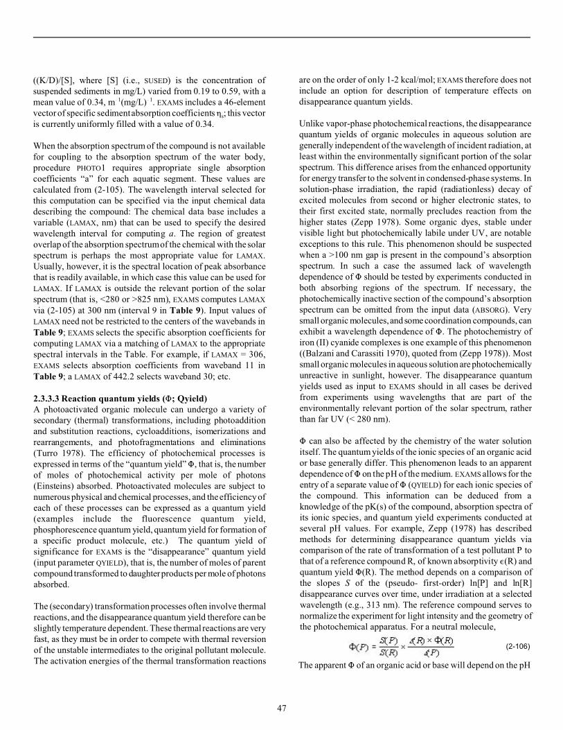
((K/D)/[S], where [S] (i.e., SUSED) is the concentration of suspended sediments in mg/L) varied from 0.19 to 0.59, with a mean value of 0.34, m! 1(mg/L)!1. EXAMS includes a 46-element vector of specific sediment absorption coefficients 0s; this vector is currently uniformly filled with a value of 0.34.
When the absorption spectrum of the compound is not available for coupling to the absorption spectrum of the water body, procedure PHOTO1 requires appropriate single absorption coefficients “a” for each aquatic segment. These values are calculated from (2-105). The wavelength interval selected for this computation can be specified via the input chemical data describing the compound: The chemical data base includes a variable (LAMAX, nm) that can be used to specify the desired wavelength interval for computing a. The region of greatest overlap of the absorption spectrum of the chemical with the solar spectrum is perhaps the most appropriate value for LAMAX. Usually, however, it is the spectral location of peak absorbance that is readily available, in which case this value can be used for LAMAX. If LAMAX is outside the relevant portion of the solar spectrum (that is, <280 or >825 nm), EXAMS computes LAMAX
via (2-105) at 300 nm (interval 9 in Table 9). Input values of LAMAX need not be restricted to the centers of the wavebands in Table 9; EXAMS selects the specific absorption coefficients for computing LAMAX via a matching of LAMAX to the appropriate spectral intervals in the Table. For example, if LAMAX = 306, EXAMS selects absorption coefficients from waveband 11 in Table 9; a LAMAX of 442.2 selects waveband 30; etc.
2.3.3.3 Reaction quantum yields (M; Qyield) A photoactivated organic molecule can undergo a variety of secondary (thermal) transformations, including photoaddition and substitution reactions, cycloadditions, isomerizations and rearrangements, and photofragmentations and eliminations (Turro 1978). The efficiency of photochemical processes is expressed in terms of the “quantum yield” M, that is, the number of moles of photochemical activity per mole of photons (Einsteins) absorbed. Photoactivated molecules are subject to numerous physical and chemical processes, and the efficiency of each of these processes can be expressed as a quantum yield (examples include the fluorescence quantum yield, phosphorescence quantum yield, quantum yield for formation of a specific product molecule, etc.) The quantum yield of significance for EXAMS is the “disappearance” quantum yield (input parameter QYIELD), that is, the number of moles of parent compound transformed to daughter products per mole of photons absorbed.
The (secondary) transformation processes often involve thermal reactions, and the disappearance quantum yield therefore can be slightly temperature dependent. These thermal reactions are very fast, as they must be in order to compete with thermal reversion of the unstable intermediates to the original pollutant molecule. The activation energies of the thermal transformation reactions
are on the order of only 1-2 kcal/mol; EXAMS therefore does not include an option for description of temperature effects on disappearance quantum yields.
Unlike vapor-phase photochemical reactions, the disappearance quantum yields of organic molecules in aqueous solution are generally independent of the wavelength of incident radiation, at least within the environmentally significant portion of the solar spectrum. This difference arises from the enhanced opportunity for energy transfer to the solvent in condensed-phase systems. In solution-phase irradiation, the rapid (radiationless) decay of excited molecules from second or higher electronic states, to their first excited state, normally precludes reaction from the higher states (Zepp 1978). Some organic dyes, stable under visible light but photochemically labile under UV, are notable exceptions to this rule. This phenomenon should be suspected when a >100 nm gap is present in the compound’s absorption spectrum. In such a case the assumed lack of wavelength dependence of M should be tested by experiments conducted in both absorbing regions of the spectrum. If necessary, the photochemically inactive section of the compound’s absorption spectrum can be omitted from the input data (ABSORG). Very small organic molecules, and some coordination compounds, can exhibit a wavelength dependence of M. The photochemistry of iron (II) cyanide complexes is one example of this phenomenon ((Balzani and Carassiti 1970), quoted from (Zepp 1978)). Most small organic molecules in aqueous solution are photochemically unreactive in sunlight, however. The disappearance quantum yields used as input to EXAMS should in all cases be derived from experiments using wavelengths that are part of the environmentally relevant portion of the solar spectrum, rather than far UV (< 280 nm).
M can also be affected by the chemistry of the water solution itself. The quantum yields of the ionic species of an organic acid or base generally differ. This phenomenon leads to an apparent dependence of M on the pH of the medium. EXAMS allows for the entry of a separate value of M (QYIELD) for each ionic species of the compound. This information can be deduced from a knowledge of the pK(s) of the compound, absorption spectra of its ionic species, and quantum yield experiments conducted at several pH values. For example, Zepp (1978) has described methods for determining disappearance quantum yields via comparison of the rate of transformation of a test pollutant P to that of a reference compound R, of known absorptivity ,(R) and quantum yield M(R). The method depends on a comparison of the slopes S of the (pseudo- first-order) ln[P] and ln[R] disappearance curves over time, under irradiation at a selected wavelength (e.g., 313 nm). The reference compound serves to normalize the experiment for light intensity and the geometry of the photochemical apparatus. For a neutral molecule,
(2-106)
The apparent M of an organic acid or base will depend on the pH
47

of the system. For a fixed pH, Eq. (2-106) can be rewritten to include the ionization equilibria and separate absorptivities and quantum yields of the various ionic species of the pollutant P. For example, a monoprotic organic acid will distribute between
!its uncharged RH3 molecule and its anion RH2 (see Chapter 2.2.4) as:
(2-107)
and
(2-108)
where " is the fraction of the total pollutant present as each of the molecular species (Ka here is the acidity constant). Equation (2-106) then becomes
(2-109)
Suppose, for example, that P is a monoprotic organic acid whose pKa = 5.0. At pH 5, the compound would distribute equally
!between RH3 and the RH2 anion. At pH 4.5, the compound would distribute as 76% RH3 and 24% RH2
! . Given, for example, , of RH3 as 5000, and , of RH2
! as 10000 at 313 nm, and experimentally determined values for the right side of Eq. (2-109) as 10 and 20 at pH 4.5 and 5.0 respectively; the quantum yields of the molecular species can be calculated via simultaneous solution of the equations:
1: (0.76)(5000)(M(RH3)) + (0.24)(10000)(M(RH2 ! )) = 10
2: (0.50)(5000)(M(RH3)) + (0.50)(10000)(M(RH2 ! )) = 20
giving a reaction quantum yield M for the uncharged molecule RH3 of 1.5×10! 4, and M(RH2
! ) = 3.9×10! 3.
Zepp and Baughman (1978) have discussed the effect of other dissolved species on the direct photolysis of synthetic organic molecules. Dissolved oxygen in some instances “quenches” photochemical reactions via energy transfer from a pollutant molecule to the oxygen molecule at the expense of transformation pathways. Disappearance quantum yields should be determined in air-saturated pure water to allow for this effect; EXAMS does not include an explicit algorithm to make allowances for varying dissolved oxygen concentrations (as sunlit waters are very rarely anaerobic). Photochemical reactions with dissolved nucleophilic species such as hydroxide, chloride, bromide, and sulfide can change the reaction quantum yield of a pollutant from the value determined in pure water system. The concentrations of these species in natural fresh waters are, however, typically much too small for them to compete with nucleophilic displacements by water itself. In
marine systems, chloride and bromide occur at concentrations (0.6 and 0.001 molar, respectively) high enough to compete, in principle, with water.
Some organic compounds that are not photoreactive in pure water are photoactive when complexed with metal ions. For example, NTA and EDTA are photochemically activated by complexation with iron (III). Photoactive co-dissolved substances (e.g., dissolved humic materials) can also mediate photoreactions of pollutant chemicals via direct energy transfer to the pollutant molecule, or by generation of reactive intermediates (e.g., singlet oxygen). These phenomena are properly termed “indirect” or “sensitized” photolysis, however, as opposed to the “direct” phototransformations that are the subject of this Chapter.
2.3.3.4 Absorption spectra (ABSORG) The absorbance of organic acids and bases in aqueous solution varies with pH, as a result of differential light absorption by the neutral molecule and its ions. The rate of photolytic transformation of an organic acid or base in natural waters thus depends on the pH of the system. EXAMS’ computations are keyed to the species-specific absorption spectra of the pollutant chemical (uncharged parent molecule and its ionic species), measured in pure water. EXAMS links the average spectral solar intensities in each layer of the water body to the absorption spectra of the compound, and thereby computes a value of Ka (Eq. (2-102)) for each dissolved molecular species.
EXAMS’ dynamic state variable is the total concentration of pollutant in each ecosystem segment, referred to the aqueous phase of the compartment. The fraction of this total concentration present as each molecular species is computed via the equilibrium ionization and sorption distribution coefficients " (Chapter 2.2.4). Once in possession of Ka (Eq. (2-102)) values for the several ionic species, EXAMS computes the contribution of each to the total pseudo-first-order direct photolysis rate constant via t he e xpr ess ion (co mpare Eq. (2
103)) where the subscript (i) refers in turn to
each of the ionic species.
This computational loop is actually iterated 3 times for each ionic species, because EXAMS incorporates the effects of sorption to sediments and complexation with DOC via a set of 3 values of QYIELD for each ionic species. In other words, for each ionic species i, EXAMS computes the total contribution of that species to the overall direct photolysis rate constant by fixing the value of i, and summing the expression
{"(i,k) × QYIELD(i,k) × Ka(i)} over the k=1 (dissolved), k=2 (sediment sorbed), plus k=3 (DOCcomplexed) forms of the compound in each sector of the ecosystem. The mechanics of this computation allow the user to control the photoreactivity of sorbed molecules via the entries in the QYIELD chemical input vectors.
48

Sorption of the pollutant to suspended sediments and complexation with “dissolved” organic carbon (DOC) can induce complex changes in both the light absorption spectra and the reaction quantum yields of the compound, and can “protect” the molecule from exposure to sunlight via migration or dissolution into the (darkened) interior of sediment particles. EXAMS’ first-order evaluations use the quantum yield parameter (QYIELD) as a mechanism for approximating the effects of sorption on the photoreactivity of pollutant chemicals; the phenomena involved are discussed in greater detail in Chapter 2.3.3.5.
In order to compute the effects of pH on light absorption and on photolytic rate constants, EXAMS requires a specific absorption spectrum (,, EXAMS ABSORG vector) for each (dissolved) molecular species of the pollutant chemical. These absorption spectra can be deduced from the pK(s) of the compound and the absorption spectra of aqueous solutions of the chemical, measured at several pHs. The procedure is analogous to that described for reaction quantum yields in Chapter 2.3.3.3. For example, Smith and coworkers ((1978)) measured the absorption spectrum of p-Cresol at pH 5.1, 7.0, and 8.9 (Table 10). Para-cresol is a weak organic acid (pKa = 10.2); at pH 5.1, 7.0, and 8.9 the anion is present as only 0.00079, 0.063, and 4.77 percent of the total concentration. The observed spectra (Table 10) clearly indicate that the anion is the more strongly absorbing species.
Table 10. Light absorption spectra of p-Cresol in pure water. Measured values at pH 5.1, 7.0, and 8.9 from Smith et al. 1978. Calculation of molecular species absorbance and estimated pH 7 solution absorbance described in text. pKa=10.2
-1M-1Center Spectral Absorp tion Coefficients ,, cm
8, nm pH 5.1 pH 7.0 pH 8.9 RH3 RH2 - pH 7.0
297 .5 14 18 193 14 3767 16
300 .0 3.8 7.2 173 3.8 3551 6.0
302 .5 2.4 3.8 150 2.4 3097 4.4
307 .5 0 2 92.6 0 1941 1.2
310 .0 2 63.5 1331 0.8
312 .5 1 40.3 845 0.5
315 .0 0 24.1 505 0.3
317 .5 13.0 272 0.2
320 .0 6.2 130 0.08
323 .1 3.8 80 0.05
330 .0 0
The observed absorption coefficient at any fixed wavelength is the sum of absorbance attributable to the uncharged (RH3) molecule, plus that attributable to the anionic (RH2
! ) species.
Denoting the observed absorption coefficient as , this sum
can be expressed algebraically:
(2-110)
This equation can be used to estimate the separate absorbances !of the RH3 and RH2 molecules. For example, at 297.5 nm, for
pH 7.0: ! ,o= 18 = (0.999369) ,(RH3) + (6.31×10!4) ,(RH2 )
and at pH 8.9, ! ,o = 193 = (0.952) ,(RH3) + (0.0477) ,(RH2 )
Simultaneous solution of these equations yields
,(RH3) = 15.6 and
,(RH2 ! ) = 3734.
The uncha rged molecule is present as 99.999 2% of the total
concentration at pH 5.1, so the pH 5.1 spectrum can be taken as
a direct expe rimen tal mea surem ent of ,(RH3). Given this, the
absorption spectrum of the (RH2 ! ) anion can be calculated using
the pH 8.9 spectrum and Eq. (2-110). For example, at 297.5 nm,
!193 = (0 .952)(14) + (0.0477) , (RH2 )
!gives , (RH2 ) = 3767. The accuracy of this procedure can now
be evaluated by using Eq. (2-110) to predict absorbance of the
solution at pH 7.0:
(0.999369)(14) + (6.31×10!4)(3767) = 16 (cm!1M! 1)
as compared to the experimental value of 18 cm!1M! 1. The
computed absorption spectra of the uncharged RH3 mole cule and !the RH2 anion of p-Cresol are also shown in Table 10, along
with the projected absorption coefficients at pH 7.0. The
absorption spectra of the individ ual mo lecules are the app rop riate
data for entry into E XA M S’ chemical data base (input vectors
ABSORG).
2.3.3.5 Effects of sorption on photolysis rates
The effects on direct pho tolysis of so rption to suspended material
are incorporated into E XA M S via separate disappearance quantum
yields (QY IELD) for the sorbed forms of each dissolved species !(RH3, RH2 , etc.) of the compound. Although sorption can
produce subtle and complex changes in the photochemistry of
pollutants, light extinctio n by susp end ed p articulate matter, and
capture of sorption-prone chemicals by bottom sediments,
relega te the effects of sorption to a secondary role. It should not
be assumed, however, that sorption inevitably “protects” a
chem ical from direc t interactio n with solar radiation, so E XA M S
allows for alternatives to this assumption via the QYIELD
chemical input ve ctor. (T his cap ability is only available for
49

compounds for which the absorption spectrum is known.)
The “sorption” process includes adsorption of a chemical onto
particle surfaces, dissolution of uncharged species into suspended
organic materials, and migration into the interior of particles via
diffusion along pore channels. The particle microenvironment is
often very different from that of the surrounding aqueous milieu.
For example, the surface acidity of clay minerals can result in
protonation of organic bases beyond that predicted by
solution-phase pH and pK (Karickhoff and Bailey 1976). This
effect can, at least in principle, be represented via EX AM S’
separated partition coefficients for the ionic species of a pollutant
(Chapter 2.2.2). The extent of the sorption/pro tonation process
is influenced, however, by particle size, interactions with the
solution-phase carbonate system, and inorganic cations adsorbed
on the clay surface. These complexities, and the fact that mineral
clays constitute a varying proportion of natural sediments, restrict
E XA M S to the phenomenological approach described in Chapter
2.2.2. The photoreactivity of an organic acid or base can be
affected by ionic speciation at the surface of adsorbent particles.
Bailey and Karickhoff (1973) demonstrated this effect via its
converse: these authors showed that UV spectroscopy can be
used to monitor surface acidity of clay minerals via the shift in
the absorption spectrum of adsorbed organic bases from that of
the uncharged, to the protonated, molecular species.
The dissolution of neutral organic pollutants into suspended
organic matter or surface organic films also removes the
chemical from aqueous solution to a very different
microenvironment. This organic microenvironment may alter the
absorption spectrum, quantum yields, and photochemical
reactions of a sorbed molecule, for organic sorbents usually
differ from water in both refractive index and polarity. A change
in the refractive index of the absorbing medium implies changes
in spectral radiation density (erg cm! 3 per unit frequency range)
in the medium, and therefore in the apparent absorption spectrum
of a pollutant chemical. Although the effects of such phenomena
can be computed in some cases (Strickler and B erg 1962), the
heterogeneity of natural suspended organic matter defies
description. Particle size distribution (i.e., light extinction in the
interior of the particle) would also affect the average radiation
density experienced by a sorbed-phase pollutant.
In addition, reaction conditions within a suspended particle
microenvironment must differ from those of aqueous solution;
these differences can alter the reaction quantum yields and the
kinds of photochemical products that result from irradiation of
the system (Miller and Zepp 1979b). Suspended sediments may
also retard sorbed-phase photoreactions by quenching excited
states of the molecule, and may enhance photoreaction via
indirect processes or “sensitized” reactions. Possible indirect
reactions include the production of excited states or free rad icals
via irradiation of the organic matrix of the suspended particles,
and photoelectric excitation of semiconductors, such as TiO2,
which are a common constituent of many natural sediments
(Oliver et al. 1979).
A few phenomenological investigations of the effects of natural
suspended sediments on photochemical kinetics have appeared
in the literature ; the complexity of the phenomena has led their
authors to describe their findings via apparent effects on reaction
quantum yields. Oliver, Cosgrove, and Carey (Oliver et al. 1979)
compared the effect of purified TiO2 semiconductor to the
photochemical efficacy of Ti ores (ilmenite and rutile) and
natural river suspensoids. Although purified TiO2 was an
efficient photochemical catalyst, the T i ores and the natural
sediments alike simply suppressed the photochemistry of the test
materials via competitive light absorption. Miller and Zepp
(1979b), from studies of the photolysis of DDE and
m-trifluoromethylpentadecanophenone (TPP) in natural
suspended sedim ents, concluded that the sediment
microenvironment is similar to a saturated hydrocarbon solvent.
These authors reported an apparent increase in the disappearance
quantum yield of sorbed DDE to 1.5 times its value in aqueous
solution, and a factor of 2 to 6 decrease in the apparent quantum
yield of TPP . Both results were consistent with the behavior of
these compounds in organic solvents. Miller and Zepp (1979a)
concluded that the competitive absorption of light by suspensoids
is nonetheless the dominant effect of suspended particles on
photolysis in natural waters.
2.3.3.5.1 Sensitivity analysis of sorption effects on direct
photolysis
Photolytic transformation of pollutant chemicals is an important
process in many aquatic systems, most especially when
photochemical transformation is the only degradation process
capable of limiting organism exposures under environmental
conditions. This process is critically dependent on competitive
light absorption by suspended materials, and on the effects of
sorption on the availability of a pollutant to photochemical
processes.
In a natural water body, capture of a pollutant by benthic
sediments removes the compound to a photochemically inactive
(dark) sector of the ecosystem. The net photochemistry of a
pollutant chemical thus depends on solution- and sorbed-phase
photoreactivity, competitive light absorption by suspensoids, and
capture of the pollutant by the benthic subsystem. The
interactions among these processes can be explored via E XA M S.
For the example simulations, the ecosystem was a small (1 ha)
static pond, 2 m deep, with a 1 cm active benthic subsystem of
bulk density 1.75 g/cc and water content 150% . The example
compound had a near-surface half-life of 1 hour in solution, but
was a full order of magnitude more photoreactive when sorbed
with suspended sediments (QY IELD(1,1) = 1.0, QY IELD(2,1) =
10.0). The distribution function (DFA CG) was taken as 1.20;
E XA M S used the sum of light absorption by water itself (at 300
nm), plus the absorbance attributable to suspended sediments, to
compute the average light intensity in the water column (Eq. (2
104)). Systematic changes in the partition coefficient of the
50

chemical (KPS) and the concentration of suspended sediments
(SUSED) were then used to elucidate their net effect on the
photochemistry of the compound, under conditions most
favorable for enhancement of phototransformation kinetics by
sorption.
The results of simulations using a suspended sediment
concentration of 10 mg/L and varying partition coefficients
(0–1×10⁶ L/kg) are given in Table 11. These results are given in
terms of pseudo-first-order half-lives for the water column
subsystem alone, and for the entire pond ecosystem. (The
whole-system half-lives assume that the rate of transport from the
benthic subsystem into the water column does not limit the rate
of photochemical transformation of the compound.) Under these
environmental conditions, less than 1% of the compound in the
water column is in the sorbed state for a partition coefficient less
than 1000 L/kg. When the partition coefficient is greater than
1000, however, more than 85% of the resident material is
captured by the (dark) benthic subsystem. T he system-level half-
life of the compound increases steadily with increasing Kp,
despite the greater photoreactivity of the sorbed material.
The effect of competitive light absorption by suspended materials
was examined by fixing the partition coefficient at 100 L/kg, and
systematically increasing the concentration of suspended
sediments from 0 to 10000 mg/L (Table 12). In this case, light
absorption by the suspended sediments rapidly increased the
photochemical half-life of the compound. This effect
overwhelmed the enhanced photoreactivity of the sorbed
material, despite the fact that more than half of the total
compound in the system resided in the water column (at steady
state).
Table 11. Effect of partition coefficient Kp (L/kg) on net photoreactivity when suspended sediment concentration = 10 mg/L (Average light intensity in water column 11.8% of surface value)
Kp % of Water % of Total Pseudo-First-Order Half-L/kg Column in Resident in lives, h
Dissolved Benthic State Zone Water Whole
Column System
0 100 0.29 8.50 8.52
1 100 0.87 8.50 8.57
10 100 5.8 8.49 9.01
100 99.9 36.9 8.42 13.4
1000 99.0 85.2 7.80 52.9
10000 90.9 98.2 4.68 253
100000 50.0 99.7 1.55 452
1000000 9.09 99.8 0.93 492
Table 12. Effect of suspended sediment concentration [S] on net photoreactivity when partition coefficient Kp = 100 L/kg
[S] % of Water % of Total Mean Pseudo-First-Order mg/L Column in Resident in Iz/Io Halflives, h
Dissolved Benthic (%) State Zone Water Whole
Column System
0 100 36.96 84.8 1.18 1.87
1 100 36.96 59.3 1.68 2.67
10 99.9 36.93 11.8 8.42 13.4
100 99.0 36.73 1.22 75.2 119
1000 90.9 34.77 0.12 449 688
10000 50.0 22.67 0.012 1484 1918
The system-level pseudo-first-order half life indicates the
outcome of the interaction between competitive light absorption
by suspended materials, capture of the compound by bottom
sediments, and enhanced photoreactivity in the sorbed state.
Table 13 gives the system-level photochemical half life of a
compound that is 100 times more reactive in the sorbed, than in
the dissolved, state, for a range of Kp and sediment
concentrations unlikely to be exceeded in nature. As compared
with the 1.18 hour half-life of the unsorbed, clean-water baseline,
an increase in sorption leads to a net suppression of the rate of
photochemical transformation of the compound in all cases,
despite the uniquely (and unrealistically) favorable conditions
assumed for the analysis. In sum, the effects of residence in the
sorbed state on photoreactivity are of secondary importance, and
can be adequately summarized via a simple descriptive parameter
(QY IELD).
Table 13. Effect of suspended sediment concentration (mg/L) and partition coefficient (Kp, L/kg) on system-level pseudo-first-order photochemical half-life (hours) when sorbed chemical is 100 times more reactive than dissolved species
Kp Suspended Sediment Concentration, mg/L
L/kg
0 1 10 100 1000 10000
0 1.18 1.69 8.52 82.2 819 8182
1 1.19 1.70 8.57 81.8 749 4157
10 1.25 1.79 8.93 79.1 437 861
100 1.87 2.65 12.3 65.4 125 209
1000 8.06 10.5 29.1 51.7 63.3 137
10000 69.9 50.0 45.9 49.0 56.6 130
100000 689 89.6 49.2 48.6 55.9 129
1000000 6876 97.4 49.6 48.6 55.8 129
51

The effects of sorp tion to organic slicks at the air-water interface
are not included in E XA M S for similar reasons: Although the
concentration in the slick can be large, the total fraction of the
pollutant resident in the film is probably too small to have much
effect on the system-wide kinetics of pollutant chemicals (Zepp
and Baughman 1978).
E XA M S represents the photochemical effects of sorption to
suspended sediments, and complexation with DOC, via separate
entries in the QYIELD vectors. Note that these vectors represent
the effect of residence in the biosorbed state on the direct
photolysis of the pollutant; they are not intended to represent
photosensitization or photobiological transformation of
pollutants by phytoplankton. Although qualitative studies have
indicated that this pathway exists, as yet a quantitative basis for
predicting its magnitude and importance in natural systems has
not been developed (Zepp 1980).
2.3.3.6 Near-surface solar beam and sky irradiance
The spectral light field is calculated by E XA M S as a vector
(“WLAM” for W8) of 46 photon irradiances. W 8 is the total
(solar beam plus skylight) irradiance under clear (cloudless)
conditions, just below the air-water interface (that is, after
subtracting reflected light from the light incident on the surface).
E XA M S corrects the input irradiance for effects of cloud cover
using the empirical relationship:
(2-111)
(Büttner 1938), cited from (Zepp 1980); see also (Schultz and
Gräfe 1969).
The cloudiness (EXAMS’ input CLOUD) term is the average
opaque sky cover in tenths, with a range from 0 (clear sky) to 10
(full cover). Opaque sky cover may also be reported in oktas; an
okta is one eighth of the celestial dome. Conversion from oktas
to tenths may be made as follows:
WMO Oktas Tenths
Code
0 (clear) 0 0
1 1 okta or less, 1/10 or less, but not zero
but not zero
2 2 oktas 2/10 - 3/10
3 3 oktas 4/10
4 4 oktas 5/10
5 5 oktas 6/10
6 6 oktas 7/10 - 8/10
7 7 oktas or more, 9/10 or more, but not
but not 8 oktas 10/10
8 8 oktas 10/10
9 sky obscured by fog or other meteorological
phenomenon
15 cloud cover indiscernible for reasons other than
fog or other meteorological phenomenon, or
observation not made
W
Clear-sky irradiance at the earth’s surface depends on latitude,
site elevation, atmospheric turbidity and water vapor content, and
the ozone content of the stratosphere (Leighton 1961).
Computational methods for estimating spectral irradiance have
been explored by a number of authors (e.g., Leighton 1961,
Green et al. 1974, Dozier 1980, Green et al. 1980, Green and
Schippnick 1980, Green and Schippnick 1982). Zepp and Cline
((1977)), using a computer program (“SOLAR”) available on
request from those authors, calculated photon scalar irradiance
8 at 39 of the wavelength intervals adopted for E XA M S. (They
reported “midseason,” “midday” spectral irradiance at 40° N
latitude. For E XA M S, such values must be reduced by a day length
factor (daylight hours/24), and sinusoid averaging over the
photoperiod (i.e., multiplied by 2/B).
Irradiance spectra are often computed or measured in energy
units. These spectra can be converted to photon irradiances via
Planck’s law. For example, given an energy spectrum (“Es”) in
:Watts cm! 2 nm! 1, W 8 in photons cm! 2 s! 1 (N nm bandwidth)! 1
can be computed from:
W 8 = Es ×5.047×109 × 8 (nm) × N (nm)
where 8 is the wavelength of the incident radiation, and
5.047×109 ={10! 6 (J/s)/(µWatt)×10! 9m/nm}/{6.6262×10! 34 J@s
×2.99m/s}. At 297.5 nm, for example, the appropriate conversion
factor for E XA M S’ bandwidth of 2.5 nm is:
W 8 = Es ×5.047×109 × 297.5 × 2.5 = 3.754 ×10¹² Es
Procedure PHOTO1 begins from near-surface pre-computed
photolysis rate constants (KDP), and thus does not use the spectral
irradiance vector W 8 in its computations. PHOTO1 adjusts KDP via
a cloudiness correction (2-111), and also corrects KDP for the
geographic translation from the latitude at which each KDP was
measured (RFLAT) to the latitude of the ecosystem (LAT). The
correction term is computed from the total annual solar + sky
radiation received at latitudes RFLAT and LAT . Ground-level
radiation was computed as a function of latitude at 10 degree
intervals via procedures described by List (1966) using an
atmospheric transmission coefficient of 0.90. Estimated total
radiation increased from 1.038×10⁵ cal cm! 2 yr! 1 at the po le, to
52

2.744×10⁵ langley yr! 1 at the equator. Regression of the (8) estimates on:
Y = a + b cos(2L)
where L is the latitude in radians, yielded a = 1.917×10⁵, b = 8.705×10⁴, and accounted for 99.7% of the variation in total irradiance (Y) with latitude. In procedure PHOTO1, the correction term for KDP is computed as:
For example, for a rate constant measured at the equator and a polar ecosystem,
This procedure is based on total solar energy input, and thus may underestimate the latitude dependence of photochemical transformation of pollutants that absorb sunlight most strongly at wavelengths < 320 nm.
2.3.3.7 Input data and computational mechanics – Summary Procedure PHOTO1 was designed to evaluate chemicals whose absorption spectrum has not been quantified. Its primary input datum, KDP, is a vector of pseudo-first-order photolysis rate constants. A separate value of KDP can be entered for each existing ionic species (RH3, RH4
+, etc.). KDP must be calculated as an annual average value applicable to near-surface waters, under cloudless conditions and full-day average solar irradiance. EXAMS then adjusts the rate constant for light extinction in the water column, effects of cloud cover, and departure of the latitude of the environment (LAT) from the latitude at which the rate constant was measured (RFLAT). Effects of sorption and DOC-complexation cannot be represented; only the dissolved form of the chemical photolyzes.
The computations executed by procedure PHOTO1 are inherently less accurate than wavelength-specific computations based on the chemical’s absorption spectrum (PHOTO2), because PHOTO1 cannot evaluate the effects of spectrally differentiated light extinction in the water column.
Procedure PHOTO2 couples the absorption spectra of the compound (ABSORG(1-46,k)) to the irradiance spectrum incident on the water body (W8). The QYIELD matrix contains measured disappearance quantum yields; it is also used in EXAMS to account for effects of sorption and complexation with DOC.
Both photolysis procedures operate on the incident light field to compute the average light intensity in each compartment of the ecosystem. (In PHOTO1, the incident light field has a nominal value of 1.0, because KDP has built into it the clear-sky irradiance at latitude RFLAT.) PHOTO1 uses a spectral
composite light absorption coefficient for each sector of the water body computed via Eq. (2-105) at the user-specified wavelength (LAMAX); PHOTO2 computes the absorption
coefficient for every spectral waveband (Table 9) from the
pigment (CH L), disso lved o rganic carbon (DOC), and suspended
sediment (SUSED) concentrations in each compartment
(Equation (2-105)).
The water column (“E” and “H” compartment types) can be
subdivided into as m any ho rizontal slices as se ems a ppr opr iate
for a particular wa ter bo dy. EXAM S traces light extinction
vertica lly through the slices by compu ting irradiance at the
bottom of each compartment, as well as the average irradiance
used for computing photolysis rate constants. When the (J-1)
compartment is another E or H segment, irradiance at the bottom
of the (J-1 ) com partm ent is taken as the starting point for
irradiance computations in the current (J) sector. This scheme
will fail, howe ver, if the system definition rules given in Chapter
2.3.1.1 are disregarded.
An exam ple o f a logical, but improper, segmentation scheme is
shown in Figure 7.
Figure 7. Improper segmentation: incomplete vertical definition
Calls to EXAMS’ photolysis procedures are executed in compartment order. For this ecosystem, the first call computes photolysis in compartment 1, a (L)ittoral water column compartment. The incident light field at the air-water interface is identified as the light intensity at the top of the compartment, and EXAMS computes both average light intensity and irradiance at the bottom of compartment 1. Compartment 2 is a (B)enthic compartment; EXAMS simply sets the photolysis rate to 0 and does not call a photolysis procedure. Upon reaching compartment 3, EXAMS checks the compartment type of the (J-1) compartment. As compartment 2 is “B” (benthic), the incident light field is used to start the computations. A photolysis procedure is not invoked for (B)enthic compartment 4. When EXAMS now calls for irradiance computations for the (H)ypolimnion compartment (5), an error occurs. EXAMS
inspects (J-1) compartment 4, finds it to be (B)enthic, and starts
53

its computations for the hypolimnion using the surface incident light field, rather than intensity at the bottom of the epilimnion.
The proper system definition is shown in Figure 8.
Figure 8. Proper segmentation: complete vertical definition.
In this case, upon initiation of computations for the hypolimnion (now numbered 6), EXAMS finds that the (J-1) compartment (5) is not (B)enthic, as it is an (E)pilimnion segment. The light intensity at the bottom of compartment 5 (internal variable BOTLIT in PHOTO1, vector BOTLAM in PHOTO2) is therefore retrieved and used to start the irradiance computations for the hypolimnion.
EXAMS reports the average light intensity in each sector of the ecosystem as part of its “canonical profile” of the system. These reports are given as a percentage of the light field incident on the water body, integrated over the ultraviolet portion of the spectrum (278.75–395 nm).
References for Chapter 2.3.3. Bailey, G. W., and S. W. Karickhoff. 1973. An ultraviolet
spectroscopic method for monitoring surface acidity of clay minerals under varying water content. Clays and Clay Minerals 21:471-477.
Bailey, R. A., H. M. Clarke, J. P. Ferris, S. Krause, and R. L. Strong. 1978. Chemistry of the Environment. Academic Press, New York.
Baker, K. S., and R. C. Smith. 1982. Bio-optical classification and model of natural waters. 2. Limnology and Oceanography 27:500-509.
Balzani, V., and V. Carassiti. 1970. Photochemistry of Coordination Compounds. Academic Press, London and New York.
Büttner, K. 1938. Physikal Bioklimatologie (Physik. Bioklimat.), Leipzig.
Calvert, J. G., and J. N. Pitts, Jr. 1966. Photochemistry. John Wiley and Sons, Inc., New York.
Dozier, J. 1980. A clear-sky spectral solar radiation model for
snow-covered mountainous terrain. Water Resources Research 16:709-718.
Green, A. E. S., K. R. Cross, and L. A. Smith. 1980. Improved analytic characterization of ultraviolet skylight. Photochemistry and Photobiology 31:59-65.
Green, A. E. S., T. Sawada, and E. P. Shettle. 1974. The middle ultraviolet reaching the ground. Photochemistry and Photobiology 19:251-259.
Green, A. E. S., and P. F. Schippnick. 1980. UV-B reaching the ground. in Conference in Ultraviolet Light in Marine Ecosystems, Copenhagen.
Green, A. E. S., and P. F. Schippnick. 1982. UV-B reaching the surface. Pages 5-27 in J. Calkins, editor. The Role of Solar Ultraviolet Radiation in Marine Ecosystems. Plenum Press, New York.
Hojerslev, N. K. 1973. Inherent and apparent optical properties of the western Mediterranean and the Hardangerfjord. 21, Univ. Copenhagen, Inst. Phys. Oceanogr., Copenhagen.
Hojerslev, N. K. 1974. Inherent and apparent optical properties of the Baltic. 23, Univ. Copenhagen, Inst. Phys. Oceanogr.
Hutchinson, G. E. 1957. A Treatise on Limnology. Vol. I. Geography, Physics, and Chemistry. John Wiley and Sons, Inc, New York.
Jerlov (Johnson), N. G., and G. Liljequist. 1938. On the angular distribution of submarine daylight and the total submarine illumination. Sven. Hydrogr.- Biol. Komm. Skr., Ny Ser. Hydrogr. 14:15.
Jerlov, N. G. 1976. Marine Optics. Elsevier Sci. Publ. Co, Amsterdam-Oxford-New York.
Karickhoff, S. W., and G. W. Bailey. 1976. Protonation of organic bases in clay-water systems. Clays and Clay Minerals 24:170-176.
Leighton, P. A. 1961. Solar radiation and its absorption. Pages 6-41 in Photochemistry of Air Pollution. Academic Press, New York and London.
List, R. J. 1966. Smithsonian Meteorological Tables, 6th edition. Smithsonian Institution, Washington, D.C.
Mickle, A. M., and R. G. Wetzel. 1978. Effectiveness of submersed angiosperm-epiphyte complexes on exchange of nutrients and organic carbon in littoral systems. II. Dissolved organic carbon. Aquatic Botany 4:317-329.
Miller, G. C., and R. G. Zepp. 1979a. Effects of suspended sediments on photolysis rates of dissolved pollutants. Water Research 13:453-459.
Miller, G. C., and R. G. Zepp. 1979b. Photoreactivity of aquatic pollutants sorbed on suspended sediments. Environmental Science and Technology 13:860-863.
Oliver, B. G., E. G. Cosgrove, and J. H. Carey. 1979. Effect of suspended sediments on the photolysis of organics in water. Environmental Science and Technology 13:1075-1077.
Poole, H. H., and W. R. G. Atkins. 1926. On the penetration of light into sea-water. Journal of the marine biological Association of the U.K. 14:177-198.
Preisendorfer, R. W. 1958a. Directly observable quantities for
54

light fields in natural hydrosols. Visibility Laboratory Report SIO Reference 58-46, Scripps Institution of Oceanography, La Jolla, California.
Preisendorfer, R. W. 1958b. Unified Irradiance Equations. Visibility Laboratory Report SIO Reference 58-43, Scripps Institution of Oceanography, La Jolla, California.
Schultz, R., and K. Gräfe. 1969. Consideration of sky ultraviolet radiation in the measurement of solar ultraviolet radiation. Pages 359-373 in F. Urbach, editor. The Biologic Effects of Ulraviolet Radiation. Pergamon Press, Oxford.
Smith, J. H., W. R. Mabey, N. Bohonos, B. R. Holt, S. S. Lee, T.-W. Chou, D. C. Bomberger, and T. Mill. 1978. Environmental Pathways of Selected Chemicals in Freshwater Systems: Part II. Laboratory Studies. EPA-600/7-78-074, U.S. Environmental Protection Agency, Athens, Georgia.
Smith, R. C., and K. S. Baker. 1978. Optical classification of natural waters. Limnology and Oceanography 23:260-267.
Smith, R. C., and J. E. Tyler. 1976. Transmission of solar radiation into natural waters. Photochemistry and Photobiology Reviews 1:117-155.
Strickler, S. J., and R. A. Berg. 1962. Relationship between absorption intensity and fluorescence lifetime of molecules. Journal of Chemical Physics 37:814-822.
Talling, J. F., R. B. Wood, M. V. Prosser, and R. M. Baxter. 1973. The upper limit of photosynthetic productivity by phytoplankton: Evidence from Ethiopian soda lakes. Freshwater Biology 3:53-76.
Turro, N. J. 1978. Modern Molecular Photochemistry. The Benjamin/Cummings Publ. Co., Inc., Menlo Park, California.
Wetzel, R. G. 1975. Limnology. W.B. Saunders Co., Philadelphia.
Zepp, R. G. 1978. Quantum yields for reaction of pollutants in
2.3.4 Specific Acid, Specific Base, and Neutral Hydrolysis Many organic compounds react directly with water in the aqueous solvent system. In addition, water dissociates into hydronium and hydroxide ions, and the concentrations of these subsidiary species often affect the rates of chemical transformations. EXAMS includes kinetic constants for three kinds of hydrolytic pathways: specific-acid (H3O
+) catalyzed, neutral hydrolysis, and specific-base (OH! ) catalyzed transformations.
The breakdown of esters to yield a carboxylic acid and an alcohol is a convenient example of hydrolytic transformations. The overall reaction is:
(2-112)
where R and R’ can be any alkyl or acyl moiety. Although this equation accurately depicts the stoichiometry of ester hydrolysis,
dilute aqueous solution. Environmental Science and Technology 12:327-329.
Zepp, R. G. 1980. Assessing the photochemistry of organic pollutants in aquatic environments. Pages 69-110 in R. Haque, editor. Dynamics, Exposure and Hazard Assessment of Toxic Chemicals. Ann Arbor Science Publishers, Ann Arbor.
Zepp, R. G., and G. L. Baughman. 1978. Prediction of photochemical transformation of pollutants in the aquatic environment. Pages 237-263 in O. Hutzinger, I. H. v. Lelyveld, and B. C. J. Zoeteman, editors. Aquatic Pollutants: Transformation and Biological Effects. Pergamon Press, Oxford.
Zepp, R. G., and D. M. Cline. 1977. Rates of direct photolysis in aquatic environment. Environmental Science and Technology 11:359-366.
Zepp, R. G., and P. F. Schlotzhauer. 1981. Comparison of photochemical behavior of various humic substances in water: III. Spectroscopic properties of humic substances. Chemosphere 10:479-486.
Zepp, R. G., N. L. Wolfe, L. V. Azarraga, R. H. Cox, and C. W. Pape. 1977. Photochemical transformation of the DDT and methoxychlor degradation products, DDE and DMDE, by sunlight. Archives of Environmental Contamination and Toxicology 6:305-314.
Zepp, R. G., N. L. Wolfe, J. A. Gordon, and G. L. Baughman. 1975. Dynamics of 2,4-D esters in surface waters: hydrolysis, photolysis, and vaporization. Environmental Science and Technology 9:1144-1150.
Zepp, R. G., N. L. Wolfe, J. A. Gordon, and R. C. Fincher. 1976. Light-induced transformations of methoxychlor in aquatic systems. Journal of Agricultural and Food Chemistry 24:727-733.
it does not serve as a defining equation for computing the velocity of the reaction. The rate of transformation of any specific ester is fundamentally dependent on its chemical structure. The speed of the reaction often depends on the pH of the medium as well, however, because ester hydrolysis can proceed via three distinct pathways (acid/base catalysis, neutral) with identical net stoichiometry.
Because chemical reactions involve shifts in electronic bonding orbitals, organic compounds are most readily attacked by groups that can donate or accept electrons from the target molecule. Electron-deficient chemical species (e.g., hydronium ions,H3O
+) are called “electrophiles.” Electrophiles are particularly attracted to atoms with negative charge, to a lone pair of electrons, and to the electron-dense region of a double bond. Chemical groups with extra non-bonding electrons are called “nucleophiles.” The electronegative hydroxide ion is a relatively strong nucleophile. The water molecule is itself nucleophilic, because the oxygen
55

atom of this “polar” molecule has a lone pair of electrons.
The mechanisms of the formation and hydrolysis of organic esters have been reviewed by Kirby ). Tinsley (Tinsley 1979:105 ff) has summarized the routes and mechanisms of ester hydrolysis under environmental conditions, where in all probability only the “A(AC)2”and “B(AC)2”mechanisms are significant. Although all three routes of ester hydrolysis involve nucleophilic phenomena, the mechanism of the pathway is somewhat different in each case.
Acid-catalyzed ester hydrolysis is a true “catalysis” reaction in that the hydronium ion participates in the reaction but is not consumed by the reaction sequence. In the first step of this pathway, the electrophilic hydronium ion protonates the carbonyl (C=O) oxygen. The protonated ester then undergoes a nucleophilic addition of water to give a tetrahedral intermediate; this step is catalyzed by a second water molecule acting as a general base. Finally, the tetrahedral intermediate breaks down via two additional (fast) steps to yield the product carboxylic acid and alcohol, and to regenerate the catalytic hydronium ion.
Because two water molecules are involved in the formation of the tetrahedral intermediate, the specific-acid catalyzed hydrolysis of the ester bond is “second-order” in water. With water as the solvent medium for the dissolved phase of the compound, however, the water concentration does not change during the course of the reaction and need not be incorporated in the kinetic expression. The observed rate constants are nonetheless subject to solvent effects and should be measured using pure water as the solvent whenever possible. The direct involvement of the water molecule in the reaction also imposes a need for care in the extrapolation of hydrolysis rate constants (measured in pure water) to compounds sorbed with sediments.
In EXAMS, all concentrations are referenced to the water phase of each compartment (Eq. (2-1)). The total pollutant concentration [C] (units mg/liter of water), when multiplied by the appropriate distribution coefficient ", gives the dissolved concentration of pollutant in the aqueous phase of each compartment, including that in the interstitial pore water of a benthic sediment. This fraction of the pollutant hydrolyzes at the rate measured via a homogeneous phase (pure water) experiment. EXAMS computes the effects of residence in a sorbed state (where water concentration can be quite small) on the reactivity of the compound via an additional set of input parameters (Chapter 2.3.4.3).
Neutral hydrolysis of organic esters proceeds via a mechanism similar to that of the second stage of the acid-catalyzed pathway. Two molecules of water are again involved in the formation of a tetrahedral intermediate, with one molecule of water acting as the nucleophile and a second water molecule acting as a general base catalyst. Although the neutral reaction is usually treated as
a simple first-order process (Wolfe 1980), it is in fact technically second-order in water concentration. This reaction is thus also subject to solvent effects, and requires the same caution in extrapolation to sorbed states as was mentioned above for acid-catalyzed hydrolysis.
Alkaline hydrolysis, the third hydrolytic mechanism considered in EXAMS, is not strictly speaking a hydroxide-“catalyzed” reaction, for hydroxide ion is consumed in the reaction sequence, yielding the ester’s constituent alcohol and the anion of its carboxylic acid. At trace concentrations of the ester in buffered natural waters, however, this distinction is of no practical significance. As in the neutral and acid-catalyzed pathways, a tetrahedral intermediate species is probably involved in alkaline hydrolysis. In this case, however, the intermediate is usually envisioned as resulting from a direct nucleophilic attack of hydroxide ion on the carbonyl carbon, with formation of the tetrahedral intermediate as the rate-limiting step in the reaction pathway. The tetrahedral intermediate then breaks down via release of an R’O! anion, and rapid proton transfer (to R’O! ), to yield the products of the reaction (R’OH and RCOO! ).
The overall rate of hydrolytic transformation is thus the sum of three competing reactions, and the observed rate constant (Kobs, units /h) can be computed as the sum of contributions from acid-catalyzed (KAH), neutral (KNH), and base-catalyzed (KBH) reactions (Wolfe 1980):
(2-113)
Kobs is a pseudo-first-order (h! 1) rate constant under the specified environmental conditions (pH, pOH) in pure water. After incorporation of the effects of ionization and sorption on reactivity, Kobs becomes the hydrolytic contribution to the overall pseudo-first-order rate constant K of Eq. (2-1). The second-order transformation rate constants are part of EXAMS’ input chemical data base. KAH and KBH have units of reciprocal molarity and reciprocal hours (M! 1h! 1). KNH, the neutral hydrolysis rate constant, has units h! 1. The environmental data for this computation are entered as a separate pH and pOH for each sector (compartment) of the ecosystem; the EXAMS variables are “PH” and “POH,” respectively.
The utility of this approach is not, of course, limited to chemical transformations of carboxylic acid esters. For example, amides, carbamates, and organophosphates break down via hydrolytic mechanisms (Tinsley 1979). Also, manyhalogenatedcompounds are subject to unimolecular and bimolecular nucleophilic substitution (SN1 and SN2) or elimination (E1 and E2) reactions whose kinetics can be represented via Eq. (2-113).
Experimental studies of the rate of hydrolysis in buffered aqueous solution can be used to determine Kobs at fixed pH levels. In many cases KAH and KBH can be determined at low and high pH, respectively, where only one reaction pathway is significant. The pH-rate profile, a plot of log Kobs vs. pH, then
56

includes a descending (acid catalyzed) and ascending (alkaline) limb, with slopes of -1.0 and +1.0, respectively ( Figure 9). These lines intersect at the theoretical rate minimum, giving the best pH for an experimental determination of any neutral contribution (KNH). One or more of the reaction pathways may be undetectably slow for a particular compound, resulting in a simplified pH-rate profile. The use of pH-rate profiles for calculating hydrolysis rate constants has been described in more detail by Kirby (Kirby 1972:153) and by Mabey and Mill (1978).
Figure 9. Hydrolysis pH-rate profile of phenyl acetate at 25°C.Profile constructed via rate constant data summarized byMabey and Mill 1978 .
Reported chemical rate constants are often based on the second or minute as the unit of time. For use in EXAMS, such data must be converted to units based on the hour. For example, the neutral hydrolysis rate constant of phenyl acetate is 6.6×10⁻⁸ s! 1 ( Figure 9). EXAMS’ chemical input parameter (KNH, units /h) would be 6.6×10⁻⁸ (s! 1)×3600 (s/h)=2.38×10-4 h! 1.
2.3.4.1 Temperature effectsEach hydrolytic rate constant in EXAMS’ chemical data base (KAH, KNH, KBH) has a paired input parameter that allows for alternative entry of the chemical information as an (Arrhenius) function of temperature. The pairings are KAH–EAH, KNH–ENH, and KBH–EBH, respectively. The rate constant variables (KAH
etc.) are interpreted as the (Briggsian logarithm of the) “preexponential” or “frequency” factor in an Arrhenius function, only when the parallel activation energies (EAH etc.) are non-zero. When the input energy parameter is set to zero, EXAMS
accepts the kinetic parameter (KAH, etc.) as the rate constant itself (compare Chapter 2.3.2.1). For example, an activation energy (Ea) for the neutral hydrolysis of phenyl acetate (ENH) of, say, 20,000. cal/mole would imply a frequency factor A =KNH / exp(-Ea/RT), (T in Kelvin) or, given KNH = 2.38×10⁻⁴ h! 1 at 25° C (Figure 9), A=2.38×10⁻⁴/exp(-20000./(1.99×298.15)) = 1.04×10¹¹ h! 1, and log A, the EXAMS input (KNH) = 11.02 h! 1.
In this instance, if EXAMS were loaded with KNH=2.38×10! 4 and
ENH = 0.0, KNH would be used as the rate constant for neutral hydrolysis irrespective of the temperature (environmental input parameter TCEL) obtaining in the system compartments. Alternatively, EXAMS could be loaded with KNH = 11.02 and ENH
= 20.0. In the latter case EXAMS would compute local (compartment specific) values of the neutral hydrolysis rate constant KNH via: log KNH = KNH!((1000×ENH)/4.58(TCEL+273.15)) or, at TCEL = 25°C,
log KNH = 11.02!(1000×20)/(4.58×298.15) = !3.626 and
KNH = 2.36×10⁻⁴ h! 1.
In many cases the temperature dependence of a chemical rate constant is reported in terms of transition state theory, that is, as an enthalpy (H) and entropy (S) of activation. Given H in calories/mole and S in cal/deg/mole (also called “entropy units,” e.u.), data reported under this convention can be converted to Arrhenius functions via (Bunnett 1961):
(2-114)
and
(2-115)
in which Ea has units of calories/mole, and A is in h! 1. (Because the RT term is only about 600 cal/mol at room temperature, however, in many cases reported values of H are in fact uncorrected Arrhenius activation energies (Ea).)
For example, Wolfe and coworkers (Wolfe et al. 1977) found that malathion (O,O-dimethyl-S- (1,2-dicarbethoxy) ethylphosphorodithioate) breaks down via an acid catalyzed degradation with an enthalpy of activation (H) of 22.3 kcal/mol and an entropy of activation (S) of -4.1 eu. Using 15°C as the temperature for conversion, Eq.(2-114) gives Ea = 22300 + (1.987)(288.15) = 22872 cal/mol and an EXAMS input of EAH = 22.87 kcal/mol. The frequency factor A (Eq.(2-115)) would be: log A = !4.1/4.58 + log(288.15) + 14.319, yielding log A = 15.88 h! 1 = KAH.
When a compound is subject to more than one degradation pathway, the rate constants must be combined prior to entry in EXAMS’ chemical data base. For example, malathion undergoes an alkaline carboxyl ester hydrolysis plus an E2 elimination reaction kinetically dependent on hydroxide ion concentration [OH! ] (Wolfe et al. 1977). These authors computed entropies and (uncorrected) enthalpies of activation for both reactions; this information could be used to generate an Arrhenius approximation for the total alkaline disappearance rate constant KBH via the transition state theory equation
KBH (h! 1) = (7.5018×10¹³)(T)×exp(-H/RT)×exp(S/R),
57

where H = Ea - RT, as in Eq.(2-114). Whenever possible, however, it is probably better to rely on experimental determinations of the total disappearance rate constant, measured at environmentally relevant temperatures. In this case, the total (second-order) disappearance rate constant was measured at 0° and at 27° C; it was 0.067 and 5.5 M! 1s! 1, respectively. The activation energy and frequency factor can be easily computed from these data, giving KBH = 23.67 h! 1 and EBH = 26.6 kcal/mol.
2.3.4.2 Ionization effectsAnions and cations of organic acids and bases can hydrolyze at rates differing greatly from those of the parent unionized species. This phenomenon can give rise to pH-rate profiles very unlike the archetypal example of phenyl acetate (Figure 9), including an apparent kinetic dependence on fractional powers of {H3O
+} or {OH! }. In order to encompass these phenomena, each of EXAMS’ input kinetic parameters (and parallel activation energies) is set up as a 3×7 matrix of variables. The second index of these parameter matrices specifies the ionic species for which a particular rate constant applies. The first index allows for specification of the effects of sediment sorption and DOC
complexation on reactivity; this aspect of EXAMS’ input data is discussed in Chapter 2.3.4.3.
Consider, for example, the hydrolysis of the series of substituted 2- phenyl-1,3-dioxanes studied by Bender and Silver (1963). All the acetals in the series showed the usual acid-catalyzed hydrolysis, but those members containing an o- or p-phenolic substituent were reactive at alkaline pH as well. The pH-rate profile for one member of this series, 2-(4-hydroxy-5-nitrophenyl)-1,3-dioxane (“HND”), is shown in Figure 10. This profile includes a descending limb of slope -1.0 at low pH, a zone of little change in Kobs suggestive of a neutral mechanism, followed by a second descending limb in the alkaline pH range, which begins in the vicinity of pH = pKa.
Figure 10. Hydrolysis pH-rate profile for a substituted 2-Phenyl-1,3-Dioxane. Data from Bender and Silver 1963.
From a comparison of the kinetics of o- and p-phenolic substituted acetals, and from the effect of deuterium oxide on these kinetics, Bender and Silver (1963) concluded that the hydrolysis of these compounds does not in fact proceed via a neutral mechanism. Instead, the initial descending limb is the result of the usual acid-catalyzed hydrolysis of the unionized species, and the descending limb in the alkaline pH region results from a similar acid- catalyzed hydrolysis of the phenolate anion (Figure 10). The anion is 860 times more reactive than the unionized species. The uniformity of Kobs at intermediate pH results from the increasing importance of the phenolate anion, as a fraction of the total concentration, in this pH range.
M
The hydrolytic kinetics of HND can be completely specified in EXAMS’ chemical data base via the pKa of the compound and the rate constants for acid hydrolysis (KAH) of the uncharged and the anionic species. The existence of the unionized species and the phenolate anion is signaled by setting SPFLG(1) and SPFLG(5) to 1 (Chapter 2.2.1), and the pKa of HND is specified via PK(1) = 6.63. The second-order rate constants are 540 and 4.68×10⁵
! 1h! 1 for the parent compound and the anion respectively (Figure 10). This information is loaded to EXAMS by setting KAH(1,1) to 540, and KAH(1,5)=4.68E5. The first index (Chapter 2.3.4.3) simply denotes the form of the compound (1=dissolved). The second index specifies the ionic species to be transformed. Subscript (1,1) thus specifies the unionized dissolved HND as reacting at rate (540)[H3O
+] h! 1, and subscript (1,5) specifies the phenolate anion as reacting at rate (4.68×10⁵)[H3O
+] h! 1.
2.3.4.3 Sorption effects Sorption of a compound with sediment phases or complexation with DOC removes the compound to a microenvironment that can be very different from the free water phase of the system. For example, Miller and Zepp (1979) found that the daughter product yields resulting from photolysis of DDE shifted from p , p ’ - d i c h l o r o b e n z o p h e n o n e t o w a r d D D M U (1,1-bis(p-chlorophenyl)- 2- chloroethylene) when the parent DDE was sorbed with suspended sediments. Photolysis of DDE dissolved in hexane also gave enhanced yields of DDMU. The authors concluded that the sorbed compound experienced a microenvironment similar to that of an organic solvent, very different from that of the aqueous phase.
Similar effects can be postulated for the majority of modes of chemical reaction of organic compounds in the environment. Presumably reactions like the neutral hydrolysis of carboxylic acid esters, in which the water molecule participates in the reaction, would be substantially inhibited by residence of the target molecule in a sorbed state. An E1 or SN1 reaction might be little affected, however. Furthermore, the possibility of accelerated (sediment “catalyzed”) reactions cannot be disregarded. Although no definitive studies on the effects of residence in a sorbed state on chemical reactivity have appeared in the literature, such exploratory experiments as have been
58

undertaken indicate that sorption “protects” many compounds from hydrolytic transformation. This is not a universal phenomenon, however, for in some cases the reactivity of compounds was not affected by residence in a sorbed state (Macalady and Wolfe 1985).
Obviously, then, the differences between the sorbed form of an organic compound and its dissolved phase can be as profound as the differences between, for example, an organic acid and its anions (Chapter 2.3.4.2). EXAMS therefore provides for the entry of rate constants (or Arrhenius functions) that specify the kinetics of sorbed forms completely independently of the reactivity of the aqueous dissolved phase of the compound. Each named kinetic parameter is a matrix with 21 elements, allowing for up to 7 ionic species with 3 forms (dissolved, sediment-sorbed, and DOC-complexed) of the parent (uncharged) compound and of its ions.
EXAMS computes the rate of reaction of the sorbed species under the assumption that the reaction is first-order in sorbed substrate. The model used to calculate these reaction rates can be described via a simplified example. In general, the rate of transformation of dissolved compound is given by:
(2-116)
where [CW] is aqueous concentration (mg/L) and KW is a first-order (or pseudo-first-order) rate constant (units h! 1). Similarly, the rate of transformation of the sorbed phase of the compound can be taken as:
(2-117)
where [CS] is the concentration of the sorbed phase of the compound (mg/kg dry sediment) and KS is a first-order rate constant.
Under EXAMS’ assumption that a rapid (i.e., faster than the reaction rates) sorption equilibrium is maintained, [CW] and [CS] are in constant proportion to [CT], where [CT] is the total concentration of pollutant in the system. (In this context, “system” is equivalent to a single ecosystem sector (compartment), a well-mixed chemical apparatus, etc.) Within EXAMS, chemical concentrations are carried internally in units of mass/unit aqueous volume. Consequently the total rate of transformation of a compound is represented as:
(2-118)
where D is the sediment/water ratio (kg/L), that is, SEDCOL in the language of Chapter 2.2.2.
Given that the assumption of a rapid local sorption equilibrium holds good, however,
(2-119)
and
(2-120)
where " 1=1/(1+DKp), and " 2=DKp/(1+DKp),Kp the partition coefficient as described in Chapter 2.2.4. Substitution of Eq. (2119) and Eq. (2-120) into Eq. (2-118) gives:
(2-121)
Equation (2-121) is (a simplified form of) the defining equation used to build EXAMS’ algorithm for combining the reactivity of dissolved and sorbed forms into a single pseudo-first-order rate constant.
This formulation makes the conversion of experimental observations into a form suitable for EXAMS relatively straightforward. Suppose, for example, that a neutral organic compound (“NOC”), subject to a pH-independent transformation, is observed to have a half-life in pure water of 33 hours. The rate constant describing this process is Kw=-(ln0.5)/33=0.021 h! 1.
This rate constant enters EXAMS’ chemical data base via KNH(1,1) = 0.021. The first subscript of KNH denotes the dissolved form (1) of the compound; the second denotes an uncharged molecule. (As NOC is a neutral compound, only SPFLG(1) is set (i.e., = 1), and SPFLG(2...7) are 0, denoting the non-existence of any ionic species.)
Suppose, now, that NOC has a partition coefficient on a particular sediment of 90000 (mg/kg)/(mg/L), and an experimental determination is made of the half-life of the compound after sorption equilibration on a 100 mg/L suspension of the sediment. (So long as local sorption equilibrium is maintained, the half-life can be ascertained by following either CW or CS over time.) The fraction of CT present as dissolved and as sorbed NOC can be computed using D and K . Thep
sediment/water ratio D is (100 mg/L)×(10-6 kg/ml) = 10-4 kg/L; the dissolved fraction is thus " 1=1/(1+DKp) = 1/(1+(90000×10-4)) = 0.10. Similarly, the fraction sorbed is " =DKp/(1+DKp) = (90000×10-4)/(1+(90000×10-4)) = 0.90.
2
This experiment has three obvious possible outcomes. First, sorption may have no effect on the reactivity of the compound. Second, the observed half- life may be increased in strict proportion with " 1, that is, sorption may “protect” the compound. Finally, an altered half-life may be indicative of an altered, but non-zero, reactivity of the sorbed phase of the compound.
In the first case, when the presence of the sediment suspension has no effect on the rate of transformation of the compound, KS
is identically the same as KW. EXAMS could then be loaded with KNH(2,1) = 0.021; the subscript “2" denotes the sediment-sorbed form of NOC.
59

When residence in a sorbed state inhibits the transformation reaction, the observed rate constant Kobs will decrease in proportion with the residual water concentration of the compound. From Eq. (2-121), Kobs = " 1Kw + " 2Ks. In this example, " 1 = 0.10, and, if Ks = 0, then Kobs = (0.10)(0.021) = 0.0021 h! 1.
The possibility that sorption “protects” the compound can thus be evaluated via the compound’s half-life in a sediment suspension. Here, given Kobs = 0.0021, the half-life J is given by:
J = -(ln 0.5)/(0.0021) = 330 hours.
In other words, an observed half-life that was not significantly different from 330 hours would be a clear indication that Ks = 0, and EXAMS could be loaded with KNH(2,1) = 0.
Finally, the observed half-life may be neither 33 nor 330 hours, indicating that the sorbed state, while reactive, does not transform at the same rate as the aqueous-phase dissolved compound. (In the event that the observed half-life were longer than 330 hours, Ks would be negative. The most probable explanation of such an event, however, is that either the sediment was contaminated with the study compound prior to the experiment, or that the assumption of rapid local equilibrium has been violated.) Any half-life >0 and #330 hours can be converted to a value of Ks via Eq. (2-121). If the half-life were less than 33 hours, the transformation must have been accelerated in the sediment phase and Ks > Kw. Suppose, however, that the half-life of NOC in the 100 mg/L sediment suspension was 150 hours. The first-order rate constant Kobs is then:
Kobs = -(ln 0.5)/(150) = 4.621×10⁻³.
Given Kobs = " 1 KW + " 2 KS, then
4.621×10-3 = (0.1)(0.021) + (0.9) Ks
and Ks = 2.80×10⁻³. The rate of reaction of NOC in the sorbed state was thus 13.3% of that of the dissolved phase of the compound. This information could now be entered into EXAMS
via the command SET KNH(2,1)=2.8E-3.
Second-order pH-mediated reactions occurring on sediments are accommodated in EXAMS in a wholly analogous way. EXAMS
2.3.5 Indirect Photochemistry, Oxidation and Reduction Direct photolysis is not the sole pollutant transformation process driven by the solar flux in aquatic systems. The simultaneous occurrence of plant decomposition products (“humic materials”), dissolved oxygen, and sunlight often results in an acceleration of the rate of transformation of organic pollutants (Zepp 1988a).
uses the solution-phase pH and pOH to compute rates of reaction, so of course the input data must also be developed from this perspective. The full 21-element matrices of KAH, KNH, and KBH allow for the specification of effects of both sediment sorption and DOC complexation on first-order, [H3O
+] mediated, and [OH! ] mediated reactions. In addition, any of these rate parameters can alternatively be specified via an Arrhenius function, as described in Chapter 2.3.4.1.
References for Chapter 2.3.4. Bender, M. L., and M. S. Silver. 1963. The hydrolysis of
substituted 2-phenyl-1,3-dioxanes. Journal of the American Chemical Society 85:3006-3010.
Bunnett, J. F. 1961. The interpretation of rate data. Pages 177283 in S. L. Friess, E. S. Lewis, and A. Weissberger, editors. Technique of Organic Chemistry Vol. VIII Part I. Interscience Publ. Inc., New York.
Kirby, A. J. 1972. Hydrolysis and formation of esters of organic acids. Pages 57-207 in C. H. Bamford and C. F. H. Tipper, editors. Comprehensive Chemical Kinetics Vol. 10--Ester Formation and Hydrolysis and Related Reactions. Elsevier Publishing Co., Amsterdam-London-New York.
Mabey, W., and T. Mill. 1978. Critical review of hydrolysis of organic compounds in water under environmental conditions. Journal of Physical and Chemical Reference Data 7:383-415.
Macalady, D. L., and N. L. Wolfe. 1985. Effects of sediment sorption on abiotic hydrolyses. I. Organophosphorothioate esters. Journal of Agricultural and Food Chemistry 33:167-173.
Miller, G. C., and R. G. Zepp. 1979. Photoreactivity of aquatic pollutants sorbed on suspended sediments. Environmental Science and Technology 13:860-863.
Tinsley, I. J. 1979. Chemical Concepts in Pollutant Behavior. John Wiley and Sons, New York-Chichester-Brisbane-Toronto.
Wolfe, N. L. 1980. Determining the role of hydrolysis in the fate of organics in natural waters. Pages 163-178 in R. Haque, editor. Dynamics, Exposure and Hazard Assessment of Toxic Chemicals. Ann Arbor Science Publishers, Ann Arbor.
Wolfe, N. L., R. G. Zepp, J. A. Gordon, G. L. Baughman, and D. M. Cline. 1977. Kinetics of chemical degradation of malathion in water. Environmental Science and Technology 11:88-93.
Zepp et al. (1977a), for example, found that methoxychlor, with a direct photolysis halflife of more than 300 hours, had a halflife of as little as 2.2 hours under irradiation in natural waters containing dissolved humic materials. Further, Ross and Crosby (1975) found that a solution of aldrin in water from a taro paddy can be photochemically converted to dieldrin, despite the fact that aldrin does not absorb sunlight.
60
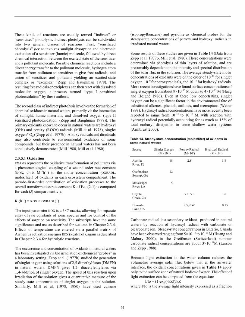
These kinds of reactions are usually termed “indirect” or “sensitized” photolysis. Indirect photolysis can be subdivided into two general classes of reactions. First, “sensitized photolysis” per se involves sunlight absorption and electronic excitation of a sensitizer (humic) molecule, followed by direct chemical interaction between the excited state of the sensitizer and a pollutant molecule. Possible chemical reactions include a direct energy transfer to the pollutant molecule, hydrogen atom transfer from pollutant to sensitizer to give free radicals, and union of sensitizer and pollutant yielding an excited-state complex or “exciplex” (Zepp and Baughman 1978). The resulting free radicals or exciplexes can then react with dissolved molecular oxygen, a process termed “type I sensitized photooxidation” by these authors.
The second class of indirect photolysis involves the formation of chemical oxidants in natural waters, primarily via the interaction of sunlight, humic materials, and dissolved oxygen (type II sensitized photooxidation (Zepp and Baughman 1978)). The primary oxidants known to occur in natural waters are hydroxyl (OHC) and peroxy (ROOC) radicals (Mill et al. 1978), singlet oxygen (1O2) (Zepp et al. 1977b). Alkoxy radicals and diradicals may also contribute to environmental oxidation of some compounds, but their presence in natural waters has not been conclusively demonstrated (Mill 1980, Mill et al. 1980).
2.3.5.1 OxidationEXAMS represents the oxidative transformation of pollutants via a phenomenological coupling of a second-order rate constant (KOX, units M! 1h! 1) to the molar concentration (OXRADL, moles/liter) of oxidants in each ecosystem compartment. The pseudo-first-order contribution of oxidation processes to the overall transformation rate constant K of Eq. (2-1) is computed for each (J) compartment via:
K (h! 1) = KOX × OXRADL(J)
The input parameter KOX is a 3×7 matrix, allowing for separate entry of rate constants of ionic species and for control of the effects of sorption on reactivity. The subscripts have the same significance and use as described for KAH etc. in Chapter 2.3.4. Effects of temperature are entered via a parallel matrix of Arrhenius activation energies EOX (kcal/mol), again as described in Chapter 2.3.4 for hydrolytic reactions.
The occurrence and concentration of oxidants in natural waters has been investigated via the irradiation of chemical “probes” in a laboratory setting. Zepp et al. (1977b) studied the generation of singlet oxygen using solutions of 2,5-dimethylfuran (DMFN) in natural waters. DMFN gives 1,2- diacetylethylenes via 1,4-addition of singlet oxygen. The speed of this reaction upon irradiation of the solution gives a quantitative measure of the steady-state concentration of singlet oxygen in the solution. Similarly, Mill et al. (1978, 1980) have used cumene
(isopropylbenzene) and pyridine as chemical probes for the steady-state concentrations of peroxy and hydroxyl radicals in irradiated natural waters.
Some results of these studies are given in Table 14 (Data from Zepp et al. 1977b, Mill et al. 1980). These concentrations were determined via photolysis of thin layers of solution, and are presumably dependent on the intensity and spectral distribution of the solar flux in the solution. The average steady-state molar concentrations of oxidants were on the order of 10! 13 for singlet oxygen, 10! 9 for peroxy radicals, and 10! 17 for hydroxyl radicals. More recent investigations have found surface concentrations of singlet oxygen from about 9×10! 13 M down to 4×10! 15 M (Haag and Hoigné 1986). Even at these low concetratins, singlet oxygen can be a significant factor in the environmental fate of substituted alkenes, phenols, anilines, and mercaptans (Weber 1998). Hydroxyl radical concentrations have more recently been reported to range from 10! 15 to 10! 18 M, with reaction with hydroxyl radical potentially accounting for as much as 15% of total carbaryl dissipation in some shallow water systems (Armbrust 2000).
Table 14. Steady-state concentration (moles/liter) of oxidants in some natural waters
Source Singlet Oxygen Peroxy Radical Hydroxyl Radical (M×1013) (M×109) (M×1017)
Aucilla 18 2.8 1.8 River, FL
Okefenokee 22 Swamp, GA
Mississippi 5 River, LA
Coyote 9.1, 5.0 1.6 Creek, CA
Boronda 9.5, 0.45 0.15 Lake, CA
Carbonate radical is a secondary oxidant, produced in natural waters by reaction of hydroxyl radical with carbonate or bicarbonate ion. Steady-state concentrations in Ontario, Canada have been observed ranging from 5×10! 15 to 10! 13 M (Huang and Mabury 2000); in the Greifensee (Switzerland) summer carbonate radical concentrations are about 3×10! 14M (Larson and Zepp 1988).
Because light extinction in the water column reduces the volumetric average solar flux below that at the air-water interface, the oxidant concentrations given in Table 14 apply only to the surface zone of natural bodies of water. The effect of light extinction can be computed from the equation:
I/Io = (1-exp(-kZ))/kZ where I/Io is the average light intensity expressed as a fraction
61

of its surface value (Io), k is a diffuse attenuation coefficient (/m), and Z is the depth of the compartment (m). The factor I/Io is calculated by EXAMS for the UV light important in generating photochemical oxidants (280-395 nm), and then used to generate depth-corrected oxidant concentrations:
OXRADL = OXRAD × (I/Io)
EXAMS allows for the entry of environmental concentrations of only one kind of oxidant other than singlet oxygen, which is treated separately (Chapter 2.2.5.2). For a compound reactive with more than one oxidant species, the rate constant and environmental concentration giving the most significant transformation rate can be entered, or a composite rate constant and environmental oxidant concentration can be computed and loaded in the data bases.
2.3.5.2 Singlet OxygenSinglet oxygen (1O2), an electronically excited state of the dioxygen molecule (O2), is formed in natural waters by the transfer of solar energy from illuminated DOM. EXAMS calculates the concentration of 1O2 in each surface water segment, using methods described by Zepp and coworkers (Zepp et al. 1985, Zepp 1988b), corrects for depth and couples the result to a 3×7 matrix of second-order reaction rate constants K1O2 for application in the mass balance Eq. (2-1). Generation of 1O2
begins with the production of electronically excited triplet states (S*) via absorption of sunlight energy by dissolved organic matter (S). The wavelength-specific quantum yields N used in EXAMS for this process were computed from the relationship N=0.015 exp(0.01(366-8), where 8 is the wavelength in nm. The pre-exponential factor in this relationship was derived from the average value of N (0.015) reported for 11 natural waters at 366 nm (Zepp et al. 1977b), corrected as per (Haag et al. 1984a). The slope (0.01) was calculated from the observation that N at 313 nm is approximately 0.025 (Haag et al. 1984b, Zepp et al. 1985). Example values are given in Table 15. Computation of light absorption by DOC uses the specific absorption coefficients , of Table 9.
Table 15. Example quantum yields for production of triplet sensitizer S* from DOC
8 (nm) N 8 (nm) N
280 0.035 400 0.011
300 0.029 450 0.006
312.5 0.026 490 0.004
350 0.016 650 0.0009
(second-order process rate constant Kqnch with units M! 1 s! 1). The second-order rate constant (Kox) for the production of singlet oxygen by energy transfer to dissolved oxygen from S* is between 1×10⁹ and 3×10⁹ (R. G. Zepp 2000, oral comm.), for EXAMS it is taken as 2×10⁹ M! 1 s! 1 (Zepp et al. 1985). Singlet oxygen undergoes rapid physical quenching by water to ground state dioxygen with a pseudo-first-order rate constant KdecO2 of 2.5×10⁵ s! 1 ((Rodgers and Snowden 1982) cited from (Haag et al. 1984a)). These reactions can be summarized by Eq. (2-122)-(2-124), where D is the distribution function and Iave is the average light intensity. The quantity (N , Iave) is integrated across the sunlight spectrum during EXAMS’ computations.
(2-122)
(2-123)
(2-124)
The steady-state concentration of 1O2 in sunlit surface waters is given by
(2-125)
where
(2-126)
Increasing the oxygen concentration from 2.6×10! 4 M (air saturated) to 1.2×10! 3 M (oxygen saturated) decreases [S*(ss)] by some 4× (Zepp et al. 1985). Given Kox[O2], the sum of the other terms in the denominator of Eq. (2-126) (KdecS3 and Kqnch[DOC]) is 1.6×10⁵. These experiments were conducted using [DOC] of about 20 mg/L (R. G. Zepp 2000, oral comm.). For EXAMS, the terms were equally partitioned, thus giving KdecS3 = 8.0×10⁴ (s! 1) and Kqnch = 4,000 (s! 1(mg/L)! 1) for calculating steady-state concentrations of triplet sensitizer and singlet oxygen. Model performance can be gauged by comparison of EXAMS’ calculated values to published estimates of surface concentrations of 1O2 (Zepp et al. 1977b, Haag and Hoigné 1986). The calculated 1O2 concentrations (Table 16) are acceptable except in the case of the three USA rivers with [DOC] < 15 mg/L; these waters (from the Wakulla, St. Marks, and Mississippi rivers) contained significant quantities of non-colored DOC (R. G. Zepp 2000, oral com.).
S* decays back to its ground state by spontaneous decay (with first-order rate constant KdecS3, with units s! 1) and self-quenching interactions with other components of the DOM
62

Table 16. Comparison of EXAMS’ singlet oxygen estimates with literature values
Water [DOC] [1O2]ss ×1014 M
mg/L Lit Val EXAMS
Lentic
Türlersee1 8.3 2.8 9.7
Greifensee1 3.5 3.3 4.5
Lützelsee1 7.9 5.4 9.3
Etang de la Gruère1
13 11.6 14.
Okefenokee2 24 17.8 6.9
Lotic
Rhine1 3.2 2.4 4.1
Kleine Emme1 3.2 4.1 4.1
Glatt1 4.1 4.6 5.2
Aucilla2 24 14.6 6.9
Ecofina2 41 15.4 9.0
Fenholloway2 77 13.8 11.
Wakulla2 6 0.16 2.4
St. Marks2 9 0.49 3.3
Mississippi2 14 0.41 4.8
1. June Swiss values from Haag and Hoigné 1986, corrected to full day values by daylength and factor of 2/B 2. December USA values from Zepp et al. 1977b, corrected as above, normalized to flat water body by division by 2, and corrected for updated DMF rate constant via division by 1.6
2.3.5.3 ReductionAnaerobic (reducing) environments are common in nature, including many groundwaters and saturated soils, aquatic sediments below the surface oxidized layer, waterlogged peats and marshlands, and, at least periodically, the hypolimnion of stratified lakes. Chemicals notoriously persistent in aerobic environments can be remarkably less so under anaerobic conditions (Macalady et al. 1986). In anaerobic sediments, the transformation half-lives of nitroaromatics can be from minutes to hours, with formation of aromatic amines as hazardous daughter products (Weber 1998). The responsible reducing agents may include ferrous iron, iron sulfides and dissolved sulfidic species (Simon et al. 2000), biochemical agents
produced by the benthos, and direct biolysis. Reductive transformations encompass a variety of reaction types and chemical classes, including reductive dechlorination, (or, more generally, reductive dehalogenation), reduction of nitroaromatic and azo compounds, reduction of N-nitrosamines across either the N-N or N-O bond, reduction of sulfoxides to thioethers, of quinones, and reductive dealkylation (Larson and Weber 1994). Prediction of the environmental concentrations of reducing agents has thus far proved intractable. The situation is further complicated by the observation that, although sorption inhibits reduction reactions, the velocity of the reaction increases with increasing sediment concentration. This result suggests that regeneration of the reducing agent by “electron-transfer mediators” may play in important role in governing the velocity of reduction pathways (Weber 1998), and that reducing agents maintain stable levels in the presence of low concentrations of reacting pollutants.
As with oxidants, EXAMS provides a phenomenological coupling between a reaction rate constant structure (the 3×7 matrices KRED) and an array (monthly for each environmental segment) of molar concentrations of reducing agents (REDAG). Effects of temperature are entered via a parallel matrix of Arrhenius activation energies ERED (kcal/mol), again as described in Chapter 2.3.4 for hydrolytic reactions. EXAMS does not include nominal values for REDAG.
References for Chapter 2.3.5. Armbrust, K. L. 2000. Pesticide hydroxyl radical rate constants:
Measurements and estimates of their importance in aquatic environments. Environmental Toxicology and Chemistry 19:2175-2180.
Haag, W. R., and J. Hoigné. 1986. Singlet oxygen in surface waters. 3. Photochemical formation and steady-state concentrations in various types of waters. Environmental Science and Technology 20:341-348.
Haag, W. R., J. Hoigné, E. Gassman, and A. M. Braun. 1984a. Singlet oxygen in surface waters - Part I: Furfuryl alcohol as a trapping agent. Chemosphere 13:631-640.
Haag, W. R., J. Hoigné, E. Gassman, and A. M. Braun. 1984b. Singlet oxygen in surface waters - Part II: Quantum yields of its production by some natural humic materials as a function of wavelength. Chemosphere 13:641-650.
Huang, J., and S. A. Mabury. 2000. Steady-state concentrations of carbonate radicals in field waters. Environmental Toxicology and Chemistry 19:2181-2188.
Larson, R. A., and E. J. Weber. 1994. Reaction Mechanisms in Environmental Organic Chemistry. CRC Press, Boca Raton, Florida.
Larson, R. A., and R. G. Zepp. 1988. Reactivity of the carbonate radical with aniline derivatives. Environmental Toxicology and Chemistry 7:265-274.
Macalady, D. L., P. G. Tratnyek, and T. J. Grundl. 1986. Abiotic reduction reactions of anthropogenic chemicals in anaerobic
63

systems: A critical review. Journal of Contaminant Hydrology 1:1-28.
Mill, T. 1980. Chemical and photo oxidation. Pages 77-105 in O. Hutzinger, editor. The Handbook of Environmental Chemistry. Volume 2 Part A-Reactions and Processes. Springer-Verlag, Berlin-Heidelberg-New York.
Mill, T., D. G. Hendry, and H. Richardson. 1980. Free-radical oxidants in natural waters. Science 207:886-887.
Mill, T., H. Richardson, and D. G. Hendry. 1978. Oxidation of organic compounds in aquatic systems: the free radical oxidation of cumene. Pages 223-236 in O. Hutzinger, I. H. v. Lelyveld, and B. C. J. Zoeteman, editors. Aquatic Pollutants: Transformation and Biological Effects. Pergamon Press, Oxford.
Rodgers, M. A. J., and P. J. Snowden. 1982. Journal of the American Chemical Society 104:5541-5543.
Ross, R. D., and D. G. Crosby. 1975. The photooxidation of aldrin in water. Chemosphere 4:277-282.
Simon, R., D. Colón, C. L. Tebes-Stevens, and E. J. Weber. 2000. Effect of redox zonation on the reductive transformation of p-cyanonitrobenzene in a laboratory sediment column. Environmental Science and Technology 34:3617-3622.
Weber, E. J. 1998. Abiotic transformation reactions. Pages 259281 in G. Schüürmann and B. Markert, editors. Ecotoxicology: Ecological Fundamentals, Chemical Exposure, and Biological Effects. John Wiley & Sons, Inc., New York, and Spektrum Akademischer Verlag, Heidelberg.
Zepp, R. G. 1988a. Environmental photoprocesses involving natural organic matter. Pages 193-214 in F. H. Frimmel and R. F. Christmam, editors. Humic Substances and Their Role in the Environment. John Wiley & Sons, New York.
Zepp, R. G. 1988b. Factors affecting the photochemical treatment of hazardous waste. Environmental Science and Technology 22:256-257.
Zepp, R. G., and G. L. Baughman. 1978. Prediction of photochemical transformation of pollutants in the aquatic environment. Pages 237-263 in O. Hutzinger, I. H. v. Lelyveld, and B. C. J. Zoeteman, editors. Aquatic Pollutants: Transformation and Biological Effects. Pergamon Press, Oxford.
Zepp, R. G., P. F. Schlotzhauer, and R. M. Sink. 1985. Photosensitized transformations involving electronic energy transfer in natural waters: Role of humic substances. Environmental Science and Technology 19:74-81.
Zepp, R. G., N. L. Wolfe, L. V. Azarraga, R. H. Cox, and C. W. Pape. 1977a. Photochemical transformation of the DDT and methoxychlor degradation products, DDE and DMDE, by sunlight. Archives of Environmental Contamination and Toxicology 6:305-314.
Zepp, R. G., N. L. Wolfe, G. L. Baughman, and R. C. Hollis. 1977b. Singlet oxygen in natural waters. Nature 267:421-423.
2.3.6 Microbial Transformations Microbial communities are a ubiquitous constituent of almost all aquatic ecosystems. The microbiota play a central role in the remineralization of plant and animal debris; they have evolved the capacity to transform and harvest energy from an immense array of naturally occurring organic compounds. The optimistic hope that “the solution to pollution is dilution” to some extent had its origin in a naive faith in the ability of saprobic microbes to utilize any and all synthetic organic compounds in their metabolic mills.
Total faith in the ability of natural systems to absorb and detoxify synthetic chemicals was, of course, shaken by the discovery of the world-wide dispersal (and bioconcentration) of synthetic biocides, notably DDT and the related compounds DDE and DDD. It is now “axiomatic that micro-organisms are fallible and that many synthetic organic compounds are recalcitrant ... and accumulating in some environments” (Alexander 1979b). In con sequence, qualita tive “biodegradability” tests (Swisher 1970) are now routine in the detergent industry, and “sludge” tests have been suggested (Buzzell et al. 1969) as a routine procedure for evaluating industrial synthetic organic compounds. The latter tests can also provide some assurance that the compound will not destroy the microbial communities that serve man in sewage treatment plants, as well as providing an evaluation of the biodegradability of the compound (e.g., Baird et al. 1974).
The discovery of microbial fallibility has led to a more critical and quantitative view of microbial metabolism of synthetic organics; it no longer suffices to know that a compound is “biodegradable.” Instead the rates, products, microbial populations, and environmental conditions surrounding an observed biodegradation are of increasing interest to the microbiological and ecological community. Given that the natural microbial substrates can massively accumulate in special circumstances (e.g., peat bogs and swamps), a degree of skepticism is obviously warranted toward any claim of universal, unconditional biodegradability of a synthetic organic compound. The rates at which a compound is biodegraded must depend upon both the structure of the compound, and on the metabolic capacity of the microbial community resident in the ecosystem receiving the compound.
Microbial communities derive energy for metabolism and growth from the breakdown of organic compounds, and the kinetics of growth and substrate utilization have been of interest to microbiologists for many years. Both population growth and substrate utilization rate have been described via Monod’s (1942) analogy with Michaelis-Menten enzyme kinetics (Slater 1979). In this approach, the growth of a microbial population in a non-limiting environment is described by
(2-127)
64

where µ is called the “specific growth rate” and N is microbial biomass or population size. The Monod equation modifies Eq. (2-127) via the recognition that consumption of resources in a finite environment must at some point curtail the rate of increase (dN/dt) of the population. This fact is typically incorporated into Eq. (2-127) via
(2-128)
µin which [S] is the concentration of the growth limiting substrate,
max is the “maximum specific growth rate” obtaining when [S] is present in excess (i.e., non-limiting), and KS, the “halfsaturation constant” is that value of [S] allowing the population to grow at rate µmax/2. An equation describing the behavior of the growth substrate [S] over time, and thus by implication the dynamics of a biodegradable synthetic compound, follows via a simple derivation (Slater 1979): Assuming that a fixed amount of growth results from metabolism (and therefore loss from solution) of a unit quantity of S, then dN = -Y dS, where Y is the “yield coefficient” in cells or biomass produced per unit S metabolized. Taking
(2-129)
gives dS/dt = -(µ/Y) N, or, substituting Eq. (2-128) for µ,
(2-130)
The observed microbial growth yield Y is often calculated from the amount of microbial biomass produced during the course of transformation of a measured quantity of substrate. Because a microbial population must satisfy maintenance requirements before any growth can occur, the apparent yield Y can fall quite drastically at low concentrations of S. Expressions with separated growth and maintenance yields have been developed by Pirt (1975) and it is possible to compute the separate magnitudes of growth and maintenance yields from microbial growth experiments (Slater 1979).
The Monod formulation (Eq. (2-130)) has been successfully applied to biotransformation of synthetic chemicals in a laboratory setting. These studies have demonstrated that a Monod analysis need not be restricted to single-species populations, that is, the Monod equations can serve as adequate descriptors of substrate transformation by “mixed” or “heterogeneous” (i.e., multi-species) microbial populations. In one example, Paris, Lewis, and Wolfe (1975) isolated a 4-species consortium of organisms able to use malathion as its sole source of carbon. Analysis of the growth response of the population and of concurrent malathion transformation rates then gave the Monod parameters µmax = 0.37 /h, KS = 2.17 :mol/L (0.716 mg/L), and Y = 4.1×10¹⁰ cells/:mol (1.2×10¹¹ cells/mg).
In a similar study, Smith and coworkers (1978) investigated the degradation of p-cresol by mixed microbial cultures able to use the compound as a sole carbon source. These authors expressed their results in terms of Monod parameters, finding µmax = 0.62 /h, Y = 1.8×10⁹ cells/mg, and KS = 0.84 mg/L.
Unfortunately, these elegant applications of classical microbiological methods to the biotransformation or “biolysis” of synthetic organic compounds are difficult to extrapolate to a broader ecological context. The first difficulty, which has received some attention in the microbiological literature, is primarily mechanical: The Monod formulation (Eq.(2-130)) is non-linear in its parameters, and thus imposes a high cost in computation time when used in a computer program or mathematical model. For trace concentrations of pollutants (i.e., [S] << KS), however, the term (KS + [S]) in the denominator of Eq.(2-130) can be approximated by KS, giving the linear approximation
(2-131)
µ
This formulation is similar to the “second-order” equations used to describe the kinetics of chemical reactions, and the term
max/(Y KS) can by analogy be termed a second-order biolysis rate constant KB2, with units /h/(cells/L) when population sizes N are expressed in cells/L.
K
The propriety of this substitution can be readily evaluated. For malathion, µmax/(Y KS) = 0.37/(4.1×1010×2.17) =4.16×10⁻¹²
/h/(cells/L). Paris et al. (1975) also computed values of KB2 from microbial population sizes and malathion transformation rates in their experimental studies, finding a mean value for KB2 of (2.6±0.7)×10-12 (95% confidence interval) /h/(cells/L) for a series of 8 experimental determinations spanning a concentration range from 0.0273 to 0.33 :mol/L in malathion. The measured
B2 differed from µmax/(Y KS) by less than a factor of 2, suggesting that simplified kinetic experiments could be used to develop second-order rate constants, in lieu of a detailed elaboration of µmax, Y, and KS, when the region of concern is restricted to levels of compound << KS.
Furthermore, dissolved pesticide concentrations in surface waters are often very low indeed. For example, dieldrin, lindane, and DDT have been found primarily at ng/L levels both in the USA(1972) and in Britain (Brooks 1972). For industrial chemicals, however, the situation can be somewhat different. For example, the release of phenolic wastes into the St. Lawrence River results in riverine concentrations of 0.01 to 0.15 mg/L (Visser et al. 1977). Although these high concentrations are restricted to a dispersion cone immediately downstream of the effluents, KS for p-cresol (0.84 mg/L) is uncomfortably close to the highest measured concentrations.
65

The need for a thorough evaluation of the propriety of Eq. (2131) as an adequate approximation to the Monod formula (Eq. (2-130)) disappears, however, upon examination of the conceptual difficulties standing in the way of the application of either equation to environmental situations. A natural microbial community derives its energy from a large variety of organic detrital materials. A microbial species restricted to a trace-level synthetic compound as its sole carbon source would be at a severe competitive disadvantage; there is no way of predicting a priori the population densities the degrader could attain in real systems. Even when a synthetic compound is sufficiently similar to natural substrates that it can be indifferently degraded by the microbial community as a whole, the presence of multiple energy-yielding substrates in the environment violates a fundamental assumption underlying the Monod approach, that is, that [S], the synthetic compound, limits growth. In many instances, moreover, a compound may be transformed or degraded in an energy-requiring detoxification process, making the concept of cell yield (Y) of dubious utility. When the compound, for whatever reason, is degraded in the absence of a change in population size, the apparent zero yield forces abandonment of Eq.(2-130) and (2-131) alike. This phenomenon is sometimes called “cometabolism,” e.g., (Alexander 1979a, Jacobson et al. 1980).
Despite these difficulties, the rate of transformation of organic pollutants must depend on the structure of the compound and the metabolic capacity of microbial communities. The simplest expression of this duality is the second-order equation
(2-132)
µ
which asserts that the rate of biolysis (d[S]/dt) is first-order in compound concentration [S] and in microbial activity, biomass, or population size B, and in which the identification of KB2 with
max/(Y KS) is discounted. This approach requires that the second-order rate constant be determined via laboratory studies of relatively undisturbed samples drawn from natural microbial communities. It also requires demonstration that d[S]/dt is linearly proportional to [S] for fixed levels of B, and that appropriate measures of B be found.
One conventional microbiological technique for characterizing microbial populations is simple population size, measured, for example, by colony counts on pour-plate agars (APHA 1976.). To the extent that population size is an adequate measure of community metabolic capacity, simple microbiological techniques could serve to characterize the rate of biotransformation of synthetic compounds in natural environments. This hypothesis has been explored for three compounds – the butoxyethyl ester of 2,4-D (2,4-DBE), malathion, and chlorpropham – by Paris and coworkers (Baughman et al. 1980, Paris et al. 1981). These authors
investigated biotransformation of their study compounds in samples of natural waters drawn from 40 locations in the continental USA. Ambient water temperatures at the collection points ranged from 1° to 29° C, and the laboratory studies were conducted at the observed ambient temperature of the sampled environments. Ambient bacterial populations, as measured by 48-hour incubation on TGE (tryptone glucose extract) agar at 22° C, ranged from 4×10² to 9×10⁵ cells/ml (Paris et al. 1981). Biolysis of these chemicals was demonstrably first-order in compound concentration and in population size, and was relatively independent of temperature. The 95% confidence intervals (based on among-site variation) for KB2 (/h/(cell/L)) and the number of sites for these compounds were (5.42±0.97)×10-10
(2,4-DBE, 31 sites), (4.54±0.74)×10-11 (malathion, 14 sites), and (2.63±0.72)×10-14 (chlorpropham, 11 sites).
Evaluation of biolysis in such “river die-away” studies is particularly difficult when a combination of small populations and slow rates of biodegradation leads to inconveniently long biolysis halflives. In such cases population densities must be augmented via centrifugation or supplemental nutrient broth. The latter procedure can have the disadvantage of favoring opportunistic heterotrophs at the expense of organisms better equipped to degrade more recalcitrant compounds. For example, the second-order biolysis rate constant (KB2) for chlorpropham is unaffected when population densities are augmented via nutrient broth supplementation, but the measured KB2 for phenanthrene decreases in approximate proportion with the population increase (Paris 1982, oral comm.).
Baughman, Paris, and Steen (1980) also reported second-order rate constants for biotransformation of synthetic chemicals by populations derived from aquatic sediments. The observed rate constants for 2,4-DBE and malathion were consistent with the rate of degradation by water-column populations, at KB2 of 2.3×10⁻¹⁰ and 4.0×10⁻¹¹ /h/(cell/L) respectively. Aerobic biolysis of chlorpropham by the sediment-derived populations was, however, almost an order of magnitude faster (KB2 = 1.42×10⁻¹³) than biolysis by the water-column populations (KB2 = 2.4×10⁻¹⁴
/h/(cell/L)). By varying the sediment/water ratio, these authors also demonstrated that chlorpropham, methoxychlor, and several phthalate esters were unavailable to biolytic organisms when sorbed to suspended sediments.
Plate-count estimates of bacterial population densities are extremely selective and can underestimate total population sizes by three or more orders of magnitude (Jannasch and Jones 1959, Wetzel 1975:571, Fletcher 1979). Furthermore, although increases in pollutant flux (that is, kg m-3 s-1 or mass degraded/time) with increasing chemical concentration (consonant with pseudo-first-order kinetics) have been observed in nature (e.g., Sherrill and Sayler 1980), it is also true that, at elevated pollutant concentrations, both a reduction in the apparent first-order rate constant (Tinsley 1979:149ff), and
66

zero-order kinetics (Visser et al. 1977) have been observed. The latter phenomena are consonant (mathematically) with Eq. (2130). It is not clear, however, whether these kinetics are a reflection of the maximum growth rate of a specialized sub-population of degraders or result from toxic effects of elevated concentrations on the microbial community.
In any case, it is clear that the studies of second-order kinetics cited above are a useful beginning in the detailed quantitative study of rates of biotransformation of pollutant chemicals. Little more extrapolative power can be developed until such time as the environmental coupling variables that govern the metabolic capacity of natural and laboratory microbial populations have been rigorously determined and measured in both kinds of systems.
As a first approximation, EXAMS utilizes a simple second-order equation (Eq.(2-132)) to compute the rate of biotransformation of pollutant chemicals. Microbial population densities (as “colony forming units” (abbrev. cfu)) for each sector of the ecosystem enter EXAMS’ environmental data base via the BACPL
and BNBAC vectors. For water column compartments, BACPL has units of cfu/mL; BNBAC for benthic compartments has units cfu/100 g dry weight of sediment. (A useful summary of observed bacterial population densities in aquatic systems can be found at pp. 571-596 of (Wetzel 1975). ) Second-order biolysis rate constants enter EXAMS’ chemical data base via separated parameters for water-column (KBACW) and benthic (KBACS) populations. The nominal units are h-1(cfu/mL)-1 in both cases. EXAMS internally converts benthic microbialpopulation densities to units (cfu/mL of water) commensurate with the units of the rate constant KBACS. This conversion is executed via the expression (BNBAC × SEDMSL)/(100×WATVOL) where SEDMSL is the mass of sediment in the compartment (kg), WATVOL is the volume of water contained in the compartment (Liters) (Eq. (221)), and the numerical factor (100) is a units conversion term (1000(mL/L)/10(decagrams/kg).
Despite the ruthless parsimony imposed on EXAMS’ representation of biolysis kinetics, the degree of chemical detail provided by EXAMS’ allowance for ionic and sorptive speciation leads to fairly substantial opportunities for the inclusion of biolytic kinetic detail. Both KBACW and KBACS are 4×7 element matrices for each chemical under study; each element represents a separate rate constant for the ionic and sorbed species of the pollutant. (The use of the matrix indices to specify chemical species is described in Chapter 2.3.4.) In addition, biolysis rate constants can be entered either as temperature-independent single values, or a Q10 function can be invoked to depict the effects of temperature on biolysis rates.
The Q10 values (i.e., increase in biolysis rate per 10° C change in temperature) for KBACW and KBACS occur as the parallel matrices QTBAW and QTBAS, respectively. When the value of
parameter QTBAW or QTBAS is non-zero, EXAMS takes the corresponding member of KBACW or KBACS as the biolysis rate constant at 25° C (in accordance with Subpart N guidelines), and recalculates the second-order rate constant via the Q10 equation:
(2-133)
Because microbial communities frequently adapt their metabolic capacity to keep pace with slow secular (e.g. seasonal) changes in environmental temperatures, temperature responses measured in a laboratory setting do not always apply to environmental conditions. This limitation should be recognized when interpreting the results of EXAMS simulations that include temperature effects on biolysis rate constants.
Although the nominal units for bacterial numbers and for KBAC
include bacterial population densities expressed as numbers/mL, clearly these variables can in both instances be redefined to encompass any environmental coupling variable of utility in estimating biodegradation rates in aquatic ecosystems. It is, however, especially important that these units be commensurate: For example, if the rate constants were determined via viable plate counts, and the natural population estimated via direct counts, biolysis rates would probably be grossly overstated. Furthermore, the simple second-order equation allows for a multiplicity of estimators of microbial capacity. For example, Neely (1980:117ff)) lists 7 commonly used estimators of microbial biomass or activity, including counting techniques, ATP and DNA analyses, and oxygen uptake. By suitable (user) redefinition of the nominal units of KBACs, BACPL, and BNBAC, EXAMS can be used to compute pseudo-first-order rate constants as a function of environmental variation in the presumed governing variable, so long as the rate constants and the bacterial population sizes are entered into EXAMS’ data bases in commensurate units.
The mechanics of EXAMS’ conversion of second-order biolysis rate constants and the compartment-specific environmental coupling variables to pseudo-first-order form are completely homologous with the equations used for chemical reactions. The total pseudo-first-order biolysis rate constant K is accumulated as the sum of expressions of the form K = " × KBAC × B, where " is the fraction of the total pollutant concentration present in each existing ionic or sorbed chemical species, KBAC
is the appropriate element of matrix KBACW or KBACS (corrected as needed for environmental temperatures using the Q10
equation), and B is the degrader population density or metabolic capacity of the microbial community in each ecosystem compartment. The sum of these pseudo-first-order (/h) expressions then becomes the biolysis contribution to the overall (compartment-specific) pseudo-first-order rate constant K of Eq. (2-1).
67

References for Chapter 2.3.6 Alexander, M. 1979a. Biodegradation of toxic chemicals in
water and soil. Pages 179-190 in R. Haque, editor. Dynamics, Exposure, and Hazard Assessment of Toxic Chemicals. Ann Arbor Science Publishers, Ann Arbor, Michigan.
Alexander, M. 1979b. Recalcitrant molecules, fallible microorganisms. Pages 246-253 in J. M. Lynch and N. J. Poole, editors. Microbial Ecology: A Conceptual Approach. Blackwell Scientific Publications, Oxford.
APHA. 1976. Standard Methods for the Examination of Water and Wastewater (Fourteenth Edition). American Public Health Association, Washington, D.C.
Baird, R. B., C. L. Kuo, J. S. Shapiro, and W. A. Yanko. 1974. The fate of phenolics in wastewater--determination by direct-injection GLC and Warburg respirometry. Archives of Environmental Contamination and Toxicology 2:165-178.
Baughman, G. L., D. F. Paris, and W. C. Steen. 1980. Quantitative expression of biotransformation rate. Pages 105-111 in A. W. Maki, K. L. Dickson, and J. C. Cairns, Jr., editors. Biotransformation and Fate of Chemicals in the Aquatic Environment. American Society for Microbiology, Washington, D.C.
Brooks, G. T. 1972. Pesticides in Britain. Pages 61-114 in F. Matsumura, G. M. Boush, and T. Misato, editors. Environmental Toxicology of Pesticides. Academic Press, New York and London.
Buzzell, J. C., Jr., C. H. Thompson, and D. W. Ryckman. 1969. Behavior of Organic Chemicals in the Aquatic Environment. Part III--Behavior in Aerobic Treatment Systems (Activated Sludge). Manufacturing Chemists Association, Washington, D.C.
Fletcher, M. 1979. The aquatic environment. Pages 92-114 in J. M. Lynch and N. J. Poole, editors. Microbial Ecology: A Conceptual Approach. Blackwell Scientific Publications, Oxford.
Jacobson, S. N., N. L. O'Mara, and M. Alexander. 1980. Evidence for cometabolism in sewage. Applied and Environmental Microbiology 40:917-921.
Jannasch, H. W., and G. E. Jones. 1959. Bacterial populations in sea water as determined by different methods of enumeration. Limnology and Oceanography 4:128-139.
Matsumura, F. 1972. Current pesticide situation in the United
2.4 Input Pollutant LoadingsThe flux of a pollutant chemical entering an ecosystem (term “Le” in Eq. (2-1)) is a primary determinant of the ultimate exposure experienced by resident organisms. EXAMS does not compute pollutant loadings. Loadings may be developed via projected or measured industrial effluent fluxes, agricultural runoff, by transfer from the PRZM model, landfill seepages, etc., but these computations must be executed externally to EXAMS.
States. Pages 33-60 in F. Matsumura, G. M. Boush, and T. Misato, editors. Environmental Toxicology of Pesticides. Academic Press, New York and London.
Monod, J. 1942. Recherches sur la croissance des cultures bacteriennes. Herman et Cie, Paris.
Neely, W. B. 1980. Chemicals in the Environment: Distribution, Transport, Fate, Analysis. Marcel Dekker, Inc., New York and Basel.
Paris, D. F., D. L. Lewis, and N. L. Wolfe. 1975. Rates of degradation of malathion by bacteria isolated from aquatic system. Environmental Science and Technology 9:135-138.
Paris, D. F., W. C. Steen, G. L. Baughman, and J. T. Barnett, Jr. 1981. Second-order model to predict microbial degradation of organic compounds in natural waters. Applied and Environmental Microbiology 41:603-609.
Pirt, S. J. 1975. Principles of microbe and cell cultivation. Blackwell Scientific Publications, Oxford.
Sherrill, T. W., and G. S. Sayler. 1980. Phenanthrene biodegradation in freshwater environments. Applied and Environmental Microbiology 39:172-178.
Slater, J. H. 1979. Microbial population and community dynamics. Pages 45-63 in J. M. Lynch and N. J. Poole, editors. Microbial Ecology: A Conceptual Approach. Blackwell Scientific Publications, Oxford.
Smith, J. H., W. R. Mabey, N. Bohonos, B. R. Holt, S. S. Lee, T.-W. Chou, D. C. Bomberger, and T. Mill. 1978. Environmental Pathways of Selected Chemicals in Freshwater Systems: Part II. Laboratory Studies. EPA-600/7-78-074, U.S. Environmental Protection Agency, Athens, Georgia.
Swisher, R. D. 1970. Surfactant Biodegradation. Marcel Dekker, Inc., New York.
Tinsley, I. J. 1979. Chemical Concepts in Pollutant Behavior. John Wiley and Sons, New York-Chichester-Brisbane-Toronto.
Visser, S. A., G. Lamontagne, V. Zoulalian, and A. Tessier. 1977. Bacteria active in the degradation of phenols in polluted waters of the St. Lawrence River. Archives of Environmental Contamination and Toxicology 6:455-469.
Wetzel, R. G. 1975. Limnology. W.B. Saunders Co., Philadelphia.
EXAMS provides input vectors for 5 kinds of loadings to each compartment of the system. These are: point-source or stream-borne loadings (STRLD), non-point-source loadings (NPSLD), contaminated ground-water seepage entering the system (SEELD), precipitation washout from the atmosphere (PCPLD), and spray-drift (or miscellaneous) loadings (DRFLD). The loadings have units of kg (of chemical)/hour in all cases. These loadings are taken as time-invariant constants in EXAMS’ steady-state computations, or as monthly values when EXAMS is
68

run in mode 3. In addition, both Mode 2 and Mode 3 provide for event loadings by specification of the date, chemical, and kg mass of the event.
Each non-zero pollutant loading must conform to the hydrologic definition of the ecosystem, or EXAMS will not implement the loading. For example, EXAMS will cancel a STRLD, NPSLD, or SEELD for a given compartment, if that compartment does not receive an appropriate carrier flow STFLO, NPSFL, or SEEPS
respectively. (Definition and entry of the hydrologic variables is discussed in Chapter 2.3.1.1.) Precipitation (RAIN) is a monthly climatic variable in EXAMS; a PCPLD is therefore allowed only for compartments possessing an air-water interface. Non-zero PCPLD
s are automatically canceled in the case of B (benthic) or H (hypolimnion) compartments. A PCPLD is unconditionally permitted for compartment number 1, which will always have an air-water interface if the system definition rules discussed in Chapter 2.3.1.1 are followed. For all other water-column compartments, EXAMS simply looks back at the (J-1) compartment. If this (J-1) compartment is also part of the water column, it is assumed to be directly above the current (J) compartment and any non-zero PCPLD is removed. Compartments with an air-water interface are always preceded by a benthic (B) compartment when EXAMS’ system definition conventions (Chapter 2.3.1.1) are observed.
EXAMS’ subroutine CKLOAD evaluates the propriety of the four kinds of loadings that enter via carrier flows. These loadings are evaluated against the volume of the carrier flows and the water quality characteristics of the target compartment. These evaluations were designed to prevent inadvertent specification of a loading outside EXAMS’ operating range. In particular, EXAMS makes no provision for crystallization of the compound from solution, nor does the program allow for a gradual dissolution of chemical from a condensed (solid or liquid) phase. In addition, the non-linearities potentially present at high chemical concentrations (non-linear sorption isotherms, appreciable light absorption by the compound, zero-order biolysis, etc.) are not incorporated in the code. EXAMS’ loading check computations are divided into two groups: checks based on carrier flows of water alone (PCPLD and SEELD), and checks based on carrier flows of water plus an entrained sediment loading (STRLD and NPSLD).
Ground-water seep and rainfall loadings are simply constrained to aqueous solubility. In these computations, the temperature (TCEL) and pH (PH and POH) of the compartment receiving the load are used to compute (as appropriate) the solubilities of each ionic species of the compound, and the distribution of the pollutant among its ionic species (distribution coefficients ", computed as described in Chapter 2.2). EXAMS then computes the concentration of pollutant in the carrier flow. If the solubility criterion is exceeded, EXAMS reduces the load to the extent necessary to conform to the upper limit of EXAMS’ operating
range, notifies the user of the modification(s), and returns control to the user without executing a simulation. The loadings are recomputed as the product of the limiting concentration and the carrier flow rate, that is,
(2-134)
where Load is in kg/h, Inflow in L/h, Limit (kg/L) is one-half the solubility of the least soluble chemical species, and $ is the fraction of the total concentration present in the least soluble dissolved form.
Each streamflow(STFLO) or non-point-source water flow (NPSFL) entering a compartment may have an associated stream sediment (STSED) or non-point-source sediment (NPSED) loading (kg sediment/h) to the compartment. STSED and NPSED are not used in transport computations (see Chapter 2.3.1.3). In the course of evaluating stream-borne and non-point-source pollutant loadings, EXAMS computes a sorption equilibrium for capture of the pollutant by entrained sediments in the stream or non-point-source flows entering each compartment. These computations use the temperature, pH, and sediment partitioning parameters (e.g., organic carbon content (FROC) and ion exchange capacities (AEC and CEC)) of the receiving compartment. From the sediment/water ratio of the carrier flow, EXAMS computes the distribution coefficients (") of the chemical in the carrier flow.
If the residual aqueous concentration of any dissolved species exceeds its concentration limit, the offending loading is reduced via Eq. (2-134), the simulation is aborted, and control is returned to the user for evaluation. EXAMS’ method for calculating concentration limits that ensure linearity of sorption isotherms is described in Chapter 2.2.2.
After checking the loadings and making any necessary modifications, summing all external loads and units conversion from kg/h to mg/h yields term Le of Eq. (2-1).
“Drift” loadings (DRFLD) are initially implemented uncritically. If, however, EXAMS’ computations result in final steady-state chemical concentrations above EXAMS’ operating range, any DRFLD s are then sequentially reduced until the computationally invalid estimates are corrected. (If MODE>1, or no drift loads were specified and the results are outside the operating range, EXAMS aborts the run and returns control to the user for corrective action.)
The DRFLD vector can be used to specify miscellaneous loadings not encompassed in EXAMS’ four other monthly loading types. EXAMS, for example, does not allow for entry of pollutant across the air-water interface from a polluted atmosphere (Chapter
69

h
2.3.2). The impact of a polluted atmosphere can, however, be computed from the bulk atmospheric partial pressure of the contaminant, and entered into EXAMS via the DRFLD vector. The net flux of pollutant across the air-water interface (F, moles m! 2
! 1) is given (see Eq. (2-71)) by F = Kl (Pg/H - Cl) where Kl is the exchange constant (m h! 1), and both (Pg/H) and have Cl units of (moles m! 3). By assuming the bulk atmosphere to be uncontaminated (Pg / 0.0), the term (Pg/H) was discarded in the development of EXAMS’ algorithm for computing volatilization losses of pollutants from aquatic systems. In much the same way, the gross pollutant loadings imposed by a contaminated atmosphere can be computed by taking Cl / 0.0.
Non-zero boundary conditions can be loaded into EXAMS via the DRFLD vector. EXAMS’ environmental input data can include a characteristic length (CHARL), cross-sectional area (XSTUR), and dispersion coefficient (DSP) at any boundary of the system (by setting either JTURB or ITURB to zero, as described in Chapter 2.3.1.4). The exchange flow of water across the boundary is given by
FLOW (liters/h) = (1000)(DSP)(XSTUR)/(CHARL)
If the inlet exchange flow is contaminated to a level of [C] mg/L, the loading (kg/h) on the system of interest is simply:
LOAD = FLOW × [C] ×10! 6 (kg/mg)
This load can be imposed on the receptor compartment via the appropriate element of the DRFLD vector.
The final term in Eq. (2-1) is “Li,” the sum of the internal loadings on the system compartments. Internal loads areis from two sources: chemical and biological transformation processes, and internal transport processes. The transport loadings arise from flows of contaminated water, sediments, and plankton among the physical sectors (compartments) of the ecosystem. Their magnitudes can be computed from the magnitudes of the flows, the distribution of the compound among its dissolved and sorbed species, and the concentration of the pollutant in the source compartments (expressed as mass/unit aqueous volume). EXAMS uses the WATFL (L/h) and SEDFL (kg/h) flow matrices (see Chapter 2.3.1.5) to compute a matrix of internal loading factors (EXAMS’ internal variable INTINL), by associating carrier flows with appropriate elements of the " matrix (Chapter 2.2.4). This computation results in terms which, when multiplied by the total concentration of pollutant in the source compartments (mg/L), yield the mass loadings Li (mg/h) on the target compartments, constituents of the final term in Eq. (2-1).
2.4.1 Product ChemistryTransformation products are an additional element in the internal loadings of some compounds. These are specified to EXAMS by setting the activity database (ADB) number of the parent and
daughter within the current simulation specifications, the process generating the product, the reactive form of the parent molecule, the process yield, and, if desired, the enthalpy of the transforming process. The EXAMS input parameters are CHPAR, the chemical parent ADB number, TPROD, the transformation product ADB number, NPROC, the number of the process, RFORM, the reactive form of the parent molecule, yield, the (M/M) process yield, and EAYLD, the enthalpy (kcal).
The generating process is specified using the following codes for NPROC:
1 = specific acid hydrolysis 2 = neutral hydrolysis 3 = specific base hydrolysis 4 = direct photolysis 5 = singlet oxygen 6 = free radical oxidation (e.g., hydroxyl radical) 7 = water column bacterial biolysis 8 = benthic sediment bacterial biolysis 9 = reduction
Twenty-eight reactive forms are available for specifying RFORM, in addition to which total dissolved etc. can be specified using an RFORM of
29 = all dissolved species 30 = all sediment-sorbed species 31 = all DOC-complexed species 32 = all biosorbed species
(The complete list of RFORM specifications is given at the RFORM
entry in the EXAMS data dictionary in Chapter 6 of this document.) The process YIELD may be entered as the simple mole of product per mole reacted, or as an Arrhenius function, in which case the enthalpy of the reaction is entered as EAYLD.
Entering transformation process chemisty requires specification of these parameters using a “pathway number” as the index for each complete reaction path. For example, if the parent compound (parathion) is recalled as ADB chemical 1, and the product (paraoxon) is recalled as ADB chemical 2, then a reaction scheme in which direct photolysis of DOC-complexed parathion yields a 50% generation of paraoxon , and hydroxyl radical oxidation of dissolved parathion produces paraoxon in mole-for-mole formation, would be specified to EXAMS as follows:
CHPAR 1 1 TPROD 2 2 NPROC 4 6 RFORM 3 1 YIELD 0.5 1 EAYLD 0 0 Pathway: 1 2
Given these specifications, EXAMS calculates the resultant
70

generating flux (in this case of paraoxon, chemical number 2) from the breakdown of the parent material(s) (in this example, parathion, chemical number 1), and adds the resulting terms to the mass loadings Li (mg/h) in each segment, thus completing Eq. (2-1).
EXAMS allows for multiple transformations; any one of the chemicals being studied can generate any of the others. Among the possibilities thus available are regeneration of parent from product, generation of multiple products from a single starting material, reaction chains, etc.
2.5 Data Assembly and Solution of Equations EXAMS includes three “modes” of operation: direct calculation of the “steady-state” outcome of long-term contamination (Mode 1), step-wise computation of the time course of contaminant exposure under a specified set of environmental conditions, (Mode 2), and computation of daily exposure concentrations using monthly updates of environmental conditions (Mode 3). The numerical integration techniques are the same, and the output summaries analogous, for each operating “mode” of the program.
2.5.1 Exposure After computing all terms in Eq. (2-1), the resulting system of mass-balance equations can be divided through by the volume of the compartments to give a set of equations describing the rate of change of chemical concentration over time:
(EXAMS allows the volumes of system elements to be altered by the user during the course of an analysis (except in Mode 1), and makes appropriate modifications to exposure levels. This feature is difficult to use, however, and requires care in interpretation. A version of EXAMS that includes dynamic changes in storage volumes (Mode 4) is in preparation.)
As time passes, the system evolves toward an ultimate “steady-state” condition at which the concentrations achieve stable values. This endpoint is defined by the condition d [C]/dt = 0.0 for every compartment. At steady state, then, the concentration of pollutant in each sector of the ecosystem is given by
(2-135)
Numerical integration to steady state is notoriously profligate of computational resources, so EXAMS contains an explicit procedure (subroutine STEADY) designed to solve the equations for these concentrations, which define long-term exposure levels of the pollutant and can serve as a useful adjunct to any exposure
analysis.
The logic of the situation can be illustrated via an elementary example. For the example, consider the behavior of a non-sorbing chemical, subject to neutral hydrolysis as its sole transformation process, in a static one-hectare pond. The pond is 1 meter deep, with VOL V therefore 10,000 m3 (107 L). The benthic subsystem consists of a 5 cm active depth of material with a bulk density (BULKD) of 1.5 g/cc and a water content (PCTWA) of 150%. The environmental volume of the benthic zone (VOL) is 500 m3; its aqueous volume is 250,000 liters of water (Eq. (2-21)). Defining exchange between the benthic subsystem and the water column via XSTUR = 10,000 m2, CHARL = (1.05/2) = 0.525 m, and DSP = 10! 4 m2/h, the rate of exchange of fluid volume between the water column and the interstitial pore water (Chapter 2.3.1.4) is
This exchange flow of water can be reduced to its pseudo-first-order effect on chemical concentrations (Kt, /h) in the water column (w) and the benthic (b) subsystem via:
Kt(w) = 952.4/107 = 9.524×10! 5 /h, and
Kt(b) = 952.4/250,000 = 3.810×10! 3 /h
As the compound does not sorb, transport of sediment and plankton can in this instance be ignored.
The internal loadings on the system arise from pollutant contamination of the 952.4 L/h exchange flow between the system compartments. All the compound is present in dissolved form in this example; sorbed and complexed exchange processes are here immaterial. EXAMS computes its internal load factors Li/V by dividing the elements of INTINL by the volume of the target compartment. In this instance, the load factor on the benthic subsystem resulting from contamination of the water column is
INTINL(b,w) 7 (952.4 × 1.00)/250,000 = 3.810×10! 3 /h
and the load factor on the water column resulting from contamination of the benthic interstitial water is
INTINL(w,b) 7 (952.4 × 1.00)/107 = 9.524×10! 5 /h
(INTINL and Kt are equal in this much simplified example; this is not usually the case.)
Finally, given an external load on the water column (here a DRFLD) of, say, 0.02 kg/h, and a neutral hydrolysis rate
71

constant of 0.01 /h, the behavior of the chemical in the system is given by:
d[Cw]/dt=(0.02×106/107)+9.524×10! 5(Cb)-(0.01 + 9.524×10! 5)Cw
d[Cb]/dt= 3.810×10! 3(Cw) - (0.01 + 3.810×10! 3)Cb
where Cw is the aqueous concentration in the water column and Cb is the aqueous concentration in the interstitial pore water (mg/L). At steady state, d[Cw]/dt = d[Cb]/dt = 0.0, resulting in 2 equations in 2 unknowns:
- 0.01009524 Cw + 0.00009524 Cb = - 0.002
0.00381 Cw - 0.01381 Cb = 0.0
This elementary example can be easily solved to give Cw = 0.1986 and Cb = 0.0548 mg/L. EXAMS solves the simultaneous linear equations that describe steady-state concentrations by Gaussian elimination (Chapter 2.3.1.2). EXAMS’ output for the example system described above is given in Exams Output Table 10.
Ecosystem: Static 1-hectare pond, 1 meter deepChemical: Unsorbed chemical subject to neutral hydrolysis--------------------------------------------------------------Table 15.01. Distribution of chemical at steady state.--------------------------------------------------------------Seg Resident Mass ******** Chemical Concentrations ********* # Total Dissolved Sediments Biota
Kilos % mg/* mg/L ** mg/kg ug/g--- -------- ------ --------- --------- --------- --------In the Water Column: 1 2.0 100.00 0.199 0.199 0.00 0.00 ======== ====== 2.0 99.32
and in the Benthic Sediments: 2 1.37E-02 100.00 2.740E-02 5.479E-02 0.00 0.00 ======== ====== 1.37E-02 0.68
Total Mass (kilograms) = 2.000 --------------------------------------------------------------* Units: mg/L in Water Column; mg/kg in Benthic Zone.** Excludes complexes with "dissolved" organics.
Exams Output Table 10. EXAMS output tabulation of steady-state concentrations.
As Gaussian elimination is not an infallible mechanism for executing these computations, EXAMS includes a second technique for computing the solution to the system of equations (Eq. (2-135)), which is invoked in those cases for which Gaussian elimination fails. This algorithm is an iterative “linear cascade” method that applies Eq. (2-135) to each compartment in turn, and then repeats the entire process until such time as the successive estimates for each compartment change by less than 0.0001%. EXAMS allows for up to 100,000 iterations of the full “linear cascade” computation. If the linear cascade terminates without full convergence, EXAMS aborts the run; this event generally can be taken as an indication that steady-state concentrations are unbounded. For example, a
non-transformable chemical in a static pond without any export pathways will accumulate indefinitely; in this situation no “steady-state” condition can be computed. The degree of convergence achieved by EXAMS for the full ecosystem can be examined in the mass balance check printed as the final entry (“Residual Accumulation Rate”) in EXAMS’ output table entitled “Analysis of Steady-State Fate of Organic Toxicant.”
In the elementary example given above, the linear cascade solution would proceed:
Iteration 1, step 1: solve for Cw (compartment number 1)
Cw = (Le/V + Li/V)/K = (0.002 + 9.524×10! 5(Cb)) / 0.01009524
giving, as Cb at the moment = 0.0,
Cw = 0.002/0.01009524 = 0.19811
Iteration 1, step 2: solve for Cb (compartment number 2)
Cb = (Le/V + Li/V)/K = 0.00381(Cw)/0.01381
= (0.00381×0.19811)/0.01381 = 0.05467
From the initial estimates, the second iteration proceeds to compute a refined estimate of Cw and Cb:
Cw=(0.002+(9.524×10! 5×0.05467))/0.01009524=0.19863
Cb=(0.00381×0.19863)/0.01381 = 0.054799
The convergence test is computed for each compartment by calculating the relative change in the estimate. The change in Cw was
1 - 0.19811/0.19863 = 0.0026
and the change in Cb was
1 - 0.05467/0.054799 = 0.0026
As these test values are greater than EXAMS’ convergence criterion (10! 6), EXAMS continues with a third iteration of the linear cascade. EXAMS judges convergence to be complete only when the relative change in every compartment is less than 10-6.
In mode 2, EXAMS integrates from time “TINIT” to time “TFINAL” with output and intervals of “CINT” in units specified by “TCODE.” At the end of an integration (“RUN”), the simulation is paused and the user can evaluate the results and choose to “CONTINUE” the simulation to some new value of TFINAL. In Mode 3, the minimum run time is one year, with monthly updates of environmental properties. Multiple years (“NYEAR”) can be run as a single unit, or the continue command can be used to run blocks of years. When EXAMS is used in conjunction with the PRZM model, EXAMS reads the climate time-series used with
72

PRZM and build a climatic data set consistent with the PRZM data.
2.5.2 FateAfter computing exposure concentrations, EXAMS evaluates the impact of each transport and transportation process on the behavior of the compound. During the course of reducing its input data to pseudo-first-order form, EXAMS preserves the value of each process’ contribution to the overall pseudo-first- order rate constant K (Eq. (2-1)) for each compartment. The flux of chemical transformed or transported (mass/time) is then given by the product of the process rate constant, the concentrations, and the aqueous volume of each compartment. In the instance under review, the chemical fluxes attributable to neutral hydrolysis are
Fw = Khyd × Cw × WATVOL(w) × 10-6 (kg/mg)
= (0.01)(0.1986)(107)(10-6) = 0.01986 kg/h
in the water column, and
Fb = (0.01)(0.05479)(2.5×10⁵)(10-6) = 0.000137 kg/h
in the benthic subsystem.
EXAMS sums the fluxes (by process) over the entire system, and computes the significance of the process via division of the process flux by the sum of the external loadings on the system, followed by conversion of this result to a percentage basis. In the example, the total flux is (0.01986 + 0.000137) kg/h, the total loading was 0.02 kg/h, thus hydrolytic transformation accounts for 100(0.01986 + 0.000137)/0.02 = 100% of the input loadings, as of course it must in this elementary example.
EXAMS’ output table containing the results of the flux analysis, entitled “Sensitivity Analysis of Chemical Fate,” also includes estimated half-lives for removal or dissipation of the chemical from the system. These half-lives are computed under the assumption that internal transport delays are insignificant, giving a supplemental view of the general significance of each process. The half-life computations are executed via division of the total process fluxes by the total mass of pollutant resident in the system to give a system-wide pseudo-first-order rate constant Kpr. The half-life is then simply
T½ = - ln(0.5)/Kpr
In the example case, the total resident mass (computed as the sum of volumes and concentrations) is 2.00 kg (Exams Output Table 10), and the projected hydrolytic half-life is therefore
T½ = (0.69315 × 2.00)/(0.01986 + 0.000137) = 69.3 hours.
EXAMS does not inflexibly report fluxes and half lives in hours, for in many instances the hour is an inconveniently small reporting unit. Instead, the program makes a preliminary
evaluation of the total transport and transformation flux through the ecosystem, and computes a first-order estimate of the total half-life of the compound. This preliminary estimate is then used to select the most appropriate (hours, days, months, or years) time scale for reporting the results of all succeeding time-dependent computations. This estimate of the “system-level” half-life is also used to set the time intervals for EXAMS’ Mode 1 “persistence” computations, as described in Chapter 2.5.3.
EXAMS’ flux computations, along with its table of compartment-specific pseudo-first-order rate constants (output table “Kinetic Profile of Synthetic Chemical”) provide a sensitivity analysis of the behavior of the pollutant in the particular ecosystem under study. These tables indicate the relative strength of the transformation processes, and thereby indicate which processes are in need of the most scrupulous and exact experimental determinations of rate constants. In addition, EXAMS interactive capabilities allow a user to vary the input data over a reported error bound, and thus determine, for example, the degree of uncertainty implied for exposure concentrations.
2.5.3 PersistenceEXAMS’ final round of computations deal directly with a third (after exposure and fate) aspect of exposure evaluation in aquatic systems, that of the “persistence” of the compound. (These are a feature of Mode 1 only.) It should perhaps be emphasized that EXAMS computes local, rather than global, persistence, that is, EXAMS’ computations address the persistence of compounds in the specific ecosystem under review, and do not address the global issue of the persistence of a compound after it leaves the local ecosystem. Thus, for example, a compound that is not subject to any transformation processes is ipso facto (globally) persistent. Within the more limited context of a particular ecosystem, however, export processes will ultimately result in a “cleanup” of the system, and the time required for this cleanup process can be computed. (As the ultimate exposure concentrations for a transformationally persistent chemical in a static (closed) system are unbounded, EXAMS never encounters the resulting infinite cleanup times.)
EXAMS begins its Mode 1 persistence computations by using the steady-state concentrations of pollutant in the system as a set of starting values or “initial conditions.” These initial conditions are presented to the numerical integration package (subroutine DRIVER et seq.). The relevant set of differential equations, describing the behavior of the pollutant over time, is essentially Eq. (2-1) with the external loadings (Le) set to zero or struck from the equations:
In Mode 1, EXAMS computes the dissipation of the compound
73

over time, taking the time required to encompass 2 (estimated) system-level half-lives as the endpoint of the simulation. The results of this simulation are summarized in EXAMS’ output table entitled “Exposure Analysis Summary.”
EXAMS makes use of two integration packages (Malanchuk et al. 1980). EXAMS initially calls upon a variable stepsize, variable order (1-12) Adams PECE2 method. In the event that the equations prove to be mathematically “stiff,” the partially complete integration is remanded to an alternate package that integrates stiff equations by a variable-order, variable stepsize code employing multistep backward differentiation methods of order 1 through 6. The Adams method code was taken from (Shampine and Gordon 1975); the stiff equations method was derived from an algorithm originally developed by Gear (Gear 1971c, b, a).
EXAMS limits the expense incurred in the integration via a limitation on the total number of steps which these routines are permitted to execute. EXAMS writes out the secular dissipation of the compound at 12 equally spaced times, up to the endpoint (TFINAL) defined by 2 estimated system-level half-lives. If the integrators exceed their allotted expense allowance prior to integration to TFINAL, control is relinquished by the integrator for evaluation of the situation. If the integrators have failed to reach the first output point (TFINAL/12), EXAMS aborts all further persistence computations and so notifies the user. If at least one output point has been passed, EXAMS uses the latest point reached by the integrators in its persistence computations, and notifies the user that the dissipation simulation was abbreviated.
Integration expense is also influenced by the precision demanded. This can be controlled by the user by alteration of ABSER and RELER, the absolute and relative error criteria used by the numerical integration package. The smaller their values, the greater the precision of the analysis, but the greater the performance costs incurred. These parameters cannot be made arbitrarily small due to the intrinsic limitations of digital computing machinery; upon invocation EXAMS evaluates the numerical precision limitations of the computing platform and establishes limits for ABSER and RELER. If these are too large, the integrators will encounter stability problems, so it is sometimes worth experimenting with ABSER and reler to optimize the conditions of an analysis.
In the vast majority of cases, EXAMS’ dissipation simulations conclude with a successful integration to TFINAL. EXAMS’ output summary of the time course of dissipation via neutral hydrolysis in the static pond used as an example in Chapter 2.5.1 is given in Exams Output Table 11.
2 So called from their successive operations of prediction, derivative evaluation, correction, and final derivative evaluation.
Ecosystem: Static 1-hectare pond, 1 meter deepChemical: Unsorbed chemical subject to neutral hydrolysis----------------------------------------------------------------Table 19. Summary time-trace of dissipation of steady-statechemical mass following termination of allochthonous loadings.
----------------------------------------------------------------Time Average Chemical Concentrations Total Chemical Mass ----- ------------------------------- ------------------Hours Water Column Benthic Sediments Water Col Benthic -------------------- ------------------- --------- -------Free-mg/L Sorb-mg/kg Pore-mg/L Sed-mg/kg Total kg Total kg
----------------------------------------------------------------0 0.20 0.0 5.48E-02 0.0 2.0 1.37E-02
12 0.18 0.0 5.43E-02 0.0 1.8 1.36E-02 24 0.16 0.0 5.30E-02 0.0 1.6 1.32E-02 36 0.14 0.0 5.11E-02 0.0 1.4 1.28E-02 48 0.12 0.0 4.87E-02 0.0 1.2 1.22E-02 60 0.11 0.0 4.62E-02 0.0 1.1 1.15E-02 72 9.63E-02 0.0 4.34E-02 0.0 0.96 1.09E-02 84 8.53E-02 0.0 4.06E-02 0.0 0.85 1.01E-02 96 7.56E-02 0.0 3.78E-02 0.0 0.76 9.44E-03 108 6.70E-02 0.0 3.50E-02 0.0 0.67 8.75E-03 120 5.94E-02 0.0 3.23E-02 0.0 0.59 8.08E-03 132 5.27E-02 0.0 2.97E-02 0.0 0.53 7.43E-03 144 4.67E-02 0.0 2.73E-02 0.0 0.47 6.82E-03
Exams Output Table 11. Sample EXAMS output for dissipation of chemical after removal of external loadings.
EXAMS prints a summary of the exposure and fate information generated by the program and also estimates and reports the length of time required for cleanup of the ecosystem. EXAMS
reports, in the first instance, the percentage of the initial chemical masses in the entire water column and benthic subsystem that had been dissipated by time TFINAL. EXAMS then weights these dissipations according to the initial distribution of the chemical in the system, and reports a first-order estimate of the time required for the system to cleanse itself of the chemical mass accumulated at steady state. This estimate is computed as 5 (pseudo-first-order, weighted) half-lives; in a true first-order system this would correspond to dissipation of 97% of the mass of chemical initially present in the system. (The actual (mathematical) “order” of the system is defined by the number of compartments used to describe the ecosystem. For example, when a water-body is described to EXAMS via 20 segments, EXAMS compiles 20 linked first-order differential equations, and solves this system of equations to generate its outputs. The data used in EXAMS’ persistence time computations is generated by summing the residual chemical masses over compartments, thereby following the dissipation of the chemical in the entire system. The computations are in this sense reduced order approximations; thus EXAMS reports are given as “rough” estimates (e.g., Exams Output Table 12).)
This computation can be illustrated via the results of the sample simulation given in Exams Output Table 11. At the expiration of 144 hours, the resident pollutant mass had fallen from 1.986 to 0.467 kg in the water column. This dissipation of the pollutant represents a loss of
100 (1 - (0.467/1.986)
or 76.5% of the original material. Similarly, the benthic subsystem has lost (0.0137 - 0.00682) = 0.00688 kg or 50.2% of its original mass of chemical. (The benthic sediment exhibits a slower loss of chemical as a result of continuing recontamination
74

(Li, Eq. 10) of this subsystem from the water column.)
In a first-order system, the decrease of an initial mass of material Qo over time is given by
Q(t) = Q(0) exp(-k × t), or
ln(Q(t)/Q(0)) = -k×t
where k is the first-order rate constant and t is time. The half-life is defined as the time required for Q(t) to reach Q(0)/2 or for Q(t)/Q(0) = 0.5, that is,
H = -ln(0.5)/k
The first-order half-lives (H) for these water-column (Hw) and benthic (Hb) subsystems are, therefore:
Hw = (0.69315)(144) / ln(0.467/1.986) = 69.0 hrs, and
Hb = (0.69315)(144) / ln(0.00682/0.0137) = 143.4 hrs
At steady state, 99.32% of the compound is present in the water column, and only 0.68% is in the benthic subsystem (Exams Output Table 10). EXAMS thus estimates the time required for dissipation of the chemical as:
Td = 5 (0.9932 (Hw) + 0.0068 (Hb))
= 5 (0.9932 (69.0) + 0.0068 (143.4)) = 347.5 hrs
or 14.5 days. EXAMS output summary for this example is given in Exams Output Table 12.
Ecosystem: Static 1-hectare pond, 1 meter deepChemical: Unsorbed chemical subject to neutral hydrolysis--------------------------------------------------------------Table 20.01. Exposure analysis summary.--------------------------------------------------------------Exposure (maximum steady-state concentrations):Water column: 0.199 mg/L dissolved; total = 0.199Benthic sediments: 5.479E-02 mg/L dissolved in pore water;
mg/L
maximum total concentration = 2.740E-02 mg/kg (dry weight).Biota (ug/g dry weight): Plankton: Benthos:
Fate: Total steady-state accumulation: 2.00 kg, with 99.32% in the water column and 0.68% in the benthic sediments.
Total chemical load: 2.00E-02 kg/ hour. Disposition: 100.00%chemically transformed, 0.00% biotransformed, 0.00% volatilized, and 0.00% exported via other pathways.
Persistence: After 144. hours of recovery time, the water column hadlost 76.49% of its initial chemical burden; the benthic zonehad lost 50.21%; system-wide total loss of chemical = 76.3%. Five half-lives (>95% cleanup) thus require ca. 14. days.
Exams Output Table 12. Example summary output table (Mode 1).
If the majority of the chemical had been present in the benthic zone, EXAMS would of course have given computational precedence to dissipation in the sediment subsystem for its
estimate of decontamination time.
A more detailed evaluation of the persistence of the chemical can be executed via a graphical analysis of the time course of pollutant dissipation, plotted from the results of EXAMS’ numerical simulation of this phenomenon (Exams Output Table 11). In interpreting EXAMS’ estimate of the time required to dissipate the chemical, it should be remembered that EXAMS’ estimate represents five half-lives, or about 97% removal of the initial mass. If this removal suggests that the chemical would still occur at unacceptable concentrations, a first-order evaluation of the time required to achieve a specified reduction can be computed from EXAMS’ outputs. Suppose, for example, that the time to reduce the chemical to 0.01% of its initial value were the time of interest. This time is given by the expression (-ln(Q/Q(0))/K), where Q/Q(0) is in this case 0.0001. EXAMS’ estimate of decontamination time is computed as (5)(0.69315)/K, where K can be regarded as a weighted whole-system first-order decay constant. EXAMS’ estimate of dissipation time Td can thus be expanded via the approximation:
In this instance, Q/Q(0) = 0.0001, -ln(Q/Q(0)) = 9.21, and the time to reduce the chemical to 0.01% of its steady-state value is
approximately days.
Note, however, that a continued first-order decay of chemical in the benthic subsystem would, at 37 days (888 hours), result in a residual of
100 exp(888 ( ln 0.5 / Hb) )
or 1.4% of the original benthic pollutant mass. The system-wide dissipation of the chemical may leave pockets of higher concentration in zones of restricted physical transport.
Extrapolations of EXAMS’ results beyond the designed operating range of the program are probably ill-advised. If necessary, however, a plot of the results of EXAMS’ dissipation simulation should be used to evaluate the propriety of a first-order extrapolation of system self-purification times.
References for Chapter 2.5. Gear, C. W. 1971a. Algorithm 407: DIFSUB for solution of
ordinary differential equations. Communications of the ACM 14:185-190.
Gear, C. W. 1971b. The automatic integration of ordinary differential equations. Communications of the ACM 14:176-179.
Gear, C. W. 1971c. Numerical Initial Value Problems in Ordinary Differential Equations. Prentice-Hall, Englewood Cliffs, N.J.
Malanchuk, J., J. Otis, and H. Bouver. 1980. Efficient
75

Algorithms for Solving Systems of Ordinary of Ordinary Differential Equations: The Initial ValueDifferential Equations for Ecosystem Modeling. EPA- Problem. W.H. Freeman, San Francisco.600/3-80-037, U.S. Environmental Protection Agency,Athens, Georgia.
Shampine, L. F., and M. K. Gordon. 1975. Computer Solution
76

3.0 Tutorials and Case Studies
3.1 Tutorial 1: Introduction to Exposure Analysis with EXAMS – Laboratory 1
I. First computer run of EXAMS (the overall Lab plan)
! Follow the directions in the “Lab 1, Exercise 1: Steady-State Analysis (Mode 1)” (page 85) through line 30. This will introduce you to the basics of running the program.
! Review the principles of running the program in “Mode 1” (the default mode, steady-state analysis).
! Stop and review the inputs, outputs, and interrelationships, complete the worksheets on pages 79 and 80 , and prepare for Lab. 2 by entering the Lab. 1 data for methyl parathion chemistry and its behavior in the standard pond on pages 83 and 84.
Ia. Running the program: Inputs
EXAMS has “User Data Bases” (UDB) for Chemicals, Environments, Loads, and Products (i.e., products of transformation processes). Eachentry in the UDB is accessed by its number, e.g., CHEM 11. To run a simulation, you must
! Recall an environment (ENV)! Recall at least one chemical (CHEM)! Recall or set an input LOAD (i.e., the amount of pesticide added over time, or an event loading from spray drift or runoff).! Set a MODE (default is Mode 1, steady-state analysis)
The RECALL command (REC) loads data from the UDB into the Activity Data Base (ADB), and changes the UDB number to an ADBnumber. For example, when you RECALL CHEM 11, its number in the ADB becomes CHEM 1.
Only one ENVIR can be active at any time. More than one CHEM can be active; this is especially useful when you specify the generationof a transformation product, e.g., production of 2,4-D by hydrolysis of 2,4DBE, the butoxyethyl ester of 2,4-D. In addition to thecontinuous long-term loads of Mode 1, you can also specify load events (as direct initial conditions in Mode 2, or from PRZM transferfiles in Mode 3) and piece-wise (monthly) continuous loads.
Once you have specified the required information, the RUN command executes a simulation.
EXAMS Laboratory Exercises . . . . . . . . . . . . . . . . . . . . . . . . . . . . . . . . . . . . . . . . . . . . . . . . . . . . . . . . . . . . . . . . . . . . . . . . . . . . Page 77

Ib. Running the program: Outputs
EXAMS produces at least 20 output tables for each simulation. For complex, multi-year studies the total output can rapidly becomeoverwhelming. In most cases, you will want to examine the ecotoxicological exposure information in one or a few tables and graphics,as you did in the introductory tutorial. Warning: when requesting a plot, make note of the variables you have asked for and their units,because the graphic will not provide the labels.
Type LIST HELP to display a list of the available input and output tables (as at lines 18 and 19 of the first introductory exercise). On somecomputers, [Shift][PrintScrn] will print the list.
! Note that Table 1 is an echo of the chemical input data.! Because transformation product chemistry was not entered, Table 2 is empty.! Because no pulse loads were specified (and are in any case irrelevant to steady-state analyses), Table 3 is also empty.! Tables 4 through 13 are the environmental model, again an echo of the input data although Table 12 and Table 13 contain some
inferred values. You will need to examine these tables to see what kind of an environment ENV 2 is so you can label your diagram on page 4. The EXAMS “data dictionary” (pages 175 ff.) includes descriptions and units for the parameters given in the tables.
! Table 14 contains load information. ! Tables 15 through 20 are output results.
For reference, you can PRINT ALL to get a paper copy of all the input and output tables (Tables 1-20, which may in some instances have several sub-tables).
Warning: The output file “report.xms” is overwritten each time you make an EXAMS run.
Once you have completed the worksheets on pages 79 and 80 , you may return to the introductory exercises to explore Mode 2 (initial value approaches) and Mode 3 (seasonal effects).
EXAMS Laboratory Exercises . . . . . . . . . . . . . . . . . . . . . . . . . . . . . . . . . . . . . . . . . . . . . . . . . . . . . . . . . . . . . . . . . . . . . . . . . . . . Page 78

Name
EXAMS Lab Assignment – Introduction
1. Working from the Mode 1 analysis, make a half-page diagram of the EXAMS pond environment (on the next page). Include the compartments, their sizes, numbers, and types, and the geometry and hydrology of the system.
2. What is the water solubility of methyl parathion?
3. What mass (kg) of chemical is resident in the littoral water column at steady state?
4. What concentration (mg/L or ppm) of the chemical is dissolved in the littoral?
5. What is the bulk mass (kg) of the chemical in the benthic sediment?
6. What is the analytical concentration (mg/kg dry weight) in the sediment?
7. What is the exposure of benthic organisms (i.e., ppm dissolved in pore water)?
Do the different locations of the chemical and its concentration in the various media (water column, benthic sediments, pore water) make sense to you? If not, please discuss with your instructor – this is an important part of the exercise.
8. Of the processes considered, which two were responsible for the greatest loss of chemical?
(1)
(2)
9. Of the processes considered, which two were least responsible for loss of chemical?
(1)
(2)
Go back and examine the properties of the chemical and the environment and determine why these processes had the relative importance they did.
Given the properties of methyl parathion and the pond environment, propose at least three questions that the model could help you study (for methyl parathion or a related chemical, for the pond or a related environment). For example, if the pond were more oligotrophic with less numerous bacteria, what would be the steady-state exposure?
EXAMS Laboratory Exercises . . . . . . . . . . . . . . . . . . . . . . . . . . . . . . . . . . . . . . . . . . . . . . . . . . . . . . . . . . . . . . . . . . . . . . . . . . . . Page 79

Diagram of EXAMS’ Constructed Farm Pond
Your questions:
(1)
(2)
(3)
EXAMS Laboratory Exercises . . . . . . . . . . . . . . . . . . . . . . . . . . . . . . . . . . . . . . . . . . . . . . . . . . . . . . . . . . . . . . . . . . . . . . . . . . . . Page 80

3.2 Tutorial 1: Introduction to Exposure Analysis with EXAMS – Laboratory 2
EXAMS’ second tutorial (beginning on page 113) is a substantial exercise in assembling chemical data, building an environmental model (of the lower basin of Lake Zurich, Switzerland), validating the model against observed data and exploring the dynamics of an environmental pollutant. Here we will use the first part of that tutorial (chemistry of 1,4 dichlorobenzene) to illustrate chemical data entry and basic studies of the environmental behavior of pesticides and other organic chemicals.
1. Restart EXAMS from the DOS prompt. (It is sometimes safer to re-start the program when beginning a new problem to ensure that all previous results are deleted.)
2. Review what you did in Lab1. Note that the only required EXAMS commands were RECALL CHEM 11 RECALL ENV 2 SET STRL(1,1,13)=.01
All the other commands you used (e.g., HELP, SHOW, CATALOG CHEMICAL, etc.) were optional entries to teach you how to use the program.
3. Add another chemical to the user database (UDB) and use it in the standard pond.
Type the following series of commands (note the similarity to the first part of the Lake Zurich tutorial). Press the Enter key after each line.
EXAMS (To re-start the program)REC CHEM 1 (This entry in the UDB is an empty template for loading new data.)CHEM NAME IS 1,4-Dichlorobenzeneset mwt(1)=147.0change sol(1,1) to 73.8set kow(1)=2340set henry(1)=2.66e-3cat chem (To see how many chemicals are in the UDB)sto chem 12 (Assuming you have no CHEM 12 now)REC ENV 2SET STRL(1,1,13)=.01RUNPRINT 15PRINT 18PRINT 20
If your computer doesn’t print, use the screen listings (LIST 15, etc.) to start filling out the tables on pages 83 and 84.
4. Modify (eutrophy) the pond to increase the organic carbon content of the sediment (both the suspended sediment in the water column and the benthic sediment).
SHOW FROC(1,13) (Write down what you see) SHOW FROC(2,13) (Write down what you see)
Look in the EXAMS User’s guide for an explanation of the FROC parameter.
SET FROC(1,13)=0.4SET FROC(2,13)=0.4SHOW FROC(1,13) (Write down what you see) SHOW FROC(2,13) (Write down what you see)
EXAMS Laboratory Exercises . . . . . . . . . . . . . . . . . . . . . . . . . . . . . . . . . . . . . . . . . . . . . . . . . . . . . . . . . . . . . . . . . . . . . . . . . . . . Page 81

SHOW CHEM (Check that the values you added for the chemical are there; EXAMS may have added additional properties basedon its understanding of pesticide chemistry. If so, you can use the HELP function to gain an understanding of these new values.SHOW LOAD (Check to see that the load is what you expect it to be.)RUNLIST 15 (Fill in some of the table data on pages 83 and 84)LIST 6LIST 1LIST 18LIST 20ENV NAME IS Hyper-eutrophic Pond (You are naming and will store this environment)CAT ENV (To see how many you have)STOR ENV 6 (Assuming you have 5)CAT ENV (To make sure it took)
5. Determine how the first chemical (methyl parathion) would behave in the hyper-eutrophic pond.
REC CHEM 11 REC ENV 6 SET STRL(1,1,13)=.01 RUN LIST 15 (Write your answers on the Tables) LIST 6 LIST 1 LIST 18 LIST 20
EXAMS Laboratory Exercises . . . . . . . . . . . . . . . . . . . . . . . . . . . . . . . . . . . . . . . . . . . . . . . . . . . . . . . . . . . . . . . . . . . . . . . . . . . . Page 82

Name
1. Compare the chemical properties of methyl parathion and p-DCB. Provide number and units. a. In what table are these variables found? b. Where are the units listed? c. Fill in the table. If necessary, use EXAMS’ “help” functions to generate a consistent data set.
Chemical Property Units Methyl Parathion 1,4-Dichlorobenzene
Molecular Weight
Solubility
Kow (n-Octanol:water solubility ratio)
Henry’s Law Constant
KBACW
KBACS
If a value has not been entered or calculated by EXAMS, the EXAMS table entry is blank and its value is zero.
d. List the major differences between these chemicals that affect their fate and exposure. I. ii. iii.
2. Compare the standard and the hyper-eutrophic ponds. a. Define FROC ( , ) units
Variable Standard Pond Hyper-Eutrophic Pond
FROC (1,13)
FROC (2,13)
EXAMS Laboratory Exercises . . . . . . . . . . . . . . . . . . . . . . . . . . . . . . . . . . . . . . . . . . . . . . . . . . . . . . . . . . . . . . . . . . . . . . . . . . . . Page 83

3. Compare the distribution and transformation of the two chemicals in the two environments.
Variable EXAMS
Table No. Methyl Parathion 1,4-DCB
Std. Pond Eutr pond Std. Pond Eutr pond
% in water column
Kg in water col.
% in benthic zone
Kg in benthic zone
Total mass (Kg)
Conc in plankton (µg/g)
Conc in benthos (µg/g)
Flux (%load) from
Bacterioplankton
Water-borne export
Volatilization
Persistence: time to 95% dissipation
4. Using the numbers you filled in above, explain why increasing the organic carbon content of the suspended and bed sediment had a major impact on 1,4-DCB, but not on methyl parathion. Is this realistic? If you think not, re-run the analysis and revise your conclusions.
5. Which of these chemicals would have a different environmental fate and exposure if the numbers of bacteria in the water column or benthic zone were changed. Why?
EXAMS Laboratory Exercises . . . . . . . . . . . . . . . . . . . . . . . . . . . . . . . . . . . . . . . . . . . . . . . . . . . . . . . . . . . . . . . . . . . . . . . . . . . . Page 84

3.3 Command Sequences for Tutorial 1, Lab. 1
3.3.1 Lab. 1, Exercise 1: Steady-State Analysis (Mode 1)Introduction to EXAMS. Execute the following commands at the EXAMS prompt. The object of the exercises is to gain a basic familiarity with the EXAMS command interface.
1 HELP
2 HELP HELP
3 HELP USER
4 HELP PAGES
5 SHOW VAR
6 HELP MODE
7 CATALOG CHEMICAL
8 CATALOG ENVIRONMENT
9 CAT
10 LO
11 HELP RECALL
12 REC CHEM 11
13 RECALL ENV 2
14 HELP LOAD
15 SHOW LOAD
16 SET STRL(1,1,13)=.01
17 RUN
18 LIST
19 HELP
20 20
21 LIST 18
22 LIST 15
23 HELP PLOT
24 PLOT
25 KI
26 PL
27 3
28 6
29 0
30 0
EXAMS Introductory Laboratory (Mode 1) . . . . . . . . . . . . . . . . . . . . . . . . . . . . . . . . . . . . . . . . . . . . . . . . . . . . . . . . . . . . . . . . Page 85

1
2
3
4
5
6
7
8
9
10
11
12
13
14
15
16
17
18
19
20
21
22
23
24
25
26
27
28
29
30
31
32
33
3.3.2 Lab. 1, Exercise 2: Mode 2 Analysis of Initial Value Problems – Sixty Day RUn Time
REC CHEM 11
REC ENV 2
SET STRLD(1,1,13)=0.01
SET MODE=2
SHOW TI FR
HELP TCODE
SET TCODE=2
SET TEND=60
SET CINT=1
SHOW TI FR
RUN
PLOT KI PL
3
6
0
0
SHOW LOAD
ZERO LOAD
SHOW LOAD
SET ICHEM(1)=1
SET ISEG(1)=1
SET IMASS(1)=.1
SHO PU
SET TEND=14
RUN
PL KI PL
3
6
0
0
CONTINUE
28
CONTINUE
EXAMS Introductory Laboratory (Mode 2) . . . . . . . . . . . . . . . . . . . . . . . . . . . . . . . . . . . . . . . . . . . . . . . . . . . . . . . . . . . . . . . . Page 86

34 60
35 PL KI PL
36 3
37 6
38 0
39 0
40 PL KI PL
41 6
42 0
43 0
EXAMS Introductory Laboratory (Mode 2) . . . . . . . . . . . . . . . . . . . . . . . . . . . . . . . . . . . . . . . . . . . . . . . . . . . . . . . . . . . . . . . . Page 87

1
2
3
4
5
6
7
8
9
10
11
12
13
14
15
16
17
18
19
20
21
22
23
24
25
26
27
28
29
30
31
32
33
34
3.3.3 Lab. 1, Exercise 3: Time-varying seasonal analysis using Mode 3
REC CHEM 11
SET MODE=3
REC ENV 3
SET ICHEM(1)=1
SET ISEG(1)=1
SET IMASS(1)=.1
SET IMON(1)=5
SET IDAY(1)=15
SET ICHEM(2)=1
SET ICHEM(3)=1
SET ISEG(2)=1
SET ISEG(3)=1
SET IMASS(2)=.1
SET IMASS(3)=.1
SET IMON(2)=6
SET IMON(3)=6
SET IDAY(2)=1
SET IDAY(3)=15
SHO PU LO
RUN
PL KI PL
3
6
0
0
PL KI PL
3
0
0
CONTINUE
PLOT KI PL
3
0
0
EXAMS Introductory Laboratory (Mode 3) . . . . . . . . . . . . . . . . . . . . . . . . . . . . . . . . . . . . . . . . . . . . . . . . . . . . . . . . . . . . . . . . Page 88

35 LIST 20
36 Y
37 QUIT
EXAMS Introductory Laboratory (Mode 3) . . . . . . . . . . . . . . . . . . . . . . . . . . . . . . . . . . . . . . . . . . . . . . . . . . . . . . . . . . . . . . . . Page 89

3.4 Introduction to EXAMS – Lab. 1 Exercises with Complete EXAMS Responses
These three exercises illustrate the E XA M S command line interface, data entry, and operations “modes.” The commands in the summary
listings are given here in BOLD/ITALIC . Note that E XA M S starts in Mode 1 when it is initially invoked, i.e., the default “Mode” is 1.
3.4.1 Lab. 1, Exercise 1: Steady-State Analysis (Mode 1)
To begin, at the DOS prompt, enter
C:> EXAMS Welcome to EXAMS Release <current release number>
Exposure Analysis Modeling System
Technical Contact: Lawrence A. Burns, Ph.D.U.S. Environmental Protection Agency
960 College Station RoadAthens, GA 30605-2700 USA
Phone: (706) 355-8119 (Fax) 355-8104Internet: [email protected]
Latest Maintenance <date of latest maintenance>
Type HELP and press the RETURN key for command names,HELP USER for a summary of command functions,HELP PAGES for a list of information pages,
or HELP EXAMS for introductory information.
Please stand by while EXAMS checks the computational precisionof this computer and initializes the Activity Data Base.
EXAMS-> HELP
EXAMS includes these system commands:
AUDIT CATALOG CHANGE DO (@) ERASE HELP PASSWORD PLOT PRINT RECALL RUN SET WRITE ZERO
CONTINUE DESCRIBELIST NAMEQUIT READSHOW (?) STORE
Help pages describe the commands and additional topics:ADB, COMMAND, EXAMS, INPUTS, LOADS, LODNAM, NEWDAT, TABLE,TABNUM, TUTOR, UDB, USER, WILD
Text describing the commands, and the text of the additionaltopics, can be seen by entering HELP <topic>, where <topic>is either a command, one of the additional topics above, orthe name of one of EXAMS' input data parameters.
USER gives a summary list of EXAMS' command functions.PAGES gives an annotated list of EXAMS' information pages.TUTOR is an introduction to using the HELP facility.
EXAMS-> HELP HELP
The HELP command invokes EXAMS' HELP facility to display
Introduction to EXAMS . . . . . . . . . . . . . . . . . . . . . . . . . . . . . . . . . . . Page 90

information about a particular EXAMS topic. For a tutorialexplanation of the HELP command, now type HELP TUTOR and pressthe RETURN key. For more detail on the available information,now type HELP USER or HELP PAGES and press the RETURN key.
Related topics: DESCRIBESyntax: HELP [command], or [EXAMS parameter]
HELP is also available from the interior of most EXAMS commands.A list of the "parameters" available through HELP can be invokedby typing "SHOW VAR". HELP provides definitions and dimensionsof all these input data and control variables.
EXAMS-> HELP USER
Command ===========
Summary Description ================================================
AUDIT CATALOG CHANGE/SETCONTINUE DESCRIBE DO ERASE HELP LIST
Start/Stop user notepad for recording proceduresList the contents of User Databases (UDBs)Enter/reset input data and program controlsResume integration (Modes 2 and 3 only)Report dimensions and data type of parameterExecute file of EXAMS commands (file.EXA)Clear section of stored database (UDB)Describes access to EXAMS on-line HELP facilityShow tabular results on the screen
NAME PASSWORD PLOT
Specify the name of a UDB, e.g., CHE NAME IS ...Restrict Recall/Store access to UDB datasetsPlot results on the screen
PRINT QUITREAD/WRITERECALL RUN SHOW STORE ZERO
Queue tabular results for hardcopy printingAbort command, or End interactive sessionUpload/download data from non-EXAMS disk filesActivate data from stored database (UDB)Begin simulation runDisplay current data values or control settingsDownload current data into stored database (UDB)Clear loadings, pulses, or current concentration
EXAMS-> HELP PAGES
ADB defines the term "activity database"COMMAND tells how to use EXAMS' system commandsEXAMS describes the scope and operation of the programINPUTS describes EXAMS input data and data manipulationLOADS explains how to specify chemical loads on the ecosystemLODNAM gives EXAMS' special names for the chemical loadingsNEWDAT tells how to begin entry of a new datasetHELP gives more explanation of the HELP facilityTABLE explains why your initial outputs seem to disappearTABNUM explains the numbering system used for EXAMS' outputsTUTOR introduces EXAMS' HELP utilityUDB defines the term "user database"USER gives a general command summary.WILD describes the use of wild cards in SET/CHANGE commands
Enter HELP and the name of a topic for further information.
EXAMS-> SHOW VAR
Introduction to EXAMS . . . . . . . . . . . . . . . . . . . . . . . . . . . . . . . . . . . Page 91

CHEMNA ECONAM LOADNM PRODNM TYPE AIRTY FIXFIL IUNIT MCHEM KCHEM MODE PRSW MONTH NYEAR YEAR1 TCODE CINT TEND TINIT ABSER RELER SPFLG MWT SOL ESOL PK EPK KOC KOW KPB KPDOC KPS KIEC HENRY EHEN VAPR KNH
EVPR ENH
QUANTKBH
KDP EBH
RFLAT KOX
ABSOR EOX
LAMAX K1O2
KAH EK1O2
EAH KRED
ERED JTURB
KBACW ITURB
QTBAWXSTUR
KBACS CHARL
QTBASDSP
KOUNT SUSED
JFRAD BULKD
ITOAD FROC
ADVPR CEC
AEC PCTWA TCEL PH POH OXRAD REDAG BACPL BNBAC PLMAS BNMAS KO2 DOC CHL CLOUD DFAC DISO2 OZONE VOL AREA DEPTH XSA LENG WIDTH RAIN EVAP LAT LONG WIND ELEV RHUM ATURB STFLO STSED NPSFL NPSED SEEPS STRLD NPSLD PCPLD DRFLD PRBEN SEELD IMASS ISEG ICHEM IMON IDAY IYEAR SPRAY CHPAR TPROD NPROC RFORM YIELD EAYLD
EXAMS-> HELP MODE
MODE is an integer scalar.MODE sets the operating "mode" of EXAMS. Three operating modesare available; these are selected by SETting MODE to 1, 2, or 3.
MODE Operational characteristics of EXAMS ---- --------------------------------------------------
1 Long-term (steady-state) analysis.2 Pulse analysis--specifiable initial chemical mass
(IMASS) and time frame, time-invariant environment.3 Monthly environmental data, daily pulse loads IMASS
and monthly chemical loadings of other types.
EXAMS-> CATALOG CHEMICAL
Catalog of CHEMICAL parameter sets
UDB No. Name of Entry Volume======= =======================
1 Chemical Data Entry Template2 p-Cresol3 Benz[a]anthracene4 Benzo[a]pyrene5 Quinoline6 Benzo[f]quinoline7 9H-Carbazole
8 7H-Dibenzo[c,g]carbazole9 Benzo[b]thiophene
10 Dibenzothiophene11 Methyl Parathion12 Mirex
13 Heptachlor (Heptachlorodicyclopentadiene)14 Speciation Test Data
EXAMS-> CATALOG ENVIRONMENT
Catalog of ENVIRONMENTal models
UDB No. Name of Entry Volume======= =======================
1 Environmental Data Entry Template2 Pond -- code test data -- mean values only3 Monthly pond -- code test data4 Lake Zurich (Untersee), Switzerland: annual means
Introduction to EXAMS . . . . . . . . . . . . . . . . . . . . . . . . . . . . . . . . . . . Page 92

5 Georgia Pond-Stream (R. Lee)6 GApond USEPA
EXAMS-> CAT
Enter Environment, Chemical, Load, Product,Help, or Quit-> LO
Catalog of Chemical LOADings
UDB No. =======
Name of Entry Volume =======================
1 2
Load Data Entry TemplateTest input loadings for EXAMS 2.97
EXAMS-> HELP RECALL
RECALL transfers data from permanent storage (UDB) to activitydatabases (ADB). The data to be used by EXAMS for an analysisare held in a foreground memory bank or ADB (activity database).When EXAMS is started, the ADB is empty. Use the RECALL commandto transfer data from the User Databases (UDBs) to foregroundmemory (ADB). Be sure to STORE all new data before you QUITfrom EXAMS: the ADB is discarded at the end of each session!!
===========================================Related topics: CATALOG, ERASE, NAME, STORE
Syntax: RECALL <datatype> <UDB#> [AS ADB#]where <datatype> can be CHEM, ENV, LOAD, or PRODUCT
EXAMS uses these four kinds of datasets: 1. CHEMICAL reactivity and partitioning (up to MCHEM sectors),
2. ENVIRONMENTal physical and chemical parameters,3. allochthonous chemical LOADings, and
4. PRODUCT chemistry for generating interconversionsamong multiple chemicals in an analysis.
For more information: ADB, AS, UDB
EXAMS-> REC CHEM 11
Selected compound is "Methyl Parathion"
EXAMS-> RECALL ENV 2
Selected environment is "Pond -- code test data -- mean values only"
EXAMS-> HELP LOAD
Enter allochthonous loadings of synthetic chemicals either asinstantaneous pulses, or as stable (or average) values thatpersist for at least one month. SHOW PULSE displays pulsedloadings; SHOW LOADS displays the steady loadings. Steadyloadings are entered by specifying the type of load (STRLD,etc.), the segment, ADB number of the chemical, month of theloading, and the mass loading (kg/hour). For example, command:EXAMS-> SET STRLD(1,2,8) TO 0.01sets an August load of 0.01 kg/h of chemical #2 on segment #1.
Pulse loads are entered by "event number." Each event includesthe ADB # of the chemical, the month and day of the event, the
Introduction to EXAMS . . . . . . . . . . . . . . . . . . . . . . . . . . . . . . . . . . . Page 93

---------------------------------------------------------------
---------------------------------------------------------------
--- --------- --------- --------- --------- ---------
---------------------------------------------------------------
target segment, and the mass (kg) of the pulse.
If, during a RUN, a loading violates assumptions of the model(e.g., by super-saturating an incoming flow), or is found to beimpossible (e.g., a PCPLD to a (B)enthic segment), the load isreduced or deleted. The corrected loadings are stored in theLOADS matrix and returned to the user, i.e., the unusableloadings are discarded and the new values are substituted.
EXAMS-> SHOW LOAD
Name of environment: Pond -- code test data -- mean values onlyTotal number of segments (KOUNT) = 2Segment Number: 1 2Segment "TYPE": L B
Exposure Analysis Modeling System -- EXAMS Version 2.97, Mode 1Ecosystem: Pond -- code test data -- mean values onlyChemical: 1) Methyl Parathion
Mean of year 1989: allochthonous chemical loads (kg/h).
Load data--Seg Streams Rainfall Seeps NPS Loads Drift
1 2
EXAMS-> SET STRL(1,1,13)=.01
Command complete; ready for input.
EXAMS-> RUN
Simulation beginning for:Environment: Pond -- code test data -- mean values onlyChemical 1: Methyl Parathion
RUN command completed.
EXAMS-> LIST
At the prompt, enter a Table number, "Quit,"or "Help" to see a catalog of the output tables.Enter Table Number -> HELP
1 Chemical inputs: FATE Data2 Chemical inputs: PRODUCT Chemistry3 PULSE Chemical Loadings4 Environmental Input Data: BIOLOGICAL Parameters5 Environmental Input Data: HYDROLOGIC Parameters6 Environmental Input Data: SEDIMENT Properties7 Environmental Input Data: PHYSICAL GEOMETRY8 MISCellaneous Environmental Input Data: Wind, D.O., etc.9 Input specifications: ADVECTIVE transport field
10 Input specifications: DISPERSIVE transport field11 Environmental Input Data: GLOBAL site parameters12 KINETIC PROFILE of Synthetic Chemical13 Chemical REACTIVITY PROFILE of Ecosystem
Introduction to EXAMS . . . . . . . . . . . . . . . . . . . . . . . . . . . . . . . . . . . Page 94

---------------------------------------------------------------
---------------------------------------------------------------
14 Allochthonous Chemical LOADS and Pulses 15 DISTRIBUTION of Chemical in Environment 16 Chemical SPECIATION of Dissolved Concentrations 17 Chemical Concentration MEANS, Maxima, and Minima18 Sensitivity Analysis of Chemical FATE19 Summary TIME-TRACE of Chemical Concentrations20 Exposure Analysis SUMMARYALL Entire Report
At the prompt, enter a Table number, "Quit,"or "Help" to see a catalog of the output tables.Enter Table Number -> 20Ecosystem: Pond -- code test data -- mean values onlyChemical: Methyl Parathion
Table 20.01. Exposure analysis summary.
Exposure (maximum steady-state concentrations):Water column: 7.352E-02 mg/L dissolved; total = 7.364E-02 mg/LBenthic sediments: 1.683E-02 mg/L dissolved in pore water;
maximum total concentration = 0.848 Biota (ug/g dry weight): Plankton: 27.
mg/kg (dry weight).Benthos: 6.3
Fate: Total steady-state accumulation: 2.05 kg, with 72.01%
in the water column and 27.99% in the benthic sediments. Total chemical load: 1.00E-02 kg/ hour. Disposition: 2.27%
chemically transformed, 78.10% biotransformed, 0.02% volatilized, and 19.62% exported via other pathways.
Persistence: After 288. hours of recovery time, the water column hadlost 84.39% of its initial chemical burden; the benthic zonehad lost 30.09%; system-wide total loss of chemical = 69.2%.
Five half-lives (>95% cleanup) thus require ca. 49. days.
EXAMS-> LIST 18
Introduction to EXAMS . . . . . . . . . . . . . . . . . . . . . . . . . . . . . . . . . . . Page 95

---------------------------------------------------------------
---------------------------------------------------------------
--------------------- ---------- --------- ----------
---------------------------------------------------------------
---------------------------------------------------------------
---------------------------------------------------------------
---------------------------------------------------------------
--- -------- ------ --------- --------- --------- ---------
---------------------------------------------------------------
Ecosystem: Pond -- code test data -- mean values onlyChemical: Methyl Parathion
Table 18.01. Analysis of steady-state fate of organic chemical.
Steady-state Values Mass Flux % of Load Half-Life* by Process Kg/ hour hours
Hydrolysis 1.4064E-04 1.41 1.0080E+04ReductionRadical oxidationDirect photolysis 8.6310E-05 0.86 1.6426E+04Singlet oxygen oxidationBacterioplankton 6.7642E-03 67.64 209.6Benthic Bacteria 1.0455E-03 10.45 1356.Surface Water-borne Export 1.9617E-03 19.62 722.7Seepage exportVolatilization 1.7646E-06 0.02 8.0339E+05
Chemical Mass Balance: Sum of fluxes = Sum of loadings =
Allochthonous load: Autochthonous load:
Residual Accumulation =
1.0000E-021.0000E-02
100.00.0
9.31E-10 0.0
* Pseudo-first-order estimates based on flux/resident mass.
EXAMS-> LIST 15Ecosystem: Pond -- code test data -- mean values onlyChemical: Methyl Parathion
Table 15.01. Distribution of chemical at steady state.
Seg Resident Mass ******** Chemical Concentrations ********* # Total Dissolved Sediments Biota
Kilos % mg/* mg/L ** mg/kg ug/g
In the Water Column: 1 1.5 100.00 7.364E-02 7.352E-02 3.68 27.3
======== ====== 1.5 72.01
and in the Benthic Sediments: 2 0.57 100.00 0.848 1.683E-02 0.842 6.25
======== ====== 0.57 27.99
Total Mass (kilograms) = 2.045
* Units: mg/L in Water Column; mg/kg in Benthos.** Excludes complexes with "dissolved" organics.
EXAMS-> HELP PLOT
Use the PLOT command to display results of the current analysis.Three kinds of PLOTs are available on-line from EXAMS: POINT,PROFILE, and KINETIC. Each PLOT requires the specification ofseveral options; these can either be entered on the systemcommand line or entered in response to EXAMS' prompts. You canenter HELP in response to any of these prompts; EXAMS will thendescribe the available options.
Introduction to EXAMS . . . . . . . . . . . . . . . . . . . . . . . . . . . . . . . . . . . Page 96

Related topics: LIST, PRINT
Syntax: PLOT <option1 option2 option3>
For more information on option1: type HELP POINT,HELP PROFILE, orHELP KINETIC
HELP for options 2 and 3 is available inside the PLOT command.
EXAMS-> PLOT
The following options are available:
POint - Vertical concentration profilePRofile - Longitudinal concentration profileKinetic - List or plot kinetic outputsHelp - This messageQuit - Return to the EXAMS program prompt
Option-> KI
The following KINETIC options are available:
List - lists selected KINETIC output parametersPlot - plots selected KINETIC output parametersHelp - this messageQuit - return to the EXAMS prompt
Option-> PL
Chemical: Methyl ParathionEnvironment: Pond -- code test data -- mean values only
Simulation units: Hours Number of segments: 2Segment Number: 1 2Segment "TYPE": L B
The following parameters are available for time-trace plottingof values averaged over the ecosystem space:
1 - Water Column: average dissolved (mg/L)2 - average sorbed (mg/kg)3 - total mass (kg)4 - Benthic: average dissolved (mg/L)5 average sorbed (mg/kg)6 total mass (kg)
Enter parameters, one per line;enter "0" to end data entry and proceed.
Parameter-> 3
Parameter-> 6
Parameter-> 0
The following parameters are available for each segment:1 - Total concentration (Water Column, mg/L; benthic, mg/kg)2 - Dissolved (mg/liter of fluid volume)
Introduction to EXAMS . . . . . . . . . . . . . . . . . . . . . . . . . . . . . . . . . . . Page 97

3 - Sorbed (mg/kg of sediment)4 - Biosorbed (ug/g)5 - Mass (grams/square meter of AREA)
Enter segment-parameter number pair, one number per line;enter 0 when data entry is complete; or Quit to cancel.
Enter segment number---> 0System: Pond -- code test data -- mean values onlyChemical: Methyl Parathion
1.47 I* I I * I I *
0.982 I I * I * I * I+ + + + *
0.491 I + + + + + + I * * + + +
I * * I *
I 0.000 I
+----+----+----+----+----+----+----+----+----+----+ 0.000 57.6 115. 173. 230. 288.
28.8 86.4 144. 202. 259. Time, Hours
Introduction to EXAMS . . . . . . . . . . . . . . . . . . . . . . . . . . . . . . . . . . . Page 98

3.4.2 Lab. 1, Exercise 2: EXAMS in Mode 2
Using E XA M S to solve initial value problems. Mode 2 can be used to study details of exposure during brief (60 days in the example)
periods, or through a series of episodic contaminant releases. If you have not continued on directly from Exercise 1, after starting
EXAMS you should first issue the commands to “R EC AL L C HE M 11” (methyl parathion), “REC ENV 2”, “SET STRLD(1,1,13)=0.01” and
“RUN” to begin this exercise.
EXAMS-> SET MODE=2Command complete; ready for input.
EXAMS-> SHOW TI FRA RUN will integrate fromwith output at intervals of
0. to 288. Hours 24.00 Hours
(CINT =TEND =
24.00 TINIT = 288. TCODE = 1)
0.
EXAMS-> HELP TCODE TCODE is an integer scalar.The value of Time_CODE sets the units of TINIT, TEND, and CINTSET TCODE to 1 (hours), 2 (days), 3 (months), or 4 (years).
TCODE is under full user control only in Mode 2. In mode 2 TCODEcontrols the time frame of the study: e.g., given TINIT=0, TEND=24, and CINT=2; CHANge TCODE from 1 to 3 to convert a 0-24 hourstudy into 0-24 months (bimonthly reports). In mode 1, EXAMSselects the units for reporting results from the probable half-life of the study chemical(s). In mode 3, a RUN encompasses oneyear or longer, and the timing is set to produce standard output
EXAMS-> SET TCODE=2Command complete; ready for input.EXAMS-> SET TEND=60Command complete; ready for input.EXAMS-> SET CINT=1Command complete; ready for input.EXAMS-> SHOW TI FRA RUN will integrate from 0. to 60. Dayswith output at intervals of 1.00 Days(CINT = 1.00 TINIT = 0. TEND = 60. TCODE = 2)
EXAMS-> RUNSimulation beginning for:Environment: Pond -- code test data -- mean values onlyChemical 1: Methyl ParathionRUN command completed.
EXAMS-> PLOT KI PLChemical: Methyl ParathionEnvironment: Pond -- code test data -- mean values onlySimulation units: DaysNumber of segments: 2Segment Number: 1 2Segment "TYPE": L B
The following parameters are available for time-trace plottingof values averaged over the ecosystem space:
Introduction to EXAMS . . . . . . . . . . . . . . . . . . . . . . . . . . . . . . . . . . . Page 99

1 - Water Column: average dissolved (mg/L)2 - average sorbed (mg/kg)3 - total mass (kg)4 - Benthic: average dissolved (mg/L)5 average sorbed (mg/kg)6 total mass (kg)
Enter parameters, one per line;enter "0" to end data entry and proceed.
Parameter-> 3
Parameter-> 6
Parameter-> 0
The following parameters are available for each segment:1 - Total concentration (Water Column, mg/L; benthic, mg/kg)2 - Dissolved (mg/liter of fluid volume)3 - Sorbed (mg/kg of sediment)4 - Biosorbed (ug/g)5 - Mass (grams/square meter of AREA)
Enter segment-parameter number pair, one number per line;enter 0 when data entry is complete; or Quit to cancel.
Enter segment number---> 0
System: Pond -- code test data -- mean values onlyChemical: Methyl Parathion
1.47 I ******************************* I ******* I **** I ** I **
0.979 I * I * I * I * I * ++
0.490 I +++++++++++++++++++++ I * +++++++++ I ++++++ I * +++++ I ++++
0.000 I+++++ +----+----+----+----+----+----+----+----+----+----+
0.000 12.0 24.0 36.0 48.0 60.0 6.00 18.0 30.0 42.0 54.0
Time, Days
Introduction to EXAMS . . . . . . . . . . . . . . . . . . . . . . . . . . . . . . . . . . . Page 100

---------------------------------------------------------------
---------------------------------------------------------------
--- --------- --------- --------- --------- ---------
---------------------------------------------------------------
---------------------------------------------------------------
---------------------------------------------------------------
--- --------- --------- --------- --------- ---------
---------------------------------------------------------------
---------------------------------------------------------------
---------------------------------------------------------------
EXAMS-> SHOW LOAD
Name of environment: Pond -- code test data -- mean values onlyTotal number of segments (KOUNT) = 2Segment Number: 1 2Segment "TYPE": L B
Exposure Analysis Modeling System -- EXAMS Version 2.97, Mode 2Ecosystem: Pond -- code test data -- mean values onlyChemical: 1) Methyl Parathion
Mean of year 1989: allochthonous chemical loads (kg/h).
Load data--Seg Streams Rainfall Seeps NPS Loads Drift
1 1.000E-02 2
EXAMS-> ZERO LOAD
All allochthonous loads removed.
EXAMS-> SHOW LOAD
Name of environment: Pond -- code test data -- mean values onlyTotal number of segments (KOUNT) = 2Segment Number: 1 2Segment "TYPE": L B
Exposure Analysis Modeling System -- EXAMS Version 2.97, Mode 2Ecosystem: Pond -- code test data -- mean values onlyChemical: 1) Methyl Parathion
Mean of year 1989: allochthonous chemical loads (kg/h).
Load data--Seg Streams Rainfall Seeps NPS Loads Drift
1 2
EXAMS-> SET ICHEM(1)=1Command complete; ready for input.
EXAMS-> SET ISEG(1)=1Command complete; ready for input.
EXAMS-> SET IMASS(1)=.1Command complete; ready for input.
EXAMS-> SHO PUExposure Analysis Modeling System -- EXAMS Version 2.97, Mode 2Ecosystem: Pond -- code test data -- mean values onlyChemical: 1) Methyl Parathion
Table 3. Chemical input data: pulse loadings.*
Introduction to EXAMS . . . . . . . . . . . . . . . . . . . . . . . . . . . . . . . . . . . Page 101

---------------------------------------------------------------
Load Entry--ICHEM-ADB# 1ISEGment 1IMASS (kg) 0.100Event Number 1
* N.B.: These values represent the input request stream only;they may be revised during simulation.
EXAMS-> SET TEND=14Command complete; ready for input.EXAMS-> RUNSimulation beginning for:Environment: Pond -- code test data -- mean values onlyChemical 1: Methyl ParathionRUN command completed.
EXAMS-> PL KI PLChemical: Methyl ParathionEnvironment: Pond -- code test data -- mean values only
Simulation units: DaysNumber of segments: 2Segment Number: 1 2Segment "TYPE": L B
The following parameters are available for time-trace plottingof values averaged over the ecosystem space:
1 - Water Column: average dissolved (mg/L)2 - average sorbed (mg/kg)3 - total mass (kg)4 - Benthic: average dissolved (mg/L)5 average sorbed (mg/kg)6 total mass (kg)
Enter parameters, one per line;enter "0" to end data entry and proceed.
Parameter-> 3
Parameter-> 6
Parameter-> 0
The following parameters are available for each segment:1 - Total concentration (Water Column, mg/L; benthic, mg/kg)2 - Dissolved (mg/liter of fluid volume)3 - Sorbed (mg/kg of sediment)4 - Biosorbed (ug/g)5 - Mass (grams/square meter of AREA)
Enter segment-parameter number pair, one number per line;enter 0 when data entry is complete; or Quit to cancel.
Enter segment number---> 0
Introduction to EXAMS . . . . . . . . . . . . . . . . . . . . . . . . . . . . . . . . . . . Page 102

System: Pond -- code test data -- mean values onlyChemical: Methyl Parathion0.100 I*
I I * I I *
6.667E-02 I I * I * I I *
3.333E-02 I * * I * I * * I * * * I + + + + + + + + + + + + +
0.000 I+ + +----+----+----+----+----+----+----+----+----+----+
0.000 2.80 5.60 8.40 11.2 14.0 1.40 4.20 7.00 9.80 12.6
Time, Days
EXAMS-> CONTINUE
Initial time for integration will be 14.0 DaysEnter ending time of integration, Help, or Quit-> 28Simulation continuing for:Environment: Pond -- code test data -- mean values onlyChemical 1: Methyl Parathion
CONTINUE command completed.
EXAMS-> CONTINUEInitial time for integration will be 28.0 DaysEnter ending time of integration, Help, or Quit-> 60Simulation continuing for:Environment: Pond -- code test data -- mean values onlyChemical 1: Methyl Parathion
CONTINUE command completed.
EXAMS-> PL KI PL
Chemical: Methyl ParathionEnvironment: Pond -- code test data -- mean values only
Simulation units: DaysNumber of segments: 2Segment Number: 1 2Segment "TYPE": L B
The following parameters are available for time-trace plottingof values averaged over the ecosystem space:1 - Water Column: average dissolved (mg/L)2 - average sorbed (mg/kg)3 - total mass (kg)4 - Benthic: average dissolved (mg/L)5 average sorbed (mg/kg)6 total mass (kg)
Introduction to EXAMS . . . . . . . . . . . . . . . . . . . . . . . . . . . . . . . . . . . Page 103

Enter parameters, one per line;enter "0" to end data entry and proceed.Parameter-> 3
Parameter-> 6
Parameter-> 0
The following parameters are available for each segment:1 - Total concentration (Water Column, mg/L; benthic, mg/kg)2 - Dissolved (mg/liter of fluid volume)3 - Sorbed (mg/kg of sediment)4 - Biosorbed (ug/g)5 - Mass (grams/square meter of AREA)
Enter segment-parameter number pair, one number per line;enter 0 when data entry is complete; or Quit tocancel.Enter segment number---> 0
Notice how the pulse isSystem: Pond -- code test data -- mean values
repeated on each “continue”onlyChemical: Methyl Parathion if it is not explicitly removed.
0.111 I * *
I
I* * * I I * * *
7.421E-02 I * I * * I * * * I * * I * * *
3.711E-02 I * ** * I ** * * I * ** ** I *** +++++++++++++++++++++++++ I +++++++++++ **+++++++++++++
0.000 I+++ ********* +----+----+----+----+----+----+----+----+----+----+
0.000 12.0 24.0 36.0 48.0 60.0 6.00 18.0 30.0 42.0 54.0
Time, Days
EXAMS-> PL KI PL
Chemical: Methyl ParathionEnvironment: Pond -- code test data -- mean values only
Simulation units: DaysNumber of segments: 2Segment Number: 1 2Segment "TYPE": L B
The following parameters are available for time-trace plottingof values averaged over the ecosystem space:
1 - Water Column: average dissolved (mg/L)2 - average sorbed (mg/kg)3 - total mass (kg)
Introduction to EXAMS . . . . . . . . . . . . . . . . . . . . . . . . . . . . . . . . . . . Page 104

4 - Benthic: average dissolved (mg/L)5 average sorbed (mg/kg)6 total mass (kg)
Enter parameters, one per line;enter "0" to end data entry and proceed.
Parameter-> 6Parameter-> 0
The following parameters are available for each segment:1 - Total concentration (Water Column, mg/L; benthic, mg/kg)2 - Dissolved (mg/liter of fluid volume)3 - Sorbed (mg/kg of sediment)4 - Biosorbed (ug/g)5 - Mass (grams/square meter of AREA)
Enter segment-parameter number pair, one number per line;enter 0 when data entry is complete; or Quit to cancel.
Enter segment number---> 0
System: Pond -- code test data -- mean values onlyChemical: Methyl Parathion1.574E-02 I *****
I * ** I * ** I ******* * *** I * ** *
1.049E-02 I * ** I * ** I ** I ******** ** I ** **
5.247E-03 I * ** I I * I * I
0.000 I* +----+----+----+----+----+----+----+----+----+----+
0.000 12.0 24.0 36.0 48.0 60.0 6.00 18.0 30.0 42.0 54.0
Time, Days
Introduction to EXAMS . . . . . . . . . . . . . . . . . . . . . . . . . . . . . . . . . . . Page 105
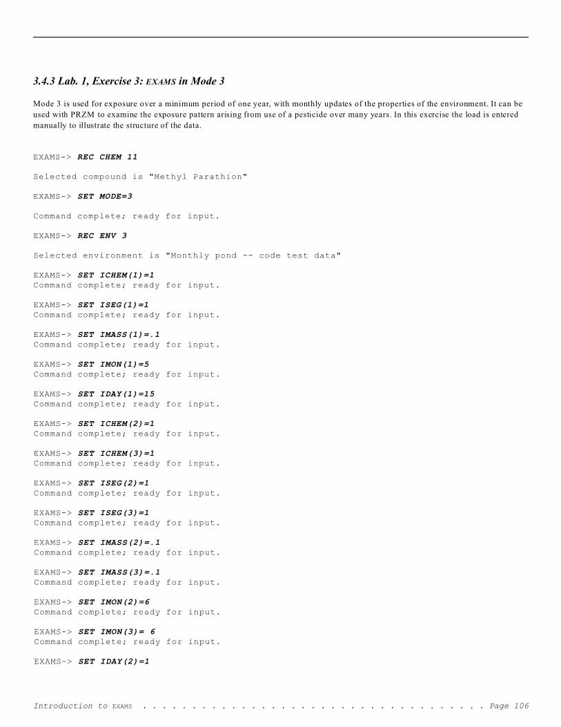
3.4.3 Lab. 1, Exercise 3: EXAMS in Mode 3
Mode 3 is used for exposure over a minimum period of one year, with monthly updates of the properties of the environment. It can be
used with PRZM to examine the exposure pattern arising from use of a pesticide over many years. In this exercise the load is entered
manually to illustrate the structure of the data.
EXAMS-> REC CHEM 11
Selected compound is "Methyl Parathion"
EXAMS-> SET MODE=3
Command complete; ready for input.
EXAMS-> REC ENV 3
Selected environment is "Monthly pond -- code test data"
EXAMS-> SET ICHEM(1)=1Command complete; ready for input.
EXAMS-> SET ISEG(1)=1Command complete; ready for input.
EXAMS-> SET IMASS(1)=.1Command complete; ready for input.
EXAMS-> SET IMON(1)=5Command complete; ready for input.
EXAMS-> SET IDAY(1)=15Command complete; ready for input.
EXAMS-> SET ICHEM(2)=1Command complete; ready for input.
EXAMS-> SET ICHEM(3)=1Command complete; ready for input.
EXAMS-> SET ISEG(2)=1Command complete; ready for input.
EXAMS-> SET ISEG(3)=1Command complete; ready for input.
EXAMS-> SET IMASS(2)=.1Command complete; ready for input.
EXAMS-> SET IMASS(3)=.1Command complete; ready for input.
EXAMS-> SET IMON(2)=6Command complete; ready for input.
EXAMS-> SET IMON(3)= 6Command complete; ready for input.
EXAMS-> SET IDAY(2)=1
Introduction to EXAMS . . . . . . . . . . . . . . . . . . . . . . . . . . . . . . . . . . . Page 106

---------------------------------------------------------------
---------------------------------------------------------------
---------------------------------------------------------------
Command complete; ready for input.
EXAMS-> SET IDAY(3)=15Command complete; ready for input.
EXAMS-> SHO PU LO
Exposure Analysis Modeling System -- EXAMS Version 2.97, Mode 3Ecosystem: Monthly pond -- code test dataChemical: 1) Methyl Parathion
Table 3. Chemical input data: pulse loadings.*
Load Entry--
IMONth 5 6 6 IDAY 15 1 15 ICHEM-ADB# 1 1 1 ISEGment 1 1 1 IMASS (kg) 0.100Event Number 1
0.100 2
0.100 3
* N.B.: These values represent the input request stream only;they may be revised during simulation.
EXAMS-> RUN
Simulation beginning for:Environment: Monthly pond -- code test dataChemical 1: Methyl Parathion
RUN command completed.
EXAMS-> PL KI PL
Chemical: Methyl ParathionEnvironment: Monthly pond -- code test data
Simulation units: DaysNumber of segments: 2Segment Number: 1 2Segment "TYPE": L B
The following parameters are available for time-trace plottingof values averaged over the ecosystem space:
1 - Water Column: average dissolved (mg/L)2 - average sorbed (mg/kg)3 - total mass (kg)4 - Benthic: average dissolved (mg/L)5 average sorbed (mg/kg)6 total mass (kg)
Enter parameters, one per line;enter "0" to end data entry and proceed.Parameter-> 3
Parameter-> 6
Parameter-> 0
The following parameters are available for each segment:1 - Total concentration (Water Column, mg/L; benthic, mg/kg)
Introduction to EXAMS . . . . . . . . . . . . . . . . . . . . . . . . . . . . . . . . . . . Page 107

2 - Dissolved (mg/liter of fluid volume)3 - Sorbed (mg/kg of sediment)4 - Biosorbed (ug/g)5 - Mass (grams/square meter of AREA)
Enter segment-parameter number pair, one number per line;enter 0 when data entry is complete; or Quit to cancel.
Enter segment number---> 0
System: Monthly pond -- code test dataChemical: Methyl Parathion0.111 I *
I * I * * I * I * *
7.425E-02 I * * I * * I * * I * * * I * * *
3.712E-02 I * * * I * * ++ I * ++*++++ I *+**** +++++ I +++ ** ++++++++++
0.000 I+++++++++++++++++++ ***************++++++++++ +----+----+----+----+----+----+----+----+----+----+
0.000 73.0 146. 219. 292. 365. 36.5 110. 183. 256. 329.
Time, Days
EXAMS-> PL KI PL
Chemical: Methyl ParathionEnvironment: Monthly pond -- code test data
Simulation units: DaysNumber of segments: 2Segment Number: 1 2Segment "TYPE": L B
The following parameters are available for time-trace plottingof values averaged over the ecosystem space:
1 - Water Column: average dissolved (mg/L)2 - average sorbed (mg/kg)3 - total mass (kg)4 - Benthic: average dissolved (mg/L)5 average sorbed (mg/kg)6 total mass (kg)
Enter parameters, one per line;enter "0" to end data entry and proceed.
Parameter-> 3Parameter-> 0
The following parameters are available for each segment:
Introduction to EXAMS . . . . . . . . . . . . . . . . . . . . . . . . . . . . . . . . . . . Page 108

1 - Total concentration 2 - Dissolved 3 - Sorbed 4 - Biosorbed 5 - Mass
(Water Column, mg/L; benthic, mg/kg)(mg/liter of fluid volume)(mg/kg of sediment)(ug/g)(grams/square meter of AREA)
Enter segment-parameter number pair, one number per line;enter 0 when data entry is complete; or Quit to cancel.
Enter segment number---> 0
System: Monthly pond -- code test dataChemical: Methyl Parathion0.111 I *
I * I * * I * I * *
7.425E-02 I * * I * * I * * I * * * I * * *
3.712E-02 I * * * I * * * I * * * I * **** I ** **
0.000 I******************* ************************* +----+----+----+----+----+----+----+----+----+----+
0.000 73.0 146. 219. 292. 365. 36.5 110. 183. 256. 329.
Time, Days
EXAMS-> CONTINUECONTinuing integration through 31 December 1990.
Simulation continuing for:Environment: Monthly pond -- code test dataChemical 1: Methyl Parathion
CONTINUE command completed.
EXAMS-> PLOT KI PL
Chemical: Methyl ParathionEnvironment: Monthly pond -- code test dataSimulation units: DaysNumber of segments: 2Segment Number: 1 2Segment "TYPE": L B
The following parameters are available for time-trace plottingof values averaged over the ecosystem space:
1 - Water Column: average dissolved (mg/L)2 - average sorbed (mg/kg)3 - total mass (kg)4 - Benthic: average dissolved (mg/L)5 average sorbed (mg/kg)6 total mass (kg)
Introduction to EXAMS . . . . . . . . . . . . . . . . . . . . . . . . . . . . . . . . . . . Page 109

Enter parameters, one per line;enter "0" to end data entry and proceed.
Parameter-> 3Parameter-> 0
The following parameters are available for each segment:1 - Total concentration (Water Column, mg/L; benthic, mg/kg)2 - Dissolved (mg/liter of fluid volume)3 - Sorbed (mg/kg of sediment)4 - Biosorbed (ug/g)5 - Mass (grams/square meter of AREA)
Enter segment-parameter number pair, one number per line;enter 0 when data entry is complete; or Quit to cancel.
Enter segment number---> 0System: Monthly pond -- code test dataChemical: Methyl Parathion0.111 I * *
I * * I * * * * I * * I * * * *
7.425E-02 I ** ** I ** ** I * * * * I * ** * ** I *** ***
3.713E-02 I *** *** I *** *** I *** *** I *** *** I * ** * **
0.000 I********** ********************** ************* +----+----+----+----+----+----+----+----+----+----+
0.000 146. 292. 438. 584. 730. 73.0 219. 365. 511. 657.
Time, Days
EXAMS-> LIST 20
Introduction to EXAMS . . . . . . . . . . . . . . . . . . . . . . . . . . . . . . . . . . . Page 110

-----------------------------------------------------------------------------
Exposure Analysis Modeling System -- EXAMS Version 2.97, Mode 3Ecosystem: Monthly pond -- code test dataChemical: Methyl ParathionTable 20.01. Exposure analysis summary: Maximum Events of 1989.
Event Duration 96-hour 21-day 60-day 90-day 1989==============----==== --------- --------- --------- --------- --------
***** Ecotoxicological Direct Exposure Concentrations ******Water Column Base 2.873E-03 5.675E-04 1.391E-04 6.194E-05 0.000 dissolved mg/L Mean
Peak 4.074E-03 5.559E-03
2.489E-03 5.559E-03
1.542E-03 5.559E-03
1.057E-03 5.559E-03
2.838E-045.559E-03
Benthic Sediment Base 7.801E-04 6.817E-04 4.466E-04 2.998E-04 0.000 mg/L dissolved
in pore water Mean Peak
7.837E-04 7.854E-04
7.489E-04 7.854E-04
6.258E-04 7.854E-04
5.399E-04 7.854E-04
1.860E-047.854E-04
***** Ecotoxicological Trophic Exposure Concentrations *****Water Column Base 1.07 0.211 5.169E-02 2.301E-02 0.000 ug/g dry weight Mean 1.51 0.925 0.573 0.393 0.105
of plankton Peak 2.07 2.07 2.07 2.07 2.07Benthic Sediment Base 0.290 0.253 0.166 0.111 0.000 ug/g dry weight Mean 0.291 0.278 0.232 0.201 6.910E-02
of benthos Peak 0.292 0.292 0.292 0.292 0.292 ***** Total Media Concentrations ***************************
Water Column Base 2.878E-03 5.685E-04 1.394E-04 6.205E-05 0.000 total mg/L Mean 4.081E-03 2.493E-03 1.545E-03 1.059E-03 2.842E-04
Peak 5.568E-03 5.568E-03 5.568E-03 5.568E-03 5.568E-03Benthic Sediment Base 3.929E-02 3.434E-02 2.249E-02 1.510E-02 0.000 total mg/kg Mean 3.947E-02 3.772E-02 3.152E-02 2.719E-02 9.369E-03
dry weight Peak 3.956E-02 3.956E-02 3.956E-02 3.956E-02 3.956E-02
More? (Yes/No/Quit)-> Y
Introduction to EXAMS . . . . . . . . . . . . . . . . . . . . . . . . . . . . . . . . . . . Page 111

-----------------------------------------------------------------------------
Exposure Analysis Modeling System -- EXAMS Version 2.97, Mode 3Ecosystem: Monthly pond -- code test dataChemical: Methyl ParathionTable 20.01. Exposure analysis summary: Maximum Events of 1990.
Event Duration 96-hour 21-day 60-day 90-day 1990==============----==== --------- --------- --------- --------- --------
***** Ecotoxicological Direct Exposure Concentrations ******Water Column Base 2.873E-03 5.679E-04 1.394E-04 6.209E-05 6.350E-07 dissolved mg/L Mean
Peak 4.074E-03 5.560E-03
2.489E-03 5.560E-03
1.543E-03 5.560E-03
1.058E-03 5.560E-03
2.847E-045.560E-03
Benthic Sediment Base 7.822E-04 6.833E-04 4.494E-04 3.040E-04 3.961E-06 mg/L dissolved
in pore water Mean Peak
7.857E-04 7.874E-04
7.508E-04 7.874E-04
6.276E-04 7.874E-04
5.415E-04 7.874E-04
1.921E-047.874E-04
***** Ecotoxicological Trophic Exposure Concentrations *****Water Column Base 1.07 0.211 5.178E-02 2.306E-02 2.359E-04 ug/g dry weight Mean 1.51 0.925 0.573 0.393 0.106
of plankton Peak 2.07 2.07 2.07 2.07 2.07Benthic Sediment Base 0.291 0.254 0.167 0.113 1.472E-03 ug/g dry weight Mean 0.292 0.279 0.233 0.201 7.135E-02
of benthos Peak 0.293 0.293 0.293 0.293 0.293 ***** Total Media Concentrations ***************************
Water Column Base 2.878E-03 5.688E-04 1.396E-04 6.219E-05 6.361E-07 total mg/L Mean 4.081E-03 2.493E-03 1.545E-03 1.059E-03 2.852E-04
Peak 5.569E-03 5.569E-03 5.569E-03 5.569E-03 5.569E-03Benthic Sediment Base 3.940E-02 3.442E-02 2.264E-02 1.531E-02 1.995E-04 total mg/kg Mean 3.957E-02 3.782E-02 3.161E-02 2.728E-02 9.674E-03
dry weight Peak 3.966E-02 3.966E-02 3.966E-02 3.966E-02 3.966E-02
EXAMS-> QUIT
Introduction to EXAMS . . . . . . . . . . . . . . . . . . . . . . . . . . . . . . . . . . . Page 112

3.5 Tutorial 2: Chemical & Environmental Data Entry
This tutorial example illustrates the entry of EXAMS chemical
and environmental data and the exploration of alternative
process models and parameters. The E XA M S session duplicates
the problem analysis in the text beginning on page 38; it
should be executed using that text as a guide. Note that the
3.5.1 Exercise 4: p-DCB in Lake Zurich
environmental data are not a complete characterization of Lake
Zurich; they include only a simple geometry plus the
parameters needed to construct a volatilization model for
E XA M S. The data entry sequence contains some errors; these
are intended as illustrations of error recovery methods.
! Commands for Lake Zurich analysis of p-DCB
1 REC CHEM 1
2 CHEM NAME IS 1,4-Dichlorobenzene
3 set mwt(1)=147.0
4 change sol(1,1) to 73.8
5 set kow(1)=2340
6 set henry(1)=2.66e-3
7 cat chem
8 stor chem 20
9 rec env 1
10 env name is Lake Zurich - central basin (Untersee)
11 set elev=431
12 set airty(*)=r
13 set lat=47.5
14 set lon=8.5
15 SET KO2(1,13)=2.5
16 SET WIND(13)=1.38
17 HELP WIND
18 SET WIND(1,13)=1.38
19 SHOW KOUNT
20 SET KOUNT=3
21 SET TYPE(1)=E
22 SET TYPE(2)=H
23 SET TYPE(3)=B
24 SET DEPTH(1)=10
25 SET VOL(1)=6.8E8
26 SET DEPTH(2)=40
27 SET VOL(2)=2.72E9
28 SET DEPTH(3)=0.02
29 SET VOL(3)=1.36E6
E XA M S Lake Zurich Data Entry Laboratory . . . . . . . . . . . . . . . . . . . . . . . . . . . . . . . . . . . . . . . . . . . . . . . . . . . . . . . . . . . . . . . . Page 113

30 SET AREA(*)=6.8E7
31 SET TCEL(1,13)=11
32 SET TCEL(2,13)=5.6
33 SET TCEL(3,13)=5.6
34 SET DSP(1,13)=0.2
35 SET DSP(2,13)=1.E-4
36 SET XST(*)=6.8E7
37 SET JTUR(1)=1
38 SET ITUR(1) TO 2
39 CHA JTUR(2)=2
40 SET ITUR(2)=3
41 SHO DISP
42 HELP CHARL
43 SET CHARL(1)=25
44 SET CHARL(2)=20.01
45 SHO DISP
46 SET SUSED(*,13)=5
47 SET BULKD(3,13)=1.5
48 SET PCTWA(3,13)=150
49 SET FROC(*,13)=.02
50 SET STRFL(1,13)=3.E5
51 HELP STFL
52 SET STF(1,13)=3.E5
53 SET STSED(1,13)=1500
54 SET STRLD(1,1,13)=0.01
55 RUN
56 SET JFR(1)=1
57 SET ITO(1)=0
58 SET ADVPR(1)=1.0
59
60
61
62
63
64
65
66
67
68
69
70
SHO AD
RUN
LI 15
list 18
list 20
CAT ENV
ERA ENV 5
STOR ENV 5
SET DRFL(2,1,13)=1.5E-3
SET STRL(1,1,13)=8.5E-3
ENV NAME IS Lake Zurich with partial load to hypolimnion
run
E XA M S Lake Zurich Data Entry Laboratory . . . . . . . . . . . . . . . . . . . . . . . . . . . . . . . . . . . . . . . . . . . . . . . . . . . . . . . . . . . . . . . . Page 114

71 li 15
72 list 18
73 li 20
74 zero load
75 set strl(1,1,13)=0.01
76 cat chem
77 rec chem 20
78 env name is Lake Zurich with oceanic wind and reaeration
79 show ko2(1,13)
80 set ko2(1,13)=20
81 sho wind(1,13)
82 set wind(1,13)=2.6245
83 run
84 list 15
85 list 18
86 era chem 20
87 quit
E XA M S Lake Zurich Data Entry Laboratory . . . . . . . . . . . . . . . . . . . . . . . . . . . . . . . . . . . . . . . . . . . . . . . . . . . . . . . . . . . . . . . . Page 115

3.5.2 Exercise 4 (Lake Zurich) with Complete EXAMS Responses
Welcome to EXAMS Release <current release number> Exposure Analysis Modeling System
Technical Contact: Lawrence A. Burns, Ph.D.U.S. Environmental Protection Agency
960 College Station RoadAthens, GA 30605-2700 USA
Phone: (706) 355-8119 (Fax) 355-8104Internet: [email protected]
Latest Maintenance <date of latest maintenance>
Type HELP and press the RETURN key for command names,HELP USER for a summary of command functions,HELP PAGES for a list of information pages,
or HELP EXAMS for introductory information.
Please stand by while EXAMS checks the computational precisionof this computer and initializes the Activity Data Base.
EXAMS-> REC CHEM 1Selected compound is "Chemical Data Entry Template"
EXAMS-> CHEM NAME IS 1,4-Dichlorobenzene
EXAMS-> set mwt(1)=147.0EXAMS-> change sol(1,1) to 73.8EXAMS-> set kow(1)=2340EXAMS-> set henry(1)=2.66e-3EXAMS-> cat chem
Catalog of CHEMICAL parameter sets
UDB No. Name of Entry Volume======= =======================
1 Chemical Data Entry Template2 p-Cresol3 Benz[a]anthracene4 Benzo[a]pyrene5 Quinoline6 Benzo[f]quinoline7 9H-Carbazole
8 7H-Dibenzo[c,g]carbazole9 Benzo[b]thiophene
10 Dibenzothiophene11 Methyl Parathion12 Mirex
13 Heptachlor (Heptachlorodicyclopentadiene)14 Speciation Test Data
EXAMS-> store chem 20Chemical stored: "1,4-Dichlorobenzene"
E XA M S Lake Zurich Data Entry Laboratory . . . . . . . . . . . . . . . . . . . . . . . . . . . . . . . . . . . . . . . . . . . . . . . . . . . . . . . . . . . . . . . . Page 116

---------------------------------------------------------------
EXAMS-> rec env 1Selected environment is "Environmental Data Entry Template"
EXAMS-> env name is Lake Zurich - central basin (Untersee)
EXAMS-> set elev=431EXAMS-> set airty(*)=rEXAMS-> set lat=47.5EXAMS-> set lon=8.5
EXAMS-> SET KO2(1,13)=2.5EXAMS-> SET WIND(13)=1.38Invalid number of subscripts.
EXAMS-> HELP WIND
WIND is a Real Matrix with 32 rows and 13 columns.WINDspeed (segment,month) Units: meters/secondAverage wind velocity at a reference height of ten centimetersabove the water surface. Parameter is used to compute a pistonvelocity for water vapor (Liss 1973, Deep-Sea Research 20:221)in the 2-resistance treatment of volatilization losses.
EXAMS-> SET WIND(1,13)=1.38EXAMS-> SHOW KOUNTKOUNT is 1
EXAMS-> SET KOUNT=3
EXAMS-> SET TYPE(1)=E
EXAMS-> SET TYPE(2)=HEXAMS-> SET TYPE(3)=B
EXAMS-> SET DEPTH(1)=10EXAMS-> SET VOL(1)=6.8E8
EXAMS-> SET DEPTH(2)=40EXAMS-> SET VOL(2)=2.72E9
EXAMS-> SET DEPTH(3)=0.02
EXAMS-> SET VOL(3)=1.36E6
EXAMS-> SET AREA(*)=6.8E7
EXAMS-> SET TCEL(1,13)=11
EXAMS-> SET TCEL(2,13)=5.6
EXAMS-> SET TCEL(3,13)=5.6
EXAMS-> SET DSP(1,13)=0.2
EXAMS-> SET DSP(2,13)=1.E-4
EXAMS-> SET XST(*)=6.8E7
EXAMS-> SET JTUR(1)=1
EXAMS-> SET ITUR(1) TO 2
EXAMS-> CHA JTUR(2)=2
EXAMS-> SET ITUR(2)=3
EXAMS-> SHO DISP
Name of environment: Lake Zurich - central basin (Untersee)Total number of segments (KOUNT) = 3Segment Number: 1 2 3Segment "TYPE": E H B
E XA M S Lake Zurich Data Entry Laboratory . . . . . . . . . . . . . . . . . . . . . . . . . . . . . . . . . . . . . . . . . . . . . . . . . . . . . . . . . . . . . . . . Page 117

---------------------------------------------------------------
---------------------------------------------------------------
---------------------------------------------------------------
---------------------------------------------------------------
---------------------------------------------------------------
Table 10.13. Mean dispersive transport field.
J TURB 1 2 I TURB 2 3 XS TUR m2 6.800E+07 6.800E+07 CHARL m 1.00 0.000 DSP m2/h*Path No.:
0.200 1
1.000E-042
* Average of 12 monthly mean values.
EXAMS-> HELP CHARL
CHARL is a real vector with 300 elements.CHARacteristic_Length or mixing length (path) Units: metersAverage of segment dimensions normal to the exchange interfacelinking segment numbers JTURB(p) and ITURB(p). The matching ("p"subscript) members of JTURB, ITURB, CHARL, DSP, and XSTUR definedefine a dispersive transport pathway. N.B.: A given segmentmay have different mixing lengths at different interfaces.CHARL can also be calculated from the distance along a path thatconnects the centers of segments JTURB(p) and ITURB(p), passingthrough the interface whose area is XSTURG(p).See also: DSP, ITURB, JTURB, XSTUR
EXAMS-> SET CHARL(1)=25
EXAMS-> SET CHARL(2)=20.01
EXAMS-> SHO DISP
Name of environment: Lake Zurich - central basin (Untersee)Total number of segments (KOUNT) = 3Segment Number: 1 2 3Segment "TYPE": E H B
Table 10.13. Mean dispersive transport field.
J TURB 1 2I TURB 2 3XS TUR m2 6.800E+07 6.800E+07CHARL m 25.0 20.0 DSP m2/h* 0.200 1.000E-04 Path No.: 1 2
* Average of 12 monthly mean values.
EXAMS-> SET SUSED(*,13)=5
EXAMS-> SET BULKD(3,13)=1.5
EXAMS-> SET PCTWA(3,13)=150
EXAMS-> SET FROC(*,13)=.02EXAMS-> SET STRFL(1,13)=3.E5Option not identified.
EXAMS-> HELP STFLSTFLO is a real matrix with 100 rows and 13 columns.STream_FLOws (segment,month) Units: cubic meters/hourFlow into head reach of river or estuary; segment tributariesand creeks or other streamflows entering a lake or pond. Notethat STFLO represents stream flow entering system segments fromexternal sources ONLY. EXAMS itself computes hydrologic flows
E XA M S Lake Zurich Data Entry Laboratory . . . . . . . . . . . . . . . . . . . . . . . . . . . . . . . . . . . . . . . . . . . . . . . . . . . . . . . . . . . . . . . . Page 118

---------------------------------------------------------------
---------------------------------------------------------------
---------------------------------------------------------------
---------------------------------------------------------------
---------------------------------------------------------------
--- -------- ------ --------- --------- --------- ---------
among segments that are part of the waterbody being studied, viathe specified advective and dispersive flow patterns (see JFRAD,JTURB, etc.). Therefore, DO NOT compute net water balances foreach segment and enter these into the database--enter ONLY thoseflows entering the system across external boundaries!
EXAMS-> SET STF(1,13)=3.E5
EXAMS-> SET STSED(1,13)=1500
EXAMS-> SET STRLD(1,1,13)=0.01
EXAMS-> RUN
Simulation beginning for:Environment: Lake Zurich - central basin (Untersee)Chemical 1: 1,4-DichlorobenzeneHydrologic definition of segment 1 is improper.There is a net advected flow leaving this segment,but the flow pathway has not been specified. Simulation aborted.RUN command completed.
EXAMS-> SET JFR(1)=1
EXAMS-> SET ITO(1)=0
EXAMS-> SET ADVPR(1)=1.0
EXAMS-> SHO AD
Name of environment: Lake Zurich - central basin (Untersee)Total number of segments (KOUNT) = 3Segment Number: 1 2 3Segment "TYPE": E H B
Table 9. Input specifications -- advective transport field.
J FR AD 1I TO AD 0ADV PR 1.00 Path No.: 1
EXAMS-> RUN
Simulation beginning for:Environment: Lake Zurich - central basin (Untersee)Chemical 1: 1,4-DichlorobenzeneRUN command completed.EXAMS-> LI 15Ecosystem: Lake Zurich - central basin (Untersee)Chemical: 1,4-Dichlorobenzene
Table 15.01. Distribution of chemical at steady state.
Seg Resident Mass ******** Chemical Concentrations ********* # Total Dissolved Sediments Biota
Kilos % mg/* mg/L ** mg/kg ug/g
In the Water Column:
E XA M S Lake Zurich Data Entry Laboratory . . . . . . . . . . . . . . . . . . . . . . . . . . . . . . . . . . . . . . . . . . . . . . . . . . . . . . . . . . . . . . . . Page 119

---------------------------------------------------------------
---------------------------------------------------------------
---------------------------------------------------------------
--------------------- ---------- --------- ----------
---------------------------------------------------------------
---------------------------------------------------------------
---------------------------------------------------------------
---------------------------------------------------------------
1 7.3 20.00 1.074E-05 1.074E-05 2.060E-04 0.000 2 29. 80.00 1.074E-05 1.074E-05 2.060E-04 0.000
======== ====== 37. 99.22
and in the Benthic Sediments: 3 0.29 100.00 2.114E-04 1.074E-05 2.060E-04 0.000
======== ====== 0.29 0.78
Total Mass (kilograms) = 36.80
* Units: mg/L in Water Column; mg/kg in Benthos.** Excludes complexes with "dissolved" organics.
EXAMS-> list 18Ecosystem: Lake Zurich - central basin (Untersee)Chemical: 1,4-Dichlorobenzene
Table 18.01. Analysis of steady-state fate of organic chemical.
Steady-state Values Mass Flux % of Load Half-Life* by Process Kg/ day days
HydrolysisReductionRadical oxidationDirect photolysisSinglet oxygen oxidationBacterioplanktonBenthic BacteriaSurface Water-borne Export 7.7315E-02 32.21 329.9Seepage exportVolatilization 0.1627 67.79 156.8
Chemical Mass Balance: Sum of fluxes = Sum of loadings =
Allochthonous load: Autochthonous load:
Residual Accumulation =
0.24000.2400
100.00.0
2.24E-08 0.0
* Pseudo-first-order estimates based on flux/resident mass.
EXAMS-> list 20
Ecosystem: Lake Zurich - central basin (Untersee)Chemical: 1,4-Dichlorobenzene
Table 20.01. Exposure analysis summary.
Exposure (maximum steady-state concentrations):Water column: 1.074E-05 mg/L dissolved; total = 1.074E-05 mg/LBenthic sediments: 1.074E-05 mg/L dissolved in pore water;
maximum total concentration = 2.114E-04 mg/kg (dry weight).Biota (ug/g dry weight): Plankton: Benthos:
Fate: Total steady-state accumulation: 36.8 kg, with 99.22%
in the water column and 0.78% in the benthic sediments. Total chemical load: 0.24 kg/ day. Disposition: 0.00%
chemically transformed, 0.00% biotransformed, 67.79%
E XA M S Lake Zurich Data Entry Laboratory . . . . . . . . . . . . . . . . . . . . . . . . . . . . . . . . . . . . . . . . . . . . . . . . . . . . . . . . . . . . . . . . Page 120

---------------------------------------------------------------
---------------------------------------------------------------
--- -------- ------ --------- --------- --------- ---------
volatilized, and 32.21% exported via other pathways.
Persistence: After 216. days of recovery time, the water column hadlost 50.51% of its initial chemical burden; the benthic zonehad lost 19.54%; system-wide total loss of chemical = 50.3%.
Five half-lives (>95% cleanup) thus require ca. 36. months.
EXAMS-> CAT ENVCatalog of ENVIRONMENTal models
UDB No. Name of Entry Volume======= =======================
1 Environmental Data Entry Template2 Pond -- code test data -- mean values only3 Monthly pond -- code test data4 Lake Zurich (Untersee), Switzerland: annual means5 Georgia Pond-Stream (R. Lee)6 GApond USEPA
EXAMS-> erase env 5
Environment 5 erased.Password protections for this entry have been removed.
EXAMS-> STORE ENV 5
Environment stored: "Lake Zurich - central basin (Untersee)"
EXAMS-> SET DRFL(2,1,13)=1.5E-3
EXAMS-> SET STRL(1,1,13)=8.5E-3
EXAMS-> ENV NAME IS Lake Zurich with partial load to hypolimnion
EXAMS-> run
Simulation beginning for:Environment: Lake Zurich with partial load to hypolimnionChemical 1: 1,4-DichlorobenzeneRUN command completed.EXAMS-> li 15Ecosystem: Lake Zurich with partial load to hypolimnionChemical: 1,4-Dichlorobenzene
Table 15.01. Distribution of chemical at steady state.
Seg Resident Mass ******** Chemical Concentrations ********* # Total Dissolved Sediments Biota
Kilos % mg/* mg/L ** mg/kg ug/g
In the Water Column: 1 7.3 16.59 1.074E-05 1.074E-05 2.060E-04 0.000 2 37. 83.41 1.350E-05 1.349E-05 2.589E-04 0.000
======== ====== 44. 99.19
and in the Benthic Sediments: 3 0.36 100.00 2.657E-04 1.349E-05 2.589E-04 0.000
======== ====== 0.36 0.81
E XA M S Lake Zurich Data Entry Laboratory . . . . . . . . . . . . . . . . . . . . . . . . . . . . . . . . . . . . . . . . . . . . . . . . . . . . . . . . . . . . . . . . Page 121

---------------------------------------------------------------
---------------------------------------------------------------
---------------------------------------------------------------
--------------------- ---------- --------- ----------
---------------------------------------------------------------
---------------------------------------------------------------
---------------------------------------------------------------
---------------------------------------------------------------
Total Mass (kilograms) = 44.37
* Units: mg/L in Water Column; mg/kg in Benthos.** Excludes complexes with "dissolved" organics.
EXAMS-> list 18Ecosystem: Lake Zurich with partial load to hypolimnionChemical: 1,4-Dichlorobenzene
Table 18.01. Analysis of steady-state fate of organic chemical.
Steady-state Valuesby Process
Mass Flux Kg/ day
% of Load Half-Life*days
HydrolysisReduction Radical oxidation Direct photolysisSinglet oxygen oxidationBacterioplanktonBenthic Bacteria Surface Water-borne ExportSeepage exportVolatilization
7.7315E-02
0.1627
32.21
67.79
397.8
189.1
Chemical Mass Balance: Sum of fluxes = Sum of loadings =
Allochthonous load: Autochthonous load:
Residual Accumulation =
0.24000.2400
100.00.0
0.0 0.0
* Pseudo-first-order estimates based on flux/resident mass.
EXAMS-> li 20Ecosystem: Lake Zurich with partial load to hypolimnionChemical: 1,4-Dichlorobenzene
Table 20.01. Exposure analysis summary.
Exposure (maximum steady-state concentrations):Water column: 1.349E-05 mg/L dissolved; total = 1.350E-05 mg/LBenthic sediments: 1.349E-05 mg/L dissolved in pore water;
maximum total concentration = 2.657E-04 mg/kg (dry weight).Biota (ug/g dry weight): Plankton: Benthos:
Fate: Total steady-state accumulation: 44.4 kg, with 99.19%
in the water column and 0.81% in the benthic sediments. Total chemical load: 0.24 kg/ day. Disposition: 0.00%
chemically transformed, 0.00% biotransformed, 67.79% volatilized, and 32.21% exported via other pathways.
Persistence: After 252. days of recovery time, the water column hadlost 54.35% of its initial chemical burden; the benthic zonehad lost 25.70%; system-wide total loss of chemical = 54.1%.
Five half-lives (>95% cleanup) thus require ca. 37. months.
EXAMS-> zero loadAll allochthonous loads removed.
E XA M S Lake Zurich Data Entry Laboratory . . . . . . . . . . . . . . . . . . . . . . . . . . . . . . . . . . . . . . . . . . . . . . . . . . . . . . . . . . . . . . . . Page 122

---------------------------------------------------------------
---------------------------------------------------------------
--- -------- ------ --------- --------- --------- ---------
---------------------------------------------------------------
EXAMS-> cat chemCatalog of CHEMICAL parameter setsUDB No. Name of Entry Volume======= =======================
1 Chemical Data Entry Template2 p-Cresol3 Benz[a]anthracene4 Benzo[a]pyrene5 Quinoline6 Benzo[f]quinoline7 9H-Carbazole
11 Methyl Parathion20 1,4-Dichlorobenzene
EXAMS-> rec chem 20Selected compound is "1,4-Dichlorobenzene"EXAMS-> rec env 5Selected environment is "Lake Zurich - central basin (Untersee)"EXAMS-> env name is Lake Zurich with oceanic wind and reaeration
EXAMS-> show ko2(1,13)KO2(1,13) is 2.500 EXAMS-> set ko2(1,13)=20
EXAMS-> sho wind(1,13)WIND(1,13) is 1.380
In this study, we wish to set Vw to 3000 cm/h. Use Eq. (2-82) (On page 36) to calculate the required value for WIND. EXAMS-> set wind(1,13)=2.6245EXAMS-> set strl(1,1,13)=0.01
EXAMS-> runSimulation beginning for:Environment: Lake Zurich with oceanic wind and reaerationChemical 1: 1,4-DichlorobenzeneRUN command completed.EXAMS-> list 15Ecosystem: Lake Zurich with oceanic wind and reaerationChemical: 1,4-Dichlorobenzene
Table 15.01. Distribution of chemical at steady state.
Seg Resident Mass ******** Chemical Concentrations ********* # Total Dissolved Sediments Biota
Kilos % mg/* mg/L ** mg/kg ug/g
In the Water Column: 1 1.3 20.00 1.952E-06 1.952E-06 3.746E-05 0.000 2 5.3 80.00 1.952E-06 1.952E-06 3.746E-05 0.000
======== ====== 6.6 99.22
and in the Benthic Sediments: 3 5.23E-02 100.00 3.844E-05 1.952E-06 3.746E-05 0.000
======== ====== 5.23E-02 0.78
Total Mass (kilograms) = 6.691
* Units: mg/L in Water Column; mg/kg in Benthos.** Excludes complexes with "dissolved" organics.EXAMS-> list 18Ecosystem: Lake Zurich with oceanic wind and reaerationChemical: 1,4-Dichlorobenzene
E XA M S Lake Zurich Data Entry Laboratory . . . . . . . . . . . . . . . . . . . . . . . . . . . . . . . . . . . . . . . . . . . . . . . . . . . . . . . . . . . . . . . . Page 123
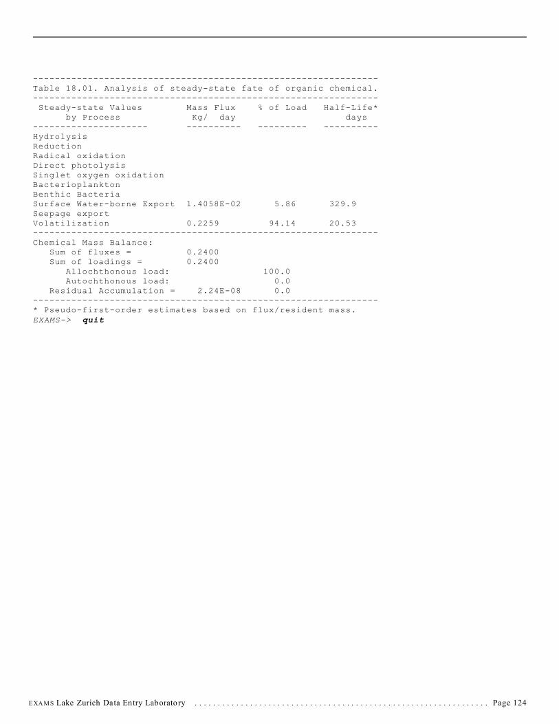
---------------------------------------------------------------
---------------------------------------------------------------
--------------------- ---------- --------- ----------
---------------------------------------------------------------
---------------------------------------------------------------
Table 18.01. Analysis of steady-state fate of organic chemical.
Steady-state Values Mass Flux % of Load Half-Life* by Process Kg/ day days
HydrolysisReductionRadical oxidationDirect photolysisSinglet oxygen oxidationBacterioplanktonBenthic BacteriaSurface Water-borne Export 1.4058E-02 5.86 329.9Seepage exportVolatilization 0.2259 94.14 20.53
Chemical Mass Balance: Sum of fluxes = Sum of loadings =
Allochthonous load: Autochthonous load:
Residual Accumulation =
0.24000.2400
100.00.0
2.24E-08 0.0
* Pseudo-first-order estimates based on flux/resident mass.EXAMS-> quit
E XA M S Lake Zurich Data Entry Laboratory . . . . . . . . . . . . . . . . . . . . . . . . . . . . . . . . . . . . . . . . . . . . . . . . . . . . . . . . . . . . . . . . Page 124

4.0 EXAMS Command Language Interface (CLI) User’s Guide
Introduction This Chapter describes the E XA M S command
language, including usage and reference information. The first
part provides an overview of the command language and its
grammar. The second part contains detailed descriptions of each
command. The commands are listed in alphabetical order.
4.1 Conventions Used in this Chapter
Convention Meaning
CTRL/x The phrase CTRL/x indicates that you must press
the key labeled CTRL while simultaneously pressing
another key, for example, CTRL/Q.
-> LIST 7
.
Vertical series of periods, or ellipsis, mean that
not all the data E XA M S would
.
.
.
display in response to
the particular command is shown,
or that not all
. the data a user would enter is
. shown.
keyword, ... Horizontal ellipsis indicates that additional
key-words, command parameters, or data can be
entered in a command sequence, or that EXAM S
displays additional data as part of the sample
output line.
[keyword] Square brackets indicate that the item enclosed is
optional, that is, the entity can be omitted from the
command line altogether.
<option> Angle brackets indicate that a command requires a
choice among two or more options.
4.2 OverviewThe E XA M S command language provides a set of commands for
! Entering, storing, and manipulating data describing the
reaction chemistry of synthetic comp ound s, the
environmental parameters governing their transport and
transformation in aquatic systems, patterns of allochthonous
loadings, and product chemistry.
! Studying the results of an analysis by listing tabular output
on a terminal, plotting the concentration data (“Expected
Environmental Concentrations” or EECs) computed during
simulations, and printing paper copy.
! Choosing among analytical frameworks for investigating
exposure to chemicals in a particular case study. E XA M S
includes three operational modalities or “MODEs”
MODE Analytical Methodology
1 Long-term consequences of continued releases of
chemicals; steady-state analysis.
2 Detailed examination of immediate consequences of
chemical releases; initial-value problems.
3 Intermediate-scale resolution of events over several
years, including effects of seasonal environmental
variability; analysis of time-series data.
4.3 Entering Commands E XA M S commands are composed of English-language words
(mostly verbs) that describe what you want E XA M S to do. Some
commands require qualifiers and parameters. These give E XA M S
more information on how to execute the command. Command
parameters describe the object to be acted upon by the command.
In some cases, the object is a keyword (as in the HE LP command);
in others, it is an E XA M S data element (SET command) or a
section of a file of input data or analysis results to manipulate
(STORE and LIST commands).
Throughout this Chapter , E XA M S commands are printed in
uppercase letters for the sake of clarity. However, E XA M S will
accept commands entered in uppercase, lowercase, or a mixture
of uppercase and lowercase letters. Most E XA M S commands and
keywords can be abbreviated to the least number of characters
needed to uniquely distinguish them from other options available.
For example, to end E XA M S you can enter “QUIT”, “QUI”, “QU”,
or “Q”. The least number of required characters depends on the
context, however, but is never more than three. For example, the
SHOW command includes among its options both <QUALITY> and
<QUIT>; in this case you must enter three characters for E XA M S
to distinguish between them. In E XA M S’ “help fields” and
prompts, capitalization is used to show you how many characters
are required for uniqueness.
The following example shows an AU DIT command and EXAM S’
response, as they would appear on a terminal.
E XA M S-> AUDIT ON
All input will now be cop ied into the file
named “AUDOUT” on Fortran Unit Number 4
125

------------------------------------------
-----------------------------------------
------------------------------------------
E XA M S-> ! This Command File should be renamed file.EXA
E XA M S->
E XA M S analyzes the parts of the above example as follows.
E XA M S-> The E XA M S system prompt for command input; a
greater-than (->) means that E XA M S’ command
interpreter is ready for a command to be entered.
AU DIT The command name, requesting that E XA M S
enable/disable the User Notepad/Command File
Creation facility.
ON An option of the AU DIT command, requesting that the
Notepad/Create facility be enabled.
All input will now be copied into the file
named “AUDOUT” on Fortran Unit Number 4
A message from the AU DIT command, indicating that
the command completed successfully. The command
interpreter used the value of AUDOUT (4) to establish
communication with an external file.
E XA M S-> The next system command prompt, confirming that
the command has completed its operations (AU DIT
has opened communications with an external file
and started recording terminal inputs), and E XA M S
is ready for additional input.
! This Command File should be renamed file.EXA
A comment entered by the user. Comment lines must
begin with an exclamation point (!) or an asterisk (*).
You can use comments, as need ed, to document E XA M S
analysis sessions or command procedures.
E XA M S-> The next E XA M S system command prompt,
confirming that the comment has been recorded in
the Notepad/Command file and E XA M S is ready to
accept another command.
4.4 Command Prompting When you enter a command at the terminal, you need not enter
the entire command on a single line. If you enter a command that
requires that you specify its range or the object of the requested
action, and you do not include the needed information, E XA M S’
command interpreter prompts you for all missing information.
For example:
E XA M S-> AU DIT
The following AU DIT options are available
ON -- begins a new Audit file,
OFF -- ends Audit recording of input commands,
Help -- this message,
Quit -- return to the E XA M S prompt.
AU DIT-> ON
All input will now be copied into the
file named “AUDOUT” on Fortran unit number 4
In this example, no AU DIT option was entered, so E XA M S prompts
for a more complete specification of the intended action. The line
ending with a -> indicates that E XA M S is waiting for the
additional input.
In many cases, E XA M S’ prompts do not include an automatic
description of the full range of possible response options. Often,
however, entering HE LP in response to the prompt will display a
list of available choices, as in the following example.
E XA M S-> LIST
At the prompt, enter a T able number, “Quit,” or “Help” to see a
catalog of the output tables.
Enter Table Number -> HE LP
1 Chemical inputs: FATE Data
2 Chemical inputs: PRODUCT Chemistry
3 PULSE Chemical Loadings
.
.
.
20 Exposure Analysis SUMMARY
ALL Entire Report
At the prompt, enter a Table number, “Quit,”
or “Help” to see a catalog of the output tables.
Enter Table Number -> 18
Ecosystem: Name of Water bodyChemical: Name of chemical
Table 18.01. Analysis of steady-state fate
.
. (body of table)
.
In the example above, LIST is entered without the number of the
output table to be displayed. E XA M S prompts for the missing
information; typing HE LP in response to the LIST prompt d isplays
a catalog of E XA M S output tables.
126

4.5 EXAMS Messages When a command is entered incorrectly, E XA M S displays a
descriptive error message indicating what is wrong. For example,
if a data subscript larger that the maximum available is entered,
E XA M S will respond
Subscript out-of-range.
You can then retype the command correctly.
Other error messages may be produced during the execution of
a command, or during a simulation or data display sequence.
These messages indicate such things as incomplete
environmental data, character data entered where numeric data
are required, or typographic errors during entry of commands.
E XA M S will respond to typographic errors in command entries by
displaying:
Command not recognized. Type HELP for command
information.
Because the messages are descriptive, it is usually possible to
determine what corrective action is required in order to proceed.
When this is not the case, E XA M S’ HE LP facility contains a large
body of additional and supplementary information available
through the HE LP, DESCRIBE, and SHOW commands.
4.6 The HELP Command Consulting a printed guide is not the most convenient way to get
a summary of the syntax of a command or a definition of an input
datum. E XA M S’ HELP command provides this information in
E XA M S’ interactive environment. For example, you can type the
command:
E XA M S-> HELP LIST
E XA M S responds by displaying a description of the LIST
command, its syntax, and the options needed to specify the range
of the command.
The HE LP facility also provides on-line assistance for E XA M S’
input data, e.g.,
E XA M S-> HELP QYIELD
will display the subscript ranges, their meanings, the physical
dimensions, and the English definition of E XA M S chemical input
datum “QYIELD”. This information is available online for all
EX AM S’ input data and contro l parameters. The names of all of
E XA M S’ input variables were selected as mnemonics for their
English-language names. (For example, QYIELD is the
photochemical quantum yield.) These mnemonics are used in
E XA M S’ output tables; definitions are given in the Data
Dictionary (pages 175 ff.) as well as in the on-line HE LP.
E XA M S’ HE LP facility supplies lists of individual topics and
subtopics. The HE LP command is described in more detail later
in this Chapter, and a tutorial explanation of the command is
available online by entering
E XA M S-> HELP TUTOR
4.7 Command Procedures A command procedure is a file that contains a sequence of
E XA M S commands, op tionally interspersed with descriptive
comments (lines with “!” or “*” in column one). By placing sets
of frequently-used commands and/or response options in a
command procedure, all the commands in it can be executed as
a group using a single command. For example, suppose a file
called START.EXA were to contain these command lines and
comments:
SET MODE TO 3
SET KCHEM TO 4
SET NYEAR TO 5
RECALL LOAD 7
! Loadings UDB Sector 7 is the spray drift study
The four commands in this file can be executed by entering the
command
E XA M S-> DO START
or E XA M S-> @START
You do not have to specify the file type of a command procedure
when you use the @ command, so long as the file type is
“.EXA”--the default file type for E XA M S’ @ command. You can
use another file suffix, if you so inform E XA M S when you enter
the command request. For example, to execute commands in a
file named START.UP
E XA M S-> @START.UP
4.8 Wild Card CharactersSome E XA M S commands accept a “wild card” character in the
input command specifications. The asterisk (*) is the only
symbol having this function in E XA M S. Wild card characters are
used to refer to a range of data subscripts, or other entities, by a
general name, rather than having to enter a specific name for
each member of the group. Particular uses of wild cards in
E XA M S vary with the individual commands. The command
descriptions later in this Chapter indicate where wild cards are
allowed and describe their effects.
127

4.9 Truncating Command Names and Keywords All keywords and names of input data that are entered as
command input can be abbreviated . Only enough characters to
uniquely distinguish a keyword or datum from others with similar
names need be entered (often only one).
4.10 Summary Description of EXAMS’ System Commands
E XA M S Command Summary Description
AU DIT Start/Stop user notepad for recording procedures
CATALOG List the contents of User Databases (UDBs)
CHANGE/SET Enter/reset input data and program controls
CONTINUE Resume integration (Modes 2 and 3 only)
DESCRIBE Report dimensions and data type of parameter
DO or @ Execute file of E XA M S commands (file.EXA)
ERASE Clear section of stored database (UDB)
HE LP Describes access to E XA M S on-line HE LP facility
LIST Show tabular results on the screen
N A M E Specify the name of a UDB, e.g., CHEM NAM E IS ...
PLOT Plot results on the screen
PRINT Queue tabular results for hardcopy printing
QUIT Abort command, or End interactive session
READ Upload data from non-E XA M S ASCII disk file
REC ALL Activate data from stored database (UDB)
RUN Begin simulation run
SHOW Display current data values or control settings
STORE Download current data into stored database (UDB)
WRITE Download data to AS CII disk file
ZERO Clear chemical loadings, pulses, or residuals
128

5.0 System Command Descriptions
A U D I T
Creates a copy of user input commands and responses in an external file.
Related: Control variables: AUDOUT
Commands: DO
Syntax: AU DIT <option>
Options
ON
OFf
Prompt: The following AU DIT options are available
ON -- begins a new Audit file,
OFf -- ends Audit recording of input commands,
Help -- this message,
Quit -- return to the E XA M S prompt.
AU DIT->
Options: OFf
Ends copying of E XA M S commands to the external file.
ON
Begins copying of E XA M S commands to an external file.
Description: The AU DIT command starts copying inputs typed at the terminal, into an external file. These inputs include E XA M S commands,
and user responses to E XA M S prompts and option selections. The output terminus for the copy is a file named “AUDOUT,”
connected to Fortran logical unit number AUDOUT. The resulting output file can be used to record an analysis procedure, or
as a general notepad. The output file can be renamed “file.EXA” and used as an E XA M S command (DO) file.
Examples:
1. E XA M S-> AU DIT
The following AU DIT options are available:
ON -- begins a new Audit file,
OFf -- ends Audit recording of input commands,
Help -- this message,
Quit -- return to the E XA M S prompt.
AU DIT-> ON
All input will now be copied into the
file named AUDOUT on Fortran Unit Number 4
This command begins recording of input from the terminal into an external file. The output will go to a disk file named “AUDOUT.”
After leaving E XA M S, this file can be printed to give a permanent record of the analysis.
129

2. E XA M S-> AUD IT OFF
The AU DIT option has been terminated.
This command ends copying of E XA M S commands and responses to the external medium (usually a disk file).
3. E XA M S-> AUDIT ON
All input will now be copied into the
file named “AUDOUT” on Fortran Unit Number 4
E XA M S-> RECALL ENV 2
Selected environment is: Phantom Inlet
E XA M S-> R EC ALL C H EM 2
Selected compo und is: D ichloroexample
E XA M S-> R EC ALL C H EM 4 AS 2
Selected compound is: T etrabromoexample
E XA M S-> AUD IT OFF
These commands build a file (AUDOUT) that can later be used as a command file upon entering the E XA M S system. In this instance, the
file would be renamed (e.g., MYCOMAND.EXA) and used to execute the above series of commands as a unit--
E XA M S-> DO MYCOMAND
130

C A T A L O G
Lists, by accession number, the title of all current entries in the specified User Database (UDB).
Related: Control variables: none
Commands: ERASE, N A M E, REC ALL, STORE
Syntax: CATALOG <option>
Options: CHEMICAL, ENVIRONMENT, LOAD, PRODUCT
Prompt: Enter Environment, Chemical, Load, Product, Help, or Quit->
Options: CHEMICAL
Lists the titles, by access number, of chemical databases currently in the User Database. Each entry corresponds to a single
chemical, and contains the laboratory data describing ionization and (species-specific) partitioning and reaction kinetics.
ENVIRONMENT
List the titles, by access number, of environmental databases currently in the User Database. Each entry contains a “canonical”
physical and chemical model of an aquatic system, including the environmental data needed to compute reactivity and transport
of synthetic chemicals in the system.
LOAD
Lists the titles, by access number, o f allochthonous chemical loading patterns stored in the User Database. These data include
monthly values (kg/hour) for stream-loads, non-point-source loads, groundwater seepage loads, precipitation loads, and drift loads
of chemicals entering the aquatic environment, plus specification of pulse loadings. The pulse load data include the magnitude
(kg), target environmental segment, and scheduling (month and day) of pulses of synthetic chemicals entering the system.
PRODUCT
Lists the titles, by access number, of reaction or transformation product chemistries stored in the User Database. These data
include the Activity Database numbers of chemical parent and product compounds, the number of the process responsible for the
transformation, and the yield efficiency (mole/mole) as an (optional) function of temperature.
Description: The CATALOG command inventories the contents of the specified User Database (UDB) and lists the titles of active entries on
the terminal screen. Four types of UDBs are available, corresponding to the four options available to the CATALOG command.
The titles are listed by accession number; this number is used to STORE, REC ALL, or ERASE database entries.
Examples:
1. E XA M S-> CA TALO G H ELP
The CATALOG command requires that you specify either:
1. Environment,
2. Chemical,
3. Load,
4. Product,
5. Help (this option), or
6. Quit.
Enter Environment, Chemical, Load, Product, Help, or Quit-> CHEMICAL
Catalog of CHEMICAL parameter sets
UDB No. Name of Entry Volume
131

1 Chemical Data Entry T emplate
2 p-Cresol
3 Benz[a]anthracene
.
.
.
E XA M S->
This example use of the CATALOG command lists the contents of the current User Database for chemical data. Any of these datasets can
be loaded into the Activity Database (ADB) for study, using the REC ALL command and the appropriate access number. The first entry
(“Chemical Data Entry Template”) is a blank data area reserved for entering new chemical data.
2. E XA M S-> CATALOG ENVIRON
Catalog of ENVIRONMENTal models
UDB No. Name of Entry Volume
1 Environmental Data Entry Template
2 Pond -- code test data
3 Connecticut River estuary
.
.
This example CATALOG command generates a listing of the environmental datasets present in the User Database. Any of these can be
retrieved for study using a REC ALL command and the accession number. The first entry (“Environmental Data Entry Template”) is a
template for entering a new environmental model.
132

C H A N G E
Use to enter data into the activity database (synonymous with SET).
Related: Commands: DESCRIBE, HE LP, SET
Syntax: CHANGE <name of variable> TO <new value>
or SET <name of variable> = <new value>
Prompt: Enter name=value command->
Variable: The data entry or variable to be entered can be specified either as a single datum or, using wild cards (*), as an entire vector,
row/column of a matrix, etc.
Description: Use the CHANGE command to specify the values of data in the activity database. “Value” can be any numerical quantity or
literal characters, as appropriate. “Variable” specifies an individual element of input data or a program control parameter.
Entire vectors, rows/columns of matrices, etc. can be set to a single uniform value using wild cards (*).
Examples:
1. E XA M S-> CHANGE VOL(153) TO 7E5
Subscript out-of-range.
E XA M S-> DESCRIBE VOL
VOL is a Real Vector with 100 elements.
E XA M S> CHANGE VOL(2) TO E
Invalid numeric quantity after TO or =.
E XA M S-> CHANGE VOL(2) TO 7E5
This command sets the environmental volume of segment 2 to 7.0E+05 cubic meters. The initial attempt to set the volume of segment 153
was rejected by E XA M S because the version in use was set up for environmental models of 100 segments at most. The DESCRIBE command
was used to check the number of subscripts and the dimensional size of the variable “VOL”. The accidental entry of an alphabetic character
(“E”) for the volume was trapped by the CHANGE command; VOL(2) was not altered.
2. E XA M S-> HELP TCEL
TCEL is a Real Matrix with 100 rows and 13 columns.
Temperature-CELsius (segment, month) Units: degrees C.
Average temperature of ecosystem segments. Used (as enabled by input data) to compute effects of temperature on transformation rates
and other properties of chemicals.
133

E XA M S-> CHANGE TCEL(2,7) TO 24
This command changes the July temperature in segment 2 to 24° C. The HELP command was used to check subscript dimensions,
maximum values, the meaning of the subscripts (subscript #1 denotes the segment, subscript #2, the month), and the proper units for the
input datum (degrees Celsius).
3. E XA M S-> HELP POH
POH is a Real Matrix with 100 rows and 13 columns.
pOH (segment, month) Units: pOH units
The negative value of the power to which 10 is raised in order to obtain the temporally averaged concentration of hydroxide [OH-]
ions in gram-equivalents per liter.
E XA M S-> CHANGE POH(*,13) TO 6.2
This command sets the average pOH (sector 13) of every segment to 6.2. Note use of wild card “*” to specify that all segments are to be
changed. As in the previous example, HE LP was used to check subscript dimensions, units, etc. T his step, of course, is optional.
134

C O N T I N U E
The CONTINUE command resumes E XA M S’ simulation analysis of chemical dynamics beginning from the current state of the system.
Related: Control variables: CINT, TIN IT, TEND, TCODE, NYEAR
Commands: RUN, SHOW_T IM E_F RA M E
Syntax: CONTINUE
Prompt: (In M ode 2 only:)
Initial time for integration will be (nn.n) units
Enter ending time of integration, Help, or Q uit->
Options: None. Reply to prompt with a value greater than (nn.n).
Description: The CONTINUE command resumes E XA M S’ simulation analysis of chemical dynamics, beginning from the current state of the
system. Chemical loadings and other input data can be altered (CHANGEd or SET) between simulation time segments; E XA M S
will re-evaluate equation parameters as needed to incorporate the changed conditions into the analysis. CONTINUE cannot be
invoked from M ode 1, where it is not appropriate. The S H OW T IM E FR AM E (abbreviate to SH T F) command can be used to
examine the current state of the integrator timer controls. In Mode 2, the Communications INTerval CINT can be used to vary
the temporal resolution in different segments of the analysis (see Example 1). In Mode 3, NYEAR, the number of years in a
simulation time segment, can similarly be altered.
Examples:
1. E XA M S-> SET MODE=2
E XA M S-> S H OW T IM E FR AM E
A RUN will integrate from 0. to 24. Hours
with output at intervals of 2.00 Hours
E XA M S-> SET TCODE=2
E XA M S-> SET TEND=10
E XA M S-> SET CINT=1
E XA M S-> SH TI F
A RUN will integrate from 0 to 10 D ays
with output at intervals of 1 Days
E XA M S-> RUN
Simulation beginning for:
Environment: Pond -- code test data
Chemical 1: Dichloroexample
Run complete
E XA M S-> PLOT KIN PL (3,0,0 -- see PLOT command)
135

System: Pond -- code test data Chemical: Dichloroexample
2.00 I** *** I * **** **** I **** **** *** I * **** **** ** I ** ***
1.33 I I I I I
0.667 I I I I I
0.000 I +----+----+----+----+----+----+----+----+----+----+
0.000 2.00 4.00 6.00 8.00 10.0 1.00 3.00 5.00 7.00 9.00
Time, Days
E XA M S-> CONTINUE
Initial time for integration will be 10.0 Days
Enter ending time of integration, Help, or Quit-> 30
Simulation beginning for:
Environment: Pond -- code test data
Chemical 1: Dichloroexample
Run complete.
E XA M S-> SET CINT=10
E XA M S-> ZERO PULSE LOAD
E XA M S-> CONTINUE
Initial time for integration will be 30.0 Days
Enter ending time of integration, Help, or Quit-> 90
Simulation beginning for:
Environment: Pond -- code test data
Chemical 1: Dichloroexample
Run complete.
E XA M S-> PLOT KINETIC PLOT (3,0,0)
136

System: Pond -- code test data Chemical: Dichloroexample
3.49 I * I ** I ** I * I **
2.33 I ** I* ** I*** *** I *** I ** *
1.16 I * I * I * * * I I
0.000 I +----+----+----+----+----+----+----+----+----+----+
0.000 18.0 36.0 54.0 72.0 90.0 9.00 27.0 45.0 63.0 81.0
Time, Days
These commands show the use of the CONTINUE com mand in Mode 2. The objective of the analysis was to introduce two pulses
of chemical separated by 10 days and to follow exposure over 90 days. Note the phased increase in the Communications INTerval
CINT from 1 to 10 days. Note the use of the ZERO command to clear the pulse load ADB before the simulation of dissimilation from
day 30 through day 90. If this w ere not done, E XA M S would introduce an additional pulse on day 30.
2. E XA M S-> SET MODE=3
E XA M S-> SHO TI FR
A RUN will integrate from 1 January 1989
through 31 December 1989.
(YEAR1 = 1989, and NYEAR = 1.)
E XA M S-> RUN
Simulation beginning for:
Environment: Pond -- code test data
Chemical 1: Dichloroexample
Run complete.
E XA M S-> SHO TI FR
A RUN will integrate from 1 January 1989
through 31 December 1989.
(YEAR1 = 1989, and NYEAR = 1.)
CONTinuation will proceed through 31 December 1990
(NYEAR = 1.)
E XA M S-> SET NYEAR=3
E XA M S-> SH TI F
137

A RUN will integrate from 1 January 1989
through 31 December 1991.
(YEAR1 = 1989, and NYEAR = 3.)
CONTinuation will proceed through 31 December 1992
(NYEAR = 3.)
E XA M S-> CONTINUE
CONTinuing integration through 31 December 1992.
Simulation beginning for:
Environment: Pond -- code test data
Chemical 1: Dichloroexample
Run complete.
E XA M S->
These commands illustrate the use of the CONTINUE com mand in Mode 3. “SHOW TIME FRAM E” is used to check the state of the
integrator timer controls.
138

D E S C R I B E
Reports the data type, dimensionality, and implemented size of parameters.
Related: Control variables:
Com mands: HELP
Syntax: DESCRIBE <parameter>
Parameters:
Any “system parameter”--any chem ical or environm ental input datum , control parameter (e.g ., MODE, CINT), etc.
Prompt: Enter name of input parameter->
Options: Any parameter accessible to the CHANGE and SET commands can be inspected using the DESCRIBE command.
Description: The DESCRIBE command returns information about E XA M S’ input data and control parameters. All variables whose values
can be altered using the CHANGE and SET commands can be inspected by the DESCRIBE command. The information returned
by DESCRIBE includes the data type (real, integer, character), dimensionality (scalar, vector, matrix (2-dimensional), tab le
(3-dimensional matrix)) and implemented size in the version of E XA M S in use. The DESCRIBE command is the first recourse
when a CHANGE or SET command fails.
Examples:
1. E XA M S-> DESR MODE
Comm and not recognized. Type HELP for command information.
E XA M S-> DESCR
Enter name of input parameter-> MODE
MODE is an Integer Scalar.
These commands establish that “MODE” is an integer scalar. Note that the initial typing error (DESR) resulted in a “not recognized”
error message followed by return to the E XA M S prompt.
2. E XA M S-> CHANGE VOL(133) TO 7E5
Subscript out-of-range.
E XA M S-> DESCRIBE VOL
VOL is a Real Vector with 100 elem ents.
This com mand reports that VOL is a real variable, with 100 elements. In this example, the number of segments (NPX) in the
version of E XA M S currently in use is set for 100 at most. Any (intentional or accidental) attempt to set “KOUNT” to a value > 100,
139

or to enter a value for the VOLume of a segm ent > 100 (e.g., VOL(133)) will fail, as illustrated above. DESCRIBE can be used to
check the reason for a failure of the CHANGE or SET command when a problem with dimension sizes is suspected.
3. E XA M S-> DESCRIBE QYIELD
QYIELD is a Real Table with dimensions (3,7,4)
E XA M S-> HELP QYIELD
QYIELD is a Real Table with dimensions (3,7,4)
Quantum_YIELD (form , ion, chemical) Units: dimension less
Reaction quantum yield for direct photolysis of chemicals--fraction of the total light quanta absorbed by a chemical that results
in transformations. Separate values (21) for each potential molecular type of each chemical allow the effects of speciation and
sorption on reactivity to be specified in detail. The matrix of 21 values specifies quantum yields for the (3) physical forms: (1)
dissolved, (2) sediment-sorbed, and (3) DOC-complexed; of each of (7) possible chemical species: neutral molecules (1), cations
(2-4), and anions (5-7). (QYIELD is an eff iciency.)
These commands report the data type and dimensionality of E XA M S’ input “QYIELD” (result of “DESCRIBE QYIELD”) and then
report the meaning of the dimensions and the physical units of the variable (result of “HELP QYIELD”). The local implementation
of E XA M S used in this example has the capacity to sim ulate the behavior of no more than four chemicals simultaneously. Thus,
QUANT was DESCRIBEd as consisting of a set of four matrices, each of (fixed) size (3,7).
140

D O
Executes a comm and procedure; requests that E XA M S read subsequent input from a specific file.
Related: Control variables:
Com mands: AU DIT
Syntax: DO <name of command file>
Prompt: Enter name of file (no more than nn characters), Help, or Quit->
Parameters: nam e of file
Specifies the file from which to read a series of E XA M S comm ands. If you do not specify a file type suffix, E XA M S uses a
default file type of EXA (e.g., “filename.EXA”). Wild cards are not allowed in the file specification.
Description: Use command procedures to catalog frequently used sequences of commands. An E XA M S command procedure can contain
! Any valid E XA M S com mand. The comm and line can include all the necessary options and data to build a complete command
(exception: kinetic plots).
! Parameters or response options for a specific command. When the currently executing comm and requires additional parameters,
the next line of the com mand file is searched for appropriate input.
! Data. When the currently executing com mand requires numerical or character data entry, the next line of the comm and file is
searched for input.
! Comment lines. Any line that contains an exclamation point (!) or asterisk (*) in column one is ignored by E XA M S’ command
interpreter. These lines can be used as needed to document the command procedure.
Command procedures must not contain a request to execute another command procedure. (In other words, a DO file must not
contain a DO (@) com mand; E XA M S’ DO commands cannot be nested.) Command procedures can be constructed as external files
using your favorite editor, or they can be constructed in teractively through the E XA M S system command processor, as illustrated
below. The default file type is “EXA”, but files of any type (suffix) can be used if the entire file name is specified when entering
the DO command.
Examples: 1. E XA M S-> AUDIT ON
All input will now be copied into the
file named “AUDOUT” on Fortran Unit Number 4
E XA M S-> RECALL
Enter Environment, Chemical, Load, Product, Help or Quit-> ENV
Enter environment UDB catalog number, Help, or Quit-> 2
Selected environment is: Phantom Inlet
E XA M S-> R EC A LL CH EM 2
Selected compound is: Dichloroexample
E XA M S-> RECALL LOAD 2
141

Selected load is: Aedes control spray drift
E XA M S-> ! Load 2 is the Phantom Inlet salt marsh study
E XA M S-> SET KCHEM TO 2
E XA M S-> R EC A LL CH EM 4 AS 2
Selected compound is: Tetrabromoexample
E XA M S-> AUDIT OFF
These commands build a file (AUDOUT.DAT) that can later be used as a command file upon entering the E XA M S system. In this
instance, the file could be renamed (e.g ., SETUP.EXA) and used to execute the above series of comm ands as a unit:
E XA M S-> DO SETUP
or, E XA M S-> @SETUP
The completed command file appears as follows
RECALL
ENV
2
R EC A LL CH EM 2
RECALL LOAD 2
! Load 2 is the Phantom Inlet salt marsh study
SET KCHEM TO 2
R EC A LL CH EM 4 AS 2
AUDIT OFF
Note that comm and files that are constructed interactively will include “AUDIT OFF” as the final instruction. This can, of course,
be removed by editing the file if it is undesirable.
2. E XA M S-> DO
Enter name of file (no more than nn characters), Help, or Quit-> HELP
The “DO” or “@” command provides a means of executing stored E XA M S com mands. In response to the prompt, enter the name
of the file that contains the stored comm ands. A three-character filename extension of “EXA” is added to the name if no period
is present in the name as entered. The maximum length for file names is nn characters; this limit includes the .EXA suffix.
Enter name of file (no more than nn characters), Help, or Quit-> AUDOUT
E XA M S/DO-> ! Audit trail of input sequence from E XA M S.
E XA M S/DO-> RECALL
Enter Environment, Chemical, Load, Product, Help, or Quit->
E XA M S/DO-> ENV
Enter environment UDB catalog number, Help, or Quit->
E XA M S/DO-> 2
Selected environment is: Phantom Inlet
E XA M S/DO-> R EC A LL CH EM 2
Selected compound is: Dichloroexample
E XA M S/DO-> RECALL LOAD 2
142

Selected load is: Aedes control spray drift
E XA M S/DO-> ! Load 2 is the Phantom Inlet salt marsh study
E XA M S/DO-> SET KCHEM TO 2
E XA M S/DO-> R EC A LL CH EM 4 AS 2
Selected compound is: Tetrabromoexample
E XA M S/DO-> AUDIT OFF
The AU DIT option has been terminated.
This comm and requests execution of the com mand procedure constructed in Example 1 above. The default name (AUDOUT) was not
altered, so the complete file specification was given to the DO command as the entry parameter. The DO file transfers a set of two
chemicals, an environmental model, and a load pattern from the stored UDB to the ADB for study and analysis.
143

E R A S E
Deletes, by accession number, the data stored at a single sector of a User Database (UDB) library (chemical, environm ental, loadings,
product chem istry).
Related: Control variables:
Com mands: CATALOG, RECALL, STORE
Syntax: ERASE <option> <accession number>
Options
CHEMICAL
ENVIRONMENT
LOAD
PRODUCT
Prompt: Enter Environment, Chemical, Load, Product, Help, or Quit->
Options: CHEMICAL
Deletes the contents, by entry access number, of chemical databases currently in the User Database. Each en try corresponds to
a single chemical, and contains the laboratory data describing ionization and (species-specific) partitioning and reaction kinetics.
ENVIRONMENT
Deletes the contents, by entry access number, of environmental databases currently in the User Database. Each entry contains
a canonical physical and chemical model of an aquatic system, including the environmental data needed to compute the reactivity
and transport of synthetic chemicals in the system.
LOAD
Deletes the contents, by entry access number, of chemical loading patterns stored in the User Database. These data include
monthly values (kg/hour) for stream loads, non-point-source loads, groundwater seepage loadings, precipitation loads, and drift
loads of chemicals entering the aquatic environment, plus the magnitude (kg), target environmental sector, and scheduling (m onth
and day) of chemical pulse loads.
PRODUCT
Deletes the contents, by entry access number, of chemical product data stored in the User Database (UDB). These data include
the Activity Database numbers of reactants and products, the number code of the chemical process, and yield efficiencies
(mole/mole) as an (optional) function of temperature.
Description: ERASE deletes the contents of a single sector of the specified User Database (UDB) library (chemical, environmental, loads,
or product chem istry). The data to be deleted are selected by choosing the appropriate accession num ber. (If you work in
a multi-user environment, be sure to avoid erasing o thers’ data.)
Examples:
1. E XA M S-> ERASE ENV 20
144

Environment 20 erased.
This command erases the data stored at Environmental UDB sector number twenty. The space is now available for storing another
dataset.
2. E XA M S-> ERASE
Enter Environment, Chemical, Load, Product, Help, or Quit-> HELP
The ERASE comm and requires that you specify either:
1. Environm ent,
2. Chemical,
3. Load,
4. Product,
5. Help (this option), or
6. Quit.
Enter Environment, Chemical, Load, Product, Help, or Quit-> LOAD
Enter allochthonous loading UDB catalog number, Help, or Quit-> 10
Load 10 erased.
This comm and erases the data stored at Loadings UDB sector num ber ten. The space is now available for another dataset.
145

E X I T
EX IT can be used as a synonym for QU IT to end an interactive session.
Related: Control variables:
Com mands: QU IT is used to abort commands in progress.
Syntax: EX IT
Prompt: None
Options: None
Description: If EX IT is entered from the E XA M S prompt command level, E XA M S stops and returns control to the computer operating system.
Examples:
1. E XA M S-> EX IT
This command terminates an interactive E XA M S session.
146

H E L P
Displays, on the terminal, information available in E XA M S’ help files. E XA M S provides descriptions of its commands, input data, control
param eters, and general concepts and analysis procedures.
Related: Control variables:
Com mands: DESCRIBE
Syntax: HELP [keyword]
Promp t: None
Keyword: Specifies a keyword (a topic or an element of E XA M S input data) that tells E XA M S what information to display.
! None--if HELP is typed with no keyword, E XA M S lists the keywords that can be specified to obtain information about other
topics.
! Topic-name--describes either a basic E XA M S command, an information page, or a “system param eter.” System parameters
include chem ical and environm ental input data, system control parameters (e.g., CINT), and parameters that control the
current analysis (e .g., IMASS).
Ambiguous abbreviations result in a failure to achieve a match on the keyword, and an error message is displayed.
Description: The HELP command provides access to E XA M S’ collection of on-line user aids and information texts. This material includes
! Brief discussions of the syntax and function of each of E XA M S’ command words (RECALL, RUN, etc.)
! Definitions, physical dimensions, and m eanings of subscripts for E XA M S’ chemical and environmental input data and control
param eters.
! A series of information pages providing orientation to the concepts implemented in the E XA M S program, the range of capabilities
and analyses that can be executed with the program, and brief expositions on data structures and program control options.
Examples:
1. E XA M S-> HELP
E XA M S includes these system commands:
.
. HELP message text and list of command and
. information topics
Issuing the HELP command without any keywords produces a list of the HELP topics in E XA M S main comm and library. When
responding to one of the topics on the list, E XA M S displays a HELP message on that topic, and a list of subtopics (if any).
2. E XA M S-> HE LP Q UO IT
147

No information availab le for this request.
E XA M S->
When you request information for a topic not on file, E XA M S displays a message to that effect and returns you to the E XA M S->
prompt.
3. E XA M S-> HELP QYIELD
QYIELD is a Real Table with dimensions(3,7,4)
Quantum_YIELD (form , ion, chemical) Units: dimension less
Reaction quantum yield for direct photolysis of chemicals--fraction of the total light quanta absorbed by a chemical that results
in transformations. Separate values (21) for each potential molecular type of each chemical allow the effects of speciation and
sorption on reactivity to be specified in detail. The matrix of 21 values specifies quantum yields for the (3) physical forms: (1)
dissolved, (2) sediment-sorbed, and (3) DOC-complexed; of each of (7) possible chemical species: neutral molecules (1), cations
(2-4), and anions (5-7). (QYIELD is an eff iciency.)
You can request information about any input datum (chemical, environmental, control parameters, analysis param eters) accessible
to the CHANGE and SET commands. E XA M S then displays on the screen the characteristics of the variable (equivalent to the results of
DESCRIBE), followed by a discussion of the variable that echoes the entry in the Data Dictionary (page 175).
148

L I S T
Displays an E XA M S output table on the terminal screen.
Related: Control variables: FIX FIL
Com mands: PLOT, PRINT
Syntax: LIST <option>
Options
table-#
ALL
HELP
Prompt: Enter Table Number -> option
Options: table-# specifies the number of an E XA M S output table to be displayed.
ALL Sequential display of all current output tables.
HELP Displays a list of titles of E XA M S output tables.
Description: The LIST command displays E XA M S’ output tables at the term inal. To temporarily halt the output and resum e it at the line
where it was interrupted, use CTRL/S followed by CTRL/Q.
When you request a primary table number (that is, an integer from 1 to 20) E XA M S displays the first table of that number present
in the analysis file. If additional tables of that type are present in the file, E XA M S will display the first, and then search for more
tables of that type and, if any are found, ask if you want to see them.
Examples:
1. E XA M S-> LIST
accessed after issuing the com mand: SET FIXFIL TO 1
E XA M S-> SET FIXFIL TO 1
E XA M S-> LIST
Enter Table Number -> HELP
1 Chem ical inputs: FATE Data
2 Chem ical inputs: PRODUCT Chemistry
3 PULSE Chemical Loadings
.
. If results exist from a previous simulation, these can be RUN command was issued before executing a PLOT, orLIST,PRINTA
149

----------------------------------------------------------
----------------------------------------------------------
----------------------------------------------------------
----------------------------------------------------------
----------------------------------------------------------
----------------------------------------------------------
----------------------------------------------------------
.
.
18 Sensitivity Analysis of Chemical FATE
19 Summary T IM E-TRACE of Chemical Concentrations
20 Exposure Analysis SUMMA RY
ALL Entire Report
Table-> 18
Ecosystem: Name of Water bodyChemical: Name of chemical
TABLE 18.01. Analysis of steady-state fate ...
.
. (body of table)
.
The LIST command requests that output Table 18 from an E XA M S results file be displayed on the terminal. For illustrative purposes,
it was assumed that the user had left E XA M S and then returned to inspect Table 18 generated in the previous session.
2. E XA M S-> LIST 20
Ecosystem: Name of Water bodyChemical: Name of FIRST chemical
TABLE 20.01. Exposure analysis summary: 1983--1985.
.
. (body of table)
.
More? (Yes/No/Quit)-> Y
Ecosystem: Name of Water bodyChemical: Name of SECOND chemical
TABLE 20.02. Exposure analysis summary: 1983--1985.
.
. (body of table)
.
In this example, E XA M S was used to investigate the behavior of two chemicals over a period of several years, using Mode 3
simulations. The analysis began with year 1983, and NYEAR was set to 3 to produce an analysis of the period 1983 through 1985. The
LIST command requests that all versions of Table 20 in the analysis file be displayed, with a pause between each for inspection of the
results. In the exam ple, the analyst chose to examine the output for both chem icals. If the analysis is now CONTINUEd, the current set
of tables will be replaced with new results. The PRINT command should be used to make copies of all intermediate results you want
to save.
The sub-table numbers of E XA M S’ output tables identify the ADB number of the chemical, the indexes of any ions (see SPFLG in the
Data Dictionary on page 175), and the m onth of the year, as follows.
150

Table Sub-tables Examples Sub-table Meaning
1 1.cc.i 1.01 .1 Table.chemical.ion
4-6, 8, NN.mm 4.01 Table.month
10,11,13 10.13 (13 = annual mean)
12 12.cc.mm 12.01.12 Table.chemical.month
14 (Mode 1/2) 14.cc 14.01 Table.chemical
14 (Mode 3) 14.cc.mm 14.01.12 Table.chemical.month
15-18,20 NN.cc 18.01 Table.chemical
20.01
151

N A M E
Use the N A M E command to attach unique names to datasets.
Related: Control Variables: MCHEM
Com mands: CATALOG, ERASE, STORE, RECALL
Syntax: <datatype> NA M E IS a[aa...] (up to 50 characters), where <datatype> can be CHEmical, ENvironment, LOad, or PROduct
Prompt: Options available are:
Help - this message.
Quit - return to E XA M S command mode.
<carriage return> = H elp
<any other response> - accepted as the new name.
Enter new name->
<datatype>: E XA M S uses these four kinds of datasets:
1. CHEMICAL reactivity and partitioning,
2. ENVIRONMENTal physico /chemical parameters,
3. allochthonous chemical LOADings, and
4. PRODUCT chem istry for generating interconversions am ong multiple chemicals in an analysis
Description: The N A M E command is used to associate unique names with datasets in the UDB. These names can be STOREd in the
CATALOGs; they are printed in the headers of E XA M S’ output tables. When naming CHEMICAL datasets, the ADB number of
the chemical to be named is given by MCHEM ; use “SET MCHEM TO n” before naming dataset “n”.
Examples:
1. E XA M S-> CH EM NA M E IS Tetrachloroexample
The N A M E com mand associates the name “Tetrachloro...” with the chem ical data in the sector of the activity database (ADB) given
by the current value of MCHEM . This name will be printed on all subsequent appropriate output tables, and it will be used as a
title for the database if the STORE command is used to download the data into the User Database (UDB).
2. E XA M S-> SET MCHEM = 2
E XA M S-> CH EM NA M E IS Dich loroexample
The chemical name comm and always addresses the MCHEM sector of the chemical ADB, thus, this example names chemical
number 2 to “Dichloro...”.
3. E XA M S-> EN VIR NA M E IS Pogue Sound
This com mand names the current environmental dataset “Pogue Sound”. The name will now appear on ou tput tables, and remain
with the dataset if it is downloaded to the UDB permanent files.
152

P L O T
Used to plot character graphics for the chemical state of the ecosystem.
Related: Control Variables: MCHEM
Com mands: LIST, PRINT
Syntax: PLOT <Option1, Option2, Option3>
Options
POINT
PROFILE
KIN ETIC
Prompt: The following options are available:
POint - Vertical concentration profile
PRofile - Longitudinal concentration profile
Kinetic - List or plot kinetic outputs
Help - This message
Quit - Return to the E XA M S program prompt
Option->
Plot options: POINT
“POINT” plots are generalized profiles of chemical concentrations. These also require selection of a variable to be displayed (total
concentration, dissolved concentration, etc.) and a “statistical” class (average values, minima, or maxima).
PROFILE
“PROFILE” plots are longitudinal profiles of chemical concentrations. These require selection of a concentration variable (total
concentration, dissolved concentration, etc.) and an environmental sector (w ater column or benthic sediments). The abscissa of
the resulting plot is set up by increasing segment number, which in mo st cases should represent an upstream-downstream
progression. When the aquatic model includes both longitudinal and vertical segmentation, each section of the plot begins at the
air-water or water/benthic interface and proceeds vertically downward (the bars are presented along the abscissa).
KIN ETIC
“KIN ETIC” plots display the results of integration of the governing equations over the time spans selected for simulation. These
plots also require selection of concentration variables and either particular segments, or summary “statistics,” for display. Time
is used as the abscissa for the plot.
Description: Use the PLOT com mand to display results of the current analysis. Three kinds of character graphic PLOTs are available on-line
from E XA M S: POINT, PROFILE, and KINETIC. Each PLOT requires the specification of several options; these can either be
entered on the system command line or entered in response to E XA M S prom pts. The available second- and third-level options
153

are illustrated in the examples below. The results available to POINT and PROFILE plots depend on the Mode used in the
simulation. In Mode 1, the outputs are steady-state concentrations. In Mode 2, the results are a snap-shot of concentrations
as of the end of the current temporal simulation segment. In Mode 3, the results are time-averaged concentrations over the
most recent temporal simulation segment of length NYEAR.
Examples:
1. E XA M S-> PLOT POINT
The following concentration options are available:
Total - mg/L in Water Column
- mg/kg in Benthic Sediments
Dissolved - “Dissolved” (mg/L)
(aqueous + complexes with “dissolved” organics)
Particu late - Sediment-sorbed (mg/kg dry weight)
Biota - Biosorbed (ug/g dry weight)
Mass - Chemical mass as grams/square meter AREA
Help - This message
Quit - Return to the E XA M S prompt
Option-> DISSOLVED
The following statistical options are available:
MAX - Maximum concentration
M IN - Minimum concentration
AVE - Average concentration
Help - This message
Quit - Return to the E XA M S prompt
Option-> AVERAGE
9.00E-04 -I I I AAAAAAAAAAA I A|||||||||A
C I A|||||||||AO 8.00E-04 -I A|||||||||AN I A||||D||||A D
A C I A||||I||||A I V E I A||||S||||A S E N I A||||S||||A S R T 7.00E-04 -I A||||O||||A O A R I A||||L||||A L G A I A||||V||||A V E T I A||||E||||A E I I A||||D||||A D O 6.00E-04 -I A|||| ||||AN I A||||M||||A M
I A||||G||||A AAAAAGAAAAAI A||||/||||A A||||/||||AI A||||L||||A A||||L||||A
5.00E-04 -+_AAAAAAAAAAA_AAAAAAAAAAAWater Col Benthic
EXAMS-> SET MCHEM=2
EXAMS-> PL PO DI AV
154

4.00E-04
C O 3.50E-03 N
A C V E E N R T 3.00E-03 A R G A E T I O 2.50E-03 N
2.00E-03
-I I I II
-II D DI I II S SI S AAAAASAAAAA
-I I
O L
A||||O||||AA||||L||||A
I AAAAAVAAAAA A||||V||||AI A||||E||||A A||||E||||AI A||||D||||A A||||D||||A
-I A|||| ||||A A|||| ||||AI A||||M||||A A||||M||||AI A||||G||||A A||||G||||AI A||||/||||A A||||/||||AI A||||L||||A A||||L||||A-+_AAAAAAAAAAA_AAAAAAAAAAA
Water Col Benthic
This example illustrates E XA M S’ internal prompting for POINT plots. Note that the analysis included two chem icals; the plot for
chemical num ber two was obtained by first SETting MCHEM =2. The second plot was requested via a single command line, thus
bypassing the PLOT prom pts.
2. E XA M S-> PLOT PROF
The following concentration options are available:
Total
Dissolved
Particu late
Biota
Mass
Help
Quit
- mg/L in Water Column
- mg/kg in Benthic Sediments
- “Dissolved” (mg/L)
(aqueous + complexes with “dissolved” organics)
-
-
-
-
-
Sediment-sorbed (mg/kg dry weight)
Biosorbed (ug/g dry weight)
Chemical mass as grams/square meter AREA
This message
Return to the E XA M S prompt
Option-> TOTAL
The following options are available:
WATER - Water Column concentrations
SEDIMENTS - Benthic Sediment concentrations
Help - This message
Quit - Return to the E XA M S prompt
Option-> WATER
155

8.00E-01 -I I I I
C I T O 6.00E-01 -I O N I T C I 015 A E L N
T M R G A / TL I
O N
4.00E-01
2.00E-01
I I
-I I I I I
-I I I I I
H|H014 H|HH|H H|HH|H H|H
013 H|H H|HE|E H|H H|H
012 E|E H|H H|H010 011 E|E E|E H|H H|H
009 E|E E|E E|E E|E H|H H|H008 E|E E|E E|E E|E E|E H|H H|H
005 006 007 E|E E|E E|E E|E E|E E|E H|H H|H002 003 004 E|E E|E E|E E|E E|E E|E E|E E|E E|E H|H H|H
0.00E+00 -+_001_EEE_EEE_EEE_EEE_EEE_EEE_EEE_EEE_EEE_EEE_EEE_EEE_HHH_HHH WATER COLUMN
The above exam ple illustrates E XA M S’ internal prompts for a PROFILE plot. As with the POINT option, this entire command could be
entered on a single line:
E XA M S-> PLOT PROF TOT WAT
3. E XA M S-> PLO T K IN
The following KIN ETIC options are available:
List - lists selected KIN ETIC output parameters
Plot - plots selected KIN ETIC output parameters
Help - this message
Quit - return to the E XA M S prompt
Option-> PLOT
Chemical: Methyl Parathion
Environment: Pond -- code test data
Simulation units: Days
Number of segm ents: 2
1 2
Type of segm ent (TYPE): L B
The following parameters are available for time-trace plotting
of values averaged over the ecosystem space:
(“Dissolved” = aqueous + complexes with “dissolved” organics.)
1 - Water Column: average “dissolved” (mg/L)
2 - average sorbed (mg/kg)
3 - total mass (kg)
4 - Benthic: average “dissolved” (mg/L)
156

5 average sorbed (mg/kg)
6 total mass (kg)
Enter parameters, one per line;
enter 0 to end data entry and proceed.
Parameter-> 3
Parameter-> 6
Parameter-> 0
The following parameters are available for each segm ent:
1 - Total concentration (Water Column, mg/L; benthic, mg/kg)
2 - “Dissolved” (mg/liter of fluid volume)
3 - Sorbed (mg/kg of sediment)
4 - Biosorbed (ug/g)
5 - Mass (grams/square meter of AREA)
Enter segment-parameter number pair, one number per line;
enter 0 when data entry is complete; Quit to abort.
Enter segment number---> 0
System: Monthly pond -- code test dataChemical: Methyl Parathion
0.160 I ** I * I ** * I * I * *
0.106 I * * I * * I * * I * +++ I * ++* +++
5.322E-02 I * ++ * +++ I ** * + ** +++ I * ++ * ++++ I * * *+ ** +++++ I *+++++++ **** ++++++++++
0.000 I++++++++++++++++****** *****************+ +----+----+----+----+----+----+----+----+----+----+
0.000 73.0 146. 219. 292. 365 Time, Days
This example illustrates E XA M S’ prompting in KIN ETIC plots. The numerical options cannot be entered on the command line, bu t must
be entered in response to the prompts.
157

P R I N T
Use the PRINT command to queue an output table for hardcopy printing.
Related: Control variables: FIX FIL
Com mands: LIST
Syntax: PRINT <option>
Options:
table-#
ALL
Help
Quit
Prompt: Enter Table Number->
Options: table-# specifies the number of an E XA M S output table to be displayed.
ALL Sequential printing of all current output tables.
HELP Displays a list of titles of E XA M S output tables.
Description: The PRINT command transfers E XA M S results tables to an output queue for printing. The command functions identically with
the LIST command, except that ou tput is saved for hardcopy printing rather than being routed to your interactive terminal.
If the PRINT com mand results in output at your term inal, you may need to consult with site ADP personnel to properly direct
the print stream to a hardcopy printer.
Examples: See the documentation for the LIST command.
158

--
--
--
--
Q U I T
Use QU IT to abort a command in progress or to end an interactive E XA M S session.
Related: Control variables:
Com mands: EX IT
Syntax: QU IT
Prompt: None
Options: None
Description: Entering QU IT at the E XA M S prompt command level will terminate an interactive session, returning control to the computer’s
operating system . QU IT is included as an option of many E XA M S commands to allow the command to be aborted.
Examples:
1. E XA M S-> AU DIT
The following AU DIT options are available
ON begins a new audit file,
OFf ends Audit record ing of input commands,
Help this message,
Quit return to the E XA M S prompt.
AU DIT-> QU IT
E XA M S->
This command terminates processing of the AU DIT command and returns control to the E XA M S prompt command level. The current
status of AU DIT is not altered.
2. E XA M S-> QU IT
This command terminates an interactive E XA M S session.
159

R E A D
Use the READ command to transfer data from a properly organized non-E XA M S file into the Activity Data Base (ADB).
Related: Control variables: MODE, MCHEM , PRBEN
Com mands: WRITE
Syntax: READ <datatype> <name of file>
Prompt: Enter Environment, Chem ical, PRZM, Meteorology, Help, or Quit->
Description: The READ command provides a facility for up-loading E XA M S datasets from external AS CII sequential files. These non-E XA M S
files can be stored entirely separately from the main E XA M S User Data Base (UDB), which is contained in a direct access file
named “E XA M S.DAF”. Data are transferred directly to the Activity Data Base (foreground memory ADB) rather than to the
User Data Base (UDB) file area, so the STORE command must be used to transfer data to the UDB from the ADB after invoking
READ or they will be discarded when you exit from E XA M S.
Under the ENVIRONMENT option of READ, the entire ADB dataset (“months” 1 through 13) will be uploaded from the external file
called <name of file>.
Under the CHEMICAL option of READ, the chemical dataset to be uploaded from <name of file> is put into the MCHEM sector of
the Activity Data Base (ADB).
In the PRZM option of the READ com mand, E XA M S acquires a set of external loadings generated by the Pesticide Root Zone Model
(PRZM). This facility transfers chemicals exported from the land surface in to an adjacent aquatic system. The PRZM transfer file
is a mode 3 construct, in which the first set of loadings contains the application rate of the pesticide, and the succeeding loadings
contain runoff events generating water-borne and sediment-borne chemical transfers to the aquatic system. The parameter PRBEN
(c.f.) controls E XA M S’ treatment of sediment-borne materials. When PRBEN is zero, all sediment-borne materials are equilibrated
with the water column upon entry into the system. When PRBEN is 1.0, all sediment-borne materials are routed directly to the
benthic zone. PRBEN has a default value of 0.5, based on the observation that, in general, about 50% of sorbed chem ical is usually
labile, and about 50% recalcitrant, to rapid re-equilibration in water. Runoff f rom PRZM is translated into monthly non-point-
source water and sediment input.
The METEOROLOGY option reads a PRZM meteorology file. These files contain daily values of precipitation, pan evaporation,
temperature, and wind speed. If an E XA M S environment has been selected, the period-of-record monthly averages are transferred
to the corresponding E XA M S variables. In addition, a d igest of monthly mean values is prepared for each year of data in the file;
when a PRZM transfer file is read, the weather data for that year is loaded into E XA M S.
160

Examples:
1. Transfer an environmental dataset from a file called “INLET.DAT” on the default directory; the dataset can then be then STOREd in
E XA M S’ direct access UDB file.
E XA M S-> READ
Enter Environment, Chemical, Load, Help, or Quit-> EN
Enter name of file, Help, or Quit-> INLET.DAT
2. Read precipitation, pan evaporation, temperature, and wind speed from a meteorology file. Note that a directory other than the
default can be specified as part of the READ command <name of file> option; the default suffix for meteorology files is “.met”.
E XA M S-> SET MODE=3
E XA M S-> READ MET C:\E XA M S\PROJECTX\W13873
3. To read a PRZM transfer file, first set MODE to 3, and then read the dataset. Note the convention for nam ing of PRZM transfer files--
the base name is always “PRZM2EXA” or “P2E-Cn” and the suffix indicates the year--in this case data from 1989 (“D89"). Because
E XA M S will accept any file name for acquisition by the READ command, these files can be renamed to any convenient file name for
archiving or to prevent subsequent PRZM runs from over-writing them.
E XA M S-> READ PRZM PRZM2EXA.D89
161
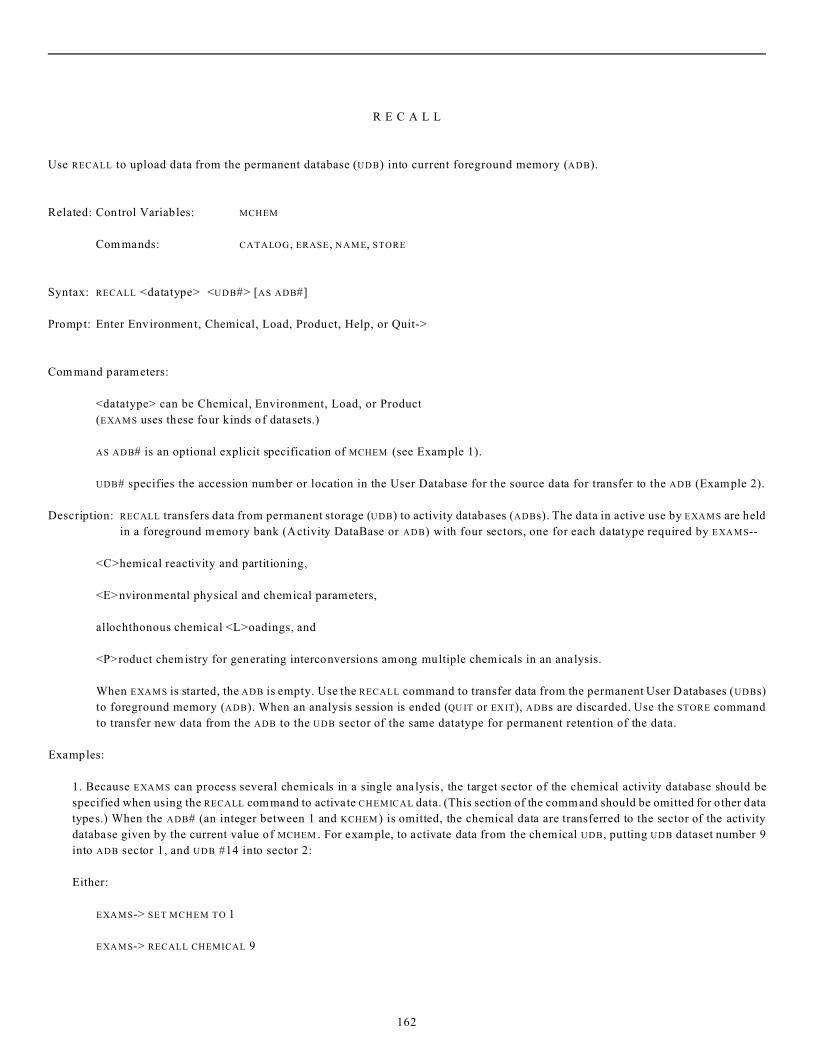
R E C A L L
Use RECALL to upload data from the permanent database (UDB) into current foreground memory (ADB).
Related: Control Variables: MCHEM
Com mands: CATALOG, ERASE, N A M E, STORE
Syntax: RECALL <datatype> <UDB#> [AS ADB#]
Prompt: Enter Environment, Chemical, Load, Product, Help, or Quit->
Com mand parameters:
<datatype> can be Chemical, Environment, Load, or Product
(E XA M S uses these four kinds of datasets.)
AS ADB# is an optional explicit specification of MCHEM (see Example 1).
UDB# specifies the accession number or location in the User Database for the source data for transfer to the ADB (Example 2).
Description: RECALL transfers data from permanent storage (UDB) to activity databases (ADBs). The data in active use by E XA M S are held
in a foreground m emory bank (Activity DataBase or ADB) with four sectors, one for each datatype required by E XA M S--
<C>hemical reactivity and partitioning,
<E>nvironmental physical and chemical parameters,
allochthonous chemical <L>oadings, and
<P>roduct chemistry for generating interconversions among multiple chemicals in an analysis.
When E XA M S is started, the ADB is empty. Use the RECALL command to transfer data from the permanent User Databases (UDBs)
to foreground memory (ADB). When an analysis session is ended (QU IT or EX IT), ADBs are discarded. Use the STORE command
to transfer new data from the ADB to the UDB sector of the same datatype for permanent retention of the data.
Examples:
1. Because E XA M S can process several chemicals in a single ana lysis, the target sector of the chemical activity database should be
specified when using the RECALL com mand to activate CHEMICAL data. (This section of the comm and should be omitted for other data
types.) When the ADB# (an integer between 1 and KCHEM ) is omitted, the chemical data are transferred to the sector of the activity
database given by the current value of MCHEM . For exam ple, to activate data from the chemical UDB, putting UDB dataset number 9
into ADB sector 1, and UDB #14 into sector 2:
Either:
E XA M S-> SET MCHEM TO 1
E XA M S-> RECALL CHEMICAL 9
162

E XA M S-> SET MCHEM TO 2
E XA M S-> RECALL CHEMICAL 14
or, equivalently:
E XA M S-> RECALL CHEMICAL 9 AS 1
E XA M S-> RECALL CHEMICAL 14 AS 2
2. Long-term retention of data required by E XA M S is provided by storage in the “User Database” (UDB, generally resident on a physical
device--e.g., a hard d isk) for Chemicals, Environments, Loads, or Products. Within each UDB sector, each dataset is catalogued via
a unique accession number (UDB#). When transferring data to foreground memory (the activity database or ADB) from a UDB, the
source location must be specified by the name of the UDB sector and the accession number within the sector. For example, to RECALL
an environmental dataset:
E XA M S-> RECALL ENVIR 2
Selected environment is: Phantom Inlet, Bogue Sound
E XA M S->
163

R U N
The RUN command begins a simulation analysis.
Related: Control Variables: MODE
Com mands: CONTINUE
Syntax: RUN
Prompt: None
Description: The RUN command executes an analysis and creates the output files accessed by the LIST and PLOT com mands. The activity
database (ADB) must be loaded, either via entry of new data or by RECALL from the UDB, before a RUN can be started.
Examples:
1. E XA M S-> RECALL CHEMICAL 22
Selected compound is: Dibromoexample
E XA M S-> RECALL ENVIRON 17
Selected environment is: Albemarle Sound--Bogue Bank
E XA M S-> SET STRL(1,1,13)=.01
E XA M S-> RUN
Simulation beginning for:
Environment: Albemarle Sound--Bogue Bank
Chemical 1: Dibromoexample
Run complete.
E XA M S->
In this example, a steady-state (MODE=1) analysis is conducted by selecting a chem ical and an environment, imposing a loading
of chemical 1 on segment 1 under average conditions (i.e., data sector 13, E XA M S initial default value) and invoking E XA M S’
simulation algorithms with the RUN command.
164

S E T
Use SET to specify the values of data in the activity database.
Related: Com mands: CHANGE (synonym), DESCRIBE, HELP
Syntax: SET <name of variable> TO <new value>
or
SET <name of variable> = <new value>
Prompt: Enter name=value com mand->
Variable: The data entry or variable to be SET can be specified either as a single datum or, using wild cards (*), as an entire vector,
row/column of a matrix, etc.
Description: Use the SET com mand to specify the values of data in the activity database. “Value” can be any num erical quantity or literal,
as appropr iate. “Variable” specifies an individual element of input data or a program control parameter. Entire vectors,
rows/columns of matrices, etc. can be set to single values using wild cards (*).
Examples:
1. E XA M S-> SET VOL(167) TO 7E5
Subscript out-of-range.
E XA M S-> DESCRIBE VOL
VOL is a Real Vector with 100 elem ents.
E XA M S> SET VOL(2) TO E
Invalid numeric quantity after TO.
E XA M S-> SET VOL(2) TO 7E5
This command sets the environmental volume of segment 2 to 7.0E+05 cubic meters. The initial attempt to set the volume of segment
67 was rejected by E XA M S because the version in use was set up for environmental models of 100 segments at most. The DESCRIBE
command was used to check the number of subscripts and the dimensional size of the variable “VOL”. The erroneous entry of an
alphabetic for the volume was trapped by the SET comm and; the initial value of VOL(2) was not altered.
2. E XA M S-> HELP TCEL
TCEL is a Real Matrix with 100 rows and 13 columns.
Temperature-CELsius (segment, month) Units: degrees C.
Average temperature of ecosystem segments. Used (as enabled by input data) to compute effects of temperature on transformation
rates and o ther properties of chem icals.
165

E XA M S-> SET TCEL(2,7)=24
This comm and changes the July temperature in segment 2 to 24°C. The HELP command was used to check subscript dimensions,
maximum values, the meaning of the subscripts (subscript #1 denotes the segment; subscript #2, the month), and the proper units for
the input datum (degrees Celsius).
3. E XA M S-> HELP POH
POH is a Real Matrix with 100 rows and 13 columns.
pOH (segment, month) Units: pOH units
The negative value of the power to which 10 is raised in order to obtain the temporally averaged concentration of hydroxide [OH-]
ions in gram-molecules per liter.
E XA M S-> SET POH(*,13) TO 6.2
This command sets the average pOH (sector 13) of every segment to 6.2. Note use of w ild card “*” to specify that all segments are
to be changed. As in the previous exam ple, HELP was used to check subscript dimensions, units, etc. This step, of course, is optional.
166

S H O W
Use SHOW to display current data values or control settings.
Related: Control Variables: MCHEM , MON TH
Com mands: CHANGE, SET
Syntax: SHOW <option> [range]
Prompt: The following options are available:
Advection, Chemistry, Dispersion, GEometry,
GLobals, Loads, PLot, PUlse Loads,
PRoducts, QUAlity, Time Frame, Variables,
Help, or QUIt->
Com mand parameters:
Range: Some options of the SHOW command accept the specification of a range of values to define the scope of the data to be
displayed (see Example 1). Use MCHEM to delimit the range of SHOW Chemistry, and MON TH for GEometry, QUAlity, etc.
Options:
ADVECTION
SHOW ADVECTION gives the advective hydrologic flow structure of the current aquatic system. A single element in a dataset might
typically look like the following example.
J FR AD 1 J FRom ADvection: Source Segment
I TO AD 3 I TO ADvection: Terminus
ADV PR 1.00 ADVection Proportion: Percent
of total JFRAD flow on path
Path No.: 1 Vector index for SETting data
No more than NCON hydrologic pathways can be specified. If more are needed, special versions of E XA M S can be produced. Specify
export pathways by entering a zero (0) for the number of the segment to receive the flow (ITOAD). Do not specify a hydrologic source
term by entering zero in the JFRAD vector; instead use stream flows, non-point-source flows, etc.
DISPERSION
SHOW DISPERSION displays the input data describing transport in the active (loaded in the ADB) Environm ental dataset. The index
vectors (JTURB, ITURB) define the existence of inter-segment dispersive transport paths. A zero in either vector, when paired with a
non- zero value at the corresponding position in the other index vector, is taken as a boundary condition with an uncontaminated body
of water. A single element in a dataset might typically be displayed like the following example.
J TURB 1 Segment number for dispersion
I TURB 2 Segment number for dispersion 2
XS TUR m 5.000E+04 Cross-sectional area of path
CHARL m 2.53 CHARacteristic_Length of path
167

DSP m2/h 4.676E-05 Eddy DiSPersion coefficient
Path N o.: 1 Vector index for data entry
No more than NCON hydrologic pathways can be specified. If more are needed, this number can be increased and E XA M S recompiled.
CHEMISTRY
SHOW CHEMISTRY displays the chemical output data currently in the ADB (foreground memory bank). The sector of the ADB denoted
by the current value of MCHEM is displayed. Within each sector of the ADB (that is, for each chemical under active review), the data
for each ionic species are presented separately, and photochemical data are presented on separate screens.
GEOMETRY
S H O W GEOMETRY returns a segment-by-segment description of the geom etry (volum es, areas, etc.) of the current ecosystem. The
segment number reported with each block of data is the first subscript for modifying the datum using CHANGE or SET. The month to
be displayed is set by the current value of MON TH (explicit mean values are denoted by MON TH number 13): the month is the second
subscript of such data as WIND, STFLO, etc.
GLOBALS
SHOW GLOBALS displays the input data that are “global” in extent, that is, “global” data apply to all segments of the current ecosystem.
LOADS
SHOW LOADS displays the current state of allochthonous chemical loadings. The form of the display depends on the current operational
MODE: initial values are ignored in Mode 1 as they have no effect on the analysis results. The value of PRSW also affects the display:
when PRSW is 0, SHOW LOADS returns a summary of annual loadings; when PRSW=1, a month-by-month tabulation is d isplayed as well.
This display may not represent the final values used in the analysis, because E XA M S will modify loads that result in violation of the
linearizing assumptions used to construct the program. After a RUN has been executed, however, SHOW LOADS will display the
corrected values.
PRODUCTS
SHOW PRODUCTS displays the specifications for product chemistry currently in the ADB. Each entry is identified and loaded according
to a unique “pathway number.” A single element of a dataset might look like this:
CH PAR 1 ADB number of CHemical PARent
T PROD 2 ADB number of Transformation PRODuct
N PROC 7 Number of transforming PROCess
R FORM 29 Reactive FORM (dissolved, etc.)
YIELD M/M 0.100 Mole/Mole YIELD of product
EAYLD Kcal 0.000 Enthalpy of yield (if appropriate)
Pathway: 1 Number of the pathway
More detail as to the numbering of NPROC and RFORM is given in the Data Dictionary (page 175), which can also be accessed on-line
using the HELP command. No more than NTRAN transformation pathways can be specified. If more are needed, a special version of
E XA M S can be created.
168

PLOT
SHOW PLOT examines the contents of the concentration time-series and steady-state files, and reports the names of the chemicals and
ecosystem used in the analysis.
PULSE LOADS
SHOW PULSE LOADS displays the specifications for allochthonous pulses of chemicals entering the system. This display may not
represent the final values used in the analysis, because E XA M S will modify loads that result in violation of the linearizing assumptions
used to construct the program. Although faulty pulse loads are discarded, E XA M S does not correct the input pulse load data, because
the occurrence of load constraint violations depends on the context (i.e., the size of current stream load ings, etc.). Thus, unlike SHOW
LOADS, the SHOW PU LSE display following execution of a RUN does not display corrected data. The pulses actually used during an
analysis are instead entered into E XA M S’ output tables, where they can be examined using the LIST and PRINT commands.
QUALITY
SHOW QUALITY returns a segment-by-segment display of the canonical water-quality data included in the current Environm ental ADB
dataset. The month to be displayed is set by the current value of MON TH (explicit mean values are denoted by MON TH number 13).
The month is the second subscript of such data as pH, pOH, etc. The first subscript is the segment number; thus these data are entered
(CHANGE/SET) as “datum(segment,month)”.
T IM E FR A M E
SHOW T IM E FR A M E displays the current status of the parameters needed to control the temporal aspects of a Mode 2 or Mode 3
simulation.
VARIABLES
SHOW VARIABLES displays a list of the names of E XA M S input data and control parameters. These nam es must be used to SET/CHANGE,
SHOW values, HELP/DESCRIBE, etc.
Description: Use the SHOW command to examine the current contents of the ADB, that is, the foreground datasets used for the current
analysis. The SHOW comm and can be used to examine clusters of similar data, the values of individual parameters, or the
data contained in entire vectors. Typing SHOW without an option will display a list of the available options.
Examples: 1. The SHOW command can be used to examine the value of single parameters. For example, the pH of segment
7 of the current ecosystem during September could be inspected by entering:
E XA M S-> SHOW PH(7,9)
Using wild cards (*), the SHOW command can also be used to display the data in an entire vector or row/column of a data matrix.
For example, the pH in every segment of the current ecosystem during September could be displayed by entering:
E XA M S-> SHOW PH(*,9)
and the pH of segment 7 through the year could be displayed by:
E XA M S-> SHOW PH(7,*)
169

S T O R E
Use STORE to download current (ADB) data into the permanent database (UDB).
Related: Control Variables: MCHEM
Com mands: CATALOG, ERASE, N A M E, RECALL
Syntax: STORE <datatype> [ADB# IN] <UDB#>
Prompt: Enter Environment, Chemical, Load, Product, Help, or Quit->
Com mand parameters:
<datatype> can be Chemical, Environment, Load, or Product
(E XA M S uses these four kinds of datasets.)
ADB# IN is an optional explicit specification of MCHEM (see Example 1).
UDB# specifies the accession num ber or location in the User Database for storage of the current ADB sector (Example 2).
Description: STORE dow nloads data from activity databases (ADBs) into the permanent User DataBases (UDBs). The data in active use by
E XA M S are held in a foreground m emory bank (Activity DataBase or ADB) with four sectors, one for each datatype required
by E XA M S:
CHEMICAL reactivity and partitioning,
ENVIRONMENTal physical and chemical parameters,
allochthonous chem ical LOADings, and
PRODUCT chemistry for generating interconversions among multiple chemicals in an analysis.
When an analysis session is ended (QU IT or EX IT), these data are discarded. Use the STORE command to transfer data from the
ADB to the UDB sector of the same datatype for permanent retention of the data.
Examples: 1. Because E XA M S can process several chemicals in a sing le analysis, the source sector of the chemical activity
database should be specified when using the STORE command to download CHEMICAL data. (This section of
the command should be omitted for other data types.) When the ADB# (an integer from 1 to KCHEM ) is omitted,
the chem ical data are taken from the sector of the activity database given by the current value of MCHEM . For
example, to STORE data in the UDB, putting ADB sector 1 into the chemical UDB under catalog/accession 9 and
ADB sector 2 into UDB sector 14:
Either:
E XA M S-> SET MCHEM TO 1
E XA M S-> STORE CHEMICAL 9
E XA M S-> SET MCHEM TO 2
E XA M S-> STORE CHEMICAL 14
or, equivalently:
170

E XA M S-> STORE CHEMICAL 1 IN 9
E XA M S-> STORE CHEMICAL 2 IN 14
2. Long-term retention of data required by E XA M S is provided by storage in the “User Database” (UDB, generally resident on a
physical device--e.g., a hard disk) for Chemicals, Environments, Loads, or Products. Within each of these UDB sectors, each
dataset is CATALOGued via a unique accession number (UDB#). When transferring data between foreground m emory (the activity
database or ADB) and a UDB, the target location must be specified by the name of the UDB sector and the accession number within
the sector. For example, to STORE the current environmental dataset:
E XA M S-> STORE ENVIR 2
Environment record 2 is in use with
Pond -- code test data
Replace?-> no
Nothing changed.
E XA M S-> STORE ENVIR 14
Environment stored: Phantom Inlet-Bogue Sound Study Data
E XA M S->
Note that E XA M S provides a measure of protection against accidental overwriting of existing datasets, an important courtesy in
a multi-user environment.
171
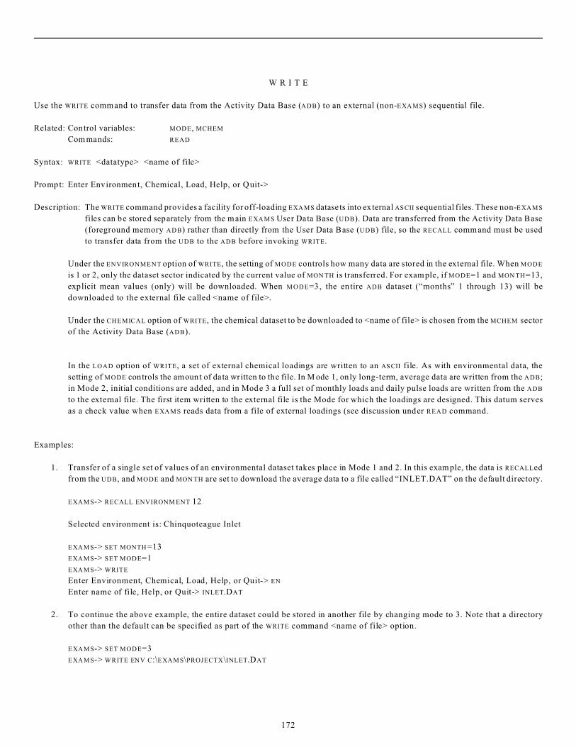
W R I T E
Use the WRITE command to transfer data from the Activity Data Base (ADB) to an external (non-E XA M S) sequential file.
Related: Control variables: MODE, MCHEM
Com mands: READ
Syntax: WRITE <datatype> <name of file>
Prompt: Enter Environment, Chemical, Load, Help, or Quit->
Description: The WRITE command provides a facility for off-loading E XA M S datasets into ex ternal AS CII sequential files. These non-E XA M S
files can be stored separately from the main E XA M S User Data Base (UDB). Data are transferred from the Activity Data Base
(foreground memory ADB) rather than directly from the User Data Base (UDB) file, so the RECALL command must be used
to transfer data from the UDB to the ADB before invoking WRITE.
Under the ENVIRONMENT option of WRITE, the setting of MODE controls how many data are stored in the external file. When MODE
is 1 or 2, only the dataset sector indicated by the current value of MON TH is transferred. For example, if MODE=1 and MON TH=13,
explicit mean values (only) will be downloaded. When M O D E=3, the en tire ADB dataset (“months” 1 through 13) will be
downloaded to the external file called <name of file>.
Under the CHEMICAL option of WRITE, the chemical dataset to be downloaded to <name of file> is chosen from the MCHEM sector
of the Activity Data Base (ADB).
In the LOAD option of WRITE, a set of external chemical loadings are written to an AS CII file. As with environmental data, the
setting of MODE controls the amount of data written to the file. In M ode 1, only long-term, average data are written from the ADB;
in Mode 2, initial conditions are added, and in Mode 3 a full set of monthly loads and daily pulse loads are written from the ADB
to the external file. The first item written to the external file is the Mode for which the loadings are designed. This datum serves
as a check value when E XA M S reads data from a file of external loadings (see discussion under READ command.
Examples:
1. Transfer of a single set of values of an environmental dataset takes place in Mode 1 and 2. In this exam ple, the data is RECALLed
from the UDB, and MODE and MON TH are set to download the average data to a file called “INLET.DAT” on the default directory.
E XA M S-> RECALL ENVIRONM ENT 12
Selected environment is: Chinquoteague Inlet
E XA M S-> SET MONTH =13
E XA M S-> SET MODE=1
E XA M S-> WRITE
Enter Environment, Chemical, Load, Help, or Quit-> EN
Enter name of file, Help, or Quit-> INLET.DAT
2. To continue the above example, the entire dataset could be stored in another file by changing mode to 3. Note that a directory
other than the default can be specified as part of the WRITE command <name of file> option.
E XA M S-> SET MODE=3
E XA M S-> WRITE ENV C:\E XA M S\PROJECTX\INLET.DAT
172
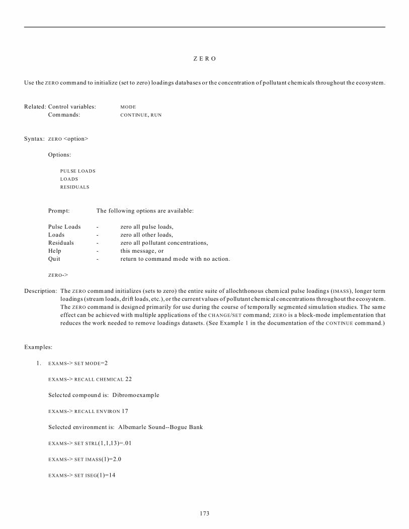
Z E R O
Use the ZERO command to initialize (set to zero) loadings databases or the concentration of pollutant chemicals throughout the ecosystem.
Related: Control variables: MODE
Com mands: CONTINUE, RUN
Syntax: ZERO <option>
Options:
PULSE LOADS
LOADS
RESIDUALS
Prompt: The following options are available:
Pulse Loads - zero all pulse loads,
Loads - zero all other loads,
Residuals - zero all pollutant concentrations,
Help - this message, or
Quit - return to command mode with no action.
ZERO->
Description: The ZERO comm and initializes (sets to zero) the entire suite of allochthonous chem ical pulse loadings (IMASS), longer term
loadings (stream loads, drift loads, etc.), or the current values of pollutant chemical concentrations throughout the ecosystem.
The ZERO command is designed primarily for use during the course of temporally segmented simulation studies. The same
effect can be achieved with multiple applications of the CHANGE/SET com mand; ZERO is a block-mode implementation that
reduces the work needed to remove loadings datasets. (See Example 1 in the documentation of the CONTINUE com mand.)
Examples:
1. E XA M S-> SET MODE=2
E XA M S-> RECALL CHEMICAL 22
Selected compound is: Dibromoexample
E XA M S-> RECALL ENVIRON 17
Selected environment is: Albemarle Sound--Bogue Bank
E XA M S-> SET STRL(1,1,13)=.01
E XA M S-> SET IMASS(1)=2.0
E XA M S-> SET ISEG(1)=14
173

E XA M S-> SET ICHEM(1)=1
E XA M S-> RUN
Simulation beginning for:
Environment: Albemarle Sound--Bogue Bank
Chemical 1: Dibromoexample
Run complete.
.
.
.
E XA M S-> ZERO PULSE LOADS
E XA M S-> CONTINUE
In this example, an initial-value (MODE=2) analysis is begun by selecting a chemical and an environment, imposing an allochthonous
load of chemical 1 on segment 1 under average conditions (i.e., data sector 13, E XA M S’ initial default value), and specifying the initial
presence (or introduction at time zero) of 2.0 kg of material in segment 14. At the end of the initial RUN segm ent, one m ight want to
examine the output tables, plot the results, etc. Then, before CONTINUing, the ZERO command is used to remove the pulse load
specifications. If this were not done, E XA M S would introduce a second 2.0 kg pulse into segment 14 at the beginning of the
continuation segment. Alternatively, the other loadings could have been removed, and the effect of a series of pulse loads could be
studied by issuing a sequence of CONTINUE commands.
174

6.0 EXAMS Data Dictionary
ABSER ADVPR
ABSolute ERror tolerance of integrators ADVection PRoportion (path)
Units: n/a Range: > 0 – 1.0
When the characteristics of the chemical and ecosystem are
such as to result in “stiff” equations, numerical errors may PRoportion of flow ADVected from segm ent JFRAD that
lead to small negative numbers in the time series. If desired, enters ITOAD. The matching (same subscript) members of
the value of ABSER and RELER can be decreased in order to JFRAD, ITOAD, and ADVPR define an advective hydrologic
achieve greater precision in the sim ulation ou tputs. flow pathway. Although usually 1, ADVPR lets one enter
braided channels, etc. The total of ADVPR s for each segment
ADB must sum to either 0 or 1 , failing which, E XA M S aborts the
Activity DataBase RUN. The flow data can be inspected by typing SHOW ADV;
path numbers are given above each active dataset. Enter
E X AM S provides for long-term storage of CHEM ical, data via CHANGE or SET commands.
ENVironmental, transformation PRODuct chemistry, and
allochthonous LOADings databases in a User DataBase or Additional information available: JFRAD, ITOAD
UDB. The actual analyses are conducted on particular
datasets drawn from these files (or entered via AEC
SET/CHANGE). Particular cases are loaded from the UDB into Anion Exchange Capacity (segment, month)
the foreground transient memory of your computer in an Units: meq/100 g (dry)
Activity DataBase or ADB, using the RECALL command.
Because E XA M S simulates the behavior of several (MCHEM ) Anion exchange capacity of sediment phase of each
chemicals simultaneously, the ADB for chemicals has segm ent. Useful in relating sediment sorption (partitioning)
MCHEM separate sectors. These data are lost when you EX IT of anions to a variable characteristic of system sediments.
from E XA M S, so be sure to STORE any new or corrected
datasets before leaving E XA M S. AIRTY
AIR mass TYpe (month)
ABSOR Units: letter codes
ABSORption spectra (wavelength, ion, chem ical)
Units: cm-1(mole/L)-1 Select: Rural (default), Urban , Maritime, or Tropospheric
Mean decadic molar light extinction coefficients in 46 AREA
wavelength intervals over 280 – 825 nm. For wavelength AREA (segm ent)
“w” and chemical “c”: Units: m2
ABSOR(w,1,c) is molar absorption coefficient of RH3
(neutral molecule)
ABSOR(w,2,c) is molar absorption coefficient of RH4+ (+1
cation)
ABSOR(w,3,c) is molar absorption coefficient of RH52+ (+2
cation)
ABSOR(w,4,c) is molar absorption coefficient of RH63+ (+3
cation)
Top plan area of each model segment of the water body. For
Epilimnion and Littoral segments, AREA is the area of the
air-water interface; for Hypolimnion segm ents AREA is the
area of the thermocline; for Benthic segments it is the
surface area of the bottom. In the latter case AREA may
differ from XSTUR in a dispersive exchange pair because of
reduction in exchanging area due to rock outcrops, etc.
!ABSOR(w,5,c) is molar absorption coefficient of RH2 (!1 ATURB
anion) Atmospheric TURBidity (month)
ABSOR(w,6,c) is molar absorption coefficient of RH2! (!2 Units: km
anion)
ABSOR(w,7,c) is molar absorption coefficient of R3! (!3 Equivalent aerosol layer thickness.
anion)
AUDOUT
While the AU DIT directive is in effect, a copy of user inputs
175

and responses is written to the file connected to
FORTRAN Logical Unit Number AUDOUT.
BACPL
BACterioPLankton population (segment, month)
Units: cfu/mL
Population density of bacteria capable of degrading
xenobiotics. The abbreviation “cfu” stands for a “colony
form ing unit.”
BNBAC
BeNthic BACteria (segment, month)
Units: cfu/100g dry sediment
Population density of benthic bacteria that degrade
xenobio tics. The abbreviation “cfu” stands for a “colony
form ing unit.”
BNMAS
BeNthic bioMASs (segment, month)
Units: g(dry)/m2
Biomass of small benthos – infauna subject to biosorption.
BULKD
BULK Density (segment, month)
Units: g/cm3
Fresh weight per unit volum e of ben thic sediments.
CEC
Cation Exchange Capacity (segment, month)
Units: meq/100g (dry)
Cation exchange capacity of sediment phase in each
segm ent. Useful in relating sediment sorption (partitioning)
of cations to a variable characteristic of system sediments.
CHARL
CHARacteristic Length or mixing length (path)
Units: m
Average of segment dimensions normal to the exchange
interface linking segment numbers JTURB(p) and ITURB(p).
The matching (same “p” subscript) members of JTURB,
ITURB, CHARL, DSP, and XSTUR together define a dispersive
transport pathway. A given segment may have different
mixing lengths at different interfaces. CHARL can also be
calculated from the distance along a path that connects the
centers of segm ents JTURB(p) and ITURB(p), passing through
the interface whose area is XSTUR(p).
See also: DSP, ITURB, JTURB, XSTUR
CHEMNA
CHEM ical NAme of compounds (50 characters,chem)
Units: n/a
Do not use “CHANGE” or “SET” to enter names! The NAme
for a CHEMical is entered into the database via the command
sequence:
E XA M S-> CH EM ICA L N AM E IS nnn ...
where “nnn... “ can include as many as 50 characters. This
name is associated with chemical library entries and is
printed in the header information of the appropriate output
tables.
CHL
CHLorophylls + pheophytins (segment, month)
Units: mg/L
Concentration of chlorophyll plus chlorophyll-like
pigments. Used to compute spectral light absorption
coefficients due to pigments which absorb light from the
water column and thus compete with photolysis of synthetic
chem icals.
CHPAR
CHemical PARent compound (path)
Units: n/a Range: 1– KCHEM
CHPAR(p) gives the ADB location of the parent source of
TPROD(p). The matching (same transformation path number
“p”) mem bers of CHPAR and TPROD give the location
numbers in the active database of the parent chemical and
the transformation product for pathway “p”. For example,
“SET CHPAR(p) TO 1", and TPROD(p) TO 4, to show that the
chemical in ADB sector 4 is produced via transformation of
the chemical in ADB sector 1, via process data defined by
the remaining members of product chemistry sector “p”.
See also: EAYLD, NPROC, RFORM, TPROD, YIELD
CINT
Communications INTerval for dynam ic simulations.
Units: see TCODE
CI NT is the interval between output cycles from the
integrators. In Mode 2, CINT can be set to produce any
desired output frequency, so long as the resulting reporting
interval is >1 hour. When CINT is set to 0, E XA M S (Mode 2)
sets CINT to report at the 12 equal-increment periods most
closely matching the duration specified by (TEND - TIN IT).
CINT is under full user control only in Mode 2; in Modes 1
and 3 E XA M S itself sets the value of CINT according to the
needs of the analysis.
176

CLOUD
CLOUDiness (month)
Units: dimensionless Range: 0 – 10
Mean monthly cloudiness in tenths of full sky cover.
DEPTH
DEPTH (segm ent)
Units: m
Average vertical depth of each segm ent.
DFAC
Distribution FACtor (segment, month)
Units: dimensionless ratio
Ratio of optical path length to vertical depth, range 1.0 –
2.0. A vertical light beam has a DFAC of 1.0; a fully diffused
light field has a DFAC of 2.0. For whole days, a value of
1.19 is often adequate; E XA M S defaults to this value when
the entry for DFAC is outside the range 1.0 – 2.0.
DISO2
DISsolved O2 (segment, month)
Units: mg/L
Concentration of dissolved oxygen (O2) in each segment of
ecosystem.
DOC
Dissolved Organic Carbon (segment, month)
Units: mg/L
Used for computing spectral light absorption, singlet
oxygen concentrations, and complexation.
DRFLD
DRiFt LoaD (segment, chemical, month)
Units: kg/hour
Drift loadings: aerial drift, direct applications, stack fallout
(etc.) of chemical on each system element.
DSP
DiSPersion coefficient (path, month)
Units: m2/hour
Eddy diffusivity to be applied to dispersive exchange
pairing “p”. The matching (same “p” subscript) members of
JTURB, ITURB, CHARL, and XSTUR together define a
dispersive transport pathway. In the case of horizontal
mixing, DSP is the longitudinal dispersion coefficient; for
vertical mixing it may represent exchange across the
thermocline or exchanges with bottom sediments. In the
latter case DSP is a statistical kinetic composite
incorporating direct sorption to the sediment surface,
mixing of the sediments by ben thos (bioturbation), stirring
by demersal fishes, etc.
See also: CHARL, ITURB, JTURB, XSTUR
EAH
E for Acid Hydrolysis (form , ion, chemical) a
Units: kcal/mol
Arrhenius activation energy Ea of specific-acid-catalyzed
hydrolysis of chemicals. Matrix indices match those of KAH,
giving, for each chemical, data for 3 forms (1: dissolved, 2:
solids-sorbed, 3: DOC-complexed) of 7 ionic species (1:
neutral; 2, 3, 4: cations; 5, 6, 7: anions). When EAH is
non-zero, the second-order rate constant K (M-1h-1) is
calculated from:
EAYLD
EA YieLD (path)
Units: kcal
EAYLD(p) is activation energy Ea to compute transformation
product yield as a function of environmental temperatures
(TCEL). When EA_YieLD(p) is zero, YIELD(p) gives the
dimensionless molar product yield. A non-zero EAYLD(p)
invokes a re-evaluation in which YIELD(p) is interpreted as
the Briggsian logarithm of the pre-exponential factor in an
Arrhenius-type function, giving product yield as a function
of temperature (varying with position and time)
(TCEL(segment, month)):
See also: CHPAR, NPROC, RFORM, TPROD, YIELD
EBH
E for Base Hydrolysis (form , ion, chemical) a
Units: kcal/mol
Arrhenius activation energy Ea of specific-base catalyzed
hydrolysis of chemicals. Matrix indices match those of KBH,
giving, for each chemical, data for 3 forms (1: dissolved, 2:
solids-sorbed, 3: DOC-complexed) of 7 ionic species (1:
neutral, 2, 3, 4: cations, 5, 6, 7: anions). When EBH is
non-zero, the second-order rate constant K (M-1h-1) is
calculated from:
177

EHEN
Enthalpy term for HENry’s law (chemical)
Units: kcal/mol
Used to compute Henry’s law constants as a function of
TCEL (environmental temperature). When EHEN is non-zero,
the Henry’s law constant (H) affecting volatilization a t a
particular (segment, month) is computed from TCEL:
EK1O2
E K1O2 (singlet oxygen) (form, ion, chemical) a
Units: kcal/mol
Arrhenius activation energy for singlet oxygen
photo-oxygenation of chemicals. Matrix indices match those
of K1O2, giving, for each chemical, data for 3 forms (1:
dissolved, 2: solids-sorbed, 3: DOC-complexed) of 7 ionic
species (1: neutral, 2, 3, 4: cations, 5, 6, 7: anions). When -1h-1)EK1O2 is non-zero, the second-order rate constant K (M
is calculated as:
ELEV
ELEVation
Units: meters above mean sea level
Ground station elevation.
ENH
E for Neutral Hydrolysis (form , ion, chemical) a
Units: kcal/mol
Arrhenius activation energy for neutral hydrolysis of
chemicals. Matrix indices match those of KNH, giving, for
each chemical, data for 3 forms (1: dissolved, 2:
solids-sorbed, 3: DOC-com plexed) of 7 ionic species (1:
neutral, 2, 3, 4: cations, 5, 6, 7: anions). When ENH is
non-zero, the pseudo-first-order rate constant (h-1) is
calculated from:
EOX
E OXidation (form , ion, chemical) a
Units: kcal/mol
Arrhenius activation energy for oxidative transformations of
chem icals. Matrix indices match those of KOX, giving, for
each chemical, data for 3 forms (1: dissolved, 2:
solids-sorbed, 3:DOC-com plexed) of 7 ionic species (1:
neutral, 2, 3, 4: cations, 5, 6, 7: anions). When EOX is
non-zero, the second-order rate constant K (M-1h-1) is
calculated from:
EPK
Enthalpy term for pK (ion, chem ical)
Units: kcal/mol
When EPK is non-zero, pK is computed as a function of
temperature via:
The vector indices for EPK (“c” denotes the chemical) are
EPK(1,c) contains datum for generation of RH4+ from RH3
+EPK(2,c) contains datum for generation of RH5
2+ from RH4 2+
EPK(3,c) contains datum for generation of RH63+ from RH5
EPK(4,c) contains datum for generation of RH2- from RH3
-EPK(5,c) contains datum for generation of RH= from RH2
EPK(6,c) contains datum for generation of R3- from RH=
ERED
E REDuction (form, ion, chemical) a
Units: kcal/mol
Arrhenius activation energy for reductive transformations of
chem icals. Matrix indices match those of KRED, giving, for
each chem ical, data for three forms (1: dissolved, 2:
solids-sorbed, 3: DOC-complexed) of seven ionic species (1:
neutral, 2, 3, 4: cations, 5, 6, 7: anions). When ERED is
non-zero, the second-order rate constant K (M-1h-1) is
calculated as:
ESOL
Enthalpy term for SOLubility (ion, chem ical)
Units: kcal/mol
ESOL describes chemical solubility as a function of
temperature (TCEL). The matrix indices (“c” denotes the
chemical) denote:
ESOL(1,c) is datum for solubility of neutral molecules RH3
ESOL(2,c) is datum for solubility of singly charged cations
178

RH4+
ESOL(3,c) is datum for solubility of doubly charged cations
RH52+
ESOL(4,c) is datum for solubility of triply charged cations
RH63+
ESOL(5,c) is datum for solubility of singly charged anions
RH2-
ESOL(6,c) is datum for solubility of doubly charged anions
RH=
ESOL(7,c) is datum for solubility of triply charged an ions R3
EVAP
EVAPoration (segment, month)
Units: mm /month
(Monthly) evaporative water losses from ecosystem
segments.
EVPR
Molar hEat of VaPoRization (chemical)
Units: kcal/mol
Enthalpy term for computing vapor pressure as a function
of TCEL (environmental temperature (segment,month)).
When EVPR is non-zero, vapor pressure Va is computed
from:
FIX FIL
FIX FIL signals the existence of output data for LISTs and
PLOTs.
To access results from a prior run, “SET FIXFIL TO 1.” FIX FIL
is set to zero when E XA M S is invoked, so that the LIST and
PLOT commands are protected from attem pts to access
non-existent output data files. When results exist from a
previous simulation, you can reset FIX FIL to 1 in order to
gain access to them.
FROC
FRaction Organic Carbon (segment, month)
Units: dimension less
Organic carbon content of solids as fraction of dry weight.
FROC is coupled to KOC to generate the sediment partition
coefficient for neutral chemicals (R-H3) as a function of a
property (organic carbon content) of the sedim ent.
HENRY
HENRY’s law constant (chem ical)
Units: atmosphere-m 3/mole
Used in computation of air/water exchange rates
(volatilization). If parameter EHEN is non-zero, HENRY is
used as the pre-exponential factor in computing the Henry’s
law constant H as a function of environmental temperatures
(TCEL):
ICHEM
I CHEM ical (event)
Units: n/a Range: 1--KCHEM
Event “e” is a pulse of chemical number ICHEM(e) in the
active database ICHEM identifies the location in the A ctivity
Database (ADB) of the chemical entering the ecosystem via
pulse load event “e”. When, for example, chemical data are
loaded into ADB sector 3 (whether RECALLed from the User
Database Library (UDB) (via, for example, the command
sequence “R EC A LL CH EM 7 AS 3") or entered as new data),
ICHEM(e) can be SET to 3 to create a pulse load event of that
chemical.
See also: IDAY, IMASS, IMON, ISEG
IDAY
I DAY (event)
Units: n/a Range: 1--31
Pulse load ev ent “e” takes place on day IDAY(e) of month
IMON(e). The pulse load data are organized by vertical event
colum ns, that is, the set of pu lse load variables (IMASS(e),
ICHEM(e), ISEG(e), IMON(e), and IDAY(e)) with the same
vector subscript describes a single chemical pulse event.
Thus a pulse of chem ical ICHEM(e), of magnitude
IMASS(e), is released into segm ent ISEG(e) on day IDAY(e)
of month IMON(e). During mode 2 simulations, IDAY and
IMON are inoperative.
See also: ICHEM, IMASS, IMON, ISEG
IMASS
Initial MASS (event)
Units: kg
IM ASS gives the magnitude of chemical pulse load event
“e”. In mode 2, pulses are entered at time 0 (i.e., as initial
conditions), and at the outset of each CONTINUation of the
simulation. In mode 3, IMON and IDAY specify the date of
the load events. An event recurs in each year of the RUN or
CONTINUed simulation. The pulse load data are organized by
vertical event columns; that is, the series of pulse load
variables (IMASS, ICHEM, ISEG, IMON, and IDAY) with the
same vector subscrip t describes a single even t.
179

See also: ICHEM, IDAY, IMON, ISEG
IMON
I MONth (event)
Units: n/a Range: 1--12
Pulse load event “e” takes place on day IDAY(e) of month
IMON(e). The pulse load data are organized by vertical event
colum ns; that is, the set of pulse load variables (IMASS(e),
ICHEM (e), ISEG(e), IMON(e), and IDAY(e)) with the same
vector subscript describes a single chemical pulse event.
Thus a pulse of chem ical ICHEM(e), of magnitude IMASS(e),
is released into segm ent ISEG(e) on day IDAY(e) of month
IMON(e). During mode 2 simulations, IDAY and IMON are
inoperative.
See also: IDAY, ICHEM, IMASS, ISEG
ISEG
I SEGment (event)
Units: n/a Range: 1--KOUNT
Pulse load even t “e” loads chem ical ICHEM(e) on segment
ISEG(e). Any segment can receive a pulse load. Should the
pulse loads increase the free concentration of unionized
chemical above 10-5 M (or half its aqueous solubility,
whichever is less), the size of the event is reduced, to avoid
violating the linearizing assumptions used to create E XA M S.
The pulse load data are organized by vertical event
colum ns; that is, the pulse load variables having the same
vector subscrip t define a sing le chemical pulse event.
See also: ICHEM, IDAY, IMASS, IMON
ITOAD
I TO ADvection (path)
Units: n/a Range: 0--KOUNT (0 = export)
Chemicals are advected to segm ent ITOAD(p) from segment
JFRAD(p). The matching (same subscript) members of
JFRAD, ITOAD, and ADVPR define an advective hydrologic
flow pathway carrying entrained chemicals and solids
through the water body. When ITOAD(p) is 0, the pathway
advects water and entrained substances across system
boundaries, i.e., ITOAD(p) = 0 specifies an export pathway.
The flow data can be inspected by typing “SHOW ADV”; path
numbers are given above each active dataset. Enter data
with SET or CHANGE commands.
See also: JFRAD, ADVPR
ITURB
I TURBulent dispersion (path)
Units: n/a Range: 0--KOUNT
Segments ITURB(p) and JTURB(p) exchange via turbulent
dispersion. The matching (same “p” subscript) members of
ITURB, JTURB, CHARL, DSP, and XSTUR together define a
dispersive transport pathway; ITURB(p) and JTURB(p)
indicate which segments are linked by dispersive transport
pathway “p”. A “0" in ITURB paired with a non-zero
segment number in JTURB denotes a boundary condition
with a pure (zero chemical) water-body. The input data can
be exam ined via SHOW TURBULENCE; pathway numbers are
shown with each dataset.
See also: CHARL, DSP, JTURB, XSTUR
IUN IT
IUN IT controls the printing of diagnostics from the
integrators.
Normally zero (off), it may be turned on when problems
occur. To manually set IUN IT to generate integrator
diagnostic messages, SET IUNIT TO 1. The message generator
can be disabled at any time by SETting IUN IT to 0.
JFRAD
J FRom ADvection (path)
Units: n/a Range: 1– KOUNT
Chemicals are advected from segm ent JFRAD(p) to segment
ITOAD(p). The matching (same subscript) members of
JFRAD, ITOAD, and ADVPR define an advective hydrologic
flow pathway. E XA M S computes the total net flow availab le
for advection from segm ent JFRAD(p). Of the total flow, the
fraction A DVPR(p) flows from segm ent JFRAD(p) into
segment ITOAD(p). The hydrologic flow carries an entrained
mass of chemical along the pathway. The flow
specifications can be inspected by typing SHOW ADV;
pathway numbers are given above each active dataset. Enter
data with SET or CHANGE commands.
See also: ITOAD, ADVPR
JTURB
J TURBulent dispersion (path)
Units: n/a Range: 0--KOUNT
Segments JTURB(p) and ITURB(p) exchange via turbulent
dispersion. The matching (same “p” subscript) members of
JTURB, ITURB, CHARL, DSP, and XSTUR together define a
dispersive transport pathway; JTURB(p) and ITU RB(p)
indicate which segments are linked by dispersive transport
pathway “p”. A “0" in JTURB paired with a non-zero
segment number in ITURB denotes a boundary condition
with a pure (zero chemical) water-body. The input data can
be examined via SHOW TURBULENCE; pathway numbers are
shown with each dataset.
180

See also: CHARL, DSP, ITURB, XSTUR
KAH
K Acid Hydrolysis (form , ion, chemical)
Units: per mole [H+] per hour
Second-order rate constant for specific-acid-catalyzed
hydrolysis of chemicals. When the matching (same
subscripts) Arrhenius activation energy (EAH) is zero, KAH
is interpreted as the second-order rate constant. When the
matching entry in EAH is non-zero , KAH is interpreted as the
(Briggsian) logarithm of the frequency factor in an
Arrhenius equation, and the 2nd-order rate constant is
computed as a function of segment temperatures TCEL.
Matrix indices refer to three forms--1: aqueous, 2:
solids-sorbed, and 3: DOC-complexed; by seven ions--1:
neutral, 2-4: cations, and 5-7: anions.
KBACS
K BACteria benthoS (form , ion, chemical)
Units: (cfu/mL)-1 hour-1
Second-order rate constants--benthic sediment bacterial
biolysis of chemicals normalized by “colony form ing units”
(cfu) per mL. W hen the matching (same subscripts) Q10
(QTBAS) is zero, KBACS is interpreted as the second-order
rate constant. When the matching entry in QTBAS is
non-zero, KBACS is interpreted as the numerical value of the
second-order rate constant at 25°C, and local values of the
rate constant are computed as a function of temperature
(TCEL) in each ecosystem segm ent. Indices refer to four
forms--1: aqueous, 2: solids-sorbed, 3: DOC-complexed, and
4: bio-sorbed; by seven ions--1: neutral, 2-4: cations, and
5-7: anions.
KBACW
K BACterioplankton Water (form, ion, chemical)
Units: (cfu/mL)-1 hour-1
Second-order rate constants K for water column bacterial
biolysis of chemicals normalized by “colony forming units”
(cfu) per mL. When the matching (same subscripts) Q10
(QTBAW) is zero, KBACW is interpreted as the second-order
rate constant. When the matching entry in QTBAW is
non-zero, KBACW is interpreted as the numerical value of
the second-order rate constant at 25°C, and local values of
the rate constant are computed as a function of temperature
(TCEL) in each ecosystem segment. Indices refer to four
forms--1: aqueous, 2: solids-sorbed, 3: DOC-complexed, and
4:bio-sorbed; by seven ions--1: neutral, 2-4: cations, and
5-7: anions.
KBH
K Base Hydrolysis (form , ion, chemical)
Units: per mole [OH-] per hour
Second-order rate constant for specific-base-catalyzed
hydrolysis of chemicals. When the matching (same
subscripts) Arrhenius activation energy (EBH) is zero, KBH
is interpreted as the second-order rate constant. When the
matching entry in EBH is non-zero , KBH is interpreted as the
(Briggsian) logarithm of the frequency factor in an
Arrhenius equation, and the 2nd-order ra te constant is
computed as a function of segm ent temperatures TCEL.
Matrix indices refer to three forms--1: aqueous, 2:
solids-sorbed, and 3: DOC-complexed; by seven ions--1:
neutral, 2-4: cations, and 5-7: anions.
KCHEM
Number of chemicals under review in current study.
Units: n/a
KDP
K Direct Photo lysis (ion , chem ical)
Units: hour-1
Estimated photolysis rates--use only when ABSOR, the actual
light absorption spectra of the compound in pure water, are
unavailable. KDP is an annual average pseudo-first-order
pho tolysis rate constant under cloudless conditions at
RFLAT, where
KDP(1,c) are pseudo-first-order photolysis ra te constants of
neutral molecules RH3
KDP(2,c) are pseudo-first-order photolysis rate constants of
singly charged cations RH4+
KDP(3,c) are pseudo-first-order photolysis rate constants of
doubly charged cations RH52+
KDP(4,c) are pseudo-first-order photolysis ra te constants of
triply charged cations RH63+
KDP(5,c) are pseudo-first-order photolysis rate constants of
singly charged anions RH2-
KDP(6,c) are pseudo-first-order photolysis rate constants of
doubly charged anions RH=
KDP(7,c) are pseudo-first-order photolysis ra te constants of
triply charged anions R3
KIEC
Kp for Ion Exchange Capacity (ion, chemical)
Units: Kp (meq/100g dry)-1
Coefficient relating sediment partition coefficient Kp of
ions to exchange capacity of sediments. KIEC times the
cation exchange capacity CEC(seg, month) (or anion
exchange capacity AEC for anionic species) gives the Kp for
sorption of ions with solid phases. This com putation is
overridden by explicit (non-zero) values of KPS, i.e., a non
zero value of KPS takes precedence over a Kp computed by
181

E XA M S using KIEC.
KIEC(1,c) is datum for relating CEC and sorption of singly
charged cation RH4+
KIEC(2,c) is datum for relating CEC and sorption of doubly
charged cation RH52+
KIEC(3,c) is datum for relating CEC and sorption of triply
charged cation RH63+
KIEC(4,c) is datum for relating AEC and sorption of sing ly
charged anion RH2-
KIEC(5,c) is datum for relating AEC and sorption of doubly
charged anion RH=
KIEC(6,c) is datum for relating AEC and sorption of triply
charged anion R3
KINOUT
Logical Unit Number for writing results of numerical
integration to kinetics plotting file.
KNH
K Neutral Hydrolysis (form , ion, chemical)
Units: hour-1
Pseudo-first-order rate constants for neutral hydrolysis of
chem icals. When the matching (same subscripts) Arrhenius
activation energy (ENH) is zero, KNH is interpreted as the
first-order rate constant. When the matching entry in ENH is
non-zero, KNH is interpreted as the (Briggsian) logarithm of
the frequency factor in an Arrhenius equation, and the
1st-order rate constant is computed as a function of segment
temperatures TCEL. Matrix indices refer to three forms--1:
aqueous, 2: solids-sorbed, and 3: DOC-complexed; by seven
ions--1: neutral, 2-4: cations, and 5-7: anions.
KOC
KOC (chemical)
Units: [(mg/kg)/(mg/L)] (organic carbon fraction)-1
KOC is partition coefficient (Kp) keyed to organic carbon
content FROC(s, m) of the sediment solids in each (s)
segm ent, during each (m) month of simulation of chemical
behavior in the system. Multiplication of KOC by the organic
carbon fraction FROC(s) of the solids in each segment
yields the partition coefficient (Kp) for sorption of
unionized (R-H 3) species w ith those solids:
Kp(chemical, segment, month)=
KOC(chemical) × FROC(segment, month)
KOUNT
Number of segments used to define current ecosystem.
Units: n/a
KOW
Octanol-Water partition coefficient (chemical)
Units: (mg/L)/(mg/L)
Kow is an experimentally determined chemical descriptor.
Kow (KOW(c)) can be used to estimate Koc (c.f.), and thus
relate the Kp of a chemical to the organic carbon content of
sediments.
KOX
K OXidation (form , ion, chemical)
Units: per mole [OXRAD] per hour
Second-order rate constants for free-radical (OXRAD)
oxidation of chemicals. When the matching (same
subscripts) Arrhenius activation energy (EOX) is zero, KOX
is interpreted as the second-order rate constant. When the
matching entry in EOX is non-zero , KOX is interpreted as the
(Briggsian) logarithm of the frequency factor in an
Arrhenius equation, and the 2nd-order rate constant is
computed as a function of segm ent tem peratures TCEL.
Matrix indices refer to three forms--1: aqueous, 2:
solids-sorbed, and 3: DOC-complexed; by seven ions--1:
neutral, 2-4: cations, and 5-7: anions.
KO2
KO2 (segment, month)
Units: cm/hour
Oxygen exchange constant or piston velocity at 20 degrees
C in each ecosystem segm ent.
KPB
KP for Biomass (ion , chem ical)
Units: (ug/g) / (mg/L)
Partition coefficient (Kp) for computing equilibrium
biosorption. The “c” subscript denotes the chemical; the
“ion” subscripts identify:
KPB(1,c) datum for biosorption of neutral molecules RH3
KPB(2,c) datum for biosorption of sing ly charged cations
RH4+
KPB(3,c) datum for biosorption of doubly charged cations
RH52+
KPB(4,c) datum for biosorption of triply charged cations
RH63+
KPB(5,c) datum for biosorption of singly charged anions
RH2-
KPB(6,c) datum for biosorption of doubly charged anions
RH=
KPB(7,c) datum for biosorption of triply charged anions R3
182

KPDOC
KP Dissolved Organic Carbon (ion , chem ical)
Units: (ug/g)/(mg/L)
Partition coefficient (Kp) for equilibrium com plexation with
DOC. The “c” subscript denotes the chemical; the “ion”
subscripts identify:
KPDOC(1,c) datum for complexation of neutral molecules
RH3
KPDOC(2,c) datum for complexation of singly charged
cations RH4+
KPDOC(3,c) datum for complexation of doubly charged
cations RH52+
KPDOC(4,c) datum for complexation of triply charged
cations RH63+
KPDOC(5,c) datum for complexation of singly charged
anions RH2-
KP D O C(6,c) datum for complexation of doubly charged
anions RH=
KPDOC(7,c) datum for complexation of triply charged
anions R3
KPS
KP for Sedim ent solids (ion , chem ical)
Units: (mg/kg)/(mg/L)
Partition coefficients (Kp) for computing sorption with
sediments. The “c” subscript denotes the chemical; the
“ion” subscripts identify:
KPS(1,c) datum for sorption of neutral molecules RH3
KPS(2,c) datum for sorption of sing ly charged cations RH4+
KPS(3,c) datum for sorption of doubly charged cations
RH52+
KPS(4,c) datum for sorption of triply charged cations RH63+
KPS(5,c) datum for sorption of singly charged anions RH2-
KPS(6,c) datum for sorption of doubly charged anions RH=
KPS(7,c) datum for sorption of triply charged an ions R3
KRED
K REDuction (form, ion, chemical)
Units: per mole [REDAG] per hour
Second-order rate constants for REDucing AGent chemical
reduction of compounds. When the matching (same
subscripts) Arrhenius activation energy (ERED) is zero,
KRED is interpreted as the second-order rate constant. When
the matching entry in ERED is non-zero , KRED is interpreted
as the (Briggsian) logarithm of the frequency factor in an
Arrhenius equation, and the 2nd-order rate constant is
computed as a func tion of segment temperatures TCEL.
Matrix indices refer to three forms--1: aqueous, 2:
solids-sorbed, and 3: DOC-complexed; by seven ions--1:
neutral, 2-4: cations, and 5-7: anions.
K1O2
K1O2 (singlet oxygen) (form, ion, chemical)
Units: per M [1O2] per hour
Second-order rate constants for singlet oxygen
photo-oxygenation of chemicals. When the matching (same
subscripts) Arrhenius activation energy (EK1O2) is zero,
K1O2 is interpreted as the second-order rate constant. When
the matching entry in EK1O2 is non-zero , K1O2 is
interpreted as the (Briggsian) logarithm of the frequency
factor in an Arrhenius equation, and the 2nd-order rate
constant is computed as a function of segment temperatures
TCEL. Matrix indices refer to three forms--1: aqueous, 2:
solids-sorbed, and 3: DOC-complexed; by seven ions--1:
neutral, 2-4: cations, and 5-7: anions.
LAMAX
LAMbda MAXimum (ion, chem ical)
Units: nanometers
Wavelength of maximum absorption of light by each ionic
species, or wavelength of maximum overlap of solar
spectrum and chemical’s absorption spectrum (of each ion).
Indices match w ith KDP matrix. LAMAX selects the
wavelengths used to compute light extinction factors for
photochemical transformation, in those cases where the
absorption spectrum of the com pound is not available, but
the results of simple photochemical experiments can be
used as a coarse estimate of rates of photochemical
transformations (i.e., KDP > 0.0). When set to zero, LAMAX
defaults to 300 nm.
LAT
LATitude
Units: degrees and tenths (e.g., 37.24)
Geographic latitude of the ecosystem . E XA M S uses latitude
and longitude for retrieving data and for calculating
climatological parameters. When entering latitude and
longitude of a study site, enter south latitude as a negative
number; north latitude as a positive number.
LENG
LENGth (segment)
Units: m
Length of a reach – used to compute volume, area, depth.
LOADNM
LOADings database NaMe (50 characters)
Units: n/a
183

Do not use “CHANGE” or “SET” to enter names! The NaMe
for a LO ADings database is entered via the command
sequence:
E XA M S-> LO AD NA M E IS nnn ...
where “nnn... “ can include as many as 50 characters. This
name is associated w ith chemical loadings database library
entries, so that load patterns can be found in the catalog.
The Ith character can be corrected with a CHANGE or SET
command. For exam ple, to repair the 7th character, “SET
LOADNM(7) TO ... .”
LONG
LONGitude
Units: degrees and tenths (e.g., -83.2)
Geographic longitude of the ecosystem. E XA M S uses
longitude and latitude for retrieving data and for calculating
climatological parameters. When entering longitude and
latitude of a study site , enter west longitude as a negative
number; east longitude as a positive num ber.
MCHEM
M CHEM ical
Units: n/a
Number of chemical in activity data base.
MODE
MODE sets the operating “mode” of E XA M S.
Three operating modes are available; these are selected by
SETting MODE to 1, 2, or 3:
MODE Operational characteristics of E XA M S
1 Long-term (steady-state) analysis.
2 Pulse analysis -- specifiable initial chemical mass
(IMASS) and time frame, time-invariant environment.
3 Monthly environmental data, daily pulse loads IMASS
and m onthly chemical loadings of other types.
MON TH
MON TH
Units: n/a
Set MON TH to inspect a specific block of environmental
data. Months 1--12 correspond to January--December;
month 13 is average data.
MP
MeltingPoint (chem ical)
Units: degrees Celsius
range of sorption isotherm.
Melting Point is used in the calculation of the maximum
concentrations within the range of linear isotherms. When
computing the crystal energy term for chemicals that are
solids at the ambient temperature (Karickhoff 1984, J.
Hydraulic Eng. 110:707-735) the solute entropy of fusion
is taken as 13 eu.
M W T
Gram Molecular WeighT (chemical)
Units: g/mole
Molecular weight of the neutral species of each study
chemical. Changes in molecular weight due to ionization are
neglected.
NPROC
Number of PROCess (path)
Units: n/a Range: 1--9
Signals the type of process transforming CHPAR(p) into
TPROD(p). NPROC can be set to the following:
1 --> specific acid hydrolysis
2 --> neutral hydrolysis
3 --> specific base hydrolysis
4 --> direct photo lysis
5 --> singlet oxygen reactions
6 --> free radical oxidation
7 --> water column bacterial biolysis
8 --> benthic sed iment bacterial biolysis
9 --> reductions, e.g., reductive dechlorination
See also: CHPAR, EAYLD, RFORM, TPROD, YIELD
NPSED
Non-Point-Source SEDiment (segment, month)
Units: kg/hour
Non-point-source sediment loads entering ecosystem
segments.
NPSFL
Non-Point-Source FLow (segment, month)
Units: m3/hour
Non-point-source water flow entering ecosystem segments.
NPSLD
Non-Point-Source LoaD (segment, chemical, month)
Units: kg/hour
Chemical loadings entering segm ents via non-point sources.
Melting point of the chemical – used for calculating linear
184

NYEAR
Number of YEARs
Units: n/a
NYEAR is num ber of years to be simulated for a mode 3 run.
OXRAD
OXidant RADicals (month)
Units: moles/L
Concentration of environmental oxidants in near-surface
waters (e.g., peroxy radicals). E XA M S com putes
segm ent-specific oxidant concentrations using ultra-violet
light extinction in the system.
OZONE
OZONE (month)
Units: centimeters NTP Typically 0.2--0.4 cm
Mean (monthly) ozone (O 3) content of atmosphere.
E XA M S includes a database (ozone.daf) of total column
ozone data summarized from the Total Ozone Mapping
Spectrometer (TOMS) that flew on the Nimbus7 spacecraft
from 11/Nov/78 through 06/May/93. From the latitude and
longitude of the environment, E XA M S finds its position in a
1 degree latitude by 1.25 degree longitude grid of the Earth
and retrieves monthly mean ozone for the site. In this grid,
south latitude is negative, north latitude positive; west
longitude is negative, east longitude positive.
PCPLD
PreCiPitation LoaD (segment, chemical, month)
Units: kg/hour
Chemical loadings entering each segm ent via rainfall.
P CT W A
PerCenT W Ater (segment, month)
Units: dimension less
Percent water in bottom sediments of benthic segments.
Elem ents of these vectors that correspond to water column
segm ents are not used (dummy values). P CT W A should be
expressed as the conventional soil science variable (the
fresh weight : dry weight ratio times 100); all values must
be greater than or equal to 100. An entry in P CT W A that is
less than 100.0 for a benthic segment raises an error
condition, and control is returned to the user for correction
of the input data.
PH
pH (segment, month)
Units: pH units
The negative value of the power to which 10 is raised in
order to obtain the temporally averaged concentration of
hydronium ions [H3O+] in gram-equivalents per liter.
PK
pK (ion, chem ical)
Negative of base-10 logarithm of acid/base dissociation
constants. When the matching value in the EPK matrix is
zero, PK(I, c) is taken as the pK value. (To “match” is to
have the same subscript values.) When EPK(I, c) is non-zero,
PK is taken as the base-10 logarithm of the pre-exponential
factor in the equation for pK as a function of environmental
temperature TCEL.
The vector indices for PK (“c” denotes the chemical) are
PK(1,c) contains datum for generation of R-H4+ from RH3
+PK(2,c) contains datum for generation of R-H5
2+ from RH4 2+
PK(3,c) contains datum for generation of R-H63+ from RH5
PK(4,c) contains datum for generation of R-H2-1 from RH3
-PK(5,c) contains datum for generation of R-H= from RH2
PK(6,c) contains datum for generation of R3- from RH=
PLMAS
PLanktonic bioMASs (segment, month)
Units: mg (dry weight)/L
Total plankton subject to biosorption of synthetic chemicals.
POH
pOH (segment, month)
Units: pOH units
The negative value of the power to which 10 is ra ised in
order to obtain the temporally averaged concentration of
hydroxide [OH-] ions in gram-equivalents per liter.
PRBEN
PRoportion of sorbed chemical delivered to BENthic zone
Unitless
The PRZM model generates an output file that can be read by
the READ command in E XA M S. PRZM reports, for each runoff
date , contaminant dissolved in the flow, and contaminant
sorbed to entrained particulate matter. Use PRBEN (SET to a
value between 0.0 and 1 .0) to indicate how much of the
sorbed material is to sink through the water column and
become incorporated into the benthic sediments. Based on
the generalization that about 50% of sorbed contam inant is
typically quite labile, and 50% is refractory, the default
value of PRBEN is set to 0.50.
PRINTR
185

Logical Unit Number used for printing results on a line
printer.
PRODNM
PRODuct chemistry database NaMe (50 characters)
Units: n/a
Do not use “CHANGE” or “SET” to enter names! The NaMe
for a PRODuct chemistry database is entered via the
comm and sequence:
E XA M S-> PRO DU CT N AM E IS nnn ...
where “nnn... “ can include as many as 50 characters. This
name is associated w ith product chem istry database library
entries, so that databases can be found in the catalog. Use a
CHANGE or SET command to repair single characters in the
name. For example, to repair character seven, enter “SET
PRODNM(7) TO ... .”
PRSW
PRint SWitch
Units: n/a
PRSW is a switch for controlling printing options. In mode
3, when PRSW is set to 0 (the default), average values of the
environmental parameters are recorded in the run log. When
PRSW is 1, a separate table is produced for each (monthly)
data set, except for those values which are invariant (VOL
etc.).
QTBAS
Q Ten BActeria benthoS (form , ion, chemical)
Units: dimension less
Q10 values for benthic bacterial biolysis (see KBACS) of
chemical. “Q10" is the increase in the second-order rate
constant due to a 10°C increase in temperature. Indices refer
to 28 molecular spp: 4 forms--1:aqueous, 2:solids-sorbed,
3:DOC-complexed, and 4: bio-sorbed; by 7 ions--1:neutral,
2-4:cations, and 5-7:anions. When QTBAS is non-zero , the
matching (sam e subscripts) rate constant is com puted as:
(TCEL(seg,month)-25)/10 × KBACS(f,i,c) KBACS(f,i,c)=QTBAS(f,i,c)
QTBAW
Q Ten BActeria Water (form, ion, chemical)
Units: dimension less
Q10 values for bacterioplankton biolysis (see KBACW) of
chemical. “Q10" is the increase in the second-order rate
constant due to a 10°C increase in temperature. Indices refer
to 28 molecular spp: 4 forms--1:aqueous, 2:solids-sorbed,
3:DOC-complexed, and 4: bio-sorbed; by 7 ions--1:neutral,
2-4:cations, and 5-7 :anions. When QTBAW is non-zero, the
matching (sam e subscripts) rate constant is com puted as:
(TCEL(seg,month)-25/10 × KBACW(f,i,c)KBACW(f,i,c)=QTBAW(f,i,c)
QYIELD
Quantum_YIELD (form , ion, chemical)
Units: dimension less
Reaction quantum yield for direct photolysis of
chemicals--fraction of the total light quanta absorbed by a
chemical that results in transformations. Separate values
(21) for each potential molecular type of each chemical
allow the effects of speciation and sorption on reactivity to
be specified in detail. The matrix of 21 values specifies
quantum yields for the (3) physical forms: (1) dissolved, (2)
sediment-sorbed, and (3) D O C-complexed; of each of (7)
possible chemical species: neutral molecules (1), cations
(2-4), and anions (5-7). (QYIELD is an eff iciency.)
RA IN
RA INfall (month)
Units: mm /month
Average (monthly) rainfall in geographic area of system.
RANUNT
Logical Unit Number for the UTILITY file support.
The UTILITY file is used for retrieving and storing chemical
and environmental param eters, for supporting the on-line
assistance facility, and to support the SYSTEM PARAMETERS
operations.
REDAG
REDucing AGents (segment, month)
Units: moles/L
Molar concentration of reducing agents in each system
segm ent.
RELER
RELative ERror tolerance for integrators.
When the characteristics of the chemical and ecosystem are
such as to result in “stiff” equations, numerical errors may
lead to small negative numbers in the time series. If desired,
the value of ABSER and RELER can be decreased in order to
achieve greater precision in the sim ulation ou tputs.
RFLAT
ReFerence LATitude (ion, chem ical)
Units: degrees (e.g., 40.72)
186

(RFLAT - LAT) corrects for North or South displacement of
the ecosystem LATitude from the location (RFLAT) of a
photochemical study used to develop a matched (same
subscript) KDP pseudo-first-order rate constant.
RFLAT(1,c) refer to photolysis of neutral molecules RH3
RFLAT(2,c) refer to photolysis of singly charged cations
RH4+
RFLAT(3,c) refer to photolysis of doubly charged cations
RH52+
RFLAT(4,c) refer to photolysis of triply charged cations
RH63+
RFLAT(5,c) refer to photolysis of singly charged anions RH2-
RFLAT(6,c) refer to photolysis of doubly charged anions
RH=
RFLAT(7,c) refer to photolysis of triply charged anions R3
RFORM
Reactive FORM (path)
Units: n/a Range: 1--32
RFORM gives the reactive molecular form (ionic species in
each of the possible sorptive states) of CHPAR(p) resulting in
product TPROD(p). The fo llowing table shows the value of
RFORM for each molecular entity, including values for total
dissolved (29), solids-sorbed (30), etc.
See also: CHPAR, EAYLD, NPROC, TPROD, YIELD
Ionic species Neutral Cations Anions Total
Valence 0 1+ 2+ 3+ 1 2 3- (all)
Form s: Dissolved 1 5 9 13 17 21 25 29
Solids-sorbed 2 6 10 14 18 22 26 30
DOC-complexed 3 7 11 15 19 23 27 31
Biosorbed 4 8 12 16 20 24 28 32
RHUM segm ent. SEEPS usually enter via a benthic segment. SEEPS
Relative HUMidity (month) are assumed to lack an entrained sediment flow; that is, they
Units: %, i.e ., saturation = 100% R.H. are flows of water only.
Mean (monthly) relative humidity during daylight hours.
Data typical of daylight hours are needed because their
primary use is to characterize light transmission in the
atmosphere.
RPTOUT
Logical Unit Number for data written to tabular report file.
SEELD
SEEpage LoaD (segment, chemical, month)
Units: kg/hour
Chemical loadings entering the system via “interflows” or
seepage (all sub-surface water flows entering the system,
(usually) via a benthic segment).
SEEPS
SEEPage flowS (segment, month)
Units: m3/hour
Interflow (subsurface water flow, seepage) entering each
SOL
SOLubility (ion, chem ical)
Units: mg/L
Aqueous solubility of each species (neutral molecule + all
ions). When the matching value in the ESOL matrix is zero,
SOL(I, c) is taken as the aqueous solubility in mg/L. (To
“match” is to have the same subscript values.) When ESOL(I,
c) is non-zero , SOL(I, c) is taken as the base-10 logarithm of
the pre-exponential factor of the equation describing the
molar solubility of the species as a function of
environmental temperature (TCEL). The vector indices for
SOL are given in the text describing ESOL. Solubility must
be specified, because it is used as a constraint on loads.
SPFLG
SPecies FLaGs (ion, chem ical)
Takes on values of “1” (exists) or “0”
This vector of “flags” or “sw itches” shows which ions exist.
Set the flags (“SET SPFLG(I, c)=1”) when entering chemical
187

data in order to show E XA M S the ion ic structure of the
chemical. When E XA M S starts, only SPFLG(1,*) are set,
i.e., the default chemical structure is a neutral (non
ionizing) molecule. As additional SPFLG are set, E XA M S
displays the additional chemical data tables needed to
display the properties of the ionic species.
set SPFLG(1,c)=1 to signal existence of a neu tral molecu le
RH3
set SPFLG(2,c)=1 to signal existence of a singly charged
cation RH4+
set SPFLG(3,c)=1 to signal existence of a doubly charged
cation RH52+
set SPFLG(4,c)=1 to signal existence of a triply charged
cation RH63+
set SPFLG(5,c)=1 to signal existence of a singly charged
anion RH2
set SPFLG(6,c)=1 to signal existence of a doubly charged
anion RH=
set SPFLG(7,c)=1 to signal existence of a triply charged
anion R3
SPRAY
SPRAY drift from agricultural chemicals
Unitless percentage
The PRZM model generates an output file that can be read by
the READ command in E XA M S. PRZM3 reports, for each
application date, the application rate and the percentage drift
to adjacent aquatic ecosystems. Use SPRAY to set a drift
percentage for earlier versions of PRZM. E XA M S defaults
SPRAY to 10%. Note that values of S P RA Y are entered as
percentages rather than as fractions.
SSOUT
Logical Unit Number for data w ritten to p lotting file
containing E XA M S’ steady-state chemical concentrations.
STFLO
STream FLOws (segment, month)
Units: m3/hour
Flow into head reach of river or estuary; segment tributaries
and creeks or other stream flows entering a lake or pond.
Note that STFLO represents stream flow entering system
segments from external sources only . E XA M S itself computes
hydrologic flows among segm ents that are part of the water
body being studied, via the specified advective and
dispersive flow patterns (see JFRAD, JTURB, etc.). Therefore,
do not com pute net water balances for each segm ent and
enter these into the database--enter only those flows
entering the system across external boundaries!
STRLD
STReam LoaD (segment, chemical, month)
Units: kg/hour
Chemical loadings entering ecosystem segm ents via stream
flow.
STSED
STream-borne SEDiment (segment, month)
Units: kg/hour
Stream-borne sediment load entering ecosystem segments.
SUSED
SUspended SEDiment (segment, month)
Units: mg/L
Suspended particu late matter – applicable to the water
column only.
SYSTYP
Name of aquatic ecoSYStem TYPe (50 characters)
Units: n/a
Do not use “CHANGE” or “SET” to enter names! The name of
a water body is entered into the database via the command
sequence:
E XA M S-> EN VIR ON M EN T N AM E IS nnn ...
where “nnn... “ can include as many as 50 characters. This
name is associated with environmental library entries (the
UDB catalog) and is printed in the header information of the
appropriate output tables. Use SET and CHANGE to correct
single characters in the name. For example, to correct the
seventh character in a name,
E XA M S-> CHAN SYSTYP(7) TO ...
TCEL
Temperature in CELsius (segment, month)
Units: degrees C
Average temperature of ecosystem segments. Used (as
enabled by input data) to compute effects of temperature on
transformation rates and other properties of chemicals.
TCODE
The value of Time CODE sets the units of TIN IT, TE N D, and
CINT.
TCODE can be SET to 1 (hours), 2 (days), 3 (months), or 4
(years). TCODE is under full user control only in Mode 2. In
mode 2, TCODE controls the time frame of the study. For
188

example, given TIN IT=0., TEND=24., and CINT=2.;
C H A Nging TCODE from 1 to 3 converts a 0-24 hour
study into 0-24 months, with bimonthly reports. In
mode 1, E XA M S selects the units for reporting results,
from the probable half-life of the study chemical(s). In
mode 3, a RUN encompasses one year or longer, and the
timing is set to produce standard outputs.
TEND
Time END for a dynamic simulation segm ent.
Units: see TCODE
A simulation segment encompasses the period TIN IT through
TEND. At the end of each integration, TIN IT is reset to TEND.
The simulation can be extended by invoking the
“CONTINUE” command; E XA M S will then request a new
value of TEND. Pulse loads ( IMASS) and longer-term
chemical loads (STRLD, NPSLD, etc.) can be modified or
deleted during the pause between simulation segments.
TIN IT
Time INITial for a dynamic simulation segm ent.
Units: see TCODE
A simulation R U N encompasses the period TIN IT through
TEND. At the end of each integration, TEND is transferred to
TIN IT. The simulation results can be evaluated, and the study
continued via the “CONTINUE” command. E XA M S will note
the new value of TIN IT and request a new endpoint. Pulse
and other chemical loadings can be modified or deleted
between simulation segments.
TPROD
Transformation PRODuct (path)
Units: n/a Range: 1-KCHEM
TPROD(p) -- ADB location of the transformation product of
CHPAR(p). The matching (same transformation path number
“p”) members of CHPAR and TPROD give the location
numbers in the active database of the parent chemical and
the transformation product for pathway “p”. For example,
SET CHPAR(p) TO 1, and TPROD(p) to 4, to show that the
chemical in ADB sector 4 is produced via transformation of
the chemical in ADB sector 1, via process data defined by
the remaining members of product chemistry sector “p”.
See also: CHPAR, EAYLD, NPROC, RFORM, YIELD
TTY IN
Logical Unit Number for interactive input commands.
TTYOUT
Logical Unit Number for output error messages and
warnings, and for E XA M S’ interactive responses.
TYPE
Segment TYPE (segm ent)
Units: letter codes
Letter codes designating segment types used to define
ecosystems.
Available types: Littoral, Epilimnion, Hypolimnion, and
Benthic.
UDB
User DataBase
Long-term retention of data required by E XA M S is provided
by storage in the “User Database” (UDB, generally resident
on a physical device, e.g., a hard disk) for CHEMICALs,
ENVIRONMENTs, LOADs, or PRODUCTs. Within each of these
U DB sectors, each dataset is CATALOGued via a unique
accession number (UDB#). When transferring data between
foreground mem ory (the activity database or AD B) and a
UDB, the target location must be specified by the name of
the UDB sector and the accession number within the sector.
For example, to STORE the current pattern of chemical
loadings: STORE L O A D 7. Similarly, to retrieve or RECALL
data from a UDB into the ADB for use in an analysis, one
could enter: RECALL LOAD 7.
VAPR
VAPoR pressure (chemical)
Units: Torr
Used to compute Henry’s law constant when HENRY datum
is zero (0) but VAPR is non-zero:
HENRY = (VAPR/760) / (SOL/M W T)
If the associated molar heat of vaporization (EVPR) is
non-zero, VAPR is taken as the base-10 logarithm of the
pre-exponential factor in an exponential function describing
vapor pressure as a function of temperature (TCEL).
VOL
VOLume (segment)
Units: m3
Total environm ental volume of ecosystem segments.
WIDTH
WIDTH (segm ent)
Units: m
Average bank-to-bank distance–for computing volume,
area, depth of lotic systems described via length, width, and
cross-sectional areas.
189

WIND
WINDspeed (segment, month)
Units: meters/second
Average wind velocity at a reference height of ten
centimeters above the water surface. Parameter is used to
compute a piston velocity for water vapor (Liss 1973,
Deep-Sea Research 20:221) in the 2-resistance treatment of
volatilization losses.
XSA
Cross-sectional (XS) Area (segment)
Units: m2
Area of water body in section along advective flowpath.
XSTUR
X Section for TURbulent dispersion (path)
Units: m2
XSTUR is cross-sectional area of a dispersive exchange
interface at the boundary between segm ents JTURB(p) and
ITURB(p). The matching (same “p” subscript) members of
JTURB, ITURB, CHARL, DSP, and XSTUR collectively define a
dispersive transport pathway. The exchange constant E(p)
is computed as:
E(p) (m3/hour) = DSP(p) × XSTUR(p) / CHARL(p)
See also: CHARL, DSP, ITURB, JTURB
YEAR1
YEAR 1
Units: n/a
Starting year for mode 3 simulation (e.g., 1985).
YIELD
YIELD of product (path)
Units: mole per mole
YIELD(p) is the product yield from the transformation
pathway “p” with dimensions mole of transformation
product TPROD(p) produced per mole of parent compound
CHPAR(p) reacted (dimensionless).
See also: CHPAR, EAYLD, NPROC, RFORM, TPROD
190

Appendices Appendix A
Partitioning to Natural Organic Colloids
E XA M S uses the octanol:water partition coefficien t (Kow) to
estimate binding constants (Kpdoc) for “dissolved” (i.e.,
colloidal) organic matter (DOC). The calculation factor is a
simple ratio to Kow (Seth et al. 1999). For developing the
E XA M S factor, values of partitioning on water samples containing
com plete DOC (only) were tabulated, i.e., studies on chem ically
separated fractions were not utilized. Measurement methods
included, inter alia, dialysis (Carter and Suffet 1982), reversed-
phase separation (Landrum et al. 1984) and solubility
enhancement (Chiou et al. 1986); values developed using
fluorescence quenching methods (Gauthier et al. 1986) were
excluded because this method is subject to interferences that
often lead to over-estimates of Koc ((Laor and Rebhun 1997),
(Danielson et al. 1995), (Tiller and Jones 1997)).
Compound CAS # Reference Log
Kow(1)
log Kpdoc and Kpdoc/Kow ratios
limnetic ratio benthic ratio
1,3,6,8-TCDD 33423-92-6 (Servos and Muir 1989) 7.13(2) 5.50 0.023 6.06 0.085
1,3,6,8-TCDD 33423-92-6 (Servos et al. 1989) 7.13(2) 5.12 0.010
H7CDD 37871-00-4 (Servos et al. 1989) 8.20(2) 6.85 0.045
O8CDD 3268-87-9 (Servos et al. 1989) 8.60(2) 5.78 0.002
p,p '-DDT 50-29-3 (Carter and Suffet 1982) 6.36 4.84 0.030
p,p '-DDT 50-29-3 (Landrum et al. 1984) 6.36 4.52 0.014
p,p '-DDT 50-29-3 (Chiou et al. 1987) 6.36 4.39 0.011
p,p '-DDT 50-29-3 (Eadie et al. 1990) 6.36 4.36 0.010
p,p '-DDT 50-29-3 (Kulovaara 1993) 6.36 3.81 0.003
Benzo[a]pyrene 50-32-8 (Landrum et al. 1984) 5.97 4.56 0.039
Benzo[a]pyrene 50-32-8 (Alberts et al. 1994) 5.97 4.80 0.068
Benzo[a]pyrene 50-32-8 (Landrum et al. 1985) 5.97 5.56 0.389
Benzo[a]pyrene 50-32-8 (Morehead et al. 1986) 5.97 4.80 0.068
Benzo[a]pyrene 50-32-8 (Kukkonen et al. 1989) 5.97 5.33 0.229
Benzo[a]pyrene 50-32-8 (McCarthy et al. 1989) 5.97 5.16 0.155
Benzo[a]pyrene 50-32-8 (Kukkonen et al. 1990) 5.97 5.18 0.162
Benzo[a]pyrene 50-32-8 (Eadie et al. 1990) 5.97 4.57 0.040
Benzo[a]pyrene 50-32-8 (Kukkonen and Oikari 1991) 5.97 5.00 0.107
Benzo[a]pyrene 50-32-8 (Kulovaara 1993) 5.97 4.36 0.025
191

Compound CAS # Reference Log
Kow(1)
log Kpdoc and Kpdoc/Kow ratios
limnetic ratio benthic ratio
Dehydroabietic acid 1740-19-8 (Kukkonen and Oikari 1991) 4.80(3) 2.70 0.008
Dieldrin 60-57-1 (Kosian et al. 1995) 5.25(3) 4.43 0.151
Fluoranthene 206-44-0 (Brannon et al. 1995) 4.95 3.83 0.076
Mirex 2385-85-5 (Yin and Hassett 1989) 6.89(4) 6.08 0.155
Naphthalene 91-20-3 (Kukkonen et al. 1990) 3.30 3.00 0.501
Phenanthrene 85-01-8 (Landrum et al. 1985) 4.46 4.18 0.525
Phenanthrene 85-01-8 (Landrum et al. 1987) 4.46 4.04 0.380
Phenanthrene 85-01-8 (Chin and Gschwend 1992) 4.46 4.19 0.537
4-PCB 2051-62-9 (Eadie et al. 1990) 4.40 4.02 0.417
2,4,4'-PCB 7012-37-5 (Chiou et al. 1987) 5.62 3.55 0.009
2,4,2',4'-PCB 2437-79-8 (Landrum et al. 1987) 6.29 5.49 0.158
2,4,2',4'-PCB 2437-79-8 (Caron and Suffet 1989) 6.29 5.21 0.083
2,4,2',4'-PCB 2437-79-8 (Kukkonen et al. 1990) 6.29 4.30 0.010
2,4,2',4'-PCB 2437-79-8 (Hunchak-Kariouk and Suffet 1994) 6.29 4.68 0.025
2,5,2',5'-PCB 35693-99-3 (Landrum et al. 1984) 6.09 3.88 0.006
2,5,2',5'-PCB 35693-99-3 (Eadie et al. 1990) 6.09 3.88 0.006
2,5,2',5'-PCB 35693-99-3 (Kukkonen et al. 1990) 6.09 4.60 0.032
3,4,3',4'-PCB 32598-13-3 (Kukkonen et al. 1990) 5.62(5) 4.90 0.191
3,4,3',4'-PCB 32598-13-3 (Kukkonen and Oikari 1991) 5.62 4.00 0.024
2,4,5,2',5'-PCB 37680-73-2 (Chiou et al. 1987) 6.11 4.05 0.009
2,4,5,2',4,5'-PCB 35065-27-1 (Kukkonen et al. 1990) 7.75(5) 5.54 0.006
2,4,5,2',4,5'-PCB 35065-27-1 (Eadie et al. 1990) 7.75 4.42 0.0005
Pyrene 129-00-0 (Landrum et al. 1987) 5.18 4.71 0.339
Pyrene 129-00-0 (Eadie et al. 1990) 5.18 3.76 0.038
Pyrene 129-00-0 (Chin and Gschwend 1992) 5.18 4.73 0.355
6 PAH (Lüers and ten Hulscher 1996) 3.326
37 Compounds (Ozretich et al. 1995) 0.072
Averages 0.074
1. Kow from ChemFate database (http://esc.syrres.com/efdb.htm) except as otherwise indicated.
192
0.46

2. (Govers and Krop 1998)
3. Kow cited by author
4. (Devillers et al. 1996)
5. (Rapaport and Eisenreich 1984)
References for Appendix A
Alberts, J. J., C. Griffin, K. Gwynne, and G. J. Leversee. 1994.
Binding of natural humic matter to polycyclic aromatic
hydrocarbons in rivers of the southeastern United States.
Water Science and Technology 30:199-205.
Brannon, J. M., J. C. Pennington, W. D. Davis, and C. Hayes.
1995. Fluoranthene KDOC in sediment pore waters.
Chemosphere 30:419-428.
Caron, G., and I. H. Suffet. 1989. Binding of nonpolar pollutants
to dissolved organic carbon: Environmental fate modeling.
Pages 117-130 in I. H. Suffet and P. M acCarthy, editors.
Aquatic Humic Substances: Influence on Fate and
Treatment of Pollutants. American Chemical Society,
Washington, D.C.
Carter, C. W., and I. H. Suffet. 198 2. Bind ing of DD T to
dissolved humic materials. Environmental Science and
Technology 16:735-740.
Chin, Y.-P., and P. M. Gschwend. 1992. Partitioning of
polycyclic arom atic hydrocarbons to marine porewater
organic colloids. Environmental Science and Technology
26:1621-1626.
Chiou, C. T., D. E. Kile, T . I. Brinton, R . L. Malcolm, J. A.
Leenheer, and P. MacCarthy. 1987. A comparison of water
solub ility enhancements of organic solutes by aquatic humic
materials and com mercial humic acids. Environmental
Science and Technology 21:1231-1234.
Chiou, C. T., R. L. Malcolm, T. I. Brinton, and D. E. Kile. 1986.
Water solubility enhancement of some organic pollutants
and pesticides by dissolved humic and fulvic acids.
Environmental Science and Technology 20:502-508.
Danielson, K. M., Y.-P. Chin, J. S. Buterbaugh, T. L. Gustafson,
and S. J. Traina. 1995. Solubility enhancement and
fluorescence quenching of pyrene by humic substances: The
effect of dissolved oygen on quenching processes.
Environmental Science and Technology 29:2162-2165.
Devillers, J., S. Bintein, and D. Domine. 1996. Comparison of
BCF models based on log P. Chemosphere 33:1047-1065.
Eadie, B. J., N. R. Morehead, and P. F. Landrum. 1990. Three-
phase partition ing of hydrophobic organic com pounds in
Great Lakes waters. Chemosphere 20:161-178.
Gauthier, T. D., E. C. Shane, W. F. Guerin, W. R. Sietz, and C.
L. Grant. 1986. Fluorescence quenching method for
determining equilibrium constants for polycyclic aromatic
hydrocarbons binding to dissolved humic materials.
Environmental Science and Technology 20:162-1166.
Govers, H. A. J., and H. B. Krop. 1998. Partition constants of
chlorinated dibenzofurans and dibenzo-p-dioxins.
Chemosphere 37:2139-2152.
Hunchak-Kariouk, K., and I. H. Suffet. 1994. Binding of organic
pollu tants to dissolved organic matter in anoxic pore waters.
Pages 1031-1036 in N. Senesi and T. M. Miano, editors.
Humic Substances in the Global Environment and
Implications on Hum an Health. Elsevier Science B.V.,
Amsterdam.
Kosian, P. A., R. A. Hoke, G. T. Ankley, and F. M.
Vandermeiden. 1995. Determination of dieldrin b inding to
dissolved organic material in sediment pore water using a
reverse-phase separation techn ique . Environm ental
Toxicology and Chemistry 14:445-450.
Kukkonen, J., J. F. McCarthy, and A. Oikari. 1990. Effects of
XAD-8 fractions of dissolved organic carbon on the
sorption and bioavailability of organic m icropollutants.
Archives of Environmental Contamination and Toxicology
19:551-557.
Kukkonen, J., and A. Oikari. 1991 . Bioavailab ility of organic
pollu tants in boreal waters with varying levels of dissolved
organic matter. Water Research 25:455-463.
Kukkonen, J., A. Oikari, S. Johnsen, and E. Gjessing. 1989.
Effects of humus concentrations on benzo[a]pyrene
accumulation from water to Daphnia magna: Comparison
of natural waters and standard preparations. Science of the
Total Environment 79:197-207.
Kulovaara, M. 1993. Distribution of DDT and benzo[a]pyrene
between water and disso lved organic matter in natural
humic water. Chemosphere 27:2333-2340.
Landrum, P. F., S. R. Nihart, B. J. Eadie, and W. S. Gardner.
1984. Reverse-phase separation method for determining
pollutant binding to Aldrich humic acid and dissolved
organic carbon of natural waters. Environmental Science
and Technology 18:187-192.
Landrum, P. F., S. R. Nihart, B. J. Eadie, and L. R. Herche.
1987. Reduction in bioavailability of organic contaminants
to the am phipod Pontoporeia hoyi by dissolved organic
matter of sediment interstitial waters. Environmental
Toxicology and Chemistry 6:11-20.
Landrum, P. F., M. D. Reinhold, S. R. Nihart, and B. J. Eadie.
1985. Predicting the bioavailability of organic xenobiotics
to Pontoporeia hoyi in the presence of humic and fulvic
materials and natural dissolved organic matter.
Environmental Toxicology and Chemistry 4:459-467.
Laor, Y., and M. Rebhun. 1997. Complexation-flocculation: A
new method to determine binding coefficients of organic
contaminants to dissolved hum ic substances. Environmental
Science and Technology 31:3558-3564.
Lüers, F., and T. E. M. ten Hulscher. 1996. Temperature effect
on the partitioning of polycyclic aromatic hydrocarbons
between natural organic carbon and water. Chemosphere
193

33:643-657.
McCarthy, J. F., L. E. Roberson, and L. W . Burrus. 1989.
Association of benzo(a)pyrene with dissolved organic
matter: Prediction of Kdom from structural and chemical
properties of the organic matter. Chem osphere 19:1911-
1920.
Morehead, N. R., B. J. Eadie, B. Lake, P. F. Landrum, and D.
Berner. 1986. The sorption of PAH onto dissolved organic
matter in Lake Michigan waters. Chemosphere 15:403-412.
Ozretich, R. J., L. M. Smith, and F. A. Roberts. 1995. Reversed-
phase separation of estuarine interstitial water fractions and
the consequences of C18 retention of organic matter.
Environmental Toxicology and Chemistry 14:1261-1272.
Rapaport, R. A., and S. J. Eisenreich. 1984. Chromatographic
determination of octanol-water partition coefficients (Kow's)
for 58 polychlorinated bipheny congeners. Environmental
Science and Technology 18:163-170.
Servos, M. R., and D. C. G. Muir. 1989 . Effect of dissolved
organic matter from Canadian Shield lakes on the
bioavailability of 1,3,6,8-tetrachlorodibenzo-p-dioxin to the
amphipod Crango nyx laurentianus. Environm ental
Toxicology and Chemistry 8:141-150.
Servos, M. R., D. C. G. Muir, and G. R. B. Webster. 1989. The
effect of dissolved organic matter on the bioavailability of
polychlorinated dibenzo-p-dioxins. Aquatic Toxicology
14:169-184.
Seth, R., D. Mackay, and J. Muncke. 1999. Estimating the
organic carbon partition coefficient and its variability for
hydrophobic chemicals. Environmental Science and
Technology 33:2390-2394.
Tiller, C. L., and K. D. Jones. 1997. Effects of dissolved oxygen
and light exposure on determination of Koc values for PAHs
using fluorescence quenching. Environmental Science and
Technology 31:424-429.
Yin, C., and J. P. Hassett. 1989. Fugacity and phase distribution
of mirex in Oswego River and Lake Ontario waters.
Chemosphere 19:1289-1296.
194

Appendix B EXAMS data entry template for chemical molar absorption spectra (ABSOR)
Waveband Waveband
No. Center Band- ABSOR No. Center Band- ABSOR
width width
nm nm cm-1 M-1 nm nm cm-1 M-1
1 280 .0 2.5 24 380 .0 10.0
2 282 .5 2.5 25 390 .0 10.0
3 285 .0 2.5 26 400 .0 10.0
4 287 .5 2.5 27 410 .0 10.0
5 290 .0 2.5 28 420 .0 10.0
6 292 .5 2.5 29 430 .0 10.0
7 295 .0 2.5 30 440 .0 10.0
8 297 .5 2.5 31 450 .0 10.0
9 300 .0 2.5 32 460 .0 10.0
10 302 .5 2.5 33 470 .0 10.0
11 305 .0 2.5 34 480 .0 10.0
12 307 .5 2.5 35 490 .0 10.0
13 310 .0 2.5 36 503.75 17.5
14 312 .5 2.5 37 525 .0 25.0
15 315 .0 2.5 38 550 .0 25.0
16 317 .5 2.5 39 575 .0 25.0
17 320 .0 2.5 40 600 .0 25.0
18 323 .1 3.75 41 625 .0 25.0
19 330 .0 10.0 42 650 .0 25.0
20 340 .0 10.0 43 675 .0 25.0
21 350 .0 10.0 44 706.25 37.5
22 360 .0 10.0 45 750 .0 50.0
23 370 .0 10.0 46 800 .0 50.0
195

Appendix C Implementing the microcomputer runtime EXAMS
EXAMS program files are installed from a self-unpacking archival compressed format(Instxms.exe). The files require a total of about 3 Mb of mass storage for transfer to yourhard disk, plus an additional 20 megabytes for storage of the files as they are retrievedfrom the Archives, plus additional working space for the files produced while EXAMS runs.
The files include, besides the file README.XMS you are now reading,o The file for installing the EXAMS program, in file INSTXMS.EXE, within
which is contained:o The task image in file EXAMS.EXE, which allows space for five simul
taneous chemicals (or one chemical and two degradation products,etc.), and environmental models of up to one hundred segments.
o The unformatted direct access data- and help-file EXAMS.DAF,with space for 25 chemical datasets, 10 environmental datasets,5 external chemical load series, and 5 product chemistries.
o A global database of total column ozone (ozone.daf) from the TOMS(Total Ozone Mapping Spectrometer) flown on the Nimbus-7 spacecraft.
o An EXAMS command file for testing the installation, in TEST.EXA.o TESTOUT.XMS, a sample output for comparison with the results of the
installation test run.o the User’s Guide for EXAMS (file EXAMS.pdf) in Adobe PDF (Portable
Document Format). This file can be read and printed using the AdobeAcrobat reader, available gratis from
http://www.adobe.com/products/acrobat/readstep.html
EXAMS makes use of the Phar Lap DOS-extender to access extended memoryEXAMS will require time to set up its virtual memory system whenloaded from DOS; load time can usually be reduced by running as aWindows task. When running in a DOS session under MS-Windows set allmemory properties to “Auto” except DPMI memory. Set DPMI memory to 65535.
First, make sure that your IBM PC/AT 386/486/Pentium or “Compatible”measures up to the following minimum hardware and software specifications.
o appropriate diskette drive (for installation from diskette only)
o 20 megabyte available mass storage (hard disk)
o 80x87 math co-processor
o MS-DOS version 5.0 or higher
If your machine does not conform to these minimum specifications, theEXAMS program WILL NOT execute properly.
- more
196

Then, to install the program
1. Transfer the file ‘instxms.exe’ to your hard disk in some suitablesubdirectory or partition and install EXAMS.
a. Set the default drive to the mass storage device (e.g., hard disk “C”): C:
b. Create an EXAMS directory: (BUT, if MKDIR EXAMS installing as part of PIRANHA, thePIRANHA\EXAMS directory already exists.Do NOT create another EXAMS directory)
c. Request verification of copy results: VERIFY ON
d. Change default directory to EXAMS, CD\EXAMS or to PIRANHA EXAMS subdirectory CD\PIRANHA\EXAMS
e. If necessary, transfer the files fromdiskette (e.g., “A”) to the hard disk: COPY A:*.*
f. Execute the file INSTXMS.EXE to recover files from the archives: INSTXMS
2. Start the EXAMS program from the EXAMS directory.
a. Start the EXAMS program: EXAMS
b. When you reach the EXAMS systemprompt, start the test command file: EXAMS-> DO TEST
3. When the test run finishes compare the outcome (in file REPORT)with the file TESTOUT supplied with the program:
FC REPORT.XMS TESTOUT.XMS
Files TESTOUT.XMS and TEST.EXA are not needed for routine operation of EXAMS and can be deleted, as can file INSTXMS.EXE.
4. EXAMS uses Logical Unit Number (LUN) Seven, writing to devicePRN, for its Print command. As part of starting the program under DOS,you may wish to make the DOS print routine memory-resident (i.e., set upa print spooler) before starting EXAMS.
a. Load the DOS print routine (optional) PRINT
b. Start the EXAMS program: EXAMS
197