Makoto Chikaraishi, Akimasa Fujiwara, Junyi Zhang, Kay W. Axhausen 1

Exploring Variation Properties of Departure Time Choice Behavior Using Multilevel Analysis Approach1 Makoto Chikaraishi Ph.D. Candidate Graduate School for International Development and Cooperation, Hiroshima University 1-5-1, Kagamiyama, Higashi-Hiroshima 739-8529, Japan Tel/Fax: +81-82-424-6957; E-mail: chikaraishi@hiroshima-u.ac.jp Akimasa Fujiwara Professor Graduate School for International Development and Cooperation, Hiroshima University 1-5-1, Kagamiyama, Higashi-Hiroshima 739-8529, Japan Tel/Fax: +81-82-424-6921; E-mail: afujiw@hiroshima-u.ac.jp Junyi Zhang Associate Professor Graduate School for International Development and Cooperation, Hiroshima University 1-5-1, Kagamiyama, Higashi-Hiroshima 739-8529, Japan Tel/Fax: +81-82-424-6919; E-mail: zjy@hiroshima-u.ac.jp Kay W. Axhausen Professor Swiss Federal Institute of Technology, Zurich, Switzerland Tel.: +41-44-633 3943; Fax: +41-44-633 1057 E-mail: axhausen@ivt.baug.ethz.ch Word Count: 5,825 words + 5 tables/figures = 7,075 equivalent words Key Words: Behavioral variations, Departure time choice, Multilevel analysis, Mobidrive data

1 Paper submitted to the 88th Annual Meeting of the Transportation Research Board, January 11-15, 2009,

Washington D. C., responding to the Call For Papers of the “Towards Dynamic Models of Activity-Travel Patterns” by the Committee “ADB10 – Traveler Behavior and Values”

Please send any correspondence to Mr. Chikaraishi, Tel./fax: +81-824-24-6957; e-mail: chikaraishi@hiroshima-u.ac.jp

Makoto Chikaraishi, Akimasa Fujiwara, Junyi Zhang, Kay W. Axhausen 2

ABSTRACT This paper examines the variation properties of departure time choice behavior by activity type, using a continuous six-week travel survey collected in the cities of Karlsruhe and Halle in Germany in 1999. Total variation of departure time choice is decomposed into five variation components: spatial variation, temporal variation at aggregate level, inter-household variation, inter-individual variation, and intra-individual variation. These variations are first quantitatively analyzed using multilevel modeling approach without considering the influences of explanatory variables. Then, based on the clarified variations patterns, the paper further examines how much of the variations can be captured by explanatory variables. It is confirmed that different activities show quite different variations and among the variations, the intra-individual variation accounts for the largest percentage of the total variation. Model estimation results further underscore the needs of simultaneously dealing with unobserved macro-level variations, especially inter-individual, inter-household and spatial variations, as well as the intra-individual variation, even when the explanatory variables are included in the model. Such quantitative assessment of various types of variations based on the multi-level modeling approach could provide a useful guide for the specification of behavior models, and deepen the knowledge of behavioral variability by going beyond the traditional paradigm which only focuses on a limited set of variations.

Makoto Chikaraishi, Akimasa Fujiwara, Junyi Zhang, Kay W. Axhausen 3

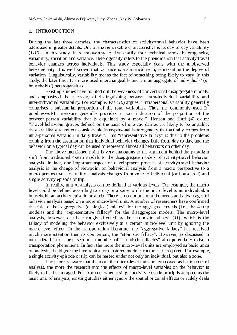
1. INTRODUCTION During the last three decades, the characteristics of activity/travel behavior have been addressed in greater details. One of the remarkable characteristics is its day-to-day variability (1-10). In this study, it is noteworthy to first clarify four technical terms: heterogeneity, variability, variation and variance. Heterogeneity refers to the phenomenon that activity/travel behavior changes across individuals. This study especially deals with the unobserved heterogeneity. It is well known that variance is a statistical term, representing the degree of variation. Linguistically, variability means the fact of something being likely to vary. In this study, the later three terms are used interchangeably and are an aggregate of individuals’ (or households’) heterogeneities.

Existing studies have pointed out the weakness of conventional disaggregate models, and emphasized the necessity of distinguishing between intra-individual variability and inter-individual variability. For example, Pas (10) argues: “Intrapersonal variability generally comprises a substantial proportion of the total variability. Thus, the commonly used R2 goodness-of-fit measure generally provides a poor indication of the proportion of the between-person variability that is explained by a model”. Hanson and Huff (4) claim: “Travel-behaviour groups defined on the basis of one-day dairies are likely to be unstable; they are likely to reflect considerable inter-personal heterogeneity that actually comes from intra-personal variation in daily travel”. This “representative fallacy” is due to the problems coming from the assumption that individual behavior changes little from day to day, and the behavior on a typical day can be used to represent almost all behaviors on other day.

The above-mentioned point is very analogous to the argument behind the paradigm shift from traditional 4-step models to the disaggregate models of activity/travel behavior analysis. In fact, one important aspect of development process of activity/travel behavior analysis is the change of viewpoint on behavioral analysis from a macro perspective to a micro perspective, i.e., unit of analysis changes from zone to individual (or household) and single activity episode or trip. In reality, unit of analysis can be defined at various levels. For example, the macro level could be defined according to a city or a zone, while the micro level to an individual, a household, an activity episode or a trip. There is no doubt about the needs and advantages of behavior analysis based on a more micro-level unit. A number of researchers have confirmed the risk of the “aggregative (ecological) fallacy” for the aggregate models (i.e., the 4-step models) and the “representative fallacy” for the disaggregate models. The micro-level analysis, however, can be strongly affected by the “atomistic fallacy” (11), which is the fallacy of modeling the behavior exclusively at a certain micro-level unit by ignoring the macro-level effect. In the transportation literature, the “aggregative fallacy” has received much more attention than its counterpart, the “atomistic fallacy”. However, as discussed in more detail in the next section, a number of “atomistic fallacies” also potentially exist in transportation phenomena. In fact, the more the micro-level units are employed as basic units of analysis, the bigger the hierarchical or clustered model structures are required. For example, a single activity episode or trip can be nested under not only an individual, but also a zone.

The paper is aware that the more the micro-level units are employed as basic units of analysis, the more the research into the effects of macro-level variables on the behavior is likely to be discouraged. For example, when a single activity episode or trip is adopted as the basic unit of analysis, existing studies either ignore the spatial or zonal effects or rudely deals

Makoto Chikaraishi, Akimasa Fujiwara, Junyi Zhang, Kay W. Axhausen 4

with them by using, for example, a dummy variable. However, if such zonal effects are not ignorable, then the assumption that the units of analysis are independent, which is often made in the statistical models applied in practice, becomes unrealistic. Consequently, this may lead to a misunderstanding of the determinants of activity/travel behavior. Such arguments might also be applicable to other macro-level effects. These macro-level effects have not been satisfactorily explored in existing literature, leading to misspecification of model structure. In this sense, the problem could come down to how to handle the unobserved heterogeneities in a number of macro level effects, which have complicated properties such as hierarchical and/or cross-classification structures, and what types of macro level effects should be taken into account for the analysis.

In this study, in order to examine the aforementioned complicated characteristics of activity/travel behavior, multilevel modeling approach is used. To quantitatively assess the impacts of unobserved heterogeneity at various macro-levels on the behavior, we focus on variation component, which corresponds to the degree of variation caused by the unobserved heterogeneity at a level of interest. An empirical analysis is conducted on departure time choice. More explicitly, this paper attempts to first decompose the total variation of departure time choice by activity type into five variance components: spatial variation, temporal variation at aggregate level (i.e., the whole population or its segments), inter-household variation, inter-individual variation, and intra-individual variation. Second, the effects of each type of variation on departure time choices are examined. In addition, how much of each variation can be explained by observed variables is also evaluated. It is expected that such analysis of variation properties could provide much deeper knowledge of behavioral mechanisms beyond the traditional paradigm which only focuses on a single or a limited set of variations. From the modeling perspective, such analysis could provide a useful guide in the specification of model structure because detailed variation patterns can be identified. An empirical analysis is conducted by using a continuous six-week travel survey data (called Mobidrive data) collected in the cities of Karlsruhe and Halle in Germany in 1999 (12). Mobidrive data is one of the few data sets to allow us to address this type of analysis.

This paper is organized as follows. The next section reviews the previous studies focusing on variation properties of activity/travel behavior. In section 3, the multilevel modeling approach is described. In the following section, the data set used in this study is briefly explained, and the results of model estimations are presented. In the final section, key conclusions and future tasks are summarized. 2. LITERATURE REVIEW As discussed above, this paper classified the variations of activity/travel behavior into five major categories. Here, since inter-personal variation has been well represented in existing studies, the review is given only with respect to intra-individual variation and the macro-level variations including spatial variation, temporal variation at aggregate level and inter-household variation. 2.1. Studies of Intra-Individual Variation As mentioned in Section 1, the importance of day-to-day variability of activity/travel

Makoto Chikaraishi, Akimasa Fujiwara, Junyi Zhang, Kay W. Axhausen 5

behavior at individual level has been recognized. One of the straightforward approaches to confirm the day-to-day variability might be to ask how similar the behaviors are within the same person or same sub-group. In this context, a number of similarity measures have been proposed to capture the degree of repetitiousness of the day-to-day behavior. For example, Hanson and Huff (4), Jones and Clarke (13), Pas (14), and Joh et al. (15) propose different similarity measures, and Schlich (6) and Schlich and Axhausen (7) compare these measures. The comparison results suggest that different measures of similarity detect different levels of similarity. In this sense, these measures should be further refined.

Focusing on components of total variation, Pas (10) highlights that a model based on cross-sectional data explains only inter-individual variation, and model performance could be apparently good because the total variation does not include intra-individual variation. His analysis shows that intra-individual variation comprises a substantial proportion (around 50%) of the total variation in terms of trip generation per day. In the same way, Pendyala (16) confirms a high percentage of the day-to-day variability in terms of trip frequency, travel time, travel distance and departure/arrival time. Susilo and Kitamura (8) examine the day-to-day variation in the context of individuals’ action space, and conclude that compared to other activities, discretionary activities are performed at various locations, showing higher randomness of action space (more than 85% of total variation is explained by unobserved intra-individual variation). Kitamura et al. (9) examine the day-to-day variability of the origin vertices of workers’ morning prisms using the stochastic frontier model. The result shows a much smaller day-to-day variation than the actual departure times of the first trips, although around 35% of total variation in the prism vertex is the intra-individual variation. All of the above studies indicate that individual behavior may undergo significant fluctuations from day to day, and the “representative fallacy” could be remarkable. Even if the selected representative samples could perfectly represent the characteristics of the population and the estimated behaviors have no bias, it does not mean that the results could be directly used to represent the behaviors on other day(s) (10). 2.2. Studies of Macro-Level Variations To begin with, it can be assumed that an individual is grouped within several macro-level units. In this section, we consider household, spatial and temporal attributes as macro-level units.

First, effects of the household unit on individual behavior are considered. It has been widely acknowledged in the transportation literatures that the activities conducted by members of multi-person households interact with each other (e.g., 17-19). Pas and Sundar (20) assume that an individual is nested within household, and show that the household-level effects on activity/travel behavior could be measured as the proportion of inter-household variation to total variation. Goulias (21) also confirms that inter-household variation is important from the perspective of time allocation behavior. Actually, both studies show that inter-household variation is more than 1/3 of the inter-personal variation. These results indicate that the independence assumption of the units of analysis will not hold if inter-household variation cannot be ignored, and as a result, “atomistic fallacy” may arise.

Second, spatial elements, such as land use, location of urban facilities and population distribution, would also have some impacts on daily activity participation. These kinds of impacts have been treated in the aggregate models. These methods have been criticized about

Makoto Chikaraishi, Akimasa Fujiwara, Junyi Zhang, Kay W. Axhausen 6

their inflexibility and inaccuracy, and the “aggregative fallacy” is an often quoted argument of disaggregate models. However, it does not directly imply that the disaggregate models have an edge on zonal aggregated models. For instance, if there is a positive intra-zonal correlation, then it will become unrealistic to assume that the units of analysis (individual or activity episode) are independent. Actually, disaggregate and zonal aggregate models elucidate different aspects of transport phenomena—disaggregate models mainly focus on the impacts of factors at the level of decision maker, while aggregate models mainly focus on the impacts of zonal attributes, such as land use pattern and accessibility. For example, Bhat (22) shows that ignoring the spatial context (zonal effect), in which individuals make mode choice decisions, can lead to an inferior data fit and provides inconsistent evaluations of transportation policy measures. Bhat and Zhao (23) also confirm that travel-related choices are intrinsically spatial in the context of activity stop generation. Thus, more precise analyses require that both individuals and spatial attributes should be treated simultaneously.

Third, impacts of temporal elements, such as date, day-of-week and season, on individual behavior are considered. Levinson and Kumar (24) show that the behaviors on different days are not same and they may change between weekdays and weekends, and travel patterns vary seasonally with respect to activity duration, trip frequency, trip duration and trip distance by activity type in the aggregate units. Kitamura and van der Hoorn (25) show that out-of-home social/recreational and shopping activities increase from Monday toward Friday, and it is further revealed that some systematic variations exist across days of the week in time use and trip generation. These studies indicate individual behavior shows some systematic variations over time. Note that it might be better to distinguish systematic day-to-day variation at aggregate level from intra-personal variability. To avoid confusion, we henceforth treat the term “temporal variation” as systematic day-to-day variation at aggregate level. Distinction between these two day-to-day variations is also useful to a better understanding of the nature of variation in activity/travel behavior.

In summary, activity/travel behavior could show various variations and as a result, a

better understanding of the behavior requires simultaneous representation of these variations. In line with such consideration, multilevel analysis approach is a promising tool to examine the influences of these variations.

3. MULTILEVEL MODEL As reviewed in section 2, the behavior in a given context does not only differ from individual to individual, but also vary within individual (intra-individual variation) and differ between households, zones or weekdays (macro-level variations). In macro-level variations, some of them have hierarchical structures, and some have cross-classification structures. To deal with these complicated variation patterns, we employ multilevel modeling (26-28), which might be one of the best approaches to addressing the behavior with various types of variations. This method essentially treats multiple hierarchical and cross-classification unobserved heterogeneities by corresponding variation components, and allows for flexible decomposition of total variation into the variations from various sources, such as the macro-level effects and the micro-level effects mentioned above. Although a number of applications can be found in transportation literature (21, 22-23, 29-35), to the authors’

Makoto Chikaraishi, Akimasa Fujiwara, Junyi Zhang, Kay W. Axhausen 7

knowledge, three major variation components in travel behavior, i.e., decision maker attributes, temporal attributes and spatial attributes, have not been examined simultaneously, mainly because of data limitation. In this empirical analysis we decompose total variation of departure time choice for each activity type into 5 variation components, which are 1) inter-individual variation, 2) inter-household variation, 3) spatial variation (derived from differences between the combinations of OD pair and residential location), 4) temporal variation (systematic day-to-day variation at aggregate level) and 5) intra-individual variation. In addition, how much of these variations can be explained by observed variables is also examined. To describe the departure time choice behavior by activity type j, we adopt the following equation:

jtihds

js

jd

jh

jih

jjtihdsy j

tihdsj

0 xβ (1) where, yj

tihds is the dependent variable (departure time) of the t-th trip for activity j made by person i of household h on day d traveling between location pairs s. βj

0 and βj are unknown parameters, xj

tihds indicates explanatory variables including situational attributes (e.g., size of party, job-related duties), individual attributes (e.g., gender, age, employment status), household attributes (e.g., number of household vehicles, household income), temporal attributes (e.g., day of week, holiday, long vacation) and/or spatial attributes (e.g., level of service between zones, attractiveness of location, spatial distribution of households and facilities). εj

tihds, γjih, γj

h, γjd and γj

s represent the random components which indicate intra-individual variation (error terms), inter-individual variation, inter-household variation, temporal variation (date specific error component) and spatial variation (the combination of OD pair and residential location specific error component), respectively. Let these random components be normally distributed as follows:

2|0

2|

2|

2|

2|

,0~,,0~

,,0~,,0~,,0~

jj

tihdsjsj

id

jdj

hjhj

hjihj

ih

NN

NNN (2)

where σ2

ih|j, σ2h|j, σ2

d|j, σ2s|j and σ2

0|j are variances of the random components. These random components are all assumed to be uncorrelated, thus the variance-covariance matrix can be written below:

2|0

2|

2|

2|

2|

jtihds

j0 x,β,|Var jjsjdjhjihjj

tihdsy (3) 2|

2|

2|

2|'''',Cov jssjddjhhjihhi

jsdhti

jtihds yy (4)

where δk are dummy variables (1: k=k’; 0: k≠k’;k=i, h, d, s). Note that Var (yj

tihds) and Cov (yj

tihds, yjt’i’h’d’s’) correspond to the variance-covariance matrix of the samples. This matrix

offers several useful functions for understanding variation properties of activity/travel behavior. First, consider the model without explanatory variables (called Null model). Using the Null model, it is possible to clarify the reasons of “why the behavior fluctuates?” based on the components of Var (yj

tihds). Furthermore, the degree of behavioral similarity can be measured as the correlation which is defined as Cov (yj

tihds, yjt’i’h’d’s’) / Var (yj

tihds). For example, in case that two departure time choices are observed on the same day and at the same space,

Makoto Chikaraishi, Akimasa Fujiwara, Junyi Zhang, Kay W. Axhausen 8

but made by different individuals, the correlation can be defined as (σ2ih|j +σ2

h|j) / Var (yjtihds).

The existence of the non-zero correlation suggests that traditional estimation procedures such as OLS are not suitable (28), because the units of analysis are not independent and consequently the “atomistic fallacy” occurs. Meanwhile, the existence of a non-zero intra-individual variation εj

tihds means that the behaviors fluctuate not only across decision makers, spatial and temporal attributes, but also across situation/context-dependent attributes. If this kind of variation is ignored, the “representative fallacy” comes into being. When the model includes explanatory variables (called Full model), the total variation of y j

tihds can be calculated as the following equation.

2|0

2|

2|

2|

2|

jtihds

j xβVarVar jjsjdjhjihj

tihdsy (5) Theoretically, all the estimated variation components of the random components in the Full model should be smaller than those in the Null model because Var(βjxj

tihds) explains a part of the total variation. It is further expected that increasing the number of explanatory variables decreases the variances σ2

ih|j, σ2h|j, σ2

d|j, σ2s|j and σ2

0|j. It is very interesting to know how much these variances are explained for several reasons. The main interest is that remaining variations offer information about which type of explanatory variables is still lacking and which direction future research should take. For example, if the specified set of explanatory variables could not reduce the spatial variation or it still remains at a high rate, it may imply that spatial variables are potentially more important. However, the determination of which explanatory variables reduce the unobserved heterogeneities is less certain because especially micro-level variables have cross-level influences and it is rare to eliminate the unobserved variation within each level completely (36). For example, the duration of the commute trip might be categorized as situational attributes, but it is not difficult to imagine that there is also big difference between individuals or OD pairs. Therefore, the model including the duration of the commute trip as explanatory variable may reduce not only intra-individual variation, but also other variations. In this paper, thus we mainly focus on the variation properties of departure time choices, and which factor is the ultimate trigger for creating fluctuation sets is a secondary objective. The set of unknown parameters in the model, β j

0, βj, σ2ih | j, σ2

h | j, σ2d | j, σ2

s | j and σ20 | j,

are estimated based on full maximum likelihood estimate method. The likelihood function for each activity type Lj can be defined as follows:

γ

jjjj0

jj0 γσ|γγ,β,||σ,β, dfypyL

jtihdsN

jjj

tihdsjj

tihdsj

j (6)

where fj(γj|σj) means the quadravariate normal distribution with a mean 0 and variances σ2ih|j,

σ2h|j, σ2

d|j and σ2s|j . Note that no correlation between these variances is included as mentioned

previously. pj(y jtihds | βj

0, βj, γj) represents the normal distribution with a mean β j0+βjx j

tihds+γj and variance σ2

0 | j. N jtihds is the set of all the observed trips for activity type j, reported by

person i within household h on day d traveling between given spaces s. To calculate the integral in equation (6), we adopt adaptive Gaussian quadrature approximations using software R (37). For the sake of simplifying the discussion of variation patterns, the model is estimated separately for each activity type, leaving the analysis of interrelated choices of different activities and travels as a future research issue.

Makoto Chikaraishi, Akimasa Fujiwara, Junyi Zhang, Kay W. Axhausen 9

4. EMPIRICAL ANALYSIS 4.1. Data The Mobidrive data set (12) is used in the empirical analysis. It includes a six-week travel diary survey conducted in Karlsruhe (West Germany) and Halle (East Germany), in fall of 1999. Including the pilot survey, a total of 361 persons from 162 households participated in this survey. Total recorded dates are 119 days, including 56 days from the pilot survey (May 31 through July 25) and 63 days from the main survey (September 13 through November 14). Table 1 provides the number of trips by activity type and the number of observations by individual, household, observed date, OD pairs and residential locations. Note that origin (O), destination (D) and residential locations are classified into 4 zones: CBD, inner city, suburbs and others for each city. Thus the maximum number of the combinations is 128 (=4[origins]×4[destinations]×4[residential locations] ×2[cities]). 4.2. Model Estimation and Discussion First, the Null model (i.e., the model without explanatory variables) is estimated for each activity type and the results are presented in Table 2. The dependent variable, i.e., the departure time, is expressed in minutes counted from midnight as zero. Test of significance for each random component is conducted based on Chi-squared statistics by comparing the models with and without the corresponding random component (28). If a random component included in the model does not improve the log-likelihood significantly, we exclude it from the model, implying that the corresponding variation could be ignored in the analysis. Model estimation results reveal that the day-to-day variation for Pick-up/Drop-off, inter-individual variation for Non-daily Shopping, and inter-household and day-to-day variations for mandatory activities (School, Work and Work-related activities) could be ignorable. All of the remaining random components are statistically significant. The proportions of variations are summarized in Table 3 and major findings are described below.

(i) Intra-individual variation shows the biggest impact on the departure time choices of almost all the activities. The relevant shares of total variations range from 35.0% to 75.6%. This suggests that the choices of daily departure times are mainly determined by the factors changing from time to time and/or from context to context. This is especially true with respect to Pick-up/Drop-off, Private business, Work-related activities, Leisure and Home activities in this case study.

(ii) The variations related to individual attributes (the sum of inter-individual and inter-household variations) account for the second largest proportion (11.0%~36.0%) of total variation, regardless of activity types. However, the proportions of inter-household variation and inter-individual variation vary greatly with activity types. For instance, the inter-individual variation shows extremely high influence on departure time choice for mandatory activities (School, Work and Work-related activities), while the inter-household variation imposes higher impact on Daily shopping, Non-daily shopping and Leisure activities.

(iii) The spatial variation especially shows much larger influence on the departure time choices of the mandatory activities than those of other activities.

(iv) The departure time choices for shopping and leisure activities are highly influenced by

Makoto Chikaraishi, Akimasa Fujiwara, Junyi Zhang, Kay W. Axhausen 10

systematic day-to-day variation, compared to other activities. Thus, the variations presented in Table 3 could provide a useful guide for the design of a dynamic modeling framework. For example, in this case study, it could be suggested to especially incorporate intra-individual variation into the model development of departure time choice. On the other hand, such significant variations obviously suggest the necessity of introducing some observed variables to represent departure time choice behavior. Next, it is necessary to examine how much of the above unobserved variances of random components can be explained by observed information. The estimation results of Full models, which contain observed (explanatory) variables, are presented in Table 4. Explanatory variables were selected based on a preliminary analysis, which was conducted to select statistically significant variables (at least at the significance level of 90%). The selected variables vary from activity to activity. The resulting variance components by activity type for both the Null and Full models are illustrated in Figure 1. It is confirmed that the reduction of variations is very different not only among activity types, but also among variation types. The findings are summarized below.

Comparing the Null and Full models, it is found that the biggest reduction rate is observed with respect to the temporal variations. For example, in the case of Daily shopping, the variation is reduced from 4607.1 to 9.1. Temporal variations in Private business, Non-daily shopping, Leisure and Home in the Full models are also reduced by more than 70% from those in the Null models. On the other hand, the smallest reduction rate is observed in intra-individual variation (4%~16%). Explaining intra-individual variation by explanatory variables seems to be quite difficult for all activity types. This implies that, at least in departure time choice, we need additional information to capture intra-individual variations. As for other components of variations (inter-individual, inter-household and spatial variations), the reduction rates vary greatly with activity types: inter-individual variation ranging from 20% to 83%, inter-household variation from 27% to 65%, and spatial variation from 30% to 82%.

In the Full models, inter-individual variation, inter-household variation and spatial variation are estimated to be statistically significant, suggesting that it is necessary to further introduce more appropriate observed variables to explain these variations. As for the remaining types of variations, statistical significances vary with activity types. On the other hand, temporal variations are estimated to be insignificant for Daily shopping and Home, suggesting that the relevant random components could be ignored in the model. The reasons might be two-folded. One is because the introduced day-of-week dummies works well to reduce such variations. However, the empirical analysis reveals that introducing other types of variables could also reduce such temporal variations, For example, when day-of-week dummies are excluded from the model for Daily shopping, the temporal variation is estimated to be 2713.3, which is much smaller than 4607.1. This suggests that another reason causing the reduction of temporal variation is due to the introduction of other observed variables. Such observation also implies that some observed factors could play the role of the confounding factors, i.e., one factor could be influential to two or more types of variations. 5. CONCLUSION In the analysis of activity/travel behavior, use of micro-level unit usually discourages the

Makoto Chikaraishi, Akimasa Fujiwara, Junyi Zhang, Kay W. Axhausen 11

analysis of the effects of macro-level variables. One of the reasons is because behavioral variations could come from various sources, but these variations have not been properly evaluated before model development due to the lack of reliable methodologies. Focusing on departure time choice, this study has attempted to explore its variation properties based on the multilevel modeling approach, which can simultaneously deal with various types of variations based on the concept of variance component.

This study decomposes the total variation in departure time choice behavior into five major categories: spatial variation, temporal variation at aggregate level, inter-household, inter-individual, and intra-individual variations. The Mobidrive data with a continuous six-week travel dairy data is adopted. Model estimation results first confirm that the behavioral variations of departure time choice vary largely with activity type, and among all the variations, the intra-individual variations are most influential in the sense that its share in the total variation is the largest. It is further revealed that some types of variations cannot be ignored even after incorporating its influence by using some observed information. It is also observed that a number of observed variables are influential to several types of variations. These findings underscore the needs of simultaneously dealing with unobserved variations from macro-level to micro-level. These quantitative assessments of various types of variations could provide useful guide for the model specification, and deepen the knowledge of behavioral variability by going beyond the traditional paradigm which only focuses on a limited set of variations. The empirical analysis of this study is an initial attempt of understanding various variations in activity/travel behavior. More extensive applications are needed before giving any general conclusions. From modeling perspective, the multilevel model requires the macro-level units to be pre-defined; however, different definitions might lead to different conclusions. This is because, for example, homogeneity is usually assumed with respect to the behavior at zone level and change of zone size means the change of influence of such homogeneity assumption. It is worth exploring the influence of such zone size on behavioral variability. One of the most challenging parts in the future might be how to connect knowledge of behavioral variability with policy making. For this purpose, the observed variability should cover various contexts over a longer time period. However, the problem is how to collect such data in practice, with consideration of limited survey budget. In line with such consideration, it is expected that the voluntary, incentive-based participatory self-reporting (VIP-SR) survey method proposed by Zhang (38) could provide such data. The VIP-SR survey completely relies on citizens’ voluntary spirit. It does not limit the survey period and targets the whole population across a much longer time period, unlike traditional survey methods, which usually select respondents from a small portion of the whole population (usually several percentages) within a limited time period (e.g., a week) to collect the information on one representative day, or at most several adjacent days. It is empirically confirmed that the VIP-SR is highly acceptable to the public, using a small-scaled web-based survey. One of the unsolved issues related to the VIP-SR survey is whether it could collect representative samples. In this sense, such new survey method should be seriously taken into account in the analysis of activity/travel behavior and transportation decisions. More research efforts are required.

Makoto Chikaraishi, Akimasa Fujiwara, Junyi Zhang, Kay W. Axhausen 12

REFERENCES 1. van der Hoorn, T.: Travel Behaviour and the Total Activity Pattern, Transportation, Vol. 8,

pp. 309-328, 1979. 2. Hanson, S., Huff, J.: Classification Issues in the Analysis of Complex Travel Behavior,

Transportation, Vol. 13, pp. 271-293, 1986. 3. Pas, E. I., Koppelman, F. S.: An Examination of the Determinants of Day-to-Day

Variability in Individuals' Urban Travel Behavior, Transportation, 13, pp. 183-200, 1986. 4. Hanson, S., Huff, J.: Repetition and Day-to-Day Variability in Individual Travel Patterns:

Implications for Classification, in R.G. Golledge and H. Timmermans (eds.) Behavioural Modelling in Geography and Planning, Croom Helm, London, pp. 368-398, 1988.

5. Kitamura, R.: An Analysis of Weekly Activity Patterns and Travel Expenditure, in R.G. Golledge and H. Timmermans (eds.) Behavioural Modelling in Geography and Planning, Croom Helm, London, pp. 399-423, 1988.

6. Schlich, R.: Analyzing Intrapersonal Variability of Travel Behavior Using the Sequence Alignment Method, Paper presented at the European Transport Conference, Cambridge, 2001.

7. Schlich, R., Axhausen, K. W: Habitual travel behaviour: Evidence from a six-week travel diary, Transportation, Vol. 30, pp. 13–36, 2003.

8. Susilo, Y. O., Kitamura, R.: Analysis of Day-to-Day Variability in an Individual’s Action Space: Exploration of 6-Week Mobidrive Travel Diary Data, Transportation Research Record, No. 1902, pp. 124-133, 2005.

9. Kitamura, R., Yamamoto, T., Susilo, Y. O., Axhausen, K. W.: How Routine is a Routine? An Analysis of the Day-to-Day Variability in Prism Vertex Location, Transportation Research Part A, Vol. 40, pp. 259–279, 2006.

10. Pas, E. I.: Intrapersonal Variability and Model Goodness-of-Fit, Transportation Research Part A, Vol. 21, pp. 431-438, 1987.

11. Diez-Roux, A. V.: Bringing Context Back into Epidemiology: Variables and Fallacies in Multilevel Analysis, American Journal of Public Health, Vol. 88, pp. 216-222, 1998.

12. Axhausen, K. W., Zimmermann, A., Schonfelder, S., Rindsfuser, G., Haupt, T.: Observing the Rhythms of Daily Life: A Six-Week Travel Diary, Transportation, Vol. 29, pp. 95-124, 2002.

13. Jones, P., Clarke, M.: The Significance and Measurement of Variability in Travel Behaviour, Transportation, Vol. 15, pp. 65-87, 1988.

14. Pas, E. I.: a Flexible and Integrated Methodology for Analytical Classification of Daily Travel-Activity Behaviour, Transportation Science, Vol. 17, pp. 405-429, 1983.

15. Joh, C-H., Arentze, T., Hofman, F., Timmermans, H.: Activity Pattern Similarity: A Multidimensional Sequence Alignment Method, Transportation Research Part B, Vol. 36, pp. 385-403, 2002.

16. Pendyala, R. M.: Measuring Day-to-Day Variability in Travel Behavior Using GPS Data, Final Report DTFH61-99-P-00266., FHWA, U.S. Department of Transportation, Washington, D.C. , 1999 (http://www.fhwa.dot.gov/ohim/gps/index.html).

17. Zhang, J., Timmermans, H. and Borgers, A.: A utility-maximizing model of household time use for independent shared and allocated activities incorporating group decision mechanisms. Transportation Research Record, 1807, pp. 1-8, 2002.

18. Zhang, J., Kuwano, M., Lee, B., and Fujiwara, A.: Modeling household discrete choice

Makoto Chikaraishi, Akimasa Fujiwara, Junyi Zhang, Kay W. Axhausen 13

behavior incorporating heterogeneous group decision-making mechanisms. Transportation Research Part B (forthcoming), 2008.

19. Gliebe, J. P., Koppelman, F. S.: A Model of Joint Activity Participation between Household Members, Transportation, Vol. 29, pp. 49-72, 2002.

20. Pas, E. I., Sundar, S.: Intrapersonal Variability in Daily Urban Travel Behavior: Some Additional Evidence, Transportation, Vol. 22, pp. 135-150, 1995.

21. Goulias., K. G.: Multilevel Analysis of Daily Time Use and Time Allocation to Activity Types Accounting for Complex Covariance Structures Using Correlated Random Effects, Transportation, Vol. 29, pp. 31-48, 2002.

22. Bhat, C. R.: A Multi-Level Cross-Classified Model for Discrete Response Variables, Transportation Research B, Vol. 34, pp. 567-582, 2000.

23. Bhat, C. R., Zhao, H.: The Spatial Analysis of Activity Stop Generation, Transportation Research Part B, Vol. 36, pp. 557-575, 2002.

24. Levinson, D., Kumar, A.: Temporal Variations on the Allocation of Time, Transportation Research Record, No. 1493, pp. 118-127, 1995.

25. Kitamura, R., van der Hoorn, T.: Regularity and Irreversibility of Weekly Travel Behavior, Transportation, Vol. 14, pp. 227-251, 1987.

26. Hox, J. J: Applied Multilevel Analysis, TT-Publikaties, Amsterdam, 1995. 27. Kreft, I., de Leeuw, J.: Introducing Multilevel Modeling, Sage Publications Ltd., 1998. 28. Goldstein, H.: Multilevel Statistical Models, Third Edition, Edward Arnold, London,

2003. 29. Weber, J., Kwan, M-P.: Evaluating the Effects of Geographic Contexts on Individual

Accessibility, Urban Geography, Vol. 24, pp. 647-671, 2003. 30. Khandker, M., Habib, N. M., Miller, E. J.: Modeling Skeletal Components of Workers'

Daily Activity Schedules, Transportation Research Record, No. 1985, pp. 88-97, 2006. 31. Khandker, M., Habib, N. M., Miller, E. J.: Modeling Individuals’ Frequency and Time

Allocation Behavior for Shopping Activities Considering Household-Level Random Effects, Transportation Research Record, No. 1985, pp. 78-87, 2006.

32. Yavuz, N., Welch, E. W., Sriraj, P. S.: Individual and Neighborhood Determinants of Perceptions of Bus and Train Safety in Chicago, Illinois—Application of Hierarchical Linear Modeling—, Transportation Research Record, No. 2034, pp. 19-26, 2007.

33. Kweon, Y-J.: Prediction of Fatality Rates for Comparison between States, Transportation Research Record, No. 2019, pp. 127-135, 2007.

34. Carrasco, J-A., Miller, E. J., Wellman, B.: How Far and with Whom Do People Socialize? Empirical Evidence about the Distance between Social Network Members, CD-ROM, Presented at the 87th Annual Meeting of the Transportation Research Board, 2008.

35. Habib, M. A., Miller, E. J.: Influence of Transportation Access and Market Dynamics on Property Values: Multilevel Spatio-Temporal Models of Housing Price, CD-ROM, Presented at the 87th Annual Meeting of the Transportation Research Board, 2008.

36. Teune, H.: Cross-Level Analysis: A Case of Social Inference, Quality and Quantity, Vol. 13, pp. 527-537, 1979.

37. R development core team: R: A Language and Environment for Statistical Computing. Vienna: R Foundation for Statistical computing, 2005 (http://www.R-project.org/, Accessed on June 10, 2008).

38. Zhang, J.: A self-reporting survey method: Public acceptance analysis, Paper submitted to

Makoto Chikaraishi, Akimasa Fujiwara, Junyi Zhang, Kay W. Axhausen 14

the 88th Annual Meeting of the Transportation Research Board, Washington, D.C., January 11-15, 2009.

Makoto Chikaraishi, Akimasa Fujiwara, Junyi Zhang, Kay W. Axhausen 15

Table 1 Number of Samples in the Case Study

Activity type Number of micro-level

observations (Number of trips)

Number of observations at the macro(subgroup) level Decision maker

attributes Temporal elements Spatial elements

Number of individuals

Number of households Number of

observed dates Number of the

combination of OD pairs and residential locations*

Pick-up/Drop-off 1,749 244 127 109 78 Private business 3,998 348 159 113 88 Work-related activity 1,440 143 99 95 74 School 2,576 114 65 99 47 Work 4,761 193 120 112 69 Daily shopping 4,653 343 162 116 85 Non-daily shopping 1,846 332 158 105 78 Leisure 8,720 360 161 119 97 Home 22,261 361 162 119 45

Total 52,004 361 162 119 115 * Origin, destination and residential location are classified into 4 zones which are CBD, inner city, suburbs and elsewhere for each city (Karlsruhe and Halle).

Makoto Chikaraishi, Akimasa Fujiwara, Junyi Zhang, Kay W. Axhausen 16

Table 2 Estimation Results (Null models)

Activity Type μj

LL(0) LL(C) LL(β) χ2 test -2[LL(C)-LL(β)] Number of sample

Parameter t-stat

Pick up/Drop off 887.98 55.10 -14,399 -12,281 -12,154 254.00 ** 1,749 Private business 791.70 48.57 -32,428 -26,981 -26,731 500.08 ** 3,998 Work-related activity 723.79 47.55 -11,569 -9,714 -9,585 257.07 ** 1,440 School 608.36 28.65 -19,750 -16,401 -15,967 868.58 ** 2,576 Work 612.07 34.88 -36,926 -31,943 -30,846 2194.70 ** 4,761 Daily shopping 781.50 28.95 -37,668 -31,113 -30,345 1535.48 ** 4,653 Non-daily shopping 798.60 65.15 -15,019 -12,177 -11,978 398.84 ** 1,846 Leisure 901.85 41.44 -71,995 -59,783 -58,820 1926.58 ** 8,720 Home 918.52 63.08 -184,180 -154,528 -153,517 2021.40 ** 22,261

Activity Type

Decision-maker attributes Temporal elements Spatial elements Intra-indiv

idual variation

Total

variation Inter-individual variation Inter-household

variation Systematic day-to-day variation

Variation of OD

matrix and residential location

σ2ih | j (χ2) σ2

h | j (χ2) σ2d | j (χ2) σ2

s | j (χ2) σ20 | j Var(yj

tihds) Pick up/Drop off 8409.8 (28.7) ** 6940.7 (8.0) ** (0) (0.9) 3503.7 (19.8) ** 55464.0 74318.2 Private business 4381.5 (75.2) ** 3979.9 (20.5) ** 807.7 (18.5) ** 1516.4 (26.1) ** 33193.1 43878.6 Work-related activity 7486.4 (90.0) ** (0) (0.0) (0) (1.1) 5472.6 (102.6) ** 31027.1 43986.1 School 10022.0 (287.0) ** (0) (2.3) (0) (0.0) 12600.1 (270.7) ** 12159.5 34781.5 Work 17737.8 (1462) ** (0) (0.5) (0) (0.0) 9813.9 (427) ** 21673.7 49225.4 Daily shopping 4371.5 (136.5) ** 6939.2 (42.7) ** 4607.1 (566.5) ** 1052.5 (29.3) ** 22759.4 39729.7 Non-daily shopping (0) (2.45) 7237.2 (229.6) ** 3575.5 (140.6) ** 1172.8 (20.8) ** 20657.0 32642.5 Leisure 3199.0 (138.7) ** 6650.2 (54.1) ** 2964.9 (435.2) ** 2974.2 (190.2) ** 38391.1 54179.4 Home 3748.0 (451.9) ** 3288.1 (28.4) ** 658.7 (120.3) ** 1352.0 (140.6) ** 54976.8 64023.6 Notes: χ2 is referred to chi-square statistics between LL(β) and LL(β') which is excluded a corresponding

random effect. If a corresponding random effect is not significant, we exclude it from the model. ** significant at 1%

Makoto Chikaraishi, Akimasa Fujiwara, Junyi Zhang, Kay W. Axhausen 17

Table 3 Proportion of Variation (Null models)

Activity Type

Decision-maker attributes Temporal elements Spatial elements

Intra-individual variation

Total

variation Inter-individual variation Inter-household

variation Subtotal Systematic day-to-day variation

Variation of OD

matrix and residential location

σ2ih | j σ2

h | j σ2ih | j+σ2

h | j σ2d | j σ2

s | j σ20 | j Var(yj

tihds) Pick up/Drop off (11.3%) (9.3%) 20.7% 0.0% 4.7% 74.6% 100.0% Private business (10.0%) (9.1%) 19.1% 1.8% 3.5% 75.6% 100.0% Work-related activity (17.0%) (0.0%) 17.0% 0.0% 12.4% 70.5% 100.0% School (28.8%) (0.0%) 28.8% 0.0% 36.2% 35.0% 100.0% Work (36.0%) (0.0%) 36.0% 0.0% 19.9% 44.0% 100.0% Daily shopping (11.0%) (17.5%) 28.5% 11.6% 2.6% 57.3% 100.0% Non-daily shopping (0.0%) (22.2%) 22.2% 11.0% 3.6% 63.3% 100.0% Leisure (5.9%) (12.3%) 18.2% 5.5% 5.5% 70.9% 100.0% Home (5.9%) (5.1%) 11.0% 1.0% 2.1% 85.9% 100.0%

Makoto Chikaraishi, Akimasa Fujiwara, Junyi Zhang, Kay W. Axhausen 18

Table 4 Estimation results (Full models)

Variables Activity type

Pick up /Drop off

Private business

Work related School Work Daily

shopping Non-daily shopping Leisure Home

Explanatory variables Constant 884.0 (25) 747.6 (32) 630.5 (14) 474.6 (19) 739.8 (25) 812.5 (27) 799.1 (28) 1019 (35) 859.4 (33) Individual attributes Male [D] - 13.9 (1.7) - -35.4 (-3.6) - - - 14.3 (1.9) 16.1 (2.5) Married [D] - - - -73.5 (-2.8) - -27.6 (-2.2) -26.8 (-2.1) - -24.7 (-2.3) Parent [D] - - - -85.2 (-2.9) - 25.4 (1.7) - 40.6 (3.2) - Employed [D] - -19.5 (-1.9) -134 (-2.7) - - -97.6 (-2.6) - - - Fixed commitment [D] - - - 20.9 (1.7) - - - -19.6 (-2.2) - Part-time [D] 42.9 (2.1) - 99.6 (2.2) - - 103.6 (2.8) - - 17.7 (2.3) Full-time [D] - - 189 (3.2) -100 (-1.9) - 128.2 (3.1) - - - Self-employed [D] - - - - - 102.7 (1.9) - - - Household member helping [D] - - - - - - -128 (-2.7) - - Age - -2.4 (-8.8) - 4.3 (5.0) - -2.5 (-6.5) -2.1 (-5.4) -3.1 (-9.2) -0.9 (-2.9) Vehicle license [D] -108 (-4.5) - - 69.6 (4.1) - - - - - Household attributes Number of children in household - - - - - - - - 25.4 (2.0) Number of household members - - - - - -15.0 (-2.0) -17.1 (-2.7) -26.9 (-4.3) -22.2 (-2.1) Number of personal vehicles - - - - - - - - - Bus stop: Distance (in 100m) - - - 2.2 (2.6) - - - - - LRT stop: Distance (in 100m) - - - - - - - -0.4 (-1.8) -0.3 (-1.7) Heavy rail stop: Distance (in 100m) - - - - - - - 0.03 (1.8) - Household income (in 1000DM) - 6.5 (2.2) - - - 6.3 (1.8) 12.9 (3.6) - 5.2 (1.8) Spatial attributes Living in inner city [D] - 36.9 (2.7) - - - - - - - Living in Karlsruhe [D] 56.1 (2.0) 24.9 (1.9) - - - 23.7 (1.7) 28.5 (1.8) 62.5 (3.6) 35.8 (2.5) Temporal attributes Thursday [D] - - - - - - - - 9.1 (2.0) Friday [D] - -44.5 (-4.9) -36.5 (-2.8) -21.2 (-3.8) -11.7 (-2.2) -17.2 (-2.9) - 34.6 (4.5) -19.0 (-4.3) Saturday [D] - -40.0 (-3.3) - - - -139 (-22) -103 (-9.4) -24.7 (-3.3) -53.4 (-10) Sunday [D] - 58.3 (3.8) - 99.9 (2.3) 59.3 (3.4) -78.1 (-4.6) - -79.2 (-10) -21.9 (-3.8)

Makoto Chikaraishi, Akimasa Fujiwara, Junyi Zhang, Kay W. Axhausen 19

Table 4 (cont’d) Estimation results (Full models)

Variables Activity type

Pick up /Drop off

Private business

Work related School Work Daily

shopping Non-daily shopping Leisure Home

Episode unit attributes Travel time (min) -1.1 (-3.2) -0.4 (-1.7) -0.4 (-2.7) - 0.5 (2.5) - - -0.5 (-8.6) - Number of activities per day 7.1 (2.9) 2.6 (2.0) 4.3 (2.0) 8.1 (6.2) 3.4 (2.6) 4.4 (4.0) 6.2 (4.1) 10.8 (9.7) 5.4 (6.7) First trip is commute on the day [D] 187.1 (9.8) 204.3 (22) 79.6 (5.6) 229.6 (5.2) -132 (-18) 163.8 (22) 136.7 (13) 124.7 (17) 143.4 (28) Size of party (household member) -27.4 (-3.0) 54.5 (8.5) - - -36.4 (-2.7) 53.7 (10.5) 32.4 (5.3) 15.9 (4.7) 42.0 (18.7) Size of party (other member) 39.6 (5.4) 9.2 (3.7) - 6.6 (7.1) 11.6 (3.8) 25.0 (3.8) - -2.9 (-3.7) 3.2 (2.6) Main mode = walk [D] - - 68.9 (1.8) - 70 (3.7) -21.2 (-2.7) - - -24.6 (-4.6) Main mode = cycling [D] - -36.9 (-3.1) 148.8 (3.7) - -74.1 (-4.1) -25.2 (-2.6) - - -34.9 (-5.5) Main mode = motorcycles [D] - 100.8 (2.7) 267.9 (3.3) - - - - -57.8 (-2.2) 38.6 (1.9) Main mode = vehicle driver [D] - -35.3 (-4.0) 68.0 (2.0) - -48.9 (-3) -22.4 (-2.7) - -38.8 (-5.7) - Main mode = vehicle passenger [D] - -30.0 (-2.5) 98.2 (2.7) - - - - -30.7 (-4.4) 48.7 (7.9) Main mode = Bus [D] - -53.4 (-2.5) - -36.1 (-2.6) -107 (-3.7) - - -48.8 (-2.5) -48.2 (-3.9) Main mode = LRT [D] - -47.5 (-4.2) 71.6 (1.8) -71.5 (-8.3) -62.3 (-3.3) - - -30.9 (-3.4) -39.8 (-5.7) Main mode = Heavy Rail [D] - - - -150 (-3.2) -148.4 (-4) - -322(-2.2) -147 (-5.3) - Var(βx) 9735.1 10351.3 3826.2 4484.8 5283.1 12586.4 8084.0 10354.5 7802.9 Random effects Inter-individual variation 4542.2 2042.1 5963.6 1678.3 13576.8 1965.4 - 2346.5 2316.8 [17.7] [25.4] [78.0] [78.5] [1084.1] [58.7] [105.8] [253.6] Inter-household variation 5096.9 1687.6 - - - 2405.5 2948.1 2812.6 1819 [9.4] [10.7] [25.5] [93.1] [33.7] [25.1] Temporal variation - 208.3 - - - 9.1 388.4 163.7 0 [3.1] [0.02] [6.8] [4.4] [0.0] Spatial variation 2147.1 272 3715.3 8008.9 6864.8 473.6 674.1 1869.3 433.1 [13.5] [5.6] [67.3] [186] [197.36] [10.7] [12.7] [91.5] [35] Intra-individual variation 51929.7 29031.6 29616.0 11674.5 19428.5 20397.7 19010.6 36198.1 51444.0 Converged log-likelihood -12,069 -26,368 -9,539 -15,836 -30567 -29,893 -11,813 -58,419 -152,645 χ2 {-2[L L(C)- L(u,β)]} 424 1226 349 1131 2752 2439 729 2729 3765 Number of explanatory variables 9 21 14 17 14 21 12 23 24 Sample size 1,749 3,998 1,440 2,576 4,761 4,653 1,846 8,720 22,261 Notes: [D] indicates dummy variable. “()” corresponds to t-statistic and “[]” represents chi-square statistics between LL(β) and LL(β’) which exclude a corresponding random effect from the full model. “-” correspond to coefficient with a t statistics < 1.645, and we excluded the pertinent variables from the model.

Makoto Chikaraishi, Akimasa Fujiwara, Junyi Zhang, Kay W. Axhausen 20

0

5000

10000

15000

20000

25000

(Var

(βx)

)

Inte

r-in

divi

dual

va

riat

ion

Inte

r-ho

useh

old

vari

atio

n

Tem

pora

l var

iatio

n

Spat

ial v

aria

tion

Intr

a-in

divi

dual

va

riat

ion

Work

0 5000

10000 15000 20000 25000 30000 35000

(Var

(βx)

)

Inte

r-in

divi

dual

va

riat

ion

Inte

r-ho

useh

old

vari

atio

n

Tem

pora

l var

iatio

n

Spat

ial v

aria

tion

Intr

a-in

divi

dual

va

riat

ion

Private Business

0 10000 20000 30000 40000

50000 60000

(Var

(βx)

)

Inte

r-in

divi

dual

va

riat

ion

Inte

r-ho

useh

old

vari

atio

n

Tem

pora

l var

iatio

n

Spat

ial v

aria

tion

Intr

a-in

divi

dual

va

riat

ion

Pick up /Drop off

0 5000

10000 15000 20000 25000 30000 35000

(Var

(βx)

)

Inte

r-in

divi

dual

va

riat

ion

Inte

r-ho

useh

old

vari

atio

n

Tem

pora

l var

iatio

n

Spat

ial v

aria

tion

Intr

a-in

divi

dual

va

riat

ion

Work related

0

5000

10000

15000

20000

25000

(Var

(βx)

)

Inte

r-in

divi

dual

va

riat

ion

Inte

r-ho

useh

old

vari

atio

n

Tem

pora

l var

iatio

n

Spat

ial v

aria

tion

Intr

a-in

divi

dual

va

riat

ion

Daily shopping

0

5000

10000

15000

20000

25000

(Var

(βx)

)

Inte

r-in

divi

dual

va

riat

ion

Inte

r-ho

useh

old

vari

atio

n

Tem

pora

l var

iatio

n

Spat

ial v

aria

tion

Intr

a-in

divi

dual

va

riat

ion

Non-daily shopping

0 5000

10000 15000 20000 25000 30000 35000 40000 45000

(Var

(βx)

)

Inte

r-in

divi

dual

va

riat

ion

Inte

r-ho

useh

old

vari

atio

n

Tem

pora

l var

iatio

n

Spat

ial v

aria

tion

Intr

a-in

divi

dual

va

riat

ion

Leisure

0 10000

20000 30000 40000 50000 60000

(Var

(βx)

)

Inte

r-in

divi

dual

va

riat

ion

Inte

r-ho

useh

old

vari

atio

n

Tem

pora

l var

iatio

n

Spat

ial v

aria

tion

Intr

a-in

divi

dual

va

riat

ion

Home

0 2000 4000 6000 8000

10000 12000 14000

(Var

(βx)

)

Inte

r-in

divi

dual

va

riat

ion

Inte

r-ho

useh

old

vari

atio

n

Tem

pora

l var

iatio

n

Spat

ial v

aria

tion

Intr

a-in

divi

dual

va

riat

ion

School

83%36% 4%

53%82%

16%

58%74%

43%

8%

59%89%

24%

30%

10%

46%39%

6%

27%

27% 37%

6%

58%95% 38% 68%

6%

45% 100%

55%55%

10%

65%100%

20% 32%

5%

1) □: Full model; ■: Null model 2) --% : Reduction rate of variation in Full model relative to that in Null model

Figure 1 Comparison of Variations between the Null and Full Models