arX

iv:2

106.

1514

3v1

[as

tro-

ph.H

E]

29

Jun

2021

MNRAS 000, 1–12 (2021) Preprint 30 June 2021 Compiled using MNRAS LATEX style file v3.0

Exploring the inner-disk region of the atoll source 4U 1705-44 using

AstroSat’s SXT and LAXPC observations

Malu S,1★ K. Sriram,1 S. Harikrishna,1 Vivek K. Agrawal21Department of Astronomy, University College of Science, Osmania University, Hyderabad, India2Space Astronomy Group, ISITE Campus, U R Rao Satellite Center, 560037, Bangalore, India

Accepted XXX. Received YYY; in original form ZZZ

ABSTRACT

For the first time, simultaneous broadband spectral and timing study of the atoll source 4U1705-44 was performed using AstroSat Soft X-ray Telescope (SXT) and Large Area X-rayProportional Counter (LAXPC) data (0.8-70 keV). Based on the HID, the source was in thesoft banana state during these observations. Spectral modeling was performed using the fullreflection framework and an inner disk radii of 14 Rg was obtained. A hard powerlaw tail wasnoticed in the soft state and hot component fluxes and varying powerlaw indices point towardsa varying corona/sub-keplerian flow. Based on the spectral fits the boundary layer radius andmagnetospheric radius were constrained to be ∼ 14-18 km and ∼ 9-19 km respectively. Cross-Correlation Function studies were performed between the 0.8-3 keV soft SXT lightcurve and10-20 keV hard LAXPC lightcurve and correlated and anticorrelated lags were found, whichwas used to constrain the coronal height to 0.6-20 km (V=0.1). Since the inner disk radius isnot varying during the observations, we conclude that the detected lags are possibly caused bya varying structure of corona/boundary layer in the inner region of the accretion disk. Basedon the observations, a geometrical model is proposed for explaining the detected lags in theatoll source 4U 1705-44.

Key words: accretion, accretion disk—binaries: close—stars: individual (4U 1705-44)—X-rays: binaries

1 INTRODUCTION

The geometry and structural configuration of Neutron Star Low

mass X-ray binaries (NS LMXBs) is an open question, especially

with respect to the location and geometry of the Corona. Spectral

and timing differences have been noted for the two major subcat-

egories of NS LMXBs, namely, Z and atoll sources, but a unified

model, especially to address the geometry, is currently lacking. Z

sources trace out a Z track in Hardness Intensity Diagram (HID)

and atoll sources trace out a C shaped track in the HID with Z

sources being highly luminous sources in the X-ray regime with

L ∼ 0.5-1 L�33 (van der Klis 2005), while atoll sources are less

luminous X-ray sources with L ∼ 0.001-0.5 L�33 (eg. Ford et al.

2000, van der Klis 2006). Atoll sources have two primary branches

called island and banana states (Hasinger & van der Klis 1989; van

der Klis 2006), with the banana state being further categorized into

the lower and upper banana state. The banana state is the soft state

with higher luminosities while the island state is characterized by

harder spectra and lower luminosity (Barret 2001; Church et al.

2014). The causative mechanism that drives these sources along the

HID is an ambiguous territory with some claims of it being due

★ E-mail:malu.sudhaj@gmail.com

to varying mass accretion rates and others being instabilities due

to accretion flow solutions or radiation pressure at the inner disk

radius or boundary layer around the NS surface (Homan et al. 2002,

2010; Lin et al. 2007).

The picture understood so far has been that of a disk formed

via Roche lobe overflow from the secondary star, with the disk be-

ing truncated (Esin et al. 1997; see Done et al. 2007), a boundary

layer around the NS surface which is the site where the disk mate-

rial reaches the relatively slowly spinning NS (Shakura & Sunyaev

1988; Popham & Sunyaev 2001), a compact corona/hot electron

cloud close to the NS (Sunyaev et al. 1991). In the island state

of atoll sources the disk has been considered to be comparatively

further away from the NS as opposed to the banana state where it

approaches the ISCO (Barret & Olive 2002, Egron et al. 2013). But

the exact location or structural setup in this region or the extent of

the corona and its nature is not clearly understood. A combination of

broadband spectral and timing studies, specifically time lag studies

(Cross Correlation Function) may contribute towards this cause by

providing an opportunity to utilize information about the different

soft and hard X-ray emitting regions.

Spectral model degeneracy is an issue when it comes to

these sources but the spectrum is considered to be mainly mod-

eled using two components viz. a soft/thermal component and a

© 2021 The Authors

2 S. Malu et al.

hard/Comptonized component. While the classic Eastern model

(Mitsuda et al. 1984) uses a multicolor disk blackbody (MCD) for

the thermal component and a weakly Comptonized blackbody for

the Comptonzed component, the Western model (White et al. 1988)

uses a single temperature blackbody (BB) for the emission from

the boundary layer and a Comptonized emission from the disk. Lin

et al. (2007) used a hybrid model based on the study of two atoll

sources, that uses a single temperature blackbody and a broken pow-

erlaw (BPL) when the source is in the hard state and a constrained

BPL and two thermal components (MCD and BB) in the soft state.

This model presents a weak Comptonization solution that differs

as opposed to the strong Comptonization solution offered by the

two component models proposed prior to this. Cackett et al. (2010)

used a power-law instead of a BPL for the same hybrid model when

modeling the continuum for a sample consisting of both atoll and

Z sources. The hard X-ray photons originating from the boundary

layer or the Corona illuminates the disk and the disk material re-

processes it, producing a reflection spectrum. Reflection modeling

in NS LMXBs can help constrain the radial extent of NS (Cackett

et al.2008; Miller et al. 2013). Still, a consensus on a model that

best describes the inner accretion disk corona geometry is lacking.

More broadband spectral studies encompassing the extremely soft

and hard regimes of such NS LMXBs can help in gaining a better

understanding of the state of these sources.

The timing technique of Cross-Correlation Function (CCF)

study between soft and hard X-ray energy bands can be used to

probe the regions emitting these photons, as the relation between

the emission of soft and hard photons are associated with the relative

variations in the structure or configuration of the soft and hard X-

ray emitting regions. Lags obtained between soft and hard energy

X-ray photons vary from short to long timescales. Lei et al. (2013)

performed CCF studies on the atoll source 4U 1735-44 and found

soft and hard lags of a few hundred seconds, where soft lag refers

to the lagging of soft X-ray photons to hard photons and similarly

hard photons lagging to soft photons are termed as hard lags. They

interpreted the anticorrelated lags to be due to variation in the disk

structure. Sriram et al. (2012) performed CCF studies on the Z

source GX 5-1 and found few ten to hundred seconds lag in the

HB and NB of the HID, which were explained in the context of the

re-condensation of the coronal material within the inner region of

the accretion disk.

CCF studies performed by Sriram et al. (2019) on the Z source

GX 17+2, using RXTE and NuStar satellite data, showed evidence

of the CCF lags being caused primarily by the readjustment of the

corona. In this study, the disk was found to be almost at the last stable

orbit and the viscous time scale of the disk was estimated to be few

tens of seconds. This would imply that the few hundred seconds lag

should be the readjustment time scale of the coronal structure, and

an equation was arrived at for estimating coronal height based on

the observed lags. Here the coronal velocity was assumed to be a

V times that of the disk velocity where V 6 1. Coronal height was

constrained to be of the order of few tens of km. Similarly for the

first time, using AstroSat LAXPC (hard) and SXT (soft) data of GX

17+2, Malu et al. (2020) found correlated and anticorrelated lags

of the order of a hundred seconds, which were used to constrain

the coronal height to few tens of km. AstroSat LAXPC hard and

soft lightcurves were used by Sriram et al. (2021) to perform CCF

studies which again revealed a few ten to hundred seconds lag in

the HB and NB of GX 17+2. Such a study based on longer CCF

lags can reveal vital information about the physical variability of

the inner region of the disk and the coronal structure.

A few milli-seconds hard time lag is indicative of the Comp-

tonization process which reprocesses the soft photons from the disk

or the NS surface to hard photons in the hotter Compton cloud/jet

(Vaughan et al. 1999; Kotov et al. 2001; Qu et al. 2004; Arevalo

& Uttley 2006; Reig & Kylafis 2016). In the opposite scenario of

a few milli-second soft lag (soft photons lagging the hard photons,

negative lag in the CCF profile), a shot model (Alpar & Shaham

1985) or a two-layer Comptonization model (Nobili et al. 2000)

have been used. Similar timing studies of atoll sources may help in

better understanding the coronal/sub-keplerian flow and structure

around the NS.

4U 1705-44 is a type 1 X-ray burster, that is an atoll type NS

LMXB (Hasinger & van der Klis 1989). It is located at a distance of

7.4 kpc (Haberl & Titarchuk 1995, Galloway et al. 2008). Piraino et

al. (2007) found an inclination angle of 20◦ - 50◦ based on the spec-

tral fitting of BeppoSAX observations of the source, whereas the

spectral modeling of Chandra observations yielded an inclination

angle of 58◦ - 84◦ (Di Salvo et al. 2005). The Fe emission line has

been observed in the hard and soft states. Di Salvo et al. (2015) stud-

ied the source in the hard state and found reflection features in the

spectrum with parameters consistent with that in the soft state with

an inner disk radii that is not truncated at a larger radius. D’ Ai et al.

(2010) modeled the hard state with a very soft thermal disk emission

with a larger inner disk radius and a thermal Comptonized emis-

sion. The iron line was also explained using the reflection model

even with a truncated accretion disk. While Di Salvo et al. (2009)

arrived at an inner disk radius (R8=) of ∼ 2.3 ISCO based on the

spectral modeling of the iron emission line in the XMM-Newton

observations, Reis et al. (2009) obtained an R8= value of 1.75 ISCO

based on Suzaku observations. Phenomenological modeling of the

asymmetric Fe K emission line, by Cackett et al. (2010), constrained

R8= to be 1.0–6.5 ISCO. Egron et al. (2013) found that for 4U 1705-

44 in the soft state R8= ∼ 10–16 Rg and up to 26–65 Rg in the hard

state. AstroSat LAXPC observation of the source when it was in

the soft banana state was modeled by Agrawal et al. (2018) which

resulted in an R8= of 26–68 km. This was based on the DiskBB

normalization parameter used in the continuum modeling which

was then also colour corrected. A hard X-ray tail has been noted

when the source is in the soft state (Piraino et al. 2007, 2016, Lin et

al. 2010) using BeppoSAX observations and Suzaku observations.

Using LAXPC observations of the source. Agrawal et al. (2018) has

also noted a varying powerlaw tail in the soft state.

For the first time using simultaneous AstroSat SXT and

LAXPC data, the energy dependent CCF studies between the soft

(0.8-3 keV) and hard (10-20 keV) is being reported here and a

geometrical model to explain the lags is presented. A broadband

spectral study (0.8-70 keV) has been performed for the source using

simultaneous SXT and LAXPC spectral data which has not been

previously done. The soft energy band information ( <3 keV) in both

temporal and spectral analysis can be very crucial to get a complete

picture of the geometrical configuration of the source, especially

the truncation radius.

2 DATA REDUCTION AND ANALYSIS

Using AstroSat, regular pointing observations of 4U 1705-44 were

made for 12 satellite orbits based on our proposal in AO cycle 3 (Obs

ID: A03_073T01_9000001498) from 2017, August 29, 01:53:37 to

2017, August 30, 01:06:48 for an effective exposure time of ∼ 36.8

ks. We have used both LAXPC (Large Area X-ray Proportional

Counter) and SXT (Soft X-ray Telescope) simultaneous data of the

source. LAXPC comprises of 3 identical proportional counter units

MNRAS 000, 1–12 (2021)

Exploring the inner-disk region of the atoll source 4U 1705-44 using AstroSat’s SXT and LAXPC observations 3

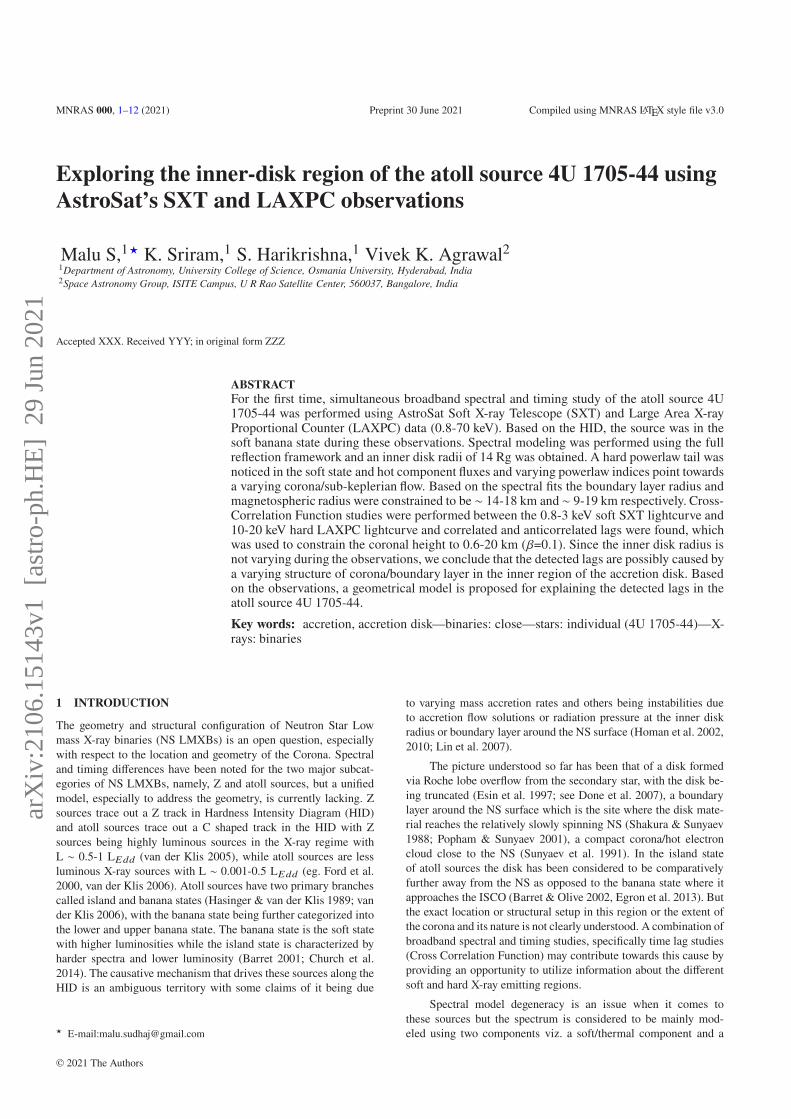
Figure 1. Top: SXT image of the source and the extraction regions used for

source (solid annulus) and background (dashed annulus) extraction. Cali-

bration sources can be seen in the four corners of the image.

(LAXPC 10,20 and 30) with a total effective area ∼ 6000 cm2 at

15 keV and it operates in the 3-80 keV energy range (Yadav et al.

2016a; Agrawal et al. 2017; Antia et al. 2017). We have used data in

the Event Analysis (EA) mode with a time resolution of 10`s. SXT

operated in the 0.3-8 keV energy range and has an effective area of

∼ 128 cm2 at 1.5 keV (Singh et al. 2017). We have used data in the

Photon Counting (PC) mode which has a time resolution of ∼ 2.4 s.

LAXPC level 1 data were processed using the LAXPC soft-

ware (Format A, May 19, 2018 version)1 provided by the As-

troSat Science Support Center (ASSC). Standard procedures for

data reduction were followed, with event files and GTI files

were generated using the laxpc_make_event and laxpc_make_stdgti

routines. Lightcurves and spectra were generated using the

laxpc_make_lightcurve and laxpc_make_spectra routines. Corre-

sponding standard routines were used to generate the background

files. laxpc_make_spectra routine also generates the appropriate re-

sponse files needed for the spectra.

A merged cleaned event file was generated for the SXT

level 2 data using the event merger code and the appropri-

ate ancillary response file was generated using the sxtARF-

module, both provided by the SXT team 2. Lightcurves and

spectra were extracted from the SXT image of the source

using XSELECT (V2.4e). For spectral analysis, response file

(sxt_pc_mat_g0to12.rmf) and deep blank sky background spectrum

file (SkyBkg_comb_EL3p5_Cl_Rd16p0_v01.pha) provided by the

SXT team were utilized. Similar to the procedure adopted in Malu

et al. (2020), the source was extracted with a 1′-10′ annulus to take

care of the pile-up effect (see Figure 1), since the count rate was

> 40 cts s−1 (see AstroSat handbook 3). Background extraction for

the lightcurves was performed using a 13′-15′ annulus. See Figure

2 for the extracted SXT and LAXPC lightcurves.

LAXPC 10 data alone was used for analysis as it is well-

calibrated and has less background issues (Agrawal et al. 2020).

For spectral analysis, LAXPC 10 top layer spectra alone were used

to minimize the background (eg. Beri et al. 2019). Joint spectral

analysis were performed using the LAXPC spectrum in the range

1 http://astrosat-ssc.iucaa.in/?q=laxpcData2 https://www.tifr.res.in/∼astrosat_sxt/dataanalysis.html3 http://www.iucaa.in/∼astrosat/AstroSat_handbook.pdf

01

02

03

04

0

Ra

te(c

ts/s

)

SXT 0.8−3 keV

0 2×104 4×104 6×104 8×104

50

01

00

01

50

0

Ra

te(c

ts/s

)

Time (s)

LAXPC 3−70 keV

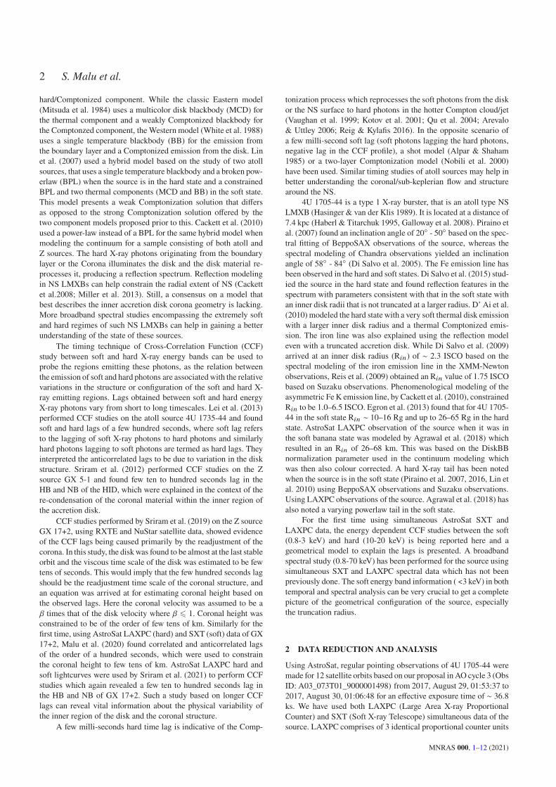
Figure 2. Top: SXT light curve in the 0.8–3 keV energy range. Bottom:

LAXPC 10 light curve in the 3–70 keV energy range. Both lightcurves are

plotted using a time bin of SXT resolution ∼ 2.4 s

5-70 keV and SXT spectrum in the range 0.8-7 keV. Owing to un-

certainties in response, data below 0.8 keV were not considered for

SXT (Bhargava et al. 2019). A 3% systematic error was introduced

while performing spectral fitting 4 (eg. Jithesh et al. 2019, Bhargava

et al. 2019).

3 SPECTRAL ANALYSIS

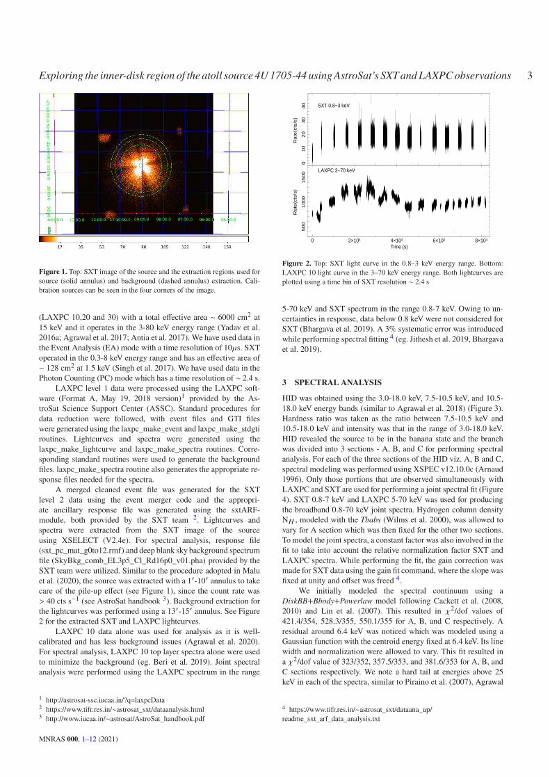
HID was obtained using the 3.0-18.0 keV, 7.5-10.5 keV, and 10.5-

18.0 keV energy bands (similar to Agrawal et al. 2018) (Figure 3).

Hardness ratio was taken as the ratio between 7.5-10.5 keV and

10.5-18.0 keV and intensity was that in the range of 3.0-18.0 keV.

HID revealed the source to be in the banana state and the branch

was divided into 3 sections - A, B, and C for performing spectral

analysis. For each of the three sections of the HID viz. A, B and C,

spectral modeling was performed using XSPEC v12.10.0c (Arnaud

1996). Only those portions that are observed simultaneously with

LAXPC and SXT are used for performing a joint spectral fit (Figure

4). SXT 0.8-7 keV and LAXPC 5-70 keV was used for producing

the broadband 0.8-70 keV joint spectra. Hydrogen column density

N� , modeled with the Tbabs (Wilms et al. 2000), was allowed to

vary for A section which was then fixed for the other two sections.

To model the joint spectra, a constant factor was also involved in the

fit to take into account the relative normalization factor SXT and

LAXPC spectra. While performing the fit, the gain correction was

made for SXT data using the gain fit command, where the slope was

fixed at unity and offset was freed 4.

We initially modeled the spectral continuum using a

DiskBB+Bbody+Powerlaw model following Cackett et al. (2008,

2010) and Lin et al. (2007). This resulted in j2/dof values of

421.4/354, 528.3/355, 550.1/355 for A, B, and C respectively. A

residual around 6.4 keV was noticed which was modeled using a

Gaussian function with the centroid energy fixed at 6.4 keV. Its line

width and normalization were allowed to vary. This fit resulted in

a j2/dof value of 323/352, 357.5/353, and 381.6/353 for A, B, and

C sections respectively. We note a hard tail at energies above 25

keV in each of the spectra, similar to Piraino et al. (2007), Agrawal

4 https://www.tifr.res.in/∼astrosat_sxt/dataana_up/

readme_sxt_arf_data_analysis.txt

MNRAS 000, 1–12 (2021)

4 S. Malu et al.

0.45

0.5

0.55

0.6

0.65

0.7

700 800 900 1000 1100 1200 1300 1400

CBA

Hard

ness

Ratio

(10.5

-18 k

ev/

7.5

-10.5

keV

)

Intensity (cts/s)

Figure 3. HID for 4U 1705-44 using AstroSat LAXPC observations. Hard-

ness ratio is defined as 10.5-18.0/7.5-10.5 keV and intensity is that in the

range 3.0-18.0 keV range. Demarcations show separations of HID into A, B

and C sections.

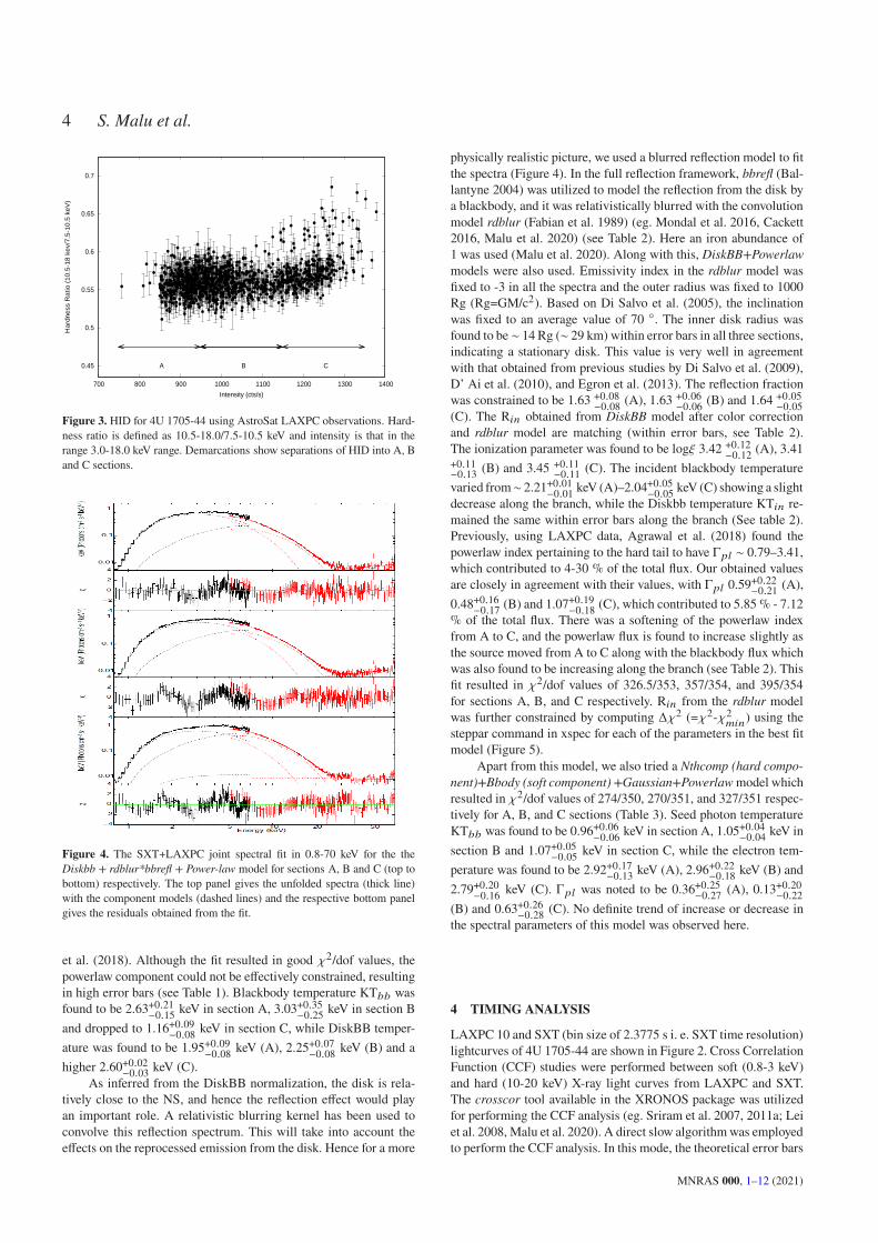
Figure 4. The SXT+LAXPC joint spectral fit in 0.8-70 keV for the the

Diskbb + rdblur*bbrefl + Power-law model for sections A, B and C (top to

bottom) respectively. The top panel gives the unfolded spectra (thick line)

with the component models (dashed lines) and the respective bottom panel

gives the residuals obtained from the fit.

et al. (2018). Although the fit resulted in good j2/dof values, the

powerlaw component could not be effectively constrained, resulting

in high error bars (see Table 1). Blackbody temperature KT11 was

found to be 2.63+0.21−0.15

keV in section A, 3.03+0.35−0.25

keV in section B

and dropped to 1.16+0.09−0.08

keV in section C, while DiskBB temper-

ature was found to be 1.95+0.09−0.08

keV (A), 2.25+0.07−0.08

keV (B) and a

higher 2.60+0.02−0.03

keV (C).

As inferred from the DiskBB normalization, the disk is rela-

tively close to the NS, and hence the reflection effect would play

an important role. A relativistic blurring kernel has been used to

convolve this reflection spectrum. This will take into account the

effects on the reprocessed emission from the disk. Hence for a more

physically realistic picture, we used a blurred reflection model to fit

the spectra (Figure 4). In the full reflection framework, bbrefl (Bal-

lantyne 2004) was utilized to model the reflection from the disk by

a blackbody, and it was relativistically blurred with the convolution

model rdblur (Fabian et al. 1989) (eg. Mondal et al. 2016, Cackett

2016, Malu et al. 2020) (see Table 2). Here an iron abundance of

1 was used (Malu et al. 2020). Along with this, DiskBB+Powerlaw

models were also used. Emissivity index in the rdblur model was

fixed to -3 in all the spectra and the outer radius was fixed to 1000

Rg (Rg=GM/c2). Based on Di Salvo et al. (2005), the inclination

was fixed to an average value of 70 ◦. The inner disk radius was

found to be ∼ 14 Rg (∼ 29 km) within error bars in all three sections,

indicating a stationary disk. This value is very well in agreement

with that obtained from previous studies by Di Salvo et al. (2009),

D’ Ai et al. (2010), and Egron et al. (2013). The reflection fraction

was constrained to be 1.63 +0.08−0.08

(A), 1.63 +0.06−0.06

(B) and 1.64 +0.05−0.05

(C). The R8= obtained from DiskBB model after color correction

and rdblur model are matching (within error bars, see Table 2).

The ionization parameter was found to be logb 3.42 +0.12−0.12

(A), 3.41+0.11−0.13

(B) and 3.45 +0.11−0.11

(C). The incident blackbody temperature

varied from∼ 2.21+0.01−0.01

keV (A)–2.04+0.05−0.05

keV (C) showing a slight

decrease along the branch, while the Diskbb temperature KT8= re-

mained the same within error bars along the branch (See table 2).

Previously, using LAXPC data, Agrawal et al. (2018) found the

powerlaw index pertaining to the hard tail to have Γ?; ∼ 0.79–3.41,

which contributed to 4-30 % of the total flux. Our obtained values

are closely in agreement with their values, with Γ?; 0.59+0.22−0.21

(A),

0.48+0.16−0.17

(B) and 1.07+0.19−0.18

(C), which contributed to 5.85 % - 7.12

% of the total flux. There was a softening of the powerlaw index

from A to C, and the powerlaw flux is found to increase slightly as

the source moved from A to C along with the blackbody flux which

was also found to be increasing along the branch (see Table 2). This

fit resulted in j2/dof values of 326.5/353, 357/354, and 395/354

for sections A, B, and C respectively. R8= from the rdblur model

was further constrained by computing Δj2 (=j2-j2<8=

) using the

steppar command in xspec for each of the parameters in the best fit

model (Figure 5).

Apart from this model, we also tried a Nthcomp (hard compo-

nent)+Bbody (soft component) +Gaussian+Powerlaw model which

resulted in j2/dof values of 274/350, 270/351, and 327/351 respec-

tively for A, B, and C sections (Table 3). Seed photon temperature

KT11 was found to be 0.96+0.06−0.06

keV in section A, 1.05+0.04−0.04

keV in

section B and 1.07+0.05−0.05

keV in section C, while the electron tem-

perature was found to be 2.92+0.17−0.13

keV (A), 2.96+0.22−0.18

keV (B) and

2.79+0.20−0.16

keV (C). Γ?; was noted to be 0.36+0.25−0.27

(A), 0.13+0.20−0.22

(B) and 0.63+0.26−0.28

(C). No definite trend of increase or decrease in

the spectral parameters of this model was observed here.

4 TIMING ANALYSIS

LAXPC 10 and SXT (bin size of 2.3775 s i. e. SXT time resolution)

lightcurves of 4U 1705-44 are shown in Figure 2. Cross Correlation

Function (CCF) studies were performed between soft (0.8-3 keV)

and hard (10-20 keV) X-ray light curves from LAXPC and SXT.

The crosscor tool available in the XRONOS package was utilized

for performing the CCF analysis (eg. Sriram et al. 2007, 2011a; Lei

et al. 2008, Malu et al. 2020). A direct slow algorithm was employed

to perform the CCF analysis. In this mode, the theoretical error bars

MNRAS 000, 1–12 (2021)

Exploring the inner-disk region of the atoll source 4U 1705-44 using AstroSat’s SXT and LAXPC observations 5

0

50

100

150

200

250

5 10 15 20 25 30 35 40 45 50

Χ2 -Χ2 m

in

Rin (Rg)

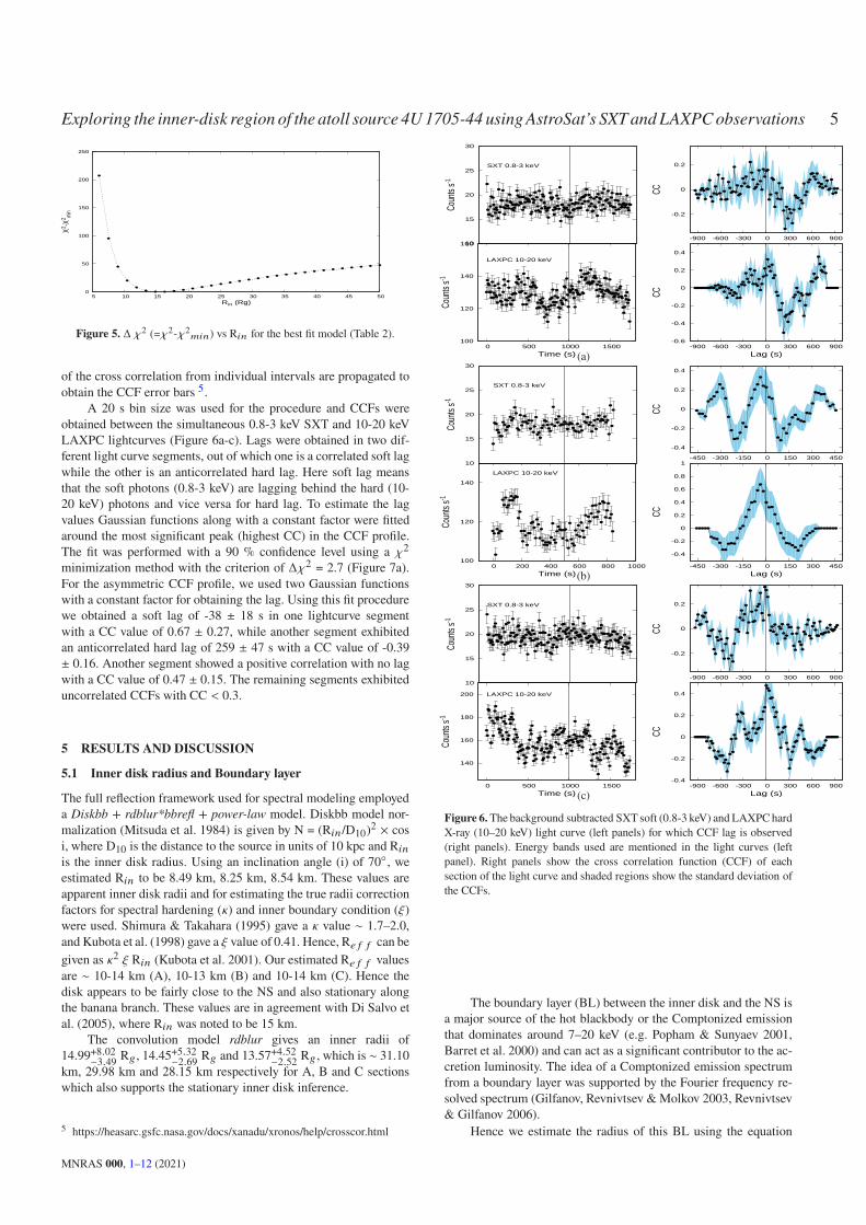
Figure 5. Δ j2 (=j2-j2<8=) vs R8= for the best fit model (Table 2).

of the cross correlation from individual intervals are propagated to

obtain the CCF error bars 5.

A 20 s bin size was used for the procedure and CCFs were

obtained between the simultaneous 0.8-3 keV SXT and 10-20 keV

LAXPC lightcurves (Figure 6a-c). Lags were obtained in two dif-

ferent light curve segments, out of which one is a correlated soft lag

while the other is an anticorrelated hard lag. Here soft lag means

that the soft photons (0.8-3 keV) are lagging behind the hard (10-

20 keV) photons and vice versa for hard lag. To estimate the lag

values Gaussian functions along with a constant factor were fitted

around the most significant peak (highest CC) in the CCF profile.

The fit was performed with a 90 % confidence level using a j2

minimization method with the criterion of Δj2 = 2.7 (Figure 7a).

For the asymmetric CCF profile, we used two Gaussian functions

with a constant factor for obtaining the lag. Using this fit procedure

we obtained a soft lag of -38 ± 18 s in one lightcurve segment

with a CC value of 0.67 ± 0.27, while another segment exhibited

an anticorrelated hard lag of 259 ± 47 s with a CC value of -0.39

± 0.16. Another segment showed a positive correlation with no lag

with a CC value of 0.47 ± 0.15. The remaining segments exhibited

uncorrelated CCFs with CC < 0.3.

5 RESULTS AND DISCUSSION

5.1 Inner disk radius and Boundary layer

The full reflection framework used for spectral modeling employed

a Diskbb + rdblur*bbrefl + power-law model. Diskbb model nor-

malization (Mitsuda et al. 1984) is given by N = (R8=/D10)2 × cos

i, where D10 is the distance to the source in units of 10 kpc and R8=

is the inner disk radius. Using an inclination angle (i) of 70◦, we

estimated R8= to be 8.49 km, 8.25 km, 8.54 km. These values are

apparent inner disk radii and for estimating the true radii correction

factors for spectral hardening (^) and inner boundary condition (b)

were used. Shimura & Takahara (1995) gave a ^ value ∼ 1.7–2.0,

and Kubota et al. (1998) gave a b value of 0.41. Hence, R4 5 5 can be

given as ^2 b R8= (Kubota et al. 2001). Our estimated R4 5 5 values

are ∼ 10-14 km (A), 10-13 km (B) and 10-14 km (C). Hence the

disk appears to be fairly close to the NS and also stationary along

the banana branch. These values are in agreement with Di Salvo et

al. (2005), where R8= was noted to be 15 km.

The convolution model rdblur gives an inner radii of

14.99+8.02−3.49

R6, 14.45+5.32−2.69

R6 and 13.57+4.52−2.52

R6, which is ∼ 31.10

km, 29.98 km and 28.15 km respectively for A, B and C sections

which also supports the stationary inner disk inference.

5 https://heasarc.gsfc.nasa.gov/docs/xanadu/xronos/help/crosscor.html

10

15

20

25

30

SXT 0.8-3 keV

Coun

ts s-1

-0.6

-0.4

-0.2

0

0.2

0.4

-900 -600 -300 0 300 600 900

CC

Lag (s)

-0.2

0

0.2

-900 -600 -300 0 300 600 900

CC

100

120

140

160

0 500 1000 1500

LAXPC 10-20 keV

Coun

ts s-1

Time (s) (a)

10

15

20

25

30

SXT 0.8-3 keV

Coun

ts s-1

-0.4

-0.2

0

0.2

0.4

0.6

0.8

1

-450 -300 -150 0 150 300 450

CC

Lag (s)

-0.4

-0.2

0

0.2

0.4

-450 -300 -150 0 150 300 450

CC

100

120

140

0 200 400 600 800 1000

LAXPC 10-20 keV

Coun

ts s-1

Time (s)(b)

10

15

20

25

30

SXT 0.8-3 keV

Coun

ts s-1

-0.4

-0.2

0

0.2

0.4

-900 -600 -300 0 300 600 900

CC

Lag (s)

-0.2

0

0.2

-900 -600 -300 0 300 600 900

CC

140

160

180

200

0 500 1000 1500

LAXPC 10-20 keV

Coun

ts s-1

Time (s) (c)

Figure 6. The background subtracted SXT soft (0.8-3 keV) and LAXPC hard

X-ray (10–20 keV) light curve (left panels) for which CCF lag is observed

(right panels). Energy bands used are mentioned in the light curves (left

panel). Right panels show the cross correlation function (CCF) of each

section of the light curve and shaded regions show the standard deviation of

the CCFs.

The boundary layer (BL) between the inner disk and the NS is

a major source of the hot blackbody or the Comptonized emission

that dominates around 7–20 keV (e.g. Popham & Sunyaev 2001,

Barret et al. 2000) and can act as a significant contributor to the ac-

cretion luminosity. The idea of a Comptonized emission spectrum

from a boundary layer was supported by the Fourier frequency re-

solved spectrum (Gilfanov, Revnivtsev & Molkov 2003, Revnivtsev

& Gilfanov 2006).

Hence we estimate the radius of this BL using the equation

MNRAS 000, 1–12 (2021)

6 S. Malu et al.

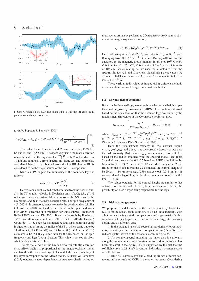
-0.8

-0.6

-0.4

-0.2

0

0.2

0.4

-600 -300 0 300 600

CC

Lag (s)

-0.4

0

0.4

0 200 400 600

(a)

-0.4

-0.2

0

0.2

0.4

0.6

0.8

1

-300 -150 0 150 300

CC

Lag (s)

-0.4

0

0.4

0.8

-200 -100 0 100

(b)

Figure 7. Figure shows CCF lags fitted using a Gaussian function using

points around the maximum peak.

given by Popham & Sunyaev (2001),

;>6('�! − '#() ∼ 5.02 + 0.245

[

;>6( ¤"

10−9.85 "⊙HA−1

)

]2.19

(1)

This value for sections A,B and C came out to be, 15.74 km

(A and B) and 16.52 km (C) respectively using the mass accretion

rate obtained from the equation L= �" ¤"' with M = 1.4 M⊙ , R =

10 km and luminosity from spectral fit (Table 2). The luminosity

considered here is that obtained from the hot BB flux as BL is

considered to be the major source of the hot BB component.

Kluzniak (1987) gave the luminosity of the boundary layer as

follows,

!�! = (1 − Z)2�" ¤"

2'#((2)

Here we consider L�! to be that obtained from the hot BB flux.

Z is the NS angular velocity in Keplerian units (Ω∗/Ω: ('#()), G

is the gravitational constant, M is the mass of the NS, R#( is the

NS radius, and ¤" is the mass accretion rate. The spin frequency of

4U 1705-44 is unknown, hence we make the consideration (similar

to D’Ai et al. 2010) that the difference between the upper and lower

kHz QPOs is near the spin frequency for some sources (Méndez &

Belloni 2007; van der Klis 2004). Based on the study by Ford et al.

1998, this difference would be ∼ 330 Hz for 4U 1705-44. Hence Z

would be ∼ 0.15. Then we estimated ¤" and substituted this value

in equation 1 to estimate the radius of the BL, which came out to be

14.20 km (A), 15.49 km (B) and 18.14 km (C). D’ Ai et al. (2010)

estimated a 1.8-2.1 R#( outer radii for the BL based on the spin

frequency and L�!/L�8B: fraction. This value is not too far from

what has been estimated here.

The magnetic field of the NS can also truncate the accretion

disk. Alfven radius is proportional to the magnetospheric radius

and based on the transition layer (TL) model, the outer boundary of

this layer corresponds to the Alfven radius. Kulkarni & Romanova

(2013) obtained a new dependence of magnetospheric radius on

mass accretion rate by performing 3D magnetohydrodynamics sim-

ulation of magnetospheric accretion,

A< ∼ 2.50 × 106`2/5 ¤<−1/5"−1/10'3/10 2< (3)

Here, following Asai et al. (2016), we substituted ` = B R3, with

B ranging from 0.5–3.5 × 108 G, where R=R#(=10 km. In this

equation, `, the magnetic dipole moment in units of 1026 G cm3,

¤< is in units of 1016 g s−1, M is in units of 1.4 M⊙ and R in units

of 106 cm. For estimating r<, we used the ¤< obtained from the

spectral fits for A,B and C sections. Substituting these values we

estimated, 8-19 km for section A,B and C for magnetic field B =

0.5–3.5 × 108 G.

These various radii values estimated using different methods

as shown above are well in agreement with each other.

5.2 Coronal height estimates

Based on the detected lags, we can estimate the coronal height as per

the equation given by Sriram et al. (2019). This equation is derived

based on the consideration that the obtained lags are primarily the

readjustment timescales of the Corona/sub-keplerian flow.

�2>A>=0 =

[

C;06 ¤<

2c'38B:�38B: d− '38B:

]

× V 2< (4)

where H38B: = 108 U−1/10 ¤<3/20

16'

9/8

105 3/20 cm, d = 7 × 10−8

U−7/10 ¤<11/20 '−15/8 5 11/20 g cm−3, f = (1-(RB /R)1/2)1/4

(Shakura & Sunyaev 1973, Sriram et al. 2019).

Here the readjustment velocity in the coronal region

v2>A>=0=Vv38B: and V is 6 1 as the coronal viscosity is less than

the disk viscosity. Disk radius R38B: was considered to be 30 km

based on the radius obtained from the spectral model (see Table

2) and V was taken to be 0.1–0.5 based on MHD simulations by

Manmoto et al. 1997, Pen et al. 2003 and McKinney et al. 2012.

Based on these considerations we estimated the coronal height to

be 20 km – 110 km for a lag of 259 s and V = 0.1–0.5. Similarly, if

we considered a lag of 38 s, the height estimates are found to be 0.6

km – 3.37 km.

The values obtained for the coronal height are similar to that

obtained for the BL and TL radii, hence we can not rule out the

possibility of such a layer being responsible for the lags.

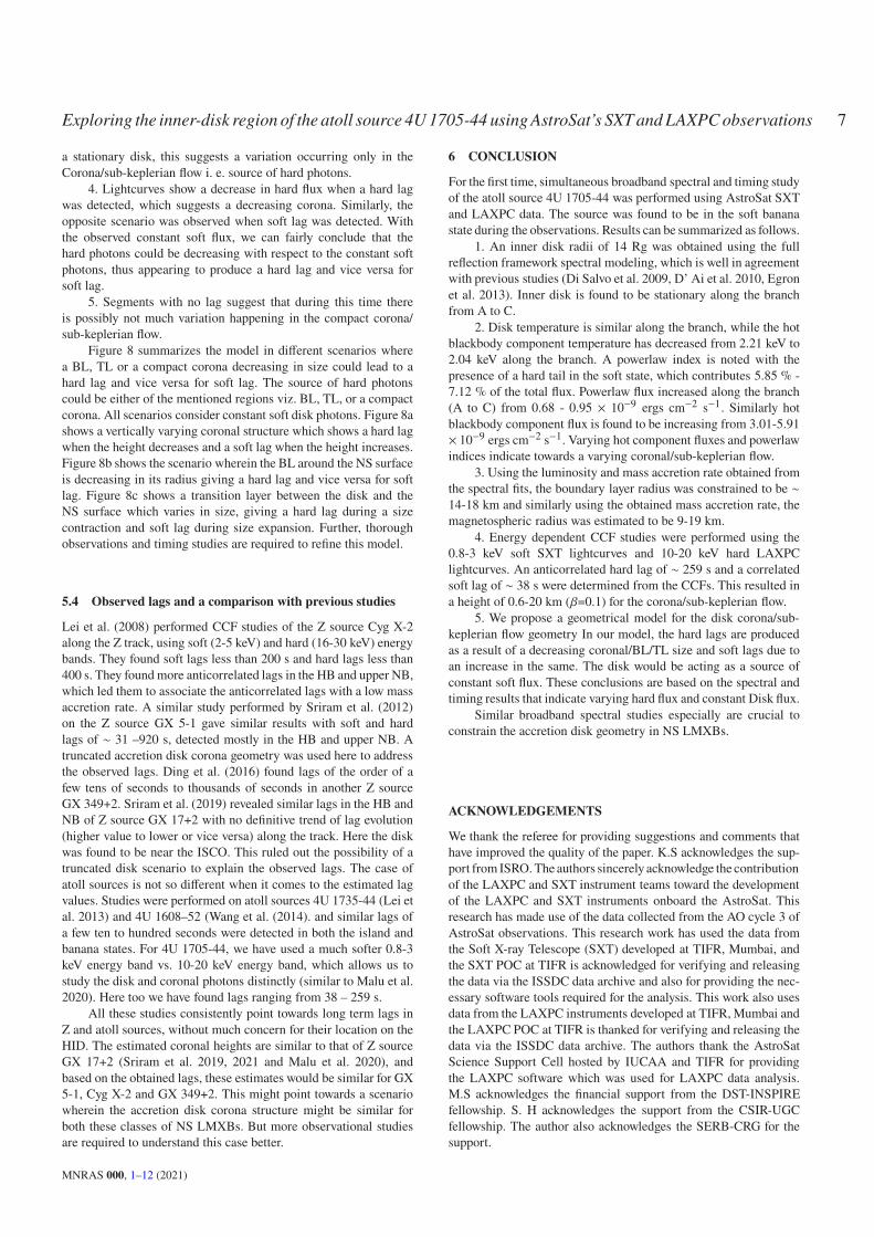
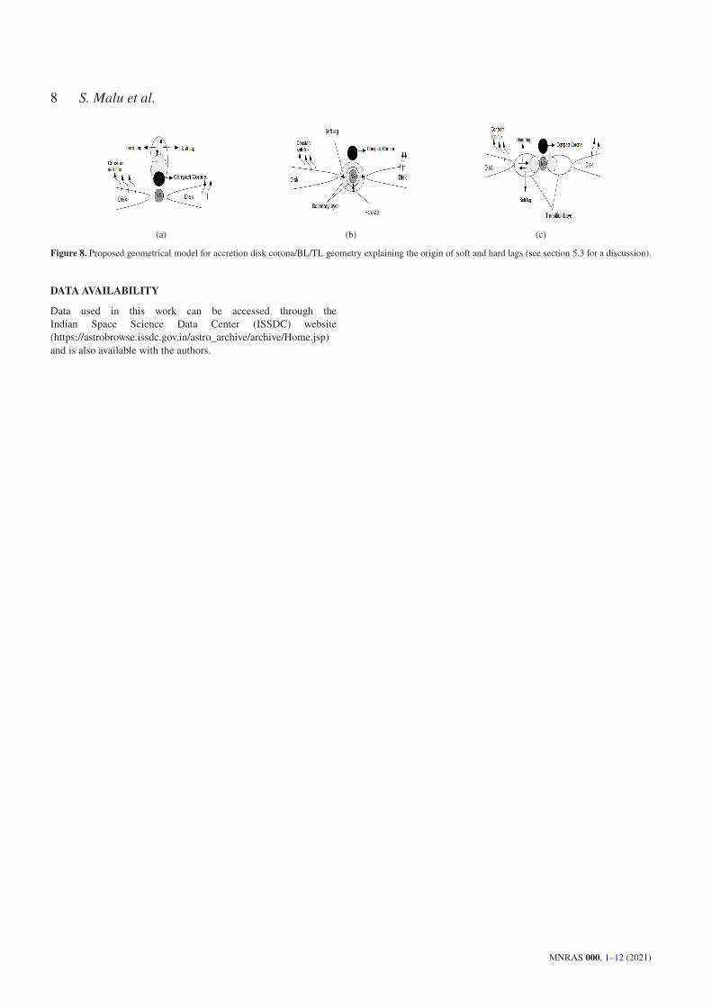
5.3 Disk-corona geometry

We propose a model similar to the one proposed by Kara et al.

(2019) for the Disk Corona geometry of a black-hole transient, with

a hot corona having a static compact core and a geometrically thin

accretion disk (see Figure 8a). Their model also suggests a varying

corona and a stationary disk.

1. In the banana branch the source has a relatively lower hard-

ness, indicating a low temperature compact corona (Table 3) i. e. a

reduced spatial extent of the corona, as seen in figure 8a.

2. As per the spectral modeling the inner disk is stationary

along the branch, indicating a constant influx of disk photons as has

been indicated in the figure. This is supported by the fact that the

soft light curve in 0.8-3 keV is constant indicating a constant source

of soft photons.

3. But CCF shows a soft and a hard lag in two different seg-

ments, and uncorrelated CCFs in the other segments. Considering

MNRAS 000, 1–12 (2021)

Exploring the inner-disk region of the atoll source 4U 1705-44 using AstroSat’s SXT and LAXPC observations 7

a stationary disk, this suggests a variation occurring only in the

Corona/sub-keplerian flow i. e. source of hard photons.

4. Lightcurves show a decrease in hard flux when a hard lag

was detected, which suggests a decreasing corona. Similarly, the

opposite scenario was observed when soft lag was detected. With

the observed constant soft flux, we can fairly conclude that the

hard photons could be decreasing with respect to the constant soft

photons, thus appearing to produce a hard lag and vice versa for

soft lag.

5. Segments with no lag suggest that during this time there

is possibly not much variation happening in the compact corona/

sub-keplerian flow.

Figure 8 summarizes the model in different scenarios where

a BL, TL or a compact corona decreasing in size could lead to a

hard lag and vice versa for soft lag. The source of hard photons

could be either of the mentioned regions viz. BL, TL, or a compact

corona. All scenarios consider constant soft disk photons. Figure 8a

shows a vertically varying coronal structure which shows a hard lag

when the height decreases and a soft lag when the height increases.

Figure 8b shows the scenario wherein the BL around the NS surface

is decreasing in its radius giving a hard lag and vice versa for soft

lag. Figure 8c shows a transition layer between the disk and the

NS surface which varies in size, giving a hard lag during a size

contraction and soft lag during size expansion. Further, thorough

observations and timing studies are required to refine this model.

5.4 Observed lags and a comparison with previous studies

Lei et al. (2008) performed CCF studies of the Z source Cyg X-2

along the Z track, using soft (2-5 keV) and hard (16-30 keV) energy

bands. They found soft lags less than 200 s and hard lags less than

400 s. They found more anticorrelated lags in the HB and upper NB,

which led them to associate the anticorrelated lags with a low mass

accretion rate. A similar study performed by Sriram et al. (2012)

on the Z source GX 5-1 gave similar results with soft and hard

lags of ∼ 31 –920 s, detected mostly in the HB and upper NB. A

truncated accretion disk corona geometry was used here to address

the observed lags. Ding et al. (2016) found lags of the order of a

few tens of seconds to thousands of seconds in another Z source

GX 349+2. Sriram et al. (2019) revealed similar lags in the HB and

NB of Z source GX 17+2 with no definitive trend of lag evolution

(higher value to lower or vice versa) along the track. Here the disk

was found to be near the ISCO. This ruled out the possibility of a

truncated disk scenario to explain the observed lags. The case of

atoll sources is not so different when it comes to the estimated lag

values. Studies were performed on atoll sources 4U 1735-44 (Lei et

al. 2013) and 4U 1608–52 (Wang et al. (2014). and similar lags of

a few ten to hundred seconds were detected in both the island and

banana states. For 4U 1705-44, we have used a much softer 0.8-3

keV energy band vs. 10-20 keV energy band, which allows us to

study the disk and coronal photons distinctly (similar to Malu et al.

2020). Here too we have found lags ranging from 38 – 259 s.

All these studies consistently point towards long term lags in

Z and atoll sources, without much concern for their location on the

HID. The estimated coronal heights are similar to that of Z source

GX 17+2 (Sriram et al. 2019, 2021 and Malu et al. 2020), and

based on the obtained lags, these estimates would be similar for GX

5-1, Cyg X-2 and GX 349+2. This might point towards a scenario

wherein the accretion disk corona structure might be similar for

both these classes of NS LMXBs. But more observational studies

are required to understand this case better.

6 CONCLUSION

For the first time, simultaneous broadband spectral and timing study

of the atoll source 4U 1705-44 was performed using AstroSat SXT

and LAXPC data. The source was found to be in the soft banana

state during the observations. Results can be summarized as follows.

1. An inner disk radii of 14 Rg was obtained using the full

reflection framework spectral modeling, which is well in agreement

with previous studies (Di Salvo et al. 2009, D’ Ai et al. 2010, Egron

et al. 2013). Inner disk is found to be stationary along the branch

from A to C.

2. Disk temperature is similar along the branch, while the hot

blackbody component temperature has decreased from 2.21 keV to

2.04 keV along the branch. A powerlaw index is noted with the

presence of a hard tail in the soft state, which contributes 5.85 % -

7.12 % of the total flux. Powerlaw flux increased along the branch

(A to C) from 0.68 - 0.95 × 10−9 ergs cm−2 s−1. Similarly hot

blackbody component flux is found to be increasing from 3.01-5.91

× 10−9 ergs cm−2 s−1. Varying hot component fluxes and powerlaw

indices indicate towards a varying coronal/sub-keplerian flow.

3. Using the luminosity and mass accretion rate obtained from

the spectral fits, the boundary layer radius was constrained to be ∼

14-18 km and similarly using the obtained mass accretion rate, the

magnetospheric radius was estimated to be 9-19 km.

4. Energy dependent CCF studies were performed using the

0.8-3 keV soft SXT lightcurves and 10-20 keV hard LAXPC

lightcurves. An anticorrelated hard lag of ∼ 259 s and a correlated

soft lag of ∼ 38 s were determined from the CCFs. This resulted in

a height of 0.6-20 km (V=0.1) for the corona/sub-keplerian flow.

5. We propose a geometrical model for the disk corona/sub-

keplerian flow geometry In our model, the hard lags are produced

as a result of a decreasing coronal/BL/TL size and soft lags due to

an increase in the same. The disk would be acting as a source of

constant soft flux. These conclusions are based on the spectral and

timing results that indicate varying hard flux and constant Disk flux.

Similar broadband spectral studies especially are crucial to

constrain the accretion disk geometry in NS LMXBs.

ACKNOWLEDGEMENTS

We thank the referee for providing suggestions and comments that

have improved the quality of the paper. K.S acknowledges the sup-

port from ISRO. The authors sincerely acknowledge the contribution

of the LAXPC and SXT instrument teams toward the development

of the LAXPC and SXT instruments onboard the AstroSat. This

research has made use of the data collected from the AO cycle 3 of

AstroSat observations. This research work has used the data from

the Soft X-ray Telescope (SXT) developed at TIFR, Mumbai, and

the SXT POC at TIFR is acknowledged for verifying and releasing

the data via the ISSDC data archive and also for providing the nec-

essary software tools required for the analysis. This work also uses

data from the LAXPC instruments developed at TIFR, Mumbai and

the LAXPC POC at TIFR is thanked for verifying and releasing the

data via the ISSDC data archive. The authors thank the AstroSat

Science Support Cell hosted by IUCAA and TIFR for providing

the LAXPC software which was used for LAXPC data analysis.

M.S acknowledges the financial support from the DST-INSPIRE

fellowship. S. H acknowledges the support from the CSIR-UGC

fellowship. The author also acknowledges the SERB-CRG for the

support.

MNRAS 000, 1–12 (2021)

8 S. Malu et al.

(a) (b) (c)

Figure 8. Proposed geometrical model for accretion disk corona/BL/TL geometry explaining the origin of soft and hard lags (see section 5.3 for a discussion).

DATA AVAILABILITY

Data used in this work can be accessed through the

Indian Space Science Data Center (ISSDC) website

(https://astrobrowse.issdc.gov.in/astro_archive/archive/Home.jsp)

and is also available with the authors.

MNRAS 000, 1–12 (2021)

Exploring the inner-disk region of the atoll source 4U 1705-44 using AstroSat’s SXT and LAXPC observations 9

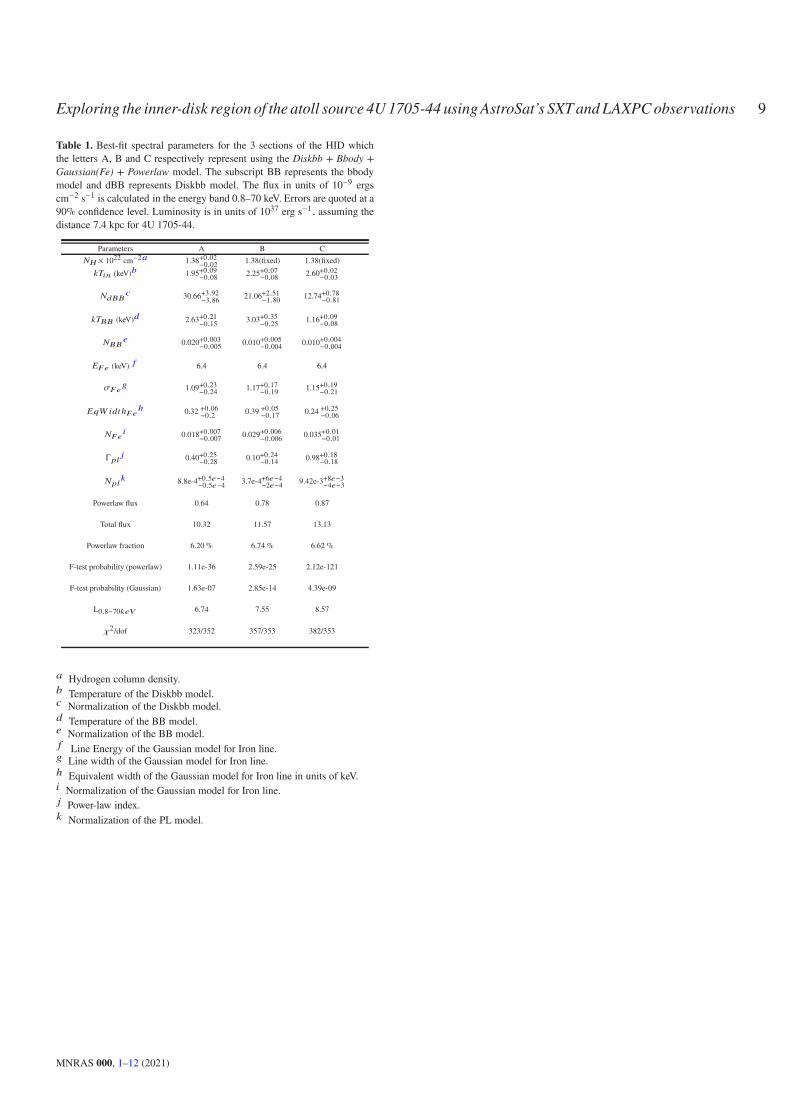
Table 1. Best-fit spectral parameters for the 3 sections of the HID which

the letters A, B and C respectively represent using the Diskbb + Bbody +

Gaussian(Fe) + Powerlaw model. The subscript BB represents the bbody

model and dBB represents Diskbb model. The flux in units of 10−9 ergs

cm−2 s−1 is calculated in the energy band 0.8–70 keV. Errors are quoted at a

90% confidence level. Luminosity is in units of 1037 erg s−1. assuming the

distance 7.4 kpc for 4U 1705-44.

Parameters A B C

#�× 1022 cm−20 1.38+0.02−0.02

1.38(fixed) 1.38(fixed)

:)8= (keV)1 1.95+0.09−0.08

2.25+0.07−0.08

2.60+0.02−0.03

#3��2 30.66+3.92

−3.8621.06+2.51

−1.8012.74+0.78

−0.81

:)�� (keV)3 2.63+0.21−0.15

3.03+0.35−0.25

1.16+0.09−0.08

#��4 0.020+0.003

−0.0050.010+0.005

−0.0040.010+0.004

−0.004

��4 (keV) 5 6.4 6.4 6.4

f�46 1.09+0.23

−0.241.17+0.17

−0.191.15+0.19

−0.21

�@, 83Cℎ�4ℎ 0.32 +0.06

−0.20.39 +0.05

−0.170.24 +0.25

−0.06

#�48 0.018+0.007

−0.0070.029+0.006

−0.0060.035+0.01

−0.01

Γ?;9 0.40+0.25

−0.280.10+0.24

−0.140.98+0.18

−0.18

#?;: 8.8e-4+0.54−4

−0.54−43.7e-4+64−4

−24−49.42e-3+84−3

−44−3

Powerlaw flux 0.64 0.78 0.87

Total flux 10.32 11.57 13.13

Powerlaw fraction 6.20 % 6.74 % 6.62 %

F-test probability (powerlaw) 1.11e-36 2.59e-25 2.12e-121

F-test probability (Gaussian) 1.63e-07 2.85e-14 4.39e-09

L0.8−70:4+ 6.74 7.55 8.57

j2 /dof 323/352 357/353 382/353

0 Hydrogen column density.1 Temperature of the Diskbb model.2 Normalization of the Diskbb model.3 Temperature of the BB model.4 Normalization of the BB model.5 Line Energy of the Gaussian model for Iron line.6 Line width of the Gaussian model for Iron line.ℎ Equivalent width of the Gaussian model for Iron line in units of keV.8 Normalization of the Gaussian model for Iron line.9 Power-law index.: Normalization of the PL model.

MNRAS 000, 1–12 (2021)

10 S. Malu et al.

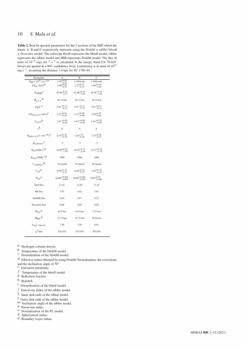
Table 2. Best-fit spectral parameters for the 3 sections of the HID which the

letters A, B and C respectively represent using the Diskbb + rdblur*bbrefl

+ Powerlaw model. The subscript bbrefl represents the bbrefl model, rdblur

represents the rdblur model and dBB represents Diskbb model. The flux in

units of 10−9 ergs cm−2 s−1 is calculated in the energy band 0.8–70 keV.

Errors are quoted at a 90% confidence level. Luminosity is in units of 1037

erg s−1. assuming the distance 7.4 kpc for 4U 1705-44.

Parameters A B C

#�× 1022 cm−20 1.39+0.02−0.02

1.39(fixed) 1.39(fixed)

:)8= (keV)1 1.68+0.02−0.02

1.72+0.13−0.11

1.66+0.03−0.03

#3��2 45.09+2.47

−2.3142.49+8.45

−7.6545.56+3.16

−2.92

'4 5 53 10-14 km 10-13 km 10-14 km

logb 4 3.42 +0.12−0.12

3.41 +0.11−0.13

3.45 +0.11−0.11

:)11A4 5 ; (keV) 5 2.21+0.01−0.01

2.13+0.08−0.06

2.04+0.05−0.05

fA4 5 ;6 1.63 +0.08

−0.081.63 +0.06

−0.061.64 +0.05

−0.05

Iℎ 0 0 0

N11A4 5 ; (1 ×10−26)8 0.75+0.26−0.19

1.04+.35−0.26

1.37+0.36−0.31

VA31;DA9 -3 -3 -3

R8=(GM/c2): 14.99+8.02−3.49

14.45+5.32−2.69

13.57+4.52−2.52

R>DC (GM/c2); 1000 1000 1000

i◦A31;DA< 70 (fixed) 70 (fixed) 70 (fixed)

Γ?;= 0.59+0.22

−0.210.48+0.16

−0.171.07+0.19

−0.18

#?;> 0.002+0.005

−0.0010.002+0.001

−0.0010.01+0.01

−0.006

Total flux 11.61 11.62 13.19

BB flux 3.01 4.02 5.91

DiskBB flux 6.63 6.67 6.23

Powerlaw flux 0.68 0.85 0.94

'B?? 6.62 km 6.63 km 7.53 km

'�!@ 15.74 km 15.74 km 16.52 km

L0.8−70:4+ 7.58 7.58 8.61

j2 /dof 326/353 357/354 395/354

0 Hydrogen column density.1 Temperature of the Diskbb model.2 Normalization of the Diskbb model.3 Effective radius obtained by using Diskbb Normalization, the corrections

and the inclination angle of 70◦

4 Ionization parameter.5 Temperature of the bbrefl model.6 Reflection fraction.ℎ Redshift8 Normalization of the bbrefl model.9 Emissivity Index of the rdblur model.: Inner disk radii of the rdblur model.; Outer disk radii of the rdblur model.< Inclination angle of the rdblur model.= Power-law index.> Normalization of the PL model.? Spherization radius@ Boundary Layer radius

MNRAS 000, 1–12 (2021)

Exploring the inner-disk region of the atoll source 4U 1705-44 using AstroSat’s SXT and LAXPC observations 11

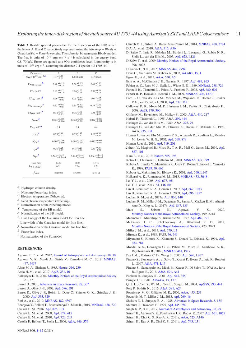
Table 3. Best-fit spectral parameters for the 3 sections of the HID which

the letters A, B and C respectively represent using the Nthcomp + Bbody +

Gaussian(Fe) + Powerlaw model. The subscript bb represents Bbody model.

The flux in units of 10−9 ergs cm−2 s−1 is calculated in the energy band

0.8–70 keV. Errors are quoted at a 90% confidence level. Luminosity is in

units of 1037 erg s−1, assuming the distance 7.4 kpc for 4U 1705-44.

Parameters A B C

#�× 1022 cm−20 1.47+0.11−0.11

1.47(fixed) 1.47(fixed)

Γ#Cℎ2><?1 2.48 +0.15

−0.132.56 +0.15

−0.142.41 +0.16

−0.14

:)4 (keV)2 2.92 +0.17−0.13

2.96+0.22−0.18

2.79+0.20−0.16

:)11 (keV)3 0.96 +0.06−0.06

1.05 +0.04−0.04

1.07 +0.05−0.05

##Cℎ2><?4 0.32 +0.03

−0.030.31 +0.02

−0.020.33 +0.02

−0.02

:)�� (keV) 5 0.34+0.03−0.03

0.36+0.02−0.02

0.36+0.02−0.02

#��6 0.021+0.005

−0.0040.022+0.001

−0.0010.022+0.001

−0.001

��4 keV ℎ 6.4 6.4 6.4

f�48 0.99+0.46

−0.720.99+0.47

−0.451.02+0.38

−0.32

#�49 0.007+0.006

−0.0060.008+0.007

−0.0070.015+0.009

−0.009

Γ?;: 0.36+0.25

−0.270.13+0.20

−0.220.63+0.26

−0.28

#?;; 7.5e-4+14−3

−0.54−43.9e-4+54−4

−24−42.38e-3+44−3

−14−3

Total flux 10.59 11.86 13.45

L0.8−70:4+ 6.91 7.74 8.78

j2 /dof 274/350 270/351 327/351

0 Hydrogen column density.1 Nthcomp Power-law index.2 Electron temperature (Nthcomp).3 Seed photon temperature (Nthcomp).4 Normalization of the Nthcomp model.5 Temperature of the BB model.6 Normalization of the BB model.ℎ Line Energy of the Gaussian model for Iron line.8 Line width of the Gaussian model for Iron line.9 Normalization of the Gaussian model for Iron line.: Power-law index.; Normalization of the PL model.

REFERENCES

Agrawal P. C., et al., 2017, Journal of Astrophysics and Astronomy, 38, 30

Agrawal V. K., Nandi A., Girish V., Ramadevi M. C., 2018, MNRAS,

477, 5437

Alpar M. A., Shaham J., 1985, Nature, 316, 239

Antia H. M., et al., 2017, ApJS, 231, 10

Ballantyne D. R., 2004, Monthly Notices of the Royal Astronomical Society,

351, 57

Barret D., 2001, Advances in Space Research, 28, 307

Barret D., Olive J.-F., 2002, ApJ, 576, 391

Barret D., Olive J. F., Boirin L., Done C., Skinner G. K., Grindlay J. E.,

2000, ApJ, 533, 329

Beri A., et al., 2019, MNRAS, 482, 4397

Bhargava Y., Belloni T., Bhattacharya D., Misra R., 2019, MNRAS, 488, 720

Cackett E. M., 2016, ApJ, 826, 103

Cackett E. M., et al., 2008, ApJ, 674, 415

Cackett E. M., et al., 2010, ApJ, 720, 205

Casella P., Belloni T., Stella L., 2006, A&A, 446, 579

Church M. J., Gibiec A., Bałucińska-Church M., 2014, MNRAS, 438, 2784

D’Aì A., et al., 2010, A&A, 516, A36

Di Salvo T., Iaria R., Méndez M., Burderi L., Lavagetto G., Robba N. R.,

Stella L., van der Klis M., 2005, ApJ, 623, L121

Di Salvo T., et al., 2009, Monthly Notices of the Royal Astronomical Society,

398, 2022

Di Salvo T., et al., 2015, MNRAS, 449, 2794

Done C., Gierliński M., Kubota A., 2007, A&ARv, 15, 1

Egron E., et al., 2013, A&A, 550, A5

Esin A. A., McClintock J. E., Narayan R., 1997, ApJ, 489, 865

Fabian A. C., Rees M. J., Stella L., White N. E., 1989, MNRAS, 238, 729

Farinelli R., Titarchuk L., Paizis A., Frontera F., 2008, ApJ, 680, 602

Fender R. P., Homan J., Belloni T. M., 2009, MNRAS, 396, 1370

Ford E. C., van der Klis M., Méndez M., Wijnands R., Homan J., Jonker

P. G., van Paradijs J., 2000, ApJ, 537, 368

Galloway D. K., Muno M. P., Hartman J. M., Psaltis D., Chakrabarty D.,

2008, ApJS, 179, 360

Gilfanov M., Revnivtsev M., Molkov S., 2003, A&A, 410, 217

Haberl F., Titarchuk L., 1995, A&A, 299, 414

Hasinger G., van der Klis M., 1989, A&A, 225, 79

Hasinger G., van der Klis M., Ebisawa K., Dotani T., Mitsuda K., 1990,

A&A, 235, 131

Homan J., van der Klis M., Jonker P. G., Wijnands R., Kuulkers E., Méndez

M., Lewin W. H. G., 2002, ApJ, 568, 878

Homan J., et al., 2010, ApJ, 719, 201

Jithesh V., Maqbool B., Misra R., T A. R., Mall G., James M., 2019, ApJ,

887, 101

Kara E., et al., 2019, Nature, 565, 198

Kotov O., Churazov E., Gilfanov M., 2001, MNRAS, 327, 799

Kubota A., Tanaka Y., Makishima K., Ueda Y., Dotani T., Inoue H., Yamaoka

K., 1998, PASJ, 50, 667

Kubota A., Makishima K., Ebisawa K., 2001, ApJ, 560, L147

Kulkarni A. K., Romanova M. M., 2013, MNRAS, 433, 3048

Lei Y. J., et al., 2008, ApJ, 677, 461

Lei Y.-J., et al., 2013, AJ, 146, 60

Lin D., Remillard R. A., Homan J., 2007, ApJ, 667, 1073

Lin D., Remillard R. A., Homan J., 2009, ApJ, 696, 1257

Ludlam R. M., et al., 2017a, ApJ, 836, 140

Ludlam R. M., Miller J. M., Degenaar N., Sanna A., Cackett E. M., Altami-

rano D., King A. L., 2017b, ApJ, 847, 135

Malu S., Sriram K., Agrawal V. K., 2020,

Monthly Notices of the Royal Astronomical Society, 499, 2214

Manmoto T., Mineshige S., Kusunose M., 1997, ApJ, 489, 791

McKinney J. C., Tchekhovskoy A., Blandford R. D., 2012,

Monthly Notices of the Royal Astronomical Society, 423, 3083

Miller J. M., et al., 2013, ApJ, 779, L2

Mitsuda K., et al., 1984, PASJ, 36, 741

Miyamoto S., Kimura K., Kitamoto S., Dotani T., Ebisawa K., 1991, ApJ,

383, 784

Mondal A. S., Dewangan G. C., Pahari M., Misra R., Kembhavi A. K.,

Raychaudhuri B., 2016, MNRAS, 461, 1917

Pen U.-L., Matzner C. D., Wong S., 2003, ApJ, 596, L207

Piraino S., Santangelo A., di Salvo T., Kaaret P., Horns D., Iaria R., Burderi

L., 2007, A&A, 471, L17

Piraino S., Santangelo A., Mück B., Kaaret P., Di Salvo T., D’Aì A., Iaria

R., Egron E., 2016, A&A, 591, A41

Popham R., Sunyaev R., 2001, ApJ, 547, 355

Pringle J. E., 1981, ARA&A, 19, 137

Qu J. L., Chen Y., Wu M., Chen L., Song L. M., 2004, Ap&SS, 293, 441

Reig P., Kylafis N., 2016, A&A, 591, A24

Revnivtsev M. G., Gilfanov M. R., 2006, A&A, 453, 253

Reynolds M. T., Miller J. M., 2013, ApJ, 769, 16

Shakura N. I., Sunyaev R. A., 1988, Advances in Space Research, 8, 135

Shimura T., Takahara F., 1995, ApJ, 445, 780

Singh K. P., et al., 2017, Journal of Astrophysics and Astronomy, 38, 29

Sriram K., Agrawal V. K., Pendharkar J. K., Rao A. R., 2007, ApJ, 661, 1055

Sriram K., Choi C. S., Rao A. R., 2011a, A&A, 525, A146

Sriram K., Rao A. R., Choi C. S., 2011b, ApJ, 743, L31

MNRAS 000, 1–12 (2021)

12 S. Malu et al.

Sriram K., Rao A. R., Choi C. S., 2012, A&A, 541, A6

Sriram K., Malu S., Choi C. S., 2019,

The Astrophysical Journal Supplement Series, 244, 5

Sriram K., Chiranjeevi P., Malu S., Agrawal V. K., 2021, arXiv e-prints,

p. arXiv:2103.05794

Syunyaev R. A., et al., 1991, Soviet Astronomy Letters, 17, 409

Titarchuk L. G., Bradshaw C. F., Geldzahler B. J., Fomalont E. B., 2001,

ApJ, 555, L45

Vaughan B. A., van der Klis M., Lewin W. H. G., van Paradijs J., Mitsuda

K., Dotani T., 1999, A&A, 343, 197

Vrtilek S. D., Raymond J. C., Garcia M. R., Verbunt F., Hasinger G., Kurster

M., 1990, A&A, 235, 162

White N. E., Stella L., Parmar A. N., 1988, ApJ, 324, 363

Wilms J., Allen A., McCray R., 2000, ApJ, 542, 914

Yadav J. S., et al., 2016, Large Area X-ray Proportional Counter (LAXPC)

instrument onboard ASTROSAT. p. 99051D, doi:10.1117/12.2231857

van der Klis M., 2005, in Burderi L., Antonelli L. A., D’Antona F., di Salvo T.,

Israel G. L., Piersanti L., Tornambè A., Straniero O., eds, American In-

stitute of Physics Conference Series Vol. 797, Interacting Binaries: Ac-

cretion, Evolution, and Outcomes. pp 345–358, doi:10.1063/1.2130253

van der Klis M., 2006, Rapid X-ray Variability. pp 39–112

This paper has been typeset from a TEX/LATEX file prepared by the author.

MNRAS 000, 1–12 (2021)

This figure "specall.jpg" is available in "jpg" format from:

http://arxiv.org/ps/2106.15143v1

This figure "specall.png" is available in "png" format from:

http://arxiv.org/ps/2106.15143v1