Exploring parameter constraints on quintessential dark energy: The exponential model

Exploring Parameter Constraints on Quintessential Dark Energy: The ExponentialModel

Brandon Bozek, Augusta Abrahamse, Andreas Albrecht, and Michael BarnardPhysics Department, University of California, Davis.

(Dated: February 12, 2013)

We present an analysis of a scalar field model of dark energy with an exponential potential usingthe Dark Energy Task Force (DETF) simulated data models. Using Markov Chain Monte Carlosampling techniques we examine the ability of each simulated data set to constrain the parameterspace of the exponential potential for data sets based on a cosmological constant and a specificexponential scalar field model. We compare our results with the constraining power calculatedby the DETF using their “w0 − wa” parametrization of the dark energy. We find that respectiveincreases in constraining power from one stage to the next produced by our analysis give resultsconsistent with DETF results. To further investigate the potential impact of future experiments,we also generate simulated data for an exponential model background cosmology which can not bedistinguished from a cosmological constant at DETF “Stage 2”, and show that for this cosmologygood DETF Stage 4 data would exclude a cosmological constant by better than 3σ.

PACS numbers:

I. INTRODUCTION

In the late 90’s, two independent teams presented evi-dence from supernova observations that the universe, in-stead of slowing down due to gravity, is accelerating [1, 2].In the standard cosmological framework, the accelerationis caused by a mysterious new form of matter, dubbed“Dark Energy”, that makes up roughly 70% of the uni-verse. There is a wide variety of possible explanations fordark energy. The simplest model that provides a goodfit to the data is a cosmological constant. A cosmologi-cal constant is equivalent to a homogeneous fluid with aconstant energy density and a ratio of pressure to energydensity (the “equation of state parameter” w), equal to−1 at all times. Yet, despite compelling evidence for theexistence of dark energy, it is unclear whether the darkenergy density is constant or varies with time. There aremany different proposals for a dynamical form of darkenergy, one of them being quintessence. Quintessencedescribes the acceleration being caused by a scalar field,φ, but even just among quintessence models there is atremendous variety of possible behaviors. There is con-siderable interest in acquiring better data in order to im-prove our understanding of dark energy.

Recently the Dark Energy Task Force (DETF) re-leased a report charting a course for future experiments[3]. They modeled dark energy as a homogeneous andisotropic fluid with an equation of state parameterized byw(a) = w0 + wa(1− a), where the scale factor a = 1 to-day. Defining Stage 1 to be what is already known, theyforecasted data for three additional experimental stages:Stage 2 data represents on-going experiments that willbe completed in the near future. Stage 3 data sets repre-sent medium sized proposed experiments. Lastly, Stage 4data sets represent proposed large scale future space andground-based experiments. Each stage is further catego-rized as either “optimistic” or “pessimistic” depending onhow well the systematics are expected to be constrained.

The scientific impact of a stage was quantified in termsof a “Figure of Merit” (FoM). The Figure of Merit is de-fined to be the ratio of the area of the 2σ contour of thew0 − wa space for Stage 2 divided by the area of the 2σcontour of the w0 − wa space for Stage 3 (or 4).

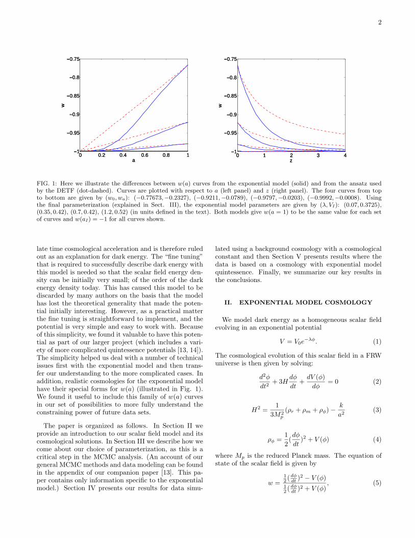
The DETF analysis leaves several open questions,some of which our research seeks to address. The w0−waparameterization is not motivated by a physical model ofdark energy and provides cosmological solutions that maybe very different from a scalar field model. As illustratedin Fig. 1, the w curves generated by the exponentialscalar field model that we consider in this paper are notespecially well fit by curves in the w0−wa family, exceptfor those nearly identical to w = −1. Thus the relation-ship between the DETF results and the impact of futureexperiments on scalar field models is not clear. A goodway to clarify this point is to model the impact of futuredata sets directly on particular scalar field quintessencemodels, which is what we do here. Our work comple-ments the DETF report as well as work by other authorsusing alternative w(a) parameterizations [4, 5], parame-terizations of ρDE [6], and model independent scalar fieldparameters [7].

The exponential scalar field model has been used inmany different cosmological contexts due to its ability togive scaling solutions for the scalar field energy densityρφ where d(log(ρφ))

d(log(a)) → β. The constant β depends on pa-rameters in the scalar field potential as well as the otherforms of matter present in the universe . Originally thepotential was used for power law inflation models and wasshown to have a range of attractor solutions [8]. Its abil-ity to produce attractor solutions that scale like the back-ground energy density made it an interesting choice for adark matter candidate [9, 10, 11]. The variety of scalingsolutions is well covered by Copeland, et al. [12] wherethey argue that consideration of “fine tuning”parametersand constraints from nucleosynthesis give λ > 20 as anatural choice. This range of λ values wouldn’t allow for

arX

iv:0

712.

2884

v1 [

astr

o-ph

] 1

8 D

ec 2

007

2

0 0.2 0.4 0.6 0.8 1−1

−0.95

−0.9

−0.85

−0.8

−0.75

a

w

Student Version of MATLAB

0 1 2 3 4−1

−0.95

−0.9

−0.85

−0.8

−0.75

z

w


FIG. 1: Here we illustrate the differences between w(a) curves from the exponential model (solid) and from the ansatz usedby the DETF (dot-dashed). Curves are plotted with respect to a (left panel) and z (right panel). The four curves from topto bottom are given by (w0, wa): (−0.77673,−0.2327), (−0.9211,−0.0789), (−0.9797,−0.0203), (−0.9992,−0.0008). Usingthe final parameterization (explained in Sect. III), the exponential model parameters are given by (λ, VI): (0.07, 0.3725),(0.35, 0.42), (0.7, 0.42), (1.2, 0.52) (in units defined in the text). Both models give w(a = 1) to be the same value for each setof curves and w(aI) = −1 for all curves shown.

late time cosmological acceleration and is therefore ruledout as an explanation for dark energy. The “fine tuning”that is required to successfully describe dark energy withthis model is needed so that the scalar field energy den-sity can be initially very small; of the order of the darkenergy density today. This has caused this model to bediscarded by many authors on the basis that the modelhas lost the theoretical generality that made the poten-tial initially interesting. However, as a practical matterthe fine tuning is straightforward to implement, and thepotential is very simple and easy to work with. Becauseof this simplicity, we found it valuable to have this poten-tial as part of our larger project (which includes a vari-ety of more complicated quintessence potentials [13, 14]).The simplicity helped us deal with a number of technicalissues first with the exponential model and then trans-fer our understanding to the more complicated cases. Inaddition, realistic cosmologies for the exponential modelhave their special forms for w(a) (illustrated in Fig. 1).We found it useful to include this family of w(a) curvesin our set of possibilities to more fully understand theconstraining power of future data sets.

The paper is organized as follows. In Section II weprovide an introduction to our scalar field model and itscosmological solutions. In Section III we describe how wecome about our choice of parameterization, as this is acritical step in the MCMC analysis. (An account of ourgeneral MCMC methods and data modeling can be foundin the appendix of our companion paper [13]. This pa-per contains only information specific to the exponentialmodel.) Section IV presents our results for data simu-

lated using a background cosmology with a cosmologicalconstant and then Section V presents results where thedata is based on a cosmology with exponential modelquintessence. Finally, we summarize our key results inthe conclusions.

II. EXPONENTIAL MODEL COSMOLOGY

We model dark energy as a homogeneous scalar fieldevolving in an exponential potential

V = V0e−λφ. (1)

The cosmological evolution of this scalar field in a FRWuniverse is then given by solving:

d2φ

dt2+ 3H

dφ

dt+dV (φ)dφ

= 0 (2)

H2 =1

3M2p

(ρr + ρm + ρφ)− k

a2(3)

ρφ =12

(dφ

dt)2 + V (φ) (4)

where Mp is the reduced Planck mass. The equation ofstate of the scalar field is given by

w =12 (dφdt )2 − V (φ)12 (dφdt )2 + V (φ)

, (5)

3

−6 −4 −2 0 2

0.2

0.4

0.6

0.8

1

φ

V


0 0.2 0.4 0.6 0.8 1−1

−0.99

−0.98

−0.97

−0.96

−0.95

−0.94

−0.93

−0.92

z

w


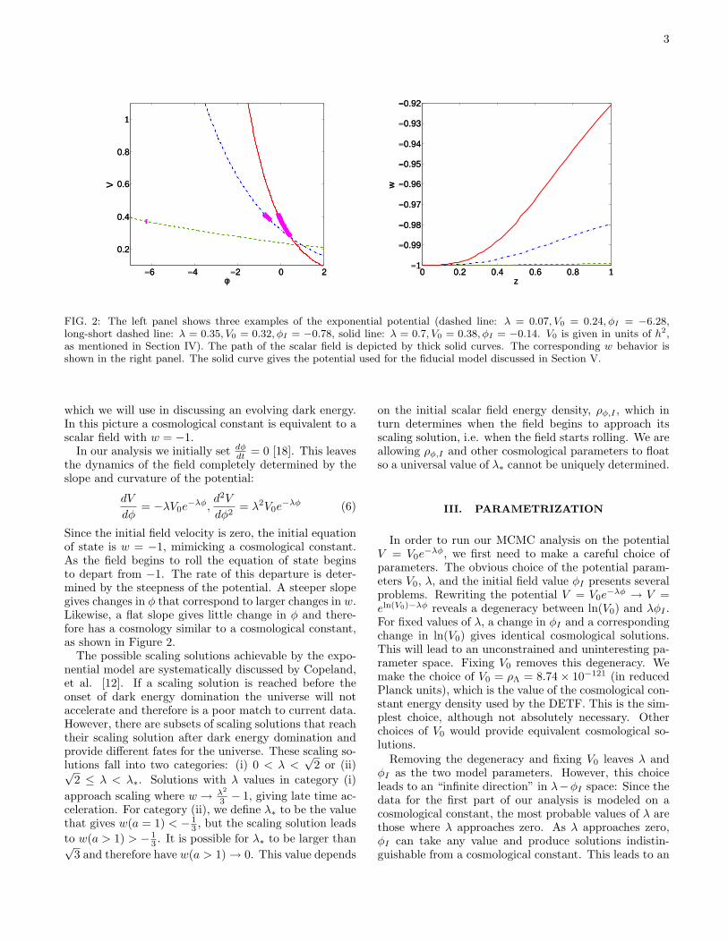
FIG. 2: The left panel shows three examples of the exponential potential (dashed line: λ = 0.07, V0 = 0.24, φI = −6.28,long-short dashed line: λ = 0.35, V0 = 0.32, φI = −0.78, solid line: λ = 0.7, V0 = 0.38, φI = −0.14. V0 is given in units of h2,as mentioned in Section IV). The path of the scalar field is depicted by thick solid curves. The corresponding w behavior isshown in the right panel. The solid curve gives the potential used for the fiducial model discussed in Section V.

which we will use in discussing an evolving dark energy.In this picture a cosmological constant is equivalent to ascalar field with w = −1.

In our analysis we initially set dφdt = 0 [18]. This leaves

the dynamics of the field completely determined by theslope and curvature of the potential:

dV

dφ= −λV0e

−λφ,d2V

dφ2= λ2V0e

−λφ (6)

Since the initial field velocity is zero, the initial equationof state is w = −1, mimicking a cosmological constant.As the field begins to roll the equation of state beginsto depart from −1. The rate of this departure is deter-mined by the steepness of the potential. A steeper slopegives changes in φ that correspond to larger changes in w.Likewise, a flat slope gives little change in φ and there-fore has a cosmology similar to a cosmological constant,as shown in Figure 2.

The possible scaling solutions achievable by the expo-nential model are systematically discussed by Copeland,et al. [12]. If a scaling solution is reached before theonset of dark energy domination the universe will notaccelerate and therefore is a poor match to current data.However, there are subsets of scaling solutions that reachtheir scaling solution after dark energy domination andprovide different fates for the universe. These scaling so-lutions fall into two categories: (i) 0 < λ <

√2 or (ii)√

2 ≤ λ < λ∗. Solutions with λ values in category (i)approach scaling where w → λ2

3 − 1, giving late time ac-celeration. For category (ii), we define λ∗ to be the valuethat gives w(a = 1) < − 1

3 , but the scaling solution leadsto w(a > 1) > − 1

3 . It is possible for λ∗ to be larger than√3 and therefore have w(a > 1)→ 0. This value depends

on the initial scalar field energy density, ρφ,I , which inturn determines when the field begins to approach itsscaling solution, i.e. when the field starts rolling. We areallowing ρφ,I and other cosmological parameters to floatso a universal value of λ∗ cannot be uniquely determined.

III. PARAMETRIZATION

In order to run our MCMC analysis on the potentialV = V0e

−λφ, we first need to make a careful choice ofparameters. The obvious choice of the potential param-eters V0, λ, and the initial field value φI presents severalproblems. Rewriting the potential V = V0e

−λφ → V =eln(V0)−λφ reveals a degeneracy between ln(V0) and λφI .For fixed values of λ, a change in φI and a correspondingchange in ln(V0) gives identical cosmological solutions.This will lead to an unconstrained and uninteresting pa-rameter space. Fixing V0 removes this degeneracy. Wemake the choice of V0 = ρΛ = 8.74× 10−121 (in reducedPlanck units), which is the value of the cosmological con-stant energy density used by the DETF. This is the sim-plest choice, although not absolutely necessary. Otherchoices of V0 would provide equivalent cosmological so-lutions.

Removing the degeneracy and fixing V0 leaves λ andφI as the two model parameters. However, this choiceleads to an “infinite direction” in λ−φI space: Since thedata for the first part of our analysis is modeled on acosmological constant, the most probable values of λ arethose where λ approaches zero. As λ approaches zero,φI can take any value and produce solutions indistin-guishable from a cosmological constant. This leads to an

4

λ

Vi

Stage 2

0 0.5 1 1.50.3

0.35

0.4

0.45

0.5

0.55


λ

Vi

Stage 3 Photo Optimistic

0 0.5 1 1.50.3

0.35

0.4

0.45

0.5

0.55


λ

Vi

Stage 4 Ground LST Optimistic

0 0.5 1 1.50.3

0.35

0.4

0.45

0.5

0.55


λ

Vi

Stage 4 Space Optimistic

0 0.5 1 1.50.3

0.35

0.4

0.45

0.5

0.55


FIG. 3: Likelihood contours in the VI−λ space for cosmological constant data models. The three contours give 68.27%, 95.44%,and 99.73% confidence regions.

infinite unconstrained direction in parameter space thatis uninteresting and also fatal to the MCMC techniques.

One can resolve this problem by placing a bound on λor φI . For small values of λ, a bound placed on λ is nearlyequivalent to placing a bound on w(a = 1). A choiceof a bound on λ can be chosen such that the differencefrom w = −1 is small, however the choice is arbitrary.Further, for data based on a Λ universe, the closer thebound is placed to λ = 0, the more the allowed region ofparameter space squeezes against this bound as smallervalues of λ allow a wider range of φI , basically partiallyrestoring the degeneracy we are trying to eliminate. Thisarbitrariness and distortion of allowed parameter rangesmake bounding λ a poor choice for addressing the pa-rameter space degeneracies in this model. The squeezingeffect leads to incorrect conclusions about allowed valuesof λ. The space appears to disfavor larger values of λ,or equivalently larger departures from w(a = 1) = −1,than would the space in the final parameterization thatwe discuss next.

We find the best choice of free model parameters to be

VI , where VI = V (φI), and λ. The value of φI is thendetermined from λ and VI . This parameterization avoidsthe degeneracy discussed in the previous paragraph sincea cosmological constant of a particular value is only rep-resented at one point (VI = ρΛ and λ = 0) in the λ− VIspace. Values similar to a cosmological constant are ex-plored without an arbitrary bound placed on any param-eter. This allows the MCMC method freedom to explorea more natural space.

There is no loss of generality with this choice of param-eterization as is easily seen by the slope and curvature ofthe potential in the new parameters:

dV

dφ= −λVI ,

d2V

dφ2= λ2VI (7)

This parameterization allows a simple intuition about therole of these parameters forming the solutions. Smallvalues of λ give a flat potential and the scalar field willbe stationary, independent of the choice of VI . For largevalues of λ the field will roll and the amount to which itdoes will depend on the value of VI .

5

λ

δωD

E

Stage 2

0 0.5 1 1.50

0.04

0.08

0.12

0.16

0.2


λ

δωD

E


0 0.5 1 1.50

0.04

0.08

0.12

0.16

0.2


λ

δωD

E


0 0.5 1 1.50

0.04

0.08

0.12

0.16

0.2


λ

δωD

E


0 0.5 1 1.50

0.04

0.08

0.12

0.16

0.2


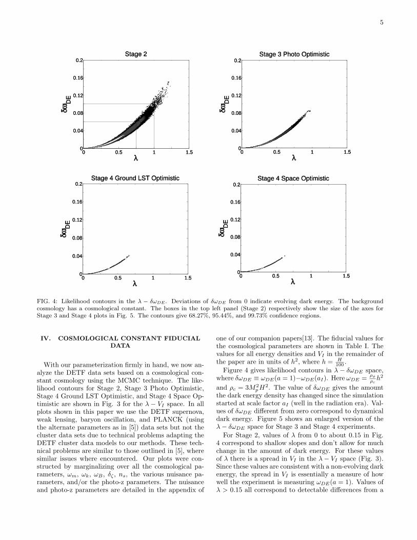
FIG. 4: Likelihood contours in the λ − δωDE . Deviations of δωDE from 0 indicate evolving dark energy. The backgroundcosmology has a cosmological constant. The boxes in the top left panel (Stage 2) respectively show the size of the axes forStage 3 and Stage 4 plots in Fig. 5. The contours give 68.27%, 95.44%, and 99.73% confidence regions.

IV. COSMOLOGICAL CONSTANT FIDUCIALDATA

With our parameterization firmly in hand, we now an-alyze the DETF data sets based on a cosmological con-stant cosmology using the MCMC technique. The like-lihood contours for Stage 2, Stage 3 Photo Optimistic,Stage 4 Ground LST Optimistic, and Stage 4 Space Op-timistic are shown in Fig. 3 for the λ − VI space. In allplots shown in this paper we use the DETF supernova,weak lensing, baryon oscillation, and PLANCK (usingthe alternate parameters as in [5]) data sets but not thecluster data sets due to technical problems adapting theDETF cluster data models to our methods. These tech-nical problems are similar to those outlined in [5], wheresimilar issues where encountered. Our plots were con-structed by marginalizing over all the cosmological pa-rameters, ωm, ωk, ωB , δζ , ns, the various nuisance pa-rameters, and/or the photo-z parameters. The nuisanceand photo-z parameters are detailed in the appendix of

one of our companion papers[13]. The fiducial values forthe cosmological parameters are shown in Table I. Thevalues for all energy densities and VI in the remainder ofthe paper are in units of h2, where h = H

100 .Figure 4 gives likelihood contours in λ − δωDE space,

where δωDE ≡ ωDE(a = 1)−ωDE(aI). Here ωDE = ρφρch2

and ρc = 3M2pH

2. The value of δωDE gives the amountthe dark energy density has changed since the simulationstarted at scale factor aI (well in the radiation era). Val-ues of δωDE different from zero correspond to dynamicaldark energy. Figure 5 shows an enlarged version of theλ− δωDE space for Stage 3 and Stage 4 experiments.

For Stage 2, values of λ from 0 to about 0.15 in Fig.4 correspond to shallow slopes and don’t allow for muchchange in the amount of dark energy. For these valuesof λ there is a spread in VI in the λ− VI space (Fig. 3).Since these values are consistent with a non-evolving darkenergy, the spread in VI is essentially a measure of howwell the experiment is measuring ωDE(a = 1). Values ofλ > 0.15 all correspond to detectable differences from a

6

λ

δωD

E


0 0.25 0.5 0.75 10

0.02

0.04

0.06

0.08

0.1


λ

δωD

E


0 0.25 0.5 0.750

0.02

0.04

0.06


λ

δωD

E


0 0.25 0.5 0.750

0.02

0.04

0.06


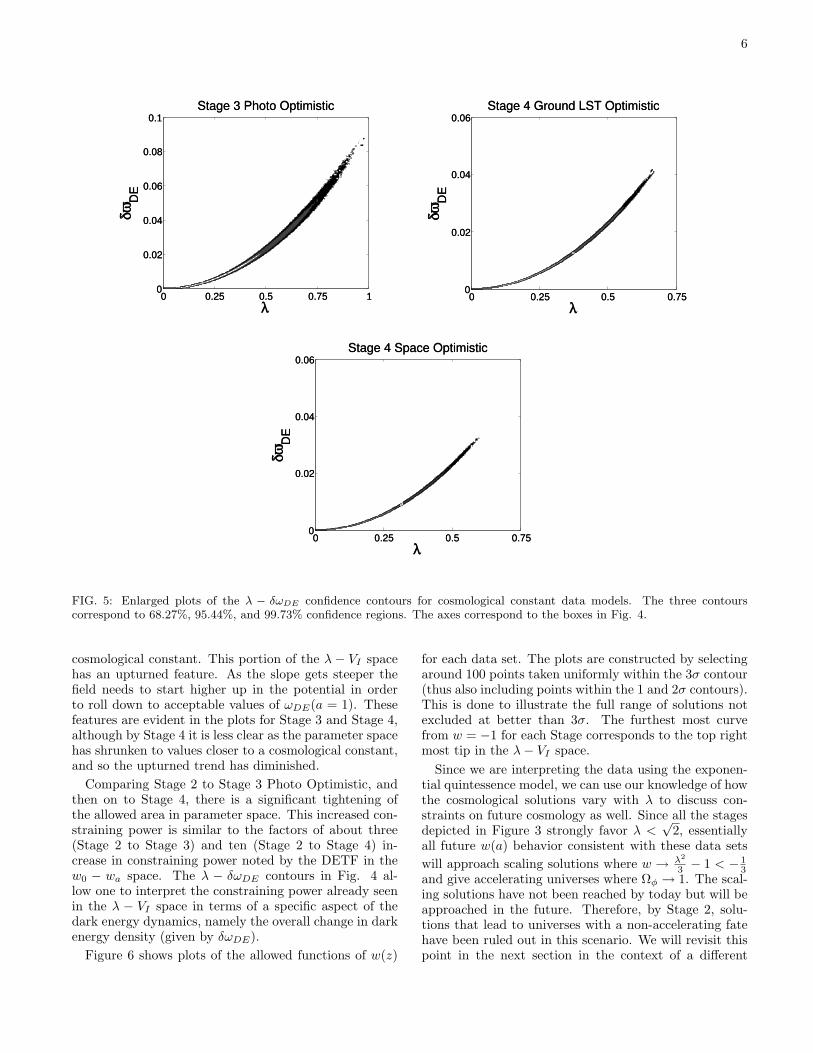
FIG. 5: Enlarged plots of the λ − δωDE confidence contours for cosmological constant data models. The three contourscorrespond to 68.27%, 95.44%, and 99.73% confidence regions. The axes correspond to the boxes in Fig. 4.

cosmological constant. This portion of the λ − VI spacehas an upturned feature. As the slope gets steeper thefield needs to start higher up in the potential in orderto roll down to acceptable values of ωDE(a = 1). Thesefeatures are evident in the plots for Stage 3 and Stage 4,although by Stage 4 it is less clear as the parameter spacehas shrunken to values closer to a cosmological constant,and so the upturned trend has diminished.

Comparing Stage 2 to Stage 3 Photo Optimistic, andthen on to Stage 4, there is a significant tightening ofthe allowed area in parameter space. This increased con-straining power is similar to the factors of about three(Stage 2 to Stage 3) and ten (Stage 2 to Stage 4) in-crease in constraining power noted by the DETF in thew0 − wa space. The λ − δωDE contours in Fig. 4 al-low one to interpret the constraining power already seenin the λ − VI space in terms of a specific aspect of thedark energy dynamics, namely the overall change in darkenergy density (given by δωDE).

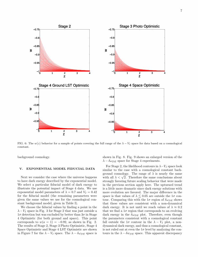
Figure 6 shows plots of the allowed functions of w(z)

for each data set. The plots are constructed by selectingaround 100 points taken uniformly within the 3σ contour(thus also including points within the 1 and 2σ contours).This is done to illustrate the full range of solutions notexcluded at better than 3σ. The furthest most curvefrom w = −1 for each Stage corresponds to the top rightmost tip in the λ− VI space.

Since we are interpreting the data using the exponen-tial quintessence model, we can use our knowledge of howthe cosmological solutions vary with λ to discuss con-straints on future cosmology as well. Since all the stagesdepicted in Figure 3 strongly favor λ <

√2, essentially

all future w(a) behavior consistent with these data setswill approach scaling solutions where w → λ2

3 − 1 < − 13

and give accelerating universes where Ωφ → 1. The scal-ing solutions have not been reached by today but will beapproached in the future. Therefore, by Stage 2, solu-tions that lead to universes with a non-accelerating fatehave been ruled out in this scenario. We will revisit thispoint in the next section in the context of a different

7

0 1 2 3 4−1

−0.95

−0.9

−0.85

−0.8

−0.75Stage 2

z

w


0 1 2 3 4−1

−0.95

−0.9

−0.85

−0.8

−0.75Stage 3 Photo Optimistic

z

w


0 1 2 3 4−1

−0.95

−0.9

−0.85

−0.8

−0.75

z

w



0 1 2 3 4−1

−0.95

−0.9

−0.85

−0.8

−0.75Stage 4 Space Optimistic

z

w


FIG. 6: The w(z) behavior for a sample of points covering the full range of the λ− VI space for data based on a cosmologicalconstant.

background cosmology.

V. EXPONENTIAL MODEL FIDUCIAL DATA

Next we consider the case where the universe happensto have dark energy described by the exponential model.We select a particular fiducial model of dark energy toillustrate the potential impact of Stage 4 data. We useexponential model parameters of λ = 0.7 and VI = 0.42for the fiducial model (the remaining parameters weregiven the same values we use for the cosmological con-stant background model, given in Table I).

We choose the fiducial values by finding a point in theλ−VI space in Fig. 3 for Stage 2 that was just outside a1σ detection but was excluded by better than 3σ in Stage4 Optimistic (for both ground and space). This pointcorresponds to w(a = 1) = −0.92, as shown in Fig. 2.The results of Stage 2, Stage 3 Photo Optimistic, Stage 4Space Optimistic and Stage 4 LST Optimistic are shownin Figure 7 for the λ− VI space. The λ− δωDE space is

shown in Fig. 8. Fig. 9 shows an enlarged version of theλ− δωDE space for Stage 4 experiments.

For Stage 2, the likelihood contours in λ−VI space looksimilar to the case with a cosmological constant back-ground cosmology. The range of λ is nearly the samewith all λ <

√2. Therefore the same conclusions about

strongly favoring future scaling behavior that were madein the previous section apply here. The upturned trendis a little more dramatic since dark energy solutions withmore evolution are favored. The major difference in thespace is that values of λ . 0.05 are outside the 1σ con-tour. Comparing this with the 1σ region of δωDE showsthat these values are consistent with a non-dynamicaldark energy. It is not until we reach values of λ ≈ 0.2that we find a 1σ region that corresponds to an evolvingdark energy in the δωDE plot. Therefore, even thoughthe parameters consistent with a cosmological constantfall outside the 1σ contour in the λ − VI plot, a non-dynamical dark energy, and thus a cosmological constant,is not ruled out at even the 1σ level by analyzing the con-tours in the λ− δwDE space. This apparent discrepancy

8

λ

Vi

Stage 2

0 0.5 1 1.50.3

0.35

0.4

0.45

0.5

0.55


λ

Vi


0 0.5 1 1.50.3

0.35

0.4

0.45

0.5

0.55


λ

Vi

Stage 4G LST Optimisstic

0 0.5 1 1.50.3

0.35

0.4

0.45

0.5

0.55


λ

Vi


0 0.5 1 1.50.3

0.35

0.4

0.45

0.5

0.55


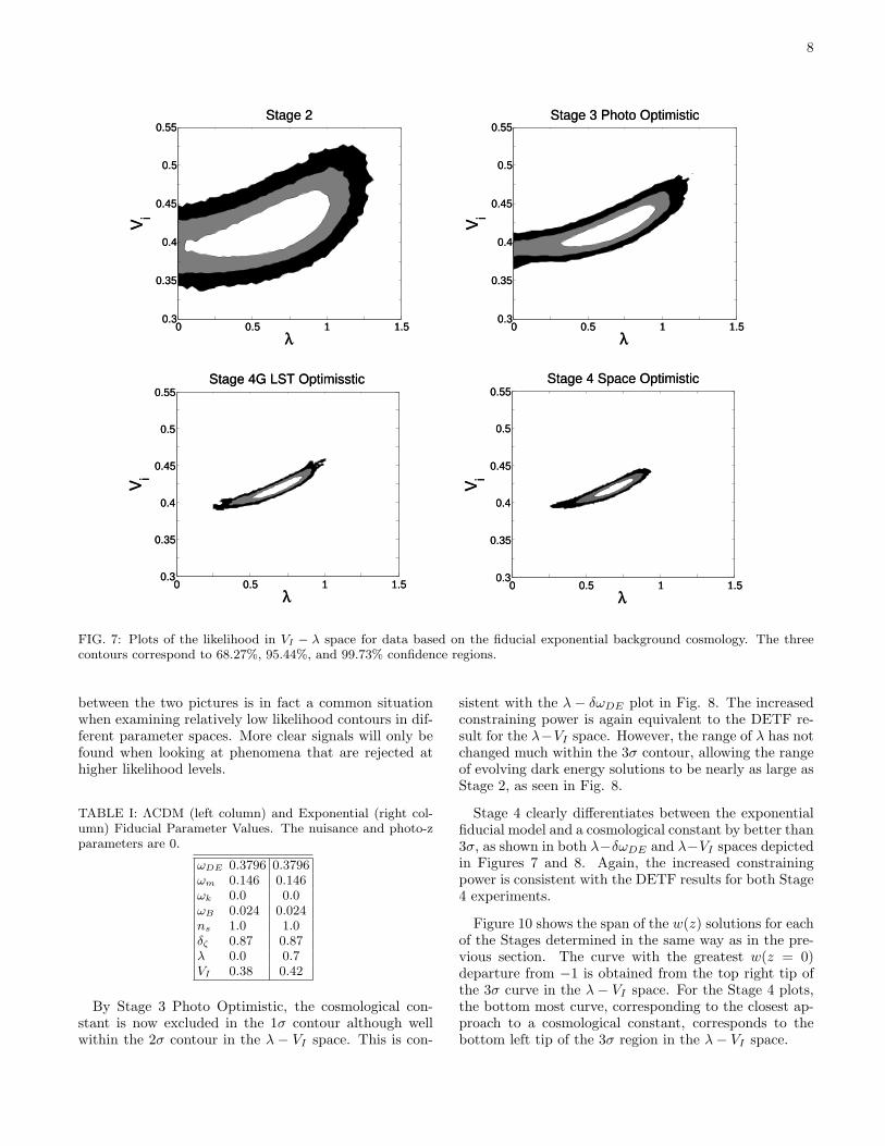
FIG. 7: Plots of the likelihood in VI − λ space for data based on the fiducial exponential background cosmology. The threecontours correspond to 68.27%, 95.44%, and 99.73% confidence regions.

between the two pictures is in fact a common situationwhen examining relatively low likelihood contours in dif-ferent parameter spaces. More clear signals will only befound when looking at phenomena that are rejected athigher likelihood levels.

TABLE I: ΛCDM (left column) and Exponential (right col-umn) Fiducial Parameter Values. The nuisance and photo-zparameters are 0.

ωDE 0.3796 0.3796ωm 0.146 0.146ωk 0.0 0.0ωB 0.024 0.024ns 1.0 1.0δζ 0.87 0.87λ 0.0 0.7VI 0.38 0.42

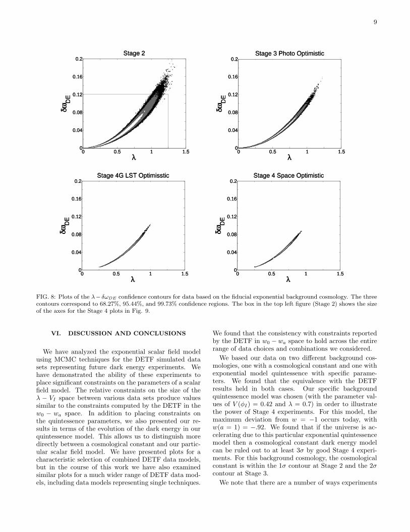
By Stage 3 Photo Optimistic, the cosmological con-stant is now excluded in the 1σ contour although wellwithin the 2σ contour in the λ − VI space. This is con-

sistent with the λ− δωDE plot in Fig. 8. The increasedconstraining power is again equivalent to the DETF re-sult for the λ−VI space. However, the range of λ has notchanged much within the 3σ contour, allowing the rangeof evolving dark energy solutions to be nearly as large asStage 2, as seen in Fig. 8.

Stage 4 clearly differentiates between the exponentialfiducial model and a cosmological constant by better than3σ, as shown in both λ−δωDE and λ−VI spaces depictedin Figures 7 and 8. Again, the increased constrainingpower is consistent with the DETF results for both Stage4 experiments.

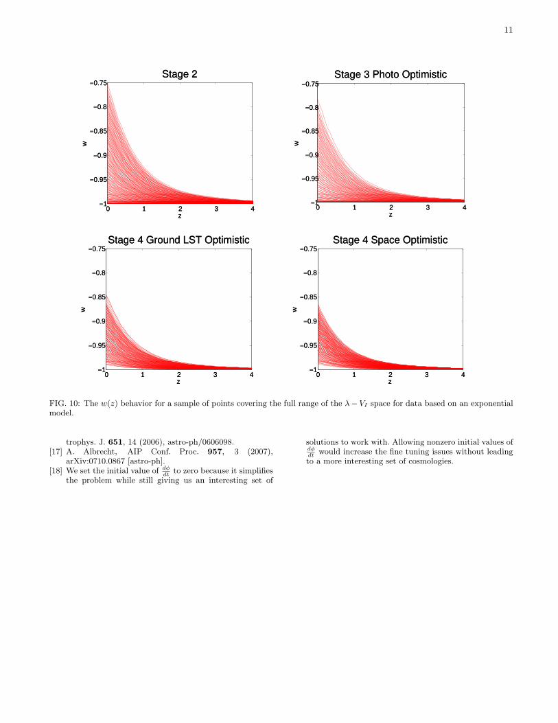
Figure 10 shows the span of the w(z) solutions for eachof the Stages determined in the same way as in the pre-vious section. The curve with the greatest w(z = 0)departure from −1 is obtained from the top right tip ofthe 3σ curve in the λ− VI space. For the Stage 4 plots,the bottom most curve, corresponding to the closest ap-proach to a cosmological constant, corresponds to thebottom left tip of the 3σ region in the λ− VI space.

9

λ

δωD

E

Stage 2

0 0.5 1 1.50

0.04

0.08

0.12

0.16

0.2


λ

δωD

E


0 0.5 1 1.50

0.04

0.08

0.12

0.16

0.2


λ

δωD

E


0 0.5 1 1.50

0.04

0.08

0.12

0.16

0.2


λ

δωD

E


0 0.5 1 1.50

0.04

0.08

0.12

0.16

0.2


FIG. 8: Plots of the λ− δωDE confidence contours for data based on the fiducial exponential background cosmology. The threecontours correspond to 68.27%, 95.44%, and 99.73% confidence regions. The box in the top left figure (Stage 2) shows the sizeof the axes for the Stage 4 plots in Fig. 9.

VI. DISCUSSION AND CONCLUSIONS

We have analyzed the exponential scalar field modelusing MCMC techniques for the DETF simulated datasets representing future dark energy experiments. Wehave demonstrated the ability of these experiments toplace significant constraints on the parameters of a scalarfield model. The relative constraints on the size of theλ − VI space between various data sets produce valuessimilar to the constraints computed by the DETF in thew0 − wa space. In addition to placing constraints onthe quintessence parameters, we also presented our re-sults in terms of the evolution of the dark energy in ourquintessence model. This allows us to distinguish moredirectly between a cosmological constant and our partic-ular scalar field model. We have presented plots for acharacteristic selection of combined DETF data models,but in the course of this work we have also examinedsimilar plots for a much wider range of DETF data mod-els, including data models representing single techniques.

We found that the consistency with constraints reportedby the DETF in w0 − wa space to hold across the entirerange of data choices and combinations we considered.

We based our data on two different background cos-mologies, one with a cosmological constant and one withexponential model quintessence with specific parame-ters. We found that the equivalence with the DETFresults held in both cases. Our specific backgroundquintessence model was chosen (with the parameter val-ues of V (φI) = 0.42 and λ = 0.7) in order to illustratethe power of Stage 4 experiments. For this model, themaximum deviation from w = −1 occurs today, withw(a = 1) = −.92. We found that if the universe is ac-celerating due to this particular exponential quintessencemodel then a cosmological constant dark energy modelcan be ruled out to at least 3σ by good Stage 4 experi-ments. For this background cosmology, the cosmologicalconstant is within the 1σ contour at Stage 2 and the 2σcontour at Stage 3.

We note that there are a number of ways experiments

10

λ

δωD

E


0 0.25 0.5 0.75 1 1.250

0.04

0.08

0.12


λ

δωD

E


0 0.25 0.5 0.75 1 1.250

0.04

0.08

0.12


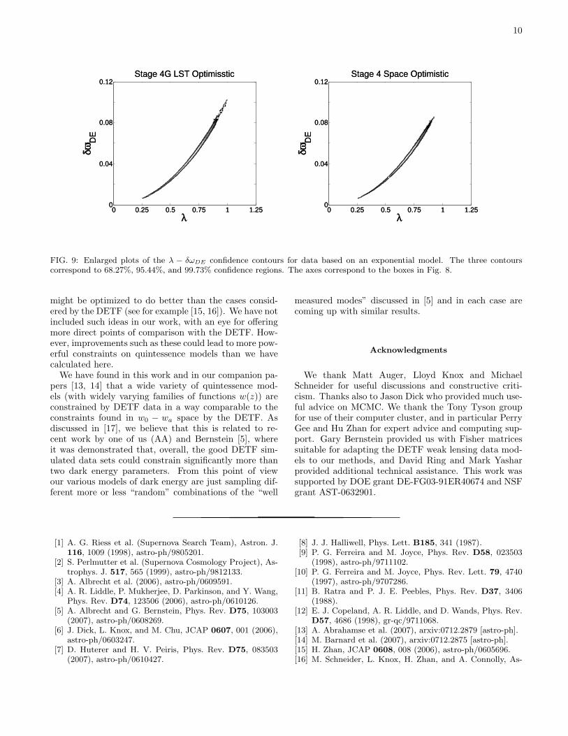
FIG. 9: Enlarged plots of the λ − δωDE confidence contours for data based on an exponential model. The three contourscorrespond to 68.27%, 95.44%, and 99.73% confidence regions. The axes correspond to the boxes in Fig. 8.

might be optimized to do better than the cases consid-ered by the DETF (see for example [15, 16]). We have notincluded such ideas in our work, with an eye for offeringmore direct points of comparison with the DETF. How-ever, improvements such as these could lead to more pow-erful constraints on quintessence models than we havecalculated here.

We have found in this work and in our companion pa-pers [13, 14] that a wide variety of quintessence mod-els (with widely varying families of functions w(z)) areconstrained by DETF data in a way comparable to theconstraints found in w0 − wa space by the DETF. Asdiscussed in [17], we believe that this is related to re-cent work by one of us (AA) and Bernstein [5], whereit was demonstrated that, overall, the good DETF sim-ulated data sets could constrain significantly more thantwo dark energy parameters. From this point of viewour various models of dark energy are just sampling dif-ferent more or less “random” combinations of the “well

measured modes” discussed in [5] and in each case arecoming up with similar results.

Acknowledgments

We thank Matt Auger, Lloyd Knox and MichaelSchneider for useful discussions and constructive criti-cism. Thanks also to Jason Dick who provided much use-ful advice on MCMC. We thank the Tony Tyson groupfor use of their computer cluster, and in particular PerryGee and Hu Zhan for expert advice and computing sup-port. Gary Bernstein provided us with Fisher matricessuitable for adapting the DETF weak lensing data mod-els to our methods, and David Ring and Mark Yasharprovided additional technical assistance. This work wassupported by DOE grant DE-FG03-91ER40674 and NSFgrant AST-0632901.

[1] A. G. Riess et al. (Supernova Search Team), Astron. J.116, 1009 (1998), astro-ph/9805201.

[2] S. Perlmutter et al. (Supernova Cosmology Project), As-trophys. J. 517, 565 (1999), astro-ph/9812133.

[3] A. Albrecht et al. (2006), astro-ph/0609591.[4] A. R. Liddle, P. Mukherjee, D. Parkinson, and Y. Wang,

Phys. Rev. D74, 123506 (2006), astro-ph/0610126.[5] A. Albrecht and G. Bernstein, Phys. Rev. D75, 103003

(2007), astro-ph/0608269.[6] J. Dick, L. Knox, and M. Chu, JCAP 0607, 001 (2006),

astro-ph/0603247.[7] D. Huterer and H. V. Peiris, Phys. Rev. D75, 083503

(2007), astro-ph/0610427.

[8] J. J. Halliwell, Phys. Lett. B185, 341 (1987).[9] P. G. Ferreira and M. Joyce, Phys. Rev. D58, 023503

(1998), astro-ph/9711102.[10] P. G. Ferreira and M. Joyce, Phys. Rev. Lett. 79, 4740

(1997), astro-ph/9707286.[11] B. Ratra and P. J. E. Peebles, Phys. Rev. D37, 3406

(1988).[12] E. J. Copeland, A. R. Liddle, and D. Wands, Phys. Rev.

D57, 4686 (1998), gr-qc/9711068.[13] A. Abrahamse et al. (2007), arxiv:0712.2879 [astro-ph].[14] M. Barnard et al. (2007), arxiv:0712.2875 [astro-ph].[15] H. Zhan, JCAP 0608, 008 (2006), astro-ph/0605696.[16] M. Schneider, L. Knox, H. Zhan, and A. Connolly, As-

11

0 1 2 3 4−1

−0.95

−0.9

−0.85

−0.8

−0.75Stage 2

z

w


0 1 2 3 4−1

−0.95

−0.9

−0.85

−0.8

−0.75Stage 3 Photo Optimistic

z

w


0 1 2 3 4−1

−0.95

−0.9

−0.85

−0.8

−0.75Stage 4 Ground LST Optimistic

z

w


0 1 2 3 4−1

−0.95

−0.9

−0.85

−0.8

−0.75Stage 4 Space Optimistic

z

w


FIG. 10: The w(z) behavior for a sample of points covering the full range of the λ− VI space for data based on an exponentialmodel.

trophys. J. 651, 14 (2006), astro-ph/0606098.[17] A. Albrecht, AIP Conf. Proc. 957, 3 (2007),

arXiv:0710.0867 [astro-ph].[18] We set the initial value of dφ

dtto zero because it simplifies

the problem while still giving us an interesting set of

solutions to work with. Allowing nonzero initial values ofdφdt

would increase the fine tuning issues without leadingto a more interesting set of cosmologies.

Exploring parameter constraints on quintessential dark energy: The exponential model

Documents

Transcript of Exploring parameter constraints on quintessential dark energy: The exponential model