EXPERIMENTAL SHOCK T U B E STUDY OF IGNITION PROMOTION FOR

M E T H A N E UNDER ENGINE R E L E V A N T CONDITIONS

BY

JIAN H U A N G

B.Sc, Shanghai Maritime University, 1996

A THESIS SUBMITTED IN PARTIAL FULFILLMENT OF

T H E REQUIREMENT FOR T H E DEGREE OF

MASTER OF APPLIED SCIENCE

in

T H E F A C U L T Y OF G R A D U A T E STUDIES

Department of Mechanical Engineering

We accept this thesis as confirming

to the required standard

T H E UNIVERSITY OF BRITISH COLUMBIA

November 2001

© Jian Huang, 2001

In presenting this thesis in partial fulfilment of the requirements for an advanced

degree at the University of British Columbia, I agree that the Library shall make it

freely available for reference and study. I further agree that permission for extensive

copying of this thesis for scholarly purposes may be granted by the head of my

department or by his or her representatives. It is understood that copying or

publication of this thesis for financial gain shall not be allowed without my writ ten

permission.

The University of British Columbia Vancouver, Canada

Department

DE-6 (2/88)

ABSTRACT

The ignition delay time of methane and various methane-additives mixed homogeneously

with air has been measured experimentally using a reflected shock technique for pressures

from 16 to 40 atm and temperatures from 950 to HOOK.

A non-constant-specific-heat model has been developed for calculating initial experimental

conditions. A good agreement has been found between the model and the experimental

results.

The ignition delay time measured in the current study has been found to depend strongly on

temperature and moderately on pressure, and is significantly different from that reported by

previous workers whose experiments have been conducted at lower pressures. Empirical

equations correlating the ignition delay time with the initial temperature, pressure and fuel

concentration have been obtained based on the experimental results.

Hydrogen and D M E (dimethyl ether) have been investigated for their efficiencies as ignition

promoters for methane under engine relevant conditions. A prominent reduction of the

ignition delay has been found for methane with 35% hydrogen added. With 15% hydrogen

addition, the promotion effect is mainly evident at low pressures. D M E has been found to

cause moderate reduction on the ignition delay of methane.

Computational results using detailed reaction mechanisms have shown disagreements with

the current experimental measurements. Further tuning of the mechanisms has been

suggested for high-pressure methane ignitions.

T A B L E OF CONTENTS

Abstract ii

Table of Contents iii

List of Tables vi

List of Figures vii

Nomenclature xii

Acknowledgements xiii

Dedication xiv

CHAPTER I Introduction 1

CHAPTER H Shock Tube and Modeling 3

2.1 Introduction 3

2.2 Background 3

2.2.1 Shock Tube 3

2.2.2 Normal Shock Relations 5

2.2.3 Pressure Distribution in Shock Tube and Tailored Interface 7

2.3 Experimental Apparatus 9

2.4 Shock Tube Modeling 11

2.4.1 Ideal Model 11

2.4.2 Model Results and Comparisons 18

2.4.3 Modified Model 23

2.5 Uncertainty of Experimental Conditions 28

2.6 Reflected Shock Boundary Layer Interaction 30

2.7 Contact Surface Instability 37

CHAPTER III Shock Tube Study of Methane Ignition at Engine-Relevant Conditions 39

3.1 Introduction 39

3.2 Background 39

i i i

3.2.1 Oxidation of Methane 39

3.2.2 Previous Work 41

3.3 Results and Discussions 45

3.3.1 Pressure History of Methane Self-ignition Process 45

3.3.2 Strong Ignition Limit 48

3.3.3 Ignition Delay of Methane at High Pressure 51

3.3.4 Correlation Equations 55

3.3.5 Comparison of Experimental and Computational Results 58

CHAPTER IV Shock Tube Study of Ignition Promotion for Methane at Engine-Relevant

Conditions 60

4.1 Introduction 60

4.2 Background 61

4.2.1 Mechanism of Ignition Promotion 61

4.2.2 Previous Work 62

4.3 Results and Discussions 68

4.3.1 Efficiency of Ignition Promotion for Hydrogen 68

4.3.2 Comparisons of Experimental and Computational Results 72

4.3.3 Efficiency of Ignition Promotion for D M E 74

4.3.4 Strong Ignition Limit of Methane with Additives 76

CHAPTER V Conclusions and Future Work

5.1 Conclusions 78

5.1.1 Shock Tube and Modeling 78

5.1.2 Ignition Delay of Methane under Engine-Relevant

Conditions 78

5.1.3 Ignition Promotion for Methane under Engine-Relevant

Conditions 79

IV

5.2 Problems with Current Experimental Apparatus and

Shock Tube Upgrades 80

5.2.1 Design of Shock Tube Optical Access 81

5.2.2 Length Calculation for Increasing Experimental Time 84

5.3 Recommended Future Work 85

References 86

Appendix A Method of Characteristics 89

Appendix B Uncertainty of Calculated Experimental Temperature 98

Appendix C PCB Pressure Transducer Calibration 100

Appendix D A Computer Model for 2-D Compressible Boundary Layer Flow 102

Appendix E A Computer Model for Calculating Adiabatic Flame Temperature for

Methane- Air/Oxygen Reaction with Dissociation 110

Appendix F Thermodynamic Properties for Driver and Driven Gases 115

Appendix G List of Experimental Conditions and Results 119

V

LIST OF TABLES

Chapter III

3.1 Experimental Conditions and Empirical Coefficients for Previous Work

Measuring the Ignition Delay of Methane 43

3.2 Empirical Coefficients for the Ignition Delay of Methane Obtained

in the Current Study 56

Chapter IV

4.1 Correlation Coefficients for the Ignition Delay of Methane and Hydrogen 63

by Oppenheim et al.

VI

LIST OF FIGURES

Chapter II

2.1 Shock Tube Working Principle 4

2.2 Moving Shock and Equivalent Stationary Normal Shock 5

2.3 Three Possible Situations after the Reflected Shock Wave Travels Across the

Contact Surface 8

2.4 Schematic of the Shock Tube and Attached Equipment 9

2.5 Double Diaphragms 10

2.6 Coordinates Transformation for an Incident Shock Wave 12

2.7 Coordinates Transformation for a Reflected Shock Wave 12

2.8 Property Variations Across an Isentropic Wave in Wave Fixed Coordinates 13

2.9 Solution Procedure for the Incident Shock Velocity 15

2.10 Solution Procedure for Tailored Interface Conditions 16

2.11 Model Prediction of the Experimental Time 18

2.12 Pressure Distribution in the Shock Tube at Different Moments 18

2.13 Positions of Shock Wave, Contact Surface and Rarefaction Fan versus Time 20

2.14 Measured Incident Shock Displacement versus Time 21

2.15 Comparison of Measured and Calculated Incident Shock Velocities

for the Same Initial Pressure Ratio 21

2.16 Comparison of Measured and Calculated Reflected Shock Velocities

for the Same Incident Shock Velocity 22

2.17 Comparison of Measured and Calculated Experimental Time 23

2.18 Control Volume Analysis for the Throttling Loss at the Exit

of the Driver Section 24

2.19 Estimation of the Experimental Time using the Modified Model 26

2.20 Model Prediction of the Helium Fraction in the Driver Gas for Tailoring

Conditions with the Given Initial Pressure Ratio 27

2.21 Model Prediction of the Incident Shock Velocity for the Given

v i i

Initial Pressure Ratio 27

2.22 Procedure of Applying the Modified Model 28

2.23 Comparison of Measured and Calculated Pressures behind the Reflected Shock

for the Same Incident Shock Velocity 29

2.24 Comparison of Calculated Temperatures Using Two Different Methods 30

2.25 Velocity Profile of the Incoming Flow in Reflected-Shock-Fixed Coordinates 31

2.26 Bifurcation Foot of the Reflected Shock in Shock-Fixed Coordinates 32

2.27 Oblique Shock Wave and Equivalent Normal Shock Wave 33

2.28 Mean Flow Passing Through Two Oblique Shocks 35

2.29 Comparison of the Time for the Cooling Gas to Reach the End Wall with

Calculated Experimental Time versus the Incident Shock Velocity 37

Chapter ITJ

3.1 Ignition Delay of a Stoichiometric Methane-Air Mixture Calculated Using

Different Empirical Equations for an initial pressure of 2 atm 44

3.2 Ignition Delay of a Stoichiometric Methane-Air Mixture Calculated Using

Different Empirical Equations for an Initial Pressure of 30 atm 45

3.3 Pressure History of a Stoichiometric Methane-Air Mixture Ignition Process

(P i n i= 16+2 atm) 46

3.4 Pressure History of a Stoichiometric Methane-Air Mixture Ignition Process

(P i n i = 23±2 atm) 46

3.5 Pressure History of a Stoichiometric Methane-Air Mixture Ignition Process

(P i n i = 30±2 atm) 47

3.6 Pressure History of a Stoichiometric Methane-Air Mixture Ignition Process

(Pini = 40±2 atm) 47

3.7 Measured Strong Ignition Limit for Stoichiometric Methane-Air Mixtures

at Pressures from 16 to 40 atm 49

3.8 Mild to Strong Ignition - 4 Different Ignition Patterns 50

V l l l

3.9 Measured Ignition Delay Time of Stoichiometric Methane-Air Mixture

at Different Pressures 51

3.10 Measured Ignition Delay Time of Lean Methane-Air Mixture at Different

Pressures 52

3.11 Comparison of Ignition Delay for Lean and Stoichiometric Methane-Air

Mixtures at 16 arm 54

3.12 Comparison of Ignition Delay for Lean, Rich and Stoichiometric

Methane-Air Mixtures at 40 atm 55

3.13 Ignition Delay of a Stoichiometric Methane-Air Mixture by Equation (3.6) 57

3.14 Ignition Delay of a Lean Methane-Air Mixture by Equation (3.6) 57

3.15 Difference Between Lean and Stoichiometric Mixtures for Ignition Delay Time 58

3.16 Comparison of Computational Results and Experimental Measurements

for the Ignition Delay of Stoichiometric Methane-Air Mixtures 59

Chapter TV

4.1 Comparison of Ignition Delay Time for Stoichiometric Methane-Air

Mixtures Calculated Using Oppenheim's Equation with Different Hydrogen

Concentrations at 1 atm

4.2 Measured Ignition Delay Time of Methane with 0%, 15% and 35%

Hydrogen Added at 16+2 atm

4.3 Measured Ignition Delay Time of Methane with 0%, 15% and 35%

Hydrogen Added at 40±2 atm

4.4 Measured Ignition Delay Time of Methane at 16±2, 30±2 and 40±2 atm

with 35% Hydrogen Added.

4.5 Comparison of Computational Results Using Detailed Reaction Mechanism

and Experimental Measurements for P=16 atm

4.6 Comparison of Computational Results Using Detailed Reaction Mechanism

and Experimental Measurements for P=40 atm

4.7 Measured Ignition Delay of Methane with 5% D M E Added at P=16±2 atm

63

69

70

72

73

74

75

4.8 Measured Ignition Delay of Methane with 5% D M E Added at P=30±2 arm 75

4.9 Pressure Histories of Methane and Methane-Hydrogen Ignition Processes

Showing 3 Distinctive Ignition Patterns 76

4.10 Strong Ignition Limits for Methane with Different Hydrogen Concentrations

from 16 to 40 atm 77

Chapter V

5.1 Schematic of the Shock Tube Optical Access System 81

5.2 Calculated Experimental Time with Respect to Various Driver and

Driven Section Lengths 84

Appendix A

A . l Right Moving Isentropic Wave 89

A.2 Left Moving Isentropic Wave 90

A.3 Time-Space Mesh for a Subsonic A. Wave 92

A.4 Time-Space Mesh for a Subsonic (3 Wave 94

A.5 Time-Space Mesh for a P Wave in a Supersonic Flow from Left to Right 94

A.6 Time-Space Mesh for a A. Wave in a Supersonic Flow from Right to Left 95

Appendix C

C l Schematic of the Experimental Configuration for Calibrating the PCB Pressure

Transducer Mounted on the Endplate. 101

C. 2 Calibration Chart for the PCB Pressure Transducer 101

Appendix D

D. l Calculated Boundary Layer Thickness versus Time Using Laminar 107

and Turbulent Models

D.2 Velocity Profiles of Laminar and Turbulent Boundary Layers at 0.43 ms after the

Passage of the Incident Shock Wave 108

x

Appendix E

E. 1 Solution Procedure for Calculating the Equilibrium Temperature with

Dissociation 111

E.2 Calculated Equilibrium Temperature as a Function of A. 114

XI

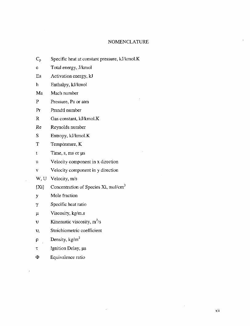
N O M E N C L A T U R E

C p Specific heat at constant pressure, kJ/kmol.K

e Total energy, J/kmol

Ea Activation energy, kJ

h Enthalpy, kJ/kmol

Ma Mach number

P Pressure, Pa or atm

Pr Prandtl number

R Gas constant, kJ/kmol.K

Re Reynolds number

S Entropy, kJ/kmol.K

T Temperature, K

t Time, s, ms or us

u Velocity component in x direction

v Velocity component in y direction

W, U Velocity, m/s

[Xi] Concentration of Species Xi , mol/cm3

y Mole fraction

Y Specific heat ratio

jj. Viscosity, kg/m.s

v Kinematic viscosity, m2/s

Vi Stoichiometric coefficient

p Density, kg/m3

x Ignition Delay, us

<J> Equivalence ratio

xii

ACKNOWLEDGEMENTS

I wish to express my sincerest appreciation to my supervisors, Dr. Philip Hill and Dr. Kendal

Bushe, for their dedications, instructions, and firm supports throughout the project. Extra

thanks are to Dr. Hill for his contribution to the shock tube model, which has become the

theoretical basis of this project, as well as to Dr. Bushe for his computer code for the ignition

simulations.

I would like to acknowledge Dr. Sandeep Munshi and Westport Innovations Inc. of

Vancouver B.C. as well as C.R.D. grant for the sustained technical and financial support that

made this project possible.

Thanks also to Alan Reid, a previous graduate student and my friend, who has devoted

tremendous time and efforts on designing and building the shock tube as well as performing

many precursory experiments. His work has provided valuable experiences on how to

operating the shock tube.

In addition, I would like to thank the faculty, staff, and students of the department of

Mechanical Engineering for their continuous interest and support of the current study.

X l l l

Dedicated to Yongning, Yanhua, Jun and Wen,

my loving and supportive

parents, brother,

and wife

xiv

C H A P T E R I

Natural-gas-fueled internal combustion engines have been undergoing a fast development

in recent years. They offer an attractive combination of reduced engine emission and

lower fuel cost. The wide availability of natural gas makes it an ideal alternative fuel that

provides practical solutions to the increasingly restrictive emissions control requirement.

A more recent step is to use natural gas (NG) in heavy-duty diesel engines. The high

pressure direct injection technique (HPDI) developed by Westport Innovations Inc. (WII)

has made it possible to achieve a significant reduction of the N O x and particulate

emissions by running the engine on natural gas while maintaining the performance and

efficiency of a conventional diesel engine.

A major problem associated with the natural gas direct injection system comes from the

poor compression ignitability of natural gas, or, more precisely, of methane, which is a

major component of natural gas. So far the HPDI system has to use a pilot diesel fuel to

ignite natural gas. This impairs a further reduction of engine emissions and increases the

system complexity as well as the cost.

Early research on methane ignition indicates that the ignition delay of methane can be

reduced by blending it with some other active gaseous fuels. Experiments conducted by

Oppenheim and Chan [1], Frenklach and Bornside [2], Lifshitz et al. [3, 4] have all

shown significant promotion effects on the ignition of methane by mixing additives such

as hydrogen and propane at low pressures. This provides the possibility to run a diesel

engine on natural gas enriched by ignition promoters eliminating the dependence on the

pilot fuel or other extra ignition sources.

Despite many previous efforts to measure the ignition delay of methane at low pressures

and high temperatures, the ignition delay time at engine-like conditions, (which

incorporate high pressures and low temperatures), remains uncertain. This was the

incentive to carry out the current experimental studies on measuring the ignition delay of

methane and methane-additives under conditions that are directly engine-relevant, so as

to find out the most suitable ignition promoter for N G engine applications.

For a homogeneously charged spark ignition N G engine, on the other hand, we need to

prevent autoignition, which may lead to a problem called engine knock. This also

requires comprehensive information on the variation of the ignition delay for methane

1

with respect to different pressures and temperatures as well as fuel concentrations.

Especially, we need to find the limit of strong ignition, which is an explosive combustion

at a relatively high temperature generating rapid pressure increase that may damage the

engine.

A shock tube, which is an efficient and reliable instrument for measuring ignition delay,

has been used in the current study. The merits of using a shock tube instead of other

combustion devices come from its close-to instantaneous pressure and temperature rises

which minimize the effects of heating process. The constant initial conditions obtained

behind the reflected shock wave make it easy to detect the variation of pressure or

temperature caused by an ignition. Another merit of using a shock tube is that the

experimental conditions in the shock tube can be calculated with a good reliability by

using the measured shock velocity. The method provides a practical solution to the

problem of accurately measuring the temperature within a very short residence time.

2

C H A P T E R II

2.1 Introduction

Shock wave research and shock tube development have been receiving sustained interest

in various scientific disciplines for more than half a century. Besides use in studying

supersonic and hypersonic aerodynamic problems, this instrument also provides a cheap,

reliable method to obtain instant high-enthalpy reservoirs for studies of high-temperature

chemical reaction phenomena such as combustion.

When it comes to measuring ignition delay time, the shock tube is one of the most widely

used instrument. The merit of an 'instantaneous' rise of pressure and temperature

minimizes the effects of heating process as inherent to other instruments and thus makes

the experimental results more accurate.

Measuring the rapid temperature change in combustion devices such as internal

combustion engines remains a difficult engineering problem. In a shock tube experiment,

the temperature can be calculated from the shock propagation velocity, which can be

measured with high accuracy. The shock tube is also capable of achieving temperatures

and pressures similar to those found in internal combustion engines, (typically from 900

to 1200 K and 20 to 70 atm).

In the study described in this thesis, a shock tube is used to investigate ignition delay

times for various gaseous fuel-air mixtures at pressures from 16 to 40 atm and

temperatures from 950 to 1400 K. It is necessary for us to understand the nature of the

shock tube working under such conditions so that the uncertainty of the experimental

conditions can be found and minimized. The primary purpose of this chapter is to discuss

shock tube modeling and problems associated with its application as well as to compare

the model with the experimental results.

2.2 Background

2.2.1 Shock Tube

A schematic of the shock tube and its working principle is shown is figure 2 . 1 .

A shock tube is a device in which a high-pressure driver gas and a low-pressure driven

gas are separated by one or two diaphragms. When the diaphragms burst, a shock wave is

3

generated. The shock wave, which is a high-enthalpy compression wave with its local

Mach number higher than one, travels downstream into the driven gas causing a pressure

and temperature jump across the shock front. A contact surface that separates the driver

gas from the driven gas follows the incident shock wave and travels at a lower speed. At

the same time, a rarefaction fan composed of a series of expansion waves fans out into

the upstream driver gas.

(a)

(b)

(c)

Driven gas / Diaphragm

Incident shock froi \ /surface

U i lyf TTP,

u 4

Reflected shock f"'front Reflected rarefaction fan

P 5 Us P 2 =P 3

Fig. 2.1 Shock tube working principle, (a) Initial state: the high-pressure driver gas is separated from the

low-pressure driven gas by the diaphragm, (b) An incident shock wave forms right after the bursting of the

diaphragm, (c) The shock wave reflects from the end of the driven section (d) The shock wave passes

through the contact surface.

4

The shock wave, upon reflection from the end wall of the shock tube, interacts with the

driven gas set to move by the incident shock and brings it to a stop. The static high-

temperature and high-pressure reservoir generated behind the reflected shock wave can

be readily used for studies of various purposes.

Under ideal conditions as we will explain later, the pressure and temperature in the

experimental area can be kept constant until the arrival of the reflected rarefaction fan.

2.2.2 Normal Shock Relations

A normal shock is a shock wave with its front normal to the direction in which it travels.

We consider a normal shock wave propagating into an undisturbed fluid with velocity U i .

The pressure, density, and temperature of the fluid ahead of the shock are P a, pa, and T a ,

and those behind the shock are Pt>, pD, Tb. The velocity behind the shock wave is U2. By

switching from laboratory coordinates to shock fixed coordinates, we bring the wave to

rest as illustrated in figure 2.2. This stationary shock sees the undisturbed gas

approaching with velocity U a and the gas behind it travels at a velocity U 0 , where Ua=Ui

and U b=Ui-U 2 .

Pa Pa T a

u,

Pb Pb T b

U 2

Pa Pa T a

u a = u,

Pb Pb T b

U b = U1-U2

Fig. 2.2 Moving shock and equivalent stationary normal shock

Applying a control volume analysis across the shock and neglecting viscous effects and

body forces we can write one-dimensional continuity, momentum and energy equations

as:

PaUa = P„Ub

(2.1)

(2.2)

5

1 , 1 , h+-U2=hh+-Ul.

2 2 (2.3)

With the ideal gas assumption, we can also have the equation of state

= RT. (2.4)

For given initial conditions ahead of the shock front, we can solve Eqs. (2.1) - (2.4) to

get Pb, Pb,TD and Ub. For a constant specific heat ratio Y=Cp/ cv> the solution is most

conveniently written in terms of the Mach numbers.

Mai 1 + ^ M « 2

(2.5)

pb = (Y+l)Mfl a

2

p a a + ( Y - l ) M a a

2 (2.6)

^ = l + ^ - ( M a 2 -1 ) Pa 7 + 1 (2.7)

L = 1 + 2 ( Y - 1 ) ^1+YMa 2 ^

(Y+ry Mai (2.8)

Here M a a and Mab are local Mach numbers ahead and behind the shock wave. The Mach

number is defined as Ma = u/a and a is the local sound speed given by

a = jyRT. (2.9)

6

2.2.3 Pressure Distribution in Shock Tube and Tailored Interface

In laboratory coordinates the incident shock travels at a constant velocity U i . The

corresponding Mach number is Mai • The Mach number and pressure of the flow behind

the shock wave according to Eqs (2.5) and (2.6) - denoted as U2 and P2 - are constant.

Since no velocity jump is allowed across the contact surface to satisfy continuity, U 2

equals the velocity U 3 with which the contact surface moves. Also, there is no pressure

variation across the contact surface so that P2=P3 as shown in figure 2.1 (c). After the

shock wave reflects from the end wall, it travels first into the driven gas and then crosses

the contact surface entering the driver gas. The pressure of the driven gas is boosted by

the reflected shock to Ps, which is the desired experimental pressure. The pressure behind

the reflected shock in the driver gas is denoted as P6 as illustrated in figure 2.1 (d).

Hurle and Gayden [30] discussed three possible situations that may occur after the

reflected shock crosses the contact surface depending on the difference between P5 and

P6. They are under-tailoring, over-tailoring, and tailoring.

1) Under-tailoring

When P5 of the driven gas is lower than P6 of the driver gas, we have under-tailoring. As

shown in figure 2.3 (a), the pressure jump across the contact surface will form a

secondary shock wave, which travels back into the driven gas and further increases its

pressure and temperature. The contact surface, due to this favored pressure gradient, will

further move ahead until the pressure of P5 adjusts enough to balance P6.

2) Over-tailoring

If P5 is higher than P6, we will have over-tailoring. In such a case, an expansion wave will

be generated from the contact surface and travels towards the end of the driven section.

Meanwhile, the contact surface will bounce back when the driven gas expands to reduce

Ps.

3) Tailored-interface

When P 5 exactly equals P6, we have a tailored-interface condition. When such a condition

is obtained, only Mach waves are generated when the shock passes the contact surface.

7

The pressure and temperature in the experimental area will be kept constant until the

arrival of the reflected rarefaction fan. The experimental time can thus be significantly

increased.

X

Fig. 2.3 Three possible situations after the reflected shock wave travels across the contact surface: (a) under-tailoring; (b) over-tailoring; (c) tailored interface.

If we assume the same composition for both driver and driven gas with constant specific

heat ratio y, from equation (2.7) we can calculate the pressure behind the shock wave. In

a real experiment, the initial temperatures for the driver and the driven gases are usually

the same (Ti=T4). The expansion of the driver gas reduces its temperature from T4 to T3,

while the incident shock wave raises the driven gas temperature from Ti to T2. Since the

local sound speed is proportional to the square root of the temperature if R and 7 are

constant, with the condition T 2 » T 3 , we must have a2>a3. Thus it is reasonable to get

Ma5<Ma6 for the same reflected shock velocity. (In most cases, the reflected shock

velocity does vary across the contact surface. However, the change compared with the

8

change of sound speed is small, so we can still get a higher Mach number for the shock

wave traveling in the driver gas than in the driven gas). Since initially we have P3 = P2,

after the passage of the shock, there will be P6>P5-The above analysis shows that we will always end up with an under-tailored condition if

the same gas is used in both the driver and the driven sections. In order to achieve a

balance between P5 and P6, it is necessary to increase the sound speed on the driver gas

side so that we can reduce the Mach number properly for the equivalent end pressure. In

the current experiment, we mix helium, whose gas constant and specific heat ratio is

much higher, with air to get the desired sound speed. Calculations are needed to decide

the proportion of the two gases, as a function of different incident shock speed, in order

to achieve a tailored interface.

2.3 Experimental Apparatus A schematic of the experimental apparatus is shown in figure 2.4. The bore of the shock

tube used in the current study is 0.059 m. The lengths of the driver and driven section are

3.18 meters and 4.25 meters respectively. The device has been designed and tested to

work under a maximum pressure of 200 atm [5], which is equivalent to the pressure

achieved when a stoichiometric methane-air mixture with an initial pressure of 95 atm

burns to completion at constant volume (see appendix E for details).

Data Acquisition System

Double Diaphragm

Static Pressure Sensor

Air Helium

Driven Section Driver Section

Fig. 2.4 Schematic of the shock tube and attached equipment

9

The initial pressure in the driver section is measured with an Eclipse static pressure

transducer, and that in the driven section is measured by an Auto Tran vacuum sensor. A

series of five PCB 112B11 piezoelectric pressure transducers with a minimum response

time of 3 microseconds are flush mounted along the driven section of the shock tube.

They are used to measure the passage time of the shock wave and the associated pressure

rise. The incident shock velocity is calculated from the measured time for the shock

passing each sensor and the distance between the sensors.

A double diaphragm technique [5] is used to guarantee the diaphragms burst at the

desired pressure as shown in figure 2.5. An intermediate flange is placed between the

driver and driven sections. A piece of diaphragm is inserted between the intermediate

plate and the driver and driven sections respectively. When charging the driver section,

first open the intermediate valve and charge the driver and small chamber simultaneously

to a pressure P g a p ( P g a p < P 4 ) . Then the intermediate valve is closed and the driver pressure

is further raised to P 4 . To trig a shock, the release valve is opened and the pressure in the

small chamber drops quickly. The increased pressure difference causes the diaphragms to

burst consecutively.

Double Diaphragms

P. V / / / ^ / / /

Driven Section

Intermediate Valve

'v / / / / / / / / / / / ^—r^

• gap

Driver Section

Release Valve

Fig. 2.5 Double diaphragms

In the current experiment, we mix helium and air in the driver section in order to achieve

tailored interface conditions. Details of calculating the initial helium concentration in the

driver gas with respect to different experimental conditions will be provided in the

following section.

10

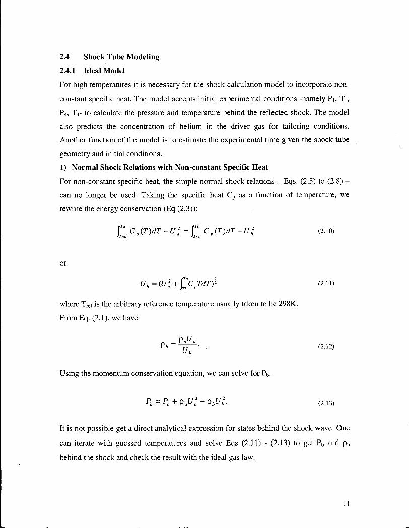
2.4 Shock Tube Modeling

2.4.1 Ideal Model

For high temperatures it is necessary for the shock calculation model to incorporate non-

constant specific heat. The model accepts initial experimental conditions -namely Pi , T i ,

P 4 , T 4 - to calculate the pressure and temperature behind the reflected shock. The model

also predicts the concentration of helium in the driver gas for tailoring conditions.

Another function of the model is to estimate the experimental time given the shock tube

geometry and initial conditions.

1) Normal Shock Relations with Non-constant Specific Heat

For non-constant specific heat, the simple normal shock relations - Eqs. (2.5) to (2.8) -

can no longer be used. Taking the specific heat C p as a function of temperature, we

rewrite the energy conservation (Eq (2.3)):

£ Cp(T)dT +U2

a = £ Cp(T)dT + Ub

2 (2.10)

or

Ub=(U2

a+£cpTdT)> (2.11)

where T r e i is the arbitrary reference temperature usually taken to be 298K.

From Eq. (2.1), we have

D - P ' U ' Pb- • . (2.12) u b

Using the momentum conservation equation, we can solve for Pb.

Pb=Pa+PaU2

a-pbUl (2.13)

It is not possible get a direct analytical expression for states behind the shock wave. One

can iterate with guessed temperatures and solve Eqs (2.11) - (2.13) to get Pb and pb

behind the shock and check the result with the ideal gas law.

11

We abandon the specific heat ratio and Mach number here for the reason that little

simplification can be obtained when assuming a non-constant specific heat.

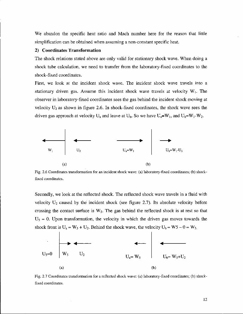
2) Coordinates Transformation

The shock relations stated above are only valid for stationary shock wave. When doing a

shock tube calculation, we need to transfer from the laboratory-fixed coordinates to the

shock-fixed coordinates.

First, we look at the incident shock wave. The incident shock wave travels into a

stationary driven gas. Assume this incident shock wave travels at velocity Wj. The

observer in laboratory-fixed coordinates sees the gas behind the incident shock moving at

velocity U2 as shown in figure 2.6. In shock-fixed coordinates, the shock wave sees the

driven gas approach at velocity U a and leave at U b . So we have U a = W i , and Ub=Wi-W2.

w. u2 u„=w, ub=wru2

(a) (b)

Fig. 2.6 Coordinates transformation for an incident shock wave: (a) laboratory-fixed coordinates; (b) shock-

fixed coordinates.

Secondly, we look at the reflected shock. The reflected shock wave travels in a fluid with

velocity U 2 caused by the incident shock (see figure 2.7) . Its absolute velocity before

crossing the contact surface is W 5 . The gas behind the reflected shock is at rest so that

U 5 = 0. Upon transformation, the velocity in which the driven gas moves towards the

shock front is U a = W 5 + U 2 . Behind the shock wave, the velocity U b = W5 - 0 = W 5 .

U 5 = 0 w5 U 2 ua=w5 Ub= W5+U2

(a) (b)

Fig. 2.7 Coordinates transformation for a reflected shock wave: (a) laboratory-fixed coordinates; (b) shock-

fixed coordinates.

12

A similar transformation can also be applied after the reflected shock wave crosses the

contact surface, for which we change W5 into W 6 and replace U2 with U 3 .

3) Calculate Incident Shock Velocity from Initial Pressure Ratio

In the ideal model, we assume no momentum or energy loss due to viscous effects and

also no throttling caused by the burst diaphragm. We also neglect heat transfer to the wall

of the shock tube due to the very short over-all experimental time and high Reynolds

number. The adiabatic inviscid expansion of the driver gas from P 4 to P 3 satisfies

isentropic flow conditions. The expansion wave travels at the local sound speed and

causes a small but continuous disturbance behind it. In wave-fixed coordinates, we

denote the pressure and velocity change behind the wave with dU, dP and dp respectively

as shown in figure 2.8.

Fig.2.8 Property variations across an isentropic wave in wave fixed coordinates

For a small value of dP and dU, we can assume the flow to be steady state, for which the

a, P, p •

a + dU, P+dP, p+dp

•

steady flow continuity and momentum equations are

pa = (p + df))(a + dU ) (2.14)

p + pu2 = (P + dP) + (p + dp)(U + dUf. (2.15)

Rearranging and eliminating high-order terms, we get

pdU = -adp (2.16)

and

-dP = 2apdU + a2dp. (2.17)

13

Substituting Eq. (2.16) into Eq. (2.17), we obtain a simple relation between dP and dU.

-dP = apdU. (2.18)

For the driver gas, we can reasonably assume a constant specific heat ratio because of its

low temperature so that the isentropic flow relations are

dP _ y dT _ 2y da

P y - l T y - l a (2.19)

and

P = a2p

(2.20)

Using Eqs. (2.19) and (2.20) to eliminate P in Eq. (2.18), we get an important relation

that is valid for any arbitrary isentropic wave:

7 -1 d(a + L^-U) = 0, (2.21)

or

7 - 1 A, = a + U = const. (2.22)

We will come back to equation (2.22) later when we discuss the method of

characteristics. For now, we use equation (2.21) to derive an expression for the velocity

of contact surface U3. Integrating Eq. (2.21) from SL4 to a3 we get

2

For isentropic flow,

U3 = - ( a 4 - a 3 ) . 7 - 1

(2.23)

P4

17-1

T v 4 ;

__ (Y - l

(2.24)

Substituting equation (2.23) into equation (2.24), we obtain an expression for U3 in terms

of the pressure ratio and the initial sound speed of the driver gas:

14

Meanwhile, the pressure and velocity behind the incident shock wave, P 2 and U2, must

equal P 3 and U 3 . With a given initial condition Pi, P 4 and Ti, T4, a calculation for the

incident shock velocity can be accomplished with an iterative method illustrated by the

flowchart in figure 2.9.

Input Pi, P 4 , T i , T 4

Guess incident shock velocity Wi

Guess temperature T 2 behind incident shock

Solve (2.11) - (2.13) for P 2, p 2

behind incident shock

False.

False

Fig. 2 . 9 Solution procedure for the incident shock velocity

15

4) Predict Helium Concentration in Driver Gas

For different experimental conditions, the helium concentration in the driver gas should

be varied in order to achieve a tailored interface. Iteration with different initial helium

concentrations is necessary to find the point where the calculated P5 equals P6. This

procedure is shown in figure 2.10.

f > Input Initial Conditions Pi, P4, T i , T 4 1

1 • Guess helium concentration

Calculate incident shock velocity Wi using iterative method

« * / Data: Wi ^

* Calculate fluid properties behind incident shock

•/Data: U 2 , P 2, T 2 , / 4 / p 2 , U 3 , P 3 , T 3 , p 3 /

Calculate reflected shock velocity using iterative method <—y D a t a : w 5 /

Calculate fluid properties behind reflected shock in area 5

> / Data: U 5 , P 5, /

*""7 T ^ / v

Calculate reflected shock velocity after crossing contact surface 4 / Data: W 6 /

V Calculate fluid properties behind reflected shock in area 6

•/Data: U 6 , P 6, / 4 / T 6 , p 6 /

^ True

( End )

Fig. 2.10 Solution procedure for tailored interface conditions

16

5) Experimental Time

In designing a shock tube experiment, it is essential to know the maximum experimental

time that can be obtained. If a tailored interface is established, the contact surface

separating the driver gas from the driven gas will stay still and conditions in the

experimental area can be kept constant until the arrival of the reflected rarefaction fan.

For this reason, we need to calculate the velocity of the rarefaction fan to decide when its

leading edge starts to enter the experimental region, whose border is defined by the

location of the contact surface.

In the current model, we use the method of characteristics to accomplish this task (see

appendix A for details). The method of characteristics can tell us the location of any

isentropic expansion wave that composes the rarefaction fan in space at a given time.

With this information, we can evaluate the velocity field as well as the pressure

distribution of the driver gas at any moment of interest. We define the experimental time

as the duration between the reflection of the incident shock wave from the end wall to the

moment when the leading edge of the rarefaction fan reaches the contact surface.

However, the isentropic assumption is only valid before the reflected rarefaction fan

makes contact with the reflected shock wave. Since the shock wave is not isentropic, we

can not apply the method of characteristics further. Early research indicates that the

contact will slightly weaken and deflect both of these waves. We thus assume the leading

edge of the rarefaction fan will maintain its speed after it travels into the region behind

the reflected shock. The assumption gives us a conservative estimate of the experimental

time as shown in figure 2.11. The formula is given by

t — t — t H — exp shock ref f ^ \

(2.26) V ^ JX,shock

Here tshock means the time when the rarefaction fan hits the reflected shock wave; tref

represents the time when the incident shock wave reflects from the end wall; xc is the

location of the contact surface while xs is the position of the shock front; (dx/dt) .Shock is

the velocity of the leading A, wave when it hits the reflected shock.

17

2.4.2 Model Results and Comparisons

1) Calculated Pressure Distribution and Wave Velocities

Figure 2.12 shows a model-predicted pressure distribution in the shock tube. Each line

represents a snapshot at a particular moment listed in the legend. The time is set to 0

immediately after the diaphragm bursts. The time here is in milliseconds.

9.00E+06

8.00E+06

7.00E+06

6.00E+06

— 5.00E+06 03 D-

°- 4.00E+06

3.00E+06

2.00E+06

1.00E+06

O.OOE+00

\ \ \3.0 2.0 \ l . O 0.0

\ \ 4.0 \ \

X-- \ \ \ \

5.0 \ ^ \ ^

fi 0

i i i

4

x[m]

Figure 2.12 Pressure distribution in the shock tube at different moments. Initial conditions: Pj= 1 atm, P 4 =

77 atm, T!=T4=298 K. Driver gas - air, driven gas - 99.9% helium.

18

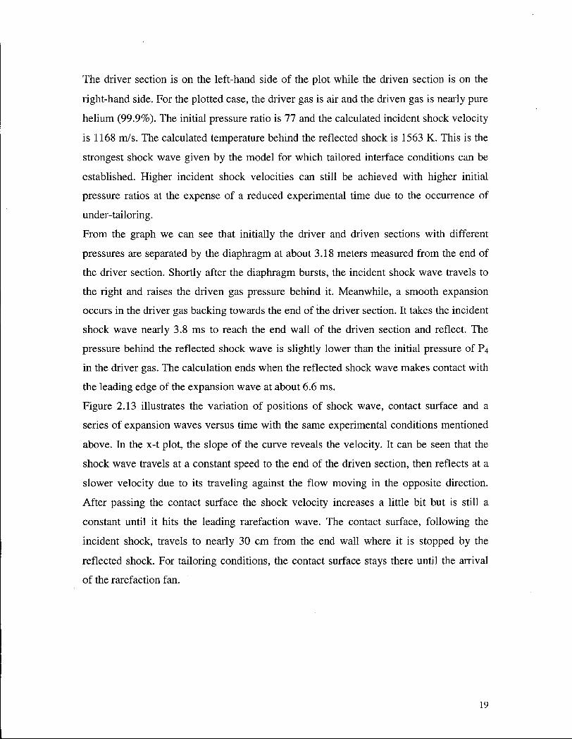
The driver section is on the left-hand side of the plot while the driven section is on the

right-hand side. For the plotted case, the driver gas is air and the driven gas is nearly pure

helium (99.9%). The initial pressure ratio is 77 and the calculated incident shock velocity

is 1168 m/s. The calculated temperature behind the reflected shock is 1563 K. This is the

strongest shock wave given by the model for which tailored interface conditions can be

established. Higher incident shock velocities can still be achieved with higher initial

pressure ratios at the expense of a reduced experimental time due to the occurrence of

under-tailoring.

From the graph we can see that initially the driver and driven sections with different

pressures are separated by the diaphragm at about 3.18 meters measured from the end of

the driver section. Shortly after the diaphragm bursts, the incident shock wave travels to

the right and raises the driven gas pressure behind it. Meanwhile, a smooth expansion

occurs in the driver gas backing towards the end of the driver section. It takes the incident

shock wave nearly 3.8 ms to reach the end wall of the driven section and reflect. The

pressure behind the reflected shock wave is slightly lower than the initial pressure of P 4

in the driver gas. The calculation ends when the reflected shock wave makes contact with

the leading edge of the expansion wave at about 6.6 ms.

Figure 2.13 illustrates the variation of positions of shock wave, contact surface and a

series of expansion waves versus time with the same experimental conditions mentioned

above. In the x-t plot, the slope of the curve reveals the velocity. It can be seen that the

shock wave travels at a constant speed to the end of the driven section, then reflects at a

slower velocity due to its traveling against the flow moving in the opposite direction.

After passing the contact surface the shock velocity increases a little bit but is still a

constant until it hits the leading rarefaction wave. The contact surface, following the

incident shock, travels to nearly 30 cm from the end wall where it is stopped by the

reflected shock. For tailoring conditions, the contact surface stays there until the arrival

of the rarefaction fan.

19

0

Contact 'Surrace"

Leading Expansion

1 4

t[ms]

Expansion

8

Figure 2.13 Positions of shock wave, contact surface and rarefaction fan versus time. Numbers in the

legend are values of X or P that characterize the expansion waves; x_s denotes shock positions and x_c

denotes contact surface positions.

On the other hand, the leading rarefaction wave travels back to the end of the driver

section at the local sound speed, then reflects and speeds up in the flow moving in the

same direction. At about 6.6 ms, it hits the reflected shock. We extend the line from this

point to the contact surface in order to estimate the experimental time. The final

experimental time calculated in this way is 3.8 ms.

2) Comparisons with Experimental Results

Passage of an incident shock wave is recorded by the pressure transducer sampling at a

rate of 166.7 KHz. The distance of each sensor measured from the exit of the driver

section is plotted with the time when the incident shock is recorded. The slope of a linear

fit to the measurements gives the incident shock velocity as shown in figure 2.14. It is

encouraging to find that for all the experiments, the measured incident shock velocities

are constant (the coefficient of determination, r , for the least square fit by a linear

correlation is always higher than 0.995). This is very important to both the shock

calculation and the establishment of desired experimental conditions.

20

1.5

1

0.5

0

0 0.5 1 1.5 2 2.5 3 3.5

t [ms]

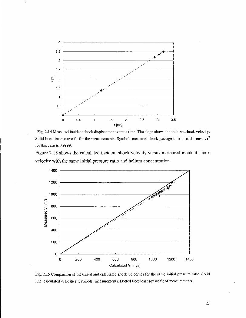
Fig. 2.14 Measured incident shock displacement versus time. The slope shows the incident shock velocity.

Solid line: linear curve fit for the measurements. Symbol: measured shock passage time at each sensor, r2

for this case is 0.9999.

Figure 2.15 shows the calculated incident shock velocity versus measured incident shock

velocity with the same initial pressure ratio and helium concentration.

1400

T3 CD

co

200 400 600 800

Calculated Vi [m/s]

1000 1200 1400

Fig. 2.15 Comparison of measured and calculated shock velocities for the same initial pressure ratio. Solid

line: calculated velocities. Symbols: measurements. Dotted line: least square fit of measurements.

21

It can be seen that for all these cases the results from the model slightly over-predict the

incident shock velocity. The reason for the lower value of the experimental incident

shock velocity is that in the model, we assume no loss at the driver section; the expansion

from P 4 to P 3 is isentropic. However, in reality, the inner diameter of the burst diaphragm

is always smaller than the inner diameter of the tube, which causes a significant throttling

loss when a high-speed flow passes through. Also there are losses due to viscous effects

along the whole driver section. The least square fit of the measurements shows that the

difference caused by the loss increases with an increasing initial pressure ratio as well as

with an increasing incident shock velocity.

Figure 2.16 compares the reflected shock velocity obtained from both experiments and

the model for the same incident shock velocity.

500.0

450.0

400.0

350.0

300.0

1 250.0

>

200.0

150.0

100.0

50.0

0.0 900 950 1000 1050 1100

Vi [m/s]

1150 1200 1250

Fig. 2.16 Comparison of measured and calculated reflected shock velocities for the same incident shock

velocity. Solid line: calculated velocity. Symbols: measured velocity. Dashed line: least square fit of

measurements.

We find that the reflected shock velocity predicted by the model is slightly lower than the

measurements. The difference increases with increasing incident shock velocity.

22

The disagreement could be mainly attributed to the attenuation of the flow velocity

behind the incident shock that increases the reflected shock velocity in the laboratory-

fixed coordinates as well as to the increasing error of the measured reflected shock

velocity.

Finally, we checked the calculated experimental time using measurements for the same

initial pressure ratio and helium concentration. The calculated experimental time is

slightly shorter than the measurements, which is due to the 'conservative' estimation

explained above.

0.00500 i -X

•W 0.00400 CD

E

•£ 0.00300 CD

E k_ CD

a. w 0.00200 T 3 CD t_

0 3 CO

2 0.00100

0.00000 ^ ' ' ' 1 1

0 0.001 0.002 0.003 0.004 0.005

Calculated Experimental Time [s]

Fig. 2.17 Comparison of measured and calculated experimental time.

2.4.3 Modified Model

In the modified model, which is currently being used for experimental calculations, we

input the measured incident shock velocity and calculate conditions behind the reflected

shock accordingly. The measurement of the incident shock velocity, as we will show

later, can be quite accurate.

Modifications have been made to the conservation equations to take into account the

throttling loss at the exit of the driver section. Variations in driver gas properties brought

about by throttling can cause corresponding changes in tailoring conditions as well as the

calculated experimental time.

23

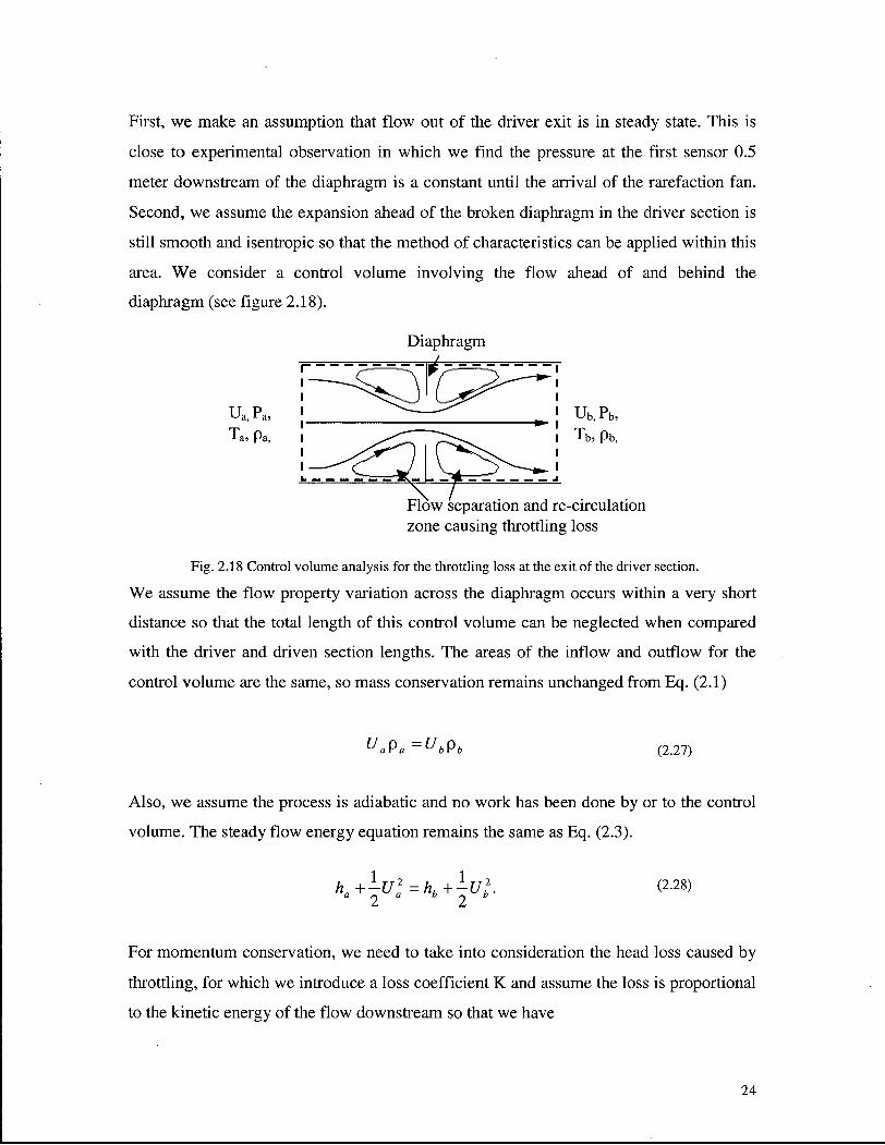
First, we make an assumption that flow out of the driver exit is in steady state. This is

close to experimental observation in which we find the pressure at the first sensor 0.5

meter downstream of the diaphragm is a constant until the arrival of the rarefaction fan.

Second, we assume the expansion ahead of the broken diaphragm in the driver section is

still smooth and isentropic so that the method of characteristics can be applied within this

area. We consider a control volume involving the flow ahead of and behind the

diaphragm (see figure 2.18).

U a P a , T a, Pa,

U b , P b ,

T b , pb,

Flow separation and re-circulation zone causing throttling loss

Fig. 2.18 Control volume analysis for the throttling loss at the exit of the driver section.

We assume the flow property variation across the diaphragm occurs within a very short

distance so that the total length of this control volume can be neglected when compared

with the driver and driven section lengths. The areas of the inflow and outflow for the

control volume are the same, so mass conservation remains unchanged from Eq. (2.1)

uapa=ubPb (2.27)

Also, we assume the process is adiabatic and no work has been done by or to the control

volume. The steady flow energy equation remains the same as Eq. (2.3).

1 9 1 9

h + -U2=hh + -U2. 2 2

(2.28)

For momentum conservation, we need to take into consideration the head loss caused by

throttling, for which we introduce a loss coefficient K and assume the loss is proportional

to the kinetic energy of the flow downstream so that we have

24

( 1 + -K

2 We also know that the upstream flow satisfies isentropic relations:

1 (2.29)

__

P<

( T V 1

a T

f V Pa (2.30)

The incident shock velocity can be obtained from measurements. Hence, the flow

properties behind the incident shock, i.e., Ub, Pb are known. Recalling the discussion of

the isentropic expansion in the previous section, we know that the velocity at any point

can be related with the pressure ratio so that

u = 2 a< 7-1 '(2.31)

Replacing the pressure ratio with the temperature ratio by using Eq. (2.30), we rewrite

Eq. (2.31) as

u = 2 a* 7-1

1-(T \ l

T \ 4 J

(2.32)

Substituting Eq. (2.30) and Eq. (2.32) into the continuity equation and applying the ideal

gas law, we obtain an expression for down stream temperature

UbPb<X-l)

2a4p4R

( T ^

a 2 ( T \

a T T

-1

|Y-1 (2.33)

Here, R is the gas constant of driver gas. Substituting Eqs. (2.32) and (2.33) into Eq.

(2.28) and assuming constant specific heat, we get

25

2 a A

( 7 - i r 1-x' - c, ubpb<x-n\

2a4p4R

1 7+1 l-vl 2 *

(2.34)

where x is the temperature ratio x=(T a/T4). Here the only unknown is x, for which we can

solve by iteration so that the value of T a can be found. Once T a is known, other properties

can be solved easily with isentropic relations and conservation equations from (2.27) to

(2.29).

Finally, we solve the momentum equation for the loss coefficient K. The calculated K

remains constant as long as the flow across the diaphragm is steady. This is true until the

arrival of the reflected rarefaction fan. The velocity of the leading edge of the rarefaction

fan after leaving the control volume above can be obtained by calculating the velocity of

a sound wave traveling in the flow of driver gas moving at the constant velocity U 3 . We

apply the method of characteristics up to the exit of the driver section. The model predicts

the total experimental time, as illustrated in figure 2.19.

Constant Left speed boundary ^ ofMOCv

Shock wave

Contact surface

Leading edge of rarefaction fan

Fig. 2.19 Estimation of the experimental time using the modified model

It is worthwhile to point out that the value of K calculated in this way represents the

overall non-isentropic effect on the driver gas including friction and throttling losses. It

depends strongly on the burst condition of the diaphragm, which may vary with different

designs, materials and machining accuracy. For the current experiment the value of K is

found mostly between 0.2 to 1 and has an average of 0.4.

26

The initial helium concentration in the driver gas and the incident shock velocity

predicted by the modified model for tailoring conditions are compared with the

experimental results for the same initial pressure ratio in figures 2 . 2 0 and 2 . 2 1 .

0.99

0.98

0.97

0.96

« 0.95

0.94

0.93

0.92 —f^-

0.91 '-

0.9

35 45 55 65 75 85 95

Initial Pressure Ratio (P4/P1)

Fig.2.20 Model prediction of the helium fraction in the driver gas for tailoring conditions with the given

initial pressure ratio. Solid line: model with throttling effects (K=0.4). Dotted line: model without throttling

effects (K=0). Symbols: experiments in which tailoring conditions have been achieved.

1400 -| 1

1200

1000

_ 800

1

> 600

400

200

0

30 40 50 60 70 80 90 100

Initial Pressure Ratio (P4/P1)

Fig.2.21 Model prediction of the incident shock velocity for the given initial pressure ratio. Solid line:

model with throttling effects (K=0.4). Dotted line: model without throttling effects (K=0). Symbols:

measurements.

27

It can be seen that by taking into consideration the throttling effects, the agreement

between the model and the experimental measurements has been improved. The

procedure for applying the modified model can be illustrated by the flowchart shown in

figure 2.22.

For each batch of diaphragms of the same specification, do 3 to 4 preliminary tests to estimate the average value of K

r

Use K achieved abo\ pressure ratio and he for desired incident s as well as tailored inl

'& to calculate initial Hum concentration hock wave velocity .erface condition.

Do a shock tube experiment

Recalculate experimental conditions with measured incident shock velocity.

Check the value of K and make adjustments if necessary.

Fig. 2.22 Procedure of applying the modified model

2.5 Uncertainty of Experimental Conditions

Before we move on to reach any conclusions from our experiments, it is essential for us

to find the uncertainty of our shock wave calculation and measurements and to take

whatever measures possible to reduce the error.

The incident and reflected shock wave velocities are calculated by dividing the distance

between 2 sensors by the measured time duration for the shock wave to pass between

them. The sampling rate of PCB pressure transducers is set at 166.67 kHz, which

converts to 6 microseconds for each sample; so the uncertainty of our time measurement

28

is ±6 us. We estimate the uncertainty of the length measurements to be 0.2% of the

overall length plus the radius of the pressure transducer. The calculated uncertainty (see

appendix B for details) for the incident shock velocity is about 0.31% and that for the

reflected shock is 2.2%. The corresponding uncertainty for temperature T 5 is 5 to 7 K for

the current experimental range. It increases to 9 to 13 K when the reflected shock velocity

is also used in the calculation. However, the value is still small compared with T5 that is

usually over 1000K.

Since we do not have independent verification of experimental temperatures, we use

measured pressures and velocities to check our calculations.

Figure 2.23 is a comparison between calculated and measured pressures behind the

reflected shock - P 5 . The error in pressures measured by PCB transducers is roughly 5%.

The plot demonstrates a good agreement between the calculations and the measurements

although the least square fit of measured pressures shows a slight bias towards under-

prediction at the high pressures.

0 10 20 30 40 50

Calculated P5 [atm]

Fig. 2.23 Comparison of measured and calculated pressures behind the reflected shock for the same

incident shock velocity. Solid line: calculated pressure. Symbols: measured pressure. Dashed line: least

square fit of measurements.

As we have shown in the previous section, the measured reflected shock velocity is

generally higher than calculated for the same incident shock speed. To establish the

29

extent to which this difference is going to affect calculated temperature, we modified the

model and input both measured incident and reflected shock velocities. We compared the

results with model predictions by using only measured incident shock velocities. The

comparison is shown in figure 2.24.

1600 i 1

900

800 ' 1 1 ' ' 1 ' 1 '

800 850 900 950 1000 1050 1100 1150 1200 1250

Incident Shock Velocity [m/s]

Fig. 2.24 Comparison of calculated temperatures using two different methods: (a) measured incident shock

velocity, (b) both measured incident and measured reflected shock velocities. Symbols: diamonds - (a),

squares - (b). Solid lines are least square fits.

The difference between calculated temperatures, AT, using the two aforementioned

methods increases with an increasing incident shock velocity. The biggest gap appears at

the highest initial temperature, for which it is nearly 37 K. For the majority of the

temperature range the differences are less than 25K.

2.6 Reflected Shock Boundary Layer Interaction

One famous phenomenon observed in shock tube experiments is reflected shock/wave

boundary layer interaction [6,7,11]. In the aforementioned one-dimensional model used

for shock calculations, we always assume uniform inflow/outflow velocity profiles. This

is certainly valid for the incident shock wave, which travels into a gas at rest. However,

for the reflected shock, which travels in a flow set in motion by the incident shock, the

30

velocity profile of the incoming flow is no longer uniform due to the viscous effects near

the wall of the shock tube. Figure 2.25 illustrates the velocity profile of the incoming

flow in reflected-shock fixed coordinates.

W 5

Reflected shock U 2 +W 5 Incoming flow

Wall

Fig. 2.25 Velocity profile of the incoming flow in reflected-shock-fixed coordinates.

The flow velocity at the wall is the same as the wall velocity. For shock-fixed

coordinates, the wall moves at the reflected shock velocity W 5 . The velocity of the main

stream is the sum of the flow velocity behind the incident shock and the velocity of the

reflected shock.

It has been observed by early researchers [9,10] that the interaction between the reflected

shock and the boundary layer may cause the boundary layer to separate with separation

bubble producing a shock bifurcation at the foot of the reflected shock (see figure 2.26).

Holder [11] in his shock tube experiment observed a stream of cold gas along the side

wall penetrating into the hot gas behind the reflected shock and meeting the end plate of

the driven section. The phenomenon was believed to relate directly with the reflected

shock/boundary layer interaction.

There are two possible influences that may be brought about by this non-uniform velocity

profile of the incoming flow based on the above observations. The first is direct cooling

of the hot gas close to the end wall by the cold flow emerging from the bifurcated shock

foot. Since we define the experimental time starting from the shock wave reflection from

the end wall of the driven section, and the observed ignition actually starts very close to

the end wall, we need to examine the time when the gas starts to change the temperature

31

at this crucial area and make sure that the temperature is not significantly reduced before

ignition. The second is that the boundary layer thickness may grow to such an extent

that the uniform flow assumption becomes no longer valid. Our entire calculation of

experimental conditions behind the reflected shock need to be reevaluated for such a

condition.

Fig. 2.26 Bifurcated foot of the reflected shock in shock-fixed coordinates

Mark [9] developed a simple model for the reflected shock - boundary layer interaction.

The model was extended by Davies [6] to calculate the time required for the emerging

cooling flow from the reflected shock bifurcation foot to reach the end wall. In the Mark

and Davies model, the boundary layer in the path of the reflected shock is taken to be a

layer of gas of unspecified thickness't' at wall temperature and having the wall velocity

with the pressure equal to free stream value. The observed flow separation at the shock

foot is explained as the boundary layer being brought to rest by the reflected shock in

shock-fixed coordinates. It has been shown by Mark that for air, the stagnation pressure

for incident shock Mach number ranging from 1.8 to 16 is less than the pressure behind

the normal shock. The boundary layer flow is thus barred from entering the region behind

the reflected shock. Instead, it gathers under the shock foot growing as the reflected

shock travels upstream and causes bifurcation of the shock to form forward and backward

limbs denoted by OA and OB as shown in figure 2.26.

Part of the main flow outside the boundary layer is turned to pass through the forward

limb and then further compressed by the backward limb. Experimental observations

reveal that the flow direction is turned parallel to the main stream flow behind the

reflected shock after emerging from the two oblique shocks. It can be shown that this

32

flow, with its velocity faster than the flow velocity behind the normal shock, has an

absolute velocity towards the end wall.

For a flow passing an oblique shock, the normal shock relation can still be valid if we

choose to use the velocity component normal to the shock front. The velocity component

parallel to the shock front will not be affected after passage as illustrated in figure 2.27.

p-e

v 2

W i p

u 2

Fig. 2.27 Oblique shock wave and equivalent normal shock wave

It can be shown that the following relations hold for a perfect gas passing an oblique

shock.

P l = (7+l)Mfla

2sin2p-

p 2 l + (7 - l )Ma 2 s in 2 p (2.35)

= l + ^ ( M a 2 s i n 2 p - l ) 7 + l v 0 '

(2.36)

T2 _ 1 | 2(7-1)

T, (7+D 2

l + 7 M . ^ i n 2 p V 2 s i n 2 p _ l }

(2.37) M a 2 sin 2 p

where Ma a is the flow Mach number ahead of the oblique shock and P is the angle

between moving direction of the incoming flow and the shock front. The Mach number

behind the shock wave is given by:

33

M a 2 sin 2(p -0 ) 1 + Ma] sin 2 B

2

7 M a f l

2 s i n 2 ( 3 - ^

(2.38)

Also the deflection angle 0 can be calculated from

tan0 = 2cotp M a 2 sin 2 P -1

2 + M a 2 (7 + cos 2p)

(2.39)

Returning to the bifurcated foot of the reflected shock, we can calculate the flow

properties after passing two oblique shocks (OA and AB), however we need to calculate

the angles with respect to the moving direction of the incoming flow so that the oblique

shock relations, Eq. (2.35) to (2.39), can be applied. In the Mark and Davies model, two

assumptions have been made to calculate these angles. First, the pressure under the

triangle OAB is assumed the same as the stagnation pressure. Second, the flow leaves the

rear limb AB having the same pressure as that behind the normal shock. Since we have

already assumed the temperature of the boundary layer is the wall temperature, we can

obtain the local sound speed and, from that, the local Mach number for the boundary

flow. The stagnation pressure can be calculated by the Rayleigh supersonic pitot formula.

st.bl

7+1 Ma bl

y-l

(2.40)

27 7+1

Ma2

bl ~ Y - l 7+1 J

7-1

Here, Ps t,bi is the stagnation pressure and P a is the pressure of the boundary layer flow,

which is assumed the same as that of the main flow; Ma^ is the boundary layer (wall)

Mach number. Once we know the stagnation pressure, with assumption 1, the angle P or

COA of the forward limb (see figure 2.28) can be calculated from Eq. (2.36).

34

Fig. 2.28 Mean flow passing through two oblique shocks. Ma represents the local Mach number of the

flow.

Mai sin 2 COA = _ a

2Y

(2.41)

The flow direction after passing the forward limb is given by

tan(COA - COB) _ (7 - l )Ma 2 sin 2 CO A + 2

tan(COA) (7 + \)Ma2 sin 2 CO A (2.42)

Also the flow Mach number between two limbs is obtained using Eq. (2.38).

Ma] sin 2 (COA-COB) ( 7 - l ) ^ + (Y+D

_ 0

p (2.43)

The flow Mach number Mas after passing the rear limb can be obtained from Ma x and

(P5/Pst.w) in similar equations.

35

+ (7+1)

Ma* 2 sin 2 (DAB -DAC) = st.bl (2.44)

1 stM

Finally, the absolute velocity with which the cooling flow approaches the end wall is

given by (U5*-W 5), where U5* denotes the relative velocity of the flow emerging from

It is shown by the model that before the reflected shock passes the contact surface, the

flow temperature of driven gas after being compressed by two oblique limbs is very close

to the temperature in the main flow. However, after the shock passes the contact surface

and traveling into the driver gas, the temperature of the flow emerging from the

bifurcated foot is much lower than the temperature in the experimental area.

Despite the obvious crudeness of this model, it is observed by Mark and later researchers

that the 'model provided a most useful and sometimes surprisingly accurate description

of the bifurcation phenomenon' [6]. The predicted cooling flow velocity has been

verified by the heat transfer experiment conducted by Davies.

We use Davies' model to calculate the flow velocity after passing the bifurcation foot in

the current experiments so that we can evaluate the time for the cooling gas to reach the

end wall. We compare it with previously calculated experimental time for various initial

conditions. The result is shown in figure 2.29.

It can be seen that for an incident shock velocity higher than 1030m/s, the cold gas

passing the bifurcation foot is able to reach the end wall prior to the arrival of the

rarefaction fan. The experimental time for those cases could be shorter than that predicted

before. The temperature of this stream is much lower than the main flow temperature

(around 266-269K for the current experimental range), and increases slightly with a

decrease of the incident shock velocity.

AB.

36

0.009

0.008

0.007

0.006

0.005

0.004

0.003

0.002

0.001

800 850 900 950 1000 1050 Vi [m/s]

1100 1150 1200

Fig. 2.29. Comparison of the time for the cooling gas to reach the end wall with calculated experimental

time versus the incident shock velocities. Time starts from the shock reflection at the end wall. Dotted line:

experimental time. Solid line: time for the cooling gas to reach the end wall. Driver gas: Helium mixed

with air. Driven gas: air.

We also calculated the boundary layer thickness of the flow behind the incident shock

using a numerical model (see appendix D for details). It is found that for the current

experimental range, the boundary layer thickness does not bring a significant effect on

the one-dimensional shock tube model.

2.7 Contact Surface Instability

Another factor that contributes to the premature termination of constant conditions in the

experimental area is contact surface instability. Lapworth [7,8] reported the duration of

constant temperature behind the reflected shock is much shorter than the duration of

constant pressure when hydrogen is used to drive nitrogen in his shock tube experiment.

A similar phenomenon has been reported by Lapworth and Townsend for their helium-

nitrogen system. The problem is examined by Bird et al [14] and is attributed to the

37

instability of a "shocked" contact surface- a contact surface through which a shock has

passed - that causes cooling of the hot gas.

Taylor [15] discussed the stability of an interface between two fluids of different

densities when the two fluids are accelerated in a direction perpendicular to their

interface. He used the velocity potential to show that the rate of development of the

instability is proportional to

P2-P1 •, (2.45)

VP2 + P1 where pi and p 2 are the densities of the two fluids.

Markstein [16] developed Taylor's analysis and applied it to a 'shocked' contact surface

in a shock tube experiment. The result is an expression for the velocity field for the

disturbance flow, which has the form

i , ( r -TJhA ^ 5 k(±x+iy)

u{x,y) -UkA- -e . ,2.46) (Ps + Pe)

Here, U is the velocity difference between reflected shock and the driver gas behind the

reflected shock; k equals 2n/X where X is the wavelength of the disturbance of the

interface, ps and p6 are the densities of driven and driver gas behind the reflected shock,

and A is an amplitude factor. It is interesting to notice that the sign of the perturbation

velocity depends on (p5- P6). Davies [6] used this analysis to show that for a helium-

nitrogen system neutral stability happens when Mi=3.56 so that ps=p6 and u vanishes.

For any Mach number higher than that, the perturbation flow will move towards the

driven gas and change the constant conditions there. A calculation using the current

shock tube model shows that for our helium-air system, within the entire experimental

range (Mj<3.5), we have P5>p6 which means the perturbation always propagates towards

the driver side. The contact surface instability should not affect the experimental

conditions for the current study.

38

C H A P T E R III

3.1 Introduction

Accurate measurements of the ignition delay for natural gas under engine-relevant

conditions provide important information to obtain an optimal control for a natural-gas-

fueled engine. For a direct injection natural gas engine, the ignition delay determines

directly the injection advance. On the other hand, for a homogeneously charged spark

ignition engine, a short ignition delay that leads to an autoignition may result in engine

knock and thus must be avoided.

Historically, the study of the ignition for methane - a major component of natural gas -

has enjoyed wide attention. However, despite many experiments measuring the ignition

delay for methane in air or oxygen, there are surprisingly few published for high pressure

(P>15 atm) and low temperature (T<1400 K) methane ignition, on which engine

designers' interests are focused. A simple extrapolation of empirical equations derived

from low-pressure high-temperature experiments generates dubious and usually

inaccurate results.

The lack of experimental data in this area also affects the applicable range of chemical

kinetics, which have been developed to match experimental measurements.

A primary purpose of the current project is to measure the ignition delay for methane

under engine-relevant conditions and to correlate the ignition delay with key

environmental parameters such as temperature and pressure.

It is the author's hope that the results of the present study may serve as a guide to

understanding ignition in natural gas engines as well as provide help in extending the

reaction mechanism for high-pressure methane ignition.

3.2 Background

3.2.1 Oxidation of Methane

Among the hydrocarbons, methane is the one of the more "inactive" fuels. The energy

required to break the primary C - H bond in methane is 439.3 kJ/mole, which is

significantly higher than longer-chain hydrocarbons.

39

Glassman [29] divided the mechanism for methane oxidation into two regimes of

temperature with respective dominant kinetics. The slow reaction speed of methane may

be mainly attributed to the following:

1) Slow chain initiation.

The major initiation steps for methane oxidation are:

CH4+O2 => CH3+HO (low temperature) (3.R1)

CH4+M => CH3+H+M (high temperature) (3.R2)

The high C-H bond energy of methane prevents these steps from proceeding rapidly

especially at low temperatures.

2) At high temperature (1000K or above), the equilibrium of an important chain

propagating step, i.e.,

C H 3 + 0 2 O H O + H 2 C O ( 3 R 3 )

shifts strongly towards the reactants and the overall reaction to form formaldehyde

and hydroxyl can not proceed.

3) Another major oxidation destruction path of the methoxy radical, i.e.,

CH 3 +0 2 => CH3O+O ( 3 R 4 )

is highly endothermic requiring large activation energy, and thus, quite slow for a

chain step.

4) In the presence of high concentration of CO formed by precursory chain propagation

steps, reactions

40

CH 4+OH->CH 3+H 20 (3.R5)

and

CO+OH->C0 2+H ( 3 R 6 )

compete for hydroxyl radicals. Since reaction (3.R5) is faster than reaction (3.R6), the net

result of this competition is the reduction of the fuel consumption rate.

3.2.2 Previous Work

Experimental studies on methane-air/methane-oxygen autoignition have been reported by

Lifshitz et al. (1971), Grillo and Slack (1976), Seery and Bowman (1970), Tsuboi and

Wagner (1974), Hidaka et al. (1978), Oppenheim and Cheng (1984), Cowell and

Lefebvre (1987) etc. Among these studies, the shock tube was used as the primary

experimental instrument because of its instantaneous temperature and pressure rise that

minimizes the effects of heating process. Other methods, such as rapid compression

machines or heated air experiments by Cowell and Lefebvre [18], are also used in

ignition measurements.

The criteria that define the onset of ignition vary from sudden changes of temperature and

pressure to the appearance of certain radical peaks as well as the variation of density of

the mixture. Zhou and Karim [19] examined the different criteria numerically using a

detailed reaction mechanism, and found little difference among different criteria used for

ignition delay at low temperatures (<1100K), but relatively large scatter for higher

temperatures. The criteria based on the sudden changes in pressure and temperature are

recommended for the reason that the ignition delay time measured by such methods

always lies in the middle of the results obtained using different criteria. Furthermore,

temperature and pressure are the most readily measurable parameters, and are thus

considered more reliable. In reality, rapid change in temperature is usually more difficult

to measure than that of pressure because of the short residence time. The response of

pressure-measuring instruments available in the market is usually much faster than that of

most instruments that measure temperature.

The measured ignition delay is often correlated with pressure, temperature and reactant

concentrations using global reaction formulas. It is worthwhile to point out that even the

simplest combustion reaction will involve dozens of intermediate species and hundreds of

41

forward and backward reaction steps. It is far too complicated to be represented by any

one step reaction mechanism. However, empirical equations do provide valuable

information to both the development of detailed reaction mechanism and practical

engineering applications by establishing how the ignition-delay time changes with the

variation of system parameters.

In its general form, the rate of a chemical reaction is expressed as

(a=kU[Xl]v', (3-D i=i

where [X;] is the concentration of reactant i raised to the power of its stoichiometric

coefficient V{. k is the reaction rate constant, which is given by the Arrhenius expression

k = Aexp RT

(3.2)

Here A is the Arrhenius constant, E is a global activation energy, and R is the universal

gas constant. For an empirical expression of the reaction rate, stoichiometric coefficients

in Eq. (3.1) are replaced by empirical coefficients to fit experimental measurements. For

an air/oxygen-fuel reaction system, the empirical expression becomes

co =k[oxygen]~b[fuel] " p m , ( 3 3 )

where a, b and m are empirical coefficients; p is the mixture pressure in atm. The unit for

concentrations of oxygen and fuel is mol/cm3. The ignition delay time is considered

proportional to the inverse of the initial reaction rate and is given by the general form

T = A e x p f - ^ \oxygenr[fuel]bPmTn-a-°-5, ( 3 . 4 )

where T 0 ' 5 comes from the molecular collision theory. The last term (Tn"a"0,5) of equation

(3.4) is usually neglected unless one is working with a wide temperature range [20].

42

The most common form of the empirical equation for a methane-air/oxygen system thus

becomes

x = Aexp b nm RT [02]a[CH4rP (3.5)

The empirical coefficients from previous studies, along with their experimental

conditions are tabulated in table 3.1. These coefficients are achieved normally by fitting

experimental data using regression methods.

Pressure

(atm)

Temperature

(K)

a b m A Ea Experimental

Method

Seery and

Bowman

1.5-4 1300-1900 0.4 -1.6 0 7.65E-12 215 Shock tube

Premixed

Lifshitz et

al.

2-10 1500-2150 0.33 -1.03 0 3.62E-08 195 Shock tube

Premixed

Tsuboi and

Wagner

2-3 1200-2100 0.32 -1.02 0 2.50E-09 222 Shock tube

Premixed

Cheng and

Oppenheim

1-3 1100-2200 0.48 -1.94 0 1.19E-12 194 Shock tube

Premixed

Walker et

al.

1.5-15 ? 0.33 -1.05 0 2.21E-08 189 Shock tube

Premixed

Grillo and

Slack

1-6 1640-2150 0.33 -1.03 0 4.40E-09 219 Shock tube

Premixed

Hidaka et

al.

0.47-0.74 1800-2500 0.37 -0.64 0 4.54E-04 149 Shock tube

Premixed

Cowell and

Lefebvre

7-10 <1000

0.19

-1 1.99E-01 105 Heated Air

Non-premixed

Table 3.1. Experimental conditions and empirical coefficients for previous work measuring the ignition delay of methane

The calculated ignition delay is in microseconds. Other units are: kJ/mol for Ea, K for T,

mol/cm3 for [CH4] and [0 2 ] , and kJ/mol.K for the gas constant R.

Clearly, there is a lack of data in the literature for low temperatures and high pressures

that one would expect in an engine environment.

43

It is interesting to compare the ignition delay time calculated from all these equations to

see how they agree with each other. In figure 3.1, calculated ignition delay times are

shown in an Arrhenius plot (logx versus the inverse of temperature) within their

respective temperature ranges for a pressure of 2 atm and an equivalence ratio of 1.

1.0E+00 1 1

0.400 0.500 0.600 0.700 0.800 0.900 1.000

1000K/T

Fig. 3.1 Ignition Delay of a stoichiometric methane-air mixture calculated using different empirical

equations for an initial pressure of 2 atm

At this low pressure, different empirical equations show relatively good agreement with

each other. However, when trying to extrapolate these equations to low temperature and

high pressure conditions close to that of engine environments, we find a big scatter of

calculated ignition delay time as shown in figure 3.2, where the initial pressure has been

raised to 30 atm.

It is obvious that using these empirical equations out of the scope where they are derived

generates unreliable results.

The lack of experimental results for the ignition delay of CH4-air mixture at engine

relevant conditions is what has activated the experiments to be decided herein.

44

1 .OE+06

1.0E+05

C o . o CD

2 1 .OE+04 o

__

Q 1.0E+03 c

g 'E __>

1.0E+02

1.0E+01

jr.'' '

\ € ^ '-

y -^-"-"""^ y — f s '

-""* # y '

t S '

s'

'' ' &**jy t y'

jX ' '

/ y' y'

r y'

s'

y'

- Seery and Bowman

Lifshitz et al

•Tsuboi and Wanger

• Chen and Oppenhem

-Walket al

-Grillo and Slack

-Cowell and Lefebvre

0.700 0.800 " 0.900 1.000 1000K/T

Fig. 3.2 Ignition Delay of a stoichiometric methane-air mixture calculated using different empirical

equations for an initial pressure of 30 atm

Using the shock tube introduced in the previous chapter, we have conducted a series of

ignition experiments for methane and air premixed inside the driven section of the shock

tube with desired equivalence ratio. A 20-30 minute relaxation time is given before each

experiment to allow complete mixing of fuel and air. Various experimental temperatures

and pressures have been obtained by changing the initial driver and driven pressures and

helium concentrations according to calculations using the method introduced in chapter

II.

3.3 Results and Discussions

3.3.1 Pressure History of Methane Self-ignition Process

The pressure histories detected at the end wall of the shock tube behind the reflected

shock wave for initial pressures from 16 to 40 atm are shown in figures 3.3 to 3.6. The

experimental temperature covers a range from 1000 to 1400 K. Below 1000 K, we find

that either the ignition delay exceeds the maximum experimental time or the pressure

variation may be too weak to be detected by the pressure sensor due to a slow

combustion. In either event, for these conditions, we are unable to measure ignition delay

with the present system.

45

It can be seen that the pressure trace is a flat curve initially after the reflection of the

shock wave. After a short delay time, the pressure starts to rise, which is an indication of

the beginning of ignition. The ignition delay time is then defined for our study as the time

duration from the shock reflection to the time when the maximum curvature on the

pressure trace is found. This criterion has also been used by early researchers including

Frenklanch and Bornside [2].

46

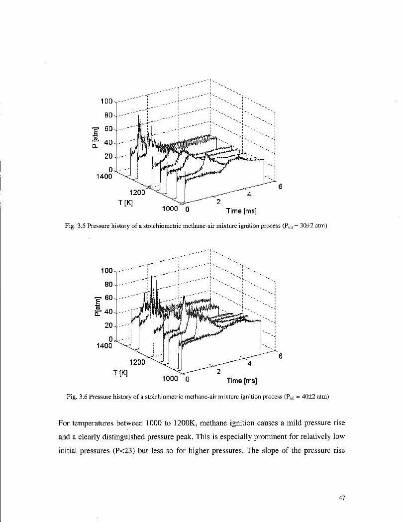
1000 0 T ime[ms]

Fig. 3.5 Pressure history of a stoichiometric methane-air mixture ignition process (P;ni •= 30±2 atm)

0 1400

T [K] 1000 0 T ime[ms]

Fig. 3.6 Pressure history of a stoichiometric methane-air mixture ignition process (Pini = 40±2 atm)

For temperatures between 1000 to 1200K, methane ignition causes a mild pressure rise

and a clearly distinguished pressure peak. This is especially prominent for relatively low

initial pressures (P<23) but less so for higher pressures. The slope of the pressure rise

47

grows steeper with the increase of temperature. At the same temperature the increase is

sharper for a higher initial pressure than that for a lower one.

A noticeable change of the ignition pattern occurs when the temperature is raised to

around 1250 K. Trie ignition becomes less ordered. Specifically, we no longer see a

unique maximum in pressure. In some cases, a sharp, secondary pressure peak whose

magnitude can usually exceed the first one starts to appear.

With further increase of temperature to over 1300K, strong ignitions, which are

characterized by a sudden increase of pressure followed by violent pressure oscillations,

are found. The peak pressure of such an ignition may be 1.5 to 2 times higher than that of

the mild ignition, and has a maximum value up to 100 atm. The blast wave formed by

this sudden pressure jump traveling at a very high velocity may catch up with the

reflected shock wave, and form a detonation front that propagates downstream

supersonically.

It is noticeable that the change from weak to strong ignition happens within a short

temperature range. There is no obvious variation of the magnitude of peak pressure as the

temperature approaches the strong ignition limit. Similar observation of this discontinuity

is reported by Chang and Oppenheim [1] as well as by Fieweger et al. [21] in their

respective studies, which we will discuss in the following section.

3.3.2 Strong Ignition Limit

The mild ignition observed at a low temperature is considered to be an autoignition that

originates from one or several hot spots in the experimental area and proceeds

inhomogeneously. In a spark ignition engine such an ignition, which evolves primarily

into a deflagration causing only mild pressure rise, is not commonly termed knock [23]. It

is, rather, the appearance of a strong ignition that brings a sudden and big jump of the

pressure, which may quickly damage the engine.

Oppenheim and Cheng [1] discuss strong ignition based on their study of

methane/hydrogen-air mixture ignition at low pressures. They attribute the cause of

strong ignition to coherence in the exothermic processes, which quickly produces a

sufficiently strong power per unit mass to generate a blast wave. They further relate this

48

coherence with the standard deviation of the temperature field during the induction

period, the heat release of reactions, the reaction rate, and also a critical value of (3T/3T)P.

It should be mentioned that the coherence of the exothermic processes is not exclusively

decided by temperature and pressure; factors such as shock wave / boundary layer

interaction can also influence the appearance of strong ignition provided that they change

the homogeneity of the reactive mixture.

Figure 3.7 shows P-T conditions where strong and mild ignitions are measured in the

current experiment.

50

10

5

0 I—1—1—1—1—1—1—1—L—1—1—1—1—1—1—1111—1—1—1—1—1—1—1—1—<—1—1— 900 1000 1100 1200 1300 1400 1500

T [ K ]

Fig. 3.7 Measured strong ignition limit for stoichiometric methane-air mixtures at pressures from 16 to 40

atm. Symbols: diamonds - mild ignition, squares - strong ignition.

The fact that the observed temperature limit for strong ignition decreases with an increase

of pressure is readily explained. The high energy released per unit volume mixture at

high pressure increases the possibility of generating a blast wave - the indication of a

strong ignition.

Different ignition patterns from mild to strong ignition recorded in the present study are

given in figure 3.8.

49

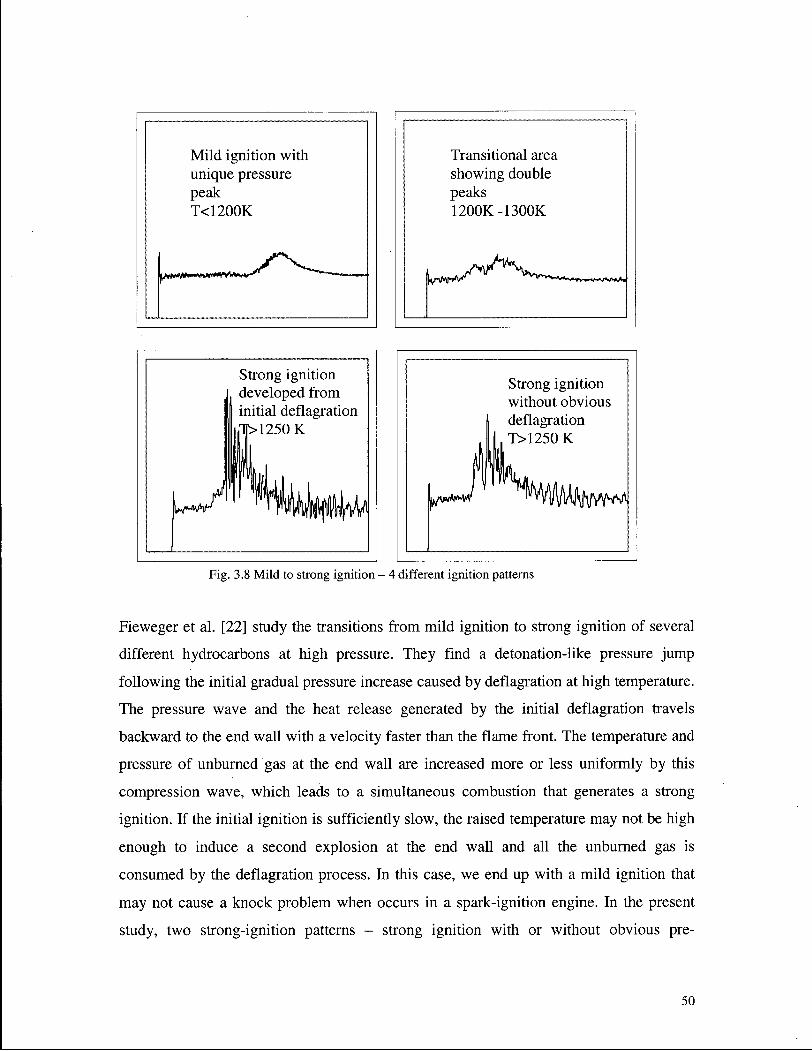
Mild ignition with unique pressure peak T<1200K

Transitional area showing double peaks 1200K-1300K

Strong ignition developed from initial deflagration [f>1250 K

Strong ignition without obvious deflagration

J T>1250K

Fig. 3.8 Mild to strong ignition - 4 different ignition patterns

Fieweger et al. [22] study the transitions from mild ignition to strong ignition of several

different hydrocarbons at high pressure. They find a detonation-like pressure jump

following the initial gradual pressure increase caused by deflagration at high temperature.

The pressure wave and the heat release generated by the initial deflagration travels

backward to the end wall with a velocity faster than the flame front. The temperature and

pressure of unburned gas at the end wall are increased more or less uniformly by this

compression wave, which leads to a simultaneous combustion that generates a strong

ignition. If the initial ignition is sufficiently slow, the raised temperature may not be high

enough to induce a second explosion at the end wall and all the unburned gas is

consumed by the deflagration process. In this case, we end up with a mild ignition that

may not cause a knock problem when occurs in a spark-ignition engine. In the present

study, two strong-ignition patterns - strong ignition with or without obvious pre-

50

deflagration - are found at nearly the same temperature range. This may be related to the

difference in positions where ignitions start. If the ignition starts very close to the end

wall, the compression happens so quickly that it can hardly be distinguished from the

subsequent strong ignition. Otherwise, the compression process takes longer time and we

can observe a clear mild pressure rise before the occurrence of a secondary explosion.

3.3.3 Ignition Delay of Methane at High Pressure

Figures 3.9 and 3.10 are Arrhenius plots showing the changes of measured ignition delay

with respect to initial temperature at different pressures. The equivalence ratios here are 1

and 0.7 respectively.

1.0E+04 i 1

• o

^ 1 .OE+03

o

1.0E+02 1 ' ' ' 1 1 1

0.7 0.75 0.8 0.85 0.9 0.95 1

1000K/T

Fig. 3.9 Measured ignition delay time of stoichiometric methane-air mixture at different pressures.

Symbols: squares - 16 atm, diamonds - 30 atm, circles - 40 atm. Solid lines are the least square fits to the

experimental measurements.

51

1.0E+04

t= o o CD w o g

CP Q

c o

'

1.0E+03

1.0E+02

0.7 0.75 0.8 0.85

1000K/T

0.9 0.95

Fig. 3.10 Measured ignition delay time of lean methane-air mixture at different pressures (4>=0.7).

Symbols: triangles - 16 atm, diamonds - 30 atm, circles - 40 atm. Solid lines are the least square fits to the

experimental measurements.

An obvious disagreement can be seen between the present results and those shown in

figure 3.2 using previous empirical equations. The ignition delay time obtained in the

current study for high pressures is significantly shorter than that from early low-pressure

experiments.

We now discuss three factors that are considered as major contributors to the ignition

delay time according to the global reaction mechanism: temperature, pressure and

fuel/oxidizer concentrations.

1) Temperature

Temperature is the most important factor that determines the ignition delay. It can be

seen that the ignition delay time increases dramatically with the decrease of temperature.

In most of the previous work on global reaction rates, the activation energy is assumed to

be a constant. The Arrhenius plot of ignition delay is then a straight line with its slope

revealing the global activation energy. At high temperature and low pressure, this value is

52

found to be approximately 180-220 kJ/mol as reported by many previous workers

[1,3,23]. However, by scrutinizing the activation energy obtained in early experiments,

one may find a clear trend of it decreasing in magnitude as the experimental temperature

is reduced, e. g., Cowell and Lefebvre [20]'s experiment conducted at low temperature

(<1000 K) and moderate pressure (7-10 atm) yields Ea=105 kcal/mol. Zhou and Karim

[19] use detailed mechanism to simulate the ignition process of methane and suggest

using 3 different values for activation energy in different temperature ranges in their

conclusions. In the present results, it is found that the measured ignition delay time at

given pressure is not fit well with a straight line in the Arrhenius plot. This is especially

true for high-pressure stoichiometric mixtures where the trend line follows a reversed 'S'

curve. Similar curves are found in high-pressure shock tube ignition tests for high-order

hydrocarbons by Fieweger et al. [22]. The range (roughly HOOK to 1200K) where

ignition delay time shows less sensitivity to the change of temperature is not very

prominent for lean mixtures, whose curves are more straight than are those of

stoichiometric mixtures.

2) Pressure 1

In most of the previous work, pressures are either sub-atmospheric or slightly higher than

1 atm. The pressure effect is usually neglected. Cowell and Lefebvre investigate the

ignition delay of methane in heated-air flow from 7 to 10 atm, and find that it is

proportional to the inverse of pressure.

Figure 9 and 10 shows an obvious reduction of ignition delay time from 16 to 30 atm, but

the difference diminishes when the pressure is further increased to 40 arm. Also the

ignition delay does not change significantly for different pressures when the temperature

is high. In terms of kinetics, this may suggest a shift of dominant reactions in an ignition

process when the temperature changes from low to high, and the low temperature

mechanism is more pressure-sensitive than the high temperature one.

3) Concentrations of Fuel and Oxidizer

Increase of reactant concentration increases the possibility for inter-molecular collisions,

and thus the chance for the reaction to take place. In the fuel-air reaction system for a

53

given pressure and temperature, the concentration of fuel and oxidizer can be varied with

different equivalence ratios.

In figures 3.11 and 3.12, stoichiometric results at a given pressure are compared with lean

and rich results to show the effect of equivalence ratio on ignition delay. It can be seen

that at 16 atm, a lean mixture generates a slightly longer ignition delay at high

temperature; the difference increases sharply when the temperature decreases. However,

with an increase of pressure, the ignition delay time of the lean mixture moves closer to

the stoichiometric one. At P=40 atm, it even cross the stoichiometric line at low

temperatures. With the same pressure, a rich mixture shows a significantly longer ignition

delay time at low temperature but at high temperature it has almost the same delay as the

stoichiometric one.

10000

•o o o CD w o o "E 1000

CD Q o

'•4—'

'rz

100

-

Lean

Stoichiometric

i i i i i

0.70 0.75 0.80 0.85

1000K/T

0.90 0.95 1.00

Fig. 3.11 Comparison of ignition delay for lean and stoichiometric methane-air mixtures at 16 atm.

Symbols: squares - lean (<E>=0.7), diamonds - stoichiometric (<&=1). Splines are used to show the trend of

change.

54

10000

100

0.70 0.75 0.80 0.85

1000K/T

0.90 0.95 1.00

Fig. 3.12 Comparison of ignition delay for lean, rich and stoichiometric methane-air mixtures at 40 atm.

Symbols: squares - lean (0=0.7), diamonds - stoichiometric (0=1), triangles - rich (O = 1.3). Splines are

used to show the trend of change.

3.3.4 Correlation Equations

An empirical equation has been derived using the linear regression method based on the

present experimental results

Clearly, the activation energy of the methane-air ignition process can not be represented

by a simple constant. It is observed that the activation energy is close to a third order

polynomial within the experimental range in the Arrhenius plot. Also, the pressure

dependence drops with the increase of temperature. The modified Arrhenius-type

equation is thus given by

x = A exp 'Ta\ cH,r{py (3.6)

55

where Ta is the activation temperature given by the equation

Ta = a\ (I) 2

+ b T

K1 J T

+ c. (3.7)

The global activation energy Ea is related to Ta by the universal gas constant R

Ea = TaxR. Q ^

The concentration of oxygen is absorbed in [CH 4 ] m for a given equivalence ratio for an

air-fuel reaction system.

A, a, b, c and m are empirical coefficients that are determined experimentally as listed in

table 3.2:

Coefficients q?=l 0=0.7

A, us.(cm3/mole)m(atm)T/n 1.20E-17 1.24E+14

a, K 3 9.71E+10 4.46E+10

b , K 2 2.46E+8 -1.06E+8

c , K 2.20E+5 1.04E+5

m 1.52 4.44

n , K -2.41E+3 -6.03E+3

Table 3.2 Empirical coefficients for the ignition delay of methane obtained in the current study

The equation has been found being able to fit the experimental results reasonably well.

Overall changes of ignition delay with respect to pressure and temperature for

stoichiometric and lean mixtures are presented in figures 3.13 and 3.14. It can be seen

that both surfaces turn upward steeply with decreasing temperature and pressure. Also,

the difference between the lean and stoichiometric surface (shown in figure 3.15) shrinks

as the temperature and pressure increase.

56

T [ K ] 1 4 0 0 15 P t a t m ]

Fig. 3.13 Ignition delay of a stoichiometric methane-air mixture by equation (3.6) (0=1)

12000

10000

8000-

6000-

" 4000

2000-|

0 1000

T [K ] 1400 15

P [atm]

Fig. 3.14 Ignition delay of a lean methane-air mixture by equation (3.6) (0=0.7)

57

1400 15 P[atm] T [K]

Fig. 3.15 Difference between lean and stoichiometric mixtures for ignition delay time

It's interesting to notice that unlike the equation presented by Cowell and Lefebvre, the

coefficient for the fuel concentration - m- obtained by us is negative, which suggests that

ignition delay time may be shorter for lean mixtures at certain conditions.

3.3.5 Comparisons of Experimental and Computational Results

A computer model incorporating detailed reaction mechanism has been developed to

simulate the ignition process in the shock tube. The initial condition behind the reflected

shock is modeled as an adiabatic and constant volume one. Gasdynamic effects brought

about by heat release and shock wave boundary layer interaction are neglected in the

current model. The methane-air kinetic mechanism is taken from GRI-Mech (version 3.0)

[31]. That generates 53 intermediate species and 318 reaction steps. Chemkin-II (version

1.6) developed by Kee et. al. [32] of the Sandia National Laboratory is used as the

mechanism interpreter. The differential equations in the model are solved using LSODE

(1987 version) [33]. The same pressure criterion is used to define the onset of the

ignition. The computational results are plotted in figure 3.16 together with the

experimental measurements.

58

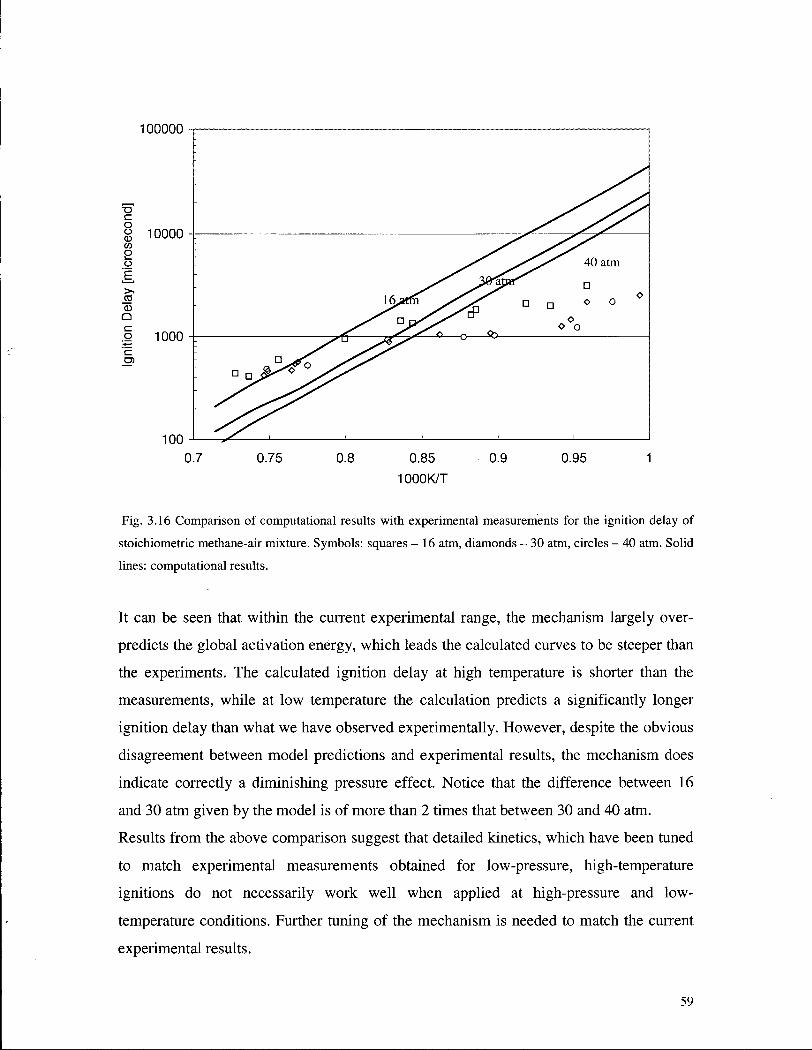
100000

1000K/T

Fig. 3.16 Comparison of computational results with experimental measurements for the ignition delay of

stoichiometric methane-air mixture. Symbols: squares - 16 atm, diamonds - 30 atm, circles - 40 atm. Solid

lines: computational results.

It can be seen that within the current experimental range, the mechanism largely over-

predicts the global activation energy, which leads the calculated curves to be steeper than

the experiments. The calculated ignition delay at high temperature is shorter than the

measurements, while at low temperature the calculation predicts a significantly longer

ignition delay than what we have observed experimentally. However, despite the obvious

disagreement between model predictions and experimental results, the mechanism does

indicate correctly a diminishing pressure effect. Notice that the difference between 16

and 30 atm given by the model is of more than 2 times that between 30 and 40 atm.

Results from the above comparison suggest that detailed kinetics, which have been tuned

to match experimental measurements obtained for low-pressure, high-temperature

ignitions do not necessarily work well when applied at high-pressure and low-

temperature conditions. Further tuning of the mechanism is needed to match the current

experimental results.

59

C H A P T E R IV

4.1 Introduction

A major problem associated with using natural gas as a fuel for compression ignition

engines comes from its very long ignition delay time at engine relevant conditions.

Different strategies involving injection with a pilot fuel, using a spark plug or glow plug,

etc., are being developed to address this problem. An alternative, and possibly preferable

approach for engine makers, is to blend natural gas with some other active gaseous fuel,

known as an ignition promoter, to shorten the ignition delay time. This would make it

possible to run a diesel-based engine on natural gas without making major modifications

to engine components.

Although promotion for natural gas/methane ignition has been a subject of study in the

field of combustion for some time, there are few publications revealing the behavior of

ignition promoter under diesel engine conditions, which requires high pressure (20-70

atm) and low temperature (900 - 1200 K). Clearly, the efficiency of an ignition promoter

will be significantly different under these conditions compared to that at low pressure and

high temperature as are found in many experiments. Furthermore, the way in which the

promoter and the fuel is introduced into the combustion chamber, i.e. homogenous charge

or direct injection, can also play an important role in the ignition progress, and

consequently, the ignition delay time. With direct injection ignition is a more complicated

process in which transport phenomena of two different fuels have to be taken into

consideration.

In the current study, we have carried out literature researches as well as conducted

experiments to investigate efficiencies of different promoters for a high-pressure low-

temperature methane-air reaction system. The objective is to find out possible candidates

for natural gas engine applications.

Meanwhile, gasdynamic features of ignitions with and without promotion have be

studied. The strong ignition limit, which is fuel dependent, has been explored for its close

relationship with engine knock problems.

60

4.2 Background

4.2.1 Mechanism of Ignition Promotion

Frenklach and Bornside [2] study the detailed chemical kinetics of methane ignition

based on their shock tube experimental results. They find that the oxidation of methane

during the induction period (ignition delay) proceeds through three distinct phases:

initiation, determined by decomposition and H-abstraction reaction of methane; oxidation

of methyl radicals by molecular oxygen; and oxidation of CH3 by HO2 radicals and, to a

less extent, O and O H radicals.

For methane-air reactions without promotion, the large energy required to break the C-H

bond in a methane molecule makes the initiation process slower than that of other

hydrocarbons. Also the high activation energy and highly endothermic nature of the

methyl-oxygen reaction makes this chain step quite slow.

In general, there are two major mechanisms in terms of shortening the reaction time. The

first one is the thermal promotion, which can be achieved by quickly oxidizing the

promoter to release energy to increase the mixture temperature. Since the reaction time is

a strong function of temperature, the higher the temperature the shorter the subsequent

reaction time. The second mechanism is through adding extra active species (radicals) at

the chain initiation and propagation stages to speed up the chain reaction. These species

are generated by fast promoter decomposition at the beginning of the reaction. The

second mechanism is found especially effective in a nonbranched system [24]. The

ignition delay time in such a system may be reduced by several orders of magnitude

through decomposition of the additive. However, it only weakly affects branched

systems.

For most ignition promoters, both of the mechanisms are involved simultaneously.

Zamansky and Borisov [24] use heat balance equation for the molecular reaction to show

that for a typical reaction system, purely thermal promotion can show its effectiveness

only when the concentration of the promoter is higher than 20-30% with respect to the

fuel, while it only takes 0.6% of the fuel concentration for a chain-initiation promoter to

show significant effects. As the conclusion of this estimation, they suggest the initial

radical concentration provided by the promoter to be 0.5-5% with respect to the total fuel

for a chain-thermal promotion and 20-30% for a pure thermal promotion.

61

4.2.2 Previous Work

Comprehensive studies of various ignition promoters for methane have been reported by

Zamansky and Borisov [24], as well as by Golovitchev and Chomiak [25]. Additives

discussed in their studies include hydrogen, high-order hydrocarbons, nitrocompound,

hydrogen peroxide, ozone, and dimethyl ether.

1) Hydrogen

a) Efficiency of Hydrogen in Homogeneous System

Chen and Oppenheim investigate the ignition delay time of methane-hydrogen-oxygen

mixtures diluted with argon using a reflected shock technique. The experimental

conditions cover temperatures from 800 to 2400 K and pressures from 1 to 3 atm. A

generalized Arrhenius type empirical equation is obtained by fitting experimental data

with a non-linear regression method for both methane and hydrogen. It is observed that

the global activation energy of the mixture is proportional to the ratio between

concentration of C H 4 and H 2 . Their proposed expression for ignition delay time of

methane-hydrogen mixtures is

T _ T d - e ) T e X - ~ C H t

T H 2 (4.1)

where e is the mole fraction of hydrogen in the total fuel. The correlation incorporates the

expression for both the ignition delay for methane, T C H 4 , and the ignition delay for

hydrogen, Xm, which come from their respective correlation equations with a general

formula

T = A[Juel]x[02Y exp(E/RT) ( 4 2 )

The empirical coefficients x, y, A, E are listed in table 4.1.

62

X y A E (kJ/mole)

C H 4 0.48 -1.94 1.19E"12 194.0

H 2 0.145 -0.56 1.54E"4 71.9

Table 4.1 Correlation coefficients for methane and hydrogen ignition delay by Oppenheim et al.

Here, T is the initial temperature in K and R is the universal gas constant in kJ/mol.

concentrations of reactants are in mol/cm , which can be calculated from the initial partial

pressure and temperature.

The ignition delay time calculated according to above equations for a premixed methane-

hydrogen-air reaction system is shown in figure 4.1.

1.00E+06 x

1.00E+01 J 1 1 1 1

0.5 0.6 0.7 0.8 0.9 1

1000K/T

Fig.4.1 Comparison of ignition delay time for stoichiometric methane-air mixture using Oppenheim's

equation with different hydrogen concentrations at 1 atm.

It can be seen that at 1 atm and 1000 K, with 15% methane replaced by hydrogen, the

ignition delay time predicted by equation (4.1) is 4 times lower than the promotion free

mixture, while it is less than 2 times lower when the temperature exceeds 1500 K.

Further reduction can be achieved with higher concentrations of hydrogen. With 35%

hydrogen added at 1000K the predicted ignition delay is reduced by nearly an order of

magnitude compared with that of pure methane.

63

b) Efficiency of Hydrogen in Diffusive System

The monotonic increase of promotion with increasing hydrogen concentration found in

Oppenheim's experiment is not observed in the study carried out by Fotache et al. [18].

They test the ignition temperature of hydrogen enriched methane by heated air using a

variable-pressure counter-flow facility. Unlike the shock tube experiment

aforementioned, Fotache's experiment is designed to study the non-premixed diffusive

system. Besides finding a substantial decrease of ignition temperature by adding H2 to the

jet flow of fuel composed of methane and nitrogen, they have also observed three distinct

regimes of promotion efficiency in terms of hydrogen concentration in the fuel.

• Hydrogen-assisted ignition regime, for hydrogen concentration below 6-7%, in which

the ignition of methane is facilitated by the hydrogen addition. But by replacing

methane with nitrogen on the fuel side makes the hydrogen fail to ignite.

• Transition regime (7 to 30% hydrogen concentrations). In this regime the reduction of

ignition temperature grows with increasing hydrogen concentration. Unlike in the

hydrogen-assisted regime, replacing methane with nitrogen reduces the ignition

temperature of hydrogen.

• Hydrogen-dominated regime, for hydrogen concentrations in excess of 30%, in which

the ignition temperature converges to nearly 934 K despite the further increase of

hydrogen proportion in the fuel.

An analysis of the system response curve reveals that in the first and second regimes, the

thermal feedback plays an important role in the ignition process while the third regime is

mainly dominated by the kinetics.

The residence time in their experiment is 10-100 ms, which is much longer than that of

shock tube experiments. Residence time in the latter is usually less than 10 ms. The

largest reduction brought about by hydrogen addition occurs when the hydrogen

concentration is under 15% of the total fuel. Above that, little further reduction can be

achieved even by increasing the hydrogen proportion over 35%.

The dominant ignition chemistry involved in the reactions is discussed in the same paper.

The difficulty of methane ignition is largely attributed to the competition between a

major chain branching reaction

64

C H 3 + H 0 2 => OH+CH3O (4.R1)

and the recombination step

C H 3 + C H 3 + (M) => C 2 H 6 (+M). ( 4 ' R 2 )

The direct result of this competition is that the chain branching efficiency is weak, and

the thermal feedback is required to speed up the forward reaction to achieve ignition.

However, the appearance of hydrogen in the system yields extra H radicals through the

reaction with O H radicals coming from fuel decomposition.

O H + H 2 => H + H 2 0 (4.R3)

This reaction is highly exothermic and the H radical generated is more active than the

C H 3 radical generated in the initiation stage of methane oxidation.

OH + C H 4 => C H 3 + H 2 0 (4.R4)

The oxidation process can be greatly facilitated by hydrogen addition for the above

reasons. However, it is obvious that the reaction (4.R3) must compete with reaction

(4.R4) for OH radicals. Moreover, the H radical may recombine with methane to form

methyl

H + CH4 => C H 3 + H 2 ( 4 R 5 )

Reactions (4.R4) and (4.R5) are the main reasons why significant inhibitive effect is

found by methane on hydrogen ignition in homogenous system where abundant C H 4 is

available to scavenge the H radicals. While in the diffusion system, as pointed out by

Fotache et al , the higher diffusivity of hydrogen might help to separate its stoichiometric

line from that of methane in the flow. In practice, using the counter flow facility, the

stoichiometric location of hydrogen air mixture moves slightly towards the oxidizer side

65

while that for methane is closer to the jet side. The separation yields a more dramatic

promotion effect due to the partial de-coupling of hydrogen oxidation from reactions with

methane. The role played by hydrogen is thus, partially, a pilot fuel in the diffusive

system.

The pressure effect on ignition delay time from 0.2 to 8 atm was also studied in the

Fotache's experiment. It is found that the ignition temperature decreases with the

increasing pressure, while the difference due to the variation of the hydrogen

concentration in the fuel become smaller at the same time.

c) Autoignition of Hydrogen at High Pressure

The existence of three explosion limits of hydrogen from classical hydrogen ignition

theory indicates the peculiar nature of its oxidation rate which, unlike most other fuels,

does not increase monotonically with temperature. The autoignition characteristics of

hydrogen at high pressure, are believed to relate directly to its behavior as an ignition

promoter in the current experiment.

Gordon et al. [31] in their early shock tube study find that for pressures above 2 atm, the

explosive mode of various hydrogen-oxygen-diluent systems can be found only when the

temperature behind the reflected shock wave reaches over 1100 K. A similar observation

is made by Voevodsky and Soloukhin [32], who report only weak ignition, or

deflagration, could be established when the temperature is lower than the observed

explosion limit.

Cain [26] investigates spontaneous ignition of hydrogen at pressures between 35 and 70

bars with a free piston compressor driven by compressed air. Hydrogen is mixed with

oxygen and diluted with helium in the driven section. A computer model incorporating a

hydrogen-oxygen reaction mechanism and gasdynamic features of compression process

has been compared with experimental result, and good agreement has been reported. It is

found that the spontaneous ignition (strong ignition according to his definition) happens

during compression at a temperature well above that at which the third limit is normally

placed. The measured and calculated temperature for this critical point is 1150 K and is

insensitive to pressure. His study of the mechanism shows that at high pressure, the long

induction periods of HO2 and H2O2 retard the ignition until the temperature exceeds 1150

66

K, after which the rate of breakdown of H2O2 into O H is sufficient to initiate explosion.

In terms of ignition delay time, their calculated values for stoichiometric H2-O2 mixtures

diluted by 30% helium at an initial temperature of 1100, 1200 and 1300 K are 770, 150,

and 38 ps respectively. It is noticeable that the value at HOOK is much larger than that

reported by Oppenheim whose experiment concentrates on low-pressures.

2) Higher-Order Paraffins

The effectiveness of higher-order paraffins such as ethane and propane on the ignition

delay of methane have been studied in order to understand the difference in ignition

characteristics between methane and natural gas.

Frenklach and Bornside conduct series of shock tube experiments on CH4-02-Ar

mixtures with propane added. They find that the addition of a relatively small amount of

propane is able to affect methane oxidation due to an increased amount of CH3 radicals

and H atoms brought about by propane decomposition. Specifically, within their

experimental range from 1300 to 1600 K, 20% propane additive (with respect to

methane) reduces the ignition delay by about a factor of 5, while the global activation

energy remains unchanged.

Lifshitz and coworkers have reported from their early work the "unexpected result" that

hydrogen is less efficient than propane in terms of promoting methane ignition. They

rationalize this "singular" result by making the following assumptions: 1. The two

ignition reactions (i.e.n that of the additive and that of methane) are completely

uncoupled. 2. The shortening of the induction time of methane is merely an outcome of

the heat released by the ignition of the additive. The heat of combustion of propane (488

kcal/mol) is almost 8.5 times that of hydrogen (58 kcal/mol). Therefore, propane releases

more heat and raises the reaction mixture to a higher temperature for the same volume

percent addition.

These assumptions may not be completely correct from the viewpoint of kinetics, but the

fact that heat addition plays an important role for promoters like hydrogen and propane

has been confirmed both experimentally and computationally [2].

67

3) Nitrocompounds

Nitrocompounds, such as NO x , C 3 H 7 O N 0 2 , C 2 H 5 N 0 2 , C H 3 O N 0 2 , are believed to be

among the most effective ignition promoters [24]. These compounds work by quick

decomposition via breaking of O-N bond or via fission of C2H5 radical to form H atoms

as well as N 0 2 or NO to enhance branching.

Dabora [24] use a reflected shock technique to measure the ignition of methane-air

mixture with 0.12% N 0 2 additive and achieve a 2-3 times shorter ignition delay.

However, the restrictive requirement of limiting N O x in engine emission clearly

discourages using any of these compounds in practical engine applications.

4) Dimethyl Ether (DME)

Dimethyl ether has been used as an ignition promoter for methanol-fueled diesel engine

by Karpuk et al. [25]. Its efficiency as a promoter for methane ignition has been explored

numerically by Golovitchev and Chomiak. It is found that the initial reaction of D M E at

the presence of oxygen evolved into generating high concentration of H 2 0 2 radicals,

which, together with formaldehyde, C H 2 0 , are effective branching intermediates. The

numerical simulation incorporating a detailed mechanism for methane and D M E

oxidation shows that by adding 5% D M E , the ignition delay time of methane-air mixture

at 40 atm can be reduced by about 5 times for a initial temperature at 1000K.

It should be pointed out that the vapor pressure of D M E is low (P s a t < 5 atm). When

mixed with methane, its partial pressure must be maintained lower than P s a t to prevent it

from condensing. For a pressurized bottle of methane whose initial pressure is about 100

atm, the D M E additive can not exceed 5% by volume.

Despite all aforementioned studies, we find an obvious lack of experiments on promoting

methane ignition under high-pressure and low-temperature conditions, which are engine

relevant. This motivated us to conduct experimental studies that can lead to results for

direct engine applications.

4.3 Results and Discussions

4.3.1 Efficiency of Ignition Promotion for Hydrogen

68

The ignition delay times for 15% and 35% hydrogen balanced by methane (with respect

to the total fuel) at 16 and 40 atm are shown in figures 4.2 and 4.3.

10000 -i 1

100 J ' ' ' ' ' 0.70 0.75 0.80 0.85 0.90 0.95 1.00

1000K/T

Fig. 4.2 Measured ignition delay time of methane with 0%, 15% and 35% hydrogen added at 16±2 atm

Symbols: Diamonds - hydrogen free, triangles - 85% C H 4 15% H 2 , squares - 65% C H 4 35% H 2 . All tests

are done for stoichiometric fuel-air mixture without dilution. Splines are used to indicate the trend of

change.

It is clear that the reduction of ignition delay time given by hydrogen additive is much

less dramatic than that predicted by equation (4.1). For an initial pressure of 16 atm and

initial temperature around 1050 K the measured ignition delay with 35% hydrogen

additive is only 3 times less than that of pure methane. The ratio reduces to about 2 when

the initial temperature rises to 1350 K. At this pressure, it is found that the reduction

achieved by adding 15% hydrogen is fairly close to that by 35% hydrogen addition. This

confirms the observation in Fotache's experiment that by adding extra hydrogen the

ignition temperature levels off as the system approaches a hydrogen-dominated regime.

It is observed that at low temperatures, the ignition delay time of methane with 15%

hydrogen additive deviates from that of 30% line and approaches that of pure methane.

69

10000

100 ' ' ' 1 ' 1 1 1 0.70 0.75 0.80 0.85 0.90 0.95 1.00 1.05

1000K/T

Fig. 4.3 Measured ignition delay time of methane with 0%, 15% and 35% hydrogen added at 40±2 atm a.

Symbols: Diamonds- hydrogen free, Triangles- 85% C H 4 15% H 2 , squares - 65% CH 4 35% H 2 . All tests

are done for stoichiometric fuel-air mixture without dilution. Splines are used to indicate the trend of

change.

When the pressure is raised to 40 atm, the trend of measured ignition delay of methane

without promotion is a reversed 'S' shape in the Arrhenius plot. From 1100 to 1200 K the

ignition delay time is mostly insensitive to the variation of temperature. Below this

temperature, it rises sharply. It is interesting to find that the trendline of the ignition

delay time of methane with 15% hydrogen merges with that of pure methane for most of

the temperatures range. The promotion effect of hydrogen does not appear until the

temperature drops below 1030 K, from where an increasing reduction effect starts to

show up. At the same time, prominent reduction can still be observed through the entire

experimental temperature range for 35% hydrogen added.

70

For a given induction time of 2 ms, adding 35% hydrogen at 16 atm brings the ignition

temperature down from 1080K to 1020 K , while at 40 atm the same amount of hydrogen

will lower the ignition temperature by nearly 75 K to 975 K . This is significantly less

than the over 200K reduction found in Fotache's experiment with the same amount of

hydrogen added. This is likely due to differences in the ignition mechanisms between

diffusive and homogenous ignition processes.

The obvious inefficiency of hydrogen in promoting methane ignition at high pressures

can be rationalized in light of the chemical kinetics described earlier in this section. The

abundance of CH4 in a high-pressure stoichiometric homogenous methane/air system

effectively impairs the formation of active H radical pools. Meanwhile, reaction (4.R2) as

a major chain termination step, can be greatly facilitated with the high concentration of

third bodies.

The noticeable increase of promotion efficiency with 35% hydrogen addition for

temperatures over 1150 K agrees well with the results of Cain [26]. The dramatic

increase of decomposition rate of HO2 and H2O2 above 1150 K triggers the explosive

mode with a significant ratio of thermal feedback that instantaneously promotes the

ignition of the system. The precondition for this mechanism to work is that the system

must have a high concentration of hydrogen initially, i.e., the system is in a hydrogen-

dominated regime. For lower hydrogen concentration, formation of HO2 and H2O2

radicals could be strongly influenced by the methane oxidation reactions, which possibly

accounts for the small reduction in ignition delay found with 15% hydrogen added to the

system.

Although the high pressure reduces the efficiency of hydrogen as an ignition promoter, it

also results in an overall reduction of ignition delay time of the methane/methane-

additive system as shown in figure 4.4.

The weakened promotion given by the additive is effectively compensated by the

increasing overall reaction rate due to the higher concentration of all reactants.

71

10000

•o tz

100 J ' 1 1 1 1 1 1

0.70 0.75 0.80 0.85 0.90 0.95 1.00 1.05

1000K/T

Fig. 4.4 Measured ignition delay time of methane at 16±2, 30±2 and 40±2 atm with 35% hydrogen added.

Symbols: diamonds - 16±2 atm, triangles - 30+2 atm, squares - 40±2 atm. All tests are done for

stoichiometric fuel-air mixture without dilution. Splines are used to indicate the trend of change.

4.3.2 Comparisons of Experimental and Computational Results

Numerical simulations incorporating detailed reaction mechanisms for both methane and

hydrogen oxidation have been carried out for comparisons to these experiments. The

CH 4-H 2-air kinetic mechanism is taken from GRI-Mech (version 3.0) [31]. That

generates 53 intermediate species and 318 reaction steps. Chemkin-II (version 1.6)

developed by Kee et. al. [32] of the Sandia National Laboratory is used as the mechanism

interpreter. The differential equations in the model are solved using LSODE (1987

version) [33]. The condition in the experimental zone of the shock tube is modeled to be

adiabatic and constant-volume. Gasdynamic effects induced by heat release and shock

wave boundary layer interaction are neglected here. The onset of ignition is defined to be

at the time when the maximum curvature on the P-t curve is found.

The calculated results are plotted in Figures 4.5 to 4.6 together with the experimental

measurements.

72

100000

10 I 1 1 1 1 1 '

0.7 0.75 0.8 0.85 0.9 0.95 1

1000K/T

Fig. 4.5 Comparison of computational results using detailed reaction mechanism and experimental

measurements for P=16 atm. Lines represent computational results. Symbols represent experimental

measurements: diamonds H 2 free, triangles - 85% CH415% H 2 , squares - 65% C H 4 35% H 2 .

It can be seen that within the whole experimental range, the current mechanism largely

over-predicts the global activation energies, which leads the calculated curves to be

steeper than those of measured in the Arrhenius plots. The calculations intersect with the

measurements at medium temperatures from HOOK to 1200 K. It under-predicts the

ignition delay at high temperature by 4 times but over-predict it at low temperature by

almost an order of magnitude. Moreover, the change of ignition delay time yielded by the

mechanism in Arrhenius plot is nearly a straight line rather than a reversed S curve as

shown by the experiments. Although there is an obvious disagreement between the

computational and the experimental results, it is interesting to find that the mechanism

shows a separation of reduced ignition delay time between 15% and 35% hydrogen

addition for temperatures higher than HOOK, which is also observed in the experiments

(more obvious at higher pressure).

73

100000

1.05

1000K/T

Fig. 4.6 Comparison of computational results using detailed reaction mechanism and experimental

measurements for P=40 atm. Lines represent computational results. Symbols represent experimental

measurements: diamonds H 2 free, triangles - 85% CH 4 15% H 2 , squares - 65% CH 4 35% H 2 .

4.3.3 Efficiency of Ignition Promotion for D M E

Shown in figures 4.7 and 4.8 are measured ignition delay time with 5% D M E added at 16

and 30 atm respectively.

The results are rather disappointing when compared with Golovitchev's numerical model,

which predicts a strong reduction for methane ignition delay by adding 5% D M E for

temperatures below 1200K. For the current experiments, D M E shows only moderate

effects on reducing the ignition delay of methane at high and low temperatures, and even

a modestly inhibitive effect at around 1100 K . Further studies are considered necessary

for the mechanism to involve D M E and methane oxidations at high pressure.

74

10000

100 J 1 1 1 1 1 1 1 1

0.70 0.75 0.80 0.85 0.90 0.95 1.00 1.05 1.10

1000K/T

Fig. 4.7 Measured ignition delay of methane with 5% DME added at P=16±2 atm. Symbols: diamonds -

DME free, squares - 5% DME 95% C H 4 All tests are done for stoichiometric fuel-air mixture without

dilution. Splines are used to indicate the trend of change.

10000 . 1

"D

100 1 1 1 1 1 1 1

0.70 0.75 0.80 0.85 0.90 0.95 1.00

1000K/T

Fig. 4.8 Measured ignition delay of methane with 5% DME added at P=30±2 atm. Symbols: diamonds -

DME free, squares - 5% DME 95% C H 4 All tests are done for stoichiometric fuel-air mixture without

dilution. Splines are used to indicate the trend of change.

75

4.3.4 Strong Ignition Limit of Methane with Additives

Three distinctive ignition patterns for methane and methane-additives (i.e., mild ignition,

transition from mild to strong ignition and strong ignition) are observed in the current

study as shown in figure 4.9.

T= 1364 K

Fig. 4.9 Pressure histories of methane and methane-hydrogen ignition processes showing 3 distinctive

ignition patterns (P = 16 ± 2 atm): a. mild ignition with unique pressure peak; b. transition from mild to

strong ignition; c. strong ignition causing sharp pressure rise and violate oscillation.

Additional hydrogen is found not only to shorten the ignition delay time of methane, but

also to promote the entire combustion process. The peak pressure for methane -

hydrogen mixture ignition is noticeably higher than that for pure methane ignition due to

the faster reaction speed.

The changes of strong ignition limit by ignition promoters have been measured and

shown in figure 4.10. It is found that an addition of 15% or 35% hydrogen to methane

significantly reduces the strong ignition limit. Also, the pressure dependence of the strong

ignition limit becomes more prominent for higher hydrogen fractions in the fuel. By

increasing the pressure from 15 atm to 40 atm, we lower the strong ignition limit by

nearly 200 K with 35% hydrogen added to methane. With the same pressure increase, the

change of strong ignition limit for 15% hydrogen addition is just slightly over 100 K.

76

Meanwhile, 5% D M E causes virtually no change to the strong ignition l imit of pure

methane at both high and low pressures.

Fig. 4.10 Strong ignition limit for methane with different hydrogen concentrations for pressures from 16 to

40 atm. Symbols represent experimental measurements. Solid line - strong ignition limit for methane with

35% and 15% hydrogen additions. Dashed line - measured strong ignition limit for pure methane and

methane with 5% DME.

However, upon comparison with other conventional fuels whose strong ignition limits are

usually less than 1000 K, we find that methane, even enriched with hydrogen, has the

highest strong ignition l imit, making it a safe and stable fuel for IC engines, and indicates

the potential for increased thermal efficiency by rising IC engine compression ratios.

77

C H A P T E R V

5.1 Conclusions

5.1.1 Shock Tube and Modeling

1) A one-dimensional model using non-constant specific heat for the shock tube

calculation has been built up and modified according to experimental results.

2) Comparisons between model predictions and experimental measurements have been

carried out. The model has shown good agreement with the experimental results.

3) The uncertainty of the experimental temperature has been investigated. It is found

that the uncertainty for calculated temperature is 5 to 7 K by using measured incident

shock velocity and 9 to 13 K by using both measured incident and measured reflected

shock velocities.

4) Disturbing effects for the constant experimental conditions resulting from the

reflected shock/boundary layer interaction and the contact surface instability have

been investigated numerically. The boundary layer cooling flow is found to shorten

the experimental time for an incident shock velocity higher than 1020 m/s. The

contact surface instability is found to have no significant effect on the current system.

5.1.2 Ignition Delay of Methane under Engine-Relevant Conditions

1) Previous studies on methane ignition delay have been reviewed. The empirical

equations derived in early experiments are found not suitable for use outside their

respective experimental ranges.

2) High-pressure shock tube experiments on methane-air ignition have been carried out

for temperatures from 1000 to HOOK and pressures from 16 to 40 atm with different

equivalence ratios. Significant differences have been found between the current study

and previous work due to the difference in experimental conditions.

78

3) A modified Arrhenius-type empirical equation for the measured ignition delay of

methane has been derived assuming a non-constant global activation energy and

variable pressure effects.

4) The effects on ignition delay of pressure, temperature, and concentrations of reactants

are discussed based on the experimental measurements. The ignition delay of

methane has been found to increase strongly with temperature and to decrease with

pressure.

5) The strong ignition limit of methane-air mixture has been measured. It has been found

to decrease with increasing pressure.

6) A computer model incorporating detailed reaction mechanism to simulate the ignition

process in the shock tube has been compared to the current experiments.

Disagreements have been found. Further tuning of the mechanism is suggested in

order to match the experimental results.

5.1.3 Ignition Promotion for Methane under Engine-Relevant Conditions

1) A literature review on methane ignition promotion has been carried out. Mechanisms

involving different promoters in various reaction systems have been discussed.

2) The efficiency of hydrogen at promoting methane autoignition for pressures from 16

to 40 atm has been investigated with a reflected shock technique. Hydrogen

concentrations are selected at 15% and 35% with respect to the total fuel. It is found

that at high pressure, the efficiency of hydrogen as an ignition promoter is much

lower than that reported by previous work at low pressure.

3) Disagreement between the model prediction using the latest elementary chemical

kinetic mechanism for methane-hydrogen-air reaction and experimental results has

been found. The model largely over-predicts the global activation energy for the

experimental conditions.

79

4) Efficiency of 5% D M E in promoting methane ignition has been investigated in the

current shock tube experiment. D M E has been found to have a limited effect in

promoting methane ignition within the experimental range.

5) Gasdynamic features associated with strong and mild ignition for different methane-

additive ignition processes have been examined. Hydrogen addition has been found to

lower the strong ignition limit of methane, while 5 % D M E addition makes no change

to the limit.

5.2 Problems with Current Experimental Apparatus and Shock Tube Upgrades

At low temperatures, an autoignition in the experimental region of the shock tube results

in a deflagration and all the mixture is consumed slowly by a propagating flame front

without generating a strong pressure rise. The detection of such a mild ignition by

pressure transducers is sometimes difficult especially when it comes to determining the

onset of the ignition process.

On the other hand, light emission associated with an ignition can be detected readily even

if the ignition is a very weak one. The current experimental range can be extended by

adding light detecting devices to the shock tube to help in observing low temperature

ignitions. Also, the results achieved from the optical access can be used as an

independent verification of the ignition delay time measured currently by using only

pressure signals.

As a part of the future plan, with the help of more sophisticated optical devices, we hope

to observe the combustion process directly in the shock tube. It will greatly facilitate our

study of natural gas direct injection as well as many other combustion systems.

Lower temperature also means longer ignition delay time. Besides maximizing the

experimental time by obtaining tailored interface, we can also extend it by increasing the

length of the shock tube. Optimization is needed to find the best proportion between the

driver and the driven section for a given total length of the shock tube.

80

5.2.1 Design of Shock Tube Optical Access

The working principle of the optical access being designed currently is shown in figure

5.1.

The optical access includes a quartz window, which can be mounted on a through hole on

the shock tube to allow light emissions to be transmitted and also to withstand the highest

pressure and temperature in the shock tube during ignition tests. The signal is picked up

by an optical fiber mounted right behind the quartz window and conducted to a

photomultiplier. The function of the photomultiplier is to amplify the received light

signals and to convert them into standard electric signals with corresponding

characteristic frequencies. A bandwidth filter is then used to filter out signals of

unwanted frequencies and leave only those in which we are interested. Finally the signal

is transferred into the data acquisition system and stored in a computer.

Ignition inside the shock tube

V

hock tube wall

Quartz window

Optical fiber 3-

Bandwidth filter .

Photo A , multiplier W

V

Data acquisition system

o o o

Fig.5.1 Schematic of the shock tube optical access system

As a part of the optical access, the quartz window is to be designed in such a way that it

can be easily fitted in and/or removed from the existing pressure taps on the driven

section of the shock tube. No significant variation of the present configuration of the

shock tube is necessary. The window should have a good transmittance value so that

81

interesting bandwidths can be readily detected by the optical instrument installed behind

it.

First we need to calculate the maximum pressure in the driven section in order to decide

the thickness of the quartz window. For a high-temperature ignition the process goes so

fast that a detonation occurs, which ignites all the mixture at the end of the driven section

almost simultaneously. In such a case, the driven has little time to expand because of the

extremely fast rate of combustion. The process can be modeled as an adiabatic constant-

volume combustion problem. The maximum pressure is calculated from the adiabatic

flame temperature and the known initial pressure and temperature using the ideal gas law.

The adiabatic flame temperature of the mixture can be calculated by the conservation of

energy. A general equation for the combustion of C H 4 in air/oxygen can be written as

CH4 + ax02 + a2N2 -»bC0 2 + cH20 + dCO + e02 +fH2+ gN2 + hNO + qCH4. (5.1)

For this equation, we assume the initial mole number for methane is 1. Three dissociation

reactions, which happen simultaneously, are

2C02^2CO + 02 (5-2>

2H20 <=> 2H2 + 02

N2+02d 2NO.

(5.3)

(5.4)

Eqs (5.2) - (5.4) have their own equilibrium constants, which are functions of the

reaction temperature and pressure, determining the final composition of the products. A

computer model has been built to solve Eqs. (5.2)-(5.4) simultaneously and to iterate with

temperature T to satisfy the energy conservation based on Eq (5.1) (See appendix E for

details).

The condition in the experimental region is modeled as constant volume so that the ideal

gas law simplifies to:

82

The maximum initial pressure P5 is set to be 95 atm. The initial temperature T5 is decided

by the maximum experimental temperature reached so far, which is about 1500 K. The

adiabatic flame temperature is found to be from 3072 K (with 3 dissociation reactions) to

3324 K (complete reaction) under these initial conditions. (In a real shock tube

experiment, the short residence time prevents the system from reaching complete

equilibrium, so that the real temperature should lies between the equilibrium temperature

and the complete reaction temperature.). The calculated maximum pressure using Eq.

(5.5) is 210 atm at the end of the driven section.

The thickness of the quartz window is obtained by an empirical equation designed

specifically for calculating the rupture pressure of a quartz plate. For a plate with a

clamped edge, the equation is

P = 2.28Sm a x4> (5.6)

where S m a x is the maximum tensile stress, (with a safety factor of 10, this value is

approximately 4.8xl06 Pa); 'r 0' is the unsupported disc radius which is determined by the

radius of the pressure tap (3 mm), and t is the disc thickness. Substituting the maximum

pressure from the above calculation we get a minimum window thickness of 4.19 mm.

Considering the load is a shock rather than a steady one, we apply an extra safety factor

of 2 on the base of 4.19 mm, which makes the final window thickness 8.38 mm.

From the average transmittance curve for fused quartz we found that a quartz window is

very effective in transmitting light in the visible as well as parts of the infrared ranges.

For a 10 mm thick window, the transmittance is nearly 90% for wavelengths from 270

nm to 2.5um. This is ideal to detect C H and O H emissions whose wave lengths are 432

nm and 307 nm respectively. But the transmittance drops quickly outside this range. This

83

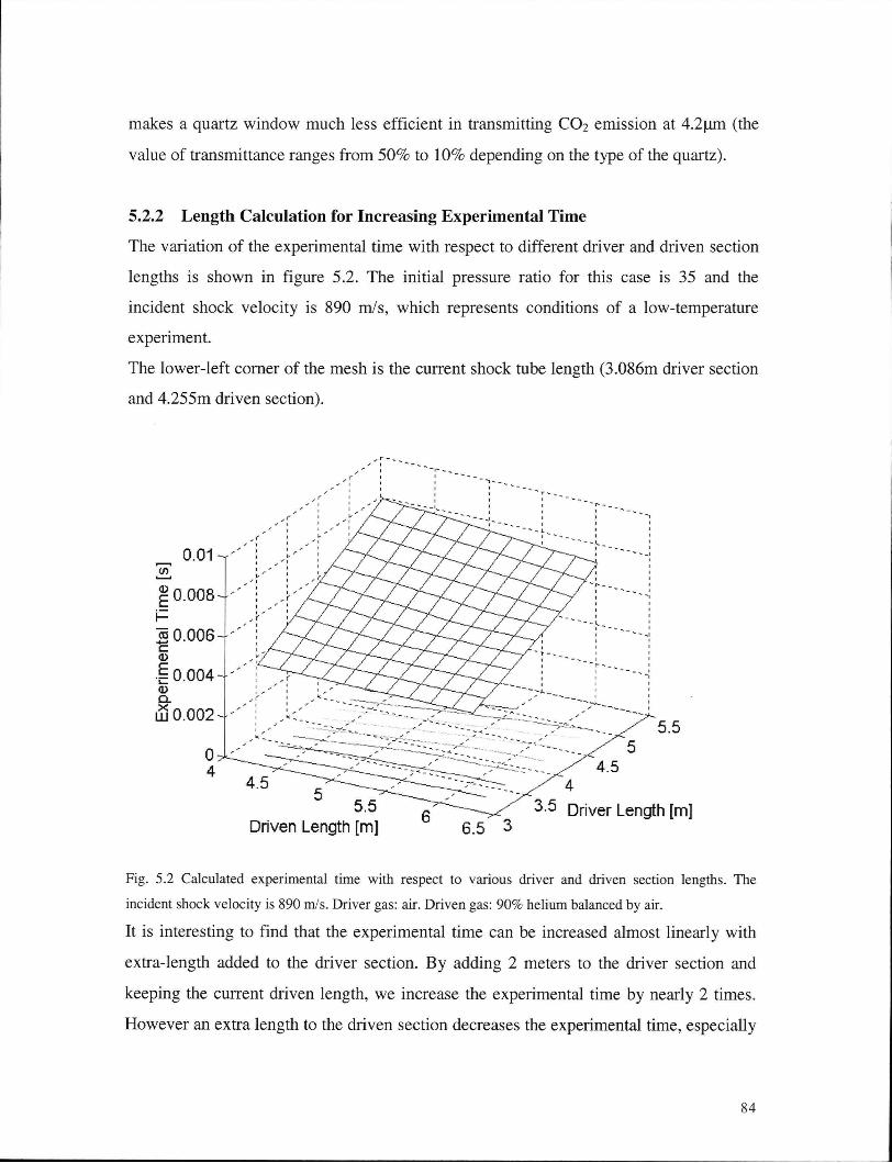
makes a quartz window much less efficient in transmitting C 0 2 emission at 4.2um (the

value of transmittance ranges from 50% to 10% depending on the type of the quartz).

5.2.2 Length Calculation for Increasing Experimental Time

The variation of the experimental time with respect to different driver and driven section

lengths is shown in figure 5.2. The initial pressure ratio for this case is 35 and the

incident shock velocity is 890 m/s, which represents conditions of a low-temperature

experiment.

The lower-left corner of the mesh is the current shock tube length (3.086m driver section

and 4.255m driven section).

Fig. 5.2 Calculated experimental time with respect to various driver and driven section lengths. The

incident shock velocity is 890 m/s. Driver gas: air. Driven gas: 90% helium balanced by air.

It is interesting to find that the experimental time can be increased almost linearly with

extra-length added to the driver section. By adding 2 meters to the driver section and

keeping the current driven length, we increase the experimental time by nearly 2 times.

However an extra length to the driven section decreases the experimental time, especially

84

when the driver section is long. It is understandable that for a long driven section the

incident shock wave takes a longer time to travel to the end wall, while the average

velocity of the reflected rarefaction fan is higher than that of the incident shock wave so

that the absolute time from the shock reflection to the arrival of the rarefaction fan

becomes shorter. For an extreme case of a very short driven section and a very long

driver section, the reflected rarefaction fan may catch up with the incident shock wave

before it reflects so that the experimental time drops to 0. Trie same trend is also observed

for higher initial incident shock velocities within the current experimental range.

However, a long driven section does help to increase the distance between the end wall

and the reflected-shock-stopped contact surface so that disturbances such as boundary

layer cooling flow take longer to start affecting the end wall area. When choosing a new

length for the shock tube, comprehensive considerations are necessary to reach an

optimal solution for different experimental ranges.

5.3 Recommended Future Work

1) Complete the design and installation of the shock tube optical access to be used in

future experiments.

2) Use the shock tube to study the combustion process with natural gas direct injection

or HPDI systems.

3) Further test the ignition promotion of premixed and non-premixed natural gas by

using different additives.

4) Design a more sophisticated optical access and install image capture devices on the

shock tube for a deeper study of various combustion phenomena.

5) Redesign major shock tube components (change the slot design of the diaphragm and

change the driver and driven section lengths) to improve the repeatability and

accuracy of experimental measurements as well as to broaden the experimental range.

85

R E F E R E N C E S

1. Cheng, R. K., Oppenheim, A. K., "Autoignition in Methane-Hydrogen Mixtures,"

Combustion and Flame, Vol. 58, No. 2, pp. 125-139, November 1984.

2. Frenklach, M . , Bornside, D., "Shock-Ignition in Methane-Propane Mixture,"

Combustion and Flame, 56:1-27, 1984.

3. Lifshitz, A., Scheller, K., Burcat, A., Skinner, G.B., "Kinetics of Methane

Oxidation," Journal of Chemical Physics, Vol. 56, pp. 3853.

4. Lifshitz. A., Scheller, K., Brecat, A., "Shock-Tube Investigation of Ignition in

Methane-Oxygen-Argon Mixtures," Combustion and Flame, Vol. 16, 311-321, 1971.

5. Reid, A., "Development of an Apparatus for the Study of Ignition Delay for Gaseous

Fuels", MASc Thesis, UBC, Chapter 3, 2001.

6. Davies, L. , "The Interaction of the Reflected Shock with the Boundary Layer in A

Shock Tube and its Influence on the Duration of Hot Flow in the Reflected-Shock

Tunel," A.R.Cpaper, No. 880-881, 1967.

7. Lapworth, K. C , "Temperature Measurements in a Hypersonic Shock Tunnel," pp.

255-269, Pergamon Press, 1964.

8. Lapworth, K. C , Townsend, J. E . G., "Temperature and Pressure Study in the

Reservoir of a Reflected-Shock Hypersonic Tunnel," A..R.C. paper 26110, 1964.

9. Mark, H., "The Interaction of a Reflected Shock Wave with the Boundary Layer in a

Shock Tube", NACA paper, T M 1418, 1958.

10. Xu, L . G., Gourlay, C. M . , Stalker, R. J., "Reduction of Driver Gas Contamination in

a Reflected Shock Tube by Boundary Layer Suction," 16th International Symposium

on Shock Tubes and Waves, pp. 637-643, 1987.

11. Holder, D. W., Stuart, C. M. , North, R. J., "The Interaction of a Reflected Shock with

the Contact Surface and Boundary Layer in a Shock Tube," A.R.C. paper22 891,

1961.

12. Takano, Y. , "Simulation for Effects of Side-Wall Boundary-Layer on Reflected-Sock

Flowfields in Shock Tubes," 16th International Symposium on Shock Tubes and

Waves, pp. 645-651, 1987.

86

13. Pulliam, T. H. , Chaussee, D. S., "A Diagonal Form of an Implicit Approximate-

Factorization Algorithm," Computational Physics, Vol. 39, pp. 347-363, 1981.

14. Bird, K. D., Martin, J. F., Bell, T. J., "Recent Development in the Use of the

Hypersonic Shock Tunnel as a Research and Development Facility," Third

Hypervelocity Techniques Symposium, 1964.

15. Taylor, G. I., "The Instability of Liquid Surface When Accelerated in a Direction

Perpendicular to Their Planes 1. Proc. Roy. Soc, A 201, 1950.

16. Markstein, G. H., "Flow Disturbance Induced Near a Slightly Wavy Contact Surface

or Flame Front Traversed by a Shock Wave," J. Aeronaut Sci., Vol. 24, pp. 238-239,

1957.

17. Seery, D. J. , Bowman, C. T., "An Experimental and Analytical Study of Methane

Oxidation Behind Shock Waves," Combustion and Flame, Vol. 14, pp. 37-47 1970.

18. Fotache, C. G., Dreutz, T, G., Law, C. K., "Ignition of Hydrogen-Enriched Methane

by Heated Air", Combustion and Flame, 110:429-440, 1997.

19. Karim, G. A., Zhou, G., "An Analytical Examination of Various Criteria for Defining

Autoignition Within Heated Methane-Air Homogenous Mixture," Journal of Energy

Resource Technology, Vol. 114, 175-189, 1994.

20. Cowell, L . H., Lefebvre, A, H., "Influence of Pressure on Autoignition

Characteristics of Gaseous Hydrocarbon-Air Mixtures," SAE paper 860068, 1987.

21. Fieweger, K., Blumenthal, R., Adomeit, G., "Self-Ignition of S.I Engine Model Fuels:

A shock Tube Investigation at High Pressure," Combustion and Flame 109: 599-619,

1997.

22. Fieweger, K., Blumenthal, R., Adomeit, G., "Shock-Tube Investigation on The Self-

ignition of Hydrocarbon-Air Mixture at High Pressures," 25th Symposium

[International] on Combustion, The Combustion Institute, pp. 1579-1585, 1994.

23. Spadaccini, L. J. , Colket III, M . B., "Ignition Delay Characteristics of Methane

Fuels," Prog Energy Combust Sci. Vol.20, pp. 431-460, 1994.

24. Zamansky, V. M . , Borisov, A. A., " Promotion of High-Temperature Self-Ignition",

Prog Period Energy Combustion Science Vol. 18 pp. 297-325, 1992.

25. Golovitchev, V. I., Chomiak, J . , "Evaluation of Ignition Improvers for Methane

Autoignition", Combust. Sci. and Tech., Vol. 135, pp. 31-47, 1998.

87

26. Cain, T. M . , "Autoignition of Hydrogen at High Pressure," Combustion and Flame,

Vol. I l l , pp. 124-132, 1997.

27. Van Wylen, G. J., Sonntag, R. E. , "Fundamentals of Classical Thermodynamics",

Second Edition, John Wiley & Sons, 1978.

28. Naber, J. D., Siebers, D. L. , Caton, J. A., Westbrook, C. K., Julio, S. S. D., "Natural

Gas Autoignition Under Diesel Conditions: Experiments and Chemical Kinetic

Modeling", SAE Paper 942034, 1994.

29. Glassman, I., "Combustion", Second Edition, pp. 81-84, 1987.

30. Hurle, I. R., Gaydon, A. G., "The Shock Tube in High-Temperature Chemical

Physics", 1963.

31. Kee, R. J., Rupley, F, M . , Miller, J. A., "Chemkin-II: A Fortran Chemical Kinetics

Package for the Analysis of Gas-Phase Chemical Kinetics", Sandia Report SAND89-

8009.UC-401, 1989.

32. Smith, G. P., Golden, D. M . , Frenklach, M . , Moriarty, N. W., Eiteneer, B.,

Goldenberg, M. , Bowman, C. T., Hanson, R. K., Song, S. S., Gardiner, W. C ,

Lissianski, V. V., Qin, Z., "GRI-MECH 3.0," http://www.me.berkeley.edu/gri_mech/.

33. Hindmarsh, A. C , " ODEPACK, A Summarized Collection of ODE Solvers,"

Scientific Computing, pp. 55-64, 1983.

34. Higgin, R. M . R., Williams, A., "A Shock-Tube Investigation of the Ignition of Lean

Methane and n-Butane Mixtures with Oxygen", 12th Symposium of Combustion,

1968.

35. Arad, E. , Wolfshtein, M . , "Gradient Boundary Conditions for Turbulent Flows,"

International Symposium on Computational Fluid Dynamics, pp. 205-213, 1987.

36. Gordon, W. E. , Mooradian, A. J., Harper, S. A. , Seventh Symposium on Combustion,

pp. 297-283, 1965.

37. Voevodsky, V. V., Soloukhin, R. I., Thirteenth Symposium (International) on

Combustion, The Combustion Institute, pp. 1153, 1970.

88

Appendix A

Method of Characteristics

A .1 Characteristics of Isentropic Wave

Equation (2.23) tells us that for any isentropic wave, the value of A is constant. It does not

vary in time or space with the movement of the wave provided that isentropic conditions

are satisfied. In the shock tube experiment, isentropic expansion waves may travel in the

same or opposite directions as that of the fluid. We'll treat these two situations separately.

A.1.1 Right Moving Wave

We define the positive flow direction being from left to right. A right moving wave

travels in the same direction of the fluid. For a flow velocity U and local sound speed a,

the absolute velocity of the wave is U+a. The wave causes a small disturbance of fluid

properties behind it as shown in figure A. 1.

U + A ^ T T

-a-dU

U-dU P-dP p-dp

(a)

U P

P

P-dP p-dp

P

P

(b)

Fig. A .l Right moving isentropic wave: (a) laboratory-fixed coordinates (b) wave-fixed coordinates

First we transfer from absolute coordinates to wave fixed coordinates. Using the same

approach solving the continuity and momentum equations as we have done before, we

find that for the right moving wave, the characteristic value A, is as follows:

7 - 1 X = a-\ U - const. (A.1)

We therefore call the right moving wave a A. wave and the velocity of such a wave in the

absolute coordinates is

89

'dx}

\ d t A = U + a.

(A.2)

A.1.2 Left Moving Wave

a-U

U P

P (a)

U+dU P+dP p+dp

a P P

(b)

a+dU

P+dP p+dp

Fig. A.2 Left moving isentropic wave, (a) laboratory-fixed coordinates (b) wave-fixed coordinates

We can deal with a left moving wave using a similar method. For this wave, we find its

characteristic value, which we call it P, is given by

(A.3)

and the absolute wave velocity is

Kdt , = U-a. (A.4)

We call this left-moving wave a P wave.

A.2 Description of Rarefaction Fan with X and p.

90

For any isentropic wave, the value of A, or P remains the same as it propagates

undisturbed along the flow field. The rarefaction fan being composed of a series of such

expansion waves can be readily described by these elemental waves. Since any point in

the rarefaction fan, such as its leading edge, has its unique characteristic value that does

not change in time, we can locate such a point at any moment, by finding where in the

flow field this characteristic value exists.

We first describe the velocity field of the fluid in terms of A and p. With equation (A.l)

and (A.3), it is easy to show

U= — £ (A.5) 7 - 1

and

a •• (A.6)

Substituting Eqs. (A.5), (A.6) into Eqs. (A.2) and (A.4), we rewrite the absolute

propagation speed of the wave as

— = BX-A$ (A-7)

U A =AX-B$ ( A . 8 ) V

d t ft

where A=(3-Y)/2(y-l) and B=(Y+1)/2(Y-1).

A.3 Numerical Scheme

We now discuss the transport of wave characteristics in a one-dimensional mesh space

with respect to time.

A.3.1 Subsonic Flow

91

For a subsonic flow, the local sound velocity is higher than the flow velocity. For a flow

traveling from left to right, the X wave should propagate down-stream to the left and the i

P wave should move upstream to the right as shown in figures A.3 and A.4 respectively.

For a certain node point i at time t, we need to find out the value of X and P in the next

time step, so that all other properties, such as flow velocity, can be calculated. A linear

interpolation method, which has the first-order accuracy in both time and space, has been

used here.

1 n+1 -v n+1 A.i-1 / ^ Ai f

M • "\ r

t+At

Ai-ln / X?

r

t

l- l Ax ^ U * J i i+1

Fig. A.3 Time-space mesh for a subsonic X wave

At certain time t, the characteristic X at node points i and i-1 are denoted by Xi and Xi-i

respectively. After a small time step At, these two X waves move downstream to new

locations, which are given by

^=xi_l+Vi_lAt (A-9)

and

' = xt +Vi Ar. (A. 10) ..n+1

Here V is the absolute velocity of the X wave; n denotes nth time step and i denotes ith

node point. We can find the new value of Xi at t+At by interpolating between these two

points.

X^ =X1 ^ - T W - X 1 ! , ) ( A - n )

' ' n+1 _ n+I. v ' 1 - 1 ' Xi Xi-l

92

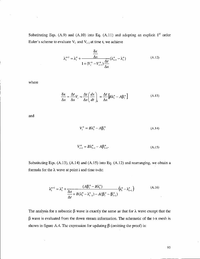
Substituting Eqs. (A.9) and (A.10) into Eq. (A. l l ) and adopting an explicit 1st order

Euler's scheme to evaluate V; and Vj_i at time t, we achieve

Xf = xt+-

8x

Ax

i+fyr-v,:,) Ar Ax

( A . 1 2 )

where

bx _ At y _ At

Ax Ax ' Ax

At_

Ax [BX:-A^] (AI3>

and

Vi" = BX1 - A P ; ( A . 1 4 )

VrLX=BXU-A$lv ( A . 1 5 )

Substituting Eqs. (A. 13), (A. 14) and (A.15) into Eq. (A.12) and rearranging, we obtain a

formula for the X wave at point i and time t+At:

X"+L =X"+ — Ax

(AW-BXD ( A . 1 6 )

_ + B ( V - A ; _ I ) - A O ; - P - 1 ) At

The analysis for a subsonic p wave is exactly the same as that for X wave except that the

P wave is evaluated from the down stream information. The schematic of the t-x mesh is

shown in figure A.4. The expression for updating P (omitting the proof) is:

9 3

pr1 - P,"+ Ax

At + B ( P - 1 - P I - ) - A ( A ; + 1 - A , - )

•fe"+,-Pi") (A.17)

A.3.2 Supersonic Flow

If a supersonic flow moves from left to right, for a A. wave the solution is exactly the

same as that for the subsonic flow. However, for a P wave the situation is sonewhat

different. Because the flow speed is higher than the local sound speed, no information can

travel upstream from the right. We can only evaluate P from left of the node.

Pi-i" P i n + 1 Pi" t+At

Flow | — ^ direction

Pi- iV

J K

P" ( t

y i - l Ax U

8x ^ • *J

i i+1

Fig. A.5 Time-space mesh for a p wave in a supersonic flow from left to right

94

The wave move from left to right with a velocity (dx/dt)p=U-a. Interpolation at point i

and time t+At yields

IT 1 = Pi" + (BW-AX1)

Ax

At •fl(Pl"-Pl"_1) + A(V-A,"_1)

•(P;-P«"-I) (A. 18)

On the other hand, if the supersonic flow moves from right to left as that shown in figure

A.6, we have to rewrite the expression for the A, wave.

AT 1 = A" + ( A p Y - Z ^ )

Ax

At • 5 ( A ; + 1 - A r ) + A ( p ; + 1 - p ; " )

-fa*-*;) (A.19)

A- i n + 1 . — i*\

A i n + 1

•N r *\ (~\ Aui1 1

t+At

^—1 Flow t direction

i-1 Ax ^ ^ fcJ

i i+1

Fig. A.6 Time-space mesh for a X wave in a supersonic flow from right to left

In summary, when the absolute wave velocity is positive, we evaluate the next time step

with information coming from upstream; when the absolute wave velocity is negative, we

use downstream information to predict the characteristic value at the next time step.

With an explicit scheme, the C F L number, which is defined as UAt/Ax should always be

less than one in order to achieve computational stability. Here, U is the velocity of the

fluid or wave, At is the time duration in one time step, and Ax is the length between two

consecutive nodes. This means the displacement of the fluid or wave in one time step can

not exceed the size of a unit mesh. In our case, the maximum velocity occurs for a wave

traveling in the flow direction. We can calculate the corresponding maximum time for

each time step, which is given by

95

(A.20)

A.4 Boundary Conditions

We apply the method of characteristics for driver gas expansion from the contact surface

to the end of the driver section. The contact surface is moving at a constant velocity U3,

which can be calculated by the method introduced in 2.4.1. At the contact surface we can

calculate the value for A. and P as our right boundary condition (assuming the shock wave

is traveling from left to right), with

. _ _1Z1TT A c ~ f l 3 0 2 ( A - 2 1 )

and

where a3 denotes the local sound speed for the driver gas at the contact surface. The

specific heat ratio 7 for the driver gas is assumed constant. The location of the contact

surface at any given time is calculated by

XC = U3t. (A.23)

At the end of the driver section, a wall condition applies. The velocity drops to zero so

that

^wall - ft wall (A.24)

where P can be evaluated from Eq. (A. 18) as we do for any other node point.

The initial condition for the rest of the gas inside the driver section can be obtained from

a=a4 and U=0. That gives

96

Ki = Pfo, = aA (A.25)

One extra initial condition we consider is choked flow at the exit of the driver section

when the down stream flow is supersonic. According to nozzle flow theory, when the

flow reaches the local sound velocity no further acceleration can be achieved unless we

expand the flow area downstream of the choking point. We may or may not have choking

when the diaphragm bursts depending on whether the flow is locally supersonic or

subsonic. If the flow velocity U3 is subsonic, free expansion is allowed from P 4 to P3.

However, if U3 is supersonic, we need to set the initial velocity at the exit of the driver

section so that

U'=a, .(A.26)

where the asterisk denotes the diaphragm location. The initial condition tells us

P o ~ a 4 ' (A.27)

where 0 denotes the location of the right boundary. According to Eq. (A.3), we solve for

* TT*

a =U =

f 2 A (A.28)

Finally, we write the formula for A, and P at the choking point as

• y — 1 * 1 Xn=U a = a, (A.29)

0 2 Y + l 4

and

D TT*^V-1 * (A-3°) Po = U +—^a =a4

97

Appendix B

Uncertainty of Calculated Experimental Temperature

B . l General Formula

The general formula of the uncertainty for a calculated value R, for which R = f(xi, x2, . . .

x„), is

2 2 VV. + . . .

J 1 I3*- J (B.l)

where wi.. .wn are the respective uncertainties of independent variables xi.. .xn.

B.2 Uncertainties for Measured Shock Velocities

The shock velocity is calculated from

Here U is the velocity in m/s; X is the distance between first and last sensor in meters; t is

the time duration for the shock wave to travel between the two sensors in seconds. We

estimate the error of measured distance by the formula

The second term in Eq. (B.3) comes from the radius of the sensor.

The sampling rate of the PCB pressure transducers has been set at 166.667 kHz , which

converts to 6 ps/sample, so that the uncertainty of the time measurement is

us=xs/ts. (B.2)

wx =0.002X +0.002. (B.3)

w, = 6E - 6. (B.4)

Substituting Eq. (B.2) into Eq. (B.l), the uncertainty of calculated velocity U is

u (B.5)

98

For the incident shock, x from the current sensor configuration is 3.493 m and x for the

reflected shock it is 0.151m. A typical experimental value for the incident shock velocity

is lOOOm/s and that for the reflected shock velocity is 380m/s. Using Eq. (B.2), we

calculate the time for the incident shock, which is 0.00349s, and that for the reflected

shock is 0.000378s. Substituting Eqs. (B.3) and (B.4) into Eq. (B.5) and using estimated

x, and t, we obtain uncertainties for the incident and the reflected shock velocities. For

the incident shock, wu is 3.09m/s or 0.309% with respect to the incident shock velocity.

For the reflect shock, wu is 8.81m/s or 2.2% with respect to the reflected shock velocity.

In the current model, the experimental temperature is a function of the shock velocity.

Given the uncertainty of the shock velocity in shock fixed coordinates, we can calculate

the uncertainty for the experimental temperature using Eq. (B.l). As a result, the

uncertainty of calculated temperature using the incident shock velocity is 5 to 7 K. The

uncertainty increases to 9 to 13 K when the reflected shock velocity is also used in the

calculation.

99

Appendix C

C l PCB Pressure Transducer Calibration

The PCB pressure transducer mounted at the end wall of the shock tube has been

calibrated using the following method.

First we disconnect the driver section from the driven section and put in a diaphragm

separating the driver section from the intermediate plate (see figure C l ) . The end plate is

then moved from the end of the driven section to the outer side of the intermediate plate.

That forms a small chamber between the end plate and the diaphragm.

Secondly, we charge the driver section with compressed air to a pressure P. The value of

P can be read from the static pressure transducer mounted on the driver section (with an

error range of 5%). We then charge the small chamber to the same pressure by quickly

opening the valve connecting the driver section and the small chamber. The pressure

detected by the PCB transducer is recorded during this charging process. For the same

pressure P, this reading is a function of the charging speed, which can be varied by

changing the opening speed of the intermediate valve.

Finally, we plot the peak value of the sensor reading with respect to the time it takes for

the pressure in the small chamber to reach P. The value of P hardly changes before and

after charging the chamber since the volume in the chamber is much less than that in the

driver section. The variation of peak readings as a function of the charging speed or time

t for the same P is shown in figures C.2. It is found that the relationship is nearly linear.

We then extrapolate the line to t=0 which represents the instantaneous rise of pressure

behind the shock wave. The final pressure/voltage ratio, which varies very little for Ps

from 15 to 44 arm, is found to be 63.2 atm/volt. This value is used in the current study to

convert the initial sensor reading to the final pressure.

100

Intermediate One-way Plate V a l v e

Fig.C.l Schematic of the experimental configuration for calibrating the PCB pressure transducer mounted

on the endplate.

0.25

0.225

0.2

0.175

S ° - 1 5

f 0.125 o

> 0.1

0.075

0.05

0.025

0

-0.0002X + 0.226

• V_pcb — Linear (V_pcb)

50 100 150

t [ms]

200 250

Fig.C.2 Calibration Chart for the PCB Pressure Transducer (P=15 atm). The y axis is the reading from the

PCB pressure transducer. The x axis is the time for the pressure rise.

101

Appendix D

A Computer Model for 2-D Compressible Boundary Layer Flow

The Mark and Davies model does not tell us to what extent the cooling gas is going to

affect the overall temperature inside the experimental area. The thickness of the boundary

layer remains unspecified. We don't know yet what is the real shape of the flow towards

the reflected shock and whether this non-uniform velocity profile leads to problems in

our application of the one-dimensional shock model.

Since the boundary layer flow behind the incident shock can be either laminar or

turbulent, we will treat these two situations separately. Although it is very possible that

the flow may go through the transition from laminar to turbulent, which is a highly

complicated problem, our single-status analysis here can serve as the upper and lower

limits when estimating the boundary layer thickness.

A two-dimensional numerical simulation of the flow behind the incident shock wave

propagating in the shock tube has been carried out for both laminar and fully developed

turbulent cases.

D . l Governing Equations for Laminar and Turbulent Compressible Flows

D . l . l Laminar Flow

For a laminar flow, a 2 - D thin-layer compressible-flow Navier-Stokes equation proposed

by Takano [ 1 2 ] has been employed, which is written as follows

dQ dE dF dS „ — + — + — = — + SS (D.r dt dx dy dy

where

Q =

Q. fpv 1 ro ^

P« pu2+P pwv P« E =

pu2+P F = S =

pv pMV pv2+P fM-v,

, e J u(e + p) ^ v(e + P) J {j\lvyv+\iuuy+kTy ^

102

The source term S s for this laminar flow is 0.

Here t represents time, u and v are velocity components in x and y direction, u. is the

viscosity coefficient and k is the heat conductivity. The pressure P is related with total

energy e by

P = (y-l)[e-±p(u2+v2)] = pRT (D.3)

u. and k are related by the equation

= Pr = (cp+1.25R) (D.4)

where Pt is the Prandtl number, c p the specific heat and R the universal gas constant. The

no-slip and constant temperature boundary conditions have been applied to the wall of

the shock tube. The left boundary is a uniform flow behind the incident shock and the

right boundary is a free inflow.

D.1.2 Turbulent Flow

For the turbulent flow, a modified k-e model embedded into the laminar model has been

used. Two extra equations have been added to equation (D.2) to calculate the turbulent

kinetic energy and its dissipation rate. Eq. (D.2) then becomes

Q =

9) (pu } fpv ^ pu pu2 +P pwv pv ph

E = puv

puh F =

pv 2 +P

pvh s =

k 0 0

V

f ( n + m ) v y

( n , + ^ ( p * ) , - f p , )

(lL+\Jit/Ok)ky

(|i + | i ; / a e ) e y

(D.5)

where k is the turbulent kinetic energy and e is the dissipation rate of the turbulent kinetic

energy, h is the total enthalpy given by

103

h = cpT + \(u2 + v2); (D-6)

HT is the heat transfer coefficient in Eq. (D.l). Gk and a e are empirical coefficients taken

to be 1.0 and 1.3. The turbulent viscosity Ut is calculated from

e

where is another coefficient equals 0.09 for a fully developed turbulent flow. For a

viscous sublayer very close to the wall, the law of the wall applies. This layer is defined

by

30<^^<100 (D.8) ^ lam

where y is the perpendicular distance from the wall and U x is resultant friction velocity.

In this region we know that

p ^

Here, x is the wall shear stress. The wall skin friction factor, s, which is defined by

s - T

p V 2

(D.10)

in which V is the fluid speed, is determined from the formula

•Jl = j=r- (D.l l) ln(1.01 + E R e V j )

where K, the Kaman constant, is equal to 0.435, E, the wall roughness parameter, usually

be set to 9.0 for smooth walls, an Re, the local Reynolds number, which is defined by the

formula

104

R e = Z ^ . (D.12)

For a given velocity and location, we can calculate, with some iterations, the value of s

from Eq. (D.ll) to solve for the wall shear stress in Eq. (D.10). Once x is solved, we can

get U x easily using Eq. (D.9) so that we can decide whether or not the fluid is in the

sublayer defined by Eq. (D.8). If this is true, we can apply the law of the wall, which

gives the turbulent kinetic energy and its dissipation rate by following formulas.

K ' (D.13)

1.5

e = 0.1643 k

K y (D.14)

For a turbulent flow, we need to add source terms for k and e, which are given by the

general formula

(D.15)

where <j) represents k or e.

For k source term:

Sc =v,pG (D.16)

SL=CDC^kpht

where G is the turbulent generation rate given by

G =

for a 2D boundary layer flow.

(D.17)

(D.18)

105

For e source term:

Sc=CnCDpkCieG (D.19)

S^C^C^C^k/v, ( D - 2 0 )

where C i e and C2Eare also empirical coefficients set to be 1.44 and 1.92 respectively.

D.2 Numerical Schemes

To solve equation (1), the splitting technique of finite difference method proposed by

Takano has been adopted. Eq. (D.l) has been divided into three independent sub-

equations.

— + = 0 (D.22) dt dy

dS n

— = 0 (D.23) dt dy

and in case of turbulence

^--S = 0. (D-24) dt

A second order Crank-Nicolson scheme is used to solve x-direction convection and y-

direction diffusion. The y-direction convection term is solved using Beam-Warming

scheme introduced by Pullian and Chaussee [13] for improving the numerical stability. A

fourth order Rungae-Kutta scheme is used to solve the turbulent source term. For the first

three schemes, a subroutine is written to solve the tri-diagonal matrix composed of flux

jacobians using Thomas algorithm.

106

D.3 Computational Mesh

A 40x80 uniform mesh is generated for the laminar flow, and a 40x120 mesh is used for

calculating the turbulent flow. Geometry of the computational domain is obtained from

the current shock tube with selected length scales. Takano used transformation method to

convert a uniform mesh to a non-uniform mesh to increase the resolution close to the

wall. However, the transformation is not used in the current simulation because it leads to

stability problems.

Since the observed ignition starts near the end wall of the driven section, we run our

calculation up to the time when the reflected shock reaches 12 cm away from the end

wall or roughly 0.43 ms after the passage of the incident shock. For a typical case, the

calculated boundary layer thickness is a function of time for both turbulent and laminar

flow as plotted in figure D . l .

0.012

0.01

0.008

.§. 0.006

0.004

0.002

0.0001 0.0002 0.0003 0.0004 0.0005 t[s]

Fig. D.l Calculated boundary layer thickness versus time using laminar and turbulent models.

The boundary layer is defined as a layer of flow close to the side wall of the shock tube

with it velocity less than 99% of the mean stream velocity. Two cases have been tested

107

for different initial conditions. The first one comes from a typical shock tube experiment

whose initial pressure in the driven section is 5 psi and incident shock velocity is 1000

m/s. The Reynolds number of the flow behind the incident shock is 2.099x106, which is

well above the transitional condition for a pipe flow. It can be seen from the plot that the

boundary layer thickness given by the turbulent model is much larger than that calculated

from the laminar model due to the presence of turbulent viscosity. In reality, for a flow of

such a large Reynolds number, the transition from laminar to turbulent happens within a

very short distance, so presumably the real flow condition is closer to the line given by

the full turbulent model. At a very low initial pressure, as in the second testing case,

where the laminar equation can be confidently applied (Re<2300 for the pipe flow), the

calculation shows a much thicker laminar boundary layer. The velocity profile of the

laminar boundary is largely different from that of the turbulent boundary layer, which has

a much fuller shape as illustrated in figure D.2.

0.035

0.03

"E 0.025

j5 0.02

E

i 0.015 o c ca

g 0.01

0.005

0

Laminar Turbulent y Re=2099 Re=2.099xl0V^^ .

0 100 200 600 700 800 300 400 500

Velocity [m/s]

Fig. D.2 Velocity profiles of laminar and turbulent boundary layers at 0.43 ms after the passage of the

incident shock wave (or for the reflected shock to reach 12 cm from the end wall). The incident shock

velocity for both cases is lOOOm/s. The initial driven pressure for the turbulent model is 5 psi and that for

the laminar model is 0.005 psi.

108

It is more meaningful for us to compare the displacement thickness of the laminar and

turbulent boundary layer given their different shapes. The definition of the displacement

thickness is

(D.25)

where 8 is the boundary layer thickness, u is the local velocity in the boundary layer and

u e is the free-stream velocity. At the same location as that in figure D2, the displacement

thickness of the turbulent boundary layer is 0.75 mm, while that of the laminar boundary

layer is 2.3 mm. The corresponding area ratio between displaced boundary layer and

entire pipe cross section is 5% for the turbulent flow and 15.4% for the laminar flow.

Also revealed by the simulation is a phenomenon called thermal suction. This appears

when a constant temperature boundary layer is applied to the wall of the shock tube.

Since the wall temperature is much lower than the inner flow temperature, quick cooling

happens close to the wall, which generates a pressure drop. The effect, when applied to

the region behind the reflected shock, is beneficial because the pressure gradient between

the inner and outer layers of the flow prevents the disturbing boundary layer stream from

mixing quickly with the hot core of gas in the experimental area.

The simulation, although still a crude one, shows Us that when the flow behind the

incident shock is laminar, which may happen for very low initial pressure, the boundary

layer thickness is much larger than that of the high pressure turbulent flow as we have in

the current study. For the latter, we can likely neglect the boundary layer thickness in our

calculation, especially for the region close to the end wall of the driven section.

109

Appendix E

A Computer Model for Calculating Adiabatic Flame Temperature for Methane-

Air/Oxygen Reaction with Dissociation

E . l Methodology

In reality, no chemical reaction can go along a single direction to a completion. There are

always backward reactions that involve product recombination or dissociation. The

equilibrium point at which the forward and backward reactions reach a balance shifts

with the variation of temperature. This causes a corresponding change of final product

compositions, and further affect the equilibrium temperature as well.

We now start to build a computer model for calculating the reaction temperature for

methane oxidization at equilibrium. For a closed system the first law of thermodynamics

tells us that there is no enthalpy loss, which means that that the total enthalpy of the

products should be the same as that of the reactants at the beginning of the reaction no

matter how the reactions take place. For ideal gases, enthalpies are only functions of T.

Our final solution of T should, thus, satisfies the enthalpy conservation. While the final

composition, which is decided by equilibrium constant K of reactions involved, is also a

function of T. We thus start our calculation from guessing the final temperature. We use

guessed T to calculate the product composition, then use the energy conversation to

check the correctness of our guess and go iteration reguessing T until the conservation

equation is balanced. The flowchart illustrating this procedure is shown in figure E . l .

110

Calculate the initial total enthalpy of all the reactants in the system, huntiai.

Guess the final temperature T

I Find the equilibrium constant K for each reaction involved according to T

Calculate the equilibrium composition with K

With the composition known, calculate the total enthalpy of products

False

Fig.E.l Solution procedure for calculating the equilibrium temperature with dissociation

E.2 Reaction Equations

A general equation for the combustion of CH4 in air/oxygen can be written as

CHA + ax02 + a2N2 -> bC02 + cH20 + dCO + e02 + fH2 + gN2 + hNO + qCH4 (E1)

Here, we assume the initial mole number for methane is 1. For a given air/fuel ratio,

denoted as A,, the mole number for oxygen ai is 2X. If the oxidizer is air, we need to add

nitrogen so that the coefficient a 2 equals to 7.52A, otherwise, a2 is just 0 for oxygen.

i l l

Three dissociation reactions, which happen simultaneously, are given by

2C02<=$ 2CO + 02 (E.2)

2H20a2H2+02 (E.3)

N2 + 02 <=> 2NO. (E.4)

E.2.3 Computer Model

In the current program, we use the concept of finite difference method to discrete single

reactions. Instead of calculating all those reactions simultaneously, we can calculate one

reaction at one step and use the calculate results to update the product composition. The

next reaction happens on the basis of the previous one. After several iterations, we should

see the final composition converges to a steady value, which is the solution for the

equilibrium composition.

We start our calculation from assuming a complete reaction. We now discuss the product

composition of methane combustion according to 3 different cases: a) fuel lean, b) fuel

rich, and c) stoichiometric.

For the fuel lean case, the only products for this complete reaction are CO2, H2O, and

excessive O2 and N2. Given X, we can easily find their mole numbers by Eq. (1). It turns

out that for 1 mole of C H 4 in the initial reactants the coefficients for the products are: 1

for b, 2 for c, (2X-2) and 7.52A, for e and g. All other coefficients are 0.

For the fuel rich case, we have some excessive fuel in the products. Similar analysis

shows that the system should end up with X moles of CO2, 2X moles of H2O, 7.52 moles

of N2 and (1-X) mole of CH4. Again, other coefficients in Eq. (E.l) are set to be 0.

When the initial mixture is stoichiometric, for a complete combustion, no excessive

oxygen or methane can be found in the products. This case can be combined into either

the rich or the lean case by setting the value of A, to be 1.

The total mole number of the products is achieved by summarizing all the coefficients of

the products and mole composition of a certain product i is just yi=molei/moletotai-

112

We then start to guess a temperature T, and find equilibrium constants for reactions (E.2)

to (E.4) from the thermodynamic table [27]. Assuming the initial total mole number of all

products is Mtotai, and mole numbers of reactants and products is M a , Mb, M c and Mj. At

the state of equilibrium, e moles of reactant 'a' have dissociated, so that the final mole

fractions become:

v - M « - £

y a M „+i (E.5) l V 1 total

M n+1 total

(E.6)

Mc+-

M n+1 total

(E.7)

yd

v„

M n+1 total

(E.8)

where

M' ,=M ,+—(v + v , - v - v . V l r t total l r l total T V v

c ^ v d v a v f c / ' v„

(E.9)

v denotes stoichiometric coefficients. The equilibrium constant K is related to reactant

fractions by

K = yc

cy/ ya'yb

(E.10)

where P is the total pressure and P 0 is a reference pressure. When K is known,

substituting Eqs. (E.5) to (E.8) into Eq. (E.10), the degree of reaction e can be calculated

using an iterative method.

113

We do this procedure from Eqs. (E.2) to (E.4) iteratively and update the product

composition for each step. Finally, the equilibrium composition converges. The total

enthalpy is calculated by

Kal =Y.M ikl (E.ll)

where Mj is the mole number of the ith product and h ; is its specific enthalpy at T.

E.2.4 Computational Results

We calculate the adiabatic flame temperature of methane-air mixture as a function of A,.

The initial temperature of reactants is set to be 1500 K so that it matches the highest

initial temperature behind the reflected shock wave achieved so far in our current

experiment. The initial pressure is 95 atm. The result is plotted in figure E.2. We can see

that the highest temperature appears for a stoichiometric mixture, for which T is 3072 K

with 3 dissociation reactions. The peak value increases to 3324K when assuming

complete reaction without dissociation. We use this temperature to calculate the

corresponding maximum pressure in the experimental area.

3500

3000

2500

2000

1500

1000

500

0

0.6 0.8 1.2 1.4 1.6 1.8

F/A Ratio

Fig. E.2 Calculated equilibrium temperature as a function of X. Solid line: complete reaction. Dotted line:

with 3 dissociation reactions.

114

Appendix F

Thermodynamic Properties for Driver and Driven Gases in the Shock Tube

F . l Specific Heat

The specific heat calculated from following equations is in kJ/kmol.K unless otherwise

specified *.

The specific heat for oxygen and nitrogen is calculated using empirical equations listed in

the table in Van Wylen and Sonntag's thermodynamic book.

Cp for 0 2

CpO2=37.432+0.020102x1-5 -178.57/x15 +236.88/T2 (F.l)

Cp for N 2

CpN2=39.060-512.79/T15 +1072.7/T2 -820.40/T3 (F.2)

Here x is defined by T/100

Cp for air

Cpa ir=0.21CpO2+0.79CpN2 (F.3)

For temperatures below 298.15K, Cp a; r is taken as a constant that equals 29.09.

The specific heat for methane and hydrogen is calculated using empirical equations

provided by Spencer et al..

Cp for H 2

CpH2=4.186(6.947-0.2xl0"3T+0.4808xl0-6T2) (F.4)

Cp for C H 4

115

CpCH4=(4.171+14.450x0.001 T+0.267X 1 e-6T2- 1.722x1 e-9T3)x4.186 (F.5)

Cp for He

C p for helium is taken as a constant since the temperature for the driver gas is low.

CpHe=20.81 (F.6)

Cp for driver gas

Denote the helium fraction in the driver gas as Xhe, Cp for the driver gas is then

C P d r v =XheCpHe+(l-Xhe)Cp a i r (F.7)

Cp for mixed fuel

For a mixture of CH4 and H2, denote the mole fraction of H2 with respect to the total fuel

as c|. Cp for the fuel can be written as

CP f i i e l=^CpH2+(l-|)CpcH4. (F.8)

Cp for driven gas

Denote the equivalence ratio in the driven gas as O. Cp for the driven gas is given by

Cpdrn- Cpfte,C/(C+l)+Cpair / d+0 (F.9)

where £ is the fuel/air ratio given by

C-0.210>/(0.5l+2(l-D). (F.10)

116

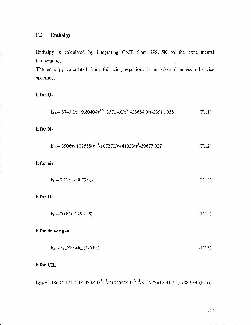
F.2 Enthalpy

Enthalpy is calculated by integrating CpdT from 298.15K to the experimental

temperature.

The enthalpy calculated from following equations is in kJ/kmol unless otherwise

specified.

h for 0 2

hG 2= 3743.2T +0.80408x25+35714.0/xa5-23688.0/x-23911.058 (F.l 1)

h for N 2

hN 2= 3906x+102558/xa5-107270/x+41020/x2-39677.027 (F.12)

h for air

hair=0.21hO2+0.79hN2 (F.l 3)

h for He

hHe=20.81(T-298.15) (F.l 4)

h for driver gas

hdrv=hHeXhe+hair(l-Xhe) (F.15)

h for C H 4

hCH4=4.186 (4.171T+14.450xl0"3T2/2+0.267xl0"6T3/3-1.772xle-9T4/ 4)-7889.34 (F.16)

117

h for H 2

hH 2= 4.186 (6.947T-0.2xl0"3T2/2+0.4808xl0"6T3/3)-8559.44 (F.17)

h for mixed fuel

h&el- |flH2+(l-|)hcH4 (F.l8)

h for driven gas

hdrn= [hfoel C/(C+D+hair] / d+C) (F.l9)

F.3 Molecular Weight (denoted by M , unit kg/kmol)

Molecular weight for driver gas

Mdrv=28.97(l-Xhe)+4.003Xhe (F.20)

Molecular weight for driven gas

M d m = {C[2!+16(l-D]+28.97>/(l+Q (F.21)

* Cp and h used in the conservation equations are base on per kilogram. We need to

convert Cp or h based on per mole calculated using above equations into the

correct unit by dividing it with the molecular weigh.

118

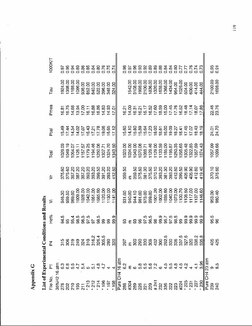
'-3 a CU a, a <

s Vi

cu

a CJ Vi a ©

o o o

CO

CO CD E Q_

CO o a.

CO o

h-

CD X

c o

u e cu

a cu

a Q-

a.

-• E

C D

CM X

vi ® 3 i l

ID Oi CO LO "3- o CD LO oo 1^ CD co CM Oi Oi oo O CO co LO Oi Oi oo oo oo co co 03 Oi Oi Oi 00 co oo 00 CO CO Oi Oi d d d d d d d d d d d d d d d d d d d d d d d d d d d d d

o o o o o o o o o o o o o o o o o o o o o o o o o o o o o o o o o o o o o o o o o o o o

cd co CD o p o p o p o CM d d d d d d d o d o o o o d d CM Oi CO CO CD CM d eg d co "3- o Oi o co CM CO co CO CM • t d o oi co i — o co LO CM Oi CM LO i — Oi T— CO co co CO LO o o o T—• i — co

Oi co oo LO CO co CO CO CM o> LO co CM

LO co o 00 CO CO CO o 1^ CM o Oi o LO CO CM co co CO CD CO N- CD Oi p 1— oo 00 co Oi p CM o CO CM LO p LO o LO p 00 CD CD co CD CD CD d d d LO d d d d d d CM d

CM CM

0) CM h~ co 1— oo CD LO CM o o o Oi co o o Oi LO co Oi o LO o o CM o CD —; CD co oo CD CNJ p CO o o <M O O

LO CO d d LO LO LO LO d d d oi d d 1 d d CM CM

a LO CD CO o O o o o CO CD o (35 o t-~ LO LO 00 LO Oi co Oi CD O o —• LO CM o LO o o o o o LO o oo CO CO oo LO O CD 05 O) CD oi d d co •sr d d d oi d d d d d d d CM 1 oi CM CD CM LO CO LO o CM CM CO oo CM CM CO oo Oi LO o CM LO LO Oi O o o i — 1— CM CO co CO o o o o o CM CM CO CO CO co O o

o o o o o o o o o o o o o o o O o o o o o o o o o o O o CO CD CM CM CM CM CM LO CM CM CD LO LO CO oq CD •— CM co CM CO LO CT> Oi CD CD d ID 1^ co co oi —'• CO CM d d LO d d d —: d CM oi d d CM oi d d

co 00 co Oi oi Oi Oi a> 1— LO LO 00 CT) 00 1— Oi o o T T— CO CO CO CO CO CO CO CO CO CO CO E CO CO CO co CO co co co co "3- co co

o o o o o o o o o o o o o o o o o O o O o p p p o CO o o o o o o o o o CM p oo o o LO p p co o o co LO p oi oo CM _! LO d d p o p p p CM d d d d d d o CD oi oi o CM LO 00 CM co T— d T— d d O o CO 1"- o o T—• co d d LO CD o o o o o co CO Oi O o o o o T T T— 1— T LO 00 Oi o> Oi a> Oi Oi Oi Oi CT) Oi

LO LO LO LO LO LO LO CT> LO LO Oi Oi Oi Oi LO LO LO CO CO 00 CT> d co CO CO d oo oi d 1 d Oi oi oi oi oi d CD

Oi a> Oi a Oi Oi o> Oi CT> Oi E Oi Oi Oi Oi Oi Oi 03 Oi Oi Oi CT) Oi Oi Oi Oi Oi

CM LO LO LO p CM 00 LO CD Oi Oi o CD d LO o o i^- o O o oo CM o CM o CO o d d LO LO T o r— CM T— T— CM o co CM _ o Oi co o co o a> co co CO CM CM co co o CM CO CO co (M CO CO co co co CM co CM E co CM co co co CM CO CO CO CO co co co

E LO E LO ^—' co co LO t- T-• 00 CO CM oo LO CD CM LO LO oo LO CM i - • p CO LO CD CD LO LO LO LO CD d E CO d d d CD d ^ d co Oi d

T— CM X X o o co CM CO 00 CD "3- LO o CD 00 CM o LO T—• —• T— a> Oi co o Oi oo 1 — Oi CM co CM co CM CM CO CM co — Oi o N- o o> T— CM CM CM T— 1— - • CO CO 00 CM CM CM CM CO CO CM CM CM CM CM CM CM CO CM CM CM CM * * * * * * 0. CM CM CM CM CM CM CO CM CM * * * CM CM

I S - I S - C O co C O L O C O O cn I S - C D Tf C M I S - Tf Tf o> L O Oi C D L O Tf Oi C D co C M cn I S - I S -00 oo oo C O I S - I S - I S - I S - q q cn Oi Oi Oi Oi cn co oo C O I S - I S - Oi cn cn Oi co oo co co co I S - I S ; I S :

d d d d d d d d d d d d d d d d d d d d d d d d d d d d d d d d

o o o o o o o o o o o o o o o o o o o o o o o q o o o o o o o o o o o o o o o o o o o o o o o o o o o o o o d Tf d co o o o o q C M d d d Tf d d C M d d o o o d d Tf d d d q o o o o o C D co C M C M Tf Tf' Tf d C M I— Tf co Oi o oo Tf C M C D L O C M d d o C D C D C D co L O d C M Tf Tf d d L O 1— o O Oi C M co co C D L O I S - C D Oi co C M Tf co C M o C O co L O 1— Tf C M o o co L O C O oo I S - Tf I S - C D L O Tf Tf Tf Tf C M C M C M C M C M cn I S - C M C M C M

" co L O L O C O L O L O

o C M o 00 L O L O o C O C M I s - L O Tf Tf Tf C O C M Oi co L O cn C M I S - O C O C O cn 00 L O o cn O O C D cn o cn o I S - Oi Tf C M o co q q q I S ; C M Tf cq Tf q Tf q q o o q I S - q cn °°. Oi d co Tf co Tf C M oo Tf L O I S-' oo i ^ d I s ! d oi C M d d d d d T—- 1—• C M C M C M C M C M C M C M C M C M C O C O co co co co co co C O C O C O C M

o o o co L O o I S - cn o 1— o o o C O o Oi Tf o I S - C M co O C D o o Tf oo L O co I S - o C D o O C D I S - o C M i— C O Oi I S - co C M I S - C D L O C M i— C O Tf q I S ; O q q L O C M o Tf C M q I S - q I S - Tf C M O d T T Tf L O L O C M Tf L O L O 1 ^ d d d co d oi d d c\i C M d d .—• d d d i—• C M d C M C M C M C M C M C M C M C M C M co C O C O C O C O C O C O C O C O co C O C M

o O o C O L O 00 O C O o o o o co o co Tf oo I S - co Tf C O O C O Tf C D C O o C O O o q cn o O o Tf O C M C O o L O o o o C O o C M o cn Tf Tf q C O O h - Tf I S - cn o Tf L O q o co Tf C O C M C M ^ L O C O C O C O o o L O d d d d d d d Tf d d d Tf T—- l< d d Tf oi d Tf

T J - T T O Tf oo C O co Tf d 1 ,— C M Tf C D 00 Oi Tf 00 C O C D C M o Tf L O C O C D o C M co I S - o o o C M C M C M co co co o Oi Oi o O o o o o C M co o o O o C M C M C M C M C O co

o o O O O o o o o o o C D o o o o o o o o O o o C O o o o o o O o O o o L O C D L O q q Tf q T I S - 1— Tf C O 1— q C M co q q C M q C D q Is- L O C O t— C D q C M C D o L O

d cri C M d oi C M c\i oi C M d Tf d Tf L O d L O oi oi d C M d d Tf Tf d d d d oi d C M oi oi I s - Oi I S - Oi T i — T i — I S - C D I S - L O I S - I S - I S - C O 00 Oi Oi cn ^— C M co C D L O I S - I S - I S - I S - Oi cn Oi Oi C O C O Tf co C O Tf T T Tf Tf C O C O co C O co co co C O C O C O C O C O Tf Tf C O C O C O co co co co co co Tf C O C O

o o o O O o o o o o o o o o o o o O o o o q Oi o q q q o o o o o O o o o o O q q co C M C M o o o o o cn Tf 00 T 00 I S - cq C O cn oi T T oi C M co d d q C D o q q q Tf C O d d d C M d I S - q o I S ; d h-i 1 ^ d d i ^ 1— o o Tf C D Oi i— C M Tf T L O d C M C M T— d T Tf C M L O L O O Tf oi d I— d T T Tf L O C D 00 o o oo o o o o o T— T— C D C M co Tf L O C D I S - cn cn o o o T T Tf L O L O Oi O o O O o T i — Oi Oi Oi cn Oi Oi Oi Oi Oi CO Oi Oi Oi cn Oi

Oi L O Oi cq Oi Oi q C D C O q cn L O C M L O q q cn Oi Tf I S -

L O I S - oi oo oo oi oi oi oi C O C O C M C M C O L O Tf C D C D I s - d oi oi d Tf d L O L O d 1 d oi oi oi d cn a> Oi Oi Oi Oi Oi Oi Oi Oi Oi Oi Oi Oi Oi cn Oi cn cn Oi cn Oi Oi cn cn Oi Oi Oi cn cn Oi Oi Oi cn cn

L O L O C D L O cq L O q q C M q L O q I S - oo C M Tf Tf C M Tf I S - L O L O

co Oi 1 ^ C M L O o C M C D C O co L O L O d L O Oi d d Tf d d d Tf c\i C M T— d d d o Tf C M d o C M oo C O C O co C M Tf I S - i — C M i — "1— T T— T o "1 C M o o o C O oo I S - Tf Tf L O C D Tf Tf o Tf C D o Tf Tf co Tf Tf C O L O Tf Tf C O C O co C O C O C O C O C O C O C O C O C O co co L O L O L O L O L O L O L O L O C D L O L O L O

itm

L O L O L O E q Oi C O C O Tf co cq f- C M I S - r - L O Oi C D Oi C O C O Oi C O L O L O I S - Tf I S - q Oi 03 d d 00 I S - C O O q L O

C D 1 ^ U O d L O d L O L O L O L O d C D L O d L O d d d Tf d Tf d O C O

oi d oi co Is-' d

L U Tf X

Q o co C O L O

C O C D Tf C M CD co C D L O Tf oo

L O oo L O I S - L O o C O C O TT Tf C M ,— C M L O o C O cn T— co C D co L O Tf o Oi Tf co I S - C D C D C M C M co C M C M oo oo Tf co co C M C M C M _ L cn L O Oi Oi Oi L O cn Tf L O Tf Tf Tf Tf C M C D C D L O I S - L O L O L O C M * * C O co C O C M co C M C M C M 4c * * O C M C M C M C M C M C M C M C M C M C M C M C M C M * 0 . C M C O C M C M C M C M C M ft ft * *

CD LO LO co LO o CM CM oo Tf CO CO co LO Is- LO co co LO O co CD Is- LO LO Tf Oi LO Oi Is- Is- Oi Oi Oi Oi Oi oo co oo oo Is- I s- Oi Oi Oi co co oo Is- CO Oi Oi cn Oi co oo Is-

d d d d d d d d d d d d d d d d d d d d d d d d d d d d d

o o o o o o o o o o o o o o o o o o o o o o o o o o o o o o o o o o o o o o o o o o o o o CM d d Tf d o o o o o o d d CM Tf o o q (—) d d CM d d q o Tf d d Is- CM CM I s- o d CM CM d d d Tf CM LO Tf d CM d /—\ o CJ5 T co CO d d Is- CD CM CM o Oi LO Oi LO 00 CO CM CO CM T o CD Tf o 03 CM CM co CM co LO Tf Tf Tf CM 1 Oi LO LO Oi LO Tf co 1 1 Is- CD Tf d 05 LO

CM o Is- o O O o CD LO o LO co o o CM CO CD co I s- CD Tf CO o o o o o O o O o o q CM Is- Tf Tf o oo Is- Oi q I s - co o CD o q co I s; Tf Oi Tf q CM T— CM q q q co CM q

d d oi d oi oi oi oi oi d d d y-l oi d d d d d d oi oi d d oi oi oi d d CO CM CO co Tf co co co co Tf co co Tf co co co CM CM oo CM CM CO co CM CM CM CM CM CM CM CM CM

Oi O Tf o o o o o CO I s- O o o LO co o o o o O o o o o O o o O O O O o o

q Tf CD q CO Is- CM CM CM q LO q CO CO LO q Oi CM Is- I s ; CD Oi q CM q co I s; q q LO Oi Is-oi d d oi d d d CM y-l d oi d d y-l y-l CM d d y-l Tf .—• d T—• y-l d oi d

co CM co co co co co Tf Tf Tf Tf Tf CO Tf Tf Tf CO CO CO CO CO CO CO Tf CO CO CO CO co co co CO CM CO

UO O CM o o o o o Is- CO o co o o CD o o o o o o o o o o o o o o o o O o oo O oo o q o o o q Tf o CD Tf q Oi LO q o o o o o q o q q o o o o o o o o

d oi d d d d Tf d oi d d T—: d oi d d d i^ oi d CM d T—• d Tf d Tf d Is-' d o CO CO CM CM CM LO co CO Tf Oi o o oo CO co LO co co Is- LO co CM o o Tf co LO LO CD CM I s- CO CO CO co o o O o o o CM CM CM CO o o o T— CM CM LO o o o o o o O CM

o o o CO o o o CM o o o o o o o o o o O o O O o Tf o o CD o o o O o O

CM CM Is- CD T— CD LO CO q CM LO CO I s- LO CD CD CD Oi Oi LO LO Is- LO q o Is- co CO CM 1 d d Tf d d d d Tf d 1 oi d Tf oi d y-l d d d d 1 oi oi Tf d d Tf d d d CO o> CO CD I s- I s- Is- I s- LO CO 00 oo Oi Is- Tf LO I s- co Is- I s - Is- o CD Tf LO CO co LO Is- CD LO Is- cn CO CO Tf CO 00 co co co co co co co oo E co CO co oo co co co co Tf Oi co co co CO CO co CO co co oo

O o o o o o o o o o o o o o o o Tf Tf CD o o o o o o o CD q o o co I s- o o o Is- q CD CM CD o o o o o o o o T— T—

d d Is- I s- Oi LO I s ; 1 Tf d Tf CD LO CM d d Tf ,_: CM LO LO o co CO CM 1 o CM CM Tf d d d T d d o Tf Tf LO Oi CM d Tf oi i — Tf 00 O Tf d d o o Tf d d d CO oo

co co co LO Oi Is- Is- o o o o o 1 Tf CD Is- o o o T CM CM CO LO Tf LO LO CD Oi O o Oi Oi O) Oi Oi 03 Oi Oi Oi Oi Oi Oi Oi cn Oi cn Oi

Oi o> CM LO CM LO LO I s: q Oi Oi Oi Oi q CO LO co CD CM CM oo q Tf LO I s; oi oi d d d d d LO LO LO d i^ d CM oi oi CM d Tf d d oi Oi d CM CM d d CO d d Is- d Oi Oi Oi Oi G3 Oi Oi Oi O) Oi Oi Oi O) Oi Oi Oi Oi Oi Oi Oi Oi Oi Oi Oi Oi cn Oi Oi cn Oi cn

oo LO q co q q Tf CM LO CM CD LO LO Tf Tf q Tf d o d LO d y-l Tf o LO d Tf o CM Tf d LO d CM CM o o d o T— LO CM CO d o CO LO LO o CD CO o oo co o CM CO CO CO CD oo co co oo LO CD LO LO CO o Is- CD oo Is- oo co co Is- Tf LO LO LO LO CD Is- CD CD I

s - Is- Is- Is- Is- Is- LO Is- LO LO LO LO LO LO LO CO LO LO LO LO LO LO LO LO LO LO

I atm

co oo q q Is- q oo 00 I s- Is- CM co q q Tf q CM Is-CD LO I

atm

Tf LO Tf d CM LO Tf d y-l c\i o LO CO CM CM y-l d CM q CM d LO Tf Tf d I s- C J Tf oi _ Q T ~ T— oi d CO CO E oi d 1

Tf O CO co

X CM o o Tf X co

Tf CO co CD CD o CD CM CD CM CM y— o Is- Oi LU CM T—

LO CO LO i _ ^~ co Oi 00 o Is- Is- LO Is- oo co I s- CD LO CO CM oo oo CO Is- «5 co CD oo Is- O Is- LO co o o CM CO CM Oi o CD CD I s- CM CM I s- CM ft CM CM CM LO CO 00 oo CO CM CM CM CM T— o o T o o o CO co * * * 0_ co Tf co co co ft CM ft * * * * co CM CM CM CM * * * * Q Tf co CO Tf CO CO CO co * *

CT> oo

d d

o o o o d d LO co LO co

CT> oo CM CM

O O CO LO d d co co

o o o o d T-1

co co CM CM

i - i - O C O " 3 - C O —• O CD rooioicococococoN <^cid>did>d>cid>di

o o o o CD co C M o

o o o o o o o

i o o o

i - CM LO 0 0 CM CM CM CM 1— i— N O) U) O (D —• —• as I s- L O I s-

o o o o o o o o o o o o n S N ' t x - ^ N C D T - O ^ C O N l O W N S N C O C D i n c O t D C D C D

o o o o o o o o o o o o o c D C M C 0 L q ^ c q L o c M O 5 c r ) c o L q c q

o o o o o o o o o o o o o o o o o o o o o o o o o o w ^ o i r i m s c d d N N N W ^ N T - ^ c o m c D O ^ c o O ' ^ m T -O T - O O O O i - • —• —• CMCMCMCO

CD oo oo CO CT> LO Is- Is- CT) LO I s-Is- co Is- oo CT) CO Is- co co oo CJ) CT) oo co co co

d d d d d d d d d d d d d d d d d d d

o o o o o o o o o o o o o o o o o o p o o o o o o o p p p o d p p o o d d d o o o d d d d CM CM d o CD CM CM d CM CO CO o d d d CD CT) CM CD CM 0 0 LO LO LO "sT CM oo CM o CD Is- o CO LO O O T oo

LO CD LO LO •t LO o CM CM o

o o o o O o o o o o o o o O o O o o o CO CO 1 — ' CM p o o Is- o oo CO CO —•

d d 1 ^ "* d d d T—• d 1 ^ d d d d d CM CM CM CM co co co co CM co CM CM CO —•

o o O O o o o o o o O o o o o o o o o CO LO co O co o co CM CM O o oq CM CT) co CT) p Is-d d d d d d d d CM d 1 ^ d d d d 1 ^ d CM CM CM CM co CO CO CO CM CO CM CM co co

o o O O o o o o o o O o O o o o o o o o o O O o o o o o O O o O o o o o o p d d d d d d d d d d d d d C\i d CT) T— co O LO co Is- CM CO O oo CM LO CM CT) CO o co — • CO CO o • — CO CO T ~ 1 — o o , — CM CM

O o co O o co o _. o O o O o oo o o o o O o O O O O o O o o o o CM CM f - Is- LO LO CO co LO CO CM o T— o CD LO CM Is- O Is- CM p O p p T—' i —

d d d d •r d d —• d i ^ d d d d d d d d d d d d o CT) CD CO LO oo LO 0 0 Is- O) O) 0 0 CT) CO i — Is- CT) Is- O) CT) CD Is- CO CT) CT> oo co co co CO CO co CO co co O) co co co CO co co co co co co CO co co CO CO co CO CO co co

o o o o o o o o o o o o o o O o o o LO I s- o O o o o O o p Is- T T oo Is- o I s- LO CO CM p o Is- CT) CO o o o 1 ^ CO —• p o CO •— CM d d d d CO d 1 ^ d LO d d d d d "* LO CT)

oo CT) d d d 1 ^ CM T— T T LO Is- co T 1— i — o o CO o d o CM o o co d d d o o co CT) LO Is- 0 0 co O ) o o o o o T oo 1— o —- o CO o T— o o CT) LO co CT) O) CT) O) CT) CT) CT) CT) CT) CT)

CD CO CD CM Is- CM CO oo LO Is- co LO Is- LO O) LO LO CM d d LO LO LO LO LO "* d d 1 ^ d d d LO d d CT) d d "* d d d d d r- d d CT> CT) O CT) O) CT> CT) CT) O) O) CJ) O) CT) O) O) O) O) O) CJ) CT) CT) CT) CT) CT) CT) O) CT) O) CT> CT) CJ)

CO "* LO co LO LO LO co LO oo LO d o o o 1" LO CM LO LO d o oo CO o d CD r- O Is- d CM CM CM — : d LO CM CM o O O O CM CM CT) T T o CM o Is- —• o T CM CO CM o CD LO CT) CO oo oo LO LO CO co co co CO CO CO CO CM CO CO CO CO CO LO LO CD CO CO CO LO LO CM "* CO co

CM CO O N CD i-; CM If) N S O) N CO CO O) CO CO CO CO

o o o o co co L O

C M d ^ CO C M LO LO 0 ) 0 0 0 CT) —• •— —•

CD N N CO CT) CT) O) O)

LO ^ (D CO (D O i - C M CT) C O C O C O C M

^ CM 1 ^ 1 ^

"* O O o CO CO

tm

LO "3- 0 0 LO LO

CO CD

d d CD CO CO d d LO "*

H2

LO CM CO

"* CO

LO o "3-

o LO o "*

CM CM CO

CD co

co co

1"". co co

CM co

i : o) — co

co co

CD ^ CD

H—

Q

X

o CD i_ CL

CO CD s

co CM

0 0 CT)

C O

p — . CM — .

o co T—• CM co co CO

co CO

CT) 0 0

N S C O T - T -

C 0 " * CO CO LO CD oo CT)

CO CO CO CO CO CO CO co co co

d

CO —• CT) C O C M

^£ d "* c CO CD

_ J

X CO CO 0 0 co

co CO CO co

CN

C D C D C O Is-; I— Is-o d d

o o o o o o o d d <y> CT> o C O C D C D

o o o p CM CM d d d

o o o p Is- p d d d

o o o o o o d C M d •— —• C D co co co

o o

o co

co E co

o o o Tf —• o

Tf Tf CT) CT) CM O O —•

O) CT) r- O) CT) E O)

C D C O CT) ( - 0 0 C M E C M

Is-d

Is-; d

L O co Tf <D Tf C O C O

co co

TT CO CM CM CM o Is- LO Is- CM CT) O) O) O) CT) CT) co 0 0 0 0 Is- Is-d d d d d d d d d d d

o o o o o o o o o o o o o o o o o o o d Tf CM CM CM TT d CM o o o CM LO CM CT) CD co TT CJ) CM TT d CD 1— Tr CO CO Tf o CM Tf Tf CM co Tf

o o o o o o o o o o o o o CM CM TT oo p CM • — Tf Tf CM d CM CM CM — : .—• T—• CM co co CO co co co co co co co CO

o o o o o o o o o o o Tf p p p p Is- p Is-; Is-; p

CM CM T—• — : d — ' • — : CM CO CO CO co co co co co co co co

o o o o o o o o o o o o p p p p p o o o o o d d CM CM T—• —•' TT d CM d d CD Is- oo oo O) T TT Is- CO CT) CT) o o o o o CM CM co

o o co TT o CO CM CM o r-. Is-Is- p — • p CD CD Tf Tf

d d Tf d d d d d d d d Is- Is- CD TT Is- Tf Is- Is- Is- O) CT) co co co co co CO CO co co CO CO

o o o o o o o o o o o CM CD Is- — •

cq CT) co Is- p oo CT) Tf d — ! d T - d d d T d d T TT 0 0 CO Tf Tr LO LO CD Is- CT) o o o — •

CO O) O) CT) O) O) CT)

CM Tf p p p p d d CO d d Tf LO CD Is- d d CT) CT) CT) CT) CT) CT) CT) CT) O) CJ) O)

CM CO co CO Is-; p p d d d 1 ^ 1 ^ CM CM CT) CD o

Is- Is- Is- Is- Is- Is- CD LO LO TT CD LO LO LO LO LO LO LO LO LO LO LO

CT) Is- co co CT) LO _ : — ! d d CM p p

d d d 1 ^ Is-

CD CO Is- LO Tf co CM CT) o O) LO LO LO LO LO LO LO LO LO LO CO co CO co co CO CO co CO CO CO

Is-;

d

E 4—>

CO o TT —

CO CD I

TT X o

d oo CD LO CD CT) > o Is- — • — • CM Is- co o oo Is- CM O) CT) CT) CT) 0 0 Q oo Is- Is- Is- O CT) oo co co Is- Is- o d d d d d d d d d d d d d d d • —

o o o o o O o o o p p p o o p o o o o p o o o o o o d d d d d d o o o o d Tf o o o o d CM CD Tf 1— LO co d TT d CO d d Tf CM Tf Is- co LO Tf o o CT) CT) co LO o o Is- CM CM T — CD

Is- CD LO CM CT) Is- CD CD CM

o o o o o o O o o o o o o o O o o p p CD p CT) LO Tf p p —• p — ; CM p O p Tf d d d d 1 ^ d d d d d d d d d d Tf CO CO CO CO CO CO CO CO CO CO CO CO co CO co

o o o o o o o o o o o o o o o o o Is-; p Is-; p p p o 1—• CM p p p LO p p • — CO d d d d d d o d d — ^ d d d d d d d co CO CO CO CO CO d co TT Tf CO CO CO Tf CO CO CO oo

o o o o o o o o o o o o o o o o p o o o o p o o o o o o o o o o d — ! d d d d ,—! d d o d d d d CM d o T — Tf Tf 0 0 CM

^ LO CT) Tf o CM CO Tf o Tf CO O) CM

o o o o T CM CM CO CT) o I CM CM CM CM co CT)

o o TT CD o CD co CM Tf O o co Is- O CO Tf — - LO Tr Is- CM CT) CD TT LO • — • — p Tf CT) CM p

d d d Tr d d d d d d d d r- i— d d d d Is- Is- Tr LO Is- Is- CT) o Is- 1— Tf Is- CO 0 0 CT) O CT) Tf co 0 0 co CO co co CO Tt co co co CO 0 0 CO Tf CO CO

o o o o o O o o o o o o o o o p CO O) Is- CO O o Tf CT) p p oo o Is- p — • LO — ; d d d T-' d p Tf d Tf d CM d CJ) d d Tr Tf- CO i — CO 0 0 1— Ti­ d d CM CD 0 0 — • CM d — - CM co LO co o o o T CJ) oo O O o y— o CT) CT) CT) CT) CT) co CT) CT)

CD O) CM p LO LO LO en LO LO LO p p O p CM CM d d Tf d co d O) d CM Tr" d CO d d d d 0 ) O) O) CT) CT) O) CT) O) O) CT) O) CT) CT) O) O) O) CT) O)

CD LO LO p p oo o d o o O) CD o oo O o O) CD LO oo CD o 1— oo CT) oo co CT) oo oo oo O) oo co CM CM o CD CD Is- Is- CD CD CO CD CD CD CD CD CD CD CD CD CD Is-

p ^ —

Is- CM p LO CD E LO LO CD CD LO Tf Tf- CM _ ! d 0 0 CM co co Is- CM — ! O p p p CZ

^—' LO d d d o T T , d d d co 1—

T T o — Tf o CM i r X

co CM T— o LO CT) CT) 0 0 oo Is- CO LO TT Is- Is- Is- Tr

-T— O CO CM 1— 0 0 CO r- Tf

co co Is- Is- Is- Is- Is- co co co _L O) co 0 0 oo co co co LO o CO CO co co 0 0 co co * + * ' O co co co CO * * * Tf

Tf CN

CD T— CM o I s - Tf CD Tf CO o oo CD o CD Tf CM co LO co cn co oo oo I s- I s- q q cn CD q 0 0 q rx IX d d d d d d d d d d d d d d d d d

o o o o o o o o o o o cq o q o o o o o o o o o o o o o o o T T d Tf d Tf" o o q q d d d d o d q o o q T o CD LO I s - d d d d 0 0 LO CO Tf d LO CM d Tf d CD oo T T— o CD Tf I s- CD cn CD T Tf o o CD CD

Tf cn co LO Tf CO IX co CM

O o o o o o o o o o o o o o o o o o o LO cq CD Tf Tf o CM q q CM CM CO q IX CM Tf CO d i x d d i x d d d d IX d IX IX d | x d d d d co CO CO CO CO Tf CO CO co CO CO CO CO CO co CO co co co

o o o o o o o o o o o o O o o o o o o CO I s- 0 0 I s- oo LO Is-; cn CM Tf CM cn IX IX q co IX LO cn co d d i x d y—1 d d d IX d d d d d d d d d co co co co co Tf CO CO CO CO CO CO CO CO co Tf co Tf CO

o o o o o O o o o o o o o o o o o o o o o o o o o o o o o o o o o o o o q co Tf d d d d d d d o d d d d d d d d d CO o CO T Tf co CM T— LO d o T— oo o CM oo CM oo co o o CM co co IX o o o CM CM co

o co CM CM co o Tf LO LO CO co co o IX o o cq I s- CD cq LO cq I s- Tf IX co q IX CM CM Tf Tf o

Tf d y-l d T— Tf d d Tf d y-l Tf IX d d d d Tf oo CD I s - co LO C O CD o T— Tf LO oo CO oo cn cn cn T— co co co oo co co CO CO Tf Tf CO CO CO CO CO CO CO CO Tf Tf

o o o o o o o o O o o o o o T co IX o LO o o o o o CO co T— y— LO o co CM IX CM d IX d IX o q •>— o d d d d d i x cn d d T— Tf CD T— Tf d d T— Tf CM o LO CD o co Tf co I s- cn o o o T— 1— T— CM Tf LO cn o o o T— T—

CD O) CD cn cn cn cn cn cn

co LO LO co cn cn co CM q LO LO LO q q q Tf Tf Tf CO d IX co d d CM d d Tf LO d IX d d d

O) CD o> cn cn cn cn cn cn cn CD cn CD cn CD CD CD CD

Tf Tf cq LO q q LO Tf CM y-l y-l CM CM Tf d d d o LO Tf CM CM o Tf 1— o T— o o o CO co co CD cn cn o T o o o o o IX IX I s- IX IX I s - CD LO CD CD CD CD IX | x IX | x IX IX | X

CD co I s- co Is-; LO q q

CO cn IX q IX q 0 0 Tf CM d CM CM ^ d q q d d Tf Tf co CM y-l d o 0 0

d d co d o Tf CM X

I s- CD LO Tf CM co CO o CM y o oo CM O) cn CD O) O) cn cn c£ CO LO Tf o T ^— T— o o O co o cn CO CO CO CO co LO Tf Tf Tf Tf Tf Tf Tf Tf ft Tf co * + * * * CO Tf Tf Tf * * * * * * *

o -t—' CD E O ) CO I

_c C L CO

3 3

CD

CL E o o

_CZ

V) ^—'

c ^ "~ co

2 g w Q * ft