Coastal Engineering 58 (2011) 606–622

Contents lists available at ScienceDirect

Coastal Engineering

j ourna l homepage: www.e lsev ie r.com/ locate /coasta leng

Experimental investigations of the bed evolution in wave flumes: Performance of 2Dand 3D optical systems

Enrico Foti a, Ivan Cáceres Rabionet b, Alberto Marini a, Rosaria E. Musumeci a,⁎, Agustín Sánchez-Arcilla b

a Department of Civil and Environmental Engineering, University of Catania, V.le A. Doria 6, 95125 Catania, Italyb Laboratori d'Enginyeria Marítima, Universitat Politècnica de Catalunya, C/ Jordi Girona, 1-3 Edificio D1, Campus Nord (UPC), 0834 Barcelona, Spain

⁎ Corresponding author. Tel.: +39 0957382727; fax:E-mail address: rmusume@dica.unict.it (R.E. Musum

0378-3839/$ – see front matter © 2011 Elsevier B.V. Adoi:10.1016/j.coastaleng.2011.01.007

a b s t r a c t

a r t i c l e i n f o

Available online 26 February 2011

Keywords:Optical measurementsStructured lightStereo visionMorphodynamicsSwash zone

Optical systems can provide very accurate measurements of bottom morphology in wave flumes. However, itis often necessary, e.g. when laser scanners are used, to stop the experiments and disturbing significantly thesandy bed itself, by emptying the flume. In the present work measurement strategies based on computervision techniques which permit measurements also in the presence of water are applied in wave flumes atsmall and at large scale. Such techniques, based on the use of structured light, are demonstrated to be able toperform measurements of 2D and 3D bed evolution also in a very active area, such as the swash zone, wherethe alternating presence and absence of water makes it difficult to recover the bed morphology in a dynamicway.The main technical enhancements of such techniques developed in the framework of the HYDRALAB III, JointResearch Activity SANDS project vis-a-vis the present state of the art of other instruments, commonlyadopted, are discussed.

+39 0957382748.eci).

ll rights reserved.

© 2011 Elsevier B.V. All rights reserved.

1. Introduction

The investigation of sediment transport and related morphody-namics is a key issuewhen dealingwith coastal engineering problems.Indeed, sediment transport in littoral areas can affect the effectivenessof several coastal structures at a large extent.

Although extensive research on this field has been carried out inthe last decades, a good understanding of the basic mechanisms of thecomplex non-linear interaction between fluid flows induced by wavesand currents, seabed morphology and sediments is still missing.

Because of the presence of a high number of parameters thatcharacterize the phenomenon, laboratory investigations at small or,better, at large scale, are often preferred in order to analyze the role ofspecific mechanisms in a well controlled environment. However, thesignificance of the obtained data and the quality of their analysis notonly depends on the geometrical scale of reduction but also on theaccuracy and reliability of the adopted measurement systems.

Considering the investigation of the morphodynamics of amovable bed in wave flumes, recently, optical instrumentations arebecoming more diffused because of the large amount of informationthey can provide. Moreover, the advantages of such techniques aremainly due to the fact that, when a proper visualization method isadopted, the instrument mimics the human eye, therefore the results

are provided in a form which is closer to the operator's perception,thus allowing for an easier interpretation of the data to be performed.

Probably the simplest way of optically measuring localizedfeatures of the sandy bottom is by the use of thin measuring pins.By adopting such a methodology, Sumer and Fredsøe (2001) wereable to measure the wave induced scour at the base of a large verticalcircular cylinder. A similar approach has been used also for theinvestigation of the scour at the roundhead of a low crested structure(Sumer et al., 2005). The accuracy of such a methodology along thevertical direction is strictly related to the accuracy of the scale on thepins and to its visibility, turning out to be of O(0.001m); however, dueto difficulties in automatizing the image analysis, its application ismainly limited to the analysis of equilibrium conditions only.

Nowadays, laser scanners are widely used to collect detailedbathymetric data, with a resolution which depends on the number ofsampling points. Obviously a compromise has to be made among therequired accuracy, the extent of the investigated area, the spatialresolution and the time necessary to perform the measurement. Forexample, van der Werf et al. (2006) and O'Donoghue et al. (2006)investigated the bed morphology evolution under the action of anoscillatory motion, from flat bed to full scale ripples, within two watertunnel facilities, namely the Aberdeen Oscillatory Flow Tunnel (AOFT)and the Large Oscillating Water Tunnel (LOWT) at the Deltares. AtAOFT a movable laser displacement sensor, which made pointmeasurements of bed elevation with a 50 μm resolution along thevertical direction, was adopted at six parallel profiles with a spatialresolution of 0.005m in the streamwise direction and of 0.04m in thetransverse direction. At LOWT, a bed profiler was used, which

607E. Foti et al. / Coastal Engineering 58 (2011) 606–622

consisted of a laser sheet 0.5×10−3 m thick sent along the entirewater tunnel width, i.e. 0.3 m, recorded by a camera. The obtainedmeasurements, performed at every centimeter of the tunnel length,had a 0.001m vertical resolution. However O'Donoghue et al. (2006)state clearly that, by using these instruments, although bed elevationmeasurements of very high quality were obtained, the processresulted to be time-consuming and could not be carried out while theflowwas active. Due to compaction of the soil, smoothing of small-scalebedforms, topping of suspended sediment or even sand losses, duringthe drainage of the tank, vanderWerf et al. (2006) report randomerrorsin the estimate of the net sediment transport rate up to 20%.

Some laser profilers are able to measure even in the presence ofstill clear water, but in that case the suspended sediment has to settledown, by stopping the flow. It turns out that laser bed profilers do notallow continuous measurements of the evolution of the morphody-namic processes to be performed.

The development of automated photogrammetry has encouragedthe use of such techniques also for the investigation of sedimenttransport. Stojic et al. (1998) and Brasington and Smart (2003) useddigital photogrammetry to survey the network and basin evolution ina laboratory simulator, 2m×1m large, due to simulated rainfall. Inparticular, in the latter work, sequential comparisons of very denseDigital Elevation Models (DEMs) allowed not only the morphometricchanges, but also the sediment yields and the dynamic characteristicsof the sediment transport to be determined. The vertical accuracy ofthe DEMwas estimated to be equal to 1.2×10−3m. However it shouldbe mentioned that such analyses require: (i) sophisticated topo-graphic tools for the calibration procedure; (ii) a very accurate verticalcamera positioning; (iii) stopping the experiment and draining theexperimental basin at each image acquisition in order to measure thebottom morphology also below water level inside the channels. Thethird step can induce modification of the erosive bottom, as theovernight appearance of desiccation cracks, that were reported byBrasington and Smart (2003).

In the field of coastal engineering, automated photogrammetry hasbeen mainly applied to the analysis of three-dimensional character-istics of surface waves (see for example (Dickerson, 1950; Pos et al.,1988; Shemdin and Tran, 1992; Benetazzo, 2006; Wanek and Wu,2006). During the last decades, the Argus video system has beensuccessfully applied in the field to determine the position of longshoresubmerged bars, but also to investigate flow characteristics. Someapplications of the Argus system has been recently performed in thelarge wave flume of the Oregon State University, for example tomeasure the tsunami propagation in a constructed environment (Coxet al., 2008), but no extensive application of automated photogram-metry to coastal morphodynamics has been done in the laboratoryyet, at least to the knowledge of the writers. This is probably due tothe fact that the application of such kind of techniques requires theimages of the measured surface to be characterized by a well-definedtexture so that the so-called “correspondence problem", i.e. theproblem of matching two points on the stereo pairs corresponding tothe same point in the real world, can be easily solved by using a pixel-correlation-based algorithm. Images of the water surface topography,depending on the lighting condition, have generally a clear texturedue to the capillary waves that naturally form on the surface, whereasimages of sandy bottom are usually more even and therefore deprivedof any reference point.

To overcome some of the limits of the above mentionedmethodologies, recently optical systems based on Computer Vision(CV) techniques were introduced (Faraci et al., 2000; Baglio et al.,2001b). Such techniques, which are inspired by machine visionsystems, try to simulate portions of the human eye and braincapabilities through three steps: i) image formation; ii) imageanalysis; iii) image interpretation. The first step consists of bothcreating and acquiring good quality images for automatic treatment.Therefore, a proper combination of light source and sensors, which

must be appropriately chosen in order to avoid poor contrast,undesired shadow and unpredictable reflections, is required. Theimage analysis is a post-processing step aimed at extracting onlyuseful information from pictures bymeans of appropriate processes offiltering and morphologycal transformation of the images. Finally, theimage interpretation allows to extract quantitative information (e.g.dimensions, shape, etc) and it has to rely on some camera calibrationprocedure.

It is worth pointing out that CV techniques allow time resolvedmeasurements of bed morphology evolution to be easily performedby means of even non-professional camcorder, which typically haveframerate of 30 fps. Moreover, by using an appropriate laser light witha cylindrical or diffractive lens, it is possible to perform 2D or 3Dmeasurements of bottom evolution with the same optical equipmentby changing only the solving algorithms. Indeed, in the first case justthe horizontal and vertical pixel-to-meter transformation coefficientshave to be determined, while in the second case a stereo matchingalgorithm needs to be applied.

Previous applications of CV have been made in quite restrictiveconditions, that is, in well controlled small scale wave flumes in whichinformation regarding limited areas with characteristic length of O(0.1 m) were gathered. In the present work, such optical techniqueshave been further developed in order to be applied also in large waveflumes.

In particular, the bottom evolution within a very active region,such as the swash zone, has been considered as a case-study.

Indeed, the swash zone is interested by the alternating presenceand absence of water, during run-up and run-down respectively,along with an extremely high dynamics of sediment transport. Someauthors claim that in this region most of the coastal sedimenttransport takes place (Elfrink and Baldock, 2002; Masselink and Puleo,2006). However, it is difficult to make dynamic measurements of thebottom morphology directly inside such an area (Hughes and Turner,1999; Longo et al., 2002), due both to the hydrodynamic conditions,shallow, aerated, turbulent and rapidly varying swash flow, and to themorphodynamic conditions, large magnitude of the sediment fluxes(Masselink and Hughes, 1998) as well as to various modes oftransport involved, including bed load and suspended load, sheetflow and even single-phase flow at the end of the backwash (Hugheset al., 1997).

According to Masselink and Puleo (2006) high-resolution (spatialand temporal) measurements of the beachface morphology, obtainedeither manually (Duncan, 1964; Eliot and Clarke, 1986; Masselinket al., 1997) or by remote sensing techniques (Holland and Puleo,2001) can be used to derive net sediment transport rates in the swashzone. Instruments such as sediment traps (James and Brenninkmeyer,1977; Hardisty et al., 1984; Masselink and Hughes, 1998; Jacksonet al., 2004) and pump samplers (Kroon, 1991) are able to measurethe bulk sediment load and give information on event-scale sedimenttransport rates, for example, the transport over an uprush/backwashcycle. However, such instruments are implemented directly inside theswash-zone, therefore they can interact with the swash process itselfat a large extent, whereas the use of the noninvasive optical systemsproposed here allows to avoid any interference with the water-sediment flows.

Evolution of 2D and 3D CV techniques based on the use ofstructured light are presented here. Precisely, two different 3Dstrategies have been considered: the first one based on thestereoscopic approach of Baglio et al. (2001b), described in the nextsection, and the second one based on the application of a commercialstereo-head, usually adopted in the field of robotics (Livatino et al.,2008). Such methodologies were selected, upgraded and applied inorder to satisfy the requirements of not draining the flume during themeasurements of bottom evolution and to be characterized byflexibility in order to be applied both at small and at large scale forthe analysis of bottom changes due to the shoreline motion.

608 E. Foti et al. / Coastal Engineering 58 (2011) 606–622

The paper is organized as follows: in Section 2, a synthesis of thetheoretical background of the 2D and 3D Computer Vision techniquesis reported; in Section 3 themain technical improvements, introducedin the context of the HYDRALAB III J.R.A. SANDS project, are presentedalong with a validation of the proposed measurement strategies bothat small scale and at large scale; finally the experimental resultsregarding the measure of the morphodybnamics of the swash zoneboth at small scale and at large scale are reported in Section 4; thepaper ends with Section 5 in which some conclusions are drawn.

2. 2D and 3D Computer Vision methodologies for recoveringsandy bottom morphodynamics

Here the twomeasurement techniques suitable for both 2D and 3Dmorphodynamic investigation of sandy bottoms are presented.

Two-dimensional measurements of a movable sandy bed havebeen performed in a non-pervasive way by developing a technique,initially proposed by Faraci et al. (2000). The image formation stepwas accomplished bymeans of a sheet of laser light, obtained by usinga cylindrical lens on a laser generator. The light sheet is cast onto thebottom, thus obtaining a light line that follows the shape of thebottom itself, by providing a cross-section view of the bedmorphology, which in turn can be video recorded. Particular caremust be taken when obtaining images of the bottom. Indeed, in orderto reduce perspective effects, the camera and the laser must be placedboth pointing to the bottom and almost parallel to each other. Indeed,a small angle between the laser sheet and the image plane could leadto a wrong calibration of the images. Moreover, the laser and thecamera should not be located on the same side of the wave flume,in order to avoid ‘flat’ images, where it is difficult to appreciatedifferences of the elevation of the bottom. In Fig. 1 a) and b) theimages of the adopted laser line, as seen when projected onto a flatand a rippled bed respectively, are shown.

The image analysis stage is performed by recovering the positionof the relevant points in pixels on the image plane. The identificationof such points can be made automatic, to manage the analysis of alarge number of images, when dynamic analysis are carried out. Forinstance, in Fig. 1 c) the grayscale image of a rippled bed has beentransformed into a black andwhite picture, by applying a threshold onthe intensity of the image in order to discriminate between the darkerbackground and the lighter laser line. In Fig. 1 d) the numericalrepresentation, i.e. a matrix of ‘zeros’ and ‘ones’, of the previous blackand white image is shown. It can be noticed that the thickness of thecurvilinear stripe of ‘ones’ representing the ripple profile is only fewpixels large (1÷4 pixels). It follows that the analysis of the numericalmatrix can be easily coded, to find the pixel positions of the bottomsection and to identify relevant points, such as minima and maxima.

Fig. 1. 2D CV technique for bed shape mapping. Image formation: a) laser light line projeprocessing: c) black and white image of a rippled bed; d) numerical representation of a bcalibration tool; f) sketch for the determination of the horizontal and vertical calibration co

Finally, the image interpretation step, i.e. the definition of acorrespondence between pixels and the real horizontal and verticaldimensions on the pictures, is performed by projecting the light lineonto an object with known dimensions. This phase is calledcalibration procedure and the known object is named calibrationtool (see Fig. 1e), since the horizontal and the vertical calibrationcoefficients, Ch and Cv, can be found as

Ch =Lcalh

lcalh

=m

pixels

� �ð1Þ

Cv =Lcalv

lcalv

=m

pixels

� �ð2Þ

where Lhcal and Lv

cal are some relevant horizontal and verticaldimensions of the calibration tool in [m], and lh

cal and lvcal are the

corresponding pixel dimensions. Once the calibration coefficients areknown, any horizontal and vertical unknown real dimension, Lh andLv, can be determined by means of its image dimensions as

Lh = Ch⋅ lh =m

pixels

� �⋅ pixels½ � ð3Þ

Lh = Ch⋅ lh =m

pixels

� �⋅ pixels½ � ð4Þ

A simple sketch of the adopted procedure is shown in Fig. 1f).The aforementioned technique has been previously successfully

applied at small scale O(0.1m) to investigate both the scour evolutionat the toe of a cylindrical vertical pile (Faraci et al., 2000) and themorphodynamics of a rippled bed (Faraci and Foti, 2001, 2002).

A similar techniquewas also adopted by Jarno-Druaux et al. (2004)for the investigation of the dynamic evolution of ripples in a waveflume, but still over a length of O(0.1m).

At a small scale many disturbing effects, such as perspective effectsor signal noise, can be considered negligible. In these conditions, bytaking into account both the intrinsic uncertainty of the video cameraand the uncertainty related to the laser sheet thickness that must beevaluated during the calibration process, Baglio et al. (2001a)estimated that the vertical uncertainty was equal to ±0.6×10−3m.

Regarding the 3D CV technique, the measurement technique isbased on the stereoscopic approach, which tries to simulate thehuman capability of getting a three-dimensional perception of theworld by coupling the information coming from two images, takenfrom two different points of view.

cted onto a flat sandy bottom; b) laser light line projected onto a rippled bed; Imagelack and white image of a rippled bed; Calibration: e) laser light projected onto theefficients.

609E. Foti et al. / Coastal Engineering 58 (2011) 606–622

Here two different stereoscopic methodologies are discussed. Thefirst one is based on the classical stereoscopy approach. The secondone is based on an on purpose developed technique.

Classical stereoscopy relies on several hypotheses which the twoused cameras must satisfy. In particular, (i) the two cameras musthave the same focal length; (ii) the focal axes have to be parallel,(iii) the orientation of the image planes has to be the same, i.e. norelative rotation of such planes is allowed; (iv) the distance betweenthe two centers of the lenses, referred to as base line, must be known.

The focal lengths, the position of the image planes and the baseline distance B can be known a-priori, i.e. the manufacturer of theoptical system can provide the user with the values of thosecharacteristics, but in that case the system has to be very stable andextremely carefully managed, since even minimum relative move-ments of the two cameras cannot be permitted. This is clearly possibleonly in well controlled environments, such as installations forindustrial applications, but it is not always practical. In particular,hydraulic laboratories are often crowded with many differentmeasurement instruments, the optical devices being only some ofthem. As a precise and stable positioning of the system is not feasiblein most cases, a more flexible approach is required. The problem isusually overcome by implementing a camera calibration procedure inorder to determine the intrinsic and extrinsic parameters of thecameras, i.e. the parameters associated to the optical system and theones associated to the position of the cameras respectively (Tsai,1987).

In the proposed stereo measurement methodology, named in thefollowing Structured Light Stereo Vision (SLSV), the image formationstep is accomplished by using a grid of laser light points, obtained bycoupling a laser beam with a diffractive lens. Such an approach wasinitially introduced by Baglio et al. (2001b). The projection of theaforementioned grid allows to materialize the measuring points ontothe even surface of the texture free sandy bottom. In particular the useof coherent light permits to reduce the errors related to thepositioning of the measuring points. In Fig. 2 a) and b) an exampleof the stereo pairs gathered by projecting the laser grid onto a rippledbed is shown.

The aim of the proposed measurement methodology is to providea simple, flexible, robust and, above all, economic alternative to theout-of-the-shelf 3D vision systems commercially available nowadays,such as the laser scanners described previously. Therefore theaforementioned restrictive classical stereoscopy hypotheses havebeen removed. Indeed, according to geometrical optics, it is possibleto establish a non bi-unique linear correspondence between the 3Dreal coordinates of a point in the spaceX=(X, Y, Z) and its coordinateson the corresponding images x=(x, y) as

AX = x ð5Þ

where the values of the terms of the matrix A can be found byperforming a camera calibration. Indeed, by following Baglio et al.(2001b), considering n≥6 points with known coordinates both in the2D image spaces of the camera xn, and in the 3D real space Xn, thecoefficients of the calibration matrix A can be determined, by usingthe pseudo inverse matrix method, so that

A = xnXTn XnX

Tn

� �−1 ð6Þ

where the superscript T indicates thematrix transpose, andXnT(XnXn

T)−1

is the pseudo inverse matrix of Xn.The stereoscopic approach requires two images of the same object

in order to obtain a three-dimensional reconstruction. The calibrationmatrices A1 and A2 of the two cameras can be determined throughEq. (6) by using a calibration tool, where the real word coordinates ofthe calibration points are known in a reference system integral withthe tool itself.

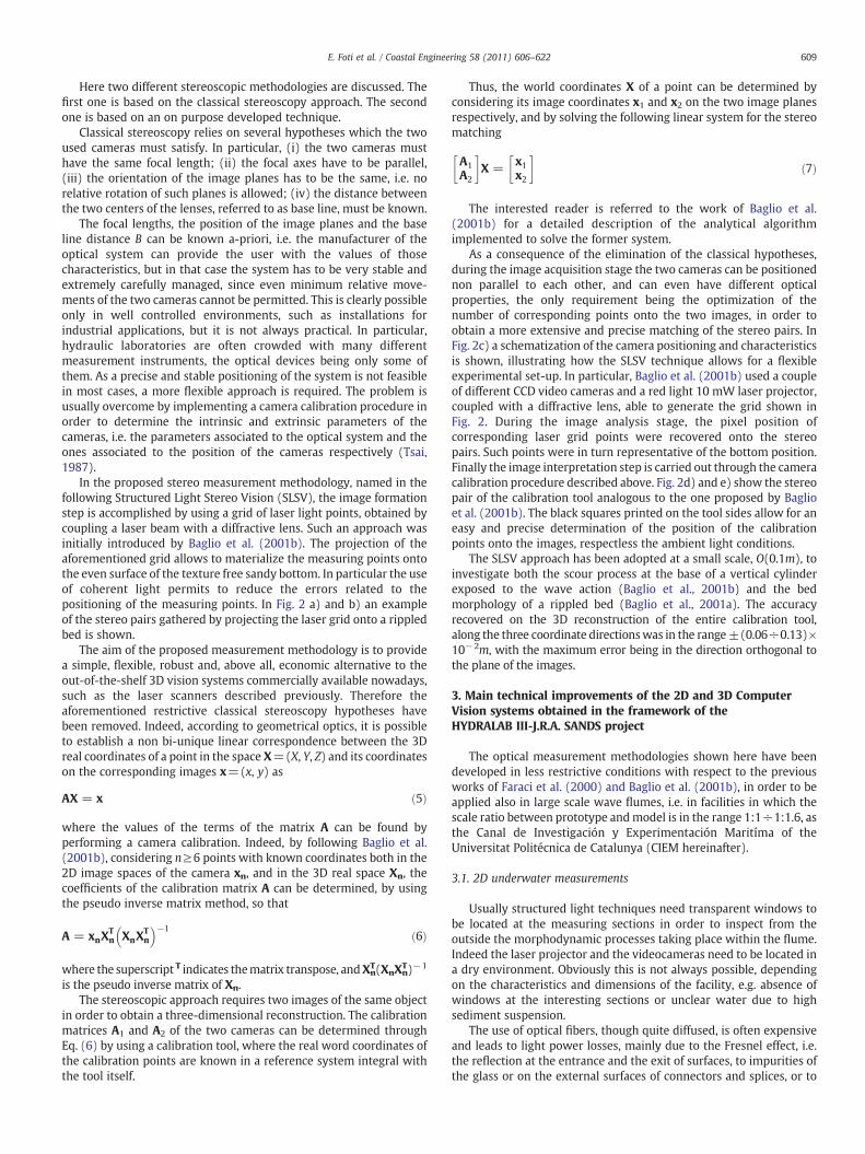
Thus, the world coordinates X of a point can be determined byconsidering its image coordinates x1 and x2 on the two image planesrespectively, and by solving the following linear system for the stereomatching

A1A2

� �X = x1

x2

� �ð7Þ

The interested reader is referred to the work of Baglio et al.(2001b) for a detailed description of the analytical algorithmimplemented to solve the former system.

As a consequence of the elimination of the classical hypotheses,during the image acquisition stage the two cameras can be positionednon parallel to each other, and can even have different opticalproperties, the only requirement being the optimization of thenumber of corresponding points onto the two images, in order toobtain a more extensive and precise matching of the stereo pairs. InFig. 2c) a schematization of the camera positioning and characteristicsis shown, illustrating how the SLSV technique allows for a flexibleexperimental set-up. In particular, Baglio et al. (2001b) used a coupleof different CCD video cameras and a red light 10 mW laser projector,coupled with a diffractive lens, able to generate the grid shown inFig. 2. During the image analysis stage, the pixel position ofcorresponding laser grid points were recovered onto the stereopairs. Such points were in turn representative of the bottom position.Finally the image interpretation step is carried out through the cameracalibration procedure described above. Fig. 2d) and e) show the stereopair of the calibration tool analogous to the one proposed by Baglioet al. (2001b). The black squares printed on the tool sides allow for aneasy and precise determination of the position of the calibrationpoints onto the images, respectless the ambient light conditions.

The SLSV approach has been adopted at a small scale, O(0.1m), toinvestigate both the scour process at the base of a vertical cylinderexposed to the wave action (Baglio et al., 2001b) and the bedmorphology of a rippled bed (Baglio et al., 2001a). The accuracyrecovered on the 3D reconstruction of the entire calibration tool,along the three coordinate directionswas in the range±(0.06÷0.13)×10−2m, with the maximum error being in the direction orthogonal tothe plane of the images.

3. Main technical improvements of the 2D and 3D ComputerVision systems obtained in the framework of theHYDRALAB III-J.R.A. SANDS project

The optical measurement methodologies shown here have beendeveloped in less restrictive conditions with respect to the previousworks of Faraci et al. (2000) and Baglio et al. (2001b), in order to beapplied also in large scale wave flumes, i.e. in facilities in which thescale ratio between prototype andmodel is in the range 1:1÷1:1.6, asthe Canal de Investigación y Experimentación Maritíma of theUniversitat Politécnica de Catalunya (CIEM hereinafter).

3.1. 2D underwater measurements

Usually structured light techniques need transparent windows tobe located at the measuring sections in order to inspect from theoutside the morphodynamic processes taking place within the flume.Indeed the laser projector and the videocameras need to be located ina dry environment. Obviously this is not always possible, dependingon the characteristics and dimensions of the facility, e.g. absence ofwindows at the interesting sections or unclear water due to highsediment suspension.

The use of optical fibers, though quite diffused, is often expensiveand leads to light power losses, mainly due to the Fresnel effect, i.e.the reflection at the entrance and the exit of surfaces, to impurities ofthe glass or on the external surfaces of connectors and splices, or to

Fig. 2. 3D technique for bed shape mapping. SLSV approach: Image formation: a) and b) Stereo pairs of the laser light point grid projected onto the a rippled bed; Imageacquisition: c) Sketch of the position of the image plane according to the approach proposed by (Baglio et al., 2001b); Calibration: d) and e) Stereo pairs of the tool for thecamera calibration.

610 E. Foti et al. / Coastal Engineering 58 (2011) 606–622

the excessive bending of the fiber itself. Thus more powerful lasergenerators would be required, which would lead to safety problemsand to the adoption of severe security protocols.

Here a simple and non expensive system has been designed,capable both of bringing the point of light emission under the waterlevel and of avoiding losses of laser power as much as possible. Thesystem has been implemented here with reference to the 2Dtechnique, but an extension to the 3D case should be straightforward.

A plexiglass pipe, filled with air, has been used in order to allowthe light beam to go from above to below water level, i.e. withoutencountering additional surfaces, such as glass walls or the waterfree surface. The external pile diameter is 0.04 m. At the end of thepipe a cylindrical lens, adopted to transform the laser beam into alight sheet, has been fit. The system actually permits to decrease thenumber of surfaces intersected by the laser ray, since the air-lens-air-glass-water passage, characteristic of the previous dry system,

611E. Foti et al. / Coastal Engineering 58 (2011) 606–622

has been reduced to the powerwise less expensive, air-lens-waterpassage.

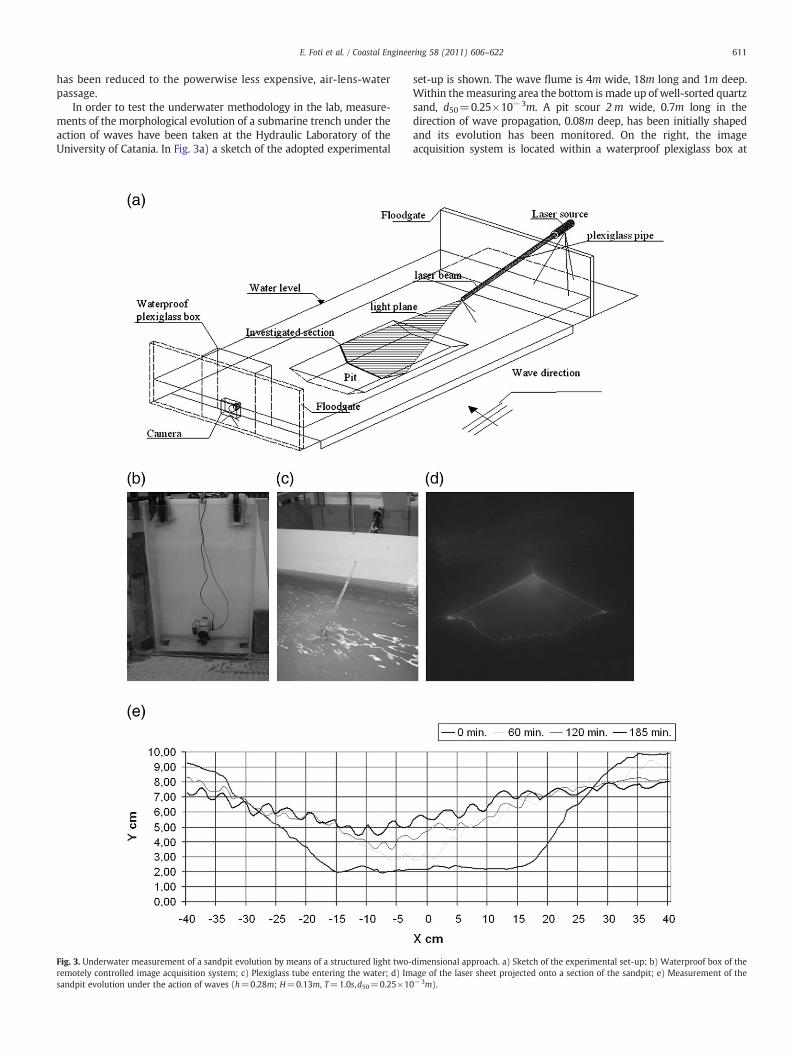
In order to test the underwater methodology in the lab, measure-ments of the morphological evolution of a submarine trench under theaction of waves have been taken at the Hydraulic Laboratory of theUniversity of Catania. In Fig. 3a) a sketch of the adopted experimental

Fig. 3. Underwater measurement of a sandpit evolution by means of a structured light two-remotely controlled image acquisition system; c) Plexiglass tube entering the water; d) Imsandpit evolution under the action of waves (h=0.28m; H=0.13m, T=1.0s,d50=0.25×10

set-up is shown. The wave flume is 4m wide, 18m long and 1m deep.Within themeasuring area the bottom is made up of well-sorted quartzsand, d50=0.25×10−3m. A pit scour 2 m wide, 0.7m long in thedirection of wave propagation, 0.08m deep, has been initially shapedand its evolution has been monitored. On the right, the imageacquisition system is located within a waterproof plexiglass box at

dimensional approach. a) Sketch of the experimental set-up; b) Waterproof box of theage of the laser sheet projected onto a section of the sandpit; e) Measurement of the−3m).

612 E. Foti et al. / Coastal Engineering 58 (2011) 606–622

one side of the wave flume. The camera used is a 3.1MegaPixel FujifilmFinePix S3000. The shape and the section of the box have been designedin order tominimize the disturbance to the flow and to permit a remotecontrol of the camera. A picture of the adopted waterproof box isreported in Fig. 3b).On the left, thepositionof the laser projector and thecouplingwith the plexiglass pipe are shown, as reported also in Fig. 3c).The 10 mWlaser generator produces a red light beam,withwavelengthin the range of 625-749 nm and with beam diameter of 0.8 mm. Thecylindrical lens is produced by Edmund Optics and it allows a 60∘

deviation of the incident light ray to produce the light sheet. It should bepointed out that the optical system, though quite stable during theexperiments, has to be carefully aligned at the beginning. Moreover itshould be emphasized that the small dimension of the plexiglass pipepermits to limit as much as possible disturbances to the flow. Finally inFig. 3d) an image of the final morphology of the scour, as evidenced bythe laser light sheet, is displayed, whereas Fig. 3e reports theexperimental data on the sandpit morphology at different time stepsfor an extreme case, during which the scour was washed out by thewave action and sandforms were formed.

3.2. Extension to large wave flume application of the 3D system

From the hydro-morphodynamic point of view, the use of close-to-prototype-scale models is extremely important in order to controlscale effects. However, undesired side effects are always presents, forexample during movable bed experiments a lot of suspension may bepresent, creating additional noise for optical measurements. More-over there are a number of technical optical problems related to thelarger field view, such as camera resolution, power of the lightgenerator and distance from the surface to the cameras, along withdifficulties related to the different conditions of the experimentalenvironment, such as water quality, ambient light, proper definitionof the experimental set-up. Indeed, while the above mentioned issuescan be more or less easily faced in smaller facilities, in larger facilitiesthey may become so important to partially or completely inhibit theuse of optical measuring methodologies.

In the case being, beforemoving to the large wave flume, a numberof preliminary dry tests have been carried out at the University ofCatania, by placing four cameras 5 m far from the target objects to bemeasured, a distance which was similar to the one to be used at largescale. Different set-ups of the cameras have been tested and it turnedout that, even though no rigid constraints are required, a reasonablygood positioning of the cameras is obtained when they face themeasuring surface more or less perpendicularly and when theiroptical axes are almost parallel. Such a set-up allows the matrix of the

Fig. 4. Laser grids projected onto a sandy bottom produced a) by a Gaussian diffractive lens,work.

linear system of Eq. (7) to be well conditioned and the measuringerrors to be comprised in the range of 0.01÷0.02m along the vertical.Moreover it has been verified that increasing the number of theadopted cameras, from the classical two cameras up to four, couldhelp to improve the measurement accuracy. However, the reductionof the measuring error, although sensible, is not dramatic since theerrors remain of the same order with respect to adopting only twocameras, i.e. O(0.01m). Hence, two cameras have been usedthroughout the experiments also at the large wave flume.

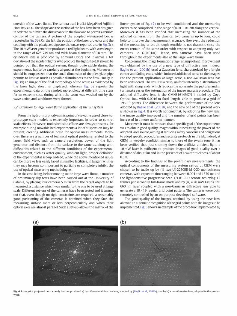
Concerning the image formation stage, an important improvementwas obtained by the use of a new type of diffractive lens. Indeed,Baglio et al. (2001b) used a Gaussian lens, characterized by a brightcenter and fading ends, which induced additional noise to the images.For the present application at large scale, a non-Gaussian lens hasbeen considered. The result is a crisp, uniform intensity distribution oflight with sharp ends, which reduces the noise into the pictures and inturn make easier the automation of the image analysis procedure. Theadopted diffractive lens is the GMN31614MCN-1 model by GoyoOptical Inc., with 0.0016 m focal length, able to produce a grid of19×19 points. The difference between the performance of the lensadopted by Baglio et al. (2001b) and the new one of the present workis shown in Fig. 4. It is worth noticing that, by adopting the new lens,the image quality improved and the number of grid points has beenincreased in a more uniform manner.

Moreover, it must be stressed that a specific goal of the experimentswas to obtain good quality images without increasing the power of theadopted laser source, aimingat reducing safety concerns andobligationsto adopt specific procedures and security protocols in the lab. Indeed, atCIEM, in wet-dry condition similar to those of the swash zone, it hasbeen verified that, just shutting down the artificial ambient light, a10 mW laser is sufficient to produce images of good quality over adistance of about 5m and in the presence of a water thickness of about0.5m.

According to the findings of the preliminary measurements, theoptical components of the measuring system set-up at CIEM werechosen to be made up by (i) two UI-2250RE-M CCD monochromecameras, with exposure time ranging between 0.094 and 1570 ms andthe light-sensitive progressive scan 1/1.8” CCD sensor achieving 12frames per second in full-frame mode and by (ii) a 20 mW Lasiris SNF660 nm laser coupled with a non-Gaussian diffractive lens able togenerate a 19×19 regular grid point pattern. The cameras were bothremotely controlled by an on purpose developed software.

The good quality of the images, obtained by using the new lens,allowed an automatic recognition of the grid points onto the images to beimplemented. Fig. 5 shows an example of the procedure implemented by

adopted by (Baglio et al., 2001b), and by b) a non-Gaussian lens, adopted in the present

Fig. 5. Automatic detection of the structured light grid points onto the images: a) original grayscale image; b) top-hat image; c) black and white image; d) centroids of the laser grid.

613E. Foti et al. / Coastal Engineering 58 (2011) 606–622

meansof aMatlab script for recovering thepositionof thegridpoints. Theoriginal image (see Fig. 5a) is filtered bymeans of a Gaussian filter and ofa morphological top hat filter, performed by using a circular structuringelement,whosediameter is comparable to the size of the grid points ontothe image (see Fig. 5b). Thus, the image is converted into a black andwhite image, which is again morphologically treated to obtain only theinterestinggridpoints (see Fig. 5c). Finally, thepositionof the centroidsofthewhite areas is determinedbymeasuring thegeometrical properties ofeach single region (see Fig. 5d).

At CIEM, the optimal placement of the cameras has beendetermined by analyzing three different positions with respect tothe sandy bed surface, namely with (i) the cameras 1m far from eachother, symmetric with respect to the laser projector, the entire systembeing located at about 3m from the bottom surface; (ii) the camerasmore distant from each other and asymmetricwith respect to the laserprojector, one camera being 2m far from the laser; (iii) the cameraslocatedmuch heigherwith respect to the laser projector, about 3m far.

A detailed investigation has been carried out at CIEM regarding thecalibration procedure that needs to be performed in order to obtainswash zone measurements. In particular, in order to determine theappropriate shape and size of the calibration tool to be used, but alsoto perform a sensitive analysis on the calibration procedure itself,unevenly spaced industrially shaped plastic blocks have been gluedonto a rigid board (see Fig. 6). Rather than constructing in-house thecalibration tool, the use of such sharp coloured blocks, which havevery well-controlled dimensions, offer the possibility to easily changeboth shape and dimensions of the tool itself, according to theexperimental needs (Nielsen, 2007). Moreover, the calibration

arrangement shown in Fig. 6 provides the possibility to have a sparseensemble of points within the measurement area which can be usedeither as calibration points or as known points, to estimate themeasuring errors.

The tool has been then located in themeasuring area and a numberranging from 42 up to 150 points has been used to calibrate the stereopairs. Indeed, the subplots of Fig. 6 show the regions which have beenconsidered as calibration regions, meaning that the image coordinatesof the corners of the blocks, which can be clearly detected onto theimages by comparison with the dark background, have been used todetermine the calibration matrices A1 and A2 in Eq. (7). In particular,the three set-ups of the cameras previously described have been usedin conjunction with the two configurations of the calibration tool,with one and two layers of plastic blocks respectively, leading to sixset-up, as reported in Table 1. Therefore, by using the SLSV approach,all the relevant points of the calibration tool have been reconstructedduring each test, by using as calibration points only those comingfrom the areas highlighted in Fig. 6.

Error maps, i.e. the spatial distributions of the global e on the 3Dcoordinate of each point of the calibration tool, have been obtained foreach set-up, where e is calculated as

e =ffiffiffiffiffiffiffiffiffiffiffiffiffiffiffiffiffiffiffiffiffiffiffiffiffiffiffiffiffiffie2X + e2Y + e2Z

qð8Þ

with eX,eY and eZ being the errors on the single world coordinates ofthe point (X,Y,Z).

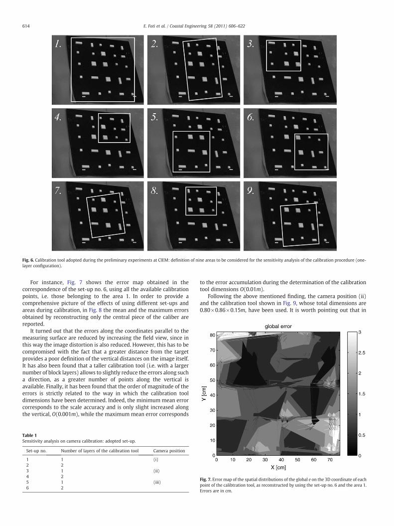
Fig. 6. Calibration tool adopted during the preliminary experiments at CIEM: definition of nine areas to be considered for the sensitivity analysis of the calibration procedure (one-layer configuration).

614 E. Foti et al. / Coastal Engineering 58 (2011) 606–622

For instance, Fig. 7 shows the error map obtained in thecorrespondence of the set-up no. 6, using all the available calibrationpoints, i.e. those belonging to the area 1. In order to provide acomprehensive picture of the effects of using different set-ups andareas during calibration, in Fig. 8 the mean and the maximum errorsobtained by reconstructing only the central piece of the caliber arereported.

It turned out that the errors along the coordinates parallel to themeasuring surface are reduced by increasing the field view, since inthis way the image distortion is also reduced. However, this has to becompromised with the fact that a greater distance from the targetprovides a poor definition of the vertical distances on the image itself.It has also been found that a taller calibration tool (i.e. with a largernumber of block layers) allows to slightly reduce the errors along sucha direction, as a greater number of points along the vertical isavailable. Finally, it has been found that the order of magnitude of theerrors is strictly related to the way in which the calibration tooldimensions have been determined. Indeed, the minimum mean errorcorresponds to the scale accuracy and is only slight increased alongthe vertical, O(0.001m), while the maximum mean error corresponds

Table 1Sensitivity analysis on camera calibration: adopted set-up.

Set-up no. Number of layers of the calibration tool Camera position

1 1 (i)2 23 1 (ii)4 25 1 (iii)6 2

to the error accumulation during the determination of the calibrationtool dimensions O(0.01m).

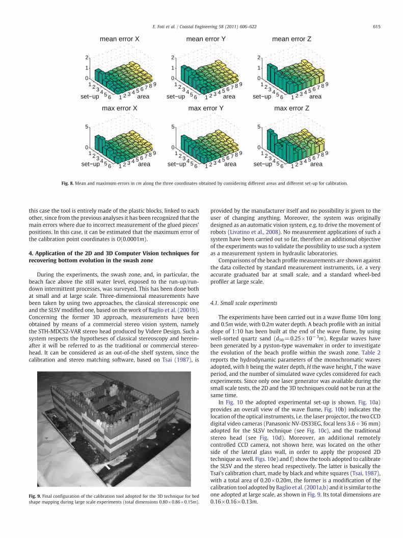
Following the above mentioned finding, the camera position (ii)and the calibration tool shown in Fig. 9, whose total dimensions are0.80×0.86×0.15m, have been used. It is worth pointing out that in

Fig. 7. Error map of the spatial distributions of the global e on the 3D coordinate of eachpoint of the calibtration tool, as reconstructed by using the set-up no. 6 and the area 1.Errors are in cm.

1 2 3 4 5 6 7 8 91 2 3 4 5 6

0

1

2

area

mean error X

set−up 1 2 3 4 5 6 7 8 91 2 3 4 5 6

0

1

2

areaset−up 1 2 3 4 5 6 7 8 91 2 3 4 5 6

0

1

2

areaset−up

mean error Y mean error Z

1 2 3 4 5 6 7 8 91 2 3 4 5 6

0

5

area

max error X

set−up 1 2 3 4 5 6 7 8 91 2 3 4 5 6

0

5

areaset−up 1 2 3 4 5 6 7 8 91 2 3 4 5 6

0

5

areaset−up

max error Y max error Z

Fig. 8. Mean and maximum errors in cm along the three coordinates obtained by considering different areas and different set-up for calibration.

615E. Foti et al. / Coastal Engineering 58 (2011) 606–622

this case the tool is entirely made of the plastic blocks, linked to eachother, since from the previous analyses it has been recognized that themain errors where due to incorrect measurement of the glued pieces'positions. In this case, it can be estimated that the maximum error ofthe calibration point coordinates is O(0.0001m).

4. Application of the 2D and 3D Computer Vision techniques forrecovering bottom evolution in the swash zone

During the experiments, the swash zone, and, in particular, thebeach face above the still water level, exposed to the run-up/run-down intermittent processes, was surveyed. This has been done bothat small and at large scale. Three-dimensional measurements havebeen taken by using two approaches, the classical stereoscopic oneand the SLSVmodified one, based on the work of Baglio et al. (2001b).Concerning the former 3D approach, measurements have beenobtained by means of a commercial stereo vision system, namelythe STH-MDCS2-VAR stereo head produced by Videre Design. Such asystem respects the hypotheses of classical stereoscopy and herein-after it will be referred to as the traditional or commercial stereo-head. It can be considered as an out-of-the shelf system, since thecalibration and stereo matching software, based on Tsai (1987), is

Fig. 9. Final configuration of the calibration tool adopted for the 3D technique for bedshape mapping during large scale experiments (total dimensions 0.80×0.86×0.15m).

provided by the manufacturer itself and no possibility is given to theuser of changing anything. Moreover, the system was originallydesigned as an automatic vision system, e.g. to drive the movement ofrobots (Livatino et al., 2008). No measurement applications of such asystem have been carried out so far, therefore an additional objectiveof the experiments was to validate the possibility to use such a systemas a measurement system in hydraulic laboratories.

Comparisons of the beach profile measurements are shown againstthe data collected by standard measurement instruments, i.e. a veryaccurate graduated bar at small scale, and a standard wheel-bedprofiler at large scale.

4.1. Small scale experiments

The experiments have been carried out in a wave flume 10m longand 0.5mwide, with 0.2mwater depth. A beach profile with an initialslope of 1:10 has been built at the end of the wave flume, by usingwell-sorted quartz sand (d50=0.25×10−3m). Regular waves havebeen generated by a pyston-type wavemaker in order to investigatethe evolution of the beach profile within the swash zone. Table 2reports the hydrodynamic parameters of the monochromatic wavesadopted, with h being the water depth, H the wave height, T the waveperiod, and the number of simulated wave cycles considered for eachexperiments. Since only one laser generator was available during thesmall scale tests, the 2D and the 3D techniques could not be run at thesame time.

In Fig. 10 the adopted experimental set-up is shown. Fig. 10a)provides an overall view of the wave flume, Fig. 10b) indicates thelocation of the optical instruments, i.e. the laser projector, the two CCDdigital video cameras (Panasonic NV-DS33EG, focal lens 3.6÷36 mm)adopted for the SLSV technique (see Fig. 10c), and the traditionalstereo head (see Fig. 10d). Moreover, an additional remotelycontrolled CCD camera, not shown here, was located on the otherside of the lateral glass wall, in order to apply the proposed 2Dtechnique as well. Figs. 10e) and f) show the tools adopted to calibratethe SLSV and the stereo head respectively. The latter is basically theTsai's calibration chart, made by black and white squares (Tsai, 1987),with a total area of 0.20×0.20m, the former is a modification of thecalibration tool adoptedbyBaglio et al. (2001a,b) and it is similar to theone adopted at large scale, as shown in Fig. 9. Its total dimensions are0.16×0.16×0.13m.

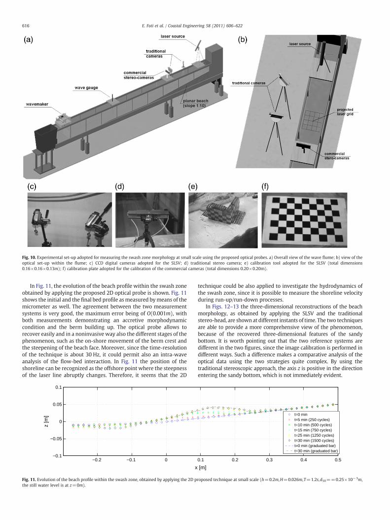
Fig. 10. Experimental set-up adopted for measuring the swash zone morphology at small scale using the proposed optical probes. a) Overall view of the wave flume; b) view of theoptical set-up within the flume; c) CCD digital cameras adopted for the SLSV; d) traditional stereo camera; e) calibration tool adopted for the SLSV (total dimensions0.16×0.16×0.13m); f) calibration plate adopted for the calibration of the commercial cameras (total dimensions 0.20×0.20m).

616 E. Foti et al. / Coastal Engineering 58 (2011) 606–622

In Fig. 11, the evolution of the beach profile within the swash zoneobtained by applying the proposed 2D optical probe is shown. Fig. 11shows the initial and the final bed profile as measured bymeans of themicrometer as well. The agreement between the two measurementsystems is very good, the maximum error being of O(0.001m), withboth measurements demonstrating an accretive morphodynamiccondition and the berm building up. The optical probe allows torecover easily and in a noninvasive way also the different stages of thephenomenon, such as the on-shore movement of the berm crest andthe steepening of the beach face. Moreover, since the time-resolutionof the technique is about 30 Hz, it could permit also an intra-waveanalysis of the flow-bed interaction. In Fig. 11 the position of theshoreline can be recognized as the offshore point where the steepnessof the laser line abruptly changes. Therefore, it seems that the 2D

−0.2 −0.1 0−0.1

−0.05

0

0.05

0.1

x

z [m

]

Fig. 11. Evolution of the beach profile within the swash zone, obtained by applying the 2D pthe still water level is at z=0m).

technique could be also applied to investigate the hydrodynamics ofthe swash zone, since it is possible to measure the shoreline velocityduring run-up/run-down processes.

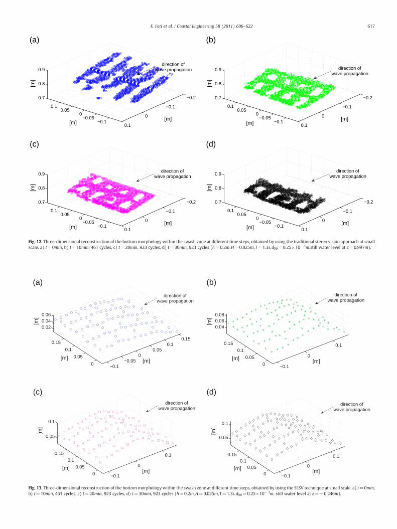
In Figs. 12–13 the three-dimensional reconstructions of the beachmorphology, as obtained by applying the SLSV and the traditionalstereo-head, are shown at different instants of time. The two techniquesare able to provide a more comprehensive view of the phenomenon,because of the recovered three-dimensional features of the sandybottom. It is worth pointing out that the two reference systems aredifferent in the two figures, since the image calibration is performed indifferent ways. Such a difference makes a comparative analysis of theoptical data using the two strategies quite complex. By using thetraditional stereoscopic approach, the axis z is positive in the directionentering the sandy bottom, which is not immediately evident.

0.1 0.2 0.3 0.4 0.5

[m]

t=0 mint=5 min (250 cycles)t=10 min (500 cycles)t=15 min (750 cycles)t=25 min (1250 cycles)t=30 min (1500 cycles)t=0 min (graduated bar)t=30 min (graduated bar)

roposed technique at small scale (h=0.2m,H=0.026m,T=1.2s,d50==0.25×10−3m,

−0.1−0.05

00.05

0.1

−0.2

−0.1

0

0.1

0.7

0.8

0.9

[m]

(a)

[m]

[m]

−0.1−0.05

00.05

0.1

−0.2

−0.1

0

0.1

0.7

0.8

0.9

[m]

(b)

[m]

[m]

−0.1−0.05

00.05

0.1

−0.2

−0.1

0

0.1

0.7

0.8

0.9

[m]

(c)

[m]

[m]

−0.1−0.05

00.05

0.1

−0.2

−0.1

0

0.1

0.7

0.8

0.9

[m]

(d)

[m]

[m]

direction ofwave propagation direction of

wave propagation

direction ofwave propagation

direction ofwave propagation

Fig. 12. Three-dimensional reconstruction of the bottommorphology within the swash zone at different time steps, obtained by using the traditional stereo vision approach at smallscale. a) t=0min, b) t=10min, 461 cycles, c) t=20min, 923 cycles, d) t=30min, 923 cycles (h=0.2m,H=0.025m,T=1.3s,d50=0.25×10−3m,still water level at z=0.997m).

−0.1−0.05

00.05

0.10.15

0

0.05

0.1

0.15

0.020.040.06

[m]

(a)

[m]

[m]

−0.1

0

0.1

0

0.05

0.1

0.15

0.040.060.08

[m]

(b)

[m]

[m]

−0.1

0

0.1

0

0.05

0.1

0.15

0.05

0.1

[m]

(c)

[m]

[m]

−0.1

0

0.1

00.05

0.10.15

0.05

0.1

[m]

(d)

[m]

[m]

direction ofwave propagation

direction ofwave propagation

direction ofwave propagation

direction ofwave propagation

Fig. 13. Three-dimensional reconstruction of the bottommorphology within the swash zone at different time steps, obtained by using the SLSV technique at small scale. a) t=0min,b) t=10min, 461 cycles, c) t=20min, 923 cycles, d) t=30min, 923 cycles (h=0.2m,H=0.025m,T=1.3s,d50=0.25×10−3m, still water level at z=−0.246m).

617E. Foti et al. / Coastal Engineering 58 (2011) 606–622

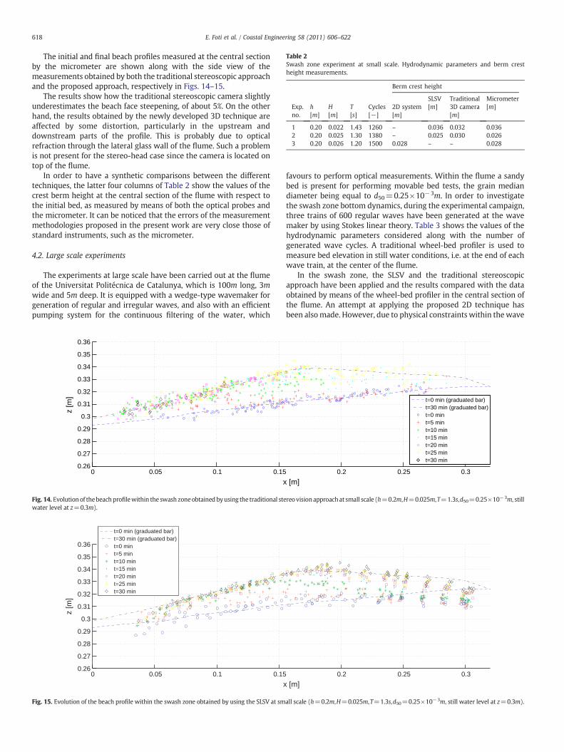
Table 2Swash zone experiment at small scale. Hydrodynamic parameters and berm crestheight measurements.

Berm crest height

SLSV Traditional MicrometerExp.no.

h H T Cycles 2D system [m] 3D camera [m][m] [m] [s] [−] [m] [m]

1 0.20 0.022 1.43 1260 – 0.036 0.032 0.0362 0.20 0.025 1.30 1380 – 0.025 0.030 0.0263 0.20 0.026 1.20 1500 0.028 – – 0.028

618 E. Foti et al. / Coastal Engineering 58 (2011) 606–622

The initial and final beach profiles measured at the central sectionby the micrometer are shown along with the side view of themeasurements obtained by both the traditional stereoscopic approachand the proposed approach, respectively in Figs. 14–15.

The results show how the traditional stereoscopic camera slightlyunderestimates the beach face steepening, of about 5%. On the otherhand, the results obtained by the newly developed 3D technique areaffected by some distortion, particularly in the upstream anddownstream parts of the profile. This is probably due to opticalrefraction through the lateral glass wall of the flume. Such a problemis not present for the stereo-head case since the camera is located ontop of the flume.

In order to have a synthetic comparisons between the differenttechniques, the latter four columns of Table 2 show the values of thecrest berm height at the central section of the flume with respect tothe initial bed, as measured by means of both the optical probes andthe micrometer. It can be noticed that the errors of the measurementmethodologies proposed in the present work are very close those ofstandard instruments, such as the micrometer.

4.2. Large scale experiments

The experiments at large scale have been carried out at the flumeof the Universitat Politécnica de Catalunya, which is 100m long, 3mwide and 5m deep. It is equipped with a wedge-type wavemaker forgeneration of regular and irregular waves, and also with an efficientpumping system for the continuous filtering of the water, which

0 0.05 0.1 0.150.26

0.27

0.28

0.29

0.3

0.31

0.32

0.33

0.34

0.35

0.36

x

z [m

]

Fig. 14. Evolutionof thebeachprofilewithin the swash zoneobtainedbyusing the traditional stewater level at z=0.3m).

0 0.05 0.1 0.150.26

0.27

0.28

0.29

0.3

0.31

0.32

0.33

0.34

0.35

0.36

x

z [m

]

t=0 min (graduated bar)t=30 min (graduated bar)t=0 mint=5 mint=10 mint=15 mint=20 mint=25 mint=30 min

Fig. 15. Evolution of the beach profile within the swash zone obtained by using the SLSV at sm

favours to perform optical measurements. Within the flume a sandybed is present for performing movable bed tests, the grain mediandiameter being equal to d50=0.25×10−3m. In order to investigatethe swash zone bottom dynamics, during the experimental campaign,three trains of 600 regular waves have been generated at the wavemaker by using Stokes linear theory. Table 3 shows the values of thehydrodynamic parameters considered along with the number ofgenerated wave cycles. A traditional wheel-bed profiler is used tomeasure bed elevation in still water conditions, i.e. at the end of eachwave train, at the center of the flume.

In the swash zone, the SLSV and the traditional stereoscopicapproach have been applied and the results compared with the dataobtained by means of the wheel-bed profiler in the central section ofthe flume. An attempt at applying the proposed 2D technique hasbeen alsomade. However, due to physical constraints within thewave

0.2 0.25 0.3

[m]

t=0 min (graduated bar)t=30 min (graduated bar)t=0 mint=5 mint=10 mint=15 mint=20 mint=25 mint=30 min

reovisionapproachat small scale (h=0.2m,H=0.025m,T=1.3s,d50=0.25×10−3m, still

0.2 0.25 0.3

[m]

all scale (h=0.2m,H=0.025m,T=1.3s,d50=0.25×10−3m, still water level at z=0.3m).

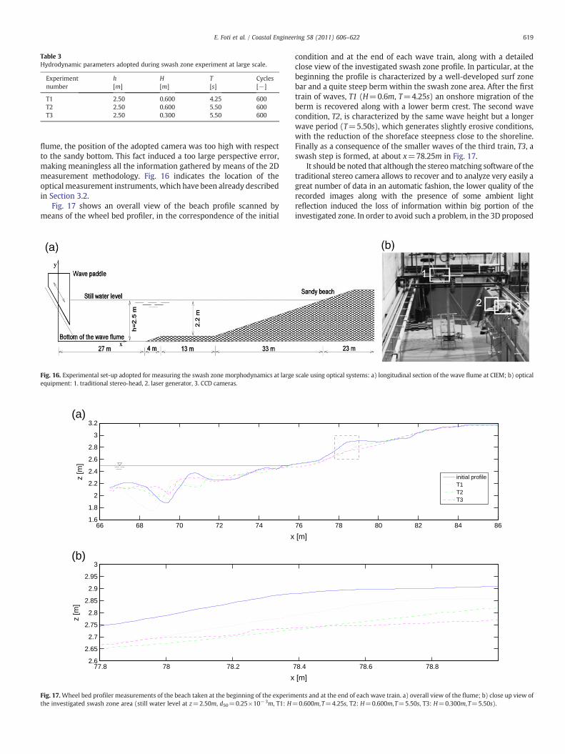
Table 3Hydrodynamic parameters adopted during swash zone experiment at large scale.

Experimentnumber

h[m]

H[m]

T[s]

Cycles[−]

T1 2.50 0.600 4.25 600T2 2.50 0.600 5.50 600T3 2.50 0.300 5.50 600

619E. Foti et al. / Coastal Engineering 58 (2011) 606–622

flume, the position of the adopted camera was too high with respectto the sandy bottom. This fact induced a too large perspective error,making meaningless all the information gathered by means of the 2Dmeasurement methodology. Fig. 16 indicates the location of theoptical measurement instruments, which have been already describedin Section 3.2.

Fig. 17 shows an overall view of the beach profile scanned bymeans of the wheel bed profiler, in the correspondence of the initial

Fig. 16. Experimental set-up adopted for measuring the swash zone morphodynamics at largeequipment: 1. traditional stereo-head, 2. laser generator, 3. CCD cameras.

66 68 70 72 741.6

1.8

2

2.2

2.4

2.6

2.8

3

3.2

x

z [m

]

(a)

77.8 78 78.22.6

2.65

2.7

2.75

2.8

2.85

2.9

2.95

3

x

z [m

]

(b)

Fig. 17.Wheel bed profiler measurements of the beach taken at the beginning of the experimthe investigated swash zone area (still water level at z=2.50m, d50=0.25×10−3m, T1: H=

condition and at the end of each wave train, along with a detailedclose view of the investigated swash zone profile. In particular, at thebeginning the profile is characterized by a well-developed surf zonebar and a quite steep berm within the swash zone area. After the firsttrain of waves, T1 (H=0.6m, T=4.25s) an onshore migration of theberm is recovered along with a lower berm crest. The second wavecondition, T2, is characterized by the same wave height but a longerwave period (T=5.50s), which generates slightly erosive conditions,with the reduction of the shoreface steepness close to the shoreline.Finally as a consequence of the smaller waves of the third train, T3, aswash step is formed, at about x=78.25m in Fig. 17.

It should be noted that although the stereomatching software of thetraditional stereo camera allows to recover and to analyze very easily agreat number of data in an automatic fashion, the lower quality of therecorded images along with the presence of some ambient lightreflection induced the loss of information within big portion of theinvestigated zone. In order to avoid such a problem, in the 3D proposed

scale using optical systems: a) longitudinal section of the wave flume at CIEM; b) optical

76 78 80 82 84 86

[m]

initial profileT1T2T3

78.4 78.6 78.8

[m]

ents and at the end of each wave train. a) overall view of the flume; b) close up view of0.600m,T=4.25s, T2: H=0.600m,T=5.50s, T3: H=0.300m,T=5.50s).

77.8 78 78.2 78.4 78.6 78.8 792.6

2.65

2.7

2.75

2.8

2.85

2.9

2.95

3

x [m]

z [m

]initial profileT1T2T3initial profile (profiler)T1 (profiler)T2 (profiler)T3 (profiler)

Fig. 18. Large scale experiments: beach profile within the swash zone obtained by both the wheel bed profiler and by using the traditional stereo camera (still water level at z=2.5m,d50=0.25×10−3m, T1: H=0.600m,T=4.25s, T2: H=0.600m,T=5.50s, T3: H=0.300m,T=5.50s).

620 E. Foti et al. / Coastal Engineering 58 (2011) 606–622

technique the identification of the laser grid points is controlled by theoperator, which leads to a more consistent set of data.

The side view of the same data along the direction of wavepropagation are plotted in Figs. 18–19 compared with those collectedby the profiler at the same phases. Fig. 18 shows that the traditionalstereo camera leads not only to a great dispersion of the results, butalso to some large mistakes; as, for example, for the T1 case. Besides,although the trend of the movement of the bottom seems to agreewith the bottom profiler results, the quantification of the morpho-logical change of the bed seems to be generally underestimated. Theresults obtained by using the proposed technique seems to be moreconsistent with the profiler data. Indeed the dispersion of theexperimental measurement is reduced, the slopes of the surfaceprofiles are better represented, and the sandy bed changes appears tobe quantitatively similar to the one measured in a standard way.Similarly to the small scale experiments a deviation of the results ispresent in the offshore part of the profile, i.e. in the furthest zone ofthe images, where according to Baglio et al. (2001a,b) the perspectiveerrors are greater.

A comparison of the measures obtained from images with thoseobtained by the wheel-bed profiler was made, by consideringdifferent transect. To this aim, three-dimensional effects on thebottom morphology of the wave flume have been considered asnegligible, and all the errors have been attributed only to the opticaltechniques. Hence, in order to calculate the absolute vertical errors

77.8 78 78.22.6

2.65

2.7

2.75

2.8

2.85

2.9

2.95

3

x

z [m

]

initial profileT1T2T3initial profile (profiler)T1 (profiler)T2 (profiler)T3 (profiler)

Fig. 19. Large scale experiments: beach profile within the swash zone obtained by both the wH=0.600m,T=4.25s, T2: H=0.600m,T=5.50s, T3: H=0.300m,T=5.50s).

along the x direction, the reference values of the bed elevation at suchtransects have been obtained through a 2D polynomial best fit of eachone of the measured sets of 3D optical data. The results are shown inTable 4 with reference to the system adopted in Fig. 19, namely at thesections located at x=78.1,78.3,78.5,78.7m. In particular at the firstsection no data from the SLSV were available. The absolute errors, i.e.the differences between the CV measurements and the data comingfrom the profile, have been computed and the results are shown inFig. 20. The two techniques provide generally fair results, withmaximum absolute errors of O(10cm). However, the SLSV approachseems to behave better, since the maximum error is halved withrespect to the traditional stereo method, being of about 5% instead of10% of the overall linear extension of the investigated area. Thegreatest errors are obtained at section z=78.7m, confirming thetendency to the distortion of the proposed measurement strategy inthe furthest field. Instead, as regards the method using the traditionalstereo-head, such large errors are related to the difficulty of thecommercial software to perform the stereo matching on texture freesurfaces, such as the sandy bottom. This causes a wrong computationof the disparity coefficients, necessary for the determination of the 3Dcoordinates of the measuring points, and in turn the 3D reconstruc-tion of the measuring area appears as a cloud of very sparse 3Dcoordinates. Moreover, as shown in Fig. 18, the commercial softwareis not able to recover large portion of the investigated area, due topoor quality of the images.

78.4 78.6 78.8 79

[m]

heel bed profiler and by using SLSV (still water level at z=2.5m, d50=0.25×10−3m, T1:

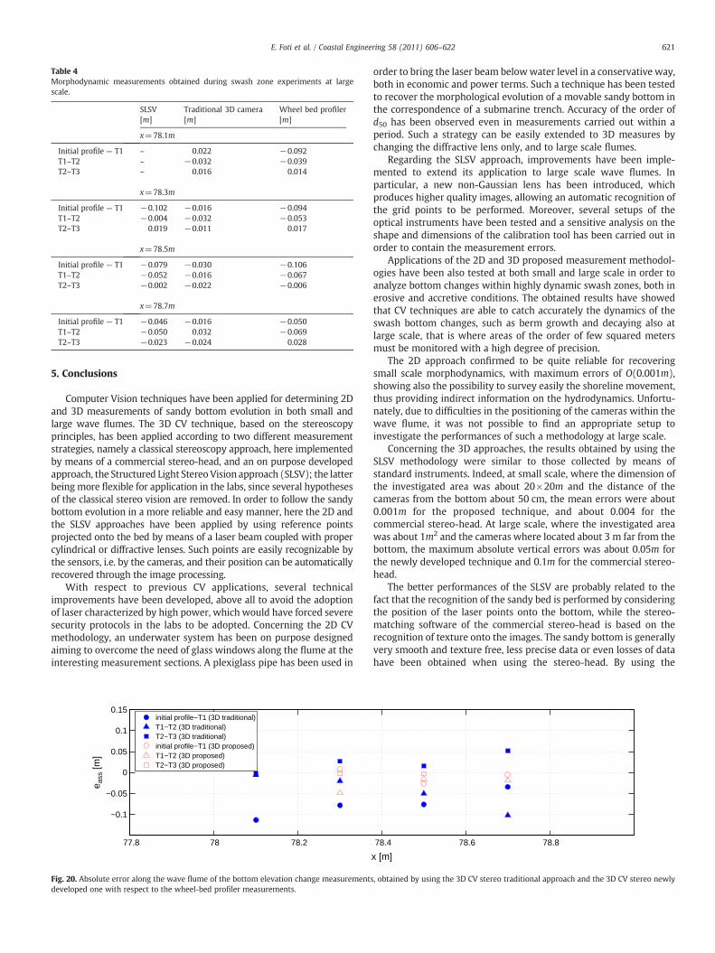
Table 4Morphodynamic measurements obtained during swash zone experiments at largescale.

SLSV[m]

Traditional 3D camera[m]

Wheel bed profiler[m]

x=78.1m

Initial profile — T1 – 0.022 −0.092T1–T2 – −0.032 −0.039T2–T3 – 0.016 0.014

x=78.3m

Initial profile — T1 −0.102 −0.016 −0.094T1–T2 −0.004 −0.032 −0.053T2–T3 0.019 −0.011 0.017

x=78.5m

Initial profile — T1 −0.079 −0.030 −0.106T1–T2 −0.052 −0.016 −0.067T2–T3 −0.002 −0.022 −0.006

x=78.7m

Initial profile — T1 −0.046 −0.016 −0.050T1–T2 −0.050 0.032 −0.069T2–T3 −0.023 −0.024 0.028

621E. Foti et al. / Coastal Engineering 58 (2011) 606–622

5. Conclusions

Computer Vision techniques have been applied for determining 2Dand 3D measurements of sandy bottom evolution in both small andlarge wave flumes. The 3D CV technique, based on the stereoscopyprinciples, has been applied according to two different measurementstrategies, namely a classical stereoscopy approach, here implementedby means of a commercial stereo-head, and an on purpose developedapproach, the Structured Light Stereo Vision approach (SLSV); the latterbeing more flexible for application in the labs, since several hypothesesof the classical stereo vision are removed. In order to follow the sandybottom evolution in a more reliable and easy manner, here the 2D andthe SLSV approaches have been applied by using reference pointsprojected onto the bed by means of a laser beam coupled with propercylindrical or diffractive lenses. Such points are easily recognizable bythe sensors, i.e. by the cameras, and their position can be automaticallyrecovered through the image processing.

With respect to previous CV applications, several technicalimprovements have been developed, above all to avoid the adoptionof laser characterized by high power, which would have forced severesecurity protocols in the labs to be adopted. Concerning the 2D CVmethodology, an underwater system has been on purpose designedaiming to overcome the need of glass windows along the flume at theinteresting measurement sections. A plexiglass pipe has been used in

77.8 78 78.2

−0.1

−0.05

0

0.05

0.1

0.15

e ass

[m]

initial profile−T1 (3D traditional)T1−T2 (3D traditional)T2−T3 (3D traditional)initial profile−T1 (3D proposed)T1−T2 (3D proposed)T2−T3 (3D proposed)

Fig. 20. Absolute error along the wave flume of the bottom elevation change measurementsdeveloped one with respect to the wheel-bed profiler measurements.

order to bring the laser beam belowwater level in a conservative way,both in economic and power terms. Such a technique has been testedto recover the morphological evolution of a movable sandy bottom inthe correspondence of a submarine trench. Accuracy of the order ofd50 has been observed even in measurements carried out within aperiod. Such a strategy can be easily extended to 3D measures bychanging the diffractive lens only, and to large scale flumes.

Regarding the SLSV approach, improvements have been imple-mented to extend its application to large scale wave flumes. Inparticular, a new non-Gaussian lens has been introduced, whichproduces higher quality images, allowing an automatic recognition ofthe grid points to be performed. Moreover, several setups of theoptical instruments have been tested and a sensitive analysis on theshape and dimensions of the calibration tool has been carried out inorder to contain the measurement errors.

Applications of the 2D and 3D proposed measurement methodol-ogies have been also tested at both small and large scale in order toanalyze bottom changes within highly dynamic swash zones, both inerosive and accretive conditions. The obtained results have showedthat CV techniques are able to catch accurately the dynamics of theswash bottom changes, such as berm growth and decaying also atlarge scale, that is where areas of the order of few squared metersmust be monitored with a high degree of precision.

The 2D approach confirmed to be quite reliable for recoveringsmall scale morphodynamics, with maximum errors of O(0.001m),showing also the possibility to survey easily the shoreline movement,thus providing indirect information on the hydrodynamics. Unfortu-nately, due to difficulties in the positioning of the cameras within thewave flume, it was not possible to find an appropriate setup toinvestigate the performances of such a methodology at large scale.

Concerning the 3D approaches, the results obtained by using theSLSV methodology were similar to those collected by means ofstandard instruments. Indeed, at small scale, where the dimension ofthe investigated area was about 20×20m and the distance of thecameras from the bottom about 50 cm, the mean errors were about0.001m for the proposed technique, and about 0.004 for thecommercial stereo-head. At large scale, where the investigated areawas about 1m2 and the cameras where located about 3 m far from thebottom, the maximum absolute vertical errors was about 0.05m forthe newly developed technique and 0.1m for the commercial stereo-head.

The better performances of the SLSV are probably related to thefact that the recognition of the sandy bed is performed by consideringthe position of the laser points onto the bottom, while the stereo-matching software of the commercial stereo-head is based on therecognition of texture onto the images. The sandy bottom is generallyvery smooth and texture free, less precise data or even losses of datahave been obtained when using the stereo-head. By using the

78.4 78.6 78.8

x [m]

, obtained by using the 3D CV stereo traditional approach and the 3D CV stereo newly

622 E. Foti et al. / Coastal Engineering 58 (2011) 606–622

proposed approach, thanks to higher qualities of the cameras and tothe operator-assisted image analysis, no data losses were recorded.

Although the accuracy of the presented techniques is not very highat large scale with respect to other traditional measurementstrategies, because of the possibility to perform dynamic measure-ments without stopping the flow and of the very low cost of theadopted instrumentation, we are confident that the CV techniqueswill be more andmore diffused in experimental facilities to substitutethe use of traditional time-consuming instruments, such aswheel-bedprofilers as soon as an user-friendly automatic recognition and stereomatching of the laser dots will be available.

In particular, the future developments of the 3D technique aremainly related (i) to the modification of the solving linear algorithmto correct for lens distortion (ii) to further improvement of theautomatic recognition and stereo matching of the laser dots, whichwill allow also an easier analysis of a huge number of images.

Acknowledgements

This work has been partly funded in the framework of the EUresearch project HYDRALAB III- Joint Research Activity SANDS (contractno. 0224411(RII3)). Dr. Luca Cavallaro and Giovanni Paratore areacknowledged for carrying out some of the experiments on theunderwater system. Laura Stancanelli is also acknowledged forperforming part of the measurements obtained by means of thetraditional stereoscopic cameras.

References

Baglio, S., Faraci, C., Foti, E., Musumeci, R., 2001a. Analysis of small scale beforms with2D and 3D image acquisition techniques. Oceans 2001 IEEE InternationalConference, Honolulu, Hawaii,USA. 11-14 November 2001.

Baglio, S., Faraci, C., Foti, E., Musumeci, R., 2001b. Measurements of the 3D scour processaround a pile in an oscillating flow through a stereo vision approach. Measurement30 (2), 145–160.

Benetazzo, A., 2006. Measurements of short water waves using stereo matched imagesequences. Coastal Eng. 53, 1013–1032.

Brasington, J., Smart, M.A., 2003. Close range digital photogrammetric analysis ofexperimental drainage basin evolution. Earth Surf. Processes Landforms 28,231–247.

Cox, D., Tomita, T., Lynett, P., Holman, R., 2008. Tsunami inundation with macro-roughness in the constructed environment. Proc. Int. Conf. Coastal Eng. 1421–1432.

Dickerson, L.A., 1950. Stereogrammetric wave measurement. Bull. Beach Erosion Board4 (4), 40–45.

Duncan, J.R., 1964. The effects of water table and tide cycle on swash-backwashsediment distribution and beach profile development. Mar. Geol. 2, 186–197.

Elfrink, B., Baldock, T., 2002. Hydrodynamics and sediment transport in the swash zone:a review and perspectives. Coastal Eng. 45, 149–167.

Eliot, I.G., Clarke, D.J., 1986. Minor storm impact on the beach face of a sheltered sandybeach. Mar. Geol. 73, 61–83.

Faraci, C., Foti, E., 2001. Evolution of small scale regular patterns generated by wavespropagating over a sandy bottom. Phys. Fluids 13 (6), 1624–1634.

Faraci, C., Foti, E., 2002. Geometry, migration and evolution of small-scale bedformsgenerated by regular and irregular waves. Coastal Eng. 47, 35–52.

Faraci, C., Foti, E., Baglio, S., 2000. Measurements of sandy bed scour processes in anoscillating flow by using structured light. Measurements 28 (3), 159–174.

Hardisty, J., Collier, J., Hamilton, D., 1984. A calibration of the Bagnold beach equation.Mar. Geol. 61, 95–101.

Holland, K.T., Puleo, J.A., 2001. Variable swashmotions associatedwith foreshore profilechange. J. Geophys. Res. 106, 4613–4623.

Hughes, M.G., Turner, I., 1999. The beach face. In: Short, A.D. (Ed.), Handbook of Beachand Shoreface Morphodynamics. Wiley, Chichester, pp. 119–144.

Hughes, M., Masselink, G., Hanslow, D., Mitchell, D., 1997. Towards a betterunderstanding of swash zone sediment transport. Proceedings Coastal Dynamics.ASCE, pp. 804–823.

Jackson, N.L., Masselink, G., Nordstrom, K.F., 2004. The role of bore collapse and localshear stresses on the spatial distribution of sediment load in the uprush of anintermediate-state beach. Mar. Geol. 203, 109–118.

James, C.P., Brenninkmeyer, B.M., 1977. Sediment entrainment within bores andbackwash Geoscience and Man. Res. Coastal Env. 61–68.

Jarno-Druaux, A., Brossard, J., Marin, F., 2004. Dynamical evolution of ripples in a wavechannel. Eur. J. of Mech. B. Fluids 23, 695–708. doi:10.1016/j.euromechflu.2004.02.002.

Kroon, A., 1991. Suspended sediment concentrations in a barred near shore zone.Proceedings Coastal Sediments. ASCE, pp. 371–384.

Livatino, S., Muscato, G., Sessa, S., Köffel, C., Arena, C., Pennisi, A., Di Mauro, D.,Malkondu, E., 2008. Mobile robotic teleguide based on video images. ComparisonBetween Monoscopic and Stereoscopic Visualization. IEEE Rob. AutomMag. 15 (4),58–67.

Longo, S., Petti, M., Losada, I.J., 2002. Turbulence in the surf and swash zones: a review.Coastal Eng. 45, 129–147.

Masselink, G., Hughes, M., 1998. Field investigation of sediment transport in the swashzone. Cont. Shelf Res. 18, 1179–1199.

Masselink, G., Puleo, J.A., 2006. Swash-zone morphodynamics. Cont. Shelf Res. 26,661–680.

Masselink, G., Hegge, B.J., Pattiaratchi, C.B., 1997. Beach cusp morphodynamics. EarthSurf. Process. Land. 22, 1139–1155.

Nielsen, P., 2007. On the usage of industrially shaped plastic blocks in hydrauliclaboratories. Personal communication.

O'Donoghue, T., Doucette, J.S., van der Werf, J.J., Ribberink, J.S., 2006. The dimensions ofsand ripples in full-scale oscillatory flows. Coastal Eng. 53, 997–1012.

Pos, J.D., Adams, L.P., Kilner, F.A., 1988. Synoptic wave height and pattern measure-ments in laboratory wave basins using close-range photogrammetry. Photogramm.Eng. Remote Sens. 54 (12), 1749–1756.

Shemdin, O.H., Tran, H.M., 1992. Measuring short surface waves with stereophotog-raphy. Photogramm. Eng. Remote Sens. 58 (3), 311–316.

Stojic, M., Chandler, J., Ashmore, P., Luce, J., 1998. The assessment of sediment transportrates by automated digital photogrammetry. Photogramm. Eng. Remote Sens. 64(5), 387–395.

Sumer, B.M., Fredsøe, J., 2001. Wave scour around a large vertical circular cylinder.J. Waterw. Port Coastal Ocean Eng. 127 (3), 125–134.

Sumer, B.M., Fredsøe, J., Lamberti, A., Zanuttigh, B., Dixen, M., Gislason, K., Di Penta, A.F.,2005. Local scour at roundhead and along the trunk of low crested structures.Coastal Eng. 52, 995–1025.

Tsai, R.Y., 1987. A versatile camera calibration technique for high accuracy machinemetrology using Off the Shelf TV Cameras and lenses. IEEE J. Rob. Autom. Mag RA-3(4), 323–344.

van der Werf, J.J., Ribberink, J.A., O'Donoghue, T., Doucette, J.S., 2006. Modelling andmeasurement of sand transport processes over full-scale ripples in oscillatory flow.Coastal Eng. 53, 657–673.

Wanek, J.M., Wu, C.H., 2006. Automated trinocular stereo imaging system for three-dimensional surface wave measurements. Ocean Eng. 33, 723–747.