Experimental Investigation of Liquid Fuel Vaporization and ...

Experimental Investigation of Liquid Fuel Vaporization and Mixing in

Steam and Air

Andrew Campbell Lee

A thesis submitted in partial fulfillment of the requirements for the degree of

Master of Science in Mechanical Engineering

University of Washington

2003

Program Authorized to Offer Degree: Mechanical Engineering

University of Washington

Graduate School

This is to certify that I have examined this copy of a master’s thesis by

Andrew Campbell Lee

and have found that it is complete and satisfactory in all respects,

and that any and all revisions required by the final

examining committee have been made.

Committee Members:

________________________________________________________

Philip C. Malte

________________________________________________________

John C. Kramlich

________________________________________________________

Joseph L. Garbini

Date: ____________________________

In presenting this thesis in partial fulfillment of the requirements for a Master’s degree at the University of

Washington, I agree that the Library shall make its copies freely available for inspection. I further agree

that extensive copying of this thesis is allowable only for scholarly purposes, consistent with “fair use” as

prescribed in the U.S. Copyright Law. Any other reproduction for any purposes or by any means shall not

be allowed without my written permission.

Signature_________________________________

Date_____________________________________

Abstract

Experimental Investigation of Liquid Fuel Vaporization and Mixing in

Steam and Air

Andrew Campbell Lee

Supervisory Committee Chairperson: Professor Philip C. Malte

Department of Mechanical Engineering

Laser-induced Rayleigh scattering measurements are utilized to examine the outlet

stream of two liquid fuel injector systems. The first injector examined, designed for

steam reformation application, uses superheated steam to atomize and vaporize diesel

fuel and light naphtha. The temperature of the fuel and steam mixture ranges from 325

°C to 500°C, with fuel mole fractions ranging from 0.008 to 0.04. The second injector

tested is the staged prevaporizing premixing (SPP) injector, which was developed to

intensely mix and vaporize liquid fuels into air for combustion applications. The SPP

injector is operated at temperatures ranging from 350 °C to 600 °C, giving an internal

residence time of 4 to 12 milliseconds, with a fixed equivalence ratio of 0.5 for diesel

fuel.

The results obtained for the steam injector demonstrate a high degree of mixing and

lack of droplets in the exit stream for almost all tested conditions. Vapor lock, or

premature boiling of the liquid fuel, is apparent at low fuel flow rates, but can be

suppressed through the use of a coolant stream. The results obtained for the SPP

injector also display a high degree of mixing, with very few, if any, droplets in the exit

stream. Operation with the 1st stage temperature above 400 °C and sufficient atomizer

air produces a well-mixed fuel and air stream. Carbon deposits were not observed upon

post inspection for either injector.

Table of Contents

List of Figures iv

List of Tables vii

List of Symbols viii

List of Terms xi

Chapter 1 : Introduction and Objective

1.1 Introduction 1

1.2 Objective 2

1.3 Steam Injector Background 3

1.4 SPP Injector Background 4

1.5 LRS Measurements 5

1.6 Overview of the Present Study 6

Chapter 2 : Atomization and Vaporization

2.1 Atomization Introduction 7

2.2 Vaporization Introduction 9

2.3 Steam Injector Drop Size and Lifetime 14

2.4 SPP Injector Drop Size and Lifetime 16

2.5 Fuels 19

Chapter 3 : Laser Induced Rayleigh Scattering Measurement Technique

3.1 Introduction to LRS 20

3.2 Incident Light and Collection Optics System Specifications 24

3.3 Pure Gas Tests and Alignment 29

3.4 Liquid Fuel Mixtures and Additional Considerations 31

Chapter 4 : Steam Injector Concept, Experimental System

4.1 Steam Injector Rig Overview 34

4.2 Steam Generator Consisting of Boiler, Superheater, 34

and Measuring Orifice

4.3 Injector and Mixing Tube 37

4.4 Additional Steam Injector Testing Considerations 40

i

Chapter 5 : Steam Injector Experimental Results

5.1 Test Conditions and Method 42

5.2 Results with 5 Mixing Tube 43

5.3 Results with 10 Mixing Tube 52

5.4 Variable Mixing Tube Temperature Effects 54

5.5 Naphtha Results with 5 Mixing Tube 59

5.6 Vapor Lock Considerations 62

5.7 Spatial Uniformity in the Mixing Tube 64

5.8 Summary of Steam Injector Results 66

Chapter 6 : SPP Injector Concept, Experimental System

6.1 SPP Concept 68

6.2 Atomizer Air and Fuel Systems 71

6.3 First Stage 73

6.4 Second Stage 74

6.5 Additional SPP System Considerations 75

Chapter 7 : SPP Injector Experimental Results and Analysis

7.1 LRS Testing of the SPP Injector 77

7.2 Operation with Reduced Atomizer Air Flow 91

7.3 Spatial Variation in Scattering Signal 97

7.4 Summary of SPP Injector Results 99

Chapter 8 : Conclusions and Recommendations

8.1 Steam Injector Conclusions and Recommendations 101

8.2 SPP Injector Conclusions and Recommendations 102

Bibliography 104

Appendix A : Optical System Specifications

A.1 Collection Optics and Signal Processing Parts List and Schematic 106

A.2 Laser System Parts List and Specifications 109

A.3 Laser Single-Line-Operation Procedure 109

Appendix B : Steam Injector System Specifications

B.1 Steam Injector Parts List 112

B.2 Steam Injector Test Stand and Calibration 116

B.3 Steam Injector Test Stand Operating Procedure 120

ii

Appendix C : SPP Injector System Specifications

C.1 SPP Injector Parts List 122

C.2 SPP Injector Test Stand Calibration 126

C.3 SPP Injector Operation Procedure 126

Appendix D : Combustion Testing of SPP Injector at Low Residence Times

D.1 Experimental System and Gas Sampling 129

D.2 Experimental Results 130

D.3 Brief Summary 138

D.4 Operation Procedure and Checklist 138

Appendix E : LRS Raw Data Tabulated

E.1 Steam Injector Tabulated Data 141

E.2 SPP Injector Tabulated Data 146

Appendix F : Preliminary SPP Injector LRS Testing

F.1 Preliminary LRS Measurements for SPP Injector 152

iii

List of Figures

Figure 2.1.1 – Schematic Representation of plain jet airblast atomizer. 7

Figure 2.3.1 – Evaporation time plotted against initial droplet diameter 15

for tetradecane and heptane at various quiescent steam

temperatures.

Figure 2.4.1 – Evaporation time plotted against initial droplet diameter 18

for tetradecane and heptane at various quiescent air

temperatures.

Figure 3.2.1 – Top view schematic of collection optics. 25

Figure 3.2.2 – Digital photograph of the collection optics’ interior. 27

Figure 3.2.3 – Digital photograph of the laser, collection optics, and 28

test section.

Figure 3.3.1 – Pure gas scattering data for comparison with calculated 31

RSC, and linearity check.

Figure 3.4.1 – Time trace of fuel and steam mixture during fuel flow 33

instability.

Figure 4.1.1 – Schematic representation of the steam generator and 35

injector.

Figure 4.3.1 – SolidWorks section view of the steam injector. 39

Figure 5.2.1 – Mixing tube residence time plotted against steam flow 43

rate.

Figure 5.2.2 – Time traces at 153 mg/s steam flow, and various fuel 45

flow rates.


flow rates.


flow rates.


flow rates.


flow rates.


flow rates.

Figure 5.2.8 – Unmixedness plotted against the fuel concentration for 51

6 steam flow rates with the 5” mixing tube.

Figure 5.3.1 – Unmixedness plotted against the fuel concentration for 53

6 steam flow rates with the 10” mixing tube.

Figure 5.4.1 – Unmixedness plotted against mixture temperature for 55

200 mg/s steam and 37 mg/s TPD.

Figure 5.4.2 – Time traces taken at varying temperatures for 200 mg/s 56

steam and 37 mg/s TPD.

iv

Figure 5.4.3 – Mean scattering signal plotted against mixing temperature 57

for the steam injector.

Figure 5.4.4 – Linearity test of the PMT response at 600 VDC. 58

Figure 5.5.1 – Unmixedness plotted against fuel concentration for KLN 60

for various steam flow rates.

Figure 5.5.2 – Mean scattering signal plotted against fuel concentration 61

for TPD and KLN, for the steam injector.

Figure 5.6.1 – Time traces of vapor lock effects with and without cooling. 63

Figure 5.6.2 – Time traces of vapor lock effects with and without cooling. 63

Figure 5.7.1 – Spatial variation in mean scattering signal, standard 65

deviation, and unmixedness.

Figure 6.1.1 – Schematic of the SPP injector and primary process flow 69

streams.

Figure 6.1.2 – CAD representation of the SPP injector 2nd

stage with the 70

nozzle block.

Figure 6.1.3 – CAD representation of the SPP injector 1st stage with the 70

PJAA.

Figure 6.2.1 – CAD representation of the plain jet airblast atomizer for 72

the SPP injector.

Figure 7.1.1 – Time traces for 5/32/85 air flow split at various temperature 79

splits for an equivalence ratio of 0.5.







Figure 7.1.5 – Mean scattering signal plotted aginst 2nd

stage mixture 84

temperature.

Figure 7.1.6 – Unmixedness plotted against 1st stage mixture temperature 85

Figure 7.1.7 – Unmixedness plotted against 2nd

stage mixture temperature 86

Figure 7.1.8 – Unmixedness plotted against incident laser power at a fixed 87

Figure 7.1.9 – Mean scattering signal plotted against incident laser power,

linearity regression at 5/85/85 slpm 400/500 °C and phi = 0.5. 88

Figure 7.1.10 – Mean scattering signal plotted against air temperature. 90

Figure 7.2.1 – Time traces of 4/32/85 air flow split at various temperatures 92

and an equivalence ratio of 0.5.





v

Figure 7.2.4 – Unmixedness plotted against 1st stage temperature for an 95

equivalence ratio of 0.5.

Figure 7.2.4 – Unmixedness plotted against 2nd

stage temperature for an 96

equivalence ratio of 0.5.

Figure 7.3.1 – Spatial variation in the measured scattering signal and the 98

unmixedness.

Figure A.1.1 – Collection system digital photograph. 107

Figure A.1.2 – Collection optics digital photograph. 108

Figure B.1.1 – Digital photograph of the steam injector test stand process 113

components.

Figure B.1.2 – Digital photograph of the steam injector test stand flow 114

controls.

Figure B.1.3 – Digital photograph of the steam injector assembly. 115

Figure B.1.4 – Digital photograph of the fuel feed tube tip. 116

Figure B.2.1 – Rotometer calibration curves for water, KLN and TPD fuel. 118

Figure C.1.1 – Digital photograph of the SPP test stand. 123

Figure C.1.2 – Digital photograph of the SPP test stand air flow system. 124

Figure C.1.3 – Digital photograph of the SPP injector. 125

Figure C.2.1 – Calibration curve for SPP injector liquid fuel rotometer 128

Figure D.1.1 – Digital photograph of the 64 cc JSR and 6 mm nozzle block. 131

Figure D.2.1 – JSR temperature scans displaying the radial profile. 136

Figure D.2.1 – JSR concentration scans displaying the radial profile. 137

Figure F.1.1 – Time traces of 3.5/54/54 air flow split at various 154

temperature splits for an equivalence ratio of 0.52.











Figure F.1.7 – Mean scattering signal plotted against approximate 162

mixture temperature.

vi

List of Tables

Table 2.3.1 – Nominal steam injector properties for droplet calculation. 14

Table 2.4.1 – Nominal SPP atomizer properties for droplet calculation. 16

Table 2.5.1 – Liquid fuel properties. 19

Table 5.1.1 – Completed steam injector test matrix. 42

Table 7.1.1 – SPP injector test matrix for uneven air flow splits. 78

Table A.1.1 – Collection system parts list and specifications. 106

Table A.2.1 – Laser system parts list and specifications. 109

Table B.1.1 – Steam injector test stand major parts list and specifications. 112

Table B.2.1 – Measurement orifice discharge coefficient calculations. 119

Table C.1.1 – SPP injector test stand and major parts list and specifications. 122

Table D.2.1 – Test matrix for SPP injector combustion preliminary propane 132

tests.

Table D.2.2 – Test matrix for SPP injector combustion preliminary CLSD 133

tests.

Table D.2.3 – Test matrix for SPP injector combustion tests at high 134

temperature and air flow rate.

Table E.1.1 – LRS data tabulated for 5 mixing tube steam injector 142

testing on TPD.


testing on TPD.


testing on TPD at variable mixing tube temperatures.


testing on TPD at variable spatial locations.


testing on KLN.

Table E.2.1 – Tabulated data for SPP injector preliminary tests with φ ~ 0.5. 147

Table E.2.2 – Tabulated data for SPP injector preliminary tests with φ ~ 0.6. 148

Table E.2.3 – Tabulated data for the SPP injector at uneven air flow splits 149

with 5 slpm atomizer air flow.

Table E.2.4 – Tabulated data for the SPP injector at uneven air flow splits 150

with 4 slpm atomizer air flow.

Table E.2.5 – Tabulated data for SPP injector spatial variation test. 151

Table F.1.1 – Preliminary LRS test matrix I and residence time calculation 152

Table F.1.2 – Preliminary LRS test matrix II and residence time calculation 157

vii

List of Symbols

Lower Case

cp specific heat (kJ/kgK)

k thermal conductivity (W/mK)

k gas constant (kJ/moleculeK)

m mass

n number density (molecules/volume)

n empirical constant

n index of refraction

r radius

t time

x axial distance

Upper Case

ALR air to liquid mass ratio

A area

B nondimensional transfer number

BFL back focal length

Bm mass transfer number

Bh heat transfer number

C constant

Cd discharge coefficient

Hfg latent heat of vaporization

I intensity

K optical constant

MW molecular mass (kg/kmol)

viii

N number of terms in series

P static pressure

Ru universal gas constant

R specific gas constant

R2

regression measure

T temperature

U velocity

V volume

Y mole fraction

Z compressibility

Z transmissivity

Greek

β PMT efficiency

e index of refraction

φ fuel equivalence ratio

λ wavelength

λ evaporation constant

µ viscosity (kg/sm)

Ω solid angle

ρ density

σ scattering cross section

σ surface tension

τ time

ix

Subscripts

0 initial / upstream state

∞ far state

a air

bn normal boiling point

cr critical property

f fuel

fv fuel vapor

g gas mixture

H2O water/steam property

hu heat up

L liquid property

mix mixture property

r reference state

s surface state

sat saturated state

st steady state

x

List of Terms

BFL back focal length

BP band pass

CLSD Chevron Low Sulfur Diesel

ID inner diameter

KLN Kern Light Naphtha

LRS Laser-induced Rayliegh Scattering

MFC mass flow controller

ND neutral density

OD outer diameter

PC plano-convex

PJAA plain jet airblast atomizer

PMT photomultiplier tube

SMD Sauter mean diameter

SPP Staged Premixing Prevaporizing

TPD Texaco Premium Diesel

Unmixedness standard deviation / mean signal

VAC alternating current Volts

VDC direct current Volts

xi

Acknowledgements

I would like to thank Professor Malte for his effort and guidance throughout the

duration of my graduate studies. I would also like to thank Professor Kramlich and

Professor Garbini for their input and for being on my thesis committee. Tom Collins,

in the ME machine shop, contributed a great deal in the design and fabrication of

various components, as did Andrew Chong Sun Lee. I also owe thanks to Dr. John Lee

for his advice.

I am extremely grateful for research support from the WTC and Innovatek for the steam

injector study. I would also like to express appreciation to AGTSR/DOE and the

Parker Hannifin Corporation for funding the SPP research. I owe thanks to the

Mechanical Engineering Department and College of Engineering at the UW, both of

which also provided financial assistance.

Finally, I must thank my family and Patricia Carrillo for their support.

xii

1

Chapter 1

Introduction, Objectives and Background

1.1 Introduction

Prevaporizing and premixing are of key importance in the field of power generation.

Lean, prevaporized, premixed combustion technologies rely directly upon mixing at the

molecular level to facilitate low NOx emissions. NOx emissions have come under

scrutiny as air quality becomes of increasing importance. NOx contributes to

photochemical smog, by reacting with ozone and hydrocarbons present in the air.

Land-based gas turbine engines, which are widely used to produce power, typically rely

on liquid fuels when the natural gas supply is limited or interrupted during cold

weather. Liquid fuels pose the problems of atomization and vaporization, both of

which must be completed before autoignition occurs. If the liquid fuel is not vaporized

and mixed completely, near stoichiometric conditions can exist, which have an

associated high temperature that can further increase NOx production.

Hydrogen production is another power generation technology that presents a potential

use of liquid fuels. Emerging PEM fuel cell technologies are a prime

industrial/commercial end use of hydrogen. One method of producing hydrogen is

through steam reformation of heavy hydrocarbons. Steam reformers rely on intimate

mixing of steam and fuel so that the catalyst used for cracking heavier hydrocarbons

does not become laden with coke or gum deposits. The primary purpose of the steam is

to provide a gaseous medium for the fuel to vaporize, which reduces the coke formation

from boiling fuel near hot, metal walls. Industry generally uses a nickel-based catalyst

to promote the steam-fuel reaction CnHm + H2O n CO + (n + 0.5m) + H2, the

products of which can be then sent to a water-gas shift catalyst to convert excess water

vapor to hydrogen. The heat required for the steam generation can be partially supplied

by the heat rejection of a fuel cell or a gas turbine, and combustion of the reformate gas.

A majority of steam reformers operate using methane, which is much more easily

2

premixed than liquid fuels and not as prone to carbon formation. Methane and

hydrogen, however, lack the energy density of heavier liquid hydrocarbons, which is

especially important for long-range or remote transportation and man-portable

applications.

Atomization, vaporization and mixing of a liquid into a gaseous medium such as air or

steam is generally achieved through the atomization of the liquid into fine droplets or

ligaments from the initial bulk liquid stream, and subsequent evaporation of the liquid.

The vaporized liquid can then be mixed into the gaseous medium. Ideally, the time and

space required for complete vaporization should be minimized to minimize cost and

size. This requires the production of the smallest possible droplets and the maximum

possible evaporation rate of the liquid in the gaseous medium. This problems of

atomization and vaporization are not evident with gaseous fuels, since the gas-phase

molecules more readily diffuse and do not require energy and time input to reach the

gas phase.

1.2 Objective

This experimental study includes two fuel injector systems, using steam and air as the

respective atomizing fluids and Chevron Low Sulfur Diesel (CLSD), Texaco Premium

Diesel (TPD) and Kern Light Naphtha (KLN) as the liquid fuels. TPD is the primary

fuel in this study, and the more volatile KLN is used only for comparison. The CLSD

is used only during several combustion tests. The first injector to be studied uses

superheated steam to atomize liquid fuel via a plain-jet airblast-type atomizer, and

includes a heated mixing tube downstream of the nozzle to facilitate vaporization. The

second injector to be examined is the Staged Prevaporizing Premixing injector (SPP),

which was developed at UW to vaporize and mix liquid fuel and air intensely at short

injector residence times.

3

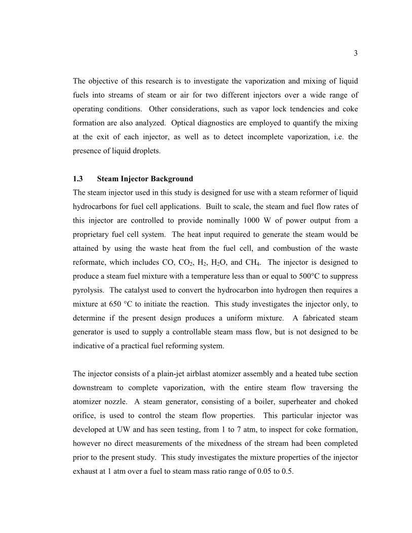
The objective of this research is to investigate the vaporization and mixing of liquid

fuels into streams of steam or air for two different injectors over a wide range of

operating conditions. Other considerations, such as vapor lock tendencies and coke

formation are also analyzed. Optical diagnostics are employed to quantify the mixing

at the exit of each injector, as well as to detect incomplete vaporization, i.e. the

presence of liquid droplets.

1.3 Steam Injector Background

The steam injector used in this study is designed for use with a steam reformer of liquid

hydrocarbons for fuel cell applications. Built to scale, the steam and fuel flow rates of

this injector are controlled to provide nominally 1000 W of power output from a

proprietary fuel cell system. The heat input required to generate the steam would be

attained by using the waste heat from the fuel cell, and combustion of the waste

reformate, which includes CO, CO2, H2, H2O, and CH4. The injector is designed to

produce a steam fuel mixture with a temperature less than or equal to 500°C to suppress

pyrolysis. The catalyst used to convert the hydrocarbon into hydrogen then requires a

mixture at 650 °C to initiate the reaction. This study investigates the injector only, to

determine if the present design produces a uniform mixture. A fabricated steam

generator is used to supply a controllable steam mass flow, but is not designed to be

indicative of a practical fuel reforming system.

The injector consists of a plain-jet airblast atomizer assembly and a heated tube section

downstream to complete vaporization, with the entire steam flow traversing the

atomizer nozzle. A steam generator, consisting of a boiler, superheater and choked

orifice, is used to control the steam flow properties. This particular injector was

developed at UW and has seen testing, from 1 to 7 atm, to inspect for coke formation,

however no direct measurements of the mixedness of the stream had been completed

prior to the present study. This study investigates the mixture properties of the injector

exhaust at 1 atm over a fuel to steam mass ratio range of 0.05 to 0.5.

4

1.4 SPP Injector Background

The SPP injector was develop at the University of Washington by John Lee (2000), and

has been tested extensively in conjunction with a 15.8cc jet-stirred reactor (JSR) to

determine pollutant formation chemistry of various liquid fuels operated under lean,

prevaporized, premixed conditions. All emission data taken by Lee (2000) and

Edmonds (2002) were done in conjunction with the 15.8cc JSR, and achieved SPP

residence times as low as 12 milliseconds. The present study examines the SPP injector

when operated at lower residence times, in the range of 4 to 9 milliseconds. JSR gas

sample measurements are an indicator of the mixedness produced from the SPP, but the

addition of the jet stirred reactor causes several significant perturbations. The JSR and

SPP coupling of previous work, when operated at fuel residence times less than 15

milliseconds in the SPP, produces an internal pressure in the SPP of roughly 2

atmospheres. In addition to the added back pressure, the nozzle which is used to form

the main jet for the JSR may act as an additional mixing mechanism. Several brief tests

are conducted here using a 64 cc JSR and 6 mm nozzle to determine the NOx

concentrations at shorter SPP injector residence times. In order to determine the

mixedness produced solely from the SPP internal geometry at 1 atm, the nozzle and

JSR must be removed. This configuration allows for optical diagnostic measurements

of the SPP injector outlet stream. All laser diagnostics performed on the SPP injector

are without the nozzle and JSR attached.

The SPP injector, designed for gas turbine applications, uses three independent air

streams to atomize and vaporize liquid fuel. The atomizer air, unlike the steam injector,

represents only a small fraction of the flow. The 1st stage air is used to vaporize the

lighter components, and begin vaporization of heavy components. This air stream

represents cooled compressor discharge and reduces the risk of autoignition, so shorter

residence times are not as crucial. The 2nd

stage air enters the SPP at higher

temperature than the first stage, and is used for final mixing of the fuel and air. The

majority of the airflow is sent through the 2nd

stage, which completes vaporization of

5

the heavy components during a short residence time. The total residence time target of

the fuel in the SPP is 4 - 9 milliseconds for this study.

1.5 Laser-induced Rayliegh Scattering Measurements

Point-volume-averaged Laser-induced Rayliegh Scattering (LRS) is used to directly

quantify the mixing in an optically defined test volume for both injectors. This

technique utilizes an incident laser beam and scattered light collection optics system to

measure the instantaneous composition and fluctuations of a binary mixture at a known,

constant temperature by capturing some portion of the elastically-scattered light in the

test volume. Note that LRS does not directly measure species concentration, but rather

indicates the relative concentrations in a binary mixture at a fixed number density. LRS

is beneficial because it gives a direct measurement of the mixing in a binary flow

system, and can be spatially varied, without noticeably disturbing the flow system. Gas

sample probes can be used, but these are invasive, and liquid fuel vapors pose the

problem of gumming or fouling of the probe. In addition, a steam/diesel mixture would

pose a challenge for most gas analyzers. LRS is well suited for the present study

because there is a significant difference in the scattering cross section of air and steam

compared to diesel and naphtha, or any heavy hydrocarbon based fuel. Fluctuations in

the mixture are clearly noticeable since an air and fuel mixture or steam and fuel

mixture will contain species of greatly different scattering cross sections, and

intermediate concentrations or mixtures will be distinguishable by the measured

scattering signal. LRS is especially sensitive to particles in the flow, including dust or

droplets. Since all gaseous and liquid streams are filtered, scattering from dust or

foreign particles is negligible. Droplets, however, are potentially present, and are

clearly detectable using the LRS collection system. Particles and droplets with length

scales of the same magnitude of the Laser beam wavelength or larger will scatter

according to Mie theory, at over ten times the magnitude of molecular scattering.

6

1.6 Overview of the Present Study

The chapters immediately following provide background information on atomization-

vaporization of liquid fuels, and laser- induced Rayliegh scattering measurements,

respectively. These sections are provided to give a basic knowledge of the listed

processes. Following these background chapters, the steam injector test stand is

described, and the steam injector experimental results and discussion are presented.

The optical diagnostic testing of the steam injector is performed over a wide range of

fuel concentrations and steam flow mass flow rates.

The SPP injector test stand is described and then the SPP injector experimental results

are presented in Chapters 6 and 7. The LRS measurements are taken with the SPP

injector operating at a wide range of air flow rates and temperatures, however the fuel

concentration is fixed to give an equivalence ratio of 0.5.

7

Chapter 2

Atomization, Vaporization and Mixing

2.1 Atomization Introduction

Atomization describes the process of breaking up a volume of liquid into discreet

droplets to ease dispersion and evaporation of the liquid in the bulk gas flow. There are

a multitude of geometries and approaches to accomplish this task, each with varying

effectiveness, complexity and cost. Lefebvre (1989) provides qualitative and

quantitative explanations of the most frequently utilized methods of atomization and the

relative benefits and parameter correlations for the various techniques. The type of

atomizer used in this study, for both the steam system and the SPP system, is the plain-

jet airblast atomizer. This design is used for relative simplicity and proven

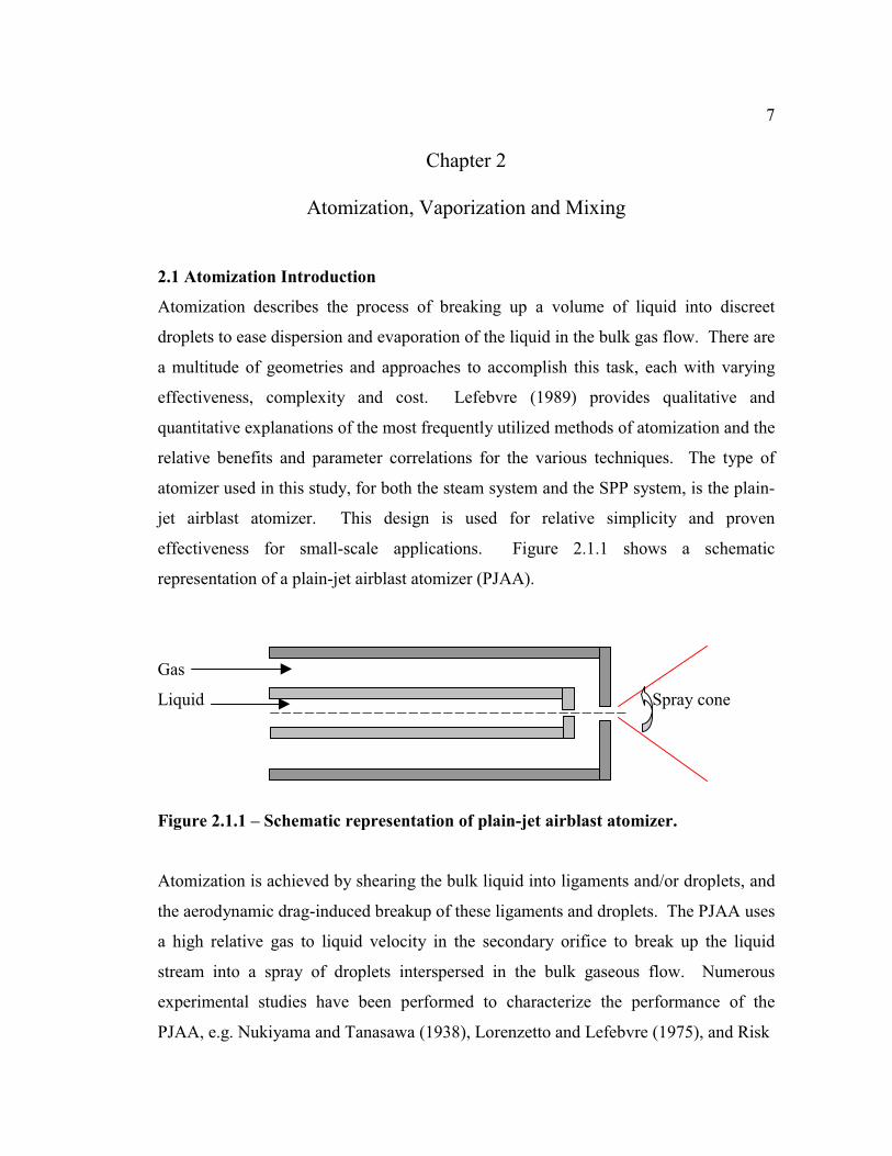
effectiveness for small-scale applications. Figure 2.1.1 shows a schematic

representation of a plain-jet airblast atomizer (PJAA).

Gas

Liquid Spray cone

Figure 2.1.1 – Schematic representation of plain-jet airblast atomizer.

Atomization is achieved by shearing the bulk liquid into ligaments and/or droplets, and

the aerodynamic drag-induced breakup of these ligaments and droplets. The PJAA uses

a high relative gas to liquid velocity in the secondary orifice to break up the liquid

stream into a spray of droplets interspersed in the bulk gaseous flow. Numerous

experimental studies have been performed to characterize the performance of the

PJAA, e.g. Nukiyama and Tanasawa (1938), Lorenzetto and Lefebvre (1975), and Risk

8

and Lefebvre (1979). There are several trends upon which these investigators agree.

As the relative gas to liquid velocity, downstream pressure, mass ratio of gas to liquid,

and gas density are increased, droplet size is reduced. Higher liquid surface tension

produces a higher resistance to surface area distortions of the droplet, hence increasing

droplet size. Droplet size is usually represented by a size distribution of drop diameter,

since the dispersion of droplets is not uniform. The Sauter mean diameter (SMD)

represents the diameter of a droplet with a volume to surface area ratio equal to that of

the entire droplet distribution (Lefebvre, 1989). There are various experimentally

derived correlations to estimate Sauter mean diameter exiting from the atomizer,

several of which are provided in Equations 2.1.1 and 2.1.2 (see nomenclature list for

variable descriptions).

+

σρµ

+

+

ρσ=

ALR

11

dd15.

ALR

11

dUd48.SMD

5.

0L

2L

0

4.4.

02RA

0 Eq. 2.1.1

Equation 2.1.1 displays a correlation for Sauter mean diameter of droplets for PJAA.

This correlation was derived under test conditions including an air to liquid mass ratio

(ALR) of 2 to 8, and air velocity of 10 to 120 m/s (Rizk and Lefebvre, 1979) as

measured at the point where the air meets the liquid. This is assumed to be the air

velocity at the nozzle throat. Equation 2.1.2 displays another correlation for SMD of

70.15.

L

02L

70.1

R30.A

37.L

33.L

.

ALR

11

d13.0

ALR

11

U

)m(95.0SMD

+

σρµ+

+

ρρσ= Eq. 2.1.2

droplets for the PJAA, derived under test conditions including an ALR of 1 to 16, and

air velocity of 70 to 180 m/s (Lorenzetto and Lefebvre, 1975).

9

Note that similar parameters are included in each correlation, and each is dimensionally

correct. The steam injector uses steam as the atomizing gas, which was not included in

the above correlations. In this situation, steam properties will substituted for air

properties, so that drop size is estimated. The included correlations show that SMD is

proportional to d00.6

and d00.5

, where d0 is the liquid fuel orifice. The fuel orifice used in

this study is 5-10 times smaller in diameter than those used in the studies on which the

correlations are based.

2.2 Vaporization Introduction

Vaporization is the next process required downstream of initial atomization for the

intimate mixing of liquid fuel and gaseous medium for use in combustion or steam

reformation. If a spray of droplets is desired, then vaporization is of no concern, but if

a gas phase mixture is desired, the droplets must be vaporized. Vaporization is the

process of converting liquid phase fuel droplets into vapor phase molecules, which are

readily mixed with the bulk gaseous fluid molecules. Droplet evaporation is governed

by the vapor pressure of the liquid fuel, the temperature of the liquid fuel and

surrounding gaseous medium, and the vapor phase fuel concentration in the gaseous

medium immediately surrounding the droplet. The time necessary for evaporation is

the quantity that will be derived from these properties and analyzed. The evaporation

time consists of two parts including a transient heat up period and a steady state droplet

lifetime that ends when the diameter of the droplet is zero. The following method for

calculating droplet lifetime is taken from Lefebvre (1989), along with the temperature

dependent fluid property correlations.

Mass and heat diffusion govern the vaporization process, and can be complicated by the

presence of convection effects. Convection will be ignored for the initial calculations.

If a droplet is assumed to have a uniform temperature, then the mass transfer number is

given by Equation 2.2.1, and the heat transfer number is given by Equation 2.2.2.

10

fs

fsm

Y1

YB

−= Eq. 2.2.1

fg

sg,ph

H

)TT(CB

−= ∞

Eq. 2.2.2

During the heat up period, the heat transfer number is larger than the mass transfer

number, signifying that more energy is entering the droplet through heat transfer than is

leaving through evaporation. Equations 2.2.3 through 2.2.7 give the correlations for

heat up time, nominal heat up drop diameter, nominal heat up surface temperature and

reference gas temperature exterior to the droplet. Note that the heat up surface

temperature is a weighted sum of the initial temperature and steady state temperature.

The heat up drop diameter represents the nominal droplet size during the transient heat

up process.

( )

−+

−ρ=

1B

BH)B1ln(k12

)TT(Dcct

m

hfgmg

0sst,s2hug,pL,fL,f,p

hu Eq. 2.2.3

( )

5.0

m

hfg

0sst,sL,f,p0hu

1B

BH2

)TT(c1DD

−

−

−+= Eq. 2.2.4

)TT(6.0TT 0sst,s0shu,s −+= Eq. 2.2.5

)TT(3

1TT hu,shu,shu,r −+= ∞ Eq. 2.2.6

11

( ) 5.0L,f

L,f,p)001(.

T35.3760c

ρ+= Eq. 2.2.7

The mass transfer number, heat transfer number, heat of vaporization, and liquid

density in the above calculation are determined using the surface heat up temperature.

The coefficient of 0.6 in Equation 2.2.5 is determined from Lefebvre (1989). The heat

up reference temperature is used to determine gaseous mixture properties outside of the

droplet. The surface temperature at steady state is found by setting Equations 2.2.1 and

2.2.2 equal and solving for temperature, representing the droplet surface temperature

that balances the heat diffusion into the droplet and evaporation of liquid.

Upon steady state, the heat addition to the droplet is balanced by the removal of energy

from the droplet by evaporation. For mixtures with a Lewis number of unity, the mass

transfer number must equal the heat transfer number. This condition allows the

evaporation constant to be used, simplifying the relationship between drop diameter

and time. Equations 2.2.8 through 2.2.10 display the evaporation constant and droplet

lifetime calculation.

λ−= )t(DD

t22

0st Eq. 2.2.8

fg,p

g

c

)B1ln(k8

ρ+

=λ Eq. 2.2.9

sthu ttlife_drop += Eq. 2.2.10

The steady state and heat up times are summed to provide the total droplet lifetime.

The gas and liquid properties that are included in Equations 2.2.1 through 2.2.9 require

some approximation. For example, the temperature at which the gas properties are to

12

be evaluated at must be calculated from the droplet surface temperature and quiescent

temperature. The drop lifetime calculation is an involved one, requiring several steps.

Following are the steps used to calculate droplet lifetime, and the temperature-

dependant property equations used to complete the iteration.

The first step in the iteration process is the determination of the droplet surface

temperature at steady state, assuming the droplet has a uniform temperature. This is

done by guessing a surface temperature, calculating the vapor pressure and fuel mass

fraction, and then checking if the mass transfer number is equal to the heat transfer

number. The surface temperature must be adjusted until the transfer numbers are equal.

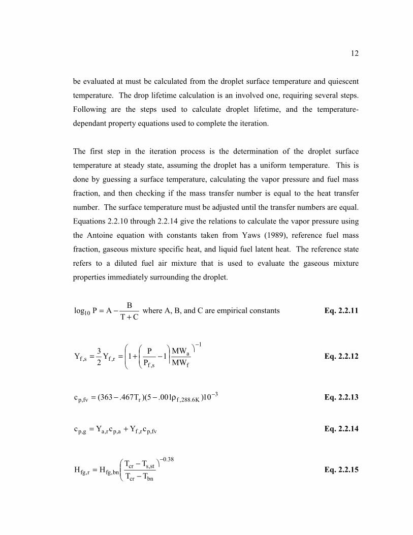
Equations 2.2.10 through 2.2.14 give the relations to calculate the vapor pressure using

the Antoine equation with constants taken from Yaws (1989), reference fuel mass

fraction, gaseous mixture specific heat, and liquid fuel latent heat. The reference state

refers to a diluted fuel air mixture that is used to evaluate the gaseous mixture

properties immediately surrounding the droplet.

CT

BAPlog10 +

−= where A, B, and C are empirical constants Eq. 2.2.11

1

f

a

s,fr,fs,f

MW

MW1

P

P1Y

2

3Y

−

−+== Eq. 2.2.12

3K6.288,frfv,p 10)001.5)(T467.363(c −ρ−−= Eq. 2.2.13

fv,pr,fa,pr,ag,p cYcYc += Eq. 2.2.14

38.0

bncr

st,scrbn,fgr,fg

TT

TTHH

−

−−

= Eq. 2.2.15

13

At this point, the transfer numbers can be calculated, and the surface temperature

iterated until they agree. The steady state time can now be calculated based on the

surface temperature and initial drop size. Once this has been completed, the heat up

reference and nominal surface temperature can be calculated. The heat up time and

nominal drop diameter must be calculated by determining properties at the heat up

reference temperature and heat up surface temperature. Equation 2.2.15 displays the

correlation to approximate the thermal conductivity for fuel vapor and the mixture.

( )( )n

bnr,fv273

T273T0313.02.13k

−−= Eq. 2.2.16

2

bnT

T0372.02n

−= Eq. 2.2.17

r,fvr,fr,ar,ag kYkYk += Eq. 2.2.18

Equations 2.2.1 through 2.2.17 allow the vaporization time to be calculated based on

quiescent air surroundings. The presence of convection works to increase the

vaporization rate by increasing the heat transfer and mass transfer. The SPP injector is

designed to maximize the convective affects, through introduction of high speed air

jets, to further increase droplet breakup and vaporization. This means that the droplet

lifetimes calculated using the above correlations give the worst case vaporization times

in the SPP injector. Convection effects can be added by including terms dependant on

the dimensionless Reynolds number and Prandlt number. Lefebvre (1989) includes

several correlations for including convection effects.

14

2.3 Steam Injector Droplet Size and Lifetime

Using the method detailed in Lefebvre (1989), droplet size and lifetime calculations are

completed for the steam injector over a range of nominal operating conditions. Table

2.3.1 shows the system parameters used for the calculations. These test conditions

represent nominal values; actual test matrices of experiments performed will be given

in the results sections. The set of parameters included in Table 2.3.1 spans the

operating range of the steam injector. The droplet size calculations based on this data

produce SMD values less than 10 µm. This droplet size is relatively small, but the

steam is near choked (see Chapter 4 for the nozzle pressure drop) at the airblast nozzle,

which could produce a steam to fuel relative velocity of over 600 m/s. Equations 2.1.1

and 2.1.2 are based on data taken with air velocities less than 200 m/s. Figure 2.3.1

displays a plot of evaporation time as a function of initial drop diameter for quiescent

steam conditions. Tetradecane (C14H30) and heptane (C7H16) are used for comparison.

The residence time of the fuel in the vaporizing tube can be approximated with

Equation 2.3.1, assuming the mixture is an ideal gas. The nominal residence time range

in the steam injector (5 length) is 5 to 10 milliseconds.

Table 2.3.1 – Nominal steam injector properties for droplet calculations. Note that

the liquid fuel is assumed to be at 27°C, although some preheating occurs.

fuel type fuel flow steam flow fuel orifice steam orifice steam T fuel T

g/s g/s mm mm °C °C

TPD 0.04 0.15 0.1524 0.7874 400 27

TPD 0.04 0.15 0.1524 0.7874 500 27

TPD 0.04 0.2 0.1524 0.7874 400 27

TPD 0.04 0.2 0.1524 0.7874 500 27

TPD 0.05 0.25 0.1524 0.7874 400 27

TPD 0.05 0.25 0.1524 0.7874 500 27

=ρ=τ

i

.

iu

.

i

MW

m*R*T

V*P

m

V Eq. 2.3.1

0.0

00

1

0.0

01

0.0

1

0.11

05

01

00

15

02

00

25

03

00

Init

ial

Dro

p D

iam

ete

r ( µ µµµ

m)

Evaporation Time (s)

tetr

ad

eca

ne

, 7

23

K

tetr

ad

eca

ne

, 6

23

K

he

pta

ne

, 7

73

K

he

pta

ne

, 7

23

K

he

pta

ne

, 6

23

K

Fig

ure

2.3

.1 –

Evap

ora

tion

plo

tted

again

st i

nit

ial

dro

ple

t d

iam

eter

for

tetr

ad

ecan

e an

d h

epta

ne

at

vari

ou

s

qu

iesc

ent

stea

m t

em

per

atu

res.

15

16

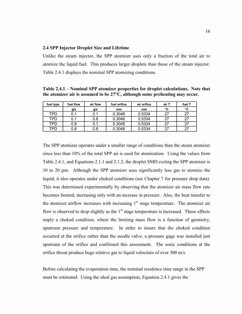
2.4 SPP Injector Droplet Size and Lifetime

Unlike the steam injector, the SPP atomizer uses only a fraction of the total air to

atomize the liquid fuel. This produces larger droplets than those of the steam injector.

Table 2.4.1 displays the nominal SPP atomizing conditions.

Table 2.4.1 – Nominal SPP atomizer properties for droplet calculations. Note that

the atomizer air is assumed to be 27°C, although some preheating may occur.

fuel type fuel flow air flow fuel orifice air orifice air T fuel T

g/s g/s mm mm °C °C

TPD 0.1 0.1 0.3048 0.5334 27 27

TPD 0.1 0.8 0.3048 0.5334 27 27

TPD 0.8 0.1 0.3048 0.5334 27 27

TPD 0.8 0.8 0.3048 0.5334 27 27

The SPP atomizer operates under a smaller range of conditions than the steam atomizer

since less than 10% of the total SPP air is used for atomization. Using the values from

Table 2.4.1, and Equations 2.1.1 and 2.1.2, the droplet SMD exiting the SPP atomizer is

10 to 20 µm. Although the SPP atomizer uses significantly less gas to atomize the

liquid, it also operates under choked conditions (see Chapter 7 for pressure drop data).

This was determined experimentally by observing that the atomizer air mass flow rate

becomes limited, increasing only with an increase in pressure. Also, the heat transfer to

the atomizer airflow increases with increasing 1st stage temperature. The atomizer air

flow is observed to drop slightly as the 1st stage temperature is increased. These effects

imply a choked condition, where the limiting mass flow is a function of geometry,

upstream pressure and temperature. In order to insure that the choked condition

occurred at the orifice rather than the needle valve, a pressure gage was installed just

upstream of the orifice and confirmed this assessment. The sonic conditions at the

orifice throat produce huge relative gas to liquid velocities of over 300 m/s.

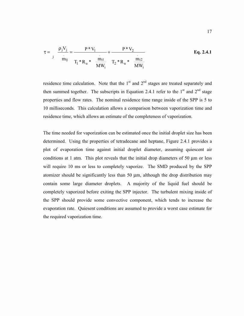
Before calculating the evaporation time, the nominal residence time range in the SPP

must be estimated. Using the ideal gas assumption, Equation 2.4.1 gives the

17

+=ρ

=τ

i

2i

.

u2

2

i

1i

.

u1

1

ij

.

jj

j

MW

m*R*T

V*P

MW

m*R*T

V*P

m

VEq. 2.4.1

residence time calculation. Note that the 1st and 2

nd stages are treated separately and

then summed together. The subscripts in Equation 2.4.1 refer to the 1st and 2

nd stage

properties and flow rates. The nominal residence time range inside of the SPP is 5 to

10 milliseconds. This calculation allows a comparison between vaporization time and

residence time, which allows an estimate of the completeness of vaporization.

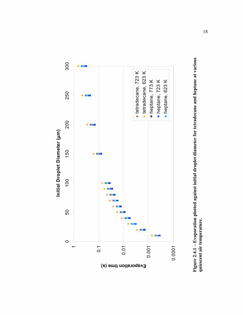
The time needed for vaporization can be estimated once the initial droplet size has been

determined. Using the properties of tetradecane and heptane, Figure 2.4.1 provides a

plot of evaporation time against initial droplet diameter, assuming quiescent air

conditions at 1 atm. This plot reveals that the initial drop diameters of 50 µm or less

will require 10 ms or less to completely vaporize. The SMD produced by the SPP

atomizer should be significantly less than 50 µm, although the drop distribution may

contain some large diameter droplets. A majority of the liquid fuel should be

completely vaporized before exiting the SPP injector. The turbulent mixing inside of

the SPP should provide some convective component, which tends to increase the

evaporation rate. Quiesent conditions are assumed to provide a worst case estimate for

the required vaporization time.

0.0

00

1

0.0

01

0.0

1

0.11

05

01

00

15

02

00

25

03

00

Init

ial

Dro

ple

t D

iam

ete

r ( µ µµµ

m)

Evaporation time (s)

tetr

ad

eca

ne

, 7

23

K

tetr

ad

eca

ne

, 6

23

K

he

pta

ne

, 7

73

K

he

pta

ne

, 7

23

K

he

pta

ne

, 6

23

K

Fig

ure

2.4

.1 –

Evap

ora

tion

plo

tted

again

st i

nit

ial

dro

ple

t d

iam

eter

for

tetr

ad

ecan

e an

d h

epta

ne

at

vari

ou

s

qu

iesc

ent

air

tem

pera

ture

.

18

19

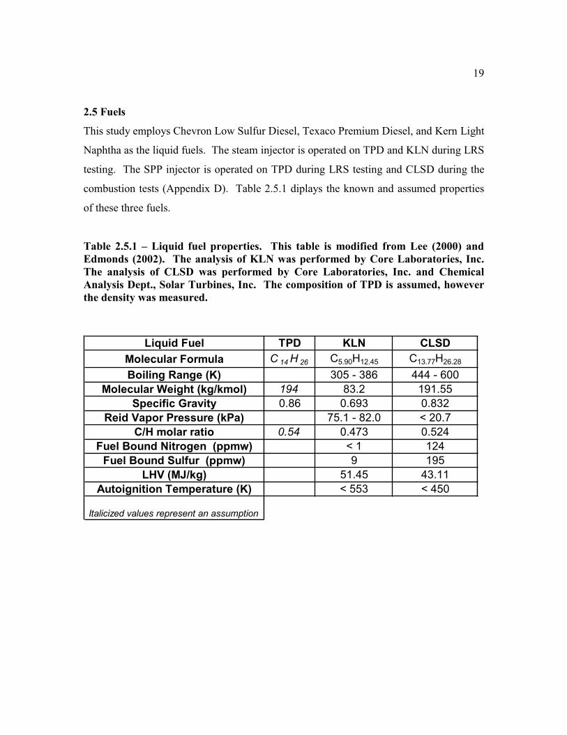
2.5 Fuels

This study employs Chevron Low Sulfur Diesel, Texaco Premium Diesel, and Kern Light

Naphtha as the liquid fuels. The steam injector is operated on TPD and KLN during LRS

testing. The SPP injector is operated on TPD during LRS testing and CLSD during the

combustion tests (Appendix D). Table 2.5.1 diplays the known and assumed properties

of these three fuels.

Table 2.5.1 – Liquid fuel properties. This table is modified from Lee (2000) and

Edmonds (2002). The analysis of KLN was performed by Core Laboratories, Inc.

The analysis of CLSD was performed by Core Laboratories, Inc. and Chemical

Analysis Dept., Solar Turbines, Inc. The composition of TPD is assumed, however

the density was measured.

Liquid Fuel TPD KLN CLSD

Molecular Formula C 14 H 26 C5.90H12.45 C13.77H26.28

Boiling Range (K) 305 - 386 444 - 600

Molecular Weight (kg/kmol) 194 83.2 191.55

Specific Gravity 0.86 0.693 0.832

Reid Vapor Pressure (kPa) 75.1 - 82.0 < 20.7

C/H molar ratio 0.54 0.473 0.524

Fuel Bound Nitrogen (ppmw) < 1 124

Fuel Bound Sulfur (ppmw) 9 195

LHV (MJ/kg) 51.45 43.11

Autoignition Temperature (K) < 553 < 450

Italicized values represent an assumption

20

Chapter 3

Laser-induced Rayliegh Scattering Measurement Technique

3.1 Introduction to LRS

Rayliegh scattering describes the elastic scattering of incident light by molecules or

particles with characteristic length scales less than the wavelength of the incident light.

Molecules scattering according to Rayliegh theory will scatter light with the same

wavelength as the incident light, as opposed to Raman scattering which entails a

frequency shift in the scattered light that is unique to the species. Incident light induces

an electric dipole moment in the molecule or atom. This dipole oscillation produces

radiation in the form of scattered light with a direction vector that is dependant upon the

incident radiation and the polarizability of the molecule or atom. This electromagnetic

interaction describes the mechanism by which the sky appears blue. The Rayleigh

scattering cross section of a group of molecules is proportional to one over the fourth

power of the incident wavelength, causing the lower wavelength blue light to be

scattered more than the rest of the visible spectrum. This also explains why the sky

appears red at sunset, when the long atmospheric path length reduces the intensity of

the lower wavelength visible spectrum. If a focused, coherent light source at a

constant, known wavelength is used as the incident light source, the elastic scattering

from a specific group of molecules or particles can be analyzed directly. The laser

provides a high intensity, monochromatic incident light source that can be used in

conjunction with Rayleigh scattering theory for experimentation.

Laser induced Rayliegh Scattering (LRS) provides a means to investigate mixing on

fine temporal and spatial scales, and has been used extensively to examine

concentration and temperature fluctuations of gas mixtures, e.g. Dibble and Hollanbach

(1981), Espey (1997), Robben (1976) and Seasholtz (1998). Since a molecule’s size

and composition will determine with what intensity light is scattered,

21

LRS can be used to investigate mixture properties and determine the component

concentration of a binary mixture, or the temperature of a known mixture. LRS is

especially useful when the test mixture contains species of vastly different scattering

cross sections, signifying that the scattering signal can be readily correlated to the local,

instantaneous concentration.

The scattering cross section of a molecule is the quantity that governs the portion of an

incident light source that is scattered elastically. Equation 3.1.1 shows how the

Rayleigh scattering cross section of a molecule is calculated for a given incident

wavelength. In Equation 3.1.1, ε is the index of refraction of the gas, n is the number

42

222

n

sin)1(4

λθ−επ=σ Eq. 3.1.1

density at STP conditions, λ is the incident laser wavelength, and θ is the angle

between the observation and incident light (90° for this study). Also, note that the units

of the scattering cross section are reported here as cm2/srad. The Rayleigh scattering

cross section (RSC) increases with the index of refraction of a molecule, and decreases

with incident wavelength. The RSC of a mixture, containing N gases of different

Rayleigh scattering cross sections, can be calculated as shown in Equation 3.1.2.

i

N

1imix x σ=σ Eq. 3.1.2

The RSC value is then used to determine the ratio of scattered light power to incident

light power. Equation 3.1.3 shows how the scattered intensity is related to the mixture

properties and RSC values of the component gases.

22

βΩ=σ= ZL*constantK whereKn

I

Imix

incident

.

scattered

.

Eq. 3.1.3

The scattering intensity is proportional to the product of the incident intensity (Iincident),

optical system constant (K), number density (n), and mean mixture RSC. The optical

constant, K, takes into account the length of the observed beam, the solid angle over

which measurements are taken, the transmissivity of the optical processing

components, and the efficiency of the PMT. K will be assumed constant for each test,

but will vary between the steam injector and SPP injector testing. This variation is due

to the change in the collection system settings accompanying each injector system. The

signal to noise ratio (SNR) can be estimated by calculating the number of measured,

scattered photons (Robben, 1976). The SNR is equal to the square root of the photon

count. The optical setup and laser used in this study are estimated to measure 1e5 to

1e6 photons per second. This range gives a SNR range of 0.1 to 0.3 %, based solely

upon the collection optics system.

Note that the refractivity is required, along with the component density, to determine

the scattering cross section. Gardiner (1981) lists the refractivities of various gases and

vapors at 514.5 nm, from which the index of refraction and scattering cross section can

be derived. The fuels used in this study are premium diesel (nominally C14H26) and

light naphtha (C5.90H12.45), which are not included in Gardiner’s work, and the heaviest

alkane included in Gardiner’s work is octane (C8H18). The refractivity increases with

carbon atoms for hydrocarbons, so hydrocarbons heavier than octane have higher

refractivities and scattering cross sections.

The number density, appearing in Equation 3.1.3, is a function of temperature, pressure,

and mixture components. Air can be approximated as an ideal gas, since the

generalized compressibility chart gives Z 1, for a temperature of 350°C and 1 atm.

The SPP injector is operated with an overall equivalence ratio of 0.5 for a majority of

23

the presented test results. Assuming a nominal diesel fuel chemical composition of

C14H26 , there are 195 air molecules for every 1 fuel molecule, signifying that most

molecular collisions will be ideal gas collisions. The steam injector operates with a fuel

to steam mass ratio range of 0.05 to 0.5, or a steam to fuel mole ratio range of 22 to 216

for the same diesel formula. The generalized compressibility chart gives 1>Z > 0.95,

for superheated steam at 400 °C and 1 atm, so steam closely resembles an ideal gas.

Cengel and Boles (1998) list the error between the ideal gas specific volume and actual

specific volume to be 0.1% at the aforementioned conditions. The steam-fuel mixture

is also approximated here as an ideal gas mixture. This simplifies Equation 3.1.3, since

the number density can now be written in terms of measurable thermodynamic

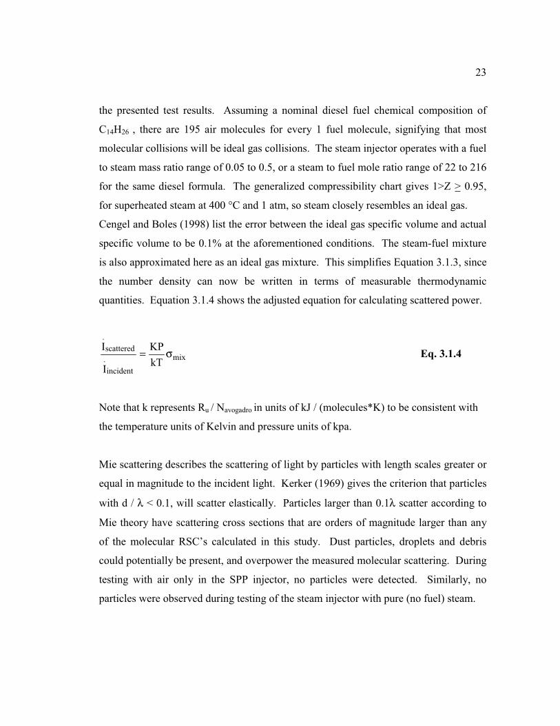
quantities. Equation 3.1.4 shows the adjusted equation for calculating scattered power.

mix

incident

.

scattered

.

kT

KP

I

I σ= Eq. 3.1.4

Note that k represents Ru / Navogadro in units of kJ / (molecules*K) to be consistent with

the temperature units of Kelvin and pressure units of kpa.

Mie scattering describes the scattering of light by particles with length scales greater or

equal in magnitude to the incident light. Kerker (1969) gives the criterion that particles

with d / λ < 0.1, will scatter elastically. Particles larger than 0.1λ scatter according to

Mie theory have scattering cross sections that are orders of magnitude larger than any

of the molecular RSC’s calculated in this study. Dust particles, droplets and debris

could potentially be present, and overpower the measured molecular scattering. During

testing with air only in the SPP injector, no particles were detected. Similarly, no

particles were observed during testing of the steam injector with pure (no fuel) steam.

24

The study employs small-volume averaged, LRS measurements to diagnose mixing.

To accomplish this, a laser beam is passed through the test mixture, and scattering

measurements are made perpendicular to the axis of the beam. The light scattering

from a small volume, defined by the laser beam diameter and length of beam observed,

is projected onto a photomultiplier tube (PMT). The signal measured by the

photomultiplier tube is an average of the incident signal, meaning that spatial scales

smaller than the measuring volume cannot be resolved. The temperature, pressure,

species concentrations, and incident light intensity are all spatially averaged in the

measurement volume, and this averaged signal is measured as a function of time.

3.2 Incident Light and Collection Optics System Specifications

The optical diagnosing system uses a single line CW laser in conjunction with an

optical focusing system to measure scattered light to examine mixing. The collection

optics system consists of several plano-convex lenses to guide the scattered light, a

bandpass filter to block unwanted wavelengths, a photomultiplier tube to convert the

photon signal into a current signal, an oscillliscope to display the signal as a function of

time, and a PC to store and manipulate the data. This system was designed to collect

the scattering signal over a lens-defined solid angle from a small test volume, and to

measure this signal with time. A complete parts list, system schematics and relevant

procedures are included in Appendix A.

The incident light is provided by a continuous operation, 514.5 nm single line argon ion

laser (Coherent Innova 308 model with Powertrack) with adjustable light output. The

nominal output laser power is 1 W for 514.5 nm single line operation. The nominal

diameter of the beam is 1.8 mm, and the light output power is regulated in the “light

constant” mode. Power measurements taken with a separate power meter agree with

the onboard power measurement, so the onboard measurement is used. This model of

laser requires water cooling, using a closed cooling loop (Laserpure laser cooler) to

reject heat via a heat exchanger to an open cooling system (plant water). The beam is

25

passed through the injector’s exit, so that the mixing in the exhaust can be measured

directly. After traversing the test volume, the beam is terminated into a beam dump,

consisting of a 6 black iron pipe with a welding brick at the far end. The dump

prevents the beam from bouncing around the laboratory and creating adverse safety,

signal noise considerations.

The collection optics are perpendicular to the laser beam, with an optical path axis at

the same height as the beam. Figure 3.2.1 displays a schematic representation of the

optical setup for clarification.

Mixture to be examined Slit Bandpass filter PMT

PC Lenses Neutral Density Filter

Figure 3.2.1 – Top view schematic of collection optics. The slit is used to truncate

the laser beam image.

The front 50.8φ mm (2 ) plano-convex lens is used to collect the scattering signal from

the beam located at the lens focal point (67.3 mm BFL from the lens face). This lens

has an antireflection coating to minimize loss of the signal. The geometry of the first

collection lens determines the solid angle that the signal is taken over. The solid angle

for this lens is approximately 0.45 srad based upon the Equation 3.2.1. Upon leaving

2

2lens

2 BFL

r

R

A π==Ω Eq. 3.2.1

26

this lens the light is now parallel to the axis of the lens. The second 2 plano-convex

lens receives the parallel light and focuses the signal into an image of the original

beam, projected on the slit front face. The BFL of the second 50.8φ mm lens is also

67.3 mm. The slit assembly’s primary functions are to truncate the beam image, thus

defining the measuring volume, and to terminate any other light signal not admitted

through the slit aperture. The slit width used in this study is 1mm, which couples with

the laser beam diameter, to give a cylindrical measuring volume of 2.54 mm3.

After truncation at the slit, the image is expanded until reaching a .5 φ (12.7mm) plano-

convex lens which again produces a parallel light signal. This lens is needed not to

produce an image but rather to condition the light normal to the plane of the filters,

located before the photomultiplier tube. The signal is passed through a 514.5 nm

bandpass filter to block transmission of any light at wavelengths other than 514.5 nm.

This component has a transmissivity of 50% at 514.5 nm. The light signal is now

projected onto the photomultiplier tube (PMT) face, or passed through a 10%

transmission neutral density filter and then projected onto the PMT. The PMT, an RCA

1P28 model, receives between 600 and 1000 VDC from a Keithley 244 power supply,

depending upon the test performed, and produces a signal that is read on a Fluke

PM3384 Auto-Ranging Combiscope. The lenses, filters, slit assembly and PMT are

enclosed in an aluminum case, with flat-black interior, to minimize the background

light noise and dust that could perturb the signal. Figure 3.2.2 is a digital picture of the

enclosure without the cover. Figure 3.2.3 shows a digital picture of the laser, optics and

test section (SPP) configuration. Note that the laser and collection optics are aligned,

and then fixed spatially to hold this alignment. The test section is then moved into

position such that the focal point of the front PC lens is located in the appropriate

portion of the flow.

The data used for analysis are taken from the Fluke Combiscope. The Combiscope

exports a snapshot of the screen to the PC, which includes the numerical data. The data

Fig

ure

3.2

.2 –

Dig

ital

pic

ture

of

the

coll

ecti

on

op

tics

’ in

teri

or.

PC

len

ses

and

tri

po

d

lens

ho

lder

s

Ban

dp

ass

filt

er

PM

TS

lit

asse

mb

ly

27

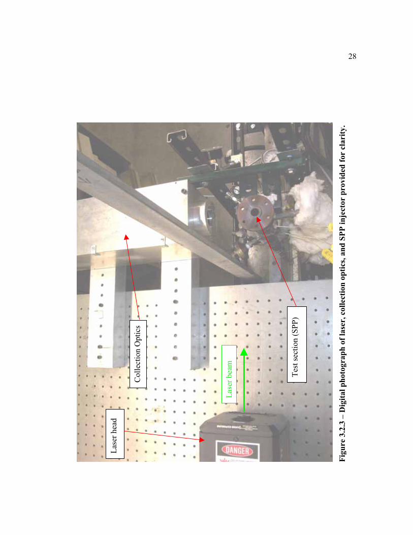
Fig

ure

3.2

.3 –

Dig

ital

ph

oto

gra

ph

of

lase

r, c

oll

ecti

on

op

tics

, an

d S

PP

in

ject

or

pro

vid

ed f

or

clari

ty.

Las

er h

ead

Las

er b

eam

Coll

ecti

on O

pti

cs

Tes

t se

ctio

n (

SP

P)

28

29

points can then be reformatted into an MS Excel spreadsheet, from which the signal can

be plotted and statistical calculations can be performed. After numerous tests with the

steam and SPP injectors, it was observed that a 0.2044 second snapshot containing 512

points (a point to point time interval of 0.4 milliseconds) gave the best representation of

the fluctuations in the measuring volume. This time scale represents a 20 millisecond

division on the Combiscope. Longer time intervals tend to obscure the fluctuations’

structure and time scale, while shorter time intervals are of the same time scale as the

fluctuations. One subtlety of the PMT wiring is that the measured signal is negative, so

larger scattering signals read as more negative. Whenever statistical calculations are

performed, the negative sign is removed. Also note that the PMT wiring contains a R-

C circuit to convert the current signal into a voltage signal, as measured by the

Combiscope.

3.3 Pure Gas Tests and Alignment

A cylindrical, three filament mercury lamp was used to align the optics vertically and

horizontally, since it produces a line of light emission similar in geometry to the laser

beam. The mercury lamp is much easier to operate and maneuver than the laser, and

produces a higher intensity, more easily tracked radially-emitted light path than that of

the scattered light from the laser beam.

Once constructed, the collection optics system was first tested on pure gases in order to

insure alignment of the components and gain experience. Several pure gases were

tested, and the measured scattering signal ratios were compared to the ratio of the

RSC’s calculated at 300K and 1 atm. In addition to testing the ability of the collection

system to distinguish different gases in the test volume, linearity tests were also

performed. The laser power was adjusted to values ranging from 0 W to 1.25 W, and

the mean scattering signal was recorded. Based upon Equation 3.1.3, the scattering

signal should be linearly proportional to the incident laser power. A linearity test was

done for several pure gases, and for ambient air, so that the scattering ratios and

30

linearity could be presented on one plot. The calculated ratio of diatomic nitrogen to

helium RSC’s is 74, and the measured ratio was 63 (at 1.25 W, with 22 mV noise

subtracted). This measurement is partially obscured by noise, since He scatters weakly

and is read on the low scale of the Combiscope. The calculated ratio of methane to

nitrogen RSC’s is 2.2, while the measured value is 1.95 (at 1.25 W with 22 mV noise

subtracted). The calculated ratio of nitrogen to hydrogen RSC’s is 4.6, while the

measured value is 4.8 (at 1.20 W with 20 mV noise subtracted). The measured ratios

are in agreement with the calculated values. Also note that, although it was not

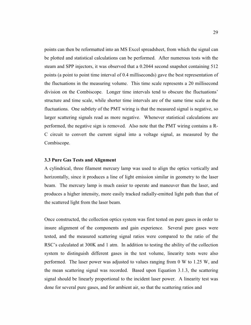
measured, the calculated ratio of steam to nitrogen RSC’s is 0.71. Figure 3.3.1 displays

the plot of mean scattering signal as a function of incident laser power for 3 pure gases

and ambient air. Theoretically, the ambient air should be close in scattering signal to

pure N2, but dust in the air causes the signal to be noisy.

Initially, the collection system could only weakly distinguish different gases such as N2

and He, even though these gases have a RSC ratio of 74. It was determined that stray

light was leaking past the slit assembly, reaching the PMT, and overpowering the small

helium signal. A set of blinds was installed around the slit assembly, made of dull

black thin-board, to block the extraneous signal. This alteration did in fact allow the

collection system to distinguish gases more readily. All data, including Figure 3.3.1,

are captured with the blinds in place.

The regression curve for helium in Figure 3.3.1 is omitted due to noise considerations.

The Combiscope’s maximum range is 25 Volts, which means the helium signal is 1000

times smaller in magnitude than the maximum range. The helium data points in Figure

3.3.1 are roughly linear, with a R2 value of .952, but some significant portion of this

signal is noise, so the curve fit was not included.

31

y = 1.2001x + 0.0279

R2 = 0.9999

y = 1.0793x + 0.0319

R2 = 0.9959

y = 0.622x + 0.0023

R2 = 0.9977

0

0.2

0.4

0.6

0.8

1

1.2

1.4

1.6

1.8

0 0.2 0.4 0.6 0.8 1 1.2 1.4

Incident Laser Power (Watts)

Scatt

eri

ng

Sig

nal

(Vo

lts)

CH4

Ambient

N2

He

Linear (CH4)

Linear (Ambient)

Linear (N2)

Linear (He)

Figure 3.3.1 – Pure gas scattering data for comparison with calculated RSC, and

linearity check. The PMT was set to 1000 VDC for this data. The ambient air

contains particles and dust, which produce a much larger mean scattering signal

than N2.

3.4 Liquid Fuel Mixtures and Additional Considerations

Liquid fuel mixtures pose several problems that the tested pure gases do not. At room

temperature and pressure, the majority of the liquid fuel’s components tend to the liquid

phase, thus the scattering signal of pure fuel cannot be measured at ambient conditions.

Also, droplets smaller than 0.1λ may scatter according to Rayleigh theory and become

indistinguishable from the vapor phase mixture.

Using an ideal gas assumption, and Equation 3.1.1, octane was estimated to have a

scattering cross section about 2 orders of magnitude greater than that of air or water

32

vapor. Espey (1997) determined the RSC ratio of a diesel fuel mixture and air to be

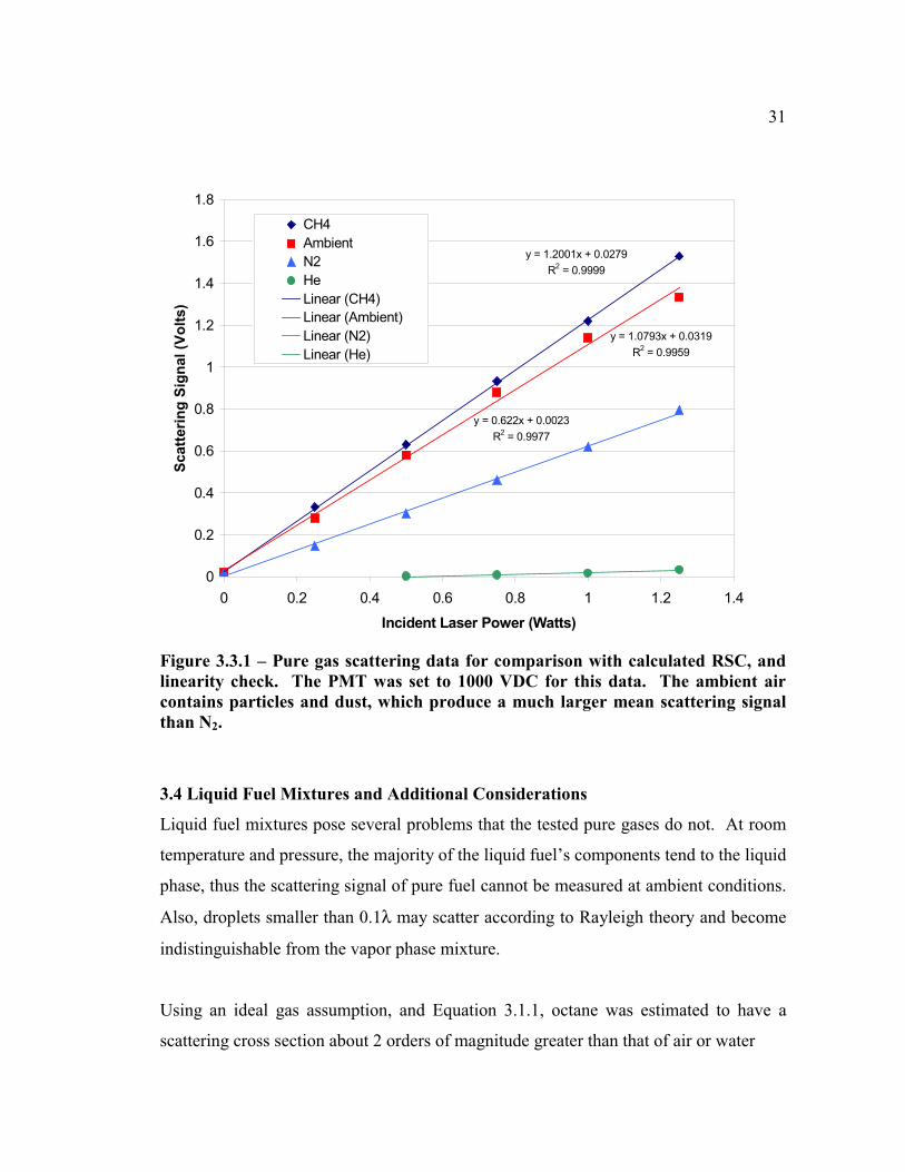
305. Figure 3.4.1 shows a time trace taken of a fuel-steam mixture during fuel flow

instability. The fuel is in the vapor phase at all points, no droplet scattering is observed.

This figure illustrates the resolution LRS provides in examining fuel vapor mixtures.

Note the significant difference between fuel lean and fuel rich scattering signals.

Temperature fluctuations can increase the unmixedness by causing variations in the

number density. It is reasonable that the local temperature fluctuations should correlate

negatively to the local fuel concentration fluctuations for a vaporizing flow. This

correlation would cause fuel rich fluctuations to have a lower temperature, and thus a

larger number density. Fluctuations in the scattering signal due to species

concentration would be amplified by the local temperature fluctuations. The SPP

injector 2nd

stage injects hot air into a cooler, fuel-rich mixture. High temperature

would be associated with pure air and cooler temperatures with the vaporizing fuel.

Measured fluctuations in species concentration assuming constant temperature would

then be an overestimate. The steam injector uses a wall-heated vaporizing tube, so

temperature fluctuations can arise from vaporizing fuel or movement of the gas near the

hot wall into the cooler flow.

If the mixture is assumed to be an ideal gas, the number density should be proportional

to 1 / T. Chapters 5 and 7 display experimental data in which the scattering signal at a

fixed composition decreases as a stronger inverse function of temperature. This may be

due to several effects. Non-ideal gas behavior may cause some deviation from the 1 / T

functional dependency. Vaporized hydrocarbon fuel, just above the saturation

temperature may not exhibit ideal gas behavior. As mentioned earlier, droplets may

scatter as molecules if their length scales are small enough, which would cause the

lower temperatures conditions to have higher scattering signals. Chapter 7 also

includes a plot of the scattering signal for pure air as a function of temperature, which

displays a trend very near to 1 / T.

-3.5

0

-3.0

0

-2.5

0

-2.0

0

-1.5

0

-1.0

0

-0.5

0

0.0

00.0

00

.05

0.1

00

.15

0.2

0

Tim

e (

s)

Scattering Signal (Volts)

Fig

ure

3.4

.1 –

Tim

e tr

ace

of

fuel

an

d s

team

mix

ture

du

rin

g f

uel

flo

w i

nst

ab

ilit

y. T

he

regio

ns

that

ap

pea

r to

have

a s

catt

erin

g s

ign

al

of

0 V

olt

s are

pu

re s

tea

m.

Fu

el

rich

Fu

el

lean

33

34

Chapter 4

Steam Injector Concept, Experimental System

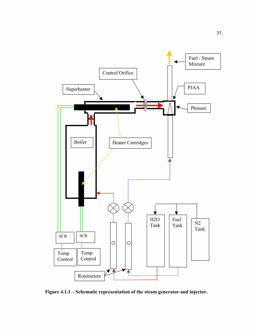
4.1 Steam Injector Rig Overview

The steam injector used in this study has two main flow systems; the steam generator

and the fuel injection system. A boiler and superheater are used to produce a stream of

superheated steam at elevated pressure in the range of 446 to 790 kPa (50 to 100 psig)

with a temperature range of 400 to 500 °C. This mixture is then throttled through a

square-edged, circular orifice operating under choked conditions. The lower pressure,

superheated steam then flows into a small plenum volume and flows through another

orifice, which serves as the air-blast secondary nozzle. The liquid fuel orifice is located

just upstream of the secondary nozzle, completing the PJAA assembly. Down stream

of the atomizer, a heated section of tube is used to complete droplet vaporization.

Figure 4.1.1 displays a schematic of the steam generator and injector. A component

list, along with calibration data is also included in Appendix B.

4.2 Steam Generator Consisting of Boiler, Superheater and Measuring Orifice

The boiler, used to create a saturated mixture of water at a specified temperature,

consists of a 0.38 m (15 ) long, 0.114 m (4.5 ) diameter stainless steel pipe section (4

schedule 80 nominal pipe). The boiler is sealed with 3/4 (19 mm) thick flanges at

either end, and has an interior capacity of 2.7 liters. The boiler is secured to the test

stand by three welded struts directed out radially from the boiler, which are bolted to

cross bars on the test stand. A 1800 W (@120 VAC), 6 (0.152 m) long, 3/4 φ (19

mm) Inconel sheathed cartridge heater, is inserted through the bottom flange of the

boiler via 3/4 NPT tapped hole. The top flange has several exit ports, in the form of

welded 6.35 mm (1/4 OD), stainless steel tubing sections. One port is used as a

blowout flange, as a safety precaution when operating the pressurized boiler. The

blowout flange consists of foil sheets pressed between bolted flanges with 1/4 holes

35

Figure 4.1.1 – Schematic representation of the steam generator and injector.

Boiler

Superheater

Plenum

N2

Tank

Control Orifice

Fuel / Steam

Mixture

H2O

Tank

Fuel

Tank

SCRSCR

Temp.

Control

Temp.

Control

Rotometers

PJAA

Heater Cartridges

36

on center. The second port is used to measure the boiler pressure via a 0-160 psig

range pressure gage. The last port is the exit tube for the saturated steam, which then

flows to the superheater. The bottom, welded flange of the boiler has one inlet port.

This port functions as a drain to evacuate water from the boiler after testing, and as a

fill to replenish the boiler during operation. Water is fed into the boiler during steady

state operation to replace the vacated steam. This is done to prevent the water level

from falling and exposing the heater cartridge tip to saturated vapor, which could cause

a local overheating of the element. This water flow rate is monitored by an ABB model

10A6132DB1B1 rotometer with 0.125 (3.175 mm) SS ball float. A water tank is

mounted on the test stand, and is pressurized to 50-120 psig by N2 or He cylinder gas,

to supply the refill water. Note, the steam flow-rate is governed by the choked orifice,

so the addition of water to the boiler during operation does not affect the steam flow

rate unless the water flow is sufficient to cool the boiler.

The superheater assembly is located just downstream of the boiler. The superheater

consists of a 1 OD (25.4 mm OD - 22.6 mm ID) stainless steel tube, with a 500 W, 4

(0.102 m) long, 3/4 φ (19 mm) Inconel sheathed heater cartridge inserted concentrically

to created an annular passage for steam superheating. The pressure does not change

during the heat addition from the superheater, i.e. there is negligible pressure drop

across the superheater), only the temperature rises and the saturated vapor becomes

superheated. This is a key characteristic, since now the superheated steam’s pressure

and temperature can be varied independently. The exit stream from the superheater is

reduced back to 6.35 mm tubing through use of a Swagelok reducer tube compression

fitting.

The boiler and superheater temperatures are controlled through Watlow series 989

temperature controllers, operated in the cascade configuration, which modulate Watlow

DIN a Mite 1φ SCR power regulators. The process set point is entered by the user on

the controller interface, and a PID control signal is sent to the SCR. The boiler operates

37

on 208 VAC single phase, while the superheater operates on 110VAC single phase.

The cascade feature allows a second temperature to be monitored and used as a heater

output limit. The cartridge heaters include a K-type thermocouple installed in the

interior of the Inconel sheath. This thermocouple, which gives the heater element

temperature, is used as a limitation for the temperature controller. This feature allows

for large increases of the controller set-point, with reduced possibility of heater over

temperature and failure.

The choked orifice regulates the steam mass flow rate predictably, and was chosen for

low cost, ease in fabrication and simplicity/repeatability in flow correlations. The

orifice used here was drilled with a #71 drill bit (φ=0.026”), or 0.660 mm in diameter.

Equation 4.2.1 includes the choked orifice flow correlation used to derive steam mass

flow rate from measured pressure and temperature data.

)1k(2

1k5.0

5.0O

OOdactual

.

1k

2

R

k)R,k(C where

T

PCACm

−+

+

== Eq. 4.2.1

The discharge coefficient was experimentally determined to be 0.87 (determination of

Cd data included in Appendix B). The steam exiting the measurement orifice is at 17 to

34 psig depending upon the steam flowrate. Downstream of the orifice, there is a 50

mm straight length of 6.35 mm tubing before the injector assembly. This short length

of tubing is spiral wrapped with a 24 (0.61 m) Watlow heating tape wired through a

110 VAC Variac, and then insulated to prevent heat loss. Included in this length of

tubing is a side port for measuring pressure, which is used to calculate the pressure drop

across the injector.

4.3 Injector and Mixing Tube

The injector assembly consists of a steam plenum, liquid fuel injector, secondary

atomizing nozzle, and heated mixing tube. This entire assembly is then spiral wrapped

38

with 24” (.61 m) Watlow heating tape wired across a 110 VAC Variac. The function of

the injector and mixing tube is to combine the superheated steam and liquid fuel, and

produce a temporally and spatially uniform, vapor phase mixture. Figure 4.3.1 displays

the injector and mixing tube.

The liquid fuel feed tube consists of 3 concentric tubes that direct the flow of liquid

fuel, incoming cooling medium, and exiting cooling medium. The inner tube, which

contains the liquid fuel flow is .125” OD SS tubing. The incoming and exiting cooling

medium tubes are 1/4 OD and 3/8 OD respectively. The tip of the liquid fuel tube,

which contains a 0.006 (0.1524mm) orifice, is actually a truncated jewelers torch tip,

made of tapered 0.125 OD copper tubing with a ruby inset, that is silver-soldered onto

the stainless steel tube assembly. Figure 4.3.1 shows a Solidworks section view of the

injector assembly and liquid fuel tip. The liquid fuel flow rate is monitored by a FP

model 10A1338 rotometer and controlled with a metering valve.

The atomizer nozzle plate consists of a 0.10 (2.54 mm) thick, 3/4 φ (19 mm) solid

stainless steel disk, with a #68 (φ 0.031 or 0.787 mm) drilled hole in the center. The

upstream face of the plate, which is 0.040 from the liquid orifice, is countersunk at 90°

about 1 mm deep. The inlet flow chamfer reduces the loss across the nozzle (Lefebvre,

1989), and helps to guide the liquid jet in the case of slight misalignment of the liquid

fuel orifice. The atomizing nozzle presents the steam flow with a step increase in

hydraulic diameter upon exiting the nozzle. This step produces a recirculation zone on

the back side of the nozzle plate, and an increased risk of coking due to increased fuel

residence time near the hot metal walls.

The mixing tube consists of a 0.375 OD (9.53 mm), 0.275 ID (6.99 mm) stainless

steel tube. The original tube is 5 (127 mm) long, but an extension piece consisting of

tube length and compression fitting is used to produce a 10 (254 mm) length. The

interior volume of this tube is used in the residence time calculation. The mixing tube

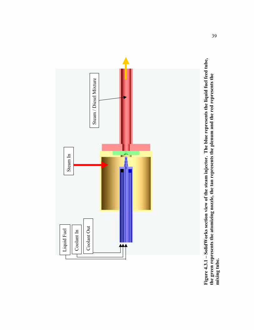
Fig

ure

4.3

.1 –

Soli

dW

ork

s se

ctio

n v

iew

of

the

stea

m i

nje

cto

r. T

he

blu

e re

pre

sen

ts t

he

liq

uid

fu

el f

eed

tu

be,

the

gre

en r

epre

sen

ts t

he

ato

miz

ing n

ozz

le, th

e ta

n r

epre

sen

ts t

he

ple

nu

m a

nd

th

e re

d r

epres

ents

th

e

mix

ing

tu

be.

Liq

uid

Fu

el

Co

ola

nt

In

Co

ola

nt

Ou

t

Ste

am I

n

Ste

am /

Die

sel

Mix

ture

39

40

is silver-soldered onto an 8 hole flange which secures the nozzle plate, and is wrapped

with a majority of the 24 heating tape, to produce a heated vaporization zone for the

fuel. A thermocouple is periodically placed into the mixing tube to obtain the exiting

mixture temperature. The laser shutter is closed when the thermocouple is inserted, so

that reflected light will not pose a safety hazard. During operation, the lower outer wall

of the mixing tube (adjacent to heating tape) is observed to glow red/orange, signifying

a metal temperature of over 500 °C. The mixture temperature is measured to be

nominally 50 °C less than the wall temperature at the tube exit.

4.4 Additional Steam Injector Testing Considerations

LRS testing with gaseous fuels allows the PMT voltage to be set to 1000 VDC, without

the risk of swamping the Combiscope. Liquid fuel vapors, however, produce much

larger scattering signals. In order to keep the measured scattering signal in range on the

Combiscope, the PMT voltage was turned to 600 VDC. This lower voltage reduces the

PMT output such that the signal is in the appropriate range. One drawback to this

adjustment is that the PMT response ceases to be linear. At lower signal values, the

response flattens, and the overall correlation is 2nd

order. Higher fuel concentrations

and cooler temperatures still produce stronger scattering signals, but the functional

dependence is changed. The fluctuations in signal, however, are the primary

observation, and are evident regardless of the nonlinear response of the PMT.

During any test with the steam injector, there is some heat up period, where the metal

and heater assemblies are brought up to test conditions. If the fuel injector feed tube

was allowed to heat, the introduction of fuel could initiate coke formation from the hot

metal walls. To circumvent this concern, and to keep debris from plugging the small

liquid orifice, an N2 purge was used constantly during heat up and cool down. A 3-way

valve was installed in the feed tube line just upstream of the fuel injector assembly.

This valve allows either liquid fuel or N2 to be directed through the injector assembly.

A practical, mobile system would probably not have access to a compressed N2

41

cylinder, so some other non-coking, process liquid or gas could be used, such as water,

steam, or reformate gas.

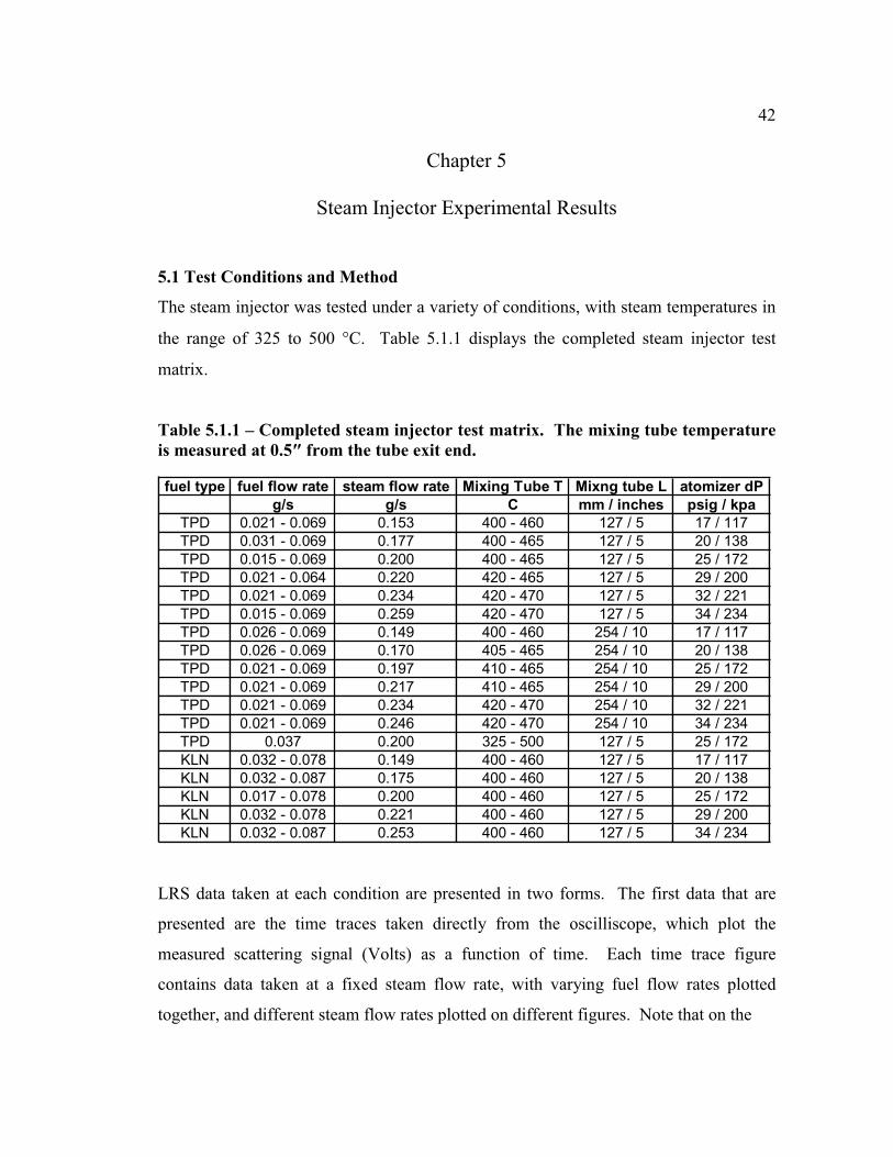
42

Chapter 5

Steam Injector Experimental Results

5.1 Test Conditions and Method

The steam injector was tested under a variety of conditions, with steam temperatures in

the range of 325 to 500 °C. Table 5.1.1 displays the completed steam injector test

matrix.

Table 5.1.1 – Completed steam injector test matrix. The mixing tube temperature

is measured at 0.5 from the tube exit end.

fuel type fuel flow rate steam flow rate Mixing Tube T Mixng tube L atomizer dP

g/s g/s C mm / inches psig / kpa

TPD 0.021 - 0.069 0.153 400 - 460 127 / 5 17 / 117

TPD 0.031 - 0.069 0.177 400 - 465 127 / 5 20 / 138

TPD 0.015 - 0.069 0.200 400 - 465 127 / 5 25 / 172

TPD 0.021 - 0.064 0.220 420 - 465 127 / 5 29 / 200

TPD 0.021 - 0.069 0.234 420 - 470 127 / 5 32 / 221

TPD 0.015 - 0.069 0.259 420 - 470 127 / 5 34 / 234

TPD 0.026 - 0.069 0.149 400 - 460 254 / 10 17 / 117

TPD 0.026 - 0.069 0.170 405 - 465 254 / 10 20 / 138

TPD 0.021 - 0.069 0.197 410 - 465 254 / 10 25 / 172

TPD 0.021 - 0.069 0.217 410 - 465 254 / 10 29 / 200

TPD 0.021 - 0.069 0.234 420 - 470 254 / 10 32 / 221

TPD 0.021 - 0.069 0.246 420 - 470 254 / 10 34 / 234

TPD 0.037 0.200 325 - 500 127 / 5 25 / 172

KLN 0.032 - 0.078 0.149 400 - 460 127 / 5 17 / 117

KLN 0.032 - 0.087 0.175 400 - 460 127 / 5 20 / 138

KLN 0.017 - 0.078 0.200 400 - 460 127 / 5 25 / 172

KLN 0.032 - 0.078 0.221 400 - 460 127 / 5 29 / 200

KLN 0.032 - 0.087 0.253 400 - 460 127 / 5 34 / 234

LRS data taken at each condition are presented in two forms. The first data that are

presented are the time traces taken directly from the oscilliscope, which plot the

measured scattering signal (Volts) as a function of time. Each time trace figure

contains data taken at a fixed steam flow rate, with varying fuel flow rates plotted

together, and different steam flow rates plotted on different figures. Note that on the

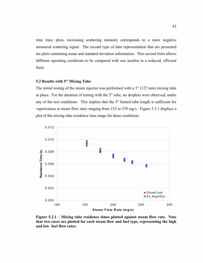
43

time trace plots, increasing scattering intensity corresponds to a more negative

measured scattering signal. The second type of data representation that are presented

are plots containing mean and standard deviation information. This second form allows

different operating conditions to be compared with one another in a reduced, efficient

form.

5.2 Results with 5 Mixing Tube

The initial testing of the steam injector was performed with a 5 (127 mm) mixing tube

in place. For the duration of testing with the 5” tube, no droplets were observed, under

any of the test conditions. This implies that the 5 heated tube length is sufficient for

vaporization at steam flow rates ranging from 153 to 259 mg/s. Figure 5.2.1 displays a

plot of the mixing tube residence time range for these conditions.

0.000

0.002

0.004

0.006

0.008

0.010

0.012

100 150 200 250 300

Steam Flow -R ate (m g/s)

Re

sid

en

ce

Tim

e (

s)

Diesel fuel

KL Naphtha

Figure 5.2.1 – Mixing tube residence times plotted against steam flow rate. Note

that two cases are plotted for each steam flow and fuel type, representing the high

and low fuel flow rates.

44

Figures 5.2.2 through 5.2.7 show time traces of the measured scattering signal as a

function of time for various steam flow rates. Each plot contains several traces, each at

a different TPD flow rate. Note that very few spikes in the signal are seen, indicating

that the fuel is completely vaporized. There is some temperature variation in the

mixing tube among the steam flow rates. At a given steam flow rate, the mixing tube

temperature decreases linearly with the addition of fuel.

Vapor lock is illustrated on several of the figures, indicating that the liquid fuel’s

residence time in the delivery tube is excessive. Vapor lock is indicated by large

amplitude, low frequency fluctuations of the scattering signal. Although a majority of

the time traces show fluctuations, the vapor lock conditions are extreme. The mixture

oscillates between pure steam and fuel rich (relative to mean), which produces large

temporal unsteadiness in fuel concentration.

Equation 5.2.1 displays the equation used calculate a mixing parameter called

unmixedness here. The unmixedness for this set of test conditions is generally 10% or

signalmean

deviationdardtanssUnmixednes = Eq. 5.2.1

less, except when vapor lock conditions arise. The baseline noise was determined to

give an apparent unmixedness value of 5%, although this number depends upon the

magnitude of the scattering signal. Smaller mean signals are more susceptible to noise

and generally produce higher standard deviations for the given system. Figure 5.2.8

displays the unmixedness plotted against the fuel concentration. The unmixedness is

roughly constant for all of the steam flowrates and fuel concentrations, which implies

that the mixing is good within mixing tube. Most conditions, except vapor lock,

provide unmixedness values of less than 5% relative to the noise baseline.

-4.0

-3.5

-3.0

-2.5

-2.0

-1.5

-1.0

-0.5

0.0

0.0

00

.05

0.1

00.1

50

.20

Tim

e (

s)


26 m

g/s

fu

el

32 m

g/s

fu

el

37 m

g/s

fu

el

42 m

g/s

fu

el

48 m

g/s

fu

el

53 m

g/s

fu

el

58 m

g/s

fu

el

64 m

g/s

fu

el

69 m

g/s

fu

el

Fig

ure

5.2

.2 –

Tim

e tr

aces

at

153 m

g/s

ste

am

flo

w r

ate

, an

d v

ari

ou

s fu

el f

low

rate

s. N

ote

th

at

the

larg

e gap

in

sca

tter

ing s

ign

al

from

64 m

g/s

to 5

8 m

g/s

may b

e d

ue

to r

oto

met

er s

ett

lin

g.

45

-2.0

0

-1.8

0

-1.6

0

-1.4

0

-1.2

0

-1.0

0

-0.8

0

-0.6

0

-0.4

0

-0.2

0

0.0

00.0

00

.05

0.1

00

.15

0.2

0

Tim

e (

s)


31 m

g/s

fu

el

37 m

g/s

fu

el

42 m

g/s

fu

el

53 m

g/s

fu

el

58 m

g/s

fu

el

64 m

g/s

fu

el

69 m

g/s

fu

el

Fig

ure

5.2

.3 –

Tim

e tr

aces

at

177 m

g/s

ste

am

flo

w r

ate

, an

d v

ari

ou

s fu

el f

low

rate

s.

Note

th

e vap

or

lock

in

stab

ilit

y a

t a

fu

el f

low

ra

te o

f 3

1 m

g/s

.

46

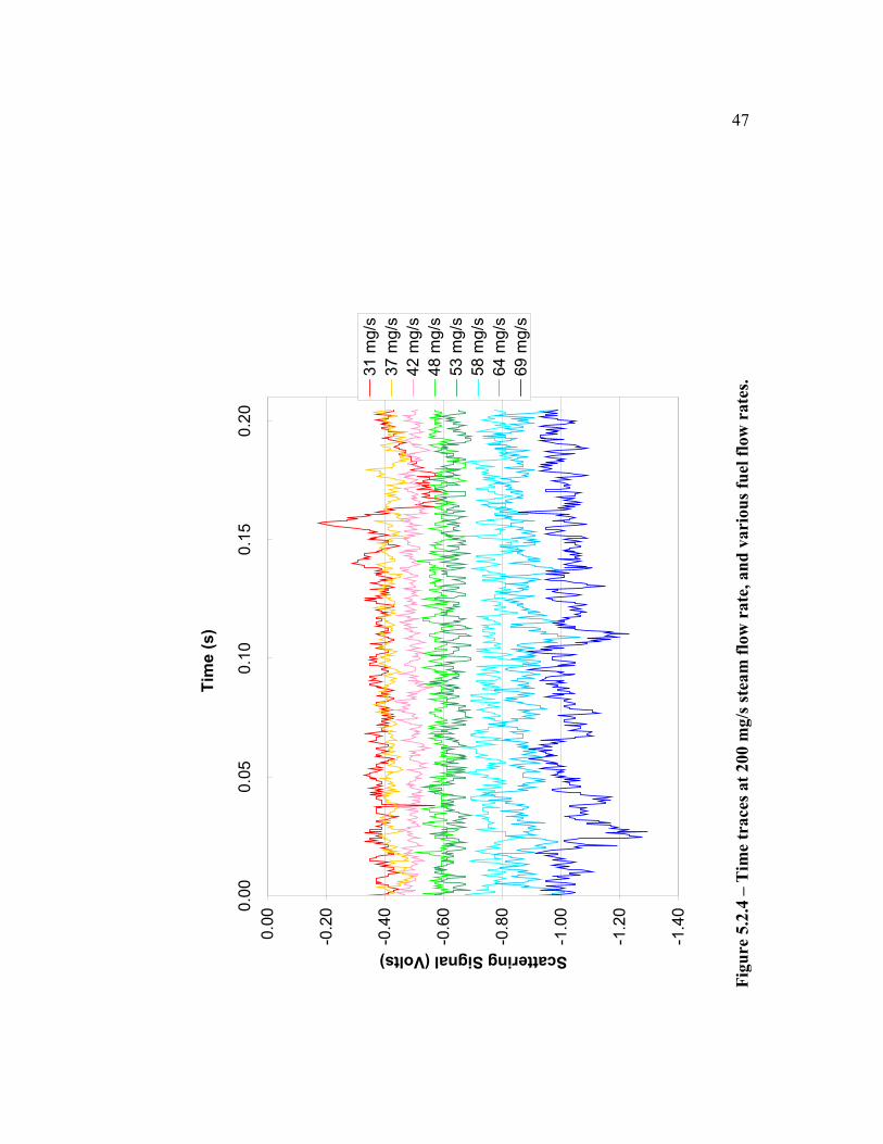
-1.4

0

-1.2

0

-1.0

0

-0.8

0

-0.6

0

-0.4

0

-0.2

0

0.0

00.0

00.0

50.1

00.1

50

.20

Tim

e (

s)


31 m

g/s

37 m

g/s

42 m

g/s

48 m

g/s

53 m

g/s

58 m

g/s

64 m

g/s

69 m

g/s

Fig

ure

5.2

.4 –

Tim

e tr

aces

at

200 m

g/s

ste

am

flo

w r

ate

, an

d v

ari

ou

s fu

el f

low

rate

s.

47

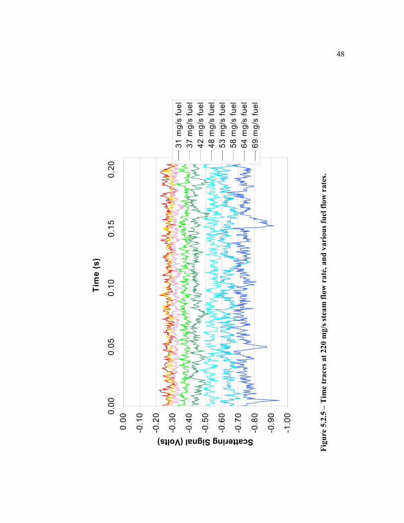
-1.0

0

-0.9

0

-0.8

0

-0.7

0

-0.6

0

-0.5

0

-0.4

0

-0.3

0

-0.2

0

-0.1

0

0.0

00.0

00

.05

0.1

00

.15

0.2

0

Tim

e (

s)


31

mg

/s f

ue

l

37

mg

/s f

ue

l

42

mg

/s f

ue

l

48

mg

/s f

ue

l

53

mg

/s f

ue

l

58

mg

/s f

ue

l

64

mg

/s f

ue

l

69

mg

/s f

ue

l

Fig

ure

5.2

.5 –

Tim

e tr

aces

at

220 m

g/s

ste

am

flo

w r

ate

, an

d v

ari

ou

s fu

el f

low

rate

s.

48

-1.6

0

-1.4

0

-1.2

0

-1.0

0

-0.8

0

-0.6

0

-0.4

0

-0.2

0

0.0

00.0

00

.05

0.1

00

.15

0.2

0

Tim

e (

s)


21 m

g/s

fu

el

31 m

g/s

fu

el

37 m

g/s

fu

el

42 m

g/s

fu

el

48 m

g/s

fu

el

53 m

g/s

fu

el

58 m

g/s

fu

el

64 m

g/s

fu

el

69 m

g/s

fu

el

Fig

ure

5.2

.6 –

Tim

e tr

aces

at

234 m

g/s

ste

am

flo

w r

ate

, an

d v

ari

ou

s fu

el f

low

rate

s.

Roto

mete

r re

ad

ing s

usp

ect,

flo

w m

ay n

ot

have

sett

led

an

d f

uel

flo

w m

ay b

e to

o h

igh

.

49

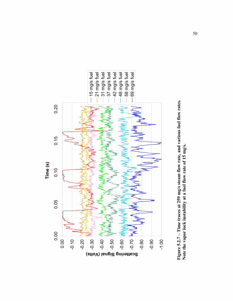
-1.0

0

-0.9

0

-0.8

0

-0.7

0

-0.6

0

-0.5

0

-0.4

0

-0.3

0

-0.2

0

-0.1

0

0.0

00.0

00

.05

0.1

00

.15

0.2

0

Tim

e (

s)


15 m

g/s

fu

el

21 m

g/s

fu

el

31 m

g/s

fu

el

37 m

g/s

fu

el

42 m

g/s

fu

el

48 m

g/s

fu

el

58 m

g/s

fu

el

69 m

g/s

fu

el

Fig

ure

5.2

.7 –

Tim

e tr

aces

at

259 m

g/s

ste

am

flo

w r

ate

, an

d v

ari

ou

s fu

el f

low

rate

s.

Note

th

e vap

or

lock

in

stab

ilit

y a

t a

fu

el f

low

ra

te o

f 1

5 m

g/s

.

50

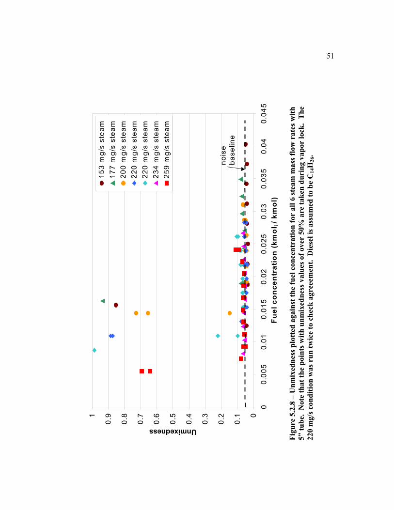
0

0.1

0.2

0.3

0.4

0.5

0.6

0.7

0.8

0.91

00

.00

50

.01

0.0

15

0.0

20

.02

50

.03

0.0

35

0.0

40

.04

5

Fu

el

co

nc

en

tra

tio

n (

km

ol i

/ k

mo

l)

Unmixedness

15

3 m

g/s

ste

am

17

7 m

g/s

ste

am

20

0 m

g/s

ste

am

22

0 m

g/s

ste

am

22

0 m

g/s

ste

am

23

4 m

g/s

ste

am

25

9 m

g/s

ste

am

no

ise

ba

se

lin

e

Fig

ure

5.2

.8 –

Un

mix

edn

ess

plo

tted

again

st t

he

fuel

con

cen

trati

on

for

all

6 s

team

ma

ss f

low

rate

s w

ith

5” t

ub

e. N

ote

th

at

the

poin

ts w

ith

un

mix

edn

ess

valu

es o

f over

50%

are

tak

en d

uri

ng v

ap

or

lock

. T

he

220 m

g/s

con

dit

ion

was

run

tw

ice

to c

hec

k a

gree

em

ent.

D

iese

l is

ass

um

ed t

o b

e C

14H

26.

51

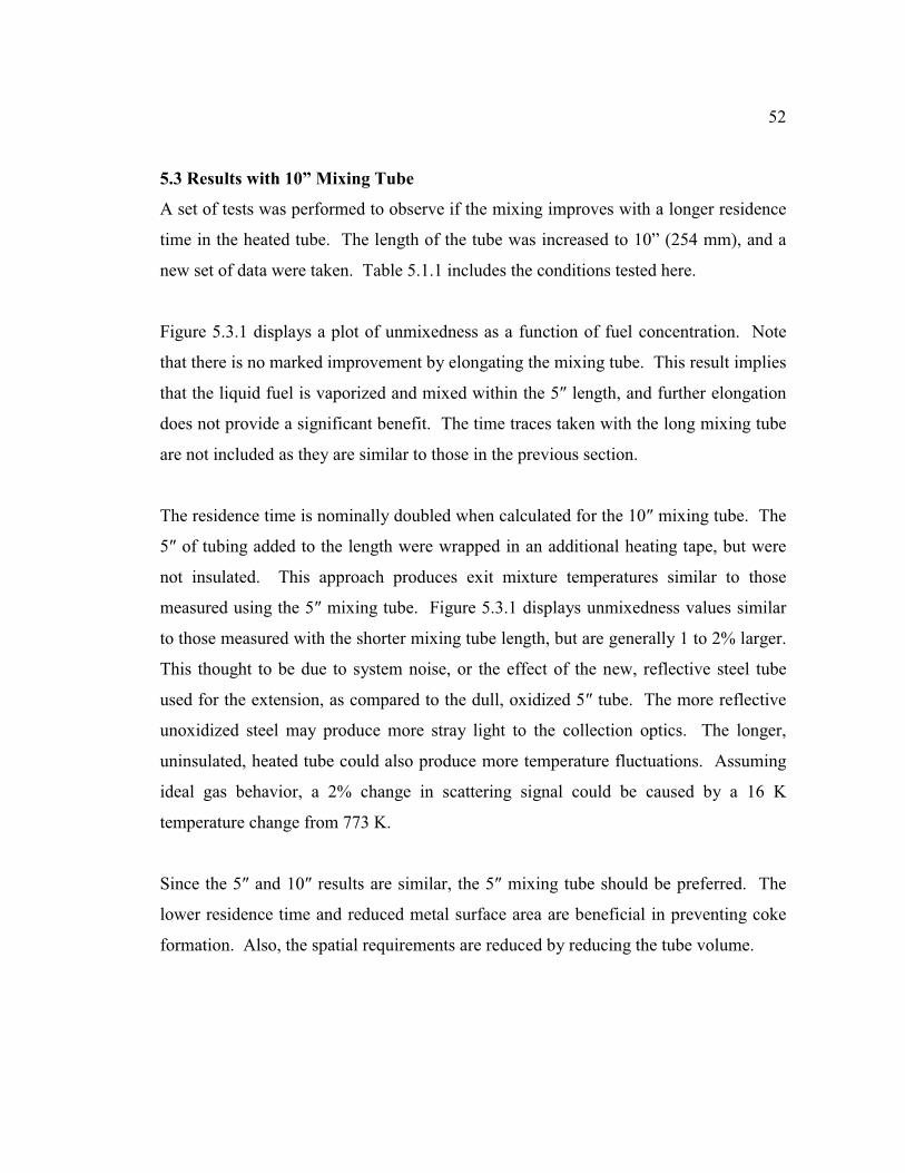
52

5.3 Results with 10” Mixing Tube

A set of tests was performed to observe if the mixing improves with a longer residence

time in the heated tube. The length of the tube was increased to 10” (254 mm), and a

new set of data were taken. Table 5.1.1 includes the conditions tested here.

Figure 5.3.1 displays a plot of unmixedness as a function of fuel concentration. Note

that there is no marked improvement by elongating the mixing tube. This result implies

that the liquid fuel is vaporized and mixed within the 5 length, and further elongation

does not provide a significant benefit. The time traces taken with the long mixing tube

are not included as they are similar to those in the previous section.

The residence time is nominally doubled when calculated for the 10 mixing tube. The

5 of tubing added to the length were wrapped in an additional heating tape, but were

not insulated. This approach produces exit mixture temperatures similar to those

measured using the 5 mixing tube. Figure 5.3.1 displays unmixedness values similar

to those measured with the shorter mixing tube length, but are generally 1 to 2% larger.

This thought to be due to system noise, or the effect of the new, reflective steel tube

used for the extension, as compared to the dull, oxidized 5 tube. The more reflective

unoxidized steel may produce more stray light to the collection optics. The longer,

uninsulated, heated tube could also produce more temperature fluctuations. Assuming

ideal gas behavior, a 2% change in scattering signal could be caused by a 16 K

temperature change from 773 K.

Since the 5 and 10 results are similar, the 5 mixing tube should be preferred. The

lower residence time and reduced metal surface area are beneficial in preventing coke

formation. Also, the spatial requirements are reduced by reducing the tube volume.

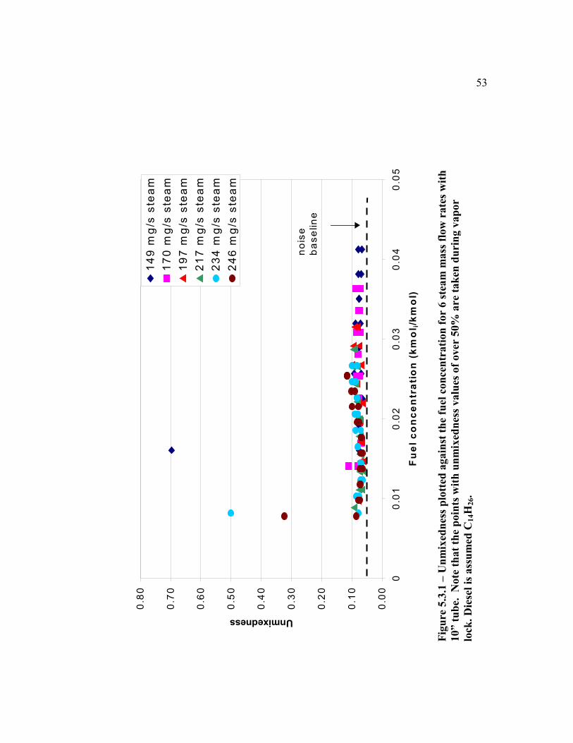
0.0

0

0.1

0

0.2

0

0.3

0

0.4

0

0.5

0

0.6

0

0.7

0

0.8

0

00

.01

0.0

20

.03

0.0

40

.05

Fu

el

co

nc

en

tra

tio

n (

km

ol i/k

mo

l)

Unmixedness

14

9 m

g/s

ste

am

17

0 m

g/s

ste

am

19

7 m

g/s

ste

am

21

7 m

g/s

ste

am

23

4 m

g/s

ste

am

24

6 m

g/s

ste

am

no

ise

ba

se

lin

e

Fig

ure

5.3

.1 –

Un

mix

edn

ess

plo

tted

again

st t

he

fuel

con

cen

trati

on

for

6 s

tea

m m

ass

flo

w r

ate

s w

ith

10” t

ub

e. N

ote

th

at

the

poin

ts w

ith

un

mix

edn

ess

valu

es o

f over

50%

are

tak

en d

uri

ng v

ap

or

lock

. D

iese

l is

ass

um

ed C

14H

26.

53

54

5.4 Variable Mixing Tube Temperature Effects

The previous tests consisted of fixing the steam flow rate, and varying the fuel mass

flow rate and hence the mixing tube exit temperature. This set of tests consisted of

setting the steam and fuel mass flow rates, and then incrementally increasing the

mixing tube exit temperature, from 325 °C to 500 °C. The steam and fuel mass flow

rates were held constant at 200 mg/s and 37 mg/s respectively. The mixture exit

temperature is controlled by adjustment of the variac setting, which changes the heat

flux from the heating tape through the mixing tube outer wall.

Higher temperatures should increase the evaporation rate of the droplets and expedite

mixing. The residence time however is decreased by an increase in mixture

temperature. Figure 5.4.1 displays a plot of unmixedness against the mixing tube exit

temperature. The unmixed is 12% at 325 °C, and decreases to less than 10% as the

temperature is raised. At temperatures higher than 425 °C, the unmixedness range is

roughly constant between 6 and 9%, indicating a weak dependence of mixing on the

tube temperature. The small droplets produced by the steam injector are able to

vaporize completely at temperatures above 330 °C. Figure 5.4.2 shows time traces

taken at 330, 400, 450, and 500 °C.

Figure 5.4.3 displays the mean scattering signal plotted against the mixture

temperature. The additional points represent 1 / T correlations based on the 325 and

500 °C set points. The experimental data shows an increased slope, signifying that the

scattering signal is decreasing due to some other parameter. The PMT response is

nonlinear at the 600 VDC setting used, but the deviation from linear behavior is not

pronounced when the scattering signal is between 0.4 and 1.4 Volts (lower signals are

more nonlinear). Figure 5.4.4 displays a linearity test performed by varying laser

power. Note that the R2 value of performing a linear regression is 0.9896. As

mentioned in Chapter 3, this trend may be due to non-ideal gas behavior, small droplets

or cracking of the larger hydrocarbon molecules.

0.0

0

0.0

2

0.0

4

0.0

6

0.0

8

0.1

0

0.1

2

0.1

4

30

03

50

40

04

50

50

05

50

T (

°C)

Unmixedness

Fig

ure

5.4

.1 –

Un

mix

edn

ess

plo

tted

again

st m

ixtu

re

tem

per

atu

re,

for

200 m

g/s

ste

am

an

d 3

7 m

g/s

TP

D.

55

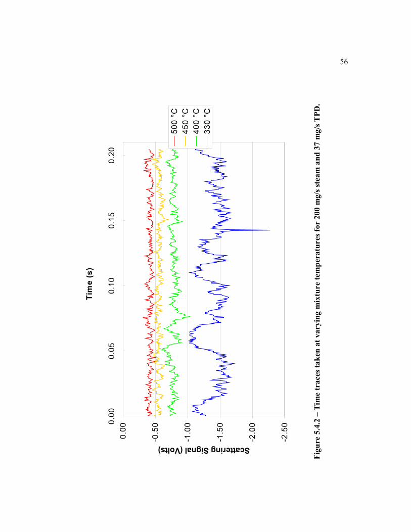
-2.5

0

-2.0

0

-1.5

0

-1.0

0

-0.5

0

0.0

00.0

00

.05

0.1

00

.15

0.2

0

Tim

e (

s)


50

0 °

C

45

0 °

C

40

0 °

C

33

0 °

C

Fig

ure

5.4

.2 –

Tim

e tr

aces

tak

en a

t va

ryin

g m

ixtu

re

tem

per

atu

res

for

200 m

g/s

ste

am

an

d 3

7 m

g/s

TP

D.

56

0.0

0

0.2

0

0.4

0

0.6

0

0.8

0

1.0

0

1.2

0

1.4

0

1.6

0

30

03

50

40

04

50

50

05

50

T (

°C)

Mean Scattering Signal (Volts)

Te

st

da

ta

1/T

ma

tch

ed

at

32

5 °

C

1/T

ma

tch

ed

at

50

0 °

C

Fig

ure

5.4

.3 –

Mea

n s

catt

erin

g s

ign

al

plo

tted

again

st m

ixtu

re t

em

pera

ture

. T

he

ad

dit

ion

al

data

poin

ts

rep

rese

nt

(Con

stan

t /

T )

rel

ati

on

s b

ase

d o

n t

he

corr

esp

on

din

g d

ata

poin

ts.

57

y =

1.2

86

38

52

0x -

0.0

61

96

43

8

R2 =

0.9

89

62

40

9

y =

0.6

31

44

22

8x

2 +

0.4

65

51

02

3x +

0.1

71

66

92

6

R2 =

0.9

99

16

20

5

0.0

0

0.2

0

0.4

0

0.6

0

0.8

0

1.0

0

1.2

0

1.4

0

00

.20

.40

.60

.81

1.2

La

se

r P

ow

er

(Wa

tts

)

Mean scattering signal (Volts)

Fig

ure

5.4

.4 –

Lin

eari

ty t

est

of

the

PM

T r

esp

on

se a

t 600 V

DC

.

58

59

5.5 Naphtha Results with 5” Mixing Tube

The previous experimental results display good mixing of the TPD and steam. Kern

Light Naphtha is examined next to observe the effects of fuel volatility. The test

conditions ran are included in Table 5.1.1.

Figure 5.5.1 displays the unmixedness plotted vs. KLN concentration. Note the general

form of the plot is consistent with Figures 5.2.8 and 5.3.1, with the unmixedness value

being almost flat for the higher fuel concentrations, rising sharply as vapor lock

conditions arise. Cooling air was required at almost all of the data points to suppress

vapor lock.

It is important to note that KLN has a density of 693 kg/m3, and is lighter than TPD,

which has a density of about 860 kg/m3. The molecular mass of KLN is 83.20 kg/kmol,

while diesel fuel has a molecular mass of between 190 and 200 kg/kmol generally.

KLN produces a weaker scattering signal, as can be seen by Figure 5.5.2. The lower

mean scattering signal of KLN also reduces the signal to noise ratio, signifying that the

unmixedness values given in Figure 5.5.1 are high. Figure 5.5.2 displays the mean

scattering signal of TPD and KLN plotted against fuel concentration. A third order fit

is used to obtain desirable behavior from the TPD regression. The TPD signal is large

compared to the background noise, so the regression curve is forced to zero at zero fuel

concentration. The KLN, however, has a mean scattering signal much closer to the

pure steam signal. The regression curve for KLN is not forced through zero as a result.

Note that the data points plotted for both fuels consist of all steam mass flow rates

tested, so there is some scatter of the data points due to variations in temperature.

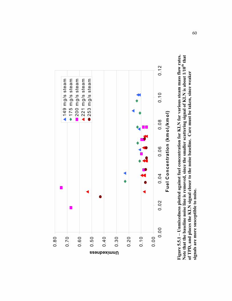
0.0

0

0.1

0

0.2

0

0.3

0

0.4

0

0.5

0

0.6

0

0.7

0

0.8

0 0.0

00

.02

0.0

40

.06

0.0

80

.10

0.1

2

Fu

el

Co

nc

en

tra

tio

n (

km

ol i

/km

ol)

Unmixedness

14

9 m

g/s

ste

am

17

5 m

g/s

ste

am

20

0 m

g/s

ste

am

22

1 m

g/s

ste

am

25

3 m

g/s

ste

am

Fig

ure

5.5

.1 –

Un

mix

edn

ess

plo

tted

again

st f

uel

con

cen

trati

on

for

KL

N f

or

vari

ou

s st

eam

mass

flo

w r

ate

s.

Note

th

at

the

base

lin

e n

ois

e li

ne

is r

em

oved

, si

nce

th

e s

mall

er s

catt

eri

ng s

ign

al

of

KL

N i

s ab

ou

t 1/1

0th

th

at

of

TP

D, an

d p

lace

s th

e K

LN

sig

nal

close

r to

th

e n

ois

e b

ase

lin

e. C

are

mu

st b

e ta

ken

, si

nce

wea

ker

sign

als

are

mo

re s

usc

epti

ble

to n

ois

e.

60

y =

14

.84

65

7x

2 -

0.2

60

24

x +

0.0

39

59

R2 =

0.9

32

30

y =

52

75

3.5

43

34

x3 -

10

86

.21

53

5x

2 +

27

.08

11

7x

R2 =

0.9

80

25

0

0.51

1.52

2.53

3.54 0

.00

0.0

20

.04

0.0

60

.08

0.1

0

Fu

el

Co

nc

en

tra

tio

n (

km

ol i/k

mo

l)

TPD Mean Scattering Signal (Volts)

0.0

0

0.0

5

0.1

0

0.1

5

0.2

0

0.2

5

0.3

0

0.3

5

0.4

0

KLN Mean Scattering Signal (Volts)

TP

D

KL

N

Po

ly.

(KL

N)

Po

ly.

(TP

D)

Fig

ure

5.5

.2 –

Mea

n s

catt

erin

g s

ign

al

plo

tted

again

st f

uel

con

cen

trati

on

for

TP

D a

nd

KL

N.

61

62

5.6 Vapor Lock Considerations

Vapor lock defines the premature boiling of fuel components prior to liquid injection,

and is caused by heating of the fuel delivery tube until the local liquid temperature is

equal to the fuel saturation temperature at the local fuel pressure. This is especially

significant for volatile fuels, and was determined to occur over a wider range of

conditions for KLN than TPD. This process causes a liquid flow rate unsteadiness that

is audibly observable by a consistent ragged, “spitting” in the steam injector. The

effects of vapor lock are large temporal changes in fuel concentration, and possible

carbon deposit formation at the spatial region of boiling. Edwards (1992) performed a

series of experiments in which liquid fuel was boiled in the absence of O2 (N2 purged

environment), and observed carbon deposits at the point of fuel phase change.

When the steam injector is operated with TPD, the tendency for vapor lock is relegated

to the lower fuel flow rates when no coolant is present. Low fuel flow rates dictate that

the residence time of the fuel in the heated region is larger, and thus the fuel

temperature will be larger. The fuel instability can, however, be suppressed with the

introduction of a cooling medium through the cooling passages of the fuel feed tube.

The experimental setup allowed air or water to be used for cooling, although it was

determined that water reduced the mixture temperature excessively and did not produce

a steady cooling effect. The results of KLN provided similar observations. Air cooling

reduced the vapor lock tendency of the injector when operated on KLN, but the

instability was difficult to eliminate. Figures 5.6.1, and 5.6.2 each show two time

traces taken at low fuel flow rates. One trace represents the scattering signal without

cooling effects, and the other trace represents the same conditions with cooling. The

data points displayed in Figures 5.6.1 and 5.6.2 were taken within 10 seconds of each

other, enough time to introduce the cooling medium. The frequency of the

concentration oscillations was calculated to be 20 Hz with a standard deviation of 3 Hz,

by calculating the fuel concentration peak to peak time period.

63

-0.50

-0.45

-0.40

-0.35

-0.30

-0.25

-0.20

-0.15

-0.10

-0.05

0.00

0.00 0.05 0.10 0.15 0.20

Time (s)S

catt

eri

ng

Sig

nal (V

olt

s)

without cooling

with cooling

Figure 5.6.1 – Time traces of vapor lock effects with and without cooling.

Test conditions were 15 mg/s TPD and 234 mg/s steam with 5” tube.

-1.60

-1.40

-1.20

-1.00

-0.80

-0.60

-0.40

-0.20

0.00

0.00 0.05 0.10 0.15 0.20

Time (s)

Scatt

eri

ng

Sig

nal

(Vo

lts)

without cooling

with cooling

Figure 5.6.2 – Time traces of vapor lock effects with and without cooling.

Test conditions were 26 mg/s TPD and 153 mg/s steam with 5” tube.

64

5.7 Spatial Uniformity in the Mixing Tube

The inner diameter of the mixing tube is 6.99 mm. The length scale of the measuring

volume is 1 – 2 mm, so some limited spatial resolution is possible. A brief test was

performed to examine the spatial variation in the mixture properties. This was

accomplished by traversing the collection optics assembly parallel to the laser beam

across the test mixture exiting from the mixing tube. The constant operating conditions

during this test were 200 mg/s steam and 37 mg/s TPD. Figure 5.7.1 displays a plot of

mean scattering signal, standard deviation, and unmixedness as a function of radial

position from the centerline of the mixing tube. The mean and standard deviation are

constant in the middle of the jet to within 2%. This implies that the mixing tube

provides a spatially similar mixture. At the inner walls of the mixing tube, the mean

signal is seen to decrease. This occurs because the measuring volume now includes

some ambient air. The inclusion of ambient air also brings dust and particles into the

measuring volume, which raises the standard deviation and unmixedness in this region.

Outside of the tube, the pure ambient air signal has a mean value of 25 times less than

that in the center of the tube. The ambient air is noise when measured with the PMT

and Combiscope settings, and has an associated large unmixedness value.

Since the fuel and steam mixture enters the mixing tube as a high-speed jet through the

atomizing nozzle, it is expected that the droplets will be dispersed throughout the

mixing tube cross section. The flow downstream of the atomizing nozzle can be

compared that of a confined jet. Confined jets entrain fluid via momentum transfer, but

without second stream the jet will consume itself. This consumption causes a

recirculation zone on the downstream side of the nozzle plate. The distance required to

entrain a mass flow equal to that traversing the atomizing nozzle is about 5 mm based

on Equation 5.7.1 from Beér (1983) assuming constant density.

1d

x32.0

m

m

00

e −

= Eq. 5.7.1

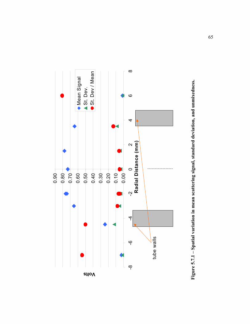
0.0

0

0.1

0

0.2

0

0.3

0

0.4

0

0.5

0

0.6

0

0.7

0

0.8

0

0.9

0

-8-6

-4-2

02

46

8

Ra

dia

l D

ista

nc

e (

mm

)

Volts

Me

an

Sig

na

l

St.

De

v.

St.

De

v /

Me

an

tub

e w

alls

Fig

ure

5.7

.1 –

Sp

ati

al

va

ria

tio

n i

n m

ean

sca

tteri

ng

sig

na

l, s

tan

da

rd d

evia

tio

n,

an

d u

nm

ixed

nes

s.

65

66

5.8 Summary of Steam Injector Results

A wide range of test conditions were imposed upon the steam injector. The following

bullets restate the primary experimental results with some discussion.

• Droplets were not observed at the measurement location at the test conditions

included. This implies that the 5 heated tube length is more than adequate to

completely vaporize the liquid fuel droplets created by the atomizer.

• The unmixedness was measured to be less than 10% for almost all TPD test

conditions, except when vapor lock is present. The nominal baseline noise of the

collection system gives an apparent unmixedness value of 5%. Most test

conditions produced standard deviation / mean values of 6 to 8% (1 – 3% relative

to the noise baseline).

• No carbon deposits were observed, upon post inspection, for any of the tested

conditions. No particles were detected in the measurement volume for any of the

performed tests. Some liquid diesel residue was found on the interior walls of the

mixing tube, which may have been deposited during startup or shutdown

sputtering of the fuel flow.

• Vapor lock is a problem at fuel flow rates of 31 mg/s or less. This is most likely

due to heat transfer from the 400+ °C superheated steam to the exposed copper

fuel injector tip. Larger fuel mass flow rates, shorter fuel injector residence times

and less volatile fuels reduce the effects of this problem. The vapor lock frequency

of the TPD fuel unsteadiness is about 20 Hz.

• The steam injector provides a spatially uniform mixture. No significant variation in

mean signal or unmixedness is observed as the measurement location above the

mixing tube is radially varied.

• Temperature has some effect upon the vaporization and mixing. At 325 °C, the

unmixedness is 12%, with large time scale (20 ms) fluctuations. The unmixedness

and time scale of the fluctuations decreases with an increase in temperature. The

unmixedness at 500 °C is 8%. Note that the mean scattering signal at 500 °C is

about 0.4 Volts while the mean scattering signal at 325 °C is 1.4 Volts. This

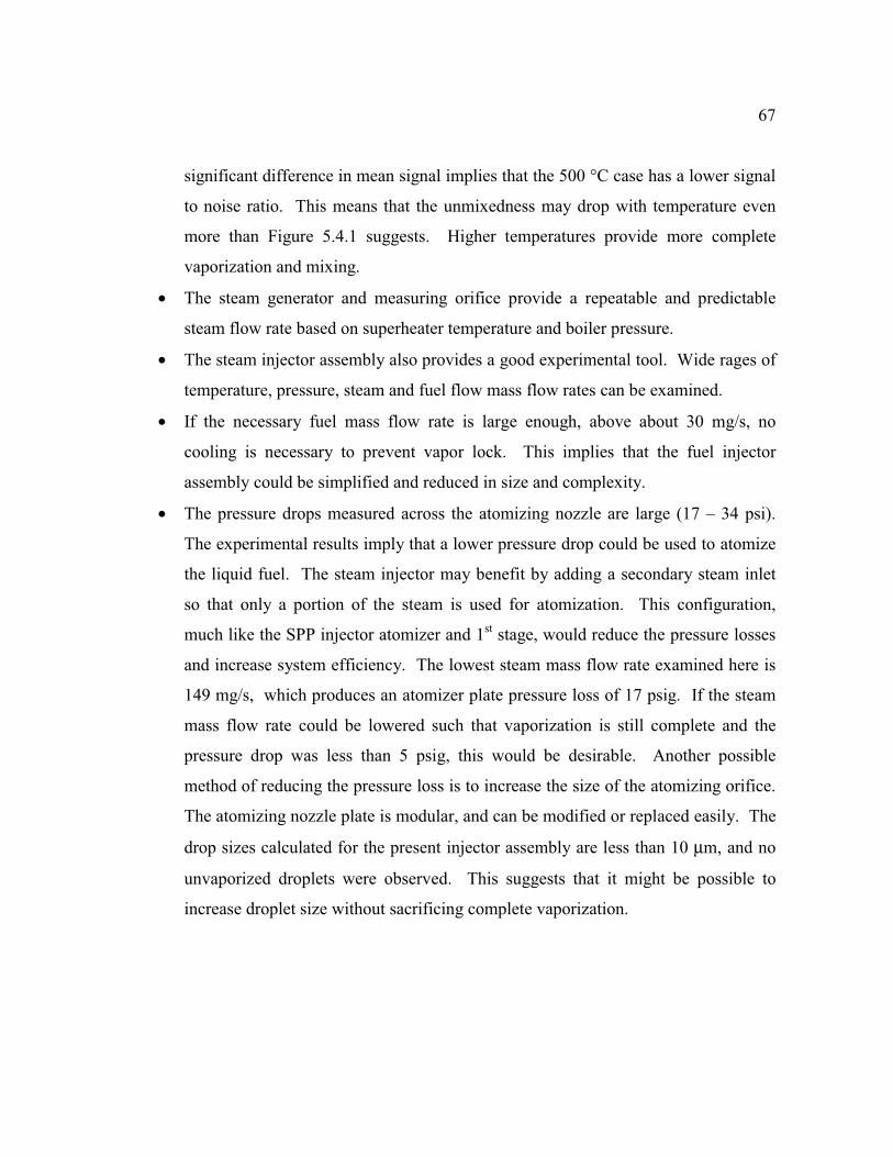
67

significant difference in mean signal implies that the 500 °C case has a lower signal

to noise ratio. This means that the unmixedness may drop with temperature even

more than Figure 5.4.1 suggests. Higher temperatures provide more complete

vaporization and mixing.

• The steam generator and measuring orifice provide a repeatable and predictable

steam flow rate based on superheater temperature and boiler pressure.

• The steam injector assembly also provides a good experimental tool. Wide rages of

temperature, pressure, steam and fuel flow mass flow rates can be examined.

• If the necessary fuel mass flow rate is large enough, above about 30 mg/s, no

cooling is necessary to prevent vapor lock. This implies that the fuel injector

assembly could be simplified and reduced in size and complexity.

• The pressure drops measured across the atomizing nozzle are large (17 – 34 psi).

The experimental results imply that a lower pressure drop could be used to atomize

the liquid fuel. The steam injector may benefit by adding a secondary steam inlet

so that only a portion of the steam is used for atomization. This configuration,

much like the SPP injector atomizer and 1st stage, would reduce the pressure losses

and increase system efficiency. The lowest steam mass flow rate examined here is

149 mg/s, which produces an atomizer plate pressure loss of 17 psig. If the steam

mass flow rate could be lowered such that vaporization is still complete and the

pressure drop was less than 5 psig, this would be desirable. Another possible

method of reducing the pressure loss is to increase the size of the atomizing orifice.

The atomizing nozzle plate is modular, and can be modified or replaced easily. The

drop sizes calculated for the present injector assembly are less than 10 µm, and no

unvaporized droplets were observed. This suggests that it might be possible to

increase droplet size without sacrificing complete vaporization.

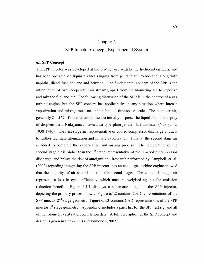
68

Chapter 6

SPP Injector Concept, Experimental System

6.1 SPP Concept

The SPP injector was developed at the UW for use with liquid hydrocarbon fuels, and

has been operated on liquid alkanes ranging from pentane to hexadecane, along with

naphtha, diesel fuel, toluene and benzene. The fundamental concept of the SPP is the

introduction of two independent air streams, apart from the atomizing air, to vaporize

and mix the fuel and air. The following discussion of the SPP is in the context of a gas

turbine engine, but the SPP concept has applicability in any situation where intense

vaporization and mixing must occur in a limited time/space scale. The atomizer air,

generally 2 – 5 % of the total air, is used to initially disperse the liquid fuel into a spray

of droplets via a Nukiyama / Tawazawa type plain jet air-blast atomizer (Nukiyama,

1938-1940). The first stage air, representative of cooled compressor discharge air, acts

to further facilitate atomization and initiate vaporization. Finally, the second stage air

is added to complete the vaporization and mixing process. The temperature of the

second stage air is higher than the 1st stage, representative of the un-cooled compressor

discharge, and brings the risk of autoignition. Research performed by Campbell, et. al.

(2002) regarding integrating the SPP injector into an actual gas turbine engine showed

that the majority of air should enter in the second stage. The cooled 1st stage air

represents a loss in cycle efficiency, which must be weighed against the emission

reduction benefit. Figure 6.1.1 displays a schematic image of the SPP injector,

depicting the primary process flows. Figure 6.1.2 contains CAD representations of the

SPP injector 2nd

stage geometry. Figure 6.1.3 contains CAD representations of the SPP

injector 1st stage geometry. Appendix C includes a parts list for the SPP test rig, and all

of the rotometer calibration/correlation data. A full description of the SPP concept and

design is given in Lee (2000) and Edmonds (2002).

69

Up to 220 V, 30 A Ouput

Convectronix

Air Heater

Heated 1

st Stage

Air In

Cold Air In

Liquid Fuel &

Atomizer AirIn

Jet-Stirred Reactor

Exhaust Drain H oles

Watlow

Cascade

Controller

Watlow SCR

K-Type TC

4-20 mA

Output

Fluke NetDAQData Logger

R-Type TC

Gas Analyzers

& Sampling

System

Quartz Probe

Input 1 Input 2

K-Type TC

Gaseous Fuel In

Blowout Flange

Film Atom izer

H eated 2nd

Stage

Air In (Similar Controller and

Heater Setup as

1st Stage Air)

K-T ype TC

Air Cooled

Nukiyama-Tanassawa Type Nozzle

Fuel Spray

Second Stage

First Stage

Staggered High

Velocity Mixing Jets

High Veloc ity

Mixing &

Atom ization Jets

Nozzle Block

Figure 6.1.1 – Schematic of the SPP injector and primary process flow streams.

This particular configuration represents that used during LPP combustion testing

with the JSR. The LRS testing configuration is essentially the same, except the

nozzle block and JSR are removed, and no data logger is used. This figure is

taken from Edmonds (2002).

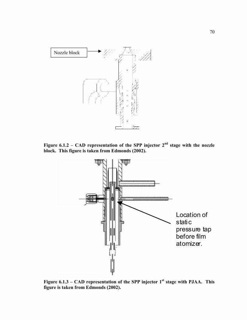
70

Figure 6.1.2 – CAD representation of the SPP injector 2nd

stage with the nozzle

block. This figure is taken from Edmonds (2002).

Location ofstaticpressure tapbefore filmatomizer.

Figure 6.1.3 – CAD representation of the SPP injector 1st stage with PJAA. This

figure is taken from Edmonds (2002).

Nozzle block

71

6.2 Atomizer Air and Fuel Systems

The plain jet airblast atomizer is air-cooled, and operates on an air to liquid mass ratio

of nominally 1. The liquid fuel orifice is 0.012 (0.305 mm) in diameter, with a 45°

inlet chamfer to increase the discharge coefficient (Lefebvre, 1989). The thickness to

diameter ratio of the fuel orifice is 3.75. The secondary (air) orifice is 0.021 (0.533

mm) in diameter, with a 0.048 (1.22 mm) gap between liquid and air atomizing

nozzles. In Chapter 2, it was calculated that the SMD of the droplets from this atomizer

is in the range of 10 to 20 µm. Figure 6.2.1 displays a CAD representation of the

atomizer assembly (Lee, 2000).

The atomizer airflow, and atomizer cooling airflow are controlled and monitored via a

0 to 150 psig pressure regulator and FP-10A3555 rotometer with FP-1/8-G-25-5/84

tube and 1/8 SS float. The cooling airflow is not measured explicitly, but is adjusted

to suppress vapor lock and coking at the atomizer tip. The atomizer airflow is not

actively heated, although it may be heated by conduction through the outer wall of the

air feed tube. It was found experimentally that the pressure measured at the rotometer

was equal to the pressure measured just upstream of the atomizer to within 2 psig.

The liquid fuel flow rate is monitoreded via an ABB 10A6130 rotometer with 250psig

tube and SS ball float, and controlled with a metering valve. The liquid fuel tank is

always pressurized to 45 psig with a N2 cylinder.

Note that if the fuel flow rate is adjusted during a particular test, the atomizer air-flow

will be affected via back pressure at the atomizing nozzle, so adjustment is needed to

correct for this. It was also observed that the atomizer airflow tends to decrease as the

1st stage temperature is increased. This occurs because any increase in 1

st stage air

temperature will also tend to heat the atomizer assembly, and the atomizer airflow.

This temperature increase of the atomizer airflow reduces the density, since the

pressure is held constant via a pressure regulator, and thus the mass flow rate through

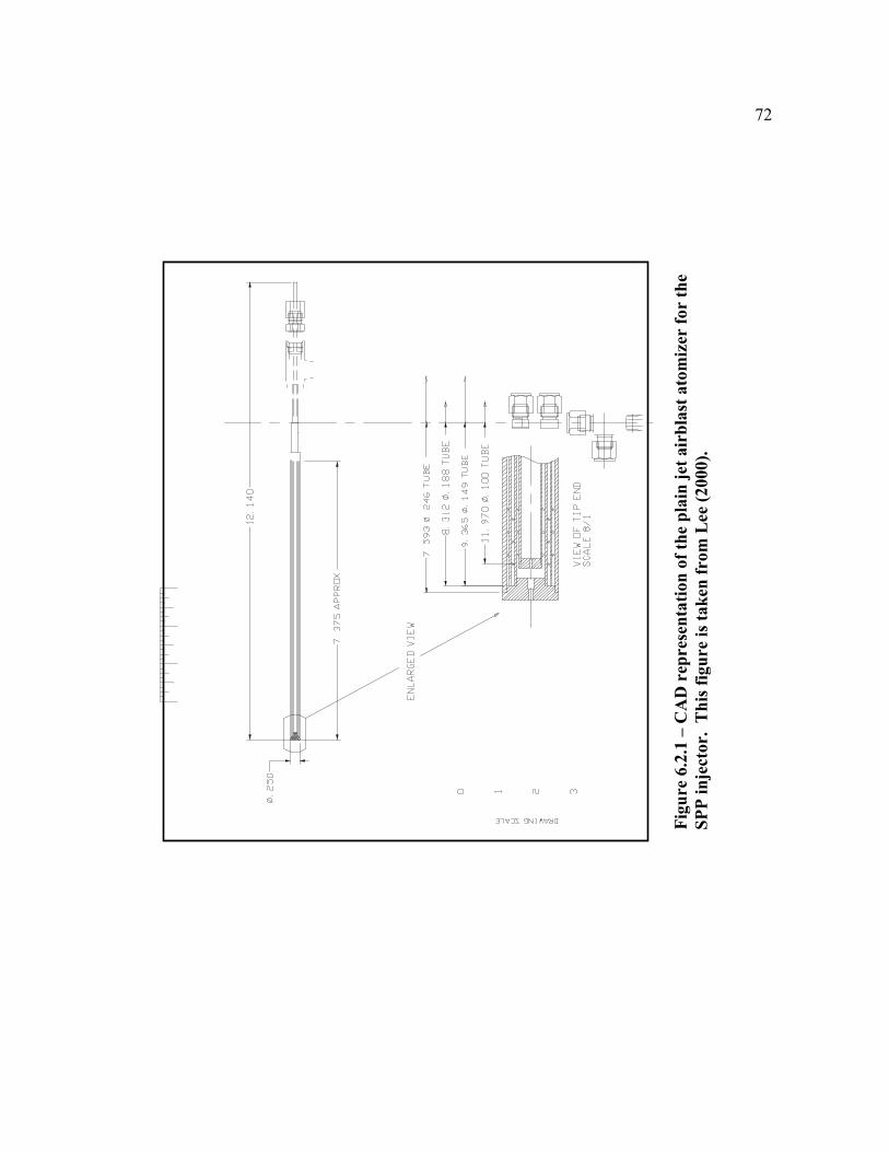
72

Fig

ure

6.2

.1 –

CA

D r

epre

sen

tati

on

of

the

pla

in j

et a

irb

last

ato

miz

er f

or

the

SP

P i

nje

ctor.

T

his

fig

ure

is

tak

en f

rom

Lee

(2000).

73

the atomizing nozzle decreases, assuming operation at the choked condition.

6.3 First Stage

The first stage air enters the SPP injector through an annular plenum. A perforated

plate is used to distribute the flow and direct it into the two distinct first stage zones, the

wall flow and the vaporization flow, giving a total first stage volume of 7.40e-06 m3 for

liquid fuel operation (gaseous fuels enter at a different location). The inner diameter of

the 1st stage is .5 (12.7 mm). The 1

st stage airflow is monitored and controlled via a

½ NPT, 150 scfm, 5 to 125 psig output range pressure regulator and FP-10A3555

rotometer with FP-1/2-27-G-10/83 tube and GNSVT 48A float. Appendix C contains

the rotometer airflow correlations and specifications. The regulator and rotometer are

plumbed in series with a needle valve. A 5 µm particulate filter is used to clean the oil-

free air supply and eliminate non-droplet Mie scattering particles at the measurement

section.

The vaporization flow is directed concentrically around the plain jet airblast atomizer,

while the wall flow is directed parallel to the wall via a concentric divider. The divider

also acts to create a shear-flow region at its downstream tip, further increasing the

mixing. Since the overall equivalence ratio is fixed at 0.5 - 0.6, the mixture in the first

stage is richer than this, in the range of 1 to 2. The wall flow prevents this fuel rich

mixture from depositing droplets onto the hot SPP walls. Equation 6.3.1 shows the

calculation of 1st stage equivalence ratio.

stoichf

.

a

.

total,a

.

f

.

1,a

.

total,a

.

1,a

.

total,a

.

overall1

m

m

m

m

m

m

m

m

=

φ=φ Eq. 6.3.1

The 1st stage employs a wound-wire immersed heating element, surrounded by a quartz

sleeve to control the stage 1 mixture temperature. Watlow Series 989 temperature

74

controllers are utilized in the cascade configuration to maintain the user-defined stage-

temperature set-point. The process temperature is measured from a K-type

thermocouple located in the first stage mixture volume. The current instrumentation of

the SPP injector does not allow the incoming air temperature to be measured, only the

mixture in the first stage is recorded. The heater-element limiting temperature (user

defined to reduce the risk of heater over-temperature) is measured directly after the

heater element, also with a K-type thermocouple. This control configuration uses a

Watlow DIN-a-Mite 240VAC max, 3φ optional, SCR to regulate 110 VAC and provide

the necessary power to the heater. As a precaution, some minimal air flow is necessary

before turning on the heating controls. This prevents the element from heating

uncontrollably, since the no air flow condition renders the cascade and control

thermocouples ineffective (convection is minimized) in representing the heater

temperature. For additional control, a 120VAC Powerstat variac is installed in series

with the power connection, to allow greater control of the heater voltage. This variac is

generally set to 100% during testing to provide adequate and timely heating of the air

during testing. Lower flow rates, less than 50 slpm (standard liters per minute), can

decrease the convective heat transfer from the heater to the point that the set point

cannot be reached.

6.4 Second Stage

The second stage air also enters through an annular plenum, and is injected into the SPP

in a series of holes facing the SPP axis. This airflow has a higher temperature than the

first stage, and is primarily used to further vaporize the lower vapor pressure

components. The 2nd

stage was redesigned by Edmonds (2002) due to material warping

and leaking of the airflow and/or fuel mixture out of the SPP prior to the JSR. The

general geometry remained the same, however the current design of the 2nd

stage

employs 16, 0.06 holes, with 4 located every 90° circumferentially (Edmonds, 2002).

These holes are angled at 45° from the axis of the SPP, to provide the penetration

necessary for good mixing while reducing pressure drop. The inner wall of the 2nd

75

stage is tapered to allow for the increase in mass flow introduced through the jets

without creating step recirculation zones that could promote autoignition. The

geometry of the second stage produces an interior volume of 2.04e-05 m3. The inner

diameter of the 2nd

stage at the flow exit is 0.675 (17.15 mm).

The second stage airflow is monitored and controlled during LRS testing via a pressure

regulator (same model as stage 1) and 10A3565 rotometer with FP-1/2-27-G-10/55 tube

and GSVT 48A float. A needle valve is employed to further control the second stage

airflow.

A wound-wire immersed heating element surrounded by a quartz sleeve is also used for

the 2nd

stage heater to heat the 2nd

stage inlet air. The heater control is identical to the

first stage, but 220 VAC 1φ is used to increase the capability of the heater. A 240 VAC

Powerstat variac is connected in series with the power connection to further control the

heater system. Since the second stage uses 220 VAC, and the majority of vaporization

has already taken place in the first stage of the SPP, the heater system has no problem

reaching setpoints up to 600 °C at flow rates of up to 85 slpm. The variac is generally

set to between 50 and 60 % for all of the test cases.

6.5 Additional SPP System Considerations

During LRS testing of the SPP injector, the neutral density filter was in place. The ND

filter is located just after the 0.5 PC lens, and before the bandpass filter. This

component allows the PMT voltage to be set at 1000 VDC without the strong fuel

vapor mixture scattering signal reading off scale on the Combiscope. The flange at the

outlet of the SPP, generally used to attach the nozzle and JSR, presented an obstruction

to the measured light cone. In order to accommodate this geometry, a semicircular

blind was placed over the bottom half of the front lens. This blind blocked any stray

light from entering the lens through the portion where the signal was blocked. The only

76

consequence to this addition is that the solid angle is now bisected to 0.23 srad. The

BFL of the first PC lens requires that the collection optics assembly be in close

proximity to the hot injector exit. Throughout testing, the collection face was

monitored, and was cool to the touch, indicating that heat transfer to the front face of

the collection assembly was negligible.

77

Chapter 7

SPP Injector Experimental Results and Analysis

7.1 LRS Testing of the SPP Injector

This set of LRS testing was performed with the 2nd

stage air flow rate larger than the

1st, and with the 2

nd stage temperature higher than the 1

st stage. The atomizer air flow

rate was set to 5 slpm, similar to conditions tested by Lee (2000) and Edmonds (2002).

The equivalence ratio is held at 0.5 for all of the included tests. These conditions

should produce small droplets from the atomizer, and increased 1st stage residence time

for vaporization. Table 7.1.1 is the test matrix completed for this set of experiments.

Data are taken with the 2nd

stage air flow fixed at 85 slpm. The 1st stage airflow rate,

and the temperatures of the 1st and 2

nd stage mixtures are varied. Note that Appendix F

contains some preliminary LRS data taken with the SPP injector.

Data is presented in this chapter is in similar form to that presented in Chapter 5. Time

traces, which plot the instantaneous scattering signal as a function of time, are given

first. This Figures 7.1.1 through 7.1.4 display time traces of the four air flow splits

considered. Note the lack of droplets present, signifying near complete vaporization of

the liquid fuel. Even low temperature splits, namely 350/350 and 350/400 °C (this

notation is used to denote 1st stage / 2

nd stage properties), show very few droplets

exiting the injector. No large time scale fluctuations are observed, or vapor lock

behavior.

Figures 7.1.1 through 7.1.4 show near-complete vaporization of the fuel droplets, even

at temperatures as low as 350 °C. The absence of large numbers of droplets allows

mean and standard deviation data to be analyzed without taking into account the

perturbations caused by the droplets. The 1st stage air flow rate affects the vaporization

of the fuel. The 5/85/85 air flow split shows a higher occurrence of droplets than the

lower 1st stage air flow rates.

78

Table 7.1.1 – SPP injector test matrix for uneven air flow splits.

atomizer 1st stage 1st stage T 2nd stage 2nd stage T phi res time

slpm slpm °C slpm °C mass sec

5 32 324 85 350 0.50 10.5

5 32 335 85 400 0.50 10.0

5 32 347 85 450 0.50 9.6

5 32 364 85 500 0.50 9.2

5 32 380 85 550 0.50 8.8

5 32 387 85 600 0.50 8.6

5 44 350 85 350 0.51 8.5

5 44 350 85 400 0.51 8.1

5 44 350 85 450 0.51 7.9

5 44 350 85 500 0.51 7.6

5 44 400 85 500 0.51 7.3

5 44 400 85 550 0.51 7.1

5 44 423 85 550 0.51 7.0

5 44 425 85 550 0.51 7.0

5 44 438 85 600 0.51 6.7

5 53 350 85 350 0.51 7.6

5 53 350 85 400 0.51 7.3

5 53 350 85 450 0.51 7.0

5 53 350 85 500 0.51 6.8

5 53 400 85 500 0.51 6.5

5 53 400 85 550 0.51 6.3

5 53 450 85 550 0.51 6.1

5 53 450 85 600 0.51 5.9

5 85 350 85 350 0.51 5.6

5 85 350 85 400 0.51 5.4

5 85 350 85 450 0.51 5.2

5 85 350 85 500 0.51 5.0

5 85 400 85 500 0.51 4.8

5 85 400 85 550 0.51 4.6

5 85 428 85 550 0.51 4.5

5 85 446 85 600 0.51 4.4

Figure 7.1.5 displays the mean scattering signal for all of the test conditions listed in

Table 7.1.1. The mean scattering signal decreases with temperature for each air flow

split case, but there is a significant spread at 2nd

stage temperatures below 550 °C. As

the first stage air flow rate is increased, the mean scattering signal decreases for a fixed

2nd stage air flow rate and fixed temperature split. The 2nd

stage heater and

thermocouple placement are most likely the cause of this drift in mean signal at the

lower 2nd

stage temperatures. The 2nd

stage heater increases the 2nd

stage inlet air

-3.0

0

-2.5

0

-2.0

0

-1.5

0

-1.0

0

-0.5

0

0.0

00.0

00

.05

0.1

00

.15

0.2

0

Tim

e (

s)


38

7/6

00

38

0/5

50

36

4/5

00

34

7/4

50

33

5/4

00

32

4/3

50

Fig

ure

7.1

.1 –

Tim

e tr

aces

for

5/3

2/8

5 a

ir f

low

sp

lit

at

vari

ou

s te

mp

era

ture

sp

lits

for

an

eq

uiv

ale

nce

rati

o o

f 0.5

.

79

-3.0

0

-2.5

0

-2.0

0

-1.5

0

-1.0

0

-0.5

0

0.0

00.0

00

.05

0.1

00

.15

0.2

0

Tim

e (

s)


43

8/6

00

42

5/5

50

40

0/5

00

35

0/5

00

35

0/4

50

35

0/4

00

35

0/3

50

Fig

ure

7.1

.2 –

Tim

e tr

aces

for

5/4

4/8

5 a

ir f

low

sp

lit

at

vari

ou

s te

mp

era

ture

sp

lits

for

an

eq

uiv

ale

nce

rati

o o

f 0.5

.

80

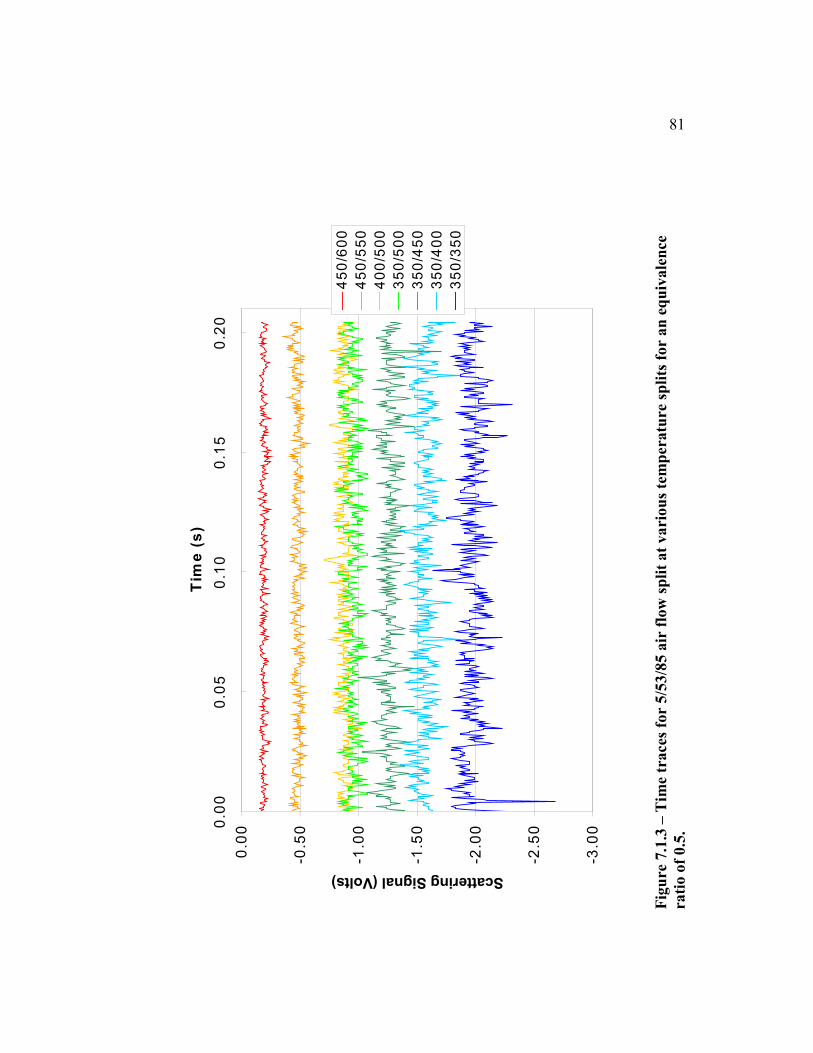
-3.0

0

-2.5

0

-2.0

0

-1.5

0

-1.0

0

-0.5

0

0.0

00.0

00

.05

0.1

00

.15

0.2

0

Tim

e (

s)


45

0/6

00

45

0/5

50

40

0/5

00

35

0/5

00

35

0/4

50

35

0/4

00

35

0/3

50

Fig

ure

7.1

.3 –

Tim

e tr

aces

for

5/5

3/8

5 a

ir f

low

sp

lit

at

vari

ou

s te

mp

era

ture

sp

lits

for

an

eq

uiv

ale

nce

rati

o o

f 0.5

.

81

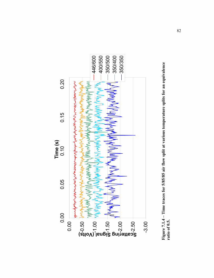
-3.0

0

-2.5

0

-2.0

0

-1.5

0

-1.0

0

-0.5

0

0.0

00.0

00.0

50.1

00.1

50.2

0T

ime (

s)


446/6

00

400/5

50

350/5

00

350/4

00

350/3

50

Fig

ure

7.1

.4 –

Tim

e tr

aces

for

5/8

5/8

5 a

ir f

low

sp

lit

at

vari

ou

s te

mp

era

ture

sp

lits

for

an

eq

uiv

ale

nce

rati

o o

f 0.5

.

82

83

temperature to maintain a user-defined 2nd

stage mixture temperature. At higher 2nd

stage temperatures, the heater assembly is observed to glow orange, signifying the

increased element temperature necessary to maintain the 2nd

stage mixture temperature.

The increase in the SPP 2nd

stage metal temperature may act to increase the mixture

temperature between the 2nd

stage thermocouple and the measuring volume. More heat

needed by the 2nd

stage heater would translate into higher 2nd

stage metal and gas

temperatures and thus lower scattering signals. The temperature gap between different

1st stage air flow rate conditions appears proportional to the difference in 1

st stage air

flow rate. Figure 7.1.5 suggests that this heat transfer effect may account for up to 100

°C temperature difference at different air flow rate conditions.

Figures 7.1.6 and 7.1.7 display the unmixedness plotted against the 1st and 2

nd stage

mixture temperatures. Generally the unmixedness is less than 10% (5% relative to the

noise baseline) for these test cases, but is observed to increase with 2nd

stage

temperature. This result can be misleading if not interpreted in the contexts of the

collection systems inherent noise and temperature. The larger 2nd

stage temperatures

provide a lower number density mixture at the measuring volume through the laser is

passed. This in turn reduces the scattered signal, by an order of magnitude between 350

and 600 °C. If some portion of the noise fluctuations do not scale down by the same

factor, then the signal to noise ratio can decrease and the calculated unmixedness will

increase. Figure 7.1.8 shows a plot of unmixedness, for a fixed air flow, fuel flow and

temperature split, against incident laser power. The unmixedness at the fixed test

condition is observed to increase by 60% as the laser power is decreased. Since test

conditions were held constant, this increase is attributed to decreased signal to noise

ratio. The mean scattering signal is plotted against incident laser power in Figure 7.1.9

to demonstrate linearity that is consistent with Rayleigh theory. In addition to the rise

in unmixedness as the signal becomes weaker, temperature fluctuations can produce

scattering signal fluctuations. Temperature fluctuations of 100 °C could produce

unmixedness values of 10 to 15 %, assuming a fixed, constant fuel concentration.

y =

-0

.00

57

5x +

3.6

48

73

R2 =

0.9

95

75

y =

-0

.00

75

9x

+ 4

.69

36

6

R2 =

0.9

88

29

y =

-0

.00

71

1x +

4.4

35

03

R2 =

0.9

95

54

y =

-0

.00

81

7x

+ 5

.03

65

4

R2 =

0.9

94

38

0.0

0

0.5

0

1.0

0

1.5

0

2.0

0

2.5

0

30

03

50

40

04

50

50

05

50

60

06

50

70

0

2n

d S

tag

e T

(°C

)


5/3

2/8

5 a

irs

plit

ph

i=.5

5/4

4/8

5 a

irs

plit

ph

i=.5

5/5

3/8

5 a

irs

plit

ph

i=.5

5/8

5/8

5 a

irs

plit

ph

i=.5

Lin

ea

r (5

/85

/85

air

sp

lit

ph

i=.5

)

Lin

ea

r (5

/44

/85

air

sp

lit

ph

i=.5

)

Lin

ea

r (5

/53

/85

air

sp

lit

ph

i=.5

)

Lin

ea

r (5

/32

/85

air

sp

lit

ph

i=.5

)

Fig

ure

7.1

.5 –

Mea

n s

catt

erin

g s

ign

al

plo

tted

again

st 2

nd s

tage

mix

ture

tem

pera

ture

.

84

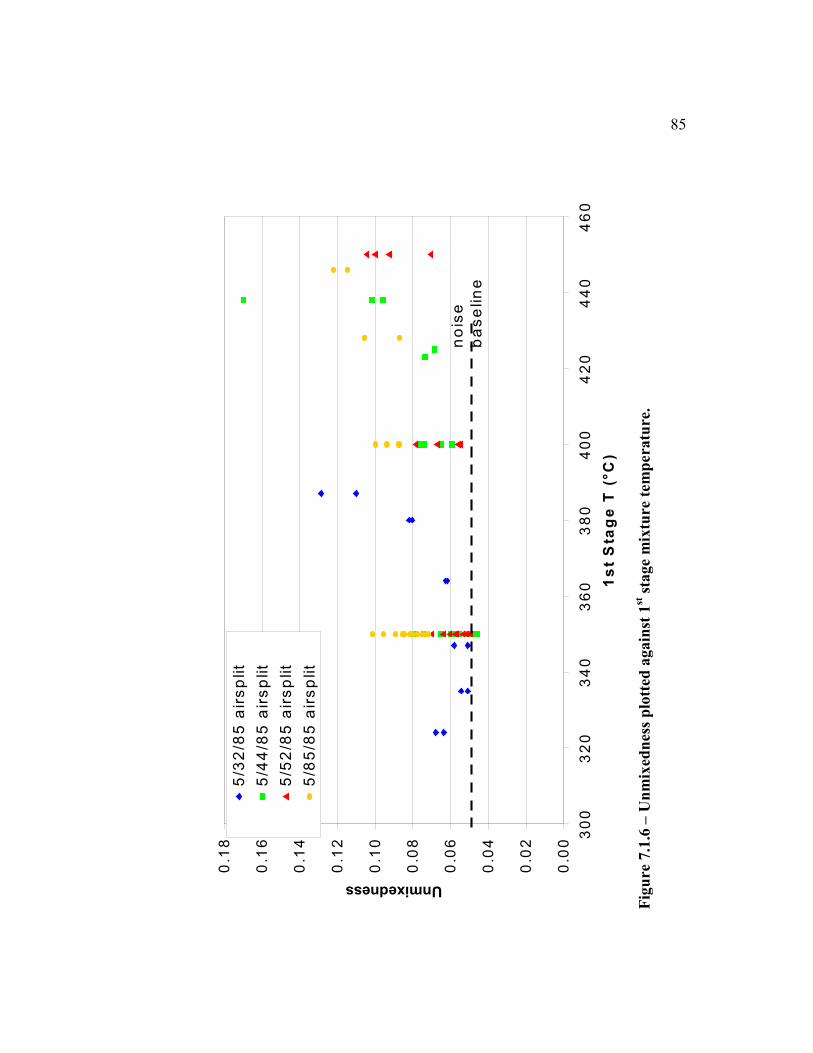
0.0

0

0.0

2

0.0

4

0.0

6

0.0

8

0.1

0

0.1

2

0.1

4

0.1

6

0.1

8

30

03

20

34

03

60

38

04

00

42

04

40

46

0

1s

t S

tag

e T

(°C

)

Unmixedness

5/3

2/8

5 a

irs

plit

5/4

4/8

5 a

irs

plit

5/5

2/8

5 a

irs

plit

5/8

5/8

5 a

irs

plit

no

ise

ba

se

lin

e

Fig

ure

7.1

.6 –

Un

mix

edn

ess

plo

tted

ag

ain

st 1

st s

tage

mix

ture

tem

pera

ture

.

85

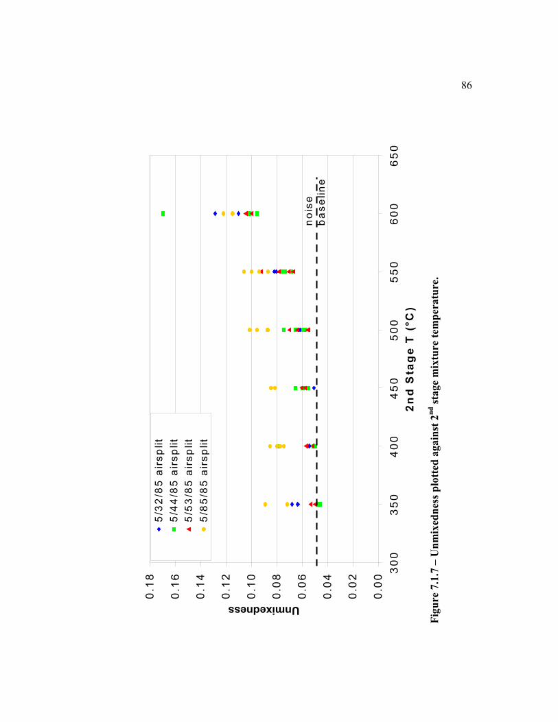
0.0

0

0.0

2

0.0

4

0.0

6

0.0

8

0.1

0

0.1

2

0.1

4

0.1

6

0.1

8

30

03

50

40

04

50

50

05

50

60

06

50

2n

d S

tag

e T

(°C

)

Unmixedness

5/3

2/8

5 a

irs

pli

t

5/4

4/8

5 a

irs

pli

t

5/5

3/8

5 a

irs

pli

t

5/8

5/8

5 a

irs

pli

t

no

ise

ba

se

lin

e

Fig

ure

7.1

.7 –

Un

mix

edn

ess

plo

tted

ag

ain

st 2

nd s

tage

mix

ture

tem

pera

ture

.

86

0.0

0

0.0

5

0.1

0

0.1

5

0.2

0

0.2

5

0.3

0

0.3

5

0.4

0

0.4

5 0.0

00

.20

0.4

00

.60

0.8

01

.00

1.2

01

.40

1.6

0

La

se

r P

ow

er

(Wa

tts

)

Unmixedness

Fig

ure

7.1

.8 -

Un

mix

edn

ess

plo

tted

ag

ain

st i

nci

den

t la

ser

po

wer

at

a f

ixed

co

nd

itio

n o

f 5/8

5/8

5 s

lpm

an

d 4

00

/50

0 °

C.

87

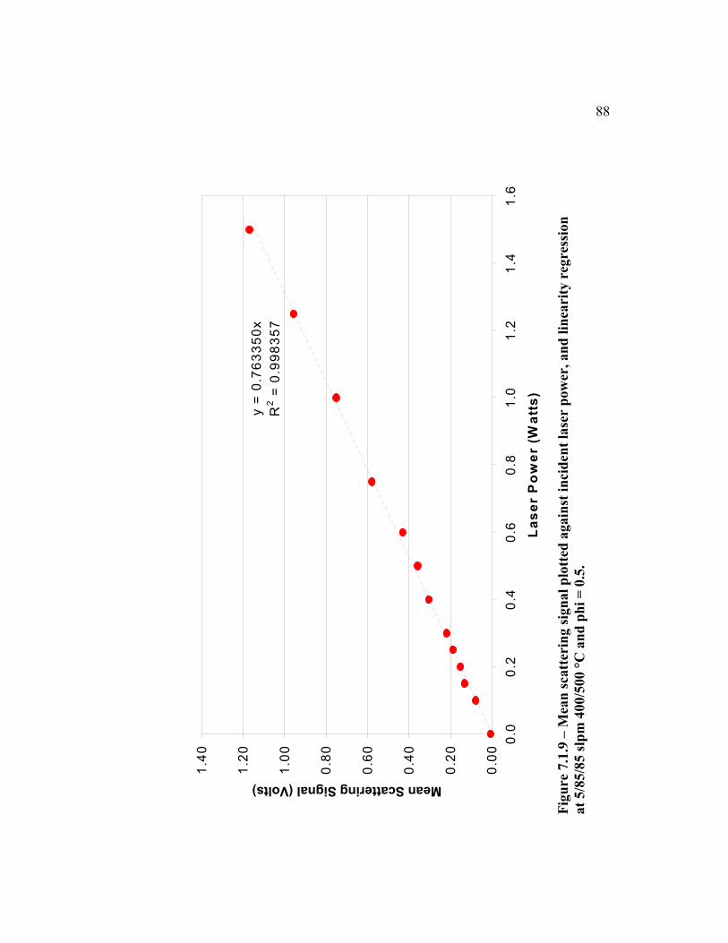
y =

0.7

63

35

0x

R2 =

0.9

98

35

7

0.0

0

0.2

0

0.4

0

0.6

0

0.8

0

1.0

0

1.2

0

1.4

0

0.0

0.2

0.4

0.6

0.8

1.0

1.2

1.4

1.6

La

se

r P

ow

er

(Wa

tts

)


Fig

ure

7.1

.9 –

Mea

n s

catt

erin

g s

ign

al

plo

tted

again

st i

nci

den

t la

ser

pow

er, an

d l

inea

rity

reg

ress

ion

at

5/8

5/8

5 s

lpm

40

0/5

00

°C

an

d p

hi

= 0

.5.

88

89

Another consideration resulting from the order of magnitude drop in mean

scattering signal when the 2nd

stage temperature is increased from 350 to 600 °C

is that the scattering theory predicts a reduction in signal of only 30% (1 - 623 /

873). This effect may be due to the departure of the mixture from ideal gas

behavior, droplets scattering according to Rayleigh theory, or the cracking of the

diesel molecules at higher temperature conditions. The TPD fuel used for the

duration of the LRS testing of the SPP injector is a mixture of unknown

composition, but nominally is assumed to be C14H26.

In order to insure that the collection optics system would measure a 1 / T

(Kelvins) relationship for air, a pure air test was performed. The neutral density

filter was removed, since, in the absence fuel, it would only reduce the signal to

noise ratio. Figure 7.1.10 displays a plot of the mean scattering signal against the

2nd

stage mixture temperature, which should closely represent the mixture

temperature at the measuring volume. The 1 / T functional calculation is a good

approximation of the collection system response up to about 350 °C, at which the

noise overpowers the signal, and the measured signal flattens out at around 40

mV. Figures 7.3.9 and 7.3.10 suggest that the collection system’s response is

linearly proportional to the scattering signal predicted by Rayleigh scattering

theory.

The experimental results imply that the SPP injector provides a well-mixed

stream of air and vaporized liquid fuel. The SPP injector internal residence times

of 4.4 to 10.5 milliseconds are adequate to vaporize and mix the liquid fuel and

air to an unmixedness value of 5% relative. The conditions that represent the best

mixing (at a fixed 2nd

stage air flow rate) occur at 1st stage air flows of 32, 44, 53

slpm at temperature splits above 400 °C. Temperatures below 400 °C do not

vaporize the fuel completely, and a 1st stage air flow rate of 85 slpm reduces the

residence time sufficiently to degrade vaporization.

0

0.0

1

0.0

2

0.0

3

0.0

4

0.0

5

0.0

6

0.0

7

0.0

8

0.0

9

01

00

20

03

00

40

05

00

60

0

2n

d S

tag

e M

ixtu

re T

(°C

)


1/T

fu

nctio

n f

it a

t 1

8°C

Exp

eri

me

nta

l d

ata

Fig

ure

7.1

.10 –

Mea

n s

catt

erin

g s

ign

al

plo

tted

again

st a

ir t

em

per

atu

re.

C

on

dit

ion

s are

pu

re a

ir

at

5/8

5/8

5 s

lpm

.

90

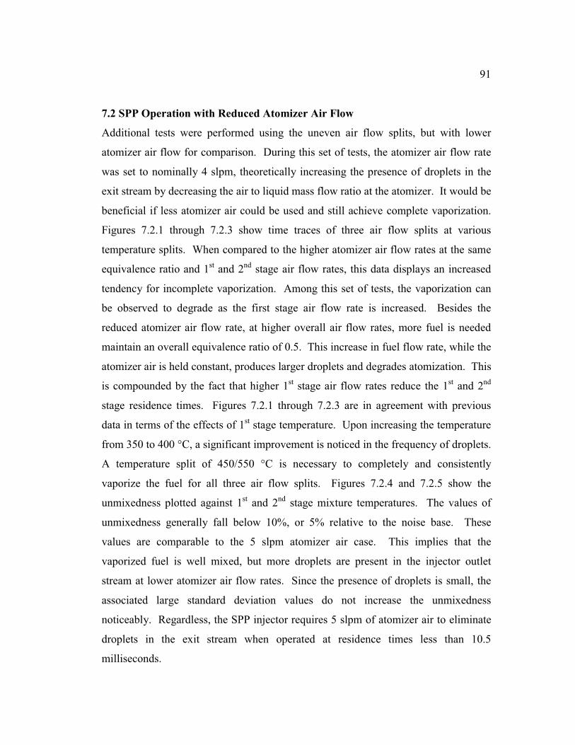
91

7.2 SPP Operation with Reduced Atomizer Air Flow

Additional tests were performed using the uneven air flow splits, but with lower

atomizer air flow for comparison. During this set of tests, the atomizer air flow rate

was set to nominally 4 slpm, theoretically increasing the presence of droplets in the

exit stream by decreasing the air to liquid mass flow ratio at the atomizer. It would be

beneficial if less atomizer air could be used and still achieve complete vaporization.

Figures 7.2.1 through 7.2.3 show time traces of three air flow splits at various

temperature splits. When compared to the higher atomizer air flow rates at the same

equivalence ratio and 1st and 2

nd stage air flow rates, this data displays an increased

tendency for incomplete vaporization. Among this set of tests, the vaporization can

be observed to degrade as the first stage air flow rate is increased. Besides the

reduced atomizer air flow rate, at higher overall air flow rates, more fuel is needed

maintain an overall equivalence ratio of 0.5. This increase in fuel flow rate, while the

atomizer air is held constant, produces larger droplets and degrades atomization. This

is compounded by the fact that higher 1st stage air flow rates reduce the 1

st and 2

nd

stage residence times. Figures 7.2.1 through 7.2.3 are in agreement with previous

data in terms of the effects of 1st stage temperature. Upon increasing the temperature

from 350 to 400 °C, a significant improvement is noticed in the frequency of droplets.

A temperature split of 450/550 °C is necessary to completely and consistently

vaporize the fuel for all three air flow splits. Figures 7.2.4 and 7.2.5 show the

unmixedness plotted against 1st and 2

nd stage mixture temperatures. The values of

unmixedness generally fall below 10%, or 5% relative to the noise base. These

values are comparable to the 5 slpm atomizer air case. This implies that the

vaporized fuel is well mixed, but more droplets are present in the injector outlet

stream at lower atomizer air flow rates. Since the presence of droplets is small, the

associated large standard deviation values do not increase the unmixedness

noticeably. Regardless, the SPP injector requires 5 slpm of atomizer air to eliminate

droplets in the exit stream when operated at residence times less than 10.5

milliseconds.

-3.0

0

-2.5

0

-2.0

0

-1.5

0

-1.0

0

-0.5

0

0.0

00.0

00

.05

0.1

00

.15

0.2

0

Tim

e (

s)


35

0/3

50

air

40

0/6

00

38

5/5

50

35

0/5

00

35

0/4

50

35

0/4

00

34

8/3

50

Fig

ure

7.2

.1 –

Tim

e tr

aces

of

4/3

2/8

5 a

ir f

low

sp

lit

at

vari

ou

s te

mp

eratu

res

an

d a

n e

qu

ivale

nce

rati

o o

f 0.5

.

92

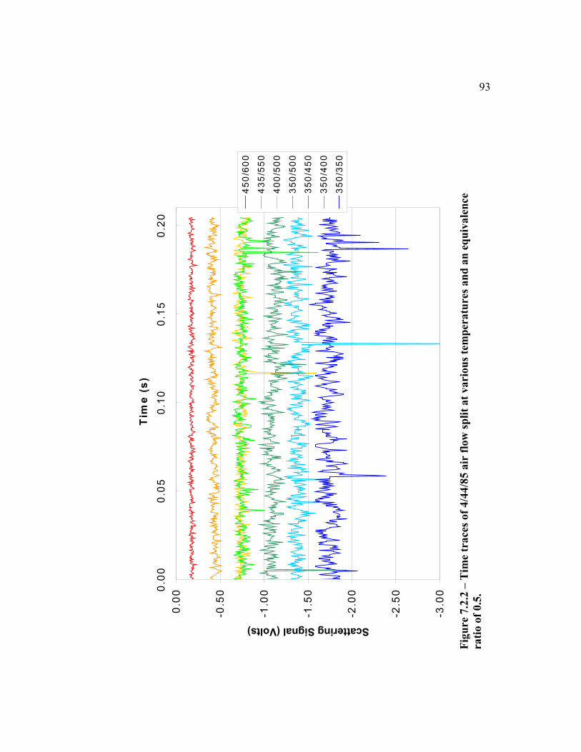
-3.0

0

-2.5

0

-2.0

0

-1.5

0

-1.0

0

-0.5

0

0.0

00.0

00

.05

0.1

00

.15

0.2

0

Tim

e (

s)


45

0/6

00

43

5/5

50

40

0/5

00

35

0/5

00

35

0/4

50

35

0/4

00

35

0/3

50

Fig

ure

7.2

.2 –

Tim

e tr

aces

of

4/4

4/8

5 a

ir f

low

sp

lit

at

vari

ou

s te

mp

eratu

res

an

d a

n e

qu

ivale

nce

rati

o o

f 0.5

.

93

-3.0

0

-2.5

0

-2.0

0

-1.5

0

-1.0

0

-0.5

0

0.0

00.0

00

.05

0.1

00

.15

0.2

0

Tim

e (

s)


45

0/6

00

45

0/5

50

40

0/5

00

35

0/5

00

35

0/4

50

35

0/4

00

35

0/3

50

Fig

ure

7.2

.3 –

Tim

e tr

aces

of

4/5

3/8

5 a

ir f

low

sp

lit

at

vari

ou

s te

mp

eratu

res

an

d a

n e

qu

ivale

nce

rati

o o

f 0.5

.

94

0.0

0

0.1

0

0.2

0

30

03

50

40

04

50

50

0

1s

t S

tag

e T

(°C

)

Unmixedness

4/3

2/8

5

4/4

4/8

5

4/5

2/8

5

no

ise

ba

se

lin

e

Fig

ure

7.2

.4 –

Un

mix

edn

ess

plo

tted

ag

ain

st 1

st s

tage

tem

per

atu

re

for

an

eq

uiv

ale

nce

rati

o o

f 0.5

.

95

0.0

0

0.1

0

0.2

0

30

03

50

40

04

50

50

05

50

60

06

50

70

0

2n

d S

tag

e T

(°C

)

Unmixedness

4/3

2/8

5

4/4

4/8

5

4/5

2/8

5

no

ise

ba

se

lin

e

Fig

ure

7.2

.5 –

Un

mix

edn

ess

plo

tted

ag

ain

st 2

nd s

tage

tem

per

atu

re

for

an

eq

uiv

ale

nce

rati

o o

f 0.5

.

96

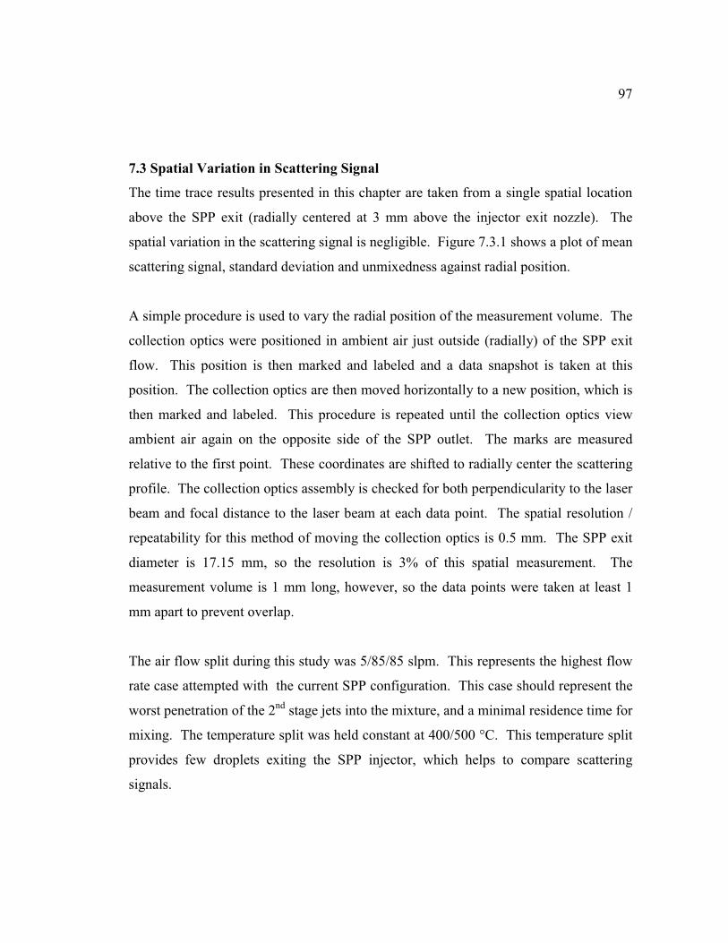
97

7.3 Spatial Variation in Scattering Signal

The time trace results presented in this chapter are taken from a single spatial location

above the SPP exit (radially centered at 3 mm above the injector exit nozzle). The

spatial variation in the scattering signal is negligible. Figure 7.3.1 shows a plot of mean

scattering signal, standard deviation and unmixedness against radial position.

A simple procedure is used to vary the radial position of the measurement volume. The

collection optics were positioned in ambient air just outside (radially) of the SPP exit

flow. This position is then marked and labeled and a data snapshot is taken at this

position. The collection optics are then moved horizontally to a new position, which is

then marked and labeled. This procedure is repeated until the collection optics view

ambient air again on the opposite side of the SPP outlet. The marks are measured

relative to the first point. These coordinates are shifted to radially center the scattering

profile. The collection optics assembly is checked for both perpendicularity to the laser

beam and focal distance to the laser beam at each data point. The spatial resolution /

repeatability for this method of moving the collection optics is 0.5 mm. The SPP exit

diameter is 17.15 mm, so the resolution is 3% of this spatial measurement. The

measurement volume is 1 mm long, however, so the data points were taken at least 1

mm apart to prevent overlap.

The air flow split during this study was 5/85/85 slpm. This represents the highest flow

rate case attempted with the current SPP configuration. This case should represent the

worst penetration of the 2nd

stage jets into the mixture, and a minimal residence time for

mixing. The temperature split was held constant at 400/500 °C. This temperature split

provides few droplets exiting the SPP injector, which helps to compare scattering

signals.

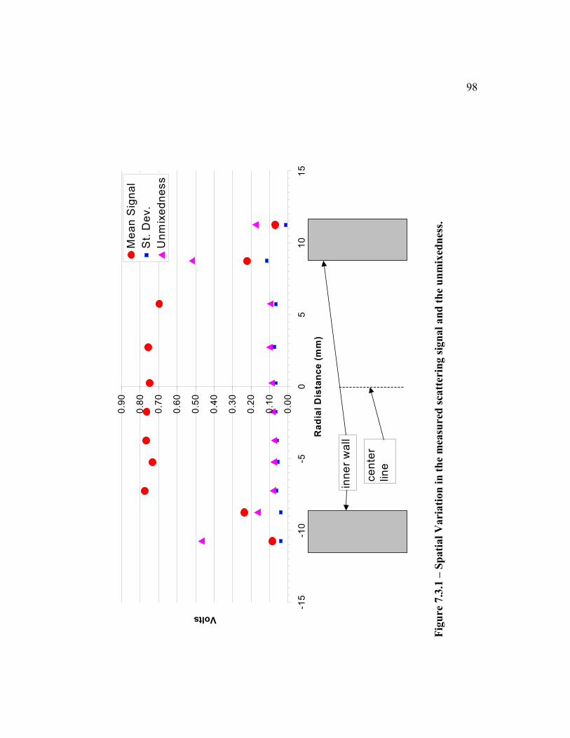
0.0

0

0.1

0

0.2

0

0.3

0

0.4

0

0.5

0

0.6

0

0.7

0

0.8

0

0.9

0

-15

-10

-50

51

01

5

Ra

dia

l D

ista

nc

e (

mm

)

Volts

Me

an

Sig

na

l

St.

De

v.

Un

mix

ed

ne

ss

inn

er

wa

ll

ce

nte

r

lin

e

Fig

ure

7.3

.1 –

Sp

ati

al

Va

ria

tio

n i

n t

he

mea

sure

d s

catt

eri

ng

sig

na

l a

nd

th

e u

nm

ixed

nes

s.

98

99

The mean scattering signal is constant across the SPP exit to within 4%. This implies

that the mixture is spatially uniform, to a measuring volume resolution of 2.54 mm3.

7.4 Summary of SPP Injector Results

The SPP injector was tested over a wide range of air flow and temperature conditions.

The following bullets state the primary experimental results with a brief discussion.

• The SPP provides well-mixed air and fuel with near complete vaporization. The

atomizer airflow must be at least 5 slpm to accomplish sufficient atomization for

complete vaporization. The optimum operating conditions among those tested

consist of air flow splits of 5/32/85, 5/44/85 and 5/53/85 at temperature splits

above 400 °C

• The atomizer airflow is a strong parameter in the complete vaporization of diesel

fuel.

• The time traces generally produce unmixedness values of 5% or less (relative to

the noise baseline). The mixture is spatially uniform to within 4% across the

diameter of the test mixture exiting the SPP injector. This implies that the 2nd

stage jets fully penetrate the mixture.

• Residence times of between 4 and 11 milliseconds were achieved within the

current SPP injector configuration.

• LRS testing of the SPP injector produced results consistent with previous work.

The low NOx concentrations measured by Lee (2000) and Edmonds (2002)

implied the absence of liquid phase droplets and well-mixed fuel and air. With

sufficient atomizer air flow and mixture temperatures, few droplets are observed.

• The SPP injector continues to be an excellent research tool, allowing insight into

the parameters affecting atomization and vaporization. The intense mixing within

the SPP injector also allows LPP combustion testing of liquid fuels.

• The pressure loss of the SPP air flow is significant. Currently, high-speed jets are

used to introduce the atomizer and 1st stage air flows, and are accompanied by

large losses. The 1st stage air inlet produces a pressure drop of up to 30 psid. The

101

Chapter 8

Conclusions and Recommendations

8.1 Steam Injector Conclusions and Recommendations

The steam injector was tested over a wide range of steam and fuel flow rates, and

consistently produced a well-mixed stream of steam and vaporized fuel. The

unmixedness values were less than 5% relative to the noise baseline for almost all

conditions tested with diesel fuel. Operation on naphtha produced similar results,

although the unmixedness value was generally 1-2% higher which is perhaps due to the

lower scattering signal and lower signal to noise ratio compared to TPD. The only

exception to the 5% relative unmixedness was during vapor lock in the fuel feed tube

for low fuel flow rates. This fuel flow instability produces dramatic oscillations in the

fuel concentration exiting the injector. If the time constant of the downstream

processes is much greater than the period of oscillations, then the fluctuations may be

of little consequence, but the risk of carbon deposition in the fuel feed tube is increased

by the oscillation. Vapor lock could probably be eliminated if the fuel delivery

geometry were amended to reduce contact with the superheated steam, and to reduce

the residence time of the liquid fuel in the heated environment. Operation on naphtha

required some cooling at all fuel flow rates to suppress vapor lock. Droplets were not

observed at the conditions tested in this study, except during the introduction or

termination of fuel flow, in which cases the fuel flow is drastically unsteady.

The current injector design, and the utilization of a modular atomizing plate, is

convenient for experimental purposes. This modularity allows for different atomizing

nozzles to be used without disrupting the entire geometry. The injector is geometrically

simple, and easy to inspect for coking. The injector has proven robust during previous

and current testing to date, and requires little maintenance. The N2 purge that is used in

102

the absence of fuel flow provides a simple means of cooling the fuel tip, but is not

practical for field use, and would need to be replaced with some other process flow.

Currently, the steam injector operates with large pressure drops of 17 to 34 psi across

the atomizing nozzle. One remedy for this would be to decrease the amount of steam

traversing the atomizing nozzle, such that good atomization and vaporization still

occur. Since no degradation is observed by reducing the steam flow rate from 259 mg/s

to 149 mg/s, it is reasonable that further reduction in steam flow is possible. The

remaining steam flow could then be brought into the mixture with less pressure drop

and mixing intensity, perhaps as a film along the metal walls. Any further design

should not include a protruding fuel orifice tip, similar to the present copper tip with

ruby insert. This geometry increases the risk of vapor lock, which requires the

introduction of cooling medium. The annular cooling passages of the fuel feed tube

provide some heat shielding, whether or not a cooling medium is introduced. No

carbon deposits were observed during visual post-inspection at any of the tested

conditions.

The 5 mixing tube provided ample residence time for the liquid fuel drops to vaporize.

This vaporizing volume most likely could be reduced without adverse effects. Minimal

vaporizing length scales are preferred since this reduces material needs, heat and

pressure losses, and provides less metal surface area for deposition of carbon. The

plenum, in which steam enters directly upstream of fuel atomization, could also be

reduced in volume and length scale to tighten the design.

8.2 SPP Injector Conclusions and Recommendations

The SPP injector was tested over a wide range of air and fuel flow rates, and

consistently produced a well-mixed stream of steam and vaporized fuel at total

residence times of 4.3 to 8.6 milliseconds. The unmixedness values were less than 5%

relative to the noise baseline for many of the conditions tested. Droplets were

103

observed, unlike the steam injector, at several of the SPP operating conditions. The

atomizer air flow rate needs to be at least 5 slpm to suppress droplets at 1st stage

temperatures as low as 350 °C. Higher temperatures more easily vaporize the droplets,

and diminish the tendency for incomplete atomization at atomizer air flow rates less

than 5 slpm. When operated with more air entering through the 2nd

stage than the 1st

stage, the SPP injector displays higher degrees of mixedness. Naphtha was not tested

because previous work by Lee (2000) and Edmonds (2002) showed a vapor lock

tendency for this fuel. The fuel phase change is undesirable in the delivery tube, and

could increase the risk of carbon deposits and fuel orifice plugging.

The present SPP injector design utilizes high speed jets to introduce the three air flow

streams. This method of introducing the air streams relies on large pressure

differentials and losses, which are not indicative of practical systems. The present

atomizer operates at the choked condition, and requires a pressure drop of over 30 psi

when operated at the lowest residence time conditions with an equivalence ratio of 0.5.

The 1st stage flow geometry presents a pressure drop of up to 30 psi at the lowest

residence time conditions.

The SPP concept is applicable for gas turbine engines. The large geometry associated

with industrial gas turbines may allow for more SPP design options. Prefilming airblast

atomizers are generally preferred to plain jet airblast atomizers in terms of fuel

dispersion and atomization, but do not lend themselves as readily to laboratory scale

testing. Prefilming atomizers can readily use swirling air flows to break up the fuel

sheet, which generally introduce less flow loss than the high speed jet approach.

104

Bibliography

Beer, J.M. , Chigier, N.A. “Combustion Aerodynamics” 1983 Robert E. Krieger

Publishing Company, Inc. Malabar, FL.

Campbell, J. S. Jr., de Bruyn Kops, S., Lee, J., Malte, P., Novosselov, I., Benjamin, M.

A. “Integrating the Staged Prevaporizer-Premixer Into Gas Turbine Cycles” 2002. GT-

2002-30081. Proceedings of ASME Turbo Expo 2002.

Cavaliere, A., Ragucci, R., D’Alessio, A., Noviello, C. “Analysis of Diesel Sprays

Through Two-Dimensional Laser Light Scattering” 22nd

International Symposium on

Combustion, 1988. The Combustion Institute, Pittsburgh, PA. pp. 1973 – 1981.

Cengel, Y.A. Boles, M.A. “Thermodynamics: An Engineering Approach” 1998 Third

Edition McGraw Hill. New York, NY.

Chemical Engineering Information Research Center (2002)

http://www.cheric.org/kdb/kdb/hcprop/

Dibble, R. W. Hollenbach, R. E. “Laser Rayleigh Thermometry in Turbulent Flames”

18th

International Symposium on Combustion. 1981. The Combustion Institute,

Pittsburgh, PA. pp. 1489 – 1499.

Edmonds, Ryan. “Prevaporized Premixed Combustion at Short Residence Times”

Master’s Thesis 2002. University of Washington. Seattle, WA

Edwards, T. “Deposition During Vaporization of Jet Fuel in a Heated Tube” AIAA 92-

0687 1992. 30th

Aerospace Sciences Meeting & Exhibit, 1992.

Espey, C., Dec, J. “Planar Laser Rayleigh Scattering for Quantitative Vapor-Fuel

Imaging in a Diesel Jet” Combustion and Flame, Volume 109, 1997. The Combustion

Institute, Pittsburgh, PA. pp. 65 – 86.

Gardiner, W. C., Hidaka, Y., Tanzawa, T. “Refractivity of Combustion Gases”

Combustion and Flame, Volume 40. 1981. The Combustion Institute, Pittsburgh, PA.

pp. 213 – 219.

Johnson, Charles S. Gabriel, Don A. “Laser Light Scattering” 1981 Dover

Publications, Inc. New York, NY .

Kays, W.M. Crawford, M. E. “Convective Heat and Mass Transfer” 1993 Third Edition

McGraw-Hill, Inc. New York, NY.

105

Kerker, M. “The Scattering of Light and Other Electromagnetic Radiation” 1969.

Academic Press. New York, NY.

Laurendeau, Normand M. “Temperature Measurements by Light Scattering Methods”

1991 Combustion Measurements. Edited by Norman Chigier. Hemisphere Publishing

Corporation. New York, NY. pp. 95 – 142.

Lee, John C. Y. “Reduction of NOx Emission for Lean Prevaporized-Premixed

Combustors” Ph.D. Dissertation 2000. University of Washington. Seattle, WA

Lefebvre, Arthur H. “Atomization and Sprays” 1989. Hemisphere Publishing

Corporation. New York, NY.

Mongia, Rajiv. “Optical Probe for Measuring the Extent of Air and Fuel Mixing in

Lean Premixed Combustors and the Effect of Air and Fuel Mixing on Combustor

Performance” Ph. D. Dissertation 1998. University of California Berkeley. Berkeley,

CA.

Nukiyama, S., Tanasawa, Y. “Experiments on the Atomization of Liquids in an

Airstream” Volume 5,1939. Transaction of the Society of Mechanical Engineers

(Japan), Translated for the Department of National Defense, Canada.

Pitts, William M. “Rayliegh Light Scattering for Concentration Measurements in

Turbulent Flows” Rayliegh Scattering Diagnostics Workshop, NASA. 1995

Publication 10186. pp. 69 – 74.

Robben, Frank. “Comparison of Density and Temperature Measurement Using Raman

Scattering and Rayleigh Scattering” 1976 Published in Combustion Measurements –

Modern Techniques and Measurements, Edited by R. Goulard, Hemisphere Publishing

Corp. New York, NY. pp. 180 - 196

Seasholtz, Richard G., Greer, Lawrence C. III “Rayliegh Scattering Diagnostics for

Measurements of Temperature and Velocity in Harsh Environments” AIAA-98-0206

1998. NASA/TM-1998-206980

Wark, Kenneth “Advanced Thermodynamics for Engineers” 1995 McGraw Hill, Inc.

New York, NY.

Yaws, C. L., Yank, H. C. “To Estimate Vapor Pressures Easily” 1989 Hydrocarbon

Process., Volume 68, #10. pp. 65 – 68.

Yee, Dan “Experimental Study of Turbulent Mixing in Nonburning and Burning

Hydrogen-Air Coaxial Jets” Ph. D. Dissertation 1982. Washington State University.

106

Appendix A

Optical System Specifications

A.1 Collection Optics and Signal Processing Parts List and Schematic

The collection optics system used in this study was designed to collect and process a

scattered light signal at 514.5 nm. Table A.1.1 gives a list of components and

specifications used in the collection system, with reference to numbered arrows in the

digital pictures displayed by Figures A.1.1 and A.1.2.

Table A.1.1 – Collection system parts list and specifications.

# Name Part #/model Vendor Specification Notes

1 Front PC lens KPX181AR14 Newport 50.8mmφ, 67.43mm BFL AR14 coating

2 Front PC lens holder NA fabricated nylon insert to hold lens bolted from inside

3 2nd PC lens KPX181 Newport 50.8mmφ, 67.43mm BFL

4 final PC lens KPX040 Newport 12.7mmφ, 15.48mm BFL

5 Bandpass filter 10LF10-515 Newport 514nm +/- 2 nm FWHM 10+/- 2 nm

6 Neutral density filter FRQ-ND10 Newport 10% transmission

7 slit assembly NA in lab 1 mm aperture

8 slit holder NA fabricated allows 1D adjustment

9 1 axis linear stage TSX-1D Newport 3x3" w/ 1" travel max x3 in enclosure

10 PMT RCA 1P28 in lab

11 Aluminum enclosure NA fabricated flat black interior

12 Power supply 244 Keithly Adjustable DC supply

13 Combiscope PM3384 Fluke

14 PC NA Fluke Windows NT

An Oriel mercury lamp is used for preliminary optical alignment, which strobes at 120

Hz (absolute value sine wave from 120 VAC input), allowing experience to be gained

with the optics system and the Combiscope settings. The bandpass filter and neutral

density filter are removed during initial alignment with the mercury lamp. The slit is

moved in the horizontal plane, and the lenses are moved in the vertical plane until the

light emitted from the measuring volume projects onto the face of the PMT. After this

initial alignment the collection optics enclosure is secured to the optical table and

aligned with the laser beam. This is done by adjusting the optics enclosure height via

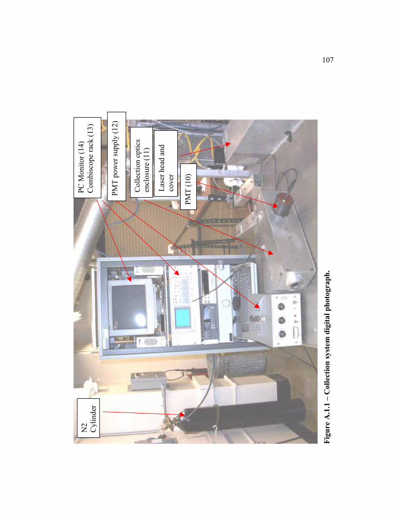
Fig

ure

A.1

.1 –

Co

llec

tio

n s

yst

em

dig

ita

l p

ho

tog

rap

h.

PC

Monit

or

(14)

Com

bis

cope

rack

(13

)

PM

T p

ow

er s

upply

(12)

Co

llec

tio

n o

pti

cs

encl

osu

re (

11

)

PM

T (

10)

N2

Cyli

nd

er

Las

er h

ead a

nd

cover

107

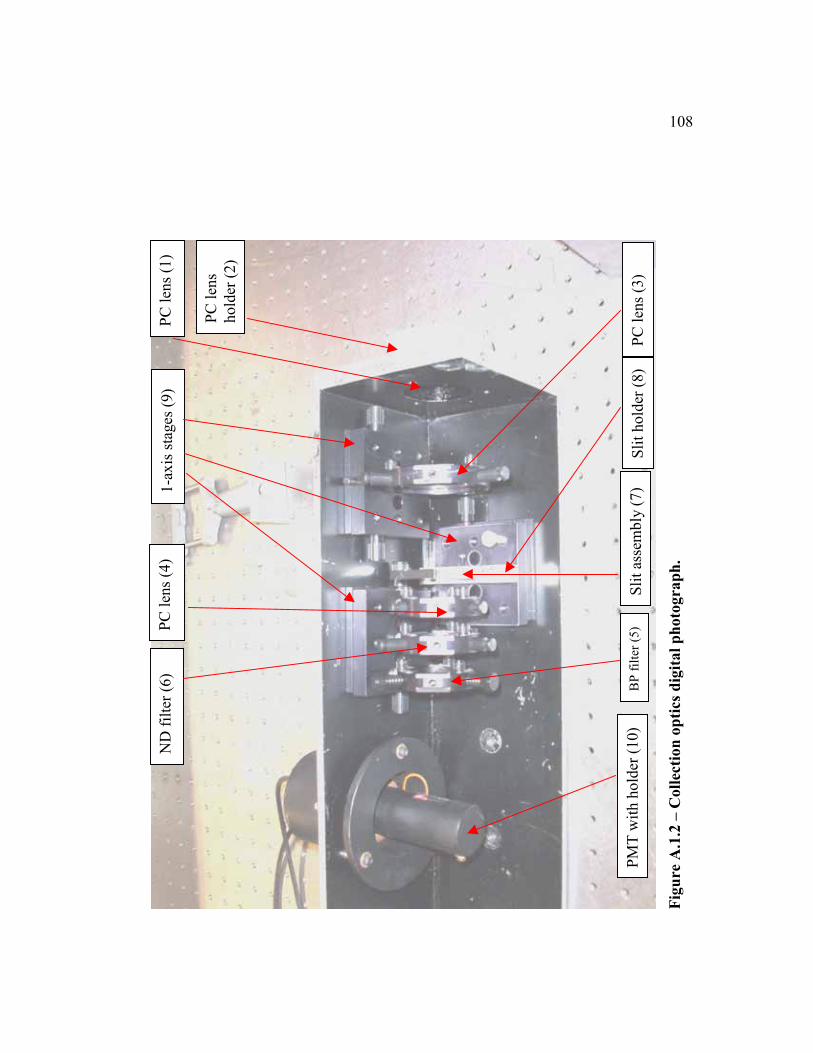
Fig

ure

A.1

.2 –

Co

llec

tio

n o

pti

cs d

igit

al

ph

oto

gra

ph

.

PC

len

s (1

)

PC

len

s

hold

er (

2)

PC

len

s (3

)S

lit

ho

lder

(8

)

1-a

xis

sta

ges

(9)

Sli

t as

sem

bly

(7

)

PC

len

s (4

)N

D f

ilte

r (6

)

BP

fil

ter

(5)

PM

T w

ith h

old

er (

10)

108

109

aluminum automotive shims until the focal volume and laser beam are coincident.

Lastly, the plano convex lenses used in this study are accompanied by a back focal

length (BFL) dimension. This dimension is dependent upon the incident light

wavelength. The BFL values listed in Table A.1.1 are for a incident wavelength of

546.1 nm. The thin lens formula can be used to correct the BFL to the proper

wavelength. The difference in the BFL for 546.1 and 514.5 nm is negligible (.1 mm),

and beyond the resolution of this experimental configuration. Equation A.1.1 displays

the thin lens formula. Note that n is the index of refraction.

( )( )1n

1nBFLBFL

nm5.514

nm1.546nm1.546nm5.514 −

−= Eq. A.1.1

A.2 Laser System Parts List and Specifications

The laser used in this study requires large power inputs (roughly 20 kW) to produce the

nominal 1 W of laser output. This large power requirement necessitates water cooling.

Table A.2.1 gives a parts list for the laser system, along with specifications.

Table A.2.1 – Laser system parts list and specifications.

Component Manufacturer specifications and notes

Laser Head and Power Supply Coherent

Innova 308 Argon Ion laser w/ Powertrak

requires max 55 amps per phase, 208VAC 3φ

Laser chiller Coherent Laserpure 40 requires 10amps at 220 VAC 1φ

Beam Dump NA

6ft. Long, 1" black iron pipe with welding

brick at far end.

A.3 Laser Single-Line-Operation Procedure

Operating the laser system is straight forward, but several safety precautions should be

recognized. A general procedure for normal operation of the Innova 308 Argon Ion

laser is given below.

110

1. Unlock the 240 VAC 3φ breaker, and switch to ON position. This will initiate

safety lighting at the laboratory doors.

2. Turn laser chiller ON. Any warnings will be noticeable by the front panel

lighting. The laser chiller requires distilled water, and contains a de-

oxygenating-de-ionizing filter.

3. Using the key, switch the laser power supply to ON position. The remote

control keypad, attached via ethernet cable to the power supply, screen should

light up. Make sure closed loop water flow rate is 2.8 to 3 gpm.

4. Allow the photocell temperature to reach 51.4 °C, which takes approximately

10 minutes.

5. Roughly position the beam dump in position. It is advantageous to leave the

dump in position from test to test so that it does not need realignment.

6. Using the arrows keys, enter the desired laser output on the keypad screen. This

action alone will not turn the laser on. Note that the laser can be set to regulated

power input or light output mode. Constant light output is preferred for LRS

testing.

7. Open the plant water gate valve to give a flow rate of 3 to 4 gpm, as read on

inline water flow meter.

8. Press the ON button (white) on the keypad. A 30 second countdown will begin

until laser initiation. Laser safety goggles should be worn after this point. The

shutter and aperture should be opened now.

9. Once the countdown has been completed, the laser should provide a 514.5

single line green emission. The laser dump should now be adjusted to terminate

the beam.

10. Proceed with testing.

11. Upon completion of testing, the OFF button (white) on the keypad can be

pressed.

12. Close the shutter and aperture.

111

13. Allow the laser head and power supply to cool before shutdown. This should be

done until the plant outlet water is cool to the touch or at least 5 minutes.

14. Close the plant water gate valve.

15. Turn OFF the laser power supply.

16. Turn OFF the laser chiller.

17. Place sheet metal cover on laser head.

18. Close 3φ breaker and lock.

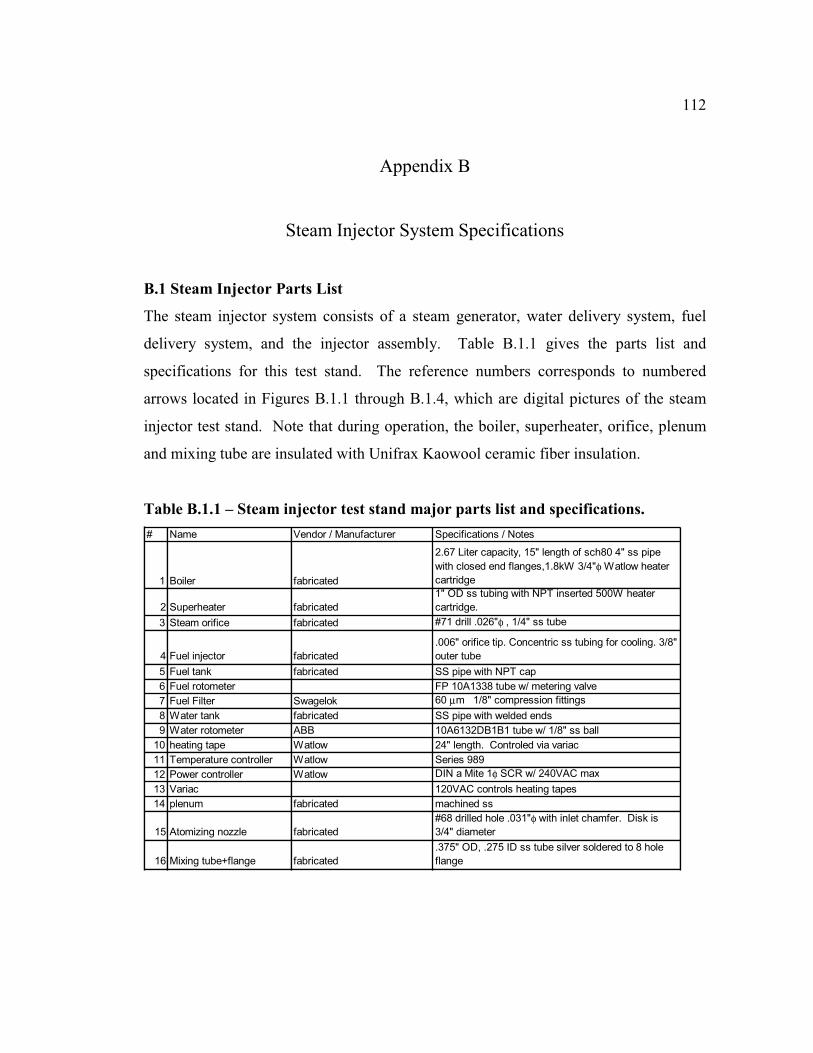
112

Appendix B

Steam Injector System Specifications

B.1 Steam Injector Parts List

The steam injector system consists of a steam generator, water delivery system, fuel

delivery system, and the injector assembly. Table B.1.1 gives the parts list and

specifications for this test stand. The reference numbers corresponds to numbered

arrows located in Figures B.1.1 through B.1.4, which are digital pictures of the steam

injector test stand. Note that during operation, the boiler, superheater, orifice, plenum

and mixing tube are insulated with Unifrax Kaowool ceramic fiber insulation.

Table B.1.1 – Steam injector test stand major parts list and specifications.

# Name Vendor / Manufacturer Specifications / Notes

1 Boiler fabricated

2.67 Liter capacity, 15" length of sch80 4" ss pipe

with closed end flanges,1.8kW 3/4"φ Watlow heater

cartridge

2 Superheater fabricated

1" OD ss tubing with NPT inserted 500W heater

cartridge.

3 Steam orifice fabricated #71 drill .026"φ , 1/4" ss tube

4 Fuel injector fabricated

.006" orifice tip. Concentric ss tubing for cooling. 3/8"

outer tube

5 Fuel tank fabricated SS pipe with NPT cap

6 Fuel rotometer FP 10A1338 tube w/ metering valve

7 Fuel Filter Swagelok 60 µm 1/8" compression fittings

8 Water tank fabricated SS pipe with welded ends

9 Water rotometer ABB 10A6132DB1B1 tube w/ 1/8" ss ball

10 heating tape Watlow 24" length. Controled via variac

11 Temperature controller Watlow Series 989

12 Power controller Watlow DIN a Mite 1φ SCR w/ 240VAC max

13 Variac 120VAC controls heating tapes

14 plenum fabricated machined ss

15 Atomizing nozzle fabricated

#68 drilled hole .031"φ with inlet chamfer. Disk is

3/4" diameter

16 Mixing tube+flange fabricated

.375" OD, .275 ID ss tube silver soldered to 8 hole

flange

Fig

ure

B.1

.1 –

Dig

ital

ph

oto

gra

ph

of

the

stea

m i

nje

cto

r te

st s

tan

d p

roce

ss c

om

pon

ents

.

Boil

er (

1)

Super

hea

ter

(2)

4, 14, 1

5, 1

6M

easu

rem

ent

ori

fice

(3)

Wat

er ta

nk (

8)

Fuel

ta

nk (

5)

113

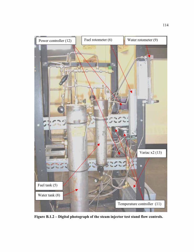
114

Figure B.1.2 – Digital photograph of the steam injector test stand flow controls.

Water rotometer (9)Fuel rotometer (6)

Variac x2 (13)

Water tank (8)

Fuel tank (5)

Power controller (12)

Temperature controller (11)

Fig

ure

B.1

.3 –

Dig

ital

ph

oto

gra

ph

of

the

stea

m i

nje

cto

r ass

em

bly

.

Mix

ing T

ube

(16

)A

tom

izin

g n

ozz

le (

15)

Ple

num

(14)

Fuel

inje

ctor

(4)

Ste

am i

nle

t

115

116

Figure B.1.4 – Digital photograph of the fuel feed tube tip.

The boiler, superheater and fuel injector are assemblies consisting of fabricated and off-

the-shelf components, but are listed as single units.

B.2 Steam Injector Test Stand Calibration

The fuel and water rotometers required calibration, as well as the measuring orifice.

Calibration curves existed for the fuel rotometer when operated on TPD, so several

points were checked periodically to insure this calibration remained valid. The water

rotometer also had been calibrated previously. KLN operation required a new

calibration curve, and was performed using a stopwatch and laboratory beaker. Note

that operation on KLN used the same rotometer and float as TPD operation. Figure

B.2.1 gives a plot of the calibration curves for TPD, KLN and water for the two steam

injector rig rotometers.

The measuring orifice operates under choked conditions, thus requiring knowledge of

the discharge coefficient to correlate the mass flow rate with measured thermodynamic

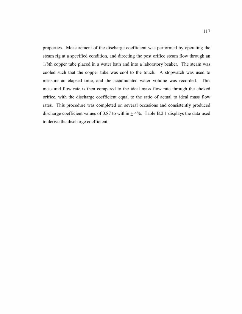
117

properties. Measurement of the discharge coefficient was performed by operating the

steam rig at a specified condition, and directing the post orifice steam flow through an

1/8th copper tube placed in a water bath and into a laboratory beaker. The steam was

cooled such that the copper tube was cool to the touch. A stopwatch was used to

measure an elapsed time, and the accumulated water volume was recorded. This

measured flow rate is then compared to the ideal mass flow rate through the choked

orifice, with the discharge coefficient equal to the ratio of actual to ideal mass flow

rates. This procedure was completed on several occasions and consistently produced

discharge coefficient values of 0.87 to within + 4%. Table B.2.1 displays the data used

to derive the discharge coefficient.

y =

3.8

0x -

11

3.6

0

y =

0.5

36

x -

27

.46

4

y =

-0

.00

55

1x

2 +

1.6

05

58

x +

1.7

40

47

0

50

10

0

15

0

20

0

25

0

30

0

35

0

40

0

05

01

00

15

02

00

Ro

tom

ete

r S

ca

le

Mass Flow Rate (mg/s)

H2

O

KL

N

TP

D

Lin

ea

r (H

2O

)

Lin

ea

r (T

PD

)

Po

ly.

(KL

N)

Fig

ure

B.2

.1 –

Ro

tom

ete

r ca

lib

rati

on

cu

rves

for

wate

r, K

LN

fu

el a

nd

TP

D f

uel

. N

ote

th

at

the

fuel

cu

rves

corr

esp

on

d t

o t

he

sam

e ro

tom

eter

tub

e an

d f

loat,

bu

t th

e w

ate

r cu

rve

corre

spon

ds

to t

he

wate

r ro

tom

ete

r tu

be

an

d f

loat.

118

119

Table B.2.1 – Measurement orifice discharge coefficient calculations.

Performed prior to 5" tests

volume (ml) 100 100 P psig T C mg/s ideal

time elapsed in seconds 477 458 60 244 242

flow rate (mg/s) 210 218

Actual / Ideal = Cd 0.87 0.90

volume (ml) 100 100 P psig T C mg/s ideal

time elapsed in seconds 389 379 80 275 298

flowrate (mg/s) 257 264

Actual / Ideal = Cd 0.86 0.88

volume (ml) 100 P psig T C mg/s ideal

time elapsed in seconds 405 80 340 282

flowrate (mg/s) 247

Actual / Ideal = Cd 0.88

Performed Prior to 10" test



flowrate (mg/s) 149




flowrate (mg/s) 170




flowrate (mg/s) 199




flowrate (mg/s) 217




flowrate (mg/s) 233




flowrate (mg/s) 247


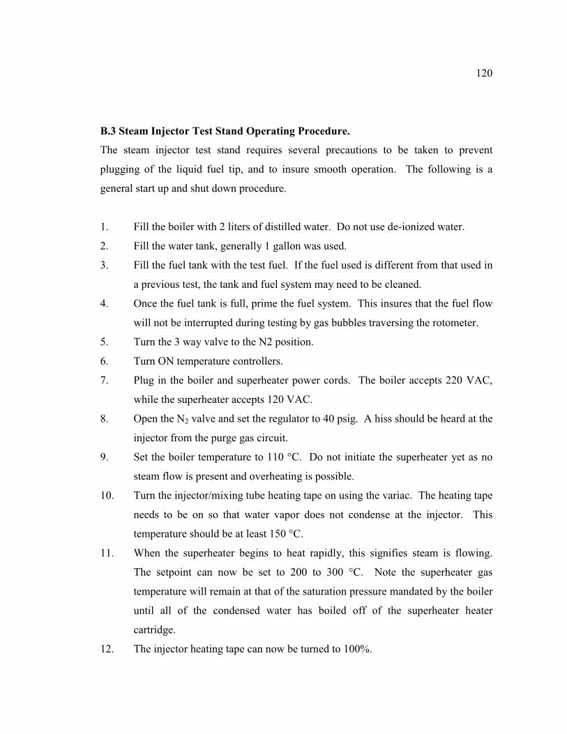
120

B.3 Steam Injector Test Stand Operating Procedure.

The steam injector test stand requires several precautions to be taken to prevent

plugging of the liquid fuel tip, and to insure smooth operation. The following is a

general start up and shut down procedure.

1. Fill the boiler with 2 liters of distilled water. Do not use de-ionized water.

2. Fill the water tank, generally 1 gallon was used.

3. Fill the fuel tank with the test fuel. If the fuel used is different from that used in

a previous test, the tank and fuel system may need to be cleaned.

4. Once the fuel tank is full, prime the fuel system. This insures that the fuel flow

will not be interrupted during testing by gas bubbles traversing the rotometer.

5. Turn the 3 way valve to the N2 position.

6. Turn ON temperature controllers.

7. Plug in the boiler and superheater power cords. The boiler accepts 220 VAC,

while the superheater accepts 120 VAC.

8. Open the N2 valve and set the regulator to 40 psig. A hiss should be heard at the

injector from the purge gas circuit.

9. Set the boiler temperature to 110 °C. Do not initiate the superheater yet as no

steam flow is present and overheating is possible.

10. Turn the injector/mixing tube heating tape on using the variac. The heating tape

needs to be on so that water vapor does not condense at the injector. This

temperature should be at least 150 °C.

11. When the superheater begins to heat rapidly, this signifies steam is flowing.

The setpoint can now be set to 200 to 300 °C. Note the superheater gas

temperature will remain at that of the saturation pressure mandated by the boiler

until all of the condensed water has boiled off of the superheater heater

cartridge.

12. The injector heating tape can now be turned to 100%.

121

13. When the superheater temperature begins to increase from the saturation

temperature, the setpoint can be raised to the desired level, usually done by 100

°C increments.

14. The boiler temperature setpoint can now be set to the desired setting. This can

be done any time after the superheater has warmed.

15. Once the system gas temperatures have reached the desired state, the water refill

for the boiler can be introduced. Open the tank pressure valve, thus pressurizing

the tank, and open the needle valve while watching the rotometer.

16. To introduce fuel, first open the tank pressure valve. Once pressurized, open

the needle valve at the base of the fuel tank, switch the 3 way valve to fuel

position, and then open the needle valve on the rotometer while monitoring the

fuel rotometer. A short delay may be experienced while liquid fuel fills the

plumbing downstream of the 3-way valve.

17. Measurements can now be taken.

18. Upon completion of measurements, turn the 3 way valve back to N2 purge

position. Close the fuel tank pressure valve, close needle valves (softly), and

vent tank pressure plumbing.

19. Close the water feed valve and depressurize the tank. Vent the pressure

plumbing.

20. Lower the boiler temperature to 15 °C (lowest setting).

21. Lower the superheater temperature such that it still remains higher than the

saturation temperature to prevent premature condensation. Maintain the heating

tape power to prevent condensation inside the mixing tube.

22. Once cooled, the N2 purge can be removed by closing the N2 tank.

23. Turn off electronics and unplug heater power cords.

122

Appendix C

SPP Injector System Specifications

C.1 SPP Injector Parts List

The SPP injector system consists of a PJAA, 1st stage, 2

nd stage, 3 separate air flow

systems, and a liquid fuel delivery system. Table C.1.1 gives the parts list and

specifications for the test stand. The reference numbers correspond to numbered

arrows located on Figures C.1.1 through C.1.3, which are digital pictures of the SPP

injector test stand. Note that during operation, the SPP injector assembly and air

heaters are insulated with Unifrax Kaowool ceramic fiber insulation.

Table C.1.1 – SPP injector test stand major parts list and specifications.

# Name Vendor / Manufacturer Specifications / Notes

1 Atomizer air rotometer Fischer Porter FP-1/8-G-25-5/84 tube, 1/8" ss float

2 Atomizer air pressure reg. 0 - 100 psig range

3 1st stage air rotometer Fischer Porter

FP-1/2-27-G-10/83 tube, GNSVT -48A

float

4 1st stage pressure regulator 0 - 100 psig range

5 1st stage heater Watlow 110 VAC operation

6 2nd stage air rotometer Fischer Porter

FP-1/2-27-G-10/55 tube, GSVT - 48A

float

7 2nd stage pressure regulator 0 - 100 psig range

8 2nd stage heater Watlow 220 VAC operation

9 Fuel tank fabricated SS pipe with NPT cap

10 Fuel rotometer ABB 10A6130 with ss ball float

11 Fuel Filter Swagelok 60 µm 1/4" compression fittings

12 PJAA fabricated .012" fuel orifice, .021" air orifice

13 1st stage fabricated volume = 7.40e-6 m3 , 0.50" ID

14 2nd stage fabricated volume =2.04e-5 m3 , .675" exit ID

15 Temperature controller Watlow Series 989

16 Power controller Watlow DIN a Mite 3φ SCR w/ 240VAC max

17 Variac Powerstat 120VAC controls 1st stage

18 Variac Powerstat 220VAC controls 2nd stage

123

Figure C.1.1 – Digital picture of the SPP test stand.

Temperature controllers (15)

Fuel tank (9)

Variacs (17,18)

Fuel rotometer (10)Fuel filter (11)

124

Figure C.1.2 – Digital picture of the SPP test stand air flow system.

1st Stage air rotometer (3)

2nd

Stage air rotometer (6)Atomizer air rotometer (1)

Air pressure regulators (4,7)

125

Figure C.1.3 – Digital picture of the SPP injector.

Exit flange

2nd

stage (14)

2nd

stage air inlet from heater

1st stage (13)

126

C.2 SPP Injector Test Stand Calibration

The air flow rates entering the SPP injector or monitored and regulated with three

rotometers. The correlation relating the rotometer scale reading and pressure to air

flow rate is given by Equation C.2.1. Pressure, as included in Equation C.2.1, is

measured in atmospheres. The maximum flow rate is dependant upon the tube and

Pscalemax

scale)RateFlowMaximum(SCFM

= Eq. C.2.1

float combination used. The maximum flow rate for the atomizer air rotometer is 3720

sccm. The maximum flow rates for the 1st and 2

nd stage rotometers are 5.93 and 4.9

scfm, respectively. The maximum scale for the atomizer rotometer tube is 25, while the

maximum scale for the 1st and 2

nd stage rotometers is 100.

The liquid fuel rotometer was calibrated using a timer and laboratory beaker over the

operating range of fuel flow. Figure C.2.1 displays the calibration curves of TPD and

CLSD using a stainless steel float. The CLSD calibration curve was taken from

Edmonds (2002).

C.3 SPP Injector Operation Procedure

Operating the SPP injector for LRS measurements is significantly simpler than

operating the SPP injector with the JSR. The following is a general procedure for

operating the SPP injector under non-burning conditions.

1. Fill the liquid fuel tank with the fuel to be tested.

2. Open the air gate valve located on the overhead plant air line.

3. Adjust the three air pressure regulators so that some air is flowing through all of

the streams entering the SPP injector. This will prevent the heaters from

overheating in the case that the room temperature is less than 15°C.

127

4. Turn on the temperature controllers.

5. Plug in the 2 heater power cords into the proper outlets. Make sure that the

variacs are turned to zero at this point.

6. Set the air flow rates to those needed for testing.

7. Set the stage temperatures to those needed for testing.

8. Once the temperatures have been reached, liquid fuel can be introduced. It is

important to note that the addition of liquid fuel into a cold SPP injector (less

than 300 °C), will result in poor vaporization, and may deposit liquid fuel onto

the metal walls within the SPP injector.

9. To introduce fuel, pressurize the fuel tank with a N2 cylinder to 45 psig. Then

open the shutoff fuel valve and slowly open the metering valve.

10. The addition of liquid fuel will affect the atomizer air flow rate. This air flow

stream will need to be iterated with the fuel flow to achieve the desired flow

rates.

11. LRS measurements can now be taken. The atomizer air flow system may need

to be adjusted slightly to maintain the prescribed airflow as the 1st stage

temperature is increased.

12. Once testing is completed, shut off the fuel shutoff valve. Then gently close the

metering valve. Note that the metering valve does not need to be closed

completely. Close and vent the N2 cylinder.

13. The variacs can be set to zero and the heaters unplugged once the SPP injector

starts to cool.

14. Reduce the SPP injector stages flow rates to facilitate slow cooling of the metal

parts.

15. Once cooled, shut off the air supply and turn off the temperature controllers.

y =

0.2

66

5x

2 +

0.1

76

6x -

0.0

38

3

R2 =

0.9

97

8

y =

0.3

86

9x

2 -

0.0

15

7x +

0.0

06

R2 =

0.9

99

8

0

0.0

5

0.1

0.1

5

0.2

0.2

5

0.3

0.3

5

0.4

0.4

5

00

.20

.40

.60

.81

1.2

No

rma

lize

d R

oto

me

ter

Sc

ale

(s

ca

le/2

50

)

Flow Rate (g/s)

CL

SD

TP

D

Po

ly.

(TP

D)

Po

ly.

(CL

SD

)

Fig

ure

C.2

.1 –

Cali

bra

tion

cu

rve

for

SP

P i

nje

cto

r li

qu

id f

uel

roto

mete

r.

128

129

Appendix D

Combustion Testing of SPP Injector at Low Residence Times

D.1 Experimental System and Gas Sampling

Utilizing the SPP injector and 64cc jet-stirred reactor, several combustion tests were run

at low residence times, with a goal of 5 to 10 milliseconds in the SPP injector. The 15.8

cc JSR used by Lee (2000) and Edmonds (2002) was replaced with a 64 cc JSR to

facilitate lower back pressure inside of the SPP, thus reducing the SPP residence time.

Two separate fuels were tested, industrial propane and Chevron Low-Sulfur Diesel

(C13.77H26.28), along with mixtures of these two. Emission data were recorded to observe

the effects of SPP residence time on pollutant formation.

The SPP injector was not modified for this set of combustion tests after the new 2nd

stage

was redesigned by Edmonds (2002). All instrumentation and controls remained intact,

except for the jet stirred reactor and nozzle block. The nozzle block is 0.755 thick

(highest point) with two bolt circles for the SPP outlet flange and the JSR flange. The jet

diameter of the nozzle block is nominally 6 mm, with a 37.4° inlet chamfer through.

Figure D.1.1 displays digital pictures of the nozzle block and JSR used. The propane,

atomizer air, 1st stage air and 2

nd stage air flows are controlled with Laminar Technology

model UFC MFC’s. The liquid fuel flow rate is monitored with the same rotometer used

for the LRS testing of Chapter 7, although the CLSD has a different calibration curve

than the TPD (see Appendix C). The first stage heater presented a testing limitation, due

to the increased air flow and liquid fuel flow in the 1st stage. The vaporization of the

liquid fuel requires sensible enthalpy transferred from the 1st stage air, so the heater

limited the mixture temperature in the 1st stage. In order to circumvent this limitation,

and still maintain high air flow rates, propane was introduced and the CLSD flow rate

was decreased, in a proportion that maintained the 1480 °C reactor temperature

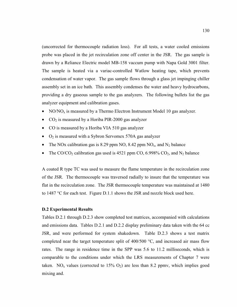
130

(uncorrected for thermocouple radiation loss). For all tests, a water cooled emissions

probe was placed in the jet recirculation zone off center in the JSR. The gas sample is

drawn by a Reliance Electric model MB-158 vaccum pump with Napa Gold 3001 filter.

The sample is heated via a variac-controlled Watlow heating tape, which prevents

condensation of water vapor. The gas sample flows through a glass jet impinging chiller

assembly set in an ice bath. This assembly condenses the water and heavy hydrocarbons,

providing a dry gaseous sample to the gas analyzers. The following bullets list the gas

analyzer equipment and calibration gases.

• NO/NOx is measured by a Thermo Electron Instrument Model 10 gas analyzer.

• CO2 is measured by a Horiba PIR-2000 gas analyzer

• CO is measured by a Horiba VIA 510 gas analyzer

• O2 is measured with a Sybron Servomex 570A gas analyzer

• The NOx calibration gas is 8.29 ppm NO, 8.42 ppm NOx, and N2 balance

• The CO/CO2 calibration gas used is 4521 ppm CO, 6.998% CO2, and N2 balance

A coated R type TC was used to measure the flame temperature in the recirculation zone

of the JSR. The thermocouple was traversed radially to insure that the temperature was

flat in the recirculation zone. The JSR thermocouple temperature was maintained at 1480

to 1487 °C for each test. Figure D.1.1 shows the JSR and nozzle block used here.

D.2 Experimental Results

Tables D.2.1 through D.2.3 show completed test matrices, accompanied with calculations

and emissions data. Tables D.2.1 and D.2.2 display preliminary data taken with the 64 cc

JSR, and were performed for system shakedown. Table D.2.3 shows a test matrix

completed near the target temperature split of 400/500 °C, and increased air mass flow

rates. The range in residence time in the SPP was 5.6 to 11.2 milliseconds, which is

comparable to the conditions under which the LRS measurements of Chapter 7 were

taken. NOx values (corrected to 15% O2) are less than 8.2 ppmv, which implies good

mixing and.

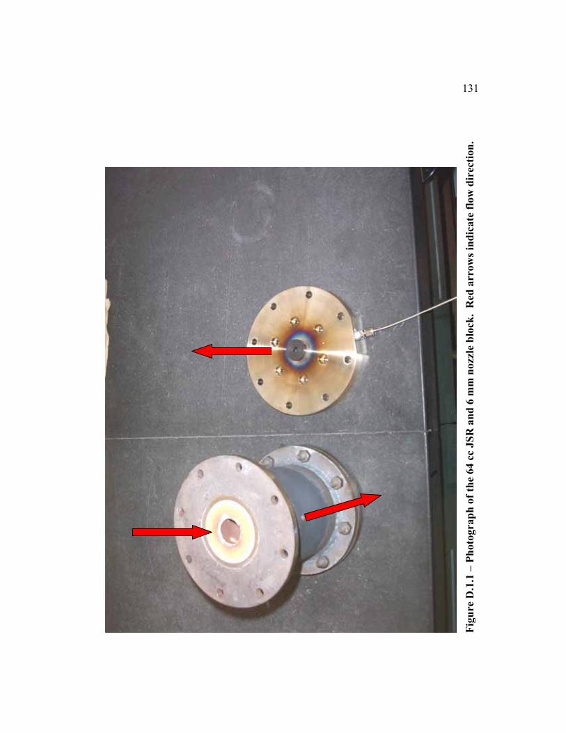
Fig

ure

D.1

.1 –

Ph

oto

gra

ph

of

the

64 c

c JS

R a

nd

6 m

m n

ozzl

e b

lock

. R

ed a

rro

ws

ind

ica

te f

low

dir

ecti

on

.

131

Tab

le D

.2.1

– T

est

ma

trix

for

SP

P i

nje

cto

r co

mb

ust

ion

pre

lim

inary

pro

pan

e te

sts.

Measu

rem

en

tU

nit

ste

st

1te

st

2te

st

3te

st

4te

st

5te

st

6te

st

7

Ato

miz

er

air

slp

m5

55

55

55

Ato

miz

er

air

kg

/s1.0

0E

-04

1.0

0E

-04

1.0

0E

-04

1.0

0E

-04

1.0

0E

-04

1.0

0E

-04

1.0

0E

-04

1st

sta

ge a

irslp

m30

30

30

30

30

30

30

1st

sta

ge a

irkg

/s6.0

0E

-04

6.0

0E

-04

6.0

0E

-04

6.0

0E

-04

6.0

0E

-04

6.0

0E

-04

6.0

0E

-04

2n

d s

tag

e A

irslp

m100

100

100

100

100

100

100

2n

d s

tag

e A

irkg

/s2.0

0E

-03

2.0

0E

-03

2.0

0E

-03

2.0

0E

-03

2.0

0E

-03

2.0

0E

-03

2.0

0E

-03

1st

Sta

ge T

°C250

250

250

250

250

250

250

2n

d S

tag

e T

°C350

350

350

350

350

350

350

Pro

pan

eslp

m2.9

6245

2.9

6245

2.9

6245

2.9

6245

2.9

6245

2.9

6245

2.9

6245

Pro

pan

eg

/s0.0

88

0.0

88

0.0

88

0.0

88

0.0

88

0.0

88

0.0

88

JS

R T

°C1478

1480

1483

1485

1486

1488

1489

Po

sit

ion

cm

42

42.3

42.8

43

43.5

44

44.5

Po

sit

ion

fro

m c

en

ter

cm

3.4

45

3.1

45

2.6

45

2.4

45

1.9

45

1.4

45

0.9

45

Calc

ula

tio

ns

Un

its

test

1te

st

2te

st

3te

st

4te

st

5te

st

6te

st

7

eq

uiv

ale

nce r

ati

o m

ass

0.5

10.5

10.5

10.5

10.5

10.5

10.5

1

resid

en

ce t

ime 1

sec

0.0

066

0.0

066

0.0

066

0.0

066

0.0

066

0.0

066

0.0

066

resid

en

ce t

ime 2

sec

0.0

042

0.0

042

0.0

042

0.0

042

0.0

042

0.0

042

0.0

042

tota

l ti

me 1

+2

sec

0.0

108

0.0

108

0.0

108

0.0

108

0.0

108

0.0

108

0.0

108

Em

issio

ns

Un

its

test

1te

st

2te

st

3te

st

4te

st

5te

st

6te

st

7

CO

%0.0

77

0.0

82

0.0

91

0.0

98

0.1

10.1

08

0.1

35

CO

2%

7.9

57.9

57.9

57.9

57.9

57.9

7.9

O2

%7.8

7.8

7.8

7.8

7.8

7.8

7.8

NO

xp

pm

v12

12.5

13

13

13

13.5

14

NO

x 1

5%

O2

pp

mv

5.4

5.6

5.9

5.9

5.9

6.1

6.3

JS

RU

nit

ste

st

1te

st

2te

st

3te

st

4te

st

5te

st

6te

st

7

den

sit

y in

JS

Rkg

/m3

0.2

06

0.2

06

0.2

05

0.2

05

0.2

05

0.2

05

0.2

05

JS

R r

es. T

ime

sec

0.0

0473

0.0

0472

0.0

0471

0.0

0471

0.0

0470

0.0

0470

0.0

0469

132

Tab

le D

.2.2

- T

est

matr

ix f

or

SP

P i

nje

cto

r co

mb

ust

ion

pre

lim

inary

CL

SD

tes

ts.

Me

as

ure

me

nt

Un

its

tes

t 1

tes

t 2

tes

t 3

tes

t 4

tes

t 5

tes

t 6

tes

t 7

Ato

miz

er

air

slp

m5

55

55

55

Ato

miz

er

air

kg

/s1

.00

E-0

41

.00

E-0

41

.00

E-0

41

.00

E-0

41

.00

E-0

41

.00

E-0

41

.00

E-0

4

1s

t s

tag

e a

irs

lpm

30

30

30

30

30

30

30

1s

t s

tag

e a

irk

g/s

6.0

0E

-04

6.0

0E

-04

6.0

0E

-04

6.0

0E

-04

6.0

0E

-04

6.0

0E

-04

6.0

0E

-04

2n

d s

tag

e A

irs

lpm

10

01

00

10

01

00

10

01

00

10

0

2n

d s

tag

e A

irk

g/s

2.0

0E

-03

2.0

0E

-03

2.0

0E

-03

2.0

0E

-03

2.0

0E

-03

2.0

0E

-03

2.0

0E

-03

1s

t S

tag

e T

°C2

50

25

02

50

25

02

50

25

02

50

2n

d S

tag

e T

°C3

50

35

03

50

35

03

50

35

03

50

Ro

tom

ete

r R

ea

din

g1

29

12

91

29

12

91

29

12

91

29

LS

Dg

/s0

.09

90

.09

90

.09

90

.09

90

.09

90

.09

90

.09

9

JS

R T

°C1

47

81

48

01

48

31

48

51

48

61

48

81

48

9

Po

sit

ion

cm

42

42

.34

2.8

43

43

.54

44

4.5

po

sit

ion

fro

m c

en

ter

cm

3.4

45

3.1

45

2.6

45

2.4

45

1.9

45

1.4

45

0.9

45

Ca

lcu

lati

on

sU

nit

ste

st

1te

st

2te

st

3te

st

4te

st

5te

st

6te

st

7

eq

uiv

ale

nc

e r

ati

o m

as

s0

.53

0.5

30

.53

0.5

30

.53

0.5

30

.53

res

ide

nc

e t

ime

1s

ec

0.0

07

00

.00

70

0.0

07

00

.00

70

0.0

07

00

.00

70

0.0

07

0

res

ide

nc

e t

ime

2s

ec

0.0

04

30

.00

43

0.0

04

30

.00

43

0.0

04

30

.00

43

0.0

04

3

tota

l ti

me

1+

2s

ec

0.0

11

20

.01

12

0.0

11

20

.01

12

0.0

11

20

.01

12

0.0

11

2

Em

iss

ion

sU

nit

ste

st

1te

st

2te

st

3te

st

4te

st

5te

st

6te

st

7

CO

%0

.11

10

.11

50

.12

20

.12

80

.15

50

.15

10

.17

CO

2%

8.7

38

.73

8.7

08

.68

8.6

58

.65

8.6

3

O2

%8

.10

8.1

08

.10

8.0

08

.00

8.0

08

.00

NO

xp

pm

v1

61

71

71

71

7.5

17

.51

8

NO

x 1

5%

O2

pp

mv

7.4

7.8

7.8

7.8

8.0

8.0

8.2

JS

RU

nit

ste

st

1te

st

2te

st

3te

st

4te

st

5te

st

6te

st

7

de

ns

ity

in

JS

Rk

g/m

30

.20

70

.20

70

.20

60

.20

60

.20

60

.20

60

.20

5

JS

R r

es

. T

ime

se

c0

.00

47

30

.00

47

20

.00

47

10

.00

47

10

.00

47

00

.00

47

00

.00

47

0

133

Tab

le D

.2.3

- T

est

matr

ix f

or

SP

P i

nje

cto

r co

mb

ust

ion

tes

ts a

t h

igh

tem

per

atu

re

an

d a

ir f

low

rate

. N

ote

tha

t te

st 3

da

ta w

as

tak

en w

ith

th

e J

SR

ou

t o

f th

erm

al

equ

ilib

riu

m.

Measu

rem

en

tU

nit

ste

st

1te

st

2te

st

3te

st

4te

st

5te

st

6te

st

7te

st

8te

st

9te

st

10

test

11

Ato

miz

er

air

slp

m5

55

55

55

55

55

Ato

miz

er

air

kg

/s1.0

0E

-04

1.0

0E

-04

1.0

0E

-04

1.0

0E

-04

1.0

0E

-04

1.0

0E

-04

1.0

0E

-04

1.0

0E

-04

1.0

0E

-04

1.0

0E

-04

1.0

0E

-04

1st

sta

ge a

irslp

m50

50

50

90

100

100

100

99.5

99.5

99.5

100

1st

sta

ge a

irkg

/s1.0

0E

-03

1.0

0E

-03

1.0

0E

-03

1.8

0E

-03

2.0

0E

-03

2.0

0E

-03

2.0

0E

-03

1.9

9E

-03

1.9

9E

-03

1.9

9E

-03

2.0

0E

-03

2n

d s

tag

e A

irslp

m100

100

100

100

100

100

100

100

100

100

100

2n

d s

tag

e A

irkg

/s2.0

0E

-03

2.0

0E

-03

2.0

0E

-03

2.0

0E

-03

2.0

0E

-03

2.0

0E

-03

2.0

0E

-03

2.0

0E

-03

2.0

0E

-03

2.0

0E

-03

2.0

0E

-03

1st

Sta

ge T

°C400

400

401

352

338

334

340

358

378

385

392

2n

d S

tag

e T

°C521

522

523

500

496

502

501

525

557

557

572

Pro

pan

eslp

m8.7

28.7

20

00

010

10

10

10

10

Pro

pan

eg

/s0.0

86

0.0

86

0.0

00

0.0

00

0.0

00

0.0

00

0.0

99

0.0

99

0.0

99

0.0

99

0.0

99

Liq

uid

Fu

el L

S-D

read

ing

00

128

142

146

145

43

34

23

24

22.3

Liq

uid

Fu

el L

S-D

g/s

0.0

000

0.0

00

00

.0975

0.1

19

60

.1264

0.1

24

70

.0137

0.0

09

90

.0066

0.0

06

80

.0064

PS

PP

psig

44

5.7

56

66.2

6.5

6.5

6.5

6.6

No

zzle

T°C

NA

NA

NA

NA

NA

560

554

560

575

578

585

JS

R T

°C1483

1483

1482

1485

1483

1480

1483

1483

1480

1480

1487

Calc

ula

tio

ns

Un

its

test

1te

st

2te

st

3te

st

4te

st

5te

st

6te

st

7te

st

8te

st

9te

st

10

test

11

eq

uiv

ale

nce r

ati

o m

ass

0.4

30.4

30.3

60.4

30.4

50.4

4N

AN

AN

AN

AN

A

resid

en

ce t

ime 1

sec

0.0

043

0.0

04

30

.0035

0.0

03

10

.0029

0.0

02

90

.0028

0.0

02

80

.0027

0.0

02

70

.0026

resid

en

ce t

ime 2

sec

0.0

037

0.0

03

70

.0029

0.0

03

30

.0032

0.0

03

20

.0032

0.0

03

10

.0030

0.0

03

00

.0030

tota

l ti

me 1

+2

sec

0.0

079

0.0

07

90

.0064

0.0

06

40

.0061

0.0

06

10

.0060

0.0

05

90

.0057

0.0

05

70

.0056

Em

issio

ns

Un

its

test

1te

st

2te

st

3te

st

4te

st

5te

st

6te

st

7te

st

8te

st

9te

st

10

test

11

CO

%0.0

92

0.1

01

0.1

25

0.1

39

0.1

42

0.1

40.1

11

0.1

05

0.0

99

0.0

99

0.0

98

CO

2%

6.8

66.8

57.5

77.4

97.4

67.3

66.8

26.5

86.3

76.3

76.3

5

O2

%9.7

9.8

9.9

9.9

9.9

10.1

9.9

10.2

10.5

10.5

10.6

NO

xp

pm

v11

11

14.5

14

13.5

13

10

9.5

9.5

9.5

10

NO

x 1

5%

O2

pp

mv

5.8

5.8

7.8

7.5

7.2

7.1

5.4

5.2

5.4

5.4

5.7

JS

RU

nit

ste

st

1te

st

2te

st

3te

st

4te

st

5te

st

6te

st

7te

st

8te

st

9te

st

10

test

11

den

sit

y in

JS

Rk

g/m

30.2

05

0.2

05

0.2

06

0.2

05

0.2

05

0.2

06

0.2

05

0.2

04

0.2

05

0.2

05

0.2

04

JS

R r

es. T

ime

sec

0.0

0411

0.0

041

10

.00411

0.0

032

70

.00311

0.0

031

10

.00311

0.0

031

20

.00312

0.0

031

20

.00310

134

135

the lack of droplets. Equation D.2.1 gives the correlation for the gas turbine standard

15% O2 correction

dry,meas,2meas,x%15,x

O9.20

159.20NONO

−−= Eq. D.2.1

The temperatures listed are stage temperatures of the mixture. Propane was mixed into

the diesel for several tests to facilitate raising the temperatures in the SPP, since liquid

fuel requires additional heat input to vaporize. The 64 cc JSR and nozzle create 6.6 psig

or less of back pressure inside of the SPP at the conditions tested, which is 1.4

atmospheres absolute, compared to the 2 atmosphere conditions used previously. This

reduction in back pressure provides the practical means to attain SPP residence times less

than 10 milliseconds with the current configuration.

Note that the preliminary tests were completed at fixed temperature and flow rates, but

the position of the gas sample probe within the JSR was varied. This was done to locate

the recirculation zone in the JSR, and determine the best temperature measurement and

gas sample locations. The higher flow rate and temperature tests were performed with

the gas sample probe located at 0.945 cm from the centerline. The thermocouple was

position in the zone of the JSR with a flat radial temperature profile. Figures D.2.1 and

D.2.2 show radial variation in the reactor temperature and combustion product

concentrations. Note that there is a small central region in which the temperature drops,

which is due to the initial jet traversing the nozzle plate consisting of raw air and fuel

mixture. Away from the center of the JSR, about 8 mm radially, the gas temperature

within the JSR is nearly constant. It should also be noted that the inner wall of the JSR is

located at approximately 20 mm from the centerline. There are 8, 1/8 ports arranged

circumferentially around the JSR casing which are used for temperature and gas sample

measurements, and JSR flow exits. None of these unused ports were blocked as in

previous work, to facilitate lower pressures within the SPP injector and JSR.

10

00

11

00

12

00

13

00

14

00

15

00

16

00

05

10

15

20

Ra

dia

l P

os

itio

n (

mm

)

Temperature (°C)

Pro

pa

ne

LS

D

Fig

ure

D.2

.1 –

JS

R t

em

pera

ture

sca

ns

dis

pla

yin

g t

he

rad

ial

pro

file

. D

ata

tak

en a

t 5/3

0/1

00 a

ir f

low

sp

lit.

136

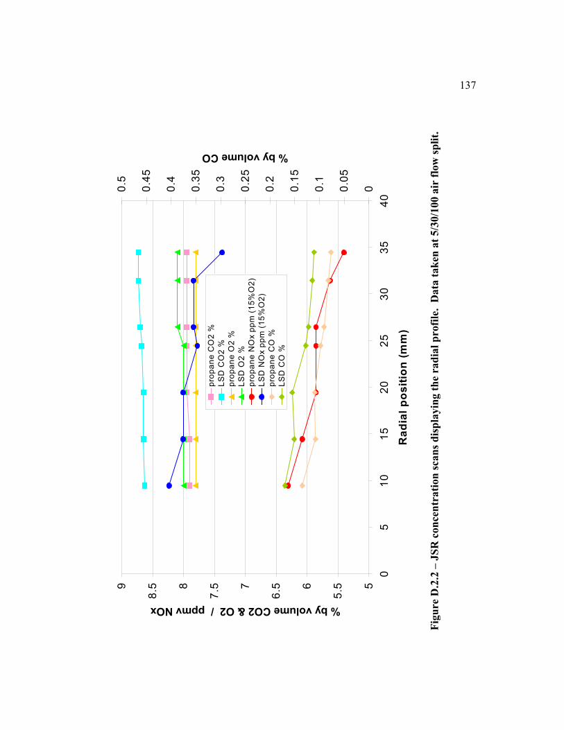
5

5.56

6.57

7.58

8.59

05

10

15

20

25

30

35

40

Ra

dia

l p

os

itio

n (

mm

)

% by volume CO2 & O2 / ppmv NOx

00.0

5

0.1

0.1

5

0.2

0.2

5

0.3

0.3

5

0.4

0.4

5

0.5

% by volume CO

pro

pa

ne

CO

2 %

LS

D C

O2

%

pro

pa

ne

O2

%

LS

D O

2 %

pro

pa

ne

NO

x p

pm

(1

5%

O2

)

LS

D N

Ox p

pm

(1

5%

O2

)

pro

pa

ne

CO

%

LS

D C

O %

Fig

ure

D.2

.2 –

JS

R c

on

cen

tra

tio

n s

can

s d

isp

lay

ing t

he

rad

ial

pro

file

. D

ata

ta

ken

at

5/3

0/1

00

air

flo

w s

pli

t.

137

138

D.3 Brief Summary

The SPP, operated with residence times of 5.6 to 11.2 milliseconds, provides a well-

mixed vapor to the JSR. NOx measurements are less than 8.2 ppmv at 15% O2 for

propane, Chevron LSD, and mixtures of the two for JSR temperatures of 1478 to 1490

°C. LSR measurements at similar conditions show that very few droplets are present,

which further validates the low NOx measurements. The addition of the large JSR and

the 6 mm nozzle block allowed low SPP internal pressures of 1.4 atm to be reached. The

1st stage heater presents a limitation, and may need to be replaced or upgraded to increase

capacity. The larger air and fuel flow rates included in this study, demand larger heat

inputs than those cases examined previously.

No tar or coke was observed in the gas sample probe and associated plumbing, implying

near complete vaporization and mixing. Care was taken not to draw gas samples from

within the unreacted core in the center of the JSR, which brings the heavy risk of tar

condensation in the probe.

D.4 Operating Procedure and Checklist

The following checklist should be completed prior to testing.

Perform a system check – thermocouples, sample probe, wiring, obvious

problems or damage.

Print out a data sheet for manual data collection

Turn ON computer and MFC power/interface

Turn ON stage air heater power and temperature controller power

Turn ON pressure transducer power if necesary

Turn ON Nox analyzer, but DO NOT TURN ON OZONE yet

Turn ON CO and CO2 analyzers

139

Fill liquid fuel tank with desired fuel

Prime the liquid fuel line to evacuate air, making sure to reconnect fuel line

Using N2, pressurize the liquid fuel tank

Position the gas sample probe, which entails the following

• Place probe in Microton positioner

• Insert probe into JSR until the tip can be seen in one of the perpendicular

instrumentation ports

• Mark this position

• Using the Microton, back the probe off center (standard sampling location)

• Mark this location

• Remove the sample probe until needed

The operating and warm up procedure is as follows. Click on the SPP icon on the PC

Desktop, and make sure all of the necessary channels are functioning. Turn on the

hydrogen pressure to 50 psig and the propane pressure to 50 psig. Set the stage 1 air to

12 slpm, stage 2 air to 10 slpm, and atomizer air to 5 slpm, leaving the gaseous fuel off

for the moment. Turn on sparker power and variable VAC supply, and insert the sparker

into the JSR until the marked line is flush with the outer face of the JSR housing. Turn

on sparker and slowly increase H2 flow until light off, then adjust fuel for a reactor

temperature of 800 °C. Turn off the sparker, and then increase the air flow to 30/30

SLPM split still maintaining reactor temperature. Remove the sparker and insert a

ceramic blank, letting the system warm for roughly 5-10 minutes.

Now that the system is warm, the fuel will slowly be transitioned from hydrogen to

propane. Add 0.4 slpm of propane, and allow the system to warm. Increase the propane

flow-rate while simultaneously decreasing the hydrogen flow-rate, until the system is

running entirely on propane with a reactor temperature of 1300 °C. Turn off the

hydrogen pressure, and allow the system to warm. Set the 1st stage air temperature

setpoint to 150 °, and 2nd

stage air temperature setpoint to 350 °C, keeping in mind that

140

1650 °C is ultimate upper limit of the JSR. Let the system warm, and prepare the gas

analyzer. Note that the heaters are not initiated until the hydrogen has been turned off, to

reduce the risk of flashback into the SPP injector.

Reduce the flame temperature, and slowly introduce liquid fuel. As the reactor

temperature increases, reduce the gaseous fuel, and increase the liquid fuel flow-rate to

maintain the reactor temperature. Slowly turn off the gaseous fuel, and set the liquid fuel

flow-rate to the desired condition.

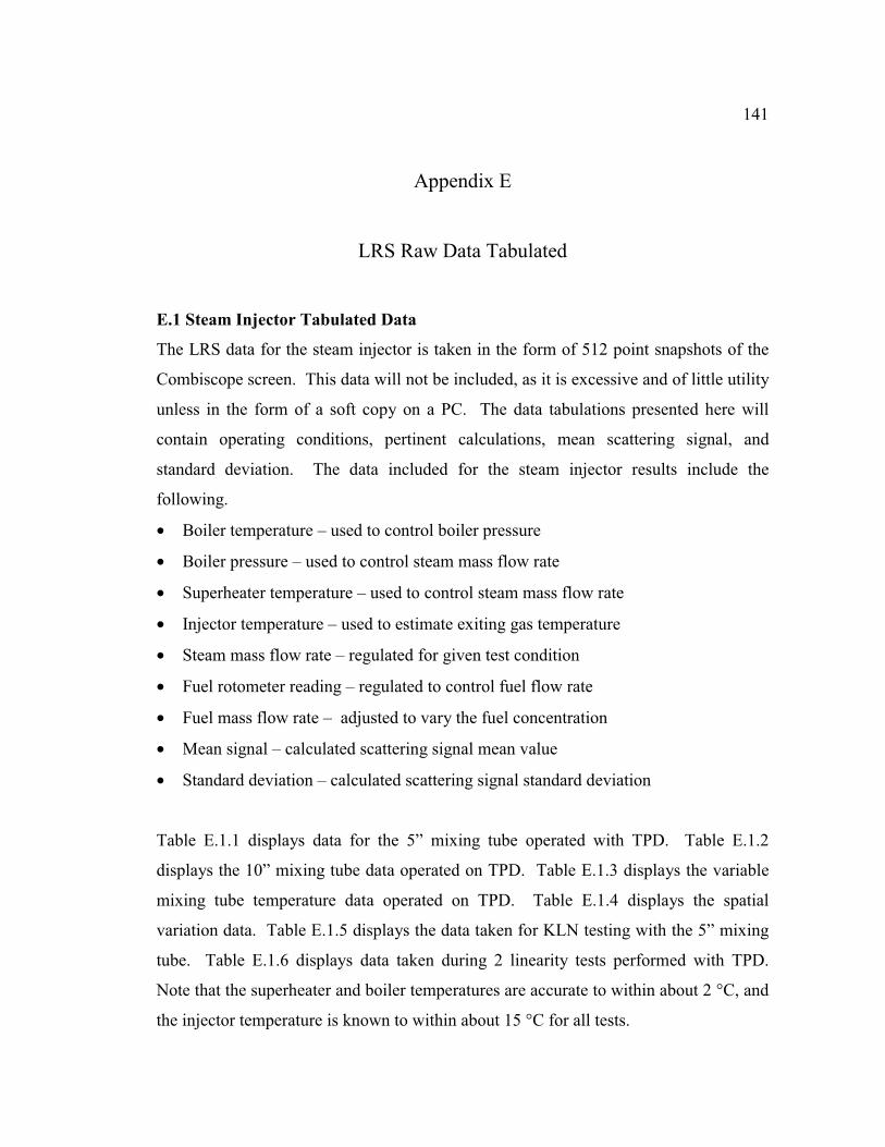
141

Appendix E

LRS Raw Data Tabulated

E.1 Steam Injector Tabulated Data

The LRS data for the steam injector is taken in the form of 512 point snapshots of the

Combiscope screen. This data will not be included, as it is excessive and of little utility

unless in the form of a soft copy on a PC. The data tabulations presented here will

contain operating conditions, pertinent calculations, mean scattering signal, and

standard deviation. The data included for the steam injector results include the

following.

• Boiler temperature – used to control boiler pressure

• Boiler pressure – used to control steam mass flow rate

• Superheater temperature – used to control steam mass flow rate

• Injector temperature – used to estimate exiting gas temperature

• Steam mass flow rate – regulated for given test condition

• Fuel rotometer reading – regulated to control fuel flow rate

• Fuel mass flow rate – adjusted to vary the fuel concentration

• Mean signal – calculated scattering signal mean value

• Standard deviation – calculated scattering signal standard deviation

Table E.1.1 displays data for the 5” mixing tube operated with TPD. Table E.1.2

displays the 10” mixing tube data operated on TPD. Table E.1.3 displays the variable

mixing tube temperature data operated on TPD. Table E.1.4 displays the spatial

variation data. Table E.1.5 displays the data taken for KLN testing with the 5” mixing

tube. Table E.1.6 displays data taken during 2 linearity tests performed with TPD.

Note that the superheater and boiler temperatures are accurate to within about 2 °C, and

the injector temperature is known to within about 15 °C for all tests.

142

Table E.1.1 - LRS data tabulated for 5” mixing tube steam injector testing onTPD.

Note that tests are in chronological order of time performed.

Boiler T Boiler P SH T Inj T steam fuel rot fuel flow fuel/steam fuel concentration mean st dev. mix

°C psig °C °C mg/s reading mg/s mass mol/mol Volts Volts

167 90 400 420 259 180 69.0 0.266 0.038 0.778 0.072 0.092

167 90 400 425 259 170 63.7 0.246 0.035 0.666 0.046 0.069

167 90 400 430 259 160 58.3 0.225 0.033 0.632 0.037 0.059

167 90 400 435 259 150 52.9 0.204 0.030 0.484 0.030 0.061

167 90 400 440 259 140 47.6 0.184 0.027 0.479 0.027 0.057

167 90 400 445 259 130 42.2 0.163 0.024 0.392 0.025 0.064

167 90 400 450 259 120 36.9 0.142 0.021 0.301 0.019 0.062

167 90 400 455 259 110 31.5 0.122 0.018 0.258 0.013 0.052

167 90 400 460 259 100 26.1 0.101 0.015 0.224 0.014 0.062

167 90 400 465 259 90 20.8 0.080 0.012 0.204 0.016 0.078

167 90 400 470 259 80 15.4 0.060 0.009 0.189 0.131 0.692

154 60 460 400 177 180 69.0 0.390 0.055 1.390 0.111 0.080

154 60 460 409 177 170 63.7 0.360 0.051 1.178 0.088 0.074

154 60 460 419 177 160 58.3 0.329 0.047 1.027 0.074 0.072

154 60 460 428 177 150 52.9 0.299 0.043 0.867 0.049 0.057

154 60 460 437 177 140 47.6 0.269 0.039 0.921 0.049 0.053

154 60 460 446 177 130 42.2 0.239 0.034 0.736 0.041 0.056

154 60 460 456 177 120 36.9 0.208 0.030 0.618 0.048 0.078

154 60 460 465 177 110 31.5 0.178 0.026 0.542 0.742 1.368

159 71 483 400 200 180 69.0 0.345 0.049 1.105 0.073 0.066

159 71 483 409 200 170 63.7 0.318 0.045 0.973 0.049 0.050

159 71 483 419 200 160 58.3 0.291 0.042 0.832 0.041 0.049

159 71 483 428 200 150 52.9 0.265 0.038 0.709 0.030 0.043

159 71 483 437 200 140 47.6 0.238 0.034 0.588 0.028 0.047

159 71 483 446 200 130 42.2 0.211 0.031 0.496 0.021 0.043

159 71 483 456 200 120 36.9 0.184 0.027 0.420 0.025 0.060

159 71 483 465 200 110 31.5 0.157 0.023 0.405 0.294 0.727

163 80 487 420 220 180 69.0 0.314 0.045 0.741 0.043 0.058

163 80 487 425 220 170 63.7 0.289 0.041 0.657 0.038 0.058

163 80 487 430 220 160 58.3 0.265 0.038 0.547 0.026 0.047

163 80 487 435 220 150 52.9 0.241 0.035 0.489 0.019 0.039

163 80 487 440 220 140 47.6 0.216 0.031 0.376 0.016 0.043

163 80 487 445 220 130 42.2 0.192 0.028 0.317 0.015 0.046

163 80 487 450 220 120 36.9 0.168 0.024 0.284 0.015 0.053

163 80 487 455 220 110 31.5 0.143 0.021 0.272 0.018 0.067

163 80 487 460 220 100 26.1 0.119 0.017 0.293 0.259 0.885

163 80 487 465 220 90 20.8 0.094 0.014 0.253 0.365 1.441

163 80 400 420 234 180 69.0 0.295 0.042 1.206 0.080 0.067

163 80 400 426 234 170 63.7 0.272 0.039 1.019 0.062 0.061

163 80 400 431 234 160 58.3 0.249 0.036 0.790 0.049 0.062

163 80 400 437 234 150 52.9 0.226 0.033 0.686 0.039 0.056

163 80 400 442 234 140 47.6 0.203 0.029 0.560 0.031 0.055

163 80 400 448 234 130 42.2 0.180 0.026 0.437 0.024 0.056

163 80 400 453 234 120 36.9 0.158 0.023 0.377 0.022 0.059

163 80 400 459 234 110 31.5 0.135 0.020 0.320 0.021 0.065

163 80 400 464 234 100 26.1 0.112 0.016 0.276 0.016 0.056

163 80 400 470 234 90 20.8 0.089 0.013 0.250 0.016 0.064

143

Table E.1.2 - LRS data tabulated for 10” mixing tube steam injector testing

onTPD. Note that tests are in chronological order of time performed.

Boiler T Boiler P SH T Inj. T steam flow fuel rot. fuel flow fuel/steam fuel concentration mean st. Dev mix

°C psig °C °C mg/s reading mg/s mass moli / mol Volts Volts

148 50 483 400 149 180 69.0 0.463 0.041 2.874 0.229 0.080

148 50 483 408 149 170 63.7 0.427 0.038 1.991 0.156 0.078

148 50 483 415 149 160 58.3 0.391 0.035 1.760 0.135 0.076

148 50 483 423 149 150 52.9 0.355 0.032 1.381 0.122 0.089

148 50 483 430 149 140 47.6 0.319 0.029 1.089 0.085 0.078

148 50 483 438 149 130 42.2 0.283 0.026 0.847 0.078 0.092

148 50 483 445 149 120 36.9 0.247 0.022 0.710 0.046 0.065

148 50 483 453 149 110 31.5 0.211 0.019 0.603 0.045 0.075

148 50 483 460 149 100 26.1 0.175 0.016 0.466 0.325 0.697

154 59 480 405 170 180 69.0 0.406 0.036 1.930 0.167 0.087

154 59 480 413 170 170 63.7 0.374 0.034 1.763 0.130 0.074

154 59 480 420 170 160 58.3 0.343 0.031 1.301 0.110 0.084

154 59 480 428 170 150 52.9 0.311 0.028 1.086 0.084 0.077

154 59 480 435 170 140 47.6 0.280 0.025 0.887 0.075 0.085

154 59 480 443 170 130 42.2 0.248 0.023 0.722 0.054 0.075

154 59 480 450 170 120 36.9 0.217 0.020 0.493 0.038 0.077

154 59 480 458 170 110 31.5 0.185 0.017 0.446 0.032 0.072

154 59 480 465 170 100 26.1 0.154 0.014 0.390 0.043 0.111

159 70 470 410 197 180 69.0 0.350 0.031 1.408 0.128 0.091

159 70 470 416 197 170 63.7 0.323 0.029 1.271 0.121 0.095

159 70 470 422 197 160 58.3 0.296 0.027 1.012 0.071 0.070

159 70 470 428 197 150 52.9 0.269 0.024 0.838 0.070 0.084

159 70 470 434 197 140 47.6 0.242 0.022 0.611 0.039 0.065

159 70 470 441 197 130 42.2 0.214 0.019 0.466 0.035 0.076

159 70 470 447 197 120 36.9 0.187 0.017 0.390 0.028 0.071

159 70 470 453 197 110 31.5 0.160 0.015 0.333 0.024 0.071

159 70 470 459 197 100 26.1 0.133 0.012 0.335 0.024 0.071

159 70 470 465 197 90 20.8 0.105 0.010 0.302 0.024 0.079

163 78 460 410 217 180 69.0 0.318 0.029 1.043 0.094 0.090

163 78 460 416 217 170 63.7 0.293 0.026 0.891 0.086 0.096

163 78 460 422 217 160 58.3 0.269 0.024 0.786 0.072 0.091

163 78 460 428 217 150 52.9 0.244 0.022 0.588 0.048 0.082

163 78 460 434 217 140 47.6 0.219 0.020 0.468 0.035 0.074

163 78 460 441 217 130 42.2 0.195 0.018 0.354 0.025 0.071

163 78 460 447 217 120 36.9 0.170 0.016 0.294 0.022 0.074

163 78 460 453 217 110 31.5 0.145 0.013 0.249 0.018 0.073

163 78 460 459 217 100 26.1 0.120 0.011 0.240 0.018 0.076

163 78 460 465 217 90 20.8 0.096 0.009 0.224 0.021 0.093

166 86 470 420 234 180 69.0 0.295 0.027 0.812 0.082 0.100

166 86 470 426 234 170 63.7 0.272 0.025 0.750 0.075 0.100

166 86 470 431 234 160 58.3 0.249 0.023 0.670 0.055 0.082

166 86 470 437 234 150 52.9 0.226 0.021 0.539 0.049 0.091

166 86 470 442 234 140 47.6 0.203 0.019 0.400 0.035 0.087

166 86 470 448 234 130 42.2 0.180 0.016 0.351 0.028 0.079

166 86 470 453 234 120 36.9 0.158 0.014 0.281 0.020 0.070

166 86 470 459 234 110 31.5 0.135 0.012 0.249 0.018 0.071

166 86 470 464 234 100 26.1 0.112 0.010 0.225 0.017 0.077

144


on TPD at variable mixing tube temperatures.

Boiler T Boiler P SH T injector T steam flow fuel rot. fuel flow fuel/steam fuel concentration mean st. dev. mix


159 69 448 325 200 120 36.9 0.184 0.017 1.277 0.158 0.123

159 69 448 325 200 120 36.9 0.184 0.017 1.383 0.162 0.117

159 69 448 330 200 120 36.9 0.184 0.017 1.396 0.173 0.124

159 69 448 330 200 120 36.9 0.184 0.017 1.330 0.163 0.123

159 69 448 350 200 120 36.9 0.184 0.017 1.234 0.089 0.072

159 69 448 350 200 120 36.9 0.184 0.017 1.061 0.101 0.095

159 69 448 365 200 120 36.9 0.184 0.017 0.985 0.082 0.083

159 69 448 365 200 120 36.9 0.184 0.017 0.912 0.071 0.078

159 69 448 375 200 120 36.9 0.184 0.017 0.846 0.065 0.077

159 69 448 380 200 120 36.9 0.184 0.017 0.890 0.098 0.110

159 69 448 400 200 120 36.9 0.184 0.017 0.783 0.059 0.075

159 69 448 400 200 120 36.9 0.184 0.017 0.740 0.055 0.074

159 69 448 420 200 120 36.9 0.184 0.017 0.716 0.067 0.094

159 69 448 420 200 120 36.9 0.184 0.017 0.669 0.064 0.096

159 69 448 430 200 120 36.9 0.184 0.017 0.583 0.045 0.077

159 69 448 430 200 120 36.9 0.184 0.017 0.612 0.043 0.071

159 69 448 440 200 120 36.9 0.184 0.017 0.557 0.038 0.068

159 69 448 450 200 120 36.9 0.184 0.017 0.558 0.040 0.071

159 69 448 460 200 120 36.9 0.184 0.017 0.530 0.045 0.086

159 69 448 460 200 120 36.9 0.184 0.017 0.491 0.037 0.076

159 69 448 470 200 120 36.9 0.184 0.017 0.467 0.035 0.075

159 69 448 470 200 120 36.9 0.184 0.017 0.525 0.039 0.074

159 69 448 480 200 120 36.9 0.184 0.017 0.480 0.035 0.073

159 69 448 485 200 120 36.9 0.184 0.017 0.476 0.032 0.067

159 69 448 495 200 120 36.9 0.184 0.017 0.446 0.033 0.074

159 69 448 495 200 120 36.9 0.184 0.017 0.453 0.036 0.080

159 69 448 500 200 120 36.9 0.184 0.017 0.417 0.034 0.082

159 69 448 500 200 120 36.9 0.184 0.017 0.403 0.030 0.073


on TPD at variable spatial locations.

Boiler T Boiler P SH T Inj T steam flow fuel flow position radial position mean st. dev. mix

°C psig °C °C mg/s mg/s title mm Volts Volts

163 80 400 435 234 52.9 point -0.5 -3 0.653 0.052 0.079

163 80 400 435 234 52.9 point 1 0 0.733 0.037 0.050

163 80 400 435 234 52.9 point 2 1.5 0.776 0.044 0.057

163 80 400 435 234 52.9 point 3 3.5 0.644 0.086 0.133

163 80 400 435 234 52.9 point 4 (air) 6 0.013 0.011 0.807

163 80 400 435 234 52.9 point 0 -2 0.762 0.037 0.049

163 80 400 435 234 52.9 point -1 -4.5 0.244 0.122 0.500

163 80 400 435 234 52.9 point -2 (air) -7 0.026 0.014 0.544

163 80 400 435 234 52.9 point 0 -2 0.745 0.048 0.065

145


on KLN. Note that air cooling is used at all conditions, so SH temperature is

larger than for TPD operation.

Boiler T Boiler P SH T Inj T steam fuel rot. fuel fuel / steam fuel concentration mean st. dev. mix


159 71 482 400 200 60 78.2 0.391 0.078 0.127 0.007 0.056

159 71 482 410 200 50 68.2 0.341 0.069 0.089 0.008 0.094

159 71 482 421 200 40 57.1 0.286 0.058 0.081 0.008 0.097

159 71 482 433 200 30 44.9 0.225 0.046 0.066 0.005 0.078

159 71 482 446 200 20 31.6 0.158 0.033 0.043 0.032 0.747

159 71 482 460 200 10 17.2 0.086 0.018 0.037 0.025 0.669

163 80 480 400 221 60 78.2 0.354 0.071 0.101 0.007 0.072

163 80 480 398 221 50 68.2 0.309 0.063 0.079 0.006 0.081

163 80 480 397 221 40 57.1 0.259 0.053 0.071 0.004 0.062

163 80 480 395 221 30 44.9 0.203 0.042 0.058 0.004 0.071

163 80 480 460 221 20 31.6 0.143 0.030 0.051 0.027 0.536

148 50 499 400 149 60 78.2 0.524 0.102 0.167 0.021 0.128

148 50 499 413 149 50 68.2 0.457 0.090 0.132 0.022 0.164

148 50 499 427 149 40 57.1 0.383 0.076 0.112 0.013 0.116

148 50 499 443 149 30 44.9 0.301 0.061 0.092 0.010 0.110

148 50 499 460 149 20 31.6 0.212 0.044 0.077 0.018 0.232

155 61 500 400 175 70 87.1 0.499 0.097 0.137 0.018 0.133

155 61 500 410 175 60 78.2 0.448 0.088 0.136 0.015 0.110

155 61 500 420 175 50 68.2 0.391 0.078 0.099 0.013 0.129

155 61 500 432 175 40 57.1 0.327 0.066 0.085 0.011 0.128

155 61 500 446 175 30 44.9 0.257 0.053 0.071 0.008 0.111

155 61 500 460 175 20 31.6 0.181 0.038 0.050 0.011 0.229

169 95 500 400 253 70 87.1 0.344 0.069 0.085 0.006 0.071

169 95 500 410 253 60 78.2 0.309 0.063 0.072 0.004 0.058

169 95 500 420 253 50 68.2 0.270 0.055 0.059 0.003 0.056

169 95 500 432 253 40 57.1 0.226 0.047 0.049 0.003 0.063

169 95 500 446 253 30 44.9 0.178 0.037 0.041 0.003 0.065

169 95 500 460 253 20 31.6 0.125 0.026 0.031 0.013 0.430

146

E.2 SPP Injector Tabulated Data

The LRS data for the steam injector is taken in the form 512 point snapshots of the

Combiscope screen. This data will not be included, as it is excessive and of little utility

unless in the form of a soft copy on a PC. The data tabulations presented here will

contain operating conditions, pertinent calculations, mean scattering signal, and

standard deviation.

The tabulated data for the SPP injector results include the following.

• Atomizer air rotometer – used to calculate atomizer air flow rate

• Atomizer air pressure – measured at the rotometer

• 1st stage rotometer – used to calculate 1

st stage air flow rate

• 1st stage pressure – measured at the rotometer

• 1st stage temperature – controlled and used for residence time calculation

• 2nd

stage rotometer – used to calculate 2nd

stage air flow rate

• 2nd

stage pressure – measured at the rotometer

• 2nd

stage temperature – controlled and used for residence time calculation

• Fuel rotometer – used to regulate fuel mass flow rate

• Equivalence ratio – regulated to nominally 0.5 or 0.6

• Mean scattering signal – calculated from time traces

• Standard deviation – calculated from time traces

• Radial position – measured from SPP injector centerline

Table E.2.1 displays preliminary data taken with the SPP injector with an equivalence

ratio of 0.5. Table E.2.2 displays preliminary data taken with the SPP injector with an

equivalence ratio of 0.6. Table E.2.3 displays data taken at uneven air flow splits and 5

slpm atomizer air flow rate. Table E.2.4 displays data taken at uneven air flow splits

and 4 slpm atomizer air flow rate. Table E.2.5 displays spatial variation data.

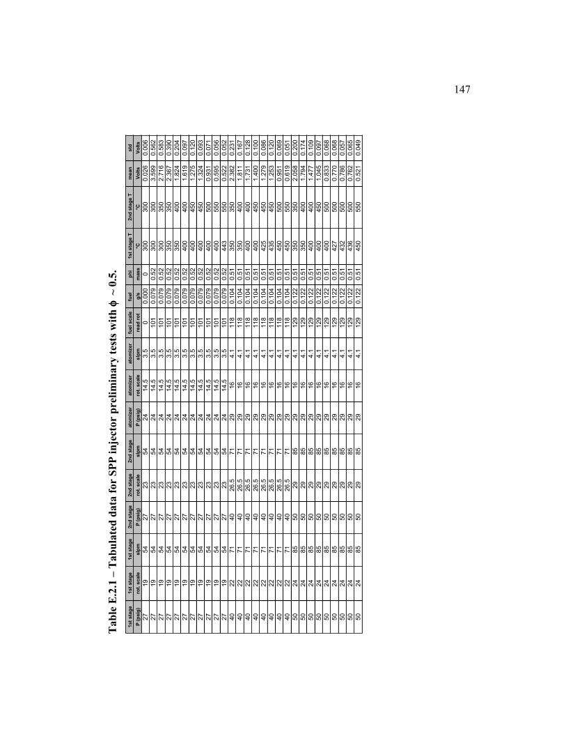
Tab

le E

.2.1

– T

ab

ula

ted

data

for

SP

P i

nje

cto

r p

reli

min

ary

tes

ts w

ith

φ φφφ=

==

= ~

0.5

.

1st

sta

ge

1st

sta

ge

1st

sta

ge

2n

d s

tag

e2n

d s

tag

e2n

d s

tag

eato

miz

er

ato

miz

er

ato

miz

er

fuel scale

fuel

ph

i1st

sta

ge T

2n

d s

tag

e T

mean

std

P (

psig

)ro

t. s

cale

slp

mP

(p

sig

)ro

t. s

cale

slp

mP

(p

sig

)ro

t. s

cale

slp

m

read

ro

tg

/sm

ass

°C°C

Vo

lts

Vo

lts

27

19

54

27

23

54

24

14.5

3.5

00.0

00

03

00

300

0.0

26

0.0

06

27

19

54

27

23

54

24

14.5

3.5

101

0.0

79

0.5

23

00

300

3.5

99

0.5

62

27

19

54

27

23

54

24

14.5

3.5

101

0.0

79

0.5

23

00

350

2.7

16

0.5

83

27

19

54

27

23

54

24

14.5

3.5

101

0.0

79

0.5

23

50

350

2.3

67

0.3

90

27

19

54

27

23

54

24

14.5

3.5

101

0.0

79

0.5

23

50

400

1.8

24

0.2

04

27

19

54

27

23

54

24

14.5

3.5

101

0.0

79

0.5

24

00

400

1.6

19

0.0

97

27

19

54

27

23

54

24

14.5

3.5

101

0.0

79

0.5

24

00

450

1.2

75

0.1

20

27

19

54

27

23

54

24

14.5

3.5

101

0.0

79

0.5

24

00

450

1.3

24

0.0

93

27

19

54

27

23

54

24

14.5

3.5

101

0.0

79

0.5

24

00

500

0.9

31

0.0

71

27

19

54

27

23

54

24

14.5

3.5

101

0.0

79

0.5

24

00

550

0.5

95

0.0

56

27

19

54

27

23

54

24

14.5

3.5

101

0.0

79

0.5

24

43

550

0.5

22

0.0

52

40

22

71

40

26

.571

29

16

4.1

118

0.1

04

0.5

13

50

350

2.3

82

0.2

31

40

22

71

40

26

.571

29

16

4.1

118

0.1

04

0.5

13

50

400

1.8

11

0.1

67

40

22

71

40

26

.571

29

16

4.1

118

0.1

04

0.5

14

00

400

1.7

31

0.1

28

40

22

71

40

26

.571

29

16

4.1

118

0.1

04

0.5

14

00

450

1.4

00

0.1

00

40

22

71

40

26

.571

29

16

4.1

118

0.1

04

0.5

14

25

450

1.2

79

0.0

86

40

22

71

40

26

.571

29

16

4.1

118

0.1

04

0.5

14

35

450

1.2

53

0.1

20

40

22

71

40

26

.571

29

16

4.1

118

0.1

04

0.5

14

50

500

0.9

51

0.0

69

40

22

71

40

26

.571

29

16

4.1

118

0.1

04

0.5

14

50

550

0.6

19

0.0

51

50

24

85

50

29

85

29

16

4.1

129

0.1

22

0.5

13

50

350

2.0

58

0.2

00

50

24

85

50

29

85

29

16

4.1

129

0.1

22

0.5

13

50

400

1.7

94

0.1

74

50

24

85

50

29

85

29

16

4.1

129

0.1

22

0.5

14

00

400

1.4

77

0.1

09

50

24

85

50

29

85

29

16

4.1

129

0.1

22

0.5

14

00

450

1.0

45

0.0

97

50

24

85

50

29

85

29

16

4.1

129

0.1

22

0.5

14

00

500

0.8

33

0.0

68

50

24

85

50

29

85

29

16

4.1

129

0.1

22

0.5

14

27

500

0.7

70

0.0

68

50

24

85

50

29

85

29

16

4.1

129

0.1

22

0.5

14

32

500

0.7

86

0.0

57

50

24

85

50

29

85

29

16

4.1

129

0.1

22

0.5

14

36

500

0.7

62

0.0

65

50

24

85

50

29

85

29

16

4.1

129

0.1

22

0.5

14

50

550

0.5

21

0.0

49

147

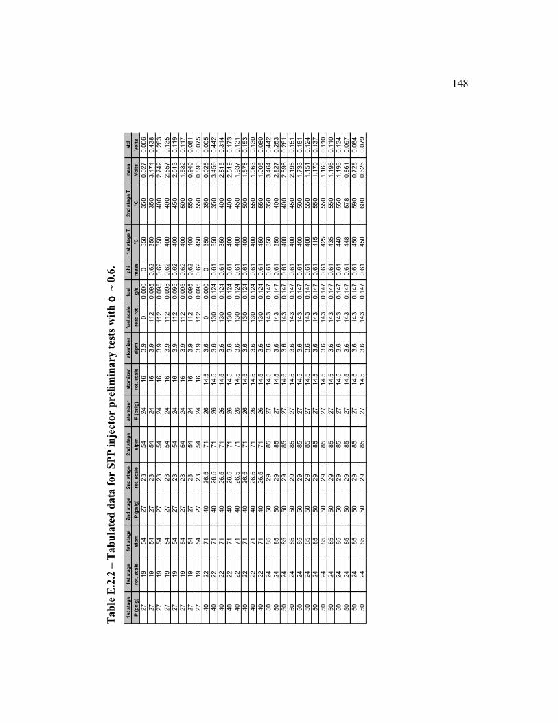
Tab

le E

.2.2

– T

ab

ula

ted

data

for

SP

P i

nje

cto

r p

reli

min

ary

tes

ts w

ith

φ φφφ=

==

= ~

0.6

.

1st

sta

ge

1st

sta

ge

1st

sta

ge

2n

d s

tag

e2n

d s

tag

e2n

d s

tag

eato

miz

er

ato

miz

er

ato

miz

er

fuel scale

fuel

ph

i1st

sta

ge T

2n

d s

tag

e T

mean

std

P (

psig

)ro

t. s

cale

slp

mP

(p

sig

)ro

t. s

cale

slp

mP

(p

sig

)ro

t. s

cale

slp

m

read

ro

tg

/sm

ass

°C°C

Vo

lts

Vo

lts

27

19

54

27

23

54

24

16

3.9

00.0

00

0350

350

0.0

27

0.0

06

27

19

54

27

23

54

24

16

3.9

11

20.0

95

0.6

2350

350

3.4

74

0.4

38

27

19

54

27

23

54

24

16

3.9

11

20.0

95

0.6

2350

400

2.7

42

0.2

63

27

19

54

27

23

54

24

16

3.9

11

20.0

95

0.6

2400

400

2.5

57

0.1

35

27

19

54

27

23

54

24

16

3.9

11

20.0

95

0.6

2400

450

2.0

13

0.1

19

27

19

54

27

23

54

24

16

3.9

11

20.0

95

0.6

2400

500

1.5

32

0.1

17

27

19

54

27

23

54

24

16

3.9

11

20.0

95

0.6

2400

550

0.9

40

0.0

81

27

19

54

27

23

54

24

16

3.9

11

20.0

95

0.6

2450

550

0.8

90

0.0

75

40

22

71

40

26

.571

26

14.5

3.6

00.0

00

0350

350

0.0

25

0.0

05

40

22

71

40

26

.571

26

14.5

3.6

13

00.1

24

0.6

1350

350

3.4

56

0.4

42

40

22

71

40

26

.571

26

14.5

3.6

13

00.1

24

0.6

1350

400

2.8

15

0.3

14

40

22

71

40

26

.571

26

14.5

3.6

13

00.1

24

0.6

1400

400

2.5

19

0.1

73

40

22

71

40

26

.571

26

14.5

3.6

13

00.1

24

0.6

1400

450

1.9

37

0.1

31

40

22

71

40

26

.571

26

14.5

3.6

13

00.1

24

0.6

1400

500

1.5

78

0.1

53

40

22

71

40

26

.571

26

14.5

3.6

13

00.1

24

0.6

1400

550

1.0

63

0.1

30

40

22

71

40

26

.571

26

14.5

3.6

13

00.1

24

0.6

1450

550

1.0

05

0.0

80

50

24

85

50

29

85

27

14.5

3.6

14

30.1

47

0.6

1350

350

3.4

64

0.4

42

50

24

85

50

29

85

27

14.5

3.6

14

30.1

47

0.6

1350

400

2.8

27

0.2

53

50

24

85

50

29

85

27

14.5

3.6

14

30.1

47

0.6

1400

400

2.8

98

0.2

61

50

24

85

50

29

85

27

14.5

3.6

14

30.1

47

0.6

1400

450

2.1

95

0.1

51

50

24

85

50

29

85

27

14.5

3.6

14

30.1

47

0.6

1400

500

1.7

33

0.1

81

50

24

85

50

29

85

27

14.5

3.6

14

30.1

47

0.6

1400

550

1.1

51

0.1

24

50

24

85

50

29

85

27

14.5

3.6

14

30.1

47

0.6

1415

550

1.1

70

0.1

37

50

24

85

50

29

85

27

14.5

3.6

14

30.1

47

0.6

1425

550

1.1

60

0.1

10

50

24

85

50

29

85

27

14.5

3.6

14

30.1

47

0.6

1435

550

1.1

95

0.1

10

50

24

85

50

29

85

27

14.5

3.6

14

30.1

47

0.6

1440

550

1.1

93

0.1

34

50

24

85

50

29

85

27

14.5

3.6

14

30.1

47

0.6

1448

578

0.8

61

0.0

97

50

24

85

50

29

85

27

14.5

3.6

14

30.1

47

0.6

1450

590

0.7

28

0.0

84

50

24

85

50

29

85

27

14.5

3.6

14

30.1

47

0.6

1450

600

0.6

26

0.0

79

148

Tab

le E

.2.3

– T

ab

ula

ted

data

for

SP

P i

nje

cto

r at

un

even

air

flo

w s

pli

ts w

ith

5 s

lpm

ato

miz

er

air

flo

w.

1st

sta

ge

1st

sta

ge

1st

sta

ge

2n

d s

tag

e2n

d s

tag

e2n

d s

tag

eato

miz

er

ato

miz

er

ato

miz

er

fuel sc

ale

fue

l p

hi

1s

t sta

ge

T2n

d s

tag

e T

mean

std

P (

psig

)ro

t. s

cale

slp

mP

(psig

)ro

t. s

cale

slp

mP

(psig

)ro

t. s

cale

slp

m

read

ro

tg

/sm

ass

°C°C

Vo

lts

Vo

lts

23

12

32

50

29

85

38

17.5

5105

0.0

85

0.5

0324

350

2.2

28

0.1

42

23

12

32

50

29

85

38

17.5

5105

0.0

85

0.5

0335

400

1.7

99

0.0

91

23

12

32

50

29

85

38

17.5

5105

0.0

85

0.5

0347

450

1.2

99

0.0

66

23

12

32

50

29

85

38

17.5

5105

0.0

85

0.5

0364

500

0.8

58

0.0

54

23

12

32

50

29

85

38

17.5

5105

0.0

85

0.5

0380

550

0.5

35

0.0

43

23

12

32

50

29

85

38

17.5

5105

0.0

85

0.5

0387

600

0.2

06

0.0

23

25

16

44

50

29

85

38

17.5

5111

0.0

93

0.5

1350

350

2.1

17

0.0

97

25

16

44

50

29

85

38

17.5

5111

0.0

93

0.5

1350

400

1.5

89

0.0

79

25

16

44

50

29

85

38

17.5

5111

0.0

93

0.5

1350

400

1.6

77

0.0

86

25

16

44

50

29

85

38

17.5

5111

0.0

93

0.5

1350

450

1.2

76

0.0

71

25

16

44

50

29

85

38

17.5

5111

0.0

93

0.5

1350

500

0.9

57

0.0

55

25

16

44

50

29

85

38

17.5

5111

0.0

93

0.5

1400

500

0.7

81

0.0

46

25

16

44

50

29

85

38

17.5

5111

0.0

93

0.5

1400

550

0.4

86

0.0

37

25

16

44

50

29

85

38

17.5

5111

0.0

93

0.5

1425

550

0.4

90

0.0

33

25

16

44

50

29

85

38

17.5

5111

0.0

93

0.5

1438

600

0.1

99

0.0

20

30

18

53

50

29

85

39

18

5115

0.0

99

0.5

1350

350

1.9

68

0.0

98

30

18

53

50

29

85

39

18

5115

0.0

99

0.5

1350

400

1.5

59

0.0

81

30

18

53

50

29

85

39

18

5115

0.0

99

0.5

1350

450

1.2

64

0.0

73

30

18

53

50

29

85

39

18

5115

0.0

99

0.5

1350

500

0.9

47

0.0

61

30

18

53

50

29

85

39

18

5115

0.0

99

0.5

1400

500

0.8

77

0.0

48

30

18

53

50

29

85

39

18

5115

0.0

99

0.5

1400

550

0.4

91

0.0

33

30

18

53

50

29

85

39

18

5115

0.0

99

0.5

1450

550

0.4

76

0.0

34

30

18

53

50

29

85

39

18

5115

0.0

99

0.5

1450

600

0.1

90

0.0

20

50

24

85

50

29

85

42

17

5129

0.1

22

0.5

1350

350

1.6

69

0.1

20

50

24

85

50

29

85

42

17

5129

0.1

22

0.5

1350

400

1.3

12

0.1

05

50

24

85

50

29

85

42

17

5129

0.1

22

0.5

1350

450

1.0

82

0.0

88

50

24

85

50

29

85

42

17

5129

0.1

22

0.5

1350

500

0.7

74

0.0

74

50

24

85

50

29

85

42

17

5129

0.1

22

0.5

1400

500

0.7

68

0.0

67

50

24

85

50

29

85

42

17

5129

0.1

22

0.5

1400

550

0.4

59

0.0

43

50

24

85

50

29

85

42

17

5129

0.1

22

0.5

1428

550

0.4

55

0.0

40

50

24

85

50

29

85

42

17

5129

0.1

22

0.5

1446

600

0.2

21

0.0

25

149

Tab

le E

.2.4

– T

ab

ula

ted

data

for

SP

P i

nje

cto

r at

un

even

air

flo

w s

pli

ts w

ith

4 s

lpm

ato

miz

er

air

flo

w.

1st

sta

ge

1st

sta

ge

1st

sta

ge

2n

d s

tag

e2n

d s

tag

e2n

d s

tag

eato

miz

er

ato

miz

er

ato

miz

er

fuel scale

fuel

ph

i1st

sta

ge T

2n

d s

tag

e T

mean

std

P (

psig

)ro

t. s

cale

slp

mP

(p

sig

)ro

t. s

cale

slp

mP

(p

sig

)ro

t. s

cale

slp

m s

sre

ad

ro

tg

/sm

ass

°C°C

Vo

lts

Vo

lts

23

12

32

50

29

85

29

15.6

40

0.0

00

0.0

0350

350

0.0

20

0.0

05

23

12

32

50

29

85

29

15.6

4105

0.0

85

0.5

1348

350

1.8

61

0.0

83

23

12

32

50

29

85

29

15.6

4105

0.0

85

0.5

1350

400

1.5

41

0.0

70

23

12

32

50

29

85

29

15.6

4105

0.0

85

0.5

1350

450

1.1

08

0.0

54

23

12

32

50

29

85

29

15.6

4105

0.0

85

0.5

1350

500

0.8

28

0.0

48

23

12

32

50

29

85

29

15.6

4105

0.0

85

0.5

1365

500

0.8

56

0.0

47

23

12

32

50

29

85

29

15.6

4105

0.0

85

0.5

1385

550

0.4

64

0.0

33

23

12

32

50

29

85

29

15.6

4105

0.0

85

0.5

1400

600

0.1

68

0.0

18

25

16

44

50

29

85

29

15.5

4110

0.0

92

0.5

0350

350

1.7

43

0.1

04

25

16

44

50

29

85

29

15.5

4110

0.0

92

0.5

0350

400

1.4

17

0.0

70

25

16

44

50

29

85

29

15.5

4110

0.0

92

0.5

0350

450

1.1

03

0.0

77

25

16

44

50

29

85

29

15.5

4110

0.0

92

0.5

0350

500

0.7

52

0.0

66

25

16

44

50

29

85

29

15.5

4110

0.0

92

0.5

0400

500

0.6

98

0.0

45

25

16

44

50

29

85

29

15.5

4110

0.0

92

0.5

0400

550

0.4

10

0.0

30

25

16

44

50

29

85

29

15.5

4110

0.0

92

0.5

0435

550

0.4

22

0.0

30

25

16

44

50

29

85

29

15.5

4110

0.0

92

0.5

0450

600

0.1

81

0.0

17

30

18

53

50

29

85

30

15.5

4114

0.0

98

0.5

0350

350

1.8

07

0.1

43

30

18

53

50

29

85

30

15.5

4114

0.0

98

0.5

0350

400

1.3

55

0.1

02

30

18

53

50

29

85

30

15.5

4114

0.0

98

0.5

0350

450

1.0

68

0.0

72

30

18

53

50

29

85

30

15.5

4114

0.0

98

0.5

0350

500

0.7

96

0.0

88

30

18

53

50

29

85

30

15.5

4114

0.0

98

0.5

0400

500

0.7

58

0.0

51

30

18

53

50

29

85

30

15.5

4114

0.0

98

0.5

0400

550

0.4

35

0.0

32

30

18

53

50

29

85

30

15.5

4114

0.0

98

0.5

0450

550

0.4

48

0.0

33

30

18

53

50

29

85

30

15.5

4114

0.0

98

0.5

0450

600

0.1

75

0.0

18

150

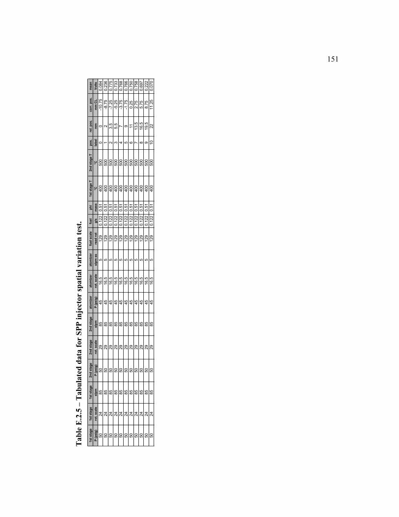
Tab

le E

.2.5

– T

ab

ula

ted

data

for

SP

P i

nje

cto

r sp

ati

al

vari

ati

on

tes

t.

1st

sta

ge

1s

t s

tag

e1st

sta

ge

2n

d s

tag

e2

nd

sta

ge

2n

d s

tag

eato

miz

er

ato

miz

er

ato

miz

er

fue

l sc

ale

fue

l p

hi

1st

sta

ge

T2n

d s

tag

e T

po

s.

rel. p

os.

co

rr. p

os.

mean

P (

psig

)ro

t. s

ca

les

lpm

P (

psig

)ro

t. s

ca

leslp

mP

(p

sig

)ro

t. s

ca

les

lpm

ss

rea

d r

ot

g/s

mas

s°C

°Cla

bel

mm

mm

CL

Vo

lts

50

24

85

50

29

85

45

16.5

5129

0.1

22

0.5

1400

500

00

-10.7

50.0

84

50

24

85

50

29

85

45

16.5

5129

0.1

22

0.5

1400

500

12

-8.7

50.2

36

50

24

85

50

29

85

45

16.5

5129

0.1

22

0.5

1400

500

23.5

-7.2

50.7

75

50

24

85

50

29

85

45

16.5

5129

0.1

22

0.5

1400

500

35.5

-5.2

50.7

33

50

24

85

50

29

85

45

16.5

5129

0.1

22

0.5

1400

500

47

-3.7

50.7

68

50

24

85

50

29

85

45

16.5

5129

0.1

22

0.5

1400

500

59

-1.7

50.7

66

50

24

85

50

29

85

45

16.5

5129

0.1

22

0.5

1400

500

611

0.2

50.7

50

50

24

85

50

29

85

45

16.5

5129

0.1

22

0.5

1400

500

713.5

2.7

50.7

58

50

24

85

50

29

85

45

16.5

5129

0.1

22

0.5

1400

500

816.5

5.7

50.6

97

50

24

85

50

29

85

45

16.5

5129

0.1

22

0.5

1400

500

919.5

8.7

50.2

22

50

24

85

50

29

85

45

16.5

5129

0.1

22

0.5

1400

500

10

22

11.2

50.0

70

151

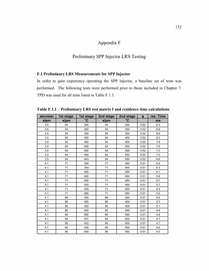
152

Appendix F

Preliminary SPP Injector LRS Testing

F.1 Preliminary LRS Measurements for SPP Injector

In order to gain experience operating the SPP injector, a baseline set of tests was

performed. The following tests were performed prior to those included in Chapter 7.

TPD was used for all tests listed in Table F.1.1.

Table F.1.1 – Preliminary LRS test matrix I and residence time calculations.

atomizer 1st stage 1st stage 2nd stage 2nd stage φφφφ res. Time

slpm slpm °C slpm °C ms

3.5 54 300 54 300 0.52 9.3

3.5 54 300 54 350 0.52 8.9

3.5 54 350 54 350 0.52 8.6

3.5 54 350 54 400 0.52 8.2

3.5 54 400 54 400 0.52 7.9

3.5 54 400 54 450 0.52 7.6

3.5 54 400 54 500 0.52 7.3

3.5 54 400 54 550 0.52 7.0

3.5 54 443 54 550 0.52 6.8

4.1 71 350 71 350 0.51 6.5

4.1 71 350 71 400 0.51 6.3

4.1 71 400 71 400 0.51 6.1

4.1 71 400 71 450 0.51 5.8

4.1 71 425 71 450 0.51 5.7

4.1 71 435 71 450 0.51 5.7

4.1 71 450 71 500 0.51 5.4

4.1 71 450 71 550 0.51 5.2

4.1 85 350 85 350 0.51 5.6

4.1 85 350 85 400 0.51 5.3

4.1 85 400 85 400 0.51 5.1

4.1 85 400 85 450 0.51 4.9

4.1 85 400 85 500 0.51 4.8

4.1 85 427 85 500 0.51 4.7

4.1 85 432 85 500 0.51 4.7

4.1 85 436 85 500 0.51 4.6

4.1 85 450 85 550 0.51 4.5

153

The first and second stage air flow rates were set equal for these tests. The equivalence

ratio was held to nominally 0.5 while the temperatures were adjusted at fixed air and

fuel flow conditions, with the resulting residence times of 4.5 to 9.3 milliseconds below

that of previous work. Each of the conditions listed in Table F.1.1 has corresponding

time trace data, several of which are plotted in Figures F.1.1 through F.1.3. Note that

the increasing 2nd

stage temperature causes a decrease in number density and scattering

signal, thus producing a signal with a mean value closer to zero. The sign of the

scattering signal is negative due to the PMT wiring, so stronger scattering produces a

more negative signal. The pure air scattering signal at 300/300 °C temperature split has

a mean value of 26 mV, while the weaker fuel-air mixtures have a mean signal of 500

to 600 mV. Figure F.1.1 demonstrates that the pure air scattering signal is negligible,

even when taken at a high number density condition.

Droplets, noticeable by spikes in the time traces, are present at many of the conditions

tested. Generally, any condition where the first stage temperature is less than 400 °C

has droplets in the exit stream. At the 85/85 slpm air flow split, frequent droplets are

observed up to temperatures split of 436/500 °C. This is due to the decreased air to fuel

mass ratio in the atomizer, and the decrease in residence time for these droplets to

vaporize. At temperature splits above 350/400 °C, droplets are seen, but much less

frequently than the low temperature cases.

Based upon this set of data, the SPP atomizes and vaporizes the liquid fuel completely

only at higher temperature splits. The 54/54 slpm airflow split requires a temperature

split of at least 400/500 °C for complete vaporization of the droplets. The 71/71 slpm

airflow split requires a temperature split of 450/500 °C for complete vaporization.

Finally, the 85/85 slpm airflow split, which has the lowest residence times of these

three airflow splits, vaporizes the fuel completely only at the 450/550 °C temperature

split.

-3.5

0

-3.0

0

-2.5

0

-2.0

0

-1.5

0

-1.0

0

-0.5

0

0.0

00.0

00

.05

0.1

00

.15

0.2

0

Tim

e (

s)


30

0/3

00

air

44

3/5

50

40

0/5

00

40

0/4

50

35

0/4

00

35

0/3

50

Fig

ure

F.1

.1 –

Tim

e tr

aces

of

3.5

/54/5

4 a

ir f

low

sp

lit

at

vari

ou

s te

mp

era

ture

sp

lits

for

an

eq

uiv

ale

nce

rati

o o

f 0.5

2.

154

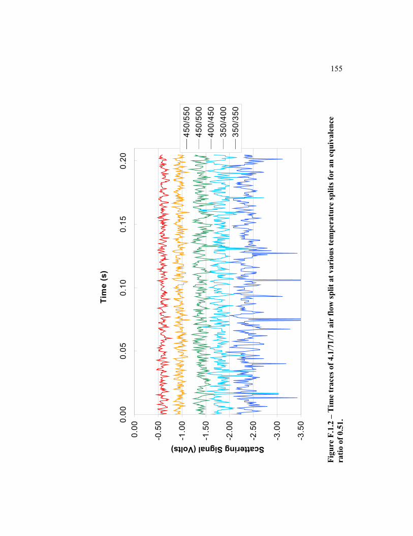
-3.5

0

-3.0

0

-2.5

0

-2.0

0

-1.5

0

-1.0

0

-0.5

0

0.0

00.0

00

.05

0.1

00

.15

0.2

0

Tim

e (

s)


45

0/5

50

45

0/5

00

40

0/4

50

35

0/4

00

35

0/3

50

Fig

ure

F.1

.2 –

Tim

e tr

aces

of

4.1

/71/7

1 a

ir f

low

sp

lit

at

vari

ou

s te

mp

era

ture

sp

lits

for

an

eq

uiv

ale

nce

rati

o o

f 0.5

1.

155

-3.0

0

-2.5

0

-2.0

0

-1.5

0

-1.0

0

-0.5

0

0.0

00.0

00

.05

0.1

00

.15

0.2

0

Tim

e (

s)


45

0/5

50

43

6/5

00

40

0/4

50

40

0/4

00

35

0/3

50

Fig

ure

F.1

.3 –

Tim

e tr

aces

of

4.1

/85/8

5 a

ir f

low

sp

lit

at

vari

ou

s te

mp

era

ture

sp

lits

for

an

eq

uiv

ale

nce

rati

o o

f 0.5

1.

156

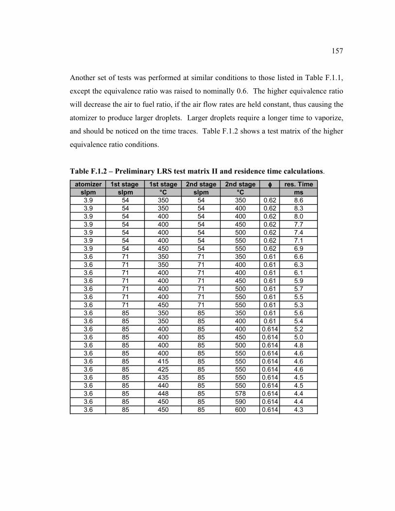
157

Another set of tests was performed at similar conditions to those listed in Table F.1.1,

except the equivalence ratio was raised to nominally 0.6. The higher equivalence ratio

will decrease the air to fuel ratio, if the air flow rates are held constant, thus causing the

atomizer to produce larger droplets. Larger droplets require a longer time to vaporize,

and should be noticed on the time traces. Table F.1.2 shows a test matrix of the higher

equivalence ratio conditions.

Table F.1.2 – Preliminary LRS test matrix II and residence time calculations.

atomizer 1st stage 1st stage 2nd stage 2nd stage φφφφ res. Time

slpm slpm °C slpm °C ms

3.9 54 350 54 350 0.62 8.6

3.9 54 350 54 400 0.62 8.3

3.9 54 400 54 400 0.62 8.0

3.9 54 400 54 450 0.62 7.7

3.9 54 400 54 500 0.62 7.4

3.9 54 400 54 550 0.62 7.1

3.9 54 450 54 550 0.62 6.9

3.6 71 350 71 350 0.61 6.6

3.6 71 350 71 400 0.61 6.3

3.6 71 400 71 400 0.61 6.1

3.6 71 400 71 450 0.61 5.9

3.6 71 400 71 500 0.61 5.7

3.6 71 400 71 550 0.61 5.5

3.6 71 450 71 550 0.61 5.3

3.6 85 350 85 350 0.61 5.6

3.6 85 350 85 400 0.61 5.4

3.6 85 400 85 400 0.614 5.2

3.6 85 400 85 450 0.614 5.0

3.6 85 400 85 500 0.614 4.8

3.6 85 400 85 550 0.614 4.6

3.6 85 415 85 550 0.614 4.6

3.6 85 425 85 550 0.614 4.6

3.6 85 435 85 550 0.614 4.5

3.6 85 440 85 550 0.614 4.5

3.6 85 448 85 578 0.614 4.4

3.6 85 450 85 590 0.614 4.4

3.6 85 450 85 600 0.614 4.3

158

The higher equivalence ratio conditions, when operated at the same air flow rates and

temperatures, produce stronger scattering signals consistent with the Rayliegh

scattering theory. Figures F.1.4 through F.1.6 show time traces for the three air flow

rate splits for various temperatures.

Droplets are present at almost all of the conditions tested at the 0.61 equivalence ratios.

The residence is the same as the 0.51 condition, ranging from 4.3 to 8.6 milliseconds,

but the largest droplets produced by the atomizer are still not completely vaporized.

Temperature does reduce the frequency of droplets as expected, and a noted

improvement in vaporizing is seen by increasing the 1st stage temperature from 350 to

400 °C. This effect, however, diminishes as the air flow rates are increased.

Figure 7.2.7 displays the mean scattering signal for the 0.51 and 0.61 equivalence ratio

tests as a function of the 2nd

stage temperature. The mixture leaving the SPP is

approximately equal to the 2nd

stage temperature, so the measurement represents the

mixture temperature at the measurement volume. This plot is used to compare the test

conditions, since fixed fuel concentrations at a given temperature should provide

similar mean scattering signals regardless of air flow rate (in the absence of droplets).

A majority of the preliminary test conditions, at equivalence ratios of 0.51 and 0.61,

feature unvaporized droplets exiting the SPP injector. This is undesirable for lean

premixed combustion applications, since liquid droplets can provide small scale regions

of stoichiometric conditions, which produce high temperatures and thermal NOx. Initial

drop size can be reduced, along with vaporization time, by increasing the atomizer air

flow.

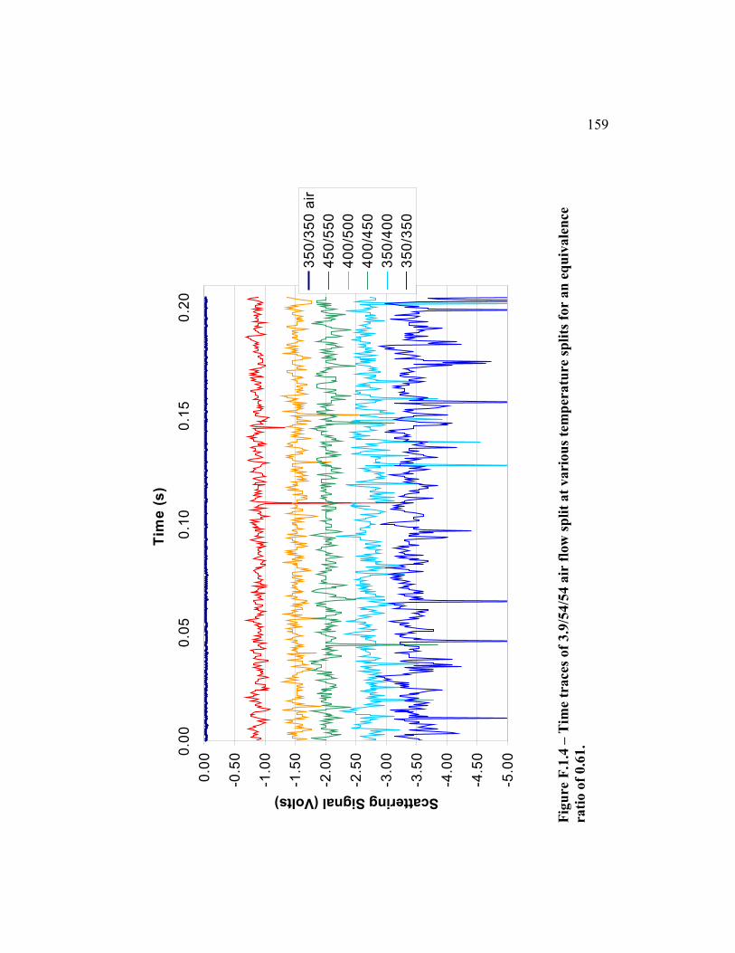
-5.0

0

-4.5

0

-4.0

0

-3.5

0

-3.0

0

-2.5

0

-2.0

0

-1.5

0

-1.0

0

-0.5

0

0.0

00.0

00

.05

0.1

00

.15

0.2

0

Tim

e (

s)


35

0/3

50

air

45

0/5

50

40

0/5

00

40

0/4

50

35

0/4

00

35

0/3

50

Fig

ure

F.1

.4 –

Tim

e tr

aces

of

3.9

/54/5

4 a

ir f

low

sp

lit

at

vari

ou

s te

mp

era

ture

sp

lits

for

an

eq

uiv

ale

nce

rati

o o

f 0.6

1.

159

-5.0

0

-4.5

0

-4.0

0

-3.5

0

-3.0

0

-2.5

0

-2.0

0

-1.5

0

-1.0

0

-0.5

0

0.0

00.0

00

.05

0.1

00

.15

0.2

0

Tim

e (

s)

Scattering Signal (volts)

35

0/3

50

air

45

0/5

50

40

0/5

00

40

0/4

50

35

0/4

00

35

0/3

50

Fig

ure

F.1

.5 –

Tim

e tr

aces

of

3.6

/71/7

1 a

ir f

low

sp

lit

at

vari

ou

s te

mp

era

ture

sp

lits

for

an

eq

uiv

ale

nce

rati

o o

f 0.6

1.

160

-5.0

0

-4.5

0

-4.0

0

-3.5

0

-3.0

0

-2.5

0

-2.0

0

-1.5

0

-1.0

0

-0.5

0

0.0

00.0

00

.05

0.1

00

.15

0.2

0

Tim

e (

s)


44

8/5

78

40

0/5

50

40

0/5

00

40

0/4

50

35

0/3

50

Fig

ure

F.1

.6 –

Tim

e tr

aces

of

3.6

/85/8

5 a

ir f

low

sp

lit

at

vari

ou

s te

mp

era

ture

sp

lits

for

an

eq

uiv

ale

nce

rati

o o

f 0.6

1.

161

0.0

0

0.5

0

1.0

0

1.5

0

2.0

0

2.5

0

3.0

0

3.5

0

4.0

0

25

03

50

45

05

50

65

0

2n

d S

tag

e T

(°C

)

Mean Scattering Signal (Volts)3

.6/5

4/5

4 p

hi=

.51

4.1

/71

/71

ph

i =

.5

1

4.1

/85

/85

ph

i =

.5

1

3.9

/54

/54

ph

i=.6

1

3.6

/71

/71

ph

i =

.6

1

3.6

/85

/85

ph

i =

.6

1

no

fu

el

ad

de

d,

on

ly

he

ate

d a

ir

Fig

ure

F.1

.7 –

Mea

n s

catt

erin

g s

ign

al

plo

tted

again

st a

pp

roxim

ate

mix

ture

tem

per

atu

re.

162

Experimental Investigation of Liquid Fuel Vaporization and ...

Documents

Transcript of Experimental Investigation of Liquid Fuel Vaporization and ...