Experimental identification of a nonlinear model for composites using the grid technique coupled to...

Experimental identification of a nonlinear model for composites

using the grid technique coupled to the virtual fields method

H. Chalal, S. Avril*, F. Pierron, F. Meraghni

LMPF, ENSAM, rue Saint Dominique, BP508, 51006 Ch?Ions en Champagne, France

Received 23 November 2004; revised 8 April 2005; accepted 16 April 2005

Abstract

The present paper shows some experimental results of the identification of the full set of parameters driving a nonlinear model for the in-

plane behaviour of a unidirectional composite laminate. The strain field at the surface of a rectangular coupon submitted to a shear/bending

loading is measured using the grid technique. The strain fields are then processed by the virtual fields method to retrieve the six constitutive

parameters: the linear elastic orthotropic in-plane stiffnesses Qxx, Qyy, Qxy, Qss and softening parameters K and 30s driving the shear

nonlinearity. It is shown that the shear response is correctly identified, with coefficients of variation similar to the ones of standard tests. The

other parameters are identified with larger errors and higher coefficients of variation because their identification is affected by the lower

normal strain levels in the specimen. It is therefore necessary to design new tests providing balanced strain levels for improving the

identification procedure.

q 2005 Elsevier Ltd. All rights reserved.

Keywords: B. Optical techniques; C. Damage mechanics; D. Mechanical testing; Virtual fields method

1. Introduction

The analysis of the overall response of composite

structures requires the knowledge of the parameters

governing the mechanical constitutive material behaviour.

Generally, nonlinear models for composite materials are

formulated through tensorial approaches involving coupling

terms [1]. To reach simultaneously all of the behaviour law

parameters, experimental tests must give rise to hetero-

geneous strain/stress fields. Indeed, these parameters are

expected to be all involved when the global response is

heterogeneous. Therefore, intrinsic material constants can

be extracted through an identification strategy using

kinematic fields obtained from one single coupon. Among

the identification procedures, those based on the updating of

finite element models [2,3] are the most widespread. In fact,

in the case of heterogeneous tests, no closed-form relations

between loads and displacements are available. In the

general case, the material parameters are estimated through

1359-835X/$ - see front matter q 2005 Elsevier Ltd. All rights reserved.

doi:10.1016/j.compositesa.2005.04.020

* Corresponding author.

E-mail address: [email protected] (S. Avril).

an optimisation procedure performed iteratively until

the experimental data match the simulated ones. This

technique is general and very flexible, full-field measure-

ments are not necessarily required. However, it suffers from

a number of shortcomings such as the sensitivity to the

modeling of the boundary conditions and to initial

parameter values, for instance (Grediac et al., [4]).

An alternative strategy specifically developed to process

full-field data is the so-called virtual fields method (VFM).

It was first imagined by Grediac [5] and has been

successfully applied to the cases of in-plane [6] and

through-thickness [7,8] mechanical rigidities of anisotropic

composite materials. The identification technique relies on

the processing of the strain fields when expressing the global

equilibrium of a structure through the wellknown principle

of virtual work expressed with specific virtual kinematic

fields. In this case, one obtains a set of linear equations

which can be inverted to extract the material unknown

parameters. Currently, several improvements to the VFM

are now available, notably those concerning the automatic

generation of optimal virtual fields [4,9,10].

A validation of the numerical procedure has been

published recently using simulated strain fields [11], in

order to focus on the performance of the identification

Composites: Part A 37 (2006) 315–325

www.elsevier.com/locate/compositesa

http://www.elsevier.com/locate/compositesa

H. Chalal et al. / Composites: Part A 37 (2006) 315–325316

strategy. The numerical stability of the identification

strategy was illustrated by estimating linear and nonlinear

in-plane material constants from these simulated strain

fields containing random noise. The present paper is a

follow up that examines the experimental application of this

methodology.

2. Non-linear material model

2.1. Experimental justification of the nonlinear shear

behaviour of a unidirectional composite

The in-plane shear behaviour of unidirectional polymer

matrix fibre composites is widely recognized to be highly

nonlinear [12–14], and full characterisation requires the

entire stress–strain curve. The purpose of this analysis is to

provide reference values of the parameters governing the in-

plane shear response of a unidirectional composite.

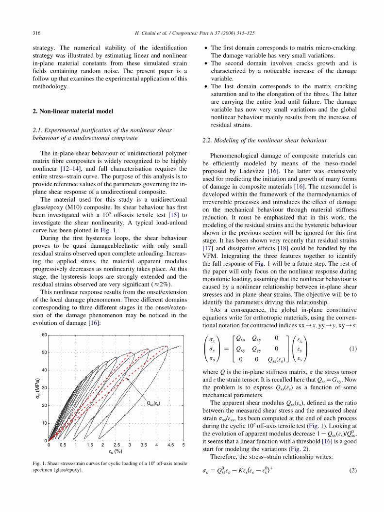
The material used for this study is a unidirectional

glass/epoxy (M10) composite. Its shear behaviour has first

been investigated with a 108 off-axis tensile test [15] to

investigate the shear nonlinearity. A typical load-unload

curve has been plotted in Fig. 1.

During the first hysteresis loops, the shear behaviour

proves to be quasi damageableelastic with only small

residual strains observed upon complete unloading. Increas-

ing the applied stress, the material apparent modulus

progressively decreases as nonlinearity takes place. At this

stage, the hysteresis loops are strongly extended and the

residual strains observed are very significant (z2%).

This nonlinear response results from the onset/extension

of the local damage phenomenon. Three different domains

corresponding to three different stages in the onset/exten-

sion of the damage phenomenon may be noticed in the

evolution of damage [16]:

Fig. 1. Shear stress/strain curves for cyclic loading of a 108 off-axis tensile

specimen (glass/epoxy).

† The first domain corresponds to matrix micro-cracking.

The damage variable has very small variations.

† The second domain involves cracks growth and is

characterized by a noticeable increase of the damage

variable.

† The last domain corresponds to the matrix cracking

saturation and to the elongation of the fibres. The latter

are carrying the entire load until failure. The damage

variable has now very small variations and the global

nonlinear behaviour mainly results from the increase of

residual strains.

2.2. Modeling of the nonlinear shear behaviour

Phenomenological damage of composite materials can

be efficiently modeled by means of the meso-model

proposed by Ladeveze [16]. The latter was extensively

used for predicting the initiation and growth of many forms

of damage in composite materials [16]. The mesomodel is

developed within the framework of the thermodynamics of

irreversible processes and introduces the effect of damage

on the mechanical behaviour through material stiffness

reduction. It must be emphasized that in this work, the

modeling of the residual strains and the hysteretic behaviour

shown in the previous section will be ignored for this first

stage. It has been shown very recently that residual strains

[17] and dissipative effects [18] could be handled by the

VFM. Integrating the three features together to identify

the full response of Fig. 1 will be a future step. The rest of

the paper will only focus on the nonlinear response during

monotonic loading, assuming that the nonlinear behaviour is

caused by a nonlinear relationship between in-plane shear

stresses and in-plane shear strains. The objective will be to

identify the parameters driving this relationship.

bAs a consequence, the global in-plane constitutive

equations write for orthotropic materials, using the conven-

tional notation for contracted indices xx/x, yy/y, xy/s:

sx

sy

ss

0B@

1CA Z

Qxx Qxy 0

Qxy Qyy 0

0 0 Qssð3sÞ

264

375

3x

3y

3s

0B@

1CA (1)

where Q is the in-plane stiffness matrix, s the stress tensor

and 3 the strain tensor. It is recalled here that QssZGxy. Now

the problem is to express Qss(3s) as a function of some

mechanical parameters.

The apparent shear modulus Qss(3s), defined as the ratio

between the measured shear stress and the measured shear

strain sss/3ss, has been computed at the end of each process

during the cyclic 108 off-axis tensile test (Fig. 1). Looking at

the evolution of apparent modulus decrease 1KQssð3sÞ=Q0ss,

it seems that a linear function with a threshold [16] is a good

start for modeling the variations (Fig. 2).

Therefore, the stress–strain relationship writes:

ss Z Q0ss3s KK3sh3s K30

s iC (2)

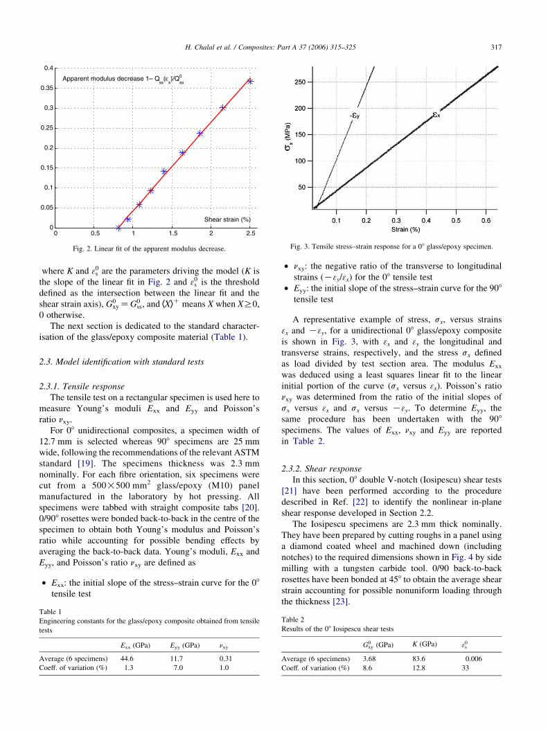
Fig. 2. Linear fit of the apparent modulus decrease. Fig. 3. Tensile stress–strain response for a 08 glass/epoxy specimen.

H. Chalal et al. / Composites: Part A 37 (2006) 315–325 317

where K and 30s are the parameters driving the model (K is

the slope of the linear fit in Fig. 2 and 30s is the threshold

defined as the intersection between the linear fit and the

shear strain axis), G0xy ZG0

ss, and hXiC means X when XR0,

0 otherwise.

The next section is dedicated to the standard character-

isation of the glass/epoxy composite material (Table 1).

2.3. Model identification with standard tests

2.3.1. Tensile response

The tensile test on a rectangular specimen is used here to

measure Young’s moduli Exx and Eyy and Poisson’s

ratio nxy.

For 08 unidirectional composites, a specimen width of

12.7 mm is selected whereas 908 specimens are 25 mm

wide, following the recommendations of the relevant ASTM

standard [19]. The specimens thickness was 2.3 mm

nominally. For each fibre orientation, six specimens were

cut from a 500!500 mm2 glass/epoxy (M10) panel

manufactured in the laboratory by hot pressing. All

specimens were tabbed with straight composite tabs [20].

0/908 rosettes were bonded back-to-back in the centre of the

specimen to obtain both Young’s modulus and Poisson’s

ratio while accounting for possible bending effects by

averaging the back-to-back data. Young’s moduli, Exx and

Eyy, and Poisson’s ratio nxy are defined as

† Exx: the initial slope of the stress–strain curve for the 08

tensile test

Table 1

Engineering constants for the glass/epoxy composite obtained from tensile

tests

Exx (GPa) Eyy (GPa) nxy

Average (6 specimens) 44.6 11.7 0.31

Coeff. of variation (%) 1.3 7.0 1.0

† nxy: the negative ratio of the transverse to longitudinal

strains (K3y/3x) for the 08 tensile test

† Eyy: the initial slope of the stress–strain curve for the 908

tensile test

A representative example of stress, sx, versus strains

3x and K3y, for a unidirectional 08 glass/epoxy composite

is shown in Fig. 3, with 3x and 3y the longitudinal and

transverse strains, respectively, and the stress sx defined

as load divided by test section area. The modulus Exx

was deduced using a least squares linear fit to the linear

initial portion of the curve (sx versus 3x). Poisson’s ratio

nxy was determined from the ratio of the initial slopes of

sx versus 3x and sx versus K3y. To determine Eyy, the

same procedure has been undertaken with the 908

specimens. The values of Exx, nxy and Eyy are reported

in Table 2.

2.3.2. Shear response

In this section, 08 double V-notch (Iosipescu) shear tests

[21] have been performed according to the procedure

described in Ref. [22] to identify the nonlinear in-plane

shear response developed in Section 2.2.

The Iosipescu specimens are 2.3 mm thick nominally.

They have been prepared by cutting roughs in a panel using

a diamond coated wheel and machined down (including

notches) to the required dimensions shown in Fig. 4 by side

milling with a tungsten carbide tool. 0/90 back-to-back

rosettes have been bonded at 458 to obtain the average shear

strain accounting for possible nonuniform loading through

the thickness [23].

Table 2

Results of the 08 Iosipescu shear tests

G0xy (GPa) K (GPa) 30

s

Average (6 specimens) 3.68 83.6 0.006

Coeff. of variation (%) 8.6 12.8 33

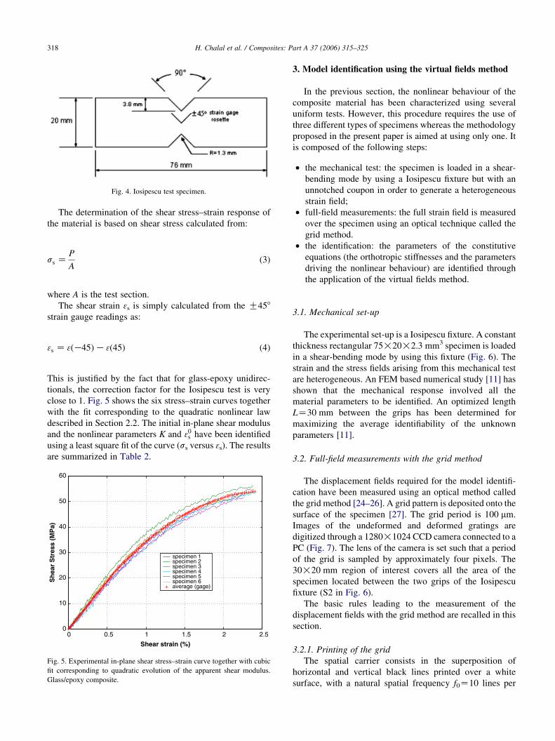
Fig. 4. Iosipescu test specimen.


The determination of the shear stress–strain response of

the material is based on shear stress calculated from:

ss ZP

A(3)

where A is the test section.

The shear strain 3s is simply calculated from the G458

strain gauge readings as:

3s Z 3ðK45ÞK3ð45Þ (4)

This is justified by the fact that for glass-epoxy unidirec-

tionals, the correction factor for the Iosipescu test is very

close to 1. Fig. 5 shows the six stress–strain curves together

with the fit corresponding to the quadratic nonlinear law

described in Section 2.2. The initial in-plane shear modulus

and the nonlinear parameters K and 30s have been identified

using a least square fit of the curve (ss versus 3s). The results

are summarized in Table 2.

Fig. 5. Experimental in-plane shear stress–strain curve together with cubic

fit corresponding to quadratic evolution of the apparent shear modulus.

Glass/epoxy composite.

3. Model identification using the virtual fields method

In the previous section, the nonlinear behaviour of the

composite material has been characterized using several

uniform tests. However, this procedure requires the use of

three different types of specimens whereas the methodology

proposed in the present paper is aimed at using only one. It

is composed of the following steps:

† the mechanical test: the specimen is loaded in a shear-

bending mode by using a Iosipescu fixture but with an

unnotched coupon in order to generate a heterogeneous

strain field;

† full-field measurements: the full strain field is measured

over the specimen using an optical technique called the

grid method.

† the identification: the parameters of the constitutive

equations (the orthotropic stiffnesses and the parameters

driving the nonlinear behaviour) are identified through

the application of the virtual fields method.

3.1. Mechanical set-up

The experimental set-up is a Iosipescu fixture. A constant

thickness rectangular 75!20!2.3 mm3 specimen is loaded

in a shear-bending mode by using this fixture (Fig. 6). The

strain and the stress fields arising from this mechanical test

are heterogeneous. An FEM based numerical study [11] has

shown that the mechanical response involved all the

material parameters to be identified. An optimized length

LZ30 mm between the grips has been determined for

maximizing the average identifiability of the unknown

parameters [11].

3.2. Full-field measurements with the grid method

The displacement fields required for the model identifi-

cation have been measured using an optical method called

the grid method [24–26]. A grid pattern is deposited onto the

surface of the specimen [27]. The grid period is 100 mm.

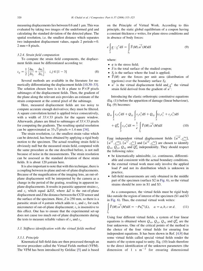
Images of the undeformed and deformed gratings are

digitized through a 1280!1024 CCD camera connected to a

PC (Fig. 7). The lens of the camera is set such that a period

of the grid is sampled by approximately four pixels. The

30!20 mm region of interest covers all the area of the

specimen located between the two grips of the Iosipescu

fixture (S2 in Fig. 6).

The basic rules leading to the measurement of the

displacement fields with the grid method are recalled in this

section.

3.2.1. Printing of the grid

The spatial carrier consists in the superposition of

horizontal and vertical black lines printed over a white

surface, with a natural spatial frequency f0Z10 lines per

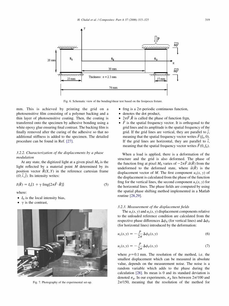
Fig. 6. Schematic view of the bending/shear test based on the Iosipescu fixture.


mm. This is achieved by printing the grid on a

photosensitive film consisting of a polymer backing and a

thin layer of photosensitive coating. Then, the coating is

transferred onto the specimen by adhesive bonding using a

white epoxy glue ensuring final contrast. The backing film is

finally removed after the curing of the adhesive so that no

additional stiffness is added to the specimen. The detailed

procedure can be found in Ref. [27].

3.2.2. Characterization of the displacements by a phase

modulation

At any state, the digitized light at a given pixel M0 is the

light reflected by a material point M determined by its

position vector ðRðX;YÞ in the reference cartesian frame

ðO; ði; ðjÞ. Its intensity writes:

Ið ðRÞ Z I0f1 Cg frng½2p ðF$ ðR�g (5)

where:

† I0 is the local intensity bias,

† g is the contrast,

Fig. 7. Photography of the experimental set-up.

† frng is a 2p-periodic continuous function,

† denotes the dot product,

† 2p ðF : ðR is called the phase of function frgn,

† ðF is the spatial frequency vector. It is orthogonal to the

grid lines and its amplitude is the spatial frequency of the

grid. If the grid lines are vertical, they are parallel to ðj,meaning that the spatial frequency vector writes ðFðf0; 0Þ.

If the grid lines are horizontal, they are parallel to ði,meaning that the spatial frequency vector writes ðFð0; f0Þ.

When a load is applied, there is a deformation of the

structure and the grid is also deformed. The phase of

the function frng at pixel M0 varies ofK2p ðF :ðuð ðRÞ from the

undeformed to the deformed state, where ðuð ðRÞ is the

displacement vector of M. The first component ux(x, y) of

the displacement is calculated from the phase of the function

frng for the vertical lines, the second component uy(x, y) for

the horizontal lines. The phase fields are computed by using

the spatial phase shifting method implemented in a Matlab

routine [28,29].

3.2.3. Measurement of the displacement fields

The ux(x, y) and uy(x, y) displacement components relative

to the unloaded reference condition are calculated from the

respective phase differences DfX (for vertical lines) and DfY

(for horizontal lines) introduced by the deformation:

uxðx; yÞ ZKp

2pDfXðx; yÞ (6)

uyðx; yÞ ZKp

2pDfY ðx; yÞ (7)

where pZ0.1 mm. The resolution of the method, i.e. the

smallest displacement which can be measured in absolute

value, depends on the measurement noise. The noise is a

random variable which adds to the phase during the

calculation [28]. Its mean is 0 and its standard deviation is

denoted sf. In our experiments, sf lies between 2p/100 and

2p/150, meaning that the resolution of the method for


measuring displacements lies between 0.6 and 1 mm. This was

evaluated by taking two images of the undeformed grid and

calculating the standard deviation of the detected phase. The

spatial resolution, i.e. the smallest distance which separates

two independent displacement values, equals 2 periodsZ0.

2 mmZ8 pixels.

3.2.4. Strain field computation

To compute the strain field components, the displace-

ment fields must be differentiated according to:

3ij Z1

2

vui

vxj

Cvuj

vxi

�; i; j2½1 K3� (8)

Several methods are available in the literature for nu-

merically differentiating the displacement fields [10,30–33].

The solution chosen here is to fit a plane to P!P pixels

subimages of the displacement fields. Then, the gradient of

the plane along the relevant axis provides an estimate of the

strain component at the central pixel of the subimage.

Here, measured displacement fields are too noisy to

compute accurate enough derivatives; they must be filtered.

A square convolution kernel is applied twice consecutively,

with a width of 33!33 pixels for the square window.

Afterwards, planes are fitted to subimages of 33!33 pixels

for computing the gradients. The resulting spatial resolution

can be approximated as 33ffiffiffi3

ppixelsx1:4 mm [34].

The strain resolution, i.e. the smallest strain value which

can be detected, has been obtained by applying a rigid body

motion to the specimen. The actual resulting strain field is

obviously null but the measured strain field, computed with

the same procedure as the one described before, is not null

because of noise in the measurements. The strain resolution

can be assessed as the standard deviation of these strain

fields. It is about 120 mstrain here.

It is also important to note that with this technique, there is

a coupling between in-plane and out-of-plane displacements.

Because of the magnification of the imaging lens, an out-of-

plane displacement will be interpreted by the camera as a

change in the period of the grating, resulting in apparent in-

plane displacements. It results in parasitic apparent strains 3x

and 3y which equal DZ/Z, where DZ is the out-of-plane

displacement and Z the distance between the CCD sensor and

the surface of the specimen. Here, Z is 250 mm, so there is a

parasitic strain of 4 mstrain which adds to 3x and 3y for each

micrometer of out-of-plane displacement; 3s is insensitive to

this effect. One has to ensure that the experimental set-up

does not cause too much out-of plane displacements during

the tests to measure reliable values of 3x and 3y.

3.3. Stiffness identification with the virtual fields method

3.3.1. Principle

Kinematical full-field data are then processed through an

inverse procedure called the Virtual Fields method (VFM).

The VFM has been introduced by Grediac [5] and is based

on the Principle of Virtual Work. According to this

principle, the static global equilibrium of a coupon having

a constant thickness e writes, for plane stress conditions and

in absence of body forces:

e

ðS

s : 3dS Z

ðSf

ðT ðMÞ:u�!ðMÞdS (9)

where:

†�s�

is the stress field;

† S is the total surface of the studied coupon;

† Sf is the surface where the load is applied;

† ðT ðMÞ are the forces per unit area (distribution of

tractions) over the boundary surface Sf;

† u�! is the virtual displacement field and�3

�

the virtual

strain field derived from the gradient of u�!.

Introducing the elastic orthotropic constitutive equations

(Eq. (1)) before the apparition of damage (linear behaviour),

Eq. (9) becomes:

Qxx

ðS

3x3x dS CQyy

ðS

3y3y dS CQxy

ðS

ð3x3y C3y3x ÞdS

CQ0ss

ðS

3s3s dS Z

1

e

ðSf

ðT ðMÞ:u�!ðMÞdS ð10Þ

Four independent virtual displacement fields fu�a�!; 3ag,

fu�b�!

; 3bg, f u�c�!; 3cg and fu�d

�!; 3d g are chosen to identify

Qxx, Qyy, Qxy and Q0ss independently. They should respect

the following rules:

† be kinematically admissible, i.e. continuous, differenti-

able and consistent with the actual boundary conditions,

† the external virtual work must only involve the applied

load P and not its distribution which is unknown in

practice,

† full-field measurements are only obtained in the middle

part of the specimen (surface S2 in Fig. 6), so the virtual

strains should be zero in S1 and S3.

As a consequence, the virtual fields must be rigid body

like outside the region of interest of the specimen (S1 and S3

in Fig. 6). Thus, the external virtual work writes:ðSf

ðT ðMÞ:u�!ðMÞdS ZKPuay ðLÞ; a Z a; b; c or d: (11)

Using four different virtual fields, a system of four linear

equations is obtained where Qxx, Qyy, Qxy and Q0ss are the

four unknowns. One of the critical points of the method is

the choice of the four virtual fields for ensuring four

independent equations. It has been shown in Ref. [4,9] that

some virtual fields called special virtual fields render the

matrix of the system equal to unity. Eq. (10) leads therefore

to the direct identification of the unknown parameters (the

dimension of 1 s mK2 for ensuring dimensional


homogeneity). Finally, the solution is:

Qxx ZK1!Pua

y ðLÞ

eQyy ZK1!

Puby ðLÞ

e

Qxy ZK1!Puc

y ðLÞ

eQ0

ss ZK1!Pud

y ðLÞ

e

(12)

3.3.2. Choice of virtual fields

At the beginning, the virtual fields were expanded as

polynomial functions defined over the whole region of

interest [4,9,11]. In the present approach, the virtual fields

are defined by subdomains, as piecewise defined functions

[35]. Shape functions such as that in the finite element

method are used to expand the virtual fields. The first asset

of this approach is that the degree of the shape functions is

lower than the degree of previously used polynomials,

which brings up more stability and robustness. The second

asset is that only the virtual displacement fields have to be

continuous. It is not necessary that their gradient is also

continuous at the edges of the subdomains, which relaxes

the conditions of virtual fields construction. However, still

an infinity of piecewise defined virtual fields can be chosen

for deriving the unknown stiffnesses from Eq. (12). A

method for selecting the virtual fields has recently been

developed [10]. It relies on the minimization of noise

effects. Only the main features of this method will be

recalled here.

The model assumed here for the noise is a Gaussian

white noise. Although the present authors are well aware

that this assumption is too simplistic, it is still thought

that it could be a helpful criterion to select good virtual

fields among the many available special fields. So, this

noise, respectively, gNx, gNy and gNs, adds to 3x, 3y and

3s. g is a strictly positive real number that represents the

random variability of the strain measurements (it is

interpreted as the uncertainty of the strain measure-

ments). The noise is assumed to be uncorrelated from

one measurement location to another in the current

model. The components are also assumed to be

uncorrelated between each other. Again, since exper-

imentally, the strains will be derived from the two in-

plane displacement components bearing the noise, this is

not strictly true but this assumption is needed to keep the

process analytical.

Since 3x, 3y and 3s contain random noise, the value of

each unknown parameter identified from 3x, 3y and 3s with

Eq. (12) is a random variable. It writes, for example for Qxx:

Qxx ZKPua

y ðLÞ

eCg Qxx

ðS2

Nx3ax dS CQyy

ðS2

Ny3ay dS

24

CQ0ss

ðS2

Ns3as dS CQxy

ðS2

½Nx3ay dS CNy3a

x dS�

35 ð13Þ

Qyy, Qxy and Q0ss are also random variables. According to

Eq. (13), it can be shown that the variances of Qxx, Qyy, Qxy

and Q0ss write [10]:

VðQxxÞ Z ðhaÞ2g2

VðQyyÞ Z ðhbÞ2g2

VðQxyÞ Z ðhcÞ2g2

VðQ0ssÞ Z ðhdÞ2g2

8>>>>><>>>>>:

(14)

where:

ðhaÞ2 ZbL

ðS2

½Q2xx CQ2

xy�ð3ax Þ2dS

8<:

C

ðS2

½Q2yy CQ2

xy�ð3ay Þ2dSC

ðS2

½Q0ss�

2ð3as Þ2dS

C2

ðS2

½QxyðQxx CQyyÞ�ð3ax 3a

y ÞdS

9=; for a Za;b;c; and d:

(15)

Therefore, computing ha quantifies the sensitivity to

noise of the method. For a given virtual field, the lowest

ha, the most accurate the identification. It has been

shown in Ref. [10] that, for a given strain field 3x, 3y et

3s, there is a unique set of special virtual fields

fu�a�!;3ag, fu�b

�!;3bg, f u�c�!

;3cgetfu�d�!

;3d g which

minimize, respectively, the sensitivity to noise ha, for

aZa, b, c, or d. These four virtual fields are deduced

from the resolution of a constrained minimization

problem. The unknowns of this minimization problem

are the components of the virtual fields expanded in a

suitable basis of continuous functions. The Lagrangian of

the problem is written. Its unique saddle point is found

[10], yielding the virtual field the least sensitive to noise

for each unknown constitutive parameter. Then, each

unknown constitutive parameter can be identified by

applying the VFM with the deduced virtual fields.

However, the problem is not explicit because the

unknowns Qxx, Qyy, Qxy and Q0ss are involved in the

expression of ha. The problem is solved by an iterative

algorithm where the unknown parameters are replaced by

their identified values. A first set of initial values is chosen.

Tests show that this algorithm converges in less than four

iterations whatever the choice of the initial values [10].

3.4. Nonlineary identification with the virtual fields method

When the specimen is loaded in the nonlinear part of its

behaviour (here, PO800 N), Qss is not a constant anymore

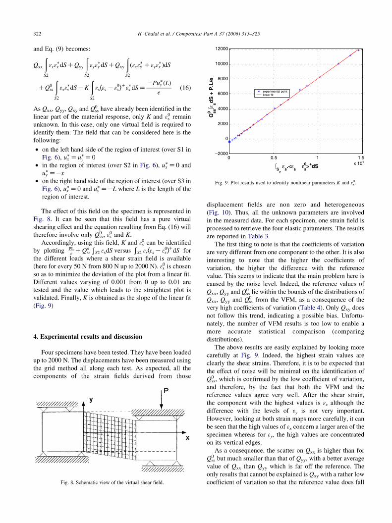
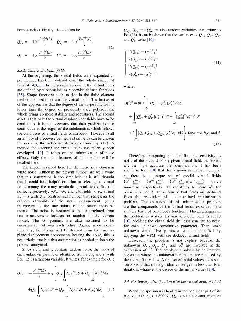
Fig. 9. Plot results used to identify nonlinear parameters K and 30s .


and Eq. (9) becomes:

Qxx

ðS2

3x3x dSCQyy

ðS2

3y3y dSCQxy

ðS2

ð3x3y C3y3x ÞdS

CQ0ss

ðS2

3s3s dSKK

ðS2

3sh3s K30s i

C3s dS Z

KPuy ðLÞ

eð16Þ

As Qxx, Qyy, Qxy and Q0ss have already been identified in the

linear part of the material response, only K and 30s remain

unknown. In this case, only one virtual field is required to

identify them. The field that can be considered here is the

following:

† on the left hand side of the region of interest (over S1 in

Fig. 6), ux Zu

y Z0

† in the region of interest (over S2 in Fig. 6), ux Z0 and

uy ZKx

† on the right hand side of the region of interest (over S3 in

Fig. 6), ux Z0 and u

y ZKL where L is the length of the

region of interest.

The effect of this field on the specimen is represented in

Fig. 8. It can be seen that this field has a pure virtual

shearing effect and the equation resulting from Eq. (16) will

therefore involve only Q0ss, 30

s and K.

Accordingly, using this field, K and 30s can be identified

by plotting PLe

CQoss

ÐS2 3sdS versus

ÐS2 3sh3sK30

s iCdS for

the different loads where a shear strain field is available

(here for every 50 N from 800 N up to 2000 N). 30s is chosen

so as to minimize the deviation of the plot from a linear fit.

Different values varying of 0.001 from 0 up to 0.01 are

tested and the value which leads to the straightest plot is

validated. Finally, K is obtained as the slope of the linear fit

(Fig. 9)

4. Experimental results and discussion

Four specimens have been tested. They have been loaded

up to 2000 N. The displacements have been measured using

the grid method all along each test. As expected, all the

components of the strain fields derived from those

Fig. 8. Schematic view of the virtual shear field.

displacement fields are non zero and heterogeneous

(Fig. 10). Thus, all the unknown parameters are involved

in the measured data. For each specimen, one strain field is

processed to retrieve the four elastic parameters. The results

are reported in Table 3.

The first thing to note is that the coefficients of variation

are very different from one component to the other. It is also

interesting to note that the higher the coefficients of

variation, the higher the difference with the reference

value. This seems to indicate that the main problem here is

caused by the noise level. Indeed, the reference values of

Qxx, Qyy and Q0ss lie within the bounds of the distributions of

Qxx, Qyy and Q0ss from the VFM, as a consequence of the

very high coefficients of variation (Table 4). Only Qxy does

not follow this trend, indicating a possible bias. Unfortu-

nately, the number of VFM results is too low to enable a

more accurate statistical comparison (comparing

distributions).

The above results are easily explained by looking more

carefully at Fig. 9. Indeed, the highest strain values are

clearly the shear strains. Therefore, it is to be expected that

the effect of noise will be minimal on the identification of

Q0ss, which is confirmed by the low coefficient of variation,

and therefore, by the fact that both the VFM and the

reference values agree very well. After the shear strain,

the component with the highest values is 3x although the

difference with the levels of 3y is not very important.

However, looking at both strain maps more carefully, it can

be seen that the high values of 3x concern a larger area of the

specimen whereas for 3y, the high values are concentrated

on its vertical edges.

As a consequence, the scatter on Qxx is higher than for

Q0ss but much smaller than that of Qyy, with a better average

value of Qxx than Qyy which is far off the reference. The

only results that cannot be explained is Qxy with a rather low

coefficient of variation so that the reference value does fall

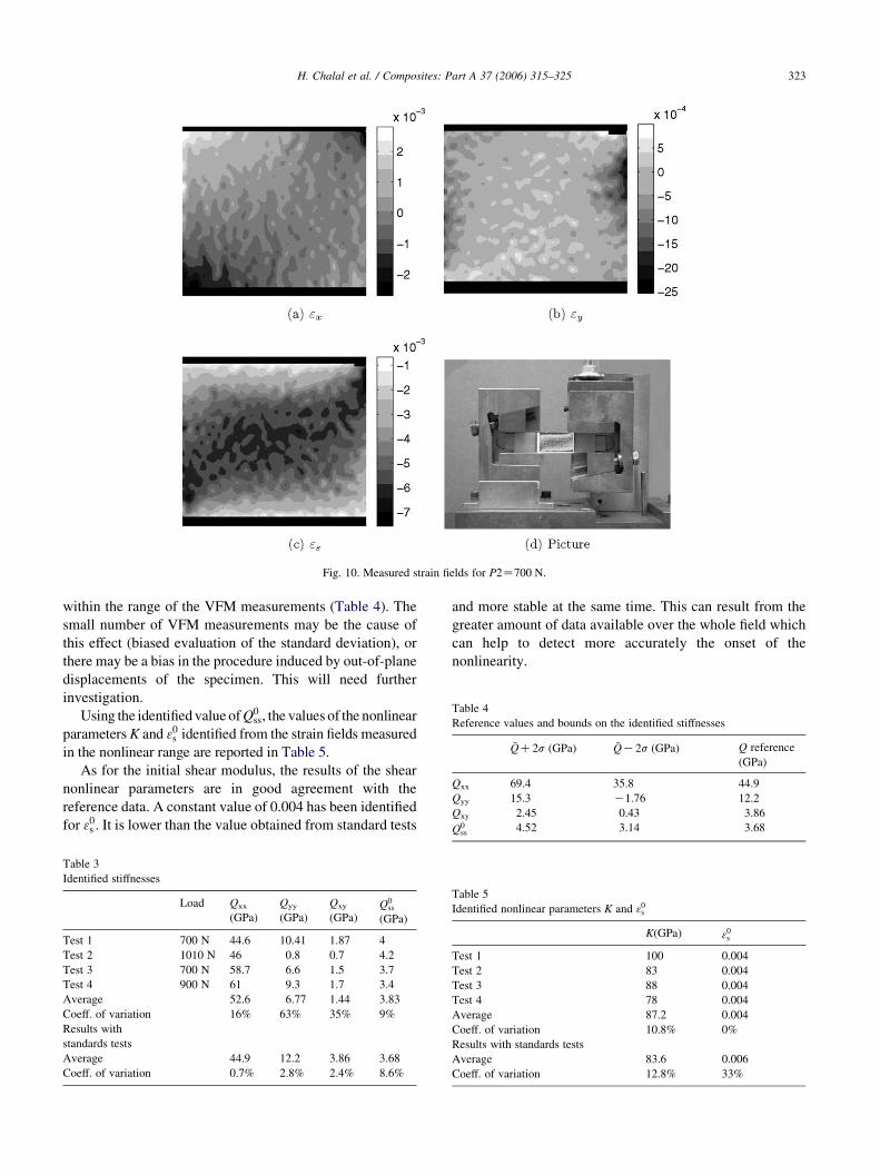
Fig. 10. Measured strain fields for P2Z700 N.

Table 4

Reference values and bounds on the identified stiffnesses

�QC2s (GPa) �QK2s (GPa) Q reference

(GPa)

Qxx 69.4 35.8 44.9

Qyy 15.3 K1.76 12.2

Qxy 2.45 0.43 3.86

Q0ss 4.52 3.14 3.68


within the range of the VFM measurements (Table 4). The

small number of VFM measurements may be the cause of

this effect (biased evaluation of the standard deviation), or

there may be a bias in the procedure induced by out-of-plane

displacements of the specimen. This will need further

investigation.

Using the identified value of Q0ss, the values of the nonlinear

parameters K and 30s identified from the strain fields measured

in the nonlinear range are reported in Table 5.

As for the initial shear modulus, the results of the shear

nonlinear parameters are in good agreement with the

reference data. A constant value of 0.004 has been identified

for 30s . It is lower than the value obtained from standard tests

Table 3

Identified stiffnesses

Load Qxx

(GPa)

Qyy

(GPa)

Qxy

(GPa)Q0

ss

(GPa)

Test 1 700 N 44.6 10.41 1.87 4

Test 2 1010 N 46 0.8 0.7 4.2

Test 3 700 N 58.7 6.6 1.5 3.7

Test 4 900 N 61 9.3 1.7 3.4

Average 52.6 6.77 1.44 3.83

Coeff. of variation 16% 63% 35% 9%

Results with

standards tests

Average 44.9 12.2 3.86 3.68

Coeff. of variation 0.7% 2.8% 2.4% 8.6%

and more stable at the same time. This can result from the

greater amount of data available over the whole field which

can help to detect more accurately the onset of the

nonlinearity.

Table 5

Identified nonlinear parameters K and 30s

K(GPa) 30s

Test 1 100 0.004

Test 2 83 0.004

Test 3 88 0.004

Test 4 78 0.004

Average 87.2 0.004

Coeff. of variation 10.8% 0%

Results with standards tests

Average 83.6 0.006

Coeff. of variation 12.8% 33%

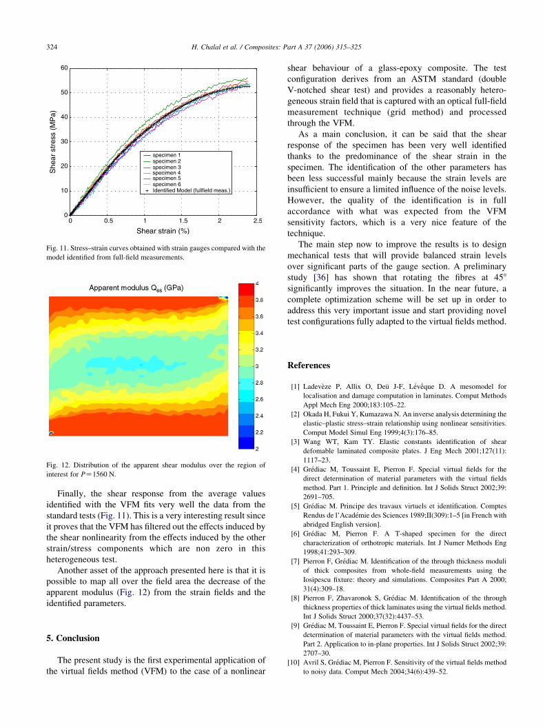
Fig. 11. Stress–strain curves obtained with strain gauges compared with the

model identified from full-field measurements.

Fig. 12. Distribution of the apparent shear modulus over the region of

interest for PZ1560 N.


Finally, the shear response from the average values

identified with the VFM fits very well the data from the

standard tests (Fig. 11). This is a very interesting result since

it proves that the VFM has filtered out the effects induced by

the shear nonlinearity from the effects induced by the other

strain/stress components which are non zero in this

heterogeneous test.

Another asset of the approach presented here is that it is

possible to map all over the field area the decrease of the

apparent modulus (Fig. 12) from the strain fields and the

identified parameters.

5. Conclusion

The present study is the first experimental application of

the virtual fields method (VFM) to the case of a nonlinear

shear behaviour of a glass-epoxy composite. The test

configuration derives from an ASTM standard (double

V-notched shear test) and provides a reasonably hetero-

geneous strain field that is captured with an optical full-field

measurement technique (grid method) and processed

through the VFM.

As a main conclusion, it can be said that the shear

response of the specimen has been very well identified

thanks to the predominance of the shear strain in the

specimen. The identification of the other parameters has

been less successful mainly because the strain levels are

insufficient to ensure a limited influence of the noise levels.

However, the quality of the identification is in full

accordance with what was expected from the VFM

sensitivity factors, which is a very nice feature of the

technique.

The main step now to improve the results is to design

mechanical tests that will provide balanced strain levels

over significant parts of the gauge section. A preliminary

study [36] has shown that rotating the fibres at 458

significantly improves the situation. In the near future, a

complete optimization scheme will be set up in order to

address this very important issue and start providing novel

test configurations fully adapted to the virtual fields method.

References

[1] Ladeveze P, Allix O, Deu J-F, Leveque D. A mesomodel for

localisation and damage computation in laminates. Comput Methods

Appl Mech Eng 2000;183:105–22.

[2] Okada H, Fukui Y, Kumazawa N. An inverse analysis determining the

elastic–plastic stress–strain relationship using nonlinear sensitivities.

Comput Model Simul Eng 1999;4(3):176–85.

[3] Wang WT, Kam TY. Elastic constants identification of shear

defomable laminated composite plates. J Eng Mech 2001;127(11):

1117–23.

[4] Grediac M, Toussaint E, Pierron F. Special virtual fields for the

direct determination of material parameters with the virtual fields

method. Part 1. Principle and definition. Int J Solids Struct 2002;39:

2691–705.

[5] Grediac M. Principe des travaux virtuels et identification. Comptes

Rendus de l’Academie des Sciences 1989;II(309):1–5 [in French with

abridged English version].

[6] Grediac M, Pierron F. A T-shaped specimen for the direct

characterization of orthotropic materials. Int J Numer Methods Eng

1998;41:293–309.

[7] Pierron F, Grediac M. Identification of the through thickness moduli

of thick composites from whole-field measurements using the

Iosipescu fixture: theory and simulations. Composites Part A 2000;

31(4):309–18.

[8] Pierron F, Zhavaronok S, Grediac M. Identification of the through

thickness properties of thick laminates using the virtual fields method.

Int J Solids Struct 2000;37(32):4437–53.

[9] Grediac M, Toussaint E, Pierron F. Special virtual fields for the direct

determination of material parameters with the virtual fields method.

Part 2. Application to in-plane properties. Int J Solids Struct 2002;39:

2707–30.

[10] Avril S, Grediac M, Pierron F. Sensitivity of the virtual fields method

to noisy data. Comput Mech 2004;34(6):439–52.


[11] Chalal H, Meraghni F, Pierron F, Grediac M. Direct identification of

the damage behaviour of composite materials using the virtual fields

method. Composites Part A 2004;35:841–8.

[12] Camus G, Guillaumat L, Baste S. Development of damage in a 2D

woven C/SiC composite under mechanical loading: I. Mechanical

characterization. Compos Sci Technol 1996;56:1363–72.

[13] Camus G. Modelling of the mechanical behavior and damage

processes of fibrous ceramic matrix composites: application to a 2D

SiC/SiC. Int J Solids Struct 2000;37:919–42.

[14] Zhou G, Green ER, Morrison C. In-plane and interlaminar shear

properties of carbon/epoxy laminates. Compos Sci Technol 1995;55:

187–93.

[15] Kawai M, Morishita M, Satoh H, Tomura S, Kemmochi K. Effects of

end-tab shape on strain field of unidirectional carbon/epoxy composite

specimens subjected to off-axis tension. Composites Part A 1997;28A:

267–75.

[16] Ladeveze P, Le Dantec E. Damage modeling of the elementary

ply for laminated composites. Compos Sci Technol 1992;43(3):

257–68.

[17] Grediac M, Pierron F. Applying the virtual fields method to the

identification of elasto-plastic constitutive parameters. Int J Plast; in

revision.

[18] Giraudeau A, Pierron F. Identification of stiffness and damping

properties of thin isotropic vibrating plates using the virtual fields

method. Theory and simulations. J Sound Vib; accepted for

publication.

[19] ASTM D3039-76. Test method for tensile properties of fiber-resin

composites.: American Society for the Testing of Materials; 1976.

[20] Carlsson LA, Pipes RB, editors. Experimental characterization of

advanced composite materials. Technomic Publishing Co., Inc.; 1997.

[21] ASTM D5379-93. Standard method for shear properties of composite

materials by the V-notched beam method.: American Society for the

Testing of Materials; 1993.

[22] Pierron F, Vautrin A. Accurate comparative determination of the in-

plane shear modulus of T300/914 using the Iosipescu and 458 off-axis

tests. Compos Sci Technol 1994;52(1):61–72.

[23] Pierron F. Saint-Venant effects in the Iosipescu specimen. J Compos

Materials 1998;32(22):1986–2015.

[24] Surrel Y. Moire and grid methods: a signal-processing approach. In:

Pryputniewicz RJ, Stupnicki J, editors. Interferometry’94: photo-

mechanics, vol. SPIE 2342.

[25] Avril S, Ferrier E, Hamelin P, Surrel Y, Vautrin A. A full-field optical

method for the experimental analysis of reinforced concrete beams

repaired with composites. Composite Part A; 35(7).

[26] Avril S, Vautrin A, Surrel Y. Grid method: application to the

characterization of cracks. Exp Mech 2004;44(3):37–43.

[27] Piro J-L, Grediac M. Producing and transferring low-spatial-

frequency grids for measuring displacement fields with moire and

grid methods. Exp Tech 2004;28(4):23–6.

[28] Surrel Y. Fringe analysis. In: Rastogi PK, editor. Photomechanics.

Berlin: Springer; 1999. p. 57–104.

[29] Surrel Y. Design of algorithms for phase measurements by the use of

phase-stepping. Appl Opt 1996;35:51–60.

[30] Perie J-N, Calloch S, Cluzel C, Hild F. Analysis of a multiaxial test on

a C/C composite by using digital image correlation and a damage

model. Exp Mech 2004;42(3):318–28.

[31] Kajberg J, Lindkvist G. Characterisation of materials subjected to

large strains by inverse modelling based on in-plane displacement

fields. Int J Solids Struct 2004;41:3439–59.

[32] Roux S, Hild F, Berthaud Y. Correlation image velocimetry: a spectral

approach. Appl Opt 2002;41(1):108–15.

[33] Wagne B, Roux S, Hild F. Spectral approach to displacement

evaluation from image analysis. Eur Phys J Appl Phys 2002;17:

247–52.

[34] Bulhak J, Surrel Y. Mesure de deplacements et de deformations:

quelle resolution spatiale? Actes du congres PhotoMecanique2001

2001 p 1–8 [in French].

[35] Toussaint E, Grediac M, Pierron F. The virtual fields method with

piecewise virtual fields. Int J Mech Sci; submitted for publication.

[36] Avril S, Pierron F, Grediac M. Design of suitable testing

configurations for identifying mechanical constitutive equations

from full-field measurements Xth SEM international congress on

experimental mechanics.: Society for Experimental Mechanics; 2004.

Experimental identification of a nonlinear model for composites using the grid technique coupled to...

Documents

Transcript of Experimental identification of a nonlinear model for composites using the grid technique coupled to...