NTN

UN

orw

egia

n U

nive

rsity

of S

cien

ce a

nd T

echn

olog

yFa

culty

of I

nfor

mat

ion

Tech

nolo

gy a

nd E

lect

rical

Eng

inee

ring

Dep

artm

ent o

f Com

pute

r Sci

ence

Tobias Meyer AndersenKjerand EvjeHåvard Stavnås Markhus

Experimental comparison of hillclimbing variants on CVRP

Bachelor’s project in Computer ScienceSupervisor: Alexander Holt

May 2021

Bach

elor

’s pr

ojec

t

Tobias Meyer AndersenKjerand EvjeHåvard Stavnås Markhus

Experimental comparison of hillclimbing variants on CVRP

Bachelor’s project in Computer ScienceSupervisor: Alexander HoltMay 2021

Norwegian University of Science and TechnologyFaculty of Information Technology and Electrical EngineeringDepartment of Computer Science

Preface

This paper will describe a project about route optimization for waste collection and research regardinghow to use different local search algorithms to solve a variant of the ”capacitated vehicle routing prob-lem.” The purpose of this document is to explain the background theory of the problem at hand, howthe product was developed, and discuss the research results from the conducted algorithmic experiment.

Two out of the three people writing this paper worked for the startup that provided the task. Thestartup worked on an internal project for waste collection and wanted a route optimization tool and ananalytic tool for waste collectors. The team was interested in the route optimization part, as the prob-lem is heavily centered around algorithms. All participants in the team are interested in optimizationtechniques and developing useful algorithms. In addition to working on something of personal interest,the team also had the opportunity to create a valuable product for their startup.

The team thanks the representatives from Favn Software AS and the supervisor from NTNU for thesupport provided during the project:

• Anders Hallem Iversen, Bjørnar Østtveit and Sveinung Øverland from Favn for providing guidancefor the task, helping keep the team on the right track for the product and providing the resourcesneeded to develop the product.

• Alexander Holt from NTNU for guiding the team through the development of the thesis.

Tobias Meyer Andersen Kjerand Evje Havard Stavnas Markhus

1

Task

”The task is to develop a prototype for a service that will be a part of a larger pilot project in cooperationwith the waste company Remiks in Tromsø. The goal of the pilot project is to make it possible to orderwaste pickup via an app, instead of driving oneself to a recycling station (The app is not a part of thistask)”. This statement from Favn declares the background of the project. Additionally, their suggestionof what precisely should be created was the following: ”The task is to create an interface in the form ofa website, and a back-end that will handle orders, route optimization, and data analysis.”

Including developing the system tasked by Favn, the team will develop and compare the performance ofseveral hill climbing algorithms for route optimization.

2

Summary

Routing problems in its different forms are ubiquitous in society. From postman deliveries to computerchip manufacturing, finding paths that minimize some criteria play a central role in many different in-dustries. This thesis involves exploring such a concrete optimization problem, namely the vehicle routingproblem. Determining an optimal solution to this problem is NP-hard, meaning that computing an op-timal route in complex cases requires an extreme amount of computing power. This is not practical forapplications that should quickly and reliably deliver solutions to these problems. It is therefore commonto use heuristics that approximate the solution. The challenge with this is that the performance of dif-ferent heuristics are situational and specific to the problems.

This thesis saw the creation of a system that could handle truck fleets and orders to be picked up,in addition to efficient routing for picking up the orders utilizing the available fleet. Within the thesis,experiments were conducted to test how certain known algorithms would perform when adjusted to workon a specific use case of the vehicle routing problem. Very broadly the algorithms tested all work byquickly producing a placeholder solution and gradually improving it in small increments, when done in acertain way it is known as hill climbing.

This document introduces the problem first, then lays the theoretical foundation of the terms used andthe problem to be studied. Subsequently, the method of both development and the scientific experimentsis described before the results are presented. The conducted experiments will answer the thesis question,which revolves around comparing different route-optimizing algorithms that build on the principle ofhill climbing. The experiment tested the run time of different algorithms and the quality of the routesproduced.The engineering professional approach and the development process of the product utilizing thealgorithms are also documented. After the results, a chapter will discuss how to interpret the results andwhat the data indicates. The thesis is concluded with some pointers to further work for both the productdeveloped and to route optimization will be left for the reader.

The experiments indicated that the teams implementation of Adaptive Iterated Local Search scaledworse than normal hill climbing and simulated annealing, but reliably provided better routes. The dif-ference in scalability is significant as the sheer size of the route grows large limiting certain applicationsusing this algorithm.

3

Contents

List of Figures 7

1 Introduction 81.1 Background . . . . . . . . . . . . . . . . . . . . . . . . . . . . . . . . . . . . . . . . . . . . 81.2 Research question . . . . . . . . . . . . . . . . . . . . . . . . . . . . . . . . . . . . . . . . . 81.3 Document structure . . . . . . . . . . . . . . . . . . . . . . . . . . . . . . . . . . . . . . . 81.4 Nomenclature . . . . . . . . . . . . . . . . . . . . . . . . . . . . . . . . . . . . . . . . . . . 9

2 Theory 102.1 Greedy algorithms . . . . . . . . . . . . . . . . . . . . . . . . . . . . . . . . . . . . . . . . 102.2 Relevant problems . . . . . . . . . . . . . . . . . . . . . . . . . . . . . . . . . . . . . . . . 10

2.2.1 Travelling Salesman . . . . . . . . . . . . . . . . . . . . . . . . . . . . . . . . . . . 102.2.2 Capacitated Vehicle Routing Problem (CVRP) . . . . . . . . . . . . . . . . . . . . 11

2.3 Clustering . . . . . . . . . . . . . . . . . . . . . . . . . . . . . . . . . . . . . . . . . . . . . 112.3.1 Nearest neighbor clustering . . . . . . . . . . . . . . . . . . . . . . . . . . . . . . . 112.3.2 Randomized proximity clustering . . . . . . . . . . . . . . . . . . . . . . . . . . . . 12

2.4 Optimization . . . . . . . . . . . . . . . . . . . . . . . . . . . . . . . . . . . . . . . . . . . 122.4.1 Local search . . . . . . . . . . . . . . . . . . . . . . . . . . . . . . . . . . . . . . . . 122.4.2 Hill climbing . . . . . . . . . . . . . . . . . . . . . . . . . . . . . . . . . . . . . . . 13

2.4.2.1 Intra-route 2-opt . . . . . . . . . . . . . . . . . . . . . . . . . . . . . . . . 132.4.2.2 Intra-route exchange . . . . . . . . . . . . . . . . . . . . . . . . . . . . . . 142.4.2.3 Intra-route or-opt . . . . . . . . . . . . . . . . . . . . . . . . . . . . . . . 142.4.2.4 Intra-route relocate . . . . . . . . . . . . . . . . . . . . . . . . . . . . . . 152.4.2.5 Inter-route relocate . . . . . . . . . . . . . . . . . . . . . . . . . . . . . . 152.4.2.6 Inter-route exchange . . . . . . . . . . . . . . . . . . . . . . . . . . . . . . 162.4.2.7 Inter-route cross exchange . . . . . . . . . . . . . . . . . . . . . . . . . . 162.4.2.8 Inter-route icross exchange . . . . . . . . . . . . . . . . . . . . . . . . . . 172.4.2.9 Inter-route 2-opt . . . . . . . . . . . . . . . . . . . . . . . . . . . . . . . . 17

2.4.3 Iterated Local Search . . . . . . . . . . . . . . . . . . . . . . . . . . . . . . . . . . 172.4.3.1 Concentric removal . . . . . . . . . . . . . . . . . . . . . . . . . . . . . . 182.4.3.2 Removal by proximity . . . . . . . . . . . . . . . . . . . . . . . . . . . . . 182.4.3.3 Sequence removal . . . . . . . . . . . . . . . . . . . . . . . . . . . . . . . 192.4.3.4 Insertion by proximity . . . . . . . . . . . . . . . . . . . . . . . . . . . . . 192.4.3.5 Insertion by cost . . . . . . . . . . . . . . . . . . . . . . . . . . . . . . . . 20

2.4.4 Adaptive Iterated Local Search . . . . . . . . . . . . . . . . . . . . . . . . . . . . . 202.4.5 Simulated Annealing . . . . . . . . . . . . . . . . . . . . . . . . . . . . . . . . . . . 212.4.6 Feasibility . . . . . . . . . . . . . . . . . . . . . . . . . . . . . . . . . . . . . . . . . 21

3 Method 233.1 Process . . . . . . . . . . . . . . . . . . . . . . . . . . . . . . . . . . . . . . . . . . . . . . 233.2 Choice of technologies . . . . . . . . . . . . . . . . . . . . . . . . . . . . . . . . . . . . . . 24

3.2.1 Rust . . . . . . . . . . . . . . . . . . . . . . . . . . . . . . . . . . . . . . . . . . . . 243.2.2 Firebase . . . . . . . . . . . . . . . . . . . . . . . . . . . . . . . . . . . . . . . . . . 24

3.2.2.1 Firebase Firestore (NoSQL) . . . . . . . . . . . . . . . . . . . . . . . . . . 253.2.2.2 Cloud Functions for Firebase . . . . . . . . . . . . . . . . . . . . . . . . . 253.2.2.3 Cloud pub/sub functions . . . . . . . . . . . . . . . . . . . . . . . . . . . 25

3.2.3 Google Cloud Platform . . . . . . . . . . . . . . . . . . . . . . . . . . . . . . . . . 253.2.4 React . . . . . . . . . . . . . . . . . . . . . . . . . . . . . . . . . . . . . . . . . . . 253.2.5 TypeScript . . . . . . . . . . . . . . . . . . . . . . . . . . . . . . . . . . . . . . . . 263.2.6 Google Maps . . . . . . . . . . . . . . . . . . . . . . . . . . . . . . . . . . . . . . . 263.2.7 Docker . . . . . . . . . . . . . . . . . . . . . . . . . . . . . . . . . . . . . . . . . . . 26

4

3.2.8 Open Source Routing Machine (OSRM) . . . . . . . . . . . . . . . . . . . . . . . . 263.3 System architecture . . . . . . . . . . . . . . . . . . . . . . . . . . . . . . . . . . . . . . . 27

3.3.1 Web application and Firebase entity system . . . . . . . . . . . . . . . . . . . . . . 283.4 Testing, integration and deployment . . . . . . . . . . . . . . . . . . . . . . . . . . . . . . 293.5 Trucks and orders implementation . . . . . . . . . . . . . . . . . . . . . . . . . . . . . . . 293.6 Graph compression and representation . . . . . . . . . . . . . . . . . . . . . . . . . . . . . 293.7 Visualization tool . . . . . . . . . . . . . . . . . . . . . . . . . . . . . . . . . . . . . . . . . 303.8 Simulation tool . . . . . . . . . . . . . . . . . . . . . . . . . . . . . . . . . . . . . . . . . . 313.9 Hill climbing implementation . . . . . . . . . . . . . . . . . . . . . . . . . . . . . . . . . . 323.10 Simulated Annealing implementation . . . . . . . . . . . . . . . . . . . . . . . . . . . . . . 323.11 Adaptive Iterated Local Search implementation . . . . . . . . . . . . . . . . . . . . . . . . 32

3.11.1 Summary of the implementation . . . . . . . . . . . . . . . . . . . . . . . . . . . . 333.11.2 Initial clustering . . . . . . . . . . . . . . . . . . . . . . . . . . . . . . . . . . . . . 333.11.3 Perturbation . . . . . . . . . . . . . . . . . . . . . . . . . . . . . . . . . . . . . . . 333.11.4 Neighborhood search . . . . . . . . . . . . . . . . . . . . . . . . . . . . . . . . . . . 34

3.11.4.1 Local search heuristic . . . . . . . . . . . . . . . . . . . . . . . . . . . . . 353.11.5 Acceptance criterion and adaptivity . . . . . . . . . . . . . . . . . . . . . . . . . . 353.11.6 The algorithm . . . . . . . . . . . . . . . . . . . . . . . . . . . . . . . . . . . . . . 36

3.12 Run time experiments . . . . . . . . . . . . . . . . . . . . . . . . . . . . . . . . . . . . . . 363.13 Distribution of roles . . . . . . . . . . . . . . . . . . . . . . . . . . . . . . . . . . . . . . . 37

4 Results 384.1 Scientific results . . . . . . . . . . . . . . . . . . . . . . . . . . . . . . . . . . . . . . . . . 38

4.1.1 Hill climbing results . . . . . . . . . . . . . . . . . . . . . . . . . . . . . . . . . . . 384.1.2 Simulated Annealing results . . . . . . . . . . . . . . . . . . . . . . . . . . . . . . . 384.1.3 Adaptive Iterated Local Search results . . . . . . . . . . . . . . . . . . . . . . . . . 38

4.2 Engineering professional results . . . . . . . . . . . . . . . . . . . . . . . . . . . . . . . . . 384.2.1 Final product overview . . . . . . . . . . . . . . . . . . . . . . . . . . . . . . . . . 384.2.2 Functional requirements . . . . . . . . . . . . . . . . . . . . . . . . . . . . . . . . . 39

4.2.2.1 Authentication system . . . . . . . . . . . . . . . . . . . . . . . . . . . . . 394.2.2.2 Interactive front-end showing the orders . . . . . . . . . . . . . . . . . . . 394.2.2.3 Communication from waste company to users app . . . . . . . . . . . . . 394.2.2.4 Generic route optimization . . . . . . . . . . . . . . . . . . . . . . . . . . 394.2.2.5 Estimating time and fuel use, number of trips required . . . . . . . . . . 394.2.2.6 Displaying information about space and weight used in trucks . . . . . . 404.2.2.7 Possibility to change how many trucks a company has available . . . . . 404.2.2.8 Simulation tool to optimize use . . . . . . . . . . . . . . . . . . . . . . . . 40

4.2.3 Non-functinoal requirements . . . . . . . . . . . . . . . . . . . . . . . . . . . . . . 404.3 Administrative results . . . . . . . . . . . . . . . . . . . . . . . . . . . . . . . . . . . . . . 40

4.3.1 Work schedule plan . . . . . . . . . . . . . . . . . . . . . . . . . . . . . . . . . . . 404.3.2 The development process . . . . . . . . . . . . . . . . . . . . . . . . . . . . . . . . 41

5 Discussion 425.1 Scientific results . . . . . . . . . . . . . . . . . . . . . . . . . . . . . . . . . . . . . . . . . 42

5.1.1 Experiment metrics . . . . . . . . . . . . . . . . . . . . . . . . . . . . . . . . . . . 425.1.2 Other notes on the experiment . . . . . . . . . . . . . . . . . . . . . . . . . . . . . 425.1.3 Hill climbing . . . . . . . . . . . . . . . . . . . . . . . . . . . . . . . . . . . . . . . 435.1.4 Simulated Annealing . . . . . . . . . . . . . . . . . . . . . . . . . . . . . . . . . . . 445.1.5 Adaptive Iterated Local Search . . . . . . . . . . . . . . . . . . . . . . . . . . . . . 455.1.6 Comparison . . . . . . . . . . . . . . . . . . . . . . . . . . . . . . . . . . . . . . . . 45

5.2 Engineering professional results . . . . . . . . . . . . . . . . . . . . . . . . . . . . . . . . . 475.2.1 Final result . . . . . . . . . . . . . . . . . . . . . . . . . . . . . . . . . . . . . . . . 475.2.2 Strengths . . . . . . . . . . . . . . . . . . . . . . . . . . . . . . . . . . . . . . . . . 47

5

5.2.3 Weaknesses . . . . . . . . . . . . . . . . . . . . . . . . . . . . . . . . . . . . . . . . 485.2.4 Testing . . . . . . . . . . . . . . . . . . . . . . . . . . . . . . . . . . . . . . . . . . 485.2.5 Ethical, social and environmental results . . . . . . . . . . . . . . . . . . . . . . . . 49

5.3 Administrative results . . . . . . . . . . . . . . . . . . . . . . . . . . . . . . . . . . . . . . 495.3.1 Work schedule discussion . . . . . . . . . . . . . . . . . . . . . . . . . . . . . . . . 495.3.2 Development process discussion . . . . . . . . . . . . . . . . . . . . . . . . . . . . . 49

6 Conclusion and further work 516.1 Conclusion . . . . . . . . . . . . . . . . . . . . . . . . . . . . . . . . . . . . . . . . . . . . 516.2 Further work . . . . . . . . . . . . . . . . . . . . . . . . . . . . . . . . . . . . . . . . . . . 51

7 Attachments 53

References 54

6

List of Figures

1 Illustration of TSP solution . . . . . . . . . . . . . . . . . . . . . . . . . . . . . . . . . . . 102 Illustration of CVRP solution based on clustering then solving multiple TSP’s . . . . . . . 113 TSP 2-opt heuristic . . . . . . . . . . . . . . . . . . . . . . . . . . . . . . . . . . . . . . . . 134 TSP exchange heuristic . . . . . . . . . . . . . . . . . . . . . . . . . . . . . . . . . . . . . 145 TSP or-opt heuristic . . . . . . . . . . . . . . . . . . . . . . . . . . . . . . . . . . . . . . . 146 TSP relocate heuristic . . . . . . . . . . . . . . . . . . . . . . . . . . . . . . . . . . . . . . 157 VRP relocate optimization heuristic . . . . . . . . . . . . . . . . . . . . . . . . . . . . . . 158 VRP exchange optimization heuristic . . . . . . . . . . . . . . . . . . . . . . . . . . . . . . 169 VRP cross exchange . . . . . . . . . . . . . . . . . . . . . . . . . . . . . . . . . . . . . . . 1610 VRP icross exchange . . . . . . . . . . . . . . . . . . . . . . . . . . . . . . . . . . . . . . . 1711 VRP 2-opt . . . . . . . . . . . . . . . . . . . . . . . . . . . . . . . . . . . . . . . . . . . . 1712 Removing a given amount of vertices closest to a random vertex, including the random

vertex . . . . . . . . . . . . . . . . . . . . . . . . . . . . . . . . . . . . . . . . . . . . . . . 1813 Removing a given amount of vertices that are rated as the furthest away from their routes 1814 Removing random sequences of a given amount of vertices from a route . . . . . . . . . . 1915 Inserting vertex in the route closest to the vertex, at the position with lowest cost . . . . 1916 Inserting vertex in the minimum cost position . . . . . . . . . . . . . . . . . . . . . . . . . 2017 illustration of the overall system technology and how the system communicates . . . . . . 2718 model of the domains in the system . . . . . . . . . . . . . . . . . . . . . . . . . . . . . . 2819 Example of visualization of a set of routes . . . . . . . . . . . . . . . . . . . . . . . . . . . 3020 The simulation report tool . . . . . . . . . . . . . . . . . . . . . . . . . . . . . . . . . . . . 3121 Results of HC graphed and compared to number of orders. . . . . . . . . . . . . . . . . . 4322 Results of SA graphed and compared to number of orders. . . . . . . . . . . . . . . . . . . 4423 Results of AILS graphed and compared to number of orders. . . . . . . . . . . . . . . . . 4524 Quickest version of each algorithm compared. . . . . . . . . . . . . . . . . . . . . . . . . . 4525 Slowest versions of each algorithm compared. . . . . . . . . . . . . . . . . . . . . . . . . . 46

7

1 Introduction

1.1 Background

Favn Software is a startup company located in Trondheim, Norway. It was founded in 2020 by studentsfrom NTNU (Norwegian University of Science and Technology). Favn is a consulting company specializ-ing in developing software. This includes developing software for customers, including websites, mobileapplications, back-end systems, and more.

Favn had for some time been interested in developing a system for waste collectors. The companyhad been in talks with Remiks (a waste company located in Tromsø), and there seemed to be interestin such a product. This system would include a route optimizing engine for the waste collectors and afront-end system for ordering waste pick-up.

The primary purpose of this system is to make the waste-collecting process more effective by computingoptimized routes for the waste trucks. Normal people would not have to drive themselves to a recyclingstation, generating pollution and traffic in the process. Having a select few trucks collecting the items is,therefore, an opportunity for the waste company and the customers.

The role of the team during development will be to focus on the routing optimizing part of the system.This will include implementing different algorithms and optimizing them to produce the best possibleresults.

1.2 Research question

Formally the optimization problem the team received from Favn Software AS can be described as follow-ing: given a set of trucks with weight and space capacities, and a set of orders with a location, weight,and space assigned, produce a set of routes for the trucks such that each order is picked up within a timelimit, minimizing the total travel time. It is also given that all the trucks start at the depot where theyshould return with all the orders. This is a variant of what is known as the capacitated vehicle routingproblem, first formally studied in 1959 by Dantzig and Ramser[1].

Given the time at disposal, the approach of the team will be to implement different versions of hillclimbing algorithms that are known to work for very similar problems and compare how they perform onthis exact application. Hill climbing was chosen in particular as various sources state that iterative routeoptimizers using metaheuristics have been very successful[2][3].In addition, the goal is to find out what works well in practice on realistic data and not to optimizetheoretical worst-case scenarios. The thesis question is then:

How do different versions of hill climbing compare when adjusted to solve thecapacitated vehicle routing problem with time limits on realistic map data?

1.3 Document structure

Here is a brief overview of the structure of the document.

• Introduction - background information and thesis question.

• Theory - brief summary of relevant background theory to understand the method, results anddiscussion.

• Method - explanation of how the algorithms were made and tested, development process of theteam and technologies used.

8

• Results - a chapter showing the experimental results of the algorithms, team results in terms ofdevelopment and administrative documentation generated in the project.

• Discussion - a discussion trying to put the results into context and reflecting on their meaning.

• Conclusion - answer of the thesis question using the results and their interpretation from thediscussion, also a brief note on future work to be done around the thesis question.

• References - list of sources cited in the document.

• Attachments - list of attachments that constitute the rest of the delivery for the thesis.

1.4 Nomenclature

AILS Adaptive Iterated Local Search

API Application Programming interface

GCP Google Cloud Platform

HC Hill Climb

ILS Iterated Local Search

LS Local Search

OSRM Open Street Routing Machine

SA Simulated Annealing

UI User Interface

UX User Experience

VM Virtual Machine

9

2 Theory

2.1 Greedy algorithms

An algorithm is considered greedy if it computes something by making the immediate best move, withno regard for future planning or past computation, usually in an iterative fashion. To illustrate this,consider trying to purchase as many items as possible from a store. An optimal greedy solution would beto pick items one by one, always selecting the cheapest item available. This strategy will guarantee themost items being purchased, and the greedy part is to select the cheapest one available. Although thisparticular greedy algorithm is optimal, that is not the case in general. Despite that, greedy algorithmsare widely used within optimization, including route optimization. This is mostly because results can becomputed very fast when the simplification of not considering the future or past is made.

2.2 Relevant problems

2.2.1 Travelling Salesman

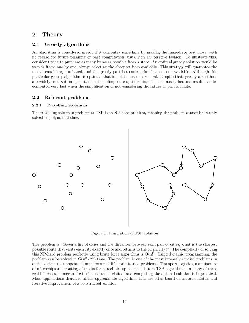
The travelling salesman problem or TSP is an NP-hard problem, meaning the problem cannot be exactlysolved in polynomial time.

Figure 1: Illustration of TSP solution

The problem is ”Given a list of cities and the distances between each pair of cities, what is the shortestpossible route that visits each city exactly once and returns to the origin city?”. The complexity of solvingthis NP-hard problem perfectly using brute force algorithms is O(n!). Using dynamic programming, theproblem can be solved in O(n2 · 2n) time. The problem is one of the most intensely studied problems inoptimization, as it appears in numerous real-life optimization problems. Transport logistics, manufactureof microchips and routing of trucks for parcel pickup all benefit from TSP algorithms. In many of thesereal-life cases, numerous ”cities” need to be visited, and computing the optimal solution is impractical.Most applications therefore utilize approximate algorithms that are often based on meta-heuristics anditerative improvement of a constructed solution.

10

2.2.2 Capacitated Vehicle Routing Problem (CVRP)

CVRP is a generalization of the traveling salesman problem. The problem statement usually is definedas: ”Given a list of cities to visit with a weight assigned, and a list of vehicles with a given capacity,minimize the total distance traveled while having the trucks combined visit all cities exactly once withoutsurpassing their capacity.”

Figure 2: Illustration of CVRP solution based on clustering then solving multiple TSP’s

CVRP can therefore explained as a traveling salesman problem with capacity constraints and multiplesalesmen. As a generalization of an NP-hard problem, this is also a NP-hard problem. The simplestedge case is when one vehicle can visit all the cities, that special case is the regular traveling salesman.Otherwise, one must also figure out which orders should be picked up by which vehicles and optimizethose individual trips. As with most NP-hard problems, finding an exact solution requires a large amountof computation. This suggests that approximation is needed in order to be able to compute good routeswithin a reasonable amount of time for practical applications. Different approximations will be explainedlater.

2.3 Clustering

Clustering is trying to single out meaningful groups of data. For instance, one can group books by genre,publisher, or release date. Clustering algorithms receive a dataset as input and tries to categorize thembased on some metric of similarity. Clustering algorithms are often divided into two types, supervisedand unsupervised. In the CVRP problem, the vehicles are groups, and the goal is to distribute the citiesinto the group to which they belong. Since an analyst defines the groups before running the clusteringalgorithm, it is categorized as supervised. The clustering methods described in this document are allsupervised.

2.3.1 Nearest neighbor clustering

Nearest neighbor clustering groups data by iteratively finding the most similar data point to the previous,sometimes limited by some sort of group size constraint. This is a typical example of a greedy algorithm.This can be illustrated by using it as a heuristic to quickly produce a valid solution for CVRP. With thisalgorithm, the solution would be constructed node by node. Start by selecting any truck; the first orderto pick up will be the closest one. The next order will be the closest order to the previous one that is notyet visited; the pattern repeats until the truck cannot pick up any of the other orders, at which point onereturns to the starting node. This procedure is repeated for all the trucks available until all the orders

11

are picked up. The solutions of the CVRP should minimize total distance. Hence the next order to visitis always the closest unvisited one.

The nearest neighbor clustering method is widely used within data science and optimization algorithms,primarily because it is intuitive, very quick in its greedy nature, and often yielding useful results, forinstance, in many TSP algorithms. In that case, ignore the capacity of the trucks, allowing a singleone to pick up all the orders. For symmetric TSP, it has been experimentally shown to usually producesolutions 25% worse than the global minima [4]. Symmetric means that the graph used by the travelingsalesman algorithm is undirected, the distance between a pair of nodes is the same in both directions.As this thesis uses Open Street Map data from real cities, this problem is an example of an unsymmetrictraveling salesman.

2.3.2 Randomized proximity clustering

Another clustering method is Randomized Proximity Clustering. In light of the application, the algorithmwill be explained using the terms in the thesis question where orders need to be picked up by trucks thatdrive a given route instead of vehicles visiting cities. This initial cluster is based on the clustering methoddescribed in [5]. The algorithm is defined as:

1. At the start of the algorithm, a number m is calculated, representing the number of routes thatshould be driven. S is the set of orders, and sc is the capacity needed to pick up a certain order,q average truck capacity. Therefore, m is the number of routes needed to pick up all of the orderswith the following formula:

m = [1

q

∑s∈S

sc] (1)

2. Assign a random order to each of the routes.

3. Go through all the unassigned orders and assign them to the route which they are the closest to interms of some proximity measure. This could be implemented in many different ways; for instance,the team has used the proximity insertion metric described in 2.4.3.4.

4. Although all the orders now should be picked up by precisely one truck; the route may not satisfythe capacity restriction. In that case, the suggested clustering needs to go through some sort ofcorrection to guarantee that a valid solution is produced by the clustering algorithm. The teamimplemented the feasibility function described in 2.4.6 to assure the creation of valid clusters.

2.4 Optimization

2.4.1 Local search

In many optimization problems, the goal is to find a configuration that maximizes some evaluation func-tion. Often it can be very complicated and even unpractical to produce this solution from the bottomup. If it is easy to generate an arbitrary solution, although it may not be optimal, local search can be avery efficient way to improve that solution into a good one.

Local search is usually implemented as a graph search, where each node represents a possible solu-tion to the problem. In the context of optimization problems, the goal will then be to find the node withthe greatest value given some starting node. The adjacent nodes are those solutions one would have bymaking a certain change to the current one. The most common way to implement a local search is toclearly define what types of changes one can make in a solution to obtain another valid solution. In thisway, it is possible to generate all of the neighboring nodes given the current solution, making the memoryusage O(1) with respect to the number of nodes in the graph. Local search in the context of optimizationproblems can be thought of as making small adjustments to a solution repeatedly until some criteria aresatisfied.

12

2.4.2 Hill climbing

Hill climbing is a greedy local search algorithm. It is common to generate a random solution as the startingnode for the search, which can be far from optimized. As hill climbing is a local search algorithm, allthe neighboring nodes of a solution can be generated and evaluated in terms of desirability. The mostcommon greedy variant of hill climbing will move to the first generated neighbor with higher desirabilitythan the current one. This is repeated until it converges to a local (possibly global) maximum in termsof the evaluation function. Another notable implementation of this is the steepest ascent hill climb,where all the neighboring nodes are generated, and one visits the node with the greatest desirability.Hill climbing is a straightforward technique that is quite fast but will not guarantee the optimal solutionin general. It is possible to run several subsequent hill climbs starting from random solutions in hopesof converging to a better local optimum. Having no specific strategy when generating the next startingpoint is known as the ”Random Restart Hill Climb.” If one instead applies a specific modification to theresult of the hill climb and start the next search from there, one has an implementation of what is knownas ”Iterated Local Search”.

Intra route heuristics

In this thesis, the team used the heuristics described below to modify valid or invalid solutions intosolutions that are better and more feasible. These are ”intra heuristics,” meaning that they modify aspecific route for a single truck. Since these transformations changes the current solution, these heuristicswill generate all neighboring nodes for a particular state. To make it clear, the graphs shown belowrepresent a single trip, or route, that will be driven by a truck. Note that the classic TSP terminologyof cities is used in the following figures showing each type of move used by the team to optimize singletrips. These intra heuristics are described in [2].

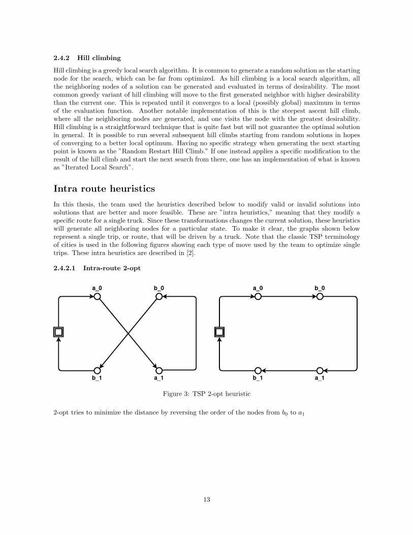
2.4.2.1 Intra-route 2-opt

Figure 3: TSP 2-opt heuristic

2-opt tries to minimize the distance by reversing the order of the nodes from b0 to a1

13

2.4.2.2 Intra-route exchange

Figure 4: TSP exchange heuristic

The exchange heuristic swaps the position of two cities in the route. a1 is swapped to be visited betweenb0 and b2, while b1 is swapped to be visited between a0 and a2. See figure 4.

2.4.2.3 Intra-route or-opt

Figure 5: TSP or-opt heuristic

The or-opt heuristic checks for a segment of 1, 2 or three consecutive Cities can be relocated to anotherplace in the route order. In the case of figure 5 two cities are moved.

14

2.4.2.4 Intra-route relocate

Figure 6: TSP relocate heuristic

The relocate heuristic checks for a single city to be relocated to another place in the route.

Inter route heuristics

Inter route heuristics are move heuristics that moves cities/orders between two routes. These heuristics inthe HC implementation also modify valid or invalid solutions to solutions that are better and, if invalid,more feasible. The ones implemented by the team in the HC algorithm described in 3.9 are shown below;note again that the graphs shown represent the actual changes in a solution. These inter heuristics aredescribed in [2].

2.4.2.5 Inter-route relocate

Figure 7: VRP relocate optimization heuristic

This optimization technique checks a candidate node in one route cluster for relocation to another can-didate position in another cluster.

15

2.4.2.6 Inter-route exchange

Figure 8: VRP exchange optimization heuristic

This technique checks one node from two different routes and exchanges the position of the nodes in thetwo routes.

2.4.2.7 Inter-route cross exchange

Figure 9: VRP cross exchange

The cross exchange heuristic swaps two intervals of consecutive orders from different clusters with eachother.

16

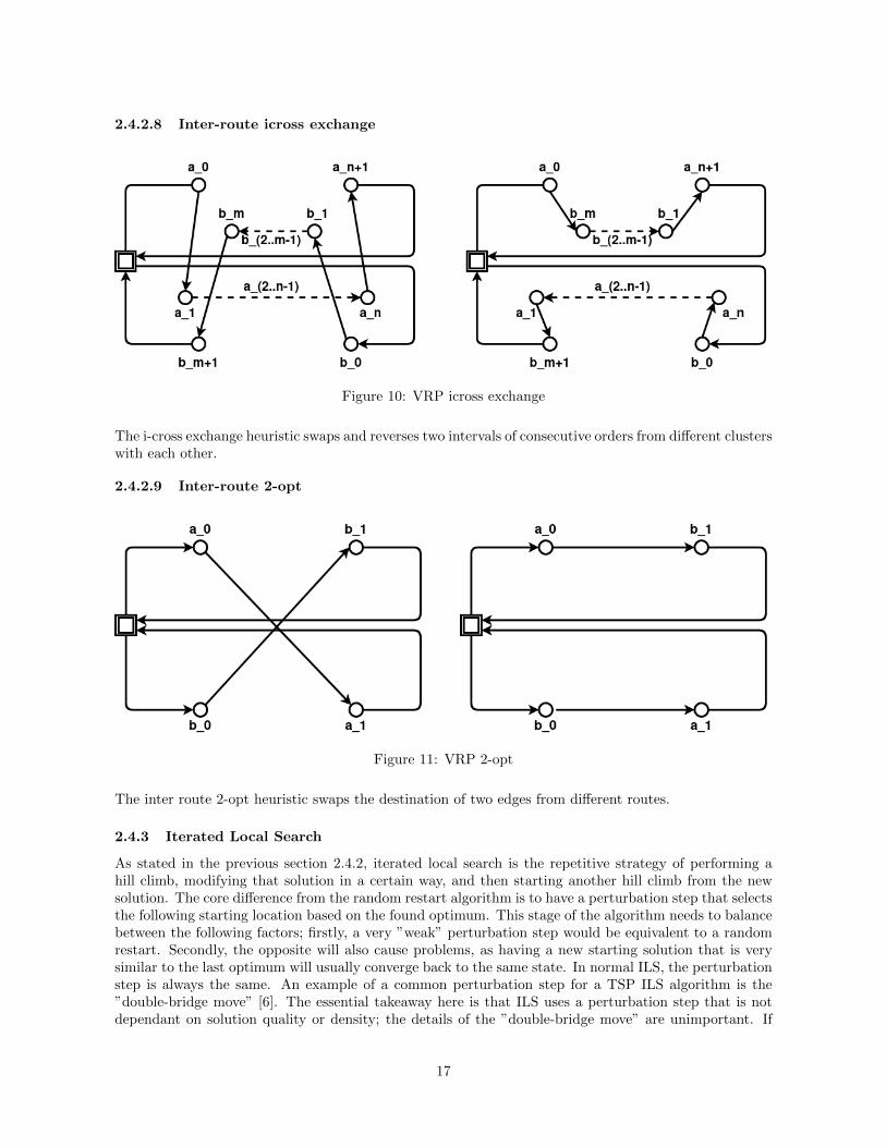
2.4.2.8 Inter-route icross exchange

Figure 10: VRP icross exchange

The i-cross exchange heuristic swaps and reverses two intervals of consecutive orders from different clusterswith each other.

2.4.2.9 Inter-route 2-opt

Figure 11: VRP 2-opt

The inter route 2-opt heuristic swaps the destination of two edges from different routes.

2.4.3 Iterated Local Search

As stated in the previous section 2.4.2, iterated local search is the repetitive strategy of performing ahill climb, modifying that solution in a certain way, and then starting another hill climb from the newsolution. The core difference from the random restart algorithm is to have a perturbation step that selectsthe following starting location based on the found optimum. This stage of the algorithm needs to balancebetween the following factors; firstly, a very ”weak” perturbation step would be equivalent to a randomrestart. Secondly, the opposite will also cause problems, as having a new starting solution that is verysimilar to the last optimum will usually converge back to the same state. In normal ILS, the perturbationstep is always the same. An example of a common perturbation step for a TSP ILS algorithm is the”double-bridge move” [6]. The essential takeaway here is that ILS uses a perturbation step that is notdependant on solution quality or density; the details of the ”double-bridge move” are unimportant. If

17

the algorithm considers the history of local optima reached when choosing how to perturb, one wouldhave an example of an adaptive iterated local search.

In the next few subsections, the heuristics used in the perturbation step of the AILS implementationof the team are shown. All of the perturbation heuristics are based on the heuristics described in [5].These graphs show routes with multiple trucks to pick up the orders. In the descriptions, the orders arereferred to as ”vertices”.

2.4.3.1 Concentric removal

Figure 12: Removing a given amount of vertices closest to a random vertex, including the random vertex

This heuristic selects a random vertex vr in the graph, removes the vertex and a given amount of verticesclosest to vr. This way the heuristic removes vertices within a coverage area, using the vertex vr ascenter.

2.4.3.2 Removal by proximity

Figure 13: Removing a given amount of vertices that are rated as the furthest away from their routes

In this heuristic a given number of vertices are removed that are rated the furthest away from their routes,based on a proximity index. The proximity index indicates a relative distance from the route, and not aeuclidean one. The proximity index for a vertex compared to a route is calculated with this equation:

prox(v, p,RSj ) =minset(minp, |RSj | − 2,ΠRSj

(v))

minp, |RSj | − 2(2)

The value ΠRSj(v) is a set containing the distance rank of the other vertices in route RSj to vertex v. if

Rsj = 3, 6, 7, v = 6 in a system of 10 vertices V = 1, 2, ..., 9 and vertex 3, 7 are the 3rd and 6th closest

18

vertices to vertex v = 6, then ΠRSj(6) = 3, 6.

minset(a, set) is defined as the sum of the a smallest elements in the set ”set”.The proximity function (2) gives an index of relatively how close a vertex is to a route. In the proximityremoval heuristic one therefore compares all vertices to its route with the proximity function (2) andremove the vertices with the highest proximity indexes.

2.4.3.3 Sequence removal

Figure 14: Removing random sequences of a given amount of vertices from a route

In the sequence removal heuristic a given number of vertices are removed by randomly selecting sequencesof vertices in a route and removing these from the solution.

2.4.3.4 Insertion by proximity

Figure 15: Inserting vertex in the route closest to the vertex, at the position with lowest cost

This is a heuristic in which one inserts a vertex into a route based on proximity. First, one needs tofind which route is closest to the vertex. Compare the vertex to every route in the solution using theproximity function (2) and find the route with the smallest proximity index:

RSj = argminRsj∈Routesprox(v, p,Rsj) (3)

p is a random integer in the interval [1, [n/m]], where n is the amount of vertices, and m is the amount ofroutes in the current solution. The route RSj is the one with the lowest proximity index. Next, find theposition within the route to place the vertex. This is done by calculating the insertion cost with following

19

equation for a route Rj = vj0, vj1, ..., v

jnj:

i = arg mini∈(0,1,...nj)

d(vji , v) + d(vji+1, v)− d(vji , vji+1) (4)

The index i to insert the vertex is calculated with this equation, where v is the inserted vertex, vi is avertex in the route, and d is the distance between two given vertices. This results in inserting the vertexat the index i, which is the index with the lowest insertion cost.

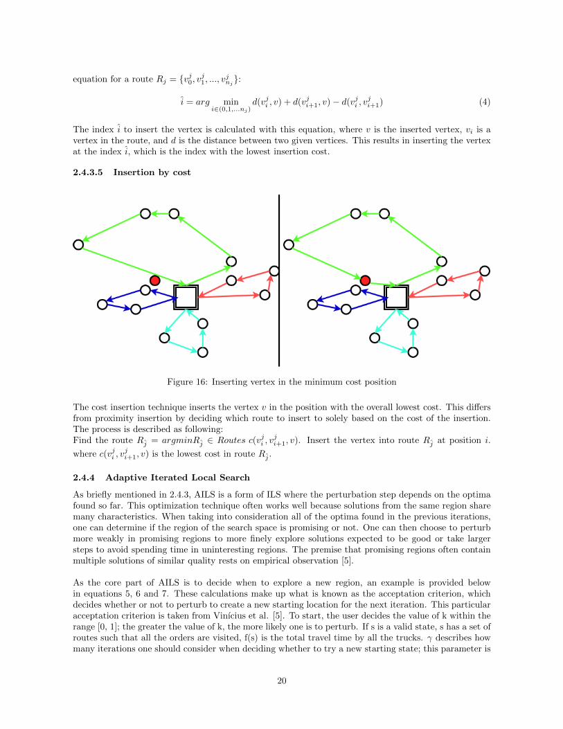
2.4.3.5 Insertion by cost

Figure 16: Inserting vertex in the minimum cost position

The cost insertion technique inserts the vertex v in the position with the overall lowest cost. This differsfrom proximity insertion by deciding which route to insert to solely based on the cost of the insertion.The process is described as following:Find the route Rj = argminRj ∈ Routes c(vji , v

ji+1, v). Insert the vertex into route Rj at position i.

where c(vji , vji+1, v) is the lowest cost in route Rj .

2.4.4 Adaptive Iterated Local Search

As briefly mentioned in 2.4.3, AILS is a form of ILS where the perturbation step depends on the optimafound so far. This optimization technique often works well because solutions from the same region sharemany characteristics. When taking into consideration all of the optima found in the previous iterations,one can determine if the region of the search space is promising or not. One can then choose to perturbmore weakly in promising regions to more finely explore solutions expected to be good or take largersteps to avoid spending time in uninteresting regions. The premise that promising regions often containmultiple solutions of similar quality rests on empirical observation [5].

As the core part of AILS is to decide when to explore a new region, an example is provided belowin equations 5, 6 and 7. These calculations make up what is known as the acceptation criterion, whichdecides whether or not to perturb to create a new starting location for the next iteration. This particularacceptation criterion is taken from Vinıcius et al. [5]. To start, the user decides the value of k within therange [0, 1]; the greater the value of k, the more likely one is to perturb. If s is a valid state, s has a set ofroutes such that all the orders are visited, f(s) is the total travel time by all the trucks. γ describes howmany iterations one should consider when deciding whether to try a new starting state; this parameter is

20

a user-defined positive integer. f is simply the best solution found in the last minγ, it iterations, where

it is the number of the current iteration. f is a weighted average of the quality of the last iterationsupdated as shown in equation 5. Both f and f both have a starting value of 0. Using equation 7 b will

be a value in the range [f , f ]

fnext =

fprev · (1− 1

γ ) + f(s)γ , it > γ

fprev·(it−1)+f(s)it , it ≤ γ

(5)

ηnext = maxε, k · ηprevkr

(6)

b = f + η · (f − f) (7)

All of the equations are calculated each iteration of the AILS algorithm. If the current solution found isbetter than the calculated b then the current solution will be the starting point of the following search;otherwise, continue to search for solutions from the same starting state.

2.4.5 Simulated Annealing

Simulated annealing is a probabilistic version of hill climbing. Analogous to a material cooling down, thealgorithm keeps track of a temperature that steadily decreases by a constant factor. The most importantdifference from the hill climbing algorithm is that there is a nonzero probability of exploring a stateof lower desirability. The exact formula for the probability is shown in equation 9, where ∆D is thedifference in solution quality of two adjacent states, and T is the temperature at that point in time. Ifthe considered neighboring solution is an improvement, then the search will always explore that state,hence the probability of 1. Note that these equations are written on the form where one seeks to minimizesome loss function instead of maximizing some value function.

∆D = loss(statecurrent)− loss(statenew) (8)

P (∆D,T ) =

1, ∆D ≤ 0

e−∆DT , ∆D > 0

(9)

In practice, the search will be very exploratory in the beginning and slowly start to converge to a localoptimum. This technique will often outperform hill climbing as it gets to explore a greater varietyof solutions and converges to a better one. It has even been proved that with infinitely slow cooling,the global optimum can be guaranteed [7]. This is clearly infeasible for complex applications as thecomputational power needed also goes to infinity. This means that one needs to fine-tune the coolingfactor to let the algorithm spend as much time as one can afford in practice. It should be noted thatin some problems, only very specific changes to a solution will be improvements. This can result insimulated annealing being worse than hill climbing as it will not have time to converge to any optima atall if it rarely has the chance even to make a single improvement.

2.4.6 Feasibility

In the CVRP, the feasibility of a solution is critical. This, however depends on if the constraints arehard or soft. This paragraph focuses on hard constraints, meaning the solution should not violate theconstraints at all. As with many versions of the VRP, some constraints have to be met in the solution. Inthe CVRP, the constraint is the capacity of the vehicle, where each city to visit has a weight that fills thecapacity of a vehicle. In the CVRP, the value of a move is measured by the difference in the total distanceof the solution and the gain of feasibility. An infeasible solution might need to visit neighboring solutionsthat are more feasible to converge toward a potentially feasible solution. In ILS and AILS, the step ofperturbing the solution might result in transforming a feasible solution into an infeasible one, but thisis often appropriate. This is appropriate because one might find a feasible local optima that otherwise

21

would not have been discovered in the neighborhood search process. By defining a process for evaluatingthe slack, it can be determined that the feasibility gain for a specific move between neighboring nodesin the search process. In this case slack means spare capacity or the amount a constraint is violated ina route. The feasibility gain can be determined by measuring slack before and after a move has been made.

In the AILS algorithm proposed by Vinicıcius et al. [5], The neighborhood search process is split into twoparts: a feasibility procedure and a local search procedure. The feasibility procedure receives a potentiallyinfeasible solution, then performs optimizations valuing feasibility gain to converge to a feasible solution.If a feasible solution is not found with the current set of routes, another route is added. This increasesthe capacity of the routes in the current solution. The process is then repeated with the newly addedempty route. This process repeats until a feasible solution is found. The local search procedure thensearches the neighborhood of the feasible solution, valuing moves that make the total distance shorter,as well as requiring any move to either gain feasibility or keep feasibility the same.

22

3 Method

3.1 Process

In this project, the task was to develop a functional system for Favn. This system includes a route op-timization algorithm and a user interface with connected functionalities. Due to the project not havingall the specific system requirements set in stone at the beginning of the project, and because the thesisquestion was not yet decided, it made sense to develop iteratively to focus on adaptability. The teamconsisted only of three developers and decided that the overhead and complications of following a strictversion of a comprehensive development style like Scrum would not be worth it. The team also had plansto focus on the algorithmic part of the system, meaning the development process might not need to bevery user-centered. However, the team focused on keeping an iterative and lean development strategy.

Before the project began Favn Software AS produced a list of different properties they wished a fi-nal product would have and what might be interesting for the team to work on. This list was extensive asit included both details about the algorithms and specific properties of front-end components. This listwas the foundation for the vision document. For this reason, the vision document is also quite ambitious.There was an understanding between the team and Favn that the team would have some freedom duringthe project to pick out what parts they wished to work on as completing all of it seemed unlikely from thestart. Throughout the project, the team and Favn agreed that the project would focus on the algorithmicpart of the product. Therefore, some front-end goals relating to user functionality were deprioritized tolet the team delve deeper into route optimization techniques.

The team discussed creating a Gantt diagram for long-term planning. However, since the project timeframe was long and the specifics of the task were uncertain, the team and the supervisor deemed it unnec-essary to produce such an extensive diagram that might quickly grow obsolete during the development.The team instead created a road map for long-term planning at the start of the development. The roadmap contained clear overarching goals for each two-week sprint. The document was created to have someoversight of the overall progress compared to the time remaining for the project, without having to use alot of time planning, making it easy to change this during development. The goals created for the roadmap are based on the design document and its user stories and should line up with these stories andrequirements when initially creating it.

During the development phase, the team had sprints that lasted two weeks. As the team consists ofonly three people, it was preferable to have more than one week for each sprint. This was done to set arealistic short-term goal for each sprint more easily and still successfully meet the goal within one sprint.Since the time frame for the project is set to several months, it also seems feasible to have some lengthto the sprints, but not so much that it is hard to determine how much can be accomplished in one sprint.For these reasons, a two-week-long sprint is the most reasonable. At the end of each sprint, there was asprint review/sprint planning meeting with Favn, where the team presented the progress achieved duringthe sprint and planned on what to do for the next sprint. The team received feedback on what wasimplemented to ensure that the project was moving in the right direction. During the meeting, the goalfor the next sprint from the road map would also be discussed. A clear goal for the sprint would be set,and potential changes to the road map would also be discussed in these meetings. This way, the processstayed iterative and agile.

In addition to the sprint review and planning meeting, the team also held a couple of stand-up meetingseach week. The purpose of these meetings was to inform the team of the status of the current task eachperson was working on. This means informing what the person has done since last meeting, what taskthe person is doing currently, and what might block them from doing the task. These meetings also forcepeople to be assigned a task if they are not doing something productive. Usually, with bigger teams, thesesorts of meetings should be held every day. The team normally kept in contact, which kept the teamsufficiently up to date on what was being worked on. This made performing daily stand-up meetings

23

superfluous.

As part of the agile development process, the team used a Github task board to keep track of thetasks during a sprint. The task board is populated by using the clear goal produced in the sprint plan-ning. The product to produce and the vision for the project are susceptible to change under development.Therefore, the team decided not to use much time to produce an overall product backlog but insteaddecided on a clear goal and produced tasks for each sprint based on the goal set for the sprint. Thetask-board set up for this project in Github consists of four columns: ”Tasks, Doing, Testing, Review.”Meaning each task has to be tested and reviewed by the rest of the team before it is considered done.This ensures quality assurance on completed tasks as long as the process is followed.

3.2 Choice of technologies

3.2.1 Rust

The route optimization server is written in Rust [8]. As this server is made to run extensive calculations, avery efficient language was a prerequisite for real-time results. Rust also has a strict compiler that ensuresmemory safety, increasing the confidence of the team that specific bugs are not present in the code aftercompilation. Rust is also a very modern language with libraries (called crates in Rust), so one can easilycreate web APIs as an interface to communicate with the server. This is where Rust differentiated itselffrom C++, which is another fast programming language typically used for rapid computations. C++has also been used to write route optimizing APIs, such as the open-source project VROOM. C++ isan older language where working with web APIs and JSON structures would have taken us quite a bitmore time to implement, which would leave the team less time to focus on the actual problem at hand.The web framework used to set up the endpoints and the rest API was Actix, one of the fastest webframeworks in Rust [9].

In the vision document one of the functional properties of the system is a simulation tool, where thereis a critical need for the possibility of rapidly generating solutions. The tool should be able to simulateroute generation long-term. This means that it should be possible to generate hundreds of solutions thatshow how the results would be over a long time period. The simulation tool therefore indicates it iscritical that good solutions can be generated as quickly as possible. This means the drawbacks in Rust ofneeding more time to implement features is worth the payoff of getting optimal execution times. Anotherfunctional property in the vision document is the ability to generate a route for a user and to visualizeit. For this use case, a quick route optimizer server is vital, as responsiveness is very important in usersystems. This is another reason why Rust is a logical choice for the system.

3.2.2 Firebase

For this project, the team used Firebase as the back-end platform. This was a forced decision by Favnas a non-functional requirement of the project described in the vision document. Firebase is a platformmade by Google which offers a range of back-end functionality like cloud functions, NoSQL database,authentication, hosting, machine learning, and more. One of the main reasons the team chose Firebase isthat it is the main platform used by the client, Favn Software. As the project is part of a larger system,it makes sense for the team to use the same platforms as implementations used in the other parts of thelarger system. When it is time to merge the different parts of th system, it will be easier to manage thanusing different platforms.

Firebase also offers all the back-end functionalities that the team needed for the project, including cloudfunctions and a NoSQL database. Another reason the team chose Firebase is that it integrates very wellwith the React framework described in 3.2.4.

24

3.2.2.1 Firebase Firestore (NoSQL)

Firebase Firestore is a NoSQL database integrated into the Firebase platform [10]. For this project, itis preferable with a NoSQL database as it is very fast and scalable. This is important since the teamneeded to store large amount of route data into the database. It also allows for both structured andunstructured data, which is very useful as the data is quite dynamic. NoSQL makes it easy to changethe structure of the data while developing, which is very likely in the project. The set structure andmetadata of the routes constantly change depending on requirements figured out while developing thesystem. Firestore database is also accessible directly from front-end applications for a lot of languages,including javascript. This means that data can be fetched directly from the database, using firebaseauthentication and security rules in the database.

3.2.2.2 Cloud Functions for Firebase

Firebase also allows for Cloud Functions, which is an essential feature for the project. Cloud functionsare serverless endpoints managed by google, which scale automatically based on demand. They also havegood support for testing and running these functions locally, so the development of the back-end solutionstays simple while also ensuring scalability. The drawback of this serverless solution is that the functionshave a slow start-up time, meaning that data gathered from a cloud function might take a lot longertime than with a server-based distributed system. However, by using cloud functions for features thatare bound to be somewhat slow anyway, this drawback is negligible. For just reading and fetching datafrom the database, this can be done directly in the UI. This is feasible by having good security rules inthe database. Cloud Functions can also be triggers. A trigger is a cloud function that activates whensomething is added, changed, or removed in the database. As the system is planned to automaticallyupdate routes for different time interval instances as soon as a new order is added, the trigger functionfeature is very useful.

3.2.2.3 Cloud pub/sub functions

pub/subs are similar to Cloud functions, as they are computing endpoints that scale automatically.However, pub/subs read messages with data put on a queue by other cloud services in the GCP project.The pub/sub reads incoming messages on the queue and handle the data passed in the message to performcomputations with these. This computation flow is a good fit for the simulation tool planned in the visiondocument, as huge workloads and long computation times are needed to generate all the results neededfrom a simulation.

3.2.3 Google Cloud Platform

Google Cloud Platform is a platform for cloud computing services [11], including Firebase(3.2.2). Favnhas most of its applications built with GCP technologies, and the same was planned for the task. Whilealready using other technologies within Google Cloud, integrating new technologies under the same groupof computing services is simple. As well as using firebase and cloud pub/subs, The team utilized thevirtual machines service in Google cloud platform to host the route optimization API and OSRM API.This was because the integration of this service was simple and could be connected to the same GoogleCloud project as the rest of the back-end system.

3.2.4 React

The product was initially planned to have a web application for garbage collection participants, so a userinterface that utilizes the system is needed. For developing this front-end, web application the technologyused is React [12]. One of the reasons for choosing this technology was that it was recommended by Favn,as they have expertise with this technology and can help out if needed. React is also easy to learn andhas a lot of community support. Also, as the intention of the task was to focus on the optimization partof the system and developing this, it is critical that the team can quickly create components in the webapplication to test the core of the task. React makes it easy to create high-quality components quickly,

25

and it is easy to create and reuse other react components.

Another alternative that was considered during planning was vue.js. This framework works well forsmaller projects and has an easy learning curve. This seems very appropriate for the scale of UI devel-opment that was planned for the task. However, this project has a bigger vision for the web applicationthan what was planned in the task. React is then the better option. React works well for larger scaleapplications, which is the plan for future work on this project. Since the application needs maps to showresulting routes for participants to use, React is also a good choice, as it has good libraries for mapsolutions like Google Maps.

3.2.5 TypeScript

TypeScript was chosen as the development language in the front-end components and cloud functions[13]. TypeScript is a superset of Javascript made by Microsoft. Our choice was between TypeScript andJavaScript, as these are languages that are well suited for web development and integrate well with React,Firebase, and Google Maps. The reason TypeScript was chosen over JavaScript is because of the abilityto add static types in TypeScript. This makes handling orders and complex routes more manageable,while it also makes for better error handling. It also makes the code more maintainable for future work,since types make the code more readable.

3.2.6 Google Maps

The user interface of the system requires a map in order to show the generated routes and order infor-mation. The route data on the server-side uses standard WGS84/EPSG 4326 coordinate standard, thesame as Google Maps. This makes it easy to integrate the route data to a library utilizing the googlemaps API. Google Maps has the most extensive API for web applications, making it easy to configureand integrate features to the map, like order information and markers for generated routes. Since Reactalready has some well-implemented libraries for Google Maps, this was the simplest and best choice.Another reason for this is that the project mostly already utilizes google technology via Google CloudPlatform. This makes a Google Maps API key easily accessible and simple to set up.

3.2.7 Docker

The system developed in this task uses several services in the backend. The user interface interactswith Firebase, which is serverless, and firebase ensures scalability by default. Both cloud functions andFirestore database scale automatically based on demand. However, firebase cloud functions utilize theroute-optimizer service, a REST API, and not serverless. The route-optimizer is also built on top of theOSRM API, which is also a server-based API. To ensure simple scalability in these services, Docker [14]has been utilized to containerize these APIs. This allows the APIs to be more portable. The OSRMservice is dockerized by having a large container that fetches the latest Norwegian map data and sets upthe newest version of OSRM from git. The route-optimizer API is also dockerized and automated forthe same reasons as OSRM; simpler scaling. Both of the APIs are stateless, except for OSRM needingto specify which map to build the service on. However, since the project is planned for Norwegian roads,the state is the same in every case, rendering the service technically stateless. By dockerizing these APIs,the process of setting up virtual machines or future clusters for these services is simplified.

3.2.8 Open Source Routing Machine (OSRM)

OSRM is an open-source routing API written in C++ [15]. It is among the quickest of its sort and allowsall the key features required for the project. Most importantly, it allows for sending a list of coordinatesand receiving the shortest path matrix back. This matrix contains the shortest path between all thepairs of the points sent to it. In this context, the length of the shortest path is measured in seconds,as the time it takes to drive from one place to another is the most interesting. This happens extremelyquickly and lets the team greatly reduce the complexity of the problem by compressing the map. OSRM

26

gets its map data from Open Street Map, which is another open-source project. Open Street Map isregularly updated and allows for getting the travel time between points. All of this considered, OSRM isa well-performing, completely free way to get necessary geographic data and help reduce the complexityof the problem. As this solution is satisfactory, paid options like Google Maps were looked away from forfetching shortest path data quickly. Additionally, OSRM is free to use in commercial settings, which isanother requirement of Favn Software AS.

3.3 System architecture

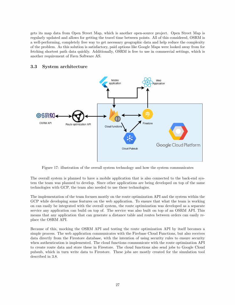
Figure 17: illustration of the overall system technology and how the system communicates

The overall system is planned to have a mobile application that is also connected to the back-end sys-tem the team was planned to develop. Since other applications are being developed on top of the sametechnologies with GCP, the team also needed to use these technologies.

The implementation of the team focuses mostly on the route optimization API and the system within theGCP while developing some features on the web application. To ensure that what the team is workingon can easily be integrated with the overall system, the route optimization was developed as a separateservice any application can build on top of. The service was also built on top of an OSRM API. Thismeans that any application that can generate a distance table and routes between orders can easily re-place the OSRM API.

Because of this, mocking the OSRM API and testing the route optimization API by itself becomes asimple process. The web application communicates with the Firebase Cloud Functions, but also receivesdata directly from the Firestore database, with the intention of using security rules to ensure securitywhen authentication is implemented. The cloud functions communicate with the route optimization APIto create route data and store these in Firestore. The cloud functions also send jobs to Google Cloudpubsub, which in turn write data to Firestore. These jobs are mostly created for the simulation tooldescribed in 3.8.

27

3.3.1 Web application and Firebase entity system

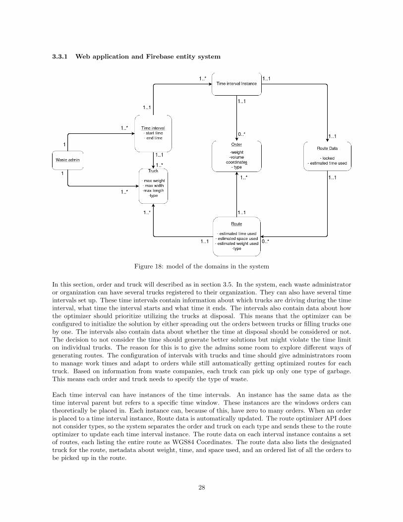
Figure 18: model of the domains in the system

In this section, order and truck will described as in section 3.5. In the system, each waste administratoror organization can have several trucks registered to their organization. They can also have several timeintervals set up. These time intervals contain information about which trucks are driving during the timeinterval, what time the interval starts and what time it ends. The intervals also contain data about howthe optimizer should prioritize utilizing the trucks at disposal. This means that the optimizer can beconfigured to initialize the solution by either spreading out the orders between trucks or filling trucks oneby one. The intervals also contain data about whether the time at disposal should be considered or not.The decision to not consider the time should generate better solutions but might violate the time limiton individual trucks. The reason for this is to give the admins some room to explore different ways ofgenerating routes. The configuration of intervals with trucks and time should give administrators roomto manage work times and adapt to orders while still automatically getting optimized routes for eachtruck. Based on information from waste companies, each truck can pick up only one type of garbage.This means each order and truck needs to specify the type of waste.

Each time interval can have instances of the time intervals. An instance has the same data as thetime interval parent but refers to a specific time window. These instances are the windows orders cantheoretically be placed in. Each instance can, because of this, have zero to many orders. When an orderis placed to a time interval instance, Route data is automatically updated. The route optimizer API doesnot consider types, so the system separates the order and truck on each type and sends these to the routeoptimizer to update each time interval instance. The route data on each interval instance contains a setof routes, each listing the entire route as WGS84 Coordinates. The route data also lists the designatedtruck for the route, metadata about weight, time, and space used, and an ordered list of all the orders tobe picked up in the route.

28

3.4 Testing, integration and deployment

The team decided to implement unit tests and use both continuous integration and continuous deploy-ment. The unit tests were made in Rust and tested that all route optimization heuristics worked asintended. Passing the tests would mean that only legal actions were performed on the solutions; in thisway, the team could trust the result. There is also an integration test that checks if the route API isstable. The test sends a standard http request with a data set of trucks and orders to the main endpointfor route generation on the server, and checks if the response is valid. The test also calculates the totaldistance of the solution it receives. These tests were also connected to Github Actions, which can performcertain actions if a success criterion is met. The continuous integration part of the workflow is then thatall the tests are run on Github on the latest commit to see if the latest version is stable or not. Inaddition, the team also used a Github action that listened for commits on the Dev branch. If there wasa commit and it passed all the tests, the results were deployed on a development server that Favn hasaccess to. This was agreed upon with Favn to have an overview of our progress and give feedback on thecompleted features. Only completed features were pulled into the dev branch to ensure that Favn couldinspect a stable version. This continuous deployment would be healthy for the cooperation between theteam and Favn.

3.5 Trucks and orders implementation

Orders have been mentioned many times so far, but this shall be clearly defined before the implementa-tion of the algorithms are discussed. An order is associated with a geographical coordinate, a weight, andsome volume. The order represents something someone wants to be picked up by a truck; that is, a truckneeds to travel to where the order is placed and pick it up. The coordinate is a basic pair of latitude andlongitude, which is where it should be picked up. The weight and volume describe the thing to be pickedup itself, and this is taken into consideration because they are the limiting factor for the trucks to be used.

What exactly is meant by truck shall be fleshed out now. All the algorithms take in a parameterwhich is the set of trucks that can be used. These trucks can be different. Each truck has the followingattributes clearly defined; a max weight, width, and length of the truck’s cargo space. In addition to this,the trucks are assumed to have the same starting point; this is where all the orders should be returned

3.6 Graph compression and representation

The input to all the optimization algorithms is, as stated earlier, the set of orders and trucks. To runany variant hill climbing, the state must be clearly defined. A state is a current solution; that is, all theorders are distributed in some way among the trucks without breaking the weight or space constraints.Before the actual optimization algorithm is run, all the orders are sent to the OSRM service to retrievethe shortest path matrix. This matrix stores the shortest path among all pairs of orders. This matrixrepresents a complete graph (all nodes are related to all other nodes). From now on, the program willwork with this graph. The graph has thus been simplified from the entire road network of the city intoan n by n matrix where n is the number of orders plus one for the starting point of the trucks. Thiswill make all future path computations very fast as one can find the shortest path between two orders inO(1) time. This compression is lossless in the sense that one always wants to drive between these pointsin the final route, so no critical data is lost.

When working with routes, one has to decide how to represent a path in the graph. All the pathsthat the trucks will drive start and end in the same place; in graph theory terminology, this type of pathis known as a circuit. These circuits only visit each node/order once, so the team decided to store thepaths simply as a list associated with a truck. This list contains all the orders to be picked up by theassociated truck. This was chosen because it is then easy to see which orders a truck should pick upand because a list is ordered. Due to the inherent order of a list, information can be extrapolated aboutthe path. Since one always drives to and from an order only once, one can assume that there is an edge

29

between consecutive orders in the list. With this assumption, a truck always starts at the first order inits list and then visits the second, then the third, and so on. Note that there is an extra edge from thelast element of the list back to the first one to complete the circuit.

3.7 Visualization tool

As part of the system, it is necessary to have tools to visualize and communicate the route that isgenerated. Without such tools, the route optimizer would not be usable for practical purposes. Thegenerated route is a list of latitudes and longitudes and would therefore be incomprehensible without avisualization. Such a tool is also useful when testing out different algorithms. When visualizing a route,it is often possible to see whether the route makes logical sense or not. If the route does not make sense,it is likely something wrong with the implementation of the algorithm.

Figure 19: Example of visualization of a set of routes

The visualization tool is part of the front-end part of the system and is built on top of Google Maps.It provides a series of different functionalities for the user. It displays all the different routes for thechosen time interval by color-coded lines. Each route is coded by color, and the relevant information forthat route is displayed on the right. This includes information such as space used by each truck, weightused, how much time is used and what type of waste that truck collects. Each order in each route isalso enumerated based on the order the truck will drive. Information about a given order is accessible byclicking on it, displaying a popup with information about the given order, such as an address, postcode,weight, volume, latitude, and longitude. Part of the tool is also the functionality for adding new ordersto the route. It is possible to place a marker anywhere on the map, then input the weight in the top leftcorner and then send it to the route. This will trigger a cloud function that will generate a new set ofroutes that includes the new order.

30

3.8 Simulation tool

Another functionality implemented in the system is the ability to run simulations on the routing algorithm.This is a useful function for companies to simulate what impact a potential change might have. Forexample, simulating the impact of acquiring a new truck will have on fuel and time use over a year. Sucha tool could guide a company on what changes might be beneficial economically and environmentally.

(a) A form where the user can specify the attributesof the report

(b) Dashboard with a graph displaying the totaltime used for the different simulations per day

Figure 20: The simulation report tool

In the UI, one is presented with a form where it is possible to specify all of the following parameters:

• Length of simulated time-span

• Time limit of a route

• Daily order frequency

• Number of trips per week

• Area the generated orders are in

• Number of extra trucks

• whether to prioritize distributing the orders evenly when clustering

When the attributes have been chosen and sent, the routing server will run the algorithm for all the daysin the given time frame. All the different attributes specified by the user are taken into consideration.After the simulation is done, the user is presented with a dashboard displaying the results. Among otherthings, it is then possible to see what effect the different choices have on the time used. In figure 20, thestandard route is marked by the blue line, and the route with the additional truck is marked with thegreen line. In this case, the standard route uses less time than the route with more trucks, with somedays there being quite a big difference. Therefore for this scenario, the additional truck might not bethat beneficial.

31

3.9 Hill climbing implementation

The hill climbing algorithm implementation needs a starting solution to begin the local search. It uses anearest neighbor clustering method to very quickly create a route satisfying the weight and space limita-tions. Note that the time limit constraint can be broken in this starting solution. The reason for usinga clustering algorithm and not just a completely random solution is that a better starting solution willrequire fewer iterations to converge, making it faster.

The algorithm takes a parameter that dictates the max amount of iterations that will be run. Aniteration consists of generating all conceivable improvement heuristics, performing them if they reducethe total travel time while respecting the weight and volume constraints. Generating all conceivable im-provement heuristics means trying all pairs of indices in the same route of a truck and using those as thestarting points for all the intra-route heuristics, or all pairs of indices of different routes as the startingpoints for the inter-heuristics. The algorithm also keeps track of whether an improvement has been madein this iteration. This way, it can terminate when it has completed the maximum number of iterations orrun a whole iteration without improving. This can safely be done as one would be guaranteed not to findan improvement in any of the subsequent iterations anyway. All the heuristics are generated in the sameorder each time, and the clustering phase depends on the order that the trucks are received. Thereforethe algorithm is completely deterministic.

Note that there exists a problematic edge case without allowing the trucks to drive multiple trips withinthe time limit. Imagine that there are many orders right next to the depot, but they are so heavy thata truck can only drive one order at a time. In this case, the trucks can drive back and forth within thetime limit, but multiple trips are usually not allowed in default implementations. This will make thealgorithm unable to find a valid solution. The team came up with a trick to solve this without increasingthe complexity. By copying the trucks, each of the copies can have its own circuit. To validate whetherthe set of trucks constitute a valid solution, one has to summarize the distances traveled by the differentcopies of the same car to make sure it can make all the trips within the time limit; everything else willwork as normal. This trick is implemented in the hill climbing algorithm and in the simulated annealingone, but not for AILS as it has its own mechanism for adjusting the number of trucks to use.

3.10 Simulated Annealing implementation

Equivalent to the hill climbing implementation, the starting solution of SA is based on the deterministicnearest neighbor clustering algorithm. The simulated annealing implementation takes in two parameters,starting temperature and cooling factor. The starting temperature will dictate just how exploratorythe algorithm is, especially in the beginning. The cooling factor reduces the temperature over time; thealgorithm terminates when the temperature has reached 1 degree. Each time the temperature is decreased,a random heuristic move is generated, which is a suggestion for a change in the current solution. Thechange to be analyzed can be any conceivable move as described in the theory section of TSP and CVRP.The total distance of the current and candidate solution is calculated and feed to equation 9 to calculatethe chance of making a move. The equation states that all improvements should be performed. If thetemperature is high, or the move is only somewhat bad, then there is a chance to perform the move toexplore more of the search space. Additional restraints still hold; changes in the solution must respectthe weight and space limits of the truck.

3.11 Adaptive Iterated Local Search implementation

The Adaptive Iterative Local Search implementation is based on the AILS algorithm explained in [5].The implementation of the team is written in rust on the route-optimizer service in the system of theteam. The paper describes an AILS algorithm for the CVRP explained in 2.4.4. The implementation isdifferent in that the problem of the system is not directly the CVRP described in 2.2.2, but a problemwhere the vehicles can have different weight and space constraints. The vehicles also have a potential

32

time constraint that is the same for all cars, but each order can be picked up by any truck. For thesereasons, the team tweaked the AILS implementation to fit their application.

3.11.1 Summary of the implementation

The algorithm creates an initial solution using proximity clustering described in 2.3.2.After getting an initial solution, which might not be feasible based on the time, space, and weightconstraints, the algorithm uses a feasibility heuristic to find the closest feasible solution. After this pre-process, the iterations start. In each iteration, the algorithm perturbs the current reference solution.This means that it swaps up the orders in the solution and creates a different and potentially infeasiblesolution. With this perturbed solution, it runs it through the feasibility heuristic again to find a feasiblesolution. After getting a feasible solution, it performs a neighborhood search to find a local optimum, atemporary best solution. The algorithm performs acceptance criteria to see if this new solution shouldbe set as the reference solution for the next iteration. The algorithm also updates some parameters forthe perturbation step to make this step adapt to the results of previous iterations. If the solution isbetter than any other solution found in a previous iteration, it is saved as the current best solution. Theiteration repeats until the max amount of iterations is run and returns the best solution found. Theoverall algorithm is described in Algorithm 5

3.11.2 Initial clustering

The initial clustering in the implementation calculates the minimum amount of needed trucks based onweight, initializes empty routes using the calculated amount of trucks needed, and randomly assigns eachroute in one order. The rest of the orders are then inserted based on proximity. The implementationis just like the one described in 2.3.2. It does not consider the additional constraints in the problemat hand, as the initial solution does not need to be feasible. The initial solution needs only be quicklygenerated and somewhat reasonable.

3.11.3 Perturbation

A perturbation step is needed in an iterative local search. The algorithm should explore different parts ofthe global scope to find in an attempt to find the global optima and not just find the first local optima asa solution. A perturbation step perturbs the current reference solution in an iteration of the algorithm byremoving orders from routes and inserting them differently. This potentially creates a solution far enoughaway from the reference solution that the algorithm can potentially find another local optimum than theprevious iteration. The AILS implementation uses the removal and insertion heuristics described in 2.4.3to perturb a solution. This step in the algorithm also does not require a feasible solution but actuallypotentially transforms a feasible solution into an infeasible one. Because of this, the implementation ofthis step is the same as with the CVRP. The implementation is described like this:

Algorithm 1 Perurbation Procedure

Data: Solution s and removal heuristic Hr

Result: Solution s′

s′ ← sRemove random route with probability 1/γ as long as m ≥ mRemove ωHr orders from solution s′ based on heuristic Hr

Randomly select an insertion heuristic Ha1 , H

a2 and add all removed orders with the heuristic

In the perturbation algorithm, Ha1 , H

a2 are the insertion heuristics described in 2.4.3.4 and 2.4.3.5.

Hr is an assigned removal heuristic described in 2.4.3.2, 2.4.3.1 or 2.4.3.3. ωHr is an integer related tothe removal heuristic that decides how many orders will be removed from the solution. γ is a constantcalibrated by the team based on testing results. m is the estimated least amount of routes needed to geta feasible solution.

33

3.11.4 Neighborhood search

The neighborhood search explores the neighborhood and tries to find the local optima closest to thesolution it optimizes on. The neighborhood search also includes a feasibility heuristic that looks formoves with high feasibility gain and requires having a feasible solution before it finishes optimizing. Theimplementation of the neighborhood search is different from the one described for the CVRP, as thefeasibility heuristic has to account for several constraints. The feasibility search algorithm is describedlike this:

Algorithm 2 feasibility heuristic

LM ← ∅repeat

foreach RSi ∈ Routes doUpdate LM(RSi , LM, s)

endwhile |LM | > 0 do

Find the inter-route move mov between route RSi and RSj resulting in s′ in LM with highestfeasibility gains← s′

remove all moves from LM involving the routes RSi RSi

Do intra-route local search to routes RSi and RSjUpdate LM(RSi , LM, s) and Update LM(RSj , LM, s)

endif s is infeasible then

Add a new route Routes ← Routes ∪ RSm+1 with the truck Ti that has used the least amount oftime.

end

until s is feasible OR it > itmax

The algorithm for updating the list of moves LM is described like this:

Algorithm 3 Update LM

Data: Rsi , LM, sResult: Updated LMforeach vik ∈ RSi do

foreach vjl ∈ δ(vik)|i 6= j and RSi and RSj meet feasibility condition described in equation 10 doforeach inter-route move heuristic Nk ∈movement heuristics do

if Nk gives a solution s′′ that respects condition 12 then

if ∃ (move between vik and vjl ) ∈ LM but s” has higher feasibility gain then

replace move between vik and vjl in LM with new moveend

if @(move between vik and vjl ) ∈ LM then

LM ← LM∪ (move between vik and vjl using move heuristic Nk)end

end

end

end

end

δ(vik) is the set of orders closest (by proximity) to RSi

34

the movement heuristics are the ones described in 2.4.2.6, and 2.4.2.5, 2.4.2.9

slack(RSi ) ≥ 0 XOR slack(RSj ) ≥ 0 (10)

In condition 10 slack describes a number indicating the capacity of a given route.In the implementation, this slack function returns negative if any constraints are violated: used time,weight, or space. Any violations of these constraints are summed up using the real value of the constraintviolation. e.g: if a route uses a truck Ti with 50 max weight, and the orders in the route add up to60 weight, and no other constraints are violated, the slack function gives a value of -10. If time is alsoviolated, meaning the total time of all the routes RSx the truck TSi = TSx in RSi is driving, this violationis also added to the slack value. So if truck TSi has an estimated time use of 3000, and the limit is 2500,the slack adds up to -510. These values are also weighted in an attempt to balance these numbers out,valuing time, space, and weight equally.

The feasibility condition for a given move candidate can be described using the teams implementation offeasibility gain:

Ω(s, s′) = min0, slack(Rsi′)+min0, slack(Rsj

′) −min0, slack(RSi ) −min0, slack(RSj ) (11)

Ω(s, s′′) > 0 (12)

Equation 11 calculates a number indicating the feasibility gain by getting the difference in slack betweenthe solutions s and s′ when committing to a move between routes Ri and Rj

3.11.4.1 Local search heuristic

The neighborhood search also has a similar process to the local search process that optimizes a feasiblesolution. The process is very similar to the feasibility heuristic, except some of the conditions are differ-ent.In the update LM algorithm for the local search heuristic, every other route is considered when consider-ing move candidates as no route should have a slack() value under 0. Candidate moves must also resultin a shorter total distance, as well as having positive feasibility gain (condition 12). This is to explorethe neighborhood for better solutions without finding infeasible solutions.

3.11.5 Acceptance criterion and adaptivity

For the algorithm to be adaptive, there is an acceptance criterion that manages the reference solutionused in each iteration of the algorithm. There is also a system for updating the ω values for the removalheuristics described in 2.4.3. The implementation of these systems is similar to those explained in [5] asthey as well do not account for feasibility in any way, making it the same for the thesis problem. Becauseof this, the implementation of the acceptance criterion is described in 2.4.4.The update of the removal heuristic ω values is implemented like this:

35

Algorithm 4 Update ωHrkData: Solutions s and sr, itHrk , dHrk , dβ and nResult: Updated ωHrkitHrk ← itHrk + 1

dHrk ←dHr

k(itHr

k−1)+d(s,sr)

itHrk

if itHrk = γ then

ωHrk ←ωHr

kdβ

dHrk

ωHrk ← minn,max1, ωHrkitHrk , dHrk ← 0

end

itHrk describes the number of times the removal heuristic has been used since the last time ωHrl was up-dated. dHrk is the average distance between local optima found by the removal heuristic and the referencesolution sr since the last update of ω. dβ and γ are, in this case, constant integers with a value calibratedby the team based on testing. n is the number of orders in the solution.

Algorithm 4 updates the omega value for one specific removal heuristic Hrl . The goal of this algo-

rithm is to compare the current solution with the reference solution from before the iteration and give ωa new value based on this.

3.11.6 The algorithm

The team combines all the parts described in 3.11.2, 3.11.3, 3.11.4 and 3.11.5 to create an AILS algorithmtailored for the teams task and system. The overall algorithm is quite similar to the one described in [5],but tweaked to fit the custom CVRP the team is tasked with.

Algorithm 5 AILS

Data: orders, truck data, time limit per truckResult: Best solution s∗

sr ← Initial solution from initial clustering described in 3.11.2sr, s∗ ← feasibility heuristic(sr) - as described in Algorithm 2it← 1 repeatHr ← Choose a random removal heuristic Hr ∈ Hr

1 .Hr2 , H

r3 - described in 2.4.3.1, 2.4.3.2 and

2.4.3.3s← Perturbation procedure(sr, Hr) - as described in Algorithm 1s← feasibility heuristic(s) - as described in Algorithm 2s← Local search heuristic(s) - as described in Algorithm 2 using tweaks explained in 3.11.4.1.Update ωHrk - as described in Algorithm 4sr ← Apply from s based on acceptation criterion as described in 2.4.4if s is a better solution than s∗ thens∗ ← s

endit← it+ 1

until it ≥ itmax;

3.12 Run time experiments

To experimentally test the solution quality and run time of the different algorithms, the team has run aseries of tests. All the tests were run on a Google Cloud virtual machine. The VM is running on a 2.00GHz Intel Xeon CPU. The results shown are an average from running 50 tests in three different cities

36

(Oslo, Trondheim, Tromsø). Each test is to optimize a route that picks up all the orders. The set oftrucks are the same throughout all the tests, although the generated trucks themselves do not need tobe identical. All trucks need to return to the starting point within a 6-hour time limit for the routesgenerated. The 50 requests sent are unique, but the same set is sent to the same city during the sameiteration for all the algorithms. This is done so that the results are comparable as each algorithm tries tofind a route based on the same orders and trucks. The orders are generated on the spot, the number ofsections and weights used in the order are random within a limit. The weights for each order are between1 and 100, but have a ten percent chance of being ten times larger. The reason for this randomness isbased on information from waste companies, saying that about 1 in 10 waste pickups are much largercontainers of waste. The sections used for each order is a random amount between 1 and 5. The mostimportant thing is that the weight and space usage was generated so that both can break the constraintsof a car, meaning that the improvements must carefully balance both constraints.

The requests are sequentially sent to the route optimization server; note that the run time is calcu-lated on the optimization server to avoid tracking the network lag. The timer used is from the ’time’module of the standard Rust library. What is referred to as distance in the result section is the totaldriving time of all the trucks; this is the ”distance” metric that the algorithm minimizes. The purposeof the experiment is to experimentally show how the different proposed algorithms scale with regard tothe number of orders, the number of iterations, and how that affects the quality of the solution. Forthis reason, there is more than one test for each algorithm; HC and AILS are tested with 1, 5, and20 iterations to see how run time and solution quality scales with the number of iterations. The SAalgorithm is always run with a starting temperature of 100 degrees as it was tested to give good results,and the cooling factors are 0.9999, 0.99998, and 0.999996. The AILS takes two parameters more thanHC, namely k, which is set to 0.5, and γ, which is set to 10. All of the parameters were selected as theyseemingly yielded the best results.

3.13 Distribution of roles

The role distribution for the development of the product was not very established. This means thatevery team member worked on most aspects of the product, but some worked more on specific areas thanothers. However, the role distribution for the process was very specific. The roles were distributed likethis:

• Havard Stavnas Markhus: For system development focused on system architecture, automation,system structure, testing, and backend development. Responsible for setting up meetings and beingchairman in these meetings.

• Tobias Meyer Andersen: For system development focused on backend development, algorithmresearch, and algorithm development. Responsible for writing meeting reports and quality assurancefor documents.

• Kjerand Evje: For system development focused on front-end development, Responsible for structur-ing documentation and making sure documents are available to whomever the document concerns.

37

4 Results

4.1 Scientific results

4.1.1 Hill climbing results

HC 1 iteration 5 iterations 20 iterationsorders/trucks run time(ms) distance(s) run time(ms) distance(s) run time(ms) distance(s)

10/2 35.0 7604.0 40.0 7480.3 40.3 7480.325/3 56.0 17316.3 90.3 16946.3 91.3 16946.350/4 103.7 32977.0 213.3 32511.0 223.7 32503.799/6 218.3 62010.0 487.3 61476.3 500.0 61470.3

4.1.2 Simulated Annealing results

The starting temperature for all SA runs was 100 degrees. CF is an abreviation for cooling factor.

SA cf=0.9999 cf=0.99998 cf-0.999996orders/trucks run time(ms) distance(s) run time(ms) distance(s) run time(ms) distance(s)

10/2 56.7 7501.0 223.3 7441.0 1056.0 7427.025/3 64.0 17200.0 235.3 16901.7 1092.7 16754.750/4 76.3 32971.7 251.7 32457.3 1260.0 31973.099/6 107.0 62320.3 289.3 61646.0 1199.3 60805.7

4.1.3 Adaptive Iterated Local Search results

AILS parameters: k = 0.5, γ=10

AILS 1 iteration 5 iterations 20 iterationsorders/trucks run time(ms) distance(s) run time(ms) distance(s) run time(ms) distance(s)

10/2 18.3 7422.3 27.7 7370.7 56.0 7349.325/3 64.0 16700.0 115.3 16524.0 283.3 16384.750/4 248.0 32048.0 481.0 31646.0 1381.0 31373.399/6 1375.7 60899.0 2648.0 60115.7 7129.0 59353.3

4.2 Engineering professional results

4.2.1 Final product overview

The overall goal of the project was to develop a route optimization engine with an administrative webapplication for waste collection companies. The administration tool would have access to route generationfor waste collection orders coming from a mobile app for waste collection customers. Orders would comein from paying users, and waste administrators would manage these orders and have routes generated forpicking these up optimally. The task initially had a vast scope, and the plan was for the team to choosewhich parts to focus on. The team focused on developing the routing engine and prioritizing this butdeveloping some key features to the administration application. The final product has a competitivelyfast routing engine with the route optimization API built with Rust and Actix web on top of the OSRMAPI. The engine is also open for utilizing more sophisticated algorithms for close to optimal solutionswith the drawback of longer run times and worse scalability in regards to the number of orders. Therouting performance of the routing engine is extensively experimented with and tested, giving the teama good indication of how the engine performs in different situations using different algorithms. The teamalso built some key features in the web application and firebase that utilize the routing engine, includingtruck management, a simulation tool for the route generator, and visualization of the routes.

38

The system was built in Google Cloud Platform, which merges well with the mobile application built ontop of firebase and the rest of the project the team did not focus on. The system is also horizontallyscalable as the routing engine, and OSRM API is stateless and dockerized. The OSRM API is config-urable for different countries by initializing the API using different map files. This makes the systemconfigurable for other countries as well as the intended country, Norway.

4.2.2 Functional requirements

In this chapter, how and in what way different functional requirements defined in the vision documentwere met will be described. The order is the same as in the vision document. Recall that the visiondocument was intentionally somewhat over-ambitious so the team could have some freedom in decidingwhat part of the system to develop based on personal interest.

4.2.2.1 Authentication system

As the focus of the project was mostly centered around algorithmic optimization, it was both unnecessaryand unnatural to spend time developing an authentication system that would restrict the usage of theoptimizer to only those with access. This was agreed upon by all parties.

4.2.2.2 Interactive front-end showing the orders

The team implemented functionality to view data of the orders when accessing a time interval instance,as this was the most important feature while developing the optimization engine. The orders are storedand used in the system but do not have relevant, interactive components, as this was deprioritizedafter discussing with Favn and the team. The feature was originally planned as a feature the teamwould implement in the roadmap. However, later in the development of the system, the team and Favndecided that the team would focus on key parts of the front-end system that helps reinforce testing theoptimization engine. This resulted in the deprioritization of the feature.

4.2.2.3 Communication from waste company to users app

This was also looked away from as the user part of the system was not central to the project; this wasagreed upon by all parties. The feature is not at all related to the route-optimization, and therefore notprioritized in the same way as other features.

4.2.2.4 Generic route optimization

The goal stated in the vision document was to create a generic route optimizer that takes into consid-eration space, weight, and time. This criterion was met by creating a route optimizer that takes intoconsideration the weight and space limits of the trucks. It is general in that it can be applied for varyingamounts of trucks. It is not limited to some specific geographical location; it also works for a varyingnumber of orders and any starting point for the trucks. The algorithm that was finally chosen for theoptimizer was HC.

4.2.2.5 Estimating time and fuel use, number of trips required

The route optimizer creates metadata for estimated time for each route and estimated total time usedfor all routes. Estimated fuel use is not implemented, as the team and Favn agreed to focus on the timemetric provided by OSRM and optimize based on this. The route optimizer API supports giving thesame truck several trips if necessary. All implemented optimization algorithms take the possibility of onetruck driving several trips into consideration.

39

4.2.2.6 Displaying information about space and weight used in trucks

The web application implements this feature by showing the estimated time, space, and weight used foreach route in the same component that shows the generated routes on a map. The page indicates whichroute on the map refers to which route information using color-coding.

4.2.2.7 Possibility to change how many trucks a company has available

This criterion was also met. Users now have front-end access to both add and remove trucks. Thesetrucks are given to the route optimizer when creating the route, as also specified in the vision document.

4.2.2.8 Simulation tool to optimize use

The original criterion was for the simulation tool to determine what sort of parameters or adjustmentswould give the best route generation over time. However, the team did, during meetings throughoutthe project, agree that it would be satisfactory to have a simulation tool that would allow the user totest different parameters and simulate how they would affect the routes over time. This was solved withthe simulation report function, where users can analyze route trends over long periods of time. Theuser can test things such as the impact of adding more trucks, area of service, prioritizing filling onetruck up before using another, how much load would be expected in the time period, and how long ofa period to simulate. The user can also control the time limit, which is analogous to the length of aworking shift but can also choose to look away from a time limit altogether. All of this combined lets theuser explore different ways to run their pick-up service in order to understand what the data suggestswould be beneficial in terms of route length and truck usage. They would also receive feedback if someroutes were not possible to be generated due to no route being found that satisfies the time/weight/spaceconstraints.

4.2.3 Non-functinoal requirements

Favn Software AS had two non-functional requirements of the final product, both described in the visiondocument. The first one was to use Firebase as a back-end solution. This requirement was made asthe company primarily uses this and has experience with it, and thus they could, as the further work,merge it with the front end part of the user application. This requirement was met, as made clear earlier.The other non-functional requirement was to use either Vue or React as a front-end framework. Thisconstraint was created for a similar reason, as they would more easily allow Favn to develop the productfurther later. As also made clear earlier, the team chose to use React to develop the front-end.

4.3 Administrative results

During the completion of this project, different development tools were utilized to ensure that the processwas kept systematic. This involved using a sprint-focused development method based on the roadmapmade at the start of the project. The project was also documented by status reports, time-sheets, andstatus meeting logs throughout the project.

4.3.1 Work schedule plan

The work schedule on the project was based on 2-week long sprints. This schedule was kept by the teamthroughout the project. In the roadmap, it was set up to be nine sprints in total, all of which werecompleted. There was some variation in the amount of work done and time used on each sprint. Aspeople on the team were busy with other subjects at university and other work, the team used less timeon each sprint at the start of the project than at the end. The workload steadily increased from the startin January until the completion in May.

40

4.3.2 The development process

As mentioned, the team focused on a lean and iterative, sprint-focused development process. All the teammembers were familiar with and had experience in using Scrum beforehand, so the team quickly becameefficient in using this development process. The sprints lasted two weeks each, with some exceptionsat the end of the project. Each sprint was concluded with a sprint planning meeting where the teammet with Favn to discuss the previous sprint and plan the next sprint. During these meetings, the teamcontinually got feedback on the product, and as the product evolved, the demands for the product alsoevolved. The team planned the first seven sprints in the road-map for developing the product and thelast two sprints for writing the paper and finishing up on documentation.

After the product was finished, the team and Favn came to an agreement it would not be necessaryto continue the sprint planning meetings, as Favn was only involved in the development of the product.The team was also successful in using a task board for managing what tasks needed to be done, whattasks were ongoing, and what was finished. At the start of each sprint, the team reviewed the task-boardand added the new tasks that would be necessary to achieve the goals for the coming sprint.

Covid-19 also had some impact on the development process. This resulted in that quite a lot of thework on the project was done remotely and over voice chat instead of meeting in person and working. Allthe sprint planning meetings where held over video chat as well as all the meetings with the supervisor.Favn opened up the possibility of using their offices for the project once a week, which the team oftenutilized. In the last few weeks of the project the team could meet more often and Favn had more freespace in their offices, which led to working more in person when completing the project.

41

5 Discussion

5.1 Scientific results

What the thesis is trying to explore is ”How do different versions of hill climbing compare when adjustedto solve the capacitated vehicle routing problem with time limits on realistic map data.” To answer thisquestion, three different forms of hill climbing were implemented. The simplest one is the standard formof hill climbing, another one taking the probabilistic approach of simulated annealing, and a third onebuilding on a more sophisticated series of hill climbs. The algorithms were tested using 150 orders fromdifferent cities, using real coordinates and addresses from Open Street Map. It was then tested both howthe algorithms scale with regard to the number of orders and compared to the number of iterations/howlong the algorithms get to run. The grounds on which the algorithms shall be compared are explainedas the metrics used are discussed in the next paragraph.

5.1.1 Experiment metrics

Ass seen in tables of 4.1.1, 4.1.2, and 4.1.3 the metrics measured were run time and distance.

Run time is, as stated earlier, calculated on the rust server; it represents the time it takes for theoptimization algorithm itself to run. The time is measured in ms and is, as states before, an average from50 requests for the same amount of orders in three different cities to increase the empirical foundation ofthe results. The time measured is a central metric because it uncovers how well an algorithm scales inpractice. An algorithm can also have a different application based on how fast or slow it is.

Some trouble was encountered when measuring the time of the execution. Under the heavy tests, whichlasted more than one or two minutes, the algorithm seemed to perform very poorly. On closer inspection,the Google Cloud interface showed that the CPU usage went down, even though the program was notfinished. This could be due to OS deprioritizing a long-lasting process or due to hardware limitationsthat, for instance, slowed down the process to avoid generating too much heat. In any case, the teamhandled this by having the program that sent the requests to sleep between them; this seemingly fixedthe program and decreased the run time drastically. This was, however, not done on all the tests, as theless computationally heavy ones did not seem to suffer in the first place; this issue could have producedsome inconsistencies by increasing the run time.

Distance in time or the total amount of driving time to complete the route was the other recordedmetric. This data is based on OSRM data of how long it would take to drive the sequence of orders ofeach car, adding 300 seconds per order to give time to pick up the items in the order. This metric decidesthe quality of a solution, as the total driving time should be minimized.

5.1.2 Other notes on the experiment

This paragraph shall highlight some questions that might be raised in relation the run time experimentsconducted.

Firstly, lets address why there is no comparison to exact solutions and other benchmark solutions. Thesequestions are both answered by recalling that the exact problem to be solved for Favn is not the stan-dard form of CVRP. Most importantly, the problem at hand features two different capacity constraints(weight, and space) in addition to the time limit. This is not the case for the more common problemwhich only has one capacity constraint. Due to this the experiments are not truly comparable with otherbenchmark solutions that solve that problem. In addition this prevents us from using common data-setsused for benchmark purposes as they do not feature the necessary data for this application. This limitsthe thesis to only using its own implementations as a ground for comparison. For the simpler cases onecould feasibly brute force the exact solution, but as that would at best only be done for the simplestcases. The team therefore chose to be consistent and only compare the different solutions found by their

42

own implementations to each other. Had the problem at hand been the standard the team could alsohave used common benchmark data-sets with known exact solutions. This does limit the conclusion toonly answering which of these techniques are better than the others that were implemented, one can notdeduce how good these solutions are in absolute terms.

Secondly, lets address why the data-sets stop at 99 orders, and why the amount of orders per car staysabout the same through all the test cases. The limitation of 99 orders is unfortunately limited by theconfiguration of the OSRM server that the team has running to answer requests. This was not fixablewithin the deadlines used to guide the project. Therefore the team had to accept that the experimentcould not feature a test case using 250 orders that was originally planned. Having 250 orders would besignificant to verify how the algorithms scale on bigger problem sets. This would particularly have beenvaluable to distinguish HC implementation of 5 and 20 iterations as will be commented in 5.1.3. Lastlylets address why the number of orders per truck is more or less the same throughout the tests. Thepurpose of this thesis comes from real life applications of collecting items and returning them to a singleplace within a workday. The time limit used in the experiment was 6 hours. Due to this the team placedsome limitations on how many orders there were compared to the number of trucks. The team ran sometests of their own and noticed the routes could not always be generated within this limit when one gotclose to 20 orders per truck. Therefore the team stayed clear of this limit in the experiment to ensurethat valid routes always were found. Other than that the team did not aim for some exact ratio besidesalways making sure there were more than one truck to make it a true vehicle problem.

5.1.3 Hill climbing

(a) Graph showing the run time of HC comparedto the number of orders

(b) Graph showing the distance of HC solutionscompared to the number of orders

Figure 21: Results of HC graphed and compared to number of orders.

Lets first consider the run time of the HC algorithm using a different number of iterations. It can be seenthat the run time is virtually the same when using 5 and 20 iterations, this is caused by the algorithmterminating as soon as a local optima is found. This means that even though the max limit was set to 20iterations it rarely needed to run more than 5, so computationally they are almost identical for datasetsof this size, with similar constraints on the truck. 1 Iteration clearly distinguishes itself as much moreefficient, having significantly better running time on the heavier test cases. Interestingly its total distancein the largest test case is still less than a percent worse than the 20 iterations version although it usesmore than half the time. So altough a 250 order test set might have separated the 5 and 20 iterationversion a bit better it probably would not have a big relative impact on the distance results.

43

5.1.4 Simulated Annealing

(a) Graph showing the run time of SA compared tothe number of orders

(b) Graph showing the distance of SA solutionscompared to the number of orders

Figure 22: Results of SA graphed and compared to number of orders.

The SA algorithm looks for the same amount of possible moves to improve the solution regardless of theamount of orders. This is because the amount of moves to consider solely depends on starting tempera-ture and cooling factor. This is supported by the graph above showing that the run time does not seemto depend significantly on the amount of orders. The different cooling factors still have very differentrun times, and provide somewhat different results in regard to the quality of the solutions. At most theworst solution is 3.1% worse than the best (50 orders, 4 trucks). SA is very scalable in terms of run time.Despite this it seems reasonable that the solution quality will eventually drop off in large enough cases.This is expected as some very large cases will require the use of so many heuristics to produce a goodsolution that it its unlikely for the SA to generate them all without having a slower cooling factor. Aswill be discussed later this ceiling for the SA is not yet reached in our test cases.

One thing that is worth mentioning is the anomaly in the version of SA with the highest cooling factorThe run time is not the highest for the highest amount of orders, he most reasonable explanation for thisis the run time issue on the VM described in 5.1.1.

44

5.1.5 Adaptive Iterated Local Search

(a) Graph showing the run time of AILS comparedto the number of orders

(b) Graph showing the distance of AILS solutionscompared to the number of orders

Figure 23: Results of AILS graphed and compared to number of orders.

As clearly seen in the figure the AILS scales unfavourably. From the second last text case (50 orders, 4trucks), to the last (99 orders, 6 trucks), the run time is a bit more than quadrupled. This suggests a runtime just over Θ(n2) where n is the number of orders. For this algorithm the different iterations makesthe biggest difference at 99 orders and 6 trucks where the worst performing solution using 1 iterationis 2.6% worse than the solution found using 20 iterations. This is an interesting result as the adaptivepart of the algorithm probably does not really get into play with just 1 iteration. With 1 iterations thealgorithm runs the clustering phase and optimizes it with a neighborhood search. After that it performsa single perturbation phase and tries to find a better solution after making one inter route change.

5.1.6 Comparison

(a) Graph showing the run time of the quickest ver-sions of the algorithms compared to the number oforders

(b) Graph showing the distance of the quickest ver-sions of the algorithms compared to the number oforders

Figure 24: Quickest version of each algorithm compared.

Lets interpret the results shown figure 24. The most clear observation to make is that AILS scalessignificantly worse than both SA and HC, and HC worse than SA. The latter is to be expected as run

45

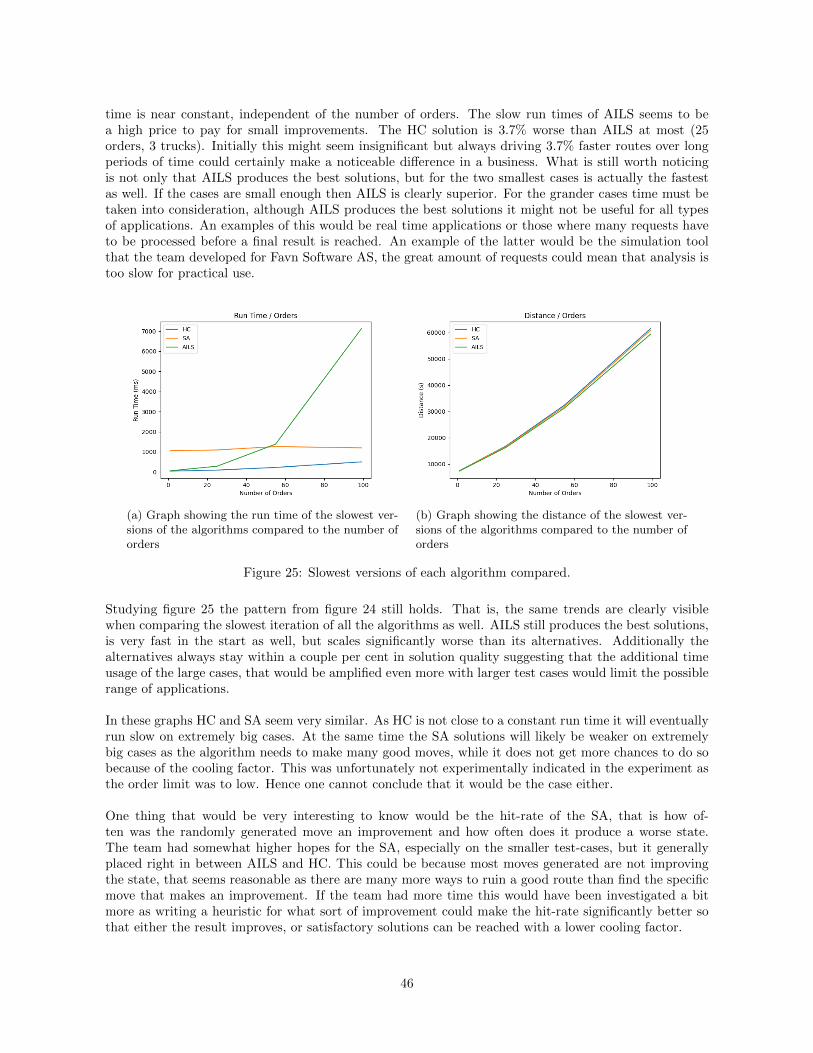
time is near constant, independent of the number of orders. The slow run times of AILS seems to bea high price to pay for small improvements. The HC solution is 3.7% worse than AILS at most (25orders, 3 trucks). Initially this might seem insignificant but always driving 3.7% faster routes over longperiods of time could certainly make a noticeable difference in a business. What is still worth noticingis not only that AILS produces the best solutions, but for the two smallest cases is actually the fastestas well. If the cases are small enough then AILS is clearly superior. For the grander cases time must betaken into consideration, although AILS produces the best solutions it might not be useful for all typesof applications. An examples of this would be real time applications or those where many requests haveto be processed before a final result is reached. An example of the latter would be the simulation toolthat the team developed for Favn Software AS, the great amount of requests could mean that analysis istoo slow for practical use.

(a) Graph showing the run time of the slowest ver-sions of the algorithms compared to the number oforders

(b) Graph showing the distance of the slowest ver-sions of the algorithms compared to the number oforders

Figure 25: Slowest versions of each algorithm compared.

Studying figure 25 the pattern from figure 24 still holds. That is, the same trends are clearly visiblewhen comparing the slowest iteration of all the algorithms as well. AILS still produces the best solutions,is very fast in the start as well, but scales significantly worse than its alternatives. Additionally thealternatives always stay within a couple per cent in solution quality suggesting that the additional timeusage of the large cases, that would be amplified even more with larger test cases would limit the possiblerange of applications.

In these graphs HC and SA seem very similar. As HC is not close to a constant run time it will eventuallyrun slow on extremely big cases. At the same time the SA solutions will likely be weaker on extremelybig cases as the algorithm needs to make many good moves, while it does not get more chances to do sobecause of the cooling factor. This was unfortunately not experimentally indicated in the experiment asthe order limit was to low. Hence one cannot conclude that it would be the case either.

One thing that would be very interesting to know would be the hit-rate of the SA, that is how of-ten was the randomly generated move an improvement and how often does it produce a worse state.The team had somewhat higher hopes for the SA, especially on the smaller test-cases, but it generallyplaced right in between AILS and HC. This could be because most moves generated are not improvingthe state, that seems reasonable as there are many more ways to ruin a good route than find the specificmove that makes an improvement. If the team had more time this would have been investigated a bitmore as writing a heuristic for what sort of improvement could make the hit-rate significantly better sothat either the result improves, or satisfactory solutions can be reached with a lower cooling factor.

46

It seems that if many large routes had to be calculated to analyse long lasting trends as fast as pos-sible SA or HC would be way to go as they scale very well. Keep in mind that solving many routingproblems quickly is a non-issue for AILS as long as the individual routes themselves do not consist ofa large amount of orders. It seems only certain specific applications would require us the sacrifice thesomewhat better routes of AILS for practical reasons. In the context of Favn Software AS one could forinstance consider calculating all actual routes with AILS, however having a simulation tool that choosesa routing algorithm that will run in a more practical amount of time, which depends on the parametersgiven by the user. So if it saw many large cases incoming it could switch to HC or SA as they would onlybe a little bit off, even in the long run.

5.2 Engineering professional results

5.2.1 Final result

As described in section 4, the team did not develop every feature in the planned project, but focused onthe routing engine while building a shell or MVP for the administrative web application and the neededback-end functionality. In early development, the team used a lot of time researching ways to optimizeon different Vehicle routing problems and how to get the applicable data needed to develop such analgorithm. The first sprints were used to plan the problem that needed solving and developing a firstiteration of the route optimization API. The team used quite a lot of time on developing a first iterationthat was not built on top of a routing machine, but instead manually tried to manage an entire roadnetwork data set in order to optimize routes. Because of this, the team wrote a lot of code that endedup not being used, as this was later replaced with a separate routing machine the team would build ontop of. The team could have saved a lot of time by starting out with this approach. However, the actof actually willing to move over to a better approach is far better than continuing development on thepotentially more time consuming approach the team was initially going for. By simplifying the problemand abstracting the map data away from the routing engine, it also follows the loosely coupled patternand makes it easy to replace any of the services.

When the team initially had a first version of the routing engine, the focus shifted over to developingthe platform for utilizing the engine. As there was not a lot of time for focusing on the web application,the team ended up focusing on core features like route visualization and the simulation tool. Whiledeveloping these tools, the team developed and improved on the routing engine and adapting on it basedon information from Favn. This way of developing worked well for the development of the routing engine,but at the cost of not being able to implement all planned features for the web application. After gettingthe simulation tool down as planned with the road map and iteration over the road map during devel-opment, the team decided to continue development on the routing engine. The team and Favn agreedthat the progress so far on the administrative tool was far enough, and iterating over the routing enginewould be preferable both to the thesis and the product.

The team planned adding alternatives to the algorithm, implementing algorithms that does not onlyhill climb, but also try to explore several local optima in order to find a better global optima. This madethe final work on the product to implement Simulated annealing and AILS in the routing engine as wellas a tool for researching the implementations and their performance. These implementations gave a lotof insight on how the normal hill climb compared to more sophisticated hill climbing heuristics with theteams specific routing problem, as well as improving on the routing engine itself, giving better solutionsfaster.

5.2.2 Strengths

As the team has focused a lot on the algorithmic foundation of the product this is one of the strengthsas well. The routes are created quickly and produce similar results to more complex routing algorithms.The algorithm is also robust and general in the sense that the users can send in different forms of outputand can expect reasonable results. This is best shown in the report generator that takes in many different

47

parameters and simulates how that set of strategies and limitations would pan out over time.

Another good quality the systems has is that the different components are clearly separated, makingit easier to maintain, change components and scale horizontally. This is an example of a loosely cou-pled architecture. Another key point here it that the route optimization server is stateless, making itparticularly easy to horizontally scale this central component.

5.2.3 Weaknesses

As it has not been the primary focus of the project the front-end is not as fleshed out and functional asthe team had wished for. Some of it was entirely out of the scope of the project, such as user friendlyfront-end to create orders, which the team has created the back-end for. An example of something theteam would have added if the project had had more time would be more UI for managing the organization.More interfaces to manage time intervals and their trucks etc. This would have made the product morevaluable faster as it would be easier to use and more functional, the current method of managing timeintervals is directly in Firebase. There are also some known critical bugs, including the simulation toolsometimes not generating a result because of timeouts in the cloud function, the results of the simulationsnot showing trucks used correctly, and firestore documents becoming too large when the routes containtoo many coordinates.

5.2.4 Testing

As mentioned earlier, the team implemented unit tests for the algorithm, combined it with Github Ac-tions to practice continuous integration, and had a server be continuously updated to allow for Favn toinspect the latest stable version. The unit tests worked just as intended; the team was able to quicklyidentify if their commits had unintentionally harmed the route optimizer. This sometimes happened asthere were many changes throughout the project regarding what parameters and metadata were givento the route optimizer. Continuous integration was turned out to be a helpful tool for the developers.Continuous deployment was also implemented for Favn to give feedback on the system more easily andstay updated on the latest stable versions. This was used in, for instance, sprint meetings as the teamcould in real-time evaluate and discuss the results of the previous sprint.

The team is also aware that there are many other types of tests that could have been implemented;lets go through the most relevant ones, what they do, and how they could have benefited the project.

Integration testing revolves around confirming that different system components manage to cooperate asexpected with each other. This is relevant to this project as the system depends on multiple differentservers communicating through various APIs. Automating the process of checking that these are func-tional would quickly give the team confidence that the system works as intended. It would probablyhave made the development process more robust and somewhat more effective if bugs regarding inter-component communication were automatically detected.

End-to-end tests can be a way to make sure that the system in its entirety is behaving as expectedon a macro level. It is usually implemented as simulating a user event and checking to see if the activitypropagated through the entire as expected; this is like a broader version of an integration test. Thesetests can be a bit complicated to maintain if the architecture of the system is varying, and the run timecan be a bit slower than other types as well.

Something that would have been particularly relevant to this project, in particular, would be perfor-mance tests. Those types of tests measure the run time of different parts of the system, usually to ensurethat some upper limit that is specified in the vision document is not broken. For the teams use case, itcould have been used to track how different updates changed the run time of the algorithm to automat-ically detect changes that probably were not implemented in an efficient way to look over. This would

48

be useful in order to have a history of how fast the calculations have been over time and figure out whatimpact certain commits had on the performance. This was not formally implemented as a test. However,as the development consisted of many requests being sent to check that the resulting solutions cameout as expected, the team got a feel of how each change impacted the run time. Having formalized thisprocess would definitely serve as useful documentation and aid the development process of the algorithms.

The reason these types of tests were not implemented in spite of the good reasons listed above camedown to multiple reasons. In part, it was because it was not really necessary for a project of this size,though this argument does not hold when the project is expanded. Another reason is that some of themwere in part manually tested informally, such as when the run time was observed by the developersfrequently. A third reason was that there was a limited amount of time and the team prioritized puredevelopment over always taking the most cautious path to the goal by having formal tests to make sureeverything was working perfectly at every step of the way. All in all had the team had more time, thesetypes of tests would have been a great addition to the code base as it could have made the project moremaintainable and safer to develop.

5.2.5 Ethical, social and environmental results

In 2018, Norway created 49% more waste than average among the European OECD countries [16]. Morewaste means a bigger need for environmentally friendly handling of the extra waste. The waste flowproject the team has helped with developing aims to streamline the waste collection process in biggercities and creating a platform for easy disposal of waste. Based on conversations with waste collectioncompanies, the traffic for dropping special waste in recycling facilities is very high on weekends. Thecollective traffic of people wanting to drop off their waste at the same time creates potential traffic jams.This could be streamlined with a system for ordering waste collection. The project aims to lower thethreshold for disposing of waste and potentially prevent unnecessary use of gas, which in turn helps theenvironment. The area of this project the team has focused on tries to effectively generate well-optimizedroutes for waste collection companies, which also aims to save gas usage when collecting orders for wastecollection.

5.3 Administrative results

5.3.1 Work schedule discussion

The team managed to keep the planned work schedule pretty well throughout the project. Each sprintwas marked by a goal, such as finishing a certain part of the system, having finished an MVP, for instance.The team managed to more or less hit these goals throughout the development and therefore managedto keep on track with the work schedule. If some small part of the goals for the last sprint were not fullycompleted, the team would start the next sprint by finishing up these goals first. As the product evolved,these goals also needed to change. Some changes were made to the road-map during the development,but not any significant changes. As mentioned in the result section, the workload was done by the teamsteadily increased during the project timeline. This was planned by the team from the start, as themembers had more available time towards the end of the project phase.

5.3.2 Development process discussion

As mentioned, the team utilized a lean and iterative Scrum variant. Two of the team members alreadyhad experience working together at Favn and utilizing Scrum on projects there. In addition to this, allthree team members have worked together on a project before, also using Scrum. For this reason, thedevelopment process was adopted easily by all the team members. As the team members had workedtogether multiple times before, they knew each other’s strengths and weaknesses. This meant the teamcould fit the development process to what had worked in the previous development projects. This ledthe team to opt-out of some aspects of Scrum, such as using a Scrum master. It was also decided uponbetween the supervisor and the team members not to use a Gantt diagram in the development, as it was

49

agreed that such a diagram in our case most likely turn out not to be very accurate. Instead, it wasagreed to use a roadmap for setting up the overreaching goals of the project.

In addition to the sprint planning meetings with Favn at the end of each sprint, the team had inter-mediate status meetings where the members updated each other on what was being worked on, whatneeded to be done, and whether someone needed help with anything. These status meetings were not heldon a regular basis but rather when the team deemed it necessary. In retrospect, this worked quite well,but it would not hurt with more structure. The team spent quite a lot of time working over voice chatduring the project, where the team discussed and worked together on tasks. Because of this, the teammembers were updated on what the other members were working on most of the time. For this reason, theteam deemed it not to be necessary to have status meetings all that often, but rather when the need arose.

50

6 Conclusion and further work

6.1 Conclusion

he thesis question was; ”How do different versions of hill climbing compare when adjusted to solve thecapacitated vehicle routing problem with time limits on realistic map data.” The team presented threedifferent approaches to the problem. The first, HC, tries to quickly approach a local optima and usesthis as the result. The second, SA, randomizes the hill climb somewhat and aims to use more resourcesto not get stuck in the local optima, and find better alternative solutions. AILS aims to converge towardan optimal solution. The results conducted were discussed in the previous chapter and now it is time toconclude what the data indicates. AILS is the superior algorithm as it consistently finds the best routes.This is true although for very large cases its run time could be unpractical for some applications. Forthese very computationally heavy cases the experiments indicate that both SA and HC will find solutionsthat are worse, but only within the margin of a few per cent. For some very large applications a near-perfect solution all the time might also be a valid sacrifice in order to produce the results quickly. Theconclusion is then that for most cases the experiments indicate that AILS and sacrificing some computetime to find a better local optima is superior, but for very large applications one might have to resort toHC and SA, which yield one somewhat worse results, but at a much faster run time.

The vision document of the product described the vision for the entire project. The end product ofthe team met some of the requirements found in the vision document, but finished most of the require-ments the team aimed to complete. The product is currently an MVP application that has the bareminimum features of the waste administrative tool described in the document. As well as a simulationtool for waste administrators. The main focus of the team, the route optimization part, put out ac-ceptable results for routing solutions in short enough execution times, even with large data sets. Sincethe route optimizer can output good solutions at a fast enough rate, it can be concluded that the corefunctionality of the project performs within practical limitations and is therefore a good starting pointfor the project. The administrative platform that utilizes the optimizer, is however currently lackingcompared to the project vision, but is reasonable as this was not the primary focus of the project.

6.2 Further work

Before continuing on additional features, it is trivial to mention that bugs, such as specified in 5.2.3. Asfor the product developed for Favn Software AS, a natural next step would be to advance the front-endand merge the result of the other bachelor thesis, which worked on a mobile application that would beused to, for instance, generate orders to pick up. The front-end and firebase parts of the system needan authentication system and thorough security rules. The security rules are rules specified in Firestore,which is needed for the application to prohibit users from accessing data they are not authenticated for.

The web application still needs an order overview for the waste administrators, a notification feature,the possibility to create new organizations and users for these, the possibility to add time intervals andcustom configurations for them, and a way to communicate with users.

Authentication for using the route optimization API is also needed. As of now, the API is not lim-ited in any way, and the deployed optimization API can be accessed and utilized by anyone. This shouldbe limited only to the cloud functions for the project when in production. The same goes for the OSRMAPI. OSRM should only allow requests from the route optimizer. The routing API should be able todeliver infeasible solutions when the request specifies it as a simulation and report these solutions asviolations instead of returning errors.

In terms of route optimization, many different paths could lead to better results that are possibly worthexploring; a brief comment shall now be offered to a couple of these paths.

51

Improving the optimizations of HC. The current implementation of HC exhaustively goes through allthe possible heuristics. It seems natural to analyze how often the different heuristics are used andhow good the solution is with and without different heuristics. This could expose that some of them aresuperfluous or negligible. This seems like a clear way to speed up the algorithm even more at a small cost.

One could create a sophisticated heuristic chooser for SA. The SA generates a random pair of nodesand selects a random improvement heuristic to use on those points. It seems feasible to create someheuristics that either predicts what sort of heuristic should be used or where those improvements shouldbe made so that the algorithm optimizes with a bit more purpose. It is likely, although not confirmedas stated in the discussion, that the SA probably has a very low hit rate right now, and guiding whereimprovements should be made could make a big difference in how fast decent solutions can be produced.This sort of heuristics could be based on proximity metrics to find outliers that would have a higherprobability of being changed, or if one cluster is breaking the time constraint, it could be more likely tobe picked for a heuristic.

The AILS implementation is already heavily based on the paper by Vinıcius et al. [5], adding thepath relinking stage described by them yielded good results for them but was too complex to be donewithin the limits of this projects. This would probably make the solutions even better, and if the so-lutions were good enough, one could use fewer iterations to find a good solution making the run timein practice reduce, although this should be verified thoroughly. Fully implementing their algorithm andadjusting it for our constraints, which once again are unusual due to both space and weight limit, couldbe interesting to test if their results effectively carry over as well. Significantly improved results seemreasonable as relinking has yielded good results in other papers as well, for example, Ribeiro et al. [17].That paper goes as far as to say that ”Path-relinking is a major enhancement to heuristic search methodsfor solving combinatorial optimization problems.” Simply put, path relinking starts by finding a couple ofdecent solutions. Using the defined heuristics, one of these solutions can gradually morph into another.On this path from one good solution to another, there possibly lies a solution that combines the twoqualities that make the individual solutions good. This sort of structure seems to be common in manyoptimization problems. Path relinking has been successfully applied many times, for instance, on thep-median problem, the Steiner tree problem, the capacitated minimum spanning tree problem accordingto Resende et al. [18].

Another interesting approach to the CRVP takes an entirely different approach to anything implementedin this project, namely evolutionary algorithms. This group of algorithms keeps track of a group ofpopulations called the population and uses genetic operations to merge different solutions. The goal ofthe algorithm is to simulate an evolutionary process where the population adapts to the environment,which in this case is analogous to the loss function, which is solution distance. Note that these sorts ofsolutions could be combined with some of the iterative solutions implemented in this project as ”puregenetic algorithms are not competitive with the best published results” [19].

52

7 Attachments

• Attachment A - Vision document

• Attachment B - Project handbook

• Attachment C - Design document

• Attachment D - System document

• Attachment E - Hill climbing experiments document

53

References

[1] J. H. R. G. B. Dantzig, “The truck dispatching problem,” 1959. https://pubsonline.informs.

org/doi/abs/10.1287/mnsc.6.1.80.

[2] H. G. Tonci Caric, Vehicle Routing Problem, ch. 1, p. 16. In-Teh, 2008.

[3] K. S. E. A. Daniel Palhazi Cuervo, Peter Goos, “An iterated local search algorithm for thevehicle routingproblem with backhauls,” 2014. https://www.researchgate.net/publication/

262560532_An_iterated_local_search_algorithm_for_the_vehicle_routing_problem_with_

backhauls.

[4] L. A. M. David S. Johnson, “The traveling salesman problem: A case study in local optimization,”1995. https://www.cs.ubc.ca/~hutter/previous-earg/EmpAlgReadingGroup/TSP-JohMcg97.

pdf.

[5] M. C. V. N. Vinıcius R. Maximo, “A hybrid adaptive iterated local search with diversification controlto the capacitated vehicle routing problem,” 2020. https://arxiv.org/pdf/2012.11021.pdf.

[6] T. S. H.L. Lourenco, O.C. Martin, Handbook of Metaheuristics, ch. 11, pp. 321–353. Kluwer Aca-demics, 2003.

[7] F. Busetti, “Simulated annealing overview,” 2001. https://www.researchgate.net/publication/238690391_Simulated_annealing_overview.

[8] “Rust home page.” https://www.rust-lang.org/ (accessed: 06.05.2021).

[9] “Actix home page.” https://actix.rs (accessed: 06.05.2021).

[10] “Firebase home page.” https://firebase.google.com/ (accessed: 06.05.2021).

[11] “Google cloud home page.” https://cloud.google.com/ (accessed: 06.05.2021).

[12] “React home page.” https://reactjs.org/ (accessed: 06.05.2021).

[13] “Typescript home page.” https://www.typescriptlang.org/ (accessed: 06.05.2021).

[14] “Docker home page.” https://www.docker.com/ (accessed: 06.05.2021).

[15] “Osrm home page.” http://project-osrm.org/ (accessed: 06.05.2021).

[16] “Oecd norway municipal waste.” https://data.oecd.org/waste/municipal-waste.htm/ (accessed:19.05.2021).

[17] M. G. C. R. Celso C. C. Ribeiro, “Path-relinking intensification methods for stochastic local searchalgorithms,” 2010. http://mauricio.resende.info/doc/spr.pdf.

[18] C. C. R. Mauricio G.C.Resende, “Grasp iwth path-relinking: Recent advances and applications,”2005. http://www2.ic.uff.br/~celso/artigos/sgrasppr.pdf.

[19] O. Braysy, “Genetic algorithms for the vehicle routing problem with time windows,” 2001. https:

//neo.lcc.uma.es/radi-aeb/WebVRP/data/articles/GA4VRPTW-Sols.pdf.

54

NTN

UN

orw

egia

n U

nive

rsity

of S

cien

ce a

nd T

echn

olog

yFa

culty

of I

nfor

mat

ion

Tech

nolo

gy a

nd E

lect

rical

Eng

inee

ring

Dep

artm

ent o

f Com

pute

r Sci

ence

Tobias Meyer AndersenKjerand EvjeHåvard Stavnås Markhus

Experimental comparison of hillclimbing variants on CVRP

Bachelor’s project in Computer ScienceSupervisor: Alexander Holt

May 2021

Bach

elor

’s pr

ojec

t